stanford cs223b computer vision, winter 2006 lecture 3 more on features
DESCRIPTION
Stanford CS223B Computer Vision, Winter 2006 Lecture 3 More On Features. Professor Sebastian Thrun CAs: Dan Maynes-Aminzade and Mitul Saha [with slides by D Forsyth, D. Lowe, M. Polleyfeys, C. Rasmussen, G. Loy, D. Jacobs, J. Rehg, A, Hanson, G. Bradski,…]. Today’s Goals. Canny Edge Detector - PowerPoint PPT PresentationTRANSCRIPT

1Sebastian Thrun CS223B Computer Vision, Winter 2005
Stanford CS223B Computer Vision, Winter 2006
Lecture 3 More On Features
Professor Sebastian Thrun
CAs: Dan Maynes-Aminzade and Mitul Saha
[with slides by D Forsyth, D. Lowe, M. Polleyfeys, C. Rasmussen, G. Loy, D. Jacobs, J. Rehg, A, Hanson, G. Bradski,…]

2Sebastian Thrun CS223B Computer Vision, Winter 2005
Today’s Goals
• Canny Edge Detector
• Harris Corner Detector
• Hough Transform
• Templates and Image Pyramid
• SIFT Features

3Sebastian Thrun CS223B Computer Vision, Winter 2005
Features in Matlabim = imread('bridge.jpg');
bw = double(im(:,:,1)) ./ 256;
edge(im,’sobel’) - (almost) linear
edge(im,’canny’) - not local, no closed form

4Sebastian Thrun CS223B Computer Vision, Winter 2005
Sobel Operator
-1 -2 -1 0 0 0 1 2 1
-1 0 1-2 0 2 -1 0 1
S1= S2 =
Edge Magnitude =
Edge Direction =
S1 + S12 2
tan-1S1
S2

5Sebastian Thrun CS223B Computer Vision, Winter 2005
Sobel in Matlab
edge(im,’sobel’)

6Sebastian Thrun CS223B Computer Vision, Winter 2005
Canny Edge Detector
edge(im,’canny’)

7Sebastian Thrun CS223B Computer Vision, Winter 2005
Comparison
CannySobel

8Sebastian Thrun CS223B Computer Vision, Winter 2005
Canny Edge Detection
Steps:1. Apply derivative of Gaussian
2. Non-maximum suppression• Thin multi-pixel wide “ridges” down to single
pixel width
3. Linking and thresholding• Low, high edge-strength thresholds• Accept all edges over low threshold that are
connected to edge over high threshold

9Sebastian Thrun CS223B Computer Vision, Winter 2005
Non-Maximum Supression
Non-maximum suppression:Select the single maximum point across the width of an edge.
10Sebastian Thrun CS223B Computer Vision, Winter 2005
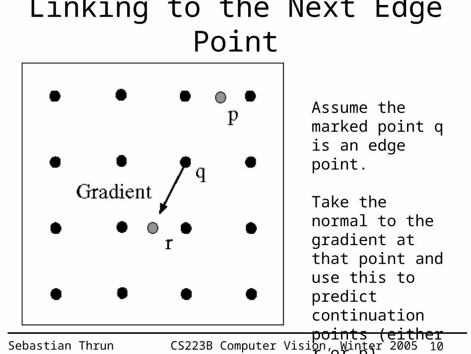
Linking to the Next Edge Point
Assume the marked point q is an edge point.
Take the normal to the gradient at that point and use this to predict continuation points (either r or p).
11Sebastian Thrun CS223B Computer Vision, Winter 2005
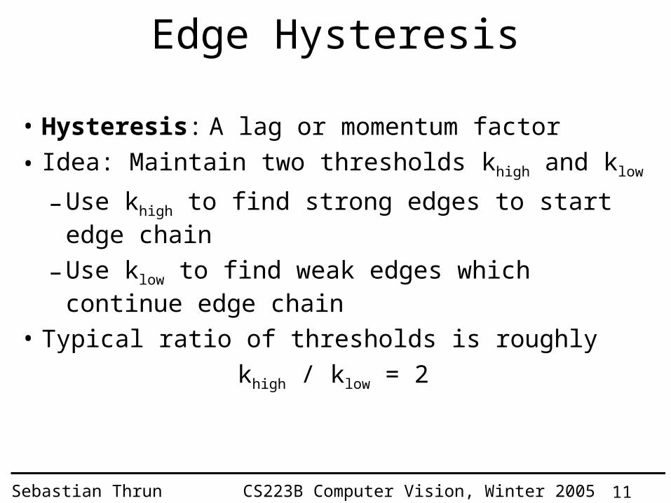
Edge Hysteresis
• Hysteresis: A lag or momentum factor
• Idea: Maintain two thresholds khigh and klow
– Use khigh to find strong edges to start edge chain
– Use klow to find weak edges which continue edge chain
• Typical ratio of thresholds is roughly
khigh / klow = 2
12Sebastian Thrun CS223B Computer Vision, Winter 2005
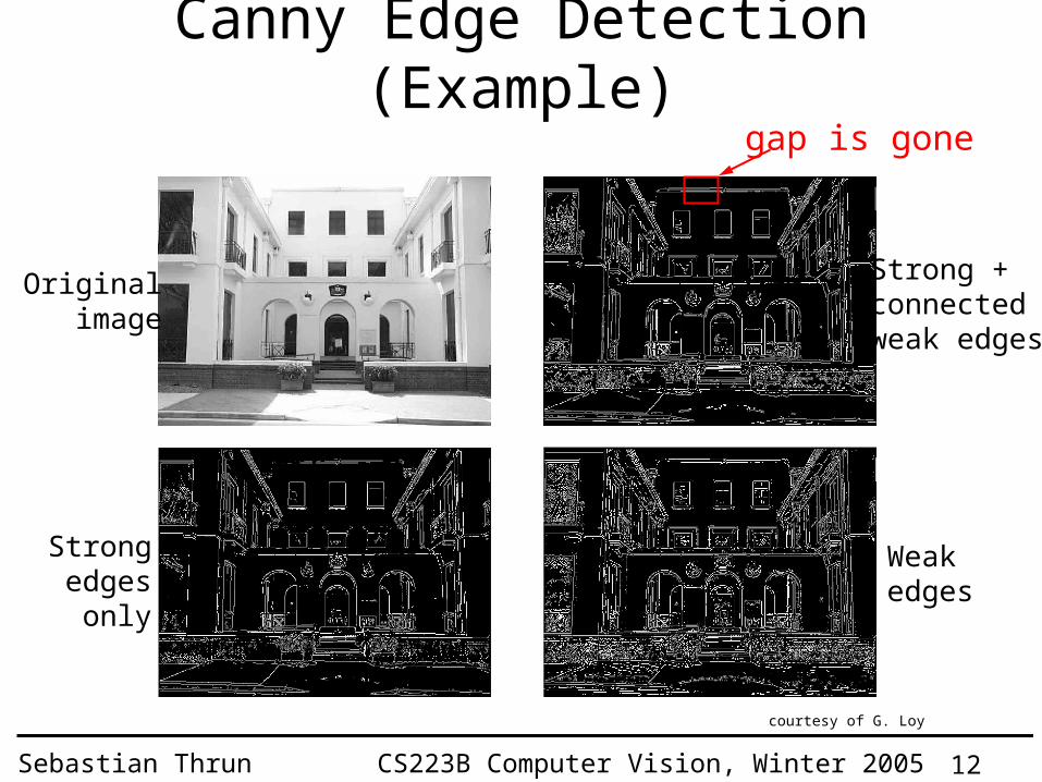
Canny Edge Detection (Example)
courtesy of G. Loy
gap is gone
Originalimage
Strongedges
only
Strong +connectedweak edges
Weakedges
13Sebastian Thrun CS223B Computer Vision, Winter 2005
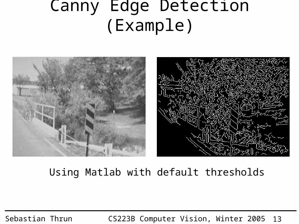
Canny Edge Detection (Example)
Using Matlab with default thresholds
14Sebastian Thrun CS223B Computer Vision, Winter 2005
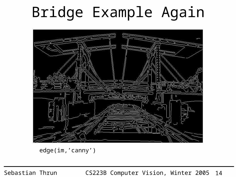
Bridge Example Again
edge(im,’canny’)

15Sebastian Thrun CS223B Computer Vision, Winter 2005
Corner Effects

16Sebastian Thrun CS223B Computer Vision, Winter 2005
Today’s Goals
• Canny Edge Detector
• Harris Corner Detector
• Hough Transform
• Templates and Image Pyramid
• SIFT Features

17Sebastian Thrun CS223B Computer Vision, Winter 2005
Finding CornersEdge detectors perform poorly at corners.
Corners provide repeatable points for matching, so are worth detecting.
Idea:
• Exactly at a corner, gradient is ill defined.
• However, in the region around a corner, gradient has two or more different values.

18Sebastian Thrun CS223B Computer Vision, Winter 2005
The Harris corner detector
2
2
yyx
yxx
III
IIIC
Form the second-moment matrix:
Sum over a small region around the hypothetical corner
Gradient with respect to x, times gradient with respect to y
Matrix is symmetric Slide credit: David Jacobs
19Sebastian Thrun CS223B Computer Vision, Winter 2005
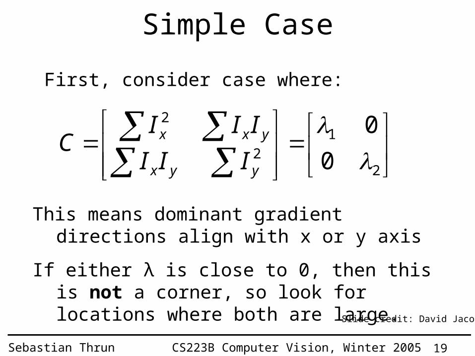
Simple Case
2
12
2
0
0
yyx
yxx
III
IIIC
First, consider case where:
This means dominant gradient directions align with x or y axis
If either λ is close to 0, then this is not a corner, so look for locations where both are large.
Slide credit: David Jacobs
20Sebastian Thrun CS223B Computer Vision, Winter 2005
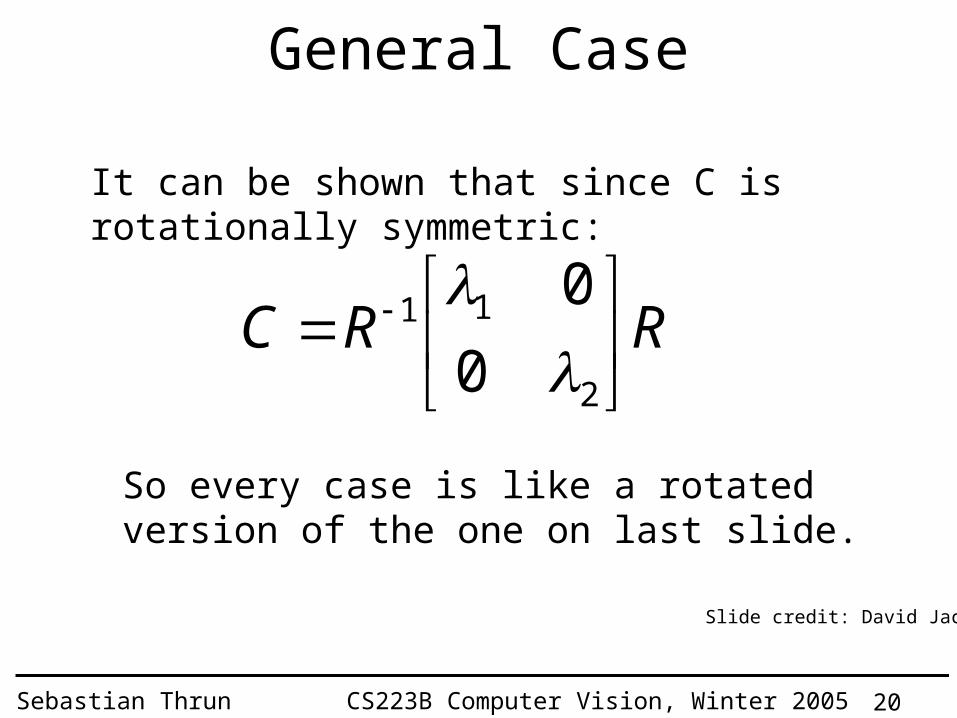
General Case
It can be shown that since C is rotationally symmetric:
RRC
2
11
0
0
So every case is like a rotated version of the one on last slide.
Slide credit: David Jacobs

21Sebastian Thrun CS223B Computer Vision, Winter 2005
So, To Detect Corners
• Filter image with Gaussian to reduce noise• Compute magnitude of the x and y gradients at
each pixel• Construct C in a window around each pixel
(Harris uses a Gaussian window – just blur)• Solve for product of s (determinant of C)• If s are both big (product reaches local
maximum and is above threshold), we have a corner (Harris also checks that ratio of s is not too high)

22Sebastian Thrun CS223B Computer Vision, Winter 2005
Gradient Orientation
Closeup

23Sebastian Thrun CS223B Computer Vision, Winter 2005
Corner Detection
Corners are detected where the product of the ellipse axis lengths reaches a local maximum.
24Sebastian Thrun CS223B Computer Vision, Winter 2005
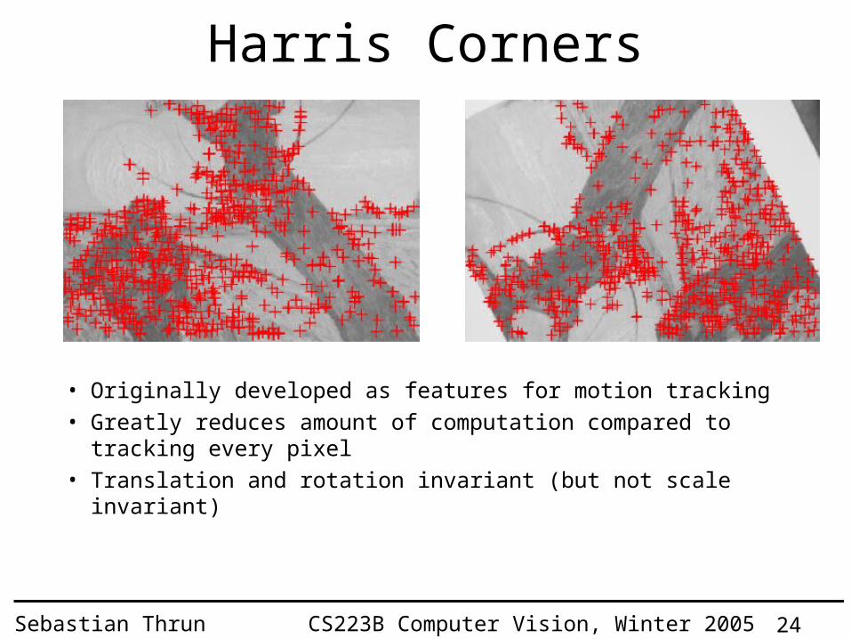
Harris Corners
• Originally developed as features for motion tracking• Greatly reduces amount of computation compared to
tracking every pixel• Translation and rotation invariant (but not scale invariant)

25Sebastian Thrun CS223B Computer Vision, Winter 2005
Harris Corner in Matlab% Harris Corner detector - by Kashif Shahzadsigma=2; thresh=0.1; sze=11; disp=0;
% Derivative masksdy = [-1 0 1; -1 0 1; -1 0 1];dx = dy'; %dx is the transpose matrix of dy % Ix and Iy are the horizontal and vertical edges of imageIx = conv2(bw, dx, 'same');Iy = conv2(bw, dy, 'same'); % Calculating the gradient of the image Ix and Iyg = fspecial('gaussian',max(1,fix(6*sigma)), sigma);Ix2 = conv2(Ix.^2, g, 'same'); % Smoothed squared image derivativesIy2 = conv2(Iy.^2, g, 'same');Ixy = conv2(Ix.*Iy, g, 'same'); % My preferred measure according to research papercornerness = (Ix2.*Iy2 - Ixy.^2)./(Ix2 + Iy2 + eps); % We should perform nonmaximal suppression and thresholdmx = ordfilt2(cornerness,sze^2,ones(sze)); % Grey-scale dilatecornerness = (cornerness==mx)&(cornerness>thresh); % Find maxima[rws,cols] = find(cornerness); % Find row,col coords.
clf ; imshow(bw);hold on;p=[cols rws];plot(p(:,1),p(:,2),'or');title('\bf Harris Corners')
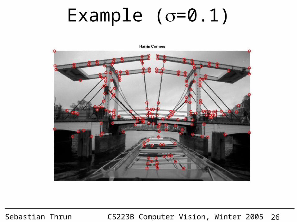
26Sebastian Thrun CS223B Computer Vision, Winter 2005
Example (=0.1)

27Sebastian Thrun CS223B Computer Vision, Winter 2005
Example (=0.01)

28Sebastian Thrun CS223B Computer Vision, Winter 2005
Example (=0.001)

29Sebastian Thrun CS223B Computer Vision, Winter 2005
Harris: OpenCV Implementation
30Sebastian Thrun CS223B Computer Vision, Winter 2005
Harris Corners for Optical Flow
Will talk about this later (optical flow)

31Sebastian Thrun CS223B Computer Vision, Winter 2005
Today’s Goals
• Canny Edge Detector
• Harris Corner Detector
• Hough Transform
• Templates and Image Pyramid
• SIFT Features
32Sebastian Thrun CS223B Computer Vision, Winter 2005
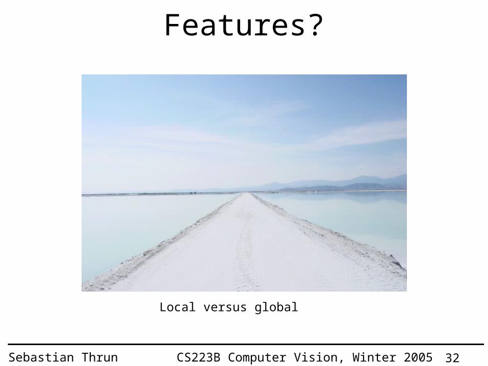
Features?
Local versus global

33Sebastian Thrun CS223B Computer Vision, Winter 2005
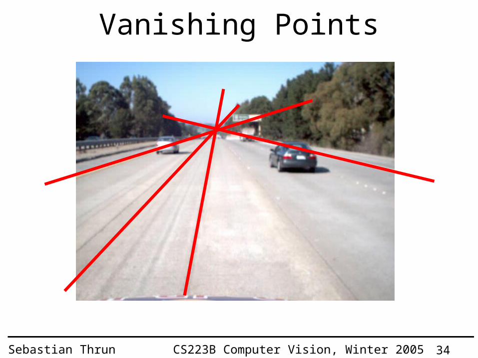
Vanishing Points
34Sebastian Thrun CS223B Computer Vision, Winter 2005
Vanishing Points
35Sebastian Thrun CS223B Computer Vision, Winter 2005
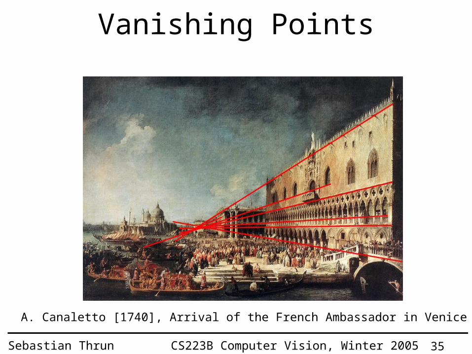
Vanishing Points
A. Canaletto [1740], Arrival of the French Ambassador in Venice

36Sebastian Thrun CS223B Computer Vision, Winter 2005
Vanishing Points…?
A. Canaletto [1740], Arrival of the French Ambassador in Venice

37Sebastian Thrun CS223B Computer Vision, Winter 2005
From Edges to Lines
38Sebastian Thrun CS223B Computer Vision, Winter 2005
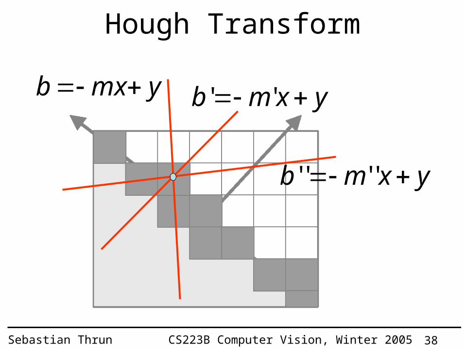
Hough Transform
ymxb yxmb ''
yxmb ''''

39Sebastian Thrun CS223B Computer Vision, Winter 2005
Hough Transform: Quantization
m
b
mm
Detecting Lines by finding maxima / clustering in parameter space

40Sebastian Thrun CS223B Computer Vision, Winter 2005
Hough Transform: Algorithm
• For each image point, determine – most likely line parameters b,m (direction of
gradient)– strength (magnitude of gradient)
• Increment parameter counter by strength value
• Cluster in parameter space, pick local maxima
41Sebastian Thrun CS223B Computer Vision, Winter 2005
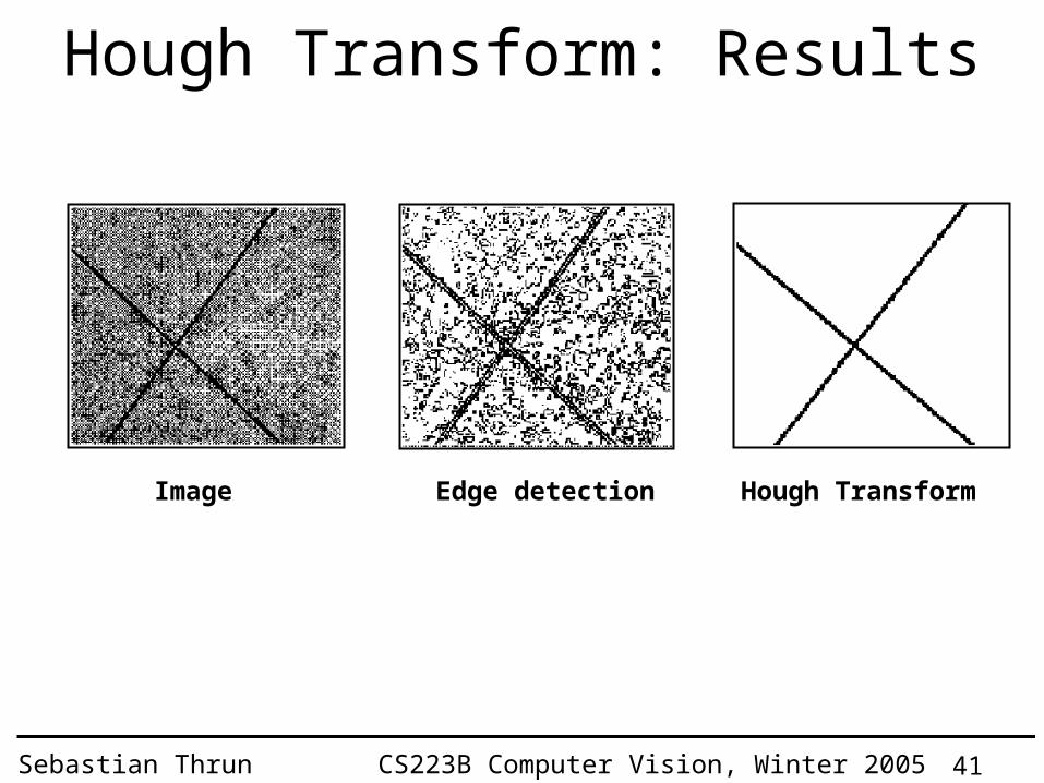
Hough Transform: Results
Hough TransformImage Edge detection
42Sebastian Thrun CS223B Computer Vision, Winter 2005
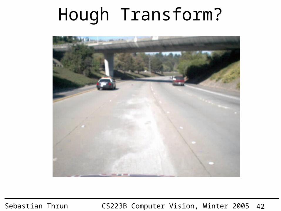
Hough Transform?

43Sebastian Thrun CS223B Computer Vision, Winter 2005
Summary Hough Transform
• Smart counting– Local evidence for global features– Organized in a table– Careful with parameterization!
• Subject to Curse of Dimensionality– Works great for simple features with 3
unknowns– Will fail for complex objects (e.g., all faces)

44Sebastian Thrun CS223B Computer Vision, Winter 2005
Today’s Goals
• Canny Edge Detector
• Harris Corner Detector
• Hough Transform
• Templates and Image Pyramid
• SIFT Features

45Sebastian Thrun CS223B Computer Vision, Winter 2005
Problem: Features for Recognition
Want to find… in here
46Sebastian Thrun CS223B Computer Vision, Winter 2005
Templates
• Find an object in an image!
• Want Invariance!– Scaling– Rotation– Illumination– Deformation
47Sebastian Thrun CS223B Computer Vision, Winter 2005
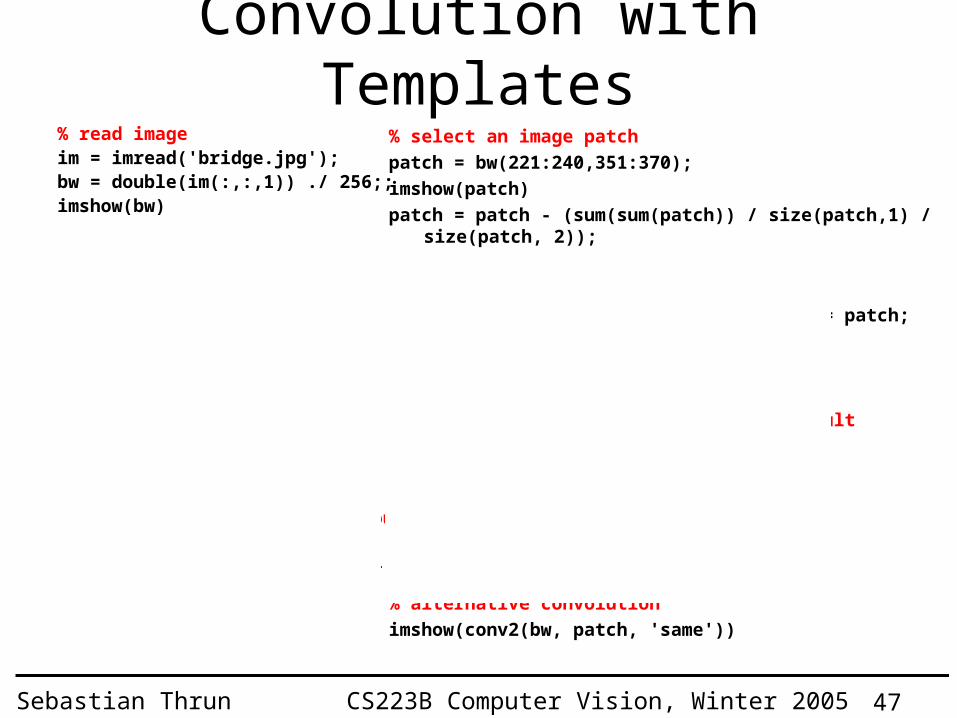
Convolution with Templates% read imageim = imread('bridge.jpg');bw = double(im(:,:,1)) ./ 256;;imshow(bw)
% apply FFTFFTim = fft2(bw);bw2 = real(ifft2(FFTim));imshow(bw2)
% define a kernelkernel=zeros(size(bw));kernel(1, 1) = 1;kernel(1, 2) = -1;FFTkernel = fft2(kernel);
% apply the kernel and check out the result
FFTresult = FFTim .* FFTkernel;result = real(ifft2(FFTresult));imshow(result)
% select an image patch
patch = bw(221:240,351:370);
imshow(patch)
patch = patch - (sum(sum(patch)) / size(patch,1) / size(patch, 2));
kernel=zeros(size(bw));
kernel(1:size(patch,1),1:size(patch,2)) = patch;
FFTkernel = fft2(kernel);
% apply the kernel and check out the result
FFTresult = FFTim .* FFTkernel;
result = max(0, real(ifft2(FFTresult)));
result = result ./ max(max(result));
result = (result .^ 1 > 0.5);
imshow(result)
% alternative convolution
imshow(conv2(bw, patch, 'same'))

48Sebastian Thrun CS223B Computer Vision, Winter 2005
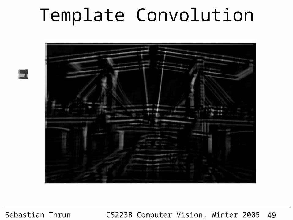
Template Convolution
49Sebastian Thrun CS223B Computer Vision, Winter 2005
Template Convolution
50Sebastian Thrun CS223B Computer Vision, Winter 2005
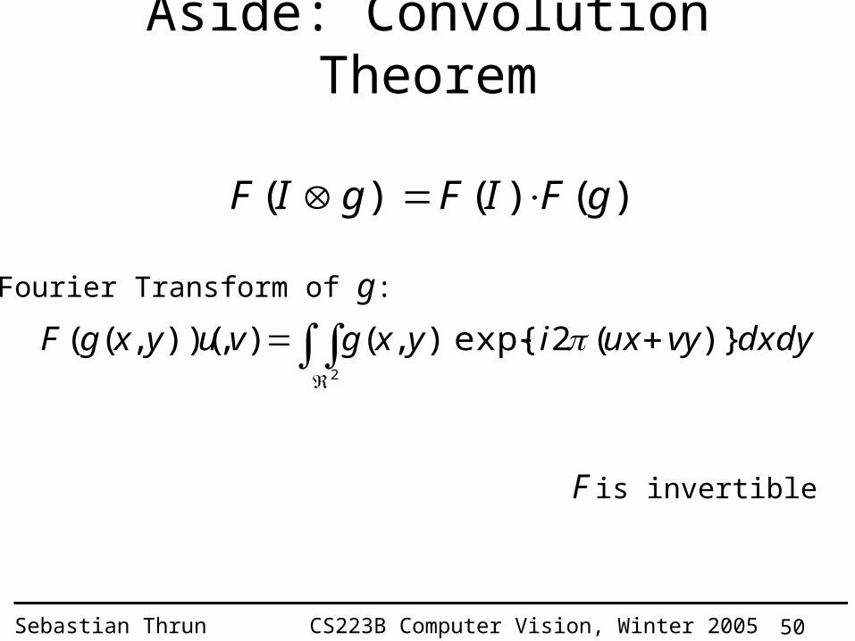
Aside: Convolution Theorem
)()()( gFIFgIF
2
)}(2exp{),(),))(,(( dydxvyuxiyxgvuyxgF Fourier Transform of g:
F is invertible

51Sebastian Thrun CS223B Computer Vision, Winter 2005
Convolution with Templates% read imageim = imread('bridge.jpg');bw = double(im(:,:,1)) ./ 256;;imshow(bw)
% apply FFTFFTim = fft2(bw);bw2 = real(ifft2(FFTim));imshow(bw2)
% define a kernelkernel=zeros(size(bw));kernel(1, 1) = 1;kernel(1, 2) = -1;FFTkernel = fft2(kernel);
% apply the kernel and check out the result
FFTresult = FFTim .* FFTkernel;result = real(ifft2(FFTresult));imshow(result)
% select an image patch
patch = bw(221:240,351:370);
imshow(patch)
patch = patch - (sum(sum(patch)) / size(patch,1) / size(patch, 2));
kernel=zeros(size(bw));
kernel(1:size(patch,1),1:size(patch,2)) = patch;
FFTkernel = fft2(kernel);
% apply the kernel and check out the result
FFTresult = FFTim .* FFTkernel;
result = max(0, real(ifft2(FFTresult)));
result = result ./ max(max(result));
result = (result .^ 1 > 0.5);
imshow(result)
% alternative convolution
imshow(conv2(bw, patch, 'same'))

52Sebastian Thrun CS223B Computer Vision, Winter 2005
Convolution with Templates
• Invariances:– Scaling– Rotation– Illumination– Deformation
• Provides– Good localization
No
No
No
MaybeNo

53Sebastian Thrun CS223B Computer Vision, Winter 2005
Scale Invariance: Image Pyramid
54Sebastian Thrun CS223B Computer Vision, Winter 2005
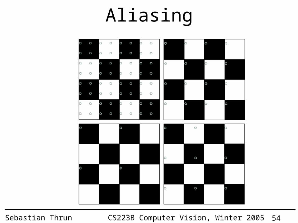
Aliasing
55Sebastian Thrun CS223B Computer Vision, Winter 2005
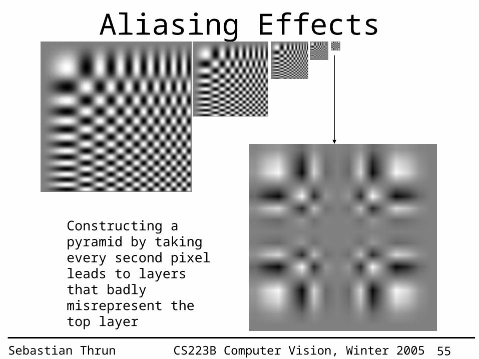
Aliasing Effects
Constructing a pyramid by taking every second pixel leads to layers that badly misrepresent the top layer

56Sebastian Thrun CS223B Computer Vision, Winter 2005
Solution to Aliasing
• Convolve with Gaussian

57Sebastian Thrun CS223B Computer Vision, Winter 2005
Templates with Image Pyramid
• Invariances:– Scaling– Rotation– Illumination– Deformation
• Provides– Good localization
No
Yes
No
MaybeNo
58Sebastian Thrun CS223B Computer Vision, Winter 2005
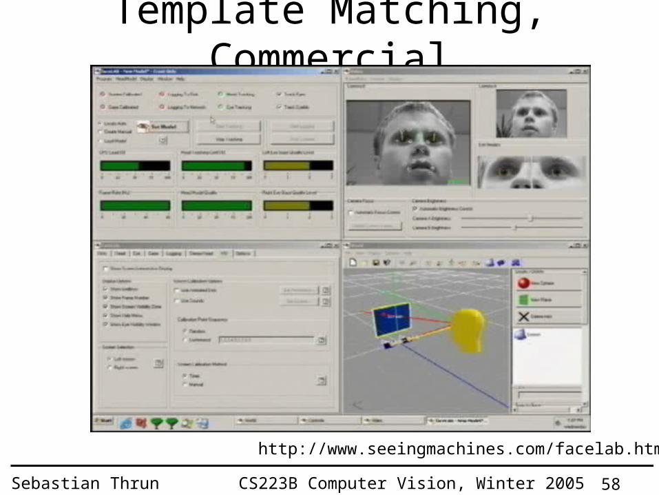
Template Matching, Commercial
http://www.seeingmachines.com/facelab.htm
59Sebastian Thrun CS223B Computer Vision, Winter 2005
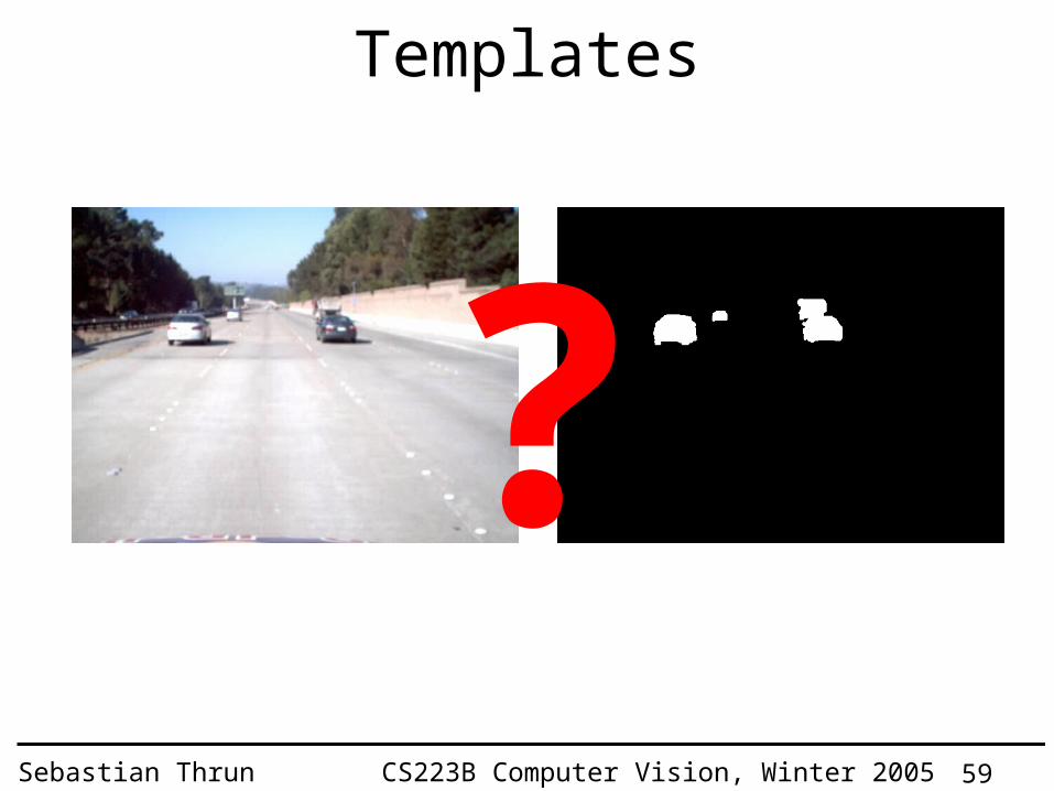
Templates
?
60Sebastian Thrun CS223B Computer Vision, Winter 2005
Today’s Goals
• Canny Edge Detector
• Harris Corner Detector
• Hough Transform
• Templates and Image Pyramid
• SIFT Features

61Sebastian Thrun CS223B Computer Vision, Winter 2005
Let’s Return to this Problem…
Want to find… in here

62Sebastian Thrun CS223B Computer Vision, Winter 2005
SIFT
• Invariances:– Scaling– Rotation– Illumination– Deformation
• Provides– Good localization
Yes
Yes
Yes
MaybeYes
63Sebastian Thrun CS223B Computer Vision, Winter 2005
SIFT Reference
Distinctive image features from scale-invariant keypoints. David G. Lowe, International Journal of Computer Vision, 60, 2 (2004), pp. 91-110.
SIFT = Scale Invariant Feature Transform
64Sebastian Thrun CS223B Computer Vision, Winter 2005
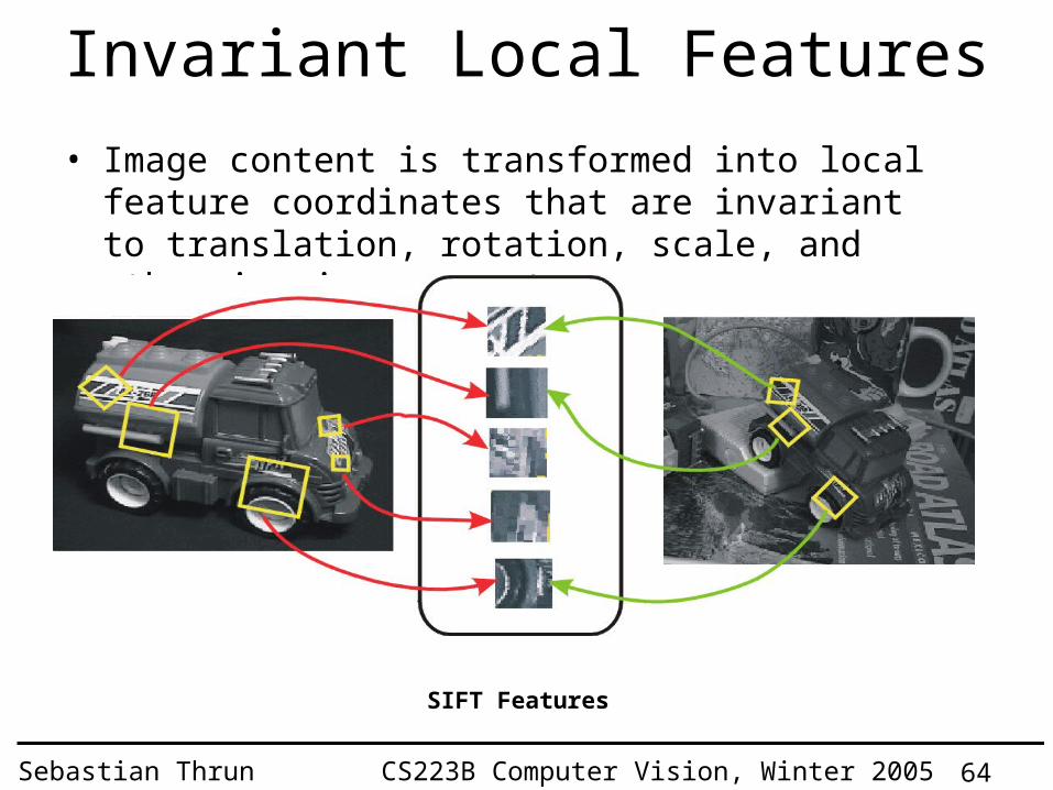
Invariant Local Features
• Image content is transformed into local feature coordinates that are invariant to translation, rotation, scale, and other imaging parameters
SIFT Features

Advantages of invariant local features
• Locality: features are local, so robust to occlusion and clutter (no prior segmentation)
• Distinctiveness: individual features can be matched to a large database of objects
• Quantity: many features can be generated for even small objects
• Efficiency: close to real-time performance
• Extensibility: can easily be extended to wide range of differing feature types, with each adding robustness

66Sebastian Thrun CS223B Computer Vision, Winter 2005
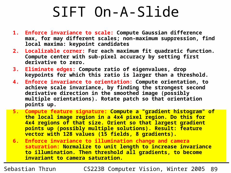
SIFT On-A-Slide1. Enforce invariance to scale: Compute Gaussian difference max, for
may different scales; non-maximum suppression, find local maxima: keypoint candidates
2. Localizable corner: For each maximum fit quadratic function. Compute center with sub-pixel accuracy by setting first derivative to zero.
3. Eliminate edges: Compute ratio of eigenvalues, drop keypoints for which this ratio is larger than a threshold.
4. Enforce invariance to orientation: Compute orientation, to achieve scale invariance, by finding the strongest second derivative direction in the smoothed image (possibly multiple orientations). Rotate patch so that orientation points up.
5. Compute feature signature: Compute a "gradient histogram" of the local image region in a 4x4 pixel region. Do this for 4x4 regions of that size. Orient so that largest gradient points up (possibly multiple solutions). Result: feature vector with 128 values (15 fields, 8 gradients).
6. Enforce invariance to illumination change and camera saturation: Normalize to unit length to increase invariance to illumination. Then threshold all gradients, to become invariant to camera saturation.

67Sebastian Thrun CS223B Computer Vision, Winter 2005
SIFT On-A-Slide1. Enforce invariance to scale: Compute Gaussian difference max, for
may different scales; non-maximum suppression, find local maxima: keypoint candidates
2. Localizable corner: For each maximum fit quadratic function. Compute center with sub-pixel accuracy by setting first derivative to zero.
3. Eliminate edges: Compute ratio of eigenvalues, drop keypoints for which this ratio is larger than a threshold.
4. Enforce invariance to orientation: Compute orientation, to achieve scale invariance, by finding the strongest second derivative direction in the smoothed image (possibly multiple orientations). Rotate patch so that orientation points up.
5. Compute feature signature: Compute a "gradient histogram" of the local image region in a 4x4 pixel region. Do this for 4x4 regions of that size. Orient so that largest gradient points up (possibly multiple solutions). Result: feature vector with 128 values (15 fields, 8 gradients).
6. Enforce invariance to illumination change and camera saturation: Normalize to unit length to increase invariance to illumination. Then threshold all gradients, to become invariant to camera saturation.

68Sebastian Thrun CS223B Computer Vision, Winter 2005
Find Invariant Corners1. Enforce invariance to scale: Compute Gaussian difference
max, for may different scales; non-maximum suppression, find local maxima: keypoint candidates

69Sebastian Thrun CS223B Computer Vision, Winter 2005
Finding “Keypoints” (Corners)
Idea: Find Corners, but scale invariance
Approach:
• Run linear filter (diff of Gaussians)
• At different resolutions of image pyramid

70Sebastian Thrun CS223B Computer Vision, Winter 2005
Difference of Gaussians
Minus
Equals

71Sebastian Thrun CS223B Computer Vision, Winter 2005
Difference of Gaussians
surf(fspecial('gaussian',40,4))
surf(fspecial('gaussian',40,8))
surf(fspecial('gaussian',40,8) - fspecial('gaussian',40,4))
72Sebastian Thrun CS223B Computer Vision, Winter 2005
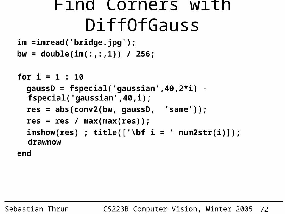
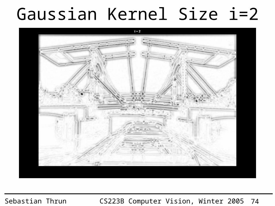
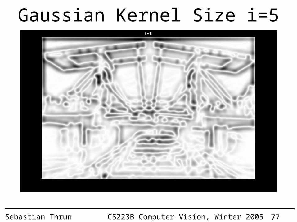
Find Corners with DiffOfGauss
im =imread('bridge.jpg');
bw = double(im(:,:,1)) / 256;
for i = 1 : 10
gaussD = fspecial('gaussian',40,2*i) - fspecial('gaussian',40,i);
res = abs(conv2(bw, gaussD, 'same'));
res = res / max(max(res));
imshow(res) ; title(['\bf i = ' num2str(i)]); drawnow
end

73Sebastian Thrun CS223B Computer Vision, Winter 2005
Gaussian Kernel Size i=1
74Sebastian Thrun CS223B Computer Vision, Winter 2005
Gaussian Kernel Size i=2

75Sebastian Thrun CS223B Computer Vision, Winter 2005
Gaussian Kernel Size i=3

76Sebastian Thrun CS223B Computer Vision, Winter 2005
Gaussian Kernel Size i=4
77Sebastian Thrun CS223B Computer Vision, Winter 2005
Gaussian Kernel Size i=5

78Sebastian Thrun CS223B Computer Vision, Winter 2005
Gaussian Kernel Size i=6

79Sebastian Thrun CS223B Computer Vision, Winter 2005
Gaussian Kernel Size i=7

80Sebastian Thrun CS223B Computer Vision, Winter 2005
Gaussian Kernel Size i=8

81Sebastian Thrun CS223B Computer Vision, Winter 2005
Gaussian Kernel Size i=9

82Sebastian Thrun CS223B Computer Vision, Winter 2005
Gaussian Kernel Size i=10

83Sebastian Thrun CS223B Computer Vision, Winter 2005
Key point localization
• Detect maxima and minima of difference-of-Gaussian in scale space
B l u r
R e s a m p l e
S u b t r a c t

84Sebastian Thrun CS223B Computer Vision, Winter 2005
Example of keypoint detection
(a) 233x189 image(b) 832 DOG extrema(c) 729 above threshold

85Sebastian Thrun CS223B Computer Vision, Winter 2005
SIFT On-A-Slide1. Enforce invariance to scale: Compute Gaussian difference max, for
may different scales; non-maximum suppression, find local maxima: keypoint candidates
2. Localizable corner: For each maximum fit quadratic function. Compute center with sub-pixel accuracy by setting first derivative to zero.
3. Eliminate edges: Compute ratio of eigenvalues, drop keypoints for which this ratio is larger than a threshold.
4. Enforce invariance to orientation: Compute orientation, to achieve scale invariance, by finding the strongest second derivative direction in the smoothed image (possibly multiple orientations). Rotate patch so that orientation points up.
5. Compute feature signature: Compute a "gradient histogram" of the local image region in a 4x4 pixel region. Do this for 4x4 regions of that size. Orient so that largest gradient points up (possibly multiple solutions). Result: feature vector with 128 values (15 fields, 8 gradients).
6. Enforce invariance to illumination change and camera saturation: Normalize to unit length to increase invariance to illumination. Then threshold all gradients, to become invariant to camera saturation.

86Sebastian Thrun CS223B Computer Vision, Winter 2005
Example of keypoint detection
Threshold on value at DOG peak and on ratio of principle curvatures (Harris approach)
(c) 729 left after peak value threshold (from 832)(d) 536 left after testing ratio of principle curvatures

87Sebastian Thrun CS223B Computer Vision, Winter 2005
SIFT On-A-Slide1. Enforce invariance to scale: Compute Gaussian difference max, for
may different scales; non-maximum suppression, find local maxima: keypoint candidates
2. Localizable corner: For each maximum fit quadratic function. Compute center with sub-pixel accuracy by setting first derivative to zero.
3. Eliminate edges: Compute ratio of eigenvalues, drop keypoints for which this ratio is larger than a threshold.
4. Enforce invariance to orientation: Compute orientation, to achieve scale invariance, by finding the strongest second derivative direction in the smoothed image (possibly multiple orientations). Rotate patch so that orientation points up.
5. Compute feature signature: Compute a "gradient histogram" of the local image region in a 4x4 pixel region. Do this for 4x4 regions of that size. Orient so that largest gradient points up (possibly multiple solutions). Result: feature vector with 128 values (15 fields, 8 gradients).
6. Enforce invariance to illumination change and camera saturation: Normalize to unit length to increase invariance to illumination. Then threshold all gradients, to become invariant to camera saturation.

88Sebastian Thrun CS223B Computer Vision, Winter 2005
Select canonical orientation
• Create histogram of local gradient directions computed at selected scale
• Assign canonical orientation at peak of smoothed histogram
• Each key specifies stable 2D coordinates (x, y, scale, orientation)
0 2
89Sebastian Thrun CS223B Computer Vision, Winter 2005
SIFT On-A-Slide1. Enforce invariance to scale: Compute Gaussian difference max, for
may different scales; non-maximum suppression, find local maxima: keypoint candidates
2. Localizable corner: For each maximum fit quadratic function. Compute center with sub-pixel accuracy by setting first derivative to zero.
3. Eliminate edges: Compute ratio of eigenvalues, drop keypoints for which this ratio is larger than a threshold.
4. Enforce invariance to orientation: Compute orientation, to achieve scale invariance, by finding the strongest second derivative direction in the smoothed image (possibly multiple orientations). Rotate patch so that orientation points up.
5. Compute feature signature: Compute a "gradient histogram" of the local image region in a 4x4 pixel region. Do this for 4x4 regions of that size. Orient so that largest gradient points up (possibly multiple solutions). Result: feature vector with 128 values (15 fields, 8 gradients).
6. Enforce invariance to illumination change and camera saturation: Normalize to unit length to increase invariance to illumination. Then threshold all gradients, to become invariant to camera saturation.

90Sebastian Thrun CS223B Computer Vision, Winter 2005
SIFT vector formation
• Thresholded image gradients are sampled over 16x16 array of locations in scale space
• Create array of orientation histograms• 8 orientations x 4x4 histogram array = 128 dimensions

91Sebastian Thrun CS223B Computer Vision, Winter 2005
Nearest-neighbor matching to feature database
• Hypotheses are generated by approximate nearest neighbor matching of each feature to vectors in the database – SIFT use best-bin-first (Beis & Lowe, 97)
modification to k-d tree algorithm– Use heap data structure to identify bins in order
by their distance from query point
• Result: Can give speedup by factor of 1000 while finding nearest neighbor (of interest) 95% of the time

92Sebastian Thrun CS223B Computer Vision, Winter 2005
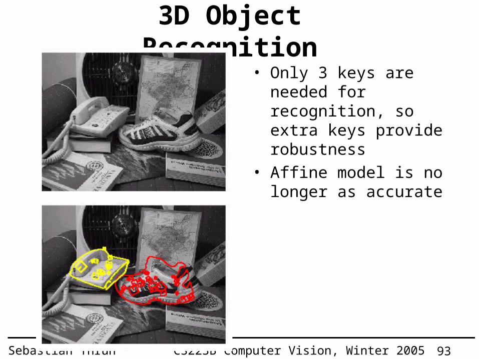
3D Object Recognition
• Extract outlines with background subtraction
93Sebastian Thrun CS223B Computer Vision, Winter 2005
3D Object Recognition• Only 3 keys are needed
for recognition, so extra keys provide robustness
• Affine model is no longer as accurate

94Sebastian Thrun CS223B Computer Vision, Winter 2005
Recognition under occlusion
95Sebastian Thrun CS223B Computer Vision, Winter 2005
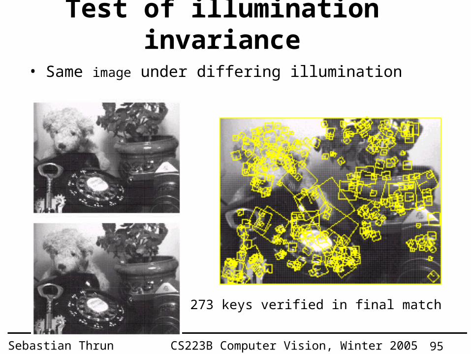
Test of illumination invariance
• Same image under differing illumination
273 keys verified in final match

96Sebastian Thrun CS223B Computer Vision, Winter 2005
Examples of view interpolation

97Sebastian Thrun CS223B Computer Vision, Winter 2005
Location recognition
98Sebastian Thrun CS223B Computer Vision, Winter 2005
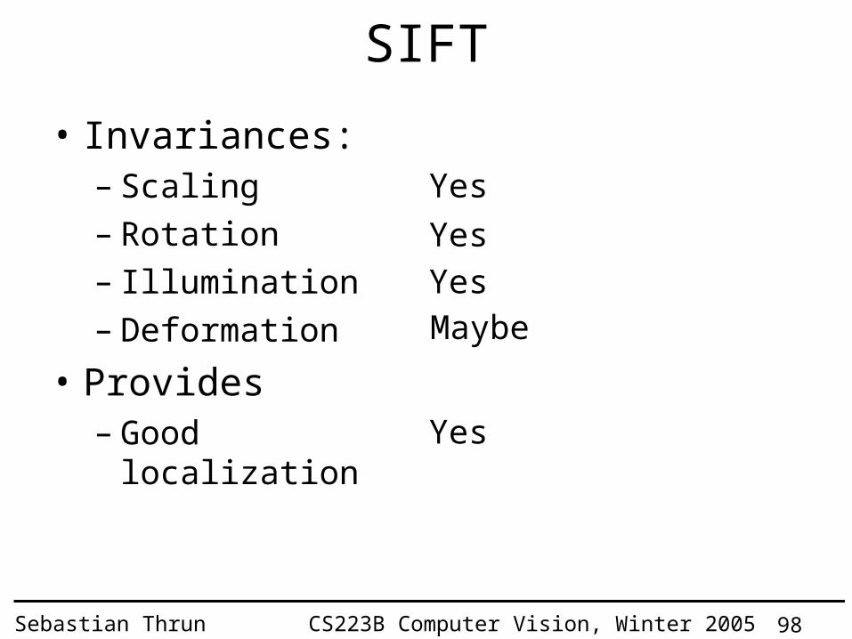
SIFT
• Invariances:– Scaling– Rotation– Illumination– Deformation
• Provides– Good localization
Yes
Yes
Yes
MaybeYes

99Sebastian Thrun CS223B Computer Vision, Winter 2005
Today’s Goals
• Canny Edge Detector
• Harris Corner Detector
• Hough Transform
• Templates and Image Pyramid
• SIFT Features