stanford university psych 221 / ee 362 winter 2002-2003 stanford university psych 221 / ee 362...

Stanford University

Psych 221 / EE 362

Winter 2002-2003

Stanford University

Psych 221 / EE 362

Winter 2002-2003

Patrick Y. Maeda 3/10/03

Zernike Polynomials and Their Use in Describing the Wavefront Aberrations of the

Human Eye

Psych 221/EE362 Applied Vision and Imaging Systems

Course Project, Winter 2003

Patrick Y. [email protected]

Stanford University

Stanford University

Psych 221 / EE 362

Winter 2002-2003

Stanford University

Psych 221 / EE 362

Winter 2002-2003


Introduction and MotivationIntroduction and Motivation

Great interest in correcting higher order aberrations of the eye Laser eye surgery (PRK, LASIK)

– Currently, only defocus and astigmatism being corrected (2nd order aberrations)

– Improve vision better than 20/20

– Correct problems caused or induced by current generation of laser surgery

Imaging of the retina and other structures in the eye using adaptive optics

Correction requires measurement of optical aberrations Defocus and astigmatism can be determined using sets of lenses

Measurement of higher orders require more sophisticated techniques

– Measurement of the wavefront aberration with Shack-Hartmann Wavefront Sensor

Mathematical description of the aberrations needed Accurate description of wave aberration function

Accurate estimation of wave aberration function from measurement data

Stanford University

Psych 221 / EE 362

Winter 2002-2003

Stanford University

Psych 221 / EE 362

Winter 2002-2003


Project OutlineProject Outline

Introduction/Motivation

General Optical System Description

Monochromatic Wavefront Aberrations

PSF and MTF calculations

Why Use Zernike Polynomials?

Definition of Zernike Polynomials

Describing Wave Aberrations using Zernike Polynomials

Simulating the Effects of Wave Aberrations

Wavefront Measurement and Data Fitting with Zernike Polynomials

Conclusion, References, Source Code Appendix

Stanford University

Psych 221 / EE 362

Winter 2002-2003

Stanford University

Psych 221 / EE 362

Winter 2002-2003


Coordinate SystemsCoordinate Systems

Optical System

Optical Axis

y

z

xy

x

Object Plane

Image Plane

y

x

Object Height

h’

h

Image Height

Optical System

Optical Axis

y

z

xy

x

Object Plane

Image Plane

y

x

Object Height

h’

h

Image Height

θ

y

x

r

a

x = r cos(θ)y = r sin(θ)θ = tan-1(x/y)r = (x2+y2)1/2

θ

y

x

ρ

1

x = ρ cos(θ)y = ρ sin(θ)θ = tan-1(x/y)ρ = r/a = (x2+y2)1/2

Normalized Pupil Coordinate SystemPupil Coordinate System

θ

y

x

r

a

x = r cos(θ)y = r sin(θ)θ = tan-1(x/y)r = (x2+y2)1/2

θ

y

x

ρ

1

x = ρ cos(θ)y = ρ sin(θ)θ = tan-1(x/y)ρ = r/a = (x2+y2)1/2

Normalized Pupil Coordinate SystemPupil Coordinate System

Stanford University

Psych 221 / EE 362

Winter 2002-2003

Stanford University

Psych 221 / EE 362

Winter 2002-2003


Wave AberrationWave Aberration

The wavefront aberration, W(x,y), is the distance, in optical path length (product of the refractive index and path length), from the reference sphere to the wavefront in the exit pupil measured along the ray as a function of the transverse coordinates (x,y) of the ray intersection with the reference sphere. It is not the wavefront itself but it is the departure of the wavefront from the reference sphere.

y

zx

ExitPupil

ImagePlane

AberratedWavefront Reference

Spherical Wavefront

Wave Aberration

W(x,y)

0,0

2

,

),(2

22

),(

),(1

),(

yx

yx

ss

yx

d

yf

d

xf

yxWi

p

PSFFT

PSFFTssMTF

eyxpFTAd

yxPSF

Stanford University

Psych 221 / EE 362

Winter 2002-2003

Stanford University

Psych 221 / EE 362

Winter 2002-2003


Describing Optical AberrationsDescribing Optical Aberrations

Optical system aberrations have historically been described, characterized, and catalogued by power series expansions

Many optical systems have circular pupils

Application of experimental results typically require data fitting

It is, therefore, desirable to expand the wave aberration in terms of a complete set of basis functions that are orthogonal over the interior of a circle

Stanford University

Psych 221 / EE 362

Winter 2002-2003

Stanford University

Psych 221 / EE 362

Winter 2002-2003


Why Use Zernike Polynomials?Why Use Zernike Polynomials?

Zernike polynomials form a complete set of functions or modes that are orthogonal over a circle of unit radius Convenient for serving as a set of basis functions

Expressible in polar coordinates or Cartesian coordinates

Scaled so that non-zero order modes have zero mean and unit variance

– Puts modes in a common reference frame for meaningful relative comparison

Other power series descriptions are not orthogonal

Wave aberrations in an optical system with a circular pupil accurately described by a weighted sum of Zernike polynomials

The Orthonormal set of Zernike polynomials is recommended for describing wave aberration functions and for data fitting of experimental measurements for the eye7

– Terms are normalized so that the coefficient of a particular term or mode is the RMS contribution of that term

Stanford University

Psych 221 / EE 362

Winter 2002-2003

Stanford University

Psych 221 / EE 362

Winter 2002-2003


Mathematical Formulae 3Mathematical Formulae 3

sn

mn

s

sm

n

mn

mmm

mn

mn

mn

mn

mn

mn

mn

smnsmns

snR

R

mmn

N

N

nnnnmn

mmRN

mmRNZ

22)(

0

000

3

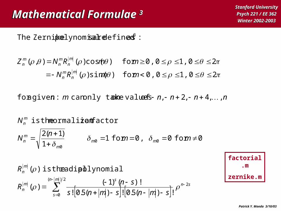
!)(5.0!)(5.0!

)!()1()(

polynomial radial theis )(

0for 0 , 0for 11

)1(2

factorion normalizat theis

,,4,2, of on values only takecan :given afor

20 , 10 , 0for )sin()(

20 , 10 , 0for )cos()(),(

:as defined are spolynomial ZernikeThe

factorial.m

zernike.m

Stanford University

Psych 221 / EE 362

Winter 2002-2003

Stanford University

Psych 221 / EE 362

Winter 2002-2003


List of Zernike Polynomials 7, 9,10List of Zernike Polynomials 7, 9,10

)4(c10 4 4 14

mAstigmatisSecondary )2cos(3410 2 4 13

Defocus ,Aberration Spherical 1665 0 4 12

mAstigmatisSecondary )2sin(3410 2- 4 11

)4(sin10 4- 4 10

)3(c8 3 3 9

axis- xalong Coma )cos(238 1 3 8

axis-y along Coma )sin(238 1- 3 7

)3(sin8 3- 3 6

90or 0at axis with mAstigmatis )2(c6 2 2 5

Defocus curvature, Field 123 0 2 4

45at axis with mAstigmatis )2(sin6 2- 2 3

Distortion direction,-in xTilt )cos(2 1 1 2

Distortion direction,-yin Tilt )(sin2 1- 1 1

Pistonor erm,Constant t 1 0 0 0

Meaning ,

frequencyorder mode

4

24

24

24

4

3

3

3

3

2

2

2

os

os

os

Zmnj mn

Stanford University

Psych 221 / EE 362

Winter 2002-2003

Stanford University

Psych 221 / EE 362

Winter 2002-2003


Wave Aberration DescriptionWave Aberration Description

),(),(

))cos()(())sin()((

),(),(

:spolynomial Zernikeof sum weighteda as expressed is aberration waveThe

max

0

0

1

7

j

jjj

k

n

n

m

mn

mn

mn

nm

mn

mn

mn

k

n

n

nm

mn

mn

yxZWyxW

mRNWmRNW

ZWW

WaveAberration.m

Stanford University

Psych 221 / EE 362

Winter 2002-2003

Stanford University

Psych 221 / EE 362

Winter 2002-2003


Double-Index Zernike Polynomials Double-Index Zernike Polynomials

Azimuthal Frequency, m-6 -5 -4 -3 -2 -1 0 1 2 3 4 5 6

Radial Order, n

0

1

2

3

4

5

6

Common Names7

Piston

Tilt

Astigmatism (m=-2,2), Defocus(m=0)

Coma (m=-1,1), Trefoil(m=-3,3)

Spherical Aberration (m=0)

Secondary Coma (m=-1,1)

Secondary Spherical Aberration (m=0)

,mnZ ZernikePolynomial.m

Stanford University

Psych 221 / EE 362

Winter 2002-2003

Stanford University

Psych 221 / EE 362

Winter 2002-2003


Double-Index Zernike Polynomial PSFsDouble-Index Zernike Polynomial PSFs


Radial Order, n

0

1

2

3

4

5

6

Common Names7

Piston

Tilt






,mnZ ZernikePolynomialPSF.m

Stanford University

Psych 221 / EE 362

Winter 2002-2003

Stanford University

Psych 221 / EE 362

Winter 2002-2003


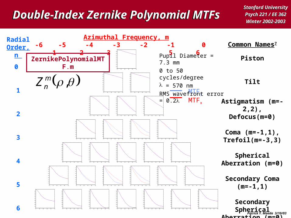
Double-Index Zernike Polynomial MTFsDouble-Index Zernike Polynomial MTFs

,mnZ


Radial Order, n

0

1

2

3

4

5

6

0 10 20 30 40 500

0.1

0.2

0.3

0.4

0.5

0.6

0.7

0.8

0.9

1

0 10 20 30 40 500

0.1

0.2

0.3

0.4

0.5

0.6

0.7

0.8

0.9

1

0 10 20 30 40 500

0.1

0.2

0.3

0.4

0.5

0.6

0.7

0.8

0.9

1

0 10 20 30 40 500

0.1

0.2

0.3

0.4

0.5

0.6

0.7

0.8

0.9

1

0 10 20 30 40 500

0.1

0.2

0.3

0.4

0.5

0.6

0.7

0.8

0.9

1

0 10 20 30 40 500

0.1

0.2

0.3

0.4

0.5

0.6

0.7

0.8

0.9

1

0 10 20 30 40 500

0.1

0.2

0.3

0.4

0.5

0.6

0.7

0.8

0.9

1

0 10 20 30 40 500

0.1

0.2

0.3

0.4

0.5

0.6

0.7

0.8

0.9

1

0 10 20 30 40 500

0.1

0.2

0.3

0.4

0.5

0.6

0.7

0.8

0.9

1

0 10 20 30 40 500

0.1

0.2

0.3

0.4

0.5

0.6

0.7

0.8

0.9

1

0 10 20 30 40 500

0.1

0.2

0.3

0.4

0.5

0.6

0.7

0.8

0.9

1

0 10 20 30 40 500

0.1

0.2

0.3

0.4

0.5

0.6

0.7

0.8

0.9

1

0 10 20 30 40 500

0.1

0.2

0.3

0.4

0.5

0.6

0.7

0.8

0.9

1

0 10 20 30 40 500

0.1

0.2

0.3

0.4

0.5

0.6

0.7

0.8

0.9

1

0 10 20 30 40 500

0.1

0.2

0.3

0.4

0.5

0.6

0.7

0.8

0.9

1

0 10 20 30 40 500

0.1

0.2

0.3

0.4

0.5

0.6

0.7

0.8

0.9

1

0 10 20 30 40 500

0.1

0.2

0.3

0.4

0.5

0.6

0.7

0.8

0.9

1

0 10 20 30 40 500

0.1

0.2

0.3

0.4

0.5

0.6

0.7

0.8

0.9

1

0 10 20 30 40 500

0.1

0.2

0.3

0.4

0.5

0.6

0.7

0.8

0.9

1

0 10 20 30 40 500

0.1

0.2

0.3

0.4

0.5

0.6

0.7

0.8

0.9

1

0 10 20 30 40 500

0.1

0.2

0.3

0.4

0.5

0.6

0.7

0.8

0.9

1

0 10 20 30 40 500

0.1

0.2

0.3

0.4

0.5

0.6

0.7

0.8

0.9

1

0 10 20 30 40 500

0.1

0.2

0.3

0.4

0.5

0.6

0.7

0.8

0.9

1

0 10 20 30 40 500

0.1

0.2

0.3

0.4

0.5

0.6

0.7

0.8

0.9

1

0 10 20 30 40 500

0.1

0.2

0.3

0.4

0.5

0.6

0.7

0.8

0.9

1

0 10 20 30 40 500

0.1

0.2

0.3

0.4

0.5

0.6

0.7

0.8

0.9

1

0 10 20 30 40 500

0.1

0.2

0.3

0.4

0.5

0.6

0.7

0.8

0.9

1

0 10 20 30 40 500

0.1

0.2

0.3

0.4

0.5

0.6

0.7

0.8

0.9

1

MTFy

MTFx

Common Names7

Piston

Tilt






Pupil Diameter = 4 mm

0 to 50 cycles/degree = 570 nm

RMS wavefront error = 0.2

ZernikePolynomialMTF.m

Stanford University

Psych 221 / EE 362

Winter 2002-2003

Stanford University

Psych 221 / EE 362

Winter 2002-2003


Double-Index Zernike Polynomial MTFsDouble-Index Zernike Polynomial MTFs


Radial Order, n

0

1

2

3

4

5

6

MTFy

MTFx

Common Names7

Piston

Tilt






0 10 20 30 40 500

0.1

0.2

0.3

0.4

0.5

0.6

0.7

0.8

0.9

1

0 10 20 30 40 500

0.1

0.2

0.3

0.4

0.5

0.6

0.7

0.8

0.9

1

0 10 20 30 40 500

0.1

0.2

0.3

0.4

0.5

0.6

0.7

0.8

0.9

1

0 10 20 30 40 500

0.1

0.2

0.3

0.4

0.5

0.6

0.7

0.8

0.9

1

0 10 20 30 40 500

0.1

0.2

0.3

0.4

0.5

0.6

0.7

0.8

0.9

1

0 10 20 30 40 500

0.1

0.2

0.3

0.4

0.5

0.6

0.7

0.8

0.9

1

0 10 20 30 40 500

0.1

0.2

0.3

0.4

0.5

0.6

0.7

0.8

0.9

1

0 10 20 30 40 500

0.1

0.2

0.3

0.4

0.5

0.6

0.7

0.8

0.9

1

0 10 20 30 40 500

0.1

0.2

0.3

0.4

0.5

0.6

0.7

0.8

0.9

1

0 10 20 30 40 500

0.1

0.2

0.3

0.4

0.5

0.6

0.7

0.8

0.9

1

0 10 20 30 40 500

0.1

0.2

0.3

0.4

0.5

0.6

0.7

0.8

0.9

1

0 10 20 30 40 500

0.1

0.2

0.3

0.4

0.5

0.6

0.7

0.8

0.9

1

0 10 20 30 40 500

0.1

0.2

0.3

0.4

0.5

0.6

0.7

0.8

0.9

1

0 10 20 30 40 500

0.1

0.2

0.3

0.4

0.5

0.6

0.7

0.8

0.9

1

0 10 20 30 40 500

0.1

0.2

0.3

0.4

0.5

0.6

0.7

0.8

0.9

1

0 10 20 30 40 500

0.1

0.2

0.3

0.4

0.5

0.6

0.7

0.8

0.9

1

0 10 20 30 40 500

0.1

0.2

0.3

0.4

0.5

0.6

0.7

0.8

0.9

1

0 10 20 30 40 500

0.1

0.2

0.3

0.4

0.5

0.6

0.7

0.8

0.9

1

0 10 20 30 40 500

0.1

0.2

0.3

0.4

0.5

0.6

0.7

0.8

0.9

1

0 10 20 30 40 500

0.1

0.2

0.3

0.4

0.5

0.6

0.7

0.8

0.9

1

0 10 20 30 40 500

0.1

0.2

0.3

0.4

0.5

0.6

0.7

0.8

0.9

1

0 10 20 30 40 500

0.1

0.2

0.3

0.4

0.5

0.6

0.7

0.8

0.9

1

0 10 20 30 40 500

0.1

0.2

0.3

0.4

0.5

0.6

0.7

0.8

0.9

1

0 10 20 30 40 500

0.1

0.2

0.3

0.4

0.5

0.6

0.7

0.8

0.9

1

0 10 20 30 40 500

0.1

0.2

0.3

0.4

0.5

0.6

0.7

0.8

0.9

1

0 10 20 30 40 500

0.1

0.2

0.3

0.4

0.5

0.6

0.7

0.8

0.9

1

0 10 20 30 40 500

0.1

0.2

0.3

0.4

0.5

0.6

0.7

0.8

0.9

1

0 10 20 30 40 500

0.1

0.2

0.3

0.4

0.5

0.6

0.7

0.8

0.9

1

Pupil Diameter = 7.3 mm

0 to 50 cycles/degree = 570 nm

RMS wavefront error = 0.2 ,mnZ


Stanford University

Psych 221 / EE 362

Winter 2002-2003

Stanford University

Psych 221 / EE 362

Winter 2002-2003


Simulation based on Human Eye DataSimulation based on Human Eye Data

0 10 20 30 40 500

0.2

0.4

0.6

0.8

1

sx (cycle/deg)

MTF of Zero Aberration System, 5.4mm pupil

0 10 20 30 40 500

0.2

0.4

0.6

0.8

1

sy (cycle/deg)

MTF of Zero Aberration System, 5.4mm pupil

0 10 20 30 40 500

0.2

0.4

0.6

0.8

1

sx (cycle/deg)

MTF of Aberrated System, Wrms = 0.85012

0 10 20 30 40 500

0.2

0.4

0.6

0.8

1

sy (cycle/deg)

MTF of Aberrated System, Wrms = 0.85012

Mode j Coefficient (m) RMS Coefficient (m)

0 0 01 0 02 0 03 1.02 0.4164132564 0 05 0.33 0.1347219366 0.21 0.0742462127 -0.26 -0.0919238828 0.03 0.0106066029 -0.34 -0.12020815310 -0.12 -0.03794733211 0.05 0.01581138812 0.19 0.08497058313 -0.19 -0.06008327614 0.15 0.047434165

Total RMS Wavefront Error (m) 0.484608089

WaveAberration.m WaveAberrationPSF.m

WaveAberrationMTF.m

Stanford University

Psych 221 / EE 362

Winter 2002-2003

Stanford University

Psych 221 / EE 362

Winter 2002-2003


Measurement SetupMeasurement Setup

Pupil

Retina

Iris

RealAberrated Wavefront

IdealPlanar

Wavefront

y

zx

IncomingLight Beam

Stanford University

Psych 221 / EE 362

Winter 2002-2003

Stanford University

Psych 221 / EE 362

Winter 2002-2003


Shack-Hartmann Sensor LayoutShack-Hartmann Sensor Layout

CCDPupil Relay OpticsPBS

Light Source

Lenslet Array

Stanford University

Psych 221 / EE 362

Winter 2002-2003

Stanford University

Psych 221 / EE 362

Winter 2002-2003


Shack-Hartmann Wavefront SensorShack-Hartmann Wavefront Sensor

Lenslet Array

Focal Length f

y(x1, y1)

y(x1, y2)

y(x1, y3)

y(x1, y4)

Aberrated Wavefront

Stanford University

Psych 221 / EE 362

Winter 2002-2003

Stanford University

Psych 221 / EE 362

Winter 2002-2003


Data Fitting with Zernike PolynomialsData Fitting with Zernike Polynomials

(15) ),(),(

(14) ),(),(

),(),(

),(),(

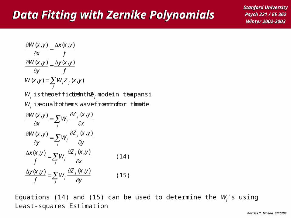
modefor that error wavefrontrms the toequal is

expansion in the mode theoft coefficien theis

),(),(

),(),(

),(),(

y

yxZW

f

yxy

x

yxZW

f

yxx

y

yxZW

y

yxW

x

yxZW

x

yxW

W

ZW

yxZWyxW

f

yxy

y

yxW

f

yxx

x

yxW

j

jj

j

jj

j

jj

j

jj

j

jj

jjj

Equations (14) and (15) can be used to determine the Wj’s using Least-squares Estimation

Stanford University

Psych 221 / EE 362

Winter 2002-2003

Stanford University

Psych 221 / EE 362

Winter 2002-2003


Least-squares Estimation Least-squares Estimation

of nsposematrix tra theis where

)(

:bygiven is of estimate squares-Least The

2

),(),(),(

),(),(),(

),(),(),(

),(),(),(

),(),(),(

),(),(),(

),(

),(

),(

),(

),(

),(

formmatrix in expressed becan (15) and (14) Equations

),(),(

and ),(),(

),(),(

and ),(),(

Let,

1LS

max2

max

2

1

max21

21max212211

11max112111

max21

21max212211

11max112111

21

11

21

11

T

TT

j

kkjkkkk

j

j

kkjkkkk

j

j

kk

kk

jj

jj

or

jk

W

W

W

yxhyxhyxh

yxhyxhyxh

yxhyxhyxh

yxgyxgyxg

yxgyxgyxg

yxgyxgyxg

yxc

yxc

yxc

yxb

yxb

yxb

yxhy

yxZyxg

x

yxZ

yxcf

yxyyxb

f

yxx

Stanford University

Psych 221 / EE 362

Winter 2002-2003

Stanford University

Psych 221 / EE 362

Winter 2002-2003


Benefits of Orthogonality Benefits of Orthogonality

1

22LS

11

)( matrix, dconditione-ill

an ofinversion in theresult may functions basis ofset orthogonal-non a that Note

matrix diagonal aby tion multiplica

and spolynomial Zernike theof sderivative partial theonto data

theof projectionby obtained are tscoefficien aberration waveThe

matrix diagonal a is where

elements diagonal zero-nonh matrix wit diagonal a is ere wh

orthogonal are in columns theTherefore

orthogonal arey in sderivative partialTheir

orthogonal arein x sderivative partialTheir

:orthogonal are s' theSince

T

T

T

j

DD

DD

Z

Stanford University

Psych 221 / EE 362

Winter 2002-2003

Stanford University

Psych 221 / EE 362

Winter 2002-2003


ConclusionsConclusions

Zernike Polynomials well suited for Describing wave aberration functions of optical systems with circular

pupils

Estimation of wave aberration coefficients from wavefront measurements

Able to integrate Psych 221 learning with material from optical systems and Fourier optics courses

Linear systems theory make image formation and image quality evaluation straightforward

Suggestions for future work Extend simulation to incorporate chromatic effects

Investigate the how wave aberration changes with accommodation

Conduct simulations on a wide set of patient data

Simulate the higher order aberrations induced by the PRK and LASIK

Research some of the new wavefront technologies like implantable lenses

Stanford University

Psych 221 / EE 362

Winter 2002-2003

Stanford University

Psych 221 / EE 362

Winter 2002-2003


ReferencesReferences

[1] MacRae, S. M., Krueger, R. R., Applegate, A. A., (2001), Customized Corneal Ablation, The Quest for SuperVision, Slack Incorporated.

[2] Williams, D., Yoon, G. Y., Porter, J., Guirao, A., Hofer, H., Cox, I., (2000), “Visual Benefits of Correcting Higher Order Aberrations of the Eye,” Journal of Refractive Surgery, Vol. 16, September/October 2000, S554-S559.

[3] Thibos, L., Applegate, R.A., Schweigerling, J.T., Webb, R., VSIA Standards Taskforce Members (2000), "Standards for Reporting the Optical Aberrations of Eyes," OSA Trends in Optics and Photonics Vol. 35, Vision Science and its Applications, Lakshminarayanan,V. (ed) (Optical Society of America, Washington, DC), pp: 232-244.

[4] Goodman, J. W. (1968). Introduction to Fourier Optics. San Francisco: McGraw Hill

[5] Gaskill, J. D. (1978). Linear Systems, Fourier Transforms, Optics. New York: Wiley

[6] Fischer, R. E. (2000). Optical System Design. New York: McGraw Hill

[7] Thibos, L. N.(1999), Handbook of Visual Optics, Draft Chapter on Standards for Reporting Aberrations of the Eye. http://research.opt.indiana.edu/Library/HVO/Handbook.html

[8] Bracewell, R. N. (1986). The Fourier Transform and Its Applications. McGraw Hill

[9] Mahajan, V. N. (1998). Optical Imaging and Aberrations, Part I Ray Geometrical Optics, SPIE Press

[10] Liang, L., Grimm, B., Goelz, S., Bille, J., (1994), “Objective Measurement of Wave Aberrations of the Human Eye with the use of a Hartmann-Shack Wave-front Sensor,” J. Opt. Soc. Am. A, Vol. 11, No. 7, 1949-1957.

[11] Liang, L., Williams, D. R., (1997), “Aberration and Retinal Image Quality of the Normal Human Eye,” J. Opt. Soc. Am. A, Vol. 14, No. 11, 2873-2883.

Stanford University

Psych 221 / EE 362

Winter 2002-2003

Stanford University

Psych 221 / EE 362

Winter 2002-2003


Appendix IAppendix I

Matlab Source Code Files:

zernike.m

ZernikePolynomial.m

ZernikePolynomialPSF.m


WaveAberration.m

WaveAberrationPSF.m

WaveAberrationMTF.m

stanford university psych 221 / ee 362 winter 2002-2003 stanford university psych 221 / ee 362...

Documents