AppendicesAppendix A Installing the Toolboxes

Appendix B Simulink®

Appendix C Matlab® Objects

Appendix D Linear Algebra Refresher

Appendix E Ellipses

Appendix F Gaussian Random Variables

Appendix G Jacobians

Appendix H Kalman Filter

Appendix I Homogeneous Coordinates

Appendix J Graphs

Appendix K Peak Finding

AAppendix

The Toolboxes are freely available from the book’s home page

http://www.petercorke.com/RVC

which also has a lot of additional information related to the book such as web links (allthose printed in the book and more), code, figures, exercises and errata.

Files and Paths

The files for both Toolboxes reside in a top-level directory called rvctools and be-neath this are a number of subdirectories:

robot The Robotics Toolbox.vision The Machine Vision Toolbox.common Utility functions common to the Robotics and Machine Vision

Toolboxes.simulink Simulink® blocks for robotics and vision, as well as examples.contrib Code written by third-parties.

Downloading

The Toolboxes are each packaged in a single zip format file (rtb.zip or mvtb.zip).The download site requests some information such as your country, type of organiza-tion and application. There is nothing sinister in this, just a means to gauge interestand gather some feedback for the software which is a substantial personal effort.

Installing

Use your favourite unarchiving tool to unpack the files that you downloaded.To add the Toolboxes to your MATLAB® path execute the command

>> addpath RVCDIR ;>> startup_rvc

where RVCDIR is the full pathname of the directory where you unpacked the top-leveltoolbox directory rvctools. The script startup_rvc adds various subfolders toyour path and displays the version of the Toolboxes.

This command can be executed interactively or placed in your startup.m file tobe executed automatically every time you start MATLAB®. Alternatively, for Linux andMac OS systems, you could add the paths to the environment variable MATLABPATHwhich is a colon-separated list of paths.

Installing the Toolboxes

500

MEX-Files

Some functions in the Toolbox are implemented as MEX-files, that is, they are writtenin C for computational efficiency but are callable from MATLAB® just like any otherfunction. Prebuilt MEX binaries are provided for Ubuntu Linux, MacOS 10.6 (32 bit)and Windows, but the C source code is also provided. Specific details and build in-structions for MEX-files can be found on the book’s website.

Online Discussion Group

An online discussion group is available via the book’s website and provides answers toquestions, discussions and bug fixes.

Contributed Code

A number of useful related functions are provided by third-parties and wrappers have beenwritten to make them consistent with other Toolbox functions. All such code resides inthe subdirectory contrib. To access this functionality you must first download the filecontrib.gz or contrib.zip and unarchive it into the top-level directory rvctools.

If you do not download the contributed code but access a function within the con-tributed code base, you will receive an error message. The contributed code can bedownloaded and installed at any time.

Many of these contributed functions are part of active software projects and thedownloadable file is a snapshot that has been tested and works as described in thisbook. These functions are being improved over time and the book’s web page haslinks to the home pages of these various projects.

Licence

All the non third-party code is released under the LGPL licence. This means you are freeto distribute it in original or modified form provided that you keep the licence and au-thorship information intact.

The third-party code modules are provided under various open-source licences. TheToolbox compatibility wrappers for these modules are provided under compatible licences.

MATLAB® Versions

The Toolbox software for this book has been developed and tested using MATLAB®R2011a and R2012a under Mac OS X (Snow Leopard). A number of recent features ofMATLAB® are used so older versions of MATLAB® are increasingly unlikely to work.Please do not report bugs if you are using a MATLAB® version older than R2010a.

Octave

GNU Octave (www.octave.org) is an impressive piece of free software that implementsa language that is close to, but not the same as, MATLAB®. However the two languages areconverging and once massive differences with respect to graphics and object handlingare reducing over time. However it is unlikely that Octave will have GUI or Simulink®-likecapability in the near future. Currently the arm-robot functions of the Toolbox, Chap. 7–9,have been ported to Octave and this code is distributed in RVCDIR/robot/octave.

Appendix A · Installing the Toolboxes

BAppendix

Simulink® is the block diagram editing and simulation environment for MATLAB®. Itis a separately licenced module but the functionality is included in the student versionof MATLAB®. Simulink® provides a very convenient way to create and visualize com-plex dynamic systems, and is particularly applicable to robotics. Users with no previ-ous Simulink® experience are advised to read the relevant Mathworks manuals andexperiment with the examples supplied. Experienced Simulink® users should find theuse of the Robotics blocks quite straightforward. Generally there is a one-to-one cor-respondence between Simulink® blocks and Toolbox functions.

Using Simulink®

If you have installed the Toolboxes then the Simulink® blocks and examples will beavailable for use. The Toolbox block library is loaded and displayed by

>> roblocks

and the blocks can be dragged and dropped into a model. Example Simulink® models usedin this book are included in the directory rvctools/simulink/examples. These areall prefixed with sl_ and are listed in the index of functions on page 557. A model is loadedand displayed in Simulink® by just entering the model name at the prompt, for example

>> sl_lanechange

To display the underlying model for any block, right-click on it and choose Lookunder mask.

Signals and Display Format

The wires in a Simulink® model can carry a scalar, vector or matrix. To explicitly showthe type of the signal on each wire set the options Format+PortSignal Displays+SignalDimensions and Format+PortSignal Displays+Wide Nonscalar Lines from theSimulink® toolbar.

Workspace Variables and Callbacks

Most Toolbox Simulink® blocks have parameters and these can be any MATLAB® ex-pression comprising constants, function calls or MATLAB® workspace variables. Some ofthe provided Simulink® models set their own parameters in the workspace, by using acallback function. Each model has a number of callback functions that are invoked on dif-ferent events, these can be seen from the menu at File+Model Properties+Callbacks. ThePreLoadFcn callback is invoked when the model is being loaded and is used by some mod-els to set the parameters. As a Toolbox convention, this parameter initialization code dis-plays a message in the command window to let you know that it has updated the workspace.

Simulink®

502

Simulink® Version

The Simulink® models for this book has been developed and tested using MATLAB®R2010a under Mac OS X. A number of recent features of Simulink® are used so olderversions are unlikely to work. Please do not report bugs if you are using Simulink®with a MATLAB® version older than R2010a.

Notes on Implementation

Some of the Simulink® blocks are implemented in MATLAB® code as S-files. Theseare functions written in the MATLAB® M language in a proscribed form in order tointerface with the Simulink® simulation engine. While at first sight quite daunting thewrapping of existing functions is quite straightfoward and has the advantage that triedand true functions can be made accessible to the Simulink® environment. See the rel-evant Mathworks manuals for more information about writing S-files.

Simulink® Blocks

Arm Robots

Robot represents a serial-link robot, with input of generalized joint forceinput and output of joint coordinates, velocities and accelerations.The parameters are the robot object to be simulated and the initialjoint angles. It computes the forward dynamics of the robot.

RNE computes the inverse dynamics using the recursive Newton-Euleralgorithm. Inputs are joint coordinates, velocities and accelerationsand the output is the generalized joint force. The robot object is aparameter.

jacob0 outputs a manipulator Jacobian matrix, with respect to theworld frame, based on the input joint coordinate vector. The robotobject is a parameter.

jacobn outputs a manipulator Jacobian matrix, with respect to theend-effector frame, based on the input joint coordinate vector. Therobot object is a parameter.

fkine outputs a homogeneous transformation for the pose of theend-effector corresponding to the input joint coordinates. Therobot object is a parameter.

plot creates a graphical animation of the robot in a new window. Therobot object is a parameter.

Other Robots

Bicycle is the kinematic model of a mobile robot that uses the bicyclemodel. The inputs are speed and steer angle and the outputs areposition and orientation.

Pose integral integrates a spatial velocity over time and outputs a homogeneoustransformation. The parameter is the initial pose.

Quadrotor is the dynamic model of a quadrotor. The inputs are rotor speedsand the output is translational and angular position and velocity.Parameter is a quadrotor structure.

ControlMixer accepts thrust and torque commands and outputs rotor speeds fora quadrotor.

Appendix B · Simulink®

SerialLink.fdyn

SerialLink.rne

SerialLink.jacob0

SerialLink.jacobn

SerialLink.fkine

SerialLink.plot

503

Quadrotor plot creates a graphical animation of the quadrotor in a new window.Parameter is a quadrotor structure.

Trajectory

jtraj outputs coordinates of a point following a quintic polynomial as afunction of time, as well as its derivatives. Initial and final velocityare assumed to be zero. The parameters include the initial andfinal points as well as the overall motion time.

lspb outputs coordinates of a point following an LSPB trajectory as afunction of time. The parameters include the initial and finalpoints as well as the overall motion time.

circle outputs the xy-coordinates of a point around a circle. Parametersare the centre, radius and angular frequency.

Vision

camera input is a camera pose and the output is the coordinates of pointsprojected on the image plane. Parameters are the camera objectand the point positions.

camera2 input is a camera pose and point coordinate frame pose, and theoutput is the coordinates of points projected on the image plane.Parameters are the camera object and the point positions relativeto the point frame.

image Jacobian input is image points and output is the point feature Jacobian.Parameter is the camera object.

image Jacobiansphere input is image points in spherical coordinates and output is the

point feature Jacobian. Parameter is a spherical camera object.Pose estimation computes camera pose from image points. Parameter is the camera

object.

Miscellaneous

Inverse outputs the inverse of the input matrix.Pre multiply outputs the input homogeneous transform pre-multiplied by the

constant parameter.Post multiply outputs the input homogeneous transform post-multiplied by the

constant parameter.inv Jac inputs are a square Jacobian J and a spatial velocity ν and outputs

are J−1ν and the condition number of J.

pinv Jac inputs are a Jacobian J and a spatial velocity ν and outputs are J+νand the condition number of J.

tr2diff computes ∆(·), the difference between two homogeneous trans-formations as a 6-vector comprising the translational and rota-tional difference.

xyz2T converts a translational vector to a homogeneous transformationmatrix.

rpy2T converts a vector of roll-pitch-yaw angles to a homogeneoustransformation matrix.

eul2T converts a vector of Euler angles to a homogeneous transfor-mation matrix.

Appendix B · Simulink®

jtraj

lspb

Camera.project

Camera2.project

CentralCamera.visjac

SphericalCamera.visjac

CentralCamera.estpose

tr2delta

transl

rpy2tr

eul2tr

504

T2xyz converts a homogeneous transformation matrix to a translationalvector.

T2rpy converts a homogeneous transformation matrix to a vector ofroll-pitch-yaw angles.

T2eul converts a homogeneous transformation matrix to a vector ofEuler angles.

angdiff computes the difference between two input angles modulo 2π .

Appendix B · Simulink®

angdiff

transl

tr2rpy

tr2eul

CAppendix

The MATLAB® programming language, known as ‘M’, has syntax and semantics some-what similar to the classical computer language Fortran. In particular array indices startfrom one not zero, and subscripts are indicated by parentheses just like function callarguments. In early versions of MATLAB® the only data type was a two-dimensionalmatrix of real or complex numbers and a scalar was just a 1× 1 matrix. This changedwith the release of MATLAB® version 5.0 in 1997 which introduced many features thatare part of the language today: structures, cells arrays and classes.

The early computer languages (Fortran, Pascal, C) are imperative languages in which theprogrammer describes computation in terms of actions that change the program’s state –its data. The program is a logical procedure that takes input data, processes it, and producesoutput data. As program size and complexity grew the limitations of imperative program-ming became evident and new languages were designed to address these shortcomings.

A very powerful idea, dating from the mid 1980s, was object-oriented programming(OOP). The OOP programming model is organized around objects rather than actions.Each object encapsulates data and the functions, known as methods, to manipulate thatobject’s data. The inner details of the object need not be known to the programmer usingthe object. The object presents a clean interface through its methods which makes largesoftware projects easier to manage.

OOP languages support the concept of object classes. For example, we might define aclass that represents a quaternion and which has methods to return the inverse of thequaternion, multiply two quaternions or to display a quaternion in a human-readableform. Our program might have a number of quaternion variables, or objects, and each isan instance of the quaternion class. Each instance has its own value, the data part of theobject, but it shares the methods defined for the class.

Well known OOP languages such as C++, Java, Python and Ruby are still impera-tive in style but have language features to support objects. MATLAB® shares manyfeatures with these other well-known OOP languages and the details are provided inthe MATLAB® documentation. The Toolboxes define a number of classes to representrobot arms, robot arm links, quaternions, robot path planners and various types of imagefeature. Toolbox classes are shown in bold font in the index of functions on page 554.

The use of objects provides a solution to the namespace pollution problem that occurswhen using many MATLAB® toolboxes. When a MATLAB® function is invoked it issearched for in a list of directories – the MATLAB® search path. If the search path con-tains lots of Toolboxes from various sources the chances of two functions having thesame name increases and this is problematic. If instead of functions we provide methodsfor objects then those method names don’t occupy the function namespace, and can onlybe invoked in the context of the appropriate object.

Using a Class

The following illustrates some capabiltiies of the quaternion class provided as part ofthe Robotics Toolbox. A quaternion object is created by

>> q = Quaternion( rotx(0.2) );

MATLAB® Objects

506

which invokes the constructor method for the class. By convention class names beginwith a capital letter. This method checks the types of arguments and computes theequivalent quaternion. The quaternion’s scalar and vector components are stored withinthis particular object or instance of the quaternion class. In MATLAB® the data part ofan object is referred to as its properties. The arguments to the constructor can be arotation matrix (as in this case), an angle and a vector, a 4-vector comprising the scalarand vector parts, or another quaternion. The result is a new object in the workspace

>> about(q)q [Quaternion] : 1x1 (88 bytes)

and it has the type Quaternion. In a program we can inquire about the type of an object>> class(q)ans = Quaternion

which returns a string containing the name of the object’s class. All MATLAB® objectshave a class

>> x = 3>> class(x)ans = double

and this class double is built in, unlike Quaternion which is user defined. We cantest the class of an object

>> isa(q, 'double')ans = 0>> isa(q, 'Quaternion')ans = 1

We can access the properties of the quaternion object by>> q.sans = 0.9950

which returns the value of the scalar part of the quaternion. However the Toolboximplementation of the Quaternion does not allow this property to be set

>> q.s = 0.5;??? Setting the 's' property of the 'Quaternion' class is not allowed.

since the scalar and vector part should be set together to achieve some consistentquaternion value.

We can compute the inverse of the quaternion by

>> qi = inv(q);

which returns a new quaternion qi equal to the inverse of q.MATLAB® checks the type of the first argument and because it is a Quaternion

it invokes the inv method of the Quaternion class. Most object-oriented languagesuse the dot notation which would be

>> qi = q.inv();

which makes it very clear that we are invoking the inv method of the object q. Eithersyntax is permissible in MATLAB® but in this book we use the dot notation for clarity.MATLAB® does not require the empty parentheses either, we could write

>> qi = q.inv

but for consistency with object-oriented practice in other languages, and to avoid con-fusion with accessing properties, we will always include them.

Appendix C · Matlab® Objects

507

Any MATLAB® expression without a trailing semicolon will display the value of theexpression. For instance

>> qiqi =0.995 < -0.099833, 0, 0 >

causes the display method of the quaternion to be invoked. It is exactly the same as typing>> qi.display()qi =0.995 < -0.099833, 0, 0 >

This in turn invokes the char method to convert the quaternion value to a string>> s = qi.char();>> about(s)s [char] : 1x25 (50 bytes)

We will create another quaternion>> q2 = Quaternion( roty(0.3) );

and then compute the product of the two quaternions which we can write concisely as

>> q * q2

This is an example of operator overloading which is a feature of many object-orientedlanguages. MATLAB® interprets this as

>> q.mtimes(q2)

For more complex expressions operator overloading is critical to expressivity, for ex-ample we can write

>> q*q2*qans =0.96906 < 0.19644, 0.14944, 0 >

and MATLAB® does the hardwork of computing the first product q*q2 into a tempo-rary quaternion, multiplying that by q and then deleting the temporary quaternion. Toimplement this without operator overloading would be the nightmare expression

>> q.mtimes( q2.mtimes(q) )ans =0.96906 < 0.19644, 0.14944, 0 >

which is both difficult to read and to maintain.

Creating a Class

The quaternion class is defined by the Toolbox file Quaternion.m which is over 500lines long but the basic structure is

1 classdef Quaternion23 properties (SetAccess = private)4 s % scalar part5 v % vector part6 end78 methods910 function q = Quaternion(a1, a2)11 % constructor12 end13 .14 % other methods15 .16 .17 end18 end

Appendix C · Matlab® Objects

508

The properties block, lines 3–6, defines the data associated with each quaternioninstance, in this case the internal representation is the scalar part in the variable s andthe vector part in the variable v. The methods block, lines 8–17, defines all the meth-ods that the class supports. The name after classdef at line 1 must match the nameof the file and is the name of the class.

The properties have a SetAccess mode private which means that the proper-ties can be read directly by programs but not set. If q is a quaternion object then q.swould be the value of the scalar part of the quaternion. This is a matter of program-ming style, and some people prefer that all access to object properties is via explicitgetter functions such as q.get_s().

Every class must have a constructor method which is a function with the same nameas the class. The constructor is responsible for initialising the data of the object, in thiscase its properties s and v. Some object-oriented languages also support a destructorfunction that is invoked when an object is no longer needed, in MATLAB® this is theoptional method delete.

The quaternion class implements 20 different methods. Each method is written asa MATLAB® function with an end statement. The first argument to each method isthe quaternion object itself. For example the method that returns the inverse of aquaternion is

function qi = inv(q) qi = Quaternion( [q.s -q.v] );end

which uses the constructor method Quaternion to create the quaternion that itreturns.

The method to convert a quaternion to a string is

function s = char(q) s = [ num2str(q.s), ' < ' num2str(q.v(1)) ... ', ' num2str(q.v(2)) ', ' num2str(q.v(3)) ' >' ];end

The method mtimes is invoked for operator overloading whenever the operand oneither side of an asterisk is a quaternion object.

function qp = mtimes(q1, q2) if ~isa(q1, 'Quaternion') error('left-hand side of * must be a Quaternion'); end

if isa(q2, 'Quaternion') %Multiply unit-quaternion by unit-quaternion s1 = q1.s; v1 = q1.v; s2 = q2.s; v2 = q2.v; qp = Quaternion([s1*s2-v1*v2' s1*v2+s2*v1+cross(v1,v2)]); elseif isa(q2, 'double'), if length(q2) == 3 % Multiply vector by unit-quaternion qp = q1 * Quaternion([0 q2(:)']) * inv(q1); qp = qp.v(:); elseif length(q2) == 1 % Multiply quaternion by scalar qp = Quaternion( double(q1)*q2); else error('quaternion-vector product: must be a 3-vectoror scalar'); end endend

The method tests the type of the second operand and computes either a quaternion-quaternion, quaternion-vector or quaternion-scalar product.

Appendix C · Matlab® Objects

509

MATLAB® classes support inheritance. This is a feature whereby a new class caninherit the properties and methods of an existing class and extend that with addi-tional properties or methods. In Part II the various planners such as Dstar and RRTinherit from the class Navigation and in Part IV the different types of camera suchas CentralCamera and FishEyeCamera inherit from the class Camera. Inherit-ance is indicated at the classdef line, for example

classdef Dstar < Navigation

Inhertitance, particularly multiple inheritance, is a complex topic and the MATLAB®documentation should be referred to for the details.

The MATLAB® functions methods and properties return the methods andproperties of an object. The function metaclass returns a data structure that in-cludes all methods, properties and parent classes.

Pass by Reference

One particularly useful application of inheritance is to get around the problem ofpass by value. Whenever a variable is passed to a function MATLAB® passes its value,that is a copy of it, rather than a reference to it. This is normally quite convenient, butconsider now the case of some object which has a method that changes a property. Ifwe write

>> myobj.set_x(2);

then MATLAB® creates a copy of the object myobj and invokes the set_x() methodon the copy. However since we didn’t assign the copied object to anything the changeis lost. The correct approach is to write this as

>> myobj = myobj.set_x(2);

which is cumbersome. If however the object myobj belongs to a reference class thenwe can write

>> myobj.set_x(2);

and the value of myobj would change. To create a reference class the class must in-herit from the handle class

classdef MyClass < handle

A number of classes within the Toolbox, but not the Quaternion class, are refer-ence classes. A possible trap with reference classes is that an assignment of a referenceclass object

>> myobj2 = myobj;

means that myobj2 points to the same object as myobj. If myobj changes then sodoes myobj2. It is good practice for an object constructor to accept an argument ofthe class type and to return a copy

>> myobj2 = MyClass(myobj);

so now changes to myobj will not effect myobj2

Arrays of Objects

MATLAB® handles arrays or vectors of objects in a very familiar way. Consider theexample of an array of SIFT feature objects (from page 384)

Appendix C · Matlab® Objects

510

>> s1 = isurf(im1);

which returns a vector of SurfPointFeature objects. We can determine the num-ber of objects in the vector

>> n = length(s1)n = 1288

or perform indexing operations such as

>> x = s1(1:100);>> y = s1(1:20:end);

Note that the SurfPointFeature objects are reference objects so the elementsof x and y are the same objects as referred to by s1. We can also delete objects fromthe vector

>> s1(50:end) = [];

Invoking a method on an object array, for example the hypothetical method

>> z = s1.fewer();

results in the entire vector being passed to the methodfunction r = fewer(s) r = s(1:20:end);end

so methods can perform operations on single objects or arrays of objects.A class that supports vectors must have a constructor that handles the case of no

passed arguments.

Multi-File Implementation

For a complex class a single file might be too long to be workable and it would be prefer-able to have multiple files, one per method or group of methods. This would certainly bethe case if some of the methods were defined as MEX-files rather than M-files.

In MATLAB® this is handled by creating a directory in the MATLAB® search pathwith an ‘@’ symbol prefix. The SerialLink class which represents a robot arm isdefined this way, and all its files are within a directory called @SerialLink.

Appendix C · Matlab® Objects

DAppendix

A taxonomy of matrices is shown in Fig. D.1. In this book we are concerned only withreal m× n matrices

with m rows and n columns. If n=m the matrix is square.The transpose is

and it can be shown that

Linear Algebra Refresher

Fig. D.1. Taxonomy of matrices.Classes of matrices that are alwayssingular are shown in red, those thatare never singular are shown in blue

512

A square matrix may have an inverse A−1 in which case

where

is the identity matrix, a unit diagonal matrix. The inverse exists provided that thematrix is non-singular, that is its determinant det(A)≠ 0. If A and B are square andnon-singular then

and also

For a square matrix if

A=AT the matrix is symmetric. The inverse of a symmetric matrix is alsosymmetric. Many matrices that we encounter in robotics are symmet-ric, for example covariance matrices and manipulator inertia matrices.

A=−AT the matrix is anti-symmetric or skew-symmetric. Such a matrix hasa zero diagonal and the property that vTS(v)=0, ∀v. For the 3×3 case

(D.1)

and the inverse operation is

Also v1× v2 = S(v1)v2.A−1=AT the matrix is orthogonal. The matrix is also known as orthonormal

since its column vectors (and row vectors) must be of unit length andorthogonal to each other. The product of two orthogonal matrices ofthe same size is an orthogonal matrix. The set of n× n orthogonalmatrices forms a group O(n), known as the orthogonal group. Thedeterminant of an orthogonal matrix is either +1 or −1. The sub-group SO(n) consisting of orthogonal matrices with determinant +1is called the special orthogonal group, and each of its elements is aspecial orthogonal matrix. The columns (and rows) are orthogonalvectors, that is, their dot product is zero. The product of two orthogo-nal matrices is also orthogonal.

A=MTM the matrix is normal and can be diagonalized by an orthogonalmatrix U so that UTAU is a diagonal matrix. All symmetric, skew-symmetric and orthogonal matrices are normal matrices.

For a non-square matrix A∈Rm×n we can determine the left generalized inverse orpseudo inverse or Moore-Penrose pseudo inverse

Appendix D · Linear Algebra Refresher

Ai = inv(A)

S = skew(v)

v = vex(S)

A=MMT

513

where A+= (ATA)−1AT. The right generalized inverse

where A+= AT(AAT)−1.The square matrix A ∈Rn×n can be applied as a linear transformation to a vector

x ∈ Rn

which results in another vector, generally with a change in its length and direction.However there are some important special cases. If A∈ SO(n) the transformation isisometric and the vector’s length is unchanged |x′| = |x|.

In 2-dimensions if x is the set of all points lying on a circle then x′ defines pointsthat lie on an ellipse. The MATLAB® builtin demonstration

>> eigshow

shows this very clearly as you interactively drag the tip of the vector x around theunit circle.

The eigenvectors of a square matrix are those vectors x such that

(D.2)

that is, their direction is unchanged when transformed by the matrix. They are simplyscaled by λi, the corresponding eigenvalue. The matrix has n eigenvalues which can bereal or complex. For an orthogonal matrix the eigenvalues lie on a unit circle in thecomplex plane, |λi| = 1, and the eigenvectors are all orthogonal to one another.

A symmetric matrix is positive definite if all its eigenvalues are positive

and is positive semi-definite if

If A is non singular then the eigenvectors of A−1 are the same as A and the eigenval-ues of A−1 are the reciprocal of those of A. The eigenvalues of AT are the same as thoseof A but the eigenvectors are different.

The matrix form of Eq. D.2 is

where X∈Rn×n is a matrix of eigenvectors of A, arranged column-wise, and Λ is a diago-nal matrix of corresponding eigenvalues. If X is not singular we can rearrange this as

which is the eigenvalue or spectral decomposition of the matrix. This implies that thematrix can be diagonalized by a similarity transform

If A is normal (for example symmetric) then X is orthogonal and we can instead write

(D.3)

Appendix D · Linear Algebra Refresher

[x,e] = eig(A)

514

The matrices ATA and AAT are always symmetric and positive semidefinite. Thisimplies than any symmetric matrix A can be written as

where L is the Cholesky decomposition of A.The matrix R such that

is the square root of A or AC.If T is any non-singular matrix then

is known as a similarity transform and A and B are said to be similar, and it can beshown that the eigenvalues are unchanged by the transformation.

The determinant of a square matrix A∈Rn×n is the factor by which the transfor-mation changes changes volumes in an n-dimensional space. For 2-dimensions imag-ine a shape defined by points xi with an enclosed area a. The shape formed by thepoints Axi would have an enclosed area a det(A). If A is singular the points Axi wouldlie at a single point or along a line and have zero enclosed area. In a similar way for3-dimensions, the determinant is a scale factor applied to the volume of a set of pointsmapped through the transformation A. The determinant of a skew-symmetric matrixis always zero det(S(·))= 0.

The determinant is equal to the product of the eigenvalues

thus a matrix with one or more zero eigenvalues will be singular. A positive definitematrix, λi> 0, therefore has det(A)> 0 and is not singular. The trace of a matrix is thesum of the diagonal elements

which is also the sum of the eigenvalues

The columns of A= (c1c2� cn) can be considered as a set of vectors that definea space – the column space. Similarly, the rows of A can be considered as a setof vectors that define a space – the row space. The column rank of a matrix is thenumber of linearly independent columns of A. Similarly, the row rank is the numberof linearly independent rows of A. The column rank and the row rank are alwaysequal and are simply called the rank of A and the rank has an upper bound ofmin (m, n). A square matrix for which rank(A)< n is said to be rank deficient ornot of full rank.

If the matrix A is not of full rank then it has a finite null space or kernel. A vector xlies in the null space of the matrix if

Appendix D · Linear Algebra Refresher

L = chol(A)

det(A)

trace(A)

rank(A)

515

More precisely this is the right-null space. A vector lies in the left-null space if

The left null space is equal to the right null space of AT.The null space is defined by a set of orthogonal basis vectors whose dimension is

called the nullity of A and is equal to n− rank(A). Any linear combination of thesenull-space basis vectors lies in the null space.

For a non-square matrix A∈ Rm×n the analog to Eq. D.2 is

where ui∈ Rm and vi∈ Rn are respectively the right- and left-singular vectors of A,and σi its singular values. The singular values are non-negative real numbers that arethe square root of the eigenvalues of AAT and ui are the corresponding eigenvectors.vi are the eigenvectors of ATA.

The singular value decomposition or SVD of the matrix A is

where U∈Rm×m and V ∈Rn×n are both orthogonal matrices comprising, as columns,the corresponding singular vectors ui and vi. Σ∈R

n×m is a diagonal matrix of thesingular values

where r= rank(A) is the rank of A. For the case where r< n the diagonal will havezero elements as shown. The condition number of a matrix A is maxσi/minσi and ahigh value means the matrix is close to singular or “poorly conditioned”.

The matrix quadratic form

(D.4)

is a scalar. For the case that A is diagonal this can be written

which is a weighted sum of squares. If A is symmetric then

the result also includes products or correlations between elements of x.Real matrices are a subset of all matrices. For the general case of complex matrices

the term Hermitian is the analog of symmetric, and unitary the analog of orthogo-nal. AH denotes the Hermitian transpose, the complex conjugate transpose of the com-plex matrix A.

Appendix D · Linear Algebra Refresher

cond(A)

null(A)

[U,S,Vt] = svd(A)

516

Solving Systems of Equations

We frequently need to solve systems of linear equations

where A∈Rn×m and b ∈Rn are known, and x∈Rm is unknown. If n=m then A issquare, and if A is non-singular then the solution is obtained using the matrix inverse

If n>m the system is over constained we use the pseudo inverse

which gives x that minimizes the norm of the residual |Ax− b|. Using SVD whereA=UΣVT this is

where Σ−1 is simply the element-wise inverse of the diagonal elements of ΣT.If the matrix is singular, or the system is under constrained n<m, then there infi-

nitely many solutions. We can again use the SVD approach

where this time Σ−1 is the element-wise inverse of the non-zero diagonal elementsof Σ, all other zeros are left in place.

In MATLAB® all these problems can be solved using the backslash operator

>> x = A\b

Singular value decomposition can also be used to estimate a rotation matrix given aset of vectors {(pi, qi), i= 1�N} for which qi= Rpi. We first compute the momentmatrix

and take then compute the SVD M=UΣVT. The least squares estimate of the rotationmatrix is

and is guaranteed to be an orthogonal matrix.

Appendix D · Linear Algebra Refresher

EAppendix

An ellipse belongs to the family of planar curves known as conics. The simplest formof an ellipse is defined implicitly

and is shown in Fig. E.1a. This canonical ellipse is centered at the origin and has itsmajor and minor axes aligned with the x- and y-axes. The radius in the x-direction isa and in the y-direction is b. The longer of the two radii is known as the semi-majoraxis length and the other is the semi-minor axis length.

We can write the ellipse in matrix quadratic form Eq. D.4 as

(E.1)

(E.2)

In the most general form E is a symmetric matrix

(E.3)

and its determinant det(E)= AB− C2 defines the type of conic

Ellipses

Fig. E.1. Ellipses. a Canonical el-lipse centred at the origin andaligned with the x- and y-axes;b general form of ellipse

518

An ellipse is therefore represented by a positive definite symmetric matrix E. Con-versely any positive definite symmetric matrix, such as an inertia matrix or covari-ance matrix, can be represented by an ellipse.

Non-zero values of C change the orientation of the ellipse. The ellipse can be arbi-trarily centred at xc by writing it in the form

which leads to the general ellipse shown in Fig. E.1b.Since E is symmetric it can be diagonalized by Eq. D.3

where X is an orthogonal matrix comprising the eigenvectors of E. The inverse is

so the quadratic form becomes

This is similar to Eq. E.2 but with the ellipse defined by the diagonal matrix Λ withrespect to the rotated coordinated frame x′= XT

x. The major and minor ellipse axesare aligned with the eigenvectors of E. The squared radii of the ellipse are the eigen-values of E or the diagonal elements of Λ.

For the general case of E∈Rn×n the result is an ellipsoid in n-dimensional space.The Toolbox function plot_ellipse will draw an ellipse for the n= 2 case and anellipsoid for the n= 3 case.

Alternatively the ellipse can be represented in polynomial form. If we write the ellipse as

and expand we obtain

where e1= a, e2= b, e3= 2c, e4=−2(ax0+ cy0), e5=−2(by0+ cx0) and e6= ax02+ by0

2

+ 2cx0y0− 1. The ellipse has only five degrees of freedom, its centre coordinate andthe three unique elements in E. For a non-degenerate ellipse e1≠ 0 and we rewrite thepolynomial in normalized form

(E.4)

with five unique parameters.

Properties

The area of an ellipse is πab and its eccentricity is

The eigenvectors of E define the principal directions of the ellipse and the squareroot of the eigenvalues are the corresponding radii.

Appendix E · Ellipses

519

Consider the ellipse

which is represented in MATLAB® by

>> E = [2 -1; -1 1];

We can plot this by

>> plot_ellipse(E)

which is shown in Fig. E.2.The eigenvectors and eigenvalues of E are

>> [x,e] = eig(E)x = -0.5257 -0.8507 -0.8507 0.5257e = 0.3820 0 0 2.6180

and the ellipse radii are

>> r = sqrt(diag(e))r = 0.6180 1.6180

which correspond to b and a respectively. If either radius is equal to zero the ellipse isdegenerate and becomes a line. If both radii are zero the ellipse is a point.

The eigenvectors are unit vectors in the minor- and major-axis directions and wewill scale them by the radii to yield radius vectors which we can plot

>> arrow([0 0]', x(:,1)*r(1));>> arrow([0 0]', x(:,2)*r(2));

The orientation of the ellipse is the angle of the major-axis with respect to the hori-zontal axis and is

For our example this is>> atan2(x(2,2), x(1,2)) * 180/pians = 148.2825

in units of degrees.

Fig. E.2.Ellipse corresponding to sym-

metric 2× 2 matrix, and the unitcircle shown in red. The arrows

indicate the major and minoraxes of the ellipse

Appendix E · Ellipses

520

The ellipse area is πr1r2 and the ellipsoid volume is 4/3πr1r2r3 where the radii ri = λ̂iwhere λi are the eigenvalues of E. Since det(E)=Πλi the area or volume is propor-tional to _detg(gE).

Drawing an Ellipse

In order to draw an ellipse we first define a point y= [x, y]T on the unit circle

and rewrite Eq. E.3 as

where EC is the matrix square root (MATLAB® function sqrtm). Equating these twoequations we can write

It is clear that

which we can rearrange as

which transforms a point on the unit circle to a point on an ellipse. If the ellipse iscentered at x

c rather than the origin we can perform a change of coordinates

from which we write the transformation as

Continuing the MATLAB® example above

>> E = [2 -1; -1 1];

We define a set of points on the unit circle

>> th = linspace(0, 2*pi, 50);>> y = [cos(th); sin(th)];

which we transform to points on the perimeter of the ellipse

>> x = (sqrtm(E) * y)';>> plot(x(:,1), x(:,2));

which is encapsulated in the Toolbox function

>> plot_ellipse(E, [0 0])

An ellipsoid is described by a positive-definite symmetric 3× 3 matrix. Drawing anellipsoid is tackled in an analogous fashion and plot_ellipse is also able to dis-play a 3-dimensional ellipsoid.

Appendix E · Ellipses

521

Fitting an Ellipse to Data

From a Set of Interior Points

We wish to find the equation of an ellipse that best fits a set of points that lie within the el-lipse boundary. A common approach is to find the ellipse that has the same mass proper-ties as the set of points. From the set of N points xi= (xi, yi) we can compute the moments

The centre of the ellipse is taken to be the centroid of the set of points

which allows us to compute the central second moments

The inertia matrix for a general ellipse is the symmetric matrix

where the diagonal terms are the moments of inertia and the off-diagonal terms arethe products of inertia. Inertia can be computed more directly by

Fig. E.3.Point data

Appendix E · Ellipses

522

The relationship between the inertia matrix and the symmetric ellipse matrix is

To demonstrate this we can create a set of points that lie within the ellipse used inthe example above

1 % generate a set of points within the ellipse2 p = [];3 while true4 x = (rand(2,1)-0.5)*4;5 if norm(x'*inv(E)*x) <= 16 p = [p x];7 end8 if numcols(p) >= 5009 break;10 end11 end12 plot(p(1,:), p(2,:), '.')1314 % compute the moments15 m00 = mpq_point(p, 0,0);16 m10 = mpq_point(p, 1,0);17 m01 = mpq_point(p, 0,1);18 xc = m10/m00; yc = m01/m00;1920 % compute second moments relative to centroid21 pp = bsxfun(@minus, p, [xc; yc]);2223 m20 = mpq_point(pp, 2,0);24 m02 = mpq_point(pp, 0,2);25 m11 = mpq_point(pp, 1,1);2627 % compute the moments and ellipse matrix28 J = [m20 m11; m11 m02];29 E_est = 4 * J / m00

which results in an estimate

>> E_estE_est = 0.9776 0.9395 0.9395 1.8976

which is similar to the original value of E. The point data is shown in Fig. E.3. We canoverlay the estimated ellipse on the point data

>> plot_ellipse(E_est, [xc yc], 'r')

and the result is shown in red in Fig. E.3.

From a Set of Boundary Points

We wish to find the equation of an ellipse given a set of points (xi, yi) that define theboundary of an ellipse. Using the polynomial form of the ellipse Eq. E.4 for each pointwe write this in matrix form

and for N≥ 5 we can solve for the ellipse parameter vector.

Appendix E · Ellipses

FAppendix

The 1-dimensional Gaussian function

(F.1)

is described by the position of its peak µ and its width σ. The total area under thecurve is unity and g(x)> 0, ∀x.

The function can be plotted using the Toolbox function gaussfunc

>> x = linspace(-6, 6, 500);>> plot(x, gaussfunc(0, 1, x) )>> hold on>> plot(x, gaussfunc(0, 2^2, x), '--' )

and Fig. F.1 shows two Gaussians with zero mean and σ= 1 and σ= 2. Note that thesecond argument to gaussfunc is the variance not standard deviation.

If the Gaussian is considered to be a probability density function (PDF) then thisis the well known normal distribution and the peak position µ is the mean value andthe width σ is the standard deviation. A random variable drawn from a normal dis-tribution is often written as X∼ N(µ, σ2), and N(0, 1) is referred to as the standardnormal distribution. The probability that a random value falls within an intervalx ∈ [x1, x2] is obtained by integration

or evaluation of the cumulative distribution function Φ(x). The marked points inFig. F.1 at µ± 1σ delimit the 1σ confidence interval. The area under the curve overthis interval is 0.68, so the probability of a random value being drawn from this inter-val is 68%.

Gaussian Random Variables

Fig. F.1.Two Gaussian functions, both

with with mean µ= 0, and withstandard deviation σ= 1 (solid),and σ= 2 (dashed). The markers

indicate the points x= µ± 1σ .The dashed curve is wider but

less tall, since the total areaunder the curve is unity

524

The n-dimensional Gaussian, or multivariate normal distribution, is

(F.2)

and compared to the scalar case of Eq. F.1 x and µ have become n-vectors, the squaredterm in the exponent has been replaced by a matrix quadratic form, and σ2, the vari-ance, has become a covariance matrix C. The diagonal elements represent the varianceof xi and the off-diagonal elements Cij are the correlationss between xi and xj. If thevariables are uncorrelated the matrix C would be diagonal. The covariance matrix issymmetric and positive definite.

We can plot a 2-dimensional Gaussian

>> [x,y] = meshgrid(-5:0.1:5, -5:0.1:5);>> C = diag([1 2^2]);>> g = gaussfunc([0 0], C, x, y) ;>> axis([-5 5 -5 5 -.05 .12]); hold on>> surfc(x, y, g)

as a surface which is shown in Fig. F.2. In this case µ= (0, 0) and C= diag(12, 22) whichcorresponds to uncorrelated variables with standard deviation of 1 and 2 respectively.Figure F.2 also shows a number of contour lines for the surface which we see are ellip-tical, and the radii in the y- and x-directions are in the ratio 2:1 as defined by thestandard deviations.

Looking at the exponent in Eq. F.2 we see the equation of an ellipse. All the pointsthat satisfy

result in a constant probability density value, that is, a contour line corresponding tothe 1σ boundary. For higher order Gaussians, n> 2, the corresponding confidenceinterval is a surface of an ellipsoid in n-dimensional space.

Consider that this 2-dimensional probability density function represents the positionof a robot in the xy-plane. The most likely position for the robot is at (0, 0) and we wouldhave a 68% probability of being inside the ellipse corresponding to the 1σ boundary

>> plot_ellipse(C, [0 0])

The size of the ellipse says something about our spatial certainty. A large ellipse im-plies we have a 68% probability being anywhere within a large area, whereas a smallellipse means we have the same probability to be within a much smaller area. A usefulmeasure of ellipse size is det(C) as discussed in Appendix E. We can also say that ouruncertainty is higher in the y-direction than the x-direction.

Fig. F.2.The 2-dimensional Gaussian withcovariance C=diag(12, 22). Con-tours lines of constant probabil-ity density are shown beneath

Appendix F · Gaussian Random Variables

525

In estimation filters for localization, Chap. 6, it is common to represent the robot’suncertainty graphically as an ellipse. If the covariance matrix is diagonal then theellipse is aligned with the x- and y-axes as we saw in Appendix E. This indicates thatthe two variables are independent and have zero correlation. Conversely a rotated el-lipse indicates that the covariance is not diagonal and the two variables are correlated.

If x∈Rn is drawn from a multivariate Gaussian its distance from the point µ is

and this scalar has a chi-squared distribution with n degrees of freedom

The Mahalanobis distance is a scalar measure

of the unlikeness of the point x with respect to the distribution µ and C.

Appendix F · Gaussian Random Variables

GAppendix

A scalar-valued function of a vector f :Rn→R has a derivative with respect to the vector x

and is itself a vector that points in the direction at which the function f(x) has maximal in-crease. It is often written as ∇xf to make explicit that the differentiation is with respect to x.

A vector-valued function of a vector f :Rm→R

n can be written as

where fi:Rm→R for i ∈ {1, 2,� n}. The derivative of f with respect to the vector x

can be expressed in matrix form as a Jacobian matrix

which can also be written as

This derivative is also known as the tangent map of f, denoted Tf, or the differen-tial of f denoted Df. To make explicit that the differentiation is with respect to x thiscan be denoted as Jx, Txf, Dxf or even ∂f/∂x. Jacobians of functions are required formany optimization algorithms as well as for the extended Kalman filter, and can beevaluated numerically or symbolically.

Consider equation Eq. 6.9 for the range and bearing angle of a landmark given thepose of the vehicle and the position of the landmark. We can express this as the verysimple MATLAB® function1 function z = zrange(xi, xv, w)2 z = [ sqrt((xi(1)-xv(1))^2 + (xi(2)-xv(2))^2) + w(1);3 atan((xi(2)-xv(2))/(xi(1)-xv(1)))-xv(3) + w(2) ];

To estimate the Jacobian Hxv=∂h/∂xv for xv= (1, 2, þ ) and xi= (10, 8) we can com-pute a first order numerical difference

>> xv = [1, 2, pi/3]; xi = [10, 8]; w= [0,0];>> h0 = zrange(xi, xv, w)

Jacobians

528

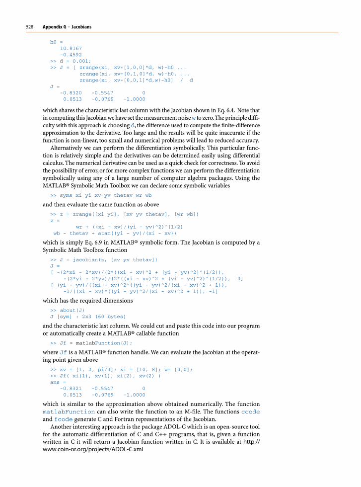
h0 = 10.8167 -0.4592>> d = 0.001;>> J = [ zrange(xi, xv+[1,0,0]*d, w)-h0 ... zrange(xi, xv+[0,1,0]*d, w)-h0, ... zrange(xi, xv+[0,0,1]*d,w)-h0] / dJ = -0.8320 -0.5547 0 0.0513 -0.0769 -1.0000

which shares the characteristic last column with the Jacobian shown in Eq. 6.4. Note thatin computing this Jacobian we have set the measurement noise w to zero. The principle diffi-culty with this approach is choosing d, the difference used to compute the finite-differenceapproximation to the derivative. Too large and the results will be quite inaccurate if thefunction is non-linear, too small and numerical problems will lead to reduced accuracy.

Alternatively we can perform the differentiation symbolically. This particular func-tion is relatively simple and the derivatives can be determined easily using differentialcalculus. The numerical derivative can be used as a quick check for correctness. To avoidthe possibility of error, or for more complex functions we can perform the differentiationsymbolically using any of a large number of computer algebra packages. Using theMATLAB® Symbolic Math Toolbox we can declare some symbolic variables

>> syms xi yi xv yv thetav wr wb

and then evaluate the same function as above

>> z = zrange([xi yi], [xv yv thetav], [wr wb])z = wr + ((xi - xv)/(yi - yv)^2)^(1/2) wb - thetav + atan((yi - yv)/(xi - xv))

which is simply Eq. 6.9 in MATLAB® symbolic form. The Jacobian is computed by aSymbolic Math Toolbox function

>> J = jacobian(z, [xv yv thetav])J =[ -(2*xi - 2*xv)/(2*((xi - xv)^2 + (yi - yv)^2)^(1/2)), -(2*yi - 2*yv)/(2*((xi - xv)^2 + (yi - yv)^2)^(1/2)), 0][ (yi - yv)/((xi - xv)^2*((yi - yv)^2/(xi - xv)^2 + 1)), -1/((xi - xv)*((yi - yv)^2/(xi - xv)^2 + 1)), -1]

which has the required dimensions

>> about(J)J [sym] : 2x3 (60 bytes)

and the characteristic last column. We could cut and paste this code into our programor automatically create a MATLAB® callable function

>> Jf = matlabFunction(J);

where Jf is a MATLAB® function handle. We can evaluate the Jacobian at the operat-ing point given above

>> xv = [1, 2, pi/3]; xi = [10, 8]; w= [0,0];>> Jf( xi(1), xv(1), xi(2), xv(2) )ans = -0.8321 -0.5547 0 0.0513 -0.0769 -1.0000

which is similar to the approximation above obtained numerically. The functionmatlabFunction can also write the function to an M-file. The functions ccodeand fcode generate C and Fortran representations of the Jacobian.

Another interesting approach is the package ADOL-C which is an open-source toolfor the automatic differentiation of C and C++ programs, that is, given a functionwritten in C it will return a Jacobian function written in C. It is available at http://www.coin-or.org/projects/ADOL-C.xml

Appendix G · Jacobians

HAppendix

Consider the discrete-time linear time-invariant system

with state vector x∈Rn. The vector u∈Rm is the input to the system at time k, forexample a velocity command, or applied forces and torques. The vector z∈Rp repre-sents the outputs of the system as measured by sensors. The matrix F∈Rn×n describesthe dynamics of the system, that is, how the states evolve with time. The matrix G∈Rn×m

describes how the inputs are coupled to the system states. The matrix H∈Rp×n de-scribes how the system states are mapped to the observed outputs.

To account for errors in the model (represented by F and G) and also unmodeled dis-turbances we introduce a Gaussian random variable v∈Rn termed the process noise.vhki∼N(0, V), that is, it has zero-mean and covariance V. The sensor measurementmodel H is not perfect either and this is modelled by measurement noise, another Gaussianrandom variable w∈Rp and whki∼N(0, W). The covariance matrices V∈Rn×n andW∈Rp×p are symmetric and positive definite.

The general problem that we confront is:

given a model of the system, the known inputs u and some noisy sensor measure-ments z, estimate the state of the system x.

In a robotic localization context x is the unknown pose of the robot, u is the com-mands sent to the motors and z is the output of various sensors on the robot. For aflying robot x could be the attitude, u the known forces applied to the airframe and zare the measured accelerations and angular velocities.

The Kalman filter is an optimal estimator for the case where the process andmeasurement noise are zero-mean Gaussian noise. The filter has two steps. The firstis a prediction of the state based on the previous state and the inputs that wereapplied.

(H.1)

(H.2)

where ' is the estimate of the state and Ï∈Rn×n is the estimated covariance, or uncer-tainty, in '. This is an open-loop step and its accuracy depends completely on the qual-ity of the model F and G and the ability to measure the inputs u. The notation k+ 1|kmakes explicit that the left-hand side is an estimate at time k+ 1 based on informa-tion from time k.

The prediction of P involves the addition of two positive-definite matrices so theuncertainty, given no new information and the uncertainty in the process, has increased.To improve things we have to introduce new information and that comes from mea-

Kalman Filter

530

surements obtained using sensors. The new information that is added is known as theinnovation

which is the difference between what the sensors measure and what the sensors arepredicted to measure. Some of the difference will be due to the noise in the sensor, themeasurement noise, but the remaining discrepancy indicates that the predicted statewas in error and does not properly explain the sensor observations.

The second step of the Kalman filter, the update step, uses the Kalman gain

(H.3)

to map the innovation into a correction for the predicted state, optimally tweaking theestimate based on what the sensors observed

Importantly we note that the uncertainty is now decreased or deflated, since thesecond term is subtracted from the predicted covariance. The term indicated by S isthe estimated covariance of the innovation and comes from the uncertainty in thestate and the measurement noise covariance. If the innovation has high uncertainty inrelation to some states this will be reflected in the Kalman gain which will make corre-spondingly small adjustment to those states.

The covariance update can also be written in the Joseph form

which has improved numerical properties and keeps the covariance estimate symmet-ric, but it is computationally more costly.

The equations above constitute the classical Kalman filter which is widely used inapplications from aerospace to econometrics. The filter has a number of importantcharacteristics. Firstly it is recursive, the output of one iteration is the input to thenext. Secondly, it is asynchronous. At a particular iteration if no sensor information isavailable we perform just the prediction step and not the update. In the case that thereare different sensors, each with their own H, and different sample rates, we just applythe update with the appropriate z and H. The Kalman-Bucy filter is a continuous-timeversion of this filter.

The filter must be initialized with some reasonable value of ' and Ï. The filter alsorequires our best estimates of the covariance of the process and measurement noise.In general we do not know V and W but we have some estimate Í and Ñ that we use inthe filter. From Eq. H.2 we see that if we overestimate Í our estimate of P will be largerthan it really is giving a pessimistic estimate of our certainty in the state. Conversely ifwe overestimate Í the filter will be overconfident of its estimate.

The covariance matrix Ï is rich in information. The diagonal elements Ïii are thevariance, or uncertainty, in the state xi. The off-diagonal elements Ïij are the correla-tions between states xi and xj. The correlations are critical in allowing any piece ofnew information to flow through to adjust multiple states that affect a particular pro-cess output.

The term FPhk|kiFThki in Eq. H.2 is interesting. Consider a one dimensional examplewhere F is a scalar and the state estimate úhki has a PDF that is a Gaussian with a mean–xhki and a variance σ2hki. The prediction equation maps the state and its Gaussian dis-

Appendix H · Kalman Filter

531

tribution to a new Gaussian distribution with a mean F–xhki and a variance F2σ

2hki. Theterm FPhk|kiFThki is the matrix form of this since

and appropriately scales the covariance. The term HPhk+1|kiHT in Eq. H.3 projects thecovariance of the state estimate into the observed values.

Now consider the case where the system is not linear

where f and h are now functions instead of constant matrices. f :Rn,Rm→R

n is afunction that describes the new state in terms of the previous state and the input to thesystem. The function h :Rn

→Rp maps the state vector to the sensor measurements.

To use the linear Kalman filter with a non-linear system we first make a local linearapproximation

where Fx∈Rn×n, Fu∈R

n×m, Fv∈Rn×n, Hx∈R

p×n and Hw∈Rp×p are Jacobians of the

functions f(·) and h(·) and are evaluated at each time step.We define a prediction error

and a measurement residual

which are linear and the Kalman filter equations above can be applied. The predictionstep of the extended Kalman filter is

and the update step is

where the innovation is

and the Kalman gain is

A fundamental problem with the extended Kalman filter is that PDFs of the ran-dom variables are no longer Gaussian after being operated on by the non-linear

Appendix H · Kalman Filter

532

functions f(·) and h(·). We can easily illustrate this by considering a scalar systemwith the PDF of the state estimate being the Gaussian N(5, 2)

>> x = linspace(0, 20, 100);>> g = gaussfunc(5, 2, x);>> plot(x, g);

Now consider the nonlinear function y= x2/5 and we overlay the PDF of y

>> y = x.^2 / 5;>> plot(y, g, 'r');

which is shown in Fig. H.1. We see that the PDF of y has its peak, the mode, at the samelocation but the distribution is no longer Gaussian. It has lost its symmetry so themean value will actually be greater than the mode. The Jacobians that appear in theEKF equations appropriately scale the covariance but the resulting non-Gaussian dis-tributions break the assumptions which guarantee that the Kalman filter is an optimalestimator. Alternatives include the iterated EKF described by Jazwinski (1970) or theUnscented Kalman Filter (UKF) (Julier and Uhlmann 2004) which uses discrete samplepoints to approximate the PDF.

Fig. H.1.PDF of the state x (blue) which isGaussian N(5, 2) and the PDF ofthe non-linear function x2/5 (red)

Appendix H · Kalman Filter

IAppendix

A point in n-dimensional Euclidean space x∈Rn is represented by a coordinatevector (x1, x2� xn). The corresponding point in homogeneous coordinates, or the pro-jective space x ∈ Pn is represented by a coordinate vector (²1, ²2� ²n+1). The Euclid-ean coordinates are related to the projective coordinates by

Conversely a homogeneous coordinate vector can be constructed from a Euclideancoordinate vector by

and the tilde is used to indicate that the quantity is homogeneous.The extra degree of freedom offered by projective coordinates has several advantages.

It allows points and lines at infinity, known as ideal points and lines, to be representedusing only real numbers. It also means that scale is unimportant, that is x and x′= αxboth represent the same Euclidean point for all α≠ 0. We express this as x� x′. Points inhomogeneous form can also be rotated with respect to a coordinate frame and translatedsimply by multiplying the homogeneous coordinate by an (n+ 1)× (n+ 1) homoge-neous transformation matrix.

Homogeneous vectors are important in computer vision when we consider pointsand lines that exist in a plane – a camera’s image plane. We can also consider that thehomogeneous form represents a ray in Euclidean space, and the relationship betweenpoints and rays is at the core of the projective transformation.

In P2 a line is defined by a 3-tuple, ~` = (`1, `2, `3)T, not all zero, and the equation of

the line is the set of all points

which expands to `1x+ `2y+ `3= 0 and can be manipulated into the more familiar rep-resentation of a line. Note that this form can represent a vertical line, parallel to the y-axis,which the familiar form y=mx+ c cannot. This is the point equation of a line. The non-homogeneous vector (`1, `2) is a normal to the line, and (−`2, `1) is parallel to the line.

A duality exists between points and lines. A point is defined by the intersection oftwo lines. If we write the point equations for two lines

~`1

Tp= 0 and ~`2

Tp= 0 their inter-section is the point

and is known as the line equation of a point. Similarly, a line joining two points p1and p2 is given by the cross-product

Homogeneous Coordinates

534

Consider the case of two parallel lines at 45° to the horizontal axis

>> l1 = [1 -1 0]';>> l2 = [1 -1 -1]';

which we can plot

>> plot_homline(l1, 'b')>> plot_homline(l2, 'r')

The intersection point of these parallel lines is>> cross(l1, l2)ans = 1 1 0

This is an ideal point since the third coordinate is zero – the equivalent Euclideanpoint would be at infinity. Projective coordinates allow points and lines at infinity tobe simply represented and manipulated without special logic to handle the specialcase of infinity.

The distance from a point p to a line ~` is

(I.1)

In the projective space P3 a duality exists between points and planes: three pointsdefine a plane, and the intersection of three planes defines a point.

Appendix I · Homogeneous Coordinates

JAppendix

A graph is an abstract representation of a set of objects connected by links anddepicted graphically as shown in Fig. J.1. Mathematically a graph is denotedG(V, E) where V, are called vertices or nodes, and the links, E, that connect somepairs of vertices are called edges or arcs. Edges can be directed (arrows) or un-directed as in this case. Edges can have an associated weight or cost associatedwith moving from one vertex to another. A sequence of edges from one vertexto another is a path, and a sequence that starts and ends at the same vertex is acycle. An edge from a vertex to itself is a loop. Graphs can be used to representtransport, communications or social networks, and this branch of mathematics isgraph theory.

The Toolbox provides a MATLAB® graph class called PGraph that supports em-bedded graphs where the vertices are associated with a point in an n-dimensionalspace. To create a new graph

>> g = PGraph()g = 2 dimensions 0 vertices 0 edges 0 components

and by default the nodes of the graph exist in a 2-dimensional space. We can add nodesto the graph

>> g.add_node( rand(2,1) );>> g.add_node( rand(2,1) );>> g.add_node( rand(2,1) );>> g.add_node( rand(2,1) );>> g.add_node( rand(2,1) );

Graphs

Fig. J.1.An example graph generated by

the PGraph class

536

and each has a random coordinate. A summary of the graph is given with its display method>> gg = 2 dimensions 5 vertices 0 edges 5 components

and shows that the graph has 5 nodes but no edges. The nodes are numbered 1 to 5and we add edges between pairs of nodes

>> g.add_edge(1, 2);>> g.add_edge(1, 3);>> g.add_edge(1, 4);>> g.add_edge(2, 3);>> g.add_edge(2, 4);>> g.add_edge(4, 5);>> gg = 2 dimensions 5 vertices 6 edges 1 components

By default the distance between the nodes is the Euclidean distance between the verti-ces but this can be overridden by a third argument to add_edge. This class supportsonly undirected graphs so the order of the vertices provided to add_edge does notmatter. The graph has one component, that is all the nodes are connected into onenetwork. The graph can be plotted by

>> g.plot('labels')

as shown in Fig. J.1. The vertices are shown as blue circles, and the option 'labels'displays the vertex index next to the circle. Edges are shown as black lines joining verti-ces. Note that only graphs embedded in 2- and 3-dimensional space can be plotted.

The neighbours of vertex 2 are>> g.neighbours(2)ans = 3 4 1

which are vertices connected to vertex 2 by edges. Each edge has a unique index andthe edges connecting to vertex 2 are

>> e = g.edges(2)e = 4 5 1

The cost or length of these edges is>> g.cost(e)ans = 0.9597 0.3966 0.6878

and clearly edge 5 has a lower cost than edges 4 and 1. Edge 5

>> g.vertices(5)ans = 2 4

joins vertices 2 and 4, and vertex 4 is clearly the closest neighbour of vertex 2. Fre-quently we wish to obtain a node’s neighbouring vertices and their distances at thesame time, and this can be achieved conveniently by

>> [n,c] = g.neighbours(2)n = 3 4 1c = 0.9597 0.3966 0.6878

Appendix J · Graphs

537

To plan a path through the graph we specify the goal vertex

>> g.goal(5)

which assigns every node in the graph its distance from the goal in a breadth-firstfashion. To find a path to the goal from a specified starting vertex is

>> g.path(3)ans = 3 2 4 5

In this case the shortest path from vertex 3 to vertex 5 is via vertices 2 and 4. The ver-tex closest to the coordinate (0.5, 0.5) is

>> g.closest([0.5, 0.5])ans = 4

The minimum cost path between any two nodes in the graph can be computed usingwell known algorithms such as A* (Nilsson 1971)

>> g.Astar(3, 5)ans = 3 2 4 5

or the earlier method by Dijstrka (1959).

Appendix J · Graphs

KAppendix

A commonly encountered problem is estimating the position of the peak of some dis-crete signal y(k), k ∈Z, see for example Fig. K.1a

>> load peakfit1>> plot(y, '-o')

Finding the peak to the nearest integer is straightforward using MATLAB’s max function

>> [ypk,xpk] = max(y)ypk = 0.9905xpk = 8

which indicates the peak occurs at the eighth element and has a value of 0.9905. In thiscase there is more than one peak and we can use the Toolbox function peak instead

>> [ypk,xpk] = peak(y)ypk = 0.9905 0.6718 -0.5799xpk = 8 25 16

which has returned three maxima in descending magnitude. A common test of thequality of a peak is its magnitude and the ratio of the height of the second peak to thefirst peak

>> ypk(2)/ypk(1)

which is called the ambiguity ratio and is ideally small.This signal is a sampled representation of a continuous underlying signal y(x) and

the real peak might lie between the samples. If we look at a zoomed version of thesignal, Fig. K.1b, we can see that although the eighth point is the maximum the ninth

Fig. K.1. Peak fitting. a A signalwith several local maxima; b close-up view of the first maxima withthe fitted curve (red) and the esti-mated peak (red-◊)

Peak Finding

540

point is only slightly lower so the peak lies somewhere between points eight and nine.A common approach is to fit a parabola

(K.1)

to the points surrounding the peak. For the discrete peak that occurs at (xpk, ypk) thenδ= 0 corresponds to xpk and the discrete x-coordinates on either side correspond toδ=−1 and δ=+1 respectively. Substituting the points (−1, y(−1)), (0, y(0)) and(1, y(1)) into Eq. K.1 we can write three equations

or in compact matrix form as

and then solve for the parabolic coefficients

(K.2)

The maxima of the parabola occurs when its derivative is zero

and substituting the values of a and b from Eq. K.2 we find the displacement of thepeak of the fitted parabola with respect to the discrete maxima

so the refined, or interpolated, position of the maxima is at

The coefficient a, which is negative for a maxima, indicates the sharpness of thepeak which can be useful in determining whether a peak is sufficiently sharp. A largemagnitude of a indicates a well defined sharp peak wheras a low value indicates a verybroad peak for which estimation of a refined peak detection may not be so accurate.

Continuing the earlier example we can use the Toolbox function peak to estimatethe refined peak positions

>> [ymax,xmax] = peak(y, 'interp', 2)ymax = 0.9905 0.6718 -0.5799xmax = 8.4394 24.7299 16.2438

where the argument after the 'interp' option indicates that a second order poly-nomial should be fitted. The fitted parabola is shown in red in Fig. K.1b and is plottedif the option 'plot' is given.

Appendix K · Peak Finding

541

If the signal has superimposed noise then there are likely to be multiple peaks,many of which are quite minor, and this can be overcome by specifying the scale of thepeak. For example the peaks that are greater than all other values within ±5 values inthe horizontal direction are

>> peak(y, 'scale', 5)ans = 0.9905 0.8730 0.6718

In this case the result is unchanged since the signal is fairly smooth.For a 2D signal we follow a similar procedure but instead fit a paraboloid

(K.3)

which has five coefficients that can be calculated from the centre value (the discretemaximum) and its four neighbours (north, south, east and west) using a similar pro-cedure to above. The displacement of the estimated peak with respect to the centralpoint is

In this case the coefficients a and b represent the sharpness of the peak inthe x- and y-directions, and the quality of the peak can be considered as beingmin a, b.

A 2D discrete signal was loaded from peakfit1 earlier

>> zz = 0.0800 0.2000 0.3202 0.4400 0.5600 0.0400 0.1717 0.3662 0.4117 0.5200 0.0002 0.2062 0.8766 0.4462 0.4802 -0.0400 0.0917 0.2862 0.3317 0.4400 -0.0800 0.0400 0.1602 0.2800 0.4000

In this small example it is clear that the peak is at element (3, 3) but programaticallythis is

>> [zmax,i] = max(z(:))zmax = 0.8766i = 13

and the maximum is at the thirteenth element in row-major order� which we convertto array subscripts

>> [ymax,xmax] = ind2sub(size(z), i)xmax = 3ymax = 3

We can find this more conveniently using the Toolbox function peak2

>> [zm,xy]=peak2(z)zm = 0.8766xy = 3 3

Counting the elements, starting with 1at the top-left down each column thenback to the top of the next rightmostcolumn.

Appendix K · Peak Finding

542

This function will return all non-local maxima where the size of the local region isgiven by the 'scale' option. As for the 1-dimensional case we can refine the esti-mate of the peak

>> [zm,xy]=peak2(z, 'interp')zm = 0.8839xy = 2.9637 3.1090

that is, the peak is at element (2.9637, 3.1090). When this process is applied to imagedata it is referred to as subpixel interpolation.

Appendix K · Peak Finding

Agrawal M, Konolige K, Blas M (2008) CenSurE: Center surround extremas for realtime feature detec-tion and matching. In: Forsyth D, Torr P, Zisserman A (eds) Lecture notes in computer science.Computer Vision – ECCV 2008, vol 5305. Springer-Verlag, Berlin Heidelberg, pp 102–115

Altmann SL (1989) Hamilton, Rodrigues, and the Quaternion scandal. Math Mag 62(5):291–308Andersen N, Ravn O, Sørensen A (1993) Real-time vision based control of servomechanical systems.

In: Chatila R, Hirzinger G (eds) Lecture Notes in Control and Information Sciences. ExperimentalRobotics II, vol 190. Springer-Verlag, Berlin Heidelberg, pp 388–402

Andersson RL (1989) Dynamic sensing in a ping-pong playing robot. IEEE T Robotic Autom 5(6):728–739

Antonelli G (2006) Underwater robots: Motion and force control of vehicle-manipulator systems, 2nd ed.Springer Tracts in Advanced Robotics, vol 2. Springer-Verlag, Berlin Heidelberg

Arkin RC (1999) Behavior-based robotics. The MIT PressArmstrong WW (1979) Recursive solution to the equations of motion of an N-link manipulator. In:

Proc. 5th World Congress on Theory of Machines and Mechanisms, Montreal, Jul, pp 1343–1346Armstrong BS (1988) Dynamics for robot control: Friction modelling and ensuring excitation during

parameter identification. Stanford UniversityArmstrong B (1989) On finding exciting trajectories for identification experiments involving systems

with nonlinear dynamics. Int J Robot Res 8(6):28Armstrong-Hélouvry B, Dupont P, De Wit CC (1994) A survey of models, analysis tools and compensa-

tion methods for the control of machines with friction. Automatica 30(7):1083–1138Arun KS, Huang TS, Blostein SD (1987) Least-squares fitting of 2 3-D point sets. IEEE T Pattern Anal

9(5):699–700Asada H (1983) A geometrical representation of manipulator dynamics and its application to arm

design. J Dyn Syst-T ASME 105:131Azarbayejani A, Pentland AP (1995) Recursive estimation of motion, structure, and focal length. IEEE

T Pattern Anal 17(6):562–575Baldridge AM, Hook SJ, Grove CI, Rivera G (2009) The ASTER spectral library version 2.0. Remote Sens

Environ 113(4):711–715Ballard DH (1981) Generalizing the Hough transform to detect arbitrary shapes. Pattern Recogn

13(2):111–122Banks J, Corke PI (2001) Quantitative evaluation of matching methods and validity measures for ste-

reo vision. Int J Robot Res 20(7):512–532Bar-Shalom Y, Fortmann T (1988) Tracking and data association. Mathematics in Science and Engi-

neering, vol 182. Academic PressBar-Shalom Y, Rong Li X, Thiagalingam Kirubarajan (2001) Estimation with applications to tracking

and navigation. Wiley-InterscienceBauer J, Sünderhauf N, Protzel P (2007) Comparing several implementations of two recently published

feature detectors. In: IFAC Symposium on Intelligent Autonomous Vehicles (IAV), ToulouseBay H, Ess A, Tuytelaars T, Van Gool L (2008) Speeded-up robust features (SURF). Comput Vis Image

Und 110(3):346–359Benosman R, Kang SB (2001) Panoramic vision: Sensors, theory, and applications. Springer-VerlagBenson KB (ed) (1986) Television engineering handbook. McGraw-HillBesl PJ, McKay HD (1992) A method for registration of 3-D shapes. IEEE T Pattern Anal 14(2):239–256Bhat DN, Nayar SK (2002) Ordinal measures for image correspondence. IEEE T Pattern Anal 20(4):

415–423Bishop CM (2006) Pattern recognition and machine learning. Information Science and Statistics.

Springer-Verlag, New YorkBolles RC, Baker HH, Marimont DH (1987) Epipolar-plane image analysis: An approach to determin-

ing structure from motion. Int J Comput Vision 1(1):7–55, MarBolles RC, Baker HH, Hannah MJ (1993) The JISCT stereo evaluation. In: Image Understanding Work-

shop: proceedings of a workshop held in Washington, DC apr 18–21, 1993. Morgan Kaufmann,pp 263

Bibliography

544 Bibliography

Borenstein J, Everett HR, Feng L (1996) Navigating mobile robots: Systems and techniques. AK Peters,Ltd. Natick, MA, USA, Out of print and available at http://www-personal.umich.edu/˜johannb/Papers/pos96rep.pdf

Borgefors G (1986) Distance transformations in digital images. Comput Vision Graph 34(3):344–371Bouguet J-Y (2010) Camera calibration toolbox for MATLAB. http://www.vision.caltech.edu/bouguetj/

calib_docBradski G, Kaehler A (2008) Learning OpenCV: Computer vision with the OpenCV library. O’Reilly

MediaBrady M, Hollerbach JM, Johnson TL, Lozano-Pérez T, Mason MT (eds) (1982) Robot motion: Planning

and control. The MIT PressBraitenberg V (1986) Vehicles: Experiments in synthetic psychology. The MIT PressBrockett RW (1983) Asymptotic stability and feedback stabilization. In: Brockett RW, Millmann RS,

Sussmann HJ (eds) Progress in mathematics. Differential geometric control theory, vol 27. pp 181–191Broida TJ, Chandrashekhar S, Chellappa R (1990) Recursive 3-D motion estimation from a monocular

image sequence. IEEE T Aero Elec Sys 26(4):639–656Brooks R (1986) A robust layered control system for a mobile robot. IEEE T Robotic Autom 2(1):14–23Brooks RA (1989) A robot that walks: Emergent behaviors from a carefully evolved network. MIT AI

Lab, Memo 1091Brown MZ, Burschka D, Hager GD (2003) Advances in computational stereo. IEEE T Pattern Anal

25(8):993–1008Buehler M, Iagnemma K, Singh S (eds) (2007) The 2005 DARPA grand challenge: The great robot race.

Springer Tracts in Advanced Robotics, vol 36. Springer-VerlagBuehler M, Iagnemma K, Singh S (eds) (2010) The DARPA urban challenge. Tracts in Advanced Robot-

ics, vol 56. Springer-VerlagBukowski R, Haynes LS, Geng Z, Coleman N, Santucci A, Lam K, Paz A, May R, DeVito M (1991) Robot

hand-eye coordination rapid prototyping environment. In: Proc ISIR, pp 16.15–16.28Buttazzo GC, Allotta B, Fanizza FP (1993) Mousebuster: A robot system for catching fast moving ob-

jects by vision. In: Proc. IEEE Int. Conf. Robotics and Automation, Atlanta. pp 932–937Calonder M, Lepetit V, Strecha C, Fua P (2010) BRIEF: Binary robust independent elementary features.

In: Daniilidis K, Maragos P, Paragios N (eds) Lecture notes in computer science. Computer Vision –ECCV 2010, vol 6311. Springer-Verlag, Berlin Heidelberg, pp 778–792

Canny JF (1983) Finding edges and lines in images. MIT, Artificial Intelligence Laboratory, AI-TR-720.Cambridge, MA

Canny J (1987) A computational approach to edge detection. Readings in computer vision: issues, prob-lems, principles, and paradigms 184

Chahl JS, Srinivasan MV (1997) Reflective surfaces for panoramic imaging. Appl Optics 31(36):8275–8285

Chaumette F (1990) La relation vision-commande: Théorie et application et des tâches robotiques.Université de Rennes 1

Chaumette F (1998) Potential problems of stability and convergence in image-based and position-based visual servoing. In: Kriegman DJ, Hager GD, Morse AS (eds) Lecture notes in control andinformation sciences. The confluence of vision and control, vol 237. Springer-Verlag, pp 66–78

Chaumette F (2004) Image moments: A general and useful set of features for visual servoing. IEEE TRobotic Autom 20(4):713–723

Chaumette F, Hutchinson S (2006) Visual servo control 1: Basic approaches. IEEE T Robotic Autom13(4):82–90

Chaumette F, Hutchinson S (2007) Visual servo control 2: Advanced approaches. IEEE T Robotic Autom14(1):109–118

Chaumette F, Rives P, Espiau B (1991) Positioning of a robot with respect to an object, tracking it andestimating its velocity by visual servoing. In: Proc. IEEE Int. Conf. Robotics and Automation, Seoul.pp 2248–2253

Chesi G, Hashimoto K (eds) (2010) Visual servoing via advanced numerical methods. Lecture notes incomputer science, 401. Springer-Verlag

Chiaverini S, Sciavicco L, Siciliano B (1991) Control of robotic systems through singularities. LectureNotes in Control and Information Sciences. Advanced Robot Control, Proceedings of the Interna-tional Workshop on Nonlinear and Adaptive Control: Issues in Robotics, vol 162. Springer-Verlag,pp 285–295

Chiuso A, Favaro P, Jin H, Soatto S (2002) Structure from motion causally integrated over time. IEEE TPattern Anal 24(4):523–535

Choset HM, Lynch KM, Hutchinson S, Kantor G, Burgard W, Kavraki LE, Thrun S (2005) Principles ofrobot motion. The MIT Press

Chum O, Matas J (2005) Matching with PROSAC – Progressive sample consensus. In: IEEE Conf. onComputer Vision and Pattern Recognition, vol 2. San Diego, pp 220–226

Colicchia G, Waltner C, Hopf M, Wiesner H (2009) The scallop’s eye – A concave mirror in the contextof biology. Physics Education 44(2):175–179

545Bibliography

Commission Internationale de L’Éclairage (1987) Colorimetry, 2nd ed. Commission Internationale deL’Eclairage, CIE No 15.2

Corke PI (1994) High-performance visual closed-loop robot control. University of Melbourne, Dept.Mechanical and Manufacturing Engineering. http://eprints.unimelb.edu.au/archive/00000547/01/thesis.pdf

Corke PI (1996a) In situ measurement of robot motor electrical constants. Robotica 14(4):433–436Corke PI (1996b) Visual control of robots: High-performance visual servoing. Mechatronics, vol 2. Re-

search Studies Press (John Wiley). Out of print and available at http://www.petercorke.com/bluebookCorke PI (2001) Mobile robot navigation as a planar visual servoing problem. In: Jarvis RA, Zelinsky A

(eds) Springer tracts in advanced robotics. Robotics Research: The 10th International Symposium,vol 6. IFRR, Lorne, pp 361–372

Corke PI (2007) A simple and systematic approach to assigning Denavit-Hartenberg parameters. IEEET Robotic Autom 23(3):590–594

Corke PI (2010) Spherical image-based visual servo and structure estimation. In: Proc. IEEE Int. Conf.Robotics and Automation, Anchorage, pp 5550–5555

Corke PI, Armstrong-Hélouvry BS (1994) A search for consensus among model parameters reported forthe PUMA 560 robot. In: Proc. IEEE Int. Conf. Robotics and Automation, San Diego. pp 1608–1613

Corke PI, Armstrong-Hélouvry B (1995) A meta-study of PUMA 560 dynamics: A critical appraisal ofliterature data. Robotica 13(3):253–258

Corke PI, Good MC (1992) Dynamic effects in high-performance visual servoing. In: Proc. IEEE Int.Conf. Robotics and Automation, Nice. pp 1838–1843

Corke PI, Good MC (1996) Dynamic effects in visual closed-loop systems. IEEE T Robotic Autom12(5):671–683

Corke PI, Hutchinson SA (2001) A new partitioned approach to image-based visual servo control. IEEET Robotic Autom 17(4):507–515

Corke PI, Dunn PA, Banks JE (1999) Frame-rate stereopsis using non-parametric transforms and pro-grammable logic. In: Proc. IEEE Int. Conf. Robotics and Automation, Detroit. pp 1928–1933

Corke PI, Strelow D, Singh S (2004) Omnidirectional visual odometry for a planetary rover. In: Proc.Int. Conf on Intelligent Robots and Systems (IROS), Sendai. pp 4007–4012

Corke PI, Spindler F, Chaumette F (2009) Combining Cartesian and polar coordinates in IBVS. In: Proc.Int. Conf on Intelligent Robots and Systems (IROS), St. Louis. pp 5962–5967

Craig JJ (1987) Adaptive control of mechanical manipulators. Addison-WesleyCraig JJ (2004) Introduction to robotics: Mechanics and control. Prentice HallCraig JJ, Hsu P, Sastry SS (1987) Adaptive control of mechanical manipulators. Int J Robot Res 6(2):16Cummins M, Newman P (2008) FAB-MAP: Probabilistic localization and mapping in the space of ap-

pearance. Int J Robot Res 27(6):647Cutting JE (1997) How the eye measures reality and virtual reality. Behav Res Meth Ins C 29(1):27–36Daniilidis K, Klette R (eds) (2006) Imaging beyond the pinhole camera. Computational Imaging, vol 33.

Springer-VerlagDavison AJ, Reid ID, Molton ND, Stasse O (2007) MonoSLAM: Real-time single camera SLAM. IEEE T

Pattern Anal 29(6):1052–1067Deguchi K (1998) Optimal motion control for image-based visual servoing by decoupling translation

and rotation. In: Proc. Int. Conf on Intelligent Robots and Systems (IROS), Victoria, Canada. Oct,pp 705–711

Dellaert F, Seitz SM, Thorpe CE, Thrun S (2000) Structure from motion without correspondence. In:IEEE Conf. on Computer Vision and Pattern Recognition, Hilton Head Island, SC. pp 557–564

DeMenthon D, Davis LS (1992) Exact and approximate solutions of the perspective-three-point prob-lem. IEEE T Pattern Anal 14(11):1100–1105

Denavit J, Hartenberg RS (1955) A kinematic notation for lower-pair mechanisms based on matrices.J Appl Mech-T ASME 22(1):215–221

Deo AS, Walker ID (1995) Overview of damped least-squares methods for inverse kinematics of robotmanipulators. J Intell Robot Syst 14(1):43–68

Deriche R, Giraudon G (1993) A computational approach for corner and vertex detection. Int J ComputVision 10(2):101–124

DeWitt BA, Wolf PR (2000) Elements of photogrammetry (with applications in GIS). McGraw-HillHigher Education

Dickmanns ED (2007) Dynamic vision for perception and control of motion. Springer-Verlag, LondonDickmanns ED, Graefe V (1988a) Applications of dynamic monocular machine vision. Mach Vision

Appl 1:241–261Dickmanns ED, Graefe V (1988b) Dynamic monocular machine vision. Mach Vision Appl 1(4):

223–240Dickmanns ED, Zapp A (1987) Autonomous high speed road vehicle guidance by computer vision. In:

Tenth Triennial World Congress of the International Federation of Automatic Control, vol 4. Munich,pp 221–226

Dijkstra EW (1959) A note on two problems in connexion with graphs. Numer Math 1(1):269–271

546 Bibliography

Dougherty ER, Lotufo RA (2003) Hands-on morphological image processing. Society of Photo-Opti-cal Instrumentation Engineers (SPIE)

Duda RO, Hart PE (1972) Use of the Hough transformation to detect lines and curves in pictures.Commun ACM 15(1):11–15

Espiau B, Chaumette F, Rives P (1992) A new approach to visual servoing in robotics. IEEE T RoboticAutom 8(3):313–326

Everett HR (1995) Sensors for mobile robots: Theory and application. AK Peters, Ltd.Faugeras OD (1993) Three-dimensional computer vision: A geometric viewpoint. The MIT PressFaugeras OD, Lustman F (1988) Motion and structure from motion in a piecewise planar environment.

Int J Pattern Recogn 2(3):485–508Faugeras O, Luong QT, Papadopoulou T (2001) The geometry of multiple images: The laws that govern

the formation of images of a scene and some of their applications. The MIT PressFeatherstone R (1987) Robot dynamics algorithms. Kluwer AcademicFeddema JT (1989) Real time visual feedback control for hand-eye coordinated robotic systems. Purdue

UniversityFeddema JT, Mitchell OR (1989) Vision-guided servoing with feature-based trajectory generation. IEEE

T Robotic Autom 5(5):691–700Feddema JT, Lee CSG, Mitchell OR (1991) Weighted selection of image features for resolved rate visual

feedback control. IEEE T Robotic Autom 7(1):31–47Felzenszwalb PF, Huttenlocher DP (2004) Efficient graph-based image segmentation. Int J Comput

Vision 59(2):167–181Ferguson D, Stentz A (2006) Using interpolation to improve path planning: The Field D* algorithm.

J Field Robotics 23(2):79–101Fischler MA, Bolles RC (1981) Random sample consensus: A paradigm for model fitting with applica-

tions to image analysis and automated cartography. Commun ACM 24(6):381–395Fisher RB (2004) The PETS04 surveillance ground-truth data sets. In: Proc. 6th IEEE International

Workshop on Performance Evaluation of Tracking and Surveillance, Prague. pp 1–5Fomena R, Chaumette F (2007) Visual servoing from spheres using a spherical projection model. In:

Proc. IEEE Int. Conf. Robotics and Automation, Rome, pp 2080–2085Förstner W (1994) A framework for low level feature extraction. In: Ecklundh J-O (ed) Lecture notes in

computer science. Computer Vision – ECCV 1994, vol 800. Springer-Verlag, Berlin Heidelberg,pp 383–394

Förstner W, Gülch E (1987) A fast operator for detection and precise location of distinct points, cornersand centres of circular features. In: ISPRS Intercommission Workshop, Interlaken, pp 149–155

Forsyth DA, Ponce J (2002) Computer vision: A modern approach. Prentice HallFreeman H (1974) Computer processing of line-drawing images. ACM Comput Surv 6(1):57–97Friedman DP, Felleisen M, Bibby D (1987) The little LISPer. MIT PressFunda J, Taylor RH, Paul RP (1990) On homogeneous transforms, quaternions, and computational

efficiency. IEEE T Robotic Autom 6(3):382–388Gans NR, Hutchinson SA, Corke PI (2003) Performance tests for visual servo control systems, with

application to partitioned approaches to visual servo control. Int J Robot Res 22(10–11):955Gautier M, Khalil W (1992) Exciting trajectories for the identification of base inertial parameters of

robots. Int J Robot Res 11(4):362Geraerts R, Overmars MH (2004) A comparative study of probabilistic roadmap planners. In: Boissonnat

J-D, Burdick J, Goldberg K, Hutchinson S (eds) Springer Tracts in Advanced Robotics. AlgorithmicFoundations of Robotics V, vol 7. Springer-Verlag, pp 43–58

Geyer C, Daniilidis K (2000) A unifying theory for central panoramic systems and practical implica-tions. In: Vernon D (ed) Lecture notes in computer science. Computer vision – ECCV 2000, vol 1843.Springer-Verlag, pp 445–461

Goldberg K (ed) (2001) The robot in the garden: Telerobotics and telepistemology in the age of theinternet. The MIT Press

Goldberg K, Siegwart R (eds) (2001) Beyond webcams: An introduction to online robots. The MITPress

Gonzalez R, Woods R (2008) Digital image processing, 3rd ed. Prentice HallGonzalez R, Woods R, Eddins S (2009) Digital image processing using MATLAB, 2nd ed. GatesmarkGroves PD (2008) Principles of GNSS, inertial, and multisensor integrated navigation systems. Artech

HouseHager GD, Toyama K (1998) X Vision: A portable substrate for real-time vision applications. Comput

Vis Image Und 69(1):23–37Hamel T, Mahony R (2002) Visual servoing of an under-actuated dynamic rigid-body system: An im-

age based approach. IEEE T Robotic Autom 18(2):187–198Hamel T, Mahony R, Lozano R, Ostrowski J (2002) Dynamic modelling and configuration stabilization for

an X4-flyer. IFAC World Congress 1(2), p 3. Available at: http://citeseerx.ist.psu.edu/viewdoc/downloadHansen P, Corke PI, Boles W (2010) Wide-angle visual feature matching for outdoor localization. Int J

Robot Res 29(1–2):267–297

547Bibliography

Harris CG, Stephens MJ (1988) A combined corner and edge detector. In: Proceedings of the FourthAlvey Vision Conference, Manchester. pp 147–151

Hart PE (2009) How the Hough transform was invented [DSP history]. IEEE Signal Proc Mag 26(6):18–22

Hartenberg RS, Denavit J (1964) Kinematic synthesis of linkages. McGraw-Hill New York, availableonline at http://kmoddl.library.cornell.edu/bib.php?m=23

Hartley R, Zisserman A (2003) Multiple view geometry in computer vision. Cambridge University Press,New York

Harvey P (nd) ExifTool. http://www.sno.phy.queensu.ca/~phil/exiftoolHashimoto K (ed) (1993) Visual servoing. In: Robotics and automated systems, vol 7. World ScientificHashimoto K, Kimoto T, Ebine T, Kimura H (1991) Manipulator control with image-based visual servo.

In: Proc. IEEE Int. Conf. Robotics and Automation, Seoul. pp 2267–2272Hellerstein JL, Diao Y, Parekh S, Tilbury DM (2004) Feedback control of computing systems. IEEE Press

– WileyHill J, Park WT (1979) Real time control of a robot with a mobile camera. In: Proc. 9th ISIR, SME, Wash-

ington, DC. Mar, pp 233–246Hoag D (1963) Consideration of Apollo IMU gimbal lock. MIT Instrumentation Laboratory, E–1344,

http://www.hq.nasa.gov/alsj/e-1344.htmHollerbach JM (1980) A recursive Lagrangian formulation of manipulator dynamics and a compara-

tive study of dynamics formulation complexity. IEEE T Syst Man Cyb 10(11):730–736, NovHollerbach JM (1982) Dynamics. In: Brady M, Hollerbach JM, Johnson TL, Lozano-Perez T, Mason MT

(eds) Robot motion – Planning and control. The MIT Press, pp 51–71Horaud R, Canio B, Leboullenx O (1989) An analytic solution for the perspective 4-point problem.

Comput Vision Graph 47(1):33–44Horn BKP (1987) Closed-form solution of absolute orientation using unit quaternions. J Opt Soc Am A

4(4):629–642Horn BKP, Hilden HM, Negahdaripour S (1988) Closed-form solution of absolute orientation using

orthonormal matrices. J Opt Soc Am A 5(7):1127–1135Hosoda K, Asada M (1994) Versatile visual servoing without knowledge of true Jacobian. In: Proc. Int.

Conf on Intelligent Robots and Systems (IROS), Munich. Sep, pp 186–193Howard TM, Green CJ, Kelly A, Ferguson D (2008) State space sampling of feasible motions for high-

perfor-mance mobile robot navigation in complex environments. J Field Robotics 25(6–7):325–345Hu MK (1962) Visual pattern recognition by moment invariants. IRE T Inform Theor 8:179–187Huang TS, Netravali AN (1994) Motion and structure from feature correspondences: A review. P IEEE

82(2):252–268Humenberger M, Zinner C, Kubinger W (2009) Performance evaluation of a census-based stereo match-

ing algorithm on embedded and multi-core hardware. In: Proc. 19th Int. Symp. on Image and SignalProcessing and Analysis (ISPA). Sep, pp 388–393

Hunt RWG (1987) The reproduction of colour, 4th ed. Fountain PressHunter RS, Harold RW (1987) The measurement of appearance. John WileyHutchinson S, Hager G, Corke PI (1996) A tutorial on visual servo control. IEEE T Robotic Autom

12(5):651–670Iwatsuki M, Okiyama N (2002a) A new formulation of visual servoing based on cylindrical coordinate

system with shiftable origin. In: Proc. Int. Conf on Intelligent Robots and Systems (IROS), Lausanne,pp 354–359

Iwatsuki M, Okiyama N (2002b) Rotation-oriented visual servoing based on cylindrical coordinates.In: Proc. IEEE Int. Conf. Robotics and Automation, Washington, DC. May, pp 4198–4203

Izaguirre A, Paul RP (1985) Computation of the inertial and gravitational coefficients of the dynamicsequations for a robot manipulator with a load. In: Proc. IEEE Int. Conf. Robotics and Automation.Mar, pp 1024–1032

Jägersand M, Fuentes O, Nelson R (1996) Experimental evaluation of uncalibrated visual servoing forpre-cision manipulation. In: Proc. IEEE Int. Conf. Robotics and Automation, Albuquerque, NM.pp 2874–2880

Jarvis RA, Byrne JC (1988) An automated guided vehicle with map building and path finding capabili-ties. In: Robotics Research: The Fourth international symposium. The MIT Press, pp 497–504

Jazwinski AH (1970) Stochastic processes and filtering theory. Academic PressJebara T, Azarbayejani A, Pentland A (1999) 3D structure from 2D motion. IEEE Signal Proc Mag 16(3):66–84Julier SJ, Uhlmann JK (2004) Unscented filtering and nonlinear estimation. P IEEE 92(3):401–422Kahn ME (1969) The near-minimum time control of open-loop articulated kinematic linkages. Stanford

University, AIM-106Kálmán RE (1960) A new approach to linear filtering and prediction problems. J Basic Eng-T Asme 82(1):

35–45Kane TR, Levinson DA (1983) The use of Kane’s dynamical equations in robotics. Int J Robot Res 2(3):3–21Kavraki LE, Svestka P, Latombe JC, Overmars MH (1996) Probabilistic roadmaps for path planning in

high-dimensional configuration spaces. IEEE T Robotic Autom 12(4):566–580

548 Bibliography

Kelly R (1996) Robust asymptotically stable visual servoing of planar robots. IEEE T Robotic Autom12(5):759–766

Kelly R, Carelli R, Nasisi O, Kuchen B, Reyes F (2002a) Stable visual servoing of camera-in-hand ro-botic systems. IEEE-ASME T Mech 5(1):39–48

Kelly R, Shirkey P, Spong MW (2002b) Fixed-camera visual servo control for planar robots. In: Proc.IEEE Int. Conf. Robotics and Automation. IEEE, Washington, DC, pp 2643–2649

Khalil W, Creusot D (1997) SYMORO+: A system for the symbolic modelling of robots. Robotica 15(2):153–161

Khalil W, Dombre E (2002) Modeling, identification and control of robots. Kogan Page ScienceKing-Hele D (2002) Erasmus Darwin’s improved design for steering carriages and cars. Notes and

Records of the Royal Society of London 56(1):41–62Klafter RD, Chmielewski TA, Negin M (1989) Robotic engineering – An integrated approach. Prentice-HallKlein CA, Huang CH (1983) Review of pseudoinverse control for use with kinematically redundant

manipulators. IEEE T Syst Man Cyb 13:245–250Klette R, Kruger N, Vaudrey T, Pauwels K, van Hulle M, Morales S, Kandil F, Haeusler R, Pugeault N,

Rabe C (2011) Performance of correspondence algorithms in vision-based driver assistance usingan online image sequence database. IEEE T Veh Technol 60(5):2012–2026

Koenderink JJ (1984) The structure of images. Biol Cybern 50(5):363–370Koenig S, Likhachev M (2002) D* Lite. In: Proceedings of the National Conference on Artificial Intelli-

gence, Menlo Park, CA; Cambridge, MA; London; AAAI Press; MIT Press; 1999, pp 476–483Koenig S, Likhachev M (2005) Fast replanning for navigation in unknown terrain. IEEE T Robo-

tic Autom 21(3):354–363Kriegman DJ, Hager GD, Morse AS (eds) (1998) The confluence of vision and control. Lecture Notes in

Control and Information Sciences, vol 237. Springer-VerlagKuipers JB (1999) Quaternions and rotation sequences: A primer with applications to orbits, aeroespace

and virtual reality. Princeton University PressLamport L (1994) LATEX: A document preparation system. User’s guide and reference manual. Addison-

Wesley Publishing Company, Reading, MaLaValle SM (1998) Rapidly-exploring random trees: A new tool for path planning. Computer Science

Dept., Iowa State University, TR 98–11LaValle SM (2006) Planning algorithms. Cambridge Univ PressLaValle SM, Kuffner JJ (2001) Randomized kinodynamic planning. Int J Robot Res 20(5):378–400Leavers VF (1993) Which Hough transform? Comput Vis Image Und 58(2):250–264Lee CSG, Lee BH, Nigham R (1983) Development of the generalized D’Alembert equations of motion

for mechanical manipulators. In: Proc. 22nd CDC, San Antonio, Texas. pp 1205–1210Lepetit V, Moreno-Noguer F, Fua P (2009) EPnP: An accurate O(n) solution to the PnP problem. Int J

Comput Vision 81(2):155–166Li H, Hartley R (2006) Five-point motion estimation made easy. In: 18th Int. Conf. on Pattern Recogni-

tion ICPR 2006, Hong Kong, pp 630–633Lin Z, Zeman V, Patel RV (1989) On-line robot trajectory planning for catching a moving object. In:

Proc. IEEE Int. Conf. Robotics and Automation. pp 1726–1731Lindeberg T (1993) Scale-space theory in computer vision. Springer-VerlagLloyd J, Hayward V (1991) Real-time trajectory generation using blend functions. In: Proc. IEEE Int.

Conf. Robotics and Automation, Seoul. pp 784–789Longuet-Higgins H (1981) A computer algorithm for reconstruction of a scene from two projections.

Nature 293:133–135Lourakis MIA, Argyros AA (2009) SBA: A software package for generic sparse bundle adjustment.

ACM T Math Software 36(1):1–30Lovell J, Kluger J (1994) Apollo 13. Coronet BooksLowe DG (1991) Fitting parametrized three-dimensional models to images. IEEE T Pattern Anal 13(5):

441–450Lowe DG (2004) Distinctive image features from scale-invariant keypoints. Int J Comput Vision 60(2):

91–110Lucas SM (2005) ICDAR 2005 text locating competition results. In: Proceedings of the Eighth Interna-

tional Conference on Document Analysis and Recognition, ICDAR05, pp 80–84Lucas BD, Kanade T (1981) An iterative image registration technique with an application to stereo

vision. In: International joint conference on artificial intelligence (IJCAI), Vancouver, vol 2. http://ijcai.org/Past%20Proceedings/IJCAI-81-VOL-2/PDF/017.pdf, pp 674–679

Luh JYS, Walker MW, Paul RPC (1980) On-line computational scheme for mechanical manipulators.J Dyn Syst-T ASME 102(2):69–76

Lumelsky V, Stepanov A (1986) Dynamic path planning for a mobile automaton with limited informa-tion on the environment. IEEE T Automat Contr 31(11):1058–1063

Luong QT (1992) matrice fondamentale et autocalibration en vision par ordinateur. Universitéde Paris-Sud, Orsay, France

Ma Y, Kosecka J, Soatto S, Sastry S (2003) An invitation to 3D. Springer-Verlag

549Bibliography

Maimone M, Cheng Y, Matthies L (2007) Two years of visual odometry on the Mars exploration rovers.J Field Robotics 24(3):169–186

Makhlin AG (1985) Stability and sensitivity of servo vision systems. In: Proc 5th Int Conf on RobotVision and Sensory Controls – RoViSeC 5. IFS (Publications), Amsterdam, pp 79–89

Malis E, Vargas M (2007) Deeper understanding of the homography decomposition for vision-basedcontrol. INRIA, 6303

Malis E, Chaumette F, Boudet S (1999) 2-1/2D visual servoing. IEEE T Robotic Autom 15(2):238–250Marey M, Chaumette F (2008) Analysis of classical and new visual servoing control laws. In: Proc. IEEE

Int. Conf. Robotics and Automation, Pasadena, pp 3244–3249Mariottini GL, Prattichizzo D (2005) EGT for multiple view geometry and visual servoing: Robotics

vision with pinhole and panoramic cameras. IEEE T Robotic Autom 12(4):26–39Mariottini GL, Oriolo G, Prattichizzo D (2007) Image-based visual servoing for nonholonomic mobile

robots using epipolar geometry. IEEE T Robotic Autom 23(1):87–100Marr D (2010) Vision: A computational investigation into the human representation and processing of

visual information. The MIT PressMartin D, Fowlkes C, Tal D, Malik J (2001) A database of human segmented natural images and its

application to evaluating segmentation algorithms and measuring ecological statistics. Proc. 8th Int’lConf. Computer Vision, vol 2, pp 416–423

Masutani Y, Mikawa M, Maru N, Miyazaki F (1994) Visual servoing for non-holonomic mobile robots.In: Proc. Int. Conf on Intelligent Robots and Systems (IROS), Munich, pp 1133–1140

Matariõ MJ (2007) The robotics primer. MIT PressMatas J, Chum O, Urban M, Pajdla T (2004) Robust wide-baseline stereo from maximally stable extremal

regions. Image Vision Comput 22(10):761–767Matthews ND, An PE, Harris CJ (1995) Vehicle detection and recognition for autonomous intelligent

cruise control. Image, Speech and Intelligent Systems 6Matthies L (1992) Stereo vision for planetary rovers: Stochastic modeling to near real-time implemen-

tation. Int J Comput Vision 8(1):71–91Mayeda H, Yoshida K, Osuka K (1990) Base parameters of manipulator dynamic models. IEEE T Ro-

botic Autom 6(3):312–321McLauchlan PF (1999) The variable state dimension filter applied to surface-based structure from

motion. University of Surrey, VSSP-TR-4/99Merlet JP (2006) Parallel robots. Kluwer AcademicMettler B (2003) Identification modeling and characteristics of miniature rotorcraft. Kluwer AcademicMiãuïík B, Pajdla T (2003) Estimation of omnidirectional camera model from epipolar geometry. In:

IEEE Conf. on Computer Vision and Pattern Recognition, Madison, vol 1. pp 485–490Middleton RH, Goodwin GC (1988) Adaptive computed torque control for rigid link manipulations.

Syst Control Lett 10(1):9–16Mikolajczyk K, Schmid C (2004) Scale and affine invariant interest point detectors. Int J Comput Vision

60(1):63–86Mikolajczyk K, Schmid C (2005) A performance evaluation of local descriptors. IEEE T Pattern Anal

27(10):1615–1630Mindell DA (2008) Digital Apollo. MIT PressMolton N, Brady M (2000) Practical structure and motion from stereo when motion is unconstrained.

Int J Comput Vision 39(1):5–23Montemerlo M, Thrun S, Koller D, Wegbreit B (2002) FastSLAM: A factored solution to the simulta-

neous localization and mapping problem. In: Proceedings of the AAAI National Conference onArtificial Intelligence. AAAI, Edmonton, Canada

Moravec H (1980) Obstacle avoidance and navigation in the real world by a seeing robot rover. StanfordUniversity

Morel G, Liebezeit T, Szewczyk J, Boudet S, Pot J (2000) Explicit incorporation of 2D constraints invision based control of robot manipulators. In: Corke PI, Trevelyan J (eds) Lecture notes in controland information sciences. Experimental robotics VI, vol 250. Springer-Verlag, pp 99–108

NASA (1970) Apollo 13: Technical air-to-ground voice transcription. Test Division, Apollo SpacecraftProgram Office, http://www.hq.nasa.gov/alsj/a13/AS13_TEC.PDF

Nayar SK (1997) Catadioptric omnidirectional camera. In: IEEE Conf. on Computer Vision and PatternRecognition, Los Alamitos, CA, pp 482–488

Nethery JF, Spong MW (1994) Robotica: A mathematica package for robot analysis. IEEE T RoboticAutom 1(1):13–20

Ng J, Bräunl T (2007) Performance comparison of bug navigation algorithms. J Intell Robot Syst50(1):73–84

Niblack W (1985) An introduction to digital image processing. Strandberg Publishing CompanyBirkeroed, Denmark

Nilsson NJ (1971) Problem-solving methods in artificial intelligence. McGraw-HillNistér D (2003) An efficient solution to the five-point relative pose problem. In: IEEE Conf. on Com-

puter Vision and Pattern Recognition, vol. 2. Madison, pp 195–202

550 Bibliography

Nistér D, Naroditsky O, Bergen J (2006) Visual odometry for ground vehicle applications. J Field Ro-botics 23(1):3–20

Nixon MS, Aguado AS (2008) Feature extraction and image processing. Academic PressNoble JA (1988) Finding corners. Image Vision Comput 6(2):121–128Okutomi M, Kanade T (1993) A multiple-baseline stereo. IEEE T Pattern Anal 15(4):353–363Ollis M, Herman H, Singh S (1999) Analysis and design of panoramic stereo vision using equi-angular pixel

cameras. Robotics Institute, Carnegie Mellon University, CMU-RI-TR-99-04, Citeseer, Pittsburgh, PAOrin DE, McGhee RB, Vukobratovic M, Hartoch G (1979) Kinematics and kinetic analysis of open-

chain linkages utilizing newton-euler methods. Math Biosci 43(1/2):107–130Ortega R, Spong MW (1989) Adaptive motion control of rigid robots: A tutorial. Automatica 25(6):877–888Otsu N (1975) A threshold selection method from gray-level histograms. Automatica 11:285–296Papanikolopoulos NP, Khosla PK (1993) Adaptive robot visual tracking: Theory and experiments. IEEE

T Automat Contr 38(3):429–445Papanikolopoulos NP, Khosla PK, Kanade T (1993) Visual tracking of a moving target by a camera

mounted on a robot: A combination of vision and control. IEEE T Robotic Autom 9(1):14–35Park FC (1994) Computational aspects of the product-of-exponentials formula for robot kinematics.

Automatic Control, IEEE Transactions on 39(3):643–647Paul R (1972) Modelling, trajectory calculation and servoing of a computer controlled arm. Stanford

UniversityPaul R (1979) Manipulator Cartesian path control. IEEE T Syst Man Cyb 9:702–711Paul RP (1981) Robot manipulators: Mathematics, programming, and control. MIT Press, Cambridge,

MassachusettsPaul RP, Shimano B (1978) Kinematic control equations for simple manipulators. In: IEEE Conference

on Decision and Control, vol 17. pp 1398–1406Paul RP, Zhang H (1986) Computationally efficient kinematics for manipulators with spherical wrists

based on the homogeneous transformation representation. Int J Robot Res 5(2):32–44Piepmeier JA, McMurray G, Lipkin H (1999) A dynamic quasi-Newton method for uncalibrated visual

servoing. In: Proc. IEEE Int. Conf. Robotics and Automation, Detroit. pp 1595–1600Pilu M (1997) A direct method for stereo correspondence based on singular value decomposition. In:

Proc. Computer Vision and Pattern Recognition, IEEE Computer Society, San Juan, pp 261–266Pollefeys M, Nistér D, Frahm JM, Akbarzadeh A, Mordohai P, Clipp B, Engels C, Gallup D, Kim SJ,

Merrell P, et al. (2008) Detailed real-time urban 3D reconstruction from video. Int J Comput Vi-sion 78(2):143–167, Jul

Pomerleau D, Jochem T (1995) No hands across America Journal. http://www.cs.cmu.edu/~tjochem/nhaa/Journal.html

Pomerleau D, Jochem T (1996) Rapidly adapting machine vision for automated vehicle steering. IEEEExpert 11(1):19–27

Pounds P (2007) Design, construction and control of a large quadrotor micro air vehicle. AustralianNational University

Pounds P, Mahony R, Gresham J, Corke PI, Roberts J (2004) Towards dynamically-favourable quad-rotor aerial robots. In: Proc. Australasian Conf. on Robotics and Automation, Canberra

Pounds P, Mahony R, Corke PI (2006) A practical quad-rotor robot. In: Proc. Australasian Conf. onRobotics and Automation, Auckland

Pounds P, Mahony R, Corke PI (2007) System identification and control of an aerobot drive system. In:Information, Decision and Control. pp 154–159

Poynton CA (2003) Digital video and HDTV: Algorithms and interfaces. Morgan KaufmannPress WH, Teukolsky SA, Vetterling WT, Flannery BP (2007) Numerical recipes, 3rd ed. Cambridge Uni-

versity PressProuty RW (2002) Helicopter performance, stability, and control. KriegerPynchon T (2006) Against the day. Jonathan CapeRabaud V (nd) Vincent’s structure from motion toolbox. http://vision.ucsd.edu/~vrabaud/toolboxRives P, Chaumette F, Espiau B (1989) Positioning of a robot with respect to an object, tracking it and

estimating its velocity by visual servoing. In: Hayward V, Khatib O (eds) Lecture Notes in Controland Information Sciences. Experimental Robotics I, vol 139. Springer-Verlag, pp 412–428

Rizzi AA, Koditschek DE (1991) Preliminary experiments in spatial robot juggling. In: Chatila R,Hirzinger G (eds) Lecture Notes in Control and Information Sciences. Experimental Robotics II,vol 190. Springer-Verlag, pp 282–298

Roberts LG (1963) Machine perception of three-dimensional solids. MIT Lincoln Laboratory, TR 315,http://www.packet.cc/files/mach-per-3D-solids.html

Rosenfield GH (1959) The problem of exterior orientation in photogrammetry. Photogramm Eng25(4):536–553

Rosten E, Porter R, Drummond T (2010) FASTER and better: A machine learning approach to cornerdetection. IEEE T Pattern Anal 32:105–119

Sakaguchi T, Fujita M, Watanabe H, Miyazaki F (1993) Motion planning and control for a robot per-former. In: Proc. IEEE Int. Conf. Robotics and Automation, Atlanta. May, pp 925–931

551Bibliography

Salvi J, Matabosch C, Fofi D, Forest J (2007) A review of recent range image registration methods withaccuracy evaluation. Image Vision Comput 25(5):578–596

Samson C, Espiau B, Le Borgne M (1990) Robot control: The task function approach. Oxford UniversityPress

Sanderson AC, Weiss LE, Neuman CP (1987) Dynamic sensor-based control of robots with visual feed-back. IEEE T Robotic Autom RA-3(5):404–417

Scharstein D, Pal C (2007) Learning conditional random fields for stereo. In: IEEE Computer SocietyConference on Computer Vision and Pattern Recognition (CVPR 2007), Minneapolis, MN

Scharstein D, Szeliski R (2002) A taxonomy and evaluation of dense two-frame stereo correspondencealgorithms. Int J Comput Vision 47(1):7–42

Serra J (1983) Image analysis and mathematical morphology. Academic PressShi J, Tomasi C (1994) Good features to track. In: Proc. Computer Vision and Pattern Recognition. IEEE

Computer Society, Seattle, pp 593–593Shirai Y (1987) Three-dimensional computer vision. Springer-Verlag, New YorkShirai Y, Inoue H (1973) Guiding a robot by visual feedback in assembling tasks. Pattern Recogn

5(2):99–106Shoemake K (1985) Animating rotation with quaternion curves. In: Proceedings of ACM SIGGRAPH,

San Francisco, pp 245–254Siciliano B, Khatib O (eds) (2008) Springer handbook of robotics. Springer-Verlag, New YorkSiciliano B, Sciavicco L, Villani L, Oriolo G (2008) Robotics: Modelling, planning and control. Springer-

VerlagSiegwart R, Nourbakhsh IR, Scaramuzza D (2011) Introduction to autonomous mobile robots. The

MIT PressSilver WM (1982) On the equivalance of Lagrangian and Newton-Euler dynamics for manipulators. Int

J Robot Res 1(2):60–70Sivic J, Zisserman A (2003) Video Google: A text retrieval approach to object matching in videos. In:

Proc. Ninth IEEE Int. Conf. on Computer Vision, pp 1470–1477Skaar SB, Brockman WH, Hanson R (1987) Camera-space manipulation. Int J Robot Res 6(4):20–32Skofteland G, Hirzinger G (1991) Computing position and orientation of a freeflying polyhedron from

3D data. In: Proc. IEEE Int. Conf. Robotics and Automation, Seoul. pp 150–155Slama CC (ed) (1980) Manual of photogrammetry, 4th ed. American Society of PhotogrammetrySobel D (1996) Longitude: The true story of a lone genius who solved the greatest scientific problem of

his time. Fourth Estate LondonSoille P (2003) Morphological image analysis: Principles and applications. Springer-VerlagSpong MW (1989) Adaptive control of flexible joint manipulators. Syst Control Lett 13(1):15–21Spong MW, Hutchinson S, Vidyasagar M (2006) Robot modeling and control. WileySrinivasan VV, Venkatesh S (1997) From living eyes to seeing machines. Oxford University PressStentz A (1994) The D* algorithm for real-time planning of optimal traverses. The Robotics Institute,

Carnegie-Mellon University, CMU-RI-TR-94-37Strelow D, Singh S (2004) Motion estimation from image and inertial measurements. Int J Robot Res

23(12):1157–1195Sussman GJ, Wisdom J, Mayer ME (2001) Structure and interpretation of classical mechanics. The MIT PressSutherland IE (1974) Three-dimensional data input by tablet. P IEEE 62(4):453–461Svoboda T, Pajdla T (2002) Epipolar geometry for central catadioptric cameras. Int J Comput Vision

49(1):23–37Szeliski R (2011) Computer vision: Algorithms and applications. Springer-VerlagTahri O, Chaumette F (2005) Point-based and region-based image moments for visual servoing of

planar objects. IEEE T Robotic Autom 21(6):1116–1127Tahri O, Mezouar Y, Chaumette F, Corke PI (2009) Generic decoupled image-based visual servoing for

cameras obeying the unified projection model. In: Proc. IEEE Int. Conf. Robotics and Automation,Kobe, pp 1116–1121

Taylor RA (1979) Planning and execution of straight line manipulator trajectories. IBM J Res Dev23(4):424–436

ter Haar Romeny BM (1996) Introduction to scale-space theory: Multiscale geometric image analysis.Utrecht Univ.

Thrun S, Burgard W, Fox D (2005) Probabilistic robotics. The MIT PressTissainayagam P, Suter D (2004) Assessing the performance of corner detectors for point feature track-

ing applications. Image Vision Comput 22(8):663–679Tomasi C, Kanade T (1991) Detection and tracking of point features. Carnegie Mellon University, CMU-

CS-91-132Torr PHS (2002) A structure and motion toolkit in MATLAB – Interactive adventures in S and M.

Microsoft Research. MSR-TR-2002-56, Cambridge, UKTriggs B, McLauchlan P, Hartley R, Fitzgibbon A (2000) Bundle adjustment – A modern synthesis.

Lecture notes in computer science. Vision algorithms: theory and practice, vol 1883. Springer-Verlag,pp 153–177

552

Tsakiris D, Rives P, Samson C (1998) Extending visual servoing techniques to nonholonomic mobilerobots. In: Kriegman DJ, Hager GD, Morse AS (eds) Lecture Notes in Control and Information Sci-ences. The confluence of vision and control, vol 237. Springer-Verlag, pp 106–117

Uicker JJ (1965) On the dynamic analysis of spatial linkages using 4 by 4 matrices. Dept. MechanicalEngineering and Astronautical Sciences, NorthWestern University

Usher K (2005) Visual homing for a car-like vehicle. Queensland University of TechnologyUsher K, Ridley P, Corke PI (2003) Visual servoing of a car-like vehicle – An application of omnidirec-

tional vision. In: Proc. IEEE Int. Conf. Robotics and Automation, Taipai. Sep, pp 4288–4293Vedaldi A, Fulkerson B (2008) VLFeat: An open and portable library of computer vision algorithms.

http://www.vlfeat.orgWalker MW, Orin DE (1982) Efficient dynamic computer simulation of robotic mechanisms. J Dyn

Syst-T ASME 104(3):205–211Walter WG (1950) An imitation of life. Sci Am 182(5):42–45Walter WG (1951) A machine that learns. Sci Am 185(2):60–63Walter WG (1953) The living brain. Duckworth LondonWeiss LE (1984) Dynamic visual servo control of robots: An adaptive image-based approach. Carnegie-

Mellon UniversityWeiss L, Sanderson AC, Neuman CP (1987) Dynamic sensor-based control of robots with visual feed-

back. IEEE T Robotic Autom 3(1):404–417Westmore DB, Wilson WJ (1991) Direct dynamic control of a robot using an end-point mounted cam-

era and Kalman filter position estimation. In: Proc. IEEE Int. Conf. Robotics and Automation, Seoul.Apr, pp 2376–2384

Whitney DE (1969) Resolved motion rate control of manipulators and human prostheses. IEEE T ManMachine 10(2):47–53

Wiener N (1965) Cybernetics or control and communication in the animal and the machine. The MITPress

Wolf PR (1974) Elements of photogrammetry. McGraw-HillWoodfill J, Von Herzen B (1997) Real-time stereo vision on the PARTS reconfigurable computer. In:

Proc. IEEE Symposium on FPGAs for Custom Computing Machines, Grenoble. pp 201–210Xu G, Zhang Z (1996) Epipolar geometry in stereo, motion, and object recognition: A unified approach.

Springer-VerlagYing X, Hu Z (2004) Can we consider central catiodioptric cameras and fisheye cameras within a uni-

fied imaging model. In: Pajdla T, Matas J (eds) Lecture notes in computer science. Computer vision– ECCV 2004, vol 3021. Springer-Verlag, pp 442–455

Yoshikawa T (1984) Analysis and control of robot manipulators with redundancy. In: Brady M, Paul R(eds) Robotics Research: The First International Symposium. The MIT Press, pp 735–747

Zabih R, Woodfill J (1994) Non-parametric local transforms for computing visual correspondence. In:Ecklundh J-O (ed) Lecture notes in computer science. Computer Vision – ECCV 1994, vol 800.Springer-Verlag, Berlin Heidelberg, pp 151–158

Zarchan P, Musoff H (2005) Fundamentals of Kalman filtering: A practical approach. Progress in As-tronautics and Aeronautics, vol 208. American Institute of Aeronautics and Astronautics

Zhang Z, Faugeras O, Kohonen T, Hunag TS, Schroeder MR (1992) Three D-dynamic scene analysis:A stereo based approach. Springer-Verlag, New York

Bibliography

Index of People

A

Ackerman, Rudolph 69

B

Bayer, Bryce E. 230Bayes, Reverand Thomas 119Beer, August 225Black, Harold 4Bode, Henrik 4Boltzman, Ludwig 223Braitenberg, Valentino 88Bryan, George 30

C

Cardano, Gerolamo 30Chrétien, Henri 290Cook, Captain James 108Coriolis, Gaspard-Gustave de 197Coulomb, Charles-Augustin de 202

D

Davy, Sir Humphry 225Delaunay, Boris 98Denavit, Richard 138, 139Descartes, René 17Devol, Jr., George 3Draper, Charles Stark (Doc) 54, 55,112

E

Edison, Thomas Alva 225Engelberger, Joseph F. 3Euclid of Alexandria 19Euler, Leonhard 29, 195

G

Galileo, Galilei 269Gauss, Carl Friedrich 41, 307Goetz, Raymond 5

H

Hamilton, Sir William Rowan 35, 40, 41Harrison, John 108

Index

Hartenburg, Jacques 138, 140Hough, Paul 377

J

Jacobi, Carl Gustav Jacob 175

K

Kálmán, Rudolf 113

L

Lagrange, Joseph-Louis 195Laplace, Pierre-Simon 308Laussedat, Aimé 280Lazzarini, Mario 125Leclerc, Georges-Louis 125

M

Markov, Andrey 98Marr, David 320McCarthy, John 4McCulloch, Warren 4Metropolis, Nicholas 125Minsky, Marvin 4Moler, Cleve 7

N

Newell, Allen 4Newton, Sir Isaac 194, 217, 223, 269Nyquist, Harold 4, 325

P

Pitts, Walter 4Planck, Max 223

R

Rodrigues, Olinde 34, 41

S

Scheinman, Victor 137Schmidt, Stanley F. 112Shannon, Claude 4, 325

554 Index

Simon, Herbert 4Sobel, Irwin 330Soderberg, Lena 302Stefan, Joz̆ef 223Swan, Sir Joseph 225

T

Tait, Peter 30, 40Turing, Alan 4

U

Ulam, Stanislaw 125

V

von Karman, Theodor 140Von Neuman, John 125Voronoy, Georgy Feodosevich 98

W

Walter, William Grey 4, 88Wien, Wilhelm 223Wiener, Norbert 4

A

about 49, 50, 83, 91, 104, 146, 154, 162, 185, 192, 286–288, 290, 302,324, 350, 408, 439, 468, 489, 506, 507, 528

abs 293AlphaBeta 495AlphaBetaFilter 448anaglyph 417angdiff 71, 85, 485, 504angvec2r 34atan2 296AxisWebCamera 290, 332

–, .grab 291–, .size 290

B

BagOfWords 434, 436, 438–, .contains 435–, .exemplars 435, 448–, .occurrence 435–, .remove_stop 436–, .similarity 437, 438–, .wordfreq 435–, .words 435–, .wordvector 436

bicycle 78bitand 296blackbody 224, 236, 240, 241boundmatch 359bug2 90

–, .goal 90–, .path 91, 94

C

camcald 264, 281Camera 258, 270, 272, 274, 282, 509

–, .project 503cast 296CatadioptricCamera 269ccdresponse 228

ccode 528CentralCamera 254, 258, 270, 272, 274, 282, 389, 390, 397, 399, 401,

423, 457, 460, 462, 466, 474, 475, 484, 485, 489, 509–, .C 257, 426–, .clf 282–, .E 390, 403, 423–, .estpose 266, 457, 503–, .F 389–, .f 462–, .flowfield 462–, .fov 258–, .hold 282–, .invE 403, 424–, .invH 399, 430–, .K 257, 475–, .mesh 260, 261, 270, 272, 282–, .move 391, 404, 427–, .plot 258–260, 282, 395, 423, 457, 466–, .plot_epiline 389, 394, 401–, .pp 466–, .project 254–256, 258, 259, 266, 460, 475–, .ray 404, 425, 427–, .T 260–, .visjac 503–, .visjac_e 475–, .visjac_p 462, 464–, .visjac_p_polar 484

circle 474closest 421cmfrgb 232, 233cmfxyz 235colnorm 398colorkmeans 342, 344, 378colorname 236, 240, 247, 344, 346, 413colorseg 245, 247colorspace 237, 238, 245, 249ctraj 6, 51, 155, 156cylinder 260

D

delta2tr 53, 466

Index of Functions, Classes and Methods

Classes are shown in bold, Simulink® models in italics, and methods are prefixed bya dot. All others are Toolbox functions.

555

DHFactor 160–, .dh.command 164

diff 304distance 383double 288Dstar 95, 509

–, .costmap 95–, .modify_cost 96–, .niter 96–, .path 96, 97–, .plan 96

DXform 94–, .path 94–, .plan 93, 94, 96–, .visualize 93, 94–, .visualize3d 94

E

e2h 24, 388, 426eig 34EKF 113–123, 129, 131ellipsoid 260epidist 393eul2jac 177eul2r 29, 30, 39eul2tr 39, 57

F

fcode 528FeatureMatch 384, 385, 394, 401, 418

–, .inlier 394, 400, 401, 404–, .outlier 394, 401–, .plot 385, 394–, .ransac 394, 400, 401–, .show 394, 400–, .subset 385, 394, 401, 404

FishEyeCamera 271, 282, 509fmatrix 392, 393, 423

G

gamma 244gaussfunc 523, 524, 532genpath 499grey 288

H

h2e 24, 388, 389, 395homography 396, 429, 448homtrans 24, 163, 391, 396–398, 421, 427, 475homwarp 430, 432Hough 362–364, 376

–, .lines 363, 364–, .plot 364–, .show 363

humoments 356

I

ianimate 439, 440ibbox 350

iblobs 354, 355, 357, 358, 378IBVS 466

–, .plot_camera 485–, .plot_error 485–, .plot_vel 485–, .step 467

IBVS_polar 485IBVS_sph 487icanny 308, 362, 364iclose 321, 322, 346icolor 293, 297iconv 300, 301, 304–307, 310, 320icorner 368–371, 382, 383, 440icp 421, 422idecimate 325idisp 244, 245, 247, 278, 279, 287, 288, 292, 294, 296–299, 301, 302, 305, 306,

314, 316–318, 322, 324, 337, 340, 341, 344, 346–350, 357, 364, 368–371,373, 375, 382, 385, 394, 400, 404, 406, 410, 412, 413, 428, 434, 437

idisplabel 247idouble 286, 288, 293, 296, 327, 328iendpoint 323igamma 244, 296, 297igraphcut 378ihist 293–295, 297, 338, 370, 385, 410, 441iint 293ilabel 346iline 292ImageSource 289, 290imeshgrid 277, 327–329, 413, 415imoments 353imono 293imser 341imorph 106, 318, 320, 322imser 341, 378inormhist 293, 295interp2 278, 279, 327–329invcamcal 264iopen 321, 322, 344ipaste 292, 431, 432ipixswitch 298, 410, 414, 416ipyramid 326, 333irank 316, 317, 320, 415iread 244, 245, 277, 285–289, 291, 297, 298, 301, 304, 314, 321, 324,

329, 337, 340, 342, 349, 355, 358, 361, 364, 368, 370, 371, 373, 382,400, 402, 405, 416, 418, 428, 430, 431, 434, 437, 439

irectify 418ireplicate 325iroi 312, 324irotate 306, 328, 362isamesize 298iscale 326, 328, 333iscalemax 373iscalespace 371, 373isift 378isimilarity 314, 316, 333ismooth 302, 326isobel 308istereo 406, 408, 410, 412, 418istretch 295isurf 374, 375, 378, 382, 384, 400, 418, 432, 434, 437, 510ithin 98, 323ithresh 338, 378itriplepoint 323iwindow 316, 320

Index of Functions, Classes and Methods

556 Index

J

jsingu 178jtraj 146, 153, 155, 158, 192, 212, 213, 503

K

KalmanFilter 448kcircle 101, 292, 303, 321, 322, 344, 346kdgauss 307, 308kgauss 301, 307klog 310kmeans 342

L

lambda2rg 233, 234lambda2xy 235, 236, 240, 241, 243LineFeature 364

–, .plot 364, 365–, .seglength 364

Link 139, 141, 142, 158, 159, 202–, .A 140–, .a 140–, .offset 140, 159

loadspectrum 225, 226, 229, 241, 243, 249lscov 189lspb 45, 46, 50, 56, 153, 503luminos 227

M

makemap 92, 106Map 116, 118, 121, 123, 126match 384–386, 400, 401, 418, 432matlabFunction 528max 296, 299mdl_puma560 143, 146, 150, 171, 192, 194, 212, 213mdl_quadrotor 83mdl_twolink 142meshgrid 194, 195, 277, 279, 524metaclass 509methods 507, 509min 296mkcube 259–261, 263, 266, 270, 272, 274, 423mkgrid 258, 396, 419, 457, 466Movie 289, 298

–, .framerate 290–, .grab 290, 298, 299–, .nframes 290–, .size 290–, .skiptoframe 290–, .skiptotime 290

mplot 181mpq 351, 352, 358mpq_point 522mpq_poly 358, 482mstraj 47, 48, 57, 86, 162, 166mtraj 46, 49, 57, 153

N

Navigation 92–94, 100, 509ncc 312, 313, 384

niblack 340npq 356npq_poly 358numcols 100, 194, 195, 308, 475, 522numrows 94, 162, 308

O

oa2r 33, 39otsu 340

P

ParticleFilter 126, 127PBVS 457–459, 471

–, .step 459peak 294, 539–541peak2 314, 541, 542PGraph 97, 535

–, .add_edge 536, 537–, .add_node 535–, .closest 537–, .cost 536–, .edges 536–, .goal 537–, .neighbours 536–, .path 537–, .plot 536–, .vertices 536

pinv 183, 185, 186, 189, 466ploop 210, 217plot 389plot_box 351, 354, 357plot_circle 314plot_ellipse 115, 118, 179, 199, 353, 354, 518–520, 522, 524plot_frame 265plot_homline 534plot_point 23, 247, 314, 342, 400, 404plot_poly 428plot_sphere 265, 387, 397plot2 104, 234, 235, 468pnmfilt 332PointFeature 368–370, 373, 382, 383, 440

–, .descriptor 383–, .plot 368, 370, 382

PRM 99, 100–, .path 100–, .plan 99, 100, 102–, .visualize 100

properties 509

Q

q.get_s() 508q.plot 39q.r 39qplot 153Quaternion 35–37, 41, 49, 506–508

–, .char 507–, .delete 508–, .display 507–, .dot 55–, .interp 49, 57–, .inv 36, 506

557

–, .mtimes 507, 508–, .norm 36–, .plot 36–, .r 36–, .s 506, 508–, .unitize 56–, .v 508

quaternion 39quaternion 507–509

–, .mtimes 507

R

r2t 39rand 99, 101randinit 101, 131, 342randn 101RandomPath 112, 113, 118, 121, 123, 126RangeBearingSensor 117–123, 126, 130

–, .h 118–, .H_w 118–, .H_x 118–, .reading 117

ransac 393, 394, 398, 400, 401, 418, 432Ray3D 404

–, .intersect 404, 425, 427RegionFeature 353–355, 357, 358

–, .moments 354–, .plot 358–, .plot_boundary 357–, .plot_box 354, 357–, .plot_centroid 354–, .plot_ellipse 354–, .shape 353–, .theta 353–, .uc 353

roblocks 71rotx 27, 28, 38, 39, 52, 506roty 27–29, 39, 48, 52, 507rotz 29, 39, 48, 52rotvec2tr 39rpy2jac 177rpy2r 30, 33, 38, 39rpy2tr 35, 38, 39, 49, 152, 264, 419, 421RRT 102–106, 509

–, .path 104–, .plan 103–, .visualize 103

rt2tr 403

S

sad 312, 313ScalePointFeature 373, 374se2 22, 23, 39, 328Sensor 117, 121

–, .H_xf 121sensorfield 89, 106SerialLink 141–143, 150, 151, 153, 155, 160, 164, 166–168, 174, 192,

194, 202, 212, 213, 502, 510–, .accel 202–, .base 145, 194–, .coriolis 192, 197–, .fdyn 203, 502

–, .fkine 142, 145–149, 153, 171, 172, 181, 502–, .gravity 194–, .gravload 193, 194, 198–, .hold 168–, .ikine 149, 150, 152, 157, 166, 170–, .ikine6s 147–149, 152, 153, 155–158, 163, 170–, .inertia 192, 195, 197, 199–, .jacob0 174–179, 183, 185, 187, 199, 502–, .jacobn 176, 189, 502–, .jtraj 146, 153–, .links 151, 159, 193, 198, 202–, .maniplty 152, 157, 179, 180, 200–, .nofriction 204–, .payload 197–, .plot 143, 144, 149, 152, 153, 158, 163, 168, 169, 189, 203, 502–, .rne 192, 193, 198, 502–, .teach 169, 170–, .tool 145, 163

SiftPointFeature 378skew 51sl_arm_ibvs 488sl_bicycle 70sl_braitenberg 89sl_driveline 73sl_drivepoint 71, 72sl_drivepose 77sl_drivepose_vs 492sl_ibvs 468sl_jspace 155sl_lanechange 70sl_mobile_vs 490sl_partitioned 483sl_pursuit 74sl_quadrotor 82sl_quadrotor_vs 493sl_rrmc 180sl_rrmc2 182sl_ztorque 203sphere 260, 265, 387, 397SphericalCamera 274, 282, 487, 492, 503

–, .grab 289–, .mesh 274–, .size 289–, .visjac 503

spy 122sqrt 293sqrtm 520ssd 312, 313stdisp 405, 406, 418stereo 406, 407, 410SurfPointFeature 374, 382, 384, 400, 418, 432, 434, 437, 510

–, .fewer 510–, .match 384–386, 400, 401, 418, 432–, .plot_scale 375, 382–, .scale 375–, .support 434

T

t2r 38, 39t2rt 403, 426testpattern 291, 362tpoly 44–46, 49, 50, 56, 153, 423, 424tr2angvec 33

Index of Functions, Classes and Methods

558 Index

tr2delta 53, 181, 182tr2eul 29, 30, 39, 57tr2jac 175, 186tr2rotvec 39tr2rpy 30, 39, 46, 48, 50, 154, 155, 403, 431tr2rpyl 39Tracker 440, 449

–, .plot 441–, .step 449–, .tracklengths 441

tranimate 27, 41, 49, 50, 57transl 6, 38, 39, 46, 49, 50, 53, 145, 148, 150, 152–156, 158, 163–166,

168, 175, 181, 186, 255, 258–261, 264, 266, 386, 391, 396, 419, 421,423, 457, 460, 466, 471, 485, 487, 489

trinterp 49, 50, 457triplepoint 99tristim2cc 235, 240, 245, 297trnorm 55, 457, 466trotx 38, 39, 49, 53, 145, 153, 158, 163, 164, 194, 261, 266, 396, 423, 460, 489troty 39, 49, 53, 151, 156, 175, 259–261, 266, 279, 386, 396trotz 39, 49, 53, 166, 261, 279, 423, 457, 466, 471, 485, 487trplot 23, 27, 28, 38, 39, 41, 447trplot2 23trprint 422

U

upq 352, 358upq_poly 358

V

var 316, 415Vehicle 115Vehicle 112–114, 116, 118, 121, 123, 126

–, .Fv 114–, .Fx 114–, .step 113

vex 52, 173VideoCamera 289, 290

–, .grab 289–, .size 289

VisualServo 459, 466vloop 206, 217vloop_test 206vloop_test2 209

X

xv 527, 528xycolorspace 235, 245, 247, 343xycolorspaces 250

Z

zcross 311zncc 313zsad 313zssd 313

General Index

Symbols

\-operator 44, 426, 475, 5163D reconstruction 381, 414

A

aberration–, chromatic 261, 269–, spherical 261

absorption, light 225, 242–, underwater 226

acceleration sensor 54accelerometer 32, 33, 54Ackerman steering 69actuator 204–, series-elastic 214addition, Minkowski 101, 319adjustment, bundle 281affine transformation 253Airy pattern 301algorithm

–, bug 90–, k-means 342

aliasing–, anti- 292–, spatial 325, 409

alpha transparency 428ambiguity ratio 409, 447anaglyph image 416, 417, 445

analysis–, connected component 346–, connectivity 346

analytical Jacobian 177angle

–, joint 139–, nautical 30–, roll-pitch-yaw 30, 31, 66, 176

–, rate 82, 176–, singularity 30

–, solid 229, 258–, Tait-Bryan 30

angle-axis representation 33, 51angular

–, momentum 193–, velocity 51, 54, 177, 192, 193

–, matrix 51anthropomorphic 105, 144, 145anti-aliasing 292aperture, lens 253Apollo

–, 13 31–, Lunar Module 31, 32, 54

approach vector 32architecture, subsumption 90Asimo humanoid robot 5aspect ratio 255, 290, 352, 402astigmatism 261autocorrelation matrix 367automata 90

559

automated guided vehicle 62autonomous surface vehicle 63availability, selective 109axis

–, of motion 46–, optical 33, 251, 254, 255–, principal 352

B

back EMF 209bag of words 434balancing, white 242barrel distortion 261base force 198Bayer filtering 229, 230Beer’s law 225behaviour-based robot 90bicycle model 68binarization 337black level 313blackbody 239

–, radiator 223blend 45

–, parabolic 45Boltzmann’s constant 223boundary

–, detection 322–, effect 304

–, purple 233–, representation 356

bounding box 350Braitenberg vehicle 88Buffon’s needle problem 125bug algorithm 90bundle adjustment 281

C

C-space 65calibration, camera 257, 262, 266camera

–, baseline 405–, calibration 257, 262, 266–, catadioptric 269, 272, 445, 486

–, matrix 264–, toolbox 266–, homogeneous transform

method 262–, non-linear method 266

–, centre 263–, fisheye lens 269, 270, 486–, infra-red 248–, location determination problem 265–, matrix 254, 257, 262, 264, 404, 425–, motion 460–, omni-directional 258–, panoramic 258–, parameter

–, extrinsic 257–, intrinsic 257, 262–, matrix 255, 257, 399

–, pin-hole 221, 254–, resectioning 281

–, retreat 471, 481–, spherical 273, 274, 492–, verged 392

Canny edge operator 308Cardan angle sequence 28Cartesian

–, coordinate system 19–, motion 49, 155

catoptrics 269caustic 272census metric 315, 384central

–, imaging 272, 279–, moment 351, 521–, perspective model 252

centre of–, expansion 441–, gravity law 234–, mass 193

centripetal force 193charge well 260, 287child region 354Cholesky decomposition 514chroma keying 296chromaticity 239

–, coordinates 233–, diagram 233, 235–, space 233

CIE (see Commission Internationale de l’Eclairage)circle feature 474city block distance 93classification 337

–, binary 337–, grey-level 337

cleaning up 413clustering, k-means 342CMOS sensor 260coarse-to-fine strategy 326code, Freeman chain 357coefficient, viscous friction 201colatitude 274, 486color 223, 227

–, blindness 230–, change due to absorption 242–, classification 342–, constancy 241–, gamut 234–, image 245–, matching 231–, name 236

–, functions 232, 235–, plane 245, 288, 297, 300, 371–, space 236

–, CIE L*C*h 237–, CIE L*u*v 238–, HSV 237–, perceptually uniform 238

–, reproduction 230–, YUV 238

–, temperature 241colorimetry 234column space 514Commission Internationale de l’Eclairage (CIE) 234

–, 1976 standard primary 230

General Index

560 Index

–, color space–, L*C*h 237–, L*u*v 238

–, XYZ primary 235compensation, gravity 83compliant drive 214compound

–, eye 221–, lens 251

compression–, gamma 244–, image 286, 289, 367

concurrent mapping and localization 123condition number (see matrix condition number)cone cell 227configuration

–, change 157–, kinematic 139, 147, 157–, space 65, 66, 67, 78, 81, 103, 139, 143, 150

conformal mapping 253conics 253, 275conjugate point 386, 388, 390, 391, 393, 397, 402, 405connected components

–, analysis 346–, graph 100, 536–, image 346, 349

connectivity analysis 346consistency, left-right, check 410constant

–, Boltzmann’s 223–, Planck’s 223

constraint, non-holonomic 67, 69control 191

–, feedforward 83, 210, 211–, flexible transmission 213–, integral

–, action 207–, windup 217

–, loop, nested 205–, model-based 211–, proportional 205, 209–, proportional-integral 207–, resolved-rate motion 177, 180–, shared 6–, torque

–, computed 211–215–, feedforward 208, 211

–, traded 6– vision-based 455–, visual servo 453

convolution 300, 307–, kernel 300–, properties of 300

coordinate–, frame 19, 174

–, end-effector 175–, multiple 3-dimensional 17–, right-handed 24–, rotation 26, 51–, time varying 51

–, generalized 65, 191–, homogeneous 533–, joint, generalized 139–, system, Cartesian 19

Coriolis–, force 191, 193, 196

–, matrix 196corner

–, detector–, classical 366–, Plessey 367–, scale-space 371–, Shi-Tomasi 367

–, feature (see also point feature) 365–, points 365

correction–, gamma 244

–, perspective 428correspondence problem 120corresponding point 406cost map 95Coulomb friction 201covariance matrix 110, 112, 114, 116, 117, 121, 122, 524

–, correlation 110, 524, 530–, ellipse 114–, extending 121

crack code 357cropping 324curvature, principal 367cybernetics 1, 4, 88, 105

D

D* 95D65 white 240damped inverse 182data association 120, 382, 392, 394

–, error 109dead reckoning 54, 63, 107, 111decimation, image 325decoding, gamma 244, 296, 297, 342decomposition

–, Cholesky 514–, pyramidal 326–, spectral 513

decompression, gamma 244definition, ellipse 517degrees of freedom 31, 46, 65, 66, 67, 78, 136, 137, 140, 148, 150, 152,

174, 177, 179, 182, 184, 460, 478, 481, 493Denavit-Hartenberg

–, notation 137, 138, 150, 151, 158–160, 163, 167–, modified 160

–, parameters 139–, determination 159

depth 469–, of field 254

derivative of–, Gaussian 309

–, kernel 367–, quaternion 55

description 350detector, zero crossing 311determinant 21, 178, 183, 369, 514

–, of the Hessian 369difference of Gaussian 310dimension, singleton 288dioptrics 269direct linear transform 281

561

disparity 406–, image 406–, space image 408

display, 3D texture mapped 415distance

–, city block 93–, Euclidean 19, 93–, Hamming 315–, Mahalanobis 525–, Manhattan 93–, transform 93, 96, 99, 100, 102

distortion–, barrel 261–, geometric 261–, pincushion 261–, radial 261–, tangential 261

dnapped robot 127DoG kernel 307, 310DoH 369drawing 162drive

–, compliant 214–, train 200

Dubbins car 68dynamic range 287dynamics 191

–, forward 202–, integral 202–, inverse 191, 211, 213–, rigid-body 191

E

eccentricity 276, 518edge

–, detector 304, 316–, operator, Canny 308–, preserving filter 317

effective inertia 205effector, picket fence 409eigenvalue 34, 114, 179, 199, 200, 352, 367, 419, 513eigenvector 34, 352, 419, 513EISPACK 7element, structuring 317ellipse 517

–, definition 517–, drawing 520–, error 114, 115, 119, 122, 124–, fitting 521–, inertia of 521–, properties 518

ellipsoid, equivalent 419Elsie 61, 87encoding, gamma 244, 296end-effector 137end-point

–, closed-loop 455–, open-loop 455

ephemeris 108epipolar

–, line 386, 388, 391, 393, 394, 401, 405, 441–, plane 386

epipolar-aligned image 417

epipole 388, 389, 441equal-energy white 240equation

–, lens 251–, linear, solving 516

–, of motion 191'"'–, of plane 420–, solving system 516

equiangular mirror 271equivalent ellipsoid 419error 109

–, ellipse 114, 115, 119, 122, 124–, reprojection 425

essential matrix 390, 391, 399, 402, 403, 423estimation 110

–, Monte-Carlo 125Euclidean

–, distance 19, 93–, homography 398, 430

Euler–, angle 29, 176

–, singularity 30–, equation of motion 80, 191, 192–, rotation theorem 25, 28

EXIF file format 289, 402, 430expansion, centre 441exposure

–, interval 260–, value 287

extended Kalman filter 113, 527, 529, 531exteroceptive 3

–, sensor 3eye

–, compound 221–, cone cell 227, 229–, dynamic range 287–, evolution of 221–, fovea 229–, lens-based 221–, reflector-based 221–, rod cell 227, 287

eye-in-hand 455

F

f-number 253feature

–, boundary 356–, circle 474–, correspondence 382–, descriptor 368, 375, 383–, Harris corner 367, 368, 370, 371, 382–384–, image 335–, line 361–, motion controlling 464–, region 337, 350–, sensitivity matrix 460

feedforward control 83, 210, 211field

–, of view 258, 268–, robot 2, 63

file format–, image 288–, JFIF 244

General Index

562 Index

fill factor 259, 260filter

–, edge preserving 317–, Kalman 113, 529

–, extended 113, 527, 529, 531–, median 316–, particle 125

filtering, Bayer 229fisheye lens

–, camera 269, 270, 486–, projection model 271

flow, optical 440, 462, 481, 486, 488–, derotation 470

flux, luminous 229focal

–, length 251–, point 252

following–, line 72–, path 74

force–, centripetal 193–, Coriolis 191, 193, 196–, friction 191–, generalized 191

foreshortening 253, 428, 429form

–, homogeneous 22, 24, 388, 425–, Joseph 530

formula–, Planck radiation 223–, Rodrigues rotation 34

forward–, dynamics 202–, kinematics 140, 145

–, instantaneous 174fovea 229frame

–, body-fixed 31, 54, 79–, coordinate, right-handed 24–, transforming wrench 186–, world coordinate 16

freedom, degrees of 31, 46, 65, 66, 67, 78, 136, 137, 140, 148, 150,152, 174, 177, 179, 182, 184, 460, 478, 481, 493

Freeman chain code 357friction 201

–, coefficient, viscous 201–, Coulomb 201–, force 191–, stiction 201

fully actuated 65function, probability density 109, 114, 125, 523fusion 119

G

gait pattern 167Galileo 109gamma 243

–, compression 244–, correction 244–, decoding 244, 296, 297, 342–, decompression 244–, encoding 244, 296–, sRGB 244, 296

gantry robot 135Gaussian

–, derivative 309–, difference 310–, function 301, 307

–, width 301, 302–, kernel 325, 367, 371, 374

–, derivative 367–, Laplacian of 309

–, Laplacian of 310, 371, 374–, noise 264, 266, 419, 422–, properties of 302–, smoothing 349–, width of 302

generalized–, coordinate 65, 191–, force 191–, joint coordinate 139–, matrix inverse 512–, Voronoi diagram 323

Gestalt principle 349gimbal lock 31, 148, 156, 177Global Hawk unmanned aerial vehicle (UAV) 3Global Positioning System (GPS) 81, 107, 109, 424

–, differential 109–, multi-pathing 107–, RTK 109–, selective availability 109

GLONASS 109goal seeking 90GPS (see Global Positioning System)gradient, image 366, 367graph 97, 99, 349, 535

–, embedded 535Grassmann laws 231gravity

–, compensation 83–, law, centre 234–, load 191, 193, 203, 207, 208–, term 193

grey value 286group, special

–, Euclidean 17, 22, 38–, orthogonal 21, 27, 512

gyroscope 31, 54, 69, 111, 193–, strapdown 193

H

Hamming distance 315Harris corner feature 367, 368, 370, 371, 382–384heading rate (see yaw rate)Hessian

–, determinant 369–, matrix 369

histogram 286, 293, 297, 338, 370, 384, 441–, 2-dimensional 245–, normalization 295

hit-and-miss transform 323homogeneous

–, form 22, 388, 425–, transformation 22, 37, 38, 140, 145, 171, 255, 257, 258, 389,

399, 403, 419, 533–, interpolation 49–, normalization 55, 457, 466

563

–, sequence 146, 163, 423homography 396, 397, 398, 400, 401, 418, 429, 430, 432

–, Euclidean 398, 430–, geometry 399–, planar 396–, projective 399

Hough transform 362hue 232, 237humanoid robot 2hybrid

–, trajectory 45–, visual servo 481

hysteresis threshold 308

I

IBVS–, spherical camera 486–, polar coordinates 484

ICP 421, 424ideal

–, line 259, 533–, point 533

identity quaternion 36illuminance 229image

–, anaglyph 417, 445–, compression 286, 289, 367–, coordinate, canonical 254–, disparity 406

–, space 408–, normalized 254, 329, 390, 398, 461, 475, 485

–, decimation 325–, epipolar-aligned 417–, feature 335, 473–, formation 251

–, extraction 335–, file

–, format 288–, raw 229

–, from–, camera 289–, motion 460–, movie 289–, code 291–, file 285–, web 290

–, gradient 366, 367–, Jacobian 460, 462, 469, 484, 486–, Lena 302–, matching 433–, moment 351–, monochromatic 286–, multiple 381–, noise 260–, obtaining 285–, perspective, synthetic 278–, plane 251, 533–, processing 285, 439–, pyramid 326–, rectification 417–, region 346–, resizing 324–, retrieval 433–, segmentation 337

–, similarity 311, 366–, census 315–, non-parameteric 315–, rank transform 315

–, sphere 273–, stabilization 433–, stitching 431–, subsampling 325, 403–, warping 267, 277, 327, 418, 429, 432

imaging–, central 272, 279–, non-central 272–, unified 275

–, model 275impulse noise 316IMU 32, 54incandescence 223inertia

–, effective 205–, matrix 195, 419–, moment of 81, 352, 521–, product of 81, 352, 521–, rotational 81, 192

inertial–, measurement unit 32, 54, 493–, navigation system 54, 80, 81–, reference frame 53

Inf 407infra-red

–, camera 248–, radiation 224, 225

inheritance 509innovation 117INS 54integral

–, dynamics 202–, windup 207

intelligence, artificial 4intensity, luminous 229interaction matrix 460interest point 365International Telecommunication Union (ITU) 234interpolation

–, spherical linear 49–, subpixel 542

interval, property 117intrinsic parameter 390invariance 355, 375, 376

–, rotational 367–, shift 300

inverse–, dynamic control 212–, dynamics 191, 211, 213

iterative closest point 421ITU (see International Telecommunication Union)

J

Jacobian 113, 157, 174, 527–, analytical 176, 177–, damped inverse 182–, geometric 174–, image 460, 462, 469, 484, 486–, manipulator 171, 174, 186, 191–, numerical 527

General Index

564 Index

–, robot–, over-actuated 184–, under-actuated 183

–, singularity 177, 182–, symbolic 528

jerk 43JFIF file format 244joint

–, angle 139, 158–, control, manipulator 204–, space 139

joint-space trajectory 153Joseph form 530

K

k-means 245, 434–, algorithm 342–, clustering 342

Kalman filter 113, 529kernel

–, convolution 300–, DoG 307, 310–, Gaussian 325, 367, 371, 374

–, derivative of 367–, Laplacian 309, 371

–, LoG 309, 310, 374–, Mexican hat 309–, Sobel 306–, top hat 303

keypoint 365keystone 428

–, distortion 429kinematic

–, configuration 139, 147, 157–, model 69

kinematics 137–, forward 140, 145

–, instantaneous 174–, inverse 146, 187

–, closed form 146–, numerical 149, 187

L

Lambertian reflection 346landmark 108Laplacian

–, kernel 309, 371–, of Gaussian 309, 310, 371, 374

lateral motion 69latus rectum 276law

–, Beer 225–, Grassmann 231–, Newton, second 79, 191, 192–, Stefan-Boltzman 224–, Wien displacement 224

left-right consistency check 410Lena image 302length, focal 251lens

–, anamorphic 290–, aperture 253

–, compound 251–, distortion 261–, entrance pupil 263–, equation 251–, f-number 253–, fisheye 269, 486–, focal length 251–, simple 251–, thin 251–, zoom 258

light 223–, absorption 225, 242–, monochromatic 223–, solar spectrum 225–, visible 223

line–, epipolar 386, 388, 391, 393, 394, 401, 405, 441–, equation of a point 533–, feature 361, 473–, following 72–, ideal 259, 533–, of no motion 68

LINPACK 7load, gravity 191, 193, 203, 207, 208localization 107, 123

–, and mapping, simultaneous 123–, Monte-Carlo 125

locus, spectral 233–235LoG kernel 309, 310, 374longitude problem 108LORAN 109LSPB trajectory 45lumen 227luminance 226, 229, 232, 233, 235, 236, 240, 243, 286luminosity 227luminous

–, flux 229–, intensity 229

M

Manhattan distance 93manifold 65manipulability, dynamic 198manipulator (see also robot) 135

–, Jacobian 171, 174, 186, 191–, joint control 204–, redundant 150–, serial-link 137–, under-actuated 149

manufacturing robot 2map

–, creation 120–, using 116

mapping 123–, and localization, concurrent 123–, conformal 253–, texture 278, 416

Marr-Hildreth operator 309Mars rover 5mass, centre 193matching, trichromatic 231mathematical morphology 98, 317

–, closing 320, 345

565

–, dilation 101, 318–, erosion 318–, hit and miss 323

–, end point 323–, skeleton 323–, triple point 323

–, opening 320, 344–, properties of 319–, triple point 99

MATLAB®–, objects 505–, software 7–, versions 500

matrix–, matrix, angular velocity 51–, anti-symmetric 512–, autocorrelation 367–, camera 254, 257, 262, 264, 404, 425

–, parameter 255, 257, 399–, condition number 178, 465, 467, 515–, covariance 110, 112, 114, 116, 117, 121, 122, 524

–, correlation 110, 524, 530–, ellipse 114

–, essential 390–, extending 121

–, damped inverse 182–, diagonalization 513–, essential 390, 391, 399, 402, 403, 423–, feature sensitivity 460–, fundamental 388, 391, 443–, Hessian 369–, inertia 195, 419–, interaction 460–, inverse, generalized 512–, normal 512–, null space of 185, 188, 389, 464, 514–, orthogonal 21, 27, 512, 515–, orthonormal (see matrix, orthogonal)–, positive

–, definite 513–, semi-definite 513

–, projection 254–, pseudo inverse 183, 184, 465, 466, 477–, rank 177, 263, 514–, rotation 20, 27, 29, 32, 34, 36, 176, 328, 431, 492

–, derivative 51, 173–, estimating 421, 516–, reading 27

–, similar 514–, skew-symmetric 51, 512–, symmetric 195, 367, 512–, trace of 514

maximally stable extremal region 341maximum

–, suppression, non-local 308, 317, 364, 367, 369, 542–, torque 207–, velocity 45

measurement–, noise 112, 117–, unit, inertial 32, 54, 493

median filter 316metamer 230MEX-files 500Mexican hat kernel 309

mile, nautical 107minimum-norm solution 184Minkowski addition 101, 319mirror, equiangular 272missing parts problem 409mixed pixel problem 315, 411mobile robot 61, 489mobility 65model

–, bicycle 68–, central perspective 252–, imaging, non-perspective 269–, kinematic 69–, Reeds-Shepp 68–, unified imaging 275, 481

moment 351, 521–, central 351, 521–, image 351–, invariant 356–, normalized 356–, of inertia 81, 352, 521–, principle 352

momentum, angular 193monochromatic

–, image 286–, light 223

Monte-Carlo–, estimation 125–, localization 125

Moore-Penrose pseudo inverse 512Moravec interest operator 366morphology, mathematical 98, 317

–, closing 320, 345–, dilation 101, 318–, erosion 318–, hit and miss 323

–, end point 323–, skeleton 323–, triple point 323

–, opening 320, 344–, properties of 319–, triple point 99

mosaicing 431motion 43, 422

–, axis 46–, Cartesian 49, 155–, control, resolved-rate 177, 180–, equation, Euler 80, 191, 192–, incremental 52–, joint-space 153–, lateral 69–, longitudinal 69–, perceptibility 465–, robot leg 165, 166–, straight-line 155–, through singularity 156

motor–, limit 207–, torque 204

moving–, to a point 71–, to a pose 75

multi-pathing 107multi-segment trajectory 46

General Index

566 Index

N

NaN 407, 414nautical

–, angle 30–, mile 107

navigation 87–, celestial 108–, reactive 88–, system, inertial 53, 54, 80, 81

NCC 312, 333, 444Newton’s second law 79, 191, 192Newton-Euler, recursive 191Niblack threshold 340Noble corner detector 367noise

–, dark current 260–, Gaussian 264, 266, 419, 422–, image 260–, impulse 316–, measurement 112, 117–, pixel 307, 260–, process 112, 529–, removal 321–, salt and pepper 316

normal matrix 512normalization

–, homogeneous transformation 55, 457, 466–, quaternion 55–, transform 54

normalized–, image coordinate 254, 329, 390, 398, 461, 475, 485–, moment 356

null space of matrix 185, 188, 389, 464, 514

O

observation 116occlusion 346occupancy grid 90, 92odometer 111odometry 111, 424

–, visual 445omni-directional

–, camera 258–, wheel 67

operation–, diadic 296–, monadic 293–, non-linear 316–, spatial 299

operator–, Canny edge 308–, Marr-Hildreth 309–, Moravec interest 366–, overloading 507

optical–, axis 33, 251, 254, 255–, flow 440, 462, 481, 486, 488

–, derotation 470orientation 15, 37

–, 3-dimensional 25–, interpolation 48–, vector 32

orthophoto 433Otsu’s method threshold 339

P

parallel-link robot 135parameter

–, camera matrix 255, 257, 399–, Denavit-Hartenberg 139

particle filter 125path 43

–, following 74pattern, Airy 301payload effect 197peak

–, finding 338, 359, 539–, refinement 412

pencil of lines 392pendulum, bifilar 216perceptibility, motion 465performance issue 471perspective

–, correction 428–, distortion 428–, model, cetral 525–, projection 253, 254, 257, 259, 278, 280, 388, 391, 425, 460,

461–, transform 251

perspective-n-point problem 266photogrammetry 280, 442photometric unit 228photopsin 228photosite 229, 255, 287phototaxis 88picket fence effector 409pin-hole camera 221, 254pincushion distortion 261pixel

–, noise 307–, non-uniformity noise 260–, value 286

Planck radiation formula 223Planckian source 223Planck’s constant 223plane

–, epipolar 386–, equation of 420–, fitting data to 419

planning, map-based 91Plessey corner detector 367PnP 266point

–, 3D 420–, cloud 419–, conjugate 386, 388, 390, 391, 393, 397, 402, 405–, corresponding 406–, equation of a line 533–, feature 365

–, scale-space 374–, SIFT 374–, SURF 374, 382, 384, 394, 400, 401, 418, 434

–, focal 252–, ideal 533–, line equation 533

567

–, principal 255, 261, 262, 270, 271, 276, 278, 279, 403, 433, 461,462, 466, 484

–, salient 365–, white 237

polynomial, quintic 43pose 15

–, 2-dimensional 19–, 3-dimensional 24–, estimation 113, 266, 455–, relative 15, 17–, singular 177

position 15posterior probability 119posterization 296power distribution, spectral (SPD) 249precession 193primary

–, CIE 230, 239–, CIE 1976 230–, CIE XYZ 235–, standard 239–, transforming 238

principle–, Gestalt 349–, moment 352

prior probability 119PRM 99probability

–, density function 109, 114, 125, 523–, posterior 119–, prior 119

problem–, correspondence 120–, longitude 108–, missing parts 409–, mixed pixel 315, 411–, target association 120

process noise 112, 529processing, image 285product of inertia 81, 352, 521projection

–, matrix 254–, stereographic 276

proof mass 54property interval 117proprioceptive 3pseudo inverse 512, 516

–, Moore-Penrose 512Puma 560 robot 144pure

–, pursuit 74–, quaternion 36

purple boundary 233

Q

quadrotor 78, 492–, dynamics 80

quantum efficiency 260quaternion 35

–, computational efficiency 36–, conjugate 36–, convert to rotation matrix 36–, identity 36

–, interpolation 49–, normalization 55–, pure 36, 37–, unit 35, 36

quiver plot 308

R

radiation–, infra-red 224, 225–, ultra-violet 224, 225

radio navigation aid 54, 109random

–, number 101–, variable, Gaussian 523

range, dynamic 287rank

–, filter 316–, of matrix 514–, transform 315, 348

RANSAC 393, 394, 398, 400, 401, 420, 432, 441Rapidly-exploring Random Tree 103ratio, ambiguity 409, 447raxel 404recap 360reconstruction 413rectification 417redundant robot 150, 182Reeds-Shepp model 68reference frame, inertial 53reflectance 226, 242reflection 226

–, Lambertian 346–, specular 269, 346

reflectivity 226region

–, area 351–, aspect ratio 352–, bounding box 350–, centroid 351–, child 358–, circularity 355–, equivalent ellipse 352–, inertia matrix 352–, maximally stable extremal 341–, of interest 324–, orientation 353–, support 373, 375, 384

replanning, incremental 95representation, three-angle 28reprojection error 425resampling 126resectioning 108

–, camera 281–, space 281

resolved-rate motion control 177, 180response

–, photopic 227–, scotopic 227

retreat, camera 471, 481right-hand rule 25rigid scene 441rigid-body dynamics 191

–, compensation 211

General Index

568 Index

roadmap 98–, probabilistic 99

robot (see also manipulator) 135–, 2-link 141–, 6-axis 2, 143–, aerial 492–, arm 137

–, kinematics 137–, arm-type 135, 488–, base transform 145, 160–, behaviour-based 90–, definition of 3–, end-effector 136, 137–, field 2, 63–, flying 78–, gantry 135–, humanoid 2–, joint 137

–, angle 138–, offset 138

–, leg motion 165, 166–, prismatic 137–, revolute 137

–, kidnapped 127–, link 137

–, length 137–, twist 138

–, manipulability 152, 157, 178, 179–, manufacturing 2–, maximum payload 197–, mobile 61, 67, 489

–, vehicles 65–, holonomic 489–, land-based 3–, non-holonomic 491

–, over-actuated 182, 184–, parallel-link 135–, Puma 560 144–, redundant 150, 182–, SCARA 135, 149–, service 2–, singularity 148, 156–, tele- 5–, tool transform 145, 160, 163, 164–, tortoise 61–, under-actuated 149, 183–, Unimation 2–, walking 163

rod cell 227Rodrigues rotation formula 34roll-pitch-yaw angle 30, 31, 66, 176

–, rate 82, 176–, singularity 30

Rossum’s Universal Robots (RUR) 2rotation

–, centre, instantaneous 68–, matrix 20, 27, 29, 32, 34, 36, 176, 328, 431, 492

–, derivative 51, 173–, estimating 421, 516

rotational–, inertia 81,192–, invariance 367

row space 514RRT 102, 103rule, right-hand 24, 25

S

SAD 312, 316salient point 365salt and pepper noise 316sampling rate, spatial 325saturation 232, 237scale

–, characteristic 371–, space 307, 326, 384

SCARA robot 135, 149scene, rigid 441SE(2) 22SE(3) 38SEA 214segmentation

–, graph-based 349–, image 337

sensor–, acceleration 54–, angular velocity 54–, CMOS 260–, exteroceptive 3–, fusion 119–, proprioceptive 3–, range and bearing 116

serial-link manipulator 137service robot 2servo-mechanism 455servoing, visual 481

–, image-based 456, 459–, position-based 455, 456

Shakey 61shape changing 324Shi-Tomasi corner detector 367shift invariance 300similar matrix 514similarity transform 514Simulink® 501

–, blocks 502–, running 71–, version 502

singleton dimension 288singular

–, pose 177–, value 515

–, decomposition (SVD) 515–, vector 515

singularity 31–, Euler angle 30–, Jacobian 177–, representational 177–, robot 148, 156–, roll-pitch-yaw angle 30–, three angle representation 31

skeleton, topological 98skeletonization 99skid steering 67SLAM 123smoothing 301SO(2) 21SO(3) 27Sobel kernel 306solar spectrum 225solid angle 229, 258

569

solution–, closed-form 146–, minimum-norm 184–, numerical 149

source, Planckian 223space

–, chromaticity 233–, joint 139–, resectioning 281–, task 65, 143, 150

sparse stereo 401, 405, 470spatial

–, aliasing 325, 409–, sampling rate 325–, velocity 53, 174, 175, 182, 186, 460, 464, 489

special–, Euclidean group 17, 22, 38–, orthogonal group 21, 27, 512

spectral–, decomposition 513–, locus 233–235–, power distribution (SPD) 249

spectrum, solar 225spherical

–, aberration 261–, camera 273, 274, 492–, linear interpolation 49–, wheel 67–, wrist 146

SSD 312, 366, 433stabilization, image 433Stanford arm 137steering, Ackerman 69Stefan-Boltzman law 224steradian 258stereo

–, failure mode 408–, matching 405–, pair 405–, vision 401

stereopsis 405stop word 436straight-line motion 155strapdown inertial measurement system 54strategy, coarse-to-fine 326structure 422

–, tensor 367subpixel interpolation 542subsampling, image 325, 403subsumption architecture 90support region 373, 375, 384SVD (see singular value decomposition)Swedish wheel 67symmetric matrix 195, 367, 512system

–, non-integrable 67–, strapdown inertial measurement 54–, under-actuated 66–, vehicle coordinate 69–, Wide Area Augmentation 109

T

Tait-Bryan angle 30target association problem 120

task space 65, 143, 150taxis 88TCP 145tele-robot 5template matching 311, 406tensor

–, structure 367–, trifocal 443

texture mapping 278, 416theorem

–, Euler rotation 25, 28–, rotation, Euler’s 25

thin lens 251thinning 98, 99threshold

–, fixed 337–, hysteresis 308–, method, Otsu’s 339–, Niblack 340

thresholding 294, 337tie point 432time 43tone matching 433tool centre point 145Toolbox

–, installing 499–, obtaining 499

top hat kernel 303torque–, control#2, 212#

–, computed 213–, feedforward 208, 211

–, maximum 207–, velocity coupling 193

trace of matrix 514trajectory 43, 70, 149, 152, 153, 162, 165, 191, 192, 204, 209, 210, 423

–, Cartesian 155–, hybrid 45–, joint-space 153–, LSPB 45–, multi-dimensional 46–, multi-segment 46–, one-dimensional 43–, polynomial 43–, trapezoidal 45

transconductance 204transform

–, direct linear 281–, distance 93, 96, 99, 100, 102–, hit-and-miss 322, 323–, Hough 362–, normalization 54–, perspective 251–, similarity 514

transformation–, affine 253–, approach, homogeneous 262–, conformal 253–, homogeneous 22, 37, 38, 140, 145, 171, 255, 257, 258, 262,

389, 399, 403, 419, 533–, interpolation 49–, normalization 55, 457, 466–, sequence 146, 163, 423

–, projective 253translation 37

General Index

570 Index

transmission, flexible 213transparency, alpha 428traversability 91, 95, 96triangulation 108, 381trifocal tensor 443triple point 99tristimulus 229, 230–233, 235–240, 242, 244, 245, 288turning radius 68

U

UAV 78ultra-violet radiation 224, 225under-actuated

–, robot 149, 183–, system 66

unified imaging model 275, 481Unimation Inc. 6

–, robot, first 2unit

–, photometric 228–, quaternion 35, 36–, radiometric 228

unmanned aerial vehicle 78

V

value–, decomposition, singular (SVD) 515–, pixel 286–, singular 515

vanishing point 253, 259, 365Vaucanson’s duck 1vector

–, approach 32–, orientation 32–, representation 32–, rotation 33–, singular 515

vectorizing 415vehicle

–, automated guided 62–, autonomous surface 63–, Braitenberg 88–, coordinate system 69–, modeling 111–, non-holonomic 67–, unmanned aerial 78

velocity 174–, coupling torques 193–, loop 205–, angular 51, 177, 192, 193–, maximum 45–, relationships 171–, spatial 53, 174, 175, 182, 186, 460, 464, 489

view–, field of 258, 268–, fronto-parallel 430, 459–, multiple 386

viscous friction coefficient 201vision 221, 401visual

–, odometry 445–, servo control 453–, vocabulary 435–, word 434

Voronoi–, diagram 98, 100

–, generalized 99, 323–, roadmap method 97–, tessellation 98

W

WAAS 109walking robot 163waypoint 112wheel

–, omni-directional 67–, spherical 67–, Swedish 67

white 240–, balancing 241, 242–, D65 240–, equal-energy 240–, point 237

Wide Area Augmentation System 109Wien displacement law 224window, convolution 299word, visual 434world coordinate frame 16wrench 186, 191, 198

–, transforming 186wrist, spherical 146

X

XY/Z-partitioned IBVS 481

Y

yaw rate 69, 119

Z

zero crossing detector 311ZNCC 312, 407, 433zoom lens 258ZSAD 312ZSSD 312