arX

iv:1

704.

0733

1v2

[he

p-ph

] 1

9 Ju

l 201

7

KCL-PH-TH/2017-17, CERN-PH-TH/2017-071

UT-17-16, ACT-03-17, MI-TH-1752

UMN-TH-3623/17, FTPI-MINN-17/08

Starobinsky-like Inflation, Supercosmology

and Neutrino Masses in No-Scale Flipped SU(5)

John Ellisa, Marcos A. G. Garciab, Natsumi Nagatac,

Dimitri V. Nanopoulosd and Keith A. Olivee

aTheoretical Particle Physics and Cosmology Group, Department of Physics,

King’s College London, London WC2R 2LS, United Kingdom;

Theoretical Physics Department, CERN, CH-1211 Geneva 23, Switzerland

bPhysics & Astronomy Department, Rice University, Houston, TX 77005, USA

cDepartment of Physics, University of Tokyo, Bunkyo-ku, Tokyo 113–0033, Japan

dGeorge P. and Cynthia W. Mitchell Institute for Fundamental Physics and Astronomy,

Texas A&M University, College Station, TX 77843, USA;

Astroparticle Physics Group, Houston Advanced Research Center (HARC),

Mitchell Campus, Woodlands, TX 77381, USA;

Academy of Athens, Division of Natural Sciences, Athens 10679, Greece

eWilliam I. Fine Theoretical Physics Institute, School of Physics and Astronomy,

University of Minnesota, Minneapolis, MN 55455, USA

ABSTRACT

We embed a flipped SU(5)×U(1) GUT model in a no-scale supergravity framework, and discuss

its predictions for cosmic microwave background observables, which are similar to those of the

Starobinsky model of inflation. Measurements of the tilt in the spectrum of scalar perturbations

in the cosmic microwave background, ns, constrain significantly the model parameters. We also

discuss the model’s predictions for neutrino masses, and pay particular attention to the behaviours

of scalar fields during and after inflation, reheating and the GUT phase transition. We argue in

favor of strong reheating in order to avoid excessive entropy production which could dilute the

generated baryon asymmetry.

April 2017

1

1 Introduction

One of the biggest issues in particle physics is how to construct a testable theory of unifi-

cation that goes beyond the Standard Model and also incorporates our phenomenological

knowledge of neutrino masses and mixing. In parallel, one of the key issues in cosmology

is how to construct a model of cosmological inflation that accommodates the current ex-

perimental constraints and relates it to particle physics in a testable way, e.g., by making

specific predictions for reheating after inflation.

Flipped SU(5) × U(1) [1–4] offers a promising framework for supersymmetric grand

unification that offers resolutions of several important phenomenological issues in particle

physics. For example, in addition to accommodating small neutrino masses [3,5–7], it pro-

vides a minimal mechanism for splitting the masses of the triplet and doublet components

of the fiveplets of GUT Higgs fields [3]. Moreover, flipped SU(5)× U(1) can be extracted

from string theory [4, 8].

In parallel, a very attractive framework for constructing models of cosmological infla-

tion [9–15] is provided by no-scale supergravity [16,17], which offers a positive semi-definite

potential that accommodates naturally an asymptotically-flat direction that makes predic-

tions similar to the Starobinsky model [18–20] that is highly consistent with the available

cosmological data [21]. The next frontier in the phenomenology of Starobinsky-like models

is to construct a model of post-inflationary reheating [15], which is testable in principle

by a precise measurement of the tilt in the scalar perturbation spectrum, ns. We ad-

dressed this issue recently in the framework of an SO(10) model of grand unification [22]:

here we revisit Starobinsky-like inflation in the framework of the supersymmetric flipped

SU(5)×U(1) GUT.

Working within such a specific framework enables—indeed, requires—us to address

a wide range of related issues. For example, in connection with particle physics, one must

check consistency with the available information on neutrino masses and mixing [3–7,23–26],

proton stability [27–30] and provide for the cold dark matter of the Universe [31–33]. Also,

in connection with cosmology, one must check the evolution in the early Universe of the

various scalar fields that necessarily appear in any more complete model of inflation [34].

Finally, one should aim at a successful scenario for generating the cosmological baryon

asymmetry [35, 36].

In this paper we address these issues in the supersymmetric flipped SU(5) × U(1)

GUT framework. We consider various possible identifications of the inflaton, and analyze

the circumstances under which they can reproduce successful Starobinsky-like predictions

for the tensor-to-scalar perturbation ratio, r, as well as the scalar tilt, ns. We also study

numerically the cosmological evolutions of the various GUT-singlet and massive sneutrino

2

fields in the theory. Concerning reheating, we find a non-trivial link between the reheating

temperature, and hence ns, and the values of the neutrino masses. In the contexts of

two specific scenarios for the masses and couplings of the singlet fields in the model, we

show that experimental measurements of ns constrain significantly the model parameters.

We also consider the GUT phase transition in the supersymmetric flipped SU(5) × U(1)

model, following [6, 37]. We argue that so long as the inflationary reheat temperature is

sufficiently high (higher than the strong coupling scale associated with SU(5)), excessive

entropy release can be avoided, and it is relatively easy to obtain an adequate cosmological

baryon asymmetry.

The layout of this paper is as follows. In Section 2 we introduce the flipped SU(5)×U(1) GUT model that we study, Section 3 discusses cosmological inflation in this model,

considering various possible inflaton assignments and the corresponding constraints on the

model parameters that yield Starobinsky-like inflation. This Section also contains our

numerical analysis of the behaviours of the various scalar fields during and after inflation.

Neutrino masses and the decays of scalar fields are discussed in Section 4, and the GUT

transition and scenarios for baryogenesis are discussed in Section 5. Finally, Section 6

summarizes and discusses our results.

2 The No-Scale Flipped SU(5)× U(1) GUT model

The field content of the flipped SU(5) × U(1) GUT we consider [1–4] consists of three

generations of Standard Model (SM) matter fields, each with the addition of a right-handed

neutrino, arranged in a 10, 5, and 1 of SU(5) with the right-handed electrons and neutrinos,

as well as the up- and down-type right-handed quarks, “flipped” with respect to a standard

SU(5) assignment. The SU(5)×U(1) GUT group is subsequently broken to the SM group

via 10+ 10 representations of SU(5), and subsequently to the SU(3)×U(1) symmetry via

electroweak doublets in 5+ 5 representations. Our notations for the fields and their gauge

representations are as follows:

Fi = (10, 1)i ∋ dc, Q, νci ,

fi = (5,−3)i ∋ uc, Li ,ℓci = (1, 5)i ∋ eci ,H = (10, 1) ,

H = (10,−1) ,

h = (5,−2) ,

h = (5, 2) , (1)

3

where the subscripts i = 1, 2, 3 are generation indices that we suppress for clarity when

they are unnecessary. Following the notation of [3], the states in H will be labeled by the

same symbols as in the Fi, but with an additional subscript: dcH , QH , . . ., and states in H

are similarly labelled including bars. States in h are denoted by (D,D,D, h−, h0) and in

h by (D, D, D, h+, h0)T . With these charge assignments, the hypercharge Y is given by

a linear combination of the SU(5) generator T24 ≡ diag(2, 2, 2,−3,−3)/√60 and the U(1)

charge QX as

Y =1√15

T24 +1

5QX . (2)

Hence, the hypercharge Y is not traceless in this model, contrary to a conventional SU(5)

GUT.

The model also employs four singlet fields, which have no U(1) charges and are de-

noted by φa = (1, 0), a = 0, . . . , 3. As we comment below, it is also sufficient to consider

only 3 singlets. In this case, the inflaton (associated with one combination of the singlets)

participates in the neutrino mass matrix as in the SO(10) model discussed in Ref. [22].

The generic form for the superpotential of the theory can be written as1

W = λij1 FiFjh + λij

2 Fifj h+ λij3 fiℓ

cjh+ λ4HHh+ λ5HHh

+ λia6 FiHφa + λa

7hhφa + λabc8 φaφbφc + µabφaφb , (3)

where the indices i, j run over the three fermion families, for simplicity we have suppressed

gauge group tensor indices, and we impose a Z2 symmetry

H → −H , (4)

that prevents the mixing of SM matter fields with Higgs colour triplets and members of

the Higgs decuplets. This symmetry also suppresses the supersymmetric mass term for H

and H , which has the advantage of suppressing the dangerous dimension-five proton decay

operators as we discuss below. Expansion of the superpotential (3) in component fields

reveals the following couplings

W ⊃ µabφaφb + λabc8 φaφbφc + λia

6 νci ν

cHφa , (5)

for the SM gauge singlets φa.

The Kahler potential for the model is assumed to have the no-scale form

K = −3 ln

[

T + T − 1

3

(

|φa|2 + |ℓc|2 + f †f + h†h + h†h + F †F +H†H + H†H)

]

. (6)

1Note that these couplings are exactly what would be allowed by SO(10). In the case where the

SU(5) × U(1) gauge group is embedded into SO(10), the couplings λ1, λ2, and λ3 are unified to a single

Yukawa coupling. Moreover, in this case, additional chiral superfields need to be introduced so that H and

H are embedded into SO(10) representations.

4

Therefore, in the absence of any moduli dependence of the gauge kinetic function, the scalar

potential will have the form

V = e2K/3

(

|Wi|2 +1

2DaDa

)

, (7)

where the D-term part of the potential in the limit of vanishing SM non-singlets has the

form2

DaDa =

(

3

10g25 +

1

80g2X

)

(

|νci |2 + |νc

H |2 − |νcH |2)2

, (8)

where we have rescaled the U(1) gauge coupling by a factor of√40; namely, the U(1) charges

in (1) are expressed in units of 1/√40. The SU(5)×U(1) GUT symmetry is therefore broken

along the F - and D-flat direction 〈νcH〉 = 〈νc

H〉 6= 0. These vevs, which can naturally be

large thanks to the F - and D-flatness, are induced by the soft supersymmetry-breaking

masses. The resultant symmetry-breaking pattern is

SU(5)× U(1) → SU(3)C × SU(2)L × U(1)Y . (9)

Notice that this symmetry-breaking pattern is unique, contrary to the case of an ordinary

supersymmetric SU(5) GUT, which has degenerate vacua, so that SU(5) may be broken

into other gauge groups such as SU(4) × U(1). We also note that this model is free from

any monopole problem, since the SU(5)× U(1) gauge group is not simple [2].

After H and H develop vevs, thirteen gauge fields (out of the twenty-five in SU(5)×U(1)) acquire masses of order the GUT scale by absorbing the corresponding Nambu–

Goldstone chiral superfields in H and H . The remaining seven chiral superfields in H and

H appear as physical states: one is a SM singlet and the others are the dcH and dcH. The

former, which is a linear combination of νcH and νc

H, is massless in the supersymmetric

limit due to the presence of an F - and D-flat direction in the potential, and has a mass

of order the soft supersymmetry-breaking mass scale; we denote this combination by Φ,

and refer to it as the flaton. On the other hand, the dcH and dcH

are combined with the

D and D in h and h via the couplings λ4 and λ5, respectively, have GUT-scale masses.

The minimal supersymmetric Standard Model (MSSM) Higgs multiplets hd and hu in h

and h, respectively, do not acquire masses through the vevs of νcH and νc

H, and thus remain

light. This realizes the so-called missing-partner mechanism [3, 38], which solves naturally

the doublet-triplet splitting problem. We note that the flat direction is expected to be

lifted by a higher order operator of the form (HH)n/M2n−3P in the superpotential 3. In

order to obtain a GUT scale vev, we should have n ≥ 4. As a result, we expect flaton and

2We can always rotate the vacuum expectation values (vevs) of H and H into the νcH and νcH

directions,

respectively, via SU(5) gauge transformations.3We use natural units with M−2

P = 8πGN ≡ 1 throughout this paper.

5

flatino masses to be of order M6GUT/M

5P , i.e., of order the supersymmetry-breaking scale,

facilitating their decays into lighter MSSM particles.

In order to achieve successful electroweak symmetry breaking, we need a µ-term

for h and h of order the supersymmetry-breaking scale. This can be generated via the

Giudice–Masiero (GM) mechanism [39] or through the coupling λa7 with supersymmetry-

breaking scale vevs of φa [3], as in the next-to-minimal supersymmetric Standard Model

(NMSSM). In order for φa to develop a TeV-scale vev, its supersymmetric mass term should

be . O(1) TeV. In this case, a supersymmetry-breaking soft mass for φa, which is driven

negative by renormalization-group effects, allows φa to acquire a vev of order the soft mass

scale, which can naturally explain the origin of the TeV-scale MSSM µ-term. When only

three singlets are included in the model, a µ term generated by the GM mechanism is

necessary.

As we have mentioned above, a superpotential µ-term for H and H is suppressed

by the Z2 symmetry, and thus the chirality flip between the color-triplet Higgs multiplets

can occur only via the µ-term for h and h 4 Since the dimension-five proton-decay process

through the color-triplet Higgs exchange requires a chirality flip, this rate is suppressed by

a factor of (µ/MHC)2, where MHC

denotes the color-triplet Higgs mass. As a consequence,

this model can easily avoid the dimension-five proton decay limit from the p → K+ν mode,

τ(p → K+ν) > 6.6× 1033 yrs [40], without relying on multi-TeV scale sfermions. This can

enlarge the MSSM parameter space where both the correct dark matter density and the

125 GeV Higgs boson mass are obtained [41].

In an SU(5) × U(1) GUT, the SU(3)C and SU(2)L gauge couplings unify at a high

scale, M32 ≡ MGUT, into a single SU(5) gauge coupling α5:

α3(M32) = α2(M32) = α5(M32) = 0.0374 , (10)

where M32 = 1.2 × 1016 GeV when we use α3(MZ) = 0.1181 [42], the SM beta functions

below 10 TeV, and the MSSM beta functions above 10 TeV—both at two-loop level—and

neglect threshold corrections. At this scale, the hypercharge gauge coupling α1 ≡ 5αY /3 is

matched onto the U(1) gauge coupling αX as

25

α1(M32)=

1

α5(M32)+

24

αX(M32). (11)

4It is also possible that a GM term for H and H could be generated in the Kahler potential through loop

corrections accompanied by an explicit Z2-symmetry-breaking effect. Such a term would also contribute to

the mass of the flaton and flatino. In addition, such an explicit Z2-symmetry-breaking term can prevent the

generation of domain walls when the field H acquires a vev. This Z2-symmetry-breaking effect would also

generate a dimension-five proton-decay operator, but its contribution to the proton decay rate is suppressed

by a factor of (µH/MHC)2 (where µH is the induced µ-term for H and H), and thus does not lead to a

proton decay problem.

6

We see in these equations that the U(1) gauge coupling αX is not necessarily equal to the

SU(5) gauge coupling α5 at M32. These couplings may unify at a higher scale, which is

required if the SU(5)×U(1) gauge group is embedded into a simple group such as SO(10)

at high energies, and in string constructions.

Since the unification of α3 and α2 should occur below the scale of complete unification,

the first unification scale M32 is expected to be smaller than the unification scale in the

minimal SU(5) GUT [43, 44]. This indicates that the proton decay rate of the p → e+π0

channel in this model, which is induced by the exchange of the SU(5) gauge bosons with

masses around M32, may be larger than that in the ordinary SU(5) GUT. The proton

lifetime in the supersymmetric flipped SU(5)×U(1) model was evaluated in Ref. [29] as 5:

τp = 4.6× 1035 ×(

M32

1016 GeV

)4

×(

0.0374

α5(M32)

)2

yrs . (12)

This may be compared with the current experimental limit on the p → e+π0 channel given

by the Super-Kamiokande collaboration, which is τ(p → e+π0) > 1.6 × 1034 yrs [46]. This

sets a lower limit on the scale M32:

M32 > 4.3× 1015 GeV×(

α5(M32)

0.0374

)1

2

, (13)

which is generically satisfied when the low-energy matter content is the MSSM [43,44]. A

part of the predicted range of proton lifetimes may be within the reach of future proton

decay experiments, such as the Hyper-Kamiokande experiment [47].

3 Inflation

The inflaton, which we denote by S, is in general a linear combination of the singlet fields

φa, a = 0, 1, 2, 36. The asymptotically-flat Starobinsky potential is realized for S if its

superpotential takes the form 7 [9]

W ⊃ m

(

S2

2− S3

3√3

)

, (14)

5The lifetime would be much shorter if there were additional vector-like multiplets at the TeV scale [30],

since they would give a positive contribution to the gauge coupling beta functions, making the GUT-scale

gauge coupling larger. In general, such extra matter multiplets at low energies can enhance proton decay

rate considerably [45].6The discussion in this section is not affected by the number of singlets, and models with just three

singlets with a = 0, 1, 2 are also possible.7An alternative choice of superpotential involving the moduli is W = S(T − 1/2) [48]. Families of

superpotentials that lead to the Starobinsky potential were discussed in [10].

7

with m ≃ 10−5 set by the measured primordial power spectrum amplitude. One would

expect that the dimensionful couplings µab in (5) would naturally be around the GUT scale

MGUT ∼ 10−2, which is a few orders of magnitude above the intermediate scale set by

the magnitude of m. Two scenarios for these couplings are possible: (1) the light state S

appears along with three heavy states upon diagonalizing a nearly-degenerate matrix µab,

and (2) through an unspecified mechanism, some or all of the couplings are µab . 10−5

at the inflation scale, implying that there may be more than one light scalar field, and in

principle any of the φa could be identified with the inflaton. We consider both possibilities

in what follows, and derive the corresponding phenomenological constraints on the model

parameters.

3.1 Scenario (1): hierarchy of singlet masses with one light state

The simplest realization of (14) corresponds to the assumption that the state S is the light

eigenstate of a nearly-degenerate mass matrix µab. We identify S with the rotated field φD0

in the diagonal basis denoted by subscripts D, where

µabD = diag

(

m/2, µ11D , µ22

D , µ33D

)

, µabD ≤ MGUT , (15)

with m ≃ 10−5. Such a light eigenstate exists if detµab ≪ M4GUT.

In order to realize successful Starobinsky-like inflation as in (14), in the diagonal basis

the Yukawa coupling must satisfy

− 3√3λ000

8,D = m. (16)

For the remainder of this (sub)section we drop the index D, assuming implicitly that we

refer to rotated fields and couplings.

We now investigate the conditions for sufficient inflation. Expanding the (F -term)

scalar potential for the singlet fields reveals that large masses for the fields νc and νcHmay

be induced during inflation:

VF = e2K/3

[

m2|S − S2/√3|2 +

∑

i

(

|λi06 ν

cHS|2 + |λi0

6 νciS|2

)

+ · · ·]

≃ 3

4m2(

1− e−√

2/3 s)2

+3

4sinh2(

√

2/3 s)∑

i

|λi06 |2(

|νcH |2 + |νc

i |2)

+1

8m2e

√2/3s

(

|νcH |2 +

∑

i

|νci |2)

+ · · · . (17)

where s =√6 tanh−1(S/

√3) denotes the canonically-normalized inflaton and the index

i = 1, 2, 3. In the second expression for VF , we see the standard Starobinsky potential,

8

followed by correction terms. At large s, we see the origin of the large masses for νc and

νcH. Therefore, for generic couplings, νc and the GUT-breaking field νc

H will be driven to

zero in about one Hubble time during inflation, leaving the Universe in the symmetric phase

at the end of inflation. A subsequent phase transition driven by the renormalization-group

(RG) flow of the soft masses of H and H via the couplings λ4,5,6 can lead to the breaking

of the SU(5) × U(1) symmetry [3] 8. No constraints on the couplings λi06 are necessary

for a successful inflationary phase, and we assume from now on that νc = νcH = 0 during

inflation.

Another source for a deformation of the inflationary potential is the coupling of S

with the other φi fields. In order to determine its effect, we evaluate the gradient of the

scalar potential during inflation:

e−2K/3 ∂V

∂φa=∑

b

W b

(

2

3KaWb + Wab

)

. (18)

During inflation, the fields φj (as well as any other scalars) get large masses,

∂2V

∂φi∂φj=

2

3eKm2|S − S2/

√3|2δij + · · · ≃ 1

8m2e

√2/3sδij + · · · ≫ H2 , (19)

and hence fluctuations displacing them from the origin can be neglected. Since all non-

singlet fields vanish, and we assume we are in the µ-diagonal basis, the superpotential

derivatives that appear in this expression correspond to

W i = 3λ00i8 S2 + 2

∑

j

(µij + 3λ0ij8 S)φj + 3

∑

j,k

λijk8 φjφk , (20)

W 0 = m(S − S2/√3) + 6S

∑

j

λ00j8 φj + 3

∑

j,k

λ0jk8 φjφk , (21)

Wab = 2µab + 6λ8 0abS + 6∑

j

λ8 abjφj . (22)

We notice that, unless λ00i8 = 0, (18) implies that the singlet fields will relax to non-

zero values during inflation. The scenario in which φi = 0 is possible if µab and λ0ab8 can be

diagonalized simultaneously. In that case, the couplings λ00i8 are all absent and substituting

φi = 0 into the effective potential yields

Vinf =3

4m2(

1− e−√

2/3 s)2

, (23)

i.e., simply the Starobinsky potential.

8We note that entropy could be released during this transition [6, 37], whose amount and potential

danger we discuss in Section 5.

9

If µab and λ0ab8 are not simultaneously diagonalizable, then λ00i

8 may not vanish and

thus φi may be non-zero during inflation. Since m ≃ 10−5, and during inflation when s is

large, S ∼√3, we can disregard the contribution proportional toW 0 in (18) for the solution

of the values of φi, if in addition λ00i8 ≪ λ0ij

8 . This would imply that the instantaneous

singlet vevs correspond approximately to the solutions of the equations W i = 0. The scalar

potential during inflation then takes the form

V ≃ e2K/3∣

∣

∣m(S − S2/

√3) + 6S

∑

i

λ00i8 φi + 3

∑

j,k

λ0jk8 φjφk

∣

∣

∣

2

. (24)

For λ00a8 ≪ λ0ij

8 , the singlet vevs are approximately given by the solution of the system of

equations

3λ00i8 S2 + 2

∑

j

(µij + 3λ0ij8 S)φj ≃ 0 , (25)

and the effective potential (24) can be approximately written as

Vinf ≃3

4m2(

1− e−√

2/3 s)2

+3√3m sinh(

√

2/3 s)

2(1 + tanh(s/√6))

[

2√3 tanh (s/

√6)∑

i

λ00i8 φi +

∑

i,j

λ0ij8 φiφj

]

+ h.c. (26)

In general, the singlet vevs may be obtained by inverting the matrix (µij + 3λ0ij8 S), but

the resulting general expressions are not particularly enlightening. Instead, let us consider

two limiting cases. First, let us assume that the couplings λ0ij8 & µij. As S = O(1) during

inflation, in this case we can disregard the µab term in (25), and the effective potential (24)

takes the approximate form

Vinf ≃3

4m2(

1− e−√

2/3 s)2

+27m sinh2(s/

√6)

2(1 + tanh(s/√6))

(

∑

i

λ00i8 φi + h.c.

)

(27)

≃ 3

4m2(

1− e−√

2/3 s)2

+27√3

4mΛ e−s/

√6 sinh3(s/

√6) . (28)

where we have defined

Λ ≡ −∑

i,j

(λ0ij8 )−1λ00i

8 λ00j8 + h.c. (29)

The left panel of Fig. 1 shows the form of the scalar potential (28) as a function of Λ.

Starobinsky-like inflation with a total number of e-folds N > 60 is realized only if Λ .

10−10, which corresponds, schematically, to λ00i8 . 10−5(λ0ij

8 )1/2 9. The left panel of Fig. 2

9In general, as we see also in later examples, Starobinsky-like inflation occurs if the deviation from the

minimal Starobinsky potential is small for values of the inflaton field that are . 6.

10

2 4 6 8 10 12

0.2

0.4

0.6

0.8

1.0

1.2

2 4 6 8 10 12

0.2

0.4

0.6

0.8

1.0

1.2

Figure 1: The effective inflationary potentials (28) and (30) for different values of Λ (left)

and Λ′ (right), with m = 10−5. The curves labeled Λ,Λ′ = 0 correspond to the Starobinsky

potential (23).

shows the parametric dependence of the scalar tilt ns and the tensor-to-scalar ratio r on Λ,

and compares them to the 68% and 95% CL constraints from Planck and other data [21]. We

see that the model predicts r . 0.007 for the number of e-folds to the end of inflation, N∗ >

50, within a factor∼ 2 of the Starobinsky prediction and far below the current experimental

upper limit. On the other hand, for either N∗ = 50 or Nmax∗ , Planck compatibility with

the 95% CL range of ns is lost for λ00i8 & 10−4.8(λ0ij

8 )1/2, and for N∗ = 60 this occurs for

λ00i8 & 10−4.9(λ0ij

8 )1/2. Here Nmax∗ is defined as the maximum number of e-folds after horizon

crossing, which is compatible with the bound on the reheating temperature due to thermal

production of gravitinos (see section 5.3.3 for a detailed discussion). Nmax∗ is a function of

the energy density at horizon crossing V∗, and therefore it is dependent on Λ; the curve

shown in Fig. 2 takes into account this dependence, which is very weak, merely a . 0.3%

overall variation with respect to the Starobinsky limit Nmax∗ ≃ 53.3.

If instead λ0ij8 . µij, as would be the case for a strongly-segregated inflaton sector,

the effective potential can be approximated by

Vinf ≃3

4m2(

1− e−√

2/3 s)2

+ 81m sinh4(s/√6)(

tanh(s/√6)− 1

)

∑

i

[

µ−1i (λ00i

8 )2 + h.c.]

,

(30)

where µa ≡ µaa since we have already assumed a basis where µ is diagonal. This potential

is shown in the right panel of Fig. 1, where we have denoted

Λ′ = −∑

a

µ−1i (λ00i

8 )2 + h.c.. (31)

In this case, Starobinsky-like inflation is obtained for Λ′ . 10−11, or λ00i8 . 10−5.5(µi)1/2 ∼

10−6.5. As shown in the right panel of Fig. 2, whereas the model prediction for r is again

11

Figure 2: Parametric (ns, r) curves as functions of Λ (left) and Λ′ (right) for N∗ = 50, 60

and Nmax∗ ≃ 53.3, with the 68% and 95% CL constraints from Planck and other data [21]

shown in the background. The solid curves show the parametric dependence using the an-

alytical approximations (28) and (30). The dashed curve uses these analytical approxima-

tions together with (108) to determine the dependence at Nmax∗ . The dotted curves are for

illustrative values of Λ,Λ′.

similar to the Starobinsky prediction, compatibility with the 95% Planck range of ns is lost

for λ00i8 & 10−6.2 when N∗ = 50 or Nmax

∗ , and for λ00i8 & 10−6.3 when N∗ = 60.

We now discuss the dynamics of the scalar fields subsequent to inflation. If µab and

λ0ab8 are simultaneously diagonalizable, the potential gradient for the non-inflaton singlet

fields vanishes, implying they are not excited during reheating. If λ0ab8 is not diagonal in the

rotated basis, the singlets start oscillations about their minima, as they have non-zero vevs

during inflation. Moreover, these oscillations are forced, driven by the oscillating inflaton

S. To see this, let us investigate the potential gradient with respect to φi:

∂V

∂φi≃∑

j

[

4(

|µi|2δji + 3µiλ0ij8 S + 3λ8 0ijµ

jS + 9|S|2∑

k

λ0jk8 λ8 0ik

)

φj + 18λ8 0ijλ00j8 |S|2S

]

+ 6µiλ00i8 S2 + · · · . (32)

Since we assume that µi ≫ m and 〈φi〉inf ≪ 1, the fields φi will track quasi-statically the

solution of the vev condition, ∂V/∂φi = 0. Naively, this implies that during reheating the

singlets will remain small, φi ∼ λ00i8 . In general, however, if λ0ij

8 & µij , this may only be

true during the first oscillation(s) of the inflaton S, as the approximation (32) breaks down

12

if

det(

|µi|2δji + 3µiλ0ij8 S + 3λ8 0ijµ

jS + 9|S|2∑

k

λ0jk8 λ8 0ik

)

= 0 . (33)

If a real solution exists, the φi exhibit resonant behaviour for S ≃ 0 10. Therefore, in this

case, numerical integration of the equations of motion is necessary, as the singlets can in

principle drain the energy density from the inflaton, and thereby be responsible for the

eventual reheating of the Universe. We explore this effect in Section 3.3.

If no real solution for (33) exists, for λ0ij8 & µij the singlets evolve adiabatically

with the inflaton oscillation. Modeling the inflaton oscillation as s ≃ s0 sin(mt)/mt and

H ≃ 2/3t, with s0 ≃ 0.6 [13], the time evolution of φi previous to the decay of S can be

approximated by

φi(t) ≃ − 1

2√2

∑

j

(λ0ij8 )−1λ00j

8 s0

(

sinmt

mt

)

, tend . t . treh , (34)

disregarding corrections due to the finite mass of φa at the points for which S = 0, which

slightly overdamp the amplitude of the oscillations (see below). The timescales tend and trehdenote the times when inflation has ended and reheating has taken place respectively 11.

(34) implies that the ratio of the energy densities stored in the fields is given approximately

by

ρφi

ρs∼(

λ00i8 s0m

)2(sinmt

mt

)2

. (35)

Therefore, for λ00i8 . 10−5, the energy density during reheating is always dominated by the

oscillating inflaton, meaning that any phenomenological constraints related to the decay of

the singlet fields, such as gravitino overproduction, can be reduced to the usual discussion

for reheating bounds. Of course, this is the case as long as the singlet excitations decay

sufficiently rapidly to avoid a matter-dominated era after reheating, which needs to be

checked on a case-by-case basis (see Section 4.3). We further note that this limit on λ00i8 is

less constraining than the previous limit from sufficient inflation.

When the strong segregation condition λ0ij8 . µi is satisfied, the right-hand side of

(32) is simply given by

∂V

∂φi≃ 4|µi|2φi + 6µiλ

00i8 S2 + 18

∑

j

λ8 0ijλ00j8 |S|2S + · · · , (36)

10Equation (33) is a polynomial equation of the form∑6

n=0anS

n = 0, with a0 ≪ a1 ≪ · · · ≪ a6, for

which a solution (if it is real) is given by S0 ≃ −a0/a1 ≪ 1. As S oscillates about the origin with an initial

amplitude S ∼ O(1), it crosses this point at least once.11See [13] for more precise definitions of these quantities.

13

and thus the evolution is always adiabatic. Under the same assumptions as in the previous

case, the time evolution of φi previous to the decay of S can be approximated by

φi(t) ≃ −3λ00i8 s204µi

(

sinmt

mt

)2

, tend . t . treh . (37)

Substitution shows that the ratio of the energy densities is also given by (35). Thus, in

this case reheating through S decay also occurs, given that λ00i8 . 10−5.

3.2 Scenario (2): multiple light singlet states

We now consider the case with multiple light singlet states, and assume that the relation

− 3√3λ000

8 = 2µ00 = m (38)

is realized off-diagonally, i.e., in a basis where φ0 is not a mass eigenstate. In this case,

the superpotential parameters µ0i and λ0ij8 must be constrained in order to allow for

Starobinsky-like inflation. Despite the increased number of problematic parameters, the

analysis is analogous to that in the previous Section. The singlet fields φi develop non-

vanishing vevs during inflation, which can be found by solving (18), where in this case the

superpotential derivatives are given by

W i = 2µ0iS + 3λ00i8 S2 + 2

∑

j

(µij + 3λ0ij8 S)φj + 3

∑

jk

λijk8 φjφk , (39)

W 0 = m(S − S2/√3) + 2

∑

j

(µ0j + 3λ00j8 S)φj + 3

∑

jk

λ0jk8 φjφk , (40)

Wab = 2µab + 6λ8 0abS + 6∑

j

λ8 abjφj . (41)

The effective potential during inflation then takes the form

V = e2K/3∣

∣

∣m(S − S2/

√3) + 2

∑

i

(µ0i + 3λ00i8 S)φi + 3

∑

i,j

λ0ij8 φiφj

∣

∣

∣

2

(42)

≃ 3

4m2(

1− e−√

2/3 s)2

+

√3m sinh(

√

2/3 s)

2(1 + tanh(s/√6))

[

2∑

i

(µ0i + 3√3λ00i

8 tanh (s/√6))φi + 3

∑

i,j

λ0ij8 φiφj

]

+ h.c. ,

(43)

where in the second line we have assumed that µ0i, λ00i8 ≪ 1, in which case the singlet vevs

are approximately given by the solution of the system of equations

2µ0jS + 3λ00j8 S2 + 2

∑

k

(µjk + 3λ0jk8 S)φk ≃ 0 . (44)

14

0 2 4 6 8 10

0.2

0.4

0.6

0.8

1.0

1.2

Figure 3: The effective inflationary potential (45) for different values of Λ21/mΛ2. The

curve labeled Λ21/mΛ2 = 0 is the Starobinsky potential.

As was done in the previous Section, the system of equations (44) can be formally solved

and substituted into (43) in order to obtain the S-dependent effective inflationary potential.

However, once again the resulting expression is not particularly illustrative. Let us write

schematically λ00i8 S ∼ µ0i ∼ Λ1 and λ0ij

8 S ∼ µij ∼ Λ2, so that 〈φi〉inf ∼ Λ1/Λ2, and

∆Vinf ∼√3m sinh(

√

2/3 s)

2(1 + tanh(s/√6))

Λ21

Λ2∼ m

√3Λ2

1

8Λ2e√

2/3 s . (45)

Fig. 3 shows the form of the scalar potential (43) as a function of Λ21/mΛ2, demonstrating

that the mixing parameters µ0i, λ00i8 need only be small compared to (mΛ2)

1/2 in order

to allow for inflation. Fig. 4 displays the corresponding CMB parameters ns and r, and

compares them with the 68% and 95% CL limits from Planck and other data [21]. As in

the previous cases, we see that r lies within a factor ∼ 2 of the Starobinsky prediction,

far below the current upper limit, whereas ns lies beyond the Planck 95% CL range for

Λ21/mΛ2 < 10−3.3, 10−3.4, 10−3.5 for N∗ = 50, Nmax

∗ , 60.The curves shown in Fig. 3 must be taken with a pinch of salt, as the approximation

(45) is only an order-of-magnitude estimate for the shape of the inflationary potential. In

general, the couplings µab and λabc8 will be unrelated, and the corresponding effective po-

tential can acquire a more complicated structure. The potential can for example, begin to

rise exponentially, or develop a secondary minimum thus preventing the successful realiza-

tion of Starobinsky inflation. In Fig. 5, we show the form of the effective potential for an

acceptable set of parameters where we have taken µ0i = λ00i8 = 10−6 and a representative

set of parameters in the range µij ∼ (0.1− 0.8)MGUT, λ0ij8 and λijk

8 ∼ ±(0.1− 1). We see a

simple valley structure in which the evolution of s will lead to a standard Starobinsky-like

15

Figure 4: Parametric (ns, r) curves as functions of Λ21/mΛ2 for N∗ = 50, 60 and Nmax

∗ ≃53.3, with the 68% and 95% CL constraints from Planck and other data [21] shown in

the background. The solid curves illustrate the parametric dependence using the analytical

approximation (45). The dashed curve uses the analytical approximation (45) together with

(108) to determine the dependence at Nmax∗ . The dotted curves are for illustrative values

of Λ21/mΛ2.

inflationary behavior, as discussed in more detail in the next subsection. Note that the

evolution in Fig. 5 would appear to involve a change in direction of the fields in field space.

In principle, this could have a significant effect on the final values of the anisotropy pa-

rameters ns and r [50]. However, the field remains closely aligned with the instantaneous

minimum and inflation proceeds as in the single field case, although this is not apparent

in the figure, because of the range of scales plotted. There is no significant production of

isocurvature perturbations, even for singlets φi lighter than the inflaton, as the no-scale

structure naturally constrains the width of the inflationary valley so that during inflation,

their masses are much larger than the Hubble scale as we already saw in Eq. (19) and as

illustrated in Fig. 5.

After inflation ends, S and the other singlets φi undergo damped oscillations. As-

suming that during these oscillations the φi remain small, the evolution will track the

16

Figure 5: The effective inflationary potential for a representative set of parameters with

µij ∼ (0.1 − 0.8)MGUT, λ0ij8 and λijk

8 ∼ ±(0.1 − 1) and µ0i = λ00i8 = 10−6. The singlets

φ2 and φ3 are ‘integrated out’ numerically for every value of s. The evolution is seen to

proceed to s = 0, yielding Starobinsky-like inflation.

instantaneous solution to the system of equations

∂V

∂φi≃ 4

∑

j,k

(

µikµkj + 3µikλ

kj08 S + 3λ8 ik0µ

jkS + 9|S|2λ0jk8 λ8 0ik

)

φj

+ 2S∑

j

(

2µijµj0 + 3µijλ

00j8 S + 6µ0jλ8 0ijS + 9λ8 0ijλ

00j8 |S|2

)

+ · · · . (46)

Similarly to the case studied in the previous Section, this approximation may break down

for λ0ij8 & µij . When this is not the case, and if for simplicity we assume that µ0i & λ00i

812,

the equations (46) can be solved trivially, resulting in the ratio

ρφi

ρs∼ m−2

∑

j

µ0jµ0j . (47)

Therefore, reheating through inflaton decay requires µ0i < 10−5.

3.3 Numerical results

In subsections 3.1 and 3.2 we have discussed the analytical constraints on the superpotential

parameters µ0i and λ00i8 that are imposed by the requirement of successful Starobinsky-like

inflation. We now show numerical results that support these conclusions.

12Otherwise, if µ0i . λ00i8 , the result reduces to (35).

17

0.0 0.5 1.0 1.5

0

1

2

3

4

5

0.0 0.5 1.0 1.5-2

0

2

4

6

8

10

0.0 0.5 1.0 1.5

-4

-2

0

2

4

Figure 6: Evolution of the canonically-normalized inflaton s and the SM singlet fields φ1

and φ2 during inflation, for µ0i = λ00i

8 = 10−6 and the same representative set of parameters

as used in Fig. 5. The fields are assumed to start along the inflationary trajectory.

18

0.0 0.5 1.0 1.5

0.0

0.5

1.0

1.5

0.0 0.5 1.0 1.5

-1.0

-0.5

0.0

0.5

1.0

0.0 0.5 1.0 1.5

-1.0

-0.5

0.0

0.5

1.0

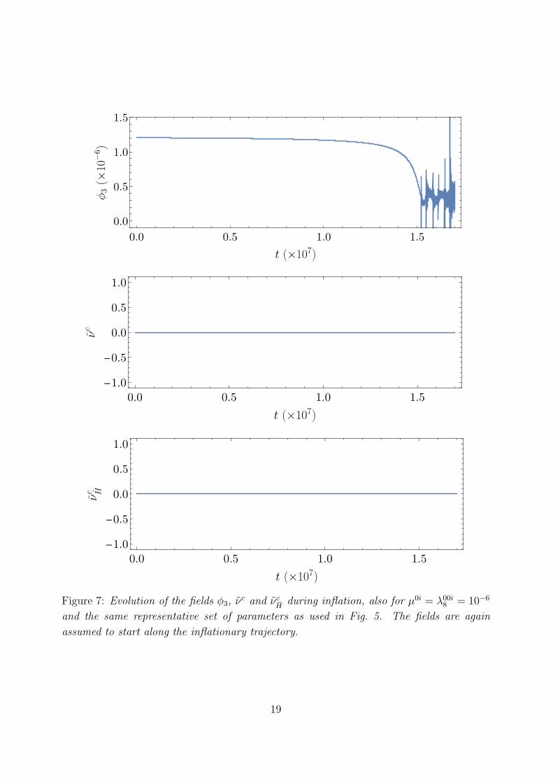
Figure 7: Evolution of the fields φ3, νc and νc

Hduring inflation, also for µ0i = λ00i

8 = 10−6

and the same representative set of parameters as used in Fig. 5. The fields are again

assumed to start along the inflationary trajectory.

19

Figures 6 and 7 show the time evolutions of all the scalar singlet fields and νc, νcHfor

µ0i = λ00i8 = 10−6 and the same representative set of parameters as used in Fig. 5, assuming

that the fields start along the bottom of the inflationary ‘valley’ in field space. These results

were obtained by numerical integration of the supergravity equations of motion:

Ψα + 3HΨα + ΓαβγΨ

βΨγ +Kαβ ∂V

∂Ψβ= 0 . (48)

Here the indices run over all field components, with Ψα ≡ T, φa, νc, νc

H, · · · , Kαβ denotes

the inverse Kahler metric, and the connection coefficients are given by

Γαβγ = Kαδ∂βKγδ . (49)

It is clear from the evolution of s in Fig. 6 that Starobinsky-like inflation is realized. Figs. 6

and 7 show that after the end of inflation the singlets φi undergo forced oscillations, with

amplitudes much larger than the expected values assuming an adiabatic tracking of the

inflaton value. This is an illustration of the phenomenon discussed around (33), namely

that adiabaticity is violated when relatively large values for the parameters λ0ij8 are chosen.

As Fig. 8 demonstrates, after a few oscillations a significant fraction of the energy stored in

the inflaton oscillations is transferred to the singlets φi. The lower panel of Fig. 8 exhibits

resonant enhancement of the φ2 amplitude when the solution of ∂φiV = 0 is divergent, i.e.,

around the points where (46) cannot be inverted. As expected, the enhancement occurs

when s ≪ 1. This result confirms that strong segregation is a sufficient condition for

reheating to occur through the decay of s.

Figs. 9 and 10 show the corresponding numerical results for a solution with the same

parameters, but with a perturbed initial condition νcH= 5× 10−3. This perturbation seeds

the oscillations of the remaining SM singlets, and drives an uphill roll of the inflaton due

to the connection-dependent terms in (48), namely:

ΓSαβΨ

αΨβ ≃ − 1

2√3sinh(

√

2/3 s)(

φ21 + φ2

2 + φ23 + ( ˙νc)2 + ( ˙νc

H)2)

+ · · · . (50)

As the value of s increases, the oscillations of the fields are rapidly damped, and the

subsequent evolution resembles that shown in Fig. 6 and Fig. 7, though with an increased

total number of e-folds, and Starobinsky-like values of (ns, r).

Fig. 11 shows the constraints from Planck and other data [21] on the model in the

(µ0i, λ00i8 ) plane, calculated in a fully numerical fashion. Due to the large number of in-

dependent parameters, we have made the simplifying assumption µ0i = µ0i′ for any i, i′

(and similarly λ00i8 = λ00i′

8 ). In the left panel the constraints are calculated for the same

representative set of parameters as used in Fig. 5. We note that, e.g., the upper limit for

µ0i is reasonably close to the analytical approximation Λ1 ∼ (10−3.3mΛ2)1/2 obtained in

20

1.5 1.6 1.7 1.8 1.9 2.0 2.1

-0.2

-0.1

0.0

0.1

0.2

0.3

0.4

1.5204 1.5208 1.5212

- 1.0

- 0.5

0.0

0.5

1.0

1.5

1.5482 1.5486 1.5490 1.5494

Figure 8: Evolution of the canonically-normalized inflaton s and the SM singlet φ2 during

reheating, for µ0i = λ00i8 = 10−6 and the same representative set of parameters as used in

Fig. 5. Upper panel: evolution of the inflaton field s (blue, continuous), compared to the

pure Starobinsky case (orange, dashed). Lower panel: evolution of the singlet field φ2 (blue,

continuous), compared to the instantaneous solution of the equations ∂φiV = 0 (orange,

dashed). Notice the different horizontal scales in the two panels.

Fig. 4. In the right panel, the constraints correspond to the same representative set of

parameters, but with the λijk8 → 10−2λijk

8 . Here the solution is reasonably close to the

analytical approximation (45). We have also verified that the 68% and 95% CL contours

are unchanged under the assumption of multiple light states with µij . 10−5.

3.4 A symmetry argument for segregation

As we have seen above, the parameters that cause mixing between the inflaton field S and

other singlet fields φi, such as λ00i8 and µ0i, must be strongly suppressed in order to achieve

successful inflation. In fact, such a suppression can naturally be obtained if one adopts an

21

0.01 0.10 1 10 100 1000

5

10

15

20

25

30

0.01 0.10 1 10 100 10004

6

8

10

12

0.01 0.10 1 10 100 1000

-1.0

-0.8

-0.6

-0.4

-0.2

Figure 9: Evolution of the canonically-normalized inflaton s and the SM singlets φ1 and

φ2 during inflation, for µ0i = λ00i8 = 10−6 and the same representative set of parameters as

used in Fig. 5. The perturbed initial condition νcH= 5× 10−3 is assumed.

22

0.01 0.10 1 10 100 10001.1

1.2

1.3

1.4

1.5

1.6

1.7

1.8

1.9

0.01 0.10 1 10 100 1000

-2

-1

0

1

2

0.01 0.10 1 10 100 1000

-2

-1

0

1

2

Figure 10: Evolution of the fields φ3, νc and νc

Hduring inflation, also for µ0i = λ00i

8 = 10−6

and the same representative set of parameters as used in Fig. 5. The perturbed initial

condition νcH= 5× 10−3 is again assumed.

23

95% 68% Planck+BKP+BAO

-6.0 -5.5 -5.0 -4.5

-6.0

-5.5

-5.0

(a) µij . 10−2, λijk8

. 1

95% 68% Planck+BKP+BAO

-7.0 -6.5 -6.0 -5.5-7.0

-6.8

-6.6

-6.4

-6.2

-6.0

-5.8

(b) µij , λijk8

. 10−2

Figure 11: The numerically-calculated 68% and 95% CL regions in the (µ0i, λ00i8 ) plane

at N∗ = 50 for the no-scale model with superpotential (5). Here for simplicity we have

assumed that µ0i = µ0i′ for any i, i′, and similarly λ00i8 = λ00i′

8 .

appropriate definition of R-parity. Let us assign odd R-parity to the matter superfields F ,

f , and ℓc, and even R-parity to the Higgs multiplets h and h, as usual. We also assign R-

parity even to H , H , and S, while φi are assumed to be R-parity odd. With this assignment

as well as the Z2 parity defined in (4), we can forbid the following couplings:

λi06 = λi

7 = λ00i8 = λijk

8 = µ0i = 0 . (51)

Note that with this R-parity assignment, the inflationary potential would be of the exact

Starobinsky form given in (23). On the other hand, λ0ij8 couplings are allowed by this Z2

symmetry, but as we have seen in our previous numerical results, taking these couplings of

order unity does not adversely affect inflation. Thus, this R-parity assignment would be

sufficient for obtaining the necessary strong segregation. We also note that this R-parity is

not broken by the vevs of H and H since they are R-parity even. Therefore, this R-parity

is respected at low energies unless φi acquire vevs.13

4 Reheating Constraints

In this section, we study the neutrino mass structure in this model and discuss its connection

to reheating after inflation. As we see below, neutrino mass terms are provided by Yukawa

13 This R-parity assignment differs from that used in [31]. With this assignment R-parity is exact unless

some of the couplings in (51) are turned on.

24

couplings in the superpotential. In GUTs, these Yukawa couplings may be related to other

Yukawa couplings—thus, we first discuss Yukawa unification in our model in Section 4.1.

We then study the neutrino mass structure in Section 4.2 and its connection to reheating

dynamics in Section 4.3.

4.1 Yukawa unification

The Yukawa coupling terms in the low-energy effective theory of this model are given by

WYukawa = fuhuQu+ fνhuLνcR − fdhdQd− fehdLe , (52)

where we have suppressed generation indices for simplicity. In ordinary SU(5) GUTs, we

expect

fd(MGUT) = fe(MGUT) , (53)

at the GUT scale. For the third generation (bottom and tau) Yukawa couplings, this

relation is satisfied at the O(10)% level. For the first two generations, however, there

are O(1) differences. Such deviations may be explained by means of higher-dimensional

operators suppressed by the Planck-scale [51] or higher-dimensional Higgs representations

[52] within the framework of SU(5) GUTs.

In the case of flipped SU(5)× U(1), on the other hand, we have

fu(MGUT) = fν(MGUT) , (54)

as these two Yukawa couplings come from the same λ2 term in (3). In this case, the down-

type Yukawa coupling fd, which is matched onto λ1, is unrelated to the charged lepton

Yukawa coupling fe, which originates from λ3. Therefore, the less successful prediction

(53) for the first two generations in ordinary SU(5) GUTs is not problematic in flipped

SU(5)×U(1) models. As we see below, even though we have the unification condition (54)

for fν , we can explain the observed pattern of neutrino mass differences and mixing angles

by choosing λia6 and µab appropriately.

4.2 Neutrino masses

Next, let us investigate the neutrino mass matrix in flipped SU(5) × U(1). After h, h,

H , and H develop vevs, the Yukawa terms λ2 and λ6 lead to Dirac mass terms for ν, νc,

and φa, where φa denotes the fermionic component of φa. If the singlet fields φa acquire

vevs, the Higgsino may also mix with right-handed neutrinos via the λia6 couplings, which

results in the R-parity violation. The R-parity violating effects may also be induced by

Higgsino-singlet mixing via the λa7 couplings. Here, we focus on the following two cases

25

where there is no (strong) R-parity violation: (A) No singlet field develops a vev, 〈φa〉 = 0,

and the inflaton S = φ0 does not participate in the neutrino mass generation. This setup is

realized when λi06 = λi

7 = 0 (though λ07 is allowed). Note that this scenario requires at least

four singlets, our default assumption. (B) One of the φi fields (denoted by φi′) acquires a

non-zero vev. If this field is responsible for the µ term, its R-parity must be positive, and

thus does not couple to the neutrino sector. Instead of this φi′, the inflaton S plays a role

in neutrino mass generation. Thus only λi′

7 is non-zero and in particular, λ07 = 0. In the

case of three singlets, since the R-parity of all three singlets must be negative, λ7 = 0 for

all three, and a GM term is necessary to produce a µ term. Note that in this case, there

is some R-parity violation due to the presence of both quadratic and cubic superpotential

terms, though the R-parity violation is weakly transmitted to the matter sector, and the

lifetime of the lightest supersymmetric particle (LSP) remains sufficiently long [11]. In

what follows, we study separately the neutrino mass structure and reheating dynamics for

these two scenarios (A) and (B).

4.2.1 Scenario (A): inflaton decouples from the neutrino sector

Here we assume 〈φa〉 = 0, which is achieved when all of the µab are much larger than the

supersymmetry-breaking scale. In this case, we need to introduce a Giudice–Masiero term

to obtain the MSSM Higgs µ-term. We further assume

λi06 = λi

7 = µ0i = 0 , (55)

which is assured by the R-parity discussed in Section 3.4. This prevents the fermionic

component of φ0 from mixing with neutrinos. The mass matrix for νi, νci , and φi is then

given by [5–7]

L(ν)mass = −1

2

(

νi νci φi

)

(Mν)ij

νjνcj

φj

+ h.c. , (56)

with

(Mν)ij ≡

0 λij2 〈h0〉 0

λT ij2 〈h0〉 0 λij

6 〈νcH〉

0 λT ij6 〈νc

H〉 2µij

, (57)

where we have used two-component notation. The mass matrix Mν is a complex sym-

metric matrix and thus can be diagonalized with a unitary matrix. By using |λij2 〈h0〉| ≪

|λij6 〈νc

H〉|, |µij|, we obtain the following mass matrix for the three light active neutrinos:

ML ≃ 2〈h0〉2〈νc

H〉2[

λ2

(

λT6

)−1µλ−1

6 λT2

]

. (58)

26

Thus, light neutrino masses can naturally be explained by the (double) seesaw mecha-

nism [53, 54]. Even though the structure of the matrix λ2 is related to the up-quark

Yukawa matrix through the unification relation (54), we still have a sufficient number of

degrees of freedom in the matrices λ6 and µ, and thus can easily find a form of ML that

fits the neutrino oscillation data. The couplings λij6 and µij in general contain extra CP

phases, and non-zero µij cause lepton-number violation. As a consequence, this model may

explain baryon asymmetry of the Universe via thermal leptogenesis [55, 56].14

Finally, the mass matrices of heavier states are given by

MH =

(

0 λij6 〈νc

H〉

λT ij6 〈νc

H〉 2µij

)

. (59)

If furthermore, λij6 〈νc

H〉 ≪ µij, then the corresponding heavy mass eigenvalues are of order

(λij6 〈νc

H〉)2/µij and µij.

4.2.2 Scenario (B): The inflaton couples to the neutrino sector

Next, we discuss the case where a combination of the singlet fields φi, called φi′, acquires a

vev: 〈φi′〉 6= 0. We assume that this singlet field does not have a coupling to Fi, in order to

suppress R-parity violation: λii′

6 = 0. In this case, the λi′

7 term leads to the MSSM µ-term,

µ = λi′

7 〈φi′〉. To obtain three massive active neutrinos, we instead couple the inflaton field

to Fi: λi06 6= 0. We then suppress the λ0

7 coupling to avoid R-parity violation.

For i, j 6= i′, the neutrino mass matrix has the same structure as Mν in (57), and

thus light neutrino masses for these generations are again given by (58) 15. For i = j = i′,

on the other hand, the mass matrix is given by

L(i′)mass = −1

2

(

νi′ νci′ S

)

0 λi′i′

2 〈h0〉 0

λi′i′

2 〈h0〉 0 λi′06 〈νc

H〉

0 λi′06 〈νc

H〉 m

νi′

νci′

S

+ h.c. , (60)

where S denotes the fermionic partner of the inflaton S. The light mass eigenvalue for this

mass matrix is then given by

mνi′≃ m

(

λi′i′

2 〈h0〉)2

(

λi′06 〈νc

H〉)2 , (61)

14 As we discuss in Section 4.3.1, in this scenario the inflaton does not decay directly into heavy neutrinos,

leaving thermal leptogenesis as a possibility. For this to occur, we need a high reheating temperature, and

thus the strong reheating case discussed in Section 5.3.2 is favored in this scenario.15Here, we neglect the effects of λi0

6 and µi0 for simplicity. The generalization to non-zero λi06 and µi0 is

straightforward. We also neglect mixing among generations, which is expected to be sizable according to

neutrino oscillation data, to simplify the expressions, but the generalization is again straightforward. For

more concrete expressions, see Ref. [7].

27

while the heavier eigenvalues have masses

mNi′1,2=

1

2

[

m∓√

(

2λi′06 〈νc

H〉)2

+m2

]

, (62)

where Ni′1 andNi′2 are νci′- and S-like states, respectively. Form ≪ λ6〈νc

H〉, these two states

form a pseudo-Dirac state with mass λ6〈νcH〉 with splitting of order m. It is interesting to

note the role played by the inflaton mass, m for neutrino masses 16. The light (mostly

left-handed) neutrino masses are proportional to the inflaton mass, whilst the heavy state

masses are split by the inflaton mass.

The part of the superpotential relevant for the νci′ and S couplings can be written as

W = λi′j2 νc

i′Ljhu + λi′06 νc

i′νcHS +

m

2S2 . (63)

Rotating the νci′ and S fields into the mass eigenstates:

(

Ni′1

Ni′2

)

=

(

cos θ sin θ

− sin θ cos θ

)(

νci′

S

)

, (64)

with

tan 2θ = −2λi′06 〈νc

H〉

m, (65)

the superpotential (63) can then be expressed as

W = λi′j2 (cos θNi′1 − sin θNi′2)Ljhu +

1

2mNi′1

N2i′1 +

1

2mNi′2

N2i′2 , (66)

where the masses mNi′1,2are given in (62).

As we see below, the neutrino mass structure in this scenario is restricted by the

constraint on the reheating temperature. We will discuss the compatibility of this constraint

with the observed neutrino oscillation data in Section 4.3.2.

4.3 Singlet decays

Now we consider inflaton decay in the two scenarios discussed in the previous subsection.

In Scenario (A), the inflaton does not couple to the neutrino sector, so at the tree level

it can decay only into Higgs bosons and Higgsinos. In Scenario (B), on the other hand,

the inflaton S does couple to right-handed neutrinos but its coupling to the MSSM Higgs

fields is suppressed in order to evade R-parity violation. We will find that there is a tight

connection between neutrino masses and reheating dynamics in this case.

16The parameter m is inflaton mass during inflation and reheating when the GUT symmetry remains

exact. After GUT symmetry breaking the scalars associated with the inflaton multiplet receive GUT scale

masses proportional to λ6〈νcH〉.

28

4.3.1 Scenario (A): inflaton decay into Higgs/Higgsino

Assuming (55), the superpotential couplings relevant to the inflaton decay are given by

WS decay = λij1 FiFjh+ λij

2 Fifj h+ λij3 fiℓ

cjh + λ0

7Shh+ 3λ0ij8 Sφiφj +

m

2S2 . (67)

If the mass eigenvalues of the mass matrix (59) are larger than the inflaton massm, then the

inflaton decay via the couplings λ0ij8 is suppressed by a small light-heavy neutrino mixing

angle of O(λ2〈h0〉/(µ, λ6〈νcH〉)), and thus is negligible. The λ0

7 coupling gives rise to the

inflaton-Higgs/Higgsino interactions:

Lint = − λ07√2shuhd −

m∗λ07√

2shuhd + h.c. , (68)

which yields the following singlet decay rate:

Γ(s → huhd) = Γ(s → huhd) ≃|λ0

7|28π

|m| . (69)

The cross terms between the λ1,2,3 and λ7 terms in (67) also induce singlet-sfermion cou-

plings. These couplings give rise to either three-body decay or two-body decay suppressed

by the Higgs vev 〈h0〉. Hence, these sfermion decay channels are sub-dominant.

As we discuss in Section 5.1, an upper limit on the inflaton decay rate is given by the

over-production of gravitinos, which restricts the coupling λ07 as 17

|λ07| . 10−5∆ , (70)

though it could be substantially smaller. Since the inflaton plays no role in the neutrino

mass generation, this limit has no implication for the neutrino mass structure, contrary to

Scenario (B) discussed below.

4.3.2 Scenario (B): inflaton decay into neutrinos

In this case, the λ07 coupling is set to be zero to avoid R-parity violation. Thus, the

Higgs/Higgsino decay modes of the inflaton are suppressed. Instead, the inflaton couples

to the neutrino sector through the λi′06 coupling, and thus can decay into a lepton and

a Higgsino, or a slepton and a Higgs boson. Other decay channels are three-body decay

processes or those dependent on a small vev, 〈φi′〉 or 〈h0〉, and are thus subdominant.

17The constant ∆ ≥ 1 parametrizes any dilution of the gravitino relic density posterior to reheating, due

to the entropy increase produced by the decay of a long-lived particle (see Section 5.3.3).

29

The relevant interactions are readily obtained from the superpotential (66), from

which we evaluate the decay rates of the s-like state Re(√2Ni′2):

Γ(s → Lj hu) = Γ(s → Ljhu) ≃|λi′j

2 sin θ|28π

mNi′2. (71)

We then obtain a constraint on sin θ as in (70):

|λi′j2 sin θ| . 10−5∆ . (72)

We now discuss the implication of this constraint for light neutrino masses. We

work on the basis where λ2 is diagonalized. We first consider the case i′ = 3, where

λ332 ≃ mt/〈h0〉 ≃ 1. In this case, the constraint (72) leads to

10−5∆ & | sin θ| ≃∣

∣

∣

∣

λ306 〈νc

H〉

m

∣

∣

∣

∣

. (73)

With (61), this bound gives

mν3 & 1010 · m2t

m∆−2 ∼ 10 GeV∆−2 , (74)

which, in the absence of significant entropy production, is much larger than the current

experimental limit from the Lyman α forest power spectrum obtained by BOSS in combi-

nation with the Planck 2015 CMB data [57]:∑

ν mν < 0.12 eV.

In the i′ = 2 case, although the bound is relaxed by a factor of 10−4, the resultant

neutrino mass value is still above this limit. In the i′ = 1 case, however, λ112 ≃ mu/〈h0〉 ≃

10−5, and thus the constraint (72) gives no limit on the mixing angle θ. In this case, the

neutrino mass is given by

mν1 ≃ 10−9 ×(

m

3× 1013GeV

)( |λ106 |

10−3

)−2( |〈νcH〉|

1016 GeV

)−2

eV , (75)

which evades the experimental limit.

Recent global fits to neutrino oscillation data give [58]

|δm2| ≡ |m2ν2−m2

ν1| ≃ 7.4× |10−5 eV2 ,

|∆m2| ≡ |m2ν3 − (m2

ν2 +m2ν1)/2| ≃ 2.5× 10−3 eV2 . (76)

These values as well as the result in (75) indicate that, unless |λ106 〈νc

H〉| is extremely small,

a Normal Hierarchy (NH) mass spectrum, i.e., mν1 ≪ mν2 < mν3, is favored in this model.

The other light neutrino masses in this case are predicted to be

mν2 ≃ |δm2| 12 ≃ 9× 10−3 eV ,

mν3 ≃ |∆m2| 12 ≃ 5× 10−2 eV . (77)

We can easily obtain these values by choosing appropriately µ and λ6 in (58): reheating

does not impose significant restrictions for these two generations.

30

5 Post-Inflation

5.1 Reheating

The temperature of the Universe following inflation depends on the inflaton decay rate,

which we parameterize as Γs = |y|2m/8π. For case (A), y =√2λ0

7, and for case (B),

y =√2λi′j

2 sin θ. This decay rate is bounded by the upper limit on the density of gravitinos

produced in the relativistic plasma arising from the inflaton decay products [15,59–77]. Big-

Bang Nucleosynthesis (BBN) imposes tight constraints on the decay rate of the inflaton

for small gravitino masses [67, 72, 73, 77–80]. However, if one assumes that the gravitino

is sufficiently heavy to decay before BBN [79, 80], the dominant bound on its abundance

comes from its contribution to the cold dark matter relic density. Assuming a present dark

matter density Ωcoldh2 = 0.12 [21] and a standard thermal history with no post-reheating

entropy production, we find the following constraint on the inflaton decay coupling y [15]:

|y| < 2.7× 10−5

(

1 + 0.56m2

1/2

m23/2

)−1(

100GeV

mLSP

)

, (78)

implying that Γs . 900 GeV for m = 3× 1013 GeV. When the limit on y is saturated, the

relic density of the LSP is obtained by the non-thermal decay of the gravitino. For smaller

y, the LSP abundance from decay is reduced and other mechanisms (such as freeze-out or

coannihilations) must be operating so as to give the correct cold dark matter density.

Equivalently, in terms of the reheating temperature,

Treh ≡(

40

grehπ2

)1/4

(ΓsMP )1/2

.

(

915/4

greh

)1/4

(1.7× 1010GeV) , (79)

where greh is the number of relativistic degrees of freedom at Treh. We use here the reference

value gMSSM = 915/4 instead of gSU(5)×U(1) = 1545/4, as most of the difference is due to

heavy fields, whose production is kinematically forbidden. However, as is well known, the

reheating temperature does not constitute an upper bound on the effective instantaneous

temperature T , as higher effective temperatures can be reached during the reheating process

[15, 70, 81]. Using the relation

T =

(

30ργπ2g(T )

)1/4

, (80)

where ργ denotes the instantaneous energy density of the relativistic decay products, an

effective instantaneous temperature during reheating may be defined. This leads to a

maximum temperature of the dilute plasma shortly after the start of inflaton decay, which

may be written as

Tmax ≃ 0.74

(

ΓsmM2P

gmax

)1/4

.

(

915/4

gmax

)1/4

(3.8× 1012GeV) , (81)

31

where the inequality is due to the gravitino production bound. As discussed in [15], because

of the finite rate of the thermalization process, the actual maximum temperature of the

Universe is in the range Tmax & T > Treh.

The previous constraints on the decay rate of the inflaton, and the maximum tempera-

tures during and after reheating, change if there is an intermediate matter-dominated phase

between the end of reheating and the end of the radiation-dominated era. We consider this

effect in Section 5.3.3.

5.2 Supercosmology and The GUT phase transition

The maximum temperature during reheating is typically a few orders of magnitude lower

than the GUT scale. However, due to the stabilization of νcH , ν

cH

at their origins during

inflation, the Universe enters the reheating epoch in an SU(5) × U(1) symmetric state.

The eventual breaking of the symmetry takes place along an F - and D-flat direction of

the potential νcH = νc

H≡ Φ and finite-temperature corrections to the effective potential

must be taken into account. As we will see, the strong coupling behaviour of SU(5) at low

temperatures help drive the transition [37, 82].

The leading-order running of the SU(5) gauge coupling is

1

α5(µ)=

1

αGUT− b5

2πln

(

MGUT

µ

)

, (82)

where b5 = 15− (n5+3n10)/2 with n5 (n10) the number of 5 and 5 (10 and 10) multiplets.

For the field content introduced in Section 2, n5 = 5 and n10 = 5, and thus b5 = 5. As

discussed above in (10), αGUT ≃ 0.0374 for MGUT ≃ 1.2× 1016GeV, and equation (82) im-

plies that the SU(5) group is asymptotically free, with the coupling in the unbroken phase

becoming strong at a large energy scale Λc ≫ mW . Naively, this scale would be associated

with the condition g5 ∼ 1, corresponding to µ ∼ 2 × 108 GeV, but symmetry-breaking bi-

linear condensates may be formed above/below this threshold. These condensates acquire

masses of order Λc and effectively decouple from the low-energy theory. The nature of the

condensates and their transformation properties can in principle be investigated using a

generalization of the so-called most attractive channel (MAC) hypothesis [83,84]. Schemati-

cally, lattice calculations have indicated that the exchange potential for the fermion bilinear

may be sufficiently large for condensation to occur if [85]

g2(Λc)∆C ≡ g2(Λc)(Cc − C1 − C2) ≃ 4, αc ≡ α(Λc) ≃1

π∆C, (83)

where Cc, C1 and C2 denote the quadratic Casimirs of the composite channel and the

32

two elementary supermultiplets, respectively 18. More specifically, it is assumed that the

channel that maximizes the effective coupling (the MAC) is the one that condenses first.

Then, a second MAC condensate may form in the new broken phase, further reducing the

symmetry group of the model. Successive MACs continue to condense until the non-Abelian

gauge group is completely broken.

The MAC spectrum for the flipped model was studied within this approach in [37],

under the additional condition that supersymmetry remains unbroken during the MAC

formation. We do not repeat that analysis here, but summarize the results. All in all,

the total number of light states in the strong-coupling phase is expected to be at most

4(1i) + 1(1) + 14(14) + 3(1j) + 3(ℓci) = 25 where (as discussed in detail in [37]), the 1i are

singlet fields arising from 10i×10H condensation (where i = 1, 2, 3, H), 1 is a singlet arising

from 5h × 5h condensation, and the 1j are SU(4) singlets in the 5j matter representations.

Among these, 14 get masses ∝ Φ and 11 do not, which is fewer than in [37], as the singlets

φa are not included among the light states, as we assume here the presence of the bilinear

couplings µab. This is to be contrasted with the SU(5)×U(1)-symmetric phase, which has

103 light superfield degrees of freedom, and the Higgs phase, in which 62 do not acquire

masses ∼ Φ.

As a representative example of the net Casimir coefficient ∆C in a specific MACs,

we may take ∆C = 245in (83), which gives αc ≃ 0.0663. Then, from Eq. (82) we have

Λc ≃ MGUT exp

[

−2π

b5

(

1

αGUT− 1

αc

)]

. (84)

Using our previous estimate that α(MGUT) = 0.0374, we find that strong-coupling dynamics

will be important for

Λc ≃ 4× 10−7MGUT . (85)

Using also our estimate MGUT = 1.2 × 1016 GeV, we then have Λc ≃ 5 × 109 GeV. Again

using (83), other MAC channels give estimates of Λc between 108 and 1014 GeV 19. As we

will see in Section 5.3, if TR & Λc &√

|mΦ|MGUT ∼ 1010 GeV, the oscillation of the Φ field

occurs incoherently, which minimizes the entropy release due to Φ decay. Eq. (85) suggests

that it is plausible that Λc falls into this region, within the large current uncertainties.

The difference in the number of light degrees of freedom between the symmetric,

strongly-coupled and Higgs phases of the theory is crucial for the onset of the SU(5) ×U(1) → SU(3) × SU(2) × U(1) phase transition, as we now show. From the one-loop

18Larger values of αc are estimated in the ladder approximation [86]. The differences between the various

estimates of αc stem from our incomplete understanding of strong dynamics.19For example, ∆C = 36/5 gives αc = 0.0442 and Λc = 6 × 10−3MGUT, ∆C = 18/5 gives αc = 0.0884

and Λc = 4 × 10−9MGUT, and ∆C = 15/4 gives αc = 0.0849 and Λc = 7× 10−9MGUT. See [37] for more

details.

33

0.1 0.5 1 5 10-50

-40

-30

-20

-10

0

Figure 12: The evolution with temperature of the effective potential Veff(Φ, T ) (87) in

strongly-coupled SU(5)× U(1).

temperature-dependent correction to the effective potential, we have a contribution from

light superfields that remain massless in the broken phases equivalent to that of an ideal

ultrarelativistic gas, i.e.,

Veff, light = −π2T 4

90g , (86)

and the Φ-independent heavy states will have negligible contributions. For the states with

Φ-dependent masses, there are contributions to the chiral mass-squared matrices propor-

tional to |λ4,5,6|2Φ2, and to g2CaΦ2 for the vector superfields. Under the assumption that

λ4,5,6, gaCa ∼ O(1) in the strong-coupling domain, we may write a phenomenological fit to

the temperature-dependent effective potential of the form

Veff(Φ, T ) ≈ NΦT 4

2π2

∑

α=0,1

(−1)α∫ ∞

0

dy y2 ln[

1− (−1)α exp(

−√

y2 + (Φ/T )2)]

, (87)

where NΦ denotes the number of Φ-dependent massive superfields in the corresponding

regime. Fig. 12 shows the resulting shape of the effective potential as a function of Φ when

T/Λc = O(1). For definiteness, we have used a smooth (logistic function) interpolation for

g and NΦ around the strong-coupling-transition scale Λc. In the topmost curve, a barrier

that might trap Φ near the origin when T < Λc is apparent. This effect may be an artifact

of the approximations that we have considered, and we expect in any case that strong-

coupling and thermal effects would easily make an end run around any such barrier when

T ∼ Λc.

34

5.3 Entropy release

Having verified how the phase transition takes place, we now estimate the amount of entropy

it releases. In what follows, we denote the decay rate of the flat direction by ΓΦ, and the

scale factor by a. As we will discuss below, the amount of entropy release will be dependent

on whether it is possible or not for the flat direction Φ to undergo coherent oscillations

after the completion of the phase transition [36].

One possibility is that reheating takes place at temperatures lower than the strong-

coupling scale, Treh < Λc. In this weak reheating scenario, the SU(5) × U(1) gauge sym-

metry is not restored after inflation, and the field Φ eventually reaches its low-energy

minimum and reheats the Universe through the coherent decay of its oscillations. Disre-

garding non-renormalizable terms that could lift the flat direction, field dependence in the

zero-temperature effective potential for Φ can only come from a supersymmetry-breaking

term ∼ m2ΦΦ

2, where m2Φ is assumed to be negative. The energy stored in the scalar field

oscillations of Φ following the phase transition may then be simply estimated as

ρΦ ≃ |m2Φ|〈Φ〉2

(

a(t)

aΦ

)−3

. (88)

where 〈Φ〉 denotes the low-temperature vev of Φ, responsible for the breaking of the GUT

symmetry, and aΦ denotes the size of the scale factor at the onset of Φ-oscillations.

In contrast, for strong reheating, Treh & Λc, and the Φ field starts growing as the

temperature falls below Λc. This growth, however, will be driven by incoherent fluctuations,

in which there is a sizeable kinetic energy for the Φ field, Φ ∼ T 2. For Λc > (|mΦ|Φ)1/2, theincoherent component of Φ will dominate and destroy any coherent contribution 20. The

flat direction will then redshift as radiation until its temperature decreases sufficiently to

bring it to the non-relativistic regime, during which it eventually decays and reheats the

Universe.

In the following subsections we determine the amount of entropy released by the decay

of Φ in the weak and strong reheating scenarios, and determine their effect on the final

baryon asymmetry.

5.3.1 Weak reheating

We consider first the weak reheating case, for which the GUT gauge symmetry is not

restored after inflation, and the Φ condensate oscillates coherently about its low-energy

20Even in the presence of coherence, the condition for fast damping of the field oscillations, |mΦ| ∼H ∼ Λ2

c/MP , is not violated by more than an order of magnitude, implying complete damping after a few

oscillations.

35

minimum. Dependent on the magnitudes of the decay rates of the inflaton s and the flat

direction Φ, the later can begin its oscillations and/or decay before or after the completion

of reheating. It is clear that a short-lived Φ, namely one which decays before the end

of reheating, will not contribute significantly towards the production of entropy, which

continues until the end of reheating. Therefore, to explore the potential entropy injection

produced by Φ decay, we need to consider only the case in which Γs > ΓΦ. Let us assume

first that the flat direction starts oscillations during the radiation-dominated era with

|mΦ| < Γs. As the energy density of the inflaton decay products at the end of reheating is

ργ, reh ∼ Γ2sM

2P [13, 15], we can write at later times

ργ ∼ Γ2sM

2P

(

a(t)

areh

)−4

. (89)

With a(t) ∼ t1/2 during radiation domination and the Hubble parameter given by Hγ ∼ρ1/2γ /MP , and assuming for simplicity the instantaneous onset of oscillations and decay of

Φ when H(tΦ) ∼ |mΦ| and H(tdΦ) ∼ ΓΦ, respectively, the ratio

ρΦργ

∣

∣

∣

∣

dΦ

∼ |m2Φ|〈Φ〉2Γ2sM

2P

a3ΦadΦa4reh

≃ |mΦ|1/2〈Φ〉2

Γ1/2Φ M2

P

, (90)

will be smaller than one if the following constraint on the decay rate of Φ is satisfied,

ΓΦ

|mΦ|>

( 〈Φ〉MP

)4

& 2× 10−11 , (91)

for 〈Φ〉 & 5 × 1015 GeV as required by the proton lifetime (see Eq. (13)). If this occurs, a

negligible amount of entropy will be released upon Φ decay. When (91) is not satisfied, the

oscillations of Φ will eventually dominate the energy density of the Universe. In this case,

from (88) and (89), we can compute the scale factor a∗ at Φ-radiation equality as

a∗aΦ

≃(

MPΓs

|mΦ|〈Φ〉

)2(arehaΦ

)4

≃(

MP

〈Φ〉

)2

. (92)

With the Hubble parameter during Φ domination given by

HΦ ∼ |mΦ|〈Φ〉MP

(aΦa

)3/2

, (93)

and the decay of the flat direction occurring at ΓΦ ∼ HΦ, we can re-calculate the ratio (90)

for the flat direction-dominated case as21

ρΦργ

∣

∣

∣

∣

dΦ

=

(

adΦa∗

)

=

(

adΦaΦ

)(

aΦa∗

)

∼( |mΦ|〈Φ〉4

ΓΦM4P

)2/3

. (94)

21 Here we have assumed that ργ goes as a−4 during the whole epoch. Generically speaking, during

the coherent oscillation of Φ, the radiation originating from the decay of Φ might have dominated that

from inflaton decay. In this case, the Universe would experience non-adiabatic expansion and ργ goes as

a−3/2 [87]. However, it turns out that the non-adiabatic expansion occurs only at a very low temperature

because of the small decay rate of Φ (see below), and thus this modification would be negligible in our

scenario.

36

which is > 1, consistent with the violation of the condition (91).

Let us now assume that the oscillation of Φ starts during reheating, |mΦ| > Γs. In

this case we can interpolate between the start of oscillations of the flat direction and the

end of reheating as(

arehaΦ

)

∼( |mΦ|

Γs

)2/3

. (95)

If the Universe is dominated by radiation by the time of the decay of Φ, we will have

ρΦργ

∣

∣

∣

∣

dΦ

∼ |m2Φ|〈Φ〉2Γ2sM

2P

(

aΦareh

)3(adΦareh

)

≃ Γ1/2s 〈Φ〉2

Γ1/2Φ M2

P

. (96)

Thus, no significant amount of entropy will be released if the following constraint on the

decay rate of Φ is satisfied,

ΓΦ

Γs

>

( 〈Φ〉MP

)4

>∼ 2× 10−11 . (97)

Conversely, if the previous relation is violated, the flat direction oscillations will dominate

the energy density until their decay. In this scenario, we can write

ρΦργ

∣

∣

∣

∣

dΦ

=

(

adΦa∗

)

=

(

adΦaΦ

)(

aΦa∗

)

∼(

Γs〈Φ〉4ΓΦM4

P

)2/3

> 1 . (98)

With the entropy density in radiation given by sγ = 4/3(grehπ2/30)1/4ρ

3/4γ , and a similar

expression for the entropy density produced from Φ decays, we can summarize the amount

of entropy released in both scenarios as

∆ ≡ sΦsγ

∣

∣

∣

∣

dΦ

∼(

gdΦgreh

)1/4(min[|mΦ|,Γs]〈Φ〉4

ΓΦM4P

)1/2

. (99)

As was discussed in [37], the decay rate of the flat direction occurs via the effective

D-term diagrams shown in Fig. 13, which lead to the decay rate

ΓΦ ≃9λ4

1,2,3,7

2048π5

(

|mΦ|m2F,f ,ℓc,φa

〈Φ〉2

)

. (100)

The gravitino production constraint implies that Γs . 900GeV (see (78)) and, if we assume

that the effective mass in the flat direction is heavier than the weak scale, the entropy ratio

(99) evaluates to

∆ ≃ 1.5× 108 λ−21,2,3,7

(

gdΦgreh

)1/4( 〈Φ〉5× 1015GeV

)3((10TeV)3

m2F,f ,ℓc,φa

|mΦ|

)1/2(Γs

900GeV

)1/2

≃

6.2× 107 λ−21,2,3,7

(

gdΦgreh

)1/4( 〈Φ〉5× 1015GeV

)3((10TeV)3

m2F,f ,ℓc,φa

|mΦ|

)1/2( y

10−5

)

(

m

3× 1013GeV

)1/2

.

(101)

37

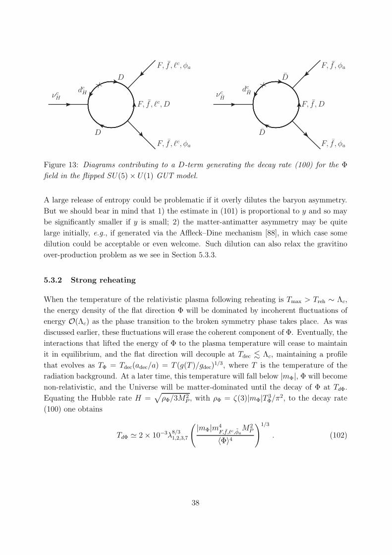
νcH

F, f , ℓc, φa

F, f , ℓc, φa

F, f , ℓc, D

D

D

dcH×

νcH

F, f , φa

F, f , φa

F, f , D

D

D

dcH

×

Figure 13: Diagrams contributing to a D-term generating the decay rate (100) for the Φ

field in the flipped SU(5)× U(1) GUT model.

A large release of entropy could be problematic if it overly dilutes the baryon asymmetry.

But we should bear in mind that 1) the estimate in (101) is proportional to y and so may

be significantly smaller if y is small; 2) the matter-antimatter asymmetry may be quite

large initially, e.g., if generated via the Affleck–Dine mechanism [88], in which case some

dilution could be acceptable or even welcome. Such dilution can also relax the gravitino

over-production problem as we see in Section 5.3.3.

5.3.2 Strong reheating

When the temperature of the relativistic plasma following reheating is Tmax > Treh ∼ Λc,

the energy density of the flat direction Φ will be dominated by incoherent fluctuations of

energy O(Λc) as the phase transition to the broken symmetry phase takes place. As was

discussed earlier, these fluctuations will erase the coherent component of Φ. Eventually, the

interactions that lifted the energy of Φ to the plasma temperature will cease to maintain

it in equilibrium, and the flat direction will decouple at Tdec . Λc, maintaining a profile

that evolves as TΦ = Tdec(adec/a) = T (g(T )/gdec)1/3, where T is the temperature of the

radiation background. At a later time, this temperature will fall below |mΦ|, Φ will become

non-relativistic, and the Universe will be matter-dominated until the decay of Φ at TdΦ.

Equating the Hubble rate H =√

ρΦ/3M2P , with ρΦ = ζ(3)|mΦ|T 3

Φ/π2, to the decay rate

(100) one obtains

TdΦ ≃ 2× 10−3λ8/31,2,3,7

(

|mΦ|m4F,f,ℓc,φa

M2P

〈Φ〉4

)1/3

. (102)

38

Upon the decay of Φ, the Universe will be once again dominated by radiation, with a

temperature now given by

T ′reh =

(

40

gdΦπ2

)1/4

(ΓΦMP )1/2 ≃ 5× 10−3g

−1/4dΦ λ2

1,2,3,7

(

|mΦ|m2F,f,ℓc,φa

MP

〈Φ〉2

)1/2

, (103)

where we have neglected the delay arising from the conversion of the heavy supersymmetric

decay products into the truly relativistic Standard Model particles. For 〈Φ〉 ≃ 5×1015 GeV,

λ1,2,3,7 ∼ 1 and mΦ,F,f,ℓc,φa& 10TeV, this temperature is T ′

reh & 1MeV, remarkably around

what is needed to re-start nucleosynthesis. The amount of entropy released by the decay

of Φ can therefore be estimated as

∆ =gdΦT

′3reh

(g(T )T 3)|dΦ=

gdΦT′3reh

gdecT3dΦ

(104)

≃ 8× 103 λ−21,2,3,7

(

gdΦ43/4

)1/4(915/4

gdec

)( 〈Φ〉5× 1015GeV

)(

10TeV

m2F,f ,ℓc,φa

/|mΦ|

)1/2

. (105)

Therefore, in the strong reheating scenario the entropy dilution is reduced by O(104) with

respect to weak reheating, providing more leeway for the initial asymmetry-generating

mechanism.

5.3.3 Entropy production and the gravitino bound on reheating

A late injection of entropy would dilute any previously produced relics, such as gravitinos

or their decay products. In particular, the gravitino yield Y3/2 ≡ n3/2/nγ would be reduced

by a factor of ∆−1. Since in the absence of a secondary matter-dominated era driven by

Φ, the yield at late times is given approximately by [15]

Y3/2(T ) ≃ 0.0036

(

1 + 0.56m2

1/2

m23/2

)

(

Γs

MP

)1/2

, (106)

the extra dilution would weaken the decay rate constraint imposed by the LSP relic density

by a factor of ∆2, thus allowing a higher reheat temperature by a factor of ∆. More

specifically, (78) would now become

|y| < 2.7× 10−5∆

(

1 + 0.56m2

1/2

m23/2

)−1(

100GeV

mLSP

)

, (107)

and Treh . ∆(1010GeV). Thus, the strong reheating condition Treh & Λc would automati-

cally be allowed by the late decay of the flaton Φ.

39

An additional effect of the entropy increase (101) or (105) would be a shift in the

number of e-folds of inflation after the pivot scale k∗ crosses the horizon, due to the non-

standard thermal history [89,90]. In the slow-roll approximation, the number of e-folds to

the end of inflation can be expressed as [21, 49, 91]

N∗ = ln

(

ρ1/4rehareh√3a0H0

)

− ln

(

k∗a0H0

)

+1

4ln

(

V 2∗

M4Pρend

)

+1− 3wint

12(1 + wint)ln

(

ρrehρend

)

, (108)

where a0 and H0 are the present cosmological scale factor and Hubble expansion rate,

respectively, V∗ is the inflationary energy density at the reference scale, ρend and ρreh are the

energy densities at the end of inflation and after reheating, and wint is the e-fold average

of the equation-of-state parameter during the thermalization epoch. For the standard

thermal history (STH), the first term evaluates to 66.9 − 112ln greh, as entropy is assumed

to be conserved after reheating. In our case of an intermediate matter-dominated era, it

can be rewritten as

ln

(

ρ1/4rehareh√3a0H0

)

= ln

(

ρ1/4dΦ adΦ√3a0H0

)

+ ln

(

ρ1/4rehareh

ρ1/4dΦ adΦ

)

, (109)

where now the first term of (109) can be evaluated assuming entropy conservation, and

the second term is directly related to the dilution factor ∆. We obtain for the number of

e-folds the following expression,

N∗ = NSTH∗ − 1

3ln∆ . (110)

At first sight, the reduction of N∗ due to the late entropy injection might appear to put

Starobinsky-like inflation under stress, as the Planck data disfavors N∗ . 50 (44) at the

68% (95%) CL. However, the physical range for N∗ depends on the underlying particle

model, since the last term in (108) depends implicitly on the decay rate of the inflaton.

For Starobinsky-like inflation, it can be evaluated in the perturbative regime as [13]

1− 3wint

12(1 + wint)ln

(

ρrehρend

)

≃ 1− 3wint

12(1 + wint)

(

2 ln

(

Γs

m

)

+ const.

)

, (111)

where wint ≃ 0.782/ ln(2m/Γs). In the STH case, the gravitino upper bound for Γs con-

strains N∗ to be less than Nmax∗ ≃ 53.3. However, in the case of intermediate Φ-domination,

this maximum value is reduced due to the modified e-fold expression (110), and also in-

creased because of the weakened gravitino bound (107). These two effects combine to

give

∆Nmax∗ ≃ −4 × 10−3 ln∆ . (112)

Therefore, the favored range for N∗ is practically unchanged for strong reheating when one

accounts for the increased decay rate limit. In the weak reheating regime, the maximum

40

value for N∗ cannot be reached within perturbation theory, as for |y| . 1 the number of

e-folds is limited to N∗ . 49 with ∆ ≃ 5× 108, the value of the entropy factor obtained by

taking min[|mΦ|,Γs] = |mΦ| in (99). Hence, for weak reheating, the inflationary predictions

lie outside the 1σ Planck bounds.

5.3.4 Baryon asymmetry

Finally, let us investigate the generation of the baryon asymmetry in this class of models.

In Scenario (A), as we noted earlier, at the tree level the inflaton decays primarily to

Higgs bosons and Higgsinos, and there is no decay to neutrinos. At one-loop, through the

exchange of a heavy right-handed neutrino, there is the possibility of a lepton-number-

violating decay to two neutrinos. However, in that case, in order to obtain a net lepton

asymmetry one must consider the interference between one-loop diagrams and their two-

loop corrections, greatly suppressing the final lepton asymmetry.

However, in the case of strong reheating in Scenario (A), it may be possible to pro-

duce thermally the right-handed neutrinos, though this is possible only if the reheating

temperature is comparable to the right-handed neutrino mass. We recall however, that in

Scenario (A) the right-handed neutrino mass is of order λij6 〈νc

H〉 (for νc

H〉 ∼ µij) and, from

(79), the reheating temperature is TR . 8.7 × 1014 |λ07| GeV . 8.7 × 109∆ GeV. Thus we

would require

λij6 . 1.7× 10−6

(

5× 1015GeV

〈νcH〉

)

∆ . (113)

Taking into account the entropy production factor in (104), this is a viable path towards

producing the final baryon asymmetry.

Generating the baryon asymmetry is more straightforward in Scenario (B), in which

the inflaton decays to Lh in much the same way that right-handed neutrinos decay in

standard out-of-equilibrium leptogenesis models [55]. At the end of inflation, the lepton and

baryon asymmetries can be related directly to the reheat temperature, TR, by [5,61,92–94]

nB

s∼ nL

s∼ ǫ

∆fns

T 3R

∼ ǫ

∆fTR

m, (114)

where ns is the number density of inflatons at the time of their decay, and f is the branching

fraction into Lh, (f ∼ 1 for Scenario (B)). The amount of C and CP is given by [7, 95]

ǫ ≃ − 3

4π

1(

U †νc(λ

D2 )

2Uνc

)

11

∑

i=2,3

Im

[

(

U †νc(λ

D2 )

2Uνc

)2

i1

]

m

Mi, (115)

where Uνc is a mixing matrix associated with the diagonalization of νci and S in the basis

where λ2 is diagonalized to λD2 [7], and we assume for simplicity that the second and third

41

generation heavy neutrino states (two states for each generation) have similar masses M2

and M3, and m ≪ Mi. Generically, we expect (U †νc(λ

D2 )

2Uνc)11 ∼ (λD2 )

233 ∼ mt/〈h0〉 ∼ 1 is

the largest entry in (λD2 )

2. This gives

|ǫ| ∼ 7× 10−3 ×(

m

3× 1013 GeV

)(

Mi

1015 GeV

)−1

× δ . (116)

where δ denotes an O(1) factor that depends on the amount of CP violation in the matrix

U †νc(λ

D2 )

2Uνc . From Eq. (79)

TR ≈ 0.07|y|(

915/4

greh

)1/4

(mMP )1/2

≈ 6× 1014|y|(

915/4

greh

)1/4(m

3× 1013GeV

)1/2

, (117)

we havenB

s∼ 20

ǫ

∆f |y|

(

915/4

greh

)1/4(3× 1013GeV

m

)1/2

. (118)

In the weak reheating scenario, the entropy dilution factor is given by (101), and leads

to

nB

s∼ 7.3×10−12ǫfλ2

1,2,3,7

(

43/4

gdΦ

)1/4(5× 1015GeV

〈Φ〉

)3(m2F,f ,ℓc,φa

|mΦ|(10TeV)3

)1/2(3× 1013GeV

m

)

,

(119)

from which it is clear that the enormous amount of dilution will lead to an insufficient

asymmetry. Note that this estimate is now independent of the inflaton coupling y.

However, in the strong reheating regime, (105) implies that

nB

s≃ 2.7× 10−8 ǫfλ2

1,2,3,7

(

43/4

gdΦ

)1/4(915/4

greh

)1/4(gdec915/4

)

( y

10−5

)

×(

5× 1015GeV

〈Φ〉

)(m2F,f ,ℓc,φa

/|mΦ|10TeV

)1/2(m

3× 1013GeV

)−1/2

. (120)

Substituting the expression (116) for ǫ and taking M2,3 ∼ λ26〈Φ〉2/µ ∼ λ2

6〈Φ〉 from (59)

with 〈Φ〉 ∼ µ, we have

nB

s≃ 3.8× 10−11 δfλ2

1,2,3,7λ−26

(

43/4

gdΦ

)1/4(915/4

greh

)1/4(gdec915/4

)

( y

10−5

)

×(

5× 1015GeV

〈Φ〉

)2(m2F,f,ℓc,φa

/|mΦ|10TeV

)1/2(m

3× 1013GeV

)1/2

. (121)

Thus, if the product δfλ21,2,3,7/λ

26 is of order 2.2, we obtain the correct baryon asymme-

try. Moreover, this estimate for the asymmetry increases significantly if the weakened

42

gravitino production bound (107) is saturated, in which case we would have nB/s ≃8.4× 10−7 δfλ2

1,2,3,7/λ26.

Finally, we note that previously we had argued against the strong reheating case, on

the basis of a potential overdensity of flatinos, Φ [31]. However, there it was presumed

that the only sources for the flatino mass were radiative [32], making it likely that the

flatino was a long-lived LSP. However, as we have argued earlier, the flaton and flatino

may receive significant mass contributions from either a GM term or a higher-dimensional

superpotential term needed to lift the flat direction (or both). In such a case, we would not

expect the flatino to be the LSP. The thermal LSP density may be less than the observed

cold dark matter if there is significant entropy production, but the correct non-thermal

density from gravitino decays could be obtained when the reheating bound is saturated.

6 Summary and Discussion

We have discussed in this paper the scope for constructing models of cosmological inflation

based on a flipped SU(5)× U(1) GUT model within the framework of no-scale supergrav-

ity. These two model ingredients are each attractive in their own rights, since flipped

SU(5) × U(1) avoids the problem of proton stability that plagues many GUT models by

incorporating a minimal and elegant missing-partner mechanism, and no-scale supergrav-

ity avoids the cosmological issues of generic supergravity models by ensuring a positive

semi-definite effective potential with asymptotically-flat directions that are suitable for ac-

commodating Starobinsky-like inflation. Moreover, both flipped SU(5)×U(1) and no-scale

supergravity emerge naturally in models of string compactification.

Within this no-scale flipped SU(5)×U(1) framework, we have focused on realizations

of inflation via a superpotential resembling (14), which can yield predictions for the CMB

observables (ns, r) that resemble those of the Starobinsky model. The minimal flipped

SU(5)×U(1) model contains 4 singlet fields that mix, in general, and we have studied the

circumstances under which one of these could be the inflaton field. Generically, one may

consider a scenario in which the inflaton eigenstate is hierarchically lighter than the other

singlet mass eigenstates, or a scenario in which there is no such mass hierarchy. In both

scenarios, we have studied the constraints on the couplings of the model for it to lead to

Starobinsky-like predictions. Typically, we find predictions for the tensor-to-scalar ratio r

that are within a factor O(2) of the Starobinsky prediction, but the predictions for ns are

much more sensitive to the model parameters, as seen in Fig. 4, and measurements of ns

provide the tightest CMB constraints on them, as seen in Fig. 11.

It is important, when evaluating the no-scale flipped SU(5)×U(1) predictions, to take

into account the cosmological evolutions of all the Standard Model singlet fields, including

43

the νc components of the 10 representations F of matter fields, and their analogues in

the 10 + 10 Higgs representations, as seen in Figs. 6 to 10. These effects were taken

into account numerically in deriving the model parameter constraints shown in Fig. 11.

As we have discussed, the upper limits on model parameters could be respected naturally

by postulating a symmetry argument for ‘segregation’ between the inflaton and the other

singlet fields.

Neutrino masses and mixing provide another relevant set of constraints on the no-

scale flipped SU(5)× U(1) framework, which depend whether the inflaton decouples from

the neutrino sector. If it does, the inflationary implications for the neutrino mass matrix

are not important, whereas if the inflaton does not decouple there are interesting model

indications in favour of a Normal Hierarchy of the light neutrino masses, with predictions

for the masses of the eigenstates, see (77).

We have also addressed the evolution of the Universe after inflation, discussing the

post-inflationary reheating, which imposes a constraint on the inflaton decay coupling via

the upper limit on the density of supersymmetric relic particles produced by the decays

of gravitinos. We have also discussed the GUT phase transition, building upon a previous

MAC analysis of the breaking pattern of the flipped SU(5) × U(1) gauge group. A final

set of issues that we have studied in this paper was the amount of entropy release and the

baryon asymmetry. This would have diluted the baryon asymmetry, and may be substantial

in weak reheating scenarios, see (101), providing potentially an important constraint on

the couplings responsible for the decays of the singlet fields in our model 22. The entropy

release would be considerably smaller in strong reheating scenarios, leading to a smaller

dilution of the initial matter-antimatter asymmetry and facilitating the possibility that it

was generated in the decays of heavy neutrinos [55].

The overall conclusion of our work is that the ambitious no-scale flipped SU(5)×U(1)

framework is capable of satisfying the many different types of constraints ranging from

CMB measurements to neutrino masses, the dark matter density and the generation of

the cosmological baryon asymmetry. The particular line we have followed is based on

superpotentials resembling (14), and it should be emphasized that this is not the only option

for obtaining successful Starobinsky-like predictions for the CMB observables. Nevertheless,

the consistency of our framework with the available constraints, coupled with the facts that

both no-scale supergravity and flipped SU(5)× U(1) emerge naturally in models of string

compactification, suggests that it may provide a good avenue for linking a wide range of

particle and cosmological phenomenology to an underlying string model.

22On the other hand, the cosmological baryon asymmetry might have been generated in a different way,

e.g., via the Affleck–Dine mechanism.

44

Acknowledgements

The work of J.E. was supported in part by the UK STFC via the research grant ST/J002798/1.

The work of D.V.N. was supported in part by the DOE grant DE-FG02-13ER42020 and

in part by the Alexander S. Onassis Public Benefit Foundation. The work of K.A.O. was

supported in part by DOE grant de-sc0011842 at the University of Minnesota. The work

of N.N. was supported by the Grant-in-Aid for Scientific Research (No.17K14270).

References

[1] S. M. Barr, Phys. Lett. 112B (1982) 219; S. M. Barr, Phys. Rev. D 40, 2457 (1989).

[2] J. P. Derendinger, J. E. Kim and D. V. Nanopoulos, Phys. Lett. 139B (1984) 170.

[3] I. Antoniadis, J. R. Ellis, J. S. Hagelin and D. V. Nanopoulos, Phys. Lett. B 194 (1987)

231.

[4] I. Antoniadis, J. R. Ellis, J. S. Hagelin and D. V. Nanopoulos, Phys. Lett. B 205 (1988)

459; Phys. Lett. B 208 (1988) 209 Addendum: [Phys. Lett. B 213 (1988) 562]; Phys.

Lett. B 231 (1989) 65.

[5] J. R. Ellis, J. L. Lopez and D. V. Nanopoulos, Phys. Lett. B 292, 189 (1992)

[hep-ph/9207237].

[6] J. R. Ellis, D. V. Nanopoulos and K. A. Olive, Phys. Lett. B 300, 121 (1993)

[hep-ph/9211325].

[7] J. R. Ellis, J. L. Lopez, D. V. Nanopoulos and K. A. Olive, Phys. Lett. B 308, 70

(1993) [hep-ph/9303307].

[8] B. A. Campbell, J. R. Ellis, J. S. Hagelin, D. V. Nanopoulos and R. Ticciati, Phys.

Lett. B 198, 200 (1987); J. L. Lopez, D. V. Nanopoulos and K. j. Yuan, Nucl. Phys. B

399, 654 (1993) [hep-th/9203025].

[9] J. Ellis, D. V. Nanopoulos and K. A. Olive, Phys. Rev. Lett. 111 (2013) 111301

[arXiv:1305.1247 [hep-th]].

[10] J. Ellis, D. V. Nanopoulos and K. A. Olive, JCAP 1310 (2013) 009 [arXiv:1307.3537

[hep-th]].

[11] J. Ellis, D. V. Nanopoulos and K. A. Olive, Phys. Rev. D 89, 043502 (2014)

[arXiv:1310.4770 [hep-ph]].

45

[12] J. Ellis, M. A. G. Garcia, D. V. Nanopoulos and K. A. Olive, JCAP 1510, 003 (2015)

[arXiv:1503.08867 [hep-ph]].

[13] J. Ellis, M. A. G. Garcia, D. V. Nanopoulos and K. A. Olive, JCAP 1507, 050 (2015)

[arXiv:1505.06986 [hep-ph]].

[14] J. Ellis, M. A. G. Garcia, D. V. Nanopoulos and K. A. Olive, Class. Quant. Grav. 33,

no. 9, 094001 (2016) [arXiv:1507.02308 [hep-ph]].

[15] J. Ellis, M. A. G. Garcia, D. V. Nanopoulos, K. A. Olive and M. Peloso, JCAP 1603,

008 (2016) [arXiv:1512.05701 [astro-ph.CO]].

[16] E. Cremmer, S. Ferrara, C. Kounnas and D. V. Nanopoulos, Phys. Lett. B 133 (1983)

61; J. R. Ellis, A. B. Lahanas, D. V. Nanopoulos and K. Tamvakis, Phys. Lett. B 134

(1984) 429.

[17] A. B. Lahanas and D. V. Nanopoulos, Phys. Rept. 145 (1987) 1.

[18] A. A. Starobinsky, Phys. Lett. B 91, 99 (1980).

[19] V. F. Mukhanov and G. V. Chibisov, JETP Lett. 33, 532 (1981) [Pisma Zh. Eksp.

Teor. Fiz. 33, 549 (1981)].

[20] A. A. Starobinsky, Sov. Astron. Lett. 9, 302 (1983).

[21] P. A. R. Ade et al. [Planck Collaboration], Astron. Astrophys. 594, A13 (2016)

[arXiv:1502.01589 [astro-ph.CO]]. P. A. R. Ade et al. [Planck Collaboration], Astron.

Astrophys. 594, A20 (2016) [arXiv:1502.02114 [astro-ph.CO]].

[22] J. Ellis, M. A. G. Garcia, N. Nagata, D. V. Nanopoulos and K. A. Olive, JCAP 1611

(2016) no.11, 018 [arXiv:1609.05849 [hep-ph]].

[23] S. A. Abel, Phys. Lett. B 234, 113 (1990).

[24] I. Antoniadis, J. Rizos and K. Tamvakis, Phys. Lett. B 279, 281 (1992).

[25] G. K. Leontaris and J. D. Vergados, Phys. Lett. B 305, 242 (1993) [hep-ph/9301291].

[26] J. Rizos and K. Tamvakis, Phys. Lett. B 685, 67 (2010) [arXiv:0912.3997 [hep-ph]].

[27] J. R. Ellis, J. L. Lopez and D. V. Nanopoulos, Phys. Lett. B 252, 53 (1990).

[28] G. K. Leontaris and K. Tamvakis, Phys. Lett. B 260, 333 (1991).

[29] T. Li, D. V. Nanopoulos and J. W. Walker, Nucl. Phys. B 846, 43 (2011)

[arXiv:1003.2570 [hep-ph]].

46

[30] T. Li, D. V. Nanopoulos and J. W. Walker, Phys. Lett. B 693, 580 (2010)

[arXiv:0910.0860 [hep-ph]]; T. Li, J. A. Maxin, D. V. Nanopoulos and J. W. Walker,

Eur. Phys. J. C 72, 2246 (2012) [arXiv:1208.1999 [hep-ph]].

[31] J. R. Ellis, J. S. Hagelin, S. Kelley, D. V. Nanopoulos and K. A. Olive, Phys. Lett. B

209, 283 (1988).

[32] M. Drees and X. Tata, Phys. Lett. B 206, 259 (1988).

[33] J. McDonald, Phys. Lett. B 225, 133 (1989); S. A. Abel, W. N. Cottingham and

I. Whittingham, Phys. Lett. B 244, 327 (1990).

[34] M. U. Rehman, Q. Shafi and J. R. Wickman, Phys. Lett. B 688, 75 (2010)

[arXiv:0912.4737 [hep-ph]]; J. Ellis, T. E. Gonzalo, J. Harz and W. C. Huang, JCAP

1503, 039 (2015) [arXiv:1412.1460 [hep-ph]].

[35] B. Campbell, J. R. Ellis, J. S. Hagelin, D. V. Nanopoulos and K. A. Olive, Phys. Lett.

B 200, 483 (1988);

[36] J. R. Ellis, J. S. Hagelin, D. V. Nanopoulos and K. A. Olive, Phys. Lett. B 207, 451

(1988).

[37] B. A. Campbell, J. R. Ellis, J. S. Hagelin, D. V. Nanopoulos and K. A. Olive, Phys.

Lett. B 197, 355 (1987).

[38] A. Masiero, D. V. Nanopoulos, K. Tamvakis and T. Yanagida, Phys. Lett. 115B, 380

(1982); B. Grinstein, Nucl. Phys. B 206, 387 (1982).

[39] G. F. Giudice and A. Masiero, Phys. Lett. B 206, 480 (1988).

[40] V. Takhistov [Super-Kamiokande Collaboration], arXiv:1605.03235 [hep-ex]; K. Abe

et al. [Super-Kamiokande Collaboration], Phys. Rev. D 90, no. 7, 072005 (2014)

[arXiv:1408.1195 [hep-ex]].

[41] J. Ellis, J. L. Evans, N. Nagata, D. V. Nanopoulos and K. A. Olive, Eur. Phys. J. C

77, no. 4, 232 (2017) [arXiv:1702.00379 [hep-ph]].

[42] C. Patrignani et al. [Particle Data Group], Chin. Phys. C 40, no. 10, 100001 (2016).

[43] J. R. Ellis, J. L. Lopez and D. V. Nanopoulos, Phys. Lett. B 371, 65 (1996)

[hep-ph/9510246].

[44] J. R. Ellis, D. V. Nanopoulos and J. Walker, Phys. Lett. B 550, 99 (2002)

[hep-ph/0205336].

47

[45] J. Hisano, D. Kobayashi and N. Nagata, Phys. Lett. B 716, 406 (2012)

[arXiv:1204.6274 [hep-ph]].

[46] K. Abe et al. [Super-Kamiokande Collaboration], Phys. Rev. D 95, no. 1, 012004

(2017) [arXiv:1610.03597 [hep-ex]].

[47] K. Abe et al., arXiv:1109.3262 [hep-ex].

[48] S. Cecotti, Phys. Lett. B 190 (1987) 86.

[49] A. R. Liddle and S. M. Leach, Phys. Rev. D 68, 103503 (2003)

doi:10.1103/PhysRevD.68.103503 [astro-ph/0305263].

[50] J. Ellis, M. A. G. Garcia, D. V. Nanopoulos and K. A. Olive, JCAP 1501, 010 (2015)

[arXiv:1409.8197 [hep-ph]].

[51] J. R. Ellis and M. K. Gaillard, Phys. Lett. 88B, 315 (1979); D. V. Nanopoulos and

M. Srednicki, Phys. Lett. 124B, 37 (1983); C. Panagiotakopoulos and Q. Shafi, Phys.

Rev. Lett. 52, 2336 (1984).

[52] H. Georgi and C. Jarlskog, Phys. Lett. 86B, 297 (1979).

[53] P. Minkowski, Phys. Lett. B 67, 421 (1977); T. Yanagida, Conf. Proc. C 7902131,

95 (1979); M. Gell-Mann, P. Ramond and R. Slansky, Conf. Proc. C 790927, 315

(1979) [arXiv:1306.4669 [hep-th]]; S. L. Glashow, NATO Sci. Ser. B 59, 687 (1980);

R. N. Mohapatra and G. Senjanovic, Phys. Rev. Lett. 44, 912 (1980); R. N. Mohapatra

and G. Senjanovic, Phys. Rev. D 23, 165 (1981); J. Schechter and J. W. F. Valle, Phys.

Rev. D 22, 2227 (1980); J. Schechter and J. W. F. Valle, Phys. Rev. D 25, 774 (1982).

[54] H. Georgi and D. V. Nanopoulos, Nucl. Phys. B 155, 52 (1979).

[55] M. Fukugita and T. Yanagida, Phys. Lett. B 174, 45 (1986).

[56] G. F. Giudice, A. Notari, M. Raidal, A. Riotto and A. Strumia, Nucl. Phys. B 685

(2004) 89 [hep-ph/0310123].

[57] N. Palanque-Delabrouille et al., JCAP 1511, no. 11, 011 (2015) [arXiv:1506.05976

[astro-ph.CO]].

[58] I. Esteban, M. C. Gonzalez-Garcia, M. Maltoni, I. Martinez-Soler and T. Schwetz,

JHEP 1701, 087 (2017) [arXiv:1611.01514 [hep-ph]]; F. Capozzi, E. Di Valentino,

E. Lisi, A. Marrone, A. Melchiorri and A. Palazzo, arXiv:1703.04471 [hep-ph].

[59] S. Weinberg, Phys. Rev. Lett. 48, 1303 (1982).

48

[60] J. R. Ellis, A. D. Linde and D. V. Nanopoulos, Phys. Lett. B 118, 59 (1982).

[61] D. V. Nanopoulos, K. A. Olive and M. Srednicki, Phys. Lett. B 127, 30 (1983).

[62] J. Ellis, J. Hagelin, D. Nanopoulos, K. Olive and M. Srednicki, Nucl. Phys. B 238

(1984) 453.

[63] M. Y. Khlopov and A. D. Linde, Phys. Lett. B 138, 265 (1984).

[64] J. R. Ellis, J. E. Kim and D. V. Nanopoulos, Phys. Lett. B 145, 181 (1984).

[65] R. Juszkiewicz, J. Silk and A. Stebbins, Phys. Lett. B 158 (1985) 463.

[66] T. Moroi, H. Murayama and M. Yamaguchi, Phys. Lett. B 303, 289 (1993).

[67] M. Kawasaki and T. Moroi, Prog. Theor. Phys. 93, 879 (1995) [hep-ph/9403364,

hep-ph/9403061].

[68] T. Moroi, hep-ph/9503210.

[69] J. R. Ellis, D. V. Nanopoulos, K. A. Olive and S. J. Rey, Astropart. Phys. 4, 371

(1996) [hep-ph/9505438].

[70] G. F. Giudice, A. Riotto and I. Tkachev, JHEP 9911, 036 (1999) [hep-ph/9911302].

[71] M. Bolz, A. Brandenburg andW. Buchmuller, Nucl. Phys. B 606, 518 (2001) [Erratum-

ibid. B 790, 336 (2008)] [hep-ph/0012052].

[72] K. Kohri, T. Moroi and A. Yotsuyanagi, Phys. Rev. D 73, 123511 (2006)

[arXiv:hep-ph/0507245].

[73] F. D. Steffen, JCAP 0609, 001 (2006) [arXiv:hep-ph/0605306].

[74] J. Pradler and F. D. Steffen, Phys. Rev. D 75, 023509 (2007) [hep-ph/0608344].

[75] J. Pradler and F. D. Steffen, Phys. Lett. B 648, 224 (2007) [hep-ph/0612291].

[76] V. S. Rychkov and A. Strumia, Phys. Rev. D 75, 075011 (2007) [hep-ph/0701104].

[77] M. Kawasaki, K. Kohri, T Moroi and A.Yotsuyanagi, Phys. Rev. D 78, 065011 (2008)

[arXiv:0804.3745 [hep-ph]].

[78] D. Lindley, Astrophys. J. 294 (1985) 1; J. R. Ellis, D. V. Nanopoulos and S. Sarkar,

Nucl. Phys. B 259 (1985) 175; M. Kawasaki and K. Sato, Phys. Lett. B 189 (1987) 23;

S. Dimopoulos, R. Esmailzadeh, L. J. Hall and G. D. Starkman, Nucl. Phys. B 311,

699 (1989); J. R. Ellis, G. B. Gelmini, J. L. Lopez, D. V. Nanopoulos and S. Sarkar,

49

Nucl. Phys. B 373, 399 (1992); M. Y. Khlopov, Y. .L. Levitan, E. V. Sedelnikov and

I. M. Sobol, Phys. Atom. Nucl. 57 (1994) 1393 [Yad. Fiz. 57 (1994) 1466]; E. V. Sedel-

nikov, S. S. Filippov and M. Y. Khlopov, Phys. Atom. Nucl. 58 (1995) 235 [Yad. Fiz.

58 (1995) 280]; E. Holtmann, M. Kawasaki, K. Kohri and T. Moroi, Phys. Rev. D 60,

023506 (1999) [arXiv:hep-ph/9805405]; M. Kawasaki, K. Kohri and T. Moroi, Phys.

Rev. D 63, 103502 (2001) [hep-ph/0012279]; K. Kohri, Phys. Rev. D 64 (2001) 043515

[arXiv:astro-ph/0103411]; R. H. Cyburt, J. Ellis, B. D. Fields and K. A. Olive, Phys.

Rev. D 67, 103521 (2003) [astro-ph/0211258]; M. Kawasaki, K. Kohri and T. Moroi,

Phys. Lett. B 625 (2005) 7 [arXiv:astro-ph/0402490]; J. R. Ellis, K. A. Olive and

E. Vangioni, Phys. Lett. B 619, 30 (2005) [arXiv:astro-ph/0503023]; D. G. Cerdeno,

K. Y. Choi, K. Jedamzik, L. Roszkowski and R. Ruiz de Austri, JCAP 0606, 005 (2006)

[arXiv:hep-ph/0509275]; K. Jedamzik, K. Y. Choi, L. Roszkowski and R. Ruiz de Austri,

JCAP 0607, 007 (2006) [arXiv:hep-ph/0512044]; R. H. Cyburt, J. R. Ellis, B. D. Fields,

K. A. Olive and V. C. Spanos, JCAP 0611, 014 (2006) [astro-ph/0608562]; J. Pradler

and F. D. Steffen, Phys. Lett. B 666, 181 (2008) [arXiv:0710.2213 [hep-ph]]; S. Bailly,

K. Jedamzik and G. Moultaka, Phys. Rev. D 80 (2009) 063509 [arXiv:0812.0788 [hep-

ph]]; K. Jedamzik and M. Pospelov, New J. Phys. 11, 105028 (2009) [arXiv:0906.2087

[hep-ph]]; M. Pospelov and J. Pradler, Ann. Rev. Nucl. Part. Sci. 60, 539 (2010)

[arXiv:1011.1054 [hep-ph]]; R. H. Cyburt, J. Ellis, B. D. Fields, F. Luo, K. A. Olive

and V. C. Spanos, JCAP 1212, 037 (2012) [arXiv:1209.1347 [astro-ph.CO]].

[79] M. Kawasaki, K. Kohri and T. Moroi, Phys. Rev. D 71 (2005) 083502

[arXiv:astro-ph/0408426].

[80] R. H. Cyburt, J. Ellis, B. D. Fields, F. Luo, K. A. Olive and V. C. Spanos, JCAP

0910, 021 (2009) [arXiv:0907.5003 [astro-ph.CO]]; R. H. Cyburt, J. Ellis, B. D. Fields,

F. Luo, K. A. Olive and V. C. Spanos, JCAP 1010, 032 (2010) [arXiv:1007.4173 [astro-

ph.CO]]; R. H. Cyburt, J. Ellis, B. D. Fields, F. Luo, K. A. Olive and V. C. Spanos,

JCAP 1305, 014 (2013) [arXiv:1303.0574 [astro-ph.CO]].

[81] D. J. H. Chung, E. W. Kolb and A. Riotto, Phys. Rev. D 60, 063504 (1999)

[hep-ph/9809453].

[82] D. V. Nanopoulos and K. Tamvakis, Phys. Lett. B 110, 449 (1982); M. Srednicki, Nucl.

Phys. B 202, 327 (1982); M. Srednicki, Nucl. Phys. B 206, 132 (1982); D. V. Nanopou-

los, K. A. Olive and K. Tamvakis, Phys. Lett. B 115, 15 (1982); D. V. Nanopoulos,

K. A. Olive, M. Srednicki and K. Tamvakis, Phys. Lett. 124B, 171 (1983).

[83] S. Raby, S. Dimopoulos and L. Susskind, Nucl. Phys. B 169, 373 (1980).

50

[84] H. Georgi, L. J. Hall and M. B. Wise, Phys. Lett. 102B, 315 (1981) Erratum: [Phys.

Lett. 104B, 499 (1981)].

[85] J. B. Kogut, M. Stone, H. W. Wyld, S. H. Shenker, J. Shigemitsu and D. K. Sinclair,

Nucl. Phys. B 225, 326 (1983).

[86] T. Appelquist, K. D. Lane and U. Mahanta, Phys. Rev. Lett. 61 (1988) 1553; D. D. Di-

etrich and F. Sannino, Phys. Rev. D 75, 085018 (2007) [hep-ph/0611341].

[87] R. J. Scherrer and M. S. Turner, Phys. Rev. D 31, 681 (1985).

[88] I. Affleck and M. Dine, Nucl. Phys. B 249, 361 (1985).

[89] R. Easther, R. Galvez, O. Ozsoy and S. Watson, Phys. Rev. D 89, no. 2, 023522 (2014)

[arXiv:1307.2453 [hep-ph]].

[90] P. Adshead, R. Easther, J. Pritchard and A. Loeb, JCAP 1102, 021 (2011)

[arXiv:1007.3748 [astro-ph.CO]].

[91] J. Martin and C. Ringeval, Phys. Rev. D 82, 023511 (2010) [arXiv:1004.5525 [astro-

ph.CO]].

[92] A.D. Dolgov, and A.D. Linde, Phys. Lett. B116 (1982) 329.

[93] B. A. Campbell, S. Davidson and K. A. Olive, Nucl. Phys. B 399, 111 (1993)

[hep-ph/9302223].

[94] N. Nagata, K. A. Olive and J. Zheng, JCAP 1702, no. 02, 016 (2017) [arXiv:1611.04693

[hep-ph]].

[95] L. Covi, E. Roulet and F. Vissani, Phys. Lett. B 384, 169 (1996) [hep-ph/9605319].

51