stasinakis, charalampos (2013) applications of hybrid...
TRANSCRIPT

Glasgow Theses Service http://theses.gla.ac.uk/
Stasinakis, Charalampos (2013) Applications of hybrid neural networks and genetic programming in financial forecasting. PhD thesis. http://theses.gla.ac.uk/4921/ Copyright and moral rights for this thesis are retained by the author A copy can be downloaded for personal non-commercial research or study, without prior permission or charge This thesis cannot be reproduced or quoted extensively from without first obtaining permission in writing from the Author The content must not be changed in any way or sold commercially in any format or medium without the formal permission of the Author When referring to this work, full bibliographic details including the author, title, awarding institution and date of the thesis must be given.

Applications of Hybrid Neural Networks
and Genetic Programming in Financial
Forecasting
Charalampos Stasinakis
Submitted in fulfillment of the requirements
for the Degree of Doctor in Philosophy
Adam Smith Business School
College of Social Sciences
University of Glasgow
October, 2013

2
Abstract
This thesis explores the utility of computational intelligent techniques and aims to
contribute to the growing literature of hybrid neural networks and genetic programming
applications in financial forecasting. The theoretical background and the description of the
forecasting techniques are given in the first part of the thesis (chapters 1-3), while the
contribution is provided through the last five self-contained chapters (chapters 4-8).
Chapter 4 investigates the utility of the Psi Sigma neural network when applied to
the task of forecasting and trading the Euro/Dollar exchange rate, while Kalman Filter
estimation is tested in combining neural network forecasts. A time-varying leverage
trading strategy based on volatility forecasts is also introduced. In chapter 5 three neural
networks are used to forecast an exchange rate, while Kalman Filter, Genetic Programming
and Support Vector Regression are implemented to provide stochastic and genetic forecast
combinations. In addition, a hybrid leverage trading strategy tests if volatility forecasts and
market shocks can be combined to boost the trading performance of the models. Chapter 6
presents a hybrid Genetic Algorithm – Support Vector Regression model for optimal
parameter selection and feature subset combination. The model is applied to the task of
forecasting and trading three euro exchange rates. The results of these chapters suggest that
the stochastic and genetic neural network forecast combinations present superior forecasts
and high profitability. In that way, more light is shed in the demanding issue of achieving
statistical and trading efficiency in the foreign exchange markets.
The focus of the next two chapters shifts from exchange rate forecasting to inflation
and unemployment prediction through optimal macroeconomic variable selection. Chapter
7 focuses on forecasting the US inflation and unemployment, while chapter 8 presents the
Rolling Genetic – Support Vector Regression model. The latter is applied to several
forecasting exercises of inflation and unemployment of EMU members. Both chapters
provide information on which set of macroeconomic indicators is found relevant to
inflation and unemployment targeting on a monthly basis. The proposed models
statistically outperform traditional ones. Hence, the voluminous literature, suggesting that
non- linear time-varying approaches are more efficient and realistic in similar applications,
is extended. From a technical point of view, these algorithms are superior to non-adaptive
algorithms; avoid time consuming optimization approaches and efficiently cope with
dimensionality and data-snooping issues.

3
Contents
Abstract ............................................................................................................................ 2
Contents............................................................................................................................ 3
List of Tables.................................................................................................................. 10
List of Figures ................................................................................................................ 14
Acknowledgements ........................................................................................................ 16
Declaration ..................................................................................................................... 17
List of Abbreviations..................................................................................................... 19
1. Introduction ............................................................................................................... 21
1.1 General Background and Motivation .................................................................... 21
1.2 Outline and Contribution....................................................................................... 23
2. Financial forecasting and trading strategies: a survey .......................................... 27
2.1 Technical Analysis Overview ................................................................................ 27
2.1.1 Technical Analysis vs. Fundamental Analysis................................................. 28
2.1.2 Efficient Market Hypothesis and Random Walk Theory................................. 29
2.1.3 Profitability of Technical Analysis and Criticism............................................ 30
2.2 Technical Trading Rules ........................................................................................ 32
2.2.1 The benchmark ‘Buy-and-Hold’ Rule.............................................................. 32

4
2.2.2 Mechanical Trading Rules ............................................................................... 33
2.2.2.1 Filter Rules ................................................................................................. 33
2.2.2.2 Moving Average Rules............................................................................... 34
2.2.2.3 Oscillators and Momentum Rules .............................................................. 36
2.2.3 Other Trading Rules ......................................................................................... 39
2.2.3.1 Contrarian Rules......................................................................................... 39
2.2.3.2 Trading Range Break Rules ...................................................................... 40
2.2.3.3 Breakout Rules ........................................................................................... 40
2.2.3.4 Pattern Rules .............................................................................................. 41
2.3 Automated Trading Strategies and Systems........................................................... 43
3. Forecasting Techniques ............................................................................................ 45
3.1 Literature Review ................................................................................................... 45
3.2 Neural Networks Architectures .............................................................................. 48
3.2.1 Multi-Layer Perceptron ................................................................................... 50
3.2.2 Recurrent Neural Network .............................................................................. 51
3.2.3 Psi Sigma Network........................................................................................... 53
3.3 Kalman Filter Modelling ........................................................................................ 55
3.4 Support Vector Regression (SVR) ......................................................................... 56
3.4.1 ε-SVR ............................................................................................................... 57
3.4.2 ν-SVR ............................................................................................................... 59
3.4.3 SVR parameter selection .................................................................................. 60
3.5 Genetic Algorithms Modelling............................................................................... 61
3.5.1 Genetic Programming ..................................................................................... 61

5
3.5.2 Hybrid Genetic Algorithm – Support Vector Regression Modelling .............. 63
3.5.2.1 Hybrid Genetic Algorithm – Support Vector Regression .......................... 64
3.5.2.2 Hybrid Rolling Genetic – Support Vector Regression............................... 67
4. Forecasting and Trading the EUR/USD Exchange Rate with Stochastic Neural
Network Combination and Time-Varying Leverage ................................................. 68
4.1 Introduction ............................................................................................................ 68
4.2 The EUR/USD Exchange Rate and Related Financial Data .................................. 69
4.3 Forecasting Models ................................................................................................ 72
4.3.1 Benchmark Forecasting Models....................................................................... 72
4.3.1.1 Naive Strategy ............................................................................................ 72
4.3.1.2 Auto-Regressive Moving Average Model ................................................ 73
4.3.2 Neural Networks ............................................................................................. 73
4.4 Forecasting Combination Techniques .................................................................... 74
4.4.1 Simple Average ................................................................................................ 74
4.4.2 Bayesian Averaging ......................................................................................... 75
4.4.3 Granger and Ramanathan Regression Approach ............................................ 76
4.4.4 Least Absolute Shrinkage and Selection Operator .......................................... 77
4.4.5 Kalman Filter.................................................................................................... 78
4.5 Statistical Performance........................................................................................... 78
4.6 Trading Performance .............................................................................................. 81
4.6.1 Trading Strategy and Transaction Costs .......................................................... 81
4.6.2 Trading Performance before Leverage............................................................. 81
4.6.3 Leverage to exploit high Information Ratios ................................................... 84

6
4.7 Conclusions ............................................................................................................ 88
5. Stochastic and Genetic Neural Network Combinations in Trading and Hybrid
Time-Varying Leverage Effects ................................................................................... 89
5.1 Introduction ............................................................................................................ 89
5.2 The EUR/USD Exchange Rate and Related Financial Data .................................. 92
5.3 Forecasting Models ................................................................................................ 94
5.3.1 Benchmark Forecasting Models....................................................................... 94
5.3.1.1 Random Walk ............................................................................................ 95
5.3.1.2 Auto-Regressive Moving Average Model ................................................ 95
5.3.1.3 Smooth Transition Autoregressive Model ................................................ 96
5.3.2 Neural Networks ............................................................................................. 97
5.4 Forecasting Combination Techniques .................................................................... 98
5.4.1 Simple Average ................................................................................................ 98
5.4.2 Least Absolute Shrinkage and Selection Operator ......................................... 99
5.4.3 Kalman Filter.................................................................................................... 99
5.4.4 Genetic Programming ................................................................................... 100
5.4.5 Support Vector Regression ............................................................................ 100
5.5 Statistical Performance ........................................................................................ 103
5.6 Trading Performance ........................................................................................... 106
5.6.1 Trading Performance without Leverage......................................................... 107
5.6.2 Trading Performance exploiting Hybrid Leverage ........................................ 111
5.6.2.1 Volatility Leverage ................................................................................. 111
5.6.2.2 Index Leverage ....................................................................................... 112
5.6.2.3 Hybrid Leverage Performance ................................................................ 113

7
5.7 Conclusions .......................................................................................................... 117
6. Modeling and Trading the EUR Exchange Rates with Hybrid Genetic Algorithms –
Support Vector Regression Forecast Combinations ................................................ 118
6.1 Introduction .......................................................................................................... 118
6.2 The EUR/USD, EUR/GBP and EUR/JPY Exchange Rates and Related Financial
Data ...................................................................................................................... 120
6.3 Theoretical Background ....................................................................................... 122
6.4 Hybrid Genetic Algorithm – Support Vector Regression ................................... 123
6.4.1 Architecture .................................................................................................... 123
6.4.2 Feature Space, Feature Subset Selection and Benchmark Models................. 124
6.5 Statistical Performance......................................................................................... 127
6.6 Trading Performance ............................................................................................ 130
6.7 Conclusions .......................................................................................................... 133
7. Inflation and Unemployment Forecasting with Genetic Support Vector
Regression .................................................................................................................... 134
7.1 Introduction .......................................................................................................... 134
7.2 Data Description................................................................................................... 137
7.3 Benchmark Forecasting Models ........................................................................... 139
7.3.1 Random Walk Model .................................................................................... 140
7.3.2 Auto-Regressive Moving Average Model .................................................... 140
7.3.3 Moving Average Convergence/Divergence Model ....................................... 140
7.3.4 Neural Networks ........................................................................................... 141
7.3.5 Genetic Programming ................................................................................... 141

8
7.4 Hybrid Genetic Algorithm – Support Vector Regression ................................... 142
7.5 Empirical results................................................................................................... 143
7.5.1 Selection of Predictors ................................................................................... 143
7.5.2 Statistical Performance................................................................................... 146
7.6 Conclusions .......................................................................................................... 150
8. Rolling Genetic Support Vector Regressions: An Inflation and Unemployment
Forecasting Application in EMU ............................................................................... 152
8.1 Introduction .......................................................................................................... 152
8.2 Data Description................................................................................................... 154
8.3 Benchmark Forecasting Models ........................................................................... 156
8.3.1 ‘Fixed ρ’ Random Walk ................................................................................ 156
8.3.2 Atkeson and Ohanian Random Walk ............................................................ 157
8.3.3 Smooth Transition Autoregressive Model .................................................... 157
8.4 Rolling Genetic – Support Vector Regression .................................................... 158
8.5 Empirical Results ................................................................................................. 160
8.5.1 Selection of predictors.................................................................................... 161
8.5.1.1 Inflation Exercise ..................................................................................... 161
8.5.1.2 Unemployment Exercise .......................................................................... 171
8.5.2 Statistical Performance................................................................................... 182
8.5.2.1 Inflation Exercise ..................................................................................... 182
8.5.2.2 Unemployment Exercise .......................................................................... 184
8.6 Conclusions .......................................................................................................... 185

9
9. General Conclusions ............................................................................................... 187
Appendices ................................................................................................................... 189
Appendix A (Chapter 3) ................................................................................................. 189
A.1 Kalman Filter and Smoothing Process .................................................................... 189
Appendix B (Chapter 4).................................................................................................. 191
B.1 The ARMA model................................................................................................. 191
B.2 NNs’ Training Characteristics ................................................................................ 192
B.3 Bayesian Information Criteria ................................................................................ 192
B.4 The Statistical and Trading Performance Measures .................................................. 193
B.5 Diebold-Mariano Statistic for Predictive Accuracy .................................................. 194
B.6 RiskMetrics Volatility Model ................................................................................. 195
Appendix C (Chapter 5).................................................................................................. 196
C.1 NNs’ Training Characteristics and Inputs................................................................ 196
C.2 Genetic Programming Characteristics ..................................................................... 196
Appendix D (Chapter 6) ................................................................................................. 199
D.1 Non-linear Models ................................................................................................ 199
D.1.1 Nearest Neighbours Algorithm ........................................................................ 199
D.1.2 Neural Networks ............................................................................................. 200
Appendix E (Chapter 7) .................................................................................................. 203
E.1 Technical Characteristics of NN’s and GP............................................................... 203
Appendix F (Chapter 8) .................................................................................................. 205
F.1 Highlighted Months and Related Information .......................................................... 205
F.2 Optimized Parameters ............................................................................................ 205
Bibliography ................................................................................................................ 215

10
List of Tables
CHAPTER 4
Table 4-1: The EUR/USD Dataset - Neural Networks’ Training Datasets..................... 70
Table 4-2: Explanatory Variables ................................................................................... 72
Table 4-3: Summary of In-Sample Statistical Performance............................................ 80
Table 4-4: Summary of Out-of-Sample Statistical Performance .................................... 80
Table 4-5: Summary results of Diebold-Mariano statistic for MSE/MAS loss
functions ........ ................................................................................................................. 80
Table 4-6: Summary of In-Sample Trading Performance .............................................. 83
Table 4-7: Summary of Out-of-Sample Trading Performance ....................................... 83
Table 4-8: Classification of Leverage in Sub-Periods .................................................... 85
Table 4-9: Summary of Out-of-Sample Trading Performance - final results ................. 87
CHAPTER 5
Table 5-1: The EUR/USD Dataset and Neural Networks’ Training Sub-periods for the
three forecasting exercises .............................................................................................. 93
Table 5-2: Summary of In-Sample Statistical Performance.......................................... 104
Table 5-3: Summary of Out-of-Sample Statistical Performance .................................. 105
Table 5-4: Summary results of Modified Diebold-Mariano statistics for MSE and
MAE loss function ........................................................................................................ 105
Table 5-5: Summary of In-Sample Trading Performance............................................. 109
Table 5-6: Summary of Out-of-Sample Trading Performance ..................................... 110
Table 5-7: Classification of Volatility Leverage in sub-periods ................................... 111

11
Table 5-8: Classification of Index Leverage in sub-periods ......................................... 113
Table 5-9: Summary of Out-of-Sample Trading Performance - final results ............... 116
CHAPTER 6
Table 6-1: The Total Dataset - Neural Networks’ Training Datasets ........................... 120
Table 6-2: GA Characteristics and Parameters ............................................................. 124
Table 6-3: The summary description of the linear models............................................ 125
Table 6-4: The parameters of the SVR model for each exchange rate under study...... 127
Table 6-5: Summary of In-Sample Statistical Performance.......................................... 128
Table 6-6: Summary of Out-of-Sample Statistical Performance .................................. 128
Table 6-7: The Diebold-Mariano statistics of MSE and MAE loss functions .............. 129
Table 6-8: Summary of In-Sample Trading Performance............................................. 131
Table 6-9: Summary of Out-of-Sample Trading Performance ..................................... 132
CHAPTER 7
Table 7-1: List of all the variables ................................................................................ 139
Table 7-2: GA Characteristics and Parameters ............................................................. 143
Table 7-3: The selected predictors for US inflation and unemployment ..................... 144
Table 7-4: Summary of In-Sample Statistical Performances ........................................ 147
Table 7-5: Summary of Out-of-Sample Statistical Performances................................. 148
Table 7-6: Modified Diebold-Mariano statistics for MSE and MAE loss functions .... 149
CHAPTER 8
Table 8-1: List of all the variables ................................................................................ 155
Table 8-2: GA Characteristics and Parameters ............................................................. 160
Table 8-3: The selected predictors for the Belgian inflation......................................... 162
Table 8-4: The selected predictors for the French inflation .......................................... 163
Table 8-5: The selected predictors for the German inflation ........................................ 164
Table 8-6: The selected predictors for the Greek inflation ........................................... 166

12
Table 8-7: The selected predictors for the Irish inflation .............................................. 167
Table 8-8: The selected predictors for the Italian inflation ........................................... 168
Table 8-9: The selected predictors for the Portuguese inflation ................................... 169
Table 8-10: The selected predictors for the Spanish inflation ...................................... 170
Table 8-11: The selected predictors for the Belgian unemployment ............................ 172
Table 8-12: The selected predictors for the French unemployment.............................. 173
Table 8-13: The selected predictors for the German unemployment ............................ 174
Table 8-14: The selected predictors for the Greek unemployment ............................... 176
Table 8-15: The selected predictors for the Irish unemployment ................................. 177
Table 8-16: The selected predictors for the Italian unemployment .............................. 178
Table 8-17: The selected predictors for the Portuguese unemployment ....................... 179
Table 8-18: The selected predictors for the Spanish unemployment ............................ 180
Table 8-19: Out-of-Sample statistical performances for the inflation exercise ............ 183
Table 8-20: Out-of-Sample statistical performances for the unemployment exercise.. 184
APPENDICES
APPENDIX B
Table B-1: The NNs’ training characteristics ............................................................... 192
Table B-2: Calculation of weights for the AIC and SIC Bayesian Averaging model .. 193
Table B-3: Statistical Performance Measures and Calculation ..................................... 193
Table B-4: The Trading Performance Measures and Calculation ................................ 194
APPENDIX C
Table C-1: The NNs training characteristics ................................................................. 197
Table C-2: Explanatory variables for each NN ............................................................. 197
Table C-3: GP parameters’ setting ................................................................................ 198
APPENDIX D
Table D-1: Nearest Neighbours Algorithm Parameters ................................................ 200

13
Table D-2: Neural Network Inputs................................................................................ 201
Table D-3: Neural Network Design and Training Characteristics ................................ 202
APPENDIX E
Table E-1: GP parameters setting.................................................................................. 203
Table E-2: Neural Network Design and Training Characteristics for all periods under
study .............. ............................................................................................................... 204
APPENDIX F
Table F-1: Highlighted Months and Related Information............................................. 206
Table F-2: Optimized SVR parameters for Belgium .................................................... 207
Table F-3: Optimized SVR parameters for France ....................................................... 208
Table F-4: Optimized SVR parameters for Germany ................................................... 209
Table F-5: Optimized SVR parameters for Greece ....................................................... 210
Table F-6: Optimized SVR parameters for Ireland ....................................................... 211
Table F-7: Optimized SVR parameters for Italy ........................................................... 212
Table F-8: Optimized SVR parameters for Portugal..................................................... 213
Table F-9: Optimized SVR parameters for Spain ......................................................... 214

14
List of Figures
CHAPTER 3
Figure 3-1: A single output, fully connected MLP model (bias nodes are not shown for
simplicity)........................................................................................................................ 50
Figure 3-2: Elman RNN with two nodes in the hidden layer.......................................... 52
Figure 3-3: A PSN with one output layer........................................................................ 53
Figure 3-4: a) The f(x) curve of SVR and the ε-tube, b) plot of the ε-sensitive loss
function and c) mapping procedure by φ(x).................................................................... 58
Figure 3-5: GP Architecture ............................................................................................ 63
Figure 3-6: Hybrid GA-SVR and RG-SVR flowchart .................................................... 66
CHAPTER 4
Figure 4-1: EUR/USD Frankfurt daily fixing prices....................................................... 70
Figure 4-2: EUR/USD Returns Summary Statistics ...................................................... 71
Figure 4-3: Leverages assigned in the out-of-sample period .......................................... 86
CHAPTER 5
Figure 5-1: EUR/USD Frankfurt daily fixing prices and the three out-of-sample
periods under study ......................................................................................................... 93
Figure 5-2: The Volatility Leverage and Index Leverage values assigned to the SVR
model for each period under study ................................................................................ 114
CHAPTER 6
Figure 6-1: The EUR/USD, EUR/GBP and EUR/JPY total dataset. ............................ 121
Figure 6-2: The GA-SVR chromosome ........................................................................ 125

15
CHAPTER 7
Figure 7-1: The historical monthly series of US CPI and Unemployment Rate in
levels ............................................................................................................................. 138
APPENDICES
Figure B-1: The ARMA model detailed output ........................................................... 191

16
Acknowledgements
I would like to express my utmost gratitude to my supervisors, Dr. Georgios Sermpinis and
Dr. Dimitris Korobilis, for their professional guidance, expertise, moral support and
constant engagement with my research interests. I feel blessed for collaborating with them.
Their friendship is more important to me than any potential academic gain deriving from
this thesis.
I should also thank my external supervisor, Prof. Christian L. Dunis, and Jason
Laws, whose expertise in realistic trading applications has been vital for the respective
parts of my research. In addition, I am obligated to acknowledge the help from
Konstantinos Theofilatos regarding the computational aspects of some of the proposed
models of this thesis.
I must express my appreciation to the academic staff of Economics department of
the Adam Smith Business School. Many thanks deserve, especially, Dr. Konstantinos
Angelopoulos and Dr. Joseph Byrne for their support and help to all the Ph.D. candidates
and me.
They say that scientific research is a lonely path, but I always thought that
socializing is always necessary and morally uplifting. Therefore, I should not forget my
excellent colleagues and friends. I wish them all the best. Last but by no means least, a big
thank you to my family. If it was not for them, their constant loving care and financial
support during the past years, I would not be writing these acknowledgements.

17
Declaration
I declare that, except where explicit reference is made to the contribution of others,
that this dissertation is the result of my own work and has not been submitted for any other
degree at the University of Glasgow or any other institution.
Signature:
Printed name: Charalampos Stasinakis

18
“Human behavior flows from three main sources: Desire, Emotion, and Knowledge.’’
Plato
“Effort only fully releases its reward after a person refuses to quit.”
Napoleon Hill
“Success is not final, failure is not fatal: it is the courage to continue that counts.”
Winston Churchill

19
List of Abbreviations
A/D Accumulation/Distribution Rule
AIC Akaike Information Criterion
AO-RW Atkeson and Ohanian Random Walk
ARMA Autoregressive Moving Average
BB Bollinger Bonds
BH Buy and Hold
CHB Channel Breakout Rule
CHO Chaikin Oscillator
CPI Consumer Price Index
CT Contrarian Rule
DM Diebold-Mariano test
DPO Detrended Price Oscillator
DTB Double Tops and Double Bottoms Rule
ECB European Central Bank
EMA Exponential Moving Average
FP Flags and Pennants Rule
FR Filter Rule
GA Genetic Algorithm
GA-SVR Genetic Algorithm - Support Vector Regression
GP Genetic Programming
GRR Granger-Ramanathan Regression
HONN Higher Order Neural Network
HS Head and Shoulder Rule
k-NN Nearest Neighbours Algorithm
LASSO Least Absolute Shrinkage and Selection Operator
MA Moving Average

20
MACD Moving Average Convergence/Divergence
MDM Modified Diebold-Mariano test
MLP Multi-Layer Perceptron
MT Momentum Rule
NN Neural Network
OT Oscillator Rule
PO Price Oscillator
PSN Psi Sigma Network
RBF Radial Basis Function
RG-SVR Rolling Genetic – Support Vector Regression
RNN Recurrent Neural Network
RSI Relative Strength Index
RW Random Walk
SIC Schwarz Bayesian Information Criterion
SMA Simple Moving Average
SO Stochastic Oscillator
STAR Smooth Transition Autoregressive Model
SVM Support Vector Machine
SVR Support Vector Regression
TR Triangles and Rectangles Rule
TRB Trading Range Break Rule
TRIX Triple Exponential Moving Average
UNEMP Unemployment Rate
VOLB Volatility Breakout Rule
WMA Weighted Moving Average

21
Chapter 1
Introduction
1.1 General Background and Motivation
The majority of human activity is motivated, influenced and driven by forecasts, namely
predictions of the future. This can be verified by numerous examples in daily life. For
instance, an employee going to work on time every morning has to go through a
subconscious forecasting process in his mind. In that case the forecasted variable is the
time needed to reach the workplace. The accuracy of this daily forecast depends on many
factors and assumptions, such as distance between home and office, traffic, walking pace,
weather etc. Although some factors can be fixed through time, most of them are constantly
changing, resulting in punctual and late employees. Unwillingness to set assumptions for a
forecast is equivalent to not being willing to forecast at all. Consequently, forecasting and
uncertainty are concepts highly inter-connected.
In financial decisions, though, the impacts of wrong forecasts are substantially
greater than being late for work one morning. Additionally, the financial world is so
complex that forecasts might be affected by a myriad of factors compared to the simple
example above. Investors attempt to forecast events that might affect a company, such as
sales expectations, and then decide whether the price of its shares will increase or not. A
business decision to lend or borrow money would depend on forecasts of future cash flows
or expected returns. Economists in central banks are particularly interested in the
extrapolation of future inflation or unemployment trends, since these lead to monetary
policy changes. Therefore, the development of accurate financial forecasting techniques is
of paramount importance, especially in times of global economic turmoil and market
uncertainty. This is when financial time series are found to be most ‘noisy’ and non-
linearities and structural breaks rule the common macroeconomic explanatory variables.

22
During these periods the abovementioned task becomes extremely challenging for
academic researchers, investors and relevant market and policy practitioners. Under this
context, all previous parties attempt to model economic and financial activity with
computational techniques that would be successful, where traditional statistical approaches
would fail.
Computational intelligence is a scientific field that develops and models techniques
that could achieve human cognitive capabilities. These capabilities could be described in
short by three words: Reasoning; Understanding; and Learning. According to Bezdek
(1994) a computationally intelligent system has pattern recognition ability and exhibits
computational adaptivity and fault tolerance. At the same time, though, its turn-around
speed and error rates approximate the human brain’s performance. Such computational
approaches have been extensively utilized in forecasting applications. Specifically, Neural
Networks (NNs), Genetic Algorithms (GAs) and Support Vector Machines (SVMs) are
very common in the voluminous financial forecasting literature (see amongst others Adya
and Collopy (1998), Tay and Chao (2001 and 2002), Chen et al. (2003), Kim (2006), Ahn
and Kim (2009) and Huang et al. (2013)).
The difference of such models with statistical ones lies in their adaptive nature.
They can take many different forms and have as inputs any potential explanatory variable.
Non-linearity is not possible to be measured in statistical terms and therefore these models
have the advantage in tasks where the exact nature of the series under study is unknown.
Sceptics argue that the lack a formal statistical theoretical background behind such
approaches makes them useless in Finance. However, financial series are dominated by
factors (e.g. behavioural factors, politics…) that time-series analysis and statistics are
unable to capture in a single model. Hence, a statistical model that will capture such
pattern in a time-series is in the long-run infeasible. Although computational models
present encouraging results, there is an open discussion regarding their ability to overcome
computational and complexity issues, deriving from their underlying engineering structure
and atheoritical exploitation of the available financial data.
Over-fitting is one of the issues that can arise during statistical inference using
flexible computational models. The term applies when a supervised learning algorithm is
trained to perform well in a training dataset, but fails in the important test period. One
solution to this problem is the split of the dataset into an in-sample and out-of-sample
period. Thus, the model’s parameters are only tuned in-sample. Popular anti-over-fitting
techniques are the ‘early stopping procedure’ (Lin et al. (2009) and Prechelt (2012)), cross

23
validation (Zhang et al. (1999), Amjady and Keynia (2009) and Sermpinis et al. (2012b))
and pruning parameter approaches (Castellano et al. (1997) and Wang et al. (2010)).
Another related drawback of computational intelligence methods is the dimensionality
issues deriving from the large inputs fitted to the model. This is highly correlated with the
optimal feature selection process, where from the sparse training space the model selects
only appropriate data subsets to optimize its parameters. This issue can be handled with
techniques such as principal component methods (Jollife, 1986), filtering techniques
(Mundra and Rajapakse, 2007), and embedded techniques (Hsieh et al., 2011). Finally, one
serious disadvantage of some computational intelligence techniques is the low degree of
theoretical interpretability. Many consider them ‘black boxes’ because of their
computational complexity, which requires professional expertise. Over-simplifying them,
though, leads to opposite results in terms of performance. The feature selection is one way
to create a trade-off between the previous statements. Implementing or incorporating fuzzy
rules in these algorithms could be another efficient solution (Hua et al. (2007) and
Khemchandani et al. (2009)).
The promising empirical evidence from computational intelligence techniques,
such as NNs, GAs and SVMs, allows them to remain in the central scope of much financial
research. On the other hand, the inefficiencies deriving from the abovementioned
computational issues point out that these models perform well in a task-specific modelling
environment. Therefore, generalizing their performance to a more universal modelling
framework presents limitations. For the sake of providing a point of reference, similar
limitations apply to most modern statistical and econometric models. A recent trend to
dealing with these limitations is to introduce hybrid models that combine the attributes of
each technique, minimize over- fitting effects and optimally cope with the curse of high
dimensionality (see amongst others Huang et al. (2012), Dunis et al. (2013) and Lin et al.
(2013)). All the above conclude in a general application framework, which motivates this
thesis.
1.2 Outline and Contribution
In light of the motivation outlined above, this thesis contributes in the field of
computational financial economics by developing new hybrid/adaptive predictive models
based on advanced computational intelligence techniques and examining various financial

24
forecasting and trading applications. These applications are presented in five self-contained
chapters (chapters 4-8). In order to avoid unnecessary repetitions, all the forecasting
techniques and models used in these chapters are thoroughly described in chapter 3.
Finally, chapter 2 is a survey of the trading techniques used in financial forecasting. This is
presented prior of all the other chapters in order to motivate and explain the trading
rationale of the applications in chapters 4-6.
In Chapter 4 a robust NN, namely the Psi Sigma Neural Network (PSN), is applied to the
task of forecasting and trading the Euro/Dollar exchange rate. At the same time, the value
of Kalman Filter estimation in combining NN forecasts is tested. Additionally, a time-
varying leverage trading strategy based on volatility forecasts is introduced to further
improve the performance of the models and their combinations. Based on several statistical
criteria, the results show that the stochastic NN forecast combinations present superior
forecasts. Furthermore, the trading strategy is successful in an economic sense, leading to
high profitability from all models under study.
Through chapter 5 the literature of forecasting and trading the Euro/Dollar exchange rate is
extended and the contribution is threefold. Firstly, three NNs are trained with a specialized
fitness function to forecast this exchange rate. The function creates a trade-off between
statistical accuracy and trading profitability. Secondly, techniques, such as the Kalman
Filter, Genetic Programming (GP) and Support Vector Regression (SVR), are implemented
to provide stochastic and genetic forecast combinations. Thirdly, a hybrid leverage trading
strategy is introduced. The trading strategy tests if volatility forecasts and market shocks
can be combined with forecasted daily returns in order to improve the trading performance
of the models under study.
In chapter 6 a hybrid Genetic Algorithm – Support Vector Regression (GA-SVR) model
for optimal parameter selection and feature subset combination is proposed. The GA-SVR
model is applied to the task of forecasting and trading three euro exchange rates. Taking
the previous chapters one step further, this application uses a feature space comprising
from individual NNs’ forecasts (as presented in chapter 4 and 5) and forecasts from
traditional models. The GA-SVR forecast combinations present the best performance in
terms of statistical accuracy and trading efficiency for all the exchange rates under study.
That way, two key targets are achieved through this chapter. Firstly, the proposed model
fills the gap of the literature regarding the exploitation of GAs in order to tune the SVR
parameters, instead of the SVM ones. Secondly, the theory of combining forecasts to
achieve higher accuracy is validated and expanded. The extension refers to the fact that the

25
model combines the forecasts that are found more relevant for each task, instead of taking
simple averages, whether using equal or not weights, of the individual models.
In general the three previous chapters attempt to shed more light in the demanding issue of
achieving statistical and trading efficiency in the foreign exchange markets through
computational intelligent models. Successful application of the proposed trading strategies,
in conjunction with the training fitness functions suggested, leads to one conclusion: the
necessity for a shift from purely statistically based models to models that are optimized in
a hybrid trading and statistical approach.
The focus of the next two chapters shifts from exchange rate forecasting to inflation and
unemployment prediction through optimal macroeconomic variable selection. Chapter 7
focuses on forecasting changes in monthly US inflation and unemployment. The proposed
hybrid GA-SVR model features several novelties, as it captures asymmetries and
nonlinearities evident in the given set of predictors; it selects the optimal feature subsets;
and it provides a single robust SVR forecast. The rolling forward sample evaluation adds
validity to the results of the forecasting exercise. Most importantly, it indicates which
predictors are significant in the pro-crisis period, while it shows if these remain significant
in crisis and after crisis periods. Chapter 8 introduces an extension of the GA-SVR, namely
the Rolling Genetic – Support Vector Regression (RG-SVR) model in forecasting the
monthly inflation and unemployment of eight EMU countries. Similarly to chapter 7, RG-
SVR selects optimal indicators from a large space of potential inputs. Instead of using
rolling samples, RG-SVR implements a rolling window exercise. This provides a mapping
of the relevant inflation and unemployment predictors in a month per month and country
per country analysis. The task is also achieved with the minimum complexity in terms of
support vectors. Both models outperform traditional models with constant or limited sets of
independent variables. Hence, they extend the voluminous literature which suggests that
non- linear time-varying approaches are more efficient and realistic in similar studies. From
a technical point of view, these algorithms are superior to non-adaptive algorithms, avoid
time consuming optimization approaches and efficiently cope with dimensionality and
data-snooping issues.
In general, each chapter includes the specific motivation, modelling techniques, empirical
results, technical details and contribution. Thus, the reader is able to follow the rationale of
each application in a practical and concise way. Most chapters are considered for
publication, while they are already presented to academic peers through conferences.
Chapter 2 is a forthcoming chapter of a book. Chapter 4 has been presented in Forecasting

26
Financial Markets 2011 conference in Marseille. Its extended version is published in the
academic journal Decision Support Systems. Similarly, Chapter 5 has been included in the
Asset Pricing Workshop 2012 organized by University of Glasgow. It has also been
presented in Forecasting Financial Markets 2012 conference in Marseille. Currently it is
under resubmission to the academic Journal of International Financial Markets, Institutions
and Money. Finally, Chapters 6 and 7 have been presented in Forecasting Financial
Markets 2013 in Hannover. At the moment they are being review by the academic Journal
of American Statistical Association and Journal of Forecasting respectively.
.

27
Chapter 2
Financial forecasting and trading strategies: a survey
2.1 Technical Analysis Overview
Forecasting the market behavior has always been in the center of scientific research by
academics, financial and government institutions, investors, market speculators and
practitioners. This task has proven to be extremely challenging and controversial due to the
noisy and non-stationary nature of financial time series, especially in periods of economic
turmoil. In order to quantify the results of financial forecasts in practical market terms, the
above mentioned parties combine their forecasting methods with sets of rules regarding
trade orders and capital management. These rules are called trading strategies. This
chapter attempts to present a general survey of the trading rules originating from the
technical market approach and link them with their modern automated equivalents and
trading systems.
Technical analysis is a financial market technique that focuses on studying and
forecasting the ‘market action’, namely the price, volume and open interest future trends,
using charts as primary tools. Charles Dow set the roots of technical analysis in late 18th
century. The main principle of his Dow Theory is the trending nature of prices, as a result
of all available information in the market. These trends are confirmed by volume and do
persist despite the ‘market noise’, as long as there are not definitive signals to imply
otherwise.
Another interesting definition of technical analysis is given by Pring (2002, p.2).
‘The technical approach to investment is essentially a reflection of the idea that prices
move in trends that are determined by the changing attitudes of investors toward a variety
of economic, monetary, political, and psychological forces.’ Furthermore he adds that ‘the
art of technical analysis, for it is an art, is to identify a trend reversal at a relatively early

28
stage and ride on that trend until the weight of the evidence shows or proves that the trend
has reversed.’.
In order to fully understand the concept of technical analysis, it is essential to
clearly distinct it from the fundamental one. It is also important to discuss the Efficient
Market Hypothesis and the Random Walk Theory.
2.1.1 Technical Analysis vs. Fundamental Analysis
In order to fully understand the concept of technical analysis, it is essential to clearly
distinct it from the fundamental one. The premises of the technical approach are basically
that market action discounts all available information, prices move in trends and history
tends to repeat itself. On the other hand, fundamental analysis is based on information
regarding supply and demand, the two major economic forces affecting the prices’
direction change. Both approaches aim to solve the same problem, but ‘the fundamentalist
studies the cause of market movement, while the technician studies the effect’ (Murphy,
(1996, p. 5)).
In reality the complete separation between the fundamentalist and the technician is
not so easy to be made, although there is always basis of conflict. For example, institutions
that need a long term assessment of their stock turn to fundamental analysis, while short-
term traders use technical one. The company’s financial health is evaluated with the
technical approach, whereas its long-term potential is based on fundamental
approximations. Such examples show that both techniques have advantages and
disadvantages and one does not exclude the other. The greatest benefit derived from
fundamental analysis is the ability to understand market dynamics and not panic in periods
of extreme market volatility. On the other hand, technical analysis does not utilize any
economic data or market event news, just simple tools that are easy to understand in
comparison with fundamental indicators. The technicians are also able to adapt in any
trading medium or time dimension and therefore they gain extra market flexibility
compared to fundamentalists. In conclusion, technical analysis appears able to capture
trends and extreme market events that the fundamental one discovers and explains, after
they are already been well established.

29
2.1.2 Efficient Market Hypothesis and Random Walk Theory
Fama (1970) introduced the concept of capital market efficiency. This influential paper
established the framework implied by the context of the term ‘Efficient Market
Hypothesis’. According to Fama (1970), a market is efficient if the prices always reflect
and rapidly adjust to the known and new information respectively. The basis of this
hypothesis is the existence of rational investors in an uncertain environment. A rational
investor is following the news and reacts immediately to all important news that affect
directly or indirectly his investment, capital, security price etc. The Efficient Market
Hypothesis is also connected with the Random Walk Theory, which suggests that the
market price movements are random.
The assumptions of the Efficient Market Hypothesis can be summarized as:
• Prices reflect all relevant information available to investors.
• All investors are rational and informed.
• There are no transaction costs and no arbitrage opportunities (perfect operational
and allocation efficiency).
Fama (1970) further classifies market efficiency into three forms, based on the
information taken under consideration:
• The weak form applies when all past information is fully reflected in market
prices. The weakly efficient markets are linked with the Random Walk Theory. If
the current prices fully reflect all past information, then the next day’s price
changes would be the result of new information only. Since the new information
arrives at random, the price changes must also be random.
• The semi-strong form requires all publicly available information to be reflected in
market prices. This form is based on the competition among analysts, who attempt
to take advantage of the new information constantly generating from market
actions. If this competition is perfect and fair, then there would be no analyst who
would be able to make abnormal profits.
• The strong form implication is that market prices should reflect all available
information, including that available only to insiders. This form of market

30
efficiency is the most demanding, because it concludes that profits cannot be
achieved by inside information.
There is a general agreement that developed financial markets would meet the
conditions of semi-strong efficiency, despite of some anomalies. These anomalies are
related to abnormal returns that can be evident simultaneously with the release time of the
new information. On the other hand, the concept of strongly efficient markets is not easily
accepted. This is because most of the countries already have anti- insider-trading laws, in
order to prevent excessive returns from inside information.
Accepting or not the Efficient Market Hypothesis is one of the core financial debates
of our times. The relevant literature is voluminous (see amongst others Jensen (1978),
LeRoy and Porter (1981) Malkiel (2003), Timmerman and Granger (2004), Yen and Lee
(2008), Lim and Brooks (2011) and Guidi and Gupta (2013)). The empirical results of this
extensive literature are ambiguous and controversial. Especially during the 1980s and
1990s, the Efficient Market Hypothesis was under siege. Recent case studies present more
results in favor of the market efficiency, but the debate is still ongoing. In fact, the main
question remains: ‘Does market efficiency exist?’ The practical market experience shows
that trends are ‘somewhat’ existent and predictable, so strictly speaking the Efficient
Market Hypothesis can be stated as false (Abu-Mostafa and Atiya, 1996). There is also the
opinion that science tries to find the best hypothesis. Therefore, criticism is of limited
value, unless the hypothesis is replaced by a better one (Sewell, 2011).
2.1.3 Profitability of Technical Analysis and Criticism
From all the above, it is clear that technical analysis is in contrast with the idea of market
efficiency. The main reason for this conflict is that technical analysis opposes the accepted
view of what is profitability in an efficient capital market. Technical analysis is based on
the principal that investors can achieve greater returns than those obtained by holding a
randomly chosen investment with comparable risk for a long time. Hence, the market can
be indeed beaten.
However, claiming that there is a direct link between profitability and technical
trading rules is justified. For example, Brock et al. (1992) in their pioneering paper present
evidence of profitability of several trading rules using bootstrap methodology, when

31
applied to the task of forecasting the Dow Jones Industrial Average index. Bessembinder
and Chan (1995) extend the use of those rules to predict Asian stock index returns with
similar results. These studies created a research trend in technical analysis’ efficiency and
utility. Menkhoff and Schmidt (2005), Hsu and Kuan (2005) and Park and Irwin (2007)
summarize relevant empirical evidence in surveys that focus on the profitability of the
technical approach. Especially the latter provide an interesting separation of the
corresponding literature into two periods: The early (1960– 1987) and modern (1988–
2004) studies periods. This classification is based on the available tools, factors, models,
tests and drawbacks that the researcher of period had to face (i.e. Transaction costs, Risk
Factor Analysis, Data Mining and Pattern Recognition issues, Parameter Optimization,
Out-of-sample verification processes, Bootstrap and White Reality Checks, Neural
Networks and Genetic Programming architectures). Park and Irwin (2007) also note that
most of the studies conducted in 1960s were more or less published during and after the
1990s. The main reasons for that is, firstly, the fact that the computational resources
‘flourished’ during that period. Secondly, the benefits of technical analysis also emerged
through several seminal papers, which till that period were not well known to the scientific
public.
Taken all the above under consideration, it is very logical to wonder why technical
analysis remains under constant criticism. Especially academics have an extreme and
attacking attitude towards the technical approach, which can be ‘colourfully’ described as
follows. ‘Technical analysis is anathema to the academic world. We love to pick on it. Our
bullying tactics are prompted by two considerations: (1) the method is patently false; and
(2) it’s easy to pick on. And while it may seem a bit unfair to pick on such a sorry target,
just remember: it is your money we are trying to save.’ (Malkiel, (2007, pp. 127-128)).
The main reasoning for this critique can be summarized as:
• Technical analysis does not accept the Efficient Market Hypothesis.
• Widely cited academic studies conclude that technical rules are not useful (Fama
and Blume (1966); Jensen and Benington (1970)).
• Traders use the well-known charts and see the same signals. Their actions go in a
way that the market complies with the overriding wisdom. Thus, technical
analysis is a ‘self-fulfilling prophecy’.
• Chart patterns tell us where the market has been, but cannot tell us where it is
going. In other word the past cannot predict the future.

32
• The technical approach is ‘trapped’ between the psychology of the trader and the
‘insensitivity’ of an automatic computational system, where no human
intervention is allowed in real time.
2.2 Technical Trading Rules
There is a wide variety of technical trading rules applied everyday by market practitioners,
trading experts and technical analysts. This section attempts to present an overview of the
‘universe’ of these rules and to classify them in some basic categories.
2.2.1 The benchmark ‘Buy-and-Hold’ Rule (BH)
The ‘Buy-and-Hold’ rule (BH) is a passive investment strategy, which is thought to be the
benchmark of all trading rules in the market. BH aligns with the Efficient Market
Hypothesis (see Section 1). Its principle is that investors buy stocks and hold them for a
long period of time, without being concerned about short-term price movements, technical
indicators and market volatility. Although ‘Buying-and-Holding’ is not a ‘sophisticated’
investment strategy, historical data show that it might be quite effective, especially with
equities given a long timeline. Typical BH investors use passive elements, such as dollar-
cost averaging and index funds, focusing on building a portfolio instead of security
research.
There is ground for criticism, especially from technical analysts, who after the
Great Recession declared the death of BH rules. Corrado and Lee (1992), Jegadeesh and
Titman (1993), Gençay (1998), Levis et al. (1999), Fernández-Rodrıguez et al. (2000),
O’Neil (2001), Barber et al. (2006) and recently Szafarz (2012) perform competitions of
trading strategies, with BH being the main benchmark. Although in most cases BH
strategies are being outperformed, there are cases of returns of more than 10% per annum.

33
2.2.2 Mechanical Trading Rules
Charting is subjective to the technician’s interpretation of the historical price patterns.
Such subjectivity allows emotions to affect the technical decisions and trading strategies.
This class of mechanical rules attempts to constrain these personal intuitions of the traders
by introducing a certain decision discipline, which is based on identifying and following
trends.
2.2.2.1 Filter Rules (FRs)
Filter Rules (FRs) generate long (short) signals when the market price rises (drops)
multiplied by the per cent above (below) the previous trough (peak). This means that ‘if the
stock market has moved up ‘x’ per cent, it is likely to move up more than ‘x’ per cent
further before it moves down by ‘x’ per cent’ (Alexander, (1961, p.26)). A trader using
FRs, assumes that in each transaction he/she could always buy at a price exactly equal to
the low plus ‘x’ per cent and sell at the high minus ‘x’ per cent, where ‘x’ is the size of the
filter (threshold). Such mechanical rules attempt to exploit the market’s momentum.
Setting up a filter rule requires two decisions. The first is the specification of the threshold.
The second is the determination of the window length, meaning how far back the rule
should go in finding a recent minimum. These decisions are obviously connected with the
subjective view of the trader on the historical data at hand and the relevant past experience.
Common thresholds values fluctuate between 0.5 percent and 3 percent, while a typical
window length is about five trading days.
FRs have a prominent place among the common tools in technical analysis,
although the studies of the 1960s tend to understate their performance in comparison to the
‘buy-and-hold’ rule. Several examples in the literature show that filtering techniques are
capable of exhibiting profits. Dooley and Shafer (1983) conduct one of the earliest studies
that focus on applying FRs to trading in the foreign exchange market. Their results show
substantial profitability for most thresholds implemented over the period 1973–1981 for
the DEM, JPY and GBP currencies. Sweeney (1986) suggests that a filter of 0.5% is
outperforming a BH of 4% per annum strategy, using daily USD/DEM data during late

34
1970s. The bootstrap technique first used by Brock et al. (1992) and later by Levich and
Thomas (1993) address the issue of the significance of such FRs’ returns in the context of
the stock market. Qi and Wu (2006) report evidence on the profitability and statistical
significance of over 2000 trading rules, including FRs with various threshold sizes. Dunis
et al. (2006 and 2008) forecast feature spreads with neural networks and apply filter
trading rules. In their approach, they experiment beyond the boundaries of the traditional
threshold approaches by implementing correlation and transitive filters (see Guégan and
Huck (2004) and Dunis et al. (2005) respectively). These FRs, especially the transitive one
combined with a recurrent neural network, present impressive results in terms of
annualised returns. FRs can be used also as technical indicators that measure the strength
of the trend. Dunis et al. (2011) also apply filter strategies to the task of forecasting the
EUR/USD exchange rate. In their application, their confirmation filter does not allow
trades that will result in returns lower than the transaction costs. Finally, Kozyra and Lento
(2011) compare filter trading rules with the contrarian approach (see Section 2.4) and note
that the filter technique is less profitable in periods of high market volatility in particular.
2.2.2.2 Moving Average Rules (MAs)
Moving Average rules (MAs) are also common mechanical indicators and their
applications are known for many decades in trading decisions and systems. In simple
words, a MA is the mean of a time series, which is recalculated every trading day. Their
main characteristic is the length window, namely the number of trading days that are going
to be used to calculate the rolling mean of the high frequency data. MAs are identifiers of
short- or long-term trends, so the window length can be short (short MAs – 1 to 5 lags) or
long (long MAs- 10 to 100 lags). The intuition behind them is that buy (sell) signals are
triggered when closing prices cross above (below) the x day MA. Another variation is to
buy (sell) when x day MA crosses above (below) the y day MA.
Assuming that the length window is n days, the current period’s t closing price Pt,
MAs can be further divided into three main categories:
• Simple MA (SMA): 1 1 1(1/ )( ... )t t t t nSMA n P P P+ − − += + + (2.1)
• Exponential MA (EMA): 1 ( )t t t tEMA EMA P EMAα+ = + − (2.2)

35
• Weighted MA (WMA):
[ ] [ ]1 1 2 1( 1) ... 2 ) / ( 1) / 2t t t t n t nWMA nP n P P P n n+ − − + − += + − + + + (2.3)
The SMA is an average of values recalculated every day. The EMA is adapting to the
market price changes by smoothing constant parameter α. The smoothing parameter
expresses how quickly the EMA reacts to price changes. If α is low, then there is little
reaction to price differences and vice versa. The WMA give weights to the prices used a
lags. These weights are higher in recent periods, giving higher importance in recent closing
prices. All these MAs are using the closing price as the calculation parameter, but open,
high and low prices could also be used.
MAs are also well documented in the literature. Brock et al. (1992) and Hudson et al.
(1996) analyse the Dow Jones Industrial Average and Financial Times Industrial Ordinary
Index respectively with MAs and conclude that they have predictive ability if sufficiently
long series of data are considered. Especially from the first study, it is suggested the best
rule is 50-day MA, which generates an annual mean return of 9.4%. Applications of
artificial intelligence technologies, such as artificial neural networks and fuzzy logic
controllers, have also uncovered technical trading signals in the data. For example, Gençay
(1998 and 1999) investigates the non-linear predictability of foreign exchange and index
returns by combining neural networks and MA rules. The forecast results indicate that the
buy–sell signals of the MAs have market timing ability and provide statistically significant
forecast improvements for the current returns over the random walk model of the foreign
exchange returns. LeBaron (1999) finds that a 150-day MA generates Sharpe ratios of
0.60–0.98 after transaction costs in DEM and JPY markets during 1979–1992. LeBaron
and Blake (2000) further examine their profitability and note that it would be interesting to
determine more complex combinations of MAs that are able to project even higher returns.
Gunasekarage and Power (2001) apply the variable length MA and fixed length MA in
forecasting the Asian stock markets. The first rule examines whether the short-run MA is
above (below) the long-run MA, implying that the general trend in prices is upward
(downward). The second rule focuses on the crossover of the long-run MA by the short-run
MA. Their results show that equity returns in these markets are predictable and that the
variable length MA is very successful.
On the other hand, Fong and Wong (2005) attempt to evaluate the fluctuations of the
internet stocks with a recursive MA strategy applied to over 800 MAs. Their empirical
results show no significant trading profits and align the internet stocks with the Efficient
Market Hypothesis. Chiarella et al. (2006) analyze the impact of long run MAs on the

36
market dynamics. When examining the case of the impact between fundamentalists and
chartists being unbalanced, they present evidence that the lag length of the MA rule can
destabilize the market price. Zhu and Zhou (2009) analyze the efficiency of MAs from an
asset selection perspective and based on the principle that existing studies do not provide
guidance on optimal investment, even if trends can be signaled by MAs. For that reason,
they combine MAs with fixed rules in order to identify market timing strategies that shift
money between cash and risky assets. Their approach outperforms the simple rules and
explains why both risk aversion and degree of predictability affect the optimal use of the
MA. Milionis and Papanagiotou (2011) test the significance of the predictive power of the
MAs on the New York Stock Exchange, Athens Stock Exchange and Vienna Stock
Exchange. Their contribution is that the proposed MA performance is a function of the
window length and that it outperforms BH strategies. This happens especially when the
changes in the performance of the MA occur around a mean level, which is interpreted as a
rejection of the weak-form efficiency. Finally, Bajgrowicz and Scaillet (2012) revisit the
historical success of technical analysis on Dow Jones Industrial Average index from 1897
to 2011 and use the false discovery rate for data snooping. In their review they present the
profitability of MAs during these years, but call into serious question the economic value
of technical trading rules that have been reported in the period under study.
2.2.2.3 Oscillators (OTs) and Momentum Rules (MTs)
The third class of mechanical trading rules consists of the Oscillators (OTs) and
Momentum Rules (MTs). OTs are techniques that do not follow the trend. Actually, they
try to identify when the trend is apparent for too long or ‘dying’. Therefore they are also
called ‘non-trending market indicators’. The main drawback of MAs is the inability to
identify the quick and violent swifts in price direction, which lead to capital loss by
generating wrong trading signals. This performance gap is filled from OT indices. Their
basic intuition is that a reversal trend is eminent, when the prices move away from the
average. Simple OT rules are based on the difference between two MAs and generate buy
(sell) signals when prices are too low (have risen extremely). Nonetheless, being a
difference of MA rules, OTs can also present buy and sell position, when the index crosses
zero. The boundaries between OTs and MTs can be a bit vague depending on the case,
because MTs can be applied to MAs and OTs. The main difference is that OTs are non-

37
trend indicators, whereas MTs are capitalizing on the endurance of a trend in the market. A
simple MT rule would be the difference between today’s closing price and the closing
price of x days ago. The trading signal is generated based on this momentum. To put it
simply, the buy (sell) signal is given when today’s closing price is higher than the closing
price x days ago. Setting properly the x day’s price that is going to be used is also a matter
of trader intuition, market knowledge and historical experience (5 and 20 days are
common).
There are many types of OTs and MTs used in trading applications. Some typical
examples are summarized, interpreted in short and followed by relevant research
applications below:
• Moving Average Convergence/Divergence (MACD): MACD is calculated as the
difference between short- and long-term EMAs and identifies where crossovers
and diverging trends to generate buy and sell signals.
• Accumulation/Distribution (A/D): A/D is a momentum indicator which measures
if investors are generally buying (accumulation) or selling (distribution) base on
the volume of price movement.
• Chaikin Oscillator (CHO): CHO is calculated as the MACD of A/D.
• Relative Strength Index (RSI): The RSI is calculated based on the average ‘up’
moves and average ‘down’ moves and is used to identify overbought (when its
value is over 70 – sell signal) or oversold (when its value is under 30-buy)
• Price Oscillator (PO): PO is identifying the momentum between two EMAs.
• Detrended Price Oscillator (DPO): DPO eliminates long-term trends in order to
easier identify cycles and measures the difference between closing price and
SMA.
• Bollinger bands (BB): BBs are based on the difference of closing prices and
SMAs and determine if securities are overbought or oversold.
• Stochastic Oscillator (SO): SO is based on the assumptions that as prices rise, the
closing price tends to reach the high prices in the previous period.
• Triple EMA (TRIX): TRIX is a momentum indicator between three EMAs and
triggers buying and selling signals base on zero crossovers.

38
The exact specifications and formulas of the abovementioned indicators can be found
in Gifford (1995), Chang et al. (1996) and Edwards and Magee (1997) or in any common
textbook of technical analysis. Their utility though has been eminent years before that. The
pioneering paper of Brock et al. (1992) presents evidence of profitability of MACD, as for
MAs and FRs mentioned above. Kim and Han (2000) propose a hybrid genetic algorithm –
neural network model that uses OTs, such as PO, SO, A/D and RSI, along with simple
momentum rules to predict the stock market. Leung and Chong (2003) compare the
profitability of MA envelopes and BBs. Their results suggest BBs do not outperform the
MA envelopes, despite being able to capture sudden price fluctuations. Shen and Loh
(2004) propose a trading system with rough sets to forecast S&P 500 index, which
outperforms BH rules. In order to set up this hybrid trading system, they search for the
most efficient rules based on the historical data from a pool of technical indicator, such as
MACD, RSI and SO. Lento et al. (2007) also present empirical evidence that prove BBs’
inability to achieve higher profits compared to a BH strategy, when tested on tested on the
S&P/TSX 300 Index, the Dow Jones Industrial Average Index, NASDAQ Composite
Index and the Canada/USD exchange rate. Chong and Ng (2008) examine the profitability
of MACD and RSI using 60-year data of the London Stock Exchange and found that the
RSI as well as the MACD rules can generate returns higher than the BH strategy in most
cases.
Ye and Huang (2008) extends Frisch’s (1993) damping OT with a non-classical OT.
The non-classical OT introduces Quantum Mechanics in the market, which is treated as an
apparatus that can measure the value and produces a price as a result. With the numerical
simulations presented, the OT under study explains qualitatively the persistent fluctuations
in stock markets. Aggarwal and Krishna (2011) explore Support Vector Machines and
Decision Tree classifiers in the task of direction accuracy prediction. In their application,
the company's stock value history is evaluated based on the daily high, open, close, low
prices and volumes traded over the last 5-10 years. The performance of their techniques
provides impressive forecasting accuracy of over 50% and is tested with several OTs and
MTs (i.e. MACD, DPO, SO, A/D and RSI). Finally, Dunis et al. (2011) and more recently
Sermpinis et al. (2012b) forecast exchange rates with several neural networks. In those
applications, MACD are used as benchmarks, but they do not present significant
profitability.

39
2.2.3 Other Trading Rules
The rules presented above are the main market indicators of technical analysis, but their
‘universe’ is in a way limitless. Technical analysts and practitioners tend to create new
trading rules, which in reality are small specification alternatives of the existing ones. Such
offsprings are commonly cited in the literature with different and more appealing names,
despite their direct correlation with the basic mechanical rules presented in the previous
section.
2.2.3.1 Contrarian Rules (CTs)
One such example is the contrarian approach in trading, or in other words the Contrarian
Rules (CTs). Their logic and specification is very simplistic. For every simple trading rule
that triggers a sell signal, there is the corresponding CT that triggers a buy signal and vice
versa. Technical analysts, that use the contrarian approach, believe that the price changes
can be temporary and the market tends to return to its steady state. Typical handbooks that
refer to CTs are LeBaron and Vaitilingam (1999) and Siegel (2000). Forner and
Marhuenda (2003) explore the profitability of the momentum and contrarian in the Spanish
stock market. They find that a 12-month momentum strategy and the five-year contrarian
strategy yield significant positive returns, even after risk adjustments have been made.
Menkhoff and Schmidt (2005) compare BH, MT and CT traders and suggest that the later
are overconfident and willing to hold on against the market. In other words, contrarians are
long-run arbitrageurs, but tend to perform worse than Buyers-and-Holders or MT traders.
More recently, Park and Sabourian (2011) also compare the ‘herding’ and ‘contrarian’
psychology of trade agents. The ‘herding’ trader follows the trend, whereas a ‘contrarian’
goes against it. Their main conclusion is that herding and contrarianism lead to price
volatility and lower liquidity. It is also noted that herding trades are self-enforcing, while
contrarian trades are self-defeating.

40
2.2.3.2 Trading Range Break Rules (TRBs)
Trading Range Break Rules (TRBs) is also an evident class of technical rules in the
literature. TRBs can be thought as MT indicators, since their main premise is that a
positive or negative momentum is built, when a stock breaks through or falls below its
trading range after several days of trading. Trading range is the spread between the recent
minimum and maximum of the current price. TRBs generate buy positions, when the
current price exceeds the recent maximum by at least a band. Similarly, they emit sell
signals, when the current price falls below the recent minimum by at least the band. For
example, Brock et al. (1992) and Bessembinder and Chan (1995) apply TRBs over the
period 50, 150 and 200 days and use bands of 0 and 1%. Coutts and Cheung (2000)
investigates the applicability and validity of trading rules in the Hang Seng Index on the
Hong Kong Stock Exchange for the period January 1985 to June 1997.
Although TRBs are by far the most common, in terms of implementation they fail
to provide positive abnormal returns, net of transaction costs and opportunity costs of
investing. Park and Irwin (2007) in their technical analysis survey also include TRBs in the
pool of profitable trading rules. In a more recent application, Wang et al. (2012) present a
weight reward strategy, which combines MAs and TRBs to create a pool of 140
component trading rules. The proposed hybrid trading system employs a Particle Swarm
Optimization algorithm and the optimized combinations of MAs and TRBs are found to
outperform the best individual MA and TRB.
2.2.3.3 Breakout Rules
Another interesting category of trading rules is the Channel Breakout (CHB) and Volatility
Breakout (VOLB) rules. The CHBs are originating from Richard Donchian, a pioneer in
futures’ trading (Kestner, 2003). The idea behind them is that a ‘channel’ of price changes
is incorporated in the trading strategy. This ‘x days’ channel’ is created by the plot of the
high and lows of the price during x days and is also a measure of market volatility. Trading
entries happen when prices remain into the channel. A buy (sell) position is taken when
today’s close is higher (lower) than the previous x day’s closes.

41
The VOLBs entries are decided in a similar logic, but based on the three following
parameters:
• The reference value gives a measurement value to the price move.
• The volatility measure is a computational calculation of the market volatility and it
is used to identify significant movements from random prices.
• The volatility multiplier specifies how sensitive the price move is.
The combination of these parameters results in a high and low trigger point. This
allows the trader to buy (sell) when the closing price is above the upper (below the lower)
trigger. Levitt (1998) compared two trend following trading systems employing CHB and
VOLB strategies using standard and Daily Market Time Data from 1987 to1996. Both
rules are profitable but especially VOLB presents average annual returns of more than
10%. Qi and Wu (2006) in their extensive search of profitable trading rules suggest that the
best rule for trading the JPY and CHF exchange rate is the CHB rule. Marshall et al.
(2008) examine the profitability of intraday technical analysis in US equity market and
compare FRs, MAs, TRBs and VOLBs. Their findings show that VOLBs are the most
profitable family of trading indicators.
2.2.3.4 Pattern Rules
Head-and-Shoulders (HSs), Double-Tops-and-Double-Bottoms (DTBs), Triangles-and-
Rectangles (TRs) and Flags-and-Pennants (FPs) are types of rules that attempt to identify
and establish pattern on pricing charts. They can also be thought as classes of MAs, OTs or
MTs, and their short descriptions are given below:
• HS is a trading rule based on the tops of ‘up-trends’ and bottoms of ‘down-trends’.
In each period, the higher price peak (head), the two higher picks before (left
shoulder) and after the head (right shoulder) are identified. The two lowest prices
(points) during this period create a line, called HS ‘neckline’. In an ‘up-trend’, a
HSs rule will act as a reversal point, only when the price succeeds to break down
the HS ‘neckline’. Alternatively, it will go up and may retest the HS ‘neckline’ in
the future. HSs are commonly used by daily currency traders.
• DTBs are also frequently used as reversal pattern indicators by the FOREX market
participants. A ‘double top’ is formed by two price peaks at approximately the

42
same level and the ‘neckline’ is similarly formed as in HSs. This pattern is
completed, when a price closes below the lowest price that has been reached
between the two peaks.
• TRs are formed by two converging trend lines (triangles) or pairs of horizontal
trend lines (rectangles), one connecting highest peaks and one connecting lower
peaks. A triangle is completed when the closing price goes outside one of its trend
lines (similar to the CHBs). The vertical line (called base) connecting the initial
point of the converging trend line is called ‘base’ and the point of convergence is
called ‘apex of the triangle’. The ‘base’ and the ‘apex’ are used to identify prices
breakouts and moves respectively. Similarly, a rectangle is completed when the
prices closes out of the horizontal trend lines. In the rectangles there is no ‘base’ or
‘apex’, but the distance between the horizontal lines is always recalculated, if a
rectangle is completed.
• FPs are indicators of pattern continuation. The ‘flag’ is a rectangle that slopes
against the eminent trend, while ‘pennants’ are formed a symmetrical triangles (see
TRs). The FP patterns are completed, when the closing price breaks through one of
their trend lines.
The applications of the above pattern rules are quite extensive in the literature too.
Clyde and Osler (1998) examine how graphical technical modelling methods may be
viewed as equivalent to nonlinear prediction methods. Evidence in support of this
hypothesis is presented by applying HS algorithm to high-dimension nonlinear data and
they suggest that HSs can be successful in pattern identification and prediction. Lo et al.
(2000) develop a pattern detection algorithm based on kernel regressions. Their
methodology is able to identify price patterns, including HSs in the US stock market over
the period 1962–1996. Lucke (2003) also explores if HSs are profitable technical
indicators in FOREX markets. In the study many HS combination are implemented, but the
results present not significant or even negative returns. Hsu and Kuan (2005) reexamine
the utility of technical analysis and in their survey pattern rules like, HSs, DTBs, TRs and
FPs, have a prominent place in the ‘universe’ of the trading rules under study. Friesen et al.
(2009) develop a theoretical framework that confirms the apparent success of both trend-
following and pattern-based technical trading rules, as HSs and DBTs. Finally, extensive
applications and specifications for the above pattern rules can also be found in Murphy
(2012).

43
2.3 Automated Trading Strategies and Systems
Many issues and variables have to be taken under consideration by managers and market
practitioners, in order to reach the final specification and implementation phase of a trading
strategy. These can be summarized as follows:
• Identifying trading opportunities
• Trading schedule and timing
• Trading costs
• Price appreciation and market impact
• Risk evaluation of alternative strategies
• Ability of execution of each strategy
All the above can be evaluated through fundamental or technical approaches.
Nonetheless, the modern market practice has a tendency to turn to market technical
indicators, whose variety and computational demands are increasing exponentially. This is
the main reason that technical analysis and computing appear to be linked now more than
ever before. Charting software are applied every day to actual or virtual financial markets.
Optimization algorithms are automatically integrated in trading platforms, such as
Bloomberg, and make the life of the intraday trader much easier. Consequently, modern
trading projects aim to develop automated decision support systems based on technical
market technology and evolutionary computing. Fuzzy logic, artificial neural networks,
genetic algorithms and programming are already established as the core of the automated
trading approach (Deboeck, 1994).
Allen and Karjalainen (1999) present an automated decision tree that selects the
optimal technical rules by genetic algorithms. Dempster and Jones (2001) also try to
emulate successful trade agents by developing a rule system based on combinations of
different indicators at different frequencies and lags, which are selected with genetic
programming optimization process. Shapiro (2002) notes that merging technologies, such
us neural networks, evolutionary algorithms and fuzzy logic can provided alternatives to a
strictly knowledge-driven reasoning decision system or a purely data-driven one and lead
to more accurate and robust solutions. Thawornwong et al. (2003) evaluate the use neural
networks as a decision maker to uncover the underlying nonlinear pattern of these
indicators. The overall results indicate that the proportion of correct predictions and the
profitability of stock trading guided by these neural networks are higher than those guided

44
by their benchmarks. Dempster and Leemans (2006) propose the use of adaptive
reinforcement learning as the basis for a fully automated trading system application. The
system is designed to trade foreign exchange (FX) markets relying on a layered structure
consisting of a machine learning algorithm, a risk management overlay and a dynamic
utility optimization layer. Their approach allows for a risk-return trade-off to be made by
the user within the system, while the trading system is able to make consistent gains and
avoid large draw-downs out-of-sample. Izumi et al. (2009) construct an artificial-market
system based on support vector machines and genetic programming. Their system
evaluates the risks and returns of the strategies in various market environments and tests
the market impact of automated trading. Their results reveal that the market impact of the
strategies may not only depend on their rule content but also on the way they are combined
with other strategies.
The above cited applications prove that automated trading is and will be dominant in
financial markets and forecasting tasks, although its academic philosophy appears to be
ambiguous. The utility of trading systems is usually criticized in the traditional financial
literature, because of their dependence on strict engineering and computational rules. The
modern market reality, though, shows that returns are driven by trading systems’ results,
rather than the human trading behavior. On the other hand, automated trading applications
and algorithms present practical drawbacks associated mainly with their parameter
calibration. Therefore, financial researchers and computer engineers need to shed more
light in this demanding and complex optimization problem.

45
Chapter 3
Forecasting Techniques
3.1 Literature Review
Neural Networks (NNs) are computational models that embody data-adaptive learning and
clustering abilities, deriving from parallel processing procedures (Kröse and Smagt, 1996).
They provide enough learning capacity and are more likely to capture the complex non-
linear relationships which are dominant in the financial markets. Those advantages are well
documented in the literature and a review of relevant studies is presented in De Gooijer’s
and Hyndman’s (2006). However, skeptics on the NNs argue that they present practical
inefficiencies related to the ‘parameter’ tuning process and the generalization of their
performance. For that reason, researchers apply either novel NN algorithms that try to
overcome some of these limitations (Ling et al. (2003) or forecast combination techniques
that seem able to combine the virtues of different networks for superior forecasts (see
amongst others Harrald and Kamstra (1997) and Teräsvirta et al. (2005)).
The most common NN architecture is the MLP and seems to perform well at time-
series financial forecasting (Makridakis et al. (1982)). The empirical evidence, though, are
contradictory in many cases. For example, Tsaih et al. (1998) attempt to forecast the S&P
500 stock index futures and in their application Reasoning Neural Networks perform better
than MLPs. Lam (2004) examines the financial forecasting performance of feed-forward
NNs and concludes that they fail to outperform the maximum benchmarks in all cases. Ince
and Trafalis (2006a) forecast the EUR/USD, GBP/USD, JPY/USD and AUD/USD
exchange rates with MLP and Support Vector Regression and their results show that MLP
achieves less accurate forecasts. Finally, according to Alfaro et al. (2008) the AdaBoost
algorithm is superior to MPLs, when applied to the task of forecasting bankruptcy of
European firms. On the other hand, Tenti (1996) and Dunis and Huang (2003) achieved

46
encouraging results also by using RNNs to forecast the exchange rates. But the PSN
architecture presents remarkable empirical evidence compared to both MLP and RNN.
PSNs were first introduced by Ghosh and Shin (1991) as architectures able to capture high-
order correlations. Ghosh and Shin (1991 and 1992) also present results on their
forecasting superiority in function approximation, when compared with a MLP network
and a Higher Order Neural Network (HONN). Ghazali et al. (2006) compare PSN with
HONN and MLP in terms of forecasting and trading the IBM common stock closing price
and the US 10-year government bond series. PSN presented improved statistical accuracy
and annualised return compared with both benchmarks. Satisfactory forecasting results of
PSN were presented by Hussain et al. (2006) on the EUR/USD, the EUR/GBP and the
EUR/JPY exchange rates using univariate series as inputs in their networks. On the other
hand, Dunis et al. (2011) also study the EUR/USD series with PSN and fail to outperform
MLP, RNN and HONN in a simple trading application.
Bates and Granger (1969) and Newbold and Granger (1974) suggested combining
rules based on variances-covariances of the individual forecasts, while Granger and
Ramanathan (1984) presented a regression combination forecast framework with
encouraging results. According to Palm and Zellner (1992), it is sensible to use simple
average for combination forecasting, while Deutsch et al. (1994) achieved substantially
smaller squared forecasts errors combining forecasts with changing weights. The
regression framework, presented in the 90s, performs poorly though in many cases, which
leads the research to turn to more sophisticated methods. For example, Chan et al. (1999)
suggested the use of Ridge Regression, while Swanson and Zeng (2001) use Bayesian
Information Criteria. However, in real applications there are also contradictory results
regarding both these models (see Stock and Watson (2004) and Rapach and Strauss
(2008)).
Time-series analysis is often based on the assumption that the parameters are fixed.
However, in reality financial data and the correlation structure between financial variables
are time-varying. Harvey (1990) and Hamilton (1994) both suggest using state space
modelling, such as Kalman Filter, for representing dynamic systems, where unobserved
variables (so-called ‘state’ variables) can be integrated within an ‘observable’ model.
Anandalingam and Chen (1989) compare Kalman Filter with Bayesian combination
forecast model, while Sessions and Chatterjee (1989) conclude that recursive methods are
found to be very effective. LeSage and Magura (1992) extend the Granger-Ramanathan
combination method by allowing time-varying weights and their methodology outperforms
traditional and other forecast combinations. Terui and Dijk (2002) also suggest that the

47
combined forecasts perform well, especially with time varying coefficients. Stock and
Watson (2004) try to forecast the output growth of seven countries and note that time-
varying combination forecasts can lack in robustness, despite performing well in many
cases. Kalman Filter is also considered an optimal time-varying financial forecast for
financial markets (Dunis and Shannon, 2005). Finally, according to Goh and Mandic
(2007) the recursive Kalman Filter is suitable for processing complex-valued nonlinear,
non-stationary signals and bivariate signals with strong component correlations.
Support Vector Machines (SVMs) were originally developed for solving
classification problems in pattern recognition frameworks. The introduction of Vapnik’s
(1995) insensitive loss function has extended their use in non-linear regression estimation
problems (Support Vector Regressions (SVRs)). SVRs’ main advantage is that they
provide global and unique solutions and do not suffer from multiple local minima, while
they present a remarkable ability of balancing model accuracy and model complexity
(Kwon and Moon (2007) and Suykens (2005)).
Support vector hybrid applications (SVMs and SVRs) are already very popular in
the literature (Lo, 2000). Lee et al. (2004) propose the multi-category SVM as an extension
of the traditional binary SVM and apply it in two different case studies with promising
results. They note that their proposed methodology can be a useful addition to the class of
nonparametric multi-category classification methods. Liu and Shen (2006) advance the
previous mentioned approach by presenting the multi-category ψ- learning methodology.
The main advantage of their model is that the convex SVM loss function is replaced by a
non-convex ψ-loss function, which leads to smaller number of support vectors and a more
sparse solution. Wang and Shen (2007) propose multiclass SVM, which performs
classification and variable selection simultaneously through an L1-norm penalized sparse
representation. This methodology appears to be very competitive in terms of prediction
accuracy when compared with other multiclass classification techniques like the OVA
approach. Wu and Liu (2007) introduce the Robust Truncated Hinge Loss SVM and claim
that their model can overcome drawbacks of traditional SVM models, such as the outliers’
sensitivity in the training sample and the large number of support vectors. Hsu et al.(2009)
integrate SVR in a two-stage architecture for stock price prediction and present empirical
evidence that show that its forecasting performance can be significantly enhanced
compared to a single SVR model. Lu et al. (2009) and Yeh et al. (2011) propose also
hybrid SVR methodologies for forecasting the TAIEX index and conclude that that they
perform better than simple SVR approaches and other autoregressive models. Finally,
Huang et al. (2010) forecast the EUR/USD, GBP/USD, NZD/USD, AUD/USD, JPY/USD

48
and RUB/USD exchange rates with a hybrid chaos-based SVR model. In their application,
they confirm the forecasting superiority of their proposed model compared to chaos-based
neural networks and several traditional non-linear models.
Genetic Algorithms (GAs) and their class, namely the Genetic Programming (GP),
are popular evolutionary approaches for solving complex computational problems with
high degree of optimization difficulty. The theory of GAs was first presented by Holland
(1975) and since then GAs are in the center of the research undertaken by the machine
learning community. Genetic applications in financial forecasting are numerous (see
amongst others Mahfoud and Mani (1996), Allen and Karjalainen (1999), Kim and Han
(2002). Their success, though, is ambiguous since they are unable to efficiently perform
local searching. Therefore, researchers combine the virtues of GAs with the ones of SVMs
in order to overcome these limitations. For example, Leigh et al. (2002) present novel
experiments of combining pattern recognition, NNs and genetic algorithms, in order to
forecast price changes for the NYSE Composite Index. From their approach stock market
purchasing opportunities are identified and encouraging decision-making results are
achieved. Min et al. (2006) and Wu et al. (2007) use hybrid GA-SVM models in order to
forecast the bankruptcy risk. In both applications, the GAs optimizes the parameters of the
SVM and selects the financial ratios that most affect bankruptcy. Dunis et al. (2013)
developed a GA-SVM algorithm and applied to the task of trading the daily and weekly
returns of the FTSE 100 and ASE 20 indices. Pai et al. (2006) also apply linear and non-
linear SVM with genetically optimized parameters in forecasting exchange rates, while
Chen and Wang (2007) forecast the tourist demand in China by applying GAs in the
parameter optimization process of their SVR model. More recently, Yuang (2012) suggests
that a GA-SVR model is more efficient than traditional SVR and neural network models,
when applied to the task of forecasting sales volume.
3.2 Neural Networks Architectures
A standard neural network has at least three layers. The first layer is called the input layer
(the number of its nodes corresponds to the number of explanatory variables). The last
layer is called the output layer (the number of its nodes corresponds to the number of
response variables). An intermediary layer of nodes, the hidden layer, separates the input
from the output layer. Its number of nodes defines the amount of complexity the model is

49
capable of fitting. In addition, the input and hidden layer contain an extra node called the
bias node. This node has a fixed value of one and has the same function as the intercept in
traditional regression models. Normally, each node of one layer has connections to all the
other nodes of the next layer.
The network processes information as follows: the input nodes contain the value of
the explanatory variables. Since each node connection represents a weight factor, the
information reaches a single hidden layer node as the weighted sum of its inputs. Each
node of the hidden layer passes the information through a nonlinear activation function and
passes it on to the output layer if the calculated value is above a threshold.
The training of the network (which is the adjustment of its weights in the way that the
network maps the input value of the training data to the corresponding output value) starts
with randomly chosen weights and proceeds by applying a learning algorithm called back-
propagation of errors 1 (Shapiro, 2000).The learning algorithm simply tries to find those
weights which minimize an error function (normally the sum of all squared differences
between target and actual values). Since networks with sufficient hidden nodes are able to
learn the training data (as well as their outliers and their noise) by heart, it is crucial to stop
the training procedure at the right time to prevent over- fitting (this is called ‘early
stopping’). This can be achieved by dividing the dataset into 3 subsets respectively called
the training and test sets used for simulating the data currently available to fit and tune the
model and the validation set used for simulating future values. The training of a network is
stopped when the mean squared forecasted error is at minimum in the test-sub period. The
network parameters are then estimated by fitting the training data using the above
mentioned iterative procedure (back-propagation of errors). The iteration length is
optimised by maximising the forecasting accuracy for the test dataset. Then the predictive
value of the model is evaluated applying it to the validation dataset (out-of-sample
dataset).
1 Back-propagation networks are the most common multi-layer networks and are the most commonly used type in financial time series forecasting (Kaastra and Boyd, 1996)

50
3.2.1 Multi-Layer Perceptron (MLP)
One of the NN architectures used in this thesis’ applications is the Multi-Layer Perceptron (MLP).
MLPs are feed-forward layered NNs, trained with a back-propagation algorithm. According to
Kaastra and Boyd (1996), they are the most commonly used types of artificial networks in financial
time-series forecasting. The training of the MLP network is processed on a three-layered
architecture, as described previously. A typical MLP model is shown in the following figure.
Figure 3-1: A single output, fully connected MLP model (bias nodes are not shown for simplicity)
Where:
• ( )[ ] 1, 2, , 1ntx n k= + are the inputs (including the input bias node) at time t
• ( )[ ] 1, 2,..., 1mth m j= + are the hidden nodes outputs (including the hidden bias node)
at time t
• tY is the MLP output
• ujk, wj are the network weights
• is the transfer sigmoid function ( ) xexS −+=
11
(3.1)
• is a linear function ( ) ∑=i
ixxF (3.2)
The Error Function to be minimized is:
MLP
][ktx
[ ]mth
jku jw
tY

51
( ) ( )( )2
1
1 ˆ, ,T
jk j t t jk jt
E u w Y Y u wT =
= −∑ (3.3)
In the last equation tY is the target value.
MLPs are used in chapters 4-8 with some slight modifications in their training process.
These alterations are explained within each chapter.
3.2.2 Recurrent Neural Network (RNN)
The Recurrent Neural Network (RNN) is another popular NN model. The complete
explanation of RNN models is beyond the scope of this thesis. Nonetheless, a brief
explanation of the significant differences between RNN and MLP architectures is
summarized. An exact specification of RNNs is given by Elman (1990).
A simple recurrent network has an activation feedback which embodies short-term
memory. The advantages of using recurrent networks over feed- forward networks for
modeling non- linear time series have been well documented in the past. However, as
mentioned by Tenti (1996), “the main disadvantage of RNNs is that they require
substantially more connections and more memory in simulation than standard back-
propagation networks” (p. 569), thus resulting in a substantial increase in computational
time. However, having said this, RNNs can yield better results in comparison with simple
MLPs due to the additional memory inputs.
A simple illustration of the architecture of an Elman RNN is presented below.

52
Figure 3-2: Elman RNN with two nodes in the hidden layer
Where:
• [ ] [1] [2]( 1, 2,..., 1), ,nt t tx n k u u= + are the RNN inputs at time t (including bias node)
• ty is the output of the RNN
• [ ] ( 1, 2)ftd f = and [ ] ( 1, 2,..., 1)n
tw n k= + are the weights of the network
• [ ] , (1, 2)ftU f = is the output of the hidden nodes at time t
• is the transfer sigmoid function : ( ) xexS −+=
11
(3.4)
• is a linear function: ( ) ∑=i
ixxF
(3.5)
The Error Function to be minimized is:
( ) ( )( )∑=
−=T
ttttttt wdyy
TwdE
1
2,~1, (3.6)
In short, the RNN architecture can provide more accurate outputs because the inputs are
(potentially) taken from all previous values (see inputs ]1[1−jU and
]2[1−jU in the figure
above). RNNs are used in chapters 4-8 and any changes in their training procedure are
included within each chapter, similarly to MLPs.

53
3.2.3 Psi Sigma Network (PSN)
The final NN architecture utilized throughout the forecasting applications of this thesis is
the Psi Sigma Network (PSN). The PSNs are a class of Higher Order Neural Networks
with a fully connected feed-forward structure. Ghosh and Shin (1991) are the first to
introduce the PSN, trying to reduce the numbers of weights and connections of a Higher
Order Neural Network. Their goal was to combine the fast learning property of single-layer
networks with the mapping ability of Higher Order Neural Networks and avoid increasing
the required number of weights. The training process is again three-layered.
The PSN architecture of a one-output layer is shown in figure 3-3 below.
Figure 3-3: A PSN with one output layer
Where:
• xt (n=1,2,…,k+1) are the model inputs (including the input bias node)
• ,t ty y are the PSN input and output respectively
• wj (j=1,2..,k) are the adjustable weights (k is the desired order of the network)

54
• The hidden layer activation function: ( ) ∑=i
ixxh (3.7)
• The output sigmoid activation function (c the adjustable term):
1( )1 xcx
eσ −=
+ (3.8)
The Error Function minimized in this case:
( ) ( )( )∑=
−=T
tkttj cwyy
TwcE
1
2,~1, (3.9)
The training of the PSN is achieved also with the back-propagation and the ‘early-
stopping’ procedure, as described previously. The structure of the PSN and the sigmoid
output function require the normalisation of the inputs and the de-normalisation of the
outputs. Based on Ghazali et.al (2006), the inputs are normalised between the values of 0.2
and 0.8 and at the end the outputs of the network are de-normalised back.
For example, a Psi Sigma network is considered and fed with a N+1 dimensional
input vector TNxxx ),...,,1( 1= . These inputs are weighted by K weight factors
TNjjjj wwww ),...,,( 10= , Kj ,..2,1= and summed by a layer of K summing units. As
mentioned before, K is the desired order of the network. The output of the j-th summing
unit, jh in the hidden layer, is given by:
∑=
+==N
kojkkj
Tjj wxwxwh
1
,j=1,2,…, K (3.10)
Hence, the output y~ of the network is:
∏Κ
=
=1
)(~j
jhy σ
(3.11)
Note that by using products in the output layer the capabilities of higher order networks
are directly incorporated with a smaller number of weights and processing units. For
example, a k-th degree higher order neural network with d inputs needs ∑= +
−+k
i diid
0 )!1(!)!1(
weights if all products of up to k components are to be incorporated. A similar PSN needs
only (d+1)*k weights.

55
It should also be noted that the sigmoid function is neuron adaptive. As the network is
trained not only the weights but also c is adjusted (see equation 3.8). This strategy seems to
provide better fitting properties and increases the approximation capability of a neural
network by introducing an extra variable in the estimation, compared to classical
architectures with sigmoidal neurons (Vezzi et al., 1998).
The price for the flexibility and speed of Psi Sigma networks is that they are not universal
approximators. A suitable order of approximation (or else the number of hidden units)
must be chosen by considering the estimated function complexity, amount of data and
amount of noise present. The PSN architecture is utilized in chapters 4-6. Some expansions
to their training are also presented in each chapter.
3.3 Kalman Filter Modelling
Kalman Filter is an efficient recursive filter that estimates the state of a dynamic system
from a series of incomplete and noisy measurements. In the applications of this thesis it is
used in order to perform time-varying forecast combinations. These individual forecasts
are derived by the previously mentioned NN architectures. Nonetheless, the Kalman Filter
process description is needed to fully grasp the motivation behind these implementations.
The description is given in detail in Appendix A.
The time-varying coefficient combination forecast suggested in chapters 4 and 5 is
shown below:
• Measurement Equation: ( )3
2
1, ~ 0,t t t
i i t ti
cNNsf a f NID εε ε σ
=
= +∑ (3.12)
• State Equation: 1 2, ~ (0, )t ti i t t na a n n NID σ−= + (3.13)
Where:
• tcNNs
f is the dependent variable (combination forecast) at time t
• ( 1, 2, 3)ti if = are the independent variables (individual forecasts) at time t
• ( 1, 2, 3)ti ia = are the time-varying coefficients at time t for each NN
• εt, nt are the uncorrelated error terms (noise)

56
When Kalman Filter is applied, all tia are estimated in time, along with the log-
likelihood of the model based on the observations up to time t. Then the likelihood
function is maximized with a numerical optimization algorithm, based on 2nσ . The updated
alphas for the state equation are estimated at time t based on the new observations at time t
and then the state estimates are propagated in time t+1. Thus, the Kalman Filter update can
be considered as the best unbiased linear estimate of the individual forecasts tif , given
tcNNs
f and the prior information.
After Kalman Filter and the numerical optimization algorithm, a Kalman
smoothing algorithm should be applied, because the accuracy is increased to the end of the
sample. This algorithm ‘smoothes’ the estimates by running backwards in time and using
information acquired after time t and allows this model to compute forecasts, which use all
available measurement data over the forecast sample. Following Welch and Bishop (2001)
and Dunis et al. (2010) in this study the alphas are calculated by a simple random walk,
while it is set 1 0ε = .
3.4 Support Vector Regression (SVR)
Support Vector Machine (SVM) is a well-known approach in the machine learning
community. It was originally developed for solving classification problems in supervised
learning frameworks. The introduction of the ε-sensitive loss function by Vapnik (1995)
though established Support Vector Regression (SVR) as a robust technique for
constructing data-driven and non- linear empirical regression models. Recently SVR and its
hybrid applications have become popular for time-series prediction and financial
forecasting applications. They provide global and unique solutions and do not suffer from
multiple local minima (Suykens, 2002), while SVRs seem also able to cope well with high-
dimensional, noisy and complex feature problems. Moreover, they present a remarkable
ability of balancing model accuracy and model complexity, depending on the available
data (Montana and Parrella (2008), Lu et al. (2009)).
SVR is one of the core forecasting techniques in the following chapters. In chapter
5 SVR is used as an individual forecast combination technique. Similarly, a genetic
algorithm is intergraded to the SVR of chapter 6, aiming to improve traditional SVR
forecast combination techniques. In chapters 7 and 8, the hybrid SVR approaches do not

57
take into account individual forecasts from other forecasting techniques, but they select
appropriate macroeconomic indicators in order to provide a single superior forecast. In all
cases, though, a theoretical background is needed for the deeper understanding of the
challenges arising from adopting such a technique in the forecasting tasks at hand. This
background is provided below.
3.4.1 ε-SVR
Considering the training data (x1,y1), (x2,y2), (xn,yn), where
, , 1...i ix X R y Y R i n∈ ⊆ ∈ ⊆ = and n the total number of training samples, the SVR
function can be specified as:
( ) ( )Tf x w x bϕ= + (3.14)
Here w and b are the regression parameter vectors of the function and φ(x) is the
non- linear function that maps the input data vector x into a feature space where the training
data exhibit linearity (see figure 3-4 (c)). The ε-sensitive loss Lε function finds the
predicted points that lie within the tube created by two slack variables *,i iξ ξ :
0 | ( ) |
( ) ,| ( ) |
i ii
i i
if y f xL x
y f x if otherε εε
− ≤ ε= ≥ 0 − −
(3.15)
In other words ε is the degree of model noise insensitivity and Lε finds the predicted
values that have at most ε deviations from the actual obtained values yi (see figure 3-4 (a)
and 3-4 (b)).

58
Figure 3-4: a) The f(x) curve of SVR and the ε-tube, b) plot of the ε-sensitive loss function
and c) mapping procedure by φ(x)
The goal is to solve the following argument:
Minimize 2*
1
1( )2
n
i ii
C wξ ξ=
+ +∑ subject to *
0
00
i
i
C
ξ
ξ
≥
≥ >
and *
( )
( )
Ti i iT
i i i
y w x bw x b y
ϕ ε ξ
ϕ ε ξ
− − ≤ + +
+ − ≤ + + (3.16)
The above quadratic optimization problem is transformed in a dual problem and its
solution is based on the introduction of two Lagrange multipliers *,i ia a and mapping with a
kernel function ( , )iK x x :
*
1( ) ( ) ( , )
n
i i if x a a K x x bι=
= − +∑ where *0 ,i ia a C≤ ≤ (3.17)
Factor b is computed following the Karush-Kuhn-Tucker conditions. A detailed
mathematical analysis of the above solution is given by Vapnik (1995). Support Vectors
(SVs) are called all the xi that contribute to the previous equation, thus they lie outside the

59
ε-tube, whereas non-SVs lie within the ε-tube. 2 Increasing ε leads to less SVs’ selection,
whereas decreasing it results to more ‘flat’ estimates. The norm term 2w characterizes the
complexity (flatness) of the model and the term *
1( )
n
i ii
ξ ξ=
+
∑ is the training error, as
specified by the slack variables. Consequently the introduction of the parameter C satisfies
the need to trade model complexity for training error and vice versa (Cherkassky and Ma,
2004).
3.4.2 ν-SVR
The v-SVR algorithm encompasses the ε parameter in the optimization process and
controls it with a new parameter (0,1)v∈ (Basak et al., 2007). In v-SVR the optimization
problem transforms to:
Minimize 2*
1
1 1( )2
n
i ii
C v wn
ε ξ ξ=
+ + +
∑ subject to *
0
00
i
i
C
ξ
ξ
≥
≥ >
and *
( )
( )
Ti i iT
i i i
y w x bw x b y
ϕ ε ξ
ϕ ε ξ
− − ≤ + +
+ − ≤ + + (3.18)
The methodology remains the same as in ε-SVR and the solution takes a similar
form:
*
1( ) ( ) ( , )
n
i i if x a a K x x bι=
= − +∑ where *0 ,i iCa an
≤ ≤
(3.19)
Based on the ‘v-trick’, as presented by Scholkopf et al. (1999), increasing ε leads to
the proportional increase of the first term of *
1
1 ( )n
i ii
vn
ε ξ ξ=
+ +
∑ , while its second term
decreases proportionally to the fraction of points outside the ε-tube. So v can be considered
as the upper bound on the fraction of errors. On the other hand, decreasing ε leads again to
a proportional change of the first term, but also the second term’s change is proportional to
2 A SV is either a boundary vector ( [ ]* *( ) / , / , 0i i i ia a C n C n ξ ξ− ∈ − = = ) or an error vector
( * *, / , 0i i i ia a C n and ξ ξ= > ).

60
the fraction of SVs. That means that ε will shrink as long as the fraction of SVs is smaller
than v, therefore v is also the lower band in the fraction of SVs.
3.4.3 SVR parameter selection
Although SVR has emerged as a highly effective technique for solving non- linear
regression problems, designing such a model can be impeded by the complexity and
sensitivity of selecting its parameters. This procedure can be summarized in the following
steps:
1. Selection of the kernel function
2. Selection of the regularization parameter C
3. Selection of parameters of the kernel function
4. Selection of the tube size of the ε-sensitive loss function
This selection can be even more complicated and computationally demanding,
since individual optimization of the parameters of the above steps is not sufficient. Thus,
SVR’s performance depends on all parameters being set optimally. Numerous approaches
for this optimization have been presented in literature. For example in the ε-SVR,
parameter ε can be set simply as a non-negative constant for convenience (ε=0 or equal to
a very small value) (see Trafalis and Ince (2000)). This parameter can also be calculated by
maximizing the statistical efficiency of a location parameter estimator (Smola et al.
(1998)). Many researchers turn to the v-SVR approach because it is easier to control
parameter ε with parameter v (see Scholkopf et al. (1999) and Basak et al. (2007)).
Cherkassky and Ma (2004) apply RBF kernels in v-SVR and propose a data-driven choice
of parameter C, based on the range of the output values of the training data. But the most
popular approach is to use the cross-validation technique (see amongst others Cao et al.
(2003) and Duan et al. (2003)) or grid-search algorithms over the dataset (Scholkopf and
Smola (2002) and Smola and Scholkopf (2004)).

61
3.5 Genetic Algorithms Modelling
All the genetic approaches adopted in the forecasting tasks of the thesis are presented in
this subsection of the chapter. Genetic Algorithms (GAs), formerly introduced by Holland
(1975), are search algorithms inspired by the principle of natural selection. They are useful
and efficient if the search space is big and complicated or there is not any available
mathematical analysis of the problem. They form populations of candidate solutions, called
chromosomes. Those are optimized via a number of evolutionary cycles and genetic
operations, such as crossovers or mutations. Chromosomes consist of genes, which are the
optimizing parameters. At each iteration (generation), a fitness function is used to evaluate
each chromosome. In that way the quality of all the solutions is measured. Then, the fittest
chromosomes are selected to survive. This evolutionary process is continued until some
termination criteria are met. In general, GAs have the ability to cope with large search
spaces and at the same time resist to get trapped in local optimal solutions, like other
search algorithms. GAs are integrated in all the hybrid models of chapters 6-8. In every
each one of these applications, the GA implemented has a dual goal: The optimization of
the SVR parameters and the optimal feature subset selection.
Genetic Programming (GP) algorithms, as presented by Koza (1992), are a class of
GAs. The intuition behind this technique is the Darwinian principle of reproduction and
survival of the fittest. The Darwinian Theory is applied through GPs to a population of
computer programs of varying sizes and shapes, which run in various environments in
order to produce forecasts at a high level of accuracy (Chen, 2002). The GP technique is
used in chapters 5 and 7. The aim of the GP in chapter 5 is to genetically combine
individual forecasts. On the other hand, in chapter 7 it provides a single forecast by
identifying connections between the available macroeconomic indicators through
evolutionary steps.
3.5.1 Genetic Programming (GP)
Dissimilar to previously analyzed NN architectures, GP creates an initial population of
models and evolves it using genetic operators. The result is to perform mathematical
expressions that best fit to the given input (data). The GP application proposed and

62
implemented in chapters 5 and 7 forms tree-based structures. These structures comprise of
sub-trees (models) with input and output. It uses algebraic expressions that enable the
analysis and optimization of results in a genetic tree. This tree consists of nodes, which are
essentially functions that perform actions within its structure. The maximum tree depth is
the maximum length of each model (of each tree structure) and it depends on the functions
and terminals of each individual model. The NNs’ individual forecasts and the pool of
macroeconomic indicators are used as inputs in chapter 5 and 7 respectively. The output
signals are then generated through the nodes’ functions.
In the design phase of this GP algorithm the main focus is on optimizing execution
time and limiting the ‘bloat effect’, a similar issue to over- fitting in NNs mentioned in the
beginning of this chapter. The GP reproduces newer models replacing the weaker ones in
the population according to their fitness. In this case, the fitness value is defined as the
Mean Squared Error (MSE) of the forecast. Obviously the lowest MSE is considered as a
criterion of better fitness. Then, the best models (tournament winners) are exposed to two
genetic operators, known as mutation and crossover. Mutation is the creation of a new
model that is mutated randomly from an existing one. This is calibrated in the model by
setting a mutation probability. On the other hand, crossover is the creation of two new
models from existing ones by genetically recombining randomly chosen parts of them. In
this way, future trials will contain parts from superior models. With the crossover trial
parameter the practitioner is able to specify the number of generations allowed to this GP
algorithm.
This genetic procedure creates superior offsprings, replacing the worst models
(tournament losers), and rearranges the initial population for the next iteration. This is
constrained by the size of the models, namely the tournament size, and their goodness of
fit. The iterations stop and the final forecast results are obtained when the model reaches
the critical value of the termination criterion. The termination criterion is in general
arbitrarily chosen and task-specific. For example, in chapter 5 the termination criterion is
set based on optimizing the trading performance with the least possible ‘bloat effect’ in the
in-sample period. Since in chapter 7 there is no trading undertaken, the critical value is
calculated through the same process, but now taking into account the statistical
performance of each in-sample period. The functionality aspects of GP and the genetic
operators are described in detail by Koza and Andre (1996) and Koza and Poli (2005).
A final step to the optimal setup of this model is to run the GP algorithm in a
steady-state mode. This allows only a single member of the population to be replaced at a
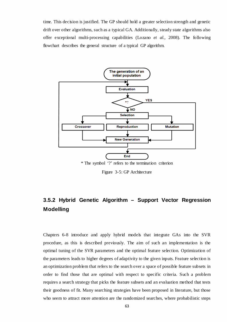
63
time. This decision is justified. The GP should hold a greater selection strength and genetic
drift over other algorithms, such as a typical GA. Additionally, steady state algorithms also
offer exceptional multi-processing capabilities (Lozano et al., 2008). The following
flowchart describes the general structure of a typical GP algorithm.
* The symbol ‘?’ refers to the termination criterion
Figure 3-5: GP Architecture
3.5.2 Hybrid Genetic Algorithm – Support Vector Regression Modelling
Chapters 6-8 introduce and apply hybrid models that integrate GAs into the SVR
procedure, as this is described previously. The aim of such an implementation is the
optimal tuning of the SVR parameters and the optimal feature selection. Optimization of
the parameters leads to higher degrees of adaptivity to the given inputs. Feature selection is
an optimization problem that refers to the search over a space of possible feature subsets in
order to find those that are optimal with respect to specific criteria. Such a problem
requires a search strategy that picks the feature subsets and an evaluation method that tests
their goodness of fit. Many searching strategies have been proposed in literature, but those
who seem to attract more attention are the randomized searches, where probabilistic steps

64
are applied (Sun et al., 2004). Therefore, the use of GAs for such a task is appropriate and
justified (Siedlecki and Sklansky (1989)).
3.5.2.1 Hybrid Genetic Algorithm – Support Vector Regression (GA-SVR)
This subsection presents the hybrid Genetic Algorithm – Support Vector
Regression (GA-SVR) model for optimal SVR parameter and feature subset combination
(chapter 6) or selection (chapter 7). The proposed model genetically searches over a large
pool of potential inputs and provides an out-of-sample optimized SVR forecast for each
series under study. In order to achieve this, a simple GA is used. Its chromosome
comprises feature genes that encode the best feature subset and parameter genes that
encode the best choice of parameters. One such chromosome is depicted in chapter 6 (see
figure 6-1).
The lack of information on the noise of the training datasets makes the a priori ε-
margin setting of ε-SVR a difficult task. In order to overcome this and decrease the
computational demands of the methodology, a RBF v-SVR approach is taken during the
design of this hybrid model. The virtues of using RBF kernels are stated by many
researchers, when SVR is applied in financial forecasting (i.e. Min and Lee (2005), Ding et
al. (2009) and Kao et al. (2013)). Their advantage is that they efficiently overcome over-
fitting and seem to excel in directional accuracy. A RBF kernel is in general specified as:
2( , ) exp( ), 0γ γ= − − >i iK x x x x (3.20)
where γ represents the variance of the kernel function. Consequently, the parameters
optimized by the GA are C, v and γ.3
The GA uses the one-point crossover and the mutation operators. The one-point
crossover provides two offsprings from every two parents. Then the algorithm randomly
selects the parents and a crossover point cx. The two offsprings are made by both
concatenating the genes that precede cx in the first parent with those that follow (and
include) cx in the second parent. The probability for selecting an individual as a parent for
3As shown in subsection 3.4 xi are the support vectors and x the data vectors.

65
the crossover operator is called crossover probability and in all the applications is
generally set high to ensure that some population is kept for the next generation. In that
way the GA creates better new chromosomes from good parts of the old chromosomes.
The offspring produced by the crossover operator replaces their parents in the population.
On the other hand, the mutation operator places random values in randomly selected genes
with a certain probability named as mutation probability. This operator is very important
for avoiding local optima and exploring a larger surface of the search space. This
probability is always set low in order to prevent the algorithm from performing a random
search.
For the selection step of the GA, the roulette wheel selection process is used
(Holland (1995)). In roulette wheel selection chromosomes are selected according to their
fitness. The better the chromosomes are, the more chances to be selected they have. Elitism
is used to raise the evolutionary pressure in better solutions and to accelerate the evolution.
The best solution is copied without changes to the new population. Thus, the best solution
found can survive at the end of every generation. Similarly to the NNs, the GA-SVR model
requires training and test subsets to validate the goodness of fit of each chromosome. The
population of chromosomes is initialized in the training sub-period. The optimal selection
of chromosomes is achieved through a fitness function. Then, the optimized parameters
and selected predictors of the best solution are used to train the SVR and produce the final
optimized forecast, which is evaluated over the out-of-sample period. In genetic algorithm
modelling, though, fitness functions need to be increasing functions. The fitness function is
chosen based on the forecasting task at hand. The details of the fitness functions used in
each application are given at each specific chapter.
Finally, the size of the initial population and the maximum number of generations
needs to be chosen beforehand. This is done through a sensitivity analysis from the user of
the algorithm based on the given inputs to the algorithm. These details are also provided in
each chapter. Another issue that needs to be taken into account is the population
convergence which is associated with the termination criterion of the GA. In all chapters,
the population is deemed as converged when the average fitness across the current
population is less than 5% away from the best fitness of the current population. In that
way, the GA avoids keeping populations that their diversity is very low. If the algorithm
evolved such populations, it would be unlikely to produce different and better individuals
than the existing ones or those qualified to be kept in previous generations. The flowchart
of the designed GA-SVR is shown in figure 3-6.

66
Figure 3-6: Hybrid GA-SVR and RG-SVR flowchart

67
3.5.2.2 Hybrid Rolling Genetic – Support Vector Regression (RG-SVR)
The GA-SVR previously explained is providing a single out-of-sample optimized SVR
forecast for each series under study. Nonetheless, it is selecting parameters and feature
subsets based on a fixed in-sample period. It is well established in the financial and
economic literature, that the more recent the data are, the more significant is the
information that they incorporate. Thus, the relevance of the predictors should have a
changing composition. In order to expand the mapping ability of the algorithm to the given
inputs and derive more realistic forecasts, the GA-SVR is extended to a Rolling Genetic –
Support Vector Regression (RG-SVR) in chapter 8.
The logic and the design of the RG-SVR model is the same as in GA-SVR. The novelty
lies in the fact that each chromosome is now selected through a rolling in-sample period
(rolling window). The algorithm requires the window size to be further divided in a
training and test subset in order to validate the goodness of fit of each chromosome, as in
GA-SVR. The population of chromosomes is initialized in each training sub-period. The
optimal selection of chromosomes is achieved, when their forecasts maximize the fitness
function in the test-sub period. These optimized parameters and selected predictors of the
best solution are used to train the SVR and produce the final optimized forecast for the
next observation. After this is completed, the window rolls forward by one observation and
the procedure is repeated. In that way, the RG-SVR model presents single rolling forecasts.
For each of these forecasts, the algorithm retains the optimized C, γ and v parameters and
set of optimal predictors, creating an image of how the relevance of these inputs fluctuates
as time goes by.
The flowchart of this technique is also given by the previous figure. The reader
should bear in mind, though, that the in-sample dataset in this case is changing in every
iteration. In addition, the out-of-sample dataset represents just the next observation, since
the model derives only one forecast at each loop. This brings forward again the curse of
dimensionality in such techniques, as referred in the general motivation of this thesis. The
integrated rolling forward estimation raises the computational demands of the algorithm.
Its accuracy depends on the trade-off between a high-complexity model (over-fitting) and a
large-margin (incorrect setting of the SVR ‘tube’). For that reason, another new attribute of
RG-SVR is that the SVR procedure is performed with the minimum support vectors.

68
Chapter 4
Forecasting and Trading the EUR/USD Exchange Rate with Stochastic Neural Network Combination
and Time-Varying Leverage
4.1 Introduction
The term of Neural Network (NN) originates from the biological neuron connections of
human brain. The artificial NNs are computation models that embody data-adaptive
learning and clustering abilities, deriving from parallel processing procedures (Krose and
Smagt, 1996). The NNs are considered a relatively new technology in Finance, but with
high potential and an increasing number of applications. However, their practical
limitations and contradictory empirical evidence lead to skepticism on whether they can
outperform existing traditional models.
The motivation of this chapter is to investigate the statistical and trading performance of a
novel Neural Network (NN) architecture, the Psi Sigma Neural Network (PSN), and
explore the utility of Kalman Filters in combining NN forecasts. Firstly, the EUR/USD
European Central Bank (ECB) fixing series is applied to a Naive Strategy, an
Autoregressive Moving Average (ARMA) model and three NNs, namely a Multi-Layer
Perceptron (MLP), a Recurrent Network (RNN) and a PSN. Secondly, the Kalman Filter is
compared with four forecast combination methods. That is the traditional Simple Average,
the Bayesian Average, Granger- Ramanathan’s Regression Approach (GRR) and the Least
Absolute Shrinkage and Selection Operator (LASSO). The models’ performance is
estimated using the EUR/USD ECB fixing series of the period of 2002-2010, using the last
two years for out-of-sample testing. Finally, a time-varying leverage strategy based on
RiskMetrics volatility forecasts is introduced.

69
The results show that PSN outperforms its NN and statistical benchmarks in terms of
annualised returns and information ratios. The NN forecast combinations, excluding the
Bayesian Average model, present improved annualised returns and information ratios and
in almost all cases outperform every individual NN performance. More specifically, the
Kalman Filter outperforms all individual models and combination forecasts. The Kalman
Filter forecasts are also found statistically different from their benchmarks under the
Diebold-Marino test (1995). Finally, all models except ARMA show substantial increase
in their trading performance, after applying the time-varying leverage strategy,
In section 4.2 follows the detailed description of the EUR/USD ECB fixing series, used as
dataset in this study. Section 4.3 gives an overview of the forecasting, while section 4.4
describes the forecast combination methods implemented. The statistical and trading
performance of the models is presented in Sections 4.5 and 4.6. Finally, some concluding
remarks are summarized in section 4.7.
4.2 The EUR/USD Exchange Rate and Related Financial Data
The European Central Bank (ECB) publishes a daily fixing for selected EUR exchange
rates: these reference mid-rates are based on a daily concentration procedure between
central banks within and outside the European System of Central Banks, which normally
takes place at 2.15 p.m. ECB time. The reference exchange rates are published both by
electronic market information providers and on the ECB's website shortly after the
concentration procedure has been completed. Although only a reference rate, many
financial institutions are ready to trade at the EUR fixing and it is therefore possible to
leave orders with a bank for business to be transacted at this level.
In this chapter, the EUR/USD is examined over period 2002 -2010, using the last
two years for out-of-sample. In order to train the NNs, the in-sample dataset is further
divided in two sub-periods (see chapter 3).

70
Table 4-1: The EUR/USD Dataset - Neural Networks’ Training Datasets
The graph below shows the total dataset for the EUR/USD and its volatile trend
since early 2008.
Figure 4-1: EUR/USD Frankfurt daily fixing prices
The EUR/USD time series, shown above, is non-normal and non-stationary.
Jarque-Bera statistics confirm its non-normality at the 99% confidence interval with slight
skewness and low kurtosis. To overcome the non-stationary issue, the EUR/USD series is
transformed into a daily series of rate returns. So given the price level P1, P2, …, Pt, the
return at time t is calculated as:
1
1tt
t
PRP−
= −
(4.1)
The stationary property of the EUR/USD return series is confirmed at the 1%
significance level (ADF and PP test statistics) and its summary statistics are shown in
Figure 4-2. From those it is obvious that the slight skewness and low kurtosis remain. The
Jarque-Bera statistic confirms again that the EUR/USD series is non-normal at the 99%
confidence interval. For more details on Jarque-Bera statistics see Jarque and Bera (1980).
0,6
0,8
1
1,2
1,4
1,6
1,8
3/1/
2002
3/5/
2002
3/9/
2002
3/1/
2003
3/5/
2003
3/9/
2003
3/1/
2004
3/5/
2004
3/9/
2004
3/1/
2005
3/5/
2005
3/9/
2005
3/1/
2006
3/5/
2006
3/9/
2006
3/1/
2007
3/5/
2007
3/9/
2007
3/1/
2008
3/5/
2008
3/9/
2008
3/1/
2009
3/5/
2009
3/9/
2009
3/1/
2010
3/5/
2010
3/9/
2010
1 January 2002 to 31 December 2010
EU
R/U
SD
PERIODS TRADING DAYS START DATE END DATE Total Dataset 2295 3/01/2002 31/12/2010 Training Dataset (In-sample) 1270 3/01/2002 29/12/2006 Test Dataset (In-sample) 511 02/01/2007 31/12/2008 Validation Dataset (Out-of-sample) 514 02/01/2009 31/12/2010

71
Figure 4-2: EUR/USD Returns Summary Statistics
There is no formal theory behind the selection of the inputs of a neural network.
Therefore, neural networks experiments and a sensitivity analysis on a pool of potential
inputs in the training dataset are conducted to help with this decision. The aim is to select
the set of inputs for each network which is the more likely to lead to the best trading
performance in the out-of-sample dataset. In this application, the set of variables that
provide the higher trading performance for each network in the test sub-period are selected.
Surprisingly, this set of inputs is identical for all neural network models. All sets of inputs
are presented in table 2 below4.
4 They are also explored as inputs autoregressive terms of other exchange rates (e.g. the USD/JPY and GBP/JPY exchange rates), commodit ies prices (e.g. Gold Bullion and Brent Oil) and stock market prices (e.g. FTSE100 and DJIA). However, the set of inputs presented in table 4-2 gave to the NNs the highest trading performance in the training period and were thus retained.

72
* In this application the term ‘Lag 1’ means that today’s closing price is used to forecast the tomorrow’s one.
Table 4-2: Explanatory Variables
4.3 Forecasting Models
4.3.1 Benchmark Forecasting Models
In this chapter two traditional forecasting strategies, the Naive Strategy and the Auto-
Regressive Moving Average (ARMA) model are used, in order to benchmark the
efficiency of the NNs’ performance.
4.3.1.1 Naive Strategy
The Naive Strategy is considered to be the simplest strategy to predict the future. That is to
accept as a forecast for time t+1, the value of time t, assuming that the best prediction is
the most recent period change. Thus, the model takes the form:
1t tY Y+ = (4.2)
tY is the actual rate of return at time t and 1tY + is the forecast rate of return at time t+1. In
order to evaluate the Naive trading performance, a simulated strategy is used.
Νumber Explanatory Variables Lag*
1 EUR/USD Exchange Rate Return 1 2 EUR/USD Exchange Rate Return 2 3 EUR/USD Exchange Rate Return 4 4 EUR/USD Exchange Rate Return 5 5 EUR/USD Exchange Rate Return 8 6 EUR/USD Exchange Rate Return 10 7 EUR/GBP Exchange Rate Return 1 8 EUR/GBP Exchange Rate Return 2 9 EUR/JPY Exchange Rate Return 1

73
4.3.1.2 Auto-Regressive Moving Average Model (ARMA)
The ARMA model is based on the assumption that the current value of a time-series is a
linear combination of its previous values plus a combination of current and previous values
of the residuals (Brooks, 2008). Thus, the ARMA model embodies autoregressive and
moving average components and can be specified as below:
0 1 1 2 2 1 1 2 2... ...t t t p t p t t t q t qY Y Y Y w w wϕ ϕ ϕ ϕ ε ε ε ε− − − − − −= + + + + + − − − − (4.3)
Where:
• Yt is the dependent variable at time t
• Yt-1,Yt-2,…Yt-p are the lagged dependent variables
• φ0,φ1,…,φp are the regression coefficients
• εt is the residual term
• εt-1,εt-2,…,εt-q are the previous values of the residual terms
• w1, w2,…,wq are the residual weights
Based on the in-sample correlogram (training and test subsets), a restricted ARMA
(13, 13) model is chosen as the best for an out-of-sample estimation (Appendix B.1). The
ARMA model, used for this application, can be specified as follows:
3 4 6 9 13 3 4
6 9 13
0.0288 0.2689 0.6028 0.3921 0.6884 0.3641 0.2638 0.590.3916 0.6227 0.3165t t t t t t t t
t t t
Y Y Y Y Y Y ε εε ε ε
− − − − − − −
− − −
= − + − − + + −+ + − (4.4)
The evaluation of the ARMA model selected comes in terms of trading performance.
4.3.2 Neural Networks (NNs)
In this chapter three NN architectures, namely the MLP, RNN and the novel PSN, are used
to forecast the series under study. All these models are thoroughly explained in chapter 6
(training process and specification). In this part it should be noted that the starting point for
each network is a set of random weights. Therefore, forecasts can differ between networks.
In order to eliminate any variance between the derived NN forecasts and add robustness to

74
the results, a simple average of a committee of 10 NNs is used. Those 10 NNs are those 10
MLPs, RNNs and PSNs that present the highest profit in the training sub-period. This is a
necessary process in order to eliminate any outlier network that could jeopardise the final
conclusions. The technical characteristics of the NNs used in this task are presented in
Appendix B.2.
4.4 Forecasting Combination Techniques
The five techniques that are used to combine the NNs forecasts are presented in this
section. It is important to outline that a forecast combination targets either to follow the
trend of the best individual forecast (‘combining for adaptation’) or to significantly
outperform each one of them (‘combining for improvement’) (Yang, 2004). Consequently,
the naive strategy and the ARMA are rejected from the combination techniques. Both
strategies present a considerably worse trading performance than their NNs’ counterparts
both in-sample and out-of-sample. Therefore, their inclusion in the combination techniques
would deteriorate their performance rather than improve it.
4.4.1 Simple Average
The first forecasting combination technique used in this chapter is Simple Average, which
can be considered a benchmark forecast combination model. Given the three NNs’
forecasts , ,t t tMLP RNN PSNf f f at time t, the combination forecast at time t is calculated as:
3( ) /MLP RNN PSNNNs
t t t tcf f f f= + + (4.5)

75
4.4.2 Bayesian Averaging
A Bayesian Average model specifies optimal weights for the combination forecast based
on the Akaike Information Criterion (AIC) and Schwarz Bayesian Information Criterion
(SIC). According to Buckland et. al. (1997) the Bayesian weights using AIC, can be
estimated as:
0.5
, 30.5
1
i
j
C
AIC iC
j
ewe
− ∆ΑΙ
− ∆ΑΙ
=
=
∑
(4.6)
Where:
• i=1,2,3 for , ,MLP RNN PSNf f f respectively
• ΔAICi = AICi – AICi,min (4.7)
Based on the above, the combination forecast at time t is ,
3
1( ) / 3AIC i i
t t
iNNscf w f
=
= ∑ and
in this case the AIC Bayesian models take the following form:
(0.33421 0.33081 0.33492 ) / 3AIC
t t t tc MLP RNN PSNf f f f= + +
(4.8)
The Bayesian Average weights for SIC are defined similarly and in this case the
SIC Bayesian model is specified as follows:
(0.33421 0.330833 0.33491 ) / 3SIC
t t t tc MLP RNN PSNf f f f= + +
(4.9)
Equations 4.8 and 4.9 are similar as the AIC and SIC criteria for the NNs in the in-
sample period are very close. For that reason, in the results only the Bayesian Average
based on the AIC criterion is presented. This is the case where the results are marginally
better in terms of trading performance in-sample. Nonetheless, the weights are in favor
(maximized) of PSN, namely the model with the minimum AIC and SIC respectively. For
details on the exact calculation of the AIC and SIC and their Bayesian Average weights see
appendix B.3.

76
4.4.3 Granger and Ramanathan Regression Approach (GRR)
According to Bates and Granger (1969) a combining set of forecasts outperforms the
individual forecasts that the set consists of. Taking this basic idea one step further, Granger
and Ramanathan (1994) suggested three regression models as follows:
1 0 11
n
c i ii
f a a f ε=
= + +∑ (4.10)
2 21
n
c i ii
f a f ε=
= +∑ (4.11)
3 31 1
, 1n n
c i i ii i
f a f where aε= =
= + =∑ ∑ (4.12)
Where
• fi, i=1,...,n are the individual one-step-ahead forecasts,
• fc1, fc2, fc3 are the combination forecast of each model,
• α0 is the constant term of the regression
• αi are the regression coefficients of each model
• ε1, ε2, ε3 are the error terms of each regression model
The model specified in equation 4.10, which is selected for this case, is usually
preferred in order to avoid forecasts errors correlated with the individual forecasts fi
(Swanson and Zeng, 2001). Thus, the GRR model at time t used in this chapter is specified
as shown below:
tt
PSNt
RNNt
MLPt
c ffffNNs
ε++++= 132.56461.13023.350422.0 (4.13)
However, the variety of data and the biased and correlated forecasts raise questions
on GRR model selection or modification, which are further discussed in the literature
(Diebold and Pauly (1987) and Coulson and Robins (1993)).

77
4.4.4 Least Absolute Shrinkage and Selection Operator (LASSO)
The LASSO Regression is a class of Shrinkage or Regularization Regressions, which
applies when multicollinearity exists among the regressors (Sundberg, 2002). The main
difference between this technique and the Ordinary Least Squares (OLS) Regression is that
LASSO method also minimizes the residual squared error, by adding a coefficient
constraint (similarly to Ridge Regression (Chan et al., 1999)).
Compared to Ridge Regression, LASSO best applies in samples of few variables
with medium/large effect such in this case (Hastie et al., 2009). For more details on the
mathematical specifications of LASSO see Wang et al. (2007). Given the vectors of
independent and dependent variables:
1 11 1
1
1, ( ,..., )
T
TN
N
N NN
TN
X
X
x x
x xY y y
==
(4.14)
and the training data (X1,y1),…,(XN,yN), the LASSO coefficients are estimated based on
the following argument:
1
2
01 1
, 0ˆ arg mind
jj
N d
i i iji j
lasso subject to k ky xβ ββ β β== =
≤ > = − −
∑∑ ∑ (4.15)
This argument is based on Breiman’s non-negative garrote minimization process
(Yuan and Lin, 2007). Here k stands for the ‘tuning parameter’, because it controls the
amount of shrinkage applied to the coefficients (Tibshirani, 2011). In this case, I
experimented with various values of k in the in-sample period and concluded that the best
results in terms of trading performance are acquired when the constraint takes the
following form:
10.6MLP RNN PSNβ β β+ + ≤ (4.16)
Subject to this constraint the model takes the form:
tt
PSNt
RNNt
MLPt
c ffffNNs
ε+++= 623.5591.1284.3 (4.17)
This LASSO constraint makes the model adaptive, since it creates a penalization
balance on each estimate, by leading some coefficients to zero or close to zero (see the

78
unconstrained regression of GGR (equation 4.13) compared to the LASSO one (equation
4.17). This process favors the PSN architecture.
4.4.5 Kalman Filter
Kalman Filter is an efficient recursive filter that is described in chapter 3 and appendix A.
The time-varying coefficient combination forecast suggested in this chapter is shown
below:
5.80 1.16 75.89NNs
t t t tc MLP RNN PSN tf f f f ε= + + + (4.18)
From the above equation, which represents the final state, the Kalman filtering
process favors the PSN model. This is what one would expect, since it is the model that
performs best individually. In order to achieve optimal Kalman Filter estimation, it is
important though to introduce a noise ratio5:
2 2/r nn εσ σ= (4.19)
The results are becoming more adaptive when the noise ratio rises (Dunis et al.,
2010).When 2 0nσ = , the model transforms to the typical OLS model.
4.5 Statistical Performance
As it is standard in literature, in order to evaluate statistically the derived forecasts, the
RMSE, MAE, MAPE and Theil-U statistics are computed (see amongst others Dunis and
Williams (2002) and Dunis and Chen (2005)). The statistical analysis will provide some
information regarding the accuracy of the forecasts and strengthen the final conclusions.
The RMSE and MAE statistics are scale-dependent measures but give a basis to compare
volatility forecasts with the realized volatility while the MAPE and the Theil-U statistics
are independent of the scale of the variables. In particular, the Theil-U statistic is 5 As stated in chapter 3, the 2 2, nεσ σ represent the variances of the error terms of the measurement and state equations

79
constructed in such a way that it necessarily lies between zero and one, with zero
indicating a perfect fit. A more detailed description of these measures can be found on
Theil (1966) and Pindyck and Rubinfeld (1998), while their mathematical formulas are
presented in appendix B.4. For all four of the error statistics retained (RMSE, MAE,
MAPE and Theil-U) the lower the output, the better the forecasting accuracy of the model
concerned.
The in-sample and out-of-sample period performances are presented in tables 4-3
and 4-4 respectively. The results indicate that from the individual forecasts, the PSN
outperformed all other models in both the in-sample and out-of-sample periods. Similarly,
for the forecast combinations methodologies the Kalman Filter beat its benchmarks for the
four statistical criteria retained in both estimation periods. Adding to the above statistical
performance of the Kalman Filter, the Diebold-Mariano (1995) statistic for predictive
accuracy is also computed for both MSE and MAE loss functions. The details on the
Diebold-Mariano statistic are given in appendix B.5. The results of the Diebold-Mariano
statistic, comparing Kalman filter with each other method, are summarized in Table 4-5.
From the table 4-5, the null hypothesis of equal predictive accuracy is rejected for
all comparisons and for both loss functions at 5% confidence interval, since the test results
|sMSE|>1.96 and |sMAE|>1.96. Moreover, the statistical superiority of the Kalman Filter
forecasts is confirmed as for both loss functions the realizations of the statistic are
negative 6. Finally, the second best model in statistical terms, the LASSO regression, has
the closest forecasts with Kalman Filter.
6 In this study the Diebold-Mariano test is applied to couples of fo recasts (Kalman Filter vs. another forecasting model). A negative realizat ion of the Diebold-Mariano test statistic indicates that the first forecast (Kalman Filter) is more accurate than the second forecast. The lower the negative value, the more accurate are the Kalman Filter forecasts.

Table 4-3: Summary of In-Sample Statistical Performance
Table 4-4: Summary of Out-of-Sample Statistical Performance
Table 4-5: Summary results of Diebold-Mariano statistic for MSE and MAS loss functions
TRADITIONAL TECHNIQUES NEURALNETWORKS FORECAST COMBINATIONS
NAIVE ARMA MLP RNN PSN Simple Average Bayesian Average GRR LASSO Kalman Filter
MAE 0.0065 0.0045 0.0044 0.0042 0.0039 0.0037 0.0037 0.0035 0.0038 0.0033
MAPE 399.44% 122.20% 97.13% 93.35% 89.43% 84.98% 85.13% 82.78% 87.63% 71.51%
RMSE 0.0086 0.0060 0.0053 0.0050 0.0041 0.0036 0.0036 0.0032 0.0037 0.0023
Theil-U 0.7021 0.6948 0.6686 0.5087 0.4292 0.4522 0.4625 0.4245 0.4613 0.2713
TRADITIONAL TECHNIQUES NEURAL NETWORKS FORECAST COMBINATIONS
NAIVE ARMA MLP RNN PSN Simple Average Bayesian Average GRR LASSO Kalman Filter
MAE 0.0084 0.0059 0.0058 0.0056 0.0048 0.0048 0.0048 0.0047 0.0046 0.0044
MAPE 405.62% 131.20% 112.37% 105.97% 97.88% 94.07% 93.76% 92.83% 92.05% 88.37%
RMSE 0.0107 0.0077 0.0061 0.0060 0.0054 0.0053 0.0051 0.0049 0.0053 0.0043
Theil-U 0.7958 0.8749 0.7301 0.6001 0.4770 0.5672 0.5598 0.5297 0.6142 0.5212
NAIVE ARMA MLP RNN PSN Simple Average Bayesian Average GRR LASSO
sMSE -9.307 -9.321 -6.244 -5.698 -5.184 -4.869 -4.896 -4.351 -4.112
sMAE -9.845 -9.832 -9.189 -8.881 -8.159 -7.851 -7.873 -7.679 -7.352
80

81
4.6 Trading Performance
4.6.1 Trading Strategy and Transaction Costs
The trading strategy applied in this chapter is to go or stay ‘long’ when the forecast return
is above zero and go or stay ‘short’ when the forecast return is below zero. The ‘long’ and
‘short’ EUR/USD position is defined as buying and selling Euros at the current price
respectively. The transaction costs for a tradable amount, say USD 5-10 million, are about
1 pip (0.0001 EUR/USD) per trade (one way) between market makers. But the EUR/USD
time series is considered as a series of middle rates, the transaction costs is one spread per
round trip. With an average exchange rate of EUR/USD of 1.369 for the out-of-sample
period, a cost of 1 pip is equivalent to an average cost of 0.007% per position.
4.6.2 Trading Performance before Leverage
The trading performance measures and their calculation description are presented in
appendix B.4. Table 4-6 presents the in-sample trading performance of the models and
forecast combinations before and after transaction cost. All models present a positive
trading performance after transaction costs. From the single forecasts the PSN outperforms
each NN and statistical benchmark in terms of annualised return and information ratio. The
other two artificial intelligence models, the RNN and the MLP, present the second and
third best trading performance respectively. Concerning the forecast combinations, the
Kalman Filter is found to have the best trading performance with an annualised return of
41.78% and an information ratio of 4.47 after transaction costs. It is also worth noting that
all forecast combinations outperform the best single forecast, the PSN, in terms of trading
performance.
The out-of-sample performance of the models before and after transaction costs is
shown in table 4-7.The last two rows of this table suggest that the PSN continues to
outperform all other single forecasts in terms of trading performance. From the forecast
combinations point of view, only the Kalman Filter and the LASSO methods seem to beat
the best single forecast. The Simple Average, Bayesian Average and GRR methods, which
demonstrated a better performance in the in-sample period, seem unable to maintain this

82
superiority in the out-of-sample period. Moreover, the trading performance of the Bayesian
Average and Simple Average strategies is very close. This is expected as the AIC and the
BIC information criteria for the three NNs are very close in the in-sample period. On the
other hand, the GRR strategy still outperforms the MLP and the RNN models in terms of
annualised return and information ratio. That could be thought as a trend to adapt to the
best individual performance (‘combining for adaptation’, (Yang, 2004)). Finally, the
Kalman Filter achieves a 10% higher annualised return than the second best methodology,
the LASSO regression. It seems that the ability of Kalman Filter to provide efficient
computational recursive means to estimate the state of the process gives it a considerable
advantage compared to the tested fixed parameters combination models.

Table 4-6: Summary of In-Sample Trading Performance
TRADITIONAL TECHNIQUES
NEURAL NETWORKS
FORECAST COMBINATIONS
NAIVE ARMA MLP RNN PSN Simple Average Bayesian Average GRR LASSO Kalman Filter Annualised Return (excluding costs) -4.80% 10.60% 14.80% 16.07% 18.37% 16.37% 16.59% 16.99% 20.23% 28.79%
Annualised Volatility 12.03% 11.07% 11.83% 11.02% 10.89% 10.85% 10.85% 11.02% 10.99% 10.92% Information Ratio (excluding costs) -0.4 0.96 1.25 1.46 1.69 1.51 1.53 1.54 1.84 2.64
Maximum Drawdown -6.41% -6.23% -6.23% -6.23% -6.31% -6.31% -6.31% -6.31% -6.31% -6.31%
Annualised Transactions 77 54 71 71 76 70 71 63 69 73
Transaction Costs 0.54% 0.38% 0.50% 0.50% 0.53% 0.49% 0.50% 0.44% 0.48% 0.51% Annualised Return
(including costs) -5.34% 10.22% 14.30% 15.57% 17.84% 15.88% 16.09% 16.55% 19.75% 28.28%
Information Ratio (including costs) -0.44 0.92 1.21 1.41 1.64 1.46 1.48 1.50 1.80 2.59
Table 4-7: Summary of Out-of-Sample Trading Performance
TRADITIONAL TECHNIQUES
NEURAL NETWORKS
FORECAST COMBINATIONS
NAIVE ARMA MLP RNN PSN Simple Average Bayesian Average GRR LASSO Kalman Filter
Annualised Return (excluding costs) 1.49% 13.87% 23.19% 26.14% 28.10% 32.74% 32.39% 33.99% 30.57% 42.63%
Annualised Volatility 9.68% 9.70% 9.38% 9.59% 9.23% 9.51% 9.52% 9.49% 9.54% 9.35% Information Ratio (excluding costs) 0.15 1.43 2.47 2.73 3.05 3.44 3.4 3.58 3.21 4.56
Maximum Drawdown -8.59% -6.52% -5.91% -6.55% -6.55% -6.55% -6.55% -6.55% -6.55% -6.66% Annualised
Transactions 130 100 121 136 74 107 106 104 106 121
Transaction Costs 0.91% 0.70% 0.85% 0.95% 0.52% 0.75% 0.74% 0.73% 0.74% 0.85% Annualised Return
(including costs) 0.58% 13.17% 22.34% 25.19% 27.58% 31.99% 31.65% 33.26% 29.83% 41.78%
Information Ratio (including costs) 0.06 1.36 2.38 2.63 2.99 3.36 3.32 3.50 3.13 4.47
83

84
4.6.3 Leverage to exploit high Information Ratios
In order to further improve the trading performance of the previous models, a leverage is
introduced based on RiskMetrics one day ahead volatility forecasts 7. The details of the
RiskMetrics model are in appendix B.6. The intuition of the strategy is to avoid trading
when volatility is very high while at the same time exploiting days when the volatility is
relatively low. As mentioned by Bertolini (2010) there are few papers on market-timing
techniques for foreign exchange, with the notable exception of Dunis and Miao (2005,
2006). The opposition between market-timing techniques and time-varying leverage is
apparent, as time-varying leverage can be easily achieved by scaling position sizes
inversely to recent risk behaviour measures.
The process starts with forecasting with RiskMetrics the one day ahead realised
volatility of the EUR/USD exchange rate in the test and validation sub-periods. Then,
following Dunis and Miao (2005, 2006), these two periods are split into six sub-periods,
ranging from periods with extremely low volatility to periods experiencing extremely high
volatility. Periods with different volatility levels are classified in the following way:
Initially the average (μ) difference between the actual volatility in day t and the
forecasted for day t+1 and its ‘volatility’ (measured in terms of standard deviation σ) are
calculated. The periods where the difference is between μ plus one σ are classified as
‘Lower High Vol. Periods’. Similarly, ‘Medium High Vol.’ (between μ + σ and μ + 2σ) and
‘Extremely High Vol.’ (above μ + 2σ) periods can be defined. Periods with low volatility
are also defined following the same 1σ and 2σ approach, but with a minus sign. After the
six periods are formed, the next step is to assign the appropriate leverage factors. In each
sub-period, leverage is assigned starting with 0 for periods of extremely high volatility to a
leverage of 2.5 for periods of extremely low volatility. The following table presents the
sub-periods and their relevant leverages.
7 A GJR (1, 1) is also explored to model in forecasting volatility. Its statistical accuracy in the test sub-period in terms of the MAE, MAPE, RMSE and the Theil-U statistics is only slightly better compared with RiskMetrics. However, when the utility of GJR in terms of trading efficiency is measured for our models within the context of the strategy in the test sub-period, the results in terms of annualised returns are slightly better with RiskMetrics for most of the models. Moreover, RiskMetrics is simpler to implement than the more complicated GJR. Therefore, in this chapter the results obtained with RiskMetrics are presented. It is also worth noting that the ranking of the models in terms on information ratio and annualised return is the same, whether GJR or RiskMetrics are used.

85
Extremely Low Vol.
Medium Low Vol.
Lower Low Vol.
Upper High Vol.
Medium High Vol.
Extremely High Vol.
Leverage 2.5 2 1.5 1 0.5 0
Table 4-8: Classification of Leverage in Sub-Periods
The parameters of the strategy (μ and σ) are updated every three months by rolling
forward the estimation period. So for example, for the first three months of the validation
period, μ and σ are computed based on the eighteen months of the test sub-period. For the
following three months, the two parameters are computed based on the last fifteen months
of test sub-period and the first three of the validation sub-period. Figure 4-3 summarizes
the leverages assigned in the trading days of the out-of-sample period, based on the above
strategy. The cost of leverage (interest payments for the additional capital) is calculated at
1.75% p.a. (that is 0.0069% per trading day8). The final results are presented in table 4-9.
The most striking performance achieved by the time-varying leverage strategy is
the significant reduction in the maximum drawdown, the essence of risk for an investor in
financial markets. Not only do all models, except ARMA, experience a higher performance
in terms of return or risk-adjusted return, but maximum drawdowns are reduced by as
much as 50%, from 6.31% to 3.38% in the case of the Kalman Filter combination. Even
the naive strategy seems to try to invert its previous discouraging performance (see table 4-
7). The PSN still outperforms every NN and increases its annualised profit over 3%.
Similarly the Bayesian Average and Simple Average combination methods present a 3%
increase of annualised return, but they still cannot outperform the PSN and RNN individual
performance. The other two forecast combination techniques, the GGR and the LASSO,
also present an increased annualised return and information ratio. Finally, the Kalman
Filter continues to present a remarkable trading performance with the highest information
ratio and a 5.67% increase in terms of annualised return. When transaction and leverage
costs are included, the profit decreases, but the trend of the results is not affected. That
allows me to conclude, that in all cases the Kalman Filter can be considered by far the
optimal forecast combination for the dataset and models under study.
8 The interest costs are calculated by considering a 1.75% interest rate p.a. (the Euribor rate at the time of calculation) divided by 252 trad ing days. In reality, leverage costs also apply during non-trading days so that I should calculate the interest costs using 360 days per year. But for the sake of simplicity, I use the approximation of 252 t rading days to spread the leverage costs of non-trading days equally over the trading days. This approximation allows me not to keep track of how many non-trading days a position is hold.

Figure 4-3: Leverages assigned in the out-of-sample period
0
0.5
1
1.5
2
2.5
302
Jan
2009
15 Ja
n 20
0928
Jan
2009
10 F
eb 2
009
23 F
eb 2
009
06 M
ar 2
009
19 M
ar 2
009
01 A
pr 2
009
16 A
pr 2
009
29 A
pr 2
009
13 M
ay 2
009
26 M
ay 2
009
08 Ju
n 20
0919
Jun
2009
02 Ju
l 200
915
Jul 2
009
28 Ju
l 200
910
Aug
200
921
Aug
200
903
Sep
200
916
Sep
200
929
Sep
200
912
Oct
200
923
Oct
200
905
Nov
200
918
Nov
200
901
Dec
200
914
Dec
200
928
Dec
200
911
Jan
2010
22 Ja
n 20
1004
Feb
201
017
Feb
201
002
Mar
201
015
Mar
201
026
Mar
201
012
Apr
201
023
Apr
201
006
May
201
019
May
201
001
Jun
2010
14 Ju
n 20
1025
Jun
2010
08 Ju
l 201
021
Jul 2
010
03 A
ug 2
010
16 A
ug 2
010
27 A
ug 2
010
09 S
ep 2
010
22 S
ep 2
010
05 O
ct 2
010
18 O
ct 2
010
29 O
ct 2
010
11 N
ov 2
010
24 N
ov 2
010
07 D
ec 2
010
20 D
ec 2
010
31 D
ec 2
010
Leve
rage
86

Note: The average leverage factor ex post is computed as the ratio of the annualised returns after costs of tables 4-7 and 4-9 for those models which achieved an in-sample information ratio of at least 2 and, as such, would have been candidates for leveraging out-of-sample. In the final results of this table, I do not take into account the interest that could be earned during times, where the capital is not traded (non-trading days) or not fully invested.
Table 4-9: Summary of Out-of-Sample Trading Performance - final results
TRADITIONAL TECHNIQUES
NEURAL NETWORKS
FORECAST COMBINATIONS
NAIVE ARMA MLP RNN PSN Simple Average
Bayesian Average GRR LASSO Kalman
Filter Annualised Return (excluding costs) -2.34% 7.28% 18.13% 19.44% 22.28% 19.12% 19.36% 22.37% 25.08% 34.46%
Annualised Volatility 10.14% 10.44% 9.90% 9.04% 9.85% 9.09% 9.13% 9.38% 9.20% 9.32% Information Ratio (excluding costs) -0.23 0.7 1.83 2.15 2.26 2.1 2.12 2.38 2.73 3.7
Maximum Drawdown -3.50% -3.20% -3.66% -3.14% -3.66% -2.98% -3.21% -2.83% -2.94% -3.38%
Annualised Transactions 122 90 115 117 122 111 113 97 110 114
Average Leverage Factor (ex post) n.a. n.a. 1.13 1.19 1.12 1.09 1.09 1.26 1.18 1.15
Transaction and Leverage Costs 1.79% 1.57% 1.74% 1.75% 1.79% 1.72% 1.73% 1.62% 1.71% 1.73%
Annualised Return (including costs) -4.13% 5.71% 16.39% 17.69% 20.49% 17.40% 17.63% 20.75% 23.37% 32.73%
Information Ratio (including costs) -0.41 0.55 1.66 1.96 2.08 1.91 1.93 2.21 2.54 3.51
87

88
4.7 Conclusions
In this chapter the trading and statistical performance of a Neural Network (NN)
architecture, the Psi Sigma Neural Network (PSN), is investigated. Then the utility of
Kalman filters in combining NN forecasts is explored. Firstly, the EUR/USD European
Central Bank (ECB) fixing series is applied to a Naive Strategy, an Autoregressive Moving
Average (ARMA) model and three NNs, namely a Multi-Layer Perceptron (MLP), a
Recurrent Network (RNN) and a PSN. Secondly, a Kalman filter-based combination is
compared with four other forecast combination methods. That is the traditional Simple
Average, the Bayesian Average, Granger- Ramanathan’s Regression Approach (GRR) and
the Least Absolute Shrinkage and Selection Operator (LASSO). The models’ performance
is estimated through the EUR/USD ECB fixing series of the period of 2002-2010, using
the last two years for out-of-sample testing. Finally, a time-varying leverage strategy is
introduced based on RiskMetrics volatility forecasts.
As it turns out, the PSN outperforms its benchmarks models in terms of statistical
accuracy and trading performance. It is also shown that all the forecast combinations,
outperform out-of-sample all the single models except the PSN for the statistical and
trading terms retained. It is interesting that the ‘combining for improvement’ pattern that
all combination forecasts showed in the in-sample period, changes regarding the out-of-
sample combination forecasts. Simple Average, Bayesian Average and GRR do not
continue to outperform PSNs’ best individual performance but are better than MLP and
RNN, while LASSO and Kalman Filter present the best results. It seems that the ability of
Kalman Filter to provide efficient computational recursive means to estimate the state of
the process gives it a considerable advantage compared to the fixed parameters
combination models. Finally, all models except ARMA show a substantial increase in their
trading performance and a striking reduction in maximum drawdowns after applying time-
varying leverage. In all these cases, Kalman Filter remains the best approach. Its
remarkable trading performance of Kalman Filter suggests that it can be considered as an
optimal forecast combination for the models and time-series under study. These results
should go some way towards convincing a growing number of quantitative fund managers
to experiment beyond the bounds of the more traditional models and trading strategies. The
results in table 4-9, with an information ratio in excess of 3, should also provide motivation
for the use of Kalman Filter in combining model based forecasts.

89
Chapter 5
Stochastic and Genetic Neural Network Combinations in Trading and Hybrid Time-Varying Leverage Effects
5.1 Introduction
Neural Networks (NNs) are similar to any advanced statistical model. They are optimized
in an in-sample period and applied for prediction in an out-of-sample period. The
difference between NNs and statistical models is that the first have an adaptive nature.
NNs can take many different forms and have as inputs any potential explanatory variable.
Therefore they are capable of exploring different forms of non- linearity and theoretically
provide a superior performance than statistical-econometrical models. Non- linearity is not
possible to be measured in statistical terms and therefore models such as NNs have the
advantage in problems where the exact nature of the series under study is unknown.
Sceptics argue that the lack a formal statistical theoretical background in NNs
makes them useless in Finance. However, financial series and especially exchange rates are
dominated by factors (e.g. behavioural factors, politics…) that time-series analysis and
statistics are unable to capture in a single model. Based on this, it can be argued that a
time-series statistical model that will capture the pattern of exchange rates is in the long-
run impossible. Statistical theory and mathematics will never be able to explain such a
complex relationship. Researchers and traders should seek for the models that are closest to
the actual pattern of the financial series under study. The flexibility and the non- linear
nature of NNs make them perfect candidates for such a problem. This study aims to
provide empirical evidence that will convince scientists and decision investment managers
to experiment beyond the traditional bounds of mathematics and statistics.

90
This chapter attempts to evaluate the performance of a Multi-Layer Perceptron
(MLP), a Recurrent Neural Network (RNN) and a Psi-Sigma Network (PSN) architecture
in forecasting and trading the Euro/Dollar (EUR/USD) exchange rate. Then, the utility of
Kalman Filter, Genetic Programming (GP) and Support Vector Regression (SVR)
algorithms is explored as forecasting combination techniques. The used benchmarks for the
NNs are a Random Walk model (RW), an Autoregressive Moving Average model
(ARMA) and a Smooth Transition Autoregressive Model (STAR). The forecast
combination techniques are then benchmarked by a Simple Average and a Least Absolute
Shrinkage and Selection Operator (LASSO). The forecasts are evaluated in terms of
statistical accuracy and trading efficiency. The EUR/USD exchange rate is highly liquid
and well known for its high volatility in our days. It seems as the perfect series for a
forecasting exercise with non-linear models.
The rationale of the chapter is multiple. It is explored if non-linear models such as
NNs are able to outperform traditional models such as RW, ARMA and STAR. The STAR
model acts as statistical non- linear benchmark, while the comparison of the results with a
RW model adds to the on-going debate if financial forecasting models can outperform a
RW. In this forecasting competition structural macroeconomic models are not included.
Such models are presented by Flannery and Protopapadakis (2002), Andersen et al. (2003),
Pierce and Solakoglu (2007), Evans and Speight (2010) and recently Bacchetta and
Wincoop (2013). The main reason for that choice is the unavailability of daily data of
relevant macroeconomic indicators. Comparing the models with benchmarks generated by
lower frequency data would make the forecasting competition unfair and unequal.
This study also checks if statistical models like the LASSO and the Kalman Filter
can combine the derived forecasts successfully in order to provide a superior trading
performance. Their results will be benchmarked against those generated by two advanced
non- linear techniques, a SVR and a GP model. SVR and GP algorithms have provided
promising results in many field of Science, but they are rarely used as forecast combination
techniques. The success of the best forecast combination model is also validated through
the Modified Diebold-Mariano (1997) test.
The proposed trading strategy based on volatility forecasts tests if volatility
forecasts and market shocks can be combined with the daily return forecasts to improve the
trading performance of the models. Lastly the implemented loss function for NN models
adds to the literature on the utility of NNs in Finance. Until now researchers are applying
statistical loss functions to generate trading signals through NNs. However, statistical

91
accuracy is not always synonymous with financial profitability. The proposed loss function
attempts to bring a balance between these two terms.
Many researchers have attempted to forecast exchange rates, but their empirical
results are often contradictory. Meese and Rogoff (1983a, 1983b) examine the Frenkel-
Bilson, Dornbusch-Frankel, and Hooper-Morton structural exchange rate models and find
that the random walk performs better. The authors conclude that the out-of-sample failure
of these models is due to the volatile nature of exchange rates, the poor inflation
measurements and their money demand misspecifications. On the other hand, Tenti (1996)
presents promising results in predicting the exchange rate of the Deutsche Mark with three
different RNN architectures. Hussain et al. (2006) provide statistical accurate results with
PSN, when applied in forecasting the EUR/USD, EUR/GBP and EUR/JPY exchange rates
and using two simple MLP and HONN architectures as benchmarks. Bissoondeeal et al.
(2008) use linear and nonlinear methods in forecasting AUD/USD and GBP/USD
exchange rates and conclude that NNs outperform the traditional ARMA and GARCH
models. Moreover, Kiani and Kastens (2008) forecast the GBP/USD, USD/CAD and
USD/JPY exchange rates with feed-forward and recurrent NNs. Although the USD/CAD
forecasts fail to outperform the ARMA model benchmark, the results are satisfying when
forecasting GBP/USD and USD/JPY exchange rates. Grossman and McMillan (2010)
propose a time-varying ESTR equilibrium exchange rate model for forecasting the bilateral
rates between the US Dollar and the Canadian Dollar, the Japanese Yen and the British
Pound. Their non-linear model provides superior forecasts in terms of directional change
accuracy when compared to their linear alternatives. Finally, Dunis et al. (2011) and
Sermpinis et al. (2012a), who conduct a forecast and trading competitions with several
different NNs architectures present ambiguous results over the superiority of their models.
The idea of combining forecasts to improve prediction accuracy originates from
Bates and Granger (1969), who suggested combining rules based on variances-covariances
of the individual forecasts. Since then, many forecasting combination methods have been
proposed and applied in financial research. Donaldson and Kamstra (1999) use
combination techniques, such as weighted OLS, to benchmark the performance of artificial
NN forecasts of S&P 500 stock index and conclude that the NNs are more statistically
accurate. Hu and Tsoukalas (1999) combine the individual volatility forecasts of four
models with simple averaging, ordinary least squares model and a NN. Their result suggest
that the NN combination model performed better during the August 1993 crisis, especially
in terms of root mean absolute forecast error. De Menezes and Nikolaev (2006) present
promising forecasting results with their polynomial neural network forecasting system,

92
which combines genetic programming with NN models. Altavilla and De Grauwe (2008)
compare the performance of linear and nonlinear models in forecasting exchange rates.
Although linear models are better at short forecasting horizons and nonlinear models
dominate at longer forecasting horizons, they suggest that combining different forecasting
techniques generally produces more accurate forecasts. Guidolin and Timmermann (2009)
combine forecasts of future spot rates with forecasts of macroeconomic variables and
conclude that this improves the out-of-sample forecasting performance of US short-term
rates. Andrawis et al. (2011) attempt to predict the daily cash withdrawal amounts from
ATM machines. In their application, they forecast over one hundred time series with eight
classes of linear and non- linear models. Their results show that a simple average of NN,
Gaussian process regression and linear models’ forecasts is the optimal. Ebrahimpour et al.
(2011) apply and compare three NN combining methods and an Adaptive Network-Based
Fuzzy Inference System to trend forecasting in the Tehran stock exchange. The mixture of
MLP experts is the model that presents the best hybrid model in this competition, but all
NN combining models present promising forecasting performance.
The rest of the chapter is organized as follows. Section 5.2 gives a detailed
description of the EUR/USD ECB fixing series, used as a dataset. Section 5.3 is an
overview of the benchmark and NNs models, while section 5.4 describes the forecast
combination methods implemented. The statistical and trading performance of these
models is presented in Sections 5.6 and 5.7. Finally, conclusions are given in Section 5.8.
5.2 The EUR/USD Exchange Rate and Related Financial Data
Similarly to the rational of the chapter 4, the ECB fixings of EUR/USD are selected for
this forecasting and trading application. The ECB daily fixings of the EUR exchange rate
are tradable levels and using them is a more realistic alternative to, say, London closing
prices. In this chapter, the EUR/USD is examined over the period of 1999-2012 in three
rolling forecasting exercises (F1, F2 and F3) on a daily basis. Each exercise studies a
decade of the EUR/USD using the last two years for out-of-sample evaluation. F1 focus on
the decade of 1999-2008 while F2 and F3 examine the periods 2001-2010 and 2003-2012
respectively. Table 5-1 presents these three sub-periods.

Table 5-1: The EUR/USD Dataset and Neural Networks’ Training Sub-periods for the three forecasting exercises
Figure 5-1: EUR/USD Frankfurt daily fixing prices and the three out-of-sample periods under study
F1 F2 F3
PERIODS DAYS PERIOD DAYS PERIOD DAYS PERIOD
Total Dataset 2540 01/02/1999 - 31/12/2008 2560 02/01/2001 - 31/12/2010 2564 02/01/2003 - 31/12/2012 Training Dataset
(In-sample) 1517 01/02/1999 - 31/12/2004 1535 02/01/2001 - 29/12/2006 1537 02/01/2003 - 31/12/2008
Test Dataset (In-sample) 512 03/01/2005 -29/12/2006 511 02/01/2007 -31/12/2008 514 02/01/2009 -31/12/2010
Validation Dataset (Out-of-sample) 511 02/01/2007 -31/12/2008 514 02/01/2009 -31/12/2010 513 03/1/2011 -31/12/2012
93

94
The in-sample datasets for each exercise are further divided in two sub-periods, the
training and test sub-period. This is done for training purposes of the NNs. The three
rolling forward sub-periods add validity to the forecasting exercise and increase the
robustness of the results. The out-of-sample periods are dominated by the effects of the
debt and the mortgage crises. Using a rolling forward the estimation is an attempt to
capture the effect of these crises to the extent that is possible. The rolling forward
estimation and the fact that the parameterization of the models is conducted entirely in-
sample acts as a shield against data-snooping bias’ effects.
The previous figure shows the total dataset of the EUR/USD and its volatile trend.
The out-of-sample periods of each exercise are also highlighted. The EUR/USD time
series, shown above, is non-normal and non-stationary. Jarque-Bera statistics confirm its
non-normality at the 99% confidence interval with slight skewness and high kurtosis. To
overcome the non-stationary issue, the EUR/USD series is transformed into a daily series
of rate returns. So given the price level P1, P2, …, Pt the return at time t is calculated as:
1
1tt
t
PRP−
= −
(5.1)
The Jarque-Bera statistic confirms again that the EUR/USD return series is non-
normal at the 99% confidence interval. For more details on Jarque-Bera statistics see
Jarque and Bera (1980).
5.3 Forecasting Models
5.3.1 Benchmark Forecasting Models
As mentioned previously, three traditional forecasting strategies, namely a RW, an ARMA
and a STAR are used in order to benchmark the efficiency of the NN models. The aim of
these models is to forecast the one day ahead return of the series under study for each
forecasting exercise.

95
5.3.1.1 Random Walk (RW)
The RW is a process where the current value of a variable is calculated from the past value
plus an error term. The error term follows the standard normal distribution. The
specification of the model is:
1ˆ , ~ (0,1)t t t tY Y e e N−= + (5.2)
In this equation tY is the forecasted value for period t and 1tY − is the actual value of
period t-1. The RW is a non-stationary process with a constant mean, but not a constant
variance.
5.3.1.2 Auto-Regressive Moving Average Model (ARMA)
The ARMA model specification is described in chapter 4. Using as a guide the information
criteria in the in-sample subset the optimal ARMA structures are selected. In all cases, the
null hypotheses that all coefficients (except the constant) are not significantly different
from zero and that the error terms are normally distributed are rejected at the 95%
confidence interval. The specifications of the ARMA models selected for out-of-sample
estimation in each exercise are presented below:
1
2
[ ]1 2 5 9 1 2
5 9
]1 3 5 7 1 3
5
ˆ 0.00012 0.4258 0.0787 0.1588 0.6869 0.4235 0.07340.1575 0.6934
ˆ 0.00023 0.0758 0.2157 0.1331 0.7891 0.0905 0.20950.1104 0.78
Ft t t t t t t
t t
Ft t t t t t t
t
Y Y Y Y Y
Y Y Y Y Y
ε εε ε
ε εε
− − − − − −
− −
− − − − − −
−
= + − + − − +− +
= − − + + + +− −
3
7
[ ]1 3 6 7 1 3
6 7
79
ˆ 0.00013 0.9542 0.1819 0.8341 0.9196 0.9525 0.17170.8336 0.9319
t
Ft t t t t t t
t t
Y Y Y Y Y
ε
ε εε ε
−
− − − − − −
− −
= + − + − − + − +
(5.3)

96
5.3.1.3 Smooth Transition Autoregressive Model (STAR)
STARs initially proposed by Chan and Tong (1986) are extensions of the traditional
autoregressive models (ARs). The STAR combines two AR models with a function that
defines the degree of non- linearity (smooth transition function). The general two-regime
STAR specification is the following:
1 2ˆ (1 ( , , )) ( , , )t t t t t tY F z F z uζ λ ζ λ′ ′= Φ Χ − +Φ Χ + (5.4)
Where:
• tY the forecasted value at time t
• ,0 ,1 ,( , ,... ), 1, 2i i i i p iϕ ϕ ϕΦ = = and ,0 ,1 ,, ,...i i i pϕ ϕ ϕ the regression coefficients of the two
AR models
• (1, )t tχ′ ′Χ = with 1( ,..., )t t t pY Yχ − −′ =
• 0 ( , , ) 1tF z ζ λ≤ ≤ the smooth transition function
• , 0t t dz Y d−= > the lagged endogenous transition variable
• ζ the parameter that defines the smoothness of the transition between the two
regimes
• λ the threshold parameter
• ut the error term
The main characteristic of a STAR is that tY is calculated at any given t as a
weighted average of two AR models. The weights of the two AR models are defined based
on the value of ( , , )tF z ζ λ . The regime-switching ability of STARs derives from the fact
that at each t a regime is selected based on the values of zt and ( , , )tF z ζ λ . In this chapter
the series is best modelled as an Exponentional STAR process, following Lin and
Terasvitra (1994).

97
. 5.3.2 Neural Networks (NNs)
This chapter attempts to evaluate the performance of a MLP, RNN and PSN architecture in
forecasting and trading the Euro/Dollar (EUR/USD) exchange rate. The specifications of
these models are given in chapter 3 in detail. For training purposes of the NNs, the in-
sample dataset is further divided in two sub-periods, the training and test sub-period.
Similarly to the route taken in chapter 4, the sensitivity analysis on a pool of potential
inputs in each one of the in-sample datasets is needed. In this application, the training sub-
period is used to select as inputs the set of variables that provides the higher trading
performance in the test sub-period. This optimization procedure is the most popular in NNs
and superior to cross validation for datasets of that size (Zhu and Rohwer, 1996). The set
of inputs for the F1, F2 and F3 can be found in appendix C.1.
The training process of the previous chapter is extended in these three exercises. The NNs
are specially designed for financial purposes. Therefore, a novel fitness function is applied.
This specialised fitness function focuses on achieving two goals at the same time. First of
all, the annualised return in the test period should be maximized and secondly the Root
Mean Square Error (RMSE) of the networks output should be minimized. Based on the
above the fitness function for all the NNs takes the following form and equation 5.4 is
maximized:
Fitness = Annualised_Return – 10*RMSE (5.4)
After the optimization of the networks, the predictive value of each model is
evaluated by applying it to the validation dataset (out-of-sample dataset). Since the starting
point for each network is a set of random weights, forecasts can slightly differ between
same networks. In order to eliminate any variance between the NN forecasts and add
robustness to the results, a simple average of a committee of 20 NNs is used. This
committee comprises of these NNs that provided the highest profit in each in-sample sub-
period of F1, F2 and F3. This is necessary, because otherwise outlier networks can be
included to the committee, used for the final forecasts. The characteristics of these NNs for
each forecasting exercise are also presented in Appendix C.1.
Several NNs trading applications suffer for the data snooping effect. Data-snooping
occurs when a given set of data is used more than once. This can leads to the possibility
that the results achieved may be due to chance rather than an inherent merit in the method.

98
In order to avoid this effect, the guidelines of James et al. (2012) are followed. The data
are clearly subdivided in in-sample (training and test subsets) and out-of-sample
(validation subset). The out-of-sample subset is not used in any part of the NN parameter
selection procedure. A final ‘safe-lock’ against data-snooping is provided by the
implementation of the Hansen (2005) test. As benchmark for this comparison, a simple
martingale model is used. The results indicate that the NNs committees (the forecasting
performance of which is presented in the following sections) are free from the data
snooping bias at the 5% level in all out-of-sample subsets.
5.4 Forecasting Combination Techniques
The techniques that are used to combine the NNs forecasts are presented in this section.
Similarly to the approach of the previous chapter, RW, ARMA and STAR are discarded
from the forecast combinations. The reason is that they all present considerably worse
trading performances than their NNs’ counterparts both in-sample and out-of-sample,
throughout all exercises (as it will be shown in the next sections).
5.4.1 Simple Average
The first forecasting combination technique used in this chapter is a Simple Average,
which can be considered a benchmark forecast combination model. Given the three NNs’
forecasts , ,t t tMLP RNN PSNf f f at time t, the combination forecast at time t and exercise Fi is
calculated as:
[ ] [ ] [ ] [ ] 3 , 1, 2,3( ) /MLP RNN PSNi i i i
NNs
F F F Ft t t tc if f f f == + + (5.5)

99
5.4.2 Least Absolute Shrinkage and Selection Operator (LASSO)
The LASSO Regression is also used to combine the individual forecasts from the
qualifying NN committees. The exact specification of this method is explained in chapter
4. In this chapter, the best results in terms of trading performance are acquired, when the
constraints take the following forms:
1 1 1
2 2 2
3 3 3
[ ] [ ] [ ]
[ ] [ ] [ ]
[ ] [ ] [ ]
3.1
1.9
2.3
F F FMLP RNN PSN
F F FMLP RNN PSN
F F FMLP RNN PSN
β β β
β β β
β β β
+ + ≤ + + ≤
+ + ≤
(5.6)
Subject to the above, the final LASSO forecast combinations are given by the
following set of equations:
1 1 1 1 1
2 2 2 2 2
3 3 3 3 3
[ ] [ ] [ ] [ ] [ ]
[ ] [ ] [ ] [ ] [ ]
[ ] [ ] [ ] [ ] [ ]
0.125 0.723 1.534
0.021 0.218 1.452
0.095 0.314 1.684
NNs
NNs
NNs
F F F F Ft t t tc MLP RNN PSN t
F F F F Ft t t tc MLP RNN PSN t
F F F F Ft t t tc MLP RNN PSN t
f f f f
f f f f
f f f f
ε
ε
ε
= + + + = + + +
= + + +
(5.7)
Each constraint makes the model adaptive, since it creates a penalization balance
on each estimate by leading some coefficients to zero or close to zero. In all cases, the
weight of the PSN forecast is higher than the rest ones.
5.4.3 Kalman Filter
The Kalman Filter is an efficient recursive filter that is described in chapter 3 and appendix
A. The time-varying coefficient combination forecast suggested in this chapter is shown
below. These are the final states for the respective three exercises:

100
1 1 1 1 1
2 2 2 2 2
3 3 3 3 3
[ ] [ ] [ ] [ ] [ ]
[ ] [ ] [ ] [ ] [ ]
[ ] [ ] [ ] [ ] [ ]
0.152 0.785 1.485
0.081 0.976 1.322
0.108 0.655 1.271
NNs
NNs
NNs
F F F F Ft t t tc MLP RNN PSN t
F F F F Ft t t tc MLP RNN PSN t
F F F F Ft t t tc MLP RNN PSN t
f f f f
f f f f
f f f f
ε
ε
ε
= + + + = + + +
= + + +
(5.8)
From the above set of equations it is obvious that the Kalman filtering process, as
in the case of LASSO, favors PSN forecasts regardless the period under study. This is what
one would expect, since it is the model that performs best individually.
5.4.4 Genetic Programming (GP)
Genetic Programming (GP) algorithms are a class of Genetic Algorithms and their
description is given in chapter 3. In this chapter the NNs’ individual forecasts are used as
inputs. The parameters of the GP application are defined based on which model presents
optimized trading results in the in-sample sub-period. These parameters, finally, remain the
same throughout exercises F1, F2 and F3 and are given in appendix C.2.
5.4.5 Support Vector Regression (SVR)
The Support Vector Regression (SVR) and its theoretical background are thoroughly
explained in chapter 3. Except the utility of Kalman Filter and GP, the SVR algorithm is
explored as forecasting combination techniques. As mentioned previously, the RBF kernels
are the most common in similar SVR applications (see and Ince and Trafalis (2006b and
2008)). This is based on the fact that they efficiently overcome over-fitting and seem to
excel in directional accuracy.

101
Having made that choice of Kernel, this application follows Cherkassky’s and Ma’s
(2004) RBF application of optimal choice of C through a standard parameterization of the
SVR solution. Based on their approach:
* *
1 1 1( ) ( ) ( , ) ( ) ( , ) ( , )
sv sv svn n n
i i i i i i ii i i
f x a a K x x a a K x x C K x x= = =
≤ − ≤ − ⋅ ≤ ⋅∑ ∑ ∑ (5.9)
For 2( , ) exp( ) 1i iK x x x xγ= − − ≤ , the upper bound of the SVR function is obtained as:
( ) svf x C n≤ ⋅ (5.10)
Thus, the estimation of C independently of the number of support vectors nsv is given by
( )C f x≥ for all training samples. In other words, the optimal choice of C is equal to the
range of the output values of the training data. In order to overcome outliers, the final C is
computed as:
max( 3 , 3 )y yC y yσ σ= + − (5.11)
where , yy σ is the mean and the standard deviation of the training responses respectively.
Based on that the parameters for every exercise are calculated as CF1=0.02,
CF2=0.022 and CF3=0.0021. In most SVR studies, the model parameters are determined
one at a time by letting each parameter taking a range of different values and then
identifying the value that corresponds to the best model performance assessed by cross-
validation (see Chalimourda et al. (2004) and Smola and Scholkopf (2004)). In this case it
is applied a 5-fold cross-validation for calculating the optimal v and γ in the in-sample
datasets, having set the parameter C for the respective exercise. During this cross-
validation process, the in-sample period is partitioned into five equal subsamples. From
those subsamples, a single subsample is retained as the validation data for testing the
model and the remaining four subsamples are used as training data. The cross-validation

102
process is then repeated five times with each one of the subsamples used only once as the
validation data. As suggested by Duan et al. (2003) keeping the number of folds moderate,
i.e. five, offers efficient parameter estimation with constraining substantially computational
costs.
For example, regarding the exercise F1 the cross-validation is performed for the v
parameter with CF1=0.02 and fixed values of γF1. This selection is based on the best trading
performance in the F1 in-sample dataset. Nonetheless, the value of the parameter γF1 is not
constrained. In order to overcome this issue, the proposed SVR model encompasses a
pseudo-R2 criterion (Veall and Zimmermann, 1996). This criterion is calculated based on
the residual sum of squared errors of each model (RSSv) and a ‘default model’ (RSSdef).
This is the model which does not use information from the independent variables for the
prediction of the dependent variable. According to the least square principle, the default
model is simply the mean of the dependent variable computed in the training sample:
2 1def
RSSpseudo RRSS
ν− = − , where ( )def i trainRSS y y= −∑
(5.12)
The pseudo-R2 criterion allows firstly the retain of those v values that present
simultaneously high trading performances and higher criterion values and secondly
constrain the range of the fixed values of γ, saving a great amount of computational time.
For 1 1.33Fγ ≥ the criterion obtains values close to zero or even negative, which is
evidence of over- fitting. Based on the above, the optimal vF1=0.64 is calculated. The final
step is to perform again the cross-validation process for γ parameter, with CF1=0.02 and
vF1=0.64, but also with the constraint provided by the pseudo-R2criterion, namely
1 1.33Fγ ≤ . Based on this procedure, the final F1 forecast combinations are derived with
CF1=0.02, vF1=0.54 and γF1=0.63 selected as parameters for the RBF v-SVR model.

103
Similarly, for F2 and F3 I obtain CF2=0.022, vF2=0.71, γF2=1.41 and CF3=0.021, vF3=0.32,
γF3=0.98 respectively. Small values of γ are in general welcome because they result in
smoother marginal decisions. The restrictiveness of the SVR ‘tube’ though depends on all
three parameters and therefore it is difficult to assess if the proposed model is more
adaptive in one exercise than another.
5.5 Statistical Performance
As it is standard in the literature, in order to evaluate statistically the forecasts, the RMSE,
the MAE, the MAPE and the Theil-U statistics are computed. For all four of the error
statistics retained the lower the output, the better the forecasting accuracy of the model
concerned. Their mathematical formulas are presented in Appendix B.4.
Table 5-3 summarizes the in-sample statistical performances of every model in
each exercise. The results of the table suggest that the SVR presents the best in-sample
statistical in all out-of-sample sub-periods. All forecast combinations are statistically more
accurate than the NNs. Concerning the individual models, the PSN architecture seems
superior for the statistical measures retained from the individual forecasts, having a close
performance with the Simple Average. RNN and MLP are following with the second and
third more statistically accurate forecasts for individual models, while the RW, ARMA and
STAR strategies present the less accurate in-sample forecasts for the series and periods
under study. The worse realizations of the statistics are given in F2, while the best ones are
attained during F3.
The statistical performances of the models in every out-of-sample period are
provided in table 5-4. The statistical accuracy ranking of the models does not change from
the in-sample to the out-of-sample periods. The SVR confirms its forecasting superiority
for all the statistical measures and forecast combinations retained. Similarly with the in-
sample periods, the PSN is outperforming the RNN and MLP which remain the second and
third best individual models in statistical terms. During 2009 – 2010 the models present the
worse statistical performance. This period coincides with the start of the EU debt crisis. In
the next sub-period, the models perform considerably better. This is happening despite the
fact that the EMU debt crisis is in peak and the euro presents a volatile behavior.
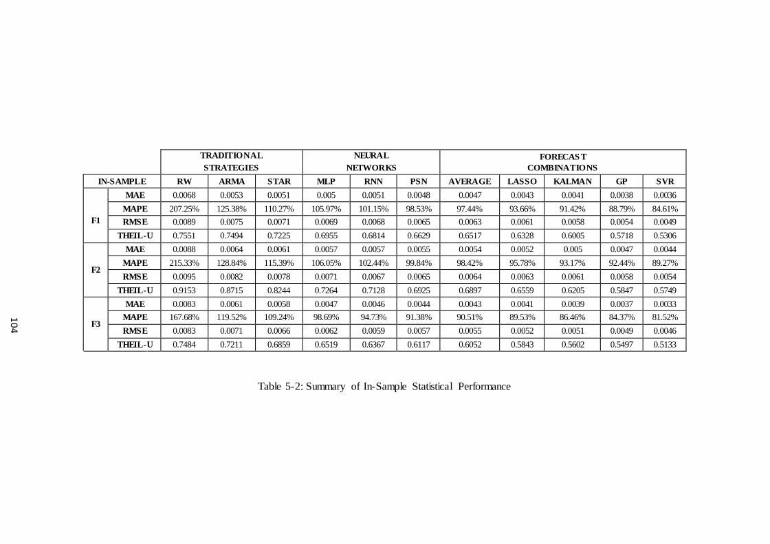
Table 5-2: Summary of In-Sample Statistical Performance
TRADITIONAL STRATEGIES
NEURAL NETWORKS
FORECAS T COMBINATIONS
IN-SAMPLE RW ARMA STAR MLP RNN PSN AVERAGE LASSO KALMAN GP SVR
F1
MAE 0.0068 0.0053 0.0051 0.005 0.0051 0.0048 0.0047 0.0043 0.0041 0.0038 0.0036 MAPE 207.25% 125.38% 110.27% 105.97% 101.15% 98.53% 97.44% 93.66% 91.42% 88.79% 84.61% RMSE 0.0089 0.0075 0.0071 0.0069 0.0068 0.0065 0.0063 0.0061 0.0058 0.0054 0.0049
THEIL-U 0.7551 0.7494 0.7225 0.6955 0.6814 0.6629 0.6517 0.6328 0.6005 0.5718 0.5306
F2
MAE 0.0088 0.0064 0.0061 0.0057 0.0057 0.0055 0.0054 0.0052 0.005 0.0047 0.0044 MAPE 215.33% 128.84% 115.39% 106.05% 102.44% 99.84% 98.42% 95.78% 93.17% 92.44% 89.27% RMSE 0.0095 0.0082 0.0078 0.0071 0.0067 0.0065 0.0064 0.0063 0.0061 0.0058 0.0054
THEIL-U 0.9153 0.8715 0.8244 0.7264 0.7128 0.6925 0.6897 0.6559 0.6205 0.5847 0.5749
F3
MAE 0.0083 0.0061 0.0058 0.0047 0.0046 0.0044 0.0043 0.0041 0.0039 0.0037 0.0033 MAPE 167.68% 119.52% 109.24% 98.69% 94.73% 91.38% 90.51% 89.53% 86.46% 84.37% 81.52% RMSE 0.0083 0.0071 0.0066 0.0062 0.0059 0.0057 0.0055 0.0052 0.0051 0.0049 0.0046
THEIL-U 0.7484 0.7211 0.6859 0.6519 0.6367 0.6117 0.6052 0.5843 0.5602 0.5497 0.5133
104

Table 5-3: Summary of Out-of-Sample Statistical Performance
Note: MDM1and MDM2 are the statistics computed for the MSE and MAE loss function respectively.
Table 5-4: Summary results of Modified Diebold-Mariano statistics for MSE and MAE loss function
TRADITIONAL STRATEGIES
NEURAL NETWORKS
FORECAS T COMBINATIONS
OUT-OF-SAMPLE RW ARMA STAR MLP RNN PSN AVERAGE LASSO KALMAN GP SVR
F1
MAE 0.0081 0.0065 0.006 0.0058 0.0056 0.0053 0.0052 0.0047 0.0046 0.0043 0.0039 MAPE 221.18% 129.58% 116.23% 106.87% 104.25% 101.28% 98.37% 95.71% 92.49% 89.54% 86.67% RMSE 0.0094 0.0083 0.0075 0.0074 0.0072 0.0069 0.0066 0.0063 0.0061 0.0057 0.0053
THEIL-U 0.8867 0.8355 0.7854 0.7578 0.7519 0.7226 0.6951 0.6795 0.6732 0.6429 0.6117
F2
MAE 0.0096 0.0079 0.0073 0.0063 0.0061 0.0059 0.0059 0.0056 0.0055 0.0052 0.0048 MAPE 234.17% 131.22% 121.76% 107.48% 105.37% 103.72% 101.56% 99.27% 98.13% 95.27% 92.84% RMSE 0.0152 0.0094 0.0081 0.0074 0.0072 0.007 0.0069 0.0066 0.0064 0.0061 0.0058
THEIL-U 0.9815 0.9125 0.8654 0.7972 0.7895 0.7664 0.7351 0.7005 0.6886 0.6758 0.6328
F3
MAE 0.0079 0.0063 0.0059 0.0051 0.0049 0.0048 0.0047 0.0045 0.0043 0.0041 0.0037 MAPE 186.21% 123.68% 114.78% 99.52% 98.06% 96.84% 95.73% 93.12% 89.57% 87.33% 85.27% RMSE 0.0086 0.0077 0.0074 0.0066 0.0065 0.0064 0.0061 0.0058 0.0055 0.0053 0.0051
THEIL-U 0.8358 0.7841 0.7059 0.6529 0.6458 0.6297 0.6218 0.6014 0.5788 0.5617 0.5419
RW ARMA STAR MLP RNN PSN AVERAGE LASSO KALMAN GP
F1 MDM1 -12.71 -11.24 -10.97 -9.37 -9.13 -8.08 -7.95 -6.25 -5.15 -4.26 MDM2 -15.85 -14.37 -13.49 -12.64 -11.97 -10.05 -8.57 -7.06 -6.53 -5.56
F2 MDM1 -14.08 -13.19 -12.91 -11.18 -10.27 -8.57 -8.16 -7.59 -6.87 -6.31 MDM2 -17.28 -15.21 -14.08 -13.57 -12.37 -10.58 -9.18 -8.17 -9.25 -8.19
F3 MDM1 -11.39 -10.23 -9.25 -7.69 -7.81 -6.28 -5.24 -4.38 -4.09 -3.67 MDM2 -13.77 -12.19 -10.88 -10.32 -10.11 -9.84 -7.93 -6.81 -5.48 -4.39
105

106
In order to further verify the statistical superiority of the best proposed architecture,
the Modified Diebold-Mariano (MDM) statistic for forecast encompassing is computed, as
proposed by Harvey et al. (1997). The null hypothesis of the test is the equivalence in
forecasting accuracy between a couple of forecasting models. The MDM statistic is an
extension of the Diebold-Mariano (1995) test (see appendix B.5.) and its statistic is
presented below:
( ) 1/21/2 11 2 1MDM T T k T k k DM− − = + − + − (5.13)
where T the number of the out-of-sample observations and k the number of the step-ahead
forecasts. In this case the MDM test is applied to couples of forecasts (SVR vs. another
forecasting model). A negative realization of the MDM test statistic indicates that the first
forecast (SVR) is more accurate than the second forecast. The lower the negative value, the
more accurate are the SVR forecasts. The MDM test follows the student distribution with
T-1 degrees of freedom.
The use of MDM is common practice in forecasting because it is found to be robust
in assessing the significance of observed differences between the performances of two
forecasts (Barhoumi et al., 2010). MDM also overcomes the problem of over-sized DMs in
moderate samples (Dreger and Kholodilin, 2013). The statistic is measured in each out-of-
sample period, while MSE and MAE are used as loss functions. Table 5-5 given previously
presents the values of the statistics, comparing the GA-SVR with its benchmarks. The
MDM null hypothesis of forecast encompassing is rejected for all comparisons and for
both loss functions at the 1% confidence interval. The table results confirm the statistical
superiority of the SVR forecasts as the realizations of the MDM statistic are all negative
for both loss functions.
5.6 Trading Performance
Further to a statistical evaluation, the proposed models are evaluated also in terms of
trading efficiency. It is indeed interesting to see if their trading performance is consistent
with their statistical accuracy. The trading performance of the models and the effect of the
proposed fitness function are analysed in section 5.6.1. below. In section 5.6.2 a more

107
sophisticated trading strategy is introduced and the results test if its application can
increase the models’ profitability.
5.6.1 Trading Performance without Leverage
The trading strategy is to go or stay ‘long’ when the forecast return is above zero and go or
stay ‘short’ when the forecast return is below zero. The ‘long’ and ‘short’ EUR/USD
position is defined as buying and selling Euros at the current price respectively. The
transaction costs for a tradable amount, say USD 5-10 million, are about 1 pip (0.0001
EUR/USD) per trade (one way) between market makers. The EUR/USD time series is
considered as a series of middle rates, so the transaction costs are one spread per round
trip. The average of EUR/USD is 1.421, 1.36 and 1.338 for the F1, F2 and F3 out-of-
sample period respectively. Therefore, the respective costs of 1 pip are equivalent to an
average cost of 0.007%, 0.0074% and 0.0075% per position.
The trading performance measures and their calculation are presented in appendix
B.4. Table 5-6 that follows presents the in-sample trading performances of the models and
forecast combinations after transaction costs for each exercise. These results show that all
the NN and forecast combination models present a positive trading performance after
transaction costs. From the single forecasts, the PSN outperforms each NN and statistical
benchmark in terms of annualised return and information ratio. The other two NNs
architectures, the RNN and the MLP, present the second and third best trading
performance respectively. This ranking is consistent in all three exercises. Concerning the
forecast combinations, it is obvious that the SVR model is superior in all periods with an
average annualised return of 28.71% and an information ratio of 2.89 after transaction
costs. It is also worth noting that all the forecast combinations outperform the best single
forecast, the PSN, in terms of trading performance.
The out-of-sample trading performances of the models are summarized in table 5-7
that also follows. The results indicate that the PSN continues to outperform all other single
forecasts in terms of trading efficiency. For the three out-of-sample periods the PSN
presents on average 2.59 % higher annualised return and 0.25 higher information ratio
compared to the second best single model, the RNN. On the other hand, all forecast
combination models present improved out-of-sample trading performance, verifying a
‘combining for improvement’ trend. The SVR forecast combination continues to

108
outperform its benchmarks achieving on average 4.12% and 2.42% higher annualized
return compared to the Kalman Filter and GP model respectively. The trading performance
of the models in F1, F2 and F3 sub-period coincides with the statistical one. The best
trading results are obtained during F3 and the worst during F2. In addition to the above, it
is noted that combining forecasts decreases the maximum drawdown, the essence of risk
for an investor in financial markets.
Concerning the proposed fitness function in equation 5.4, the results from the
statistical and trading evaluation of the individual and combining forecasts seem
promising. Firstly, all the NNs present significant profits after transaction costs in all out-
of-sample sub-periods. Moreover, there are not large inconsistencies in the statistical and
trading performance of the NNs models between the in-sample and out-of-sample. Large
inconsistencies could indicate that the training of the NNs is biased to either statistical
accuracy or trading efficiency. This could possibly lead to promising in-sample forecasts
but disastrous out-of-sample results. In the next section, a trading strategy is introduced to
further improve the trading performance of the models.

Table 5-5: Summary of In-Sample Trading Performance
TRADITIONAL STRATEGIES
NEURAL NETWORKS
FORECAST COMBINATIONS
IN-SAMPLE RW ARMA STAR MLP RNN PSN AVERAGE LASSO KALMAN GP SVR
F1
Information Ratio (including costs)
-0.25 0.42 0.60 1.57 1.71 1.98 2.12 2.38 2.84 2.71 2.90
Annualised Return (including costs)
-2.59% 4.57% 6.28% 15.41% 16.86% 19.39% 21.27% 23.18% 25.86% 26.95% 29.51%
Annualised Volatility 10.27% 10.79% 10.44% 9.82% 9.84% 9.77% 10.05% 9.75% 9.12% 9.96% 10.17%
Maximum Drawdown -25.78% -19.15% -15.37% -13.41% -15.55% -16.17% -13.25% -11.28% -10.94% -10.71% -
10.06%
F2
Information Ratio (including costs)
-0.28 0.33 0.53 1.23 1.44 1.65 1.66 1.81 2.06 2.16 2.35
Annualised Return (including costs) -3.18% 3.89% 5.89% 13.27% 14.75% 16.42% 17.56% 18.25% 20.29% 22.17% 25.11%
Annualised Volatility 11.32% 11.79% 11.07% 10.78% 10.23% 9.95% 10.59% 10.07% 9.87% 10.25% 10.67%
Maximum Drawdown -32.45% -22.21% -17.52% -15.68% -16.32% -16.75% -14.33% -11.96% -11.27% -10.98% -
10.85%
F3
Information Ratio (including costs)
-0.12 0.52 0.82 1.79 1.99 2.22 2.47 2.79 2.92 3.11 3.42
Annualised Return (including costs)
-1.22% 5.67% 8.26% 17.33% 19.49% 21.37% 23.68% 25.64% 26.03% 27.58% 31.52%
Annualised Volatility 10.32% 10.89% 10.13% 9.67% 9.78% 9.61% 9.59% 9.18% 8.92% 8.87% 9.22%
Maximum Drawdown -22.18% -15.43% -13.48% -12.39% -14.78% -13.88% -11.26% -10.83% -10.71% -10.57% -9.84%
109

Table 5-6: Summary of Out-of-Sample Trading Performance
TRADITIONAL STRATEGIES
NEURAL NETWORKS
FORECAST COMBINATIONS
OUT-OF-SAMPLE RW ARMA STAR MLP RNN PSN AVERAGE LASSO KALMAN GP SVR
F1
Information Ratio (including costs)
-0.11 0.21 0.32 1.03 1.35 1.58 1.46 1.68 1.93 2.05 2.10
Annualised Return (including costs)
-1.18% 2.29% 3.41% 9.15% 12.08% 14.49% 14.68% 16.23% 18.05% 19.94% 22.18%
Annualised Volatility 10.35% 11.05% 10.67% 8.92% 8.94% 9.19% 10.08% 9.68% 9.35% 9.74% 10.55%
Maximum Drawdown -15.57% -17.26% -16.55% -15.18% -14.73% -13.25% -12.37% -11.79% -11.81% -10.91% -10.82%
F2
Information Ratio (including costs)
-0.37 0.18 0.27 0.80 0.83 1.14 1.32 1.56 1.66 1.68 1.73
Annualised Return (including costs) -4.52% 1.86% 3.02% 7.81% 8.22% 11.26% 12.08% 14.14% 15.37% 16.17% 18.43%
Annualised Volatility 12.22% 10.51% 11.12% 9.78% 9.96% 9.84% 9.15% 9.06% 9.25% 9.65% 10.67%
Maximum Drawdown -21.42% -19.58% -18.49% -13.73% -14.21% -12.88% -12.44% -12.03% -11.95% -12.15% -11.94%
F3
Information Ratio (including costs)
0.02 0.41 0.51 1.14 1.46 1.68 1.81 2.00 2.01 2.28 2.77
Annualised Return (including costs)
0.27% 4.33% 5.51% 11.26% 14.08% 16.41% 17.32% 19.91% 20.19% 22.62% 25.37%
Annualised Volatility 11.55% 10.67% 10.92% 9.88% 9.64% 9.78% 9.56% 9.97% 10.02% 9.92% 9.17%
Maximum Drawdown -19.45% -13.67% -13.88% -11.76% -11.23% -11.65% -10.83% -10.67% -10.83% -10.84% -10.13%
110

111
5.6.2 Trading Performance exploiting Hybrid Leverage
In order to further improve the trading performance of the models, this section introduces a
hybrid leverage based on two time-varying factors, a leverage based on daily volatility
forecasts (L1) and a leverage based on market shocks (L2). The proposed leverage for
every trading day is simply the average of L1 and L2. In the next sections it is explained
how L1 and L2 are assigned.
5.6.2.1 Volatility Leverage (L1)
The intuition of the Volatility Leverage (L1) is to avoid trading when volatility of the
exchange rate returns is very high, while at the same time exploiting days with relatively
low volatility. Firstly, I forecast with a GJR (1, 1)9 the one day ahead realised volatility of
the EUR/USD exchange rate in the test and validation sub-periods. Then, I split these two
periods into six sub-periods, ranging from periods with extremely low volatility to periods
experiencing extremely high volatility. The process of forming these six periods is the
same as in chapter 4. For each sub-period a daily leverage factor L1 is assigned starting
with 0 for periods of extremely high volatility to a L1of 2 for periods of extremely low
volatility. Table 5-8 below presents the sub-periods and their relevant L1s.
Table 5-7: Classification of Volatility Leverage (L1) in sub-periods
9 It is also explored the RiskMetrics, GARCH (1, 1) and GARCH-M models for forecasting volatility. Their statistical accuracy in all three test sub-periods is slightly worse compared with the GJR (1, 1) daily volatility forecasts. Moreover, when their utility is measured in terms of trading efficiency for our models within the context of our strategy in the test sub-period, the results in terms of annualised returns are slightly better with GJR (1, 1) for most of the models. The ranking of the models in terms of information ratio and annualised return is the same whether I use GJR (1, 1) or the other explored alternatives.
Extremely Low Vol.
Medium
Low Vol.
Lower
Low Vol.
Lower
High Vol. Medium
High Vol. Extremely High Vol.
L1 2 1.5 1 1 0.5 0

112
The parameters of the strategy (μ and σ) are updated every three months by rolling forward
the estimation period, similarly to the update of chapter 4.
5.6.2.2 Index Leverage (L2)
The L1 measure presented above exploits periods of low volatility, but it does not take into
account the effects on the EUR/USD exchange rate deriving from possible daily shocks in
the EU and USA stock markets. For that reason, this section introduces an Index Leverage
(L2), based on two representative indices, the Dow Jones Industrial Average Index (DJIA)
and the Dow Jones EuroStoxx 50 Index (SX5E). These indices efficiently reflect any
shocks in the USA and EMU economies and are used as their proxies in a wealth of
relevant studies (see amongst others Charles and Darne (2006), Tastan (2006), Hemminki
and Puttonen (2008) and Awartani et al. (2009)).
The intuition of this leverage is to capture the shocks that the models are unable to
incorporate in the short-run (for example the devaluation from a rating agency of an EMU
country or a change in US interest rates). These changes will be instantly reflected in the
affected stock market and the next day in the ECB EUR/USD fixing. However, the models
will need some period to adjust to these shocks and are certainly unable to reflect them in
the short-run.
The methodology is similar to the one followed for L1. Firstly, it is defined the
daily difference δE-U as:
5E U SX E DJIAR Rδ − = − (5.14)
where 5SX ER and DJIAR are the daily SX5E and DJIA stock index returns respectively.10
The mean of that difference (μ΄) and its standard deviation (σ΄) are calculated. Then based
on δE-U, μ΄ and σ΄, I split again every three months of the test and the out-of-sample into six
sub-periods. The parameters of the strategy (μ΄ and σ΄) are updated every three months by
rolling forward the estimation period. The sub-periods are generated as in L1. Namely, the
periods where the difference δE-U is between μ΄ and one σ΄ are classified as ‘Lower High δE-
10 DJIA’s closing time is at 4:30 a.m. (ECT), while SX5E is closing at 6:00 p.m. (ECT). Since ECB’s daily fixing is available at 2.15 p.m. (ECT), I calcu late today’s δE-U with the first lags of the stock index returns RSX5E and RDJIA. Both RSX5E and RDJIA are calculated as in equation (1).

113
U Periods’. Similarly, ‘Medium High δE-U’ (between μ΄+σ΄ and μ΄+2σ΄) and ‘Extremely
High δE-U’ (above μ΄+2σ΄) periods can be defined. Periods with low difference δE-U are also
defined following the same 1σ΄ and 2σ΄ approach, but with a minus sign. When δE-U is
considerably higher than the average (a positive shock in the euro zone), the EUR is
expected to appreciate.
In order to justify the application of this leverage, though, the trading days must be
further separated based on the sign of the daily forecast. Thus, the following two scenarios
are possible:
• If the sign of the forecast is positive (‘long’ position), a leverage (L2+) of more than
1 is applied.
• If the sign of the forecast is negative (‘short’ position), a leverage (L2-) of less than
1 is applied.
When the δE-U is considerably lower than the average (a negative shock in the euro zone), a
depreciation of the euro should be expected. Thus, the assigned leverage has the opposite
trend in the corresponding scenario. The final classification of L2 is shown in the
following table.
Table 5-8: Classification of Index Leverage (L2+ and L2-) in sub-periods
5.6.2.3 Hybrid Leverage Performance
From the above, the L1 and L2 (depending on the scenario, L2+ or L2-) factors are
available for each trading day. The daily hybrid leverage applied is equal to the simple
average of L1 and L2. The next step is to examine if this trading strategy improves the
profitability of the models. For the model with the best statistical and trading performance,
the SVR NN forecast combination, the L1 and L2 factors for F1, F2 and F3 exercises are
presented in figure 5-2.
Extremely Low δE-U
Medium Low δE-U
Lower
Low δE-U
Lower
High δE-U
Medium
High δE-U
Extremely
High δE-U
L2+ 0 0.5 1 1 1.5 2
L2- 2 1.5 1 1 0.5 0

114
Figure 5-2: The Volatility Leverage (L1) and Index Leverage (L2) values assigned to the
SVR model for each period under study
From the figure above it is noted that the volatility based leverage (L1) takes
mainly low values during 2008, through the F2 and the first semester of the F3 sub-period.
Regarding L2, the trend is more irregular and in general more extreme, going from very
low values to high ones in short period intervals. This can be attributed to the economic
turbulence that dominates the out-of-sample periods and the shocks in the two benchmark
markets. The L1 and L2 graphs for the other NN and forecast combination models present
similar behaviors for the three periods.

115
The cost of leverage (interest payments for the additional capital) is calculated at
0.504% p.a. (that is 0.002% per trading day11). The final results are presented in table 5-10
that follows. Based on these results, it is obvious that the hybrid trading strategy is
successful for all the models and periods. The SVR forecast combination seems to exploit
the trading strategy well and achieves on average an annualized return of 25.08% after
costs, increasing its profitability by 3.05%, 4.16% and 2.05% during F1, F2 and F3 sub-
periods respectively. GP and Kalman Filter remain the second and the third most profitable
models, achieving both on average annualised returns over 20%, regardless the period
under study. In general all forecasting models increase their trading performance by 1.69%
on average, while their maximum drawdown is decreased on average by 1.01%. In all
three sub-periods, the EUR/USD exchange rate is dominated by shocks and high volatility.
The proposed leverage factors manage to exploit this environment and increase the trading
performance of all the models, in a period where uncertainty is present in the market.
11 The interest costs are calculated by considering a 0.504% interest rate p.a. (the Euribor rate at the time of calculation) d ivided by 252 trading days. In reality, leverage costs also apply during non-trading days. Hence, the interest costs should be calculated using 360 days per year. But for the sake of simplicity, the approximation of 252 t rading days is used to spread the leverage costs of non-trading days equally over the trading days. This approximation allows the practit ioner not to keep track of how many non-trading days a position is hold.
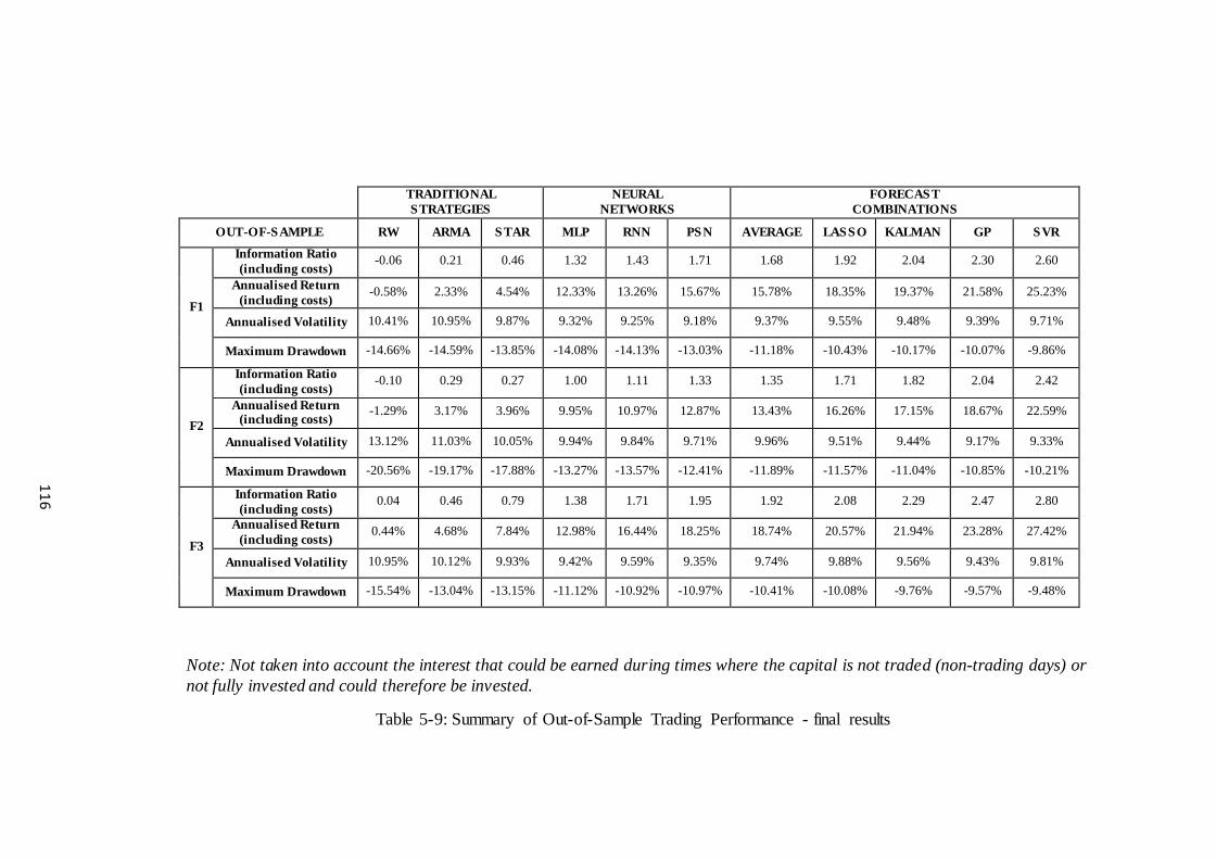
Note: Not taken into account the interest that could be earned during times where the capital is not traded (non-trading days) or not fully invested and could therefore be invested.
Table 5-9: Summary of Out-of-Sample Trading Performance - final results
TRADITIONAL STRATEGIES
NEURAL NETWORKS
FORECAST COMBINATIONS
OUT-OF-SAMPLE RW ARMA STAR MLP RNN PSN AVERAGE LASSO KALMAN GP SVR
F1
Information Ratio (including costs)
-0.06 0.21 0.46 1.32 1.43 1.71 1.68 1.92 2.04 2.30 2.60
Annualised Return (including costs)
-0.58% 2.33% 4.54% 12.33% 13.26% 15.67% 15.78% 18.35% 19.37% 21.58% 25.23%
Annualised Volatility 10.41% 10.95% 9.87% 9.32% 9.25% 9.18% 9.37% 9.55% 9.48% 9.39% 9.71%
Maximum Drawdown -14.66% -14.59% -13.85% -14.08% -14.13% -13.03% -11.18% -10.43% -10.17% -10.07% -9.86%
F2
Information Ratio (including costs)
-0.10 0.29 0.27 1.00 1.11 1.33 1.35 1.71 1.82 2.04 2.42
Annualised Return (including costs)
-1.29% 3.17% 3.96% 9.95% 10.97% 12.87% 13.43% 16.26% 17.15% 18.67% 22.59%
Annualised Volatility 13.12% 11.03% 10.05% 9.94% 9.84% 9.71% 9.96% 9.51% 9.44% 9.17% 9.33%
Maximum Drawdown -20.56% -19.17% -17.88% -13.27% -13.57% -12.41% -11.89% -11.57% -11.04% -10.85% -10.21%
F3
Information Ratio (including costs)
0.04 0.46 0.79 1.38 1.71 1.95 1.92 2.08 2.29 2.47 2.80
Annualised Return (including costs)
0.44% 4.68% 7.84% 12.98% 16.44% 18.25% 18.74% 20.57% 21.94% 23.28% 27.42%
Annualised Volatility 10.95% 10.12% 9.93% 9.42% 9.59% 9.35% 9.74% 9.88% 9.56% 9.43% 9.81%
Maximum Drawdown -15.54% -13.04% -13.15% -11.12% -10.92% -10.97% -10.41% -10.08% -9.76% -9.57% -9.48%
116

117
5.7 Conclusions
The aim of this chapter is to examine the performance of a Multi-Layer Perceptron (MLP),
a Recurrent Neural Network (RNN) and a Psi-Sigma Network (PSN) architecture in
forecasting and trading the Euro/Dollar (EUR/USD) exchange rate and explore the utility
of Kalman Filter, Genetic Programming (GP) and Support Vector Regression (SVR)
algorithms as forecasting combination techniques. As benchmarks for the NNs I use a RW,
an ARMA and a STAR, while for the forecast combination techniques a Simple Average
and a Least Absolute Shrinkage and Selection Operator (LASSO). A new fitness function
is also introduced for NNs in trading applications and a hybrid leverage trading strategy, in
order to evaluate if their application can improve the trading performance of the models.
In terms of the results, the PSN from the individual forecasts and the SVR from the
forecasting combination techniques outperform their benchmarks in terms of statistical
accuracy and trading efficiency. All NN forecast combinations achieve higher annualised
returns and information ratios, presenting a “combining for improvement” pattern.
Concerning the hybrid leverage strategy, it is noted that all models exploit it by increasing
annualised returns and decreasing maximum drawdowns. The hybrid leverage factors
applied serve their purpose, since they are more effective in periods of increased market
volatility and risk. Moreover, the proposed fitness function for NNs is promising as all
networks produce high profitability in both in- and out-of-sample periods and present a
consistency between their statistical and trading ranking. Finally, it is observed that the
ranking of all models is consistent in statistical and trading terms.
The remarkable trading performance of the SVR indicates that it can be considered
as the optimal forecasting combination for the models and time-series under study. The
successful application of the proposed hybrid trading strategy and fitness function
demonstrates the necessity for a shift from purely statistically based models to models that
are optimized in a hybrid trading and statistical approach. In general, the results should go
some way towards convincing scientists and investment managers to experiment beyond
the bounds of traditional models and trading strategies.

118
Chapter 6
Modeling and Trading the EUR Exchange Rates
with Hybrid Genetic Algorithms – Support Vector Regression Forecast Combinations
6.1 Introduction
Forecasting financial time series appears to be a challenging task for the scientific
community because of its non-linear and non-stationary structural nature. On one hand,
traditional statistical methods fail to capture this complexity while on the other hand, non-
linear techniques present promising empirical evidence. However, their practical
limitations and the expertise required to optimize their parameters are creating skepticism
on their utility.
The motivation for this chapter is to introduce a novel hybrid Genetic Algorithm –
Support Vector Regression (GA-SVR) algorithm for optimal parameter selection and
feature subset combination, when applied to the task of forecasting and trading the
EUR/USD, EUR/GBP and EUR/JPY exchange rates. The proposed model genetically
searches over a feature space (pool of individual forecasts) and then combines the optimal
feature subsets (SVR forecast combinations) for each exchange rate. This is achieved by
applying a fitness function specialized for financial purposes. This function not only
minimizes the error of the forecasts, but also increases the profitability of the final forecast
combinations. This is crucial in financial applications where statistical accuracy is not
always synonymous with the financial profitability of the deriving forecasts. The GA-SVR
algorithm is benchmarked with SVR models with non-genetically optimized parameters,

119
such as ε-SVR and v-SVR. The statistical and trading performance of all models is
investigated during the period of 1999-2012, using the last two years for out-of-sample
testing.
To the best of my knowledge, the proposed methodology has not been applied in
relevant applications. In the literature there are similar hybrid applications which are either
limited in classification problems (Min et al. (2006), Huang and Wang (2006), Wu et al.
(2007) and Dunis et al. (2013)) or the GA does not extend to optimal feature subset
selection (Pai et al. (2006), Chen and Wang (2007), Yuang (2012)). The novelty of the
model lies in its ability to genetically optimize the SVR parameters, combine the optimal
feature subsets and apply a fitness function, which aims to maximize not only the
statistically accuracy of the forecasts but also their financial profitability. Compared to
non-adaptive algorithms presented in the literature, this proposed architecture does not
require from the practitioner to follow any time consuming optimization approach (such as
cross validation or grid search) and is free from the data snooping bias. The latter is
achieved because all parameters of the GA-SVR model are optimized in a single
optimization procedure.
From this analysis it emerges that the GA-SVR presents the best performance in
terms of statistical accuracy and trading efficiency for all exchange rates under study. GA-
SVR’s trading performance and forecasting superiority not only confirms the success of
the implemented fitness function. In additions it is validated from the results that applying
GAs in this hybrid model to optimize the SVR parameters is more efficient compared to
the optimization approaches (cross validation and grid search algorithms) that dominate the
relevant literature.
The rest of the chapter is organized as follows. Section 6-2 describes the
EUR/USD, EUR/GBP and EUR/JPY ECB fixing series, used as dataset, while section 6-3
summarizes the theoretical background needed for the complete understanding of the
proposed methodology. In section 6-4 follows the complete description of the hybrid GA-
SVR model. The statistical and trading performance of the models is presented in sections
6-5 and 6-6 respectively. Finally, some concluding remarks are provided in section 6-7.

120
6.2 The EUR/USD, EUR/GBP and EUR/JPY Exchange Rates and Related Financial Data
The European Central Bank (ECB) publishes a daily fixing for selected EUR exchange
rates. These reference mid-rates are based on a daily concentration procedure between
central banks within and outside the European System of Central Banks. The rational of
the selection of the ECB daily fixings is explained in previous chapters. The main intuition
is that many financial institutions are ready to trade at the EUR fixing, leaving orders with
a bank for business to be transacted at this level. Thus, the ECB daily fixings of the EUR
exchange rate are tradable levels and using them is a realistic choice.
This chapter examines the ECB daily fixings of EUR/USD, EUR/GBP and
EUR/JPY exchange rates over the period of 1999-2012, as described in Table 1 below.
Table 6-1: The Total Dataset - Neural Networks’ Training Datasets
The graph below shows the total dataset for the three exchange rates under study.
PERIODS TRADING DAYS START DATE END DATE Total Dataset 3395 01/02/1999 30/04/2012
In-sample Dataset 2878 01/02/1999 29/04/2010 Out-of-sample Dataset 517 30/04/2010 30/04/2012
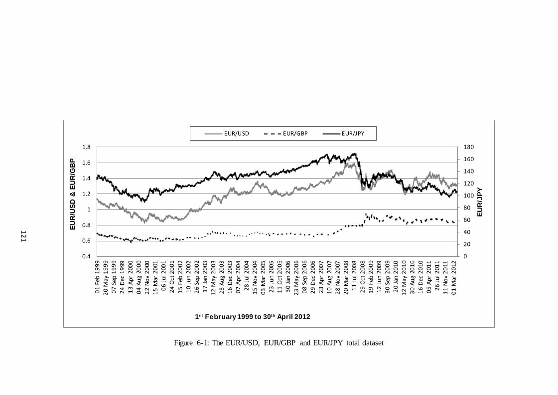
Figure 6-1: The EUR/USD, EUR/GBP and EUR/JPY total dataset
0
20
40
60
80
100
120
140
160
180
0.4
0.6
0.8
1
1.2
1.4
1.6
1.8
01 F
eb 1
999
20 M
ay 1
999
07 S
ep 1
999
24 D
ec 1
999
13 A
pr 2
000
04 A
ug 2
000
22 N
ov 2
000
15 M
ar 2
001
06 Ju
l 200
124
Oct
200
115
Feb
200
210
Jun
2002
26 S
ep 2
002
17 Ja
n 20
0312
May
200
328
Aug
200
316
Dec
200
307
Apr
200
428
Jul 2
004
15 N
ov 2
004
03 M
ar 2
005
23 Ju
n 20
0511
Oct
200
530
Jan
2006
23 M
ay 2
006
08 S
ep 2
006
29 D
ec 2
006
23 A
pr 2
007
10 A
ug 2
007
28 N
ov 2
007
20 M
ar 2
008
11 Ju
l 200
829
Oct
200
819
Feb
200
912
Jun
2009
30 S
ep 2
009
20 Ja
n 20
1012
May
201
030
Aug
201
016
Dec
201
005
Apr
201
126
Jul 2
011
11 N
ov 2
011
01 M
ar 2
012
EUR
/JPY
EUR
/USD
& E
UR
/GB
P
1st February 1999 to 30th April 2012
EUR/USD EUR/GBP EUR/JPY
121

122
The three observed time series are non-normal (Jarque-Bera statistics (1980)
confirm their non-normality at the 99% confidence interval) containing slight skewness
and high kurtosis. They are also non-stationary and hence I transform them into three daily
series of rate returns12 using the following formula:
1
ln tt
t
PRP−
=
(6.1)
Where Rt is the rate of return and Pt is the price level at time t.
The summary statistics of the EUR/USD, EUR/GBP and EUR/JPY return series
reveal that the slight skewness and high kurtosis remain. In addition, the Jarque-Bera
statistic confirms again their non-normality at the 99% confidence interval. The aim is to
forecast and trade the one day ahead return (E (Rt)) of the three exchange rates. As a first
step, the three return series are estimated with several linear and non- linear models. Then
these estimations are used as potential inputs to the proposed GA-SVR algorithm.
6.3 Theoretical Background
As mentioned before, the intention of this chapter combine and integrate the virtues of
GAs to an SVR process. The reason is to face and efficiently cope with issues of optimal
parameter tuning and feature selection. For that reason, a short theoretical background on
all these issue is crucial to fully understand the attributes of the GA-SVR and identify its
novelty. The explanation of the SVR process and the optimization of its parameters are
given in detail in chapter 3. Feature selection is an optimization problem that refers to the
search over a space of possible feature subsets in order to find those that are optimal with
respect to specific criteria. Chapter 3 is also engaged with this issue in detail. Therefore,
these issues are not further elaborated in this chapter, relieving the reader from unnecessary
repetitions.
12 Confirmat ion of their stationary property is obtained at the 1% significance level by both the Augmented Dickey Fuller (ADF) and Phillips-Perron (PP) test statistics.

123
6.4 Hybrid Genetic Algorithm – Support Vector Regression (GA-SVR)
The hybrid Genetic Algorithm – Support Vector Regression (GA-SVR) model for optimal
parameter selection and feature subset combination is presented in this section. Initially,
the generic architecture of the methodology is described. Then the feature space, in which
the model searches for the optimal subsets and combinations, is identified along with the
models that are going to be used as benchmarks.
6.4.1 Architecture
The proposed model genetically searches over a feature space (pool of individual forecasts)
and then combines the optimal feature subsets (SVR forecast combinations) for each
exchange rate. In order to achieve this, a simple GA is used. Each chromosome includes
feature genes that encode the best feature subsets and parameter genes that encode the best
choice of parameters. The model is explained in detail in chapter 3.
A two-objective fitness function is applied to the hybrid approach in order to
achieve the optimal selection of the feature subsets (individual forecasts). Firstly the
annualised return of the SVR forecast combinations should be maximized and secondly the
Root Mean Square Error (RMSE) of the output should be minimized in the test sub-period.
Based on the above, the fitness function takes the form of equation 6.2.:
Fitness = Annualised_Return – 10*RMSE (6.2)
The aim is to maximize the previous equation13, since in genetic modelling the fitness
function have to be increasing functions. This function aims to bring a balance between
trading profitability (first factor of equation) and statistical accuracy (second factor of the
equation). In trading applications this is a very important virtue, because the statistical
accuracy does not always imply financial profitability.
13 The RMSE is multiplied by 10 so the two factors in our equation are more or less equal in levels.

124
The size of the initial population is set to 40 chromosomes while the maximum
number of generations is set to 200. The algorithm, though, terminates when the number of
generations is 60 on average, regardless the series under study. This number must be
reached in combination with a termination method that stops the evolution, when the
population is deemed as converged. As mentioned in chapter 3, the population is deemed
as converged when the average fitness across the current population is less than 5% away
from the best fitness of the current population. The summary of the GA’s characteristics is
presented in table 6-2 below. Finally, the detailed flowchart of the proposed methodology
is depicted in figure 3-6 in chapter 3.
Population Size 40
Maximum Generations 200
Selection Type Roulette Wheel Selection
Elitism Best member of every population is maintained in the next generation.
Crossover Probability 0.9
Mutation Probability 0.1
Fitness Function Annualised_Return – 10*RMSE
Table 6-2: GA Characteristics and Parameters
6.4.2 Feature Space, Feature Subset Selection and Benchmark Models
The forecasting ability of the proposed methodology is evaluated over a feature space
(pool of individual forecasts) that is synthesized by individual linear and non- linear
forecasts of each exchange rate. More specifically, the pool comprises of a series of
Autoregressive (AR), Moving Average (MA), Autoregressive Moving Average (ARMA)
linear models and five non-linear algorithms, namely a Nearest Neighbours Algorithm (k-
NN) a Multi-Layer Perceptron (MLP), a Recurrent Neural Network (RNN), a Higher Order
Neural Network (HONN) and a Psi-Sigma Neural Network (PSN). A summary of the
linear models is presented in table 6-3 below, while the non- linear models are explained in
Appendix D.

125
LINEAR MODELS DESCRIPTION
RW ( ) , ~ (0,1)t t tE R e e Nµ= + where μ the in-sample mean
AR (p) 01
( )p
t i t ii
E R Rβ β −=
= +∑ where p=1,…,20 and β0, βi the regression coefficients
MA (q) 1 1( ) ( ... ) /t t t qE R R R q− − += + + , where q=3...25
ARMA (m, n) 0 0
1 1( )
m n
t j t j k t kj k
E R R a w aϕ ϕ − −= =
= + + +∑ ∑ ,where m, n=1,..,15, φ0,φj are the
regression coefficients, α0, at-k the residual terms and wk the weights of the residual
terms
Table 6-3: The summary description of the linear models
Note: (a) shows a possible selected feature subset. This subset gene includes the forecasts of AR (2), AR (i),
MA(1), MLP and PSN. (b) refers to the parameters gene which includes the three parameters C, δ2, ν (δ2=γ).
The two genes together comprise the output chromosome, while the three encoded parameters are used to
provide the final SVR forecast for the given example.
Figure 6-2: The GA-SVR chromosome

126
In this chapter, the algorithm genetically searches the above feature space and
finally selects as optimal feature subsets the MLP, RNN and PSN individual forecasts for
all three exchange rates under study. This means that the proposed methodology rejects all
linear approaches, the k-NN and the HONN models over the MLP, RNN and PSN.
Regarding the linear models, that is expected because of the non- linearity that dominates
financial time series. Concerning the k-NN and HONNs models, the algorithm identifies
that their individuals forecasts are either not adding any value as inputs to the GA-SVR
algorithms or their forecasts are encompassed to the ones selected. Knowing the feature
subsets that qualify from the feature space, the final stage of this methodology can be
reached. This is the combination of the individual forecasts of MLP, RNN and PSN with
SVR to produce the final forecasts. In this final step, the optimized parameters are used, as
the GA produced for the specific set of inputs during the previous selection process (see
figure 6-2 above).
The statistical and trading efficiency of the hybrid model is evaluated by benchmarking
GA-SVR with more traditional SVRs, such as ε-SVR and v-SVR, whose parameters are
not genetically optimized. The ε-SVR and v-SVR alternatives are described in detail in
chapter 3. The RBF kernel and the optimal selected inputs (MLP, RNN and PSN
individual forecasts) are used in all SVR benchmarks in order to achieve a fair comparison
with the proposed model. Based on this research background, the following benchmark
alternatives are identified:
• An ε-SVR model that implements a 5-fold cross-validation and a simple data-
driven calculation on the in-sample dataset to calculate parameters ε, γ and C
respectively (ε-SVR1) (see SVR process of chapter 5).
• A v-SVR model that calculates its parameters v, γ and C as the ε-SVR1 (v-SVR1).
• An ε-SVR and v-SVR model that all parameters are selected based on a grid-search
algorithm in the in-sample dataset (ε-SVR2 and v-SVR2).
For more on the ε-SVR1 and v-SVR1 approaches see Duan et al. (2003) and Cherkassky
and Ma (2004), while for the ε-SVR2 and v-SVR2 see Scholkopf and Smola (2002). The
parameters of the benchmark SVRs and the proposed GA-SVR are shown in the following
table:
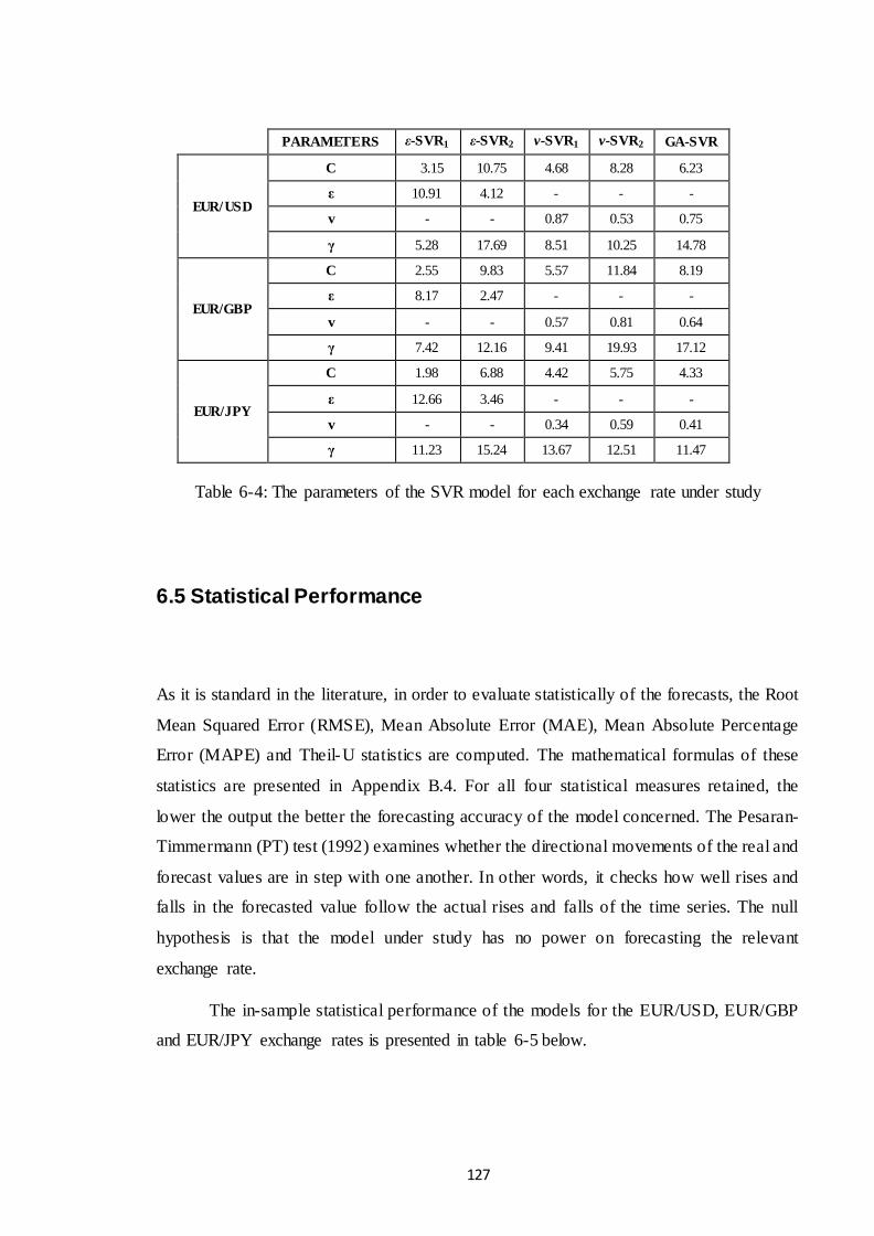
127
Table 6-4: The parameters of the SVR model for each exchange rate under study
6.5 Statistical Performance
As it is standard in the literature, in order to evaluate statistically of the forecasts, the Root
Mean Squared Error (RMSE), Mean Absolute Error (MAE), Mean Absolute Percentage
Error (MAPE) and Theil-U statistics are computed. The mathematical formulas of these
statistics are presented in Appendix B.4. For all four statistical measures retained, the
lower the output the better the forecasting accuracy of the model concerned. The Pesaran-
Timmermann (PT) test (1992) examines whether the directional movements of the real and
forecast values are in step with one another. In other words, it checks how well rises and
falls in the forecasted value follow the actual rises and falls of the time series. The null
hypothesis is that the model under study has no power on forecasting the relevant
exchange rate.
The in-sample statistical performance of the models for the EUR/USD, EUR/GBP
and EUR/JPY exchange rates is presented in table 6-5 below.
PARAMETERS ε-SVR1 ε-SVR2 v-SVR1 v-SVR2 GA-SVR
EUR/USD
C 3.15 10.75 4.68 8.28 6.23
ε 10.91 4.12 - - -
v - - 0.87 0.53 0.75
γ 5.28 17.69 8.51 10.25 14.78
EUR/GBP
C 2.55 9.83 5.57 11.84 8.19
ε 8.17 2.47 - - -
v - - 0.57 0.81 0.64
γ 7.42 12.16 9.41 19.93 17.12
EUR/JPY
C 1.98 6.88 4.42 5.75 4.33
ε 12.66 3.46 - - -
v - - 0.34 0.59 0.41
γ 11.23 15.24 13.67 12.51 11.47

128
IN-SAMPLE ε-SVR1 ε-SVR2 v-SVR1 v-SVR2 GA-SVR
EUR/USD
MAE 0.00445 0.00428 0.00399 0.00364 0.00328 MAPE 90.41% 89.94% 86.22% 81.66% 75.27% RMSE 0.00613 0.00569 0.00561 0.00529 0.00488 Theil-U 0.58874 0.56416 0.53672 0.51407 0.46310
PT-statistic 8.34 9.55 10.89 11.95 14.82
EUR/GBP
MAE 0.00436 0.00402 0.00388 0.00356 0.00317 MAPE 89.59% 88.67% 86.22% 82.29% 78.14% RMSE 0.00568 0.00537 0.00514 0.00483 0.00443 Theil-U 0.59148 0.56416 0.53472 0.50526 0.47538
PT-statistic 7.86 9.15 10.66 11.55 14.21
EUR/JPY
MAE 0.00485 0.00453 0.00433 0.00401 0.00358 MAPE 92.47% 91.68% 89.41% 86.28% 81.79% RMSE 0.00627 0.00598 0.00561 0.00522 0.00478 Theil-U 0.52338 0.49954 0.47852 0.44771 0.40659
PT-statistic 9.17 10.21 11.51 13.21 15.07
Table 6-5: Summary of In-Sample Statistical Performance
From the results above it is suggested that the GA-SVR presents the best in-sample
statistical performance for every exchange rate under study and for all four statistical
measures retained. The PT-statistics rejects the null hypothesis of no forecasting power at
the 1% confidence interval for all models and series under study. It seems that none of the
SVR approaches projects poor directional change forecasts in the in-sample period.
Moreover, it is noted that the v-SVR models (v-SVR1 and v-SVR2) seem to have better
realizations of the statistical measures than the ε-SVR ones (ε-SVR1 and ε-SVR2). Table
6-6 summarizes the statistical performance of the models in the out-of-sample period.
OUT-OF-SAMPLE ε-SVR1 ε-SVR2 v-SVR1 v-SVR2 GA-SVR
EUR/USD
MAE 0.00491 0.00475 0.00437 0.00404 0.00358 MAPE 95.51% 93.69% 90.78% 85.74% 80.68% RMSE 0.00653 0.00637 0.00593 0.00568 0.00519 Theil-U 0.63415 0.62478 0.57038 0.53874 0.48994
PT-statistic 7.89 8.01 9.14 10.21 12.77
EUR/GBP
MAE 0.00474 0.00428 0.00408 0.00386 0.00344 MAPE 94.25% 91.95% 88.61% 86.11% 81.95% RMSE 0.00571 0.00542 0.00522 0.00507 0.00555 Theil-U 0.63914 0.60144 0.58194 0.65276 0.62334
PT-statistic 6.38 7.15 8.41 9.27 12.15
EUR/JPY
MAE 0.00525 0.00507 0.00480 0.00448 0.00394 MAPE 97.17% 94.53% 91.22% 87.16% 82.19% RMSE 0.006825 0.00649 0.00618 0.00579 0.00583 Theil-U 0.60571 0.59341 0.55948 0.50489 0.48921
PT-statistic 7.42 8.23 9.21 11.26 13.75
Table 6-6: Summary of Out-of-Sample Statistical Performance

129
From the results of table 6-6 it is obvious that the proposed methodology retains its
forecasting superiority for the statistical measures applied in the out-of-sample period.
Once more, the v-SVR approaches outperform the ε-SVR models and the PT-statistics
indicate that all models forecast accurately the directional change of the exchange rates
under study. Finally, it also obvious that the v-SVR model that optimizes its parameters
with the grid-search algorithm (v-SVR2) retains the second more accurate statistical
performance after the hybrid proposed methodology.
Similarly to previous chapters, the statistical superiority of the best proposed architecture,
the GA-SVR, is evaluated also by computing the Diebold-Mariano (1995) DM statistic for
predictive accuracy (see appendix B.5.). In this study, both MSE and MAE are considered
as loss functions. Table 6-7 below presents the DM statistic comparing the GA-SVR with
its benchmarks.
Loss Functions ε-SVR1 ε-SVR2 v-SVR1 v-SVR2
EUR/USD sMSE -6.258 -5.997 -4.841 -3.957 sMAE -11.539 -10.165 -8.412 -5.331
EUR/GBP sMSE -5.894 -5.233 -4.014 -3.108 sMAE -9.568 -7.129 -5.743 -4.157
EUR/JPY sMSE -8.027 -7.549 -6.138 -4.147 sMAE -11.622 -12.057 -10.619 -7.219
Table 6-7: The Diebold-Mariano statistics of MSE and MAE loss functions
The table validates that the null hypothesis of equal predictive accuracy is rejected
for all comparisons and for both loss functions at the 1% confidence interval (absolute
values higher than the critical value of 2.33). Moreover, the statistical superiority of the
GA-SVR forecasts is confirmed as the realizations of the DM statistic are negative for both
loss functions14. It is also found that the second best model in statistical terms, the v-SVR2,
has the closest forecasts with the GA-SVR model.
Under the above given computational and statistical context, it is worth repeating that the
proposed GA-SVR methodology is fully adaptive. The practitioner does not need to
experiment with the parameters of the algorithm in order to optimize the forecasts. The
GA-SVR structure and parameters are generated in a single optimization procedure, a
procedure which prevents the data snooping effect.
14 In this chapter the Diebold-Mariano test is applied to couples of forecasts (GA-SVR vs. another forecasting model). A negative realizat ion of the Diebold-Mariano test statistic indicates that the first forecast (GA-SVR) is more accurate than the second forecast. The lower the negative value, the more accurate are the GA-SVR forecasts.

130
6.6 Trading Performance
In the previous section the forecasts are evaluated through a series of statistical accuracy
measures and tests. However, statistical accuracy is not always synonymous with financial
profitability. In financial applications, the practitioner’s utmost interest is to produce
models that can be translated to profitable trades. It is therefore crucial to further examine
the proposed model and evaluate its utility through a trading strategy. The trading strategy
applied is simple. The trading signals are ‘long’ when the forecast return is above zero and
‘short’ when the forecast return is below zero. The ‘long’ and ‘short’ EUR/USD,
EUR/GBP or EUR/JPY position is defined as buying and selling Euros at the current price
respectively. Appendix B.4 includes the specification of the trading performance measures
used in this chapter.
Based on the trading rational of chapters 4 and 5, the transaction costs for a
tradable amount are about 1 pip per trade (one way) between market makers. The
EUR/USD, EUR/GBP and EUR/JPY time series are considered a series of middle rates,
the transaction cost is one spread per round trip. For the given dataset a cost of 1 pip is
equivalent to an average cost of 0.0074%, 0.0117% and 0.0091% per position for the
EUR/USD, the EUR/GBP and the EUR/JPY respectively.
Table 6.8 that follows presents the summary of the out-of-sample trading
performance of the models for each exchange rate under study. From the results of this
table it is suggested that the GA-SVR demonstrates the superior trading performance in
terms of annualised return and information ratio for all exchange rates in the in-sample
period. The GA-SVR yields on average 4.13% higher annualised returns than v-SVR2,
which is the second most profitable SVR approach. Referring to the statistical performance
of the models during the same period (see table 6-5), the statistical ranking of the models
is similar to their ranking in trading terms.
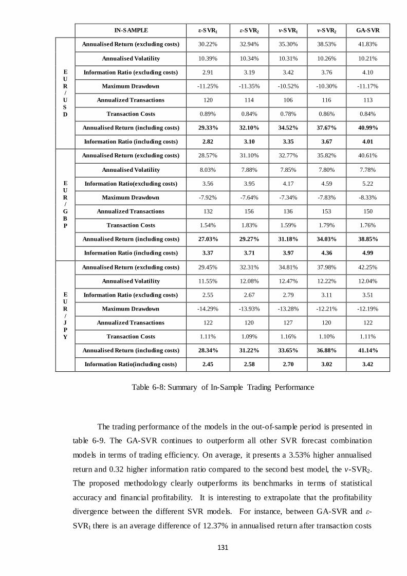
131
IN-SAMPLE ε-SVR1 ε-SVR2 v-SVR1 v-SVR2 GA-SVR
E U R / U S D
Annualised Return (excluding costs) 30.22% 32.94% 35.30% 38.53% 41.83%
Annualised Volatility 10.39% 10.34% 10.31% 10.26% 10.21%
Information Ratio (excluding costs) 2.91 3.19 3.42 3.76 4.10
Maximum Drawdown -11.25% -11.35% -10.52% -10.30% -11.17%
Annualized Transactions 120 114 106 116 113
Transaction Costs 0.89% 0.84% 0.78% 0.86% 0.84%
Annualised Return (including costs) 29.33% 32.10% 34.52% 37.67% 40.99%
Information Ratio (including costs) 2.82 3.10 3.35 3.67 4.01
E U R / G B P
Annualised Return (excluding costs) 28.57% 31.10% 32.77% 35.82% 40.61%
Annualised Volatility 8.03% 7.88% 7.85% 7.80% 7.78%
Information Ratio(excluding costs) 3.56 3.95 4.17 4.59 5.22
Maximum Drawdown -7.92% -7.64% -7.34% -7.83% -8.33%
Annualized Transactions 132 156 136 153 150
Transaction Costs 1.54% 1.83% 1.59% 1.79% 1.76%
Annualised Return (including costs) 27.03% 29.27% 31.18% 34.03% 38.85%
Information Ratio (including costs) 3.37 3.71 3.97 4.36 4.99
E U R / J P Y
Annualised Return (excluding costs) 29.45% 32.31% 34.81% 37.98% 42.25%
Annualised Volatility 11.55% 12.08% 12.47% 12.22% 12.04%
Information Ratio (excluding costs) 2.55 2.67 2.79 3.11 3.51
Maximum Drawdown -14.29% -13.93% -13.28% -12.21% -12.19%
Annualized Transactions 122 120 127 120 122
Transaction Costs 1.11% 1.09% 1.16% 1.10% 1.11%
Annualised Return (including costs) 28.34% 31.22% 33.65% 36.88% 41.14%
Information Ratio(including costs) 2.45 2.58 2.70 3.02 3.42
Table 6-8: Summary of In-Sample Trading Performance
The trading performance of the models in the out-of-sample period is presented in
table 6-9. The GA-SVR continues to outperform all other SVR forecast combination
models in terms of trading efficiency. On average, it presents a 3.53% higher annualised
return and 0.32 higher information ratio compared to the second best model, the v-SVR2.
The proposed methodology clearly outperforms its benchmarks in terms of statistical
accuracy and financial profitability. It is interesting to extrapolate that the profitability
divergence between the different SVR models. For instance, between GA-SVR and ε-
SVR1 there is an average difference of 12.37% in annualised return after transaction costs
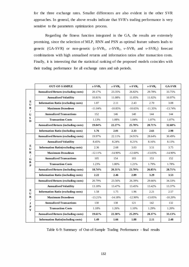
132
for the three exchange rates. Smaller differences are also evident in the other SVR
approaches. In general, the above results indicate that SVR’s trading performance is very
sensitive to the parameters optimization process.
Regarding the fitness function integrated in the GA, the results are extremely
promising, since the selection of MLP, RNN and PSN as optimal feature subsets leads to
genetic (GA-SVR) or non-genetic (ε-SVR1, ε-SVR2, v-SVR1 and v-SVR2) forecast
combinations with high annualised returns and information ratios after transaction costs.
Finally, it is interesting that the statistical ranking of the proposed models coincides with
their trading performance for all exchange rates and sub periods.
OUT-OF-SAMPLE ε-SVR1 ε-SVR2 v-SVR1 v-SVR2 GA-SVR
E U R / U S D
Annualised Return (excluding costs) 20.17% 23.35% 26.82% 29.78% 33.75%
Annualised Volatility 10.81% 11.08% 11.05% 11.02% 10.97%
Information Ratio (excluding costs) 1.87 2.11 2.43 2.70 3.08
Maximum Drawdown -11.04% -10.85% -10.65% -11.35% -13.74%
Annualized Transactions 152 146 140 144 144
Transaction Costs 1.13% 1.08% 1.04% 1.07% 1.07%
Annualised Return (including costs) 19.04% 22.27% 25.78% 28.71% 32.68%
Information Ratio (including costs) 1.76 2.01 2.33 2.61 2.98
E U R / G B P
Annualised Return (excluding costs) 19.97% 22.11% 24.91% 28.64% 30.49%
Annualised Volatility 8.45% 8.24% 8.21% 8.16% 8.13%
Information Ratio(excluding costs) 2.36 2.68 3.03 3.51 3.75
Maximum Drawdown -12.11% -14.90% -12.60% -13.03% -14.90%
Annualized Transactions 105 154 103 153 152
Transaction Costs 1.23% 1.80% 1.21% 1.79% 1.78%
Annualised Return (including costs) 18.74% 20.31% 23.70% 26.85% 28.71%
Information Ratio (including costs) 2.22 2.46 2.89 3.29 3.53
E U R / J P Y
Annualised Return (excluding costs) 20.79% 23.56% 26.39% 29.66% 34.33%
Annualised Volatility 13.18% 13.47% 13.45% 13.42% 13.37%
Information Ratio (excluding costs) 1.58 1.75 1.96 2.21 2.57
Maximum Drawdown -13.21% -14.18% -12.90% -13.05% -10.20%
Annualized Transactions 130 138 121 142 132
Transaction Costs 1.18% 1.26% 1.10% 1.29% 1.20%
Annualised Return (including costs) 19.61% 22.30% 25.29% 28.37% 33.13%
Information Ratio(including costs) 1.49 1.66 1.88 2.11 2.48
Table 6-9: Summary of Out-of-Sample Trading Performance - final results

133
6.7 Conclusions
In this chapter the hybrid Genetic Algorithm – Support Vector Regression (GA-SVR)
model for optimal parameter selection and feature subset combination is introduced. It is
applied to the task of forecasting and trading the EUR/USD, EUR/GBP and EUR/JPY
exchange rates. The proposed model genetically searches over a feature space and then
combines the optimal feature subsets for each exchange rate. This is achieved by applying
a fitness function specialized for financial purposes. The individual forecasts are derived
from several linear and non- linear models. Finally, the GA-SVR is benchmarked with non-
genetically optimized SVRs, such as ε-SVR and v-SVR.
The GA-SVR model presents the best performance in terms of statistical accuracy
and trading efficiency for all the exchange rates under study. GA-SVR’s superiority not
only confirms the success of the implemented fitness function, but also validates the
benefits of applying GAs to SVR models. Regarding the fitness function integrated to the
GA, the results are interesting. The selection of MLP, RNN and PSN as optimal feature
subsets leads to genetic (GA-SVR) or non-genetic (ε-SVR1, ε-SVR2, v-SVR1 and v-SVR2)
forecast combinations with high annualised returns and information ratios after transaction
costs. Finally, it is interesting that the statistical ranking of the proposed models coincides
with their trading performance for all exchange rates and sub periods.
The large differences in the trading performance of the models under study,
indicates the sensitivity of SVRs to their parameters optimization processes. Consequently,
with the empirical evidence of this chapter a contribution is made to the extensive literature
that covers the issues of parameter tuning. In conclusion, the results point out that the SVR
practitioners should experiment beyond the bounds of traditional SVRs.

134
Chapter 7
Inflation and Unemployment Forecasting with
Genetic Support Vector Regression
7.1 Introduction
Developing highly accurate techniques for predicting the inflation and the unemployment
is a crucial problem for economists and bankers. The forecasts for the unemployment and
inflation play a crucial role in almost any monetary and policy decision process. As a result
the empirical literature on forecasting macroeconomic variables is wealthy and extensive.
Several statistical, technical and econometrical techniques have been applied to the
problem with ambiguous results. Although researchers seem able to capture the pattern of
the macroeconomic variables under normal market conditions, these models fail to provide
accurate results during periods of recessions and economy shocks (Ager et al. (2009),
Cogley et al. (2010) and Li (2012)). This can be explained by the fact that the relevant
literature is dominated by linear models and/or models based on a fixed set of predictors.
Inflation and unemployment though are affected by a number of different macroeconomic
indicators and the underlying relation is likely to be changing depending on the state of the
economy (D’Agostino et al., 2013).
In this chapter a hybrid Genetic Algorithm – Support Vector Regression (GA-SVR)
model in economic forecasting and macroeconomic variable selection is introduced.
Extending the GA-SVR model of chapter 6, in this application the GA-SVR does not
perform genetic SVR forecast combinations. The proposed algorithm is applied to the task
of forecasting the US inflation and unemployment. The GA-SVR genetically optimizes the
SVR parameters and adapts to the optimal feature subset from a feature space of potential
inputs. The feature space includes a wide pool of macroeconomic variables that might
affect the two series under study. The forecasting performance of the GA-SVR is

135
benchmarked with a random walk model (RW), an Autoregressive Moving Average model
(ARMA), a Moving Average Convergence/Divergence model (MACD), a Multi-Layer
Perceptron (MLP), a Recurrent Neural Network (RNN) and a Genetic Programming (GP)
algorithm. In terms of the results, GA-SVR outperforms all benchmark models and
provides evidence on what macroeconomic variables can be relevant predictors of US
inflation and unemployment in the specific period under study.
The novelty of this model lies in its ability to capture the asymmetries and
nonlinearities in the given sample of predictors, select the optimal feature subsets and
provide a single robust SVR. In that way, the GA-SVR sheds more light on the quest of
nonlinear mapping of macroeconomic variables. From a technical point of view, the
proposed model is superior to non-adaptive algorithms presented in the literature. It does
not require analytic parameter calculation as Cherkassky and Ma (2004) propose, but also
avoids time consuming optimization approaches (cross validation or grid search) that are
used in similar applications ( Lu et al. (2009) and Kim and Sohn (2010)). Additionally it is
free from the data snooping bias, since all parameters of the GA-SVR model are optimized
in a single optimization procedure.
The GA-SVR is applied to the task of forecasting the US inflation and
unemployment and attempts to capture the complex and non- linear behavior that
dominates the two series. As potential inputs, the proposed algorithm uses a pool of 110
potential predictors. This increases the model’s flexibility and allows it to explore a large
universe of potential relationships between the 110 predictors and the US inflation and
unemployment. The selection of the proposed model’s inputs and parameters is based on a
GA algorithm, while the pool of potential inputs is only limited by the data availability. All
models present forecasts for the periods from January 1974 to December 2012. The periods
from January 1997 to December 2000, January 2001 to December 2004, January 2005 to
December 2008 and January 2009 to December 2012 act as out-of-samples by rolling
forward the estimation by four years. From an econometric perspective the rolling forward
estimation adds validity to the results of the forecasting exercise. From an economic
perspective, the unique architecture of the GA-SVR model will allow to study if variables
that are significant in forecasting the inflation and the unemployment in the pro-crisis
period (1997-2004) remain significant in crisis and after crisis period (2005-2012). The
above selection of the out-of-sample periods tests if the forecasting power of the models is
reduced during the recession period, as it is repeatedly reported in the recent relevant
literature.

136
During the last decades the dynamics of US inflation have changed considerably.
Inflation forecasters have implemented a wide variety of multivariate models, such as
Cogley and Sargent (2005) and Cogley et al. (2010). These models attempt to outperform
simple univariate models like the Atkeson-Ohanian’s (2001) random walk model or time
varying models with unobserved components as presented by Stock and Watson (2007).
Their success though is inconsistent and their inflation forecasts are unstable. A concise
survey of the instability of these models is given by Stock and Watson (2009). Stock and
Watson (2003, 2004) also propose that the best predictive performance is attained through
simple averaging of inflation forecasts derived from a very large number of models.
McAdam and McNelis (2005) perform an inflation forecasting exercise in US, Japan and
Euro area, where GAs are combined with NNs in order to achieve optimal non- linear
Phillips curve specifications. Based on their results, the authors conclude that the payoff of
the NN strategy comes in periods of structural change and uncertainty. Ang et al. (2007)
compare and combine the forecasting power of several linear and non-linear models of
forecasting U.S. inflation with survey-based measures. Their study shows that the use of
surveys’ information can lead to superior individual forecasts. Furthermore, Inoue and
Kilian (2008) apply the method of bootstrap forecast aggregation to the task of forecasting
the US CPI inflation, also known as bagging. The empirical evidence confirms the
superiority of this method to the Bayesian model averaging or Bayesian shrinkage
estimators used by other researchers (see amongst others Groen et al. (2010), Koop and
Korobilis (2012) and Stock and Watson (2012)). The authors, though, note that the utility
of the bagging method should be further explored in other empirical cases. All these
approaches attempt to pool forecasts from many macroeconomic predictors, but they are
highly demanding computational tasks. The proposed GA-SVR algorithm is able to exploit
a large pool of potential inputs computationally efficiently, since it can be implemented
with the help of any modern laptop in a couple of hours.
Forecasting unemployment rates is also a well-documented case study in the
literature (Rothman (1998), Montgomery et al. (1998)). Swanson and White (1998)
forecast several macroeconomic time series, including US unemployment, with linear
models and Neural Networks (NNs). In their approach, NNs present promising empirical
evidence against the linear VAR models. Moshiri and Brown (2004) apply a back-
propagation model and a generalized regression NN model to estimate post-war aggregate
unemployment rates in the USA, Canada, UK, France and Japan. The out-of-sample results
confirm the forecasting superiority of the NN approaches against traditional linear and
non- linear autoregressive models. Smooth transition vector error-correction models are
also used to forecast the unemployment rates, as in the non-Euro G7 countries’ study of

137
Milas and Rothman (2008). The proposed model outperforms the linear autoregressive
benchmark and improves significantly the forecasts of the US and UK unemployment rate
during business cycle expansions. Wang (2010) combines several rival individual US
unemployment forecasts with directed acyclical graphs. The results indicate that models
that are not directly causally linked can be combined to project a more accurate composite
forecast. Chua et al. (2012) present a latent variable approach to the same forecasting task.
Their model exploits the time series properties of US unemployment, while satisfying the
economic relationships specified by Okun’s law and the Phillips curve. The specification is
advantageous since it provides an unemployment forecast consistent with both theories, but
at the same time is less computational demanding than equivalent atheoretical models like
VAR and BVAR. Finally, Olmedo (2013) performs a competition between non- linear
models to forecast different European unemployment rate time series. The best results are
provided by a vector autoregressive and baricentric predictor, but as the forecasting
horizon lengthens the performance deteriorates.
The rest of the chapter is organized as follows. Section 7-2 describes the dataset
used for this study, while a brief description of the benchmark models is given in section 7-
3. In Section 7-4 follows the description of the hybrid GA-SVR model. The empirical
results are presented in sections 7-5. The final section 7-6 includes the concluding remarks
of this chapter.
7.2 Data Description
This chapter implements two forecasting exercises with monthly data over the period of
January 1974 to December 2012. The first exercise attempts to forecast the percentage
change in the US inflation. As a proxy for the US inflation, the US Consumer Price Index
(CPI) is employed. The second one focuses on predicting the percentage change of the US
unemployment rate (UNEMP). Figure 7-1 below presents the two series under study in
levels.

138
Figure 7-1: The historical monthly series of US CPI and Unemployment Rate in levels
Following similar studies (Wright (2009) and Koop and Korobilis (2012)), eleven
predictors are selected that can explain the economic premises of inflation and
unemployment or are found to be useful in forecasting them. The pool of the potential
inputs includes the first ten autoregressive terms of these predictors. Thus, the feature
space consists of hundred ten series of monthly percentage changes. All series are
seasonally adjusted, where applicable. The sources of the data are the Federal Reserve
Bank of St. Louis (FRED) and Bloomberg (BLOOM). Table 7-1 below summarizes the
variables used for the purpose of this forecasting exercise.
2
3
4
5
6
7
8
9
10
11
12
30
50
70
90
110
130
150
170
190
210
230
250
01/0
1/74
01/0
9/75
01/0
5/77
01/0
1/79
01/0
9/80
01/0
5/82
01/0
1/84
01/0
9/85
01/0
5/87
01/0
1/89
01/0
9/90
01/0
5/92
01/0
1/94
01/0
9/95
01/0
5/97
01/0
1/99
01/0
9/00
01/0
5/02
01/0
1/04
01/0
9/05
01/0
5/07
01/0
1/09
01/0
9/10
01/0
5/12
US
UN
EMPL
OYM
ENT
RAT
E
US
CO
NSU
MER
PR
ICE
IND
EX
January 1974 to December 2012
CPI
UNEMP

139
No MNEMONIC DESCRIPTION SOURCE
1 CPI US Consumer Price Index for All Urban Consumers: All Items (SA) FRED
2 UNEMP US Civilian Unemployment Rate (SA) FRED 3 JPY JPY/USD Exchange Rate (NSA) FRED 4 GBP GBP/USD Exchange Rate (NSA) BLOOM
5 HOUSE US Housing Starts Total: New Privately Owned Housing Units Started (SA) FRED
6 INDP US Industrial Production Index (SA) FRED 7 M1 US M1 Money Stock (SA) FRED
8 EMPL US All Employees: Total nonfarm (SA) FRED
9 PCE US Personal Consumption Expenditures (SA) FRED
10 PI US Personal Income (SA) FRED
11 TBILL US 3-Month Treasury Bill: Secondary Market Rate (NSA) FRED
12 WAGE US Average Hourly Earnings of Production and Nonsupervisory Employees: Manufacturing (SA) FRED
13 DJIA Dow Jones Industrial Average (NSA) BLOOM Note: CPI and UNEMP2 are observed variables. The pool of predictors consists of the first ten
autoregressive terms o f variables 3-13 (110 series in total). FRED refers to the FRED database of the St.
Louis Federal Reserve Bank, while BLOOM stands for Bloomberg. All series are in monthly percentage
changes.SA and NSA means that the series is seasonally adjusted and not seasonally adjusted
respectively.
Table 7-1: List of all the variables
7.3 Benchmark Forecasting Models
The proposed GA-SVR model is benchmarked with a Random Walk model (RW), an
Autoregressive Moving Average model (ARMA), a Moving Average
Convergence/Divergence Model (MACD), a Multi-Layer Perceptron (MLP), a Recurrent
Neural Network (RNN) and a Genetic Programming (GP) algorithm. This section provides
a brief description of these models.

140
7.3.1 Random Walk Model (RW)
The RW is a process where the current value of a variable is calculated from the past value
plus an error term. The error term follows the standard normal distribution. The
specification of the model is:
1ˆ , ~ (0,1)t t t tY Y e e N−= + (7.1)
where tY is the forecasted inflation/unemployment for period t and 1tY − is the actual
inflation/unemployment of period t-1. The RW is a non-stationary process with a constant
mean, but not a constant variance.
7.3.2 Auto-Regressive Moving Average Model (ARMA)
An ARMA model embodies autoregressive and moving average components. The exact
specification of the model is given in chapter 4. The ARMA models are selected using the
correlogram and the information criteria in the in-sample period as a guide, as described in
previous chapters. The back-casting technique is used to obtain pre-sample estimates of the
error terms (Box and Jenkins, 1976). The null hypotheses that all coefficients (except the
constant) are not significantly different from zero and that the error terms are normally
distributed are rejected at the 95% confidence interval.
7.3.3 Moving Average Convergence/Divergence Model (MACD)
A moving average model is defined as:
( )1 2 1... /t t t t nM Y Y Y n− − − += + + + (7.2)

141
Where:
• Mt : moving average at time t
• n: the number of terms in the moving average
• Yt-1,…, Yt-n+1: the actual inflation/unemployment at periods t-1,…,t-n+1
The MACD line derived by two moving average series with different lengths (short
and long) is used to forecast the two series under study. The short and long terms used in
the estimation of the moving averages are commonly determined based on the forecaster’s
judgment and practical previous knowledge. In this case, the combinations that perform
best over the in-sample sub-period are retained for out-of-sample evaluation.
7.3.4 Neural Networks (NNs)
The Multi-Layer Perceptron (MLP) and the Recurrent Neural Network (RNN) are the two
traditional NNs used as benchmarks for this forecasting application. Their specifications
are presented in chapter 3. Here it should be noted that the specialized function that trained
the NNs in chapters 5 and 6 it has no practical use in the forecasting exercised
implemented in this chapter. The obvious reason for that is that there is no trading
application. The rationale behind the selection of the inputs of NNs is explained thoroughly
in the applications of previous chapters. The aim is to select as inputs those sets of
variables that provide the best statistical performance for each network in the in-sample
period. Based on the guidelines (Lisboa and Vellido (2000) and Zhang (2009)) of NN
modelling, I experiment with the first fifteen autoregressive terms of each forecasted series
in all in-sample periods. More details about the design and training characteristics the NNs
are included in appendix E.
7.3.5 Genetic Programming (GP)
Genetic Programming (GP) algorithms are a class of Genetic Algorithms and their
description is given in chapter 3. In chapter 5, the GP is applied in a forecasting
combination scheme. The inputs in that case are individual forecasts. I include the GP in
these forecasting exercises in order to give a viable ‘genetic opponent’ to the GA-SVR

142
approach. The large pool of relevant predictors is given as input to the algorithm and
through its genetic adaptive nature (see chapter 3) it achieves the final forecast. The
parameters of the GP in this application are defined based on which model presents the
best statistical performance in the in-sample sub-period and are presented in appendix E.
7.4 Hybrid Genetic Algorithm – Support Vector Regression (GA-SVR)
The proposed hybrid Genetic Algorithm – Support Vector Regression (GA-SVR) model is
provided in this section. The theoretical background needed for the deeper understanding
of the methodology is the same as in chapter 6. In addition, the extensive description of the
model is given in chapter 3. The algorithm genetically searches over the feature space.
Differently from the previous chapter, the pool of inputs described by table 7-1 does not
include individual forecasts of inflation or unemployment, but indicators that considered
relevant to these two series.
Extending the GA-SVR model of chapter 6, in this application the GA-SVR is
able to capture the asymmetries and nonlinearities in the given sample of predictors, select
the optimal feature subsets and provide a single robust SVR. In order to achieve this, a GA
is used which evaluates chromosomes, similar to figure 6-2 in the previous chapter. The
chromosome again consists of feature genes and parameter genes. But in this case, the
feature gene encodes the selected autoregressive terms of the inflation or unemployment
series. The parameter genes include the optimal parameters for this feature gene and are
used to give the final SVR forecast. This forecast is evaluated over the out-of-sample
period. The function used to evaluate the fitness of each chromosome is specified as:
Fitness= 1/ (1+MSE) (7.3)
The function is maximized. The size of the initial population is set to 400 chromosomes
while the maximum number of generations is set to 5000. The algorithm terminates at
3000 generations on average. This number must be achieved, as long as convergence of the
population has not already happened (see chapter 3). The flowchart of the GA-SVR
methodology is depicted in detail in figure 3-6 of chapter 3. The summary of the GA’s
characteristics is presented in the following table.

143
Population Size 400 Maximum Generations 5000
Selection Type Roulette Wheel Selection
Elitism Best member of every population is maintained in the next generation. Crossover Probability 0.85 Mutation Probability 0.15
Fitness Function 1/(1+MSE)
Table 7-2: GA Characteristics and Parameters
7.5 Empirical results
The empirical results of the proposed methodology are presented in this section. Here the
adaptive selection of the macroeconomic variables is described for each forecasting
exercise. Then, the statistical evaluation of the optimized GA-SVR forecasts follows in
regard to its benchmarks and a robustness test.
7.5.1 Selection of Predictors
The macroeconomic contribution of this chapter is based on the fact that GA-SVR
algorithm is able to genetically adapt in the most relevant predictors for the US inflation
and unemployment. The selected variables for both forecasting exercises and all out-of-
sample periods are presented Table 7-3. This selection corresponds to the chromosomes
that provide the best forecasts of CPI and UNEMP.

144
Note: The bold predictors in the second column represent the commonly selected variables for both exercises regardless the out-of-sample period. The bold values in the fourth and sixth column are the common predictors for both forecasting exercises in the respective out-of-sample sub-periods. * CPI: Population=60, Generations=440, C=61.5, γ=0.015, v=0.47, UNEMP: Population=200, Generations=500, C=143.8, γ=0.91, v=0.54. **CPI: Population=110, Generations=280, C=54.3, γ=0.03, v=0.55, UNEMP: Population=300, Generations=400, C=121.4, γ=0.75, v=0.63. *** CPI: Population=80, Generations=220, C=37.8, γ=0.042, v=0.31, UNEMP: Population=140, Generations=250, C=94.6, γ=0.88, v=0.77. **** CPI: Population=75, Generations=550, C=51.5, γ=0.025, v=0.59, UNEMP: Population=130, Generations=430, C=135.3, γ=0.56, v=0.37.
Table 7-3: The selected predictors for US inflation and unemployment (best CPI and UNEMP chromosome)
O UT-O F-SAMPLE PERIO DS
ALL PREDICTO RS
CPI PREDICTO RS
SELECTED LAGS
UNEMP PREDICTO RS
SELECTED LAGS
01/1997 – 12/2000*
JPY - - - - GBP - - - -
HOUSE HOUSE 1,2 HOUSE 2,3,4 INDP INDP 1,2,3 INDP 1,2,3,4 M1 M1 2,3 M1 3,4
EMPL EMPL 1,4 EMPL 2,3 PCE PCE 4 PCE 4
PI PI 3,4 PI 1,3,5 TBILL - TBILL 2,3 WAGE WAGE 1,2,3 WAGE 2,4,5 DJIA DJIA 5 DJIA 3
TOTAL 8 16 9 21
01/2001 – 12/2004**
JPY - - - - GBP - - - -
HOUSE HOUSE 2,3,4 HOUSE 1,2 INDP INDP 3,4,5 INDP 1,2,3,4 M1 M1 2 M1 2,3
EMPL EMPL 1,3,4 EMPL 3 PCE PCE 1,4 PCE 2,3,4
PI PI 4 PI 4,5 TBILL - - TBILL 1 WAGE WAGE 2,3 WAGE 1,2,4 DJIA DJIA 4,5 DJIA 2,5
TOTAL 8 17 9 20
01/2005 – 12/2008***
JPY - - - - GBP - - - -
HOUSE - - - - INDP INDP 1,2 INDP 1,2,3,4 M1 M1 2,3 M1 3
EMPL - - EMPL 2,3 PCE PCE 1,2 PCE 1,3
PI - - PI 1,2 TBILL TBILL 1,2 - - WAGE WAGE 1,2,3 WAGE 2,4 DJIA - - - -
TOTAL 5 11 6 13
01/2009 – 12/2012****
JPY - - - - GBP - - - -
HOUSE - - - - INDP INDP 1 INDP 1,2,3,4 M1 M1 1,2 M1 2
EMPL - - EMPL 1 PCE PCE 1,2 PCE 2
PI PI 1,2,3 - - TBILL - - - - WAGE - - WAGE 2,3 DJIA - - - -
TOTAL 4 8 5 9

145
Concerning the inflation exercise, the results show that the algorithm retains
maximum seventeen time series from the overall one hundred ten as inputs. During the
1997-2000 and 2001-2004 those series are autoregressive terms up to the order of five of
eight variables, the HOUSE, INDP, M1, EMPL, PCE, PI, WAGE and DJIA. For the 2005-
2008 sub-period, the GA-SVR discards the HOUSE, EMPL, PI, DJIA variables and adds
the TBILL. It seems that in this period, there is a structural break for inflation and the set
of variables that have explanatory value has changed. In the last sub-period, the algorithm
selects eight inputs (autoregressive terms of the INDP, M1, PCE and PI variables). The
second lag of M1 is always selected as input from the model. The different set of inputs in
each sub-period reveals that inflation is difficult to predict and models with a constant or a
limited set of independent variables will have no value in the long-run.
In the case of unemployment, the GA-SVR selects more macroeconomic variables
and respective lags than in the inflation exercise. This might indicate that forecasting the
US unemployment is a more complex and demanding task that requires a larger set of
independent variables than the US inflation. The set of potential inputs suggests that the
second lag of WAGE is always selected and that the first four autoregressive lags of IND
are a popular choice from the algorithm. The set of inputs changes for each sub-period.
This indicates that structural breaks dominate unemployment forecasting as the set of
explanatory variables is constantly changing.
INDP, M1 and PCE are the only common economic indicators in the four periods
under study for both inflation and unemployment. In each out-of-sample, though, the
algorithm accepts different autoregressive lags of them as common inputs. For example,
the first three autoregressive terms of INDP, the third of M1 and the fourth of PCE are
common predictors of inflation and unemployment during 1997-2000. In the period of
2001-2004 the algorithm selects the third and fourth lag of INDP, the second lag of M1
and the fourth lag of PCE for forecasting both series. Similarly during 2005-2008, the first
two autoregressive terms of INDP, the third of M1 and the first of PCE qualify as potential
predictors for both CPI and UNEMP. Finally, in 2009-2012 the first lag of INP and the
second of M1 and PCE are kept in the inputs’ pool for each exercise. The exchange rates
are found to be irrelevant for all the out-of-samples. The HOUSE variable is pooled during
1997- 2000 and 2001-2004, but discarded for the periods 2005-2008 and 2009-2012
(during and after the US housing bubble burst). It is interesting to note that autoregressive
terms of the potential inputs with order of six or higher have no value for the model. More

146
specifically for the periods 2005-2008 and 2009-2012 the majority of the selected inputs
are first and second autoregressive lags of the respective macroeconomic variables.
From a technical point of view, the selection process of GA-SVR does not suffer
from over- fitting since in both exercises and all out-of-sample periods the parameter γ is
relatively small (see table 7-3 note). Small values of γ are in general welcome because they
result in smoother marginal decisions. The restrictiveness of the SVR ‘tube’ though
depends on all three parameters and therefore it is difficult to assess if the genetic SVR
procedure is more adaptive in the CPI or UNEMP forecasting exercise. In general, the
algorithm requires more time (iterations15) to converge in UNEMP optimal chromosomes
than CPI ones.
7.5.2 Statistical Performance
Similar to previous chapters, the forecasts are evaluated by means of Root Mean Squared
Error (RMSE), Mean Absolute Error (MAE), Mean Absolute Percentage Error (MAPE)
and Theil-U statistics. The mathematical formulas of these statistics are presented in
Appendix B.4. For all four statistical measures retained, the lower the output the better the
forecasting accuracy of the model concerned.
The in-sample statistical performances of the models for the CPI and UNEMP during all
relevant periods are presented in table 7.4 that follows. The results indicated that GA-SVR
presents the best in-sample statistical performance for both series under study for all the
statistical measures. The second best model is GP. It outperforms both NNs and the
traditional strategies, but it is always inferior to the GA-SVR. Although the models
perform differently during each period in both forecasting tasks, the ranking of the models
remains the same throughout 1974-2008. The worst performances are observed in the
1982-2004 and 1986-2008. Table 7-5 summarizes the statistical performances of the
models in the relevant out-of-sample periods for CPI and UNEMP. From the results of
Table 7-5, it is obvious that GA-SVR retains its forecasting superiority for the statistical
measures applied in all four out-of-sample sub-periods. The statistical ranking of the
models remains consistent with the in-sample results. Once more, the GP outperforms the
MLP and RNN, while traditional models like RW, ARMA and MACD present the worst
forecasts in term of statistical accuracy. The worst statistical results are attained in the
15 Iterations = Population * Generations

147
2005-2008 and 2009-2012 sub-periods. It seems the US subprime crisis increases the
difficulty in this forecasting exercise. Nonetheless, the performance of the GA-SVR seems
robust in both periods of economic instability.
IN-SAMPLE PERIODS MODELS
C P I
01/1974 – 12/1996 RW ARMA MACD MLP RNN GP GA-SVR
MAE 0.0153 0.0151 0.0087 0.0058 0.0056 0.0051 0.0047 MAPE 102.23% 101.86% 98.54% 62.67% 63.14% 59.79% 53.44%
RMSE 0.0095 0.0091 0.0084 0.0069 0.0068 0.0061 0.0055 Theil-U 0.8561 0.8456 0.6758 0.5881 0.5721 0.5377 0.5112
U N E M P
01/1974 – 12/1996 RW ARMA MACD MLP RNN GP GA-SVR MAE 0.0171 0.0168 0.0093 0.0062 0.0059 0.0055 0.0052
MAPE 101.21% 98.67% 87.94% 62.89% 61.34% 57.51% 56.47% RMSE 0.0175 0.0169 0.0144 0.0124 0.0099 0.0092 0.0087
Theil-U 1.2595 1.2568 0.9884 0.8197 0.8155 0.7823 0.7514
C P I
01/1978 – 12/2000 RW ARMA MACD MLP RNN GP GA-SVR
MAE 0.0155 0.0154 0.0084 0.0055 0.0054 0.0052 0.0046 MAPE 105.98% 102.15% 98.85% 63.03% 63.19% 58.99% 53.17%
RMSE 0.0121 0.0102 0.0081 0.0068 0.0066 0.0063 0.0056
Theil-U 0.8573 0.8511 0.6692 0.5775 0.5659 0.5412 0.5067
U N E M P
01/1978 – 12/2000 RW ARMA MACD MLP RNN GP GA-SVR
MAE 0.0188 0.0187 0.0089 0.0063 0.0058 0.0054 0.0053 MAPE 98.15% 97.88% 86.53% 63.27% 62.14% 58.71% 55.84%
RMSE 0.0166 0.0158 0.0139 0.0116 0.0098 0.0094 0.0089 Theil-U 1.1884 1.1825 0.9992 0.8341 0.8216 0.8013 0.7673
C P I
01/1982 – 12/2004 RW ARMA MACD MLP RNN GP GA-SVR MAE 0.0239 0.0233 0.0094 0.0074 0.0072 0.0069 0.0064
MAPE 132.09% 131.84% 103.25% 69.88% 67.26% 64.21% 61.42% RMSE 0.0132 0.0129 0.0091 0.0076 0.0077 0.0072 0.0069
Theil-U 0.9764 0.9715 0.8469 0.7198 0.7145 0.6755 0.6211
U N E M P
01/1982 – 12/2004 RW ARMA MACD MLP RNN GP GA-SVR
MAE 0.0202 0.0196 0.0098 0.0081 0.0079 0.0075 0.0068 MAPE 124.11% 123.27% 90.37% 73.89% 71.26% 68.55% 63.37%
RMSE 0.0215 0.0189 0.0157 0.0101 0.0099 0.0096 0.0093
Theil-U 1.3965 1.3947 1.2558 0.9377 0.9358 0.9122 0.8847
C P I
01/1986– 12/2008 RW ARMA MACD MLP RNN GP GA-SVR
MAE 0.0191 0.0188 0.0092 0.0071 0.0069 0.0064 0.0061 MAPE 118.64% 113.58% 99.56% 64.55% 63.17% 62.44% 59.83%
RMSE 0.0129 0.0098 0.0085 0.0072 0.0072 0.0069 0.0065 Theil-U 0.9322 0.9126 0.7941 0.6853 0.6751 0.6239 0.5845
U N E M P
01/1986 – 12/2008 RW ARMA MACD MLP RNN GP GA-SVR MAE 0.0112 0.0106 0.0088 0.0075 0.0073 0.0068 0.0064
MAPE 102.87% 100.68% 84.57% 68.12% 67.89% 64.58% 60.29% RMSE 0.0175 0.0168 0.0135 0.0097 0.0096 0.0093 0.0091
Theil-U 1.2801 1.2745 0.9957 0.9254 0.9136 0.8947 0.8667
Table 7-4: Summary of In-Sample Statistical Performances
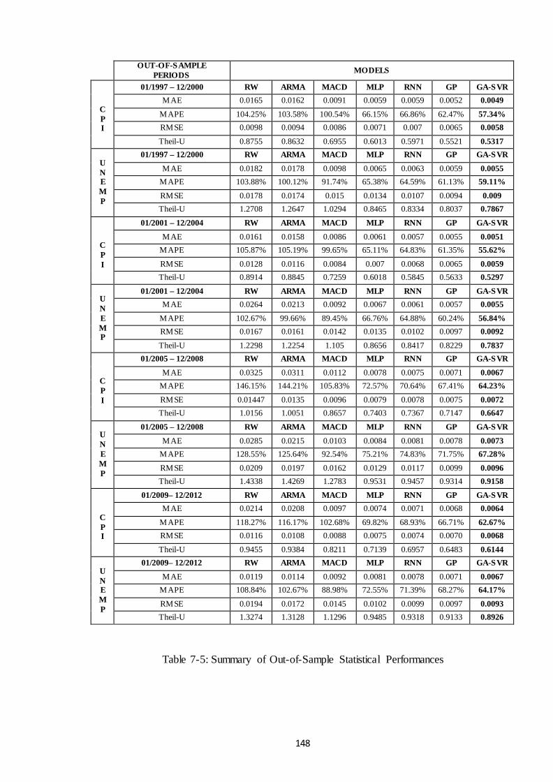
148
OUT-OF-SAMPLE PERIODS MODELS
C P I
01/1997 – 12/2000 RW ARMA MACD MLP RNN GP GA-SVR MAE 0.0165 0.0162 0.0091 0.0059 0.0059 0.0052 0.0049
MAPE 104.25% 103.58% 100.54% 66.15% 66.86% 62.47% 57.34% RMSE 0.0098 0.0094 0.0086 0.0071 0.007 0.0065 0.0058
Theil-U 0.8755 0.8632 0.6955 0.6013 0.5971 0.5521 0.5317
U N E M P
01/1997 – 12/2000 RW ARMA MACD MLP RNN GP GA-SVR
MAE 0.0182 0.0178 0.0098 0.0065 0.0063 0.0059 0.0055 MAPE 103.88% 100.12% 91.74% 65.38% 64.59% 61.13% 59.11%
RMSE 0.0178 0.0174 0.015 0.0134 0.0107 0.0094 0.009 Theil-U 1.2708 1.2647 1.0294 0.8465 0.8334 0.8037 0.7867
C P I
01/2001 – 12/2004 RW ARMA MACD MLP RNN GP GA-SVR
MAE 0.0161 0.0158 0.0086 0.0061 0.0057 0.0055 0.0051 MAPE 105.87% 105.19% 99.65% 65.11% 64.83% 61.35% 55.62%
RMSE 0.0128 0.0116 0.0084 0.007 0.0068 0.0065 0.0059 Theil-U 0.8914 0.8845 0.7259 0.6018 0.5845 0.5633 0.5297
U N E M P
01/2001 – 12/2004 RW ARMA MACD MLP RNN GP GA-SVR MAE 0.0264 0.0213 0.0092 0.0067 0.0061 0.0057 0.0055
MAPE 102.67% 99.66% 89.45% 66.76% 64.88% 60.24% 56.84% RMSE 0.0167 0.0161 0.0142 0.0135 0.0102 0.0097 0.0092
Theil-U 1.2298 1.2254 1.105 0.8656 0.8417 0.8229 0.7837
C P I
01/2005 – 12/2008 RW ARMA MACD MLP RNN GP GA-SVR
MAE 0.0325 0.0311 0.0112 0.0078 0.0075 0.0071 0.0067 MAPE 146.15% 144.21% 105.83% 72.57% 70.64% 67.41% 64.23%
RMSE 0.01447 0.0135 0.0096 0.0079 0.0078 0.0075 0.0072 Theil-U 1.0156 1.0051 0.8657 0.7403 0.7367 0.7147 0.6647
U N E M P
01/2005 – 12/2008 RW ARMA MACD MLP RNN GP GA-SVR
MAE 0.0285 0.0215 0.0103 0.0084 0.0081 0.0078 0.0073 MAPE 128.55% 125.64% 92.54% 75.21% 74.83% 71.75% 67.28%
RMSE 0.0209 0.0197 0.0162 0.0129 0.0117 0.0099 0.0096 Theil-U 1.4338 1.4269 1.2783 0.9531 0.9457 0.9314 0.9158
C P I
01/2009– 12/2012 RW ARMA MACD MLP RNN GP GA-SVR MAE 0.0214 0.0208 0.0097 0.0074 0.0071 0.0068 0.0064
MAPE 118.27% 116.17% 102.68% 69.82% 68.93% 66.71% 62.67% RMSE 0.0116 0.0108 0.0088 0.0075 0.0074 0.0070 0.0068
Theil-U 0.9455 0.9384 0.8211 0.7139 0.6957 0.6483 0.6144
U N E M P
01/2009– 12/2012 RW ARMA MACD MLP RNN GP GA-SVR
MAE 0.0119 0.0114 0.0092 0.0081 0.0078 0.0071 0.0067 MAPE 108.84% 102.67% 88.98% 72.55% 71.39% 68.27% 64.17%
RMSE 0.0194 0.0172 0.0145 0.0102 0.0099 0.0097 0.0093 Theil-U 1.3274 1.3128 1.1296 0.9485 0.9318 0.9133 0.8926
Table 7-5: Summary of Out-of-Sample Statistical Performances

149
The statistical superiority of the best proposed architecture is further validated by the
Modified Diebold-Mariano (MDM) statistic for forecast encompassing, as proposed by
Harvey et al. (1997). The MDM statistic is an extension of the Diebold-Mariano (1995)
statistic (DM) and its formula is the following:
( ) 1/21/2 11 2 1MDM T T k T k k DM− − = + − + − (7.4)
where T the number of the out-of-sample observations and k the number of the step-ahead
forecasts.
The use of MDM is common practice in forecasting because it is found to be robust
in assessing the significance of observed differences between the performances of two
forecasts (Hassani et al. (2009) and Barhoumi et al. (2012)). MDM also overcomes the
problem of over-sized DMs in moderate samples. The statistic is measured in each out-of-
sample period and the MSE and the MAE are used as loss functions. The MDM test
follows the Student’s t-distribution with f-1 degrees of freedom, where f is the number of
forecasts. Table 7-6 below presents the values of the statistics, comparing the GA-SVR
with its benchmarks.
PERIODS VARIABLES STATISTICS RW ARMA MACD MLP RNN GP
01/1997 – 12/2000
CPI
MDM1 -7.22 -7.19 -6.65 -4.54 -3.92 -3.15 MDM2 -9.81 -9.45 -8.77 -7.19 -6.98 -5.19
UNEMP
MDM1 -5.21 -5.09 -4.91 -4.13 -4.08 -3.02 MDM2 -7.71 -7.68 -7.43 -5.51 -4.98 -4.51
01/2001 – 12/2004
CPI
MDM1 -7.07 -6.96 -6.53 -4.24 -3.97 -3.22 MDM2 -9.34 -8.97 -8.58 -7.81 -7.12 -6.79
UNEMP
MDM1 -5.23 -5.03 -4.84 -4.19 -4.10 -3.26 MDM2 -7.90 -7.82 -7.48 -5.40 -4.97 -4.87
01/2005 – 12/2008
CPI
MDM1 -8.14 -8.05 -7.54 -7.19 -6.88 -6.34 MDM2 -9.84 -9.80 -9.30 -8.95 -8.80 -8.62
UNEMP
MDM1 -9.25 -9.16 -8.73 -8.15 -7.51 -7.07 MDM2 -10.37 -10.27 -9.81 -9.54 -9.17 -8.75
01/2009 – 12/2012
CPI
MDM1 -6.46 -6.27 -5.92 -5.71 -5.48 -4.77 MDM2 -7.95 -7.88 -7.71 -7.44 -7.32 -7.04
UNEMP
MDM1 -7.82 -7.66 -7.08 -6.77 -6.33 -6.09 MDM2 -8.75 -8.54 -8.28 -7.83 -7.39 -7.25
Note: MDM1and MDM2 are the statistics computed for the MSE and MAE loss function respectively.
Table 7-6: Modified Diebold-Mariano statistics for MSE and MAE loss functions

150
The MDM null hypothesis of forecast encompassing is rejected for all comparisons and for
both loss functions at the 1% confidence interval. The statistical superiority of the GA-
SVR forecasts is also confirmed as the realizations of the MDM statistic are always
negative 16. GP is found to have the closest forecasts with the GA-SVR model and remains
the second best model in statistical terms. From the MDM values it is safe to claim that
there is no conclusive evidence of encompassing between the GA-SVR forecasts of
inflation and unemployment and their benchmarks. Finally, the in-sample and out-of-
sample results indicate that the models implementing genetic approaches, GP and GA-
SVR, project in general more accurate forecasts in comparison with popular NN
techniques (MLP, RNN) or traditional linear models (RW, ARMA, MACD).
7.6 Conclusions
The motivation of this chapter is to introduce a hybrid Genetic Algorithm – Support Vector
Regression (GA-SVR) model in economic forecasting and macroeconomic variable
selection. The proposed algorithm is applied to the task of forecasting the US inflation and
unemployment. The GA-SVR genetically optimizes the SVR parameters and adapts to the
optimal feature subset from a feature space of potential inputs. The feature space includes a
wide pool of economic indicators that might affect the two series under study. The
forecasting performance of the GA-SVR is benchmarked with a Random Walk model
(RW), an Autoregressive Moving Average model (ARMA), a Moving Average
Convergence/Divergence model (MACD), a Multi-Layer Perceptron (MLP), a Recurrent
Neural Network (RNN) and a Genetic Programming (GP) algorithm. More specifically, the
statistical performance of all models is investigated in four rolling samples during the
period of 1974-2012.
In terms of the results, the GA-SVR outperforms all benchmark models for both
forecasting exercises. The model is able to genetically adapt to a small number of relevant
variables and project superior forecasts at the same time. This performance is consistent
also in periods of economic turmoil, which proves that the genetic SVR selection of the
predictors is both computationally and statistically efficient. With this variable selection
process, GA-SVR attempts to provide evidence on what inputs can be important predictors
16 The MDM test is applied to couples of forecasts (GA-SVR vs. another forecasting model). A negative MDM value indicates that the first forecast (GA-SVR) is more accurate than the second forecast. The lower the negative value, the more accurate are the GA-SVR forecasts.

151
of US inflation and unemployment in the specific periods under study. The autoregressive
lags of the past quarter are found to be of great importance, while information going back
more than a semester seems irrelevant. The in-sample and out-of-sample results show that
the models implementing genetic approaches, GP and GA-SVR, project the most accurate
forecasts and outperform their benchmarks. This superiority is further validated by the
MDM test. In general, the two forecasting exercises of this chapter attempt to shed more
light on the difficult quest of nonlinear mapping of macroeconomic variables over different
sample periods.

152
Chapter 8
Rolling Genetic Support Vector Regressions: An Inflation and Unemployment Forecasting Application in EMU.
8.1 Introduction
Predicting inflation and unemployment changes is an issue of paramount importance for
economists, bankers and government officials. Many monetary and policy decisions are
made by appraising such forecasts. As a result the empirical literature on forecasting
macroeconomic variables is voluminous (see amongst others Ang et al. (2007), Stock and
Watson (2009) and Cogley et al. (2010). The challenge, though, is that in periods of
economic instability, traditional statistical models do not project accurate results (Ager et
al., 2009). In such periods of recessions and structural breaks, suggested linear models
based on a fixed set of predictors are not efficient. Therefore, the following idea can be
generally postulated: Realistic inflation and unemployment forecasts in a constantly
changing world should depend on a number of different macroeconomic variables, rather
than on fixed underlying relationships.
The economies of the European Monetary Union (EMU) members are perfect
examples to evaluate the validity of the above statement. In 2009 the sovereign debt crisis
broke out in Greece and then spread in all Europe. This contagion originated from the
unstable integration of peripheral countries in the common currency and the inability of
core countries to lead to decisive changes in the EMU’s monetary and fiscal policy
(Lapavitsas et al. (2010)). Austerity measures, political instability, negative Euro
speculation provided regular economic shocks in countries, such as Greece, Ireland, Italy,
Portugal and Spain. The effects of this contagion are evident throughout all Europe today

153
and heavily endanger the EMU’s future. Therefore, traditional core countries, such as
Belgium, France and Germany, also cannot ‘feel safe’ through this turmoil.
In this chapter a hybrid Rolling Genetic – Support Vector Regression (RG-SVR) model is
introduced in economic forecasting and macroeconomic variable selection. The proposed
algorithm is applied to a monthly rolling forecasting task of inflation and unemployment in
the abovementioned eight EMU countries. The RG-SVR genetically optimizes the SVR
parameters and adapts to the monthly optimal feature subset from a feature space of
potential inputs. The feature space includes a wide pool of macroeconomic indicators that
might affect the two series under study of every country. The forecasting performance of
the RG-SVR is benchmarked with a ‘fixed’ Random Walk model (f-RW), an Atkeson and
Ohanian Random Walk (AO-RW) and a Smooth Transition Autoregressive Model
(STAR). The study engages with two rolling forecasting exercises over the period of
August 1999 to April 2013. The first exercise focuses on forecasting the inflation of these
countries, while the second one attempts to predict their unemployment. The statistical
performance of RG-SVR is benchmarked with a f-RW, an AO-RW and a STAR. The
results prove that RG-SVR statistically outperforms all benchmark models. It also presents
evidence on what macroeconomic variables can be relevant predictors of the monthly
inflation and unemployment and how these vary in each EMU country during the specific
period under study.
The novelty of the model lies in its ability to capture the monthly asymmetries and
nonlinearities in the given sample of predictors, select the optimal feature subsets and
provide robust rolling SVR forecasts for the specific country and series under study. As
potential inputs, the proposed algorithm uses a pool of one hundred sixty eight potential
predictors. From an economic perspective, this increases the model’s flexibility and allows
it to explore a large universe of potential relationships between those predictors of each
country’s inflation and unemployment. The selection of the proposed model’s inputs and
parameters is based on a GA algorithm, while the pool of potential inputs is only limited
by the monthly data availability. From an econometric perspective the rolling forward
estimation makes the results of the forecasting exercise more realistic and robust. From a
technical point of view, the proposed model is superior to non-adaptive algorithms
presented in the literature. Similarly to the GA-SVR proposed and implemented in
previous chapters, RG-SVR does not require analytic parameter calculation as Cherkassky
and Ma (2004) propose, but also avoids time consuming optimization approaches (cross
validation or grid search) that are used in similar applications ( Lu et al. (2009) and Kim
and Sohn (2010)). An additional attribute of RG-SVR in comparison to GA-SVR is that

154
SVR optimization is achieved with the minimum number of support vectors, while its
single optimization procedure restrains data snooping bias effects.
The rest of the chapter is organized as follows. Section 8.2 describes the dataset
used for this study, while a brief description of the benchmark models is given in section 8-
4. Section 8-5 describes the hybrid RG-SVR model. Finally, the empirical results and
conclusions are presented in Section 8-6 and 8-7 respectively.
8.2 Data Description
This chapter implements two rolling forecasting exercises with monthly data over the
period of August 1999 to April 2013. The first exercise attempts to forecast the percentage
change of the inflation of eight European countries, namely Belgium, France, Germany,
Greece, Ireland, Italy, Portugal and Spain. The Consumer Price Index (CPI) of each
country is used as a proxy of its inflation. The second exercise focuses on predicting the
percentage change of the unemployment rate (UNEMP) of the above countries.
Following similar studies (Stock and Watson (2003), Wright (2009) and Groen
et.al (2012)), I select fourteen predictors that can explain the economic premises of
inflation and unemployment or are found to be useful in forecasting them. Four predictors
are individual macroeconomic indicators of each country. Since the RG-SVR model is
applied to a Eurozone case study, the rest ten predictors are country non-specific indicators
that qualify as explanatory variables of the euro area economic activity and structure. The
final pool of the potential inputs includes the first twelve autoregressive terms of these
predictors. Thus, the feature space consists of hundred sixty eight series of monthly
percentage changes. The sources of the data are Bloomberg (BLOOM) and the Statistical
Data Warehouse of the European Central Bank (ECB). The series are seasonally adjusted,
where applicable. Table 8-1 below summarizes the list of variables used in this application.

155
No MNEMONIC DESCRIPTION SOURCE
1 CPI Consumer Price Index (SA) BLOOM
2 UNEMP Eurostat Unemployment Rate (SA) BLOOM
3 INDP Eurostat Industrial Production: Total Industry excluding Construction Nace 2 Rev. (SA) BLOOM
4 ESI European Commission Economic Sentiment Indicator (SA) BLOOM
5 LOAN EU MFI Balance Sheet Outstanding Amounts: Government Loans to Euro area residents (SA) BLOOM
6 TRBAL Eurostat External Trade Balance (SA) BLOOM
7 EUM1 ECB Money Supply M1 (SA) BLOOM
8 USD EUR/USD Exchange Rate (NSA) BLOOM
9 JPY EUR/JPY Exchange Rate (NSA) BLOOM
10 GBP EUR/GBP Exchange Rate (NSA) BLOOM
11 FTSE FTSE 100 Index (NSA) BLOOM
12 STOXX50 Eurostoxx 50 Index (NSA) BLOOM
13 GDAX Deutsche Borse AG German Stock Index (NSA) BLOOM
14 OIL Brent Crude Oil 1-month Forward (fob) per barrel (SA) ECB
15 SP1 Spread between swaps 6-month Euribor and benchmark bonds of 2-year maturity (SA) ECB
16 SP2 Spread between swaps 6-month Euribor and benchmark bonds of 10-year maturity (SA) ECB
Note: CPI and UNEMP are the two observed variables. INDP, ESI, LOAN and TRADE are
individual indicators of each country. The rest are country non-specific Eurozone indicators.
The pool of predictors consists of the first twelve autoregressive terms of variables 3-16 (168
series in total). BLOOM refers to the Bloomberg database, while ECB stands for the Statistical
Data Warehouse of the European Central Bank. All series are in monthly percentage changes.
SA and NSA means that the series is seasonally adjusted and not seasonally adjusted
respectively.
Table 8-1: List of all the variables
The proposed methodology evaluates depending on the country the underlying
domestic and external economic forces that could rule the inflation and unemployment
changes in Eurozone. For example, INDP, LOAN and TRBAL are commonly selected as
relevant individual indicators in similar studies (see Schirm (2003), Stock and Watson
(2004) and Rondorf (2012)). Including each country’s ESI into the pool of potential inputs
adds extra validity to this effort, since it is considered a leading macroeconomic indicator
for every EMU country (see Banerjee et al. (2005), Diron (2008) and Giannone et al.
(2012)). Based on Eurostat’s definition, ESI is a composite indicator that comprises of four
confidence indicators with different weights, namely the Industrial confidence indicator

156
(weight 40%), Consumer confidence indicator (weight 20%), Construction confidence
indicator (weight 20%) and Retail trade confidence indicator (weight 20%). Those
indicators are derived from business and consumer surveys, which provide a realistic
consensus of the business activity, consumers’ purchasing power and price trend. Other
researchers believe that the EMU economy can be appraised as a whole and based on that
premise they form their analysis (Marcellino (2004) and Ruth (2008)). For that reason,
country non-specific EMU indicators, such as EUM1, main ECB exchange rates and stock
indices, OIL, SP1 and SP2 are also used in each country’s analysis.
8.3 Benchmark Forecasting Models
The forecasting efficiency of the RG-SVR model is benchmarked with three traditional
models, namely a ‘fixed ρ’ Random Walk (f-RW), an Atkeson and Ohanian Random Walk
(AO-RW) and a Smooth Transition Autoregressive Model (STAR). These benchmark
models aim to forecast the one month ahead inflation and unemployment value in
percentage changes.
8.3.1 ‘Fixed ρ’ Random Walk (f-RW)
The simple RW is a non-stationary process, where the current value of a variable is
calculated from the past value plus an error term. The error term follows the standard
normal distribution. Instead of using a simple RW, this application follows Faust and
Wright (2012) that use a ‘Fixed ρ’ forecast as their baseline inflation benchmark. Thus,
both target series are fitted to an AR (1) process with a fixed slope coefficient ρ. The
specification of the model is the following:
1ˆ , ~ (0,1)t t t tY Y e e Nρ −= + (8.1)

157
Where tY is the forecasted value for period t, 1tY − is the actual value of period t-1 and
ρ=0.4617.
8.3.2 Atkeson and Ohanian Random Walk (AO-RW)
Atkenson and Ohanian (2001) note that inflation indicators cannot show the short term
changes of inflation reliably. Therefore, they suggest that a RW forecasting the current
value of a variable based on its previous four lags is preferable to a simple RW. Following
again Faust and Wright (2012), the AO-RW is adopted as a benchmark forecasting model
and specified as below:
1 2 3 41ˆ ( ) , ~ (0,1)4t t t t t t tY Y Y Y Y Nε ε− − − −= + + + + (8.2)
Where:
• tY is the forecasted value at time t
• Yt-1,Yt-2, Yt-3 and Yt-4 are the four previous actual values
• εt is the error term
8.3.3 Smooth Transition Autoregressive Model (STAR)
The STAR combines two AR models with a function that defines the degree of non-
linearity (smooth transition function). The general two-regime STAR specification is the
following:
1 2ˆ (1 ( , , )) ( , , )t t t t t tY F z F z uζ λ ζ λ′ ′= Φ Χ − +Φ Χ + (8.3)
17 Based on Faust and Wright (2012) the value of ρ is the slope coefficient that is derived from fitting an AR (1) to the 1985Q1 vintage GDP deflator inflation from 1947Q2 to 1959Q4.

158
Where:
• tY the forecasted value at time t
• ,0 ,1 ,( , ,... ), 1, 2i i i i p iϕ ϕ ϕΦ = = and ,0 ,1 ,, ,...i i i pϕ ϕ ϕ the regression coefficients of the two
AR models
• (1, )t tχ′ ′Χ = with 1( ,..., )t t t pY Yχ − −′ =
• 0 ( , , ) 1tF z ζ λ≤ ≤ the smooth transition function
• , 0t t dz Y d−= > the lagged endogenous transition variable
• ζ the parameter that defines the smoothness of the transition between the two
regimes
• λ the threshold parameter
• ut the error term
The main characteristic of a STAR is that tY is calculated at any given t as a
weighted average of two AR models. The weights of the two AR models are defined based
on the value of ( , , )tF z ζ λ . The regime-switching ability of STARs derives from the fact
that at each t a regime is selected based on the values of zt and ( , , )tF z ζ λ . In this chapter,
both series are best modeled as Logistic STAR (LSTAR) processes for all eight
countries.18 The LSTAR approach allows the association of the two regimes with large and
small values of zt relatively to λ. Such a regime-switching is useful to identify expansions
and recessions in the business cycle (Lin and Terasvitra (1994)).
8.4 Rolling Genetic – Support Vector Regression (RG-SVR)
This sections includes the description and specification of the hybrid Rolling Genetic –
Support Vector Regression (RG-SVR) model for rolling optimal SVR parameter and
monthly macroeconomic variable selection. This model genetically searches over a feature
space (the pool of macroeconomic predictors as in Table 8-1) and then provides a single
optimized SVR rolling forecast for each series under study. The required theoretical
background of SVR, GAs and genetic feature selection and the extension of this model in 18 I also experimented with a Multip le Reg ime STAR (MRSTAR) of more than two reg imes, as described in detail by Dijk and Franses (1999). LSTAR though presented better statistical performance than MRSTAR in all cases. This plus the lower model complexity of LSTAR allows me to disqualify MRSTAR from our benchmark models’ selection.

159
comparison to the GA-SVR is given in detail chapter 3. Extending the GA-SVR model of
chapter 7, in this application the RG-SVR is able to capture the monthly asymmetries and
nonlinearities in the given sample of predictors, but most importantly select the optimal
monthly feature subsets. The GA in this case evolves chromosomes, similar to figure 6-2
in chapter 6. The chromosome again consists of feature genes and parameter genes.
In order to better distinguish the extension of RG-SVR to GA-SVR, the forecasting
process needs to be explained. The RG-SVR model performs a rolling window forecasting
exercise as follows. The window size is always equal to hundred twenty five observations
(months). The algorithm requires the window size to be further divided in a training and
test subset in order to validate the goodness of fit of each chromosome. The first eighty
nine observations are the training subset. The rest thirty six form the test subset. The
population of chromosomes is initialized in the training sub-period. The optimal selection
of chromosomes is achieved, when their forecasts minimize the MSE in the test-sub
period. Then, the optimized parameters and selected predictors of the best solution are
used to train the SVR and produce the final optimized forecast for the next observation.
After this is completed, the window rolls forward by one observation and the procedure is
repeated. In that way, the RG-SVR model presents forty monthly rolling forecasts. For
each of these forecasts, the algorithm stores its optimized C, γ and v parameters and set of
optimal predictors.19Obviously, the GA-SVR technique is not able to do that and the only
way to approximate RG-SVR performance is to drastically decrease the length of the
rolling periods that are evaluated (see the three periods of chapter 7). These would incur
many repetitions and increase substantially the computational demands of the task.
Nonetheless, the RG-SVR rolling procedure as explained before can also be
computationally heavy. Its accuracy depends on the trade-off between a high-complexity
model (over – fitting) and a large-margin (incorrect setting of the ‘tube’). The number of
support vectors can vary from few to every single observation (complete over- fitting).
Algorithms attempting to use efficiently extensive datasets and simultaneous take into
account large sets of variables suffer from computational complexity. This complexity
burden makes them practically infeasible and their results cannot be used in realistic terms.
RG-SVR is able to overcome this issue by giving optimal SVR forecasts with the 19 The monthly data start on August 1999 and end on April 2013. In order to derive the first forecast (January 2010), RG-SVR uses the first 89 months (August 1999 - December 2006) as a training subset and the rest 36 months (January 2007-December 2009) as a test subset. The second forecast (February 2010) is similarly given by rolling forward the previous samples by one month. Thus, the second training subset is from September 1999 till January 2007, while the second test subset extends from February 2007 till January 2010. The exercise ends when all the RG-SVR forecasts from January 2007 until April 2013 are gathered (40 months).

160
minimum number of support vectors, which further contributes to the algorithm’s novelty.
Indicative is the fact that RG-SVR is implemented in a modern mainstream computer
within a couple of hours for this specific dataset.
In genetic algorithm modeling the fitness functions need to be increasing functions.
Therefore, the algorithm is minimizing the MSE by maximizing the following function:
Fitness= 1/ (1+MSE) (8.4)
The size of the initial population is set to 600 chromosomes while the maximum number of
generations is set to 5000. The algorithm in general terminates when the number of
generations is 4000 on average. This process is also associated with the convergence of the
evaluated population (see chapter 3). Convergence is needed in order to keep populations
that can lead to more efficient ones as the process goes on. The summary of the GA’s
characteristics is presented in the following table, while the detailed flowchart is given in
figure 3-6 of chapter 3.
Population Size 600 Maximum Generations 5000
Selection Type Roulette Wheel Selection Elitism Best member of every population is maintained in the next generation.
Crossover Probability 0.80 Mutation Probability 0.20
Fitness Function 1/(1+MSE) Window size 125
Support Vectors Minimized
Table 8-2: GA Characteristics and Parameters
8.5 Empirical Results
This section summarizes the empirical results of this application. The macroeconomic
contribution of this chapter is based on the fact that proposed algorithm is able to
genetically adapt in the most relevant variables for forecasting the inflation and
unemployment of eight EMU countries. The first subsection describes the predictor
selection for each country for both exercises, while the second one evaluates statistically
the derived CPI and UNEMP forecasts.

161
8.5.1 Selection of predictors
The RG-SVR algorithm examines the cases of three core countries (Belgium, France and
Germany) and five peripheral ones (Greece, Ireland, Italy, Portugal and Spain), mapping
their relevant indicators for forty months (January 2010 – April 2013). In every table20
presenting the selected predictors, seven specific months are highlighted. These months
could be considered as structural breaks in the Eurozone economy during this volatile
period. These derive from EU central financial and political decisions, events and news’
reports, which lead to positive or negative speculation in the Euro area in general. More
details regarding the highlighted months are given in appendix F.1.
8.5.1.1 Inflation Exercise
The following three tables refer to the three core countries, namely Belgium, France and
Germany. Table 8-3 presents the selected predictors of CPI for the case of Belgium. The
results show that INDP, ESI, STOXX50, GDAX and OIL are selected almost in all months
as potential inputs, while FTSE is always discarded. LOAN, TRBAL, EUM1, USD, JPY,
GBP are all not found important before April 2011. SP1 and SP2 are pooled only after
January 2012. The selected macroeconomic variables of CPI for the French case follow in
Table 8-4. From this table is suggested that only OIL is always selected for all the months.
SP1 and SP2 are discarded, except of one month for SP1. EMU1, USD and FTSE are
found irrelevant before February 2012, while STOXX50 and GDAX after February 2012.
ESI is always kept in the pool after April 2011. The German monthly pool of predictors is
given in Table 8-5. The German EUM1, USD, GDAX and OIL are included in the pool
during all months, while LOAN, JPY, GBP and FTSE are not. INDP is not selected only
during five months, whereas STOXX50 is included only for three months. ESI and
TRBAL are relevant indicators after September 2011, while SP1 and SP2 after September
2010.
20 In every table the numbers represent the orders of the autoregressive terms. For example, the number 1 in the column of IND means that RG-SVR selects as input the first autoregressive term of the Industrial Production.

Table 8-3: The selected predictors for the Belgian inflation
BELGIUM CPI INDP ESI LOAN TRBAL EUM1 USD JPY GBP FTSE STOXX50 GDAX OIL SP1 SP2
Jan-10 2, 3 2, 4 - - - - - - - 1, 3 1, 4 3, 5 - - Feb-10 1, 3 1, 2 - - - - - - - 3, 4 4, 5 1, 3 - - Mar-10 1, 3 1, 3, 4 - - - - - - - 1 1, 3 3 - - Apr-10 3 2, 3, 5 - - - - - - - 4 3, 5 1, 2, 4 - - May-10 1, 2, 5, 6 2, 3 - - - - - - - 2, 4 1, 2, 6 1, 2, 4 - - Jun-10 1,2, 4, 5 1, 4 - - - - - - - 5 3 4, 5 - - Jul-10 2, 4 6 - - - - - - - 2, 3, 5 1 5 - - Aug-10 - 1 - - - - - - - 1, 4 3, 4, 5 1, 2 - - Sep-10 - 1 - - - - - - - 1, 2 4, 6 2, 3, 5 - - Oct-10 2, 4, 6 2, 4 - - - - - - - 1 2, 4 6 - - Nov-10 2, 4, 6 4 - - - - - - - 1, 2, 4 1, 2, 3 3, 5 - - Dec-10 4 5 - - - - - - - 1 2, 3, 5 1, 2 - - Jan-11 1 5 - - - - - - - 5, 6 1, 2 4 - - Feb-11 1, 5, 6 1, 2 - - - - - - - 2, 4 2, 3, 6 1, 4 - - Mar-11 1, 5 3 - - - - - - - 2, 3, 6 1 5 - - Apr-11 2, 3, 4, 5, 6 4, 5 - 2, 5 2, 3 6 2, 5 1, 2, 4 - 5 3, 4 2 - - May-11 1, 4 1, 3 - 3, 5 1, 2 4 1, 2 4, 5 - 1 1, 4 6 - - Jun-11 6 4 - 4 5 1 2, 3 3, 5 - 5 6 3 - - Jul-11 6 5 - 1 2, 3 1 2 4 - 5, 6 2, 3, 6 3 - - Aug-11 1 2, 3 - 3 1, 2 1, 3, 4 1 5 - 1, 5 1, 2 5 - - Sep-11 2, 3, 5 4 2,3,5 3, 4, 5 5 - - - - 5 6 2 - - Oct-11 - 2, 5 4 1 3, 5 - - - - 1, 4 3, 5 4 - - Nov-11 - 4 1 2, 3, 5 1, 4 - - - - 1, 2 3, 4 2, 3, 6 - - Dec-11 3, 6 1, 2 1, 5, 6 5, 6 5 - - - - 1, 3, 4 1, 3 1, 4 - - Jan-12 3, 6 1, 5 3, 4 - - - - - 1, 2, 4 3 2, 4 - - Feb-12 1, 4, 5, 6 3, 5, 6 3, 4 2, 3 - 1 1, 3 1, 5 - 5 3 1, 3, 4 2 5 Mar-12 1, 2, 4, 5 1 1, 2, 4 1, 5 1 3, 4, 5 4, 5 1, 3 - 3, 4, 5 1 1, 2 4, 5 5 Apr-12 1, 2, 4 1 1, 3 2 2, 4 - 1, 3 3, 4, 5 - 1, 2 2, 3, 5 - 1, 3 5 May-12 2, 3, 6 1 3 2 2, 3, 5 - 2, 4 1, 3, 5, 6 - 2 1, 4 - 5, 6 3, 4, 5 Jun-12 1, 4 1 1, 3 2, 5 2 - 1 1,2,4 - 3, 4, 5 2 - 1, 5 4 Jul-12 1, 4, 5, 6 1 3 2, 5 1, 5 5, 6 1,2,4 - - 2, 4 2, 3 - 2, 3 2, 4 Aug-12 1, 2 3, 4 2, 4, 5 1, 2, 4 - - - - - 3 3, 5 3 3, 4, 5 4, 5 Sep-12 - 2, 4 5 2, 3, 5 - - - - - 3 3, 4, 5 1, 2 1, 5 4, 5 Oct-12 - 2 3 5, 6 - - - - - 1, 4 3, 4 2, 4 1, 4 3, 5 Nov-12 - 3 4, 5 4, 5 - - - - - 5 3, 6 3, 5 2, 4 6 Dec-12 5 5, 6 5 1, 4 - - - - - 5 1 5, 6 4 5 Jan-13 1, 2, 6 1, 2 1 1, 2, 3 - - - - - 1, 3, 4 2, 3, 5 1, 2, 3 3, 5 3, 4, 5 Feb-13 5, 6 3, 5 5, 6 2, 4 - - - - - 3, 4 2 1, 2, 3 2 6 Mar-13 1, 3, 5 1, 4 1, 3, 4 1, 2 - - - - - 5 2, 5 2, 4 2, 4 1, 5 Apr-13 2, 6 4 2 1, 2 - - - - - 1, 2 2, 4 4, 5 1, 2 4, 5
162

Table 8-4: The selected predictors for the French inflation
FRANCE CPI INDP ESI LOAN TRBAL EUM1 USD JPY GBP FTSE STOXX50 GDAX OIL SP1 SP2
Jan-10 1, 4 5 2, 3 1 - - - - - 2 2, 4 1, 2 - - Feb-10 1, 4 4 2, 4 3, 4, 5 - - - - - 2, 3 4 3, 4, 5 - - Mar-10 3, 4 5 2 3, 6 - - - - - 3, 6 4, 5, 6 3 - - Apr-10 3, 4 5 2 2, 3 - - - - - 6 4,5 4 - - May-10 3, 4 2 1, 2 - - - - - - 3, 4, 5 - 4 - - Jun-10 1, 5 2, 3 3 - - - - - - 3 - 2, 3 - - Jul-10 3, 4, 6 2 4, 6 - - - - - - 3 - 2 - - Aug-10 2, 4 4, 5, 6 3 - - - - - - 1, 2, 3 - 2, 4 - - Sep-10 2 - 2, 4, 6 - - - - - - 3 - 1, 3, 4 - - Oct-10 2 - 5, 6 1, 5 - - - - - 1 - 2 - - Nov-10 1 - 6 2, 3 - - - - - 2, 5 - 3, 4 - - Dec-10 4, 5 - 3, 6 1, 2 - - - - - 2, 3 - 1, 3, 6 - - Jan-11 1, 3, 6 - 3 4, 6 - - - - - 1, 2 - 2 - - Feb-11 3, 4, 6 - 3 3, 6 - - - - - 1, 4, 5 - 2 - - Mar-11 1, 2 - 4, 6 6 - - - - - 2 - 3, 4, 5 - - Apr-11 - - 3, 6 - - - - - - 2 - 6 - - May-11 - 2, 3, 6 2 - - - 5 1, 2 - 1, 3 3 5 - - Jun-11 - 5, 6 2, 5 - - - 2 2, 3 - 3 3, 4, 5 6 - - Jul-11 - 2, 3, 4, 5, 6 3, 6 - - - 2, 5 1, 5, 6 - 5, 6 4 2, 5, 6 - - Aug-11 - 2, 3, 4 5 - - - 2, 3 4 - 1, 3, 5 4 4, 6 - - Sep-11 - 3, 4 5 - - - 2, 4 4 - 2 4 2 - - Oct-11 1, 6 2 1, 4 - - - 1, 4, 5 4 - 2 4 3, 4 - - Nov-11 3, 4 2, 3 2, 4 - - - 2 2, 3 - 2 2, 4 2, 5 3, 4, 5 - Dec-11 2, 5, 6 4 5 - - - 2, 3 2, 6 - 4, 5 4, 6 2, 5, 6 - - Jan-12 4, 5 4, 5 6 - - - 1, 4, 5, 6 5, 6 - 6 4 2 - - Feb-12 1, 4, 5 6 - - 3 2, 4 1 2, 5, 6 - - - 2, 4 - - Mar-12 3 2, 6 - 4 4, 5, 6 4, 6 5 4 2 - - 1 - - Apr-12 4 2, 5 - 4, 5 1, 2 4 1, 3 4 2 - - 1 - - May-12 1, 3 1, 2, 5 - 3 3 5 5 4 1 - - 1, 4, 5 - - Jun-12 4 1, 4 - 4 2, 3 4 2 2, 3 1, 2 - - 1 - - Jul-12 - 5, 6 - 1, 4 3 4 3, 5 - 5 - - 1 - - Aug-12 - 1, 3, 5 3 3, 4 3 1 1, 6 - 5 - - 2 - - Sep-12 - 4, 5 3 1, 3, 4 3, 4 2 1, 2 - 5, 6 - - 2, 5 - - Oct-12 - 1, 5 1 3, 5 4 1, 2 2 - 2, 6 - - 2, 6 - - Nov-12 - 1, 5 3 5 4, 5 1, 2 2, 4 - 2, 3 - - 1, 2 - - Dec-12 - 5 3, 5 3, 4, 5 3 2 2, 4 - 2, 3 - - 2, 4, 5 - - Jan-13 - 5 3, 4 1, 2 1, 2, 5, 6 2 1, 2 - 2 - - 3 - - Feb-13 - 1, 2 3 1 4, 5, 6 6 2 - 6 - - 3 - - Mar-13 - 1, 2 2,3 1 4, 5 6 2 3 4, 5 - - 3, 6 - - Apr-13 - 3 4 1 4 5, 6 2, 3 2, 4, 5, 6, 3, 5 - - 2, 3 - -
163

Table 8-5: The selected predictors for the German inflation
GERMANY CPI INDP ESI LOAN TRBAL EUM1 USD JPY GBP FTSE STOXX50 GDAX OIL SP1 SP2
Jan-10 2 - - - 1 2 - - - - 1 1 - - Feb-10 2 - - - 2, 4 1, 2 - - - - 3, 4 4 - - Mar-10 2 - - - 3, 4, 5 2 - - - - 2, 3, 6 4 - - Apr-10 2, 3 - - - 4, 5 2, 5 - - - - 4, 6 4 - - May-10 3 - - - 2 3, 5 - - - - 3, 5 4 - - Jun-10 3 - - - 1 1, 4 - - - - 3, 4 2, 4 - - Jul-10 1 - - - 1 2 - - - - 3, 6 2, 5 - - Aug-10 - - - - 1 4, 5 - - - - 4, 6 4 - - Sep-10 - - - - 2 4, 5 - - - - 3, 4, 5 4 - - Oct-10 - - - - 2 1, 2, 5 - - - - 4, 5 4 - - Nov-10 - - - - 2, 3 5, 6 - - - - 2, 3 4 3 - Dec-10 - - - - 3 2, 4 - - - - 1, 2 3, 5 3 - Jan-11 1, 3 - - - 2, 3 1, 2, 5 - - - - 1, 2, 5 5 2 - Feb-11 3 - - - 3 3, 5 - - - - 2 1, 4 2, 5 - Mar-11 3 - - - 1 1, 4 - - - - 2 5 3 - Apr-11 5 - - - 6 1, 6 - - - - 2, 6 5 3, 5 1 May-11 5, 6 - - - 4, 6 6 - - - - 2, 3 5 2 1 Jun-11 4, 5 - - - 2, 4 6 - - - - 1, 3, 4 5 2 1 Jul-11 5 - - - 4, 6 6 - - - - 3 4 2, 1 1 Aug-11 5 - - - 3, 5 6 - - - - 3, 5 2, 4 1 2, 5 Sep-11 5 - - - 3 1 - - - - 3 1, 5 1, 2 1 Oct-11 5 2, 3 - - 1, 2, 5 1, 2 - - - 2 3 1, 4 3 1 Nov-11 1, 4 3 - - 3 2 - - - - 1, 3 4 3 2, 5 Dec-11 4 3, 4 - - 3 2, 4 - - - - 3 4 3 1 Jan-12 4 3, 5 - - 2 2, 5 - - - - 3 4, 5 3 2 Feb-12 4, 5 1, 2 - 2, 3 2 4, 5 - - - - 3 5, 6 3 2 Mar-12 1, 2, 4 2 - 3, 4 2 3, 5 - - - - 1 1 3 2 Apr-12 3, 4 2 - 1, 2, 5 2 5, 6 - - - - 1 2 3 1 May-12 2, 3, 4 1, 3 - 4 2 5 - - - - 2, 4 2 2, 4 1 Jun-12 4 1, 2 - 5, 6 1, 2 2, 5 - - - - 1 2, 3 3 2 Jul-12 4, 5 6 - 1, 5 2, 4 1, 3 - - - 2, 4 3, 6 3 3 1 Aug-12 2 4, 5 - 5 3 3, 5 - - - - 6 3, 4 1, 3 3 Sep-12 3 5 - 5, 6 3 3, 6 - - - - 6 4, 6 3 3 Oct-12 1 5 - 1, 5 3, 5 5, 6 - - - - 5, 6 3, 5 1, 2, 5 5, 6 Nov-12 1 5, 6 - 1, 4 5 3, 4, 6 - - - - 3, 5 6 1 6 Dec-12 1, 2 3 - 2, 6 1, 6 3, 5 - - - - 4, 6 6 3 2, 5 Jan-13 2 2 - 3 3, 4 3 - - - 2, 5 4 6 3, 4 3, 5 Feb-13 6 1, 2 - 1, 5 4 1, 4 - - - - 1, 3, 6 6 3, 5 2, 5 Mar-13 5 2 - 5 4, 6 1 - - - - 1, 2, 5 1 3, 6 2, 4 Apr-13 5, 6 1, 4 - 6 6 1, 3 - - - - 3, 5, 6 1 5 5, 6
164

165
The results of the previous three tables indicate that OIL is a common relevant
predictor for the core countries during all months under study. ESI is always kept in the
pool of potential inputs after October 2011, while JPY, GBP and FTSE always discarded
before April 2011. All monthly forecasts are derived by less than thirty inputs from the
hundred sixty eight in total, which are autoregressive terms with order up to six. Finally,
the average number of terms selected for a monthly forecast is seventeen.
The next five tables present the same information for the five peripheral countries,
namely Greece, Ireland, Italy, Portugal and Spain. In Table 8-6 the results for the Greek
case are summarized. TRBAL, USD, JPY, GBP and OIL are not useful to predict the
Greek CPI. On the other hand, autoregressive terms of EUM1, SP1 and SP2 are always
used for this task. ESI is selected only before June 2010 and after August 2011.The rest of
the predictors are included in the pool of potential inputs only for limited number of
months. Table 8-7 describes the Irish inflation predictors, selected by the RG-SVR. This
pool of predictors indicates that only SP2 is found irrelevant for all months. All the other
variables are found important during different months. For example, INDP is selected after
January 2011, except from the period of September 2011 to February 2012. ESI is found
insignificant mainly July 2011, while LOAN from November 2010 to March 2012. FTSE
and SP1 are included only in the last months of the exercise. Finally, JPY, GBP, FTSE and
GDAX are all not found relevant macroeconomic indicators of Irish inflation before July
2011. Next, the Italian case is analyzed. Table 8-8 shows that GBP is found important in
all the forecast period, while FTSE is not. SP2 is kept in the Italian pool of predictors only
after April 2012. The rest of the indicators are selected in various patterns. ESI, TRBAL,
EMU1 and GDAX all disqualify as potential inputs during May 2011 to September 2011.
Similarly, INDP, EMU1, JPY and GDAX are not selected during February 2012 till May
2012. The Portuguese relevant macroeconomic variables are presented in table 8-9. From
the above it is obvious that TRBAL and FTSE are common variables throughout the forty
months. On the other hand, INDP, LOAN, USD, JPY, GBP and OIL are not kept in the
pool of potential inputs. SP1 is not selected only from September 2010 to April 2010. ESI,
EMU1, STOXX50, GDAX and SP2 are found irrelevant during almost the whole 2012.
Finally, the Spanish inflation predictors are summarized in the table 8-10. In this case RG-
SVR discards many indicators during the forecast period (LOAN, TRBAL, USD, JPY,
GBP, FTSE, OIL, SP1 and SP2), but always keeps as potential inputs autoregressive terms
of ESI and EMU1. INDP, STOXX50 and GDAX are also macroeconomic variables used
throughout most of the forty months, except some consecutive months.
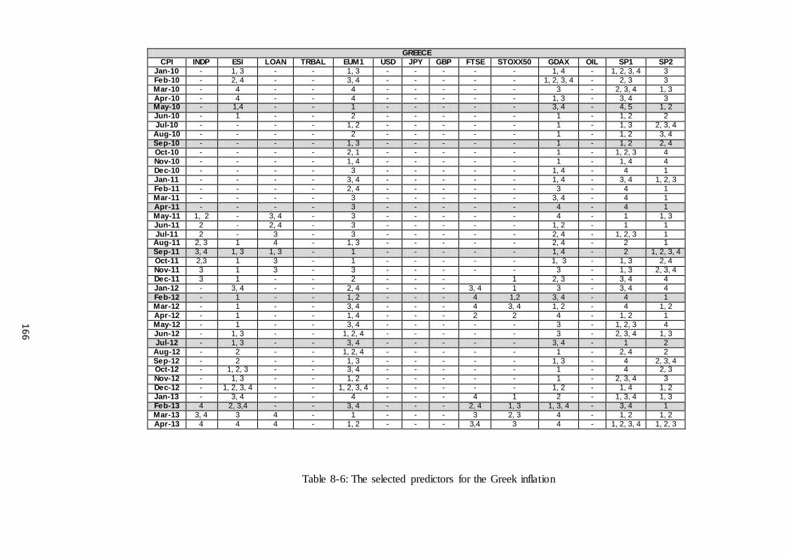
Table 8-6: The selected predictors for the Greek inflation
GREECE CPI INDP ESI LOAN TRBAL EUM1 USD JPY GBP FTSE STOXX50 GDAX OIL SP1 SP2
Jan-10 - 1, 3 - - 1, 3 - - - - - 1, 4 - 1, 2, 3, 4 3 Feb-10 - 2, 4 - - 3, 4 - - - - - 1, 2, 3, 4 - 2, 3 3 Mar-10 - 4 - - 4 - - - - - 3 - 2, 3, 4 1, 3 Apr-10 - 4 - - 4 - - - - - 1, 3 - 3, 4 3 May-10 - 1,4 - - 1 - - - - - 3, 4 - 4, 5 1, 2 Jun-10 - 1 - - 2 - - - - - 1 - 1, 2 2 Jul-10 - - - - 1, 2 - - - - - 1 - 1, 3 2, 3, 4 Aug-10 - - - - 2 - - - - - 1 - 1, 2 3, 4 Sep-10 - - - - 1, 3 - - - - - 1 - 1, 2 2, 4 Oct-10 - - - - 2, 1 - - - - - 1 - 1, 2, 3 4 Nov-10 - - - - 1, 4 - - - - - 1 - 1, 4 4 Dec-10 - - - - 3 - - - - - 1, 4 - 4 1 Jan-11 - - - - 3, 4 - - - - - 1, 4 - 3, 4 1, 2, 3 Feb-11 - - - - 2, 4 - - - - - 3 - 4 1 Mar-11 - - - - 3 - - - - - 3, 4 - 4 1 Apr-11 - - - - 3 - - - - - 4 - 4 1 May-11 1, 2 - 3, 4 - 3 - - - - - 4 - 1 1, 3 Jun-11 2 - 2, 4 - 3 - - - - - 1, 2 - 1 1 Jul-11 2 - 3 - 3 - - - - - 2, 4 - 1, 2, 3 1 Aug-11 2, 3 1 4 - 1, 3 - - - - - 2, 4 - 2 1 Sep-11 3, 4 1, 3 1, 3 - 1 - - - - - 1, 4 - 2 1, 2, 3, 4 Oct-11 2,3 1 3 - 1 - - - - - 1, 3 - 1, 3 2, 4 Nov-11 3 1 3 - 3 - - - - - 3 - 1, 3 2, 3, 4 Dec-11 3 1 - - 2 - - - 1 2, 3 - 3, 4 4 Jan-12 - 3, 4 - - 2, 4 - - - 3, 4 1 3 - 3, 4 4 Feb-12 - 1 - - 1, 2 - - - 4 1,2 3, 4 - 4 1 Mar-12 - 1 - - 3, 4 - - - 4 3, 4 1, 2 - 4 1, 2 Apr-12 - 1 - - 1, 4 - - - 2 2 4 - 1, 2 1 May-12 - 1 - - 3, 4 - - - - - 3 - 1, 2, 3 4 Jun-12 - 1, 3 - - 1, 2, 4 - - - - - 3 - 2, 3, 4 1, 3 Jul-12 - 1, 3 - - 3, 4 - - - - - 3, 4 - 1 2 Aug-12 - 2 - - 1, 2, 4 - - - - - 1 - 2, 4 2 Sep-12 - 2 - - 1, 3 - - - - - 1, 3 - 4 2, 3, 4 Oct-12 - 1, 2, 3 - - 3, 4 - - - - - 1 - 4 2, 3 Nov-12 - 1, 3 - - 1, 2 - - - - - 1 - 2, 3, 4 3 Dec-12 - 1, 2, 3, 4 - - 1, 2, 3, 4 - - - - - 1, 2 - 1, 4 1, 2 Jan-13 - 3, 4 - - 4 - - - 4 1 2 - 1, 3, 4 1, 3 Feb-13 4 2, 3,4 - - 3, 4 - - - 2, 4 1, 3 1, 3, 4 - 3, 4 1 Mar-13 3, 4 3 4 - 1 - - - 3 2, 3 4 - 1, 2 1, 2 Apr-13 4 4 4 - 1, 2 - - - 3,4 3 4 - 1, 2, 3, 4 1, 2, 3
166

Table 8-7: The selected predictors for the Irish inflation
IRELAND CPI INDP ESI LOAN TRBAL EUM1 USD JPY GBP FTSE STOXX50 GDAX OIL SP1 SP2
Jan-10 3 1, 4 5 2 4 2, 5 - - - 5 - 1, 2 - - Feb-10 - 5 5 1, 2 4, 5 1, 6 - - - 2 - 2 - - Mar-10 - 2, 5 2, 5 - 1, 4 2, 3 - - - 2, 5, 6 - 3, 4 - - Apr-10 - - 1, 3 - 1, 6 2 - - - 2, 3, 4 - 2, 4 - - May-10 - - 3, 4 - - 2 - - - 2, 4 - 1, 2 - - Jun-10 - - 5 - - 1, 3 - - - 1, 2, 4 - 2 - - Jul-10 - - 1, 2, 3, 5 - - 1, 2 - - - 1, 2 - 4, 5 - - Aug-10 - - 2, 4, 6 - - 2 - - - 5, 6 - 2, 4 - - Sep-10 - - 1, 2 - - 3, 4, 5 - - - 2, 3, 4 - 1, 2 - - Oct-10 - 1, 4 4 - - 2, 4 - - - 1 - 4 - - Nov-10 - 4, 6 - - - - - - 5, 6 - 1, 4 - - Dec-10 - 6 - 3 - 2, 4 - - - 1, 3 - 1, 3 - - Jan-11 - 6 - 1, 3 - 4 - - - 5 - 5, 6 - - Feb-11 4, 5, 6 4 - 1 - 2, 4 - - - 2, 4, 5 - 2, 3 - - Mar-11 3, 4 4, 6 - 1 - 5 - - - 3, 5 - 2, 4, 5 - - Apr-11 3, 4 1, 3, 4 - 3 - 2, 3, 5 - - - 1, 6 - 2 - - May-11 1, 3 4, 5 - 2 - 1, 4 - - - 1, 2 - 1, 3 - - Jun-11 1, 2 1, 4 - 2, 4 - 1, 2 - - - 2 - 5 - - Jul-11 3 1, 5 - 1, 2 - 2, 4 - - - 2, 4 - 4, 5, 6 - - Aug-11 1, 2, 4 - - 3 - 2, 3, 6 - - - 2 2, 4 1, 2, 5 - - Sep-11 - - - 1, 2 - 5 2 - 1, 3 2, 3,6 5 - - Oct-11 - - - 1 3, 6 1 2, 5 - 3 2 1, 4 - - Nov-11 - - - 1, 2, 4 1, 3, 6 1, 2 1, 2 - - 2 3, 5 1, 2 - - Dec-11 - - - 3, 4 3 - 2 - - 2, 3 2 1, 3, 4 - - Jan-12 - - - 1, 2, 4 2, 4 - 3, 4, 5 - - - 1, 3 1, 2, 6 - - Feb-12 - - - 1, 3 5 - 2, 4 - - - 3, 4, 6 5 - - Mar-12 2, 3, 5 - - 3, 4 1, 2 - 1, 2 - - - 1, 3 3, 4, 5 - - Apr-12 1, 4, 5 - 1, 2 1, 2 2 - 2 - - - 1, 2, 4 2, 3 - - May-12 2, 4 - 2 1, 2, 3, 4 3, 4, 5 - 3, 4, 5 1, 3, 4 - - 2 2 - - Jun-12 5 - 3, 5 5, 6 2, 3 - 2, 3 2, 5 - - 2 2 - - Jul-12 2, 3, 5 - 2, 4 - 4, 5 - 2 1, 2, 5 - - 2, 4 1, 3 - - Aug-12 1, 2 - 1, 4 - 3, 5 - 2 1, 6 - - 3 3 - - Sep-12 2 - 5 - 5, 6 - 1, 3 6 - - 1, 4 , 5 3 2, 5 - Oct-12 3, 4, 5 - 3, 4 - 5 - 4, 6 2, 4 - - 3, 6 1, 4 5 - Nov-12 3, 4 - 5 - 2, 5 - 1, 3 5 - - 2, 5, 6 5 1, 4 - Dec-12 1, 2 - 1, 2 - 1, 3 - 3, 4 2, 3, 5 2, 4 2, 3 1, 4, 5, 6 5 4, 5, 6 - Jan-13 1, 2, 3, 4 - 5 - 3 - 1, 2, 4, 6 1 1, 2 2, 4 1, 2, 4 1, 3, 4 1, 2 - Feb-13 2, 3 - 5 - 1, 4 1 3, 5, 6 2, 3 3 2, 4 2, 3, 5 3, 4 2, 5 - Mar-13 2 - 1, 2 - 2 1, 3 1, 4 3, 5 1, 4 1, 2 2, 5 5 2 - Apr-13 2 - 2 - 1 3, 4 2, 4, 6 1, 4, 5, 6 5 2 5, 6 1, 2 2,4 -
167
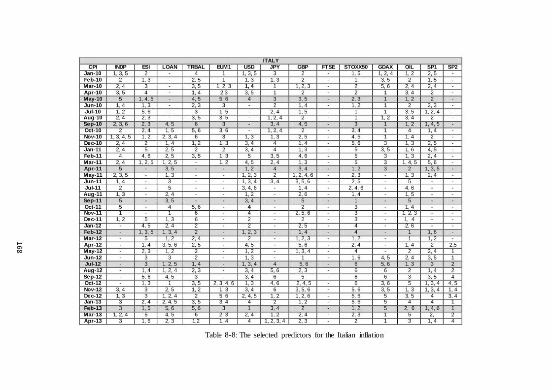
Table 8-8: The selected predictors for the Italian inflation
ITALY CPI INDP ESI LOAN TRBAL EUM1 USD JPY GBP FTSE STOXX50 GDAX OIL SP1 SP2
Jan-10 1, 3, 5 2 - 4 1 1, 3, 5 3 2 - 1, 5 1, 2, 4 1, 2 2, 5 - Feb-10 2 1, 3 - 2, 5 1 1, 3 1, 3 2 - 1 3, 5 2 1, 5 - Mar-10 2, 4 3 - 3, 5 1, 2, 3 1, 4 1 1, 2, 3 - 2 5, 6 2, 4 2, 4 - Apr-10 3, 5 4 - 1, 4 2,3 3, 5 1 2 - 2 1 3, 4 2 - May-10 5 1, 4, 5 - 4, 5 5, 6 4 3 3, 5 - 2, 3 1 1, 2 2 - Jun-10 1, 4 1, 3 - 2, 3 3 - 2 1, 4 - 1, 2 1 2 2, 3 - Jul-10 1, 2 5, 6 - 3 1, 5 - 2, 4 1, 5 - 1 1 3, 5 1, 2, 4 - Aug-10 2, 4 2, 3 - 3, 5 3, 5 - 1, 2, 4 2 - 1 1, 2 3, 4 2 - Sep-10 2, 3, 6 2, 3 4, 5 6 3 - 3, 4 4, 5 - 3 1 1, 2 1, 4, 5 - Oct-10 2 2, 4 1, 5 5, 6 3, 6 - 1, 2, 4 2 - 3, 4 1 4 1, 4 - Nov-10 1, 3, 4, 5 1, 2 2, 3, 4 6 3 1, 3 1, 3 2, 5 - 4, 5 1 1, 4 2 - Dec-10 2, 4 2 1, 4 1, 2 1, 3 3, 4 4 1, 4 - 5, 6 3 1, 3 2, 5 - Jan-11 2, 4 5 2, 5 2 2 3, 4 4 1, 3 - 5 3, 5 1, 6 4, 5 - Feb-11 4 4, 6 2, 5 3, 5 1, 3 5 3, 5 4, 6 - 5 3 1, 3 2, 4 - Mar-11 2, 4 1, 2, 5 1, 2, 5 - 1, 2 4, 5 2, 4 1, 3 - 5 3 1, 4, 5 5, 6 - Apr-11 5 - 3, 5 - - 1, 2 4 3, 4 - 1, 2 3 2 1, 3, 5 - May-11 2, 3, 5 - 1, 3 - - 1, 2, 3 2 1, 2, 4, 6 - 2, 3 - 1, 3 2, 4 - Jun-11 1, 4 - 3 - - 1, 3, 4 3, 4 3, 5, 6 - 2, 5 - 5 - - Jul-11 2 - 5 - - 3, 4, 6 - 1, 4 - 2, 4, 6 - 4, 6 - - Aug-11 1, 3 - 2, 4 - - 1, 2 - 2, 6 - 1, 4 - 1, 5 - - Sep-11 5 - 3, 5 - - 3, 4 - 5 - 1 - 5 - - Oct-11 5 - 4 5, 6 - 4 - 2 - 3 - 1, 4 - - Nov-11 1 - 1 6 - 4 - 2, 5, 6 - 3 - 1, 2, 3 - - Dec-11 1, 2 5 1, 3 6 - 2 - 2 - 3 - 1, 4 - - Jan-12 - 4, 5 2, 4 2 - 2 - 2, 5 - 4 - 2, 6 - - Feb-12 - 1, 3, 5 1, 3, 4 2 - 1, 2, 3 - 1, 4 - 4 - 1 1, 6 - Mar-12 - 5 1, 2 2, 4 - 2 - 1, 2, 3 - 1, 2 - 1 1, 2 - Apr-12 - 1, 4 3, 5, 6 2, 5 - 4, 5 - 5, 6 - 2, 4 - 1, 4 2 2,5 May-12 - 2, 3 1, 2 2 - 1, 2 - 1, 3, 4 - 4 - 2 2, 4 1 Jun-12 - 3 3 2 - 1, 3 - 1 - 1, 6 4, 5 2, 4 3, 5 1 Jul-12 - 3 1, 2, 5 1, 4 - 1, 3, 4 4 5, 6 - 6 5, 6 1, 3 3 2 Aug-12 - 1, 4 1, 2, 4 2, 3 - 3, 4 5, 6 2, 3 - 6 6 2 1, 4 2 Sep-12 - 5, 6 4, 5 3 - 3, 4 6 5 - 6 6 3 3, 5 4 Oct-12 - 1, 3 1 3, 5 2, 3, 4, 6 1, 3 4, 6 2, 4, 5 - 6 3, 6 5 1, 3, 4 4, 5 Nov-12 3, 4 3 2, 5 1, 2 1, 3 3, 4 6 3, 5, 6 - 5, 6 3, 5 1, 3 1, 3, 4 1, 4 Dec-12 1, 3 3 1, 2, 4 2 5, 6 2, 4, 5 1, 2 1, 2, 6 - 5, 6 5 3, 5 4 3, 4 Jan-13 3 2, 4 2, 4, 5 3, 5 3, 4 4 2 1, 2 - 5. 6 5 4 4 1 Feb-13 3 1, 5 5, 6 5, 6 3 1 3, 4 2 - 1, 2 5 2, 6 1, 4, 6 1 Mar-13 1, 2, 4 5 4, 5 6 2, 3 2, 4 1, 2 2, 4 - 2, 3 1 5 2, 2 Apr-13 3 1, 6 2, 3 1,2 1, 4 4 1, 2, 3, 4 2, 3 - 2 1 3 1, 4 4
168

Table 8-9: The selected predictors for the Portuguese inflation
PORTUGAL CPI INDP ESI LOAN TRBAL EUM1 USD JPY GBP FTSE STOXX50 GDAX OIL SP1 SP2
Jan-10 - 2 - 1 2 - - - 2, 4 1 2 - 2 2, 3 Feb-10 - 2, 4 - 1 - - - - 1, 3 1 2, 4 - 2,3 1, 2 Mar-10 - 3 - 1, 2 - - - - 2 1 2 - 3 1, 3 Apr-10 - 3 - 2, 4 - - - - 1, 4 1 2, 3 - 1, 4 1, 5 May-10 - 2, 4 - 1 - - - - 1, 2 3 2 - 1 1 Jun-10 - 4 - 1 - - - - 2, 4 4 4 - 1 1 Jul-10 - 4 - 2, 3 - - - - 2 3 4 - 1 1 Aug-10 - 4 - 2 - - - - 1, 2 3 4 - 1 1, 4 Sep-10 - 1, 2 - 1 - - - - 3 - - - - 1, 3 Oct-10 - 2 - 2, 4 - - - - 1 - - - - 1, 3 Nov-10 - 2 - 3 3, 4 - - - 4 - - - - 1, 3 Dec-10 - 1, 3 - 3 3 - - - 1 - - - - 1, 4 Jan-11 - 3 - 1, 3 2, 4 - - - 1, 4 - - - - 1, 2 Feb-11 - - - 3 2, 4 - - - 2, 3 - - - - 1 Mar-11 - - - 3 2 - - - 3 - - - - 1 Apr-11 - - - 2, 4 1, 3 - - - 3 - - - - 3 May-11 - - - 1, 4 - - - - 1 - - - 4 3, 4 Jun-11 - - - 4 - - - - 2 - - - 4 3 Jul-11 - - - 1, 3 - - - - 3, 4 - - - 4 - Aug-11 - - - 4 - - - - 4 - - - 4 - Sep-11 - - - 4 - - - - 4 - - - 4 - Oct-11 - - - 3, 4 - - - - 1, 2 - - - 3 - Nov-11 - - - 4 - - - - 3, 4 - - - 3 - Dec-11 - - - 1, 3 - - - - 1, 2 - - - 3, 4 - Jan-12 - - - 2 - - - - 1, 4 - - - 1, 2 - Feb-12 - - - 1, 2 - - - - 2, 3 - - - 1 - Mar-12 - 3, 4 - 2 - - - - 1 2, 3 2, 4 - 1 - Apr-12 - 1, 2 - 1 1 - - - 1 2, 4 4 - 1 - May-12 - 2, 3 - 2 2, 4 - - - 1 1 3, 4 - 1 - Jun-12 - 3 - 1, 2 2, 3 - - - 1 1 4 - 1 - Jul-12 - 3 - 3 1, 2 - - - 1 - 4 - 2, 3 - Aug-12 - 1 - 1 3 - - - 1 - 1, 3 - 3 - Sep-12 - 1 - 2, 4 3 - - - 1 - 1, 4 - 3 - Oct-12 - 1 - 2, 3 3 - - - 3, 2 - 1, 2 - 3 1, 3 Nov-12 - 1 - 1, 3 4 - - - 2 - 1 - 3 2 Dec-12 - 1, 2, 4 - 2 4 - - - 2, 5 - 1 - 2, 4 2 Jan-13 - 2, 3 - 3 1, 2 - - - 4 - 1, 3 - 3 2 Feb-13 - 4 - 4 2, 4 - - - 4 - 3 - 3 3, 4 Mar-13 - 1, 2 - 3 1, 2, 3, 4 - - - 1, 3 - 3 - 1, 3 1, 2 Apr-13 - 2 - 1, 2 1, 2 - - - 3 - 1 - 4 2
169
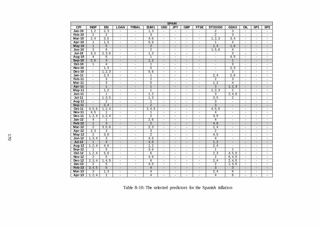
Table 8-10: The selected predictors for the Spanish inflation
SPAIN CPI INDP ESI LOAN TRBAL EUM1 USD JPY GBP FTSE STOXX50 GDAX OIL SP1 SP2
Jan-10 1, 2 2, 3 - - 1, 3 - - - - 2 3 - - - Feb-10 2 2 - - 3 - - - - 2 3 - - - Mar-10 2, 4 3, 5 - - 4, 6 - - - - 1, 2, 3 3, 4 - - - Apr-10 1 1, 5 - - 5, 6 - - - - 1 4 - - - May-10 1 6 - - 2 - - - - 1, 4 1, 6 - - - Jun-10 3 6 - - 2 - - - - 1, 5, 6 4 - - - Jul-10 3, 5 2, 3, 6 - - 1, 3 - - - - - 3 - - - Aug-10 4 6 - - 1 - - - - - 4, 5 - - - Sep-10 2, 6 3 - - 1, 2 - - - - - 1 - - - Oct-10 1 4 - - 1 - - - - - 3 - - - Nov-10 - 1, 3 - - 5 - - - - - 2, 3 - - - Dec-10 - 1, 2, 3 - - 5, 6 - - - - - 3 - - - Jan-11 - 2, 3 - - 1 - - - - 2, 4 2, 6 - - - Feb-11 - 3 - - 2 - - - - 2 3 - - - Mar-11 - 3 - - 5 - - - - 1, 2 4 - - - Apr-11 - 1 - - 1 - - - - 3 1, 2, 3 - - - May-11 - 1, 2 - - 1 - - - - 1, 2, 3 2 - - - Jun-11 - 1 - - 1, 2 - - - - 3 2, 4, 6 - - - Jul-11 - 1, 3, 5 - - 1, 3 - - - - 3, 5 2 - - - Aug-11 - 2 - - 1 - - - - 3 - - - - Sep-11 - 2, 4 - - 2 - - - - 3 - - - - Oct-11 4, 5, 6 1, 2, 4 - - 2, 4, 5 - - - - 4, 5, 6 - - - - Nov-11 4, 5 1 - - 1 - - - - 4 - - - - Dec-11 1, 2, 4 1, 2, 4 - - 2 - - - - 3, 5 - - - - Jan-12 4 1 - - 2, 6 - - - - 4 - - - - Feb-12 1 3 - - 2 - - - - 4, 6 - - - - Mar-12 2 3, 5, 6 - - 2, 3 - - - - 1, 4 - - - - Apr-12 2, 3 3 - - 3 - - - - 2 - - - - May-12 2 3, 6 - - 2 - - - - 4, 5 - - - - Jun-12 1, 3, 4 3 - - 4, 5 - - - - 4 - - - - Jul-12 1 4 - - 4, 6 - - - - 1, 2 - - - - Aug-12 1, 2, 4 4, 6 - - 1, 2 - - - - 2, 4 - - - - Sep-12 1 5 - - 3, 6 - - - - 1 1 - - - Oct-12 1, 2, 4 5, 6 - - 6 - - - - 2, 3 4, 5, 6 - - - Nov-12 2 5 - - 4, 6 - - - - 2 6, 4, 5 - - - Dec-12 2, 3, 4 1, 4, 5 - - 6 - - - - 2, 4 2, 4, 5 - - - Jan-13 2 5 - - 4, 5 - - - - 2 1, 3, 6 - - - Feb-13 3, 4, 5 5 - - 4 - - - - 3 3 - - - Mar-13 3 1, 3 - - 4 - - - - 2, 4 6 - - - Apr-13 1, 2, 4 1 - - 4 - - - - 4 6 - - -
170

171
Taking under consideration the results from the previous five tables, FTSE is found
to be a common relevant indicator for all periphery countries, except Portugal, for the
majority of the months. Prior to August 2011, JPY and GBP are always discarded from the
pool of potential inputs with the Italian case to be the only exception. GDAX and EMU1
are common predictors for all these five countries before September 2010 and after
September 2012 respectively. The same is confirmed for ESI after March 2012, but not for
Ireland. The monthly forecasts of the periphery countries are also derived by less than
thirty inputs from the hundred sixty eight in total. Those inputs are autoregressive terms
with order up to six. The exception is the Greek CPI, which is forecasted by autoregressive
terms with order of four or lower. Finally, the average number of terms selected for a
monthly forecast is twelve. Summarizing the predictor selection evidence from this
inflation exercise leads to the following conclusions. ESI is a common inflation indicator
for all countries under study after March 2012, with Ireland being the only exception. On
the other hand, JPY and GBP are discarded prior to April 2011, except from the Italian
case.
8.5.1.2 Unemployment Exercise
The next three tables, as previously, refer to the three core countries and their
unemployment predictor selection. Initially the Belgium case is presented in Table 8-11. It
is found that ESI, GDAX and OIL qualify as potential predictors of Belgian unemployment
in the majority of the months under study. The opposite happens in terms of GBP and
STOXX50. ESI, TRBAL, USD, JPY and FTSE are constantly included in the predictors’
pool after September 2011. SP1 and SP2 are both relevant predictors within April 2011
and February 2012, but both are discarded before that time. Table 8-12 below describes
France’s pool of potential inputs. In this case LOAN and OIL are always included in this
pool. The same applies for ESI, EUM1 and FTSE in the majority of the months, but not for
USD, JPY, SP1 and SP2. GBP is a relevant input only after September 2011. Finally,
autoregressive terms of INDP, ESI, LOAN, GBP, STOXX50 and OIL are repeatedly
considered in the pool after July 2012. Next follow the German predictors (table 8-12). The
results indicate that EUM1, STOXX50, OIL and LOAN, USD, JPY, GBP, FTSE are found
relevant and not relevant indicators in the whole sample respectively. INDP and TRBAL
are selected after October 2011, while SP1 and SP2 are not included in the selection prior
to February 2012.

Table 8-11: The selected predictors for the Belgian unemployment
BELGIUM UNEMP INDP ESI LOAN TRBAL EUM1 USD JPY GBP FTSE STOXX50 GDAX OIL SP1 SP2 Jan-10 5, 6 2, 3, 6 3, 4, 6 - 5, 6 1, 5 - 2, 3, 6 - - 2 3, 5 - - Feb-10 1, 2 1, 4 3 - 5, 6 1, 5 - 1, 4 - - 2, 4 - - - Mar-10 - 1, 4 3 - 1, 2 5 - 5 - - 1, 2 2, 5 - - Apr-10 - 1, 4 5 - 2, 3,4 - - 5, 6 - - 5, 6 - - - May-10 - 1, 4 2 - 2, 3,4 - - 2, 3, 4, 5, 6 - - 2 - - - Jun-10 - 5, 6 4 - 1, 4, 5 - - - - - 2, 4 1, 4, 5, 6 - - Jul-10 - 1, 2, 3, 4 2, 3, 6 - 2 1, 2 - - - - 5 1, 4, 5 - - Aug-10 - 5 1, 4 - 2, 3 2 - - - - 3, 4, 6 2, 4 - - Sep-10 - 2 2, 4 - 1, 4, 5, 6 3, 5 - - - - - 2, 4 - - Oct-10 - 1, 2 1, 3, 4 - 1 - - - - - - - - - Nov-10 1, 2 3, 5 1, 2 - 3, 4, 5 - - - - - 1, 2 1, 4, 5 - - Dec-10 5, 6 3, 5 3 - 1, 3, 3 - - - - - 1, 3, 3 - - - Jan-11 2, 3, 5 5, 6 4 - 5 - - - - - 1, 4, 5, 6 2, 3, 6 - - Feb-11 2 5, 6 4 - 1, 2 - - - - - 2, 5, 6 - - - Mar-11 4 - 4 - 3, 5 - - - - - 3, 5 - - - Apr-11 1, 6 - - 1, 4, 5 1, 6 - - - - 1, 4 3 - 2 1, 3, 3 May-11 1, 2, 4 - - 3 2 - - - - 1, 4, 5 3, 4, 6 3, 5 2, 5 1, 3 Jun-11 4 - - 2, 3,4 2 - - - - 4 1, 4 3, 4, 5 2, 4 3, 4, 5 Jul-11 4 - - 3 2, 4 - - - - 4 4 4 5 3 Aug-11 4 - - 1, 4 2, 4 - - - - 1, 4 - 1, 3, 4 2, 5 3 Sep-11 4 - - 4, 5, 6 1, 2 2, 3, 4, 5, 6 1, 3, 4 - 2 - - 5, 6 5 3 Oct-11 5, 6 1, 4, 5 - 3, 4 3, 4, 5 1, 3 3, 5 - 2, 3 - - 3 3, 5 2, 4 Nov-11 - 3 - 5 - 5, 6 2, 5 - 3, 4, 6 - 3, 4, 5 1, 3, 4 3, 6 3, 4, 6 Dec-11 - 4 - 3, 4, 6 - 1, 2 4, 5 - 2, 3,4 - - 3 3, 5 2, 4 Jan-12 - 3, 4, 6 - 1 - 5, 6 2,6 - 2, 3 - - 1, 2 3, 4, 5 5, 6 Feb-12 - 1, 4, 5, 6 - 1, 4, 5, 6 - 1, 5 2, 3, 6 - 2 - 2, 3, 4, 5, 6 3 - - Mar-12 - 3, 5 - 1, 2 4, 5 5, 6 1 - 5, 6 - 2, 5 1, 2 - - Apr-12 - 1 - 1, 5 5 3 1, 4, 5 - 1 - 3, 5 2, 4 - - May-12 - 3 - 5 - 1, 5 4 - 2, 5 - 5 1, 4, 5 - - Jun-12 - 5, 6 - 1 - 1, 4, 5 4 - 2, 3, 6 - 3, 5 1, 2 - - Jul-12 2, 3, 5 2 3 5, 6 - 1, 5, 6 4 - 1, 4, 5, 6 - 5 1, 2 3 5, 6 Aug-12 1, 3 3, 5, 6 3, 4, 5 1 2, 3,4 2, 5 5, 6 - 4 - 5, 6 1, 4, 5 1, 4, 5, 6 1 Sep-12 3, 4 1, 3, 6 1, 6 3 1, 2 2, 3 2, 4 - 1, 2, 3 - - 2 - 3 Oct-12 3, 4, 5, 6 2, 5 5 1, 3, 4 1, 2 1, 4, 5, 6 1 - 4 - - 3, 4, 6 - 1, 2, 4 Nov-12 1, 2, 4 4 3 1, 4, 5 1, 2 3, 4 1 - 1, 2 - - 2, 3,4 - 3 Dec-12 5, 6 4 1, 2, 3 1, 4, 5 2, 3,4 1, 4 3, 4, 5 - 4 - 1, 4, 5 3 3, 5 1, 2 Jan-13 2, 4 3, 4, 6 3 3 5 5 1 - 1 - 5 3 5 1, 3 Feb-13 1, 2, 3 2 4 1, 2 5 2, 4, 5 1, 3, 6 - 2, 3,4 - 5, 6 3, 4 3 1, 3 Mar-13 3, 5 3 1, 2 1, 6 2, 5 1, 5 1, 5 - 3 - 5 1 1 5 Apr-13 5, 6 1, 2 2 1, 2 1 2 2, 3,4 - 2, 5 - 1, 4, 5 1, 2 2, 3 2, 5
172
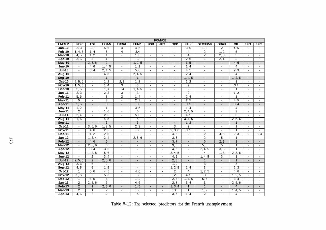
Table 8-12: The selected predictors for the French unemployment
FRANCE UNEMP INDP ESI LOAN TRBAL EUM1 USD JPY GBP FTSE STOXX50 GDAX OIL SP1 SP2 Jan-10 2, 3 1,3 5, 6 4 4, 6 - - - 3, 5 1, 2 2 4, 5 - - Feb-10 1, 4, 5 1, 4 3 4 3,4 - - - 4 2 1, 2 5 - - Mar-10 4, 5 1, 2 1 - 1, 3 - - - 4 2 2, 3 5 - - Apr-10 3, 5 3 1 - 3 - - - 2, 5 1 2, 4 3 - - May-10 - 2, 3, 6 2 - 1, 2, 5 - - - 3, 5 - - 4, 6 - - Jun-10 - 4, 6 1, 4, 5 - 1, 2 - - - 1, 4 - - 4 - - Jul-10 - 3, 4 2, 4, 5 - 5, 6 - - - 4, 5 - - 2, 3 - - Aug-10 - - 4, 5 - 2, 4, 5 - - - 2, 4 - - 4 - - Sep-10 - - 1 - 1 - - - 1, 4, 5 - - 1, 2, 5 - - Oct-10 2, 5, 6 - 1, 2 2, 3 1, 2 - - - 1, 2 - - 1 - - Nov-10 1, 5, 6 - 1, 4 3 3 - - - 2 - - 3,4 - - Dec-10 5, 6 - 1,3 3,4 1, 4, 5 - - - 2 - - 1 - - Jan-11 2, 3 - 2, 3 3 3 - - - 2 - - 1, 2 - - Feb-11 5, 6 - 3 3 1, 4 - - - 2, 4 - - 1 - - Mar-11 5 - 3 - 2, 3 - - - 2, 5 - - 4, 5 - - Apr-11 5, 6 - 3 - 3 - - - 3, 5 - - 3, 4 - - May-11 1, 2 - 1 - 3, 5 - - - 1, 4 - - 4 - - Jun-11 2 - 1, 6 - 6 - - - 2, 4, 5 - - 3 - - Jul-11 3, 4 - 2, 5 - 5, 6 - - - 4, 5 - - 5 - - Aug-11 1, 6 - 4, 5 - 6 - - - 3, 4, 5 - - 2, 5, 6 - - Sep-11 - - 3 - 6 - - - 1, 2 - - 1 - - Oct-11 - 3, 5, 6 1, 2, 5 - 2, 3 - - 3 2 - - 1 - - Nov-11 - 4, 6 2, 5 - 3 - - 2, 3, 6 3, 5 - - 1 - - Dec-11 - 1, 2 2, 5 - 1, 2 - - 4, 6 - 2 4, 5 2, 3 - 3, 4 Jan-12 - 1, 3, 4 2, 4 - 2, 5, 6 - - 3, 5 - 2 5 1 - - Feb-12 - 4, 6 6 - - - - 3, 7 - 6 2, 3 1 - - Mar-12 - 2, 5, 6 6 - - - - 3, 6 - 5, 6 5 1 - - Apr-12 - 3, 4 3, 6 - - - - 4, 6 - 2, 4, 5 3, 5 1 - - May-12 - 1, 2, 5 5, 6 - - - - 3, 4, 5 - 4 1, 3 2, 3, 6 - - Jun-12 - 2 3, 4 - - - - 4, 5 - 1, 4, 5 3 1 - - Jul-12 2, 5, 6 2 2, 5, 6 - - - - 2, 3 - 1 - 1 - - Aug-12 2, 3 6 2 - - - - 1, 2 - 3 - 3 - - Sep-12 4, 5 6 1, 5 - - - - 1, 2, 5 1, 4 3 - 2, 3 - - Oct-12 1 5, 6 4, 5 - 4, 6 - - 2 4 1, 2, 5 - 4, 6 - - Nov-12 5, 6 5 5, 6 - 3 - - 2 4, 5 3 - 1, 2, 5 - - Dec-12 1 5, 6 6 - 1, 2 - - 2, 6 1, 4, 5 5, 6 - 3, 4 - - Jan-13 2 2, 5, 6 6 - 4, 6 - - 2, 3 3, 4 3 - 2, 5, 6 - - Feb-13 2 1 2, 3, 6 - 1, 5 - - 1, 3, 4 1 1 - 4 - - Mar-13 2 1 2 - 5 - - 3 1 1, 2 - 1, 4, 5 - - Apr-13 4, 6 2 2 - 5 - - 3, 5 1, 4 2 - 4 - -
173

Table 8-13: The selected predictors for the German unemployment
GERMANY UNEMP INDP ESI LOAN TRBAL EUM1 USD JPY GBP FTSE STOXX50 GDAX OIL SP1 SP2 Jan-10 2, 4 5, 6 - - 1, 2, 5 - - - - 5, 6 3 1, 2, 5 - - Feb-10 3 2, 4 - - 2, 4 - - - - 5, 6 3 3, 6 - - Mar-10 4 1, 2 - - 2 - - - - 1, 2 3 2, 4 - - Apr-10 - 2, 3 - - 1, 3, 6 - - - - 2, 3,4 1, 2 1, 4 - - May-10 - - - 3,4 - - - - 2, 3, 4 5 1 - - Jun-10 - - - 1, 2 - - - - 1, 4, 5 5 2, 3 - - Jul-10 - - - - 1 - - - - 2 3, 5 3, 4, 5 - - Aug-10 - - - - 1 - - - - 2, 3 5 3 - - Sep-10 - - - - 5 - - - - 1, 4, 5, 6 5, 6 3, 5 - - Oct-10 - - - - 1, 3, 4,5 - - - - 1 1 2, 4 - - Nov-10 - - - - 4, 5 - - - - 3, 4, 5 1, 2 1 - - Dec-10 - - - - 5 - - - - 1, 3, 5 2, 4 1 - - Jan-11 - - - - 2, 4 - - - - 5 - 1 - - Feb-11 - - - - 5 - - - - 1, 2 - 1, 4 - - Mar-11 - - - - 3, 4, 5 - - - - 3, 5 - 1 - - Apr-11 - - - - 1, 2, 5 - - - - 1, 6 - 5 - - May-11 - - - - 3, 4 - - - - 2 - 1 - - Jun-11 - - - - 4 - - - - 2 - 1, 2 - - Jul-11 - 2, 3 - - 4 - - - - 2, 4 - 1 - - Aug-11 - 2, 3 - - 5 - - - - 2, 4 - 1, 3, 6 - - Sep-11 - 2, 4 - - 4, 5 - - - - 1, 2 - 1 - - Oct-11 - 2, 3 - 1 - - - - 3, 4, 5 - 2 - - Nov-11 1, 3 1, 2 - 2, 4 1, 2 - - - - 5, 6 - 1, 2 - - Dec-11 4 2, 3 - 1, 3, 6 2, 4 - - - - 6 - 2, 4 - - Jan-12 4 3 - 5 3 - - - - 6 - 4 - - Feb-12 3, 5 3 - 5 3 - - - - 1, 2 - 4 - - Mar-12 2, 4 2, 4 - 1, 2 1, 2, 5 - - - - 1, 2 - 1, 4 - - Apr-12 4 2 - 2 1, 2 - - - - 2 4 4, 5 3, 5 4 May-12 4 2 - 3 2 - - - - 2 4 3 4, 6 4, 5 Jun-12 4 3 - 3 2 - - - - 2 3, 4 1, 4 2, 4 5, 6 Jul-12 4 3 - 3 1, 2 - - - - 2, 3 3 1, 2, 5 6 1, 2 Aug-12 4 2, 4 - 6 4, 5 - - - - 3, 4, 5 1, 5 3, 6 6 2 Sep-12 4 1 - 2, 6 4, 5 - - - - 3 ,4 4 - 6 3 Oct-12 5, 6 - - 3, 4, 6 5 - - - - 1 5 - 6 2, 4 Nov-12 6 - - 4, 5 3, 4, 5 - - - - 1, 2, 5 4, 5 - 3, 4, 5 2 Dec-12 4, 6 - - 5 5, 6 - - - - 1 3, 4 1, 2 6 2, 3 Jan-13 6 - - 5 3, 5 - - - - 1, 2 4 5 6 3 Feb-13 1, 2 - - 5 1, 4 - - - - 2 3, 4 4 6 2, 4 Mar-13 2 - - 2, 4 2 - - - - 2 4 5 2, 4 4 Apr-13 3, 4 - - 6 1 - - - - 1, 2 5 1 6 6
174

175
The previous three tables indicate that OIL is a common unemployment predictor
for the core countries during the period under study. ESI is always kept in the pool of
potential inputs from September 2011 till July 2012. The same applies for INDP and
EUM1 after July 2012 and up to October 2011. GBP is also constantly selected, except in
the period between May 2010 and September 2011. On the other hand, JPY is discarded
prior to September 2011, whereas SP1 and SP2 are not kept in the pool prior to April 2011.
Similarly to the inflation exercise, all monthly forecasts are obtained by using less than
thirty inputs from the hundred sixty eight in total. From the inputs autoregressive terms
with order higher than six are always rejected. The average number of terms used for each
monthly forecast of the core countries is fifteen.
The rest five tables present the cases of the periphery countries, starting with the
results for the Greek UNEMP. Table 8-14 shows that the autoregressive terms of ESI,
LOAN, EUM1 and GDAX always qualify as potential inputs, while TRBAL, USD, JPY,
GBP, FTSE and STOXX50 ones do not. INDP, OIL and SP2 are also consistently included
except during some short periods (i.e. after July 2012 for OIL). Table 8-15 summarizes the
Irish UNEMP predictors. The Irish LOAN, TRBAL, FTSE and OIL are kept in the pool for
all forty months, but EUM1, USD, JPY, STOXX50 and GDAX are not. ESI is not selected
within September 2010 and September 2011. Finally, SP1 and SP2 are discarded prior to
April 2011, while INDP after September 2011. The Italian case is described in table 8-16.
These results show that LOAN and FTSE are found always relevant indicators of Italian
UNEMP. On the other hand, USD, JPY and GBP do not. EMU1, STOXX50 and SP1 are
included into the pool after April 2011. Few autoregressive terms of INDP and ESI are
obtained, while the algorithm uses OIL and SP2 prior to April 2011. The next table focuses
on Portugal. In this case the proposed algorithm always uses autoregressive lags of LOAN,
EMU1, FTSE and OIL to forecast UNEMP. INDP’s and SP1’s term are constantly pooled
prior to April 2011, while ESI, USD, JPY, STOXX50 and GDAX only after July 2012.
SP2 is also not selected as potential input after May 2010. Finally, the Spanish relevant
macroeconomic variables are presented in table 8-18. This pool of predictors suggests that
ESI and EMU1 are always found to be relevant indicators. However, LOAN, TRBAL,
USD, JPY, GBP, FTSE, OIL, SP1 and SP2 are totally excluded from this pool. The
remaining variables, INDP, STOXX50 and GDAX, are not included in the potential inputs
except in specific short periods of consecutive months (i.e. September 2010-September
2011 for IND).
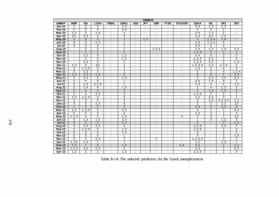
Table 8-14: The selected predictors for the Greek unemployment
GREECE UNEMP INDP ESI LOAN TRBAL EUM1 USD JPY GBP FTSE STOXX50 GDAX OIL SP1 SP2 Jan-10 1 2 4 - 1, 3 - - - - - 3, 4 1, 3 1, 3 Feb-10 2 2 4 - 3, 4 - - - - - 3 2 2 - Mar-10 1, 2 2 1, 4 - 4 - - - - - 2, 4 1, 3 2 - Apr-10 2,3 2, 3 4 - 4 - - - - - 1, 4 3, 4 1, 2 - May-10 3 3 2 - 1 - 1, 3 - - - 2 1, 3, 4 1, 4 - Jun-10 3 3 2, 3 - 1 - - - - - 2, 3 1, 3, 4 4 - Jul-10 3 3 3 - 1 - - - - - 3, 4 3 4 - Aug-10 - 3 3 - 1 - - 1, 2, 3 - - 1, 3 1, 3 1, 3 2, 3 Sep-10 - 1 1 - 1 - - - - - 1, 2, 3 2 2 1 Oct-10 - 1, 2 3 - 1, 2 - - - - - 3, 4 3 2 2 Nov-10 - 2 3 - 1, 2 - - - - - 1, 3, 4 2, 3 2 3 Dec-10 - 2, 3 3 - 2 - - - - - 1, 3, 4 3, 4 2 1, 3 Jan-11 1, 3 3 3,4 - 1 - - - - - 1, 2, 3, 4 1, 3 1, 2, 4 2 Feb-11 3 1, 2, 3 3 - 1 - - - - - 1, 3 2 4 3 Mar-11 3 2, 3 3 - 1 - - - - - 2 2 4 1, 3, 4 Apr-11 1, 3 1, 3 1, 3 - 1 - - - - - 2 2 1 2, 3 May-11 2 3, 4 2 - 1, 3 - - - - - 2 1, 2 1,4 3, 4 Jun-11 2 4 3 - 1 - - - - - 3, 5 1, 4 4 1 Jul-11 2 1, 2 1, 2, 4 - 1 - - - - - 1, 4 4 4 1, 2 Aug-11 2 1, 4 4 - 1, 3 - - - - - 1 4 1, 2 2 Sep-11 2 4 2 - 3 - - - - - 1 1, 3 1, 3 2 Oct-11 2 4 2, 3 - 3 - - - - - 1, 2, 3 2 2 1 Nov-11 2, 3 1, 2, 3 2 - 3 - - - - - 1, 2 2, 4 2 1 Dec-11 3 3 2 - 3 - - - - - 2 1, 3 1, 2, 3, 4 1, 2 Jan-12 3 3 1, 3 - 3 - - - - - 2 2 1, 2 2,3 Feb-12 1 3 2 - 3 - - - - - 2, 4 3 3, 4 3 Mar-12 1, 2 1, 3, 4 2 - 2, 4 - - - - - 3 1 1 3, 4 Apr-12 2 4 3 - 4 - - - - - 1, 3 3 1 3 May-12 1, 2, 3 4 1 - 2, 4 - - - - 4 2 3 2 3,4 Jun-12 3 1, 2 1, 2 - 2, 4 - - - - - 1 3 1, 3 3 Jul-12 3 2 2 - 1, 4 - - - - - 1 - 2 1, 3 Aug-12 3 2, 3 2, 3 - 4 - - - - - 1, 2, 3 - 1, 3 2 Sep-12 3 1, 3, 4 4 - 1, 3 - - - - - 1, 2, 4 - 2 4 Oct-12 3 4 3 - 1, 4 - - - - - 3 - 2 2 Nov-12 3 3 3 - 1 - - - - - 3 - 1 1, 3 Dec-12 3 3 2, 3 - 1 - - 2 - - 1, 2, 3, 4 - 3 2 Jan-13 1, 2,3 2, 3 1 - 1 - - - - - 1, 2 - 2, 3 1 Feb-13 2, 3 1 3 - 1, 4 - - - - 2, 4 3, 4 - 1 1, 2 Mar-13 1, 2, 3 1, 2 2, 3 - 4 - - - - - 2, 3 - 1 2, 4 Apr-13 1, 2 1 1 - 1, 2 - - - - - 1, 2, 3 - 1 4
176

IRELAND UNEMPL INDP ESI LOAN TRBAL EUM1 USD JPY GBP FTSE STOXX50 GDAX OIL SP1 SP2 Jan-10 1, 5 2, 3 6 1, 2, 4 - - - 3, 6 2, 4 - - 3, 5 - - Feb-10 3, 5, 6 4, 5 3, 5 1, 3 - - - 4, 5 2, 5 - - 1, 3 - - Mar-10 1 3, 6 1, 2 3, 4 - - - 4 4, 5 - - 5, 6 - - Apr-10 1 1, 3, 6 4 3 - - - 1, 2, 4 3, 5 - - 1, 2 - - May-10 1 1, 3 1, 4 3 - - - 5, 6 6 - - 3, 5 - - Jun-10 - 3 4, 5 3 - - - 3 1 - - 1, 3 - - Jul-10 - 2 5 1, 4 - - - 1, 3, 4 1, 2 - - 3, 5 - - Aug-10 1, 4 2, 3 1, 2 3, 4 - - - 3 2 - - 1, 4 - - Sep-10 6 - 5 1, 2, 4 - - - 1, 4 2, 5 - - 2, 3, 6 - - Oct-10 1 - 2 3, 4 - - - 3 3, 5 - - 5 - - Nov-10 2, 3 - 6 4 - - - 1, 2 1, 2 - - 3, 4, 5 - - Dec-10 4 - 4, 5 4 - - - 2, 4 3, 5 - - 1, 2, 5 - - Jan-11 3, 5 - 1, 5 1 - - - 1, 3, 5 1, 3 - - 5 - - Feb-11 1, 4 - 2, 3, 6 1, 4 - - 2, 4 1, 2 3 - - 4, 5 - - Mar-11 3 - 1, 4 3, 4 - - - 1, 2 5 - - 1 - - Apr-11 4, 5 - 2, 4 1, 3 - - - 1, 5 5, 6 - - 1, 2 - - May-11 1, 3 - 1, 3, 4 2, 1 - - - 2 5, 6 - - 2 - - Jun-11 2, 3, 5 - 1, 2 1, 4 - - - 3, 4 3, 4, 6 - - 2, 3 5, 6 2, 4 Jul-11 2, 3 - 3, 5 3 - - - 2, 3,4 6 - - 3, 5 3 2, 4 Aug-11 1, 4 - 1, 3 1, 2, 5 - - - 3 1 - - 5, 6 1, 5 1, 2 Sep-11 - - 3 3, 4 - - - 3 1, 2 - - 3 2, 3 2, 3 Oct-11 - - 5 4 - - - 3, 5 2 - - 1, 5 6 1, 4, 5, 6 Nov-11 - - 2 4 - - - 1, 2 2, 4 - - 1, 4, 5 6 2, 3,4 Dec-11 - 1, 2 6 5 - 5 - 1, 2 3, 5 - - 5, 6 1, 2, 5, 6 1, 4, 5 Jan-12 - 3 3, 5 4, 5 - - - - 5, 6 - - 1, 4 1,2, 4, 5 2 Feb-12 - 4, 5 1, 2 1, 2 - - - - 5 - - 5, 6 1, 5 5, 6 Mar-12 - 1, 5 3 2 - - - - 2, 5 - - 3 5, 6 1, 2 Apr-12 - 3, 5, 6 1, 2, 4 2 - - - - 1, 3 - - 6 - 2, 3,4 May-12 - 2, 4 1, 2, 4 1, 2 - - - - 3, 5 - - 6 2, 4, 6 - Jun-12 - 1, 2 4, 5 3, 4 - - - - 2, 5 - - 4 2, 3, 6 - Jul-12 - 1, 4 1 1, 4 - - - - 3, 5 - - 4, 6 4 - Aug-12 - 4 1 5 - - - - 1, 4 - - 2, 5 - Sep-12 - 3, 5, 6 1, 3 2 - - - 1, 4 2 - - 1, 4 1, 4, 5 - Oct-12 - 1, 2 2 3, 4 - - - 4, 6 3, 4, 6 - - 5 1, 5 - Nov-12 - 1, 3 2, 4 4, 5 - - - 1, 2, 5, 6 3, 5 - - 2, 4 3, 5 - Dec-12 - 5, 6 1, 3 5 - - - 2, 5 2 - - 2,5 6 - Jan-13 - 1, 2 2 2, 4 - - - 2 1, 2 - - 1 2, 3 - Feb-13 - 3, 5, 6 3 5 - - - 2, 5 2 - - 1 4 - Mar-13 - 1, 4, 5 1 1, 4, 6 - - - 1 2, 5 - - 1 5, 6 - Apr-13 - 2 1, 6 1, 2, 4, 5, 6 - - - 1 1, 4 - - 1 6 -
Table 8-15: The selected predictors for the Irish unemployment
177

Table 8-16: The selected predictors for the Italian unemployment
ITALY UNEMP INDP ESI LOAN TRBAL EUM1 USD JPY GBP FTSE STOXX50 GDAX OIL SP1 SP2 Jan-10 - 3, 4 2, 4 - 1, 2 - - - 3, 5 - 2 2 4 1, 2 Feb-10 - 4, 5 1, 2 - 3 - - - 1, 3 - 2 2, 4 4 2 Mar-10 - 4 1, 3, 4 - 1, 6 - - - 5, 6 - 2 1, 2 4 2 Apr-10 - 4 1, 4 - 3 - - - 1, 2 - 2 2 4 2 May-10 - 1, 4 6 - 2, 5, 6 - - - 3, 5 - 2 3, 4, 6 1 2, 5 Jun-10 - 4 1 - 1, 6 - - - 1, 3 - 2 2, 4 - 1 Jul-10 - 4 1 - 6 - - - 2 - 2, 3 1, 2 - 1 Aug-10 - - 2, 4 - 4, 6 - - - 1, 2 - 3 2 - 4, 5 Sep-10 - - 1 - - - - - 3 - 1 3, 4, 5 - 6 Oct-10 - - 2, 4 - - - - - 5 - 1 2, 4 - 6 Nov-10 - - 4 - - - - - 3, 4, 5 - 1 2 - 6 Dec-10 - - 5 - - - - - 1, 2, 5 - 1, 4 2 - 1, 3 Jan-11 - - 5 - - - - - 5 - 4 1, 5 - 2 Feb-11 - - 1, 2 - - - - - 3, 5 - 4 4, 6 - 2 Mar-11 - 3 - - - - - 5 - - 1, 3 - 1, 5 Apr-11 2 - 6 - - - - - 6 1, 4 - 3, 4 - 5 May-11 2, 3 - 3, 6 - 2, 3 - - - 2, 6 3 - 1, 2, 5, 6 3 1 Jun-11 3 - 3 - 2, 4 - - - 1, 2 1, , 5 - 6 3 1 Jul-11 3 - 3 - 2 - - - 1 3, 4 - 1, 4 3 - Aug-11 4 - 2, 3 - 2 - - - 1 4 - 2, 6 1, 5 - Sep-11 5, 6 - 4 - 1, 2 - - - 1, 4 4 - 1, 2 2 - Oct-11 - - 2, 5 - 3 - - - 3 1 2, 4 1, 5 2 - Nov-11 - - 4 - 1, 3, 4 - - - 3 1, 5 2, 4 6 2 - Dec-11 - - 1, 2 - 2, 3, 5 - - - 3 1, 2 2, 5 1, 2 1, 4 - Jan-12 - - 1, 5 - 2, 3 - - - 3 2, 4 2, 6 1, 4 4 - Feb-12 - - 3, 5, 6 - 1, 4 - - - 3 2 1, 2 2, 5 4 - Mar-12 - - 1 - 6 - - - 3 1, 2 1, 2, 3 1, 3, 5 5 - Apr-12 - - 1 - 2, 4 - - - 3 3, 5 4 4 5 - May-12 - - 5 - 2 - - - 3, 4 1, 6 4 4 5 - Jun-12 - - 2, 3 - 3 - - - 3, 5 5, 6 4 5, 6 1, 4 3, 6 Jul-12 - - 4 - 5, 6 - - - 3 1, 2 5, 6 - 3 5 Aug-12 1, 2 - 2, 5 - 5 - - - 3 1, 4 1, 3 - 2, 5 5 Sep-12 2 - 4 - 1, 4 - - - 3 2, 5 3, 4 - 3 3, 5 Oct-12 2, 4 3, 5 2 - 2, 4 - - - 1, 4 1, 2, 5 4 - 5 2, 4 Nov-12 4 5 3 - 3 - - - 4 6 4 - 5 1, 6 Dec-12 4 6 1, 2 - 4, 6 - - - 1, 5 3, 6 4 - 1 5 Jan-13 5 6 3, 5 - 3 - - - 5 1, 4 4 2 1, 5 5 Feb-13 5 1, 2 1, 4 - 2, 4, 6 - - - 1, 2 5 1, 2 2, 3 3 5 Mar-13 1, 2 2 4 - 5, 6 - - - 1, 5 3, 4, 5 2 3 2 1, 2 Apr-13 1, 2 1, 4 4 - 6 - - - 6 5, 6 2 1, 2, 3 2 2
178

Table 8-17: The selected predictors for the Portuguese unemployment
PORTUGAL UNEMP INDP ESI LOAN TRBAL EUM1 USD JPY GBP FTSE STOXX50 GDAX OIL SP1 SP2 Jan-10 1, 3 1, 2 2 - 4 - - 2, 3, 4 2, 3 - - 2 1, 3 2, 3 Feb-10 1, 3 2, 4 2 - 1, 3 - - 3 1, 2 - - 2, 3 1, 3 2 Mar-10 3 2 2, 3 - 2 - - 3, 4 1, 3 - - 3, 4 1, 2 1, 4 Apr-10 3, 4 2, 3 2 - 1, 4 - - 3 1,4 - - 1, 2 2 1, 2, 3 May-10 3 - 3, 4 - 1, 2 - - - 1 - - 3 4 1, 2, 3, 4 Jun-10 3 - 3 1, 4 2, 4 - - - 1 - - 1 1 Jul-10 3 - 3, 4 4 2 - - - 1, 4 - - 2, 4 1, 2 - Aug-10 3, 4 - 4 4 1, 2 - - - 1 - - 1 1, 3 - Sep-10 3 - 1 3 4 - - - 2, 4 - - 3 4 - Oct-10 3, 4 - 2, 3 3, 4 3 - - - 1, 3 - - 1, 2 4 - Nov-10 1, 3 - 3 2, 4 4 - - - 1, 4 - - 1 1, 4 - Dec-10 1, 3 - 2, 3 1, 2 3 - - - 1, 3 - - 1 2, 4 - Jan-11 4 - 3 2 3 - - - 3 - - 4 1 - Feb-11 1, 4 - 4 - 3, 4 - - - 1, 4 - - 3, 4 1, 3 - Mar-11 4 - 1, 3 - 1, 2 - - 1, 2, 3, 4 1, 3 - - 3 1, 4 - Apr-11 2, 4 - 1 - 3 - - 3, 4 4 - - 2 - - May-11 2, 4 - 3 - 1 - - 1, 4 1, 4 - - 3, 4 - - Jun-11 3, 4 - 4 - 2 - - 1, 4 1, 2 - - 3 - - Jul-11 - - 1, 2 - 3 - - 2, 4 3 - - 1, 2 - - Aug-11 - - 1, 4 - 2, 4 - - 1, 2 1 - - 3 - - Sep-11 - - 3 - 4 - - 1, 2 2, 4 - - 4 - - Oct-11 - - 1 - 1, 2 - - 3, 4 1, 3, 4 - - 1, 4 - - Nov-11 - - 4 - 1, 4 - - 2, 4 1, 4 - - 1 - - Dec-11 - - 2, 3 - 3, 4 - - 2, 3, 4 1 - - 3, 4 - - Jan-12 - - 1, 2 1, 2 1, 2 - - 1, 2, 4 1, 2 - - 4 - - Feb-12 - - 2, 4 1 2, 3 - - 1, 2 1, 2 - - 4 - - Mar-12 - - 2, 3 3, 4 3 - - 1 4 - - 1, 2, 3 - - Apr-12 - - 2, 4 4 3 2, 4 1, 2, 3 1 2 2, 3, 4 1, 2, 3 1 - - May-12 - - 4 2, 4 1, 3 2, 3 1, 2, 4 1, 3 3, 4 2, 4 1 4 - - Jun-12 - 4 3 4 1 2 2, 4 - 3, 4 1, 2 1, 2 1 - - Jul-12 - 4 2 1 1 3 2 - 4 1, 2 1, 4 3 - - Aug-12 - 4 4 1, 3 1 2, 4 3 - 4 2, 3 1 3 - - Sep-12 - 2 3, 4 1, 4 1 4 1 - 1 2 2, 4 4 - - Oct-12 - 2, 3 3 1 3, 4 2, 3 1 - 1, 3 2 4 2 - - Nov-12 - 3 1 1, 4 2 1, 3 1, 2 - 1, 4 2,4 1, 2, 3 1 - - Dec-12 - 4 2 - 1, 5 1, 3 1, 2 - 2, 3 1, 2 4 1 - - Jan-13 - 1, 2, 4 2, 3 - 4 1, 2 4 - 1 1 1, 2 1 - - Feb-13 - 2, 3 1 - 3, 4 2 1, 2 - 1 1 2 2 - - Mar-13 - 1, 3, 4 3 - 1 2 4 - 1 1 3, 4 1 - - Apr-13 - 2 1 - 3 3 1, 3, 4 - 1 1, 2, 3, 4 4 1, 2 - -
179

Table 8-18: The selected predictors for the Spanish unemployment
SPAIN UNEMP INDP ESI LOAN TRBAL EUM1 USD JPY GBP FTSE STOXX50 GDAX OIL SP1 SP2 Jan-10 1, 2 2, 3 - - - - - 3, 5 4 3 - 4 - - Feb-10 1, 4 2, 5 - - - - - 3 4 3, 5 - 3, 5 - - Mar-10 1, 5 3 - - - - - 4, 5 4 3 - 4 - - Apr-10 - 2, 5 - - - - - - 4 3 - 4, 5 - - May-10 - 2, 5 - - - - - - 4 1, 4 - 4 - - Jun-10 - 1 - - - - - - 4 1, 4 2 1, 2 - - Jul-10 - 4, 6 - - - - - - 5 1 1 4 - - Aug-10 - 1 - - - - - - 5 1, 2 5, 6 4, 6 - - Sep-10 - 1, 2 - - - - - - - - - 2 - - Oct-10 - 6 - - - - - - - - - 5 - - Nov-10 - 1, 2, 4 - - - - - - - - - 2 - - Dec-10 - 1 - - - - - - - - - 5, 6 - - Jan-11 - 3 - - - - - 2, 5 - - - 5 - - Feb-11 - 5, 6 - - - - - 3 - - - 1, 5 - - Mar-11 - 5, 6 - - - - - 4, 6 - - - 5 - - Apr-11 - 5 - - - - - 5 - - - 2 - - May-11 5, 6 6 - - - - - 1 - - - 5 - - Jun-11 5 6 - - - - - 2 - - - 2 - - Jul-11 4, 5 4, 6 - - - - - 2 - - - 1, 3, 4 - - Aug-11 1, 5 2, 6 - - - - - 1 - - - 1 - - Sep-11 5 6 - - - - - 2 - - - 1 - - Oct-11 3, 6 - 2 2 1, 5 - - 3 - - - 1, 2 - - Nov-11 4, 6 - 2, 5 2, 6 5 - - 4 - - - 1, 2 - - Dec-11 6 - 3 4 5 - - 5 - - - 2 - - Jan-12 4, 5 - 3, 6 2, 6 5 - - - - - - 1 - - Feb-12 1, 2, 3, 5, 6 - 4 2 5 - - - - - - 1, 3 - - Mar-12 1, 2, 5 - 4, 5 4 2 - - - - - - 2 - - Apr-12 3 - 4 4, 5 1, 2 - - - - - - 5 - - May-12 3, 4 - 2, 3 4 3 - - - - - - 3, 4, 5 - - Jun-12 2 - 3 4 4 - - - - - - 2 - - Jul-12 2 - - 1, 2, 4 6 - - - - - - 3 - - Aug-12 2, 3, 4 1, 2 - 4 3 - - - 4 2 3, 4, 5, 6 3, 6 - - Sep-12 2 1, 2 - 4 2, 3 - - - 4, 6 2 3 3 - - Oct-12 2 1, 4 - 1, 2, 3 3 - - - 5, 6 2, 3 5, 6 2, 6 - - Nov-12 2, 5 1, 3 - 2 3 - - - 5, 6 1, 3 6 3 - - Dec-12 1 1, 2, 4 - 3 3, 5 - - - 1 1, 5 4, 6 1, 5 - - Jan-13 2, 5 1, 2, 4 - 1, 3 1 - - - 3, 4 1, 6 5, 6 2, 4 - - Feb-13 1 1, 2 - 2 3 - - - 3 1, 2 6 2 - - Mar-13 4, 5, 6 2, 5 - 1 5 - - - 2, 4 3, 5 1, 2, 4, 6 1, 3, 6 - - Apr-13 4, 6 2, 4 - 1 1 - - - 5 4, 4 1 2 - -
180

181
Observing the previous five tables, OIL is found to be a relevant unemployment
indicator for all peripheral countries. Consistent to that is also the EUM1, with Ireland
being the only exception. On the contrary, USD and JPY are rejected from the pool of
potential inputs prior to February 2012. GBP is also discarded from this selection, except
in Portugal’s case. Finally, autoregressive terms of LOAN are constantly obtained by RG-
SVR algorithm, except during the period of September 2011 to July 2012 in the Spanish
analysis. The forecasts of the peripheral countries are again derived by less than thirty
inputs from the hundred sixty eight in total. Those inputs are autoregressive terms with
order of four or lower. Similar to the first exercise the exception is again the Greek CPI,
which is forecasted by autoregressive terms with order of up to four. The average number
of terms selected for a monthly forecast is thirteen in the periphery countries’ cases. The
predictor selection of the unemployment exercise concludes that EMU1 and OIL qualify
almost in all cases and months as a relevant macroeconomic indicator for Eurozone
unemployment. This is different than the inflation case. JPY, though, is never included in
the previous eight pools prior to September 2011, which is consistent with the CPI
analysis.
In general, both exercises establish an erratic mapping of the predictors in every
month per month and country per country analysis. This proves that structural breaks
dominate the Eurozone inflation and unemployment, making their forecasting a very
challenging task. Consequently, models with a constant or a limited set of independent
variables have no value in the long-run. Non- linear time-varying approaches, such as the
proposed hybrid model, can prove more efficient and realistic. The RG-SVR provides an
output of the changing composition of the relevant macroeconomic indicators for each
country, giving a glimpse of its economic and financial micro-structure. This can in a sense
extend to an ability of capturing structural breaks. In all cases the selected predictors seem
to follow and change patterns associated with the specific highlighted months. Very often
predictors are accepted or rejected from the potential pool before, after or within some of
these months. This is more clearly observed in core countries than in periphery ones. This
would be an expected outcome, since the peripheral EU economy is indeed much more
unstable compared to the core one, especially during the forty months under study.
All the forecasts are obtained by taking under consideration always autoregressive
lags less than thirty. The tables of the first exercise show that there are many cases where
individual variables are pooled with three or more autoregressive terms. This is not so
common in the second one, where usually up to two autoregressive lags seem sufficient to
describe each variable’s contribution to the final monthly forecast. The RG-SVR excludes

182
autoregressive terms with order higher than six. Nonetheless, the previous sixteen tables
show that the first four autoregressive terms are usually more evident. This suggests that
the practitioner should focus on the past quarter, while information going back more than a
semester seems irrelevant. In the periphery cases, the RG-SVR model obtains optimal
forecasts by using less five predictors on average in comparison to the core cases. It would
be interesting to see if the abovementioned optimal RG-SVR variable selection leads to
statistically robust forecasts.
8.5.2 Statistical Performance
The statistical performance of the RG-SVR forecasts follows in comparison to their
benchmarks. Similar to previous chapters, the RMSE, MAE, MAPE and Theil-U statistics
are computed in order to evaluate statistically these forecasts. This is standard in literature
and the mathematical formulas of these statistics are presented in Appendix B.4. For all
four statistical measures retained, the lower the output the better the forecasting accuracy
of the model concerned. As mentioned in the description of the model, GA-SVR stores
also the SVR parameters per month (encoded in the monthly optimal chromosome). These
parameters for both exercises are given in Appendix F.2.
8.5.2.1 Inflation Exercise
The following table presents the statistical performance of all models for each country,
when forecasting inflation.
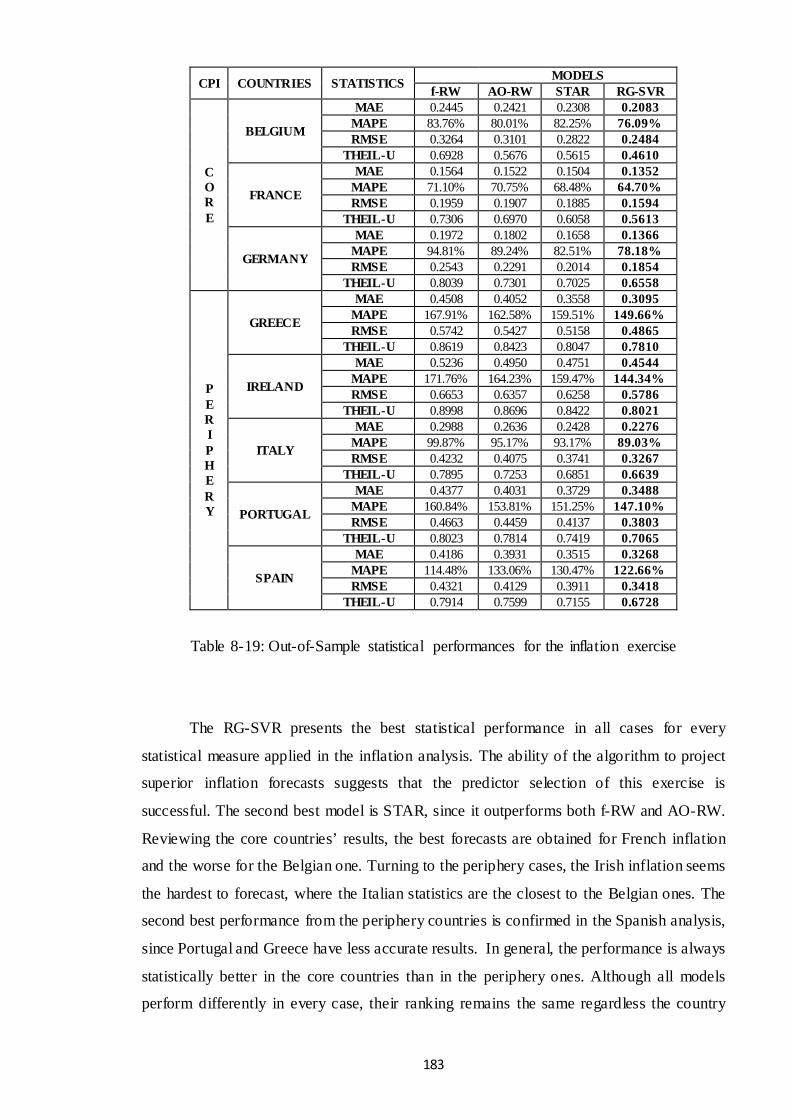
183
CPI COUNTRIES STATISTICS MODELS f-RW AO-RW STAR RG-SVR
C O R E
BELGIUM
MAE 0.2445 0.2421 0.2308 0.2083 MAPE 83.76% 80.01% 82.25% 76.09% RMSE 0.3264 0.3101 0.2822 0.2484
THEIL-U 0.6928 0.5676 0.5615 0.4610
FRANCE
MAE 0.1564 0.1522 0.1504 0.1352 MAPE 71.10% 70.75% 68.48% 64.70% RMSE 0.1959 0.1907 0.1885 0.1594
THEIL-U 0.7306 0.6970 0.6058 0.5613
GERMANY
MAE 0.1972 0.1802 0.1658 0.1366 MAPE 94.81% 89.24% 82.51% 78.18% RMSE 0.2543 0.2291 0.2014 0.1854
THEIL-U 0.8039 0.7301 0.7025 0.6558
P E R I P H E R Y
GREECE
MAE 0.4508 0.4052 0.3558 0.3095 MAPE 167.91% 162.58% 159.51% 149.66% RMSE 0.5742 0.5427 0.5158 0.4865
THEIL-U 0.8619 0.8423 0.8047 0.7810
IRELAND
MAE 0.5236 0.4950 0.4751 0.4544 MAPE 171.76% 164.23% 159.47% 144.34% RMSE 0.6653 0.6357 0.6258 0.5786
THEIL-U 0.8998 0.8696 0.8422 0.8021
ITALY
MAE 0.2988 0.2636 0.2428 0.2276 MAPE 99.87% 95.17% 93.17% 89.03% RMSE 0.4232 0.4075 0.3741 0.3267
THEIL-U 0.7895 0.7253 0.6851 0.6639
PORTUGAL
MAE 0.4377 0.4031 0.3729 0.3488 MAPE 160.84% 153.81% 151.25% 147.10% RMSE 0.4663 0.4459 0.4137 0.3803
THEIL-U 0.8023 0.7814 0.7419 0.7065
SPAIN
MAE 0.4186 0.3931 0.3515 0.3268 MAPE 114.48% 133.06% 130.47% 122.66% RMSE 0.4321 0.4129 0.3911 0.3418
THEIL-U 0.7914 0.7599 0.7155 0.6728
Table 8-19: Out-of-Sample statistical performances for the inflation exercise
The RG-SVR presents the best statistical performance in all cases for every
statistical measure applied in the inflation analysis. The ability of the algorithm to project
superior inflation forecasts suggests that the predictor selection of this exercise is
successful. The second best model is STAR, since it outperforms both f-RW and AO-RW.
Reviewing the core countries’ results, the best forecasts are obtained for French inflation
and the worse for the Belgian one. Turning to the periphery cases, the Irish inflation seems
the hardest to forecast, where the Italian statistics are the closest to the Belgian ones. The
second best performance from the periphery countries is confirmed in the Spanish analysis,
since Portugal and Greece have less accurate results. In general, the performance is always
statistically better in the core countries than in the periphery ones. Although all models
perform differently in every case, their ranking remains the same regardless the country

184
under study. It would be interesting to see if the success of the proposed algorithm in this
inflation exercise extends also in the unemployment one.
8.5.2.2 Unemployment Exercise
The table below summarizes the statistical performance of the models regarding the
unemployment of all eight countries under study.
UNEMP COUNTRIES STATISTICS MODELS f-RW AO-RW STAR RG-SVR
C O R E
BELGIUM
MAE 0.1610 0.1432 0.1214 0.1104 MAPE 53.13% 51.25% 48.11% 47.04% RMSE 0.1887 0.1728 0.1601 0.1351
THEIL-U 0.5713 0.5352 0.5039 0.4626
FRANCE
MAE 0.2567 0.2206 0.2118 0.1827 MAPE 58.68% 57.75% 54.48% 51.61% RMSE 0.2215 0.2076 0.1887 0.1603
THEIL-U 0.6178 0.5916 0.5624 0.5273
GERMANY
MAE 0.1470 0.1374 0.1254 0.1028 MAPE 49.33% 46.88% 45.74% 44.22% RMSE 0.1771 0.1638 0.1484 0.1259
THEIL-U 0.5504 0.5233 0.4958 0.4624
P E R I P H E R Y
GREECE
MAE 0.4458 0.4202 0.4098 0.3570 MAPE 105.19% 100.93% 95.51% 89.64% RMSE 0.4129 0.3854 0.3408 0.3016
THEIL-U 0.8254 0.8017 0.7881 0.7436
IRELAND
MAE 0.4135 0.4005 0.3855 0.3321 MAPE 88.37% 84.78% 81.15% 76.41% RMSE 0.3554 0.3314 0.3151 0.2837
THEIL-U 0.7758 0.7525 0.7219 0.6855
ITALY
MAE 0.3201 0.2906 0.2748 0.2453 MAPE 69.90% 64.91% 62.55% 57.85% RMSE 0.2673 0.2313 0.2178 0.1758
THEIL-U 0.6491 0.6246 0.6115 0.5675
PORTUGAL
MAE 0.3681 0.3518 0.3243 0.2958 MAPE 84.48% 80.23% 73.89% 68.13% RMSE 0.3214 0.3023 0.2871 0.2744
THEIL-U 0.7055 0.6891 0.6627 0.6218
SPAIN
MAE 0.3499 0.3144 0.2814 0.2539 MAPE 74.54% 70.47% 68.28% 61.53% RMSE 0.3009 0.2883 0.2615 0.2288
THEIL-U 0.6764 0.6407 0.6358 0.5917
Table 8-20: Out-of-Sample statistical performances for the unemployment exercise

185
The above summary suggests that RG-SVR retains its statistical superiority in all
cases of the unemployment exercise, as in the inflation one. STAR continues to outperform
the other two RW benchmarks. The analysis of the core countries reveals that the German
unemployment forecasts are the most accurate statistically. The second best core results are
given in the Belgian case. Regarding the periphery countries, the Italian unemployment
seems the easiest to forecast, while the opposite applies in the Greek case. The Spanish
analysis provides with the second lower statistic values from the rest of the periphery
countries. In Portugal more accurate results are observed in comparison with Ireland. In
general, core countries present constantly lower values than peripheral ones in all four
statistics retained in this study. Finally, the model statistical ranking in the unemployment
exercise is consistent with the inflation one.
The statistical evidence from both exercises lead to some interesting conclusions.
The proposed RG-SVR statistically outperforms all benchmark models for all countries,
regardless if CPI or UNEMP is under study. The STAR and AO-RW models are the
second and third best models, leaving f-RW last in the statistical ranking. Hence, non-
linear models with time-varying parameters are statistically more efficient from traditional
random walk approaches. All the statistics indicate that core EMU inflation is always
easier to forecast than the periphery one. Especially in the cases of Greece or Ireland this
task is even more challenging. The RG-SVR statistical performance in Italy’s case is the
only one that somewhat approaches the core countries’ performances. These results show
that the previous selection process is promising. The periphery countries are those more
affected by the Eurozone sovereign debt crisis, adopting vast austerity and economic
reform measures through the period under study. It could be expected that the algorithm
would perform poorly in those cases. The opposite, though, happens. RG-SVR adapts
efficiently to the underlying market shocks in the periphery economy by accepting or
rejecting several macroeconomic variables. This genetic mapping leads to improved
periphery CPI and UNEMP forecasts compared to tradition models such as, f-RW, AO-
RW and STAR.
8.6 Conclusions
The motivation of this chapter is to introduce a hybrid Rolling Genetic – Support Vector
Regression (RG-SVR) model in economic forecasting and monthly optimal

186
macroeconomic variable selection. The proposed algorithm is applied in a monthly rolling
forecasting task of inflation and unemployment in eight EMU countries. The RG-SVR
genetically optimizes the SVR parameters and adapts to the optimal feature subset from a
feature space of potential inputs. The feature space includes a wide pool of macroeconomic
variables that might affect the two series under study of every country. The forecasting
performance of the RG-SVR is benchmarked with a ‘fixed’ Random Walk model (f-RW),
an Atkeson and Ohanian Random Walk (AO-RW) and a Smooth Transition
Autoregressive Model (STAR). More specifically, the statistical performance of all models
is investigated over the period of August 1999 to April 2013.
In terms of the results, the proposed RG-SVR statistically outperforms all
benchmark models for all countries in both exercises. The other non-linear model, the
STAR, is always second in the statistical ranking. The RW models are less efficient in this
application, but AO-RW always beats f-RW. The performance of the model is consistent in
core and periphery cases, although core EMU inflation is proved easier to forecast than the
periphery one. Hence, the rolling genetic SVR selection of the predictors is both
computationally and statistically efficient. Every monthly forecast is obtained by
maximum thirty autoregressive term of several predictors, which is a significant decrease
from the total one hundred sixty eight available. From those the terms with order higher
than six are rejected, while the first four autoregressive terms are usually more evident.
Thus, the practitioner should focus on the past quarter, while information going back more
than a semester seems irrelevant.
In general, this chapter sheds more light on the difficult quest of non- linear
mapping of macroeconomic variables over different EMU countries. The rolling nature of
both forecasting exercises establishes erratic patterns in the selected predictors. This proves
that structural breaks dominate the Eurozone inflation and unemployment, making their
prediction a very challenging task. Consequently, models with a constant or a limited set of
independent variables are not efficient in the long-run. On the other hand, non- linear time-
varying approaches like the proposed hybrid model can prove more efficient and realistic.

187
Chapter 9
General Conclusions
Nowadays, the necessity to perform human tasks with minimum cost and higher speed,
along with the need to process voluminous data, justifies the expansion of computational
intelligent models in various scientific fields, such as Finance. Adding to this the fact that
financial forecasting is inherently connected with the high degree of uncertainty ruling the
modern world, such adaptive techniques can be efficient alternatives to traditional models.
In order to achieve that, computer engineers must put much effort into their proper
financial task-specific calibration. Nonetheless, generalizing the performance of these
models can be a ‘wall’ standing between their financial or economic interpretability and
their statistical success. The scope of this thesis is to ‘breach the wall’ by combining the
virtues of several computational intelligence models into superior hybrid architectures.
Chapter 4 -6 apply techniques, such as Neural Networks, Support Vector
Regressions and Genetic Algorithms in exchange rate forecasting and trading exercises.
Within this application framework, more specific contributions are made. Firstly,
stochastic and genetic forecast combinations are found to be successful, adding to the
existing literature of model selection and combination. Secondly, time-varying leverage
strategies are found to cope with the instability deriving from economy shocks and prove
their success in periods of market turmoil. Thirdly, architectures enabled with efficient
recursive estimation power always outperform traditional models with fixed parameters.
Finally, the empirical evidence prove that genetic tuning of the SVR parameters is
successful. Therefore, hybrid models deriving from the previous techniques are robust in
terms of statistical accuracy and trading efficiency.
The utility of these hybrid architectures is extended in macroeconomic forecasting
in chapters 7 and 8. The genetic support vector regression hybrids are providing rolling
robust estimations for inflationary and unemployment changes in US and EU, attempting
to capture and assess their world-wide constantly changing dynamics. The proposed hybrid
models feature several novelties in terms of their econometric and computational
modelling, while their ability to adapt in set of relevant predictors of changing composition
extends their realistic economic interpretability. Their genetic adaptive nature allows them

188
to capture underlying asymmetries and nonlinearities evident in the given set of predictors,
while the optimal feature selection (rolling or not) is extremely promising. The main
reason for that is that the models are providing superior forecasts in periods of recessions
(global financial crisis, Eurozone sovereign debt crisis) and win forecasting competitions
with traditional linear models or architectures with fixed sets of explanatory variables.
Hence, their introduction extends the voluminous literature, which suggests that non- linear
time-varying approaches are more efficient and realistic in similar studies.
In general, this thesis addresses issues and provides extensions to the knowledge of
the field of Finance. Although universal approximations can never been embraced in
scientific research, the evidence of previous chapters have strong implications on decision
making. Their impact on financial or economic decisions, especially, is greater within the
context of structural instabilities, market shocks and non- linearities in the information
extrapolated from large datasets. In addition, more light is shed in the demanding issue of
achieving statistical and trading efficiency in the foreign exchange markets through
computational intelligent models. Traders and hedge fund managers should experiment
beyond the boundaries of traditional models. Their trading decisions should be based on
forward-looking expectations from models and strategies that are optimized in a hybrid
trading and statistical approach. Government, institutional and central banking policies can
also be affected in the same context. All these parties do have constant interest in the
monitoring of large numbers of variables that could affect the inflation or unemployment,
and as a consequence the economy. The architectures proposed could be found particular
useful in this monitor process, while their relevant indicator mapping ability could help
with the realistic evaluation of implemented or future policies within a specific timeframe
or geographical spectrum. Nonetheless, there are still many paths to be taken in the search
of efficient calibration of computational intelligent models for financial and economic
forecasting tasks.

189
Appendices
Appendix A (Chapter 3)
A.1 Kalman Filter and Smoothing Process
A generalized linear state space model of the nx1 vector yt is defined as:
( )2, ~ 0,t t t t t ty c Z a NID εε ε σ= + + (A.1)
21 , ~ (0, )t t t t t t na d T a n n NID σ+ = + + (A.2)
In these equations,αt is a mx1 vector of possible state variables and ct, Zt, dt and Tt are
conformable vectors and matrixes. The εt and nt vectors are assumed to be serially
independent, with contemporaneous variance structure:
var'
t t tt t
t t t
H Gn G Qε
Ω = =
(A.3)
Ηt is a nxn symmetric variance matrix, Qt is a mxm symmetric variance matrix and Gt is a
nxm matrix of covariances (Welch and Bishop, 2001).
Considering the conditional distribution of the state vector αt, given information available
at time t-1, the Kalman Filter can define the mean and variance matrix of the conditional
distribution as:
| 1 1( )t t t ta E a− −= (A.4)
| 1 1 | 1 | 1[( )( ) ']t t t t t t t t tP E a a a a− − − −= − − (A.5)

190
Thus, the recursive algorithm of the Kalman filter calculates the following three:
1. The one-step ahead mean αt|t-1 and one-step ahead variance Pt|t-1 of the states.
Under the Gaussian error assumption, αt|t-1 is the minimum mean square error
estimator of αt and Pt|t-1 is the mean square error (MSE) of αt|t-1.
2. The one-step ahead estimate of yt as:
| 1 1 | 1 | 1ˆ ( ) ( | )t t t t t t t t t t t ty y y E y a c Z a− − − −= = Ε = = + (A.6)
3. The one-step ahead prediction errors and their variances respectively as:
| 1 | 1ˆ ˆt t t t t ty yε ε − −= = − (A.7)
| 1 | 1 | 1ˆ var( ) 't t t t t t t t t tF F Z P Z Hε− − −= = = + (A.8)
In this case it is set 0ˆ 0y = and P0=1. If P0 was also set equal to zero, that would
mean that there is no noise, so all the estimates would be equal to the initial state. Then, the
next step is to embody a smoothing algorithm to this process. The smoothing algorithm,
which uses all the information observed, in other words the whole sample T, to form
expectations at any period until T, is known as fixed- interval smoothing. In this way it is
possible to estimate the smooth estimates of the states and the variances:
|ˆ ( )t t T T ta E aα = = (A.9)
var ( )t T tV a= (A.10)
Additionally, the smoothed estimates of yt and their variances can be calculated based on
equations A.6, A.7 and A.8 abovementioned, but also the smoothed estimates of the εt and
nt vectors and their corresponding smoothed variance matrix:
|ˆ ( )t t T T tEε ε ε= = (A.11)
|ˆ ( )t t T T tn n E n= = (A.12)
ˆˆˆˆ varˆ ˆˆ '
t t tt t
t t t
H Gn G Q
ε Ω = =
(A.13)

191
Appendix B (Chapter 4)
B.1 The ARMA model
Figure B-1 shows the output of the ARMA model selected. The null hypothesis that all the
coefficients are not significantly different from zero is rejected at 95% confidence interval.
Figure B-1: The ARMA model detailed output

192
B.2 NNs’ Training Characteristics
Table B-1 presents the characteristics of the neural networks with the best trading
performance in the test sub-period which are used in the NN committees. The choice of
these parameters is based on an extensive experimentation in the in-sample sub-period and
on the relevant literature (Tenti (1996), Dunis and Chen (2005) and Ghazali et al. (2006)).
For example for the number of iterations, the experimentation started from 10.000
iterations and stopped at the 200.000 iterations, increasing in each experiment the number
of iterations by 5.000.
Table B-1: The NNs’ training characteristics
B.3 Bayesian Information Criteria
AIC measures the relative goodness of fit of a statistical model, as introduced by Akaike
(1974). On the other hand, SIC (also known as BIC or SBIC (Schwarz, 1978)) is
considered a criterion to select the best model among models with different numbers of
parameters. If N is the sample size of the dataset, k the total number of parameters in the
equation of interest and s2 the maximum likelihood estimate of the error variance, then
AIC and BIC are calculated as shown below :
Parameters MLP RNN PSN Learning algorithm Gradient descent Gradient descent Gradient descent
Learning rate 0.001 0.001 0.5 Momentum 0.003 0.004 0.5
Iteration steps 100000 60000 40000 Initialisation of
weights N(0,1) N(0,1) N(0,1)
Input nodes 9 9 9 Hidden nodes 7 5 4 Output node 1 1 1

193
2
2
log( ) 2log( ) log( )
AIC N s kSIC N s k N
= +
= + (B.1)
Table B-2 describes the estimation of the Bayesian Information Criteria for the
cases of MLP, RNN and PSN forecasts, based on the B.1 set of equations above:
Table B-2: Calculation of weights for the AIC and SIC Bayesian Averaging model
B.4 The Statistical and Trading Performance Measures
The statistical and trading performance measures are calculated as shown in table B-3 and
table B-4 respectively. These measures are used also for the purposes of next chapters.
Table B-3: Statistical Performance Measures and Calculation
AIC SIC ΔAIC ΔSIC wAIC wSIC MLP 1.825879871 1.832039254 0.004476988 0.004476604 0.334209988 0.334210009 RNN 1.846203174 1.852362557 0.024800291 0.024799907 0.330831059 0.330831081 PSN 1.821402883 1.827562265 0 0 0.334958953 0.33495891
STATISTICAL PERFOMANCE MEASURES DESCRIPTION
Mean Absolute Error 1
1 ˆ( )t n
tMAE Y Y
n τ ττ
+
= +
= −∑
with Yτ being the actual value and Yτthe forecasted value
Mean Absolute Percentage Error 1
ˆ1 t n
t
Y YMAPEn Y
τ τ
τ τ
+
= +
−= ∑
Root Mean Squared Error 2
1
1 ˆ( )t n
tRMSE Y Y
n τ ττ
+
= +
= −∑
Theil-U
2
1
2 2
1 1
1 ˆ( ( )
1 1ˆ
t n
t
t n t n
t t
Y YnTheil U
Y Yn n
τ ττ
τ ττ τ
+
= +
+ +
= + = +
−− =
+
∑
∑ ∑

194
TRADING PERFOMANCE MEASURES DESCRIPTION
Annualised Return 1
1252* *( )N
At
tR R
N =
= ∑ where tR the daily return
Cumulative Return ∑
=
=N
tt
C RR1
Annualised Volatility ( )∑
=
−−
=N
tt
A RRN 1
2*1
1*252σ
Information Ratio
A
A
RSRσ
=
Maximum Drawdown Maximum negative value of ( )∑ tR over the period
= ∑
===
t
ijjNtti
RMinMD,,1;,,1
Table B-4: The Trading Performance Measures and Calculation
B.5 Diebold-Mariano Statistic for Predictive Accuracy
The Diebold-Mariano (1995) statistic tests the null hypothesis of equal predictive accuracy.
If n is the sample size and e1i , e2
i (i=1,2…n) are the forecast errors of the two competing
forecasts, then the loss functions are estimated as:
1 1 2 2 2 21 2( ) ( ) , ( ) ( )MSE MSE
i i i iL e e L e e= = (B.2)
1 1 2 21 2( ) , ( )MAE MAE
i i i iL e e L e e= = (B.3)
The Diebold-Mariano statistic is based on the loss differentials:
1 21 2( ) ( )MSE MSE MSE
i i id L e L e= − (B.4)
1 21 2( ) ( )MAE MAE MAE
i i id L e L e= − (B.5)
The null hypotheses tested based on the sMSE and sMAE are:
• 0 : ( ) 0MSEiH E d = against the alternative 1 : ( ) 0MSE
iH E d ≠
• 0 : ( ) 0MAEiH E d = against the alternative
1 : ( ) 0MAEiH E d ≠
The Diebold-Mariano test statistic s is estimated as:

195
(0,1)ˆ( )
di
i
d NV d
s = → (B.6)
where
11
01
ˆ ˆ( ) 2n
i kk
V d n γ γ−
−
=
= + ∑ and 1
1( )( )
n
k i i i k ii k
n d d d dγ −−
= +
= − −∑ (B.7)
B.6 RiskMetrics Volatility Model
The RiskMetrics Volatility Model is a special case of the general Exponential Weighted Moving
Average Model (EWMA). The EWMA suggests that the variance of a financial asset can be
calculated using the formula:
2 2 21 1(1 )t t trσ λσ λ− −= + − (B.8)
where 21tσ − is the EWMA variance at time t-1, 2
1tr − the squared returns at time t-1 and λ a weight
between 0 and 1.
The RiskMetrics Volatility Model assumes that the weight λ=0.94. So in the case of this
chapter, the daily volatility is estimated with the formula below:
2 21 10.94 0.06t tRiskMetricsVol rσ − −= + (B.9)

196
Appendix C (Chapter 5)
C.1 NNs’ Training Characteristics and Inputs
Table C.1 summarizes the characteristics of the NNs with the best trading performance in
the in-sample sub-period, which are used in the applied committees. The choice of these
parameters is based on sensitivity tests in all in-sample sub-periods and on the relevant
literature (Tenti (1996), Zhang et al. (1998), Dunis et al. (2011) and Ghazali et al. (2006)).
C.2 Genetic Programming Characteristics
Table C-3 presents the parameters selected in this GP application. These parameters are
optimized in every exercise. Nonetheless, the final parameters remain the same regardless
which out-of-sample is evaluated.

Table C-1: The NNs training characteristics
MLP Lags* RNN Lags PSN Lags Explanatory
Variables F1 F2 F3 Explanatory Variables F1 F2 F3 Explanatory
Variables F1 F2 F3
EUR/USD Exch. Rate 1 1 1 EUR/USD Exch. Rate 1 1 2 EUR/USD Exch. Rate 1 3 1 EUR/USD Exch. Rate 3 4 2 EUR/USD Exch. Rate 2 3 3 EUR/USD Exch. Rate 4 4 2 EUR/USD Exch. Rate 5 5 5 EUR/USD Exch. Rate 3 5 6 EUR/USD Exch. Rate 7 5 5 EUR/USD Exch. Rate 9 6 8 EUR/USD Exch. Rate 6 7 8 EUR/USD Exch. Rate 8 7 6 EUR/USD Exch. Rate 10 7 9 EUR/USD Exch. Rate 9 11 11 EUR/USD Exch. Rate 9 9 8 EUR/USD Exch. Rate 11 8 12 EUR/USD Exch. Rate 10 12 - EUR/USD Exch. Rate - 10 11 EUR/GBP Exch. Rate 2 1 1 EUR/GBP Exch. Rate 1 1 2 EUR/GBP Exch. Rate 3 2 2 EUR/GBP Exch. Rate 4 3 - EUR/GBP Exch. Rate 4 4 - EUR/JPY Exch. Rate 4 1 - EUR/JPY Exch. Rate - 2 - EUR/JPY Exch. Rate 1 3 2 EUR/JPY Exch. Rate 4 - -
*In this case the term ‘Lag 1’ means that today’s closing price is used to forecast tomorrow’s one. F1, F2 and F3 columns present the lags selected for every NN in each forecasting exercise. Table C-2: Explanatory variables for each NN
Parameters MLP RNN PSN
Exercise F1 F2 F3 F1 F2 F3 F1 F2 F3
Learning algorithm Gradient descent
Gradient descent
Gradient descent
Gradient descent
Gradient descent
Gradient descent
Gradient descent
Gradient descent
Gradient descent
Learning rate 0.001 0.002 0.008 0.002 0.003 0.005 0.003 0.003 0.007 Momentum 0.003 0.004 0.009 0.004 0.004 0.007 0.005 0.005 0.009
Iteration steps 60000 80000 80000 75000 80000 90000 80000 65000 85000 Initialisation of
weights N(0,1) N(0,1) N(0,1) N(0,1) N(0,1) N(0,1) N(0,1) N(0,1) N(0,1)
Input nodes 8 9 7 9 9 7 8 8 7 Hidden nodes 6 7 6 5 6 6 4 6 6 Output node 1 1 1 1 1 1 1 1 1
197

198
Table C-3: GP parameters’ setting
GENETIC PROGRAMMING PARAMETERS
Population Size 250
Termination Criterion 90000
Max. tree depth 8
Function Set +, -, *, /, ^, ^2, ^3, ^1/2, ^1/3, Exp, If, sin, cos, tan
Fitness evaluation function Mean Squared Error
Tournament Size 8
Crossover trials 1
Mutation Probability 0.75

199
Appendix D (Chapter 6)
D.1 Non-linear Models
This appendix section includes a brief description of the non- linear forecasting models that
are included in the pool of potential inputs of the proposed GA-SVR algorithm of chapter
6.
D.1.1 Nearest Neighbours Algorithm (k-NN)
Nearest Neighbours is a nonlinear and non-parametric forecasting method. Its intuition is
that pieces of time series in the past present patterns, resembling patterns of the future.
This algorithm locates such patterns as ‘nearest neighbours’ using the Euclidean distance
and then they are used to predict the future. It only uses local information to forecast and
makes no attempt to fit a model to the whole time series at once.
The user defines parameters such as the number of neighbours K, the length of the
nearest neighbour’s pattern m and the weighting of final prices in a neighbour α. When α is
greater than 1, a greater emphasis is given to similarity between the more recent
observations. Guégan and Huck (2004) suggest that a good choice of the parameters K and
m can be efficiently approximated based on the size of the information set. In their study
the parameter m is chosen from the interval:
m = [R(ln(T)), R(ln(T)+2)] (D.1)
where R is the rounding function, approximating the immediate lower figure and T the size
of the dataset.

200
Guégan and Huck (2004) also approximate K by multiplying m with 2. For this
dataset m lies between 8 and 10 and K lies between 16 and 20. Based on the above
guidelines and Dunis and Nathani (2007), who apply Nearest Neighbours in financial
series, I experiment in the in-sample dataset and select the set of parameters that provide
the highest trading performance in the in-sample period. These sets of parameters for each
exchange rate under study are presented in Table D-1 below.
Table D-1: Nearest Neighbours Algorithm Parameters
D.1.2 Neural Networks
In this application, the feature space includes the forecasts of MLP, RNN, PSN and
HONN. The specifications of the first three are given in detail in chapter 3. HONN is a
primitive architecture to the PSN and its specification can be found in Dunis et al. (2010
and 2011) and Sermpinis et al. (2012a).
Concerning the inputs of the NN models, in the absence of any formal theory
behind their selection, the trading sensitivity analysis is used as explained in chapters 4 and
5. The different set of inputs of the four NNs is presented in table D-2 below for the three
series under study.
m K a
EUR/USD 8 17 1.3
EUR/GBP 8 17 1
EUR/JPY 9 19 1.1

201
*EUR/USD (1) means that as input is used the EUR/USD exchange rate lagged by one day. Thus, today’s closing price is used to forecast the tomorrow’s one.
Table D-2: Neural Network Inputs
The following table summarizes the design and training characteristics of all the
above NN architectures.
MLP RNN HONN PSN
E U R / U S D
EUR/USD (1)* EUR/USD (3) EUR/USD (2) EUR/USD (1)
EUR/USD (2) EUR/USD (5) EUR/USD (6) EUR/USD (5)
EUR/USD (5) EUR/USD (6) EUR/USD (7) EUR/USD (6)
EUR/USD (6) EUR/USD (8) EUR/USD (9) EUR/USD (8)
EUR/USD (8) EUR/USD (10) EUR/USD (10) EUR/USD (11)
EUR/USD (10) EUR/USD (11) EUR/USD (12) EUR/USD (12)
EUR/USD (11) EUR/USD (12) EUR/GBP (3) EUR/GBP (1)
EUR/GBP (1) EUR/GBP (5) EUR/GBP (5) EUR/GBP (3)
EUR/GBP (7) EUR/GBP (7) EUR/JPY (4) EUR/GBP (4)
EUR/JPY (2) EUR/JPY (1) EUR/JPY (7) EUR/JPY (4)
E U R / G B P
EUR/USD (2) EUR/USD (1) EUR/USD (4) EUR/USD (3)
EUR/USD (3) EUR/USD (2) EUR/USD (5) EUR/USD (4)
EUR/USD (5) EUR/USD (5) EUR/USD (7) EUR/USD (6)
EUR/USD (7) EUR/USD (9) EUR/USD (8) EUR/USD (7)
EUR/USD (8) EUR/USD (10) EUR/USD (11) EUR/USD (10)
EUR/USD (10) EUR/USD (12) EUR/USD (12) EUR/USD (11)
EUR/GBP (1) EUR/GBP (5) EUR/GBP (1) EUR/USD (15)
EUR/GBP (5) EUR/GBP (6) EUR/GBP (3) EUR/GBP (3)
EUR/JPY (4) EUR/GBP (8) EUR/JPY (2) EUR/GBP (5)
EUR/JPY (5) EUR/JPY (6) EUR/JPY (4) EUR/JPY (4)
E U R / J P Y
EUR/USD (1) EUR/USD (2) EUR/USD (1) EUR/USD (3)
EUR/USD (2) EUR/USD (5) EUR/USD (2) EUR/USD (6)
EUR/USD (5) EUR/USD (6) EUR/USD (4) EUR/USD (7)
EUR/USD (8) EUR/USD (7) EUR/USD (7) EUR/USD (9)
EUR/USD (9) EUR/USD (10) EUR/USD (8) EUR/USD (10)
EUR/USD (12) EUR/USD (11) EUR/USD (9) EUR/USD (12)
EUR/GBP (3) EUR/GBP (2) EUR/GBP (2) EUR/GBP (1)
EUR/GBP (4) EUR/GBP (3) EUR/GBP (4) EUR/GBP (4)
EUR/JPY (2) EUR/GBP (7) EUR/GBP (5) EUR/JPY (6)
EUR/JPY (2) EUR/JPY (5) EUR/JPY (1) EUR/JPY (7)

202
Table D-3: Neural Network Design and Training Characteristics
The fitness function used in the training of these NNs is the one presented in chapter 5. The
reason for that is that in this way the individual NN forecasts are derived under the same
context of fitness of the GA-SVR.
PARAMETERS MLP RNN HONN PSN
E U R /
U S D
Learning algorithm Gradient descent
Gradient descent
Gradient descent
Gradient descent
Learning rate 0.004 0.002 0.4 0.3 Momentum 0.005 0.003 0.5 0.4
Iteration steps 40000 30000 20000 20000 Initialisation of weights N(0,1) N(0,1) N(0,1) N(0,1)
Input nodes 10 8 10 7 Hidden nodes 8 7 5 12 Output node 1 1 1 1
E U R / G B P
Learning algorithm Gradient descent
Gradient descent
Gradient descent
Gradient descent
Learning rate 0.002 0.003 0.5 0.4 Momentum 0.004 0.005 0.5 0.5
Iteration steps 35000 30000 30000 30000 Initialisation of weights N(0,1) N(0,1) N(0,1) N(0,1)
Input nodes 8 8 9 8 Hidden nodes 9 7 5 9 Output node 1 1 1 1
E U R / J P Y
Learning algorithm Gradient descent
Gradient descent
Gradient descent
Gradient descent
Learning rate 0.003 0.003 0.5 0.3 Momentum 0.005 0.005 0.5 0.4
Iteration steps 45000 35000 30000 20000 Initialisation of weights N(0,1) N(0,1) N(0,1) N(0,1)
Input nodes 10 9 8 9 Hidden nodes 13 11 6 10 Output node 1 1 1 1

203
Appendix E (Chapter 7)
E.1 Technical Characteristics of NN’s and GP
This appendix section includes the technical characteristics of the computational models
used as benchmarks in this application. The parameter setting of the GP follows in table E-
1. In table E-2 I present the design and training characteristics of the NNs for each period.
The selection of the NN’s inputs is based on a sensitivity analysis on the in-sample period.
Similarly to previous chapters, the in-sample period is divided into two sub-periods, the
training and the test sub-periods. The test sub-period is consisted by the last four years of
the in-sample. I experiment with the characteristics and inputs of the NNs in the training
sub-period and only architectures that provided the best statistical performance in the test
sub-period are retained. No part of the out-of-sample period is involved in the NN
parameterization in any forecasting exercise. This approach is common in NN modelling
and avoids problems such as the over-fitting and the data-snooping (Lisboa and Vellido
(2000) and Zhang (2009)).
GENETIC PROGRAMMING PARAMETERS
Population Size 200 Fitness evaluation function MSE
Termination Criterion 75000 Tournament Size 20
Max. tree depth 12 Crossover trials 1
Function Set +, -, *, /, ^, ^2, ^3, ^1/2, ^1/3, Exp, If, sin, cos,
tan Mutation Probability 0.8
Table E-1: GP parameters setting

Table E-2: Neural Network Design and Training Characteristics for all periods under study
PARAMETERS 01/1974 – 12/2000 01/1978 – 12/2004 01/1982-12/2008 01/1986/12/2012 MLP RNN MLP RNN MLP RNN MLP RNN
C P I
Learning algorithm
Gradient descent
Gradient descent
Gradient descent
Gradient descent
Gradient descent
Gradient descent
Gradient descent
Gradient descent
Learning rate 0.003 0.002 0.005 0.002 0.004 0.003 0.002 0.002 Momentum 0.004 0.003 0.006 0.003 0.005 0.005 0.004 0.003
Iteration steps 50000 45000 50000 40000 35000 25000 60000 40000 Initialisation of
weights N(0,1) N(0,1) N(0,1) N(0,1) N(0,1) N(0,1) N(0,1) N(0,1)
Input nodes 9 7 8 7 7 7 9 8 Hidden nodes 6 5 6 6 4 3 5 6 Output node 1 1 1 1 1 1 1 1
UNEMP
Learning algorithm
Gradient descent
Gradient descent
Gradient descent
Gradient descent
Gradient descent
Gradient descent
Gradient descent
Gradient descent
Learning rate 0.002 0.003 0.002 0.002 0.004 0.002 0.003 0.002 Momentum 0.005 0.005 0.004 0.003 0.006 0.005 0.005 0.004
Iteration steps 35000 30000 35000 30000 35000 30000 35000 30000 Initialisation of
weights N(0,1) N(0,1) N(0,1) N(0,1) N(0,1) N(0,1) N(0,1) N(0,1)
Input nodes 7 6 8 6 9 6 8 7 Hidden nodes 6 4 5 5 7 3 4 4 Output node 1 1 1 1 1 1 1 1
204

205
Appendix F (Chapter 8)
F.1 Highlighted Months and Related Information
Table F-1 gives a summary of the related EMU policy decisions, political events, news and
reports for seven months. These months are highlighted in all the tables, presenting the
selection of the relevant predictors.
F.2 Optimized Parameters
Tables F-2 to F-9 summarize the monthly optimized parameters, as selected by RG-SVR
for every forecasting exercise, per country and month.

Note: The source of the above information is the on-line interactive application of The Guardian: Eurozone Crisis, a timeline of key events (www.theguardian.com).
Table F-1: Highlighted Months and Related Information
MONTHS INFORMATION
May 2010 • Huge Greek protests against unprecedented austerity cuts needed for an EU and IMF loans worth as much as €120bn ( 1st May ) • EU ministers agree €500bn fund to save euro from disaster (10th May) • Spain's credit rating downgraded by Ratings agency Fitch, saying austerity measures will affect growth (28th May)
September 2010
• Speculation that Greece’s exit from Eurozone is eminent (5th September) • Ireland's economic recovery stalls as figures reveal national output dropped by 1.2% in the second quarter of 2010 (23rd September) • Demonstrations planned in Brussels and dozens of European cities against austerity measures (29th September) • Spain loses top credit rating (30th September)
April 2011 • Portugal's Prime Minister makes last resort plea for a rescue package could total €80bn (7th April)
September 2011 • Ireland gets £1.2bn IMF payout (3rd September) • Italy approves €54bn austerity package (14th September) • Europe's debt crisis prompts central banks to provide dollar liquidity (15th September)
February 2012
• Greece approves extra austerity cuts to secure Eurozone bailout and avoid debt default (13rd February) • Eurozone economy shrinks for first time since 2009 (15th February) • Dow passes 13,000 before quickly dropping back, as Greek bailout package and strong corporate earnings boost US stocks (21st February)
July 2012
• Cyprus becomes fifth Eurozone country to ask for outside financial help after it is caught in backwash of Greek crisis (1st July) • Ireland returns to the debt markets with €500m sale of treasury bills (5th July) • Spanish Prime Minister announces €65bn in austerity measures for Spain (11th July) • Spain in crisis talks with Germany over €300bn bailout (23rd July) • Troika heightens fears of Greek exit from Euro (25th July)
February 2013
• France could join list of Eurozone ‘casualties’ in a fresh crisis (1st February) • Cyprus faces bailout row over fears of 'haircuts' for investors and savers (3rd February) • European Union leaders agree €34.4bn cut over next seven years after all-night discussions (8th February) • Eurozone recession to continue, European commission backtracks on previous forecasts (22nd February) • US stock markets drop as Italy election reignites fears of Europe debt crisis (25th February) • Spain falls further into recession as GDP plunges by 0.8% (28th February)
206

207
Table F-2: Optimized SVR parameters for Belgium
BELGIUM CPI UNEMP
C γ v C γ v Jan-10 779.76 0.01 0.80 390.58 0.52 0.65 Feb-10 307.07 8.47 0.86 889.47 0.22 0.54 Mar-10 423.96 0.03 0.41 1000.47 0.53 0.80 Apr-10 872.43 3.41 0.32 69.85 0.34 0.51 May-10 623.26 0.01 0.63 738.33 0.23 0.79 Jun-10 245.69 0.30 0.80 849.46 0.32 0.23 Jul-10 864.90 9.46 0.96 81.53 0.44 0.44 Aug-10 866.83 14.46 0.72 281.19 0.59 0.39 Sep-10 557.26 9.06 0.91 971.92 0.38 0.61 Oct-10 953.08 14.55 0.14 955.78 0.70 0.25 Nov-10 797.27 4.27 0.77 129.67 0.62 0.05 Dec-10 575.47 9.91 0.76 594.47 0.30 0.38 Jan-11 949.26 5.45 0.72 181.96 1.80 0.17 Feb-11 770.23 3.51 0.45 837.13 1.40 0.45 Mar-11 113.22 0.83 0.34 104.89 0.57 0.25 Apr-11 507.38 13.54 0.32 164.04 9.64 0.32 May-11 818.80 12.75 0.42 417.36 6.70 0.45 Jun-11 685.97 10.77 0.59 46.37 0.33 0.31 Jul-11 739.34 13.88 0.03 620.31 13.78 0.27 Aug-11 368.88 7.72 0.67 761.54 14.44 0.65 Sep-11 664.10 14.43 0.10 612.75 0.49 0.81 Oct-11 1007.44 14.54 0.07 36.05 5.34 0.34 Nov-11 429.72 8.09 0.91 830.64 8.70 0.40 Dec-11 501.86 3.18 0.14 180.91 8.60 0.74 Jan-12 590.82 5.35 0.58 917.19 8.09 0.02 Feb-12 309.54 8.61 0.10 830.25 15.03 0.51 Mar-12 188.92 7.56 0.61 421.79 10.70 0.10 Apr-12 837.63 6.79 0.68 868.29 14.19 0.29 May-12 0.53 7.63 0.27 788.23 13.92 0.06 Jun-12 216.09 4.41 0.41 123.54 3.81 0.94 Jul-12 644.96 2.00 0.07 909.31 0.72 0.74 Aug-12 390.86 11.34 0.92 352.45 2.39 0.58 Sep-12 86.62 4.36 0.30 601.62 15.28 0.93 Oct-12 0.55 2.56 0.22 561.80 9.75 0.95 Nov-12 183.11 2.39 0.74 691.61 12.58 0.45 Dec-12 363.66 15.84 0.08 676.07 3.48 0.46 Jan-13 824.17 0.32 0.34 232.82 1.67 0.18 Feb-13 807.50 3.38 0.50 828.24 5.35 0.87 Mar-13 969.81 7.58 0.12 469.51 7.65 0.98 Apr-13 179.92 0.56 0.66 161.13 8.90 0.29

208
FRANCE CPI UNEMP
C γ v C γ v Jan-10 4.50 263.85 0.27 794.06 0.24 0.88 Feb-10 0.05 552.48 0.66 514.38 0.13 0.06 Mar-10 5.10 836.05 0.55 192.33 0.17 0.38 Apr-10 12.14 563.57 0.04 1010.71 14.39 0.97 May-10 10.37 916.63 0.99 227.31 0.04 0.11 Jun-10 8.25 582.28 0.49 383.14 0.05 0.91 Jul-10 2.96 796.07 0.56 621.30 0.14 0.62 Aug-10 0.03 160.00 0.81 92.49 0.12 0.74 Sep-10 15.61 336.05 0.07 488.77 0.09 0.60 Oct-10 0.28 57.78 0.69 91.11 0.10 0.56 Nov-10 1.46 813.21 0.49 405.98 0.07 0.05 Dec-10 0.27 899.92 0.68 153.57 0.17 0.08 Jan-11 0.35 723.84 0.34 985.53 0.17 0.94 Feb-11 1.24 931.64 0.19 1000.78 0.19 0.58 Mar-11 0.22 98.52 0.85 742.04 0.27 0.27 Apr-11 14.81 358.17 0.89 6.35 0.01 0.25 May-11 0.25 69.17 0.81 3.68 0.02 0.57 Jun-11 0.16 275.51 0.93 440.52 0.25 0.86 Jul-11 0.64 688.28 0.23 153.65 0.13 0.92 Aug-11 0.36 121.26 0.55 214.52 0.27 0.97 Sep-11 0.26 415.22 0.15 420.23 0.16 0.87 Oct-11 0.16 247.99 0.25 478.71 0.15 0.67 Nov-11 0.14 130.50 0.77 582.79 0.13 0.64 Dec-11 2.45 487.60 0.89 195.15 0.10 0.73 Jan-12 13.50 539.67 0.58 2.50 0.04 0.43 Feb-12 11.30 102.62 0.05 201.02 9.16 0.51 Mar-12 5.18 409.29 0.75 20.95 0.51 0.93 Apr-12 10.46 771.30 0.77 544.99 0.57 0.60 May-12 2.63 400.92 0.26 1012.69 15.64 0.16 Jun-12 7.73 131.14 0.19 780.22 11.50 0.55 Jul-12 6.89 84.43 0.63 702.37 6.94 0.75 Aug-12 5.30 215.19 0.30 184.52 0.90 0.35 Sep-12 7.81 339.25 0.31 286.25 11.15 0.81 Oct-12 15.83 38.16 0.08 672.15 2.53 0.90 Nov-12 11.01 520.26 0.57 78.65 1.71 0.09 Dec-12 0.29 984.67 0.92 383.44 8.21 0.18 Jan-13 0.39 157.85 0.63 747.46 1.88 0.09 Feb-13 0.31 429.44 0.03 107.52 2.48 0.97 Mar-13 0.35 532.97 0.71 952.93 3.00 0.45 Apr-13 0.87 517.95 0.82 813.18 2.49 0.04
Table F-3: Optimized SVR parameters for France

209
GERMANY CPI UNEMP
C γ v C γ v Jan-10 757.03 14.73 0.20 397.31 0.50 0.21 Feb-10 793.43 7.13 0.77 493.34 0.32 0.19 Mar-10 96.33 12.82 0.92 657.77 1.87 0.93 Apr-10 936.76 2.71 0.90 513.34 1.01 0.87 May-10 182.74 15.38 0.60 690.10 1.56 0.68 Jun-10 400.34 2.35 0.72 569.17 1.55 0.47 Jul-10 465.09 8.33 0.15 1003.05 2.41 0.15 Aug-10 994.49 6.85 0.46 314.56 8.18 0.94 Sep-10 69.02 9.59 0.64 798.20 0.98 0.56 Oct-10 923.67 7.37 0.43 37.01 3.84 0.09 Nov-10 279.02 14.18 0.20 723.22 8.06 0.80 Dec-10 309.83 10.99 0.09 137.43 6.67 0.13 Jan-11 585.79 0.34 0.87 404.39 6.73 0.02 Feb-11 55.71 0.15 0.01 414.04 4.46 0.92 Mar-11 241.24 0.32 0.74 96.65 4.35 0.91 Apr-11 590.57 0.09 0.95 921.75 11.29 0.49 May-11 442.78 12.42 0.22 842.79 7.66 0.88 Jun-11 792.67 6.22 0.34 707.39 7.70 0.21 Jul-11 114.70 0.00 0.23 974.66 5.68 0.91 Aug-11 270.62 0.08 0.94 157.32 10.67 0.13 Sep-11 734.75 13.96 0.93 849.16 2.52 0.76 Oct-11 398.06 0.32 0.49 287.86 10.26 0.57 Nov-11 1011.84 0.13 0.64 673.25 0.58 0.56 Dec-11 886.43 12.43 0.65 97.55 7.55 0.74 Jan-12 850.50 11.09 0.09 919.37 0.57 0.52 Feb-12 163.23 11.05 0.15 70.27 8.38 0.34 Mar-12 1003.09 14.88 0.90 585.15 1.07 0.15 Apr-12 215.39 1.94 0.52 524.49 12.43 0.41 May-12 851.42 6.53 0.27 440.99 6.42 0.57 Jun-12 204.63 12.09 0.05 652.30 0.25 0.67 Jul-12 466.95 7.38 0.69 185.05 7.65 0.64 Aug-12 220.31 7.80 0.27 69.24 9.59 0.45 Sep-12 43.59 6.50 0.94 427.42 9.03 0.99 Oct-12 732.46 0.25 0.80 953.86 9.56 0.63 Nov-12 299.66 14.71 0.59 720.43 10.88 0.90 Dec-12 313.74 0.34 0.52 31.76 8.62 0.25 Jan-13 413.53 1.97 0.23 449.61 7.59 0.92 Feb-13 643.27 4.41 0.61 763.50 6.75 0.39 Mar-13 103.40 1.20 0.07 12.65 5.01 0.13 Apr-13 300.68 0.41 0.97 5.41 2.15 0.82
Table F-4: Optimized SVR parameters for Germany
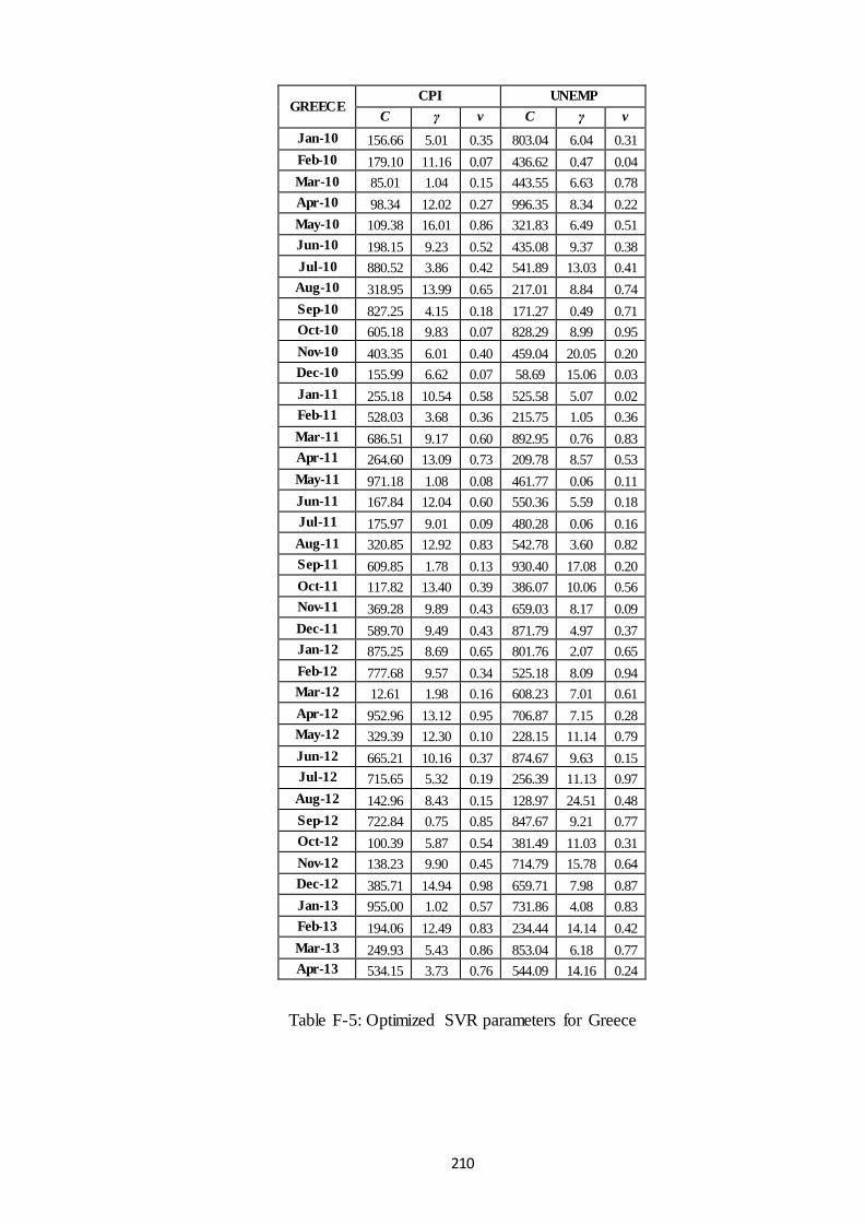
210
GREECE CPI UNEMP
C γ v C γ v Jan-10 156.66 5.01 0.35 803.04 6.04 0.31 Feb-10 179.10 11.16 0.07 436.62 0.47 0.04 Mar-10 85.01 1.04 0.15 443.55 6.63 0.78 Apr-10 98.34 12.02 0.27 996.35 8.34 0.22 May-10 109.38 16.01 0.86 321.83 6.49 0.51 Jun-10 198.15 9.23 0.52 435.08 9.37 0.38 Jul-10 880.52 3.86 0.42 541.89 13.03 0.41 Aug-10 318.95 13.99 0.65 217.01 8.84 0.74 Sep-10 827.25 4.15 0.18 171.27 0.49 0.71 Oct-10 605.18 9.83 0.07 828.29 8.99 0.95 Nov-10 403.35 6.01 0.40 459.04 20.05 0.20 Dec-10 155.99 6.62 0.07 58.69 15.06 0.03 Jan-11 255.18 10.54 0.58 525.58 5.07 0.02 Feb-11 528.03 3.68 0.36 215.75 1.05 0.36 Mar-11 686.51 9.17 0.60 892.95 0.76 0.83 Apr-11 264.60 13.09 0.73 209.78 8.57 0.53 May-11 971.18 1.08 0.08 461.77 0.06 0.11 Jun-11 167.84 12.04 0.60 550.36 5.59 0.18 Jul-11 175.97 9.01 0.09 480.28 0.06 0.16 Aug-11 320.85 12.92 0.83 542.78 3.60 0.82 Sep-11 609.85 1.78 0.13 930.40 17.08 0.20 Oct-11 117.82 13.40 0.39 386.07 10.06 0.56 Nov-11 369.28 9.89 0.43 659.03 8.17 0.09 Dec-11 589.70 9.49 0.43 871.79 4.97 0.37 Jan-12 875.25 8.69 0.65 801.76 2.07 0.65 Feb-12 777.68 9.57 0.34 525.18 8.09 0.94 Mar-12 12.61 1.98 0.16 608.23 7.01 0.61 Apr-12 952.96 13.12 0.95 706.87 7.15 0.28 May-12 329.39 12.30 0.10 228.15 11.14 0.79 Jun-12 665.21 10.16 0.37 874.67 9.63 0.15 Jul-12 715.65 5.32 0.19 256.39 11.13 0.97 Aug-12 142.96 8.43 0.15 128.97 24.51 0.48 Sep-12 722.84 0.75 0.85 847.67 9.21 0.77 Oct-12 100.39 5.87 0.54 381.49 11.03 0.31 Nov-12 138.23 9.90 0.45 714.79 15.78 0.64 Dec-12 385.71 14.94 0.98 659.71 7.98 0.87 Jan-13 955.00 1.02 0.57 731.86 4.08 0.83 Feb-13 194.06 12.49 0.83 234.44 14.14 0.42 Mar-13 249.93 5.43 0.86 853.04 6.18 0.77 Apr-13 534.15 3.73 0.76 544.09 14.16 0.24
Table F-5: Optimized SVR parameters for Greece

211
IRELAND CPI UNEMP
C γ v C γ v Jan-10 162.70 0.14 0.70 744.65 3.58 0.79 Feb-10 234.31 0.07 0.43 900.94 4.28 0.84 Mar-10 648.37 0.28 0.53 499.86 8.07 0.25 Apr-10 625.21 0.07 0.48 473.20 1.88 0.65 May-10 596.93 0.06 0.44 547.30 15.14 0.26 Jun-10 255.50 0.07 0.86 991.76 1.55 0.30 Jul-10 955.89 0.09 0.92 439.58 2.44 0.24 Aug-10 513.59 0.14 0.01 626.04 5.81 0.39 Sep-10 376.94 0.06 0.34 743.98 4.12 0.41 Oct-10 850.17 0.13 0.20 566.87 3.03 0.15 Nov-10 133.72 0.25 0.85 620.65 4.97 0.74 Dec-10 987.09 0.16 0.09 817.56 6.22 0.32 Jan-11 381.87 0.13 0.70 798.26 5.13 0.99 Feb-11 749.22 0.13 0.94 928.93 4.66 0.53 Mar-11 76.92 0.26 0.89 529.13 9.10 0.40 Apr-11 443.39 0.32 0.89 74.37 1.07 0.68 May-11 324.90 0.15 0.01 502.73 10.67 0.79 Jun-11 69.31 0.15 0.53 800.59 10.79 0.34 Jul-11 62.66 0.23 0.42 858.52 5.06 0.96 Aug-11 784.43 0.14 0.92 554.94 3.32 0.43 Sep-11 263.96 0.10 0.20 855.55 0.05 0.37 Oct-11 745.55 0.07 0.29 375.45 1.08 0.44 Nov-11 751.66 0.03 0.85 90.66 5.16 0.60 Dec-11 537.78 0.15 0.03 873.49 0.07 0.10 Jan-12 494.96 0.15 0.84 745.52 0.06 0.70 Feb-12 687.53 0.09 0.90 377.68 0.03 0.25 Mar-12 638.68 0.14 0.47 830.30 0.11 0.90 Apr-12 889.14 0.13 0.11 373.44 0.07 0.09 May-12 467.79 0.13 0.77 981.59 6.10 0.95 Jun-12 774.98 0.13 0.20 980.45 8.75 0.68 Jul-12 578.16 0.13 0.36 663.22 6.34 0.38 Aug-12 84.82 0.28 0.34 622.58 9.26 0.04 Sep-12 657.47 0.15 0.61 545.00 11.71 0.16 Oct-12 322.28 0.12 0.77 467.37 15.79 0.79 Nov-12 337.59 0.12 0.01 172.40 9.55 0.50 Dec-12 118.09 0.10 0.34 1016.05 12.33 0.31 Jan-13 950.70 0.13 0.52 226.29 3.97 0.91 Feb-13 569.21 0.26 0.16 627.47 10.44 0.36 Mar-13 296.46 0.05 0.86 54.66 7.89 0.46 Apr-13 13.40 0.13 0.76 546.73 14.36 0.95
Table F-6: Optimized SVR parameters for Ireland
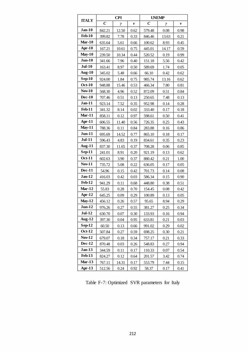
212
ITALY CPI UNEMP
C γ v C γ v Jan-10 842.21 12.50 0.62 579.48 0.08 0.98 Feb-10 399.82 7.78 0.33 846.46 13.63 0.21 Mar-10 635.64 5.61 0.66 100.62 8.93 0.45 Apr-10 167.21 10.61 0.75 445.01 14.17 0.59 May-10 239.50 10.34 0.44 520.52 0.19 0.99 Jun-10 341.66 7.96 0.40 151.18 5.56 0.42 Jul-10 163.41 8.97 0.50 589.69 1.74 0.05 Aug-10 345.02 5.48 0.66 66.10 0.42 0.62 Sep-10 924.00 1.84 0.75 985.74 13.16 0.62 Oct-10 948.88 15.46 0.53 466.34 7.80 0.81 Nov-10 568.30 4.96 0.52 872.09 0.51 0.84 Dec-10 707.46 0.51 0.13 250.65 7.48 0.13 Jan-11 923.14 7.52 0.35 952.98 0.14 0.28 Feb-11 341.32 8.14 0.02 333.40 0.17 0.18 Mar-11 858.11 0.12 0.97 598.61 0.50 0.41 Apr-11 606.55 11.40 0.56 726.35 0.25 0.43 May-11 788.36 0.11 0.84 283.88 0.16 0.86 Jun-11 695.69 14.52 0.77 865.10 0.18 0.17 Jul-11 596.43 4.83 0.19 834.61 0.35 0.23 Aug-11 837.30 11.65 0.37 708.28 0.06 0.85 Sep-11 241.01 8.91 0.20 921.19 0.13 0.62 Oct-11 602.63 3.90 0.37 880.42 0.21 1.00 Nov-11 735.72 5.08 0.22 636.05 0.17 0.05 Dec-11 54.96 0.15 0.42 701.73 0.14 0.08 Jan-12 416.03 0.42 0.03 586.34 0.15 0.90 Feb-12 941.29 0.11 0.68 448.80 0.38 0.51 Mar-12 55.83 0.28 0.70 154.45 0.08 0.42 Apr-12 645.25 0.09 0.29 100.89 0.13 0.05 May-12 456.12 0.26 0.57 95.65 8.94 0.29 Jun-12 976.26 0.27 0.55 381.27 0.25 0.34 Jul-12 630.70 0.07 0.30 133.93 0.16 0.94 Aug-12 397.30 0.04 0.95 633.81 0.21 0.03 Sep-12 60.50 0.13 0.66 991.02 0.29 0.02 Oct-12 507.84 0.27 0.59 698.25 0.30 0.21 Nov-12 679.07 0.18 0.34 757.17 0.21 0.33 Dec-12 870.48 0.03 0.26 548.83 0.27 0.94 Jan-13 344.59 0.11 0.17 110.33 0.07 0.54 Feb-13 824.27 0.12 0.64 201.57 3.42 0.74 Mar-13 767.11 14.31 0.17 553.79 7.44 0.15 Apr-13 512.56 0.24 0.92 58.37 0.17 0.41
Table F-7: Optimized SVR parameters for Italy

213
PORTUGAL CPI UNEMP
C γ v C γ v Jan-10 692.40 8.56 0.35 712.64 0.18 0.22 Feb-10 115.90 4.40 0.62 380.33 10.07 0.07 Mar-10 727.53 13.18 0.07 39.93 0.00 0.56 Apr-10 227.33 3.57 0.15 597.17 0.09 0.24 May-10 244.70 12.00 0.12 893.72 0.15 0.21 Jun-10 795.69 1.80 0.62 992.96 0.05 0.53 Jul-10 749.80 9.42 0.26 493.54 0.17 0.70 Aug-10 909.46 11.23 0.13 733.11 0.24 0.88 Sep-10 496.39 15.59 0.87 909.26 14.41 0.07 Oct-10 71.52 10.01 0.40 539.63 0.25 0.29 Nov-10 496.19 0.26 0.56 993.17 0.15 0.84 Dec-10 284.47 15.96 0.16 23.05 0.26 0.95 Jan-11 87.59 14.63 0.66 44.48 0.21 0.49 Feb-11 755.50 13.60 0.40 900.44 0.16 0.24 Mar-11 816.00 9.71 0.64 856.34 0.11 0.93 Apr-11 981.18 1.62 0.74 865.71 0.18 0.63 May-11 647.13 9.44 0.83 856.96 0.21 0.79 Jun-11 652.82 1.68 0.02 170.62 0.19 0.87 Jul-11 266.64 0.13 0.46 264.40 0.18 0.76 Aug-11 914.72 2.52 0.21 898.38 0.15 0.81 Sep-11 581.80 13.82 0.91 876.80 0.26 0.38 Oct-11 738.02 2.65 0.01 279.03 0.21 0.15 Nov-11 360.38 0.27 0.65 735.47 0.08 0.63 Dec-11 203.30 4.43 0.70 641.58 0.15 0.71 Jan-12 3.16 2.64 0.24 854.50 0.11 0.32 Feb-12 327.01 15.87 0.70 7.30 0.06 0.80 Mar-12 912.23 14.83 0.91 133.13 0.13 0.89 Apr-12 537.21 10.08 0.39 399.11 0.18 0.46 May-12 50.59 10.59 0.69 474.12 0.16 0.08 Jun-12 311.92 11.19 0.71 216.01 0.21 0.68 Jul-12 153.68 4.22 0.81 365.97 0.13 0.33 Aug-12 9.46 4.87 0.19 917.25 0.25 0.53 Sep-12 332.05 14.83 0.51 619.59 0.22 0.23 Oct-12 421.55 12.57 0.67 324.12 0.27 0.02 Nov-12 263.67 13.65 0.35 814.90 0.20 0.78 Dec-12 444.28 0.21 0.58 391.17 0.17 0.41 Jan-13 404.50 1.06 0.84 700.79 0.19 0.05 Feb-13 568.78 0.76 0.78 53.73 0.18 0.32 Mar-13 108.28 11.33 0.29 667.96 0.06 0.01 Apr-13 458.77 4.01 0.73 1000.30 0.30 0.42
Table F-8: Optimized SVR parameters for Portugal

214
SPAIN CPI UNEMP
C γ v C γ v Jan-10 276.35 6.80 0.17 463.48 0.49 0.64 Feb-10 29.00 0.09 0.71 777.71 1.46 0.28 Mar-10 919.36 3.84 0.97 627.44 0.88 0.52 Apr-10 768.65 6.53 0.86 727.94 0.49 0.78 May-10 898.11 12.84 0.33 467.27 0.39 0.01 Jun-10 543.76 14.91 0.28 793.96 6.41 0.35 Jul-10 656.04 3.51 0.01 49.24 6.19 0.51 Aug-10 106.33 1.00 0.44 876.70 8.95 0.71 Sep-10 717.35 0.39 0.25 501.07 0.39 0.19 Oct-10 960.08 4.23 0.13 583.59 0.39 0.07 Nov-10 922.19 7.69 0.57 942.23 0.78 0.15 Dec-10 568.78 7.34 0.55 634.74 0.29 0.55 Jan-11 270.50 7.60 0.03 827.66 0.68 0.49 Feb-11 390.15 2.13 0.57 858.39 1.86 0.32 Mar-11 492.03 0.84 0.02 835.86 0.88 0.83 Apr-11 396.36 4.80 0.01 920.81 0.39 0.57 May-11 358.94 12.20 0.15 294.50 2.05 0.11 Jun-11 209.76 5.06 0.56 858.22 1.76 0.01 Jul-11 690.68 0.13 0.37 995.26 3.22 0.70 Aug-11 932.10 0.10 0.18 721.95 1.66 0.72 Sep-11 746.58 5.41 0.14 509.96 3.71 0.88 Oct-11 95.95 1.44 0.55 592.71 3.22 0.51 Nov-11 631.08 14.96 0.43 536.88 7.03 0.07 Dec-11 553.03 0.68 0.56 702.63 10.55 0.27 Jan-12 69.34 15.67 0.35 292.32 6.45 0.95 Feb-12 995.55 2.54 0.10 229.95 10.35 0.56 Mar-12 413.80 4.87 0.42 709.18 9.84 0.85 Apr-12 559.02 12.38 0.10 839.79 1.41 0.81 May-12 435.30 1.70 0.72 63.44 3.36 0.34 Jun-12 273.75 13.55 0.13 469.05 2.83 0.97 Jul-12 1003.93 8.30 0.91 53.81 2.62 0.94 Aug-12 84.70 10.18 0.83 626.84 3.69 0.86 Sep-12 696.32 0.07 0.79 862.92 7.66 0.57 Oct-12 984.95 3.09 0.96 914.73 4.12 0.85 Nov-12 54.73 8.64 0.36 432.98 8.87 0.20 Dec-12 990.60 2.02 0.47 783.45 8.71 0.52 Jan-13 955.81 8.73 0.95 982.48 7.30 0.04 Feb-13 850.60 9.90 0.71 346.88 7.66 0.37 Mar-13 25.57 15.60 0.27 810.65 1.76 0.15 Apr-13 864.47 12.98 0.12 615.22 0.92 0.60
Table F-9: Optimized SVR parameters for Spain

215
Bibliography
[1] Abu-Mostafa, Y.S. and Atiya, A.F. (1996) Introduction to Financial
Forecasting, Applied Intelligence, 6 (3), pp. 205-213.
[2] Adya, M. and Collopy, F. (1998) How effective are neural networks at
forecasting and prediction? A review and evaluation, Journal of Forecasting, 17 (5-
6), pp. 481–495.
[3] Ager, P., Kappler, M. and Osterloh, S. (2009) The accuracy and efficiency
of the Consensus Forecasts: A further application and extension of the pooled
approach, International Journal of Forecasting, 25 (1), pp. 167–181.
[4] Aggarwal, S. and Krishna, V. (2011) CS698o: Project Report Stock Price
Direction Prediction, Indian Institute of Technology Kanpur, Working Paper.
[5] Ahn, H. and Kim, K.J. (2009) Bankruptcy prediction modeling with hybrid
case-based reasoning and genetic algorithms approach, Applied Soft Computing, 9
(2), pp. 599–607.
[6] Akaike, H. (1974) A new look at the statistical model identification, IEEE
Transactions on Automatic Control, 19 (6), pp.716-723.
[7] Alexander, S.S. (1961) Price movements in speculative markets: trends or
random walks, Industrial Management Review, 2 (1), pp. 7–26.
[8] Alfaro, E., García, N., Gamez, M. and Elizondo, D. (2008) Bankruptcy
forecasting: An empirical comparison of AdaBoost and neural networks, Decision
Support Systems, 45(1), pp.110-122.
[9] Allen, F. and Karjalainen, R. (1999) Using genetic algorithms to find
technical trading rules, Journal of Financial Economics, 51 (2), pp. 245–271.
[10] Altavilla, C. and De Grauwe, P. (2008) Forecasting and combining
competing models of exchange rate determination, Applied Economics, 42 (27), pp.
3455-3480.
[11] Amjady, N. and Keynia, F. (2009) Short-term load forecasting of power
systems by combination of wavelet transform and neuro-evolutionary algorithm,
Energy, 34 (1), pp. 46–57.

216
[12] Anandalingam, G. and Chen, L. (1989) Linear combination of forecasts: A
general Bayesian model, Journal of Forecasting, 8 (3), pp.199-214.
[13] Andersen, T.G, Bollerslev, T., Diebold, F.X. and Vega, C. (2003) Micro
Effects of Macro Announcements: Real-Time Price Discovery in Foreign
Exchange, American Economic Review, 93, pp. 38-62.
[14] Andrawis, R.R., Atiya, A.F. and El-Shishiny, H. (2011) Forecast
combinations of computational intelligence and linear models for the NN5 time
series forecasting competition, International Journal of Forecasting, 27(3), pp.
672–688.
[15] Ang, A., Bekaert, G. and Wei, M. (2007) Do Macro Variables, Asset
Markets, or Surveys Forecast Inflation Better? Journal of Monetary Economics, 54
(4), pp.1163–212.
[16] Atkeson, A.and Ohanian, L.E. (2001) Are Phillips Curves Useful for
Forecasting Inflation?, Federal Reserve Bank of Minneapolis Quarterly Review, 25,
pp.2-11.
[17] Awartani, B., Corradi, V. and Distaso, W. (2009) Assessing Market
Microstructure Effects via Realized Volatility Measures with an Application to the
Dow Jones Industrial Average Stocks, Journal of Business & Economic Statistics,
27 (2), pp. 251-265.
[18] Bacchettaa, P. and Wincoop, E.V. (2013) On the unstable relationship
between exchange rates and macroeconomic fundamentals, Journal of International
Economics, 91 (1), pp. 18-26.
[19] Bajgrowicz, P. and Scaillet, O. (2012) Technical trading revisited: False
discoveries, persistence tests, and transaction costs, Journal of Financial
Economics, 106 (3), pp. 473–491.
[20] Banerjee, A., Marcellino, M. and Masten, I. (2005) Leading Indicators for
Euro-area Inflation and GDP Growth, Oxford Bulletin of Economics and Statistics,
67, pp. 785-813.
[21] Barber, B.M., Lehavy, R., McNichols, M. and Trueman, B. (2006) Buys,
holds, and sells: The distribution of investment banks’ stock ratings and the
implications for the profitability of analysts’ recommendations, Journal of
Accounting and Economics, 41 (1–2), pp. 87–117.
[22] Barhoumi, K., Darne, O. and Ferrara, L. (2010) Are disaggregate data
useful for factor analysis in forecasting French GDP?, Journal of Forecasting, 29
(1-2), pp. 132–144.

217
[23] Bates, J. M. and Granger, C. W. J. (1969) The Combination of Forecasts,
Operational Research Society, 20 (4), pp. 451-468.
[24] Basak, D., Pal, S. and Patranabis, D.C. (2007) Support Vector Regression,
Neural Information Processing - Letters and Reviews, 10 (10), pp. 203-224.
[25] Bertolini, L. (2010) Trading Foreign Exchange Carry Portfolios, PhD
Thesis, Cass Business School, City University London.
[26] Bessembinder, H. and Chan, K. (1995) The profitability of technical trading
rules in the Asian stock markets, Pacific-Basin Finance Journal, 3 (2-3), pp. 257–
284.
[27] Bezdek, J. (1994) What is computational intelligence?, in: Zurada, L.,
Marks, R. and Robinson, C. (eds.), Computational Intelligence Imitating Life, IEEE
Press, NY, pp. 1-12.
[28] Bissoondeeal, R.K., Binner, J.M., Bhuruth, M., Gazely, A. and Mootanah,
V.P. (2008) Forecasting exchange rates with linear and nonlinear models, Global
Business and Economics Review, 10 (4), 414-429.
[29] Box. G.E.P. and Jenkins, G.M. (1976) Time Series Analysis: Forecasting
and Control, Revised Edition, Oakland, CA: Holden-Day
[30] Brock, W., Lakonishok, J. and LeBaron, B. (1992) Simple Technical
Trading Rules and the Stochastic Properties of Stock Returns, The Journal of
Finance, 47 (5), pp. 1731-1764.
[31] Brooks, C. (2008) Introductory econometrics for finance, 2nd revised ed.,
Cambridge University Press, Cambridge
[32] Buckland, S.T., Burnham, K.P. and Augustin, N H. (1997) Model
Selection: An Integral Part of Inference, Biometrics, 53 (2), pp. 603-618.
[33] Cao, L.J., Chua, K.S. and Guan, L.K. (2003) C-ascending support vector
machines for financial time series forecasting, Proceedings of Computational
Intelligence for Financial Engineering, pp. 317-323.
[34] Castellano, G., Fanelli, A.M. and Pelillo, M. (1997) An iterative pruning
algorithm for feed-forward neural networks, IEEE Transactions on Neural
Networks, 8 (3), pp. 519 – 531.
[35] Chalimourda, A., Schölkopf, B. and Smola, A.(2004) Experimentally
optimal ν in support vector regression for different noise models and parameter
settings, Neural Networks, 17 (1), pp. 127-141.
[36] Chan, K.S. and Tong, H. (1986) On estimating thresholds in autoregressive
models, Journal of Time Series Analysis, 7(3), pp. 178-190.

218
[37] Chan, Y. L., Stock, J. H. and Watson, M. W. (1999) A dynamic factor
model framework for forecast combination, Spanish Economic Review, 1 (2), 91-
121.
[38] Chang, J., Jung, Y., Yeon, K., Jun, J., Shin, D. and Kim, H. (1996)
Technical indicators and analysis methods, Jinritamgu Publishing, Seoul.
[39] Charles, A. and Darné, O. (2006) Large shocks and the September 11th
terrorist attacks on international stock markets, Economic Modelling, 23 (4), pp.
683-698.
[40] Chen, A.S., Leung, M.T. and Daouk, H. (2003) Application of neural
networks to an emerging financial market: forecasting and trading the Taiwan
Stock Index, Computers & Operations Research, 30 (6), pp. 901–923.
[41] Chen, K.Y. and Wang, C.H. (2007) Support Vector Regression with genetic
algorithms in forecasting tourism demand, Tourism Management, 28 (1), pp. 215-
226.
[42] Chen, S.H. (2002) Genetic algorithms and genetic programming in
computational finance, Boston: Kluwer Academic Publishers.
[43] Cherkasssky, V. and MA, Y. (2004) Practical selection of SVM parameters
and noise estimation for SVM regression, Neural Networks, 17 (1), pp. 113-126.
[44] Chiarella, C., He, X.Z. and Hommes, C. (2006) A dynamic analysis of
moving average rules, Journal of Economic Dynamics and Control, 30 (9–10), pp.
1729–1753.
[45] Chong T.T.L and Ng, W.K. (2008) Technical analysis and the London stock
exchange: testing the MACD and RSI rules using the FT30, Applied Economics
Letters, 15 (14), pp. 1111-1114.
[46] Chua, C.L, Lim, G.C. and Tsiaplias, S. (2012) A latent variable approach to
forecasting the unemployment rate, Journal of Forecasting, 31(3), pp. 229–244.
[47] Clyde, W.C. and Osler, C.L. (1998) Charting: Chaos theory in disguise?,
Journal of Futures Markets, 17 (5), pp. 489–514.
[48] Cogley, T., Primiceri, G.E. and Sargent, T.J. (2010) Inflation-gap
Persistence in the U.S., American Economic Journal: Macroeconomics, 2 (1), pp.
43-69.
[49] Cogley, T and Sargent, T.J. (2005) Drifts and volatilities: monetary policies
and outcomes in the post WWII U.S, Review of Economic Dynamics, 8 (2), pp.
262–302.

219
[50] Corrado, C.J. and Lee, S.H. (1992) Filter Rule Tests of the Economic
Significance of Serial Dependencies in Daily Stock Returns, Journal of Financial
Research, 15 (4), pp. 369-387.
[51] Coulson, N.E. and Robins, R.P. (1993) Forecast combination in a dynamic
setting, Journal of Forecasting, 12 (1), pp. 63-67.
[52] Coutts, J.A. and Cheung, K.C. (2000) Trading rules and stock returns: some
preliminary short run evidence from the Hang Seng 1985-1997, Applied Financial
Economics, 10 (6), pp. 579-586.
[53] D'Agostino, A., Gambetti, L. and Giannone, D. (2013). Macroeconomic
forecasting and structural change, Journal of Applied Econometrics, 28 (1), pp. 82–
101.
[54] De Gooijer, J.G. and Hyndman, R.J. (2006) 25 years of time series
forecasting, International Journal of Forecasting, 22 (3), pp. 443-473.
[55] De Menezes, L.M. and Nikolaev, N.Y. (2006) Forecasting with genetically
programmed polynomial neural networks, International Journal of Forecasting, 22
(2), pp. 249-265.
[56] Deboeck, G. (1994) Trading on the edge: neural, genetic, and fuzzy systems
for chaotic financial markets, New York: Wiley.
[57] Dempster, M.A.H. and Jones, C.M. (2001) A real- time adaptive trading
system using genetic programming, Quantitative Finance, 1 (4), pp. 397-413.
[58] Dempster, M.A.H. and Leemans, V. (2006) An automated FX trading
system using adaptive reinforcement learning, Expert Systems with Applications, 30
(3), pp. 543–552.
[59] Deutsch, M., Granger, C.W. J. and Teräsvirta, T. (1994) The combination of
forecasts using changing weights, International Journal of Forecasting, 10 (1), pp.
47-57.
[60] Diebold, F. X. and Mariano, R. S. (1995) Comparing Predictive Accuracy,
Journal of Business and Economic Statistics, 13 (3), pp. 253-263.
[61] Diebold, F.X. and Pauly, P. (1987) Structural change and the combination
of forecasts, Journal of Forecasting, 6 (1), pp. 21-40.
[62] Dijk, D.V. and Franses, P.H. (1999) Modeling Multiple Regimes in the
Business Cycle, Macroeconomic Dynamics, 3(3), pp. 311-340.
[63] Diron, M. (2008) Short-term forecasts of euro area real GDP growth: an
assessment of real-time performance based on vintage data, Journal of
Forecasting, 27 (5), pp. 371-390.

220
[64] Ding, Y., Song, X. and Zen, Y. (2008) Forecasting financial condition of
Chinese listed companies based on support vector machine, Expert Systems with
Applications, 34 (4), pp. 3081-3089.
[65] Donaldson, R.G. and Kamstra, M. (1999) Neural network forecast
combining with interaction effects, Journal of the Franklin Institute, 336 (2), pp.
227-236.
[66] Dooley, M.P. and Shafer, J. R. (1983) Analysis of Short-Run Exchange
Rate Behaviour: March 1973 to November 1981, in: Bigman, D. and Taya, T.
(eds.), Exchange Rate and Trade Instability: Causes, Consequences, and Remedies,
Cambridge.
[67] Dreger, C. and Kholodilin, K.A. (2013) Forecasting Private Consumption
by Consumer Surveys, Journal of Forecasting, 32 (1), pp. 10–18.
[68] Duan, K, Keerthi, S.S. and Poo, A.N. (2003) Evaluation of simple
performance measures for tuning SVM hyperparameters, Neurocomputing, 51, pp.
41-59.
[69] Dunis, C.L. and Chen, Y.X. (2005) Alternative volatility models for risk
management and trading: Application to the EUR/USD and USD/JPY rates,
Derivatives Use, Trading and Regulation, 11, pp.126-156.
[70] Dunis, C.L., Giorgioni, G., Laws, J. and Rudy, J. (2010) Statistical
Arbitrage and High-Frequency Data with an Application to Eurostoxx 50 Equities,
Working Paper, Liverpool Business School.
[71] Dunis, C.L. and Huang, X. (2002) Forecasting and trading currency
volatility: an application of recurrent neural regression and model combination,
Journal of Forecasting, 21 (5), pp. 317-354.
[72] Dunis, C.L., Laws, J. and Evans, B. (2005) Modelling and trading the
soybean-oil crush spread with recurrent and higher order neural networks: A
comparative analysis, Neural Network World, 6 (1), pp. 509–523.
[73] Dunis, C.L., Laws, J. and Evans, B. (2006) Trading futures spreads: an
application of correlation and threshold filters, Applied Financial Economics, 16
(12), pp. 903-914.
[74] Dunis, C.L., Laws, J. and Sermpinis, G. (2011) Higher order and recurrent
neural architectures for trading the EUR/USD exchange rate, Quantitative Finance,
11 (4), pp. 615-629.
[75] Dunis, C.L., Likothanassis, S.D., Karathanasopoulos, A.S., Sermpinis, G.
and Theofilatos, A. (2013) A hybrid genetic algorithm–support vector machine

221
approach in the task of forecasting and trading, Journal of Asset Management, 14
(1), pp. 57-71.
[76] Dunis, C.L. and Miao, J. (2005) Optimal trading frequency for active asset
management: Evidence from technical trading rules, Journal of Asset Management,
5 (5), pp. 305-326.
[77] Dunis, C.L. and Miao, J. (2006) Volatility filters for asset management: An
application to managed futures, Journal of Asset Management, 7 (3), pp. 179-189.
[78] Dunis, C.L. and Nathani, A. (2007) Quantitative Trading of Gold and Silver
using Nonlinear Models’, Neural Network World, 16 (2), pp. 93-111.
[79] Dunis, C. L. and Shannon, G. (2005) Emerging Markets of South-East and
Central Asia: Do they Still Offer a Diversification Benefit?, Journal of Asset
Management, 6 (3), pp.168-190.
[80] Dunis, C.L. and Williams, M. (2002) Modelling and Trading the EUR/USD
Exchange Rate: Do Neural Network Models Perform Better?, Derivatives Use,
Trading and Regulation, 8, pp. 211-239.
[81] Ebrahimpour, R., Nikoo, H., Masoudnia, S., Yousefi, M.R. and Ghaemi,
M.S. (2011) Mixture of MLP-experts for trend forecasting of time series: A case
study of the Tehran stock exchange, International Journal of Forecasting, 27(3),
pp. 804-816.
[82] Edwards, R.D. and Magee, J. (1997) Technical analysis of stock trends,
John Magee, Chicago.
[83] Elman, J.L. (1990) Finding Structure in Time, Cognitive Science, 14 (2), pp.
179-211.
[84] Evans, B. (2008) Trading futures spread portfolios: applications of higher
order and recurrent networks, The European Journal of Finance, 14 (6), pp. 503-
521.
[85] Evans, K.P. and Speight, A.E.H. (2010) Dynamic news effects in high
frequency Euro exchange rates, Journal of International Financial Markets,
Institutions and Money, 20 (3), pp. 238–258.
[86] Fama, E.F. (1970) Efficient capital markets: A review of theory and
empirical work, The Journal of Finance, 25 (2), pp. 383–417.
[87] Fama, E.F. (1991) Efficient capital markets: II, The Journal of Finance 46
(5), pp. 1575–1617.
[88] Fama, E.F. and Blume, M.E. (1966) FRs and stock-market trading, The
Journal of Business, 39 (1), pp. 226–241.

222
[89] Faust, J. and Wright J.H. (2012) Forecasting Inflation, Handbook of
Forecasting, Johns Hopkins University.
[90] Fernández-Rodrıguez, F., González-Martel, C. and Sosvilla-Rivero, S.
(2000) On the profitability of technical trading rules based on artificial neural
networks: Evidence from the Madrid stock market, Economics Letters, 69 (1), pp.
89–94.
[91] Flannery, M.J. and Protopapadakis, A.A. (2002) Macroeconomic Factors
Do Influence Aggregate Stock Returns, Review of Financial Studies, 15 (3), pp.
751-782.
[92] Fong, W.M. and Yong, H.M. (2005) Chasing trends: recursive moving
average trading rules and internet stocks, Journal of Empirical Finance, 12 (1), pp.
43–76.
[93] Forner, C. and Marhuenda, J. (2003) Contrarian and Momentum Strategies
in the Spanish Stock Market, European Financial Management, 9 (1), pp. 67–88.
[94] Friesen, G.C, Weller, P.A and Dunham, L.M. (2009) Price trends and
patterns in technical analysis: A theoretical and empirical examination, Journal of
Banking & Finance, 33 (6), pp. 1089–1100.
[95] Frisch, R. (1933) Propagation problems and impulse problems in dynamic
economics, in: Åkerman, J. and Cassel, G. (eds.) Economic Essays in Honor of
Gustav Cassel, London: Allen & Unwin, pp. 171–205.
[96] Gençay, R. (1998) Optimization of technical trading strategies and the
profitability in security markets, Economics Letters, 59 (2), pp. 249–254.
[97] Gençay, R. (1999) Linear, nonlinear and essential foreign exchange
prediction, Journal of International Economics, 47 (1), pp. 91–107.
[98] Ghazali, R., Hussain, A. J. and Merabti, M. (2006) Higher Order Neural
Networks for Financial Time Series Prediction, The 10th IASTED International
Conference on Artificial Intelligence and Soft Computing, Palma de Mallorca,
Spain, pp. 119-124.
[99] Ghosh, J. and Shin, Y. (1991) The Pi-Sigma Network: An efficient Higher-
order Neural Networks for Pattern Classification and Function Approximation,
Proceedings of International Joint Conference of Neural Networks, 1, pp. 13-18.
[100] Ghosh, J. and Shin, Y. (1992) Efficient Higher-Order Neural Networks for
Classification and Function Approximation, International Journal of Neural
Systems, 3 (4), pp. 323-350.

223
[101] Giannone, D., Henry, J., Lalik, M. and Michele Modugno, M. (2012) An
Area-Wide Real-Time Database for the Euro Area, Review of Economics and
Statistics, 94 (4), pp. 1000-1013.
[102] Gifford, E. (1995) Investor's guide to technical analysis: predicting price
action in the markets, London.
[103] Goh, S. L. and Mandic, D. P. (2007) An Augmented Extended Kalman
Filter Algorithm for Complex-Valued Recurrent Neural Networks, Neural
Computation, 19 (4), pp.1039-1055.
[104] Granger, C. W. J. and Ramanathan, R. (1984) Improved methods of
combining forecasts, Journal of Forecasting, 3 (2), pp. 197-204.
[105] Groen J, Paap R, Ravazzolo F. (2010) Real-time Inflation Forecasting in a
Changing World, Federal Reserve Bank of New York, Staff Report Number 388.
[106] Grossmann, A. and McMillan, D.G (2010) Forecasting exchange rates:
Non-linear adjustment and time-varying equilibrium, Journal of International
Financial Markets, Institutions and Money, 20 (4), pp. 436-450.
[107] Guégan, D. and Huck, N. (2004) Forecasting relative movements using
transitivity? Working paper, Institutions et Dynamiques Historiques de l’Economie.
[108] Guegan, D. and Huck, N. (2005) On the Use of Nearest Neighbours to
Forecast in Finance, Revue de l'Association française de Finance, 26, pp. 67-86.
[109] Guidi, F. and Gupta, R. (2013) Market efficiency in the ASEAN region:
evidence from multivariate and co- integration tests, Applied Financial Economics,
23 (4), pp. 265-274.
[110] Guidolin, M. and Timmermann, A. (2009) Forecasts of US short-term
interest rates: A flexible forecast combination approach, Journal of Econometrics,
150 (2), pp. 297-311.
[111] Gunasekarage, A. and Power, D.M. (2001) The profitability of moving
average trading rules in South Asian stock markets, Emerging Markets Review, 2
(1), pp. 17-33.
[112] Hamilton, J.D. (1994) Time series analysis, Princeton University Press,
Princeton, N.J.
[113] Hansen, P.R. (2005) A test for superior predictive ability, Journal of
Business & Economic Statistics, 23 (4), pp. 365–380.
[114] Harrald, P.G. and Kamstra, M. (1997) Evolving artificial neural networks to
combine financial forecasts. IEEE Transactions on Evolutionary Computation 1,
pp. 40-52.

224
[115] Harvey, A.C. (1990) Forecasting, structural time series models and the
Kalman filter, Cambridge University Press, Cambridge.
[116] Harvey, D., Leybourne, S. and Newbold, P. (1997) Testing the equality of
prediction mean squared errors, International Journal of Forecasting, 13 (2), pp.
281–291.
[117] Hassani, H., Heravi, S. and Zhigljavsky, A. (2009) Forecasting European
industrial production with singular spectrum analysis. International Journal of
Forecasting, 25 (1), pp. 103–118.
[118] Hastie, T., Tibshirani, R. and Friedman, J.H. (2009) The elements of
statistical learning: data mining, inference, and prediction, 2nd ed., Springer, New
York.
[119] Hemminki, J. and Puttonen, V. (2008) Fundamental indexation in Europe,
Journal of Asset Management, 8, pp. 401-405.
[120] Holland J. (1995) Adaptation in Natural and Artificial Systems: An
Introductory Analysis with Applications to Biology, Control and Artificial
Intelligence. Cambridge MA: MIT Press.
[121] Hsieh, T., Hsiao, H. and Yeh, W. (2011) Forecasting stock markets using
wavelet transforms and recurrent neural networks: An integrated system based on
artificial bee colony algorithm, Applied Soft Computing, 11(2), pp. 2510-2525.
[122] Hsu, S.H., Hsieh, J.J.P.A., Chih, T.C. and Hsu, K.C. (2009) A two-stage
architecture for stock price forecasting by integrating self-organizing map and
support vector regression, Expert Systems with Applications, 36(4), pp. 7947-7951.
[123] Hsu, P.H. and Kuan, C.M. (2005) Re-examining the Profitability of
Technical Analysis with Data Snooping Checks, Journal of Financial
Econometrics, 3 (4), pp. 608-628.
[124] Hu, M.Y. and Tsoukalas, C. (1999) Combining conditional volatility
forecasts using neural networks: an application to the EMS exchange rates, Journal
of International Financial Markets, Institutions and Money, 9 (4), pp. 407–422.
[125] Hua, Z., Wang, Y., Xu, X., Zhang, B. and Liang, L. (2007) Predicting
corporate financial distress based on integration of support vector machine and
logistic regression, Expert Systems with Applications, 33 (2), pp. 434–440.
[126] Huang, C.F. (2012) A hybrid stock selection model using genetic
algorithms and support vector regression, Applied Soft Computing, 12 (2), pp. 807–
818.

225
[127] Huang, C.L. and Wang, C.J. (2006) A GA-based feature selection and
parameters optimization for support vector machines, Expert Systems with
Applications, 31 (2), pp. 231-240.
[128] Huang, S.C., Chuang, P.J., Wu, C.F. and Lai, H.J. (2010) Chaos-based
support vector regressions for exchange rate forecasting, Expert Systems with
Applications, 37(12), pp. 8590-8598.
[129] Huang, S.C., Wang, N.Y, Li, T.Y, Lee, Y.C, Chang, L.F. and Pan, T.H.
(2013) Financial Forecasting by Modified Kalman Filters and Kernel Machines,
Journal of Statistics and Management Systems, 16 (2-03), pp. 163-176
[130] Hudson, R., Dempsey, M. and Keasey, K. (1996) A note on the weak form
efficiency of capital markets: the application of simple technical trading rules to
UK stock prices -1935 to 1994, Journal of Banking and Finance, 20 (6), pp. 1121–
1132.
[131] Hussain, A. J., Ghazali, R., Al-Jumeily, D. and Merabti, M. (2006)
Dynamic Ridge Polynomial Neural Network for Financial Time Series Prediction,
IEEE International conference on Innovation in Information Technology, pp. 1-5.
[132] Ince, H. and Trafalis, T. B. (2006a) A hybrid model for exchange rate
prediction, Decision Support Systems, 42 (2), pp. 1054-1062.
[133] Ince, H. and Trafalis, T.B. (2006b) Kernel methods for short-term portfolio
management, Expert Systems with Applications, 30 (3), pp. 535-542.
[134] Ince, H. and Trafalis, T.B. (2008) Short term forecasting with support
vector machines and application to stock price prediction, International Journal of
General Systems, 37 (6), pp. 677-687.
[135] Inoue, A. and Kilian, L. (2008) How useful is bagging in forecasting
economic time series? A case study of U.S. consumer price inflation, Journal of the
American Statistical Association, 103 (482), pp. 511–522
[136] Izumi, K., Toriumi, F. and Matsui, H. (2009) Evaluation of automated-
trading strategies using an artificial market, Neurocomputing, 72, (16–18), pp.
3469–3476.
[137] James, J., Marsh, I. And Sarno, L. (2012) Handbook of Exchange Rates,
Chicago,Wiley.
[138] Jarque, C. M. and Bera, A. K. (1980) Efficient tests for normality,
homoscedasticity and serial independence of regression residuals, Economics
Letters, 6 (3), pp. 255-259.

226
[139] Jegadeesh, N. and Titman, S. (1993) Returns to Buying Winners and
Selling Losers: Implications for Stock Market Efficiency, The Journal of
Finance, 48 (1), pp. 65–91.
[140] Jensen, M.C. (1978) Some anomalous evidence regarding market
efficiency, Journal of Financial Economics, 6 (2–3), pp. 95–101.
[141] Jensen, M. and Benington, G. (1970) Random Walks and Technical
Theories: Some Additional Evidence, The Journal of Finance, 25 (2), pp. 469-482.
[142] Jolliffe, I. (1986) Principal Component Analysis, NY: Springer-Verlag.
[143] Kaastra, I. and Boyd, M. (1996) Designing a Neural Network for
Forecasting Financial and Economic Time Series, Neurocomputing, 10 (3), pp.
215-236.
[144] Kao, L.J., Chiu, C.C., Lu, C.J. and Chang, C.H. (2013) A hybrid approach
by integrating wavelet-based feature extraction with MARS and SVR for stock
index forecasting, Decision Support Systems, 54 (3), pp. 1228-1244
[145] Kestner, L.N (2003) Quantitative trading strategies: harnessing the power
of quantitative techniques to create a winning trading program, Boston: McGraw-
Hill.
[146] Khemchandani, R., Jayadeva, I. and Chandra, S. (2009) Regularized least
squares fuzzy support vector regression for financial time series forecasting, Expert
Systems with Applications, 36 (1), pp. 132–138.
[147] Kiani, K. and Kastens, T. (2008) Testing Forecast Accuracy of Foreign
Exchange Rates: Predictions from Feed Forward and Various Recurrent Neural
Network Architectures, Computational Economics, 32 (4), pp. 383-406.
[148] Kim, H.S. and Sohn, S.Y. (2010) Support vector machines for default
prediction of SMEs based on technology credit, European Journal of Operational
Research, 201(3), pp. 838–846.
[149] Kim, K.J (2006) Artificial neural networks with evolutionary instance
selection for financial forecasting, Expert Systems with Applications, 30 (3), pp.
519–526.
[150] Kim, K.J. and Han, I. (2000) Genetic algorithms approach to feature
discretization in artificial neural networks for the prediction of stock price index,
Expert Systems with Applications, 19 (2), pp. 125–132.
[151] Koop, G. and Korobilis, D. (2012) Forecasting Inflation Using Dynamic
Model Averaging, International Economic Review, 53 (3), pp.867–886.
[152] Koza, J. (1992) Genetic programming: On the programming of computers
by means of natural selection, Cambridge: MIT Press, 1992.

227
[153] Koza, J. and Adre, D. (1996). Evolution of iteration in genetic
programming, in: Fogel, L.J., Angeline, P.J. and Bäck, T, Evolutionary
Programming V: Proceedings of the Fifth Annual Conference on Evolutionary
Programming, Cambridge, MIT Press.
[154] Koza, J., and Poli, R., (2005) Genetic Programming, in: Burke, E.K.,
Kendall, G. (eds.), Search Methodologies, Introductory Tutorials in Optimization
and Decision Support Techniques, Springer, pp.127-164.
[155] Kozyra, J. and Lento, C. (2011) FRs: follow the trend or take the contrarian
approach?, Applied Economics Letters, 18(3), pp. 235-237.
[156] Kröse, B. and Smagt, P.V.D. (1996) An introduction to neural networks, 8th
ed. University of Amsterdam, pp. 15.
[157] Kwon, Y.K. and Moon, B.R. (2007) A Hybrid Neurogenetic Approach for
Stock Forecasting, IEEE Transactions of Neural Networks, 18, pp. 851-864.
[158] Lam, M. (2004) Neural network techniques for financial performance
prediction: integrating fundamental and technical analysis, Decision Support
Systems, 37 (4), pp. 567-581.
[159] Lapavitsas, C., Kaltenbrunner, A., Lindo, D., Michell, J., Painceira, J.P,
Pires, E., Powell, J., Stenfors, A. and Teles, N. (2010) Eurozone crisis: beggar
thyself and thy neighbor, Journal of Balkan and Near Eastern Studies, 12, (4), pp.
321-373.
[160] LeBaron, B. (1999) Technical trading rule profitability and foreign
exchange intervention, Journal of International Economics, 49 (1), pp. 125–143.
[161] LeBaron, B. and Blake, D. (2000) The Stability of Moving Average
Technical Trading Rules on the Dow Jones Index, Derivatives Use, Trading and
Regulation, 5 (4), pp.12-34.
[162] LeBaron, B. and Vaitilingam, R. (1999) The Ultimate Investor, Dover, NH:
Capstone Publishing.
[163] Lee, Y., Lin, Y. and Wahba, G. (2004) Multicategory Support Vector
Machines, Journal of the American Statistical Association, 99 (465), pp. 67-81
[164] Leigh, W., Purvis, R. and Ragusa, J. M. (2002) Forecasting the NYSE
composite index with technical analysis, pattern recognizer, neural network, and
genetic algorithm: a case study in romantic decision support, Decision Support
Systems, 32 (4), pp. 361-377.
[165] Lento, C., Gradojevic, N. and Wright, C.S. (2007) Investment information
content in Bollinger Bands?, Applied Financial Economics Letters, 3 (4), pp. 263-
267
228
[166] LeRoy, S.F. and Porter, R.D. (1981) The present-value relation: Tests based
on implied variance bounds, Econometrica, 49 (3), pp. 555–574.
[167] Lesage, J. and Magura, M. (1992) A Mixture-Model Approach to
Combining Forecasts, Journal of Business & Economic Statistics, 10 (4), pp. 445-
452
[168] Leung, J.M.J. and Chong, T.T.L. (2003) An empirical comparison of
moving average envelopes and Bollinger Bands, Applied Economics Letters, 10 (6),
pp. 339-341.
[169] Levich, R.M. and Thomas, L.R. (1993) The significance of technical trading
rule profits in the foreign exchange market: a bootstrap approach, Journal of
International Finance and Money, 12 (5), pp. 451–74.
[170] Levis, M. and Liodakis, M. (1999) The Profitability of Style Rotation
Strategies in the United Kingdom, The Journal of Portfolio Management, 26 (1),
pp. 73-86.
[171] Levitt, M.E. (1998) Market Time Data™ : Improving Technical Analysis
and Technical Trading, Working paper.
[172] Li, K.W. (2012) A study on the volatility forecast of the US housing market
in the 2008 crisis, Applied Financial Economics, 22 (22), pp.1869-1880.
[173] Lim, K.P. and Brooks, R. (2011) The Evolution of Stock Market Efficiency
over time: A Survey of the Empirical Literature, Journal of Economic Surveys,
25(1), pp. 69–108.
[174] Lin, C.J. and Terasvirta, T. (1994) Testing the Constancy of Regression
Parameters against Continuous Structural Changes, Journal of Econometrics, 62
(2), pp. 211-228.
[175] Lin, C.L., Wang, J.F., Chen, C.Y., Chen, C.W. and Yen, C.W. (2009)
Improving the generalization performance of RBF neural networks using a linear
regression technique, Expert Systems with Applications, 36 (10), pp.12049–12053.
[176] Lin, F., Yeh, C.C. and Lee, M.Y. (2013) Hybrid Business Failure Prediction
Model Using Locally Linear Embedding and Support Vector Machines, Journal for
Economic Forecasting, 1 (1), pp. 82-97.
[177] Ling, S.H., Leung, F.H.F., Lam, H.K., Yim-Shu, L. and Tam, P.K.S. (2003)
A novel genetic-algorithm-based neural network for short-term load forecasting.
IEEE Transactions on Industrial Electronics, 50, pp. 793-799.
[178] Lisboa, P.J.G and Vellido, A. (2000) Business Applications of Neural
Networks, in: Lisboa, P.J.G, Edisbury, B. and Vellido, A. (eds.), Business

229
Applications of Neural Networks: The State-of-the-Art of Real-World Applications,
World Scientific: Singapore; vii-xxii.
[179] Liu, Y. and Shen, X. (2006) Multicategory ψ-Learning, Journal of the
American Statistical Association, 101 (474), pp. 500-509.
[180] Lo, A. (2000) Finance: A Selective Survey, Journal of the American
Statistical Association, 95 (450), pp. 629-635.
[181] Lo, A., Mamaysky, H. and Wang, J. (2000) Foundations of technical
analysis: Computational algorithms, statistical inference and empirical
implementation, The Journal of Finance, 55 (4), pp. 1705–1765.
[182] Lozano, M., Herrera, F., and Cano, J.R. (2008) Replacement strategies to
preserve useful diversity in steady-state genetic algorithms. Information Sciences,
178 (23), pp. 4421-4433.
[183] Lu, C.J., Lee, T.S. and Chiu, C.C. (2009) Financial time series forecasting
using independent component analysis and support vector regression, Decision
Support Systems, 47 (2), pp. 115-125.
[184] Lucke, B. (2003) Are technical trading rules profitable? Evidence for head-
and-shoulder rules, Applied Economics, 35 (1), pp. 33-40.
[185] Mahfoud, S. and Mani, G. (1996) Financial forecasting using genetic
algorithms, Applied Artificial Intelligence: An International Journal, 10 (6), pp.
543-566.
[186] Makridakis, S., Andersen, A. , Carbone, R., Fildes, R., Hibon, M.,
Lewandowski, R., Newton, J., Parzen, E. and Winkler, R. (1982) The accuracy of
extrapolation (time series) methods: Results of a forecasting competition, Journal
of Forecasting, 1 (2), pp.111-153.
[187] Malkiel, B.G. (2003) The efficient market hypothesis and its critics, The
Journal of Economic Perspectives, 17 (1), pp. 59–82.
[188] Malkiel, B.G. (2007) A Random Walk Down Wall Street: The Time-Tested
Strategy for Successful Investing, New York: Norton.
[189] Marcellino, M. (2004) Forecasting EMU macroeconomic variables,
International Journal of Forecasting, 20 (2), pp. 359-372.
[190] Marshall, B.R., Cahan, R.H. and Cahan, J.M. (2008) Does intraday
technical analysis in the U.S. equity market have value?, Journal of Empirical
Finance, 15 (2), pp. 199–210.
[191] McAdam, P. and McNelis, P. (2005) Forecasting inflation with thick
models and neural networks, Economic Modelling, 22(5), pp. 848–867.

230
[192] Meese, R.A. and Rogoff, K. (1983a) Empirical exchange rate models of the
seventies: Do they fit out of sample?, Journal of International Economics, 14 (1-2),
pp. 3–24.
[193] Meese, R.A. and Rogoff, K. (1983b) The out-of-sample failure of empirical
exchange rate models: sampling error or misspecification?, in: Frankel, J.A. (ed.)
Exchange rates and international macroeconomics, University of Chicago Press,
pp. 67-112.
[194] Menkhoff, L. and Schmidt, U. (2005) The use of trading strategies by fund
managers: some first survey evidence, Applied Economics, 37 (15), pp.1719-1730.
[195] Milas, C. and Rothman, P. (2008) Out-of-sample forecasting of
unemployment rates with pooled STVECM forecasts, International Journal of
Forecasting, 24 (1), pp.101–121.
[196] Milionis, A.E and Papanagiotou, E. (2011) A test of significance of the
predictive power of the moving average trading rule of technical analysis based on
sensitivity analysis: application to the NYSE, the Athens Stock Exchange and the
Vienna Stock Exchange. Implications for weak-form market efficiency testing,
Applied Financial Economics, 21 (6), pp. 421-436.
[197] Min, J.M. and Lee, Y.C. (2005) Bankruptcy prediction using support vector
machine with optimal choice of kernel function parameters, Expert Systems with
Applications, 28 (4), pp 603-614.
[198] Min, S.H., Lee, J. and Han, I. (2006) Hybrid genetic algorithms and support
vector machines for bankruptcy prediction, Expert Systems with Applications, 31
(3), pp. 652-660.
[199] Montana, G. and Parrella, F. (2008) Learning to Trade with Incremental
Support Vector Regression Experts Hybrid Artificial Intelligence Systems, in:
Corchado, E., Abraham, A. and Pedrycz, W. (Eds.), Hybrid Artificial Intelligence
Systems. Springer Berlin, Heidelberg, pp. 591-598.
[200] Montgomery, A.L., Zarnowitz,V., Tsay, R.S. and Tiao, G.C. (1998)
Forecasting the U.S. Unemployment Rate, Journal of the American Statistical
Association, 93 (442), pp. 478-493.
[201] Moshiri, S. and Brown, L. (2004) Unemployment variation over the
business cycles: a comparison of forecasting models, Journal of Forecasting, 23
(7), pp. 497–511.
[202] Mundra, P.A and Rajapakse, J.C. (2007) SVM-RFE with Relevancy and
Redundancy Criteria for Gene Selection, Pattern Recognition in Bioinformatics,
Lecture Notes in Computer Science Volume 4774, pp 242-252.

231
[203] Murphy, J.J (1999) Technical Analysis of the Financial Markets: A
Comprehensive Guide To Trading Methods And Applications. New York Institute
of Finance.
[204] Murphy, J.J. (2012) Charting Made Easy, Ellicott City: Wiley.
[205] Newbold, P. and Granger, C. W. J. (1974) Experience with Forecasting
Univariate Time Series and the Combination of Forecasts, Journal of the Royal
Statistical Society, 137 (2), pp. 131-165.
[206] Olmedo, E. (2013) Forecasting Spanish Unemployment Using Near
Neighbor and Neural Net Techniques, Computational Economics, DOI
10.1007/s10614-013-9371-1.
[207] O’Neill, M., Brabazon, A., Ryan, C. and Collins, J.J. (2001) Evolving
Market Index Trading Rules Using Grammatical Evolution, Applications of
Evolutionary Computing, Lecture Notes in Computer Science, 2037, pp. 343-352.
[208] Pai, P.F., Lin, C.S., Hong, W.C. and Chen, C.T. (2006) A Hybrid Support
Vector Machine Regression for Exchange Rate Prediction, Internation Journal of
Information and Management Sciences, 17 (2), pp. 19-32.
[209] Palm, F.C. and Zellner, A. (1992) To combine or not to combine? Issues of
combining forecasts, Journal of Forecasting, 11(8), pp. 687-701.
[210] Park, A. and Sabourian, H. (2011) Herding and Contrarian Behaviour in
Financial Markets, Econometrica, 79 (4), pp. 973–1026.
[211] Park, C.H. and Irwin, S.H. (2007) What do we know about profitability of
technical analysis?, Journal of Economic Surveys, 21 (4), pp. 786–826.
[212] Pearce, K.D. and Solakoglu M.N. (2007) Macroeconomic news and
exchange rates, Journal of International Financial Markets, Institutions and
Money, 17 (4), pp. 307–325.
[213] Pesaran, M.H. and Timmermann, A. (1992) A Simple Nonparametric test of
Predictive Performance, Journal of Business and Economic Statistics, 10 (4), pp.
461-465.
[214] Pindyck, R.S. and Rubinfeld, D L. (1998) Econometric models and
economic forecasts, 4th ed., Irwin/McGraw-Hill, Boston.
[215] Prechelt, L. (2012) Early Stopping - but when?, Neural Networks: Tricks of
the Trade', Lecture Notes in Computer Science volume 7700, pp. 53-67.
[216] Pring, M.J. (2002) Technical Analysis Explained: The Successful Investor's
Guide to Spotting Investment Trends and Turning Points, New York: McGraw-Hill.

232
[217] Qi, M. and Wu, Y. (2006) Technical Trading-Rule Profitability, Data
Snooping, and Reality Check: Evidence from the Foreign Exchange Market,
Journal of Money, Credit and Banking, 38 (8), pp. 2135-2158.
[218] Rapach, D. E. and Strauss, J.K. (2008) Forecasting US employment growth
using forecast combining methods, Journal of Forecasting, 27 (1), pp. 75-93.
[219] Rondorf, U. (2012) Are bank loans important for output growth?: A panel
analysis of the euro area, Journal of International Financial Markets, Institutions
and Money, 22 (1), pp. 103-119.
[220] Rothman, P. (1998) Forecasting Asymmetric Unemployment Rates, The
Review of Economics and Statistics, 80 (1), pp. 164-168.
[221] Ruth, K. (2008) Macroeconomic forecasting in the EMU: Does
disaggregate modeling improve forecast accuracy?, Journal of Policy Modeling, 30
(3), pp. 417-429.
[222] Scholkopf, B., Bartlett, P., Smola, A. and Williamson, R. (1999) Shrinking
the tube: a new support vector regression algorithm, in: Kearns, M.J., (ed.),
Advances in neural information processing systems 11. Cambridge, Mass, MIT
Press, pp. 330-336.
[223] Scholkopf, B. and Smola, A. (2002) Learning with kernels, Cambridge:
MIT Press.
[224] Schirm, D.C. (2003) A Comparative Analysis of the Rationality of
Consensus Forecasts of U.S. Economic Indicators, The Journal of Business, 76 (4),
pp. 547-561
[225] Schwarz, G. (1978) Estimating the Dimension of a Model, Annals of
Statistics, 6 (2), pp. 461-464.
[226] Sermpinis, G., Laws, J., Karathanasopoulos, A. and Dunis, C.L. (2012a)
Forecasting and trading the EUR/USD exchange rate with Gene Expression and Psi
Sigma Neural Networks, Expert Systems with Applications, 39 (10), pp. 8865–
8877.
[227] Sermpinis, G., Theofilatos, K., Karathanasopoulos, A., Georgopoulos, E.
and Dunis, C.L (2012b) Forecasting foreign exchange rates with adaptive neural
networks using radial-basis functions and Particle Swarm Optimization, European
Journal of Operational Research, 225 (3), pp. 528–540.
[228] Sessions, D.N. and Chatterjee, S. (1989) The combining of forecasts using
recursive techniques with non-stationary weights, Journal of Forecasting, 8 (3), pp.
239-251.

233
[229] Sewell, M. (2011) History of Efficient Market Hypothesis, UCL Department
of Computer Science, Research Note.
[230] Shapiro, A.F. (2000) A Hitchhiker's guide to the techniques of adaptive
nonlinear models, Insurance: Mathematics and Economics, 26 (2-3), pp. 119-132.
[231] Shapiro, F.A. (2002) The merging of neural networks, fuzzy logic, and
genetic algorithms, Insurance: Mathematics and Economics, 31(1), pp. 115–131.
[232] Shen, L. and Loh, H.T. (2003) Applying rough sets to market timing
decisions, Decision Support Systems, 37 (4), pp. 583–597.
[233] Siedlecki, W. and Sklansky, J. (1989) A note on genetic algorithms for
large-scale feature selection. Pattern Recognition Letters, 10 (5), pp. 335-347.
[234] Siegel, J.J. (2002) Stocks for the long run, 3rd ed. New York: McGraw-Hill.
[235] Smola, A., Murata, N., Scholkopf B. and Muller, K.R. (1998)
Asymptotically optimal choice of ε-loss for support vector machines, in: Niklasson,
L., Boden, M. and Ziemke, T. (eds.) Proceedings of the International Conference
on Artificial Neural Networks, Perspectives in Neural Computing, Berlin, Springer,
pp.105–110.
[236] Smola, A. and Scholkopf, B., (2004). A tutorial on support vector
regression, Statistics and Computing, 14, pp. 199-222.
[237] Stock, J.H. and Watson, M.W. (2003) Forecasting output and inflation: the
role of asset prices. Journal of Economic Literature, 41 (1), pp. 788–829.
[238] Stock, J.H. and Watson, M.W. (2004) Combination forecasts of output
growth in a seven country dataset, Journal of Forecasting, 23 (6), pp. 204–430.
[239] Stock, J.H. and Watson, M.W. (2007) Why Has U.S. Inflation Become
Harder to Forecast?, Journal of Money, Credit and Banking, 39 (1), pp. 3-33.
[240] Stock, J.H. and Watson, M.W. (2009) Phillips Curve Inflation Forecasts, in:
Fuhrer, J., Kodrzycki, Y., Little, J. and Olivei, G. (eds.) Understanding Inflation
and the Implications for Monetary Policy, Cambridge, MIT Press, pp. 101-186.
[241] Stock, J.H. and Watson, M.W. (2012) Generalized Shrinkage Methods for
Forecasting Using Many Predictors, Journal of Business & Economic Statistics, 30
(4), 481-493.
[242] Sun, Z., Bebis, G., Miller, R. (2004) Object detection using feature subset
selection, Pattern Recognition, 37 (11), pp. 2165–2176
[243] Sundberg, R. (2002) Shrinkage Regression, in: El-Shaarawi, A.H. and
Piegorsch, W.W. (eds.), Encyclopedia of Environmetrics, John Wiley & Sons,
Ltd., pp. 1994-1998.

234
[244] Suykens, J.A.K., Brabanter, J.D., Lukas, L. and Vandewalle, L. (2002)
Weighted least squares support vector machines: robustness and sparse
approximation, Neurocomputing, 48 (1-4), pp. 85-105.
[245] Swanson, N.R. and White, H. (1997) A Model Selection Approach to Real-
Time Macroeconomic Forecasting Using Linear Models and Artificial Neural
Networks, Review of Economics and Statistics , 79 (4), pp.540-550.
[246] Swanson, N.R. and Zeng, T. (2001) Choosing among competing
econometric forecasts: Regression-based forecast combination using model
selection, Journal of Forecasting, 20 (6), pp. 425-440.
[247] Sweeney, R.J. (1986) Beating the Foreign Exchange Market, Journal of
Finance, 41(1), pp. 163–182.
[248] Szafarz, A. (2012) Financial crises in efficient markets: How
fundamentalists fuel volatility?, Journal of Banking & Finance, 36 (1), pp. 105–
111.
[249] Tastan, H. (2006) Estimating time-varying conditional correlations between
stock and foreign exchange markets, Physica A: Statistical Mechanics and its
Applications, 360 (2), pp. 445-458.
[250] Tay, F.E.H. and Cao, L. (2001) Application of support vector machines in
financial time series forecasting, Omega, 29 (4), pp. 309–317.
[251] Tay, F.E.H. and Cao, L. (2002) Modified support vector machines in
financial time series forecasting, Neurocomputing, 48 (1-4), pp. 847–861.
[252] Tenti, P. (1996) Forecasting foreign exchange rates using recurrent neural
networks, Applied Artificial Intelligence, 10 (6), pp. 567-581.
[253] Teräsvirta, T., Dijk, V.D. and Medeiros, M.C. (2005) Linear models,
smooth transition autoregressions, and neural networks for forecasting
macroeconomic time series: A re-examination, International Journal of
Forecasting, 21(4), pp. 755-774.
[254] Terui, N. and Dijk, H.K.V. (2002) Combined forecasts from linear and
nonlinear time series models, International Journal of Forecasting, 18 (3), pp. 421-
438.
[255] Thawornwong, S, Enke, D. and Dagli, C. (2003) Neural Networks as a
Decision Maker for Stock Trading: A Technical Analysis Approach, International
Journal of Smart Engineering System Design, 5 (4), pp. 313-325.
[256] Theil, H. (1966) Applied Economic Forecasting, North-Holland Pub. Co.,
Amsterdam and Rand McNally, Chicago.

235
[257] Tibshirani, R. (2011) Regression shrinkage and selection via the lasso: a
retrospective, Journal of the Royal Statistical Society: Series B (Statistical
Methodology), 73 (3), pp. 273-282.
[258] Timmermann, A. and Granger, C.W.J. (2004) Efficient market hypothesis
and forecasting, International Journal of Forecasting, 20 (1), pp. 15–27.
[259] Trafalis, T.B. and Ince, H. (2000) Support vector machine for regression
and applications to financial forecasting, Proceedings of International Joint
Conference on Neural Networks, 1, pp. 348-353.
[260] Tsaih, R., Hsu, Y. and Lai, C.C. (1998) Forecasting S&P 500 stock index
futures with a hybrid AI system, Decision Support Systems, 23 (2), pp. 161-174.
[261] Vapnik, V. N. (1995) The nature of statistical learning theory, Springer.
[262] Veall, M.R. and Zimmermann, K.F. (1996) Pseudo-R2 measures for some
common limited dependent variable models, Journal of Economic Surveys, 10 (3),
pp. 241-259
[263] Vecci, L, Piazza, F. and Uncini, A. (1998) Learning and Approximation
Capabilities of Adaptive Spline Activation Function Neural Networks, Neural
Networks, 11 (2), pp. 259-270.
[264] Wang, Z. (2010) Directed graphs, information structure and forecast
combinations: an empirical examination of US unemployment rates, Journal of
Forecasting, 29 (4), pp. 353–366.
[265] Wang, F., Yu, P.L.H. and Cheung, D.W. (2012) Complex stock trading
strategy based on Particle Swarm Optimization, Computational Intelligence for
Financial Engineering & Economics (CIFEr), IEEE Conference, 1- 6.
[266] Wang, H., Li, G. and Jiang, G. (2007) Robust Regression Shrinkage and
Consistent Variable Selection Through the LAD-Lasso, Journal of Business and
Economic Statistics, 25 (3), pp. 347-355.
[267] Wang, L. and Shen, X. (2007) On L1-Norm Multiclass Support Vector
Machines, Journal of the American Statistical Association, 102 (478), pp. 583-594.
[268] Wang, T., Qin, Z., Jin, Z. and Zhang, S. (2010) Handling overfitting in test
cost-sensitive decision tree learning by feature selection, smoothing and pruning,
Journal of Systems and Software, 83(7), pp. 1137-1147.
[269] Welch, G. and Bishop, G. (2001) An Introduction to the Kalman Filter,
Design, 7 (1), pp. 1-16.
[270] Wright, J.H. (2009) Forecasting US Inflation by Bayesian Model
Averaging, Journal of Forecasting, 28 (2), pp.131–144.

236
[271] Wu, C.H., Tzeng, G.H., Goo, J.Y. and Fang, W.C. (2007) A real-valued
genetic algorithm to optimize the parameters of support vector machine for
predicting bankruptcy, Expert Systems with Applications, 32 (2), pp. 397-408.
[272] Wu, Y. and Liu, Y. (2007) Robust Truncated Hinge Loss Support Vector
Machines, Journal of the American Statistical Association, 102 (479), pp. 974-983.
[273] Yang, Y. (2004) Combining Forecasting Procedures: Some theoretical
results, Econometric Theory, 20 (1), pp. 176-222.
[274] Ye, C. and Huang, J.P. (2008) Non-classical oscillator model for persistent
fluctuations in stock markets, Physica A: Statistical Mechanics and its
Applications, 387 (5–6), pp. 1255–1263.
[275] Yeh, C.Y., Huang, C.W. and Lee, S.J. (2011) A multiple-kernel support
vector regression approach for stock market price forecasting, Expert Systems with
Applications, 38(3), pp. 2177-2186.
[276] Yen, G. and Lee, C.F. (2008) Efficient market hypothesis (EMH): Past,
present and future, Review of Pacific Basin Financial Markets and Policies, 11 (2),
pp. 305–329.
[277] Yuan, M. and Lin, Y. (2007) On the non-negative garrotte estimator,
Journal of the Royal Statistical Society: Series B (Statistical Methodology), 69 (2),
pp. 143-161
[278] Yuang, F.C. (2012) Parameters Optimization Using Genetic Algorithms in
Support Vector Regression for Sales Volume Forecasting, Applied Mathematics, 3
(1), pp. 1480 - 1486.
[279] Zhang, M. (2009) Artificial Higher Order Neural Networks for Economics
and Business, IGI Global: Hershey.
[280] Zhang, G. Hu, M.Y., Patuwo, B.E. and Indro, D.C. (1999) Artificial neural
networks in bankruptcy prediction: General framework and cross-validation
analysis, European Journal of Operational Research, 116 (1), pp. 16–32.
[281] Zhang, G., Patuwo, B.E. and Hu, M.Y. (1998) Forecasting with artificial
neural networks: The state of the art, International Journal of Forecasting, 14 (1),
35-62
[282] Zhu, H. and Rohwer, R.(1996) No free lunch for cross-validation, Neural
Computation, 8 (7), pp. 1421-1426.
[283] Zhu, Y. and Zhou, G. (2009) Technical analysis: An asset allocation
perspective on the use of moving averages, Journal of Financial Economics, 92 (3),
pp. 519–544.