STAT 312: Modelling High Dimensional Data

Dr Matthew Parry

Dept of Mathematics & Statistics, University of OtagoTe Tari Pangarau me te Tatauranga, Te Whare Wananga o Otakou

Semester 2, 2021

1 / 26

Lecture 30: Outline

1 t-SNE dimensionality reduction

2 How t-SNE works

3 More examples

2 / 26

1. t-SNE dimensionality reduction

t-SNE (pronounced“tee-snee”) is short for “t-distributed stochastic neighbourembedding”. Let’s jump straight in and see how it works on the MNIST data set:

This is by far the best result we have seen and was obtained simply from the commandtsne(X)!

3 / 26

MDS

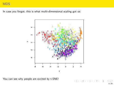
In case you forgot, this is what multi-dimensional scaling got us:

You can see why people are excited by t-SNE!

4 / 26

Epochs

t-SNE is an iterative process; here we can see the results at different “epochs”:

100 iterations 200 iterations

500 iterations 1000 iterations

5 / 26

It gets better

By default, tsne uses Euclidean distance. If we use Manhattan distance:

6 / 26

And even better

By default, tsne uses Euclidean distance. If we use Manhattan distance and changesomething called the perplexity:

7 / 26

2. How t-SNE works

t-SNE has two main steps:

1 compute pairwise similarities between the observations in high dimensions whileestimating a“bandwidth” for each observation that preserves perplexity

2 compute new coordinates in low dimensions for the observations with almost thesame pairwise similarities while solving the crowding problem

Easy!

8 / 26

Entropy

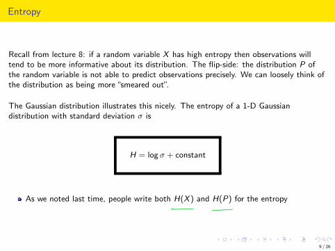
Recall from lecture 8: if a random variable X has high entropy then observations willtend to be more informative about its distribution. The flip-side: the distribution P ofthe random variable is not able to predict observations precisely. We can loosely think ofthe distribution as being more“smeared out”.

The Gaussian distribution illustrates this nicely. The entropy of a 1-D Gaussiandistribution with standard deviation 𝜎 is

H = log 𝜎 + constant

As we noted last time, people write both H(X ) and H(P) for the entropy

9 / 26

Why“entropy”?

I thought of calling it ‘information’, but the word was overly used, so I decidedto call it ‘uncertainty’. ... Von Neumann told me, ‘You should call it entropy,for two reasons. In the first place, your uncertainty function has been used instatistical mechanics under that name, so it already has a name. In the secondplace, and more important, nobody knows what entropy really is, so in a debateyou will always have the advantage.

– Claude Shannon

10 / 26

Perplexity

The perplexity is just what you get if you exponentiate the entropy. Perplexed?Perplexity really measures the same thing as entropy: a distribution with high perplexityis not able to predict outcomes precisely – it is more“perplexed”!

The perplexity PP of a 1-D Gaussian distribution with standard deviation 𝜎 is

PP ∝ 𝜎

Perplexity is usually defined for discrete distributions but the Gaussian exampleworks for us

Also some people use log2 in the formula for entropy, so for them“exponentiate”means“2 to the power of”

11 / 26

Pairwise similarities in high dimensions

The first step of t-SNE is to compute pij , the pairwise similarities between theobservations in high dimensions.

We start with:

pj|i =exp(−‖xi − xj‖2/2𝜎2

i )∑jexp(−‖xi − xj‖2/2𝜎2

i )∝ exp(−‖xi − xj‖2/2𝜎2

i )

Actually we have seen this before: it’s very similar to our Gaussian radial basisfunction k(xi , xj) except we are using 𝜎 “properly”and there is a 𝜎 for each i

Also we have normalized pj|i so that looks like a conditional probability – hence thenotation

We can also replace the squared Euclidean distance ‖xi − xj‖2 in the formula withany pairwise distance dij

12 / 26

Choosing the bandwidth

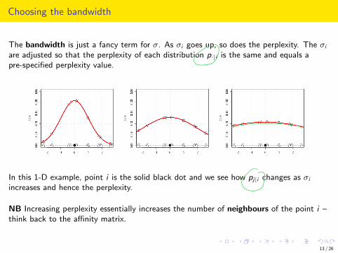
The bandwidth is just a fancy term for 𝜎. As 𝜎i goes up, so does the perplexity. The 𝜎i

are adjusted so that the perplexity of each distribution p·|i is the same and equals apre-specified perplexity value.

In this 1-D example, point i is the solid black dot and we see how pj|i changes as 𝜎i

increases and hence the perplexity.

NB Increasing perplexity essentially increases the number of neighbours of the point i –think back to the affinity matrix.

13 / 26

Final pairwise similarity

The final form of the pairwise similarity is

pij =1

n·

pj|i + pi|j

2

this takes into account j being similar to i and i being similar to j

dividing by n makes this a probability over all pairs of observations

14 / 26

Pairwise similarities in low dimensions

We will let qij denote the pairwise similarities in low dimensions. They will be a functionof zi and zj – recall that zi is the coordinates of point i in the lower dimensional space.The approach of t-SNE is to find the zi so that the qij are as close to the pij as possible.

15 / 26

Distance between distributions

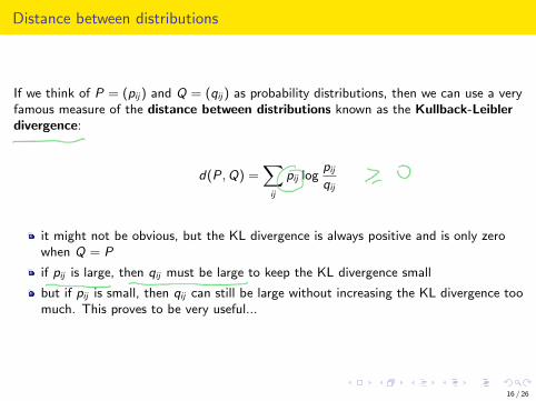
If we think of P = (pij) and Q = (qij) as probability distributions, then we can use a veryfamous measure of the distance between distributions known as the Kullback-Leiblerdivergence:

d(P, Q) =∑ij

pij logpij

qij

it might not be obvious, but the KL divergence is always positive and is only zerowhen Q = P

if pij is large, then qij must be large to keep the KL divergence small

but if pij is small, then qij can still be large without increasing the KL divergence toomuch. This proves to be very useful...

16 / 26

The crowding problem

Dimensionality reduction means“squeezing”points into lower dimensions. As we’ve seen,it is often quite difficult to find room for all the points.

t-SNE has a clever way to avoid the crowding problem: it uses a heavy-tailedt-distribution (default: 1 degree of freedom; aka the Cauchy distribution) to constructthe qij :

qij =(1 + ‖zi − zj‖2)−1∑ij(1 + ‖zi − zj‖2)−1

∝ (1 + ‖zi − zj‖2)−1

The point of the distribution being heavy-tailed is that points can be well-separatedwithout changing the value of qij too much.

17 / 26

Let the fun begin!

Now all t-SNE has to do is choose starting guesses for the zi , then iteratively move themaround until d(P, Q) is as small as possible. And this is how we got the first plot:

> library(tsne)> fun = tsne(X)

sigma summary: Min. : 0.422826979084241 |1st Qu. : 0.627751203772222 |Median : 0.702142079789048 |Mean : 0.695131663019661 |3rd Qu. : 0.767139352480269 |Max. : 0.977977608343072 |Epoch: Iteration #100 error is: 17.5459293434803Epoch: Iteration #200 error is: 0.989784276331286. . .Epoch: Iteration #800 error is: 0.773994463745339Epoch: Iteration #900 error is: 0.772523611519527Epoch: Iteration #1000 error is: 0.77147459129725

> plot(fun,pch=as.character(lab),col=colmap[1+lab],xlab="",ylab="")

by default, the perplexity is 30 and the number of iterations is 1000

we get a summary of the bandwidths 𝜎i at the start

the“error” is the KL divergence, which has pretty much levelled out by the end

18 / 26

3. More examples

t-SNE does a nice job reducing the penguin data from 4 dimensions to 2 dimensions,even for different perplexities. The obvious clusters that show up correspond to thepenguin species – but remember this is not a clustering or a classification exercise.

19 / 26

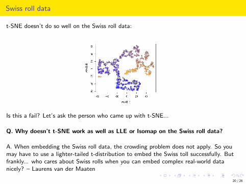
Swiss roll data

t-SNE doesn’t do so well on the Swiss roll data:

Is this a fail? Let’s ask the person who came up with t-SNE...

Q. Why doesn’t t-SNE work as well as LLE or Isomap on the Swiss roll data?

A. When embedding the Swiss roll data, the crowding problem does not apply. So youmay have to use a lighter-tailed t-distribution to embed the Swiss toll successfully. Butfrankly... who cares about Swiss rolls when you can embed complex real-world datanicely? – Laurens van der Maaten

20 / 26

Gene expression data

The following data set gives 1838 gene expression levels for 2638 cells. The cells are of 8different types. Treating the cells as the observations, we carry out PCA, colour-codingby cell-type:

> cellpc = prcomp(scale(celldat))> plot(cellpc$x[,1],cellpc$x[,2],col=1+as.numeric(celltype),xlab="",ylab="")

21 / 26

with t-SNE

For such a large data set, it is easier to use Rtsne. It uses some approximations so isquicker than tsne but it can be important that the data is scaled – see later.

> library(Rtsne)> cell_tsne = Rtsne(celldata)> plot(cell_tsne$Y,col=1+as.numeric(celltype),xlab="",ylab="")

22 / 26

Data exploration?

But what happens if we treat the genes as observations? Does t-SNE give us any insightinto how the genes might be related to each other?

> library(Rtsne)> gene_tsne = Rtsne(t(celldata))> plot(gene_tsne$Y,xlab="",ylab="")

23 / 26

Usage notes for tsne and Rtsne

Useful perplexity values tend to be between 5 and 50, but of course you may chooseothers

tsne and Rtsne choose random starting values for the zi , therefore dimensionalityreduction will look different each time

Check that the KL divergence is levelling out and adjust max_iter accordingly; forRtsne you will need to also set verbose=TRUE

It is possible to set the embedded dimension to be something other than 2 byspecifying k=... in tsne or dims=... in Rtsne

Scaling the data can help; computationally it is often useful not to have very large orvery small values in your data matrix

You can supply dist object to tsne and Rtsne instead of a data matrix, e.g.dist(X,method="manhattan") computes Manhattan distances between theobservations. In Rtsne you will need to also set is_distance=TRUE

24 / 26

General comments about t-SNE

t-SNE examples can look extra good when we have labelled data; things aren’talways so clear cut!

t-SNE is a data exploration tool but it can uncover features that are useful inclustering, classification and regression

t-SNE can suffer from the curse of dimensionality if the intrinsic dimension is highsince it typically depends on distance measures

t-SNE can be quite slow when n is large – using tsne, my laptop maxes out atabout n = 1000. The Rtsne package can be tried instead

The optimization process is also quite hard – approximation techniques areimplemented in Rtsne but there can be a loss of accuracy

25 / 26

And...

Thank you!

26 / 26