STAT 101

Topics: Syllabus, Nature of StatisticsHandouts: Green Sheet #1; Assignment Schedule; Anatomy of Statistics (2): 1) Statistical Alphabet, 2) Statistical Relationships; SYLLABUS – online on Blackboard and web pageOnline: All handouts; PowerPoint for the Nature of StatisticsCourse Assignments:

1) Review text (see syllabus for options). Scan through text for general format, etc. Review: Ch. 1, section 1.12) Go online to the Anatomy of Statistics link and look at a couple of these documents.3) Go online, scan through the SPSS Manual Procedures section to get an idea of the current manual’s format. 4) Items below

Next Class: Nature of Statistics – Terminology (cont.)

Stat Essentials (What I should know from today): Be able to: 1) define “Data”; 2) define a “Variable”; 2) distinguish between objective (response/dependent) and explanatory (independent) variables; 3) identify variables to be studied when provided a study scenario; 4) other terms if we get there; and 5) syllabus.

DATA & VARIABLES: Data: Data are “factual information (as measurements or statistics) used as a basis for reasoning, discussion, or calculation” (Merriam-Webster online dictionary definition).Variables: Variables are pieces of information (characteristics) gathered from people, squirrels, cumquats, fruit flies, businesses or other sources and which vary from one unit of the population to another. A person’s hair color and handedness represent variables, as does the circumference of ball bearings. There are two basic types of variables:

o Objective Variables (Dependent, Response): These variables represent the characteristics about which you want to learn – weight, eye color, speed of cars; life span of monarch butterflies.

o Explanatory Variables (Independent, Predictor): These variables help us refine our understanding of the Objective Variables of interest – gender, age, business size, environmental conditions.

Variables have Valueso Values may be word or numerical in nature.o The values of a variable are what are compared via data analysis processes.

Problem 1.1: Nutrition According to a study published in the Journal of the American Dietetic Association:CHICAGO – The intake of added sugars in the United States is excessive, estimated by the US Department of Agriculture in 1999-2002 as 17% of calories a day. Consuming foods with added sugars displaces nutrient-dense foods in the diet. Reducing or limiting intake of added sugars is an important objective in providing overall dietary guidance. In a study of nearly 30,000 Americans published in the August 2009 issue of the Journal of the American Dietetic Association, researchers report that race/ethnicity, family income and educational status are independently associated with intake of added sugars. Groups with low income and education are particularly vulnerable to eating diets with high added sugars. [For Release August 4, 2009; excerpt from ADA webpage 8.26.2009]

1. Identify an objective variable for this study (i.e. what do researchers want to learn about?). What values could this variable assume?

2. Identify three explanatory variables (i.e. what variables could affect the objective variable?). What values could these variables assume?

Problem 1.2: Diet Calcium & Blood PressureA heart researcher is interested in studying the relationship between diets which are high in calcium and blood pressure in adult females. The researcher randomly selects 20 female subjects who have high blood pressure. Ten subjects are randomly assigned to try a diet which is high in calcium. The other ten subjects are assigned to a diet with a standard amount of calcium. After one year the average blood pressures for subjects in both groups will be measured and compared to decide if diets high in calcium decrease the average blood pressure.

1. Identify the objective variable for this study and its associated values.

2. Identify the explanatory variable and its associated values.

Problem 1.3: Get Married - Gain Weight

11.16.2020

1

Researcher Penny Larson and her associates wanted to determine whether young couples who marry or cohabitate are more likely to gain weight than those who stay single. The researchers followed 8,000 men and women from 1995 through 2002 as they matured from the teens to young adults. When the study began, none of the participants were married or living with a romantic partner. By 2002, 14% of the participants were married and 16% were living with a romantic partner. At the end of the study, married or cohabitating women gained, on average, nine (9) pounds more than single women, and married or cohabitating men gained, on average, six (6) pounds more than single men. [p21sullivan]

1. Identify an objective variable for this study and its associated values.

2. Identify an explanatory variable and its associated values.

Problem 1.4: Obesity and Artery CalcificationScientists were interested in learning if abdominal obesity is related to coronary artery calcification (CAC). The scientists studied 2,951 participants in the Coronary Artery Risk Development in Young Adults Study to investigate a possible link. Waist and hip girths were measured in 1985-86, 1995-96 (year 10) and in 2000-01 (waist girth only). CAC measurements were taken in 2001-02. The results of the study indicated that abdominal obesity measured by waist girth is associated with early atherosclerosis as measured by the presence of CAC in participants. [p21sullivan]

1. Identify an objective variable for this study and its associated values.

2. Identify an explanatory variable and its associated values.

Problem 1.5: Balance: Eyes closed average of three trials (seconds to two decimals):

First Second Third AverageRight foot trial times: _____ _____ _____ _____Left foot trial times: _____ _____ _____ _____

One of the leading health concerns for people over 60 is falling. Balance in walking and standing is dependent on many factors. (www.vestibular.org)

As people grow older, they may have difficulty with their balance. Roughly 9 percent of adults who are 65 and older report having problems with balance. Having good balance means being able to control and maintain your body's position, whether you are moving or remaining still. An intact sense of balance helps you: walk without staggering; get up from a chair without falling; climb stairs without tripping. Balance disorders are one reason older people fall. According to the Centers for Disease Control and Prevention, more than one-third of adults ages 65 years and older fall each year. Among older adults, falls are the leading cause of injury deaths. (nihseniorhealth.gov)

Aging and balance-good news, bad news: Running & FitNews, April, 2002 Here's the bad news. Along with the visible signs of aging, and the obvious declines in the cardiovascular, respiratory, and orthopedic systems, your body is slowly assembling a collection of deficits that significantly reduce your ability to maintain balance. A decrease in balance ability, if nothing else, can increase your risk of acute running injuries such as sprains and falls.

Balance is a matter of collecting information from the environment on where your body is in space and how its position is changing, and then responding with adjustments by your musculoskeletal system. Age-related changes occur in the sensory, motor, cognitive, and musculoskeletal systems, all affecting your ability to perceive and process the necessary environmental cues, and to respond quickly and efficiently to the information. Visual acuity, depth perception, contrast sensitivity, and peripheral vision decline with age and these changes reduce or alter the environmental data your brain uses to maintain balance. Meanwhile, your sensitivity to tactile messages, such as vibration and sensory input from the soles of your feet, is also declining, causing you to rely more on your decreased visual abilities. At the same time, the tiny hair cells within the vestibular system are becoming less sensitive to head motion, diminishing the response of the ocular reflex that stabilizes your eyes. These balance deficits are probably the main reason you will almost never see individuals beyond 60 or so, riding a roller coaster for fun.

There is good news, however. First of all, runners and other athletic individuals probably suffer these declines more slowly than their sedentary contemporaries. Even better, there is still more you can do to slow declines in balance ability. To test your balance, try standing on one leg with your arms folded over the raised leg, knee tucked toward your chest, for 30 seconds. You should be able to do this without dropping the raised leg or hopping around. Next, if you felt reasonably stable on one leg, try 30 seconds with your eyes closed. Now try standing on both feet, with one foot directly in front of the other, heel touching toes. Repeat with your eyes closed. If nothing else, you will learn just how important visual cues are in maintaining balance. Exercises that challenge the multiple systems your body uses for balance, such as the two tests above, can slow age-related declines and even improve balance significantly, whatever your starting point.

One of the very best things you can do to improve and maintain balance is to use free weights for strength training. Lifting free weights requires attention to posture and form, while core-stabilizing muscles continuously adjust to the motion of the weights. Using a balance ball instead of a bench while lifting free weights, or standing on an unstable surface such as a balance board, further stimulates and challenges your balance. Include balance training in your fitness plan along with the training of the cardiovascular, musculoskeletal, and respiratory systems you get from running. It's one of the best things you can do to slow the aging process. For information on more balance exercises, go to http://gymball.com/balance_exercises.html. (Biomechanics, 2001, Vol. 8, No. 11, pp. 79-86); COPYRIGHT 2002 American Running & Fitness Association; COPYRIGHT 2003 Gale Group. Source: findarticles.com

STAT 101

2

TOPICS: Nature of Statistics Terms and RelationshipsDOCUMENTS:

HANDOUTS: Green #2; Yellow worksheet #1& 2: 1) Top Films and 2) Twenty-Five Q’s classification AVAILABLE ONLINE: All handouts listed above VIDEOS: General Terms & Measurement Scales: go to web page Stat 101 Videos listing

ASSIGNMENT: Readings: Ch. 1: sections 1.1-1.2; 1.3 (p. 20-24; sampling); Problems: p. 6 # 1-14, 21,24, 25-29; p. 13 # 1-12, 15, 16, 19–22, 29 Finish Worksheets #1 - Top Films and #2 - Twenty-Five Questions Items below

NEXT CLASS: Nature of Statistics: Sampling, etc.

Stat Essentials (taken from today): Be able to: 1) define terms and relationships as presented on the sheet Anatomy of the Basics: Statistical Terms and Relationships; 2) identify variables and their characteristics

Problem 2.1: An 8x12, 20-page Shutterfly photo book costs $29.00. How much would it cost given the above discount?

Problem 2.2: Classify each of the following as: 1) Qualitative or Quantitative; 2) Discrete or Continuous; and 3) identify the Level of Measurement.

The breaking strength of a given type of string.

The hair color of children auditioning for the musical Annie.

The number of stop signs in towns of less than 500 people.

Whether or not a faucet is defective.

The number of questions answered correctly on a standardized test.

The length of time required to answer a telephone call at a certain real estate office.

Problem 2.3: A heart researcher is interested in studying the relationship between diets which are high in calcium and blood pressure in adult females. The researcher randomly selects 20 female subjects who have high blood pressure. Ten subjects are randomly assigned to try a diet which is high in calcium. The other ten subjects are assigned to a diet with a standard amount of calcium. After one year the average blood pressures for subjects in both groups will be measured and compared to decide if diets high in calcium decrease the average blood pressure.

1) Identify the population.

2) What characteristic (variable) of the population is being measured?

3) Identify the sample.

4) Is the purpose of this data collection to perform descriptive or inferential statistics? [P15#1H&M]

5) Could blood pressure be used as an explanatory variable in this situation? Problem 2.4:

21.21.20

FREE SHIPPING on orders $39+* Code: SHIP39

3

Heroin Use: The National Center for Drug Abuse is conducting a study to determine if heroin usage among teenagers has changed. Historically, about 1.3 percent of teenagers between the ages of 15 and 19 have used heroin one or more times. In a recent survey of 1,824 teenagers, 37 indicated they had used heroin one or more times.

1) Identify the population.

2) Identify a variable of interest.

3) Identify a sample.

4) Is the purpose of this data collection descriptive or inferential?

Problem 2.5:Cell Phone Frau d : Lambert and Pinheiro (2006) described a study in which researchers try to identify characteristics of cell phone calls that suggest the phone is being used fraudulently. For each cell phone call, the researchers recorded information on its direction (incoming or outgoing), location (local or roaming), duration, time of day, day of week, and whether the call took place on a weekday or weekend. [WSed3p6]

1) Identify the observational units in this study.

2) Identify the qualitative variables and their characteristics.

3) Identify the quantitative variables and their characteristics.

4) Would call duration be a good explanatory variable? Why/why not?

Problem 2.6:Student Characteristics: A Case represents all of the information collected from one source, such as a student.Student #1 is a male who does not smoke, who lives in an urban area, and who would prefer to win an Olympic gold medal over an Academy Award or Nobel Prize. He indicates that he exercises 10 hours a week, watches television one hour per week, and has a GPA of 3.33. A resting pulse rate of 58 beats per minute, the oldest of three children and a desire to become a fireman represent other characteristics of this student.

Identify the variables for which data were obtained and classify them as qualitative (categorical)/quantitative, discrete/continuous, and provide a measurement level for each variable.

If similar information were obtained from 49 other students, which variables might most likely be used as explanatory variables?

Problem 2.7:Iceland: According to World Bank data, 90% of Icelanders have access to the Internet. In order to determine this value, what were the units from which this figure was obtained? What was the variable of interest (objective variable) and what were the values of this variable? Identify the variable’s characteristics (Qual/Quant etc.) (L5p.7)

If one were to look at the number of people worldwide with access to the Internet, we could record the proportion within each country. In doing so, what would be the population units? What was the variable of interest (objective variable) and what were the values of this variable? Identify the variable’s characteristics (Qual/Quant etc.)

4

STAT 101

TOPICS: Nature of Stats; Sampling; Combinations (?)DOCUMENTS:

HANDOUTS: Green #3; Yellow #3: Sampling AVAILABLE ONLINE: Green #3; Yellow #3: Sampling; PowerPoint

placed online (3): 1) Sampling; 2) Experimental Design; 3) Combinations & Permutations

ASSIGNMENTS: Text Readings: Ch. 1: pp. 20-22; Text Problems: p. 6 #15-20, 22, 25-27, 35-38; p.13 #17, 18, 23-

25, 30 Items below

NEXT CLASS: TOPICS: Combinations, etc., Qualitative Data (?); QUIZ #1 DUE: nothing

Stat Essentials (taken from today): Be able to: 1) identify sampling approaches; 2) understand relationships among basic statistical terms; 3) distinguish between combinations & permutations (if get there). Problem 3.1: The grade for this course is based upon 400 points. These points are converted to a 100-point base to result in a final course grade.

1. How many of the 400 points represent one point of the final grade?

2. Extra credit points are added to those you have accrued throughout the course via exams, etc. If you complete ten extra credit exercises, and receive full credit for them all (i.e. 10 points), by how many points will your final grade increase?

3. Over the course of the semester Elijah elects to not submit three, 10-point class assignments. By how many points would his final grade decrease as a result of not having submitted these three assignments?

Problem 3.2: Burglaries: ADT Security Systems advertised that “when you go on vacation, burglars go to work.” Their ad stated that “according to FBI statistics, over 26% of home burglaries take place between Memorial Day and Labor Day.” What is misleading about this statement? (Triola7ed,p15#6)

Problem 3.3: Election: Review the cartoon to the right. Assume that there are 100 boys and 100 girls. Demonstrate using these 200 students how this student’s conclusion is either correct or incorrect. Present your answer using both numerical computations and sufficient discussion to support your findings.

31.23.20

KNOW THESE RELATIONSHIPS:Population > Census > ParameterSample > Portion of a Pop. > StatisticsQualitative Variable > Word-based values > Nominal or OrdinalQuantitative Variable > Numeric > Discrete or Continuous > Interval or RatioMeasurement Levels > differences between

KNOW THE DIFFERENCES AND WHERE PROBABILITY SAMPLING COMES INTO PLAY

What is Probability Sampling Simple Random Sample (SRS) Systematic Sampling Stratified Sampling Cluster Sampling Convenience Sampling

5

Problem 3.4: Variables: Identify the explanatory and objective variables in the following pairs of variables.

A) Lung capacity and number of years smoking cigarettes

B) Blood alcohol content and the number of alcoholic drinks consumed

C) Year and world record time in a marathon

Problem 3.5: O-Tiger price hike: For many years Oneonta had a single-A farm team of the NY Yankees, which was followed by a farm team of the Detroit Tigers. When the Tigers arrived, the prices for seating changed. The following comes from an editorial in the local newspaper about the rise in ticket prices for the local single-A professional baseball team. “General admission season passes for adults will be $155, up from $70, in 2009, while six-seat boxes will go up 500 percent, from $300 to $1,500.” (source: The Daily Star, In Our Opinion column for Feb. 7 & 8, 2009, p D3; this team has since left town)

A) The $85 increase in the single seat price represents how much in terms of a percentage increase?

B) Demonstrate using a numerical analysis whether or not the cost of a six-seat box increased by 500%.

Problem 3.6: Seat Belts: Suppose that there are 300 students taking statistics and that they are asked if they always use seat belts.

A) If 27% of the students indicate that they do not always use seat belts, how many students is this?

B) Suppose that in different course 20% of the students do not use seat belts and that the 20% represents 43 students. How many students are in this class?

6

STAT 101

TOPICS: Sampling, Combinations & Permutations, Qualitative Data (?)DOCUMENTS

HANDOUTS: Green #4; Yellow #3B (sampling) & #4 (combinations); Writing descriptive statements; Quiz #1

AVAILABLE ONLINE: Green #4; Yellow #3B (sampling) & #4 (combinations); Writing descriptive statements; PowerPoints: Combinations.ppt; Qualitative ppt.; Related Anatomy Sheets (5): 1) Anatomy of a Systematic Random Sample; 2) Qualitative Frequency Table; 3) Pie Chart; 4) Pareto Chart; 5) Bar Chart

HWK: Text Readings: Ch. 2 – pp. 56-57 (pie & pareto charts); Anatomy of Statistics – Bar, Pie, Pareto Charts Text Problems: p. 23 #1-3, 7-10, 19-26 Additional problems available on Yellow #3 (Sampling) & #4 (Combinations) Review Writing Descriptive Statements (handout) Items below

Next Class: TOPICS: Qualitative Data; DUE: nothing

Stat Essentials (taken from today): Be able to: Combinations etc.:1) determine the number of samples via combinations; 2) calculating permutations, tree diagrams and the multiplication rule for independent events; Qualitative Data: 1) basics of qualitative data analysis (maybe).

COMBINATIONS & PERMUTATIONS on the TI Calculator: Math > Prob > select P or C, input the n and r values > enter; Factorials: enter the number, then go to Math > Prob > !

Problem 4.1: Identify the variables and their characteristics:1: The number of doctors who wash their hands between patient visits.2: The majors of randomly selected students at a university.3: The average weight of mature German Shepherds.4: The category which best describes how frequently a person eats chocolate: Frequently, Occasionally, Seldom, Never.5: The temperature this morning at 7:00 a.m.6: The diameter of major league baseballs.7: The average horsepower of ten randomly selected 1.6L MINI Cooper engines.

Data Source* Variable Qual/Quant Discrete/Cont Nom/Ord/Int/Ratio

1: __________ _______________ __________ __________ __________

2: __________ _______________ __________ __________ __________

3: __________ _______________ __________ __________ __________

4: __________ _______________ __________ __________ __________

5: __________ _______________ __________ __________ __________

6: __________ ______________ __________ __________ __________

7: __________ ______________ __________ __________ __________*NOTE: Data Source is the population or sample unit from which you obtain the data, not the variable information (data) collected.

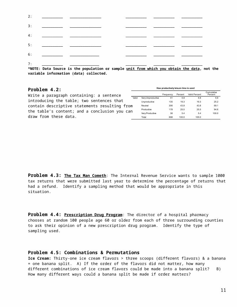
Problem 4.2:

41.28.20

GROWTH PROBLEMS (e.g. #3.5): The formula is [new value – old value]/old value]. This gives you the increase/decrease in a value over time.

7

Write a paragraph containing: a sentence introducing the table; two sentences that contain descriptive statements resulting from the table’s content; and a conclusion you can draw from these data.

Problem 4.3: The Tax Man Cometh: The Internal Revenue Service wants to sample 1000 tax returns that were submitted last year to determine the percentage of returns that had a refund. Identify a sampling method that would be appropriate in this situation.

Problem 4.4: Prescription Drug Program: The director of a hospital pharmacy chooses at random 100 people age 60 or older from each of three surrounding counties to ask their opinion of a new prescription drug program. Identify the type of sampling used.

Problem 4.5: Combinations & PermutationsIce Cream: Thirty-one ice cream flavors > three scoops (different flavors) & a banana = one banana split. A) If the order of the flavors did not matter, how many different combinations of ice cream flavors could be made into a banana split? B) How many different ways could a banana split be made if order matters?

Permutation Calculation Combination Calculation

8

STAT 101

TOPICS: Combinations; Qualitative DataDOCUMENTS

HANDOUTS: Green Sheet #5; Yellow #5; CA#1; NOTE: SS#1 Is online AVAILABLE ONLINE: Green #5; Yellow #5; CA#1 & SS#1; PowerPoints: Qualitative Data,

Contingency TablesASSIGNMENTS:

Text Readings - Ch. 2 – pp. 56-57 (pie & pareto charts); pp. 168-171 permutations & combinations Text Problems – if we get here: p. 62 #23, 24 (make bar chart instead of pie), 25, 26. CA#1 SS#1 (available at: Supporting Materials > under the Class Assignment & Statistical Software link) Items below.

FORMULAS: Multiplication Rule for Independent Events: k1 *k2 *k3∗. .. *kn-1 *kn [read as: event 1* event 2 * etc.]

Permutations: n Pr=

n!(n−r ) ! Combinations:

n C r=n !

(n−r )! r ! Next Class: TOPICS: Qualitative Data; Contingency Tables DUE: CA#1, SS#1

Stat Essentials (taken from today): Be able to: Combinations etc.:1) determine the number of samples via combinations; 2) calculating permutations, tree diagrams and the multiplication rule for independent events; Qualitative Data - 1) build qualitative tables; 2) build qualitative charts: pie, bar, pareto.

Problem 5.1: Combinations & PermutationsCoca Cola Directors: There are 11 members on the board of directors for the Coca Cola Company. A) If they must elect a chairperson, first vice president, second vice president; and secretary, how many different slates of four candidates are possible? B) If they must form a four-member ethics committee, how many different committees are possible?

Permutation Calculation Combination Calculation

Problem 5.2:In 2005 a television advertisement for Allstate Auto Insurance noted that last year (2004) 1.3 million people switched to Allstate. What is missing here?

51.30.20

9

Problem 5.3:Permutations & Combinations: You have ten paintings to hang, but only space to hang three. A) How many different ways could these paintings be hung if order matters? B) If order didn’t matter, how many different groups of three paintings could occur?

Problem 5.4:Village Life: Identify the variable characteristics below.

Variable:

Qual or Quant: Measurement Level:

Write a brief paragraph regarding the information in this table.(See how to write a paragraph on sheet #4.)

Problem 5.5:Cell Phones:

Variable: Cell Phone Satisfaction Characteristics are: Categorical/Quant Discrete/Continuous/Neither N/O/I/R

Values: 1 = Fair; 2 = Good; 3 = Very Good; 4 = ExcellentData (n=31): 1,2, 3, 3, 3, 2, 2, 3, 3, 4, 3, 1, 3, 1, 3, 3, 3, 2, 2, 4, 3, 3, 3, 2, 2, 4, 4, 3, 3, 3, 3

Task 1: Build a qualitative frequency table of the variable Cell Phone. Include a table title, the variable values, frequencies, relative frequencies, cumulative frequencies, and cumulative relative frequencies.

Task 2: Build a Bar Chart of the variable Anxiety Level. Task 3: Build a Pie Chart of the variable Anxiety Level. Task 4: Build a Pareto Chart of the variable Anxiety Level. Task5: Write a paragraph that introduces the tables & charts, two sentences that describe information

contained within the frequency table, and a summary statement.

Rating of qual i ty of l i fe in vi l lage

4 1.1 1.2 1.283 23.1 23.9 25.1

183 50.8 52.7 77.860 16.7 17.3 95.117 4.7 4.9 100.0

347 96.4 100.013 3.6

360 100.0

ExcellentVery GoodGoodFairPoorTotal

Valid

SystemMissingTotal

Frequency Percent Valid PercentCumulat ivePercent

10

STAT 101

TOPICS: Qualitative Data (practice); Contingency tables

DOCUMENTS HANDOUTS: Green Sheet #6; Contingency Tables Reference AVAILABLE ONLINE: Green #6; Yellow #6; Contingency Table and Quantitative PowerPoints; Anatomy Sheets (5):

Contingency tables; Quantitative Frequency Table; Histogram; Dot Plot; Stem-and-Leaf.HWK:

Text Readings - Ch. 2 sections 2.1 – 2.2; p. 551 – contingency tables Text Problems: p. 62-64 - # 24, 26, 33, 35 - 38. Yellow #5 problems not used in class Items below

Next Class: TOPICS: Quantitative Data: Tables & Charts

Stat Essentials (taken from today): Be able to: QUALITATIVE: 1) calculate relative frequency, cumulative frequency, and cumulative relative frequency for response values; 2) build appropriate tables and charts; CONTINGENCY TABLES: 1) build tables; 2) interpret them.

Problem 6.1:Interpreting Contingency Tables: Answer the following items based upon the accompanying contingency tables.

Table #1:1) Table Size: This is a ____ by ____ contingency table.

2) Count Question: The number of students from a rural area who indicated the importance of outdoors as being very important is ____.

3) Row Question: Among respondents indicating the importance of outdoors while growing up to be moderately important, ____ % were from an urban cluster area.

4) Column Question: Among respondents from an urban area ____ % indicated that the importance of outdoors while growing up was not really important.

5) Totals Question: Respondents from a rural area who indicated that the importance of outdoors while growing up was not really important represent ____ % of all respondents.

Problem 6.2: Pie Chart: Use the right marginal totals from Table 1 to build a pie chart and frequency table of the variable: Importance of outdoors while growing up.

62.4.20

11

STAT 101

TOPICS: Contingency Tables, Quantitative Data Tables, Charts & GraphsDOCUMENTS

HANDOUTS: Green #7; Yellow #7 (Quantitative Data); CA#2 (SS#2 is ONLINE) AVAILABLE ONLINE:

o Green #7; Yellow #7; CA#2; SS#2o PowerPoint (2): Quantitative Data; Frequency Polygons & Ogives; o Anatomy Sheets (4): Quantitative Frequency Table; Histogram, Dot Plot, Stem-and-Leaf;

HWK: Text Read: Ch. 2 sections 2.1, 2.2. Text Problems: p. 47 #2 – 5, 7, 8, 11, 19, 21, 25, 31 CA#2 SS#2 Items below.

Next Class: TOPICS: Quantitative Data – Charts (cont.) DUE: Ex#2 (Friday); CA#2, SS#2 (Tuesday)

Stat Essentials (taken from today): Be able to: CONTINGENCY TABLES: 1) build tables; 2) interpret them; Quantitative Data: 1) build a frequency table appropriate for the presentation of quantitative data; 2) identify frequency table components – classes, boundaries, etc.; 3) build charts/graphs appropriate to quantitative data – histogram, dot plot, stem-and-leaf, frequency polygon, ogive (won’t get to all today).

Problem 7.1: Contingency Tables: Using the table below, find the requested percentages or counts. The data present three cities in which houses were sold and during which month the houses sold.

What is the size of this contingency table? ____ by ____

Among houses sold in Arlington, what percent were sold in June and July?

During August _____% of the houses were sold in Fort Worth.

Among all houses _____% were sold in Dallas during September.

Looking at the right marginal totals column what does the 131 value represent?

T or F: Thirty percent of the houses sold in June were sold in Dallas.

T or F: Thirty-two percent of the houses were sold in Fort Worth.

T or F: Of the houses sold in July, approximately 25% were sold in Dallas.

72.6.20

12

Problem 7.2:

This is a ____ by ____ contingency table.

Three males (____ %) are unsure if they agree with the statement that the earth is like a spaceship with limited resources.

Among individuals who mildly disagreed with the statement that the earth is like a spaceship with limited resources, ____ % were females.

Among all respondents ____ % (n= ____) mildly agree with the statement that the earth is like a spaceship with limited resources.

Among females ____ % mildly or strongly agree with the statement that the earth is like a spaceship with limited resources.

Problem 7.3: Obtaining statistical output and providing analysisIdeal Weight: Twenty five students reported their ideal weights (in most cases, not their current weight). Weights (lb): 110 115 123 130 105 119 130 125 120 115 120 120

120 110 120 150 110 130 120 118 120 135 130 135110

Create a frequency table containing five classesWrite a paragraph containing an introduction and a minimum of two descriptive statements.

Identify:Midpoint of the third class: ___________ Boundaries of the first class; ____________

Class limits of the second class: ___________ Width of the classes: ____________

13

STAT 101

TOPICS: Quantitative Tables & Charts DOCUMENTS:

HANDOUTS: Green #8, Yellow #8 AVAILABLE ONLINE: Green #8; Yellow #8, PowerPoints (4): 1) Distribution Shapes; 2) Sigma; 3)

Quantitative Data; 4) Quantitative Charts - Freq. Polygon, Ogive, Line Chart ppt. ANATOMY REFERENCE SHEETS: various charts for quantitative data

HWK: Text Reading: Ch. 2, review sections 2.1-2.2 – graphs & charts Text Problems: p. 47 #13, 15, 19, 29, 37, using #32, only make a dot plot, no table; using #35, only make a stem-and-

leaf plot (no table) Items below

Next Class: TOPICS: Distribution shapes; SIGMA); Measures of Center (?)

Stat Essentials (as with prior class): Be able to: 1) build a frequency table appropriate for the presentation of quantitative data; 2) identify frequency table components – classes, boundaries, etc.; 3) build charts/graphs appropriate to quantitative data – histogram, dot plot, stem-and-leaf, frequency polygon, ogive.

Problem 8.1: Nutrition Bars: (NOTE: Assume Lower Class Limits are shown)

How many values are in the data set?

How many classes are there?

What is the width of a class?

How many milligrams of sodium are in the nutrition bar with the highest value?

Explain how a relative frequency histogram would differ from the displayed chart. (Hint: Think about how frequency and relative frequency bar charts differ?)

Problem 8.2: Contingency Tables: Using the contingency table, find the requested percentages or counts. The data present the opinions of students regarding ecological disaster possibilities based upon their geographic origin.

What is the size of this contingency table? ____ by ____

Among students from urban areas, what percent strongly agreed?

For Unsure respondents, _____% were from Rural areas.

Among all respondents, _____% were from Urban Clusters.

Looking at the right marginal totals column what does the 30 value represent?

Respondents who were from Urban areas and Mildly Disagree with the statement represent what percent of all respondents?

T or F: Sixty percent of the respondents were from a Rural area and indicated a Mildly Agree response.

T or F: Approximately 17% of respondents were from Urban areas.

T or F: Of the respondents selecting Strongly Agree, approximately 33% were from Rural areas.

82.11.20

14

Problem 8.3: Retirement Ages: (Larson & Farber p. 51 #39)Using the following data, build both a single stem and a double stem, stem-and-leaf.

Ages: 70 54 55 71 57 58 63 65 60 66 57 62 63 60 63 60 66 60 67 69 69 52 61 73

Problem 8.4: Retirement Ages: Using the data from problem 8.3, build a frequency table containing five classes. [NOTE: Without a stated starting point, make sure that the minimum value fits into the first class and the maximum value is within the fifth class. If the latter does not occur, either shift the starting point of the first class, while maintaining class width, or increase the size of the class width.]

15

STAT 101:

TOPICS: Distribution Shapes; Time Series Charts; Σ (Sigma); Measures of Center (?)DOCUMENTS:

HANDOUTS: Green #9; Yellow #9; CA#3; SS#3 (ONLINE) AVAILABLE ONLINE: Green #9; Yellow #9; CA#3; SS#3; PowerPoints for: 1) Sigma, 2)

Measures of Center; 3) Distributions, 4) Time Series Charts (in with Freq. Polygon & Ogive); Anatomy sheets: SigmaASSIGNMENTS:

Text Readings: Ch. 2, sections 2.3, 2.4 Text Problems: p. 48 #21, 23; p. 60 #17 (single stem), 18 (double stem), 29, 32, 34 (part c & d only; will do scatter

plots when we get to correlation) CA#3 SS#3 Items below

NEXT CLASS: Measures of Center (cont.), Variation, and Position (?) DUE: EX#3

Stat Essentials (taken from today): Be able to: DISTRIBUTIONS: 1) identify distribution shapes and characteristics; TIME SERIES: 1) create time series chars (line charts) given two variables; SIGMA: 1) understand what the symbol (Sigma) means; 2) successfully demonstrate the application of MEASURES OF CENTER 1) calculate an arithmetic mean, median, mode; 2) identify when you would use each of these measures.

Problem 9.1:An introductory statistics class had three exams, for which the grade distribution of each exam is presented to the right. For each exam describe the distribution’s shape and comment on the exam’s difficulty. [Consider the x-axis point C1 to be the exam’s mean grade.]

Distribution Shape Difficulty of Exam (easy, average, hard)

Exam #1: _________________ _________________

Exam #2: _________________ _________________

Exam #3: _________________ _________________

Problem 9.2:SIGMA: Given the following data for X and Y, determine the values of Sxx and Syy.

X Y S xx=Σx 2

−(Σx )2

n S yy=Σy 2

−(Σy )2

n =

20 4

38 10

10 2

68 8

104 28

92.13.20

16

87 23

Problem 9.3:SIGMA: Given the following data for X and Y, determine the values of r. [Note: same data as in problem 9.2.]

X Y r= nΣ xy−( Σx)( Σy )

√ [nΣx2−(Σx )2 ] [nΣy2−(Σy )2 ]=

20 4

38 10

10 2

68 8

104 28

87 23

Problem 9.4Time Series: Create a time series chart of the Murder Rates in New York City

Murder Rates in NYC*Year Rate1990 14.51991 14.21992 13.21993 13.31994 11.11995 8.51996 7.41997 6.01998 5.11999 5.02000 5.02001 5.02002 4.82003 4.92004 4.62005 4.52006 4.82007 4.22008 4.32009 4.02010 4.52011 3.92012 3.52013 3.02014 2.7

*per hundred thousand

17

STAT 101:

TOPICS: Distribution Shapes; Σ (Sigma); Measures of CenterDOCUMENTS:

HANDOUTS: Green #10 AVAILABLE ONLINE: Green #10; PowerPoints for: 1) Sigma, 2) Measures of Center; 3)

Distributions, 4) Time Series Charts (in with Freq. Polygon & Ogive); Anatomy sheets: SigmaASSIGNMENTS:

Text Readings: Ch. 2, review 2.3, 2.4 ; read 2.5 Text Problems: p. 77 # 55, 56 [NOTE: INSTRUCTIONS FOR THESE TWO PROBLEMS ARE ON P. 76 prior to problem 53],

57 (if we get to means) Items below

NEXT CLASS: Measures of Center (cont.), Variation, and Position (?)

Stat Essentials (taken from today): Be able to: DISTRIBUTIONS: 1) identify distribution shapes and characteristics;; SIGMA: 1) understand what the symbol (Sigma) means; 2) successfully demonstrate the application of MEASURES OF CENTER 1) calculate an arithmetic mean, median, mode; 2) identify when you would use each of these measures.

Problem 10.1Aggravated Harassment: Build a time series chart of the data presented in the following table.Aggravated Harasssment Cases 2000-2013NYC Polce Pricinct 1

Larose Discovering Statistics 3rd ed p.93 # 17Year 2000 2001 2002 2003 2004 2005 2006 2007 2008 2009 2010 2011 2012 2013Number 547 568 476 475 450 445 379 424 404 425 429 343 400 400

Problem 10.2Atmospheric Carbon Dioxide Levels: Build a time series chart of the data presented in the following table.Atmospheric Carbon Dioxide at Mouna LoaOctober 2012 to Septemer 2013

Larose Discovering Statistics 3rd ed p.93 # 21Month: Oct. Nov. Dec. Jan. Feb. Mar. Apr. May June July Aug. Sep.

CO2 (ppm): 391.01 392.81 394.28 395.54 396.80 397.71 398.35 399.76 398.58 397.20 395.15 393.51

Problem 10.3Aggravated Harassment: Using the data in the aggravated harassment table (above) make a frequency table containing five classes.

102.18.20

18

STAT 101

TOPICS: Measures of Center & VariationDOCUMENTS:

HANDOUTS: Green sheet #11; Yellow #11; LAB#1 AVAILABLE ONLINE: Green #11; Yellow #11; LAB#1 (located online in Class

Assignments); PowerPoint: Measures of Center, Measures of Variation, Measures of Position.ASSIGNMENTS:

Text Review: Ch. 2 section 2.3-2.5 Text Problems: p. 77 # 53, 57; p. 90 #1-5, 15-18, 25, 29 LAB#1: Turn in anytime, but ALL PARTS DUE BY Feb. 27 QUIZ #3 Tuesday: Topics: Dist. Shapes, Measures of Center; Qual & Quant. Tables and Charts, and … Items below

FORMULAS (For Samples): Mean Variance Standard Deviation

Definition formula: x=

∑i=1

n

x i

ns2=

Σ( x−x¿)2

n−1 s=√∑ ( x− x )2

n−1USE THESE FORMULAS

Computational formula: x=

∑i=1

n

x i

ns2=

nΣx2−( Σx )2

n(n−1) s=√ n∑ x2−( Σx)2

n (n−1 )

Median: 1) middle score if odd number of values; 2) mid-point between two middle scores if even number of valuesMode: most frequent value (multiple modes may exist); represents the center of qualitative data

Midrange: minimum+maximum

2

NEXT CLASS: TOPIC: Variation & Position QUIZ#3 on Tuesday (2.25) DUE: 2.27.20 LAB#1

Stat Essentials (taken from today): MEASURES OF CENTER: Be able to: 1) calculate an arithmetic mean, median, mode; 2) identify when you would use each of these measures; MEASURES OF VARIATON: Be able to:1) explain what a standard deviation represents; 2) obtain a standard deviation using either formula (definition or computational); 3) interpret what the standard deviation represents in a given situation; 4) Empirical Rule;.5) Chebychev’s Theorem.

Problem 11.1:Blood Pressure: Given the following sample of systolic blood pressures, determine their mean, median, mode, and midrange; using the COMPUTATIONAL FORMULAS, determine the variance and standard deviation for this variable.

Systolic Pressures: 120 145 86 133 115 124 153 98 144 132

112.20.20

19

Problem 11.2 CRICKETS:

THE DATA: Temperature vs. Cricket Chirps: Crickets make a chirping noise by sliding their wings over each other. Perhaps you have noticed that the number of chirps seems to increase with the temperature. The following data list the temperature (Fahrenheit) and the number of chips per second for the striped ground cricket.

X: Temperature (Fo): 69.4 69.7 71.6 75.2 76.3 79.6 80.6 80.6 82.0 82.6 83.3 83.5 84.3 88.6 93.3Y: Chirps/second: 15.4 14.7 16.0 15.5 14.4 15.0 17.1 16.0 17.1 17.2 16.2 17.0 18.4 20.0 19.8

Determine the mean, median, mode, and midrange for both of these variables.

20

STAT 101

NOTICE: ANYONE SEEKING TO TAKE THE MID-TERM EXAM AT ACCESSIBILITY RESOURCES, MUST COMPLETE A REQUEST TO DO SO ONLINE.

TOPICS: Measures of Variation; Measures of Position DOCUMENTS:

HANDOUTS: Green #12, Yellow #12 AVAILABLE ONLINE: Green #12, Yellow #12; PowerPoint: Measures of Position

ASSIGNMENT: Text Review: Ch. 2 section 2.4-2.5 LAB#1 – ALL PORTIONS DUE NO LATER THAN THURSDAY (2.27)

Items below FORMULAS (For Samples): Mean, Median, Mode, Midrange, Variance, Standard Deviation on prior page

Five-Number-Summary: Minimum – Q1 – Q2 – Q3 - MaximumChebychev’s Theorem: 1- 1/k2 where k ≥2; Used with any shape distributionEmpirical Rule: Used with normally distribution data

z-score: z= x−μ

σ Pearson’s I=3( x−median )

sCVAR= s

x¿ ∗100 % Q1=

n+14

M=Q 2=n+1

2 Q3=3(n+1)

4 Probability Rules: 1) ΣP ( X )=1 2) 0≤P( X )≤1

NEXT CLASS: TOPIC: Measures of Position/ Topic Review for Mid-Term Exam DUE: LAB#1Stat Essentials (taken from today): Measures of Variation: Be able to:1) explain what a standard deviation represents; 2) obtain a standard deviation using computational formula; 3) interpret what the standard deviation represents in a given situation; 4) Empirical Rule; Measures of Position: 1) obtain the five-number-summary; 2) interquartile range; 3) build a box plot; 4) determine variability measures: skew (Pearson’s I), Coefficient of Variability, z-score.

Problem 12.1:Blood Pressure: Given the following sample of systolic blood pressures, determine their variance, standard deviation using the computational formula.

Systolic Pressures: 120 145 86 133 115 124 153 98 144 132NOTE: Calculations for the mean, median, mode are on prior green sheet (Problem 11.1).

Problem 12.2:

12

KNOW THE FOLLOWING STATISTICAL RANGES:Probability: 0 to 1, inclusiveStandard Deviation: 0 to ∞,inclusive {Note: One cannot obtain a negative std. dev.]Correlation: -1 to +1, inclusivez-score: any value, though most are between -3 and +3

Please be aware of the following, taken from the Feb. 20 email distributed to all class members: “2) LAB:  If you were not in class today, the LAB#1 papers are available online in the Supporting Materials > Class Assignments listing. THIS IS DUE NEXT THURSDAY ***NO EXCEPTIONS, NO TIME EXTENSIONS, NO EXCUSES. If you have parts done early, please consider submitting them early so that I can get to the grading.”

21

CRICKETS: THE DATA: Temperature vs. Cricket Chirps: Crickets make a chirping noise by sliding their wings over each other. Perhaps you have noticed that the number of chirps seems to increase with the temperature. The following data list the temperature (Fahrenheit) and the number of chips per second for the striped ground cricket.

X: Temperature (Fo): 69.4 69.7 71.6 75.2 76.3 79.6 80.6 80.6 82.0 82.6 83.3 83.5 84.3 88.6 93.3Y: Chirps/second: 15.4 14.7 16.0 15.5 14.4 15.0 17.1 16.0 17.1 17.2 16.2 17.0 18.4 20.0 19.8 Given: xxyyxy

NOTE: Calculations for the mean, median, mode for both of these variables are on prior green sheet (Problem 11.2).

Problem 12.2: Using the computational formula, determine the standard deviations for these two variables.

Problem 12.3 (z-score): A temperature of 93.3o is how many standard deviations away from the mean? Sixteen chirps per second is how many standard deviations away from the mean? (z-score questions)

22

STAT 101

TOPICS: Mid-Term review SessionDOCUMENTS:

HANDOUTS: Green #13; Yellow #13 (review sheet); AVAILABLE ONLINE: Green #13; Yellow #13 (located in Course Review

Materials listing) HWK:

Text Readings: Review prior green sheets for sections. Text Problems: Review prior text problems, green sheets and yellow worksheets for problems. Items below

FORMULAS TO DATE :

Combination/Permutations/etc.: Permutations: n Pr=

n!(n−r )! Combinations:

n C r=n!

(n−r )! r ! Both where n = number of items and r = number of items being used

Multiplication Rule for Independent Events: k1 *k2*k3∗. .. *kn-1 *kn [read as: event 1* event 2 * etc.]Measures of Center & Variation (computational formulas only):

Mean Variance Standard Deviation

Computational formula(s): x=

∑i=1

n

x i

ns2=

nΣx2−( Σx )2

n(n−1) s=√ n∑ x2−( Σx)2

n (n−1 )Median: 1) middle score if odd number of values; 2) mid-point between two middle scores if even number of valuesMode: most frequent value (multiple modes may exist); represents the center of qualitative data

Midrange: minimum+maximum

2

Measures of Position:Q1=

n+14 Q2=

n+12 Q3=

3(n+1)4

NEXT CLASS: MID-TERM EXAM Stat Essentials (taken from today): Be able to: Address topics to date:

Exam 1 Topic Areas for Review:See Handouts distributed through today. This is a comprehensive, cumulative exam.Potential exam topics:1. terms and their relationships2. assessing table & chart content for accuracy3. interpretation & discussion of table & chart content 4. recognition of appropriate/inappropriate data presentation5. sampling techniques – identification 6. combinations, permutations, multiplication rule for independent events, tree diagrams 7. building qualitative tables and charts (pie, pareto, bar)8. building quantitative tables (2 types) and charts (histogram, dot plot, stem-and-leaf, ogive; freq. polygon, time series)9. Distribution shapes10. SIGMA11. measures of center: mean, median, mode, midrange12. measures of variation: range, standard deviation, inter-quartile range (Q3 –Q1)13. Empirical Rule & Chebychev’s Theorem14. measures of position: minimum, Q3, Q2, Q1, maximum15.

Exam 1 Review Materials:1. Green sheets & answer key2. Yellow sheets & answer keys3. Anatomy of Statistics sheets (online)4. Sample Exams (online)5. Course Review Materials (online)6. In-class review problems (yellow #13)7. Text book & problems8. ME – stop in or make an appointment (Office Hours before exam TODAY ONLY: 8-8:20; 11:20-12; 1:30-2:20; 4:00 – 5:009. Must be something else…10. Must be something else…

132.27.20

23

STAT 101

TOPICS: MID-TERM EXAMDOCUMENTS:

HANDOUTS: Green #14 AVAILABLE ONLINE: Green #14

ASSIGNMENTS: TAKE A BREAK AFTER YOU READ THIS (could be on the next quiz)

NEXT CLASS: TOPIC: Position Measures: Box Plots, CVAR, I, z-scores; Square root by hand; Data collection (?) Stat Essentials (taken from today): To see what we know

Portion sizes increase in 'Last Supper' paintings (An application of statistics)By Nanci Hellmich, USA TODAY (3/23/2010)

If your food portions seem to have grown larger over the years, you have some blessed company.

Two researchers analyzed the food and plate sizes in 52 of the most famous paintings of The Last Supper and found that the portion sizes in the paintings have increased dramatically over the past millennium, from years 1000 to 2000.

Using a computer program, they compared the size of loaves of bread, main dishes and plates to the size of the heads of the disciples and Jesus in the artwork, including Leonardo da Vinci's famous depiction of the event.

Findings published in April's International Journal of Obesity: Over that 1,000-year period, the main course size increased by 69%, plate size 66% and loaves of bread 23%. The biggest increases in size came after 1500.

The researchers used paintings of this event "because it is the most famous supper in history," which artists have been painting for centuries, so the paintings provide information about plate and entree sizes over time, says Brian Wansink, director of the Cornell (University) Food and Brand Lab in Ithaca, N.Y. One possible reason for the increase: Food may have become more available and less expensive, he says.

He did the research with his brother, Craig, a professor of religious studies at Virginia Wesleyan College in Norfolk, and a Presbyterian minister.

The three Gospels (Matthew, Mark and Luke), which include descriptions of The Last Supper, mention only bread and wine, but many of the paintings have other foods, such as fish, lamb, pork and even eel, says Craig Wansink.

The use of fish in the meals is symbolic because it's an image that is used to represent Christianity, he says. Among the reasons for the symbolism: A number of the disciples were fishermen, and Jesus told them "to be fishers of men," he says. Plus, he says, Jesus performed several miracles with fishes and loaves.

As Easter approaches, he says, people may want to study the paintings because they illustrate one of the "most important moments in Christianity

ABOVE: "The Last Supper" painting by Duccio, 1308-11. Note the size of the food and drink on the table compared to the size of the heads of Jesus and his disciples.BELOW: "The Last Supper" painting by Tiziano Vecellio Titian.

143.3.20

24

STAT 101:

TOPICS: Measures of Position, etc.DOCUMENTS:

HANDOUTS: Green #15; CA#4 AVAILABLE ONLINE: Green #15, PowerPoint: Measures of Position

ASSIGNMENT: Items on yellow #12 (box plots, etc.) CA#4 Items below TAKE A BREAK

FORMULAS (For Samples): Mean, Median, Mode, Midrange, Variance, Standard Deviation on prior pageFive-Number-Summary: Minimum – Q1 – Q2 – Q3 - MaximumChebychev’s Theorem: 1- 1/k2 where k ≥2; Used with any shape distributionEmpirical Rule: Used with normally distribution data

Q1=n+1

4 Q2=n+1

2 Q3=3(n+1)

4 IQR=Q3−Q1

LowerLimit=Q1−1. 5( IQR) UpperLimit=Q3+1. 5( IQR)

z-score: z= x−μ

σ Pearson’s I= 3( x−median )

sCVAR= s

x¿ ∗100 %

NEXT CLASS: TOPIC: Correlation & Regression; Data Collection for Lab#2 (?) DUE: CA#4Stat Essentials (taken from today): Measures of Position: 1) obtain the five-number-summary; 2) interquartile range; 3) build a box plot; 4) determine variability measures: skew (Pearson’s I), Coefficient of Variability, z-score.

CRICKETS: THE DATA: Temperature vs. Cricket Chirps: Crickets make a chirping noise by sliding their wings over each other. Perhaps you have noticed that the number of chirps seems to increase with the temperature. The following data list the temperature (Fahrenheit) and the number of chips per second for the striped ground cricket.

X: Temperature (Fo): 69.4 69.7 71.6 75.2 76.3 79.6 80.6 80.6 82.0 82.6 83.3 83.5 84.3 88.6 93.3Y: Chirps/second: 15.4 14.7 16.0 15.5 14.4 15.0 17.1 16.0 17.1 17.2 16.2 17.0 18.4 20.0 19.8 Given: xxyyxy

NOTE: Calculations & Statistics for Crickets can be found on Green #11 & #12.

Problem 15.1: Determine the Coefficient of Variation for these two variables.

Problem 15.2 (z-score): A temperature of 93.3o is how many standard deviations away from the mean? Sixteen chirps per second is how many standard deviations away from the mean? (z-score questions)

153.5.20

25

Problem 15.3: Determine the degree of skew for these two variables.

Problem 15.4: make box plots of the two cricket variables.

Problem 15.5: If you were around for the square root by hand demo, try it yourself.

Find: √323488. 00

26