state-of-health estimation of li-ion batteries: cycle life
TRANSCRIPT

III
THESIS FOR THE DEGREE OF LICENTIATE OF ENGINEERING
JENS GROOT
Division of Electric Power Engineering Department of Energy and Environment
CHALMERS UNIVERSITY OF TECHNOLOGY Göteborg, Sweden 2012
State-of-Health Estimation of Li-ion Batteries: Cycle Life Test Methods

IV
State-of-Health Estimation of Li-ion Batteries: Cycle Life Test Methods JENS GROOT ©JENS GROOT, 2012 Licentiate Thesis at the Graduate School in Energy and Environment Division of Electric Power Engineering Department of Energy and Environment Chalmers University of Technology SE-412 96 Göteborg Sweden Telephone: +46 (0)31 772 1000 Chalmers Bibliotek, Reproservice Göteborg, Sweden 2012

V
State-of-Health Estimation of Li-ion Batteries: Cycle Life Test Methods JENS GROOT Division of Electric Power Engineering Department of Energy and Environment CHALMERS UNIVERSITY OF TECHNOLOGY
Abstract
Despite a rapid development, cost, performance and durability of the energy storage
system are still a hindrance for a wide commercialisation of heavy-duty hybrid electric
vehicles (HEV). The purpose of the work presented in this thesis is to investigate how
different load cycle properties affect the cycle life and ageing processes of Li-ion cells
developed for use in HEVs.
The cycle life of commercial LiFePO4/graphite Li-ion cells was tested using a range of
operating conditions and battery load cycles based on conditions relevant to heavy-duty
HEVs. Established methods for cell performance evaluation have been combined with
half-cell measurements and analysis methods such as incremental capacity analysis,
differential voltage analysis and impedance spectroscopy to characterise the cell ageing
in terms of capacity fade, power fade and impedance rise. Furthermore, a simplified cell
fade model is used to distinguish between different likely ageing mechanisms.
Loss of cyclable lithium is found to be the main contribution to ageing during the first
phase of cycling, followed by an accelerated loss of active anode material towards the
end of the battery cycle life. The longest lifetime is observed for cells cycled with low
peak currents and a narrow SOC range. In addition, high charge current is found to
affect the cycle life profoundly. On the contrary, a moderate temperature increase did
not result in a shorter cycle life.
Despite similarities in average current and SOC range, the load cycle properties are
found to have a significant effect on the ageing characteristics, indicating that a more
detailed evaluation of load cycle properties is needed to enable a cycle life estimation
model.
Index Terms: State-of-health, battery model, lithium-ion battery, cycle life test, battery testing, HEV, PHEV, EV, ICA, DVA, impedance spectroscopy

VI
“It is a good morning exercise for a research scientist to discard a pet hypothesis every
day before breakfast. It keeps him young.”
Konrad Lorenz

VII
Acknowledgements First and foremost I would like to thank my tutors Dr. Helena Berg and Dr. Hanna
Bryngelsson at Volvo and Prof. Torbjörn Thiringer at Chalmers who made this research
work possible. Without your support I would definitely have got lost in the infinite ways
to test and characterise battery ageing.
Throughout the investigation I have had a close cooperation with PhD-colleagues
Rickard Eriksson (Uppsala University, Uppsala), Matilda Klett and Tommy Zavallis
(The Royal Institute of Technology, Stockholm), Pontus Svens (Scania CV AB) and
François Savoye (Volvo Technology, Lyon). Our countless discussions of test methods
and possible ageing mechanisms have been essential to bring order and structure in my
work. In addition, Dr. Matthieu Dubarry at University of Manoa, Hawaii, has
contributed with input to various analysis methods.
I would also like to thank my family and my girlfriend Corin Porter for the
encouragement to “keep up the nerdy work”.
And finally, the financial support from the Swedish Energy Agency and AB Volvo is
greatly appreciated.
Jens Groot
Göteborg, Sweden
January, 2012

VIII

IX
Preface
In 2008, AB Volvo, Scania CV AB, the Royal Institute of Technology (KTH), Uppsala
University (UU) and Chalmers University of Technology started a joint research cluster
that aims to understand the ageing mechanisms of a Li-ion battery systems used in
heavy-duty HEV powertrains. The cluster is co-funded by the Swedish Energy Agency
and the two industrial partners.
The investigation focuses on finding the correlation between operating conditions in a
real application and the fundamental ageing processes in the battery cell. Research is
made on several levels; from in situ measurements on electrode materials and research
cells made by KTH and UU to applied tests of commercially available Li-ion cells in
laboratory and field applications performed by Volvo and Scania. More specifically
Volvo focuses on the development of models for the ageing mechanisms.
This thesis gives insights of how various operating conditions affect the life time of Li-
ion batteries used in heavy-duty vehicles. In addition, it presents a number of different
characterisation techniques that can be used to evaluate and understand the ageing
mechanisms. These results will also be the base for a development of Li-ion battery
ageing models for hybrid electric vehicles which is planned for in the continuation of
this work.

X

XI
Table of Contents CHAPTER 1 INTRODUCTION ....................................................................................................... 1
1.1 PURPOSE ...................................................................................................................................... 3 1.2 OUTLINE ...................................................................................................................................... 3
CHAPTER 2 LI-ION BATTERIES & CYCLE LIFE TESTING .................................................. 5
2.1 REFERENCE ELECTRODES & HALF-CELLS ................................................................................... 7 2.2 CHARACTERISATION OF LI-ION BATTERY LIFETIME ..................................................................... 8 2.3 AGEING MECHANISMS OF LI-ION BATTERIES – A LITERATURE REVIEW .................................... 10
2.3.1 SEI formation and reformation ............................................................................................ 13 2.3.2 Contaminations .................................................................................................................... 14 2.3.3 Lithium plating ..................................................................................................................... 14 2.3.4 Corrosion ............................................................................................................................. 14 2.3.5 Gassing ................................................................................................................................. 15 2.3.6 Migration of reaction products ............................................................................................ 15
2.4 BATTERY LIFE TEST METHODS ................................................................................................. 15 2.4.1 Accelerated Testing .............................................................................................................. 15 2.4.2 Calendar Ageing .................................................................................................................. 16 2.4.3 Standardised Cycles ............................................................................................................. 16 2.4.4 Cycle Life Evaluation ........................................................................................................... 17
2.5 AGEING MODELS ....................................................................................................................... 17 2.5.1 State-of-Health Modelling .................................................................................................... 17
CHAPTER 3 CYCLE LIFE TEST PROCEDURE ........................................................................ 19
3.1 REFERENCE PERFORMANCE TESTS ............................................................................................ 20 3.1.1 Calculation of Power and DC impedance ............................................................................ 23 3.1.2 Dynamic Response Test ........................................................................................................ 25
3.2 IMPEDANCE SPECTROSCOPY ...................................................................................................... 27 3.3 IN-CYCLE SOC ADJUSTMENT ..................................................................................................... 31 3.4 TEMPERATURE CONTROL .......................................................................................................... 34 3.5 HALF-CELL TESTS ..................................................................................................................... 35
CHAPTER 4 LOAD CYCLES ........................................................................................................ 37
4.1 REFERENCE LOAD CYCLE, CYCLE A .......................................................................................... 37 4.2 SYNTHETIC CYCLE EXTRACTION ............................................................................................... 41
4.2.1 Stochastic Model of Load Cycle ........................................................................................... 42 4.2.2 Implementation ..................................................................................................................... 44 4.2.3 Battery model used for SOC-estimation ............................................................................... 46 4.2.4 SOC Control Strategy ........................................................................................................... 48 4.2.5 Optimisation ......................................................................................................................... 50 4.2.6 Evaluation ............................................................................................................................ 52
4.3 SYNTHETIC CYCLE USED IN CYCLE LIFE TESTS, CYCLE B .......................................................... 55 4.4 CONSTANT CURRENT CYCLE – WIDE SOC-RANGE, CYCLE C ..................................................... 57 4.5 CONSTANT CURRENT CYCLE – NARROW SOC-RANGE, CYCLE D ............................................... 57 4.6 PHEV CYCLE, CYCLE E ............................................................................................................. 58 4.7 LOAD CYCLE COMPARISON ....................................................................................................... 59
4.7.1 Temperature Distribution ..................................................................................................... 60 4.7.2 SOC Range ........................................................................................................................... 60 4.7.3 Current Distribution ............................................................................................................. 61 4.7.4 Voltage Distribution ............................................................................................................. 62
CHAPTER 5 EXPERIMENTAL ..................................................................................................... 67
5.1 CELL SPECIFICATION & TEST MATRIX ...................................................................................... 67 5.2 TEST EQUIPMENT ...................................................................................................................... 70

XII
CHAPTER 6 CYCLE LIFE TEST RESULTS ............................................................................... 73
6.1 CAPACITY FADE ......................................................................................................................... 74 6.2 POWER FADE ............................................................................................................................. 76 6.3 IMPEDANCE GROWTH ................................................................................................................ 78 6.4 POWER EFFICIENCY AT LOW POWER.......................................................................................... 80 6.5 CALENDAR AGEING ................................................................................................................... 81 6.6 SUMMARY .................................................................................................................................. 82
CHAPTER 7 CELL AGEING ANALYSIS .................................................................................... 83
7.1 GALVANOSTATIC VOLTAGE PROFILES ....................................................................................... 83 7.2 DIFFERENTIAL VOLTAGE ANALYSIS & INCREMENTAL CAPACITY ANALYSIS ............................ 87
7.2.1 Calculation of DVA Profile ................................................................................................... 88 7.2.2 Calculation of ICA Profile .................................................................................................... 90
7.3 HALF-CELL TEST RESULTS ........................................................................................................ 92 7.4 CELL CAPACITY FADE MODEL BASED ON HALF-CELL MEASUREMENTS .................................... 93
7.4.1 Case 1: Loss of Cyclable lithium .......................................................................................... 98 7.4.2 Case 2: Loss of Active Anode Material ............................................................................... 101 7.4.3 Case 3: Loss of Active Cathode Material ........................................................................... 105 7.4.4 Case 4: Loss of Cyclable lithium and Active Electrode Material ....................................... 108
7.5 ICA & DVA OF AGED CELLS .................................................................................................. 111 7.6 ESTIMATION OF LOSS OF ELECTRODE CAPACITY AND CYCLABLE LITHIUM ............................ 114 7.7 IMPEDANCE GROWTH .............................................................................................................. 122
CHAPTER 8 CONCLUDING REMARKS ................................................................................... 127
CHAPTER 9 FUTURE WORK ..................................................................................................... 129
CHAPTER 10 REFERENCES ......................................................................................................... 131
Glossary AC Alternating Current BOL Beginning of Life DC Direct Current DVA Differential Voltage Analysis EIS Electrical Impedance Spectroscopy ESR Equivalent Series Resistance EOL End of Life EV Electric Vehicle HEV Hybrid Electric Vehicle ICA Incremental Capacity Analysis ICE Internal Combustion Engine KTH The Royal Institute of Technology PHEV Plug-in Hybrid Electric Vehicle RMS Root-Mean-Square RPT Reference Performance Test SEI Solid Electrolyte Interface SOC State of Charge SOH State of Health UU Uppsala University

Chapter 1 Introduction
1
Chapter 1 Introduction
Over the past ten years, hybrid electric vehicles (HEV) have been successfully
introduced to the passenger car market. Following numerous demonstrator projects,
several manufacturers of heavy-duty vehicles are currently investigating and/or
introducing the HEV technology to heavy-duty vehicles. In the mean-time, plug-in
HEVs (PHEV) such as the GM Chevrolet Volt™ or the Toyota Prius Plug-in™ are
being introduced to the passenger car market. This drivetrain topology might also be
suitable for certain heavy-duty applications, at least from a technical point of view.
Although the HEV and PHEV topologies still rely on the usage of an internal
combustion engine (ICE) the possible reduction of fuel consumption and emissions is
significant and may represent a leap in transportation efficiency and sustainability.
There are several possible advantages with the HEV drivetrain compared to a
conventional driveline based solely on an internal combustion engine. First and
foremost, the HEV drivetrain recuperates brake energy which can be used to enhance
vehicle acceleration, powering of auxiliary loads or to optimise the operation point of
the ICE. In addition, it may also reduce emissions and, in the case of PHEV, provide
limited all-electric drive and silent operation.
Even though incentives and other factors related to municipality and state legislation in
many countries and cities actively drive the development towards vehicles with lower
emissions and fuel consumptions, the feasibility of heavy-duty HEVs is still strongly
dependant on the performance and additional cost of the electric driveline components
[1]. Among these comparably new vehicle components, the energy storage, usually a
battery, is the single most expensive component. Hence, the performance, cost and
durability of the energy storage are critical for the overall feasibility of a heavy-duty
HEV/PHEV.

Chapter 1 Introduction
2
There is an intense and rapid development of batteries for use in HEVs and PHEVs. Not
only the electrical performance in terms of energy and power density is improved, but
also life, safety and production cost. Despite this rapid development the cost of batteries
is still high compared to other drivetrain components. Currently lithium-ion (Li-ion)
batteries are the most attractive chemistry, first and foremost due to strict requirements
in power and energy [2].
There are a large number of different types of Li-ion batteries, ranging from low-cost
mass-produced cells used in portable consumer electronics to advanced designs tailored
to meet specific requirements of aerospace and military applications. As of 2011, there
is no high volume production of Li-ion cells for automotive applications. Although
several new manufacturers are targeting this market the volumes are still small
compared to the production of cells for consumer electronics. Moreover, there are a
large number of different electrochemical designs of Li-ion batteries, each with
advantages and disadvantages related to cost, performance, cycle life and safety.
Considering safety and production cost one of the most capable cell type is the LiFePO4
// graphite cell, introduced to market fairly recently [3], [4]. However, the lifetime of Li-
ion batteries for HEVs is still uncertain, leading to a hesitation at both the manufacturer
and potential market end. To large extent this is due to the lack of accurate models for
prediction of the highly nonlinear battery ageing mechanisms in different vehicle
applications. Such models would enable an optimization of battery usage, which in turn
would lower the total battery cost and ensure a stable fuel economy throughout the
vehicle service life.
Furthermore, the design process and the real-time control of the HEV drivetrain,
including the energy storage, rely on accurate estimations on battery wear as a function
of operating conditions and usage. With the focus set at vehicle durability, this state-of-
health (SOH) estimation has become as important to the HEV as the estimation of state-
of-charge (SOC) is for electric vehicles (EV).
Currently, the SOH estimation models for industrial battery systems are often based on
field or laboratory measurements. Despite extensive testing under a wide range of
conditions these measurements may still lack relevance to an HEV application due to
the non-linear nature of battery degradation. In other words, the results obtained after
years of cycling a battery cell to a specific drive cycle is unlikely to be directly
Chapter 1 Introduction
3
applicable to other drive patterns/applications. This is a profound difference between the
HEV market and the consumer electronics market, where the battery load cycles
(discharge / charge pattern) are similar for the majority of applications (laptops, cellular
phones, digital cameras etc.) whereas each automotive application and market segment
has different requirements and operating conditions. As an example, batteries in HEV
passenger cars and trucks are used in a profoundly different way. Additionally, the use
of trucks and buses are diverse; the same type of vehicle might be used for both city
traffic and regional traffic and in different climates. Also, requirements on performance
and durability differ between different markets. Consequently, battery requirements for
heavy-duty HEVs cover a wide range in terms of cycle life, cost, performance and
durability. In contrast, commonality between vehicles is highly desirable, especially
when introducing new technology associated with high development cost. Hence, a
reliable prediction of battery life as a function of vehicle usage reduces the risk when
investing in this new technology.
1.1 Purpose
The purpose of the work presented in this thesis is to investigate how different load
cycle properties affect the cycle life and ageing processes of Li-ion cells developed for
use in HEVs. In particular, Li-ion cells using graphite anodes and LiFePO4 cathodes are
to be studied. Furthermore, a target is to perform extensive laboratory testing of
commercial Li-ion cells to develop and evaluate test methods for cycle life tests. The
cell ageing analysis is combined with results from field testing of cells performed by
Scania CV AB and research tests performed by KTH and UU. Finally, an objective is to
initiate the modelling of SOH which is to be developed in the continuing phase of this
investigation.
1.2 Outline
A limited literature survey concerning background information on Li-ion batteries,
ageing mechanisms and test methods is summarised in Chapter 2. This background
information is followed by a detailed description of the test procedure, selected load
cycles and the experimental set-up in Chapter 3, Chapter 4 and Chapter 5, respectively.
An overview of the cycle life test results is presented in Chapter 6, followed by an
analysis of the ageing mechanisms in Chapter 7 and concluding remarks in Chapter 8.

Chapter 1 Introduction
4

Chapter 2 Li-ion Batteries & Cycle Life Testing
5
Chapter 2 Li-ion Batteries & Cycle Life Testing
Li-ion batteries have been available as commercial products since the early 1990-ies.
Today, there exist numerous different types of Li-ion batteries based on different anode
materials, cathode materials, electrolytes and separators [3],[4]. A very simplified view
of the most commonly used cell materials is presented in Figure 2.1.
Figure 2.1 Overview of the most commonly commercialised Li-ion battery concepts.
The first commercial cells were based on a metallic lithium anode and a lithium-metal
insertion oxide as cathode. Despite superior energy density compared to other
commercial rechargeable batteries this cell type faced severe issues with safety and
reliability due to un-even lithium plating on the anode if re-charging leading to so called
dendrite growth, in turn leading to internal short-circuit and pre-mature failure. The
commercialisation of Li-ion cells was enabled by the use of a graphite intercalation
electrode as anode, greatly increasing safety, life and reliability. This anode type is still
dominating the market although a number of other anode materials such as hard-carbon,
lithium-titanate and silicon recently have been introduced. Likewise to the anode
development, there has been a rapid development of all the other cell materials;
numerous metal oxides, metal phosphates [5], blends and doped materials have
successfully been used as cathode. In addition, safety and reliability have been greatly
enhanced with new electrolytes (liquid or polymer type), binders, additives and
Polymer electrolyte
Separator
Liquid electrolyte
Anode Material
•Metallic Li
•Graphite
•Hard carbon
•Li-Metal Oxides:Li4Ti5O12
Electrolyte & SeparatorCathode Material
•Li-Metal Oxides:LiCoO2
LiMn2O4
LiNi1/3Co1/3Al1/3O
•Li-Metal Phosphates:LiFePO4
LiMnPO4
LiVPO4
Chapter 2 Li-ion Batteries & Cycle Life Testing
6
separators. Nevertheless, as sub-components of the cell are improved overall, each
component faces increasing challenges in mitigating the intrinsic disadvantages.
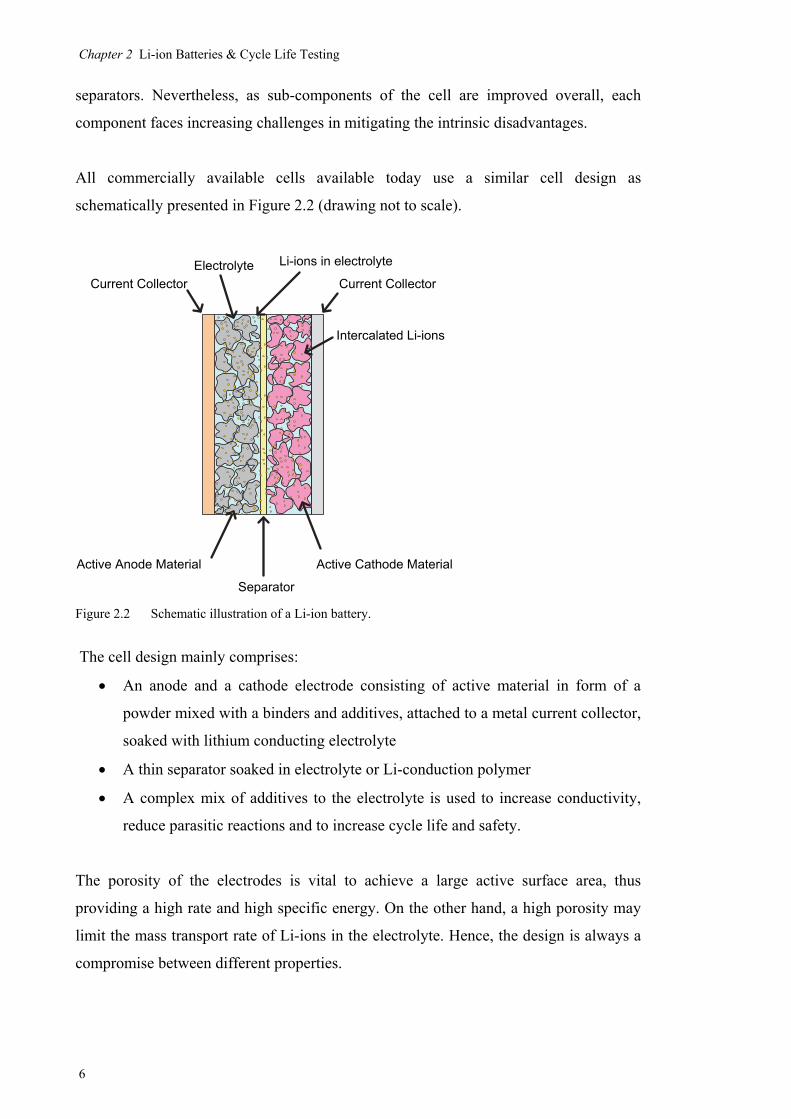
All commercially available cells available today use a similar cell design as
schematically presented in Figure 2.2 (drawing not to scale).
Figure 2.2 Schematic illustration of a Li-ion battery.
The cell design mainly comprises:
An anode and a cathode electrode consisting of active material in form of a
powder mixed with a binders and additives, attached to a metal current collector,
soaked with lithium conducting electrolyte
A thin separator soaked in electrolyte or Li-conduction polymer
A complex mix of additives to the electrolyte is used to increase conductivity,
reduce parasitic reactions and to increase cycle life and safety.
The porosity of the electrodes is vital to achieve a large active surface area, thus
providing a high rate and high specific energy. On the other hand, a high porosity may
limit the mass transport rate of Li-ions in the electrolyte. Hence, the design is always a
compromise between different properties.
Active Cathode Material
Separator
Active Anode Material
Current Collector Current Collector
Electrolyte
Intercalated Li-ions
Li-ions in electrolyte
Chapter 2 Li-ion Batteries & Cycle Life Testing
7
In a real cell each particle in the active region of the electrodes is glued together with a
binder to the current collector ensuring a good electrical conductivity between active
material and cell external terminals. The separator should block direct electron transfer
between electrodes but still provide a good path for Li-ions while maintaining
mechanical robustness and temperature stability.
The capacity and energy of a Li-ion cell is determined by the choice of active material,
and the amount of passive material. On the other hand, a comparably high ratio of
passive material such as binder, electrolyte solvent and current collectors is needed to
achieve high material transport and low losses that is vital for high-power applications.
Moreover, to maintain long cycle life and low price additional compromises with
performance is needed. In addition, the power capability of a battery is a function of a
number of factors: choice of cell materials, electrolyte, mechanical design, electrolyte
and the amount of passive material such as current collectors and terminals.
Consequently, the battery design is always a compromise between energy, power, cost
and service life.
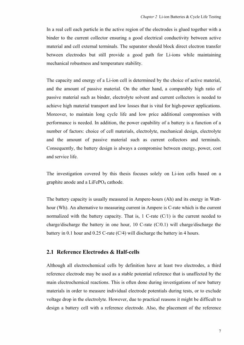
The investigation covered by this thesis focuses solely on Li-ion cells based on a
graphite anode and a LiFePO4 cathode.
The battery capacity is usually measured in Ampere-hours (Ah) and its energy in Watt-
hour (Wh). An alternative to measuring current in Ampere is C-rate which is the current
normalized with the battery capacity. That is, 1 C-rate (C/1) is the current needed to
charge/discharge the battery in one hour, 10 C-rate (C/0.1) will charge/discharge the
battery in 0.1 hour and 0.25 C-rate (C/4) will discharge the battery in 4 hours.
2.1 Reference Electrodes & Half-cells
Although all electrochemical cells by definition have at least two electrodes, a third
reference electrode may be used as a stable potential reference that is unaffected by the
main electrochemical reactions. This is often done during investigations of new battery
materials in order to measure individual electrode potentials during tests, or to exclude
voltage drop in the electrolyte. However, due to practical reasons it might be difficult to
design a battery cell with a reference electrode. Also, the placement of the reference

Chapter 2 Li-ion Batteries & Cycle Life Testing
8
electrode relative to the electrode surface will determine the outcome; essentially what
properties that can be measured with sufficient accuracy.
An alternative to the use of reference electrode may be to test one electrode at a time
against a large counter electrode with known properties. For Li-ion batteries this is
usually done by combining an anode or cathode material with a foil of metallic lithium
as counter electrode as illustrated in Figure 2.3 (drawing not to scale).
Figure 2.3 Schematic illustration of a half-cell with metallic lithium as anode.
Although this setup is not suitable for long cycle life tests because of the risk for
dendrite formation, it represents a comparably easy and reliable method to study the
properties of individual electrodes since the kinetics and reaction rate of the Li/Li+
reaction occurring at the lithium counter electrode is known.
2.2 Characterisation of Li-ion battery lifetime
All rechargeable batteries show a decreasing performance of usage and/or time. That is,
the capacity, measured as the ability to repeatedly store and release electric charge,
decreases. Likewise, the battery’s ability to be charged or recharged at high electric
power is reduced over time and the number of charge/discharge cycles. This reduction
in battery performance is usually referred to as battery ageing. For Li-ion batteries, it
has been shown the performance is affected by both storage time and usage, often

Chapter 2 Li-ion Batteries & Cycle Life Testing
9
categorized as calendar ageing [years] and cycle life [Maximum No. of cycles or
maximum operating time for a specific set of operating conditions.]. The calendar life is
often tested by storing cells in controlled temperature and at a fixed charge level. At
certain time intervals the cell performance is measured and the battery calendar life
expressed as the time the battery can be stored until the performance drops below a pre-
defined level.
The ageing of the battery is usually quantified as capacity and/or power or as a function
of number of charge/discharge cycles (defined separately), the total capacity throughput
(total amount of electric charge being cycled) or time (duration of test and/or total time
during charge / discharge). Generally, applications relying on the battery as a primary
energy source, such as electric vehicles and portable consumer electronics, are more
sensitive to capacity fade than power fade. Thus, the capacity fade is usually used to
quantify the aging for these applications. In contrast, HEVs that use the battery as an
energy buffer for short high-power charge/discharge and rarely use the full energy
storage capability of the battery are more sensitive to power fade than capacity fade.
Consequently, the power fade rate might be a better measure of ageing than capacity
fade for this type of application.
The battery cycle life can be tested by two main methods:
Simple and/or standardized cycles, often full discharge-charge profiles, used to
evaluate temperature dependency and to compare different cells / cell designs.
Evaluation of cycle life for specific applications. This includes field tests and
laboratory tests with load cycles matching the intended industrial applications.
Although the ageing mechanisms are similar, these two test methods might not provide
comparable results since most ageing processes within the cell are highly non-linear.
That is, small changes in the load cycle or operating conditions may cause one or a few
ageing processes to dominate, effectively limiting the total cycle life. Nevertheless,
analysis of the degraded cells serves as a very important input to further cell
development and optimization of the target application.

Chapter 2 Li-ion Batteries & Cycle Life Testing
10
Generally the overall process for characterising battery life time consists of three steps:
1. Measurement of initial performance at beginning-of-life (BOL)
2. Cycle life test or calendar life test with reference performance tests (RPT)
carried out on regular basis
3. Measurement of cell performance and cell degradation analysis at end-of-life
(EOL).
2.3 Ageing Mechanisms of Li-ion batteries – a Literature Review
The ageing of Li-ion batteries is complex and determined by the operating conditions
[6]-[9]. In some cases it is possible to assign the observed capacity and power fade to a
certain ageing process [10], [11]. This is typically the case when the battery is used
under extreme conditions such as elevated temperatures [6], high rate charging [12],
[13], or high SOC levels. However, in most applications where the conditions are
controlled to optimize the total life the observed performance fade is the result of
several process of which some are coupled and other can be regarded as independent
[9], [14].
The development of Li-ion batteries has been rapid since the introduction in the mid-
nineties. Hence, this survey is limited to the publications from 1999-2011 to focus at the
most recent development and cell designs used today. The following section
summarizes the main ageing mechanisms found in published papers / journals until
2011.
Being a complex combination of a large number of different processes, electrochemical,
mechanical and related to cell design, it is beyond the scope of this study to give a
comprehensive overview of all possible ageing mechanism. This section should be
regarded as a brief overview of the processes presented in selected publications
particularly useful for the work covered by this thesis.
Generally, the capacity fade of Li-ion cells is due to a combination of three main
processes [10]:
Loss of Li / loss of balance between electrodes
Loss of electrode area
Loss of electrode material / conductivity

Chapter 2 Li-ion Batteries & Cycle Life Testing
11
The loss of cyclable lithium is in turn due to side reactions such as corrosion, Li-plating
and solid electrolyte interface (SEI) formation at the graphite anode [15]-[17].
Since the graphite anode is the most widely used in present Li-ion batteries this study
has set a particular interest in this electrode material. In contrast the ageing properties of
the cathode electrodes must be discussed from case to case depending on the particular
cell design.
In addition, ageing mechanisms that reduce capacity may also lead to changes in surface
properties such as porosity and tortuosity [11]. In this reasoning it is important to state
that the available capacity might be reduced further by an increased voltage drop due to
a rise in cell impedance that prevents the battery from being fully discharged (or
charged) at a specific current [18], [19]. In most cases the capacity fade and impedance
rise are clearly correlated which will be investigated in the following sections. The
ageing processes are further complicated by the fact that many of the studied
mechanisms are coupled to a rise in cell impedance, leading first and foremost to a
notable reduction in maximum cell power.
An overview of the most significant mechanisms for power fade / impedance rise is
summarized by the following bullets and Figure 2.4:
Surface film formation of both electrodes with low conductivity [16], [20]-[22].
Loss of electrode area and electrode material leading to a higher local current
density [23].
Lower diffusivity of lithium ions into active electrode particles and slower
kinetics (increased charge transfer resistance) due to surface films
Reduced conductivity between particles due to both surface films and
degradation of binders, possibly in combination with a binder-Li reaction [23].

Chapter 2 Li-ion Batteries & Cycle Life Testing
12
Figure 2.4 Main ageing mechanisms occurring at Li-ion battery electrodes (blue text).
A summary of the main electrode ageing mechanisms, mainly described by Vetter et al.
[9], is presented in Figure 2.4. Here, ageing mechanisms can be categorized into
mechanical changes (particle cracking, gas formation), surface film formation (SEI,
lithium plating), bulk material changes (structural disordering [24]-[27]), and parasitic
reactions (binder degradation, localized corrosion). These ageing mechanisms are
described further in the following sections.
The ageing mechanisms at the electrodes are directly dependant on the choice of the
electrode material. However, there are several similarities between different electrode
materials.
According to several published papers [8], [9], [14], the bulk material properties of
anode and cathode do not change greatly over the service life of a Li-ion battery, but the
surface undergoes a significant change in mechanical structure and electrochemical
properties.
Current Collector Corrosion
SEI dissolution
SEI reformation & GrowthCathode particles acting as catalysts
Lithium plating
Graphene layers
Donor solvent
Li+Exfoliation
Current Collector Corrosion
Dissolution of soluble species
Surface film formation
Structural disordering
Graphite layers
Binder degradation
Graphite Dissordering / Particle cracking
Gas evolution
Micro-cracking
Micro-cracking

Chapter 2 Li-ion Batteries & Cycle Life Testing
13
2.3.1 SEI formation and reformation
Although being a widely used anode material for Li-ion batteries, graphite is not
electrochemically stable when used together with most common electrolytes. As the cell
is charged for the first time, lithium reacts directly with the graphite to form a thin solid
surface film (SEI) mainly consisting of Li2CO3 [28], alkyl-carbonates, and polymers.
Thereby, this process leads to an initial irreversible capacity loss. However, with a close
to completely covering film, further reaction (and consumption of lithium) is prohibited.
Since the SEI is very thin its conductivity for lithium ions remains sufficient to enable
an efficient intercalation of lithium into the graphite particles. On the other hand, a too
thin SEI allows electrons to tunnel through the film, in turn enabling other side reactions
and further SEI formation. Consequently, the SEI continues to grow until a steady-state
thickness is established which usually is reached after the few first cycles (commonly
denoted as the formation of the cell). Further formation of SEI has a significant effect
on the impedance of the cell. That is, a thin SEI is needed to limit the graphite direct
reaction with the electrolyte, but thick films are detrimental.
It has been shown that the SEI formed at low to medium temperature partly dissolves at
high temperatures, exposing the graphite surface to further reaction with electrolyte and
subsequent consumption of lithium [14].
In addition, the volume change occurring in the graphite particles upon intercalation /
de-intercalation of lithium might lead to micro cracks in the surface film, which also
exposes the graphite to further SEI formation. This is especially the case during deep
discharges since the main volume change occurs at SOC up to approximately 20%.
The SEI formation is according to Belt et al. [29] directly linked to the lithium
corrosion discussed in section 2.3.4 which produces both soluble and insoluble (SEI)
products.
A similar surface film growth may in some cases be observed at the cathode as well
[30], but as this process is less pronounced and directly dependant on the choice of
cathode material this survey includes no overview of this ageing mechanism.

Chapter 2 Li-ion Batteries & Cycle Life Testing
14
2.3.2 Contaminations
Traces of contaminations in the electrolyte stemming from either the manufacturing
process or from dissolved species from the cathode may also lead to SEI dissolving and
subsequent reformation at the expense of available lithium. Other possible processes
involve either irreversible loss of lithium or surface film formation. Especially traces of
water may accelerate ageing [31].
2.3.3 Lithium plating
The intercalation / de-intercalation of lithium into graphite occurs at an electrochemical
potential close to that of Li/Li+ and is one of the main advantages of using graphite as
anode material. On the other hand, if the surface potential of the graphite is forced
sufficiently low potentials lithium ions may form metallic lithium at the surface instead
of the intended intercalation. This process is not fully reversible as dissolution of Li
may form other compounds rather than lithium ions. Furthermore, a complete
dissolution of Li requires an electronic transfer through the SEI which, as highlighted in
section 2.3.1, is ineffective. Typically lithium plating is most pronounced at low
temperatures and / or high charge currents. In extreme cases a significant amount of the
lithium can be irreversibly consumed in just a few cycles.
2.3.4 Corrosion
Lithium corrosion is a wide definition of side reactions where lithium reacts with
electrolyte and / or electrodes to form soluble and insoluble products. Both reaction
categories primarily lead to irreversible loss of lithium. The soluble species mainly
participates in self-discharge processes and the insoluble species contributes to the SEI
formation and other relatively stable products [32].
The current collectors may also be susceptible to corrosion [33], especially if exposed to
potential close to or exceeding their electrochemical stability window determined by the
overall cell design and choice of materials.

Chapter 2 Li-ion Batteries & Cycle Life Testing
15
2.3.5 Gassing
Some parasitic reactions in the cell may lead to the formation of gaseous products,
mainly CO2. The gas evolution introduces mechanical stress to the electrodes which in
turn increases the rate of SEI reformation and, if severe, leads to a rupture of the cell
enclosure. In addition, it may reduce the active area of the porous electrode structure if
gas is trapped in pores. Furthermore some investigations [8] indicate that the presence
carbonates formed in the SEI increases the CO2 evolution.
2.3.6 Migration of reaction products
Side reactions occurring at anode and cathode may in some cases result in soluble
species that can migrate through the separator [6], [9]. The knowledge of the probable
impact of this process is not well established but it is indicated that they can increase the
formation rate of surface films at both electrodes.
2.4 Battery Life Test Methods
2.4.1 Accelerated Testing
Accelerated test methods are interesting for use by both cell manufacturers and
application developers. The combination of a narrow temperature range and non-linear
ageing reduces the possibilities to find an efficient and reliable method for significantly
reducing the time to test battery lifetime.
The studied publications mainly suggests the use of elevated temperatures (<+55 C°)
[34]-[36] in combination with medium temperatures to create models for the ageing
related to temperature within the nominal range of cell temperature. A similar approach
may be used for SOC levels [37], [38] and voltage [39], although the general feasibility
of this method depends on the choice of application and cell chemistry. To some extent
the ageing might be reduced by the use of additives to the electrolyte [40]. Generally,
the formation of surface films on electrodes accelerates significantly at elevated
temperatures [41].

Chapter 2 Li-ion Batteries & Cycle Life Testing
16
2.4.2 Calendar Ageing
Some of the ageing mechanisms occur even if the battery is not used, i.e. held at a
constant charge level or stored. This is usually tested by charging cells to a predefined
SOC level, usually 50-100%, and then storing the cell at constant temperature [36],
[42]-[44]. The charge level is often maintained by a constant voltage float charging and
the test may be accelerated by increasing the temperature [32].
It has been reported that the effect of calendar ageing is cross-dependant on cycling
[45]. In other words, the calendar ageing rate may be different if the cell was cycled
prior to the calendar test or in between calendar tests.
Heavy-duty HEVs or PHEVs are often in service for the majority of their service life in
contrast to passenger cars that are parked during the majority of their service life.
Hence, the study covered by this thesis focuses mainly on cycle life testing and cycle
life ageing.
2.4.3 Standardised Cycles
Simple and/or standardized cycles, often full discharge-charge profiles, used to evaluate
temperature dependency and to compare different cells / cell designs. There exist a
number of established test procedures including those from EUCAR [46], FreedomCar
[47] and IEC [48]. The most commonly used cycle life test is probably a 1 C-rate charge
and discharge profile using the full battery capacity (0-100% SOC) performed at room
temperature. Also, some alterations of this combining a higher discharge current with a
lower charge current or testing at a few different temperatures are commonly published
by cell manufacturers. The main disadvantage with using standardised cycles is that it is
very difficult to use the test results to evaluate the cycle life in an application not using
constant current or a wide current range. Nevertheless, the test data from these simple
cycles may still provide data for screening or comparing the general performance of
different cells/suppliers.
During the recent years there has been a trend where it is more common to use more
complex cycles as proposed by EUCAR, FreedomCar and IEC for cycle life tests. It is
however still not feasible to make an accurate estimate of the cycle life in more complex
cycles relying solely on this kind of measurements.

Chapter 2 Li-ion Batteries & Cycle Life Testing
17
2.4.4 Cycle Life Evaluation
In contrast to the simplified cycles or calendar life tests, cycle life evaluation carried out
for a specific application is usually defined in very close cooperation with the design of
the target application. That is, to evaluate the durability of a battery for an HEV a
logged load profile is used to repeat the exact usage pattern for that application.
Naturally, this provides a very reliable estimation of cycle life as long as the application
requirements do not change; a minor change in the SOC range, temperature or load
profile dynamics may yield a significant reduction in cycle life. Some applications, like
portable consumer electronics, satellites or power tools, have a very predictive usage
pattern or a short designed life time and can thus rely on cycle life tests using a narrow
range of test conditions.
2.5 Ageing Models
2.5.1 State-of-Health Modelling
A majority of the studied publications present empirical models, often based on
experimental data [49] from calendar life tests and cycle life tests with relatively simple
load cycles. Some models are based on statistical or mathematical methods [50]-[53],
other rely on models more closely built on electrochemical relations [54], There are
also semi-empirical models that are designed to model specific characteristics of the cell
like the impedance [55], [56], and models that uses a detailed empirical cell models as
the base [57], [58]. These empirical models may be especially feasible for use in HEV
simulations and drivetrain design.
The fundamental challenge in this field is to obtain a model that is both accurate and
without significant computational efforts or the absolute dependence on electrochemical
parameters that must be supplied by the cell manufacturer. However, several results
indicate that the empirical models can be used provided that their range of accuracy is
investigated in detail. For example, calendar ageing models developed for a range of
temperatures may successfully be used for prediction of SOH between the experimental
data range, although the relations between temperature and ageing is highly nonlinear.
Specific ageing processes such as the SEI growth under certain conditions can be
modelled by relatively simple relations although the complete ageing model still is very
complex [54], [59], [60]. Another approach for modelling cells and cell degradation is

Chapter 2 Li-ion Batteries & Cycle Life Testing
18
based on complex numerical 1D-models taking mass transport and reaction kinetics into
account [61]-[63]. Also, simpler models may be improved if fundamental models of the
cell surface structure are enhanced [64]. Often the ageing mechanisms on the cathode
and anode are dependent and must therefore be modelled as a coupled reaction [65].
Despite the advantages of using a detailed model based on electrochemical reactions
and transport processes, this category of ageing model is less suitable for multimodal
simulation with complex load cycles due to their requirement on ling computational
time.
Chapter 3 Cycle Life Test Procedure
19
Chapter 3 Cycle Life Test Procedure
HEVs and PHEVs may be one of the most challenging applications for battery cycle life
predictions since they have an extremely wide range usage patterns and strict
requirement of long cycle life. This is one of the key motives for the present work. In
order to evaluate and quantify battery ageing for this type of applications a customised
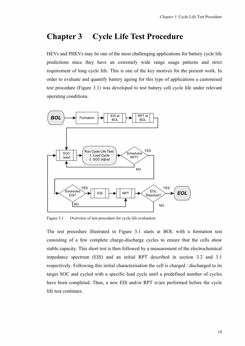
test procedure (Figure 3.1) was developed to test battery cell cycle life under relevant
operating conditions.
Figure 3.1 Overview of test procedure for cycle life evaluation.
The test procedure illustrated in Figure 3.1 starts at BOL with a formation test
consisting of a few complete charge-discharge cycles to ensure that the cells show
stable capacity. This short test is then followed by a measurement of the electrochemical
impedance spectrum (EIS) and an initial RPT described in section 3.2 and 3.1
respectively. Following this initial characterisation the cell is charged / discharged to its
target SOC and cycled with a specific load cycle until a predefined number of cycles
have been completed. Then, a new EIS and/or RPT is/are performed before the cycle
life test continues.
FormationEIS at BOL
RPT at BOL
SOC reset
Run Cycle Life Test:1. Load Cycle2. SOC adjust
Scheduled RPT?
NO
Scheduled EIS?
EIS
YES
YES
RPT
NO
EOL Reached?
NO
EOLYES
BOL

Chapter 3 Cycle Life Test Procedure
20
This process repeats until the cell performance is found to be less than the EOL criteria:
>20% loss of 1 C-rate capacity
>30% loss of power
Although EOL is defined by any of these two conditions the cycle life test has
continued in some cases to highlight interesting ageing behaviour.
Firstly, this section describes the regular RPTs and EIS measurements. Secondly, the
additional sub-procedure for maintaining a specific average SOC range is described.
Lastly, the method for controlling the cell temperature during each cycle life test is
described.
3.1 Reference Performance Tests
Even though the absolute life time of a cell cycled at different load cycles is of great
interest; it can be argued that the evolution of capacity, impedance and other cell
properties over the battery life provides profoundly more important information.
Generally, a RPT is performed regularly during a life test of a cell. Likewise to the SOC
adjustment described in section 3.3, the actual design of such test can have an effect on
the ageing it is designed to measure. That is, repeated deep discharge and full charge at
different current rates and multiple test pulses to determine the maximum power can
degrade the battery when conducted numerous times over a cycle life test.
Consequently, the design of a RPT is a compromise between quality of measured
parameters and the potential additional ageing it yields. Furthermore, according to
previous investigations [66] the design of a RPT may have a profound impact on the
measured parameters and their relevance to actual performance in a real HEV
application.

Chapter 3 Cycle Life Test Procedure
21
A customised RPT was developed within the research cluster between KTH, UU,
Scania AB, AB Volvo and Chalmers. This procedure consists of 6 main steps, see Table
1 and Figure 3.2, performed at room temperature (+23 °C).
Table 1 Reference performance test procedure performed at +23 °C.
Step Description Extracted parameters 1 Discharge to 0% SOC Residual capacity control of SOC-adjustment
procedure 2 Charge and discharge at 1 C-rate Voltage profile and standard 1C capacity 3 Charge and discharge at C/4 C-rate Voltage profile and capacity at low current rate.
Used for incremental capacity analysis and anode capacity estimation
4 Charge power at 10C-rate Dynamic response to high current rate, DC impedance at charge
5 Discharge power at 10C-rate Dynamic response to high current rate, DC impedance at discharge
6 SOC reset procedure Readjustment to target SOC, preparation for continued cycle life test
The current used for the charge and discharge power test has been 10 C-rate
respectively rather than the maximum specified cell current (see 5.1), and at a limited
SOC range in order to reduce possible ageing effects.
Figure 3.2 Overview of reference performance test procedure.
Each power pulse is 18 s in duration and followed by a 30 min rest period too allow for
accurate DC impedance calculations and temperature equalization. Charge power tests
0 5 10 15 20 25
2
2.5
3
3.5
4
Time [h]
Vol
tage
[V
]
Voltage
Step limitVoltage Limit
Step 4:Chargepower
Step 3: C/4 CapacityStep 2: C/1Capacity
Step 1: Residual capacity test
Step 5:Dischargepower
Step 6:SOCReset

Chapter 3 Cycle Life Test Procedure
22
are performed at 30, 50 and 70% SOC and discharge tests at 80, 60 and 40% SOC.
Here, the SOC is related to the nominal capacity, not the measured capacity in step 2 or
3. Consequently, the actual SOC relative to available cell capacity will change during
the cycle life test. This is, obviously, not the ideal case. However, since the anode and
cathode are likely to be cycled at a different SOC range relative to their respective Li-
content, it is barely possible to define SOC in a way that will not change with respect to
anode, cathode or cell during a long cycle life test. In addition, re-defining the nominal
capacity for each test would require significant manual work.
Three values of DC impedance are calculated (see section 3.1.1 below): ohmic
resistance, 10 s impedance and 600 s impedance.
A combined charge-discharge pulse (section 3.1.2) follows each power pulse and is
used to determine the dynamic response of the cell as well as energy efficiency during
dynamic pulses at medium power level.
In total, this test requires ca 24 h and results in two complete 100% ΔSOC cycles, one
partial cycle at ca 40% ΔSOC, and one partial cycle at 80% ΔSOC.

Chapter 3 Cycle Life Test Procedure
23
3.1.1 Calculation of Power and DC impedance
Each pulse in the power determination consists of a constant current / constant voltage
(CC/CV) charge/discharge step of 18s. The test current is set to allow the cell to reach
its upper voltage limit during charge pulses. In this way, higher cell impedance will lead
to reduced power for both charge and discharge steps. An example is shown in Figure
3.3 where a constant current of 10 C-rate is applied between t2 and t3 followed by a
constant voltage charge between t3 and t4 and a rest period.
Figure 3.3 Voltage profile for a LiFePO4 battery during a charge power test pulse (shortened rest
period t4 to t5 in this example).
The maximum discharge and charge power are tested at several SOC levels of the
battery. This internal state of the battery is directly related to the reference discharge
capacity measured during the formation of the battery and calculated from the C/4
capacity test in step 3 in Table 1.
Using the reference capacity, the SOC can be calculated by integrating the current
according to (3.1), starting at full SOC after a standard charge procedure.
RefStart
Ref
DchStart 3600
)()( start
C
dtI
SOCC
tCSOCtSOC
t
t
(3.1)
-10 0 10 20 30 40 50 60 70 80 90 100
3.3
3.4
3.5
3.6
Vol
tage
[V
]
-10 0 10 20 30 40 50 60 70 80 90 100
0
5
10
Cur
rent
[C
-rat
e]
Time [s]
U5t5
U4t4
U6t6
U3t3
U2t2
U1t1
U2t2
U3t3 U
4t4
U5t5
U6t6
U1t1

Chapter 3 Cycle Life Test Procedure
24
Different pulse power definitions can be used to extract power levels relevant for HEVs.
This specification recommends using the average pulse power for evaluation of power
fade rate.
The average pulse power is calculated using the measured voltage, current and time:
end
start
t
tstartendaverage dtIU
ttP
1
(3.2)
Note that discharge power (and discharge current) is defined to be < 0.
The ohmic resistance Rohm (3.3, 3.4) is calculated at both the start and the end of the test
pulse using a method similar to that used for power calculation, where the current I2 and
I3 are the currents measured at the start and the end of the pulse to obtain the immediate
voltage drop mainly associated to the ohmic resistance of the cell (Figure 3.3). Using a
short time difference between t1 … t2 and t4 … t5 it is possible to approximate the
measured impedance as the ohmic resistance in the cell, excluding the contribution from
the voltage drop caused by reaction kinetics and mass transport:
2
21start ohm, I
UUR
(3.3)
and
4
45end ohm, I
UUR
(3.4)
Alternatively, a separate impedance spectroscopy or AC resistance measurement at a
fixed frequency ≥1 kHz may be used to extract ohmic resistance at start as well as at the
end.
An approximate value for the total DC impedance RDC (3.5) of the cell is calculated
using the total voltage drop associated with each pulse over a set relaxation time t6-t5. In
this study two time periods were used: 10 s and 600 s.
4
64
I
UURDC
(3.5)

Chapter 3 Cycle Life Test Procedure
25
It should be emphasised that these resistance and impedance values are intended to be
used for comparisons during the cycle life tests rather than to be used in battery models,
performance calculations etc. For each measurement and calculation of Rohm and RDC the
approximate SOC level at t = t3 should be calculated and used as the actual SOC point
for each measurement rather than the initial SOC at t = t1.
Despite the varying SOC level it is still possible to use power and DC impedance to
evaluate ageing; by using the power measured power at the three SOC levels, it is
possible to make a linear interpolation to obtain the power at constant SOC level
relative to the measured capacity. This method may not be suitable for detailed forecasts
of power capability vs. SOC in a real application, but it is sufficiently accurate to give
an overview of the performance degradation over time.
3.1.2 Dynamic Response Test
In addition to the maximum pulse power measured in step 4 and 5 in Table 1, a short
sequence of charge/discharge pulses are performed to evaluate the power efficiency at
medium to low current rates (Table 2).
Table 2 Dynamic Response Test performed at +23 °C.
Step Sub-Step Description Duration
4, 5
1 Discharge CC/CV at 2 C-rate, minimum voltage Ucut-off1
10 s
2 Discharge CC/CV at 4 C-rate, minimum voltage Ucut-off1
3 Discharge CC/CV at 2 C-rate, minimum voltage Ucut-off1
4 Charge CC/CV at 2 C-rate, maximum voltage Umax1
5 Charge CC/CV at 4 C-rate, maximum voltage Umax1
6 Charge CC/CV at 2 C-rate, maximum voltage Umax1
1. According to specifications from cell manufacturer.
This sequence, also shown in Figure 3.4, contains charge and discharge pulses of 2 and
4 C-rate and is charge balanced. Thus, it can be used to give a comparable measure of
the average power efficiency at low to medium current rates. Higher impedance will
quickly lead to higher voltage drop and lower efficiency.
Chapter 3 Cycle Life Test Procedure
26
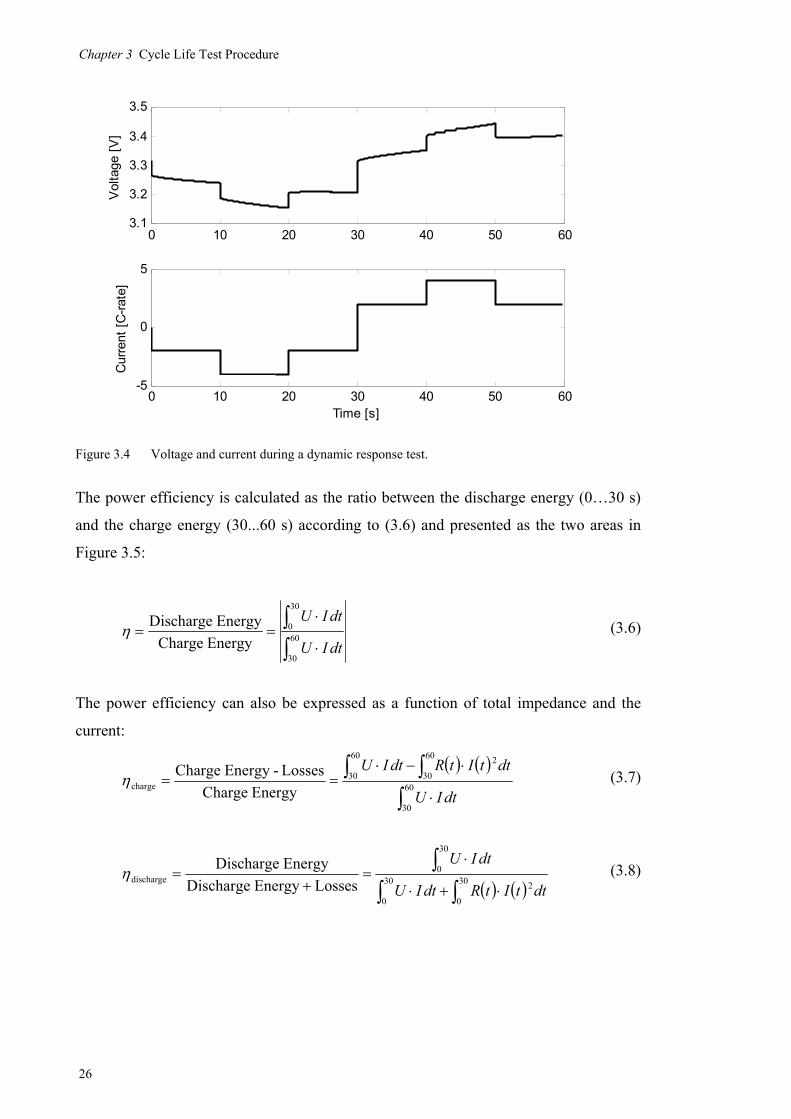
Figure 3.4 Voltage and current during a dynamic response test.
The power efficiency is calculated as the ratio between the discharge energy (0…30 s)
and the charge energy (30...60 s) according to (3.6) and presented as the two areas in
Figure 3.5:
dtIU
dtIU
60
30
30
0
Energy Charge
Energy Discharge (3.6)
The power efficiency can also be expressed as a function of total impedance and the
current:
dtIU
dttItRdtIU
60
30
260
30
60
30charge Energy Charge
Losses -Energy Charge (3.7)
dttItRdtIU
dtIU
230
0
30
0
30
0discharge LossesEnergy Discharge
Energy Discharge
(3.8)
0 10 20 30 40 50 603.1
3.2
3.3
3.4
3.5V
olta
ge [
V]
0 10 20 30 40 50 60-5
0
5
Cur
rent
[C
-rat
e]
Time [s]

Chapter 3 Cycle Life Test Procedure
27
Figure 3.5 Power and energy during a dynamic response test.
3.2 Impedance Spectroscopy
Impedance spectroscopy is an established method for analysis of batteries. It is an
especially valuable tool to calculate and observe changes in mass-transport properties,
double layer capacitance, ohmic resistance and kinetics of the cell. Nevertheless, an
extensive use of this method adds cycling of the cell, in particular if properties at
multiple SOC-levels are to be measured. Moreover, test cells often need to be manually
disconnected from the battery test equipment and tested at a separate EIS instrument,
particularly if higher frequencies are to be used. Hence, this method has not been used
as often as the RPT in the test sequence in this study.
Often EIS measurements are presented in a Nyqvist graph where the imaginary part of
the impedance is plotted vs. the real part. An example of such EIS spectrum with
included calculated values of ohmic resistance and charge transfer resistance is
presented in Figure 3.6.
0 10 20 30 40 50 60-30
-20
-10
0
10
20
30
40
Time [s]
Pow
er [
W]
Discharge Energy
Charge EnergyPower

Chapter 3 Cycle Life Test Procedure
28
Figure 3.6 Typical Nyqvist graph for one of the LiFePO4 // graphite cells at SOC=50%.
Typically, every other RPT has been followed by an EIS measurement at three SOC-
levels: 20, 40 and 60% SOC respectively. At EOL a detailed EIS was measured at
SOC-levels [0:10:100]%.
From the measured EIS a number of key parameters (see Figure 3.6) were extracted
using least-square fitting to the model [24], [67] in Figure 3.7:
Ohmic Impedance Rohm: the intersection with the real axis of the impedance
curve in the Nyqvist graph
Charge Transfer Impedance RCT: the real impedance approximately at the
position of the local minima of the impedance curve in the Nyqvist graph,
typically between 100 mHz and 10 Hz
Inductance L: inductance of battery cell and conductors, modelled with a
modification to account for measurement artefacts.
Double Layer Capacitance CDL: modelled as a constant phase element (CPE)
Warburg Impedance W: modelled as a constant phase element (CPE)
Selected impedance magnitude (Z, [Ohm]): data at frequencies 1 kHz, 100 Hz,
10 Hz, 100 mHz and 10 mHz
0 2 4 6 8 10 12 14 16
0
2
4
6
8
10
12
14
16
Real Z [m ]
-Im
ag Z
[m
]
Measured
10 mHz points100 mHz points
10 Hz points
100 Hz points
1 kHz pointsOhmic impedance R
ohm
Charge transfer impedance RCT

Chapter 3 Cycle Life Test Procedure
29
Figure 3.7 Small-signal impedance model for a Li-ion battery cell with parameters extracted via least-
square fitting method.
The transfer functions of the CPEs and the modified inductance is given by
CjZCPE
1
(3.9)
and
LjZL*
(3.10)
where 0 < α < 1.
The modification of the inductance with the use of the α-parameter causes the inductive
part of the impedance curve to bend slightly towards higher real impedance at higher
frequencies. This behaviour, as shown in the inductive part of Figure 3.8, is likely to be
due to inaccuracies in the measurements at high frequencies, stray inductance in cell
connections and the skin effect in cables

Chapter 3 Cycle Life Test Procedure
30
Figure 3.8 EIS curve example with high frequency part compared with ideal inductance and copper
wire measurement, showing the non-ideal inductance for –Imag(Z)<0.
To verify that the non-ideal inductive behaviour shown in Figure 3.8 is not caused by
the battery cell itself, an additional impedance measurement of a thin copper wire was
made in the frequency range of 1 Hz – 50 kHz. The copper wire was mounted in the
same cell fixture that was used for cell measurement (see Figure 3.9) and consisted of
nine conductors, each approximately 0.19 mm in diameter. The resistance of this wire is
approximately equal to the ohmic resistance of the cell:
m5.610959
1.01067.1
26
8
A
lRwire (3.11)
0 4 8 12 16 20 24-16
-12
-8
-4
0
4
8
Real Z [mOhm]
-Im
ag Z
[m
Ohm
]
Capacitive impedanceInductive impedance
Measured
Model
Ideal inductorCu Wire
f=2 kHz
f=10 mHz
f=50 kHz
Chapter 3 Cycle Life Test Procedure
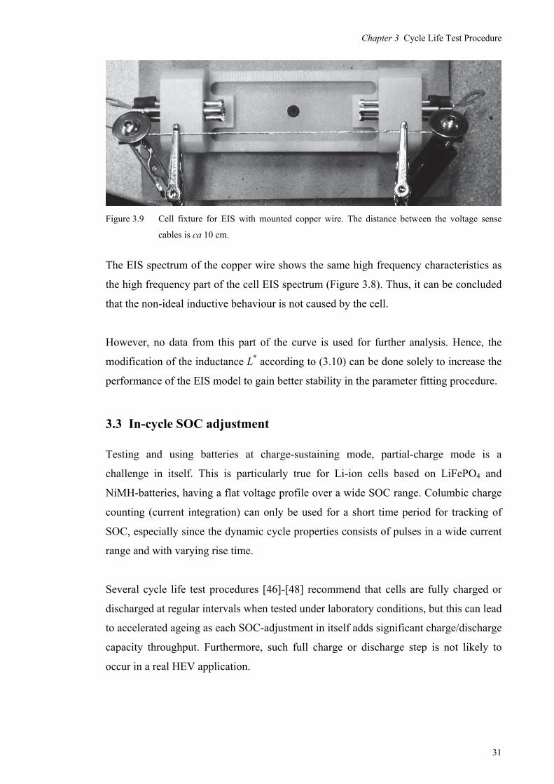
31
Figure 3.9 Cell fixture for EIS with mounted copper wire. The distance between the voltage sense
cables is ca 10 cm.
The EIS spectrum of the copper wire shows the same high frequency characteristics as
the high frequency part of the cell EIS spectrum (Figure 3.8). Thus, it can be concluded
that the non-ideal inductive behaviour is not caused by the cell.
However, no data from this part of the curve is used for further analysis. Hence, the
modification of the inductance L* according to (3.10) can be done solely to increase the
performance of the EIS model to gain better stability in the parameter fitting procedure.
3.3 In-cycle SOC adjustment
Testing and using batteries at charge-sustaining mode, partial-charge mode is a
challenge in itself. This is particularly true for Li-ion cells based on LiFePO4 and
NiMH-batteries, having a flat voltage profile over a wide SOC range. Columbic charge
counting (current integration) can only be used for a short time period for tracking of
SOC, especially since the dynamic cycle properties consists of pulses in a wide current
range and with varying rise time.
Several cycle life test procedures [46]-[48] recommend that cells are fully charged or
discharged at regular intervals when tested under laboratory conditions, but this can lead
to accelerated ageing as each SOC-adjustment in itself adds significant charge/discharge
capacity throughput. Furthermore, such full charge or discharge step is not likely to
occur in a real HEV application.

Chapter 3 Cycle Life Test Procedure
32
Despite the obvious disadvantages of a flat voltage profile depicted in Figure 3.10, one
advantage of this profile is that the phase changes of the graphite is easily detected (see
section 7.1. The phase change between stage-4 and stage-3 can be observed just below
SOC=30% for this battery type as a comparably rapid change in voltage derivative
(dU/dt). Thus, it is possible to adjust SOC to approx. 30% without discharging the cell
completely. However, in order to observe the change in voltage derivative it is vital to
ensure that the cell is in semi-steady state before start of the discharge.
Figure 3.10 Voltage profile at C/4 vs. SOC for LiFePO4 // Graphite cell.
A procedure consisting of five steps (see Figure 3.11 and Table 3) was developed and
tested.
Table 3 SOC adjustment procedure to find SOC ≈ 30%.
Sub-Step Description Limit 1 Charge at 2 C-rate Reset to start SOC 2 Charge at 1 C-rate 17.4% ΔSOC or U > 3.385 V 3 Discharge at C/4 C-rate U < 3.290 V 4 Discharge at C/4 C-rate dU/dt > -0.5 mV/min or U < 3.260 V 5 Discharge at C/4 C-rate dU/dt < -1.5 mV/min
The first two steps are performed to ensure that the battery SOC is well above the SOC
associated to the change in voltage derivative. After the charge steps, three discharge
steps are performed to detect the voltage derivative associated to the target phase
change that corresponds to the target SOC value.
0 10 20 30 40 50 60 70 80 90 100
2
2.5
3
3.5
4
SOC [%]
Cel
l Vol
tage
[V
]
Cell Voltage
Voltage Limit
Charge
Discharge
Chapter 3 Cycle Life Test Procedure
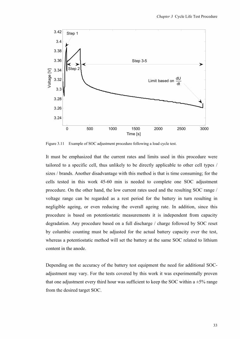
33
Figure 3.11 Example of SOC adjustment procedure following a load cycle test.
It must be emphasized that the current rates and limits used in this procedure were
tailored to a specific cell, thus unlikely to be directly applicable to other cell types /
sizes / brands. Another disadvantage with this method is that is time consuming; for the
cells tested in this work 45-60 min is needed to complete one SOC adjustment
procedure. On the other hand, the low current rates used and the resulting SOC range /
voltage range can be regarded as a rest period for the battery in turn resulting in
negligible ageing, or even reducing the overall ageing rate. In addition, since this
procedure is based on potentiostatic measurements it is independent from capacity
degradation. Any procedure based on a full discharge / charge followed by SOC reset
by columbic counting must be adjusted for the actual battery capacity over the test,
whereas a potentiostatic method will set the battery at the same SOC related to lithium
content in the anode.
Depending on the accuracy of the battery test equipment the need for additional SOC-
adjustment may vary. For the tests covered by this work it was experimentally proven
that one adjustment every third hour was sufficient to keep the SOC within a ±5% range
from the desired target SOC.
0 500 1000 1500 2000 2500 3000
3.24
3.26
3.28
3.3
3.32
3.34
3.36
3.38
3.4
3.42
Time [s]
Vol
tage
[V
]
Step 1
Step 2
Step 3-5
dUdt
Limit based on

Chapter 3 Cycle Life Test Procedure
34
3.4 Temperature Control
In addition to the SOC range, the average cell temperature has been widely considered
as an important ageing factor. Thus, all commercial HEVs and PHEVs are equipped
with a separate thermal management system to maintain the battery temperature within
a narrow temperature range. Usually, the cell temperature is controlled between +20 °C
and +45 °C during normal operation with either cooling or heating systems. In fact,
some HEV battery systems are controlled within an even more narrow temperature
range. Two cases have been studied; cells at room temperature (+23 °C) in free
convection and cells in +35 °C in forced convection in a climate chamber. It is beyond
the scope of this investigation to cover a full study of this ageing parameter. However,
the temperatures studied are still representative for what may be considered as standard
battery environment.
Cells tested with the reference Cycle A (see section 4.1) and the wide-SOC constant
current Cycle C (see section 4.4) were cycled at both room temperature and +35 °C, the
other cases were cycled at either the lower or the upper temperature. Due to internal
losses all cells under test will experience significant self-heating. Added to this, the air
convection conditions also have a significant effect on the actual, average temperature
under cycling. For cells cycled at room temperature, most cells showed 10-12 °C
increase in temperature above ambient, and the cells in the climate chamber had 5-7 °C
increase due to more effective convection and generally lower internal losses at higher
temperature. Consequently, the two selected temperature conditions are +33-35 °C for
cells outside climate chamber and +40-42 °C inside the chamber. Despite the narrow
actual temperature range, previously published results have indicated that comparably
small increases in temperature may result in a significant reduction in cycle life [39],
[38].

Chapter 3 Cycle Life Test Procedure
35
3.5 Half-Cell Tests
In order to get insights in the individual electrode properties of the graphite anode and
the LiFePO4 cathode studied in the present work a series of experiments using half-cells
(see section 5.1) was performed. First and foremost the voltage profiles as a function of
current rate and individual electrode SOC were measured and used to validate analysis
methods (see section 7.2). Although the half-cells were manufactured from commercial
grade material, their mechanical and electrical design is profoundly different from
commercial cells. Hence, their impedance is significantly higher per unit capacity than
that of the commercial, power-optimised cells used for cycle life tests. Consequently,
the voltage drop due to ohmic resistance and polarisation (mass transport) must be taken
into consideration when testing the cells. In contrast to the RPTs, the half-cell tests
involved constant current charge and discharge steps only. An overview of these tests is
given in Table 4.
Table 4 Test procedure for half-cell tests performed at +23°C.
Sub-Step Description Duration [h] 1 Discharge CC at Itest
1 C-rate, minimum voltage Ucut-off3 2-25
2 Pause 1 3 Discharge CC at Ilow
2 C-rate, minimum voltage Ucut-off3 1-5
4 Pause 3 5 Charge CC at Itest
1 C-rate, maximum voltage Umax4 2-25
6 Pause 1 7 Charge CC at Ilow
2 C-rate, maximum voltage Umax4 1-5
8 Pause 3 1. Itest = C/25, C/10, C/5, C/2, C/1 C-rate. 2. Ilow = C/25. 3. Ucut-off = 0.01 V for graphite/Li cell, 2.7 V for LiFePO4/Li cell. 4. Umax= 2.0 V for graphite/Li cell, 4.0 V for LiFePO4/Li cell.
The test procedure starts with a full discharge with constant current (Itest) until the cell
voltage is equal to Ucut-off. This step is followed by a rest period and a second discharge
at low current rate (Ilow) to ensure that the cell is fully discharged regardless of a
possible early termination of step 1 due to high voltage drop. Likewise, the cell is re-
charged with Itest and Ilow in two steps. This charge/discharge procedure is repeated three
times for each tested current rate; C/25, C/10, C/5, C/2 and C/1 C-rate. Test results from
these tests are presented in section 7.3.


Chapter 4 Load Cycles
37
Chapter 4 Load Cycles
Since the ageing mechanisms of Li-ion battery cells are non-linear and dependant, it is
rarely possible to isolate one mechanism at a time and test its specific dependence on
operating conditions. This is especially the case in HEV applications designed for
optimum cycle life; controlled temperature range, SOC range and current range. One
illustrative example is a hybrid electric city-bus designed to reduce fuel consumption by
recuperating brake energy and avoid idling. In 2009, AB Volvo introduced their first
series manufactured HEV city bus. Being one of the most likely candidates for
hybridisation of heavy-duty vehicles, this application was chosen as the basis for the
reference battery load profile, Cycle A, for the cycle life test presented in this thesis
Using this reference cycle as the premises for all tests performed, a number of different
load cycles was derived and used in cycle life tests, if possible, to find the relation
between specific ageing factors and the load cycle properties:
a synthetic load cycle, Cycle B, was designed based on stochastic process model
of the reference cycle
simplified cycles with constant current for charge and discharge; Cycle C with a
wide SOC range and Cycle D with a narrow SOC range
an adaptation of a PHEV-cycle, Cycle E, representing a compromise between
complex logged cycles and simplified average cycles.
This section describes the adaptation of a reference load cycle, the method for synthetic
load cycle extraction, the set-up of simplified load cycles and a summary of cycle
properties for all tested cycles.
4.1 Reference Load Cycle, Cycle A
Naturally, the drive cycle and corresponding load cycle for the battery differs between
markets, countries, operators, vehicle options / add-on etc. However, since the work
presented in this thesis concentrates on the actual ageing, the selection of battery load
cycle is not critical as long as it is representative for the target vehicle. A drive cycle
from a city-bus route in Gothenburg, Sweden, was selected for use as a realistic case for

Chapter 4 Load Cycles
38
a heavy-duty HEV. The speed, altitude and slope angle for this drive cycle are shown in
Figure 4.1. Here, the frequent start-stop it is noticeable as well as the low average speed.
Despite the low average speed, a high peak power outtake from the powertrain is
needed to achieve acceptable acceleration and hill-climbing capability as the bus-route
includes significant slope angles.
Figure 4.1 HEV City-bus drive cycle used to derive the reference load Cycle A.
Several test drives have been performed with a prototype HEV city-bus on this
particular drive cycle. The battery current, voltage, SOC and temperature was sampled
at 10Hz during a road test and used as the reference battery load cycle for the cycle life
tests presented in this work. This load cycle consists of about 40 000 logged values of
current vs. time. In order to use it for laboratory cycle life tests it was filtered with a 10
point / 1 s moving average filter in combination with a sample-and-hold filter. The
resulting load profile has a minimum step duration of 1.0 s, effectively reducing the
number of steps to about 2 000 with a minor loss of dynamics; the filtered cycle (Figure
4.2) shows negligible difference in current distribution, peak values and capacity
throughput compared to the logged cycle.
0 10 20 30 40 50 60 700
20
40
60
Veh
icle
Spe
ed [
km/h
]
0 10 20 30 40 50 60 700
20
40
60
80
Alti
tude
[m
]
Time [min]

Chapter 4 Load Cycles
39
Figure 4.2 Comparison of current distribution between logged and filtered/scaled load cycle.
In addition, the power in the original profile was scaled to 80% and reduced in peak
charge current to comply with the maximum current rating of the selected test cells.
A sample of the current for the first two minutes and the SOC for the entire cycle is
shown in Figure 4.3 and Figure 4.4, respectively.
Figure 4.3 Comparison of logged and filtered cycle, first 180 s.
-30 -20 -10 0 10 20 300
2
4
6
8
10
12
14
16
18
20
Current [C-rate]
Rel
ativ
e D
istr
ibut
ion
[%]
Logged Cycle
Scaled & Filtered Cycle
0 20 40 60 80 100 120-30
-20
-10
0
10
20
30
Time [s]
Cur
rent
[C
-rat
e]
Original
Filtered
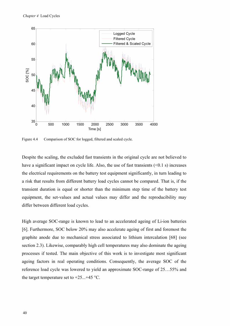
Chapter 4 Load Cycles
40
Figure 4.4 Comparison of SOC for logged, filtered and scaled cycle.
Despite the scaling, the excluded fast transients in the original cycle are not believed to
have a significant impact on cycle life. Also, the use of fast transients (<0.1 s) increases
the electrical requirements on the battery test equipment significantly, in turn leading to
a risk that results from different battery load cycles cannot be compared. That is, if the
transient duration is equal or shorter than the minimum step time of the battery test
equipment, the set-values and actual values may differ and the reproducibility may
differ between different load cycles.
High average SOC-range is known to lead to an accelerated ageing of Li-ion batteries
[6]. Furthermore, SOC below 20% may also accelerate ageing of first and foremost the
graphite anode due to mechanical stress associated to lithium intercalation [68] (see
section 2.3). Likewise, comparably high cell temperatures may also dominate the ageing
processes if tested. The main objective of this work is to investigate most significant
ageing factors in real operating conditions. Consequently, the average SOC of the
reference load cycle was lowered to yield an approximate SOC-range of 25…55% and
the target temperature set to +25...+45 °C.
0 500 1000 1500 2000 2500 3000 3500 400035
40
45
50
55
60
65
Time [s]
SO
C [
%]
Logged Cycle
Filtered CycleFiltered & Scaled Cycle

Chapter 4 Load Cycles
41
A comparison of the logged cycle, the scaled and filtered version of the reference load
cycle is shown in Table 5. Here, it should be noted that the scaled load cycle is less
severe than the logged cycle in all aspects. The definition of RMS current (root-mean-
square), average current and capacity throughput are according to (4.1) to (4.3), where
Tcycle is the total load cycle time and CNominal is the rated cell capacity.
Table 5 Comparison between measured and filtered battery load cycle.
Cycle Property Logged Cycle Filtered & Scaled Cycle Reference Cycle A Average SOC [%] 49.7 50.2 38.5 Minimum SOC [%] 37.5 40.9 22.6 Maximum SOC [%] 60.2 58.3 50.0 RMS Current [C-rate] 6.86 5.79 5.01 Average Current [C-rate] 4.17 3.65 2.82 Total Capacity Throughput [C-rate] 2.26 1.97 2.02 Peak Charge Current [C-rate] 23.9 17.3 17.3 Peak Discharge Current [C-rate] 28.2 22.3 22.3 Cell Temperature [°C] +20...+50 +25…+45 +23..+40
Nominal0
2RMS
11
Cdti
TI
cycleT
cycle
(4.1)
Nominal0
Mean
11
Cidt
TI
cycleT
cycle
(4.2)
23600
1
Nominal0
Throughput C
dtiCcycleT
(4.3)
4.2 Synthetic Cycle Extraction
Despite adding filtering and other signal conditioning of logged cycles, a logged cycle
is still only representative for a particular target vehicle and the actual operating
conditions at the time of measurement. An alternative method of extracting a shorter,
simplified load cycle based on one or several measured cycle was developed to
investigate the degree of sensitivity to simplification with regard to battery ageing
characteristics [69].

Chapter 4 Load Cycles
42
The primary target for the work presented in this section is to find an objective, reliable
method to simplify dynamic battery load cycles for use in cycle life tests. In addition,
the method should be a tool for evaluating how applicable results from different load
cycle tests are to a particular application.
First and foremost this method is developed for use in cycle life tests of Li-ion batteries
optimized for heavy-duty HEVs. There are however no direct restriction to the usage of
the method to the testing of other secondary batteries.
This method uses a statistic approach for analysing measured battery load cycles in
terms of a number of key properties such as power distribution and energy throughput.
This stochastic cycle model is then used to compare cycles and to generate new
synthetic load cycles where key parameters such as average power and current rate can
be adjusted while keeping other properties of the cycle constant. In addition, the method
can be used to reduce the total load cycle length to a minimum which further simplifies
the test setup. Specifically, this work covered an investigation of the suitability of using
a Markov chain as a model for the battery load cycle in heavy-duty HEV applications.
Firstly, the theoretical background of the method is presented. Secondly, a simplified
charge sustaining algorithm is added to the system to control the SOC during longer
load cycles. Thirdly, the method is used to generate a new synthetic load cycle based on
the reference cycle from an HEV city-bus.
4.2.1 Stochastic Model of Load Cycle
A full background to the technique is given in [70], and several papers present possible
examples where load cycles are generated by using Markov chains: [71]-[76].
This method can easily be adapted to HEV load cycles by converting the power into
discrete power levels in a state-vector S in which each level represents a unique state. A
probability matrix Q, called the Markov matrix, can then be formed where the
probability for transition from state i to state j is equal to element Qij:
)|( 1 jSiSPQ nnij (4.4)

Chapter 4 Load Cycles
43
mnmm
n
n
ij
SSSSSS
SSSSSS
SSSSSS
Q
21
22221
11211
(4.5)
where Sn+1 is the next state (power level), Sn is the current state and P is the probability
for a transition from Sn to Sn+1.
The m x m matrix Q is typically a sparse matrix with the greatest elements around the
diagonal Q1,1 to Qm,m. Each column sum must be equal to 1, since the cumulative
probability for transition to any possible new state must be unity for each current state.
This is however only true if all states in the state vector are entered in the real load
cycle. If not, numeric problems might occur depending on the implementation. The Q
matrix is defined by analysing one or several load cycles so that each element in the
matrix is populated with the corresponding probability.
A new, synthetic cycle of any length can then be calculated using a minimum of tools,
which will be further described in section 4.2.2:
1. an initial state in the S-vector for which the corresponding column sum ≠ 0
2. a random number generator
Changes and adaptations to the probabilities in the Q matrix should be avoided to
preserve stability. Instead, power levels can either be adjusted according to an
independent weight function before the population of the Q matrix or the output state
can be adjusted by selecting either a higher or lower power level than the one generated
by the random function. Even though such modifications to the cycle are in conflict to
the stochastic approach, it will in practice be necessary to include them to first and
foremost keep the SOC within the admissible range.
Chapter 4 Load Cycles
44
There is a specific issue related to the selection of states to include in the S vector.
Depending on the choice and the cycle properties the S vector and the Q matrix may
contain empty states / empty column. These states might in turn cause instabilities to the
cycle generation. There are two obvious solutions to this issue:
1. The corresponding column in Q can be populated as the linear interpolation
between adjacent columns. This method will generate a stable output but may
cause the output synthetic cycle to consist of power levels never observed in the
real cycle.
2. The SOC algorithm can be changed to avoid selecting states (power levels) not
observed in the real cycle.
In theory this choice may not be important, but in practice when using standard random
number generators in for example MATLAB® it may be relevant as described further in
the following section. The second method was selected to ensure that the procedure can
work with a large variety of load cycles in combination with a comparably large Q
matrix.
4.2.2 Implementation
Firstly, the S vector of length m is selected to correspond to the reference load cycle
properties. The m x m matrix Q is then formed by stepping through the reference load
cycle and incrementing the corresponding state Qn,x for each step, followed by the
normalization of the columns by the total column sum. The first step in this “learning”-
process can be repeated for every measured (or simulated) load cycle that should be
included in the synthesis as long as the sample rate is the same for all cycles and the
total number of cycle steps for all cycles are used to normalize the columns in the
second step.
At this stage it is also possible to introduce limitations, weight functions, or in other
ways change the properties of Q and any generated synthetic cycles compared to the
input cycle(s).
Following the calculation of the Q matrix, a synthetic cycle can be generated step-wise
using a general random number generator. In MATLAB, this can be done by creating a
support matrix, Qs, consisting of the cumulative column sum of Q and the random

Chapter 4 Load Cycles
45
generator rand; the column in Qs corresponding to the current state is compared by a
random number [0…1] and the element closest to the random number is selected as the
next state. That is, the output state is the first row index n of Qs(n,x) that satisfies the
relation Qs(n,x)> rand where x is the current state and n is the next state. Simplified
examples of Q and Qs are shown in (4.11) and (4.12). These examples are however not
representative to HEV cycles.
This short algorithm is repeated for each step in the cycle starting the initial state x0
corresponding to the initial power level. The output state n of each iteration is used as
input state I for the next calculation. There is no theoretical limit to the total length of
the synthetic cycle. In practice the length will however be limited by a lower limit
determined by the requirements on correspondence with the reference cycle (see section
4.2.6).
8.01.000000000
2.07.001.01.0000000
01.095.02.0000000
006.003.05.01.000000
004.001.017.08.0005.0002.00
00003.004.09.005.0003.00
000006.002.06.01.005.001.0
0000008.02.07.005.004.0
0000001.02.08.005.0
0000000005.09.0
Q (4.6)
1111111111
2.09.011111111
02.099.09.0111111
01.004.07.0111111
004.001.02.09.011111
00003.01.0195.0198.01
000006.01.09.0195.01
0000008.03.09.09.099.0
0000001.02.085.095.0
0000000005.09.0
sQ (4.7)
As mentioned in previously, a problem with SOC exceeding the maximum limits might
occur when battery load cycles from charge-sustaining HEVs are studied, especially if
the cycles are comparably long and the energy throughput is in the range of the usable
energy content of the battery. In such cases the SOC of the target battery must be

Chapter 4 Load Cycles
46
calculated for each time step and then, via a predefined SOC control strategy, be used to
adjust the output power for the next step to limit the required SOC range. Thus, the
battery load cycle cannot be treated as a purely stochastic process from a strictly
fundamental standpoint unless the battery capacity is infinitely large or the load cycles
are very short in duration. Nevertheless, this limitation of the proposed method is still
viable since it replicates the situation in a real HEV where the drive pattern and road
profile may be considered as stochastic whereas the actual battery current is limited and
controlled by a control unit based on a non-stochastic strategy. If, in addition, the S
vector is composed by representative levels with a high number of levels, the SOC
strategy will only have a minor impact on cycle properties in terms of power and
energy. This issue and a proposed solution are presented in detail in the following
sections, where the first part presents the definition of SOC and the associated battery
model, followed by an example of a simple SOC preserving control strategy for use in
the synthetic cycle generation.
4.2.3 Battery model used for SOC-estimation
The SOC of a battery is typically defined as the ratio between the available discharge
capacity and the maximum discharge capacity at a specific temperature and SOH:
As
As
As
AsAs
0
discharged
reference
t
reference
reference
reference
C
dtIC
C
tCCtSOC
(4.8)
While the SOC in an HEV is carefully controlled to ensure the performance and
durability of the battery throughout the design lifetime, this is not the case for the
generated stochastic cycle according to the Markov process. However, the average SOC
for any truly stochastic cycle will be equal to the initial SOC for an infinitely long cycle
if the total probability for charge is equal to the probability for discharge, capacity wise.
This is naturally not the case for real cycles of finite length, especially not for HEV
batteries with a comparably high energy throughput. Consequently, the resulting SOC
of the synthetic cycle must be controlled according to a predefined strategy using a
similar method as is implemented in a real HEV.

Chapter 4 Load Cycles
47
Firstly, a method for a step-wise calculating SOC during the extraction of the synthetic
cycle is selected. Using a simple Thevénin equivalent circuit model and a fixed value for
the reference capacity Creference, the SOC(t) is numerically calculated as the Euler
approximation of the integrated current in each step. If the load cycle is characterised by
constant power levels rather than current levels, a separate algorithm for estimation of
current must be added. Any battery model able to calculate current from a power input
is possible to use at this stage. For simplicity, a rudimental model is used here:
tItRtUtU OCV (4.9)
Assuming the typically narrow SOC range of most Li-ion batteries designed for HEVs,
the average open circuit voltage UOCV may be regarded as a constant. Similarly, the
internal resistance can be simplified using a single value or a limited set of values to
further simplify the equation. Due to limited current measurement accuracy any real
cycle life test must include a separate SOC adjustment procedure which is described
further in section 3.3 in this thesis.
Starting from the input power to the battery, the power /current relation in (4.10) must
be satisfied for all time steps.
2tItRtItUtItUtP OCV (4.10)
Solving this equation for each time instant yields a time-varying current vector to be
used in SOC-estimation.
Secondly, an appropriate SOC strategy is added to keep the SOC of the battery within
the acceptable range throughout the duration of the synthetic cycle. This approach, or
any other SOC preserving method, is absolutely essential when extracting synthetic
cycles in which the energy throughput is comparable to the maximum usable energy of
the battery.
Chapter 4 Load Cycles
48
4.2.4 SOC Control Strategy
Naturally, there are numerous ways to control the SOC in an HEV. That is especially
challenging for cycles with an energy throughput that is comparable to or exceeding the
usable battery energy. A synthetic load cycle could either be designed to replicate the
SOC trends of the target load cycle as accurately as possible, or to reflect the statistical
properties of the load cycle using an additional weight function that will control the
SOC to stay within the acceptable range. One approach to control SOC is to limit the
charge power close to the upper SOC limit and the discharge power close to the lower
limit. Rutquist et al. [77] suggested the tangent function as the optimal control function
u=f(SOC) for a simplified system with a supercapacitor energy storage. This strategy
may be expanded to batteries, at least within a narrow SOC range, and was therefore
used in this method.
Regardless of which strategy that is chosen, a stable weight function that limits the
maximum SOC range of the synthetic load cycle is needed. The reference for this
function could either be a static target (SOCtarget), a dynamic SOC signal according to
measured properties or a simulated signal assuming a constant average efficiency of the
battery cell.
Since the generated cycle is stochastic, no change made to the Q matrix will be efficient
to keep SOC within the admissible range. Even small changes in the Q matrix defining
the Markov process might cause severe stability problems in the cycle generation.
Hence, the Q matrix must be left unchanged and the output power levels must be used
to control SOC instead.
The inverse tangent function according to [77] was used to generate a limit function for
SOC. This function can be configured with different steepness at the edges (see
Figure 4.5).

Chapter 4 Load Cycles
49
Figure 4.5 Limit function using tangent function and SOC slope between 1 and 10.
For each step generated according to the method described in the previous section, the
output power level is weighed with this limit function. If the SOC is close to the target
SOC no change is made to the output power. In contrast, when the SOC is close to the
limits the target function gradually limits the charge power (at high SOC) and the
discharge power (at low SOC). The calculated new power level is then adjusted to fit
the pre-defined power levels (states) in the S vector. The adjustment factor 0...1 is based
on the MATLAB tangent function tan according to (4.11) and (4.12).
slope
targetmax
targetFcnLimit tan1
SOC
SOCSOC
SOCSOCSOC (4.11)
where
SOCtarget is the centre point of the admissible SOC-range,
SOCmax is the maximum admissible SOC,
SOCmin is the minimum admissible SOC, and
SOCslope is a control parameter typically between 1 and 10 that determines the steepness
of the limit function close to the boundaries.
20 30 40 50 60 700
0.1
0.2
0.3
0.4
0.5
0.6
0.7
0.8
0.9
1
SOC [%]
Lim
it F
cn [
-]
Limit Fcn with SOC-slope = 1..10
SOC Target
SOC Max / Min
SOC Limit Fcn
slope = 1
slope = 10

Chapter 4 Load Cycles
50
The limit function SOCLimit Fcn varies between 0...1 for SOC between SOCmin…SOCmax
and can be used directly as a multiplication factor for the output power level in each
step of the cycle generation:
1 nFcn Limitoutput SSOCP
(4.12)
The corrected output state corresponding to Poutput in (4.12) must then be selected as the
power level that best corresponds to the discrete levels in the state vector S for which
the probability is larger than zero.
4.2.5 Optimisation
Any cycle generated according to the proposed method will reflect the fundamental
properties of the reference cycle. However, the actual SOC characteristics as well as
other cycle properties will differ significantly between different synthetic cycles. To
find and evaluate solutions / versions of the synthetic cycle with good, objective
correspondence to the reference cycle, an optimisation process was run where key
aspects such as RMS power, SOC range, and power/energy distribution of the cycle
were compared to the reference cycle by means of five weighted error functions
The weighted error functions (4.13) to (4.17) are aimed to provide a continuous
feedback to the optimisation process, in turn enabling a stable optimisation process.
Difference in SOC over the complete cycle:
2
112
1 n
n referencesyntheticSOCSOC SOCSOCnn
KERR (4.13)
Difference in RMS power and maximum energy window:
kWPkWPKERR referenceRMSsyntheticRMSPPRMS ,, (4.14)
WhWWhWKERR referencewindowsyntheticwindowWWwindow ,, (4.15)
Difference in power and energy distribution:
S
referencesyntheticdistPP N
SPhist
N
SPhistKERR
dist
,,,
(4.16)

Chapter 4 Load Cycles
51
S
referencesyntheticdistWW N
SWhist
N
SWhistKERR
dist
,,,
(4.17)
where
N = number of elements
S = discrete power vector
hist(Y,X) = the histogram (distribution) of Y over X.
The weight factors KSOC, KP and KW are set for the specific application to set internal
priority between the evaluation measures.
A large number of cycles were generated, each according to the same Markov process
and with the same settings, as presented in Table 6.
Table 6 Battery properties and SOC-strategy settings.
Parameter Abbr. Value Unit
SOC strategy
Reference SOC SOCtarget 50 %
Upper SOC limit SOCmax 60 %
Lower SOC limit SOCmin 30 %
Initial SOC SOCinitial 50 %
SOC Limit Function factor SOCslope 10 -
Sampling time tstep 0.1 s
Weight factor, SOC KSOC 1/10 -
Weight factor, RMS-power KP 1/500 -
Weight factor, Energy window KW 1/40 -
Battery
Total energy WBattery 3000 Wh
Total capacity CBattery 5 Ah
Total internal resistance ESRBattery 0.45 Ω
Open circuit voltage at 50% SOC UOCV 630 V
For sufficiently long synthetic cycles the power distribution and energy distribution
over the discrete power vector are expected to be similar to that of the reference cycle.
However, this is only the case if the reference cycle can be modelled as a truly
stochastic Markov process.
Chapter 4 Load Cycles
52
Consequently, the shape of the power and energy distribution can be compared to the
reference cycle to determine
a) the validity of the Markov process to model the load cycle
b) the minimum length of the synthetic output cycle to cover the full spectrum of
the reference cycle
Previous sections described the SOC strategy as a necessary perturbation to the true
Markov cycle since it affects the power levels in the synthetic cycle when the estimated
SOC-level is close to the limits.
The method in this study uses the five presented error functions above, with weight
factors according to Table 6 set to address specific properties. If the synthetic cycle
should be similar to the reference cycle in SOC variations, a larger value should be
assigned to the factor KSOC, and similar for the other properties. Naturally it is also
viable to use a combination of the K factors to generate cycles that in average
corresponds well to the reference cycle. Nevertheless, the fourth and fifth error
functions (4.16 and 4.17) should be used to determine the minimum cycle time or
minimum cycle length which has the fundamental properties of the reference cycle in
terms of distribution of power and energy.
4.2.6 Evaluation
The feasibility of the proposed method has been evaluated based on an investigation of
a large number of synthetic load cycles extracted and compared to reference Cycle A
described in section 4.1. The Q matrix was calculated using the measured voltage and
current together with the logged SOC level based on this single reference load cycle. In
addition, the logged battery data from Cycle A was used to extract parameters for the
simple battery model needed for SOC estimation.
Using the proposed SOC strategy and general settings for SOC average and SOC limits
as well as battery data from a relevant Li-ion battery (see Table 6) a number of synthetic
cycles were generated and evaluated according to the error functions (4.13) to (4.17).
Firstly, the minimum cycle length was evaluated using error functions (4.16) and (4.17).
The outcome of this part indicated that, for this particular reference cycle and set of

Chapter 4 Load Cycles
53
conditions, the cycle must be at least 30% of the original length to capture the
fundamental properties. In Figure 4.6 the cumulative error between the power
distribution and energy distribution is presented as function of the fraction of the
reference cycle length.
Figure 4.6 Cumulative error between power and energy distribution and the reference cycle for
different synthetic cycle length.
The ability of the method to capture the distribution of power and energy is also
illustrated in Figure 4.7 where these distributions are shown for 80% cycle length.
Figure 4.7 Power (left figure) & energy (right figure) distribution at 80% cycle length.
Whereas the power distribution is almost identical to that of the original cycle, the
energy distribution shows minor differences. These are probably due to the
modifications made to the algorithm to include the SOC strategy.
0 10 20 30 40 50 60 70 80 90 1000
50
100
150
Synthetic Cycle Length [% of original]
Sum
of
erro
r ov
er c
ycle
[%
]
1/(7x3 + -16x2 + 13x + 0.95)
1/(7x3 + -29x2 + 23x + 1.7)
Energy Spectrum
Power Spectrum
Polyfit, 3rd order
-100 -80 -60 -40 -20 0 20 40 60 80 100
1
2
3
4
5
6
7
Power [% of peak]
Fre
quen
cy [
%]
Original Cycle
Synthetic Cycle
-100 -80 -60 -40 -20 0 20 40 60 80 1000
0.2
0.4
0.6
0.8
1
1.2
1.4
Power [% of peak]
Fre
quen
cy [
%]
Original Cycle
Synthetic Cycle

Chapter 4 Load Cycles
54
Other reference cycles, or the usage of a combination of cycles to calculate the Q
matrix, would most likely yield other results. In addition, the choice of the discrete
power vector S is of fundamental importance in the evaluation; if a low number of
power levels (states) are included in S, all states with high probability in the reference
cycle are likely to occur in the synthetic cycles after a comparably low number of steps.
The example in this paper used an S vector of [-100:1:100]% of rated peak power,
resulting in a 201x201 sized Q matrix. This fact will in turn require the cycle length to
be in the same range as the number of elements in Q (≈10000) to allow the cycle to span
over the complete range of states.
In addition to optimising the cycle generation process for good correspondence to the
reference cycle in terms of power distribution and energy distribution, the SOC changes
must be taken into considerations. Nevertheless, the presented method has shown
promising results and may be used for simplifying the set-up of battery tests, the
evaluation of load cycles and to combine several reference cycles into one test cycle.

Chapter 4 Load Cycles
55
4.3 Synthetic Cycle used in Cycle life Tests, Cycle B
A new synthetic cycle, Cycle B, with similar capacity throughput, current distribution,
length and RMS-current as the reference load cycle was extracted and tested in parallel
with the reference profile Cycle A. The selected cycle is presented and compared to the
original cycle in Figure 4.9 and Figure 4.8.
Figure 4.8 Comparison of SOC range for Cycle A and Cycle B, excluding SOC adjustment.
The SOC range presented in Figure 4.8 is similar between the two cycles, confirming
that the SOC strategy is sufficiently accurate, but the since Cycle B is based on the
stochastic model, the actual SOC variation is significantly different.
0 500 1000 1500 2000 2500 3000 3500 400025
30
35
40
45
50
SO
C [
%]
Time [s]
0 500 1000 1500 2000 2500 3000 3500 400025
30
35
40
45
50
SO
C [
%]
Time [s]

Chapter 4 Load Cycles
56
Figure 4.9 Current distribution comparison between reference Cycle A and synthetic Cycle B.
As can be seen Figure 4.9, the current distribution is similar for the two cycles, although
there is a difference in RMS current. A summary of the cycle properties is given in
Table 7 below.
Table 7 Comparison between reference Cycle A and synthetic Cycle B.
Cycle Property Logged Cycle Reference Cycle A Synthetic Cycle B Average SOC [%] 49.7 38.5 41.9 Minimum SOC [%] 37.5 22.6 32.5 Maximum SOC [%] 60.2 50.0 54.0 RMS Current [C-rate] 6.86 5.01 5.29 Average Current [C-rate] 4.17 2.82 3.00 Total Capacity Throughput [C-rate] 2.26 2.02 2.05 Peak Charge Current [C-rate] 23.9 17.3 15.1 Peak Discharge Current [C-rate] 28.2 22.3 23.2
Note that the resulting cycle is a compromise between similarities in SOC range,
capacity throughput and RMS current. One consequence of this compromise is that the
synthetic Cycle B is slightly more aggressive in terms of RMS current than the reference
profile Cycle A although the peak current is lower and the capacity throughput is
similar.
-25 -20 -15 -10 -5 0 5 10 15 200
5
10
15
20
25
30
35
Current [C-rate]
Rel
ativ
e D
istr
ibut
ion
[%]
Cycle A: 5.01 C-rate RMS
Cycle B: 5.29 C-rate RMS
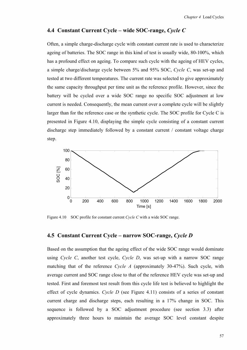
Chapter 4 Load Cycles
57
4.4 Constant Current Cycle – wide SOC-range, Cycle C
Often, a simple charge-discharge cycle with constant current rate is used to characterize
ageing of batteries. The SOC range in this kind of test is usually wide, 80-100%, which
has a profound effect on ageing. To compare such cycle with the ageing of HEV cycles,
a simple charge/discharge cycle between 5% and 95% SOC, Cycle C, was set-up and
tested at two different temperatures. The current rate was selected to give approximately
the same capacity throughput per time unit as the reference profile. However, since the
battery will be cycled over a wide SOC range no specific SOC adjustment at low
current is needed. Consequently, the mean current over a complete cycle will be slightly
larger than for the reference case or the synthetic cycle. The SOC profile for Cycle C is
presented in Figure 4.10, displaying the simple cycle consisting of a constant current
discharge step immediately followed by a constant current / constant voltage charge
step.
Figure 4.10 SOC profile for constant current Cycle C with a wide SOC range.
4.5 Constant Current Cycle – narrow SOC-range, Cycle D
Based on the assumption that the ageing effect of the wide SOC range would dominate
using Cycle C, another test cycle, Cycle D, was set-up with a narrow SOC range
matching that of the reference Cycle A (approximately 30-47%). Such cycle, with
average current and SOC range close to that of the reference HEV cycle was set-up and
tested. First and foremost test result from this cycle life test is believed to highlight the
effect of cycle dynamics. Cycle D (see Figure 4.11) consists of a series of constant
current charge and discharge steps, each resulting in a 17% change in SOC. This
sequence is followed by a SOC adjustment procedure (see section 3.3) after
approximately three hours to maintain the average SOC level constant despite
0 200 400 600 800 1000 1200 1400 1600 1800 20000
20
40
60
80
100
Time [s]
SO
C [
%]

Chapter 4 Load Cycles
58
inaccuracies in current measurement. The constant current rate is selected to match the
capacity throughput of the reference profile.
Figure 4.11 SOC profile for constant current Cycle D, 29-46% SOC, including SOC adjustment.
4.6 PHEV Cycle, Cycle E
Batteries used in PHEVs are cycled in a considerably different way than batteries used
in HEVs. In addition to recuperation of kinetic energy, the battery is usually discharged
over a couple of hours and then used in charge-sustaining mode, or re-charged under
pre-defined charging conditions. Moreover, the average current is lower to allow for a
longer period charge-depleting mode. Although this study focuses at battery load cycles
for HEVs, a limited test of ageing during a PHEV cycle, Cycle E, was included. This
load cycle is based directly on a vehicle simulation of a medium-sized city-bus. Starting
with a fully charged battery the bus is running in charge-depleting mode for
approximately one hour and then re-charged at standstill with constant current rate
resulting in the SOC profile shown in Figure 4.12.
Figure 4.12 SOC profile for the PHEV cycle, Cycle E.
0 2000 4000 6000 8000 10000 12000 14000 160000
20
40
60
80
100
Time [s]
SO
C [
%]
0 1000 2000 3000 4000 5000 60000
20
40
60
80
100
Time [s]
SO
C [
%]

Chapter 4 Load Cycles
59
During the charge-depleting mode the battery acts as the main energy source in the
vehicle but also an energy storage for recuperated brake energy. The cycle is scaled to
limit the SOC region to approximately 10-100% in order to provide sufficient power
efficiency and discharge power capability throughout the cycle.
4.7 Load Cycle Comparison
The key properties of the load cycles described in section 4.1 are given in Table 8. Here,
the HEV Cycle A, Cycle B and Cycle D all have the same characteristics in terms of
SOC and capacity throughput while the RMS and the peak currents differ. In
comparison, Cycle C has a comparable RMS and average power to the HEV-cycles but
a significantly wider SOC-range. Lastly, the PHEV Cycle E and the constant current
Cycle C have the same SOC-range but differences in RMS and average current.
Consequently, these five cycles represents a wide variation of SOC, current range and
load cycle complexity. The overall intention with this wide variation is to provide
relevant cycle life test data for both HEVs and PHEVs, in turn to be used to quantify the
most important ageing characteristics.
Table 8 Comparison between load cycles used in cycle life tests.
Cycle Property Reference Cycle A
Synthetic Cycle B
Constant current Cycle C
Constant current Cycle D
PHEV Cycle E
Average SOC [%] 38.5 41.9 53.4 54.9 58.8 Minimum SOC [%] 22.6 32.5 11.4 28.8 13.0 Maximum SOC [%] 50.0 54.0 100 39.1 100 RMS Current [C-rate] 5.01 5.29 3.59 3.33 1.68 Average Current [C-rate] 2.82 3.00 3.49 3.04 1.22 Total Capacity throughput [C-rate] 2.02 2.05 0.89 2.12 1.00 Peak Charge Current [C-rate] 17.3 15.1 3.76 3.76 3.81 Peak Discharge Current [C-rate] 22.3 23.2 3.76 3.76 4.78
During the cycle life tests these cycles are controlled in a stepwise constant current
mode with secondary limits set on voltage, temperature and SOC. Consequently, the
load cycle properties in terms of voltage range are expected to vary as the cell
impedance changes. Likewise, the average temperature distribution may change.
Section 4.7.1 to 4.7.4 contain brief overviews of the measured load cycle properties
after approximately half the total cycled time and observations of possible reasons to
their different ageing factors.

Chapter 4 Load Cycles
60
4.7.1 Temperature Distribution
Although some of the cells were cycled at slightly elevated temperature, the temperature
distribution is narrow for the complete test matrix as can be seen in Figure 4.13.
Figure 4.13 Temperature distribution for cells cycled with Cycle A-E.
This is partly due to the fact that the forced air convection inside the climate chamber is
more effective in terms of cooling than the natural convection used for the cells in room
temperature. Cells tested at Cycle A and Cycle C were cycled at both room temperature
(+23 °C) and in a climate chamber kept at +35 °C (see Chapter 5 for details).
4.7.2 SOC Range
The SOC range during cycling is known to be a profoundly important factor when Li-
ion batteries are cycled [6]. This is especially significant for graphite anodes, which
upon intercalation and de-intercalation undergo a volume change that leads to
mechanical stress, in turn leading to surface changes, degradation of particle inter-
conductivity and in some cases loss of accessible anode material. Further background to
this ageing mechanism is given in section 2.3.
A B C D E, +35C A, +35C C, +35C0
5
10
15
20
25
30
35
40
45
50
Tem
pera
ture
[ C
]
Min T
Average TMax T
Ambient +23CClimate Chamber +35C

Chapter 4 Load Cycles
61
Figure 4.14 SOC distribution for cells cycled with Cycle A-E.
All tested cells are cycled in a narrow SOC range except those cycled with constant
current Cycle C and PHEV Cycle E (see section 4.4, 4.6 and Table 8). A comparison
between the SOC distributions of all tested load cycles is graphically presented in
Figure 4.14. The three HEV cycles (Cycle A, Cycle B and Cycle D) are all kept
approximately within the range 25-58% and the constant current cycles (Cycle C and
Cycle E) has wide distribution of SOC between approximately 10-100%. Despite the
similarities in SOC range between these two categories of load profiles they do undergo
different ageing mechanisms according to the results presented in Chapter 6 and
Chapter 7.
4.7.3 Current Distribution
The current distribution is notably different between the tested cycles; whereas the
Cycle A and Cycle B have a wide distribution ranging between approximately
-20…+20 C-rates, Cycle C, Cycle D and Cycle E are all between -4 and +4 C-rate as
shown in Figure 4.15. In addition, there is a significant difference in RMS current, in
turn leading to higher heat losses inside the cells and higher average temperature.
0 10 20 30 40 50 60 70 80 90 1000
0.5
1
1.5
2
2.5
3
3.5
4
SOC [%]
Rel
ativ
e D
istr
ibut
ion
[%]
Cycle A
Cycle B
Cycle CCycle D
Cycle E

Chapter 4 Load Cycles
62
Figure 4.15 Current distribution for cells cycled with Cycle A-E.
The lower part of the brief comparison in Figure 4.15 between the distributions and the
RMS currents highlights the difference in the low current area. Notably, the dynamic
HEV cycles (Cycle A and Cycle B) all show a large relative distribution around low
currents, including zero representing the rest periods.
4.7.4 Voltage Distribution
Two voltage distributions have been calculated for each cycle: the distribution of
measured cell voltage and the voltage compensated for the voltage drop over the ohmic
resistance and the charge transfer resistance according to (4.18) to (4.20) derived from
the model presented in section 3.2.
OhmCTmeasuredmeasureddcompensate RRIUU (4.18)
TfR CT(4.19)
TfR Ohm(4.20)
-25 -20 -15 -10 -5 0 5 10 15 200
10
20
30
40
50
Current [C-rate]
Rel
ativ
e D
istr
ibut
ion
[%]
Cycle A: 5.12 C-rate RMS
Cycle B: 5.29 C-rate RMS
Cycle C: 3.59 C-rate RMSCycle D: 3.33 C-rate RMS
Cycle E: 1.68 C-rate RMS
-5 -4 -3 -2 -1 0 1 2 3 4 5
0
10
20
30
40
Current [C-rate]
Rel
ativ
e D
istr
ibut
ion
[%]

Chapter 4 Load Cycles
63
The ohmic and charge transfer resistance are calculated for the model presented in
section 3.2. In order to include the temperature dependency, an impedance spectroscopy
measurement was made at three cell temperatures: +23 °C, +32 °C and +41 °C,
respectively.
Figure 4.16 Impedance model temperature dependence.
Subsequently, the calculated values for charge transfer resistance and ohmic resistance
were fitted to a second-order polynomial. Measured values and the calculated function
of temperature are shown in Figure 4.16, where first and foremost the charge transfer
resistance shows a strong temperature dependency.
20 25 30 35 40 4520
30
40
50
60
70
80
90
100
110
120
0.0626T2-5.96T+202
Temperature [C]
Rel
ativ
e Im
peda
nce
[%]
Measured
Rtot
, Model
RCT
, Model
ROhm
, Model

Chapter 4 Load Cycles
64
Figure 4.17 Voltage distribution for cells cycled with Cycle A-E not compensated for RCT and Rohmic.
Figure 4.18 Voltage distribution for cells cycled with Cycle A-E compensated for RCT and Rohmic.
2.6 2.8 3 3.2 3.4 3.60
2
4
6
8
10
12
14
16
18
Voltage [V]
Rel
ativ
e D
istr
ibut
ion
[%]
Cycle A
Cycle B
Cycle CCycle D
Cycle E
2.6 2.8 3 3.2 3.4 3.60
5
10
15
20
25
Voltage [V]
Rel
ativ
e D
istr
ibut
ion
[%]
Cycle A
Cycle B
Cycle CCycle D
Cycle E

Chapter 4 Load Cycles
65
The voltage distribution shown in Figure 4.17 is not compensated for the voltage drop
caused by the charge transfer and ohmic impedance. Consequently, the un-compensated
voltage distribution is considerably wider than the distribution shown in Figure 4.18.
Generally, a wide voltage distribution is caused by either a wide SOC range or a wide
current range. However, there are still differences between the voltage distributions of
Cycle A, Cycle B and Cycle D despite their similarities in SOC range. This difference is
most probably caused by the differences in cycle dynamics might be one explanation to
the difference in ageing rate that is discussed further in Chapter 6 and Chapter 7.


Chapter 5 Experimental
67
Chapter 5 Experimental
Battery systems designed for use in HEVs often consists of hundreds to thousands of
cells in parallel and / or series connection. Thus, the cells used for this purpose must
have an extremely low variation in capacity, cycle life and performance. This is usually
the case when cells from medium to high volume production are chosen. However, from
a scientific point of view a test using only one cell for each test conditions is almost
without value. A larger number of cells per test condition, and multiple variations of test
conditions / load cycles quickly expand the test matrix beyond the scope of any
laboratory. For the purpose of this research a compromise between accuracy, reliable
results and test condition coverage had to be made. It was decided to use cells from high
volume production, preferably from the same production batch, and to use at least two
cells per test condition / cycle. It should be noted that for all the performed tests, no
significant variation within each cell couple was observed.
5.1 Cell Specification & Test Matrix
During the first part of the investigation 3.6 Ah cylindrical cells were used, primarily to
develop test methods and analysis tools. Although the results from these tests were
confirmed during later test activities, no deep analysis of the results have been made or
included in this thesis.
Figure 5.1 A123 ANR26650, 2.3 Ah.

Chapter 5 Experimental
68
A relatively extensive test process with commercial 2.3 Ah cylindrical cells (Figure 5.1
and Table 9) manufactured by A123 Systems was performed during 3-18 months’ time.
Table 9 Cell specification of A132 ANR26650M1A
Component / property Description / value Cathode LiFePO4 Anode Graphite Electrolyte LiPF6 in unspecified solvent Separator Unspecified Capacity 2.3 Ah Nominal voltage 3.3 V Maximum discharge current Approximately 70 A continuous Maximum charge current Approximately 10 A continuous Weight 70 g
A summary of the test matrix setup is presented in Table 10. Each test consists of two
cells tested in parallel.
Table 10 Test Matrix, main cycle life test
Cycle Description Temperature Cell Type Capacity No. of cells A Reference HEV cycle +23 °C A123 ANR26650 2.3 Ah 2 A Reference HEV cycle +35 °C A123 ANR26650 2.3 Ah 2 B Synthetic HEV cycle +23 °C A123 ANR26650 2.3 Ah 2 C Constant current 100% ΔSOC +23 °C A123 ANR26650 2.3 Ah 2 C Constant current 100% ΔSOC +35 °C A123 ANR26650 2.3 Ah 2 D Constant current 17% ΔSOC +23 °C A123 ANR26650 2.3 Ah 2 E PHEV Cycle +35 °C A123 ANR26650 2.3 Ah 2
All cell tests have been performed using a custom made cell holder (Figure 5.2) with
four-wire connections and individual cell temperature monitoring.
Figure 5.2 Custom made cell holder with four-wire connection

Chapter 5 Experimental
69
An additional support to the model development has been to test and characterise the
individual battery electrodes by performing half-cell tests (Figure 5.3) as described in
section 3.5.
Figure 5.3 A123ANR26650 cell and 3 mAh half-cell from UU.
The 3 mAh pouch-type half-cells were manufactured and supplied by UU made from
electrode material (see Table 11) manufactured by Quallion LLC, similar to the full-
cells supplied directly from Quallion LLC.
Table 11 Cell specification for half-cells
Component / property Description / value Cathode Graphite or LiFePO4 Anode Li-metal foil Electrolyte Merck 1M LiPF6, EC:DEC 1:1 Separator Solopour Capacity 3 mAh Nominal voltage 0.2 V (graphite), 3.4 V (LiFePO4) Maximum discharge current Approximately 3 mA Maximum charge current Approximately 3 mA Weight <1 g
A summary of the test matrix is given in Table 12. No cycle life tests were performed
on these cells. Further details on the tests performed are given in section 7.4.
Table 12 Test Matrix, half-cell experiments
Cycle Description Temperature Cell Type Capacity No. of cells
- Constant current tests; C/25, C/10, C/5, C/2
+23 °C Graphite // Li-
metal 3 mAh 2
- Constant current tests; C/25, C/10, C/5, C/2, C/1
+23 °C LiFePO4 // Li-
metal 3 mAh 2

Chapter 5 Experimental
70
Furthermore, tests using prototype cells manufactured by Quallion LLC with and
without a lithium-titanate reference electrode were initiated. These cells are also tested
by other cluster partners, enabling a cross-comparison between material studies at UU
and small-cell tests at KTH. The aim with these cell tests is primarily to develop test
methods and analysis tools in the continuation of this investigation, thus the test results
are not covered in this thesis.
5.2 Test Equipment
A programmable multichannel battery test equipment from MACCOR [78] was used for
all cycle life tests (Figure 5.4):
Maccor Series S4000
Current Range: -60…+60 A
Voltage Range: 0...5 V
Voltage Accuracy: 0.01% + 1 digit
Current Accuracy: 0.02% + 1 digit
Temperature Accuracy: ±0.5 °C
Figure 5.4 Maccor Series 4000 battery test equipment.
Half-cell experiments and impedance spectroscopy were performed using a
programmable potentiostat / impedance spectrometer from GAMRY [79] (Figure 5.5):

Chapter 5 Experimental
71
Figure 5.5 GAMRY Reference 3000 potentiostat [79].
GAMRY Reference 3000
Current Range: -3…+3 A
Voltage Range: 0...5 V
Voltage Accuracy: ± 1 mV ±0.3% of reading
Current Accuracy: ±0.3% range ± 10 pA
Current Ranges: 11 (300 pA-3 A)
Impedance Range: 0.1 mOhm-1 TOhm
Impedance Accuracy: see Figure 5.6

Chapter 5 Experimental
72
Figure 5.6 Accuracy for GAMRY Reference 3000 [79].
A small programmable climate chamber from MACCOR [80] was used to control the
temperature of cells cycled at +35 °C ambient temperature
MACCOR Climate Chamber
Range: ambient…+100 °C
Temperature Uniformity ±0.5 °C
Temperature Accuracy ±0.5 °C
Figure 5.7 Maccor climate chamber with cell fixture.

Chapter 6 Cycle Life Test Results
73
Chapter 6 Cycle Life Test Results
Indeed, there are numerous ways to characterise ageing. Several different methods have
been utilised in this study to highlight the main ageing effects on battery performance.
In particular, methods have been selected that stress the differences between ageing
with different load cycles. Starting from an application point of view, the main
observable ageing effects such as capacity fade and power fade was analysed, followed
by a calculation of key parameters linked to electrochemical properties like impedance,
changes in material transport and possible causes. Specifically, possible methods to
evaluate the ageing mechanisms are presented. These methods include Incremental
Capacity Analysis (ICA), Differential Voltage Analysis (DVA), EIS and a comparison
to simulated ageing using half-cell data. Most of these methods have been presented
previously in literature [81], [82]. However, this thesis presents a comparison and
evaluation of different methods when applied to cells being cycled at complex load
cycles (see Chapter 4). Also, the combined result of these methods is believed to
provide a better view of the ageing results and inputs to a correlation to the performance
degradation measures.
This chapter summarises the cell ageing test results from an application point of view;
capacity fade, power fade, increase in DC impedance and loss of efficiency.

Chapter 6 Cycle Life Test Results
74
6.1 Capacity Fade
All tested cells experience a significant capacity fade during cycling. Yet, the rate of the
capacity fade differs significantly between different load cycles (Cycle A-Cycle E) and
test conditions. In Figure 6.1 the capacity in per cent of the initial capacity is presented
for all cells in the main cycle life test (Table 10). Here, the measured 1 C-rate capacity
for all cells is presented together with a three-point symmetric moving average filter for
each cell pair vs. the total capacity throughput expressed in C-rates (3.3). According to
this definition, one capacity throughput corresponds to one full discharge and one full
charge cycle.
Figure 6.1 Capacity fade vs. capacity throughput for cells cycled with Cycle A-E.
0 2000 4000 6000 8000 10000 1200030
40
50
60
70
80
90
100
Capacity Throughput [No. 1C-cycles]
C/1
Ca
pa
city
[%]
EOL Limit
Cycle A, +23 CCycle A, +23 C, Filtered
Cycle B, +23 CCycle B, +23 C, Filtered
Cycle D, +23 CCycle D, +23 C, Filtered
Cycle C, +23 CCycle C, +23 C, Filtered
Cycle A, +35 CCycle A, +35 C, Filtered
Cycle C, +35 CCycle C, +35 C, Filtered
Cycle E, +35 CCycle E, +35 C, Filtered

Chapter 6 Cycle Life Test Results
75
All HEV-type cycles (Cycle A, Cycle B and Cycle D) show an overall moderate ageing
rate with three phases:
Phase 1: Relatively fast initial drop in capacity, probably caused by SEI growth
and stabilisation.
Phase 2: Slow and linear capacity loss
Phase 3: Accelerated loss of capacity near EOL
Cells cycled according Cycle A and Cycle B have reached EOL after approximately
10 000 cycles. Notably, the cells cycled according to Cycle A at +35 °C ambient
temperature shows a slower ageing rate than those cycled at +23 °C ambient
temperature.
The cells cycled over a wide SOC range (Cycle C and Cycle E) shows a profoundly
different ageing pattern; the capacity loss is fast and they hardly experience the Phase 2
region. Instead, the initial capacity fade rate monotonically increases over time until
EOL.
In a real application the cycle life corresponds to approximately one year for a heavy-
duty HEV and nine months for a heavy-duty PHEV:
Assumptions
Number of HEV cycles per day: 13 ≈ 16 hours
Number of PHEV cycles per day: 8 ≈ 16 hours
Days in operation per year: 350
year1.135013
5000
yearper daysdayper cycles
cyclesHEV life, cycle
NN
Nt (6.1)
year7.03508
2000
yearper daysdayper cycles
cyclesPHEV life, cycle
NN
Nt (6.2)
The assumptions above are based on a comparably severe combination of operating
conditions. Also, the tested 2.3 Ah cells are not designed specifically for heavy-duty
HEVs. Hence, significantly longer cycle life is expected for commercial battery systems
in HEVs and PHEVs.

Chapter 6 Cycle Life Test Results
76
6.2 Power Fade
The power fade may be regarded as a good indicator for the practical performance of a
battery in an HEV-application. However, it is less suitable as a qualifying parameter to
use when analysing the ageing mechanism since it is depending on several factors such
as impedance, self-heating, permitted voltage window, capacity (SOC range) and cell-
to-cell imbalance in a battery pack. In Figure 6.2 and Figure 6.3 the charge and
discharge power is presented as a function of the capacity throughput.
Figure 6.2 Charge power vs. capacity throughput for cells cycled with Cycle A-E.
Notably, the discharge power fade is significantly lower than the charge power fade,
possibly indicating an asymmetrical material transport limitation in the cell during
ageing. In a real HEV application this may lead to a decrease in recuperated energy, in
turn leading to an increase in fuel consumption.
0 2000 4000 6000 8000 10000 1200060
65
70
75
80
85
90
95
100
105
110
Capacity Throughput [No. 1C-cycles]
Ch
arg
e P
ow
er
[%]
EOL Limit
Cycle A, +23 CCycle A, +23 C, Filtered
Cycle B, +23 CCycle B, +23 C, Filtered
Cycle D, +23 CCycle D, +23 C, Filtered
Cycle C, +23 CCycle C, +23 C, Filtered
Cycle A, +35 CCycle A, +35 C, Filtered
Cycle C, +35 CCycle C, +35 C, Filtered
Cycle E, +35 CCycle E, +35 C, Filtered

Chapter 6 Cycle Life Test Results
77
Figure 6.3 Discharge power vs. capacity throughput for cells cycled with Cycle A-E.
Another aspect that is important to point out is that a rise in charge impedance leads to
an increase in charge power as long as the upper voltage limit is not reached. On the
other hand, such an increase in power is irrelevant since it also leads to a significant
reduction in power efficiency. Also, it should be noted that all cells cycled with constant
charging current over a large SOC range experience an initial and rapid increase in
charge power. This is a profoundly different ageing pattern than that of the cells cycled
according to HEV cycles.
0 2000 4000 6000 8000 10000 1200060
65
70
75
80
85
90
95
100
105
110
Capacity Throughput [No. 1C-cycles]
Dis
cha
rge
Po
we
r [%
]
EOL Limit
Cycle A, +23 CCycle A, +23 C, Filtered
Cycle B, +23 CCycle B, +23 C, Filtered
Cycle D, +23 CCycle D, +23 C, Filtered
Cycle C, +23 CCycle C, +23 C, Filtered
Cycle A, +35 CCycle A, +35 C, Filtered
Cycle C, +35 CCycle C, +35 C, Filtered
Cycle E, +35 CCycle E, +35 C, Filtered
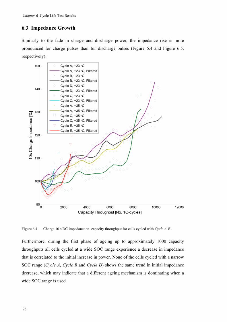
Chapter 6 Cycle Life Test Results
78
6.3 Impedance Growth
Similarly to the fade in charge and discharge power, the impedance rise is more
pronounced for charge pulses than for discharge pulses (Figure 6.4 and Figure 6.5,
respectively).
Figure 6.4 Charge 10 s DC impedance vs. capacity throughput for cells cycled with Cycle A-E.
Furthermore, during the first phase of ageing up to approximately 1000 capacity
throughputs all cells cycled at a wide SOC range experience a decrease in impedance
that is correlated to the initial increase in power. None of the cells cycled with a narrow
SOC range (Cycle A, Cycle B and Cycle D) shows the same trend in initial impedance
decrease, which may indicate that a different ageing mechanism is dominating when a
wide SOC range is used.
0 2000 4000 6000 8000 10000 1200090
100
110
120
130
140
150
Capacity Throughput [No. 1C-cycles]
10
s C
ha
rge
Imp
ed
an
ce [%
]
Cycle A, +23 CCycle A, +23 C, Filtered
Cycle B, +23 CCycle B, +23 C, Filtered
Cycle D, +23 CCycle D, +23 C, Filtered
Cycle C, +23 CCycle C, +23 C, Filtered
Cycle A, +35 CCycle A, +35 C, Filtered
Cycle C, +35 CCycle C, +35 C, Filtered
Cycle E, +35 CCycle E, +35 C, Filtered
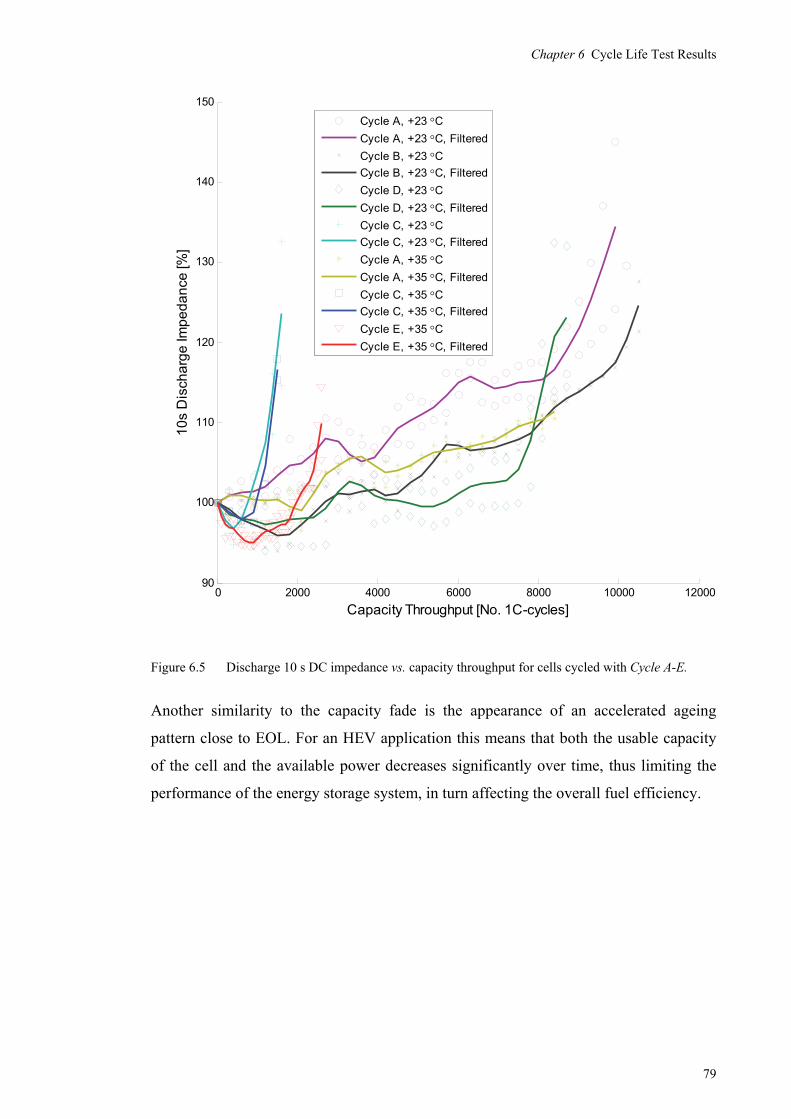
Chapter 6 Cycle Life Test Results
79
Figure 6.5 Discharge 10 s DC impedance vs. capacity throughput for cells cycled with Cycle A-E.
Another similarity to the capacity fade is the appearance of an accelerated ageing
pattern close to EOL. For an HEV application this means that both the usable capacity
of the cell and the available power decreases significantly over time, thus limiting the
performance of the energy storage system, in turn affecting the overall fuel efficiency.
0 2000 4000 6000 8000 10000 1200090
100
110
120
130
140
150
Capacity Throughput [No. 1C-cycles]
10
s D
isch
arg
e Im
pe
da
nce
[%]
Cycle A, +23 CCycle A, +23 C, Filtered
Cycle B, +23 CCycle B, +23 C, Filtered
Cycle D, +23 CCycle D, +23 C, Filtered
Cycle C, +23 CCycle C, +23 C, Filtered
Cycle A, +35 CCycle A, +35 C, Filtered
Cycle C, +35 CCycle C, +35 C, Filtered
Cycle E, +35 CCycle E, +35 C, Filtered

Chapter 6 Cycle Life Test Results
80
6.4 Power Efficiency at Low Power
Although the capacity, the maximum power and DC impedance are significantly
deteriorated during cycling, the power efficiency calculated from the dynamic response
tests (see section 3.1.2) stays surprisingly stable throughout the cycle life test (Figure
6.6).
Figure 6.6 Power efficiency vs. capacity throughput from dynamic response test for cells cycled with
Cycle A-E.
The stable power efficiency indicates that at low to medium power, the cell will be able
to provide sufficient performance in terms of power and efficiency throughout its
lifetime. It should however be emphasised that this reasoning is strongly dependant on
the definition of “low to medium power”; in this case 1-5 C-rate. Furthermore, the
results are in line with the definition of instantaneous power efficiency (3.7-3.8) where
an increase in total impedance yields a similar change in power efficiency.
0 2000 4000 6000 8000 10000 1200080
82
84
86
88
90
92
94
96
98
100
Capacity Throughput [No. 1C-cycles]
Effi
cie
ncy
[%]
Cycle A, +23 CCycle A, +23 C, Filtered
Cycle B, +23 CCycle B, +23 C, Filtered
Cycle D, +23 CCycle D, +23 C, Filtered
Cycle C, +23 CCycle C, +23 C, Filtered
Cycle A, +35 CCycle A, +35 C, Filtered
Cycle C, +35 CCycle C, +35 C, Filtered
Cycle E, +35 CCycle E, +35 C, Filtered

Chapter 6 Cycle Life Test Results
81
6.5 Calendar Ageing
The effect of calendar ageing (see section 2.4.2) was not a part of the present work.
However, all cells were manufactured at approximately the same date and the different
cycle life tests were initiated at different dates. Hence, an overview of the effect of
calendar ageing can be made using the test result from the first RPT for each cell. The
measured capacity at 1 C-rate and the 10s DC impedance for discharge at 60% SOC
(see section 3.1) is presented vs. storage time in Figure 6.7.
Figure 6.7 Capacity at 1 C-rate and 10s DC impedance for discharge at 60% SOC vs. storage time.
There is slight distribution of capacity and impedance within the cells characterised at
each time period. Typically 1-2 cell tests were characterised at approximately the same
time, yielding the five distinct groups seen in Figure 6.7. Also, the distribution of
impedance is significantly larger than for capacity. Nevertheless, the differences are
small compared to the trends observed during the cycle life tests (see section 6.1 and
6.3). The differences may also be dependent on the properties (accuracy) of the different
channels of the battery test equipment.
Since all the ageing properties evaluated within the scope of this investigation are
normalised to the respective initial property this is assumed to have a negligible effect
on the analysis.
0 50 100 150 200 250 300 350 40080
85
90
95
100
105
110
Time [days]
Rel
ativ
e C
hang
e [%
]
C/1 Capacity, measured
C/1 Capacity, polynom fit
DC Impedance, measured
DC Impedance, polynom fit

Chapter 6 Cycle Life Test Results
82
6.6 Summary
A brief analysis of the results can be summarised as follows:
The synthetic cycle (Cycle B) is more detrimental than the reference cycle
(Cycle A), during the first phase of ageing, but Cycle A results in an earlier EOL.
A higher average temperature does not necessarily lead to a faster capacity fade
in this case; there is no significant difference between the cell pairs cycled with
Cycle C at +23 °C and +35 °C. More notably, the cells cycled at Cycle A at
+35 °C shows a slower capacity fade than what is observed at +23 °C.
When cycling at constant current, the SOC range has a profound effect on the
capacity fade. Cells cycled with 17% ΔSOC (Cycle D) do not show a capacity
fade rate that is comparable to those cycled with 95-100% ΔSOC (Cycle C).
The capacity fade rate is neither constant nor monotonically increasing over
time. All cells show a capacity fade rate that varies over time.
The increase in charge impedance and the corresponding decrease in charge
power are considerably higher than the corresponding figures for discharge,
possibly leading to higher fuel consumption in an HEV. This may indicate an
“asymmetric” ageing with respect to anode and cathode.
The discharge power at high current rate and the efficiency at low to medium
current rate stay relatively constant over time.

Chapter 7 Cell Ageing Analysis
83
Chapter 7 Cell Ageing Analysis
Although battery ageing is often characterised using capacity fade and power fade as
reviewed in section 2.2 and summarised in section 6.6, there are several other possible
methods suitable for analysis and characterisation. This section presents an analysis
based on a selection of methods used within the work covered by this thesis.
Specifically, methods that can be used on commercial large cells to distinguish between
different ageing mechanisms have been evaluated.
The purpose of this section is to evaluate different methods for evaluating and
quantifying ageing mechanisms. This analysis may also provide input to how different
properties of load cycles and operating conditions affect the observed change in cell
performance during cycling.
7.1 Galvanostatic Voltage Profiles
Galvanostatic charge and discharge tests are examples of simple characterisation
techniques that clearly show how the electrochemical properties of a Li-ion cell change
during ageing. Such tests at C/1 and C/4 current rate were included in the RPTs (see
section 3.1). In good correlation to the overview in Chapter 6, these voltage profiles
provide a qualitative view of both capacity fade and impedance increase. Voltage
profiles measured at BOL and EOL for cells cycled according to Cycle A-E are shown
in Figure 7.1 and Figure 7.2.

Chapter 7 Cell Ageing Analysis
84
Figure 7.1 C/1 voltage profile vs. SOC for cells cycled with Cycle A-E.
Figure 7.1 shows the C/1 voltage profile as a function of cell SOC based on measured
capacity. That is, the reference capacity used to calculate SOC changes over time to
allow SOC=100% to correspond to a fully charged cell regardless of an observed
decrease in capacity. For cells cycled with the HEV cycles Cycle A and Cycle B the
impedance increase is more evident than for the PHEV cycles Cycle C and Cycle E.
Here, the impedance increase for Cycle A and Cycle B causes a higher voltage drop,
especially close to SOC=100% and SOC=0%, possibly indicating a slow migration of
0 20 40 60 80 1002.6
2.8
3
3.2
3.4
3.6
Vol
tage
[V
]
Cycle A
0 20 40 60 80 1002.6
2.8
3
3.2
3.4
3.6
Cycle A +35 C
0 20 40 60 80 1002.6
2.8
3
3.2
3.4
3.6
Vol
tage
[V
]
Cycle B
0 20 40 60 80 1002.6
2.8
3
3.2
3.4
3.6Cycle C
0 20 40 60 80 1002.6
2.8
3
3.2
3.4
3.6
Vol
tage
[V
]
SOC [%]
Cycle D
0 20 40 60 80 1002.6
2.8
3
3.2
3.4
3.6
SOC [%]
Cycle E
EOL
BOL

Chapter 7 Cell Ageing Analysis
85
Li-ions in the solid phase. Notably, the cells cycled with Cycle A at +35 °C do not show
higher impedance growth than those cycled at +23 °C.
Figure 7.2 C/4 voltage profile vs. capacity for cells cycled with Cycle A-E.
An alternative to comparing voltage profiles vs. SOC is to use an absolute capacity
scale. Figure 7.2 shows the voltage profile as a function of measured capacity at C/4
current rate, highlighting both the change in cell characteristics and the decrease in
capacity; first and foremost the voltage plateau close to SOC=100% is significantly
compressed for all cells, indicating that the cathode limits the charge before the anode is
0 0.5 1 1.5 2 2.52.6
2.8
3
3.2
3.4
3.6V
olta
ge [
V]
Cycle A
0 0.5 1 1.5 2 2.52.6
2.8
3
3.2
3.4
3.6
Cycle A +35 C
0 0.5 1 1.5 2 2.52.6
2.8
3
3.2
3.4
3.6
Vol
tage
[V
]
Cycle B
0 0.5 1 1.5 2 2.52.6
2.8
3
3.2
3.4
3.6Cycle C
0 0.5 1 1.5 2 2.52.6
2.8
3
3.2
3.4
3.6
Vol
tage
[V
]
Capacity [Ah]
Cycle D
0 0.5 1 1.5 2 2.52.6
2.8
3
3.2
3.4
3.6
Capacity [Ah]
Cycle E
EOL
BOL

Chapter 7 Cell Ageing Analysis
86
fully charged. The absence of a notable difference in impedance increase at C/4 further
supports the hypothesis that the large voltage drop close to SOC=0% and SOC=100%
for the HEV cycles (Figure 7.1) is caused by slow mass transport rather than an overall
loss of conductivity in electrodes or electrolyte.
The voltage profile of cells cycled according to the constant current Cycle D shows an
abnormal voltage plateau at approximately SOC=90% as illustrated in Figure 7.2 and
Figure 7.3. Also, the impedance increase is larger than what is observed for Cycle A and
Cycle B.
Figure 7.3 Detailed view of high-SOC C/4 voltage profile for cell cycled with Cycle D.
This new plateau is not related to any of the graphite stages (see section 7.2) and the
cause has not been confirmed. However, it might be due to a reversible Li-plating on the
anode since the new voltage plateau approximately corresponds to an anode potential of
0 V vs. Li/Li+. This hypothesis is discussed further in the following sections.
80 85 90 95 1003.3
3.35
3.4
3.45
3.5
3.55
SOC [%]
Vol
tage
[V
]
BOL
EOL

Chapter 7 Cell Ageing Analysis
87
7.2 Differential Voltage Analysis & Incremental Capacity Analysis
By using the galvanostatic voltage profiles at C/4 from the RPTs (described in section
3.1) it is possible to analyse and quantify the changes in electrochemical properties of
the cell further. Both the ICA and the DVA have been proposed and used before [15],
[81]-[85] and proved to serve as valuable tools.
In Figure 7.4 the different phases of graphite during intercalation/de-intercalation is
presented as suggested by [86] together with a charge and discharge voltage profile
measured on a Li//graphite half-cell (see section 7.3).
Figure 7.4 Phase diagram for Li-intercalation into graphite based on measured cell voltages at C/25
and [86].
The different plateaus and voltage gradients are directly linked to the different stages,
further quantified by Table 13 and graphically represented by Figure 7.5.
Table 13 Graphite phases in LixC6 according to [86]
SOC Range [x in LixC6] Graphite Phase 0-0.04 Stage-1(dilute) 0.04-0.12 Stage-1(dilute) & stage 4 0.12-0.20 Stage-4 & Stage-3 0.20-0.25 Stage-3 & Stage-2(liquid) 0.25-0.50 Stage-2(liquid) & Stage-2 0.50-1 Stage-2 & Stage-1
0 10 20 30 40 50 60 70 80 90 1000
0.5
1
1.5
2
1* 1*+4 4,3 3+2L 2L+2 2+1
SOC [%]
Vol
tage
[V
]
Intercalation of Li: cell charge
Deintercalation of Li: cell discharge

Chapter 7 Cell Ageing Analysis
88
Figure 7.5 Graphical representation of the different graphite stages according to [26] and [87].
The dilute sub-stage is an in-plane ordered phase with random Li-positions occupied.
Similarly, the liquid sub-stage is random but with no in-plane ordering. Several
different sub-phases have been proposed by V.A. Sethuraman et al. [26], Dahn et al.
[86] and R. Yazami et al. [87]. Note that the graphic representation in Figure 7.5 is
merely a schematic view of the lithium intercalation stages in graphite. Furthermore,
according to this model a graphite anode that is charged beyond 100% SOC will reach 0
V vs. Li/Li+ which in turn may lead to Li-plating at constant potential.
7.2.1 Calculation of DVA Profile
The DVA is a method widely used to highlight the different areas in a voltage profile
where the voltage derivative with respect to capacity is plotted as a function of capacity.
Following the cell voltage relation to electrode voltage (7.1) and the definition of
individual electrode DVA (7.2-7.3), the cell DVA is a linear combination of the two
according to (7.4).
cathodeanodecell VVV (7.1)
CfdC
dVDVA
anode
anodeanode
(7.2)
CfdC
dVDVA
cathode
cathodecathode
(7.3)
Stage-1* & Stage-4 Stage 4 & Stage 3
Stage-3 & Stage-2L Stage-2L & Stage-2 Stage-2 & Stage-1
Stage-1*Graphite
Stage-1 (LiC6)

Chapter 7 Cell Ageing Analysis
89
mAhdCCCC
VfDVADVAdC
VVd
dC
dVDVA
1,...for
maxmin
cathodeanodecell
cathodeanode
cellcell
(7.4)
A peak in the DVA spectrum denotes a relatively fast change in voltage which for
graphite electrodes is associated to the different stages of lithium intercalation. In order
to observe the peaks it is necessary to record the voltage profile at sufficiently low
current rate (usually < 1 C-rate) to avoid mass-transport related over-potential to over-
shadow the subtle changes in anode potential. An example of a DVA calculated from a
C/4 charge voltage profile for a cell cycled according to Cycle A is shown in Figure 7.6.
Figure 7.6 Example of DVA and C/4 voltage profile for a cell cycled according to Cycle A at BOL and
EOL respectively.
0 0.5 1 1.5 2 2.50
0.5
1
1.5
2
2.5
3
3.5
4
Capacity [Ah]
dV/d
Q [
V/A
h]
BOL
EOL
0 0.5 1 1.5 2 2.52.6
2.8
3
3.2
3.4
3.6
Vol
tage
[V
]
Cycle A
Diff. capacity at EOL
Peak 1
Diff. capacity at BOL
Peak 2

Chapter 7 Cell Ageing Analysis
90
The two peaks related to the two most significant voltage gradients in the charge curve
around 0.3/0.4 and 1.1/1.7 Ah (Figure 7.2) are also highlighted in this figure to show
their position change upon ageing. A reduction in anode capacity related to ageing will
cause a reduction of the peak distance in the DVA, whereas ageing solely depending on
the loss of lithium will leave the peak distance unaffected.
7.2.2 Calculation of ICA Profile
A closely related method to analyse the contributions from anode and cathode to the
total cell voltage is the ICA. The calculation of an ICA profile is in principle the inverse
of the DVA. Consequently, the anode and cathode contribution is not linearly combined
to form the total cell ICA.
The ICA relies on calculation of the differential capacity for small changes in voltage
according to (7.5-7.7).
VfdV
dCICA
anode
anodeanode
(7.5)
VfdV
dCICA
cathode
cathodecathode
(7.6)
mVdVVVV
Vf
ICAICA
DVADVADVAdV
dCICA
1,...for
11
1
11
maxmin
cathode anode
cathodeanodecell
cellcell
(7.7)
A peak in the ICA spectrum denotes a flat region in a voltage profile. If the voltage
profile is obtained at sufficiently low current rate it is possible to observe the different
voltage plateaus associated to the staging of the graphite anode (see Figure 7.4 ) as
peaks at defined voltage levels. In relation to ageing, a symmetric reduction of the peak
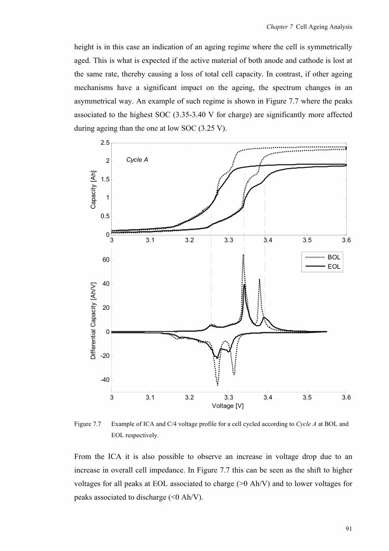
Chapter 7 Cell Ageing Analysis
91
height is in this case an indication of an ageing regime where the cell is symmetrically
aged. This is what is expected if the active material of both anode and cathode is lost at
the same rate, thereby causing a loss of total cell capacity. In contrast, if other ageing
mechanisms have a significant impact on the ageing, the spectrum changes in an
asymmetrical way. An example of such regime is shown in Figure 7.7 where the peaks
associated to the highest SOC (3.35-3.40 V for charge) are significantly more affected
during ageing than the one at low SOC (3.25 V).
Figure 7.7 Example of ICA and C/4 voltage profile for a cell cycled according to Cycle A at BOL and
EOL respectively.
From the ICA it is also possible to observe an increase in voltage drop due to an
increase in overall cell impedance. In Figure 7.7 this can be seen as the shift to higher
voltages for all peaks at EOL associated to charge (>0 Ah/V) and to lower voltages for
peaks associated to discharge (<0 Ah/V).
3 3.1 3.2 3.3 3.4 3.5 3.6
-40
-20
0
20
40
60
Voltage [V]
Diff
eren
tial C
apac
ity [
Ah/
V]
BOL
EOL
3 3.1 3.2 3.3 3.4 3.5 3.60
0.5
1
1.5
2
2.5
Cap
acity
[A
h]
Cycle A

Chapter 7 Cell Ageing Analysis
92
7.3 Half-cell Test Results
A number of constant current charge and discharge cycles were tested on the half-cells
manufactured by UU. These small pouch-type cells are made from a single coated
current collector of either graphite or LiFePO4 combined with a separator, a lithium
metal foil and electrolyte (see section 5.1). Despite their low capacity, approx. 3 mAh,
the half-cells were used to extract detailed voltage profiles for anode and cathode
voltage curves representative to LiFePO4//graphite cells in general. The measured
voltage profiles were then used to simulate different ageing mechanisms such as loss of
active lithium and loss of active material (see section 7.4). A selection of voltage
profiles with current rates ranging from C/25 to C/1 is presented in Figure 7.8 and
Figure 7.9 respectively. The SOC values in these graphs are calculated with the cell
SOC as reference, i.e. not as the individual lithium content in respective electrode.
Likewise, the current direction is also defined with a full-cell as reference.
Figure 7.8 Constant current voltage profiles for LiFePO4 // Li half-cell.
0 10 20 30 40 50 60 70 80 90 1002.4
2.6
2.8
3
3.2
3.4
3.6
3.8
4
SOC [%]
Vol
tage
[V
]
C/25 Discharge
C/25 Charge
C/5 DischargeC/5 Charge
C/2 Discharge
C/2 Charge

Chapter 7 Cell Ageing Analysis
93
Figure 7.9 Constant current voltage profiles for graphite//Li half-cell.
Judging from the constant current voltage profiles at higher current rates (>C/10), the
small half-cells have significantly higher impedance per unit capacity than the
commercial cells. Hence, they are less suitable to use in an analysis of large cell
impedance or dynamics. In addition, the impedance is not constant; close to SOC=0%
and SOC=100% the apparent impedance increases significantly, indicating a reduction
of mass transport rate. Nevertheless, analysis methods such as ICA and DVA rely on
low rate charging/discharging to characterise aging. Thus, using the low-rate profiles of
half-cells may provide an insight to ageing mechanisms in commercial cells. Such
analysis is presented in detail in the following section.
7.4 Cell Capacity Fade Model based on Half-cell Measurements
The measurements of half-cell voltage profiles at low current rate (C/25) were used to
evaluate the use of ICA and DVA to quantify full-cell ageing mechanisms. Voltage
profiles at C/25 current rate for a lithium//graphite cell between 0.01 and 2.00 V vs.
Li/Li+ and a LiFePO4//lithium cell between 2.70 and 4.00 V vs. Li/Li+ were obtained at
room temperature using a Gamry Reference 3000 potentiostat and the half-cells
manufactured by UU. An example of anode voltage, cathode voltage and a simulated
cell voltage is shown in Figure 7.10.
0 10 20 30 40 50 60 70 80 90 1000
0.1
0.2
0.3
0.4
0.5
0.6
0.7
0.8
0.9
1
SOC [%]
Vol
tage
[V
]
C/25 Discharge
C/25 Charge
C/5 DischargeC/5 Charge
C/2 Discharge
C/2 Charge
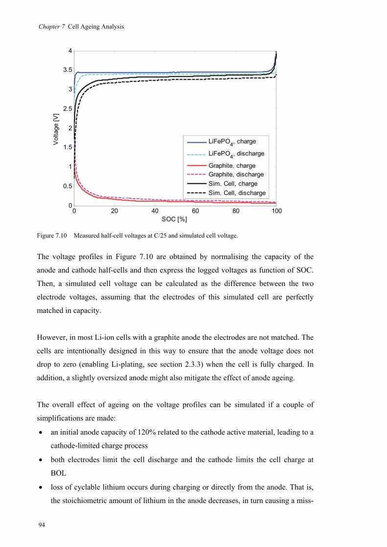
Chapter 7 Cell Ageing Analysis
94
Figure 7.10 Measured half-cell voltages at C/25 and simulated cell voltage.
The voltage profiles in Figure 7.10 are obtained by normalising the capacity of the
anode and cathode half-cells and then express the logged voltages as function of SOC.
Then, a simulated cell voltage can be calculated as the difference between the two
electrode voltages, assuming that the electrodes of this simulated cell are perfectly
matched in capacity.
However, in most Li-ion cells with a graphite anode the electrodes are not matched. The
cells are intentionally designed in this way to ensure that the anode voltage does not
drop to zero (enabling Li-plating, see section 2.3.3) when the cell is fully charged. In
addition, a slightly oversized anode might also mitigate the effect of anode ageing.
The overall effect of ageing on the voltage profiles can be simulated if a couple of
simplifications are made:
an initial anode capacity of 120% related to the cathode active material, leading to a
cathode-limited charge process
both electrodes limit the cell discharge and the cathode limits the cell charge at
BOL
loss of cyclable lithium occurs during charging or directly from the anode. That is,
the stoichiometric amount of lithium in the anode decreases, in turn causing a miss-
0 20 40 60 80 1000
0.5
1
1.5
2
2.5
3
3.5
4
SOC [%]
Vol
tage
[V
]
LiFePO4, charge
LiFePO4, discharge
Graphite, chargeGraphite, discharge
Sim. Cell, charge
Sim. Cell, discharge
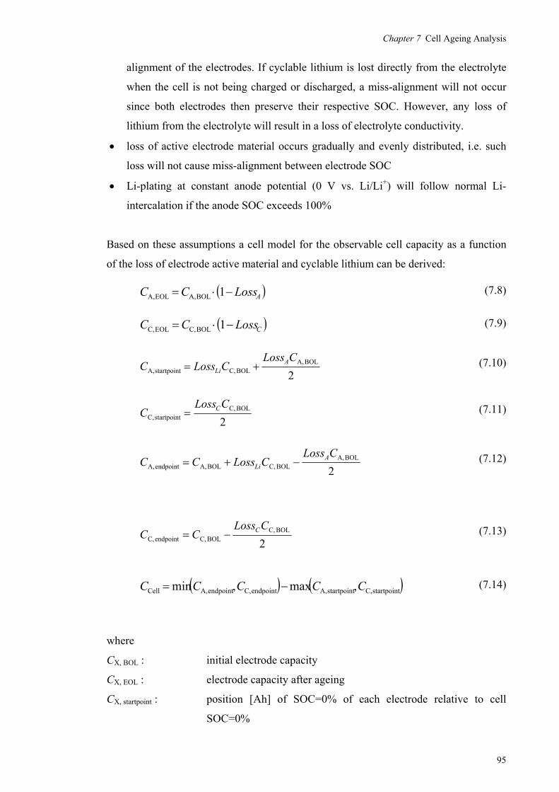
Chapter 7 Cell Ageing Analysis
95
alignment of the electrodes. If cyclable lithium is lost directly from the electrolyte
when the cell is not being charged or discharged, a miss-alignment will not occur
since both electrodes then preserve their respective SOC. However, any loss of
lithium from the electrolyte will result in a loss of electrolyte conductivity.
loss of active electrode material occurs gradually and evenly distributed, i.e. such
loss will not cause miss-alignment between electrode SOC
Li-plating at constant anode potential (0 V vs. Li/Li+) will follow normal Li-
intercalation if the anode SOC exceeds 100%
Based on these assumptions a cell model for the observable cell capacity as a function
of the loss of electrode active material and cyclable lithium can be derived:
ALossCC 1BOL A,EOL A,(7.8)
CLossCC 1BOL C,EOL C,(7.9)
2BOL A,
BOL C,startpoint A,
CLossCLossC A
Li (7.10)
2BOL C,
startpoint C,
CLossC C (7.11)
2BOL A,
BOL C,BOL A,endpoint A,
CLossCLossCC A
Li (7.12)
2BOL C,
BOL C,endpoint C,
CLossCC C (7.13)
startpoint C,startpoint A,endpoint C,endpoint A,Cell ,max,min CCCCC
(7.14)
where
CX, BOL : initial electrode capacity
CX, EOL : electrode capacity after ageing
CX, startpoint : position [Ah] of SOC=0% of each electrode relative to cell
SOC=0%

Chapter 7 Cell Ageing Analysis
96
CX, endpoint : position [Ah] of SOC=100% of each electrode relative to cell
SOC=100%
CCell : observable cell capacity.
An example of a cell simulation based on assuming 20% loss of cyclable lithium is
shown in Figure 7.11.
Figure 7.11 Calculation of observable capacity assuming 20% loss of cyclable lithium.
This simulation is made by calculating the individual electrode capacities as function of
ageing (7.8-7.9), their alignment on a normalised capacity scale (7.10-7.13) and the
resulting cell capacity as the difference between the electrode capacity positions (7.14).
The cell voltage is calculated as the difference between electrode potentials between the
two capacity boundaries used in (7.14).
In Figure 7.11 the anode limits the discharge of the cell when it reaches zero SOC (rapid
increase in potential vs. Li+/Li). Similarly, the cathode limits the charge of the cell as its
potential increase although the anode is still at SOC < 100%. The miss-alignment of the
electrodes is clearly visible in this figure as the shift in start-point of the cathode voltage
curve from zero to -0.2. Also, note that the respective electrode capacities do not change
-0.2 0 0.2 0.4 0.6 0.8 1 1.20
0.5
1
1.5
2
2.5
3
3.5
4
Cell Capacity: 80%
Capacity[-]
Vol
tage
[V
]
Anode
Cathode
Cell
CC, EOL
CA, EOL
CC, startpoint
CA, startpoint
CA, endpointC
C, endpoint
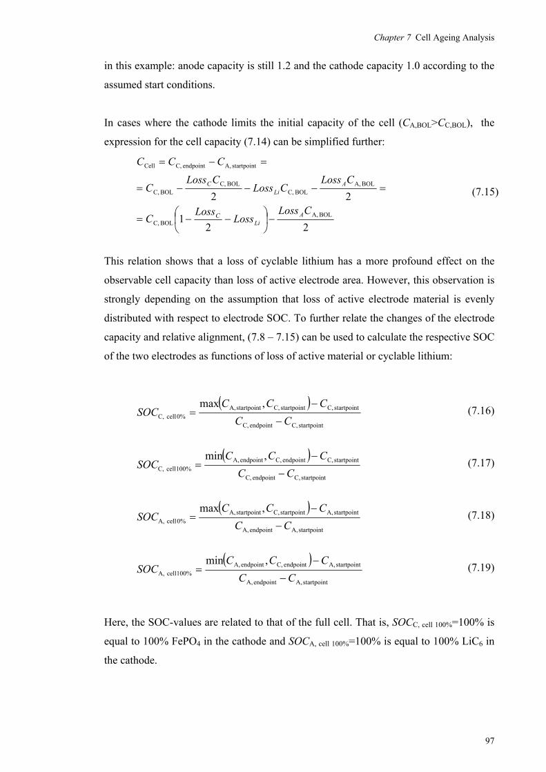
Chapter 7 Cell Ageing Analysis
97
in this example: anode capacity is still 1.2 and the cathode capacity 1.0 according to the
assumed start conditions.
In cases where the cathode limits the initial capacity of the cell (CA,BOL>CC,BOL), the
expression for the cell capacity (7.14) can be simplified further:
221
22
BOL A,BOL C,
BOL A,BOL C,
BOL C,BOL C,
startpoint A,endpoint C,Cell
CLossLoss
LossC
CLossCLoss
CLossC
CCC
ALi
C
ALi
C
(7.15)
This relation shows that a loss of cyclable lithium has a more profound effect on the
observable cell capacity than loss of active electrode area. However, this observation is
strongly depending on the assumption that loss of active electrode material is evenly
distributed with respect to electrode SOC. To further relate the changes of the electrode
capacity and relative alignment, (7.8 – 7.15) can be used to calculate the respective SOC
of the two electrodes as functions of loss of active material or cyclable lithium:
startpoint C,endpoint C,
startpoint C,startpoint C,startpoint A,0% cell C,
,max
CC
CCCSOC
(7.16)
startpoint C,endpoint C,
startpoint C,endpoint C,endpoint A,100% cell C,
,min
CC
CCCSOC
(7.17)
startpoint A,endpoint A,
startpoint A,startpoint C,startpoint A,0% cell A,
,max
CC
CCCSOC
(7.18)
startpoint A,endpoint A,
startpoint A,endpoint C,endpoint A,100% cell A,
,min
CC
CCCSOC
(7.19)
Here, the SOC-values are related to that of the full cell. That is, SOCC, cell 100%=100% is
equal to 100% FePO4 in the cathode and SOCA, cell 100%=100% is equal to 100% LiC6 in
the cathode.

Chapter 7 Cell Ageing Analysis
98
To highlight the main result of this simplified cell ageing modelling method, four
different cases of ageing are presented in this investigation:
Case 1: 0-30% loss of cyclable lithium
Case 2: 0-45% loss of active anode material
The case of 45% anode loss leads to Li-plating
Case 3: 0-30% loss of active cathode material
Case 4: 0-10% loss of cyclable lithium and 0-10% loss of active electrode
material
These four cases are presented and analysed in more detail in the following sections.
7.4.1 Case 1: Loss of Cyclable lithium
A loss of cyclable lithium may cause a miss-alignment of the electrodes and an increase
in cell impedance. That is, the amount of lithium in the anode at cell SOC=100%
decreases. In Figure 7.12 the potential of the anode, the cathode and the corresponding
simulated cell potential are presented at BOL assuming a 20% oversized anode.
Figure 7.12 Anode, cathode and simulated cell potential at BOL.
0 0.2 0.4 0.6 0.8 1 1.20
0.5
1
1.5
2
2.5
3
3.5
4
Cell Capacity: 100%
Capacity[-]
Vol
tage
[V
]
Anode
CathodeCell

Chapter 7 Cell Ageing Analysis
99
Note that at cell SOC=100%, the rise in cathode potential limits the charge, and at 0%
SOC both anode and cathode limit the cell operation as their respective rapid changes in
potential results in a rapid decrease in cell voltage.
A 30% loss of cyclable lithium was simulated using the model presented in the previous
section, causing a severe miss-alignment between electrode potentials. The effect of this
ageing mechanism on the cell voltage is presented in Figure 7.13 and Figure 7.14,
respectively.
Figure 7.13 Anode, cathode and simulated cell potential vs. capacity at 30% loss of cyclable lithium.
The indicated cell capacity in this simulation is relative to the available capacity in the
cell rather than the electrode capacities. Here, one of the most obvious effects on the
observable cell voltage is that the plateau related to the stage-2/stage-1 two-phase region
of the graphite is shortened as the cathode is limiting the charge at a lower anode charge
level (Figure 7.14). Neither the cathode nor the anode is utilized to its full extent in this
severe case of loss of cyclable lithium.
-0.4 -0.2 0 0.2 0.4 0.6 0.8 1 1.20
0.5
1
1.5
2
2.5
3
3.5
4
Cell Capacity: 70%
Capacity[-]
Vol
tage
[V
]
Anode
CathodeCell

Chapter 7 Cell Ageing Analysis
100
Figure 7.14 Cell voltage vs. normalised capacity at simulated Li-loss of 0-30%.
Furthermore, the corresponding DVA (Figure 7.15) and the ICA (Figure 7.16) profiles
also show distinguishable changes in their characteristics upon loss of cyclable lithium.
Figure 7.15 DVA at simulated Li-loss of 0-30%.
0 10 20 30 40 50 60 70 80 90 1003
3.05
3.1
3.15
3.2
3.25
3.3
3.35
3.4
3.45
3.5
Normalised Capacity [%]
Vol
tage
[V
]
Li-loss: 0%
Li-loss: 10%Li-loss: 20%
Li-loss: 30%
0 0.1 0.2 0.3 0.4 0.5 0.6 0.7 0.8 0.9 1-1
0
1
2
3
4
5
Normalised Capacity [-]
dV/d
Q [
V/Q
]
Li-loss: 0%
Li-loss: 10%
Li-loss: 20%
Li-loss: 30%

Chapter 7 Cell Ageing Analysis
101
In the DVA (Figure 7.15), the profile is almost identical for Li-loss 0-20% except an
early cut-off in the right region where the cathode limits the charge.
Figure 7.16 ICA at simulated Li-loss of 0-30%.
Likewise, the absence of the stage-2/stage-1 plateau in the graphite is shown clearly in
the ICA (Figure 7.16) where the peaks at 3.38 V(charge) and 3.31 V(discharge)
gradually disappear.
As a concluding remark, a loss of cyclable lithium results in observable changes in both
voltage profiles, DVA and ICA.
7.4.2 Case 2: Loss of Active Anode Material
When anode material is lost the effect on the cell voltage profiles are less pronounced
(Figure 7.17 and Figure 7.19). At 30% loss, the anode is fully utilized compared to the
80% utilization rate at BOL. The cell voltage profile then occurs to be compressed,
preserving the main characteristics although the stage-2/stage-1 plateau in the graphite
is widened as the cathode cuts off the charging at 100% graphite SOC.
3.1 3.15 3.2 3.25 3.3 3.35 3.4 3.45 3.5-20
-15
-10
-5
0
5
10
15
20
25
30
Voltage [V]
Diff
eren
tial C
apac
ity [
Ah/
V]
Li-loss: 0%
Li-loss: 10%Li-loss: 20%
Li-loss: 30%

Chapter 7 Cell Ageing Analysis
102
Figure 7.17 Anode, cathode and simulated cell potential vs. capacity at 30% loss of active anode
material.
When 45% active anode material is lost the anode voltage reaches 0 V vs. Li/Li+ which
in turn, in this simulation, leads to Li-plating (Figure 7.18).
Figure 7.18 Anode, cathode and simulated cell potential vs. capacity at 45% loss of active anode
material.
-0.2 0 0.2 0.4 0.6 0.8 1 1.20
0.5
1
1.5
2
2.5
3
3.5
4
Cell Capacity: 82%
Capacity[-]
Vol
tage
[V
]
Anode
CathodeCell
-0.4 -0.2 0 0.2 0.4 0.6 0.8 10
0.5
1
1.5
2
2.5
3
3.5
4
Cell Capacity: 73%
Capacity[-]
Vol
tage
[V
]
Anode
CathodeCell

Chapter 7 Cell Ageing Analysis
103
In the voltage profile this can be observed as the additional voltage plateau close to
SOC=100% at the point where the anode potential is stabilised at 0 V vs. Li/Li+ (Figure
7.19).
Figure 7.19 Cell voltage vs. normalised capacity at simulated anode material loss of 0-45%.
In this simulation no measurements of the anode potential during Li-plating has been
made. Hence, the estimated voltage profile does not take the changes in the cell
dynamics into account which leads to a discontinuous voltage profile for cell discharge.
The compression of the voltage curve and the widening of the stage-2/stage-1 plateau
are also shown in the DVA and the ICA profiles (Figure 7.20 and Figure 7.21
respectively).
0 10 20 30 40 50 60 70 80 90 1003
3.05
3.1
3.15
3.2
3.25
3.3
3.35
3.4
3.45
3.5
Normalised Capacity [%]
Vol
tage
[V
]
A-loss: 0%
A-loss: 15%A-loss: 30%
A-loss: 45%

Chapter 7 Cell Ageing Analysis
104
Figure 7.20 DVA at simulated anode material loss of 0-45%.
Figure 7.21 ICA at simulated anode material loss of 0-45%.
0 0.1 0.2 0.3 0.4 0.5 0.6 0.7 0.8 0.9 10
0.5
1
1.5
2
2.5
3
3.5
4
4.5
5
Normalised Capacity [-]
dV/d
Q [
V/Q
]
A-loss: 0%
A-loss: 15%
A-loss: 30%
A-loss: 45%
3.1 3.15 3.2 3.25 3.3 3.35 3.4 3.45 3.5-20
-15
-10
-5
0
5
10
15
20
25
30
Voltage [V]
Diff
eren
tial C
apac
ity [
Ah/
V]
A-loss: 0%
A-loss: 15%
A-loss: 30%
A-loss: 45%

Chapter 7 Cell Ageing Analysis
105
Of special interest is that the inter-distance between the peaks in the DVA profile is
reduced at the same rate as the loss of active anode material. Also, note that the peak at
3.31 V (discharge) in the ICA (Figure 7.21) increases in magnitude.
The new plateau at high SOC causes an extra peak in the DVA profile when the anode
reaches 100% SOC. Likewise, two new peaks directly related to Li-plating can be
observed in the ICA profile at 3.47 V (charge) and 3.41 V(discharge).
7.4.3 Case 3: Loss of Active Cathode Material
Despite the lack of multiple two-phase regions yielding several voltage plateaus, a loss
of active cathode changes the voltage profiles (Figure 7.22 and Figure 7.23) in a
profound way; after ageing the cathode will limit both charge and discharge, effectively
limiting the utilization of the anode until the cell operates in the mid-range of the curve
with only two observable graphite phase plateaus. In addition, the cut-off at low cell
SOC will be very sharp.
Figure 7.22 Anode, cathode and simulated cell potential vs. capacity at 30% loss of active cathode
material.
-0.2 0 0.2 0.4 0.6 0.8 1 1.20
0.5
1
1.5
2
2.5
3
3.5
4
Cell Capacity: 70%
Capacity[-]
Vol
tage
[V
]
Anode
CathodeCell
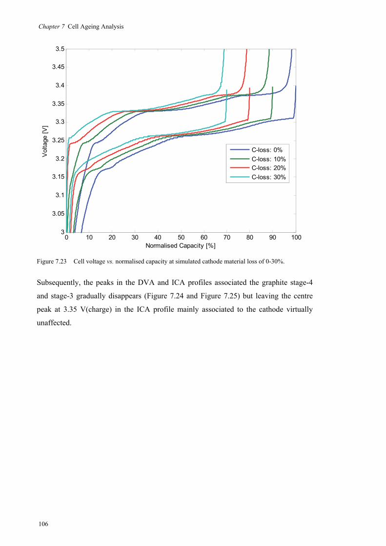
Chapter 7 Cell Ageing Analysis
106
Figure 7.23 Cell voltage vs. normalised capacity at simulated cathode material loss of 0-30%.
Subsequently, the peaks in the DVA and ICA profiles associated the graphite stage-4
and stage-3 gradually disappears (Figure 7.24 and Figure 7.25) but leaving the centre
peak at 3.35 V(charge) in the ICA profile mainly associated to the cathode virtually
unaffected.
0 10 20 30 40 50 60 70 80 90 1003
3.05
3.1
3.15
3.2
3.25
3.3
3.35
3.4
3.45
3.5
Normalised Capacity [%]
Vol
tage
[V
]
C-loss: 0%
C-loss: 10%C-loss: 20%
C-loss: 30%
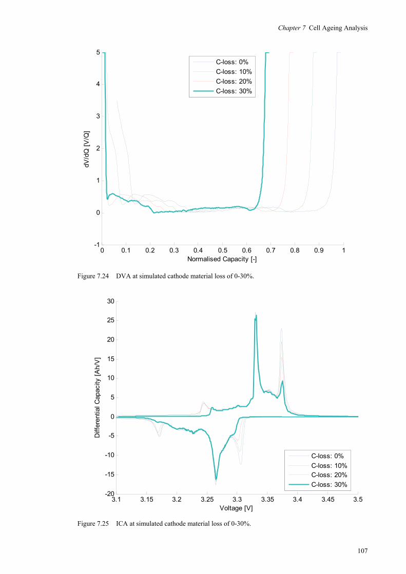
Chapter 7 Cell Ageing Analysis
107
Figure 7.24 DVA at simulated cathode material loss of 0-30%.
Figure 7.25 ICA at simulated cathode material loss of 0-30%.
0 0.1 0.2 0.3 0.4 0.5 0.6 0.7 0.8 0.9 1-1
0
1
2
3
4
5
Normalised Capacity [-]
dV/d
Q [
V/Q
]
C-loss: 0%
C-loss: 10%
C-loss: 20%
C-loss: 30%
3.1 3.15 3.2 3.25 3.3 3.35 3.4 3.45 3.5-20
-15
-10
-5
0
5
10
15
20
25
30
Voltage [V]
Diff
eren
tial C
apac
ity [
Ah/
V]
C-loss: 0%
C-loss: 10%C-loss: 20%
C-loss: 30%

Chapter 7 Cell Ageing Analysis
108
7.4.4 Case 4: Loss of Cyclable lithium and Active Electrode Material
The last example of simulated ageing is probably one of the most realistic: a
combination of loss of cyclable lithium (10%) and active electrode material (10% loss
of anode and cathode material respectively).
Starting with voltage profiles (Figure 7.26 and Figure 7.27) both the effect of lithium
loss and electrode material loss is observable in the compression of the voltage profile
and the reduction of the anode utilization range at high electrode charge level.
Figure 7.26 Anode, cathode and simulated cell potential vs. capacity at 10% loss of Li and electrode
material.
-0.2 0 0.2 0.4 0.6 0.8 1 1.20
0.5
1
1.5
2
2.5
3
3.5
4
Cell Capacity: 84%
Capacity[-]
Vol
tage
[V
]
Anode
CathodeCell

Chapter 7 Cell Ageing Analysis
109
Figure 7.27 Cell voltage vs. normalised capacity at simulated Li-loss and electrode material loss of 0-
10%.
Again, the same effect is observed in the DVA profile (Figure 7.28); a reduction of the
peak corresponding to the stage-2/stage-1 and a compression of the profile. In the ICA
profile (Figure 7.29) all peaks are reduced but with an emphasis in the 3.38 V (charge)
peak.
Despite that different ageing mechanisms have a different effect on voltage profiles,
DVA and ICA, it can be concluded that this method can prove to be a useful method
when evaluating the ageing of full-cells.
0 10 20 30 40 50 60 70 80 90 1003
3.05
3.1
3.15
3.2
3.25
3.3
3.35
3.4
3.45
3.5
Normalised Capacity [%]
Vol
tage
[V
]
Li/A/C-loss: 0%
Li/A/C-loss: 2.5%
Li/A/C-loss: 5%Li/A/C-loss: 7.5%
Li/A/C-loss: 10%
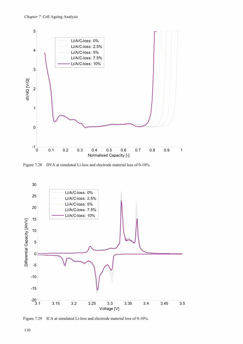
Chapter 7 Cell Ageing Analysis
110
Figure 7.28 DVA at simulated Li-loss and electrode material loss of 0-10%.
Figure 7.29 ICA at simulated Li-loss and electrode material loss of 0-10%.
0 0.1 0.2 0.3 0.4 0.5 0.6 0.7 0.8 0.9 1-1
0
1
2
3
4
5
Normalised Capacity [-]
dV/d
Q [
V/Q
]
Li/A/C-loss: 0%
Li/A/C-loss: 2.5%
Li/A/C-loss: 5%Li/A/C-loss: 7.5%
Li/A/C-loss: 10%
3.1 3.15 3.2 3.25 3.3 3.35 3.4 3.45 3.5-20
-15
-10
-5
0
5
10
15
20
25
30
Voltage [V]
Diff
eren
tial C
apac
ity [
Ah/
V]
Li/A/C-loss: 0%
Li/A/C-loss: 2.5%
Li/A/C-loss: 5%Li/A/C-loss: 7.5%
Li/A/C-loss: 10%

Chapter 7 Cell Ageing Analysis
111
7.5 ICA & DVA of Aged Cells
Incremental capacity analysis and differential capacity analysis were performed for all
cells based on the C/4 voltage profiles measured during each RPT. A collection of
results are briefly presented in this section. These results are then used to quantify the
aging in terms of loss of cyclable lithium and active electrode material (see section 7.6).
An ICA was calculated at BOL and EOL for all cells cycled according to Cycle A-E
(Figure 7.30).
Figure 7.30 ICA for cells cycled according to Cycle A-E.
3 3.2 3.4 3.6
-40
-20
0
20
40
60
Diff
eren
tial C
apac
ity [
Ah/
V] Cycle A
3 3.2 3.4 3.6
-40
-20
0
20
40
60 Cycle A +35 C
3 3.2 3.4 3.6
-40
-20
0
20
40
60
Diff
eren
tial C
apac
ity [
Ah/
V] Cycle B
3 3.2 3.4 3.6
-40
-20
0
20
40
60 Cycle C
3 3.2 3.4 3.6
-40
-20
0
20
40
60
Diff
eren
tial C
apac
ity [
Ah/
V]
Voltage [V]
Cycle D
3 3.2 3.4 3.6
-40
-20
0
20
40
60
Voltage [V]
Cycle E
EOL
BOL

Chapter 7 Cell Ageing Analysis
112
For all cells in Figure 7.30 the ICA profiles indicate that several ageing mechanisms are
contributing to the ageing. Firstly, the peak associated to the stage-2/stage-1 lithiation of
the graphite is significantly reduced, in turn indicating loss of cyclable lithium in
correspondence with the model presented in the previous section and as reported in
literature. Secondly, all other peaks are reduced in magnitude which indicates a loss of
active anode material. Lastly, the shift in peak position reveals a significant increase in
cell impedance.
There are two differences in ICA between the PHEV cycles Cycle C and Cycle E and
the HEV cycles Cycle A and Cycle B; the peak positions do not change indicating a
lower impedance increase and the reduction of the centre peak in the ICA is not at all as
reduced. Furthermore, Cycle D shows two additional peaks in the ICA profile at high
cell voltage, possibly indicating reversible Li-plating in correspondence with the results
obtained with cell fade model simulations in section 7.4.2. Similar conclusions can be
drawn from the DVA for the same cells (Figure 7.31).
The DVA profiles in Figure 7.31 are compressed representing a loss of active anode
material that can be quantified by calculating the peak distance as described in section
7.2. Also, the capacity related to the stage-2/stage-1 is greatly reduced; demonstrating
the effect of lithium loss. However, it should be noted that the cells cycled according to
Cycle C reaches EOL significantly earlier in terms of total capacity throughput than
cells cycled with Cycle A or Cycle B (see section 6.1).
EOL is reached at approximately twice the capacity throughput for Cycle E compared to
Cycle C. Hence, the ageing with the PHEV cycle is half as fast in terms of capacity
fade, but the impedance increase at EOL is comparable.
Likewise to the ICA results, there is an extra peak seen for Cycle D for high SOC,
positioned approximately where Li-plating would occur according to the cell fade
model simulation results.

Chapter 7 Cell Ageing Analysis
113
Figure 7.31 DVA for cells cycled according to Cycle A, Cycle B, Cycle C and Cycle E.
0 0.5 1 1.5 20
1
2
3
4
Diff
eren
tial V
olta
ge [
V/A
h] Cycle A
0 0.5 1 1.5 20
1
2
3
4
Cycle A +35 C
0 0.5 1 1.5 20
1
2
3
4
Diff
eren
tial V
olta
ge [
V/A
h] Cycle B
0 0.5 1 1.5 20
1
2
3
4
Cycle C
0 0.5 1 1.5 20
1
2
3
4
Diff
eren
tial V
olta
ge [
V/A
h]
Capacity [Ah]
Cycle D
0 0.5 1 1.5 20
1
2
3
4
Capacity [Ah]
Cycle E
EOL
BOL

Chapter 7 Cell Ageing Analysis
114
7.6 Estimation of Loss of Electrode Capacity and Cyclable Lithium
The method for estimating loss of active electrode material and loss of cyclable lithium
described in section 7.2 and illustrated with the cell simulations in section 7.4 was
applied to the cycle life tests with Cycle A-E using data from the C/4 voltage profiles.
Since it is not easily conceivable to distinguish between loss of cyclable lithium and
loss of active cathode material based on the presented cell model these ageing
mechanisms will be displayed as one quantity in the graphical representation. Also, the
estimation of the anode ageing is made using the same assumptions as in section 7.4
which in this case might not be fully valid since the detailed cell properties are
unknown.
In this section the C/4 capacity is shown together with the estimated cell capacity loss
due to anode loss and residual loss (cyclable lithium and cathode) for each of the tests
using load Cycle A-E.
The result from the reference Cycle A in Figure 7.32 indicates that the anode ageing rate
is lower than that of the cathode, and also lower than the rate of loss of cyclable lithium
until the last phase of the ageing where both cell capacity and anode capacity rapidly
decreases, indicating that the cell aging process undergoes several stages.
The EOL limit is set to the point when the cell capacity at 1 C-rate is 80% of the initial
capacity as defined in Chapter 3. Another observation is that the two tested cells show a
very similar ageing pattern.

Chapter 7 Cell Ageing Analysis
115
Figure 7.32 C/4 capacity and loss distribution for cells cycled with Cycle A at +23 °C.
For the cell cycled according to Cycle A in +35°C, presented in Figure 7.33, the overall
characteristics is similar to that of Cycle A in +23°C but the fade rate is, surprisingly,
lower.
0 2000 4000 6000 8000 1000060
65
70
75
80
85
90
95
100
Capacity Throughput [No. 1C-cycles]
C/4
Ca
pa
city
[%]
EOL Limit
Cycle A, +23 C, Cathode Loss and Li-loss
Cycle A, +23 C, Anode Loss
Cycle A, +23 CCycle A, +23 C, Filtered
Cycle A, +23 C, Anode

Chapter 7 Cell Ageing Analysis
116
Figure 7.33 C/4 capacity and loss distribution for cells cycled with Cycle A at +35 °C.
However, the estimated anode fade rate is comparably lower for the first phase of
ageing compared to that of Cycle A in +23°C. This can possibly indicate that initially a
more stable SEI is formed in higher temperature.
0 1000 2000 3000 4000 5000 6000 7000 8000 900060
65
70
75
80
85
90
95
100
Capacity Throughput [No. 1C-cycles]
C/4
Ca
pa
city
[%]
EOL Limit
Cycle A, +35 C, Cathode Loss and Li-loss
Cycle A, +35 C, Anode Loss
Cycle A, +35 CCycle A, +35 C, Filtered
Cycle A, +35 C, Anode

Chapter 7 Cell Ageing Analysis
117
In comparison with the reference Cycle A, the synthetic Cycle B (Figure 7.34) appears to
accelerate anode ageing although the loss of lithium and cathode loss is lower.
Figure 7.34 C/4 capacity and loss distribution for cells cycled with synthetic Cycle B at +23 °C.
Another observation is that the signature of the anode ageing is clearly visible in the
overall capacity loss; whenever there is a local increase in capacity, the same increase
can be observed in the anode capacity. The capacity is not monotonically decreasing,
possibly indicating a complex correlation between different ageing mechanisms.
0 1000 2000 3000 4000 5000 6000 7000 8000 900060
65
70
75
80
85
90
95
100
Capacity Throughput [No. 1C-cycles]
C/4
Ca
pa
city
[%]
EOL Limit
Cycle B, +23 C, Cathode Loss and Li-loss
Cycle B, +23 C, Anode Loss
Cycle B, +23 CCycle B, +23 C, Filtered
Cycle B, +23 C, Anode

Chapter 7 Cell Ageing Analysis
118
When the same analysis is applied to the constant current Cycle C (Figure 7.35 and
Figure 7.36), a similar ageing pattern is perceived although the overall fade rate is
significantly faster; the total cycle life expressed in capacity throughput is dramatically
lower than for cells cycled with HEV cycles (Cycle A, Cycle B and Cycle D).
Figure 7.35 C/4 capacity and loss distribution for cells cycled with Cycle C at +23 °C.
0 200 400 600 800 1000 1200 1400 160060
65
70
75
80
85
90
95
100
Capacity Throughput [No. 1C-cycles]
C/4
Ca
pa
city
[%]
EOL Limit
Cycle C, +23 C, Cathode Loss and Li-loss
Cycle C, +23 C, Anode Loss
Cycle C, +23 CCycle C, +23 C, Filtered
Cycle C, +23 C, Anode

Chapter 7 Cell Ageing Analysis
119
In contrast to what might have been expected, the cell life is in this case slightly higher
for the cells cycled at +35 °C (Figure 7.36) than those cycled at +23 °C (Figure 7.35).
Figure 7.36 C/4 capacity and loss distribution for cells cycled with Cycle C at +35°C.
However, the average cell temperature does not differ significantly between these two
test series since the losses are lower at +35°C and the convection is more effective in
the climate chamber.
0 500 1000 150060
65
70
75
80
85
90
95
100
Capacity Throughput [No. 1C-cycles]
C/4
Ca
pa
city
[%]
EOL Limit
Cycle C, +35 C, Cathode Loss and Li-loss
Cycle C, +35 C, Anode Loss
Cycle C, +35 CCycle C, +35 C, Filtered
Cycle C, +35 C, Anode

Chapter 7 Cell Ageing Analysis
120
Constant current Cycle D shows an ageing trend similar to that of Cycle A and Cycle B
when comparing the capacity fade (Figure 7.37).
Figure 7.37 C/4 capacity and loss distribution for cells cycled with Cycle D at +23 °C.
However, the estimated loss of lithium and cathode ageing is almost negligible
throughout the test. Towards the end of the test, the anode capacity estimated with the
presented method decreases dramatically until it, according to the model, limits the
overall cell capacity. This would by definition lead to Li-plating. Alternatively, it may
indicate that the start condition assumptions of the cell fade model must be changed.
Nevertheless, when comparing the estimated loss of anode material by Cycle D with the
results from Cycle A, Cycle B and Cycle C, it can be concluded that the loss of lithium
and cathode loss seems to be accelerated by either a wide SOC range or high peak
current. Also, results from galvanostatic voltage profiles (section 7.1), ICA and DVA
(section 7.5) all indicate a possible case of Li-plating. Despite that all these methods
0 1000 2000 3000 4000 5000 6000 7000 8000 900060
65
70
75
80
85
90
95
100
Capacity Throughput [No. 1C-cycles]
C/4
Ca
pa
city
[%]
EOL Limit
Cycle D, +23 C, Cathode Loss and Li-loss
Cycle D, +23 C, Anode Loss
Cycle D, +23 CCycle D, +23 C, Filtered
Cycle D, +23 C, Anode

Chapter 7 Cell Ageing Analysis
121
point out possible Li-plating, it is believed that further analysis such as post mortem
should be made to confirm the results.
In general, the analysis of the PHEV Cycle E test (Figure 7.38) shows a trend similar to
that of the constant current tests at wide SOC range (Cycle C); a comparably rapid
decrease of cell capacity.
Figure 7.38 C/4 capacity and loss distribution for cells cycled with Cycle E at +35 °C.
In contrast to the Cycle C, the anode ageing is negligible for the first half of the test
duration, possibly indicating that the higher current rate used in Cycle C accelerated
anode ageing in a similar respect as observed for Cycle A and Cycle B. The loss of
lithium and, and possibly, loss of cathode active material dominates the ageing until
approximately 10% of the capacity has been lost, similar to what has been showed for
LiFePO4/graphite cells before [88].
0 500 1000 1500 2000 2500 300060
65
70
75
80
85
90
95
100
Capacity Throughput [No. 1C-cycles]
C/4
Ca
pa
city
[%]
EOL Limit
Cycle E, +35 C, Cathode Loss and Li-loss
Cycle E, +35 C, Anode Loss
Cycle E, +35 CCycle E, +35 C, Filtered
Cycle E, +35 C, Anode

Chapter 7 Cell Ageing Analysis
122
7.7 Impedance Growth
In parallel with the RPTs carried out at regular basis throughout the cycle life test a
limited EIS was performed every other RPT. Numerous ways of characterising the
change in an EIS exist. In this section two of key parameters were extracted according
to the description in section 3.2 and the equivalent circuit in Figure 3.7:
Ohmic resistance Rohm approximately equal to the real impedance at the
intersection of the Nyqvist-curve with the real axis.
Charge transfer resistance RCT approximately equal to the real impedance at the
local minima found at frequencies lower than that of the depressed semi-circle.
These fitted model parameters are used instead of direct measurement in order to filter
out noise in measurements. Furthermore, since these values are extracted from small-
signal impedance spectroscopy they are not necessarily as affected by changes in mass-
transport properties as the charge and discharge impedance presented in Chapter 6.
Both the charge transfer resistance (Figure 7.40) and the ohmic resistance (Figure 7.39)
estimated from the impedance spectroscopy measurements show a good correlation
with the DC impedance measurements (Figure 6.4 and Figure 6.5). However, the trends
in the curves are more consistent, indicating that EIS may provide higher accuracy and
less noise than the DC impedance.
A noticeable difference between these two impedance measurements is that the ohmic
impedance (Figure 7.39) is more strongly correlated to the change in estimated anode
capacity than the charge transfer resistance (Figure 7.40). To some extent this is
expected since the ohmic impedance is directly dependent on the active surface area
whereas the charge transfer resistance is also linked to changes in the mass transport
properties and the reaction kinetics. Furthermore, a loss of lithium in the electrolyte is
also expected to decrease the conductivity and result in cell ohmic impedance increase.

Chapter 7 Cell Ageing Analysis
123
Figure 7.39 Ohmic impedance Rohm vs. capacity throughput for cells cycled with Cycle A-E.
In addition, the ohmic impedance may serve as an indicator of imminent cell failure; the
impedance rises quickly just before the cell capacity starts to decline rapidly.
Also, it is possible to observe a non-consistent change in the ohmic resistance evolution.
In other words, although the impedance of the cell increases significantly overtime, the
impedance is not monotonically increasing; in turn a possible indication that the cells
undergo different ageing phases involving increase (SEI growth), decrease (SEI
dissolution) and increase again (SEI formation). Towards the EOL all cells shows a
rapid increase indicating a loss of active anode material, a rapid growth of SEI and
decrease of conductivity in electrodes and electrolyte.
0 2000 4000 6000 8000 10000 1200060
80
100
120
140
160
180
200
220
Capacity Throughput [No. 1C-cycles]
Oh
mic
Imp
ed
an
ce [%
]
Cycle A, +23 CCycle A, +23 C, Filtered
Cycle B, +23 CCycle B, +23 C, Filtered
Cycle D, +23 CCycle D, +23 C, Filtered
Cycle C, +23 CCycle C, +23 C, Filtered
Cycle A, +35 CCycle A, +35 C, Filtered
Cycle C, +35 CCycle C, +35 C, Filtered
Cycle E, +35 CCycle E, +35 C, Filtered

Chapter 7 Cell Ageing Analysis
124
Figure 7.40 Charge transfer impedance RCT vs. capacity throughput for cells cycled with Cycle A-E.
Furthermore, all cells cycled with a wide SOC range (Cycle C and Cycle E) show an
initial decrease in charge transfer resistance before it increases towards EOL. This
behaviour might be linked to rapid change in the thickness of the SEI. It may also be
used as an early sign of a rapid ageing since the behaviour is only observed for cycles
resulting in an overall rapid ageing pattern.
Further analysis of the impedance growth can be made using the impedance spectra.
However, only impedance spectra measured at the same state of ageing can be
compared. In Figure 7.41 the impedance spectrum at 50% SOC is shown at BOL and
EOL (20% C/1 capacity loss) for cells cycled according to the Cycle A-E.
0 2000 4000 6000 8000 10000 1200060
80
100
120
140
160
180
200
220
Capacity Throughput [No. 1C-cycles]
Ch
arg
e T
ran
sfe
r Im
pe
da
nce
[%]
Cycle A, +23 CCycle A, +23 C, Filtered
Cycle B, +23 CCycle B, +23 C, Filtered
Cycle D, +23 CCycle D, +23 C, Filtered
Cycle C, +23 CCycle C, +23 C, Filtered
Cycle A, +35 CCycle A, +35 C, Filtered
Cycle C, +35 CCycle C, +35 C, Filtered
Cycle E, +35 CCycle E, +35 C, Filtered

Chapter 7 Cell Ageing Analysis
125
Figure 7.41 EIS at BOL and EOL for cells cycled with Cycle A-E.
There is a distribution in initial impedance spectra that most probably is due to calendar
ageing since some of the tests were initiated up to one year after the first tests. Further
details are given in section 6.5. However, the cells with the highest initial impedance
(Cycle D and Cycle E) have the lowest impedance growth at EOL, indicating that the
calendar ageing not necessarily should be treated as an offset to the cycle ageing.
Also, at approximately the same capacity loss (at EOL), all cells show the same
impedance characteristics although the impedance growth rate differs. Notably, cells
cycled according to Cycle B and Cycle D have a comparably low impedance increase.
0 2 4 6 8 10 12 14 16 18 200
2
4
6
8
10
-Im
ag Z
[m
]
Cycle A, +23 C, BOL
Cycle A, +35 C, BOL
Cycle B, +23 C, BOL
Cycle C, +23 C, BOL
Cycle C, +35 C, BOL
Cycle D, +23 C, BOL
Cycle E, +35 C, BOL
0 2 4 6 8 10 12 14 16 18 200
2
4
6
8
10
-Im
ag Z
[m
]
Real Z [m ]
Cycle A, +23 C, EOL
Cycle A, +35 C, EOL
Cycle B, +23 C, EOL
Cycle C, +23 C, EOL
Cycle C, +35 C, EOL
Cycle D, +23 C, EOL
Cycle E, +35 C, EOL


Chapter 8 Concluding Remarks
127
Chapter 8 Concluding Remarks
The loss of cyclable lithium is found to be the main contribution to ageing during the
first phase of cycling. Yet, the loss of active anode material accelerates close to EOL for
all cycle life tests presented in this thesis. As expected, the longest lifetime is observed
for cells cycled with low peak currents and a narrow SOC range and they also show the
lowest late of lithium loss. For one of the tested load cycles a possible case of reversible
Li-plating at EOL is observed.
Despite similarities in average current and SOC range, the three HEV cycles yield
different ageing characteristics, indicating that a more detailed evaluation of load cycle
properties is needed to enable a cycle life estimation model. A brief analysis of the load
cycles indicates that voltage distribution and SOC distribution over time are the most
important characteristics of a cycle.
The temperature is not found to be an important factor in the range between
+30...+45 °C. On the contrary, cells cycled according to an HEV cycle at +35 °C
ambient temperature had a slower fade rate than those cycled at +23 °C. This may
indicate that the moderately higher temperature leading to a more narrow voltage
distribution is a more important factor than the temperature induced increase of parasitic
reactions within the cell.
The work described in this thesis focused on the effect on ageing that five different load
cycles has on LiFePO4//graphite cells and an assessment of different ex situ analysis
methods. Three cycles were set-up to resemble HEV type operating conditions; wide
current distribution, high peak currents and a narrow SOC range. In addition, two cycles
were designed to highlight PHEV characteristics; narrow current distribution and wide
SOC range.
A combination of capacity and power measurements, incremental capacity analysis,
differential voltage analysis and impedance spectroscopy was used to quantify the
ageing mechanisms. Also, experiments on half-cells were used to develop a simplified
cell ageing model used to simulate loss of active electrode material and cyclable
lithium.
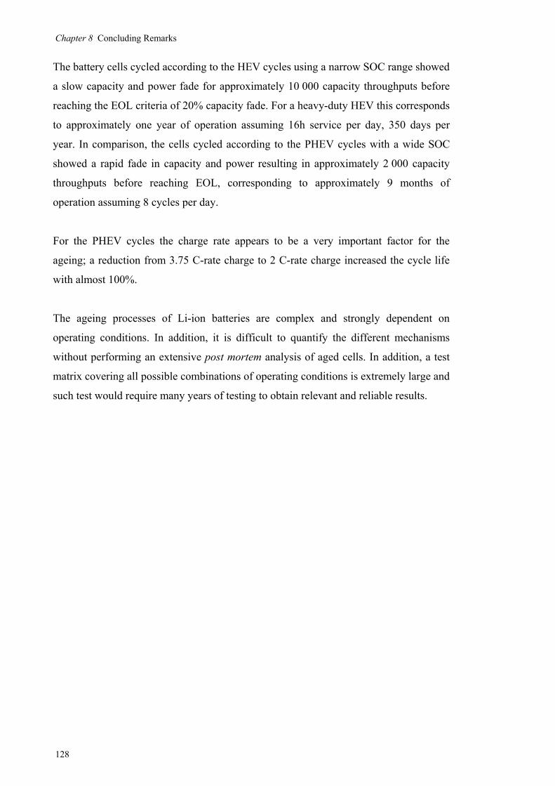
Chapter 8 Concluding Remarks
128
The battery cells cycled according to the HEV cycles using a narrow SOC range showed
a slow capacity and power fade for approximately 10 000 capacity throughputs before
reaching the EOL criteria of 20% capacity fade. For a heavy-duty HEV this corresponds
to approximately one year of operation assuming 16h service per day, 350 days per
year. In comparison, the cells cycled according to the PHEV cycles with a wide SOC
showed a rapid fade in capacity and power resulting in approximately 2 000 capacity
throughputs before reaching EOL, corresponding to approximately 9 months of
operation assuming 8 cycles per day.
For the PHEV cycles the charge rate appears to be a very important factor for the
ageing; a reduction from 3.75 C-rate charge to 2 C-rate charge increased the cycle life
with almost 100%.
The ageing processes of Li-ion batteries are complex and strongly dependent on
operating conditions. In addition, it is difficult to quantify the different mechanisms
without performing an extensive post mortem analysis of aged cells. In addition, a test
matrix covering all possible combinations of operating conditions is extremely large and
such test would require many years of testing to obtain relevant and reliable results.

Chapter 9 Future Work
129
Chapter 9 Future Work
The work presented in this thesis will continue and include further cycle life tests, cell
modelling and development of algorithms for estimating the SOH as a function of
operating conditions including the load cycle characteristics. Whereas the cycle life tests
presented in this thesis was focused on HEV and PHEV load cycles, several specific
load cycles will be developed to test the ageing factors of various load cycle properties
such as SOC range, current range and temperature.
Although the ICA and the DVA methods showed promising results as indicators of
ageing mechanisms, a post mortem analysis of aged cells will be needed to verify the
results. In addition, cells with reference electrodes may be used to confirm the validity
of these methods and possibly to quantify the loss of cyclable lithium and loss of active
cathode material.
Further cooperation with UU, KTH and Scania CV AB may also enable a correlation
between cycle life tests of large cells and small-scale research cells. This may in turn
lead to a deeper understanding of the ageing mechanisms of Li-ion batteries used in
heavy-duty HEVs and PHEVs. Furthermore, it can also facilitate the development of
more reliable test methods for accelerated ageing of cells and more accurate ex situ
characterisation methods.
The underlying questions for the future work are:
Which are the most important ageing mechanisms for different operating
conditions?
How are the different ageing mechanisms correlated and cross-dependent?
To what complexity should SOH models be developed to find a good
compromise between accuracy and suitability for applied usage?


Chapter 10 References
131
Chapter 10 References
[1] L. Gaines, R. Cuenza, “Costs of lithium-Ion Batteries for Vehicles”, Report ANL/ESD-42
(2000), Argonne National Laboratory, US.
[2] L. O. Valøen, M. I. Shoesmith, “The effect of PHEV and HEV duty cycles on battery and
battery pack performance”, Plug-in Hybrid Electric Vehicle 2007 Conference.
[3] A.G. Ritchie, ”Recent developments and likely advances in lithium rechargeable
batteries”, Journal of Power Sources 136 (2004) 285–289.
[4] A.G. Ritchie, W. Howard, ”Recent developments and likely advances in lithium-ion
batteries”, Journal of Power Sources 162 (2006) 809–812.
[5] W.F. Howard, R. Spotnitz, ”Theoretical evaluation of high-energy lithium metal phosphate
cathode materials in Li-ion batteries”, Journal of Power Sources 165 (2007) 887–891.
[6] K. Amine, C.H. Chen, J. Liu, M. Hammond, A. Jansen, D. Dees, I. Bloom, D. Vissers, G.
Henriksen, ”Factors responsible for impedance rise in high power lithium ion batteries”,
Journal of Power Sources 97-98 (2001) 684-687.
[7] I. Bloom, B.W. Cole, J.J Sohn, S.A. Jones, E.G. Polzin, V.S. Battaglia, G.L. Henriksen, C.
Motlach, R. Richardson, T. Unkelhaeuser, D. Ingersoll, H.L. Case, “An accelerated
calendar and cycle life study of Li-ion cells”, Journal of Power Sources 101 (2001) 238-
247.
[8] M. Broussely, Ph. Biensan, F. Bonhomme, Ph. Blanchard, S. Herreyre, K. Nechev, R.J.
Staniewicz, “Main aging mechanisms in Li ion batteries”, Journal of Power Sources 146
(2005) 90–96.
[9] J. Vetter, P. Novák, M.R. Wagner, C. Veit, K-C. Möller, J.O. Besenhard, M. Winter, M.
Wohlfahrt-Mehrens, C. Vogler, A. Hammouche, ”Ageing mechanisms in lithium-ion
batteries”, Journal of Power Sources 147 (2005) 269–281.
[10] D.P. Abraham, E.M. Reynolds, E. Sammann, A.N. Jansen, D.W. Dees, “Aging
characteristics of high-power lithium-ion cells with LiNi0.8Co0.15Al0.05O2 and Li4/3Ti5/3O4
electrodes”, Electrochimica Acta 51 (2005) 502–510.
[11] D.P. Abraham, S.D. Poppen, A.N. Jansen, J. Liu, D.W. Dees, ”Application of a lithium–tin
reference electrode to determine electrode contributions to impedance rise in high-power
lithium-ion cells”, Electrochimica Acta 49 (2004) 4763–4775.

Chapter 10 References
132
[12] J. Li, E. Murphy, J. Winnick, P.A. Kohl, ”Studies on the cycle life of commercial lithium
ion batteries during rapid charge–discharge cycling”, Journal of Power Sources 102
(2001) 294–301 .
[13] F. Savoye, P. Venet, M. Millet, J. Groot, “Impact of periodic current pulses on Li-ion
battery performance”, IEEE (2011).
[14] B. Markovsky, A. Rodkin, Y.S. Cohen, O. Palchik, E. Levi, D. Aurbach, H-J. Kim, M.
Schmidt, “The study of capacity fading processes of Li-ion batteries: major factors that
play a role”, Journal of Power Sources 119–121 (2003) 504–510.
[15] M. Dubarry, B.Y. Liaw, M-S. Chen, S-S. Chyan, K-C. Han, W-T. Sie, S-H. Wu,
“Identifying battery aging mechanisms in large format Liion cells”, Journal of Power
Sources 196 (2011) 3420-3425.
[16] Y. Zhang, C-Y. Wang, X. Tang, “Cycling degradation of an automotive LiFePO4 lithium-
ion battery”, Journal of Power Sources 196 (2011) 1513–1520.
[17] K.A. Striebel, J. Shim, “Cycling performance of low-cost lithium ion batteries with natural
graphite and LiFePO4”, Journal of Power Sources 119-121 (2003), 955-958.
[18] M. Dubarry, V. Svoboda, R. Hwu, B.Y. Liaw, “Capacity and power fading mechanism
identification from a commercial cell evaluation”, Journal of Power Sources 165 (2007)
566–572.
[19] M. Dubarry, V. Svoboda, R. Hwu, B.Y. Liaw, ”Capacity loss in rechargeable lithium cells
during cycle life testing: The importance of determining state-of-charge”, Journal of Power
Sources 174 (2007) 1121–1125.
[20] S.C. Nagpure, B. Bhushan, S. Babu, G. Rizzoni, “Scanning spreading resistance
characterization of aged Li-ion batteries using atomic force microscopy”, Scripta
Materialia 60 (2009) 933–936.
[21] J.R. Belt, C.D. Ho, T.J. Miller, M.A. Habib, T.Q. Duong, “The effect of temperature on
capacity and power in cycled lithium ion batteries”, Journal of Power Sources 142 (2005)
354–360.
[22] D.P. Abraham, J. Liu, C.H. Chen, Y.E. Hyung, M. Stoll, N. Elsen, S. MacLaren, R.
Twesten, R. Haasch, E. Sammann, I. Petrov, K. Amine, G. Henriksen, ”Diagnosis of power
fade mechanisms in high-power lithium-ion cells”, Journal of Power Sources 119–121
(2003) 511–516.
Chapter 10 References
133
[23] M. Kerlau, M. Marcinek, V. Srinivasan, R.M. Kostecki, Reprint of “Studies of local
degradation phenomena in composite cathodes for lithium-ion batteries”, Electrochimica
Acta 53 (2007) 1385–1392.
[24] P. Liu, J. Wang, J. Hicks-Garner, E. Sherman, S. Soukiazian, M. Verbrugge, H. Tataria, J.
Musser, P. Finamore, “Ageing Mechanisms of LiFePO4 Batteries Deduced by
Electrochemical and Structural Analyses”, Journal of The Electrochemical Society 157 (4)
(2010), A499-A507.
[25] K. A. Striebel, J. Shim, E.J. Cairns, R. Kostecki, Y.J. Lee, J. Reimer, T.J. Richardson, P.N.
Ross, X. Song, G.V. Zhuang, “Diagnostic Analysis of Electrodes from High-Power
lithium-Ion Cells Cycled under Different Conditions”, Journal of The Electrochemical
Society 151 (6) (2004), A857-A866.
[26] V. A. Sethuraman, L.J. Hardwick, V. Srinivasan, R. Kostecki, “Surface structural
disordering in graphite upon lithium intercalation/deintercalation”, Journal of Power
Sources 195 (2010) 3655–3660.
[27] G. Sarre, Ph. Blanchard, M. Broussely, “Aging of lithium-ion batteries”, Journal of Power
Sources 127 (2004) 65–71.
[28] M. Shikano, H. Kobayashi, S. Koike, H. Sakaebe, E. Ikenaga, K. Kobayashi, K. Tatsumi,
”Investigation of positive electrodes after cycle testing of high-power Li-ion battery cells II.
An approach to the power fading mechanism using hard X-ray photoemission
spectroscopy”, Journal of Power Sources 174 (2007) 795–799.
[29] J.R. Belt, C.D. Ho, C.G. Motloch, T.J. Miller, T. Q. Duong, ”A capacity and power fade
study of Li-ion cells during life cycle testing”, Journal of Power Sources 123 (2003) 241–
246.
[30] A. du Pasquier, A. Blyr, A. Cressent, C. Lenain, G. Amatucci, “An update on the high
temperature ageing mechanism in LiMn2O4-based Li-ion cells”, Journal of Power Sources
81–82 (1999) 54–59.
[31] K. Zaghib, M. Dontigny, P. Charest, J.F. Labrecque, A. Guerfi, M. Kopec, A. Mauger, F.
Gendron, C.M. Julien, “Aging of LiFePO4 upon exposure to H2O”, Journal of Power
Sources 185 (2008) 698–710.
[32] M. Broussely, S. Herreyre, P. Biensan, P. Kasztejna, K. Nechev, R.J. Staniewicz, “Aging
mechanism in Li ion cells and calendar life predictions”, Journal of Power Sources 97-98
(2001) 13-21.

Chapter 10 References
134
[33] X. Zhang, B. Winget, M. Doeff, J.W. Evans, T.M. Devine, “Corrosion of Aluminum
Collectos in lithium-Ion Batteries with Electrolytes Containing LiPF6”, Journal of The
Electrochemical Society 152(11) (2005) B448-B454.
[34] K. Amine, J. Liu, I. Belharouak, ”High-temperature storage and cycling of C-
LiFePO4/graphite Li-ion cells”, Electrochemistry Communications 7 (2005) 669–673 .
[35] S.H. Mohammadian, D. Aït-Kadi, F. Routhier, “Quantitative accelerated degradation
testing: Practical approaches”, Reliability Engineering and System Safety (2009),
doi:10.1016/j.ress.2009.09.009.
[36] E.V. Thomas, I. Bloom, J.P. Christophersen, V.S. Battaglia, “Statistical methodology for
predicting the life of lithium-ion cells via accelerated degradation testing”, Journal of
Power Sources 184 (2008) 312–317.
[37] R.G. Jungst, G. Nagasubramanian, H.L. Case, B.Y. Liaw, A. Urbina, T.L. Paez, D.H.
Doughty, ”Accelerated calendar and pulse life analysis of lithium-ion cells”, Journal of
Power Sources 119–121 (2003) 870–873.
[38] E.V. Thomas, H.L. Case, D.H. Doughty, R.G. Jungst, G. Nagasubramanian, E.P. Roth,
“Accelerated power degradation of Li-ion cells”, Journal of Power Sources 124 (2003)
254–260.
[39] K. Takei, K. Kumai, Y. Kobayashi, H. Miyashiro, N. Terada, T. Iwahori, T. Tanaka,
“Cycle life estimation of lithium secondary battery by extrapolation method and
accelerated aging test”, Journal of Power Sources 97-98 (2001) 697-701.
[40] D. Aurbach, ”A review on new solutions, new measurements procedures and new materials
for rechargeable Li batteries”, Journal of Power Sources 146 (2005) 71–78.
[41] J. Shim, R. Kostecki, T. Richardson, X. Song, K.A. Striebel, ”Electrochemical analysis for
cycle performance and capacity fading of a lithium-ion battery cycled at elevated
temperature”, Journal of Power Sources 112 (2002) 222–230.
[42] R.P. Ramasamy, R.E. White, B.N. Popov, “Calendar life performance of pouch lithium-ion
cells”, Journal of Power Sources 141 (2005) 298–306.
[43] D.P. Abraham, J.L. Knuth, D.W. Dees, I. Bloom, J.P. Christophersen, “Performance
degradation of high-power lithium-ion cells—Electrochemistry of harvested electrodes”,
Journal of Power Sources 170 (2007) 465–475.
[44] D.P. Abraham et.al, “Diagnostic Examination of Generation 2 lithium-Ion Cells and
Assessment of Performance Degradation Mechanisms”, Report ANL/-05-21 (2005),
Argonne National Laboratory, US.

Chapter 10 References
135
[45] K. L. Gering, S.V. Sazhin, D. K. Jamison, C. J. Michelbacher, B. Y. Liaw, M. Dubarry, M.
Cugnet, “Investigation of path dependence in commercial lithium-ion cells chosen for plug-
in hybrid vehicle duty cycle protocol”, Journal of Power Sources 196 (2011) 3395-3403.
[46] EUCAR Traction Battery Working Group, “Specification of Test Procedures for High
Voltage HEV Traction Batteries” (2005).
[47] FreedomCar, “FreedomCAR Battery Test Manual For Power-Assist Hybrid Electric
Vehicles”, DOE/ID-11069 (2003).
[48] IEC, “Secondary batteries for the propulsion of electric road vehicles, part 2-3”, IEC
61982-2, IEC 61982-3 (2002).
[49] R.B. Wright, J.P. Christophersen, C.G. Motloch, J.R. Belt, C.D. Ho, V.S. Battaglia, J.A.
Barnes, T.Q. Duong, R.A. Sutula, “Power fade and capacity fade resulting from cycle-life
testing of Advanced Technology Development Program lithium-ion batteries”, Journal of
Power Sources 119–121 (2003) 865–869.
[50] A.J. Salkind, C. Fennie, P. Singh, T. Atwater, D.E. Reisner, ”Determination of state-of-
charge and state-of-health of batteries by fuzzy logic methodology”, Journal of Power
Sources 80 (1999) 293–300.
[51] P. Singh, R. Vinjamuri, X. Wang, D. Reisner, ”Fuzzy logic modeling of EIS measurements
on lithium-ion batteries”, Electrochimica Acta 51 (2006) 1673–1679.
[52] P. Singh, R. Vinjamuri, X. Wang, D. Reisner, ”Design and implementation of a fuzzy logic-
based state-of-charge meter for Li-ion batteries used in portable defibrillators”, Journal of
Power Sources 162 (2006) 829–836.
[53] R. Spotnitz, “Simulation of capacity fade in lithium ion batteries”, Journal of Power
Sources 113 (2003) 72-80.
[54] P. Ramadass, B. Haran, R.White, B.N. Popov, ”Mathematical modeling of the capacity
fade of Li-ion cells”, Journal of Power Sources 123 (2003) 230–240.
[55] U. Tröltzsch, O. Kanoun, H-R. Tränkler, ”Characterizing aging effects of lithium ion
batteries by impedance spectroscopy”, Electrochimica Acta 51 (2006) 1664–1672.
[56] B.Y. Liaw, R.G. Jungst, G. Nagasubramanian, H.L. Case, D.H. Doughty, ”Modeling
capacity fade in lithium-ion cells”, Journal of Power Sources 140 (2005) 157–161.
[57] V. Pop, H.J. Bergveld, P.H.L. Notten, J.H.G. Op het Veld, P.P.L. Regtien, ”Accuracy
analysis of the State-of-Charge and remaining run-time determination for lithium-ion
batteries”, Measurement 42 (2009) 1131–1138.

Chapter 10 References
136
[58] A.T. Stamps, C.E. Holland, R.E. White, E.P. Gatzke, “Analysis of capacity fade in a
lithium ion battery”, Journal of Power Sources 150 (2005) 229–239.
[59] M. Safari, M. Morcrette, A. Teyssot, C. Delacourt, “Multimodal Physics-Based Aging
Model for Life Prediction of Li-Ion Batteries”, Journal of The Electrochemical Society 156
(3) (2009) A145-A153.
[60] J-W. Lee, Y.K. Anguchamy, B.N. Popov, “Simulation of charge–discharge cycling of
lithium-ion batteries under low-earth-orbit conditions”, Journal of Power Sources 162
(2006) 1395–1400.
[61] G. Ning, R.E. White, B.N. Popov,”A generalized cycle life model of rechargeable Li-ion
batteries”, Electrochimica Acta 51 (2006) 2012–2022.
[62] G. Ning, B.N. Popov, “Cycle Life Modeling of lithium-Ion Batteries”, Journal of the
Electrochemical Society 151 (10) (2004) A1584-A1591.
[63] K.A. Smith, C. D. Rahn, C-Y. Wang, “Control oriented 1D electrochemical model of
lithium ion battery”, Energy Conversion and Management 48 (2007) 2565–2578.
[64] F. La Mantia, J. Vetter, P. Novák, ”Impedance spectroscopy on porous materials: A general
model and application to graphite electrodes of lithium-ion batteries”, Electrochimica Acta
53 (2008) 4109–4121.
[65] R.P. Ramasamy, J-W. Lee, B.N. Popov, ”Simulation of capacity loss in carbon electrode
for lithium-ion cells during storage”, Journal of Power Sources 166 (2007) 266–272.
[66] J. Groot, “Battery Benchmarking and Cyclelife Test Methods”, conference: Transport
Research Arena (TRA) Europe 2010, Brussels.
[67] M. Montaru, S. Pelissier, “Frequency and Temporal Identification of a Li-ion Polymer
Battery Model Using Fractional Impedance”, Advances in Hybrid Powertrains (2008),
proceedings .
[68] Y. Qi, H. Guo, L.G. Hector, Jr., A. Timmons, “Threefold Increase in the Young’s Modulus
of Graphite Negative Electrode during lithium Intercalation”, Journal of The
Electrochemical Society 157 (5) (2010), A558-A566.
[69] J. Groot, “Statistic Method for Extraction of Synthetic Load Cycles for Cycle life Tests of
HEV Li-ion Batteries”, conference: International Battery, Hybrid and Fuel Cell Electric
Vehicle Symposium (EVS-24), Stavanger, Norway, 2009.
[70] W.-K. Ching, M.K. Ng, “Markov Chains: Models, Algorithms and Applications”, Springer
US, ISBN 978-0-387-29337-0, 2006.

Chapter 10 References
137
[71] A. Schell, H. Peng, D. Tran, E. Stamos, C. Lin, M. Joong Kim, “Modelling and control
strategy development for fuel cell electric vehicles”, Annual Reviews in Control 29 (2005)
159–168.
[72] S.J. Moura, D.S. Callaway, H.K. Fathy, J.L. Stein, “Impact of Battery Sizing on Stochastic
Optimal Power Management in Plug-in Hybrid Electric Vehicles”, Proceedings of the 2008
IEEE International Conference on Vehicular (2008).
[73] G. Zhang, R. Manduchi, “Prediction of the Lifetime of a Battery-Operated Video Node
Using Offline and Online Measurements”, International Workshop on Advanced Methods
for Uncertainty Estimation in Measurement (2007).
[74] D. Nydahl, M. Rydstedt, “Generation of stochastic drive cycles”, Chalmers University of
Technology, Report No. EX028/2009 (2009).
[75] P. Diaconis, “The Markov Chain Monte Carlo Revolution”, Bulletin of the American
Mathematical Society 46 (2009), 179–205.
[76] C. Chiasserini, Ramesh R. Rao, “A Model for Battery Pulsed Discharge with Recovery
Effect”, Proceedings of IEEE WCNC 1999, vol. 2, pp. 636-639.
[77] P. Rutquist, “On Infinite-Horizon State-Constrained Optimal Control”, Technical Report
No.R020/2005, Chalmers University of Technology, ISSN 1403-266X.
[78] “Series 4000 - Industry Standard Automated Cell and Battery Test System”,
http://www.maccor.com/series4000.php, accessed 2011-12-28.
[79] “Reference 3000 Potentiostat » Gamry Instruments”,
http://www.gamry.com/products/potentiostats/reference-3000, accessed 2011-12-28.
[80] “Compact 19" Rack Mountable Temperature Chamber”,
http://www.maccor.com/temperaturechamber.php, accessed 2011-12-28.
[81] M. Dubarry, V. Svoboda, R. Hwu, B.Y. Liaw, “Incremental Capacity Analysis and Close-
to-Equilibrium OCV Measurements to Quantify Capacity Fade in Commercial
Rechargeable lithium Batteries”, Electrochemical and Solid-State Letters 9 (10) (2006)
A454-A457.
[82] I. Bloom, A.N. Jansen, D.P. Abraham, J. Knuth, S.A. Jones, V.S. Battaglia, G.L.
Henriksen, “Differential voltage analyses of high-power, lithium-ion cells 1. Technique and
application”, Journal of Power Sources 139 (2005) 295–303.
[83] I. Bloom, J. Christophersen, K. Gering, “Differential voltage analyses of high-power
lithium-ion cells 2. Applications”, Journal of Power Sources 139 (2005) 304–313.

Chapter 10 References
138
[84] I. Bloom, J.P. Christophersen, D.P. Abraham, K.L. Gering, “Differential voltage analyses
of high-power lithium-ion cells 3. Another anode phenomenon”, Journal of Power Sources
157 (2006) 537–542.
[85] I. Bloom, L.K. Walker, J.K. Basco, D.P. Abraham, J.P. Christophersen, C. D.
Ho,”Differential voltage analyses of high-power lithium-ion cells. 4. Cells containing
NMC”, Journal of Power Sources 195 (2010) 877–882.
[86] J.R. Dahn, “Phase diagram of LixC6”, Physical Review B44(1991), 9170-9177.
[87] R. Yazami, Y. Reynier, “Thermodynamics and crystal structure anomalies in lithium-
intercalated graphite”, Journal of Power Sources 153 (2006) 312–318.
[88] M. Dubarry, B.Y. Liaw, “Identify capacity fading mechanism in a commercial LiFePO4
cell”, Journal of Power Sources 194 (2009) 541–549.