state of the art in electromagnetic · pdf filermxprt – analytical rotating machine...

STATE OF THE ART IN ELECTROMAGNETIC SIMULATION: RECENT PROGRESS AND APPLICATIONS

ANSYS Solutions for Oil & Gas Industry

Oil & Gas industry

- Several levels of size and complexity;

- Power grids and power distribution

- Subsea power transmission

- Offshore components

SYSTEM WIDE SIMULATION

COMPONENT LEVEL SIMULATION


ANSYS Multiphysics Solutions

Electromagnetic Simulation

Low High

Mechanical Simulation

Implicit Explicit

Computational Fluid Dynamics (CFD)

Electronics Low Frequency and EM

Maxwell

RMxprt

Simplorer

Q3D

High Frequency

HFSS

Siwave

Designer

Nexxim

Implicit

ANSYS

Mechanical

ANSYS

Structural

ANSYS

Professional

Explicit

ANSYS AUTODYN

ANSYS

LS-Dyna

Electronics cooling

ANSYS Icepak

General CFD

ANSYS CFD

Integrated Concurrent Design

Automated

Integration

AnalyticalMagnetics

Circuit - System

The total integrated

solution is more

valueable than sum

of the individual Integration

Thermal

Structural

Radiation

L,R,C Extraction

of the individual

parts


Low Frequency Applications

• Power Transformer• Motors/Generators • Subsea Power System• Induction Pipe Bending • Induction Pipe Bending

Case: WEG Transformer (3D Simulation) – Losses in the Steel Parts

3D Eddy Current Solver

needed:

• Simplified core used

(TransCore UDP) since

little influence on stray flux

paths;

• Simplified clamp used

eliminate holes, parts;

• Tank replaced with

impedance boundary on

region faces;

3ph Furnace WEG transformer:

• 30kV ∆ -1154 V ∆;

• 100 MVA power rating;

• Tap changer on HV and LV;

• OFWF cooling;

• Frequency = 60 Hz.

region faces;

• Tie plates and clamps are

perfect conductor with an

impedance boundary;

• Power Losses.

Case: WEG Transformer (3D Simulation) – Losses in the Tank Parts

3D tank wall losses due to

busbars:

• 3D Eddy Current analysis

needed;

• Simplify to model only

single tank wall which

has busbars passing

through;

• Apply impedance

boundary on this tank

• Current density inside busbars;

• Apply rated peak current to all

conductors 120deg out of

phase:

• I = 1.414 * 50,000 /

(1.73*6) = 6800A-peak

wall and also four

remaining walls using a

2D sheet object (instead

of a 3D wall with

thickness).

RMxprt – Analytical Rotating Machine Design

RMxprt is a versatile software program that speeds the design and optimization process of rotating electric machines:• Uses classical analytical motor theory and equivalent magnetic circuit methods to compute performance metrics for a specific machine design;• Accounts for nonlinear magnetic characteristics and 3D effects, such as skew and end-turn;• Exports geometry to 2D and 3D finite element simulators.

Induction machines Synchronous machinesBrush commutated

machinesElectronically

commutated machines

• Single-phase motors;

• Three-phase motors.

• Line-start PM motors;

• Salient-pole motors and generators;

• Non-salient pole motors and generators.

machines

• DC motors andgenerators;

• Permanent magnet DC motors;

• Universal motors.

commutated machines

• Brushless DC motors;

• Adjustable-speed PM motors and generators;

• Switched reluctancemotors;

• Claw-pole generators.

RMxprt – Link with Maxwell 2D and 3D

• Complete geometry creation;

• One-click FEA design;

• Option for periodic or full models;

• Automatic update with project variables.

• Geometry creation and material assignment;

• General and dedicated machine parts;

• Create new machine types with arbitrary combinations;

• Dimension variables supported.

Electric Machine Design Suite

Fast Analytical Solution: Narrow the Design Space

Parametric AnalysisOptimization

Magnetostatic/Eddy Current Analysis using FEA

Parametric AnalysisOptimization

AHA

JA ×∇×+×∇+∇−∂

∂−=×∇×∇ vV

tcs σσσυ

sc

f

f

f

f

fuu

dt

idLiRd

dt

dA

aS

lNd =+++Ω∫∫ 0=−

dt

duCi c

f

Field Equation:

Circuit Equation:

Motion Equation

externalem TTm +=+ λωα

Simultaneous Equations:

Transient Analysis using FEA

Parametric Analysis

EMF2

A

IA

A

IB

A

IC

175

V

+

VVBC

A_PHASE_N1

B_PHASE_N1

C_PHASE_N1

ROT1

ROT2

ECELink1

T

FM_ROT1

ωω

+IGBT1

IGBT2 IGBT3D2 D3

Analytical Based Model

System Level IGBT

Design

Requirements

Size/Weight Efficiency Torque Speed Cogging/Ripple Inverter Matching Thermal Stress Manufacturability Cost

1

2

3

4

Equivalent Circuit Model : High Fidelity Physics Based Model

ICA:

EMF1 175

A AM_IGBT

ECE

PP:=6

ON:=1

OFF:=0

THRESH:=400

HYST:=10

EQU theta_elect := PP * ECELink1.PHI

theta := MOD(theta_elect, 360)

IGBT4IGBT5

Drive System Design

Phase CurrentIA.I

IB.I

IC.I

t

1.00k

-1.00k

0

-500.00

500.00

0 17.27m10.00m

Torque

Torque.I

t

400.00

-100.00

0

200.00

0 17.27m10.00m

Phase Voltage

V_AB.V

t

300.00

-300.00

0

-200.00

200.00

0 17.27m10.00m

Von Mises stress

Thermal and Stress Analysis

A_PHASE_N1

A_PHASE_N2

B_PHASE_N1

B_PHASE_N2

C_PHASE_N1

C_PHASE_N2

ROTB1

ROTB2

EMSSLink1

EMF2

RA

RB

RC

A

IA

A

IB

A

IC

175

0.023

0.023

0.023

theta>90 AND theta<150theta>150 AND theta<210

theta>210 AND theta<270

theta>270 AND theta<330theta>330 OR theta<30

ICA:


EMF1 175

E1

R1

E2

R2

E3

R3

E4

R4

E5

R5

E6

R6

ctrl_1:=OFF

ctrl_6:=OFF

ctrl_1:=ON

ctrl_6:=ON

ctrl_1:=ON

ctrl_2:=ON

ctrl_1:=OFF

ctrl_2:=OFF

ctrl_2:=ON

ctrl_3:=ON

ctrl_2:=OFF

ctrl_3:=ON

ctrl_4:=ON

ctrl_4:=ON

ctrl_5:=ON

ctrl_5:=ON

ctrl_6:=ON

ctrl_5:=OFF

ctrl_6:=OFF

ctrl_3:=OFF

ctrl_3:=OFF

ctrl_4:=OFF

ctrl_4:=OFF

ctrl_5:=OFF

A AM_IGBT

+

VVBC

+

V

VGE4

MASS_ROTB1

Complete Transient FEA -Transient System Co-simulation

3

Drive System Integration with Manufacturer’s IGBTs

A_PHASE_N1

A_PHASE_N2

B_PHASE_N1

B_PHASE_N2

C_PHASE_N1

C_PHASE_N2

ROTB1

ROTB2

EMSSLink1

EMF2

RA

RB

RC

A

IA

A

IB

A

IC

175

0.023

0.023

0.023

theta>90 AND theta<150theta>150 AND theta<210


theta>270 AND theta<330theta>330 OR theta<30

ICA:


EMF1 175

E1

R1

E2

R2

E3

R3

E4

R4

E5

R5

E6

R6

ctrl_1:=OFF

ctrl_6:=OFF

ctrl_1:=ON

ctrl_6:=ON

ctrl_1:=ON

ctrl_2:=ON

ctrl_1:=OFF

ctrl_2:=OFF

ctrl_2:=ON

ctrl_3:=ON

ctrl_2:=OFF

ctrl_3:=ON

ctrl_4:=ON

ctrl_4:=ON

ctrl_5:=ON

ctrl_5:=ON

ctrl_6:=ON

ctrl_5:=OFF

ctrl_6:=OFF

ctrl_3:=OFF

ctrl_3:=OFF

ctrl_4:=OFF

ctrl_4:=OFF

ctrl_5:=OFF

A AM_IGBT

+

VVBC

+

V

VGE4

MASS_ROTB1

EM Design Environment

SIMPLORER Simulator Data BusSimulator Coupling Technology

Maxwell2D/3D

Electromagnetism

Electromechanics

C/C++ Interface

Circuit VHDL-AMS

MathCad

Simulink

Circuit Simulator Block

Diagram Simulator

State Machine Simulator

VHDL-AMS Simulator

Model Database

Electrical, Blocks, States, Machines, Automotive, Hydraulics...Mechanics, Power, Semiconductors...

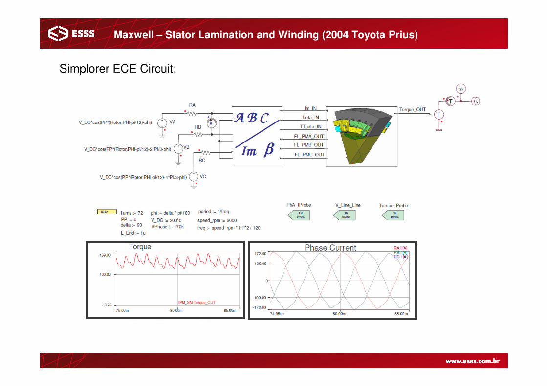
Simplorer ECE Circuit:

Maxwell – Stator Lamination and Winding (2004 Toyota Prius)

- 11Km long;

- Electrical Power, control data,

cooling, mechanical protection and

support;

- Vnom = 6400V , balanced;

- Inom= 1200A;

- Copper conductors and shields;

- Stainless Steel armature;

Case: Subsea Power Cable and Downhole Cable

- 2 Km long;

- Electrical Power, cooling,

mechanical protection;

- Vnom =6000V , balanced;

- Inom= 20A;

- Copper conductors

shields;

- Stainless Steel armature;

Umbilical Cable info Downhole Cable info30Hz

Capacitance Matrix

Phase A Phase B Phase C

Condutor 1.9671E+005 -28796 -28796

Condutor_1 -28796 1.9671E+005 -28796

Condutor_2 -28796 -28796 1.9671E+005

Conductance Matrix


Condutor 0.00036615 0.00036614 0.00036614

Condutor_1 0.00036614 0.00036615 0.00036614

Condutor_2 0.00036614 0.00036614 0.00036615

Inductance Matrix

Phase A Phase B Phase C- Stainless Steel armature; - Stainless Steel armature;Phase A Phase B Phase C

Condutor 4.097E+005 52408 42451

Condutor_1 52408 4.176E+005 46410

Condutor_2 42451 46410 3.977E+005

Resistance Matrix


Condutor 1.5616 1.2348 1.2347

Condutor_1 1.2348 1.5617 1.2347

Condutor_2 1.2347 1.2347 1.5616


Simulation of a Circuit with Power Umbilical and Downhole Cable Using Simplorer® Software

- Simulation of electrical subsea system considering FEM cable models;

Load, (representative circuit of IM start)

Q2D Downhole modelQ2D Umbilical model

Measure points

Balanced SourceAmplitude: 3021V @ 30Hz


Results:

-3.75

-2.50

-1.25

0.00

1.25

2.50

3.75

Y1

[kV

]

7.Completo 2Voltages ANSOFT

Curve Info max

VM1.VTR

3.0189

VM2.VTR

2.0935

VM3.VTR

1.5389

-3.75

-2.50

-1.25

0.00

1.12

Y1

[kV

]

7.Completo 2Voltages_Zoom ANSOFT

Curve Info max

VM1.VTR

3.0189

VM2.VTR

2.0935

VM3.VTR

1.5389

0.00 10.00 20.00 30.00 40.00 50.00 60.00 66.00Time [ms]

-1000.00

-375.00

250.00

875.00

1250.00

Y1

[A

]

7.Completo 2Currents ANSOFT

Curve Info

AM1.ITR

AM2.ITR

AM3.ITR

0.00 10.00 20.00 30.00 40.00 50.00 60.00 66.00Time [ms]

-5.00

0.00 1.00 2.00 3.00 4.00 5.00Time [ms]

-741.64

-625.00

-500.00

-375.00

-250.00

-125.00

0.00

78.45

Y1

[A

]

7.Completo 2Currents_Zoom ANSOFT

Curve Info

AM1.ITR

AM2.ITR

AM3.ITR

0.00 2.00 4.00 6.00 8.00 10.00Time [ms]

-5.00

TR

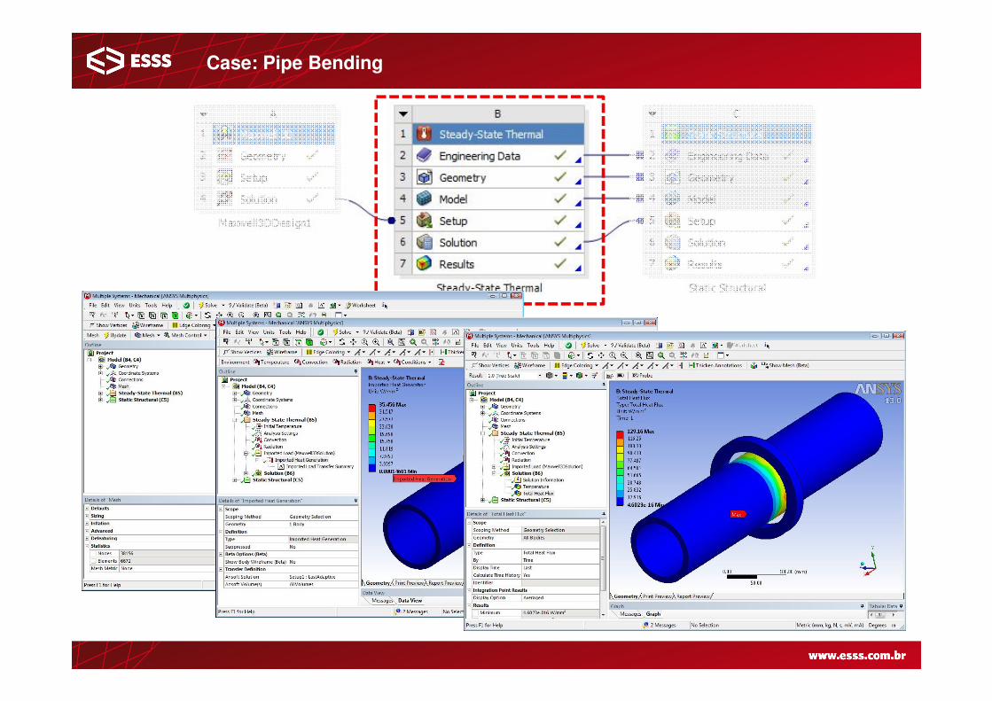
Case: Pipe Bending

- Multiphysics problem:

- Electromagnetics (induced currents)

- Thermal (Heat generation)

- Structural (Material deformation)

Case: Pipe Bending

ANSYS Solutions to Oil & Gas Industry

High Frequency Applications

• Oil Well Logging• Ground Radar• Ground Radar• Oil/Gas/Water Sensor

Oil Well Logging

• Oil Well Logging is the measurement of the physical environment around an oil drill or mandrel

⋅ - Surface measurements: ground penetrating RADAR

⋅ - Subsurface measurements: Logging While Drilling (LWD) from inside borehole

• EM is used to determine the material properties of the surrounding media via extraction of the conductivity

– Conductivity can be used to determine porosity, water/oil saturation, temperature, and anisotropy of different geologic layers

• EM simulation is key for correct interpretation, characterization and modeling of measured EM data

Oil Logging - Comparison of HFSS to Published Simulation Results

• Plot in literature compares a 3D FDTD code, 3D Finite Volume (FV) technique using Field Formulation (Similar to HFSS), and 3D FV using a Potential Formulation on left and HFSS results on the right

– Phase Difference as the sensor moves through the borehole

– Excellent correlation between HFSS and the literature

• M.S. Novo, L.C. da Silva, and F.L. Teixeira. “Analysis of Electromagnetic Well Logging

Tools for Oil and Gas Exploration using Finite Volume Techniques,” Microwave and

Optoelectronics Conference, 2007. IMOC 2007. SBMO/IEEE MTT-S International

σ=1 S/m

σ=0.01 S/m

σ=1 S/m

60 in

dz

dz = 0 in

Ground Penetrating Radar Applications

Military

Mine detection

IED detectionIndustrial IED detection

UXO detection

Industrial

Soil Moisture

Ice Thickness

Pipe detection

Geotechnical

Tunnel detection

Roadway Integrity

Etc.

Scientific/Academic

Archaeology

Lunar / Planetary Studies

Geophysical

Steady State E-Field: Metal vs Plastic Pipe

Notice the E fields are slightly different at very low levelsBut do these small differences manifest themselves at the antenna inputs?

Metal Pipe Target Plastic Pipe Target

Antenna S-Parameters


Notice there is virtually no difference in Return Loss

and little difference in TX/RX Couplingand little difference in TX/RX Coupling

Transient E-Field


Note: Color scales are not equivalent

Transient Receiver Voltage

PEC Pipe Target Plastic Pipe Target

Notice difference in RX return signal is very pronouncedNotice difference in RX return signal is very pronouncedboth in magnitude and shape

Real-Time Measurements of Oil, Gas and Water Contents in Marine Pipes

• Multiphase measurement has been an aim of the oil

and gas production industries for many years. A variety of different techniques have been developed in

an attempt to design a meter which is a realistic alternative to the bulky, off-line but accurate test separator to determine the amount of oil, water and gas in a pipeline. Liverpool John Moores University, in conjunction with Solartron ISA, have developed an

industrial prototype of a non-intrusive, real time, phase area fraction meter which uses the different electromagnetic properties of the pipeline contents to determine their relative proportions as they flow through the sensor with the use of HFSS.

Electric Field Magnetic Field

ANSYS Solutions to Oil & Gas Industry

Thank you!

[email protected]

state of the art in electromagnetic · pdf filermxprt – analytical rotating machine...

Documents