state of the art in urban drainage modelling - sintef
TRANSCRIPT
REFERENCE PROJECT
Project Number EVK1-CT-2001-00167
CARE-S Computer Aided REhabilitation of Sewer networks
WORK PACKAGE
WP3 - Hydraulic performance REPORT TITLE
State of the art in Urban Drainage Modelling
PARTICIPATING PARTNERS
University of Bologna (Work Package Leader) University of Palermo (Sub-Task Leader) SINTEF NTNU Wrc CLASSIFICATION ELECTRONIC FILE CODE NO. OF PAGES/APPENDICES
Unrestricted modeling report WP3finito 412/2 REVISION NO. REVISION
1 Gabriele Freni (Palermo), Marco Maglionico (Bologna), Vittorio Di Federico (Bologna)
DATE VALIDATION
2003-05-12 ABSTRACT / SUMMARY
The present report is the first milestone in CARE-S Work Package 3. It describes the characteristics of most used software tools for modelling urban drainage systems, waste water treatment plants and natural systems. Several aspects have been considered both concerning quantity and quality problems and different models have been analysed regarding their accessibility, completeness, level of detail in physical processes simulation, ease of use, etc. This state-of-the-art review is essential for the following project activities and the selection of tools that will be used in the project. The report consists of two parts: the first discusses several aspects of Urban Water System modelling (sewer systems, receiving waters, groundwater, WWTP); the second part describes User Interface and GIS functionalities with particular regards to data management that will be an important topic in the future developments of the project. The last chapter gives a brief summary of the conclusions rising from the modelling review.
All rights reserved. The present documentation and its basic ideas may not be used by anyone or Be handed over to a third party without prior written approval from EVK1-CT-2001-00167 CARE-S Project Coordinator

2
TABLE OF CONTENTS 1 INTRODUCTION............................................................................................................................................8 2 URBAN DRAINAGE: WATER QUANTITY MODELS.............................................................................9
2.1 BEMUS – BELGRADE MODEL OF URBAN SEWERS ..................................................................................9 2.1.1. Model availability................................................................................................................................9 2.1.2. Abstract................................................................................................................................................9 2.1.3. Usage Specifications............................................................................................................................9 2.1.4. Input and Output procedures.............................................................................................................10 2.1.5. Theoretical framework Overview ......................................................................................................11 2.1.6. Model Parameters Estimation or Assignation...................................................................................13 2.1.7. PI(s) Estimation Method....................................................................................................................13 2.1.8. Future Improvements of the Model....................................................................................................14 2.1.9. References..........................................................................................................................................14
2.2 SWMM – STORM WATER MANAGEMENT MODEL .................................................................................15 2.2.1. Model availability..............................................................................................................................15 2.2.2. Abstract..............................................................................................................................................15 2.2.3. Usage Specifications..........................................................................................................................17 2.2.4. Input and Output procedures.............................................................................................................21 2.2.5. Theoretical framework Overview ......................................................................................................21 2.2.6. Model Parameters Estimation or Assignation...................................................................................33 2.2.7. PI(s) Estimation Method....................................................................................................................33 2.2.8. Future Improvements of the Model....................................................................................................34 2.2.9. References..........................................................................................................................................37
2.3 HYDROWORKS/INFOWORKS...........................................................................................................41 2.3.1. Model availability..............................................................................................................................41 2.3.2. Abstract..............................................................................................................................................41 2.3.3. Usage Specifications..........................................................................................................................41 2.3.4. Input and Output procedures.............................................................................................................44 2.3.5. Theoretical framework Overview ......................................................................................................45 2.3.6. Model Parameters Estimation or Assignation...................................................................................56 2.3.7. PI(s) Estimation Method....................................................................................................................56 2.3.8. Future Improvements of the Model....................................................................................................56 2.3.9. References..........................................................................................................................................56
2.4 MOUSE – MODELLING OF URBAN SEWERS ............................................................................................57 2.4.1. Model availability..............................................................................................................................57 2.4.2. Abstract..............................................................................................................................................57 2.4.3. Usage Specifications..........................................................................................................................58 2.4.4. Input and Output procedures.............................................................................................................61 2.4.5. Theoretical framework Overview ......................................................................................................63 2.4.6. Model Parameters Estimation or Assignation...................................................................................84 2.4.7. PI(s) Estimation Method....................................................................................................................84 2.4.8. Future Improvements of the Model....................................................................................................84 2.4.9. References..........................................................................................................................................84
2.5 SEWERCAD ..........................................................................................................................................86 2.5.1. Model availability..............................................................................................................................86 2.5.2. Abstract..............................................................................................................................................86 2.5.3. Usage Specifications..........................................................................................................................87 2.5.4. Input and Output procedures.............................................................................................................88 2.5.5. Theoretical framework Overview ......................................................................................................88 2.5.6. Model Parameters Estimation or Assignation...................................................................................98 2.5.7. PI(s) Estimation Method....................................................................................................................99 2.5.8. Future Improvements of the Model....................................................................................................99 2.5.9. References..........................................................................................................................................99
2.6 STORMCAD........................................................................................................................................101 2.6.1. Model availability............................................................................................................................101 2.6.2. Abstract............................................................................................................................................101 2.6.3. Input and Output procedures...........................................................................................................102
3
2.6.4. Theoretical framework Overview ....................................................................................................103 2.6.5. Model Parameters Estimation or Assignation.................................................................................119 2.6.6. PI(s) Estimation Method..................................................................................................................119 2.6.7. Future Improvements of the Model..................................................................................................119 2.6.8. References........................................................................................................................................119
2.7 SIMPOL3 .............................................................................................................................................121 2.7.1. Model availability............................................................................................................................121 2.7.2. Abstract............................................................................................................................................121 2.7.3. Usage Specifications........................................................................................................................121 2.7.4. Input and Output procedures...........................................................................................................122 2.7.5. Theoretical framework Overview ....................................................................................................122 2.7.6. Model Parameters Estimation or Assignation.................................................................................122 2.7.7. References........................................................................................................................................122
2.8 COSMOSS ...........................................................................................................................................123 2.8.1. Model availability............................................................................................................................123 2.8.2. Abstract............................................................................................................................................123 2.8.3. Usage Specifications........................................................................................................................123 2.8.4. Input and Output procedures...........................................................................................................124 2.8.5. Theoretical framework Overview ....................................................................................................124 2.8.6. Model Parameters Estimation or Assignation.................................................................................125 2.8.7. PI(s) Estimation Method..................................................................................................................125 2.8.8. Future Improvements of the Model..................................................................................................125 2.8.9. References........................................................................................................................................125
2.9 DORA/DOUBLE ORDER APPROXIMATION METHOD .............................................................................127 2.9.1. Model availability............................................................................................................................127 2.9.2. Abstract............................................................................................................................................127 2.9.3. Usage Specifications........................................................................................................................128 2.9.4. Input and Output procedures...........................................................................................................128 2.9.5. Theoretical framework Overview ....................................................................................................129 2.9.6. Model Parameters Estimation or Assignation.................................................................................129 2.9.7. PI(s) Estimation Method..................................................................................................................129 2.9.8. Future Improvements of the Model..................................................................................................129 2.9.9. References........................................................................................................................................130
2.10 PRE – COMPETITIVE URBAN DRAINAGE FLOW MODELS..........................................................................131 2.10.1. Introduction ................................................................................................................................131 2.10.2. Hydrological models...................................................................................................................131 2.10.3. Physically based models .............................................................................................................132 2.10.4. Hydrological-Physically based models.......................................................................................144 2.10.5. Modelling mixed flow in storm sewers........................................................................................152 2.10.6. References...................................................................................................................................170
3 URBAN DRAINAGE: WATER QUALITY MODELS............................................................................171 3.1 SWMM – STORM WATER MANAGEMENT MODEL ...............................................................................171
3.1.1. Model availability............................................................................................................................171 3.1.2. Abstract............................................................................................................................................171 3.1.3. Usage Specifications........................................................................................................................173 3.1.4. Input and Output procedures...........................................................................................................175 3.1.5. Theoretical framework Overview ....................................................................................................175 3.1.6. Model Parameters Estimation or Assignation.................................................................................184 3.1.7. PI(s) Estimation Method..................................................................................................................185 3.1.8. Future Improvements of the Model..................................................................................................185 3.1.9. References........................................................................................................................................188
3.2 HYDROWORKS/INFOWORKS – QUALITY MODEL .........................................................................191 3.2.1. Model availability............................................................................................................................191 3.2.2. Abstract............................................................................................................................................191 3.2.3. Usage Specifications........................................................................................................................192 3.2.4. Input and Output procedures...........................................................................................................193 3.2.5. Theoretical framework Overview ....................................................................................................196 3.2.6. Model Parameters Estimation or Assignation.................................................................................200 3.2.7. PI(s) Estimation Method..................................................................................................................200

4
3.2.8. Future Improvements of the Model..................................................................................................200 3.2.9. References........................................................................................................................................200
3.3 MOUSE................................................................................................................................................202 3.3.1. Model availability............................................................................................................................202 3.3.2. Abstract............................................................................................................................................202 3.3.3. Usage Specifications........................................................................................................................203 3.3.4. Input and Output procedures...........................................................................................................207 3.3.5. Theoretical framework Overview ....................................................................................................207 3.3.6. Model Parameters Estimation or Assignation.................................................................................220 3.3.7. PI(s) Estimation Method..................................................................................................................220 3.3.8. Future Improvements of the Model..................................................................................................220 3.3.9. References........................................................................................................................................221
3.4 KOSIM - KONTINUIERLICHES LANGZEITSIMULATIONSMODELL FÜR DEN NACHWEIS VON BAUWERKEN DER REGENWASSERBEHANDLUNG.......................................................................................................................223
3.4.1. Model availability............................................................................................................................223 3.4.2. Abstract............................................................................................................................................223 3.4.3. Usage Specifications........................................................................................................................223 3.4.4. Input and Output procedures...........................................................................................................224 3.4.5. Theoretical framework Overview ....................................................................................................224 3.4.6. Model Parameters Estimation or Assignation.................................................................................225 3.4.7. PI(s) Estimation Method..................................................................................................................225 3.4.8. Future Improvements of the Model..................................................................................................225 3.4.9. References........................................................................................................................................225
3.5 SIMBA – SIMULATION OF BIOLOGICAL ACTIVITY ..............................................................................226 3.5.1. Model availability............................................................................................................................226 3.5.2. Abstract............................................................................................................................................226 3.5.3. Usage Specifications........................................................................................................................227 3.5.4. Input and Output procedures...........................................................................................................227 3.5.5. Theoretical framework Overview ....................................................................................................228 3.5.6. Model Parameters Estimation or Assignation.................................................................................231 3.5.7. PI(s) Estimation Method..................................................................................................................231 3.5.8. Future Improvements of the Model..................................................................................................231 3.5.9. References........................................................................................................................................231
3.6 SIMPOL3 .............................................................................................................................................233 3.6.1. Model availability............................................................................................................................233 3.6.2. Abstract............................................................................................................................................233 3.6.3. Usage Specifications........................................................................................................................233 3.6.4. Input and Output procedures...........................................................................................................233 3.6.5. Theoretical framework Overview ....................................................................................................234 3.6.6. Model Parameters Estimation or Assignation.................................................................................234 3.6.7. References........................................................................................................................................234
3.7 FLUPOL...............................................................................................................................................235 3.7.1. Model availability............................................................................................................................235 3.7.2. Abstract............................................................................................................................................235 3.7.3. Usage Specifications........................................................................................................................235 3.7.4. Input and Output procedures...........................................................................................................236 3.7.5. Theoretical framework Overview ....................................................................................................236 3.7.6. Model Parameters Estimation or Assignation.................................................................................236 3.7.7. References........................................................................................................................................236
3.8 HORUS ................................................................................................................................................237 3.8.1. Model availability............................................................................................................................237 3.8.2. Abstract............................................................................................................................................237 3.8.3. Usage Specifications........................................................................................................................237 3.8.4. Input and Output procedures...........................................................................................................239 3.8.5. Theoretical framework Overview ....................................................................................................239 3.8.6. Model Parameters Estimation or Assignation.................................................................................239 3.8.7. References........................................................................................................................................239
3.9 WATS: WASTEWATER AEROBIC–ANAEROBIC TRANSFORMATIONS IN SEWERS......................................241 3.9.1. Model availability............................................................................................................................241 3.9.2. Abstract............................................................................................................................................241

5
3.9.3. Usage Specifications........................................................................................................................242 3.9.4. Input and Output procedures...........................................................................................................242 3.9.5. Theoretical framework Overview ....................................................................................................242 3.9.6. Model Parameters Estimation or Assignation.................................................................................243 3.9.7. References........................................................................................................................................243
3.10 COSMOSS ...........................................................................................................................................246 3.10.1. Model availability .......................................................................................................................246 3.10.2. Abstract.......................................................................................................................................246 3.10.3. Usage Specifications...................................................................................................................246 3.10.4. Input and Output procedures ......................................................................................................247 3.10.5. Theoretical framework Overview................................................................................................247 3.10.6. Model Parameters Estimation or Assignation ............................................................................248 3.10.7. PI(s) Estimation Method .............................................................................................................248 3.10.8. Future Improvements of the Model .............................................................................................248 3.10.9. References...................................................................................................................................248
3.11 DORAT – DOUBLE ORDER APPROXIMATION METHOD FOR TRANSPORT.............................................250 3.11.1. Model availability .......................................................................................................................250 3.11.2. Abstract.......................................................................................................................................250 3.11.3. Usage Specifications...................................................................................................................251 3.11.4. Input and Output procedures ......................................................................................................252 3.11.5. Theoretical framework Overview................................................................................................252 3.11.6. Model Parameters Estimation or Assignation ............................................................................252 3.11.7. PI(s) Estimation Method .............................................................................................................253 3.11.8. Future Improvements of the Model .............................................................................................253 3.11.9. References...................................................................................................................................253
3.12 PRE COMPETITIVE SOLID TRANSPORT MODELS ......................................................................................254 3.12.1. Introduction ................................................................................................................................254 3.12.2. Sediment transport in sewers ......................................................................................................254 3.12.3. Limit of sediment deposition .......................................................................................................258 3.12.4. Sediment transport in pipes with a deposited bed.......................................................................264 3.12.5. Einstein's Side Wall Elimination.................................................................................................275 3.12.6. Vanoni-Brooks Method ...............................................................................................................277 3.12.7. Cohesive sediment transport in sewer pipes with a deposited bed .............................................278 3.12.8. Suspended solid transport...........................................................................................................279 3.12.9. REFERENCES ............................................................................................................................285
4 RECEIVING WATER BODIES MODELS ..............................................................................................290 4.1 ISIS.......................................................................................................................................................290
4.1.1. Model availability............................................................................................................................290 4.1.2. Abstract............................................................................................................................................290 4.1.3. Usage Specifications........................................................................................................................291 4.1.4. Input and Output procedures...........................................................................................................293 4.1.5. Theoretical framework Overview ....................................................................................................294 4.1.6. Model Parameters Estimation or Assignation.................................................................................294 4.1.7. PI(s) Estimation Method..................................................................................................................294 4.1.8. Future Improvements of the Model..................................................................................................294 4.1.9. References........................................................................................................................................294
4.2 MIKE11................................................................................................................................................295 4.2.1. Model availability............................................................................................................................295 4.2.2. Abstract............................................................................................................................................295 4.2.3. Usage Specifications........................................................................................................................296 4.2.4. Input and Output procedures...........................................................................................................303 4.2.5. Theoretical framework Overview ....................................................................................................304 4.2.6. Model Parameters Estimation or Assignation.................................................................................304 4.2.7. PI(s) Estimation Method..................................................................................................................304 4.2.8. Future Improvements of the Model..................................................................................................304 4.2.9. References........................................................................................................................................304
4.3 WASP6.................................................................................................................................................308 4.3.1. Model availability............................................................................................................................308 4.3.2. Abstract............................................................................................................................................308

6
4.3.3. Usage Specifications........................................................................................................................308 4.3.4. Input and Output procedures...........................................................................................................310 4.3.5. Theoretical framework Overview ....................................................................................................312 4.3.6. Model Parameters Estimation or Assignation.................................................................................313 4.3.7. PI(s) Estimation Method..................................................................................................................313 4.3.8. Future Improvements of the Model..................................................................................................313 4.3.9. References........................................................................................................................................313
5 MODELS FOR WASTE WATER TREATMENT PLANTS ANALYSIS .............................................315 5.1 STOAT .................................................................................................................................................315
5.1.1. Model availability............................................................................................................................315 5.1.2. Abstract............................................................................................................................................315 5.1.3. Usage Specifications........................................................................................................................315 5.1.4. Input and Output procedures...........................................................................................................317 5.1.5. Theoretical framework Overview ....................................................................................................317 5.1.6. Model Parameters Estimation or Assignation.................................................................................317 5.1.7. PI(s) Estimation Method..................................................................................................................318 5.1.8. Future Improvements of the Model..................................................................................................318 5.1.9. References........................................................................................................................................318
5.2 WEST-WORLDWIDE ENGINE FOR SIMULATION, TRAINING AND AUTOMATION......................................319 5.2.1. Model availability............................................................................................................................319 5.2.2. Abstract............................................................................................................................................319 5.2.3. Usage Specifications........................................................................................................................319 5.2.4. Input and Output procedures...........................................................................................................321 5.2.5. Theoretical framework Overview ....................................................................................................321 5.2.6. Model Parameters Estimation or Assignation.................................................................................322 5.2.7. PI(s) Estimation Method..................................................................................................................323 5.2.8. References........................................................................................................................................323
6 GROUNDWATER INTERACTION MODELS .......................................................................................326 6.1 MICROFEM, VERSION 3.5 ....................................................................................................................326
6.1.1. Model availability............................................................................................................................326 6.1.2. Abstract............................................................................................................................................326 6.1.3. Usage Specifications........................................................................................................................327 6.1.4. Input and Output procedures...........................................................................................................329 6.1.5. Theoretical framework Overview ....................................................................................................329 6.1.6. Model Parameters Estimation or Assignation.................................................................................330 6.1.7. PI(s) Estimation Method..................................................................................................................330 6.1.8. Future Improvements of the Model..................................................................................................330 6.1.9. References........................................................................................................................................330
6.2 GMS -GROUND WATER MODELING SYSTEM- 4 ....................................................................................331 6.2.1. Model availability............................................................................................................................331 6.2.2. Abstract............................................................................................................................................331 6.2.3. Usage Specifications........................................................................................................................336 6.2.4. Input and Output procedures...........................................................................................................340 6.2.5. Theoretical framework Overview ....................................................................................................342 6.2.6. Model Parameters Estimation or Assignation.................................................................................346 6.2.7. PI(s) Estimation Method..................................................................................................................346 6.2.8. Future Improvements of the Model..................................................................................................346 6.2.9. References........................................................................................................................................347
7 URBAN DRAINAGE MODELS: USER INTERFACE / PRE- AND POST-PROCESSORS ..............350 7.1 INTRODUCTION................................................................................................................................350 7.2 MOUSE: MODELLING OF URBAN SEWERS ............................................................................................350
7.2.1. Interfaces and processors for MOUSE............................................................................................350 7.2.2. MOUSE GIS - the GIS Interface for MOUSE/ArcView ...................................................................351
7.3 OTHER DHI SOFTWARE.........................................................................................................................353 7.3.1. MIKE 11 GIS- the GIS Interface for MIKE 11 using ArcView ........................................................353
7.4 SWMM: STORM WATER MANAGEMENT MODEL...................................................................................354 7.4.1. Interfaces and processors for SWMM..............................................................................................354

7
7.4.2. CAiCE Software Visual Hydro ........................................................................................................355 7.5 OTHER CAICE SOFTWARE....................................................................................................................360
7.5.1. Visual Culvert - graphical user interface for hydraulic design of highway culverts .......................360 7.5.2. Visual CADLinks for AutoCAD .......................................................................................................360
7.6 XP SOFTWARE ..................................................................................................................................362 7.6.1. XP-SWMM2000 - Stormwater and Wastewater Management Model..............................................362 7.6.2. Other XP Software...........................................................................................................................364
7.7 BASINS (BETTER ASSESSMENT SCIENCE INTEGRATING POINT / NON-POINT SOURCES)......................368 7.7.1. BASINS 2.0 Features .......................................................................................................................370 7.7.2. BASINS 3.0 Development ................................................................................................................372
7.8 HYSTEM - EXTRAN .............................................................................................................................374 7.8.1. PLOT ...............................................................................................................................................374 7.8.2. GIPS ................................................................................................................................................375
7.9 HYDROWORKS / INFOWORKS................................................................................................................377 7.10 HAESTAD METHODS .......................................................................................................................381
7.10.1. SewerCAD v4 ..............................................................................................................................381 7.10.2. STORMCAD................................................................................................................................382 7.10.3. PondPack ....................................................................................................................................382 7.10.4. CulvertMaster .............................................................................................................................384 7.10.5. FlowMaster .................................................................................................................................384
7.11 KOSIM .................................................................................................................................................386 7.12 CONCLUSIONS ..................................................................................................................................387
8 URBAN DRAINAGE MODELS: GIS INTERFACE...............................................................................388 8.1 INTRODUCTION................................................................................................................................388 8.2 GIS AND ITS RELATIONSHIP WITH HYDROLOGIC AND HYDRAULIC MODELLING ........388
8.2.1. Impact of GIS on hydrologic modelling...........................................................................................388 8.2.2. Impact of GIS on hydraulic modelling.............................................................................................389 8.2.3. Impact of GIS on urban drainage modelling ...................................................................................389
8.3 GIS SOFTWARE FOR URBAN DRAINAGE MODELS ..................................................................390 8.3.1. ArcGIS .............................................................................................................................................390 8.3.2. MapInfo ...........................................................................................................................................391 8.3.3. MapObject .......................................................................................................................................392
8.4 INTENSITY OF COUPLING MODELS AND GIS............................................................................393 8.5 GIS INTERFACES FOR URBAN DRAINAGE MODELS................................................................394 8.6 CONCLUSIONS AND RECOMMENDATIONS ...............................................................................396
9 GENERAL SUMMARY AND CONCLUSIONS......................................................................................397 9.1 URBAN DRAINAGE MODELS...................................................................................................................397
9.1.1. UD Quantity models ........................................................................................................................397 9.1.2. UD Quality models ..........................................................................................................................398 9.1.3. WWTP and Receiving water systems modelling ..............................................................................398
9.2 MODEL USER INTERFACE AND GIS FUNCTIONALITIES ..........................................................................399 9.3 RECOMMENDATIONS FOR FUTURE WP3 DEVELOPMENT........................................................................400
APPENDIX 1: LIST OF INDICATORS .............................................................................................................401 APPENDIX 2: LIST OF VARIABLES ...............................................................................................................405

State of the art in Urban Drainage Modelling
8
1 INTRODUCTION The present report is the first milestone in CARE-S Work Package 3 “Hydraulic performance evaluation”. It describes the characteristics of most used software tools for modelling urban drainage systems, waste water treatment plants and natural systems. Several aspects have been considered both concerning quantity and quality problems and different models have been analysed regarding their accessibility, completeness, level of detail in physical processes simulation, ease of use, etc. This state-of-the-art review is essential for the following project activities and the selection of tools that will be used in the project. The task will be based on the evaluation of available software (commercial or freeware) capable of modelling water flow, water quality and sediment transport in sewer systems, receiving water bodies, WWTP and groundwater. Modelling is needed at different level of complexity: in integrated urban drainage modelling, adoption of detailed models leads to unacceptably long calculation times and implies large memory needs. Therefore, simplified models are appropriate to simulate very quickly long rainfall time series, thus allowing for evaluating environmental impact on receiving water. However, detailed models are needed in order to evaluate discharge, depth, and velocity in each pipe of the sewer system and its ancillary structure (e.g. Combined Sewer Overflow). In the following chapters, several mathematical models have been considered and discussed, analysing the different approaches and functionalities as well as their availability. This report has a preliminary function in the development of the Work Package 3: its basic aim is to identify tools that can be potentially used for the following project activities. The report consists of two parts: the first discusses several aspects of Urban Water System modelling (sewer systems, receiving waters, groundwater, WWTP); the second part describes User Interface and GIS functionalities with particular regards to data management that will be an important topic in the future developments of the project. For modelling tools, the report will try to answer to the following question:
• Do the existing model functionalities fit the CARE-S modelling needs? • Is their theoretical approach adequate to perform hydraulic performance analysis?
Does it take into account all the aspects that are needed for the project purpose? • Is the model available and at which level? • Is the model upgradeable to fit the specific simulation needs of CARE-S project? • Is the input/output exchange adequate for linking different WPs? • Is it possible to adequate the simulation detail level to the data available and to the
needed output accuracy? For User Interfaces and GIS functionalities the report will try to answer to following question:
• How intuitive and easy to use is a model? • How effective are data verification and output representation routines? • Are GIS applications to Urban Water Systems sufficient for the project purpose? • Can we define a standard GIS format Urban Drainage data management and
visualization? • Should we extend GIS functionalities for project purpose?
The last chapter gives a brief summary of the conclusions coming from the modelling review trying to identify the future steps for WP3 development.

State of the art in Urban Drainage Modelling
9
2 URBAN DRAINAGE: WATER QUANTITY MODELS
2.1 BEMUS – BElgrade Model of Urban Sewers
2.1.1. Model availability BEMUS program (BElgrade Model of Urban Sewers) has been produced at the Institute of Hydraulic Engineering, Faculty of Civil Engineering, University of Belgrade. The main author of the program concept is Prof. Miodrag Radojkovic; several staff members from the University of Belgrade and other people have worked on BEMUS developments, among them Prof. Cedo Maksimovic, Dr. Slobodan Djordjevic, Dr Dusan Prodanovic. BEMUS is a commercial model, and a “dongle” needs to be delivered with the program and plugged in the COM1 port of the computer, otherwise, the program start is disabled. No web site and/or on-line user-manuals are at now available.
2.1.2. Abstract
2.1.2.1 Objectives and peculiarities Bemus program is assigned for the simulation of the runoff from urban catchments after rainfall and of the flow in sewer systems, both for checking the capacity of existing systems and for the design of new ones. The program have been designed for dendritic networks, and later modified in order to handle looped networks. The following processes are modelled in the program: transformation of rainfall into effective rainfall due to the infiltration and surface retention, transformation of effective rainfall into the runoff hydrographs entering the pipes (surface flow and gutter flow), transformation of hydrographs in the sewer system (pipe flow). All the phases are simulated separately by equations derived from the mass and momentum conservation equations. Continuous simulations cannot be carried out.
2.1.2.2 Performance Indicator(s) of Interest The following performance indicators can be evaluated using the output data from BEMUS: wPh5, wPh6, wPh7, wOp35 as they are defined in Appendix 1.
2.1.2.3 Brief Historical Overview of the Model Since the beginning of the eighties different pre-release versions of the model were used for solving practical problems in a number of Yugoslav cities; the first commercial program version (1.0) was completed in 1989. The version 1.1 enabled the calculation in cases when the pipe flow is partially surcharged and was released in 1991. Some minor changes and some corrections upon the users’ comments were done in the 1.11 version dated 1992. The latest BEMUS release was 2.0 in 1999, allowing for simulation of flow in looped sewer systems and for considering waste water inflows as input in nodes.
2.1.3. Usage Specifications
2.1.3.1 Programming Language(s) or Mathematical-Statistical Software(s) The program is written in FORTRAN.

State of the art in Urban Drainage Modelling
10
2.1.3.2 Functionality BEMUS consists of four basic computational modules:
o the INF module, which computes infiltration losses using the Green-Ampt method; o the SUR module, which calculates surface retention losses via the empirical formula of
Linsley, Kohler and Paulus; o the OVF module which calculates the overland and gutter runoff using the Euler
modified method for solving the kinematic wave equations; o the SEF module which routes pipe hydrographs solving the kinematic wave equations
by applying the Muskingam-Cunge method. The model can simulate flow in circular, egg-shaped, flattened, open trapezoidal, closed trapezoidal and arbitrary cross-section pipes, but does not allow for simulation of structures like weirs, pump stations, storage tanks or real time control structures, nor for modelling of water outflow from the sewer system and street flooding. The backwater effects and the surcharge conditions are taken into account via an approximated iterative calculation procedure, described later, which enables the estimation of water levels in manholes. The computational time step is not limited by stability problems and cannot be changed during the simulations.
2.1.3.3 Possible interaction with other software tools BEMUS 2.0 can be used, and data can be prepared, with 3DNET version1.1, a GIS-based graphical interface also developed at University of Belgrade. 3DNET is a tool for analysis and design of drainage systems comprising graphical interface with numerous functions for import/processing/export of maps and data, GIS analytical routines, simulation model and results’ previewers. Processing starts with georeferenced maps – fitting, scaling and export to standard formats. Terrain can be defined by isolines or isolated points. On the basis of those, firstly triangulation is done and then raster digital elevation model is created. Cover image can be defined in detail (with every single building) or via zones of equal imperviousness and water consumption. Advanced 3D visualization in real-time is enabled using scanned maps overlapped on DEM with addition of cover image. Network data are stored as 3D objects in an external ACCESS database. Algorithms check for consistency, connectivity, errors in elevation, orientation etc. Subcatchment delineation can be done on various levels, depending on the quality of data and on relative catchment slope. Parameters of each subcatchment are calculated using all available data. Preview of results can be done in tables and diagrams, through animations of hydraulic lines along profiles, and particular elements can be coloured differently depending on relative depths, max/min velocities etc. Since data are supposed to be a part of a wider Information System, import/export to ArcView is enabled.
2.1.4. Input and Output procedures
2.1.4.1 Possible Input File(s) Formats The input data are given in the following fixed format text files: BEMUS.INF, in which the name **** of the input (and output) files is chosen; ****.PAR, containing the calculation parameters; ****.RAI, containing the rainfall data, which are to be given as cumulative rainfall depths vs. time. If flow measurements data are available, they are also stored in this file, in order to enable their comparison to the simulation results;
State of the art in Urban Drainage Modelling
11
****.SUB, containing the subcatchment data. Each subcatchment is connected to one network node; ****.SEW, containing the pipe data. Optional files are: ****.NOD, containing node data, that consist in a set of water levels vs. time to be used as downstream boundary conditions; ****.HAN, containing data on nodes in which runoff hydrographs from some other catchment or from industry sewerages enter the system; ****.HYD, containing discharge data related to additional hydrographs identified in ****.HAN file; ****.DSP, containing a separate group of data, equivalent to those in ****.PAR, to be used for each subcatchment.
2.1.4.2 Possible Output File(s) Formats Results of computation are stored in the following output files: ****.OUT; ****.PLT; ****.MAN. The following data are stored in the ****.OUT file: a table containing, for each pipe, the notation of input and output nodes, the diameter (or the “equivalent” diameter for non circular pipes), the length, the slope, the maximum computed flow, the pipe capacity and filling (in percent). Other information are summarized in the file, that is data on total catchment area and percentages of different surface types, data on rain duration and maximum intensity, total volumes af rainfall, effective rainfall and runoff, maximum discharge in the outlet pipe and runoff coefficient. Moreover, a table is presented with the hyetograph and the corresponding hydrograph for all computational time steps, and finally, a table containing the calculation parameters (data from ****.PAR file). The ****.PLT file contains only the hyetograph and the corresponding hydrograph, which is separated for easier post-processing; The ****.MAN file contains water levels at all the manholes for each time step.
2.1.4.3 Raw Data Formatting The model requires a fixed format for each input file type.
2.1.5. Theoretical framework Overview BEMUS is a distributed deterministic model. The analyzed catchment is divided into a number of smaller homogeneous areas; the total area of each subcatchment is divided into impervious (roof, streets, pavements, etc.) and pervious areas (parks, gardens, etc.); runoff from each of these surfaces is calculated separately, in accordance with their percentages. It is possible to define which portion of the roofs and of the other impervious areas is drained directly to the sewer system: two calculation parameters are therefore needed to define which percentage of the total subcatchment area is effectively contributing to the overland runoff. These parameters should be determined on the basis of the real situation of the catchment (portion of the roofs directly connected to the sewer system, density and number of the inlets, etc…) The transformation of rainfall into effective rainfall is supposed to be due to the infiltration and surface retention. The infiltration in unsaturated porous media is simulated solving the Richards equation as simplified by the Green–Ampt method, which derives an equation for total depth of infiltration W:
State of the art in Urban Drainage Modelling
12
s
isws
Ki)(SK
W−
ϑ−ϑ= 2.1.5.1
where sϑ and iϑ are the saturated and initial volumetric water contents, respectively, Sw is the soil water suction at the wetting front, i is the rainfall intensity and Ks is the saturated hydraulic conductivity or Darcy coefficient. The following assumptions have to be made:
o soil moisture at the beginning of rainfall is known; o wetting front advances at a constant rate o volumetric water contents remain constant above and below the wetting front as it
moves; o soil water suction below the wetting front remains constant.
The method allows for calculating infiltration rate w (t); three calculation parameters are needed to evaluate the variables involved in the Green-Ampt formula, that is Darcy coefficient, which depends on soil type, the soil porosity, which can assume values between 0 and 1 , and the capillary height, for which the recommended approximate value is 0.002 m. The surface retention due to the filling up of small surface holes is calculated via the empirical formula proposed by Linsley, Kohler e Paulus:
)e1(h)t(h)t(h dh/hde
−−−= 2.1.5.2 where h(t) is the cumulative rainfall depth at time t, he(t) is the effective rainfall depth at time t and hd is the surface retention parameter, which depends on soil characteristics. Two calculation parameters are needed, the surface retention height for pervious areas and the surface retention height for impervious areas. The rainfall depth reduction is calculated by the:
)e)t(i)t(r dh/hd
−= 2.1.5.3 Total losses due to infiltration and surface retention are evaluated separately, giving the effective rainfall intensity to be used in the following calculations for each subcatchment:
)t(r)t(w)t(i)t(i de −−= 2.1.5.4 To analyze the surface flow each subcatchment is replaced by two equivalent rectangular areas with a constant slope (equal to the average slope of the subcatchment), from which the water flows to the gutter. Assuming an average value of water depth in the cross-section , the 2D surface flow can be supposed to be a 1D flow, which is described by mass and momentum conservation equations in the cinematic simplification written for a rectangular channel having unit width:
)t(ixq
ty
e=∂∂+
∂∂ 2.1.5.5
0gyS rb0 =
ρτ+τ
+ 2.1.5.6
where y is the water depth, q is the discharge per unit width, ie(t) is the effective rainfall intensity, S0 is the surface slope, τb is the shear stress, τr is the additional shear stress caused by raindrops impact and ρ is water density. The water level is supposed to have a parabolic shape, so that the above equations can further be reduced to an ordinary nonlinear differential equation, solved by the Euler modified method. Gutter flow is described using equations analogous to those previously mentioned, which are solved in the same way, but considering for the gutter a triangular cross-section and taking lateral inflow instead of effective rainfall. The following four calculation parameters are needed to describe surface runoff: the Manning coefficients for pervious areas, for impervious areas and for the gutters, which should be estimated from cover type, density of rough spots and vegetation, and a dimensionless
State of the art in Urban Drainage Modelling
13
coefficient called shape factor, which represents the ratio between the length and the width of rectangle by which the subcatchment area is replaced. The shape factor has to be considered as a calibration parameter and it has a considerable influence in the model results. In routing the network flow, the hydrographs coming from the upstream pipes are summed up in network nodes, as well as possible local inflows such as waste water inflows or additional external hydrographs from some other upstream subcatchment. The simulation of flow in a dendritic network is carried out solving the mass and momentum conservation equations for one-dimensional flow treated by the cinematic wave approach. The equations are solved applying the Muskingum-Cunge method. Since the cinematic wave equations cannot include the backwater effect, the water levels at manholes are determined, after the hydrograph routing, in a next step in the upstream direction. This is done by solving the energy equations for the sections at the neighbouring manholes for each time step as for the set of steady states, an for discharges at the downstream pipe end. In doing so for the free surface flow, normal depth is assumed at the upstream pipe end for sub-critical flow and critical depth for super-critical flow, if the uniform flow with this depth would give smaller energy losses than the available head difference. If not, the upstream depth is assumed to be equal to the downstream depth or to the pipe diameter. In case or surcharged flow, if the water level at some upstream manhole exceeds the ground level the calculation proceeds by taking, the ground level as the water level at that manhole. In the next iteration, hydrograph routing is repeated in the downstream direction. During the period while a pipe is pressurized (either due to the backwater effect or because the inflow discharge to this pipe is grater than its capacity), the appropriate hydrograph values are instantaneously translated to the downstream pipe end. Moreover, if the water level at the upstream pipe end reaches the ground level, it is assumed that the appropriate portion of the hydrograph outflows to the street, and that it will return to the same manhole once the piezometric head becomes smaller than the ground level. Finally, the entire calculation is repeated four times in both directions, aiming at the better convergence of the procedure. This procedure does not give the exact water level in the manholes, but it enables the estimation of the influence of backwater effect and surcharging. In the latest release of the program some procedures have been added for handling looped networks: in nodes where branching occurs (where more than one link is leaving the node), inflow hydrographs are divided by assuming quasi-steady flow for each time step and by solving Bernoulli equations at each time step. In doing so, normal depth (for sub-critical flow) or critical depth (for supercritical flow) is assumed at upstream end of channels that leave the node. The Manning coefficient parameter is the only needed calculation parameter, and should be estimated on the manufacturer’s declaration and pipe condition.
2.1.6. Model Parameters Estimation or Assignation BEMUS does not apply any deterministic and/or statistical procedure aimed to parameter sensitivity analysis, automated calibration or uncertainty estimation.
2.1.7. PI(s) Estimation Method The performance indicators listed before cannot be evaluated directly in the model framework but must be calculated as functions of the model outputs. BEMUS gives as an output the degree of fulfilment of each pipe, so that the length of sewer where surcharging, or high surcharging, occurs, in dry or wet weather, can be calculated and the wPh5, wPh6 and wPh7 indicators can be computed. The water levels at manholes are also given as output data: when the water level is greater than the ground level at that manhole, so that the number of surface flooding can be known and the
State of the art in Urban Drainage Modelling
14
wOp35 indicator can be calculated.
2.1.8. Future Improvements of the Model A new model has been developed, in a pre-release form by now, which applies the same surface runoff procedure as BEMUS, but completely different pipe flow simulation based on full-dynamic equations. The model has been called SIPSON. Apart from the Faculty of Civil Engineering at the University in Belgrade, SIPSON has been used in various arrangements by three consulting firms in Serbia. The pipeflow numerical model is based on simultaneous solving of node continuity equations, energy equations for nodes and channel ends and the full equations of flow through channels and structures. By eliminating some of the unknowns, the Preissmann method has been applied to reduce all the equations to a system of equations for node levels, solved by the conjugate gradient method after converting a sparse node matrix into a row-indexed sparse storage form. A number of problems (e.g. supercritical flow, model instabilities, pressurized) have been considered, and procedures to handle them have been developed. Pressurized and mixed flows are simulated applying the well-known open slot concept.
2.1.9. References
2.1.9.1 Theoretical Framework References Radojkovic, M., Obradovic, D., Maksimovic, C..Computers in Sanitary Engineering. Gradjevinska knjiga, Beograd, 1989, in Serbo-Croatian. Maksimovic, C., Radojkovic, M.. Fondamenti ed applicazioni del drenaggio urbano. Proc. of Conf. “Progetto e gestione assistiti di reti di drenaggio urbano”. Palermo, 1991. Djordjevic, S.. A mathematical model of the interaction between surface and buried pipe flow in urban runoff and drainage. Doctoral Thesis, 1998, in Serbo-Croatian. Djordjevic, S, Prodanovic, D., Maksimovic, C.. An approach to simulation of dual drainage. Wat. Sci. Tech. Vol.39, n. 9, 95-103, 1999. Maksimovic, C., Rajcevic, A., Djorjevic, S., Prodanovic, D. and Draskovic, M. Results of simulation with updated data and modified Bemus model., Urban Drainage - Experimental Catchments in Italy, Maratea Italy, pp. 263-?, June 1992 Despotovic, J. Compound design storm concept for rainfall-runoff analysis. Proceedings of 6th International Conference on Urban Storm Drainage, Niagara Falls Ontario Canada, pp.300-305., July 1993 Griffin, S., Bauwens, W. and Ahmad, K. UDMIA: Urban Drainage Modelling Intelligent Assistant., Proceedings of 6th International Conference on Urban Storm Drainage, Niagara Falls Ontario Canada, pp. 1314-1319., July 1993 Blagojevic B., Elgy J., Chen Z.and Maksimovic C. Airborne Videography as Data Source for an Urban Hydrological Model. Remote Sensing And GIS in Urban Waters., Moscow, Russia, pp. 121-128., Sept. 1994
2.1.9.2 Practical Use and Results References BEMUS Version 1.0 User’s Guide. IRTCUD, Belgrade, 1989 BEMUS Version 1.11 User’s Guide. IRTCUD, Belgrade, 1992 Sotic A., Despotovic J., Petrovic J., B. Babic, Djukic A., Prodanovic D. and Djordjevic S. Hydroinformatic Approach in Sewer System Design - Kumodraz System Case Study. UDM '98: Fourth International Conference on Developments in Urban Drainage Modelling. Edited by D. Butler and C. Maksimovic, London, UK, pp.341-348, September 21-24, 1998

State of the art in Urban Drainage Modelling
15
2.2 SWMM – Storm Water Management Model
2.2.1. Model availability SWMM is one of the most successful models produced by United States Environmental Protection Agency (US-EPA). This models suite has both freeware and commercial versions. The freeware version is distributed by EPA (www.epa.gov) and by some North-American universities and research institutions that provide also updates and documentation. Those institution are listed in the references.
2.2.2. Abstract
2.2.2.1 Objectives and peculiarities SWMM is a dynamic rainfall-runoff simulation model, primarily but not exclusively designed for urban drainage systems analysis and for single-event or long-term (continuous) simulation. SWMM can be considered as a complete suite of tools covering all the aspects of urban drainage simulation: runoff generation and propagation, water quality analysis on catchment surface, in the drainage system and in the receiving waters. An overview of the model structure is shown in fig. 2.2.1. In simplest terms the program is constructed in the form of “blocks” as follows: 1) Runoff Block; 2) Transport Block; 3) Extended Transport (Extran) Block; 4) Storage/Treatment Block; 5) Receive Block. Quality constituents for simulation may be arbitrarily chosen for any of the block, although the different blocks have different constrains on the number and type of constituents that may be modelled. The Extran Block is the only block that does not simulate water quality. Flow routing can be performed in the Runoff, Transport and Extran Blocks, in increasing order of sophistication. SWMM continues to be widely used throughout the world for analysis of quantity and quality problems related to stormwater runoff, combined sewers, sanitary sewers, and other drainage systems in urban areas, with many applications in non-urban areas as well. The model may be used for both planning and design. The planning mode is used for an overall assessment of the urban runoff problem and proposed abatement options. This mode is typified by continuous simulation for several years using long-term precipitation data. At design-level, event simulation also may be run using a detailed catchment schematization and shorter time steps for precipitation input. Both single-event and continuous simulation may be performed on catchments having storm sewers, or combined sewers and natural drainage, for prediction of flows, stages and pollutant concentrations. Theoretical approaches to quantity analyses result to be consistent with the actual standard in urban drainage modelling and they will extensively described in the following paragraphs.

State of the art in Urban Drainage Modelling
16
Figure 2.2.1: Overview of SWMM model structure, indicating linkages among the computational blocks.
2.2.2.2 Performance Indicator(s) of Interest SWMM is able to compute physical performance indicators wPh5, wPh6 and wPh7 as they are defined in Appendix 1. Computing also maximum, minimum and average velocities as well as other generic discharge statistics, SWMM output can be also used for generating other performance indicators such as flushing ratio (Vmax (wet period)/Vmax (dry period)). Also surface flooding performance indicators (wOp34 and wOp35) can be computed by the model.
2.2.2.3 Brief Historical Overview of the Model The EPA Stormwater Management Model SWMM has an impressive longevity: was developed in 1969-1971 and was one of the first of such models. A result of generous funding from the USEPA, the prime contractor was: Metcalf and Eddy Inc.of Palo Alto (M&E), and the sub-contractors were University of Florida (UoF), and Water Resources Engineers Inc. of Walnut Creek California (WRE). The joint venture was suggested by the EPA predecessor agency, the Federal Water Quality Administration, following receipt of three separate proposals: WRE wrote the original RUNOFF quantity, RECEIV and GRAPH routines; M&E wrote the RUNOFF quality and STORAGe/treatment routines; and UoF wrote the TRANSPORT routines. It has been used in scores of U.S. cities as well as extensively in Canada, Europe, Australia and elsewhere. A large body of literature on theory and case studies is available, partly documented in a bibliography of SWMM-related publications and elsewhere. The model has been used for very complex hydraulic analysis for combined sewer overflow mitigation as well as for many stormwater management planning studies and pollution abatement projects, and there are many instances of successful calibration and verification. Because of its public

State of the art in Urban Drainage Modelling
17
domain status, extensive feedback has been received from users on needed corrections and enhancements, and the model is continuously updated through interaction with CEAM.
- 1971 Version 1 - 1975 Version 2 produced by UoF. - 1977 EXTRAN added by CDM. - 1981 Version 3 published by UoF. - 1983 Version 3.3 reputedly a PC version issued by EPA CEAM. - 1984 PCSWMM - first user friendly personal computer version, distributed
commercially with impoved documentation by CHI. - 1988 Version 4 (current major version) - USEPA public domain personal computer
version. - 1991 version 4.05 by UoF. - 1992 version 4.2 by UoF. - 1993 version 4.21 by Oregon State University (OSU). - 1994 version 4.3 by EPA CEAM. - 1995 version 4.31 by OSU and others - 1998 version 4.4 by OSU and others - 2001 version 4.4h by OSU and others [current version]
2.2.3. Usage Specifications
2.2.3.1 Programming Language(s) or Mathematical-Statistical Software(s) The source code has been written is Fortran. Other unofficial releases has been written in C++ and Visual Basic but they are not updated continuously.
2.2.3.2 Functionality Water quantity modelling is basically demanded to Runoff Block (rainfall-runoff transformation) and to Extran Block (flow propagation). The Runoff Block has been developed to simulate both the quantity and quality runoff phenomena of a drainage basin and the routing of flows and contaminants to the major sewer lines. It represents the basin by an aggregate of idealized subcatchments and gutter or pipes. The program accepts an arbitrary rainfall or snowfall hyetograph and makes a step by step accounting of snowmelt, infiltration losses in pervious areas, surface detention, overland flow, and channel flow leading to the calculation of a number of inlet hydrographs that can be passed as input to other SWMM blocks. This Block may be run for periods ranging from minutes to year. Surface flow routing is accomplished using four types of elements:
1. Subcatchment elements (overland flow); 2. Channel elements (trapezoidal or parabolic channel flow); 3. Pipe elements (circular channel flow); 4. Control structures (weir and orifices).
Each subcatchment is schematized as in Figure 2.2.2, in which three or four subareas (depending on whether snowmelt is simulated) are used to represent different surface properties. The slope of the idealized subcatchment is in the direction perpendicular to the width. The width of the pervious subarea, A2, is the entire subcatchment width, whereas the widths of the impervious subareas, A1, A3, A4, are in proportion to the ratio of their area to the total impervious area, as implied in Figure 2.2.2. Of course, real subcatchments seldom exhibit the uniform rectangular geometries shown in Figure 2.2.2. In terms of the flow routing, all

State of the art in Urban Drainage Modelling
18
geometrical properties are merely parameters and no inherent “shape” can be assumed in the non-linear reservoir technique. However, in terms of parameter selection, the conceptual geometry is useful because it aids in explaining the flow routing. Subcatchment elements receive rainfall and snowmelt, account for losses due to evaporation and infiltration (via Horton’s or Green-Ampt equations), and permit surface depression storage to account for losses such as ponding or retention on grass or pavement (pervious or impervious areas). In fact, depression (retention) storage is a volume that must be filled to the occurrence of runoff on both pervious and impervious areas. “Losses” from infiltration may optionally be routed through a subsurface pathway, first into an unsaturated zone storage, then to a saturated zone storage from which baseflow into a inlet or channel/pipe may be generated. Surface flow from subcatchment is always into channel/pipe elements or inlets. Flow routing for both subcatchments and channel/pipes is accomplished by approximating them as non-linear reservoirs. This is simply a coupling of a spatially lumped continuity equation with Manning’s equation. Should the capacity of a channel/pipe be exceeded, “surcharge” is indicated, and excess water is stored at the upstream end until the channel/pipe can accept it.
Figure 2.2.2: Subcatchment schematization with or without Snowmelt SWMM snowmelt routines are based on earlier work done on the Canadian SWMM study by Proctor and Redfern and James F. MacLaren (1976a, 1976b, 1977). Most techniques are drawn from Anderson’s (1973) work for the National Weather Service (NWS). For continuous simulation, daily max-min temperatures are converted to hourly values to sinusoidal
State of the art in Urban Drainage Modelling
19
interpolation, as explained earlier. Urban snow removal practices may be simulated through “redistribution fractions” input for each subcatchment, through alteration of the melt coefficients and base temperatures for the regions of each subcatchment, and through the areal depletion curves used for continuous simulation. Anderson’s temperature-index and heat balance melt equations are used for melt computations during dry and rainy periods, respectively. For continuous simulation, the “cold content” of the pack is maintained in order to “ripen” the snow before melting. Routing of melt water through the snow pack is performed as a simple reservoir routing procedure, as in the Canadian study. The presence of a snow pack is assumed to have no effect on overland flow processes beneath it. Melt is routed in the same manner as rainfall. Simulation time step can not be changed during simulation but it is possible to define different values for the “wet” period (during rainfall events), the “transition” period (after the end of rainfall events, when runoff is still present on the catchment surface), the “dry” period (when no rainfall and no runoff is present on the catchment). The time step only influences the approximation of simulation outputs but not the stability of the model. Extran Block solves complete dynamic flow routing equations (St. Venant equations). This approach allows for simulating the following phenomena:
- backwater - looped connections - surcharging - pressure flow (through the application of Preismann’ slot)
Several mathematical solvers are available using both implicit and explicit routines for solving 1D DSV equations. Implicit solvers results to be slower but generally more stable. The use of this model involves the physical description of the sewer system i.e. shape, dimension, slope etc. Different elements types supplied with this block for conduits/channels are:
- circular - rectangular - Phillips standard egg shape - Boston horse-shoe - Gothic - Catenary - Louisville semi-elliptic - Basket-handle - semi-circular - modified basket-handle - rectangular-triangular bottom - rectangular-round bottom - trapezoid - parabolic - power function - user defined closed section - natural channel and user supplied (through the use HEC-2 standard format)
SWMM allows for the simulation of the following non-conduits elements: - manhole - pump stations:
- User Defined Pumps (flow-head curves can be defined by up to ten points) - Online Pumps:
Rated by dynamic head Rated by static head
State of the art in Urban Drainage Modelling
20
Rated by depth in node Variable speed
- Offline Pumps: Rated by dynamic head Rated by static head Rated by Well Volume
- Weirs: - Transverse - Side Flow - Inflatable - Bendable - User-defined
- storage units: the shape of the storage may be defined as a constant surface area (tank), a power function (for example, parabolic or elliptical), or a user defined stage versus surface area relationship. The user defined relationship may be stage versus surface area, elevation versus surface area, stage versus volume, and elevation versus volume. The routing of flows through the detention storage units is performed by the Dynamic flow equations (St Venant) in the Hydraulics layer.
- orifices: - Circular Bottom Outlet - Circular Side Outlet - Rectangular Bottom Outlet - Rectangular Side Outlet
- RTC rules: SWMM can simulate simple RTC structures by the mean of control structures (orifice, weir, storage) and boolean operators: The sensors can be any combination of nodes, conduits, pumps, weirs or orifices in the network. The parameters that can be controlled are flow, roughness, diameter, depth, pump start and stop elevations, pump speed factor, pump flow rates, well volumes, weir flow, weir crest elevation, weir surcharge elevation, weir length, weir discharge coefficient, orifice area and orifice discharge coefficient. Operators can be concatenated with Boolean operators, and parameters can be compared with other sensors or with absolute values. Real time control can also be activated only during certain hours of the day, and the real time control device can turn on and/or off over a user-defined time period.
Time steps can not be changed during simulation and it is not possible to define different time step for “wet” and “dry” periods. The time step selection is strictly dependent on the mathematical solver: explicit solvers usually need short time steps in order to satisfy Courant condition (depending on travel time in each simulated structure, time step can vary between 1-2 seconds and 30-60 seconds); implicit solvers theoretically do not have the same limitations of explicit solvers but, in any case, maximum allowable time step results to be very case dependent.
2.2.3.3 Possible interaction with other software tools Several interfaces have been developed which use freeware SWMM as mathematical engine. The availability of the model source code allows for any potential interaction with other software tools. Some programs have been developed for calibration and uncertainty analysis and they will better be discussed in the following paragraphs.
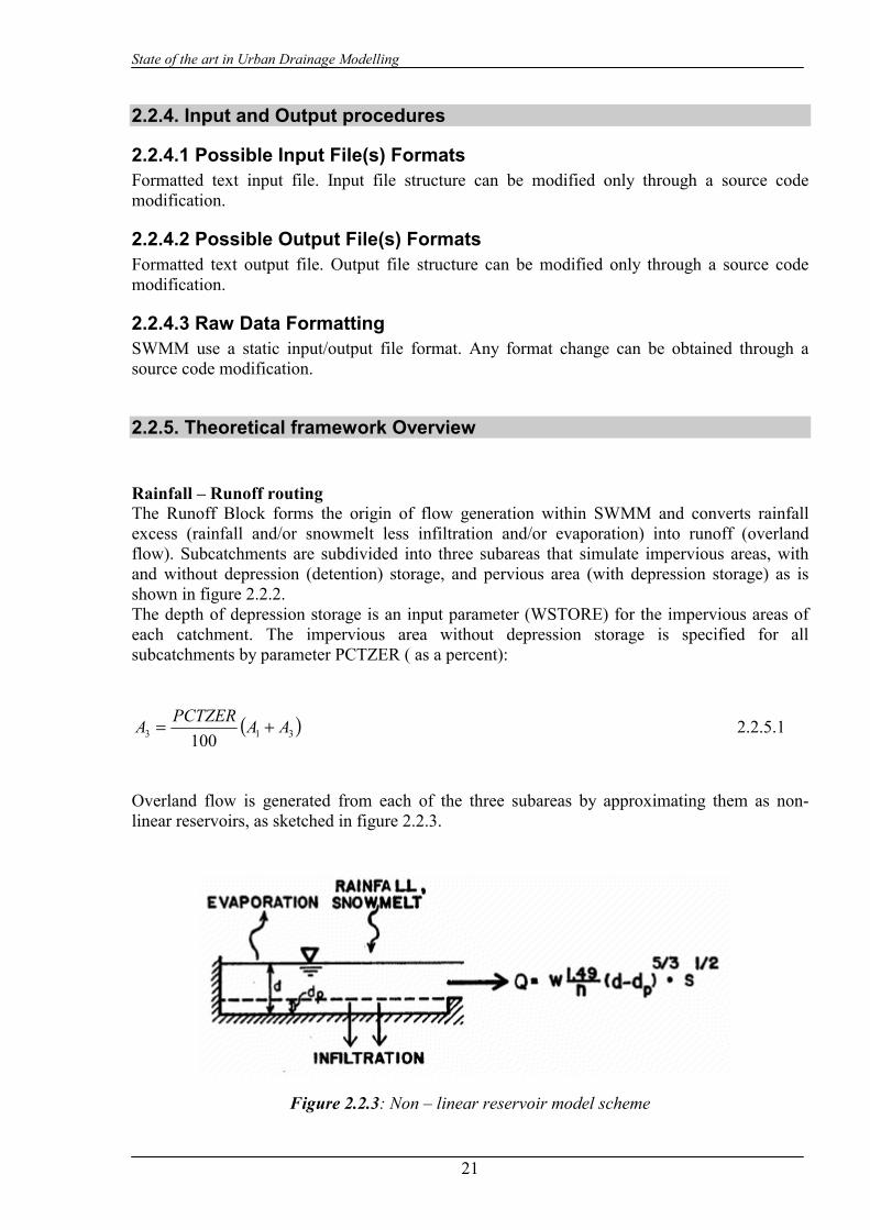
State of the art in Urban Drainage Modelling
21
2.2.4. Input and Output procedures
2.2.4.1 Possible Input File(s) Formats Formatted text input file. Input file structure can be modified only through a source code modification.
2.2.4.2 Possible Output File(s) Formats Formatted text output file. Output file structure can be modified only through a source code modification.
2.2.4.3 Raw Data Formatting SWMM use a static input/output file format. Any format change can be obtained through a source code modification.
2.2.5. Theoretical framework Overview Rainfall – Runoff routing The Runoff Block forms the origin of flow generation within SWMM and converts rainfall excess (rainfall and/or snowmelt less infiltration and/or evaporation) into runoff (overland flow). Subcatchments are subdivided into three subareas that simulate impervious areas, with and without depression (detention) storage, and pervious area (with depression storage) as is shown in figure 2.2.2. The depth of depression storage is an input parameter (WSTORE) for the impervious areas of each catchment. The impervious area without depression storage is specified for all subcatchments by parameter PCTZER ( as a percent):
( )313 100AAPCTZERA += 2.2.5.1
Overland flow is generated from each of the three subareas by approximating them as non-linear reservoirs, as sketched in figure 2.2.3.
Figure 2.2.3: Non – linear reservoir model scheme
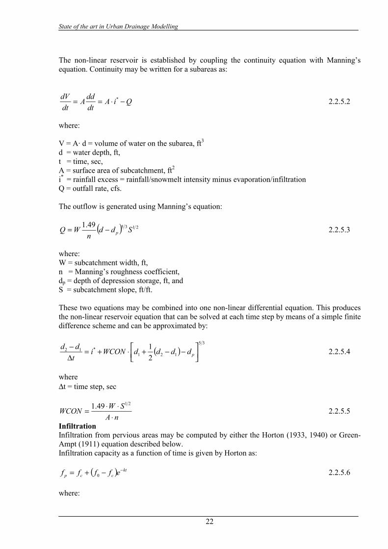
State of the art in Urban Drainage Modelling
22
The non-linear reservoir is established by coupling the continuity equation with Manning’s equation. Continuity may be written for a subareas as:
QiAdtddA
dtdV −⋅== * 2.2.5.2
where: V = A· d = volume of water on the subarea, ft3 d = water depth, ft, t = time, sec, A = surface area of subcatchment, ft2 i* = rainfall excess = rainfall/snowmelt intensity minus evaporation/infiltration Q = outfall rate, cfs. The outflow is generated using Manning’s equation:
( ) 213549.1 Sddn
WQ p−= 2.2.5.3
where: W = subcatchment width, ft, n = Manning’s roughness coefficient, dp = depth of depression storage, ft, and S = subcatchment slope, ft/ft. These two equations may be combined into one non-linear differential equation. This produces the non-linear reservoir equation that can be solved at each time step by means of a simple finite difference scheme and can be approximated by:
( )35
121*12
21
−−+⋅+=
∆−
pddddWCONitdd 2.2.5.4
where ∆t = time step, sec
nASWWCON
⋅⋅⋅=
2149.1 2.2.5.5
Infiltration Infiltration from pervious areas may be computed by either the Horton (1933, 1940) or Green-Ampt (1911) equation described below. Infiltration capacity as a function of time is given by Horton as:
( ) ktccp effff −−+= 0 2.2.5.6
where:

State of the art in Urban Drainage Modelling
23
fp = infiltration capacity into soil, ft/sec, fc = minimum or ultimate value of fp (WLMIN), ft/sec, f0 = maximum or initial value of fp (WLMAX), ft/sec, t = time from beginning of storm, sec, and k = decay coefficient (DECAY), sec-1
This equation describes the familiar exponential decay of infiltration capacity evident during heavy storms. The second infiltration option is the Green-Ampt equation that, has the advantage of physically based parameters that, in principle, can be predicted a priori. The Mein.Larson (1973) formulation of the Green-Ampt equation is a two-stage model. The first step predicts the volume of water, Fs which will infiltrate before the surface becomes saturated. From this point onward, infiltration capacity, fp, is predicted directly by Green-Ampt equation. Thus,
For F < Fs : f = I and 1−
=s
us Ki
IMDSF for i > Ks 2.2.5.7
For F ≥ Fs : f = fp and
+=
FIMDSKf u
sp 1 2.2.5.8
where: f = infiltration rate, ft/sec, fp = infiltration capacity, ft/sec, i = rainfall intensity, ft/sec, F = cumulative infiltration volume, this event, ft, Fs = cumulative infiltration volume required to cause surface saturation, ft Su = average capillary suction at the wetting front (SUCT), ft water IMD = initial moisture deficit for this event (SMDMAX), ft/ft and Ks = saturated hydraulic conductivity of soil, (HYDCON) ft/sec. Infiltration is thus related to the volume of water infiltrated as well as to the moisture conditions in the surface soil zone. Depression Storage Depression (retention) storage is a volume that must be filled prior to the occurrence of runoff on both pervious and impervious areas; a good discussion is presented by Viessman et al. (1977). It represents a loss or “initial abstraction” caused by such phenomena as surface ponding, surface wetting, interception and evaporation. In some models, “depression storage” also includes infiltration in pervious areas. In the Runoff Block, water stored as depression storage on pervious areas is subject to infiltration (and evaporation), so that it is continuously and rapidly replenished. Water stored in depression storage on impervious areas is depleted only by evaporation. Hence, replenishment typically takes much longer. Snowmelt simulation When snowmelt is simulated, a fourth subarea is added to each subcatchment as illustrated in Figure 2.2.2. The main purpose of the fourth subarea is to permit part of the impervious area (subarea A4) to be continuously snow covered (e.g., due to windrowing or dumping) and part (subareas A1 plus A3) to be “normally bare” (e.g., streets and sidewalks that are swept).

State of the art in Urban Drainage Modelling
24
During single event simulation, subarea A4 retains 100 percent snow cover until it has all melted. During continuous simulation, an areal depletion curve is used. Similarly, for single event simulation, a fraction of the pervious area remains 100 percent snow covered. During continuous simulation, the whole pervious area is subject to areal depletion curve. Initial snow depths (inches/mm water equivalent) may be entered using catchment characterization parameters. This is likely to be the only source of snow for a single event simulation although snowfall values may be entered as negative precipitation in rain data group. During continuous simulation, the effect of initial conditions will die out, given a simulation of a few months. No liquid runoff will leave the snow pack until its free water holding capacity (due to its porosity) has been exceeded. The available volume is a constant fraction, of the snow depth. During periods of no rainfall, snowmelt is computed by a degree-day or temperature index equation.
Figure 2.2.4: Snow redistribution during ploughing
Melt coefficients and base melt temperatures may be determined both theoretically and experimentally. Considering the former, it is possible to first write a snowmelt equation from a heat budget formulation that includes all relevant terms: change in snow pack heat storage, net short wave radiation entering pack, conduction of heat to the pack from underlying ground, net (incoming minus outgoing) long wave radiation entering pack, convective transport of sensible heat from air to pack, release of latent heat of vaporization by condensation of atmospheric water vapour, and advection of heat to snow pack by rain. (It is assumed here that the pack is “ripe”, i.e., just at the melting point, so that rain will not freeze and release its latent heat of
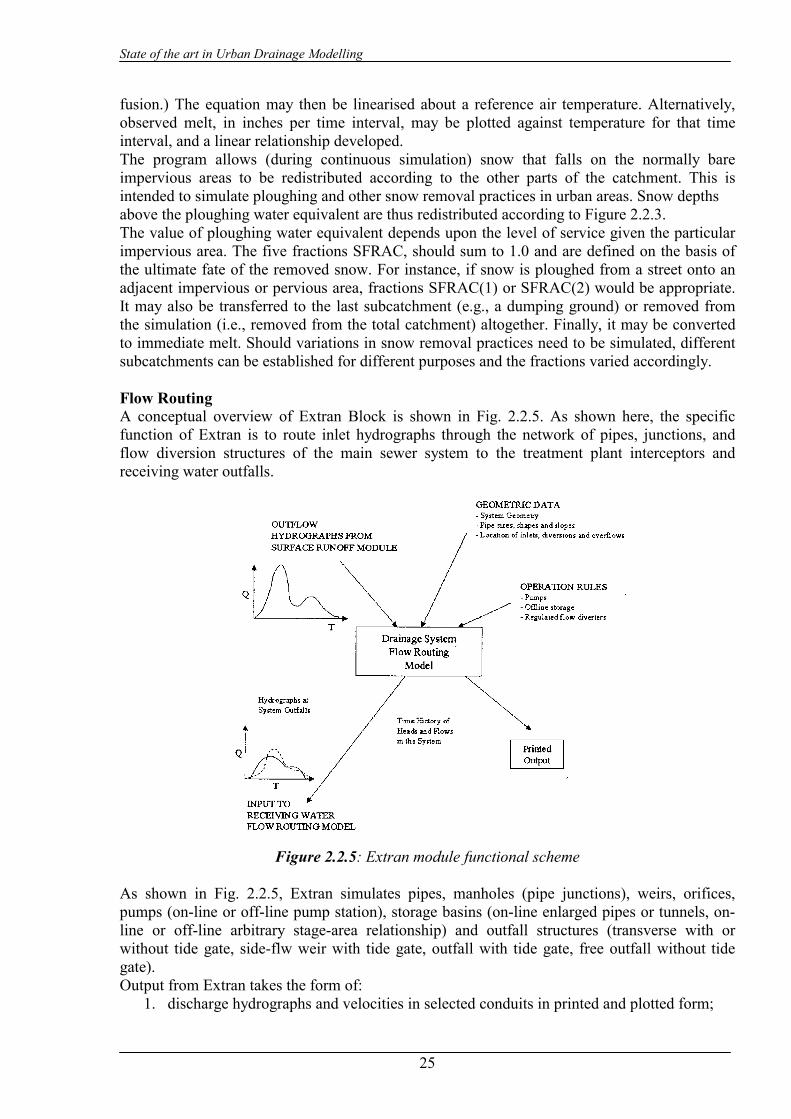
State of the art in Urban Drainage Modelling
25
fusion.) The equation may then be linearised about a reference air temperature. Alternatively, observed melt, in inches per time interval, may be plotted against temperature for that time interval, and a linear relationship developed. The program allows (during continuous simulation) snow that falls on the normally bare impervious areas to be redistributed according to the other parts of the catchment. This is intended to simulate ploughing and other snow removal practices in urban areas. Snow depths above the ploughing water equivalent are thus redistributed according to Figure 2.2.3. The value of ploughing water equivalent depends upon the level of service given the particular impervious area. The five fractions SFRAC, should sum to 1.0 and are defined on the basis of the ultimate fate of the removed snow. For instance, if snow is ploughed from a street onto an adjacent impervious or pervious area, fractions SFRAC(1) or SFRAC(2) would be appropriate. It may also be transferred to the last subcatchment (e.g., a dumping ground) or removed from the simulation (i.e., removed from the total catchment) altogether. Finally, it may be converted to immediate melt. Should variations in snow removal practices need to be simulated, different subcatchments can be established for different purposes and the fractions varied accordingly. Flow Routing A conceptual overview of Extran Block is shown in Fig. 2.2.5. As shown here, the specific function of Extran is to route inlet hydrographs through the network of pipes, junctions, and flow diversion structures of the main sewer system to the treatment plant interceptors and receiving water outfalls.
Figure 2.2.5: Extran module functional scheme As shown in Fig. 2.2.5, Extran simulates pipes, manholes (pipe junctions), weirs, orifices, pumps (on-line or off-line pump station), storage basins (on-line enlarged pipes or tunnels, on-line or off-line arbitrary stage-area relationship) and outfall structures (transverse with or without tide gate, side-flw weir with tide gate, outfall with tide gate, free outfall without tide gate). Output from Extran takes the form of:
1. discharge hydrographs and velocities in selected conduits in printed and plotted form;

State of the art in Urban Drainage Modelling
26
2. flow depths and water surface elevations at selected junctions in printed and plotted form. Hydrographs may be supplied to a subsequent module on the output interface file.
Extran uses a link-node description of the sewer system which facilities the discrete representation of the physical prototype and the mathematical solution of the gradually-varied unsteady flow (St. Venant) equations which form the mathematical basis of the model. As shown in Fig. 2.2.6, the conduit system is idealized as a series of links or pipes which are connected at nodes or junctions. Links transmit flow from node to node. Properties associated with the links are roughness, length cross-sectional area, hydraulic radius, and surface width. The last three properties are functions of the instantaneous depth of flow. The primary dependent variable in the links is the discharge, Q. The solution is for the average flow in each link, assumed to be constant over a time step. Velocity and cross sectional area of flow, or depth, are variable in the link in the numerical solution.
Fig. x2 (pag.76)
Figure 2.2.6: Node – Link computational scheme
Nodes are the storage elements of the system and correspond to manholes or pipe junctions in the physical system. The variables associated with a node are volume, head, and surface area. The primary dependent variable is the head, H, which is assumed to be changing in time but constant throughout any one node. Inflows, such as inlet hydrographs, and outflows, such as weir diversions, take place at the nodes of the idealized sewer system. The volume of the node at any time is equivalent to the water volume in the half-pipe length connected to any one node. The change in nodal volume during a given time step, ∆t, forms the basis of head and discharge calculations as discussed below. The basic differential equations for the sewer flow problem come from the gradually varied, unsteady flow equations for open channels, otherwise know as the St. Venant or shallow water equations. The unsteady flow continuity equation with surface area flow as dependent variables (Yen, 1986; Lai, 1986) is:
0=∂∂+
∂∂
xQ
tA 2.2.5.9
where: A = cross sectional area, Q = conduit flow, X = distance along the pipe/channel, and

State of the art in Urban Drainage Modelling
27
T = time. The momentum equation is (Lai, 1986):
( ) 02
=+∂∂+
∂∂+
∂∂
fgASxHgA
xAQ
tQ 2.2.5.10
where: g = gravitational constant, H = z + h = hydraulic head, z = invert elevation, h = water depth, and Sf = friction (energy) slope. (The bottom slope is incorporated into gradient of H). Extran uses the momentum equation in the links and a special lumped continuity equation for the nodes. Thus, momentum is conserved in the links and continuity in the nodes. For use in Extran, the momentum equation is combined with the continuity equations to yield an equation to be solved along each link at each time step:
02 2 =∂∂+
∂∂−
∂∂−+
∂∂
xHgA
xAV
tAVgAS
tQ
f 2.2.5.11
where: Q = discharge along the conduit, V = velocity in the conduit, A = cross-sectional area of the flow, H = hydraulic head (invert elevation plus water depth), and Sf = friction slope. The friction slope is defined by Manning’s equation, i.e.:
VQgAR
kS f 3/4= 2.2.5.12
where: k = g(n/1.49)2 for U.S. customary units and gn2 for metric units n = Mannings roughness coefficient, g = gravitational acceleration, R = hydraulic radius. Use of the absolute value on the sign on the flow term makes Sf a directional quantity and ensures that the friction force always opposes the flow. Substituting 2.2.5.12 in 2.2.5.11 and solving for Qt+∆t gives the final finite difference form of the dynamic flow equation:
( ) ( )[ ] ( )[ ]
∆−−∆−+∆∆
∆+∆+=∆ tLHHAgtLAAVtt
AVQ
VRtkQ
tttt //21
11212
2
3/4
_ 2.2.5.13

State of the art in Urban Drainage Modelling
28
In this last equation, V, R, and A are weighted averages of the conduit and values at time t, and (∆A/∆t)t is the time derivative from the previous time step. The basic unknowns in equation (2.2.5.13) are Qt+∆t, H2 and H1. The various V, R, and A can all be related to Q and H. Therefore, another equation is required relating Q and H. This can be obtained by writing the continuity equation at a node:
∑=∂∂
ts
t
t AQ
tH 2.2.5.14
Or, in finite difference form
∑ ∆+=∆+ tstttt AtQHH 2.2.5.15 where: As = surface area of node. Equation 2.2.5.13 and 2.2.5.15 can be solved sequentially to determine discharge in each link and head at each node over a time-step ∆t. The numerical integration of these two equations is accomplished by the improved polygon or modified Euler method. The results have proven to be relatively accurate and, when certain constraints are followed, stable. Fig. 2.2.7 shows how the process would work if only the discharge equation were involved.
Figure 2.2.7: Computational approximation scheme.
The first three operations determine the slope tQ ∂∂ / at the “half-step” value of discharge. In other words, it is assumed that the slope at time t+∆t/2 is the mean slope during the interval. The method is extended easily to more than one equation, although graphic representation is then very difficult. The corresponding half-step and full-step calculations of head are shown below: Half-step at node j: Time t+∆∆∆∆t/2
( ) ( ) ( ) ( ) ( ) ( )[ ] ( )[ ] ( )tAttQttQtQttHttHjsjj /2/2/2/12/2/ ∑ ∑ ∆++∆++∆+=∆+ 2.2.5.16
conduits, surface runoff diversions, pumps, outfalls Full-step at node j : Time t+∆∆∆∆t

State of the art in Urban Drainage Modelling
29
( ) ( ) ( ) ( ) ( )[ ] ( )[ ] ( )tAttQttQtQttHttH
jsjj /2/1 ∑ ∑ ∆++∆++∆+=∆+ 2.2.5.17 conduits, surface runoff diversions, pumps, outfalls The total sequence of discharge computations in the links and head computations in the nodes can be summarized as:
1. Compute half-step discharge at t+∆t/2 in all links based on preceding full-step values of head at connecting junctions.
2. Compute half-step flow transfers by weirs, orifices, and pumps at time t+∆t/2 based on preceding full-step values of head at transfer junction.
3. Compute half-step head at all nodes at time t+∆t/2 based on average of preceding full-step and current half-step discharges in all connecting conduits, plus flow transfers at the current half-step.
4. Compute full-step discharge in all links at time t+∆t based on half-step heads at all connecting nodes.
5. Compute full-step flow transfers between nodes at time t+∆t based on current half-step heads at all weir, orifice, and pump nodes.
6. Compute full-step head at time t+∆t for all nodes based on average of preceding full-step and current full-step discharge, plus flow transfers at the current full-step.
The link-node computations can be extended to include devices which divert sanitary sewage out of a combined sewer system or relieve the storm load on sanitary interceptors. In Extran, all diversions are assumed to take place at a node and are handled as inter-nodal transfer. The special flow regulation devices treated by Extran include: weirs(both side-flow and transverse), orifices, pumps, and outfalls. Each of these is discussed below.
Figure 2.2.8: Storage node computational approach.
Storage devices In-line or off-line devices act as flow control devices by providing for storage of excessive upstream flows thereby attenuating and lagging the wet weather flow hydrograph from the upstream area. The conceptual representations of a storage junction and a regular junction are illustrated in Fig. 2.2.8. An arbitrary stage-area-volume relationship may be also be input (data group E2), e.g. to represent detention ponds. Routing is performed by ordinary level-surface reservoir methods. This type of storage facility is not allowed to surcharge. Orifices Extran simulates, as is shown in Fig. 2.2.9:
- a dropout or sump orifices, and - a side outlet orifices

State of the art in Urban Drainage Modelling
30
by converting the orifices to an equivalent pipe. The conversion is made as follows. The standard orifice equation is:
ghACQ 200 = 2.2.5.18 where: C0 = discharge coefficient, A = cross-sectional area of the orifice, g = gravitational acceleration, and h = the hydraulic head on the orifice.
Figure 2.2.9: SWMM orifice scheme.
To covert the orifice to a pipe, the program equates the orifice discharge equation and the Manning pipe flow equation, i.e:
ghACSARnm 20
2/13/2 = 2.2.5.19
where: m = 1,49 for U.S. customary units and 1,0 for metric units, S = slope of equivalent pipe. Weirs A schematic illustration of flow transfer by weir diversion between two nodes is shown in Fig. 2.2.10. Flow over a weir is computed by:
−
+=aa
www gV
gVhLCQ
22
22
2.2.5.20
where: Cw = discharge coefficient, Lw = weir length (transverse to overflow),

State of the art in Urban Drainage Modelling
31
h = driving head on the weir, V = approach velocity, and a = weir exponent, 3/2 for transverse weirs and 5/3 for side flow weirs
Figure 2.2.10: Weir computational scheme.
If the weir is submerged, the flow is computed as: ( ) 2/3
clwwSUBw YYLCCQ −= 2.2.5.21 The submergence coefficient, CSUB, is taken from Roessert’s Handbook of Hydraulics and is a function of CRATIO defined as:
c
cRATIO YY
YYC−−=
1
2 2.2.5.22
The values of CRATIO and CSUB are computed automatically by Extran and no input data values are needed. If the weir is surcharged it will behave as an orifice and the flow is computed as:
( ) hgYYLCQ cTOPwSURw ′−= 2 2.2.5.23 where: YTOP = distance to top of weir opening shown in Fig.2.2.10 h1 = Y1 – maximum (Y2, Yc), CSUR = weir surcharge coefficient. The weir surcharge coefficient, CSUR, is computed automatically at the beginning of surcharge. Weir with tide gates Frequently, weirs are installed together with a tide gate at points of overflow into the receiving waters. Flow across the weir is restricted by the tide gate, which may be partially closed at times. This is accounted for by reducing the effective driving head across the weir according to an empirical factor published by Armco (undated):
−−=′
2/12 15.1exp4
hVV
ghh 2.2.5.24
where h is the previously computed head before correction for flap gate and V is the velocity of flow in the upstream conduit.
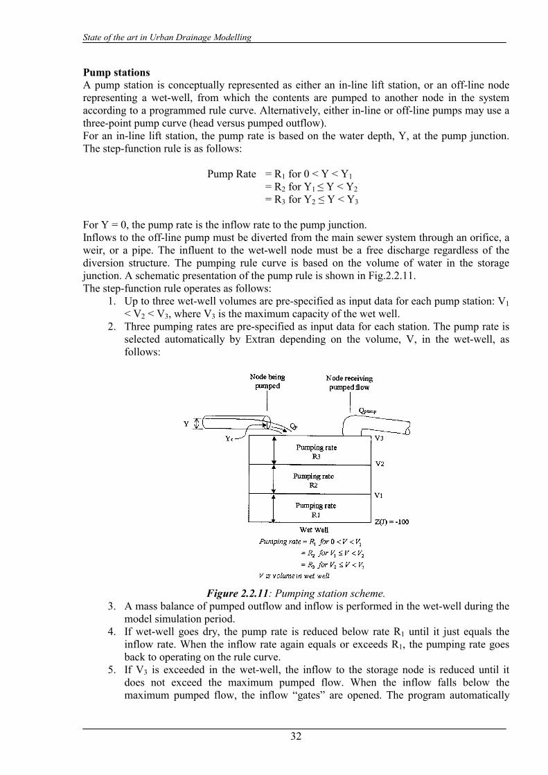
State of the art in Urban Drainage Modelling
32
Pump stations A pump station is conceptually represented as either an in-line lift station, or an off-line node representing a wet-well, from which the contents are pumped to another node in the system according to a programmed rule curve. Alternatively, either in-line or off-line pumps may use a three-point pump curve (head versus pumped outflow). For an in-line lift station, the pump rate is based on the water depth, Y, at the pump junction. The step-function rule is as follows: Pump Rate = R1 for 0 < Y < Y1 = R2 for Y1 ≤ Y < Y2 = R3 for Y2 ≤ Y < Y3 For Y = 0, the pump rate is the inflow rate to the pump junction. Inflows to the off-line pump must be diverted from the main sewer system through an orifice, a weir, or a pipe. The influent to the wet-well node must be a free discharge regardless of the diversion structure. The pumping rule curve is based on the volume of water in the storage junction. A schematic presentation of the pump rule is shown in Fig.2.2.11. The step-function rule operates as follows:
1. Up to three wet-well volumes are pre-specified as input data for each pump station: V1 < V2 < V3, where V3 is the maximum capacity of the wet well.
2. Three pumping rates are pre-specified as input data for each station. The pump rate is selected automatically by Extran depending on the volume, V, in the wet-well, as follows:
Figure 2.2.11: Pumping station scheme. 3. A mass balance of pumped outflow and inflow is performed in the wet-well during the
model simulation period. 4. If wet-well goes dry, the pump rate is reduced below rate R1 until it just equals the
inflow rate. When the inflow rate again equals or exceeds R1, the pumping rate goes back to operating on the rule curve.
5. If V3 is exceeded in the wet-well, the inflow to the storage node is reduced until it does not exceed the maximum pumped flow. When the inflow falls below the maximum pumped flow, the inflow “gates” are opened. The program automatically
State of the art in Urban Drainage Modelling
33
steps down the pumping rate by the operating rule described at point 2 as inflows and wet-well volume decrease.
When this method is used for either type of pump, iteration is performed until the dynamic head difference between the upstream and downstream nodes on either side of the pump corresponds to the flow given on the pump curve. In other words, the pump curve replaces equation 2.2.5.13. Outfall Structures Extran simulates both weir outfalls and free outfalls. Either type may be subject to a backwater condition and protected by a tide gate.
2.2.6. Model Parameters Estimation or Assignation This kind of routines is not available for the freeware version of SWMM. Nevertheless some of the commercial versions have been upgraded with this kind of features. In the following this kind of routines will be described.
2.2.6.1 Check of Parameters Significance – Internal Validation Computational Hydraulic Institute (CHI) has developed a sensitivity analysis routine for the freeware version of SWMM. Sensitivity Wizard provides an analysis of parameter sensitivity for various input functions and objective functions in the SWMM Runoff module. Through an easy step-by-step interface, the complicated and lengthy process of manual sensitivity testing is dramatically simplified and shortened. Any number of parameters and input functions can be analyzed in one session, and easily re-analyzed if model changes are made. The sensitivity results generated by Sensitivity Wizard are presented in highly customizable graphs, and both the graphs and numeric tables can be exported in various forms (e.g. printed, inserted into other documents, and/or copied to other graphing programs for further customization). This routine uses both linear and non-linear functions in order to interpolate dependency function between parameters and model output. Another tool developed by CHI allows for SWMM model calibration. The Genetic Algorithm Calibration tool is a genetic algorithm-based software tool for calibration of SWMM Runoff, Transport, Extran and/or Storage-Treatment modules. Model calibration is a crucial step in developing a useful storm water model, especially when the model is used to evaluate one or more "what-if" scenarios in an existing storm water system. While a SWMM model can be applied to very simple modelling problems, it can also be quite complex, containing thousands of significant hydraulic and hydrologic entities. As each model entity may contain as many as a dozen sensitive parameters, and as the volume of available observed time series data increases, rigorous manual calibration can be an expensive, time-consuming undertaking. For this reason, model calibration is often not performed, or performed inadequately. An automated calibration tool such as this one significantly reduces the effort required for calibration and design optimization. Such tools encourage the adoption of more thorough model development and verification protocols, and better design.
2.2.7. PI(s) Estimation Method Apart from the usual hydrological and hydraulic variables (such as peak flow, runoff volume, water levels, etc.), SWMM does not have the possibility for estimating user – defined model output. SWMM gives also some simple statistics about model runs such as maximum flow rate, maximum velocity and maximum water level. SWMM is able to compute physical performance indicators wPh5, wPh6 and wPh7 as they are defined in Appendix 1. Computing also maximum, minimum and average velocities as well as other generic discharge statistics, SWMM output can be also used for generating other

State of the art in Urban Drainage Modelling
34
performance indicators such as flushing ratio (Vmax (wet period)/Vmax (dry period)). Also surface flooding performance indicators (wOp34 and wOp35) can be computed by the model. The specification of user-defined output variables can be done only by a modification in the model source code.
2.2.8. Future Improvements of the Model A redevelopment project has been started by US EPA and by the other authors in order to update the modelling approaches, the source code structure and the user interface of SWMM4. This project will lead to the release of SWMM5 model in the second half of 2003. The goal of this project is to help meet the needs of EPA’s clients for improved computational tools for managing urban runoff and wet weather water quality problems. The redevelopment team intends to produce a new version of SWMM that incorporates modern software engineering methods as well as updated computational techniques. The specific objectives of this project are:
• To revise the architecture of the SWMM computational engine, using object oriented programming (OOP) techniques, to enhance the ability of the model to be maintained, upgraded, and interfaced with other software.
• To provide a rudimentary graphical user interface (GUI) to the engine to improve the usability of the model.
• To remove obsolete features, improve key computational aspects, and add new computational capabilities to the model where warranted.
• To develop guidelines on how SWMM can be used to model more recently developed Best Management Practices (BMP) for runoff control.
The end products from this project will consist of the following: • A newly coded version of the SWMM computational engine that can be run either
as a stand-alone application or as a Dynamic Link Library (DLL) of functions that can be called from other applications such as third party vendors of SWMM.
• A GUI shell program that will run under Windows, access the SWMM engine through DLL calls, and include a context-sensitive, on-line Help system.
• Full documentation in the form of a Users Manual, a Programmer’s Manual, and a Reference Manual.
• A manual on Modeling BMPs with SWMM that will illustrate how SWMM can be used to model various types of BMP/LID options.
This project will be a joint development effort between EPA-NRMRL’s Water Supply and Water Resources Division and Camp Dresser and McKee Inc. (CDM). CDM’s participation will be through a CRADA (Cooperative Research and Development Agreement) between itself and the Agency. The work envisioned for this project can be divided into nine task areas as follows:
1. Re-examine SWMM’s functionality 2. Re-write SWMM’s computational engine 3. Adapt an existing graphical user interface for use with SWMM 4. Update and add to SWMM’s computational algorithms 5. Develop standard formats and procedures for data transfer 6. Develop converters for input/output from previous versions of SWMM 7. Identify how state-of-the-art BMP/LID modeling can be incorporated into
SWMM 8. Prepare program documentation 9. Conduct quality assurance testing
State of the art in Urban Drainage Modelling
35
Since this project affords the opportunity to rebuild SWMM from the ground up, it seemed worthwhile to ask which computational features currently contained in SWMM could be eliminated, which should be retained in their current form, which are in need of updating, and which additional features should be added. New features that are prime candidates for inclusion in future versions of the software are:
• SCS curve number infiltration • soil moisture accounting model for groundwater • energy balance model for snowmelt • implicit dynamic wave flow routing • Lagrangian water quality transport model • bed/suspended load sediment transport model • interactive real-time control of sewer flow routing.
The computational engine which implements the modelling functionality embedded in SWMM will be re-written in C++ using an object oriented approach. The SWMM engine will be delivered in two formats. One will be a stand-alone executable that receives input from a text file and writes output to a text file and/or binary output file. The other will be a library of callable functions that can be accessed by other software, such as the SWMM Graphical User Interface module discussed below. For the Windows operating system, the library will be compiled as a DLL (Dynamic Link Library). This follows the same approach used by the highly successful EPANET model, which analyzes hydraulic and water quality behavior in drinking water distribution systems. In EPANET only one line of code needs to be changed to compile the program as a DLL as opposed to a stand-alone executable. The SWMM graphical user interface will be ported over from the previously developed EPANET user interface. The redevelopment team estimates that about 80% of the existing code can be used with either no or only minor modification. Without this high degree of re-usability it probably would not be feasible to include GUI development within this project. It will allow the user to draw a node-link representation of the drainage network on a scalable map, with the option of inserting a background reference map. Point and click actions will be used to add, delete, re-position, and edit specific objects depicted on the map. Colour coding of the map’s features are used to represent the values of user-selected design parameters or computed output. Retrofitting the EPANET GUI to meet the specific needs of SWMM will proceed in parallel with the development of the computational engine, since data definitions and file formats have to remain synchronized between the two modules. The GUI will also present a simpler way to perform testing and debugging of the engine than would the command line interface. The GUI will be subjected to the same iterative review procedures as will the engine, with the understanding that its functionality will not grow beyond what is already included in EPANET. In conjunction with the need to evaluate the functionality to be included in the updated SWMM there is also a need to evaluate which computational methods should be improved or replaced. EPA will explore making the following computational enhancements in future versions of the SWMM software:
• The current method of routing water quality constituents (which is available only with the Transport module) could be improved by adopting one of the Lagrangian methods utilized for modelling advective transport in rivers (Jobson and Schoellhamer, 1987) and water distribution pipe networks (Rossman and Boulos, 1996). Since the Extran module will become integrated with the former Transport module, water quality routing will also be available when fully dynamic flow routing is utilized.
• CDM intends to modify the explicit solution method used for dynamic flow routing in Extran to make it more efficient and robust. In addition, EPA will

State of the art in Urban Drainage Modelling
36
explore the efficacy of adding an implicit flow routing method as another alternative. Various implementations of the 4-point implicit (Preissman Box) scheme will be evaluated. These include the Extended Relaxation Technique currently employed in the NWS FLDWAV model (Lewis et al., 1996), the double sweep, recursive method of Choi and Molinas (1993), and the SUPERLINK model used in the SEWERCAT program (Ji, 1998). Other approaches, which solve the Saint-Venant equations in conservative form, include second order relaxation schemes (Aral et al., 1999) and finite volume methods (Toro, 1997).
• The sediment transport sub-model employed in SWMM will be re-visited. The use of other simplified equations for determining when scour or deposition occurs will be considered (see Zug et al., 1998 for example). More complex models, that provide refined estimates of bed shear stress and explicitly model bed transport will also be examined (Mark, 1992). An evaluation will be made to determine if an enhanced sediment model is worth including into the new SWMM based on such criteria as model reliability, robustness, and ease of implementation.
• The redevelopment team will investigate the possible advantages of replacing the current degree-day model used in SWMM’s snowmelt computation with the more physically correct heat budget model as is used in the HSPF model for example (Johanson et al., 1984).
The use of industry-standard data formats for generating input and output data for SWMM’s computational engine would facilitate its linkage with third party software, such as Geographical Information Systems (GIS), computer aided drawing (CAD) software, statistical packages, and ODBC-compliant database systems (e.g., Access, Oracle, etc.). Data format standardization would also assist in sharing of data with other government agency databases. Examples of alternative data standards include:
• ODBC-compliant database formats, such as Microsoft Access or dBase IV. • the HEC-DSS file format (HEC, 1994) used in HEC’s HMS (Hydrological
Modeling System) software for storing time series data • the USGS-WDM file format (Flynn et al., 1995) used by USGS and EPA for
storing time series data • the FGDC Utility Standards (Federal Geographic Data Committee, 2000)
developed by the Federal Geographic Data Committee for representing geo-referenced infrastructure objects
• the ArcGIS Water Facilities and Hydro data models developed by ESRI (ESRI, 2000) that allow seamless integration of numerical modeling within the ArcGIS framework
• XML (Extensible Markup Language) format (World Wide Web Consortium, 2000) which is a general method for storing hierarchical-structured data that is highly transportable between computing platforms and is finding widespread acceptance in distributed computing and web-based applications.
Each of these formats will be evaluated with respect to how they might be used with SWMM input and output data and what advantages they would bring to the overall SWMM package. Based on the results of this evaluation, one or more of these formats will be utilized by the SWMM engine or by its graphical user interface.

State of the art in Urban Drainage Modelling
37
2.2.9. References
2.2.9.1 Theoretical Framework References Huber, W. C., Cunnigham, B. A. and Cavender, K. A. (April 1986). Continuous SWMM modelling for selection of design events. Proceedings of the International Symposium on the Comparison of Urban Drainage Models with Real Catchment Data, Dubrovnik Yugoslavia, pp. 379-390. Stirrup, M. and James, W. (June 1984) Real time control of combined sewer overflows using on site microcomputer., Proceedings of 3rd International Conference on Urban Storm Drainage, Goteborg Sweden, pp. 1457-1464 P.E. Wisner, A.M. Kassem, & P. Cheung, (Jan 1980) Implementation of storm water management models: pros and cons of standardization., EPA-600/9-80-017, Gainesville, FL, pp. 306-325. P.E. Wisner, S. Gupta, & A.M. Kassem, (Jun 1980) Considerations regarding the application of SCS TR-55 procedures for runoff computations. EPA-600/9-80-064, Toronto, ON, pp. 23-44. M. Ahmad, (Jun 1980) Methodology for 'lumped' SWMM modelling., EPA-600/9-80-064, Toronto, ON, pp. 64-79. B.L. Golding, (Jun 1980) Hydrograph synthesis by the HNV-SBUH method utilizing a programmable calculator., EPA-600/9-80-064, Toronto, ON, pp. 150-177, A.T.Fok & S.H.Tan, (Jun 1980) Detention lake application in master drainage planning. EPA-600/9-80-064, Toronto, ON, pp. 178-199 Zech, Y., Sillen, X., Djeufa, S. and Pahaut, T. (July 1993) Rainfall-runoff modelling of partly urbanized watersheds-comparison between a distributed model using GIS and other models. Proceedings of 6th International Conference on Urban Storm Drainage, Niagara Falls Ontario Canada, pp. 1452-1457. A.Ashmala & M. Ahmad, (Sept 1981) Evaluation of relief alternatives for combined sewer systems., CHI-R81, Niagara Falls, ON, pp. 427-454. Shiferaw, M. (June 1984) The influence of input data on the accuracy of simulation., Proceedings of 3rd International Conference on Urban Storm Drainage, Goteborg Sweden, pp. 615-624 Wolfgang, G. (June 1984) Goodness and limits in urban runoff modelling., Proceedings of 3rd International Conference on Urban Storm Drainage, Goteborg Sweden, pp. 635-644. A.R. Perks, (Oct. 1976) Introduction to the SWMM., Conf. Proc. No. 4, Toronto, ON, pp. 26-32 W. Clark, (Oct. 1976) SWMM RUNOFF submodel - relationships for quantity simulation., Conf. Proc. No. 4, Toronto, ON, pp. 33-38 A.R. Perks, (Oct. 1976) Long-term simulation models., Conf. Proc. No. 4, Toronto, ON, pp. 50-52 C.W. Eicher, (May 1978) Application of SWMM-EXTRAN for the analysis of existing urban drainage systems., EPA-600/9-78-019, Ottawa, ON, pp. 31-48 James, W. (June 1994) Urban drainage system models: User groups and the gray literature., Integrated Urban Storm Runoff - 7th European Junior Scientist Workshop, Cemise Castle-Bechyne Czech Republic, pp. 293-302 Diniz, E.V. (April 1978) Modifications of the storm water management model and application to natural drainage systems., Proceedings of 1st International Conference on Urban Storm Drainage, South Ampton U.K., pp. 256-274. Roesner, L.A. and Shubinski, R.P. (June 1981) Improved dynamic flow routing model for storm drainage systems., Proceedings of 2nd International Conference on Urban Storm Drainage, Urbana Illinois, pp. 164-173

State of the art in Urban Drainage Modelling
38
Huber, W.C. and Heaney, J.P. (June 1981) The USEPA stormwater management model SWMM: a ten year perspective., Proceedings of 2nd International Conference on Urban Storm Drainage, Urbana Illinois, pp. 247-256. James, C.S. (June 1981) Estimation of urban flood hydrographs., Proceedings of 2nd International Conference on Urban Storm Drainage, Urbana Illinois, pp. 303-312., Rao, A.R. and Han, J. (June 1981) Optimal parameter estimation in urban runoff models., Proceedings of 2nd International Conference on Urban Storm Drainage, Urbana Illinois, pp. 384-393 Wisner, P., Rampersad, C.A. and Lam, A. (June 1984) Realistic simulation of sewer surcharge and prevention of basement flooding., Proceedings of 3rd International Conference on Urban Storm Drainage, Goteborg Sweden, pp. 375-386 Nouh, M. (June 1984) Evaluation of risk-based optimization models of sewer system design., Proceedings of 3rd International Conference on Urban Storm Drainage, Goteborg Sweden, pp. 685-694 Young, D.L., Yen, C.-L. and Chen, C.S. (August 1987) A surcharge flow model for storm sewer., Proceedings of 4th International Conference on Urban Storm Drainage, Lausanne Switzerland, pp. 214-219 James, W. and Green, W. (August 1987) Improvements to urban drainage models for combined sanitary sewers., Proceedings of 4th International Conference on Urban Storm Drainage, Lausanne Switzerland, pp. 237-241 Baffaut, C. and Delleur, J.W. (August 1987) Calibration of SWMM with an expert system., Proceedings of 4th International Conference on Urban Storm Drainage, Lausanne Switzerland, pp. 303-308 Huber, W.C. and PeQueen, J.D. (June 1990) Performance of conceptual vs physically-based models: A comparison using small-catchment data. Proceedings of 5th International Conference on Urban Storm Drainage, Tokyo Japan, pp. 281-286 Dickinson, R.E., Huber, W.C., Roesener, L.A. and Aldrich, J.A. (June 1990) Advances in SWMM EXTRAN flow routing. Proceedings of 5th International Conference on Urban Storm Drainage, Tokyo Japan, pp. 287-292 Fuchs,L. and Scheffer, C. (July 1993) Hystem-Extran- improvements to EPA-Extran., Proceedings of 6th International Conference on Urban Storm Drainage, Niagara Falls Ontario Canada, pp.237-242 Goyen, A.,Dickinson, R. and Thompson, G. (July 1993) XP-Extran the next generation unsteady flow routing system., Proceedings of 6th International Conference on Urban Storm Drainage, Niagara Falls Ontario Canada, pp.269-274. Lei, J. and Schilling, W. (July 1993) Propagation of model uncertainty., Proceedings of 6th International Conference on Urban Storm Drainage, Niagara Falls Ontario Canada, pp. 465-470 G.D.Cole, L.W.Varner, & J.W. Shutt, (Nov. 1978) SWMM usage in facilities planning., EPA-600/9-79-003, Annapolis, MD, pp. 190-217 W. James, (Nov. 1978) A pre- and post-processing program package for SWMM., EPA-600/9-79-003, Annapolis, MD, pp. 218-233 R.E.G. Sprenger & C.E. Bright, (May 1979) Use of RUNOFF/EXTRAN for hydraulic analysis of urban drainage systems., EPA-600/9-79-026, Montreal, PQ, pp. 55-87 P. Purenne, G. Courchesne & G. LeClerc, (May 1979) Simplified segmentation of an urban catchment for urban runoff simulation with SWMM., EPA-600/9-79-026, Montreal, PQ, pp. 88-111 P.E. Wisner & A.M. Kassem, (May 1979) IMPSWM. EPA-600/9-79-026, Montreal, PQ, pp. 237-241
State of the art in Urban Drainage Modelling
39
P.E. Wisner, A.M. Kassem, & P. Cheung, (Jan 1980) Comparison of design peak flows calculated by the rational method and the EPA-SWMM model., EPA-600/9-80-017, Gainesville, FL, pp. 41-74 W.M. Alley, (Jan 1980) An examination of SWMM surface-runoff-quality algorithms., EPA-600/9-80-017, Gainesville, FL, pp. 93-110 W.M. Parker, III, (Jan 1980) The use of SWMM to economically model surcharged combined sewer systems., EPA-600/9-80-017, Gainesville, FL, pp. 111-131 L.A. Roesner, A.M. Kassem, & P.E. Wisner, (Jan 1980) Improvements in EXTRAN., EPA-600/9-80-017, Gainesville, FL, pp. 132-141 W.James & H.Mitri, (Jan 1981) SWMM compatible algorithm for side weir structures., CHI-R83, Austin, TX, pp. 141-157 J.A.Aldrich & L.A.Roesner, (Mar 1982) An improved surcharge computation in EXTRAN., EPA-600/9-82-015, Washington DC, pp. 179-190, M.L.Yasenchak & T.J.McGhee, (Oct 1988) User-Defined Conduits in EXTRAN Block of SWMM., EPA-600/9-89-001, Denver, CO, pp. 1-9 J.C.Y. Guo, B.R. Urbonas, (Oct 1988) Revised Runoff Block of SWMM., EPA-600/9-89-001, Denver, CO, pp. 10-20 W.C. Huber & R.E. Dickinson, (Oct 1988) SWMM-4., EPA-600/9-89-001, Denver, CO, pp. 21-32 Jianhua Lei, James Li and Wolfgang Schilling (August 1999) Procedure of urban runoff design model and an alternative of Monte-Carlo simulation. Proceedings of 8th International Conference on Urban Storm Drainage, Sydney, Australia, pp.973-981 Milano, V., Pagliara, S. and Venutelli, M. (Sept. 1996) A Comparison between a Varied "Italian Method' and Distributed Models in Urban Drainage, Proceedings of 7th International Conference on Urban Storm Drainage, Hannover, Germany, pp. 311-316. Ball, J.E. (Sept. 1996) Enhancements to the Stormwater Management Model, Proceedings of 7th International Conference on Urban Storm Drainage, Hannover, Germany, pp. 305-310 Liong, S.Y., W.T. Chan, and L.H. Lum. (1991) Knowledge-based system for SWMM runoff component calibration., Journal of Water Resources Planning and Management, ASCE, 117(5), 507-524 J. H. Ellis, Edward A. McBean and G. Mulamoottil (1982) Design of Dual Drainage Systems Using SWMM, Journal of the Hydraulics Division, Vol. 108, No. 10 pp.1222-1227 Annette F. Semádeni-Davies (2000) Representation of Snow in Urban Drainage Models, Journal of Hydrologic Engineering, Vol. 5, No. 4 pp.363-370 Hsu, M.H., Chen, S.H. and Chang, T.J. (2000) Inundation simulation for urban drainage basin with storm sewer system, Journal of Hydrology, volume 234, n1, Elsevier Science B.V., Amsterdam, Netherlands., pp.21-37
2.2.9.2 Practical Use and Results References M. Larocque, (Sept 1983) Utilization of SWMM for the City of Saint- Laurent., GREMU 83/02, Montreal, PQ, pp. 143-158 P.R. Giguere and G.C. Riek, (Jul 1983) Infiltration/Inflow Modeling for the East Bay (Oakland-Berkeley Area) Study., U of Kentucky URBAN HYDROLOGY, HYDRAULICS AND SEDIMENT CONTROL SYMPOSIA, Kentucky, pp. 249-262. M. Ahmad, (Jan 1980) Stormwater modelling applications in the city of Edmonton., EPA-600/9-80-017, Gainesville, FL, pp. 223-242. R.J. Dever & L.A. Roesner, (Jun 1980) Development of an urban highway storm drainage model based on SWMM., EPA-600/9-80-064, Toronto, ON, pp. 121-132.

State of the art in Urban Drainage Modelling
40
C.E. Shadie and L.G. Dunbar, (Jul 1982) Hydrologic and Hydraulic Analyses for a Major Urban Flood Control Study. U of Kentucky URBAN HYDROLOGY, HYDRAULICS AND SEDIMENT CONTROL SYMPOSIA, Kentucky, pp. 141-146. M.Robinson & W. James, (Sept 1981) Continuous SWMM quality modelling using Env. Can. data files. CHI-R81, Niagara Falls, ON, pp. 469-492 H.S. Belore, (Oct. 1976) Testing SWMM on Canadian watersheds - quantity simulations., Conf. Proc. No. 4, Toronto, ON, pp. 58-64 W.E.Clarke & R.W.Kuzyk, (Mar. 1977) Systems demonstration in St. Thomas., Conf. Proc. No. 5, Toronto, ON, pp. 249-260 M. Stirrup and M. Robinson, (Feb. 1992) Microcomputer-Based RTC of CSOs in an Industrialized City., 1992 Stormwater and Water Quality Management Modelling Conference, Toronto ON., pp.243-267. Niemczynowicz, J. and Falk, J. (June 1981) Water budget for the city of Lund., Proceedings of 2nd International Conference on Urban Storm Drainage, Urbana Illinois, pp. 98-106. Mujeriego, R., Jove, J.M. and Sugranes, S. (August 1987) Storm drainage modelling in Barcelona., Proceedings of 4th International Conference on Urban Storm Drainage, Lausanne Switzerland, pp. 226-230 Hsu, M., Lai, J. and Yen, C. (June 1990) Two dimensional inundation model for Taipei City., Proceedings of 5th International Conference on Urban Storm Drainage, Tokyo Japan, pp. 169-174 Rivard, G. (July 1993) Case studies for computer modelling: sensitivity analyses for urban and semi-urban" basins.", Proceedings of 6th International Conference on Urban Storm Drainage, Niagara Falls Ontario Canada, pp.844-850 J. Niemczynowicz, (Jan 1983) An attempt to implement SWMM in Tunisia., EPA-600/9-83-015, Gainesville, FL, pp. 43-52, T.J. McGhee & M.L. Yasenchak, (Oct 1988) Application of SWMM in New Orleans Area., EPA-600/9-89-001, Denver, CO, pp. 62-72 Cermola, J.A., S. DeCarli, D.R. Sachdev, and H.M. El-Baroudi. (1979) SWMM application to combined sewerage in New Haven., Journal of the Environmental Engineering Division, ASCE, 105(6), 1035-1048
State of the art in Urban Drainage Modelling
41
2.3 HYDROWORKS/INFOWORKS
2.3.1. Model availability HydroWorks for Windows 95/98/Me or Windows NT/2000/Xp is distributed on CD-ROM. A fully working evaluation copy of HydroWorks can be downloaded, including the complete electronic on-line documentation, and/or the HydroWorks user guide and associated Engineering and File Reference guides from Wallingford Software Web Site i.e. www.wallingfordsoftware.co.uk.
2.3.2. Abstract
2.3.2.1 Objectives and peculiarities HydroWorks offers a fast, accurate and stable modeling of the key elements of wastewater and combined sewer systems. Full solution modeling of backwater effects and reverse flow, open channels, trunk sewers, complex pipe connections and complex ancillary structures can be analyzed. A wastewater generator calculates dry weather flow using population, catchment area and per capita flow. Storm water runoff is calculated using several UK and international runoff models and rainfall generators that are supplied with the software. HydroWorks provides full interactive views of data using plan views, long sections, spreadsheet and time varying graphical data. Animated presentation of the results is standard, together with results reporting in text, tables, graphs, and flood frequency analysis. The Powerful HydroWorks simulation engine provides automatic time-stepping and implicit numerical solution to optimise run time and ensure stability. The software contains comprehensive diagnostic error checking and warning, and rapid access to full on-line documentation that is integrated with the help system. Both single-event and continuous simulation may be performed on catchments having storm sewers, or combined sewers and natural drainage, for prediction of flows, stages and pollutant concentrations.
2.3.2.2 Performance Indicator(s) of Interest As the most part of hydraulic models HydroWorks is able to evaluate the basic flow variables such as discharge, velocity and water head in all the structures that are used to simulate urban drainage systems. This kind of data can be used for computing physical and operational performance indicators
2.3.2.3 Brief Historical Overview of the Model The historical development of HydroWorks/InfoWorks is not directly available. The first theoretical draft of the model has been presented in the early eighties and several versions have been developed in the last 20 years adding more and more modules and functions and upgrading the input/output interface for becoming more user-friendly.
2.3.3. Usage Specifications
2.3.3.1 Programming Language(s) or Mathematical-Statistical Software(s) The source code is not available so it is not possible to analyse directly the programming language that has been used for the model. The first draft of HydroWorks has been written in

State of the art in Urban Drainage Modelling
42
Fortran but probably the further developments have been translated in C++ in order to make them compatible with the user interface and DDE environment.
2.3.3.2 Functionality The runoff data describes the characteristics of the ground surfaces in the system, and the rainfall-runoff model which is used for each. This defines how much of the rainfall falling on the catchment becomes runoff and how quickly it enters the drainage system. Irrespective of the model option selected there is a basic conceptual framework underpinning the use of the model. First, the overall catchment model is divided into a series of sub-catchments. Each sub-catchment can then be subdivided into surface types.
Figure 2.3.1: Overview of surface hydrology model A surface type is defined for each distinct category of surface. Usually between two and five surface types are sufficient to describe the different areas of a model. Each sub-catchment can use up to 12 of the defined surface types. Twenty-one surface types are defined by default in the program. The default surface types in the .dsd and Land Use Data (.LUD) files correspond to the three surfaces for the Wallingford model for UK urban runoff. The three surfaces are shown below:
- Paved Surface (10) - Pitched Roofs (20)

State of the art in Urban Drainage Modelling
43
- Pervious Areas (21) These surface types will usually be used without alteration for UK catchments. However, in special circumstances, or for use in other countries surface types can be redefined. Examples of alternative surface types which might be defined are:
- Pervious areas with dense vegetation - Typical residential areas - Road drainage - Industrial areas
The rainfall-runoff is modelled by three concurrent processes: - initial losses (depression storage) - continuing losses (infiltration) - overland flow routing
Conventionally the first two surface types represent impervious (road and roof) areas, whereas the remainder of the sub-catchment represents pervious surfaces. The surface runoff model is divided into two major process models, representing rainfall losses and runoff routing, each of which can act independently on the surfaces in each sub-catchment (Fig. 2.3.1). 21 surface types are defined in the software to represent the hydrological response of different catchment surfaces; the parameters associated with these surfaces can be changed directly within the software. Surface types for use in the UK are numbered 10, 20 and 21 representing paved, roofed and pervious surfaces respectively. The default parameters are particular to the advised UK model and generally should not be altered when the model is used to represent UK catchments. The model has a range of cross-sectional shapes for closed pipes and open channels. Each shape has an abbreviated name in the program, i.e. for pipes:
- CIRC (circular) - EGG (touching circles) - RECT (rectangular) - EGG2 (non-touching circles) - OVAL (oval) - CNET (cunette)
and channels: - OREC (rectangular) - OT4:1 OT2:1 OT1:1 OT1:2 OT1:4 OT1:6 (trapezoidal) - OU (U-shaped) - OEGB (broad egg-shaped) - OEGN (narrow egg-shaped) - UTOP (U-shaped) - ARCH (arch-shaped)
If a user encounters an unusual pipe shape that does not match any of the pipe shapes provided, users can define their shape. The software stores the pipe shape information in a shape file. It is possible to model ancillary structures such as:
- overflows - storage tanks - pumping stations (in almost any configuration).
Control structures are represented by weir or pump. HydroWorks assumes it has zero length. The software defines the connectivity of the link in the same way as a conduit. The different types of control link are:
- orifices (standard ORIFIC, or with variable limiting discharge VLDORF) - weir (standard WEIR, variable crest level weir VCWEIR, variable width weir
VWWEIR)

State of the art in Urban Drainage Modelling
44
- compound weir or orifices (COMPND) - vortex (VORTEX) - pump (fixed discharge pump FIXPMP, rotodynamic pump ROTPMP, variable speed
pump VSPPMP, Archimedean screw pump SCRPMP) - flap valve (FLAP) - sluice gate (standard GATE, variable sluice gate VSGATE)
It is possible to apply Real Time Control (RTC) to individual, isolated, ancillary structures to provide local control of flows. It can also make global management of flows possible throughout an entire network. For example, a level meter at the top of the sewer system may operate a sluice gate near the treatment works. In this way it is possible too change the duration and intensity of the rainfall, or the wetness of the catchment before the event, or the speed that the rain will enter the system. To determine how much of the rainfall runs off the catchment into the drainage system after accounting for any initial losses, HydroWorks disposes of the follows runoff volume models: - Fixed percentage runoff model - Horton infiltration model - Wallingford runoff (fixed PR) model - U.S. Soil Conservation Service Method - New UK percentage runoff (variable PR) model The overland flow of the runoff into the drainage system can be modelled separately for each type of surface by the followed routing models: - Wallingford model - Large Catchment model - Sprint model - Desbordes model - SWMM model.
2.3.3.3 Possible interaction with other software tools HydroWorks is compatible with Dynamic Data Exchange standard and for this reason can interact with several software tools for input/output exchange.
2.3.4. Input and Output procedures
2.3.4.1 Possible Input File(s) Formats The input data are given in following files either as fixed formatted text or as binary format: .DSD Details of the drainage system (asset data). .DWF Diurnally-varying dry weather flow (dimensionless hydrograph data). .GGS Details of pipes to be gauged to gather detailed results during a simulation. .LEV Input level hydrograph data at outfalls. .LUD Land use index & other related indices. Information includes that related to the .WWG
profiles and to the sub-catchment. .PRM Details of runoff parameters. Subcatchment info related to a node. .QIN Input discharge hydrograph data at nodes. .WWG Wastewater flow (and wastewater pollutant) profiles. .RED Rainfall intensity profile across the whole catchment. .RTC Information about the operating rules for the network running under simulated real
time control .SHP Details of non-standard pipe shapes. .SIM Parameters used for numerical calculations carried out by hydraulic network model. .SPB Binary code details of the drainage system.

State of the art in Urban Drainage Modelling
45
.SPS Hydraulic state file of the network model at an instance in time.
.SPH State of runoff and washoff at end of simulation.
2.3.4.2 Possible Output File(s) Formats HydroWorks output files are categorised as follows: .hyd Details of depth hydrographs for gauged pipes. .hyq Details of discharge hydrographs for gauged pipes. .hyv Details of velocity hydrographs for gauged pipes. .log Details of input files, warnings, and errors from simulation & simulation pre-
processor. .pr1 Summary output from simulation pre-processor. .txt (by default, although user can specify any name and extension) Summary of hydraulic
simulation results in a text file. Can also include summary of water quality results. .spb Network definition of validated data. .sph State of runoff and washoff at end of simulation. .spr Hydraulic simulation results.
2.3.4.3 Raw Data Formatting HydroWorks is compatible with Dynamic Data Exchange standard and for this reason can interact with several software tools for input/output exchange.
2.3.5. Theoretical framework Overview Both the rainfall – runoff module and the transport module are divided in several routines that simulate the different aspects of the modelling activity. In the following the different routines are described starting from the hydrological depletions that are computed to obtain the effective rainfall. Initial losses Initial losses can be defined in the runoff parameters file. There are three available types of initial losses:
- Relative (depression storage depth) - Absolute (depression storage is related to ground slope by the expression skD = ,
where D is the average depth of initial losses (m), s is the ground slope (m/m) and k is a coefficient (m)). The value of k reflects such factors as the surface microtopography and layout. The default value used for paved areas is 0.000071 (m) and 0.00028 (m) for pervious surfaces.
- SCS (the value is a proportion of the storage depth that is retained. Evapotranspiration Evapotranspiration is represented as a series of potential values associated with rainfall data. These values can be obtained from nearby climatological stations (in the UK such data is available from the Meteorological Office) or from climatological models. For example, for the UK it has been shown that simple relationships such as that below provide a reasonable representation of actual evapotranspiration rates:
( )[ ]23652sin15.1 ππ −+= jEt 2.3.5.1 where: Et = potential evapotranspiration j = day number since start of year
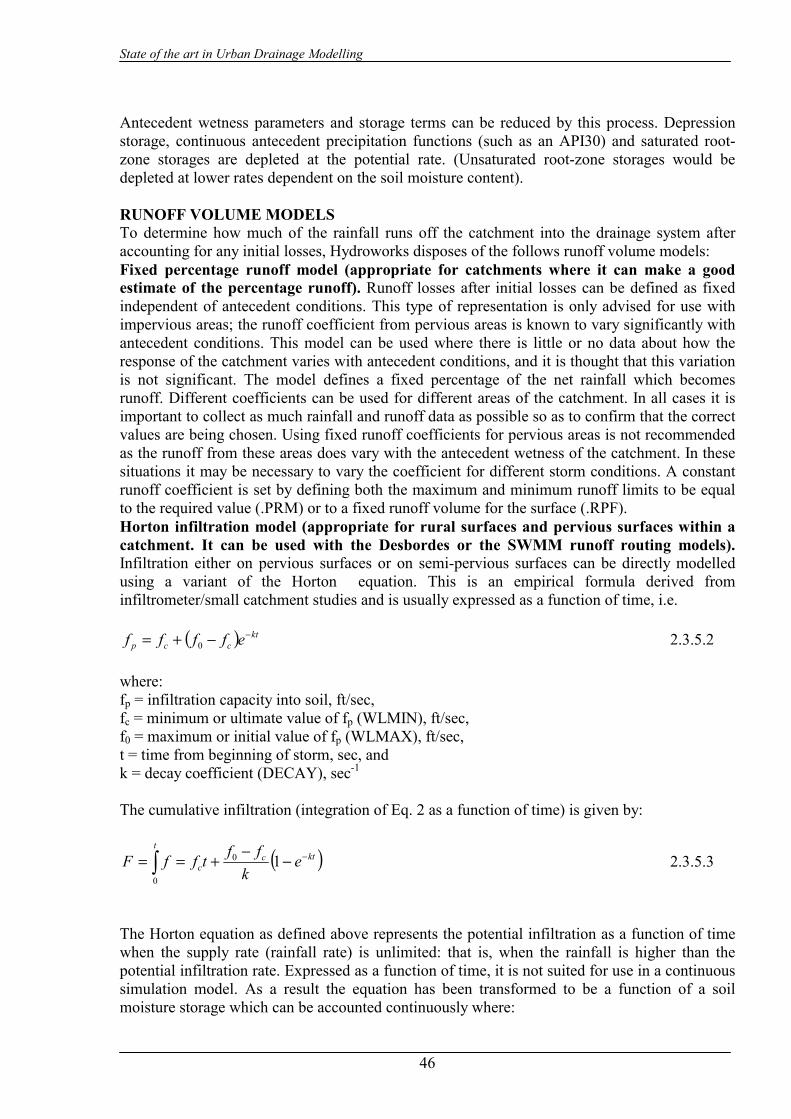
State of the art in Urban Drainage Modelling
46
Antecedent wetness parameters and storage terms can be reduced by this process. Depression storage, continuous antecedent precipitation functions (such as an API30) and saturated root-zone storages are depleted at the potential rate. (Unsaturated root-zone storages would be depleted at lower rates dependent on the soil moisture content). RUNOFF VOLUME MODELS To determine how much of the rainfall runs off the catchment into the drainage system after accounting for any initial losses, Hydroworks disposes of the follows runoff volume models: Fixed percentage runoff model (appropriate for catchments where it can make a good estimate of the percentage runoff). Runoff losses after initial losses can be defined as fixed independent of antecedent conditions. This type of representation is only advised for use with impervious areas; the runoff coefficient from pervious areas is known to vary significantly with antecedent conditions. This model can be used where there is little or no data about how the response of the catchment varies with antecedent conditions, and it is thought that this variation is not significant. The model defines a fixed percentage of the net rainfall which becomes runoff. Different coefficients can be used for different areas of the catchment. In all cases it is important to collect as much rainfall and runoff data as possible so as to confirm that the correct values are being chosen. Using fixed runoff coefficients for pervious areas is not recommended as the runoff from these areas does vary with the antecedent wetness of the catchment. In these situations it may be necessary to vary the coefficient for different storm conditions. A constant runoff coefficient is set by defining both the maximum and minimum runoff limits to be equal to the required value (.PRM) or to a fixed runoff volume for the surface (.RPF). Horton infiltration model (appropriate for rural surfaces and pervious surfaces within a catchment. It can be used with the Desbordes or the SWMM runoff routing models). Infiltration either on pervious surfaces or on semi-pervious surfaces can be directly modelled using a variant of the Horton equation. This is an empirical formula derived from infiltrometer/small catchment studies and is usually expressed as a function of time, i.e.
( ) ktccp effff −−+= 0 2.3.5.2
where: fp = infiltration capacity into soil, ft/sec, fc = minimum or ultimate value of fp (WLMIN), ft/sec, f0 = maximum or initial value of fp (WLMAX), ft/sec, t = time from beginning of storm, sec, and k = decay coefficient (DECAY), sec-1
The cumulative infiltration (integration of Eq. 2 as a function of time) is given by:
( )ktcc
t
ek
fftffF −−−+== ∫ 10
0
2.3.5.3
The Horton equation as defined above represents the potential infiltration as a function of time when the supply rate (rainfall rate) is unlimited: that is, when the rainfall is higher than the potential infiltration rate. Expressed as a function of time, it is not suited for use in a continuous simulation model. As a result the equation has been transformed to be a function of a soil moisture storage which can be accounted continuously where:
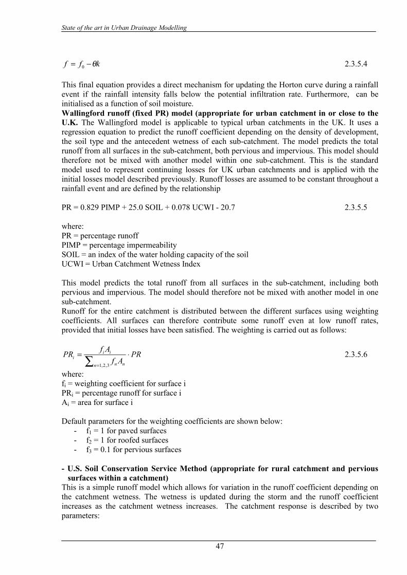
State of the art in Urban Drainage Modelling
47
kff θ−= 0 2.3.5.4
This final equation provides a direct mechanism for updating the Horton curve during a rainfall event if the rainfall intensity falls below the potential infiltration rate. Furthermore, can be initialised as a function of soil moisture. Wallingford runoff (fixed PR) model (appropriate for urban catchment in or close to the U.K. The Wallingford model is applicable to typical urban catchments in the UK. It uses a regression equation to predict the runoff coefficient depending on the density of development, the soil type and the antecedent wetness of each sub-catchment. The model predicts the total runoff from all surfaces in the sub-catchment, both pervious and impervious. This model should therefore not be mixed with another model within one sub-catchment. This is the standard model used to represent continuing losses for UK urban catchments and is applied with the initial losses model described previously. Runoff losses are assumed to be constant throughout a rainfall event and are defined by the relationship PR = 0.829 PIMP + 25.0 SOIL + 0.078 UCWI - 20.7 2.3.5.5 where: PR = percentage runoff PIMP = percentage impermeability SOIL = an index of the water holding capacity of the soil UCWI = Urban Catchment Wetness Index This model predicts the total runoff from all surfaces in the sub-catchment, including both pervious and impervious. The model should therefore not be mixed with another model in one sub-catchment. Runoff for the entire catchment is distributed between the different surfaces using weighting coefficients. All surfaces can therefore contribute some runoff even at low runoff rates, provided that initial losses have been satisfied. The weighting is carried out as follows:
PRAf
AfPRn nn
iii ⋅=
∑ = 3,2,1
2.3.5.6
where: fi = weighting coefficient for surface i PRi = percentage runoff for surface i Ai = area for surface i Default parameters for the weighting coefficients are shown below:
- f1 = 1 for paved surfaces - f2 = 1 for roofed surfaces - f3 = 0.1 for pervious surfaces
- U.S. Soil Conservation Service Method (appropriate for rural catchment and pervious
surfaces within a catchment) This is a simple runoff model which allows for variation in the runoff coefficient depending on the catchment wetness. The wetness is updated during the storm and the runoff coefficient increases as the catchment wetness increases. The catchment response is described by two parameters:
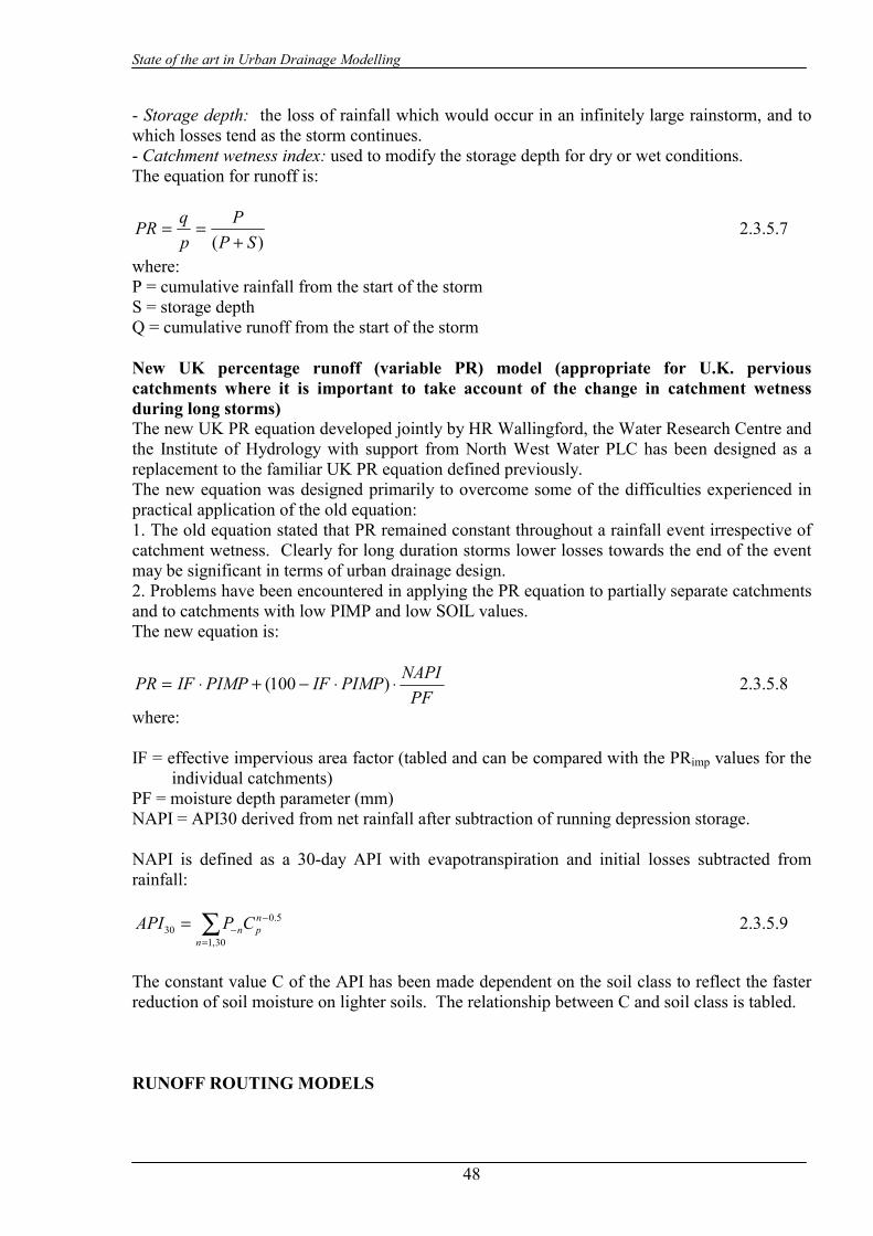
State of the art in Urban Drainage Modelling
48
- Storage depth: the loss of rainfall which would occur in an infinitely large rainstorm, and to which losses tend as the storm continues. - Catchment wetness index: used to modify the storage depth for dry or wet conditions. The equation for runoff is:
)( SPP
pqPR
+== 2.3.5.7
where: P = cumulative rainfall from the start of the storm S = storage depth Q = cumulative runoff from the start of the storm New UK percentage runoff (variable PR) model (appropriate for U.K. pervious catchments where it is important to take account of the change in catchment wetness during long storms) The new UK PR equation developed jointly by HR Wallingford, the Water Research Centre and the Institute of Hydrology with support from North West Water PLC has been designed as a replacement to the familiar UK PR equation defined previously. The new equation was designed primarily to overcome some of the difficulties experienced in practical application of the old equation: 1. The old equation stated that PR remained constant throughout a rainfall event irrespective of catchment wetness. Clearly for long duration storms lower losses towards the end of the event may be significant in terms of urban drainage design. 2. Problems have been encountered in applying the PR equation to partially separate catchments and to catchments with low PIMP and low SOIL values. The new equation is:
PFNAPIPIMPIFPIMPIFPR ⋅⋅−+⋅= )100( 2.3.5.8
where: IF = effective impervious area factor (tabled and can be compared with the PRimp values for the
individual catchments) PF = moisture depth parameter (mm) NAPI = API30 derived from net rainfall after subtraction of running depression storage.
NAPI is defined as a 30-day API with evapotranspiration and initial losses subtracted from rainfall:
∑=
−−=
30,1
5.030
n
npnCPAPI 2.3.5.9
The constant value C of the API has been made dependent on the soil class to reflect the faster reduction of soil moisture on lighter soils. The relationship between C and soil class is tabled. RUNOFF ROUTING MODELS

State of the art in Urban Drainage Modelling
49
The overland flow of the runoff into the drainage system can be modelled separately for each type of surface by the followed routing models: Wallingford (appropriate for U.K. drainage systems where most sub-catchments are under 1 ha). The flow is routed using two equal linear reservoirs in series, whose routing coefficient depends on rainfall intensity, contributing area and surface slope. Two reservoirs are applied in series for each surface type with an equivalent storage-output relationship for each reservoir. This relationship is given by:
kqS = 2.3.5.10 where: k = C i* -0.39 i*=0.5(1+i10) i10= running ten minute average of rainfall intensity. Combination of the two storage relationships with the continuity equation leads to a second-order ordinary differential equation of the form:
niqdtdqk
dtqdk =++ 22
22 2.3.5.11
This form of model was in fact first proposed for use in the UK by Sarginson and Nussey. A relationship relating C value to catchment characteristics was then developed and included in the software; the final relationship is:
24.013.0117.0 ASC −= 2.3.5.12 where: S = slope (m/m) A = area (m2)
Large Catchment (appropriate for U.K. systems where most sub-catchments are larger than 1 ha). The flow is routed using two equal linear reservoirs in series, whose routing coefficient depends on rainfall intensity, contributing area, and surface slope as in the Wallingford model. The software also applies a timestep lag and routing factor multiplier. The routing multiplier and timestep lag are functions of sub-catchment area, ground slope and catchment length as follows respectively:
321 kkkk LsACK = 2.3.5.13
where: K = routing factor multiplier A = subcatchment area (m2) s = slope (m/m) L = length (m) Ck, k1, k2 and k3 are equation coefficients. The default values are: - Ck = 0.030 - k1 = - 0.022
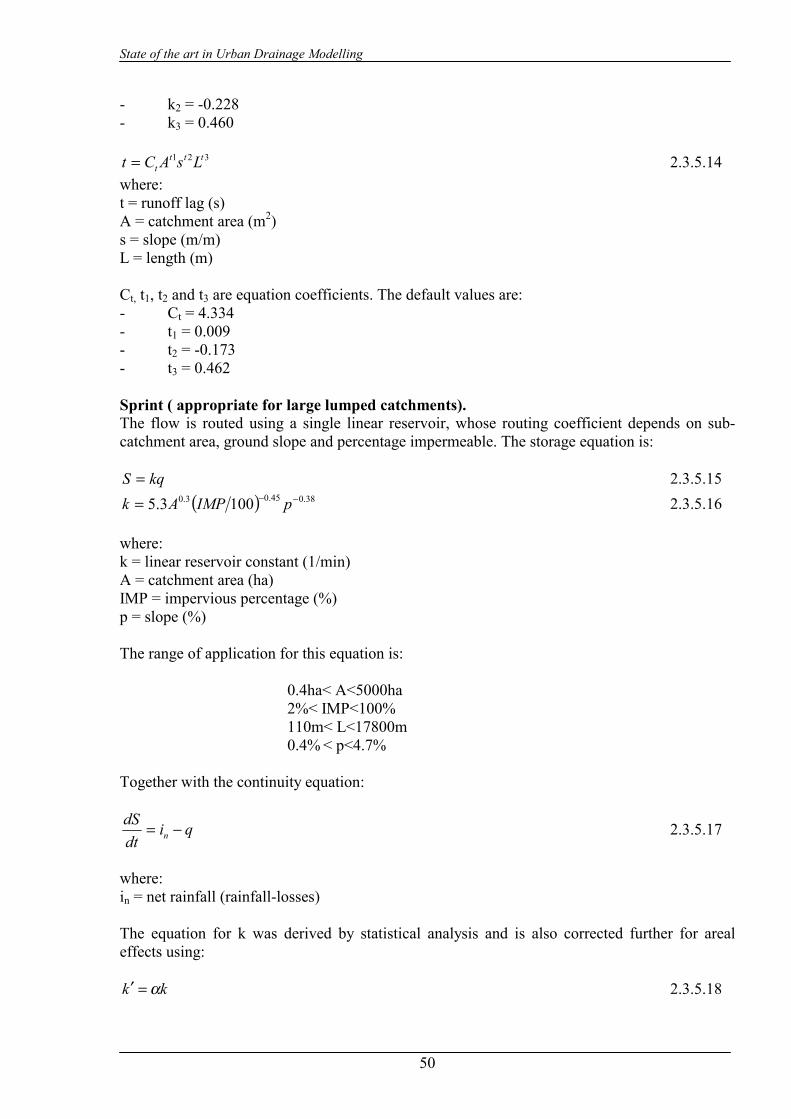
State of the art in Urban Drainage Modelling
50
- k2 = -0.228 - k3 = 0.460
321 tttt LsACt = 2.3.5.14
where: t = runoff lag (s) A = catchment area (m2) s = slope (m/m) L = length (m) Ct, t1, t2 and t3 are equation coefficients. The default values are: - Ct = 4.334 - t1 = 0.009 - t2 = -0.173 - t3 = 0.462 Sprint ( appropriate for large lumped catchments). The flow is routed using a single linear reservoir, whose routing coefficient depends on sub-catchment area, ground slope and percentage impermeable. The storage equation is:
kqS = 2.3.5.15 ( ) 38.045.03.0 1003.5 −−= pIMPAk 2.3.5.16
where: k = linear reservoir constant (1/min) A = catchment area (ha) IMP = impervious percentage (%) p = slope (%) The range of application for this equation is: 0.4ha< A<5000ha 2%< IMP<100% 110m< L<17800m 0.4% < p<4.7% Together with the continuity equation:
qidtdS
n −= 2.3.5.17
where: in = net rainfall (rainfall-losses) The equation for k was derived by statistical analysis and is also corrected further for areal effects using:
kk α=′ 2.3.5.18

State of the art in Urban Drainage Modelling
51
where: α = 0.8 (A<6 ha) α = 0.7 A0.09 (6 ha < A < 250 ha) Desbordes (appropriate for French systems running with event based simulations. Can be used for continuous simulation if it specified sub-events to define storm in the rainfall data “.RED” file). The flow is routed using a single linear reservoir, whose routing coefficient depends on sub-catchment area, ground slope, percentage impermeable, catchment length, storm duration and storm depth. The software assumes that the flow at the catchment outlet is proportional to the volume of storm-water present on that catchment (note that the term catchment here means the ground surface and the non-explicitly modelled network that contributes stormwater to that point of the urban drainage system). The basic equation is : S(t) = K Q(t) 2.3.5.19 Where: S(t) = volume of storm-water stored on the catchment (m3) at a point in time. Q(t) = discharge at the catchment outlet (m3/s) at a point in time. K = linear reservoir coefficient (s). The software calculates this from the catchment and the rainfall data. To take into account the effects of depression storage and other initial losses, the first millimetre(s) of rainfall may not contribute to the runoff. The software models depression storage in the same way as for the other runoff models. The process for initialising the parameters for the Desbordes runoff calculations is as follows: 1 - Determine the total effective rainfall:
Hpe = (Hper - Hrn) / 1000 2.3.5.20
where: Hpe = total accumulated effective rainfall (m) Hper = total rainfall (cumulated) (mm) calculated from the rainfall event. Hrn = the initial losses (mm). The software determines this from the depression storage and antecedent rainfall.
2 - Determine the calibrated coefficient: Kdesb = 50.0
This value was determined from calibrated data.
3 - Determine the linear reservoir coefficient:
( ) 07.015.021.03
9.136.018.0 1 −−− ⋅⋅⋅+⋅⋅⋅= pentrdesb HLTCPAKK 2.3.5.21
where: Ar = subcatchment area (ha) Pnt = subcatchment slope (%)

State of the art in Urban Drainage Modelling
52
C = the proportion of subcatchment area that is permeable (0 – 1) T3 = duration of the rainfall subevent (s) L = subcatchment length (m).
4 - Calculate the initial discharge coefficient:
( )40 10)0( ⋅⋅= rACQq 2.3.5.22
where: Q0 = initial discharge (m3/s). q(0) is zero unless starting from a saved hydrology state file. q(0) = initial discharge per unit of active surface (m/s). The process for calculating runoff using the Desbordes model is as follows: For each timestep: 1 - Runoff discharge per active surface unit:
( )dttieetqdttq kdt
kdt
+⋅
−+⋅=+
−−1)()( 2.3.5.23
where: d(t) = run timestep (s) q(t) = discharge per unit of active surface (m/s) K = linear reservoir coefficient (1/s) i = effective rainfall intensity (m/s). 2 - Runoff discharge
( ) ( ) 1000⋅+⋅⋅=+ dttqACdttQ r 2.3.5.24 where: Q = total discharge (m3/s) C = proportion impermeable catchment area (0...1) Ar = catchment area (ha) SWMM (appropriate for U.S.A. drainage systems using the SWMM runoff model in conjunction with the Horton or Green-Ampt runoff volume models for the pervious surface). SWMM is the Storm Water Management Model developed for the U.S. Environment Protection Agency. HydroWorks incorporates some of the features of the SWMM runoff block. The flow is routed using a single non-linear reservoir, whose routing coefficient depends on surface roughness, surface area, ground slope and catchment width. It can modelled the following features in this version of the software:
- Initial losses (depression storage) - Constant evaporation - Horton infiltration on pervious surfaces - Green-Ampt infiltration on pervious surfaces - SWMM non-linear routing
This version of HydroWorks does not model the following features:
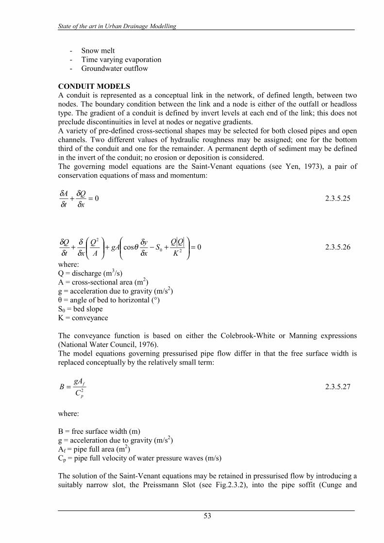
State of the art in Urban Drainage Modelling
53
- Snow melt - Time varying evaporation - Groundwater outflow
CONDUIT MODELS A conduit is represented as a conceptual link in the network, of defined length, between two nodes. The boundary condition between the link and a node is either of the outfall or headloss type. The gradient of a conduit is defined by invert levels at each end of the link; this does not preclude discontinuities in level at nodes or negative gradients. A variety of pre-defined cross-sectional shapes may be selected for both closed pipes and open channels. Two different values of hydraulic roughness may be assigned; one for the bottom third of the conduit and one for the remainder. A permanent depth of sediment may be defined in the invert of the conduit; no erosion or deposition is considered. The governing model equations are the Saint-Venant equations (see Yen, 1973), a pair of conservation equations of mass and momentum:
0=+xQ
tA
δδ
δδ 2.3.5.25
0cos 20
2
=
+−+
+
KQQ
SxygA
AQ
xtQ
δδθ
δδ
δδ 2.3.5.26
where: Q = discharge (m3/s) A = cross-sectional area (m2) g = acceleration due to gravity (m/s2) θ = angle of bed to horizontal (°) S0 = bed slope K = conveyance The conveyance function is based on either the Colebrook-White or Manning expressions (National Water Council, 1976). The model equations governing pressurised pipe flow differ in that the free surface width is replaced conceptually by the relatively small term:
2p
f
CgA
B = 2.3.5.27
where: B = free surface width (m) g = acceleration due to gravity (m/s2) Af = pipe full area (m2) Cp = pipe full velocity of water pressure waves (m/s) The solution of the Saint-Venant equations may be retained in pressurised flow by introducing a suitably narrow slot, the Preissmann Slot (see Fig.2.3.2), into the pipe soffit (Cunge and
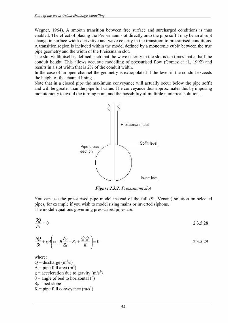
State of the art in Urban Drainage Modelling
54
Wegner, 1964). A smooth transition between free surface and surcharged conditions is thus enabled. The effect of placing the Preissmann slot directly onto the pipe soffit may be an abrupt change in surface width derivative and wave celerity in the transition to pressurised conditions. A transition region is included within the model defined by a monotonic cubic between the true pipe geometry and the width of the Preissmann slot. The slot width itself is defined such that the wave celerity in the slot is ten times that at half the conduit height. This allows accurate modelling of pressurised flow (Gomez et al., 1992) and results in a slot width that is 2% of the conduit width. In the case of an open channel the geometry is extrapolated if the level in the conduit exceeds the height of the channel lining. Note that in a closed pipe the maximum conveyance will actually occur below the pipe soffit and will be greater than the pipe full value. The conveyance thus approximates this by imposing monotonicity to avoid the turning point and the possibility of multiple numerical solutions.
Figure 2.3.2: Preissmann slot
You can use the pressurised pipe model instead of the full (St. Venant) solution on selected pipes, for example if you wish to model rising mains or inverted siphons. The model equations governing pressurised pipes are:
0=xQ
δδ 2.3.5.28
0cos 0 =
+−+
KQQ
SxygA
tQ
δδθ
δδ 2.3.5.29
where: Q = discharge (m3/s) A = pipe full area (m2) g = acceleration due to gravity (m/s2) θ = angle of bed to horizontal (°) S0 = bed slope K = pipe full conveyance (m/s2)

State of the art in Urban Drainage Modelling
55
The pressurised pipe model more accurately predicts velocities and storage than the full (St. Venant) model because it does not assign base flow or a Priessmann slot to a pipe. Each conduit is discretised by N computational points regularly spaced at an interval of 20 times the conduit diameter. The Preissmann 4-point scheme (Preissmann, 1961) is used to approximate the Saint-Venant equations, in which functions and derivatives are replaced by weighted averages over the four corners of a box in (x,t) space:
( ) ( )( )ni
ni
ni
ni fffff +−++= +
+++ 1
111 2
12
θθ 2.3.5.30
( ) ( )( )ni
ni
ni
ni ff
xff
xxf −
∆−+−
∆=
∂∂
+++
+ 111
11 θθ 2.3.5.31
( )ni
ni
ni
ni ffff
ttf −−+
∆=
∂∂
+++
+ 111
121 2.3.5.32
where fi
n denotes f(i∆x, n∆t). The implicit nature of the scheme removes any restrictions on the timestep, by the CFL condition (Courant et al, 1928) on entering the Preissmann slot and results in a range of unconditional stability that may be defined in terms of the time weighting parameter, namely θ ≥ 1/2. In practice a value of θ = 0.65 is used throughout a time varying simulation, thus introducing a small degree of numerical diffusion (Cunge et al., 1980). Each pair of adjacent points in a conduit is linked by the discrete form of the St Venant equations, resulting in 2N-2 equations available to describe the flow state. In the case of a control link the two computational points allocated are linked by the prescribed head-discharge relationship. The local equation system for a link is completed by specifying a boundary condition at each end, of the general form:
( ) 0,, == lii YyQf 2.3.5.33 relating discharge Qi and level yi to the level in the incident node Yl. The equation system is completed by the continuity equation to be satisfied at each internal node:
dtdYAQQ I
IjjI =∂+ ∑ 2.3.5.34
This is approximated by the implicit Euler Method. The discretisation of the governing equations in the conduits, at the conduit boundaries, at the control structures and in the nodes results in a large system of algebraic non-linear finite difference equations to be solved simultaneously at each time level. The stability of the calculations, particularly in the transition between pressurised and free surface flow, is ensured using the iterative Newton-Raphson method. In the Newton-Raphson Method this system for the dependant variables at the new time level must be linearised

State of the art in Urban Drainage Modelling
56
resulting in a large matrix system. A double sweep method is employed (see Liggett and Cunge, 1975 and Richens, 1985) to reduce the matrix by local elimination of computational nodes along the links between nodes.
2.3.6. Model Parameters Estimation or Assignation Not available in HydroWorks
2.3.7. PI(s) Estimation Method Not available in HydroWorks
2.3.8. Future Improvements of the Model HydroWorks/InfoWorks is constantly updated by HR Wallingford Software. The last update was release in December 2002. There are no current plans to develop a new version in the near future
2.3.9. References
2.3.9.1 Theoretical Framework References Biwater Limited, 1988 - BS3680, Methods of measurement of liquid flow in open channels, Part 4A. Thin plate weirs, 1981 Cunge JA, Holly Jr FM and Verwey A. Practical Aspects of Computational River Hydraulics, Pitman, London, 1980 Gomez et al. Hydraulic Engineering Software IV, Fliud Flow Modelling, 1992 Hydraulics Research Ltd. The Wallingford Procedure: Design and analysis of urban storm drainage. Volume 1: Principles, methods and practice,1983 Richens, P J, Development of an accurate simulation model for urban storm sewers, Report No IT297, DoE Contract PEDC 7/7/053, HR Wallingford Ltd, 1985. M. Zug, G. Magne, J.P. Tabuchi, B. Tisserand (August 1999) Development of a methodology for the definition of the exceptional event regarding to the sewerage system., Proceedings of 8th International Conference on Urban Storm Drainage, Sydney, Australia, pp.1639-1647 Mambretti, S. and Paoletti, A. (Sept. 1996) A New Approach in Overland Flow Simulation in Urban Catchments, Proceedings of 7th International Conference on Urban Storm Drainage, Hannover, Germany, pp. 965-970. Salway, A., Ahmad, K. and Collingham, S. (Sept. 1996) Safe-DIS: Computer Programs for the safe Design and Analysis of Urban Drainage Networks, Proceedings of 7th International Conference on Urban Storm Drainage, Hannover, Germany, pp. 1575-1580 Isao IDETA and K KARIYA (August 1999) Drainage improvement plan using runoff hydraulic simulation software., Proceedings of 8th International Conference on Urban Storm Drainage, Sydney, Australia, pp.64-71
2.3.9.2 Practical Use and Results References Y Shinoda, T Hasegawa and S Fujiura (August 1999) Application of the overseas urban storm drainage simulation models to Japan, Proceedings of 8th International Conference on Urban Storm Drainage, Sydney, Australia, pp.1784-1792 Ichikawa, A. and Hijioka, Y. (Sept. 1996) A Study on the Possibilities of the Application of the HydroWorks into Japanese Drainage System, Proceedings of 7th International Conference on Urban Storm Drainage, Hannover, Germany, pp. 1341-1346

State of the art in Urban Drainage Modelling
57
2.4 MOUSE – Modelling of urban sewers
2.4.1. Model availability MOUSE model is produced by DHI Water & Environment; it is a commercial model and the source code is not available. In fact, MOUSE is proprietary software and the system is therefore protected against illegal use. The protection system consists of a hardware key (dongle) and the ‘DhiLicense.dat’ file. The software can normally function only if a correct combination of the two components has been provided. The dongle has to be connected to the computer at a parallel port, and the ‘DhiLicense.dat’ file must be placed in the ‘Windows/System’ directory. Without a valid license, MOUSE functions as Demo software, which allows editing a small network. On-line help for the use of MOUSE is available for most of the functions in the MOUSE graphical user interface at the MOUSE’s web-site http://www.dhi.dk/mouse. A standard, Windows-type help facility is accessed through the “Help | Index” Main menu option.
2.4.2. Abstract
2.4.2.1 Objectives and peculiarities MOUSE is a surface runoff, open channel flow, pipe flow, water quality and sediment transport modelling package for urban drainage systems, storm water sewers and sanitary sewers. MOUSE combines complex hydrology, hydraulics, water quality and sediment transport in a completely graphical, easy-to-use interface. MOUSE is a 32-bit Windows application specifically designed to operate within Microsoft Windows® and Windows NT®, and is optimized for fast simulations and graphics. Both metric (SI) and imperial units are supported. Typical applications of MOUSE include studies of combined sewer overflows (CSO), sanitary sewer overflows (SSO), complex RTC schemes development and analysis, design of new site developments, regulatory consenting procedures and analysis & diagnosis of existing storm water and sanitary sewer systems. By applying MOUSE, it is possible known, such as:
• the return periods for overloading of various parts of the existing sewer system; • the main causes of that overloading - backwater or insufficient local pipe capacity; • the implications of replacing critical sewers, installing new basins, weirs, etc; • how is the long-term environmental impact affected by changing the operational
strategy; • where and why are sediments deposited in the sewer network; • the peak concentrations of pollutants at the overflow weir or at the treatment plant after
a rainstorm.
2.4.2.2 Performance Indicator(s) of Interest The following performance indicators can be evaluated using the output data from MOUSE: wEn3, wEn4, wEn5, wPh5, wPh6, wPh7, wOp29, wOp30, wOp35 (with symbols explained in Appendix). The model does not compute PIs directly but can the model output can be used to evaluate them.

State of the art in Urban Drainage Modelling
58
2.4.3. Usage Specifications
2.4.3.1 Programming Language(s) or Mathematical-Statistical Software(s) The source code is not available as well as information about its development.
2.4.3.2 Functionality The MOUSE system, as quantity model, is organized in several modules:
• MOUSE Runoff: surface runoff models for urban catchment applications; • MOUSE RDII: advanced hydrological model for continuous simulation; • MOUSE HD: hydrodynamic network model with some limited RTC capabilities; • MOUSE RTC: advanced reactive RTC capabilities for MOUSE pipe models; • MOUSE T: long-term hydraulic simulations with statistics;
MOUSE is a comprehensive surface runoff, open channel flow, pipe flow modeling package for urban drainage systems, storm water sewers and sanitary sewers. The MOUSE Surface Runoff Module includes three types of surface runoff computation: Model A - Time/area Method, Model B - Non-linear Reservoir (kinematic wave) Method, Model C - Linear Resevoir Method, in two sub-variants: Model C1 - Dutch runoff model Model C2 - French runoff model Surface runoff computations in MOUSE can be based on any of the three concepts, provided that the necessary data have been specified. The runoff model data and model parameters are organised in the following clusters:
• General catchment data; • Model-specific catchment data; • Model parameters.
The general catchment data are independent of the choice of the runoff model. They include basic information about catchment´s size, connection point to the network, geographical position (co-ordinates) and specification of additional, constant inflow. The model-specific catchment data comprise different sets for each of the models. These data basically provide further information about the catchments' geometry and a more or less detailed land use description. Reference to a specific parameter set is also a part of this group. Model parameters are organised in parameter sets. A parameter set is comprised of all editable parameters needed to execute certain type of runoff computation. Surface runoff computation for an individual catchment is based on the parameters contained in the set associated with the catchment. Initially, MOUSE provides a "DEFAULT" parameter set for each of the models. User can create an arbitrary number of parameter sets under user-specified names. Some parameters (for model A all parameters) from the parameter set currently associated with certain catchment can be individually edited as "Individual data", so that the edits are applied only for the individual catchment. The computed hydrographs are used as input to the MOUSE Pipe Flow model. The MOUSE Rainfall Dependent Inflow & Infiltration Module (RDII) provides detailed, continuous modeling of the complete land phase of the hydrologic cycle, providing support for urban, rural, and mixed catchments analyses. Precipitation is routed through four different types of storage: snow, surface, root zone and ground water, resulting in more accurate hydrographs. Instead of performing hydrological load
State of the art in Urban Drainage Modelling
59
analysis of the sewer system only for short periods of high intensity rainstorms, a continuous, long-term analysis can be used to look at periods of both wet and dry weather, as well as inflows and infiltration to the sewer network. This provides a more accurate picture of actual loads on treatment plants and combined sewer overflows. Further enhancements of groundwater-sewer interactions are possible by linking the MOUSE Pipe model with DHI’s distributed groundwater model MIKE SHE. The MOUSE Hydrodynamic Pipe Flow Model (HD) solves the complete St. Venant (dynamic flow) equations throughout the drainage network (looped and dendritic), which allows for modelling of backwater effects, flow reversal, surcharging in manholes, free-surface and pressure flow, tidal outfalls and storage basins. The program has been designed to handle any type of pipe network system with alternating free surface and pressurised flows as well as open channel network. Pressurised flow computations are facilitated through implementation of a narrow 'slot' ( Preissmann), as a vertical extension of a closed pipe cross section. Free surface and pressurised flows are thus described within the same basic algorithm, which ensures a smooth and stable transition between the two flow types. The computational scheme uses an implicit, finite-difference numerical solution of the St. Venant flow equations. In addition to fully dynamic description, simplified flow descriptions are available( Diffusive and Kinematic wave). The numerical algorithm uses a self-adapting time-step, which provides efficient, accurate and stable solutions in multiple connected branched and looped pipe networks and in the same time minimized the total computational effort. MOUSE includes, in fact, two different concepts for optimising the simulation time step:
• The user-specified pre-defined time step variation, specified as a time series; • The automated self-adaptive time step variation, controlled by the actual hydraulic and
operational conditions within the entire model area throughout the numerical simulation. Both of these concepts can be applied in connection with the Dynamic and Diffusive flow descriptions while they cannot be used with the Kinematic flow description. This computational scheme is applicable to unsteady flow conditions that occur in pipes ranging from small-profile collectors for detailed urban drainage, to low-lying, often pressurised, sewer mains affected by MOUSE varying outlet water levels. Both sub-critical and supercritical flows are treated by means of the same computational scheme that adapts to the local flow conditions. In addition, flow phenomena, such as backwater effects and surcharges, are precisely simulated. Within the Pipe Flow Model, advanced computational formulations enable description of a variety of pipe network elements and flow phenomena:
• flexible cross-section database, including standard shapes; • circular manholes; • detention basins; • overflow weirs; • pump operation; • flow regulation; • non-return valve; • constant or time variable outlet water level; • constant or time variable inflows into the sewer network; • head losses at manholes and basins; • depth-variable friction coefficients.
The MOUSE Real-Time Control (RTC) Module allows real-time control devices to be included in defining the urban drainage sewer network model. A selection of controllable devices is provided, along with a fully generic specification of control rules for any simple or complex
State of the art in Urban Drainage Modelling
60
reactive control scheme. The system allows the application of setting, set point (PID controller) or time-dependent control functions, with decisions based on a global system analysis. The MOUSE LTS Module allows that a MOUSE network with intermittent hydrological inputs can be set-up for a long-term simulation, covering a continuous historical period, possibly over several years. The system automatically combines dynamic pipe flow simulations during wet weather and simple hydrological simulation during dry weather periods, which results in accurate computation of wastewater treatment plant loads, CSOs and other system outputs, while preserving rationality in use of computational resources. The results are presented both in the form of time series and a range of statistical parameters for selected variables. By running simulations with the current system configuration and the planned upgrade, impacts of the planned investments (e.g. new sewers, retention tanks, RTC schemes) on the system performance can be tested. This allows the user to develop the optimal rehabilitation / upgrade strategy, e.g. for achieving the consent with the environmental regulators requirements.
2.4.3.3 Possible interaction with other software tools MOUSE utilizes a fully featured presentation tool MIKE View that can be accessed directly from MOUSE under the main menu option .Project | MIKE View. or by the .Mike View. toolbar button. The MIKE View result presentation program MIKE View is also available as an inexpensive stand-alone, multimedia-reporting tool. This allows users to include digital versions of MOUSE simulation result files, together with MIKE View, in combination with written reports and project documentation. The most important MIKE View features are:
• Results can be viewed on user configurable plan drawings, longitudinal pipe sections and as time series in graphical and tabular views;
• All results can be animated, and windows with different animations can be synchronised. For instance it is quite easy to compare the results of two or more simulations with this capability;
• More result files can be accessed and viewed simultaneously - including files from MOUSE , SWMM and MIKE 11;
• Flooding (water depths and pressure heights) can be shown and animated in the plan drawing;
• DXF, TIF and BMP files (such as CAD drawings, ortho-photos, and scanned maps) can be imported and used as background graphics;
• Elements of time series analysis (duration curves) and error estimations are included into the program;
• Full support for viewing the event- and annual based statistical data in connection with long-term simulations;
• Simulation results can be copied via the Windows Clipboard to spreadsheets and other applications for reporting;
• Individual Windows layouts or entire session layouts can be saved and reused.
The utility program MIKE Print is used for generating customized graphical reports for printing. It can be used both for reporting the results and for documenting the model. The program can be activated directly from MOUSE under the main menu option .Project | MIKE Print. or by the “Mike Print” toolbar button. MIKE Animator produces 3D animations in a number of industry standard file formats, such as *.mpg, *.avi, *.flc and separate frames in freely configurable resolutions. MIKE Animator

State of the art in Urban Drainage Modelling
61
works on result data from the DHI Software products MIKE 21 and MIKE 11. Additional products will be included in the subsequent releases of MIKE Animator. MOUSE GIS is an ArcView based application for MOUSE users. Through MOUSE GIS, MOUSE users obtain a new level of integration with GIS databases and with any inventory and asset management system that supports ODBC. Experience shows that MOUSE GIS can save enormous amounts of time in the tedious procedure of setting-up and quality-checking model networks. MOUSE GIS is available as a low-cost add-on to MOUSE. The most important MOUSE GIS features are:
• Import of sewer and drainage system data from a wide range of standard formats and automatic conversion to the MOUSE formats;
• Powerful network and catchment’s data simplification and management routines; • Presentation of simulation results;
Audit track facilities for quality checking of model building procedures. Use of MOUSE GIS requires a valid Arc View run-time license.
2.4.4. Input and Output procedures
2.4.4.1 Possible Input File(s) Formats MOUSE logically systematizes input data into a number of groups, which reflect their character. Correspondingly, MOUSE stores the input data in a number of data files. The individual MOUSE files are distinguished by file names, and the type of file is recognised by a default extension. Most of the MOUSE files have special binary formats. The MOUSE data files are:
• NETWORK DATA for the description of the drainage system network (*.SWF) • HYDRAULIC DATA describing the Q-H relations in outlets, Manning numbers for
pipes, node outlet head losses, flow regulation, etc. (*.PWF) • BOUNDARY DATA describing the boundary time series, e.g. rain intensities, water
levels, discharges, temperatures, etc, which the user wants to enter the system as input for the computation (*.BSF)
• REPETITIVE PROFILE DATA including the non-dimensional repetitive profiles, e.g. for the definition of a temporal dry weather variation (*.RPF)
• HYDROLOGICAL AND CATCHMENT DATA describing catchments and parameters such as run-off coefficient and hydrological losses (*.HGF)
• DRY WEATHER FLOW DATA including the quantification of dry weather loads (*DWF)
• MOUSE T DATA including the data relevant for the definition of a long-term discontinuous simulation (*.MTF).
In some instances, for rarely used features and/or when new MOUSE developments have been implemented on a computational level, but are still not included in the MOUSE User Interface, specification of the relevant data is handled through the ADDITIONAL PARAMETER file (*.ADP). MOUSE uses a robust, Microsoft compliant ODBC database tool for storing and manipulating network data. These features give access to a range of powerful query facilities, including a QBE (query by example) option to select e.g. those pipes having a specific diameter, shape, roughness, etc. and then make global changes to this selected data. Database query results can
State of the art in Urban Drainage Modelling
62
be displayed graphically (by highlighting the selected elements in the horizontal plan view), in tabular format, printed, or copied to other Windows applications using the Windows clipboard. Larger amounts of measured/calculated data related to the modeled system are maintained and organized in special files or directories - MOUSE databases. The databases are independent of the operating system, so boundary data can be transferred from one computer to another and used in different applications. The boundary database facility of MOUSE can also be used independently as a general hydrological database for urban catchments. In order to enable an easier data exchange with external applications, an export/import facility has been provided. This has enabled import and export the network data to/from ASCII formatted files. The ASCII file format used by MOUSE is known as the ”SVK19” format. This format was originally defined by the Danish Wastewater Committee. The original documentation is only available in Danish.
2.4.4.2 Possible Output File(s) Formats Standard results from a MOUSE network computation (flows, levels.) are stored in a *.PRF file. This file is located in the current work directory along with the input files. Optionally, a 'reduced' result file can be generated, containing only selected time series, i.e. reducing the size of the result file dramatically. This is often relevant in connection with large models and/or long simulations. In connection with MOUSE T simulations, a statistics result file can optionally be generated. The contents of this file (both in terms of the saved variables and statistical parameters) is fully user-configurable. Further, an additional result file with (extension *.XRF) can optionally be generated during a pipe flow simulation. The *.XRF file contains information on: flow velocity , Froude numbers, time step, volume in pipes, volume in nodes. The MOUSE Runoff result files include:
• *CRF _ MOUSE catchment’s results; • *NOF _ MOUSE detailed RDII result file.
The *.CRF files contain the computed runoff time series, in case of an RDII simulation separately containing SRC and FRC component (as well as the total runoff). The *.NOF result files contain details of a RDII simulation. In fact, two result files are generated by a MOUSE RDII calculation. These are: • *.CRF file, containing maximally five time series for each subcatchment, namely:
- discharge, calculated with the Surface Runoff Model (the FRC component), - discharge, calculated with the RDII model (the SRC component), - total discharge, - variation of water content in the surface storage for the Surface Runoff Model, - variation of water content in the snow storage for the Surface Runoff Model.
The *.CRF file is used as input data for a MOUSE Pipe calculation. • *.NOF file (optional), containing detailed information about the processes treated by a RDII
model, e.g.: - different flow components in the RDII model, - variation of water content in the different storage in the RDII model.
The *.NOF file is used for calibration of the SRC component. In the *.CRF file the time series are saved with two various intervals, the shorter one for the periods when the Surface Runoff Model is used, and a larger one in the remaining periods. In the two other result files the time series are saved with the larger time interval which is equal to the time step used for the RDII calculation.
State of the art in Urban Drainage Modelling
63
MOUSE LTS provides the possibility to generate a series of useful statistical results - events, annual and system statistics - related to the simulated period. Such statistical results are stored in an optional statistical result file (*.ERF).
2.4.4.3 Raw Data Formatting MOUSE uses a robust, Microsoft compliant ODBC database tool for storing and manipulating network data. In order to enable an easier data exchange with external applications, an export/import facility has been provided. This has enabled import and export the network data to/from ASCII formatted files. The ASCII file format used by MOUSE is known as the ”SVK19” format.
2.4.5. Theoretical framework Overview Three different surface runoff computation concepts are available in MOUSE as three different runoff models: Model A - Time/area Method, Model B - Non-linear Reservoir (kinematic wave) Method, Model C - Linear Resevoir Method, in two sub-variants: Model C1 - Dutch runoff model Model C2 - French runoff model Surface runoff computations in MOUSE can be based on any of the three concepts, provided that the necessary data have been specified. However, in one simulation run it is not possible to combine different runoff computation concepts for various model areas. Runoff computed by any of the three surface runoff models can be complemented by a continuous runoff component, i.e. rainfall induced infiltration can be added to the computed surface runoff hydrographs as the catchment´s "base flow". This option is available only with a valid MOUSE RDII license. The concept of surface runoff computation of MOUSE Runoff Model A is founded on the so-called "Time-Area" method. The runoff amount is controlled by the initial loss, size of the contributing area and by a continuous hydrological loss. The shape of the runoff hydrograph is controlled by the concentration time tc and by the time-area (T-A) curve. These two parameters represent a conceptual description of the catchment reaction speed and the catchment shape. The continuous runoff process is discretized in time by the computational time step t∆ .The assumption of the constant runoff velocity implies the spatial discretization of the catchment’s surface to a number of cells in a form of concentric circles with a centre point at the point of outflow. The number of cells equals to:
ttn c
∆= 2.4.5.1
where: tc = concentration time;
t∆ = simulation time step. MOUSE calculates the area of each cell on the basis of the specified time-area curve. The total area of all cells is equal to the specified impervious area. A time-area curve characterises the shape of the catchment, relating the flow time i.e. concentric distance from the outflow point and the corresponding catchment sub-area. There are three pre-defined time/area curves available in MOUSE. Irregularly shaped catchments can be more precisely described by the user-specified T/A curves.
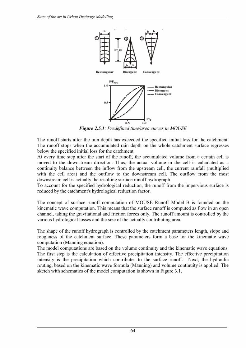
State of the art in Urban Drainage Modelling
64
Figure 2.5.1: Predefined time/area curves in MOUSE
The runoff starts after the rain depth has exceeded the specified initial loss for the catchment. The runoff stops when the accumulated rain depth on the whole catchment surface regresses below the specified initial loss for the catchment. At every time step after the start of the runoff, the accumulated volume from a certain cell is moved to the downstream direction. Thus, the actual volume in the cell is calculated as a continuity balance between the inflow from the upstream cell, the current rainfall (multiplied with the cell area) and the outflow to the downstream cell. The outflow from the most downstream cell is actually the resulting surface runoff hydrograph. To account for the specified hydrological reduction, the runoff from the impervious surface is reduced by the catchment's hydrological reduction factor. The concept of surface runoff computation of MOUSE Runoff Model B is founded on the kinematic wave computation. This means that the surface runoff is computed as flow in an open channel, taking the gravitational and friction forces only. The runoff amount is controlled by the various hydrological losses and the size of the actually contributing area. The shape of the runoff hydrograph is controlled by the catchment parameters length, slope and roughness of the catchment surface. These parameters form a base for the kinematic wave computation (Manning equation). The model computations are based on the volume continuity and the kinematic wave equations. The first step is the calculation of effective precipitation intensity. The effective precipitation intensity is the precipitation which contributes to the surface runoff. Next, the hydraulic routing, based on the kinematic wave formula (Manning) and volume continuity is applied. The sketch with schematics of the model computation is shown in Figure 3.1.

State of the art in Urban Drainage Modelling
65
Figure 2.5.2: The simulated processes in the Surface runoff model B
The simulated hydrologic processes account for various losses calculated - evaporation, wetting, infiltration and surface storage -according to the conventions and equations presented below. The remaining precipitation is called effective precipitation, defined generally as:
)()()()()()( tItItItItItI SIWEeff −−−−=
0)( ≥tI eff 2.4.5.2 where: I(t) = Actual precipitation at time t, IE(t) = Evaporation loss at time t. It should be noted that the evaporation loss for the catchment is accounted only if the RDII runoff computation is activated. IW(t) = Wetting loss at time t, II(t) = Infiltration loss at time t, IS(t) = Surface Storage loss at time t. The individual terms in the loss equation are fundamentally different, as some terms are continuous where others are discontinuous. If the calculated loss is negative, it is set to zero. The losses have a dimension of velocity [LT-1]. The actual precipitation, I(t), is assumed to be uniformly distributed over the individual catchments. Otherwise, it may vary as a random time function. The evaporation, IE(t), is a continuous loss that is normally of less significance for single event simulations. However, on a long-term basis, evaporation accounts for a significant part of hydrological losses. If included in the computation, the evaporation is the first part subtracted from the actual precipitation, according to the following:
=)()(
)(tItI
tI PEE for
for ( )( ))()(
)()(tItItItI
PE
PE
⟨≥
ANDOR ( )
( )0)(0)(
=⟩
tyty
2.4.5.3
where: I(t) = Actual precipitation at time t, IE(t) = Evaporation loss at time t. IPE(t) = Potential evaporation at time t, y(t) = Accumulated depth at time t.

State of the art in Urban Drainage Modelling
66
The wetting, IW(t), is a discontinuous loss. When the precipitation starts, a part of the precipitation is used for wetting of the surface if the surface is initially dry. The model assumes that the precipitation remaining after subtraction of the evaporation loss is used for wetting of the catchment surface. When the surface is wet, the wetting loss, IW, is set to zero. This is summarised in the following expression:
−
=0
)()()(
tItItI E
W forfor ( )
( ))()()()(
tItItyty
E
W
≤≥
OR ( )wyty ≥)( 2.4.5.4
where: I(t) = Actual precipitation at time t, IE(t) = Evaporation loss at time t. IW(t) = Wetting loss at time t, yW = Wetting depth, y(t) = Accumulated depth at time t. The infiltration, II(t), is the water loss to the lower storage caused by the porosity of the catchment surface. It is assumed that the infiltration starts when the wetting of the surface has been completed. The infiltration loss is calculated according to the following relations:
−−=0
)()()()(
)( tItItItI
tI WE
H
I
forforfor
))(()())()()((
))((
W
HWE
W
ytytItItItI
yty
⟨⟨−−
≥ AND )()()()( tItItItI HWE ≥−−
2.4.5.5 where: II(t) = Infiltration loss at time t. IH(t) = Horton's infiltration at time t (see below), yW = Wetting depth, y(t) = Accumulated depth at time t. The infiltration is a complex phenomenon, dependent on the soil porosity, moisture content, groundwater level, surface conditions, storage capacity, etc. The model calculates the infiltration loss capacity using the well-known Hortons's equation:
KatinaxinH eIIItI −⋅−+= )()( ImImIm 2.4.5.6
where: IH(t) = Infiltration loss calculated according to Horton IImax = Maximum infiltration capacity (after a long dry period), IImin = Minimum infiltration capacity (at full saturation), t = Time since the start of the reduction process, ka = Time factor (characteristic soil parameter) for wetting conditions. In the dry period following the rainfall, the infiltration capacity is gradually recovered to the initial value, using an inverse form of the Horton's equation:
KhtIaxITH eQIItI
T
/1Im )()( −⋅−+=
where:

State of the art in Urban Drainage Modelling
67
IH (t) = Infiltration loss capacity calculated according to Horton, IImax = Maximum infiltration capacity (after a long dry period), IIT = Infiltration capacity at the threshold between the wetting and drying period, t = Time since the start of the recovery process, kh = Time factor (characteristic soil parameter) for drying conditions. The surface storage. IS(t), is the loss due to filling the depressions and holes in the terrain. The model begins with the surface storage calculation after the wetting process is completed. The surface storage is filled only if the current infiltration rate is smaller than the actual precipitation intensity reduced by evaporation. The actual surface storage loss is calculated according to the following:
−−−
=0
)()()()()(
tItItItItI IWE
S forfor ( )
( ))()()()(
SW
SW
yytyyyty
+⟩+≤
2.4.5.7
where: I(t) = Precipitation intensity at time t, IS(t) = Surface storage loss at time t, II(t) = Infiltration loss at time t, IW(t) = Wetting loss at time t, IE(t) = Evaporation loss at time t, yW = Wetting depth, yS = Surface storage depth, y(t) = Accumulated depth at time t. The runoff starts when the effective precipitation intensity is larger than zero. The hydraulic process is described with the kinematic wave equations for the entire surface at once. This description assumes uniform flow conditions on the catchment surface, i.e. equal water depth over the entire surface of certain category. This type of runoff model is also called a non-linear reservoir model. The surface runoff at time t is calculated as:
3/52/1 )()( tyIBMtQ R⋅⋅⋅= 2.4.5.8 where: M = Manning's number, B = Flow channel width, computed as: B [m] = A [m2] / L [m] I = Surface slope, yR(t) = Runoff depth at time t. The depth yR(t) is determined from the continuity equation:
Adt
dytQAtI Reff ⋅=−⋅ )()( 2.4.5.9
where: Ieff = Effective precipitation,

State of the art in Urban Drainage Modelling
68
A = Contributing catchment surface area, dt = Timestep, dyR = Change in runoff depth. Surface Runoff Model B distinguishes between up to 5 different catchment surface types. This is practically handled by the model so that the individual catchment is split into up to five sub-catchments, each with the area according to the specified percentages for specific surface categories. For each surface type, only relevant processes are simulated. An overview of the processes associated with different surface types is shown in Table 2.5.1.
Table 2.5.1: Processes included for various types of catchment surface
The model treats every area with different surface category as a sub-catchment, and the runoff computations are performed individually. The total runoff from the entire catchment is obtained then as a sum of runoffs from up to five different sub-catchments. The length and width for each sub-catchment (sub-area) are calculated so that the length/width ratio for each sub-area is kept equal to the length/width ratio of the corresponding catchment. Based on the information for the whole catchment and the principle of constant length/width ratio, equivalent values of the runoff width and length are computed for all sub-areas, as illustrated in the example below (Figure 2.5.3).
Figure 2.5.3: Area distribution for a generic subcatchment

State of the art in Urban Drainage Modelling
69
The ratio between the catchment length and width in the given example corresponds to 1.33. 15% of the total area is impervious roof surface corresponding to 125 m2. Hence the runoff length is 12.9 m and the runoff width is 9.7 m for this surface type, as 12.9 * 9.7 = 125 and 9.7 * 1.33 = 12.9. The surface runoff computation of MOUSE Runoff Model C is founded on the routing of the runoff through a linear reservoir. This means that the surface runoff from a catchment is made proportional to the current water depth on the catchment. The implemented two versions of the model are equivalent to the surface runoff model used in the Netherlands (C1) and in France (C2). The runoff amount is controlled by the initial losses, size of the actually contributing area and by infiltration losses. The shape of the runoff hydrograph (phase and amplitude) is controlled by the catchment's time constant. The runoff model C computations are based on the volume continuity and the linear reservoir equations. The first step is the calculation of effective precipitation intensity. The effective precipitation intensity is the precipitation, which contributes to the surface runoff. Next, the hydraulic routing, based on the linear reservoir principle and volume continuity is applied. The hydrologic and hydraulic processes involved are shown in the diagram in Figure 2.5.4.
Figure 2.5.4: Processes simulated in Runoff model C
The simulated hydrologic processes account for the losses - evaporation, infiltration and surface storage - calculated according to the conventions and equations presented below. The remaining precipitation is called effective precipitation, defined generally as:
)()()()()( tItItItItI SIEeff −−−= 2.4.5.10 where: I(t) = Actual precipitation intensity at time t, IE(t) = Evaporation loss at time t. It should be noted that the evaporation loss for the catchment is accounted only if the RDII runoff computation is activated. IS(t) = Initial loss surface stoirageat time t, II(t) = Infiltration loss at time t. The individual terms in the loss equation are fundamentally different, as some terms are continuous where others are discontinuous. If the calculated loss is negative, it is set to zero. The losses have a dimension of velocity [LT-1]. The actual precipitation, I(t), is assumed to be uniformly distributed over the individual catchments. Otherwise, it may vary as a random time function.

State of the art in Urban Drainage Modelling
70
The evaporation, IE(t), is a continuous loss that is normally of less significance for single event simulations. However, on a long-term basis, evaporation accounts for a significant part of hydrological losses. If included in the computation, the evaporation is the first part subtracted from the actual precipitation, according to the following:
=)()(
)(tItI
tI PEE for
for ( )( ))()(
)()(tItItItI
PE
PE
⟨≥
ANDOR ( )
( )0)(0)(
=⟩
tyty
2.4.5.11
where: I(t) = Actual precipitation at time t, IE(t) = Evaporation loss at time t. IPE(t) = Potential evaporation at time t, y(t) = Accumulated depth at time t. The infiltration, II(t), is the water loss to the lower storage caused by the porosity of the catchment surface. It is assumed that the infiltration starts when the wetting of the surface has been completed. The infiltration loss is calculated according to the following relations:
−=0
)()()(
)( tItItI
tI E
H
I
forforfor
)()()()()()()()(
tItItItItItItItI
E
HE
HE
≤⟨−≥−
2.4.5.12
where: II(t) = Infiltration loss at time t. IH(t) = Horton's infiltration at time t (see below), y(t) = Accumulated depth at time t. The infiltration is a complex phenomenon, dependent on the soil porosity, moisture content, groundwater level, surface conditions, storage capacity, etc. The model calculates the infiltration loss capacity using the well-known Hortons's equation:
KatinaxinH eIIItI −⋅−+= )()( ImImIm 2.4.5.13
where: IH(t) = Infiltration loss calculated according to Horton IImax = Maximum infiltration capacity (after a long dry period), IImin = Minimum infiltration capacity (at full saturation), t = Time since the start of the reduction process, ka = Time factor (characteristic soil parameter) for wetting conditions. In the dry period following the rainfall, the infiltration capacity is gradually recovered to the initial value, using an inverse form of the Horton's equation:
KhtIaxITH eQIItI
T
/1Im )()( −⋅−+= 2.4.5.14
where: IH (t) = Infiltration loss capacity calculated according to Horton, IImax = Maximum infiltration capacity (after a long dry period), IIT = Infiltration capacity at the threshold between the wetting and drying period, t = Time since the start of the recovery process, kh = Time factor (characteristic soil parameter) for drying conditions.
State of the art in Urban Drainage Modelling
71
The surface storage. IS(t), is the loss due to filling the depressions and holes in the terrain. The model begins with the surface storage calculation after the wetting process is completed. The surface storage is filled only if the current infiltration rate is smaller than the actual precipitation intensity reduced by evaporation. The actual surface storage loss is calculated according to the following:
−−
=0
)()()()(
tItItItI IE
S forfor ( )
( )S
S
ytyyty
⟩≤)(
)( 2.4.5.15
where: I(t) = Precipitation intensity at time t, IS(t) = Surface storage loss at time t, II(t) = Infiltration loss at time t, IE(t) = Evaporation loss at time t, yS = Surface storage depth, y(t) = Accumulated depth at time t. The runoff starts when the effective precipitation intensity is larger than zero. The hydraulic process is described with the linear reservoir equation. The surface runoff at time t is calculated as: )()( tyCtQ R⋅= 2.4.5.16 where: C = Linear reservoir constant, yR(t) = Runoff depth at time t. The depth yR(t) is determined from the continuity equation:
Adt
dytQAtI Reff ⋅=−⋅ )()( 2.4.5.17
where: Ieff = Effective precipitation, A = Contributing catchment surface area, dt = Timestep, dyR = Change in runoff depth. The linear reservoir constant is calculated in different ways for the models C1 and C2. For the model C1, the constant C is calculated as:
CTAC ⋅= 2.4.5.18 where: A = Total catchment surface area, TC = Catchment time constant. For the model C2, the constant C =1/K is calculated as:
LTAC /= 2.4.5.19 where: A = Total catchment surface area, TL = Catchment lag time.
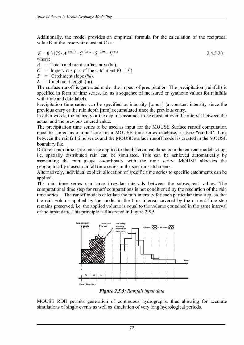
State of the art in Urban Drainage Modelling
72
Additionally, the model provides an empirical formula for the calculation of the reciprocal value K of the reservoir constant C as:
608.0401.0512.00076.03175.0 LSCAK ⋅⋅⋅⋅= −−− 2.4.5.20 where: A = Total catchment surface area (ha), C = Impervious part of the catchment (0...1.0), S = Catchment slope (%), L = Catchment length (m). The surface runoff is generated under the impact of precipitation. The precipitation (rainfall) is specified in form of time series, i.e. as a sequence of measured or synthetic values for rainfalls with time and date labels. Precipitation time series can be specified as intensity [µms-1] (a constant intensity since the previous entry or the rain depth [mm] accumulated since the previous entry. In other words, the intensity or the depth is assumed to be constant over the interval between the actual and the previous entered value. The precipitation time series to be used as input for the MOUSE Surface runoff computation must be stored as a time series in a MOUSE time series database, as type "rainfall". Link between the rainfall time series and the MOUSE surface runoff model is created in the MOUSE boundary file. Different rain time series can be applied to the different catchments in the current model set-up, i.e. spatially distributed rain can be simulated. This can be achieved automatically by associating the rain gauge co-ordinates with the time series. MOUSE allocates the geographically closest rainfall time series to the specific catchments. Alternatively, individual explicit allocation of specific time series to specific catchments can be applied. The rain time series can have irregular intervals between the subsequent values. The computational time step for runoff computations is not conditioned by the resolution of the rain time series. The runoff models calculate the rain intensity for each particular time step, so that the rain volume applied by the model in the time interval covered by the current time step remains preserved, i.e. the applied volume is equal to the volume contained in the same interval of the input data. This principle is illustrated in Figure 2.5.5.
Figure 2.5.5: Rainfall input data
MOUSE RDII permits generation of continuous hydrographs, thus allowing for accurate simulations of single events as well as simulation of very long hydrological periods.

State of the art in Urban Drainage Modelling
73
MOUSE RDII is actually a combination of any of the MOUSE Surface Runoff models for the description of the FRC component (FRC - Fast Response Component: comprises the rain induced inflow and fast infiltration component), and the NAM hydrological model for description of the SRC component (SRC - Slow Response Component: comprises slow infiltration component). “NAM” is an abbreviation of the Danish expression “Nedbør-Afstrømnings-Model”, meaning “precipitation-runoff-model”. MOUSE RDII permits generation of continuous hydrographs, thus allowing for accurate simulations of single events as well as simulation of very long hydrological periods. A computational hydrological model such as the continuous part of RDII is a set of linked mathematical statements describing, in a simplified quantitative form, the behaviour of the land phase of the hydrological cycle. The RDII model is a deterministic, conceptual, lumped type of model with moderate input data requirements. Spatial characterization of constitutive parts of the analyzed area is achieved through definition of sub-catchments, each of them described with a unique set of parameters and so the model treats every sub-catchment as one unit. The parameters and variables therefore represent an average for the whole sub-catchment. MOUSE RDII calculates the total discharge (runoff and infiltration) within the catchment area. This means that the hydraulic processes in the sewer system which affect the mass balance (e.g. overflow) are not described and, therefore, this effect is not accounted for when the total discharge from the catchment is calculated. The MOUSE Pipe Flow Model is the module for simulations of unsteady flows in pipe networks with alternating free surface and pressurised flow conditions. The computation is based on an implicit, finite difference numerical solution of basic 1-D, free surface flow equations (Saint Venant). The implemented algorithm provides efficient and accurate solutions in multiply connected branched and looped pipe networks. Computations of the unsteady flow in the links MOUSE Pipe Flow Model, applied with the dynamic wave description, performs by solving the vertically integrated equations of conservation of continuity and momentum (the 'Saint Venant' equations), based on the following assumptions:
• the water is incompressible and homogeneous, i.e. negligible variation in density; • the bottom-slope is small, thus the cosine of the angle it makes with the horizontal may
be taken as 1; • the wavelengths are large compared to the water depth. This ensures that the flow
everywhere can be regarded as having a direction parallel to the bottom, i.e. vertical accelerations can be neglected and a hydrostatic pressure variation along the vertical can be assumed;
• the flow is sub-critical (Super-critical flow is also modelled in MOUSE, but using more restrictive conditions).
The general form of the equations takes the form as follows:
0=∂∂+
∂∂
tA
xQ
2.4.5.21
of gAIgAIxygA
xA
Q
tQ =+
∂∂+
∂
∂
+∂∂
2
α 2.4.5.22
where: Q = discharge, [m3s-1] A = flow area, [m2] y = flow depth, [m] g = acceleration of gravity, [ms-2] x = distance in the flow direction, [m] t = time, [s]

State of the art in Urban Drainage Modelling
74
a = velocity distribution coefficient I0 = bottom slope If = friction slope The general flow equations are non-linear, hyperbolic partial differential equations. The equations determine the flow condition (variation in water depth and flow rate) in a pipe or channel when they are solved with respect to proper initial and boundary conditions. Analytical solutions are only possible in special cases with a rather limited number of applications, therefore the general equations have to be solved numerically.
The MOUSE Pipe Flow Model provides a choice between 3 different levels of flow description approximations: 1. Dynamic wave approach, which uses the full momentum equation, including acceleration forces, thus allowing correct simulation of fast transients and backwater profiles. The dynamic flow description should be used where the change in inertia of the water body over time and space is of importance. This is the case when the bed slope is small and bed resistance forces are relatively small. 2. Diffusive wave approach, which only models the bed friction, gravity force, and the hydrostatic gradient terms in the momentum equation. This allows the user to take downstream boundary conditions into account, and thus simulate backwater effects. The diffusive wave description ignores the inertia terms and is therefore suitable for backwater analyses in cases where the link bed and wall resistance forces dominate, and for slowly propagating waves where the change in inertia is negligible. 3. Kinematic wave approach, where the flow is calculated on the assumption of a balance between the friction and gravity forces. This means that the kinematic wave approach cannot simulate backwater effects. Thus this description is appropriate for steep pipes without backwater effects. Depending on the type of problem, the most appropriate description can be selected. All three approaches simulate branched as well as looped networks. According to DHI the dynamic wave description is recommended to be used in all cases except where it can be shown that either the diffusive or kinematic descriptions are adequate. The diffusive and kinematic wave approximations are simplifications of the full dynamic descriptions. They are implemented to offer improved computational efficiency, but should only be used when the omitted terms have insignificant influence. When there is any doubt it is better to use the full dynamic description or trials should be undertaken to establish the difference between the alternative methods, and advice sought from experienced persons. It is very important to have a solid understanding of the influence of the different terms. None of the three wave descriptions includes detailed hydraulic descriptions of hydraulic jumps. However, the chosen formulations ensure a correct description upstream and downstream of the jump. The implemented algorithm solves the flow equations by an implicit finite difference method. Setting the numerical scheme into the frame of the Double-Sweep algorithm ensures conservation of the mass continuity and compatibility of energy levels in the network nodes. The solution method is the same for each model level (kinematic, diffusive, and dynamic). The transformation of Equations 2.4.5.21 and 2.4.5.22 to a set of implicit finite difference equations is performed on a computational grid consisting of alternating Q- and h-points ("staggered" grid), i.e. points where the discharge Q and water level h, respectively, are computed at each time step (see Figure 2.5.6). The computational grid is generated automatically by the model, or with user specified number of grid points. The computational grid for a conduit contains an odd number N of Q and h points, with h points at both ends. The minimum number of computational points N in a conduit is 3, i.e. two h points and one Q point in between. The points are all equally spaced, with a distance x

State of the art in Urban Drainage Modelling
75
equal to:
1−
=∆N
lx 2.4.5.23
where l is the conduit length. On the basis of the input data and the specified time step the model automatically generates a complete computational grid, based on the velocity condition. The velocity used in the calculation is a full-flow velocity, obtained from the Manning formulation assuming completely filled conduit. If the velocity condition can not be satisfied for the specified simulation time step, which often happens with short and steep pipes, then the model issues a warning, with proposal for a shorter time step, required for the condition to be satisfied. The grid generated by the model can be altered individually for each conduit, i.e. can be made more dense or sparse, according to the needs of the current application.
Figure 2.5.6: Node discretization in pipe flow model
The implemented numerical scheme is a 6-point Abbott-scheme. The scheme for the method is shown in Figure 2.5.7.
Figure 2.5.7: Computational scheme in pipe flow model
The flow equations are approximated by finite differences. Elements available for definition of a numerical model in MOUSE are: Links
o pipes - standard and arbitrary cross-sections, o open channels - arbitrary cross-sections.
Nodes o manholes, o basins (structures), o storage nodes, o outlets.
Functions, for description of certain physical components of sewer systems, including: o overflow weirs, o pumps, o non-return valves, o flow regulators.
Controllable structures, for the simulation of reactive or time dependent operation real-time control, including:
State of the art in Urban Drainage Modelling
76
o rectangular underflow gate with movable blade weirs, o rectangular overflow weir with changeable crest elevation.
Head losses caused by the resistance in free-surface flow links are introduced as a friction slope term into the momentum equation . The friction slope If is equal to the slope of the energy grade line and is defined as:
gR
I f ρτ= 2.4.5.24
where: τ = tangential stress caused by the wall friction, [Nm-2], ρ = density of water, [kgm-3], R = hydraulic radius, [m], (= A/P, where P is the wetted parameter). The friction slope can be derived from the Manning's equation as a function of the flow parameters (Q, A and R) and the pipe roughness expressed as Manning's number (M):
34
22 RAM
QQI f = 2.4.5.25
Usage of the QQ , instead Q2 facilitates computations of the reverse flow. Parameter for controlling the extent of the head loss in the conduit is the Manning's number M (or n = 1/M), as a measure of the conduit wall and bottom roughness. Per default, MOUSE assumes a constant Manning.s number over the link section height. However, in real situations conduit wall roughness often changes with water depth, because different parts of the link cross section are exposed to quite different flow conditions during its lifetime. This introduces difficulties in fitting the computed stage-discharge curve, based on a single M value specified for a link, with the actual, measured stage-discharge relation. This is usually related to old systems, where significant sediment deposits and pipe-wall erosion are present. The MOUSE Pipe Flow Model accepts a specification of a non-linear variation of Manning number with relative elevation (water depth in the conduit). Three parameters define the Manning's number variation: bottom value, full flow value and a non-linear exponent. Intermediate values are calculated by a general expression:
( )exp
⋅−+=
DyMMMM botttopbottact 2.4.5.26
where: Mact = calculated Manning's number; Mbott, Mtop = Manning's numbers specified for the conduit bottom and top, respectively; exp = Manning's number variation exponent, default; y/D = the relative water depth in a conduit; The formula is used for relative depths h/D in the interval 0.0 - 1.0. For relative depth > 1.0 the Manning number is set to the Manningtop value. The variation between Manningbot and Manningtop is controlled by the "Variation Exponent". The variation of the Manning number in relative terms is illustrated in Figure 2.5.8.

State of the art in Urban Drainage Modelling
77
Figure 2.5.8: Relative variation of the Manning number with relative depth
Distribution of the flow within a rising main network is calculated on the basis of the continuity equation and the pressure distribution. The latter is calculated on the basis on backward integration (from the tail node) of the Colebrook-White equation. The applied Colebrook- White equation is given by:
gRVfI
Rk
f
2
Re7.4ln45.24.62
2
=
+−=
2.4.5.27
where: f = the friction number k = the roughness V = the velocity in the pipe R = the hydraulic radius Re = the Reynolds number g = the gravity constant . In order to calculate the head losses in manholes and structures, it must be say that the general flow equations are valid only for continuous conduits where, in principle, the only resistance to the flow originates from the bottom and side-wall friction. Hydraulic conditions in nodes, i.e. at manholes and structures take the role of boundary conditions for computation of the flows in the conduits. In turn, hydraulic conditions in a node depend on the flows in the inlet and outlet conduits. These hydraulic conditions, expressed in terms of the energy conservation principle, are calculated as water levels and velocity heads. The calculation is based on the mass continuity and formulation of more or less advanced energy relation between the node and the neighbouring links, with inclusion of some energy losses caused by local flow disturbances at different locations in the node. The implemented solution ensures that mutual dependence of the flows in links and hydraulic conditions in nodes are correctly resolved, even for complex branched and looped conduit networks. Energy losses in junctions are of the same order of magnitude as those caused by the pipe wall friction. Knowledge about the magnitude of these energy losses, based on experimental data, is very limited, but some theoretical results are available. Importance of a detailed evaluation of these losses is related to the relative length of the links (l/D), and grows with relative shortening of the conduits. A simplified computational model for energy losses in junctions implemented in MOUSE is based on F.A. Engelund's energy loss formulae. Furthermore, a critical depth formulation, with

State of the art in Urban Drainage Modelling
78
approximation of critical flow conditions, is used in MOUSE for simulation of a free inlet to a manhole. It is assumed that the water levels in the inlet conduit and in the manhole or structure are the same. This assumption implies that the energy loss of the flow entering and expanding in the node amounts to the difference of the velocity heads in the inlet conduit i and the node m, respectively:
gvvH mi
i 2
22 −=∆ 2.4.5.28
Essentially one-dimensional analysis in MOUSE relies on this simplification also in nodes with multiple inlet and outlet conduits, i.e. where mixing of flows of different energy levels occurs. In a case of a free inlet of a sub-critical flow, i.e. when the water level in the junction is lower than the critical depth level in the inlet link, the water level in the link is assumed to be equal to the critical depth. For different cross sections, appropriate approximations are applied, e.g. for a circular pipe as follows:
i
iic D
Qy 32.0)( = 2.4.5.29
where: Di = diameter of the circular pipe [m]. Similarly, in a case of a low water level in the junction with supercritical flow (steep inlet links), the downstream water level is set equal to normal depth in the link. All the individual losses in a node (except the inlet loss) calculated by the model are added-up at the outlet, separately for each outlet link. The outlet loss for the link j is assumed to be proportional to the velocity head in the outlet link j:
g
vH j
kjkj 2
2
∑=∆ ξ 2.4.5.30
where jkξ are individual head loss coefficients for link j, calculated on the basis of geometrical set-up of the node and flow distribution among the links attached to the node. The model distinguishes among the following losses: . Change in flow direction, . Change in elevation, . Loss due to contraction at outlet. Loss due to change in flow direction This loss is a function of the angles between the inlet and outlet links and distribution of the discharge in the inlet and outlet links. Based on the generalised notation, the calculation of the head loss coefficient is performed individually for each outlet link as follows:
2
2
1)( 90°
⋅= ∑=
ijn
i j
ijdir Q
Q θξ 2.4.5.31
where i stands for inlet links, and j stands for outlet links. Loss due to change in elevation Vertical changes in flow direction occur and cause energy losses if there is a difference in elevation between inlet and outlet link. These losses are described considering the magnitude of the difference in elevation.

State of the art in Urban Drainage Modelling
79
The individual head loss coefficient is calculated according to the following expression, where the weighting relative to the flow rates in the inlet links relative to the outlet link is also included:
( ) ( )ji
iijjijn
i j
ijlevel DD
DZDZZZQQ
⋅−−+⋅−
⋅= ∑=1
)(ξ 2.4.5.31
If the calculated head loss coefficient is smaller than 0, a zero value is assumed. Loss due to contraction The flow leaving the manhole and entering the outlet conduit is more or less contracted and due to subsequent expansion there occurs an energy loss. The outlet head loss coefficient depends on the shape of the manhole outlet, manhole and the link cross sections and distribution of flow among multiple inlet and outlet links. MOUSE calculates the outlet head loss coefficient according to the following:
⋅−⋅=
∑=
n
ii
jm
jmjcontrl
Q
QA
AK
1
)( 1ξ 2.4.5.32
where: Km = specified outlet 'shape' coefficient for the node. For relatively large basins, Km approaches
⋅contrξ Am = flow cross sectional area in the node.
Theoretically, the total energy loss at the outlet from the node, expressed as a function of the velocity head in the outlet pipe can be as high as the available energy level in the node. The limiting case occurs e.g. with completely clogged outlet (Km -> 8), with no flow in the outlet pipe. However, in computational reality, in order to preserve a robustness of the computation, various additional limitations could be introduced. With respect to that, MOUSE offers two possibilities. The first (older) limitation relates the maximum head loss to the depth in the outlet pipe:
( )
−⋅+=∆
gv
gv
hH mjoutjj 22
1,min22
ξ 2.4.5.33
It also introduces the limitation on the total head loss coefficient as: 0.1≤= ∑ jout ξξ 2.4.5.34
These limitations have caused that the computed head losses and the corresponding flow conditions around nodes in some cases were imprecise. Due to the advances in the computational implementation, the limitation from Equation 2.4.5.33 could been removed, allowing the total head loss for the outlet pipe j being computed as:
( )( )[ ]g
vH j
jcontrjleveljdirj 21,min
2
)()()( ⋅++=∆ ξξξ 2.4.5.35
The limitation of the total head loss coefficient to 1.0 is however still present. The assumption applied in the MOUSE ‘standard’ solution that the water level in the manhole and all downstream water levels of the inflowing conduits are the same, often leads to
State of the art in Urban Drainage Modelling
80
overestimates of the energy loss at the inlet. In many cases, the wetted cross-section area in the inlet pipe is smaller than in the manhole, leading to almost entire loss of the kinetic energy of the incoming flows, which is not the case. This problem is reduced by applying the effective flow area in the manhole, but this is available in MOUSE only for circular pipes and for the flow-through manholes (i.e. with one pipe in- and one pipe outflow). An alternative solution is available which fully ignores the energy loss at the inlet. For a flow-through manhole, this practically means that the energy level in the manhole is set to be equal as at the downstream end of the inlet pipe. For manholes with multiple inlets, the energy level is calculated as the weighted average of the inlet flows (i.e. large flows contribute most to the energy level). Thus, in this formulation, the total loss at the manhole is concentrated computationally at the outlet, and can be fully controlled by the user. This approach proves valuable for some specific situations, particularly for the flow-through manholes with ‘normal’ flow conditions. However, due attention must be paid for cases with high inlet energy levels, e.g. a small pipe with high-velocity flow entering a large basin. In such a case, the energy level of otherwise still water in the basin would be calculated as equal to the energy level of the approaching flow, i.e. much higher than realistic, with erroneous results as a consequence. The head loss calculation for individual nodes can be controlled by selecting one of the three computational modes for the head loss calculation. These modes distinguish the meaning of the specified head loss coefficient. Per default (a) the specified value is ‘interpreted’ as the outlet 'shape' coefficients Km. In addition to the default interpretation of the head loss coefficient Km, for individual nodes two alternative interpretations can be selected. These are: (b) Contraction head loss coefficient and (c) Total head loss coefficient. For the case (b), the model ignores the geometrical relations between the node and the outlet links (outlet shape), and applies the specified value (Contraction HCL) directly as the contrξ . The contraction losses in the outlet links are then computed by multiplying the velocity head in the respective link by the contrξ . The total head loss for an outlet link is computed as a sum of the contraction, direction and elevation loss. In case (c), the model completely ignores the geometry of the node/links, and applies the specified value (Total HLC) directly as the outrξ , the same for all outlet links at the node. The total head losses in the outlet links are then computed by multiplying the velocity head in the respective link by the specified outrξ . MOUSE allows to chose among nine different options for calculation of energy losses at junctions. Some of these options differ purely by the value of the default supplied head loss coefficient value, while some other represent a different concept of the head loss calculation. Behind some of the available choices, there is a default value for the head loss coefficient. The default values can be modified for individual nodes. When applying the kinematic wave approximation, the head loss description in nodes is based on the same equations as described above. However, in order to reduce the computational time, the energy losses are computed once for a number of different flow conditions and tabulated for use during the simulation. In cases where there is more than one inlet link in a manhole, the losses are calculated on the basis of the assumption that the flow in each link (relative to the flow in the other inlet links) is proportional to the corresponding full flow capacity. This assumption affects the energy losses due to changes in elevation and direction only when these losses are different for the different inlet links.
State of the art in Urban Drainage Modelling
81
If the water level in a manhole reaches the ground level, an artificial “inundation” basin is inserted above the node. The surface area of this basin is gradually increased from the area in the manhole or the structure to a 1000 times larger area, thus simulating the surface inundation. When the outflow from the node surmounts the inflow, the water stored in the inundation basin re-enters the system. When the water level in the node increases and is above ground level, is assumed that during a time step the surface area in the basin is calculated using the water level from the start of the actual time step. If the water level passes through the transition region between the actual manhole or structure and the artificial basin, this assumption leads to generation of water. When the increase of the water level during a time step is relatively small, then the generated water volume is negligible. If the water level is changing rapidly, the generated volume of water is important and due to that an appropriate correction is built in the program to ensure no generation of water. An alternative to the assumption of constant surface area during a time step is to introduce iterations in the simulation. Iterations would significantly increase the simulation time. Any manhole or basin can be defined as sealed. If a node is defined as a sealed node, then the maximum water level at a node is set to the ground surface. In this case, the pressure will rise without any water on the ground surface. The following relations are valid:
mm PH = for topm HP ≤ and topm HH = for topm HP ⟩ 2.4.5.36 where: Hm is the water level in the node [m], Pm is the pressure level in the node [m], Htop is the ground level for the node [m]. Manholes can be defined as spilling manholes. If the water level in a manhole defined as a spilling manhole reaches the ground level, the water will start spilling irreversibly out of the system. The flow will be computed using the MOUSE built-in weir formula (free overflow), according to the following: for topm HH ≤ : 0=spillQ 2.4.5.37
for topm HH ⟩ : ( )( ) 23
322_
−∆+⋅
+⋅⋅⋅= topm
cspill HPH
KgDSPILLRELQ π
where: Qspill is the spill discharge [m3/s], D is the manhole diameter [m], Hm is the water level in the manhole [m], Htop is the ground level in the manhole [m], P is the "buffer pressure" for the spill [m], g is the acceleration of gravity [ms-2), Kc is the head loss coefficient associated with the node, REL_SPILL is the linear scaling coefficient for the spill. The level (i.e. head) at which the spill starts can be controlled by optionally specifying the 'buffer pressure' as a relative elevation above the ground surface (default value = 0). The spilling capacity of a spilling manhole can be controlled by specifying the relative spill coefficient (default value = 1). If parts of the sewer system dry-out during the simulation, then the model artificially maintains a minimum water depth in those conduits, corresponding (per default) to 2% of the characteristic dimension of the conduit (diameter for circular pipes), or max. 0.02 m. This is necessary with regards to the numerical stability in the solution of the flow equations.
State of the art in Urban Drainage Modelling
82
This correction practically means artificial generation of water, i.e. some water volume is added to the system. As a consequence of that, the continuity status report shown at the end of the simulation does not give a fair impression of the accuracy of the simulation. MOUSE RTC simulates reactive local and global RTC systems in urban drainage and sewer networks. It permits description of various controllable devices and makes the definition of complex operational logic for interdependent regulators fully transparent and time efficient. The following controllable devices can be specified: rectangular overflow weir, rectangular underflow gate, pump. The devices may be specified as settings- or PID-controlled, with control function selection based on a global system analysis. Each regulator or a pump operates under the control logic encapsulated into a set of simple logical rules and control functions. The system allows a schematised definition of any form and size of decision tree, featuring logical operators AND, OR, NOT and NOR, in any associate combination. The process of selecting an appropriate control function under current operational situation relies on the evaluation of logical rules with operands including measurable and derived hydraulic and WQ variables (e.g. water level, flow, pollutant concentration, level difference), devices statuses (e.g. gate blade position, pump ON/OFF) and the current control function. The control functions range from the simplest constants for the operational variables (e.g. constant weir crest setting or constant flow set-point) to dynamically controlled variables, set in a continuous functional relation with any of measurable variables in the system (e.g. CSO discharge set-point as a function of flow concentration or a pump START/STOP levels as functions of water level at strategic location in the system). Some conceptualisations applied in MOUSERTC are listed below: • The program does not distinguish explicitly between local and global RTC. Per default, all
elements of a modelled RTC system are assumed available for global control. • Sensors are not specified as physical devices, but conceptually as operational points. • Any computational point in a MOUSE network can be defined as an operational point.
Operational points have not to be declared explicitly, but through definition of operational ranges, set points and control functions.
• Controllable devices (regulated structures – weirs and gates, and pumps) are specified outside the MOUSE interface and no reference to them has to be made in MOUSE standard input files.
• Controllers are not specified explicitly as physical devices, but their function (i.e. operational logic) is associated with the respective regulators.
• MOUSE RTC assumes sampling and actuation (control loop) frequency identical to the simulation time step.
• Sensor readings are simulated as perfect and with 100% availability. • Low-level logic of the pump START/STOP operation is built in the program and is
controlled by the START and STOP levels. • The PID control algorithm is built in the program and is controlled by the PID constants and
by factors for weighting the terms of the numerical solution of the control equation. At each simulation time step, the set-point is evaluated against the actual value of the control variable (flow or water level, depending on the set-point type). The actual WCL or Qpump is determined from the following equation:
++⋅= ∫ dt
deTedtT
eKuiT
di 0
1 2.4.5.38
where: u = the output signal (WCL or Qpump),

State of the art in Urban Drainage Modelling
83
e = the error to be minimised, K = the proportionality factor, Td = the derivation time, Ti = the integration time. For numerical solution, a discrete form of this equation is required. By use of the Laplace transformation one obtains:
)(1)( sEsTsT
iKsU di
⋅
⋅+
⋅+⋅= 2.4.5.39
where: U(s) = the Laplace transform of u, E(s) = the Laplace transform of e. By use of the backward Euler transformation:
zTzs
s ⋅−= 1 2.4.5.40
where Ts is the sampling period, one obtains the following discrete representation of the PID equation:
( ) ( )( ) ( ) ( )( )
( ) ( )( ) ( )12
11211)(
3
21
−+⋅−−−⋅⋅+
−−−⋅
+⋅⋅−−⋅
++⋅⋅=
nuTTlnynyK
nynyTTKnyny
TT
TTKnu
S
dref
refS
dref
S
d
i
S
α
αα
2.4.5.41 The MOUSE LTS (Long Term Statistics) Module allows that a MOUSE network with intermittent hydrological inputs can be set up for a long-term simulation, covering a long, continuous historical period, possibly over several years. The system automatically selects the periods for dynamic pipe flow simulations during wet weather. This reduces the simulation time significantly, while preserving the accuracy in the simulation of relevant dynamic effects in the system - CSOs, surcharges, etc. For the purpose of isolating the intervals relevant for dynamic simulation, MOUSE LTS generates a job list on the basis of system information and knowledge of time series for dry weather flow (i.e. wastewater), rainfall and other loads. The job list criteria represent various thresholds for the system loading, which are used to evaluate if the state of the system is within or outside the "dynamic" conditions. There are separate START criteria, which determine the start dates and times for the dynamic simulations, and a single STOP criterion, which is used for the estimation of the ending dates and times for dynamic simulations. Initially, the generated job list contains the simulation jobs which cover the intervals relevant in the total simulation period that would be simulated if no additional criteria were specified. Namely, some additional criteria (so-called 'runtime criteria') may optionally be specified, which would extend the simulations beyond the time intervals defined in the job list. In fact, Runtime Stop Criteria are evaluated during discontinuous computations in order to determine the earliest time at which the simulation can be stopped without loosing important information, i.e. in the closing phase of the simulated event. The evaluation of runtime stop criteria for the currently simulated event starts immediately after the preliminary event end (determined according to the job list) has been reached. The simulation continues as long as the runtime stop conditions are not fulfilled. Since the 'runtime criteria' are evaluated during the simulation, it is not possible to determine the exact duration of the dynamic simulation in advance. A number of independent Stop Criteria can be specified. They are evaluated through an Evaluation matrix. In fact, at every time step during computation (but only after the end time
State of the art in Urban Drainage Modelling
84
in the job list!), each criterion is subject to logical evaluation as an element of an evaluation matrix. The evaluation matrix consists of an arbitrary number of lines, each containing up to five individual criteria. Each line of the evaluation matrix represents a combination of criteria which have to be fulfilled simultaneously (i.e. criteria are linked with the logical operator AND) if the combination is to be evaluated as TRUE and the simulation stopped. If one line has been evaluated as FALSE, the evaluation algorithm jumps to the next line. This means that the successive lines are connected by the logical operator OR. The process continues until one line has been evaluated as TRUE (the simulation stops). If none of the lines has been evaluated as TRUE, the simulation continues for one time step. Then, a new evaluation cycle is initiated and the entire evaluation repeats. If no evaluation matrix is specified, periods specified in the job list will be simulated exactly, i.e. no runtime criteria will be evaluated. Moreover, MOUSE LTS provides the possibility to generate a series of useful statistical results - events, annual and system statistics - related to the simulated period.
2.4.6. Model Parameters Estimation or Assignation MOUSE does not apply any deterministic and/or statistical procedure aimed to parameter sensitivity analysis, automated calibration or uncertainty estimation. Some parameters can be assigned referring to typical values proposed in a variety of engineering libraries, providing specifications for: unit sanitary loads for different load types, roughness coefficients for the available friction loss methods, headloss coefficients for the most common minor losses and classical extreme flow factors methods coefficients.
2.4.7. PI(s) Estimation Method The performance indicators listed before cannot be evaluated directly in the model framework but they have to be calculated as functions of the model outputs. MOUSE gives as an output the full capacity, the design capacity (for fixed degree of fulfillment) and the total flow for each gravity pipe, so that the length of sewer where surcharging, or high surcharging, occurs, in dry or wet weather, can be calculated and the wPh5, wPh6 and wPh7 indicators can be computed. The total inflow volume and the total infiltration volume entering the sewer system can be evaluated, so that the wOp29 and wOp30 indicators can be computed. The hydraulic grades at manholes are also given as output data: when the hydraulic grade is greater than the ground elevation at a non bolted manhole, a flooding occurs, so that the number of surface floodings can be known and the wOp35 indicator can be calculated.
2.4.8. Future Improvements of the Model No information about future model developments are available by now.
2.4.9. References
2.4.9.1 Theoretical Framework References DHI (2000): MOUSE - User Manual and Tutorial (Version 2000), DHI, Hørsholm, Denmark. DHI (2000): MOUSE SURFACE RUNOFF - Reference Manual (Version 2000), DHI, Hørsholm, Denmark. DHI (2000): MOUSE PIPE FLOW - Reference Manual (Version 2000), DHI, Hørsholm, Denmark. DHI (2000): MOUSE RDII - User Manual (Version 2000), DHI, Hørsholm, Denmark.

State of the art in Urban Drainage Modelling
85
DHI (2000): MOUSE RTC - User Manual and Tutorial (Version 2000), DHI, Hørsholm, Denmark. DHI (2000): MOUSE LTS - User Manual (Version 2000), DHI, Hørsholm, Denmark. DHI (2000): MOUSE - Short Introduction and Tutorial (Version 2000), DHI, Hørsholm, Denmark. DHI (2000): MOUSE - User Guide (Version 2000), DHI, Hørsholm, Denmark. DHI (1992): NAM - User Manual and Reference Manual, DHI, Hørsholm,Denmark. Eriksson, B., (1983): Data concerning the precipitation climate of Sweden. Mean values for the period 1951-80. Rapport 1983:28, SMHI, Norrköping, Sweden (in Swedish). Gustafsson, A.M., (1992): The hydrological model NAM. The Calibration periods' effect on model parameters and valuation results. Thesis project, Department of hydraulics, Chalmers University of Technology, Göteborg, Sweden (in Swedish). Gustafsson, L.G., (1992): Modeling of urban hydrology. User's guide - MouseNAM. VA-forsk rapport nr 1993-04, VAV, Stockhom, Sweden (in Swedish). Niemczynowicz, J., (1984): An investigation of the areal properties of rainfall and its influence on runoff generating processes. Institutionen för teknisk vattenresurslära, Lunds Tekniska Högskola, Lund, Sweden. Wilson, E.M., (1990): Engineering Hydrology. 4th edition, Macmillan Education Ltd, London.
2.4.9.2 Practical Use and Results References DHI (2000): MOUSE - User Manual and Tutorial (Version 2000), DHI, Hørsholm, Denmark. DHI (2000): MOUSE SURFACE RUNOFF - Reference Manual (Version 2000), DHI, Hørsholm, Denmark. DHI (2000): MOUSE PIPE FLOW - Reference Manual (Version 2000), DHI, Hørsholm, Denmark. DHI (2000): MOUSE RDII - User Manual (Version 2000), DHI, Hørsholm, Denmark. DHI (2000): MOUSE RTC - User Manual and Tutorial (Version 2000), DHI, Hørsholm, Denmark. DHI (2000): MOUSE LTS - User Manual (Version 2000), DHI, Hørsholm, Denmark.
State of the art in Urban Drainage Modelling
86
2.5 SEWERCAD
2.5.1. Model availability SewerCAD program is produced by Haestad Methods; it is a commercial model and the source code is not available. Information about SewercadCAD can be found in http://www.haestad.com/software/, including detailed features list, downloadable tutorials, live e-demos and informations about training courses, but not on-line documentation.
2.5.2. Abstract
2.5.2.1 Objectives and peculiarities SewerCAD is a program for the design, analysis and planning of gravity flow and pressure flow through pipe networks. The operational behavior of various gravity and pressure network elements (manholes, outlets, junction chambers, pressure junctions, wet wells and pumping stations) can be simulated. Prototype elements can be defined with default characteristics, reducing data entry requirements if a group of network elements share common data. The sources of flow in the sewer system are called loads, and are classified as sanitary (dry weather) loads, wet weather loads and known loads; the surface runoff flows entering the sewer system during wet weather are to be previously calculated because the model does not provide any rainfall-runoff transformation. The gravity network is calculated using a built-in numerical model, which utilizes the gradually varied flow equations. Flow calculations are valid for both surcharged and varied flow situations, including backwater effects and drawdown curves. Pressure elements are simulated by the mass and momentum conservation equations ; gravity and pressure components can be mixed freely. SewerCAD can run both Steady State Analyses, modelling a single instant in time, and Extended Period Analyses, modelling a network over a specified duration of time; moreover, the program allows to automatically design gravity piping and structures, specifying the elements to be designed, from a single pipe size to the entire system, or anything in between, intending the program’s design only as a preliminary step. SewerCAD can be run utilizing its own graphical interface (stand-alone mode) or utilizing an AutoCAD interface (AutoCAD mode), which represents an additional feature of the model. SewerCAD graphical editor allows to create, move, edit, and delete network elements graphically. An automated scenario management using inheritance allows for comparing input and result data associated with different set of calculations, eliminating any need to input or maintain redundant data.
2.5.2.2 Performance Indicator(s) of Interest SewerCAD does not calculate any performance indicator directly. The following performance indicators can be evaluated using the output data from SewerCAD: wPh5, wPh6, wPh7, wOp29, wOp30, wOp35, WFi20 (see Appendix 1 for performance indicators definition).
2.5.2.3 Brief Historical Overview of the Model The first commercial version of the model was released in 1995. Many other program versions have been released through years. For example, version 4.0, released in june 1999 including new graphical environment, new loading model and a scenario automated management; version

State of the art in Urban Drainage Modelling
87
4.1, performing cost estimation and maintaining persistent user-defined tables sorts and filters; version 4.1.1, simulating diversions and overflows and using new structure headlosses calculation methods. The latest version 5.0 has been released in june 2001 and performs extended period simulations, allows for loading data import from a formatted ASCII text file, improves results reporting.
2.5.3. Usage Specifications
2.5.3.1 Programming Language(s) or Mathematical-Statistical Software(s) The source code has been written is Visual C.
2.5.3.2 Functionality SewerCAD can simulate flow in gravity and pressure systems. The pipes in a gravity system must all converge on a single termination point in a classic tree structure, while the force mains can be much more complex with loops and multiple outlet points. The choice of conveyance elements includes arch, box, circular, horizontal ellipse and vertical ellipse. The network elements that can be simulated are: manholes, used to model access hole structures; junction chambers, used to model underground structures; wet wells, which are storage nodes typically used in conjunction with one or more pumps to model a pumping station; outlets, which define the most downstream element of a network; pressure junctions, used to model a junction under pressure at the downstream end of one or several pressure pipes ; pumps, both variable speed and constant horsepower. The only way to transition between a gravity pipe and a force main in SewerCAD is through an intermediate wet well, which establishes a boundary condition for both the connecting systems. Controls can be added for pressure pipes and pumps. The status of a pipe can be either open or closed; the status of a pump can be either on or off. Control can be triggered by a specified pressure or hydraulic grade being reached in any wet well or pressure junction, or based on the time during an analysis. The program can simulate water leaks into the gravity system through joints, cracks, and other defects in the structures, and also depressed sewers (inverted siphon). SewerCAD allows for calculating a planning level estimate of the capital costs associated with an entire system or any portion of a system. The costs associated with a particular element are broken down into two categories: construction costs and non-construction costs. When running an extended period simulation two distinct time steps are used. The hydrologic time step is used to calculate the routed hydrographs and represents the time increment of all hydrographs generated during the analysis; it is also used as the calculation increment for the pressure calculations. The hydraulic time step represents how often the hydraulic calculations are performed. The hydrologic time step should be less than or equal to the hydraulic time step.
2.5.3.3 Possible interaction with other software tools SewerCAD has the ability to dynamically exchange data with a variety of applications. Connections can be established between the hydraulic model and relational and non-relational database management systems (RDBMS and DBMS), spreadsheets, and ESRI shape files. Data can be imported from AutoCAD, constructing a network based on the entities contained in an AutoCAD drawing. SewerCAD allows for importing data from the Civil Design module of AutoCAD’s Land Development Desktop, and for exporting part (or all) of the network to a database file to be imported into a Land Development Desktop project (using the Civil Design module). Background graphics in SewerCAD stand-alone mode can be imported as a .DXF file from AutoCAD or another drafting program; data can be saved by exporting to a .DXF file for use by AutoCAD, and many other common CAD-based applications.

State of the art in Urban Drainage Modelling
88
2.5.4. Input and Output procedures
2.5.4.1 Possible Input File(s) Formats All model input data are stored in a binary file which has the .SWR extension. The input data can be entered using an hydraulic element editor which organizes the element related input data in different tables. Tables can be edited, sorted and/or filtered to ease data input for specific elements, and may also customized to meet a variety of requirements. The data shown in a table may be exported to an ASCII text file in either tab or comma-delimited format. SewerCAD has the capability of reading in loading data from a fixed format ASCII text file. Input data may be also dynamically exchanged with a variety of applications as previously described.
2.5.4.2 Possible Output File(s) Formats SewerCAD calculation results are stored in binary files with .OUT extensions for the pressure system results, and .RST extensions for the gravity system results. The output data are reported in tables which can be edited, sorted and/or filtered to present the results for specific elements, and may also customized to meet a variety of requirements. The data shown in a table may be exported to an ASCII text file in either tab or comma-delimited format. Output data may be also dynamically exchanged with a variety of applications as previously described.
2.5.4.3 Raw Data Formatting The model does not accept raw data, and the structure of input files cannot be changed; the format of the files is quite simple and can be easily created by copying and pasting the data from the source application into a text editor. Input data may be also imported from different databases and spreadsheets.
2.5.5. Theoretical framework Overview SEWERCAD is a deterministic model. Loads are the sources of flow in the sanitary sewer system. There are two fundamental loading types that can be applied to the network elements, namely hydrographs and pattern loads, which are two distinct ways to describe how flow varies over time. A hydrograph is simply a time-discharge series. During a steady state analysis a hydrograph can be converted into a single load: the peak, the average or the minimum hydrograph flow can be selected to be used as the steady state load, or the hydrograph can be totally disregarded. If the duration of an extended period simulation exceeds the duration of a hydrograph, the last point of the hydrograph will remain constant for the extent of the remaining time. A pattern load consists of a single average base load and a series of dimensionless multipliers used to delineate how the load varies over time; during a steady state analysis the entered base load is used as the load regardless of the applied loading pattern, while during an extended period simulation if the duration of the simulation exceeds the duration of a pattern then the pattern will repeat itself. SewerCAD classifies loads as sanitary (dry weather) loads, resulting from human activity, wet weather loads, related to rainfall activity and caused by groundwater infiltration and rainfall inflow, and known loads, originated from external calculations or field measured data. The total load at any given point may be a combination of these basic load types. Sanitary loads can be entered either as hydrographs, as pattern loads or as unit sanitary load, based on a number of contributing units, with a specified average load per unit. Average dry

State of the art in Urban Drainage Modelling
89
weather loads can be transformed into minimum or peak loads using an extreme flow factor EFF: Qpeaked = Qbase * EFF 2.5.5.1 where: Qpeaked = transformed flow; Qbase = base flow; EFF = extreme flow factor. Four different population-based or discharge-based equation can be selected to define any extreme flow factor, namely the Babbit equation:
2.0
1000P
0.5EFF
= 2.5.5.2
the Harmon equation:
5.0
1000P0.4
0.140.1EFF
+
+= 2.5.5.3
the Ten States equation:
1000P0.4
1000P0.18
EFF+
+= 2.5.5.4
and the Fedorov equation:
121.0Q69.2EFF = 2.5.5.5
where: P = contributing population; Q = base sanitary load. A cutoff value should be given, representing the maximum possible extreme flow factor for peaking methods, which is used to prevent unrealistically high values for small populations or land areas. Other tabular extreme flow factor methods can be selected, such as daily minimum, daily maximum, extreme minimum and constant peaking factor. Extreme flow factor methods are only used during steady state analyses. During extended period simulations loading patterns can be applied to the unit dry weather base loads to account for variations in sanitary inflow over time. Wet weather loads consist of groundwater infiltration, which may occurs in gravity pipes, and rainfall inflow, which may occurs at manholes, pressure junctions, and wet wells. Infiltration loads can be entered as hydrographs, pattern loads, fixed infiltration amount or as infiltration

State of the art in Urban Drainage Modelling
90
rate per unit of: pipe length; pipe diameter times pipe length; pipe surface area; count value (number of pipe defects). Inflows can be entered as hydrographs or as pattern loads; the surface runoff flows entering the sewer system during wet weather are to be previously calculated because the model does not provide any rainfall-runoff transformation. During extended period simulations the wet weather loads are added to together as a single lump hydrograph. Known loads are a special type of fixed load. As with other fixed loads, known loads remain constant as they progress downstream and combine directly as a simple sum. The special behaviour of known loads occurs during a steady state analysis when another known load is specified at a downstream location: while most fixed loads combine directly under any circumstances, a non-zero known load at any location replaces all upstream known loads. During extended period simulations, conversely, known flows are modelled as a single constant flow hydrograph over the duration of the simulation, and are added directly to the existing flows coming from upstream sources and are all lumped together as a single hydrograph for routing; in these cases the known flows are additive and do not replace each other. In addition to the three described basic load types, also pumped loads can be taken into account, which are special kinds of loads that represent sewage pumped into the gravity system via force mains. Pumped loads are optionally determined during calculations, and cannot be input directly. During a Steady State analysis the flow is broken down into the different load categories (sanitary, wet weather, known flow, pumped loads) so that the program can apply the correct extreme flow methods. During an Extended Period Simulation all the different flows are lumped together into a single hydrograph and the initial categories are disregarded. The free surface flow in gravity pipes can be modelled using either gradually varied flow analysis or capacity analysis. The energy balance equation, related to each end of a pipe segment, is as follows:
L
22
2
21
1 Hg2
VZg2
VZ ++=+ 2.5.5.6
where: Z1 = hydraulic grade at upstream end of the segment; V1 = velocity at the upstream end of the segment; Z2 = hydraulic grade at the downstream end of the segment; V2 = velocity at the downstream end of the segment; HL = loss due to friction - other losses are assumed to be zero; g = gravitational acceleration constant. The model allows for choosing 6 different equations to calculate friction losses: Chezy, Kutter, Manning, Darcy-Weisbach, Colebrook-White, Hazen-Williams. The friction loss is computed based on the average rate of friction loss along the length of the segment:
x2
SSxSH 21avgL ∆+=∆= 2.5.5.7
where: HL = Loss across the segment Savg = Average friction slope S1 = Friction slope at the upstream end of the segment; S2 = Friction slope at the downstream end of the segment; ∆x = Length of the segment being analyzed.

State of the art in Urban Drainage Modelling
91
The conditions at one end of the segment are known through assumption or from a previous calculation step; since the friction slope is a function of velocity, which is a function of depth, the depth at the other end of the segment can be found through iteration. Two methods for this iterative solution, the standard step method and the direct step method, can be used in the program. The standard step method of gradually varied flow energy balance involves dividing the channel into segments of known length and solving for the unknown depth at one end of the segment, starting with a known or assumed depth at the other end. The standard step method can be applied to any channel, not just prismatic channels. Conversely, the direct step method assumes a depth and then solves for the segment length: it generates better resolution within the changing part of the profile, so that the gravity flow algorithm of StormCAD primarily use the direct step method. The program’s algorithm is fundamentally based on backwater analysis, starting at the network outlet (under free discharge, submerged, or tailwater control) and proceeding in an upstream direction. The program performs a frontwater analysis in steep pipes operating under supercritical flow, since these pipes are typically entrance controlled: the hydraulic control is at the upstream end of the conduit, and the gradually varied flow analysis will proceed in a downstream direction until either the normal depth is achieved, a hydraulic jump occurs, or the end of the pipe is encountered; the backwater analysis recommences from the upstream structure. When surcharging conditions occur, such that part of the section is flowing full while part of the flow remains open, the portion of the section flowing full is analyzed as pressure flow (which will described later) and the remaining portion is analyzed with gradually varied flow techniques. The program does not perform any specific force analyses that seek to precisely locate the hydraulic jumps, nor does it identify the occurrence of jumps that might happen, only performing analyses sufficient to compute hydraulic and energy grades. Gravity pipe analyses can also be carried out in the model using the capacity analysis option, which consider approximate profiles. Capacity analysis still uses a backwater approach, with the profile type for a pipe being primarily dependent on the pipe's full flow capacity and downstream hydraulic grade. The model considers two basic approximate profile cases, the full capacity profile and the excess capacity profile. Full capacity profiles occur when the pipe's actual discharge is greater than or equal to the pipe's full flow capacity. In these cases, the downstream depth is taken as the greater of the actual downstream hydraulic grade or the free discharge tailwater elevation. The free discharge tailwater depth is commonly approximated as halfway between the crown of the pipe and the pipe's critical depth (in accordance with the U.S. Federal Highway Administration's HDS-5). Starting from the tailwater elevation, the pipe's full flow friction slope is used to determine the hydraulic grade at the upstream end of the profile. Excess capacity profiles occur when the full flow capacity of the pipe is greater than the actual flow in the pipe. For these profiles, three basic tailwater conditions are considered:
1) If the hydraulic grade downstream is less than or equal to normal depth, normal depth is assumed for the pipe’s entire length;
2) If the hydraulic grade downstream is greater than normal depth, and less than or equal to pipe crown, a friction slope of zero is assumed until it either intersects the pipe’s normal depth or reaches the end of the pipe;
3) If the hydraulic grade downstream is greater than or equal to pipe crown, the hydraulic grade continues upstream following the pipe’s full flow friction slope until it either intersects the pipe crown or reaches the end of the pipe; if the full friction slope intersects the crown of the pipe, the profile will continue as in the previous case 2).
Composite excess capacity profiles can be also simulated.
State of the art in Urban Drainage Modelling
92
The capacity analysis is advantageous over the gradually varied flow analysis in terms of processing time, while the gradually varied flow algorithms are more rigorous and generate solutions that more closely reflect reality. Several common methods for computing a pipe’s average velocity are available in the model. The uniform flow velocity of a pipe is obtained by calculating the velocity in the pipe at normal depth. If the normal depth corresponds to a surcharged condition, the full flow velocity is used instead, corresponding to the velocity when the pipe is flowing full. The simple average velocity is computed by:
2VV
V dua
+= 2.5.5.8
where: Va = average velocity; Vu = upstream velocity; Vd = downstream velocity. To compute the weighted average velocity, the simple average velocity of each profile segment is considered and given a weight based on its length:
+
= ∑= t
in
1i
diuia L
L2
VVV 2.5.5.9
where: Va =average velocity for the pipe; Vui = upstream velocity for segment i ; Vdi = downstream velocity for segment i; Li = length of the profile segment i; Lt = total length of the pipe. The travel time though each pipe is computed as: t=L/V 2.5.5.10 where: t = time of travel through the pipe; V = average velocity though the pipe; L = length of the pipe. The flow in pressure pipe networks is modelled using the mass and energy conservation equations. The working system of equations, that models both heads and flows, is treated by the gradient algorithm; the conjugate gradient method is used to solve the resulting linear equations system. SewerCAD allows for simulating the operational behaviour of some gravity and pressure network elements, that is manholes, junction chambers, wet wells, outlets, pressure junctions, and pumps. Manholes are node elements used to model access hole structures; discharge loads can enter in or flow out of a manhole, and the headlosses associated with the structure can be taken into account. Whenever the elevation of water is above the manhole top elevation, a surface flooding

State of the art in Urban Drainage Modelling
93
occurs: in these situations, the backwater analysis will continue by resetting the hydraulic grade to the structure top elevation or ground elevation, whichever is higher. If the structure is defined with a bolted cover, the hydraulic grade is not reset to the top elevation. In the program, even though the governing downstream boundary for the next conduit is artificially lowered to prevent the propagation of an incorrect backwater, the peak discharges at the structure are conserved and are not reduced by the occurrence of flooding. Junction chambers are node elements used to model underground structures; discharges may be diverted but no local loads can be entered at a junction chamber; however, junction headlosses associated with this structure can be modelled. Wet wells are storage nodes typically used in conjunction with one or more pumps to model a pumping station. A local loading may be added at a wet well, but no diversion flows may be considered. Outlets are node elements that define the most downstream element of a network, specifying the starting hydraulic grade line for the backwater analysis. Gravity networks may contain only one outlet element. However, a pump may pump into more than one force main, thus allowing split flow and possibly more than one outlet in pressure networks. Pressure junctions are node elements used to model a junction under pressure at the downstream end of one or several pressure pipes. Local loadings may be added at a pressure junction. The model simulates both variable speed and constant horsepower pumps. For variable speed pumps, the general pump equation is used during the network computations:
cBQAH −= 2.5.5.11 where: H = head; Q = discharge; A,B,C = pump curve coefficients. The Levenberg-Marquardt Method is used to solve for A, B and C based on the the user-defined pump curve. If the pump is defined by a single design point (Hd ;Qd), the curve's interception with the head and discharge axes is computed as Ho = 1.33•Hd and Qo = 2.00•Qd. Constant horsepower pumps, which should to be used only during preliminary studies, the exact characteristics of the constant horsepower pump may not be known. In these cases, the assumption is often made that the pump is adding energy to the water at a constant rate; based on “power-head-flow rate” relationships, the operating point of the pump can then be determined. SewerCAD can also model an inverted siphon simply creating pipes sloping downward and upward connected at a central junction: in fact the gradually varied flow algorithm is robust enough to handle adverse slopes. Five different methods are available to automatically calculate the headlosses through any structure located at a junction in a gravity network: absolute, standard, AASHTO, generic, or HEC-22 energy. The absolute method is the simplest of the headloss methods; the structure headloss is entered as an editable value, and no computations relating to velocity, confluence angle, or other factors are needed. The standard method calculates structure headloss based on the exit pipe’s velocity; the exit velocity head is multiplied by a user-entered coefficient to determine the loss:

State of the art in Urban Drainage Modelling
94
g2V
Kh20
S = 2.5.5.12
where: hS = structure headloss; V0 = exit pipe velocity; g = gravitational acceleration constant; K = headloss coefficient. The generic method computes the structure headloss by multiplying the velocity head of the exit pipe by the user-entered downstream coefficient and then subtracting the velocity head of the governing upstream pipe multiplied by the user-entered upstream coefficient:
g2V
Kg2
VKh
21
1
20
0S += 2.5.5.13
where: hS = structure headloss; V0 = exit pipe velocity; K0 = downstream headloss coefficient; V1 = governing upstream pipe velocity; K1 = upstream headloss coefficient; g = gravitational acceleration constant; If there are multiple upstream pipes entering the junction, the governing upstream pipe can be selected based on one of the following methodologies: · the upstream pipe with the maximum flow times velocity Q*V; · the upstream pipe with the maximum velocity head; · the upstream pipe with the minimum bend angle. The AASHTO method for structure headlosses, based on power-loss methodologies, can be summarized by the following equation:
( ) SnebCS CChhhh ⋅⋅++= 2.5.5.14 where: hS = structure headloss; hC = contraction loss; hb = bend loss; he = expansion loss; Cn = correction factor for non-piped flow; CS = correction factor for shaping. The contraction loss is calculated based on the exit pipe’s velocity and a contraction coefficient, as follows:

State of the art in Urban Drainage Modelling
95
g2V
Kh20
cc = 2.5.5.15
where: hc = contraction loss (m, ft) Kc = contraction coefficient (unitless) VO = exit pipe velocity (m/s, ft/s) G = gravitational acceleration constant (m/s², ft/s²) The bend loss is calculated using:
−−=g2
VQ
Q)K1(g2
Vh
2i
0
ii20
b 2.5.5.16
where: hb = bend loss; V0 = outflow pipe velocity; Q0 = outflow pipe velocity; Vi = inflow pipe velocity; Qi = inflow pipe flow; g = gravitational acceleration constant; Ki = bend factor. Expansion losses are computed using the following equation, in which the most significant pipe is the pipe that has the greatest product of velocity and discharge, omitting any pipes that have a discharge less than 10% of the structure’s outflow:
g2V
Kh2
See = 2.5.5.17
where: he = expansion loss; Ke = expansion coefficient; Vs = most significant incoming pipe’s velocity; g = gravitational acceleration constant. Finally, if non-piped flow accounts for 10% or more of the total structure outflow, a correction factor can be applied to the total loss, and if the bottom of the structure is shaped to facilitate smoother transitions from inflow pipes to the discharge pipe, a correction factor can be applied to the total loss. In the program the described coefficients defaults to the documented values as defined in the AASHTO Model Drainage Manual, but can be changed by the user. The HEC-22 energy method correlates structure headlosses to the velocity head in the outlet pipe using an experimental coefficient, approximated by:
BpQdDO CCCCCKK = 2.5.5.18

State of the art in Urban Drainage Modelling
96
where: K = adjusted headlosses coefficient; KO = initial headlosses coefficient based on relative junction size; CD= correction factor for the pipe diameter; Cd= correction factor for flow depth; CQ=correction for relative flow; Cp=correction for plunging flow; CB=correction factor for benching. The special assumptions under which the HEC-22 energy method can be used and the equations used to calculate the headlosses coefficient and the correction factors can be found in FHWA’s Urban Drainage Design Manual, Hydraulic Engineering Circular No. 22. Minor losses in pressure pipes due to fitting, valve, meter, or other localized component are calculated using the equation:
g2V
Kh2
m = 2.5.5.19
where: hm=loss due to the minor loss element;(m, ft) V=velocity; g=gravitational acceleration constant; K =loss coefficient for the specific fitting. The transition between a gravity pipe and a force main can be simulated in SewerCAD only through an intermediate wet well, which establishes a boundary condition for both the connecting systems. During a steady state analysis the wet well level can be calculated based on generating the required HGL for the outflow to either match or exceed the inflow, or the wet well level can be fixed to a user-specified level. The inflow into the wet well is determined by summing all loads flowing to that wet well. If a force main empties into an outlet element, the hydraulic grade will be the higher of the set tailwater elevation or the crown of the pressure pipe; the hydraulic grade at a manhole or a junction chamber downstream from a discharging force main is not considered when performing pressure calculations: the boundary hydraulic grade is assumed to be equal to the crown elevation of the discharge pipe. During an extended period simulation the SewerCAD algorithm proceeds in a general downstream direction towards the outfall and occurs in the following steps:
1. the analysis begins in the gravity portion of the network. All hydrographs entering into the gravity system are routed and summed as the flows approach the bounding wet well, so determining the total inflow hydrograph to the wet well.
2. knowing the inflow to the wet well, the pressure calculations for the force main system bounded by the wet well are performed. In addition to flow velocities and pressures, the levels in the wet well are determined over time.
3. returning to the gravity portion of the network discussed in step 1), the hydraulics and HGL profiles are calculated throughout the gravity system for each time step using the known level of the wet well as the boundary condition for the backwater analysis.

State of the art in Urban Drainage Modelling
97
The process then repeats, continuing to the systems downstream of the pressure network until an outlet is reached. When running an extended period simulation, two different methods can be used in SEWERCAD to determine changes in shape and temporal distribution of a hydrograph routed through a gravity pipe: the convex routing method and the weighted translation routing method. The underlying assumption of the convex routing method is that the routed outflow for a time step is based on the inflow and outflow for the previous time step. Each outflow ordinate is calculated as:
tttt O)c1(CIO −+=∆+ 2.5.5.20 where: Ot + ∆t = outflow at time t + ∆t; t = current time; ∆t = hydrologic time step; c = convex routing coefficient; It = inflow at time t; Ot = outflow at time t . The convex routing coefficient is essentially a ratio of the hydrologic time step and representative flow travel time through the pipe and is calculated as follows:
LVt
ttct
∆=∆= 2.5.5.21
where: ∆t = hydrologic time step; tt = travel time; V = velocity established for representative flow; L = length of pipe. The velocity used to calculate the coefficient is either the normal velocity or full flow velocity generated for a user-specified percentage of the peak of the inflow hydrograph: if the percentage of the peak flow is greater than the capacity of the pipe then the full-flow velocity is used, if the percentage of the peak flow is less than the capacity the flow velocity for normal depth is used. The convex routing method is only valid when the convex routing coefficient is less than 1 or when the hydrologic time step is less than the calculated travel time. In certain cases where the travel time exceeds the hydrologic time step, SewerCAD automatically uses weighted translation routing method: each ordinate of the outflow hydrograph is derived from a weighted average of the ordinates for the current and previous time steps of the inflow hydrograph. The weights are calculated based on the Convex Routing coefficient. Each ordinate of the outflow hydrograph is calculated as follows:
tttt Ic11I
c1O
−+= ∆+ 2.5.5.22
where: Ot = outflow at current time step;

State of the art in Urban Drainage Modelling
98
C = convex routing coefficient; It - ∆t = inflow at previous time step; It = inflow at current time step. SewerCAD allows for automatic design gravity piping and structures: performing a steady state analysis, it is possible to specify the elements to be designed, from a single pipe size to the entire system, or anything in between. The design algorithm adjusts invert elevations and the section size of the pipe to meet several constraints, such as allowable ranges of slope, velocity and cover. In general, the design algorithm attempts to minimize pipe size and excavation, which is typically the most expensive part of installing sewer piping and structures. The pipes design is carried out selecting a percentage of fulfilment and choosing the smallest available pipe whose part-full capacity is greater than the required discharge. If the desired capacity cannot be met with a single pipe, the pipe can be designed with multiple barrels having the same physical characteristics: the design is carried out increasing the number of barrels and attempt to find a section size that meets the capacity, continuing until the capacity is met or the maximum number of barrels is reached. It is also possible to design limiting the size of the designed pipe. Generally the design is done so that all the designed pipes entering a structure have the same invert elevation or crown elevation, even if different elevation can be considered for the incoming pies; if an offset value is specified, the upstream pipes will be higher than the downstream pipe by the specified offset. The program can also adjust structure bottom elevations to account for the invert elevations of newly designed pipe. Finally, SewerCAD allows for calculating a planning level estimate of the capital costs associated with an entire system or any portion of a system. The costs associated with a particular element are broken down into two categories: construction costs and non-construction costs. Each construction cost item is expressed as a combination of a quantity, unit, and unit cost; the total cost associated with a single construction cost item is the quantity multiplied by the unit cost. The unit cost for each construction cost item can either be entered directly, or if the element is a pipe or gravity structure it can be calculated based on a unit cost function, which relates a property of the element, such as the diameter of a pipe, to the unit cost, so that the cost of the element is automatically updated when modifying the physical characteristics of the system. The unit cost function can be specified as either tabular data or as a formula:
b)cx(adCost −+= 2.5.5.23 where: Cost = linear cost of the pipe; X = selected attribute; a,b,c,d = user specified parameters. Non-construction costs are specified as either a lump sum or as a percentage of the total construction costs. The total cost for each element is simply the sum of the total construction and non-construction costs. The total cost for a network is computed by summing the total cost for every element selected to be included in the cost analysis.
2.5.6. Model Parameters Estimation or Assignation SewerCAD does not apply any deterministic and/or statistical procedure aimed to parameter sensitivity analysis, automated calibration or uncertainty estimation.
State of the art in Urban Drainage Modelling
99
Some parameters can be assigned referring to typical values proposed in a variety of engineering libraries, providing specifications for: unit sanitary loads for different load types, roughness coefficients for the available friction loss methods, headloss coefficients for the most common minor losses and classical extreme flow factors methods coefficients.
2.5.7. PI(s) Estimation Method The performance indicators listed before cannot evaluated directly in the model framework but must be calculated as functions of the model outputs. SewerCAD gives as an output the full capacity, the design capacity (for fixed degree of fulfilment) and the total flow for each gravity pipe, so that the length of sewer where surcharging, or high surcharging, occurs, in dry or wet weather, can be calculated and the wPh5, wPh6 and wPh7 indicators can be computed. The total inflow volume and the total infiltration volume entering the sewer system can be evaluated, so that the wOp29 and wOp30 indicators can be computed. The hydraulic grades at manholes are also given as output data: when the hydraulic grade is greater than the ground elevation at a non bolted manhole, a flooding occurs, so that the number of surface flooding can be known and the wOp35 indicator can be calculated. SewerCAD allows estimating of the construction and non construction costs associated with an entire system or any portion of a system: the cost of investments for new asset and expansion of existing network can be evaluated, and the wFi20 indicator can be computed.
2.5.8. Future Improvements of the Model No information about future model developments are available by now.
2.5.9. References
2.5.9.1 Theoretical Framework References AASHTO Model Drainage Manual, American Association of State Highway and Transportation Officials, 1991. American Society of Civil Engineers, Gravity Sanitary Sewer Design and Construction. American Society of Civil Engineers, New York, 1982. Benedict, Robert P. Fundamentals of Pipe Flow. New York: John Wiley & Sons; 1980. Brater, Ernest F.; King, Horace Williams. Handbook of Hydraulics. New York: McGraw-Hill Book Company; 1976. Brown, S.A., S.M. Stein, and J.C. Warner, Urban Drainage Design Manual. Hydraulic Engineering Circular No. 22, U.S. Department of Transportation, Federal Highway Administration, Washington, D.C., 1996. Chow, Ven Te. Open-Channel Hydraulics. New York: McGraw-Hill Book Company; 1959. Computer Applications in Hydraulic Engineering. Third Edition. Haestad Press: Haestad Press; 1999. D. Earl Jones, Jr. Design and Construction of Sanitary and Storm Sewers. ASCE Manual of Practice, No. 37; 1970. Essential Hydraulics and Hydrology. Connecticut: Haestad Press; 1998. Featherstone, R.E.; Nalluri, C. Civil Engineering Hydraulics. New York: Granada. French, Richard H. Open-Channel Hydraulics. New York: McGraw-Hill Book Company; 1985. Hwang, Ned H. C.; Hita, Carlos E. Hydraulic Engineering Systems. New Jersey: Prentice-Hall, Inc.; 1987. Hydraulic Research Station, Velocity Equations for Hydraulic Design of Pipes, Metric Edition, HMSO, London, 1951 (10/81).
State of the art in Urban Drainage Modelling
100
Hwang, Ned H.C. and Hita, Carlos E., Hydraulic Engineering Systems, Prentice-Hall Inc, New Jersey, 1987. Roberson, John A., John J. Cassidy, and Hanif M. Chaudhry, Hydraulic Engineering, Houghton Mifflin Company, Massachusetts, 1988. Roberson, John A. and Clayton T. Crowe, Engineering Fluid Mechanics (4th Edition), Houghton Mifflin Company, Massachusetts, 1990. Simon, Andrew L., Practical Hydraulics, John Wiley & Sons, Inc, New York, 1976. Singh, V.P., Hydrologic systems, Volume I.- Rainfall-runoff Modeling. Prentice Hall, New Jersey, 1988. Streeter, Victor L. and Wylie, E. Benjamin, Fluid Mechanics, McGraw-Hill Book Company, New York, 1985. Todini, E. and S. Pilati, "A Gradient Algorithm for the Analysis of Pipe Networks", Computer Applications in Water Supply, Volume 1 - Systems Analysis and Simulation, ed. By Bryan Coulbeck and Chun-Hou Orr, Research Studies Press LTD, Letchworth, Hertfordshire, England. Tchobanoglous, George, Wastewater Engineering: Collection and Pumping of Wastewater, McGraw-Hill, Inc, 1981, Zipparro, Vincent J. and Hasen Hans, Davis’ Handbook of Applied Hydraulics, McGraw-Hill Book Company, New York, 1993.
2.5.9.2 Practical Use and Results References CulvertMaster User’s Guide. Connecticut: Haestad Methods; 1998. FlowMaster PE User’s Guide. Connecticut: Haestad Methods; 1998. Practical Guide to Hydraulics and Hydrology. Connecticut: Haestad Press; 1997. SewerCAD User’s Guide. Connecticut: Haestad Methods; 2001. http://www.haestad.com/software/

State of the art in Urban Drainage Modelling
101
2.6 STORMCAD
2.6.1. Model availability StormCAD program is produced by Haestad Methods; it is a commercial model and the source code is not available. Information about StormCAD can be found in http://www.haestad.com/software/, including detailed features list, downloadable tutorials, live e-demos and informations about training courses, but not on-line documentation.
2.6.2. Abstract
2.6.2.1 Objectives and peculiarities StormCAD is a program for the design, analysis and planning of gravity flow pipe networks. The sources of flow in the storm sewer network are called loads. The surface runoff peak flow, originated from a rainfall event, is calculated using the rational method, and is called rational load; other load types can be entered, not originated from a rainfall event: additional loads and known loads. The operational behavior of various network elements (inlets, junctions, outlets) can be simulated. Prototype elements can be defined with default characteristics, reducing data entry requirements if a group of network elements share common data. The gravity network is calculated using a built-in numerical model, which utilizes the gradually varied flow equations. Flow calculations are valid for both surcharged and varied flow situations. The program allows to automatically design gravity piping and structures, and to estimate the capital costs associated with an entire system or any portion of a system. StormCAD can run only steady state analyses, modelling a single instant in time. SewerCAD can be run utilizing its own graphical interface (stand-alone mode) or utilizing an AutoCAD interface (AutoCAD mode), which represents an additional feature of the model. SewerCAD graphical editor allows creating, moving, editing and deleting network elements graphically. An automated scenario management using inheritance allows for comparing input and result data associated with different set of calculations, eliminating any need to input or maintain redundant data.
2.6.2.2 Performance Indicator(s) of Interest SewerCAD does not calculate any performance indicator directly. The following performance indicators can be evaluated using the output data from SewerCAD: wPh5, wPh6, wPh7, wOp35, WFi20.
2.6.2.3 Brief Historical Overview of the Model The first commercial version of the model was released in 1995. Many other program versions have been released through years. For example, version 4.0 released in April 2000, presents a superior level of model calculation speed, an improved constraint based design and different travel time calculation options; version 4.1.1 released in September 2000, performs cost estimation and uses the generic structure headlosses calculation method.

State of the art in Urban Drainage Modelling
102
The latest version 5.0 has been just released in january 2003 and proposes a new profile manager, a curved pipe alignments feature and HEC-22 and AASHTO headloss detailed reports.
2.6.2.4 Programming Language(s) or Mathematical-Statistical Software(s) The source code has been written is Visual C.
2.6.2.5 Functionality StormCAD can simulate flow in gravity systems; only steady state analyses can be run. Discharge loads are not necessarily originated from a rainfall event. The pipes in a gravity system must all converge on a single termination point in a classic tree structure; the choice of conveyance elements includes arch, box, circular, horizontal ellipse and vertical ellipse. The network elements that can be simulated are: junctions, used to model structures where multiple pipes join and upstream peak discharges are combined; outlets, which define the most downstream element of a network ; inlets, used to define the surface runoff peak discharge tributary to the storm sewer network nodes and to model the hydraulics of gutter flow and inlet efficiency. Four different inlet types can be considered: grate inlet, curb opening inlet, grate-curb combination inlet and slotted drain inlet; all of these may be on grade or in sag. StormCAD allows to automatically design gravity piping and structures, specifying the elements to be designed, from a single pipe size to the entire system, or anything in between, and intending the program’s design only as a preliminary step. StormCAD allows calculating a planning level estimate of the capital costs associated with an entire system or any portion of a system. The costs associated with a particular element are broken down into two categories: construction costs and non-construction costs.
2.6.2.6 Possible interaction with other software tools SewerCAD has the ability to dynamically exchange data with a variety of applications. Connections can be established between the hydraulic model and relational and non-relational database management systems (RDBMS and DBMS), spreadsheets, and ESRI shapefiles. Data can be imported from AutoCAD, constructing a network based on the entities contained in an AutoCAD drawing. SewerCAD allows for importing data from the Civil Design module of AutoCAD’s Land Development Desktop, and for exporting part (or all) of the network to a database file to be imported into a Land Development Desktop project (using the Civil Design module). Background graphics in SewerCAD stand-alone mode can be imported as a .DXF file from AutoCAD or another drafting program; data can be saved by exporting to a .DXF file for use by AutoCAD, and many other common CAD-based applications.
2.6.3. Input and Output procedures
2.6.3.1 Possible Input File(s) Formats All model input data are stored in a binary file which has the .STM extension. The input data can be entered using an hydraulic element editor which organizes the element related input data in different tables. Tables can be edited, sorted and/or filtered to ease data input for specific elements, and may also customized to meet a variety of requirements. The data shown in a table may be exported to an ASCII text file in either tab or comma-delimited format.

State of the art in Urban Drainage Modelling
103
SewerCAD has the capability of reading in rainfall intensities data from a fixed format comma, tab, or space delimited ASCII text file. Input data may be also dynamically exchanged with a variety of applications as previously described.
2.6.3.2 Possible Output File(s) Formats SewerCAD calculation results are stored in binary files with .OUT extension. The output data are reported in tables which can be edited, sorted and/or filtered to present the results for specific elements, and may also customized to meet a variety of requirements. The data shown in a table may be exported to an ASCII text file in either tab or comma-delimited format. Output data may be also dynamically exchanged with a variety of applications as previously described.
2.6.3.3 Raw Data Formatting The model does not accept raw data, and the structure of input files cannot be changed; the format of the rainfall data files is simple and can be easily created by copying and pasting the data from the source application into a text editor. Input data may be also imported from different databases and spreadsheets.
2.6.4. Theoretical framework Overview StormCAD is a deterministic model. The basic process of computation for StormCAD proceeds as follows:
• surface loads are generated and gutter/inlet computations are performed; • intercepted loads are routed downstream through the piping network; • headlosses are computed upstream through the piping network
There is a strong inter-dependency between load routing and hydraulic grade computation. The pipe profiles have an effect on travel times (which affect rational loads), and the loads have a direct effect on the pipes’ hydraulic characteristics. Because of this close relationship, the calculation process is an iterative procedure, repeating until convergence is achieved or until the maximum number of iterations has been exhausted. Loads are the sources of flow in the sewer system; different load types can be entered, not necessarily originated from a rainfall event: rational loads, additional loads and known loads. Each of these loads is combined to give the total flow at any point within the storm sewer system:
KART QQQQ ++= 2.6.4.1 where: QT = total load; QR = rational load; QA= additional load; QK= known load. The rational loads are originated from a rainfall event: the peak flow of the surface runoff hydrograph is calculated using the rational method: Q = CiA 2.6.4.2 where:

State of the art in Urban Drainage Modelling
104
Q = peak load; C = rational coefficient; i = rainfall intensity; A = watershed area. To account for the effects of different types of ground cover, composite catchments can be considered, and tha rational formula is applied in the following way:
( )∑=
=N
1jjjACiQ 2.6.4.3
where: Q = peak load; i = rainfall intensity; Ci = individual sub-catchment rational coefficient; Ai = individual sub-catchment watershed area. Rainfall data are to be given in the form of Intensity-Duration-Frequency (IDF) relationships, which can be entered either as rainfall tables or rainfall equations. Creating rainfall tables is a simple matter of picking values from a set of rainfall curves, and entering them into the table: for duration values that do not correspond directly to values entered in the table, intensities are linearly interpolated or extrapolated. When entering rainfall data as tables, the United States National Weather Service (NWS) Hydro-35 method can be chosen, which is a procedure for estimating rainfall depending durations and return periods. The method is based on entering rainfall depths for 2-year and 100-year return periods, and for 5-minute, 15-minute, and 60-minute durations. From this data, the following equations are used to generate rainfall depths for other durations and return periods: 10-minute depth = 0.41 (5-minute depth) + 0.59 (15-minute depth) 30-minute depth = 0.51 (15-minute depth) + 0.49 (60-minute depth) 5-year depth = 0.674 (2-year depth) + 0.278 (100-year depth) 10-year depth = 0.496 (2-year depth) + 0.449 (100-year depth) 25-year depth = 0.293 (2-year depth) + 0.669 (100-year depth) 50-year depth = 0.146 (2-year depth) + 0.835 (100-year depth) Since these values are rainfall depths, the intensities are determined by dividing the depth by the corresponding durations. Three different rainfall equations are used:
n)Db(ai
+= 2.6.4.4
n
mp
)Db(aR
i+
= 2.6.4.5
32 )D(lnd)D(lnc)D(lnbai +++= 2.6.4.6 where:
State of the art in Urban Drainage Modelling
105
i = rainfall intensity (mm/hr, in/hr) D = duration of rainfall; Rp = return period; a, b, c , d , m, n = coefficients. The rational load may also include an external piped load representing a fixed flow that contributes to the gutter flow approaching the inlet: the supplementary rational gutter loads that are not part of the system can be accounted for simply as an external sub-catchment having its own area and C coefficient. Additional flows are fixed loads that are not subject to peaking or other fluctuations like rational loads. Additional flows are propagated directly downstream, and combine as the simple sum of the individual additional loads, including additional loads specified at an inlet. Known flows are a special type of fixed load. Known flows remain constant as they progress downstream, and combine directly as a simple sum similar to additional loads, but when another known load is specified at a downstream inlet, the local known load replaces the upstream known load, rather than the local known load adding directly to the upstream known load. If the local known flow is left equal to 0, the upstream flow is propagated downstream without being overwritten. A non-zero flow input at any inlet will be used regardless of the magnitude of the combined incoming known flow loads. SewerCAD also classifies input flow loads and calculated flow loads referring to their location: the surface catchment loads includes rational loads from the local catchment and external piped flows from external catchments; the surface carryover loads are loads that have been bypassed from upstream gutter inlets, and are assumed to have the same time of concentration as the surface catchment load without considering the times of concentration from their original catchments; the inlet approach load is the sum of the surface catchment loads and the surface carryover loads, representing the total flow that is in the gutter or ditch immediately before it is captured or bypassed; the inlet intercepted load represents the load that is actually captured by the inlet and enters the subsurface structure; the inlet’s bypassed load is the part of the approach load that is not intercepted by the surface inlet, and may be directed to any other inlet in any pipe network, or may be lost; subsurface piped loads are those that enter a subsurface structure from upstream pipes; subsurface external loads are user-entered loads that represent flows entering the pipe network at and below an inlet, these loads are not used to analyze or design the inlet structure, but are used in analyzing or designing the pipe network; the total subsurface piped load is the total load leaving a node, and is calculated by summing all of the contributing loads: intercepted surface load, subsurface piped loads, and subsurface external loads. The free surface flow in gravity pipes can be modelled using either gradually varied flow analysis or capacity analysis. The energy balance equation, related to each end of a pipe segment, is as follows:
L
22
2
21
1 Hg2
VZg2
VZ ++=+ 2.6.4.7
where: Z1 = hydraulic grade at upstream end of the segment; V1 = velocity at the upstream end of the segment; Z2 = hydraulic grade at the downstream end of the segment; V2 = velocity at the downstream end of the segment; HL = loss due to friction - other losses are assumed to be zero; g = gravitational acceleration constant.

State of the art in Urban Drainage Modelling
106
The model allows for choosing 6 different equations to calculate friction losses: Chezy, Kutter, Manning, Darcy-Weisbach, Colebrook-White, Hazen-Williams. The friction loss is computed based on the average rate of friction loss along the length of the segment:
x2
SSxSH 21avgL ∆+=∆= 2.6.4.8
where: HL = Loss across the segment Savg = Average friction slope S1 = Friction slope at the upstream end of the segment; S2 = Friction slope at the downstream end of the segment; ∆x = Length of the segment being analyzed. The conditions at one end of the segment are known through assumption or from a previous calculation step; since the friction slope is a function of velocity, which is a function of depth, the depth at the other end of the segment can be found through iteration. Two methods for this iterative solution, the standard step method and the direct step method, can be used in the program. The standard step method of gradually varied flow energy balance involves dividing the channel into segments of known length and solving for the unknown depth at one end of the segment, starting with a known or assumed depth at the other end. The standard step method can be applied to any channel, not just prismatic channels. Conversely, the direct step method assumes a depth and then solves for the segment length: it generates better resolution within the changing part of the profile, so that the gravity flow algorithm of SewerCAD primarily use the direct step method. The program’s algorithm is fundamentally based on backwater analysis, starting at the network outlet (under free discharge, submerged, or tailwater control) and proceeding in an upstream direction. The program performs a frontwater analysis in steep pipes operating under supercritical flow, since these pipes are typically entrance controlled: the hydraulic control is at the upstream end of the conduit, and the gradually varied flow analysis will proceed in a downstream direction until either the normal depth is achieved, a hydraulic jump occurs, or the end of the pipe is encountered; the backwater analysis recommences from the upstream structure. When surcharging conditions occur, such that part of the section is flowing full while part of the flow remains open, the portion of the section flowing full is analyzed as pressure flow and the remaining portion is analyzed with gradually varied flow techniques. The program does not perform any specific force analyses that seek to precisely locate the hydraulic jumps, nor does it identify the occurrence of jumps that might happen, only performing analyses sufficient to compute hydraulic and energy grades. Gravity pipe analyses can also be carried out in the model using the capacity analysis option, which consider approximate profiles. Capacity analysis still uses a backwater approach, with the profile type for a pipe being primarily dependent on the pipe's full flow capacity and downstream hydraulic grade. The model considers two basic approximate profile cases, the full capacity profile and the excess capacity profile. Full capacity profiles occur when the pipe's actual discharge is greater than or equal to the pipe's full flow capacity. In these cases, the downstream depth is taken as the greater of the actual downstream hydraulic grade or the free discharge tailwater elevation. The free discharge tailwater depth is commonly approximated as halfway between the crown of the pipe and the pipe's critical depth (in accordance with the U.S. Federal Highway Administration's HDS-5). Starting from the tailwater elevation, the pipe's full

State of the art in Urban Drainage Modelling
107
flow friction slope is used to determine the hydraulic grade at the upstream end of the profile. Excess capacity profiles occur when the full flow capacity of the pipe is greater than the actual flow in the pipe. For these profiles, three basic tailwater conditions are considered: 1) If the hydraulic grade downstream is less than or equal to normal depth, normal depth is assumed for the pipe’s entire length; 2) If the hydraulic grade downstream is greater than normal depth, and less than or equal to pipe crown, a friction slope of zero is assumed until it either intersects the pipe’s normal depth or reaches the end of the pipe; 3) If the hydraulic grade downstream is greater than or equal to pipe crown, the hydraulic grade continues upstream following the pipe’s full flow friction slope until it either intersects the pipe crown or reaches the end of the pipe; if the full friction slope intersects the crown of the pipe, the profile will continue as in the previous case 2). Composite excess capacity profiles can also be simulated. The capacity analysis is advantageous over the gradually varied flow analysis in terms of processing time, while the gradually varied flow algorithms are more rigorous and generate solutions that more closely reflect reality. Several common methods for computing a pipe’s average velocity are available in the model. The uniform flow velocity of a pipe is obtained by calculating the velocity in the pipe at normal depth. If the normal depth corresponds to a surcharged condition, the full flow velocity is used instead, corresponding to the velocity when the pipe is flowing full. The simple average velocity is computed by:
2VV
V dua
+= 2.6.4.9
where: Va = average velocity; Vu = upstream velocity; Vd = downstream velocity. To compute the weighted average velocity, the simple average velocity of each profile segment is considered and given a weight based on its length:
+
= ∑= t
in
1i
diuia L
L2
VVV 2.6.4.10
where: Va =average velocity for the pipe; Vui = upstream velocity for segment i ; Vdi = downstream velocity for segment i; Li = length of the profile segment i; Lt = total length of the pipe. The travel time though each pipe is computed as: t=L/V 2.6.4.11 where:

State of the art in Urban Drainage Modelling
108
t = time of travel through the pipe; V = average velocity though the pipe; L = length of the pipe. StormCAD allows simulating the operational behaviour of some gravity network elements that are inlets, junctions and outlets. Inlets are node elements used to define the peak discharges tributary to the storm sewer network, to model the hydraulics of gutter flow and inlet efficiency, and to model the headloss associated with hydraulic structures. The methodology used by StormCAD to perform pavement drainage and inlet computations is described in Chapter 4 of the HEC-22 manual entitled Urban Drainage Design Manual, originally published in FHWA's HEC-12 Drainage of Highway Pavements, 1984, and AASHTO’s Model Drainage Manual, 1991. In the case of a uniform cross-slope (gutter slope Sw equal to pavement cross-slope Sx) as in Fig.2.6.1, the relationship between the gutter flow Q and the flow spread T is obtained by applying the Manning's equation, assuming normal flow:
Fig.2.6.1: Uniform Gutter Cross Slope
67.25.0
L67.1
Xc TSS
nK
Q = 2.6.4.12
where: Q = flow rate; Kc = 0.376 (0.56 in English units); n = Manning’s coefficient; SX = pavement cross-slope; SL = longitudinal pavement slope; T = width of flow (spread); SW = SX. The flow depth along the curb is: d=TSX 2.6.4.13 where:
d = depth of flow at the curb.

State of the art in Urban Drainage Modelling
109
If QW is the frontal flow, that is the portion of flow over the grate width Wg and QS is the side flow that is the flow outside of the grate width, the coefficient E0 can be defined as the ratio of flow above the grate to total flow: QW = E0Q 2.6.4.14 QS = (1-E0)Q 2.6.4.15
67.2g
0 TW
11E
−−= 2.6.4.16
In the case of a composite gutter section, (gutter slope Sw greater than pavement cross-slope Sx) as in Fig.2.6.2, the coefficient E0 is given as:
−
−++=
−167.2
X
W
x
W0 1
1WTSS
1SS
1/1E 2.6.4.17
Fig.2.6.2: Composite gutter section
The flow Q in a ditch or median section, shown in Fig.2.6.3, is expressed as:
( )[ ] 67.022
21
5.0L
67.1221
c
z1z1dBn
Sd2
zzBdK
Q++++
+
+= 2.6.4.18
where: Q = flow rate; Kc = 1.0 (1.486 in English units); n = Manning’s coefficient; B = ditch width; D = water depth; z1,z2 = ratio H:V for the ditch side slopes;

State of the art in Urban Drainage Modelling
110
SL = ditch longitudinal slope.
Fig.2.6.3: Ditch or median section
Being W the grate width, the coefficient E0 is given as:
+
+=
2zzdB
WE21
0 2.6.4.19
StormCAD considers four different inlet type, shown in Fig.2.6.4: a) grate inlet, b) curb opening inlet, c) grate-curb combination inlet and d) slotted drain inlet; all of these may be on grade or in sag.
Fig.2.6.4: Inlet types
The inlets located on a grade (SL > 0) are characterized by an efficiency E, given by:
QQE i= 2.6.4.20
where:
State of the art in Urban Drainage Modelling
111
E = inlet efficiency; Q = total gutter flow; Qi = intercepted flow. The flow that is not intercepted is called carryover or bypass flow Qb and is defined as follows: Qb = Q - Qi 2.6.4.21 By contrast with inlets on grade, the efficiency of an inlet located in a sag is always assumed to be 1.0; inlets in sag locations operate as weirs at low water depth, and as orifices at higher depth. For a grate inlet located on a grade, the ratio of the intercepted frontal flow to total frontal flow is expressed as:
)VV(K1R 0cff −−= 2.6.4.22 where: Kcf = 0.295 (0.090 in English units) V = average velocity in the gutter; V0 = gutter velocity at which splash-over first occurs. The splash over velocity is the gutter velocity at which splash-over (not all the flow passing over the grate being intercepted) first occurs; it is a function of the grate type and the grate length. The intercepted frontal flow is therefore:
wfwi QRQ = 2.6.4.23 The ratio of intercepted side flow to total side flow is expressed as:
+= 3.2
X
8.1GS
s LSVK
1/1R 2.6.4.24
where: KGS = 0.0828 (0.15 in English units); L = grate length. The intercepted side flow Qsi is therefore:
sssi QRQ = 2.6.4.25 The intercepted total flow Qi is: Qi = Qwi + Qsi 2.6.4.26 The bypass flow Qb is then: Qb = Q – Qi 2.6.4.27 and the efficiency of the grate is expressed as:

State of the art in Urban Drainage Modelling
112
E = RfE0 + Rs(1-E0) 2.6.4.28 The flow Qiw intercepted by a grate inlet operating as a weir is:
5.1Wiw PdCQ = 2.6.4.29
where: CW = weir coefficient = 1.66 (3.0 in English units); P = perimeter of the grate, disregarding the side along the curb; d = flow depth at the curb. The flow Qio intercepted by a grate inlet operating as an orifice is:
gd2ACQ g0io = 2.6.4.30 where: C0 = orifice coefficient = 0.67; Ag = clear opening of the grate; g = gravitational acceleration constant. The clear opening area depends on the opening ratio of the grate as well as the clogging factor which takes into account the reduction in efficiency of the inlet due to partial clogging by debris or leaves. The intercepted flow Qi is conservatively calculated at any flow depth by: Qi = min(Qiw, Qio) 2.6.4.31 which accounts for weir flow, orifice flow and transitional flow. For a curb inlet on grade the curb opening length LT that would be required to intercept 100% of a flow Q on a pavement with a uniform cross slope is defined as:
6.0
x
3.0L
42.0CT nS
1SQKL
= 2.6.4.32
where: KC = 0.817 (0.60 in English units) The curb opening length, LT , that would be required to intercept 100% of a flow Q on a pavement with a composite cross slope at the location of the inlet is:
6.0
e
3.0L
42.0CT nS
1SQKL
= 2.6.4.33
where:

State of the art in Urban Drainage Modelling
113
Se = equivalent cross slope (imaginary straight cross slope having a conveyance capacity equal to that of the given compound cross slope).
The efficiency of a curb opening shorter than the required length LT for total interception is:
8.1
TLL11E
−−= 2.6.4.34
where: L = curb opening length. A curb inlet in sag without a locally or continuously depressed gutter operates as a weir for depths at curb (measured from the normal cross slope) less than or equal to the curb opening height; in this case the intercepted flow Qiw is:
5.12wiw LdCQ = 2.6.4.35
where: CW2 = weir coefficient = 1.66 (3.0 in English units); L = curb opening length; d = depth at curb. The flow intercepted by a curb-opening inlet operating as a weir with a locally or continuously depressed gutter is:
( ) 5.11wiw dW8.1LCQ += 2.6.4.36
where: CW1 = weir coefficient = 1.25 (2.3 in English units); W = lateral width of depression. However, if L ≥ 3.6 m (12 ft) then the previous equation is used. A curb inlet in a sump operates as an orifice for depths at the lip of curb opening greater than 1.4 times the curb opening height; the flow Qio intercepted by a curb-opening inlet (depressed or undepressed) operating as an orifice is:
00io gd2hLCQ = 2.6.4.37 where: d0 = head measured from the centre of the orifice throat. At depths between 1.0 and 1.4 times the opening height, the flow is in a transition stage; the intercepted flow Qi is conservatively calculated at any flow depth by: Qi = min(Qiw, Qio) 2.6.4.38 The efficiency of a slotted inlet on grade with an opening width larger or equal to 45 mm (1.75 in) is calculated using the same equations as for a curb opening inlet of the same length.

State of the art in Urban Drainage Modelling
114
Slotted inlets located in sag operate as weirs to water depths d (measured at the curb from the normal cross slope) of about 0.06 m (0.2ft); the intercepted flow is expressed as:
5.1wiw LdCQ = 2.6.4.39
where: CW = weir coefficient, varying with flow depth and slot length; typically = 1.4 (2.48 in
English units); d = water depth at curb measured from the normal cross slope; L = slot length. At water depths (measured at the curb) greater than about 0.12 m (0.4 ft), slotted inlets perform as orifices. The intercepted flow is expressed as:
gd2LW8.0Qio = 2.6.4.40 where: W = slot width; d = water depth at the slot. At depths between 0.06 m (measured at the slot from the normal cross slope) and 0.12 m (measured at the slot), the flow is in a transition stage. The intercepted flow is conservatively calculated in this depth range as: Qi = min(Qiw, Qio). 2.6.4.41 For combination inlet on grade two cases can be distinguished: 1) a grate inlet and a curb opening inlet are placed side by side. In this case, the flow interception by the curb opening inlet is negligible, and the capacity of the combination inlet is identical to that of the grate alone; 2) the curb opening is extended upstream of the grate in order to intercept debris that could otherwise clog the grate inlet. In this case, the role of the curb is to intercept debris to avoid the clogging of the grate. The flow intercepted by the combination inlet is calculated as the flow intercepted by the curb opening upstream of the grate inlet, plus the portion of the remaining flow intercepted by the grate. Combination inlets are advisable for use in sags where hazardous ponding occurs. Equal length inlets refer to a grate inlet placed next to a curb opening inlet of identical length. At lower flow depths , the grate inlet is operating as a weir, and the interception capacity of the curb is negligible. However, if the grate is clogged the curb is intercepting some flow. The flow intercepted by the combination is then:
5.1wiw PdCQ = 2.6.4.42
where: CW = weir coefficient = 1.66 (3.0 in English units); P = perimeter of the grate, disregarding the side along the curb; d = flow depth at the curb.

State of the art in Urban Drainage Modelling
115
At higher flow depths, both the grate inlet and the curb opening inlet are operating as orifices. The flow intercepted by the combination inlet operating as an orifice is:
00g0io gd2hLCgd2ACQ += 2.6.4.43 where: C0 = orifice coefficient = 0.67; Ag = clear opening of the grate; g = gravitational acceleration constant; h = height of the curb opening inlet; d0 = head measured from the centre of the orifice throat. Also in this situation the clear opening area of the grate depends on the opening ratio of the grate, as well as on the clogging factor. Junctions are node elements used to model structures where multiple pipes join and upstream peak discharges are combined. Discharges may be diverted but no loads can be entered at a junction; headloss associated with this structure can be modelled. Whenever the elevation of water is above the junction top elevation, a surface flooding occurs: in these situations, the backwater analysis will continue by resetting the hydraulic grade to the structure top elevation or ground elevation, whichever is higher. If the structure is defined with a bolted cover, the hydraulic grade is not reset to the top elevation. In the program, even though the governing downstream boundary for the next conduit is artificially lowered to prevent the propagation of an incorrect backwater, the peak discharges at the structure are conserved and are not reduced by the occurrence of flooding. Outlets are node elements that define the most downstream element of a network, specifying the starting hydraulic grade line for the backwater analysis. Gravity networks may contain only one outlet element. Five different methods are available to automatically calculate the headlosses through any structure located at a junction in a gravity network: absolute, standard, AASHTO, generic, or HEC-22 energy. The absolute method is the simplest of the headloss methods; the structure headloss is entered as an editable value, and no computations relating to velocity, confluence angle, or other factors are needed. The standard method calculates structure headloss based on the exit pipe’s velocity; the exit velocity head is multiplied by a user-entered coefficient to determine the loss:
g2V
Kh20
S = 2.6.4.44
where: hS = structure headloss; V0 = exit pipe velocity; g = gravitational acceleration constant; K = headloss coefficient.
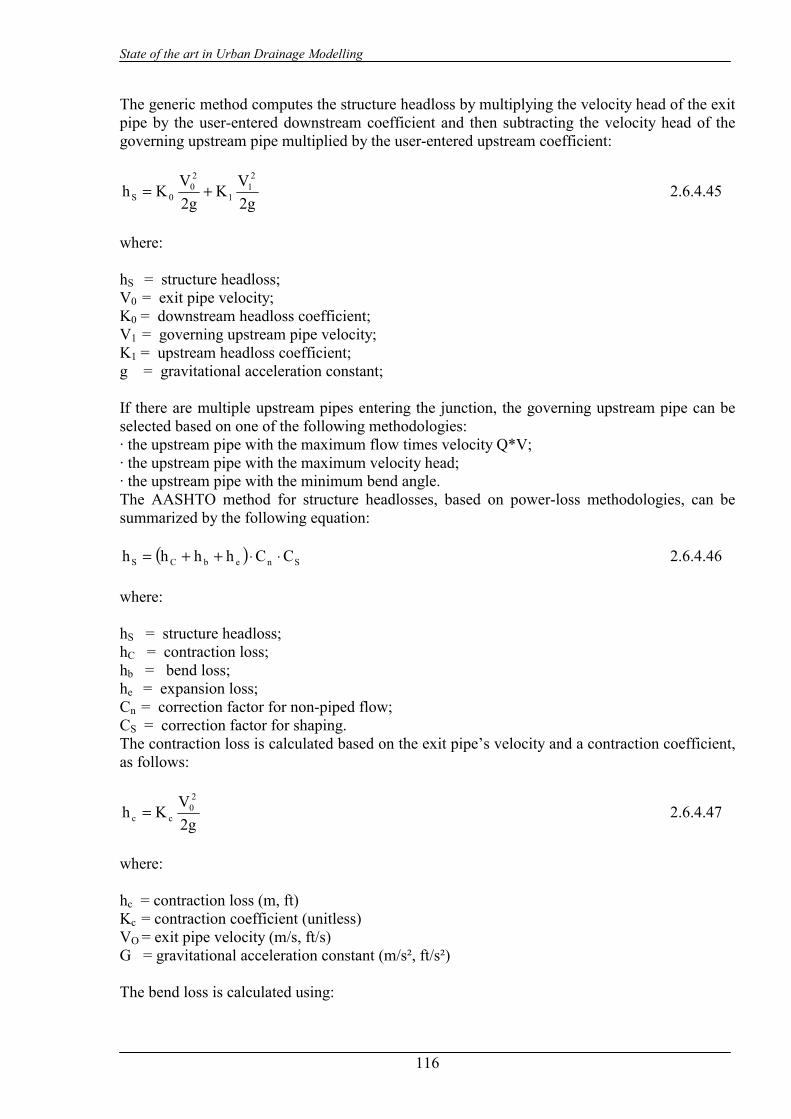
State of the art in Urban Drainage Modelling
116
The generic method computes the structure headloss by multiplying the velocity head of the exit pipe by the user-entered downstream coefficient and then subtracting the velocity head of the governing upstream pipe multiplied by the user-entered upstream coefficient:
g2VK
g2V
Kh2
11
20
0S += 2.6.4.45
where: hS = structure headloss; V0 = exit pipe velocity; K0 = downstream headloss coefficient; V1 = governing upstream pipe velocity; K1 = upstream headloss coefficient; g = gravitational acceleration constant; If there are multiple upstream pipes entering the junction, the governing upstream pipe can be selected based on one of the following methodologies: · the upstream pipe with the maximum flow times velocity Q*V; · the upstream pipe with the maximum velocity head; · the upstream pipe with the minimum bend angle. The AASHTO method for structure headlosses, based on power-loss methodologies, can be summarized by the following equation:
( ) SnebCS CChhhh ⋅⋅++= 2.6.4.46 where: hS = structure headloss; hC = contraction loss; hb = bend loss; he = expansion loss; Cn = correction factor for non-piped flow; CS = correction factor for shaping. The contraction loss is calculated based on the exit pipe’s velocity and a contraction coefficient, as follows:
g2V
Kh20
cc = 2.6.4.47
where: hc = contraction loss (m, ft) Kc = contraction coefficient (unitless) VO = exit pipe velocity (m/s, ft/s) G = gravitational acceleration constant (m/s², ft/s²) The bend loss is calculated using:

State of the art in Urban Drainage Modelling
117
−−=g2
VQ
Q)K1(g2
Vh
2i
0
ii20
b 2.6.4.48
where: hb = bend loss; V0 = outflow pipe velocity; Q0 = outflow pipe velocity; Vi = inflow pipe velocity; Qi = inflow pipe flow; g = gravitational acceleration constant; Ki = bend factor. Expansion losses are computed using the following equation, in which the most significant pipe is the pipe that has the greatest product of velocity and discharge, omitting any pipes that have a discharge less than 10% of the structure’s outflow :
g2V
Kh2
See = 2.6.4.49
where: he = expansion loss; Ke = expansion coefficient; Vs = most significant incoming pipe’s velocity; g = gravitational acceleration constant. Finally, if non-piped flow accounts for 10% or more of the total structure outflow, a correction factor can be applied to the total loss, and if the bottom of the structure is shaped to facilitate smoother transitions from inflow pipes to the discharge pipe, a correction factor can be applied to the total loss. In the program the described coefficients defaults to the documented values as defined in the AASHTO Model Drainage Manual, but can be changed by the user. The HEC-22 energy method correlates structure headloss to the velocity head in the outlet pipe using an experimental coefficient, approximated by:
BpQdDO CCCCCKK = 2.6.4.50 where: K = adjusted headloss coefficient; KO = initial headloss coefficient based on relative junction size; CD = correction factor for the pipe diameter; Cd= correction factor for flow depth; CQ= correction for relative flow; Cp=correction for plunging flow; CB=correction factor for benching.

State of the art in Urban Drainage Modelling
118
The special assumpions under which the HEC-22 energy method can be used and the equations used to calculate the headloss coefficient and the correction factors can be found in FHWA’s Urban Drainage Design Manual, Hydraulic Engineering Circular No. 22. SewerCAD allows to automatically design gravity piping and structures: it is possible to specify the elements to be designed, from a single pipe size to the entire system, or anything in between. The design algorithm adjusts structure invert elevations and the section size of the pipe to meet several constraints, such as allowable ranges of slope, velocity and cover. In general, the design algorithm attempts to minimize pipe size and excavation, which is typically the most expensive part of installing sewer piping and structures. The pipes design is carried out selecting a percentage of fulfilment and choosing the smallest available pipe whose part-full capacity is greater than the required discharge. If the desired capacity cannot be met with a single pipe, the pipe can be designed with multiple barrels having the same physical characteristics: the design is carried out increasing the number of barrels and attempt to find a section size that meets the capacity, continuing until the capacity is met or the maximum number of barrels is reached. It is also possible to design limiting the size of the designed pipe. Generally the design is done so that all the designed pipes entering a structure have the same invert elevation or crown elevation, even if different elevation can be considered for the incoming pipes; if an offset value is specified, the upstream pipes will be higher than the downstream pipe by the specified offset. The program can also adjust structure bottom elevations to account for the invert elevations of newly designed pipe. The length of any inlet can be automatically designed: the design algorithm uses the same equations used in analysis to determine the minimum available inlet length that meets the design constraints. For inlets in sag, the inlet length selected in an automatic design will be the smallest length that will generate a spread and a depth at the curb less than the maximums specified; in a case where the constraints cannot be met with any of the available lengths, the largest inlet length possible will be chosen. For inlets on grade, the inlet length selected is the smallest length that will generate inlet efficiency larger than the minimum specified. If the minimum efficiency cannot be met with any of the lengths, the largest of the available lengths will be selected. Finally, SewerCAD allows calculating a planning level estimate of the capital costs associated with an entire system or any portion of a system. The costs associated with a particular element are broken down into two categories: construction costs and non-construction costs. Each construction cost item is expressed as a combination of a quantity, unit, and unit cost; the total cost associated with a single construction cost item is the quantity multiplied by the unit cost. The unit cost for each construction cost item can either be entered directly, or if the element is a pipe or gravity structure it can be calculated based on a unit cost function, which relates a property of the element, such as the diameter of a pipe, to the unit cost, so that the cost of the element is automatically updated when modifying the physical characteristics of the system. The unit cost function can be specified as either tabular data or as a formula:
b)cx(adCost −+= 2.6.4.51 where: Cost = linear cost of the pipe; X = selected attribute; a,b,c,d = user specified parameters.
State of the art in Urban Drainage Modelling
119
Non-construction costs are specified as either a lump sum or as a percentage of the total construction costs. The total cost for each element is simply the sum of the total construction and non-construction costs. The total cost for a network is computed by summing the total cost for every element selected to be included in the cost analysis.
2.6.5. Model Parameters Estimation or Assignation SewerCAD does not apply any deterministic and/or statistical procedure aimed to parameter sensitivity analysis, automated calibration or uncertainty estimation. Some parameters can be assigned referring to typical values proposed in an engineering library providing specifications for roughness coefficients for the available friction loss methods.
2.6.6. PI(s) Estimation Method The performance indicators listed before cannot be evaluated directly in the model framework but must be calculated as functions of the model outputs. SewerCAD gives as an output the full capacity, the design capacity (for fixed degree of fulfilment) and the total flow for each gravity pipe, so that the length of sewer where surcharging, or high surcharging, occurs, in dry or wet weather, can be calculated and the wPh5, wPh6 and wPh7 indicators can be computed. The hydraulic grades at inlet and junctions can be also evaluated from output data: when the hydraulic grade is greater than the ground elevation at a non bolted junction, a flooding occurs, so that the frequency of surface flooding can be known and the wOp35 indicator can be calculated. StormCAD allows estimating of the construction and non construction costs associated with an entire system or any portion of a system: the cost of investments for new asset and expansion of existing network can be evaluated, and the wFi20 indicator can be computed.
2.6.7. Future Improvements of the Model No other information about future model developments is available by now.
2.6.8. References
2.6.8.1 Theoretical Framework References AASHTO Model Drainage Manual, American Association of State Highway and Transportation Officials, 1991. Benedict, Robert P. Fundamentals of Pipe Flow. New York: John Wiley & Sons; 1980. Brater, Ernest F.; King, Horace Williams. Handbook of Hydraulics. New York: McGraw-Hill Book Company; 1976. Brown, S.A., S.M. Stein, and J.C. Warner, Urban Drainage Design Manual. Hydraulic Engineering Circular No. 22, U.S. Department of Transportation, Federal Highway Administration, Washington, D.C., 1996. Chow, Ven Te. Open-Channel Hydraulics. New York: McGraw-Hill Book Company; 1959. Computer Applications in Hydraulic Engineering. Second Edition. Connecticut: Haestad Press; 1998. D. Earl Jones, Jr. Design and Construction of Sanitary and Storm Sewers. ASCE Manual of Practice, No. 37; 1970. Essential Hydraulics and Hydrology. Connecticut: Haestad Press; 1998. Featherstone, R.E.; Nalluri, C. Civil Engineering Hydraulics. New York: Granada. FHWA'. HEC-12 Drainage of Highway Pavements, Washington, D.C., 1984.

State of the art in Urban Drainage Modelling
120
French, Richard H. Open-Channel Hydraulics. New York: McGraw-Hill Book Company; 1985.Hwang, Ned H. C.; Hita, Carlos E. Hydraulic Engineering Systems. New Jersey: Prentice-Hall, Inc.; 1987. Hydraulic Research Station, Velocity Equations for Hydraulic Design of Pipes, Metric Edition, HMSO, London, 1951 (10/81). Hydrology, Federal Highway Administration. HEC No. 19; 1984. Roberson, John A., John J. Cassidy, and Hanif M. Chaudhry, Hydraulic Engineering, Houghton Mifflin Company, Massachusetts, 1988. Simon, Andrew L., Practical Hydraulics, John Wiley & Sons, Inc., New York, 1976. Streeter, Victor L. and Wylie, E. Benjamin, Fluid Mechanics, McGraw-Hill Book Company, New York, 1985. Wanielista, Martin P. Hydrology and Water Quantity Control. New York: John Wiley & Sons; 1990. Zipparro, Vincent J.; Hasen, Hans. Davis’ Handbook of Applied Hydraulics. New York: McGraw-Hill Book Company; 1993.
2.6.8.2 Practical Use and Results References CulvertMaster User’s Guide. Connecticut: Haestad Methods; 1998. FlowMaster PE Version 6.0 User’s Guide. Connecticut: Haestad Methods; 1998. http://www.haestad.com/software/ Practical Guide to Hydraulics and Hydrology. Connecticut: Haestad Press; 1997. StormCAD 4.1.1 User’s Guide. Connecticut: Haestad Methods; 2000.

State of the art in Urban Drainage Modelling
121
2.7 SIMPOL3
2.7.1. Model availability SIMPOL3 is a WRc product, for technical queries contact [email protected] The software is not commercially available at present.
2.7.2. Abstract
2.7.2.1 Objectives and peculiarities SIMPOL3 is an integrated, environmental modelling package which includes modules for urban drainage planning. It is used for investigating the water quality impacts caused by urban drainage systems and for identifying outline solutions which meet specified emission and environmental standards. It represents runoff, storage and water quality processes in drainage systems and associated watercourses using relatively simple algorithms. It includes both deterministic and stochastic elements and allows fast, continuous simulation. Typical runs will take minutes for multi-year simulations. This section, covering the urban drainage quantity aspects of SIMPOL3 should be read in conjunction with sections on the urban water quality and waterbody impact aspects.
2.7.2.2 Performance Indicator(s) of Interest SIMPOL relates to wPh7 (surcharging), wEn3, 4 & 5 (intermittent discharges).
2.7.3. Usage Specifications
2.7.3.1 Functionality SIMPOL3 simulates the hydrology/hydraulics of large complex drainage systems in a simplified state. The model is based upon data held in a detailed hydraulic model. The key hydraulic features in the detailed model are first identified and then conceptualised in a way which can be represented in a SIMPOL3 model. The conceptualisation creates separate subcatchments to represent distinct areas of the network which are controlled by significant throttles. A lumped parameter approach is used to represent runoff, attenuation and storage processes within subcatchments with no explicit representation of individual pipes. The parameters are calibrated by comparing the SIMPOL3 results against those from the detailed hydraulic model for a number of selected storm events with different characteristics. Rain-induced infiltration can also be included. The throttle and overflow processes are represented in some detail. Other modules which can be included in the network include offline storage tanks, pumping stations, bifurcations and large interceptor sewers. The model has the ability to represent “backing up” in a system by controlling the output from a subcatchment based upon the performance of another module– a number of RTC rules can be represented including complex emptying routines. The model simulates at an hourly time-step and runs continuously for multi-year periods
2.7.3.2 Possible interaction with other software tools SIMPOL3 is an integrated model which includes quantity and quality simulation within drainage systems and associated river systems. SIMPOL3 can accept input time-series of

State of the art in Urban Drainage Modelling
122
flows/quality generated by other models and can provide output for use in other models. The possibility of direct calls to other software exists (a current application includes a direct call to an estuary water quality model allowing both models to run together).
2.7.4. Input and Output procedures
2.7.4.1 Possible Input File(s) Formats All input files are held in MS Access database tables. Any timeseries input can be accepted in a tabular format – date/time, variable1, variable2 etc.
2.7.4.2 Possible Output File(s) Formats SIMPOL3 generates timeseries output for any specified list of variables. The output is in a format: Date/Time, Variable1, Variable2 etc at hourlt timesteps over the complete simulation period. The output can be exported as .csv, .txt, .xls or as MS Access tables. The ‘quantity’ type output includes:
• Flows (passforward and spill flows) • Water levels/volume in storage tanks
2.7.4.3 Raw Data Formatting Model data defining the model network is extracted and inserted manually into the Access database. The detailed model data can be extracted in tabular format and then manipulated using Excel to input into the SIMPOL3 database.
2.7.5. Theoretical framework Overview SIMPOL3 uses a lumped parameter approach to represent runoff and attenuation processes within sewer subcatchments. It also uses simplified algorithms to represent key hydraulic control points (e.g. pumping stations, orifices, pipe restrictions) and the filling/emptying of storages.
2.7.6. Model Parameters Estimation or Assignation The hydraulic algorithms in SIMPOL3 are calibrated by comparing the predicted flows against those from a detailed hydraulic model. A manual process is used to adjust parameters to give a best fit over a wide range of different storm types. The fit is judged subjectively.
2.7.7. References
2.7.7.1 Theoretical Framework References Williams W, Murrell K. (2001). Fast Track Urban Pollution Planning. Wastewater 2001 – A treatment and Disposal Odyssey. CIWEM 17 October 2001 Crabtree R.W., Dempsey P, Walwyn R (2003). Simplified integrated modelling of a large conurbation – the River Tame catchment case study. IMUG conference May 2003 (in preparation)

State of the art in Urban Drainage Modelling
123
2.8 COSMOSS
2.8.1. Model availability COSMOSS is a freeware model and is available through the developer at the Department of Mecanics and Materials – University of Reggio Calabria (Italy) ([email protected]).
2.8.2. Abstract
2.8.2.1 Objectives and peculiarities Summarize in few lines the main objectives (design, planning procedures, existing systems analysis) and nature of the model. Briefly describe the peculiarities of the model with respect to the task of CARE-S project (availability of long term simulation option, processes that can be simulated, ecc.). COSMOSS is a conceptual model both in the flow simulation part(i.e., the rainfall-runoff transformation and the subsequent propagation) and in the qualitative one(i.e., the build-up and the washoff of solids). The model has been tested using experimental data acquired in Parco d’Orleans catchment, Palermo, in Fossolo catchment, Bologna, and in Milijakovac catchment, Belgrade. The system (catchment and channels) is considered as a whole. The model can be divided into four parts:
• calculation of hydrological losses; • rainfall-runoff transformation and runoff propagation; • build-up of solids during dry weather • washoff.
The main goal of the model is to simulate the water quality in the best way possible.
2.8.2.2 Performance Indicator(s) of Interest COSMOSS is able to evaluate the basic flow variables such as discharge, pollution load. This kind of data can be used for computing physical and operational performance indicators, even if the model does not compute the PIs directly.
2.8.3. Usage Specifications
2.8.3.1 Programming Language(s) or Mathematical-Statistical Software(s) The source code has been written is Visual Basic.
2.8.3.2 Functionality To calculate hydrological losses the model considers primarily the loss due to retention in small reservoirs and after all the others combined into a runoff coefficient. It is necessary to take into account the retention losses in small ponds because the first part of the hydrograph, which is deeply influenced by this kind of loss, is really important for the first flush simulation. The other hydrological losses (for example, infiltration) are less important in

State of the art in Urban Drainage Modelling
124
the catchments considered in this study (catchment are totally or mainly impervious), so it is possible to take them in account as a whole by a runoff coefficient. The system (catchment and channels) is considered as a whole. To simulate the rainfall-runoff transformation COSMOSS uses the well-known linear reservoir method (see La Loggia & Viviani, 1990; Desbordes, 1975). Obviously not all urban catchments behave linearly. In case of non-linear behaviour the method does not fit with the physical reality and this can lead to large errors. The linear reservoir method has been chosen because of its widespread use throughout the world and because several formulations are available for reliably calculating the reservoir constant without any calibration (Desbordes, 1975). No RTC function is available.
2.8.3.3 Possible interaction with other software tools The software can interact with Excel and other MS Office tools.
2.8.4. Input and Output procedures
2.8.4.1 Possible Input File(s) Formats Formatted text input file.
2.8.4.2 Possible Output File(s) Formats Formatted text output file.
2.8.4.3 Raw Data Formatting Raw data can be used only modifying the source code.
2.8.5. Theoretical framework Overview To simulate the rainfall-runoff transformation COSMOSS uses the linear reservoir method that is characterized by the equation:
dQK
tWtQ += )()( 2.8.5.1
where: Q = discharge through the considered section (m3/s) W = volume accumulated upstream the considered section (m3) K = constant of the reservoir (s-1) Qd = average discharge during dry weather (m3/s). The instantaneous unit hydrograph of this model is:
)/(1)( KteK
tu −= 2.8.5.2
The convolution integral is:
∫ −−=*
0
/)( )(1)(τ τ ττ dIe
KtQ Kt 2.8.5.3
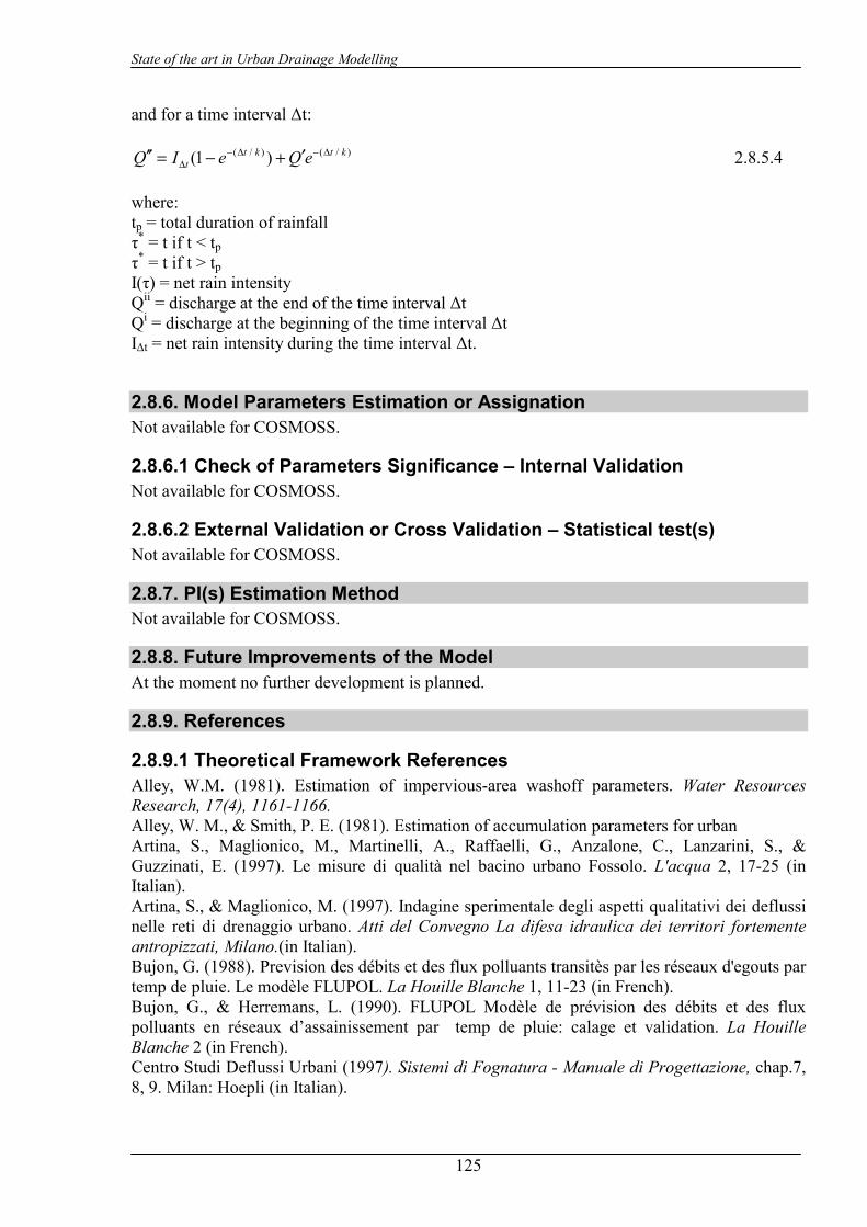
State of the art in Urban Drainage Modelling
125
and for a time interval ∆t:
)/()/( )1( ktktt eQeIQ ∆−∆−
∆ ′+−=′′ 2.8.5.4 where: tp = total duration of rainfall τ* = t if t < tp τ* = t if t > tp I(τ) = net rain intensity Qii = discharge at the end of the time interval ∆t Qi = discharge at the beginning of the time interval ∆t I∆t = net rain intensity during the time interval ∆t.
2.8.6. Model Parameters Estimation or Assignation Not available for COSMOSS.
2.8.6.1 Check of Parameters Significance – Internal Validation Not available for COSMOSS.
2.8.6.2 External Validation or Cross Validation – Statistical test(s) Not available for COSMOSS.
2.8.7. PI(s) Estimation Method Not available for COSMOSS.
2.8.8. Future Improvements of the Model At the moment no further development is planned.
2.8.9. References
2.8.9.1 Theoretical Framework References Alley, W.M. (1981). Estimation of impervious-area washoff parameters. Water Resources Research, 17(4), 1161-1166. Alley, W. M., & Smith, P. E. (1981). Estimation of accumulation parameters for urban Artina, S., Maglionico, M., Martinelli, A., Raffaelli, G., Anzalone, C., Lanzarini, S., & Guzzinati, E. (1997). Le misure di qualità nel bacino urbano Fossolo. L'acqua 2, 17-25 (in Italian). Artina, S., & Maglionico, M. (1997). Indagine sperimentale degli aspetti qualitativi dei deflussi nelle reti di drenaggio urbano. Atti del Convegno La difesa idraulica dei territori fortemente antropizzati, Milano.(in Italian). Bujon, G. (1988). Prevision des débits et des flux polluants transitès par les réseaux d'egouts par temp de pluie. Le modèle FLUPOL. La Houille Blanche 1, 11-23 (in French). Bujon, G., & Herremans, L. (1990). FLUPOL Modèle de prévision des débits et des flux polluants en réseaux d’assainissement par temp de pluie: calage et validation. La Houille Blanche 2 (in French). Centro Studi Deflussi Urbani (1997). Sistemi di Fognatura - Manuale di Progettazione, chap.7, 8, 9. Milan: Hoepli (in Italian).

State of the art in Urban Drainage Modelling
126
Deletic, A., Maksimovic, C., & Ivetic, M. (1997). Modelling of Storm Wash-off of Suspended Solids from Impervious Surfaces. Journal of Hydraulic Research (IAHR), 35(1). Desbordes, M.(1975). Un essai de modélisation des phénomènes de ruissellement pluvial urbain. T.S.M. L'EAU 3, 121-126 (in French). Huber, C., & Dickinson, R.E. (1988). Storm Water Management Model: User’s Manual. U.S. EPA/600/3-88/001a. Athens: Georgia (USA). La Loggia, G., & Viviani, G. (1990). Controllo, verifica e calibrazione di modelli di piena in un bacino urbano in Sicilia. Atti del XXII Convegno di Idraulica e Costruzioni Idrauliche, Cosenza (Italy) (in Italian). La Loggia, G., Cannarozzo, M., & Oliveri, E. (1996). Riconfigurazione del bacino sperimentale di Parco d'Orleans in base all'analisi di eventi storici. Atti del seminario nazionale Modelli di dimensionamento e di qualità per le fognature urbane, Sorrento (Italy)11-14 giugno 1996 (in Italian). Marinelli, A., Maglionico, M., & Artina, S. (1996). Simulazione della qualità delle acque in un bacino sperimentale di drenaggio urbano. Atti del XXV Convegno di Idraulica e Costruzioni Idrauliche , Torino(Italy) (in Italian). Nakamura, E. (1990). Characteristics of wet weather combined sewage - Information to the design and operation of improved systems. Proceedings of the V International conference in urban storm drainage, Osaka (Japan). Xanthopoulos, C., Hahn, H.H.(1993). Anthropogenic pollutants wash-off from street surfaces. Proceedings of the VI International Conference on Urban Storm Drainage; (Niagara).

State of the art in Urban Drainage Modelling
127
2.9 DORA/Double ORder Approximation method
2.9.1. Model availability The model has two parts: the first one is a pre and post processor that prepares the input file for the numerical engine and displays the computed results. The second part is the numerical engine. The software house that produces the first part is the “Ars Nova Multimedia” and is located in Reggio Calabria (Italy). Its web site is www.arsnova.biz. A short guide for the use of the model is easily accessible from the model itself.
2.9.2. Abstract
2.9.2.1 Objectives and peculiarities The object of the model is the existing system analysis, by means of simulation of water depths and velocities occurring in one or two drainage networks due to a time series of rainfall data and to domestic or industrial dicharges. One of the two drainage networks can be the street network, that is coupled with the underground sewer network through the water inlets. The model assumes the diffusive hypothesis and this implies that the boundary conditions are always the fluxes in the upstream nodes and the water level in the downstream nodes. The model can be used to plan a new network, a new part of an existing one or to evaluate the flooded areas during storm events. Using a project hydrograph, it is possible to test the efficiency of the upstream part of the network by assigning kinematic outflow boundary conditions at the downstream nodes. The model is unconditionally stable with respect to the size of the time step and this allows long-term simulations.
2.9.2.2 Performance Indicator(s) of Interest • wEn3 Intermittent overflow discharge frequency • wEn4 Intermittent overflow discharge volume • wEn5 Intermittent overflow discharge related to rainfall • wPh5 Surcharging in sewers in dry weather • wPh6 Surcharging in sewers in wet weather • wPh7 High sewer surcharging
2.9.2.3 Brief Historical Overview of the Model The DORA methodology is a numerical technique developed by T. Tucciarelli and other co-authors (L. Noto, D. Termini and others) for the solution of partial differential equations having a scalar potential of the flow field. The computation of the unknowns at a new time level is split in a prediction step and in a correction step. The prediction step is given by the solution of a sequence of ordinary differential equations, one for each computational node of the network. The correction step is given by the solution of a system of linear partial differential equations, that is obtained using a fully implicit finite difference discretization. The DORA technique can be applied to the water depths and velocities computation in a drainage pipe network if the diffusive hypothesis is adopted in the momentum equation, even if extension to the original complete problem has also been proposed by the same author. The main advantages of the technique are: 1) the unconditional stability with respect to the size of
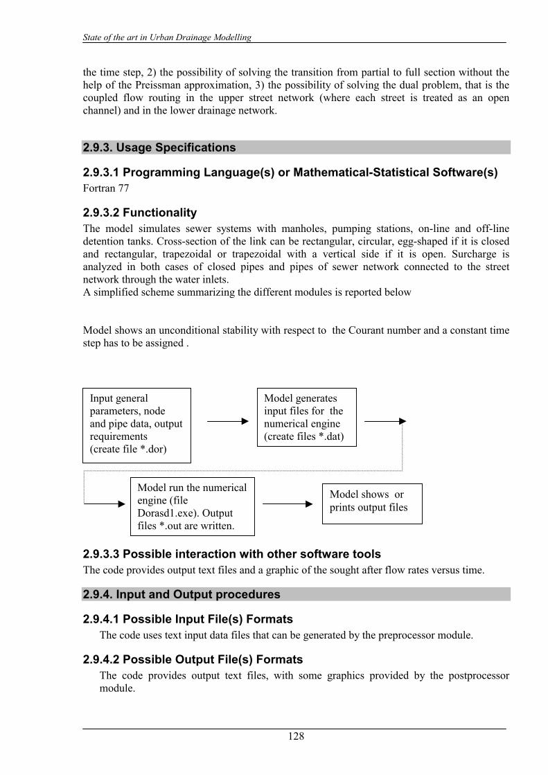
State of the art in Urban Drainage Modelling
128
the time step, 2) the possibility of solving the transition from partial to full section without the help of the Preissman approximation, 3) the possibility of solving the dual problem, that is the coupled flow routing in the upper street network (where each street is treated as an open channel) and in the lower drainage network.
2.9.3. Usage Specifications
2.9.3.1 Programming Language(s) or Mathematical-Statistical Software(s) Fortran 77
2.9.3.2 Functionality The model simulates sewer systems with manholes, pumping stations, on-line and off-line detention tanks. Cross-section of the link can be rectangular, circular, egg-shaped if it is closed and rectangular, trapezoidal or trapezoidal with a vertical side if it is open. Surcharge is analyzed in both cases of closed pipes and pipes of sewer network connected to the street network through the water inlets. A simplified scheme summarizing the different modules is reported below Model shows an unconditional stability with respect to the Courant number and a constant time step has to be assigned .
2.9.3.3 Possible interaction with other software tools The code provides output text files and a graphic of the sought after flow rates versus time.
2.9.4. Input and Output procedures
2.9.4.1 Possible Input File(s) Formats The code uses text input data files that can be generated by the preprocessor module.
2.9.4.2 Possible Output File(s) Formats The code provides output text files, with some graphics provided by the postprocessor module.
Input general parameters, node and pipe data, output requirements (create file *.dor)
Model generates input files for the numerical engine (create files *.dat)
Model run the numerical engine (file Dorasd1.exe). Output files *.out are written.
Model shows or prints output files
State of the art in Urban Drainage Modelling
129
2.9.4.3 Raw Data Formatting The model reads the data in free format. The order of the data must be, of course, the one expected by the program.
2.9.5. Theoretical framework Overview The code computes the numerical solution of the 1D shallow water equations in the diffusive form. It enforces a fractional step methodology that solves sequentially one prediction and one correction half time step. The dependant variables of the model are water depth and flow velocity. Sewer system is idealized as a series of links connected at nodes or cells. These ones are the storage elements of the system; some of them correspond to manholes or pipe junctions in the physical system, or more frequently to simple computational nodes. The computational cell is given by the sum of the half links sharing the same node. Water depths are calculated for each computational cell and velocities are calculated for each link. In the prediction step the hydraulic gradient is kept constant along the time; this allows a sequential solution of the resulting ordinary differential equations, one computational cell after the other. In the correction step a diffusive linear problem is solved using a fully implicit finite difference scheme, also to estimate the backwater effect of the channel resistance. The proposed numerical scheme can be proved, according to a linear approximation, to be unconditionally stable. This allows to solve the transition from partial to full section without the help of the Preissman approximation. The solution of the dual problem, where the upper street network and the lower sewer networks are dynamically coupled, is obtained assuming a constant flow in the vertical links (corresponding to the inlets) during the prediction step and a flux linearization with respect to the hydraulic gradient during the correction step.
2.9.6. Model Parameters Estimation or Assignation Sensitivity analysis, calibration, sensitivity estimation and validation have to be done manually by the user.
2.9.7. PI(s) Estimation Method • wEn3 Intermittent overflow discharge frequency: model allows to compute the water flux
exceeding a maximum flow rate in a given link. • wEn4 Intermittent overflow discharge volume: the same as in the previous point, after time
numerical integration of the exceeding flow rates. • wEn5 Intermittent overflow discharge related to rainfall: the same as in the previous points. • wPh5 Surcharging in sewers in dry weather: the surcharged length can be estimated as the
sum of the lengths of the links with a maximum (in time) filling ratio equal to one. • wPh6 Surcharging in sewers in wet weather: the same as in the previous point. • wPh7 High sewer surcharging: the same as in the previous point.
2.9.8. Future Improvements of the Model The developments will be mainly focused on the interaction between the GIS and the DORA environment and on the links with other programs.
State of the art in Urban Drainage Modelling
130
2.9.9. References
2.9.9.1 Theoretical Framework References • Tucciarelli T. and Fedele F. (2000). An efficient double order solution of the groundwater
contaminant transport problem. Proc., 13th Int. Conf. On Computational Methods in Water Resourc.
• Noto V. and Tucciarelli T. (2001). DORA Algorithm for network flow models with improved stability and convergence properties. J. of. Hydr. Eng., ASCE, 127(5), 380-391.
• Tucciarelli T. (2003), A new algorithm for a robust solution of the fully dynamic De Saint Venant equations. To appear in J. of Hydr. Res., 41(3).
2.9.9.2 Practical Use and Results References
State of the art in Urban Drainage Modelling
131
2.10 Pre – competitive urban drainage flow models
2.10.1. Introduction A lot of effort has been provided by several research groups in developing new approaches to drainage pipe flow simulation. The research trends in the last 10 years were addressed to two opposite approaches: on one hand new complex models have been developed in order to take into account the physicalness of the real propagation phenomenon; on the other hand very simple conceptual models have been developed in order to greatly increase the computational efficiency, allowing for a larger number of simulations needed for planning and optimization procedures. Mathematical models play a major role in designing and improving storm water collection systems. Simulation results are widely used for planning, designing, and operational purposes. Stability, speed, size, and accuracy of the models for sewer/channel networks, however, are major concerns in current engineering practice. The diversity of the problems to be solved makes it impossible to reach all of the objectives with only one tool. In fact two main families of models are available:
• The first family consists of hydrological models. The flow is computed as a function of time at one location along watercourse. The prototype of this category is the Muskingum model. These models are very simple to use, even for people who are not hydraulicians, need very few data and are very quick to run. On the other hand, they are truly unable to represent the effects of transitional flows due to problems of hydraulics or inconsistencies of networks.
• The second family consists of physically based models or distributed flow models. They are based on the complete differential equations of one-dimensional unsteady flow (the Barre de Saint Venant equations).This equations allow the flow rate and water level to be computed as a function of space and time rather than time alone as a lumped flow routing methods. This kind of model needs some important hypotheses which are not always verified in sewer systems. Anyway, they are able, in most cases, to give a correct description of gradually varied flows. The main problems with these models are the great number of data they require, the difficulty to build stable numerical schemes, their slowness, and the difficulties in interpretation of results.
2.10.2. Hydrological models Hydrological models are generally based on the conservation of mass only. The principle of mass conservation requires the difference between the inflow I at the upstream and the outflow Q at the end of the watercourse, functions of the time, to be equal to the time rate of change of the storage S within the reach, i.e.,
dtdStQtI =− )()( 2.10.2.1
The storage S is related to I and/or Q by an arbitrary empirical storage function. The most simple is a single-valued function of outflow Q, i.e., )(QfS = , or of water-surface elevation h, i.e., )(hfS = .This implies the water surface is level throughout the watercourse. A more complex relationship exists for long narrow reservoir or open channel where storage is a function of both inflow and outflow. Solution of (1) for Q(t) with various approximations for the storage constitutes lumped flow methods. The attractiveness of lumped flow method is its relative simplicity compared with distributed flow method. However, these models neglected
State of the art in Urban Drainage Modelling
132
the backwater effects and they are truly unable to represent the effects of transitional flows due to problems of hydraulics or inconsistencies of networks. The prototype of the hydrological models is the Muskingum model.
2.10.2.1 Muskingum model In the Muskingum model, it is recognized that the storage in a conduit depends on the inflow as well as the outflow. It is assumed that the storage is a linear function of inflow and outflow, such that:
))1(( QXXIKS −−= 2.10.2.2 in which K and X are empirical constants to be determined by trial and error. The time rate of change of storage dS/dt in 2.10.2.2 is represented as follws:
[ ] [ ] t
QXXIQXXIKt
SSdtdS jjjjjj
∆−+−−+=
∆−=
+++ )1()1( 111
2.10.2.3
where the subscripts j and j+1 denote the times separated by the interval t∆ . Substituting 2.10.2.3 into 2.10.2.2 yields the following:
jjjj QCICICQ 321
11 ++= ++ 2.10.2.4
in which is the Muskingum flow routing equation, where
tXKKXtC
∆+−−∆=
)1(22
1
tXKKXtC
∆+−+∆=
)1(22
2 2.10.2.5
tXKtXKC
∆+−∆−−=
)1(2)1(2
3
and where 1321 =++ CCC and KtK ≤∆≤3
is usually the range of t∆ .
The Muskingum method sometimes produces unrealistic initial negative dips in the computed hydrograph; however, it provides reasonably accurate results for, moderate to slow flood propagating through mild steep sloping watercourses. The Muskingum method is a kinematic-type routing model, and so, as well as the kinematic method, is unable to simulate the backwater effects. Beyond to the Muskingum model there are other several lumped flow methods, we can remember: SSARR ( Miller, W.A., and J.A.Cunge, „Simplified Equations of Unsteady Flow” in K. Mahmood and V.Yevjevich) , Kalinin-Miljukov, Tatum (Fread, D.L.,”Channel Routing” in M.G.Anderson and T.P.Burt).
2.10.3. Physically based models Propagation of unsteady, gradually varied, flow through sewer pipes can be most accurately described as a distributed process because the flow rate, velocity and depth vary in space (at cross sections along the pipe).Estimates of these properties in a channel system can be obtained
State of the art in Urban Drainage Modelling
133
by using distributed flow routing based on the numerical solution of the continuity and momentum Saint Venant equations.
0=−∂∂+
∂∂ q
tA
xQ (continuity equation) 2.10.3.1
)( 0 fSSgtv
xvv
xhg −=
∂∂+
∂∂+
∂∂ (momentum equation) 2.10.3.2
where Q is the discharge, x is the horizontal distance, A is the cross-sectional flow area, t is the time, q is the lateral inflow or out flow distributed along the x axis of the pipe, g is the gravitational acceleration, h is the water depth, v is the flow velocity, oS is the pipe invert slope and fS is the friction slope. These equations are valid for open channel flows, but can be extended to surcharged flows by adding a fictitious narrow slot on top of the closed conduit, as first suggested by Preissmann and developed by Cunge and Wegner (1964). When the pipe is full, the imaginary water level within this slot represents the piezometric head. Since the wave speed in the Saint equations is inversely proportional to the water surface width, use of narrow slot leads to high wave speeds, as encountered in pressurized flow (Ball, 1985). Many simplifications can be made to the Saint Venant equations according to the specific flow conditions to be simulated. A first approximation the kinematic wave model, assumes that all terms of the left-hand side of the momentum equation are insignificant.
0)( 0 =− fSS 2.10.3.3 This last simplification can easily be solved, but is not applicable when backwater conditions prevail. To take advantage of the computational speed of the kinematic wave approximation, some operational sewer models use it to compute flows as long as they remain lower than the maximum free surface capacity of the pipes. If flows computed by the kinematic wave exceed this boundary, the model switches to a simple pressurized algorithm to route flows and water levels in all conduit affected by the overloading. The SURKNET model of Pansic and Yen (1982) and SERAIL model of Chocat, Barraud, and Thibault (1983) apply this kind of approximation. Another approximation of the Saint Venant equations, the diffusion wave (zero-inertia) model, it is obtained by neglecting the convective and local accelerations in the momentum equation (( xv ∂∂ / ) and ( tv ∂∂ / ) = 0).
)( 0 fSSxh −=
∂∂ 2.10.3.4
This type of simplified routing model considers backwater effects but improperly distributes them instantaneous (in time) throughout the total routing reach; its accuracy is also deficient for very fast rising hydrographs. So, a sever limitation of these models is that they cannot take into account backwater effects other than those caused by surcharged flows and that they oversimplify the transition between free surface and pressurized flow. Distributed flow routing based on the numerical solution of the complete Saint Venant equations is commonly known as dynamic routing. Dynamic routing models can be classified as characteristic and direct methods of solving the Saint Venant equations. In the characteristic methods, these equations are first transformed into an equivalent set of four ordinary differential equations which are then approximated with finite

State of the art in Urban Drainage Modelling
134
differences to obtain solutions. Characteristic methods have not proved advantageous over the direct methods for practical flow routing applications. Direct methods can be classified further as either explicit or implicit. Explicit scheme transform the differential equations into a set of algebraic equations which are solved sequentially for the unknown flow properties at each cross section at a given time. Implicit schemes transform the Saint Venant equations into a set of algebraic equations which must be solved simultaneously for all x∆ computational reaches at a given time; this set of simultaneously equations may be either linear or nonlinear, the latter requiring an iterative solution procedure. Explicit schemes are simple and can be easily used to formulate a general network model for sewer/channel system. The explicit schemes, however, require a small time step and a minimum pipe length, as imposed by Courant criterion. This limits the computational speed of models using explicit schemes. Due to the limitations of the explicit schemes, many models have been developed in recent years using implicit schemes (Amein, 1968; Fread, 1973; Strelkoff, 1973; Prince, 1974; Joliffe, 1984; Nguyen and Kawano, 1995). The implicit schemes, in fact, allow for larger time step, even if the solution technique requires more computation time per time step. The research, in fact, indicates that the implicit schemes are mathematically more sophisticated in formulating a looped network. Some distributed flow routing models are briefly described below.
2.10.3.1 Preissmann Box Scheme A four-point implicit scheme, also called the Preissmann Box Scheme, is usually adopted. The scheme results in a sparse matrix equation for complete unsteady flow equations. The equations are then solved implicitly for flows and depths throughout a network system over a time step based on sewer/channel network connectivity and boundary conditions.
2.10.3.2 FLUSS The flow in urban sewer system (FLUSS) model (Calenda, Campisano and Modica, 1999) considers the fully-dynamic De Saint Venant equations, numerically solved by using the McCormack scheme (Garcia-Navarro et al., 1992a) with an additional procedure based on the theory of Total Variation Diminishing (TVD) (Garcia-Navarro et al., 1992b). The McCormack scheme is a "shock capturing" scheme, i.e. it is able to simulate internal discontinuities such as hydraulic jumps and shock waves. The TVD dissipation procedure reduces the numerical oscillations due to rapidly varied flow. The model is then well suited for reproducing the hydraulic behaviour, during storm flows, of devices such as weirs, gates and spill overflows and for implementing RTC strategies for the moveable regulators.
2.10.3.3 FUGAZZA model The model (Fugazza, 1992) consists of an hydrological part for the rainfall-runoff transformation and an hydraulic part for the channel routing simulation. The network model utilizes the de Saint Venant complete equations. It can consider branched and looped networks and accommodates free surface as well as pressurized flow. The inflow to the sewer due to rainfall excess (runoff) is simulated by means of lateral afflux along the channels. A FD implicit method of a solution is used with a Newton-Raphson iterative procedure. The model is the theoretical basis for a software system called MUSS (Multichannel System Simulation) whose numerical code is properly designed for channel network planning and control. The model is able to treat with prismatic conduits. For the pipes the surface width W of the flow and the wetted perimeter PW are defined as a quadratic function of the water depth h, and then computed approximately. From these two primary quantities one can obtain all the other quantities. The values of the coefficients for the defining functions are achieved by means of a
State of the art in Urban Drainage Modelling
135
least square method that minimizes the errors between the exact and the approximated values for W and PW. The computation is done at the pre-processor level of software MUSS. When the hydraulic depth h becomes greater than a values h*, corresponding to the maximum for the discharge, the pipe is considered completely filled and the piezometric slot model, according to Preissmann idea, is adopted (Chune and Wegner 1964). In every link of the network the flow is described by the fullest of the de Saint Venant equations. The complete model is always adopted (subcritical and supercritical flow) except in the case where an hydraulic jump originates and propagates along the reach. When the subcritical flow becomes supercritical an inertial term in the momentum equation is phased out for Froud number greater than a threshold level F* and removed for critical and supercritical flow. Where the flow is rapdly varied (geometrical discontinuity) a zero-legth reach is located. In this reach no longer the DSV equations are valid. Two relationships (discontinuity functions: DF), whose general form is:
),( dudu AAFQQ += 2.10.3.5
),( duu AAGQ = 2.10.3.6 The function F and G are properly defined for each case, depending on the physical phenomenon that has to be modelled. Au and Ad are respectively the wetted area in the upstream and downstream section of the discontinuity. Usually the discharge doesn’t changes trough the singularity, so that F=0. If a control section exists the equation 2.9.3.6 changes in in Qu=GAu. At each internal node j with Lj connected channels the conservation of the mass and the equality for the absolute water levels in the sections of connected channels (i=1…, Lj) add other equations. If the storage volume at the node is not taken into account we have:
01
=+∑=
jL
inji QQ
with )( njnj zfQ = 2.10.3.7
njii zzz =+= 1 (i=1,…,Lj-1) 2.10.3.8
This is possible unless there is a retention volume njnj gzV = ( where njz is the absolute water level in the node) In equation 2.9.3.7 Qnj is the local nodal discharge; it may be assigned as internal boundary condition. At the Nb boundary nodes one or two boundary conditions, for subcritical flow or supercritical inflow respectively, are assigned:
0),( =jj zQB (j=1,…,Nb) 2.10.3.9 The implicit scheme of solution for the DSV and DF equations is the Preissmann Box Scheme, in which the functions and their derivates are replaced by algebraic quantities. A spatial weighting coefficient Ψ )10( ≤Ψ≤ and a time weighting coefficient θ )10( ≤≤ θ appear in the discretization. This scheme allows to compute the unknowns A and Q at the same point and is unconditionally stable when θ⟨5,0 ; 5,0=Ψ gives the Preissmann scheme. The solving equations are linearized in terms of area and discharge. With a ‘condensation’ procedure (Uan, 1984) the complete problem in 2N-2 unknowns (N being the total number of computational points) is transformed in an internal nodes problem by means of equation 2.10.3.8.Only the
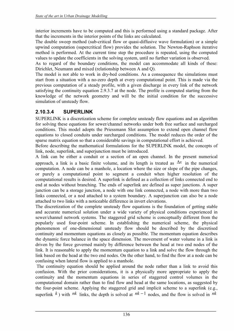
State of the art in Urban Drainage Modelling
136
interior increments have to be computed and this is performed using a standard package. After that the increments in the interior points of the links are calculated. The double sweep method (sub-critical flow or quasi-diffusive wave formulation) or a simple upwind computation (supercritical flow) provides the solution. The Newton-Raphson iterative method is performed. At the current time step the procedure is repeated, using the computed values to update the coefficients in the solving system, until no further variation is observed. As to regard of the boundary conditions, the model can accommodate all kinds of these: Dirichlet, Neumann and mixed (relationship between A and Q). The model is not able to work in dry-bed conditions. As a consequence the simulations must start from a situation with a no-zero depth at every computational point. This is made via the previous computation of a steady profile, with a given discharge in every link of the network satisfying the continuity equation 2.9.3.7 at the node. The profile is computed starting from the knowledge of the network geometry and will be the initial condition for the successive simulation of unsteady flow.
2.10.3.4 SUPERLINK SUPERLINK is a discretization scheme for complete unsteady flow equations and an algorithm for solving these equations for sewer/channel networks under both free surface and surcharged conditions. This model adopts the Priessmann Slot assumption to extend open channel flow equations to closed conduits under surcharged conditions. The model reduces the order of the sparse matrix equation so that a considerable savings in computational effort is achieved. Before describing the mathematical formulations for the SUPERLINK model, the concepts of link, node, superlink, and superjunction must be introduced. A link can be either a conduit or a section of an open channel. In the present numerical approach, a link is a basic finite volume, and its length is treated as x∆ in the numerical computation. A node can be a manhole, a location where the size or slope of the pipe changes, or purely a computational point to segment a conduit when higher resolution of the computational results is desired. A superlink is defined as a collection of links connected end to end at nodes without branching. The ends of superlink are defined as super junctions. A super junction can be a storage junction, a node with one link connected, a node with more than two links connected, or a nod attached to a system boundary. A superjunction can also be a node attached to two links with a noticeable difference in invert elevations. The discretization of the complete unsteady flow equations is the foundation of getting stable and accurate numerical solution under a wide variety of physical conditions experienced in sewer/channel network systems. The staggered grid scheme is conceptually different from the popularly used four-point scheme. In establishing the numerical scheme, the physical phenomenon of one-dimensional unsteady flow should be described by the discretised continuity and momentum equations as closely as possible. The momentum equation describes the dynamic force balance in the space dimension. The movement of water volume in a link is driven by the force governed mainly by difference between the head at two end nodes of the link. It is reasonable to apply the momentum equation to a link and solve the flow through the link based on the head at the two end nodes. On the other hand, to find the flow at a node can be confusing when lateral flow is applied to a manhole. The continuity equation should be applied around the node rather than a link to avoid this confusion. With the prior considerations, it is a physically more appropriate to apply the continuity and the momentum equations in series of staggered control volumes in the computational domain rather than to find flow and head at the same locations, as suggested by the four-point scheme. Applying the staggered grid and implicit scheme to a superlink (e.g., superlink k ) with nk links, the depth is solved at 1−nk nodes, and the flow is solved in nk
State of the art in Urban Drainage Modelling
137
links subject to the heads at two ends of the superlink. The schematic of staggered grid is snow in following figure.
Fig.2.10.1: Superlink computational scheme
The superlink algorithm with the staggered grid implicit scheme is derived in two steps for the solution. The first step is to derive the recurrence relations according to the discretised continuity equation and the momentum equation for each superlink using the staggered grid implicit scheme. The definition of the superlink facilitates the derivation, since there will be no off-diagonal nonzero elements in the coefficient matrix formulated for one superlink. A series of superlink recurrence relations relating flows and depths in the links and nodes of each superlink can be derived .A condensed sparse matrix is created in the second step of the development by applying the continuity equation to all superjunctions in the system using the recurrence relations for each superlink developed in the first step. The order of the matrix set up in this way is equal to the number of superjunctions in the system instead of twice the number of nodes in the system, as is the case in other implicit schemes directly discretised from the complete unsteady flow equations. This order reduction of the matrix facilities the solution procedure and speed up the computation. A computer model, SUPERLINK, for looped sewer/channel systems, is developed based on the SUPERLINK algorithm. The numerical experiments show that the model is robust and reliable, and produces consistent results under different grid setups. The application to a large looped sewer network shows a reasonable agreement with field measurement. A comparison between the results from the SUPERLINK and the SWMM EXTRAN model demonstrates that while maintaining the computational stability and accuracy, the computation can be sped up using the SUPERLINK algorithm for the sewer network system, which experienced a wide variety of hydrodynamic conditions. The desirable computation speed of the SUPERLINK model particularly makes the model suitable for long-term simulations and real-time control applications.
2.10.3.5 Sophie Duchesne model The developed model is based on simplifications of the continuity and momentum equations. With the assumptions given below, the two equations are solved independently for each sewer pipe in the downstream direction as long as a backwater effect does not occur. In the latter case, the equations are solved simultaneously for all pipes influenced by the backwater effect. The continuity equation is integrated in the model as follows:
[ ] 0)()()()( int =∆
∆−−+−t
ttVtVtQtQout 2.10.3.10
where V is the water volume in the pipe, inQ is the flow entering the pipe and outQ the flow leaving the pipe. The simplifications made to the momentum equation depend upon the occurrence or absence of a backwater effect. In all cases the friction slope is given by the Manning formula:
34
2
2
h
outoutf
RA
QQnS =
2.10.3.11
where n is the Manning coefficient and hR is the hydraulic radius, and where A and hR are computed from the downstream water depth.

State of the art in Urban Drainage Modelling
138
When there are no backwater effects, the model keeps the assumption of the kinematic wave to simplify the momentum equation. The acceleration and pressure differential terms are thus neglected, which leads to
of SS = 2.10.3.12
This last equation implies that the water depths upstream and downstream of the pipe are equal. This simplification is valid if variations in the hydrograph are gradual enough to result in a quasi-steady flow for each time step (Motiee et al., 1996) and if the pipe is not surcharged. If backwater effects occur, the model is able to consider two classes of these. The first type is induced by increasing water levels, which can occur due to a lateral flow inlet or to a decrease in pipe discharge capacity (decrease of the slope or diameter, increase of the roughness, etc.) in the downstream direction. The second type of backwater effects results from a critical depth boundary condition at the outflow of the sewer network. In either case, the pipes can be under free surface or pressurized conditions. These last two conditions are handled with the same equations; in surcharged areas, the water depth is replaced by piezometric head in the momentum equation. When a backwater effect occurs because of an increase in water depth (or piezometric head) from one reach to the other, the diffusion wave assumptions are kept in the momentum equation, which is integrated as follows:
)( foud SS
xhh −=
∆− 2.10.3.13
where dh is the downstream water depth and uh is the upstream water depth. This equation is solved in combination with the continuity equation by an iterative method for all pipes affected by the backwater effect, i.e. until the water surface crosses the water level computed without considering any downstream influent. When the outfall conduit of the network flows in subcritical conditions, the downstream boundary limit is the critical depth expression. In this situation, it was found that the convective acceleration term of the momentum equation is significant, especially for long conduits with low slopes. The momentum equation is then integrated as:
)(2
1 22
foudud SS
xvv
gxhh
−=∆−
+∆−
2.10.3.14
where dv is the downstream flow velocity and uv is the upstream flow velocity. Apart from the acceleration term incorporated in this last equation, the computation method for flows and water levels is the same as for backwater effects caused by an increasing water level. Other types of downstream boundary conditions can be taken into account by the model. For example, sluice gates or water level in the receiving element (river, pumping well, treatment plant, etc.) can govern the outfall conditions. In these circumstances, the model's downstream boundary conditions are given by the water level of that specific element, and all other equations (momentum and mass balance) remain the same as previously presented. The distinctive characteristic of the model lies in the algorithm used to solve the momentum and mass balance equations. As stated previously, the two equations of the model are solved independently for each sewer pipe in the downstream direction as long as a backwater effect does not occur. In such a situation, the equations are solved simultaneously for all pipes influenced by the backwater effect. These last pipes constitute what we will further call the "influenced region". In this region, flows and water depths are calculated in the upstream direction. The solving procedure hence consists, for each time step, of these embedded loops as illustrated in following figure.

State of the art in Urban Drainage Modelling
139
In this algorithm, all pipes are numbered consecutively from 1 to n, increasing in the
downstream direction.
The object of the "loop calculating ),( txQout " of this solving procedure is to find what the flow leaving pipe x should be in order to:
satisfy both the momentum and mass balance equations in each pipe of the "influenced region" of pipe x;
comply with continuity of flows and water depths at all nodes (connection points between two pipes).
To achieve this goal, an initial flow ),( txQout is first set downstream pipe x and this pipe's
downstream water 1evel is computed from ),( txQout according to the appropriate downstream boundary limit (normal depth, critical depth or other condition). Water level upstream pipe x is then computed using the momentum equation (Eqs. 2.10.3.12, 2.10.3.13 or 2.10.3.14). When
upstream and downstream water levels are known, the flow that should enter pipe x, ),( txQin , in order to satisfy the mass balance equation (Eq. 2.10.3.10) is computed. If pipe x does not cause a backwater effect in the upstream pipes, the next resolution step is to verify if the computed
),( txQin is actually equal to the flow entering pipe x , according to the flow conditions upstream that pipe. If the difference between these two flows is higher than the required
precision, then discharge downstream pipe x, ),( txQout , is modified and the procedure is repeated until the required precision is reached. If however pipe x affects the flow conditions upstream, computation is performed on all pipes influenced by backwater effect. Water level downstream pipe x-1 is then set to water level upstream pipe and the flow leaving pipe x-1 is set
State of the art in Urban Drainage Modelling
140
to ),( txQin , from which are subtracted the lateral inflows entering the sewer network at the two pipes’ junction. Water level and flow upstream pipe x-1 are afterwards computed using the procedure previously presented for pipe x, and calculations are repeated in the same manner until the upstream end of the influenced region is reached. The algorithm’s objective is then to
determine the ),( txQout value which, trough the calculation of flows in looped or branched systems. However, this model is meant to be used only in specific locations of sewer system where surcharged flow can be allowed, such as in interceptors, tunnels or storage pipes. These types of sewer network’s component do not often enclose looped or branched elements. If this kind of network is still need to be simulated by model, distribution coefficients could be used, as suggested by Motiee (1996).
Validation of the developed model was first performed by comparing its simulated results with those of the EXTRAN model (Roesner et al., 1983). This comparison showed that the model gave results similar to these of the EXTRAN model with an increase in computational speed and with the advantage of being more stable at the transition from free surface to pressurized flow. Furthermore, results of the developed model remained stable regardless of the time step used, where as this parameter had to be carefully selected in EXTRAN to avoid instability and continuity problems. Additional validation of the developed model showed that flows and water depths simulated are similar to those obtained with the SUPERLIK model and that both models have computational speed within the same order of magnitude.
The model’s capacity to compute flows and water levels for all flow regimes, including backwater effects, began the peculiarities of this model to improve the efficiency of operational RTC SWIFT model.
2.10.3.6 SWIFT SWIFT model is based on a global predictive control (GPC), an effective strategy to
perform real time management of sewers with aim to minimize overflows by optimizing water volumes stored in the sewer system.
SWIFT comprises three simulation models and an optimization algorithm. The flow values computed by the simulation models from rainfall intensity predictions are used by the optimization routine to determine the opening and closing of regulating gates in such a way that the total volume of overflow is minimized. The first simulation model is a rainfall-runoff conceptual model computing runoff on urban catchments and flow in the first conduits of the sewer network. Two hydraulic models can afterwards be used to simulate water flow transfers in sewer pipes: the Muskingum model (Cunge,1969), which computes time lag and smoothing of input hydrographs, and a linear model (piston model), which simply calculates the time lag of input hydrographs. The former model exclusively simulates free surface flow while the latter is used in pipes that are always surcharged due to their topographical situations or in shorter pipes that cannot be included in a Muskingum model owing to numerical instabilities. Consequently, the SWIFT model is unable to simulate transient situations between free surface and pressurized flow and the optimization algorithm avoids pipes overloads. However, surcharged conditions can occur frequently in combined sewers during storm events (Vitasovic, Swarner, & Speer, 1990). This type of flow can even be favourably used by RTC to take advantage of the full storage capacity of the sewer. If properly simulated, surcharged flows could be allowed by the optimization procedure and some pipes used as reservoirs, as long as the pressure resistance of the pipes is not exceeded and as water heights do not reach levels resulting in potential flooding hazards. In order to improve the efficiency of the SWIFT model in reducing overflow volumes, Sophie Duchesne et al. developed a mathematical model to compute flows and water levels for all flow regimes, including backwater effects.
State of the art in Urban Drainage Modelling
141
When integrated in SWIFT, the mathematical model developed by Sophie Duchesne et al. will only be used in sewer sections where surcharged flows should be allowed while the Muskingum model will be applied in all other pipes. This will certainly result in a much faster simulation package. In the near future, the model will then be integrated in the SWIFT RTC model to decrease CSOs during rainstorms. This integration will require adaptation of the objective function included in SWIFT, to allow surcharged flows in some parts of the sewer controlled, and validation of this enhanced optimization tool. Improvements in the reduction of overflows according to the intensity of surcharges will afterwards be evaluated.
2.10.3.7 SPIDA It is a numerical model for sewer simulation based on dynamic wave approach for pipe
routing. The model, in fact, can compute the flows in dentritic or looped sewer networks, using the full set of equations of de Saint Venant for one-dimensional gradually varied flow. The model accounts the pressurized flow, through the use of a Preissmann slot. SPIDA uses the Preissmann Box Scheme to solve the equations. The model damps out the inertial terms in the momentum equation as the Froud number increases and resumes to a diffusive wave approximation for supercritical flow. In SPIDA the optimization of the time step -as a function of changes of variables- during the calculation, reduces the computation time drastically. A comparison of simulation results of this model with another two models, EXTRAN and MOUSE, shows that the tree models may be considered of equivalent power and accuracy, with regard to standard sewer design evaluation problems. Moreover, the problem of computation efficiency should not be exaggerated, as the computation time represents only a fraction of time needed for e.g. the data management.
2.10.3.8 SNFS (Steady Non-uniform Flow in Sewers) SNFS is an evaluation/prediction model for a steady non-uniform flow in a dendritic type of sewer networks including all possible types of flow transitions. It is able to simulate the flow even when the water level reaches the ground level. The model considers the effects of sewer manholes, side weir structures without and with regulatory devices and flow through inverted siphons with a high level of accuracy. It simulates water surface profiles in sewer and channel network (e.g. in waste water treatment plants). The SFNS neglects the time variation of flow, so the governing equation for flow in sewers and channel is:
2cos FrSS
dxdy fo
−−
=φ 2.10.3.15
where
gABVFr
22 α=
2.10.3.16 is a Froude number; So= invert slope of channel; Sf = friction slope; α = the energy coefficient; A=cross-sectional area of flow; B= water-surface width; g= the gravitational constant; V= mean velocity of flow; y = depth of flow; and x= the distance along the channel measured in downstream direction.
34
22
R
VnS f =
2.10.3.17 Simulation of flow has shown the model to be able to solve many kinds of practical problems.

State of the art in Urban Drainage Modelling
142
Other several types of distributed flow routing models (dynamic, diffusion, and kinematic) are listed in Table 2.10.1.
Table 2.10.1
Model type Name Reference(s)Finete-
difference scheme
Special features Availability
Dynamic BRANCH 1 4I b,d,e,g,i,j NPDynamic BRASS 2 4I a,d,e,f,g,i,j,n,r NPDynamic CARIMA 3 4I b,d,e,f,i,j PDynamic CHARIMA 4 4I b,d,e,h,i,j NPDynamic DAMBRK 5 4I c,d,e,f,i,j,k,m NPDynamic DWOPER 5 4I b,d,e,f,g,i,j,l NPDynamic FEQ 6 4I b,d,e,f,g,i,n,l NPDynamic FLDWAV 5 4I b,c,d,e,f,g,h,i,j,k,l,m NPDynamic FLOSED 7 4I a,d,h,i NPDynamic LORIS 8 4I b,d,e,f,i,j PDynamic MOBED 9 4I h,i,j NPDynamic RICE 10 4I j,q PDynamic RUBICON 11 4I b,d,e,f,h,i,j,l PDynamic SOC/SOCJM 12 E a,i NPDynamic S11 13 6I b,c,d,e,f,h,i,j,k,l,n,p PDynamic UNET 14 4IFL b,d,e,f,i,j PDiffusion PAB 15 CI/FB b,c,f,h,j,n,p NPKinematic HEC-1 16 E k,n NPKinematic MITCAT 17 E n NPKinematic Nonlinear 18 4I NP
NP = nonproprietary a = dentric system of interconnecting channelsP = proprietary b = dentric/looped system of interconnecting channels4I = weughted 4-point nonlinear implicit c = subcritical-supercritical mixed flow4IL = weughted 4-point linear implicit d = assortment of external and internal boundaries4ILF = fully forward 4-point linear implicit e = special treatment of floodplains6I = 6-point linear implicit f = special treatment for overtopping of levelsE = explicit g = automatic calibration of variable friction coefficient4P = linear/non linear implicit h = sediment trasport (mobile-bed) effectsCI/FB = i = dead storage effects
j = variable frictionk = dam-break flood generationl = storm sewer capabilities including pressurized flowm = non-Newtonian (mud) flow capabilitiesn = hydrologic rainfall-runoff modelling capabilityp = water quality modeling capabilityq = ice effectsr = reservoir operations
Legend Special features
convolution integral (flow)/finite difference backwater equation (depth)

State of the art in Urban Drainage Modelling
143
Reference(s)
1. Schaffranek,R.W., Flow Model for Open Channel Reach or Network, Professional Paper 1384,U.S.Geological Survey,1987.
2. Colon, R., and G.F. McMahon,” BRASS Model: Application to Savannah River System Reservoirs,” J. Water Resours.Plann.Manage.,vol.113,no.2,pp.177-190,1987.
3. Cunge, J.A.,F.M. Holly, Jr.,and A. Veway, Practical Aspects of Computational River Hudrauilics, Pitman, Boston, Mass.,1980.
4. Holly, F.M., Jr., J.C. Yang, P. Schwerz, J. Schaefer, S.H.hsu, and R.Einhellig, CHARIMA- Numerical Simulation of Unsteady Water and Sediment in Multiple Connected Networks of Mobile-Bed Channels, University of Iowa, IIHR 343 Iowa City, Iowa, 1990.
5. Chow, V.T., D.R. Maidment, and L.W.Mays, Applied Hydrology, McGraw-Hill, New York, 1988.
6. Franz, D.D., Unsteady Flow Solutions: FEQ/FEQUTL, Linsley, Kraeger Associates, Ltd., Mountain View, Calif., 1991.
7. Johnson, B.H., Development of a Numerical Modeling Capability for the Computation of Unsteady Flow on the Ohio River and Its Major Contributaries, Tech. Report HL-82-20, U.S. Army Engineer Waterways Experiment Station, Vicksburg, Miss., 1982.
8. Slade, J.E., and P.G.Samuels, Modeling Complex River Networks, HR Pub.Paper 41, Hydraulics Research Limited, Wallingford, UK,1980.
9. Krishnappan, B.G., “Unsteady Flow in Mobile Boundary Channels,” Environ. Hydr. Ect., Hydr. Res. Div., National Water Res. Inst., Canada Centre for Inland Waters, Burlington, Ont.1979.
10. Lai,A.M.W., and H.T. Shen, “Mathematical Model for River Ice Process,” J.Hydraul. Res., vol.26, no.5, pp.559-568, 1988.
11. Verwey, A., and M. J. M. Haperen, “HD-System RUBICON- A User-Friendly Package for the Simulation of Unsteady Flow in Open Channel Networks,” Hydrosolf, vol.1, no. 1, pp. 3-12, 1988.
12. Garrison, J. M., J. P. Granju, and J. T. Price, “Unsteady Flow Simulation in Rivers and Reservoirs,” J. Hydraul.Eng., vol. 95, no. HY5, pp. 1559-1576, 1969.
13. Abbott, M. B., and J. A. Cunge, Engineering Applications of Computational Hydraulics, vol. 1, Pitman, London, England, 1982.
14. Barkow, R. L. , UNET One-Dimensional Unsteady Flow through a Full Network of Open Channels, User Manual, Hydrologic Engineering Center Rept CPD-66, U.S. Army Corps of Engineers, Davis, Calif., 1992.
15. Todini, E., and A.Bossi, PAB (Parabolic- and Backwater)-An Unconditionally Stable Flood Routing Scheme Particularly Suited for Real Time Forecasting and Control, Publ. 1, Univ. di Bologna, Bologna, Italy,1985.
16. Hydrologic Engineering Center, HEC-1 Flood Hydrograph Package User Manua,U.S. Army Corps of Engineers, Davis, Calif., 1982.
17. Harley, B. M., F. E. Perkins, and P.S. Eaglson, A Modular Distribution Model of Catchments Dynamics, Report 133, R. M. Parsons Lab for Water resources and Hydrodynamics, MIT, Cambridge, Mass., 1970.
18. Li, R.M.,D.B. Simons and M. A. Stevens, “Nonlinear Kinematic Wave Approximation for Water Routing,“ Water Resour. Res. Vol. 11, no. 2, pp. 245-252, 1975.

State of the art in Urban Drainage Modelling
144
2.10.4. Hydrological-Physically based models Several researchers have considered that the gap between these two categories of models, Hydrologic models and physically based models, was wide enough to give place to a new family model, easier to use than the Barre de Saint Venant equations, and able to take into account some of most important effects of the flow complexity and of the network reality. Such models need to present several pragmatic qualities:
• be able to represent the actual functioning of the drainage system whatever the type of flow (free surface or surcharged, subcritical or supercritical);
• be able to represent the functioning of the drainage system whatever the kind of network (branched or looped) and whatever the nature of the special structures that can be found inside;
• be a lot quicker in running than the Barre de Saint Venant equations; • be stable whatever the time step and the space step; • furnish results easy to understand and to use, even for a non-hydraulic people.
This type of model is usually easier to use than complete Barre de Saint Venant equations and they can give better results in applications suffering from lack of calibration data.
2.10.4.1 Mootie, Chocat and Blanpain model Motiee, Chocat, and Blanpain (1996) developed a simple sewer flow model using this approximation to compute backwater effects, and using the kinematic wave model in pipe not exposed to backwater conditions. This last model should be used with care in some sewers where the convective acceleration term can be of the same order as the variation in potential energy. This model (Motiee,1996) uses the storage concept, developed by Chocat (1978) and further developed by Blanpain (1991). It uses the continuity equation:
0),(),( =∂
∂+∂
∂t
txAx
txQ 2.10.4.1
Where ),( txQ is the flow rate and ),( txA the wetted cross section at the position x and the time t . This equation can be written between two points separated by a distance (space step) x∆ as follows:
)()()( tQtQttdV
se −=∆ 2.10.4.2
In this equation, )(tQe and )(tQs are respectively the inflow and the outflow, upstream and downstream of the reach; )(tV is the total storage volume in the reach. The second equation is the storage equation. It must link together the storage volume in the reach and the flow rates upstream and downstream:
))(),(,()( tQtQtftV se= 2.10.4.3
State of the art in Urban Drainage Modelling
145
In fact, it is always possible to express the storage volume according to the wetted area in the reach:
∫∆+
=xx
x
o
o
dxtxAtV ),()( 2.10.4.4
If the evolution of the wetted cross section is always increasing or always decreasing along the reach, we may write:
xtAtAtV avam ∆⋅−+= ))()1()(()( αα 2.10.4.5
Where )(tAam is the wetted area upstream, )(tAav is the wetted area downstream and where the α coefficient depend on the flow characteristics. Different discretization procedures can be applied to the equation 2.10.4.3 (Chow,1959;Ponce,1981). Blanpain (1993) showed that second-rate schemes, like:
2)()(
2)()()()( ttQtQttQtQ
tttVtV ssee ∆−+
−∆−+
=∆
∆−−
2.10.4.6 were never stable. For this reason he suggested using the simple implicit scheme, previously built by Chocat (1978):
)()()()( tQtQt
ttVtVse −=
∆∆−−
2.10.4.7 Blaipain (1993) showed that the results of this scheme were good. In that case, the outflow can be calculated as:
tttVtVtQtQ es ∆
∆−−−= )()()()( 2.10.4.8
To use relation 2.10.4.8, we must be able to calculate V(t). Several cases are possible. Without any backwater effect the value 1=α can be used in equation (5) (blanpain,1993). In these conditions, it easy to write an explicit equation:
xtAtV am ∆⋅= )()( 2.10.4.9 or:
)()()(
)()( tQ
tVxx
tVtQ
tV eee
e ⋅∆=∆⋅= 2.10.4.10
In equation 2.10.4.10, )(tVe is the flow velocity upstream and )(tQe the inflow rate. If the incoming hydrograph is discretized, it is possible, to calculate the flow velocity corresponding

State of the art in Urban Drainage Modelling
146
to each time step, for example by using the Manning-Strickler formula. The main hypothesis is that the variations of the hydrograph are slow enough to obtain a quasi steady flow at each time step. Equation 2.10.4.10 can be written with a temporal parameter:
)()(
tVxtTp
e
∆= 2.10.4.11
With this notation, we obtain:
)()()( tTptQtV e ⋅= 2.10.4.12 Equation 2.10.4.12 shows that this model can be understood as a conceptual, non linear model. In this way it can be related to the Kalinin-Miljukov model. Compared with simplified hydrodynamic models, this formulation of the storage model can be related to the Kinematic wave model. The patterns of surface profile supposed by the two models are actually the same, even if the ways to carry out the calculations are very different. Backwater effects can occur either if the network operates in pressure flow or if it operates with free surface flow. Whatever the case, the method is the same. It supposes that the pattern of the surface profile, inside reach affected by backwater curve, can be described by the equation 2.10.4.13:
IJxH −=
∆∆
( I = slope of the reach, J = head losses by unit of length) 2.10.4.13
Fig. 2.10.2: Pattern assumed for surface profile in case of backwater effect
For example, we can look at a simple case, consisting of two consecutive reaches (Fig.2.10.2), the second one affecting the first one, due to a smaller capacity. The problem to be solved is to calculate the correct values of V1 and Qs1 so that equations 2.10.4.14 and 2.10.4.15 are both verified:
tttVtVtQtQ es ∆
∆−−−= )()()()( 11 2.10.4.14
)()( 11 eQftV = 2.10.4.15
where 1eQ is the inflow in the first reach; 1sQ , the outflow in the first reach; 12 ee QQ = the
inflow in the second reach; 1V ,the storage volume in the first reach. Equation 2.10.4.15 represents the fact that, on the first hand, the depth of water h, calculated at
the entrance of the second reach, is directly dependent on the inflow 2eQ (hypothesis of quasi

State of the art in Urban Drainage Modelling
147
steady flow), and, on the other hand, that the storage volume )(1 tV in the upper reach is dependent on the depth. In fact equation 2.10.4.15 shows a continuously decreasing relation
between 1V and 1sQ : the greater 1sQ , the greater is h and the greater is 1V ; if 01 =sQ , then h=0
and 01 =sV .
Equation 2.10.4.14, shows a linear decreasing relation between 1sQ and 1V (if 0)(1 =tV , then,
tttVQQ es ∆
∆−+= )(111
and if 01 =sQ then tQttVtV e ∆⋅+∆−= 111 )()( .
Fig. 2.10.3: Graphic representation of the existence and unicity of equilibrium values of Qs1
and V1 There is only one equilibrium value and it always exists (Fig. 2.10.3). This equilibrium value can be found by an iterative method. Equation 2.10.4.13 shows that in the case of backwater effects, the storage model can be related to the diffusion wave model, which results from several simplifications or Barre de Saint Venant equations. Anyway, even if the two models assume a similar pattern for the surface profile, they cannot be directly assimilated because of the differences between the calculation methods. For the validation of the storage model, it has been used an empirical methodology, developed by Semsar (1995). The method consists in comparing the results given by the model to be studied with the results given by the Saint Venant equations, for a set of 15 typical networks, under 12 kinds of working conditions. The discrepancies between the results given by two of the models are measured by the discrepancies between the two hydrographs obtained at outlet of the networks. The results of this methodology show:
• compared with the Muskingum model, the storage model is able to furnish a realistic pattern of surface profile, even in the case of important backwater effects, while Muskingum model is unable to represent it;
• compared with the complete Saint Venant equations the main advantage of the storage model is that calculation time are a lot less important (the average calculation time is divided by ten in the studied cases).
• compared with models obtained by simplifying the Saint Venant equations, the main advantage of the storage model is that it uses the most appropriate simplification (diffusion wave model or kinematic wave model), depending on the flow conditions.
2.10.4.2 Modelling of unsteady flow through manholes Ball (1985) presented a methodology for modelling unsteady flows through manholes. This methodology is based on the conceptualisation of the network into a number of individual network units and the development of boundary conditions for these network units. Each
State of the art in Urban Drainage Modelling
148
network unit comprises a single link connected to two nodes located at either end of the link. The nodes in individual network units not only provide the boundary conditions for determination of flow conditions along the individual links, but also provide the connections between individual network units in the formation of the drainage network. The boundary conditions at the manholes can be developed in terms of total or piezometric energy from consideration of momentum conservation. If manhole m in connected to the upstream end of pipe p which has n calculation points along its length, then through a consideration of energy conservation a relationship between flow conditions in the pipe and the manhole can be developed as
2
21
1 2)(
Eg
uzE p
pm ∆++= 2.10.4.16
where Em is the total energy level at manhole m, zp1 is the water surface elevation relative to a datum at the intersection of the pipe and the manhole, up1 is the flow velocity at the intersection of the pipe and the manhole, g is gravitational acceleration, and 2E∆ is the change in energy due to flow entering the pipe from manhole (i.e. the pipe entry loss). An alternative is to express the relationship in terms the piezometric energy levels in the pipe and the manhole. This relationship is
21 Wzz pm ∆+= 2.10.4.17 where 2W∆ is the change in piezometric energy between the manhole and the pipe. In the same manner, can be developed a relationship between flow conditions at the downstream end of pipe p and the connected manhole (m+1):
1
2
1 2)(
Eg
uzE pn
pnm ∆−+=+ 2.10.4.18
11 Wzz pnm ∆−=+ 2.10.4.19 Where 1E∆ and 1W∆ are the changes between the pipe and the manhole in the total energy and piezometric energy respectively. To incorporate the previous equations in a numerical model describing the propagation of flood waves through urban drainage systems requires the determination of Em, 1E∆ , 2E∆ , 1W∆ and 2W∆ . Therefore, definition of flow conditions at manholes which are the most common form of node is an important aspect in the development of a model describing propagation flood waves through urban drainage system. A manhole may be considered as a short length of open channel which may, or may not, have the same cross-sectional flow area as attached links. The approach of the model is to use the principle of momentum conservation at the junction of attached links. Consider the junction of two pipes in a manhole with benching as illustrated in Fig.2.10.3 where the full lines represent the actual geometry of the junction while the broken lines represent the geometry of the junction adopted for analysis by application of the principle of momentum conservation. An enlarged portion of the channel junction defined by the broken lines is shown in Fig. 2.10.4. For the convenience of the analysis it is assumed that:
• Link 3 conveys flow away from the manhole while links 1 and 2 convey flow to the manhole.
• Wall frictional effects are negligible within the control volume.

State of the art in Urban Drainage Modelling
149
• Flow is parallel to the walls immediately upstream and downstream of the junction. • Flow depth in two upstream links immediately upstream of the junction are identical; an
assumption which has been validated by Joliffe (1980).
Fig. 2.10.3:Junction of open channels at a manhole
Fig. 2.10.4: Schematic arrangement of manhole junction
Applying the principle of the momentum conservation to the control volume, denoted by area ABCDEFGHJ in Fig. 2.10.4, yields
0FsinFsinF)uyg(Acos)uyg(Acos)uyg(A AC2ED1HJ23332
22221
2111 =+θ−θ−+−θ++θ+
2.10.4.20 where yi is the depth to the centric of the wetted cross section for link i. If a linear variation between the flow depyhs at the upstream point J and D and the downstream points H and E is assumed then, after simplifying for the hydrostatic pressure forces FAC, FED and FHJ equation 2.10.4.20 can be rearranged to give:
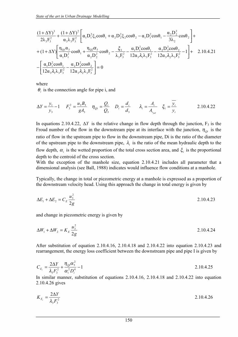
State of the art in Urban Drainage Modelling
150
0Fλα12
cosθDαFλα12
cosθDα
1Fλα12
cosθDαFλα12
cosθDαFλ
cosθDα
ηcosθ
Dααη
∆Y)(1
cosθ3λ
DαcosθDαcosθξDαcosθξDα
Fλα∆Y)(1
F2λ∆Y)(1
23323
2222
23313
1211
23323
2222
23313
1211
233
322
22
3Q212
11
3Q1
22
222
121122
22211
2112
333
2
233
3
=
−−
+
−−−−+++
+
−−++++
λλ
λλξα
2.10.4.21
where iθ is the connection angle for pipe i, and
13
1 −=∆yyY
3
3323 gA
BuF =
3QQi
Qi =η 3d
dD i
i = fulli
ii A
A=λ
i
ii y
y=ξ 2.10.4.22
In equations 2.10.4.22, Y∆ is the relative change in flow depth through the junction, F3 is the Froud number of the flow in the downstream pipe at its interface with the junction, Qiη is the ratio of flow in the upstream pipe to flow in the downstream pipe, Di is the ratio of the diameter of the upstream pipe to the downstream pipe, iλ is the ratio of the mean hydraulic depth to the flow depth, iα is the wetted proportion of the total cross section area, and iξ is the proportional depth to the centroid of the cross section. With the exception of the manhole size, equation 2.10.4.21 includes all parameter that a dimensional analysis (see Ball, 1988) indicates would influence flow conditions at a manhole. Typically, the change in total or piezometric energy at a manhole is expressed as a proportion of the downstream velocity head. Using this approach the change in total energy is given by
guCEE E 2
23
21 =∆+∆ 2.10.4.23
and change in piezometric energy is given by
guKWW E 2
23
21 =∆+∆ 2.10.4.24
After substitution of equation 2.10.4.16, 2.10.4.18 and 2.10.4.22 into equation 2.10.4.23 and rearrangement, the energy loss coefficient between the downstream pipe and pipe I is given by
1242
23
233
−+∆=ii
QiE DF
YCi α
αηλ
2.10.4.25
In similar manner, substitution of equations 2.10.4.16, 2.10.4.18 and 2.10.4.22 into equation 2.10.4.26 gives
233
2FYK
iE λ∆= 2.10.4.26

State of the art in Urban Drainage Modelling
151
The energy loss between the pipe 1 and 3 is usually considered to occur between points 1 and 3 where these points are located at the faces of the manhole. However, the analysis presented above is based on the energy loss occurring at the branch point of the manhole with consequent neglect of the energy losses between the branch point 1 and 3 respectively. To incorporate these losses, the pipe connected to the manhole are assumed to extend into the manhole and the energy losses due to flow along these sections are added to the energy losses due to flow along the physical pipe. When the flow conditions at a manhole are numerically modelled, it is convenient to consider the energy change due to entry to a manhole and an energy change to the exit from the manhole. However, solving equation 2.10.4.20 for the flow conditions at the manhole results in, as shown in equations 2.10.4.25 and 2.10.4.26, only the total energy change at the manhole. Therefore, to incorporate the model of manhole and that the level is equal to the piezometric energy in the upstream pipe, then, by equation 2.10.4.19, 1W∆ is equal to zero and
g
uKW E 2
23
2 =∆ 2.10.4.27
where KE is given by equation 2.10.4.26. The adoption of this assumption, therefore, results in boundary conditions suitable for numerical model when piezometric energy levels at the manhole are considered. However, this assumption does not assist in the subdivision of the change in total energy as this requires additional information regarding the energy level in the manhole. Consequently it is considered that only the boundary conditions related to the piezometric energy level are currently suitable for use. To ascertain the validity of this theoretical model, a physical model of a manhole was constructed and flow conditions in the attached pipes were monitored. Piezometric pressures were measured at eight locations on both the upstream and downstream pipes. Measured water surface elevations recorded at these locations were compared with theoretical flow profile. In Fig. 2.10.4.18 is snowed a sample of this comparison for steady flow conditions in the system.
Fig. 2.10.5: Comparison of measured and theoretical flow profiles
In all cases, the comparison between the theoretical and the measured flow profiles were within the accuracy of measuring the piezometric pressure in the pipes.

State of the art in Urban Drainage Modelling
152
Consequently, it was concluded that flow conditions at the manhole could be determined from a consideration of the principle of momentum conservation.
2.10.5. Modelling mixed flow in storm sewers
In normal conditions, water in urban drainage networks can be expected to flow in one direction only and to present a free-surface which undergoes a gradually-varied, nearly steady evolution. In special cases, however, more complex situations can arise due to unusual network topology (loops), topography (abrupt changes in slope), inflows (severe storm transients), or outlet conditions (high tail water levels). Under such conditions, a variety of local transitions can appear: reversal of flow direction, passage to and from subcritical and supercritical regimes, transition between free surface and submerged flow. These transitions can appear at arbitrary locations and times during transient events, and can therefore present major hurdles for the numerical routing of flows through drainage networks. In particular, it is wanted to stopped the attention on the phenomena of transition from gravity to pressurized flow, that occur in sewer pipes when the storm exceeds the design event or occur sudden changes in the boundary conditions of storm sewer system (e.g. submergence of the outfall or blockage or reduction in capacity along the sewer system). During this transition, severe pressure transients may damage the storm sewers and cause other related problems such as basement flooding and the ejection of manhole covers. In order to investigate these pressure transients in a sewer system, the researches conducted both mathematical and experimental modelling studies. Yevjevich (1975) pointed out the possibility of trapped air pockets along storm sewers and the sudden release of an air-water mixture at upstream manholes during flow transitions. Yen (1978) identified free-surface to pressurized flows as one type of hydraulic instability in storm sewers that required detailed study. Valentia (1981) investigated experimentally the hydraulic phenomena that occur during the transition between free-surface and pressurized flow in a sewer system. It was observed that high-frequency type pressure transients are induced by the compression and expansion of trapped air bubbles in the sewer model and by an abrupt escape of air al the upstream manhole. Zech (1985) conducted experiments to investigate the flow instability due lo self-priming action that leads lo pressurized flow in culverts or storm sewers. His experiments confirmed the flow instability during the transition from free-surface to pressurized flow in closed conduits. Hamam (1982) carried out a number of experiments to investigate the formation of pressurized flow in closed conduits and concluded that severe transient pressure fluctuations of water hammer type might occur during a rapid transition from free- surface to surcharged flow in closed conduits such as storm sewers. Cardle et al. (1989) observed water hammer pressure during the transition from free-surface to pressurized flow conditions in a circular pipe. Baines (1981) investigated the motion of trapped air cavities in a square duct under mixed flow conditions. All the above literature indicates that hydraulic instability may occur during the transition from free-surface to pressurized flow in storm sewers. During such a transition of flow, air may be trapped and finally released at either upstream or downstream manholes. Either the self-priming of the pipe or subsequent air release at manholes can also induce severe pressure transients. Three modelling approaches, namely the Preissmann’s slot method, the shock-fitting method, and the rigid column method, have been proposed for simulation of pressure transients during the transition from free-surface to pressurized flow in sewers and tunnels.

State of the art in Urban Drainage Modelling
153
2.10.5.1 Preissmann Slot approach Preissmann (Chardhry, 1982) recognized the similarity between the open channel and the closed conduit form of Saint Venant equations and proposed that a hypothetical slot be added at the top of a closed conduit so that both free-surface and pressurized flow could be analyzed by Saint Venant equations. When self- priming of the conduit occurs, the depth calculated by the Saint Venant equations becomes the pressure head acting on the wall at the location. Although there is no need to trace the propagation of the moving interface between free-surface and pressurized flow, this approach cannot simulate trapped air bubles and negative pressure. Joliffe (1983), Fread (1984) and Ji (1998) applied the Priessmann’s slot approach in solving mixed flows in storm sewer networks.
2.10.5.2 Shock-Fitting approach The Shock-fitting approach provides an alternative approach to treating mixed flow problems where negative pressure and trapped air bubbles occur. Not only are the two flow regimes treated separately, they are integrated together by a moving interface. During the computation, the velocity, location, and intensity of this moving interface are calculated. This is similar to the Shock-fitting method employed in gas dynamics.
2.10.5.3 Rigid Water Column approach Hamam and McCorquodale (1982) proposed a rigid water column approach to model the mixed flow pressure transients. The transition from free-surface to pressurized flow was classified into six stages, as shown in Fig 2.10.5.
Fig.2.10.5: Stage in Transition of Free-Surface to Pressurized Flow
The model assumes:
State of the art in Urban Drainage Modelling
154
• Water columns are incompressible and their flow velocities are uniform but unsteady. • A hypothetical stationary air bubble is trapped inside the sewer after the occurrence of
interfacial instability between air-water flows. • The trapped air bubble undergoes pseudo adiabatic expansion and compression.
By applying rigid water column theory to the water phase and compressible flow theory to the air phase, continuity and momentum equations were developed for Stages 2 to 4 in the previous figure. The total differential equations for each stage can be solved efficiently by a fifth-order Runge-Kutta algorithm. The travelling surge and the stationary air bubble are analyzed continuously over time in order to compute the associated pressure transients. When the computed pressure transients were compared to those measured from a physical sewer model, it was found that the simulation model over predicted the measured pressure transients by a factor of two. Beyond these approaches there are others tentative to simulate transition between free-surface and pressurized flow in sewer networks. Wiggert (1972) modified the Preissmann's slot method by introducing a moving interface between free-surface and pressurized flow. The free-surface flow was solved by the method of characteristics, while the pressurized flow was treated as plug flow. Miyashiro and Yoda (1983) analyzed an underground drainage system using the St. Venant equations for the free-surface flow and a rigid water column equation for the pressurized flow. The St. Venant equations were solved by the method of characteristics, while the pressurized flow equations were solved by the forward finite difference scheme. A continuity equation was employed at the intersection of the free-surface and pressurized flows. Song et al. (1982) and Guo and Song (1990, 1991) developed a dynamic mathematical model with options of solving the mixed flow problem, either by the Preissmann's slot or the shock-fitting method. The model was applied to a combined sewer in Chicago. It was found that the Preissmann's slot method became unstable when the pressurization wave was too steep, and the surge strength at the end of the pressurization process determined the severity of the surge problems.
2.10.5.4 McCorquodale and Li model James Li and Alex McCorquodale developed a mathematical model that can be considered as an extension and refinement of the rigid water column approach. The original rigid column model assumed that a hypothetical stationary bubble, which is formed after a priming condition, is going through a compression and extension process. However, experimental observations indicate that the trapped air pockets tend to move upstream and are released at the upstream manhole. In order to simulate the air release transients, the rigid column model is modified to allow for the transport and subsequent release of the trapped air bubble. To provide complete model development for the pressure transient problem, derivations of Stage 2 and 3 as they were defined in the previous paragraph. Derivations of Stages 4 to 5 are new in the present model.

State of the art in Urban Drainage Modelling
155
Stage 2-Surge Formation
Whenever a blockage of flow occurs, local surcharging will occur that may result in a travelling hydraulic jump (figure 2.10.6-a). This moving hydraulic jump may travel at high speed, depending on the flow conditions. By applying the 1D momentum equation to the rigid water column 2 [Fig. 2(a)], the rate of change of velocity of the water column is given by
os
F
s
S
s
s gSL
gSL
VVV
RfL
LVVgZ
dtdV +−
−
+−
−=
21
4K
22
2
2
2e
22 2.10.5.1
where V2 is the velocity of water column 2 (m/s); t is the time of simulation (s); g is the acceleration due to the free surface (m/s2); Z is the pressure head on the surcharge side of the hydraulic jump (m); V is the velocity of the moving hydraulic jump (m/s); LS is the length of water column 2 (m); Ke is the exit loss coefficient (dimensionless); f is the friction factor of the sewer wall (dimensionless); R2 is the hydraulic radius of water column 2 (m); SF is the water depth at the downstream manhole (m); and So is the slope of the sewer.
Fig.2.10.6: Definition of Symbols for Stage 2 to 5
If the velocity of the hydraulic jump is superimposed on the control volume of the flow transition, the hydraulic jump appears stationary. A continuity equation can be applied across the moving hydraulic jump to give ( ) ( ) 2211 AVVAVV ss +=+ 2.10.5.2 where V1 (m/s) and A1 (m2) are the velocity and cross-sectional flow area of water column l; and A2 (m2) is the cross-sectional flow area of water column 2. Rearranging 2.10.5.2 gives
12
2211
AAVAVAVS −
−= 2.10.5.3
The conservation of linear momentum across the hydraulic jump moving at Vs upstream gives
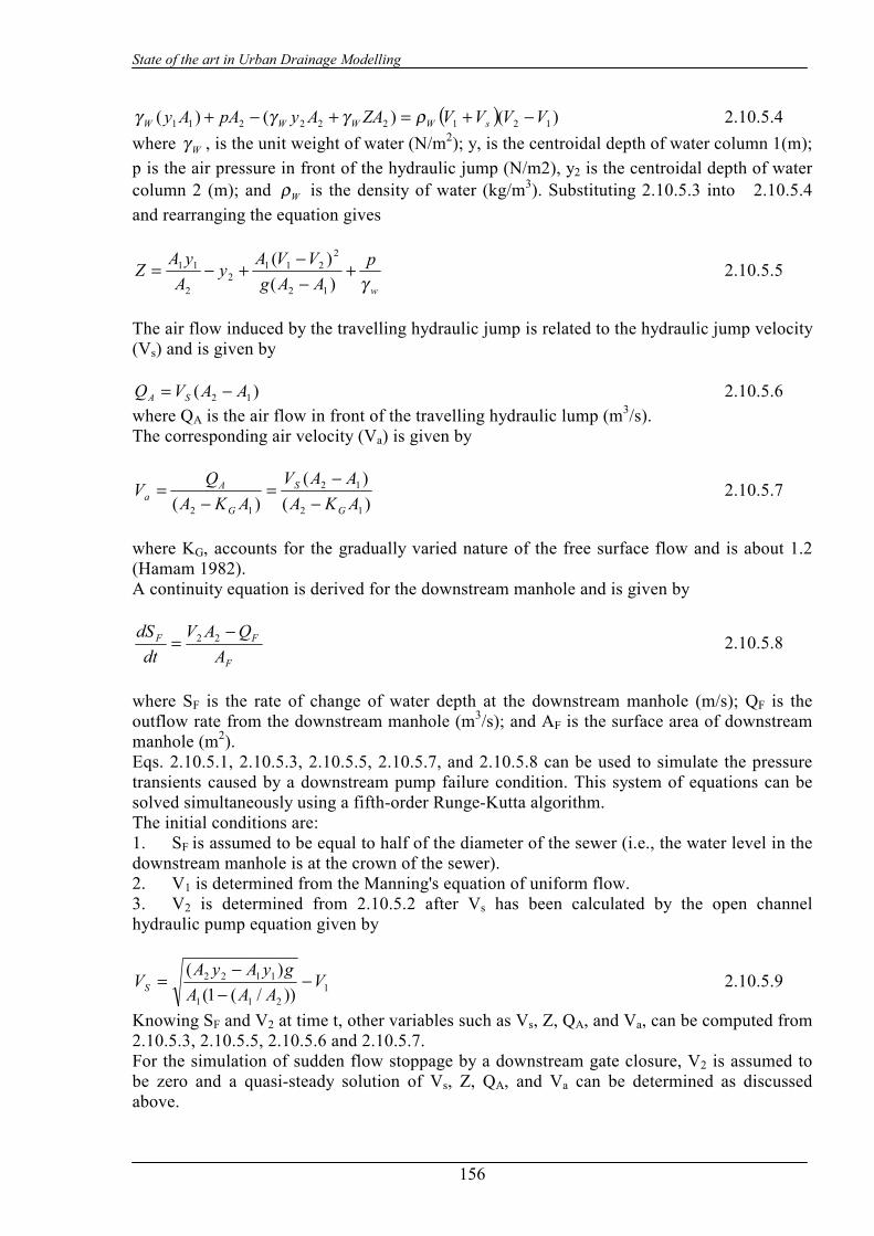
State of the art in Urban Drainage Modelling
156
( ) )()()( 121222211 VVVVZAAypAAy sWWWW −+=+−+ ργγγ 2.10.5.4 where Wγ , is the unit weight of water (N/m2); y, is the centroidal depth of water column 1(m); p is the air pressure in front of the hydraulic jump (N/m2), y2 is the centroidal depth of water column 2 (m); and Wρ is the density of water (kg/m3). Substituting 2.10.5.3 into 2.10.5.4 and rearranging the equation gives
w
pAAg
VVAyA
yAZγ
+−−
+−=)()(
12
2211
22
11 2.10.5.5
The air flow induced by the travelling hydraulic jump is related to the hydraulic jump velocity (Vs) and is given by
)( 12 AAVQ SA −= 2.10.5.6 where QA is the air flow in front of the travelling hydraulic lump (m3/s). The corresponding air velocity (Va) is given by
)()(
)( 12
12
12 AKAAAV
AKAQV
G
S
G
Aa −
−=
−= 2.10.5.7
where KG, accounts for the gradually varied nature of the free surface flow and is about 1.2 (Hamam 1982). A continuity equation is derived for the downstream manhole and is given by
F
FF
AQAV
dtdS −
= 22 2.10.5.8
where SF is the rate of change of water depth at the downstream manhole (m/s); QF is the outflow rate from the downstream manhole (m3/s); and AF is the surface area of downstream manhole (m2). Eqs. 2.10.5.1, 2.10.5.3, 2.10.5.5, 2.10.5.7, and 2.10.5.8 can be used to simulate the pressure transients caused by a downstream pump failure condition. This system of equations can be solved simultaneously using a fifth-order Runge-Kutta algorithm. The initial conditions are: 1. SF is assumed to be equal to half of the diameter of the sewer (i.e., the water level in the downstream manhole is at the crown of the sewer). 2. V1 is determined from the Manning's equation of uniform flow. 3. V2 is determined from 2.10.5.2 after Vs has been calculated by the open channel hydraulic pump equation given by
1211
1122
))/(1()( V
AAAgyAyAVS −
−−
= 2.10.5.9
Knowing SF and V2 at time t, other variables such as Vs, Z, QA, and Va, can be computed from 2.10.5.3, 2.10.5.5, 2.10.5.6 and 2.10.5.7. For the simulation of sudden flow stoppage by a downstream gate closure, V2 is assumed to be zero and a quasi-steady solution of Vs, Z, QA, and Va can be determined as discussed above.
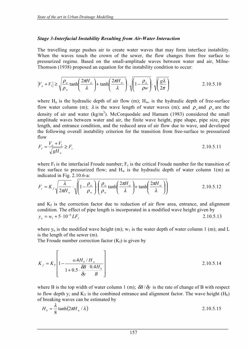
State of the art in Urban Drainage Modelling
157
Stage 3-Interfacial Instability Resulting from Air-Water Interaction The travelling surge pushes air to create water waves that may form interface instability. When the waves touch the crown of the sewer, the flow changes from free surface to pressurized regime. Based on the small-amplitude waves between water and air, Milne-Thomson (1938) proposed an equation for the instability condition to occur:
⋅
−⋅
+
≥+
πλ
ρρ
λπ
λπ
ρρ
21
2tanh
2tanh1
gw
HHVV awa
w
aa 2.10.5.10
where Ha is the hydraulic depth of air flow (m); Hw, is the hydraulic depth of free-surface flow water column (m); λ is the wave length of water waves (m); and aρ and wρ are the density of air and water (kg/m3). McCorquodale and Hamam (1983) considered the small amplitude waves between water and air, the finite wave height, pipe shape, pipe size, pipe length, and entrance condition, and the reduced area of air flow due to wave, and developed the following overall instability criterion for the transition from free-surface to pressurized flow
cw
aI F
gHVVF ≥
+= 1 2.10.5.11
where FI is the interfacial Froude number; Fc is the critical Froude number for the transition of free surface to pressurized flow; and Hw is the hydraulic depth of water column 1(m) as indicated in Fig. 2.10.6-a:
+
⋅
−⋅=
λπ
λπ
ρρ
ρρ
πλ wa
w
a
w
a
wfc
HHH
KF 2tanh
2tanh1
2 2.10.5.12
and Kf is the correction factor due to reduction of air flow area, entrance, and alignment condition. The effect of pipe length is incorporated in a modified wave height given by
Iu LFwy 61 105 −⋅+= 2.10.5.13
where yu is the modified wave height (m); w1 is the water depth of water column 1 (m); and L is the length of the sewer (m). The Froude number correction factor (Kf) is given by
⋅⋅+−=
BH
yB
HHoKKb
wbTf 4.0
5.01
/4.1
δδ
2.10.5.14
where B is the top width of water column 1 (m); yB δδ / is the rate of change of B with respect to flow depth y; and KT is the combined entrance and alignment factor. The wave height (Hb) of breaking waves can be estimated by
( )λπλ /2tanh8 wb HH ≈ 2.10.5.15

State of the art in Urban Drainage Modelling
158
where X is the wave length of the waves that may vary from 20 mm (capillary waves) to a few times yu. The criterion as stated in 2.10.5.11 is checked during the computation of Stage 2 (surge formation) in order to determine the occurrence of interfacial instability and proceed to the computation of Stage 4. Stage 4-Transition to Pressurized Flow McCorquodale and Hamam (1983) simulated the transition from free-surface to pressurized flow by assuming a hypothetical stationary air pocket inside the pipe. The flow was then divided into three rigid water columns with unsteady uniform velocities [Fig. 2.10.6-b]. Each water column was assumed to be enclosed by a fixed control volume. Continuity and momentum equations were then derived for the water columns, the interface between columns, and the upstream and downstream manholes. In the present research, it is assumed that 2.10.5.1 the hypothetical air bubble moves toward the upstream manhole at a constant velocity Vb [Fig. 2.10.6-b]; 2.10.5.2 the initial length of water column A (LAO) is approximately equal to that of water column C (Lco); and 2.10.5.3 the length of water column B (L,) and the air bubble are constant and are related by LB = L -LAO -Lco 2.10.5.16 where L is the length of the sewer (m); LAO is the initial length of water column A after the transition from free-surface to pressurized flow (m); and Lco is the initial length of water column C after the transition from free-surface to pressurized flow (m). As the length of water column B is assumed to be constant, a fixed control volume approach can be used to derive the associated continuity and momentum equations. Since water columns A and C change in size as the air bubble moves toward the upstream manhole, the fixed control volume concept cannot be used to derive the associated continuity and momentum equations. Instead, a deformable "control volume" concept should be used to describe water columns A and C. Hansen (1967) defined the deformable "control volume" as having part or its entire surface in motion at a given instant. The momentum equation for a deformable "control volume” is given by
∫∫∑ += dAVVVdVdtdF mw
vcowe ρρ
.. 2.10.5.17
where Fe are external forces acting on the deformable control volume; c.v. is the control volume; V is the flow velocity; Vo is volume; c.s. is the control surface; and Vrn is the normal component of the relative velocity of the control volume. In the derivation of the acceleration of water column A, the moving air pocket is assumed to travel, upstream at a constant velocity (Vb), and the control volume of water column A is deformed continuously. The summation of external forces on the rigid water column A [Fig. 2.10.7-a] is given by
( ) pwAA
AA
IwpowApApAe AghgVV
Kg
VSγASγLALπDτF 2
2
22ρ−
−−++−=∑ 2.10.5.18
where DP is the diameter of the sewer (m); AP is the cross-sectional area of the sewer (m2); Aτ is the shear stress of sewer wall (N/m2); LA is the length of water column A (m); h2 is the
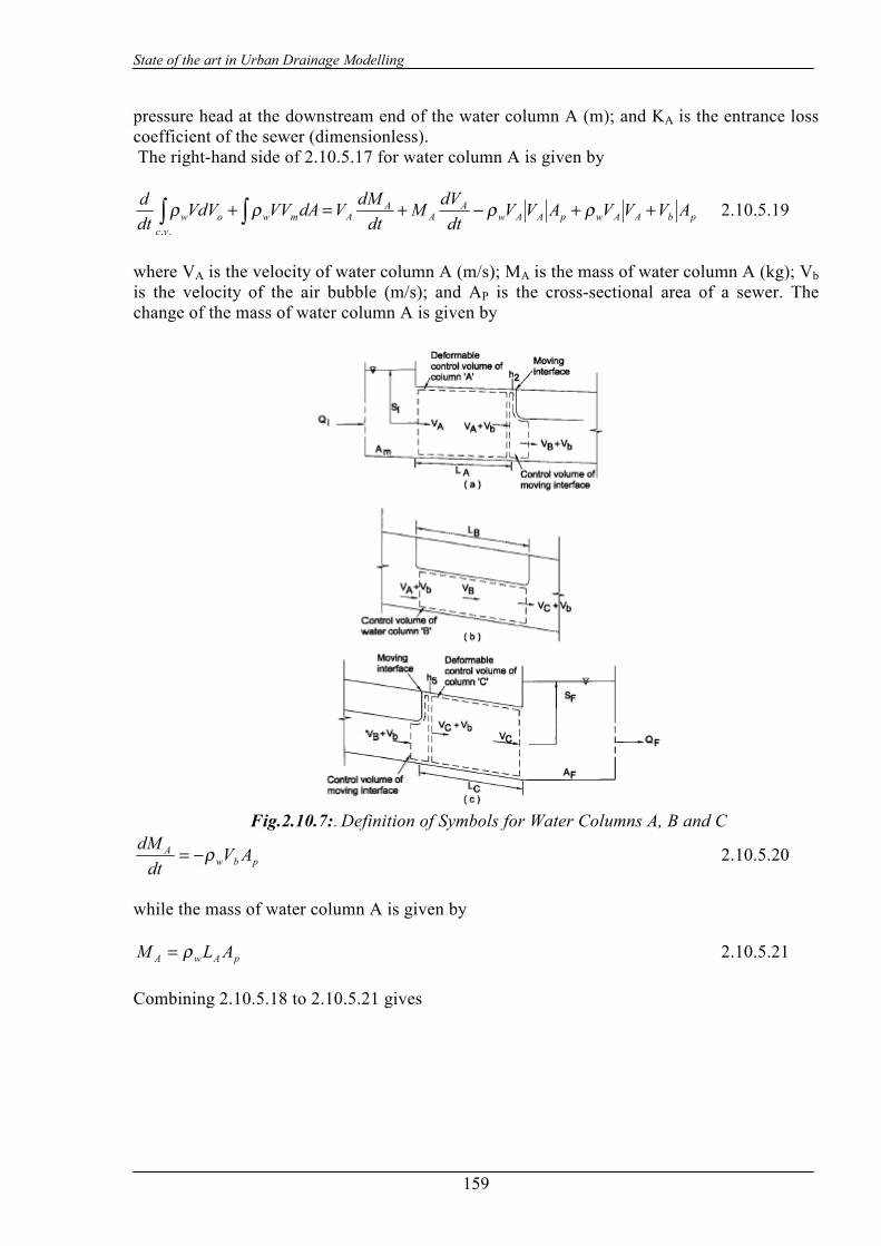
State of the art in Urban Drainage Modelling
159
pressure head at the downstream end of the water column A (m); and KA is the entrance loss coefficient of the sewer (dimensionless). The right-hand side of 2.10.5.17 for water column A is given by
pbAAwpAAwA
AA
Amwvc
ow AVVVAVVdt
dVMdt
dMVdAVVVdVdtd ++−+=+ ∫∫ ρρρρ
..
2.10.5.19
where VA is the velocity of water column A (m/s); MA is the mass of water column A (kg); Vb is the velocity of the air bubble (m/s); and AP is the cross-sectional area of a sewer. The change of the mass of water column A is given by
Fig.2.10.7:. Definition of Symbols for Water Columns A, B and C
pbwA AV
dtdM ρ−= 2.10.5.20
while the mass of water column A is given by
pAwA ALM ρ= 2.10.5.21 Combining 2.10.5.18 to 2.10.5.21 gives

State of the art in Urban Drainage Modelling
160
pAw
pw
A
bAA
A
AA
A
b
A
AAAo
AAA
AI
A
A
ALAh
RVVV
LAV
LVV
RVVf
gSgVV
Kg
VSLg
dtdV
ργ 2
22
8822
−
+−++−+
−−=
2.10.5.22
where fA is the steady-state friction factor of water column A. The conservation of momentum across the moving interface gives
( ) ( )ABpbAwpp
BBwapw VVAVVA
AAypAh −++
+= ρ
γγ
22 2.10.5.23
B
ApB L
VAA −= 2.10.5.24
in which pa, is the gauge air pressure inside the air bubble (N/m2); yB is the depth of water column B (m); AB is the average flow area of water column B (m2); VB is the velocity of water column B (m/s); Va is the volume of the air bubble (m3); and LB is the length of water column B (m). Substituting 2.10.5.23 and 2.10.5.24 into 2.10.5.22 gives the acceleration of water column A
( )( )A
ABbA
A
bAA
A
AA
A
bA
A
AAAo
Aw
p
BBwa
AAA
AI
A
A
LVVVV
RVVV
LAV
LVV
RVVf
gSL
AAy
p
gVV
Kg
VSLg
dtdV
−+−
+−
++−++
−
−−=
8
82
22
2
ρ
γ
2.10.5.25 In the derivation of the acceleration of water column B, the velocity of the moving bubble is superimposed on the fixed length control volume [Fig. 2.10.7-b]. Applying the momentum equation to the fixed control volume gives
dtdMV
dtdVML
RASLA B
BB
BBB
BBBBw +=−τγ 0 2.10.5.26
where AB is the average flow area of water column B (m2); Bτ is the wall shear stress of water column B (N/m2); RB is the hydraulic radius of water column B (m); MB is the mass of water column B (kg); LB is the length of air bubble or water column B (m); So is the sewer slope; and VB is the velocity of water column B (m/s). The rate of change of mass of water column B is given by
( )CApwB VVA
dtdM −= ρ 2.10.5.27
while the mass of water column B is given by
BBwB LAM ρ= 2.10.5.28 Substituting 2.10.5.27 and 2.10.5.28 into 2.10.5.26 gives the acceleration of water column B

State of the art in Urban Drainage Modelling
161
( )
BB
pBCA
B
BBBo
B
LAAVVV
RVVf
gSdt
dV +−−=
8 2.10.5.29
where fB is the steady-state friction factor of water column B. The acceleration of water column C is derived in a manner similar to that of water column A.
( )( )C
BCbC
C
bCC
C
CC
C
bC
C
CCCo
Cw
p
BBwa
CCC
CF
C
C
LVVVV
RVVV
LAV
LVV
RVVf
gSL
AAy
p
gVV
Kg
VS
Lg
dtdV
−+−
+−
++−++
−
−−=
8
82
22
2
ρ
γ
2.10.5.30 The rates of change of water depth at the upstream and downstream manholes are given by
m
pAII
AAVQ
dtdS −
= 2.10.5.31
F
FCF
AQAV
dtdS −
= 2 2.10.5.32
where QI is the rate of inflow at the upstream manhole (m3/s); QF is the rate of outflow at the downstream manhole (m3/s); Am is the surface area of the upstream manhole (m2); and AF is the surface area of the downstream manhole (m2).
It is noted that the sum of 2.10.5.20 , 2.10.5.27, pbwC AV
dtdM ρ= , wρ 2.10.5.31, and wρ
2.10.5.32 is equal to the net change of mass (i.e., wρ (QI -QF)) in the system. Thus, mass is conserved in the system. Applying the continuity equation to the fixed control volume of the air bubble [Fig. 2.10.7-b] gives the rate of change of air bubble volume
( ) aACa QAVV
dtdv
−−= 2 2.10.5.33
where va is the volume of air bubble (m3) and Qa is the air flow rate out of the bubble, which is zero if no air release mechanism exists along the sewer (m3/s). Using the ideal gas law with the assumption of a pseudo adiabatic compression and expansion process, the gauge air pressure inside the bubble (patm) is given by
atma
ooa p
vv
pp −
=
γ
2.10.5.34
where po is the initial absolute air pressure inside the air bubble (Pa); vo is the initial volume of the air bubble (m); γ is the ratio of specific heats of air (i.e., 1.2 for a pseudo adiabatic process); and patm is the atmospheric pressure (Pa). The pressure transients associated with the travelling compressible bubble can be simulated by solving 2.10.5.25, 2.10.5.29, 2.10.5.30, 2.10.5.31, 2.10.5.32, 2.10.5.33, and 2.10.5.34 simultaneously using a fifth-order Runge-Kutta algorithm. The initial conditions for the simulation are
2
11
AAVVA = 2.10.5.35

State of the art in Urban Drainage Modelling
162
atmoo ppp += 2.10.5.36
2VVC = 2.10.5.37 SF = from calculations in Stage 1 2.10.5.38
2p
I
DS = 2.10.5.39
( )12 AALV BA −= 2.10.5.40 Stage 5-Release of Trapped Air at Upstream Manhole When the trapped air bubble reaches the upstream manhole, a sudden release of air may cause severe pressure transients. In order for the trapped air to escape to the atmosphere, the pressure inside the bubble has to exceed a certain threshold. As this happens, an air-water mixture is forced out. After such a release of air, the pressure inside the bubble drops below the threshold value and the remaining air undergoes compression and expansion. The next release of the air-water mixture occurs when the pressure inside the air bubble exceeds the threshold value again. This process is repeated until all the trapped air is expelled. It is assumed that the threshold pressure for air release is related to the water level at the upstream manhole [Fig. 2.10.7-c] and is given by
wp
IIm
DSpp γ
−=
2 2.10.5.41
where pm is the threshold pressure for air release (Pa) and pI is the threshold pressure coefficient (dimensionless). The air mass inside the air bubble is given by
aaa vm ρ= 2.10.5.42 where ma is the air mass inside the bubble (kg); and aρ is the air density inside the bubble (kg/m2). The rate of change of air mass is then given by
dtdv
dtdv
dtdm a
aa
aa ρρ
+= 2.10.5.43
Conservation of air mass gives the rate of change of air inside the bubble
aaa Q
dtdm
ρ= 2.10.5.44
where Qa is the rate of air release (m3/s). Combining 2.10.5.42 and 2.10.5.43 gives
aaa
aa
a Qdt
dvdt
dv ρρ
ρ=+ 2.10.5.45
Assuming the air bubble undergoes a pseudo adiabatic expansion and compression process, the relationship between air pressure (pa) and density ( aρ ) inside the bubble is given by ( )
Cpp
a
atma =+
γρ 2.10.5.46

State of the art in Urban Drainage Modelling
163
where C (a constant) can be determined by substituting initial gauge pressure and density of air inside the air bubble. Rearranging 2.10.5.4.46 gives
( ) γ
ρρ
1
+=
a
atmaa
pp 2.10.5.47
Differentiating with respect to time (t) gives
dtdp
Cpp
Cdtd aatmaa
γγ
γρ
−
+
=
1
1 2.10.5.48
Applying the continuity equation to the deformable control volume B as shown in [Fig. 2.10.6-c] gives the rate of change of air bubble volume (va)
( )BpbI
mIpCa AAV
dtdSAQAV
dtdv −−
−−= 2.10.5.49
where QI is the inflow to the upstream manhole (m3/s); Am is the cross-sectional area of the upstream manhole (m2); and SI (m3/s) is the water level at the manhole from the center point of the sewer. The rate of air release (Qa) can be simulated by an orifice equation given by
( )a
aBpKa
pAAXQ
ρ2
−= 2.10.5.50
where XK is the air release coefficient (dimensionless). Substituting 2.10.5.47 to 2.10.5.50 into 2.10.5.45 gives the rate of change of gauge pressure inside the bubble:
( )
−
−−
−⋅
+
=
−
aaBpbI
mIpCaatma
a
a QAAVdt
dSAQAVC
ppvC
dtdp ρργ γ
γ 1
2.10.5.51
and
( )BpKaaaa AAXpQ −= ρρ 2 for ma pp ⟩ 2.10.5.52-a 0=aaQρ for ma pp ≤ 2.10.5.52-b
The acceleration of water column B [Fig. 2c)] can be derived by applying the continuity and momentum equations to the deformable control volume and is given by
B
bBB
B
BBBbpC
ImI
BB
B
B
BBBo
B
LVVV
LVV
AVAVdt
dSAQ
LAV
RVVf
gSdt
dV +−+
−−−−−=
8 2.10.5.53
The acceleration of water column C [Fig. 2.10.6-c] can be derived in a manner similar to that in Stage 4. Using the last computed values of the variables from Stage 4 as initial conditions,
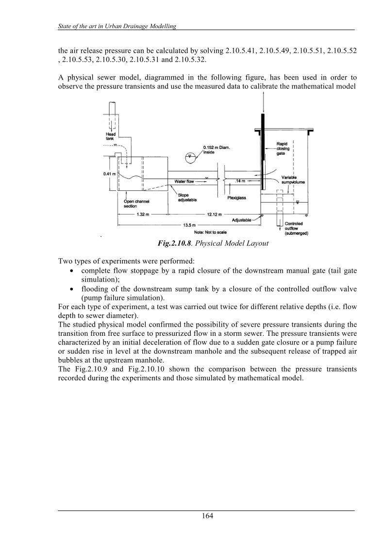
State of the art in Urban Drainage Modelling
164
the air release pressure can be calculated by solving 2.10.5.41, 2.10.5.49, 2.10.5.51, 2.10.5.52 , 2.10.5.53, 2.10.5.30, 2.10.5.31 and 2.10.5.32. A physical sewer model, diagrammed in the following figure, has been used in order to observe the pressure transients and use the measured data to calibrate the mathematical model
. Fig.2.10.8. Physical Model Layout
Two types of experiments were performed:
• complete flow stoppage by a rapid closure of the downstream manual gate (tail gate simulation);
• flooding of the downstream sump tank by a closure of the controlled outflow valve (pump failure simulation).
For each type of experiment, a test was carried out twice for different relative depths (i.e. flow depth to sewer diameter). The studied physical model confirmed the possibility of severe pressure transients during the transition from free surface to pressurized flow in a storm sewer. The pressure transients were characterized by an initial deceleration of flow due to a sudden gate closure or a pump failure or sudden rise in level at the downstream manhole and the subsequent release of trapped air bubbles at the upstream manhole. The Fig.2.10.9 and Fig.2.10.10 shown the comparison between the pressure transients recorded during the experiments and those simulated by mathematical model.

State of the art in Urban Drainage Modelling
165
Fig.2.10.9:Comparison of Pressure Transient Measured during the experiment with sudden
gate closure at relative depth of 0.76 with those predicted by numerical model
Fig.2.10.10: Comparison of Pressure Transient Measured during the experiment with pump
failure at relative depth of 0.76 with those predicted by numerical model It is noted that the pressure transients simulated by the mathematical model are fluctuating in a manner similar to those recorded during the experiments. For the initial water hammer type pressure transients, the damping of the pressure fluctuations is underestimated by the model. When the steady-state friction factor is increased by 20 times, the dumping of transient pressure is found to be close to that recorded during the experiments. Thus, the assumption of a steady-state friction factor may not be appropriate for the transient conditions (Fok, 1987). Additionally, the mathematical model predicts lower negative pressures than were observed experimentally. As numerous bubbles were formed during the experiments while a single bubble was assumed in the mathematical model, the superposition of transient pressures of various bubbles in the experiments was not accounted for in the mathematical model and may be responsible for the higher minimum pressures.
2.10.5.5 H.Capart et al. H.Capart, C. Bogaerts, J.Kevers-Leclercq and Y.Zech (1997) proposed a numerical scheme based on a finite volume formulation in order to handle flow transitions within drainage pipes
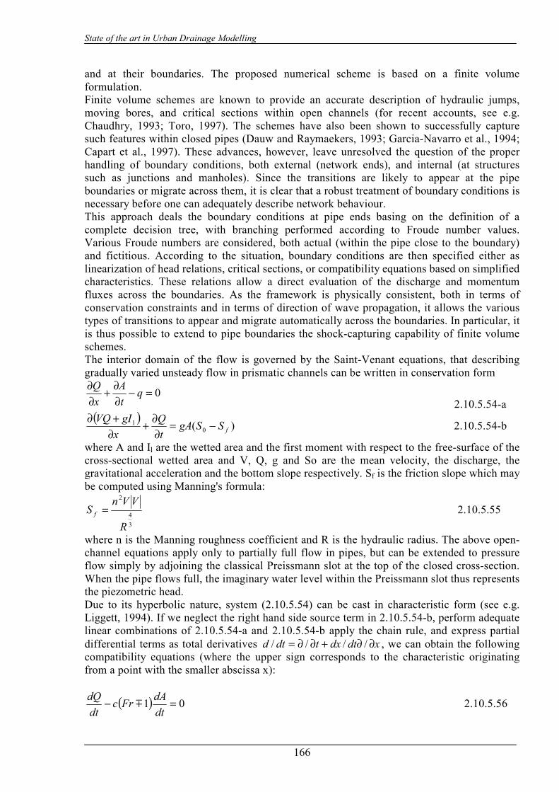
State of the art in Urban Drainage Modelling
166
and at their boundaries. The proposed numerical scheme is based on a finite volume formulation. Finite volume schemes are known to provide an accurate description of hydraulic jumps, moving bores, and critical sections within open channels (for recent accounts, see e.g. Chaudhry, 1993; Toro, 1997). The schemes have also been shown to successfully capture such features within closed pipes (Dauw and Raymaekers, 1993; Garcia-Navarro et al., 1994; Capart et al., 1997). These advances, however, leave unresolved the question of the proper handling of boundary conditions, both external (network ends), and internal (at structures such as junctions and manholes). Since the transitions are likely to appear at the pipe boundaries or migrate across them, it is clear that a robust treatment of boundary conditions is necessary before one can adequately describe network behaviour. This approach deals the boundary conditions at pipe ends basing on the definition of a complete decision tree, with branching performed according to Froude number values. Various Froude numbers are considered, both actual (within the pipe close to the boundary) and fictitious. According to the situation, boundary conditions are then specified either as linearization of head relations, critical sections, or compatibility equations based on simplified characteristics. These relations allow a direct evaluation of the discharge and momentum fluxes across the boundaries. As the framework is physically consistent, both in terms of conservation constraints and in terms of direction of wave propagation, it allows the various types of transitions to appear and migrate automatically across the boundaries. In particular, it is thus possible to extend to pipe boundaries the shock-capturing capability of finite volume schemes. The interior domain of the flow is governed by the Saint-Venant equations, that describing gradually varied unsteady flow in prismatic channels can be written in conservation form
0=−∂∂+
∂∂ q
tA
xQ
2.10.5.54-a ( )
)( 01
fSSgAtQ
xgIVQ −=
∂∂+
∂+∂ 2.10.5.54-b
where A and Il are the wetted area and the first moment with respect to the free-surface of the cross-sectional wetted area and V, Q, g and So are the mean velocity, the discharge, the gravitational acceleration and the bottom slope respectively. Sf is the friction slope which may be computed using Manning's formula:
34
2
R
VVnS f = 2.10.5.55
where n is the Manning roughness coefficient and R is the hydraulic radius. The above open-channel equations apply only to partially full flow in pipes, but can be extended to pressure flow simply by adjoining the classical Preissmann slot at the top of the closed cross-section. When the pipe flows full, the imaginary water level within the Preissmann slot thus represents the piezometric head. Due to its hyperbolic nature, system (2.10.5.54) can be cast in characteristic form (see e.g. Liggett, 1994). If we neglect the right hand side source term in 2.10.5.54-b, perform adequate linear combinations of 2.10.5.54-a and 2.10.5.54-b apply the chain rule, and express partial differential terms as total derivatives xdtdxtdtd ∂∂+∂∂= //// , we can obtain the following compatibility equations (where the upper sign corresponds to the characteristic originating from a point with the smaller abscissa x):
( ) 01 =−dtdAFrc
dtdQ
m 2.10.5.56

State of the art in Urban Drainage Modelling
167
to be integrated along characteristic paths defined by
cVdtdx ±= dx
dt =V ±c, 2.10.5.57-a,b in which Fr = V/c is the Froude number, c `= (g A/b)1/2I and b is the width of the free-surface. Alternatively, compatibility equations 2.10.5.5.3 can be written in terms of variables Q and ∑ as
( ) 01 =−∑dtdQFrc
dtd
m 2.10.5.5.5-a,b
where we have defined 1gIVQ +=∑ . Note in equations 2.10.5.56 and 2.10.5.58 the interesting parallelism between the two couples of variables (A,Q) and (Q, ∑ ). The numerical scheme adopted by this model is briefly sketched here.
Fig. 2.10.11: Finite Volume Discretization.
A finite volume statement is first obtained by discretizing system 2.10.5.54 with respect to distinct control volumes (or "cells") as shown in Fig. 2.10.11. This yields for the primitive variables A and Q the expressions
( )2/12/1
2/12/1
1 ++
+−
+ −∆∆+= j
ij
ij
ij
i QQxtAA 2.10.5.59-a
( ) ( )( ) tSSgAxtQQ j
ifoji
ji
ji
ji ∆−+∑−∑
∆∆+= +
++−
+ 2/12/1
2/12/1
1 2.10.5.59-b
in which subscript i denotes the centre of a cell, subscripts i-1/2 and i+1/2 refer to its upstream and downstream boundaries, and superscripts j and j+1 denote values of the variables at times t and t + t∆ . Flux terms Qj+1/2'and 2/1+∑ j at intermediate time j+1/2 are yet to be predicted from the known values of the cell variables at time t. This is achieved in the Pavia flux-predictor scheme of Braschi and Gallati (1992) by resorting to the characteristic equations. A short derivation, slightly different from the original presentation of those authors, is included here since a similar reasoning will be applied below for the boundaries.

State of the art in Urban Drainage Modelling
168
Fig. 2.10.12:Approximated characteristic paths: (a) subcritical case; (b) supercritical case. At intermediate section i + 1/2, reach-averaged velocity V*, wave celerity c* and corresponding Froude number Fr are defined from values at time j as: V* = 0.5 (Vi + Vi+1) ; c*= 0.5 (ci + ci+1) ; Fr* = V*/c*. 2.10.5.60-a,b,c The value of reach-averaged Froude number Fr* is used to define the local regime of flow, and characteristic paths are approximated according to the two cases shown on Fig. 2.10.12. For the subcritical case ( 1⟨Fr ), the compatibility equations 2.10.5.57 can be written
( )( )ji
ji
ji
ji AAcVQQ −−=− +
++
+2/1
2/12/1
2/1 ** 2.10.5.61-a ( )( )j
ij
ij
ij
i AAcVQQ 12/1
2/112/1
2/1 ** ++
+++
+ −+=− 2.10.5.61-b Eliminating 2/1
2/1+
+j
iA between 2.10.5.61-a and 2.10.5.61-b leads to
( )( ) ( )( ) ( )( )( )ji
ji
ji
ji
ji AAFrcQFrQFrQ 1
21
2/12/1 *1
21*1
21*1
21
+++
+ −−+−+−= 2.10.5.62-a
We can also write the compatibility equations in form 2.10.5.58 and obtain, after elimination of 2/1
2/1+
+j
iQ
( )( ) ( )( ) ( )( )( )ji
ji
ji
ji
ji QQFrcFrFr 1
21
2/12/1 *1
21*1
21*1
21
++++ −−+∑−+∑−=∑ 2.10.5.62-b
Finally, a similar reasoning for the supercritical case ( 1⟩Fr ) leads to the simple expressions
Fr* >1 : Ji
ji QQ =++
2/12/1 , J
iji ∑=∑ ++
2/12/1 2.10.5.63-a,b
Fr* <-l : Ji
ji QQ 1
2/12/1 +
++ = , J
iji 1
2/12/1 +
++ ∑=∑ 2.10.5.64-a,b
The numerical algorithm obtained by combining expressions (2.10.5.59 -2.10.5.64) guarantees strict conservation as well as a physically consistent signal propagation. This allows the scheme to deal with both subcritical and supercritical regimes, as well as automatically capture shocks and regime transitions. Note that, as the scheme is explicit, the time step must satisfy the Courant condition (see e.g. Chaudhry, 1993). Boundary conditions Let the pipe be divided into m cells numbered 1 to m. Given the finite volume principle retained for the discretization, it is natural to lei the pipe boundaries correspond, upstream, to
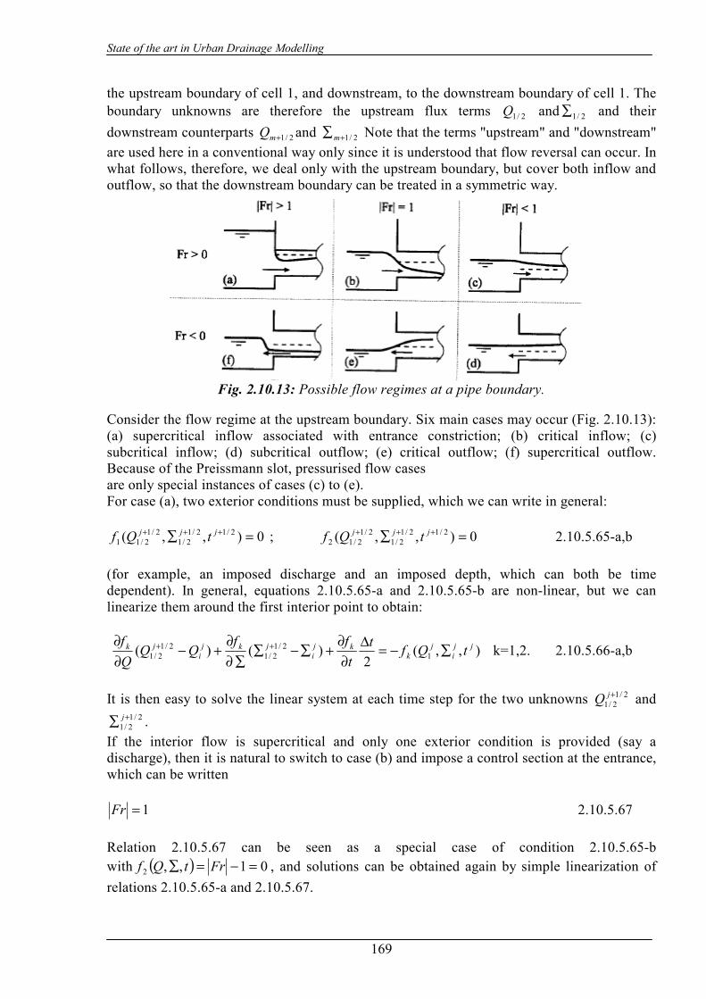
State of the art in Urban Drainage Modelling
169
the upstream boundary of cell 1, and downstream, to the downstream boundary of cell 1. The boundary unknowns are therefore the upstream flux terms 2/1Q and 2/1∑ and their downstream counterparts 2/1+mQ and 2/1+∑m Note that the terms "upstream" and "downstream" are used here in a conventional way only since it is understood that flow reversal can occur. In what follows, therefore, we deal only with the upstream boundary, but cover both inflow and outflow, so that the downstream boundary can be treated in a symmetric way.
Fig. 2.10.13: Possible flow regimes at a pipe boundary.
Consider the flow regime at the upstream boundary. Six main cases may occur (Fig. 2.10.13): (a) supercritical inflow associated with entrance constriction; (b) critical inflow; (c) subcritical inflow; (d) subcritical outflow; (e) critical outflow; (f) supercritical outflow. Because of the Preissmann slot, pressurised flow cases are only special instances of cases (c) to (e). For case (a), two exterior conditions must be supplied, which we can write in general:
0),,( 2/12/12/1
2/12/11 =∑ +++ jjj tQf ; 0),,( 2/12/1
2/12/1
2/12 =∑ +++ jjj tQf 2.10.5.65-a,b (for example, an imposed discharge and an imposed depth, which can both be time dependent). In general, equations 2.10.5.65-a and 2.10.5.65-b are non-linear, but we can linearize them around the first interior point to obtain:
),,(2
)()( 12/1
2/12/1
2/1jj
ij
kkj
ijkj
ijk tQft
tffQQ
Qf
∑−=∆∂∂
+∑−∑∑∂
∂+−
∂∂ ++ k=1,2. 2.10.5.66-a,b
It is then easy to solve the linear system at each time step for the two unknowns 2/1
2/1+jQ and
2/12/1
+∑ j . If the interior flow is supercritical and only one exterior condition is provided (say a discharge), then it is natural to switch to case (b) and impose a control section at the entrance, which can be written
1=Fr 2.10.5.67 Relation 2.10.5.67 can be seen as a special case of condition 2.10.5.65-b with ( ) 01,,2 =−=∑ FrtQf , and solutions can be obtained again by simple linearization of relations 2.10.5.65-a and 2.10.5.67.
State of the art in Urban Drainage Modelling
170
For cases (c) and (d), one exterior condition must be supplied, say by expression 2.10.5.65-a, and combined with an interior condition given by a characteristic. In the present work, we propose to use for the characteristic equation the same approximation as the one chosen for the interior domain. We assume that the negative (case c) or positive (case d) characteristic originates from the first interior point 1, and apply compatibility equation 2.10.5.59-b to obtain:
( ) 0)1()( 2/12/1
2/12/1 =−+−∑−∑ +
+++
ji
ji
ji
ji QQFrc 2.10.5.68
This linearized compatibility equation can then be combined with linearized exterior condition 2.10.5.65-a, and the system is easily solved for the two unknowns. For case (e), a linearization of condition 2.10.5.67 can be coupled with 2.10.5.68. Finally, case (l) is treated by combining two characteristics from the interior domain, and this leads to a special case of expressions 2.10.5.64-a,b.
Ji
ji QQ =++
2/12/1 ; J
iji ∑=∑ ++
2/12/1 2.10.5.69-a,b
2.10.6. References Alberto Campisano, Wolfgang Schilling, Carlo Modica, “Regulators’ setup with application to the Roma-Cecchignola combined sewer system”, Urban Water 2 (2000), pp.235-242. Bauwens, W., Angelov, D., Brauns, M., Mespreuve, M. and Smeets, M. (July 1993) “A comparison of three sewer simulation models”, Proceedings of 6th International Conference on Urban Storm Drainage, Niagara Falls Ontario Canada, pp. 1484-1489 David R. Maidment, “Handbook of Hydrology”, Editor in Chief, 1992. H. Capart, C. Bogaerts, J. Kevers-Leclercq and Y. Zech, “Robust Numerical Treatment of Flow Transitions a Drainage Pipe Boundaries”, Wat. Sci. Tech. Vol.39, No.9, pp.113-120, 1999. Homayoun Motiee, Bernard Chocat and Oliver Blanpain, “A Storage Model for the Simulation of the Hydraulic Behaviour of drainage networks” Wat. Sci. Tech. Vol. 36, No. 8-9, pp.57-63, 1997. James Ball Ball, J.E. (July 1993) ,”Modelling of unsteady flow through manholes”, Proceedings of 6th International Conference on Urban Storm Drainage, Niagara Falls Ontario Canada, pp. 116-121. James Li and Alex McCorquodale, “Modelling Mixed Flow in Storm Sewers”, Journal of Hydraulic Engineering (November 1999), pp.1170-1180. M. Fugazza (July 1993), “A Software System for Runoff and Routing Modelling in Drainage Catchment”, Proceedings of 6th International Conference on Urban Storm Drainage, Niagara Falls Ontario Canada, pp. 230-236. M. Fugazza (July 1993). “Theoretical Development of a Mathematical Model for Operation and Design of Hydraulic Channel Network”, Proceedings of 6th International Conference on Urban Storm Drainage, Niagara Falls Ontario Canada, pp. 275-281. Sophie Duchesne, Alain Mailhot, Emeric Dequidt, Jean-Pierre Villeneuve, “Mathematical modeling of sewers under surcharge for real time control of combined sewer overflow”, Urban Water 3 (2001), pp.241-252. Zhong Ji, “General Hydrodynamic Model for Sewer/Channel Network System”, Journal Of Hydraulic Engineering, March 1998, pp. 307-315.

State of the art in Urban Drainage Modelling
171
3 URBAN DRAINAGE: WATER QUALITY MODELS
3.1 SWMM – Storm Water Management Model
3.1.1. Model availability SWMM is one of the most successful models produced by United States Environmental Protection Agency (US-EPA). This models suite has both freeware and commercial versions. The freeware version is distributed by EPA (www.epa.gov) and by some North-American universities and research institutions that provide also updates and documentation. Those institution are listed in the references.
3.1.2. Abstract
3.1.2.1 Objectives and peculiarities SWMM is a dynamic rainfall-runoff simulation model, primarily but not exclusively designed for urban drainage systems analysis and for single-event or long-term (continuous) simulation. SWMM can be considered as a complete suite of tools covering all the aspects of urban drainage simulation: runoff generation and propagation, water quality analysis on catchment surface, in the drainage system and in the receiving waters. An overview of the model structure is shown in Fig. 2.2.1. In simplest terms the program is constructed in the form of “blocks” as follows: 6) Runoff Block; 7) Transport Block; 8) Extended Transport (Extran) Block; 9) Storage/Treatment Block; 10) Receive Block. Quality constituents for simulation may be arbitrarily chosen for any of the block, although the different blocks have different constrains on the number and type of constituents that may be modelled. Flow routing can be performed in the Runoff, Transport and Extran Blocks, in increasing order of sophistication. SWMM continues to be widely used throughout the world for analysis of quantity and quality problems related to stormwater runoff, combined sewers, sanitary sewers, and other drainage systems in urban areas, with many applications in non-urban areas as well. Quality routines do not use the most advanced analytical approaches but this choice allows for a simpler calibration and generally reliable results. The model may be used for both planning and design. The planning mode is used for an overall assessment of the urban runoff problem and proposed abatement options. This mode is typified by continuous simulation for several years using long-term precipitation data. At design-level, event simulation also may be run using a detailed catchment schematization and shorter time steps for precipitation input. Both single-event and continuous simulation may be performed on catchments having storm sewers, or combined sewers and natural drainage, for prediction of flows, stages and pollutant
State of the art in Urban Drainage Modelling
172
concentrations. The quality models result to have a good computational efficiency allowing for running long time series in short time.
3.1.2.2 Performance Indicator(s) of Interest SWMM is able to compute basic polluting compounds statistics in dry weather flow as well as wet weather flow. These variables (concerning both pollution concentrations and total charges) can be used to compute performance indicators for quality analysis.
3.1.2.3 Brief Historical Overview of the Model The EPA Stormwater Management Model SWMM has an impressive longevity: was developed in 1969-1971 and was one of the first of such models. A result of generous funding from the USEPA, the prime contractor was: Metcalf and Eddy Inc.of Palo Alto (M&E), and the sub-contractors were University of Florida (UoF), and Water Resources Engineers Inc. of Walnut Creek California (WRE). The joint venture was suggested by the EPA predecessor agency, the Federal Water Quality Administration, following receipt of three separate proposals: WRE wrote the original RUNOFF quantity, RECEIV and GRAPH routines; M&E wrote the RUNOFF quality and STORAGe/treatment routines; and UoF wrote the TRANSPORT routines. It has been used in scores of U.S. cities as well as extensively in Canada, Europe, Australia and elsewhere. A large body of literature on theory and case studies is available, partly documented in a bibliography of SWMM-related publications and elsewhere. The model has been used for very complex hydraulic analysis for combined sewer overflow mitigation as well as for many stormwater management planning studies and pollution abatement projects, and there are many instances of successful calibration and verification. Because of its public domain status, extensive feedback has been received from users on needed corrections and enhancements, and the model is continuously updated through interaction with CEAM.
- 1971 Version 1 - 1975 Version 2 produced by UoF. - 1977 EXTRAN added by CDM. - 1981 Version 3 published by UoF. - 1983 Version 3.3 reputedly a PC version issued by EPA CEAM. - 1984 PCSWMM - first user friendly personal computer version, distributed
commercially with impoved documentation by CHI. - 1988 Version 4 (current major version) - USEPA public domain personal computer
version. - 1991 version 4.05 by UoF. - 1992 version 4.2 by UoF. - 1993 version 4.21 by Oregon State University (OSU). - 1994 version 4.3 by EPA CEAM. - 1995 version 4.31 by OSU and others - 1998 version 4.4 by OSU and others - 2001 version 4.4h by OSU and others [current version]

State of the art in Urban Drainage Modelling
173
3.1.3. Usage Specifications
3.1.3.1 Programming Language(s) or Mathematical-Statistical Software(s) The source code has been written is FORTRAN. Other unofficial releases have been written in C++ and Visual Basic but they are not updated continuously.
3.1.3.2 Functionality Water quantity modelling is basically demanded to Runoff Block (rainfall-runoff transformation) and to Extran Block (flow propagation). The Runoff Block has been developed to simulate both the quantity and quality runoff phenomena of a drainage basin and the routing of flows and contaminants to the major sewer lines. It represents the basin by an aggregate of idealized subcatchments and gutter or pipes. Regarding the quantity analysis please refer to Chapter 2.2.3.2. For most SWMM applications, the Runoff Block is the origin of water quality constituents. Although effects of dry-weather flow and scour and deposition may be included in the Transport Block, (dry-weather flow quality may also be included in the Storage/Treatment Block), the generation of quality constituents (e.g., pollutants) in the storm water itself can only be included in the Runoff Block. Several mechanisms constitute the genesis of stormwater quality; Runoff concentrates on build-up and wash-off. In an impervious urban area, it is assumed that a supply of constituents is built up on the land surface during dry weather preceding a storm. Such a build-up may or may not be a function of time and factors such as traffic flow, dry fallout and street sweeping. With the storm the material is then washed off into the drainage system. The physics of the wash-off may involve rainfall energy, as in some erosion calculations, or may be a function of bottom shear stress in the flow as in sediment transport theory. Most often, however, wash-off is treated by an empirical equation with slight physical justification. As an alternative to the use of a build-up/wash-off formulation, quality loads (i.e., mass/time) may be generated by a rating curve approach in which loads are proportional to flow raised to some power. Such an approach may also be justified physically and is often easier to calibrate using available data. Other quality sources are catchbasins. These are treated in SWMM as a reservoir of constituents in each subcatchment available to be flushed out during the storm. Erosion of “solids” may be simulated directly be the Universal Soil Loss Equation (USLE). Since it was developed for long term predictions (e.g., seasonal or annual loads), its use during a storm event in SWMM is questionable. But it is convenient since many data are available to support it. A final source of constituents is in the precipitation itself. Much more monitoring exists of precipitation quality at present than in the past, and precipitation can contain surprisingly high concentrations of many parameters. This is treated in SWMM by permitting a constant concentration of constituents in precipitation. Many constituents can appear in either dissolved or solid forms (e.g., BOD, nitrogen, phosphorus) and may be adsorbed onto other constituents (e.g., pesticides onto “solids”) and thus be generated as a portion of such other constituents. To treat this situation, any constituent may be computed as a fraction (“potency factor”) of another. For instance, five percent of the suspended solids load could be added to the (soluble) BOD load. Or several particle size - specific gravity ranges could be generated, with other constituents consisting of fractions of each. Up to ten quality constituents may be simulated in the Runoff Block. All are user supplied, with appropriate parameters for each. All are transferred to the interface file for transmittal to subsequent SWMM blocks, but not all may be used by the blocks; see the documentation for each block. Up to five user supplied land uses may be entered to characterize different

State of the art in Urban Drainage Modelling
174
subcatchments. Street sweeping is a function of land use, and individual constituents. Constituent build-up may be a function of land use or else fixed for each constituent. Considerable flexibility thus exists. When channel/pipes are included, quality constituents are routed through them assuming complete mixing within each gutter/pipe at each time step. No scour, deposition or decay-interaction during routing is simulated in the Runoff Block. Output consists of pollutographs (concentrations versus time) at desired locations along with total loads, and flow-weighted concentration means and standard deviations. Although the conceptualization of the quality processes is not difficult, the reliability and credibility of quality parameter simulation is very difficult to establish. In fact, quality predictions by SWMM are almost useless without local data for the catchment being simulated to use for calibration and validation. If such data are lacking, results may still be used to compare relative effects of changes, but parameter magnitudes (i.e., actual values of predicted concentrations) will forever be in doubt. This is in marked contrast to quantity prediction for which reasonable estimates of hydrographs may be made in advance of calibration. Routing through the sewer may be accomplished in the Storm Water Management Model (SWMM) by the Transport Block. This block has the responsibility of coordinating not only routing of sewage quantities but also such functions as routing of quality parameters (subroutine QUAL), estimating dry-weather flow, DWF ( subroutine FILTH), estimating infiltration ( subroutine INFIL), and calling internal storage ( subroutine TSTRDT). The flows simulated by the RUNOFF model can be input to the TRANSPORT block of the SWMM model which simulates the hydraulic response of the basin from precipitation events through a solution procedure that basically follows a cinematic wave approach in which disturbances are allowed to propagate only in the downstream direction. As a consequence, backwater effects are not modelled beyond the realm of a single conduit, and downstream conditions ( e.g., tide gates, diversion structures) are assumed not to affect upstream computations. System that branch in the downstream direction can be modelled using “flow divider” elements to the extent that overflows are not affected by backwater conditions. Surcharging is modeled simply by storing excess flows at the upstream manhole until capacity exits to accept the stored volume. Pressure-flow conditions are not explicitly modeled and no attempt is made to determine if ground surface flooding exists. Up to four contaminants are handled by the Transport Block. Constituents may be introduced to the sewer system by any combination of four-means:
1. Storm-generated pollutographs computed by an upstream block are transferred on an interface file to enter the system at designated inlet manholes.
2. Special storm-generated pollutographs may be entered using data group R1 of this block at designated inlet manholes.
3. Residual bottom sediment in the pipes may be resuspended due to the flushing action of the storm flows.
4. For combined system, constant dry-weather flow pollutograph may be entered at designated inlet manholes or generated by Subroutine FILTH.
Routing of the pollutants is then done for each time step by subroutine QUAL. The maximum number of contaminants that can be routed is four. These may be selected arbitrarily from the input file, except that DWF can only be used to generate suspended solids, BOD5 and total coliforms. The scour/deposition routines may be used for any constituent. This block can also receive inputs from Storage/Treatment, Extran Blocks, and from the Transport Block itself. Time steps can not be changed during simulation and it is not possible to define different time step for “wet” and “dry” periods. In tests of sensitivity, it was found that except for very small values of DT (10 seconds), the output from Transport is insensitive to the length of the time
State of the art in Urban Drainage Modelling
175
step. Between values of two minutes and 30 minutes, hydrograph ordinates varied by less than one percent. For extremely short time step values, the peak flow moved downstream faster and never attained the maximum value that it had with a DT of two minutes and longer. Within the range commonly needed (two minutes to 30 minutes), the choice of time step will not significantly affect results. However, continuity errors can occasionally arise if the time step is longer than about two times the travel time through any conduit.
3.1.3.3 Possible interaction with other software tools Several interfaces have been developed which use freeware SWMM as mathematical engine. The availability of the model source code allows for any potential interaction with other software tools. Some programs have been developed for calibration and uncertainty analysis and they will better be discussed in the following paragraphs.
3.1.4. Input and Output procedures
3.1.4.1 Possible Input File(s) Formats Formatted text input file. Input file structure can be modified only through a source code modification.
3.1.4.2 Possible Output File(s) Formats Formatted text output file. Output file structure can be modified only through a source code modification.
3.1.4.3 Raw Data Formatting SWMM use a static input/output file format. Any format change can be obtained through a source code modification.
3.1.5. Theoretical framework Overview RUNOFF BLOCK RUNOFF block is basically the source of polluting loads that are used to feed water quality analyses in all SWMM blocks. Polluting components concentration in overland flow is originated by several process involving both quantity and quality aspects that are connected with runoff generation. In the following paragraphs the quality processes that are part of the polluting loads generation will be analysed. Build-up Formulations One of the most influential of the early studies of stormwater pollution was conducted in Chicago by the American Public Works Association (1969). As part of this project, street surface accumulation of “dust and dirt” (DD) (anything passing through a quarter inch mesh screen) was measured by sweeping with brooms and vacuum cleaners. The accumulations were measured for different land uses and curb length, and the data were normalized in terms of pounds of dust and dirt per dry day per 100 ft of curb or gutter. These well known results imply that dust and dirt build-up is a linear function of time. The dust and dirt samples were analyzed chemically, and the fraction of sample consisting of various constituents for each of four land uses was determined, leading to the results shown in Table 3.1.1.

State of the art in Urban Drainage Modelling
176
Table 3.1.1: Measured Dust and Dirt (DD) Accumulation in Chicago (APWA, 1969).
Table 3.1.2: Milligrams of Pollutant Per Gram of Dust and Dirt (Parts Per Thousand by Mass) for Four Chicago Land Uses (APWA, 1969)
From the values shown in Tables 3.1.1 and 3.1.2, the build-up of each constituent (also linear with time) can be computed simply by multiplying dust and dirt by the appropriate fraction. Since the APWA study was published during the original SWMM project (1968-1971), it represented the state of the art at the time and was used extensively in the development of the surface quality routines (Metcalf and Eddy et al., 1971). Several useful studies have been conducted since the pioneering APWA work permitting much more selectivity. Of course, the whole build-up idea essentially ignores the physics of generation of pollutants from sources such as street pavement, vehicles, atmospheric fallout, vegetation, land surfaces, litter, spills, anti-skid compounds and chemicals, construction, and drainage networks. Lager et al. (1977a) and James and Boregowda (1985) consider each source in turn and give guidance on build-up rates. But the rates that are (optionally) entered into the Runoff Block only reflect the aggregate of all sources. Modern Build-up formulations are usually based on interpolation of experimental data through the application of simple conceptual models. The Chicago data that were used in the original SWMM formulation assumed a linear build-up formulation. However, there is ample evidence that build-up can be nonlinear; Sartor and Boyd’s (1972) data are most often cited as examples. More recent data from Pitt for San Jose indicate almost linear accumulation, although some of the best fit lines had very poor correlation coefficients R, ranging from 0.35<R<0.9. Thus, the choice of the best functional form is not obvious. Whipple et al. (1977) have criticized the linear build-up formulation included in the original SWMM, although it is somewhat irrelevant since the user may insert his/her own desired initial loads, calculated by whatever procedure desired, directly in the input file, however, this is a useful option only for single-event simulation. The proper choice of the proper functional form must ultimately be the responsibility of the user. The program provides three options for “dust and dirt” build-up and three for individual constituents, namely:

State of the art in Urban Drainage Modelling
177
1) power-linear DD= DDFACT*tDDPOW DD<DDLIM
2) exponential DD= DDLIM*(1-e-DDPOW*t)
3) Michaelis-Menton. DD= DDLIM*(t/(DDFACT+t))
Figure 3.1.1: Comparison between different build-up formulations in SWMM
Linear build-up is simply a subset of a power function build-up. The shapes of the three functions are compared in Fig. 3.3.1 using the dust and dirt parameters as examples, and a strictly arbitrary assignment of numerical values to the parameters. Exponential and Michaelis-Menton functions have clearly defined asymptotes or upper limits. Upper limits for linear or power function build-up may be imposed if desired. “Instantaneous build-up” may be easily achieved using any of the formulation with appropriate parameter choices. Linear build-up is fastest in terms of computer time. For a given constituent, build-up may be computed as a fraction of dust and dirt, or individually for the constituent. If the first option is used then the rate of build-up will depend upon the fraction and the functional form used for a given land use. In other words, the functional form could vary with land use for a given constituent. If the second option is used the build-up function will be the same for all land uses (and subcatchments) for a given constituent. Wash-off Wash-off is the process of erosion or solution of constituents from a subcatchment surface during a period of runoff. It the water depth is more than a few millimetres, processes of erosion may be described by sediment transport theory in which the mass flow rate of sediment is proportional to flow and bottom shear stress, and a critical shear stress can be used to determine incipient motion of a particle resting on the bottom of a stream channel, e.g., Graf (1971),

State of the art in Urban Drainage Modelling
178
Vanoni (1975). Such a mechanism might apply over pervious areas and in street gutters and larger channels. For thin overland flow, however, rainfall energy can also cause particle detachment and motion. This effect is often incorporated into predictive methods for erosion from pervious areas (Wischmeier and Smith, 1958) and may also apply to wash-off from impervious surfaces, although in this latter case, the effect of a limited supply (build-up) of the material must be considered. Ammon (1979) reviews several theoretical approaches for urban runoff wash-off and concludes that although the sediment transport based theory is attractive, it is often insufficient in practice because of lack of data for parameter (e.g., shear stress) evaluation, sensitivity to time step and discretization and because simpler methods usually work as well (still with some theoretical basis) and are usually able to duplicate observed wash-off phenomena. Among the latter, the most often cited results are those of Sartor and Boyd (1972), shown in Figure 3.1.2, in which constituents were flushed from streets using a sprinkler system. From the figure it would appear that an exponential relationship could be developed to describe wash-off of the form: POFF(t) = PSHED0 (1 – e-kt) 3.1.5.1 where POFF is the cumulative amount washed off at time t, PSHED0 is the initial amount of quantity on surface at t = 0, and k is an exponential coefficient.
Figure 3.1.2: Wash-off of street solids by flushing with a sprinkler system (after Sartor and Boyd, 1972)
POFF is shown as the ordinate of Figure 3.1.2. Alternatively, since the amount remaining, PSHED(t), equals PSHED0-POFF, then: PSHED(t) = PSHED0 * e -kt 3.1.5.2

State of the art in Urban Drainage Modelling
179
where PSHED(t) = quantity remaining on surface at time t, PSHED0 is the initial amount of quantity on surface at t = 0, and k is an exponential coefficient as defined previously. It is clear that the coefficient, k, is a function of both particle size and runoff rate. An analysis of the Sartor and Boyd (1972) data by Ammon (1979) indicates that k increases with runoff rate, as would be expected, and decreases with particle size. The Sartor and Boyd data lend credibility to the wash-off assumption included in the original SWMM release (and all versions to date) that the rate of wash-off (e.g., mg/sec) at any time is proportional to the remaining quantity:
PSHEDkdt
dPSHED ⋅−= 3.1.5.3
The solution of equation 3.1.3 is equation 3.1.2. This was first proposed by Mr. Allen J. Burdoin, a consultant to Metcalf and Eddy, during the original SWMM development. The coefficient k may be evaluated by assuming it is proportional to runoff rate, r: k = RCOEF*r 3.1.5.4 where: RCOEF = washoff coefficient, and r = runoff rate over subcatchment. Burdoin assumed that one-half inch of total runoff in one hour would wash off 90 percent of the initial surface load, leading to the now familiar value of RCOEF of 4.6 in.-1. Sonnen (1980) estimated values for RCOEF from sediment transport theory ranging from 0.052 to 6.6 in.-1, increasing as particle diameter decreases, rainfall intensity decreases, and as catchment area decreases. He pointed out that 4.6 in.-1 is relatively large compared to most of his calculated values. Although the exponential wash-off formulation of equations 3.1.5.2 and 3.1.5.3 is not completely satisfactory as explained below, it has been verified experimentally by Nakamura (1984), who also showed the dependence of the coefficient k on slope, runoff rate and cumulative runoff volume. Even in the original SWMM release, this exponential formulation did not adequately fit some data, and as a “correction,” availability factors of the form AV = a + brc 3.1.5.5 The primary difficulty is that use of equations 3.1.5.4 and 3.1.5.5 will always produce decreasing concentrations as a function of time regardless of the time distribution of runoff. This is counter-intuitive, since it is expected that high rates during the middle of a storm might indeed produce higher concentrations than those preceding. This may be explained by observing that concentrations are calculated by dividing the load rate (e.g., mg/sec) to obtain the quantity per volume (e.g., mg/l). Thus,
ArPSHEDrRCOEFconst
QdtdPSHEDC
⋅⋅⋅== 3.1.5.6
where:

State of the art in Urban Drainage Modelling
180
C = concentration, quantity/volume, Q = A * r = flow rate, A = subcatchment area, r = runoff rate, and the constant incorporates conversion factors. Clearly, the concentration will always decrease with time since the runoff rate, r, divides out of the equation and the quantity remaining, PSHED, continues to decrease. This problem is overcome in SWMM by making wash-off at each time step, POFF, proportional to runoff rate to a power, WASHPO: -POFF(t) = dPSHED/dt = -RCOEF/3600 * rWASPO * PSHED 3.1.5.7 where: POFF = constituent load washed off at time, t, quantity/sec, PSHED = quantity of constituent available for wash-off at time, t, (e.g., mg), RCOEF = wash-off coefficient and r = runoff rate. It may be seen that if equation 3.1.5.7 is divided by runoff rate to obtain concentration, then concentration is now proportional to r(WASHPO-1). Hence, if the increase in runoff rate is sufficient, concentrations can increase during the middle of a storm even if PSHED is diminished. There are two parameters to be determined, RCOEF and WASHPO. Availability factors of the form of equation 3.1.5.5 are no longer used since there is sufficient flexibility for calibration using only equation 3.1.5.7. Of course, the original SWMM methodology can be recovered by using WASHPO = 1.0. It may be seen that concentrations may be made to increase with increasing runoff rate during the middle of a storm by increasing the value of WASHPO. However, perhaps counter intuitively, a larger value of WASHPO generally yields lower concentrations and higher values of PSHED. Increasing the value of RCOEF always increases concentrations. In subroutine QSHED of the Runoff Block, wash-off load rates are computed instantaneously at the end of a time step using equation 3.1.5.4. They are subsequently combined with other possible inflow loads to a gutter/pipe or inlet before dividing by the total inflow rate to obtain a concentration. The remaining constituent load on the subcatchment at the end of a time step is determined by using the average power of the runoff rate over the time step,(Eq. 3.1.5.8).
te)t(PSHED)tt(PSHED 2)tt(r)t(rRCOEF
WASHPOWASHPO
∆⋅⋅=∆+∆++
− 3.1.5.8
This calculation is done prior to application of equation 3.1.5.7. The average (trapezoidal rule) approximates the integral of rWASHPO over the time step. That the load rate of sediment is proportional to flow rate as in equation 3.1.5.8 is supported by both theory and data. For instance, sediment data from streams can usually be described by a sediment rating curve of the form: G = aQb 3.1.5.9 where: G = sediment load rate,

State of the art in Urban Drainage Modelling
181
Q = flow rate, and a,b = coefficients. Due to a hysteresis effect, such relationships may vary during the passing of a flood wave, but the functional form is evident in many rivers. Of particular relevance to overland flow wash-off is the appearance of similar relationships describing sediment yield from a catchment. The exponent b in equation 3.1.5.9 corresponds to the exponent WASHPO in equation 3.1.5.7, and the presence of the quantity PSHED in equations 3.1.5.7 reflects the fact that the total quantity of sediment washed off a largely impervious urban area is likely to be limited to the amount built up during dry weather. The preceding discussion assumes that urban runoff quality constituents will behave in some manner similar to “sediment” of sediment transport theory. Since many constituents are in particulate form the assumption may not be too bad. If the concentration of a dissolved constituent is observed to decrease strongly with increasing flow rate, a value of WASHPO < 1.0 could be used. Although the development has ignored the physics of rainfall energy in eroding particles, the runoff rate, r, closely follows rainfall intensity. Hence, to some degree at least, greater wash-off will be experienced with greater rainfall rates. As an option, soil erosion literature could be surveyed to infer a value of WASHPO if erosion is proportional to rainfall intensity to a power. Rating Curve As discussed above, the wash-off calculations may be avoided and load rates computed for each subcatchment at each time step by a rating curve method: POFF(t) = RCOEF * WFLOWWASPO 3.1.5.10 where: WFLOW = subcatchment runoff, cfs, (or m3/sec for metric input), POFF = constituent load washed off at time, t, quantity/sec (e.g., mg/sec), RCOEF = coefficient that includes correct units conversion, and WASHPO = exponent. Parameters RCOEF and WASHPO are entered for a particular constituent. Although used on a time step basis, the parameters for equation 3.1.5.10 are customarily determined on a storm event basis, by plotting total load versus total flow (Huber, 1980; Wallace, 1980). Two differences are apparent between equations 3.1.5.7 and 3.1.5.10. First, the former includes the quantity remaining on the surface, PSHED, in the right-hand side of the equation, leading to an exponential-type decay of the quantity in addition to being a function of runoff rate. Second, the form of the runoff rate is different in the equations. The power-exponential wash-off uses a normalized runoff rate, r over the total subcatchment surface (not just the impervious part). The rating curve, equation 3.1.5.10, also uses the total runoff, but in an unnormalized form, WFLOW. Since data for a particular catchment are often analyzed as a log-log plot of load versus flow, equation 3.1.5.10 facilitates use of the best fit line. Clearly, the rating curve will work better for some storms and parameters than for others. The rating curve method is generally easiest to use when only total runoff volumes and pollutant loads are available for calibration. In this case a pure regression approach should suffice to determine parameters RCOEF and WASHPO.
State of the art in Urban Drainage Modelling
182
Street Cleaning Street cleaning is performed in most urban areas for control of solids and trash deposited along street gutters. Although it has long been assumed that street cleaning has a beneficial effect upon the quality of urban runoff, until recently, few data have been available to quantify this effect. Within the Runoff Block, street cleaning (usually assumed to be sweeping) is performed (if desired) prior to the beginning of the first storm event and in between storm events (for continuous simulation). Unless initial constituent loads are defined in the input files (or unless a rating curve is used) a “mini-simulation” is performed for each constituent during the dry days prior to a storm during which build-up and sweeping are modelled. Removal occurs such that the fraction of constituent surface load, PSHED, remaining on the surface is REMAIN = 1.0 - AVSWP(J) * REFF(K) 3.1.5.11 where: REMAIN = fraction of constituent (or dust and dirt) load remaining on catchment surface, AVSWP = availability factor (fraction) for land use J, and REFF = removal efficiency (fraction) for constituent K. The effect of multiple passes must be included in the value of REFF. During the mini-simulation that occurs prior to the initial storm or start of simulation “dust and dirt” is also removed during sweeping using an efficiency REFFDD. It is probably reasonable to assume that dust and dirt is removed similarly to the total solids. The Runoff Block algorithm does not consider any non-linear effect sweeping removal efficiency. Rather, the same fraction is removed during each sweeping. The availability factor, AVSWP, is intended to account for the fraction of the catchment area that is actually sweepable. For instance, Heaney and Nix (1977) demonstrate that total imperviousness increases faster as a function of population density than does imperviousness due to streets only. Pollution concentration in precipitation Constituent concentrations in precipitation are entered in input files. All runoff, including snowmelt, is assumed to have at least this concentration, and the precipitation load is calculated by multiplying this concentration by the runoff rate and adding to the load already generated by other mechanisms. It may be inappropriate to add a precipitation load to loads generated by a calibration of build-up/wash-off or rating curve parameters against measured runoff concentrations, since the latter already reflect the sum of all contributions, land surface and otherwise. But precipitation loads might well be included if starting with build-up/wash-off data from other sources. They also provide a simple means for imposing a constant concentration on any Runoff Block constituent. For single event simulation, use of precipitation concentrations is a simple way in which to account for the high concentrations of several constituents found in snowpacks (Proctor and Redfern and James F. MacLaren, 1976b). It would be inappropriate for continuous simulation, however, since such high concentrations in runoff would not be expected to persist over the whole year. Urban Erosion Erosion and sedimentation are often cited as a major problem related to urban runoff. They not only contribute to degradation of land surfaces and soil loss but also to adverse receiving water quality and sedimentation in channels and sewer networks. Several ways exist to analyze
State of the art in Urban Drainage Modelling
183
erosion from the land surface (e.g., Vanoni, 1975), the most sophisticated of which include calculations of the shear stress exerted on soil particles by overland flow and/or the influence of rainfall energy in dislodging them. In keeping with the simplified quality procedures included in the rest of the Runoff Block, a widely-used empirical approach, the Universal Soil Loss Equation (USLE), has been adapted for use in SWMM. Full details and further information on the USLE are given by Heaney et al. (1975). TRANSPORT BLOCK In order to route the polluting loads generated by RUNOFF block trough the drainage system, the TRASPORT block can be used. Up to four pollutants may be arbitrarily chosen for input and routing by the TRASPORT Block. In the following, a short outline of Transport simulated processes will be performed. Decay Each pollutant may be subjected to a first order decay during the routing process by supplying a first order decay coefficient, DECAY (based on natural logarithms or base e). Although travel time through most sewer system is short enough so that decay is seldom important, the user could supply, for example, a deoxygenation coefficient, K1, for BOD if desired. Non-conservative pollutants are not linked interactively-decay of one has no effect on any other. Routing Quality routing in the Transport Block through conduit segments is accomplished by assuming complete mixing within the conduit in the manner of a continuously stirred tank reactor or “CSTR”. For the finite difference scheme, however, it may be easily shown that the negative concentrations may be predicted if:
QVt 2>∆ 3.1.5.12
where: ∆t = time step, sec, V = average volume in the conduit or storage unit, ft3, and Q = average flow through the conduit or storage unit, cfs. The governing differential equation for a completely mixed volume is:
LKCVQCCQdtdVC
dtdCV
dtdVC
ii +−−=+= 3.1.5.13
where: C = concentration in effluent and in the mixed volume, mg/L, V = volume, ft3, Qi = inflow rate, cfs, Ci = concentration of influent, mg/L, Q = outflow rate, cfs, K = first order decay coefficient, L/sec, and L = source (or sink) of pollutant to the mixed volume, mass/time. Scour and deposition Each pollutant is assigned a specific gravity (SPG) and particle size distribution, assumed to apply throughout the drainage system regardless of the source of the pollutant, e.g. stormwater or dry-weather flow. If SPG ≤ 1.0, the pollutant is considered to be entirely suspended (or

State of the art in Urban Drainage Modelling
184
dissolved) and not subject to scour and deposition. During the simulation scour and deposition are simulated using Shields’ criterion to determine the critical diameter for incipient motion and deposition. Shields’ diagram is widely accepted as a good definition of the beginning of particle motion and describes the balance between the hydrodynamic forces of drag and lift on a particle (tending to induce motion) and the submerged weight of a particle (tending to resist motion). When hydrodynamic forces acting on a sediment particle reach a value such that if increased even slightly will put the particle into motion, critical or threshold conditions are said to have been reached. Dimensional analysis of this condition leads to:
( )
=
− νγγτ duf
ds
c*
3.1.5.14
where: τc = critical shear stress required to induce particle motion, lb/ft2, γs = specific weight of the sediment, lb/ft3, γ = specific weight of water = 62.4 lb/ft3, d = sediment diameter, ft or mm, u* = shear or friction velocity, ft/sec, ν = kinematic viscosity of water, ft2/sec. The equation may be stated in words that the dimensionless critical shear stress is a function of the shear Reynolds number. The critical shear and shear velocity are related to each other and to flow properties by:
gRSu c =
= ρτ* 3.1.5.15
where: ρ = water density = 1.98 slug/ft3, g = gravity = 32.2 ft/sec2, R = hydraulic radius, ft, S = slope of energy grade line (= invert slope). In addiction, the specific weight difference may be related to the specific gravity difference between sediment and water:
( )1−=− SPGs γγγ 3.1.5.16 where: SPG = specific gravity of the sediment, and the specific gravity of water is taken as 1.
3.1.6. Model Parameters Estimation or Assignation This kind of routines is not available for the freeware version of SWMM. Nevertheless some of the commercial versions have been upgraded with this kind of features. In the following this kind of routines will be described.

State of the art in Urban Drainage Modelling
185
3.1.6.1 Check of Parameters Significance – Internal Validation Computational Hydraulic Institute (CHI) has developed a sensitivity analysis routine for the freeware version of SWMM. Sensitivity Wizard provides an analysis of parameter sensitivity for various input functions and objective functions in the SWMM Runoff module. Through an easy step-by-step interface, the complicated and lengthy process of manual sensitivity testing is dramatically simplified and shortened. Any number of parameters and input functions can be analyzed in one session, and easily re-analyzed if model changes are made. The sensitivity results generated by Sensitivity Wizard are presented in highly customizable graphs, and both the graphs and numeric tables can be exported in various forms (e.g. printed, inserted into other documents, and/or copied to other graphing programs for further customization). This routine uses both linear and non-linear functions in order to interpolate dependency function between parameters and model output. The sensitivity wizard can be applied to any output variable even including pollution concentrations and total loads. Another tool developed by CHI allows for SWMM model calibration. The Genetic Algorithm Calibration tool is a genetic algorithm-based software tool for calibration of SWMM Runoff, Transport, Extran and/or StorageTreatment modules. Model calibration is a crucial step in developing a useful storm water model, especially when the model is used to evaluate one or more "what-if" scenarios in an existing storm water system. While a SWMM model can be applied to very simple modelling problems, it can also be quite complex, containing thousands of significant hydraulic and hydrologic entities. As each model entity may contain as many as a dozen sensitive parameters, and as the volume of available observed time series data increases, rigorous manual calibration can be an expensive, time-consuming undertaking. For this reason, model calibration is often not performed, or performed inadequately. An automated calibration tool such as this one significantly reduces the effort required for calibration and design optimization. Such tools encourage the adoption of more thorough model development and verification protocols, and better design.
3.1.7. PI(s) Estimation Method Some basic pollutograph statistics are computed during SWMM quality simulations such as maximum, minimum and average concentrations as well as total loads in any model outlet. Those parameters can be used to compute physical and operational performance indicators about single pipes, CSOs or parts of the drainage systems. Other parameters, that are not computed as a standard by SWMM can be obtained through a source code modification.
3.1.8. Future Improvements of the Model A redevelopment project has been started by US EPA and by the other authors in order to update the modelling approaches, the source code structure and the user interface of SWMM4. This project will lead to the release of SWMM5 model in the second half of 2003. The goal of this project is to help meet the needs of EPA’s clients for improved computational tools for managing urban runoff and wet weather water quality problems. The redevelopment team intends to produce a new version of SWMM that incorporates modern software engineering methods as well as updated computational techniques. The specific objectives of this project are:
• To revise the architecture of the SWMM computational engine, using object oriented programming (OOP) techniques, to enhance the ability of the model to be maintained, upgraded, and interfaced with other software.
State of the art in Urban Drainage Modelling
186
• To provide a rudimentary graphical user interface (GUI) to the engine to improve the usability of the model.
• To remove obsolete features, improve key computational aspects, and add new computational capabilities to the model where warranted.
• To develop guidelines on how SWMM can be used to model more recently developed Best Management Practices (BMP) for runoff control.
The end products from this project will consist of the following: • A newly coded version of the SWMM computational engine that can be run either
as a stand-alone application or as a Dynamic Link Library (DLL) of functions that can be called from other applications such as third party vendors of SWMM.
• A GUI shell program that will run under Windows, access the SWMM engine through DLL calls, and include a context-sensitive, on-line Help system.
• Full documentation in the form of a Users Manual, a Programmer’s Manual, and a Reference Manual.
• A manual on Modeling BMPs with SWMM that will illustrate how SWMM can be used to model various types of BMP/LID options.
This project will be a joint development effort between EPA-NRMRL’s Water Supply and Water Resources Division and Camp Dresser and McKee Inc. (CDM). CDM’s participation will be through a CRADA (Cooperative Research and Development Agreement) between itself and the Agency. The work envisioned for this project can be divided into nine task areas as follows:
1. Re-examine SWMM’s functionality 2. Re-write SWMM’s computational engine 3. Adapt an existing graphical user interface for use with SWMM 4. Update and add to SWMM’s computational algorithms 5. Develop standard formats and procedures for data transfer 6. Develop converters for input/output from previous versions of SWMM 7. Identify how state-of-the-art BMP/LID modeling can be incorporated into
SWMM 8. Prepare program documentation 9. Conduct quality assurance testing
Since this project affords the opportunity to rebuild SWMM from the ground up, it seemed worthwhile to ask which computational features currently contained in SWMM could be eliminated, which should be retained in their current form, which are in need of updating, and which additional features should be added. New features that are prime candidates for inclusion in future versions of the software are:
• SCS curve number infiltration • soil moisture accounting model for groundwater • energy balance model for snowmelt • implicit dynamic wave flow routing • Lagrangian water quality transport model • bed/suspended load sediment transport model • interactive real-time control of sewer flow routing.
The computational engine which implements the modeling functionality embedded in SWMM will be re-written in C++ using an object oriented approach. The SWMM engine will be delivered in two formats. One will be a stand-alone executable that receives input from a text file and writes output to a text file and/or binary output file. The other will be a library of callable functions that can be accessed by other software, such as the SWMM Graphical User Interface module discussed below. For the Windows operating system,
State of the art in Urban Drainage Modelling
187
the library will be compiled as a DLL (Dynamic Link Library). This follows the same approach used by the highly successful EPANET model, which analyzes hydraulic and water quality behavior in drinking water distribution systems. In EPANET only one line of code needs to be changed to compile the program as a DLL as opposed to a stand-alone executable. The SWMM graphical user interface will be ported over from the previously developed EPANET user interface. The redevelopment team estimates that about 80% of the existing code can be used with either no or only minor modification. Without this high degree of re-usability it probably would not be feasible to include GUI development within this project. It will allow the user to draw a node-link representation of the drainage network on a scalable map, with the option of inserting a background reference map. Point and click actions will be used to add, delete, re-position, and edit specific objects depicted on the map. Color coding of the map’s features are used to represent the values of user-selected design parameters or computed output. Retrofitting the EPANET GUI to meet the specific needs of SWMM will proceed in parallel with the development of the computational engine, since data definitions and file formats have to remain synchronized between the two modules. The GUI will also present a simpler way to perform testing and debugging of the engine than would the command line interface. The GUI will be subjected to the same iterative review procedures as will the engine, with the understanding that its functionality will not grow beyond what is already included in EPANET. In conjunction with the need to evaluate the functionality to be included in the updated SWMM there is also a need to evaluate which computational methods should be improved or replaced. EPA will explore making the following computational enhancements in future versions of the SWMM software:
• The current method of routing water quality constituents (which is available only with the Transport module) could be improved by adopting one of the Lagrangian methods utilized for modeling advective transport in rivers (Jobson and Schoellhamer, 1987) and water distribution pipe networks (Rossman and Boulos, 1996). Since the Extran module will become integrated with the former Transport module, water quality routing will also be available when fully dynamic flow routing is utilized.
• CDM intends to modify the explicit solution method used for dynamic flow routing in Extran to make it more efficient and robust. In addition, EPA will explore the efficacy of adding an implicit flow routing method as another alternative. Various implementations of the 4-point implicit (Preissman Box) scheme will be evaluated. These include the Extended Relaxation Technique currently employed in the NWS FLDWAV model (Lewis et al., 1996), the double sweep, recursive method of Choi and Molinas (1993), and the SUPERLINK model used in the SEWERCAT program (Ji, 1998). Other approaches, which solve the Saint-Venant equations in conservative form, include second order relaxation schemes (Aral et al., 1999) and finite volume methods (Toro, 1997).
• The sediment transport sub-model employed in SWMM will be re-visited. The use of other simplified equations for determining when scour or deposition occurs will be considered (see Zug et al., 1998 for example). More complex models, that provide refined estimates of bed shear stress and explicitly model bed transport will also be examined (Mark, 1992). An evaluation will be made to determine if an enhanced sediment model is worth including into the new SWMM based on such criteria as model reliability, robustness, and ease of implementation.
State of the art in Urban Drainage Modelling
188
• The redevelopment team will investigate the possible advantages of replacing the current degree-day model used in SWMM’s snowmelt computation with the more physically correct heat budget model as is used in the HSPF model for example (Johanson et al., 1984).
The use of industry-standard data formats for generating input and output data for SWMM’s computational engine would facilitate its linkage with third party software, such as Geographical Information Systems (GIS), computer aided drawing (CAD) software, statistical packages, and ODBC-compliant database systems (e.g., Access, Oracle, etc.). Data format standardization would also assist in sharing of data with other government agency databases. Examples of alternative data standards include:
• ODBC-compliant database formats, such as Microsoft Access or dBase IV. • the HEC-DSS file format (HEC, 1994) used in HEC’s HMS (Hydrological
Modeling System) software for storing time series data • the USGS-WDM file format (Flynn et al., 1995) used by USGS and EPA for
storing time series data • the FGDC Utility Standards (Federal Geographic Data Committee, 2000)
developed by the Federal Geographic Data Committee for representing geo-referenced infrastructure objects
• the ArcGIS Water Facilities and Hydro data models developed by ESRI (ESRI, 2000) that allow seamless integration of numerical modeling within the ArcGIS framework
• XML (Extensible Markup Language) format (World Wide Web Consortium, 2000) which is a general method for storing hierarchical-structured data that is highly transportable between computing platforms and is finding widespread acceptance in distributed computing and web-based applications.
Each of these formats will be evaluated with respect to how they might be used with SWMM input and output data and what advantages they would bring to the overall SWMM package. Based on the results of this evaluation, one or more of these formats will be utilized by the SWMM engine or by its graphical user interface.
3.1.9. References
3.1.9.1 Theoretical Framework References A.Dee, T. McConville, & C. C-S Song, (Sept 1981) An integrated modelling approach for evaluating CSO treatment alternatives., CHI-R81, Niagara Falls, ON, pp. 399-426. Maalel, K. and Huber, W.C. (June 1984) SWMM calibration using continuous and multiple event simulation., Proceedings of 3rd International Conference on Urban Storm Drainage, Goteborg Sweden, pp. 595-604. Sueichi, T., Morioka, T. and Kawamoto, S. (June 1984) Comparison among models for stormwater and pollution runoff in view of their reliability, sensitivity and applicability., Proceedings of 3rd International Conference on Urban Storm Drainage, Goteborg Sweden, pp. 605-614. Huber, W.C., Driscoll, E.D. and Ink, P.L. (August 1987) Use of monitored quality frequency characteristics for SWMM quality calibration., Proceedings of 4th International Conference on Urban Storm Drainage, Lausanne Switzerland, pp.208-213. A.F. Roake, (Oct. 1976) SWMM RUNOFF submodel - relationships for quality simulation., Conf. Proc. No. 4, Toronto, ON, pp. 39-46, Reference No. S104 P. Ahem, (Oct. 1976) SWMM TRANSPORT submodel., Conf. Proc. No. 4, Toronto, ON, pp. 47-49
State of the art in Urban Drainage Modelling
189
M.A. Medina, Jr., (May 1978) A simplified continuous receiving water quality model., EPA-600/9-78-019, Ottawa, ON, pp. 174-208 S.J. Nix, J.P. Heaney & W.C. Huber, (Nov. 1978) Revised SWMM STORAGE/TREATMENT block., EPA-600/9-79-003, Annapolis, MD, pp. 1-27 Nakamaura, E. (June 1984) Factors affecting stormwater quality decay coefficient., Proceedings of 3rd International Conference on Urban Storm Drainage, Goteborg Sweden, pp. 979-988 Bennerstedt, K. and Larsson, J. (June 1984) Storage of stormwater and CSO., Proceedings of 3rd International Conference on Urban Storm Drainage, Goteborg Sweden, pp. 1261-1270 Shivalingaiah, B. and James, W. (June 1984) Algorithms for buildup washoff and routing pollutants in urban runoff., Proceedings of 3rd International Conference on Urban Storm Drainage, Goteborg Sweden, pp. 1445-1456 Delleur, J.W. and Baffaut, C. (June 1990) An expert system for urban runoff quality modelling. Proceedings of 5th International Conference on Urban Storm Drainage, Tokyo Japan, pp. 1323-1328 Ashley, R.M. and Bertrand-Krajewski, J.L. (July 1993) Sewer sediment origins and transport in small catchments., Proceedings of 6th International Conference on Urban Storm Drainage, Niagara Falls Ontario Canada, pp. 772-777 Coleman, T.J. (July 1993) A comparison of the modelling of suspended solids using SWMM3 quality prediction algorithms with a model based on sediment transport theory., Proceedings of 6th International Conference on Urban Storm Drainage, Niagara Falls Ontario Canada, pp. 790-795 P.Dick, (Oct. 1976) SWMM STORAGE/TREATMENT submodel- relationships for quality simulation., Conf. Proc. No. 4, Toronto, ON, pp. 75-78 R.B. Ambrose, Jr. & T.L. Prather, (Jan 1981) Linkage of RECEIV hydrodynamics with dynamic estuary model water quality., CHI-R83, Austin, TX, pp. 199-221 B. Shivalingaiah & W. James (Mar 1982) Atmospheric pollution in relation to storm water quality modelling: literature review for an industrial city., EPA-600/9-82-015, Washington DC, pp. 274-295 Huber, W.C. (Sept. 1996) BMP Simulation Using the U.S. EPA Storm Water Management Model (SWMM), Proceedings of 7th International Conference on Urban Storm Drainage, Hannover, Germany, pp. 1629-1634 M. Watanabe, T. Kanda, T. Etoh and F. Taniguchi (September 21-24, 1998) A Distributed Simulation Model of Water Quality and Stormwater Runoff in Combined Sewer Pipe Systems UDM '98: Fourth International Conference on Developments in Urban Drainage Modelling. Edited by D. Butler and C. Maksimovic, London, UK, pp.183-188 F.G. Carcia and R. Jiminez-Gallardo (September 21-24, 1998) Determination of the Minimum Slope of Non Sedimentation in Pipes of Unitary Sewer System. Application of the SWMM Model. UDM '98: Fourth International Conference on Developments in Urban Drainage Modelling. Edited by D. Butler and C. Maksimovic, London, UK, pp.413-416 Zaghloul, N.A. (1983) Sensitivity analysis of SWMM runoff-transport parameters and the effects of catchment discretisation., Advanced Water Resources, 6(4)
3.1.9.2 Practical Use and Results References Raymond J. Dever Jr., Lloyd E. Stom, and Dennis F. Lee. (Jul 1979) Quality of Urban Runoff in the Twin Cities Area., U of Kentucky URBAN HYDROLOGY, HYDRAULICS AND SEDIMENT CONTROL SYMPOSIA, Kentucky, pp. 143-150. R.H. Kummler, J.G. Frith, C.-S. Liang, R.L. Wilson, & S.E. Williams, (Sept 1983). SWMM Modelling of CSO Control Alternatives for Ecorse Creek., GREMU 83/02, Montreal, PQ, pp. 159-175.

State of the art in Urban Drainage Modelling
190
J.C. Anderson, (Jun 1980) Combined sewer system analysis using STORM and SWMM for the city of Cornwall., EPA-600/9-80-064, Toronto, ON, pp. 1-22 Demuynck, C., Mespreuve, M., and Bauwens, W. (July 1993) Application of a continuous simulation model on the sewer network of Brussels. Proceedings of 6th International Conference on Urban Storm Drainage, Niagara Falls Ontario Canada, pp. 1472-1477. D.Henry & W. James, (Sept 1981) Investigation of management alternatives for relieving CSOs for the city of Hamilton., CHI-R81, Niagara Falls, ON, pp. 493-512. J.D. Sharon, (Nov. 1978) CSO facilities planning in Cincinnati using SWMM (a case study)., EPA-600/9-79-003, Annapolis, MD, pp. 147-189 K.N. Irvine, B.G. Loganathan, E.J. Pratt and H.C. Sikka, (Feb. 1992) Calibration of PCSWMM to Estimate Metals, PCBs and HCB in CSOs from an Industrial Sewershed., 1992 Stormwater and Water Quality Management Modelling Conference, Toronto ON., pp.215-242 A. Kwan, D. Yue and J. Hodgson, (Feb. 1992) Application of the SWMM4 Model for Real Time Control of a Storm Trunk Sewer., 1992 Stormwater and Water Quality Management Modelling Conference, Toronto ON., pp.269-282. J. J. Warwick and P. Tadepalli (1991) Efficacy of SWMM Application, Journal of Water Resources Planning and Management, Vol. 117, No. 3., pp.352-366 J. Cagiao, F. Diaz-Fierros T., J. Suarez and J. Puertas (September 21-24, 1998) A Numerical and Experimental Model of an Urban Catchment in the North of Spain: Parameter Fitting and an Analysis of Its Behaviour UDM '98: Fourth International Conference on Developments in Urban Drainage Modelling. Edited by D. Butler and C. Maksimovic, London, UK, pp.101-114 Wang, J.S., Slocum, D.J. and Ng, K. (July 1993) Stormwater runoff analysis for a refinery plant site - case study., Proceedings of 6th International Conference on Urban Storm Drainage, Niagara Falls Ontario Canada, pp. 1762-1767

State of the art in Urban Drainage Modelling
191
3.2 HYDROWORKS/INFOWORKS – Quality Model
3.2.1. Model availability HydroWorks for Windows 95/98/Me or Windows NT/2000/Xp is distributed on CD-ROM. A fully working evaluation copy of HydroWorks can be downloaded, including the complete electronic on-line documentation, and/or the HydroWorks user guide and associated Engineering and File Reference guides from Wallingford Software Web Site i.e. www.wallingfordsoftware.co.uk.
3.2.2. Abstract
3.2.2.1 Objectives and peculiarities Hydroworks offers a fast, accurate and stable modeling of the key elements of wastewater and combined sewer systems. Full solution modeling of backwater effects and reverse flow, open channels, trunk sewers, complex pipe connections and complex ancillary structures can be analyzed. A wastewater generator calculates dry weather flow using population, catchment area and per capita flow. Storm water runoff is calculated using several UK and international runoff models and rainfall generators that are supplied with the software. HydroWorks provides full interactive views of data using plan views, long sections, spreadsheet and time varying graphical data. Animated presentation of the results is standard, together with results reporting in text, tables, graphs, and flood frequency analysis. The HydroWorks simulation engine provides automatic time-stepping and implicit numerical solution to optimise run time and ensure stability. The software contains comprehensive diagnostic error checking and warning, and rapid access to full on-line documentation that is integrated with the help system. Both single-event and continuous simulation may be performed on catchments having storm sewers, or combined sewers and natural drainage, for prediction of flows, stages and pollutant concentrations. The Quality Model (QM) is the result of an international development project between Wallingford Software Ltd in the UK and Anjou Recherche in France. QM benefits from expertise gained during the development of MOSQITO at Wallingford Software and FLUPOL at Anjou Recherche. The design for QM was initially based on a detailed comparison of these two tools, and the feedback from their users.
3.2.2.2 Performance Indicator(s) of Interest HydroWorks is able to evaluate the basic flow variables such as discharge, velocity and water head in all the structures that are used to simulate urban drainage systems. This kind of data can be used for computing physical and operational performance indicators
3.2.2.3 Brief Historical Overview of the Model The historical development of HydroWorks/InfoWorks is not directly available. The first theoretical draft of the model has been presented in the early eighties and several versions have been developed in the last 20 years adding more and more modules and functions and upgrading the input/output interface for becoming more user-friendly.

State of the art in Urban Drainage Modelling
192
3.2.3. Usage Specifications
3.2.3.1 Programming Language(s) or Mathematical-Statistical Software(s) The historical development of HydroWorks/InfoWorks is not directly available. The first theoretical draft of the model has been presented in the early eighties and several versions have been developed in the last 20 years adding more and more modules and functions and upgrading the input/output interface for becoming more user-friendly.
3.2.3.2 Functionality QM is the water quality modelling simulation module for HydroWorks. It provides water and environmental engineers with state-of-the-art technology for modelling storm water quality in urban sewer networks. QM is based on the full-solution hydraulic model that is at the heart of the HydroWorks system. This hydraulic model simulates both dendritic and flat, looped networks. Being based on this hydraulic model, QM is characterised by robustness, speed and accuracy. It’s possible to define the mass of pollutant attached to a mass of sediment through a so defined Potency Factor. Through a series of records, it’s possible to specify a global initial sediment mass to apply to each sub-catchment, to different surface type or to a particular node sub-catchment. Hydroworks contains optional files, as follow, that can be used, in conjunction with an input discharge hydrograph or level hydrograph, to define time varying pollutant and sediment profiles for point inflows: - SF1...SF9 Sediment fraction profiles - BOD Biochemical oxygen demand point input - COD Chemical oxygen demand point input - NHD Ammonia point input - TKD Kjeldahl nitrogen point input - TPD Total phosphorus point input - P1D...P4D User-defined pollutant point input - BOA Biochemical oxygen demand potency - COA Chemical oxygen demand potency - TKA Kjeldahl nitrogen potency - TPA Total phosphorus potency - P1A...P4A User-defined pollutant potency The QM hydrology model calculates the build up of pollution on catchment surfaces, and the washoff of those pollutants into the drainage system. The process is as follows: 1) Buildup of surface pollutants Hydroworks calculates the surface pollutant buildup for each subcatchment, during a buildup (or dry weather) period, before a rainfall event. The basic hypothesis is one of a time-linear accumulation of pollution on the ground, which depends on the type of activities present on the catchment or in the vicinity. That is, the buildup factor depends upon land use. 2) Buildup of pollutants in gully pots (Gully pot module) This module determines the initial concentration of dissolved pollutants in the gully pot from subcatchment data. During simulation, it modifies the pollution concentration for road surfaces (surface type 1 in .DSD file) which the washoff module provides, according to the volume of inflow from the runoff module. The basic hypothesis underlying initialisation is the time-linear accumulation of each pollutant in a gully pot, which is dependent on the activities present on the sub-catchment. The software only considers dissolved pollutants. It does not take sediment accumulation into account.
State of the art in Urban Drainage Modelling
193
3) Initialisation of the parameters for the runoff and washoff calculations. 4) Runoff calculations carried out, togheter with: 5) Washoff (QM washoff module) This module allows to define the time varying concentrations and potencies for the different pollutants. The software uses these as input data for the pollutant transport module. Washoff computation is in parallel with the runoff computation at each timestep. The runoff module provides data for the washoff module. The software calculates the washoff for each subcatchment, at each time step, and for each type of pollutant considered. The model is based, as the runoff module, on the single linear reservoir model. The software assumes that the pollutant flow at the catchment outlet is proportional to the quantity of pollutant dissolved or in suspension in the storm-water present on that catchment.
3.2.3.3 Possible interaction with other software tools HydroWorks is compatible with Dynamic Data Exchange standard and for this reason can interact with several software tools for input/output exchange.
3.2.4. Input and Output procedures
3.2.4.1 Possible Input File(s) Formats The input data are given in following files that can be given as fixed format text or binary: .WPF 1 Parameters required by the washoff model for sediment and attached pollutant from
the subcatchment 2 Parameters required by the gully-pot model for dissolved pollutants 3 Parameters required for the sediment transport model - the sediment characteristics: dimensionless grain size & specific gravity.
.CSD Initial sediment mass prior to build-up on the sub-catchment.
.PSD Global and local pipe sediment depth of the consolidated layer. All the files .SF1 - SF9, .BOD - .P4D, .BOA - P4A may be converted from results files produced by a simulation via the [Model] |Results| Files option. .SF1 Concentration of sediment fraction 1. Point input at node(s) :time-varying data. (.SF2) Concentration of sediment fraction 2. Point input at node :time-varying data. (.SF3) Concentration of sediment fraction 3 Point input at node :time-varying data. (.SF4) Concentration of sediment fraction 4 Point input at node :time-varying data. (.SF5) Concentration of sediment fraction 5 Point input at node :time-varying data. (.SF6) Concentration of sediment fraction 6 Point input at node :time-varying data. (.SF7) Concentration of sediment fraction 7 Point input at node :time-varying data. (.SF8) Concentration of sediment fraction 8 Point input at node :time-varying data. (.SF9) Concentration of sediment fraction 9 Point input at node :time-varying data. .NHD Input at a node(s) of dissolved time-varying data for NH4. .BOD Input at a node(s) of biochemical oxygen demand in two forms: dissolved time-
varying data and a constant potency (attached to each sediment fraction. .COD Input at a node of chemical oxygen demand in two forms: dissolved time-varying data
and a constant potency (attached to each sediment fraction) .TKD Input at a node of total Kjeldahl nitrogen in two forms: dissolved time-varying data
and a constant potency (attached to each sediment fraction). .TPD Input at a node of total phosphorus in two forms: dissolved time-varying data and a
constant potency (attached to each sediment fraction). .P1D Input at a node of user-defined pollutant 1 in two forms: dissolved time-varying data
and a constant potency (attached to each sediment fraction).
State of the art in Urban Drainage Modelling
194
.P2D Input at a node of user-defined pollutant 2 in two forms: dissolved time-varying data and aconstant potency (attached to each sediment fraction).
.P3D Input at a node of user-defined pollutant 3 in two forms: dissolved time-varying data and a constant potency (attached to each sediment fraction).
.P4D Input at a node of user-defined pollutant 4 in two forms: dissolved time-varying data and a constant potency (attached to each sediment fraction).
.BOA Input at node(s) of biochemical oxygen demand as time varying potency profile(s) (attached to each sediment fraction).
.COA Input at node(s) of chemical oxygen demand as time varying potency profile(s) (attached to each sediment fraction).
.TKA Input at node(s) of total Kjeldahl nitrogen as time varying potency profile(s) (attached to each sediment fraction).
.TPA Input at node(s) of total phosphorus as time varying potency profile(s) (attached to each sediment fraction).
.P1A Input at node(s) of user-defined pollutant 1 as time varying potency profile(s) (attached to each sediment fraction).
.P2A Input at node(s) of user-defined pollutant 2 as time varying potency profile(s) (attached to each sediment fraction).
.P3A Input at node(s) of user-defined pollutant 3 as time varying potency profile(s) (attached to each sediment fraction).
.P4A Input at node(s) of user-defined pollutant 4 as time varying potency profile(s) (attached to each sediment fraction).
.QSS Water quality state of the network model at an instance in time.
.QSM Parameters used for numerical calculations carried out by water quality network model.
3.2.4.2 Possible Output File(s) Formats HydroWorks output files are categorised as follows: .qsr Water quality simulation results. .cs1 Details of sediment fraction 1 mass concentration hydrographs. .cb1 Details of biochemical oxygen demand attached to sediment fraction 1 mass
concentration hydrographs. .cc1 Details of chemical oxygen demand attached to sediment fraction 1 mass
concentration hydrographs. .ck1 Details of total Kjeldahl nitrogen attached to sediment fraction 1 mass concentration
hydrographs. .cp1 Details of total phosphorus attached to sediment fraction 1 mass concentration
hydrographs. .c11 Details of user defined pollutant 1 attached to sediment fraction 1 mass concentration
hydrographs. .c21 Details of user defined pollutant 2 attached to sediment fraction 1 mass concentration
hydrographs. .c31 Details of user defined pollutant 3 attached to sediment fraction 1 mass concentration
hydrographs. .c41 Details of user defined pollutant 4 attached to sediment fraction 1 mass concentration
hydrographs. .cbd Details of biochemical oxygen demand dissolved mass concentration hydrographs. .ccd Details of chemical oxygen demand dissolved mass concentration hydrographs. .cnd Details of ammoniacal nitrogen (NH4) dissolved mass concentration hydrographs. .ckd Details of total Kjeldahl nitrogen dissolved mass concentration hydrographs.

State of the art in Urban Drainage Modelling
195
.cpd Details of total phosphorus dissolved mass concentration hydrographs.
.c1d Details of user defined pollutant 1 dissolved mass concentration hydrographs.
.c2d Details of user defined pollutant 2 dissolved mass concentration hydrographs.
.c3d Details of user defined pollutant 3 dissolved mass concentration hydrographs.
.c4d Details of user defined pollutant 4 dissolved mass concentration hydrographs.
.cbt Details of biochemical oxygen demand total concentration hydrographs.
.cct Details of chemical oxygen demand total concentration hydrographs.
.ckt Details of total Kjeldahl nitrogen total concentration hydrographs.
.cpt Details of total phosphorous total concentration hydrographs.
.c1t Details of user-defined pollutant 1 total concentration hydrographs.
.c2t Details of user-defined pollutant 2 total concentration hydrographs.
.c3t Details of user-defined pollutant 3 total concentration hydrographs.
.c4t Details of user-defined pollutant 4 total concentration hydrographs.
.ms1 Details of sediment fraction 1 mass flow hydrographs.
.mb1 Details of biochemical oxygen demand attached to sediment fraction 1 mass flow hydrographs.
.mc1 Details of chemical oxygen demand attached to sediment fraction 1 mass flow hydrographs.
.mk1 Details of total Kjeldahl nitrogen attached to sediment fraction 1 mass flow hydrographs.
.mp1 Details of total phosphorous attached to sediment fraction 1 mass flow hydrographs.
.m11 Details of user-defined pollutant 1 attached to sediment fraction 1 mass flow hydrographs.
.m21 Details of user-defined pollutant 2 attached to sediment fraction 1 mass flow hydrographs.
.m31 Details of user-defined pollutant 3 attached to sediment fraction 1 mass flow hydrographs.
.m41 Details of user-defined pollutant 4 attached to sediment fraction 1 mass flow hydrographs.
.mbd Details of biochemical oxygen demand dissolved mass flow hydrographs.
.mcd Details of chemical oxygen demand dissolved mass flow hydrographs.
.mnd Details of NH4 dissolved mass flow hydrographs.
.mkd Details of total Kjeldahl nitrogen dissolved mass flow hydrographs.
.mpd Details of total phosphorous dissolved mass flow hydrographs.
.m1d Details of user-defined pollutant 1 dissolved mass flow hydrographs.
.m2d Details of user-defined pollutant 2 dissolved mass flow hydrographs.
.m3d Details of user-defined pollutant 3 dissolved mass flow hydrographs.
.m4d Details of user-defined pollutant 4 dissolved mass flow hydrographs.
.mbt Details of biochemical oxygen demand total mass flow hydrographs.
.mct Details of chemical oxygen demand total mass flow hydrographs.
.mkt Details of total Kjeldahl nitrogen total mass flow hydrographs.
.mpt Details of total phosphorous total mass flow hydrographs.
.m1t Details of user-defined pollutant 1 total mass flow hydrographs.
.m2t Details of user-defined pollutant 2 total mass flow hydrographs.
.m3t Details of user-defined pollutant 3 total mass flow hydrographs.
.m4t Details of user-defined pollutant 4 total mass flow hydrographs.
3.2.4.3 Raw Data Formatting HydroWorks is compatible with Dynamic Data Exchange standard and for this reason can interact with several software tools for input/output exchange.
State of the art in Urban Drainage Modelling
196
3.2.5. Theoretical framework Overview The QM hydrology model calculates the build up of pollution on catchment surfaces, and the washoff of those pollutants into the drainage system. Buildup Module The basic hypothesis is one of a time-linear accumulation of pollution on the ground, which depends on the type of activities present on the catchment or in the vicinity. That is, the buildup factor depends upon land use. There is a limiting value for surface mass (Ps/K1) as the number of days of the build-up period tends to infinity. Therefore, the build-up rate is a linear function of depending on the current mass. The final equation is:
MKPdt
dMs ⋅−= 1 3.2.5.1
where: M = mass of deposit per surface unit (kg/ha) Ps = Buildup factor (kg/ha.day) K1 = Decay factor (./day) The software carries out the following process to determine the buildup of pollution for each subcatchment: i. Determine the Decay factor. ii. Determine the Buildup factor. iii. Determine the mass of deposit at the end of the buildup period:
)]1(/[0 11
NjKNjK eKPseMdM −⋅ −⋅+⋅= 3.2.5.2 where: M0 = is mass of sediment at the end of the buildup period (kg/ha) Md = is initial mass of deposit in kg/ha (from the catchment sediment data (.CSD) file) K1 = is decay factor (./day) NJ = is the duration of the dry weather period (days) Ps = is build-up factor (kg/ha.day). Gully pot module This module determines the initial concentration of dissolved pollutants in the gully pot from subcatchment data. During simulation, it modifies the pollution concentration for road surfaces (surface type 1 in .DSD file) which the washoff module provides, according to the volume of inflow from the runoff module. The basic hypothesis underlying initialisation is the time-linear accumulation of each pollutant in a gully pot, which is dependent on the activities present on the sub-catchment. The software only considers dissolved pollutants. It does not take sediment accumulation into account. The variable is the pollutant mass:
State of the art in Urban Drainage Modelling
197
1000)()0( VGULLYNJMCPGn⋅⋅+= 3.2.5.3
where: PGn(0) = pollutant mass in the gully at the end of the buildup period (kg) C = is initial pollutant concentration (mg/l) M = gradient of linear accumulation (mg/l day) or (mg/(l.day)) NJ = dry weather (buildup) period (day) VGULLY = gully volume (m3) The magnitudes of C and M will vary depending upon on the pollution index. In addition, the values differ for each pollutant type. An overall gully pot volume is defined for each sub-catchment. VGULLY = DGULLY·AREA 3.2.5.4 where: VGULLY = gully pot volume (m3) DGULLY = overall gully pot depth (m) AREA = area of road (surface type 1)(m2) The underlying assumption is even mixing of the pollutant mass in the gully-pot and that resulting from the washoff module. The resulting pollutant flow depends on the inflow from the runoff module. PINGT = Fn(t+dt)DT+PGn(t) 3.2.5.5 where: PINGT = total pollutant mass (kg) Fn(t+dt) = dissolved pollutant inflow (kg/s) DT = timestep (s) PGn(t) = pollutant in gully (kg)
DTPINGT
DTVGULLYdttQ
dttQdttFn ⋅
++
+=+)(
)()( 3.2.5.6
where: Q(t+dt) = runoff from road surface (m3/s) PGn(t+dt) = PINGT – Fn(t+dt) 3.2.5.7 N.B. In the current model no dissolved pollutants enter the gully pot from the road surface, therefore Fn(t+dt) input to the PINGT equation is always zero. QM Washoff module It defines the time varying concentrations and potencies for the different pollutants. The software uses these as input data for the pollutant transport module.
State of the art in Urban Drainage Modelling
198
The model is based, as the runoff module, on the single linear reservoir model. The software assumes that the pollutant flow at the catchment outlet is proportional to the quantity of pollutant dissolved or in suspension in the storm-water present on that catchment. Me(t) = K· F(t) 3.2.5.8 Where: Me(t) = mass of pollutant dissolved or in suspension (kg/ha) F(t) = pollutant flow (kg/s) K = linear reservoir coefficient (./s). The software uses the K value from the Desbordes runoff
model regardless of the selected runoff model. The mass of pollution available is itself a function of the rainfall intensity and the mass of deposit on the ground. dMe /dt = Ka . Mr(t) - F(t) 3.2.5.9 where: Mr(t) = mass of surface-deposit pollution (kg/ha) Ka = erosion/dissolution factor related to rainfall intensity The whole pollution study is based on the behaviour of the total suspended solids (TSS). The software assumes that there is a proportional relationship between TSS and other pollutants, through the potency factor, which depends on the rainfall intensity. The software also assumes that the potency is constant throughout a sub-event. The more intense the rainfall, the more important the proportion of mineral matters becomes. Fn(t) = Kpn (i) . Fm(t) 3.2.5.10 Where : Fn(t) = pollutant flow Kpn = potency factor Fm(t) = TSS flow Water quality conduit model As with the hydraulic conduit model, a conduit is represented as a conceptual link of defined length between two nodes in the network. Control structures are treated as links of zero length in which no erosion or deposition takes place. It is assumed that: i. The flow is one-dimensional in the conduit. ii. The concentration of any suspended sediment and dissolved pollutant is well mixed across
the section of the conduit. iii. The suspended sediment and dissolved pollutants are transported along the conduit with
the local mean velocity of the flow. iv. Dispersion of the suspended sediment and dissolved pollutant along the conduit is
negligible. v. Erosion of sediment from the bed is instantaneous, deposition of suspended sediment
depends on a settling velocity calculation.

State of the art in Urban Drainage Modelling
199
The equation describing the transport of the suspended sediment and the dissolved pollutant is based on conservation of mass:
0=+dxdcu
dtdc 3.2.5.11
where: c = is the concentration (kg/m3) u = the flow velocity (m/s) - obtained from the hydraulic simulation t = time (s) x = the spatial co-ordinate (m). The boundary condition at the upstream end required for this equation is generated by the Network Model (there is a jump to the information on the network model at the end of this topic). The carrying capacity of the flow is calculated using Ackers-White theory. The composite friction factor is calculated using Colebrook-White . This value is used to determine how much sediment is eroded/deposited between the flow and the conduit bed. Water quality network model In the model, the urban drainage network is made up of links and nodes. Nodes are used to model storage volume in the network and may be points at which conduits meet. Nodes may for example represent manholes, outfalls, tanks, pump wet-wells, or ponds. The network model is used to generate the concentration of dissolved pollutants and suspended sediment at the nodes. The governing equation at a node is given by conservation of mass. Pollutant inflows come from external sources i.e. surface washoff, foul flows, and specified point inputs (such as from industry), and also from incoming conduits:
∑∑ −+=0
00cQdt
dMcQdt
dM sJ
iii
j 3.2.5.12
where: MJ = the mass of suspended sediment or dissolved pollutant in node J (kg) Qi = the flow into node J from link i (m3/s) ci = the concentration in the flow into node J from link i (kg/m3) MsJ = the additional mass entering node J from external sources (kg) Qo = the flow from node J to link o (m3/s) co = the concentration in the flow from node J to link o (kg/m3) It is assumed that there is no deposition on the floor of the node, and that suspended sediment and dissolved pollutant inflows are well mixed in the node due to turbulence in the flow, i.e. Mj = cj Vj 3.2.5.13

State of the art in Urban Drainage Modelling
200
where: cj = the concentration in node J (kg/m3) VJ = the volume of water in node J (m3) This gives a well defined outgoing concentration, i.e. C0 = Cj 3.2.5.14 Tank structures are modelled as nodes. Suspended sediment is assumed to be well mixed throughout the tank, except for a layer of cleaner water at the surface which is discharged over the overflow. This effect maybe modelled by the use of an overflow factor, f0, i.e. for suspended sediment: C0 = f0 Cj 3.2.5.15 where
−=
000 1.0max
QA
ef jsω 3.2.5.16
where: e0 = tank efficiency associated with overflow o. The tank efficiency is defined in the .DSD file.
The default tank efficiency is zero. Therefore c0 = cj ωs = the settling velocity of the sediment (m/s) Aj = the tank area at the overflow (m2)
3.2.6. Model Parameters Estimation or Assignation Not available in HydroWorks
3.2.7. PI(s) Estimation Method Not available in HydroWorks
3.2.8. Future Improvements of the Model HydroWorks/InfoWorks is constantly updated by HR Wallingford Software. The last update was release in December 2002. There are no current plans to develop a new version in the near future
3.2.9. References
3.2.9.1 Theoretical Framework References Neylon, K.J., Price, R.K., Wixcey, J.R. and Phan, L. (Sept. 1996) A Robust Water Quality Modelling Tool for Urban Drainage Networks, Proceedings of 7th International Conference on Urban Storm Drainage, Hannover, Germany, pp. 1169-1174 Magne, G., Phan, L., Price, R. and Wixcey, J. (Sept. 1996) Validation of Hydroworks-DM, a Water Quality Model for Urban Drainage, Proceedings of 7th International Conference on Urban Storm Drainage, Hannover, Germany, pp. 1359-1364 S. K. Herath , L.N.N. Jayasuriya, C.J. Hussey (August 1999) Modelling Wastewater Quality in Sewerage Systems, Proceedings of 8th International Conference on Urban Storm Drainage, Sydney, Australia, pp.179-186

State of the art in Urban Drainage Modelling
201
Adrian J. Saul, Kapil Gupta and Virginia R. Stovin (September 21-24, 1998) Gross Solids Characteristics and An Event-Based CSO Efficiency Prediction Methodology, UDM '98: Fourth International Conference on Developments in Urban Drainage Modelling. Edited by D. Butler and C. Maksimovic, London, UK, pp.373-382 S. Arthur and R.M. Ashley (September 21-24, 1998) The Importance of Near Bed Solids Transport In Sewers, UDM '98: Fourth International Conference on Developments in Urban Drainage Modelling. Edited by D. Butler and C. Maksimovic, London, UK, pp.383-390,
3.2.9.2 Practical Use and Results References S. Artina, G. Bardasi, F. Borea, C. Franco, M. Maglionico, A. Paoletti and U. Sanfilippo (August 1999) Water quality modelling in ephemeral streams receiving urban overflows. The pilot study in Bologna., Proceedings of 8th International Conference on Urban Storm Drainage, Sydney, Australia, pp.1589-1596 A.G. Jack, R.M. Ashley, J. Akunna, D J J Wotherspoon, M. Petrie (August 1999) Total emission analysis for combined sewer and wastewater treatment plants., Proceedings of 8th International Conference on Urban Storm Drainage, Sydney, Australia, pp.1431-1438 M. Zug, G. Magne, A. Hammouda, B. De Belly (August 1999) Use of modeling to study the impact of the management of the detention basin of Gentilly on the sewage system., Proceedings of 8th International Conference on Urban Storm Drainage, Sydney, Australia, pp.713-720

State of the art in Urban Drainage Modelling
202
3.3 MOUSE
3.3.1. Model availability MOUSE model is produced by DHI Water & Environment; it is a commercial model and the source code is not available. In fact, MOUSE is proprietary software and the system is therefore protected against illegal use. The protection system consists of a hardware key (dongle) and the ‘DhiLicense.dat’ file. The software can normally function only if a correct combination of the two components has been provided. The dongle has to be connected to the computer at a parallel port, and the ‘DhiLicense.dat’ file must be placed in the ‘Windows/System’ directory. Without a valid license, MOUSE functions as Demo software, which allows editing a small network. On-line help for the use of MOUSE is available for most of the functions in the MOUSE graphical user interface at the MOUSE’s web-site http://www.dhi.dk/mouse. A standard, Windows-type help facility is accessed through the “Help | Index” Main menu option.
3.3.2. Abstract
3.3.2.1 Objectives and peculiarities MOUSE TRAP is a suite of modules of MOUSE which are capable of simulating pollution and sediment transport as well as water quality processes in sewer systems and on catchment’s surfaces. MOUSE TRAP is divided into various modules, representing different transport or water quality processes. The modules in MOUSE TRAP are:
• SRQ (SURFACE RUNOFF QUALITY), which computes the pollutants build-up and transport on catchments surfaces;
• ST (SEDIMENT TRANSPORT), which computes sediment transport in drainage networks;
• AD (ADVECTION – DISPERSION), which computes pollutants advection-dispersion in drainage networks;
• WQ (WATER QUALITY), which computes water quality processes in drainage networks
The modules can be used independently or in conjunction, which depends on the level of required sophistication. However, using the WQ module requires a simultaneous run of the AD module. Fig. 3.3.1 shows the individual modules and their connections. The SRQ module can be used by itself to study water quality and sediment transport processes on catchments. The result can be used as input to a river model (MIKE11) or to the MOUSE TRAP modules which deal with processes in the pipe model. If only dissolved pollutants are of concern, it is sufficient to use the AD-module, possibly with the WQ-module in conjunction. If the pollutants attached to sediment are to be modelled it is re-commended to use the ST, AD and the WQ-modules simultaneously. Finally, if the sediment transport is the only modelling purpose the ST module can be used separately.
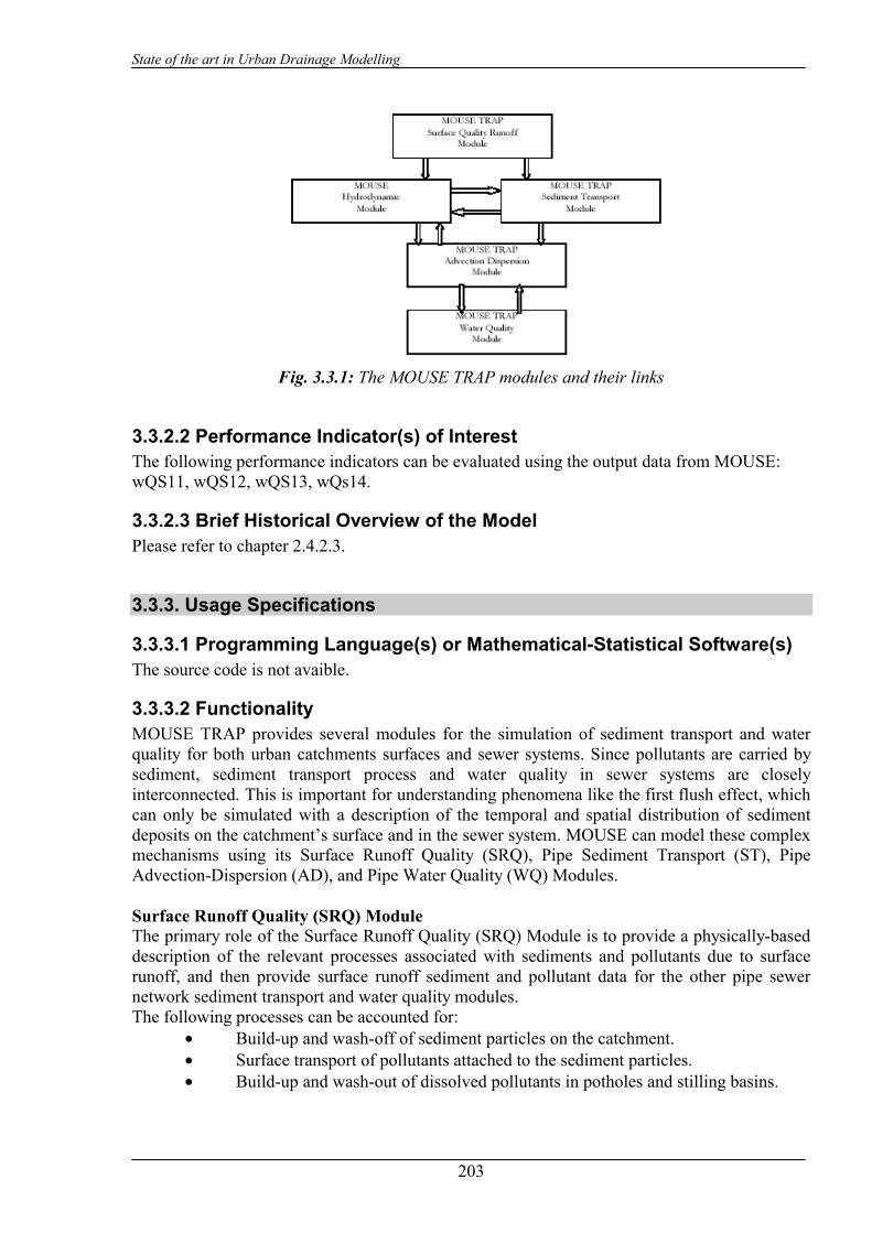
State of the art in Urban Drainage Modelling
203
Fig. 3.3.1: The MOUSE TRAP modules and their links
3.3.2.2 Performance Indicator(s) of Interest The following performance indicators can be evaluated using the output data from MOUSE: wQS11, wQS12, wQS13, wQs14.
3.3.2.3 Brief Historical Overview of the Model Please refer to chapter 2.4.2.3.
3.3.3. Usage Specifications
3.3.3.1 Programming Language(s) or Mathematical-Statistical Software(s) The source code is not avaible.
3.3.3.2 Functionality MOUSE TRAP provides several modules for the simulation of sediment transport and water quality for both urban catchments surfaces and sewer systems. Since pollutants are carried by sediment, sediment transport process and water quality in sewer systems are closely interconnected. This is important for understanding phenomena like the first flush effect, which can only be simulated with a description of the temporal and spatial distribution of sediment deposits on the catchment’s surface and in the sewer system. MOUSE can model these complex mechanisms using its Surface Runoff Quality (SRQ), Pipe Sediment Transport (ST), Pipe Advection-Dispersion (AD), and Pipe Water Quality (WQ) Modules. Surface Runoff Quality (SRQ) Module The primary role of the Surface Runoff Quality (SRQ) Module is to provide a physically-based description of the relevant processes associated with sediments and pollutants due to surface runoff, and then provide surface runoff sediment and pollutant data for the other pipe sewer network sediment transport and water quality modules. The following processes can be accounted for:
• Build-up and wash-off of sediment particles on the catchment. • Surface transport of pollutants attached to the sediment particles. • Build-up and wash-out of dissolved pollutants in potholes and stilling basins.
State of the art in Urban Drainage Modelling
204
Pipe Sediment Transport (ST) Module Four sediment transport models have been implemented in the MOUSE ST. These are: the Ackers-White Model, the Engelund-Fredsøe Model, the Engelund-Hansen Model and the van Rijn model. Further, it is possible to transport fine sediment by the use of the advection-dispersion equations. The Ackers-White and the Engelund-Hansen models calculate the total transport, while the Engelund-Fredsøe and the van Rijn models divide the sediment transport into bed load and suspended load. Furthermore, the Engelund-Fredsøe and the van Rijn models can simulate the development of sand dunes in pipes. The total bed resistance is calculated as the sum of a contribution from the skin friction acting on the dune and an expansion loss behind the dune. Sediment deposits can greatly reduce the hydraulic capacity of sewer pipes by restricting their flow area and increasing the bed friction resistance. The MOUSE TRAP Pipe Sediment Transport (ST) module can account for these problems, by simulating pipe sewer network sediment transport, including deposition and erosion from non-uniform (graded) sediments. Contributions from rainstorm wash-off and dry-weather wastewater flow can be included. The ST Module runs in conjunction with the dynamic flow routing, thereby simulating dynamic deposition of sediment and providing feedback due to the change in pipe area and resistance caused by sediment deposition. The following issues can be addressed: • Prediction of sediment deposit locations and associated pollutants and metals in the sewer
system. • Prediction of reduction in hydraulic capacity due to observed and simulated sediment
deposits. • Analysis of the sewer system due to modified regulation strategies. Pipe Advection-Dispersion (AD) Module The MOUSE TRAP Pipe Advection-Dispersion (AD) Module simulates the transport of dissolved substances and suspended fine sediments in pipe flow. Conservative materials as well as those that are subject to a linear decay can be simulated. The computed pipe flow discharges, water levels, and cross-sectional flow areas are used in the AD Module computation. The solution of the advection-dispersion equation is obtained using an implicit, finite-difference scheme which has negligible numerical dispersion. Concentration profiles with very steep fronts can be accurately modelled. The computed results can be displayed as longitudinal concentration profiles and pollutant graphs, which could be used at the inflow to a sewage treatment plant or an overflow structure. The AD Module can be linked to the MOUSE T module to provide long-term simulations of pollutant transport. Pipe Water Quality (WQ) Module The MOUE TRAP Pipe Water Quality (WQ) Module works in conjunction with the Advection-Dispersion Module, thereby providing many options for describing the reaction processes of multi-compound systems, including degradation of organic matter, bacterial fate, exchange of oxygen with the atmosphere and oxygen demand from eroded sewer sediments. This allows realistic analysis of complex phenomena related to water quality in sewer systems. The WQ Module includes diurnal variation of foul flow discharges and user-specified concentrations of foul flow components. The sediment types included in the interaction with the WQ Module are foul flow organic sediments, and fine and course mineral in-pipe sediments originating from catchment runoff, potholes, and stilling basins. The WQ Module can account for:
• Decay of BOD/COD in bio-film and water phase; • Hydrolysis of suspended matter;

State of the art in Urban Drainage Modelling
205
• Growth of suspended biomass; • Oxygen consumption from decay of BOD/COD, bio-film, and erosion of sediment; • Re-aeration; • Bacterial fate; • Interaction with sediments for nutrients and metals.
Figure 3.3.2 shows which modules should be used for a list of problem types. Figure 3.3.3 gives an overview of the required modules for different pollutant and sediment types. Finally, figure 3.3.4 systematizes the initial conditions, boundary conditions and process-related data necessary for each module and where these can be found.
Fig. 3.3.2: Problem Types and Modules

State of the art in Urban Drainage Modelling
206
Fig. 3.3.3: Overview of pollutant and sediment types and appropriate modules
Fig. 3.3.4: Input data requirements for MOUSE TRAP modules
3.3.3.3 Possible interaction with other software tools Output from MOUSE TRAP modules, such as pollutant graphs from combined sewer overflows, can then be applied directly to DHI.s receiving waters models MIKE 11 and MIKE 21. Using MIKE 11 or MIKE 21 in conjunction with MOUSE allows assessment of water

State of the art in Urban Drainage Modelling
207
quality for the water bodies receiving these sewer overflows, such as rivers, streams, lakes and coastal waters.
3.3.4. Input and Output procedures
3.3.4.1 Possible Input File(s) Formats Most of the MOUSE files have special binary formats. The MOUSE data file for water quality mode is the POLLUTANT AND SEDIMENT DATA specifying input related to pollution components and sediments (*.TRP) For water quantity model, please refer to chapter 2.4.4.1.
3.3.4.2 Possible Output File(s) Formats Standard results from a MOUSE TRAP network computation (flows, water levels, velocity, quality-concentration) are stored in *.TRP file, *.SRF file and *.SMR file .
3.3.4.3 Raw Data Formatting Please refer to chapter 2.4.4.3.
3.3.5. Theoretical framework Overview MOUSE TRAP is a suite of modules which are capable of simulating pollution- and sediment transport as well as water quality processes in sewer systems and on catchment surfaces. MOUSE TRAP is divided into various modules, representing different transport or water quality processes. The Surface Runoff Quality module is used to generate input for the sediment transport, advection-dispersion or water quality computation in the underlying pipe model. The Surface Runoff Quality module consists of three models:
• a model for the description of the accumulation (build-up) and wash-off of particles on the catchment surface;
• a model for the description of the surface transport of pollutants attached to the sediments;
• a model for the description of the build-up and wash-out of dissolved pollutants in gully pots.
The Build-up/Wash-off model consists of two sub-models: a model for the description of the accumulation of particles on the catchment and a model for the description of the detachment of particles by rainfall and subsequent routing of the wash-off by the overland flow. The model works with two sediment fractions, a fine and a coarse, each fraction characterized by its mean diameter. The fine fraction typically has a particle size less than 0.1 mm and is limited in supply. On the contrary, the coarse fraction is typically unlimited in supply. Thus, for the coarse fraction, transport capacity is always satisfied and, therefore, the build-up description is only applicable to the fine sediment fraction to determine the mass available for transport. The surface sediment transport model is based on the hydrological models available in MOUSE, ie the Surface Runoff Model A, the Surface Runoff Model B and the Surface Runoff Model C. Hence, the sediment is routed according to the hydrological description in the surface runoff models. Output from the model consists of time series of sediment transport or concentration mass and accumulated mass for each sediment fraction. In addition, a time series of mass of the fine sediment fraction on the surface is available.
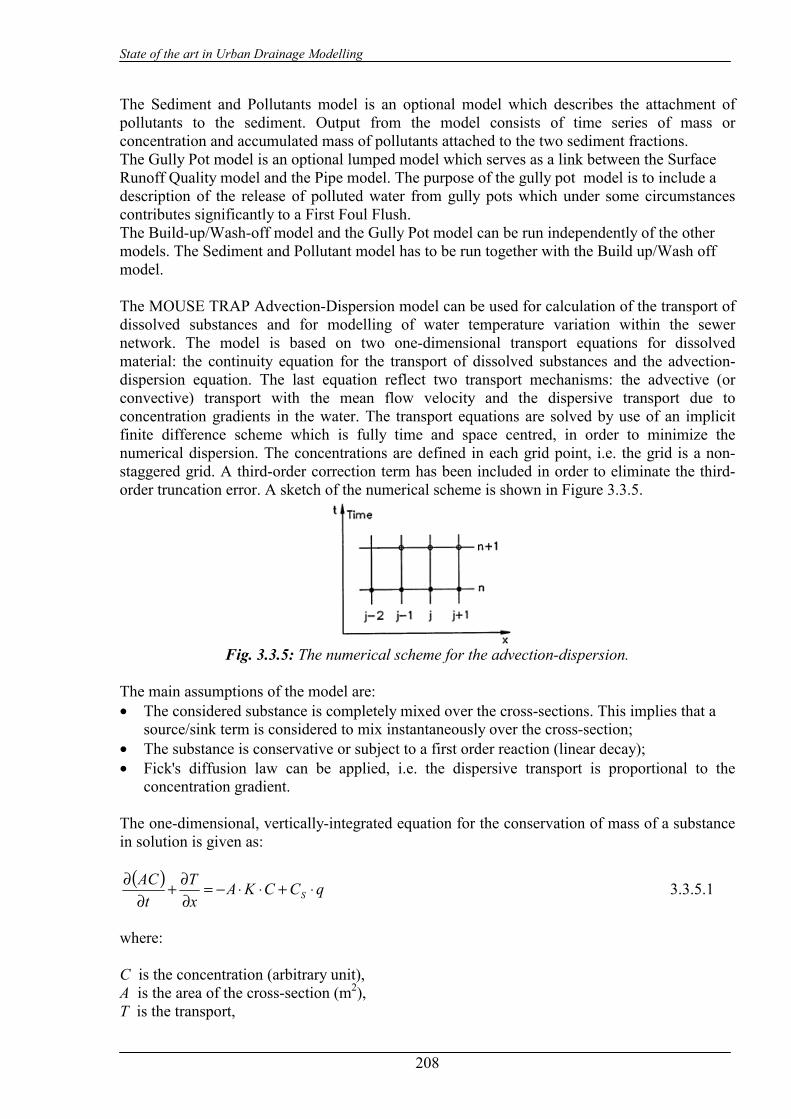
State of the art in Urban Drainage Modelling
208
The Sediment and Pollutants model is an optional model which describes the attachment of pollutants to the sediment. Output from the model consists of time series of mass or concentration and accumulated mass of pollutants attached to the two sediment fractions. The Gully Pot model is an optional lumped model which serves as a link between the Surface Runoff Quality model and the Pipe model. The purpose of the gully pot model is to include a description of the release of polluted water from gully pots which under some circumstances contributes significantly to a First Foul Flush. The Build-up/Wash-off model and the Gully Pot model can be run independently of the other models. The Sediment and Pollutant model has to be run together with the Build up/Wash off model. The MOUSE TRAP Advection-Dispersion model can be used for calculation of the transport of dissolved substances and for modelling of water temperature variation within the sewer network. The model is based on two one-dimensional transport equations for dissolved material: the continuity equation for the transport of dissolved substances and the advection-dispersion equation. The last equation reflect two transport mechanisms: the advective (or convective) transport with the mean flow velocity and the dispersive transport due to concentration gradients in the water. The transport equations are solved by use of an implicit finite difference scheme which is fully time and space centred, in order to minimize the numerical dispersion. The concentrations are defined in each grid point, i.e. the grid is a non-staggered grid. A third-order correction term has been included in order to eliminate the third-order truncation error. A sketch of the numerical scheme is shown in Figure 3.3.5.
Fig. 3.3.5: The numerical scheme for the advection-dispersion.
The main assumptions of the model are: • The considered substance is completely mixed over the cross-sections. This implies that a
source/sink term is considered to mix instantaneously over the cross-section; • The substance is conservative or subject to a first order reaction (linear decay); • Fick's diffusion law can be applied, i.e. the dispersive transport is proportional to the
concentration gradient. The one-dimensional, vertically-integrated equation for the conservation of mass of a substance in solution is given as:
( ) qCCKAxT
tAC
S ⋅+⋅⋅−=∂∂+
∂∂ 3.3.5.1
where: C is the concentration (arbitrary unit), A is the area of the cross-section (m2), T is the transport,
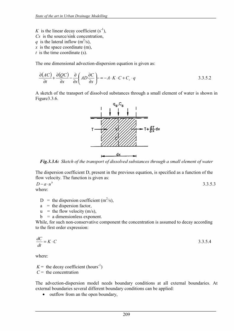
State of the art in Urban Drainage Modelling
209
K is the linear decay coefficient (s-1), Cs is the source/sink concentration, q is the lateral inflow (m2/s), x is the space coordinate (m), t is the time coordinate (s). The one dimensional advection-dispersion equation is given as:
( ) ( ) qCCKA
xCAD
xxQC
tAC
c ⋅+⋅⋅−=−
∂∂
∂∂−
∂∂+
∂∂ 3.3.5.2
A sketch of the transport of dissolved substances through a small element of water is shown in Figure3.3.6.
Fig.3.3.6: Sketch of the transport of dissolved substances through a small element of water
The dispersion coefficient D, present in the previous equation, is specified as a function of the flow velocity. The function is given as:
buaD ⋅− 3.3.5.3 where: D = the dispersion coefficient (m2/s), a = the dispersion factor, u = the flow velocity (m/s), b = a dimensionless exponent. While, for such non-conservative component the concentration is assumed to decay according to the first order expression:
CKdtdC ⋅= 3.3.5.4
where: K = the decay coefficient (hours-1) C = the concentration The advection-dispersion model needs boundary conditions at all external boundaries. At external boundaries several different boundary conditions can be applied:
• outflow from an the open boundary,

State of the art in Urban Drainage Modelling
210
• flow into an open boundary, • closed boundary.
When outflow occur, the concentration is only dependent on the concentration in the model area. The open boundary outflow condition is:
02
2
=∂∂
xC
3.3.5.5
This specifies that the gradient of the concentration with respect to the distance is constant at the outflow boundary and that the transport across the boundary is pure advection. At an open inflow boundary the concentration must be specified as function of time. If the flow direction changes an outflow boundary becomes an inflow boundary and vice versa. This scenario will typically happen when the receiving water is tidal influenced. The boundary condition then changes between the concentration in the sewer system and the concentration in the receiving water according to:
( ) mix
mix
Kt
rSr eCCCC−
−+= 3.3.5.6 where: cr is the concentration in the receiving water, cs is the concentration in the sewer system immediately before the flow direction changed, Kmix is a time scale (hrs-1), tmix is the elapsed time since the flow direction changed (hrs). No mass is transported across a closed boundary, hence it is characterized by q = 0.0 and
0=∂∂
xC
3.3.5.7
The solution of the advection-dispersion equation has to be modified at hydraulic structures in sewer systems. At manholes a local continuity equation is applied. It is assumed that the substance in the nodal point is fully mixed over the volume. The continuity equation for a manhole reads:
( )
NNN
kki
i
kki
iN
NN KCVTQC
tCV ⋅⋅−=+−∂
∂ ∑∑=
=
=
= 11
3.3.5.8
where: VN is the volume of the structure (m3/s), CN is the concentration in the node, T is the transport into the node (kg/s), KN is the decay constant for the node, kk is the number of connecting pipes. Q is the discharge in the connecting branches(m3/s). When free flow into a structure occurs, i.e. the water level in the structure is lower than the water level in the inlet pipe, the concentration in the pipe is independent of the concentration at
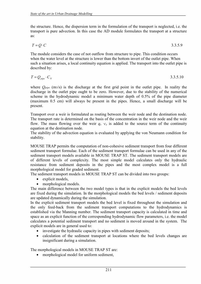
State of the art in Urban Drainage Modelling
211
the structure. Hence, the dispersion term in the formulation of the transport is neglected, i.e. the transport is pure advection. In this case the AD module formulates the transport at a structure as: CQT ⋅= 3.3.5.9 The module considers the case of not outflow from structure to pipe. This condition occurs when the water level at the structure is lower than the bottom invert of the outlet pipe. When such a situation arises, a local continuity equation is applied. The transport into the outlet pipe is described by:
Npipe CQT ⋅= 3.3.5.10 where Qpipe (m3/s) is the discharge at the first grid point in the outlet pipe. In reality the discharge in the outlet pipe ought to be zero. However, due to the stability of the numerical scheme in the hydrodynamic model a minimum water depth of 0.5% of the pipe diameter (maximum 0.5 cm) will always be present in the pipes. Hence, a small discharge will be present. Transport over a weir is formulated as routing between the weir node and the destination node. The transport rate is determined on the basis of the concentration in the weir node and the weir flow. The mass flowing over the weir qs ·cs is added to the source term of the continuity equation at the destination node. The stability of the advection equation is evaluated by applying the von Neumann condition for stability. MOUSE TRAP permits the computation of non-cohesive sediment transport from four different sediment transport formulae. Each of the sediment transport formulae can be used in any of the sediment transport models available in MOUSE TRAP ST. The sediment transport models are of different levels of complexity. The most simple model calculates only the hydraulic resistance from sediment deposits in the pipes and the most complex model is a full morphological model for graded sediment. The sediment transport models in MOUSE TRAP ST can be divided into two groups:
• explicit models, • morphological models.
The main difference between the two model types is that in the explicit models the bed levels are fixed during the simulation. In the morphological models the bed levels / sediment deposits are updated dynamically during the simulation. In the explicit sediment transport models the bed level is fixed throughout the simulation and the only feed-back from the sediment transport computations to the hydrodynamics is established via the Manning number. The sediment transport capacity is calculated in time and space as an explicit function of the corresponding hydrodynamic flow parameters, i.e. the model calculates a potential sediment transport and no sediment is moved around in the system. The explicit models are in general used to:
• investigate the hydraulic capacity in pipes with sediment deposits; • calculation of the sediment transport at locations where the bed levels changes are
insignificant during a simulation. The morphological models in MOUSE TRAP ST are:
• morphological model for uniform sediment,

State of the art in Urban Drainage Modelling
212
• morphological model for non-uniform sediment. In the morphological models the sediment transport continuity equation is solved, based on the corresponding values of the hydrodynamic parameters (i.e. discharge, water levels, etc). The feedback to the hydrodynamic module is established through dynamically changed flow area and flow resistance number. The morphological model for uniform sediment uses one grain diameter at each point in the sewer system to calculate the sediment transport. In the morphological model for non-uniform sediment it is possible to calculate the sediment transport from a range of grain diameters. For the transport of fine organic particles some of the non-uniform sediment fractions can be chosen to be transported by use of the Advection-Dispersion transport formulation instead of the non-cohesive sediment transport formula, as the transport of particles transported in suspension is better described by used of the advection-dispersion equation. The fractions transported by the advection-dispersion module are still included in the morphological calculation, but the description of erosion/deposition is changed. Note, the morphological models require sediment or bed level boundary conditions at all inflow boundaries. MOUSE TRAP ST deals the hydraulic resistance in sewer system originates from the pipe wall and from the sediment deposits on the bottom of the sewer. The resistance from the sediment deposits consists of two contributions, one part originates from the grain friction and the other part originates from the expansion loss behind the bed forms. The description of the resistance from the other factors such as: aging effects, structural failure and biological growth out is not included in MOUSE ST. MOUSE ST simulates the following bed forms: ripples, dunes, plane bed and anti-dunes.
Fig.3.3.7: Development of bed forms for increasing flow velocity.
The dimensions of the bed forms are determined by the sediment transport and the flow, the resistance from the bed forms can be described through sediment transport formulae. The average shear stress in a pipe with sediment deposits is calculated from the Einstein side-wall elimination procedure. The calculation is based on the pipe roughness and the bed shear stress calculated from the sediment deposits. The basic assumptions of the Einstein side wall elimination procedure are:
• The cross-section area can be divided into different areas where each of the flow areas can be connected to a part of the wetted perimeter,
• The mean velocity is the same for the whole section, • The hydraulic gradient is the same for the whole section.
Einstein used these assumptions to separate the resistance from the side walls and the bottom in channel flow. A definition sketch of a sewer with sediment is shown in Figure 3.3.8.

State of the art in Urban Drainage Modelling
213
Fig.3.3.8: A definition sketch of a sewer with sediment The side wall elimination procedure assumes the total flow resistance can be written as the sum of the resistance from the different parts of the flow :
SSSrrr IRPIRPPF ⋅⋅⋅+⋅⋅⋅=⋅= γγτ 3.3.5.11 By use of the Manning equation and assuming the velocity varies with the hydraulic radius in the following way:
6/16/16/1Sr R
URU
RU == 3.3.5.12
it is obtained the following equation
PnPnPn SSrr
22 ⋅+⋅= 3.3.5.13
where: Pr is the wetted perimeter of the pipe wall, Ps is the width of the sediment bed, P is the total wetted perimeter, nris the Manning number for the pipe, nsis the Manning number for the bed, n is the total resistance to the flow. It estimates the weighted resistance to the flow for a cross-section where the wall roughness differs from the bed roughness. MOUSE TRAP ST implements four non-cohesive sediment transport formulae:
• Engelund . Hansen; • Ackers . White; • Engelund - Fredsøe . Deigaard; • van Rijn.

State of the art in Urban Drainage Modelling
214
All these formulae demonstrate that the sediment transport is a highly non-linear function of the flow velocity: depending on the formulation, the sediment transport is proportional to the velocity raised to the power from 3 to 5. The Ackers-White formulae The formulae determine directly the total sediment transport. The formulae are semi-empirical, based partly on dimensional analysis and partly on physical arguments. The Engelund-Hansen formula The formula determines the total sediment transport directly. It has been derived from consideration of the work done by the flow on the sediment being transported. Originally, the formula was derived for a dune covered bed, but it was found applicable to the upper regimes (plane bed and anti-dunes) as well. The Engelund-Fredsøe-Deigaard formulae The formulae calculate the total transport as the sum of the bed load transport and the suspended transport. The sediment transport is calculated from the skin friction, i.e. the shear stress acting on SEDIMENT TRANSPORT (ST) the surface of the bed. In this formulae it is possible to describe the development of sand dunes in pipes and hence include the resulting friction into the computations. The total bed resistance is then calculated as the sum of a contribution from the skin friction acting on the dune and an expansion loss behind the dune. The van Rijn formulae In the van Rijn sediment transport formulae the sediment transport is divided into bed load and suspended load. The bed load is calculated from the saltation height, the particle velocity and the bed load concentration. The bed load computations follow the approach of Bagnold (1973), which assumes that the motion of the bed load particles is dominated by the gravity forces. When the bed shear velocity exceeds the fall velocity sediment is transported in suspension. The suspended load is calculated as the depth integration of the local concentration and flow velocity. The method uses the reference concentration computed from the bed load transport. The formula has been verified for particles in the range 200 - 2000 υm. MOUSE TRAP ST models the sediment transport in the structures in the following way: The sediment transport in manholes is routed straight through the manhole without any deposition. This is done as the level of turbulence is high in manholes and hence it is assumed that the sediment is transported in suspension. The sediment transport from a manhole is distributed according to the ratio of the outflowing discharges. A user-defined distribution can also be specified by giving the coefficients and exponents (K and n values) in the following relationship:
( )12
114
443
33
3331
3+++ +
⋅+⋅⋅= n
tntnn
nnt SS
QKQKQKS 3.3.5.14
State of the art in Urban Drainage Modelling
215
Fig.3.3.9: Distribution of sediment according to discharge.
Sediment Transport In Basins Sediment can be removed from basins according to the formula:
n
AQw
nE
−
+−=
/111 3.3.5.15
where: E is the sediment trap efficiency, w is the fall velocity, q is the discharge into the tank, a is the surface area of the basin, n is turbulence constant indication the settling performance of the basin: n = 1, for poor performance, n = 3, for good performance, n > 5, very good performance, n = ∞ , ideal performance.
Sediment Transport In Overflow Structures The sediment transport over a weir can be modelled in three different ways: a) Sweir = (1 - reductionfactor) · STotal into weir 3.3.5.16 b) Sweir = (1 - Eff(Q) ) · STotal into weir 3.3.5.17 c) Sweir = (1 - Eff(w/v0) ) · STotal into weir 3.3.5.18 ad a) the reduction factor is constant through out the whole simulation, ad b) the reduction factor is a function of the discharge flowing into the weir, ad c) the reduction factor is given as the expression below:
⋅−−⋅−=
2
2/1
σµo
o
VWExpKvwEff 3.3.5.20
Where K, µ and σ are dimensionless variables.
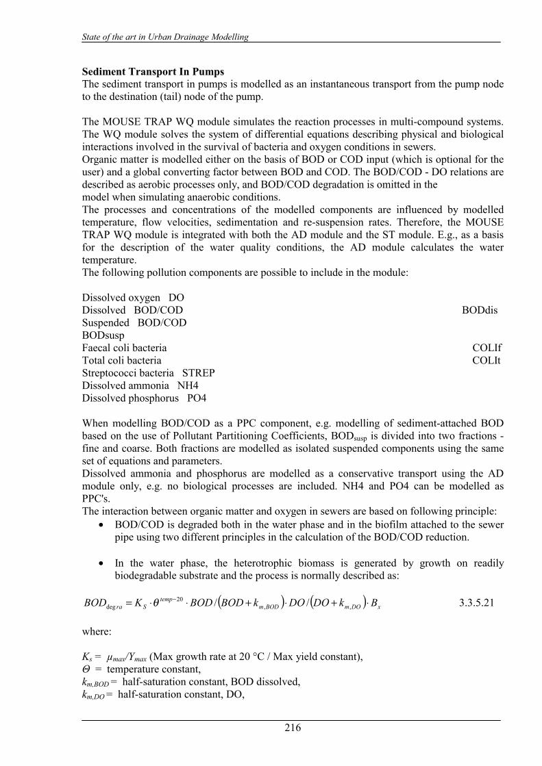
State of the art in Urban Drainage Modelling
216
Sediment Transport In Pumps The sediment transport in pumps is modelled as an instantaneous transport from the pump node to the destination (tail) node of the pump.
The MOUSE TRAP WQ module simulates the reaction processes in multi-compound systems. The WQ module solves the system of differential equations describing physical and biological interactions involved in the survival of bacteria and oxygen conditions in sewers. Organic matter is modelled either on the basis of BOD or COD input (which is optional for the user) and a global converting factor between BOD and COD. The BOD/COD - DO relations are described as aerobic processes only, and BOD/COD degradation is omitted in the model when simulating anaerobic conditions. The processes and concentrations of the modelled components are influenced by modelled temperature, flow velocities, sedimentation and re-suspension rates. Therefore, the MOUSE TRAP WQ module is integrated with both the AD module and the ST module. E.g., as a basis for the description of the water quality conditions, the AD module calculates the water temperature. The following pollution components are possible to include in the module: Dissolved oxygen DO Dissolved BOD/COD BODdis Suspended BOD/COD BODsusp Faecal coli bacteria COLIf Total coli bacteria COLIt Streptococci bacteria STREP Dissolved ammonia NH4 Dissolved phosphorus PO4 When modelling BOD/COD as a PPC component, e.g. modelling of sediment-attached BOD based on the use of Pollutant Partitioning Coefficients, BODsusp is divided into two fractions - fine and coarse. Both fractions are modelled as isolated suspended components using the same set of equations and parameters. Dissolved ammonia and phosphorus are modelled as a conservative transport using the AD module only, e.g. no biological processes are included. NH4 and PO4 can be modelled as PPC's. The interaction between organic matter and oxygen in sewers are based on following principle:
• BOD/COD is degraded both in the water phase and in the biofilm attached to the sewer pipe using two different principles in the calculation of the BOD/COD reduction.
• In the water phase, the heterotrophic biomass is generated by growth on readily
biodegradable substrate and the process is normally described as:
( ) ( ) xDOmBODmtemp
Sra BkDODOkBODBODKBOD ⋅+⋅+⋅⋅= −,,
20deg //θ 3.3.5.21
where: Ks = µmax/Ymax (Max growth rate at 20 °C / Max yield constant), Θ = temperature constant, km,BOD = half-saturation constant, BOD dissolved, km,DO = half-saturation constant, DO,

State of the art in Urban Drainage Modelling
217
Bx = biomass of active heterotrophic organisms. In MOUSE TRAP WQ it is assumed that the heterotopic biomass constitutes a certain fixed fraction of the suspended BOD/COD (0.5-1.0). Consequently, the degradation of dissolved BOD/COD by this group of micro organisms is modelled by using a fixed fraction of the suspended BOD/COD as the biomass and apply this estimated biomass to Equation 3.3.5.21. For the biofilm, it is assumed that there exists a thick biofilm in the sewer pipe, and that oxygen is the limiting factor for the degradation of dissolved BOD/COD. This means that the diffusion rate of DO from the water phase into the biofilm determines the degradation rate of dissolved BOD/COD in the biofilm attached to the sediment and the pipe. Hydrolysis of suspended BOD/COD converts the suspended material into dissolved substrate. This process can be modelled as a temperature-dependent 1st order reaction (Henze et al. 1986). Suspended BOD/COD is produced in sewers due to the growth of heterotrophic organisms. This process can be modelled by applying a yield constant to the degradation rate for dissolved BOD/COD in the water phase. The model is shown is Figure 3.3.10.
Fig. 3.3.10: Conceptual diagram of the BOD/COD-DO model. Process A is degradation in
biofilm, process B is degradation in water phase,Process Cis hydrolysis and Process D is growth of heterotrophics.
MOUSE TRAP WQ models some processes that affect the oxygen concentration: Re-aeration Re-aeration is modelled in pipes only if they are not full flowing. The reaeration equation is based on the difference between the actual and the saturation concentration of DO coupled to the hydraulic conditions : REAR = k1 (1 + k2 u2/(g dm)) (s u)k3 dm
-1 (Cs - DO) 3.3.5.22 where: k1, k2, k3 = re-aeration parameters, u = flow velocity (m/s), g = gravitation (m/s2), dm = hydraulic mean depth (m), Cs = oxygen saturation concentration (g DO/m3). The oxygen saturation concentration Cs is temperature dependent and is calculated by means of a standard equation:
( )( )TTTCs ⋅−⋅+−⋅+= 000077774.0007991.041022.0652.14 3.3.5.23

State of the art in Urban Drainage Modelling
218
where T is the water temperature (°C). Degradation of BODdis in Biofilm The degradation of dissolved BOD/COD in biofilm is described as a standard ½-order reaction combined with a temperature dependent oxygen diffusion and removal:
VADOkDBOD biofilmoftemp
biofilmra /2 2/120,deg ⋅⋅⋅⋅= −θ 3.3.5.24
where: Θ = temperature coefficient, D = diffusion coefficient of oxygen in water at 20°C (m2/s), kof = removal of oxygen in biofilm at 20°C (g DO/m3s), Abiofilm = area in pipe covered with biofilm (=water) (m2), V = water volume (m3). The value of D is 20.0 (Jensen 1983, Gujer&Boller 1990) and kof has been measured to 3.0 (Andreasen 1979, Arvin&Harremoës 1990). It must be observed that degradation of BODdis in biofilm is activated only if oxygen consumption in biofilm is modelled. Degradation of BODdis in Suspension The degradation of dissolved BOD/COD carried out by suspended heterotrophics is described as:
( ) ( ) suspbDOmBODmtemp
Ssuspra BODkkDODOkBODBODKBOD ⋅⋅+⋅+⋅⋅= −,,
20,deg //θ 3.3.5.25
where: Ks = µmax/Ymax (day-1) (Max growth rate at 20 °C / Max yield constant), Θ = temperature coefficient, km,BOD = half-saturation constant, BOD dissolved (g/m3), km,DO = half-saturation constant, DO (g/m3), kb = fraction of active heterotrophic organism in BODsusp. According to literature, µmax varies from 3.0 to 13.2 day-1 and Ymax varies from 0.6 to 0.7 kg VSS/kg BOD (Henze et al .1986). The values for Km,BOD and km,DO are by default set to 8 g BOD/m3 and 2 g DO/m3 , respectively (Henze et al .1986, Arvin & Harremoës 1990). kb varies from 0.5 to 1.0 Hydrolysis of BODsusp Hydrolysis of suspended matter is described as a temperature-dependent 1st order reaction: BODhydro = Θtemp-20 khl . BODsusp 3.3.5.26 where: Θ = temperature coefficient, khl = 1st order decay constant at 20°C (day-1).

State of the art in Urban Drainage Modelling
219
The value of khl is in the range of 0.05 - 0.10 day-1. Growth of Heterotrophics (BODsusp) The growth of heterotrophics is dependent of the BOD degradation in the water phase, and the equation reads: BODgrowth = Ymax . BODdegra,susp 3.3.5.27 Eroded Sediment Oxygen Demand When modelling ST and WQ simultaneously, eroded sediment will cause an immediate oxygen consumption. The oxygen decrease is depending of the amount of sediment eroded and its oxygen demand. The eroded sediment oxygen demand is described as: SEDox demand = ksed SEDeroded 1/(V dt) 3.3.5.28 where: ksed = oxygen demand of sediment (g DO/ m3 sediment), SEDeroded= amount of eroded sediment in timestep (m3 sediment), V = water volumen (m3), dt = timestep (days). Eroded sediment oxygen demand is activated only when ST and WQ are modelled simultaneously. Oxygen Balance (DO) The differential equation describing the effects of these processes on the dissolved oxygen concentration reads: dDO/dt = REAR - BODdegra,biofilm - BODdegra,susp - SEDox demand 3.3.5.29 Dissolved BOD/COD Balance (BODdis) The balance for BODdis is: dBODdis/dt = BODhydro - BODdegra,biofilm - BODdegra,susp 3.3.5.30 Suspended BOD/COD Balance (BODsusp) The differential equation for BODsusp reads: dBODsusp/dt = BODgrowth - BODhydro 3.3.5.31 In the MOLUSE TRAP WQ model, two methodologically defined groups of coliforms are distinguished: "Total coliform" and " Faecal coliform". The concept "Total coliform" may include a wide range of bacterial genera of which many are not specific of faecal contamination. Further more a third group of bacteria is included in the model - Streptocci bacteria. The three groups of bacteria are modelled in the water phase with a temperature-dependent 1st order decay rate. Decay Rate for Faecal Coliform (COLIf,decay)
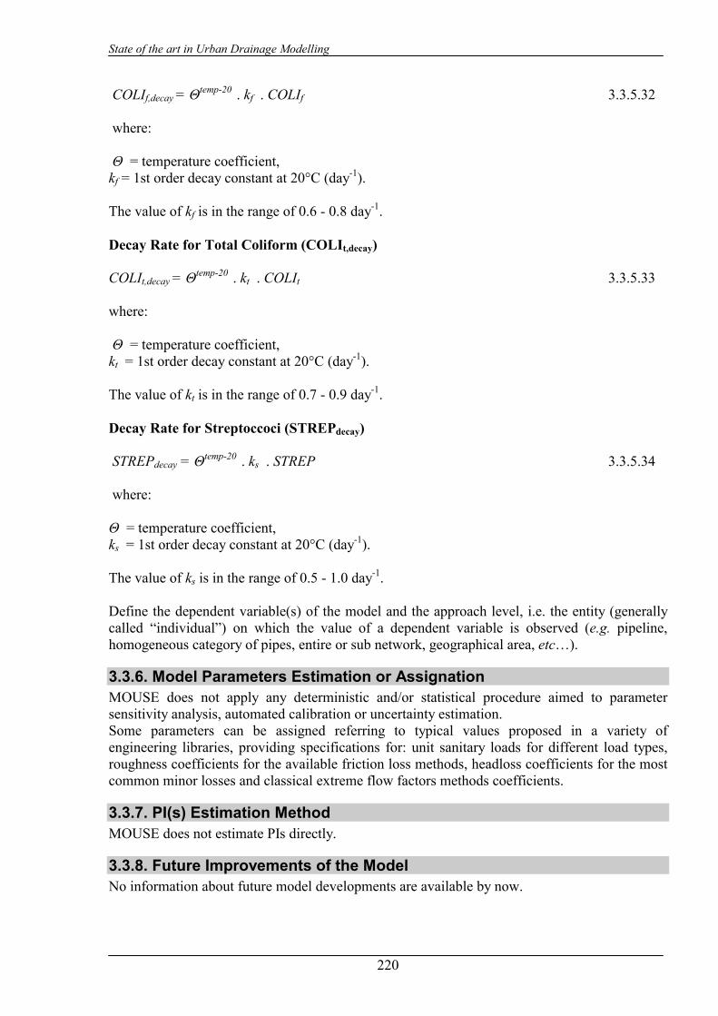
State of the art in Urban Drainage Modelling
220
COLIf,decay = Θtemp-20 . kf . COLIf 3.3.5.32 where: Θ = temperature coefficient, kf = 1st order decay constant at 20°C (day-1). The value of kf is in the range of 0.6 - 0.8 day-1. Decay Rate for Total Coliform (COLIt,decay) COLIt,decay = Θtemp-20 . kt . COLIt 3.3.5.33 where: Θ = temperature coefficient, kt = 1st order decay constant at 20°C (day-1). The value of kt is in the range of 0.7 - 0.9 day-1. Decay Rate for Streptoccoci (STREPdecay) STREPdecay = Θtemp-20 . ks . STREP 3.3.5.34 where: Θ = temperature coefficient, ks = 1st order decay constant at 20°C (day-1). The value of ks is in the range of 0.5 - 1.0 day-1. Define the dependent variable(s) of the model and the approach level, i.e. the entity (generally called “individual”) on which the value of a dependent variable is observed (e.g. pipeline, homogeneous category of pipes, entire or sub network, geographical area, etc…).
3.3.6. Model Parameters Estimation or Assignation MOUSE does not apply any deterministic and/or statistical procedure aimed to parameter sensitivity analysis, automated calibration or uncertainty estimation. Some parameters can be assigned referring to typical values proposed in a variety of engineering libraries, providing specifications for: unit sanitary loads for different load types, roughness coefficients for the available friction loss methods, headloss coefficients for the most common minor losses and classical extreme flow factors methods coefficients.
3.3.7. PI(s) Estimation Method MOUSE does not estimate PIs directly.
3.3.8. Future Improvements of the Model No information about future model developments are available by now.
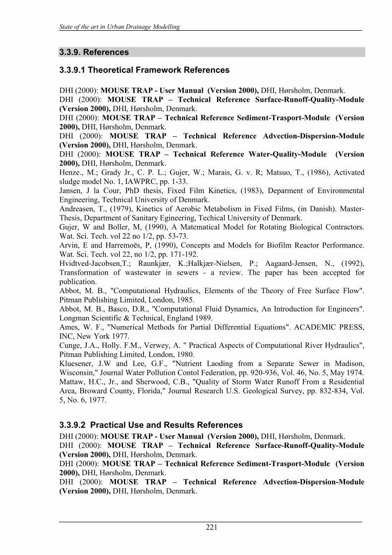
State of the art in Urban Drainage Modelling
221
3.3.9. References
3.3.9.1 Theoretical Framework References DHI (2000): MOUSE TRAP - User Manual (Version 2000), DHI, Hørsholm, Denmark. DHI (2000): MOUSE TRAP – Technical Reference Surface-Runoff-Quality-Module (Version 2000), DHI, Hørsholm, Denmark. DHI (2000): MOUSE TRAP – Technical Reference Sediment-Trasport-Module (Version 2000), DHI, Hørsholm, Denmark. DHI (2000): MOUSE TRAP – Technical Reference Advection-Dispersion-Module (Version 2000), DHI, Hørsholm, Denmark. DHI (2000): MOUSE TRAP – Technical Reference Water-Quality-Module (Version 2000), DHI, Hørsholm, Denmark. Henze., M.; Grady Jr., C. P. L.; Gujer, W.; Marais, G. v. R; Matsuo, T., (1986), Activated sludge model No. 1, IAWPRC, pp. 1-33. Jansen, J la Cour, PhD thesis, Fixed Film Kinetics, (1983), Deparment of Environmental Engineering, Technical University of Denmark. Andreasen, T., (1979), Kinetics of Aerobic Metabolism in Fixed Films, (in Danish). Master-Thesis, Department of Sanitary Egineering, Techical University of Denmark. Gujer, W and Boller, M, (1990), A Matematical Model for Rotating Biological Contractors. Wat. Sci. Tech. vol 22 no 1/2, pp. 53-73. Arvin, E and Harremoës, P, (1990), Concepts and Models for Biofilm Reactor Performance. Wat. Sci. Tech. vol 22, no 1/2, pp. 171-192. Hvidtved-Jacobsen,T.; Raunkjær, K.;Halkjær-Nielsen, P.; Aagaard-Jensen, N., (1992), Transformation of wastewater in sewers - a review. The paper has been accepted for publication. Abbot, M. B., "Computational Hydraulics, Elements of the Theory of Free Surface Flow". Pitman Publishing Limited, London, 1985. Abbot, M. B., Basco, D.R., "Computational Fluid Dynamics, An Introduction for Engineers". Longman Scientific & Technical, England 1989. Ames, W. F., "Numerical Methods for Partial Differential Equations". ACADEMIC PRESS, INC, New York 1977. Cunge, J.A., Holly. F.M., Verwey, A. " Practical Aspects of Computational River Hydraulics", Pitman Publishing Limited, London, 1980. Kluesener, J.W and Lee, G.F., "Nutrient Laoding from a Separate Sewer in Madison, Wisconsin," Journal Water Pollution Contol Federation, pp. 920-936, Vol. 46, No. 5, May 1974. Mattaw, H.C., Jr., and Sherwood, C.B., "Quality of Storm Water Runoff From a Residential Area, Broward County, Florida," Journal Research U.S. Geological Survey, pp. 832-834, Vol. 5, No. 6, 1977.
3.3.9.2 Practical Use and Results References DHI (2000): MOUSE TRAP - User Manual (Version 2000), DHI, Hørsholm, Denmark. DHI (2000): MOUSE TRAP – Technical Reference Surface-Runoff-Quality-Module (Version 2000), DHI, Hørsholm, Denmark. DHI (2000): MOUSE TRAP – Technical Reference Sediment-Trasport-Module (Version 2000), DHI, Hørsholm, Denmark. DHI (2000): MOUSE TRAP – Technical Reference Advection-Dispersion-Module (Version 2000), DHI, Hørsholm, Denmark.

State of the art in Urban Drainage Modelling
222
DHI (2000): MOUSE TRAP – Technical Reference Water-Quality-Module (Version 2000), DHI, Hørsholm, Denmark.

State of the art in Urban Drainage Modelling
223
3.4 KOSIM - KOntinuierliches LangzeitSIMulationsmodell für den Nachweis von Bauwerken der Regenwasserbehandlung
3.4.1. Model availability KOSIM for Windows is distributed Institut fur technisch-wissenschaftliche Hydrologie, Hannover (http://www.itwh.de). The licence can be purchased directly from ITWH and the cost varies between 2600 euros and 4700 euros, depending on optional modules. Software is available only in German, as well as manuals and descriptive information.
3.4.2. Abstract
3.4.2.1 Objectives and peculiarities In this model, the sewer system is represented by a number of reservoirs connected in series or in parallel. A conceptual rainfall – runoff model transforms the rainfall series into a flow series for the single sub-basin. Pollutants input are generated from the dry weather flow cycle and concentration and, during rainfall, through the principle constant concentration associated with the storm flow. Sedimentation and resuspension are simulated for each sub-basin, based on critical discharges for settlement and sediment removal. Within the system, flows and pollutants are conveyed downstream by accounting for a constant travel time. Weirs and different types of storage basins may be considered. The hydraulic calculations for these structures are based on the continuity equation, on maximum flow capacities and stage – discharge relations. In storage facilities, the settlement of pollutants and sediments is described by classical sedimentation theory. No interaction between sediments and pollutants is considered.
3.4.2.2 Performance Indicator(s) of Interest KOSIM is able to evaluate the basic flow variables such as discharge, pollution concentration and sediment load. This kind of data can be used for computing physical and operational performance indicators, even if the model does not compute the PIs directly.
3.4.2.3 Brief Historical Overview of the Model Only some historical information is available about the model: the model has been developed by Institut fur technisch-wissenschaftliche Hydrologie (Hannover) in the late ’80. Several versions has been developed during years. The current version is 6.1 and it has been released in January 2002
3.4.3. Usage Specifications
3.4.3.1 Programming Language(s) or Mathematical-Statistical Software(s) The information is not available.
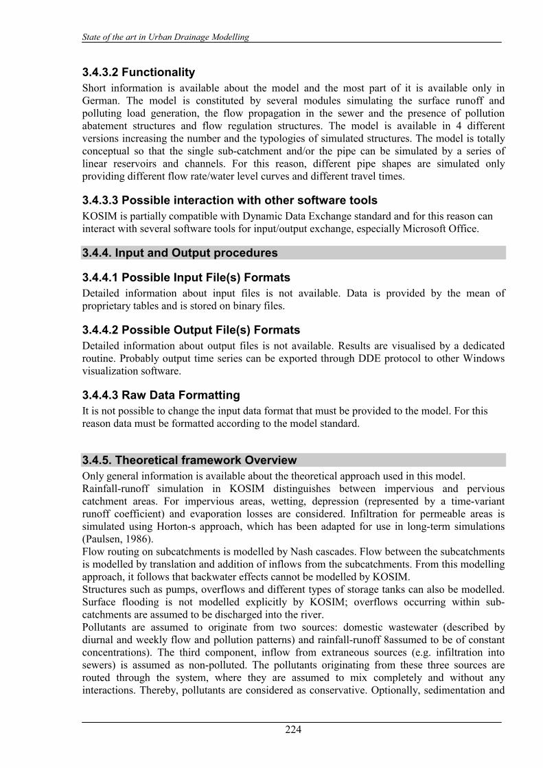
State of the art in Urban Drainage Modelling
224
3.4.3.2 Functionality Short information is available about the model and the most part of it is available only in German. The model is constituted by several modules simulating the surface runoff and polluting load generation, the flow propagation in the sewer and the presence of pollution abatement structures and flow regulation structures. The model is available in 4 different versions increasing the number and the typologies of simulated structures. The model is totally conceptual so that the single sub-catchment and/or the pipe can be simulated by a series of linear reservoirs and channels. For this reason, different pipe shapes are simulated only providing different flow rate/water level curves and different travel times.
3.4.3.3 Possible interaction with other software tools KOSIM is partially compatible with Dynamic Data Exchange standard and for this reason can interact with several software tools for input/output exchange, especially Microsoft Office.
3.4.4. Input and Output procedures
3.4.4.1 Possible Input File(s) Formats Detailed information about input files is not available. Data is provided by the mean of proprietary tables and is stored on binary files.
3.4.4.2 Possible Output File(s) Formats Detailed information about output files is not available. Results are visualised by a dedicated routine. Probably output time series can be exported through DDE protocol to other Windows visualization software.
3.4.4.3 Raw Data Formatting It is not possible to change the input data format that must be provided to the model. For this reason data must be formatted according to the model standard.
3.4.5. Theoretical framework Overview Only general information is available about the theoretical approach used in this model. Rainfall-runoff simulation in KOSIM distinguishes between impervious and pervious catchment areas. For impervious areas, wetting, depression (represented by a time-variant runoff coefficient) and evaporation losses are considered. Infiltration for permeable areas is simulated using Horton-s approach, which has been adapted for use in long-term simulations (Paulsen, 1986). Flow routing on subcatchments is modelled by Nash cascades. Flow between the subcatchments is modelled by translation and addition of inflows from the subcatchments. From this modelling approach, it follows that backwater effects cannot be modelled by KOSIM. Structures such as pumps, overflows and different types of storage tanks can also be modelled. Surface flooding is not modelled explicitly by KOSIM; overflows occurring within sub-catchments are assumed to be discharged into the river. Pollutants are assumed to originate from two sources: domestic wastewater (described by diurnal and weekly flow and pollution patterns) and rainfall-runoff 8assumed to be of constant concentrations). The third component, inflow from extraneous sources (e.g. infiltration into sewers) is assumed as non-polluted. The pollutants originating from these three sources are routed through the system, where they are assumed to mix completely and without any interactions. Thereby, pollutants are considered as conservative. Optionally, sedimentation and

State of the art in Urban Drainage Modelling
225
resuspension on the surface and in the sewers and in basins can be modelled by KOSIM. Another option allows sedimentation and pollutants in storage tanks to be modelled. If this option is not set, then pollutants are assumed to be completely mixed in storage tanks. In total, up to six pollutants can be modelled by KOSIM once the pollutant specific parameters are defined. Also several implementations of control options are available (Kollatsch and Schilling, 1990; Pracejus, 1994).
3.4.6. Model Parameters Estimation or Assignation The last version of KOSIM 6.1 can interact with a new sensitivity routine developed by ITWH.
3.4.6.1 Check of Parameters Significance – Internal Validation SINOPSYS is a sensitivity routine that can interact with KOSIM in order to evaluate the effect of parameters variation on model output and develop uncertainty analysis and calibration procedures. The sensitivity routine performs several simulations automatically changing the parameters values within the range fixed by the user. The simulations can be performed allowing for single parameters variation or multiple parameters variation (Monte Carlo Simulation). The sensitivity analysis results can be displayed or exported in tabular form or in graphic form.
3.4.7. PI(s) Estimation Method Not available in KOSIM
3.4.8. Future Improvements of the Model KOSIM is constantly updated by ITWH. The last update was release in 2002. There are no current plans to develop a new version in the near future
3.4.9. References
3.4.9.1 Theoretical Framework References Demuynck, C., Mespreuve, M., and Bauwens, W. (July 1993) “Application of a continuous simulation model on the sewer network of Brussels” Proceedings of 6th International Conference on Urban Storm Drainage, Niagara Falls Ontario Canada, pp. 1472-1477. Fuchs, L. (June 1994) “Experience of user group activities in Germany”, Integrated Urban Storm Runoff - 7th European Junior Scientist Workshop, Cemise Castle-Bechyne Czech Republic, pp. 303-304 C. Fronteau and W. Bauwens (August 1999) “Ecological interpretation of integrated model output” Proceedings of 8th International Conference on Urban Storm Drainage, Sydney, Australia, pp.1033-1040
State of the art in Urban Drainage Modelling
226
3.5 SIMBA – SIMulation of Biological Activity
3.5.1. Model availability SIMBA is a commercial toolkit for Integrated Urban Water Systems quality simulation and it is delivered by Institut für Automation und Kommunikation e.V. Magdeburg (http://www.ifak.fhg.de). SIMBA 4.0 is shipped together with the Matlab®/ Simulink™ software of MathWorks Inc.; it runs under the Windows 9x, 2000 and NT 4.0 operating systems.
3.5.2. Abstract
3.5.2.1 Objectives and peculiarities SIMBA® is a versatile software package which allows model building and dynamic simulation of biological wastewater treatment processes. For example, hydrographs and pollutographs of the plant effluent can be calculated conveniently. Without having to interfere with the real plant, dynamic simulation allows the evaluation of the plant's behaviour for different scenarios and different plant configurations. The new version SIMBA 4.0 also allows the holistic consideration of the entire urban wastewater system, including a sewer system, a wastewater treatment plant, receiving water body as well as a sludge treatment. Using information available from the plant, it is possible to set up simulation models for planning, design and optimisation of plants within a reasonable time. SIMBA is an application-oriented tool. Without any knowledge of programming, and assisted by buttons, extensive libraries and menus, the user can build models and simulate plants within a short time following a three-step approach:
• selection of model blocks required • connection of the blocks with lines according to plant configuration;
parametrisation • simulation, followed by evaluation of plots of pollutant concentrations and loads
using the build-in Monitor feature
3.5.2.2 Performance Indicator(s) of Interest SIMBA is able to evaluate the basic flow variables such as discharge, pollution concentration and sediment load. This kind of data can be used for computing physical and operational performance indicators, even if the model does not compute the PIs directly.
3.5.2.3 Brief Historical Overview of the Model SIMBA was developed in 1994 and is continuously being extended by ifak e. V. - Institut für Automation und Kommunikation. Today SIMBA is being used world wide for the design and analysis of biological wastewater treatment processes.

State of the art in Urban Drainage Modelling
227
3.5.3. Usage Specifications
3.5.3.1 Programming Language(s) or Mathematical-Statistical Software(s) The model has been written in Matlab using Simulink libraries. The source code is not directly available even if the object oriented functionalities of Simulink allow for high customization level.
3.5.3.2 Functionality The underlying model concepts, e.g. the Activated Sludge Models by IWA (formerly IAWQ), digestion models by Siegriest and pollution load models, are provided in an open format in symbolic notation. This implies that these models can be easily modified and adapted using a user-friendly model editor, which is based on the well-known ASM-Matrix notation. Predefined block libraries and additional useful tools provide the state-of-the-art in wastewater treatment modelling. The library blocks can be easily combined, thus supporting a holistic approach to wastewater management. Due to SIMBA's open structure, the user can conveniently adapt existing models and extend the model library by definition of his own models and functions. Common block and Activated Sludge libraries The Common block library represents the essential components of most activated sludge treatment plants. These include blocks for inflow, primary and secondary clarification, as well as a large number of blocks describing storage and conversion processes of wastewater and sludge. SIMBA sewer library The blocks of this library allow flow and pollutant transport and conversion processes in sewer networks to be simulated. Pollutants include soluble and particulate fractions. Sewer pipes of any profile and length as well as other hydraulic structures, such as weirs and pumps, can be modelled. Biofilm library A number of different plant configurations and biofilm structures can be modelled using parameters for the surface of the biofilm, the thickness of the layer and the pollutant transport. Different blocks are available for nitrifying and denitrifying biofilters.
3.5.3.3 Possible interaction with other software tools Being a collection of Maltab libraries, SIMBA can manage interactions on several levels: interactions inside the Matlab working environment exchanging variables and routines; interaction in DDE environment with all Windows applications exchanging graphics and data; input/output data exchange in text format.
3.5.4. Input and Output procedures
3.5.4.1 Possible Input File(s) Formats The input data are given in Matlab variables format. For this reason there is not a single input format but input files can be customised changing the routines for data reading.
3.5.4.2 Possible Output File(s) Formats Also output files can be easily customised and are usually provided in text format.

State of the art in Urban Drainage Modelling
228
3.5.4.3 Raw Data Formatting The Matlab environment allows for simple customisation of input and output files. For this reason the adaptation of the model to any raw data format is potentially possible
3.5.5. Theoretical framework Overview The model library SIMBA sewer extends the WWTP simulation software SIMBA by a set of model blocks to simulate the upstream sewer network of a treatment plant.
Fig. 3.5.1: SIMBA sewer scheme
This block set provides a vast variety of opportunities for the integrated simulation of sewer network and treatment plant. The aim of the block set SIMBA sewer is the simulation of single dynamic events with interactions between treatment plant and sewer system. Interaction between treatment plant and sewer occurs, in case there is any kind of feedback present. Feedback can originate from hydraulic effects (backwater) or from control of the sewer system using information of the current state of the treatment plant. SIMBA sewer is not a replacement for conventional sewer simulation systems but a special tool to investigate managed sewer systems and integrated systems. SIMBA sewer does not describe the catchment of rain water. Information about the several influent components to a sewer system (waste water, surface runoff, infiltration) as flow rates and concentrations must be provided by the user. This influent could be generated by conventional sewer simulation systems and provided as ASCII files for SIMBA sewer. The surface runoff models are not included in SIMBA sewer because usually no feedback exists between surface runoff, transport and storage in sewer systems. SIMBA sewer allows to simulate:
• transport of water and load of dissolved and solid pollutants in sewer networks, through the application of conceptual deposition/resuspension model
• conversion processes, by the mean of depletion curves • any kind of overflow and storage construction • controllable inputs and controllers for sewer systems
Modelling of water transport is achieved by the diffusion wave approximation of the Saint-Venant equation system - hydrodynamic model including storage, back water effects, change of
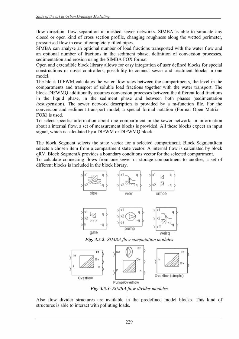
State of the art in Urban Drainage Modelling
229
flow direction, flow separation in meshed sewer networks. SIMBA is able to simulate any closed or open kind of cross section profile, changing roughness along the wetted perimeter, pressurised flow in case of completely filled pipes. SIMBA can analyse an optional number of load fractions transported with the water flow and an optional number of fractions in the sediment phase, definition of conversion processes, sedimentation and erosion using the SIMBA FOX format Open and extendible block library allows for easy integration of user defined blocks for special constructions or novel controllers, possibility to connect sewer and treatment blocks in one model. The block DIFWM calculates the water flow rates between the compartments, the level in the compartments and transport of soluble load fractions together with the water transport. The block DIFWMQ additionally assumes conversion processes between the different load fractions in the liquid phase, in the sediment phase and between both phases (sedimentation /resuspension). The sewer network description is provided by a m-function file. For the conversion and sediment transport model, a special formal notation (Formal Open Matrix - FOX) is used. To select specific information about one compartment in the sewer network, or information about a internal flow, a set of measurement blocks is provided. All these blocks expect an input signal, which is calculated by a DIFWM or DIFWMQ block. The block Segment selects the state vector for a selected compartment. Block SegmentItem selects a chosen item from a compartment state vector. A internal flow is calculated by block qRV. Block SegmentX provides a boundary conditions vector for the selected compartment. To calculate connecting flows from one sewer or storage compartment to another, a set of different blocks is included in the block library.
Fig. 3.5.2: SIMBA flow computation modules
Fig. 3.5.3: SIMBA flow divider modules
Also flow divider structures are available in the predefined model blocks. This kind of structures is able to interact with polluting loads.

State of the art in Urban Drainage Modelling
230
The blocks are hierarchical blocks which can be decomposed into more basic blocks. The blockset is easy to extend by user written blocks to fit the requirement of the considered case. The sewer models can be combined into an integrated model with SIMBA treatment plant models and blocks to describe control structures. SIMBA makes the main components available for activated sludge wastewater treatment plants as blocks in a library. The ASM 1, ASM 2 and the OB (Open SIMBA) libraries are all available in the SIMBA. All the blocks in the library ASM 1 have been specially designed to the parameter vector of the Activated Sludge Model No. 1 (13 groups of substances plus the wastewater flow), which allow simulation of the behaviour of nitrifying and denitrifying activated sludge systems. The blocks in the library ASM 2 contain the Activated Sludge Model No. 2, which allows simulation of the processes of chemical and enhanced biological phosphorus elimination in addition to ASM 1. The open block library (OB can be tailor-made to freely define wastewater flows and customised models. Users can easily integrate self-defined processes or processes with Monod-kinetics (which are described in the IAWQ-Matrix-Format) into the SIMBA system. In addition, there are blocks for measuring, controlling and monitoring as well as some of the most frequently required SIMULINK-blocks. These blocks may be used in both models. Altogether, the blocks can be divided into the following groups:
• Influent blocks o constant Influent with constant concentrations o variable influent and concentrations generated from a matrix with values and
time points of a Daily hydrograph o influent generated from values which are stored in an ASCII file, completely
with Hydrograph file, or piece wise with FromFile o the runoff graph of the Rainevent is formed by the storage capacity of the
combined sewer and the duration of rainfall • Reactors and Storage block o activated sludge tanks for Nitrification with Pressure aeration or Surface aerator o denitrification o anaerobic process ASM 1 (1M) and ASM 2 (2) reactors o storage of wastewater in a completely mixed tank with influent, effluent,
overflow and filling volume • Primary and Secondary Clarifiers o primary clarifier PC buffers the influent and eliminates particulate fractions of
COD and nitrogen through settling dependent on the hydraulic retention time o ideal secondary clarifier SC-Ideal o SC-Mix model with storage of sludge and estimation of effluent-solids
concentrations o SC-OF model with horizontal layers and classification of the sludge particles
into macro- and micro-flocs with different settling behaviours according to Otterpohl and Freund
o SC-T model with horizontal layers with an exponential function with two terms for the settling velocity according to Takacs et al.
• Distribution and Connection • Mixer that permits the confluence of two wastewater flows and realises an ideal mix • Divider or Pump divides one wastewater flow into two, whereby the ratio of division
or the pumped flow is determined by a second input signal • Line-separation and connection are used to construct simple models of plants with
several parallel lines
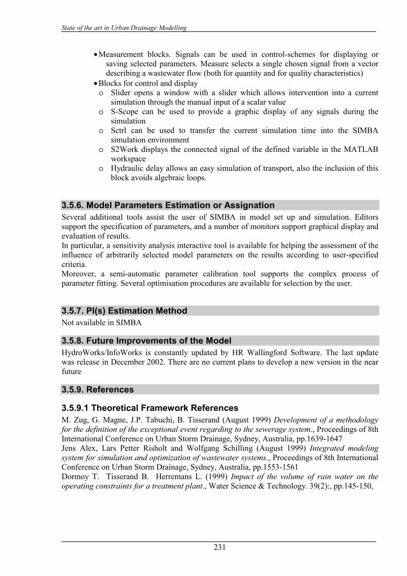
State of the art in Urban Drainage Modelling
231
• Measurement blocks. Signals can be used in control-schemes for displaying or saving selected parameters. Measure selects a single chosen signal from a vector describing a wastewater flow (both for quantity and for quality characteristics)
• Blocks for control and display o Slider opens a window with a slider which allows intervention into a current
simulation through the manual input of a scalar value o S-Scope can be used to provide a graphic display of any signals during the
simulation o Sctrl can be used to transfer the current simulation time into the SIMBA
simulation environment o S2Work displays the connected signal of the defined variable in the MATLAB
workspace o Hydraulic delay allows an easy simulation of transport, also the inclusion of this
block avoids algebraic loops.
3.5.6. Model Parameters Estimation or Assignation Several additional tools assist the user of SIMBA in model set up and simulation. Editors support the specification of parameters, and a number of monitors support graphical display and evaluation of results. In particular, a sensitivity analysis interactive tool is available for helping the assessment of the influence of arbitrarily selected model parameters on the results according to user-specified criteria. Moreover, a semi-automatic parameter calibration tool supports the complex process of parameter fitting. Several optimisation procedures are available for selection by the user.
3.5.7. PI(s) Estimation Method Not available in SIMBA
3.5.8. Future Improvements of the Model HydroWorks/InfoWorks is constantly updated by HR Wallingford Software. The last update was release in December 2002. There are no current plans to develop a new version in the near future
3.5.9. References
3.5.9.1 Theoretical Framework References M. Zug, G. Magne, J.P. Tabuchi, B. Tisserand (August 1999) Development of a methodology for the definition of the exceptional event regarding to the sewerage system., Proceedings of 8th International Conference on Urban Storm Drainage, Sydney, Australia, pp.1639-1647 Jens Alex, Lars Petter Risholt and Wolfgang Schilling (August 1999) Integrated modeling system for simulation and optimization of wastewater systems., Proceedings of 8th International Conference on Urban Storm Drainage, Sydney, Australia, pp.1553-1561 Dormoy T. Tisserand B. Herremans L. (1999) Impact of the volume of rain water on the operating constraints for a treatment plant., Water Science & Technology. 39(2):, pp.145-150,
State of the art in Urban Drainage Modelling
232
3.5.9.2 Practical Use and Results References Lars P. Risholt, Wolfgang Schilling, Jens Alex (August 1999) Towards integrated pollution based real time control of the wastewater system in Fredrikstad, Norway., Proceedings of 8th International Conference on Urban Storm Drainage, Sydney, Australia, pp.1562-1569
State of the art in Urban Drainage Modelling
233
3.6 SIMPOL3
3.6.1. Model availability SIMPOL3 is a WRc product, for technical queries contact [email protected] The software is not commercially available.
3.6.2. Abstract
3.6.2.1 Objectives and peculiarities SIMPOL3 is an integrated, environmental modelling package which includes modules for urban drainage planning. It is used for investigating the water quality impacts caused by urban drainage systems and for identifying outline solutions which meet specified emission and environmental standards. It represents runoff, storage and water quality processes in drainage systems and associated watercourses using relatively simple algorithms. It includes both deterministic and stochastic elements and allows fast, continuous simulation. Typical runs will take minutes for multi-year simulations. This section, covering the urban drainage quality aspects of SIMPOL3 should be read in conjunction with sections on the urban quantity and waterbody impact aspects.
3.6.3. Usage Specifications
3.6.3.1 Functionality SIMPOL3 simulates the water quality processes in drainage systems in a simplified state. It represents domestic and industrial inputs of BOD and ammonia and inputs from surface washoff. It includes algorithms for the settlement and resuspension of pollutants within the subcatchment modules and large offline storage tanks.
3.6.3.2 Possible interaction with other software tools SIMPOL3 is an integrated model which includes quantity and quality simulation within drainage systems and associated river systems. SIMPOL3 can accept input timeseries of flows/quality generated by other models and can provide output for use in other models. The possibility of direct calls to other software exists (a current application includes a direct call to an estuary water quality model allowing both models to run together).
3.6.4. Input and Output procedures
3.6.4.1 Possible Input File(s) Formats All input files are held in MS Access database tables. Any timeseries input can be accepted in a tabular format – date/time, variable1, variable2 etc.

State of the art in Urban Drainage Modelling
234
3.6.4.2 Possible Output File(s) Formats SIMPOL3 generates timeseries output for any specified list of variables. The output is in a format: Date/Time, Variable1, Variable2 etc at hourlt timesteps over the complete simulation period. The output can be exported as .csv, .txt, .xls or as MS Access tables. The ‘quality’ type output includes: • BOD and ammonia concentrations and loads associated with all flow streams • BOD and ammonia loads in storages • BOD and ammonia loads in sewer sediments
3.6.4.3 Raw Data Formatting Model data defining the model network is extracted and inserted manually into the Access database. The detailed model data can be extracted in tabular format and then manipulated using Excel to input into the SIMPOL3 database.
3.6.5. Theoretical framework Overview SIMPOL3 uses a mass balance approach to handle loads and concentrations passed through a network. Simplified algorithms are used to represent settlement and resuspension processes for sediment-related pollutants. No pollutant losses are considered within the drainage system.
3.6.6. Model Parameters Estimation or Assignation The settlement/resuspension algorithms in SIMPOL3 are calibrated by comparing the predicted loads and concentrations against those from survey data . A manual process is used to adjust parameters to give a best fit over the range of available data. The fit is judged subjectively.
3.6.7. References
3.6.7.1 Theoretical Framework References Williams W, Murrell K. (2001). Fast Track Urban Pollution Planning. Wastewater 2001 – A treatment and Disposal Odyssey. CIWEM 17 October 2001 Crabtree R.W., Dempsey P, Walwyn R (2003). Simplified integrated modelling of a large conurbation – the River Tame catchment case study. IMUG conference May 2003 (in preparation)
State of the art in Urban Drainage Modelling
235
3.7 FLUPOL
3.7.1. Model availability FLUPOL is research development model produced by Anjou Recherche (www.vivendiwater.com). The source code should be freely distributed but only through a direct request to the authors.
3.7.2. Abstract
3.7.2.1 Objectives and peculiarities FLUPOL is an environmental modelling package aimed to the calculation of global quantities of pollution released during long periods and to the reproduction of the response of the drainage system in pollutant flow during a rainfall event. The pollutant factors considered in the model are the total suspended solids, oxygen demand and nitrogen. The software package divides its calculations into a number of physical processes, each then being translated into a specific algorithm. FLUPOL can be defined as being of the conceptual type with the use of explicit parameters describing the catchment, network and rainfall event.
3.7.2.2 Performance Indicator(s) of Interest FLUPOL is able to evaluate the basic flow variables such as discharge, pollution load. This kind of data can be used for computing physical and operational performance indicators, even if the model does not compute the PIs directly.
3.7.2.3 Brief Historical Overview of the Model FLUPOL first version was developed in 1988 and is periodically being extended by developers. Updated version is FLUPOL 2.1, called also FLUWIN because of its compatibility with WINDOWS environment.
3.7.3. Usage Specifications
3.7.3.1 Functionality FLUPOL is a very simple model to simulate polluting loads that are generated in wet weather on the catchment surface and that are transported by the drainage system. The pollutant factors considered in the model are the total suspended solids, oxygen demand and nitrogen. The model does not consider polluting load depletion during the transport. The model needs the following type of data:
• Sub-catchments: area, slope, hydraulic lenght, runoff coefficient, soil type, population (in order to estimate dry-weather flow)
• Drainage systems: pipe shape, dimensions, slope, roughness, length, overflow discharge and pump stations
• Polluting loads: dry period antecedent to storm events, initial polluting load on the surface and in the drainage system
• Infiltration/exfiltration rate for the drainage pipes
State of the art in Urban Drainage Modelling
236
3.7.3.2 Possible interaction with other software tools Interaction can be obtained only through text input/output files.
3.7.4. Input and Output procedures
3.7.4.1 Possible Input File(s) Formats All input files are delimited text
3.7.4.2 Possible Output File(s) Formats All output files are delimited text
3.7.4.3 Raw Data Formatting It is not possible to adapt the model to drainage database but a conversion tool can be developed to translate any data format to the requirements of the model.
3.7.5. Theoretical framework Overview Pollution build-up is simulated by the Alley-Smith Formula (1981). Wash-off phenomena are simulated by the Jewell-Adrian formula (1978). Pollution transport in the drainage system is simulated by Vélikanov approach (1970).
3.7.6. Model Parameters Estimation or Assignation No optimization/calibration routine is available in FLUPOL.
3.7.7. References
3.7.7.1 Theoretical Framework References Bujon, G., Herremans, L. and Phan, L. (September 1991) FLUPOL: A forecasting model for flow and pollutant discharge from sewerage systems during rainfall events., Applications of Operations Research to Real Time Control of Water Resources Systems - 3rd European Junior Scientist Workshop, Terschelling The Netherlands, pp. 207-216. Ashley, R.M. and Bertrand-Krajewski, J.L. (July 1993) Sewer sediment origins and transport in small catchments., Proceedings of 6th International Conference on Urban Storm Drainage, Niagara Falls Ontario Canada, pp. 772-777. D. Blanc, R. Kellagher, L. Phan, R. Price, (May 1995) FLUPOL-MOSQITO, simulations, critiques et developpement., 2nd International Conference on Innovative Technologies in Urban Storm Drainage, Lyon, France, pp.111. Blanc, D. et al. (1995) FLUPOL-MOSQITO models, simulations, critical analysis, and development., Proc. 2nd Int. Conf. on Innov. Technol. in Urban Storm Drainage, NOVATECH 1995 Bujon, G. et al. (1992) FLUPOL - a forecasting model for flow and pollutant discharges from sewerage systems during rainfall events. Water Science and Technology, 25, 207

State of the art in Urban Drainage Modelling
237
3.8 HORUS
3.8.1. Model availability HORUS is research development model produced by Anjou Recherche (www.vivendiwater.com). The model cannot be yet considered as a commericial tool according to the fact that it is not yet distributed. At the moment
3.8.2. Abstract
3.8.2.1 Objectives and peculiarities The objective of this model is, taking into account the characteristics of the catchment and the structure of the sewerage system, to reproduce the hydrographs, Total Suspended Solids (TSS) and Chemical Oxygen Demand (COD) concentration generated by any rainfall. HORUS consists of main connected modules and the retained algorithms have been chosen after using a special Testing Bench of Pollution Modelling Algorithm in Urban Sewer System. The main modules are: a hydrological module (linear reservoir and runoff losses), a hydraulic module (described by the Muskingum model), a module for solids production and transport (build-up and washoff of catchment and solid transport in sewer) and a module for numerical optimisation. The improvement of the HORUS model is shown by a comparison between simulation results versus the initials algorithms. Simultaneous measurements of rainfall, hydraulic, TSS and COD concentrations on nine very different catchments and about one hundred rainfall events allowed a large range of validation which can be considered of good quality. HORUS provides a satisfying fitting of the real TSS and COD pollutographs (flow and concentration) and this, considering the global form, maximal values and the temporal position.
3.8.2.2 Performance Indicator(s) of Interest HORUS is able to evaluate the basic flow variables such as discharge, pollution load. This kind of data can be used for computing physical and operational performance indicators, even if the model does not compute the PIs directly.
3.8.2.3 Brief Historical Overview of the Model HORUS is a relatively new model that was developed in 1999. No further developments have been registred.
3.8.3. Usage Specifications
3.8.3.1 Functionality The objective of the overall model is, taking into account the characteristics of the catchments and the structure of the sewerage system, to reproduce the hydrographs and Total Suspended Solids (TSS) and Chemical Oxygen Demand (COD) concentration generated by any rain. The will to achieve a model, using a reduced number of parameters oriented the choice towards conceptual type formulations, calibrated and validated on the maximum of real sites. In addition to the initial objectives of the model, HORUS was also programmed to meet future needs like its coupling with a treatment plants model or real time control. The HORUS model (see Figure 3.8.l) consists of five main connected modules:
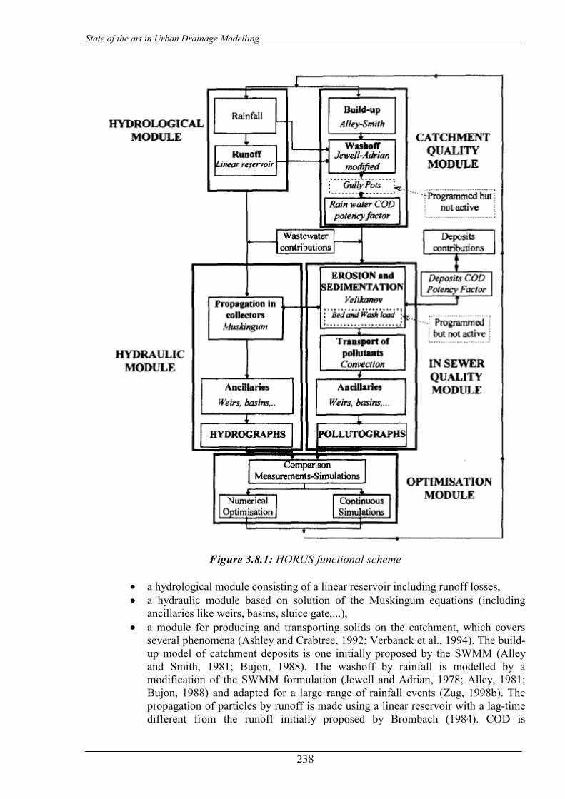
State of the art in Urban Drainage Modelling
238
Figure 3.8.1: HORUS functional scheme
• a hydrological module consisting of a linear reservoir including runoff losses, • a hydraulic module based on solution of the Muskingum equations (including
ancillaries like weirs, basins, sluice gate,...), • a module for producing and transporting solids on the catchment, which covers
several phenomena (Ashley and Crabtree, 1992; Verbanck et al., 1994). The build-up model of catchment deposits is one initially proposed by the SWMM (Alley and Smith, 1981; Bujon, 1988). The washoff by rainfall is modelled by a modification of the SWMM formulation (Jewell and Adrian, 1978; Alley, 1981; Bujon, 1988) and adapted for a large range of rainfall events (Zug, 1998b). The propagation of particles by runoff is made using a linear reservoir with a lag-time different from the runoff initially proposed by Brombach (1984). COD is
State of the art in Urban Drainage Modelling
239
calculated through a potency factor governing the relations between the pollutants and TSS (Zug, 1998). This module allows an algorithm of gully pots, this algorithm has been programmed but is not actually active.
• a module for producing and transporting solids in the sewer system The sediment transport in the sewer is modelled by the Velikanov theory (Bujon, 1988; Zug et al., 1998) with the calculation of sedimentation and erosion of solids during dry or rainy weather. Pollutographs are propagated by convection. COD is calculated through a potency factor governing the relations between this pollutants and TSS. This module allows some algorithms for bed load and wash load calculation, these algorithms have been programmed but are not actually active.
• a module for numerical optimisation using the Powell method (Numerical Recipies, 1986) and evaluation of hydraulic and pollution results for calibration and continuous simulations.
3.8.3.2 Possible interaction with other software tools Interaction can be obtained only through text input/output files.
3.8.4. Input and Output procedures
3.8.4.1 Possible Input File(s) Formats All input files are delimited text
3.8.4.2 Possible Output File(s) Formats All output files are delimited text
3.8.4.3 Raw Data Formatting It is not possible to adapt the model to drainage database but a conversion tool can be developed to translate any data format to the requirements of the model.
3.8.5. Theoretical framework Overview No information is available about model theoretical framework apart from what was discussed in the functionality description.
3.8.6. Model Parameters Estimation or Assignation Numerical optimisation is available using the Powell method (Numerical Recipies, 1986) and evaluation of hydraulic and pollution results for calibration and continuous simulations.
3.8.7. References
3.8.7.1 Theoretical Framework References Alley, W. M. (1981). Estimation ofimpervious area washoff parameters. Journal of Hydraulic Engineering, 121(2),171-183. Alley, W. M. and Smith, P. E. (1981). Estimation of accumulation parameters for urban runoff quality modelling. Water Resources Research, 6, 1657-1664. Ashley, R. M. and Crabtree, R. W. (1992). Sediment origins, deposition and build-up in combined sewer systems. Wat. Sci. Tech., 33(8), 1-12.
State of the art in Urban Drainage Modelling
240
Bertrand-Krajewski, J. L., Scrivener, O. and Briat, P. (1993). Sewer sediment production and transport modelling : A literature review. Journal of Hydraulic Research, 31(4), 435-460. Xanthopoulos, C. and Hahn, H. (1993). Anthropogenic pollutants wash-off from street surface. Proceedings of the sixth International Conference on Urban Storm drainage, Niagara Falls, Canada, 417-422. Zug, M., Bellefleur, D., Phan, L. and Scrivener, O. (1998a). Sediment transport model in sewer networks, a new utilisation of the Velikanov Model. War. Sci. Tech., 37(l),187-196. Zug, M., Phan, L., Bellefleur, D. and Scrivener, O. (1998c). Testing Bench of Pollution Modelling Algorithm in Urban Sewer Networks. Hydroinformatics 98, Copenhagen, Denmark, August 24-26, 1998, Vol 2, 1491-1497.

State of the art in Urban Drainage Modelling
241
3.9 WATS: wastewater aerobic–anaerobic transformations in sewers
3.9.1. Model availability WATS (Wastewater Aerobic/anaerobic Transformations in Sewers) has been developed by Alborg University for simulation of wastewater quality transformations and sulphide formation in sewers. The model is not yet at commercial stage.
3.9.2. Abstract
3.9.2.1 Objectives and peculiarities The model integrates processes in sewers under aerobic and anaerobic conditions. In the water phase it includes growth of the heterotrophic biomass, growth and non-growth related oxygen consumption, hydrolysis and fermentation. Concerning the bio-film processes, e.g. sulphate respiration, relatively simple descriptions in terms of surface-based transformations are used. Sewer sediment processes are not included in the model. Furthermore, sulphide formation can be predicted under changing aerobic/anaerobic conditions in both gravity sewers and pressure mains. The conceptual model is outlined in Figure 3.9.1. Further details are found in Hvitved-Jacobsen et al. (1998) and Tanaka and Hvitved-Jacobsen (1999).
Figure 3.9.1: WATS functional scheme
3.9.2.2 Performance Indicator(s) of Interest WATS is able to evaluate the basic flow variables such as discharge, pollution load with special concern on hydrogen sulfide generation. This kind of data can be used for computing physical and operational performance indicators, even if the model does not compute the PIs directly.
State of the art in Urban Drainage Modelling
242
3.9.3. Usage Specifications
3.9.3.1 Functionality WATS is still at a development level so functionalities are extending and growing in the sequence of versions that are released. The model basically simulates aerobic and anaerobic processes in sewers. For this reason is able to analyse both conservative and non conservative pollutants using also different transformation function depending on physical and chemical characteristics of the simulated process. At the present, the WATS model includes the following main aspects and simulation options of the in-sewer carbon and sulphur cycle under dry-weather conditions:
• Quality transformations for the wastewater organic matter (COD) in terms of its biodegradability
• DO mass balance for r the water phase • Sulfide formation • Description of the transformations under varying aerobic and anaerobic conditions
The WATS model is formulated in deterministic terms. However, an extension to include simple Monte-Carlo stochastic simulation is possible, taking into consideration a measured variability of the process parameters. Extension of the WATS model to integrate further dry-weather processes is considered important. Examples of such extensions are the description of the wastewater quality and nitrite/nitrate transformations under anoxic conditions and the emission of hydrogen sulfide into the sewer atmosphere followed by its transformation at the sewer walls. An extension of WATS model to include wet weather conditions requires a conceptual change by strengthening the physical processes in terms of solid deposition, erosion and transport.
3.9.3.2 Possible interaction with other software tools Interaction can be obtained only through text input/output files.
3.9.4. Input and Output procedures
3.9.4.1 Possible Input File(s) Formats All input files are delimited text
3.9.4.2 Possible Output File(s) Formats All output files are delimited text
3.9.4.3 Raw Data Formatting It is not possible to adapt the model to drainage database but a conversion tool can be developed to translate any data format to the requirements of the model.
3.9.5. Theoretical framework Overview The analytical approaches that are used in WATS are depicted in Table 3.9.1. As discussed previously the model is still developing and several aspects will be added in order to take into account different transformation processes in sewer systems.
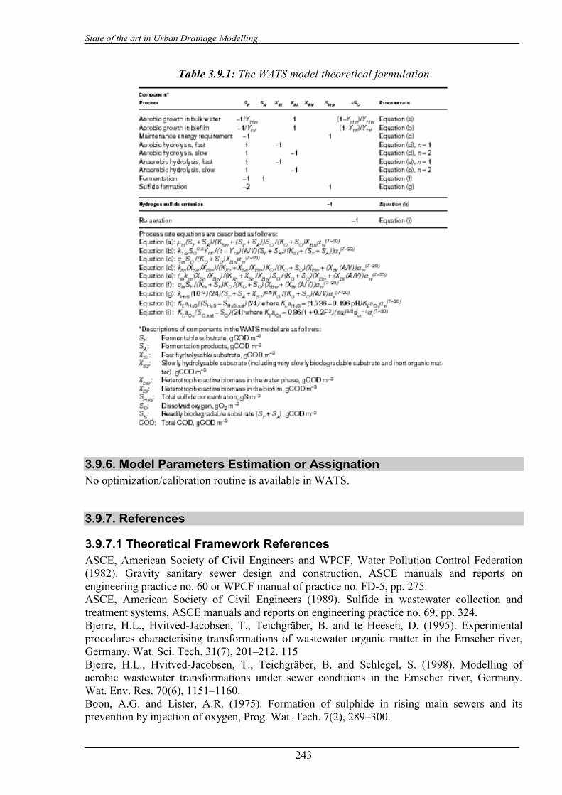
State of the art in Urban Drainage Modelling
243
Table 3.9.1: The WATS model theoretical formulation
3.9.6. Model Parameters Estimation or Assignation No optimization/calibration routine is available in WATS.
3.9.7. References
3.9.7.1 Theoretical Framework References ASCE, American Society of Civil Engineers and WPCF, Water Pollution Control Federation (1982). Gravity sanitary sewer design and construction, ASCE manuals and reports on engineering practice no. 60 or WPCF manual of practice no. FD-5, pp. 275. ASCE, American Society of Civil Engineers (1989). Sulfide in wastewater collection and treatment systems, ASCE manuals and reports on engineering practice no. 69, pp. 324. Bjerre, H.L., Hvitved-Jacobsen, T., Teichgräber, B. and te Heesen, D. (1995). Experimental procedures characterising transformations of wastewater organic matter in the Emscher river, Germany. Wat. Sci. Tech. 31(7), 201–212. 115 Bjerre, H.L., Hvitved-Jacobsen, T., Teichgräber, B. and Schlegel, S. (1998). Modelling of aerobic wastewater transformations under sewer conditions in the Emscher river, Germany. Wat. Env. Res. 70(6), 1151–1160. Boon, A.G. and Lister, A.R. (1975). Formation of sulphide in rising main sewers and its prevention by injection of oxygen, Prog. Wat. Tech. 7(2), 289–300.

State of the art in Urban Drainage Modelling
244
Boon, A.G. (1995). Septicity in sewers: causes, consequence and containment. Wat. Sci. Tech. 31(7), 237–253. Hvitved-Jacobsen, T., Jütte, B., Nielsen, P.H. and Jensen, N.Aa. (1988). Hydrogen sulphide control in municipal sewers. H.H. Hahn and R. Klute (eds.), Pretreatment in Chemical Water and Wastewater Treatment, Springer-Verlag, 239–247. Hvitved-Jacobsen, T., Raunkjær, K. and Nielsen, P.H. (1995). Volatile fatty acids and sulfide in pressure mains. Wat. Sci. Tech. 31(7), 169–179. Hvitved-Jacobsen, T., Vollertsen, J. and Nielsen, P.H. (1998a). A process and model concept for microbial wastewater transformations in gravity sewers. Wat. Sci. Tech. 37(1), 233–241. Hvitved-Jacobsen, T., Vollertsen, J. and Tanaka, N. (1988b). Wastewater quality changes during transport in sewers – an integrated aerobic and anaerobic model concept for carbon and sulfur microbial transformations. Wat. Sci. Tech. 38(10), 257–264 (read text pp. 249–256) or Wat. Sci. Tech. 39(2), 242–249. Hvitved-Jacobsen, T. and Vollertsen, J. (1998). An intercepting sewer from Dortmund to Dinslaken, Germany, report submitted to the Emschergenossenschaft, Essen, Germany, pp. 35. Kuhl, M. and Jorgensen, B.B. (1992). Microsensor measurements of sulfate reduction and sulfide oxidation in compact microbial communities of aerobic biofilms. Appl. Environ. Microbiol. 58, 1164–1174. Meyer, W.J. and Hall, G.H. (1979). Prediction of sulfide generation and corrosion in concrete gravity sewers: A case study, J.b. Gilbert and Associates, A Division of Brown and Caldwell, Sacramento, Ca., USA. Nielsen, P.H. (1987). Biofilm dynamics and kinetics during high-rate sulfate reduction under anaerobic conditions. Appl. environ. Microbiol. 53, 27–32. Nielsen, P.H. and Hvitved-Jacobsen, T. (1988). Effects of sulfate and organic matter on the hydrogen sulfide formation in biofilms of filled sanitary sewers. J. Wat. Pollut. Control Fed. 60(5), 627–634. Nielsen, P.H., Raunkjær, K. and Hvitved-Jacobsen, T. (1998). Sulfide production and wastewater quality in pressure mains. Wat. Sci. Tech. 37(1), 97–104. Norsker, N.H., Nielsen, P.H. and Hvitved-Jacobsen, T. (1995). Influence of oxygen on biofilm growth and potential sulfate reduction in gravity sewer biofilm. Wat. Sci. Tech. 31(7), 159–167. Parker, C.D. (1945). Isolation of a species of bacterium associated with the corrosion of concrete exposed to atmospheres containing hydrogen sulphides. Aust. J. Exptl. Biol. and Med. Sci. 23. Pomeroy, R.D. and Bowlus, F.D. (1946). Progress report on sulphide control research, Sewage Works Journal 18(4). Pomeroy, R.D. and Parkhurst, J.D. (1977). The forecasting of sulfide buildup rates in sewers. Prog. Wat. Techn. 9(3), 621–628. Schmitt, F. and Seyfried, C.F. (1992). Sulfate reduction in sewer sediments. Wat. Sci. Tech. 25(8), 83–90. Stemplewski, J., Schlegel, S., Stein, A., Geisler, W., Schmelz, K.-G., Hvitved-Jacobsen, T. and Vollertsen, J. (1999). Restructuring the Emscher system. Proceedings from the 11the EWPCA (the European Water Pollution Control Association) Symposium: Sewerage Systems – Cost and Sustainable Solutions, May 4–6, 1999, Munich, Germany, pp. 14. Tanaka, N. and Hvitved-Jacobsen, T. (1998). Transformations of wastewater organic matter in sewers under changing aerobic/anaerobic conditions. Wat. Sci. Tech. 37(1), 105–113. Tanaka, N., Hvitved-Jacobsen, T., Ochi, T. and Sato, N. (1998). Aerobic/anaerobic microbial wastewater transformations and reaeration in an air-injected pressure sewer, proceedings of the 71st Annual Water Environment Federation Conference and Exposition, WEFTEC ’98, Orlando, Florida, USA, October 3–7, 1998, 2, 853–864.
State of the art in Urban Drainage Modelling
245
Tanaka, N. and Hvitved-Jacobsen, T. (1999). Anaerobic transformations of wastewater organic matter under sewer conditions. 8th International Conference on Urban Storm Drainage, Sydney, Australia, August 30–September 3, 1999, pp. 8. Thistlethwayte, D.K.B. (ed.) (1972). The Control of Sulfides in Sewerage Systems, Butterworth, Sydney, Australia.

State of the art in Urban Drainage Modelling
246
3.10 COSMOSS
3.10.1. Model availability COSMOSS is a freeware model and is available through the developer at the Department of Mecanics and Materials – University of Reggio Calabria (Italy) ([email protected]).
3.10.2. Abstract
3.10.2.1 Objectives and peculiarities Summarize in few lines the main objectives (design, planning procedures, existing systems analysis) and nature of the model. Briefly describe the peculiarities of the model with respect to the task of CARE-S project (availability of long term simulation option, processes that can be simulated, ecc.). COSMOSS is a conceptual model both in the flow simulation part(i.e., the rainfall-runoff transformation and the subsequent propagation) and in the qualitative one(i.e., the build-up and the washoff of solids). The model has been tested using experimental data acquired in Parco d’Orleans catchment, Palermo, in Fossolo catchment, Bologna, and in Milijakovac catchment, Belgrade. The system (catchment and channels) is considered as a whole. The model can be divided into four parts:
• calculation of hydrological losses; • rainfall-runoff transformation and runoff propagation; • build-up of solids during dry weather • washoff
The main goal of the model is to simulate the water quality in the best way possible.
3.10.2.2 Performance Indicator(s) of Interest COSMOSS is able to evaluate the basic flow variables such as discharge, pollution load. This kind of data can be used for computing physical and operational performance indicators, even if the model does not compute the PIs directly.
3.10.3. Usage Specifications
3.10.3.1 Programming Language(s) or Mathematical-Statistical Software(s)
The source code has been written is Visual Basic.
3.10.3.2 Functionality COSMOSS simulates suspended solids: these are widely measured and studied and they are strongly correlated to other qualitative indices. The model uses an exponential equation proposed by Alley & Smith [1981]. The washoff phenomenon is treated by Nakamura equation.

State of the art in Urban Drainage Modelling
247
))(*()( tVWa
dretF −=
Sedimentation and resuspension of solids in the drainage system have been neglected by the model mainly cause to take them into account, a detailed hydraulic model should be adopted and this need does not fit with the general aim to propose a simple and conceptual model.
3.10.3.3 Possible interaction with other software tools The software can interact with Excel and other MS Office tools.
3.10.4. Input and Output procedures
3.10.4.1 Possible Input File(s) Formats Formatted text input file.
3.10.4.2 Possible Output File(s) Formats Formatted text output file.
3.10.4.3 Raw Data Formatting Raw data can be used only modifying the source code.
3.10.5. Theoretical framework Overview Build-up Total solids available at the beginning of the rainfall are evaluated by an exponential equation proposed by Alley & Smith [1981]:
3.10.5.1
where: Accu = build-up rate [kg/(ha*day)]; Ma = total mass accumulated on the surface of catchment [kg]; t = duration of elapsed dry time from last rain event [h]; Disp = decay rate [day-1]; Mr = residual mass after last event [kg]; A = the catchment surface [ha]; Peim = the percentage of impervious area. The value of the build up rate can be defined by on site studies or, if experimental data is lacking by literature values (see for example Alley & Smith [1981], Alley [1981], Bujon & Herremans [1990]). Washoff COSMOSS uses an exponential relationship between the percentage of solids available on the catchment at time t and the total cumulated discharged volume (see Nakamura [1990]). Therefore, it is possible to write:
3.10.5.2
−
−
+
−
= 24
*24
*
*1***tDisp
r
tDisp
a eMePeimADispAccuM

State of the art in Urban Drainage Modelling
248
where: Fa(t) = percentage of solids available at time t related to the mass available at the beginning of
rainfall; Vd = the cumulated volume at time t [m3]; Wr = washoff rate [m-3] (key parameter to simulate the washoff process; it is a sort of
«efficiency» in solid removal by the runoff). Thus the mass washed off during the interval t , t-1 is given by: where:
3.10.5.3
where: Mw = mass washed off [kg]; Ma = mass available at the beginning of rainfall [kg].
3.10.6. Model Parameters Estimation or Assignation Not available for COSMOSS.
3.10.6.1 Check of Parameters Significance – Internal Validation Not available for COSMOSS.
3.10.6.2 External Validation or Cross Validation – Statistical test(s) Not available for COSMOSS.
3.10.7. PI(s) Estimation Method Not available for COSMOSS.
3.10.8. Future Improvements of the Model At the moment no further development is planned.
3.10.9. References
3.10.9.1 Theoretical Framework References Alley, W.M. (1981). Estimation of impervious-area washoff parameters. Water Resources Research, 17(4), 1161-1166. Alley, W. M., & Smith, P. E. (1981). Estimation of accumulation parameters for urban Artina, S., Maglionico, M., Martinelli, A., Raffaelli, G., Anzalone, C., Lanzarini, S., & Guzzinati, E. (1997). Le misure di qualità nel bacino urbano Fossolo. L'acqua 2, 17-25 (in Italian). Artina, S., & Maglionico, M. (1997). Indagine sperimentale degli aspetti qualitativi dei deflussi nelle reti di drenaggio urbano. Atti del Convegno La difesa idraulica dei territori fortemente antropizzati, Milano.(in Italian). Bujon, G. (1988). Prevision des débits et des flux polluants transitès par les réseaux d'egouts par temp de pluie. Le modèle FLUPOL. La Houille Blanche 1, 11-23 (in French).
( ) aaaw MtFtFM )1()( −−=
State of the art in Urban Drainage Modelling
249
Bujon, G., & Herremans, L. (1990). FLUPOL Modèle de prévision des débits et des flux polluants en réseaux d’assainissement par temp de pluie: calage et validation. La Houille Blanche 2 (in French). Centro Studi Deflussi Urbani (1997). Sistemi di Fognatura - Manuale di Progettazione, chap.7, 8, 9. Milan: Hoepli (in Italian). Deletic, A., Maksimovic, C., & Ivetic, M. (1997). Modelling of Storm Wash-off of Suspended Solids from Impervious Surfaces. Journal of Hydraulic Research (IAHR), 35(1). Desbordes, M.(1975). Un essai de modélisation des phénomènes de ruissellement pluvial urbain. T.S.M. L'EAU 3, 121-126 (in French). Huber, C., & Dickinson, R.E. (1988). Storm Water Management Model: User’s Manual. U.S. EPA/600/3-88/001a. Athens: Georgia (USA). La Loggia, G., & Viviani, G. (1990). Controllo, verifica e calibrazione di modelli di piena in un bacino urbano in Sicilia. Atti del XXII Convegno di Idraulica e Costruzioni Idrauliche, Cosenza (Italy) (in Italian). La Loggia, G., Cannarozzo, M., & Oliveri, E. (1996). Riconfigurazione del bacino sperimentale di Parco d'Orleans in base all'analisi di eventi storici. Atti del seminario nazionale Modelli di dimensionamento e di qualità per le fognature urbane, Sorrento (Italy)11-14 giugno 1996 (in Italian). Marinelli, A., Maglionico, M., & Artina, S. (1996). Simulazione della qualità delle acque in un bacino sperimentale di drenaggio urbano. Atti del XXV Convegno di Idraulica e Costruzioni Idrauliche , Torino(Italy) (in Italian). Nakamura, E. (1990). Characteristics of wet weather combined sewage - Information to the design and operation of improved systems. Proceedings of the V International conference in urban storm drainage, Osaka (Japan). Xanthopoulos, C., Hahn, H.H.(1993). Anthropogenic pollutants wash-off from street surfaces. Proceedings of the VI International Conference on Urban Storm Drainage; (Niagara).

State of the art in Urban Drainage Modelling
250
3.11 DORAT – Double ORder Approximation Method for Transport
3.11.1. Model availability The model has two parts: the first one is a pre and post processor that prepares the input file for the numerical engine and displays the computed results. The second part is the numerical engine. The software house that produces the first part is the “Ars Nova Multimedia” and is located in Reggio Calabria (Italy). Its web site is www.arsnova.biz. A short guide for the use of the model is easily accessible from the model itself.
3.11.2. Abstract
3.11.2.1 Objectives and peculiarities The first purpose of the tool is to evaluate the capability of the steady-state flow in the pipes carrying domestic and industrial discharges to transport the associated bed load. The second purpose of the tool is the simulation of water depths, flow velocities, bed sediment depths and bed loads occurring in one or two drainage networks due to a time series of rainfall data. One of the two drainage networks can be the street network, that is coupled with the underground sewer network through the water inlets. The model is unconditionally stable with respect to the size of the time step and this allows long-term simulations.
3.11.2.2 Performance Indicator(s) of Interest • wEn3 Intermittent overflow discharge frequency • wEn4 Intermittent overflow discharge volume • wEn5 Intermittent overflow discharge related to rainfall • wEn6 Sediments from sewers • wPh5 Surcharging in sewers in dry weather • wPh6 Surcharging in sewers in wet weather • wPh7 High sewer surcharging
3.11.2.3 Brief Historical Overview of the Model The DORA methodology is a numerical technique developed by T. Tucciarelli and other co-authors (L. Noto, D. Termini and others) for the solution of partial differential equations having a scalar potential of the flow field. The computation of the unknowns at a new time level is split in a prediction step and in a correction step. The prediction step is given by the solution of a sequence of ordinary differential equations, one for each computational node of the network. The correction step is given by the solution of a system of linear partial differential equations, that is obtained using a fully implicit finite difference discretization. The DORA technique can be applied to the water depths, flow velocities, bed load computation in a drainage pipe network if the diffusive hypothesis is adopted in the momentum equation of the flow field, even if extension to the original complete problem has also been proposed by the same author. The main advantages of the technique are: 1) the unconditional stability with

State of the art in Urban Drainage Modelling
251
respect to the size of the step, 2) the possibility of solving the transition from partial to full section without the help of the Preissman approximation, 3) the possibility of solving the dual problem, that is the coupled flow routing in the upper street network (where each street is treated as an open channel) and in the lower drainage network.
3.11.3. Usage Specifications
3.11.3.1 Programming Language(s) or Mathematical-Statistical Software(s)
Fortran 77
3.11.3.2 Functionality The model simulates sewer systems, with manholes, pumping stations, on-line and off-line detention tanks. Cross-section of the link can be rectangular, circular, egg-shaped if it is closed and rectangular, trapezoidal or trapezoidal with a vertical side if it is open. Processes analyzed are both steady state and transient conditions in sewer and street networks. In the steady-state hypothesis the bed load, the water depth and the flow velocity corresponding to domestic and industrial discharge are computed according to the uniform flow hypothesis in each link of the network. The maximum bed load that the computed flow field can carry on without deposition is also estimated. In transient conditions the water depth, the flow rate, the bed load and the sediment depth in each node are computed in time according to the hypothesis of equilibrium between bed load and hydrodynamic conditions. Transition from free surface to pressurized flow in pipes is simulated. Surcharge is analyzed in both cases of closed pipes and pipes of sewer network connected to the street network through the water inlets. A simplified scheme summarizing different modules is reported below.
Input generalparameters, node andpipe data, outputrequirements(create file *.dor)
Model generates inputfiles for the numericalengine(create files *.dat)
Model run the numericalengine (file Dorasd1.exe).Output files *.out are written.
Model shows or printsoutput files
Model shows unconditional stability with respect to the Courant number and a constant time step has to be assigned.
3.11.3.3 Possible interaction with other software tools The code provides output text files and a graphic of the sought after flow rates versus time.

State of the art in Urban Drainage Modelling
252
3.11.4. Input and Output procedures
3.11.4.1 Possible Input File(s) Formats The code uses text data files, that can be generated by the preprocessor module.
3.11.4.2 Possible Output File(s) Formats The code provides output text files, with some graphics provided by the postprocessor module.
3.11.4.3 Raw Data Formatting The model reads the data in free format. The order of the data must be, of course, the one expected by the program.
3.11.5. Theoretical framework Overview The code computes the numerical solution of the 1D shallow water equations in the diffusive form. It enforces a fractional step methodology that solves sequentially one prediction and one correction half time step. The dependant variables of the model are water depth, flow velocity, suspended solid concentration and bed load. Sewer system is idealized as a series of links connected at nodes or cells. These ones are storage elements of the system; some of them correspond to manholes or pipe junctions in the physical system, or more frequently to simple computational nodes. The computational cell is given by the sum of the half links sharing the same node. Water depths are calculated for each computational cell and velocities are calculated for each link. In the prediction step the hydraulic gradient is kept constant along the time; this allows a sequential solution of the resulting ordinary differential equations, one computational cell after the other. In the correction step a diffusive linear problem is solved using a fully implicit finite difference scheme, also to estimate the backwater effect of the channel resistance. The proposed numerical scheme can be proved, according to a linear approximation, to be unconditionally stable. This allows to solve the transition from partial to full section without the help of the Preissman approximation. The solution of the dual problem, where the upper street network and the lower sewer networks are dynamically coupled, is obtained assuming a constant flow in the vertical links (corresponding to the inlets) during the prediction step and a flux linearization with respect to the hydraulic gradient during the correction step. Bed load transport is computed assuming the hypothesis of equilibrium between bed load and hydrodynamic conditions and neglecting the storage term of the bed load in the continuity equation of the sediment. The correction of the predicted bed elevation in the solution of the sediment continuity equation is also neglected.
3.11.6. Model Parameters Estimation or Assignation Sensitivity analysis, calibration, sensitivity estimation and validation have to be done manually by the user.
State of the art in Urban Drainage Modelling
253
3.11.7. PI(s) Estimation Method • wEn3 Intermittent overflow discharge frequency: model allows to compute the water flux
exceeding a maximum flow rate in a given link. • wEn4 Intermittent overflow discharge volume: the same as in the previous point, after time
numerical integration of the exceeding flow rates. • wEn5 Intermittent overflow discharge related to rainfall: the same as in the previous points. • wEn6 Sediments from sewers: model allows to compute the sediment depth in each
computational node of the sewer network and the corresponding sediment section; dividing by total length PI wEn6 can be calculated.
• wPh5 Surcharging in sewers in dry weather: the surcharged length can be estimated as the sum of the lengths of the links with a maximum (in time) filling ratio equal to one.
• wPh6 Surcharging in sewers in wet weather: the same as in the previous point. • wPh7 High sewer surcharging: the same as in the previous point.
3.11.8. Future Improvements of the Model The developments will be mainly focused on the interaction between the GIS and the DORA environment
3.11.9. References
3.11.9.1 Theoretical Framework References • Tucciarelli T. and Fedele F. (2000). An efficient double order solution of the groundwater
contaminant transport problem. Proc., 13th Int. Conf. On Computational Methods in Water Resourc.
• Noto V. and Tucciarelli T. (2001). DORA Algorithm for network flow models with improved stability and convergence properties. J. of. Hydr. Eng., ASCE, 127(5), 380-391.
• Tucciarelli T. (2003), A new algorithm for a robust solution of the fully dynamic De Saint Venant equations. To appear in J. of Hydr. Res., 41(3).
• Aricò C. and T. Tucciarelli, A partially coupled coupled flow and transport model for sewer networks. Proc. Of the International Conference on Sewer Operation and Maintenance, Bradford (UK), November 2002.
State of the art in Urban Drainage Modelling
254
3.12 Pre competitive solid transport models
3.12.1. Introduction Deposition of sediments in sewers can cause severe impairment of the performance of an urban drainage system. Sediments provide a reduction of the flow cross-sectional area and an increase of the sediment bed hydraulic roughness. The effective roughness value can increase up to 10% or more the pipe diameter, with a reduction of pipe full flow capacity of between 10% and 20% (Ackers et al., 1996). Local reductions in flow capacity can lead to more frequent surcharging of sewer pipes which can result in flooding and could also lead to the premature and more frequent operation of overflow structures, which release excess flows into natural watercourses. Sediments in combined sewers can show cohesive-like properties due to the nature of organic particles and to the presence of biological slimes and greases; the inorganic particles can be coated with slimes and fats and tend to show an apparent cohesive strength when subjected to shear. Types of sediments found in combined sewers can be classified in terms of physical properties, such as particle size grading, density, organic content, and pollution potential. Crabtree (1988, 1989), reporting on field studies in the United Kingdom, proposed the following classification:
• Type A – coarse granular material; • Type B – similar to type A, mixed with greases and pitch; • Type C – fine organic material, weakly resistant; • Type D – slime/mud, attached to walls of the sewer; • Type E – solids deposited on the bottom of storage tanks
Crabtree (1988, 1989) described the two most important types of sewer sediment, ‘‘Type A’’ and ‘‘Type C.’’ Type A sediments are coarse granular material , with a mean size of about 1000 µm or even more; organic content is quite low and has been observed in several field studies to range between 4% and 20 %. Type C is composed of a rather fine mobile sediment layer, with a mean size of about 150 – 300 µm, predominantly silt, clay and fine sand, either in isolation or settling on top of Type A sediment deposits during low flow conditions.
3.12.2. Sediment transport in sewers Mechanisms governing the movement of sediments in sewers are complex and dependant on many factors, including physical and chemical characteristics; for example particle size distribution, organic content, density, cohesiveness, and flow characteristics, such as velocity field and bed shear stress. When bed-shear stress exceeds the critical value for initiation of motion a grain begins to move by sliding or rolling over the bed. If the bed-shear velocity further increases, particles will hop from the bed and start to saltate. When the value of bed-shear velocity exceeds the value of fall velocity, the sediment particles can be lifted to a level at which the upward turbulent forces are comparable with or a higher order than the submerged weight of the particles and these can go in suspension. The transport of particles by rolling, sliding and saltating is called bed load transport; transport in suspension is called suspended load transport. Finer and lighter materials travel in suspension; at the opposite, heavier and coarser materials tend to travel as bed load. When flow
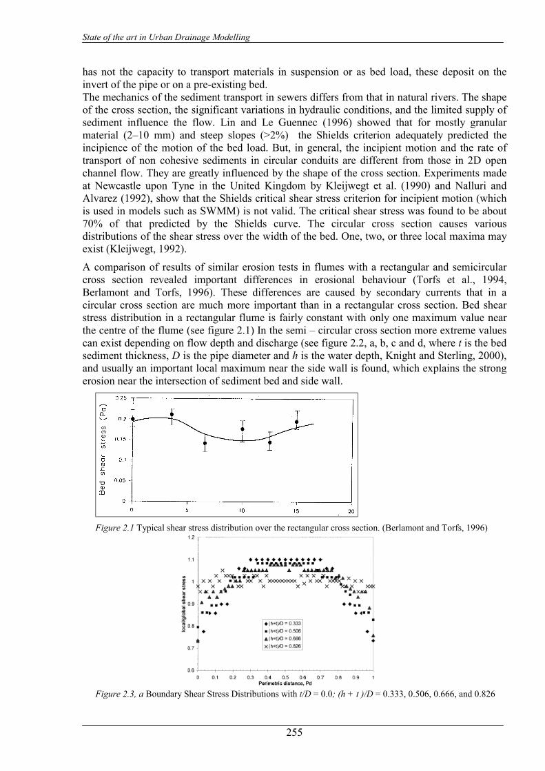
State of the art in Urban Drainage Modelling
255
has not the capacity to transport materials in suspension or as bed load, these deposit on the invert of the pipe or on a pre-existing bed. The mechanics of the sediment transport in sewers differs from that in natural rivers. The shape of the cross section, the significant variations in hydraulic conditions, and the limited supply of sediment influence the flow. Lin and Le Guennec (1996) showed that for mostly granular material (2–10 mm) and steep slopes (>2%) the Shields criterion adequately predicted the incipience of the motion of the bed load. But, in general, the incipient motion and the rate of transport of non cohesive sediments in circular conduits are different from those in 2D open channel flow. They are greatly influenced by the shape of the cross section. Experiments made at Newcastle upon Tyne in the United Kingdom by Kleijwegt et al. (1990) and Nalluri and Alvarez (1992), show that the Shields critical shear stress criterion for incipient motion (which is used in models such as SWMM) is not valid. The critical shear stress was found to be about 70% of that predicted by the Shields curve. The circular cross section causes various distributions of the shear stress over the width of the bed. One, two, or three local maxima may exist (Kleijwegt, 1992).
A comparison of results of similar erosion tests in flumes with a rectangular and semicircular cross section revealed important differences in erosional behaviour (Torfs et al., 1994, Berlamont and Torfs, 1996). These differences are caused by secondary currents that in a circular cross section are much more important than in a rectangular cross section. Bed shear stress distribution in a rectangular flume is fairly constant with only one maximum value near the centre of the flume (see figure 2.1) In the semi – circular cross section more extreme values can exist depending on flow depth and discharge (see figure 2.2, a, b, c and d, where t is the bed sediment thickness, D is the pipe diameter and h is the water depth, Knight and Sterling, 2000), and usually an important local maximum near the side wall is found, which explains the strong erosion near the intersection of sediment bed and side wall.
Figure 2.1 Typical shear stress distribution over the rectangular cross section. (Berlamont and Torfs, 1996)
Figure 2.3, a Boundary Shear Stress Distributions with t/D = 0.0; (h + t )/D = 0.333, 0.506, 0.666, and 0.826

State of the art in Urban Drainage Modelling
256
Figure 2.3, b Boundary Shear Stress Distributions with t/D =0.25; (h + t )/D = 0.333, 0.499, 0.666
Figure 2.3, c Boundary Shear Stress Distributions with (h+ t)/D = 0.666; t/D = 0.25, 0.332, 0.504
Figure 2.3, d Boundary Shear Stress Distributions with t/D =0.25; (h + t )/D = 0.755 and 0.499, 0.795
Only limited experiments have been carried out on the movement of cohesive sediments in sewers. The few available results have shown that, once the threshold of movement is exceeded,

State of the art in Urban Drainage Modelling
257
the effect of cohesion is lost and particles are transported in a way similar to non cohesive materials.
Experimental research on the erosion of mixed sediments (Torfs, 1994; Williamson et al., 1995; Berlamont and Torfs, 1996) showed an increasing erosion resistance with increasing content of cohesive material (see figure 2.3). When the mixture contains only a small amount of cohesive material, the fines are washed out of the surface layer at very low values of bed shear stress, lower than the critical shear stress needed to move the sand particles (point 1). Adding more cohesive material , the fines fill the pore spaces in between sand grains and make the mixture smoother and thus more difficult to erode (point 2). At some spots in the mixture the cohesive particles create bridges connecting sand grains (point 3). With increasing percentage of fines, these bridges change in strong bonds and eventually a cohesive network is formed in the sediment bed.
Figure 2.3 Erosion resistance of partly cohesive sediments as a function of mixture composition expressed as content of fines (Berlamont and Torfs, 1996) The following modes of transport can be observed if flow velocity and turbulence level are increased in a sewer with a preexisting bed of sediments:
• Transport over a deposited bed: initially sediment will move over a stationary bed on the pipe invert. As flow velocity increases, the surface of the bed may become rippled or duned. At higher velocities the surface may return plain, or more probably the bed sediment will be replaced by a series of dunes moving slowly downstream, separated by sections of clear pipe.
• Bed load transport without deposited material (flume traction): particles moving along the pipe invert, saltating, in continuous rolling/sliding contact or intermittent bouncing contact.
• Suspended load: sediments are maintained in suspension by turbulence, but more concentrated towards the invert of the pipe.
• Wash load: all particles are transported within and are uniformly distributed throughout the cross section and are unlikely to settle out.
In the following sections, transport theories based on limit of deposition and transport over deposited bed will be reviewed, as well as suspended transport load theory. The last section is dedicated to the effect of solid transport on the value of friction factor, even though this aspect presents till now much uncertainty.
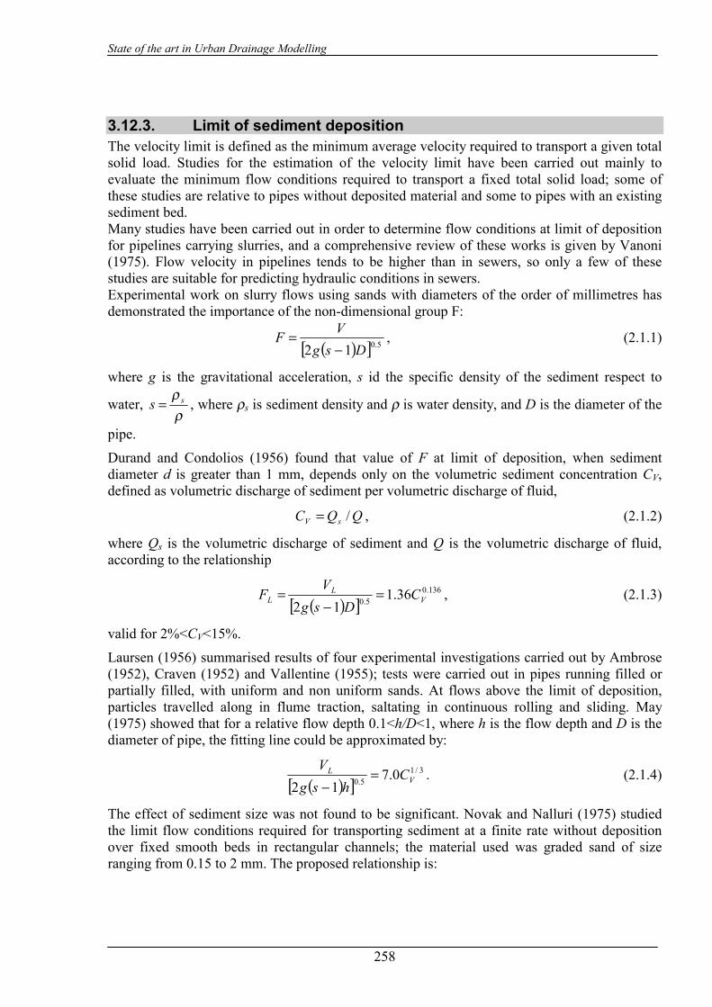
State of the art in Urban Drainage Modelling
258
3.12.3. Limit of sediment deposition The velocity limit is defined as the minimum average velocity required to transport a given total solid load. Studies for the estimation of the velocity limit have been carried out mainly to evaluate the minimum flow conditions required to transport a fixed total solid load; some of these studies are relative to pipes without deposited material and some to pipes with an existing sediment bed. Many studies have been carried out in order to determine flow conditions at limit of deposition for pipelines carrying slurries, and a comprehensive review of these works is given by Vanoni (1975). Flow velocity in pipelines tends to be higher than in sewers, so only a few of these studies are suitable for predicting hydraulic conditions in sewers. Experimental work on slurry flows using sands with diameters of the order of millimetres has demonstrated the importance of the non-dimensional group F:
( )[ ] 5.012 DsgVF−
= , (2.1.1)
where g is the gravitational acceleration, s id the specific density of the sediment respect to
water, ρρ ss = , where ρs is sediment density and ρ is water density, and D is the diameter of the
pipe.
Durand and Condolios (1956) found that value of F at limit of deposition, when sediment diameter d is greater than 1 mm, depends only on the volumetric sediment concentration CV, defined as volumetric discharge of sediment per volumetric discharge of fluid,
QQC sV /= , (2.1.2)
where Qs is the volumetric discharge of sediment and Q is the volumetric discharge of fluid, according to the relationship
( )[ ]136.0
5.0 36.112 VL
L CDsg
VF =
−= , (2.1.3)
valid for 2%<CV<15%.
Laursen (1956) summarised results of four experimental investigations carried out by Ambrose (1952), Craven (1952) and Vallentine (1955); tests were carried out in pipes running filled or partially filled, with uniform and non uniform sands. At flows above the limit of deposition, particles travelled along in flume traction, saltating in continuous rolling and sliding. May (1975) showed that for a relative flow depth 0.1<h/D<1, where h is the flow depth and D is the diameter of pipe, the fitting line could be approximated by:
( )[ ]3/1
5.0 0.712 V
L Chsg
V=
−. (2.1.4)
The effect of sediment size was not found to be significant. Novak and Nalluri (1975) studied the limit flow conditions required for transporting sediment at a finite rate without deposition over fixed smooth beds in rectangular channels; the material used was graded sand of size ranging from 0.15 to 2 mm. The proposed relationship is:

State of the art in Urban Drainage Modelling
259
( )[ ]( ) 67.0333.0622.0
05.0 632.018
RdCRsg
VV
L −=−
λ , (2.1.5)
where d is the sediment size, R is the hydraulic radius and λ0 is the Darcy – Weisbach friction factor.
Mayerle, Nalluri and Novak (1991) carried out experiments in which uniform flow conditions were established in the flume prior to sediment being injected. The sediment rate was increased up to the point where deposition started to occur. A constant rate of sediment fed just under this limiting condition was then maintained for a time sufficient for a constant rate of transport to be established over the entire length of the flume. Experiments were repeated for different conditions using two different flumes, a rectangular channel and a circular cross section channel. The limit velocity resulted to be function of sediment size, density, concentration and roughness, according to the relationships:
• Rectangular (smooth and rough walls)
( )( ) 430110150455
1..
r,g.
VL RdDC.sgd
V −−=−
, (2.1.6)
• Circular (smooth walls)
( )
( ) 68.023.032.41
−=−
RdCsgd
VV
L , (2.1.7)
where R is the hydraulic radius of the cross section and Dg,r is the dimensionless grain size, defined as
d)s(gD/
r,g
31
2
1
−=
ν, (2.1.8)
where ν is the kinematic viscosity of water. Observe that in the above equations VL is independent from the friction factor.
An alternative equation that takes into account friction factor and is applicable to both smooth and rough pipes is:
( )( ) 4321
1xs
xb
xV
xgr
L RdCXDsgd
V λ=−
, (2.1.9)
where λs is the value of the friction factor in presence of sediment transport. Parameters X, x1, x2, x3 and x4 are listed in table 2.1.1
table 2.1.1
Type of channel X x1 x2 x3 x4
Rectangular 11.5
9
-0.14 0.15 -0.43 0.18
Circular 14.4
3
-0.14 0.18 -0.56 0.18

State of the art in Urban Drainage Modelling
260
The friction factor λs accounts for the increase in resistance due to the presence of sediments and can be estimated from the Coolebrok – White equation using an equivalent roughness ks given by:
21 yV
yr,g
s CYDR
kk =− , (2.1.10)
where k is the Nikuradse roughness height and parameters Y, y1 and y2 are listed in table 2.1.2
table 2.1.2
Type of channel Y y1 y2
Rectangular 0.024
5
0.4 0.44
Circular 0.013
0.00
0.24 0.40
May (1993) proposed the following relationship:
( )[ ]( )( )
3 23602
2318/
g.
/V
L DyADsgfDCV
λΩ−
= , (2.1.11)
where A is the cross sectional area and f is a coefficient equal to 1 in smooth pipes and to 1.2 in rough pipes. The coefficient f accounts for the friction between the moving sediments and the pipe walls. Ω is a non dimensional factor depending on the particle mobility Gs, defined as:
50
50
220
18
.
Lg.
s d)s(gfV
DhG
−
=
λ, (2.1.12)
where d50 is the particle size which is larger than 50 % of the mass of all the particles in a graded sample and λg is the value of friction factor corresponding to grain shear stress, calculated from Colebrook – White resistance equation, that is:
+−=
gg VR.
Rdlog
λν
λ6270
1221 50
10 , (2.1.13)
The proposed relation between Ω and Gs is
• 015.0 =≤ ΩGs • 241258550150 .G. Ω .G. ss −=≤< • 32.278.19.055.0 +=≤< ss G ΩG
May (1994) modified May’s (1993) equation for CV and Vt (see also CIRIA, 1996), in the case of both rough and smooth pipes and for graded sediments. Modified equations are given below:
( )( )( ) ( ) ( )( ) 23246050
22 1110033 /LLt
.V sgDVVVDdAD.C −−⋅= − , (2.1.14)

State of the art in Urban Drainage Modelling
261
47.0
5050)1(125.0
−=
dhdsgVt . (2.1.15)
Threshold velocity equation (2.1.15) is valid for both rough and smooth pipes.
Ab Ghani (1993) carried out bed load sediment transport tests with the limit of deposition criterion covering the ranges of 0.76 ppm < CV < 1450 ppm and 0.46 mm < d50 < 8.3 mm.
He proposed, for both smooth and rough pipe channels the following best fit equation:
210530
50
090210
50
0831
.c
..
r,g.
VL
dRDC.
d)s(gV −−
=
−λ , (2.1.16)
where λc is the composite friction factor taking into account the increase in resistance due to sediment, computed as:
0200109800131 .
V.r,g
.c CD. λλ = , (2.1.17)
where ν is the kinematic viscosity of water and λ0 is the clean pipe friction factor.
Macke (1982) developed a theory for the transport of suspended sediments in pipes based on the assumption that the energy expended in overcoming frictional resistance is converted to turbulent fluctuations in the flow which maintain particles in suspension. Experiments were carried out to evaluate the limit of deposition for fine and medium sands in pipe flowing full and partially filled. Data from this and several previous studies were used to relate the average shear stress τ0 at limit of deposition to the quantity:
5.1* )1( sss WsgQQ −= ρ , (2.1.18)
where Qs is the volumetric rate of sediment transport and Ws is the fall velocity of a single particle, computed as, (see CIRIA, 1996):
( )( )( )d..
d..sgdWs 074405011607010
30248003869011093
292
+−+−+
= −
νν, (2.1.19)
The equation, obtained for values of 4* 100.2 −⋅≥sQ , was: 30
410641 τ−⋅= .Q*s . (2.1.20)
In order to prevent deposition at rates of transport lower than 2.0 10-4, Macke recommended that τ0 should be ≥ 1 N/m2.
Macke’s equation can be expressed in the following form:
53
511430
c
.sV
LAW)s(.C
Vλ
−= . (2.1.21)
If sediments are fed with higher rate, small deposits on the invert of the pipe begin to form. Separated groups of sediments move downstream and constitute the so-called separated dunes. May (1982) presented photographs of separated dunes and described the pattern of movement of the particles in a very detailed and precise way.
May (1982) conducted tests on limit of deposition criterion at Hydraulic Research Ltd. (HR) Wallingford (UK), using two smooth pipes (77 and 158 mm diameter) running full filled and partially filled. He used three sediment sizes, 0.6 mm, 5.8 mm and 7.9 mm, with volumetric

State of the art in Urban Drainage Modelling
262
sediment concentrations between 120 and 2110 ppm. He suggested the best fit equation for limit of deposition as:
( )( )( ) ( ) ( )( ) 23246022 1110052 /LLt
.V sgDVVVRdAD.C −−⋅= − , (2.1.22)
where Vt is the threshold velocity for sediment movement given by:
• smooth pipes (Novak and Nalluri (1975)) ( )( ) ( ) 27.05.0
, 161.0 −−== RddsgVV stt , (2.1.23 a)
• rough pipes (Novak and Nalluri (1975)) ( )( )404311 .
s,tt k/d.VV −+= , (2.1.23 b)
where Vt, is the threshold velocity in rough pipes and Vt,s the one in smooth pipes.
The structure of equation (2.1.22) allows for the introduction of a threshold velocity that is a lower limit for the existence of a non-zero transport rate, that simple equations of the type
LV VC ∝ are not able to estimate.
May et al. (1989) carried out experiments at HR Wallingford (UK) in non-uniform bed load and flow conditions. They tested the transport of separated dunes in a 300 mm diameter spun concrete pipe with a mean sediment size of 0.72 mm. Tests with separated dunes were in the range of Ys/D up to 5%, where Ys is the equivalent sediment bed thickness when the separated dunes are spread uniformly along the pipe channel bed.
The sediment transport by means of the dune movement implies a larger overall hydraulic resistance, that was observed for deposits that exceeded the thickness of 3% of pipe diameter. Moreover, the bed load versus velocity relationship was found to be strongly dependent on the Ys/D and VL values. The following relationship was proposed by May et al. (1989):
( )
2324602360
11
100
/
L
L
t..
v DsgV
VV
Rd
AD
dhNC
−
−
= , (2.1.24)
where for smooth pipes
( )( ) ( ) 230501610 ..t RdRsg.V −−= . (2.1.25)
For rough pipes, threshold velocity was found 4/3 times higher than in smooth pipes.
Values of the factor N changing from 2.11 to 14.8 have been experimentally observed, but a fit equation has not been proposed by the authors.
Nalluri, Ab Ghani and El – Zaemy (1994) stated that the most of the recent works (Novak and Nalluri, 1975, May, 1982, Mayerle et al., 1991) incorporating sediment transport theories may have been inappropriate for sewers as they did not take into account of the presence of pre-existing in-pipe deposits, for example sediment bed. Nalluri et al.(1992) investigated the effects of bed thickness.
Starting from the work of Alvarez (1992) carried out over rigid beds at Newcastle University and on new experimental data of Nalluri et al. (1994), they derived a new equation accounting for the effective width We over which sediment transport occurs. The Authors used a 12 m length and 305 mm diameter circular pipe with flat fixed bed; bed thickness was varied, form 47 mm to 120 mm; sediment size ranged from d50 = 0.53 mm to d50 = 1 mm. The proposed fit equation is:
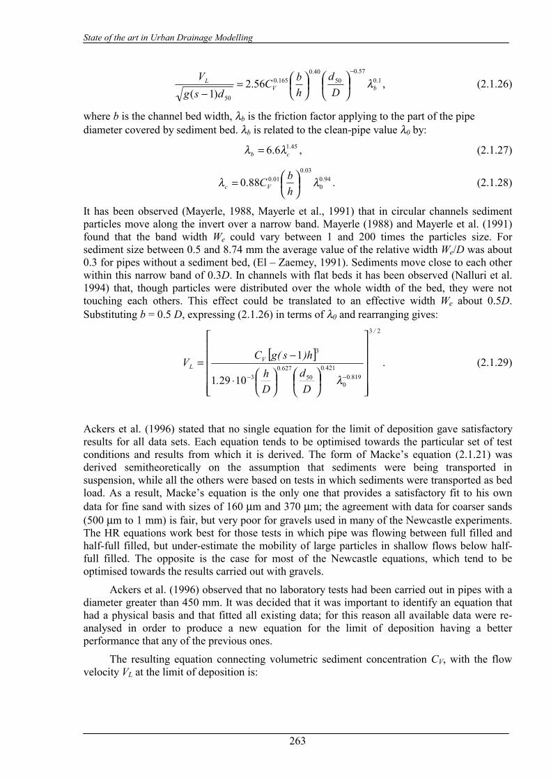
State of the art in Urban Drainage Modelling
263
1.057.0
5040.0
165.0
50
56.2)1( bV
L
Dd
hbC
dsgV
λ−
=
−, (2.1.26)
where b is the channel bed width, λb is the friction factor applying to the part of the pipe diameter covered by sediment bed. λb is related to the clean-pipe value λ0 by:
45.16.6 cb λλ = , (2.1.27)
94.00
03.001.088.0 λλ
=
hbCVc . (2.1.28)
It has been observed (Mayerle, 1988, Mayerle et al., 1991) that in circular channels sediment particles move along the invert over a narrow band. Mayerle (1988) and Mayerle et al. (1991) found that the band width We could vary between 1 and 200 times the particles size. For sediment size between 0.5 and 8.74 mm the average value of the relative width We/D was about 0.3 for pipes without a sediment bed, (El – Zaemey, 1991). Sediments move close to each other within this narrow band of 0.3D. In channels with flat beds it has been observed (Nalluri et al. 1994) that, though particles were distributed over the whole width of the bed, they were not touching each others. This effect could be translated to an effective width We about 0.5D. Substituting b = 0.5 D, expressing (2.1.26) in terms of λ0 and rearranging gives:
[ ]
23
81900
421050
62703
3
10291
1
/
...
VL
Dd
Dh.
h)s(gCV
⋅
−=
−− λ. (2.1.29)
Ackers et al. (1996) stated that no single equation for the limit of deposition gave satisfactory results for all data sets. Each equation tends to be optimised towards the particular set of test conditions and results from which it is derived. The form of Macke’s equation (2.1.21) was derived semitheoretically on the assumption that sediments were being transported in suspension, while all the others were based on tests in which sediments were transported as bed load. As a result, Macke’s equation is the only one that provides a satisfactory fit to his own data for fine sand with sizes of 160 µm and 370 µm; the agreement with data for coarser sands (500 µm to 1 mm) is fair, but very poor for gravels used in many of the Newcastle experiments. The HR equations work best for those tests in which pipe was flowing between full filled and half-full filled, but under-estimate the mobility of large particles in shallow flows below half-full filled. The opposite is the case for most of the Newcastle equations, which tend to be optimised towards the results carried out with gravels.
Ackers et al. (1996) observed that no laboratory tests had been carried out in pipes with a diameter greater than 450 mm. It was decided that it was important to identify an equation that had a physical basis and that fitted all existing data; for this reason all available data were re-analysed in order to produce a new equation for the limit of deposition having a better performance that any of the previous ones.
The resulting equation connecting volumetric sediment concentration CV, with the flow velocity VL at the limit of deposition is:
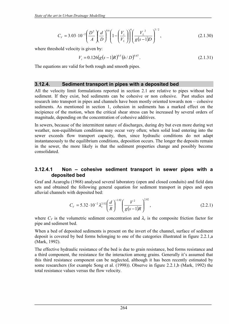
State of the art in Urban Drainage Modelling
264
( )
23246022
1110033
/
L
L
t.
V DsgV
VV
Dd
AD.C
−
−
⋅= − , (2.1.30)
where threshold velocity is given by:
( )( ) ( ) 47.05.0 /1126.0 DhRsgVt −= . (2.1.31)
The equations are valid for both rough and smooth pipes.
3.12.4. Sediment transport in pipes with a deposited bed All the velocity limit formulations reported in section 2.1 are relative to pipes without bed sediment. If they exist, bed sediments can be cohesive or non cohesive. Past studies and research into transport in pipes and channels have been mostly oriented towards non – cohesive sediments. As mentioned in section 1, cohesion in sediments has a marked effect on the incipience of the motion, when the critical shear stress can be increased by several orders of magnitude, depending on the concentration of cohesive additives.
In sewers, because of the intermittent nature of discharges, during dry but even more during wet weather, non-equilibrium conditions may occur very often; when solid load entering into the sewer exceeds flow transport capacity, then, since hydraulic conditions do not adapt instantaneously to the equilibrium conditions, deposition occurs. The longer the deposits remain in the sewer, the more likely is that the sediment properties change and possibly become consolidated.
3.12.4.1 Non – cohesive sediment transport in sewer pipes with a deposited bed
Graf and Acaroglu (1968) analysed several laboratory (open and closed conduits) and field data sets and obtained the following general equation for sediment transport in pipes and open alluvial channels with deposited bed:
( )0222021
5222
110325
...
cV RsgV
Rd.C
−
⋅=
−− λ , (2.2.1)
where CV is the volumetric sediment concentration and λc is the composite friction factor for pipe and sediment bed.
When a bed of deposited sediments is present on the invert of the channel, surface of sediment deposit is covered by bed forms belonging to one of the categories illustrated in figure 2.2.1,a (Mark, 1992).
The effective hydraulic resistance of the bed is due to grain resistance, bed forms resistance and a third component, the resistance for the interaction among grains. Generally it’s assumed that this third resistance component can be neglected, although it has been recently estimated by some researchers (for example Song et al. (1998)). Observe in figure 2.2.1,b (Mark, 1992) the total resistance values versus the flow velocity.
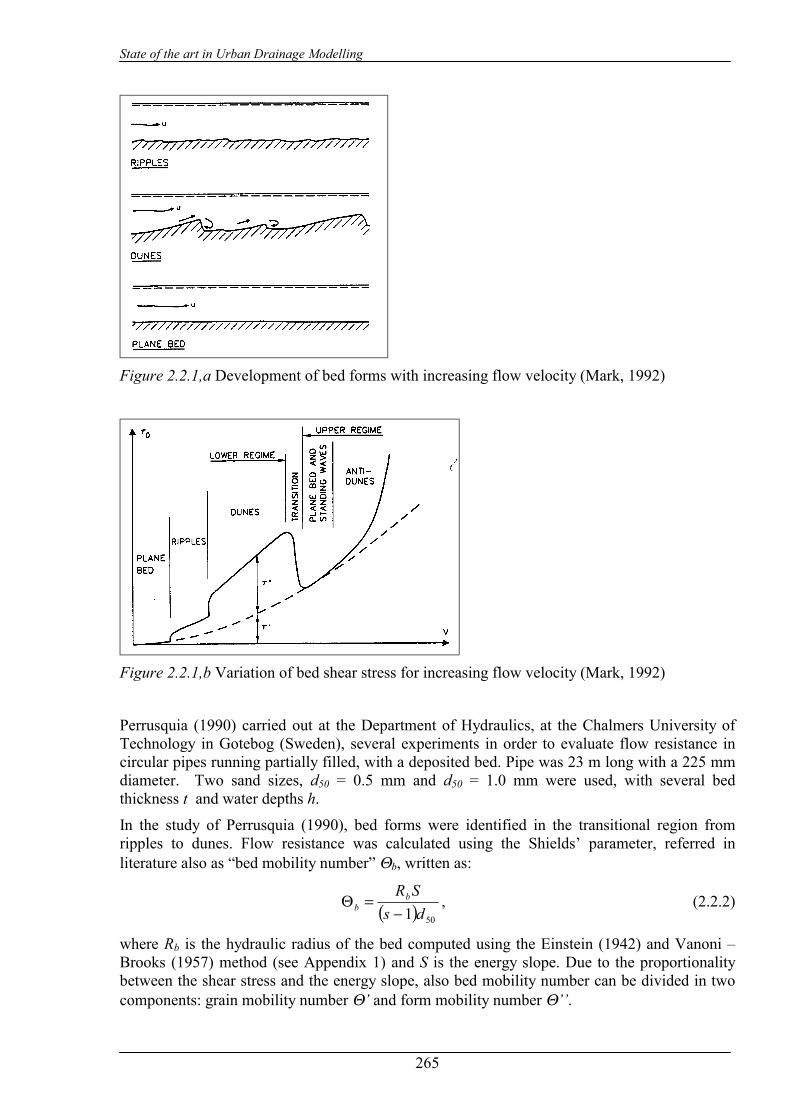
State of the art in Urban Drainage Modelling
265
Figure 2.2.1,a Development of bed forms with increasing flow velocity (Mark, 1992)
Figure 2.2.1,b Variation of bed shear stress for increasing flow velocity (Mark, 1992)
Perrusquia (1990) carried out at the Department of Hydraulics, at the Chalmers University of Technology in Gotebog (Sweden), several experiments in order to evaluate flow resistance in circular pipes running partially filled, with a deposited bed. Pipe was 23 m long with a 225 mm diameter. Two sand sizes, d50 = 0.5 mm and d50 = 1.0 mm were used, with several bed thickness t and water depths h.
In the study of Perrusquia (1990), bed forms were identified in the transitional region from ripples to dunes. Flow resistance was calculated using the Shields’ parameter, referred in literature also as “bed mobility number” Θb, written as:
( ) 501 dsSRb
b −=Θ , (2.2.2)
where Rb is the hydraulic radius of the bed computed using the Einstein (1942) and Vanoni – Brooks (1957) method (see Appendix 1) and S is the energy slope. Due to the proportionality between the shear stress and the energy slope, also bed mobility number can be divided in two components: grain mobility number Θ’ and form mobility number Θ’’.
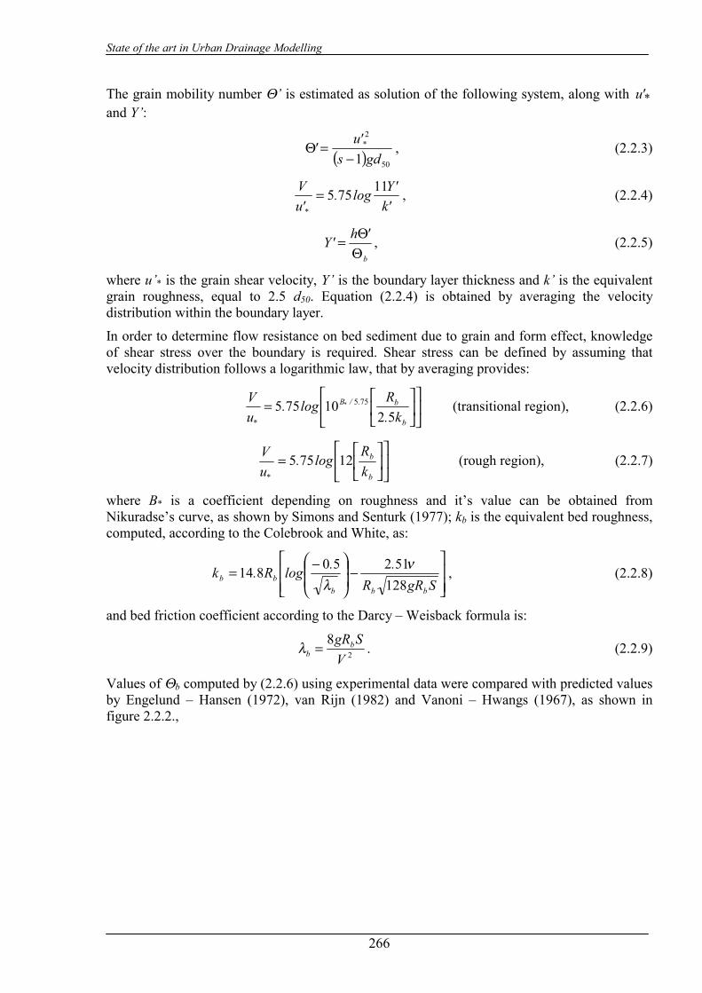
State of the art in Urban Drainage Modelling
266
The grain mobility number Θ’ is estimated as solution of the following system, along with *'u and Y’:
( ) 50
2
1 gds'u' *
−=Θ , (2.2.3)
'k'Ylog.
'uV
*
11755= , (2.2.4)
b
'h'YΘΘ= , (2.2.5)
where u’* is the grain shear velocity, Y’ is the boundary layer thickness and k’ is the equivalent grain roughness, equal to 2.5 d50. Equation (2.2.4) is obtained by averaging the velocity distribution within the boundary layer.
In order to determine flow resistance on bed sediment due to grain and form effect, knowledge of shear stress over the boundary is required. Shear stress can be defined by assuming that velocity distribution follows a logarithmic law, that by averaging provides:
=
b
b./B
* k.Rlog.
uV
*
5210755 755 (transitional region), (2.2.6)
=
b
b
* kRlog.
uV 12755 (rough region), (2.2.7)
where B* is a coefficient depending on roughness and it’s value can be obtained from Nikuradse’s curve, as shown by Simons and Senturk (1977); kb is the equivalent bed roughness, computed, according to the Colebrook and White, as:
−
−=SgRR
..logR.kbbb
bb 12851250814 ν
λ, (2.2.8)
and bed friction coefficient according to the Darcy – Weisback formula is:
2
8V
SgRbb =λ . (2.2.9)
Values of Θb computed by (2.2.6) using experimental data were compared with predicted values by Engelund – Hansen (1972), van Rijn (1982) and Vanoni – Hwangs (1967), as shown in figure 2.2.2.,

State of the art in Urban Drainage Modelling
267
Figure 2.2.2 Predicted and calculated Θb (Perrusquia, 1990)
Perrusquia (1990, 1992 and 1993) proposed an experimental relationship between total flow resistance and grain resistance. The dimensionless ratio Θb/Θc is plotted in figure 2.2.3 against the Θ’b/Θc ratio, where Θc is the critical mobility number corresponding to the condition of incipient motion and obtained from Shields’ diagram.
Figure 2.2.3 Grain mobility as function of bed mobility (Perrusquia, 1993)
Figure 2.2.3 shows the effect of bed forms on the total resistance, that can be obtained by subtracting the mobility ratio Θ’b/Θc from the total one. The best fit curve is:
ΘΘ
+=ΘΘ
c
b
c
b 'ln.. 58351 . (2.2.10)
Perrusquia (1992, 1993) extended his studies on flow conditions concerning stream traction in pipe channels running partially filled with a deposit of sediments to the evaluation of the corresponding bed load. Dimensional analysis was used to define non dimensional variables
State of the art in Urban Drainage Modelling
268
and the functional relationship governing stream traction in pipes. Characteristic parameters that define sediment transport are: flow depth h, energy gradient S, gravitational acceleration g, fluid density ρ, dynamic viscosity µ, sediment density ρs, sediment size d50, sediment thickness t, pipe diameter D and pipe roughness kw.
The dimensionless transport parameter Φb is defined as:
( ) 3501 dsg
qΦ b
b−
= , (2.2.11)
where qb is the sediment transport rate per unit. Φb is related through dimensional analysis to a set of dimensionless variables:
[ ]rrrbb kthZsDfΦ ,,,,,, *Θ= , (2.2.12)
where Z is the relative grain size d50/h, hr is the relative flow depth h/D, tr is the relative bed thickness t/D, kr is the relative pipe roughness, d50/kw. The other symbols have been already defined.
The influence that these dimensionless variables have on sediment transport was investigated using multiple regression analysis. The proposed equation which contains parameters that describe sediment transport has the form:
6207070219231046 .r
.r
..*
.bb thZD −−Θ⋅=Φ , (2.2.13)
the variables s and kr were found to have a negligible effect. Comparison between experimentally determined and analytically calculated transport parameters show good agreement and almost 90% of the predictions are within %50± deviation of the observed values.
The same Perrusquia (1993) carried out other experiments at the Department of River Engineering at Wallingford, UK, and at the Hydraulics Laboratory of the Department of Civil Engineering of the University of Newcastle, UK.
By using dimensionless analysis and modifying (2.2.16), sediment transport could be expressed as:
+Θ=Φ rr*bb k,
Dth,h,Z,s,D,f , (2.2.14)
where the relative total depth,D
th + , replaces relative bed thickness tr. This parameter was
introduced in the analysis to evaluate the possible influence of the shape of the hydraulic section.
Equations (2.2.12) and (2.2.14) were used to analyse the transport of sediment. Experimental data obtained at Wallingford were not used because equilibrium in the transport rate was not reached due to the short duration of the runs.
The proposed equation for the prediction of bed load transport was:
( )( ) 14140906231065 ...*
.bb th/hZD. −− +Θ⋅=Φ , (2.2.15)
Ackers (1984), based on the original Ackers and White (1973) sediment transport equation for alluvial channels, derived the following total load equations, changing some of the definitions of the parameters to adapt his equation to pipes.
State of the art in Urban Drainage Modelling
269
The rate of sediment movement is expressed in terms of a dimensionless transport parameter: n
*
n
e
Vr,g V
uRW
Ad
RCG
=
−1
50
, (2.2.16)
where We is the effective width of the bed and
r,gDlog..n 10560001 −= , (2.2.17)
where r,gD has been defined in (2.1.8). Gg,r depends on the mobility parameter, Fg,r, given by:
n
nn*
r,g
dRlog
VgsDuF −
−
= 1
5010
1
50 1232
. (2.2.18)
The transport and mobility parameters are related by the equation: m
gr
grr,gr,g A
)AF,max(HG
−=
0, (2.2.19)
where Agr is he value of the mobility parameter at the threshold of movement. Coefficients Agr , m and H are computed with the following equations:
r,g
gr D..A 230140 += , (2.2.20)
( ) 533862 2101010 .DlogDlog.Hlog r,gr,g −−= , (2.2.21)
r,gD..m 669341 += . (2.2.22)
For coarse sediments, when Dg,r > 60, n = 0.00, Agr = 0.17, m = 1.5 and H = 0.025.
Ackers (1991) produced a new version of the transport equations, where formulae are expressed in terms of the volumetric sediment concentration, as follows:
( )( )
−
−
=
εδγ
βα
λλRdK
RsgV
Rd
ARWJC c.ceV 501
. (2.2.23)
As in Ackers (1984), various coefficients depend on the dimensionless grain size; those which differ from the 1984 version are:
mgr
)n(m
/)m(n
A.HJ −
−
= 1
21
3118 , (2.2.24)
r,gD..m 836671 += , (2.2.25)
( ) 463980792 2101010 .Dlog.Dlog.Hlog r,gr,g −−= , (2.2.26)
n−= 1α , (2.2.27)

State of the art in Urban Drainage Modelling
270
10410 nmm −−=β , (2.2.28)
2)1( −= mnγ , (2.2.29)
gr/n)n( Ag.K 21311 −= , (2.2.30)
2/n−=δ , (2.2.31)
104 n+=ε . (2.2.32)
For coarse sediments, values of n, Agr and H remain the same as in Ackers (1984) and m is modified to 1.8.
May (1993) carried out experiments where the suspended load was totally missing. May’s calculations have been carried out in two stages. First the roughness of the sediment bed is determined and used to find the overall hydraulic resistance of the pipe. The known flow conditions are then used to calculate the rate of sediment transport.
Resistance of the bed depends on two factors: the first one is the grain mobility:
( ) 50
2
18 dsgV
F gg −
=λ
, (2.2.33)
where λg is the friction factor corresponding to the grain shear stress and is calculated from the Colebrook and White resistance equation, in the form:
+−=
gg VR.
Rdlog
λν
λ62750
1221 50 . (2.2.34)
The second one is the Froude number of the flow:
gABVFr
2
= , (2.2.35)
where A is the cross section area and B is surface width of the flow.
The friction factor for the bed, λb (grain resistance plus bed form resistance), is determined from the value of the mobility parameter Fb:
50
2
18 d)s(gV
F bb −
=λ
. (2.2.36)
Mobility parameter is selected from a table listing limits of Fg and Fr and the corresponding values for Fb (CIRIA, 1996).
The first step in determining the sediment transport is to calculate the particle Reynolds number given by:
=
νλ 50
50
8VD
R.
cc* , (2.2.37)
where the composite roughness λc of the pipe is defined as:

State of the art in Urban Drainage Modelling
271
b
bbc WP
WP++
=0
00 λλλ , (2.2.38)
where P0 is the wetted perimeter of pipe wall, Wb is the width of sediment bed and λ0 is the clean pipe friction factor obtained from the Colebrook and White equation.
The second step is to calculate the effective mobility of the sediment particles, defined as:
θgs FF = , (2.2.39)
where the friction factor θ is defined as:
11
512
512
+−= ./R
./R
c*
c*
eeθ . (2.2.40)
The volumetric sediment concentration is finally given by:
( )
−
=
DsgV
AD
DW
C gbV 18
22 θλη . (2.2.41 )
The value of the transport parameter η depends on Fs and it is obtained by selecting the appropriate equation from the following table:
( )( )
9506504060225013220402250
1061225010010
. .F...F.. .F.
.F. .F. .F
s
ss
ss
s
=≤<−+=≤<
−=≤<=≤
ηηη
η
The upper limit of Fs is based on the experimental range studied by May (1993).
Ackers (1993) observed that the sediment transport takes place only on a limited part We of the real bed width Wb. He suggested the use of the following linear variation of We:
bs
e W.Dy
..W
−+= 01033320 for 00.101.0 ≤≤
Dys , (2.2.42)
where ys is the depth of the sediment bed.
Many field and laboratory studies with fluvial sediments have shown that with non-uniform fluvial deposits the critical shear stress required to instigate motion of a grain of a given size is modified from that required for the same grain size in a uniform deposit (e.g. Wilcock and Southard, 1988). These studies have shown that finer particles in a mixture show greater resistance to motion and have a higher critical shear stress and coarser particles show less resistance to motion and have a lower critical shear stress than they would in a sediment bed composed of uniformly-sized particles. This results in a modification in the amount of bed load transport under given hydraulic conditions relatively to what would be expected from a uniform deposit.
During field work at the National CSO Test Facility at Wigan (UK) and experimental work carried out at University of Ghent (Belgium), Rushforth et al. (2002) and De Sutter et al. (2003) measured bed load transport rates from real sewer sediments; these measured rates were compared with those predicted by both the Ackers’ and May’s equations as used in CIRIA

State of the art in Urban Drainage Modelling
272
methodology (CIRIA, 1996). Sediment type found in the sewer at Wigan presented characteristics of type A (see section 1). Sediment used at Ghent were collected from a single sewer channel located in the experimental catchment “Le Marais” in Paris. Also in this case sediment presented type A characteristics, even though with a granulometric distribution smaller than that one found at Wigan (De Sutter et al., 2003). The findings were that the measured sediment transport rates were significantly greater than those predicted by these equations. In figures 2.2.4 and 2.2.5 are shown comparisons between Ghent and Wigan measured data and those ones predicted according to May’s equation. They define a performance index as the percentage of data within the discrepancy range 0.5<r<2, where r is the ratio between bed load computed and bed load measured and the prediction rate as the mean ratio between predicted and observed bed load transport rate. The performance index in the previous experiments was 70%; the other 30% are mainly very low transport rates where the formula of May predicts no transport, but low transport rates existed. In comparison with Ackers (1991) it demonstrated significantly better performance. When using data collected from the coarser bed at Wigan, May’s relation under-predicts transport to a much greater extent. In these tests the prediction ratio is 0.063 and the performance index is 0%.
In figures 2.2.6 and 2.2.7 the same comparisons are shown for Ackers’ formula. The Ghent data indicated that by using a value for d50 equal to 0.45 mm, obtained from the grain size distribution data of the deposit, this relationship significantly over-predicted transport rate. By adjusting the value of the representative grain size used in the predictive equation, the prediction ratio can be improved. The best prediction ratio, equal to 1.01, was obtained using a representative grain size equal to d65, corresponding to 0.91 mm. The performance index drops, however, to 38% because the very low transport rates are now significantly under-predicted. Also in this case, for the coarser materials found at Wigan, performance of the predictive method was still poor.
Figure 2.2.4 Comparison of predicted bedload transport rates (May, 1993) with experimental data from Ghent (De Sutter et al., 2003).
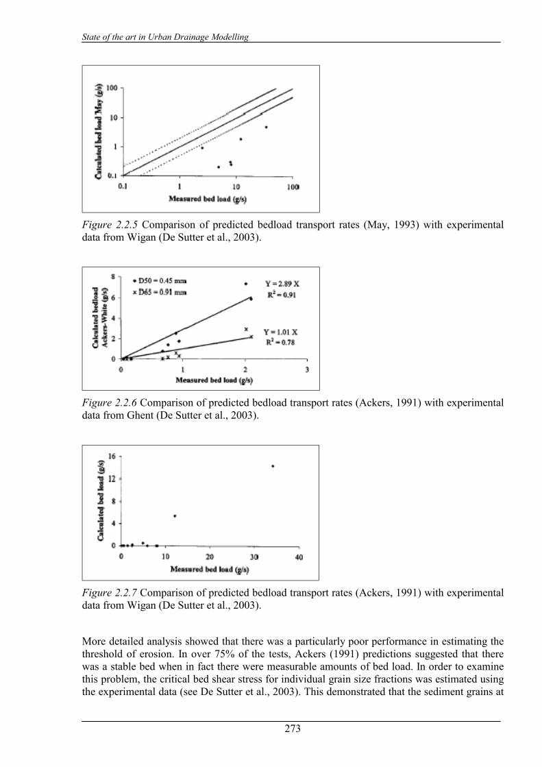
State of the art in Urban Drainage Modelling
273
Figure 2.2.5 Comparison of predicted bedload transport rates (May, 1993) with experimental data from Wigan (De Sutter et al., 2003).
Figure 2.2.6 Comparison of predicted bedload transport rates (Ackers, 1991) with experimental data from Ghent (De Sutter et al., 2003).
Figure 2.2.7 Comparison of predicted bedload transport rates (Ackers, 1991) with experimental data from Wigan (De Sutter et al., 2003).
More detailed analysis showed that there was a particularly poor performance in estimating the threshold of erosion. In over 75% of the tests, Ackers (1991) predictions suggested that there was a stable bed when in fact there were measurable amounts of bed load. In order to examine this problem, the critical bed shear stress for individual grain size fractions was estimated using the experimental data (see De Sutter et al., 2003). This demonstrated that the sediment grains at

State of the art in Urban Drainage Modelling
274
the finer end of the size range have values of threshold shear stress significantly higher than would be expected for a homogeneous sediment deposit; the coarser grain fractions, on the opposite, had values slightly below those expected for uniform sediments. These observations suggested that the most appropriate way to improve predictive performance of the Ackers (1991) relationship would be to derive a new relationship to estimate the parameter Agr, whose value is used to estimate the threshold of motion. This approach is not totally novel as it follows the work of White and Day (1982) who derived an adjustment function for the Agr value used by the original Ackers and White (1973) relationship, based on data collected in a wide rectangular laboratory containing fine river gravels.
The value of the modified threshold mobility parameter, A’gr, was obtained by comparing the measured fractional transport rates with those predicted by Ackers (1991). This process was carried out on approximately half the data set collected at Wigan and the resulting adjustment function is shown in figure 2.2.8: the ratio A’gr/Agr is plotted against di/d50, where di is the mean grain size within a particular grain size fraction and d50 is the average grain size for the in-pipe deposit grain size distribution. An adjustment for Agr has been derived, as shown in equation (2.2.43):
170
50
930.
i
gr
gr
dd.
A'A −
= , (2.2.43)
where DA was given as a function of the ratio D84/D16 (White and Day, 1982).
The improvement in the prediction performance of the remaining half data sets is clearly seen in figure 2.2.9.
The adjustment suggested by the data collected using the sewer sediments is different from the Agr adjustment suggested by White and Day (1982), shown in equation (2.2.44):
604050
.Dd
.A'A .
A
i
gr
gr +
=
−
. (2.2.44)
This indicates that the different flow conditions experienced in the narrow pipe cross-sections and the limited bed depths in comparison to a natural river affects the adjustment to the sediment threshold of motion differently. It can be seen that the in-pipe conditions result in beds weaker than would be expected in rivers, even if the deposit grain size distributions were similar. It should also be realised that the adjustment function developed from the work at Wigan is based on data from a rather narrow range of grain size distributions whereas the relationship derived by White and Day is based on tests using a number of mixed grain size distributions. It would be therefore important to validate equation (2.2.43) with a larger number of data sets, but data sets of mixed grain size sediment transport collected in pipes are unfortunately rare.
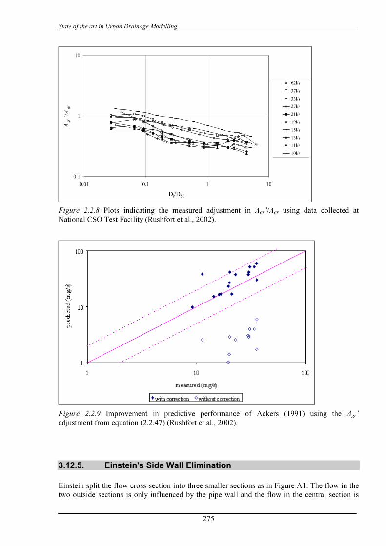
State of the art in Urban Drainage Modelling
275
0.1
1
10
0.01 0.1 1 10
Di/D50
Agr
'/A
gr
62l/s37l/s33l/s27l/s21l/s19l/s15l/s13l/s11l/s10l/s
Figure 2.2.8 Plots indicating the measured adjustment in Agr’/Agr using data collected at National CSO Test Facility (Rushfort et al., 2002).
Figure 2.2.9 Improvement in predictive performance of Ackers (1991) using the Agr’ adjustment from equation (2.2.47) (Rushfort et al., 2002).
3.12.5. Einstein's Side Wall Elimination
Einstein split the flow cross-section into three smaller sections as in Figure A1. The flow in the two outside sections is only influenced by the pipe wall and the flow in the central section is

State of the art in Urban Drainage Modelling
276
only influenced by the sediment bed. The method of partitioning the mean boundary shear stress is based on the following assumptions:
1) The energy slope is the same in all sections. 2) The mean velocity is the same in each section. 3) There is zero shear stress along the surfaces that separate the flow sections.
Pw/2 Pw/2
PB
Aw/2 Aw/2Ab
Figure A1 Flow sections for partitioning of shear stress.
Referring to Figure A1, where A is the flow cross-sectional area, P is the wetted perimeter and R is the hydraulic radius, with the subscripts w and b referring to the wall and bed flow sections respectively,
bw AAA =− (A.1)
wwww
ww PRA
PA
R =⇒= (A.2)
bbbb
bb PRA
PA
R =⇒= (A.3)
Substituting (A.2) and (A.3) into (A.1) and rearranging,
b
wwb P
PRAR
−= (A.4)
Considering Manning’s equation for the wall sections only,
w
ew
nSRV
21
32
= (A.5)
where V is the average flow velocity and Se is the slope of the energy line. Rearranging (A.5),
23
21
=
e
ww
S
VnR (A.6)
Substituting (A.6) into (A.4),

State of the art in Urban Drainage Modelling
277
b
e
ww
b P
S
VnPA
R
−
=
23
21
(A.7)
The value of Rb is entered into the following equation to find the bed shear stress, SgRbb ρτ = (A.8)
where τb is the bed shear stress and S is the bed slope, which for uniform flow is equal to the slope of the energy line.
3.12.6. Vanoni-Brooks Method The Vanoni-Brooks method is based on the following assumptions:
1. The flow cross-section can be divided as in Figure A1 and that the two areas act as independent flow channels.
2. The wetted perimeter of each section has a constant roughness, although the wall and bed roughness are different.
3. The mean flow velocities in each section are equal. These assumptions are similar to those for Einstein’s method. The estimation of λw is crucial to the solution. As hydraulically smooth walls are assumed, λw is only a function of the wall Reynolds number, Rew. According to Nikuradse,
( ) 23704221000320 .w
w Re.. +=λ (A.9)
As the mean velocities in all sections are the same
RRe
RRe
w
w = (A.10)
From the definition of friction factor
b
b
w
w RRRλλλ
== (A.11)
Combining (A.10) and (A.11)
b
b
w
w ReReReλλλ
== (A.12)
Rearranging (A.9)
237023702371 159000320 .
w
w
.w
.w
Re
..
=−
λ
λλ (A.13)
As λRe , and thus
w
wReλ
, is known, (A.13) can be used to calculate wλ by iteration. From
geometrical considerations wb AAA += (A.14)
Slight modification of the definition of friction factor gives
egSVPA
8
2λ= (A.15)
As Se, the slope of the energy line is the same for each section, (A.14) leads to
State of the art in Urban Drainage Modelling
278
wb
w
bb P
PPP λλλ −= (A.16)
Knowing λb, Rb can be calculated from (A.11). The bed shear stress is then given by (A.8) as in Einstein’s method.
3.12.7. Cohesive sediment transport in sewer pipes with a deposited bed In the past mechanisms of cohesive sediment movement in sewers have been assimilated to those studied for estuarine environments. Several researchers (Verbanck, 1995, Ristenpart, 1995) have assimilated the transport of material as bed load in rivers and estuaries to the transport in sewers. In estuarine conditions a gradual increase of the suspended sediment concentration of the fluid column towards the solid bed has a limit where a rapid gradient of concentration can be observed (Arthur and Ashley, 1998). This increase in sediment concentration forms a mud layer which can include a mobile part over a stationary part. At the base of stationary mud there may be another sharp increase in concentration (bulk density). There is no a direct evidence that sediment transported in sewers can be assimilated to a fluid mud (or dense undercurrent, as said by Verbanck, 1995). In addition, because muds are homogeneous, it is not clear whether these concepts are applicable to sewer sediments, that comprehend a variety of particle sizes and types and may be laid down in mixtures or stratified.
Bui (2000) has given a state of knowledge of cohesive sediment transport in natural streams. Sediment particles smaller than 20 µm are subject to the van der Waals attractive forces and the double layer repulsive forces. When brought together, the particles tend to position themselves at the minimum of the net interaction (Parker 1994). These electrochemical forces acting between the particles generate the cohesion that may exceed the hydrodynamic forces. The principal parameters governing the cohesion are particle size, type of clay, organic matter content; water content of sediment, salinity, temperature, and pH of the free and interstitial water (Hamm and Migniot 1994). Mehta (1994) recognized three modes of erosion or resuspension of mud in estuarine situations: surface erosion, mass erosion of the bed and entrainment of high concentration fluid mud suspension. For consolidated cohesive beds, the erosion rate E per unit bed surface is estimated in terms of the bed shear stress τb, the bed shear strength τs, assumed uniform with depth, and a constant M as:
s
sbMEτ
ττ −= . (2.2.45)
Mehta (1994) provides a graph showing the variation of M and τs with the bulk density. M can vary from 10-4 to 10-2 g cm-2 min-1, while τs can vary from 0 for organic rich floc to 10 N/m2 for hard soil.
The principal type of cohesive sediment is made of organic, mobile fine-grained material. Other types include inorganic, coarse granular material cemented with fats and tars, organic wall slimes and deposits found in tanks (Crabtree, 1988). Thus the cohesion in sewers arises from agglomeration due to tars, greases, chemical cementation and biological processes, rather than the electrostatic forces found in estuaries.
Nalluri and Alvarez (1992) carried out at the University of Newcastle upon Tyne, (UK), experiments in a circular cross section with a diameter equal to 154 mm and a bed thickness varying from 10.6 % to 39 % of the diameter.
They investigated erosion mechanisms, using first uniform non - cohesive sand with d50 = 0.12 – 4.1 mm, in order to have a basis for comparison for the cohesive sediments experiments. As
State of the art in Urban Drainage Modelling
279
mentioned above, they found that critical conditions for incipient motion occurred at lower values of mean shear stress than those of Shields’ for wide open channels.
A second series of experiment was carried out mixing cohesive additives (china clay, oil, petroleum jelly, …) to sand, in order to estimate the influence of cohesion on the erosion mechanisms.
The Authors found that: 1) critical shear stress for incipient motion was dramatically increased by several orders of magnitude, depending on the type of additive, as compared with non cohesive sediments; 2) the mode of erosion was completely different. Whereas a gradual entrainment process of sediment particles occurred in non cohesive sediment beds, a violent collapse of the entire bed structure took place in the cohesive sediment beds when the corresponding critical conditions were exceeded. It was observed that the cohesive bed was eroded in clusters of various sizes.
The Authors obtained the following Shields parameters, respectively for non cohesive and cohesive sediments:
( )62330
26761
506390
50
59781 .sb
.
b
.V
s
b
RdC.
gdλ
ρρτ
−
=
−, (2.2.46, a)
( )410
7650
504570
50
9640 .sb
.
b
.V
s
b
RdC.
gdλ
ρρτ
−
=
−. (2.2.46, b)
where τb = ρgRbS0 is the bed shear stress, Rb is the bed hydraulic radius, computed using Einstein and Vanoni – Brooks method, S0 is the bed slope and λsb is bed friction factor in presence of sediment transport. For a weak cohesive sewer sediment, they found that the maximum critical shear stress is approximately 2.5 N/m2 and for consolidated deposited sewer sediment it can be as high as 6.7 N/m2.
3.12.8. Suspended solid transport
3.12.8.1 Turbulent diffusion in particle-suspending flow Many studies on the suspended solid transport in sewers have been carried out assuming a 2D flow field on a vertical plane. They assume a mono-sized sediment particle which volumetric concentration is low enough to not affect velocity distribution and neglect interactions between particles. The relative tendency of turbulent flow to maintain particles in suspension is quantified according to Batchelor (1965) by a sedimentation parameter, η:
*
s
kuw
=η , (2.3.1)
where k is the von Karman constant ( )4.0≅ and ws is the settling velocity in calm water, computed by Stokes law.
Vertical turbulent flux of particles (per unit area) is described as '' cv (c’ is the deviation from average concentration C and v’ is the vertical velocity fluctuation), where the bar indicates the time averaging over the turbulence period. The classical assumption is that vertical upward flux

State of the art in Urban Drainage Modelling
280
of suspended particles induced by turbulence can be written as a gradient-law in analogy with diffusion processes, that is:
dydC'c'v sε−= , (2.3.2)
where y is the distance from the bed boundary. Equation (2.3.2) means that mass transport rate due to turbulent diffusion is proportional to the vertical gradient of concentration and it is acting in the direction of decreasing concentration. Coefficient εs is called eddy diffusivity for sediment (it is measured in squared meter per second), and is not a material constant of the fluid but depends on flow properties and varies accordingly with time and space.
Under equilibrium conditions, flux 'c'v must be compensated by the downward flux of heavy particles associated with the settling velocity, ws:
0=+dydCCw ss ε . (2.3.3)
Integration of equation (2.3.3) provides:
∫−=y
*a ss
*a
y dywCC
lnε
, (2.3.4)
where Cy is the suspended solids (SS) concentration at the generic water depth y, Ca* is the concentration at the reference level a*, usually taken as 5 % of full depth D. Vertical profile of SS concentration can be obtained from equation (2.3.4), if the variation of εs is predicted as function of flow variables, after reference concentration Ca*, is fixed.
The distribution of εs with depth is required to solve (2.3.4). Rouse (1937) assumed εs varying in the same way as Boussinesq eddy viscosity εm, namely:
ms βεε = , (2.3.5)
and the proportional coefficient, β, is assumed equal to 1. To simplify the problem of prediction of eddy viscosity εm, Rouse assumed that the vertical distribution of longitudinal velocity for the complete turbulent boundary layer could be described as a Prandtl – von Karman logarithmic profile:
kyu
dydu *= , (2.3.6)
where u is the longitudinal component of flow velocity.
Assuming a linear reduction of the acting shear stress with the distance from the boundary:
( )SyDgy −= ρτ , (2.3.7)
if the only component of this acting stress is the Reynolds stress of turbulence, τy can be expressed also as:
dyduvu my ρερτ =−= '' , (2.3.8)
using the Boussinesq’s εm eddy viscosity concept.
Combining equations (2.3.7) and (2.3.8) with the definition of shear velocity:
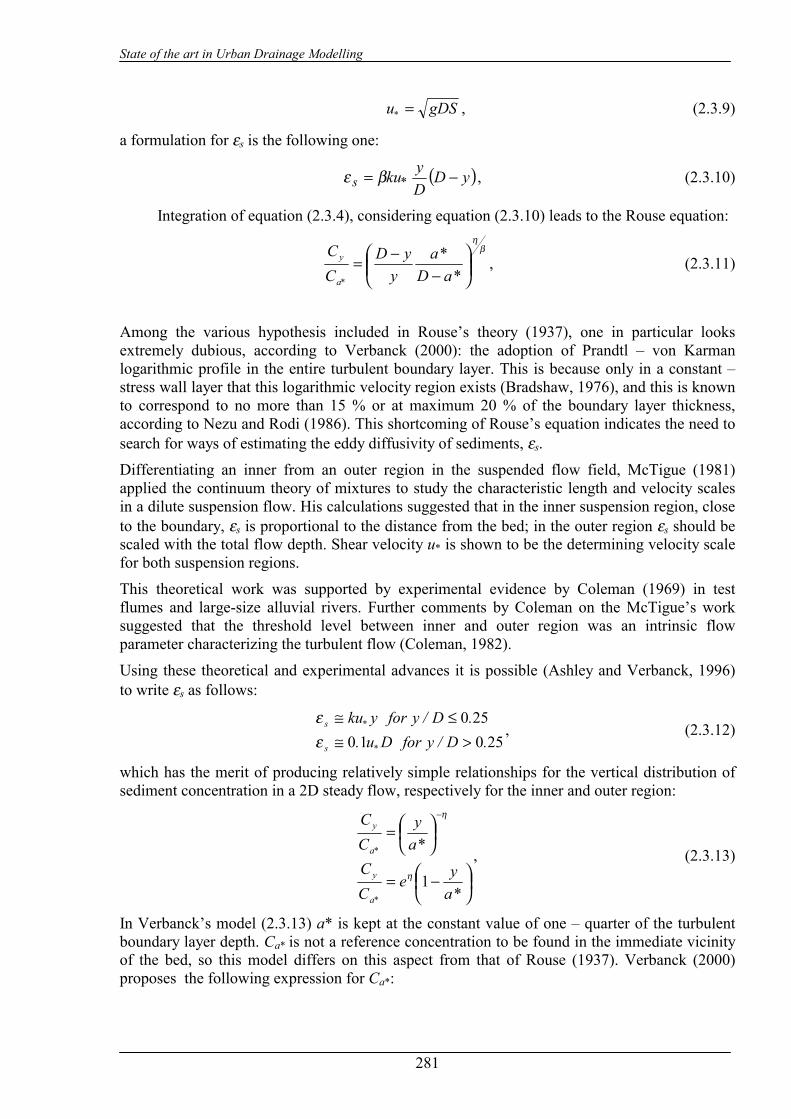
State of the art in Urban Drainage Modelling
281
gDSu* = , (2.3.9)
a formulation for εs is the following one:
( )yDDyku*s −= βε , (2.3.10)
Integration of equation (2.3.4), considering equation (2.3.10) leads to the Rouse equation:
βη
−
−=*aD
*ay
yDCC
*a
y , (2.3.11)
Among the various hypothesis included in Rouse’s theory (1937), one in particular looks extremely dubious, according to Verbanck (2000): the adoption of Prandtl – von Karman logarithmic profile in the entire turbulent boundary layer. This is because only in a constant – stress wall layer that this logarithmic velocity region exists (Bradshaw, 1976), and this is known to correspond to no more than 15 % or at maximum 20 % of the boundary layer thickness, according to Nezu and Rodi (1986). This shortcoming of Rouse’s equation indicates the need to search for ways of estimating the eddy diffusivity of sediments, εs.
Differentiating an inner from an outer region in the suspended flow field, McTigue (1981) applied the continuum theory of mixtures to study the characteristic length and velocity scales in a dilute suspension flow. His calculations suggested that in the inner suspension region, close to the boundary, εs is proportional to the distance from the bed; in the outer region εs should be scaled with the total flow depth. Shear velocity u* is shown to be the determining velocity scale for both suspension regions.
This theoretical work was supported by experimental evidence by Coleman (1969) in test flumes and large-size alluvial rivers. Further comments by Coleman on the McTigue’s work suggested that the threshold level between inner and outer region was an intrinsic flow parameter characterizing the turbulent flow (Coleman, 1982).
Using these theoretical and experimental advances it is possible (Ashley and Verbanck, 1996) to write εs as follows:
25010250
.D/y for Du..D/y for yku
*s
*s
>≅≤≅
εε
, (2.3.12)
which has the merit of producing relatively simple relationships for the vertical distribution of sediment concentration in a 2D steady flow, respectively for the inner and outer region:
−=
=
−
*aye
CC
*ay
CC
*a
y
*a
y
1η
η
, (2.3.13)
In Verbanck’s model (2.3.13) a* is kept at the constant value of one – quarter of the turbulent boundary layer depth. Ca* is not a reference concentration to be found in the immediate vicinity of the bed, so this model differs on this aspect from that of Rouse (1937). Verbanck (2000) proposes the following expression for Ca*:
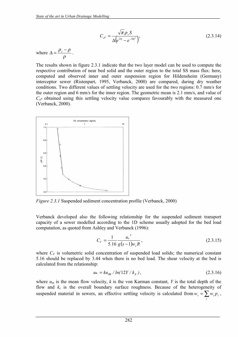
State of the art in Urban Drainage Modelling
282
( )242 ηη
ρπ−−∆
=eeS
C s*a , (2.3.14)
where ρ
ρρ −=∆ s .
The results shown in figure 2.3.1 indicate that the two layer model can be used to compute the respective contribution of near bed solid and the outer region to the total SS mass flux: here, computed and observed inner and outer suspension region for Hildensheim (Germany) interceptor sewer (Ristenpart, 1995, Verbanck, 2000) are compared, during dry weather conditions. Two different values of settling velocity are used for the two regions: 0.7 mm/s for the outer region and 6 mm/s for the inner region. The geometric mean is 2.1 mm/s, and value of Ca* obtained using this settling velocity value compares favourably with the measured one (Verbanck, 2000).
Figure 2.3.1 Suspended sediment concentration profile (Verbanck, 2000)
Verbanck developed also the following relationship for the suspended sediment transport capacity of a sewer modelled according to the 1D scheme usually adopted for the bed load computation, as quoted from Ashley and Verbanck (1996):
( ) Rwsgu
.C
s
*V 1165
1 3
−= , (2.3.15)
where CV is volumetric solid concentration of suspended load solids; the numerical constant 5.16 should be replaced by 3.44 when there is no bed load. The shear velocity at the bed is calculated from the relationship:
)k/Yln(/kuu sm* 12= , (2.3.16)
where um is the mean flow velocity, k is the von Karman constant, Y is the total depth of the flow and ks is the overall boundary surface roughness. Because of the heterogeneity of suspended material in sewers, an effective settling velocity is calculated from ∑=
iiis pww ,

State of the art in Urban Drainage Modelling
283
where wi and pi are the fall velocity and the ith proportion, by weight, of class size ith of the suspended material, respectively.
3.12.8.2 Flow field and coherent structure Turbulent components are always correlated with each other in both space and time. In such way, one can describe correlated fluid parcels (like vortices) by the appellation of “coherent”. Prior to the late 1950s, turbulent boundary layers were studied as if they were stochastic entities, consisting of rather randomized property fluctuations riding on an otherwise mean flow (Smith, 1996). It’s known that vortex deformation and evolution play a dominant role in creating and sustaining turbulence and that turbulent layer displays a deterministic structure of irregular but repetitive space – temporal flow patterns such as a low – speed wall streaks, wall region bursts, ejections and sweeps. These flow elements comprise some of what is perceived as “coherent structure” of a turbulent layer (Smith, 1996).
According to Holmes et al. (1996), the inner region is the part of the flow from which slow – moving fluid is ejected during the so called ejection phase. The associated burst of Reynolds stress would be the primary process of maintaining turbulence in the upper part of the flow. This violent updraft would be subsequently replaced, during the sweep phase, by a gentle downdraft, bringing higher speed fluid down toward the bed from the outer part of the boundary layer.
Turbulent coherent structures of this nature are likely to contribute to the mechanics of suspending particles away from a sediment bed and to the exchanging mechanisms between bed and suspended layers. Lifting force due to the turbulent bursting was shown by Sumer and Deigaard (1981) to act on particles within the inner region, which are periodically ejected upwards into the core region.
Dynamics of lifting process associated to the burst cycle is highly complex and turbulent bursting – based suspension models, as well as models describing exchanging process between suspension and bed loads, will continue to develop in the future.
3.12.8.3 Effect of bed load movement on flow friction factor In several limit of deposition formulas friction factor appears to change according to the increase in resistance due to the presence of sediments.
Till now, accurate determination of friction continues to be one of the more subjective tasks in the context of fluvial and sewer hydraulics. Generally, micro bed forms, irregular macro-geometry and the presence of sediment carried by the flow, to name a few, all contribute to the complexity of channel friction.
Song et al. (1998) carried out a series of experiment in a rectangular recirculating flume, 16.8 m long, 0.6 m wide and 0.8 m high., in order to investigate the effect of bed load on the friction factor. A movable layer with a thickness of 10 cm of uniform sediment, d = 12.3 mm, was laid on the bottom. The same sediment particles were supplied at a suitable rate, to avoid local erosion in the movable bed. Experiments were carried out under equilibrium conditions, that is without erosion or deposition of sediment particles. All test were conducted in absence of bed forms and bed load transport occurred under plane bed condition (see figure 2.1, a).
Figure 2.4.1 shows the plot of the friction factor, f, as a function of the relative depth, H/ks, where H is the flow depth and ks is the roughness of the bed, assumed equal to d. Each symbol
State of the art in Urban Drainage Modelling
284
corresponds to a different bed slope. The equation referenced in the figure represents the relationship between f and the relative depth obtained in absence of bed load transport, as follows (Song et al. 1998):
2
41
8
+
=
skHln
k
f , (2.4.1)
where V is the mean flow velocity and u* is the friction velocity. This relationship was obtained by the author carrying out other experiments without bed load movement, with a velocity V smaller than the threshold velocity of sediment bed.
Figure 2.4.1 Effect of relative depth on the friction factor with bed load movement (Song et al., 1998)
Observe that the values obtained from equation 2.4.1 are smaller than the measured values of f obtained from V and u*, and the definition of friction factor:
*uV
f=8 . (2.4.2)
In figure 2.4.2 the volumetric sediment concentration QQC s /= is plotted versus the measured
relative flow friction factor cff ; fc is the friction factor in clean water flow conditions, with the
same relative depth sk
H .

State of the art in Urban Drainage Modelling
285
Figure 2.4.2 Effect of volumetric concentration on relative flow resistance factor, f/fc (Song et al., 1998)
Data shows that the ratio f/fc grows along with the volumetric concentration. In the figure four different families of curves are shown, corresponding to four different sediment diameters. For the same bed load concentration, the larger the sediment size, the bigger the f/fc value. To take into account this effect, the dimensionless diameter Dg,r, defined in the equation (2.1.8) has been introduced. By using this dimensionless diameter, experimental data were found to fit reasonably well the following relation (Song et al., 1998):
( ) 9201430
.
r,gc
CD.ff += . (2.4.3)
According to the authors, a certain amount of scatter was observed for the smaller values of the argument in the right hand side of (2.4.3), which correspond to very low volumetric concentration. A much better correlation was observed for
( ) 211430 .CD. r,g ≥+ . (2.4.4) Observe that equation (2.4.3) preserves a finite value of the friction resistance even with a negligible bed load value, instead of other monomial expressions like (2.1.17) or (2.1.28). According to Song et al. (1998), in flows with erodible beds, particles are picked up from the bed when the instantaneous lifting force on the particles is larger than submerged weight force; particles moving near the bed collide with the stationary particles of the bed or with each other. For a larger sediment particle the intensity of collision is higher because of the larger inertia, leading to a higher loss of energy in the flow. On the other hand, an increase of the sediment transport near the bed sediments leads to an increase of the frequency of collision, resulting in a higher consumption of energy. Both these phenomena require the use of a higher friction factor.
3.12.9. REFERENCES Ab Ghani A. (1993). Sediment transport in sewers. PhD thesis, University of Newcastle upon Tyne, U.K.
Ackers J.C., Butler D. and May R.W.P. (1996). Design of sewers to control sediment problems, Report 141, Construction Industry Research and Information Association, London, UK.

State of the art in Urban Drainage Modelling
286
Ackers, P. and White, W.R. (1973). Sediment transport: new approach and analysis. Proc ASCE J. of Hyd. Div. 99, HY11, 2041-2060.
Ackers P. (1984). Sediment transport in sewers and the design implications. Prof. of Int. Conf. On the Planning, Construction, Maintainance and Operation of Sewerage Systems, Cranfield BHRA The Fluid Engineering Centre.
Ackers, P. (1991). Sediment aspects of drainage and outfall design. Proc. Of Int. Symp. on Env. Hydraulics, Hong Kong. A.A. Balkema, Rotterdam.
Alvarez E. M. (1990). The influence of cohesion on sediment movement in channels of circular cross section. Ph.D. thesis at University of Newcastle upon Tyne, UK.
Ambrose H.H. (1952). The transportation of sand in pipes – free surface flow. Proc. 5th Hydr. Conf. , Iowa Inst. Hydr. Research.
Arthur, S., and Ashley, R. M. (1998). ‘‘The influence of near bed solids transport on first foul flush in combined sewers.’’ Water Sci. and Technol., 37(1), 131–138.
Ashley R. M. and Verbanck M. (1996). Mechanics of sewer sediment erosion and transport. Journ. of Hydr. Res., 34(6), 753 – 769.
Berlamont J, E. and Torfd H., M. (1996). “Modelling (partly)cohesive sediment transport in sewer systems”. Water Sci. and Technol., 33(9), 171–178.
Bradshaw P. (1976). Turbulence. Topics in applied physics. Berlin: Springer.
Bui, T. (2000). ‘‘Cohesive sediment transport in natural streams: State of knowledge.’’ Proc., Joint Conf. of Water Resour. Engrg. and Water Resour. Plng. and Mgmt. Div., ASCE, Reston, Va.
CIRIA (1996). Design of sewers to control sediment problems. Report n. 141.
Coleman N. L. (1969). A new examination of sediment suspension in open channels. Journ. of Hydr. Res., 7(1), 67 – 82.
Crabtree R. W. (1988). “A classification of combined sewer sediment types and characteristics”, WRc Report No. ER 324 E, 1988.
Crabtree R. W. (1989). Sediment in sewers, J. Inst. Wat. Env. Man., 3.
Craven J.P. (1952). The transportation of sand in pipes – full pipe flow. Proc. 5th Hydr. Conf. , Iowa Inst. Hydr. Research.
De Sutter, R., Rushforth, P.J., Tait S.J., Huygens, M., Verhoeven, R. and Saul, A.J. (2003). Validation of existing bed load transport formulae using in-sewer sediment. Accepted for publication on ASCE Journal of Hydraulic Engineering, vol. 129, n. 4.
Durand R. and Condolios E. (1956). Donnees technique sur le refoulement hydraulique des materiaux solides en conduite. Rev. L’industrie Minerals, Special number 1F.
Einstein H. A. (1942) “Formulas for transportation of bed load”. Transaction of ASCE, Journ. of Hydr. Div., vol. 108 n. 2.
El – Zaemey A. K. S. (1988). Sediment transport over deposited beds in sewers. Ph.D thesis, University of Newcastle upon Tyne, UK.
Engelung F. and Hansen E. (1972). A monograph on sediment transport. Teknisk Forlag, Copenhagen, Denmark.
State of the art in Urban Drainage Modelling
287
Graf W. H. and Acargoglu E. R. (1968). Sediment transport in conveyance systems, Part 1. Bulletin International Association Sci. Hydr. XIII annees, n. 2.
Hamm, L., and Migniot, C. (1994). ‘‘Elements of cohesive sediment deposition, consolidation, and erosion.’’ Coastal, estuarial, and harbour engineer’s reference book, M. B. Abbott and W. A. Price, eds., Chapman & Hall, London, 93–106.
Holmes P., Lumley J. L. and Berkooz G. (1996). Turbulence, coherent structures dynamical systems and symmetry. UK, Cambridge University Press.
Kleijwegt, R. A. (1992). ‘‘Sewer sediment models and basic knowledge.’’ Water Sci. and Technol., 25(8), 123–130.
Kleijwegt, R. A., Veldkamp, R. G., and Nalluri, C. (1990). ‘‘Sediment transport in sewers: Initiation of transport.’’ Water Sci. and Technol., 22(10/11), 239–246.
Knight D. W. and Sterling M. (2000). Boundary Shear in Circular Pipes Running Partially Full. ASCE Journ of Hydr. Eng., vol. 126 n. 4. Laursen E. M. (1956). The hydraulics of a storm drain system for sediment transporting flow. Bulletin n. 5 Iowa Highway Research Board.
Lin, H., and Le Guennec, B. (1996). ‘‘Sediment transport modelling in combined sewer.’’ Water Sci. and Technol., 33(9), 61–67.
Macke, E. (1982). ‘‘About sedimentation at low concentrations in partly filled pipes.’’ Mitteilungen, Heft 76, Technische Universita¨t Braunschweig, Leichtwess—Institut fu¨r Wasserbau, Germany, 1–151.
Mark O. (1992). A sediment transport model for sewers. Water Science and Technology, vol. 25 n 8.
May R. W. P. (1975). Deposition of grits in pipes: literature survey. Hydr. Research Station, Rep. INT n. 139.
May R.W.P. (1982). Sediment transport in sewers, Report IT 222, HR Wallingford Ltd., Wallingford, UK.
May R.W.P., Brown P.M., Hare G.R. and Jones K.D. (1989). Self-cleansing conditions for sewers carrying sediment, Report SR 221, HR Wallingford Ltd., Wallingford, UK.
May R.W.P. (1993). Sediment transport in pipes and sewers with deposited beds, Report SR 320, HR Wallingford Ltd., Wallingford, UK.
May R.W.P. (1994). New equations for bed load at limit of deposition. In: Design of sewers to control sediments problems, Report 141, Construction Industry Research and Information Association, London, UK.
Mayerle R. (1988). Sediment transport in rigid boundary channels. Ph.D thesis, University of Newcastle upon Tyne, UK.
Mayerle R., Nalluri C., Novak P. (1991). Sediment transport in rigid bed conveyance. Journ of Hydr. Research, vol. 29 n. 4.
McTigue D. F. (1981). Mixture theory for suspended sediment transport. ASCE, Journ of Hydr. Eng., vol. 107 n. 6.
Mehta, A. J. (1994). ‘‘Hydraulic behaviour of fine sediment.’’ Coastal, estuarial, and harbour engineer’s reference book, M. B. Abbott and W. A. Parker, eds., Chapman & Hall, London, 575–584.

State of the art in Urban Drainage Modelling
288
Nalluri, C., Ab-Ghani, C., and El-Zaemey, A. K. S. (1994). ‘‘Sediment transport over deposited beds in sewers.’’ Water Sci. and Technol., 29(1–2), 125–133.
Nalluri, C., and Alvarez, E. M. (1992). ‘‘The influence of cohesion on sediment behaviour.’’ Water Sci. and Technol., 25(8), 151–164.
Nezu I and Rodi W. (1986). Open – channel flow measurements with a laser Doppler anemometer. ASCE, Journ. of Hydr. Eng., vol. 112, 335 – 355.
Novak P. and Nalluri C. (1975). Sediment transport in smooth fixed bed channels. ASCE Jour. Of Hydr. Div., vol. 101 n. 9.
Parchure T. M. and Metha A. J. (1985). “Erosion of soft sediment deposits” ASCE, Jour. of Hydr. Eng., vol.111, n. 10.
Parker, W. R. (1994). ‘‘Cohesive sediments—Scientific background.’’ Coastal, estuarial, and harbour engineer’s reference book, M. B. Abbott and W. A. Parker, eds., Chapman & Hall, London, 571–576.
Perrusquia G. (1990). Flow resistance in storm sewers with a sediment bed. Proc. of 5th Int. Conf. On Urban Storm Drainage, Osaka.
Perrusquia G. (1992). An experimental study on the transport of sediment in sewer pipes with permanent deposit. Wat. Sci Tech., vol. 25 n. 8.
Perrusquia G. (1993). Sediment transport in storm sewers with a permanent deposit. Proc of 6th Int. Conf. On Urban Storm Drainage.
Ristenpart E. (1995). Sediment properties and their changes in a sewer, Wat. Sci. Tech. Vol. 31 N. 7, pp. 77 – 83.
Rouse H. (1937). Modern conceptions of the mechanics of sediment suspension. Transactions ASCE, 102, 463 – 543.
Rushforth P. J., Tait S. J., Saul A. J. (2002) Optimising sewer design - considering both flow and sediment2. Proc. of Int. Conf. On Sewer Operation and Maintainance, Bradford, UK.
Simons D. and Senturk F. (1977). Sediment transport technology. Water Resuorces Publications, Colorado, USA.
Smith C. R. (1996). Coherent flow structures in smooth – wall turbulent boundary layers: facts, mechanisms and speculation. Part of Coherent flow structures in open channels, eds. Ashworth P. J., Bennett S. J., Best J. L. and McLelland S. J. John Wiley and Sons Ltd.
Song T., Chiew Y. M., Chin C. O. (1998). Effect of bed – load moving on flow friction factor. ASCE Journ. of Hydr. Eng., vol. 124 n.2.
Sumer B. M. and Deigard R. (1981). Particle motions near the bottom in turbulent flow in a open channel (part 2). Journal of Fluid Mechanics, vol. 109, 311 – 337.
Torfs, H. (1994). ‘‘Shape and scale effects on secondary currents and shear stress distribution in laboratory flumes.’’ Proc., 2nd Int. Conf. On Hydr. Modelling, Mechanical Eng. Publications, London, 287–295.
Vallentine H. R. (1955). Transportation of solids in pipelines. Commonwealth Engineering.
Vanoni V. A. (1975). Sedimentation Engineering. ASCE Manual n. 54
Vanoni V. A. and Brooks N. H. (1957). Laboratory studies of the roughness and suspended load of alluvial channels. California Institute of Technology, Report n. E – 68, USA.

State of the art in Urban Drainage Modelling
289
Vanoni V. A. and Hwang L. S. (1967). Relation between bed forms and friction in streams. ASCE, Journal of Hydraulic Division, vol. 93, n. 3.
Van Rijn L. C. (1982). Equivalent roughness of alluvial bed. ASCE, Journal of Hydraulic Division, vol. 108, n. 10.
van Rijn, L. C. (1984). ‘‘Sediment transport. Part I: Bed load transport.’’ J. Hydr. Engrg., ASCE, 110(10), 1431–1456.
Verbanck M. (1996). Assessment of sediment behaviour in a cunette – shaped sewer section. Wat. Sci. Tech. Vol. 33 n. 9, pp. 49 - 60.
Verbanck M. (2000). Computing near – bed solids transport in sewers and similar sediment – carrying open – channel flows. Urban Water vol. 2 issue 4, 277 – 284.
White, W.R. and Day, T.J. (1982). Transport of graded gravel beds. In: Gravel Bed Rivers, Hey, R.D., Bathurst, J.C. and Thorne, C.R., (eds.), John Wiley and Sons, 181-213.
Wilcock, P.R. and Southard, J.B. (1988). Experimental study of incipient motion in mixed-size sediment. Water Resources Res., 24(7), 1137-1151.
Williamson H. and Torfs H. (1995). “Erosion of mud/sand mixture”. Journ. of Coastal Eng.
State of the art in Urban Drainage Modelling
290
4 RECEIVING WATER BODIES MODELS
4.1 ISIS
4.1.1. Model availability Software house: Wallingford Software The model is commercial. Reference: http://www.wallingfordsoftware.com/products/isis_tech.asp
4.1.2. Abstract
4.1.2.1 Objectives and peculiarities ISIS Flow is a full hydrodynamic simulator for modeling flows and levels in open channels and estuaries and is at the heart of the system. ISIS Flow is able to model complex looped and branched networks, and is designed to provide a comprehensive range of methods for simulating flood plain flows. ISIS Flow incorporates both unsteady and steady flow solvers, with options that include simple backwaters, flow routing and full unsteady simulation. The simulation engine provides a direct steady-state solver and adaptive time-stepping methods to optimise run-time and enhance model stability. ISIS provides full interactive views of the model data and results using plan views, long sections, form based editing tools and time series plots. Results can also be reported in text and tabular formats. The software includes a wide range of diagnostic error checks and a comprehensive on-line help system.
4.1.2.2 Performance Indicator(s) of Interest There are no PI(s) of interest related to the software (WP1). The software calculates the value of variables, such as the main pollutants concentration in the receiving water body, that are necessary to evaluate the impact on the Environment (relevant for WPs 3.3, 5 and 6).
4.1.2.3 Brief Historical Overview of the Model ISIS has been recently included in the InfoWorks package. The program which is now named “InfoWorks RS” has been interlaced with one sewer simulation software “InfoWorks CS” and one water supply simulation software “InfoWorks WS”. InfoWorks RS combines the advanced ISIS Flow simulation engine, GIS functionality and database storage within a single environment, bringing together source data and hydraulic modelling into a unique product. InfoWorks allows planners and engineers to carry out fast, accurate modelling of the key elements of river and channel systems, and to view the model data and results in new ways. InfoWorks RS also brings full model management into the water engineering field, allowing a full audit trail to be maintained of the modelling process from source data to final outputs. Data

State of the art in Urban Drainage Modelling
291
from a wide range of sources can be brought together within the software in a rapid and flexible way. The software includes full solution modelling of open channels, floodplains, embankments and hydraulic structures. Rainfall-runoff simulation is available using both event based and conceptual hydrological methods. Full interactive views of data are available using geographical plan views, sectional view, long sections, spreadsheet and time varying graphical data. The underlying data can be accessed from any graphical or geographical view. Animated presentation of results in geographical plan, long section and cross section views is standard, including fully dynamic flood mapping, as well as results reporting and analysis using tables and graphs. The software contains comprehensive diagnostic error checking and warning, and rapid access to the full on-line documentation that is integrated with the help system. InfoWorks RS provides the ability to review current and historical model network versions and attribute data by storing information within a database environment. As well as providing full details of each modification made to the network, it also provides version ID's, date stamps and modeller details. The data views show the confidence levels that have been attached to each asset data attribute within the system. A compare function allows the comparison of two model versions and the creation of a highly detailed report outlining the differences, including changes to the data flags describing confidence and/or source of all data items. InfoWorks RS may be configured as a Workgroup application providing access to models stored in a central ‘master’ database. The centralised version control system preserves data integrity and avoids model replication. Model data security, with respect to deletion and recovery, is provided through archive and back up of the ‘master’ model database. In addition, group project management techniques enable the centralised control of multiple users on multiple projects. At the heart of InfoWorks RS is the ISIS engine, including the full functionality of v2.0 of the Flow, Hydrology and PDM modules. ISIS is a powerful open channel simulation engine, and is able to handle a wide range of channel shapes, sizes and gradients. Floodplains can be represented in a variety of ways, for example as separate floodplain channels, as a continuous part of the river channel, or as linked floodplain storage areas. The software is able to represent a huge range of channel and floodplain structures. In the channel, these include vertical and radial sluices, fixed and movable weirs, bridges, culverts, pumps and general headlosses. On the floodplain structures including embankments, causeways, culverts, and flap valves can be represented. Movable hydraulic structures can be controlled both manually and automatically, with control based on other model variables including head, flow and other gate openings. Pumps can also be operated in this way. To provide boundary conditions, InfoWorks RS includes the hydrological simulation from ISIS Hydrology, including the FSSR, SCS and FEH method. The ISIS PDM lumped conceptual simulation engine is also available. The user is able to specify flow and level data, including tidal curves, as model boundaries. Event data can be specified in either relative or absolute units of time. Multiple sets of events can be simulated with a selected network as a batch.
4.1.3. Usage Specifications
4.1.3.1 Functionality The software includes a wide range of diagnostic error checks and a comprehensive on-line help system. A key strength of ISIS Flow is the ability to model a wide range of hydraulic structures
State of the art in Urban Drainage Modelling
292
including all common types of bridges, sluices, culverts, pumps and weirs. Where ever possible, standard equations or methods are incorporated into the software so that the calculation of level and discharge relationships is fully handled by the software. For structures with automatic operation such as pumps and sluices ISIS Flow allows the user to incorporate logical control rules. A backwater solution is all that is needed for many river engineering applications. ISIS Flow incorporates a powerful steady state solver, providing engineers with an easy to use tool for day to day application in engineering design. Although easy to apply to simple systems, the steady state solver includes the full range of hydraulic structures and is able to model complex looped channels and trans-critical flows in steep rivers. This arguably gives ISIS a greater range of application than any other steady state modeling software. The modular design of ISIS allows any model constructed for backwater modeling to be used for unsteady simulation if an unsteady solution is subsequently required. Rainfall-runoff modelling provided with ISIS Flow is an event-based hydrological module. For UK use, the well established Flood Studies Report (FSR) unit hydrograph method is available, including the recommendations of FSSR 16. In the near future this will be enhanced with the methods of the new Flood Estimation Handbook (FEH). For other countries the US Soil Conservation Service (USSCS) method is available. Regardless of the method used, the software allows the user to specify observed or predicted rainfall profiles and unit-hydrographs. ISIS Quality is a fully featured water quality simulator, and includes advection / diffusion of conservative and decaying pollutants, water temperature, sediment transport, interaction of quality determinands with sediments, phytoplankton and pH. The water quality engine can be used in conjunction with a full hydrodynamic simulation to simulate water quality processes in detail, or can be driven by simpler flow routing methods for less detailed applications. The user is able to specify the processes included in the simulation, providing focus on the specific needs of the particular study and improved productivity. Processes and parameters simulated: Advection / dispersion Oxidised Nitrogen Conservative and decaying pollutants Water / sediment oxygen interactions Coliforms Phytoplankton Salt Solar radiation Water temperature Macrophytes PH Benthic Algae Oxygen balance Adsorbed Phosphorus BOD Silicates Organic Nitrogen Cohesive sediments Ammonia The PDM (Probability Distributed Moisture) model is a general-purpose, lumped conceptual model developed and maintained by the UK Institute of Hydrology. The software provides a highly effective representation of the runoff generation process and has been specifically designed to work with long records of flow and rainfall. ISIS PDM is a licensed development of the PDM model, providing conceptual hydrology support within ISIS. ISIS PDM consists of a stand-alone model setup and calibration tool, and a new ISIS Flow boundary condition for generating model inflows from a calibrated PDM model.The PDM model derives its name from the representation of soil-moisture storage, as the variation of storage capacity across a catchment is described by a probability distribution. Direct runoff from the saturated area of the catchment passes into surface storage whilst the groundwater recharge from the soil moisture store passes into groundwater storage. The outflows from both
State of the art in Urban Drainage Modelling
293
stores form the total model output at the catchment outlet. A key feature of ISIS PDM is a model calibration environment that allows for both interactive "manual" parameter estimation and automatic optimisation of individual or multiple model parameters. The user is able to see immediately the effect of modifying any model parameter, through both graphical views and statistical indices. The model parameters can also be estimated automatically using a simplex optimisation procedure and in this case the user has complete control over which parameters are optimised and the final parameters selected. ISIS Sediment is the mobile bed sediment transport module used with ISIS Flow for studying the morphology of rivers and alluvial canals. The software predicts sediment transport rates, changes in bed elevation and amounts of erosion and deposition throughout the channel system. A range of sediment transport predictors are included and additional formulae are easily incorporated. The conveyance properties of the river sections are updated throughout the simulation based on the predictions of the module. ISIS Sediment also includes the ability to simulate dredging of the channel at periodic intervals during a simulation.
4.1.3.2 Possible interaction with other software tools CAD system Text Editor GIS system
4.1.4. Input and Output procedures
4.1.4.1 Possible Input File(s) Formats InfoWorks RS supports the import of existing network and event data from ISIS and other sources:
− Direct links between InfoWorks RS and MapInfo Professional or ArcView GIS enable data to be converted directly into the InfoWorks RS model database for model build.
− Import of data from .CSV and ASCII files, including cross-section, rainfall and event data.
− Import of DTM data in a range of supported TIN formats.
4.1.4.2 Possible Output File(s) Formats A wide range of tabular outputs are available, and the software also includes a number of statistical functions for further output analysis. A graphical outputs can be displayed on-screen in a report quality format and then either printed or output to DXF for import into a CAD system. InfoWorks RS supports the export of model and other data in a variety of formats. Data export can include all network and event data, or a subset of the main data (eg all bridges). Data can be exported to:
− ISIS or FloodWorks input data files. − MapInfo Professional or ArcView GIS − .CSV files. These may subsequently be imported into Microsoft Access or Excel. − ASCII text files.

State of the art in Urban Drainage Modelling
294
4.1.4.3 Raw Data Formatting Data are iserted by the user interface. The project files are compiled automatically by the software.
4.1.5. Theoretical framework Overview
ISIS Flow is a full hydrodynamic simulator for modeling flows and levels in open channels and estuaries and is at the heart of the system. ISIS Flow is able to model complex looped and branched networks, and is designed to provide a comprehensive range of methods for simulating flood plain flows. ISIS Flow incorporates both unsteady and steady flow solvers, with options that include simple backwaters, flow routing and full unsteady simulation. The simulation engine provides a direct steady-state solver and adaptive time-stepping methods to optimise run-time and enhance model stability.
ISIS provides full interactive views of the model data and results using plan views, long sections, form based editing tools and time series plots. Results can also be reported in text and tabular formats. The software includes a wide range of diagnostic error checks and a comprehensive on-line help system.
4.1.6. Model Parameters Estimation or Assignation Sensitivity analysis, calibration, sensitivity estimation and validation have to be done manually by the user.
4.1.7. PI(s) Estimation Method There are no PI(s) calculated by the software (see paragraph 4.1.2.2)
4.1.8. Future Improvements of the Model No information about future model developments are available by now.
4.1.9. References
4.1.9.1 Theoretical Framework References Chadwick, A. and Morfett, J., (1996): Hydraulics in Civil and Environmental Engineering. ISBN 0-419-18160-1. Halcrow / HR Wallingford, (1997): ISIS Flow User Manual. Gardiner, J., (1997): Environmental Modelling in the Hydrological Cycle: What the Client Needs?.- Water and Environmental Management. The Journal of the Chartered Institution of Water and Environmental Management Vol 11 No2 April, pp 107. ISBN 0951 7395.

State of the art in Urban Drainage Modelling
295
4.2 MIKE11
4.2.1. Model availability Software house: Dainish Hydraulic Institute (DHI) The model is commercial. Reference: http://www.dhisoftware.com/mike11
4.2.2. Abstract
4.2.2.1 Objectives and peculiarities MIKE 11 is a professional engineering software package for the simulation of flows, water quality and sediment transport in estuaries, rivers, irrigation systems, channels and other water bodies. It is a dynamic, user-friendly one-dimensional modeling tool for the detailed design, management and operation of both simple and complex river and channel systems. MIKE 11 version 1999 and later is operated through an efficient Windows-based interactive Graphical User Interface including both graphical and tabular editing of data. Online help is available throughout the program. The menu-driven classical version of MIKE 11 operates in a DOS-shell under Windows 3.1x/95/NT
4.2.2.2 Performance Indicator(s) of Interest There are no PI(s) of interest related to the software (WP1). The software calculates the value of variables, such as the main pollutants concentration in the receiving water body, that are necessary to evaluate the impact on the Environment (relevant for WPs 3.3, 5 and 6).
4.2.2.3 Brief Historical Overview of the Model
1964 DHI founded as an independent applied research organisation based in Denmark with a focus on the world market for specialised consultancy services and (later) technology
1970 DHI leads the development of generalised numerical modelling packages using mainframe computers, SYSTEM 11 and SYSTEM 21 are developed as the forerunners of later PC modeling packages
1972 Computational Hydraulics Centre (CHC) founded. Development on SYSTEM 21 and SYSTEM 11 accelerates. Numerous applications by DHI on international consultancy projects
1979 First sale of DHI Software: US Army Corps of Engineers purchase SYSTEM 21 and SYSTEM 11 which are subsequently vectorized and installed at WES in Vicksburg
1983
Development of the first micro-computer based software product (MOUSE) is initiated. The development platform is an HP 150 touch-screen micro-computer running CM/S and the brand new Poly Pascal (later adopted by Borland as Turbo Pascal)
1984 The new, powerful 80286 'AT' emerges. MOUSE development concentrates on

State of the art in Urban Drainage Modelling
296
the DOS platform
1985 MOUSE is released as the first DHI Software product. Immediate success in Europe and selected international markets such as Australia and New Zealand
1987 MIKE 11 becomes the second DHI Software product as the PC adaptation of SYSTEM 11
1988 Hydroinformatics Centre is founded. Development of graphical user interfaces, database applications and "intelligent systems" are started MIKE 21 is released as the product version of SYSTEM 21 - initially as a UNIX based product
1990 Ecological Modelling Centre is founded as a joint DHI - VKI department specialising in technology and consultancy within the water environment MIKE SHE and LITPACK are released
1994 The total number of licenses sold exceeds 1,000 in 50 countries The 1st DHI Software User Conference takes place. 75 participants from 25 countries gather at DHI Horsholm
1995 The MIKE Zero initiative is started. The objective is to develop the next generation of user interfaces (based on the emerging Windows standard) and inter-communication standards for all DHI Software Products ODULA for water distribution systems is released by Hydroinform - DHI's Czech subsidiary MIKE BASIN - the first "pure" GIS DHI Software application is released MIKE 11 v. 4.0 and MOUSE v. 4.0 are released as the first true Windows products
1997
The 2nd DHI Software User Conference gathers 150 participants from 40 countries MIKE 3 is released
1998 SOS - the Software Sales and Support Centre is established
4.2.3. Usage Specifications
4.2.3.1 Programming Language(s) or Mathematical-Statistical Software(s)
4.2.3.2 Functionality MIKE11 is based on an integrated modular structure with a variety of basic modules and add-on modules, each simulating certain phenomena in river systems:
− Each module can be operated separately − Data transfer between modules is automatic − Coupling of physical processes (e.g. river morphology, sediment re-suspension, and
water quality) are facilitated
State of the art in Urban Drainage Modelling
297
− Updating or expansion of existing installations with renewed or additional modules is simple
MIKE11 includes basic modules for:
− Rainfall-Runoff − Hydrodynamics − Advection-Dispersion and cohesive sediments − Water Quality − Non-cohesive sediment transport
Rainfall-Runoff Module (RR) In addition to the provision of boundary conditions at model boundaries, the description of rainfall and associated runoff is often a key element in setting up a MIKE 11 simulation. The rainfall-runoff (RR) module contains three different models that can be used to estimate catchment runoff: NAM: A lumped, conceptual rainfall-runoff model simulating overland flow, interflow and baseflow as a function of the moisture content in each of four mutually interrelated storages:
- Snow storage - Surface storage - Root zone storage - Groundwater storage
In addition NAM allows treatment of man-made interventions in the hydrological cycle such as irrigation and groundwater pumping. The present UHM module simulates the runoff from single storm events by the use of the unit hydrograph technique and constitutes an alternative to the NAM model for flood simulation in areas where no stream flow records are available or where unit hydrograph techniques have already been well established. The module calculates simultaneously the runoff from several catchments and includes facilities for presentation and extraction of the results. The output from the module can be used as lateral inflow to the advanced hydrodynamic module in MIKE 11. SMAP: A monthly soil moisture accounting model. The RR module can either be applied independently or used to represent one or more contributing catchments that generate lateral inflows to a river network. In this manner it is possible to treat a single catchment or a large river basin containing numerous catchments and a complex network of rivers and channels within the same modelling framework. The RR module provides the following interface facilities: Input and editing of rainfall-runoff data and computational parameters required for
rainfall-runoff modeling; Specification of rainfall/runoff time series. Time series are specified on the time-series
page within the RR editor; Calculation of weighted rainfall by use of a weighting of different rainfall stations in
order to obtain representative catchment rainfall;

State of the art in Urban Drainage Modelling
298
Digitizing of catchment boundaries and rainfall stations in a graphical display (Basin View) including automatic calculation of catchment areas and mean area rainfall weights;
Presentation of Results. Specification of discharge stations used for calibration and presentation of results.
Print screen of the RR module:
An auto-calibration tool has been developed for the NAM model. The user selects up to nine different NAM parameters to be included in the auto-calibration and sets allowed minimum and

State of the art in Urban Drainage Modelling
299
maximum values for each parameter, and the tool does the rest. The tool is based on optimization of up to four objectives (water balance, overall hydrograph shape, peak flows and low flows). A global optimization routine called the Shuffled Complex Evolution (SCE) algorithm does the optimization. It typically requires about 2000 model evaluations to reach a good calibration, and this is typically done in 1-2 CPU minutes. Hydrodynamic Module (HD) The HD module contains an implicit, finite difference computation of unsteady flows in rivers and estuaries. The formulations can be applied to branched and looped networks and quasi two-dimensional flow simulation on flood plains. The computational scheme is applicable to vertically homogeneous flow conditions ranging from steep river flows to tidally influenced estuaries. Both subcritical and supercritical flow can be described by means of a numerical scheme which adapts according to the local flow conditions. The complete non-linear equations of open channel flow (Saint-Venant) can be solved numerically between all grid points at specified time intervals for given boundary conditions. In addition to this fully dynamic description, a choice of other flow descriptions is available:
- High-order, fully dynamic - Diffusive wave - Kinematic wave - Quasi-steady state
Within the standard HD module advanced computational formulations enable flow over a variety of structures to be simulated:
- Broad-crested weirs - Culverts - Regulating structures - Control structures - Dam-break structures - User-defined structures - Tabulated structures
A number of add-on modules exists for the Hydrodynamic module :Flood Forecasting module (FF), Dam-break module (DB), Structure Operation module (SO), Quasi Steady State module (QSS). Flood Forecasting (FF) Flood forecasting systems, producing real-time forecasts of river flows and levels, provide a cost-effective solution to many flood management problems. The add-on module MIKE 11 FF implements flood forecasting techniques to predict local flood levels and river discharges. The forecasts can be used to set up control strategies for reservoir operation, which will prevent or reduce flooding in the downstream reaches and avoid unnecessary waste of water resources. Moreover, the forecasts form the basis for the dissemination of warnings to local authorities and the public. The forecasts provide information on the time scale and the extent of the flood inundation expected locally. Consequently, flood forecasting techniques constitute a viable and important tool within flood management. The MIKE 11 FF module, which was developed exclusively by DHI Water & Environment, includes:
- definition of forecast length, forecasting accuracy defined as upper and lower uncertainty levels, forecast mode and forecast stations;
- definition of boundary conditions in the forecast period;

State of the art in Urban Drainage Modelling
300
- an updating routine to improve forecast accuracy. The measured and simulated water levels and discharges are compared and analyzed in the hindcast period. Based on this information, the simulations are corrected to minimize the discrepancy between the observations and the model simulations.
Print screen of the FF module:
Dam Break Analysis (DB) The dam break module developed by DHI Water & Environment can be used to assess the impact of a dam failure, and thus it constitutes a viable and cost-efficient planning tool for the establishment of adequate dam operating strategies and/or evacuation plans for the citizens living in areas of potential flood risk. Dam Break Analysis Interface The DB add-on module provides interface facilities for fast and convenient provision of data on dam geometry, breach development in time and space and failure mode. The time of dam failure can be defined by the user e.g. on the basis of a hydraulic condition such as the dam water level. Moreover the development in time of the breach can be defined, e.g. based on the structural properties of the dam.

State of the art in Urban Drainage Modelling
301
Structure Operation (SO) Control structures can be used for the following:
- To maximize the profit of hydropower - To reduce the damages caused by an extreme rainfall event - To protect the aquatic environment - For water supply
Control structures are used to regulate the flow passing through a structure on the basis of a user-defined control strategy. The gates of the control structure are operated in accordance with the user-defined control strategies. Control structures can be used to control the flow directly without taking a moveable gate into consideration. In this case the structure simulates a pump. Quasi Steady State (QSS) The quasi steady state module (QSS) provides a rapid, however simplified, method of solving the mass and flow equations. The QSS module is often used in long term morphological studies or in long-term hydraulic simulations e.g. in conjunction with the quasi steady advection-dispersion module. In setting up dynamic hydrodynamic simulations, the QSS module constitutes a viable tool for the definition of the initial conditions.http://www.dhisoftware.com/mike11/images/RR_4.gifhttp://www.dhisoftware.com/mike11/images/RR_5.gifhttp://www.dhisoftware.com/mike11/images/RR_6.gif Advection-Dispersion Module (AD) The AD module is based on the one-dimensional equation of conservation of mass of a dissolved or suspended material (e.g., salt or cohesive sediments). The behavior of conservative materials which decay linearly can be simulated. The module requires output from the hydrodynamic module, in space and time, of discharge and water level, cross-sectional area and hydraulic radius. The advection-dispersion equation is solved numerically using an implicit finite difference scheme which has negligible numerical dispersion. Concentration profiles with very steep fronts can be simulated accurately. The module includes a description of the erosion and deposition of cohesive sediment. Erosion and deposition are modeled as source/sink terms in the advection-dispersion equation. Whereas the erosion rate depends on the local hydraulic conditions, the deposition rate depends also on the concentration of suspended sediment. It is also possible to simulate non-cohesive sediments with the AD module. Here the transport of the suspended sediment is described with the advection-dispersion equation, and the erosion and deposition terms are described by conventional sediment transport formulations. Both the Advanced Cohesive Sediment Transport Module (ASC) and the Water Quality Module (WQ) are add-on modules which require the AD module. Water Quality Module (WQ) A water quality module has been developed by DHI Water & Environment. It is coupled to the advection-dispersion (AD) module and simulates the reaction processes of multi-compound

State of the art in Urban Drainage Modelling
302
systems including the degradation of organic matter, the photosynthesis and respiration of plants, nitrification and the exchange of oxygen with the atmosphere. The mass balance for the parameters involved are calculated for all grid points at all time steps using a rational extrapolation method in an integrated two-step procedure with the AD module. A number of modules have been developed describing:
- BOD-DO relationships - Nitrification - The influence of bed vegetation on water quality - Sedimentation and re-suspension - Oxygen consumption from reduced chemicals
Two add-on modules are available for the WQ-module:
- The Water Quality Heavy Metals Module (WQHM) - The Eutrophication Module (EU)
Eutrophication (EU) The eutrophication (EU) module, developed by DHI Water & Environment, is an advanced tool which has been used in a long range of contexts for calculating the consequences of human impacts on the environment. The model describes the growth of phytoplankton, zooplankton, benthic vegetation and oxygen conditions as a consequence of BOD loading, available nutrients and factors such as incident light intensity, water temperature and hydraulic conditions. The biological and chemical system described in the EU model consists of a network of coupled processes where changes in one component could influence all the other variables depending on the biological reaction. The state variables and processes included in the system are:
- Phytoplankton carbon - Phytoplankton nitrogen - Phytoplankton phosphorus - Chlorophyll concentration - Zooplankton carbon - Detritus carbon - Detritus nitrogen - Detritus phosphorus - Inorganic nitrogen - Inorganic phosphorus - Dissolved oxygen - Benthic vegetation
Sediment Transport Module (ST) The non-cohesive sediment transport module (ST) can be used to study the sediment transport and morphological conditions in rivers. The features include:
- Five models for the calculation of sediment transport capacity: Engelund-Hansen, Ackers-White, Engelund-Fredsøe, van Rijn and Smart Jeaggi;

State of the art in Urban Drainage Modelling
303
- Sediment description by an average particle size and standard deviation of the grain size distribution;
- Explicit (no feedback with HD) or morphological (with feedback via sediment continuity and bed resistance) models;
- Output of sediment transport rates, bed level changes, resistance numbers and dune dimensions.
An add-on module is available for the simulation of graded sediments (GST). Graded Sediment Transport (GST) DHI Water & Environment has developed a graded sediment transport (GST) module, which is used in river sedimentation studies that require detailed information on the spatial and temporal variation of the grain size distribution. The bed material is represented by two layers, an active layer overlying an inactive, passive layer. Each layer is divided into an equal number of fractions specified by the user. A mean grain size for each fraction and the percentage distribution for both the active and the passive layers must be specified. The fraction mean grain sizes are global but the initial percentage size distributions may be specified globally or locally. The sum of the initial percentage distributions for both the active and the passive layers must equal 100 per cent. It is possible to specify a lower limit for the active layer depth and an initial depth for the passive layer. The effects of shielding can also be included in the simulation. http://www.dhisoftware.com/mike11/images/RR_4.gifhttp://www.dhisoftware.com/mike11/images/RR_5.gifhttp://www.dhisoftware.com/mike11/images/RR_6.gif
4.2.3.3 User Interface and connectivity with GIS software MIKE 11 GIS is linked with Geographic Information Systems (GIS). It is developed as a fully integrated interface in the well-known and established ArcView GIS.
4.2.3.4 Possible interaction with other software tools MIKE11 is linked with Geographic Information Systems (GIS) by MIKE GIS. It is integrated in an interface developed in the well-known and established ArcView GIS.
4.2.4. Input and Output procedures
4.2.4.1 Possible Input File(s) Formats MIKE 11 includes multiple editors each operating on different types of data. Data from these editors must be saved in separate editor files utilising the default MIKE 11 file extensions as listed below:
- Network editor (*.NWK11); - Cross-section editor (*.XNS11); - Boundary editor (*.BND11); - Time series files (*.DFS0); - HD parameter file (*.HD11); - AD parameter file (*.AD11); - WQ parameter file (*.WQ11);

State of the art in Urban Drainage Modelling
304
- ST parameter file (*.ST11); - FF parameter file (*.FF11); - Rainfall Runoff parameter file (*.RR11).
MIKE 11 can also Copy & Paste from spreadsheet programs and importing text from ASCII file.
4.2.4.2 Possible Output File(s) Formats The output file can be edit by:
- Simulation editor (*.SIM11); - Resultfiles (*.RES11).
MIKE 11 can also Copy & paste from spreadsheet programs and exporting text to ASCII file.
4.2.4.3 Raw Data Formatting Data are iserted by the user interface. The project files are compiled automatically by the software (see 4.2.4.1 and 4.2.4.2). MIKE 11 can also inport ASCII file.
4.2.5. Theoretical framework Overview
MIKE 11 is a professional engineering software package for the simulation of flows, water quality and sediment transport in estuaries, rivers, irrigation systems, channels and other water bodies. It is a dynamic, user-friendly one-dimensional modeling tool for the detailed design, management and operation of both simple and complex river and channel systems. The solution of the equations of continuity and momentum is based on an implicit finite difference scheme developed by Abbott and Ionescu (1967). The scheme is structured in order to be independent of the wave description specified (i.e., kinematic, diffusive or dynamic). A computational grid of alternating Q (discharge) and h (water level) points is used as illustrated in Channel section with computational grid. The computational grid is automatically generated on the basis of the user requirements. Q-points are placed midway between neighbouring h-points and at structures, while h-points are located at cross-sections, or at equidistant intervals in between if the distance between cross-sections is greater than maximum dx. The discharge is defined by convention as positive in the positive x-direction (increasing chainage).
4.2.6. Model Parameters Estimation or Assignation Sensitivity analysis, calibration, sensitivity estimation and validation have to be done manually by the user.
4.2.7. PI(s) Estimation Method There are no PI(s) calculated by the software (see paragraph 4.2.2.2)
4.2.8. Future Improvements of the Model No information about future model developments are available by now.
4.2.9. References

State of the art in Urban Drainage Modelling
305
4.2.9.1 Theoretical Framework References Abbott, M.B., (1979): Computational Hydraulics. Elements of the Theory of Free Surface Flows. Pitman. Abbott, M.B. and Ionescu, F., (1967): On the numerical computation of nearly-horizontal flows. J.Hyd.Res., 5, pp. 97-117. Bier, P.E. and Delleur, J.W. (1962) Hydraulics of single span bridge constructions. Proceedings of the American Society of Civil Engineers, Journal of the Hydraulics Division, 88(HY2), March, 75-108. Bradley, J.N., (1978): Hydraulics of Bridge Waterways, Hydraulic Design Series No. 1, Federal Highway Administration, U.S. Department of Transportation, Second Edition, revised March 1978, Washington D.C. Carter, R.W., (1957): Computation of Peak Discharge at Culverts, U.S. Geological Survey Circular 376. Chow, V.T., (1959): Open-Channel Hydraulics. McGraw Hill. Cunge J.A., Holly F.M., Jr. and Verwey A. (1980): Practical Aspects of Computational River Hydraulics. Pitman. Engelund, F., (1966): Hydraulic resistance of alluvial streams. ASCE, Vol. 92, No. Hy. 2. Federal Highway Administration, (1986): Bridge Waterways Analysis Model: Research Report, Report No. FHWA/RD-86/108, July 1986, Washington D.C. Hamil, L., (1999): Bridge Hydraulics. E & FN Spon. Henderson, F.M. (1966): Open Channel Flow. MacMillan. Lundgren, H. and Jonsson, I.G., (1962): Shear and velocity distribution in shallow channels. ASCE, Vol. 90, No. HY1, pp. 1-21. Murota, A. and Tada, H. (1989): Modelling of one-dimensional analysis on the open-channel with a tributary. Toch, A.J. (1953): Discharge Characteristics of Tainter Gates, Transactions ASCE Paper No. 2739, pp. 290-300. Ackers, P. and White, W.R. (1973). "Sediment transport: new approach and analysis", Proc. ASCE, JHD, 99, HY11, pp. 2041-2060. Bagnold, R.A., (1954). "Experiments on gravity-free dispersion of large solid spheres in a Newtonion fluid under shear". Proc. R. Soc. London (A) 353. Challet, J.P. and Cunge, J.A., (1980). Simulation of unsteady flow in alluvial streams, Int. Symp. on river sedimentation March 24-29 1980, Chin. Soc. of Hydr. Eng., Beijing, China 1980.

State of the art in Urban Drainage Modelling
306
Deigaard, R. (1980). "Longitudinal and transverse sorting of grain sizes in alluvial rivers". Series Paper 26, Institute of Hydrodyn. & Hydr. Engrg., Technical University of Denmark. Egiazaroff, P.I., July (1965). Calculation of non-uniform sediment concentration, Proc. ASCE HY. Einstein, H.A., (1950). "The bed load function for sediment transportation in open channel flows". U.S. Dept. of Agriculture, Tech. Bulletin No. 1026. Engelund, F., (1966). "Hydraulic resistance of alluvial streams". ASCE, Vol. 92, No. Hy 2. Engelund, F., (1970). "Instability of erodible beds". 7. Fluid Mech.,Vol. 42, pp. 225-44. Engelund, F. and Fredsøe, J., (1976). "A sediment transport model for straight alluvial channels". Nordic Hydrology, Vol. 7, No. 5. Engelund, F. and Fredsøe, J., (1982). "Hydraulic theory of alluvial rivers", Advances in Hydro Science, Vol. 13, pp. 187-215. Engelund, F. and Hansen, E., (1967). "A monograph on sediment transport in alluvial streams", Teknisk Forlag, Copenhagen. Fredsøe, J., (1979). "Unsteady flow in straight alluvial streams: Modifications of individual dunes". J. Fluid Mech., vol. 91, pp. 497-512. Fredsøe, J., (1979). "Dimensions of stationary dunes. Part 1. Low sediment transport rate". Prog. Rep. 49, Institute of Hydrodyn. & Hydr. Engrg., Technical University of Denmark. Fredsøe, J., (1982). "Shape and Dimensions of stationary dunes in rivers". ASCE, Vol. 108, No. Hy 8. Lane, E.W and Kalinske, A.A, (1941). “Engineering calculations of suspended sediment”, Trans.Am.Geophys.Union, vol.22, pp. 603-607. Rijn, L.C. van, (1984), "Part I: Bed load transport", J.Hyd.Eng., 110, 10 Oct. Ribberink, J.S, (1987), "Mathematical modelling of one-dimensional morphological changes in rivers with non-uniform sediment". Delft University of Technology, Report No. 87-2. Rijn, L.C. van, (1984), "Part II: Suspended load transport", J. Hyd. Eng, 110, 11 Nov. Rouse, H., (1937). "Modern conceptions of the mechanics of fluid turbulence". Trans. ASCE, Vol. 102, pp. 463-543. Smart G.M., (March 1984). "Sediment transport formulae for steep channels". Journal of Hydraulic Engineering, vol.110, No.3.

State of the art in Urban Drainage Modelling
307
Smart, G.M. and Jaeggi, M.N.R. (1983): "Sediment Transport on Steep Slopes". Mitteilung nr. 64 of the Laboratory for Hydraulics, Hydrology and Glaciology at the Federal Technical University, Zurich. Vries, M. de (1981), Morphological Computations, Lecture Notes, (f10a, Delft University of Techn., Dept. of Civ.Eng., Fluid Mech. Group. White, W.R., Paris, E. and Bettess, R., (1979). "A new generation method for predicting the frictional characteristics of alluvial streams", Report No. IT 187, Hydr. Res. Station, Wallingford.

State of the art in Urban Drainage Modelling
308
4.3 WASP6 The Water Quality Analysis Simulation Program— (WASP6), an enhancement of the original WASP (Di Toro et al., 1983; Connolly and Winfield, 1984; Ambrose, R.B. et al., 1988).
4.3.1. Model availability Software house: USEPA The model is freeware. Reference: http://www.epa.gov/
4.3.2. Abstract
4.3.2.1 Objectives and peculiarities This model helps users to evaluate and predict water quality responses to natural phenomena and man made pollution for various pollution management decisions. WASP6 is a dynamic compartment-modeling program for aquatic systems, including both the water column and the underlying benthos. The time-varying processes of advection, dispersion, point and diffuse mass loading, and boundary exchange are represented in the basic program.
4.3.2.2 Performance Indicator(s) of Interest There are no PI(s) of interest related to the software (WP1). The software calculates the value of variables, such as the main pollutants concentration in the receiving water body, that are necessary to evaluate the impact on the Environment (relevant for WPs 3.3, 5 and 6).
4.3.2.3 Brief Historical Overview of the Model WASP Version 6.0 represents a complete re-design in the functionality and look and feel of the US EPA Water Quality Analysis Simulation Program (WASP). WASP uses the US EPA model source code as the basic engine for the model. A new Windows based preprocessor was developed and incorporated into the modeling framework. Now there is no distinction between the model and the preprocessor. In fact, the eutrophication model is a dynamic link library (DLL) that is executed by the preprocessor. WASP no longer requires input files, the data needed to execute the model is passed to the model DLL using dynamic data exchange. The model input dataset reading routines have been removed from the model. This was done to make a more efficient means of storing the model-input dataset and not worrying about all of the formatting issues associated with the DOS based model.
4.3.3. Usage Specifications
4.3.3.1 Programming Language(s) or Mathematical-Statistical Software(s) The code of WASP5 is written in Fortran language and it is a DOS application. The WASP6 is a WINDOWS application, and it is using a 32 bit platform.
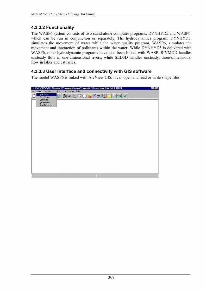
State of the art in Urban Drainage Modelling
309
4.3.3.2 Functionality The WASP6 system consists of two stand-alone computer programs: DYNHYD5 and WASP6, which can be run in conjunction or separately. The hydrodynamics program, DYNHYD5, simulates the movement of water while the water quality program, WASP6, simulates the movement and interaction of pollutants within the water. While DYNHYD5 is delivered with WASP6, other hydrodynamic programs have also been linked with WASP. RIVMOD handles unsteady flow in one-dimensional rivers, while SED3D handles unsteady, three-dimensional flow in lakes and estuaries.
4.3.3.3 User Interface and connectivity with GIS software The model WASP6 is linked with ArcView GIS, it can open and read or write shape files.
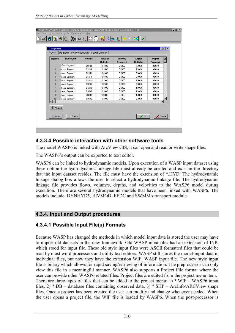
State of the art in Urban Drainage Modelling
310
4.3.3.4 Possible interaction with other software tools The model WASP6 is linked with ArcView GIS, it can open and read or write shape files.
The WASP6’s output can be exported to text editor.
WASP6 can be linked to hydrodynamic models. Upon execution of a WASP input dataset using these option the hydrodynamic linkage file must already be created and exist in the directory that the input dataset resides. The file must have the extension of *.HYD. The hydrodynamic linkage dialog box allows the user to select a hydrodynamic linkage file. The hydrodynamic linkage file provides flows, volumes, depths, and velocities to the WASP6 model during execution. There are several hydrodynamic models that have been linked with WASP6. The models include: DYNHYD5, RIVMOD, EFDC and SWMM's transport module.
4.3.4. Input and Output procedures
4.3.4.1 Possible Input File(s) Formats Because WASP has changed the methods in which model input data is stored the user may have to import old datasets in the new framework. Old WASP input files had an extension of INP, which stood for input file. These old style input files were ASCII formatted files that could be read by most word processors and utility text editors. WASP still stores the model-input data in individual files, but now they have the extension WIF, WASP input file. The new style input file is binary which allows for rapid saving/retrieving of information. The preprocessor can only view this file in a meaningful manner. WASP6 also supports a Project File format where the user can provide other WASP6 related files. Project files are edited from the project menu item. There are three types of files that can be added to the project menu: 1) *.WIF – WASP6 input files, 2) *.DB – database files containing observed data, 3) *.SHP – ArcInfo/ARCView shape files. Once a project has been created the user can modify and change whenever needed. When the user opens a project file, the WIF file is loaded by WASP6. When the post-processor is
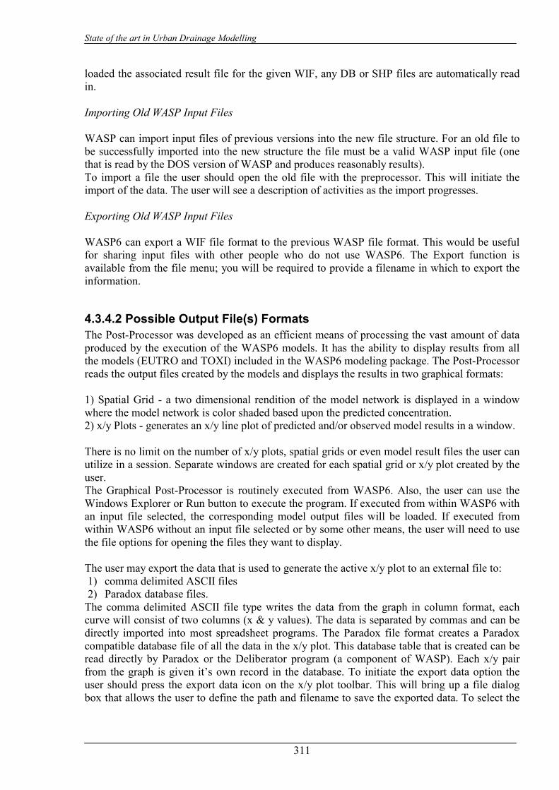
State of the art in Urban Drainage Modelling
311
loaded the associated result file for the given WIF, any DB or SHP files are automatically read in. Importing Old WASP Input Files WASP can import input files of previous versions into the new file structure. For an old file to be successfully imported into the new structure the file must be a valid WASP input file (one that is read by the DOS version of WASP and produces reasonably results). To import a file the user should open the old file with the preprocessor. This will initiate the import of the data. The user will see a description of activities as the import progresses. Exporting Old WASP Input Files WASP6 can export a WIF file format to the previous WASP file format. This would be useful for sharing input files with other people who do not use WASP6. The Export function is available from the file menu; you will be required to provide a filename in which to export the information.
4.3.4.2 Possible Output File(s) Formats The Post-Processor was developed as an efficient means of processing the vast amount of data produced by the execution of the WASP6 models. It has the ability to display results from all the models (EUTRO and TOXI) included in the WASP6 modeling package. The Post-Processor reads the output files created by the models and displays the results in two graphical formats: 1) Spatial Grid - a two dimensional rendition of the model network is displayed in a window where the model network is color shaded based upon the predicted concentration. 2) x/y Plots - generates an x/y line plot of predicted and/or observed model results in a window. There is no limit on the number of x/y plots, spatial grids or even model result files the user can utilize in a session. Separate windows are created for each spatial grid or x/y plot created by the user. The Graphical Post-Processor is routinely executed from WASP6. Also, the user can use the Windows Explorer or Run button to execute the program. If executed from within WASP6 with an input file selected, the corresponding model output files will be loaded. If executed from within WASP6 without an input file selected or by some other means, the user will need to use the file options for opening the files they want to display. The user may export the data that is used to generate the active x/y plot to an external file to: 1) comma delimited ASCII files 2) Paradox database files.
The comma delimited ASCII file type writes the data from the graph in column format, each curve will consist of two columns (x & y values). The data is separated by commas and can be directly imported into most spreadsheet programs. The Paradox file format creates a Paradox compatible database file of all the data in the x/y plot. This database table that is created can be read directly by Paradox or the Deliberator program (a component of WASP). Each x/y pair from the graph is given it’s own record in the database. To initiate the export data option the user should press the export data icon on the x/y plot toolbar. This will bring up a file dialog box that allows the user to define the path and filename to save the exported data. To select the
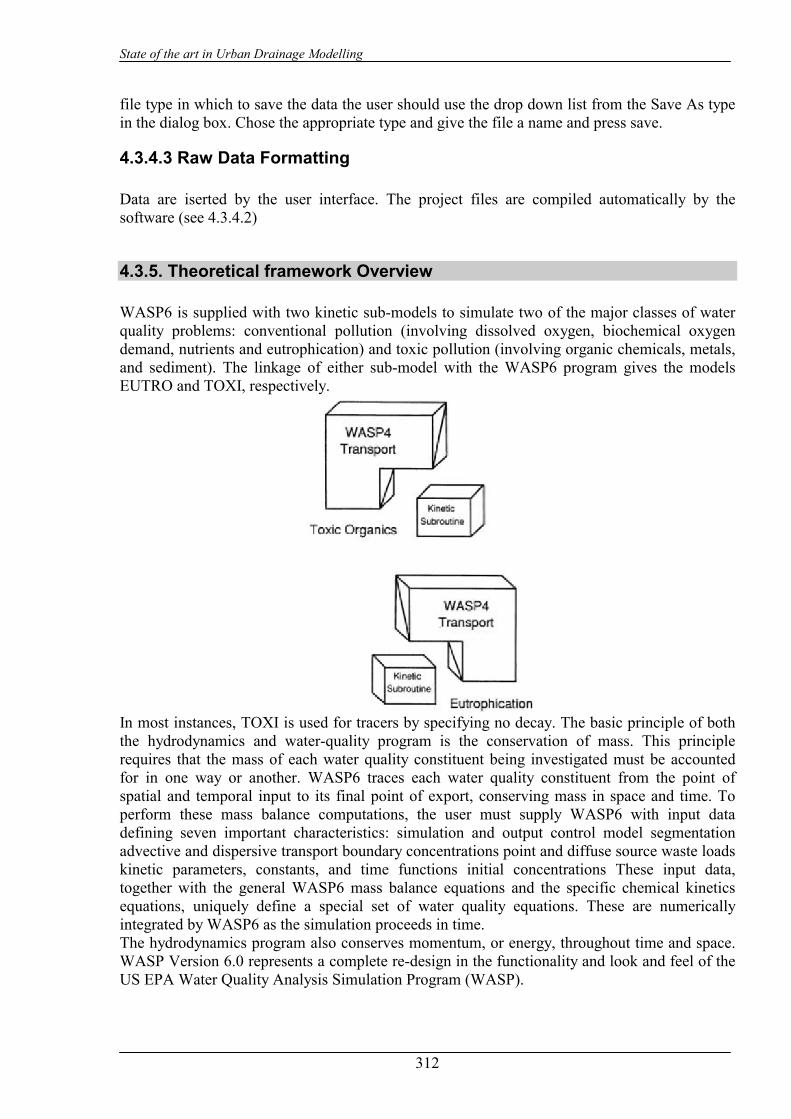
State of the art in Urban Drainage Modelling
312
file type in which to save the data the user should use the drop down list from the Save As type in the dialog box. Chose the appropriate type and give the file a name and press save.
4.3.4.3 Raw Data Formatting Data are iserted by the user interface. The project files are compiled automatically by the software (see 4.3.4.2)
4.3.5. Theoretical framework Overview WASP6 is supplied with two kinetic sub-models to simulate two of the major classes of water quality problems: conventional pollution (involving dissolved oxygen, biochemical oxygen demand, nutrients and eutrophication) and toxic pollution (involving organic chemicals, metals, and sediment). The linkage of either sub-model with the WASP6 program gives the models EUTRO and TOXI, respectively.
In most instances, TOXI is used for tracers by specifying no decay. The basic principle of both the hydrodynamics and water-quality program is the conservation of mass. This principle requires that the mass of each water quality constituent being investigated must be accounted for in one way or another. WASP6 traces each water quality constituent from the point of spatial and temporal input to its final point of export, conserving mass in space and time. To perform these mass balance computations, the user must supply WASP6 with input data defining seven important characteristics: simulation and output control model segmentation advective and dispersive transport boundary concentrations point and diffuse source waste loads kinetic parameters, constants, and time functions initial concentrations These input data, together with the general WASP6 mass balance equations and the specific chemical kinetics equations, uniquely define a special set of water quality equations. These are numerically integrated by WASP6 as the simulation proceeds in time. The hydrodynamics program also conserves momentum, or energy, throughout time and space. WASP Version 6.0 represents a complete re-design in the functionality and look and feel of the US EPA Water Quality Analysis Simulation Program (WASP).

State of the art in Urban Drainage Modelling
313
4.3.6. Model Parameters Estimation or Assignation Sensitivity analysis, calibration, sensitivity estimation and validation have to be done manually by the user.
4.3.7. PI(s) Estimation Method There are no PI(s) calculated by the software (see paragraph 4.3.2.2)
4.3.8. Future Improvements of the Model No information about future model developments are available by now.
4.3.9. References
4.3.9.1 Theoretical Framework References Di Toro, D.M., D.J. O'Connor, and R.V. Thomann. (1971). A Dynamic Model of the Phytoplankton Population in the Sacramento San Joaquin Delta. Adv. Chem. Ser. 106, Am. Chem. Soc., Washington, DC., pp. 131-180. Di Toro, D.M. and J.P. Connolly. (1980). Mathematical Models of Water Quality in Large Lakes, Part 2: Lake Erie. EPA-600/3-80-065. pp. 90-101. Di Toro, D.M. and W.F. Matystik. (1980). Mathematical Models of Water Quality in Large Lakes, Part 1: Lake Huron and Saginaw Bay. EPA-600/3-80-056. pp. 28-30. Di Toro, D.M., J.J. Fitzpatrick, and R.V. Thomann. (1981, rev. 1983). Water Quality Analysis Simulation Program (WASP) and Model Verification Program (MVP) - Documentation. Hydroscience, Inc., Westwood, NY, for U.S. EPA, Duluth, MN, Contract No. 68-01-3872. Di Toro, D.M. (1985). A Particle Interaction Model of Reversible Organic Chemical Sorption, Chemosphere 14(10):1503-1538. O'Connor. D.J. and R.V. Thomann. (1972). Water Quality Models: Chemical, Physical and Biological Constituents. In: Estuarine Modeling: An Assessment. EPA Water Pollution Control Research Series 16070 DZV, Section 702/71. pp. 102-169. O'Connor, D.J., J.A. Mueller, and K.J. Farley. (1983). Distribution of Kepone in the James River Estuary. Journal of the Environmental Engineering Division, ASCE. 109(EE2):396-413. O'Connor, D.J. (1983). Wind Effects on Gas-Liquid Transfer Coefficients. Journal of Environmental Engineering, Volume 109, Number 9, pp. 731-752.
4.3.9.2 Practical Use and Results References

State of the art in Urban Drainage Modelling
314
The software has been largely used in the past few years and a large collection of pubblications are available also on the web.

State of the art in Urban Drainage Modelling
315
5 MODELS FOR WASTE WATER TREATMENT PLANTS ANALYSIS
5.1 STOAT
5.1.1. Model availability Software house: WRc Software The model is commercial. Reference: http://www.wrcplc.co.uk/software/
5.1.2. Abstract
5.1.2.1 Objectives and peculiarities STOAT is a PC based computer modelling tool designed to dynamically simulate the performance of a wastewater treatment works. The software can be used to simulate individual treatment processes or the whole treatment works, including sludge treatment processes, septic tank imports and recycles. The model enables the user to optimise the response of the works to changes in the influent loads, works capacity or process operating conditions.
5.1.2.2 Performance Indicator(s) of Interest There are no PI(s) of interest related to the software (WP1). The software calculates the value of variables, such as the main pollutants concentration spilled into the receiving water body, that are necessary to evaluate the impact on the environment (relevant for WPs 3.3, 5 and 6).
5.1.2.3 Brief Historical Overview of the Model WRc have been investigating the modeling of wastewater treatment processes for many years. The first computer models were intended to automate manual design methods, with the inclusion of the recycle streams. Following on from this, ‘optimization methods were added to help design the ‘best’ sewage works. Dynamic models such as STOAT™, GPSX™ and Biowin™ were then developed to be able to assess more closely the day to day and hour to hour variations within a treatment plant. STOAT has been developed over the past 10 years to simulate treatment processes within wastewater treatment plants. During its development, each process model was validated against performance data from sewage treatment plants. Extensive modelling work has subsequently been undertaken to confirm the validity of individual process models.
5.1.3. Usage Specifications
5.1.3.1 Programming Language(s) or Mathematical-Statistical Software(s)

State of the art in Urban Drainage Modelling
316
5.1.3.2 Functionality STOAT can be used for:
- Improve effluent quality, reducing risk of consent failures - Reduce capital and operationalcosts - Design treatment plants more efficiently - Optimise treatment plant operation - Troubleshoot operational problems - Carry out integrated catchment simulation - Train staff in best practices
STOAT contains a wide range of features which makes it stand out from its competitors, including:
- Models all common treatment processes - Offers both BOD and COD models - New models continually being added - Integrates with leading sewerage and river quality models - Easy to use, with user friendly interface - Includes quick build wizard - Support for batch simulations - Allows simplified sewer modelling (SIMPOL) - Easy data transfer to other packages
The software contains models for the following processes:
- Storm tanks - Primary tanks - Wet wells - Equalisation tanks - Activated sludge – including oxidation ditch and N- and P- removal systems - Sequencing batch reactors - Compartmented SBRs - Tower activated sludge systems, e.g. Deep shaft - Activated sludge settling tanks - Trickling filters - Trickling filter settling tanks - BAFs - Biological fluidised beds - RB’s - Submerged biological contactors - Disinfection - Chemically assisted sedimentation - Dissolved air flotation - Chemical phosphorus removal - Mesophilic anaerobic sludge digestion - Thermophilic aerobic sludge digestion - Sludge incineration - Direct and indirect sludge drying - Heat exchangers - Sludge dewatering - PID controllers - Ladder logic controllers - Instrumentation

State of the art in Urban Drainage Modelling
317
- Detention tanks - Combined sewer overflow - "Black box" correlation based models - Sensitivity analysis - Calibration routines - Optimisation routines - Support for user-written models
5.1.3.3 User Interface and connectivity with GIS software The Windows interface allows users to quickly build a plant model and enter the input data using simple dialogue boxes. Results can be shown while a simulation is taking place and are stored as data files for subsequent analysis.
5.1.4. Input and Output procedures
5.1.4.1 Possible Input File(s) Formats Data project input is available through user graphical interface. The project data are stored in .MDB files
5.1.4.2 Possible Output File(s) Formats The project data are stored in .MDB files
5.1.4.3 Raw Data Formatting Detailed informations about Raw Data Formatting are not available.
5.1.5. Theoretical framework Overview STOAT is a PC based computer modelling tool designed to dynamically simulate the performance of a wastewater treatment works. The software can be used to simulate individual treatment processes or the whole treatment works, including sludge treatment processes, septic tank imports and recycles. The model enables the user to optimise the response of the works to changes in the influent loads, works capacity or process operating conditions.
5.1.6. Model Parameters Estimation or Assignation
5.1.6.1 Sensitivity analysis Specify one or two parameters to vary. Although you can change stream parameters these are held constant, so any diurnal variations will be lost. For each parameter you specify an initial and final value, and the step size to be used between these two limits. You also need to specify a stream or process determinand to look at, so that you can see the response. You have a choice of looking at the result as a time series, where each parameter value is plotted as a new line, or as a phase plot, where the final simulation value is plotted against parameter value.

State of the art in Urban Drainage Modelling
318
5.1.6.2 Calibration routines Select the name, stage (if applicable) and determinand. Then specify a lower and an upper bound. The initial value for the parameter will be selected at random between these bounds.
5.1.6.3 Optimisation routines Optimisation is provided through minimising the sum of the optimisation parameters. Different algorithms and parameter weights may provide different final results. You choice of the initial values for the parameters will also affect the final result. It is therefore worth trying more than one optimisation run, varying the starting values for the parameters. Algorithm A choice of minimisation algorithms. Simplex is likely to be slower than Powell but is also likely to be more robust. Maximum number of iterations If no minimum has been found after this many iterations the optimisation exercise will stop. You should look at the number of iterations actually used to decide if the optimisation work appeared to locate a minimum. Convergence tolerance The criteria is evaluated with each choice of parameters during the optimisation run. When the relative change in criteria between two sets of parameters is less than this convergence tolerance the algorithm will stop, assuming that it is now close enough to the minimum. Parameters Opens up a form that allows you to specify the parameters to be changed for the optimisation run. Constraints Opens up a form that allows you to specify the constraints on effluent quality.
5.1.7. PI(s) Estimation Method There are no PI(s) calculated by the software (see paragraph 4.1.2.2).
5.1.8. Future Improvements of the Model
Further processes and options are being added to STOAT for release. Currently under development are:
• Fate in Treatment • Industrial Treatment Processes • CFD Settling Tank Models
5.1.9. References
5.1.9.1 Theoretical Framework References Detailed informations about theoretical framework are not available.
5.1.9.2 Practical Use and Results References Detailed informations about Results References are not available.
State of the art in Urban Drainage Modelling
319
5.2 WEST-Worldwide engine for simulation, training and automation
5.2.1. Model availability Software house: Hemmis - Environmental Software The model is commercial. Reference: http://www.hemmis.com/products/west/default_west.htm
5.2.2. Abstract
5.2.2.1 Objectives and peculiarities WEST can be used for:
- Experimental design. - Evaluation of design options.
5.2.2.2 Performance Indicator(s) of Interest There are no PI(s) of interest related to the software (WP1). The software calculates the value of variables, such as the main pollutants concentration spilled into the receiving water body, that are necessary to evaluate the impact on the environment (relevant for WPs 3.3, 5 and 6).
5.2.2.3 Brief Historical Overview of the Model The development of WEST® version 1 started in the early 1990s in close collaboration with the University of Ghent (BIOMATH: Department of Applied Mathematics, Biometrics and process Control). In particular the efforts of Prof. Dr. Lic. Hans Vangheluwe made of WEST® one of the most powerful tools for dynamic modelling, simulation and optimisation.
5.2.3. Usage Specifications
5.2.3.1 Programming Language(s) or Mathematical-Statistical Software(s)
5.2.3.2 Functionality WEST can also be used to evaluate up-scaling the pilot test results on the full-scale plants:
− Process optimization − Development of control strategies − Minimization of operational costs − Evaluation of operating strategies
WEST can be used to evaluate operating strategies through:
− Prediction of dynamic responses of the system to influent variations − Bottleneck identification − Plant operation trouble shout
State of the art in Urban Drainage Modelling
320
− Decision support (operator) − Off line simulations: off line simulations may support the operator in the decision
making process − On line simulations (operator in the loop): The data of online sensors is sent directly
to WEST, with which the operator can test a number of operating strategies. − Real time control − Model based predictive control − Scenario based predictive control − Better insight in the processes
The removal of organic matter, nitrogen and phosphorus, is accomplished in a single system nowadays.
5.2.3.3 Possible interaction with other software tools
WEST® can be Linked with Visual Basic for Applications (VBA), Geographical Information Systems (GIS), supervisory control and data acquisition (SCADA).

State of the art in Urban Drainage Modelling
321
5.2.4. Input and Output procedures
5.2.4.1 Possible Input File(s) Formats WEST file types A number of file types are used in WEST: WEST Configuration (*.wco) XML based file format used to store a WEST v3 configuration WEST V2 HGE file (*.hge) TCL based file format used to store a WEST v2 configuration Model Specification Language - MSL (*.msl) file format used to write WEST models WEST Runtime model (*.wml) WEST Experiment (*.wxp) XML based file format used to store a WEST v3 experiment WEST V2 Experiment (*.wex) TCL based file format used to store a WEST v2 experiment WEST Project (*.wpr) XML based file format used to store a WEST v3 project
5.2.4.2 Raw Data Formatting It is not possible to change the input data format that must be provided to the model. For this reason data must be formatted according to the model standard.
5.2.5. Theoretical framework Overview Detailed information about theoretical framework is not available.
State of the art in Urban Drainage Modelling
322
5.2.6. Model Parameters Estimation or Assignation The parameter estimation module in WEST can be used for a fine tune these parameters. The parameter estimation module can also be used for model calibration and minimization problems. Two optimization algorithms are included (Simplex and Praxis). Two types of parameter estimation are available, i.e. Trajectory optimization and End-value optimization: Trajectory optimization In a trajectory optimization experiment a set of model parameters or derived state variables is tuned in order to fit the simulation results on one or more data sets of measurements. A number of simulation runs, with different parameter values, are executed, in order to find the optimal solution. End-value optimization In an end-value optimization experiment a set of model parameters or derived state variables is tuned in order to minimize a defined variable. A number of simulation runs, with different parameter values, are executed, in order to find the optimal solution. During the optimization experiment the algorithm tries to find the optimum for the different parameters so that the result of the simulation fits the measured data obtained by analysis on a real or pilot plant. The cost function gives an indication on how accurate the parameter estimation is. The cost function is a relation (using the squared error or absolute error method) between the measured data and the simulation results. The best fit is obtained when the cost function is minimal.
5.2.6.1 Check of Parameters Significance – Internal Validation Sensitivity function In a sensitivity analysis the absolute and relative sensitivity of a certain (sensitivity) variable due to a change in a certain (sensitivity) parameter is calculated. This is done for a number of sensitivity functions (sensitivity parameter - sensitivity variable combination). For each sensitivity function, the sensitivity is calculated as follows:
• First a reference simulation is run. • Next the parameter p is altered by a certain factor (the perturbation factor) and a new
simulation (the perturbation simulation) is run: ppert = ( 1 + perturbation factor) * pref
Then the absolute sensitivity is calculated for each time point as the difference between the variable value of the reference simulation and the variable value of the perturbation simulation divided by the difference between the parameter value of the reference simulation and parameter value of the perturbation simulation.
When using non-linear models (as often is the case in wastewater treatment modeling) attention should be paid to the perturbation factor. In order to use the finite difference method the variable should change linearly with respect to a change of the parameter. This can only be achieved by using a very small perturbation factor.

State of the art in Urban Drainage Modelling
323
• In order to quantify this problem a control simulation is performed. The parameter p is, again, altered by a certain factor (the perturbation factor multiplied with the control factor): pcont = (1 + perturbation factor * control factor) * pref Then the absolute sensitivity is calculated again and compared with the sensitivity of the perturbation simulation using the sensitivity acceptance info.
5.2.7. PI(s) Estimation Method The code WEST is able to evaluate some of the required variables, but not the PIs directly.
5.2.8. References
5.2.8.1 PROJECT AUCOWACO A water management system for the very well known Haacht Brewery (Producer of several types of beer, mineral water and soft drinks) is developed based on a new concept of optimal information exchange and optimal process control. This project is released with financial support of the European Commission in the context of the LIFE program. This project is carried out by: * EPAS NV * SEGHERS Better Technology for water * The brewery of HAACHT * HEMMIS NV
5.2.8.2 INTEGRATED URBAN WATER SYSTEM BRUSSELS Most actual regulations concerning Combined Sewer Overflow (CSO) can be classified under the Uniform Emission Standard (UES) approach. This approach focuses on emission standards, considers technology based criteria (BATNEEC) and doesn't account for local circumstances. The aim of good drainage design is to balance the effects of discharges against the assimilation capacity of the receiving water, in order to optimize the quality of the receiving water at minimal cost. Therefore the alternative approach Environmental Quality Objective / Environmental Quality Standard (EQO/EQS) imposes itself. In this approach the integrated approach (Sewer system - wastewater treatment plant - River) is considered. * The problem * The methodology * The sewer model * The WasteWater Treatment plant model * The river model * Conclusions This case study has been carried out by: W. Bauwens, C. Fronteau and M. Smeets, University of Brussels, Laboratory of Hydrology; Pleinlaan 2, 1050 Brussels, Belgium. P. Vanrolleghem, University of Ghent, Department of Applied Mathematics, Biometrics and Process Control, Coupure Links 653, 9000 Ghent, Belgium.

State of the art in Urban Drainage Modelling
324
5.2.8.3 Practical Use and Results References AQUAFIN "De invloed van textielafvalwater op biologische fosforverwijdering" ("The influence of textile wastewater on biological phosphorus removal"), Davide Bixio, Ronald Carrette and Chris Thoeye, Neerslag, vol 3, 2000. In dutch (Pdf) "Full-scale Application of the IAWQ ASM No.2d Model", R. Carrette, D. Bixio, C. Thoeye and P. Ockier, 1st World congress of the international Water Association (IWA), Paris 03/07/00. (Pdf) "Renovation of the WWTP of Bruges", I. Boonen, H. Bruynooghe, R. Carrette, D. Bixio and P. Ockier, Water Science & Technology, vol 41 n° 9, 2000. (Pdf) "Renovatie van RWZI Brugge" ("Renovation of RWZI Bruges"), R. Carrette, D. Bixio, C. Thoeye and P. Ockier, Water Science & Technology, vol 41 n° 9, 2000. In dutch (Pdf) "Impact of primary treatment technologies on BNR: The case study of the STP of Ghent", D. Bixio, P. van Hauwermeiren and C. Thoeye, WATERMATEX Ghent, 18/09/00. (Pdf) BIOMATH Coen F., Vanderhaegen B., Vanrolleghem P.A. and Van Meenen P. (1997) Improved design and control of industrial and municipal nutrient removal plants using dynamic models. Wat. Sci. Tech., 35(10), 53-61. http://biomath.rug.ac.be/~peter/ftp/pvr125.pdf Vanderhasselt A., De Clercq B., Vanderhaegen B., Verstraete W. and Vanrolleghem P.A. (1999) On-line control of polymer addition to prevent massive sludge wash-out. J. Environ. Eng., 125, 1014-1021. http://biomath.rug.ac.be/~peter/ftp/pvr215.pdf Vanhooren H., Demey D., Vannijvel I. and Vanrolleghem P.A. (2000) Monitoring and modelling an industrial trickling filter using on-line off-gas analysis and respirometry. Wat. Sci. Tech., 41(12), 139-148. http://biomath.rug.ac.be/~peter/ftp/pvr254.pdf Vanrolleghem P.A. and Gillot S. (2001) Robustness and economic measures as control benchmark performance criteria. Wat. Sci. Tech., (in Press). http://biomath.rug.ac.be/~peter/ftp/pvr300.pdf Vanhooren H., Verbrugge T., Boeije G., Demey D. and Vanrolleghem P.A. (2001) Adequate model complexity for scenario analysis of VOC stripping in a trickling filter. Wat. Sci. Tech., 43(7), 29-37. http://biomath.rug.ac.be/~peter/ftp/pvr271.pdf Gernaey K., Vanrolleghem P.A. and Lessard P. (2001) Modelling of a reactive primary clarifier. Wat. Sci. Tech., 43(7), 73-82. http://biomath.rug.ac.be/~peter/ftp/pvr272.pdf
State of the art in Urban Drainage Modelling
325
"Modelling of activated sludge acclimatisation to a non-ionic surfactant", G. Carvalho, I. Nopens, J.M. Novais, P.A. Vanrolleghem and H.M. Pinheiro. http://biomath.rug.ac.be/~peter/ftp/pvr265.pdf Deksissa T., Meirlaen J., Ashton P.J. and Vanrolleghem P.A. (2001) Simplifying dynamic river water quality modelling: A case study of inorganic nitrogen dynamics in the Crocodile river (South Africa). Wat. Sci. Tech. (in Press). http://biomath.rug.ac.be/~peter/ftp/pvr345.pdf

State of the art in Urban Drainage Modelling
326
6 GROUNDWATER INTERACTION MODELS
6.1 MicroFEM, Version 3.5
6.1.1. Model availability
MicroFEM sells for U.S. $1950 ($975 for universities). FemInvs, an inverse parameter estimation module is available as a $600 option. A single purchase includes a license for all personal computers in the purchaser’s office. MicroFEM 3.5 LT is a freeware version of the Windows package available for download from the MicroFEM Web site (microfem.com). It is limited to two aquifer layers and 2500 nodes per layer, but otherwise includes all functionality of the parent product. MicroFEM is available from Dr. C.J. Hemker, Geohydroloog, Elandsgracht 83, 1016 TR Amsterdam, The Netherlands; 31-20-6234628 (fax); [email protected]; http://www.xs4all.nl/~microfem/.
As we said a free lite-version of MicroFEM is available for downloading. For more details the reader is referred to the short guide (24 pages) and the MicroFEM tutorial (53 pages), which can also be downloaded from this web site as zip-files.
Excellent customer e-mail support is an essential part of a MicroFEM license, and an integral part of its development. Many of the MicroFEM enhancements are the result of customer suggestions.
MicroFEM is updated several times per year. Recent modifications are described in the update.txt file. Free e-mail updates of any full version of MicroFEM are available from the developers anytime.
6.1.2. Abstract
6.1.2.1 Objectives and peculiarities MicroFEM modeling features:
− Saturated single-density flow − Multiple-aquifer systems and stratified aquifers − Confined, leaky and unconfined conditions − Heterogeneous aquifers and aquitards − Steady-state and transient flow − Spatially varying anisotropic aquifers − Spatially and temporally varying wells and boundary conditions − Precipitation, evaporation, drain, river and wadi top systems
MicroFEM Program features and capabilities: − Mesh generators for regional flow models and for civil engineering models − Interactive mesh design and adjustment

State of the art in Urban Drainage Modelling
327
− Graphical user interface and data base − Interactive assignment of spatially varying properties − Up to 20 aquifers or sublayers − Up to 50,000 nodes per layer − User-assigned names for all nodes − Flow vectors and flowlines, 3-D particle tracking − Water balances for each aquifer, subarea and time step − Transient flow modeling in batch mode.
6.1.2.2 Performance Indicator(s) of Interest *wOp30 *wOp31
6.1.2.3 Brief Historical Overview of the Model The Windows version of MicroFEM is a new program, based on the DOS package Micro-Fem. It takes you through the whole process of ground-water modeling, from the generation of a finite-element grid through the stages of preprocessing, calculation, postprocessing, graphical interpretation and plotting. Confined, semi-confined, phreatic, stratified and leaky multi-aquifer systems can be simulated with a maximum of 20 aquifers. MicroFEM can simulate steady-state or transient three-dimensional flow of a constant-density fluid in confined, unconfined, and leaky aquifers. Material properties are assigned to elemental nodes. Aquifers and aquitards can be heterogeneous, and aquifers can have spatially-varying anisotropy. Up to 20 aquifer layers are supported, with up to 25,000 nodes per layer. In a graphical environment, MicroFEM includes functionality for mesh generation, interactive mesh editing, data import, and pre- and post-processing.
6.1.3. Usage Specifications
6.1.3.1 Programming Language(s) or Mathematical-Statistical Software(s) Win system Requirements: Windows 95, 98, ME, XP, 2000 or NT
6.1.3.2 Functionality MicroFEM runs on Windows 95, Windows 98, and Windows NT platforms. It requires approximately 2.5 MB hard drive space. Modeling in MicroFEM entails grid generation, model editing and parameterization, calculation of model results, and display or post-processing of results. Each of these tasks are accomplished in different modes, in the parlance of the MicroFEM paradigm. Modes are selected through the menu bar "View" item. The finite-element approach allows for accurate and efficient spatial representation of distinct hydrogeologic units. For computational efficiency, finite-difference equations are used for the vertical solution. The program supports a wide range of boundary conditions for the top layer. These include precipitation, rivers, drains, wades, and evapotranspiration. Unconfined aquifers can be simulated in the top layer.

State of the art in Urban Drainage Modelling
328
MicroFEM includes two mesh generators: one for rather evenly spaced nodes and the other for grids with a large contrast in spacings. The user specifies a series of fixed nodes and then the generator fills in the rest according to a general spacing guide that you specify. Any of the nodes can then be modified on the fly to make it fit your boundaries precisely. All parameters are assigned on a node basis. This is different from some other popular models that assign properties like hydraulic conductivity on an element basis. When assigning the properties to the regions, you can choose sections with a marker or a line tool. The finite-element solution used by MicroFEM allows anisotropy to be specified in any direction (as compared to finite-difference models, where anisotropy axes must be aligned with grid directions). This allows the user to better describe natural hydrogeologic systems. For example, permeability ellipses can be aligned with the trend of deposition of meandering river valleys or buried glacial geomorphic features. MicroFEM has an intelligent standard data structure paradigm that allows for easy and flexible import of ASCII data files of parameters. These can be either as one-dimensional vectors of values or as XYZ specifications that are interpolated to nearest nodes. MicroFEM can import as well as export a variety of ASCII file formats, including AutoCAD DXF (drawing exchange file). Input to and output from EXCEL is readily accommodated through the CSV (comma separated variable) format. HPGL file export is also included. MicroFEM can produce graphical output in the form of areal maps of water levels (or any other parameter). In addition, MicroFEM can produce cross sections showing aquifer layers with ground water levels. Flowlines created by Microfem can also be shown on these cross sections. Microfem can produce hydrographs of water levels from transient simulations.
6.1.3.3 User Interface and connectivity with GIS software
MicroFEM has an intelligent standard data structure paradigm that allows for easy and flexible import of ASCII data files of parameters. These can be either as one-dimensional vectors of values or as XYZ specifications that are interpolated to nearest nodes. MicroFEM can import as well as export a variety of ASCII file formats, including AutoCAD DXF (drawing exchange
State of the art in Urban Drainage Modelling
329
file). Input to and output from EXCEL is readily accommodated through the CSV (comma separated variable) format. HPGL file export is also included and it is compatible with Arc-Info and ArcView data files .
6.1.3.4 Possible interaction with other software tools SURFER, Excel, Arc-Info and ArcView compatible data files
6.1.4. Input and Output procedures
6.1.4.1 Possible Input File(s) Formats − Model files in ASCII format − DXF maps and flowline files import − SURFER, Excel, Arc-Info and ArcView compatible data files − Copy & Paste water budget tables
6.1.4.2 Possible Output File(s) Formats − Model files in ASCII format − SURFER, Excel, Arc-Info and ArcView compatible data files − Screen resolution output to printer − Plots of grids, contours, flowlines and time series − HPGL and DXF files export
6.1.4.3 Raw Data Formatting Detailed informations about Raw Data Formatting are not available.
6.1.5. Theoretical framework Overview Irregular grids, as typically used by finite-element programs, have several advantages compared to the more or less regular grids used by finite-difference codes. A model with a well-designed irregular grid will show more accurate results with fewer nodes, so less computer memory is required while calculations are faster. MicroFEM offers extensive possibilities as to the ease of creating such irregular grids. Two grid generators are included; one is designed for irregular geometries as often encountered in regional studies, while the other is useful for engineering applications that often require high contrasts in node spacing, e.g. sheet piling and excavations. Adding and erasing nodes, connection swapping and further modifications to the grid can be done interactively. Other MicroFEM features include the ease of data preparation and the presentation and analysis of modeling results. A flexible way of zone-selection and formula-assignment is used for all parameters: transmissivities, aquitard resistances, well discharges and boundary conditions for each layer. Depending on the type of model this can be extended with layer thicknesses, storativities, spatially varying anisotropy, topsystem and user-defined parameters. To inspect and interpret model results, maps and profiles can be used to visualize contours, heads, 3D-flowlines, flow vectors, etc. Time-drawdown curves and water balances can be selected with just a few keystrokes or mouse clicks.
State of the art in Urban Drainage Modelling
330
6.1.6. Model Parameters Estimation or Assignation Sensitivity analysis, calibration, sensitivity estimation and validation have to be done manually by the user.
6.1.7. PI(s) Estimation Method The code MicroFEM is able to evaluate some of the required variables, but not the PIs directly.
6.1.8. Future Improvements of the Model No information about future model developments are available by now.
6.1.9. References
6.1.9.1 Theoretical Framework References
MicroFEM sells for U.S. $1950 ($975 for universities). FemInvs, an inverse parameter estimation module is available as a $600 option. A single purchase includes a license for all personal computers in the purchaser’s office. MicroFEM 3.5 LT is a freeware version of the Windows package available for download from the MicroFEM Web site (microfem.com). It is limited to two aquifer layers and 2500 nodes per layer, but otherwise includes all functionality of the parent product. MicroFEM is available from Dr. C.J. Hemker, Geohydroloog, Elandsgracht 83, 1016 TR Amsterdam, The Netherlands; 31-20-6234628 (fax); [email protected]; http://www.xs4all.nl/~microfem/.
State of the art in Urban Drainage Modelling
331
6.2 GMS -Ground water Modeling System- 4
6.2.1. Model availability GMS is a commercial product. The Software house is The GMS/WMS/SMS Group. You can find information about prices and available on – line documentation on the web page: http://www.scisoft-gms.com.
Environmental Modeling Systems Incorporated (EMS-I).
email: [email protected] phone: (601) 634-4286 fax: (601) 634-4208
postal address:
WES GMS Support ATTN: CEERD-HC-HG Waterways Experiment Station 3909 Halls Ferry Road Vicksburg, MS 39180
DoD/USEPA/DoE users may direct questions about GMS to [email protected]
6.2.2. Abstract
6.2.2.1 Objectives and peculiarities The GMS Software (Groundwater Modeling System) is a comprehensive package which provides tools for every phase of a groundwater simulation including site characterization, model development, postprocessing, calibration, and visualization. GMS is the only system which supports TINs, solids, borehole data, 2D and 3D geostatistics, and both finite element and finite difference models in 2D and 3D. Currently supported models include MODFLOW, MODPATH, MT3D, RT3D, FEMWATER, SEEP2D, SEAM3D, PEST, UCODE and UTCHEM. Due to the modular nature of GMS, a custom version of GMS with desired modules and interfaces can be configured. SSG has the lowest prices for GMS on the market today. Technical support is provided directly from the developer.
GMS SOFTWARE FEATURES
• Imports/exports raster and vector GIS data from ARC/INFO, ArcView, and GRASS. • A Model Checker is provided in GMS for each model to check for potential problems
prior to saving and running a model. • All models can be launched from a GMS menu. • Latest versions of all analysis codes are provided including executable, source code, and
documentation.

State of the art in Urban Drainage Modelling
332
• Time-series plots of computed values at selected points can be generated. • Data Calculator can be used to combine data sets using any mathematical expression to
generate a new data set. • Highly-acclaimed technical documentation including an extensive reference manual and
self-guided tutorials. • Images can be copied to the clipboard and pasted into other applications for report
generation. • A simple set of drawing tools are provided for adding titles, arrows, and other
annotations to a plot in GMS. • Imports/exports DXF files including AutoCAD R13 format. • Periodic free software updates are available over the Internet. • The GMS electronic mailing list can be used for questions and to share tips with
hundreds of other GMS users. • GMS PC and UNIX versions are identical.
GMS SOFTWARE MODULESMODFLOW
MODFLOW
MODFLOW the most widely-used 3D groundwater flow model in the world. MODFLOW can represent the effects of wells, rivers, streams, drains, horizontal flow barriers, evapotranspiration, and recharge on flow systems with heterogeneous aquifer properties and complex boundary conditions to simulate groundwater flow. Using GMS, the user can select a single cell or a series of cells and then define the hydrogeologic characteristics and/or boundary conditions using interactive dialog boxes. In addition, a spread sheet dialog can be displayed allowing the user to edit the values for each individual hydrogeologic characteristic for the entire model. Input data may be imported or interpolated from a sparse set of scattered data points. All popular packages are supported including the Horizontal Flow Barrier package and the Stream/Aquifer Interaction package. GMS reads and writes native MODFLOW files. GMS supports the Observation (OBS), Sensitivity (SEN), and Parameter Estimation (PES) processes in addition to the new Layer Property Flow (LPF), Hydrogeologic Unit Flow (HUF), and Direct Solver packages. For parameter estimation, the user can choose between the PES process, PEST, or UCODE. A new pilot point method can be used for parameterization with all three methods. With the PEST option, regularization can be incorporated with the pilot point method for a powerful, robust, and easy-to-use parameter estimation solution.

State of the art in Urban Drainage Modelling
333
MODPATH
MODPATH is a 3D particle-tracking model that computes the path a particle takes in a steady-state or transient flow field over a given period of time. MODPATH uses the head values and cell-by-cell flow terms computed by MODFLOW in addition to the soil porosity to compute the movement of each particle through the flow field. By specifying individual particle locations, MODPATH will compute the location of each particle at any instance in time. Both forward and backward tracking can be performed by MODPATH making it ideal for well capture zone and wellhead protection studies. The MODPATH Interface Module provides a user-friendly graphical interface to the MODPATH particle-tracking analysis model. This Interface is used to assign boundary conditions and analysis parameters to the grid to be modeled. MODPATH provides a graphical computation of 3D flowpaths using the output from either steady-state or transient groundwater flows computed by MODFLOW. The latest version of the USGS MODPATH is also provided.
MT3D
MT3D is a 3D contaminant transport model that can simulate advection, dispersion, sink/source mixing, and chemical reactions of dissolved constituents in groundwater flow systems. MT3D assumes that changes in the contaminant concentration field will not measurably affect the flow field. This enables the flow model to be independently constructed and calibrated. MT3D will retrieve the hydraulic heads and various flow and sink/source terms computed by MODFLOW, automatically incorporating the specified hydrologic boundary conditions. The chemical reactions modeled by MT3D include equilibrium-controlled linear and nonlinear sorption and first-order irreversible decay and biodegradation. The GMS MT3D Interface Module provides a user-friendly graphical interface to the popular MT3D contaminant transport model. This Interface is used to assign boundary conditions and analysis parameters to the grid to be modeled. The MT3D model is also included.
RT3D
RT3D is a software package for simulating three-dimensional, multispecies, reactive transport in groundwater. The code is based on the 1997 version of MT3D (DOD_1.5), but has several extended reaction capabilities. RT3D can accommodate multiple sorbed and aqueous phase species with any reaction framework that the user wishes to define. With a variety of preprogrammed reaction packages and the flexibility to insert user-specific kinetics, RT3D can simulate a multitude of scenarios. For example, natural attenuation processes can be evaluated or an active remediation can be simulated. Simulations could potentially be applied to scenarios

State of the art in Urban Drainage Modelling
334
involving contaminants such as heavy metals, explosives, petroleum hydrocarbons, and/or chlorinated solvents. RT3D is highly flexible. The users can enter their own reaction kinetic expressions or choose from a suite of eight preprogrammed reaction packages. Preprogrammed packages include: (1) Two Species Instantaneous Reaction (Hydrocarbon and Oxygen); (2) Instantaneous Hydrocarbon Biodegradation Using Multiple Electron Acceptors (O2, NO3-, Fe2+, SO42-, CH4); (3) Kinetically Limited Hydrocarbon Biodegradation Using Multiple Electron Acceptors (O2, NO3-, Fe2+, SO42-, CH4); (4) Kinetically Limited Reaction with Bacterial Transport (Hydrocarbon, Oxygen, and Bacteria); (5) Non-Equilibrium Sorption/Desorption (can also be used for Non-Aqueous Phase Liquid Dissolution); (6) Reductive, Anaerobic Biodegradation of PCE/TCE/DCE/VC; and (7) Combination of #3 and #7.
FEMWATER
FEMWATER is a 3D flow and contaminant transport finite-element density-driven coupled or uncoupled model used to simulate both saturated and unsaturated conditions. It requires identification of material properties representing the hydrogeologic and transport characteristics of soil contained within the model. Boundary conditions and initial conditions are easily assigned by selecting nodes or element faces. Features such as wells, constant head, and no-flow boundaries are easily defined. Transient data (such as recharge or well pumping), which is typically available in hydrograph form, can be input and edited graphically. This data can then be interactively assigned to a single element or a series of elements. The FEMWATER Interface Module provides a user-friendly graphical interface to the FEMWATER 3D flow and contaminant transport model. This Interface is used to assign boundary conditions and analysis parameters to the 3D finite-element mesh to be modeled. The FEMWATER model is also included.

State of the art in Urban Drainage Modelling
335
SEEP2D
SEEP2D is a 2D finite-element flow model designed to compute seepage on profile such as for earthen dam and levee cross sections. SEEP2D can be used to model confined, partially confined, and unconfined flow situations. For partially-confined and unconfined flow situations, both the saturated and unsaturated flow is simulated and the phreatic surface determined. SEEP2D can model complicated 2D seepage problems involving complex model geometries and soils that are nonhomogeneous and anisotropic. SEEP2D is a steady-state flow model and will compute the flow value at each node of the finite-element mesh. From these values, flow lines and equipotential lines are plotted showing the resulting seepage flow net. The SEEP2D Interface Module provides a user-friendly graphical interface to the SEEP2D 2D flow model. This Interface is used to assign boundary conditions and analysis parameters to the finite-element mesh to be modeled. The SEEP2D model is also included
SEAM3D
The SEAM3D model is also supported in version 3.0. SEAM3D is a sophisticated hydrocarbon degradation model developed at Virginia Tech University. It is based on the MT3DMS model and simulates the transport and interaction of up to 27 different species, depending on the options chosen. In addition to a sophisticated biodegradation package, it also includes a NAPL dissolution package. This package can be used to simulate the introduction of contaminants to the aquifer via an NAPL plume floating on the groundwater table. The user enters the mass of the contaminants in the plume and a dissolution rate for each specie and SEAM3D automatically computes the appropriate level of mass transfer from the plume to the aquifer.
UTCHEM
GMS includes an interface to the UTCHEM model in the 3D grid module. UTCHEM is a multiphase flow and transport model developed by the Center for Petroleum and Geosystems Engineering at the University of Texas at Austin. UTCHEM is ideally suited for pump and treat simulations, particularly the simulation of surfactant-enhanced aquifer remediation (SEAR). Future iterations of the GMS/UTCHEM interface will include the simulation of biodegradation.

State of the art in Urban Drainage Modelling
336
PEST
PEST is a general purpose parameter estimation utility developed by John Doherty. The PEST interface in GMS can be used to perform parameter estimation for MODFLOW. The parameter zones can be assigned directly to the cells or by using GIS feature objects in the conceptual model. A unique feature of the GMS PEST interface is that it supports both head and flux observations. PEST is a model-independent interface that allows modelers to calibrate their own tailor-made "composite models" built through assimilating one or more models and appropriate preprocessing and postprocessing software into a single batch file. Enormous creativity can be exercised in the construction and calibration of these models.
UCODE
UCODE is a general purpose parameter estimation utility developed by the Colorado School of Mines and the USGS. The UCODE interface in GMS can be used to perform automated parameter estimation for MODFLOW.
6.2.2.2 Performance Indicator(s) of Interest *wOp30 *wOp31
6.2.3. Usage Specifications
6.2.3.1 Programming Language(s) or Mathematical-Statistical Software(s) The system requirements for GMS are as follows: MS Windows
• Intel Architecture* • MS Windows 95/98/NT/ME/2000/XP • 64 MB RAM** • 100 MB of free disk space • 8-bit (256) XGA (1024x768) Color Display***
* (Pentium® III processor or better recommended) ** (256 MB RAM recommended for larger models) ***(24-bit or better color display with SXGA (1280x1024) resolution recommended)
6.2.3.2 Functionality
The GMS provides an integrated and comprehensive computational environment for simulating subsurface flow, contaminant fate/transport, and the efficacy and design of remediation systems.

State of the art in Urban Drainage Modelling
337
GMS integrates and simplifies the process of groundwater flow and transport modeling by bringing together all of the tools needed to complete a successful study. GMS provides a comprehensive graphical environment for numerical modeling, tools for site characterization, model conceptualization, mesh and grid generation, geostatistics, and sophisticated tools for graphical visualization.
Several types of models are supported by GMS. The current version of GMS provides a complete interface for the codes FEMWATER, MODFLOW2000, MODPATH, MT3D, RT3D, ART3D, SEAM 3D, NUFT, UTCHEM, FACT and SEEP2D. The parameter estimation codes PEST and UCODE are also supported. Additional tools and interfaces for models are being designed in an on-going development process so stay tuned for more features.
GMS SOFTWARE MAP
The GMS Map Module allows the user to quickly develop a conceptual model and a corresponding numerical model for the area being studied, i.e., a TIFF or JPEG image of an aerial photo/scanned-in map, or an AutoCAD or MicroStation DXF drawing of the site can be displayed as background images allowing the user to define points, polylines, and polygons to represent spatially, associated modeling data. Boundary conditions/parameter values can be directly assigned to these graphical entities. Points can define well pumping data or point sources for contaminants; polylines can define rivers, drains, or model boundaries; and polygons can define areal data such as lakes, differing recharge zones or hydraulic conductivities. Once the conceptual model has been defined, GMS will construct a grid, automatically refined around the wells with the cells outside the model boundary already inactivated. The defined modeling data is then superimposed onto the grid with the appropriate parameters. For example, conductances assigned to polylines such as drains and rivers are automatically computed according to the length of the polyline segment within each cell. At this point, the model is completely defined and no cell editing is required. If the user decides to change the conceptual model (move a boundary, add additional wells, etc.), these changes can be made quickly. Drawing tools are also provided within the Map Module. These tools allow the user to draw text, lines, polylines, arrows, rectangles, etc., in order to add annotation to the graphical representation of the model. In addition, GIS data can be directly imported from or exported to ARC/INFO, ArcCAD, and ArcView.

State of the art in Urban Drainage Modelling
338
6.2.3.3 User Interface and connectivity with GIS software GIS data can be directly imported from or exported to ARC/INFO, ArcCAD, and ArcView.
6.2.3.4 Possible interaction with other software tools One of the most exciting new features in GMS v4.0 is the Data Tree. The Data Tree is located at the right side of the GMS window by default, but it can be moved to anywhere on the window since it is a "dockable" toolbar. The Data Tree contains a hierarchical representation of the data associated with a modeling project. The contents of the tree vary, depending on which module is active. For example, if the 3D Grid module is active, the Data Tree contains a list of all of the data sets and model solutions associated with the current 3D grid. The data sets and solutions are organized by folders. The user can create new folders and move data sets, solutions, and folders to other folders anywhere on the tree. A data set or folder can be deleted simply by selecting the folder and selecting the Delete key or by right-clicking on the item and selecting the Delete option in the corresponding pop-up menu. Statistics about a data set can be viewed by right-clicking on a data set and selecting the Properties option from the pop-up menu. Clicking on a solution or data set makes that item "active" and the display is automatically updated in the GMS window. For some of the modules, the Tree contains the objects associated the module. For example, in the Map Module, the tree contains coverages. The Data Tree replaces the old Coverages dialog in version 3.1. A new coverage is created by right clicking in the Data Tree Window and selecting the "New Coverage" option. Coverages are renamed by right-clicking on a coverage and selecting the "Rename" command. The coverage type can be editing by double-clicking on a coverage or by right-clicking on a coverage and selecting the "Properties" command. The toggles next to the items in the tree are used to toggle the display of coverages. Coverages can also be organized into folders. Clicking on a coverage in the Data Tree makes it the active coverage for editing.
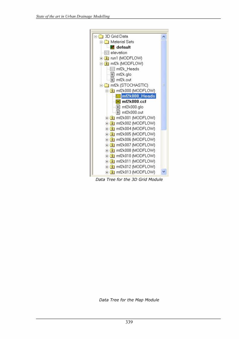
State of the art in Urban Drainage Modelling
339
Data Tree for the 3D Grid Module
Data Tree for the Map Module

State of the art in Urban Drainage Modelling
340
6.2.4. Input and Output procedures
6.2.4.1 Possible Input File(s) Formats In GMS v4.0, importing data from external sources is easier than ever due to the new Import Wizard. In previous versions of GMS, external data such as scatter point, observation well, or pumping well were imported by putting the data into a carefully formatted tabular text file and saving the file using a pre-defined file extension (such as *.sp2 for 2D scatter point data). These files were then imported to GMS using the Import command. In version 4.0, all of these data types can be exported using a simple text file with a *.txt extension or they can be pasted into GMS directly from the clipboard. The only requirement is that the text data be in a tabular (row-column) format. Text files are opened using the Open command in the File menu. Text data can be copied from external applications such as Word or Excel. In either case, GMS launches the Import Wizard once it is detected that the incoming data are in text format. The Import Wizard first allows the user to indicate the locations of the rows and columns:
(Click image for larger view)
First page of Text Import Wizard
The user then indicates the type of data being imported and allows the user to identify each of the columns in the data. Finally, the user is given the option to perform a coordinate conversion (such as from UTM to state plane coordinates) on the new data to ensure that the coordinate system for the new data matches the current project coordinate system.

State of the art in Urban Drainage Modelling
341
GMS v4.0 supports a new utility called the Database Import Wizard for importing borehole, scatter point, and observation point data from any external database. The Wizard is launched using the Import Database command in the File menu. The wizard uses the ODBC drivers included as part of the Windows OS to link to any Oracle or Access database. In the first step of the Wizard, the user links to an external database. In the next step, the user enters an SQL query to extract the desired records from the database. Frequently used queries can be saved for future use.
(Click image for larger view.)
Sample SQL query in the Database Import Wizard

State of the art in Urban Drainage Modelling
342
In the final steps, the user specifies the type of data being imported and then links the columns in the table resulting from the SQL query to recognized fields in the GMS data structure. These linkings can also be saved for future use.
6.2.4.2 Raw Data Formatting No information about Raw Data Formatting are available by now.
6.2.5. Theoretical framework Overview Stochastic Modeling One of the most exciting new features in GMS v4.0 is a suite of tools for performing stochastic simulations with MODFLOW. Two approaches are supported for setting up stochastic simulations: parameter randomization and indicator simulation. Parameter Randomization With the parameter randomization approach, the modeler first identifies a set of target parameters that will be varied during the stochastic simulation. These parameters generally correspond to polygonal zones of hydraulic conductivity or recharge, but could include such things as conductance at rivers or the maximum evapotranspiration rate. The parameters are defined using the same process that is used to define parameters for automated parameter estimation. For each model run, the selected parameters are randomized to produce a candidate set of parameters that is equally probable to other parameter sets in the stochastic simulation. The randomized parameters are combined using either a "Monte Carlo" or a "Latin Hypercube"
State of the art in Urban Drainage Modelling
343
approach. With the Monte Carlo approach, the parameters are combined in a purely random manner. With the Latin Hypercube approach, the parameters are combined in way that ensures that parameter space is explored as fully as possible given a relatively small number of runs. Indicator Simulations Rather than randomizing parameters, the indicator simulation approach randomizes the spatial distribution of the parameter zones. This is typically accomplished by transition probability geostatistics to generate N candidate model grids where each grid has an indicator value or material id assigned to it. These candidate indicator distributions are generally conditioned to borehole data, and each distribution represents an equally probable interpolation of the hard data at the boreholes. Setting up a Stochastic Simulation Stochastic simulations are extremely easy to set up. First of all, the "Stochastic Simulation" option should be selected in the "Run Options" section of the Global Options Dialog. The general stochastic simulation options are then selected in the Stochastic Options dialog.
With the Latin Hypercube or Monte Carlo approach, the user then defines a set of parameters. Each parameter is then marked for use with the stochastic simulation using the Parameters dialog. A mean value and a standard deviation is also assigned to each parameter and a linear, normal, or log-normal distribution is selected. For the Latin Hypercube method, a number of segments must also be assigned to each parameter. With the Material Set (indicator simulation) approach, the TPROGS software must be run to set up a set of N material sets or HUF array sets. Once a stochastic simulation is set up, the user simply selects the Run MODFLOW command and all N simulations are automatically executed sequentially. GMS includes an option to save then entire set of input files, or to only save the solution files (in order to preserve disk space) for each run. When the simulation is finished, the Read Solution command reads in all N simulations at once and loads them into a separate folder on the GMS Data Tree. Post-Processing Once a stochastic run is imported into GMS, contours or pathlines for each solution can be viewed simply by clicking on each of the solutions listed in the data tree. GMS v4.0 also
State of the art in Urban Drainage Modelling
344
supports a Risk Analysis Wizard that can be used to perform probabilistic threshold analyses or probabilistic capture zone delineation. Transport Simulations When running a transport simulation, GMS v4.0 checks to see if the current flow solution corresponds to a stochastic simulation. If so, the transport model is automatically launched once for each of the N flow solutions. The stochastic transport solution can be imported to GMS for post-processing. The Risk Analysis Wizard can then be used to perform probabilistic threshold analyses on the computed concentrations. The Risk Analysis Wizard is generally used in conjunction with the new stochastic modeling tools in GMS v4.0. When a stochastic solution is read into GMS, the solutions associated with the individual runs are placed in the GMS Data Tree in a separate folder. When the user right clicks on this folder, one of the options in the resulting pop-up menu is "Risk Analysis Wizard". Clicking on this option launches the Risk Analysis Wizard. The first step in the wizard is to select the type of analysis. Two types are currently supported: probabilistic threshold analysis and probabilistic capture zone delineation. Probabilistic Threshold Analysis The probabilistic threshold analysis option is designed primarily for use with results from transport simulations. With this option, the user is allowed to enter a set of rules based on whether the value of a particular data set is less than, equal to, or greater than some threshold value. For example, the user could set a rule representing TCE concentration less than some level stipulated by a regulatory agency. Multiple rules can be created if desired.
Once the rules are set up, GMS parses through the solutions in the selected folder and computes a new data set representing the probability that the rules were satisfied. This data set is added to the selected folder and can be contoured like any other data set. A sample probability distribution is shown below:

State of the art in Urban Drainage Modelling
345
Probability of exceeding a threshold concentration of chromium for a selected time step from a stochastic MT3D solution. Probabilistic Capture Zone Delineation The probabilistic capture zone delineation option is used with MODFLOW solutions. One of the drawbacks of capture zones developed by the traditional particle tracking approach with MODFLOW and MODPATH is that the capture zone is often developed from only one realization of the aquifer stratigraphy which may or may not be correct. The Risk Analysis Wizard in GMS v4.0 can be use a set of solutions from a stochastic MODFLOW run to develop a capture zone risk map with contours representing the probability of capture. To develop a visual capture zone risk map, a "capture frequency" array is generated with one entry for each cell and the array values are all initialized to zero. A particle tracking analysis with MODPATH is then run using the results from each of the MODFLOW solutions from the stochastic run. For each MODPATH run, a particle is placed at the center of each cell and is tracked forward in time. If a particle is captured by a well, the entry in the capture frequency array corresponding to the cell where the particle originated is incremented. The number of "captures" for each cell is then divided by the total number of MODPATH runs to give a percentage representing the probability of capture. These percentages are contoured as a capture zone risk map.
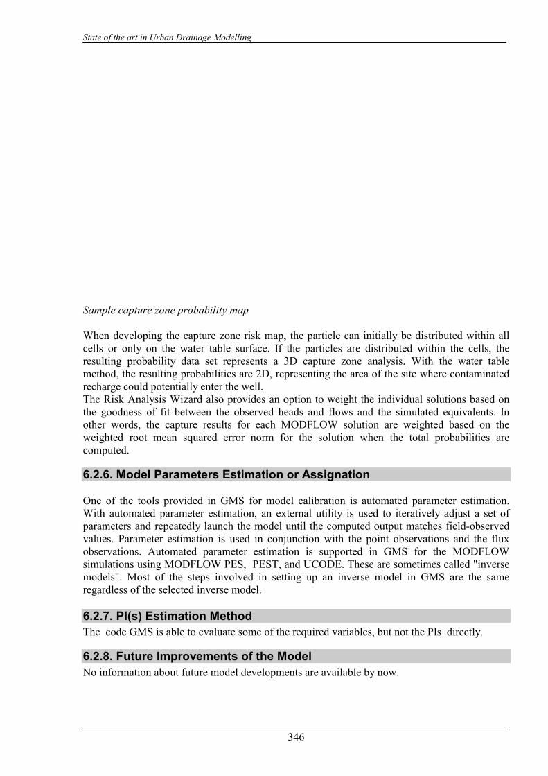
State of the art in Urban Drainage Modelling
346
Sample capture zone probability map When developing the capture zone risk map, the particle can initially be distributed within all cells or only on the water table surface. If the particles are distributed within the cells, the resulting probability data set represents a 3D capture zone analysis. With the water table method, the resulting probabilities are 2D, representing the area of the site where contaminated recharge could potentially enter the well. The Risk Analysis Wizard also provides an option to weight the individual solutions based on the goodness of fit between the observed heads and flows and the simulated equivalents. In other words, the capture results for each MODFLOW solution are weighted based on the weighted root mean squared error norm for the solution when the total probabilities are computed.
6.2.6. Model Parameters Estimation or Assignation
One of the tools provided in GMS for model calibration is automated parameter estimation. With automated parameter estimation, an external utility is used to iteratively adjust a set of parameters and repeatedly launch the model until the computed output matches field-observed values. Parameter estimation is used in conjunction with the point observations and the flux observations. Automated parameter estimation is supported in GMS for the MODFLOW simulations using MODFLOW PES, PEST, and UCODE. These are sometimes called "inverse models". Most of the steps involved in setting up an inverse model in GMS are the same regardless of the selected inverse model.
6.2.7. PI(s) Estimation Method The code GMS is able to evaluate some of the required variables, but not the PIs directly.
6.2.8. Future Improvements of the Model No information about future model developments are available by now.
State of the art in Urban Drainage Modelling
347
6.2.9. References Anderman, E.R.& Hill, M.C., MODFLOW-2000, THE U.S. GEOLOGICAL SURVEY MODULAR GROUND-WATE MODEL-DOCUMENTATION OF THE HYDROGEOLOGIC-UNIT FLOW (HUF) PACKAGE, USGS, Denver, CO, 2000. Carle, Steven F., T-PROGS: Transition Probability Geostatistical Software Version 2.1, Hydrologic Sciences Graduate Group University of California, Davis, 1999. Clough, R. W., and J. L. Tocher, (1965), Finite element stiffness matrices for analysis of plates in bending, Proc. Conf. Matrix Methods in Structural Mechanics, Wright-Patterson A.F.B., Ohio, Air Force Flight Dynamics Lab., Research and Technology Division, Air Force Systems Command, The Air Force Institute of Technology, Air University, pp. 515-545. Davis, J.C., (1986), Statistics and Data Analysis in Geology, John Wiley & Sons, New York, 550p. Deutsch, C.V., & A.G. Journel, (1992), GSLIB: Geostatistical Software Library and User's Guide, Oxford University Press, New York, 340 p. Franke, R. & G. Nielson, (1980), "Smooth interpolation of large sets of scattered data," International Journal for Numerical Methods in Engineering, Vol. 15, pp. 1691-1704. Franke, R., (1982), "Scattered data interpolation: tests of some methods", Mathematics of Computation, Vol. 38, No. 157, pp. 181-200. Harbaugh, A., Banta, E.R., Hill, M.C., & McDonald, M.G., MODFLOW-2000, THE U.S. GEOLOGICAL SURVEY MODULAR GROUND-WATER MODEL-USER GUIDE TO MODULARIZATION CONCEPTS AND THE GROUND-WATER FLOW PROCESS, USGS, Reston, VA, 2000. Heine, G. W., (1986), "A controlled study of some two-dimensional interpolation methods", COGS Computer Contributions, Vol. 2, No. 2, pp. 60-72. Jones, N. L., (1990), Solid Modeling of Earth Masses for Applications in Geotechnical Engineering, Ph.D. Dissertation, The University of Texas at Austin, 324 p. Journel, A.G., & Huijbregts, C.J., (1978), Mining geostatistics. Academic Press, New York, NY. Lam, N.S., (1983), "Spatial interpolation methods: a review", The American Cartographer, Vol. 10, No. 2, pp. 129-149. Lancaster, Peter and Kestutis Salkauskas, (1986), Curve and Surface Fitting, Academic Press, London, 280 pp. Lin, H.C., D.R. Richards, G.T. Yeh, J.R. Cheng, H.P. Chang, N.L. Jones, (1996), FEMWATER: A Three-Dimensional Finite Element Computer Model for Simulating Density Dependent Flow and Transport, U.S. Army Engineer Waterways Experiment Station Technical Report, 129 p.
State of the art in Urban Drainage Modelling
348
McDonald, M.G., & A.W. Harbaugh, (1988), A modular three-dimensional finite-difference ground-water flow model, Techniques of Water Resources Investigations 06-A1, United States Geological Survey. Moore, David S., (1995), The basic principles of statistics, W.H. Freeman and Company, New York. Olea, R.A., (1974), "Optimal contour mapping using universal kriging." J. Geophys. Res., Vol. 79, No. 5, pp. 695-702. Owen, S.J., (1992), An implementation of natural neighbor interpolation in three dimensions, Master's Thesis, Brigham Young University, 119 p. Philip, G.M., & D.F. Watson, 1986, "Comment on 'comparing splines and kriging'", Computers and Geosciences, Vol. 12, No. 2, pp. 243-245. Pollock, D.W., (1994), User's Guide for MODPATH/MODPATH-PLOT, Version 3: A particle tracking post-processing package for MODFLOW, the U.S. Geological Survey finite difference ground-water model, U.S. Geological Survey, Open-File Report 94-464, Reston, Virginia, Sept., 1994. Prudic, David E., (1989), Documentation of a computer program to simulate stream-aquifer relations using a modular, finite-difference, ground-water flow model, USGS Open-File Report 88-729, Carson City, Nevada. Royle, A. G., F. L. Clausen, & P. Frederiksen, (1981), "Practical universal kriging and automatic contouring", Geo-Processing, Vol. 1, No. 4, pp. 377-394. Shepard, D., (1968), "A two dimensional interpolation function for irregularly spaced data," Proc. 23rd National Conference of the ACM, pp. 517-523. Sibson, R., (1981), "A brief description of natural neighbor interpolation," Interpreting Multivariate Data, John Wiley & Sons, New York, pp. 21-36. Watson, D. F. and G. M. Philip, (1985), A refinement of inverse distance weighted interpolation, Geo-Processing, Vol., 2, No. 4, pp. 315-327. WES, (1994), FEMWATER Reference Manual, U.S. Army Engineer Waterways Experiment Station. Wingle, W.L., E.P. Poeter and S.A. McKenna, (1995), UNCERT User's Guide: A Geostatistical Uncertainty Analysis Package Applied to Groundwater Flow and Contaminant Transport Modeling, Colorado School of Mines. http://uncert.mines.edu/. Yeh, G.T., S.S. Hansen, B. Lester, R. Strobl, J. Scarbrough, (1992), 3DFEMWATER/3DLEWASTE: Numerical Codes for Delineating Wellhead Protection Areas in Agricultural Regions Based on the Assimilative Capacity Criterion, U.S. Environmental Protection Agency.
State of the art in Urban Drainage Modelling
349
Zheng, C., Wang, P., (1998), "MT3DMS: A Modular Three-Dimensional Multispecies Transport Model for Simulation of Advection, Dispersion and Chemical Reactions of Contaminants in Groundwater Systems." University of Alabama.

State of the art in Urban Drainage Modelling
350
7 URBAN DRAINAGE MODELS: USER INTERFACE / PRE- AND POST-PROCESSORS
7.1 INTRODUCTION The purpose of this survey is to describe the UI modules of the urban drainage modelling software and to evaluate their graphical and pre- and post-processing capabilities to provide PIs associated with the CARE-S project. It addresses issues such as product features, software requirements, data input and output as well as visualisation and animation capabilities.
7.2 MOUSE: Modelling of urban sewers
7.2.1. Interfaces and processors for MOUSE Windows 95/98 User Interface With MOUSE 4.01 DHI is introducing a new standard for the user interface for dynamic numerical models. MOUSE 4.01 is the first serious urban sewer modelling tool which gives true Windows 95/98 look-and-feel. The new MOUSE 4.01 is a result of the co-operation over the last couple of years between programmers and engineers from DHI and Hydroinform from the Czech Republic. This co-operation is now being extended to other DHI Software products as well through the MIKE Zero project. 32 Bit Architecture and Speed MOUSE 4.01 is a 100% 32 Bit application designed specifically for Windows 95/98 and Windows NT 4.0. This implies that the code is optimised for fast simulations and fast graphics. Put it on a PC with a Pentium Pro chip and see MOUSE fly. MOUSE 4.01 also includes the speed optimising features of MOUSE 3.3, including the variable time step feature. The resulting total increase in performance is stunning! New Network Editors The user interface for MOUSE 4.01 has been designed for maximum flexibility and ease of use. Data can be viewed and edited with the completely new graphical editors, which are part of MOUSE 4.01. Or data can be entered and edited through the carefully designed standard forms, which include scrollable spreadsheet like sections for efficient editing of tabulated data. These different editors or ‘views’ of the same information are of course fully linked, so that changes introduced through one editor are automatically and instantly updated in the other ‘views’. MOUSE 4.01 uses a database tool for storage of the network data. This gives access to a range of powerful query facilities, including a ‘query by example’ option. MIKE View 1.44

State of the art in Urban Drainage Modelling
351
The result viewer for MOUSE 4.01 is identical to the latest version of MIKE View. MIKE View is also maintained as an inexpensive stand-alone tool. The use of MIKE View as a ‘multi-media’ reporting tool is catching on: More and more consultants are including simulation result files together with a MIKE View in their final report to their clients. For that reason, MIKE View is now also available in ‘bundles’ at even lower prices. MIKE View release 1.44, which is part of MOUSE 4.01, includes a number of important new features compared to the previous releases: - DXF and BMF single files (eg with a street map) can be imported and used as background graphics - Simulation results can be copied directly to Microsoft Excel and Word - It is now possible to access more result files simultaneously - Flooding (water depths and pressure heights) can be shown and animated in the plan drawing - The colour palette is now user configurable. MIKE Print The presentation graphics editor in MOUSE 4.01 is called MIKE Print. MIKE Print is a plot composition tool specifically aimed at the design of report drawings of simulation results from MOUSE and MIKE 11. With MIKE Print one the user can compose a page with different types of graphical output (network drawings, time series, etc), preview the result on the computer display and then send it to a printer, when it is satisfactory. Taylor-made page layouts can be saved and reused, eg for a series of production simulations. MIKE Animator MIKE Animator produces 3D animations in a number of industry standard file formats, such as *.mpg, *.avi, *.flc and separate frames in freely configurable resolutions. MIKE Animator works on result data from the DHI Software products MIKE 21 and MIKE 11. Additional products will be included in the subsequent releases of MIKE Animator. 7.2.2. MOUSE GIS - the GIS Interface for MOUSE/ArcView MOUSE GIS is an application linking the capabilities of the numerical sewer modelling system MOUSE with the well-known Geographic Information System (GIS) ArcView developed by Environmental Systems Research Institute (ESRI) for managing, analysing and displaying geographic data and related information. MOUSE GIS works in the ArcView environment and consists of two parts: the Network Editor and the Results Presentation. Both parts support the general features available in ArcView. The Network Editor allows the user to extract data from a number of different asset manage-ment systems, to condense the network automatically and still maintain consistency in the des-cription of the physical system - and finally to store the data as a model for further analysis in MOUSE. The decisions in the simplification process made by the program are based on user-specified criteria, like: maximum pipe diameter, minimum pipe diameter, unaltered hydraulic

State of the art in Urban Drainage Modelling
352
resistance, etc. All changes are recorded on a separate file, which can later be replayed if the user wants to repeat the process after changes in the asset management system. The Results Presentation allows the user to present results from the fully dynamic MOUSE simulations combined with other GIS data. CSO points and volumes and exceedence of critical levels can, for instance, quickly be identified. By direct access to asset management databases, the simulation results can also be visualised in combination with parameters describing the actual condition of the sewer system or any other relevant information from the database. The strengths of MOUSE GIS are: - Quick and automatic simplification of sewer network systems - Presentation of combined MOUSE results and GIS data - Import and conversion of sewer network systems from other formats and databases into MOUSE format - Advanced graphical output - Easy-to-use for ArcView users.

State of the art in Urban Drainage Modelling
353
7.3 Other DHI software
7.3.1. MIKE 11 GIS- the GIS Interface for MIKE 11 using ArcView MIKE 11 GIS merges the technologies of numerical river modelling and Geographic Informat-ion Systems (GIS). It is developed as a fully integrated interface in the well-known and established ArcView GIS. MIKE 11, developed by the Danish Hydraulic Institute, is a package for the simulation of surface runoff, flow, water quality and sediment transport in channels, rivers and flood plains. ArcView GIS is developed by Environmental Systems Research Institute (ESRI). The flood maps produced by MIKE 11 GIS are generated applying an automatic and highly efficient interpolation routine. From a series of flood maps MIKE 11 GIS generates a highly visual video animation perfectly suited for presentation purposes. MIKE 11 GIS outputs also graphs of water level time series, terrain and water level profiles and flood zone statistics. Statistics can directly be imported into a word processor or spreadsheet. MIKE 11 GIS is ideally suited as a spatial decision support tool for river and flood plain management. To develop a MIKE 11 GIS application, essential information comprising a MIKE 11 river network, a MIKE 11 simulation and a Digital Elevation Model (DEM) is required. For further analysis, information such as maps/themes of rivers, infrastructure, land use, satellite/radar images and other spatial data can be included. The river network of a MIKE 11 model is geo-referenced in MIKE 11 GIS through the Branch Route System (BRS). Linking a MIKE 11 Result file to the BRS, MIKE 11 GIS produces three types of flood maps. These are depth/area inundation, duration and comparison/impact flood maps. The MIKE 11 GIS topographical module facilitates accurate and automatic extraction of flood plain topography (flood plain cross-sections and area elevation relations) from the DEM. The extracted flood plain topography can readily be imported into a MIKE 11 cross section database. The strengths of MIKE 11 GIS are: - Automatic generation and editing of DEM - Highly visual outputs (flood maps, video animations, time series, profiles and flood statistics) - Easy overlap with other geographical data - Extraction of flood plain topography - Online help system and comprehensive User Tutorial.

State of the art in Urban Drainage Modelling
354
7.4 SWMM: Storm Water management model
7.4.1. Interfaces and processors for SWMM State-of-the-art graphical user interfaces are available from third-party vendors. Most of these GUIs are constructed around the core Fortran code of the OSU model version. PCSWMM A menu-driven interface for running the model and providing hydro/pollutographs and animated hydraulic gradelines, plus sensitivity analysis and GIS options. Charge: <$400. Dr. William James or Mr. Rob James Computational Hydraulics International (CHI) 36 Stuart St. Guelph, Ontario N1E 4S5 Phone: (519) 767-0197 * FAX:(519) 767-2770 Web:www.chi.on.ca MTVE - Model Turbo-View Mainly a post-processor for Extran, including the ability to show the dynamic movement of the hydraulic grade line. Charge: <$1,000. contact: 10 Brooks Software c/o Mark TenBroek 3744 West Huron River Drive Suite 200 Ann Arbor, Michigan 48103 Phone or fax: (313) 761-1511 e-mail: [email protected] XP-SWMM or Visual SWMM A complete graphical user interface and post-processor for SWMM. Charge: varies but in the range of $4,000. Contact: XP Software 2000 NE 42 Ave., Suite 214 Portland, Oregon 97213 Phone: (888) 554-5022 FAX: (888) 554-5122 e-mail: [email protected] Also offered as Visual SWMM or Visual Hydro through: CAiCE Software Corporation 410 Ware Blvd., Suite 1200 Tampa, Florida 33619-9019 Phone: (800) 883-3487 or (813) 620-1444 FAX: (813) 620-9019 e-mail: [email protected]

State of the art in Urban Drainage Modelling
355
MIKE-SWMM The Danish Hydraulic Institute has a general GUI for the Runoff and Extran Blocks, called MIKE-SWMM, based on the DHI MOUSE model interface. Imagine the power and accuracy of the most widely applied hydraulic model enhanced with a user-friendly interface and leading-edge simulation and visualization capabilities. MIKE SWMM brings to your desktop the model-of-choice in North America for stormwater and wastewater systems (SWMM) and the user interface-of-choice in the world for stormwater and wastewater modeling (MIKE). The result of this powerful combination is a world-class, versatile, cost-effective modeling package for the accurate and reliable analysis of stormwater and wastewater systems, with a user interface that tremendously enhances productivity. MIKE SWMM 1999b and Service Pack 2 for MIKE SWMM 1999 are available for download. SP2 contains file updates to the June 1999 release of MIKE SWMM. Updates include longer node and conduit names and drawing profiles through flap gates. It is possible to download a copy of XP2MSWMM 1.03, a tool for converting XP-SWMM data sets to SWMM format. Price is in the range of $4,000. Contact: DHI, Inc. Eight Neshaminy Interplex, Suite 219 Trevose, Pennsylvania 19053 Phone: (215) 244-5344 Fax: (215) 244-9977 Web: http://www.mikeswmm.com/
7.4.2. CAiCE Software Visual Hydro Visual Hydro is a graphics-based stormwater and wastewater decision support system. It is used to model the full hydrological cycle, including stormwater and wastewater quality, build-up/wash-off, the treatment of stormwater and sanitary sewer flows, and Best Management Practice (BMP) analysis. Visual Hydro is composed of Visual Manage Visual Hydro Manager Visual SWMM Water Quality modules.
7.4.2.1 Modelling tools for Visual Hydro The Modeling Tools add-on for Visual Hydro integrates drainage and water resource engineering automation with the high-precision geometric modeling and digital terrain modeling capabilities of CAiCE. The Modeling Tools package adds the Visual COGO, Visual DTM, and Visual Site modules to Visual Hydro. Combined, these tools vastly increase the power and flexibility of the system. Visual COGO With CAiCE Visual COGO you can define the precise placement of geometric elements that are used to model the shapes and locations of drainage networks, land boundaries, utility locations, ponds, roads and highways, and other features of interest to the water resource engineer. These elements play key roles in the drainage design and analysis process. For example, the geometric layout of drainage networks can be defined using COGO points and chains. Chains and profiles can be used by Visual Hydro to perform hydrology and inlet spread analysis.
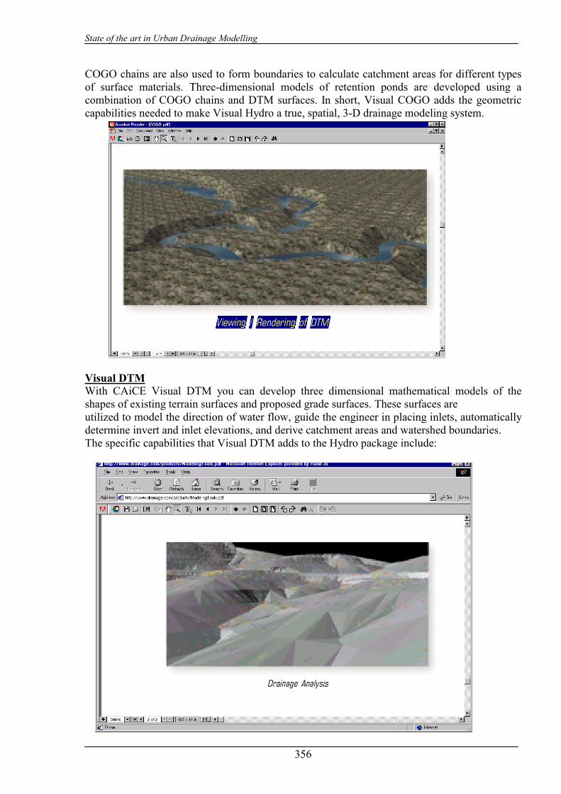
State of the art in Urban Drainage Modelling
356
COGO chains are also used to form boundaries to calculate catchment areas for different types of surface materials. Three-dimensional models of retention ponds are developed using a combination of COGO chains and DTM surfaces. In short, Visual COGO adds the geometric capabilities needed to make Visual Hydro a true, spatial, 3-D drainage modeling system.
Visual DTM With CAiCE Visual DTM you can develop three dimensional mathematical models of the shapes of existing terrain surfaces and proposed grade surfaces. These surfaces are utilized to model the direction of water flow, guide the engineer in placing inlets, automatically determine invert and inlet elevations, and derive catchment areas and watershed boundaries. The specific capabilities that Visual DTM adds to the Hydro package include:
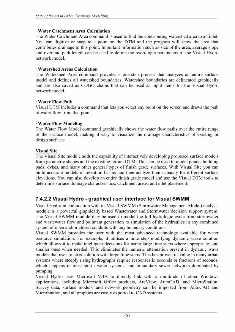
State of the art in Urban Drainage Modelling
357
· Water Catchment Area Calculation The Water Catchment Area command is used to find the contributing watershed area to an inlet. You can digitize or snap to a point on the DTM and the program will show the area that contributes drainage to this point. Important information such as size of the area, average slope and overland path length can be used to define the hydrologic parameters of the Visual Hydro network model. · Watershed Areas Calculation The Watershed Area command provides a one-step process that analyzes an entire surface model and defines all watershed boundaries. Watershed boundaries are delineated graphically and are also saved as COGO chains that can be used as input items for the Visual Hydro network model. · Water Flow Path Visual DTM includes a command that lets you select any point on the screen and draws the path of water flow from that point. · Water Flow Modeling The Water Flow Model command graphically shows the water flow paths over the entire range of the surface model, making it easy to visualize the drainage characteristics of existing or design surfaces. Visual Site The Visual Site module adds the capability of interactively developing proposed surface models from geometric shapes and the existing terrain DTM. This can be used to model ponds, building pads, dykes, and many other general types of finish grade surfaces. With Visual Site you can build accurate models of retention basins and then analyze their capacity for different surface elevations. You can also develop an entire finish grade model and use the Visual DTM tools to determine surface drainage characteristics, catchment areas, and inlet placement.
7.4.2.2 Visual Hydro - graphical user interface for Visual SWMM Visual Hydro in conjunction with its Visual SWMM (Stormwater Management Model) analysis module is a powerful graphically based Wastewater and Stormwater decision support system. The Visual SWMM module may be used to model the full hydrologic cycle from stormwater and wastewater flow and pollutant generation to simulation of the hydraulics in any combined system of open and/or closed conduits with any boundary conditions. Visual SWMM provides the user with the most advanced technology available for water resource simulation. For example, it utilises a time step modifying dynamic wave solution which allows it to make intelligent decisions for using large time steps where appropriate, and smaller ones when needed. This eliminates the numeric attenuation present in dynamic wave models that use a matrix solution with large time steps. This has proven its value in many urban systems where steeply rising hydrographs require responses in seconds or fractions of seconds, which happens in most storm water systems, and in sanitary sewer networks dominated by pumping. Visual Hydro uses Microsoft VBA to directly link with a multitude of other Windows applications, including Microsoft Office products, ArcView, AutoCAD, and MicroStation. Survey data, surface models, and network geometry can be imported from AutoCAD and MicroStation, and all graphics are easily exported to CAD systems.
State of the art in Urban Drainage Modelling
358
7.4.2.3 Visual Hydro Pro (Professional, water quality included) - professional graphical user interface for Visual SWMM
CAiCE Visual Hydro Pro is the most comprehensive storm water and wastewater management model available. It couples CAiCE's DTM, and visualization capabilities with the most advanced hydrology and hydraulics capabilities available (in the Visual SWMM module). CAiCE Visual Hydro Pro is a complete software package that combines. Visual DTM - an advanced digital terrain manager Visual SWMM - with a comprehensive hydrology/hydraulics package Visual Site.
Using this integrated package the 2-dimensional and 3-dimensional data representing the watershed is intimately connected to the hydrology and hydraulics analysis. The drainage network is generated from either survey or geometry chains in Visual Hydro Pro with the generated data consisting of invert elevations, ground elevations, and conduit lengths. Visual Hydro Pro can then show the simulation results as 2 and 3-dimensional profiles embedded in the DTM. It is both a revolutionary and evolutionary new means of designing and analysing storm and sewer networks.
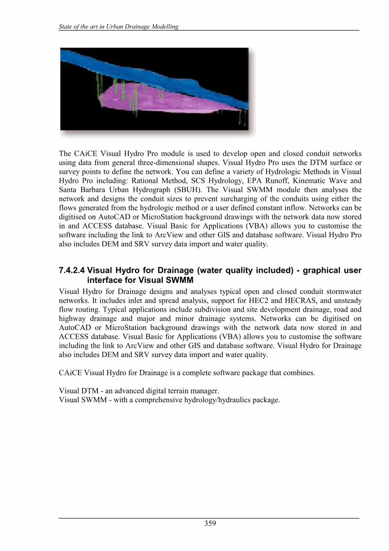
State of the art in Urban Drainage Modelling
359
The CAiCE Visual Hydro Pro module is used to develop open and closed conduit networks using data from general three-dimensional shapes. Visual Hydro Pro uses the DTM surface or survey points to define the network. You can define a variety of Hydrologic Methods in Visual Hydro Pro including: Rational Method, SCS Hydrology, EPA Runoff, Kinematic Wave and Santa Barbara Urban Hydrograph (SBUH). The Visual SWMM module then analyses the network and designs the conduit sizes to prevent surcharging of the conduits using either the flows generated from the hydrologic method or a user defined constant inflow. Networks can be digitised on AutoCAD or MicroStation background drawings with the network data now stored in and ACCESS database. Visual Basic for Applications (VBA) allows you to customise the software including the link to ArcView and other GIS and database software. Visual Hydro Pro also includes DEM and SRV survey data import and water quality.
7.4.2.4 Visual Hydro for Drainage (water quality included) - graphical user interface for Visual SWMM
Visual Hydro for Drainage designs and analyses typical open and closed conduit stormwater networks. It includes inlet and spread analysis, support for HEC2 and HECRAS, and unsteady flow routing. Typical applications include subdivision and site development drainage, road and highway drainage and major and minor drainage systems. Networks can be digitised on AutoCAD or MicroStation background drawings with the network data now stored in and ACCESS database. Visual Basic for Applications (VBA) allows you to customise the software including the link to ArcView and other GIS and database software. Visual Hydro for Drainage also includes DEM and SRV survey data import and water quality. CAiCE Visual Hydro for Drainage is a complete software package that combines. Visual DTM - an advanced digital terrain manager. Visual SWMM - with a comprehensive hydrology/hydraulics package.

State of the art in Urban Drainage Modelling
360
7.5 Other CAiCE Software
7.5.1. Visual Culvert - graphical user interface for hydraulic design of highway culverts
Visual Culvert is an interactive, software system used for designing and analysing culverts under roads and highways. It is designed to help highway and drainage engineers analyse and improve existing culverts, and to develop the best possible design for new culverts. It provides easy-to-use tools that define the culvert conditions, simulate water flows, and determine the best inlet types and conduit shapes and sizes. Visual Culvert uses industry standard methodologies that have been defined by the FHWA. CAiCE Visual Culvert extends and supplements the wide range of water resource modeling and engineering capabilities found in CAiCE Visual Hydro. Visual Culvert also includes 20 examples that are built into the interface to make it easy to learn and follow. There is an extensive online Help system and a series of culvert tutorials to get you up and running as quickly as possible. Visual Culvert computes performance and optimization curves, taking into consideration culvert flow as well as roadway overtopping and culvert end treatments such as inlet type, mitered, and tapered design. Several methods can be used for water flow calculations including the Rational Method, SCS Hydrology, IDF curves and USGS Regression equations. Visual Culvert is based on the FHWA (1985) book: "Hydraulic Design of Highway Culverts" and the Environmental Protection Agencies (EPA) Stormwater Management Model (SWMM). Visual Culvert provides easy tools for editing simulation data. Results can be viewed in various types of charts, graphs, and spreadsheets. It includes eight culvert shapes, upstream detention pond routing with weir and orifice outflow, and a multitude of downstream boundary conditions including free outfall, fixed backwater, rectangular, trapezoidal, and natural channel. The output report files are in HY8 format. The culvert design data is saved to a Microsoft Access database for easy retrieval and Microsoft Office compatibility.
7.5.2. Visual CADLinks for AutoCAD CAiCE for AutoCAD gives the user all of the modeling and computational power of CAiCE Visual 2000 product line combined with the graphics and CAD capabilities of AutoCAD 2000. This product line uses our exciting Visual CADLinks technology that lets you dynamically link CAiCE to the CAD system of your choice. CAiCE for AutoCAD gives you the best of both worlds. It includes all of the features, menus, toolbars, capabilities, and graphics power found in the standalone CAiCE products, but can also use AutoCAD as its graphics engine for viewing objects, creating drawings, and for snapping and digitising operations. CAiCE for AutoCAD runs CAiCE and AutoCAD simultaneously side by side, with both systems linked together. While AutoCAD has a working DWG file open, CAiCE also has access to its own project database. Simple toolbar functions let you control whether to produce CAiCE graphics in the AutoCAD window, the CAiCE window, or both simultaneously. If you like, you can collapse the CAiCE application window to show only the menus and toolbars, leaving all of the graphics to AutoCAD. Or you can take advantage of CAiCE’s graphics speed and rendering capabilities for visualization and drivethrough capabilities.
State of the art in Urban Drainage Modelling
361
Whenever you view objects in CAiCE, it creates new AutoCAD elements in the working DWG file. All of the feature tables and display settings in CAiCE are still active, so attributes like layer name, colour, line weight and style, font, and text size are assigned automatically based on the type of object and its feature code. Furthermore, you can still use all of the features and capabilities of AutoCAD to add and change CAD elements. CAiCE will not touch DWG objects created in AutoCAD; only those originating from CAiCE. You can also select 2-D and 3-D elements created in AutoCAD and bring them into the CAiCE database as geometry objects. For geometric layout and definition you can combine the computation-based Visual COGO module with the ease of AutoCAD graphical tools.

State of the art in Urban Drainage Modelling
362
7.6 XP SOFTWARE http://www.xpsoftware.com/ XP Software Australia XP Software USA XP Software Canada
7.6.1. XP-SWMM2000 - Stormwater and Wastewater Management Model Applications - Design and analysis of stormwater, sewer and wastewater projects Hydrology - Various Linear and Non-Linear methods Hydraulics - Dynamic Equation hydraulics (St Venants equations)

State of the art in Urban Drainage Modelling
363
State of the art in Urban Drainage Modelling
364
7.6.2. Other XP Software
7.6.2.1 XP-UDD2000 - Urban and Rural Stormwater Design and Analysis Software
Applications - Design and analysis of stormwater projects including piped and channel flows. Hydrology - Various Linear and Non-Linear methods Hydraulics - Dynamic Equation hydraulics (St Venants equations)
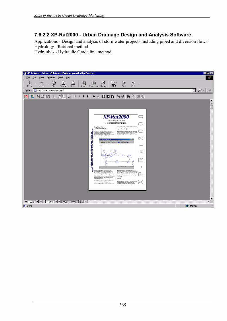
State of the art in Urban Drainage Modelling
365
7.6.2.2 XP-Rat2000 - Urban Drainage Design and Analysis Software Applications - Design and analysis of stormwater projects including piped and diversion flows Hydrology - Rational method Hydraulics - Hydraulic Grade line method

7.6.2.3 XP-Culvert2000 - Culvert Design and Analysis Software Applications - Design, size and analyse new or existing culvert systems. Hydrology - None Hydraulics - Dynamic Equation hydraulics (St Venants equations)

State of the art in Urban Drainage Modelling
367
7.6.2.4 XEC-RAS/12d Model - Terrain Modelling Package XEC-RAS/12d Model is a powerful terrain modelling, surveying and civil engineering package. It allows fast production in a wide variety of projects including roads, site layouts, subdivisions and EIS studies. Using 12d Model’s screen menus and fast interactive graphics, the user effortlessly moves through a design.
With 12d Model’s powerful design capabilities, difficult surveying and civil design tasks can be easily visualized and completed. Projects such as roads, channels, storage tanks, subdivisions, landscaping, rail studies, major pipelines, waste water reticulation and general site works are efficiently handled with 12d Model. 12d Model includes a powerful programming language, which allows users to build their own options from 12d Model’s extensive programming library. 12d Model has been specifically designed for easy use. It is ideal for use at all stages of projects, and is particularly useful for large route selection and corridor studies. 12d Model is an essential tool in today's fiercely competitive business climate.

State of the art in Urban Drainage Modelling
368
7.7 BASINS (Better Assessment Science Integrating Point / Non-point Sources)
http://www.epa.gov/ednnrmrl/projects/products/model2.htm http://www.epa.gov/OST/BASINS/support.htm With the shift of watershed management to local decision makers comes a need for models that can be applied universally. These models must include the broad-based, multiple-function pack-ages that make each watershed-specific application a special circumstance of a general water-shed condition. Although existing models often group multiple features, for example hydraulics and water quality, they address specific parts of the watershed. Individually, they do not represent a com-plete package, but collectively they provide tools to confront many problems commonly presented to local watershed managers. Many individual models leaves the user with a sub-stantial task of selecting among the multiple models and integrating the selected tools. Users need a collection of individual model applications in a single, user-friendly assemblage provid-ing common interface. EPA's Office of Science and Technology in the Office of Water developed the BASINS model collection from existing models, including:
• EPA's Hydrologic Simulation Program-FORTRAN (HSPF) model, which is a compre-hensive package developed for simulating water quantity and quality for a wide range of organic and inorganic pollutants from mixed-land-use watersheds
• QUAL2E, developed to allow analysis of pollutant fate and transport through selected stream systems
• TOXIROUTE, an EPA water quality model that provides a screening-level stream routing model that does simple dilution/decay calculations under mean and low flow conditions.
The BASINS approach, bundling existing models with a common set of provided databases, a GIS overlay and user interface, and data translation tools on a single CD ROM, is practical, well crafted and well considered. The GIS overlay provides not only for data exchange, but, at least as important, provides an information transfer mechanism to non-technical users and the public. A recognized BASINS shortcoming for its implementation in an urban watershed is the limited spatial resolution. While the individual user group can alter the resolution with compatible user-provided themes and databases, the existing resolution is designed for large watersheds. The assessment tool within BASINS, for example, is a statewide analysis. This level closely matches BASINS' primary development goal, meeting Total Maximum Daily Load mandates. Before community groups accept and use BASINS, it must readily adapt to the community's scale of scrutiny.
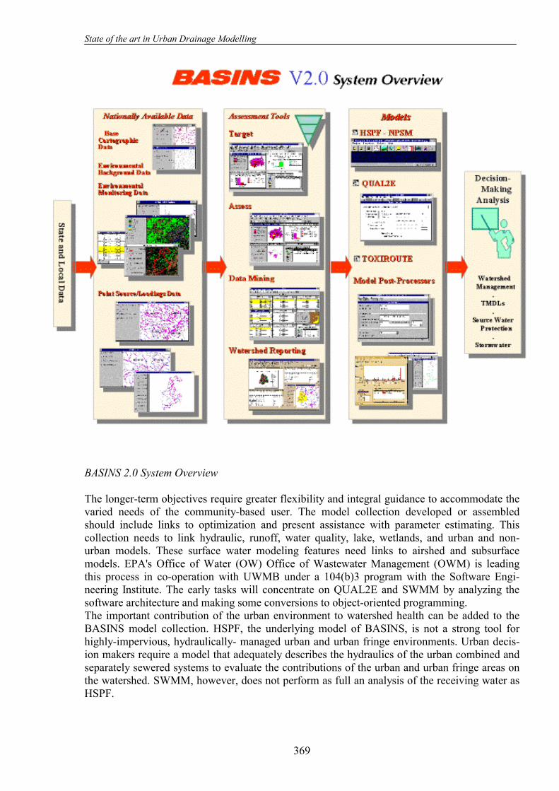
State of the art in Urban Drainage Modelling
369
BASINS 2.0 System Overview The longer-term objectives require greater flexibility and integral guidance to accommodate the varied needs of the community-based user. The model collection developed or assembled should include links to optimization and present assistance with parameter estimating. This collection needs to link hydraulic, runoff, water quality, lake, wetlands, and urban and non-urban models. These surface water modeling features need links to airshed and subsurface models. EPA's Office of Water (OW) Office of Wastewater Management (OWM) is leading this process in co-operation with UWMB under a 104(b)3 program with the Software Engi-neering Institute. The early tasks will concentrate on QUAL2E and SWMM by analyzing the software architecture and making some conversions to object-oriented programming. The important contribution of the urban environment to watershed health can be added to the BASINS model collection. HSPF, the underlying model of BASINS, is not a strong tool for highly-impervious, hydraulically- managed urban and urban fringe environments. Urban decis-ion makers require a model that adequately describes the hydraulics of the urban combined and separately sewered systems to evaluate the contributions of the urban and urban fringe areas on the watershed. SWMM, however, does not perform as full an analysis of the receiving water as HSPF.

State of the art in Urban Drainage Modelling
370
Incorporating SWMM directly into BASINS will be a formidable task. As a precursor to incorporating the SWMM model directly into BASINS, EPA should accomplish a series of intermediate steps. Many municipalities are either in the early stages of municipal data collection or planning for it in the next few years. This suggests now is the time to identify standards for SWMM data collection, generate the format requirements, data maintenance tools, and assure alternate data uses (e.g., fire and police response, emergency management, and property taxes) through common keys. While developing the GIS link, UWMB believes that it is important to assure the integration will be compatible with the BASINS collection and wherever possible use common data sources. As municipal governments begin developing a GIS infrastructure database, often for reasons unrelated to water quality, UWMB should be outlining the concurrent information that munici-palities should measure and document to support water quality and ecosystem-protection needs. Municipalities will more readily collect the necessary information when it can be concurrently collected with other data thereby lessening the incremental costs. The UWMB will begin by defining the necessary information and follow up with quality assurance recommendations. The geo-referenced data elements are of particular interest in this effort.
7.7.1. BASINS 2.0 Features Watershed Delineation Tool -- This tool allows a user to delineate a sub-watershed from within an 8-digit catalog unit using simple PC mouse point-and-click operations. With this tool, a user can target any area within a catalog unit for more detailed modelling and analysis. The watershed delineation tool will work on either RF1 (1:500K) or RF3 (1:100K) stream segments. Avenue script files have been developed to automatically extract geographic information from within the delineated area, which is then re-formatted as input files for use with the NPSM. Routing or RCHRES Module via the Nonpoint Source Model (NPSM) -- The NPSM now can produce a properly formatted input file required to run the Reaches and Reservoirs (RCHRES) module in HSPF. RCHRES is the module that allows a user to simulate both the routing of flows and water quality behavior through a connected network of reaches (this includes streams, rivers, lakes, and reservoirs). Implementation of Pervious/Impervious Land Segment HSPF Modules -- The NPSM now provides a full treatment of the pervious and impervious land segment (PERLND and IMPLND) modules. Snow, sediment, and agricultural chemicals (nitrogen, phosphorous, pesticides, moisture, and tracer) sections were added to the PERLND module; and snow and solids sections to the IMPLND module. Highly advanced tools in HSPF modelling; such as, yield-based nutrient algorithm, and SPECIAL ACTIONS, NETWORK, and MASS-LINK blocks can be created and modified external to the NPSM. RF3 Modelling -- Users can now simulate the routing of flows and water quality behaviour on RF3 (1:100K) hydrography in addition to the original RF1 (1:500K) hydrography. Modelling on RF3 requires user input under the Reach Editor within NSPM. Users input is required due to RF3's lack of rich attribute data such as mean depth, mean width, Manning's n, longitudinal reach slope, and side slopes.

State of the art in Urban Drainage Modelling
371
Reach Editor Tools -- Tools have been added to make it easier to edit the reach network, segment cross-sections, and hydrologic function tables. The reach network visualisation tool creates a stick figure reach network which can be modified by adding, removing, and modifying individual reach segments. A visualisation tool has also been added to facilitate editing the reach cross-section geometry; the default geometry is now more representative of a typical reach channel and flood plain. As in the previous version, the hydrologic function table or F-Table is created automatically with the option to manually edit the final table. The outflow depth relationship can now be viewed graphically with the "click" of a button. Simulate Point Source Contributions in NPSM -- The NPSM previously allowed the user to supply a single constant flow and load from point sources. The NPSM now allows both constant and time variable point sources flows and loads. Time variable loads are input as time series with four options on how to handle missing data, as well as the option to manually edit the data. As previously available the user can add and delete point sources in the Point Sources Set-up as well as apply flow and load multipliers. Post-Processor for HSPF/NPSM output -- The post-processor makes it easier to calibrate the HSPF against monitoring data, compare model runs against water quality standards, and evaluate the relative effect of pollution control scenarios. The post processor allows the user to import stream flow gage data as well as water quality monitoring data in order to calibrate flow and water quality modules in HSPF. Mouse and keyboard controls allow the user to focus in or zoom-out for accurate base flow and peak storm flow comparisons. Statistical plots of the arithmetic and geometric mean at different time steps can be visually compared with a numeric water quality threshold. Separate model runs can be compared visually or compared on a percent differences in load basis. Watershed Characterisation Report -- A new automated reporting function allows the user to produce electronic and hard copies of maps and summary tables for any watershed or user-delineated sub-watershed, by following a few simple instructions. A user may generate reports on STORET water quality data for any water quality parameter at monitoring stations within the study area, and produce a map of the station locations. Similarly, a user can produce a summary of Permit Compliance System discharges and loading of any constituent. Finally a user may produce a summary table of the acreage's of different land use types (classified by either Anderson Level I or Level II land use) in a watershed, plus a map of Anderson Level I land use types. Additional specialised reports include soils data and elevation data. New and Updated Data -- The information in the existing facility data sets (Permit Compliance System - PCS, Toxic Release Inventory - TRI, and Superfund National Priority List - NPL's, Industrial Facility Discharges - IFD) has been updated and expanded, and facilities from the Resource Conservation and Recovery Information System (RCRIS) have been added. In addition, a greatly expanded set of weather station data (WDM files) for the nation are now available. BASINS 2.0 contains significant new data sets as well. These include: STATSGO soils, USEPA Reach File Version 3 Alpha (RF3 Alpha), and DEM elevation data, Federal and Indian land boundaries, Water Quality Observation Data, Ecoregions, Fish and Wildlife Advisories, Shellfish Contamination, and the Clean Water Needs Survey. Local Data Incorporation -- BASINS 2.0 also supports import and use of various locally derived data sets. In addition to standard import routines for viewing data, BASINS 2.0 enables import and use of attribute data for use as input files for the Non-Point Source Model (HSPF). Users can import their own vector data sets such as 5th and 6th field hydrologic basins

State of the art in Urban Drainage Modelling
372
delineation, or new vector-based land use or DEM data sets. Data for BASINS 2.0 have been recompiled to support local data integration. In BASINS 2.0, all existing spatial data is delivered in a decimal degree (unprojected) NAD83 shape file format. ArcView then re-projects these data in any user-specified projection. The user will be prompted to choose a projection upon installation of BASINS 2.0. This enables users to easily integrate data based on their own commonly used projection. Land Use Reclassification Tool -- This tool allows a user to reclassify land use polygons from one land use category into another. For example, a user may reclassify a single land use polygon from agricultural to urban. Similarly, the user may select an area using ArcView's Select Tool and reclassify the selected area into a different land use category. This feature allows a user to weigh the potential significance of land use changes on water quality. Another feature of note, a user can convert an entire land use category into another via a pop-up menu.
7.7.2. BASINS 3.0 Development BASINS 3.0 will provide the user with a choice of watershed models; the Hydrological
Simulation Program--Fortran (HSPF v.12) and the Soil and Water Assessment Tool (SWAT). SWAT simulates hydrology, pesticide and nutrient cycling, bacteria transport, erosion and sediment transport. SWAT is ideally suited to predict effects of land use management (such as climate and vegetative changes, agricultural practices, reservoir management, groundwater withdrawals, water transfer) on water, sediment, and chemical yields from river basins. Both SWAT and HSPF are spatially distributed, lumped parameter models. They may be used to analyze watersheds and river basins by subdividing the area into homogenous parts. SWAT uses a daily time step for simulations running from 1 to 100 years; HSPF, as implemented in BASINS, uses an hourly time step. We anticipate that SWAT will meet many modeling needs for situations where TMDLs need to be developed for watersheds dominated by lands in agricultural operations. BASINS 3.0 will allow the user to delineate watershed boundaries on the basis of predeter-mined digitized boundaries (e.g., 8-, 11-, 14-digit watershed boundaries), by subdividing water-shed polygons with the aid of the mouse (as currently is done in BASINS v. 2.01), or by using the power of the GIS platform to determine the watershed that contributes to a stream based on Digital Elevation Modelling (DEM). The stream network may be determined from DEM or pre-

State of the art in Urban Drainage Modelling
373
existing digitised stream networks (e.g., RF1, RF3, NHD, or the Census Tiger Files) may be overlain and burned in. Once the watershed is spatially described and locations of point source discharges, water withdrawals, and pour point of watershed established, the user can decide which of the watershed models to run to estimate the resultant effect of point and non-point source loading to the receiving waters. The use of raster data requires ArcView's Spatial Analyst Extension (version 1.1). Recognising that some users may not be interested in purchasing this extension, we also will be releasing BASINS v. 2.1 which will provide the full functionality of HSPF through the new GenScn (which will maintain the look and feel of NPSM). However, BASINS v. 2.1 will not support SWAT or the use of DEM or MRLC data in a raster format. New data that will be packaged on BASINS 2.1/3.0 CDs are raster 90 m DEM data and the databases that support SWAT. BASINS 3.0 will perform "on the fly" gridding of existing land use and soils shape files data for use with SWAT. DEM data at 1:24,000 or other scales and the Multi Resolution Land Classification (MRLC) data may be imported and used directly in BASINS 3.0. HSPF v.11 will be replaced by HSPF v.12 which includes a simplified snow melt algorithm (i.e., degree-day approach), the ability to model land-to-land transfers, high water tables and surface ponding (wetlands), and the addition of new BMP and Reporting modules. The new SNOW module requires only precipitation and air temperature time series, while producing essentially the same output as the current module which requires five additional meteorological time series (evaporation, wind speed, solar radiation, dew point, and cloud cover). The features of NPSM, the current interface to HSPF, are being coded into (GenScn) and expanded to provide the full functionality of HSPF (i.e., Special Actions, yield-based nutrient modelling, and air deposition).
Generation and analysis of model simulation scenarios (GenScn), was developed by the U.S. Geological Survey (USGS) to create simulation scenarios, analyze results of the scenarios, and compare scenarios. GenScn provides an interactive framework for analysis built around HSPF for simulating the hydrologic and associated water quality processes on pervious and impervious land surfaces and in streams and well-mixed impoundment's. The GenScn graphical user interface (GUI) uses standard Windows 9x/NT components. This new version of GenScn, an EPA/USGS product, provides for full
State of the art in Urban Drainage Modelling
374
HSPF model set-up, execution, post-processing, display, and analysis. GenScn will also support SWAT output time-series post processing. The GenScn interface to HSPF will also include the WDM Utility (to facilitate creation and modification of weather data and other time-series files) and HSPF Parameter database (parameter values used in previously documented HSPF modelling studies across the US). We anticipate that this new implementation of GenScn will meet the needs that have been identified to us by HSPF users. Note that use of GenScn by itself does not require ArcView or have other software licencing costs. BASINS users can set up their watersheds with either version 2.1 (Arc View 3.1) or 3.0 (Arc View 3.1with Spatial Analyst 1.1), then use GenScn to analyze the watershed and management scenarios. Keeping an eye on the future, we note that the ArcView upgrade to version 4.0, due out in 2000, will dramatically change the structure of ArcView by removing support of ArcView's scripting language, AVENUE, and replacing it with the ability to interface with code written in Visual Basic or C. While BASINS 2.1/3.0 will continue to use AVENUE scripts, and thus require ArcView 3.x, we are aware of ESRI's commitment to ArcView 3.x for roughly the next three years. This move to a more fully integrated GIS and database system will provide much more flexibility to us in the long run. BASINS will evolve to a more component based architecture, so that users will need to install only the components required for their specific analysis needs.

State of the art in Urban Drainage Modelling
375
7.8 Hystem - EXTRAN
7.8.1. PLOT PLOT is a program for representation, editing and output of net-data and hydrodynamic results of HYSTEM-EXTRAN based on a graphical interface. With assistance of represented informat-ion you can analyse, estimate and if demanded directly revise sewer systems. In addition to that the program package provides the design of sewer systems as well as the import/export of sewer system data so that you can also use it as an input program for HYSTEM-EXTRAN. Results and sewer system data are put together and administered in one database. Objects in the sense of PLOT are hydraulic elements of the sewer system at first. Within the usage of PLOT no separate AutoCAD-license is required; the program is based on a version of AutoCAD R 14 OEM. The functions of PLOT are implemented in the graphical interface of AutoCAD and work layer–oriented. Standard AutoCAD commands are available and enable any drawing complement. Plotting functions: • Create, edit and sample elements of a sewer system • Automatic calculation of section of sewers data (i.e. Length and slope with relocating a
shaft) • Import/ export of sewer system files (HYSTEM-EXTRAN, ISYBAU CSV) • Modifiable import options • Possibility of export of separated sections of sewers • Fade in/out object-data • Digitizing of special profiles • Possibility of importing any number of resulting files from HYSTEM-EXTRAN • Creating a coarse-net • Generating graphics of distribution of certain object-files • Simplified creation of a plot with Borders stamp-field etc. • Selection and coloring of a sewer system concerning different criteria (even hydraulic
results) • Representation of hydrographs combined with precipitation diagram • Longitudinal section representation with max. water levels or with a continuous wave; with
additional shafts, crossing sections and representation of a parallel sewer in the background • Multiple search and analysis functions (i.e. “Where is…?”,”How many…are there?”) • Individual configuration of all objects (shaft/section labeling , colors, text) • Context menu with clicking the right mouse-button • Overview of menus of functions of PLOT • Representation of longitudinal sections Available AutoCAD functions: • Plotting with console and default selection, assignment and preview • Drawing of lines poly-lines, Text etc.

State of the art in Urban Drainage Modelling
376
• Insert DWG-Drawings or appendages of files as external references • Insert a pixel-picture • DXF-import and export • All zooming functions • Dialog for defaults of the program • Definition of displays The new version 6.8 of PLOT has become more efficient and replaces the approved version 6.5. Some menus have been complemented; in addition to that new tools have been inserted. The possibility of definition of longitudinal sections has been expanded considerably. The transpo-sition to MS-Access database-format has stood the test. In the future you are able to take hold of the same database with the tree software-packages PLOT, GIPS and HYSTEM-EXTRAN Current versions and developments The current version PLOT 6.8 is available since February 2000 Costs PLOT (incl. Examples and online user manual): 7.540,00 DM Update PLOT 6.8 (for PLOT 6.5): 870,00 DM Update PLOT 6.8 (for PLOT 6.0): 1.624,00 DM
7.8.2. GIPS GIPS is a graphical information and planning system for urban drainage. As an application on the market-leading CAD-program AutoCAD it enables design, analysis and stock-care of urban drainage system directly on the screen. GIPS provides the representation and analysis of data in different layers and in different views (Net-plan, longitudinal section or hydrograph view). It alleviates the creation of coarse-nets and thematic maps and contains functions to create and evaluate a catchment area automatically. GIPS also enables the graphically representation of results. With assistance of a digital site model additional height and area information can be derived and adopted on sewer systems. Sewer system data is administered in an Access-MDB, which also can be used respectively edited from the program packages HYSTEM-EXTRAN (since version 6.1) and PLOT (since version 6.5). In addition to that a connection to the software-package KOSIM-MRS (since version 6) is implemented so that GIPS can also be used for graphically oriented planning of Mulden-Rigolen systems. Furthermore GIPS provides diverse interfaces as i.e. ISYBAU, TIEF, DXF, CSV, etc. The program package consists of the following main modules: • ITWH-GIS: acquisition, analysis and editing of object-data • ITWH-DEM: digital height and site model ITWH-GIS • Digitalization of net and area data for conventional sewer systems and next-to-nature drain-
age systems • Automated converting of representation data in GIPS objects
State of the art in Urban Drainage Modelling
377
• Automatic calculation of data of sections of sewers (i.e. Length and slope with relocating a shaft)
• Import/ export of sewer system files and Mulden-Rigolen systems (HYSTEM-EXTRAN, ISYBAU CSV, KOSIM-MRS)
• Digitalization of coordinates of shafts and extra profiles • Import of any amount of resulting files of HYSTEM-EXTRAN • Creation of distribution graphics for certain object features • Selection and coloring of a sewer system concerning different criteria • Assignment of sewer section attributes because of former selection • Separated representation of manhole tops and surface level is possible • Representation of hydrographs combined with precipitation diagram • Longitudinal section representation with max. water levels or with a continuous wave; with
additional shafts, crossing sections and representation of a parallel sewer in the background • Coarse net representation • Multiple search and analysis functions (i.e. “Where is…?”,”How many…are there?”) • Simplified creation of a plot with Borders stamp-field etc. • Individual configuration of all objects (shaft/section labeling , colors, text) ITWH-DEM This digital site model is based on a digital description of the surface. By means of height-infor-mation, which can be gained from the object data in a database file (i.e. shaft surface heights), a belonging to co-ordinate is detected for each point in the project area. The resulting height-model is the basic for former calculation. The ratios of heights are presentable as isolines. Thereby the represented area of height, the space between and the number of generated isolines can be specified. With different calculation procedures ITWH-DEM enables widely automatic generation of section areas. The area data can be transferred to the according section, so a cal-culable net is available within the export of a sewer system file. Current versions and developments The current version 1.2 is available since December 1999. For former versions the following extensions are planned: - Connection of the module OI (optical inspection) to GIPS - Quick-view-function of hydrographs from hydraulically calculations System requires Operating system: Windows NT (recommended) or Windows 85/98; AutoCAD R14 or Auto-CAD 2000. GIPS-OEM is delivered with an AutoCAD R14 dt-OEM-Version. Hardware mini-mum demand: 80586 processor, 32 MB RAM, quick graphic-card

State of the art in Urban Drainage Modelling
378
7.9 Hydroworks / InfoWorks InfoWorks CS is a software solution integrating asset and business planning with urban drain-age network modelling.
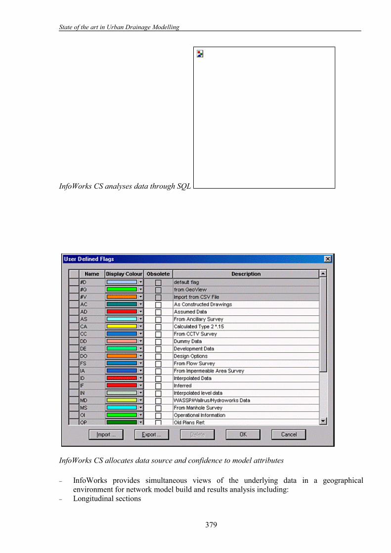
State of the art in Urban Drainage Modelling
379
InfoWorks CS analyses data through SQL
InfoWorks CS allocates data source and confidence to model attributes − InfoWorks provides simultaneous views of the underlying data in a geographical
environment for network model build and results analysis including: − Longitudinal sections

State of the art in Urban Drainage Modelling
380
− Database grid editing − Time varying graphical data − Advanced model building including: geographical model building in conjunction with a
raster or vector map background, sub-catchment boundaries import or creation over vector map backgrounds and automatic area take-off from vector maps
− Models all key elements of a drainage network: open channels, trunk sewers, complex pipe connections, ancillary and control structures
− Model merging of existing models into a larger macro model using simple 'copy' and 'pastes' facilities
− Interactive network simplification through query analysis − Fast, stable HydroWorks 'Time Series' simulation with comprehensive diagnostic informat-
ion − Ability to deal with large data sets − Produces event series data using the Wastewater and Rainfall Generatorsreturn period and
'Time Series' results analysis.
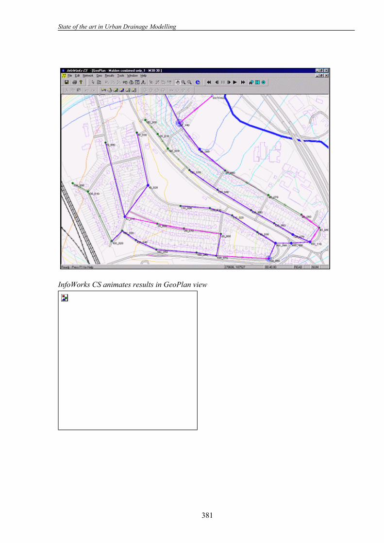
State of the art in Urban Drainage Modelling
381
InfoWorks CS animates results in GeoPlan view

State of the art in Urban Drainage Modelling
382
InfoWorks transfers data to and from third party applications: - Import all network and event data from WASSP, WALLRUS and HydroWorksimport
sub-catchment areas, area breakdown and population data directly from MapInfo Pro-fessional or ArcView GISimport asset data directly from Microsoft Access or .CSV files into the InfoWorks databaseadditional optional import of data from Thesis, STC25, STC26, FastSTC and Examiner.
- Export network and event data to HydroWorksexport data and simulation results to Map Info Professional or ArcView GIsexport network and results data to .CSV files
- Easily upgradeable to include the following optional modules: Quality Module, Real Time Control Module.

State of the art in Urban Drainage Modelling
383
InfoWorks CS displays background maps from GIS

State of the art in Urban Drainage Modelling
384
7.10 HAESTAD METHODS http://www.haestad.com/software/
7.10.1. SewerCAD v4 Sewer CAD is a design and analysis tool that allows one to layout a collection system, develop and compute sanitary loads, and simulate the hydraulic response of the entire system - including gravity collection piping and pressure force mains. SewerCAD can be run using Haestad Methods' own Stand-Alone Windows interface, or directly inside AutoCAD. SewerCAD's point-and-click network layout tools allow one to draw, label, drag, drop, and move all elements in either scaled, schematic, or mixed mode. Support for gravity systems, pressure networks, wet wells, and pump stations makes it possible to perform detailed design and analyses on your entire sanitary sewer system. Haestad Methods' incredibly stable gradually varied flow hydraulic algorithms do not fail in the toughest model-ling situations including hydraulic jumps, mixed gravity and pressure flow; and adverse or horizontal slopes. Automatic "constraint based" design options and algorithms support the design of selected gra-vity network elements, including the ability to design gravity pipes for full or partial capacity with mixed invert, crown, and/or soffit matching criteria

State of the art in Urban Drainage Modelling
385
Unit dry loads and extreme flow factor methods (peaking factor methods) can be customized to match local design criteria. Select from the numerous pre-defined extreme flow factor formulas and tables, including Babbit, Harmon, Ten State, and Federov's - or enter your own formulas or tables. Determine infiltration based on pipe length, diameter, surface area, length-diameter, or user defined count. - "What You See Is What You Get" (WYSIWYG) report, plan, and profile generation - Plan and profile views are easy to edit, color code, and label - Plot and print to any device including plotters and faxes - Exchange data with all popular site/civil/roadway software - Enhanced profiles include gradually varied flow surfaces - Dynamic annotation (labeling) and color-coding - FlexTables allow mixing of system elements (manholes, pipes, junction boxes, pressure
junctions, wet wells, and outlets) in network order or any other predefined order, provid-ing support for all agency specific formats
- Database Connections feature allows data to be easily exchanged with any database, spreadsheet, or GIS
- GIS interface now includes powerful ArcInfo/ArcView connection wizard and full Shapefile support.
7.10.2. STORMCAD StormCAD v3 for storm sewer design and analysis make it easier to design and analyse storm sewer systems from gutter to outlet.
• Inlets are designed and computed as defined by the new FHWA Hydraulic Engineering Circular 22 (formerly H.E.C. 12), including grate inlets in ditches/medians
• Inlet/gutter surface network calculations are fully integrated with pipe network calcu-lations (bypass flows can be routed to any other inlet located within any pipe network in the project)
• Inlet design is automated using a customizable inlet library (already loaded with all inlet types including grate, curb, combination, slot and ditch inlets)
• New structure hydraulic loss methods (junction losses), including FHWA H.E.C. 22 and AASHTO methods, which automatically calculate losses based on calculated bend angles and structure geometry
Once the network of inlets and pipes has been created and the rainfall data or flows are selected you can design selected network properties or elements such as pipes, inlets or invert elevations. System-wide analysis or design is also fully supported. Warning and error messages offer clear guidance for improving or fixing your data. Haestad Methods' incredibly stable gradually varied flow hydraulic algorithms do not fail in the toughest modeling situations including hydraulic jumps, mixed gravity and pressure flow; and adverse or horizontal slopes. 7.10.3. PondPack PondPack v7 for Windows is a comprehensive urban storm water solution capable of modeling gauged and synthetic rainfall, runoff hydrographs, culverts, channels, pond sizing, outlet struc-tures with tailwater effects, interconnected pond modeling, diversions, and tidal outfalls - just to

State of the art in Urban Drainage Modelling
386
name a few. PondPack models the full range of storm water projects from small simple sites to regional drainage studies. PondPack generates hydrographs and performs reach and pond routing across multiple storms and durations.
• Model any duration or distribution, for synthetic or real storm events. There is no limit to the number of storm events that can be modeled within any run
• Utilize SCS 24 hour rainfall curves that come included with PondPack, as well as Bulletin 70-71
• Generate rainfall distributions from I-D-F curves • Input I-D-F curves directly, or have PondPack develop them from I-D-F equations • Compute Tc using popular Tc- methods including: Carter, Eagleson, Espey/Winslow,
FAA, Kerby/Hathaway, Kirpich, Length/Velocity, SCS Lag, TR-55 (Sheet, Shallow Concentrated, Channel), and user defined
• Choose the SCS Unit Hydrograph method (for both triangular and curvilinear methods), the SCS TR-55 method, and make use of the SCS Unit shape factor adjustment
• Use the Rational Method Hydrograph Generation or the Modified Rational Method for I-D-F based hydrographs
• Compute an instantaneous hydrograph and route it using the Santa Barbara urban Hydrograph procedures
• Route hydrographs through irregular (natural) channels, and prismatic channels such as parabolic, rectangular, triangular, and trapezoidal channels
• Route hydrographs through piping systems PondPack models everything from simple single pond projects to complicated watersheds. You can graphically layout and analyze single pond systems, as well as detailed complex watershed networks with channel routing, diversions, multiple ponds, interconnected ponds with multiple tidal outfalls - or anything in between.
• Estimate storage requirements for given outflow restrictions • Define your pond by several available methods including: FHWA HDS-5 culverts with
inlet/outlet control checks, broad crested weirs, road overtopping, v-notch weirs, inlet boxes, stand pipes, orifices, riser perforations, user defined structures, and more
• Model underground sloped, upsized pipes for detention • Design multi-stage structures consisting of over a dozen different outlet devices, provid-
ing extreme versatility in outlet structure combinations • Model both retention and detention ponds within the same network • Computes water quality parameters such as detention time, first flush, and minimum
drain time • Automatically take into account pond and reach infiltration from the watershed system • Model fully networked watershed scenarios with multiple areas, reaches, and ponds,
including interconnected diversions • Considers tailwater during outlet structures calculations • Model the effects of tidal outfalls on the water surface level, volume, and outflow in
upstream ponds • Analyze multiple connected ponds with backwater effects • Calculate reverse flow automatically, or prevent reverse flow by incorporating flap gates

State of the art in Urban Drainage Modelling
387
7.10.4. CulvertMaster CulvertMaster is a great program that will make you stop using those old programs or nomo-graphs. We have already compared CulvertMaster to other programs, and we are so confident in the quality of this intuitive program that we unconditionally guarantee your satisfaction. Designed to fit your project, CulvertMaster's simple yet powerful interface is easy to learn and use. In fact, CulvertMaster is so easy to use, you will be modelling complex multiple barrel cross drain systems right out of the box.
• Intuitive project based interface organizes design trials into worksheets all in the same file.
• Three modeling modes; Quick Culvert Calculator, Culvert Analyzer, and Culvert Designer make modeling any project simple and straight forward
• Use the Quick Culvert Calculator for quick design or analysis trials • Use the Analyzer and Designer modes to analyze and/or design anything from simple
single pipe culvert systems to complex cross drain systems • Use the Culvert Designer to check multiple culvert designs for the same embankment,
choose the best and move it to the Culvert Analyzer for further analysis • Metric, English, or a combination of both unit systems • Get free updates over the Internet via the globe button • Tabbed dialogs organize data for easy input and output • Run under Windows 95, 98, or NT
CulvertMaster calculates headwater elevations based on both inlet and outlet control conditions. No more messy nomographs. Inlet control calculations use weir and orifice equations. Outlet control calculations use Haestad Methods' incredibly stable gradually varied flow hydraulic algorithms, which do not fail in the toughest modeling situations including hydraulic jumps, mixed gravity, and pressure flow; and adverse or horizontal slopes. 7.10.5. FlowMaster FlowMaster v6 is an efficient and powerful program for the design and analysis of pipes, ditches, open channels, weirs, orifices, and inlets. FlowMaster's "Hydraulics Toolbox" can solve or rate any unknown variable using the Manning's, Hazen-Williams', Kutter's, Darcy-Weisbach, and Colebrook-White formulas. FlowMaster's new inlet computations strictly comply with the latest FHWA Hydraulic Circular Number 22 (replacing Circular 12) and AASHTO inlet computation guidelines. FlowMaster will solve for any unknown variable in gutter cross sections, inlets, weirs, orifices, irregular channels, pressure pipes, or standard open channels. Create multiple design trials, calculate them all simultaneously, and compare the results in customizable tabular reports.
• Model curb, grate, slot, combination, and ditch inlets using calculations based on FHWA Hydraulic Engineering Circular No. 12 and Circular No. 22 methodologies
• Analyze any inlet in sag or on grade with a continuously or a locally depressed gutter • Calculate water spread and gutter depth for a gutter or pavement section • Size or evaluate flow for sharp-crested weirs, broad-crested weirs, and orifices

State of the art in Urban Drainage Modelling
388
• FlowMaster will solve for any variable, including discharge, headwater elevation, discharge coefficient and more. Even submergence (tailwater effect) in orifices and weirs is taken into account
• Enter the geometry and variable roughness for your irregular sections (open or closed) to model irregular open and closed cross sections effortlessly
• Compute composite roughness values for your irregular section using various methods including Lotter, Horton, Pavlovskii, or the Colebatch and Cox method, as well as the combination of Horton and Lotter that was available in the previous version
• Model ditches and swales regardless of size and shape. Geometric shapes include circular, rectangular, trapezoidal, triangular, gutter, and irregular
• Perform a quick check or a design on a pressure pipe by simply plugging in the known information and clicking to solve for the unknown

State of the art in Urban Drainage Modelling
389
7.11 KOSIM KOSIM-XL operates with the uniform KOSIM-Windows interface. Among other things the interface offers functions for the gathering of model parameters and precipitation data, reviewing input data and evaluating results statistically. All system data and evaluation results are putted into CVS-format and are available for any evaluation. Beside a reporting generator for generating reports this software-package offers an output of the hydrographs with the discharges of a system as an interface to HYSTEM-EXTRAN and as an interface to Excel. Current versions and developments Version 6.1 is available since April 2000. Additionally automating of simulation series with the ITWH supplementary product line SENSOR "for KOSIM" is possible. System requires 32-bit application runs under Windows NT 4 Interface is oriented at Windows-standard No internal limits concerning the number of elements Hardware minimum requirements correspond with the ones of the used operating system.

State of the art in Urban Drainage Modelling
390
7.12 CONCLUSIONS The UIs for urban drainage models share some approaches and differ in others. They use standard Windows 9x/NT components and provide for model set-up, execution, post-processing, display and analysis. The standard input data comprise catchment and pipe data, hydraulic, hydological and metheorological data. They are stored in a number of data files and can be edited and presented in text and/or graphical form, printed and plotted by means of a print/plotting system. The result variables are divided into variables attached to network nodes (manholes) and variables attached to links (pipes). The standard output data comprise computed runoff hydrographs, discharges, velocities and water levels for pipes, manholes, overflow structures, retention basins and pumping stations. Outputs produced by water quality and sediment transport modules include time series of discharge, velocity, concentrations of pollutants and sediment transport. In some cases the results of statistics on rainfall data (single events, historical rain series) and parameters which characterise the CSO spill volume and pollution load (the total overflow volume, the number of overflow events, the total duration of overflow, the total mass of the pollutant in question discharged) are added to the standard outputs. The results can be presented in a form of tables, graphs as well as in the horizontal plan plot and longitudinal profile plot. Some of the UIs have advanced graphics both on the input and output sides. Selected result variables can be displayed dynamically as a reply of the model simulation through time (animation of flows and water levels on plans and profiles in MOUSE). The most powerful user interfaces have very effective data editing facilities (QBE and other filtering techniques, SQL, etc.), comprehensive time series management facilities, automatic data consistency preservation and consistency checking, and exchange of data and graphics with other Windows-based applications. Some editors support editing the scenarios in a Scenario Manager (MOUSE 2000). Some of the UIs are based on a version of AutoCAD system and use AutoCAD as graphical engine for viewing objects, creating drawings, and for snapping and digitising operations (SewerCAD). Some of the UI software solutions, which integrate asset planning with urban drainage network modelling, have been connected to MapInfo graphical environment for desktop mapping and GIS analysis (InfoWorks environment with HydroWorks simulation engine for wastewater networks). MOUSE GIS is an ArcView based application for MOUSE users developed specially to enhance the process of setting-up and quality-checking model networks (Network Editor) and presentation of combined MOUSE results and GIS data (Results Presentation).
8 URBAN DRAINAGE MODELS: GIS INTERFACE
8.1 INTRODUCTION The main task of this survey is to obtain the information that will enable harmonisation and optimisation of CARE-S procedure using an appropriate Geographic Information System (GIS). It addresses issues such as GIS and it relationship with hydrologic and hydraulic modelling approaches, GIS software and GIS based interfaces for urban drainage models.
8.2 GIS AND ITS RELATIONSHIP WITH HYDROLOGIC AND HYDRAULIC MODELLING
8.2.1. Impact of GIS on hydrologic modelling In hydrologic modelling GIS began to be used to represent the flow of water on the land surface in early 80s. Much of the initial work dealt with the analysis of DEMs square grids of regularly spaced elevation data for hydrologic applications. There are two groups of surface functions available in GIS software used in creation of hydrologic models. A category for creating surfaces and a category for analysing surfaces. The functions in the first category, called surface interpolators, create a continuous surface from sampled input point values. Hence, a DEM is a two-dimensional array of elevation points with a constant x and y spacing. Their simple data structure has made them popular source for digital terrain modelling and catchment characterisation. Many different techniques for DEM creation are available - Inverse Distance Weighted (IDW), Spline Kriging and Trend Interpolation. The second category uses a continuos grid theme to perform a specified calculation that results in different representations of a surface or that derives patterns not readily apparent in the original surface. The hydrological function Sink identifies any sink in the original DEM. These depressions can be filled using the demfill. The hydrological function Flow Direction calculates the flow direction of each cell in the surface represented by a grid. The flow direction for a cell is the direction water will flow out of the cell. The directions are assignet on the basis of steepest descent away from the current cell. It is encoded to correspond to the orientation of one of the eight cells that surround the cell using Eight Direction Pour Point model. The hydrological function FlowAccumulation uses the output from the FlowDirection function and calculates the flow accumulation for each cell. Each cell is assigned a value equal to the number of cells that flow to it. The hydrological function Watershed determines the contributing area above each pour point. Other drainage features which can be extracted using GIS software are the catchment characteristics, such as catchment_ID, catchment_area, cetroid_x, centroid_y, mean_elevation, mean_slope and men_slope distance, the impervious are, defined by the roof areas and the paved road areas in each catchment and subcatchment

State-of-the-art in Urban Drainage modelling
392
Procedure based on DEM can be carried out using a verity of commercial GIS software and their extensions.
8.2.2. Impact of GIS on hydraulic modelling Spatial modelling has an important impact on the style of modelling practised in many fields. When it comes to water resources modelling, mathematical models can use scale/surface models to create a whole new modelling architecture. Unfortunately, the use of DEM surface is generally not suitable for the hydraulic modelling. Because they cannot vary in spatial resolution, DEMs may poorly define the land surface in areas of complex relief. For hydraulic modelling of river and storm drainage in urban setting, the triangular irregular network (TIN) to model surface was found to be more effective. BEFFA has developed the TriPaD model for flood simulations in urban areas based on a simplified flow equation that directly applies to the TIN of the ground surface. He applied both a standard finite volume (FV) model and TriPaD model in a pilot study. The TIN of ground elevation was created with Delauney triangulation. From this the uniform mesh for the FV model was generated by linear interpolation. The results of the comparison between FV and TIN based approach show that the TIN based model gives more accurate results for the channel because the edges of the TIN coincide with the direction of the flow as break-lines have been used to describe the geometry of the channel. A simultaneous modelling of the chreek and the flood plane is not practicable with the FV model as the computation time is to long.
8.2.3. Impact of GIS on urban drainage modelling Effects of link GIS with spatial analysis have made their greatest progress in the area of environmental modelling such as hydrological modelling in large river basins. So far, urban models and urban modelling application have lagged much behind. The main reason for this is the lack of the spatial component in the urban drainage mathematical models. They still rely on traditional data representation techniques by which is difficult to create a new modern architecture for building and modelling real-world surface features. In addition the mathematical description of the hydrodynamic in a sewer network and connected surface area under flooding is still a complex problem. Traditionally, surface runoff generators in urban drainage models are rather simple models, which utilise a runoff coefficient for impervious area and unit hydrograph method for generation of runoff from rainfall. Pressurised flows in a sewer network are computed by implementation of a ”slot”, a vertical extension of the closed pipe cross-section. The free surface water which flows from the underground surcharge pipes are stored in a virtual reservoir closed to the computational input node. The stored volume returns to the pipe in the same node once the system resumes free-surface pipe flow. Free surface and pressurised flows are thus described within the same basic algorithm, which ensures the smooth and stable numerical conditions. In recent years a new generation of UDMs commonly refers to as Dual Drainage models has emerged. The GIS based routines and procedures for advanced calculation of surface runoff and unsteady flows in sewer networks form the core in the new dual drainage modelling approach. In the most advanced DD models the surface model solves shallow water equation that directly applies to the TIN representation of the urban surface topology. The exchange nodes between

State-of-the-art in Urban Drainage modelling
393
surface model and underground pipe model are localised in the triangular grid of the surface model. In addition, different procedures have been developed to process model output in GIS software by integrating spatial geometry with hydraulic results (water depths and velocity vectors).
8.3 GIS SOFTWARE FOR URBAN DRAINAGE MODELS ArcGIS, MapInfo, MapObject and their extensions are the most used software for desktop mapping and GIS analysis in urban drainage modelling and management. On the other hand, many model developers have developed their own pre- and post-processing methodologies and assembled them into “toolboxes” of analysis utilities. These include creation of and procedures to analyse grid cell DEMs and TIN models. TIN models have received significant attention in recent years, while grid cell elevation models continue to be popular because they can be easily coupled to remote-sensed data structure.
8.3.1. ArcGIS ArcGIS product ArcView 3.x is the most used GIS software in urban drainage modelling. It is not yet a fully functional GIS in the way that ArcInfo could be so described, and this is acknowledged by ESRI, who promotes the idea of ‘building complete solutions’ by linking to other ESRI products. ArcView is seen very much as the front end to allow rapid access to other GIS databases. However, in its ability to provide dynamic links to other applications, initiated on the basis of a geographical query, through the Windows GUI, it succeeds. The ArcGIS 8.x products represent one of the largest changes in GIS design. The ArcGIS 8.x products ArcView version 8.1, ArcGIS Spatial Analyst and ArcGIS 3D Analyst, will completely change the architecture (utilising Geographic Makeup Language GML, a GI extension to the Extensible Makeup Language XML format) and environment of ArcView (replacing scripting language Avenue with the ability to interface with code written in Visual Basic or C). The ArcGIS project is being released in several steps: 8.0, 8.1 and 8.2. The 8.0 release focused principally on creating a whole new modern architecture for geoprocessing, but did not deliver all of the functionality that users have had in previous generation of tools. 8.1 is a significant release in that it has replicated the full functionality of ArcView and has also integrated the ArcInfo and ArcView extensions. 8.2 will finish the analysis and data modelling functionality so that virtually all software that ESRI has written will be replicated in this architecture. ArcView 8.1 is a stand-alone GIS software product. ArcView 8.1 alone cannot handle 2D/3D spatial modelling and visualisation. Two additional extensions ArcGIS Spatial Analyst and ArcGIS 3D Analyst are needed for spatial models building and sharing. ArcGIS Spatial Analyst extension allows user to create, query, map, and analyse cell-based raster data and to perform integrated vector-raster analysis. It can convert point, line, or polygon to grid themes, create raster buffers based on distance or proximity from feature or grid themes, create density maps from themes containing point features, create continuous surfaces from scattered point features, create contour, slope, and aspect maps and hill-shades of these surfaces, do cell-based map analysis, perform Boolean queries and algebraic calculations on multiple grid

State-of-the-art in Urban Drainage modelling
394
themes simultaneously, perform neighbourhood and zone analysis and do grid classification and display. It uses data from standard formats including TIFF, BIL, SunRaster, USGS DEM, SDTS, DTED, and others. ArcView 3D Analyst combines the capabilities of ArcView 3D Analyst and Arc TIN. ArcView 3D Analyst includes support for triangulated irregular networks (TINs) and Three-dimensional visualisation and analysis (extension Fly-by Animation Builder used for creating of MPEG animations or preparing for other types of animation such as AVI and animated GIF). This ArcView 8.1 extension can:
• Build surface models from any data • Perform interactive perspective viewing, including pan and zoom, rotate, tilt, and fly-
through simulations, for presentation, analysis, or export for display on the Web • Model real-world surface features such as buildings • Model subsurface features-wells, mines, groundwater, and underground storage facilities • Generate three-dimensional surfaces on-the-fly from attributes • Apply data normalisation and exaggeration on-the-fly • Drape two-dimensional data on surfaces and view in three dimensions • Calculate surface area and volume, slope, aspect, and hill-shade • Generate contours as two-dimensional or three-dimensional shapes • Perform view-shed and line-of-sight analysis, spot height interpolation, profiling, and
steepest-path determination • Use any data supported in ArcGIS including CAD, shape files, ArcInfo coverages, and
images • Query three-dimensional data based on attribute or location • Export data for display on the Web using VRML.
8.3.2. MapInfo MapInfo is the most used software for applications focusing on integration of asset and business planning with urban drainage network modelling. Key features:
• Create detailed maps to enhance presentations and aid in decision making • Reveal patterns and trends in data • Perform sophisticated and extensive data analysis • Manage geographically based assets • Plan logistics and prepare for emergency response

Extensions Vertical Mapper, which runs with MapInfo, is a suite of tools available to display, manage, and interpret spatial information. It can be accessed from three different areas within MapInfo; as a drop-down, from a dialogue called the Grid Manager, or using a Toolbar. Vertical Mapper transforms point data into continuous surfaces, or grids, which can be thematically mapped to visualise trends and queried to reveal relationships between multiple grid layers. Inverse Distance Weighting (IDW) Interpolator, Triangular Irregular Network (TIN) Interpolator, Rectangular Interpolator, Natural Neighbour Interpolator and Kriging Interpolator are available. Polygon Generator for MapInfo - Adds a tool to create Regular, Convex or Concave polygons from selected points.
8.3.3. MapObject Key Features:
• Easy-to-navigate object model • Support for data in a wide range of formats, including standard GIS formats (ArcInfo
coverages and ESRI shapefiles), CAD formats (DXF, DWG, and DGN), and a variety of image formats such as GeoTiff, JPEG, and MrSid image compression.
• Display of data as multiple layers in a map, with the ability to pan and zoom throughout all layers
• Display of features using thematic methods such as value maps and classification maps • Spatial query • Feature labeling • Advanced thematic mapping capabilities such as dot density rendering and multiple
rendering schemes • Feature attribute query using standard SQL expressions • Creatable geometric primitives • Support for measures and three-dimensional shapes • Robust on-line help, with extensive hard-copy documentation and example applications
including source code • ESRI Data and Maps, a comprehensive collection of geographic data that lets you
immediately start adding maps to your applications. Extensions MapObjects LT - Accesses an assortment of native data formats, ranging from standard GIS formats (ArcInfo coverages and ESRI shapefiles) to CAD formats (DXF, DWG, and DGN), as well as a variety of image formats, including MrSid.
State-of-the-art in Urban Drainage modelling
396
8.4 INTENSITY OF COUPLING MODELS AND GIS Four associations between models and GIS can be distinguished:
• Isolated application: The GIS and the model are run in different hardware environments, data transfer by ASCII files of-line; the user is the interface.
• Loose coupling: The coupling is carried out by means of ASCII or binary files; the user is responsible for formatting the files according to format specification of the GIS. Coupling is carried on-line.
• Tight coupling: In this case the data models can still be different, but automated exchange of data between the GIS and the model is possible through a standardised interface without user intervention.
• Full integration (model embedded in a GIS): This linkage operates like a homogeneous system from the user’s point of view; data exchange is based on a common data model and database management system.
In most cases the urban drainage model and the GIS are essentially autonomous, and also the GIS potentiality is far to be completely exploited, it offers undoubtedly a good value added. The GIS layers that are used for urban drainage modelling are: - Base map - provides an accurate description of the spatial extent of the study area. Base map can comprise a number of features such as parcels, digital orthophotography - Land use map - provides the percent imperviousness within a subcatchment - Soil map sometime combined with a geological map is used in estimating the amount of rainfall that will infiltrate and not become surface runoff - Topographic map to create a surface area (a surface TIN and a surface DEM of the surface area), to generate flow patterns and delineate subcatchments - Infrastructure map – shows the existing storm and wastewater structures. GIS tools are used to display and analyse model results. Usually, a script has been written to read data from model input and output files and to associate the model results with the junctions and conduits in a sewer system. This can be used to display information such as peak stages, flows and velocity in a sewer system. Using some of the extensions and programs these data along with digital topographic data can be used to automatically create floodplain maps. If a geo-coded street file is available, addresses from a storm/wastewater complaint database can be used to map and analyse the severity of the complaint. Photos of model structures can be associated with a structure inventory map. Many comprehensive GIS-based interfaces to a wide variety of urban drainage models have been developed in recent years, in a wide variety of configurations. They use either loos or tight method of coupling model and a GIS. The development of embedded solutions in urban drainage modelling is confined by the limitations of the GIS numerical capabilities.

State-of-the-art in Urban Drainage modelling
397
8.5 GIS INTERFACES FOR URBAN DRAINAGE MODELS The most recent trend in urban drainage modelling is characterised by recycling of old numerical methods (1D) coupled with a very high diversity of languages (going from FORTRAN to C/C++) and their integration with GIS going from the ArcGIS products ArcView and its extensions to very proprietary GU
State-of-the-art in Urban Drainage modelling
398
I environments. GIS-based interfaces cannot be easily compared to one another for the purpose of CARE-S prototype concept because the development in this market is going fast and an GIS-based interface one uses today can be gone tomorrow. In addition, most of the published reports and manuals attempt to present performance of GIS-based interfaces as universal tools aiding in the creation of both rural and urban catchments. A survey of GIS functionalities, which have been included into a wide variety of GUIs for urban drainage models is presented in chapter 4. In this chapter only the basic information on the GUIs, which have been design to support GIS analysis in urban drainage modelling is summarised. - MOUSE GIS is an ArcView based application for MOUSE users. MOUSE GIS works in the ArcView environment and consists of two parts: the Network Editor and the Results Presentation. Both parts support the general features available in ArcView. - MIKE SWMM is an interface for the public domain version of SWMM (Stormwater Management Model). MOUSE GIS can be used as the ArcView GIS link and model simplification tool for all SWMM modelling packages which apply the standard SWMM data formats. - Visual Hydro in conjunction with its Visual SWMM uses Microsoft VBA to directly link with a multitude of other applications, including ArcView and AutoCAD. -InfoWorks is an interface for HydroWorks Simulation Engine users. It has been connected to MapInfo for desktop mapping and GIS analysis. - SewerCAD uses AutoCAD as graphical engine for viewing objects, creating drawings, and for snapping and digitising operations. Interface includes ArcInfo/ArcView connection wizard and shapefile support. -HYSTEM -EXTRAN works in AutoCAD-based graphical interface GIPS (Geografisches Informations- und Planungssystem fur die Stadtentwasserung). - MIKE 11 GIS has been developed as a fully integrated interface in ArcView. It is suited as a spatial decision support tool for comprehensive applications focusing on integrated modelling of entire watersheds (MOUSE, treatment plant model STOAT and river water quality model MIKE 11).

8.6 CONCLUSIONS AND RECOMMENDATIONS GIS-based interfaces have already shown to be very important in the evolution of urban drainage models, either for their conceptual structure, like for instance the new generation of DD models, or for their visualisation, query, analysis and integration capabilities. The CARE–S prototype software will be designed as a cluster of simple and sophisticated modelling tools and will rely on a wide range of software interacting with a large number of disparate data and end users. Bringing all information, which forms the basis for hydrologic, hydraulic, environmental and structural rehabilitation of sewer systems into an assembled group will require an effective GIS-based interface and data-sharing concept. The integration of the GIS and CARE-S prototype software can come in many forms. In the simplest case, to separate systems, the GIS and the CARE-S tools, just exchange files. The tolls obtain some of its input data from the GIS and produce some of their output in a format that allows import and further processing and display with the GIS. In this case only the file formats and the corresponding input and output routines, usually of the tools, have to be adopted. Application generators and modelling capabilities with commercial GIS (ArcView Spatial Analyst and 3D Analyst Extension) also offer the possibilities of tight integration within the limits of the respective package options. One way to achieve a deeper integration is to use a higher-level application language or the application generators build into the GIS. The final selection of the GIS software in the CARE-S project will be based on the quantity of input work, the complexity of the databases, the dominant application that a GIS will be put to as well as cost-benefit analysis.
State-of-the-art in Urban Drainage modeling
400
9 GENERAL SUMMARY AND CONCLUSIONS The analysis of the previous chapters allows for some general considerations:
- Mathematical models availability is quite large and their characteristics are widely variable (ranging from very simple conceptual lumped models to complex physically based distributed models)
- Several aspects of Urban Water Cycle can be modelled, even if different considerations should be done in general for quantity and quality models
- In last years, a strong tendency to integrate different modelling aspects and processes can be identified; this trend is generated by the availability of high performance computers that incredibly increased computational resources even if a lot of work is still to be done.
- In last years, GUI and GIS interfaces were generally refined counting on higher processor performances and graphical functionalities but there is still much to do about standardization and data management
9.1 Urban drainage models
9.1.1. UD Quantity models Some considerations can be addressed to quantity models:
- Rainfall – Runoff quantity models reached high detail levels and nowadays the most diffuse commercial software can count on a wide range of possible approaches that can be sized to the characteristics of the catchment and to the availability of data
- Rainfall – Runoff quantity models are mostly conceptual-distributed and their theoretical basis is characterised by linear/non-linear reservoir approach and channel approach.
- Hydrologic depletions are based on the most diffuse either conceptual or physical approaches; commercial software generally allows the user for the selection of the most appropriate model for the specific case
- Flow propagation in the drainage system is usually performed by the use of 1D De Saint Venant Equations either in the cinematic simplification of the full dynamic approach; most diffuse commercial models are characterised by quite old mathematical solvers even if optimised for using high performance processors.
- Full dynamic 1D DSV are usually used only for storm event simulation while cinematic approach is suitable for long term simulation of historical rainfall series
- A wide range of structures can be simulated (pump stations, storage, weirs and overflows, orifices, RTC, etc.) even if only few models are able to interact with them during simulations (manually start/stop pump stations; regulate overflows, etc.); for this reason models are quite useful for system design or verification but they are sufficiently adequate for supporting system management
What is still missing: - Effective rainfall models are still too simple for managing complex hydrological
structures such as snow-melting and overland flow on highly disturbed soils - Only a few models are adequate for managing highly distributed information coming
from GIS databases (Digital Elevation Models; cellular/distributed hydrological parameters, etc.)
State-of-the-art in Urban Drainage modeling
401
- Available data are often insufficient for distributed models calibration - Approaches for pipe surcharge and surface flooding analysis are generally too simple
and need to be improved - Interaction during simulation is usually not possible or limited to only a few of
operational parameters
9.1.2. UD Quality models Some considerations can be addressed to quality models:
- Pollution dynamic on the catchment surface is usually analysed by the use of conceptual approaches and empiric formulations; the fundamental reason is connected with the complexity of the pollution propagation/transformation processes and with the lack of experimental data
- Nevertheless all the most diffuse models demonstrated good adaptability to different catchment conditions and relatively easy calibration procedures giving reliable and robust results
- Pollution/sediment transport analysis in sewers is still characterised by a low level of physical detail; only a few models simulate deposition/resuspension processes in the drainage system that is usually necessary for evaluating reduction in pipe hydraulic capacity
- A wide range of structures can be simulated (pump stations, storage, weirs and overflows, orifices, RTC, etc.) but very few models simulates detailed quality aspects of flow controls (sediment deposition; pollution abatement; etc.)
What is still missing: - More details in build-up/wash-off quality analysis - More detailed approach for pollution propagation in sewers - Only a few models are adequate for managing highly distributed information coming
from GIS databases (Digital Elevation Models; cellular/distributed hydrological parameters, etc.)
- The possibility for quality simulation of flow control structures - Available data are often insufficient for distributed models calibration - Interaction during simulation is usually not possible or limited to only a few of
operational parameters
9.1.3. WWTP and Receiving water systems modelling WWTP models are quite complete and complex; the most diffuse ones can simulate several processes and have also wide possibilities for customization. Even if most of them result to be reliable and robust in use, some features are still missing such as integration with urban drainage and receiving water systems models that, at the moment, can only exchange input/output time series. More over, source codes are generally not available and for this reason customization is possible only within the limits of the software (no input/output format change is possible; user defined variables can not be calculated). Considerations on receiving water system models are similar to those applied to urban drainage models:
- Quantity models are generally more detailed and reliable than quality models giving the possibility for analysing also complex structures such as bridges, culverts, reservoirs, etc.
- Quality models generally adopt conceptual approaches and have quite fast computational routines in order to perform long term simulations
State-of-the-art in Urban Drainage modeling
402
- The gap between quantity and quality models is generated by the difficulties in understanding quality processes and in the lack of data for model approach verification
9.2 Model User interface and GIS functionalities The UIs for urban drainage models share some approaches and differ in others. They use standard Windows 9x/NT components and provide for model set-up, execution, post-processing, display and analysis. The standard input data comprise catchment and pipe data, hydraulic, hydrological and meteorological data. They are stored in a number of data files and can be edited and presented in text and/or graphical form, printed and plotted by means of a print/plotting system. The result variables are divided into variables attached to network nodes (manholes) and variables attached to links (pipes). The standard output data comprise computed runoff hydrographs, discharges, velocities and water levels for pipes, manholes, overflow structures, retention basins and pumping stations. Outputs produced by water quality and sediment transport modules include time series of discharge, velocity, concentrations of pollutants and sediment transport. In some cases the results of statistics on rainfall data (single events, historical rain series) and parameters which characterise the CSO spill volume and pollution load (the total overflow volume, the number of overflow events, the total duration of overflow, the total mass of the pollutant in question discharged) are added to the standard outputs. The results can be presented in a form of tables, graphs as well as in the horizontal plan plot and longitudinal profile plot. Some of the UIs have advanced graphics both on the input and output sides. Selected result variables can be displayed dynamically as a reply of the model simulation through time (animation of flows and water levels on plans and profiles in MOUSE). The most powerful user interfaces have very effective data editing facilities (QBE and other filtering techniques, SQL, etc.), comprehensive time series management facilities, automatic data consistency preservation and consistency checking, and exchange of data and graphics with other Windows-based applications. Some editors support editing the scenarios in a Scenario Manager (MOUSE 2000). Some of the UIs are based on a version of AutoCAD system and use AutoCAD as graphical engine for viewing objects, creating drawings, and for snapping and digitising operations (SewerCAD). Some of the UI software solutions, which integrate asset planning with urban drainage network modelling, have been connected to MapInfo graphical environment for desktop mapping and GIS analysis (InfoWorks environment with HydroWorks simulation engine for wastewater networks). MOUSE GIS is an ArcView based application for MOUSE users developed specially to enhance the process of setting-up and quality-checking model networks (Network Editor) and presentation of combined MOUSE results and GIS data (Results Presentation).

State-of-the-art in Urban Drainage modeling
403
GIS-based interfaces have already shown to be very important in the evolution of urban drainage models, either for their conceptual structure, like for instance the new generation of DD models, or for their visualisation, query, analysis and integration capabilities.
9.3 Recommendations for future WP3 development The CARE–S prototype software will be designed as a cluster of simple and sophisticated modelling tools and will rely on a wide range of software interacting with a large number of disparate data and end users. Bringing all information, which forms the basis for hydrologic, hydraulic, environmental and structural rehabilitation of sewer systems into an assembled group will require an effective GIS-based interface and data-sharing concept. Questionnaires, which have been filled by all the partners and end-users, showed that different models are used in different European regions and even in the same Member State differences can be found between different end-users. In order to maintain the generality of project results, WP3 should have an open structure able to interact with different modelling tools. Models that have been considered in this report have a wide range of functionalities able to cover almost all aspect of urban water systems analysis. The most part of the commercial modelling tools are not open source and it is not possible to interact with them apart from input/output files exchange. For this reason, the first step in this process should be the integration between different models in order to make them usable “at user choice”, i.e. depending on user selection and availability. Consequentially, the second step regards the standardization of output files and time series. According to this consideration and to the fact that hydraulic temporal decline is not simulated by any existing modelling tool, one possible way to cope with UD modifications is to set up an interface between models and CARE-S prototype able to change UD characteristics during its life span and according to defined decline curves. The same procedure should be defined also for quality simulation in order to evaluate the impact on receiving waters. The integration of the GIS and CARE-S prototype software can come in many forms. In the simplest case, to separate systems, the GIS and the CARE-S tools, just exchange files. The tolls obtain some of its input data from the GIS and produce some of their output in a format that allows import and further processing and display with the GIS. In this case only the file formats and the corresponding input and output routines, usually of the tools, have to be adopted. Application generators and modelling capabilities with commercial GIS (ArcView Spatial Analyst and 3D Analyst Extension) also offer the possibilities of tight integration within the limits of the respective package options. One way to achieve a deeper integration is to use a higher-level application language or the application generators build into the GIS. The final selection of the GIS software in the CARE-S project will be based on the quantity of input work, the complexity of the databases, the dominant application that a GIS will be put to as well as cost-benefit analysis.

APPENDIX 1: LIST OF INDICATORS Preliminary list (selected by LNEC) regarding relevant IWA PI in the framework of CARE-S
(Total number of PI: 35) 6.1 ENVIRONMENTAL INDICATORS (wEn)
WASTEWATER wEn3 Intermittent overflow discharge frequency
(no./overflow device)
Number of overflow discharges / number of overflow devices wEn3 = wA27 / wC20
wEn4 Intermittent overflow discharge volume
(m3/overflow device)
Total volume of overflow discharges / number of overflow devices wEn4 = wA28 / wC20
wEn5 Intermittent overflow discharge related to rainfall
(%)
Total volume of overflow discharges / total volume of annual rainfall x 100 wEn5 = wA28 / wA24
SOLID RESIDUES wEn6 Sediments from sewers
(ton/km sewer)
Drained weight of sediments removed from sewers / total sewer length wEn6 = wA13 / wC1
6.3 PHYSICAL INDICATORS (wPh)
SEWERS wPh5 Surcharging in sewers in dry weather
(%)
Length of sewer where surcharging has occurred during dry weather / total sewer length x 100 wPh5 = wC2 / wC1 x 100
wPh6 Surcharging in sewers in wet weather
(%)
Length of sewer where surcharging has occurred during wet weather / total sewer length x 100 wPh6 = wC3 / wC1 x 100 This information may be obtained either by monitoring or by hydraulic modelling using real rainfall data.
wPh7 High sewer surcharging
(%)
Length of sewer where high degree surcharging has occurred / total sewer length x 100 wPh7 = wC4 / wC1 x 100 High degree surcharging means water above the pipe crown.
6.4 OPERATIONAL INDICATORS (wOp)
SEWERAGE REHABILITATION
wOp20 Sewer rehabilitation
(%)
Length of sewers rehabilitated / total sewer length x 100 wOp20 = wD25 / wC1 x 100
wOp21 --- Sewers relining
(%)
Length of sewers relined / total sewer length wOp21 = wD26 / wC1 x 100
wOp22 --- Sewers replacement or renewal
(%)
Length of sewers replaced or renewed / total sewer length wOp22 = wD27 / wC1 x 100

State-of-the-art in Urban Drainage modeling
405
wOp23 Manholes replaced, renewed or relined
(%)
Number of manholes replaced, renewed or relined / total number of manholes x 100 wOp23 = wD28 / wC22 x 100 Replacement and renewal of manhole covers only are not included.
wOp24 Replacement of manhole covers
(%)
Number of manhole covers replaced / total number of maholes x 100 wOp24 = wD29 / wC22 x 100
wOp25 Service connection rehabilitation
(%)
Number of service connections replaced or renewed / total number of service connections x 100 wOp25 = wD30 / wC31 x 100
INFLOW / INFILTRATION (I/I)
wOp28 Inflow/Infiltration/Exfiltration (I/I/E)
(%)
Volume of water entering sewers, from groundwater and wrong connections less the leakage from sewers into the ground / (collected sewage + inflow + infiltration - exfiltration) x 100 wOp28 = (wD34 + wD35 - wD36) / (wA2) x 100
wOp29 Inflow m3/km
Volume of water entering sewers from wrong connections / total sewer length wOp29 = wD34 / wC1
wOp30 Infiltration m3/km
Volume of water entering sewers from groundwater / total sewer length wOp30 = wD35 / wC1
wOp31 Exfiltration m3/km
Volume of leakage from sewers into the ground / total sewer length wOp31 = wD36 / wC1
FAILURES wOp32 Blockages (No./100 km)
Number of blockages / total sewer length x 100 wOp32 = wD37 / wC1 x 100 Pumping station blockages should be included. Include blockages in service connections only where these are the responsibility of the wastewater undertaking.
wOp33 Blockage locations
(No./100 km)
Number of individual locations where blockages occured / total sewer length x 100 wOp33 = wD38 / wC1 x 100 Locations where frequent blockages occured should only be accounted once. Pumping stations where blockages occured should be included. Include blockage locations in service connections only where these are the responsibility of the wastewater undertaking.
wOp34 Flooding from sanitary sewers
(No./100 km)
Number of flooding incidents related to sanitary sewers / total sewer length x 100 wOp34 = wD39 / wC1 x 100 Include only incidents related to sanitary sewers under responsibility of the wastewater undertaking.
wOp35 Surface water flooding
(No./100 km)
Number of surface water flooding incidents / total sewer length x 100 wOp35 = wD40 / wC1 x 100 These include only surface water flooding due to inadequacy of storm drainage system (combined sewers included) under the responsibility of the wastewater undertaking. Inadequacy relates to all causes (e.g. design, operation, etc.).
wOp36 Sewer collapses
(No./100 km)
Number of sewer collapses / total sewer length x 100 wOp36 = wD41 / wC1 x 100 Does not include collapses on service connections.

State-of-the-art in Urban Drainage modeling
406
6.5 QUALITY OF SERVICE INDICATORS (wQS)
SERVICE wQS11 Flooding of properties from sanitary sewers in dry weather
(n.º/1000 properties)
Number of properties affected by flooding from sanitary sewers in dry weather / number of connected properties x 1000 wQS11 = wF3 / wC30 x 1000 Only flooding from sanitary sewers under the responsibility of the wastewater undertaking should be included. Flooding may affect properties that are not connected to the sewer network. These should be included.
wQS12 Flooding of properties from sanitary sewers in wet weather
(n.º/1000 properties)
Number of properties affected by flooding from sanitary sewers in wet weather / number of connected properties x 1000 wQS12 = wF4 / wC30 x 1000 Only flooding from sanitary sewers under the responsibility of the wastewater undertaking should be included. Flooding may affect properties that are not connected to the sewer network. These should be included.
wQS13 Surface water flooding of properties in wet weather
(n.º/1000 properties)
Number of properties affected by surface water flooding in wet weather / number of connected properties x 1000 wQS13 = wF5 / wC30 x 1000 Include only surface water flooding due to inadequacy of the storm drainage system (including combined sewers) under the responsibility of the wastewater undertaking. (Inadequacy related to all causes)
wQS14 Interruption of wastewater collection and transport services
(%)
[Sum] (Number of properties affected by sewerage discontinuity or interruption x duration of interruptions in hours) / (number of connected properties x 24 x 365) X 100 wQS14 = wF6 / (wC30 x 24 x 365) x 100
COMPLAINTS wQS18 Blockage complaints
(No. /1000 inhab.)
Number of complaints as a result of blockages / population served x 1000 wQS18 = wF12 / wE1 x 1000 Only complaints relating to the system under the responsibility of the wastewater undertaking should be accounted for.
wQS19 Flooding complaints (No. /1000 inhab.)
Number of complaints as a result of flooding / population served x 1000 wQS19 = wF13 / wE1 x 1000 Only complaints relating to the system under the responsibility of the wastewater undertaking should be accounted for.
wQS20 Pollution incidents complaints
(No. /1000 inhab.)
Number of complaints as a result of pollution incidents / population served x 1000 wQS20 = wF14 / wE1 x 1000 Only complaints relating to the system under the responsibility of the wastewater undertaking should be accounted for.
wQS21 Odour complaints
(No. /1000 inhab.)
Number of complaints as a result of odours / population served x 1000 wQS21 = wF15 / wE1 x 1000 Only complaints relating to the system under the responsibility of the wastewater undertaking should be accounted for.
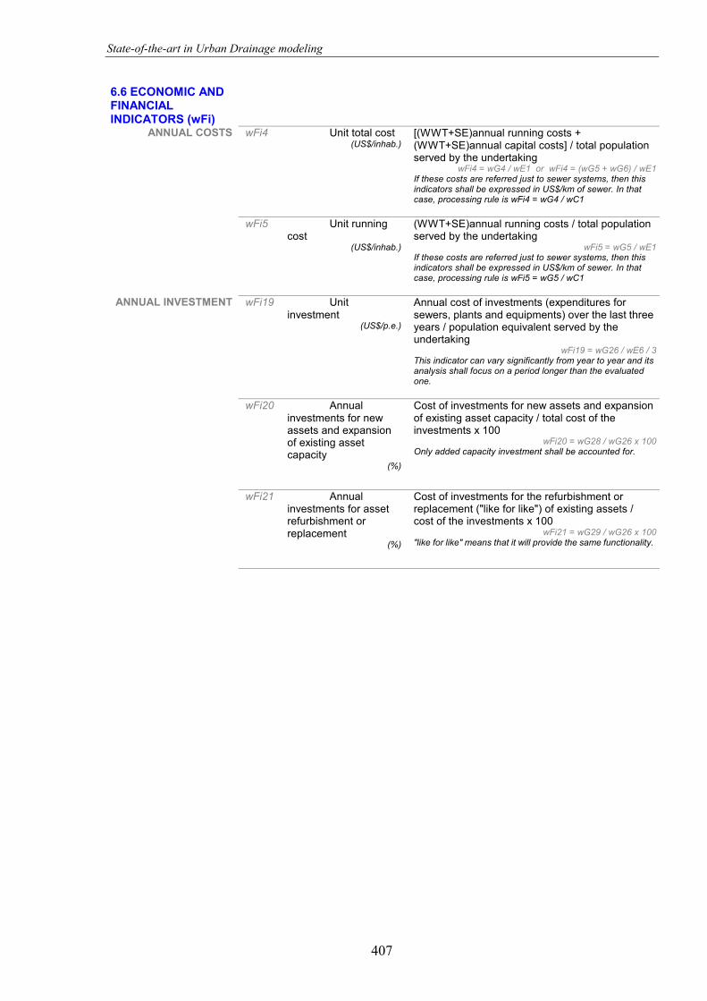
State-of-the-art in Urban Drainage modeling
407
6.6 ECONOMIC AND FINANCIAL INDICATORS (wFi)
ANNUAL COSTS wFi4 Unit total cost (US$/inhab.)
[(WWT+SE)annual running costs + (WWT+SE)annual capital costs] / total population served by the undertaking wFi4 = wG4 / wE1 or wFi4 = (wG5 + wG6) / wE1 If these costs are referred just to sewer systems, then this indicators shall be expressed in US$/km of sewer. In that case, processing rule is wFi4 = wG4 / wC1
wFi5 Unit running cost
(US$/inhab.)
(WWT+SE)annual running costs / total population served by the undertaking wFi5 = wG5 / wE1 If these costs are referred just to sewer systems, then this indicators shall be expressed in US$/km of sewer. In that case, processing rule is wFi5 = wG5 / wC1
ANNUAL INVESTMENT wFi19 Unit investment
(US$/p.e.)
Annual cost of investments (expenditures for sewers, plants and equipments) over the last three years / population equivalent served by the undertaking wFi19 = wG26 / wE6 / 3 This indicator can vary significantly from year to year and its analysis shall focus on a period longer than the evaluated one.
wFi20 Annual investments for new assets and expansion of existing asset capacity
(%)
Cost of investments for new assets and expansion of existing asset capacity / total cost of the investments x 100 wFi20 = wG28 / wG26 x 100 Only added capacity investment shall be accounted for.
wFi21 Annual investments for asset refurbishment or replacement
(%)
Cost of investments for the refurbishment or replacement ("like for like") of existing assets / cost of the investments x 100 wFi21 = wG29 / wG26 x 100 "like for like" means that it will provide the same functionality.

State-of-the-art in Urban Drainage modeling
408
APPENDIX 2: LIST OF VARIABLES
List of variables used for the assessment of the preliminary PI selected in the framework of CARE-S
Total number of variables: 44
ENVIRONMENTAL DATA
wA2 WASTEWATER TREATED UNIT OF EXPRESSION: m3 PERIOD: [dd.mm].yy-1 – [dd.mm].yy VALID VALUES: >= 0 DEFINITION: Wastewater treated by WWTP or by on-site sanitation facilities that are under the responsibility of the wastewater undertaking. PROCESSING RULE: COMMENT:
wA13 SEWER SEDIMENTS UNIT OF EXPRESSION: ton DS PERIOD: [dd.mm].yy-1 – [dd.mm].yy VALID VALUES: >= 0 DEFINITION: Drained weight of sediments removed from sewers. PROCESSING RULE: COMMENT:
wA24 ANNUAL RAINFALL UNIT OF EXPRESSION: m3 PERIOD: [dd.mm].yy-1 – [dd.mm].yy VALID VALUES: >= 0 DEFINITION: Annual volume of rainfall in the total catchment area. PROCESSING RULE: COMMENT:
wA27 NUMBER OF OVERFLOW DISCHARGES UNIT OF EXPRESSION: No. PERIOD: [dd.mm].yy-1 – [dd.mm].yy VALID VALUES: Integer DEFINITION: Number of overflow discharges occurred. PROCESSING RULE: COMMENT:
wA28 VOLUME OF OVERFLOW DISCHARGES UNIT OF EXPRESSION: m3 PERIOD: [dd.mm].yy-1 – [dd.mm].yy VALID VALUES: >= 0 DEFINITION: Total volume of overflow discharges occurred. PROCESSING RULE: COMMENT:

State-of-the-art in Urban Drainage modeling
409
PHYSICAL ASSETS DATA
wC1 TOTAL SEWER LENGTH UNIT OF EXPRESSION: km PERIOD: [dd.mm].yy-1 – [dd.mm].yy VALID VALUES: >= 0 DEFINITION: Total length of sewers managed by the undertaking. PROCESSING RULE: PHYSICAL ASSETS DATA COMMENT: Service connections excluded.
wC2 SURCHARGED SEWERS IN DRY WEATHER UNIT OF EXPRESSION: m PERIOD: [dd.mm].yy-1 – [dd.mm].yy VALID VALUES: >= 0 DEFINITION: Length of sewer where surcharging has occurred during dry weather. PROCESSING RULE: COMMENT: Service connections excluded.
wC3 SURCHARGED SEWERS IN WET WEATHER UNIT OF EXPRESSION: m PERIOD: [dd.mm].yy-1 – [dd.mm].yy VALID VALUES: >= 0 DEFINITION: Length of sewer where surcharging has occurred during wet weather. PROCESSING RULE: COMMENT: Service connections excluded.
wC4 HIGHLY SURCHARGED SEWERS UNIT OF EXPRESSION: m PERIOD: [dd.mm].yy-1 – [dd.mm].yy VALID VALUES: >= 0 DEFINITION: Length of sewer where high degree surcharging has occurred. PROCESSING RULE: COMMENT: High degree surcharging means water above the pipe crown. Service connections excluded.
wC20 OVERFLOW DEVICES UNIT OF EXPRESSION: No. PERIOD: [dd.mm].yy-1 – [dd.mm].yy VALID VALUES: Integer DEFINITION: Number of overflow devices in the sewer system. PROCESSING RULE: COMMENT:
wC22 MANHOLES UNIT OF EXPRESSION: No. PERIOD: [dd.mm].yy-1 – [dd.mm].yy VALID VALUES: Integer DEFINITION: Number of manholes in the sewer system. PROCESSING RULE: COMMENT:

State-of-the-art in Urban Drainage modeling
410
wC30 CONNECTED PROPERTIES UNIT OF EXPRESSION: No. PERIOD: [dd.mm].yy-1 – [dd.mm].yy VALID VALUES: Integer DEFINITION: Number of properties connected to the sewer system managed by the undertaking. PROCESSING RULE: COMMENT:
wC31 SERVICE CONNECTIONS UNIT OF EXPRESSION: No. PERIOD: [dd.mm].yy-1 – [dd.mm].yy VALID VALUES: Integer DEFINITION: Total number of service connections. PROCESSING RULE: COMMENT:
OPERATIONAL DATA
wD25 SEWER REHABILITATION UNIT OF EXPRESSION: km PERIOD: [dd.mm].yy-1 – [dd.mm].yy VALID VALUES: >= 0 DEFINITION: Length of sewers rehabilitated or renewed. PROCESSING RULE: COMMENT: This variable includes not only wD26 and wD27 but also the length of sewers rehabilitated with other techniques.
wD26 SEWER RELINING UNIT OF EXPRESSION: km PERIOD: [dd.mm].yy-1 – [dd.mm].yy VALID VALUES: >= 0 DEFINITION: Length of sewer relined. PROCESSING RULE: COMMENT: Service connections excluded.
wD27 SEWER REPLACEMENT AND RENEWAL UNIT OF EXPRESSION: km PERIOD: [dd.mm].yy-1 – [dd.mm].yy VALID VALUES: >= 0 DEFINITION: Sewer length replaced or renewed by trenchless techniques. PROCESSING RULE: COMMENT:
wD28 MANHOLE REPLACEMENT, RENEWAL OR RELINING UNIT OF EXPRESSION: No. PERIOD: [dd.mm].yy-1 – [dd.mm].yy VALID VALUES: Integer DEFINITION: Number of manholes replaced, renewed or relined. PROCESSING RULE: COMMENT:
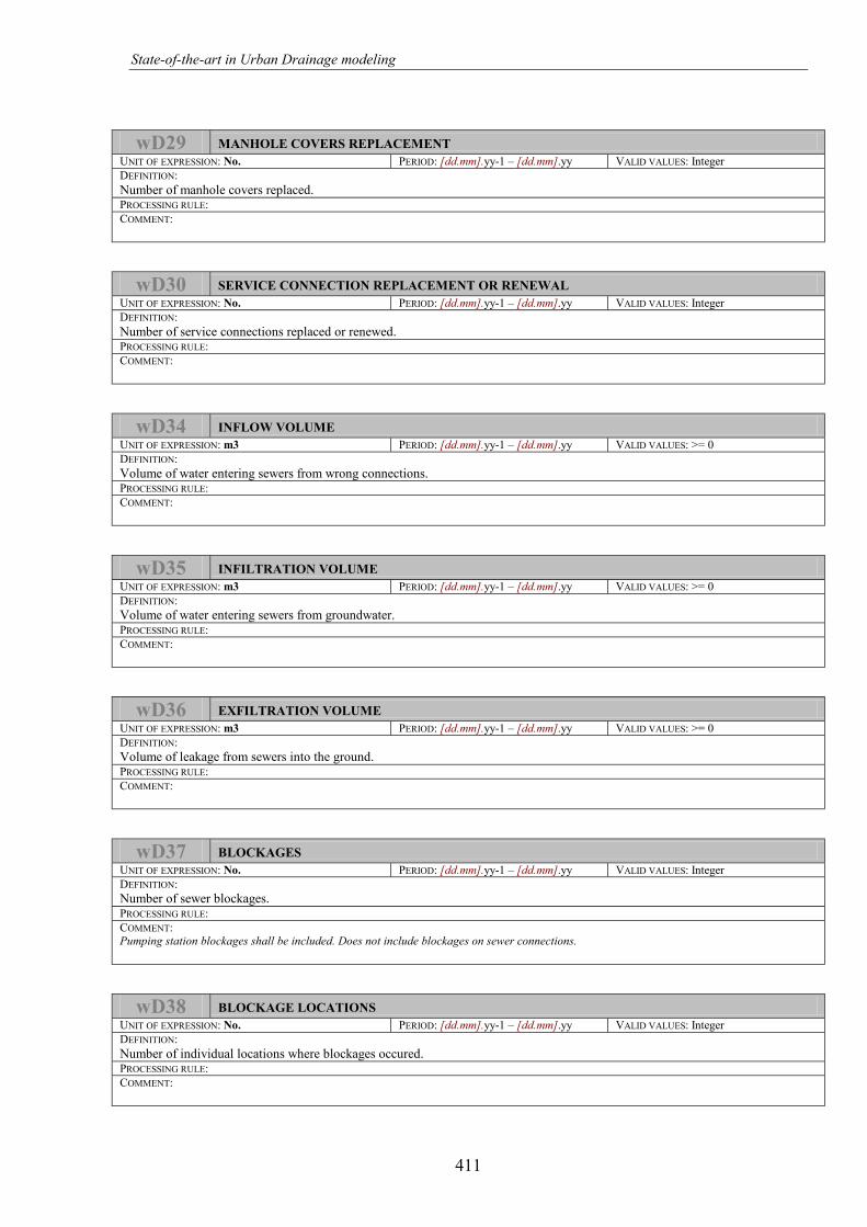
State-of-the-art in Urban Drainage modeling
411
wD29 MANHOLE COVERS REPLACEMENT UNIT OF EXPRESSION: No. PERIOD: [dd.mm].yy-1 – [dd.mm].yy VALID VALUES: Integer DEFINITION: Number of manhole covers replaced. PROCESSING RULE: COMMENT:
wD30 SERVICE CONNECTION REPLACEMENT OR RENEWAL UNIT OF EXPRESSION: No. PERIOD: [dd.mm].yy-1 – [dd.mm].yy VALID VALUES: Integer DEFINITION: Number of service connections replaced or renewed. PROCESSING RULE: COMMENT:
wD34 INFLOW VOLUME UNIT OF EXPRESSION: m3 PERIOD: [dd.mm].yy-1 – [dd.mm].yy VALID VALUES: >= 0 DEFINITION: Volume of water entering sewers from wrong connections. PROCESSING RULE: COMMENT:
wD35 INFILTRATION VOLUME UNIT OF EXPRESSION: m3 PERIOD: [dd.mm].yy-1 – [dd.mm].yy VALID VALUES: >= 0 DEFINITION: Volume of water entering sewers from groundwater. PROCESSING RULE: COMMENT:
wD36 EXFILTRATION VOLUME UNIT OF EXPRESSION: m3 PERIOD: [dd.mm].yy-1 – [dd.mm].yy VALID VALUES: >= 0 DEFINITION: Volume of leakage from sewers into the ground. PROCESSING RULE: COMMENT:
wD37 BLOCKAGES UNIT OF EXPRESSION: No. PERIOD: [dd.mm].yy-1 – [dd.mm].yy VALID VALUES: Integer DEFINITION: Number of sewer blockages. PROCESSING RULE: COMMENT: Pumping station blockages shall be included. Does not include blockages on sewer connections.
wD38 BLOCKAGE LOCATIONS UNIT OF EXPRESSION: No. PERIOD: [dd.mm].yy-1 – [dd.mm].yy VALID VALUES: Integer DEFINITION: Number of individual locations where blockages occured. PROCESSING RULE: COMMENT:

State-of-the-art in Urban Drainage modeling
412
wD39 FLOODINGS FROM SANITARY SEWERS UNIT OF EXPRESSION: No. PERIOD: [dd.mm].yy-1 – [dd.mm].yy VALID VALUES: Integer DEFINITION: Number of foul floodings occurred. PROCESSING RULE: COMMENT: Include only incidents related to sanitary sewers under responsibility of the wastewater undertaking.
wD40 SURFACE WATER FLOODINGS UNIT OF EXPRESSION: No. PERIOD: [dd.mm].yy-1 – [dd.mm].yy VALID VALUES: Integer DEFINITION: Number of surface water floodings occurred. PROCESSING RULE: COMMENT: These include only surface water flooding due to inadequacy of storm drainage system (combined sewers included) under the responsibility of the wastewater undertaking. Inadequacy relates to all causes (e.g. design, operation, etc.).
wD41 SEWER COLLAPSES UNIT OF EXPRESSION: No. PERIOD: [dd.mm].yy-1 – [dd.mm].yy VALID VALUES: Integer DEFINITION: Number of sewer collapses. PROCESSING RULE: COMMENT: Does not include collapses on sewer connections.
DEMOGRAPHY (AND CUSTOMER) DATA
wE1 POPULATION SERVED UNIT OF EXPRESSION: No. PERIOD: [dd.mm].yy-1 – [dd.mm].yy VALID VALUES: Integer DEFINITION: Total population living on a permanent basis in the area under the wastewater undertaking responsibility and, when applicable, those contributing to imported wastewater. PROCESSING RULE: COMMENT:
wE6 POPULATION EQUIVALENT SERVED UNIT OF EXPRESSION: p.e. PERIOD: [dd.mm].yy-1 – [dd.mm].yy VALID VALUES: Integer DEFINITION: Total population producing wastewater that is either collected or treated by the wastewater undertaking, including imported wastewater and industrial contributions expressed in population equivalent. PROCESSING RULE: DEMOGRAPHY (AND CUSTOMER) DATA COMMENT:
QUALITY OF SERVICE DATA
wF3 DRY WEATHER FLOODING OF PROPERTIES FROM SANITARY SEWERS UNIT OF EXPRESSION: No. PERIOD: [dd.mm].yy-1 – [dd.mm].yy VALID VALUES: Integer DEFINITION: Number of properties affected by flooding from sanitary sewers in dry weather. PROCESSING RULE: COMMENT:

State-of-the-art in Urban Drainage modeling
413
wF4 WET WEATHER FLOODING OF PROPERTIES FROM SANITARY SEWERS UNIT OF EXPRESSION: No. PERIOD: [dd.mm].yy-1 – [dd.mm].yy VALID VALUES: Integer DEFINITION: Number of properties affected by flooding from sanitary sewers in wet weather. PROCESSING RULE: COMMENT:
wF5 WET WEATHER SURFACE WATER FLOODING OF PROPERTIES UNIT OF EXPRESSION: No. PERIOD: [dd.mm].yy-1 – [dd.mm].yy VALID VALUES: Integer DEFINITION: Number of properties affected by surface water flooding in wet weather. PROCESSING RULE: COMMENT:
wF6 WASTEWATER SERVICE INTERRUPTIONS UNIT OF EXPRESSION: No. PERIOD: [dd.mm].yy-1 – [dd.mm].yy VALID VALUES: Integer DEFINITION: [Sum] (Number of properties affected by sewerage discontinuity (or interruption) x duration of interruptions in hours). PROCESSING RULE: COMMENT:
wF12 BLOCKAGE COMPLAINTS UNIT OF EXPRESSION: No. PERIOD: [dd.mm].yy-1 – [dd.mm].yy VALID VALUES: Integer DEFINITION: Number of complaints as a result of blockages. PROCESSING RULE: COMMENT: This variable includes all direct, telephone, and written complaints related to blockages.
wF13 FLOODING COMPLAINTS UNIT OF EXPRESSION: No. PERIOD: [dd.mm].yy-1 – [dd.mm].yy VALID VALUES: Integer DEFINITION: Number of complaints as a result of flooding. PROCESSING RULE: COMMENT: This variable includes all direct, telephone, and written complaints related to flooding occurences.
wF14 POLLUTION COMPLAINTS UNIT OF EXPRESSION: No. PERIOD: [dd.mm].yy-1 – [dd.mm].yy VALID VALUES: Integer DEFINITION: Number of complaints as a result of pollution incidents. PROCESSING RULE: COMMENT: This variable includes all direct, telephone, and written complaints related to pollution incidents.

State-of-the-art in Urban Drainage modeling
414
wF15 ODOUR COMPLAINTS UNIT OF EXPRESSION: No. PERIOD: [dd.mm].yy-1 – [dd.mm].yy VALID VALUES: Integer DEFINITION: Number of complaints as a result of odours. PROCESSING RULE: COMMENT: This variable includes all direct, telephone, and written complaints related to odours.
wG4 ANNUAL COSTS UNIT OF EXPRESSION: US$/year PERIOD: [dd.mm].yy-1 – [dd.mm].yy VALID VALUES: >= 0 DEFINITION: Total annual costs, including capital and running costs. PROCESSING RULE: COMMENT: Exchange rate of local currencies shall be referred to the end of the year.
FINANCIAL DATA
wG5 ANNUAL RUNNING COSTS UNIT OF EXPRESSION: US$/year PERIOD: [dd.mm].yy-1 – [dd.mm].yy VALID VALUES: >= 0 DEFINITION: Total annual operations and maintenance costs + internal manpower costs - capitalised costs of self-constructed assets. PROCESSING RULE: COMMENT: This definition has, on aggregate level, to be equivalent to the sum of the NET disaggregated values allocated at the numerator of the indicators figuring the composition of annual running costs per type of cost. Exchange rate of local currencies shall be referred to the end of the year.
wG6 ANNUAL CAPITAL COSTS UNIT OF EXPRESSION: US$/year PERIOD: [dd.mm].yy-1 – [dd.mm].yy VALID VALUES: >= 0 DEFINITION: Total annual net interest and depreciation (based on book values). PROCESSING RULE: COMMENT: The net value of interest has to be considered, being the interest income a reduction in capital costs and not a revenue. Exchange rate of local currencies shall be referred to the end of the year.
wG26 AVERAGE INVESTMENT IN TANGIBLE ASSETS OVER THE LAST THREE YEARS UNIT OF EXPRESSION: US$/year PERIOD: [dd.mm].yy-1 – [dd.mm].yy VALID VALUES: >= 0 DEFINITION: Average annual costs of the investments in tangible assets (expenditures for sewers, plants and equipment) including capilalised costs of self constructed tangible assests over the last three years. PROCESSING RULE: COMMENT: Tangible assets include investment for supporting buildings, vehicles, etc. Exchange rate of local currencies shall be referred to the end of the year.
wG28 ANNUAL INVESTMENTS FOR NEW ASSETS UNIT OF EXPRESSION: US$/year PERIOD: [dd.mm].yy-1 – [dd.mm].yy VALID VALUES: >= 0 DEFINITION: Total cost of the investments in tangible assets during the year that constitute a new development for the service including capitalised costs of self constructed assets. PROCESSING RULE: COMMENT: Exchange rate of local currencies shall be referred to the end of the year.

State-of-the-art in Urban Drainage modeling
415
wG29 ANNUAL INVESTMENTS FOR ASSETS REPLACEMENT UNIT OF EXPRESSION: US$/year PERIOD: [dd.mm].yy-1 – [dd.mm].yy VALID VALUES: >= 0 DEFINITION: Total cost of the investments related to existing assets during the year (i.e., maintaining the existing infrastructure at the same level) including capitalised costs of self-constructed replaced assets. PROCESSING RULE: COMMENT: Exchange rate of local currencies shall be referred to the end of the year.