state of the climate 2014
DESCRIPTION
Everything about climate change and global warming from American Meteorological Society. Giving you overview about environmental issues such as Sea surface temperatures, Ocean carbon, Greenland Ice Sheet, to regional climates.TRANSCRIPT

Special Supplement to theBulletin of the American Meteorological Society
Vol. 96, No. 7, July 2015
STATE OF THE CLIMATEIN 2014

Editors
Jessica Blunden Derek S. Arndt
Howard J. DiamondA. Johannes Dolman
Ryan L. FogtDale F. Hurst
Martin O. Jeffries
Gregory C. JohnsonAdeme MekonnenA. Rost Parsons
Jared RennieJames A. Renwick
Jacqueline A. Richter-MengeAhira Sánchez-LugoSharon Stammerjohn
Peter W. ThorneKate M. Willett
Chapter Editors
AmericAn meteorologicAl Society
Technical Editor
Mara Sprain
STATE OF THE CLIMATEIN 2014
How to cite this document:
Citing the complete report:
Blunden, J. and D. S. Arndt, Eds., 2015: State of the Climate in 2014. Bull. Amer. Meteor. Soc., 96 (7), S1–S267.
Citing a chapter (example):
Mekonnen, A., J. A. Renwick, and A. Sánchez-Lugo, Eds., 2015: Regional climates [in “State of the Climate in 2014”]. Bull. Amer. Meteor. Soc., 96 (7), S169–S219.
Citing a section (example):
Macara, G. R., 2015: New Zealand [in “State of the Climate in 2014”]. Bull. Amer. Meteor. Soc., 96 (7), S217–S219.
Cover Credits:
Front: AdAm Ü — Argo float WMO ID# 4900835 upon deployment at 13° 43.22' N; 105° 21.23' W on 11 September 2007. This float was still fully functional and reporting data as of June 2015.
BACk: ©iStockphotos.com/Robert Pavsic—Capital city of Maldives Male coastline.

SiJULY 2015STATE OF THE CLIMATE IN 2014 |
EDITOR & AUTHOR AFFILIATIONS (AlphABetiCAl By nAme)
Aaron-Morrison, Arlene P., Trinidad & Tobago Meteoro-logical Service, Piarco, Trinidad
Ackerman, Steven A., CIMSS, University of Wisconsin–Madison, Madison, Wisconsin
Adamu, J. I., Nigerian Meteorological Agency, Abuja, Ni-geria
Albanil, Adelina, National Meteorological Service of Mexico, Mexico
Alfaro, Eric J., Center for Geophysical Research and School of Physics, University of Costa Rica, San José, Costa Rica
Allan, Rob, Met Office Hadley Centre, Exeter, United Kingdom
Alley, Richard B., Department of Geosciences and Earth and Environmental Systems Institute, The Pennsylvania State University, University Park, Pennsylvania
Álvarez, Luis, Instituto de Hidrología de Meteorología y Estudios Ambientales de Colombia (IDEAM), Bogotá, Colombia
Alves, Lincoln M., Centro de Ciencias do Sistema Ter-restre, Instituto Nacional de Pesquisas Espaciais, Ca-choeira Paulista, Sao Paulo, Brazil
Amador, Jorge A., Center for Geophysical Research and School of Physics, University of Costa Rica, San José, Costa Rica
Andreassen, L. M., Section for Glaciers, Ice and Snow, Norwegian Water Resources and Energy Directorate, Oslo, Norway
Antonov, John, NOAA/NESDIS National Centers for Environmental Information, Silver Spring, Maryland, and University Corporation for Atmospheric Research, Boul-der, Colorado
Applequist, Scott, NOAA/NESDIS National Centers for Environmental Information, Asheville, North Carolina
Arendt, A., Geophysical Institute, University of Alaska Fairbanks, Fairbanks, Alaska
Arévalo, Juan, Instituto Nacional de Meteorología e Hi-drología de Venezuela, Caracas, Venezuela
Arguez, Anthony, NOAA/NESDIS National Centers for Environmental Information, Asheville, North Carolina
Arndt, Derek S., NOAA/NESDIS National Centers for Environmental Information, Asheville, North Carolina
Banzon, Viva, NOAA/NESDIS National Centers for Envi-ronmental Information, Asheville, North Carolina
Barichivich, J., School of Geography, University of Leeds, Leeds, United Kingdom, and Center for Climate and Re-silience Research (CR)², Chile
Baringer, Molly O., NOAA/OAR Atlantic Oceanographic and Meteorological Laboratory, Miami, Florida
Barreira, Sandra, Argentine Naval Hydrographic Service, Buenos Aires, Argentina
Baxter, Stephen, NOAA/NWS Climate Prediction Cen-ter, College Park, Maryland
Bazo, Juan, Servicio Nacional de Meteorología e Hi-drología de Perú, Lima, Perú
Becker, Andreas, Global Precipitation Climatology Cen-tre, Deutscher Wetterdienst, Offenbach, Germany
Behrenfeld, Michael J., Oregon State University, Corval-lis, Oregon
Bell, Gerald D., NOAA/NWS Climate Prediction Center, College Park, Maryland
Benedetti, Angela, European Centre for Medium-Range Weather Forecasts, Reading, United Kingdom
Bernhard, G., Biospherical Instruments, San Diego, Cali-fornia
Berrisford, Paul, European Centre for Medium-Range Weather Forecasts, Reading, United Kingdom
Berry, David I., National Oceanography Centre, South-ampton, United Kingdom
Bettolli, María L., Departamento Ciencias de la Atmós-fera y los Océanos, Facultad de Ciencias Exactas y Natu-rales, Universidad de Buenos Aires, Argentina
Bhatt, U. S., Geophysical Institute, University of Alaska Fairbanks, Fairbanks, Alaska
Bidegain, Mario, Instituto Uruguayo de Meteorologia, Montevideo, Uruguay
Bindoff, Nathan, Antarctic Climate and Ecosystems Coop-erative Research Centre, and CSIRO Marine and Atmo-spheric Laboratories, Hobart, Tasmania, Australia
Bissolli, Peter, Deutscher Wetterdienst, WMO RA VI Re-gional Climate Centre Network, Offenbach, Germany
Blake, Eric S., NOAA/NWS National Hurricane Center, Miami, Florida
Blenman, Rosalind C., Barbados Meteorological Services, Christ Church, Barbados
Blunden, Jessica, ERT, Inc., NOAA/NESDIS National Centers for Environmental Information, Asheville, North Carolina
Bond, Nick A., Joint Institute for the Study of the At-mosphere and Ocean, University of Washington, and NOAA/OAR Pacific Marine Environmental Laboratory, Seattle, Washington
Bosilovich, Mike, Global Modelling and Assimilation Of-fice, NASA Goddard Space Flight Center, Greenbelt, Maryland
Boudet, Dagne, Climate Center, Institute of Meteorology of Cuba, Cuba
Box, J. E., Geological Survey of Denmark and Greenland, Copenhagen, Denmark
Boyer, Tim, NOAA/NESDIS National Centers for Environ-mental Information, Silver Spring, Maryland
Braathen, Geir O., WMO Atmospheric Environment Re-search Division, Geneva, Switzerland
Bromwich, David H., Byrd Polar and Climate Research Center, The Ohio State University, Columbus, Ohio
Brown, L. C., Department of Geography, University of To-ronto Mississauga, Mississauga, Ontario, Canada
Brown, R., Climate Research Division, Environment Cana-da, Montreal, Quebec, Canada

Sii JULY 2015|
Bulygina, Olga N., Russian Institute for Hydrometeoro-logical Information, Obninsk, Russia
Burgess, D., Geological Survey of Canada, Ottawa, On-tario, Canada
Calderón, Blanca, Center for Geophysical Research, Uni-versity of Costa Rica, San José, Costa Rica
Camargo, Suzana J., Lamont-Doherty Earth Observa-tory, Columbia University, Palisades, New York
Campbell, Jayaka D., Department of Physics, The Univer-sity of the West Indies, Jamaica
Cappelen, J., Danish Meteorological Institute, Copenha-gen, Denmark
Carrasco, Gualberto, Servicio Nacional de Meteorología e Hidrología de Bolivia, La Paz, Bolivia
Carter, Brendan, NOAA/OAR Pacific Marine Environ-mental Laboratory, Seattle, Washington
Chambers, Don P., College of Marine Science, University of South Florida, St. Petersburg, Florida
Chandler, Elise, Bureau of Meteorology, Melbourne, Vic-toria, Australia
Chevallier, Frédéric, Laboratoire des Sciences du Climat et de l’Environnement, CEA-CNRS-UVSQ, Gif-sur-Yvette, France
Christiansen, Hanne H., Arctic Geology Department, UNIS-The University Centre in Svalbard, Longyearbyen, Norway
Christy, John R., University of Alabama in Huntsville, Huntsville, Alabama
Chung, D., Department of Geodesy and Geoinformation, Vienna University of Technology, Vienna, Austria
Ciais, Philippe, LCSE, Gif sur l’Yvette, FranceClem, Kyle R., School of Geography, Environment, and
Earth Sciences, Victoria University of Wellington, Wel-lington, New Zealand
Coelho, Caio A.S., CPTEC/INPE Center for Weather Forecasts and Climate Studies, Cachoeira Paulista, Brazil
Cogley, J. G., Department of Geography, Trent University, Peterborough, Ontario, Canada
Coldewey-Egbers, Melanie, DLR (German Aerospace Center) Oberpfaffenhofen, Wessling, Germany
Colwell, Steve, British Antarctic Survey, Cambridge, United Kingdom
Cooper, Owen R., Cooperative Institute for Research in Environmental Sciences, University of Colorado Boulder, and NOAA/OAR Earth System Research Laboratory, Boulder, Colorado
Copland, L., Department of Geography, University of Ot-tawa, Ottawa, Ontario, Canada
Cronin, Meghan F., NOAA/OAR Pacific Marine Environ-mental Laboratory, Seattle, Washington
Crouch, Jake, NOAA/NESDIS National Centers for Envi-ronmental Information, Asheville, North Carolina
Cunningham, Stuart A., Scottish Marine Institute, Oban, Argyll, United Kingdom
Davis, Sean M., Cooperative Institute for Research in En-vironmental Sciences, University of Colorado Boulder, and NOAA/OAR Earth System Research Laboratory, Boulder, Colorado
De Jeu, R. A. M., Earth and Climate Cluster, Department of Earth Sciences, Faculty of Earth and Life Sciences, VU University Amsterdam, Amsterdam, Netherlands
Degenstein, Doug, University of Saskatchewan, Saska-toon, Saskatchewan, Canada
Demircan, M., Turkish State Meteorological Service, An-kara, Turkey
Derksen, C., Climate Research Division, Environment Canada, Toronto, Ontario, Canada
Destin, Dale, Antigua and Barbuda Meteorological Service, St. John’s, Antigua
Diamond, Howard J., NOAA/NESDIS National Centers for Environmental Information, Silver Spring, Maryland
Dlugokencky, Ed J., NOAA/OAR Earth System Research Laboratory, Boulder, Colorado
Dohan, Kathleen, Earth and Space Research, Seattle, Washington
Dolman, A. Johannes, Department of Earth Sciences, Earth and Climate Cluster, VU University Amsterdam, Amsterdam, Netherlands
Domingues, Catia M., Institute for Marine and Antarctic Studies, University of Tasmania, and Antarctic Climate and Ecosystems Cooperative Research Centre, Hobart, Tasmania, Australia
Donat, Markus G., Climate Change Research Centre, Uni-versity of New South Wales, Sydney, New South Wales, Australia
Dong, Shenfu, NOAA/OAR Atlantic Oceanographic and Meteorological Laboratory, and Cooperative Institute for Marine and Atmospheric Science, Miami, Florida
Dorigo, Wouter A., Department of Geodesy and Geoin-formation, Vienna University of Technology, Vienna, Aus-tria, and Department of Forest and Water Management, Gent University, Gent, Belgium
Drozdov, D. S., Earth Cryosphere Institute, Tyumen, and Tyumen State Oil and Gas University, Tyumen, Russia
Duguay, C. R., Department of Geography & Environmental Management, University of Waterloo, Waterloo, and H2O Geomatics Inc., Waterloo, Ontario, Canada
Dunn, Robert J. H., Met Office Hadley Centre, Exeter, United Kingdom
Durán-Quesada, Ana M., Center for Geophysical Re-search and School of Physics, University of Costa Rica, San José, Costa Rica
Dutton, Geoff S., Cooperative Institute for Research in Environmental Sciences, University of Colorado Boulder, and NOAA/OAR Earth System Research Laboratory, Boulder, Colorado
Ebrahim, A., Egyptian Meteorological Authority, Cairo, Egypt
Elkins, James W., NOAA/OAR Earth System Research Laboratory, Boulder, Colorado
SiiiJULY 2015STATE OF THE CLIMATE IN 2014 |
Epstein, H. E., University of Virginia, Charlottesville, Vir-ginia
Espinoza, Jhan C., Instituto Geofisico del Peru, Lima, PeruEvans III, Thomas E., NOAA/NWS Central Pacific Hur-
ricane Center, Honolulu, HawaiiFamiglietti, James S., Department of Earth System Sci-
ence, University of California, Irvine, CaliforniaFateh, S., Islamic Republic of Iranian Meteorological Orga-
nization, IranFauchereau, Nicolas C., National Institute of Water and
Atmospheric Research, Ltd., Auckland, New ZealandFeely, Richard A., NOAA/OAR Pacific Marine Environ-
mental Laboratory, Seattle, WashingtonFenimore, Chris, NOAA/NESDIS National Centers for
Environmental Information, Asheville, North CarolinaFettweis, X., University of Liège, Liège, BelgiumFioletov, Vitali E., Environment Canada, Toronto, On-
tario, CanadaFlemming, Johannes, European Centre for Medium-
Range Weather Forecasts, Reading, United KingdomFogarty, Chris T., Canadian Hurricane Centre, Environ-
ment Canada, Dartmouth, Nova Scotia, CanadaFogt, Ryan L., Department of Geography, Ohio Univer-
sity, Athens, OhioFolland, Chris K., Met Office Hadley Centre, Exeter,
United KingdomFoster, Michael, CIMSS, University of Wisconsin–Madi-
son, Madison, WisconsinFrancis S. D., Nigerian Meteorological Agency, Abuja, Ni-
geriaFranz, Bryan A., NASA Goddard Space Flight Center,
Greenbelt, MarylandFreeland, Howard, Institute of Ocean Sciences, Fisheries
and Oceans, Sidney, British Columbia, CanadaFrith, Stacey M., NASA Goddard Space Flight Center,
Greenbelt, MarylandFroidevaux, Lucien, Jet Propulsion Laboratory, California
Institute of Technology, Pasadena, CaliforniaFrost, G. V., ABR, Inc., Fairbanks, AlaskaGanter, Catherine, Bureau of Meteorology, Melbourne,
Victoria, AustraliaGarzoli, Silvia, NOAA/OAR Atlantic Oceanographic and
Meteorological Laboratory, and Cooperative Institute for Marine and Atmospheric Science, Miami, Florida
Gerland, S., Norwegian Polar Institute, Fram Centre, Tromsø, Norway
Gitau, Wilson, Department of Meteorology, University of Nairobi, Nairobi, Kenya
Gobron, Nadine, Land Resources Monitoring Unit, Insti-tute for Environment and Sustainability, Joint Research Centre, European Commission, Ispra, Italy
Goldenberg, Stanley B., NOAA/OAR Atlantic Oceano-graphic and Meteorological Laboratory, Miami, Florida
Goni, Gustavo, NOAA/OAR Atlantic Oceanographic and Meteorological Laboratory, Miami, Florida
Gonzalez, Idelmis T., Climate Center, Institute of Meteo-rology of Cuba, Cuba
Good, Simon A., Met Office Hadley Centre, Exeter, United Kingdom
Goto, A., Japan Meteorological Agency, Tokyo, JapanGriffin, Kyle S., Department of Atmospheric and Oceanic
Sciences, University of Wisconsin–Madison, Madison, Wisconsin
Grist, Jeremy, National Oceanography Centre, Southamp-ton, United Kingdom
Grooß, J.-U., Forschungszentrum Jülich, Jülich, GermanyGuard, Charles “Chip”, NOAA/NWS Weather Forecast
Office, GuamGupta, S. K., SSAI, Hampton, VirginiaHagos, S., FCSD/ASGC Climate Physics Group, Pacific
Northwest National Laboratory, Richland, WashingtonHaimberger, Leo, Department of Meteorology and Geo-
physics, University of Vienna, Vienna, AustriaHall, Bradley D., NOAA/OAR Earth System Research
Laboratory, Boulder, ColoradoHalpert, Michael S., NOAA/NWS Climate Prediction
Center, College Park, MarylandHamlington, Benjamin D., Center for Coastal Physical
Oceanography, Old Dominion University, Norfolk, Vir-ginia
Hanna, E., Department of Geography, University of Shef-field, Sheffield, United Kingdom
Hanssen-Bauer, I., Norwegian Meteorological Institute, Blindern, Oslo, Norway
Harris, Ian, Climatic Research Unit, School of Environmen-tal Sciences, University of East Anglia, Norwich, United Kingdom
Heidinger, Andrew K., NOAA/NESDIS/STAR University of Wisconsin–Madison, Madison, Wisconsin
Heikkilä, A., Finnish Meteorological Institute, Helsinki, Finland
Heim, Jr., Richard R., NOAA/NESDIS National Centers for Environmental Information, Asheville, North Carolina
Hendricks, S., Alfred Wegener Institute, Bremerhaven, Germany
Hernandez, M., Climate Center, Institute of Meteorology of Cuba, Cuba
Hidalgo, Hugo G., Center for Geophysical Research and School of Physics, University of Costa Rica, San José, Costa Rica
Hilburn, Kyle, Remote Sensing Systems, Santa Rosa, Cali-fornia
Ho, Shu-peng (Ben), COSMIC, UCAR, Boulder, Colo-rado
Hobbs, Will R., ARC Centre of Excellence for Climate System Science, University of Tasmania, Hobart, Tasma-nia, Australia
Hu, Zeng-Zhen, NOAA/NWS National Centers for Envi-ronmental Prediction, Climate Prediction Center, Col-lege Park, Maryland
Siv JULY 2015|
Huelsing, Hannah, State University of New York, Albany, New York
Hurst, Dale F., Cooperative Institute for Research in En-vironmental Sciences, University of Colorado Boulder, and NOAA/OAR Earth System Research Laboratory, Boulder, Colorado
Inness, Antje, European Centre for Medium-Range Weather Forecasts, Reading, United Kingdom
Ishii, Masayoshi, Japan Meteorological Agency, Meteoro-logical Research Institute, Tsukuba, Japan
Jeffers, Billy, Meteorological Office, E.T. Joshua Airport, Arnos Vale, St. Vincent and the Grenadines
Jeffries, Martin O., Office of Naval Research, Arlington, Virginia
Jevrejeva, Svetlana, National Oceanography Centre, Liv-erpool, United Kingdom
Jin, Xiangze, Woods Hole Oceanographic Institution, Woods Hole, Massachusetts
John, Viju, User Service and Climate, EUMETSAT, Darm-stadt, Germany
Johns, William E., Rosenstiel School of Marine and Atmo-spheric Science, Miami, Florida
Johnsen, B., Norwegian Radiation Protection Authority, Østerås, Norway
Johnson, Bryan, NOAA/OAR Earth System Research Laboratory, Global Monitoring Division, and University of Colorado Boulder, Boulder, Colorado
Johnson, Gregory C., NOAA/OAR Pacific Marine Envi-ronmental Laboratory, Seattle, Washington
Jones, Phil D., Climatic Research Unit, School of Environ-mental Sciences, University of East Anglia, Norwich, United Kingdom, and Center of Excellence for Climate Change Research, Department of Meteorology, King Ab-dulaziz, Jeddah, Saudi Arabia
Josey, Simon A., National Oceanography Centre, South-ampton, United Kingdom
Joyette, Sigourney, Meteorological Office, E.T. Joshua Air-port, Arnos Vale, St. Vincent and the Grenadines
Jumaux, Guillaume, Météo France, RéunionKabidi, Khadija, Direction de la Météorologie Nationale
Maroc, Rabat, MoroccoKaiser, Johannes W., Max Planck Institute for Chemistry,
Mainz, Germany, and European Centre for Medium-Range Weather Forecasts, Reading, United Kingdom
Kang, K.-K., H2O Geomatics Inc., Waterloo, Ontario, Canada
Kanzow, Torsten O., Alfred Wegener Institute for Polar and Marine Research, Bremerhaven, Germany
Kao, Hsun-Ying, Earth & Space Research, Seattle, Wash-ington
Kazemi, A., Islamic Republic of Iranian Meteorological Or-ganization, Iran
Keller, Linda M., Department of Atmospheric and Ocean-ic Sciences, University of Wisconsin–Madison, Madison, Wisconsin
Kendon, Mike, Met Office National Climate Information Centre, Exeter, United Kingdom
Kennedy, John, Met Office Hadley Centre, Exeter, United Kingdom
Kerr, Kenneth, Trinidad & Tobago Meteorological Service, Piarco, Trinidad
Kheyrollah Pour, H., Department of Geography & Envi-ronmental Management, University of Waterloo, Water-loo, Ontario, Canada
Kholodov, A. L., Geophysical Institute, University of Alas-ka Fairbanks, Fairbanks, Alaska
Khoshkam, Mahbobeh, Islamic Republic of Iranian Me-teorological Organization, Iran
Kidd, R., Department of Geodesy and Geoinformation, Vienna University of Technology, Vienna, Austria
Kieke, Dagmar, Institut fuer Umweltphysik, Bremen, Ger-many
Kim, Hyungjun, Institute of Industrial Science, University of Tokyo, Japan
Kim, S.-J., Korea Polar Research Institute, Incheon, Repub-lic of Korea
Kimberlain, Todd B., NOAA/NWS National Hurricane Center, Miami, Florida
Klotzbach, Philip, Department of Atmospheric Science, Colorado State University, Fort Collins, Colorado
Knaff, John A., NOAA/NESDIS Center for Satellite Appli-cations and Research, Fort Collins, Colorado
Kobayashi, Shinya, Climate Prediction Division, Japan Me-teorological Agency, Tokyo, Japan
Kohler, J., Norwegian Polar Institute, Tromsø, NorwayKorshunova, Natalia N., All-Russian Research Institute of
Hydrometeorological Information - World Data Center, Obninsk, Russia
Koskela, T., Finnish Meteorological Institute, Helsinki, Fin-land
Kramarova, Natalya, Science Systems and Applications, Inc., NASA Goddard Space Flight Center, Greenbelt, Maryland
Kratz, D. P., NASA Langley Research Center, Hampton, Virginia
Kruger, Andries, South African Weather Service, Pretoria, South Africa
Kruk, Michael C., ERT, Inc., NOAA/NESDIS National Centers for Environmental Information, Asheville, North Carolina
Kumar, Arun, NOAA/NWS National Centers for Environ-mental Prediction, Climate Prediction Center, College Park, Maryland
Kwok, R., Jet Propulsion Laboratory, California Institute of Technology, Pasadena, California
Lagerloef, Gary S. E., Earth & Space Research, Seattle, Washington
Lakkala, K., Finnish Meteorological Institute, Arctic Re-search Centre, Sodankylä, Finland
Lander, Mark A., University of Guam, Mangilao, Guam

SvJULY 2015STATE OF THE CLIMATE IN 2014 |
Landsea, Chris W., NOAA/NWS National Hurricane Center, Miami, Florida
Lankhorst, Matthias, Scripps Institution of Oceanography, University of California, San Diego, La Jolla, California
Lantz, Kathy, Cooperative Institute for Research in Envi-ronmental Sciences, University of Colorado Boulder, and NOAA/OAR Earth System Research Laboratory, Boul-der, Colorado
Lazzara, Matthew A., Space Science and Engineering Center, University of Wisconsin–Madison, Madison, Wisconsin
Leuliette, Eric, NOAA/NWS NCWCP Laboratory for Satellite Altimetry, College Park, Maryland
L’Heureux, Michelle, NOAA/NWS Climate Prediction Center, College Park, Maryland
Lieser, Jan L., Antarctic Climate and Ecosystems Coopera-tive Research Centre, University of Tasmania, Hobart, Tasmania, Australia
Lin, I-I, National Taiwan University, Taipei, TaiwanLiu, Hongxing, Department of Geography, University of
Cincinnati, Cincinnati, OhioLiu, Yinghui, Cooperative Institute for Meteorological Sat-
ellite Studies, University of Wisconsin–Madison, Madi-son, Wisconsin
Locarnini, Ricardo, NOAA/NESDIS National Centers for Environmental Information, Silver Spring, Maryland
Loeb, Norman G., NASA Langley Research Center, Hampton, Virginia
Long, Craig S., NOAA/NWS Center for Weather and Cli-mate Prediction, College Park, Maryland
Lorrey, Andrew M., National Institute of Water and At-mospheric Research, Ltd., Auckland, New Zealand
Loyola, Diego, DLR (German Aerospace Center) Oberp-faffenhofen, Wessling, Germany
Lui, Yi Y., ARC Centre of Excellence for Climate Systems Science and Climate Change Research Centre, University of New South Wales, Sydney, New South Wales, Aus-tralia
Lumpkin, Rick, NOAA/OAR Atlantic Oceanographic and Meteorological Laboratory, Miami, Florida
Luo, Jing-Jia, Australian Bureau of Meteorology, Mel-bourne, Victoria, Australia
Luojus, K., Finnish Meteorological Institute, Helsinki, Fin-land
Lyman, John M., NOAA/OAR Pacific Marine Environmen-tal Laboratory, Seattle, Washington, and Joint Institute for Marine and Atmospheric Research, University of Ha-waii, Honolulu, Hawaii
Macara, Gregor R., National Institute of Water and At-mospheric Research, Ltd., Wellington, New Zealand
Maddux, Brent C., AOS/CIMSS University of Wisconsin–Madison, Madison, Wisconsin
Malkova, G. V., Earth Cryosphere Institute, Tyumen, and Tyumen State Oil and Gas University, Tyumen, Russia
Manney, G., NorthWest Research Associates, and New Mexico Institute of Mining and Technology, Socorro, New Mexico
Marcellin-Honore’, Vernie, Dominica Meteorological Service, Dominica
Marchenko, S. S., Geophysical Institute, University of Alaska Fairbanks, Fairbanks, Alaska
Marengo, José A., Centro Nacional de Monitoramento e Alertas aos Desastres Naturais, Cachoeira Paulista, Sao Paulo, Brazil
Marra, John J., NOAA/NESDIS National Centers for Envi-ronmental Information, Honolulu, Hawaii
Martínez-Güingla, Rodney, CIIFEN Centro Internacional para la Investigación del Fenómeno de El Niño, Guaya-quil, Ecuador
Massom, Robert A., Australian Antarctic Division, and Antarctic Climate and Ecosystems Cooperative Research Centre, University of Tasmania, Hobart, Tasmania, Aus-tralia
Mata, Mauricio M., Laboratório de Estudos dos Oceanos e Clima, Instituto de Oceanografia – FURG, Rio Grande (RS), Brazil
Mathis, Jeremy T., NOAA/OAR Pacific Marine Environ-mental Laboratory, Seattle, Washington
Mazloff, Matthew, Scripps Institution of Oceanography, University of California, San Diego, La Jolla, California
McBride, Charlotte, South African Weather Service, Pre-toria, South Africa
McCarthy, Gerard, National Oceanography Centre, Southampton, United Kingdom
McGree, Simon, Bureau of Meteorology, Melbourne, Vic-toria, Australia
McLean, Natalie, Department of Physics, The University of the West Indies, Jamaica
McVicar, Tim R., CSIRO Land and Water Flagship, Can-berra, Australian Capital Territory, and Australian Re-search Council Centre of Excellence for Climate System Science, Sydney, New South Wales, Australia
Mears, Carl A., Remote Sensing Systems, Santa Rosa, California
Meier, W., NASA Goddard Space Flight Center, Greenbelt, Maryland
Meinen, Christopher S., NOAA/OAR Atlantic Oceano-graphic and Meteorological Laboratory, Miami, Florida
Mekonnen, A., Department of Energy and Environmen-tal Systems, North Carolina A & T State University, Greensboro, North Carolina
Melzer, T., Department of Geodesy and Geoinformation, Vienna University of Technology, Vienna, Austria
Menéndez, Melisa, Environmental Hydraulic Institute, Universidad de Cantabria, Cantabria, Spain
Mengistu Tsidu, G., Department of Earth and Environ-mental Sciences, Botswana International University of Science and Technology, Botswana

Svi JULY 2015|
Meredith, Michael P., British Antarctic Survey, Cam-bridge, United Kingdom
Merrifield, Mark A., Joint Institute for Marine and Atmo-spheric Research, University of Hawaii, Honolulu, Hawaii
Mitchum, Gary T., College of Marine Science, University of South Florida, St. Petersburg, Florida
Monteiro, Pedro, CSIR Natural Resources and the Envi-ronment, Stellenbosch, South Africa
Montzka, Stephen A., NOAA/OAR Earth System Re-search Laboratory, Boulder, Colorado
Morice, Colin, Met Office Hadley Centre, Exeter, United Kingdom
Mote, T., Department of Geography, The University of Georgia, Athens, Georgia
Mudryk, L., Climate Research Division, Environment Cana-da, Toronto, Ontario, Canada
Mühle, Jens, Scripps Institution of Oceanography, Univer-sity of California, San Diego, La Jolla, California
Mullan, A. Brett, National Institute of Water and Atmo-spheric Research, Ltd., Wellington, New Zealand
Müller, R., Forschungszentrum Jülich, Jülich, GermanyNash, Eric R., Science Systems and Applications, Inc.,
NASA Goddard Space Flight Center, Greenbelt, Mary-land
Naveira Garabato, Alberto C., University of South-ampton, National Oceanography Centre, Southampton, United Kingdom
Nerem, R. Steven, Colorado Center for Astrodynamics Research, Cooperative Institute for Research in Envi-ronmental Sciences, University of Colorado Boulder, Boulder, Colorado
Newman, Louise, SOOS International Project Office, Institute for Marine and Antarctic Science, University of Tasmania, Hobart, Tasmania, Australia
Newman, Paul A., NASA Goddard Space Flight Center, Greenbelt, Maryland
Nicolaus, M., Alfred Wegener Institute, Bremerhaven, Germany
Nieto, Juan J., CIIFEN Centro Internacional para la Inves-tigación del Fenómeno de El Niño, Guayaquil, Ecuador
Noetzli, Jeannette, Department of Geography, University of Zurich, Zurich, Switzerland
O’Neel, S., USGS, Alaska Science Center, Anchorage, Alaska
Oberman, N. G., MIRECO Mining Company, Syktyvkar, Russia
Ogallo, Laban A., IGAD Climate Prediction and Applica-tions Centre, Nairobi, Kenya
Oki, Taikan, Institute of Industrial Science, University of Tokyo, Japan
Oludhe, Christopher S., Department of Meteorology, University of Nairobi, Nairobi, Kenya
Osborn, Tim J., Climatic Research Unit, School of Envi-ronmental Sciences, University of East Anglia, Norwich, United Kingdom
Overland, J., NOAA/OAR Pacific Marine Environmental Laboratory, Seattle, Washington
Oyunjargal, Lamjav, Hydrology and Environmental Moni-toring, Institute of Meteorology and Hydrology, National Agency for Meteorology, Ulaanbaatar, Mongolia
Pabón, D., CIIFEN Centro Internacional para la Investig-ación del Fenómeno de El Niño, Guayaquil, Ecuador
Parinussa, Robert M., School of Civil and Environmental Engineering, Water Research Centre, University of New South Wales, Sydney, New South Wales, Australia
Park, E-hyung, Korea Meteorological Administration, South Korea
Parker, David, Met Office Hadley Centre, Exeter, United Kingdom
Parsons, Rost, NOAA/NESDIS National Centers for Envi-ronmental Information, Silver Spring, Maryland
Pasch, Richard J., NOAA/NWS National Hurricane Cen-ter, Miami, Florida
Pascual-Ramírez, Reynaldo, National Meteorological Service of Mexico, Mexico
Pelto, Mauri S., Nichols College, Dudley, MassachusettsPeng, Liang, UCAR COSMIC, Boulder, ColoradoPerovich, D., USACE Cold Regions Research and Engineer-
ing Laboratory, Hanover, New HampshirePersson, P. O. G., Cooperative Institute for Research in
Environmental Sciences, University of Colorado Boulder, and NOAA/OAR Earth System Research Laboratory, Boulder, Colorado
Peterson, Thomas C., NOAA/NESDIS National Centers for Environmental Information, Asheville, North Carolina
Petropavlovskikh, Irina, NOAA/OAR Earth System Re-search Laboratory, Global Monitoring Division, and Uni-versity of Colorado Boulder, Boulder, Colorado
Peuch, Vincent-Henri, European Centre for Medium-Range Weather Forecasts, Reading, United Kingdom
Pezza, Alexandre B., Greater Wellington Regional Coun-cil, Wellington, New Zealand
Phillips, David, Environment Canada, Toronto, Ontario, Canada
Photiadou, C., Institute for Marine and Atmospheric Research Utrecht, Utrecht University, Utrecht, Nether-lands
Pinty, Bernard, European Commission, Joint Research Centre, Institute for Environment and Sustainability, Cli-mate Risk Management Unit, Ispra, Italy
Pitts, Michael C., NASA Langley Research Center, Hamp-ton, Virginia
Porter, Avalon O., Cayman Islands National Weather Ser-vice, Grand Cayman, Cayman Islands
Proshutinsky, A. , Woods Hole Oceanographic Institu-tion, Woods Hole, Massachusetts
Quegan, Shaun, University of Sheffield, Sheffield, United Kingdom
Quintana, Juan, Direccion Meteorologica de Chile, ChileRahimzadeh, Fatemeh, Atmospheric Science and Meteo-
rological Research Center, Tehran, IranRajeevan, Madhavan, Indian Institute of Tropical Meteo-
rology, Pune, India

SviiJULY 2015STATE OF THE CLIMATE IN 2014 |
Ramos, A., Instituto Dom Luiz, Universidade de Lisboa, Campo Grande, Lisboa, Portugal
Raynor, Darren, National Oceanography Centre, South-ampton, United Kingdom
Razuvaev, Vyacheslav N., All-Russian Research Institute of Hydrometeorological Information, Obninsk, Russia
Reagan, James, NOAA/NESDIS National Centers for Environmental Information, Silver Spring, Maryland, and Earth System Science Interdisciplinary Center/Coopera-tive Institute for Climate and Satellites–Maryland, Uni-versity of Maryland, College Park, Maryland
Reid, Phillip, Australian Bureau of Meteorology and CAW-RC, Hobart, Tasmania, Australia
Reimer, C., Department of Geodesy and Geoinformation, Vienna University of Technology, Vienna, Austria
Rémy, Samuel, Laboratoire de Météorologie Dynamique, Paris, France
Rennie, Jared, Cooperative Institute for Climate and Satel-lites, North Carolina State University, Asheville, North Carolina
Renwick, James A., Victoria University of Wellington, Wellington, New Zealand
Revadekar, Jayashree V., Indian Institute of Tropical Me-teorology, Pune, India
Richter-Menge, Jacqueline A., USACE Cold Regions Research and Engineering Laboratory, Hanover, New Hampshire
Robinson, David A., Department of Geography, Rutgers University, Piscataway, New Jersey
Rodell, Matthew, Hydrological Sciences Laboratory, NASA, Goddard Space Flight Center, Greenbelt, Mary-land
Romanovsky, Vladimir E., Geophysical Institute, Univer-sity of Alaska Fairbanks, Fairbanks, Alaska
Ronchail, Josyane, University of Paris, Paris, FranceRosenlof, Karen H., NOAA/OAR Earth System Research
Laboratory, Boulder, ColoradoRoth, Chris, University of Saskatchewan, Saskatoon, Sas-
katchewan, CanadaSabine, Christopher L., NOAA/OAR Pacific Marine Envi-
ronmental Laboratory, Seattle, WashingtonSallée, Jean-Bapiste, CNRS, L’OCEAN-IPSL, Paris,
FranceSánchez-Lugo, Ahira, NOAA/NESDIS National Centers
for Environmental Information, Asheville, North CarolinaSantee, Michelle L., NASA Jet Propulsion Laboratory,
Pasadena, CaliforniaSawaengphokhai, P., SSAI, Hampton, VirginiaSayouri, Amal, Direction de la Météorologie Nationale
Maroc, Rabat, MoroccoScambos, Ted A., National Snow and Ice Data Center,
University of Colorado Boulder, Boulder, ColoradoSchemm, Jae, NOAA/NWS Climate Prediction Center,
College Park, MarylandSchmid, Claudia, NOAA/OAR Atlantic Oceanographic
and Meteorological Laboratory, Miami, Florida
Schmidtko, Sunke, GEOMAR Helmholtz Centre for Ocean Research Kiel, Kiel, Germany
Schreck, Carl J. III, Cooperative Institute for Climate and Satellites, North Carolina State University, Asheville, North Carolina
Send, Uwe, Scripps Institution of Oceanography, Univer-sity of California, San Diego, La Jolla, California
Sensoy, Serhat, Turkish State Meteorological Service, Ka-laba, Ankara, Turkey
Setzer, Alberto, National Institute for Space Research, São Jose dos Compos-SP, Brazil
Sharp, M., Department of Earth and Atmospheric Sciences, University of Alberta, Edmonton, Alberta, Canada
Shaw, Adrian, Meteorological Service, Jamaica, Kingston, Jamaica
Shi, Lei, NOAA/NESDIS National Centers for Environmen-tal Information, Asheville, North Carolina
Shiklomanov, Nikolai I., Department of Geography, George Washington University, Washington, D.C.
Shu, Song, Department of Geography, University of Cin-cinnati, Cincinnati, Ohio
Shupe, M. D., Cooperative Institute for Research in En-vironmental Sciences, University of Colorado Boulder, and NOAA/OAR Earth System Research Laboratory, Boulder, Colorado
Siegel, David A., University of California–Santa Barbara, Santa Barbara, California
Sima, Fatou, Division of Meteorology, Department of Wa-ter Resources, Banjul, The Gambia
Simmons, Adrian J., European Centre for Medium-Range Weather Forecasts, Reading, United Kingdom
Smeed, David A., National Oceanography Centre, South-ampton, United Kingdom
Smeets, C. J. P. P., Institute for Marine and Atmospheric Research Utrecht, Utrecht University, Utrecht, Nether-lands
Smith, Cathy, Cooperative Institute for Research in En-vironmental Sciences, University of Colorado Boulder, and NOAA/OAR Earth System Research Laboratory, Boulder, Colorado
Smith, Sharon L., Geological Survey of Canada, Natural Resources Canada, Ottawa, Ontario, Canada
Smith, Thomas M., NOAA/NESDIS Center for Satel-lite Applications and Research/SCSD; and Cooperative Institute for Climate and Satellites/Earth System Science Interdisciplinary Center, University of Maryland, College Park, Maryland
Spence, Jacqueline M., Meteorological Service, Jamaica, Kingston, Jamaica
Srivastava, A. K., India Meteorological Department, Pune, India
Stackhouse Jr., Paul W., NASA Langley Research Center, Hampton, Virginia
Stammerjohn, Sharon, Institute of Arctic and Alpine Research, University of Colorado Boulder, Boulder, Colorado

Sviii JULY 2015|
Steinbrecht, Wolfgang, DWD (German Weather Ser-vice), Hohenpeissenberg, Germany
Stella, Jose L., Servicio Meteorologico Nacional, ArgentinaStephenson, Kimberly, Department of Physics, The Uni-
versity of the West Indies, JamaicaStephenson, Tannecia S., Department of Physics, The
University of the West Indies, JamaicaStrahan, Susan, Universities Space Research Association,
NASA Goddard Space Flight Center, Greenbelt, Mary-land
Streletskiy, D. A., Department of Geography, George Washington University, Washington, D.C.
Swart, Sebastiaan, CSIR Southern Ocean Carbon & Cli-mate Observatory, Stellenbosch, South Africa
Sweet, William, NOAA/NOS Center for Operational Oceanographic Products and Services, Silver Spring, Maryland
Tamar, Gerard, Grenada Airports Authority, St. George’s, Grenada
Taylor, Michael A., Department of Physics, The University of the West Indies, Jamaica
Tedesco, M., City College of New York, New York, New York, and National Science Foundation, Arlington, Vir-ginia
Thompson, L., Department of Geography, University of Ottawa, Ottawa, Ontario, Canada
Thompson, Philip, Joint Institute for Marine and Atmo-spheric Research, University of Hawaii, Honolulu, Hawaii
Thorne, Peter W., Physical Geography (Climate Science), Maynooth University, Maynooth, Ireland
Timmermans, M.-L., Yale University, New Haven, Con-necticut
Tjernström, M., Department of Meteorology and Bolin Centre for Climate Research, Stockholm University, Stockholm, Sweden
Tobin, Isabelle, LSCE-IPSL, CEA, Gif Sur Yvette, FranceTobin, Skie, Bureau of Meteorology, Melbourne, Victoria,
AustraliaTrachte, Katja, Laboratory for Climatology and Remote
Sensing, Philipps-Universität, Marburg, GermanyTrewin, Blair C., Australian Bureau of Meteorology, Mel-
bourne, Victoria, AustraliaTrigo, Ricardo, Instituto Dom Luiz, Universidade de Lis-
boa, Campo Grande, Lisboa, PortugalTrotman, Adrian R., Caribbean Institute for Meteorology
and Hydrology, Bridgetown, BarbadosTschudi, M., Aerospace Engineering Sciences, University of
Colorado Boulder, Boulder, Coloradovan de Wal, R. S. W., Institute for Marine and Atmo-
spheric Research Utrecht, Utrecht University, Utrecht, Netherlands
van den Broeke, M., Institute for Marine and Atmospheric Research Utrecht, Utrecht University, Utrecht, Nether-lands
van der A, Ronald J., KNMI (Royal Netherlands Meteoro-logical Institute), DeBilt, Netherlands
van der Schrier, Gerard, KNMI (Royal Netherlands Me-teorological Institute), De Bilt, Netherlands
van der Werf, Guido R., Faculty of Earth and Life Sci-ences, VU University Amsterdam, Netherlands
van Dijk, Albert I. J. M., Fenner School of Environment and Society, Australian National University, Canberra, Australian Capital Territory, Australia
Vautard, Robert, LSCE-IPSL, CEA, Gif Sur Yvette, FranceVazquez, J. L., National Meteorological Service of Mexico,
MexicoVega, Carla, Center for Geophysical Research, University
of Costa Rica, San José, Costa RicaVerver, G., Royal Netherlands Meteorological Institute, De
Bilt, NetherlandsVieira, Gonçalo, Center of Geographical Studies, Univer-
sity of Lisbon, PortugalVincent, Lucie A., Environment Canada, Toronto, On-
tario, CanadaVose, Russell S., NOAA/NESDIS National Centers for En-
vironmental Information, Asheville, North CarolinaWagner, W., Department of Geodesy and Geoinforma-
tion, Vienna University of Technology, Vienna, AustriaWåhlin, Anna, Department of Earth Sciences, University
of Gothenburg, Göteborg, SwedenWahr, J., Department of Physics and Cooperative Institute
for Research in Environmental Sciences, University of Colorado Boulder, Boulder, Colorado
Walker, D. A., University of Alaska Fairbanks, Fairbanks, Alaska
Walsh, J., International Arctic Research Center, University of Alaska Fairbanks, Fairbanks, Alaska
Wang, Bin, SOEST, Department of Meteorology, Univer-sity of Hawaii, and IPRC, Honolulu, Hawaii
Wang, Chunzai, NOAA/OAR Atlantic Oceanographic and Meteorological Laboratory, Miami, Florida
Wang, Junhong, State University of New York, Albany, New York
Wang, Lei, Department of Geography and Anthropology, Louisiana State University, Baton Rouge, Louisiana
Wang, M., Joint Institute for the Study of the Atmosphere and Ocean, University of Washington, Seattle, Washing-ton
Wang, Sheng-Hung, Byrd Polar and Climate Research Center, The Ohio State University, Columbus, Ohio
Wang, Shujie, Department of Geography, University of Cincinnati, Cincinnati, Ohio
Wanninkhof, Rik, NOAA/OAR Atlantic Oceanographic and Meteorological Laboratory, Miami, Florida
Weber, Mark, University of Bremen, Bremen, GermanyWerdell, P. Jeremy, NASA Goddard Space Flight Center,
Greenbelt, MarylandWhitewood, Robert, Environment Canada, Toronto, On-
tario, CanadaWilber, Anne C., Science Systems and Applications, Inc.,
Hampton, Virginia
SixJULY 2015STATE OF THE CLIMATE IN 2014 |
Wild, Jeannette D., INNOVIM, NOAA Climate Predic-tion Center, College Park, Maryland
Willett, Kate M., Met Office Hadley Centre, Exeter, United Kingdom
Williams, Michael J. M., National Institute of Water and Atmospheric Research, Wellington, New Zealand
Willis, Josh K., Jet Propulsion Laboratory, California Insti-tute of Technology, Pasadena, California
Wolken, G., Alaska Division of Geological and Geophysical Surveys, Fairbanks, Alaska
Wong, Takmeng, NASA Langley Research Center, Hamp-ton, Virginia
Wouters, B., School of Geographical Sciences, University of Bristol, Bristol, United Kingdom
Xue, Yan, NOAA/NWS National Centers for Environmen-tal Prediction, Climate Prediction Center, College Park, Maryland
Yamada, Ryuji, Climate Prediction Division, Tokyo Cli-mate Center, Japan Meteorological Agency, Tokyo, Japan
Love-Brotak, S. Elizabeth, Lead Graphics Production, NOAA/NESDIS National Centers for Environmental Information, Asheville, North Carolina
Sprain, Mara, Technical Editor, LAC Group, NOAA/NESDIS National Centers for Environmental Information, Asheville, North Carolina
Veasey, Sara W., Visual Communications Team Lead, NOAA/NESDIS National Centers for Environmental Information, Asheville, North Carolina
Griffin, Jessicca, Graphics Support, Cooperative Institute for Climate and Satellites-NC, North Carolina State University, Asheville, North Carolina
Misch, Deborah J., Graphics Support, LMI Consulting, Inc., NOAA/NESDIS National Centers for Environmental Information, Asheville, North Carolina
Riddle, Deborah B., Graphics Support, NOAA/NESDIS National Centers for Environmental Information, Asheville, North Carolina
Young, Teresa, Graphics Support, STG, Inc., NOAA/NESDIS National Centers for Environmental Information, Asheville, North Carolina
EDITORIAL AND PRODUCTION TEAM
Yashayaev, Igor, Bedford Institute of Oceanography, Fisheries and Oceans Canada, Dartmouth, Nova Scotia, Canada
Yim, So-Young, Korea Meteorological Administration, South Korea
Yin, Xungang, ERT, Inc., NOAA/NESDIS National Centers for Environmental Information, Asheville, North Carolina
Yu, Lisan, Woods Hole Oceanographic Institution, Woods Hole, Massachusetts
Zambrano, Eduardo, Centro Internacional para la Inves-tigación del Fenómeno El Niño, Guayaquil, Ecuador
Zhang, Peiqun, Beijing Climate Center, Beijing, ChinaZhou, Lin, Cold and Arid Regions Environmental and
Engineering Research Institute, Lanzhou, ChinaZiemke, Jerry, NASA Goddard Space Flight Center,
Greenbelt, Maryland

Sx JULY 2015|
SxiJULY 2015STATE OF THE CLIMATE IN 2014 |
TABLE OF CONTENTS
List of authors and affiliations ..................................................................................................................................... i Abstract ....................................................................................................................................................................... xvi
1. INTRODUCTION ............................................................................................................................................1
2. GLOBAL CLIMATE .........................................................................................................................................5 a. Overview .............................................................................................................................................................5 b. Temperature .......................................................................................................................................................9 1. Surface temperature .....................................................................................................................................9 sideBAr 2.1: UnderstAnding the stAtistiCAl UnCertAinty oF 2014's designAtion As the wArmest yeAr on reCord ..................................................................................................................................................11 2. Lower tropospheric temperature...........................................................................................................13 3. Lower stratospheric temperature ..........................................................................................................14 4. Temperature extreme indices..................................................................................................................15 c. Cryosphere .......................................................................................................................................................17 1. Permafrost .....................................................................................................................................................17 2. Northern Hemisphere snow cover ........................................................................................................18 3. Alpine glaciers ..............................................................................................................................................19 d. Hydrological cycle .......................................................................................................................................... 20 1. Surface humidity ......................................................................................................................................... 20 2. Total column water vapor ....................................................................................................................... 22 3. Upper tropospheric humidity ................................................................................................................. 23 4. Precipitation..................................................................................................................................................24 5. Cloudiness .....................................................................................................................................................24 6. River discharge ............................................................................................................................................ 26 7. Terrestrial water storage ......................................................................................................................... 27 8. Soil moisture ................................................................................................................................................ 28 e. Atmospheric circulation ............................................................................................................................... 29 1. Mean sea level pressure and related modes of variability ............................................................... 29 sideBAr 2.2: monitoring gloBAl droUght Using the selF-CAliBrAting pAlmer droUght severity index ................................................................................................................................................................... 30 2. Land surface wind speed .......................................................................................................................... 33 3. Ocean surface wind speed ....................................................................................................................... 34 4. Upper air wind speed ................................................................................................................................ 35 f. Earth radiation budget ....................................................................................................................................37 1. Earth radiation budget at top-of-atmosphere .....................................................................................37 2. Mauna Loa clear-sky atmospheric solar transmission ...................................................................... 38 g. Atmospheric chemical composition .......................................................................................................... 39 1. Long-lived greenhouse gases ................................................................................................................... 39 2. Ozone-depleting gases ............................................................................................................................. 42 3. Aerosols ........................................................................................................................................................ 43 4. Stratospheric ozone .................................................................................................................................. 44 5. Stratospheric water vapor ....................................................................................................................... 46 6. Tropospheric ozone .................................................................................................................................. 48 7. Carbon monoxide ...................................................................................................................................... 49 sideBAr 2.3: ClimAte monitoring meets Air qUAlity ForeCAsting in CAms ............................................. 50 h. Land surface properties ................................................................................................................................52 1. Forest biomass .............................................................................................................................................52 2. Land surface albedo dynamics ................................................................................................................ 53 3. Terrestrial vegetation dynamics ............................................................................................................. 55 4. Biomass burning .......................................................................................................................................... 56
Sxii JULY 2015|
3. GLOBAL OCEANS..........................................................................................................................................59 a. Overview ...........................................................................................................................................................59 b. Sea surface temperatures .............................................................................................................................59 sideBAr 3.1: the BloB: An extreme wArm AnomAly in the northeAst pACiFiC ........................................... 62 c. Ocean heat content ....................................................................................................................................... 64 sideBAr 3.2: extrAordinAry oCeAn Cooling And new dense wAter FormAtion in the north AtlAntiC ..............................................................................................................................................................67 d. Ocean surface heat and momentum fluxes ............................................................................................. 68 e. Sea surface salinity ..........................................................................................................................................71 f. Subsurface salinity ...........................................................................................................................................74 g. Surface currents ..............................................................................................................................................76 1. Pacific Ocean ................................................................................................................................................76 2. Indian Ocean ............................................................................................................................................... 77 3. Atlantic Ocean ............................................................................................................................................ 77 h. Meridional overturning circulation observations in the North Atlantic Ocean ........................... 78 i. Meridional oceanic heat transport in the Atlantic Ocean .....................................................................81 j. Sea level variability and change .................................................................................................................... 82 k. Global ocean phytoplankton ....................................................................................................................... 85 l. Ocean carbon ................................................................................................................................................... 87 1. Sea–air carbon dioxide fluxes ................................................................................................................. 88 2. Ocean carbon inventory .......................................................................................................................... 89
4. THE TROPICS .................................................................................................................................................91 a. Overview ...........................................................................................................................................................91 b. ENSO and the tropical Pacific .....................................................................................................................91 1. Oceanic conditions .....................................................................................................................................91 2. Atmospheric circulation ........................................................................................................................... 92 c. Tropical intraseasonal activity ..................................................................................................................... 93 d. Global monsoon summary .......................................................................................................................... 96 e. Intertropical convergence zones ................................................................................................................ 97 1. Pacific ............................................................................................................................................................. 97 2. Atlantic .......................................................................................................................................................... 99 f. Tropical cyclones ........................................................................................................................................... 100 1. Overview .................................................................................................................................................... 100 2. Atlantic Basin ............................................................................................................................................. 101 sideBAr 4.1: 2013 vs. 2014 AtlAntiC hUrriCAne ACtivity—A BrieF CompArison oF two Below- AverAge seAsons .............................................................................................................................................. 104 3. Eastern North Pacific and Central North Pacific Basins ............................................................... 107 sideBAr 4.2: remnAnt eAstern pACiFiC storms drive wACky weAther ACross the U.s. .......................... 108 4. Western North Pacific Basin .................................................................................................................112 5. North Indian Ocean .................................................................................................................................115 6. South Indian Ocean ..................................................................................................................................116 7. Australian Basin ..........................................................................................................................................117 8. Southwest Pacific Basin ...........................................................................................................................119 g. Tropical cyclone heat potential ..................................................................................................................121 h. Atlantic warm pool ...................................................................................................................................... 123 i. Indian Ocean dipole ...................................................................................................................................... 124
5. THE ARCTIC ................................................................................................................................................. 127 a. Overview ........................................................................................................................................................ 127 b. Air temperature ........................................................................................................................................... 128 sideBAr 5.1: ChAllenge oF ArCtiC CloUds And their impliCAtions For sUrFACe rAdiAtion .................. 130 c. Ozone and UV radiation .............................................................................................................................131 d. Terrestrial snow cover ............................................................................................................................... 133 e. Glaciers and ice caps outside Greenland ............................................................................................... 135 f. Greenland Ice Sheet .................................................................................................................................... 137 g. Terrestrial permafrost ................................................................................................................................. 139 sideBAr 5.2: deClAssiFied high-resolUtion visiBle imAgery For oBserving the ArCtiC........................... 142 h. Lake ice ........................................................................................................................................................... 144
SxiiiJULY 2015STATE OF THE CLIMATE IN 2014 |
i. Sea ice cover ................................................................................................................................................... 145 j. Sea surface temperature ............................................................................................................................. 147
6. ANTARCTICA .............................................................................................................................................. 149 a. Overview ........................................................................................................................................................ 149 b. Atmospheric circulation ............................................................................................................................. 149 c. Surface staffed and automatic weather station observations ............................................................151 d. Net precipitation (P – E) ............................................................................................................................ 153 e. 2013/14 seasonal melt extent and duration ........................................................................................... 155 sideBAr 6.1: wAis-ting AwAy? the periloUs stAte oF the west AntArCtiC iCe sheet ............................ 156 f. Southern Ocean............................................................................................................................................. 157 1. Surface temperature and circulation ................................................................................................... 158 2. Upper-ocean stratification .................................................................................................................... 158 sideBAr 6.2: the soUthern oCeAn oBserving system (soos) .................................................................. 159 3. Shelf waters................................................................................................................................................ 160 g. Sea ice extent, concentration, and duration ......................................................................................... 160 1. January–mid-April .....................................................................................................................................161 2. Mid-April–mid-August .............................................................................................................................161 3. Mid-August–mid-November ..................................................................................................................161 2. Mid-November–December ................................................................................................................... 162 sideBAr 6.3: sUCCessive AntArCtiC seA iCe extent reCords dUring 2012, 2013, And 2014 ................. 163 h. Ozone depletion........................................................................................................................................... 165
7. REGIONAL CLIMATES ........................................................................................................................... 169 a. Introduction ................................................................................................................................................... 169 b. North America ............................................................................................................................................. 169 1. Canada ......................................................................................................................................................... 169 2. United States ..............................................................................................................................................171 3. Mexico ......................................................................................................................................................... 172 c. Central America and the Caribbean ........................................................................................................174 1. Central America ........................................................................................................................................174 2. The Caribbean ...........................................................................................................................................176 d. South America .............................................................................................................................................. 178 1. Northern South America and the tropical Andes ........................................................................... 178 2. Tropical South America east of the Andes ....................................................................................... 179 sideBAr 7.1: enso Conditions dUring 2014: the eAstern pACiFiC perspeCtive ....................................... 181 3. Southern South America ........................................................................................................................ 182 e. Africa ............................................................................................................................................................... 184 1. North Africa .............................................................................................................................................. 184 2. West Africa ................................................................................................................................................ 185 3. Eastern Africa ............................................................................................................................................ 187 4. South Africa ............................................................................................................................................... 189 5. Indian Ocean .............................................................................................................................................. 190 f. Europe and the Middle East .........................................................................................................................191 1. Overview .....................................................................................................................................................191 2. Central and western Europe ................................................................................................................. 193 3. Nordic and Baltic countries ................................................................................................................... 194 4. Iberian Peninsula ....................................................................................................................................... 195 5. Mediterranean, Italy, and Balkan States ............................................................................................. 196 6. Eastern Europe ......................................................................................................................................... 197 sideBAr 7.2: devAstAting Floods over the BAlkAns .................................................................................... 198 7. Middle East ................................................................................................................................................. 199 g. Asia ...................................................................................................................................................................200 1. Overview ....................................................................................................................................................200 2. Russia ........................................................................................................................................................... 201 3. East Asia ...................................................................................................................................................... 205 4. South Asia ..................................................................................................................................................206 5. Southwest Asia..........................................................................................................................................208
Sxiv JULY 2015|
h. Oceania ........................................................................................................................................................... 209 1. Overview .................................................................................................................................................... 209 2. Northwest Pacific and Micronesia ....................................................................................................... 210 3. Southwest Pacific .......................................................................................................................................212 4. Australia .......................................................................................................................................................214 sideBAr 7.3: AUstrAliA's wArmest spring on reCord, For A seCond yeAr rUnning .................................216 5. New Zealand ..............................................................................................................................................217
APPENDIX 1: Seasonal Summaries .......................................................................................................... 221
APPENDIX 2: Relevant Datasets and Sources .................................................................................... 225
ACKNOWLEDGMENTS ................................................................................................................................ 237
ACRONYMS AND ABBREVIATIONS .................................................................................................... 238
REFERENCES ....................................................................................................................................................... 240

SxvJULY 2015STATE OF THE CLIMATE IN 2014 |
Sxvi JULY 2015|
ABSTRACT—J. BLUNDEN AND D. S. ARNDT
Most of the dozens of essential climate variables monitored each year in this report continued to follow their long-term trends in 2014, with several setting new records. Carbon dioxide, methane, and nitrous oxide—the major greenhouse gases released into Earth’s atmosphere—once again all reached record high average atmospheric concentrations for the year. Carbon dioxide increased by 1.9 ppm to reach a globally aver-aged value of 397.2 ppm for 2014. Altogether, 5 major and 15 minor greenhouse gases contributed 2.94 W m–2 of direct radiative forcing, which is 36% greater than their contributions just a quarter century ago.
Accompanying the record-high greenhouse gas concen-trations was nominally the highest annual global surface temperature in at least 135 years of modern record keeping, according to four independent observational analyses. The warmth was distributed widely around the globe's land areas, Europe observed its warmest year on record by a large margin, with close to two dozen countries breaking their previous national temperature records; many countries in Asia had an-nual temperatures among their 10 warmest on record; Africa reported above-average temperatures across most of the continent throughout 2014; Australia saw its third warmest year on record, following record heat there in 2013; Mexico had its warmest year on record; and Argentina and Uruguay each had their second warmest year on record. Eastern North America was the only major region to observe a below-average annual temperature.
But it was the oceans that drove the record global surface temperature in 2014. Although 2014 was largely ENSO-neutral, the globally averaged sea surface temperature (SST) was the highest on record. The warmth was particularly notable in the North Pacific Ocean where SST anomalies signaled a transi-tion from a negative to positive phase of the Pacific decadal oscillation. In the winter of 2013/14, unusually warm water in the northeast Pacific was associated with elevated ocean heat content anomalies and elevated sea level in the region. Globally, upper ocean heat content was record high for the year, reflect-ing the continued increase of thermal energy in the oceans, which absorb over 90% of Earth’s excess heat from greenhouse gas forcing. Owing to both ocean warming and land ice melt contributions, global mean sea level in 2014 was also record high and 67 mm greater than the 1993 annual mean, when satel-lite altimetry measurements began. Sea surface salinity trends over the past decade indicate that salty regions grew saltier while fresh regions became fresher, suggestive of an increased hydrological cycle over the ocean expected with global warm-ing. As in previous years, these patterns are reflected in 2014 subsurface salinity anomalies as well. With a now decade-long trans-basin instrument array along 26°N, the Atlantic meridi-
onal overturning circulation shows a decrease in transport of –4.2 ± 2.5 Sv decade–1.
Precipitation was quite variable across the globe. On bal-ance, precipitation over the world’s oceans was above average, while below average across land surfaces. Drought continued in southeastern Brazil and the western United States. Heavy rain during April–June led to devastating floods in Canada’s Eastern Prairies. Above-normal summer monsoon rainfall was observed over the southern coast of West Africa, while drier conditions prevailed over the eastern Sahel. Generally, summer monsoon rainfall over eastern Africa was above normal, except in parts of western South Sudan and Ethiopia. The south Asian summer monsoon in India was below normal, with June record dry.
Across the major tropical cyclone basins, 91 named storms were observed during 2014, above the 1981–2010 global aver-age of 82. The Eastern/Central Pacific and South Indian Ocean basins experienced significantly above-normal activity in 2014; all other basins were either at or below normal. The 22 named storms in the Eastern/Central Pacific was the basin's most since 1992. Similar to 2013, the North Atlantic season was quieter than most years of the last two decades with respect to the number of storms, despite the absence of El Niño conditions during both years.
In higher latitudes and at higher elevations, increased warm-ing continued to be visible in the decline of glacier mass balance, increasing permafrost temperatures, and a deeper thawing layer in seasonally frozen soil. In the Arctic, the 2014 temperature over land areas was the fourth highest in the 115-year period of record and snow melt occurred 20–30 days earlier than the 1998–2010 average. The Greenland Ice Sheet experienced extensive melting in summer 2014. The extent of melting was above the 1981–2010 average for 90% of the melt season, con-tributing to the second lowest average summer albedo over Greenland since observations began in 2000 and a record-low albedo across the ice sheet for August. On the North Slope of Alaska, new record high temperatures at 20-m depth were measured at four of five permafrost observatories.
In September, Arctic minimum sea ice extent was the sixth lowest since satellite records began in 1979. The eight lowest sea ice extents during this period have occurred in the last eight years. Conversely, in the Antarctic, sea ice extent countered its declining trend and set several new records in 2014, including record high monthly mean sea ice extent each month from April to November. On 20 September, a record large daily Antarctic sea ice extent of 20.14 × 10⁶ km2 occurred.
The 2014 Antarctic stratospheric ozone hole was 20.9 million km2 when averaged from 7 September to 13 October, the sixth smallest on record and continuing a decrease, albeit statistically insignificant, in area since 1998.
S1JULY 2015STATE OF THE CLIMATE IN 2014 |
1. INTRODUCTION—D. S. Arndt, J. Blunden, and K. W. WillettIt is our privilege to present the 25th edition of the
series now known as State of the Climate, published annually in BAMS since 1996. The series’ growth since its inception—in authorship, datasets, broader representation of the climate system—is both a credit to the discipline and rigor of its initial organizers, and a testament to the rapid escalation of climate’s importance to the meteorological community during this generation.
As is always the case, the credit for delivering such a comprehensive and complete “annual physical” of the climate system goes to the chapter editors and au-thors. They work on tight deadlines above and beyond their regular professional duties, and inevitably juggle unforeseen challenges on the sprint toward publica-tion. We thank them and their institutions for shar-ing their talent. We also thank the many anonymous external and collegial internal reviewers who keep these chapters at their best. Four new chapter editors joined the team this year; they bring new perspectives and tools to their positions. We welcome them, and we thank our outgoing editors for their care in making these transitions a success.
It is fitting that two of our new chapter editors stepped into the Oceans chapter. The year 2014 underscored, in several ways, the importance of the ocean system to the overall climate. The year saw new superlatives for global-scale aggregates of sea surface temperature, ocean heat content, and mean sea level. Our choice of front and back covers represents the prominent role of the ocean in 2014’s outcomes. The image of the Argo f loat, a lone sentinel diligently collecting measurements from literally a vast sea of potential information, waiting to be connected with like data, and wildly different data, resonated with several of us.
The state of the El Niño–Southern Oscillation (ENSO) phenomenon generally stayed neutral dur-ing 2014, although shaded toward La Niña in early months before approaching, and by some metrics, achieving, a marginal El Niño state at the end of the year. The near-global reach of ENSO is evident
throughout the chapters of this report. As with any complex phenomenon, there are several ways to mea-sure ENSO. One ENSO metric may be more relevant than another, depending on the region or phenom-enon of interest and the sensitivities thereof. For this reason, we did not impose a standard definition across all sections. We did, however, try to bring con-sistency to assertions of ENSO state and clarity about which metrics were considered by a section’s authors.
Improving the organization of this report’s many sections while incorporating new variables is an ongoing effort. New to this report are sections on upper-air winds and upper-air humidity in the Global Climate chapter. The Antarctic chapter has added a holistic assessment of the Southern Ocean and its dynamics.
As we step into the next quarter-century of this report’s life, we look forward to seeing our Earth science disciplines grow—and in particular, grow toward each other—to meet the challenges associated with documenting the evolving state of our planet’s climate system in this series. These challenges are not just in observing and documenting, but in con-necting: across the climate system’s several major components and associated myriad sub-components, the time scales and observing practices related to these, and the possibilities of satellite-era Big Data with the longevity and purpose of more traditional observations.
An overview of findings is presented in the Abstract, Fig. 1.1, and Plate 1.1. Chapter 2 features global-scale climate variables; Chapter 3 highlights the global oceans; and Chapter 4 includes tropical climate phenomena including tropical cyclones. The Arctic and Antarctic respond differently through time and are reported in separate chapters (5 and 6, respectively). Chapter 7 provides a regional perspec-tive authored largely by local government climate specialists. Sidebars included in each chapter are intended to provide background information on a significant climate event from 2014, a developing technology, or emerging dataset germane to the chapter’s content. A list of relevant datasets and their sources for all chapters is provided as an Appendix.
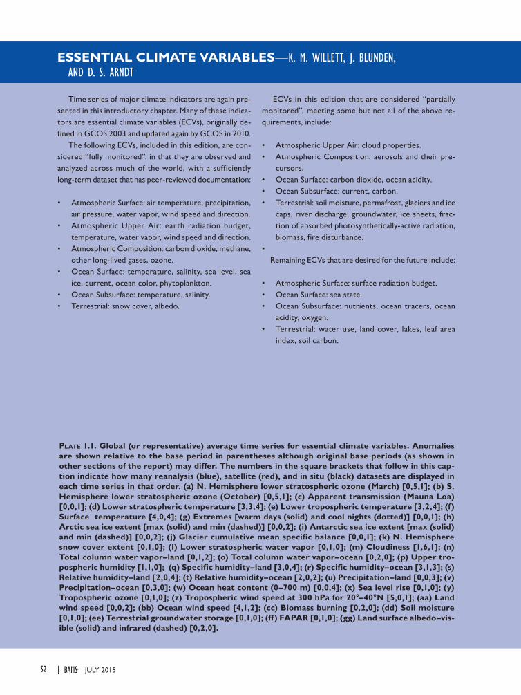
S2 JULY 2015|
ESSENTIAL CLIMATE VARIABLES—K. M. WILLETT, J. BLUNDEN, AND D. S. ARNDT
Time series of major climate indicators are again pre-sented in this introductory chapter. Many of these indica-tors are essential climate variables (ECVs), originally de-fined in GCOS 2003 and updated again by GCOS in 2010.
The following ECVs, included in this edition, are con-sidered “fully monitored”, in that they are observed and analyzed across much of the world, with a sufficiently long-term dataset that has peer-reviewed documentation:
• Atmospheric Surface: air temperature, precipitation, air pressure, water vapor, wind speed and direction.
• Atmospheric Upper Air: earth radiation budget, temperature, water vapor, wind speed and direction.
• Atmospheric Composition: carbon dioxide, methane, other long-lived gases, ozone.
• Ocean Surface: temperature, salinity, sea level, sea ice, current, ocean color, phytoplankton.
• Ocean Subsurface: temperature, salinity.• Terrestrial: snow cover, albedo.
Plate 1.1. Global (or representative) average time series for essential climate variables. Anomalies are shown relative to the base period in parentheses although original base periods (as shown in other sections of the report) may differ. The numbers in the square brackets that follow in this cap-tion indicate how many reanalysis (blue), satellite (red), and in situ (black) datasets are displayed in each time series in that order. (a) N. Hemisphere lower stratospheric ozone (March) [0,5,1]; (b) S. Hemisphere lower stratospheric ozone (October) [0,5,1]; (c) Apparent transmission (Mauna Loa) [0,0,1]; (d) Lower stratospheric temperature [3,3,4]; (e) Lower tropospheric temperature [3,2,4]; (f) Surface temperature [4,0,4]; (g) Extremes [warm days (solid) and cool nights (dotted)] [0,0,1]; (h)Arctic sea ice extent [max (solid) and min (dashed)] [0,0,2]; (i) Antarctic sea ice extent [max (solid) and min (dashed)] [0,0,2]; (j) Glacier cumulative mean specific balance [0,0,1]; (k) N. Hemisphere snow cover extent [0,1,0]; (l) Lower stratospheric water vapor [0,1,0]; (m) Cloudiness [1,6,1]; (n) Total column water vapor–land [0,1,2]; (o) Total column water vapor–ocean [0,2,0]; (p) Upper tro-pospheric humidity [1,1,0]; (q) Specific humidity–land [3,0,4]; (r) Specific humidity–ocean [3,1,3]; (s) Relative humidity–land [2,0,4]; (t) Relative humidity–ocean [2,0,2]; (u) Precipitation–land [0,0,3]; (v) Precipitation–ocean [0,3,0]; (w) Ocean heat content (0–700 m) [0,0,4]; (x) Sea level rise [0,1,0]; (y) Tropospheric ozone [0,1,0]; (z) Tropospheric wind speed at 300 hPa for 20°–40°N [5,0,1]; (aa) Land wind speed [0,0,2]; (bb) Ocean wind speed [4,1,2]; (cc) Biomass burning [0,2,0]; (dd) Soil moisture [0,1,0]; (ee) Terrestrial groundwater storage [0,1,0]; (ff) FAPAR [0,1,0]; (gg) Land surface albedo–vis-ible (solid) and infrared (dashed) [0,2,0].
ECVs in this edition that are considered “partially monitored”, meeting some but not all of the above re-quirements, include:
• Atmospheric Upper Air: cloud properties.• Atmospheric Composition: aerosols and their pre-
cursors.• Ocean Surface: carbon dioxide, ocean acidity.• Ocean Subsurface: current, carbon.• Terrestrial: soil moisture, permafrost, glaciers and ice
caps, river discharge, groundwater, ice sheets, frac-tion of absorbed photosynthetically-active radiation, biomass, fire disturbance.
• Remaining ECVs that are desired for the future include:
• Atmospheric Surface: surface radiation budget.• Ocean Surface: sea state.• Ocean Subsurface: nutrients, ocean tracers, ocean
acidity, oxygen.• Terrestrial: water use, land cover, lakes, leaf area
index, soil carbon.
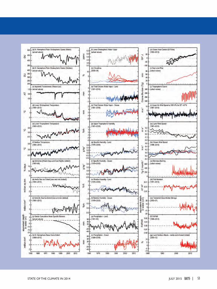
S3JULY 2015STATE OF THE CLIMATE IN 2014 |
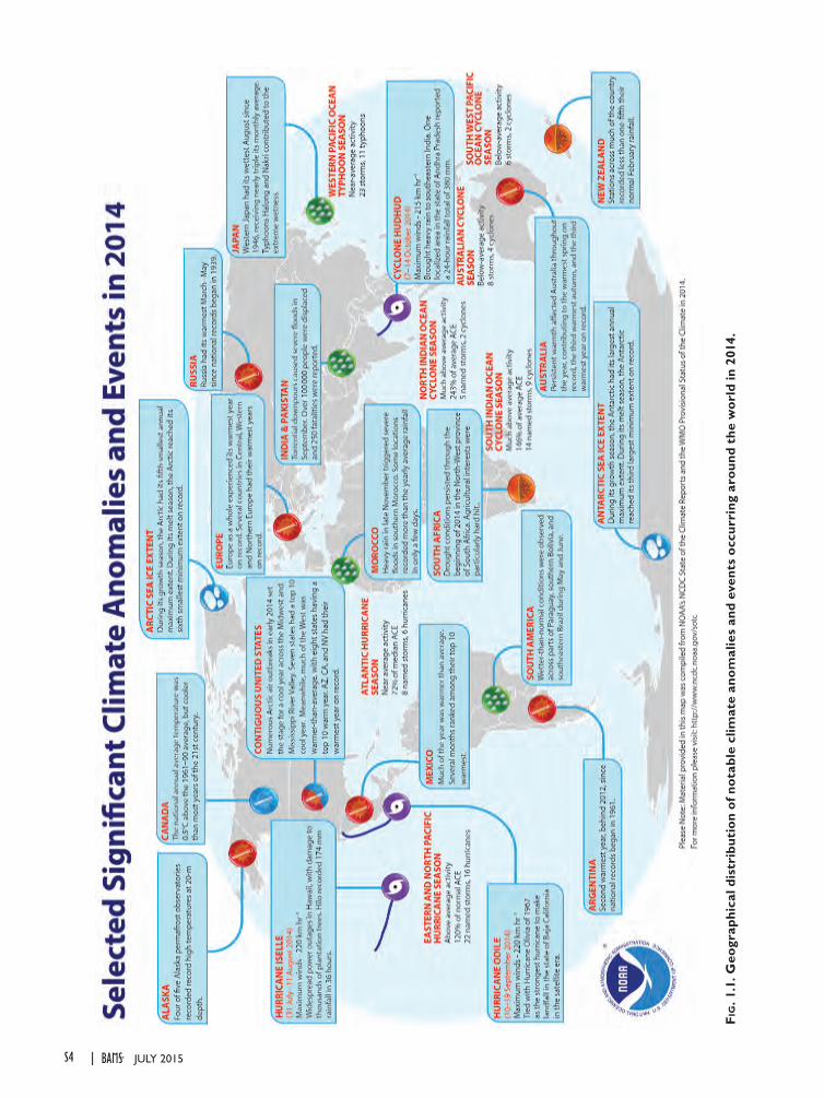
S4 JULY 2015|
Fig
. 1.1
. Geo
grap
hica
l dis
trib
utio
n of
not
able
clim
ate
anom
alie
s an
d ev
ents
occ
urri
ng a
roun
d th
e w
orld
in 2
014.
2. GLOBAL CLIMATE—K. M. Willett, A. J. Dolman, D. F. Hurst, J. Rennie, and P. W. Thorne, Eds.
a. Overview—P. W. Thorne, A. J. Dolman, D. F. Hurst, J. Rennie, and K. M. WillettThe year 2014 was forecast to be a warm year, and
it was by all accounts a very warm year, in fact record warm according to four independent observational datasets. The uncertainties associated with ranking annual global surface temperature values are dis-cussed in Sidebar 2.1. This warmth was against the backdrop of an El Niño–Southern Oscillation (ENSO) that although often approached El Niño thresholds, at the time was considered officially neutral. The year’s final months were since revised to “marginal” El Niño. The radiative forcing by long-lived green-house gases continued to increase, owing to rising levels of carbon dioxide, methane, nitrous oxide, and other radiatively active trace gases.
Over land surfaces, Eurasia and western North America were particularly warm, while notice-able cold was felt in eastern North America, which suffered several Arctic cold-air outbreaks in early 2014. The frequency of warm extreme temperatures was above average for all regions apart from North America. Similar spatial patterns were observed in the troposphere, which, although warm, was about 0.2°C below the record warmth associated with the large El Niño of 1998.
Globally, precipitation over the oceans during 2014 was above average, contrasting with below-average precipitation over land. This was also ref lected in hemispheric soil moisture: the Southern Hemisphere was wetter compared to 2013 while the Northern Hemisphere was drier. These large-scale averages masked strong diverging hydrological anomalies, of-ten within close proximity as was the case over South America. These anomalies were common across the hydrological cycle variables. During early 2014 South America showed high river discharge, in line with a general wetting stage in the Southern Hemisphere. This was also visible in the soil moisture records, with the exception of drier-than-normal northeastern Bra-zil. Water availability dominated the snow-free albedo and fraction of absorbed photosynthetically active radiation (FAPAR) variability with strong signals in the drier-than-normal Eurasia and wetter-than-normal Southern Hemisphere. Both near-surface specific humidity and total column water vapor were anomalously high, consistent with the high surface and tropospheric temperatures. However, global rela-tive humidity at the surface remained below average, continuing a trend that began around 2000.
In the cryosphere the effect of increased warming continued to be visible in the decline of glacier mass balance. With the addition of seven more reference glaciers compared to 2013, preliminary results for 2014 make it the 31st consecutive year of negative mass balance. Permafrost showed increasing tem-peratures and a deeper thawing layer in seasonally frozen soil. Northern Hemisphere snow cover extent was near-average.
The atmospheric concentrations of long-lived greenhouse gases (CO2, CH4, and N2O) contin-ued to increase, bringing total radiative forcing to 2.94 W m−2, 36% above the 1990 value. Trends in stratospheric column ozone remain difficult to detect due to interannual variations, but there is now evidence of a significant increase in the up-per stratosphere (40 km, 2 hPa) since 2000. Global mean anomalies in stratospheric water vapor were positive (wet) due to warm anomalies in tropical tropopause layer temperatures, in stark contrast to the strongly negative (dry) global anomalies in 2013. Positive anomalies of carbonaceous aerosols, carbon monoxide, and to some extent tropospheric column ozone, were again correlated with regions of seasonal biomass burning.
Over time this chapter has become substantially more comprehensive with an increasing number of essential climate variables (ECVs; Bojinski et al. 2014) included. This permits an increased portrayal of the interconnectedness of many facets of the climate system. Where possible, cross-referencing has been included to aid the reader in understanding this in-terconnectedness. This year upper air wind and upper tropospheric humidity are included for the first time. The former helps highlight, for example, the phase and variability of the quasi-biennial oscillation, and the latter plays a key feedback role in climate. Also included are three sidebars discussing uncertainty in temperature rankings, drought indices, and the Co-pernicus Atmospheric Monitoring System (CAMS).
Time series and anomaly maps for many variables described in this chapter are shown in Plates 1.1 and 2.1, respectively. Most anomalies are referenced against climatology for 1981–2010, a period with abundant satellite observations and reanalysis prod-ucts. Other periods are sometimes used due to short record lengths or other data issues; this is noted in each section. Many sections refer to online figures that can be found here: http://dx.doi.org/10.1175 /2015BAMSStateoftheClimate.2.
S5JULY 2015STATE OF THE CLIMATE IN 2014 |
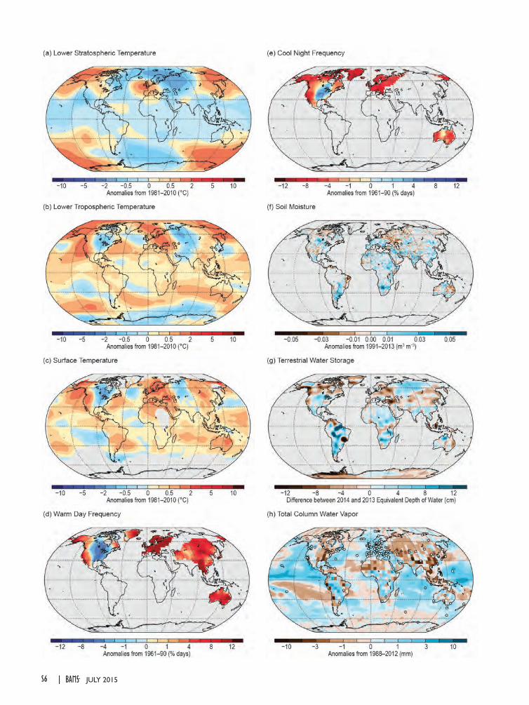
S6 JULY 2015|
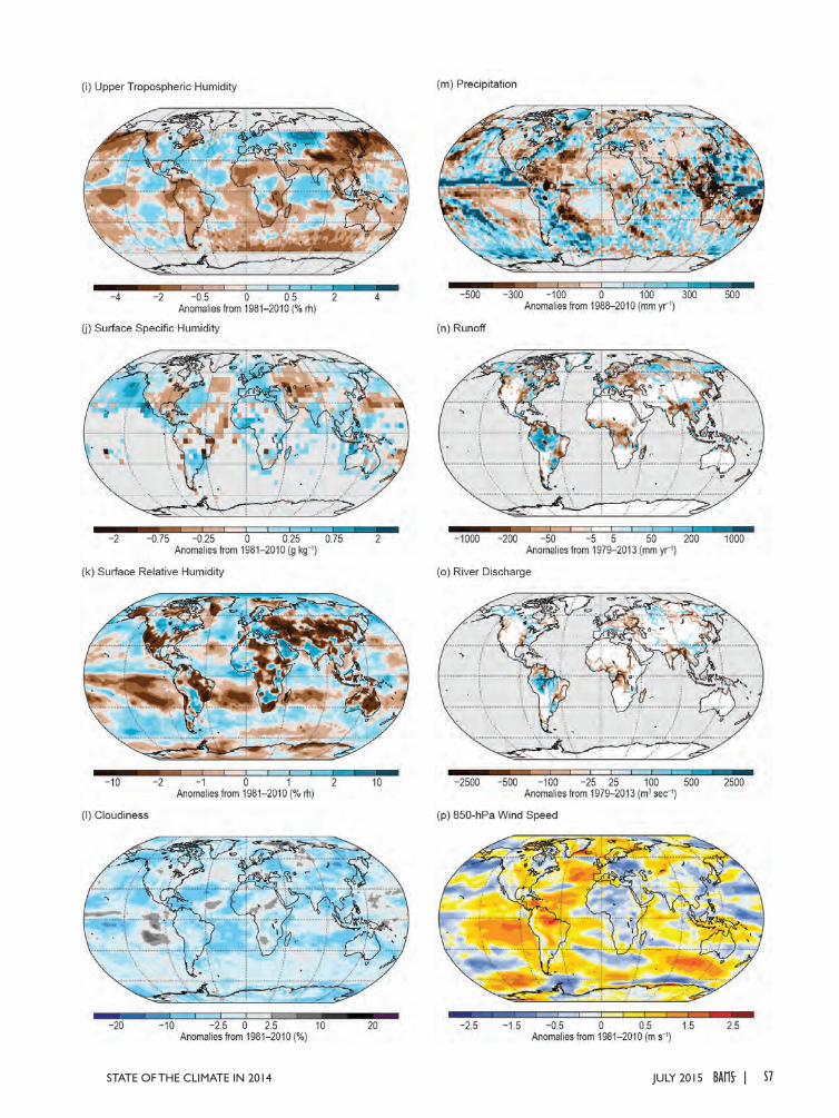
S7JULY 2015STATE OF THE CLIMATE IN 2014 |
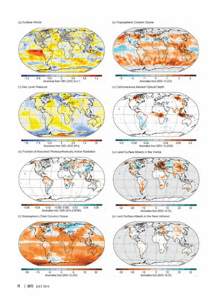
S8 JULY 2015|
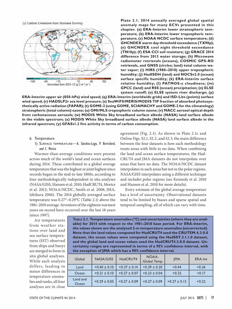
b. Temperature1) Surface temperature—A. Sánchez-Lugo, P. Berrisford,
and C. MoriceWarmer-than-average conditions were present
across much of the world’s land and ocean surfaces during 2014. These contributed to a global average temperature that was the highest or joint highest since records began in the mid-to-late 1800s, according to four methodologically independent in situ analyses (NASA/GISS, Hansen et al. 2010; HadCRUT4, Morice et al. 2012; NOAA/NCDC, Smith et al. 2008; JMA, Ishihara 2006). The 2014 globally averaged surface temperature was 0.27°–0.29°C (Table 2.1) above the 1981–2010 average. Seventeen of the eighteen warmest years on record have occurred over the last 18 years (since 1997).
Air temperatures f rom weat her sta-tions over land and sea surface tempera-tures (SST) observed from ships and buoys are merged to form in situ global analyses. While each analysis di f fers , leading to minor differences in temperature anoma-lies and ranks, all four analyses are in close
agreement (Fig. 2.1). As shown in Plate 2.1c and Online Figs. S2.1, S2.2, and S2.3, the main difference between the four datasets is how each methodology treats areas with little to no data. When combining the land and ocean surface temperatures, the Had-CRUT4 and JMA datasets do not interpolate over areas that have no data. The NOAA/NCDC dataset interpolates in such areas but not in the polar regions. NASA/GISS interpolates using a different technique and includes polar regions (see Kennedy et al. 2010 and Hansen et al. 2010 for more details).
Every estimate of the global average temperature has a level of uncertainty. Observational datasets tend to be limited by biases and sparse spatial and temporal sampling, all of which can vary with time.
Plate 2.1. 2014 annually averaged global spatial anomaly maps for many ECVs presented in this chapter. (a) ERA-Interim lower stratospheric tem-perature; (b) ERA-Interim lower tropospheric tem-perature; (c) NOAA NCDC surface temperature; (d) GHCNDEX warm day threshold exceedance (TX90p); (e) GHCNDEX cool night threshold exceedance (TN10p); (f) ESA CCI soil moisture; (g) GRACE 2014 difference from 2013 water storage; (h) Microwave radiometer retrievals (oceans), COSMIC GPS-RO retrievals, and GNSS (circles; land) total column wa-ter vapor; (i) HIRS (1980–2010) upper tropospheric humidity; (j) HadISDH (land) and NOCSv2.0 (ocean) surface specific humidity; (k) ERA-Interim surface relative humidity; (l) PATMOS-x cloudiness; (m) GPCC (land) and RSS (ocean) precipitation; (n) ELSE system runoff; (o) ELSE system river discharge; (p)
ERA-Interim upper air (850-hPa) wind speed; (q) ERA-Interim (worldwide grids) and ISD-Lite (points) surface wind speed; (r) HADSLP2r sea level pressure; (s) SeaWiFS/MERIS/MODIS TIP fraction of absorbed photosyn-thetically active radiation (FAPAR); (t) GOME-2 (using GOME, SCIAMACHY and GOME-2 for the climatology) stratospheric (total column) ozone; (u) OMI/MLS tropospheric column ozone; (v) MACC aerosol optical depth from carbonaceous aerosols; (w) MODIS White Sky broadband surface albedo (NASA) land surface albedo in the visible spectrum; (x) MODIS White Sky broadband surface albedo (NASA) land surface albedo in the infrared spectrum; (y) GFASv1.2 fire activity in terms of carbon consumption.
Table 2.1. Temperature anomalies (°C) and uncertainties (where they are avail-able) for 2014 with respect to the 1981–2010 base period. For ERA-Interim, the values shown are the analyzed 2-m temperature anomalies (uncorrected). Note that the land values computed for HadCRUT4 used the CRUTEM.4.3.0.0 dataset, the ocean values were computed using the HadSST.3.1.1.0 dataset, and the global land and ocean values used the HadCRUT4.3.0.0 dataset. Un-certainty ranges are represented in terms of a 95% confidence interval, with the exception of JMA which has a 90% confidence interval.
Global NASA/GISS HadCRUT4NOAA-
Global TempJMA ERA-Int
Land +0.40 ± 0.10 +0.37 ± 0.14 +0.39 ± 0.20 +0.44 +0.36
Ocean +0.21 ± 0.10 +0.27 ± 0.07 +0.23 ± 0.04 +0.23 +0.17
Land and Ocean
+0.29 ± 0.05 +0.27 ± 0.09 +0.27 ± 0.09 +0.27 ± 0.13 +0.22
S9JULY 2015STATE OF THE CLIMATE IN 2014 |
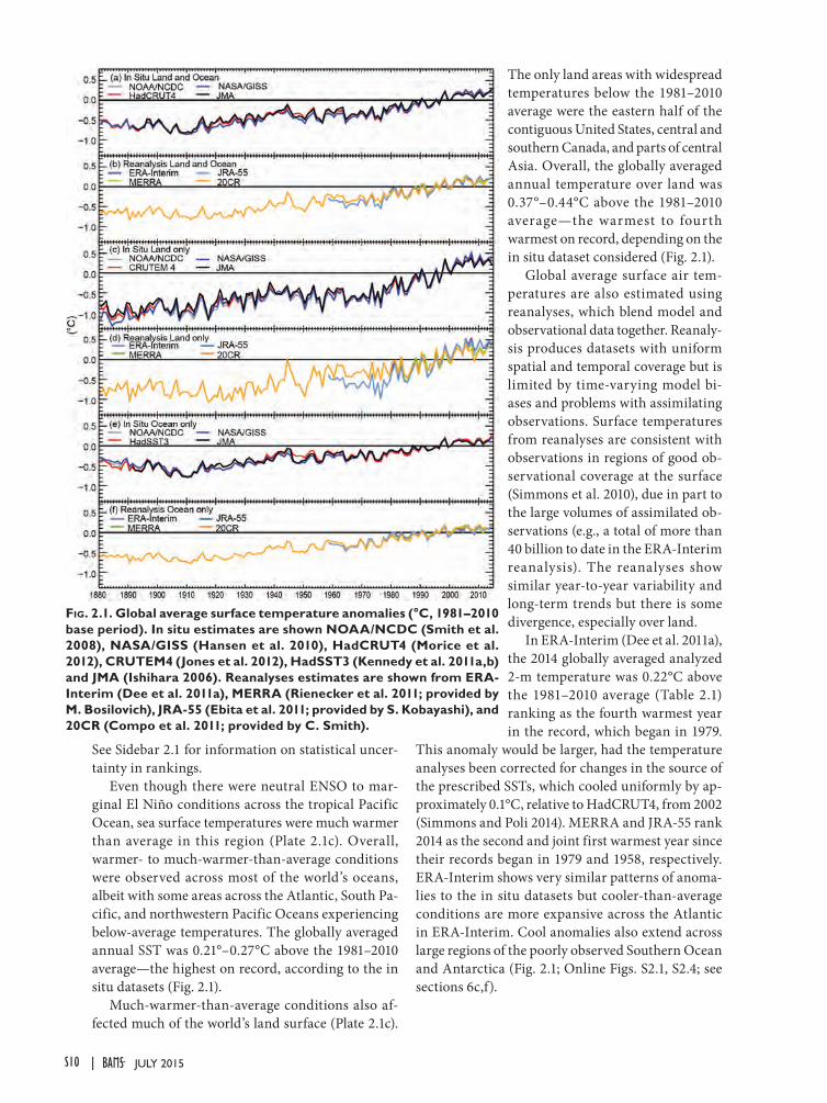
See Sidebar 2.1 for information on statistical uncer-tainty in rankings.
Even though there were neutral ENSO to mar-ginal El Niño conditions across the tropical Pacific Ocean, sea surface temperatures were much warmer than average in this region (Plate 2.1c). Overall, warmer- to much-warmer-than-average conditions were observed across most of the world’s oceans, albeit with some areas across the Atlantic, South Pa-cific, and northwestern Pacific Oceans experiencing below-average temperatures. The globally averaged annual SST was 0.21°–0.27°C above the 1981–2010 average—the highest on record, according to the in situ datasets (Fig. 2.1).
Much-warmer-than-average conditions also af-fected much of the world’s land surface (Plate 2.1c).
The only land areas with widespread temperatures below the 1981–2010 average were the eastern half of the contiguous United States, central and southern Canada, and parts of central Asia. Overall, the globally averaged annual temperature over land was 0.37°–0.44°C above the 1981–2010 average—the warmest to fourth warmest on record, depending on the in situ dataset considered (Fig. 2.1).
Global average surface air tem-peratures are also estimated using reanalyses, which blend model and observational data together. Reanaly-sis produces datasets with uniform spatial and temporal coverage but is limited by time-varying model bi-ases and problems with assimilating observations. Surface temperatures from reanalyses are consistent with observations in regions of good ob-servational coverage at the surface (Simmons et al. 2010), due in part to the large volumes of assimilated ob-servations (e.g., a total of more than 40 billion to date in the ERA-Interim reanalysis). The reanalyses show similar year-to-year variability and long-term trends but there is some divergence, especially over land.
In ERA-Interim (Dee et al. 2011a), the 2014 globally averaged analyzed 2-m temperature was 0.22°C above the 1981–2010 average (Table 2.1) ranking as the fourth warmest year in the record, which began in 1979.
This anomaly would be larger, had the temperature analyses been corrected for changes in the source of the prescribed SSTs, which cooled uniformly by ap-proximately 0.1°C, relative to HadCRUT4, from 2002 (Simmons and Poli 2014). MERRA and JRA-55 rank 2014 as the second and joint first warmest year since their records began in 1979 and 1958, respectively. ERA-Interim shows very similar patterns of anoma-lies to the in situ datasets but cooler-than-average conditions are more expansive across the Atlantic in ERA-Interim. Cool anomalies also extend across large regions of the poorly observed Southern Ocean and Antarctica (Fig. 2.1; Online Figs. S2.1, S2.4; see sections 6c,f).
Fig. 2.1. Global average surface temperature anomalies (°C, 1981–2010 base period). In situ estimates are shown NOAA/NCDC (Smith et al. 2008), NASA/GISS (Hansen et al. 2010), HadCRUT4 (Morice et al. 2012), CRUTEM4 (Jones et al. 2012), HadSST3 (Kennedy et al. 2011a,b) and JMA (Ishihara 2006). Reanalyses estimates are shown from ERA-Interim (Dee et al. 2011a), MERRA (Rienecker et al. 2011; provided by M. Bosilovich), JRA-55 (Ebita et al. 2011; provided by S. Kobayashi), and 20CR (Compo et al. 2011; provided by C. Smith).
S10 JULY 2015|
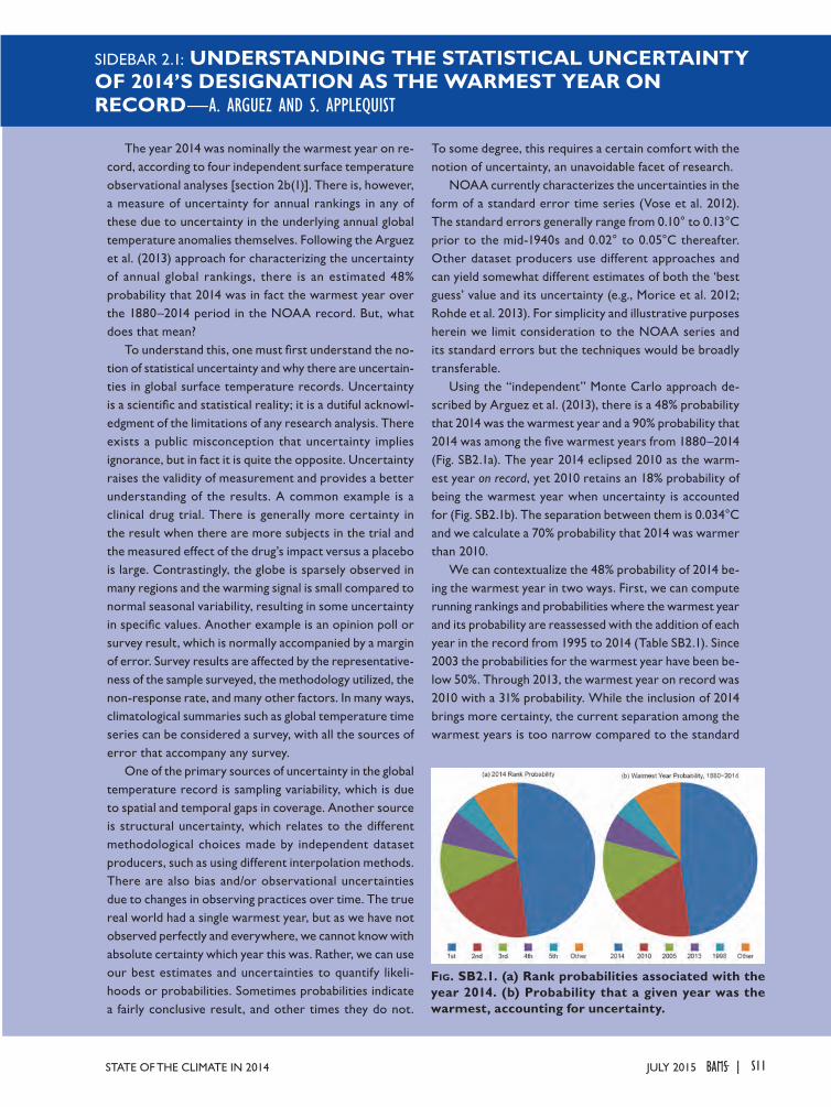
SIDEBAR 2.1: UNDERSTANDING THE STATISTICAL UNCERTAINTY OF 2014’S DESIGNATION AS THE WARMEST YEAR ON RECORD—A. ARGUEZ AND S. APPLEQUIST
The year 2014 was nominally the warmest year on re-cord, according to four independent surface temperature observational analyses [section 2b(1)]. There is, however, a measure of uncertainty for annual rankings in any of these due to uncertainty in the underlying annual global temperature anomalies themselves. Following the Arguez et al. (2013) approach for characterizing the uncertainty of annual global rankings, there is an estimated 48% probability that 2014 was in fact the warmest year over the 1880–2014 period in the NOAA record. But, what does that mean?
To understand this, one must first understand the no-tion of statistical uncertainty and why there are uncertain-ties in global surface temperature records. Uncertainty is a scientific and statistical reality; it is a dutiful acknowl-edgment of the limitations of any research analysis. There exists a public misconception that uncertainty implies ignorance, but in fact it is quite the opposite. Uncertainty raises the validity of measurement and provides a better understanding of the results. A common example is a clinical drug trial. There is generally more certainty in the result when there are more subjects in the trial and the measured effect of the drug’s impact versus a placebo is large. Contrastingly, the globe is sparsely observed in many regions and the warming signal is small compared to normal seasonal variability, resulting in some uncertainty in specific values. Another example is an opinion poll or survey result, which is normally accompanied by a margin of error. Survey results are affected by the representative-ness of the sample surveyed, the methodology utilized, the non-response rate, and many other factors. In many ways, climatological summaries such as global temperature time series can be considered a survey, with all the sources of error that accompany any survey.
One of the primary sources of uncertainty in the global temperature record is sampling variability, which is due to spatial and temporal gaps in coverage. Another source is structural uncertainty, which relates to the different methodological choices made by independent dataset producers, such as using different interpolation methods. There are also bias and/or observational uncertainties due to changes in observing practices over time. The true real world had a single warmest year, but as we have not observed perfectly and everywhere, we cannot know with absolute certainty which year this was. Rather, we can use our best estimates and uncertainties to quantify likeli-hoods or probabilities. Sometimes probabilities indicate a fairly conclusive result, and other times they do not.
To some degree, this requires a certain comfort with the notion of uncertainty, an unavoidable facet of research.
NOAA currently characterizes the uncertainties in the form of a standard error time series (Vose et al. 2012). The standard errors generally range from 0.10° to 0.13°C prior to the mid-1940s and 0.02° to 0.05°C thereafter. Other dataset producers use different approaches and can yield somewhat different estimates of both the ‘best guess’ value and its uncertainty (e.g., Morice et al. 2012; Rohde et al. 2013). For simplicity and illustrative purposes herein we limit consideration to the NOAA series and its standard errors but the techniques would be broadly transferable.
Using the “independent” Monte Carlo approach de-scribed by Arguez et al. (2013), there is a 48% probability that 2014 was the warmest year and a 90% probability that 2014 was among the five warmest years from 1880–2014 (Fig. SB2.1a). The year 2014 eclipsed 2010 as the warm-est year on record, yet 2010 retains an 18% probability of being the warmest year when uncertainty is accounted for (Fig. SB2.1b). The separation between them is 0.034°C and we calculate a 70% probability that 2014 was warmer than 2010.
We can contextualize the 48% probability of 2014 be-ing the warmest year in two ways. First, we can compute running rankings and probabilities where the warmest year and its probability are reassessed with the addition of each year in the record from 1995 to 2014 (Table SB2.1). Since 2003 the probabilities for the warmest year have been be-low 50%. Through 2013, the warmest year on record was 2010 with a 31% probability. While the inclusion of 2014 brings more certainty, the current separation among the warmest years is too narrow compared to the standard
Fig. SB2.1. (a) Rank probabilities associated with the year 2014. (b) Probability that a given year was the warmest, accounting for uncertainty.
S11JULY 2015STATE OF THE CLIMATE IN 2014 |
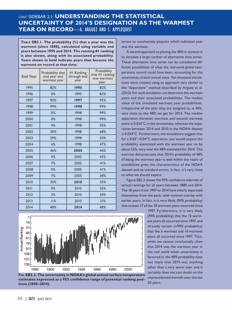
CONT. SIDEBAR 2.1: UNDERSTANDING THE STATISTICAL UNCERTAINTY OF 2014’S DESIGNATION AS THE WARMEST YEAR ON RECORD—A. ARGUEZ AND S. APPLEQUIST
errors to conclusively pinpoint which individual year was the warmest.
A second approach to placing the 48% in context is to simulate a large number of alternative time series. These alternative time series can be considered dif-ferent possibilities of what the real-world global tem-perature record could have been, accounting for the uncertainty of each annual value. Ten thousand simula-tions were created using an approach very similar to the “dependent” method described by Arguez et al. (2013). For each simulation, we determine the warmest years and their associated probabilities. The median value of the simulated warmest year probabilities, irrespective of the year they are assigned to, is 46%, very close to the 48% we get for 2014. The median separation between warmest and second warmest years is 0.024°C in the simulations, whereas the sepa-ration between 2014 and 2010 in the NOAA dataset is 0.034°C. Furthermore, the simulations suggest that for a 0.03°–0.04°C separation, you would expect the probability associated with the warmest year to be about 52%, very near the 48% estimated for 2014. This exercise demonstrates that 2014’s probability of 48% of being the warmest year is well within the realm of possibilities given the characteristics of the NOAA dataset and its standard errors. In fact, it’s very close to what we should expect.
Figure SB2.2 shows the 95% confidence intervals of annual rankings for all years between 1880 and 2014. The 18 years from 1997 to 2014 have clearly separated themselves from the pack, with minimal overlap with earlier years. In fact, it is very likely (90% probability) that at least 17 of the 18 warmest years occurred since
1997. Furthermore, it is very likely (94% probability) that the 15 warm-est years all occurred since 1997, and virtually certain (>99% probability) that the 5 warmest and 10 warmest years all occurred since 1997. Thus, while we cannot conclusively claim that 2014 was the warmest year in the real world when uncertainty is factored in, the 48% probability does not imply that 2014 was anything other than a very warm year, and it certainly does not cast doubt on the unprecedented warmth over the last 20 years.
Fig. SB2.2. The uncertainty in NOAA’s global annual surface temperature estimates expressed as a 95% confidence range of potential ranking posi-tions (1880–2014).
Table SB2.1. The probability (%) that a year was the warmest (since 1880), calculated using variable end years between 1995 and 2014. The running #1 ranking is also shown, along with its associated probability. Years shown in bold indicate years that became the warmest on record at that time.
End YearProbability that end year was warmest year
#1 Ranking through end
year
Probability that #1 ranking was warmest
year
1995 82% 1995 82%
1996 0% 1995 82%
1997 92% 1997 92%
1998 99% 1998 99%
1999 0% 1998 99%
2000 0% 1998 99%
2001 4% 1998 95%
2002 30% 1998 68%
2003 29% 1998 50%
2004 6% 1998 47%
2005 46% 2005 46%
2006 9% 2005 43%
2007 7% 2005 41%
2008 0% 2005 41%
2009 7% 2005 38%
2010 35% 2010 35%
2011 0% 2010 35%
2012 2% 2010 34%
2013 11% 2010 31%
2014 48% 2014 48%
S12 JULY 2015|
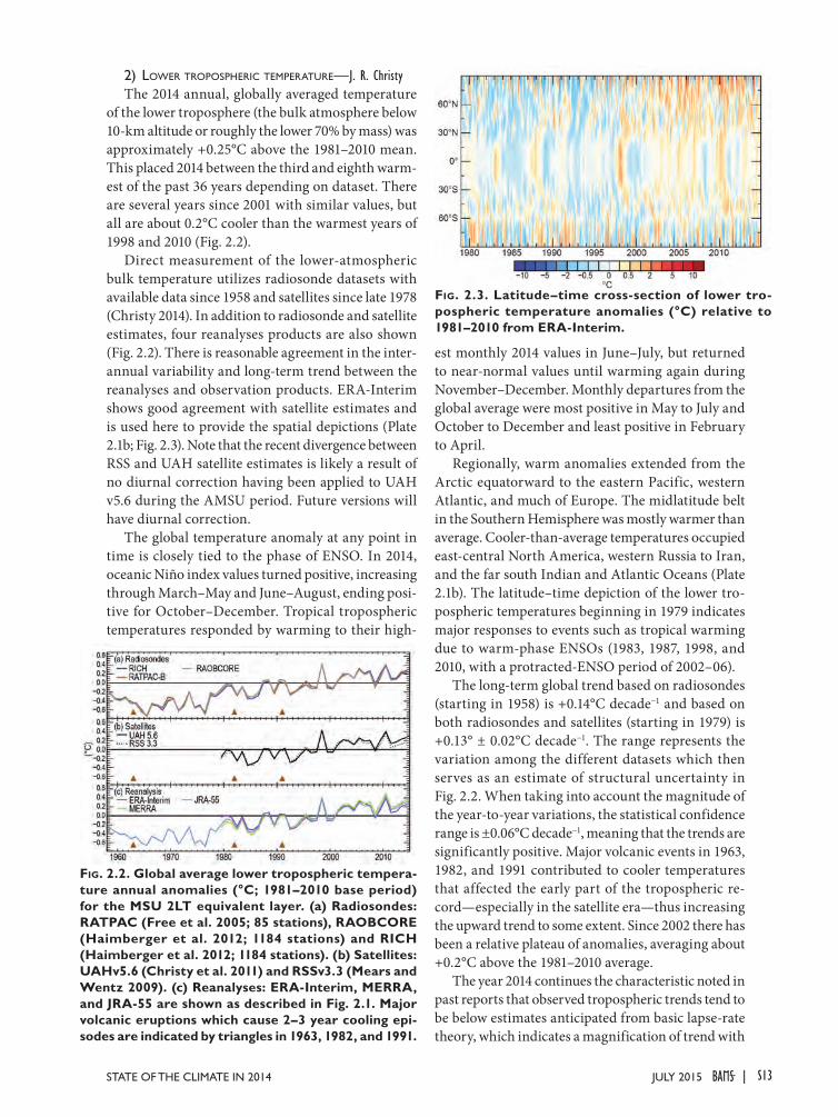
2) Lower tropoSpheric temperature—J. R. ChristyThe 2014 annual, globally averaged temperature
of the lower troposphere (the bulk atmosphere below 10-km altitude or roughly the lower 70% by mass) was approximately +0.25°C above the 1981–2010 mean. This placed 2014 between the third and eighth warm-est of the past 36 years depending on dataset. There are several years since 2001 with similar values, but all are about 0.2°C cooler than the warmest years of 1998 and 2010 (Fig. 2.2).
Direct measurement of the lower-atmospheric bulk temperature utilizes radiosonde datasets with available data since 1958 and satellites since late 1978 (Christy 2014). In addition to radiosonde and satellite estimates, four reanalyses products are also shown (Fig. 2.2). There is reasonable agreement in the inter-annual variability and long-term trend between the reanalyses and observation products. ERA-Interim shows good agreement with satellite estimates and is used here to provide the spatial depictions (Plate 2.1b; Fig. 2.3). Note that the recent divergence between RSS and UAH satellite estimates is likely a result of no diurnal correction having been applied to UAH v5.6 during the AMSU period. Future versions will have diurnal correction.
The global temperature anomaly at any point in time is closely tied to the phase of ENSO. In 2014, oceanic Niño index values turned positive, increasing through March–May and June–August, ending posi-tive for October–December. Tropical tropospheric temperatures responded by warming to their high-
est monthly 2014 values in June–July, but returned to near-normal values until warming again during November–December. Monthly departures from the global average were most positive in May to July and October to December and least positive in February to April.
Regionally, warm anomalies extended from the Arctic equatorward to the eastern Pacific, western Atlantic, and much of Europe. The midlatitude belt in the Southern Hemisphere was mostly warmer than average. Cooler-than-average temperatures occupied east-central North America, western Russia to Iran, and the far south Indian and Atlantic Oceans (Plate 2.1b). The latitude–time depiction of the lower tro-pospheric temperatures beginning in 1979 indicates major responses to events such as tropical warming due to warm-phase ENSOs (1983, 1987, 1998, and 2010, with a protracted-ENSO period of 2002–06).
The long-term global trend based on radiosondes (starting in 1958) is +0.14°C decade−1 and based on both radiosondes and satellites (starting in 1979) is +0.13° ± 0.02°C decade−1. The range represents the variation among the different datasets which then serves as an estimate of structural uncertainty in Fig. 2.2. When taking into account the magnitude of the year-to-year variations, the statistical confidence range is ±0.06°C decade−1, meaning that the trends are significantly positive. Major volcanic events in 1963, 1982, and 1991 contributed to cooler temperatures that affected the early part of the tropospheric re-cord—especially in the satellite era—thus increasing the upward trend to some extent. Since 2002 there has been a relative plateau of anomalies, averaging about +0.2°C above the 1981–2010 average.
The year 2014 continues the characteristic noted in past reports that observed tropospheric trends tend to be below estimates anticipated from basic lapse-rate theory, which indicates a magnification of trend with
Fig. 2.2. Global average lower tropospheric tempera-ture annual anomalies (°C; 1981–2010 base period) for the MSU 2LT equivalent layer. (a) Radiosondes: RATPAC (Free et al. 2005; 85 stations), RAOBCORE (Haimberger et al. 2012; 1184 stations) and RICH (Haimberger et al. 2012; 1184 stations). (b) Satellites: UAHv5.6 (Christy et al. 2011) and RSSv3.3 (Mears and Wentz 2009). (c) Reanalyses: ERA-Interim, MERRA, and JRA-55 are shown as described in Fig. 2.1. Major volcanic eruptions which cause 2–3 year cooling epi-sodes are indicated by triangles in 1963, 1982, and 1991.
Fig. 2.3. Latitude–time cross-section of lower tro-pospheric temperature anomalies (°C) relative to 1981–2010 from ERA-Interim.
S13JULY 2015STATE OF THE CLIMATE IN 2014 |
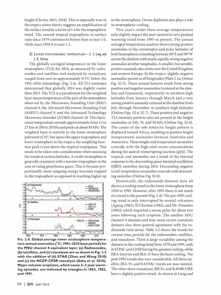
height (Christy 2013, 2014). This is especially true in the tropics where theory suggests an amplification of the surface trend by a factor of 1.4 for the tropospheric trend. The current tropical tropospheric to surface ratio since 1979 continues to be less than or near 1.0, while since 1958 it is near 1.2.
3) Lower StratoSpheric temperature—C. S. Long and J. R. Christy
The globally averaged temperature in the lower stratosphere (TLS) for 2014, as measured by radio-sondes and satellites and analyzed by reanalyses, ranged from zero to approximately 0.5oC below the 1981–2010 climatology (Fig. 2.4). All TLS estimates determined that globally 2014 was slightly cooler than 2013. The TLS is a pseudonym for the weighted layer-mean temperature of the part of the atmosphere observed by the Microwave Sounding Unit (MSU) channel 4, the Advanced Microwave Sounding Unit (AMSU) channel 9, and the Advanced Technology Microwave Sounder (ATMS) channel 10. This layer-mean temperature extends approximately from 12 to 27 km or 200 to 20 hPa and peaks at about 85 hPa. The weighted layer is entirely in the lower stratosphere poleward of 35°, but spans the upper troposphere and lower stratosphere in the tropics; the weighting func-tion peak is just above the tropical tropopause. This needs to be taken into consideration when assessing the trends at various latitudes. A cooler stratosphere is generally consistent with a warmer troposphere in the case of rising greenhouse gases. This is because pro-portionally more outgoing energy becomes trapped in the troposphere as opposed to reaching higher up
in the stratosphere. Ozone depletion also plays a role in stratospheric cooling.
This year’s cooler-than-average temperatures only slightly impact the near-neutral to very gradual warming trend from 1995 to present. The annual averaged temperature analysis shows strong positive anomalies in the extratropics and polar latitudes of both hemispheres extending between 90°E and 90°W across the dateline with nearly equally strong negative anomalies at other longitudes. A smaller, but notable, positive anomaly also exists over the United Kingdom and western Europe. In the tropics, slightly negative anomalies persist at all longitudes (Plate 2.1a; Online Fig. S2.5). These annual features result from strong positive and negative anomalies (centered at the date-line and Greenwich, respectively) in northern high latitudes from January through March and a very strong positive anomaly centered at the dateline from July through November in southern high latitudes (Online Figs. S2.6, S2.7). These positive and negative TLS anomaly patterns also are present in the height anomalies at 100, 70, and 50 hPa (Online Fig. S2.8). The center of the sub-Antarctic height pattern is displaced toward Africa, resulting in positive height (temperature) anomalies between Australia and Antarctica. These height and temperature anomalies coincide with the high total ozone concentrations during the austral winter/spring [section 2g(4)]. The tropical cool anomalies are a result of the thermal response to the descending quasi-biennial oscillation (QBO) easterlies during 2014. Descending negative (cool) temperature anomalies coincide with descend-ing easterlies (Online Fig. S2.8).
Historically, the radiosonde datasets have all shown a cooling trend in the lower stratosphere from 1958 to 1995. However, after 1995 there is not much of a trend to the present (Fig. 2.4). The pre-1995 cool-ing trend is only interrupted by several volcanoes [Agung (1963), El Chichón (1982), and Mt. Pinatubo (1991)] which imparted a warm pulse for about two years following each eruption. The satellite MSU channel 4 datasets and four most recent reanalysis datasets also show general agreement with the ra-diosonde time series. Table 2.2 shows the trends for various time periods for the radiosondes, satellites, and reanalyses. There is large variability among the datasets in the cooling trend from 1979 and 1995, with RATPAC and CFSR having the greatest cooling, while ERA-Interim and JRA-55 have the least cooling. The post-1995 trends also vary considerably. All three sat-ellite, JRA-55, and RATPAC trends are near-neutral. The other three reanalyses, RICH, and RAOBCORE have a slightly positive trend. As shown in Long and
Fig. 2.4. Global average lower stratosphere tempera-ture annual anomalies (°C; 1981–2010 base period) for the MSU channel 4 equivalent layer. (a) Radiosondes, (b) satellites, and (c) reanalyses are as shown in Fig. 2.2 with the addition of (b) STAR (Zhou and Wang 2010) and (c) the NCEP-CFSR reanalysis (Saha et al. 2010). Major volcanic eruptions, which cause 2–3 year warm-ing episodes, are indicated by triangles in 1963, 1982, and 1991.
S14 JULY 2015|
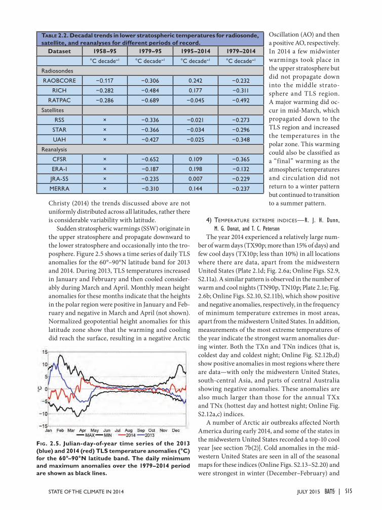
Christy (2014) the trends discussed above are not uniformly distributed across all latitudes, rather there is considerable variability with latitude.
Sudden stratospheric warmings (SSW) originate in the upper stratosphere and propagate downward to the lower stratosphere and occasionally into the tro-posphere. Figure 2.5 shows a time series of daily TLS anomalies for the 60°–90°N latitude band for 2013 and 2014. During 2013, TLS temperatures increased in January and February and then cooled consider-ably during March and April. Monthly mean height anomalies for these months indicate that the heights in the polar region were positive in January and Feb-ruary and negative in March and April (not shown). Normalized geopotential height anomalies for this latitude zone show that the warming and cooling did reach the surface, resulting in a negative Arctic
Oscillation (AO) and then a positive AO, respectively. In 2014 a few midwinter warmings took place in the upper stratosphere but did not propagate down into the middle strato-sphere and TLS region. A major warming did oc-cur in mid-March, which propagated down to the TLS region and increased the temperatures in the polar zone. This warming could also be classified as a “final” warming as the atmospheric temperatures and circulation did not return to a winter pattern but continued to transition to a summer pattern.
4) temperature extreme indiceS—R. J. H. Dunn, M. G. Donat, and T. C. Peterson
The year 2014 experienced a relatively large num-ber of warm days (TX90p; more than 15% of days) and few cool days (TX10p; less than 10%) in all locations where there are data, apart from the midwestern United States (Plate 2.1d; Fig. 2.6a; Online Figs. S2.9, S2.11a). A similar pattern is observed in the number of warm and cool nights (TN90p, TN10p; Plate 2.1e; Fig. 2.6b; Online Figs. S2.10, S2.11b), which show positive and negative anomalies, respectively, in the frequency of minimum temperature extremes in most areas, apart from the midwestern United States. In addition, measurements of the most extreme temperatures of the year indicate the strongest warm anomalies dur-ing winter. Both the TXn and TNn indices (that is, coldest day and coldest night; Online Fig. S2.12b,d) show positive anomalies in most regions where there are data—with only the midwestern United States, south-central Asia, and parts of central Australia showing negative anomalies. These anomalies are also much larger than those for the annual TXx and TNx (hottest day and hottest night; Online Fig. S2.12a,c) indices.
A number of Arctic air outbreaks affected North America during early 2014, and some of the states in the midwestern United States recorded a top-10 cool year [see section 7b(2)]. Cold anomalies in the mid-western United States are seen in all of the seasonal maps for these indices (Online Figs. S2.13–S2.20) and were strongest in winter (December–February) and
Fig. 2.5. Julian-day-of-year time series of the 2013 (blue) and 2014 (red) TLS temperature anomalies (°C) for the 60°–90°N latitude band. The daily minimum and maximum anomalies over the 1979–2014 period are shown as black lines.
Table 2.2. Decadal trends in lower stratospheric temperatures for radiosonde, satellite, and reanalyses for different periods of record.
Dataset 1958–95 1979–95 1995–2014 1979–2014
°C decade–1 °C decade–1 °C decade–1 °C decade–1
Radiosondes
RAOBCORE −0.117 −0.306 0.242 −0.232
RICH −0.282 −0.484 0.177 −0.311
RATPAC −0.286 −0.689 −0.045 −0.492
Satellites
RSS × −0.336 −0.021 −0.273
STAR × −0.366 −0.034 −0.296
UAH × −0.427 −0.025 −0.348
Reanalysis
CFSR × −0.652 0.109 −0.365
ERA-I × −0.187 0.198 −0.132
JRA-55 × −0.235 0.007 −0.229
MERRA × −0.310 0.144 −0.237
S15JULY 2015STATE OF THE CLIMATE IN 2014 |
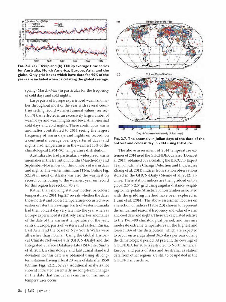
spring (March–May) in particular for the frequency of cold days and cold nights.
Large parts of Europe experienced warm anoma-lies throughout most of the year with several coun-tries setting record warmest annual values (see sec-tion 7f), as reflected in an excessively large number of warm days and warm nights and fewer-than-normal cold days and cold nights. These continuous warm anomalies contributed to 2014 seeing the largest frequency of warm days and nights on record: on a continental average over a quarter of days (and nights) had temperatures in the warmest 10% of the climatological (1961–90) temperature distribution.
Australia also had particularly widespread warm anomalies in the transition months (March–May and September–November) for the numbers of warm days and nights. The winter minimum (TNn; Online Fig. S2.19) in most of Alaska was also the warmest on record, contributing to the warmest year on record for this region [see section 7b(2)].
Rather than showing stations’ hottest or coldest temperature of 2014, Fig. 2.7 reveals whether the dates those hottest and coldest temperatures occurred were earlier or later than average. Parts of western Canada had their coldest day very late into the year whereas Europe experienced it relatively early. For anomalies of the date of the warmest temperature of the year, central Europe, parts of western and eastern Russia, East Asia, and the coast of New South Wales were all earlier than normal. Using the Global Histori-cal Climate Network-Daily (GHCN-Daily) and the Integrated Surface Database-Lite (ISD-Lite; Smith et al. 2011), a climatology and latitudinal standard deviation for this date was obtained using all long-term stations having at least 20 years of data after 1950 (Online Figs. S2.21, S2.22). Additional analysis (not shown) indicated essentially no long-term changes in the date that annual maximum or minimum temperatures occur.
The above assessment of 2014 temperature ex-tremes of 2014 used the GHCNDEX dataset (Donat et al. 2013), obtained by calculating the ETCCDI (Expert Team on Climate Change Detection and Indices, see Zhang et al. 2011) indices from station observations stored in the GHCN-Daily (Menne et al. 2012) ar-chive. These station indices are then gridded onto a global 2.5° × 2.5° grid using angular distance weight-ing to interpolate. Structural uncertainties associated with the gridding method have been explored in Dunn et al. (2014). The above assessment focuses on a selection of indices (Table 2.3) chosen to represent the annual and seasonal frequency and value of warm and cool days and nights. These are calculated relative to the 1961–90 climatological period, and measure moderate extreme temperatures in the highest and lowest 10% of the distribution, which are expected to occur on average about 36.5 days per year during the climatological period. At present, the coverage of GHCNDEX for 2014 is restricted to North America, Europe, and parts of Asia and Australia, as station data from other regions are still to be updated in the GHCN-Daily archive.
Fig. 2.6. (a) TX90p and (b) TN10p average time series for Australia, North America, Europe, Asia, and the globe. Only grid boxes which have data for 90% of the years are included when calculating the global average.
Fig. 2.7. The anomaly in Julian days of the date of the hottest and coldest day in 2014 using ISD-Lite.
S16 JULY 2015|
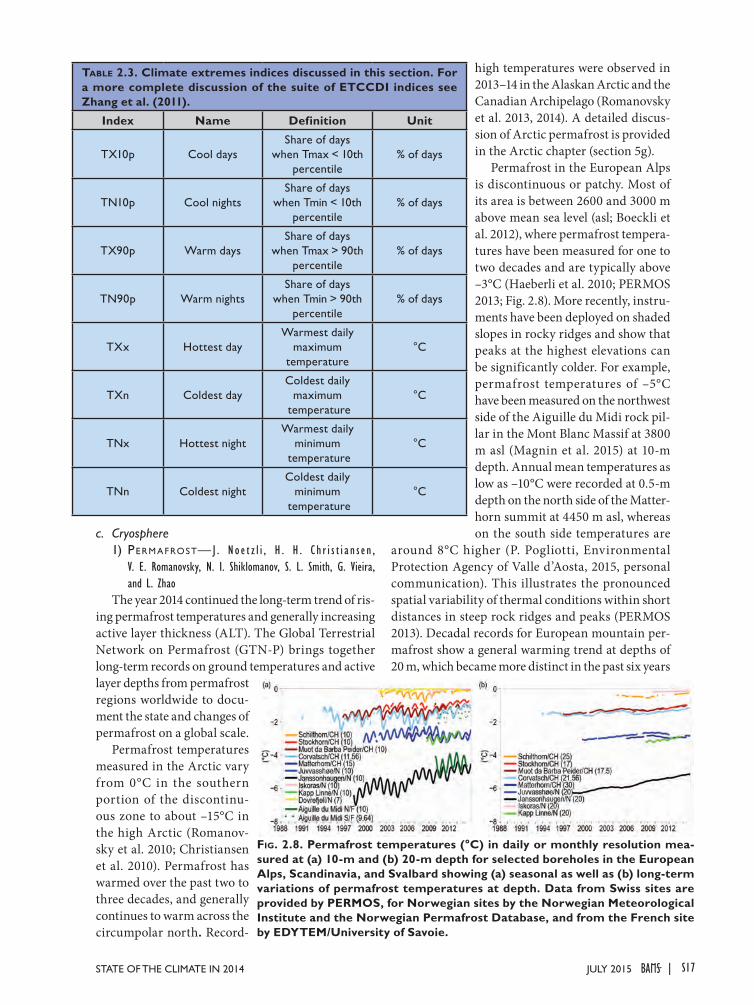
c. Cryosphere1) pe rmafroSt— J . N o e t z l i , H . H . C h r i s t i a n s e n ,
V. E. Romanovsky, N. I. Shiklomanov, S. L. Smith, G. Vieira, and L. Zhao
The year 2014 continued the long-term trend of ris-ing permafrost temperatures and generally increasing active layer thickness (ALT). The Global Terrestrial Network on Permafrost (GTN-P) brings together long-term records on ground temperatures and active layer depths from permafrost regions worldwide to docu-ment the state and changes of permafrost on a global scale.
Permafrost temperatures measured in the Arctic vary from 0°C in the southern portion of the discontinu-ous zone to about –15°C in the high Arctic (Romanov-sky et al. 2010; Christiansen et al. 2010). Permafrost has warmed over the past two to three decades, and generally continues to warm across the circumpolar north. Record-
high temperatures were observed in 2013–14 in the Alaskan Arctic and the Canadian Archipelago (Romanovsky et al. 2013, 2014). A detailed discus-sion of Arctic perma frost is provided in the Arctic chapter (section 5g).
Permafrost in the European Alps is discontinuous or patchy. Most of its area is between 2600 and 3000 m above mean sea level (asl; Boeckli et al. 2012), where permafrost tempera-tures have been measured for one to two decades and are typically above –3°C (Haeberli et al. 2010; PERMOS 2013; Fig. 2.8). More recently, instru-ments have been deployed on shaded slopes in rocky ridges and show that peaks at the highest elevations can be significantly colder. For example, permafrost temperatures of –5°C have been measured on the northwest side of the Aiguille du Midi rock pil-lar in the Mont Blanc Massif at 3800 m asl (Magnin et al. 2015) at 10-m depth. Annual mean temperatures as low as –10°C were recorded at 0.5-m depth on the north side of the Matter-horn summit at 4450 m asl, whereas on the south side temperatures are
around 8°C higher (P. Pogliotti, Environmental Protection Agency of Valle d’Aosta, 2015, personal communication). This illustrates the pronounced spatial variability of thermal conditions within short distances in steep rock ridges and peaks (PERMOS 2013). Decadal records for European mountain per-mafrost show a general warming trend at depths of 20 m, which became more distinct in the past six years
Table 2.3. Climate extremes indices discussed in this section. For a more complete discussion of the suite of ETCCDI indices see Zhang et al. (2011).
Index Name Definition Unit
TX10p Cool daysShare of days
when Tmax < 10th percentile
% of days
TN10p Cool nightsShare of days
when Tmin < 10th percentile
% of days
TX90p Warm daysShare of days
when Tmax > 90th percentile
% of days
TN90p Warm nightsShare of days
when Tmin > 90th percentile
% of days
TXx Hottest dayWarmest daily
maximum temperature
°C
TXn Coldest dayColdest daily
maximum temperature
°C
TNx Hottest nightWarmest daily
minimum temperature
°C
TNn Coldest nightColdest daily
minimum temperature
°C
Fig. 2.8. Permafrost temperatures (°C) in daily or monthly resolution mea-sured at (a) 10-m and (b) 20-m depth for selected boreholes in the European Alps, Scandinavia, and Svalbard showing (a) seasonal as well as (b) long-term variations of permafrost temperatures at depth. Data from Swiss sites are provided by PERMOS, for Norwegian sites by the Norwegian Meteorological Institute and the Norwegian Permafrost Database, and from the French site by EDYTEM/University of Savoie.
S17JULY 2015STATE OF THE CLIMATE IN 2014 |
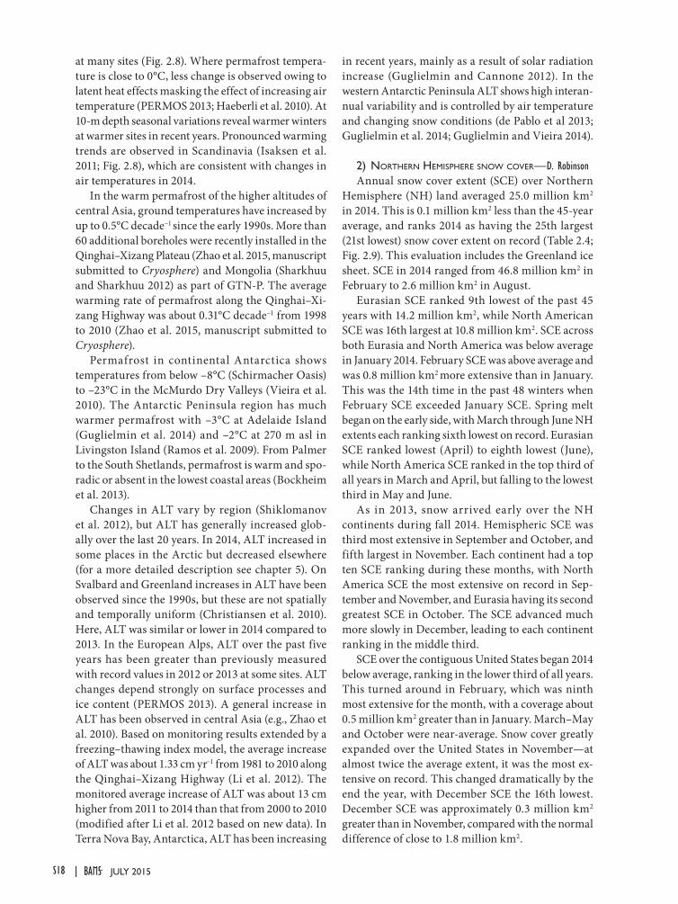
at many sites (Fig. 2.8). Where permafrost tempera-ture is close to 0°C, less change is observed owing to latent heat effects masking the effect of increasing air temperature (PERMOS 2013; Haeberli et al. 2010). At 10-m depth seasonal variations reveal warmer winters at warmer sites in recent years. Pronounced warming trends are observed in Scandinavia (Isaksen et al. 2011; Fig. 2.8), which are consistent with changes in air temperatures in 2014.
In the warm permafrost of the higher altitudes of central Asia, ground temperatures have increased by up to 0.5°C decade−1 since the early 1990s. More than 60 additional boreholes were recently installed in the Qinghai–Xizang Plateau (Zhao et al. 2015, manuscript submitted to Cryosphere) and Mongolia (Sharkhuu and Sharkhuu 2012) as part of GTN-P. The average warming rate of permafrost along the Qinghai–Xi-zang Highway was about 0.31°C decade−1 from 1998 to 2010 (Zhao et al. 2015, manuscript submitted to Cryosphere).
Permafrost in continental Antarctica shows temperatures from below –8°C (Schirmacher Oasis) to –23°C in the McMurdo Dry Valleys (Vieira et al. 2010). The Antarctic Peninsula region has much warmer permafrost with –3°C at Adelaide Island (Guglielmin et al. 2014) and –2°C at 270 m asl in Livingston Island (Ramos et al. 2009). From Palmer to the South Shetlands, permafrost is warm and spo-radic or absent in the lowest coastal areas (Bockheim et al. 2013).
Changes in ALT vary by region (Shiklomanov et al. 2012), but ALT has generally increased glob-ally over the last 20 years. In 2014, ALT increased in some places in the Arctic but decreased elsewhere (for a more detailed description see chapter 5). On Svalbard and Greenland increases in ALT have been observed since the 1990s, but these are not spa tially and temporally uniform (Christiansen et al. 2010). Here, ALT was similar or lower in 2014 compared to 2013. In the European Alps, ALT over the past five years has been greater than previously measured with record values in 2012 or 2013 at some sites. ALT changes depend strongly on surface processes and ice content (PERMOS 2013). A general increase in ALT has been observed in central Asia (e.g., Zhao et al. 2010). Based on monitoring results extended by a freezing–thawing index model, the average increase of ALT was about 1.33 cm yr−1 from 1981 to 2010 along the Qinghai–Xizang Highway (Li et al. 2012). The monitored average increase of ALT was about 13 cm higher from 2011 to 2014 than that from 2000 to 2010 (modified after Li et al. 2012 based on new data). In Terra Nova Bay, Antarctica, ALT has been increasing
in recent years, mainly as a result of solar radiation increase (Guglielmin and Cannone 2012). In the western Antarctic Peninsula ALT shows high interan-nual variability and is controlled by air temperature and changing snow conditions (de Pablo et al 2013; Guglielmin et al. 2014; Guglielmin and Vieira 2014).
2) northern hemiSphere Snow cover—D. RobinsonAnnual snow cover extent (SCE) over Northern
Hemisphere (NH) land averaged 25.0 million km2 in 2014. This is 0.1 million km2 less than the 45-year average, and ranks 2014 as having the 25th largest (21st lowest) snow cover extent on record (Table 2.4; Fig. 2.9). This evaluation includes the Greenland ice sheet. SCE in 2014 ranged from 46.8 million km2 in February to 2.6 million km2 in August.
Eurasian SCE ranked 9th lowest of the past 45 years with 14.2 million km2, while North American SCE was 16th largest at 10.8 million km2. SCE across both Eurasia and North America was below average in January 2014. February SCE was above average and was 0.8 million km2 more extensive than in January. This was the 14th time in the past 48 winters when February SCE exceeded January SCE. Spring melt began on the early side, with March through June NH extents each ranking sixth lowest on record. Eurasian SCE ranked lowest (April) to eighth lowest (June), while North America SCE ranked in the top third of all years in March and April, but falling to the lowest third in May and June.
As in 2013, snow arrived early over the NH continents during fall 2014. Hemispheric SCE was third most extensive in September and October, and fifth largest in November. Each continent had a top ten SCE ranking during these months, with North America SCE the most extensive on record in Sep-tember and November, and Eurasia having its second greatest SCE in October. The SCE advanced much more slowly in December, leading to each continent ranking in the middle third.
SCE over the contiguous United States began 2014 below average, ranking in the lower third of all years. This turned around in February, which was ninth most extensive for the month, with a coverage about 0.5 million km2 greater than in January. March–May and October were near-average. Snow cover greatly expanded over the United States in November—at almost twice the average extent, it was the most ex-tensive on record. This changed dramatically by the end the year, with December SCE the 16th lowest. December SCE was approximately 0.3 million km2 greater than in November, compared with the normal difference of close to 1.8 million km2.
S18 JULY 2015|
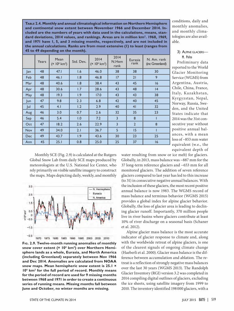
Monthly SCE (Fig. 2.9) is calculated at the Rutgers Global Snow Lab from daily SCE maps produced by meteorologists at the U.S. National Ice Center, who rely primarily on visible satellite imagery to construct the maps. Maps depicting daily, weekly, and monthly
conditions, daily and monthly anomalies, and monthly clima-tologies are also avail-able.
3) aLpine gLacierS—M. Pelto
Preliminary data reported to the World Glacier Monitoring Service (WGMS) from Argentina, Austria, Chile, China, France, Ita ly, Kazak hstan, Kyrgyzstan, Nepal, Norway, Russia, Swe-den, and the United States indicate that 2014 was the 31st con-secutive year without positive annual bal-ances, with a mean loss of −853 mm water equivalent (w.e., the equivalent depth of
water resulting from snow or ice melt) for glaciers. Globally, in 2013, mass balance was −887 mm for the 37 long-term reference glaciers and −653 mm for all monitored glaciers. The addition of seven reference glaciers compared to last year has led to this increase (to 31) in consecutive negative annual balances. With the inclusion of these glaciers, the most recent positive annual balance is now 1983. The WGMS record of mass balance and terminus behavior (WGMS 2015) provides a global index for alpine glacier behavior. Globally, the loss of glacier area is leading to declin-ing glacier runoff. Importantly, 370 million people live in river basins where glaciers contribute at least 10% of river discharge on a seasonal basis (Schaner et al. 2012).
Alpine glacier mass balance is the most accurate indicator of glacier response to climate and, along with the worldwide retreat of alpine glaciers, is one of the clearest signals of ongoing climate change (Haeberli et al. 2000). Glacier mass balance is the dif-ference between accumulation and ablation. The re-treat is a reflection of strongly negative mass balances over the last 30 years (WGMS 2013). The Randolph Glacier Inventory (RGI) version 3.2 was completed in 2014 compiling digital outlines of glaciers, excluding the ice sheets, using satellite imagery from 1999 to 2010. The inventory identified 198 000 glaciers, with a
Table 2.4. Monthly and annual climatological information on Northern Hemisphere and continental snow extent between November 1966 and December 2014. In-cluded are the numbers of years with data used in the calculations, means, stan-dard deviations, 2014 values, and rankings. Areas are in million km2. 1968, 1969, and 1971 have 1, 5, and 3 missing months, respectively, and are not included in the annual calculations. Ranks are from most extensive (1) to least (ranges from 45 to 49 depending on the month).
YearsMean
(× 106 km2)Std. Dev. 2014
(× 106 km2)
2014N.Hem
rank
Eurasia rank
N. Am. rank(inc Greenland)
Jan 48 47.1 1.6 46.0 38 38 30
Feb 48 46.1 1.8 46.8 17 21 9
Mar 48 40.6 1.8 38.4 43 45 16
Apr 48 30.6 1.7 28.6 43 48 14
May 48 19.3 1.9 17.0 43 43 38
Jun 47 9.8 2.3 6.8 42 40 45
Jul 45 4.1 1.2 2.9 40 41 32
Aug 46 3.0 0.7 2.6 32 35 23
Sep 46 5.4 1.0 7.2 3 8 1
Oct 47 18.2 2.6 22.9 3 2 8
Nov 49 34.0 2.1 36.7 5 15 1
Dec 49 43.7 1.9 43.6 30 23 25
Ann 45 25.1 0.8 25.0 25 37 16
Fig. 2.9. Twelve-month running anomalies of monthly snow cover extent (× 106 km2) over Northern Hemi-sphere lands as a whole, Eurasia, and North America (including Greenland) separately between Nov 1966 and Dec 2014. Anomalies are calculated from NOAA snow maps. Mean hemispheric snow extent is 25.1 × 10⁶ km2 for the full period of record. Monthly means for the period of record are used for 9 missing months between 1968 and 1971 in order to create a continuous series of running means. Missing months fall between June and October, no winter months are missing.
S19JULY 2015STATE OF THE CLIMATE IN 2014 |
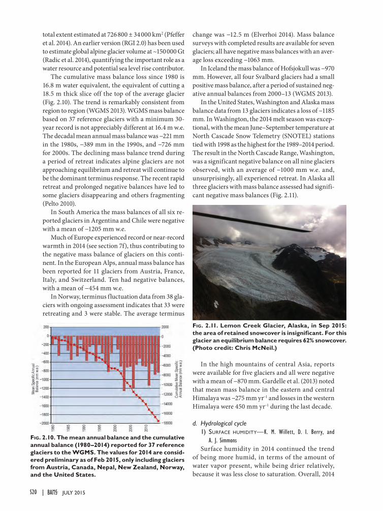
total extent estimated at 726 800 ± 34 000 km2 (Pfeffer et al. 2014). An earlier version (RGI 2.0) has been used to estimate global alpine glacier volume at ~150 000 Gt (Radic et al. 2014), quantifying the important role as a water resource and potential sea level rise contributor.
The cumulative mass balance loss since 1980 is 16.8 m water equivalent, the equivalent of cutting a 18.5 m thick slice off the top of the average glacier (Fig. 2.10). The trend is remarkably consistent from region to region (WGMS 2013). WGMS mass balance based on 37 reference glaciers with a minimum 30-year record is not appreciably different at 16.4 m w.e. The decadal mean annual mass balance was −221 mm in the 1980s, −389 mm in the 1990s, and −726 mm for 2000s. The declining mass balance trend during a period of retreat indicates alpine glaciers are not approaching equilibrium and retreat will continue to be the dominant terminus response. The recent rapid retreat and prolonged negative balances have led to some glaciers disappearing and others fragmenting (Pelto 2010).
In South America the mass balances of all six re-ported glaciers in Argentina and Chile were negative with a mean of −1205 mm w.e.
Much of Europe experienced record or near-record warmth in 2014 (see section 7f), thus contributing to the negative mass balance of glaciers on this conti-nent. In the European Alps, annual mass balance has been reported for 11 glaciers from Austria, France, Italy, and Switzerland. Ten had negative balances, with a mean of −454 mm w.e.
In Norway, terminus fluctuation data from 38 gla-ciers with ongoing assessment indicates that 33 were retreating and 3 were stable. The average terminus
change was −12.5 m (Elverhoi 2014). Mass balance surveys with completed results are available for seven glaciers; all have negative mass balances with an aver-age loss exceeding −1063 mm.
In Iceland the mass balance of Hofsjokull was −970 mm. However, all four Svalbard glaciers had a small positive mass balance, after a period of sustained neg-ative annual balances from 2000–13 (WGMS 2013).
In the United States, Washington and Alaska mass balance data from 13 glaciers indicates a loss of −1185 mm. In Washington, the 2014 melt season was excep-tional, with the mean June–September temperature at North Cascade Snow Telemetry (SNOTEL) stations tied with 1998 as the highest for the 1989–2014 period. The result in the North Cascade Range, Washington, was a significant negative balance on all nine glaciers observed, with an average of −1000 mm w.e. and, unsurprisingly, all experienced retreat. In Alaska all three glaciers with mass balance assessed had signifi-cant negative mass balances (Fig. 2.11).
In the high mountains of central Asia, reports were available for five glaciers and all were negative with a mean of −870 mm. Gardelle et al. (2013) noted that mean mass balance in the eastern and central Himalaya was −275 mm yr−1 and losses in the western Himalaya were 450 mm yr−1 during the last decade.
d. Hydrological cycle1) Surface humidity—K. M. Willett, D. I. Berry, and
A. J. SimmonsSurface humidity in 2014 continued the trend
of being more humid, in terms of the amount of water vapor present, while being drier relatively, because it was less close to saturation. Overall, 2014
Fig. 2.10. The mean annual balance and the cumulative annual balance (1980–2014) reported for 37 reference glaciers to the WGMS. The values for 2014 are consid-ered preliminary as of Feb 2015, only including glaciers from Austria, Canada, Nepal, New Zealand, Norway, and the United States.
Fig. 2.11. Lemon Creek Glacier, Alaska, in Sep 2015: the area of retained snowcover is insignificant. For this glacier an equilibrium balance requires 62% snowcover. (Photo credit: Chris McNeil.)
S20 JULY 2015|
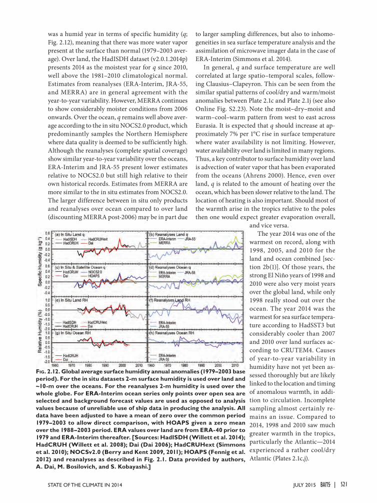
was a humid year in terms of specific humidity (q; Fig. 2.12), meaning that there was more water vapor present at the surface than normal (1979–2003 aver-age). Over land, the HadISDH dataset (v2.0.1.2014p) presents 2014 as the moistest year for q since 2010, well above the 1981–2010 climatological normal. Estimates from reanalyses (ERA-Interim, JRA-55, and MERRA) are in general agreement with the year-to-year variability. However, MERRA continues to show considerably moister conditions from 2006 onwards. Over the ocean, q remains well above aver-age according to the in situ NOCS2.0 product, which predominantly samples the Northern Hemisphere where data quality is deemed to be sufficiently high. Although the reanalyses (complete spatial coverage) show similar year-to-year variability over the oceans, ERA-Interim and JRA-55 present lower estimates relative to NOCS2.0 but still high relative to their own historical records. Estimates from MERRA are more similar to the in situ estimates from NOCS2.0. The larger difference between in situ only products and reanalyses over ocean compared to over land (discounting MERRA post-2006) may be in part due
to larger sampling differences, but also to inhomo-geneities in sea surface temperature analysis and the assimilation of microwave imager data in the case of ERA-Interim (Simmons et al. 2014).
In general, q and surface temperature are well correlated at large spatio–temporal scales, follow-ing Clausius–Clapeyron. This can be seen from the similar spatial patterns of cool/dry and warm/moist anomalies between Plate 2.1c and Plate 2.1j (see also Online Fig. S2.23). Note the moist–dry–moist and warm–cool–warm pattern from west to east across Eurasia. It is expected that q should increase at ap-proximately 7% per 1°C rise in surface temperature where water availability is not limiting. However, water availability over land is limited in many regions. Thus, a key contributor to surface humidity over land is advection of water vapor that has been evaporated from the oceans (Ahrens 2000). Hence, even over land, q is related to the amount of heating over the ocean, which has been slower relative to the land. The location of heating is also important. Should most of the warmth arise in the tropics relative to the poles then one would expect greater evaporation overall,
and vice versa.The year 2014 was one of the
warmest on record, along with 1998, 2005, and 2010 for the land and ocean combined [sec-tion 2b(1)]. Of those years, the strong El Niño years of 1998 and 2010 were also very moist years over the global land, while only 1998 really stood out over the ocean. The year 2014 was the warmest for sea surface tempera-ture according to HadSST3 but considerably cooler than 2007 and 2010 over land surfaces ac-cording to CRUTEM4. Causes of year-to-year variability in humidity have not yet been as-sessed thoroughly but are likely linked to the location and timing of anomalous warmth, in addi-tion to circulation. Incomplete sampling almost certainly re-mains an issue. Compared to 2014, 1998 and 2010 saw much greater warmth in the tropics, particularly the Atlantic—2014 experienced a rather cool/dry Atlantic (Plates 2.1c,j).
Fig. 2.12. Global average surface humidity annual anomalies (1979–2003 base period). For the in situ datasets 2-m surface humidity is used over land and ~10-m over the oceans. For the reanalyses 2-m humidity is used over the whole globe. For ERA-Interim ocean series only points over open sea are selected and background forecast values are used as opposed to analysis values because of unreliable use of ship data in producing the analysis. All data have been adjusted to have a mean of zero over the common period 1979–2003 to allow direct comparison, with HOAPS given a zero mean over the 1988–2003 period. ERA values over land are from ERA-40 prior to 1979 and ERA-Interim thereafter. [Sources: HadISDH (Willett et al. 2014); HadCRUH (Willett et al. 2008); Dai (Dai 2006); HadCRUHext (Simmons et al. 2010); NOCSv2.0 (Berry and Kent 2009, 2011); HOAPS (Fennig et al. 2012) and reanalyses as described in Fig. 2.1. Data provided by authors, A. Dai, M. Bosilovich, and S. Kobayashi.]
S21JULY 2015STATE OF THE CLIMATE IN 2014 |
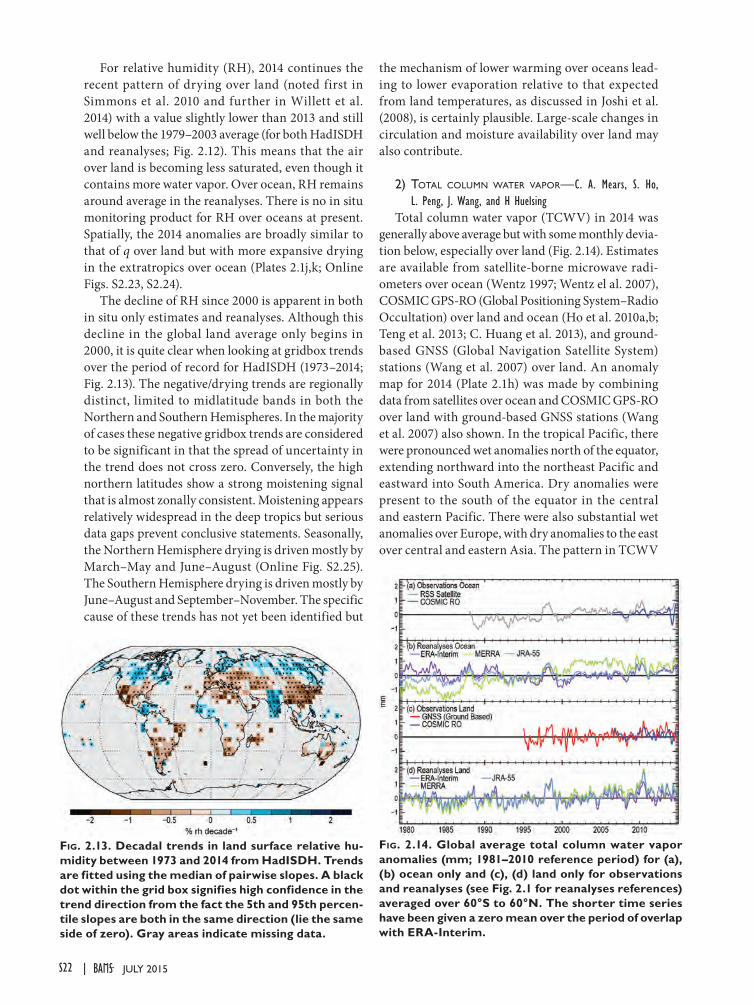
For relative humidity (RH), 2014 continues the recent pattern of drying over land (noted first in Simmons et al. 2010 and further in Willett et al. 2014) with a value slightly lower than 2013 and still well below the 1979–2003 average (for both HadISDH and reanalyses; Fig. 2.12). This means that the air over land is becoming less saturated, even though it contains more water vapor. Over ocean, RH remains around average in the reanalyses. There is no in situ monitoring product for RH over oceans at present. Spatially, the 2014 anomalies are broadly similar to that of q over land but with more expansive drying in the extratropics over ocean (Plates 2.1j,k; Online Figs. S2.23, S2.24).
The decline of RH since 2000 is apparent in both in situ only estimates and reanalyses. Although this decline in the global land average only begins in 2000, it is quite clear when looking at gridbox trends over the period of record for HadISDH (1973–2014; Fig. 2.13). The negative/drying trends are regionally distinct, limited to midlatitude bands in both the Northern and Southern Hemispheres. In the majority of cases these negative gridbox trends are considered to be significant in that the spread of uncertainty in the trend does not cross zero. Conversely, the high northern latitudes show a strong moistening signal that is almost zonally consistent. Moistening appears relatively widespread in the deep tropics but serious data gaps prevent conclusive statements. Seasonally, the Northern Hemisphere drying is driven mostly by March–May and June–August (Online Fig. S2.25). The Southern Hemisphere drying is driven mostly by June–August and September–November. The specific cause of these trends has not yet been identified but
the mechanism of lower warming over oceans lead-ing to lower evaporation relative to that expected from land temperatures, as discussed in Joshi et al. (2008), is certainly plausible. Large-scale changes in circulation and moisture availability over land may also contribute.
2) totaL coLumn water vapor—C. A. Mears, S. Ho, L. Peng, J. Wang, and H Huelsing
Total column water vapor (TCWV) in 2014 was generally above average but with some monthly devia-tion below, especially over land (Fig. 2.14). Estimates are available from satellite-borne microwave radi-ometers over ocean (Wentz 1997; Wentz el al. 2007), COSMIC GPS-RO (Global Positioning System–Radio Occultation) over land and ocean (Ho et al. 2010a,b; Teng et al. 2013; C. Huang et al. 2013), and ground-based GNSS (Global Navigation Satellite System) stations (Wang et al. 2007) over land. An anomaly map for 2014 (Plate 2.1h) was made by combining data from satellites over ocean and COSMIC GPS-RO over land with ground-based GNSS stations (Wang et al. 2007) also shown. In the tropical Pacific, there were pronounced wet anomalies north of the equator, extending northward into the northeast Pacific and eastward into South America. Dry anomalies were present to the south of the equator in the central and eastern Pacific. There were also substantial wet anomalies over Europe, with dry anomalies to the east over central and eastern Asia. The pattern in TCWV
Fig. 2.13. Decadal trends in land surface relative hu-midity between 1973 and 2014 from HadISDH. Trends are fitted using the median of pairwise slopes. A black dot within the grid box signifies high confidence in the trend direction from the fact the 5th and 95th percen-tile slopes are both in the same direction (lie the same side of zero). Gray areas indicate missing data.
Fig. 2.14. Global average total column water vapor anomalies (mm; 1981–2010 reference period) for (a), (b) ocean only and (c), (d) land only for observations and reanalyses (see Fig. 2.1 for reanalyses references) averaged over 60°S to 60°N. The shorter time series have been given a zero mean over the period of overlap with ERA-Interim.
S22 JULY 2015|
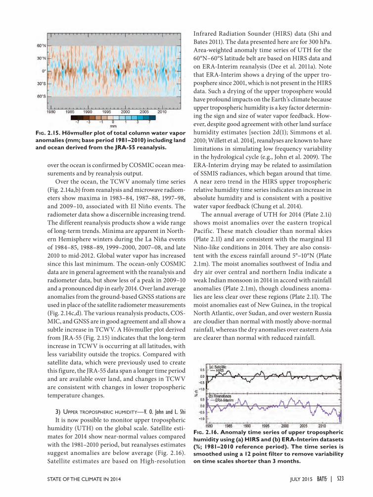
over the ocean is confirmed by COSMIC ocean mea-surements and by reanalysis output.
Over the ocean, the TCWV anomaly time series (Fig. 2.14a,b) from reanalysis and microwave radiom-eters show maxima in 1983–84, 1987–88, 1997–98, and 2009–10, associated with El Niño events. The radiometer data show a discernible increasing trend. The different reanalysis products show a wide range of long-term trends. Minima are apparent in North-ern Hemisphere winters during the La Niña events of 1984–85, 1988–89, 1999–2000, 2007–08, and late 2010 to mid-2012. Global water vapor has increased since this last minimum. The ocean-only COSMIC data are in general agreement with the reanalysis and radiometer data, but show less of a peak in 2009–10 and a pronounced dip in early 2014. Over land average anomalies from the ground-based GNSS stations are used in place of the satellite radiometer measurements (Fig. 2.14c,d). The various reanalysis products, COS-MIC, and GNSS are in good agreement and all show a subtle increase in TCWV. A Hövmuller plot derived from JRA-55 (Fig. 2.15) indicates that the long-term increase in TCWV is occurring at all latitudes, with less variability outside the tropics. Compared with satellite data, which were previously used to create this figure, the JRA-55 data span a longer time period and are available over land, and changes in TCWV are consistent with changes in lower tropospheric temperature changes.
3) upper tropoSpheric humidity—V. O. John and L. ShiIt is now possible to monitor upper tropospheric
humidity (UTH) on the global scale. Satellite esti-mates for 2014 show near-normal values compared with the 1981–2010 period, but reanalyses estimates suggest anomalies are below average (Fig. 2.16). Satellite estimates are based on High-resolution
Infrared Radiation Sounder (HIRS) data (Shi and Bates 2011). The data presented here are for 300 hPa. Area-weighted anomaly time series of UTH for the 60°N–60°S latitude belt are based on HIRS data and on ERA-Interim reanalysis (Dee et al. 2011a). Note that ERA-Interim shows a drying of the upper tro-posphere since 2001, which is not present in the HIRS data. Such a drying of the upper troposphere would have profound impacts on the Earth’s climate because upper tropospheric humidity is a key factor determin-ing the sign and size of water vapor feedback. How-ever, despite good agreement with other land surface humidity estimates [section 2d(1); Simmons et al. 2010; Willett et al. 2014], reanalyses are known to have limitations in simulating low frequency variability in the hydrological cycle (e.g., John et al. 2009). The ERA-Interim drying may be related to assimilation of SSMIS radiances, which began around that time. A near zero trend in the HIRS upper tropospheric relative humidity time series indicates an increase in absolute humidity and is consistent with a positive water vapor feedback (Chung et al. 2014).
The annual average of UTH for 2014 (Plate 2.1i) shows moist anomalies over the eastern tropical Pacific. These match cloudier than normal skies (Plate 2.1l) and are consistent with the marginal El Niño-like conditions in 2014. They are also consis-tent with the excess rainfall around 5°–10°N (Plate 2.1m). The moist anomalies southwest of India and dry air over central and northern India indicate a weak Indian monsoon in 2014 in accord with rainfall anomalies (Plate 2.1m), though cloudiness anoma-lies are less clear over these regions (Plate 2.1l). The moist anomalies east of New Guinea, in the tropical North Atlantic, over Sudan, and over western Russia are cloudier than normal with mostly above-normal rainfall, whereas the dry anomalies over eastern Asia are clearer than normal with reduced rainfall.
Fig. 2.15. Hövmuller plot of total column water vapor anomalies (mm; base period 1981–2010) including land and ocean derived from the JRA-55 reanalysis.
Fig. 2.16. Anomaly time series of upper tropospheric humidity using (a) HIRS and (b) ERA-Interim datasets (%; 1981–2010 reference period). The time series is smoothed using a 12 point filter to remove variability on time scales shorter than 3 months.
S23JULY 2015STATE OF THE CLIMATE IN 2014 |
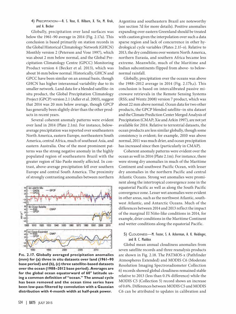
4) precipitation—R. S. Vose, K. Hilburn, X. Yin, M. Kruk, and A. Becker
Globally, precipitation over land surfaces was below the 1961–90 average in 2014 (Fig. 2.17a). This conclusion is based primarily on station records in the Global Historical Climatology Network (GHCN) Monthly version 2 (Peterson and Vose 1997), which was about 2 mm below normal, and the Global Pre-cipitation Climatology Centre (GPCC) Monitoring Product version 4 (Becker et al. 2013), which was about 16 mm below normal. Historically, GHCN and GPCC have been similar on an annual basis, though GHCN has higher interannual variability due to its smaller network. Land data for a blended satellite–in situ product, the Global Precipitation Climatology Project (GPCP) version 2.1 (Adler et al. 2003), suggest that 2014 was 20 mm below average, though GPCP has generally been slightly drier than the other prod-ucts in recent years.
Several coherent anomaly patterns were evident over land in 2014 (Plate 2.1m). For instance, below-average precipitation was reported over southeastern North America, eastern Europe, northeastern South America, central Africa, much of southeast Asia, and eastern Australia. One of the most prominent pat-terns was the strong negative anomaly in the highly populated region of southeastern Brazil with the greater region of São Paolo mostly affected. In con-trast, above-average precipitation fell over southern Europe and central South America. The proximity of strongly contrasting anomalies between northern
Argentina and southeastern Brazil are noteworthy (see section 7d for more details). Positive anomalies expanding over eastern Greenland should be treated with caution given the interpolation over such a data sparse region and lack of concurrence in other hy-drological cycle variables (Plates 2.1f–o). Relative to 2013, the dry conditions over western North America, northern Eurasia, and southern Africa became less extreme. Meanwhile, much of the Maritime and Indian subcontinents flipped from above- to below-normal rainfall.
Globally, precipitation over the oceans was above the 1988–2012 average in 2014 (Fig. 2.17b,c). This conclusion is based on intercalibrated passive mi-crowave retrievals in the Remote Sensing Systems (RSS; and Wentz 2008) version 7 product, which was about 22 mm above normal. Ocean data for two other products, the GPCP blended satellite–in situ dataset and the Climate Prediction Center Merged Analysis of Precipitation (CMAP; Xie and Arkin 1997), are not yet available for 2014. Relative to terrestrial datasets, the ocean products are less similar globally, though some consistency is evident; for example, 2010 was above normal, 2011 was much drier, and ocean precipitation has increased since then (particularly in CMAP).
Coherent anomaly patterns were evident over the ocean as well in 2014 (Plate 2.1m). For instance, there were strong dry anomalies in much of the Maritime Continent and southwest Pacific Ocean, with lesser dry anomalies in the northern Pacific and central Atlantic Oceans. Strong wet anomalies were promi-nent along the intertropical convergence zone in the equatorial Pacific as well as along the South Pacific convergence zone. Lesser wet anomalies were evident in other areas, such as the northwest Atlantic, south-west Atlantic, and Antarctic Oceans. Much of the differences between 2014 and 2013 reflect the impact of the marginal El Niño-like conditions in 2014, for example, drier conditions in the Maritime Continent and wetter conditions along the equatorial Pacific.
5) cLoudineSS—M. Foster, S. A. Ackerman, A. K. Heidinger, and B. C. Maddux
Global mean annual cloudiness anomalies from seven satellite records and three reanalysis products are shown in Fig. 2.18. The PATMOS-x (Pathfinder Atmospheres Extended) and MODIS C6 (Moderate Resolution Imaging Spectroradiometer Collection 6) records showed global cloudiness remained stable relative to 2013 (less than 0.1% difference) while the MODIS C5 (Collection 5) record shows an increase of 0.6%. Differences between MODIS C5 and MODIS C6 can be attributed to updates in calibration and
Fig. 2.17. Globally averaged precipitation anomalies (mm) for (a) three in situ datasets over land (1961–90 base period) and (b), (c) three satellite-based datasets over the ocean (1988–2012 base period). Averages are for the global ocean equatorward of 60° latitude us-ing a common definition of “ocean.” The annual cycle has been removed and the ocean time series have been low-pass filtered by convolution with a Gaussian distribution with 4-month width at half-peak power.
S24 JULY 2015|
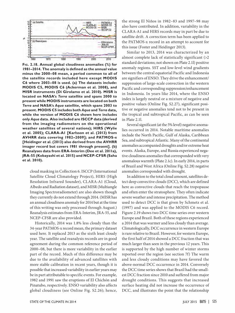
cloud masking in Collection 6. ISCCP (International Satellite Cloud Climatology Project), HIRS (High Resolution Infrared Sounder), CLARA-A1 (Cloud, Albedo and Radiation dataset), and MISR (Multiangle Imaging Spectroradiometer) are also shown though they currently do not extend through 2014. (MISR has an annual cloudiness anomaly for 2014 but at the time of this writing was only processed through August.) Reanalysis estimates from ERA-Interim, JRA-55, and NCEP-CFSR are also provided.
Historically, 2014 was 1.8% less cloudy than the 34-year PATMOS-x record mean, the primary dataset used here. It replaced 2013 as the sixth least cloudy year. The satellite and reanalysis records are in good agreement during the common reference period of 2000–08, but there is more variability in the earlier part of the record. Much of this difference may be due to the availability of advanced satellites with more stable calibration in recent years, though it is possible that increased variability in earlier years may be in part attributable to specific events. For example, 1982 and 1991 saw the eruptions of El Chichón and Pinatubo, respectively. ENSO variability also affects global cloudiness (see Online Fig. S2.26); hence,
the strong El Niños in 1982–83 and 1997–98 may also have contributed. In addition, variability in the CLARA-A1 and HIRS records may in part be due to satellite drift. A correction term has been applied to the PATMOS-x record in an attempt to account for this issue (Foster and Heidinger 2013).
Similar to 2013, 2014 was characterized by an almost complete lack of statistically significant (>2 standard deviations; not shown on Plate 2.1l) positive anomaly regions. SST and low-level wind gradients between the central equatorial Pacific and Indonesia are signifiers of ENSO. They drive the enhancement/suppression of large-scale convection in the western Pacific and corresponding suppression/enhancement in Indonesia. In years like 2014, where the ENSO index is largely neutral or a mixture of negative and positive values (Online Fig. S2.27), significant posi-tive or negative anomalies tend not to be present in the tropical and subtropical Pacific, as can be seen in Plate 2.1l.
Several significant (at the 5% level) negative anoma-lies occurred in 2014. Notable maritime anomalies include the North Pacific, Gulf of Alaska, Caribbean Sea, and subtropical Atlantic. Many of the continental anomalies accompanied droughts and/or extreme heat events. Alaska, Europe, and Russia experienced nega-tive cloudiness anomalies that corresponded with very anomalous warmth (Plate 2.1c). In early 2014, in parts of Brazil and West Africa (Online Fig. S2.28) negative anomalies corresponded with drought.
In addition to the total cloud amount, satellites de-tect deep convective clouds (DCC), which are defined here as convective clouds that reach the tropopause and often enter the stratosphere. They often indicate severe weather and intense precipitation. The method used to detect DCC is that given by Schmetz et al. (1997) and was applied to the MODIS C6 record. Figure 2.19 shows two DCC time series over western Europe and Brazil. Both of these regions experienced a 2014 that was warmer and less cloudy than average. Climatologically, DCC occurrence in western Europe is rare relative to Brazil. However, for western Europe, the first half of 2014 showed a DCC fraction that was much larger than seen in the previous 12 years. This is supported by the high number of winter storms reported over the region (see section 7f) The warm and less cloudy conditions may have favored the above-normal DCC occurrence in 2014. Conversely the DCC time series shows that Brazil had the small-est DCC fraction since 2010 and suffered from major drought conditions. This suggests that increased surface heating did not increase the occurrence of DCC, and illustrates the point that the relationship
Fig. 2.18. Annual global cloudiness anomalies (%) for 1981–2014. The anomaly is defined as the annual value minus the 2000–08 mean, a period common to all of the satellite records included here except MODIS C6 where 2003–08 is used. (a) The datasets include: MODIS C5, MODIS C6 (Ackerman et al. 2008), and MISR instruments (Di Girolamo et al. 2010). MISR is located on NASA’s Terra satellite and spans 2000 to present while MODIS instruments are located on both Terra and NASA’s Aqua satellite, which spans 2003 to present. MODIS C5 includes both Aqua and Terra data, while the version of MODIS C6 shown here includes only Aqua data. Also included are ISCCP data (derived from the imaging radiometers on the operational weather satellites of several nations); HIRS (Wylie et al. 2005); CLARA-A1 [Karlsson et al. (2013) from AVHRR data covering 1982–2009]; and PATMOS-x [Heidinger et al. (2013) also derived from the AVHRR imager record but covers 1981 through present]. (b) Reanalyses data from ERA-Interim (Dee et al. 2011a), JRA-55 (Kobayashi et al. 2015) and NCEP-CFSR (Saha et al. 2010).
S25JULY 2015STATE OF THE CLIMATE IN 2014 |

between total cloudiness and drought and/or extreme heat events is not always straightforward.
6) river diScharge—H. Kim and T. OkiThe estimated global river discharge in 2014 slight-
ly exceeded the climate normal, so the globe overall stayed in the high discharge phase that started in 2005 (Fig. 2.20). Discharge was relatively high during the boreal spring but lower from the boreal summer onwards. Strong anomalies (>2σ,) such as occurred in 2013, did not appear in 2014. Regionally, South America, Europe, and Asia were the main contribu-tors to these changes. In 2014, South America had
significantly high discharge in early months [compare the soil moisture section 2d(8) and Online Fig. S2.29], but the spatial distribution was highly heterogeneous (Plate 2.1o). The Amazon and Paraguay Rivers ex-perienced a high-discharge year but the Orinoco, Tocantins, and São Francisco Rivers experienced a low-discharge year (Plate 2.1n). The close proximity of these strong and opposite anomalies is seen in other hydrological cycle variables (e.g., precipitation in Plate 2.1m). Europe had anomalously high discharge in early 2014, which tended to intensify the global high discharge anomaly in phase with South America. However, there was a large decrease from 2013 in the following spring high-discharge season which has a considerably broad interannual variability. Most riv-ers showed low anomaly conditions except for a few rivers near the Mediterranean Sea such as the Dan-ube. Asia showed a considerable low-discharge deficit in August affecting the global balance. The Ganges–Brahmaputra, northern Indochina peninsula, Lena, and East Asia were in a low-flow state, and Kolyma, Ob, and southwestern China were in a high-flow state. The annual amount and seasonal variations of runoff in 2014 for North America, Africa, and Australia did not show considerably positive or negative deviation from the long-term climatology, though the peak oc-curred one month earlier in Australia. Rivers in the northern part of North America such as the Yukon and the Mackenzie had high discharge, and the riv-ers in the southern part of North America (e.g., the Mississippi and the Colorado) and in Africa (e.g., the Congo and the Nile) had lower discharge than their long-term mean.
River discharge has comparably long observational records compared to other fundamental hydrologi-cal variables such as precipitation. Discharge is not only convenient to measure as a tangible and highly concentrated signal within a narrow stream, it is also a critical resource to keep living organisms alive and
to develop and sustain human so-ciety. However, the latter function also restricts the availability of the measured data to the public owing to its economic and political value. Previous work has demonstrated the potential to use, for instance, altimetry remote sensing (e.g., Alsdorf and Lettenmaier 2003) and mass balance approaches by combining various sources of datasets (e.g., Syed et al. 2010). Nevertheless, global off-line model simulation still remains the only
Fig. 2.19. Time series of areal fraction of deep convec-tive cloud determined from MODIS/AQUA data over (a) western Europe and (b) Brazil. Deep convective cloud is defined as convective clouds that reach the tropopause. The black curve is a seasonal average and the gray curve is an annual average.
Fig. 2.20. Interannual variability of global runoff (blue; thick line for 12-month moving average), and seasonal variations of global and conti-nental runoff (bar for 57-year climatology with error bar for 2σ, lines for recent 4 years).
S26 JULY 2015|
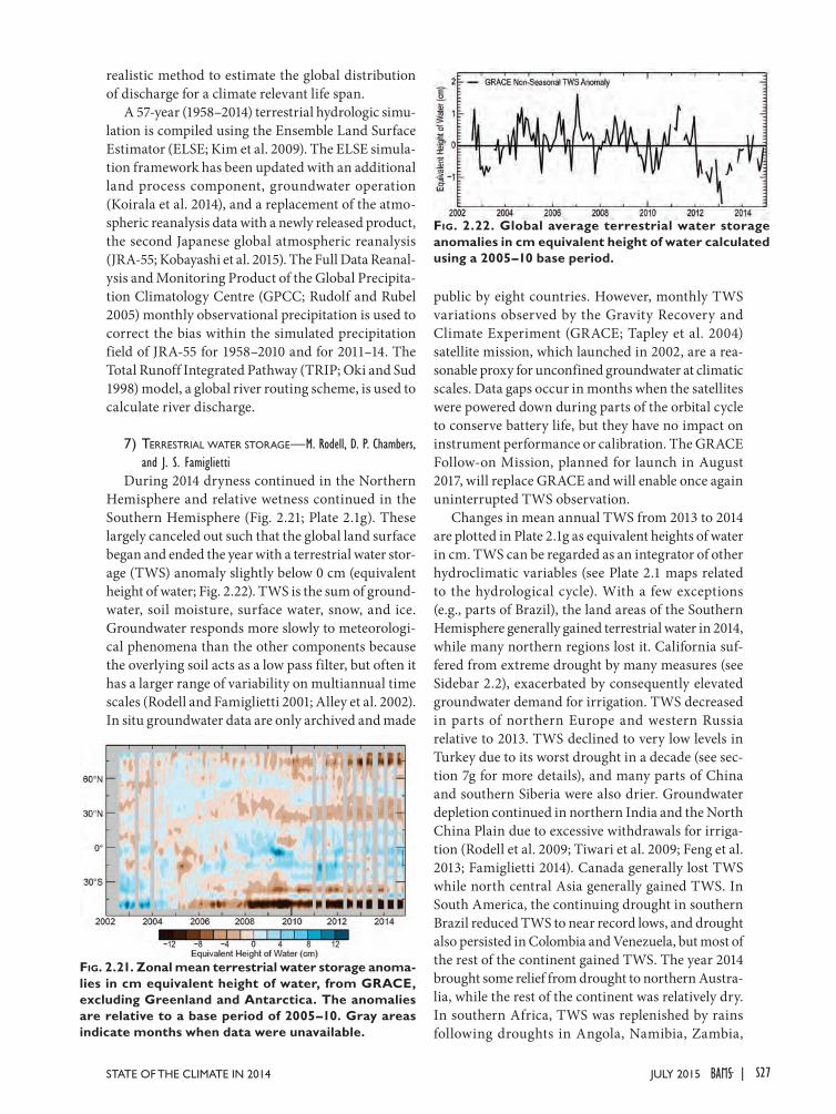
realistic method to estimate the global distribution of discharge for a climate relevant life span.
A 57-year (1958–2014) terrestrial hydrologic simu-lation is compiled using the Ensemble Land Surface Estimator (ELSE; Kim et al. 2009). The ELSE simula-tion framework has been updated with an additional land process component, groundwater operation (Koirala et al. 2014), and a replacement of the atmo-spheric reanalysis data with a newly released product, the second Japanese global atmospheric reanalysis (JRA-55; Kobayashi et al. 2015). The Full Data Reanal-ysis and Monitoring Product of the Global Precipita-tion Climatology Centre (GPCC; Rudolf and Rubel 2005) monthly observational precipitation is used to correct the bias within the simulated precipitation field of JRA-55 for 1958–2010 and for 2011–14. The Total Runoff Integrated Pathway (TRIP; Oki and Sud 1998) model, a global river routing scheme, is used to calculate river discharge.
7) terreStriaL water Storage—M. Rodell, D. P. Chambers, and J. S. Famiglietti
During 2014 dryness continued in the Northern Hemisphere and relative wetness continued in the Southern Hemisphere (Fig. 2.21; Plate 2.1g). These largely canceled out such that the global land surface began and ended the year with a terrestrial water stor-age (TWS) anomaly slightly below 0 cm (equivalent height of water; Fig. 2.22). TWS is the sum of ground-water, soil moisture, surface water, snow, and ice. Groundwater responds more slowly to meteorologi-cal phenomena than the other components because the overlying soil acts as a low pass filter, but often it has a larger range of variability on multiannual time scales (Rodell and Famiglietti 2001; Alley et al. 2002). In situ groundwater data are only archived and made
public by eight countries. However, monthly TWS variations observed by the Gravity Recovery and Climate Experiment (GRACE; Tapley et al. 2004) satellite mission, which launched in 2002, are a rea-sonable proxy for unconfined groundwater at climatic scales. Data gaps occur in months when the satellites were powered down during parts of the orbital cycle to conserve battery life, but they have no impact on instrument performance or calibration. The GRACE Follow-on Mission, planned for launch in August 2017, will replace GRACE and will enable once again uninterrupted TWS observation.
Changes in mean annual TWS from 2013 to 2014 are plotted in Plate 2.1g as equivalent heights of water in cm. TWS can be regarded as an integrator of other hydroclimatic variables (see Plate 2.1 maps related to the hydrological cycle). With a few exceptions (e.g., parts of Brazil), the land areas of the Southern Hemisphere generally gained terrestrial water in 2014, while many northern regions lost it. California suf-fered from extreme drought by many measures (see Sidebar 2.2), exacerbated by consequently elevated groundwater demand for irrigation. TWS decreased in parts of northern Europe and western Russia relative to 2013. TWS declined to very low levels in Turkey due to its worst drought in a decade (see sec-tion 7g for more details), and many parts of China and southern Siberia were also drier. Groundwater depletion continued in northern India and the North China Plain due to excessive withdrawals for irriga-tion (Rodell et al. 2009; Tiwari et al. 2009; Feng et al. 2013; Famiglietti 2014). Canada generally lost TWS while north central Asia generally gained TWS. In South America, the continuing drought in southern Brazil reduced TWS to near record lows, and drought also persisted in Colombia and Venezuela, but most of the rest of the continent gained TWS. The year 2014 brought some relief from drought to northern Austra-lia, while the rest of the continent was relatively dry. In southern Africa, TWS was replenished by rains following droughts in Angola, Namibia, Zambia,
Fig. 2.21. Zonal mean terrestrial water storage anoma-lies in cm equivalent height of water, from GRACE, excluding Greenland and Antarctica. The anomalies are relative to a base period of 2005–10. Gray areas indicate months when data were unavailable.
Fig. 2.22. Global average terrestrial water storage anomalies in cm equivalent height of water calculated using a 2005–10 base period.
S27JULY 2015STATE OF THE CLIMATE IN 2014 |
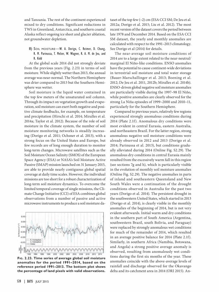
and Tanzania. The rest of the continent experienced mixed to dry conditions. Significant reductions in TWS in Greenland, Antarctica, and southern coastal Alaska reflect ongoing ice sheet and glacier ablation, not groundwater depletion.
8) SoiL moiSture—W. A. Dorigo, C. Reimer, D. Chung, R. M. Parinussa, T. Melzer, W. Wagner, R. A. M. de Jeu, and R. Kidd
At the global scale 2014 did not strongly deviate from the previous years (Fig. 2.23) in terms of soil moisture. While slightly wetter than 2013, the annual average was near-normal. The Northern Hemisphere was drier compared to 2013 but the Southern Hemi-sphere was wetter.
Soil moisture is the liquid water contained in the top few meters of the unsaturated soil column. Through its impact on vegetation growth and evapo-ration, soil moisture can exert both negative and posi-tive climate feedbacks, for example, on temperature and precipitation (Hirschi et al. 2014; Miralles et al. 2014a; Taylor et al. 2012). Because of the role of soil moisture in the climate system, the number of soil moisture monitoring networks is steadily increas-ing (Dorigo et al. 2011; Ochsner et al. 2013), with a strong focus on the United States and Europe, but few records are of long enough duration to monitor long-term changes. Microwave satellites such as the Soil Moisture Ocean Salinity (SMOS) of the European Space Agency (ESA) or NASA’s Soil Moisture Active Passive (SMAP) mission launched on 31 January 2015, are able to provide nearly contiguous global spatial coverage at daily time scales. However, the individual missions are too short for a robust characterization of long-term soil moisture dynamics. To overcome the limited temporal coverage of single missions, the Cli-mate Change Initiative (CCI) of ESA combines global observations from a number of passive and active microwave instruments to produce a soil moisture da-
taset of the top few (~2) cm (ESA CCI SM; De Jeu et al. 2012a; Dorigo et al. 2015; Liu et al. 2012). The most recent version of the dataset covers the period between late 1978 and December 2014. Based on the ESA CCI SM dataset, the yearly and monthly anomalies are calculated with respect to the 1991–2013 climatology. See Dorigo et al (2014) for details.
The near-average soil moisture conditions of 2014 are to a large extent related to the near-neutral/marginal El Niño-like conditions. ENSO anomalies have the potential to cause continent-wide deviations in terrestrial soil moisture and total water storage (Bauer-Marschallinger et al. 2013; Boening et al. 2012; De Jeu et al. 2011, 2012b; Miralles et al. 2014b). ENSO-driven global negative soil moisture anomalies are particularly visible during the 1997–98 El Niño, while positive anomalies are clearly observed for the strong La Niña episodes of 1999–2000 and 2010–11, particularly for the Southern Hemisphere.
Compared to previous years, relatively few regions experienced strongly anomalous conditions during 2014 (Plate 2.1f). Anomalous dry conditions were most evident in central Eurasia, eastern Australia, and northeastern Brazil. For the latter region, strong anomalous negative soil moisture conditions were already observed in 2012 and 2013 (Dorigo et al. 2014; Parinussa et al. 2013), but conditions gradu-ally alleviated during 2014 (Online Fig. S2.29). The anomalous dry conditions in central Eurasia mainly resulted from the excessively warm fall in this region (see sections 7g and h), which is particularly visible in the evolution of monthly soil moisture anomalies (Online Fig. S2.29). The negative anomalies in parts of inland and southeastern Queensland and New South Wales were a continuation of the drought conditions observed in Australia for the past two years (Dorigo et al. 2014). The persistent drought in the southwestern United States, which started in 2013 (Dorigo et al. 2014), is clearly visible in the monthly anomalies of the beginning of 2014, but is not very evident afterwards. Initial warm and dry conditions in the southern part of South America (Argentina, southwestern Brazil, south Bolivia, and Paraguay) were replaced by strongly anomalous wet conditions for much of the remainder of 2014, which resulted in an average positive balance for 2014 (Plate 2.1f). Similarly, in southern Africa (Namibia, Botswana, and Angola) a strong positive average anomaly is observed, resulting from anomalously wet condi-tions during the first six months of the year. These anomalies coincide with the above-average levels of rainfall and discharge observed for the Okavango delta and its catchment area in 2014 (ORI 2015). An-
Fig. 2.23. Time series of average global soil moisture anomalies for the period 1991–2014, based on the reference period 1991–2013. The bottom plot shows the percentage of land pixels with valid observations.
S28 JULY 2015|
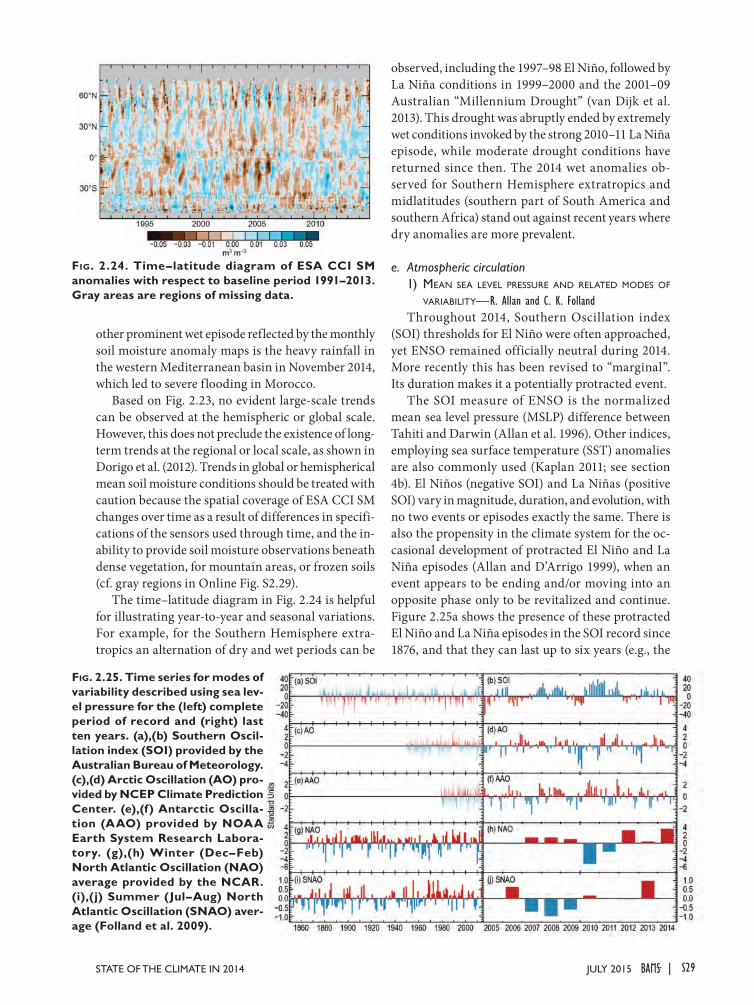
other prominent wet episode reflected by the monthly soil moisture anomaly maps is the heavy rainfall in the western Mediterranean basin in November 2014, which led to severe flooding in Morocco.
Based on Fig. 2.23, no evident large-scale trends can be observed at the hemispheric or global scale. However, this does not preclude the existence of long-term trends at the regional or local scale, as shown in Dorigo et al. (2012). Trends in global or hemispherical mean soil moisture conditions should be treated with caution because the spatial coverage of ESA CCI SM changes over time as a result of differences in specifi-cations of the sensors used through time, and the in-ability to provide soil moisture observations beneath dense vegetation, for mountain areas, or frozen soils (cf. gray regions in Online Fig. S2.29).
The time–latitude diagram in Fig. 2.24 is helpful for illustrating year-to-year and seasonal variations. For example, for the Southern Hemisphere extra-tropics an alternation of dry and wet periods can be
observed, including the 1997–98 El Niño, followed by La Niña conditions in 1999–2000 and the 2001–09 Australian “Millennium Drought” (van Dijk et al. 2013). This drought was abruptly ended by extremely wet conditions invoked by the strong 2010–11 La Niña episode, while moderate drought conditions have returned since then. The 2014 wet anomalies ob-served for Southern Hemisphere extratropics and midlatitudes (southern part of South America and southern Africa) stand out against recent years where dry anomalies are more prevalent.
e. Atmospheric circulation1) mean Sea LeveL preSSure and reLated modeS of
variabiLity—R. Allan and C. K. FollandThroughout 2014, Southern Oscillation index
(SOI) thresholds for El Niño were often approached, yet ENSO remained officially neutral during 2014. More recently this has been revised to “marginal”. Its duration makes it a potentially protracted event.
The SOI measure of ENSO is the normalized mean sea level pressure (MSLP) difference between Tahiti and Darwin (Allan et al. 1996). Other indices, employing sea surface temperature (SST) anomalies are also commonly used (Kaplan 2011; see section 4b). El Niños (negative SOI) and La Niñas (positive SOI) vary in magnitude, duration, and evolution, with no two events or episodes exactly the same. There is also the propensity in the climate system for the oc-casional development of protracted El Niño and La Niña episodes (Allan and D’Arrigo 1999), when an event appears to be ending and/or moving into an opposite phase only to be revitalized and continue. Figure 2.25a shows the presence of these protracted El Niño and La Niña episodes in the SOI record since 1876, and that they can last up to six years (e.g., the
Fig. 2.24. Time–latitude diagram of ESA CCI SM anomalies with respect to baseline period 1991–2013. Gray areas are regions of missing data.
Fig. 2.25. Time series for modes of variability described using sea lev-el pressure for the (left) complete period of record and (right) last ten years. (a),(b) Southern Oscil-lation index (SOI) provided by the Australian Bureau of Meteorology. (c),(d) Arctic Oscillation (AO) pro-vided by NCEP Climate Prediction Center. (e),(f) Antarctic Oscilla-tion (AAO) provided by NOAA Earth System Research Labora-tory. (g),(h) Winter (Dec–Feb) North Atlantic Oscillation (NAO) average provided by the NCAR. (i),(j) Summer (Jul–Aug) North Atlantic Oscillation (SNAO) aver-age (Folland et al. 2009).
S29JULY 2015STATE OF THE CLIMATE IN 2014 |
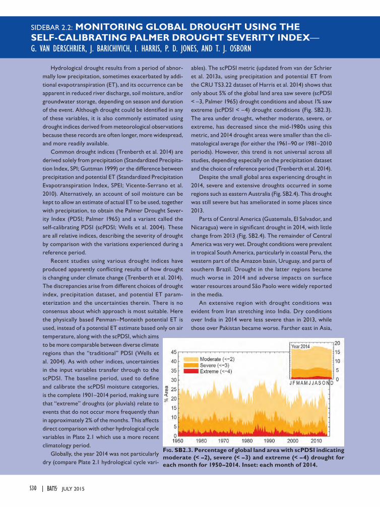
SIDEBAR 2.2: MONITORING GLOBAL DROUGHT USING THE SELF-CALIBRATING PALMER DROUGHT SEVERITY INDEX— G. VAN DERSCHRIER, J. BARICHIVICH, I. HARRIS, P. D. JONES, AND T. J. OSBORN
Hydrological drought results from a period of abnor-mally low precipitation, sometimes exacerbated by addi-tional evapotranspiration (ET), and its occurrence can be apparent in reduced river discharge, soil moisture, and/or groundwater storage, depending on season and duration of the event. Although drought could be identified in any of these variables, it is also commonly estimated using drought indices derived from meteorological observations because these records are often longer, more widespread, and more readily available.
Common drought indices (Trenberth et al. 2014) are derived solely from precipitation (Standardized Precipita-tion Index, SPI; Guttman 1999) or the difference between precipitation and potential ET (Standardized Precipitation Evapotranspiration Index, SPEI; Vicente-Serrano et al. 2010). Alternatively, an account of soil moisture can be kept to allow an estimate of actual ET to be used, together with precipitation, to obtain the Palmer Drought Sever-ity Index (PDSI; Palmer 1965) and a variant called the self-calibrating PDSI (scPDSI; Wells et al. 2004). These are all relative indices, describing the severity of drought by comparison with the variations experienced during a reference period.
Recent studies using various drought indices have produced apparently conflicting results of how drought is changing under climate change (Trenberth et al. 2014). The discrepancies arise from different choices of drought index, precipitation dataset, and potential ET param-eterization and the uncertainties therein. There is no consensus about which approach is most suitable. Here the physically based Penman–Monteith potential ET is used, instead of a potential ET estimate based only on air temperature, along with the scPDSI, which aims to be more comparable between diverse climate regions than the “traditional” PDSI (Wells et al. 2004). As with other indices, uncertainties in the input variables transfer through to the scPDSI. The baseline period, used to define and calibrate the scPDSI moisture categories, is the complete 1901–2014 period, making sure that “extreme” droughts (or pluvials) relate to events that do not occur more frequently than in approximately 2% of the months. This affects direct comparison with other hydrological cycle variables in Plate 2.1 which use a more recent climatology period.
Globally, the year 2014 was not particularly dry (compare Plate 2.1 hydrological cycle vari-
ables). The scPDSI metric (updated from van der Schrier et al. 2013a, using precipitation and potential ET from the CRU TS3.22 dataset of Harris et al. 2014) shows that only about 5% of the global land area saw severe (scPDSI < –3, Palmer 1965) drought conditions and about 1% saw extreme (scPDSI < –4) drought conditions (Fig. SB2.3). The area under drought, whether moderate, severe, or extreme, has decreased since the mid-1980s using this metric, and 2014 drought areas were smaller than the cli-matological average (for either the 1961–90 or 1981–2010 periods). However, this trend is not universal across all studies, depending especially on the precipitation dataset and the choice of reference period (Trenberth et al. 2014).
Despite the small global area experiencing drought in 2014, severe and extensive droughts occurred in some regions such as eastern Australia (Fig. SB2.4). This drought was still severe but has ameliorated in some places since 2013.
Parts of Central America (Guatemala, El Salvador, and Nicaragua) were in significant drought in 2014, with little change from 2013 (Fig. SB2.4). The remainder of Central America was very wet. Drought conditions were prevalent in tropical South America, particularly in coastal Peru, the western part of the Amazon basin, Uruguay, and parts of southern Brazil. Drought in the latter regions became much worse in 2014 and adverse impacts on surface water resources around São Paolo were widely reported in the media.
An extensive region with drought conditions was evident from Iran stretching into India. Dry conditions over India in 2014 were less severe than in 2013, while those over Pakistan became worse. Farther east in Asia,
Fig. SB2.3. Percentage of global land area with scPDSI indicating moderate (< –2), severe (< –3) and extreme (< –4) drought for each month for 1950–2014. Inset: each month of 2014.
S30 JULY 2015|
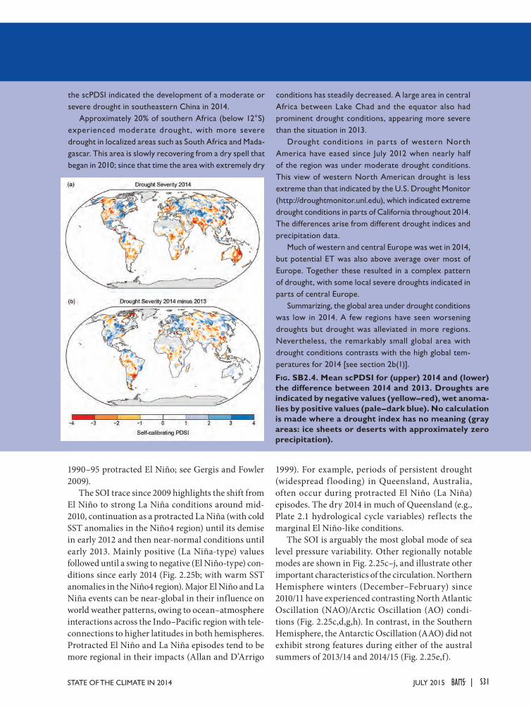
the scPDSI indicated the development of a moderate or severe drought in southeastern China in 2014.
Approximately 20% of southern Africa (below 12°S) experienced moderate drought , with more severe drought in localized areas such as South Africa and Mada-gascar. This area is slowly recovering from a dry spell that began in 2010; since that time the area with extremely dry
conditions has steadily decreased. A large area in central Africa between Lake Chad and the equator also had prominent drought conditions, appearing more severe than the situation in 2013.
Drought conditions in parts of western North America have eased since July 2012 when nearly half of the region was under moderate drought conditions. This view of western North American drought is less extreme than that indicated by the U.S. Drought Monitor (http://droughtmonitor.unl.edu), which indicated extreme drought conditions in parts of California throughout 2014. The differences arise from different drought indices and precipitation data.
Much of western and central Europe was wet in 2014, but potential ET was also above average over most of Europe. Together these resulted in a complex pattern of drought, with some local severe droughts indicated in parts of central Europe.
Summarizing, the global area under drought conditions was low in 2014. A few regions have seen worsening droughts but drought was alleviated in more regions. Nevertheless, the remarkably small global area with drought conditions contrasts with the high global tem-peratures for 2014 [see section 2b(1)].
Fig. SB2.4. Mean scPDSI for (upper) 2014 and (lower) the difference between 2014 and 2013. Droughts are indicated by negative values (yellow–red), wet anoma-lies by positive values (pale–dark blue). No calculation is made where a drought index has no meaning (gray areas: ice sheets or deserts with approximately zero precipitation).
1990–95 protracted El Niño; see Gergis and Fowler 2009).
The SOI trace since 2009 highlights the shift from El Niño to strong La Niña conditions around mid-2010, continuation as a protracted La Niña (with cold SST anomalies in the Niño4 region) until its demise in early 2012 and then near-normal conditions until early 2013. Mainly positive (La Niña-type) values followed until a swing to negative (El Niño-type) con-ditions since early 2014 (Fig. 2.25b; with warm SST anomalies in the Niño4 region). Major El Niño and La Niña events can be near-global in their influence on world weather patterns, owing to ocean–atmosphere interactions across the Indo–Pacific region with tele-connections to higher latitudes in both hemispheres. Protracted El Niño and La Niña episodes tend to be more regional in their impacts (Allan and D’Arrigo
1999). For example, periods of persistent drought (widespread f looding) in Queensland, Australia, often occur during protracted El Niño (La Niña) episodes. The dry 2014 in much of Queensland (e.g., Plate 2.1 hydrological cycle variables) ref lects the marginal El Niño-like conditions.
The SOI is arguably the most global mode of sea level pressure variability. Other regionally notable modes are shown in Fig. 2.25c–j, and illustrate other important characteristics of the circulation. Northern Hemisphere winters (December–February) since 2010/11 have experienced contrasting North Atlantic Oscillation (NAO)/Arctic Oscillation (AO) condi-tions (Fig. 2.25c,d,g,h). In contrast, in the Southern Hemisphere, the Antarctic Oscillation (AAO) did not exhibit strong features during either of the austral summers of 2013/14 and 2014/15 (Fig. 2.25e,f).
S31JULY 2015STATE OF THE CLIMATE IN 2014 |
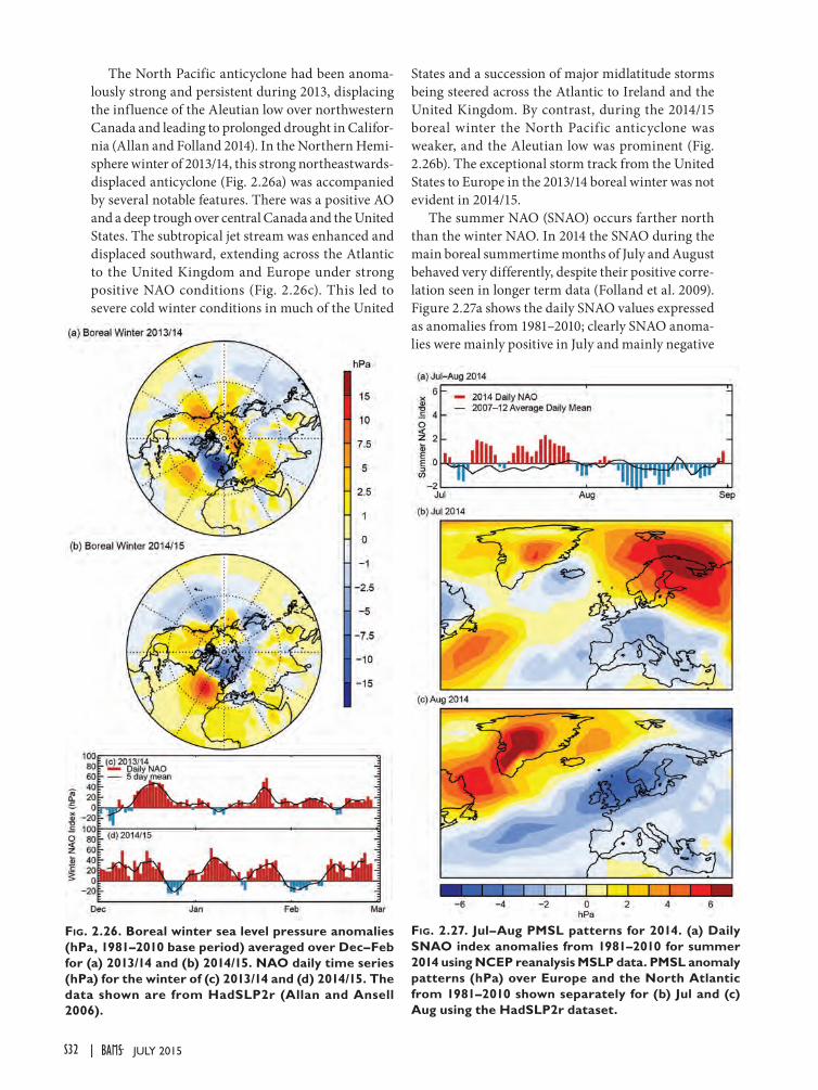
The North Pacific anticyclone had been anoma-lously strong and persistent during 2013, displacing the influence of the Aleutian low over northwestern Canada and leading to prolonged drought in Califor-nia (Allan and Folland 2014). In the Northern Hemi-sphere winter of 2013/14, this strong northeastwards-displaced anticyclone (Fig. 2.26a) was accompanied by several notable features. There was a positive AO and a deep trough over central Canada and the United States. The subtropical jet stream was enhanced and displaced southward, extending across the Atlantic to the United Kingdom and Europe under strong positive NAO conditions (Fig. 2.26c). This led to severe cold winter conditions in much of the United
States and a succession of major midlatitude storms being steered across the Atlantic to Ireland and the United Kingdom. By contrast, during the 2014/15 boreal winter the North Pacific anticyclone was weaker, and the Aleutian low was prominent (Fig. 2.26b). The exceptional storm track from the United States to Europe in the 2013/14 boreal winter was not evident in 2014/15.
The summer NAO (SNAO) occurs farther north than the winter NAO. In 2014 the SNAO during the main boreal summertime months of July and August behaved very differently, despite their positive corre-lation seen in longer term data (Folland et al. 2009). Figure 2.27a shows the daily SNAO values expressed as anomalies from 1981–2010; clearly SNAO anoma-lies were mainly positive in July and mainly negative
Fig. 2.26. Boreal winter sea level pressure anomalies (hPa, 1981–2010 base period) averaged over Dec–Feb for (a) 2013/14 and (b) 2014/15. NAO daily time series (hPa) for the winter of (c) 2013/14 and (d) 2014/15. The data shown are from HadSLP2r (Allan and Ansell 2006).
Fig. 2.27. Jul–Aug PMSL patterns for 2014. (a) Daily SNAO index anomalies from 1981–2010 for summer 2014 using NCEP reanalysis MSLP data. PMSL anomaly patterns (hPa) over Europe and the North Atlantic from 1981–2010 shown separately for (b) Jul and (c) Aug using the HadSLP2r dataset.
S32 JULY 2015|
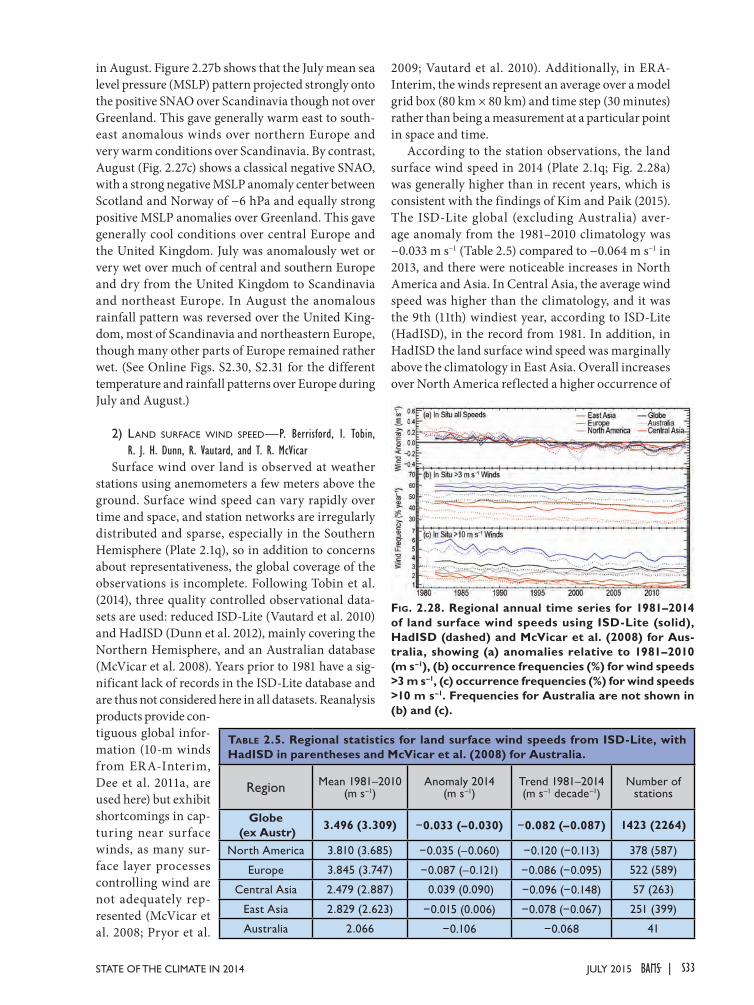
Fig. 2.28. Regional annual time series for 1981–2014 of land surface wind speeds using ISD-Lite (solid), HadISD (dashed) and McVicar et al. (2008) for Aus-tralia, showing (a) anomalies relative to 1981–2010 (m s–1), (b) occurrence frequencies (%) for wind speeds >3 m s–1, (c) occurrence frequencies (%) for wind speeds >10 m s–1. Frequencies for Australia are not shown in (b) and (c).
Table 2.5. Regional statistics for land surface wind speeds from ISD-Lite, with HadISD in parentheses and McVicar et al. (2008) for Australia.
Region Mean 1981–2010 (m s–1)
Anomaly 2014 (m s–1)
Trend 1981–2014 (m s–1 decade–1)
Number of stations
Globe (ex Austr) 3.496 (3.309) −0.033 (–0.030) −0.082 (–0.087) 1423 (2264)
North America 3.810 (3.685) −0.035 (–0.060) −0.120 (−0.113) 378 (587)
Europe 3.845 (3.747) −0.087 (–0.121) −0.086 (−0.095) 522 (589)
Central Asia 2.479 (2.887) 0.039 (0.090) −0.096 (−0.148) 57 (263)
East Asia 2.829 (2.623) −0.015 (0.006) −0.078 (−0.067) 251 (399)
Australia 2.066 −0.106 −0.068 41
in August. Figure 2.27b shows that the July mean sea level pressure (MSLP) pattern projected strongly onto the positive SNAO over Scandinavia though not over Greenland. This gave generally warm east to south-east anomalous winds over northern Europe and very warm conditions over Scandinavia. By contrast, August (Fig. 2.27c) shows a classical negative SNAO, with a strong negative MSLP anomaly center between Scotland and Norway of −6 hPa and equally strong positive MSLP anomalies over Greenland. This gave generally cool conditions over central Europe and the United Kingdom. July was anomalously wet or very wet over much of central and southern Europe and dry from the United Kingdom to Scandinavia and northeast Europe. In August the anomalous rainfall pattern was reversed over the United King-dom, most of Scandinavia and northeastern Europe, though many other parts of Europe remained rather wet. (See Online Figs. S2.30, S2.31 for the different temperature and rainfall patterns over Europe during July and August.)
2) Land Surface wind Speed—P. Berrisford, I. Tobin, R. J. H. Dunn, R. Vautard, and T. R. McVicar
Surface wind over land is observed at weather stations using anemometers a few meters above the ground. Surface wind speed can vary rapidly over time and space, and station networks are irregularly distributed and sparse, especially in the Southern Hemisphere (Plate 2.1q), so in addition to concerns about representativeness, the global coverage of the observations is incomplete. Following Tobin et al. (2014), three quality controlled observational data-sets are used: reduced ISD-Lite (Vautard et al. 2010) and HadISD (Dunn et al. 2012), mainly covering the Northern Hemisphere, and an Australian database (McVicar et al. 2008). Years prior to 1981 have a sig-nificant lack of records in the ISD-Lite database and are thus not considered here in all datasets. Reanalysis products provide con-tiguous global infor-mation (10-m winds from ERA-Interim, Dee et al. 2011a, are used here) but exhibit shortcomings in cap-turing near surface winds, as many sur-face layer processes controlling wind are not adequately rep-resented (McVicar et al. 2008; Pryor et al.
2009; Vautard et al. 2010). Additionally, in ERA-Interim, the winds represent an average over a model grid box (80 km × 80 km) and time step (30 minutes) rather than being a measurement at a particular point in space and time.
According to the station observations, the land surface wind speed in 2014 (Plate 2.1q; Fig. 2.28a) was generally higher than in recent years, which is consistent with the findings of Kim and Paik (2015). The ISD-Lite global (excluding Australia) aver-age anomaly from the 1981–2010 climatology was −0.033 m s−1 (Table 2.5) compared to −0.064 m s−1 in 2013, and there were noticeable increases in North America and Asia. In Central Asia, the average wind speed was higher than the climatology, and it was the 9th (11th) windiest year, according to ISD-Lite (HadISD), in the record from 1981. In addition, in HadISD the land surface wind speed was marginally above the climatology in East Asia. Overall increases over North America reflected a higher occurrence of
S33JULY 2015STATE OF THE CLIMATE IN 2014 |
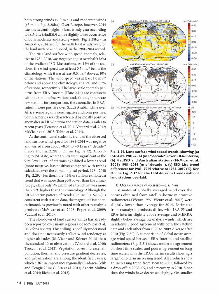
both strong winds (>10 m s−1) and moderate winds (>3 m s−1; Fig. 2.28b,c). Over Europe, however, 2014 was the seventh (eighth) least windy year according to ISD-Lite (HadISD) with a slightly lower occurrence of both moderate and strong winds (Fig. 2.28b,c). In Australia, 2014 tied for the sixth least windy year, for the land surface wind speed, in the 1981–2014 record.
The 2014 land surface wind speed anomaly, rela-tive to 1981–2010, was negative at just over half (52%) of the available ISD-Lite stations. At 12% of the sta-tions, the wind speed was at least 0.5 m s−1 below the climatology, while it was at least 0.5 m s−1 above at 10% of the stations. The wind speed was at least 1.0 m s−1 below and above the climatology, at 1.7% and 0.7% of stations, respectively. The large-scale anomaly pat-terns from ERA-Interim (Plate 2.1q) are consistent with the station observations and, although there are few stations for comparison, the anomalies in ERA-Interim were positive over Saudi Arabia, while over Africa, some regions were negative and some positive. South America was characterized by mostly positive anomalies in ERA-Interim and station data, similar to recent years (Peterson et al. 2011; Vautard et al. 2012; McVicar et al. 2013; Tobin et al. 2014).
At the continental scale, the trend of the observed land surface wind speed for 1981–2014 was negative and varied from about −0.07 to −0.15 m s−1 decade−1 (Table 2.5; Fig. 2.29a,b; Online Fig. S2.32). Accord-ing to ISD-Lite, where trends were significant at the 95% level, 71% of stations exhibited a lower trend (more negative, less positive) compared with trends calculated over the climatological period, 1981–2010 (Fig. 2.29c). Furthermore, 13% of stations exhibited a trend that was more than 30% lower than the clima-tology, while only 5% exhibited a trend that was more than 30% higher than the climatology. Although the ERA-Interim pattern of trends (Online Fig. S2.32) is consistent with station data, the magnitude is under-estimated, as previously noted with other reanalysis products (McVicar et al. 2008; Pryor et al. 2009; Vautard et al. 2010).
The slowdown of land surface winds has already been reported over many regions (see McVicar et al. 2012 for a review). This stilling is not fully understood and does not necessarily ref lect wind tendency at higher altitudes (McVicar and Körner 2013) than the standard 10-m observations (Vautard et al. 2010; Troccoli et al. 2012). Vegetation cover increase, air pollution, thermal and pressure gradient decreases, and urbanization are among the identified causes, which differ in importance regionally (Dadaser-Celik and Cengiz 2014; C. Lin et al. 2013; Azorin-Molina et al. 2014; Bichet et al. 2012).
Fig. 2.29. Land surface wind speed trends, showing (a) ISD-Lite 1981–2014 (m s–1 decade–1) over ERA-Interim, (b) HadISD and Australian stations (McVicar et al. 2008) 1981–2014 (m s–1 decade–1), (c) ISD-Lite trend differences for 1981–2014 relative to 1981–2010 (%). See Online Fig. 2.32 for the ERA-Interim trends without land stations overlaid.
3) ocean Surface wind Speed—C. A. MearsEstimates of globally averaged wind over the
oceans obtained from satellite-borne microwave radiometers (Wentz 1997; Wentz et al. 2007) were slightly lower than average for 2014. Estimates from reanalysis products differ, with JRA-55 and ERA-Interim slightly above average and MERRA slightly below average. Reanalysis winds, which are in relatively good agreement with both the satellite data and each other from 1990 to 2009, diverge after 2010 (Fig. 2.30). A comparison of global ocean aver-age wind speed between ERA-Interim and satellite radiometers (Fig. 2.31) shows moderate agreement on short time scales, and poorer agreement on long time scales, with the ERA-Interim results showing a larger long-term increasing trend. All products show an increasing trend from 1990 to 2007, followed by a drop-off in 2008–09, and a recovery in 2010. Since then the winds have decreased slightly. On smaller
S34 JULY 2015|
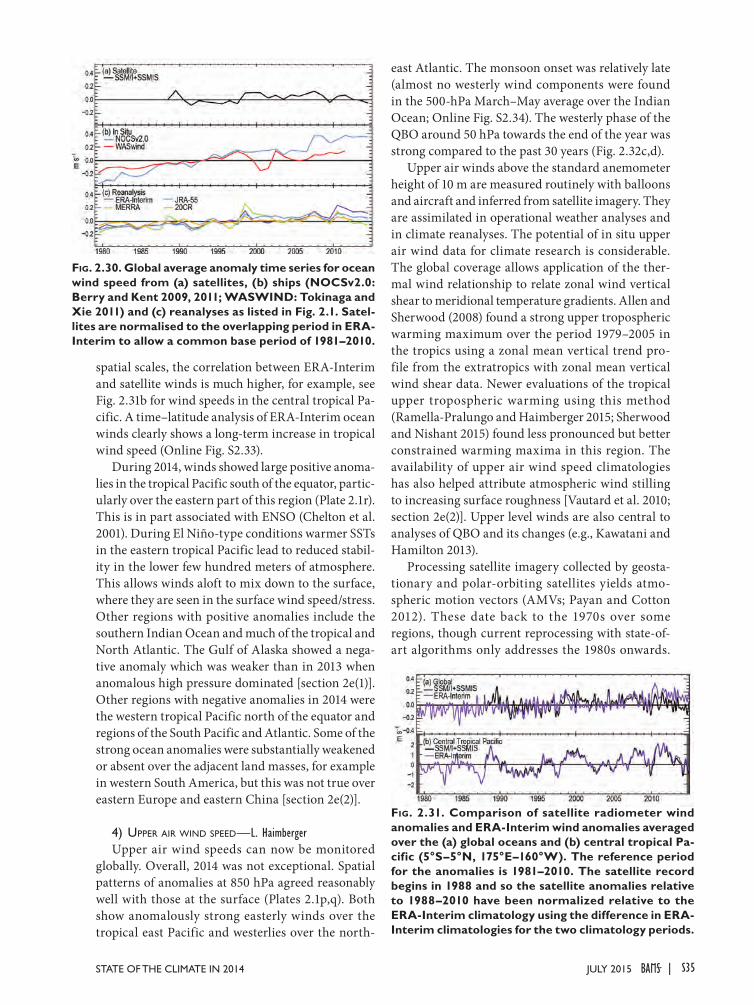
spatial scales, the correlation between ERA-Interim and satellite winds is much higher, for example, see Fig. 2.31b for wind speeds in the central tropical Pa-cific. A time–latitude analysis of ERA-Interim ocean winds clearly shows a long-term increase in tropical wind speed (Online Fig. S2.33).
During 2014, winds showed large positive anoma-lies in the tropical Pacific south of the equator, partic-ularly over the eastern part of this region (Plate 2.1r). This is in part associated with ENSO (Chelton et al. 2001). During El Niño-type conditions warmer SSTs in the eastern tropical Pacific lead to reduced stabil-ity in the lower few hundred meters of atmosphere. This allows winds aloft to mix down to the surface, where they are seen in the surface wind speed/stress. Other regions with positive anomalies include the southern Indian Ocean and much of the tropical and North Atlantic. The Gulf of Alaska showed a nega-tive anomaly which was weaker than in 2013 when anomalous high pressure dominated [section 2e(1)]. Other regions with negative anomalies in 2014 were the western tropical Pacific north of the equator and regions of the South Pacific and Atlantic. Some of the strong ocean anomalies were substantially weakened or absent over the adjacent land masses, for example in western South America, but this was not true over eastern Europe and eastern China [section 2e(2)].
4) upper air wind Speed—L. HaimbergerUpper air wind speeds can now be monitored
globally. Overall, 2014 was not exceptional. Spatial patterns of anomalies at 850 hPa agreed reasonably well with those at the surface (Plates 2.1p,q). Both show anomalously strong easterly winds over the tropical east Pacific and westerlies over the north-
east Atlantic. The monsoon onset was relatively late (almost no westerly wind components were found in the 500-hPa March–May average over the Indian Ocean; Online Fig. S2.34). The westerly phase of the QBO around 50 hPa towards the end of the year was strong compared to the past 30 years (Fig. 2.32c,d).
Upper air winds above the standard anemometer height of 10 m are measured routinely with balloons and aircraft and inferred from satellite imagery. They are assimilated in operational weather analyses and in climate reanalyses. The potential of in situ upper air wind data for climate research is considerable. The global coverage allows application of the ther-mal wind relationship to relate zonal wind vertical shear to meridional temperature gradients. Allen and Sherwood (2008) found a strong upper tropospheric warming maximum over the period 1979–2005 in the tropics using a zonal mean vertical trend pro-file from the extratropics with zonal mean vertical wind shear data. Newer evaluations of the tropical upper tropospheric warming using this method (Ramella-Pralungo and Haimberger 2015; Sherwood and Nishant 2015) found less pronounced but better constrained warming maxima in this region. The availability of upper air wind speed climatologies has also helped attribute atmospheric wind stilling to increasing surface roughness [Vautard et al. 2010; section 2e(2)]. Upper level winds are also central to analyses of QBO and its changes (e.g., Kawatani and Hamilton 2013).
Processing satellite imagery collected by geosta-tionary and polar-orbiting satellites yields atmo-spheric motion vectors (AMVs; Payan and Cotton 2012). These date back to the 1970s over some regions, though current reprocessing with state-of-art algorithms only addresses the 1980s onwards.
Fig. 2.30. Global average anomaly time series for ocean wind speed from (a) satellites, (b) ships (NOCSv2.0: Berry and Kent 2009, 2011; WASWIND: Tokinaga and Xie 2011) and (c) reanalyses as listed in Fig. 2.1. Satel-lites are normalised to the overlapping period in ERA-Interim to allow a common base period of 1981–2010.
Fig. 2.31. Comparison of satellite radiometer wind anomalies and ERA-Interim wind anomalies averaged over the (a) global oceans and (b) central tropical Pa-cific (5°S–5°N, 175°E–160°W). The reference period for the anomalies is 1981–2010. The satellite record begins in 1988 and so the satellite anomalies relative to 1988–2010 have been normalized relative to the ERA-Interim climatology using the difference in ERA-Interim climatologies for the two climatology periods.
S35JULY 2015STATE OF THE CLIMATE IN 2014 |
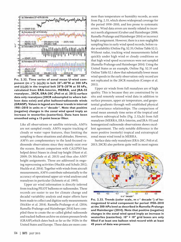
Like all observations or satellite retrievals, AMVs are not sampled evenly. AMVs require tracking of cloudy or water vapor features, thus limiting the sampling to these situations and altitudes. However, AMVs are complementary to the land-focused ra-diosonde observations since they mainly exist over the oceans. Recent comparison with CALIPSO has helped detect biases in cloud top height (Hunt et al. 2009; Di Michele et al. 2013) and thus also AMV height assignments. Those are addressed in ongo-ing reprocessing activities (Huckle and Schulz 2012; Huckle et al. 2014). Together with winds from aircraft measurements, AMVs contribute substantially to the accuracy of operational upper air wind analyses and reanalyses in particular (Schmetz et al. 1993).
Upper air wind information is directly inferred from tracking PILOT balloons or radiosondes. These records are easier to use for climate change and decadal variability analysis and major efforts have been made to collect and digitize early measurements (Stickler et al. 2014). Ramella-Pralungo et al. (2014; Ramella-Pralungo and Haimberger 2014) have com-piled these to create the so-called global radiosonde and tracked-balloon archive on sixteen pressure levels (GRASP),which dates back as far as the 1920s in the United States and Europe. These data are more com-
mon than temperature or humidity records, as seen from Fig. 2.33, which shows widespread coverage for the period 1958–2010, and less prone to systematic errors. Wind data errors are mostly related to incor-rect north alignment (Gruber and Haimberger 2008; Ramella-Pralungo and Haimberger 2014) or incorrect height assignment. However, there is a non-negligible sampling bias in early wind speed records, before ra-dar availability (Online Fig. S2.35; Online Table S2.1). Without radar, tracking wind measurements failed quickly under high wind or cloudy conditions so that high wind speed occurrences were not sampled (Ramella-Pralungo and Haimberger 2014). Using the United States as an example, Online Fig. S2.35 and Online Table S2.1 show that substantially lower mean wind speeds in the early observation-only record are not replicated in the 20CR reanalysis (Compo et al. 2011).
Upper air winds from full reanalyses are of high quality. This is because they are constrained by in situ and remotely sensed wind data in addition to surface pressure, upper air temperature, and geopo-tential gradients through well-established physical and covariance relationships. The comparison of zonal mean anomaly time series of the tropical and northern subtropical belts (Fig. 2.32a,b) from full reanalyses (MERRA, ERA-Interim, and JRA-55) and homogenized radiosonde observations shows excel-lent agreement. The only notable difference is the more positive (westerly) tropical and extratropical zonal mean wind trend in MERRA.
Surface data-only reanalyses (ERA-20C: Poli et al. 2013; 20CR) also perform quite well in most regions
Fig. 2.33. Trends (color scale, m s–1 decade–1) of ho-mogenized U-wind component for period 1958–2010 at the 300-hPa level as described in Ramella-Pralungo and Haimberger (2014). Note that positive (negative) changes in the zonal wind speed imply an increase in westerlies (easterlies). 10° × 10° grid boxes are only filled if at least one balloon wind record with at least 45 years of data was present.
Fig. 2.32. Time series of zonal mean U-wind com-ponent (m s–1): (a),(b) in belt 20°–40°N at 300 hPa and (c),(d) in the tropical belt 20°S–20°N at 50 hPa, calculated from ERA-Interim, MERRA, and JRA-55 reanalyses , 20CR, ERA-20C (Poli et al. 2013) surface data only reanalyses (20CR subsampled to where bal-loon data exist) and pilot balloon/radiosonde winds (GRASP). Values in legend are linear trends in interval 1981–2010 in units m s–1 decade–1. Note that positive (negative) changes in the zonal wind speed imply an increase in westerlies (easterlies). Data have been smoothed using a 12-point boxcar filter.
S36 JULY 2015|
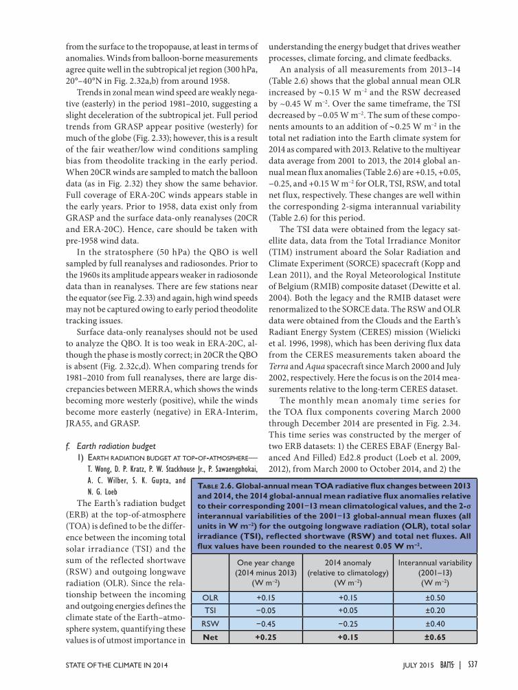
from the surface to the tropopause, at least in terms of anomalies. Winds from balloon-borne measurements agree quite well in the subtropical jet region (300 hPa, 20°–40°N in Fig. 2.32a,b) from around 1958.
Trends in zonal mean wind speed are weakly nega-tive (easterly) in the period 1981–2010, suggesting a slight deceleration of the subtropical jet. Full period trends from GRASP appear positive (westerly) for much of the globe (Fig. 2.33); however, this is a result of the fair weather/low wind conditions sampling bias from theodolite tracking in the early period. When 20CR winds are sampled to match the balloon data (as in Fig. 2.32) they show the same behavior. Full coverage of ERA-20C winds appears stable in the early years. Prior to 1958, data exist only from GRASP and the surface data-only reanalyses (20CR and ERA-20C). Hence, care should be taken with pre-1958 wind data.
In the stratosphere (50 hPa) the QBO is well sampled by full reanalyses and radiosondes. Prior to the 1960s its amplitude appears weaker in radiosonde data than in reanalyses. There are few stations near the equator (see Fig. 2.33) and again, high wind speeds may not be captured owing to early period theodolite tracking issues.
Surface data-only reanalyses should not be used to analyze the QBO. It is too weak in ERA-20C, al-though the phase is mostly correct; in 20CR the QBO is absent (Fig. 2.32c,d). When comparing trends for 1981–2010 from full reanalyses, there are large dis-crepancies between MERRA, which shows the winds becoming more westerly (positive), while the winds become more easterly (negative) in ERA-Interim, JRA55, and GRASP.
f. Earth radiation budget1) earth radiation budget at top-of-atmoSphere—
T. Wong, D. P. Kratz, P. W. Stackhouse Jr., P. Sawaengphokai, A. C. Wilber, S. K. Gupta, and N. G. Loeb
The Earth’s radiation budget (ERB) at the top-of-atmosphere (TOA) is defined to be the differ-ence between the incoming total solar irradiance (TSI) and the sum of the ref lected shortwave (RSW) and outgoing longwave radiation (OLR). Since the rela-tionship between the incoming and outgoing energies defines the climate state of the Earth–atmo-sphere system, quantifying these values is of utmost importance in
understanding the energy budget that drives weather processes, climate forcing, and climate feedbacks.
An analysis of all measurements from 2013–14 (Table 2.6) shows that the global annual mean OLR increased by ∼0.15 W m−2 and the RSW decreased by ~0.45 W m−2. Over the same timeframe, the TSI decreased by ~0.05 W m−2. The sum of these compo-nents amounts to an addition of ∼0.25 W m−2 in the total net radiation into the Earth climate system for 2014 as compared with 2013. Relative to the multiyear data average from 2001 to 2013, the 2014 global an-nual mean flux anomalies (Table 2.6) are +0.15, +0.05, −0.25, and +0.15 W m−2 for OLR, TSI, RSW, and total net flux, respectively. These changes are well within the corresponding 2-sigma interannual variability (Table 2.6) for this period.
The TSI data were obtained from the legacy sat-ellite data, data from the Total Irradiance Monitor (TIM) instrument aboard the Solar Radiation and Climate Experiment (SORCE) spacecraft (Kopp and Lean 2011), and the Royal Meteorological Institute of Belgium (RMIB) composite dataset (Dewitte et al. 2004). Both the legacy and the RMIB dataset were renormalized to the SORCE data. The RSW and OLR data were obtained from the Clouds and the Earth’s Radiant Energy System (CERES) mission (Wielicki et al. 1996, 1998), which has been deriving flux data from the CERES measurements taken aboard the Terra and Aqua spacecraft since March 2000 and July 2002, respectively. Here the focus is on the 2014 mea-surements relative to the long-term CERES dataset.
The monthly mean anomaly time series for the TOA f lux components covering March 2000 through December 2014 are presented in Fig. 2.34. This time series was constructed by the merger of two ERB datasets: 1) the CERES EBAF (Energy Bal-anced And Filled) Ed2.8 product (Loeb et al. 2009, 2012), from March 2000 to October 2014, and 2) the
Table 2.6. Global-annual mean TOA radiative flux changes between 2013 and 2014, the 2014 global-annual mean radiative flux anomalies relative to their corresponding 2001−13 mean climatological values, and the 2-σ interannual variabilities of the 2001−13 global-annual mean fluxes (all units in W m–2) for the outgoing longwave radiation (OLR), total solar irradiance (TSI), reflected shortwave (RSW) and total net fluxes. All flux values have been rounded to the nearest 0.05 W m–2.
One year change (2014 minus 2013)
(W m–2)
2014 anomaly (relative to climatology)
(W m–2)
Interannual variability (2001–13) (W m–2)
OLR +0.15 +0.15 ±0.50
TSI −0.05 +0.05 ±0.20
RSW −0.45 −0.25 ±0.40
Net +0.25 +0.15 ±0.65
S37JULY 2015STATE OF THE CLIMATE IN 2014 |
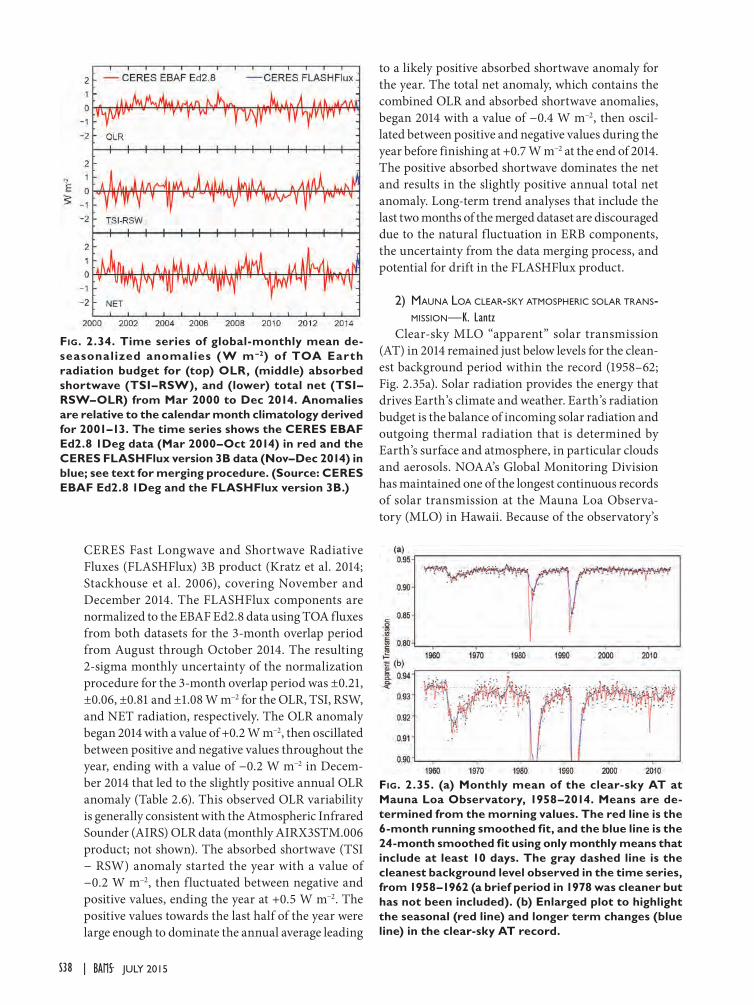
CERES Fast Longwave and Shortwave Radiative Fluxes (FLASHFlux) 3B product (Kratz et al. 2014; Stackhouse et al. 2006), covering November and December 2014. The FLASHFlux components are normalized to the EBAF Ed2.8 data using TOA fluxes from both datasets for the 3-month overlap period from August through October 2014. The resulting 2-sigma monthly uncertainty of the normalization procedure for the 3-month overlap period was ±0.21, ±0.06, ±0.81 and ±1.08 W m−2 for the OLR, TSI, RSW, and NET radiation, respectively. The OLR anomaly began 2014 with a value of +0.2 W m−2, then oscillated between positive and negative values throughout the year, ending with a value of −0.2 W m−2 in Decem-ber 2014 that led to the slightly positive annual OLR anomaly (Table 2.6). This observed OLR variability is generally consistent with the Atmospheric Infrared Sounder (AIRS) OLR data (monthly AIRX3STM.006 product; not shown). The absorbed shortwave (TSI − RSW) anomaly started the year with a value of −0.2 W m−2, then fluctuated between negative and positive values, ending the year at +0.5 W m−2. The positive values towards the last half of the year were large enough to dominate the annual average leading
to a likely positive absorbed shortwave anomaly for the year. The total net anomaly, which contains the combined OLR and absorbed shortwave anomalies, began 2014 with a value of −0.4 W m−2, then oscil-lated between positive and negative values during the year before finishing at +0.7 W m−2 at the end of 2014. The positive absorbed shortwave dominates the net and results in the slightly positive annual total net anomaly. Long-term trend analyses that include the last two months of the merged dataset are discouraged due to the natural fluctuation in ERB components, the uncertainty from the data merging process, and potential for drift in the FLASHFlux product.
2) mauna Loa cLear-Sky atmoSpheric SoLar tranS-miSSion—K. Lantz
Clear-sky MLO “apparent” solar transmission (AT) in 2014 remained just below levels for the clean-est background period within the record (1958–62; Fig. 2.35a). Solar radiation provides the energy that drives Earth’s climate and weather. Earth’s radiation budget is the balance of incoming solar radiation and outgoing thermal radiation that is determined by Earth’s surface and atmosphere, in particular clouds and aerosols. NOAA’s Global Monitoring Division has maintained one of the longest continuous records of solar transmission at the Mauna Loa Observa-tory (MLO) in Hawaii. Because of the observatory’s
Fig. 2.34. Time series of global-monthly mean de-seasonalized anomalies (W m –2) of TOA Earth radiation budget for (top) OLR, (middle) absorbed shortwave (TSI–RSW), and (lower) total net (TSI–RSW–OLR) from Mar 2000 to Dec 2014. Anomalies are relative to the calendar month climatology derived for 2001–13. The time series shows the CERES EBAF Ed2.8 1Deg data (Mar 2000–Oct 2014) in red and the CERES FLASHFlux version 3B data (Nov–Dec 2014) in blue; see text for merging procedure. (Source: CERES EBAF Ed2.8 1Deg and the FLASHFlux version 3B.)
Fig. 2.35. (a) Monthly mean of the clear-sky AT at Mauna Loa Observatory, 1958–2014. Means are de-termined from the morning values. The red line is the 6-month running smoothed fit, and the blue line is the 24-month smoothed fit using only monthly means that include at least 10 days. The gray dashed line is the cleanest background level observed in the time series, from 1958–1962 (a brief period in 1978 was cleaner but has not been included). (b) Enlarged plot to highlight the seasonal (red line) and longer term changes (blue line) in the clear-sky AT record.
S38 JULY 2015|
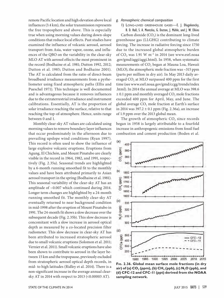
remote Pacific location and high elevation above local influences (3.4 km), the solar transmission represents the free troposphere and above. This is especially true when using morning values during down-slope conditions that reduce local effects. Past studies have examined the influence of volcanic aerosol, aerosol transport from Asia, water vapor, ozone, and influ-ences of the QBO on the variability in the clear-sky MLO AT with aerosol effects the most prominent in the record (Bodhaine et al. 1981; Dutton 1992, 2012; Dutton et al. 1985; Dutton and Bodhaine 2001). The AT is calculated from the ratio of direct-beam broadband irradiance measurements from a pyrhe-liometer using fixed atmospheric paths (Ellis and Pueschel 1971). This technique is well documented and is advantageous because it removes influences due to the extraterrestrial irradiance and instrument calibrations. Essentially, AT is the proportion of solar irradiance reaching the surface, relative to that reaching the top-of-atmosphere. Hence, units range between 0 and 1.
Monthly clear-sky AT values are calculated using morning values to remove boundary layer influences that occur predominately in the afternoon due to prevailing upslope wind conditions (Ryan 1997). This record is often used to show the influence of large explosive volcanic eruptions. Eruptions from Agung, El Chichón, and Mount Pinatubo are clearly visible in the record in 1964, 1982, and 1991, respec-tively (Fig. 2.35a). Seasonal trends are highlighted by a 6-month running smoothed fit to the monthly values and have been attributed primarily to Asian aerosol transport in the spring (Bodhaine et al. 1981). This seasonal variability of the clear-sky AT has an amplitude of ~0.007 which continued during 2014. Longer term changes are highlighted by a 24-month running smoothed fit. The monthly clear-sky AT eventually returned to near background condition in mid-1998 after the eruption of Mount Pinatubo in 1991. The 24-month fit shows a slow decrease over the subsequent decade (Fig. 2.35b). This slow decrease is concomitant with a slow increase in aerosol optical depth as measured by a co-located precision filter radiometer. This slow decrease in clear-sky AT has been attributed to increased stratospheric aerosol due to small volcanic eruptions (Solomon et al. 2011; Vernier et al. 2011). Small volcanic eruptions have also been shown to contribute to aerosol in the layer be-tween 15 km and the tropopause, previously excluded from stratospheric aerosol optical depth records, in mid- to high latitudes (Ridley et al. 2014). There is a non-significant increase in the average annual clear-sky AT in 2014 with respect to 2013 (<0.00003 AT).
g. Atmospheric chemical composition1) Long-Lived greenhouSe gaSeS—E. J. Dlugokencky,
B. D. Hall, S. A. Montzka, G. Dutton, J. Mühle, and J. W. ElkinsCarbon dioxide (CO2) is the dominant long-lived
greenhouse gas (LLGHG) contributing to climate forcing. The increase in radiative forcing since 1750 due to the increased global atmospheric burden of CO2 was 1.91 W m−2 in 2014 (see www.esrl.noaa .gov/gmd/aggi/aggi.html). In 1958, when systematic measurements of CO2 began at Mauna Loa, Hawaii (MLO), the atmospheric mole fraction was ~315 ppm (parts per million in dry air). In May 2013 daily av-eraged CO2 at MLO surpassed 400 ppm for the first time (see www.esrl.noaa.gov/gmd/ccgg/trends/index .html). In 2014 the annual average at MLO was 398.6 ± 0.1 ppm and monthly averaged CO2 mole fractions exceeded 400 ppm for April, May, and June. The global average CO2 mole fraction at Earth’s surface in 2014 was 397.2 ± 0.1 ppm (Fig. 2.36a), an increase of 1.9 ppm over the 2013 global mean.
The growth of atmospheric CO2 since records began in 1958 is largely attributable to a fourfold increase in anthropogenic emissions from fossil fuel combustion and cement production (Boden et al.
Fig. 2.36. Global mean surface mole fractions (in dry air) of (a) CO2 (ppm), (b) CH4 (ppb), (c) N2O (ppb), and (d) CFC-12 and CFC-11 (ppt) derived from the NOAA sampling network.
S39JULY 2015STATE OF THE CLIMATE IN 2014 |
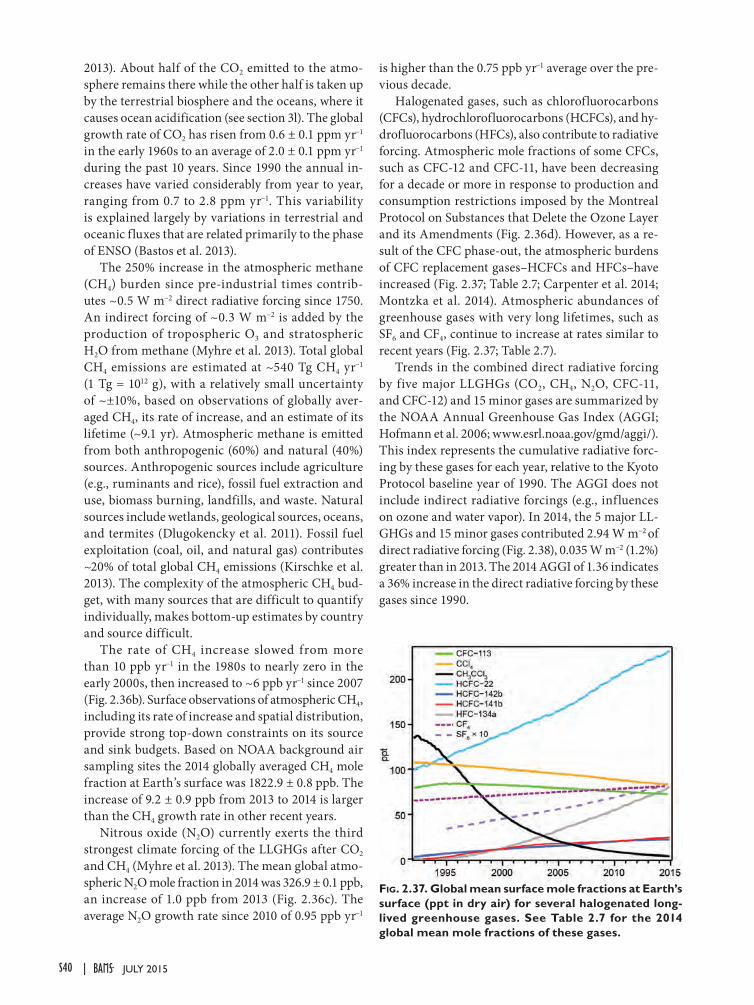
2013). About half of the CO2 emitted to the atmo-sphere remains there while the other half is taken up by the terrestrial biosphere and the oceans, where it causes ocean acidification (see section 3l). The global growth rate of CO2 has risen from 0.6 ± 0.1 ppm yr−1 in the early 1960s to an average of 2.0 ± 0.1 ppm yr−1 during the past 10 years. Since 1990 the annual in-creases have varied considerably from year to year, ranging from 0.7 to 2.8 ppm yr−1. This variability is explained largely by variations in terrestrial and oceanic fluxes that are related primarily to the phase of ENSO (Bastos et al. 2013).
The 250% increase in the atmospheric methane (CH4) burden since pre-industrial times contrib-utes ~0.5 W m−2 direct radiative forcing since 1750. An indirect forcing of ~0.3 W m−2 is added by the production of tropospheric O3 and stratospheric H2O from methane (Myhre et al. 2013). Total global CH4 emissions are estimated at ~540 Tg CH4 yr−1 (1 Tg = 1012 g), with a relatively small uncertainty of ~±10%, based on observations of globally aver-aged CH4, its rate of increase, and an estimate of its lifetime (~9.1 yr). Atmospheric methane is emitted from both anthropogenic (60%) and natural (40%) sources. Anthropogenic sources include agriculture (e.g., ruminants and rice), fossil fuel extraction and use, biomass burning, landfills, and waste. Natural sources include wetlands, geological sources, oceans, and termites (Dlugokencky et al. 2011). Fossil fuel exploitation (coal, oil, and natural gas) contributes ~20% of total global CH4 emissions (Kirschke et al. 2013). The complexity of the atmospheric CH4 bud-get, with many sources that are difficult to quantify individually, makes bottom-up estimates by country and source difficult.
The rate of CH4 increase slowed from more than 10 ppb yr−1 in the 1980s to nearly zero in the early 2000s, then increased to ~6 ppb yr−1 since 2007 (Fig. 2.36b). Surface observations of atmospheric CH4, including its rate of increase and spatial distribution, provide strong top-down constraints on its source and sink budgets. Based on NOAA background air sampling sites the 2014 globally averaged CH4 mole fraction at Earth’s surface was 1822.9 ± 0.8 ppb. The increase of 9.2 ± 0.9 ppb from 2013 to 2014 is larger than the CH4 growth rate in other recent years.
Nitrous oxide (N2O) currently exerts the third strongest climate forcing of the LLGHGs after CO2 and CH4 (Myhre et al. 2013). The mean global atmo-spheric N2O mole fraction in 2014 was 326.9 ± 0.1 ppb, an increase of 1.0 ppb from 2013 (Fig. 2.36c). The average N2O growth rate since 2010 of 0.95 ppb yr−1
is higher than the 0.75 ppb yr−1 average over the pre-vious decade.
Halogenated gases, such as chlorofluorocarbons (CFCs), hydrochlorofluorocarbons (HCFCs), and hy-drofluorocarbons (HFCs), also contribute to radiative forcing. Atmospheric mole fractions of some CFCs, such as CFC-12 and CFC-11, have been decreasing for a decade or more in response to production and consumption restrictions imposed by the Montreal Protocol on Substances that Delete the Ozone Layer and its Amendments (Fig. 2.36d). However, as a re-sult of the CFC phase-out, the atmospheric burdens of CFC replacement gases–HCFCs and HFCs–have increased (Fig. 2.37; Table 2.7; Carpenter et al. 2014; Montzka et al. 2014). Atmospheric abundances of greenhouse gases with very long lifetimes, such as SF6 and CF4, continue to increase at rates similar to recent years (Fig. 2.37; Table 2.7).
Trends in the combined direct radiative forcing by five major LLGHGs (CO2, CH4, N2O, CFC-11, and CFC-12) and 15 minor gases are summarized by the NOAA Annual Greenhouse Gas Index (AGGI; Hofmann et al. 2006; www.esrl.noaa.gov/gmd/aggi/). This index represents the cumulative radiative forc-ing by these gases for each year, relative to the Kyoto Protocol baseline year of 1990. The AGGI does not include indirect radiative forcings (e.g., influences on ozone and water vapor). In 2014, the 5 major LL-GHGs and 15 minor gases contributed 2.94 W m−2
of direct radiative forcing (Fig. 2.38), 0.035 W m−2 (1.2%) greater than in 2013. The 2014 AGGI of 1.36 indicates a 36% increase in the direct radiative forcing by these gases since 1990.
Fig. 2.37. Global mean surface mole fractions at Earth’s surface (ppt in dry air) for several halogenated long-lived greenhouse gases. See Table 2.7 for the 2014 global mean mole fractions of these gases.
S40 JULY 2015|
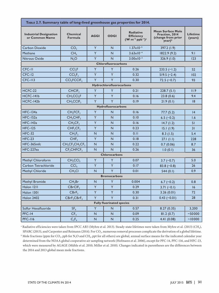
Table 2.7. Summary table of long-lived greenhouse gas properties for 2014.
Industrial Designation or Common Name
Chemical Formula AGGI ODGI
Radiative Efficiency
(W m–2 ppb–1)a
Mean Surface Mole Fraction, 2014
(change from prior year)b
Lifetime (years)
Carbon Dioxide CO2 Y N 1.37x10⁻⁵ 397.2 (1.9)
Methane CH4 Y N 3.63x10⁻⁴ 1822.9 (9.2) 9.1
Nitrous Oxide N2O Y N 3.00x10⁻³ 326.9 (1.0) 123Chlorofluorocarbons
CFC-11 CCl3F Y Y 0.26 233.5 (−1.2) 52CFC-12 CCl2F2 Y Y 0.32 519.5 (−2.4) 102CFC-113 CCl2FCClF2 Y Y 0.30 72.5 (−0.7) 93
Hydrochlorofluorocarbons
HCFC-22 CHClF2 Y Y 0.21 228.7 (5.1) 11.9
HCFC-141b CH3CCl2F Y Y 0.16 23.8 (0.6) 9.4
HCFC-142b CH3CClF2 Y Y 0.19 21.9 (0.1) 18Hydrofluorocarbons
HFC-134a CH2FCF3 Y N 0.16 77.7 (5.2) 14HFC-152a CH3CHF2 Y N 0.10 6.5 (−0.2) 1.6HFC-143a CH3CF3 Y N 0.16 14.7 (1.2) 51HFC-125 CHF2CF3 Y N 0.23 15.1 (1.9) 31HFC-32 CH2F2 N N 0.11 8.3 (1.5) 5.4HFC-23 CHF3 Y N 0.18 27.1 (1.1) 228HFC-365mfc CH3CF2CH2CF3 N N 0.22 0.7 (0.06) 8.7HFC-227ea CF3CHFCF3 N N 0.26 1.0 (0.1) 36
Chlorocarbons
Methyl Chloroform CH3CCl3 Y Y 0.07 3.7 (−0.7) 5.0
Carbon Tetrachloride CCl4 Y Y 0.17 83.8 (−0.8) 26
Methyl Chloride CH3Cl N Y 0.01 544 (0.1) 0.9Bromocarbons
Methyl Bromide CH3Br N Y 0.004 6.7 (−0.2) 0.8Halon 1211 CBrClF2 Y Y 0.29 3.71 (−0.1) 16
Halon 1301 CBrF3 Y Y 0.30 3.26 (0.01) 72
Halon 2402 CBrF2CBrF2 Y Y 0.31 0.43 (−0.01) 28Fully fluorinated species
Sulfur Hexafluoride SF6 Y N 0.57 8.27 (0.35) 3,200
PFC-14 CF4 N N 0.09 81.2 (0.7) ~50 000
PFC-116 C2F6 N N 0.25 4.41 (0.08) ~10 000
a Radiative efficiencies were taken from IPCC AR5 (Myhre et al. 2013). Steady-state lifetimes were taken from Myhre et al. (2013) (CH4), SPARC (2013), and Carpenter and Reimann (2014). For CO2, numerous removal processes complicate the derivation of a global lifetime.
b Mole fractions (ppm for CO2, ppb for N2O and CH4, ppt for all others) are global, annual surface means for the indicated calendar year determined from the NOAA global cooperative air sampling network (Hofmann et al. 2006), except for PFC-14, PFC-116, and HFC-23, which were measured by AGAGE (Mühle et al. 2010; Miller et al. 2010). Changes indicated in parentheses are the differences between the 2014 and 2013 global mean mole fractions.
S41JULY 2015STATE OF THE CLIMATE IN 2014 |
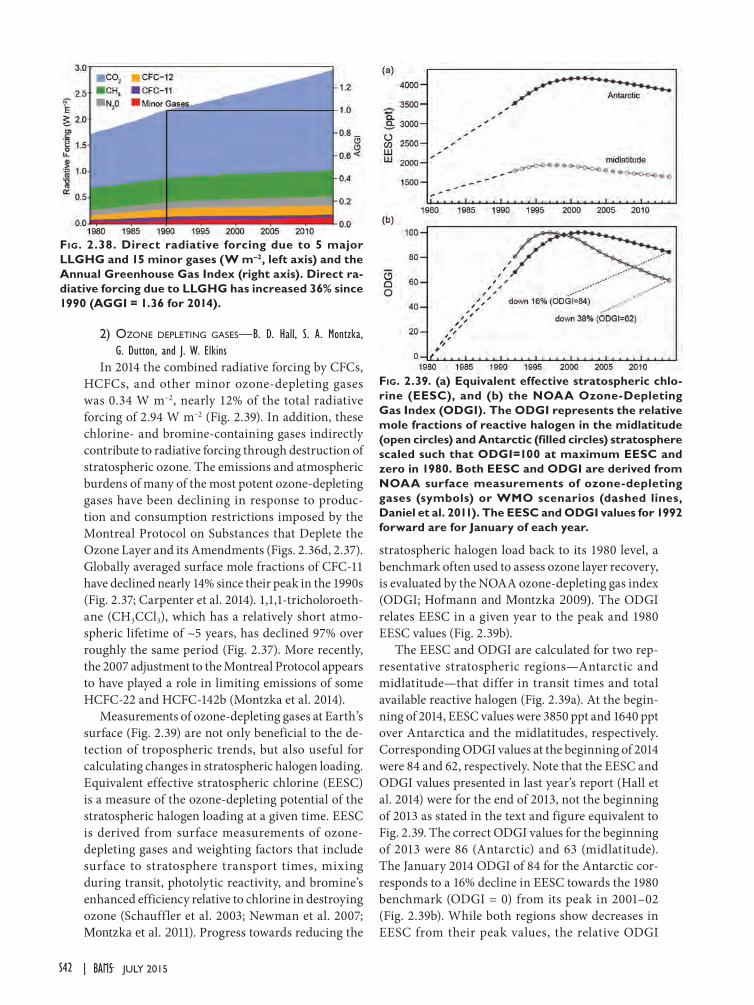
2) ozone depLeting gaSeS—B. D. Hall, S. A. Montzka, G. Dutton, and J. W. Elkins
In 2014 the combined radiative forcing by CFCs, HCFCs, and other minor ozone-depleting gases was 0.34 W m−2, nearly 12% of the total radiative forcing of 2.94 W m−2 (Fig. 2.39). In addition, these chlorine- and bromine-containing gases indirectly contribute to radiative forcing through destruction of stratospheric ozone. The emissions and atmospheric burdens of many of the most potent ozone-depleting gases have been declining in response to produc-tion and consumption restrictions imposed by the Montreal Protocol on Substances that Deplete the Ozone Layer and its Amendments (Figs. 2.36d, 2.37). Globally averaged surface mole fractions of CFC-11 have declined nearly 14% since their peak in the 1990s (Fig. 2.37; Carpenter et al. 2014). 1,1,1-tricholoroeth-ane (CH3CCl3), which has a relatively short atmo-spheric lifetime of ~5 years, has declined 97% over roughly the same period (Fig. 2.37). More recently, the 2007 adjustment to the Montreal Protocol appears to have played a role in limiting emissions of some HCFC-22 and HCFC-142b (Montzka et al. 2014).
Measurements of ozone-depleting gases at Earth’s surface (Fig. 2.39) are not only beneficial to the de-tection of tropospheric trends, but also useful for calculating changes in stratospheric halogen loading. Equivalent effective stratospheric chlorine (EESC) is a measure of the ozone-depleting potential of the stratospheric halogen loading at a given time. EESC is derived from surface measurements of ozone-depleting gases and weighting factors that include surface to stratosphere transport times, mixing during transit, photolytic reactivity, and bromine’s enhanced efficiency relative to chlorine in destroying ozone (Schauffler et al. 2003; Newman et al. 2007; Montzka et al. 2011). Progress towards reducing the
stratospheric halogen load back to its 1980 level, a benchmark often used to assess ozone layer recovery, is evaluated by the NOAA ozone-depleting gas index (ODGI; Hofmann and Montzka 2009). The ODGI relates EESC in a given year to the peak and 1980 EESC values (Fig. 2.39b).
The EESC and ODGI are calculated for two rep-resentative stratospheric regions—Antarctic and midlatitude—that differ in transit times and total available reactive halogen (Fig. 2.39a). At the begin-ning of 2014, EESC values were 3850 ppt and 1640 ppt over Antarctica and the midlatitudes, respectively. Corresponding ODGI values at the beginning of 2014 were 84 and 62, respectively. Note that the EESC and ODGI values presented in last year’s report (Hall et al. 2014) were for the end of 2013, not the beginning of 2013 as stated in the text and figure equivalent to Fig. 2.39. The correct ODGI values for the beginning of 2013 were 86 (Antarctic) and 63 (midlatitude). The January 2014 ODGI of 84 for the Antarctic cor-responds to a 16% decline in EESC towards the 1980 benchmark (ODGI = 0) from its peak in 2001–02 (Fig. 2.39b). While both regions show decreases in EESC from their peak values, the relative ODGI
Fig. 2.38. Direct radiative forcing due to 5 major LLGHG and 15 minor gases (W m–2, left axis) and the Annual Greenhouse Gas Index (right axis). Direct ra-diative forcing due to LLGHG has increased 36% since 1990 (AGGI = 1.36 for 2014).
Fig. 2.39. (a) Equivalent effective stratospheric chlo-rine (EESC), and (b) the NOAA Ozone-Depleting Gas Index (ODGI). The ODGI represents the relative mole fractions of reactive halogen in the midlatitude (open circles) and Antarctic (filled circles) stratosphere scaled such that ODGI=100 at maximum EESC and zero in 1980. Both EESC and ODGI are derived from NOAA surface measurements of ozone-depleting gases (symbols) or WMO scenarios (dashed lines, Daniel et al. 2011). The EESC and ODGI values for 1992 forward are for January of each year.
S42 JULY 2015|
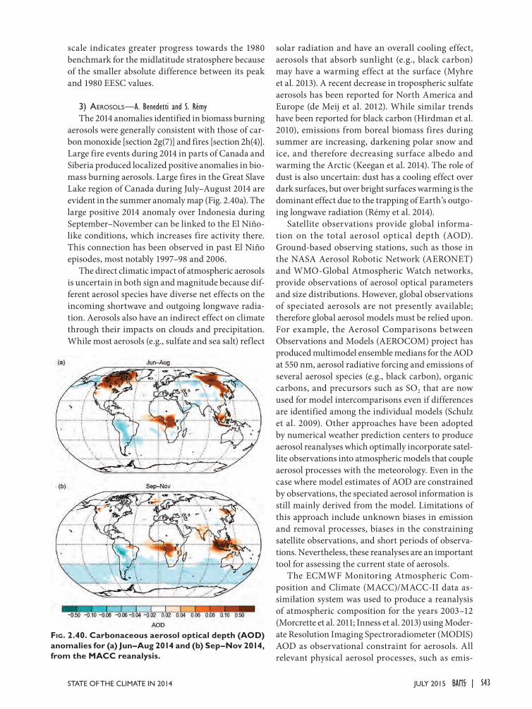
scale indicates greater progress towards the 1980 benchmark for the midlatitude stratosphere because of the smaller absolute difference between its peak and 1980 EESC values.
3) aeroSoLS—A. Benedetti and S. RémyThe 2014 anomalies identified in biomass burning
aerosols were generally consistent with those of car-bon monoxide [section 2g(7)] and fires [section 2h(4)]. Large fire events during 2014 in parts of Canada and Siberia produced localized positive anomalies in bio-mass burning aerosols. Large fires in the Great Slave Lake region of Canada during July–August 2014 are evident in the summer anomaly map (Fig. 2.40a). The large positive 2014 anomaly over Indonesia during September–November can be linked to the El Niño-like conditions, which increases fire activity there. This connection has been observed in past El Niño episodes, most notably 1997–98 and 2006.
The direct climatic impact of atmospheric aerosols is uncertain in both sign and magnitude because dif-ferent aerosol species have diverse net effects on the incoming shortwave and outgoing longwave radia-tion. Aerosols also have an indirect effect on climate through their impacts on clouds and precipitation. While most aerosols (e.g., sulfate and sea salt) reflect
solar radiation and have an overall cooling effect, aerosols that absorb sunlight (e.g., black carbon) may have a warming effect at the surface (Myhre et al. 2013). A recent decrease in tropospheric sulfate aerosols has been reported for North America and Europe (de Meij et al. 2012). While similar trends have been reported for black carbon (Hirdman et al. 2010), emissions from boreal biomass fires during summer are increasing, darkening polar snow and ice, and therefore decreasing surface albedo and warming the Arctic (Keegan et al. 2014). The role of dust is also uncertain: dust has a cooling effect over dark surfaces, but over bright surfaces warming is the dominant effect due to the trapping of Earth’s outgo-ing longwave radiation (Rémy et al. 2014).
Satellite observations provide global informa-tion on the total aerosol optical depth (AOD). Ground-based observing stations, such as those in the NASA Aerosol Robotic Network (AERONET) and WMO-Global Atmospheric Watch networks, provide observations of aerosol optical parameters and size distributions. However, global observations of speciated aerosols are not presently available; therefore global aerosol models must be relied upon. For example, the Aerosol Comparisons between Observations and Models (AEROCOM) project has produced multimodel ensemble medians for the AOD at 550 nm, aerosol radiative forcing and emissions of several aerosol species (e.g., black carbon), organic carbons, and precursors such as SO2 that are now used for model intercomparisons even if differences are identified among the individual models (Schulz et al. 2009). Other approaches have been adopted by numerical weather prediction centers to produce aerosol reanalyses which optimally incorporate satel-lite observations into atmospheric models that couple aerosol processes with the meteorology. Even in the case where model estimates of AOD are constrained by observations, the speciated aerosol information is still mainly derived from the model. Limitations of this approach include unknown biases in emission and removal processes, biases in the constraining satellite observations, and short periods of observa-tions. Nevertheless, these reanalyses are an important tool for assessing the current state of aerosols.
The ECMWF Monitoring Atmospheric Com-position and Climate (MACC)/MACC-II data as-similation system was used to produce a reanalysis of atmospheric composition for the years 2003–12 (Morcrette et al. 2011; Inness et al. 2013) using Moder-ate Resolution Imaging Spectroradiometer (MODIS) AOD as observational constraint for aerosols. All relevant physical aerosol processes, such as emis-
Fig. 2.40. Carbonaceous aerosol optical depth (AOD) anomalies for (a) Jun–Aug 2014 and (b) Sep–Nov 2014, from the MACC reanalysis.
S43JULY 2015STATE OF THE CLIMATE IN 2014 |
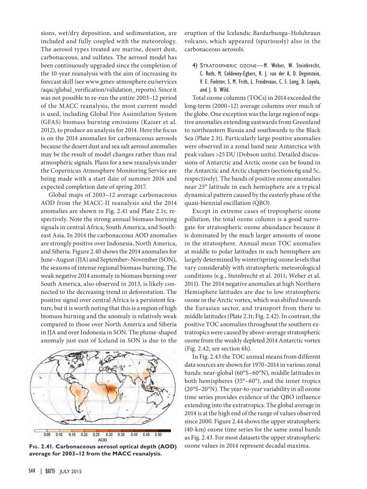
sions, wet/dry deposition, and sedimentation, are included and fully coupled with the meteorology. The aerosol types treated are marine, desert dust, carbonaceous, and sulfates. The aerosol model has been continuously upgraded since the completion of the 10-year reanalysis with the aim of increasing its forecast skill (see www.gmes-atmosphere.eu/services /aqac/global_verification/validation_reports). Since it was not possible to re-run the entire 2003–12 period of the MACC reanalysis, the most current model is used, including Global Fire Assimilation System (GFAS) biomass burning emissions (Kaiser et al. 2012), to produce an analysis for 2014. Here the focus is on the 2014 anomalies for carbonaceous aerosols because the desert dust and sea salt aerosol anomalies may be the result of model changes rather than real atmospheric signals. Plans for a new reanalysis under the Copernicus Atmosphere Monitoring Service are being made with a start date of summer 2016 and expected completion date of spring 2017.
Global maps of 2003–12 average carbonaceous AOD from the MACC-II reanalysis and the 2014 anomalies are shown in Fig. 2.41 and Plate 2.1v, re-spectively. Note the strong annual biomass burning signals in central Africa, South America, and South-east Asia. In 2014 the carbonaceous AOD anomalies are strongly positive over Indonesia, North America, and Siberia. Figure 2.40 shows the 2014 anomalies for June–August (JJA) and September–November (SON), the seasons of intense regional biomass burning. The weak negative 2014 anomaly in biomass burning over South America, also observed in 2013, is likely con-nected to the decreasing trend in deforestation. The positive signal over central Africa is a persistent fea-ture, but it is worth noting that this is a region of high biomass burning and the anomaly is relatively weak compared to those over North America and Siberia in JJA and over Indonesia in SON. The plume-shaped anomaly just east of Iceland in SON is due to the
eruption of the Icelandic Bardarbunga–Holuhraun volcano, which appeared (spuriously) also in the carbonaceous aerosols.
4) StratoSpheric ozone—M. Weber, W. Steinbrecht, C. Roth, M. Coldewey-Egbers, R. J. van der A, D. Degenstein, V. E. Fioletov, S. M. Frith, L. Froidevaux, C. S. Long, D. Loyola, and J. D. Wild.
Total ozone columns (TOCs) in 2014 exceeded the long-term (2000–12) average columns over much of the globe. One exception was the large region of nega-tive anomalies extending eastwards from Greenland to northeastern Russia and southwards to the Black Sea (Plate 2.1t). Particularly large positive anomalies were observed in a zonal band near Antarctica with peak values >25 DU (Dobson units). Detailed discus-sions of Antarctic and Arctic ozone can be found in the Antarctic and Arctic chapters (sections 6g and 5c, respectively). The bands of positive ozone anomalies near 25° latitude in each hemisphere are a typical dynamical pattern caused by the easterly phase of the quasi-biennial oscillation (QBO).
Except in extreme cases of tropospheric ozone pollution, the total ozone column is a good surro-gate for stratospheric ozone abundance because it is dominated by the much larger amounts of ozone in the stratosphere. Annual mean TOC anomalies at middle to polar latitudes in each hemisphere are largely determined by winter/spring ozone levels that vary considerably with stratospheric meteorological conditions (e.g., Steinbrecht et al. 2011; Weber et al. 2011). The 2014 negative anomalies at high Northern Hemisphere latitudes are due to low stratospheric ozone in the Arctic vortex, which was shifted towards the Eurasian sector, and transport from there to middle latitudes (Plate 2.1t; Fig. 2.42). In contrast, the positive TOC anomalies throughout the southern ex-tratropics were caused by above-average stratospheric ozone from the weakly depleted 2014 Antarctic vortex (Fig. 2.42; see section 6h).
In Fig. 2.43 the TOC annual means from different data sources are shown for 1970–2014 in various zonal bands: near-global (60°S–60°N), middle latitudes in both hemispheres (35°–60°), and the inner tropics (20°S–20°N). The year-to-year variability in all ozone time series provides evidence of the QBO influence extending into the extratropics. The global average in 2014 is at the high end of the range of values observed since 2000. Figure 2.44 shows the upper stratospheric (40-km) ozone time series for the same zonal bands as Fig. 2.43. For most datasets the upper stratospheric ozone values in 2014 represent decadal maxima.Fig. 2.41. Carbonaceous aerosol optical depth (AOD)
average for 2003–12 from the MACC reanalysis.
S44 JULY 2015|
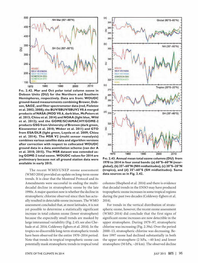
The recent WMO/UNEP ozone assessment (WMO 2014) provided an update on long-term ozone trends. It is clear that the Montreal Protocol and its Amendments were successful in ending the multi-decadal decline in stratospheric ozone by the late 1990s. A major question now is whether the decline in stratospheric chlorine observed since then has actu-ally resulted in detectable ozone increases. The WMO assessment concluded that, at most latitudes, it is not yet possible to determine a statistically significant increase in total column ozone (lower stratosphere) because the expectedly small trends are masked by large interannual variability (Fig. 2.43; see also Che-hade et al. 2014; Coldewey-Egbers et al. 2014). In the tropics no discernible long-term stratospheric trends have been observed for the entire 1970–2014 period. Note that trends in tropical tropospheric ozone can potentially mask stratospheric trends in tropical total
columns (Shepherd et al. 2014) and there is evidence that decadal trends in the ENSO may have produced tropospheric ozone increases in some tropical regions during the past two decades (Coldewey-Egbers et al. 2014).
For trends in the vertical distribution of strato-spheric ozone, however, the recent ozone assessment (WMO 2014) did conclude that the first signs of significant ozone increases are now detectible in the upper stratosphere. During 1979–97, stratospheric chlorine was increasing (Fig. 2.39a). Over the period 2000–13, stratospheric chlorine was decreasing. Be-fore 1997 ozone had declined substantially in both the upper stratosphere (2 hPa, ~40 km) and lower stratosphere (50 hPa, ~20 km). The observed decline
Fig. 2.42. Mar and Oct polar total column ozone in Dobson Units (DU) for the Northern and Southern Hemispheres, respectively. Data are from: WOUDC ground-based measurements combining Brewer, Dob-son, SAOZ, and filter spectrometer data (red, Fioletov et al. 2002; 2008); the BUV/SBUV/SBUV2 V8.6 merged products of NASA (MOD V8.6, dark blue, McPeters et al. 2013; Chiou et al. 2014) and NOAA (light blue, Wild et al. 2012); and the GOME/SCIAMACHY/GOME-2 products GSG from University of Bremen (dark green, Kiesewetter et al. 2010; Weber et al. 2011) and GTO from ESA/DLR (light green, Loyola et al. 2009; Chiou et al. 2014). The MSR V2 (multi sensor reanalysis) combines various satellite data and algorithm versions after correction with respect to collocated WOUDC ground data in a data assimilation scheme (van der A et al. 2010; 2015). The MSR dataset was extended us-ing GOME-2 total ozone. WOUDC values for 2014 are preliminary because not all ground station data were available in early 2015.
Fig. 2.43. Annual mean total ozone columns (DU) from 1970 to 2014 in four zonal bands: (a) 60°S–60°N (near-global), (b) 35°–60°N (NH midlatitudes), (c) 20°S–20°N (tropics), and (d) 35°–60°S (SH midlatitudes). Same data sources as in Fig. 2.42.
S45JULY 2015STATE OF THE CLIMATE IN 2014 |
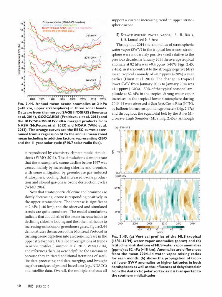
is reproduced by chemistry climate model simula-tions (WMO 2011). The simulations demonstrate that the stratospheric ozone decline before 1997 was caused mainly by increasing chlorine and bromine, with some mitigation by greenhouse gas-induced stratospheric cooling that increased ozone produc-tion and slowed gas-phase ozone destruction cycles (WMO 2014).
Now that stratospheric chlorine and bromine are slowly decreasing, ozone is responding positively in the upper stratosphere. The increase is significant at 2 hPa (~40 km), and the observed and simulated trends are quite consistent. The model simulations indicate that about half of the ozone increase is due to declining chlorine loading and the other half is due to increasing emissions of greenhouse gases. Figure 2.44 demonstrates the success of the Montreal Protocol in turning ozone depletion into an ozone increase in the upper stratosphere. Detailed investigations of trends in ozone profiles (Tummon et al. 2015; WMO 2014, and references therein) were helpful to the assessment because they initiated additional iterations of satel-lite data processing and data merging, and brought together analyses of ground-based data (e.g., NDACC) and satellite data. Overall, the multiple analyses all
support a current increasing trend in upper strato-spheric ozone.
5) Str atoSpher ic water vapor— S . M . Dav i s , K. H. Rosenlof, and D. F. Hurst
Throughout 2014 the anomalies of stratospheric water vapor (SWV) in the tropical lowermost strato-sphere were moderately positive (wet) relative to the previous decade. In January 2014 the average tropical anomaly at 82 hPa was +0.4 ppmv (+10%; Figs. 2.45, 2.46a), in stark contrast to the strongly negative (dry) mean tropical anomaly of −0.7 ppmv (−20%) a year earlier (Hurst et al. 2014). The change in tropical lower SWV from January 2013 to January 2014 was +1.1 ppmv (+30%), ~50% of the typical seasonal am-plitude at 82 hPa in the tropics. Strong water vapor increases in the tropical lower stratosphere during 2013–14 were observed at San José, Costa Rica (10°N), by balloon-borne frost point hygrometers (Fig. 2.47c) and throughout the equatorial belt by the Aura Mi-crowave Limb Sounder (MLS, Fig. 2.45a). Although
Fig. 2.44. Annual mean ozone anomalies at 2 hPa (~40 km, upper stratosphere) in three zonal bands. Data are from the merged SAGE II/OSIRIS (Bourassa et al. 2014), GOZCARDS (Froidevaux et al. 2015) and the BUV/SBUV/SBUV2 v8.6 merged products from NASA (McPeters et al. 2013) and NOAA (Wild et al. 2012). The orange curves are the EESC curves deter-mined from a regression fit to the annual mean zonal mean including in addition factors representing QBO and the 11-year solar cycle (F10.7 solar radio flux).
Fig. 2.45. (a) Vertical profiles of the MLS tropical (15°S–15°N) water vapor anomalies (ppmv) and (b) latitudinal distributions of MLS water vapor anomalies (ppmv) at 82 hPa (~18 km). Anomalies are differences from the mean 2004–14 water vapor mixing ratios for each month. (b) shows the propagation of tropi-cal lower SWV anomalies to higher latitudes in both hemispheres as well as the influences of dehydrated air from the Antarctic polar vortex as it is transported to the southern midlatitudes.
S46 JULY 2015|
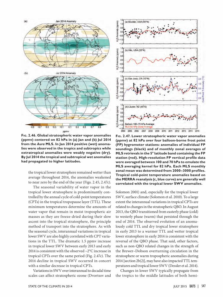
the tropical lower stratosphere remained wetter than average throughout 2014, the anomalies weakened to near zero by the end of the year (Figs. 2.45, 2.47c).
The seasonal variability of water vapor in the tropical lower stratosphere is predominantly con-trolled by the annual cycle of cold-point temperatures (CPTs) in the tropical tropopause layer (TTL). These minimum temperatures determine the amounts of water vapor that remain in moist tropospheric air masses as they are freeze-dried during their slow ascent into the tropical stratosphere, the principle method of transport into the stratosphere. As with the seasonal cycle, interannual variations in tropical lower SWV are also highly correlated with CPT varia-tions in the TTL. The dramatic 1.5 ppmv increase in tropical lower SWV between early 2013 and early 2014 is consistent with the observed ~2°C increase in tropical CPTs over the same period (Fig. 2.47c). The 2014 decline in tropical SWV occurred in concert with a similar decrease in tropical CPTs.
Variations in SWV over interannual to decadal time scales can affect stratospheric ozone (Dvortsov and
Solomon 2001) and, especially for the tropical lower SWV, surface climate (Solomon et al. 2010). To a large extent the interannual variations in tropical CPTs are related to changes in the stratospheric QBO. In August 2013, the QBO transitioned from easterly phase (cold) to westerly phase (warm) that persisted through the end of 2014. The observed evolution of an anoma-lously cold TTL and dry tropical lower stratosphere in early 2013 to a warmer TTL and wetter tropical lower stratosphere in early 2014 is consistent with the reversal of the QBO phase. That said, other factors, such as non-QBO related changes in the strength of the Brewer–Dobson overturning circulation in the stratosphere or warm tropospheric anomalies during 2014 [section 2b(2)], may have also impacted TTL tem-peratures and tropical lower SWV (Dessler et al. 2014).
Changes in lower SWV typically propagate from the tropics to the middle latitudes of both hemi-
Fig. 2.46. Global stratospheric water vapor anomalies (ppmv) centered on 82 hPa in (a) Jan and (b) Jul 2014 from the Aura MLS. In Jan 2014 positive (wet) anoma-lies were observed in the tropics and subtropics while extratropical anomalies were weakly negative (dry). By Jul 2014 the tropical and subtropical wet anomalies had propagated to higher latitudes.
Fig. 2.47. Lower stratospheric water vapor anomalies (ppmv) at 82 hPa over four balloon-borne frost point (FP) hygrometer stations: anomalies of individual FP soundings (black) and of monthly zonal averages of MLS retrievals in the 5° latitude band containing the FP station (red). High-resolution FP vertical profile data were averaged between 100 and 70 hPa to emulate the MLS averaging kernel for 82 hPa. Each MLS monthly zonal mean was determined from 2000–3000 profiles. Tropical cold-point temperature anomalies based on the MERRA reanalysis (c, blue curve) are generally well correlated with the tropical lower SWV anomalies.
S47JULY 2015STATE OF THE CLIMATE IN 2014 |
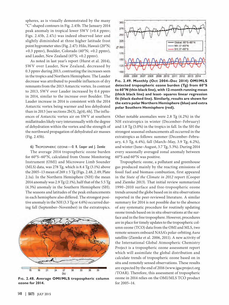
spheres, as is visually demonstrated by the many “C”-shaped contours in Fig. 2.45b. The January 2014 peak anomaly in tropical lower SWV (+0.4 ppmv; Figs. 2.45b, 2.47c) was indeed observed later and slightly diminished at three higher latitude frost point hygrometer sites (Fig. 2.47): Hilo, Hawaii (20°N; +0.3 ppmv), Boulder, Colorado (40°N; +0.2 ppmv), and Lauder, New Zealand (45°S; +0.2 ppmv).
As noted in last year’s report (Hurst et al. 2014), SWV over Lauder, New Zealand, decreased by 0.3 ppmv during 2013, contrasting the increases seen in the tropics and Northern Hemisphere. The Lauder decrease was attributed to possible influences of dry remnants from the 2013 Antarctic vortex. In contrast to 2013, SWV over Lauder increased by 0.4 ppmv in 2014, similar to the increase over Boulder. The Lauder increase in 2014 is consistent with the 2014 Antarctic vortex being warmer and less dehydrated than in 2013 [see sections 2b(3), 2g(4), 6h]. The influ-ences of Antarctic vortex air on SWV at southern midlatitudes likely vary interannually with the degree of dehydration within the vortex and the strength of the northward propagation of dehydrated air masses (Fig. 2.45b).
6) tropoSpheric ozone—O. R. Cooper and J. ZiemkeThe average 2014 tropospheric ozone burden
for 60°S–60°N, calculated from Ozone Monitoring Instrument (OMI) and Microwave Limb Sounder (MLS) data, was 278 Tg, which is 8.4 Tg (3.1%) above the 2005–13 mean of 269 ± 5 Tg (Figs. 2.48, 2.49; Plate 2.1u). In the Northern Hemisphere (NH) the mean 2014 anomaly was 2.9 Tg (2.1%), half that of the 5.5 Tg (4.3%) anomaly in the Southern Hemisphere (SH). The seasons and latitudes of the peak enhancements in each hemisphere also differed. The strongest posi-tive anomaly in the NH (3.3 Tg or 4.6%) occurred dur-ing fall (September–November) in the extratropics.
Other notable anomalies were 2.8 Tg (4.2%) in the NH extratropics in winter (December–February) and 1.8 Tg (3.0%) in the tropics in fall. In the SH the strongest seasonal enhancements all occurred in the extratropics as follows: summer (December–Febru-ary, 4.3 Tg, 6.4%), fall (March–May, 3.9 Tg, 6.2%), and winter (June–August, 3.7 Tg, 5.3%). During 2014 every seasonally averaged zonal anomaly between 60°S and 60°N was positive.
Tropospheric ozone, a pollutant and greenhouse gas produced mainly by the reacting emissions of fossil fuel and biomass combustion, first appeared in the State of the Climate in 2012 report (Cooper and Ziemke 2013). That initial review summarized 1990–2010 surface and free-tropospheric ozone trends around the globe based on in situ observations reported in the peer-reviewed literature. A similar summary for 2014 is not possible due to the absence of any systematic procedure for routinely updating ozone trends based on in situ observations at the sur-face and in the free troposphere. However, procedures are in place for timely updates to the tropospheric col-umn ozone (TCO) data from the OMI and MLS, two remote sensors onboard NASA’s polar-orbiting Aura satellite (Ziemke et al. 2006, 2011). A new activity of the International Global Atmospheric Chemistry Project is a tropospheric ozone assessment report which will assimilate the global distribution and calculate trends of tropospheric ozone based on in situ and remotely sensed observations. These results are expected by the end of 2016 (www.igacproject.org /TOAR). Therefore, this assessment of tropospheric ozone in 2014 relies on the OMI/MLS TCO product for 2005–14.
Fig. 2.48. Average OMI/MLS tropospheric column ozone for 2014.
Fig. 2.49. Monthly (Oct 2004–Dec 2014) OMI/MLS detected tropospheric ozone burden (Tg) from 60°S to 60°N (thin black line), with 12-month running mean (thick black line) and least- squares linear regression fit (black dashed line). Similarly, results are shown for the extra polar Northern Hemisphere (blue) and extra polar Southern Hemisphere (red).
S48 JULY 2015|
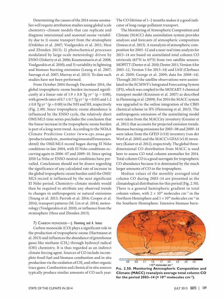
Determining the causes of the 2014 ozone anoma-lies will require attribution studies using global scale chemistry–climate models that can replicate and diagnose interannual and seasonal ozone variabil-ity due to 1) ozone transport from the stratosphere (Ordóñez et al. 2007; Voulgarakis et al. 2011; Hess and Zbinden 2013); 2) photochemical processes modulated by large-scale meteorology driven by ENSO (Doherty et al. 2006; Koumoutsaris et al. 2008; Voulgarakis et al. 2010); and 3) variability in lightning and biomass burning emissions (Leung et al. 2007; Sauvage et al. 2007; Murray et al. 2013). To date such studies have not been performed.
From October 2004 through December 2014, the global tropospheric ozone burden increased signifi-cantly at a linear rate of 1.9 ± 0.8 Tg yr−1 (p = 0.00), with growth rates of 0.7 ± 0.7 Tg yr−1 (p = 0.05) and 1.2 ± 0.8 Tg yr−1 (p = 0.00) in the NH and SH, respectively (Fig. 2.49). Since tropospheric ozone abundance is influenced by the ENSO cycle, the relatively short OMI/MLS time series precludes the conclusion that the linear increase in the tropospheric ozone burden is part of a long-term trend. According to the NOAA Climate Prediction Center (www.cpc.noaa.gov /products/analysis_monitoring/ensostuff/ensoyears.shtml) the OMI/MLS record began during El Niño conditions in late 2004, with El Niño conditions oc-curring again in 2006–07 and 2009–10. Since spring 2010 La Niña or ENSO-neutral conditions have pre-vailed. Conclusions should not be drawn regarding the significance of any calculated rate of increase in the global tropospheric ozone burden until the OMI/MLS record is inf luenced by the next significant El Niño period. Chemistry–climate models would then be required to attribute any observed trends to changes in anthropogenic or natural emissions (Young et al. 2013; Parrish et al. 2014; Cooper et al. 2014), transport patterns (M. Lin et al. 2014), meteo-rology (Voulgarakis et al. 2010), or influence from the stratosphere (Hess and Zbinden 2013).
7) carbon monoxide—J. Flemming and A. InnessCarbon monoxide (CO) plays a significant role in
the production of tropospheric ozone (Hartmann et al. 2013) and influences the abundance of greenhouse gases like methane (CH4) through hydroxyl radical (OH) chemistry. It is thus regarded as an indirect climate forcing agent. Sources of CO include incom-plete fossil fuel and biomass combustion and in situ production via the oxidation of CH4 and other organic trace gases. Combustion and chemical in situ sources typically produce similar amounts of CO each year.
The CO lifetime of 1–2 months makes it a good indi-cator of long-range pollutant transport.
The Monitoring of Atmospheric Composition and Climate (MACC) data assimilation system provides analyses and forecasts of atmospheric composition (Inness et al. 2013). A reanalysis of atmospheric com-position for 2003–12 and a near-real time analysis for 2013–14 are based on assimilated total column CO retrievals (65°N to 65°S) from two satellite sensors: MOPITT (Deeter et al. 2010; Deeter 2011; Version 4 for 2003–12, Version 5 for 2013–14) and IASI (Clerbaux et al. 2009; George et al. 2009; data for 2008–14). Through 2013 the satellite observations were assimi-lated in the ECMWF’s Integrated Forecasting System (IFS), which was coupled to the MOZART-3 chemical transport model (Kinnison et al. 2007) as described in Flemming et al. (2009). For 2014 the MACC system was upgraded to the online integration of the CB05 chemical scheme in IFS (Flemming et al. 2015). The anthropogenic emissions of the assimilating model were taken from the MACCity inventory (Granier et al. 2011) that accounts for projected emission trends. Biomass burning emissions for 2003–08 and 2009–14 were taken from the GFED (v3.0) inventory (van der Werf et al. 2010) and the MACC’s GFAS (v1.0) inven-tory (Kaiser et al. 2012), respectively. The global three-dimensional CO distribution from MACC is used here to assess CO total column anomalies for 2014. Total column CO is a good surrogate for tropospheric CO abundance because it is dominated by the much larger amounts of CO in the troposphere.
Median values of the monthly averaged total column CO during 2003–14 are presented as the climatological distribution for this period (Fig. 2.50). There is a general hemispheric gradient in total column values, with 2 × 10¹⁸ molecules cm−2 in the Northern Hemisphere and 1 × 10¹⁸ molecules cm−2 in the Southern Hemisphere. Intensive biomass burn-
Fig. 2.50. Monitoring Atmospheric Composition and Climate (MACC) reanalysis average total column CO for the period 2003–14 (× 1018 molecules cm–2).
S49JULY 2015STATE OF THE CLIMATE IN 2014 |
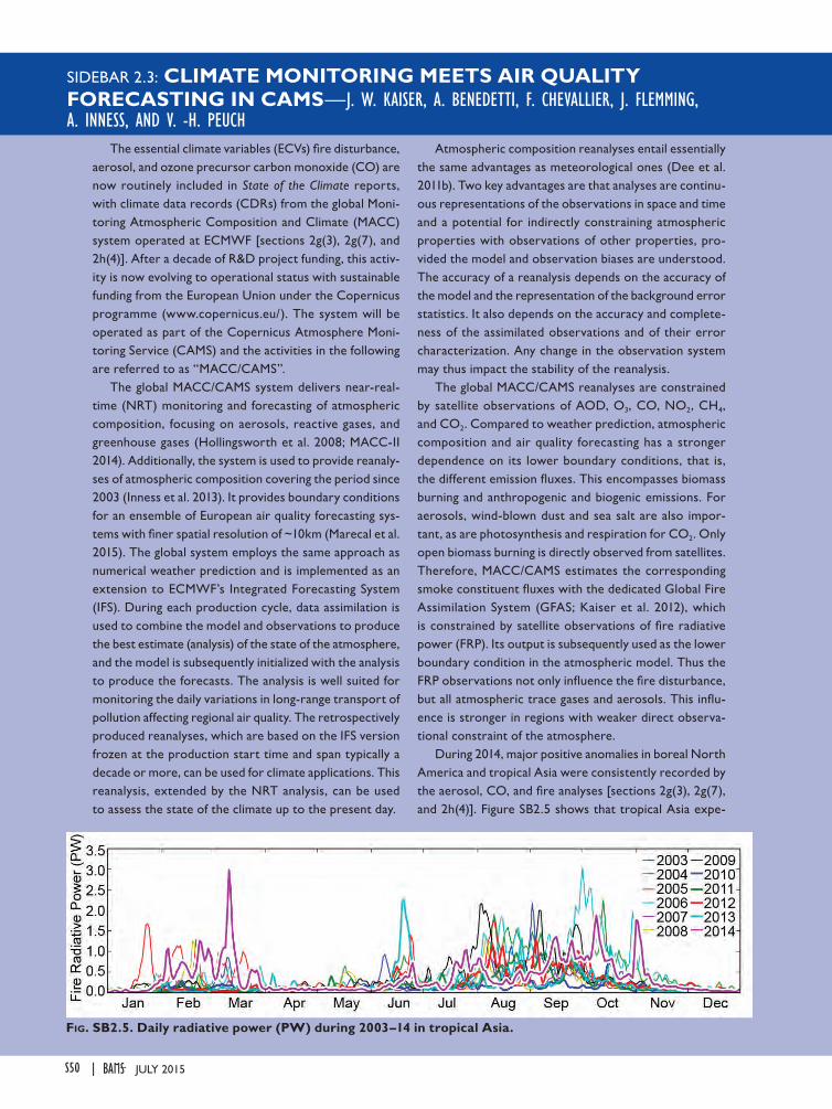
SIDEBAR 2.3: CLIMATE MONITORING MEETS AIR QUALITY FORECASTING IN CAMS—J. W. KAISER, A. BENEDETTI, F. CHEVALLIER, J. FLEMMING, A. INNESS, AND V. -H. PEUCH
The essential climate variables (ECVs) fire disturbance, aerosol, and ozone precursor carbon monoxide (CO) are now routinely included in State of the Climate reports, with climate data records (CDRs) from the global Moni-toring Atmospheric Composition and Climate (MACC) system operated at ECMWF [sections 2g(3), 2g(7), and 2h(4)]. After a decade of R&D project funding, this activ-ity is now evolving to operational status with sustainable funding from the European Union under the Copernicus programme (www.copernicus.eu/). The system will be operated as part of the Copernicus Atmosphere Moni-toring Service (CAMS) and the activities in the following are referred to as “MACC/CAMS”.
The global MACC/CAMS system delivers near-real-time (NRT) monitoring and forecasting of atmospheric composition, focusing on aerosols, reactive gases, and greenhouse gases (Hollingsworth et al. 2008; MACC-II 2014). Additionally, the system is used to provide reanaly-ses of atmospheric composition covering the period since 2003 (Inness et al. 2013). It provides boundary conditions for an ensemble of European air quality forecasting sys-tems with finer spatial resolution of ~10km (Marecal et al. 2015). The global system employs the same approach as numerical weather prediction and is implemented as an extension to ECMWF’s Integrated Forecasting System (IFS). During each production cycle, data assimilation is used to combine the model and observations to produce the best estimate (analysis) of the state of the atmosphere, and the model is subsequently initialized with the analysis to produce the forecasts. The analysis is well suited for monitoring the daily variations in long-range transport of pollution affecting regional air quality. The retrospectively produced reanalyses, which are based on the IFS version frozen at the production start time and span typically a decade or more, can be used for climate applications. This reanalysis, extended by the NRT analysis, can be used to assess the state of the climate up to the present day.
Atmospheric composition reanalyses entail essentially the same advantages as meteorological ones (Dee et al. 2011b). Two key advantages are that analyses are continu-ous representations of the observations in space and time and a potential for indirectly constraining atmospheric properties with observations of other properties, pro-vided the model and observation biases are understood. The accuracy of a reanalysis depends on the accuracy of the model and the representation of the background error statistics. It also depends on the accuracy and complete-ness of the assimilated observations and of their error characterization. Any change in the observation system may thus impact the stability of the reanalysis.
The global MACC/CAMS reanalyses are constrained by satellite observations of AOD, O3, CO, NO2, CH4, and CO2. Compared to weather prediction, atmospheric composition and air quality forecasting has a stronger dependence on its lower boundary conditions, that is, the different emission fluxes. This encompasses biomass burning and anthropogenic and biogenic emissions. For aerosols, wind-blown dust and sea salt are also impor-tant, as are photosynthesis and respiration for CO2. Only open biomass burning is directly observed from satellites. Therefore, MACC/CAMS estimates the corresponding smoke constituent fluxes with the dedicated Global Fire Assimilation System (GFAS; Kaiser et al. 2012), which is constrained by satellite observations of fire radiative power (FRP). Its output is subsequently used as the lower boundary condition in the atmospheric model. Thus the FRP observations not only influence the fire disturbance, but all atmospheric trace gases and aerosols. This influ-ence is stronger in regions with weaker direct observa-tional constraint of the atmosphere.
During 2014, major positive anomalies in boreal North America and tropical Asia were consistently recorded by the aerosol, CO, and fire analyses [sections 2g(3), 2g(7), and 2h(4)]. Figure SB2.5 shows that tropical Asia expe-
Fig. SB2.5. Daily radiative power (PW) during 2003–14 in tropical Asia.
S50 JULY 2015|
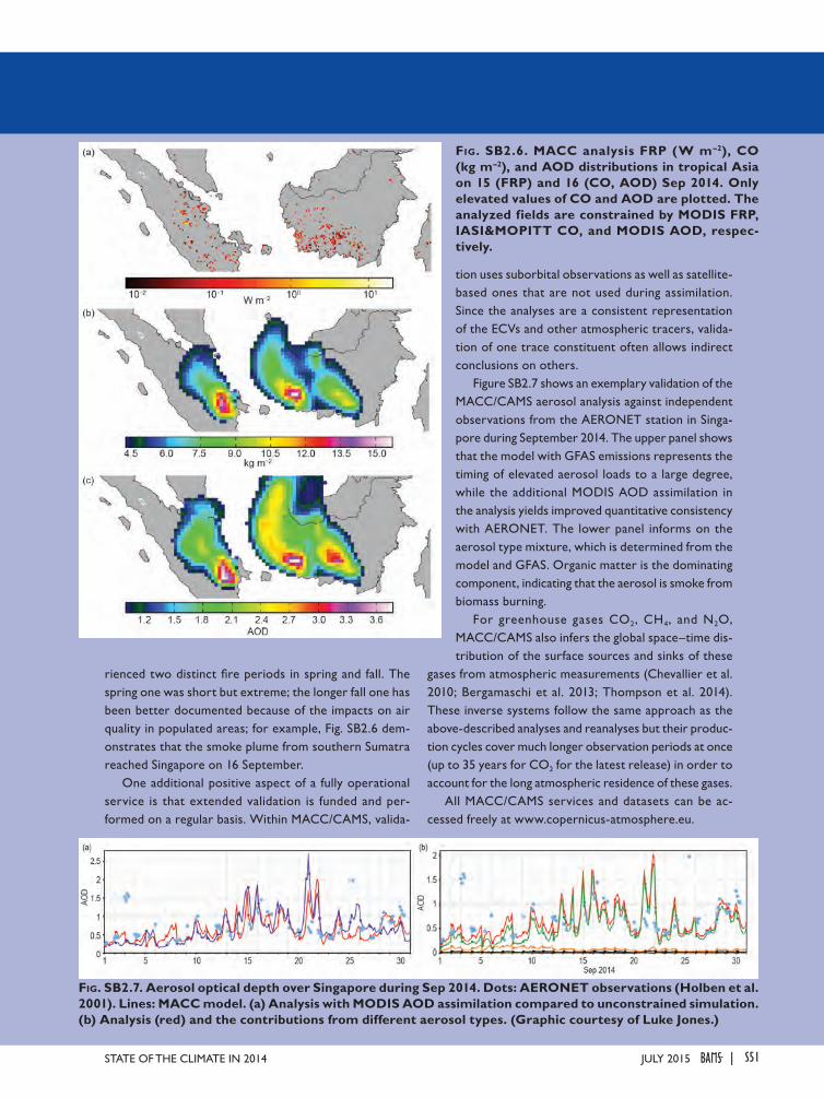
rienced two distinct fire periods in spring and fall. The spring one was short but extreme; the longer fall one has been better documented because of the impacts on air quality in populated areas; for example, Fig. SB2.6 dem-onstrates that the smoke plume from southern Sumatra reached Singapore on 16 September.
One additional positive aspect of a fully operational service is that extended validation is funded and per-formed on a regular basis. Within MACC/CAMS, valida-
tion uses suborbital observations as well as satellite-based ones that are not used during assimilation. Since the analyses are a consistent representation of the ECVs and other atmospheric tracers, valida-tion of one trace constituent often allows indirect conclusions on others.
Figure SB2.7 shows an exemplary validation of the MACC/CAMS aerosol analysis against independent observations from the AERONET station in Singa-pore during September 2014. The upper panel shows that the model with GFAS emissions represents the timing of elevated aerosol loads to a large degree, while the additional MODIS AOD assimilation in the analysis yields improved quantitative consistency with AERONET. The lower panel informs on the aerosol type mixture, which is determined from the model and GFAS. Organic matter is the dominating component, indicating that the aerosol is smoke from biomass burning.
For greenhouse gases CO2, CH4, and N2O, MACC/CAMS also infers the global space–time dis-tribution of the surface sources and sinks of these
gases from atmospheric measurements (Chevallier et al. 2010; Bergamaschi et al. 2013; Thompson et al. 2014). These inverse systems follow the same approach as the above-described analyses and reanalyses but their produc-tion cycles cover much longer observation periods at once (up to 35 years for CO2 for the latest release) in order to account for the long atmospheric residence of these gases.
All MACC/CAMS services and datasets can be ac-cessed freely at www.copernicus-atmosphere.eu.
Fig. SB2.6. MACC analysis FRP (W m–2), CO (kg m–2), and AOD distributions in tropical Asia on 15 (FRP) and 16 (CO, AOD) Sep 2014. Only elevated values of CO and AOD are plotted. The analyzed fields are constrained by MODIS FRP, IASI&MOPITT CO, and MODIS AOD, respec-tively.
Fig. SB2.7. Aerosol optical depth over Singapore during Sep 2014. Dots: AERONET observations (Holben et al. 2001). Lines: MACC model. (a) Analysis with MODIS AOD assimilation compared to unconstrained simulation. (b) Analysis (red) and the contributions from different aerosol types. (Graphic courtesy of Luke Jones.)
S51JULY 2015STATE OF THE CLIMATE IN 2014 |
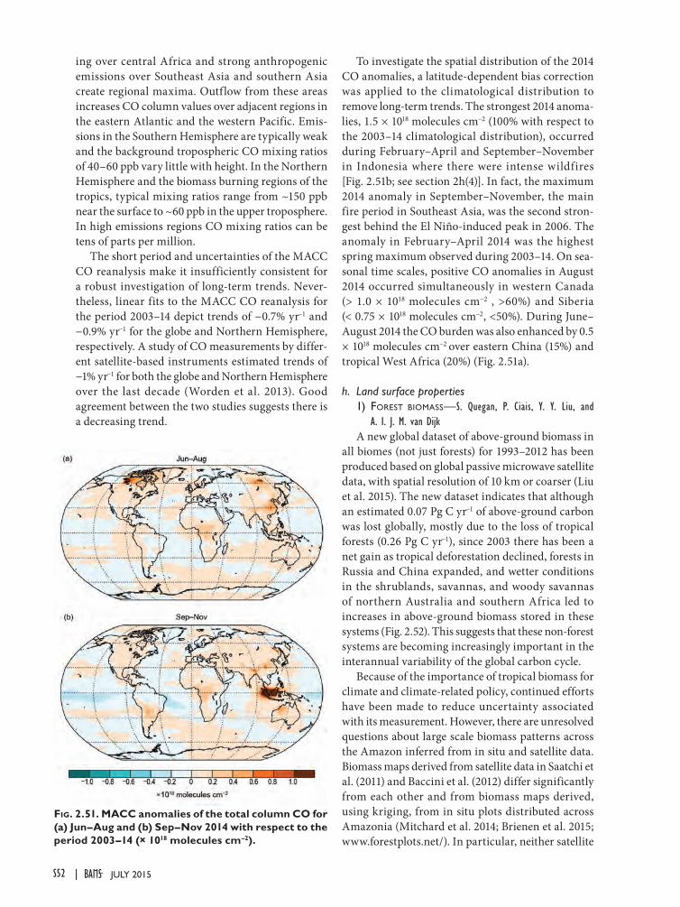
ing over central Africa and strong anthropogenic emissions over Southeast Asia and southern Asia create regional maxima. Outflow from these areas increases CO column values over adjacent regions in the eastern Atlantic and the western Pacific. Emis-sions in the Southern Hemisphere are typically weak and the background tropospheric CO mixing ratios of 40–60 ppb vary little with height. In the Northern Hemisphere and the biomass burning regions of the tropics, typical mixing ratios range from ~150 ppb near the surface to ~60 ppb in the upper troposphere. In high emissions regions CO mixing ratios can be tens of parts per million.
The short period and uncertainties of the MACC CO reanalysis make it insufficiently consistent for a robust investigation of long-term trends. Never-theless, linear fits to the MACC CO reanalysis for the period 2003–14 depict trends of −0.7% yr−1 and −0.9% yr−1 for the globe and Northern Hemisphere, respectively. A study of CO measurements by differ-ent satellite-based instruments estimated trends of −1% yr−1 for both the globe and Northern Hemisphere over the last decade (Worden et al. 2013). Good agreement between the two studies suggests there is a decreasing trend.
To investigate the spatial distribution of the 2014 CO anomalies, a latitude-dependent bias correction was applied to the climatological distribution to remove long-term trends. The strongest 2014 anoma-lies, 1.5 × 10¹⁸ molecules cm−2 (100% with respect to the 2003–14 climatological distribution), occurred during February–April and September–November in Indonesia where there were intense wildfires [Fig. 2.51b; see section 2h(4)]. In fact, the maximum 2014 anomaly in September–November, the main fire period in Southeast Asia, was the second stron-gest behind the El Niño-induced peak in 2006. The anomaly in February–April 2014 was the highest spring maximum observed during 2003–14. On sea-sonal time scales, positive CO anomalies in August 2014 occurred simultaneously in western Canada (> 1.0 × 10¹⁸ molecules cm−2 , >60%) and Siberia (< 0.75 × 10¹⁸ molecules cm−2, <50%). During June–August 2014 the CO burden was also enhanced by 0.5 × 10¹⁸ molecules cm−2 over eastern China (15%) and tropical West Africa (20%) (Fig. 2.51a).
h. Land surface properties1) foreSt biomaSS—S. Quegan, P. Ciais, Y. Y. Liu, and
A. I. J. M. van DijkA new global dataset of above-ground biomass in
all biomes (not just forests) for 1993–2012 has been produced based on global passive microwave satellite data, with spatial resolution of 10 km or coarser (Liu et al. 2015). The new dataset indicates that although an estimated 0.07 Pg C yr−1 of above-ground carbon was lost globally, mostly due to the loss of tropical forests (0.26 Pg C yr−1), since 2003 there has been a net gain as tropical deforestation declined, forests in Russia and China expanded, and wetter conditions in the shrublands, savannas, and woody savannas of northern Australia and southern Africa led to increases in above-ground biomass stored in these systems (Fig. 2.52). This suggests that these non-forest systems are becoming increasingly important in the interannual variability of the global carbon cycle.
Because of the importance of tropical biomass for climate and climate-related policy, continued efforts have been made to reduce uncertainty associated with its measurement. However, there are unresolved questions about large scale biomass patterns across the Amazon inferred from in situ and satellite data. Biomass maps derived from satellite data in Saatchi et al. (2011) and Baccini et al. (2012) differ significantly from each other and from biomass maps derived, using kriging, from in situ plots distributed across Amazonia (Mitchard et al. 2014; Brienen et al. 2015; www.forestplots.net/). In particular, neither satellite
Fig. 2.51. MACC anomalies of the total column CO for (a) Jun–Aug and (b) Sep–Nov 2014 with respect to the period 2003–14 (× 1018 molecules cm–2).
S52 JULY 2015|
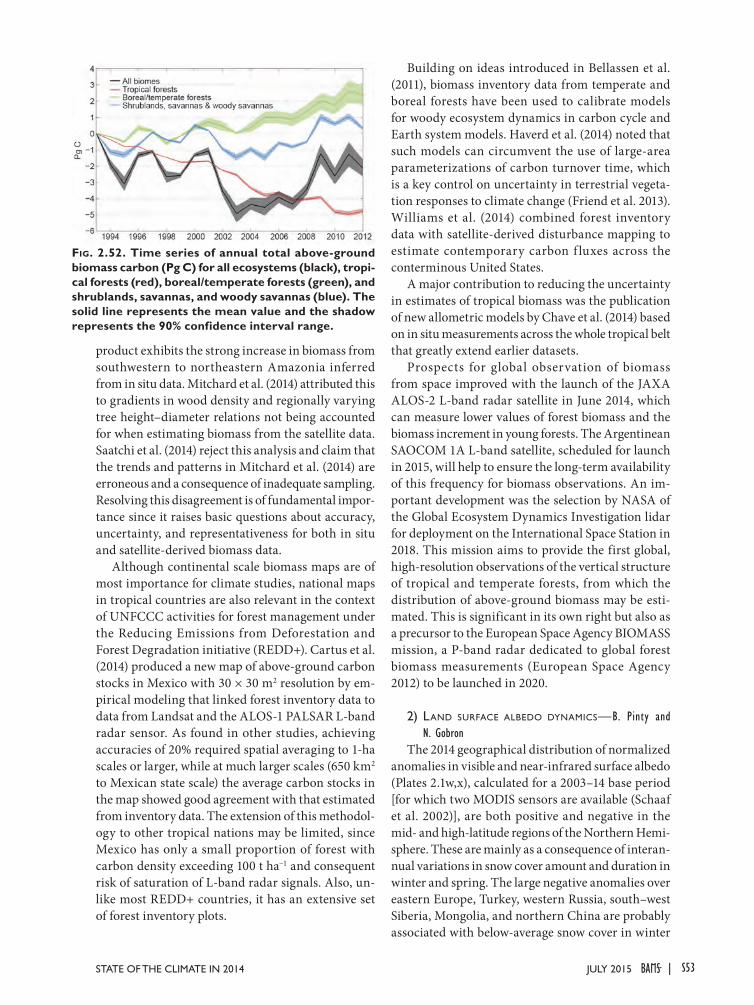
product exhibits the strong increase in biomass from southwestern to northeastern Amazonia inferred from in situ data. Mitchard et al. (2014) attributed this to gradients in wood density and regionally varying tree height–diameter relations not being accounted for when estimating biomass from the satellite data. Saatchi et al. (2014) reject this analysis and claim that the trends and patterns in Mitchard et al. (2014) are erroneous and a consequence of inadequate sampling. Resolving this disagreement is of fundamental impor-tance since it raises basic questions about accuracy, uncertainty, and representativeness for both in situ and satellite-derived biomass data.
Although continental scale biomass maps are of most importance for climate studies, national maps in tropical countries are also relevant in the context of UNFCCC activities for forest management under the Reducing Emissions from Deforestation and Forest Degradation initiative (REDD+). Cartus et al. (2014) produced a new map of above-ground carbon stocks in Mexico with 30 × 30 m2 resolution by em-pirical modeling that linked forest inventory data to data from Landsat and the ALOS-1 PALSAR L-band radar sensor. As found in other studies, achieving accuracies of 20% required spatial averaging to 1-ha scales or larger, while at much larger scales (650 km2 to Mexican state scale) the average carbon stocks in the map showed good agreement with that estimated from inventory data. The extension of this methodol-ogy to other tropical nations may be limited, since Mexico has only a small proportion of forest with carbon density exceeding 100 t ha−1 and consequent risk of saturation of L-band radar signals. Also, un-like most REDD+ countries, it has an extensive set of forest inventory plots.
Building on ideas introduced in Bellassen et al. (2011), biomass inventory data from temperate and boreal forests have been used to calibrate models for woody ecosystem dynamics in carbon cycle and Earth system models. Haverd et al. (2014) noted that such models can circumvent the use of large-area parameterizations of carbon turnover time, which is a key control on uncertainty in terrestrial vegeta-tion responses to climate change (Friend et al. 2013). Williams et al. (2014) combined forest inventory data with satellite-derived disturbance mapping to estimate contemporary carbon f luxes across the conterminous United States.
A major contribution to reducing the uncertainty in estimates of tropical biomass was the publication of new allometric models by Chave et al. (2014) based on in situ measurements across the whole tropical belt that greatly extend earlier datasets.
Prospects for global observation of biomass from space improved with the launch of the JAXA ALOS-2 L-band radar satellite in June 2014, which can measure lower values of forest biomass and the biomass increment in young forests. The Argentinean SAOCOM 1A L-band satellite, scheduled for launch in 2015, will help to ensure the long-term availability of this frequency for biomass observations. An im-portant development was the selection by NASA of the Global Ecosystem Dynamics Investigation lidar for deployment on the International Space Station in 2018. This mission aims to provide the first global, high-resolution observations of the vertical structure of tropical and temperate forests, from which the distribution of above-ground biomass may be esti-mated. This is significant in its own right but also as a precursor to the European Space Agency BIOMASS mission, a P-band radar dedicated to global forest biomass measurements (European Space Agency 2012) to be launched in 2020.
2) Land Surface aLbedo dynamicS—B. Pinty and N. Gobron
The 2014 geographical distribution of normalized anomalies in visible and near-infrared surface albedo (Plates 2.1w,x), calculated for a 2003–14 base period [for which two MODIS sensors are available (Schaaf et al. 2002)], are both positive and negative in the mid- and high-latitude regions of the Northern Hemi-sphere. These are mainly as a consequence of interan-nual variations in snow cover amount and duration in winter and spring. The large negative anomalies over eastern Europe, Turkey, western Russia, south–west Siberia, Mongolia, and northern China are probably associated with below-average snow cover in winter
Fig. 2.52. Time series of annual total above-ground biomass carbon (Pg C) for all ecosystems (black), tropi-cal forests (red), boreal/temperate forests (green), and shrublands, savannas, and woody savannas (blue). The solid line represents the mean value and the shadow represents the 90% confidence interval range.
S53JULY 2015STATE OF THE CLIMATE IN 2014 |
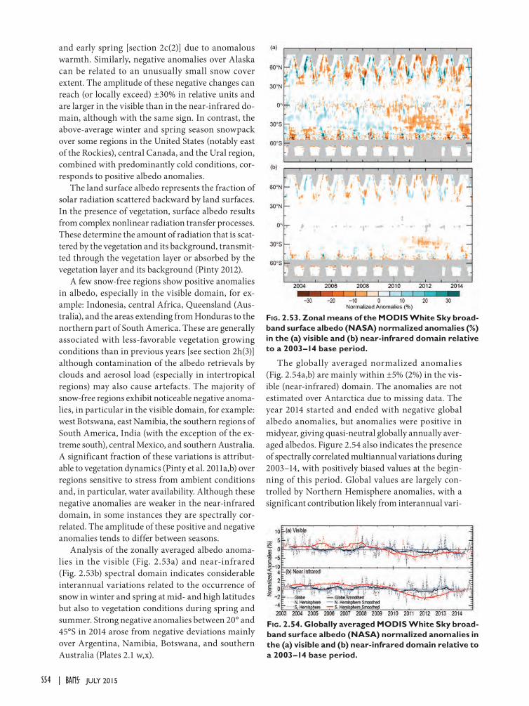
and early spring [section 2c(2)] due to anomalous warmth. Similarly, negative anomalies over Alaska can be related to an unusually small snow cover extent. The amplitude of these negative changes can reach (or locally exceed) ±30% in relative units and are larger in the visible than in the near-infrared do-main, although with the same sign. In contrast, the above-average winter and spring season snowpack over some regions in the United States (notably east of the Rockies), central Canada, and the Ural region, combined with predominantly cold conditions, cor-responds to positive albedo anomalies.
The land surface albedo represents the fraction of solar radiation scattered backward by land surfaces. In the presence of vegetation, surface albedo results from complex nonlinear radiation transfer processes. These determine the amount of radiation that is scat-tered by the vegetation and its background, transmit-ted through the vegetation layer or absorbed by the vegetation layer and its background (Pinty 2012).
A few snow-free regions show positive anomalies in albedo, especially in the visible domain, for ex-ample: Indonesia, central Africa, Queensland (Aus-tralia), and the areas extending from Honduras to the northern part of South America. These are generally associated with less-favorable vegetation growing conditions than in previous years [see section 2h(3)] although contamination of the albedo retrievals by clouds and aerosol load (especially in intertropical regions) may also cause artefacts. The majority of snow-free regions exhibit noticeable negative anoma-lies, in particular in the visible domain, for example: west Botswana, east Namibia, the southern regions of South America, India (with the exception of the ex-treme south), central Mexico, and southern Australia. A significant fraction of these variations is attribut-able to vegetation dynamics (Pinty et al. 2011a,b) over regions sensitive to stress from ambient conditions and, in particular, water availability. Although these negative anomalies are weaker in the near-infrared domain, in some instances they are spectrally cor-related. The amplitude of these positive and negative anomalies tends to differ between seasons.
Analysis of the zonally averaged albedo anoma-lies in the visible (Fig. 2.53a) and near-infrared (Fig. 2.53b) spectral domain indicates considerable interannual variations related to the occurrence of snow in winter and spring at mid- and high latitudes but also to vegetation conditions during spring and summer. Strong negative anomalies between 20° and 45°S in 2014 arose from negative deviations mainly over Argentina, Namibia, Botswana, and southern Australia (Plates 2.1 w,x).
The globally averaged normalized anomalies (Fig. 2.54a,b) are mainly within ±5% (2%) in the vis-ible (near-infrared) domain. The anomalies are not estimated over Antarctica due to missing data. The year 2014 started and ended with negative global albedo anomalies, but anomalies were positive in midyear, giving quasi-neutral globally annually aver-aged albedos. Figure 2.54 also indicates the presence of spectrally correlated multiannual variations during 2003–14, with positively biased values at the begin-ning of this period. Global values are largely con-trolled by Northern Hemisphere anomalies, with a significant contribution likely from interannual vari-
Fig. 2.53. Zonal means of the MODIS White Sky broad-band surface albedo (NASA) normalized anomalies (%) in the (a) visible and (b) near-infrared domain relative to a 2003–14 base period.
Fig. 2.54. Globally averaged MODIS White Sky broad-band surface albedo (NASA) normalized anomalies in the (a) visible and (b) near-infrared domain relative to a 2003–14 base period.
S54 JULY 2015|
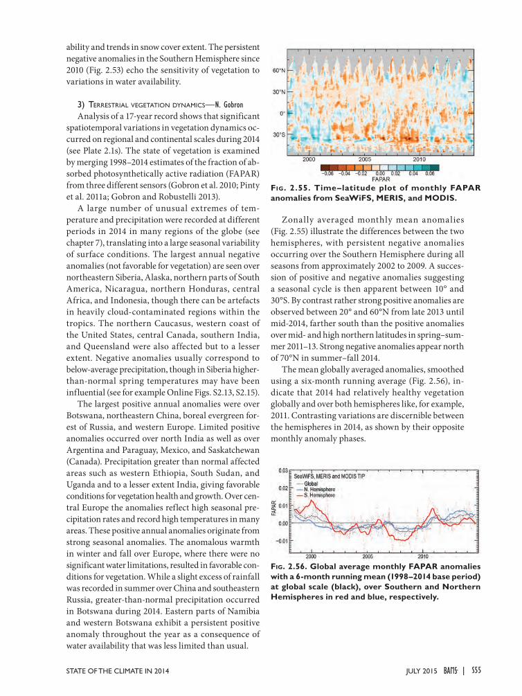
ability and trends in snow cover extent. The persistent negative anomalies in the Southern Hemisphere since 2010 (Fig. 2.53) echo the sensitivity of vegetation to variations in water availability.
3) terreStriaL vegetation dynamicS—N. GobronAnalysis of a 17-year record shows that significant
spatiotemporal variations in vegetation dynamics oc-curred on regional and continental scales during 2014 (see Plate 2.1s). The state of vegetation is examined by merging 1998–2014 estimates of the fraction of ab-sorbed photosynthetically active radiation (FAPAR) from three different sensors (Gobron et al. 2010; Pinty et al. 2011a; Gobron and Robustelli 2013).
A large number of unusual extremes of tem-perature and precipitation were recorded at different periods in 2014 in many regions of the globe (see chapter 7), translating into a large seasonal variability of surface conditions. The largest annual negative anomalies (not favorable for vegetation) are seen over northeastern Siberia, Alaska, northern parts of South America, Nicaragua, northern Honduras, central Africa, and Indonesia, though there can be artefacts in heavily cloud-contaminated regions within the tropics. The northern Caucasus, western coast of the United States, central Canada, southern India, and Queensland were also affected but to a lesser extent. Negative anomalies usually correspond to below-average precipitation, though in Siberia higher-than-normal spring temperatures may have been influential (see for example Online Figs. S2.13, S2.15).
The largest positive annual anomalies were over Botswana, northeastern China, boreal evergreen for-est of Russia, and western Europe. Limited positive anomalies occurred over north India as well as over Argentina and Paraguay, Mexico, and Saskatchewan (Canada). Precipitation greater than normal affected areas such as western Ethiopia, South Sudan, and Uganda and to a lesser extent India, giving favorable conditions for vegetation health and growth. Over cen-tral Europe the anomalies reflect high seasonal pre-cipitation rates and record high temperatures in many areas. These positive annual anomalies originate from strong seasonal anomalies. The anomalous warmth in winter and fall over Europe, where there were no significant water limitations, resulted in favorable con-ditions for vegetation. While a slight excess of rainfall was recorded in summer over China and southeastern Russia, greater-than-normal precipitation occurred in Botswana during 2014. Eastern parts of Namibia and western Botswana exhibit a persistent positive anomaly throughout the year as a consequence of water availability that was less limited than usual.
Zonally averaged monthly mean anomalies (Fig. 2.55) illustrate the differences between the two hemispheres, with persistent negative anomalies occurring over the Southern Hemisphere during all seasons from approximately 2002 to 2009. A succes-sion of positive and negative anomalies suggesting a seasonal cycle is then apparent between 10° and 30°S. By contrast rather strong positive anomalies are observed between 20° and 60°N from late 2013 until mid-2014, farther south than the positive anomalies over mid- and high northern latitudes in spring–sum-mer 2011–13. Strong negative anomalies appear north of 70°N in summer–fall 2014.
The mean globally averaged anomalies, smoothed using a six-month running average (Fig. 2.56), in-dicate that 2014 had relatively healthy vegetation globally and over both hemispheres like, for example, 2011. Contrasting variations are discernible between the hemispheres in 2014, as shown by their opposite monthly anomaly phases.
Fig. 2.55. Time–latitude plot of monthly FAPAR anomalies from SeaWiFS, MERIS, and MODIS.
Fig. 2.56. Global average monthly FAPAR anomalies with a 6-month running mean (1998–2014 base period) at global scale (black), over Southern and Northern Hemispheres in red and blue, respectively.
S55JULY 2015STATE OF THE CLIMATE IN 2014 |
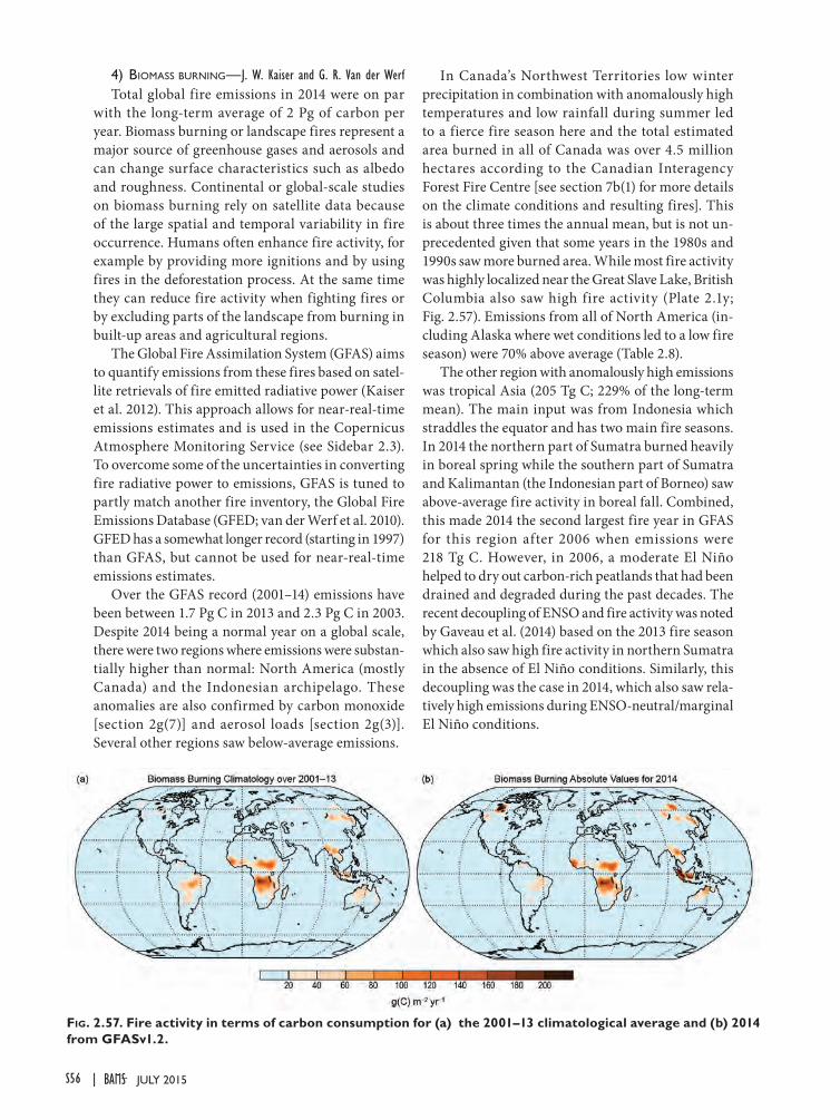
4) biomaSS burning—J. W. Kaiser and G. R. Van der WerfTotal global fire emissions in 2014 were on par
with the long-term average of 2 Pg of carbon per year. Biomass burning or landscape fires represent a major source of greenhouse gases and aerosols and can change surface characteristics such as albedo and roughness. Continental or global-scale studies on biomass burning rely on satellite data because of the large spatial and temporal variability in fire occurrence. Humans often enhance fire activity, for example by providing more ignitions and by using fires in the deforestation process. At the same time they can reduce fire activity when fighting fires or by excluding parts of the landscape from burning in built-up areas and agricultural regions.
The Global Fire Assimilation System (GFAS) aims to quantify emissions from these fires based on satel-lite retrievals of fire emitted radiative power (Kaiser et al. 2012). This approach allows for near-real-time emissions estimates and is used in the Copernicus Atmosphere Monitoring Service (see Sidebar 2.3). To overcome some of the uncertainties in converting fire radiative power to emissions, GFAS is tuned to partly match another fire inventory, the Global Fire Emissions Database (GFED; van der Werf et al. 2010). GFED has a somewhat longer record (starting in 1997) than GFAS, but cannot be used for near-real-time emissions estimates.
Over the GFAS record (2001–14) emissions have been between 1.7 Pg C in 2013 and 2.3 Pg C in 2003. Despite 2014 being a normal year on a global scale, there were two regions where emissions were substan-tially higher than normal: North America (mostly Canada) and the Indonesian archipelago. These anomalies are also confirmed by carbon monoxide [section 2g(7)] and aerosol loads [section 2g(3)]. Several other regions saw below-average emissions.
In Canada’s Northwest Territories low winter precipitation in combination with anomalously high temperatures and low rainfall during summer led to a fierce fire season here and the total estimated area burned in all of Canada was over 4.5 million hectares according to the Canadian Interagency Forest Fire Centre [see section 7b(1) for more details on the climate conditions and resulting fires]. This is about three times the annual mean, but is not un-precedented given that some years in the 1980s and 1990s saw more burned area. While most fire activity was highly localized near the Great Slave Lake, British Columbia also saw high fire activity (Plate 2.1y; Fig. 2.57). Emissions from all of North America (in-cluding Alaska where wet conditions led to a low fire season) were 70% above average (Table 2.8).
The other region with anomalously high emissions was tropical Asia (205 Tg C; 229% of the long-term mean). The main input was from Indonesia which straddles the equator and has two main fire seasons. In 2014 the northern part of Sumatra burned heavily in boreal spring while the southern part of Sumatra and Kalimantan (the Indonesian part of Borneo) saw above-average fire activity in boreal fall. Combined, this made 2014 the second largest fire year in GFAS for this region after 2006 when emissions were 218 Tg C. However, in 2006, a moderate El Niño helped to dry out carbon-rich peatlands that had been drained and degraded during the past decades. The recent decoupling of ENSO and fire activity was noted by Gaveau et al. (2014) based on the 2013 fire season which also saw high fire activity in northern Sumatra in the absence of El Niño conditions. Similarly, this decoupling was the case in 2014, which also saw rela-tively high emissions during ENSO-neutral/marginal El Niño conditions.
Fig. 2.57. Fire activity in terms of carbon consumption for (a) the 2001–13 climatological average and (b) 2014 from GFASv1.2.
S56 JULY 2015|
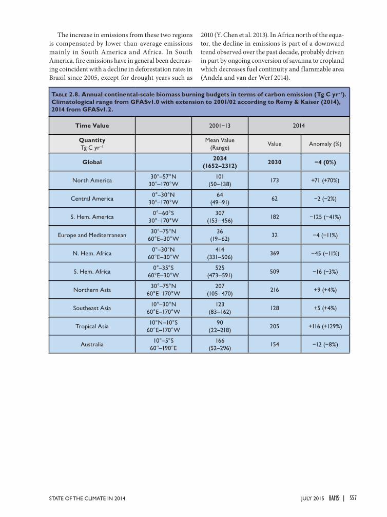
The increase in emissions from these two regions is compensated by lower-than-average emissions mainly in South America and Africa. In South America, fire emissions have in general been decreas-ing coincident with a decline in deforestation rates in Brazil since 2005, except for drought years such as
2010 (Y. Chen et al. 2013). In Africa north of the equa-tor, the decline in emissions is part of a downward trend observed over the past decade, probably driven in part by ongoing conversion of savanna to cropland which decreases fuel continuity and flammable area (Andela and van der Werf 2014).
Table 2.8. Annual continental-scale biomass burning budgets in terms of carbon emission (Tg C yr–1). Climatological range from GFASv1.0 with extension to 2001/02 according to Remy & Kaiser (2014), 2014 from GFASv1.2.
Time Value 2001−13 2014
Quantity Tg C yr–1
Mean Value (Range)
Value Anomaly (%)
Global 2034 (1652–2312) 2030 −4 (0%)
North America30°–57°N
30°–170°W101
(50–138)173 +71 (+70%)
Central America0°–30°N
30°–170°W64
(49–91)62 −2 (−2%)
S. Hem. America0°–60°S
30°–170°W307
(153–456)182 −125 (−41%)
Europe and Mediterranean30°–75°N
60°E–30°W36
(19–62)32 −4 (−11%)
N. Hem. Africa0°–30°N
60°E–30°W414
(331–506)369 −45 (−11%)
S. Hem. Africa0°–35°S
60°E–30°W525
(473–591)509 −16 (−3%)
Northern Asia30°–75°N
60°E–170°W207
(105–470)216 +9 (+4%)
Southeast Asia10°–30°N
60°E–170°W123
(83–162)128 +5 (+4%)
Tropical Asia10°N–10°S
60°E–170°W90
(22–218)205 +116 (+129%)
Australia10°–5°S
60°–190°E166
(52–296)154 −12 (−8%)
S57JULY 2015STATE OF THE CLIMATE IN 2014 |

S58 JULY 2015|
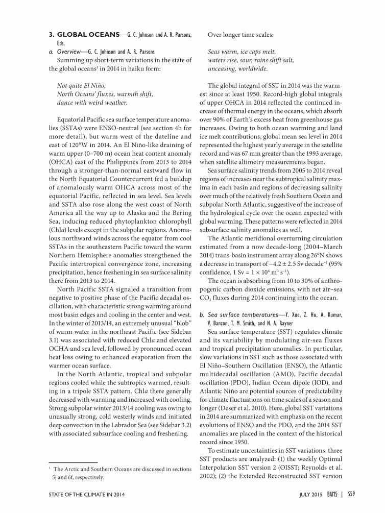
3. GLOBAL OCEANS—G. C. Johnson and A. R. Parsons, Eds.
a. Overview—G. C. Johnson and A. R. ParsonsSumming up short-term variations in the state of
the global oceans1 in 2014 in haiku form:
Not quite El Niño,North Oceans’ fluxes, warmth shift,dance with weird weather.
Equatorial Pacific sea surface temperature anoma-lies (SSTAs) were ENSO-neutral (see section 4b for more detail), but warm west of the dateline and east of 120°W in 2014. An El Niño-like draining of warm upper (0–700 m) ocean heat content anomaly (OHCA) east of the Philippines from 2013 to 2014 through a stronger-than-normal eastward f low in the North Equatorial Countercurrent fed a buildup of anomalously warm OHCA across most of the equatorial Pacific, ref lected in sea level. Sea levels and SSTA also rose along the west coast of North America all the way up to Alaska and the Bering Sea, inducing reduced phytoplankton chlorophyll (Chla) levels except in the subpolar regions. Anoma-lous northward winds across the equator from cool SSTAs in the southeastern Pacific toward the warm Northern Hemisphere anomalies strengthened the Pacific intertropical convergence zone, increasing precipitation, hence freshening in sea surface salinity there from 2013 to 2014.
North Pacific SSTA signaled a transition from negative to positive phase of the Pacific decadal os-cillation, with characteristic strong warming around most basin edges and cooling in the center and west. In the winter of 2013/14, an extremely unusual “blob” of warm water in the northeast Pacific (see Sidebar 3.1) was associated with reduced Chla and elevated OCHA and sea level, followed by pronounced ocean heat loss owing to enhanced evaporation from the warmer ocean surface.
In the North Atlantic, tropical and subpolar regions cooled while the subtropics warmed, result-ing in a tripole SSTA pattern. Chla there generally decreased with warming and increased with cooling. Strong subpolar winter 2013/14 cooling was owing to unusually strong, cold westerly winds and initiated deep convection in the Labrador Sea (see Sidebar 3.2) with associated subsurface cooling and freshening.
1 The Arctic and Southern Oceans are discussed in sections 5j and 6f, respectively.
Over longer time scales:
Seas warm, ice caps melt,waters rise, sour, rains shift salt,unceasing, worldwide.
The global integral of SST in 2014 was the warm-est since at least 1950. Record-high global integrals of upper OHCA in 2014 reflected the continued in-crease of thermal energy in the oceans, which absorb over 90% of Earth’s excess heat from greenhouse gas increases. Owing to both ocean warming and land ice melt contributions, global mean sea level in 2014 represented the highest yearly average in the satellite record and was 67 mm greater than the 1993 average, when satellite altimetry measurements began.
Sea surface salinity trends from 2005 to 2014 reveal regions of increases near the subtropical salinity max-ima in each basin and regions of decreasing salinity over much of the relatively fresh Southern Ocean and subpolar North Atlantic, suggestive of the increase of the hydrological cycle over the ocean expected with global warming. These patterns were reflected in 2014 subsurface salinity anomalies as well.
The Atlantic meridional overturning circulation estimated from a now decade-long (2004–March 2014) trans-basin instrument array along 26°N shows a decrease in transport of −4.2 ± 2.5 Sv decade−1 (95% confidence, 1 Sv = 1 × 10⁶ m3 s−1).
The ocean is absorbing from 10 to 30% of anthro-pogenic carbon dioxide emissions, with net air–sea CO2 fluxes during 2014 continuing into the ocean.
b. Sea surface temperatures—Y. Xue, Z. Hu, A. Kumar, V. Banzon, T. M. Smith, and N. A. RaynerSea surface temperature (SST) regulates climate
and its variability by modulating air-sea f luxes and tropical precipitation anomalies. In particular, slow variations in SST such as those associated with El Niño–Southern Oscillation (ENSO), the Atlantic multidecadal oscillation (AMO), Pacific decadal oscillation (PDO), Indian Ocean dipole (IOD), and Atlantic Niño are potential sources of predictability for climate fluctuations on time scales of a season and longer (Deser et al. 2010). Here, global SST variations in 2014 are summarized with emphasis on the recent evolutions of ENSO and the PDO, and the 2014 SST anomalies are placed in the context of the historical record since 1950.
To estimate uncertainties in SST variations, three SST products are analyzed: (1) the weekly Optimal Interpolation SST version 2 (OISST; Reynolds et al. 2002); (2) the Extended Reconstructed SST version
S59JULY 2015STATE OF THE CLIMATE IN 2014 |
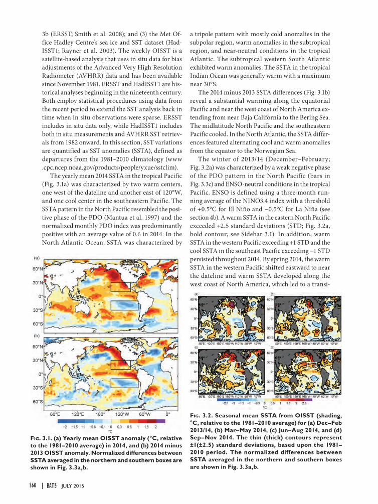
3b (ERSST; Smith et al. 2008); and (3) the Met Of-fice Hadley Centre’s sea ice and SST dataset (Had-ISST1; Rayner et al. 2003). The weekly OISST is a satellite-based analysis that uses in situ data for bias adjustments of the Advanced Very High Resolution Radiometer (AVHRR) data and has been available since November 1981. ERSST and HadISST1 are his-torical analyses beginning in the nineteenth century. Both employ statistical procedures using data from the recent period to extend the SST analysis back in time when in situ observations were sparse. ERSST includes in situ data only, while HadISST1 includes both in situ measurements and AVHRR SST retriev-als from 1982 onward. In this section, SST variations are quantified as SST anomalies (SSTA), defined as departures from the 1981–2010 climatology (www .cpc.ncep.noaa.gov/products/people/yxue/sstclim).
The yearly mean 2014 SSTA in the tropical Pacific (Fig. 3.1a) was characterized by two warm centers, one west of the dateline and another east of 120°W, and one cool center in the southeastern Pacific. The SSTA pattern in the North Pacific resembled the posi-tive phase of the PDO (Mantua et al. 1997) and the normalized monthly PDO index was predominantly positive with an average value of 0.6 in 2014. In the North Atlantic Ocean, SSTA was characterized by
a tripole pattern with mostly cold anomalies in the subpolar region, warm anomalies in the subtropical region, and near-neutral conditions in the tropical Atlantic. The subtropical western South Atlantic exhibited warm anomalies. The SSTA in the tropical Indian Ocean was generally warm with a maximum near 30°S.
The 2014 minus 2013 SSTA differences (Fig. 3.1b) reveal a substantial warming along the equatorial Pacific and near the west coast of North America ex-tending from near Baja California to the Bering Sea. The midlatitude North Pacific and the southeastern Pacific cooled. In the North Atlantic, the SSTA differ-ences featured alternating cool and warm anomalies from the equator to the Norwegian Sea.
The winter of 2013/14 (December–February; Fig. 3.2a) was characterized by a weak negative phase of the PDO pattern in the North Pacific (bars in Fig. 3.3c) and ENSO-neutral conditions in the tropical Pacific. ENSO is defined using a three-month run-ning average of the NINO3.4 index with a threshold of +0.5°C for El Niño and −0.5°C for La Niña (see section 4b). A warm SSTA in the eastern North Pacific exceeded +2.5 standard deviations (STD; Fig. 3.2a, bold contour; see Sidebar 3.1). In addition, warm SSTA in the western Pacific exceeding +1 STD and the cool SSTA in the southeast Pacific exceeding −1 STD persisted throughout 2014. By spring 2014, the warm SSTA in the western Pacific shifted eastward to near the dateline and warm SSTA developed along the west coast of North America, which led to a transi-
Fig. 3.1. (a) Yearly mean OISST anomaly (°C, relative to the 1981–2010 average) in 2014, and (b) 2014 minus 2013 OISST anomaly. Normalized differences between SSTA averaged in the northern and southern boxes are shown in Fig. 3.3a,b.
Fig. 3.2. Seasonal mean SSTA from OISST (shading, °C, relative to the 1981–2010 average) for (a) Dec–Feb 2013/14, (b) Mar–May 2014, (c) Jun–Aug 2014, and (d) Sep–Nov 2014. The thin (thick) contours represent ±1(±2.5) standard deviations, based upon the 1981–2010 period. The normalized differences between SSTA averaged in the northern and southern boxes are shown in Fig. 3.3a,b.
S60 JULY 2015|
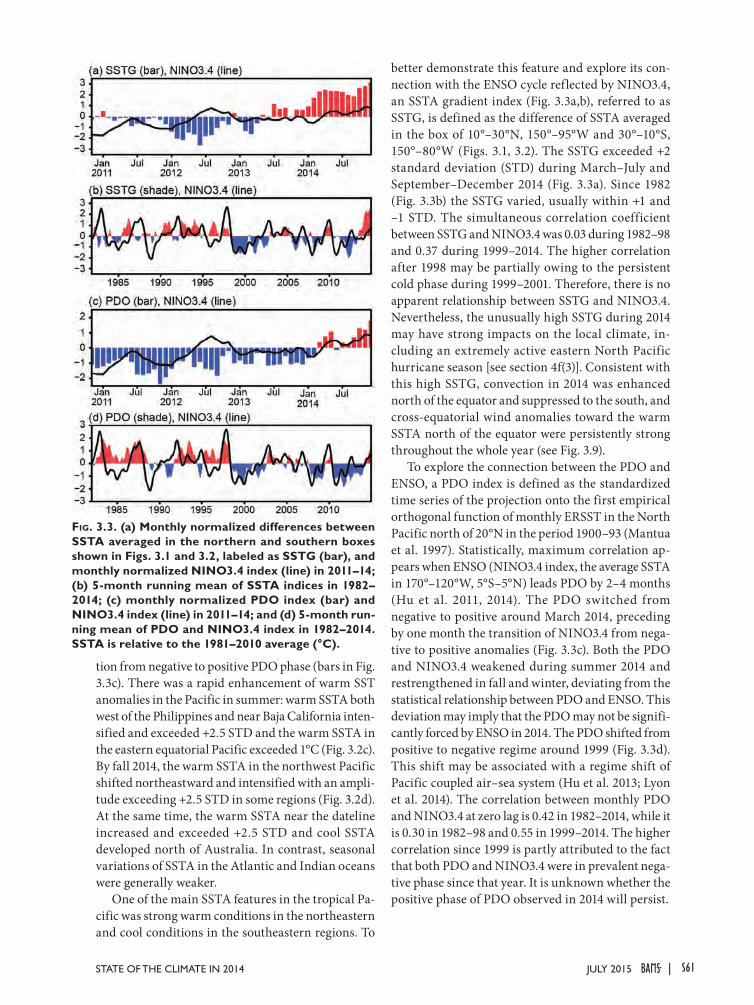
tion from negative to positive PDO phase (bars in Fig. 3.3c). There was a rapid enhancement of warm SST anomalies in the Pacific in summer: warm SSTA both west of the Philippines and near Baja California inten-sified and exceeded +2.5 STD and the warm SSTA in the eastern equatorial Pacific exceeded 1°C (Fig. 3.2c). By fall 2014, the warm SSTA in the northwest Pacific shifted northeastward and intensified with an ampli-tude exceeding +2.5 STD in some regions (Fig. 3.2d). At the same time, the warm SSTA near the dateline increased and exceeded +2.5 STD and cool SSTA developed north of Australia. In contrast, seasonal variations of SSTA in the Atlantic and Indian oceans were generally weaker.
One of the main SSTA features in the tropical Pa-cific was strong warm conditions in the northeastern and cool conditions in the southeastern regions. To
better demonstrate this feature and explore its con-nection with the ENSO cycle reflected by NINO3.4, an SSTA gradient index (Fig. 3.3a,b), referred to as SSTG, is defined as the difference of SSTA averaged in the box of 10°–30°N, 150°–95°W and 30°–10°S, 150°–80°W (Figs. 3.1, 3.2). The SSTG exceeded +2 standard deviation (STD) during March–July and September–December 2014 (Fig. 3.3a). Since 1982 (Fig. 3.3b) the SSTG varied, usually within +1 and –1 STD. The simultaneous correlation coefficient between SSTG and NINO3.4 was 0.03 during 1982–98 and 0.37 during 1999–2014. The higher correlation after 1998 may be partially owing to the persistent cold phase during 1999–2001. Therefore, there is no apparent relationship between SSTG and NINO3.4. Nevertheless, the unusually high SSTG during 2014 may have strong impacts on the local climate, in-cluding an extremely active eastern North Pacific hurricane season [see section 4f(3)]. Consistent with this high SSTG, convection in 2014 was enhanced north of the equator and suppressed to the south, and cross-equatorial wind anomalies toward the warm SSTA north of the equator were persistently strong throughout the whole year (see Fig. 3.9).
To explore the connection between the PDO and ENSO, a PDO index is defined as the standardized time series of the projection onto the first empirical orthogonal function of monthly ERSST in the North Pacific north of 20°N in the period 1900–93 (Mantua et al. 1997). Statistically, maximum correlation ap-pears when ENSO (NINO3.4 index, the average SSTA in 170°–120°W, 5°S–5°N) leads PDO by 2–4 months (Hu et al. 2011, 2014). The PDO switched from negative to positive around March 2014, preceding by one month the transition of NINO3.4 from nega-tive to positive anomalies (Fig. 3.3c). Both the PDO and NINO3.4 weakened during summer 2014 and restrengthened in fall and winter, deviating from the statistical relationship between PDO and ENSO. This deviation may imply that the PDO may not be signifi-cantly forced by ENSO in 2014. The PDO shifted from positive to negative regime around 1999 (Fig. 3.3d). This shift may be associated with a regime shift of Pacific coupled air–sea system (Hu et al. 2013; Lyon et al. 2014). The correlation between monthly PDO and NINO3.4 at zero lag is 0.42 in 1982–2014, while it is 0.30 in 1982–98 and 0.55 in 1999–2014. The higher correlation since 1999 is partly attributed to the fact that both PDO and NINO3.4 were in prevalent nega-tive phase since that year. It is unknown whether the positive phase of PDO observed in 2014 will persist.
Fig. 3.3. (a) Monthly normalized differences between SSTA averaged in the northern and southern boxes shown in Figs. 3.1 and 3.2, labeled as SSTG (bar), and monthly normalized NINO3.4 index (line) in 2011–14; (b) 5-month running mean of SSTA indices in 1982–2014; (c) monthly normalized PDO index (bar) and NINO3.4 index (line) in 2011–14; and (d) 5-month run-ning mean of PDO and NINO3.4 index in 1982–2014. SSTA is relative to the 1981–2010 average (°C).
S61JULY 2015STATE OF THE CLIMATE IN 2014 |
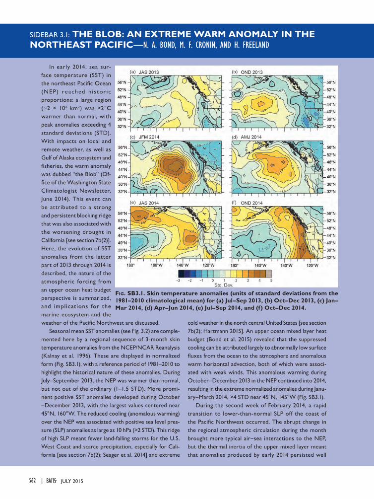
SIDEBAR 3.1: THE BLOB: AN EXTREME WARM ANOMALY IN THE NORTHEAST PACIFIC—N. A. BOND, M. F. CRONIN, AND H. FREELAND
In early 2014, sea sur-face temperature (SST) in the northeast Pacific Ocean (NEP) reached h i s tor ic proportions: a large region (~2 × 10⁶ km2) was >2°C warmer than normal, with peak anomalies exceeding 4 standard deviations (STD). With impacts on local and remote weather, as well as Gulf of Alaska ecosystem and fisheries, the warm anomaly was dubbed “the Blob” (Of-fice of the Washington State Climatologist Newsletter, June 2014). This event can be attributed to a strong and persistent blocking ridge that was also associated with the worsening drought in California [see section 7b(2)]. Here, the evolution of SST anomalies from the latter part of 2013 through 2014 is described, the nature of the atmospheric forcing from an upper ocean heat budget perspective is summarized, and implicat ions for the marine ecosystem and the weather of the Pacific Northwest are discussed.
Seasonal mean SST anomalies (see Fig. 3.2) are comple-mented here by a regional sequence of 3-month skin temperature anomalies from the NCEP/NCAR Reanalysis (Kalnay et al. 1996). These are displayed in normalized form (Fig. SB3.1), with a reference period of 1981–2010 to highlight the historical nature of these anomalies. During July–September 2013, the NEP was warmer than normal, but not out of the ordinary (1–1.5 STD). More promi-nent positive SST anomalies developed during October –December 2013, with the largest values centered near 45°N, 160°W. The reduced cooling (anomalous warming) over the NEP was associated with positive sea level pres-sure (SLP) anomalies as large as 10 hPa (>2 STD). This ridge of high SLP meant fewer land-falling storms for the U.S. West Coast and scarce precipitation, especially for Cali-fornia [see section 7b(2); Seager et al. 2014] and extreme
cold weather in the north central United States [see section 7b(2); Hartmann 2015]. An upper ocean mixed layer heat budget (Bond et al. 2015) revealed that the suppressed cooling can be attributed largely to abnormally low surface fluxes from the ocean to the atmosphere and anomalous warm horizontal advection, both of which were associ-ated with weak winds. This anomalous warming during October–December 2013 in the NEP continued into 2014, resulting in the extreme normalized anomalies during Janu-ary–March 2014, >4 STD near 45°N, 145°W (Fig. SB3.1).
During the second week of February 2014, a rapid transition to lower-than-normal SLP off the coast of the Pacific Northwest occurred. The abrupt change in the regional atmospheric circulation during the month brought more typical air–sea interactions to the NEP, but the thermal inertia of the upper mixed layer meant that anomalies produced by early 2014 persisted well
Fig. SB3.1. Skin temperature anomalies (units of standard deviations from the 1981–2010 climatological mean) for (a) Jul–Sep 2013, (b) Oct–Dec 2013, (c) Jan–Mar 2014, (d) Apr–Jun 2014, (e) Jul–Sep 2014, and (f) Oct–Dec 2014.
S62 JULY 2015|
into the year (Fig. SB3.1). January–March 2014 had near-normal SSTs in the immediate vicinity of the west coast of North America. The next three months (April–June) brought a decrease in the normalized amplitude of the warm anomaly and a horizontal expansion filling the entire NEP. This period included an extension of relatively warm water toward the northwest that continued through July–September, as indicated by SSTs >3 STD above normal in the southern Bering Sea. This sequence can presumably be attributed to advection in the northern portion of the subarctic gyre of the North Pacific; similarly it appears that the warm anomalies from 40°–50°N were carried eastward toward the U.S. West Coast with the mean flow.
There was also a reduction in the magnitude of warm SST anomalies for July–September 2014 in the coastal zone from Vancouver Island to northern California and an enhancement of warm anomalies in the Southern California Bight. These changes appear to be linked to upwelling-favorable wind anomalies in the north and downwelling-favorable winds in the south.
In October–December 2014 relatively cool water developed in the southwest portion of the domain and strongly warm anomalies extended from off the coast of California into the Gulf of Alaska and southern Bering Sea. This distribution is associated with the positive phase of the Pacific decadal oscillation (PDO; Mantua et al. 1997). In specific terms, the PDO index during December 2014 was approximately 2.5, the highest positive value since 1997 and the greatest value for a winter month in the entire record extending back to 1900 (http://jisao.washington .edu/static/pdo/PDO.latest). However, the pattern of the early 2014 warm anomaly differed significantly from the primary modes of North Pacific upper ocean variability,
namely the PDO and the North Pacific Gyre Oscillation (NPGO; Di Lorenzo et al. 2008). Prominent SST anoma-lies do not necessarily project on the primary modes of variability, and likewise, the anomalous atmospheric forc-ing also does not always mimic the leading atmospheric teleconnection patterns. At least some of the anomalous atmospheric forcing of the NEP appears to be attribut-able to a teleconnection pattern driven by deep cumulus convection in the western tropical Pacific (Seager et al. 2014), but a full understanding of the cause(s) of NEP variability is lacking.
The abnormally warm waters in the NEP had apparent implications for the marine ecosystem in the region as anomalously low near-surface chlorophyll concentra-tions were observed for the region in 2014 (see Fig. 3.30; Whitney 2015). This anomaly is likely due to the increased stratification that suppressed vertical mixing of nutrients in the mixed layer. The repercussions of low primary productivity on higher trophic levels are not yet known. Nevertheless, there were a number of unusual sightings of subtropical species well north of their usual ranges. The ocean’s warmth may also have influenced the weather downstream in the coastal region of the western United States, as suggested by the warm temperature anoma-lies that occurred from northern California to British Columbia during July–September 2014 (Fig. SB3.1). SST anomalies in the vicinity of the Blob have corresponded positively with atmospheric boundary layer temperature and humidity downstream over land in the historical re-cord back to 1948 (Bond et al. 2015). This result suggests that in certain situations, major SST anomalies such as that which occurred in the NEP in 2014 may provide a source of predictability for seasonal weather forecasts.
Yearly mean SSTAs from 1950–2014, both global and regional, from OISST, ERSST, and HadISST (Fig. 3.4), reveal that OISST averages are largely con-sistent with those of ERSST in the common period 1982–2014, except in the Southern Ocean. HadISST also agrees well with OISST and ERSST except that it is generally cooler in the tropical Indian Ocean, with differences reaching 0.2°C. While regional averages may be quite consistent among different SST analysis products as discussed here, SSTA in some locations may have large differences. For example, B. Huang et al. (2013) noted that the differences between ERSST and OISST in the NINO3.4 region in 2012 were in the range of −0.3°C to +0.4°C.
Annual mean SSTA for the global ocean is domi-nated by a warming trend superimposed with inter-annual variations largely associated with El Niño and La Niña events (Fig. 3.4a), where the peaks and valleys in the global ocean SSTA often correspond with those in the tropical Pacific SSTA (Fig. 3.4b). After a 30-year period (1970–99) of relatively rapid warming in the global ocean SST (+0.11°C and +0.06°C decade−1 in ERSST and HadISST, respectively), the warming rate for 2000–14 was slower (+0.04°C, +0.03°C, and +0.04°C decade−1 in OISST, ERSST, and HadISST, respectively).
Tropical Pacific SSTA warmed by 0.18°–0.21°C from 2013 to 2014, making 2014 the second warmest
S63JULY 2015STATE OF THE CLIMATE IN 2014 |
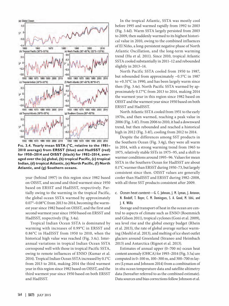
year (behind 1997) in this region since 1982 based on OISST, and second and third warmest since 1950 based on ERSST and HadISST, respectively. Par-tially owing to the warming in the tropical Pacific, the global ocean SSTA warmed by approximately 0.07°–0.08°C from 2013 to 2014, becoming the warm-est year since 1982 based on OISST, and the first and second warmest year since 1950 based on ERSST and HadISST, respectively (Fig. 3.4a).
Tropical Indian Ocean SSTA is dominated by warming with increases of 0.99°C in ERSST and 0.86°C in HadISST from 1950 to 2010, when the historical high value was reached (Fig. 3.4c). Inter-annual variations in tropical Indian Ocean SSTA correspond well with those in tropical Pacific SSTA, owing to remote influences of ENSO (Kumar et al. 2014). Tropical Indian Ocean SSTA increased by 0.1°C from 2013 to 2014, making 2014 the third warmest year in this region since 1982 based on OISST, and the third warmest year since 1950 based on both ERSST and HadISST.
In the tropical Atlantic, SSTA was mostly cool before 1995 and warmed rapidly from 1992 to 2003 (Fig. 3.4d). Warm SSTA largely persisted from 2003 to 2009, then suddenly warmed to its highest histori-cal value in 2010, owing to the combined influences of El Niño, a long-persistent negative phase of North Atlantic Oscillation, and the long-term warming trend (Hu et al. 2011). Since 2010, tropical Atlantic SSTA cooled substantially in 2011–12 and rebounded slightly in 2013–14.
North Pacific SSTA cooled from 1950 to 1987, but rebounded from approximately −0.5°C in 1987 to +0.31°C in 1990, and has been largely warm since then (Fig. 3.4e). North Pacific SSTA warmed by ap-proximately 0.17°C from 2013 to 2014, making 2014 the warmest year in this region since 1982 based on OISST and the warmest year since 1950 based on both ERSST and HadISST.
North Atlantic SSTA cooled from 1951 to the early 1970s, and then warmed, reaching a peak value in 2006 (Fig. 3.4f). From 2006 to 2010, it had a downward trend, but then rebounded and reached a historical high in 2012 (Fig. 3.4f), cooling from 2012 to 2014.
Despite the differences among SST products in the Southern Ocean (Fig. 3.4g), they were all warm in 2014, with a strong warming trend from 1965 to 1975, relatively stable SSTs in 1975–95, and a shift to warmer conditions around 1995–96. Values for mean SSTA in the Southern Ocean for HadISST are about 0.1°C warmer than ERSST during 1950–73, but largely consistent since then. OISST values are generally cooler than HadISST and ERSST during 1982–2008, with all three SST products consistent after 2009.
c. Ocean heat content—G. C. Johnson, J. M. Lyman, J. Antonov, N. Bindoff, T. Boyer, C. M. Domingues, S. A. Good, M. Ishii, and J. K. WillisStorage and transport of heat in the ocean are cen-
tral to aspects of climate such as ENSO (Roemmich and Gilson 2011), tropical cyclones (Goni et al. 2009), sea level rise and the global energy budget (Rhein et al. 2013), the rate of global average surface warm-ing (Meehl et al. 2013), and melting of ice sheet outlet glaciers around Greenland (Straneo and Heimbach 2013) and Antarctica (Rignot et al. 2013).
Estimates of annual upper (0–700 m) ocean heat content anomaly (OHCA) for 1993–2014 (Fig. 3.5a) are computed in 0–100 m, 100–300 m, and 300–700 m lay-ers (Lyman and Johnson 2014) from a combination of in situ ocean temperature data and satellite altimetry data (hereafter referred to as the combined estimate). Data sources and bias corrections follow Johnson et al.
Fig. 3.4. Yearly mean SSTA (°C, relative to the 1981–2010 average) from ERSST (blue) and HadISST (red) for 1950–2014 and OISST (black) for 1982–2014, aver-aged over the (a) global, (b) tropical Pacific, (c) tropical Indian, (d) tropical Atlantic, (e) North Pacific, (f) North Atlantic, and (g) Southern oceans.
S64 JULY 2015|
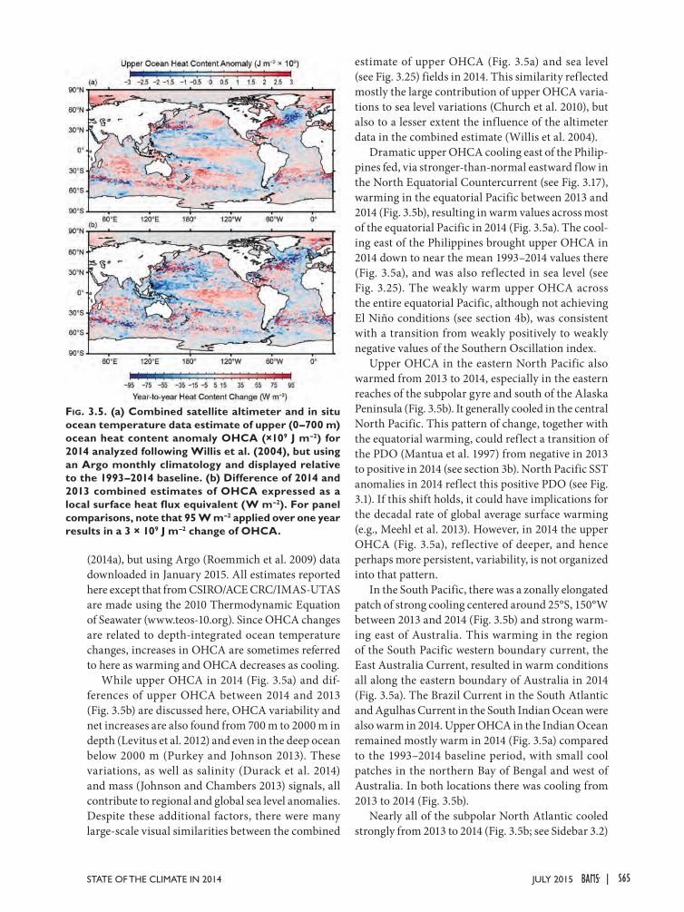
(2014a), but using Argo (Roemmich et al. 2009) data downloaded in January 2015. All estimates reported here except that from CSIRO/ACE CRC/IMAS-UTAS are made using the 2010 Thermodynamic Equation of Seawater (www.teos-10.org). Since OHCA changes are related to depth-integrated ocean temperature changes, increases in OHCA are sometimes referred to here as warming and OHCA decreases as cooling.
While upper OHCA in 2014 (Fig. 3.5a) and dif-ferences of upper OHCA between 2014 and 2013 (Fig. 3.5b) are discussed here, OHCA variability and net increases are also found from 700 m to 2000 m in depth (Levitus et al. 2012) and even in the deep ocean below 2000 m (Purkey and Johnson 2013). These variations, as well as salinity (Durack et al. 2014) and mass (Johnson and Chambers 2013) signals, all contribute to regional and global sea level anomalies. Despite these additional factors, there were many large-scale visual similarities between the combined
estimate of upper OHCA (Fig. 3.5a) and sea level (see Fig. 3.25) fields in 2014. This similarity reflected mostly the large contribution of upper OHCA varia-tions to sea level variations (Church et al. 2010), but also to a lesser extent the influence of the altimeter data in the combined estimate (Willis et al. 2004).
Dramatic upper OHCA cooling east of the Philip-pines fed, via stronger-than-normal eastward flow in the North Equatorial Countercurrent (see Fig. 3.17), warming in the equatorial Pacific between 2013 and 2014 (Fig. 3.5b), resulting in warm values across most of the equatorial Pacific in 2014 (Fig. 3.5a). The cool-ing east of the Philippines brought upper OHCA in 2014 down to near the mean 1993–2014 values there (Fig. 3.5a), and was also ref lected in sea level (see Fig. 3.25). The weakly warm upper OHCA across the entire equatorial Pacific, although not achieving El Niño conditions (see section 4b), was consistent with a transition from weakly positively to weakly negative values of the Southern Oscillation index.
Upper OHCA in the eastern North Pacific also warmed from 2013 to 2014, especially in the eastern reaches of the subpolar gyre and south of the Alaska Peninsula (Fig. 3.5b). It generally cooled in the central North Pacific. This pattern of change, together with the equatorial warming, could reflect a transition of the PDO (Mantua et al. 1997) from negative in 2013 to positive in 2014 (see section 3b). North Pacific SST anomalies in 2014 reflect this positive PDO (see Fig. 3.1). If this shift holds, it could have implications for the decadal rate of global average surface warming (e.g., Meehl et al. 2013). However, in 2014 the upper OHCA (Fig. 3.5a), ref lective of deeper, and hence perhaps more persistent, variability, is not organized into that pattern.
In the South Pacific, there was a zonally elongated patch of strong cooling centered around 25°S, 150°W between 2013 and 2014 (Fig. 3.5b) and strong warm-ing east of Australia. This warming in the region of the South Pacific western boundary current, the East Australia Current, resulted in warm conditions all along the eastern boundary of Australia in 2014 (Fig. 3.5a). The Brazil Current in the South Atlantic and Agulhas Current in the South Indian Ocean were also warm in 2014. Upper OHCA in the Indian Ocean remained mostly warm in 2014 (Fig. 3.5a) compared to the 1993–2014 baseline period, with small cool patches in the northern Bay of Bengal and west of Australia. In both locations there was cooling from 2013 to 2014 (Fig. 3.5b).
Nearly all of the subpolar North Atlantic cooled strongly from 2013 to 2014 (Fig. 3.5b; see Sidebar 3.2)
Fig. 3.5. (a) Combined satellite altimeter and in situ ocean temperature data estimate of upper (0–700 m) ocean heat content anomaly OHCA (×109 J m–2) for 2014 analyzed following Willis et al. (2004), but using an Argo monthly climatology and displayed relative to the 1993–2014 baseline. (b) Difference of 2014 and 2013 combined estimates of OHCA expressed as a local surface heat flux equivalent (W m–2). For panel comparisons, note that 95 W m–2 applied over one year results in a 3 × 10⁹ J m–2 change of OHCA.
S65JULY 2015STATE OF THE CLIMATE IN 2014 |
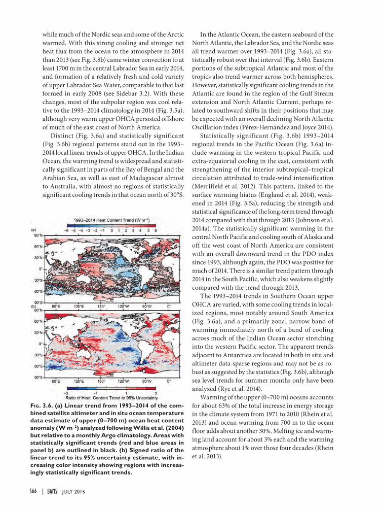
while much of the Nordic seas and some of the Arctic warmed. With this strong cooling and stronger net heat flux from the ocean to the atmosphere in 2014 than 2013 (see Fig. 3.8b) came winter convection to at least 1700 m in the central Labrador Sea in early 2014, and formation of a relatively fresh and cold variety of upper Labrador Sea Water, comparable to that last formed in early 2008 (see Sidebar 3.2). With these changes, most of the subpolar region was cool rela-tive to the 1993–2014 climatology in 2014 (Fig. 3.5a), although very warm upper OHCA persisted offshore of much of the east coast of North America.
Distinct (Fig. 3.6a) and statistically significant (Fig. 3.6b) regional patterns stand out in the 1993–2014 local linear trends of upper OHCA. In the Indian Ocean, the warming trend is widespread and statisti-cally significant in parts of the Bay of Bengal and the Arabian Sea, as well as east of Madagascar almost to Australia, with almost no regions of statistically significant cooling trends in that ocean north of 30°S.
In the Atlantic Ocean, the eastern seaboard of the North Atlantic, the Labrador Sea, and the Nordic seas all trend warmer over 1993–2014 (Fig. 3.6a), all sta-tistically robust over that interval (Fig. 3.6b). Eastern portions of the subtropical Atlantic and most of the tropics also trend warmer across both hemispheres. However, statistically significant cooling trends in the Atlantic are found in the region of the Gulf Stream extension and North Atlantic Current, perhaps re-lated to southward shifts in their positions that may be expected with an overall declining North Atlantic Oscillation index (Pérez-Hernández and Joyce 2014).
Statistically significant (Fig. 3.6b) 1993–2014 regional trends in the Pacific Ocean (Fig. 3.6a) in-clude warming in the western tropical Pacific and extra-equatorial cooling in the east, consistent with strengthening of the interior subtropical–tropical circulation attributed to trade-wind intensification (Merrifield et al. 2012). This pattern, linked to the surface warming hiatus (England et al. 2014), weak-ened in 2014 (Fig. 3.5a), reducing the strength and statistical significance of the long-term trend through 2014 compared with that through 2013 (Johnson et al. 2014a). The statistically significant warming in the central North Pacific and cooling south of Alaska and off the west coast of North America are consistent with an overall downward trend in the PDO index since 1993, although again, the PDO was positive for much of 2014. There is a similar trend pattern through 2014 in the South Pacific, which also weakens slightly compared with the trend through 2013.
The 1993–2014 trends in Southern Ocean upper OHCA are varied, with some cooling trends in local-ized regions, most notably around South America (Fig. 3.6a), and a primarily zonal narrow band of warming immediately north of a band of cooling across much of the Indian Ocean sector stretching into the western Pacific sector. The apparent trends adjacent to Antarctica are located in both in situ and altimeter data-sparse regions and may not be as ro-bust as suggested by the statistics (Fig. 3.6b), although sea level trends for summer months only have been analyzed (Rye et al. 2014).
Warming of the upper (0–700 m) oceans accounts for about 63% of the total increase in energy storage in the climate system from 1971 to 2010 (Rhein et al. 2013) and ocean warming from 700 m to the ocean floor adds about another 30%. Melting ice and warm-ing land account for about 3% each and the warming atmosphere about 1% over those four decades (Rhein et al. 2013).
Fig. 3.6. (a) Linear trend from 1993–2014 of the com-bined satellite altimeter and in situ ocean temperature data estimate of upper (0–700 m) ocean heat content anomaly (W m–2) analyzed following Willis et al. (2004) but relative to a monthly Argo climatology. Areas with statistically significant trends (red and blue areas in panel b) are outlined in black. (b) Signed ratio of the linear trend to its 95% uncertainty estimate, with in-creasing color intensity showing regions with increas-ingly statistically significant trends.
S66 JULY 2015|
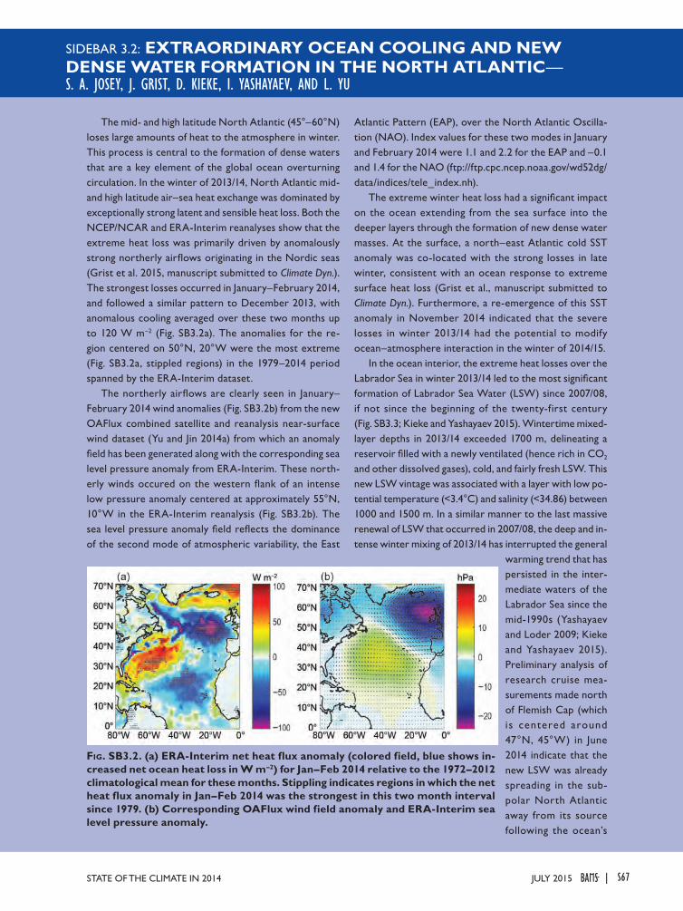
SIDEBAR 3.2: EXTRAORDINARY OCEAN COOLING AND NEW DENSE WATER FORMATION IN THE NORTH ATLANTIC— S. A. JOSEY, J. GRIST, D. KIEKE, I. YASHAYAEV, AND L. YU
The mid- and high latitude North Atlantic (45°–60°N) loses large amounts of heat to the atmosphere in winter. This process is central to the formation of dense waters that are a key element of the global ocean overturning circulation. In the winter of 2013/14, North Atlantic mid- and high latitude air–sea heat exchange was dominated by exceptionally strong latent and sensible heat loss. Both the NCEP/NCAR and ERA-Interim reanalyses show that the extreme heat loss was primarily driven by anomalously strong northerly airflows originating in the Nordic seas (Grist et al. 2015, manuscript submitted to Climate Dyn.). The strongest losses occurred in January–February 2014, and followed a similar pattern to December 2013, with anomalous cooling averaged over these two months up to 120 W m–2 (Fig. SB3.2a). The anomalies for the re-gion centered on 50°N, 20°W were the most extreme (Fig. SB3.2a, stippled regions) in the 1979–2014 period spanned by the ERA-Interim dataset.
The northerly airflows are clearly seen in January–February 2014 wind anomalies (Fig. SB3.2b) from the new OAFlux combined satellite and reanalysis near-surface wind dataset (Yu and Jin 2014a) from which an anomaly field has been generated along with the corresponding sea level pressure anomaly from ERA-Interim. These north-erly winds occured on the western flank of an intense low pressure anomaly centered at approximately 55°N, 10°W in the ERA-Interim reanalysis (Fig. SB3.2b). The sea level pressure anomaly field reflects the dominance of the second mode of atmospheric variability, the East
Atlantic Pattern (EAP), over the North Atlantic Oscilla-tion (NAO). Index values for these two modes in January and February 2014 were 1.1 and 2.2 for the EAP and –0.1 and 1.4 for the NAO (ftp://ftp.cpc.ncep.noaa.gov/wd52dg/data/indices/tele_index.nh).
The extreme winter heat loss had a significant impact on the ocean extending from the sea surface into the deeper layers through the formation of new dense water masses. At the surface, a north–east Atlantic cold SST anomaly was co-located with the strong losses in late winter, consistent with an ocean response to extreme surface heat loss (Grist et al., manuscript submitted to Climate Dyn.). Furthermore, a re-emergence of this SST anomaly in November 2014 indicated that the severe losses in winter 2013/14 had the potential to modify ocean–atmosphere interaction in the winter of 2014/15.
In the ocean interior, the extreme heat losses over the Labrador Sea in winter 2013/14 led to the most significant formation of Labrador Sea Water (LSW) since 2007/08, if not since the beginning of the twenty-first century (Fig. SB3.3; Kieke and Yashayaev 2015). Wintertime mixed-layer depths in 2013/14 exceeded 1700 m, delineating a reservoir filled with a newly ventilated (hence rich in CO2 and other dissolved gases), cold, and fairly fresh LSW. This new LSW vintage was associated with a layer with low po-tential temperature (<3.4°C) and salinity (<34.86) between 1000 and 1500 m. In a similar manner to the last massive renewal of LSW that occurred in 2007/08, the deep and in-tense winter mixing of 2013/14 has interrupted the general
warming trend that has persisted in the inter-mediate waters of the Labrador Sea since the mid-1990s (Yashayaev and Loder 2009; Kieke and Yashayaev 2015). Preliminary analysis of research cruise mea-surements made north of Flemish Cap (which is centered around 47°N, 45°W) in June 2014 indicate that the new LSW was already spreading in the sub-polar North Atlantic away from its source following the ocean’s
Fig. SB3.2. (a) ERA-Interim net heat flux anomaly (colored field, blue shows in-creased net ocean heat loss in W m–2) for Jan–Feb 2014 relative to the 1972–2012 climatological mean for these months. Stippling indicates regions in which the net heat flux anomaly in Jan–Feb 2014 was the strongest in this two month interval since 1979. (b) Corresponding OAFlux wind field anomaly and ERA-Interim sea level pressure anomaly.
S67JULY 2015STATE OF THE CLIMATE IN 2014 |
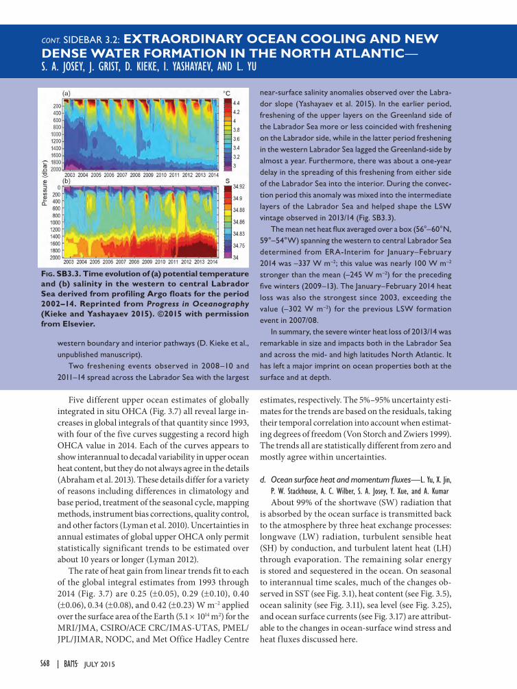
Five different upper ocean estimates of globally integrated in situ OHCA (Fig. 3.7) all reveal large in-creases in global integrals of that quantity since 1993, with four of the five curves suggesting a record high OHCA value in 2014. Each of the curves appears to show interannual to decadal variability in upper ocean heat content, but they do not always agree in the details (Abraham et al. 2013). These details differ for a variety of reasons including differences in climatology and base period, treatment of the seasonal cycle, mapping methods, instrument bias corrections, quality control, and other factors (Lyman et al. 2010). Uncertainties in annual estimates of global upper OHCA only permit statistically significant trends to be estimated over about 10 years or longer (Lyman 2012).
The rate of heat gain from linear trends fit to each of the global integral estimates from 1993 through 2014 (Fig. 3.7) are 0.25 (±0.05), 0.29 (±0.10), 0.40 (±0.06), 0.34 (±0.08), and 0.42 (±0.23) W m−2 applied over the surface area of the Earth (5.1 × 10¹⁴ m2) for the MRI/JMA, CSIRO/ACE CRC/IMAS-UTAS, PMEL/JPL/JIMAR, NODC, and Met Office Hadley Centre
estimates, respectively. The 5%–95% uncertainty esti-mates for the trends are based on the residuals, taking their temporal correlation into account when estimat-ing degrees of freedom (Von Storch and Zwiers 1999). The trends all are statistically different from zero and mostly agree within uncertainties.
d. Ocean surface heat and momentum fluxes—L. Yu, X. Jin, P. W. Stackhouse, A. C. Wilber, S. A. Josey, Y. Xue, and A. KumarAbout 99% of the shortwave (SW) radiation that
is absorbed by the ocean surface is transmitted back to the atmosphere by three heat exchange processes: longwave (LW) radiation, turbulent sensible heat (SH) by conduction, and turbulent latent heat (LH) through evaporation. The remaining solar energy is stored and sequestered in the ocean. On seasonal to interannual time scales, much of the changes ob-served in SST (see Fig. 3.1), heat content (see Fig. 3.5), ocean salinity (see Fig. 3.11), sea level (see Fig. 3.25), and ocean surface currents (see Fig. 3.17) are attribut-able to the changes in ocean-surface wind stress and heat fluxes discussed here.
CONT. SIDEBAR 3.2: EXTRAORDINARY OCEAN COOLING AND NEW DENSE WATER FORMATION IN THE NORTH ATLANTIC— S. A. JOSEY, J. GRIST, D. KIEKE, I. YASHAYAEV, AND L. YU
Fig. SB3.3. Time evolution of (a) potential temperature and (b) salinity in the western to central Labrador Sea derived from profiling Argo floats for the period 2002–14. Reprinted from Progress in Oceanography (Kieke and Yashayaev 2015). ©2015 with permission from Elsevier.
western boundary and interior pathways (D. Kieke et al., unpublished manuscript).
Two freshening events observed in 2008–10 and 2011–14 spread across the Labrador Sea with the largest
near-surface salinity anomalies observed over the Labra-dor slope (Yashayaev et al. 2015). In the earlier period, freshening of the upper layers on the Greenland side of the Labrador Sea more or less coincided with freshening on the Labrador side, while in the latter period freshening in the western Labrador Sea lagged the Greenland-side by almost a year. Furthermore, there was about a one-year delay in the spreading of this freshening from either side of the Labrador Sea into the interior. During the convec-tion period this anomaly was mixed into the intermediate layers of the Labrador Sea and helped shape the LSW vintage observed in 2013/14 (Fig. SB3.3).
The mean net heat flux averaged over a box (56°–60°N, 59°–54°W) spanning the western to central Labrador Sea determined from ERA-Interim for January–February 2014 was –337 W m–2; this value was nearly 100 W m–2 stronger than the mean (–245 W m–2) for the preceding five winters (2009–13). The January–February 2014 heat loss was also the strongest since 2003, exceeding the value (–302 W m–2) for the previous LSW formation event in 2007/08.
In summary, the severe winter heat loss of 2013/14 was remarkable in size and impacts both in the Labrador Sea and across the mid- and high latitudes North Atlantic. It has left a major imprint on ocean properties both at the surface and at depth.
S68 JULY 2015|
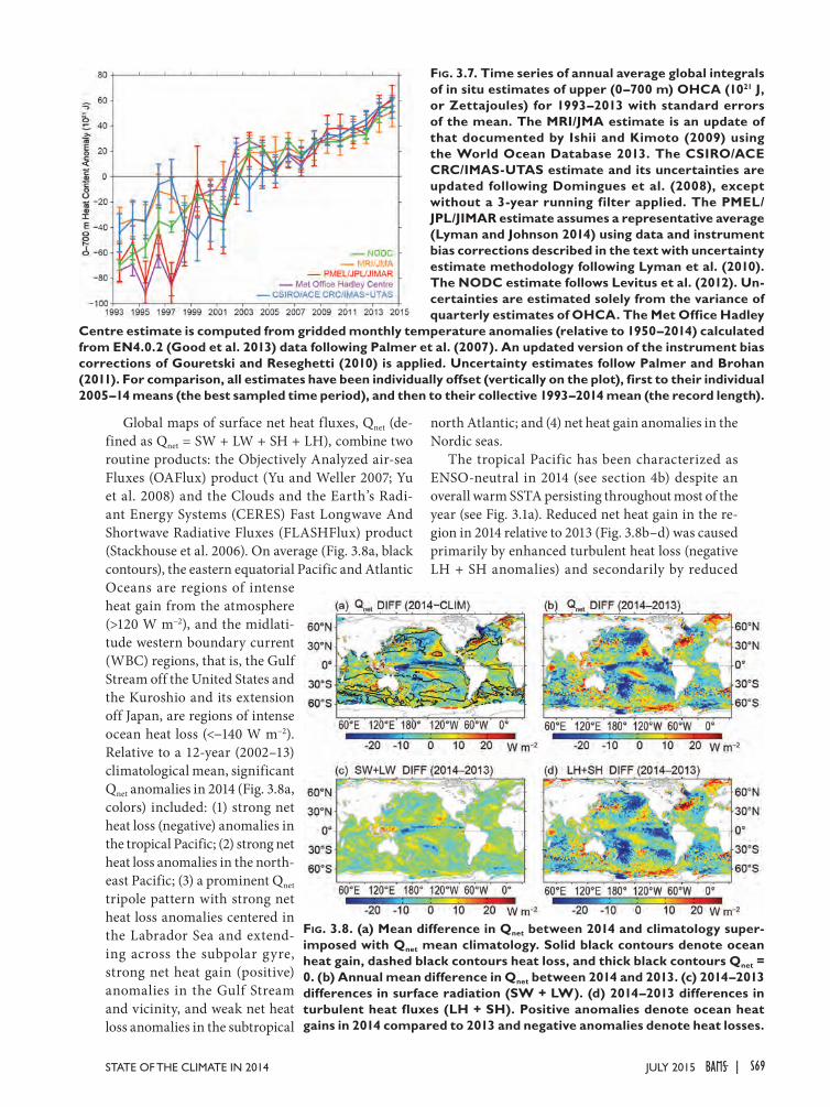
Global maps of surface net heat fluxes, Qnet (de-fined as Qnet = SW + LW + SH + LH), combine two routine products: the Objectively Analyzed air-sea Fluxes (OAFlux) product (Yu and Weller 2007; Yu et al. 2008) and the Clouds and the Earth’s Radi-ant Energy Systems (CERES) Fast Longwave And Shortwave Radiative Fluxes (FLASHFlux) product (Stackhouse et al. 2006). On average (Fig. 3.8a, black contours), the eastern equatorial Pacific and Atlantic Oceans are regions of intense heat gain from the atmosphere (>120 W m−2), and the midlati-tude western boundary current (WBC) regions, that is, the Gulf Stream off the United States and the Kuroshio and its extension off Japan, are regions of intense ocean heat loss (<−140 W m−2). Relative to a 12-year (2002–13) climatological mean, significant Qnet anomalies in 2014 (Fig. 3.8a, colors) included: (1) strong net heat loss (negative) anomalies in the tropical Pacific; (2) strong net heat loss anomalies in the north-east Pacific; (3) a prominent Qnet tripole pattern with strong net heat loss anomalies centered in the Labrador Sea and extend-ing across the subpolar gyre, strong net heat gain (positive) anomalies in the Gulf Stream and vicinity, and weak net heat loss anomalies in the subtropical
north Atlantic; and (4) net heat gain anomalies in the Nordic seas.
The tropical Pacific has been characterized as ENSO-neutral in 2014 (see section 4b) despite an overall warm SSTA persisting throughout most of the year (see Fig. 3.1a). Reduced net heat gain in the re-gion in 2014 relative to 2013 (Fig. 3.8b–d) was caused primarily by enhanced turbulent heat loss (negative LH + SH anomalies) and secondarily by reduced
Fig. 3.8. (a) Mean difference in Qnet between 2014 and climatology super-imposed with Qnet mean climatology. Solid black contours denote ocean heat gain, dashed black contours heat loss, and thick black contours Qnet = 0. (b) Annual mean difference in Qnet between 2014 and 2013. (c) 2014–2013 differences in surface radiation (SW + LW). (d) 2014–2013 differences in turbulent heat fluxes (LH + SH). Positive anomalies denote ocean heat gains in 2014 compared to 2013 and negative anomalies denote heat losses.
Fig. 3.7. Time series of annual average global integrals of in situ estimates of upper (0–700 m) OHCA (1021 J, or Zettajoules) for 1993–2013 with standard errors of the mean. The MRI/JMA estimate is an update of that documented by Ishii and Kimoto (2009) using the World Ocean Database 2013. The CSIRO/ACE CRC/IMAS-UTAS estimate and its uncertainties are updated following Domingues et al. (2008), except without a 3-year running filter applied. The PMEL/JPL/JIMAR estimate assumes a representative average (Lyman and Johnson 2014) using data and instrument bias corrections described in the text with uncertainty estimate methodology following Lyman et al. (2010). The NODC estimate follows Levitus et al. (2012). Un-certainties are estimated solely from the variance of quarterly estimates of OHCA. The Met Office Hadley
Centre estimate is computed from gridded monthly temperature anomalies (relative to 1950–2014) calculated from EN4.0.2 (Good et al. 2013) data following Palmer et al. (2007). An updated version of the instrument bias corrections of Gouretski and Reseghetti (2010) is applied. Uncertainty estimates follow Palmer and Brohan (2011). For comparison, all estimates have been individually offset (vertically on the plot), first to their individual 2005–14 means (the best sampled time period), and then to their collective 1993–2014 mean (the record length).
S69JULY 2015STATE OF THE CLIMATE IN 2014 |
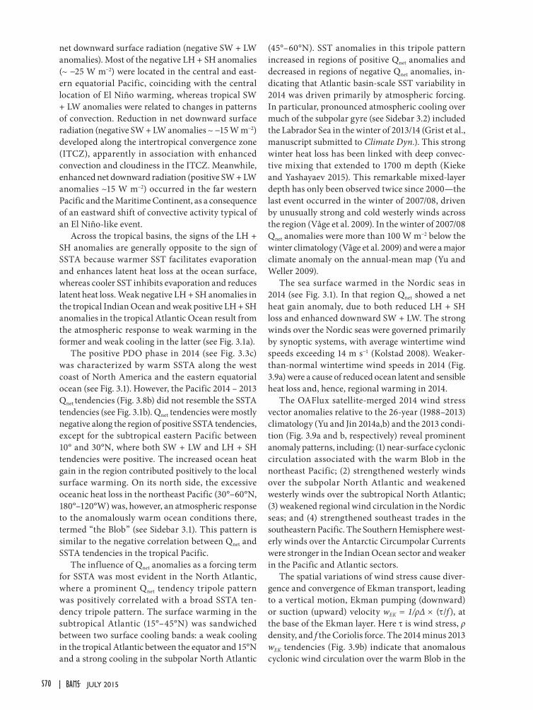
net downward surface radiation (negative SW + LW anomalies). Most of the negative LH + SH anomalies (~ −25 W m−2) were located in the central and east-ern equatorial Pacific, coinciding with the central location of El Niño warming, whereas tropical SW + LW anomalies were related to changes in patterns of convection. Reduction in net downward surface radiation (negative SW + LW anomalies ~ −15 W m−2) developed along the intertropical convergence zone (ITCZ), apparently in association with enhanced convection and cloudiness in the ITCZ. Meanwhile, enhanced net downward radiation (positive SW + LW anomalies ~15 W m−2) occurred in the far western Pacific and the Maritime Continent, as a consequence of an eastward shift of convective activity typical of an El Niño-like event.
Across the tropical basins, the signs of the LH + SH anomalies are generally opposite to the sign of SSTA because warmer SST facilitates evaporation and enhances latent heat loss at the ocean surface, whereas cooler SST inhibits evaporation and reduces latent heat loss. Weak negative LH + SH anomalies in the tropical Indian Ocean and weak positive LH + SH anomalies in the tropical Atlantic Ocean result from the atmospheric response to weak warming in the former and weak cooling in the latter (see Fig. 3.1a).
The positive PDO phase in 2014 (see Fig. 3.3c) was characterized by warm SSTA along the west coast of North America and the eastern equatorial ocean (see Fig. 3.1). However, the Pacific 2014 – 2013 Qnet tendencies (Fig. 3.8b) did not resemble the SSTA tendencies (see Fig. 3.1b). Qnet tendencies were mostly negative along the region of positive SSTA tendencies, except for the subtropical eastern Pacific between 10° and 30°N, where both SW + LW and LH + SH tendencies were positive. The increased ocean heat gain in the region contributed positively to the local surface warming. On its north side, the excessive oceanic heat loss in the northeast Pacific (30°–60°N, 180°–120°W) was, however, an atmospheric response to the anomalously warm ocean conditions there, termed “the Blob” (see Sidebar 3.1). This pattern is similar to the negative correlation between Qnet and SSTA tendencies in the tropical Pacific.
The influence of Qnet anomalies as a forcing term for SSTA was most evident in the North Atlantic, where a prominent Qnet tendency tripole pattern was positively correlated with a broad SSTA ten-dency tripole pattern. The surface warming in the subtropical Atlantic (15°–45°N) was sandwiched between two surface cooling bands: a weak cooling in the tropical Atlantic between the equator and 15°N and a strong cooling in the subpolar North Atlantic
(45°–60°N). SST anomalies in this tripole pattern increased in regions of positive Qnet anomalies and decreased in regions of negative Qnet anomalies, in-dicating that Atlantic basin-scale SST variability in 2014 was driven primarily by atmospheric forcing. In particular, pronounced atmospheric cooling over much of the subpolar gyre (see Sidebar 3.2) included the Labrador Sea in the winter of 2013/14 (Grist et al., manuscript submitted to Climate Dyn.). This strong winter heat loss has been linked with deep convec-tive mixing that extended to 1700 m depth (Kieke and Yashayaev 2015). This remarkable mixed-layer depth has only been observed twice since 2000—the last event occurred in the winter of 2007/08, driven by unusually strong and cold westerly winds across the region (Våge et al. 2009). In the winter of 2007/08 Qnet anomalies were more than 100 W m−2 below the winter climatology (Våge et al. 2009) and were a major climate anomaly on the annual-mean map (Yu and Weller 2009).
The sea surface warmed in the Nordic seas in 2014 (see Fig. 3.1). In that region Qnet showed a net heat gain anomaly, due to both reduced LH + SH loss and enhanced downward SW + LW. The strong winds over the Nordic seas were governed primarily by synoptic systems, with average wintertime wind speeds exceeding 14 m s−1 (Kolstad 2008). Weaker-than-normal wintertime wind speeds in 2014 (Fig. 3.9a) were a cause of reduced ocean latent and sensible heat loss and, hence, regional warming in 2014.
The OAFlux satellite-merged 2014 wind stress vector anomalies relative to the 26-year (1988–2013) climatology (Yu and Jin 2014a,b) and the 2013 condi-tion (Fig. 3.9a and b, respectively) reveal prominent anomaly patterns, including: (1) near-surface cyclonic circulation associated with the warm Blob in the northeast Pacific; (2) strengthened westerly winds over the subpolar North Atlantic and weakened westerly winds over the subtropical North Atlantic; (3) weakened regional wind circulation in the Nordic seas; and (4) strengthened southeast trades in the southeastern Pacific. The Southern Hemisphere west-erly winds over the Antarctic Circumpolar Currents were stronger in the Indian Ocean sector and weaker in the Pacific and Atlantic sectors.
The spatial variations of wind stress cause diver-gence and convergence of Ekman transport, leading to a vertical motion, Ekman pumping (downward) or suction (upward) velocity wEK = 1/ρΔ × (τ/f ), at the base of the Ekman layer. Here τ is wind stress, ρ density, and f the Coriolis force. The 2014 minus 2013 wEK tendencies (Fig. 3.9b) indicate that anomalous cyclonic wind circulation over the warm Blob in the
S70 JULY 2015|
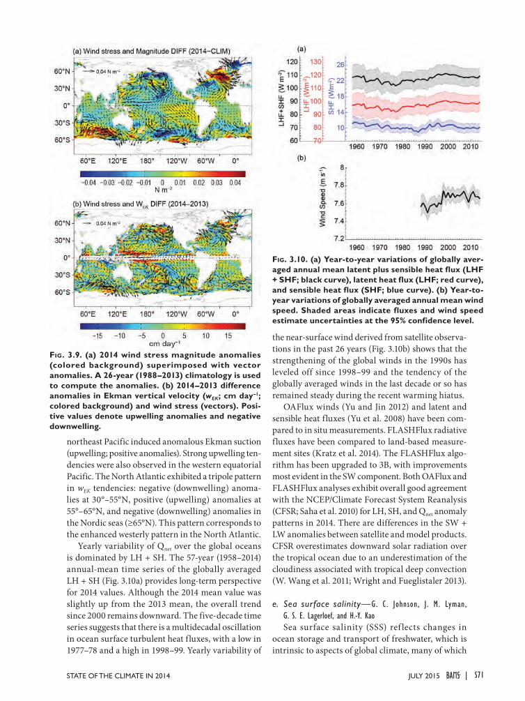
northeast Pacific induced anomalous Ekman suction (upwelling; positive anomalies). Strong upwelling ten-dencies were also observed in the western equatorial Pacific. The North Atlantic exhibited a tripole pattern in wEK tendencies: negative (downwelling) anoma-lies at 30°–55°N, positive (upwelling) anomalies at 55°–65°N, and negative (downwelling) anomalies in the Nordic seas (≥65°N). This pattern corresponds to the enhanced westerly pattern in the North Atlantic.
Yearly variability of Qnet over the global oceans is dominated by LH + SH. The 57-year (1958–2014) annual-mean time series of the globally averaged LH + SH (Fig. 3.10a) provides long-term perspective for 2014 values. Although the 2014 mean value was slightly up from the 2013 mean, the overall trend since 2000 remains downward. The five-decade time series suggests that there is a multidecadal oscillation in ocean surface turbulent heat fluxes, with a low in 1977–78 and a high in 1998–99. Yearly variability of
the near-surface wind derived from satellite observa-tions in the past 26 years (Fig. 3.10b) shows that the strengthening of the global winds in the 1990s has leveled off since 1998–99 and the tendency of the globally averaged winds in the last decade or so has remained steady during the recent warming hiatus.
OAFlux winds (Yu and Jin 2012) and latent and sensible heat fluxes (Yu et al. 2008) have been com-pared to in situ measurements. FLASHFlux radiative fluxes have been compared to land-based measure-ment sites (Kratz et al. 2014). The FLASHFlux algo-rithm has been upgraded to 3B, with improvements most evident in the SW component. Both OAFlux and FLASHFlux analyses exhibit overall good agreement with the NCEP/Climate Forecast System Reanalysis (CFSR; Saha et al. 2010) for LH, SH, and Qnet anomaly patterns in 2014. There are differences in the SW + LW anomalies between satellite and model products. CFSR overestimates downward solar radiation over the tropical ocean due to an underestimation of the cloudiness associated with tropical deep convection (W. Wang et al. 2011; Wright and Fueglistaler 2013).
e. Sea surface salinity—G. C . Johnson, J. M. Lyman, G. S. E. Lagerloef, and H.-Y. KaoSea surface salinity (SSS) ref lects changes in
ocean storage and transport of freshwater, which is intrinsic to aspects of global climate, many of which
Fig. 3.9. (a) 2014 wind stress magnitude anomalies (colored background) superimposed with vector anomalies. A 26-year (1988–2013) climatology is used to compute the anomalies. (b) 2014–2013 difference anomalies in Ekman vertical velocity (wEK; cm day–1; colored background) and wind stress (vectors). Posi-tive values denote upwelling anomalies and negative downwelling.
Fig. 3.10. (a) Year-to-year variations of globally aver-aged annual mean latent plus sensible heat flux (LHF + SHF; black curve), latent heat flux (LHF; red curve), and sensible heat flux (SHF; blue curve). (b) Year-to-year variations of globally averaged annual mean wind speed. Shaded areas indicate fluxes and wind speed estimate uncertainties at the 95% confidence level.
S71JULY 2015STATE OF THE CLIMATE IN 2014 |
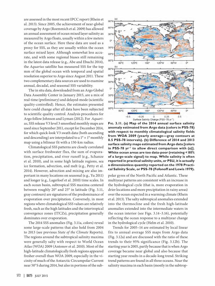
are assessed in the most recent IPCC report (Rhein et al. 2013). Since 2005, the achievement of near-global coverage by Argo (Roemmich et al. 2009) has allowed an annual assessment of ocean mixed layer salinity as measured by Argo floats, usually within a few meters of the ocean surface. Here these data are used as a proxy for SSS, as they are usually within the ocean surface mixed layer. Although somewhat less accu-rate, and with some regional biases still remaining in the latest data release (e.g., Abe and Ebuchi 2014), the Aquarius satellite has measured SSS for the top mm of the global ocean with temporal and spatial resolution superior to Argo since August 2011. These two complementary data sources are used to examine annual, decadal, and seasonal SSS variability.
The in situ data, downloaded from an Argo Global Data Assembly Center in January 2015, are a mix of real-time (preliminary) and delayed-mode (scientific quality-controlled). Hence, the estimates presented here could change after all data have been subjected to scientific quality control. Analysis procedures for Argo follow Johnson and Lyman (2012). For Aquari-us, SSS release V3 level 3 smoothed monthly maps are used since September 2011, except for December 2014, for which quick-look V3 swath data (both ascending and descending) are interpolated to a 1° × 1° monthly map using a bilinear fit with a 150-km radius.
Climatological SSS patterns are closely correlated with surface freshwater f lux, the sum of evapora-tion, precipitation, and river runoff (e.g., Schanze et al. 2010), and in some high latitude regions, sea ice formation, advection, and melt (e.g., Petty et al. 2014). However, advection and mixing are also im-portant in many locations on seasonal (e.g., Yu 2011) and longer (e.g., Lagerloef et al. 2010) time scales. In each ocean basin, subtropical SSS maxima centered between roughly 20° and 25° in latitude (Fig. 3.11, gray contours) are signatures of the predominance of evaporation over precipitation. Conversely, in most regions where climatological SSS values are relatively fresh, such as the high latitudes and the intertropical convergence zones (ITCZs), precipitation generally dominates over evaporation.
The 2014 SSS anomalies (Fig. 3.11a, colors) reveal some large-scale patterns that also hold from 2004 to 2013 (see previous State of the Climate Reports). The regions around the subtropical salinity maxima were generally salty with respect to World Ocean Atlas (WOA) 2009 (Antonov et al. 2010). Most of the high-latitude climatologically fresh regions appeared fresher overall than WOA 2009, especially in the vi-cinity of much of the Antarctic Circumpolar Current near 50°S during 2014, but also in portions of the sub-
polar gyres of the North Pacific and Atlantic. These multiyear patterns are consistent with an increase in the hydrological cycle (that is, more evaporation in drier locations and more precipitation in rainy areas) over the ocean expected in a warming climate (Rhein et al. 2013). The salty subtropical anomalies extended into the thermocline and the fresh high-latitude anomalies extended into the intermediate waters in the ocean interior (see Figs. 3.14–3.16), potentially reflecting the ocean response to a multiyear change in the hydrological cycle (Helm et al. 2010).
Trends for 2005–14 are estimated by local linear fits to annual average SSS maps from Argo data (Fig. 3.12a) and are discussed with the ratio of these trends to their 95% significance (Fig. 3.12b). The starting year is 2005, partly because that is when Argo coverage became near global and also because that starting year results in a decade-long trend. Striking trend patterns are found in all three oceans. Near the salinity maxima in each basin (mostly in the subtrop-
Fig. 3.11. (a) Map of the 2014 annual surface salinity anomaly estimated from Argo data (colors in PSS-78) with respect to monthly climatological salinity fields from WOA 2009 (yearly average—gray contours at 0.5 PSS-78 intervals). (b) Difference of 2014 and 2013 surface salinity maps estimated from Argo data [colors in PSS-78 yr–1 to allow direct comparison with (a)]. White ocean areas are too data-poor (retaining < 80% of a large-scale signal) to map. While salinity is often reported in practical salinity units, or PSU, it is actually a dimensionless quantity reported on the 1978 Practi-cal Salinity Scale, or PSS-78 (Fofonoff and Lewis 1979).
S72 JULY 2015|
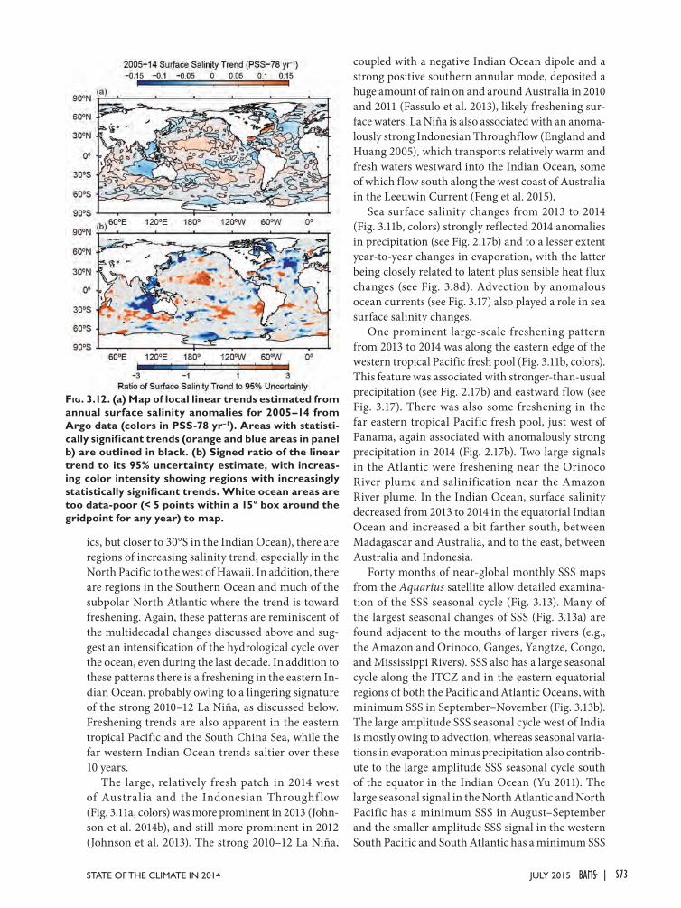
ics, but closer to 30°S in the Indian Ocean), there are regions of increasing salinity trend, especially in the North Pacific to the west of Hawaii. In addition, there are regions in the Southern Ocean and much of the subpolar North Atlantic where the trend is toward freshening. Again, these patterns are reminiscent of the multidecadal changes discussed above and sug-gest an intensification of the hydrological cycle over the ocean, even during the last decade. In addition to these patterns there is a freshening in the eastern In-dian Ocean, probably owing to a lingering signature of the strong 2010–12 La Niña, as discussed below. Freshening trends are also apparent in the eastern tropical Pacific and the South China Sea, while the far western Indian Ocean trends saltier over these 10 years.
The large, relatively fresh patch in 2014 west of Australia and the Indonesian Throughf low (Fig. 3.11a, colors) was more prominent in 2013 (John-son et al. 2014b), and still more prominent in 2012 (Johnson et al. 2013). The strong 2010–12 La Niña,
coupled with a negative Indian Ocean dipole and a strong positive southern annular mode, deposited a huge amount of rain on and around Australia in 2010 and 2011 (Fassulo et al. 2013), likely freshening sur-face waters. La Niña is also associated with an anoma-lously strong Indonesian Throughflow (England and Huang 2005), which transports relatively warm and fresh waters westward into the Indian Ocean, some of which flow south along the west coast of Australia in the Leeuwin Current (Feng et al. 2015).
Sea surface salinity changes from 2013 to 2014 (Fig. 3.11b, colors) strongly reflected 2014 anomalies in precipitation (see Fig. 2.17b) and to a lesser extent year-to-year changes in evaporation, with the latter being closely related to latent plus sensible heat flux changes (see Fig. 3.8d). Advection by anomalous ocean currents (see Fig. 3.17) also played a role in sea surface salinity changes.
One prominent large-scale freshening pattern from 2013 to 2014 was along the eastern edge of the western tropical Pacific fresh pool (Fig. 3.11b, colors). This feature was associated with stronger-than-usual precipitation (see Fig. 2.17b) and eastward flow (see Fig. 3.17). There was also some freshening in the far eastern tropical Pacific fresh pool, just west of Panama, again associated with anomalously strong precipitation in 2014 (Fig. 2.17b). Two large signals in the Atlantic were freshening near the Orinoco River plume and salinification near the Amazon River plume. In the Indian Ocean, surface salinity decreased from 2013 to 2014 in the equatorial Indian Ocean and increased a bit farther south, between Madagascar and Australia, and to the east, between Australia and Indonesia.
Forty months of near-global monthly SSS maps from the Aquarius satellite allow detailed examina-tion of the SSS seasonal cycle (Fig. 3.13). Many of the largest seasonal changes of SSS (Fig. 3.13a) are found adjacent to the mouths of larger rivers (e.g., the Amazon and Orinoco, Ganges, Yangtze, Congo, and Mississippi Rivers). SSS also has a large seasonal cycle along the ITCZ and in the eastern equatorial regions of both the Pacific and Atlantic Oceans, with minimum SSS in September–November (Fig. 3.13b). The large amplitude SSS seasonal cycle west of India is mostly owing to advection, whereas seasonal varia-tions in evaporation minus precipitation also contrib-ute to the large amplitude SSS seasonal cycle south of the equator in the Indian Ocean (Yu 2011). The large seasonal signal in the North Atlantic and North Pacific has a minimum SSS in August–September and the smaller amplitude SSS signal in the western South Pacific and South Atlantic has a minimum SSS
Fig. 3.12. (a) Map of local linear trends estimated from annual surface salinity anomalies for 2005–14 from Argo data (colors in PSS-78 yr–1). Areas with statisti-cally significant trends (orange and blue areas in panel b) are outlined in black. (b) Signed ratio of the linear trend to its 95% uncertainty estimate, with increas-ing color intensity showing regions with increasingly statistically significant trends. White ocean areas are too data-poor (< 5 points within a 15° box around the gridpoint for any year) to map.
S73JULY 2015STATE OF THE CLIMATE IN 2014 |
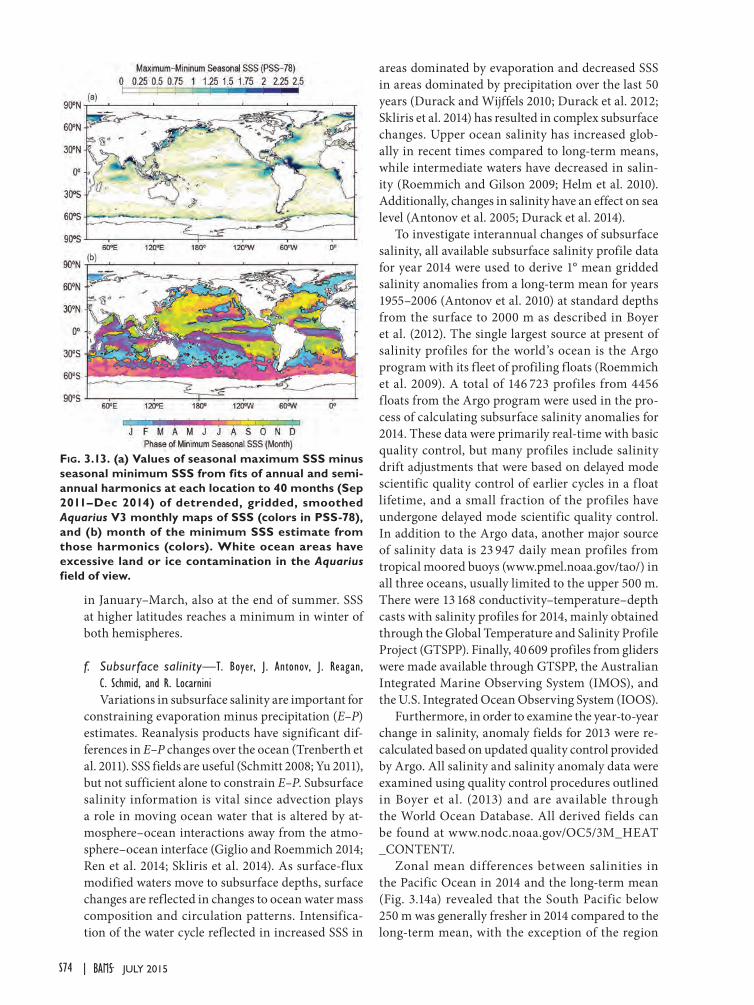
in January–March, also at the end of summer. SSS at higher latitudes reaches a minimum in winter of both hemispheres.
f. Subsurface salinity—T. Boyer, J. Antonov, J. Reagan, C. Schmid, and R. LocarniniVariations in subsurface salinity are important for
constraining evaporation minus precipitation (E–P) estimates. Reanalysis products have significant dif-ferences in E–P changes over the ocean (Trenberth et al. 2011). SSS fields are useful (Schmitt 2008; Yu 2011), but not sufficient alone to constrain E–P. Subsurface salinity information is vital since advection plays a role in moving ocean water that is altered by at-mosphere–ocean interactions away from the atmo-sphere–ocean interface (Giglio and Roemmich 2014; Ren et al. 2014; Skliris et al. 2014). As surface-flux modified waters move to subsurface depths, surface changes are reflected in changes to ocean water mass composition and circulation patterns. Intensifica-tion of the water cycle reflected in increased SSS in
areas dominated by evaporation and decreased SSS in areas dominated by precipitation over the last 50 years (Durack and Wijffels 2010; Durack et al. 2012; Skliris et al. 2014) has resulted in complex subsurface changes. Upper ocean salinity has increased glob-ally in recent times compared to long-term means, while intermediate waters have decreased in salin-ity (Roemmich and Gilson 2009; Helm et al. 2010). Additionally, changes in salinity have an effect on sea level (Antonov et al. 2005; Durack et al. 2014).
To investigate interannual changes of subsurface salinity, all available subsurface salinity profile data for year 2014 were used to derive 1° mean gridded salinity anomalies from a long-term mean for years 1955–2006 (Antonov et al. 2010) at standard depths from the surface to 2000 m as described in Boyer et al. (2012). The single largest source at present of salinity profiles for the world’s ocean is the Argo program with its fleet of profiling floats (Roemmich et al. 2009). A total of 146 723 profiles from 4456 floats from the Argo program were used in the pro-cess of calculating subsurface salinity anomalies for 2014. These data were primarily real-time with basic quality control, but many profiles include salinity drift adjustments that were based on delayed mode scientific quality control of earlier cycles in a f loat lifetime, and a small fraction of the profiles have undergone delayed mode scientific quality control. In addition to the Argo data, another major source of salinity data is 23 947 daily mean profiles from tropical moored buoys (www.pmel.noaa.gov/tao/) in all three oceans, usually limited to the upper 500 m. There were 13 168 conductivity–temperature–depth casts with salinity profiles for 2014, mainly obtained through the Global Temperature and Salinity Profile Project (GTSPP). Finally, 40 609 profiles from gliders were made available through GTSPP, the Australian Integrated Marine Observing System (IMOS), and the U.S. Integrated Ocean Observing System (IOOS).
Furthermore, in order to examine the year-to-year change in salinity, anomaly fields for 2013 were re-calculated based on updated quality control provided by Argo. All salinity and salinity anomaly data were examined using quality control procedures outlined in Boyer et al. (2013) and are available through the World Ocean Database. All derived fields can be found at www.nodc.noaa.gov/OC5/3M_HEAT _CONTENT/.
Zonal mean differences between salinities in the Pacific Ocean in 2014 and the long-term mean (Fig. 3.14a) revealed that the South Pacific below 250 m was generally fresher in 2014 compared to the long-term mean, with the exception of the region
Fig. 3.13. (a) Values of seasonal maximum SSS minus seasonal minimum SSS from fits of annual and semi-annual harmonics at each location to 40 months (Sep 2011–Dec 2014) of detrended, gridded, smoothed Aquarius V3 monthly maps of SSS (colors in PSS-78), and (b) month of the minimum SSS estimate from those harmonics (colors). White ocean areas have excessive land or ice contamination in the Aquarius field of view.
S74 JULY 2015|
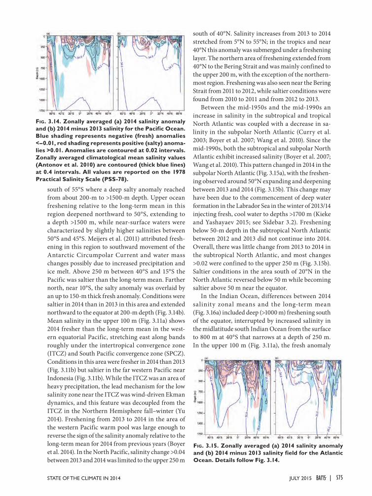
south of 55°S where a deep salty anomaly reached from about 200-m to >1500-m depth. Upper ocean freshening relative to the long-term mean in this region deepened northward to 50°S, extending to a depth >1500 m, while near-surface waters were characterized by slightly higher salinities between 50°S and 45°S. Meijers et al. (2011) attributed fresh-ening in this region to southward movement of the Antarctic Circumpolar Current and water mass changes possibly due to increased precipitation and ice melt. Above 250 m between 40°S and 15°S the Pacific was saltier than the long-term mean. Farther north, near 10°S, the salty anomaly was overlaid by an up to 150-m thick fresh anomaly. Conditions were saltier in 2014 than in 2013 in this area and extended northward to the equator at 200-m depth (Fig. 3.14b). Mean salinity in the upper 100 m (Fig. 3.11a) shows 2014 fresher than the long-term mean in the west-ern equatorial Pacific, stretching east along bands roughly under the intertropical convergence zone (ITCZ) and South Pacific convergence zone (SPCZ). Conditions in this area were fresher in 2014 than 2013 (Fig. 3.11b) but saltier in the far western Pacific near Indonesia (Fig. 3.11b). While the ITCZ was an area of heavy precipitation, the lead mechanism for the low salinity zone near the ITCZ was wind-driven Ekman dynamics, and this feature was decoupled from the ITCZ in the Northern Hemisphere fall–winter (Yu 2014). Freshening from 2013 to 2014 in the area of the western Pacific warm pool was large enough to reverse the sign of the salinity anomaly relative to the long-term mean for 2014 from previous years (Boyer et al. 2014). In the North Pacific, salinity change >0.04 between 2013 and 2014 was limited to the upper 250 m
south of 40°N. Salinity increases from 2013 to 2014 stretched from 5°N to 55°N; in the tropics and near 40°N this anomaly was submerged under a freshening layer. The northern area of freshening extended from 40°N to the Bering Strait and was mainly confined to the upper 200 m, with the exception of the northern-most region. Freshening was also seen near the Bering Strait from 2011 to 2012, while saltier conditions were found from 2010 to 2011 and from 2012 to 2013.
Between the mid-1950s and the mid-1990s an increase in salinity in the subtropical and tropical North Atlantic was coupled with a decrease in sa-linity in the subpolar North Atlantic (Curry et al. 2003; Boyer et al. 2007; Wang et al. 2010). Since the mid-1990s, both the subtropical and subpolar North Atlantic exhibit increased salinity (Boyer et al. 2007; Wang et al. 2010). This pattern changed in 2014 in the subpolar North Atlantic (Fig. 3.15a), with the freshen-ing observed around 50°N expanding and deepening between 2013 and 2014 (Fig. 3.15b). This change may have been due to the commencement of deep water formation in the Labrador Sea in the winter of 2013/14 injecting fresh, cool water to depths >1700 m (Kieke and Yashayaev 2015; see Sidebar 3.2). Freshening below 50-m depth in the subtropical North Atlantic between 2012 and 2013 did not continue into 2014. Overall, there was little change from 2013 to 2014 in the subtropical North Atlantic, and most changes >0.02 were confined to the upper 250 m (Fig. 3.15b). Saltier conditions in the area south of 20°N in the North Atlantic reversed below 50 m while becoming saltier above 50 m near the equator.
In the Indian Ocean, differences between 2014 salinity zonal means and the long-term mean (Fig. 3.16a) included deep (>1000 m) freshening south of the equator, interrupted by increased salinity in the midlatitude south Indian Ocean from the surface to 800 m at 40°S that narrows at a depth of 250 m. In the upper 100 m (Fig. 3.11a), the fresh anomaly
Fig. 3.14. Zonally averaged (a) 2014 salinity anomaly and (b) 2014 minus 2013 salinity for the Pacific Ocean. Blue shading represents negative (fresh) anomalies <–0.01, red shading represents positive (salty) anoma-lies >0.01. Anomalies are contoured at 0.02 intervals. Zonally averaged climatological mean salinity values (Antonov et al. 2010) are contoured (thick blue lines) at 0.4 intervals. All values are reported on the 1978 Practical Salinity Scale (PSS-78).
Fig. 3.15. Zonally averaged (a) 2014 salinity anomaly and (b) 2014 minus 2013 salinity field for the Atlantic Ocean. Details follow Fig. 3.14.
S75JULY 2015STATE OF THE CLIMATE IN 2014 |
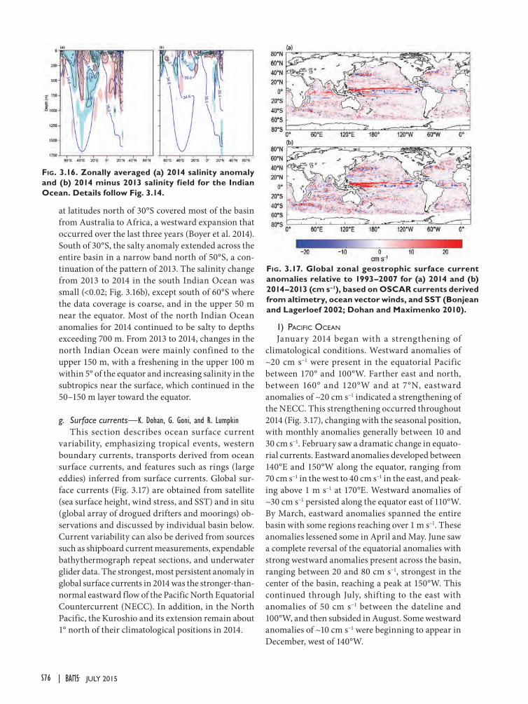
at latitudes north of 30°S covered most of the basin from Australia to Africa, a westward expansion that occurred over the last three years (Boyer et al. 2014). South of 30°S, the salty anomaly extended across the entire basin in a narrow band north of 50°S, a con-tinuation of the pattern of 2013. The salinity change from 2013 to 2014 in the south Indian Ocean was small (<0.02; Fig. 3.16b), except south of 60°S where the data coverage is coarse, and in the upper 50 m near the equator. Most of the north Indian Ocean anomalies for 2014 continued to be salty to depths exceeding 700 m. From 2013 to 2014, changes in the north Indian Ocean were mainly confined to the upper 150 m, with a freshening in the upper 100 m within 5° of the equator and increasing salinity in the subtropics near the surface, which continued in the 50–150 m layer toward the equator.
g. Surface currents—K. Dohan, G. Goni, and R. LumpkinThis section describes ocean surface current
variability, emphasizing tropical events, western boundary currents, transports derived from ocean surface currents, and features such as rings (large eddies) inferred from surface currents. Global sur-face currents (Fig. 3.17) are obtained from satellite (sea surface height, wind stress, and SST) and in situ (global array of drogued drifters and moorings) ob-servations and discussed by individual basin below. Current variability can also be derived from sources such as shipboard current measurements, expendable bathythermograph repeat sections, and underwater glider data. The strongest, most persistent anomaly in global surface currents in 2014 was the stronger-than-normal eastward flow of the Pacific North Equatorial Countercurrent (NECC). In addition, in the North Pacific, the Kuroshio and its extension remain about 1° north of their climatological positions in 2014.
1) Pacific Ocean
January 2014 began with a strengthening of climatological conditions. Westward anomalies of ~20 cm s−1 were present in the equatorial Pacific between 170° and 100°W. Farther east and north, between 160° and 120°W and at 7°N, eastward anomalies of ~20 cm s−1 indicated a strengthening of the NECC. This strengthening occurred throughout 2014 (Fig. 3.17), changing with the seasonal position, with monthly anomalies generally between 10 and 30 cm s−1. February saw a dramatic change in equato-rial currents. Eastward anomalies developed between 140°E and 150°W along the equator, ranging from 70 cm s−1 in the west to 40 cm s−1 in the east, and peak-ing above 1 m s−1 at 170°E. Westward anomalies of ~30 cm s−1 persisted along the equator east of 110°W. By March, eastward anomalies spanned the entire basin with some regions reaching over 1 m s−1. These anomalies lessened some in April and May. June saw a complete reversal of the equatorial anomalies with strong westward anomalies present across the basin, ranging between 20 and 80 cm s−1, strongest in the center of the basin, reaching a peak at 150°W. This continued through July, shifting to the east with anomalies of 50 cm s−1 between the dateline and 100°W, and then subsided in August. Some westward anomalies of ~10 cm s−1 were beginning to appear in December, west of 140°W.
Fig. 3.17. Global zonal geostrophic surface current anomalies relative to 1993–2007 for (a) 2014 and (b) 2014–2013 (cm s–1), based on OSCAR currents derived from altimetry, ocean vector winds, and SST (Bonjean and Lagerloef 2002; Dohan and Maximenko 2010).
Fig. 3.16. Zonally averaged (a) 2014 salinity anomaly and (b) 2014 minus 2013 salinity field for the Indian Ocean. Details follow Fig. 3.14.
S76 JULY 2015|
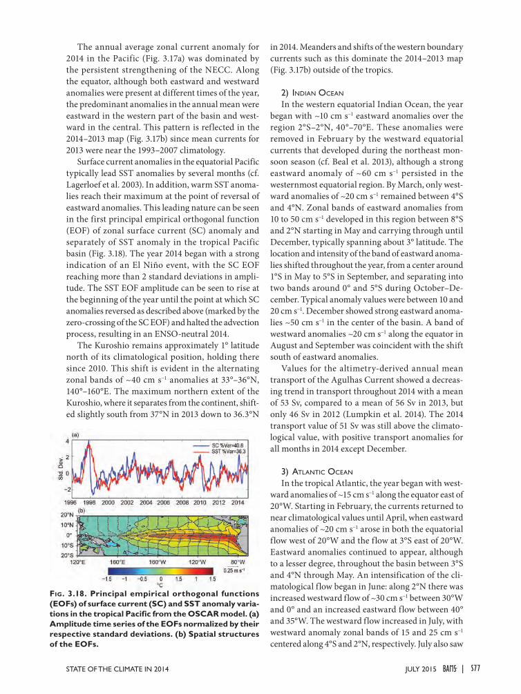
The annual average zonal current anomaly for 2014 in the Pacific (Fig. 3.17a) was dominated by the persistent strengthening of the NECC. Along the equator, although both eastward and westward anomalies were present at different times of the year, the predominant anomalies in the annual mean were eastward in the western part of the basin and west-ward in the central. This pattern is reflected in the 2014–2013 map (Fig. 3.17b) since mean currents for 2013 were near the 1993–2007 climatology.
Surface current anomalies in the equatorial Pacific typically lead SST anomalies by several months (cf. Lagerloef et al. 2003). In addition, warm SST anoma-lies reach their maximum at the point of reversal of eastward anomalies. This leading nature can be seen in the first principal empirical orthogonal function (EOF) of zonal surface current (SC) anomaly and separately of SST anomaly in the tropical Pacific basin (Fig. 3.18). The year 2014 began with a strong indication of an El Niño event, with the SC EOF reaching more than 2 standard deviations in ampli-tude. The SST EOF amplitude can be seen to rise at the beginning of the year until the point at which SC anomalies reversed as described above (marked by the zero-crossing of the SC EOF) and halted the advection process, resulting in an ENSO-neutral 2014.
The Kuroshio remains approximately 1° latitude north of its climatological position, holding there since 2010. This shift is evident in the alternating zonal bands of ~40 cm s−1 anomalies at 33°–36°N, 140°–160°E. The maximum northern extent of the Kuroshio, where it separates from the continent, shift-ed slightly south from 37°N in 2013 down to 36.3°N
in 2014. Meanders and shifts of the western boundary currents such as this dominate the 2014–2013 map (Fig. 3.17b) outside of the tropics.
2) indian Ocean
In the western equatorial Indian Ocean, the year began with ~10 cm s−1 eastward anomalies over the region 2°S–2°N, 40°–70°E. These anomalies were removed in February by the westward equatorial currents that developed during the northeast mon-soon season (cf. Beal et al. 2013), although a strong eastward anomaly of ~60 cm s−1 persisted in the westernmost equatorial region. By March, only west-ward anomalies of ~20 cm s−1 remained between 4°S and 4°N. Zonal bands of eastward anomalies from 10 to 50 cm s−1 developed in this region between 8°S and 2°N starting in May and carrying through until December, typically spanning about 3° latitude. The location and intensity of the band of eastward anoma-lies shifted throughout the year, from a center around 1°S in May to 5°S in September, and separating into two bands around 0° and 5°S during October–De-cember. Typical anomaly values were between 10 and 20 cm s−1. December showed strong eastward anoma-lies ~50 cm s−1 in the center of the basin. A band of westward anomalies ~20 cm s−1 along the equator in August and September was coincident with the shift south of eastward anomalies.
Values for the altimetry-derived annual mean transport of the Agulhas Current showed a decreas-ing trend in transport throughout 2014 with a mean of 53 Sv, compared to a mean of 56 Sv in 2013, but only 46 Sv in 2012 (Lumpkin et al. 2014). The 2014 transport value of 51 Sv was still above the climato-logical value, with positive transport anomalies for all months in 2014 except December.
3) atlantic Ocean
In the tropical Atlantic, the year began with west-ward anomalies of ~15 cm s−1 along the equator east of 20°W. Starting in February, the currents returned to near climatological values until April, when eastward anomalies of ~20 cm s−1 arose in both the equatorial flow west of 20°W and the flow at 3°S east of 20°W. Eastward anomalies continued to appear, although to a lesser degree, throughout the basin between 3°S and 4°N through May. An intensification of the cli-matological flow began in June: along 2°N there was increased westward flow of ~30 cm s−1 between 30°W and 0° and an increased eastward flow between 40° and 35°W. The westward flow increased in July, with westward anomaly zonal bands of 15 and 25 cm s−1 centered along 4°S and 2°N, respectively. July also saw
Fig. 3.18. Principal empirical orthogonal functions (EOFs) of surface current (SC) and SST anomaly varia-tions in the tropical Pacific from the OSCAR model. (a) Amplitude time series of the EOFs normalized by their respective standard deviations. (b) Spatial structures of the EOFs.
S77JULY 2015STATE OF THE CLIMATE IN 2014 |
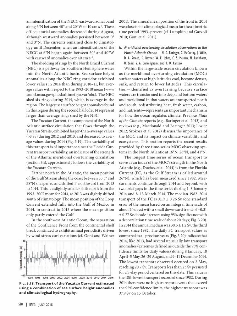
an intensification of the NECC eastward zonal band along 6°N between 40° and 20°W of 10 cm s−1. These off-equatorial anomalies decreased during August, although westward anomalies persisted between 0° and 3°N. The currents remained close to climatol-ogy until December, when an intensification of the NECC at 6°N began again between 50° and 40°W with eastward anomalies over 40 cm s−1.
The shedding of rings by the North Brazil Current (NBC) is a pathway for Southern Hemisphere water into the North Atlantic basin. Sea surface height anomalies along the NBC ring corridor exhibited lower values in 2014 than during 2010–11, but aver-age values with respect to the 1993–2010 mean (www .aoml.noaa.gov/phod/altimetry/cvar/nbc). The NBC shed six rings during 2014, which is average in the region. The largest sea surface height anomalies found in this region during the second half of 2014 represent larger-than-average rings shed by the NBC.
The Yucatan Current, the component of the North Atlantic surface circulation that flows through the Yucatan Straits, exhibited larger-than-average values (>3 Sv) during 2012 and 2013, and decreased to aver-age values during 2014 (Fig. 3.19). The variability of this transport is of importance since the Florida Cur-rent transport variability, an indicator of the strength of the Atlantic meridional overturning circulation (section 3h), approximately follows the variability of the Yucatan Current.
Farther north in the Atlantic, the mean position of the Gulf Stream along the coast between 35.5° and 38°N sharpened and shifted 1° northward from 2013 to 2014. This is a slightly smaller shift north from the 1993–2007 mean for 2014, as 2013 was slightly shifted south of climatology. The mean position of the Loop Current extended fully into the Gulf of Mexico in 2014, in contrast to 2013 where the mean position only partly entered the Gulf.
In the southwest Atlantic Ocean, the separation of the Confluence Front from the continental shelf break continued to exhibit annual periodicity driven by wind stress curl variations (cf. Goni and Wainer
2001). The annual mean position of the front in 2014 was close to its climatological mean for the altimetric time period 1993–present (cf. Lumpkin and Garzoli 2010; Goni et al. 2011).
h. Meridional overturning circulation observations in the North Atlantic Ocean—M. O. Baringer, G. McCarthy, J. Willis, D. A. Smeed, D. Rayner, W. E. Johns, C. S. Meinen, M. Lankhorst, U. Send, S. A. Cunningham, and T. O. KanzowWithin the large-scale ocean circulation known
as the meridional overturning circulation (MOC) surface waters at high latitudes cool, become denser, sink, and return to lower latitudes. This circula-tion—identified as overturning because surface waters are transformed into deep and bottom waters and meridional in that waters are transported north and south, redistributing heat, fresh water, carbon, and nutrients—represents an important mechanism for how the ocean regulates climate. Previous State of the Climate reports (e.g., Baringer et al. 2013) and reviews (e.g., Macdonald and Baringer 2013; Lozier 2012; Srokosz et al. 2012) discuss the importance of the MOC and its impact on climate variability and ecosystems. This section reports the recent results provided by three time-series MOC observing sys-tems in the North Atlantic at 16°N, 26°N, and 41°N.
The longest time series of ocean transport to serve as an index of the MOC’s strength in the North Atlantic (e.g., Duchez et al. 2014) is from the Florida Current (FC, as the Gulf Stream is called around 26°N), which has been measured since 1982. Mea-surements continue through 2014 and beyond, with two brief gaps in the time series during 1–3 January 2014 and 8–13 March 2014. The median 1982–2014 transport of the FC is 31.9 ± 0.26 Sv (one standard error of the mean based on an integral time scale of about 20 days) with a small downward trend of −0.31 ± 0.27 Sv decade−1 (errors using 95% significance with a decorrelation time scale of about 20 days; Fig. 3.20). In 2014 the annual median was 30.5 ± 1.2 Sv, the third lowest since 1982. The daily FC transport values as compared to all previous years (Fig. 3.20) indicate that 2014, like 2013, had several unusually low transport anomalies (extremes defined as outside the 95% con-fidence limits for daily values) during 8 January, 18 April–5 May, 26–29 August, and 9–11 December 2014. The lowest transport observed occured on 2 May, reaching 20.7 Sv. Transports less than 23 Sv persisted for a 5-day period centered on this date. This value is the 18th lowest transport recorded since 1982. During 2014 there were no high transport events that exceed the 95% confidence limits; the highest transport was 37.9 Sv on 15 October.
Fig. 3.19. Transport of the Yucatan Current estimated using a combination of sea surface height anomalies and climatological hydrography.
S78 JULY 2015|
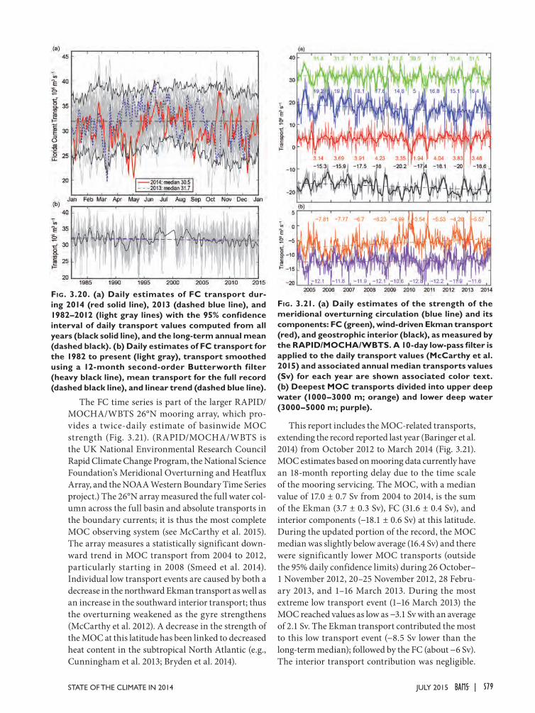
The FC time series is part of the larger RAPID/MOCHA/WBTS 26°N mooring array, which pro-vides a twice-daily estimate of basinwide MOC strength (Fig. 3.21). (RAPID/MOCHA/WBTS is the UK National Environmental Research Council Rapid Climate Change Program, the National Science Foundation’s Meridional Overturning and Heatflux Array, and the NOAA Western Boundary Time Series project.) The 26°N array measured the full water col-umn across the full basin and absolute transports in the boundary currents; it is thus the most complete MOC observing system (see McCarthy et al. 2015). The array measures a statistically significant down-ward trend in MOC transport from 2004 to 2012, particularly starting in 2008 (Smeed et al. 2014). Individual low transport events are caused by both a decrease in the northward Ekman transport as well as an increase in the southward interior transport; thus the overturning weakened as the gyre strengthens (McCarthy et al. 2012). A decrease in the strength of the MOC at this latitude has been linked to decreased heat content in the subtropical North Atlantic (e.g., Cunningham et al. 2013; Bryden et al. 2014).
This report includes the MOC-related transports, extending the record reported last year (Baringer et al. 2014) from October 2012 to March 2014 (Fig. 3.21). MOC estimates based on mooring data currently have an 18-month reporting delay due to the time scale of the mooring servicing. The MOC, with a median value of 17.0 ± 0.7 Sv from 2004 to 2014, is the sum of the Ekman (3.7 ± 0.3 Sv), FC (31.6 ± 0.4 Sv), and interior components (−18.1 ± 0.6 Sv) at this latitude. During the updated portion of the record, the MOC median was slightly below average (16.4 Sv) and there were significantly lower MOC transports (outside the 95% daily confidence limits) during 26 October– 1 November 2012, 20–25 November 2012, 28 Febru-ary 2013, and 1–16 March 2013. During the most extreme low transport event (1–16 March 2013) the MOC reached values as low as −3.1 Sv with an average of 2.1 Sv. The Ekman transport contributed the most to this low transport event (−8.5 Sv lower than the long-term median); followed by the FC (about −6 Sv). The interior transport contribution was negligible.
Fig. 3.20. (a) Daily estimates of FC transport dur-ing 2014 (red solid line), 2013 (dashed blue line), and 1982–2012 (light gray lines) with the 95% confidence interval of daily transport values computed from all years (black solid line), and the long-term annual mean (dashed black). (b) Daily estimates of FC transport for the 1982 to present (light gray), transport smoothed using a 12-month second-order Butterworth filter (heavy black line), mean transport for the full record (dashed black line), and linear trend (dashed blue line).
Fig. 3.21. (a) Daily estimates of the strength of the meridional overturning circulation (blue line) and its components: FC (green), wind-driven Ekman transport (red), and geostrophic interior (black), as measured by the RAPID/MOCHA/WBTS. A 10-day low-pass filter is applied to the daily transport values (McCarthy et al. 2015) and associated annual median transports values (Sv) for each year are shown associated color text. (b) Deepest MOC transports divided into upper deep water (1000–3000 m; orange) and lower deep water (3000–5000 m; purple).
S79JULY 2015STATE OF THE CLIMATE IN 2014 |
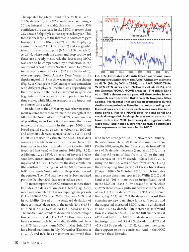
The updated long-term trend of the MOC is −4.2 ± 2.5 Sv decade−1 (using 95% confidence, assuming a 20-day integral time scale); this means there is 95% confidence the decrease in the MOC is greater than 2 Sv decade−1, slightly less than reported last year. This trend is due largely to the increase in southward gyre transport (−3.2 ± 2.0 Sv decade−1), with the FC playing a minor role (−1.2 ± 1.4 Sv decade−1) and a negligible trend in Ekman transport (0.3 ± 1.1 Sv decade−1). At 26°N, where both the upper and deep southward f lows are directly measured, the decreasing MOC was seen to be compensated by a reduction in the southward export of lower North Atlantic Deep Water in the depth range of 3–5 km (3.2 ± 1.8 Sv decade−1); whereas upper North Atlantic Deep Water in the depth range of 1.1–3 km showed no significant change (Fig. 3.21). Changes in MOC transport are coincident with different physical mechanisms depending on the time scale or the particular event in question (e.g., interior flow appears to be important for long time scales, while Ekman transports are important on shorter time scales).
In addition to the 26°N array, two other measure-ment systems are used to estimate the strength of the MOC in the North Atlantic. At 41°N, a combination of profiling Argo f loats (that measure the ocean temperature and salinity in the upper 2000 m on broad spatial scales, as well as velocity at 1000 m) and altimetry-derived surface velocity (Willis and Fu 2008) are used to estimate the MOC; these data sources are available in near real-time and hence the time series has been extended from October 2013 (reported last year) to December 2014 (Fig. 3.22). Additionally, at 16°N, an array of inverted echo sounders, current meters, and dynamic height moor-ings (Send et al. 2011) measures the deep circulation (the southward flowing part of the MOC “conveyor belt”) that sends North Atlantic Deep Water toward the equator. The 16°N data have not yet been updated past the October 2013 date reported last year.
To intercompare the MOC estimates at these three latitudes, the data are low-pass filtered (Fig. 3.22); means are computed for the overlapping time periods (2 April 2004–26 October 2013). The mean MOC and its variability (based on the standard deviation of these estimates) decreases to the north (23.1 ± 4.7 Sv at 16°N; 16.7 ± 3.3 Sv at 26°N; 14.3 ± 3.0 Sv at 41°N). The median and standard deviation of each unique time series are listed in Fig. 3.22. All three time series have a seasonal cycle but with slightly different phas-es; 41°N has a maximum MOC in May–July, 26°N has a broad maximum in July–November (Kanzow et al. 2010), and 16°N has a maximum southward flow
(and hence stronger MOC) in November–January. Reported longer-term MOC trends range from zero (Willis 2010, using the first 7 years of data from 41°N) to a −3 Sv decade−1 decrease (Send et al. 2011, using the first 9.5 years of data from 16°N), to the larg-est decrease of −5.4 Sv decade−1 (Smeed et al. 2014, using the first 8.5 years of data from 26°N). Using the overlapping time period of these observations (2 April 2004–26 October 2013), which includes more recent data than reported by Willis (2010) and Send et al. (2011), there was an insignificant trend in the MOC of −3.0 ± 7.1 Sv decade−1 at 41°N, while at 26°N there was a significant decrease in the MOC of −4.1 ± 3.2 Sv decade−1 (using 95% confidence limits; Fig. 3.22). At 16°N the deep southward flow contains no new data since last year’s report and the suggested increased MOC remains unchanged at +8.4 ± 5.6 Sv decade−1 (an increase in southward flow is a stronger MOC). For the full time series at 41°N and 16°N, the MOC trends decrease, becom-ing insignificant (−1.3 ± 4.9 Sv decade−1 at 41°N and −2.3 ± 2.9 Sv decade−1 at 16°N). At these time scales, there appears to be no consistent trend in the MOC between these latitudes.
Fig. 3.22. Estimates of Atlantic Ocean meridional over-turning circulation from the Argo/Altimetry estimate at 41°N (black; Willis 2010), the RAPID/MOCHA/WBTS 26°N array (red; McCarthy et al. 2015), and the German/NOAA MOVE array at 16°N (blue; Send et al. 2011) shown versus year. All time series have a 3-month second-order Butterworth low-pass filter applied. Horizontal lines are mean transports during similar time periods as listed in the corresponding text. Dashed lines are trends for each series over the same time period. For the MOVE data, the net zonal and vertical integral of the deep circulation represents the lower limb of the MOC (with a negative sign for south-ward flow) and hence a stronger negative southward flow represents an increase in the MOC.
S80 JULY 2015|
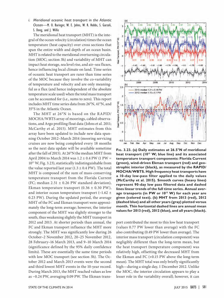
i. Meridional oceanic heat transport in the Atlantic Ocean—M. O. Baringer, W. E. Johns, W. R. Hobbs, S. Garzoli, S. Dong, and J. WillisThe meridional heat transport (MHT) is the inte-
gral of the ocean velocity (circulation) times the ocean temperature (heat capacity) over cross sections that span the entire width and depth of an ocean basin. MHT is related to the meridional overturning circula-tion (MOC; section 3h) and variability of MHT can impact heat storage, sea level rise, and air–sea fluxes, hence influencing local climate on land. Time series of oceanic heat transport are rarer than time series of the MOC because they involve the co-variability of temperature and velocity and are only meaning-ful as a flux (and hence independent of the absolute temperature scale used) when the total mass transport can be accounted for (i.e., sums to zero). This report includes MHT time series data from 26°N, 41°N, and 35°S in the Atlantic Ocean.
The MHT at 26°N is based on the RAPID/MOCHA/WBTS array of moorings, cabled observa-tions, and Argo profiling float data (Johns et al. 2011; McCarthy et al. 2015). MHT estimates from this array have been updated to include new data span-ning October 2012–March 2014 (mooring servicing cruises are now being completed every 18 months so the next data update will be available sometime after the fall of 2015). At 26°N the median MHT from April 2004 to March 2014 was 1.2 ± 0.4 PW (1 PW = 1015 W; Fig. 3.23), statistically indistinguishable from the value reported last year (1.3 ± 0.4 PW). The total MHT is composed of the sum of mass-conserving temperature transport from the Florida Current (FC; median 2.51 ± 0.26 PW standard deviation), Ekman temperature transport (0.36 ± 0.30 PW), and interior ocean temperature transport (−1.62 ± 0.23 PW). During the updated period, the average MHT of the FC and Ekman transport were approxi-mately the long-term average; however, the interior component of the MHT was slightly stronger to the south, thus weakening slightly the MHT transport in 2012 and 2013. At shorter periods than annual, the FC and Ekman transport influence the MHT more strongly. The MHT was significantly low during 26 October–2 November 2012, 20–25 November 2012, 28 February–16 March 2013, and 9–10 March 2014 (significance defined by the 95% daily confidence limits). These are essentially the same time periods with low MOC transport (see section 3h). The Oc-tober 2012 and March 2013 events were the second and third lowest MHT events in the 10-year record. During March 2013, the MHT reached values as low as −0.24 PW, averaging 0.09 PW. The Ekman trans-
port contributed the most to this low heat transport (values 0.77 PW lower than average) with the FC also contributing (0.49 PW lower than average). The interior mass transport (circulation component) was negligibly different than the long-term mean, but the heat transport (temperature component) was relatively high, offsetting the decreased MHT from the Ekman and FC (+0.15 PW above the long-term mean). The MHT total was only briefly significantly high—during a single day, 1 December 2012. Unlike the MOC, the interior circulation appears to play a lesser role in the variability overall; however, it can
Fig. 3.23. (a) Daily estimates at 26.5°N of meridional heat transport (1015 W; blue line) and its associated temperature transport components: Florida Current (green), wind-driven Ekman transport (red) and geo-strophic interior (black), as measured by the RAPID/MOCHA/WBTS. High frequency heat transports have a 10-day low-pass filter applied to the daily values (McCarthy et al. 2015). Smooth curves (heavy lines) represent 90-day low pass filtered data and dashed lines linear trends of the full time series. Annual aver-age transports (in PW or 1015 W) for each year are given (colored text). (b) MHT from 2013 (red), 2012 (dashed blue) and all other years (gray) plotted versus month. Thin horizontal dashed lines are annual mean values for 2013 (red), 2012 (blue), and all years (black).
S81JULY 2015STATE OF THE CLIMATE IN 2014 |
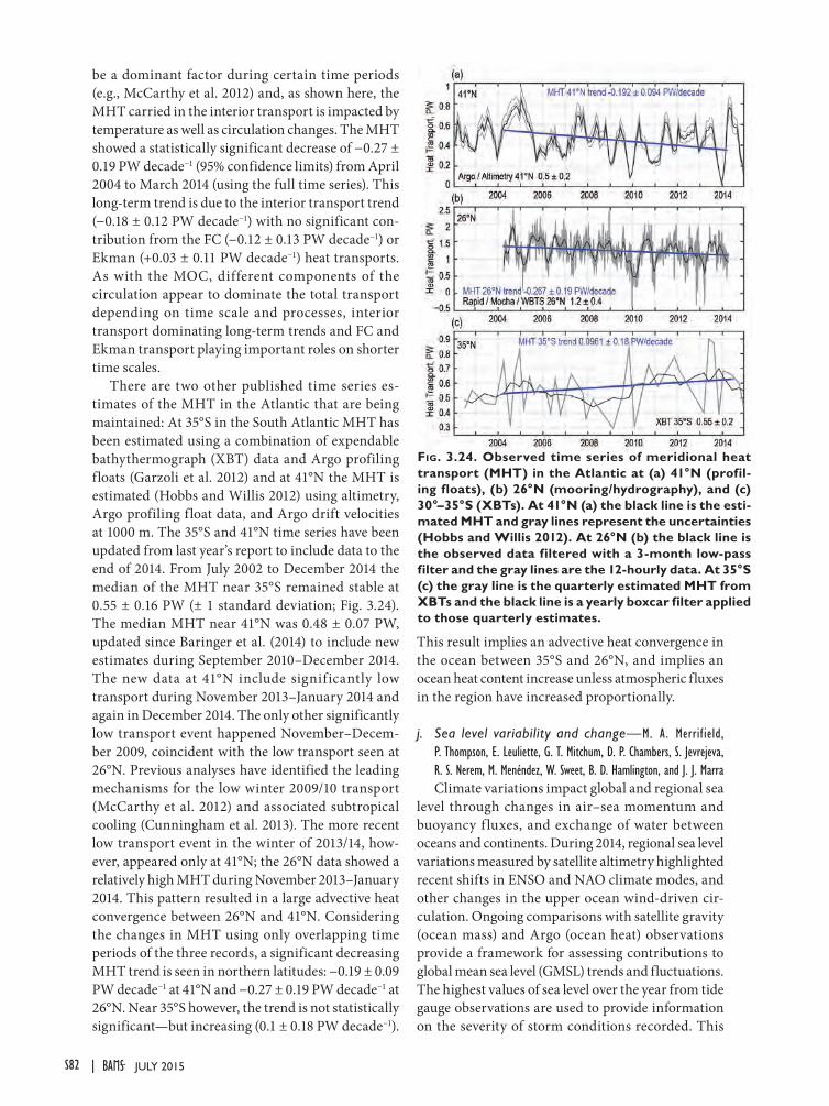
be a dominant factor during certain time periods (e.g., McCarthy et al. 2012) and, as shown here, the MHT carried in the interior transport is impacted by temperature as well as circulation changes. The MHT showed a statistically significant decrease of −0.27 ± 0.19 PW decade−1 (95% confidence limits) from April 2004 to March 2014 (using the full time series). This long-term trend is due to the interior transport trend (−0.18 ± 0.12 PW decade−1) with no significant con-tribution from the FC (−0.12 ± 0.13 PW decade−1) or Ekman (+0.03 ± 0.11 PW decade−1) heat transports. As with the MOC, different components of the circulation appear to dominate the total transport depending on time scale and processes, interior transport dominating long-term trends and FC and Ekman transport playing important roles on shorter time scales.
There are two other published time series es-timates of the MHT in the Atlantic that are being maintained: At 35°S in the South Atlantic MHT has been estimated using a combination of expendable bathythermograph (XBT) data and Argo profiling floats (Garzoli et al. 2012) and at 41°N the MHT is estimated (Hobbs and Willis 2012) using altimetry, Argo profiling float data, and Argo drift velocities at 1000 m. The 35°S and 41°N time series have been updated from last year’s report to include data to the end of 2014. From July 2002 to December 2014 the median of the MHT near 35°S remained stable at 0.55 ± 0.16 PW (± 1 standard deviation; Fig. 3.24). The median MHT near 41°N was 0.48 ± 0.07 PW, updated since Baringer et al. (2014) to include new estimates during September 2010–December 2014. The new data at 41°N include significantly low transport during November 2013–January 2014 and again in December 2014. The only other significantly low transport event happened November–Decem-ber 2009, coincident with the low transport seen at 26°N. Previous analyses have identified the leading mechanisms for the low winter 2009/10 transport (McCarthy et al. 2012) and associated subtropical cooling (Cunningham et al. 2013). The more recent low transport event in the winter of 2013/14, how-ever, appeared only at 41°N; the 26°N data showed a relatively high MHT during November 2013–January 2014. This pattern resulted in a large advective heat convergence between 26°N and 41°N. Considering the changes in MHT using only overlapping time periods of the three records, a significant decreasing MHT trend is seen in northern latitudes: −0.19 ± 0.09 PW decade−1 at 41°N and −0.27 ± 0.19 PW decade−1 at 26°N. Near 35°S however, the trend is not statistically significant—but increasing (0.1 ± 0.18 PW decade−1).
This result implies an advective heat convergence in the ocean between 35°S and 26°N, and implies an ocean heat content increase unless atmospheric fluxes in the region have increased proportionally.
j. Sea level variability and change—M. A. Merrif ield, P. Thompson, E. Leuliette, G. T. Mitchum, D. P. Chambers, S. Jevrejeva, R. S. Nerem, M. Menéndez, W. Sweet, B. D. Hamlington, and J. J. Marra Climate variations impact global and regional sea
level through changes in air–sea momentum and buoyancy f luxes, and exchange of water between oceans and continents. During 2014, regional sea level variations measured by satellite altimetry highlighted recent shifts in ENSO and NAO climate modes, and other changes in the upper ocean wind-driven cir-culation. Ongoing comparisons with satellite gravity (ocean mass) and Argo (ocean heat) observations provide a framework for assessing contributions to global mean sea level (GMSL) trends and fluctuations. The highest values of sea level over the year from tide gauge observations are used to provide information on the severity of storm conditions recorded. This
Fig. 3.24. Observed time series of meridional heat transport (MHT) in the Atlantic at (a) 41°N (profil-ing floats), (b) 26°N (mooring/hydrography), and (c) 30°–35°S (XBTs). At 41°N (a) the black line is the esti-mated MHT and gray lines represent the uncertainties (Hobbs and Willis 2012). At 26°N (b) the black line is the observed data filtered with a 3-month low-pass filter and the gray lines are the 12-hourly data. At 35°S (c) the gray line is the quarterly estimated MHT from XBTs and the black line is a yearly boxcar filter applied to those quarterly estimates.
S82 JULY 2015|
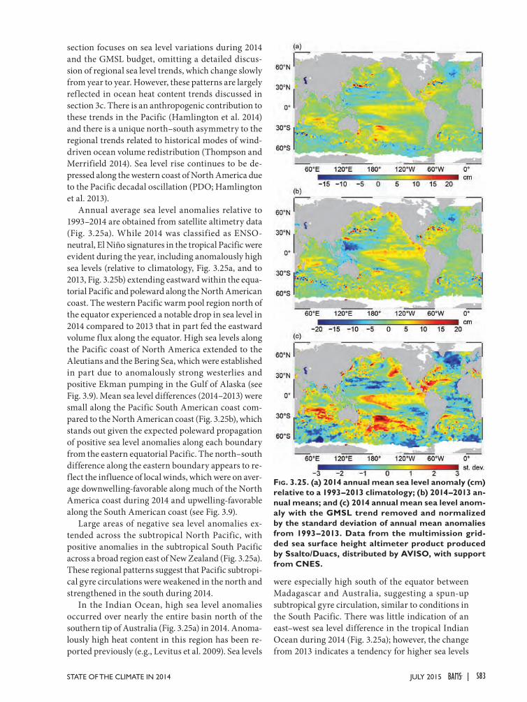
section focuses on sea level variations during 2014 and the GMSL budget, omitting a detailed discus-sion of regional sea level trends, which change slowly from year to year. However, these patterns are largely reflected in ocean heat content trends discussed in section 3c. There is an anthropogenic contribution to these trends in the Pacific (Hamlington et al. 2014) and there is a unique north–south asymmetry to the regional trends related to historical modes of wind-driven ocean volume redistribution (Thompson and Merrifield 2014). Sea level rise continues to be de-pressed along the western coast of North America due to the Pacific decadal oscillation (PDO; Hamlington et al. 2013).
Annual average sea level anomalies relative to 1993–2014 are obtained from satellite altimetry data (Fig. 3.25a). While 2014 was classified as ENSO-neutral, El Niño signatures in the tropical Pacific were evident during the year, including anomalously high sea levels (relative to climatology, Fig. 3.25a, and to 2013, Fig. 3.25b) extending eastward within the equa-torial Pacific and poleward along the North American coast. The western Pacific warm pool region north of the equator experienced a notable drop in sea level in 2014 compared to 2013 that in part fed the eastward volume flux along the equator. High sea levels along the Pacific coast of North America extended to the Aleutians and the Bering Sea, which were established in part due to anomalously strong westerlies and positive Ekman pumping in the Gulf of Alaska (see Fig. 3.9). Mean sea level differences (2014–2013) were small along the Pacific South American coast com-pared to the North American coast (Fig. 3.25b), which stands out given the expected poleward propagation of positive sea level anomalies along each boundary from the eastern equatorial Pacific. The north–south difference along the eastern boundary appears to re-flect the influence of local winds, which were on aver-age downwelling-favorable along much of the North America coast during 2014 and upwelling-favorable along the South American coast (see Fig. 3.9).
Large areas of negative sea level anomalies ex-tended across the subtropical North Pacific, with positive anomalies in the subtropical South Pacific across a broad region east of New Zealand (Fig. 3.25a). These regional patterns suggest that Pacific subtropi-cal gyre circulations were weakened in the north and strengthened in the south during 2014.
In the Indian Ocean, high sea level anomalies occurred over nearly the entire basin north of the southern tip of Australia (Fig. 3.25a) in 2014. Anoma-lously high heat content in this region has been re-ported previously (e.g., Levitus et al. 2009). Sea levels
were especially high south of the equator between Madagascar and Australia, suggesting a spun-up subtropical gyre circulation, similar to conditions in the South Pacific. There was little indication of an east–west sea level difference in the tropical Indian Ocean during 2014 (Fig. 3.25a); however, the change from 2013 indicates a tendency for higher sea levels
Fig. 3.25. (a) 2014 annual mean sea level anomaly (cm) relative to a 1993–2013 climatology; (b) 2014–2013 an-nual means; and (c) 2014 annual mean sea level anom-aly with the GMSL trend removed and normalized by the standard deviation of annual mean anomalies from 1993–2013. Data from the multimission grid-ded sea surface height altimeter product produced by Ssalto/Duacs, distributed by AVISO, with support from CNES.
S83JULY 2015STATE OF THE CLIMATE IN 2014 |
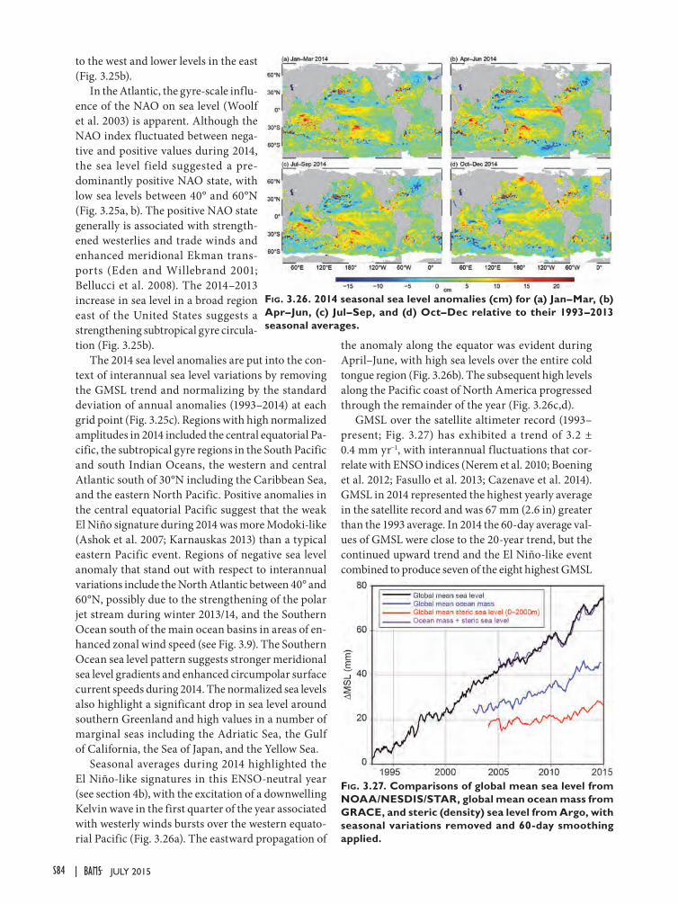
to the west and lower levels in the east (Fig. 3.25b).
In the Atlantic, the gyre-scale influ-ence of the NAO on sea level (Woolf et al. 2003) is apparent. Although the NAO index fluctuated between nega-tive and positive values during 2014, the sea level field suggested a pre-dominantly positive NAO state, with low sea levels between 40° and 60°N (Fig. 3.25a, b). The positive NAO state generally is associated with strength-ened westerlies and trade winds and enhanced meridional Ekman trans-ports (Eden and Willebrand 2001; Bellucci et al. 2008). The 2014–2013 increase in sea level in a broad region east of the United States suggests a strengthening subtropical gyre circula-tion (Fig. 3.25b).
The 2014 sea level anomalies are put into the con-text of interannual sea level variations by removing the GMSL trend and normalizing by the standard deviation of annual anomalies (1993–2014) at each grid point (Fig. 3.25c). Regions with high normalized amplitudes in 2014 included the central equatorial Pa-cific, the subtropical gyre regions in the South Pacific and south Indian Oceans, the western and central Atlantic south of 30°N including the Caribbean Sea, and the eastern North Pacific. Positive anomalies in the central equatorial Pacific suggest that the weak El Niño signature during 2014 was more Modoki-like (Ashok et al. 2007; Karnauskas 2013) than a typical eastern Pacific event. Regions of negative sea level anomaly that stand out with respect to interannual variations include the North Atlantic between 40° and 60°N, possibly due to the strengthening of the polar jet stream during winter 2013/14, and the Southern Ocean south of the main ocean basins in areas of en-hanced zonal wind speed (see Fig. 3.9). The Southern Ocean sea level pattern suggests stronger meridional sea level gradients and enhanced circumpolar surface current speeds during 2014. The normalized sea levels also highlight a significant drop in sea level around southern Greenland and high values in a number of marginal seas including the Adriatic Sea, the Gulf of California, the Sea of Japan, and the Yellow Sea.
Seasonal averages during 2014 highlighted the El Niño-like signatures in this ENSO-neutral year (see section 4b), with the excitation of a downwelling Kelvin wave in the first quarter of the year associated with westerly winds bursts over the western equato-rial Pacific (Fig. 3.26a). The eastward propagation of
the anomaly along the equator was evident during April–June, with high sea levels over the entire cold tongue region (Fig. 3.26b). The subsequent high levels along the Pacific coast of North America progressed through the remainder of the year (Fig. 3.26c,d).
GMSL over the satellite altimeter record (1993–present; Fig. 3.27) has exhibited a trend of 3.2 ± 0.4 mm yr−1, with interannual fluctuations that cor-relate with ENSO indices (Nerem et al. 2010; Boening et al. 2012; Fasullo et al. 2013; Cazenave et al. 2014). GMSL in 2014 represented the highest yearly average in the satellite record and was 67 mm (2.6 in) greater than the 1993 average. In 2014 the 60-day average val-ues of GMSL were close to the 20-year trend, but the continued upward trend and the El Niño-like event combined to produce seven of the eight highest GMSL
Fig. 3.27. Comparisons of global mean sea level from NOAA/NESDIS/STAR, global mean ocean mass from GRACE, and steric (density) sea level from Argo, with seasonal variations removed and 60-day smoothing applied.
Fig. 3.26. 2014 seasonal sea level anomalies (cm) for (a) Jan–Mar, (b) Apr–Jun, (c) Jul–Sep, and (d) Oct–Dec relative to their 1993–2013 seasonal averages.
S84 JULY 2015|
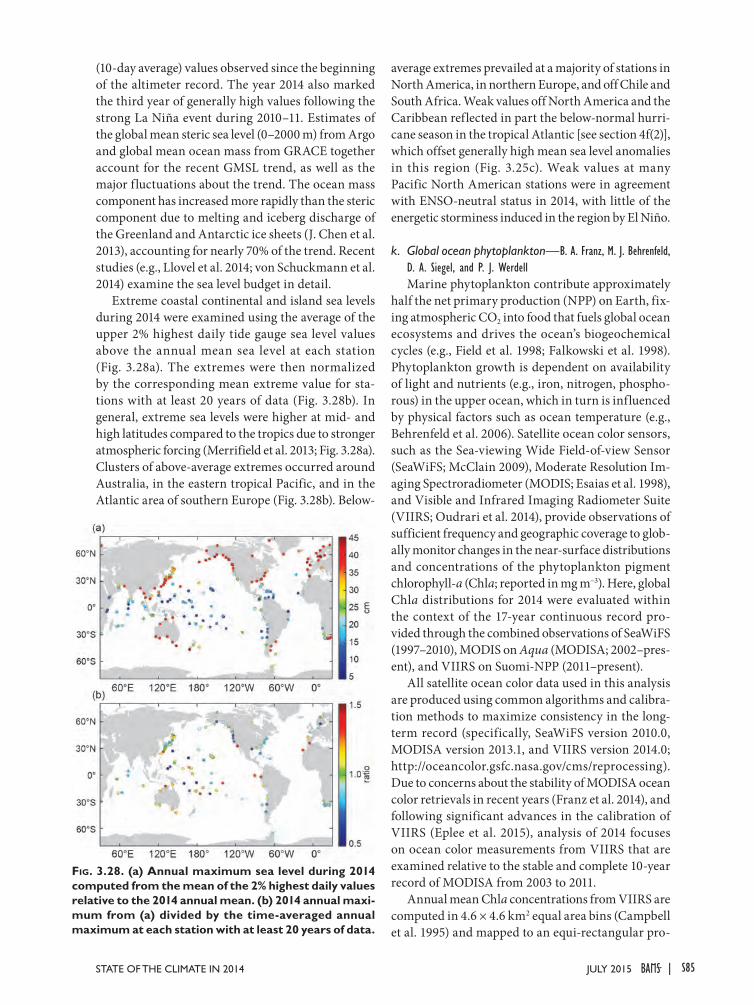
(10-day average) values observed since the beginning of the altimeter record. The year 2014 also marked the third year of generally high values following the strong La Niña event during 2010–11. Estimates of the global mean steric sea level (0–2000 m) from Argo and global mean ocean mass from GRACE together account for the recent GMSL trend, as well as the major fluctuations about the trend. The ocean mass component has increased more rapidly than the steric component due to melting and iceberg discharge of the Greenland and Antarctic ice sheets (J. Chen et al. 2013), accounting for nearly 70% of the trend. Recent studies (e.g., Llovel et al. 2014; von Schuckmann et al. 2014) examine the sea level budget in detail.
Extreme coastal continental and island sea levels during 2014 were examined using the average of the upper 2% highest daily tide gauge sea level values above the annual mean sea level at each station (Fig. 3.28a). The extremes were then normalized by the corresponding mean extreme value for sta-tions with at least 20 years of data (Fig. 3.28b). In general, extreme sea levels were higher at mid- and high latitudes compared to the tropics due to stronger atmospheric forcing (Merrifield et al. 2013; Fig. 3.28a). Clusters of above-average extremes occurred around Australia, in the eastern tropical Pacific, and in the Atlantic area of southern Europe (Fig. 3.28b). Below-
average extremes prevailed at a majority of stations in North America, in northern Europe, and off Chile and South Africa. Weak values off North America and the Caribbean reflected in part the below-normal hurri-cane season in the tropical Atlantic [see section 4f(2)], which offset generally high mean sea level anomalies in this region (Fig. 3.25c). Weak values at many Pacific North American stations were in agreement with ENSO-neutral status in 2014, with little of the energetic storminess induced in the region by El Niño.
k. Global ocean phytoplankton—B. A. Franz, M. J. Behrenfeld, D. A. Siegel, and P. J. WerdellMarine phytoplankton contribute approximately
half the net primary production (NPP) on Earth, fix-ing atmospheric CO2 into food that fuels global ocean ecosystems and drives the ocean’s biogeochemical cycles (e.g., Field et al. 1998; Falkowski et al. 1998). Phytoplankton growth is dependent on availability of light and nutrients (e.g., iron, nitrogen, phospho-rous) in the upper ocean, which in turn is influenced by physical factors such as ocean temperature (e.g., Behrenfeld et al. 2006). Satellite ocean color sensors, such as the Sea-viewing Wide Field-of-view Sensor (SeaWiFS; McClain 2009), Moderate Resolution Im-aging Spectroradiometer (MODIS; Esaias et al. 1998), and Visible and Infrared Imaging Radiometer Suite (VIIRS; Oudrari et al. 2014), provide observations of sufficient frequency and geographic coverage to glob-ally monitor changes in the near-surface distributions and concentrations of the phytoplankton pigment chlorophyll-a (Chla; reported in mg m−3). Here, global Chla distributions for 2014 were evaluated within the context of the 17-year continuous record pro-vided through the combined observations of SeaWiFS (1997–2010), MODIS on Aqua (MODISA; 2002–pres-ent), and VIIRS on Suomi-NPP (2011–present).
All satellite ocean color data used in this analysis are produced using common algorithms and calibra-tion methods to maximize consistency in the long-term record (specifically, SeaWiFS version 2010.0, MODISA version 2013.1, and VIIRS version 2014.0; http://oceancolor.gsfc.nasa.gov/cms/reprocessing). Due to concerns about the stability of MODISA ocean color retrievals in recent years (Franz et al. 2014), and following significant advances in the calibration of VIIRS (Eplee et al. 2015), analysis of 2014 focuses on ocean color measurements from VIIRS that are examined relative to the stable and complete 10-year record of MODISA from 2003 to 2011.
Annual mean Chla concentrations from VIIRS are computed in 4.6 × 4.6 km2 equal area bins (Campbell et al. 1995) and mapped to an equi-rectangular pro-
Fig. 3.28. (a) Annual maximum sea level during 2014 computed from the mean of the 2% highest daily values relative to the 2014 annual mean. (b) 2014 annual maxi-mum from (a) divided by the time-averaged annual maximum at each station with at least 20 years of data.
S85JULY 2015STATE OF THE CLIMATE IN 2014 |
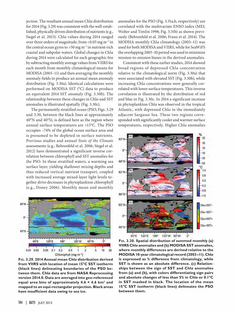
jection. The resultant annual mean Chla distribution for 2014 (Fig. 3.29) was consistent with the well-estab-lished, physically driven distribution of nutrients (e.g., Siegel et al. 2013). Chla values during 2014 ranged over three orders of magnitude, from <0.05 mg m−3 in the central ocean gyres to >50 mg m−3 in nutrient-rich coastal and subpolar waters. Global changes in Chla during 2014 were calculated for each geographic bin by subtracting monthly average values from VIIRS for each month from monthly climatological means for MODISA (2003–11) and then averaging the monthly anomaly fields to produce an annual mean anomaly distribution (Fig. 3.30a). Identical calculations were performed on MODISA SST (°C) data to produce an equivalent 2014 SST anomaly (Fig. 3.30b). The relationship between these changes in Chla and SST anomalies is illustrated spatially (Fig. 3.30c).
The permanently stratified ocean (PSO; Figs. 3.29 and 3.30, between the black lines at approximately 40°N and 40°S), is defined here as the region where annual surface temperatures are >15°C. The PSO occupies ~74% of the global ocean surface area and is presumed to be depleted in surface nutrients. Previous studies and annual State of the Climate assessments (e.g., Behrenfeld et al. 2006; Siegel et al. 2012) have demonstrated a significant inverse cor-relation between chlorophyll and SST anomalies for the PSO. In these stratified waters, a warming sea surface layer, yielding shallower mixing depths and thus reduced vertical nutrient transport, coupled with increased average mixed-layer light levels to-gether drive decreases in phytoplankton chlorophyll (e.g., Doney 2006). Monthly mean and monthly
anomalies for the PSO (Fig. 3.31a,b, respectively) are correlated with the multivariate ENSO index (MEI; Wolter and Timlin 1998; Fig. 3.31b) as shown previ-ously (Behrenfeld et al. 2006; Franz et al. 2014). The MODISA monthly Chla climatology (2003–11) was used for both MODISA and VIIRS, while for SeaWiFS the overlapping 2003–10 period was used to minimize mission-to-mission biases in the derived anomalies.
Consistent with these earlier studies, 2014 showed broad regions of depressed Chla concentration relative to the climatological norm (Fig. 3.30a) that were associated with elevated SST (Fig. 3.30b), while increasing Chla concentrations were generally cor-related with lower surface temperatures. This inverse correlation is illustrated by the distribution of red and blue in Fig. 3.30c. In 2014 a significant increase in phytoplankton Chla was observed in the tropical Atlantic, with depressed Chla in the immediately adjacent Sargasso Sea. These two regions corre-sponded with significantly cooler and warmer surface temperatures, respectively. Higher Chla anomalies
Fig. 3.30. Spatial distribution of summed monthly (a) VIIRS Chla anomalies and (b) MODISA SST anomalies, where monthly differences are derived relative to the MODISA 10-year climatological record (2003–11). Chla is expressed as % difference from climatology, while SST is shown as an absolute difference. (c) Relation-ships between the sign of SST and Chla anomalies from (a) and (b), with colors differentiating sign pairs and absolute changes of less than 5% in Chla or 0.1°C in SST masked in black. The location of the mean 15°C SST isotherm (black lines) delineates the PSO between them.
Fig. 3.29. 2014 Annual mean Chla distribution derived from VIIRS with location of mean 15°C SST isotherm (black lines) delineating boundaries of the PSO be-tween them. Chla data are from NASA Reprocessing version 2014.0. Data are averaged into geo-referenced equal area bins of approximately 4.6 × 4.6 km2 and mapped to an equi-rectangular projection. Black areas have insufficient data owing to sea ice.
S86 JULY 2015|
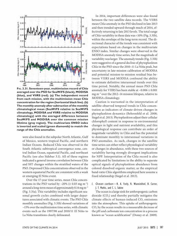
were also found in the subpolar North Atlantic, Gulf of Mexico, western tropical Pacific, and northern Indian Oceans. Reduced Chla was observed in the South Atlantic subtropical convergence zone, cen-tral Indian Ocean, equatorial Pacific, and northeast Pacific (see also Sidebar 3.1). All of these regions indicated a general inverse correlation between Chla and SST changes within the stratified waters of the PSO. Depressed Chla concentrations observed in the western equatorial Pacific are consistent with a weak or emerging El Niño event.
Over the 17-year time series, mean Chla concen-trations in the PSO varied by ~20% (± 0.03 mg m−3) around a long-term mean of approximately 0.14 mg m–3 (Fig. 3.31a). This variability includes significant sea-sonal growth cycles combined with larger depar-tures associated with climatic events. The PSO Chla monthly anomalies (Fig. 3.31b) showed variations of ~15% over the multimission time series, with climatic events such as the 1997/98 and 2010/11 El Niño to La Niña transitions clearly delineated.
In 2014, important differences were also found between the two satellite data records. The VIIRS mean Chla anomaly in the PSO declined in late 2013 and then trended upward through much of 2014, ef-fectively returning to late 2013 levels. The total range of Chla variability in these data was <10% (Fig. 3.31b), within the envelope of the long-term record. The di-rectional character of the trends was consistent with expectations based on changes in the multivariate ENSO index. Similar changes were observed in the MODISA anomaly time series, but the magnitude of variability was larger. The anomaly trends (Fig. 3.31b) were suggestive of a general decline of phytoplankton Chla in the PSO since the 2010–11 La Niña peak, but uncertainty in late-mission calibration of MODISA and potential mission-to-mission residual bias be-tween VIIRS and MODISA confound the ability to estimate definitive interannual trends over this time period. Notably, the annual mean PSO Chla anomaly for VIIRS has been stable at –0.006 ± 0.001 mg m–3 over the 2012–14 mission lifespan, relative to MODISA climatology.
Caution is warranted in the interpretation of satellite-observed temporal trends in Chla concen-tration as indicators of climate-driven changes in phytoplankton dynamics (Behrenfeld et al. 2008; Siegel et al. 2013). Phytoplankton adjust their cellular chlorophyll content in response to environmental changes in light and nutrient availability, and this physiological response can contribute an order of magnitude variability in Chla and has the potential to dominate monthly to interannual variations in PSO anomalies. As such, changes in the satellite time series can either reflect physiological variability or changes in abundance, with these two sources of variability having strongly divergent implications for NPP. Interpretation of the Chla record is also complicated by limitations in the ability to separate optical signals of phytoplankton abundance from colored dissolved organic matter, as the empirical band-ratio Chla algorithms employed here assume a fixed relationship (Siegel et al. 2013).
l. Ocean carbon—R. A. Feely, R. Wanninkhof, B. Carter, J. T. Mathis, and C. L. SabineThe ocean is a large sink for anthropogenic carbon
dioxide (CO2) and thereby partially mitigates the climate effects of human-induced CO2 emissions into the atmosphere. This uptake of anthropogenic CO2 by the ocean results in a measurable decrease of the pH and carbonate ion concentration in a process known as “ocean acidification” (Doney et al. 2009).
Fig. 3.31. Seventeen-year, multimission record of Chla averaged over the PSO for SeaWiFS (black), MODISA (blue), and VIIRS (red). (a) The independent record from each mission, with the multimission mean Chla concentration for the region (horizontal black line). (b) The monthly anomaly after subtraction of the monthly climatological mean (SeaWiFS relative to SeaWiFS climatology, MODISA and VIIRS relative to MODISA climatology) with the averaged difference between SeaWiFS and MODISA over the common mission lifetime (gray region). The multivariate ENSO index is inverted and scaled (green diamonds) to match the range of the Chla anomalies.
S87JULY 2015STATE OF THE CLIMATE IN 2014 |
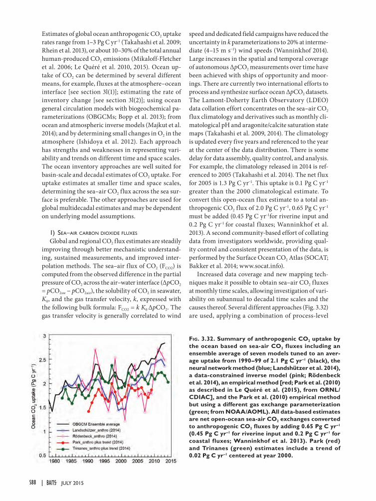
Estimates of global ocean anthropogenic CO2 uptake rates range from 1–3 Pg C yr−1 (Takahashi et al. 2009; Rhein et al. 2013), or about 10–30% of the total annual human-produced CO2 emissions (Mikaloff-Fletcher et al. 2006; Le Quéré et al. 2010, 2015). Ocean up-take of CO2 can be determined by several different means, for example, fluxes at the atmosphere–ocean interface [see section 3l(1)]; estimating the rate of inventory change [see section 3l(2)]; using ocean general circulation models with biogeochemical pa-rameterizations (OBGCMs; Bopp et al. 2013); from ocean and atmospheric inverse models (Majkut et al. 2014); and by determining small changes in O2 in the atmosphere (Ishidoya et al. 2012). Each approach has strengths and weaknesses in representing vari-ability and trends on different time and space scales. The ocean inventory approaches are well suited for basin-scale and decadal estimates of CO2 uptake. For uptake estimates at smaller time and space scales, determining the sea–air CO2 flux across the sea sur-face is preferable. The other approaches are used for global multidecadal estimates and may be dependent on underlying model assumptions.
1) Sea–air carbOn diOxide fluxeS
Global and regional CO2 flux estimates are steadily improving through better mechanistic understand-ing, sustained measurements, and improved inter-polation methods. The sea–air flux of CO2 (FCO2) is computed from the observed difference in the partial pressure of CO2 across the air–water interface (ΔpCO2 = pCO2sw − pCO2air), the solubility of CO2 in seawater, K0, and the gas transfer velocity, k, expressed with the following bulk formula: FCO2 = k K0 ΔpCO2. The gas transfer velocity is generally correlated to wind
speed and dedicated field campaigns have reduced the uncertainty in k parameterizations to 20% at interme-diate (4–15 m s−1) wind speeds (Wanninkhof 2014). Large increases in the spatial and temporal coverage of autonomous ΔpCO2 measurements over time have been achieved with ships of opportunity and moor-ings. There are currently two international efforts to process and synthesize surface ocean ΔpCO2 datasets. The Lamont-Doherty Earth Observatory (LDEO) data collation effort concentrates on the sea–air CO2 flux climatology and derivatives such as monthly cli-matological pH and aragonite/calcite saturation state maps (Takahashi et al. 2009, 2014). The climatology is updated every five years and referenced to the year at the center of the data distribution. There is some delay for data assembly, quality control, and analysis. For example, the climatology released in 2014 is ref-erenced to 2005 (Takahashi et al. 2014). The net flux for 2005 is 1.3 Pg C yr−1. This uptake is 0.1 Pg C yr−1 greater than the 2000 climatological estimate. To convert this open-ocean flux estimate to a total an-thropogenic CO2 flux of 2.0 Pg C yr−1, 0.65 Pg C yr−1 must be added (0.45 Pg C yr−1for riverine input and 0.2 Pg C yr−1 for coastal f luxes; Wanninkhof et al. 2013). A second community-based effort of collating data from investigators worldwide, providing qual-ity control and consistent presentation of the data, is performed by the Surface Ocean CO2 Atlas (SOCAT; Bakker et al. 2014; www.socat.info).
Increased data coverage and new mapping tech-niques make it possible to obtain sea–air CO2 fluxes at monthly time scales, allowing investigation of vari-ability on subannual to decadal time scales and the causes thereof. Several different approaches (Fig. 3.32) are used, applying a combination of process-level
Fig. 3.32. Summary of anthropogenic CO2 uptake by the ocean based on sea-air CO2 fluxes including an ensemble average of seven models tuned to an aver-age uptake from 1990–99 of 2.1 Pg C yr–1 (black), the neural network method (blue; Landshützer et al. 2014), a data-constrained inverse model (pink; Rödenbeck et al. 2014), an empirical method [red; Park et al. (2010) as described in Le Quéré et al. (2015), from ORNL/CDIAC], and the Park et al. (2010) empirical method but using a different gas exchange parameterization (green; from NOAA/AOML). All data-based estimates are net open-ocean sea-air CO2 exchanges converted to anthropogenic CO2 fluxes by adding 0.65 Pg C yr–1 (0.45 Pg C yr–1 for riverine input and 0.2 Pg C yr–1 for coastal fluxes; Wanninkhof et al. 2013). Park (red) and Trinanes (green) estimates include a trend of 0.02 Pg C yr–1 centered at year 2000.
S88 JULY 2015|
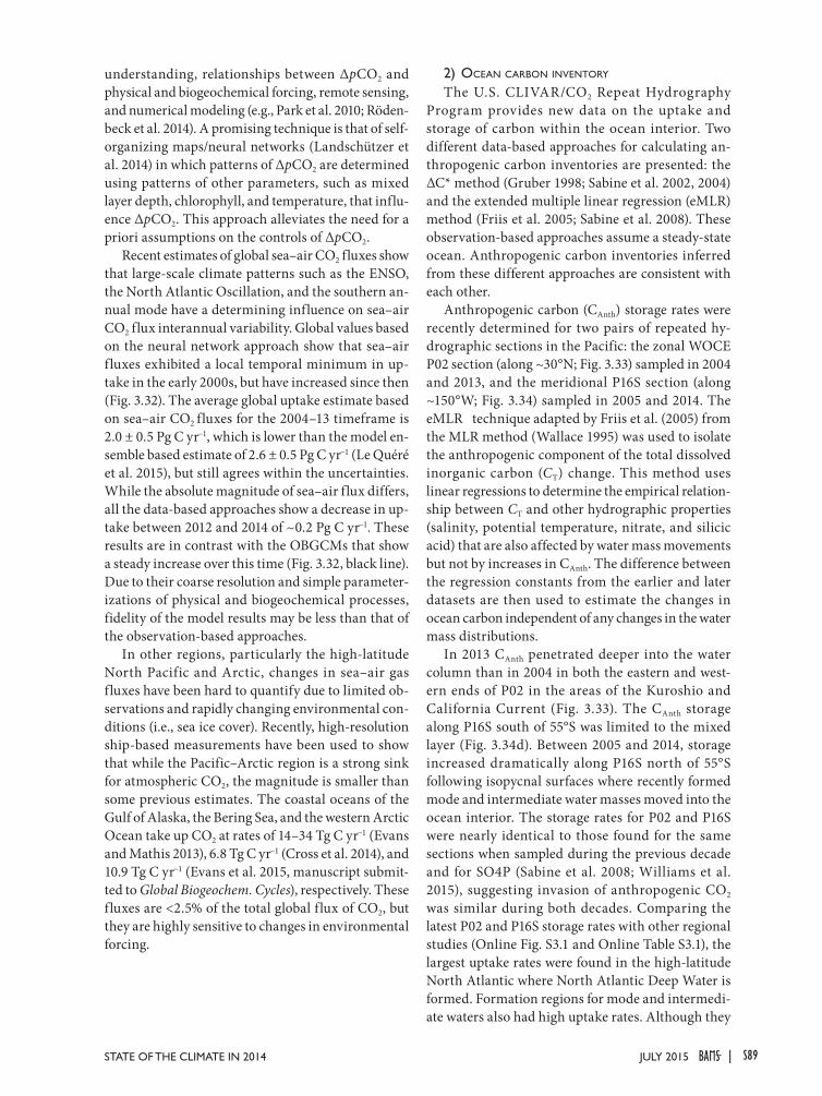
understanding, relationships between ∆pCO2 and physical and biogeochemical forcing, remote sensing, and numerical modeling (e.g., Park et al. 2010; Röden-beck et al. 2014). A promising technique is that of self-organizing maps/neural networks (Landschützer et al. 2014) in which patterns of ∆pCO2 are determined using patterns of other parameters, such as mixed layer depth, chlorophyll, and temperature, that influ-ence ∆pCO2. This approach alleviates the need for a priori assumptions on the controls of ∆pCO2.
Recent estimates of global sea–air CO2 fluxes show that large-scale climate patterns such as the ENSO, the North Atlantic Oscillation, and the southern an-nual mode have a determining influence on sea–air CO2 flux interannual variability. Global values based on the neural network approach show that sea–air f luxes exhibited a local temporal minimum in up-take in the early 2000s, but have increased since then (Fig. 3.32). The average global uptake estimate based on sea–air CO2 fluxes for the 2004–13 timeframe is 2.0 ± 0.5 Pg C yr−1, which is lower than the model en-semble based estimate of 2.6 ± 0.5 Pg C yr−1 (Le Quéré et al. 2015), but still agrees within the uncertainties. While the absolute magnitude of sea–air flux differs, all the data-based approaches show a decrease in up-take between 2012 and 2014 of ~0.2 Pg C yr−1. These results are in contrast with the OBGCMs that show a steady increase over this time (Fig. 3.32, black line). Due to their coarse resolution and simple parameter-izations of physical and biogeochemical processes, fidelity of the model results may be less than that of the observation-based approaches.
In other regions, particularly the high-latitude North Pacific and Arctic, changes in sea–air gas fluxes have been hard to quantify due to limited ob-servations and rapidly changing environmental con-ditions (i.e., sea ice cover). Recently, high-resolution ship-based measurements have been used to show that while the Pacific–Arctic region is a strong sink for atmospheric CO2, the magnitude is smaller than some previous estimates. The coastal oceans of the Gulf of Alaska, the Bering Sea, and the western Arctic Ocean take up CO2 at rates of 14–34 Tg C yr−1 (Evans and Mathis 2013), 6.8 Tg C yr−1 (Cross et al. 2014), and 10.9 Tg C yr−1 (Evans et al. 2015, manuscript submit-ted to Global Biogeochem. Cycles), respectively. These fluxes are <2.5% of the total global flux of CO2, but they are highly sensitive to changes in environmental forcing.
2) Ocean carbOn inventOry
The U.S. CLIVAR/CO2 Repeat Hydrography Program provides new data on the uptake and storage of carbon within the ocean interior. Two different data-based approaches for calculating an-thropogenic carbon inventories are presented: the ∆C* method (Gruber 1998; Sabine et al. 2002, 2004) and the extended multiple linear regression (eMLR) method (Friis et al. 2005; Sabine et al. 2008). These observation-based approaches assume a steady-state ocean. Anthropogenic carbon inventories inferred from these different approaches are consistent with each other.
Anthropogenic carbon (CAnth) storage rates were recently determined for two pairs of repeated hy-drographic sections in the Pacific: the zonal WOCE P02 section (along ~30°N; Fig. 3.33) sampled in 2004 and 2013, and the meridional P16S section (along ~150°W; Fig. 3.34) sampled in 2005 and 2014. The eMLR technique adapted by Friis et al. (2005) from the MLR method (Wallace 1995) was used to isolate the anthropogenic component of the total dissolved inorganic carbon (CT) change. This method uses linear regressions to determine the empirical relation-ship between CT and other hydrographic properties (salinity, potential temperature, nitrate, and silicic acid) that are also affected by water mass movements but not by increases in CAnth. The difference between the regression constants from the earlier and later datasets are then used to estimate the changes in ocean carbon independent of any changes in the water mass distributions.
In 2013 CAnth penetrated deeper into the water column than in 2004 in both the eastern and west-ern ends of P02 in the areas of the Kuroshio and California Current (Fig. 3.33). The CAnth storage along P16S south of 55°S was limited to the mixed layer (Fig. 3.34d). Between 2005 and 2014, storage increased dramatically along P16S north of 55°S following isopycnal surfaces where recently formed mode and intermediate water masses moved into the ocean interior. The storage rates for P02 and P16S were nearly identical to those found for the same sections when sampled during the previous decade and for SO4P (Sabine et al. 2008; Williams et al. 2015), suggesting invasion of anthropogenic CO2 was similar during both decades. Comparing the latest P02 and P16S storage rates with other regional studies (Online Fig. S3.1 and Online Table S3.1), the largest uptake rates were found in the high-latitude North Atlantic where North Atlantic Deep Water is formed. Formation regions for mode and intermedi-ate waters also had high uptake rates. Although they
S89JULY 2015STATE OF THE CLIMATE IN 2014 |
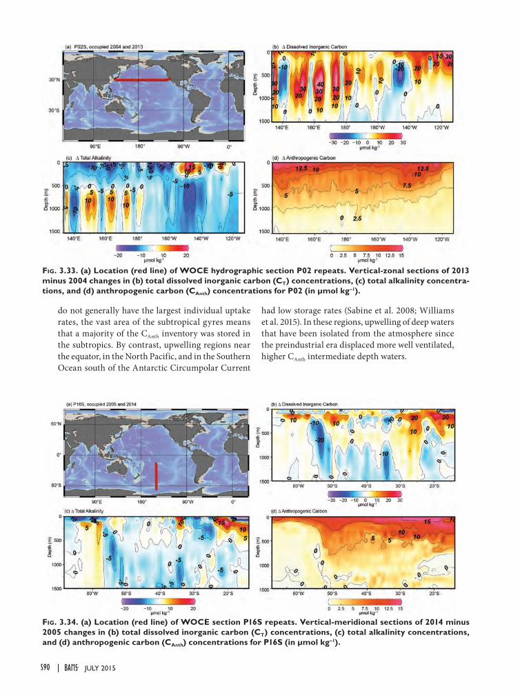
do not generally have the largest individual uptake rates, the vast area of the subtropical gyres means that a majority of the CAnth inventory was stored in the subtropics. By contrast, upwelling regions near the equator, in the North Pacific, and in the Southern Ocean south of the Antarctic Circumpolar Current
had low storage rates (Sabine et al. 2008; Williams et al. 2015). In these regions, upwelling of deep waters that have been isolated from the atmosphere since the preindustrial era displaced more well ventilated, higher CAnth intermediate depth waters.
Fig. 3.34. (a) Location (red line) of WOCE section P16S repeats. Vertical-meridional sections of 2014 minus 2005 changes in (b) total dissolved inorganic carbon (CT) concentrations, (c) total alkalinity concentrations, and (d) anthropogenic carbon (CAnth) concentrations for P16S (in µmol kg–1).
Fig. 3.33. (a) Location (red line) of WOCE hydrographic section P02 repeats. Vertical-zonal sections of 2013 minus 2004 changes in (b) total dissolved inorganic carbon (CT) concentrations, (c) total alkalinity concentra-tions, and (d) anthropogenic carbon (CAnth) concentrations for P02 (in µmol kg–1).
S90 JULY 2015|
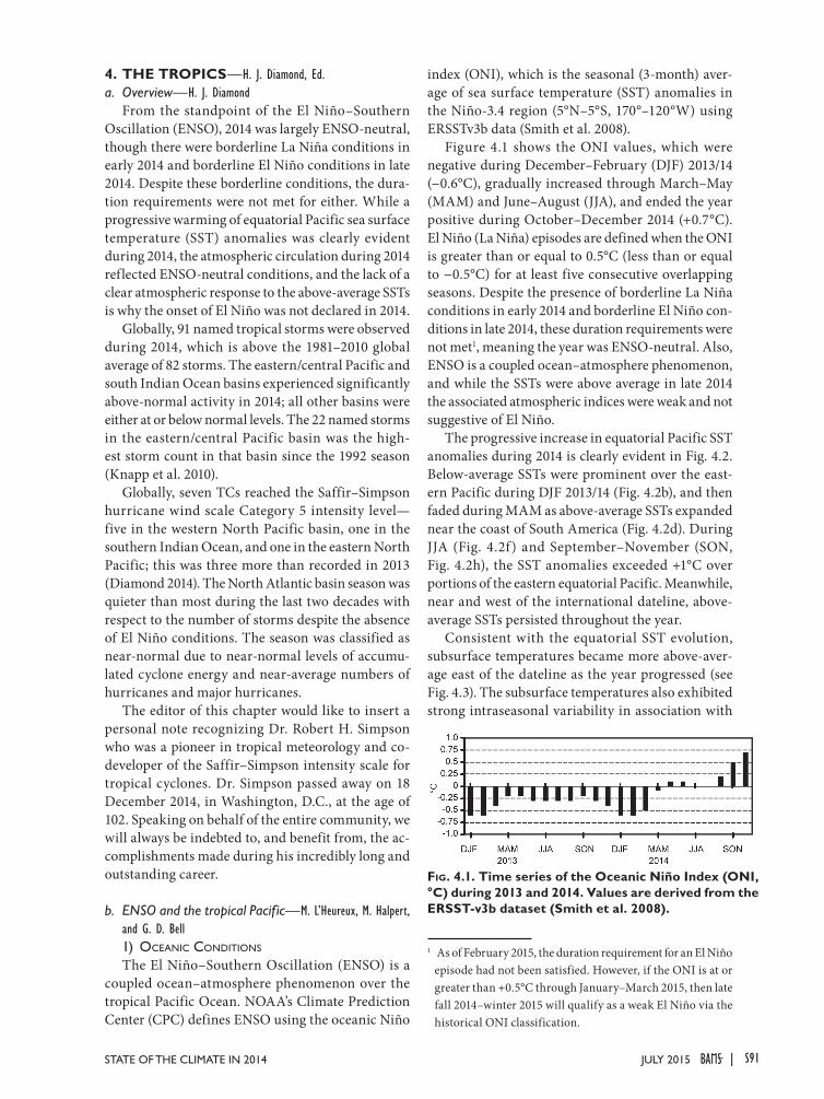
4. THE TROPICS—H. J. Diamond, Ed.a. Overview—H. J. Diamond
From the standpoint of the El Niño –Southern Oscillation (ENSO), 2014 was largely ENSO-neutral, though there were borderline La Niña conditions in early 2014 and borderline El Niño conditions in late 2014. Despite these borderline conditions, the dura-tion requirements were not met for either. While a progressive warming of equatorial Pacific sea surface temperature (SST) anomalies was clearly evident during 2014, the atmospheric circulation during 2014 reflected ENSO-neutral conditions, and the lack of a clear atmospheric response to the above-average SSTs is why the onset of El Niño was not declared in 2014.
Globally, 91 named tropical storms were observed during 2014, which is above the 1981–2010 global average of 82 storms. The eastern/central Pacific and south Indian Ocean basins experienced significantly above-normal activity in 2014; all other basins were either at or below normal levels. The 22 named storms in the eastern/central Pacific basin was the high-est storm count in that basin since the 1992 season (Knapp et al. 2010).
Globally, seven TCs reached the Saffir–Simpson hurricane wind scale Category 5 intensity level—five in the western North Pacific basin, one in the southern Indian Ocean, and one in the eastern North Pacific; this was three more than recorded in 2013 (Diamond 2014). The North Atlantic basin season was quieter than most during the last two decades with respect to the number of storms despite the absence of El Niño conditions. The season was classified as near-normal due to near-normal levels of accumu-lated cyclone energy and near-average numbers of hurricanes and major hurricanes.
The editor of this chapter would like to insert a personal note recognizing Dr. Robert H. Simpson who was a pioneer in tropical meteorology and co-developer of the Saffir–Simpson intensity scale for tropical cyclones. Dr. Simpson passed away on 18 December 2014, in Washington, D.C., at the age of 102. Speaking on behalf of the entire community, we will always be indebted to, and benefit from, the ac-complishments made during his incredibly long and outstanding career.
b. ENSO and the tropical Pacific—M. L’Heureux, M. Halpert, and G. D. Bell1) Oceanic cOnditiOns
The El Niño–Southern Oscillation (ENSO) is a coupled ocean–atmosphere phenomenon over the tropical Pacific Ocean. NOAA’s Climate Prediction Center (CPC) defines ENSO using the oceanic Niño
index (ONI), which is the seasonal (3-month) aver-age of sea surface temperature (SST) anomalies in the Niño-3.4 region (5°N–5°S, 170°–120°W) using ERSSTv3b data (Smith et al. 2008).
Figure 4.1 shows the ONI values, which were negative during December–February (DJF) 2013/14 (−0.6°C), gradually increased through March–May (MAM) and June–August (JJA), and ended the year positive during October–December 2014 (+0.7°C). El Niño (La Niña) episodes are defined when the ONI is greater than or equal to 0.5°C (less than or equal to −0.5°C) for at least five consecutive overlapping seasons. Despite the presence of borderline La Niña conditions in early 2014 and borderline El Niño con-ditions in late 2014, these duration requirements were not met1, meaning the year was ENSO-neutral. Also, ENSO is a coupled ocean–atmosphere phenomenon, and while the SSTs were above average in late 2014 the associated atmospheric indices were weak and not suggestive of El Niño.
The progressive increase in equatorial Pacific SST anomalies during 2014 is clearly evident in Fig. 4.2. Below-average SSTs were prominent over the east-ern Pacific during DJF 2013/14 (Fig. 4.2b), and then faded during MAM as above-average SSTs expanded near the coast of South America (Fig. 4.2d). During JJA (Fig. 4.2f) and September–November (SON, Fig. 4.2h), the SST anomalies exceeded +1°C over portions of the eastern equatorial Pacific. Meanwhile, near and west of the international dateline, above-average SSTs persisted throughout the year.
Consistent with the equatorial SST evolution, subsurface temperatures became more above-aver-age east of the dateline as the year progressed (see Fig. 4.3). The subsurface temperatures also exhibited strong intraseasonal variability in association with
1 As of February 2015, the duration requirement for an El Niño episode had not been satisfied. However, if the ONI is at or greater than +0.5°C through January–March 2015, then late fall 2014–winter 2015 will qualify as a weak El Niño via the historical ONI classification.
Fig. 4.1. Time series of the Oceanic Niño Index (ONI, °C) during 2013 and 2014. Values are derived from the ERSST-v3b dataset (Smith et al. 2008).
S91JULY 2015STATE OF THE CLIMATE IN 2014 |
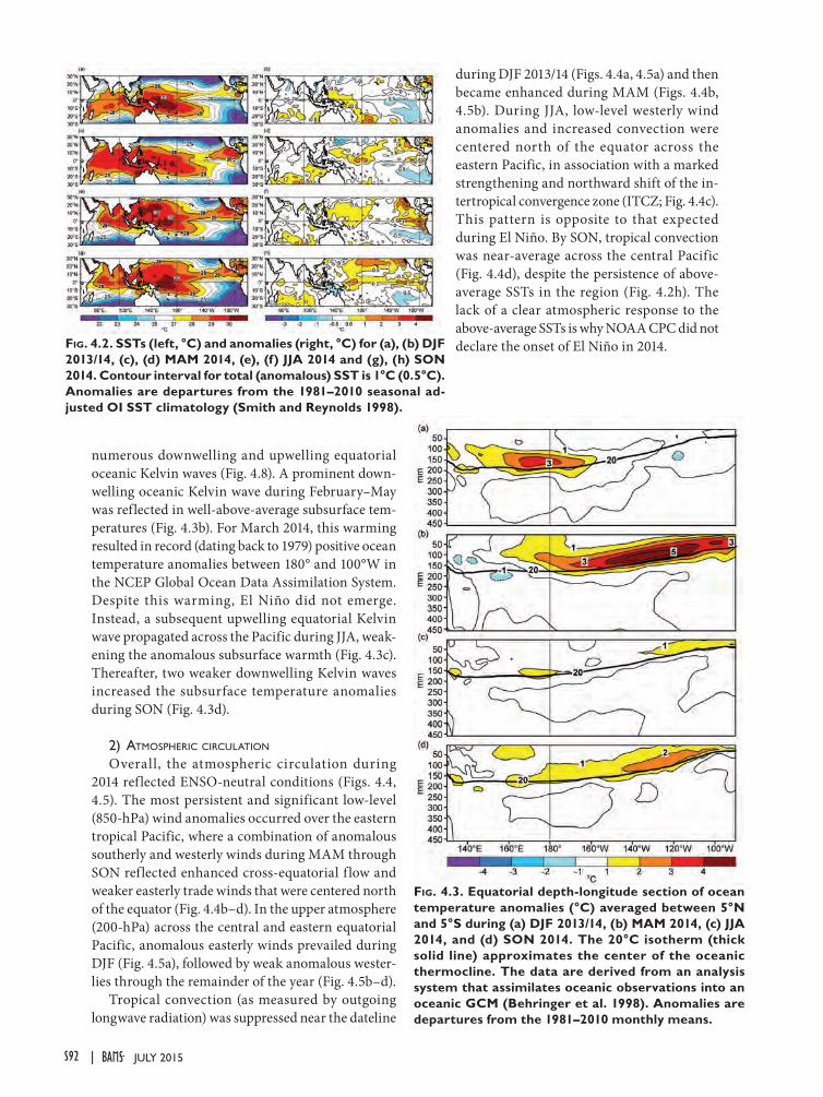
numerous downwelling and upwelling equatorial oceanic Kelvin waves (Fig. 4.8). A prominent down-welling oceanic Kelvin wave during February–May was reflected in well-above-average subsurface tem-peratures (Fig. 4.3b). For March 2014, this warming resulted in record (dating back to 1979) positive ocean temperature anomalies between 180° and 100°W in the NCEP Global Ocean Data Assimilation System. Despite this warming, El Niño did not emerge. Instead, a subsequent upwelling equatorial Kelvin wave propagated across the Pacific during JJA, weak-ening the anomalous subsurface warmth (Fig. 4.3c). Thereafter, two weaker downwelling Kelvin waves increased the subsurface temperature anomalies during SON (Fig. 4.3d).
2) atmOspheric circulatiOn
Overall, the atmospheric circulation during 2014 reflected ENSO-neutral conditions (Figs. 4.4, 4.5). The most persistent and significant low-level (850-hPa) wind anomalies occurred over the eastern tropical Pacific, where a combination of anomalous southerly and westerly winds during MAM through SON reflected enhanced cross-equatorial f low and weaker easterly trade winds that were centered north of the equator (Fig. 4.4b–d). In the upper atmosphere (200-hPa) across the central and eastern equatorial Pacific, anomalous easterly winds prevailed during DJF (Fig. 4.5a), followed by weak anomalous wester-lies through the remainder of the year (Fig. 4.5b–d).
Tropical convection (as measured by outgoing longwave radiation) was suppressed near the dateline
during DJF 2013/14 (Figs. 4.4a, 4.5a) and then became enhanced during MAM (Figs. 4.4b, 4.5b). During JJA, low-level westerly wind anomalies and increased convection were centered north of the equator across the eastern Pacific, in association with a marked strengthening and northward shift of the in-tertropical convergence zone (ITCZ; Fig. 4.4c). This pattern is opposite to that expected during El Niño. By SON, tropical convection was near-average across the central Pacific (Fig. 4.4d), despite the persistence of above-average SSTs in the region (Fig. 4.2h). The lack of a clear atmospheric response to the above-average SSTs is why NOAA CPC did not declare the onset of El Niño in 2014.Fig. 4.2. SSTs (left, °C) and anomalies (right, °C) for (a), (b) DJF
2013/14, (c), (d) MAM 2014, (e), (f) JJA 2014 and (g), (h) SON 2014. Contour interval for total (anomalous) SST is 1°C (0.5°C). Anomalies are departures from the 1981–2010 seasonal ad-justed OI SST climatology (Smith and Reynolds 1998).
Fig. 4.3. Equatorial depth-longitude section of ocean temperature anomalies (°C) averaged between 5°N and 5°S during (a) DJF 2013/14, (b) MAM 2014, (c) JJA 2014, and (d) SON 2014. The 20°C isotherm (thick solid line) approximates the center of the oceanic thermocline. The data are derived from an analysis system that assimilates oceanic observations into an oceanic GCM (Behringer et al. 1998). Anomalies are departures from the 1981–2010 monthly means.
S92 JULY 2015|
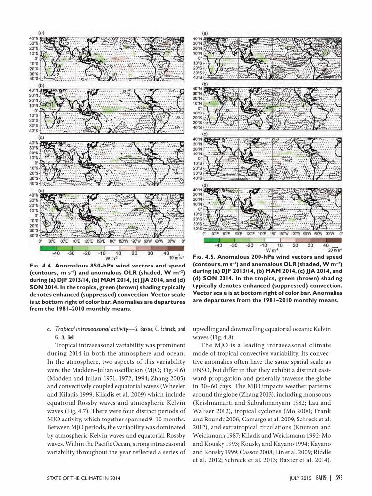
c. Tropical intraseasonal activity—S. Baxter, C. Schreck, and G. D. BellTropical intraseasonal variability was prominent
during 2014 in both the atmosphere and ocean. In the atmosphere, two aspects of this variability were the Madden–Julian oscillation (MJO; Fig. 4.6) (Madden and Julian 1971, 1972, 1994; Zhang 2005) and convectively coupled equatorial waves (Wheeler and Kiladis 1999; Kiladis et al. 2009) which include equatorial Rossby waves and atmospheric Kelvin waves (Fig. 4.7). There were four distinct periods of MJO activity, which together spanned 9–10 months. Between MJO periods, the variability was dominated by atmospheric Kelvin waves and equatorial Rossby waves. Within the Pacific Ocean, strong intraseasonal variability throughout the year reflected a series of
upwelling and downwelling equatorial oceanic Kelvin waves (Fig. 4.8).
The MJO is a leading intraseasonal climate mode of tropical convective variability. Its convec-tive anomalies often have the same spatial scale as ENSO, but differ in that they exhibit a distinct east-ward propagation and generally traverse the globe in 30–60 days. The MJO impacts weather patterns around the globe (Zhang 2013), including monsoons (Krishnamurti and Subrahmanyam 1982; Lau and Waliser 2012), tropical cyclones (Mo 2000; Frank and Roundy 2006; Camargo et al. 2009; Schreck et al. 2012), and extratropical circulations (Knutson and Weickmann 1987; Kiladis and Weickmann 1992; Mo and Kousky 1993; Kousky and Kayano 1994; Kayano and Kousky 1999; Cassou 2008; Lin et al. 2009; Riddle et al. 2012; Schreck et al. 2013; Baxter et al. 2014).
Fig. 4.4. Anomalous 850-hPa wind vectors and speed (contours, m s–1) and anomalous OLR (shaded, W m–2) during (a) DJF 2013/14, (b) MAM 2014, (c) JJA 2014, and (d) SON 2014. In the tropics, green (brown) shading typically denotes enhanced (suppressed) convection. Vector scale is at bottom right of color bar. Anomalies are departures from the 1981–2010 monthly means.
Fig. 4.5. Anomalous 200-hPa wind vectors and speed (contours, m s–1) and anomalous OLR (shaded, W m–2) during (a) DJF 2013/14, (b) MAM 2014, (c) JJA 2014, and (d) SON 2014. In the tropics, green (brown) shading typically denotes enhanced (suppressed) convection. Vector scale is at bottom right of color bar. Anomalies are departures from the 1981–2010 monthly means.
S93JULY 2015STATE OF THE CLIMATE IN 2014 |
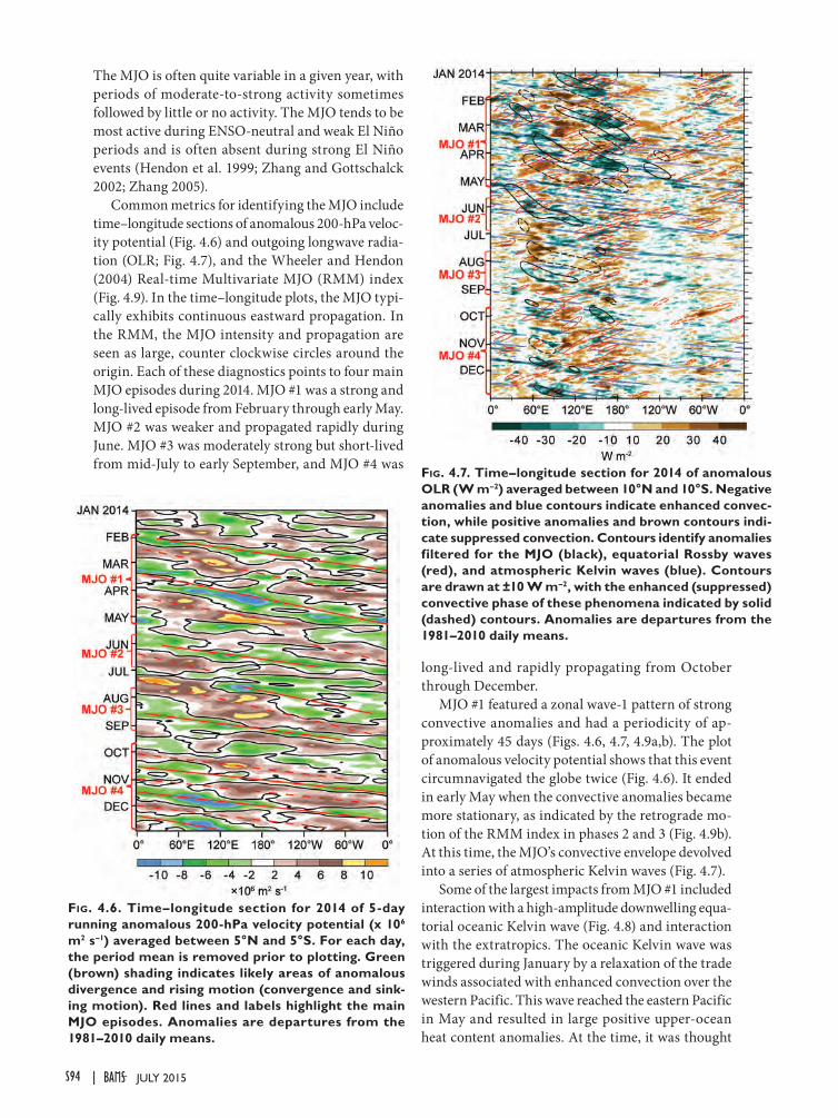
The MJO is often quite variable in a given year, with periods of moderate-to-strong activity sometimes followed by little or no activity. The MJO tends to be most active during ENSO-neutral and weak El Niño periods and is often absent during strong El Niño events (Hendon et al. 1999; Zhang and Gottschalck 2002; Zhang 2005).
Common metrics for identifying the MJO include time–longitude sections of anomalous 200-hPa veloc-ity potential (Fig. 4.6) and outgoing longwave radia-tion (OLR; Fig. 4.7), and the Wheeler and Hendon (2004) Real-time Multivariate MJO (RMM) index (Fig. 4.9). In the time–longitude plots, the MJO typi-cally exhibits continuous eastward propagation. In the RMM, the MJO intensity and propagation are seen as large, counter clockwise circles around the origin. Each of these diagnostics points to four main MJO episodes during 2014. MJO #1 was a strong and long-lived episode from February through early May. MJO #2 was weaker and propagated rapidly during June. MJO #3 was moderately strong but short-lived from mid-July to early September, and MJO #4 was
long-lived and rapidly propagating from October through December.
MJO #1 featured a zonal wave-1 pattern of strong convective anomalies and had a periodicity of ap-proximately 45 days (Figs. 4.6, 4.7, 4.9a,b). The plot of anomalous velocity potential shows that this event circumnavigated the globe twice (Fig. 4.6). It ended in early May when the convective anomalies became more stationary, as indicated by the retrograde mo-tion of the RMM index in phases 2 and 3 (Fig. 4.9b). At this time, the MJO’s convective envelope devolved into a series of atmospheric Kelvin waves (Fig. 4.7).
Some of the largest impacts from MJO #1 included interaction with a high-amplitude downwelling equa-torial oceanic Kelvin wave (Fig. 4.8) and interaction with the extratropics. The oceanic Kelvin wave was triggered during January by a relaxation of the trade winds associated with enhanced convection over the western Pacific. This wave reached the eastern Pacific in May and resulted in large positive upper-ocean heat content anomalies. At the time, it was thought
Fig. 4.6. Time–longitude section for 2014 of 5-day running anomalous 200-hPa velocity potential (x 106 m2 s–1) averaged between 5°N and 5°S. For each day, the period mean is removed prior to plotting. Green (brown) shading indicates likely areas of anomalous divergence and rising motion (convergence and sink-ing motion). Red lines and labels highlight the main MJO episodes. Anomalies are departures from the 1981–2010 daily means.
Fig. 4.7. Time–longitude section for 2014 of anomalous OLR (W m–2) averaged between 10°N and 10°S. Negative anomalies and blue contours indicate enhanced convec-tion, while positive anomalies and brown contours indi-cate suppressed convection. Contours identify anomalies filtered for the MJO (black), equatorial Rossby waves (red), and atmospheric Kelvin waves (blue). Contours are drawn at ±10 W m–2, with the enhanced (suppressed) convective phase of these phenomena indicated by solid (dashed) contours. Anomalies are departures from the 1981–2010 daily means.
S94 JULY 2015|
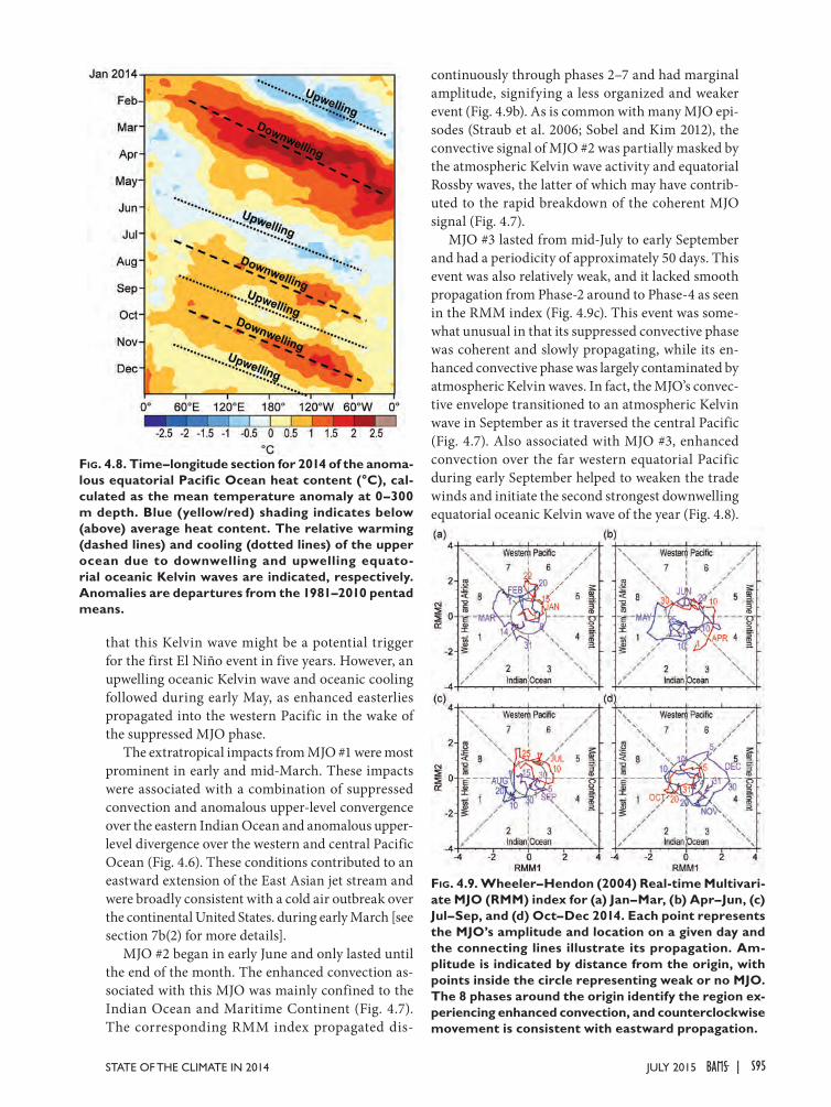
that this Kelvin wave might be a potential trigger for the first El Niño event in five years. However, an upwelling oceanic Kelvin wave and oceanic cooling followed during early May, as enhanced easterlies propagated into the western Pacific in the wake of the suppressed MJO phase.
The extratropical impacts from MJO #1 were most prominent in early and mid-March. These impacts were associated with a combination of suppressed convection and anomalous upper-level convergence over the eastern Indian Ocean and anomalous upper-level divergence over the western and central Pacific Ocean (Fig. 4.6). These conditions contributed to an eastward extension of the East Asian jet stream and were broadly consistent with a cold air outbreak over the continental United States. during early March [see section 7b(2) for more details].
MJO #2 began in early June and only lasted until the end of the month. The enhanced convection as-sociated with this MJO was mainly confined to the Indian Ocean and Maritime Continent (Fig. 4.7). The corresponding RMM index propagated dis-
continuously through phases 2–7 and had marginal amplitude, signifying a less organized and weaker event (Fig. 4.9b). As is common with many MJO epi-sodes (Straub et al. 2006; Sobel and Kim 2012), the convective signal of MJO #2 was partially masked by the atmospheric Kelvin wave activity and equatorial Rossby waves, the latter of which may have contrib-uted to the rapid breakdown of the coherent MJO signal (Fig. 4.7).
MJO #3 lasted from mid-July to early September and had a periodicity of approximately 50 days. This event was also relatively weak, and it lacked smooth propagation from Phase-2 around to Phase-4 as seen in the RMM index (Fig. 4.9c). This event was some-what unusual in that its suppressed convective phase was coherent and slowly propagating, while its en-hanced convective phase was largely contaminated by atmospheric Kelvin waves. In fact, the MJO’s convec-tive envelope transitioned to an atmospheric Kelvin wave in September as it traversed the central Pacific (Fig. 4.7). Also associated with MJO #3, enhanced convection over the far western equatorial Pacific during early September helped to weaken the trade winds and initiate the second strongest downwelling equatorial oceanic Kelvin wave of the year (Fig. 4.8).
Fig. 4.8. Time–longitude section for 2014 of the anoma-lous equatorial Pacific Ocean heat content (°C), cal-culated as the mean temperature anomaly at 0–300 m depth. Blue (yellow/red) shading indicates below (above) average heat content. The relative warming (dashed lines) and cooling (dotted lines) of the upper ocean due to downwelling and upwelling equato-rial oceanic Kelvin waves are indicated, respectively. Anomalies are departures from the 1981–2010 pentad means.
Fig. 4.9. Wheeler–Hendon (2004) Real-time Multivari-ate MJO (RMM) index for (a) Jan–Mar, (b) Apr–Jun, (c) Jul–Sep, and (d) Oct–Dec 2014. Each point represents the MJO’s amplitude and location on a given day and the connecting lines illustrate its propagation. Am-plitude is indicated by distance from the origin, with points inside the circle representing weak or no MJO. The 8 phases around the origin identify the region ex-periencing enhanced convection, and counterclockwise movement is consistent with eastward propagation.
S95JULY 2015STATE OF THE CLIMATE IN 2014 |
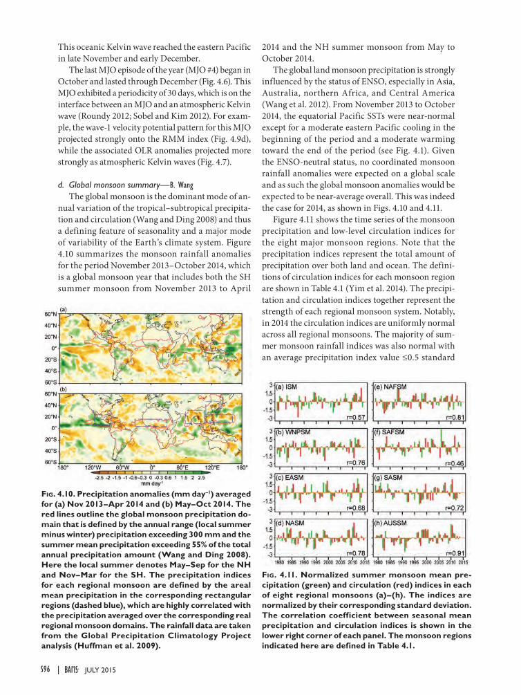
This oceanic Kelvin wave reached the eastern Pacific in late November and early December.
The last MJO episode of the year (MJO #4) began in October and lasted through December (Fig. 4.6). This MJO exhibited a periodicity of 30 days, which is on the interface between an MJO and an atmospheric Kelvin wave (Roundy 2012; Sobel and Kim 2012). For exam-ple, the wave-1 velocity potential pattern for this MJO projected strongly onto the RMM index (Fig. 4.9d), while the associated OLR anomalies projected more strongly as atmospheric Kelvin waves (Fig. 4.7).
d. Global monsoon summary—B. WangThe global monsoon is the dominant mode of an-
nual variation of the tropical–subtropical precipita-tion and circulation (Wang and Ding 2008) and thus a defining feature of seasonality and a major mode of variability of the Earth’s climate system. Figure 4.10 summarizes the monsoon rainfall anomalies for the period November 2013–October 2014, which is a global monsoon year that includes both the SH summer monsoon from November 2013 to April
2014 and the NH summer monsoon from May to October 2014.
The global land monsoon precipitation is strongly influenced by the status of ENSO, especially in Asia, Australia, northern Africa, and Central America (Wang et al. 2012). From November 2013 to October 2014, the equatorial Pacific SSTs were near-normal except for a moderate eastern Pacific cooling in the beginning of the period and a moderate warming toward the end of the period (see Fig. 4.1). Given the ENSO-neutral status, no coordinated monsoon rainfall anomalies were expected on a global scale and as such the global monsoon anomalies would be expected to be near-average overall. This was indeed the case for 2014, as shown in Figs. 4.10 and 4.11.
Figure 4.11 shows the time series of the monsoon precipitation and low-level circulation indices for the eight major monsoon regions. Note that the precipitation indices represent the total amount of precipitation over both land and ocean. The defini-tions of circulation indices for each monsoon region are shown in Table 4.1 (Yim et al. 2014). The precipi-tation and circulation indices together represent the strength of each regional monsoon system. Notably, in 2014 the circulation indices are uniformly normal across all regional monsoons. The majority of sum-mer monsoon rainfall indices was also normal with an average precipitation index value ≤0.5 standard
Fig. 4.10. Precipitation anomalies (mm day–1) averaged for (a) Nov 2013–Apr 2014 and (b) May–Oct 2014. The red lines outline the global monsoon precipitation do-main that is defined by the annual range (local summer minus winter) precipitation exceeding 300 mm and the summer mean precipitation exceeding 55% of the total annual precipitation amount (Wang and Ding 2008). Here the local summer denotes May–Sep for the NH and Nov–Mar for the SH. The precipitation indices for each regional monsoon are defined by the areal mean precipitation in the corresponding rectangular regions (dashed blue), which are highly correlated with the precipitation averaged over the corresponding real regional monsoon domains. The rainfall data are taken from the Global Precipitation Climatology Project analysis (Huffman et al. 2009).
Fig. 4.11. Normalized summer monsoon mean pre-cipitation (green) and circulation (red) indices in each of eight regional monsoons (a)–(h). The indices are normalized by their corresponding standard deviation. The correlation coefficient between seasonal mean precipitation and circulation indices is shown in the lower right corner of each panel. The monsoon regions indicated here are defined in Table 4.1.
S96 JULY 2015|
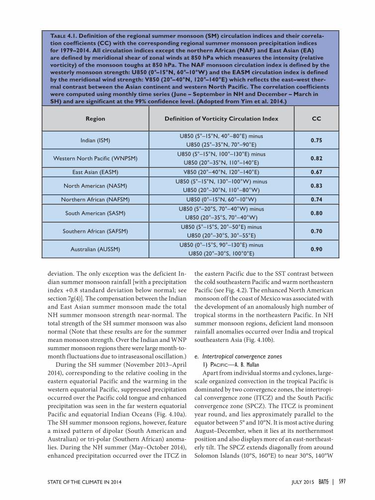
deviation. The only exception was the deficient In-dian summer monsoon rainfall [with a precipitation index +0.8 standard deviation below normal; see section 7g(4)]. The compensation between the Indian and East Asian summer monsoon made the total NH summer monsoon strength near-normal. The total strength of the SH summer monsoon was also normal (Note that these results are for the summer mean monsoon strength. Over the Indian and WNP summer monsoon regions there were large month-to-month fluctuations due to intraseasonal oscillation.)
During the SH summer (November 2013–April 2014), corresponding to the relative cooling in the eastern equatorial Pacific and the warming in the western equatorial Pacific, suppressed precipitation occurred over the Pacific cold tongue and enhanced precipitation was seen in the far western equatorial Pacific and equatorial Indian Oceans (Fig. 4.10a). The SH summer monsoon regions, however, feature a mixed pattern of dipolar (South American and Australian) or tri-polar (Southern African) anoma-lies. During the NH summer (May–October 2014), enhanced precipitation occurred over the ITCZ in
the eastern Pacific due to the SST contrast between the cold southeastern Pacific and warm northeastern Pacific (see Fig. 4.2). The enhanced North American monsoon off the coast of Mexico was associated with the development of an anomalously high number of tropical storms in the northeastern Pacific. In NH summer monsoon regions, deficient land monsoon rainfall anomalies occurred over India and tropical southeastern Asia (Fig. 4.10b).
e. Intertropical convergence zones1) pacific—A. B. MullanApart from individual storms and cyclones, large-
scale organized convection in the tropical Pacific is dominated by two convergence zones, the intertropi-cal convergence zone (ITCZ) and the South Pacific convergence zone (SPCZ). The ITCZ is prominent year round, and lies approximately parallel to the equator between 5° and 10°N. It is most active during August–December, when it lies at its northernmost position and also displays more of an east-northeast-erly tilt. The SPCZ extends diagonally from around Solomon Islands (10°S, 160°E) to near 30°S, 140°W
Table 4.1. Definition of the regional summer monsoon (SM) circulation indices and their correla-tion coefficients (CC) with the corresponding regional summer monsoon precipitation indices for 1979–2014. All circulation indices except the northern African (NAF) and East Asian (EA) are defined by meridional shear of zonal winds at 850 hPa which measures the intensity (relative vorticity) of the monsoon toughs at 850 hPa. The NAF monsoon circulation index is defined by the westerly monsoon strength: U850 (0°–15°N, 60°–10°W) and the EASM circulation index is defined by the meridional wind strength: V850 (20°–40°N, 120°–140°E) which reflects the east–west ther-mal contrast between the Asian continent and western North Pacific. The correlation coefficients were computed using monthly time series (June – September in NH and December – March in SH) and are significant at the 99% confidence level. (Adopted from Yim et al. 2014.)
Region Definition of Vorticity Circulation Index CC
Indian (ISM) U850 (5°–15°N, 40°–80°E) minus
U850 (25°–35°N, 70°–90°E)0.75
Western North Pacific (WNPSM)U850 (5°–15°N, 100°–130°E) minus
U850 (20°–35°N, 110°–140°E)0.82
East Asian (EASM) V850 (20°–40°N, 120°–140°E) 0.67
North American (NASM) U850 (5°–15°N, 130°–100°W) minus
U850 (20°–30°N, 110°–80°W)0.83
Northern African (NAFSM) U850 (0°–15°N, 60°–10°W) 0.74
South American (SASM) U850 (5°–20°S, 70°–40°W) minus
U850 (20°–35°S, 70°–40°W)0.80
Southern African (SAFSM)U850 (5°–15°S, 20°–50°E) minus
U850 (20°–30°S, 30°–55°E) 0.70
Australian (AUSSM)U850 (0°–15°S, 90°–130°E) minus
U850 (20°–30°S, 100°0°E)0.90
S97JULY 2015STATE OF THE CLIMATE IN 2014 |
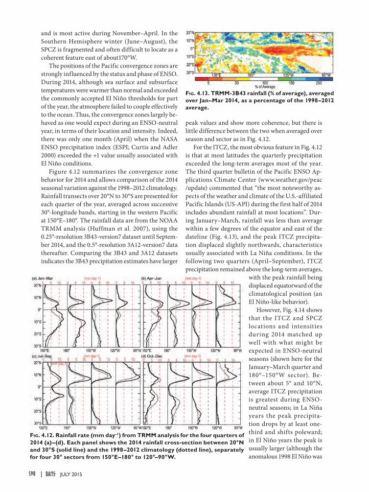
and is most active during November–April. In the Southern Hemisphere winter (June–August), the SPCZ is fragmented and often difficult to locate as a coherent feature east of about170°W.
The positions of the Pacific convergence zones are strongly influenced by the status and phase of ENSO. During 2014, although sea surface and subsurface temperatures were warmer than normal and exceeded the commonly accepted El Niño thresholds for part of the year, the atmosphere failed to couple effectively to the ocean. Thus, the convergence zones largely be-haved as one would expect during an ENSO-neutral year, in terms of their location and intensity. Indeed, there was only one month (April) when the NASA ENSO precipitation index (ESPI; Curtis and Adler 2000) exceeded the +1 value usually associated with El Niño conditions.
Figure 4.12 summarizes the convergence zone behavior for 2014 and allows comparison of the 2014 seasonal variation against the 1998–2012 climatology. Rainfall transects over 20°N to 30°S are presented for each quarter of the year, averaged across successive 30°-longitude bands, starting in the western Pacific at 150°E–180°. The rainfall data are from the NOAA TRMM analysis (Huffman et al. 2007), using the 0.25°-resolution 3B43-version7 dataset until Septem-ber 2014, and the 0.5°-resolution 3A12-version7 data thereafter. Comparing the 3B43 and 3A12 datasets indicates the 3B43 precipitation estimates have larger
peak values and show more coherence, but there is little difference between the two when averaged over season and sector as in Fig. 4.12.
For the ITCZ, the most obvious feature in Fig. 4.12 is that at most latitudes the quarterly precipitation exceeded the long-term averages most of the year. The third quarter bulletin of the Pacific ENSO Ap-plications Climate Center (www.weather.gov/peac /update) commented that “the most noteworthy as-pects of the weather and climate of the U.S.-affiliated Pacific Islands (US-API) during the first half of 2014 includes abundant rainfall at most locations”. Dur-ing January–March, rainfall was less than average within a few degrees of the equator and east of the dateline (Fig. 4.13), and the peak ITCZ precipita-tion displaced slightly northwards, characteristics usually associated with La Niña conditions. In the following two quarters (April–September), ITCZ precipitation remained above the long-term averages,
with the peak rainfall being displaced equatorward of the climatological position (an El Niño-like behavior).
However, Fig. 4.14 shows that the ITCZ and SPCZ locations and intensities during 2014 matched up well with what might be expected in ENSO-neutral seasons (shown here for the January–March quarter and 180°–150°W sector). Be-tween about 5° and 10°N, average ITCZ precipitation is greatest during ENSO-neutral seasons; in La Niña years the peak precipita-tion drops by at least one-third and shifts poleward; in El Niño years the peak is usually larger (although the anomalous 1998 El Niño was
Fig. 4.12. Rainfall rate (mm day–1) from TRMM analysis for the four quarters of 2014 (a)–(d). Each panel shows the 2014 rainfall cross-section between 20°N and 30°S (solid line) and the 1998–2012 climatology (dotted line), separately for four 30° sectors from 150°E–180° to 120°–90°W.
Fig. 4.13. TRMM-3B43 rainfall (% of average), averaged over Jan–Mar 2014, as a percentage of the 1998–2012 average.
S98 JULY 2015|
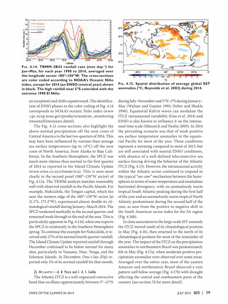
an exception) and shifts equatorward. The identifica-tion of ENSO phases in the color coding of Fig. 4.14 corresponds to NOAA’s oceanic Niño index (www .cpc.ncep.noaa.gov/products/analysis_monitoring /ensostuff/ensoyears.shtml).
The Fig. 4.12 cross-sections also highlight the above-normal precipitation off the west coast of Central America in the last two quarters of 2014. This may have been influenced by warmer-than-average sea surface temperatures (up to +2°C) off the west coast of North America, from Alaska to Baja Cali-fornia. In the Southern Hemisphere, the SPCZ was much more intense than normal in the first quarter of 2014 as reported in the Island Climate Update (www.niwa.co.nz/climate/icu). This is seen most clearly in the second panel (180°–150°W sector) of Fig. 4.12a. The TRMM analysis matches reasonably well with observed rainfall in the Pacific Islands. For example, Nuku’alofa, the Tongan capital, which lies near the western edge of the 180°–150°W sector (at 21.1°S, 175.2°W), experienced almost double its cli-matological rainfall during January–March 2014. The SPCZ weakened markedly in the second quarter, and remained weak through to the end of the year. This is particularly apparent in Fig. 4.12d, when one expects the SPCZ to reintensify in the Southern Hemisphere spring. To continue the example for Nuku’alofa, it re-ceived only 27% of its normal fourth quarter rainfall. The Island Climate Update reported rainfall through December continued to be below normal for many sites, particularly in Vanuatu, Niue, Tonga, and the Solomon Islands. In December, Ono-i-lau (Fiji) re-ported only 1% of its normal rainfall for that month.
2) atlantic—A. B. Pezza and C. A. S. CoelhoThe Atlantic ITCZ is a well-organized convective
band that oscillates approximately between 5°–12°N
during July–November and 5°N–5°S during January–May (Waliser and Gautier 1993; Nobre and Shukla 1996). Equatorial Kelvin waves can modulate the ITCZ intraseasonal variability (Guo et al. 2014) and ENSO is also known to influence it on the interan-nual time scale (Münnich and Neelin 2005). In 2014 the prevailing scenario was that of weak positive sea surface temperature anomalies in the equato-rial Pacific for most of the year. These conditions represent a warming compared to most of 2013, but are still associated with neutral ENSO conditions, with absence of a well-defined teleconnective sea surface forcing driving the behavior of the Atlantic ITCZ (Fig. 4.15). However, the intraseasonal activity within the Atlantic sector continued to respond to the typical “see-saw” mechanism between the hemi-spheres in terms of water temperature and anomalous horizontal divergence, with an anomalously warm tropical South Atlantic peaking during the first half of the year and an anomalously warm tropical North Atlantic predominant during the second half of the year, as seen from the positive to negative shift in the South American sector index for the SA region (Fig. 4.16b).
In close association to the large-scale SST anomaly the ITCZ moved south of its climatological position in May (Fig. 4.16), then returned to the north of its climatological position for most of the remainder of the year. The impact of the ITCZ on the precipitation anomalies in northeastern Brazil was predominately felt in May (Fig. 4.17a), when moderate positive pre-cipitation anomalies were observed over some areas. Averaged over the entire year, most of the eastern Amazon and northeastern Brazil observed a rain pattern well below average (Fig. 4.17b) with drought affecting the central and southeastern parts of the country (see section 7d for more detail).
Fig. 4.14. TRMM-3B43 rainfall rate (mm day–1) for Jan–Mar, for each year 1998 to 2014, averaged over the longitude sector 180°–150°W. The cross-sections are color coded according to NOAA’s Oceanic Niño index, except for 2014 (an ENSO-neutral year) shown in black. The high rainfall near 5°S coincided with the extreme 1998 El Niño.
Fig. 4.15. Spatial distribution of average global SST anomalies (°C, Reynolds et al. 2002) during 2014.
S99JULY 2015STATE OF THE CLIMATE IN 2014 |
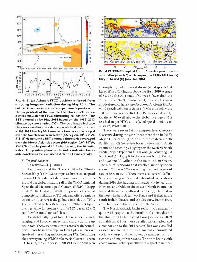
f. Tropical cyclones1) Overview—H. J. DiamondThe International Best Track Archive for Climate
Stewardship (IBTrACS) comprises historical tropical cyclone (TC) best-track data from numerous sources around the globe, including all of the WMO Regional Specialized Meteorological Centers (RSMC; Knapp et al. 2010). To date, IBTrACS represents the most complete compilation of TC data and offers a unique opportunity to revisit the global climatology of TCs. Using IBTrACS data (Schreck et al. 2014) a 30-year average value for storms (from WMO-based RSMC numbers) is noted for each basin.
The global tallying of total TC numbers is chal-lenging and involves more than simply adding up basin totals because some storms cross basin bound-aries, some basins overlap, and multiple agencies are involved in tracking and forecasting TCs. Compiling the activity (using WMO information) over all seven TC basins, the 2014 season (2013/14 in the Southern
Hemisphere) had 91 named storms (wind speeds ≥34 kts or 18 m s−1), which is above the 1981–2010 average of 82, and the 2014 total of 91 was 3 fewer than the 2013 total of 94 (Diamond 2014). The 2014 season also featured 42 hurricanes/typhoons/cyclones (HTC; wind speeds ≥64 kts or 33 m s−1), which is below the 1981–2010 average of 46 HTCs (Schreck et al. 2014). Of these, 30 (well above the global average of 21) reached major HTC status (wind speeds ≥96 kts or 49 m s−1; WMO 2015).
There were seven Saffir–Simpson level Category 5 systems during the year (three more than in 2013): Major Hurricanes (1) Marie in the eastern North Pacific, and (2) Genevieve born in the eastern North Pacific and reaching Category 5 in the western North Pacific; Super Typhoons (3) Halong, (4) Vongfong, (5) Nuri, and (6) Hagupit in the western North Pacific; and Cyclone (7) Gillian in the south Indian Ocean. The rate of typhoons that reached super typhoon status in 2014 was 67%, exceeding the previous record rate of 58% in 1970. There were also several Saffir–Simpson Category 3 and 4 intensity-level systems during 2014 that had major impacts: (1) Iselle, Julio, Norbert, and Odile in the eastern North Pacific; (2) Ian and Ita in the southwest Pacific; (3) Hudhud in the north Indian Ocean; (4) Bruce and Hellen in the south Indian Ocean; and (5) Neogury, Rammasun, and Phanfone in the western North Pacific.
The North Atlantic basin season was unusually quiet with respect to the number of storms despite the absence of El Niño conditions [see section 4f(2) and Sidebar 4.1 for more detailed information and a comparison to the 2013 season] but was classified as near-normal due to near-normal accumulated cyclone energy and near-average numbers of hur-ricanes and major hurricanes. The only basins with above-normal activity in 2014 with respect to number
Fig. 4.16. (a) Atlantic ITCZ position inferred from outgoing longwave radiation during May 2014. The colored thin lines indicate the approximate position for the six pentads of the month. The black thick line in-dicates the Atlantic ITCZ climatological position. The SST anomalies for May 2014 based on the 1982–2013 climatology are shaded (°C). The two boxes indicate the areas used for the calculation of the Atlantic index in (b). (b) Monthly SST anomaly time series averaged over the South American sector (SA region, 10°–50°W, 5°S–5°N) minus the SST anomaly time series averaged over the North Atlantic sector (NA region, 20°–50°W, 5°–25°N) for the period 2010–14, forming the Atlantic index. The positive phase of the index indicates favor-able conditions for enhanced Atlantic ITCZ activity.
Fig. 4.17. TRMM tropical South America precipitation anomalies (mm h–1) with respect to 1998–2013 for (a) May 2014 and (b) Jan–Dec 2014.
S100 JULY 2015|
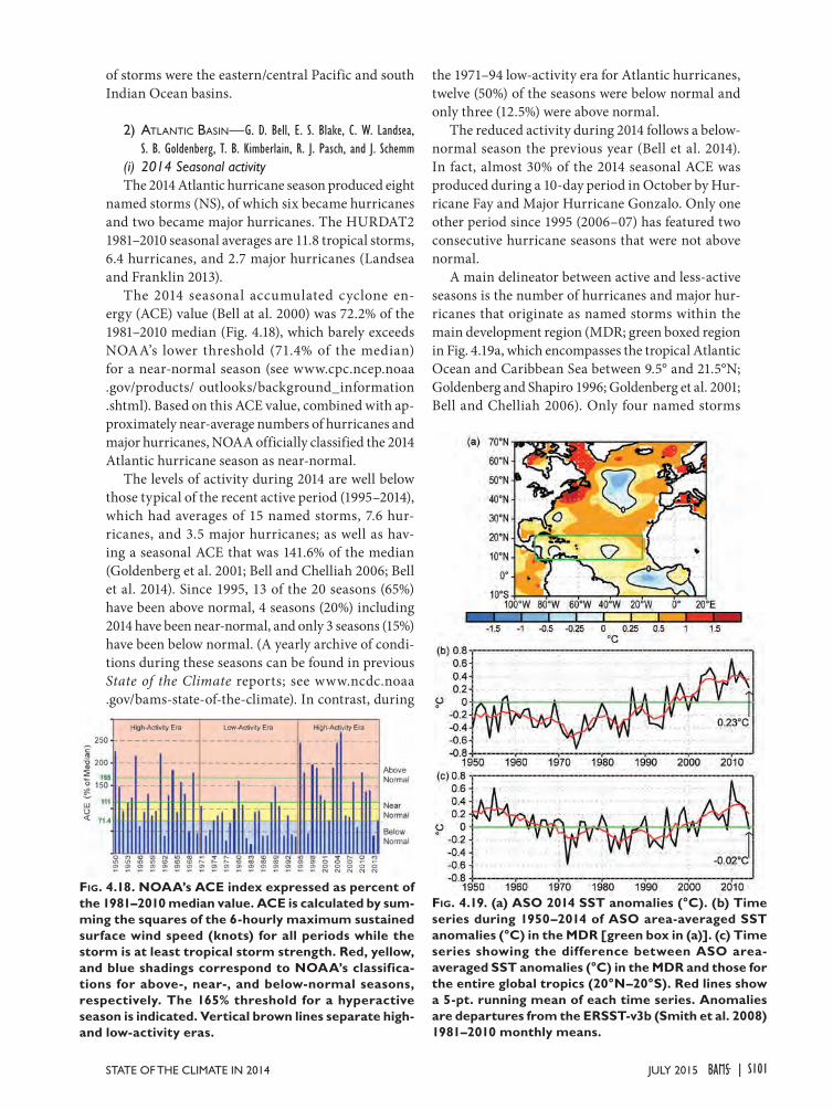
of storms were the eastern/central Pacific and south Indian Ocean basins.
2) atlantic Basin—G. D. Bell, E. S. Blake, C. W. Landsea, S. B. Goldenberg, T. B. Kimberlain, R. J. Pasch, and J. Schemm
(i) 2014 Seasonal activityThe 2014 Atlantic hurricane season produced eight
named storms (NS), of which six became hurricanes and two became major hurricanes. The HURDAT2 1981–2010 seasonal averages are 11.8 tropical storms, 6.4 hurricanes, and 2.7 major hurricanes (Landsea and Franklin 2013).
The 2014 seasonal accumulated cyclone en-ergy (ACE) value (Bell at al. 2000) was 72.2% of the 1981–2010 median (Fig. 4.18), which barely exceeds NOAA’s lower threshold (71.4% of the median) for a near-normal season (see www.cpc.ncep.noaa .gov/products/ outlooks/background_information .shtml). Based on this ACE value, combined with ap-proximately near-average numbers of hurricanes and major hurricanes, NOAA officially classified the 2014 Atlantic hurricane season as near-normal.
The levels of activity during 2014 are well below those typical of the recent active period (1995–2014), which had averages of 15 named storms, 7.6 hur-ricanes, and 3.5 major hurricanes; as well as hav-ing a seasonal ACE that was 141.6% of the median (Goldenberg et al. 2001; Bell and Chelliah 2006; Bell et al. 2014). Since 1995, 13 of the 20 seasons (65%) have been above normal, 4 seasons (20%) including 2014 have been near-normal, and only 3 seasons (15%) have been below normal. (A yearly archive of condi-tions during these seasons can be found in previous State of the Climate reports; see www.ncdc.noaa .gov/bams-state-of-the-climate). In contrast, during
the 1971–94 low-activity era for Atlantic hurricanes, twelve (50%) of the seasons were below normal and only three (12.5%) were above normal.
The reduced activity during 2014 follows a below-normal season the previous year (Bell et al. 2014). In fact, almost 30% of the 2014 seasonal ACE was produced during a 10-day period in October by Hur-ricane Fay and Major Hurricane Gonzalo. Only one other period since 1995 (2006–07) has featured two consecutive hurricane seasons that were not above normal.
A main delineator between active and less-active seasons is the number of hurricanes and major hur-ricanes that originate as named storms within the main development region (MDR; green boxed region in Fig. 4.19a, which encompasses the tropical Atlantic Ocean and Caribbean Sea between 9.5° and 21.5°N; Goldenberg and Shapiro 1996; Goldenberg et al. 2001; Bell and Chelliah 2006). Only four named storms
Fig. 4.18. NOAA’s ACE index expressed as percent of the 1981–2010 median value. ACE is calculated by sum-ming the squares of the 6-hourly maximum sustained surface wind speed (knots) for all periods while the storm is at least tropical storm strength. Red, yellow, and blue shadings correspond to NOAA’s classifica-tions for above-, near-, and below-normal seasons, respectively. The 165% threshold for a hyperactive season is indicated. Vertical brown lines separate high- and low-activity eras.
Fig. 4.19. (a) ASO 2014 SST anomalies (°C). (b) Time series during 1950–2014 of ASO area-averaged SST anomalies (°C) in the MDR [green box in (a)]. (c) Time series showing the difference between ASO area-averaged SST anomalies (°C) in the MDR and those for the entire global tropics (20°N–20°S). Red lines show a 5-pt. running mean of each time series. Anomalies are departures from the ERSST-v3b (Smith et al. 2008) 1981–2010 monthly means.
S101JULY 2015STATE OF THE CLIMATE IN 2014 |

formed in the MDR during 2014, three of which even-tually became hurricanes and two of those became major hurricanes.
The resulting ACE value from the four MDR storms was 42.8% of the median. Overall, these MDR statistics are comparable to 1981–2010 averages for the MDR during near-normal seasons of 5 named storms, 3 hurricanes, 1.5 major hurricanes, and 51.8% of the median ACE. They are far below the MDR averages for above-normal seasons (9 named storms, 6.5 hurricanes, 4 major hurricanes, and 151.1% of the median ACE).
(ii) Storm tracksThe 2014 Atlantic hurricane season featured one
main set of storm tracks, comprising five of the eight named storms. These tracks originated over the central MDR and western subtropical North Atlan-tic (see Fig. 4.20a, thick lines). Two of these storms (Hurricane Fay and Major Hurricane Gonzalo) made landfall in Bermuda, striking as Category 1 and 2 hur-ricanes, respectively (see section 7c for more details).
One storm that formed outside of the main set of tracks was Hurricane Arthur, the first storm of the season, which made landfall in the U.S. state of North Carolina as a Category 2 hurricane in July. The other two storms that formed outside of the main set of tracks were Tropical Storms Dolly and Hanna, with Dolly primarily affecting eastern Mexico and Hanna primarily affecting Nicaragua.
For the second consecutive year, no hurricanes tracked through the Caribbean Sea. This dearth of activity is linked to an anomalous circulation pattern that not only produced strong vertical wind shear and anomalous sinking motion across the region, but also steered the MDR-related storms to the north before they could reach the Caribbean Sea.
(iii) Atlantic sea surface temperaturesSea surface temperatures (SST) were gener-
ally above average across the MDR during the peak months (August–October, ASO) of the Atlantic hurricane season (Fig. 4.19a), with the mean SST departure (+0.23°C) being the 11th warmest in the 1950–2014 record (Fig. 4.19b). Consistent with this ongoing warmth, objective measures of the Atlantic multidecadal oscillation (AMO; Enfield and Mestas-Nuñez 1999), such as NOAA’s opera-tional AMO index, indicate a continuance (but at a weaker strength compared to a few years ago) of the AMO warm phase (www.esrl.noaa.gov/psd/data /correlation/amon.us.long.data).
For the first ASO season since 2009, the mean SST departure within the MDR was comparable to the average departure for the entire global tropics (Fig. 4.19c). This occurrence is not typical of the warm AMO phase (Goldenberg et al. 2001; Bell et al. 2011, 2012), which has been the primary climate factor as-sociated with the recent high-activity era for Atlantic hurricanes. The warm AMO phase is generally as-sociated with anomalously warm SSTs in the MDR compared to the remainder of the global tropics (see also the 1950–70 high-activity period as shown in Fig. 4.18), while the cool AMO phase is associated with anomalously cool SSTs in the MDR compared to the global tropics (for example, 1971–94).
Fig. 4.20. (a) ASO 2014: 200–850-hPa vertical wind shear magnitude and vectors (m s–1). (b), (c) Area-averaged magnitude of the ASO 200–850-hPa vertical wind shear vector from 1970 to 2014 for the red and blue boxes, respectively, shown in (a). In (a), orange-red shading indicates areas where vertical wind shear magnitude is ≤8 m s–1. Thick lines indicate observed named storm tracks, with yellow, red, and purple indi-cating tropical storm, hurricane, and major hurricane strength, respectively. Storm names are only shown for the storms mentioned in the text. Green box denotes the MDR. Vector scale is below right of plot. In (b) and (c), red lines show a 5-pt. running mean of the time series and green line shows the ASO 1981–2010 mean.
S102 JULY 2015|
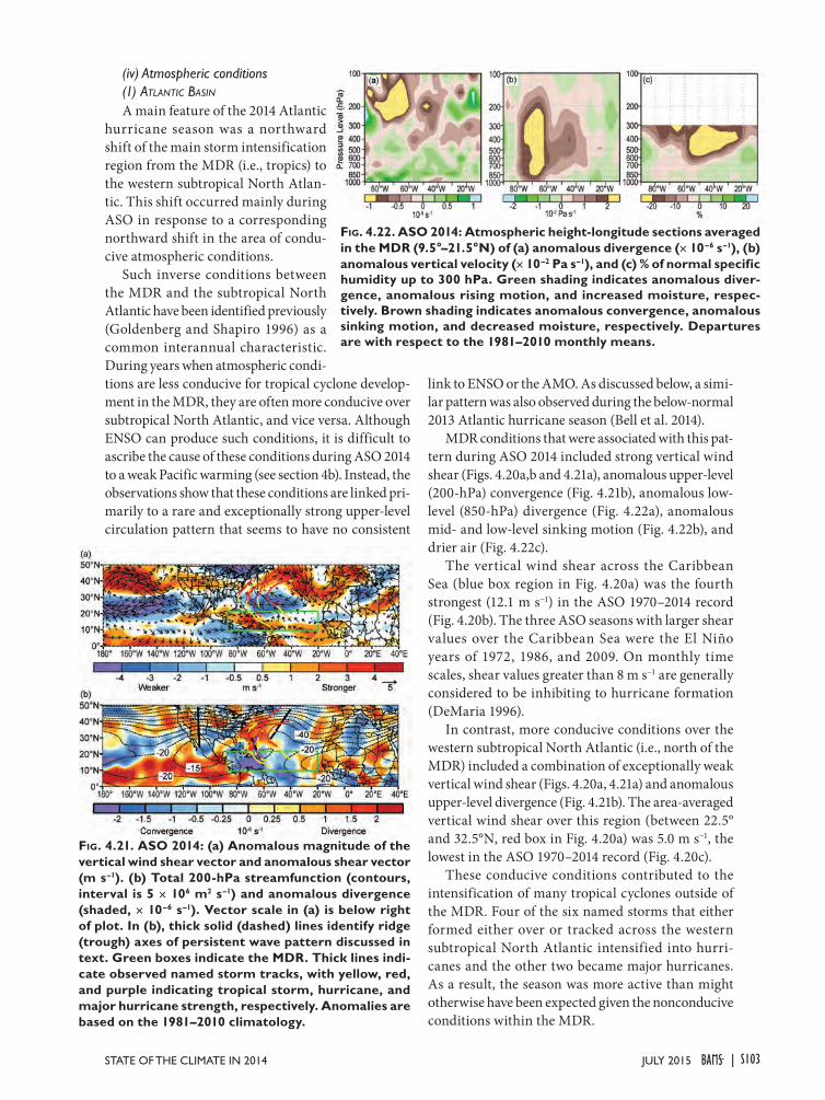
(iv) Atmospheric conditions(1) AtlAntic BAsin
A main feature of the 2014 Atlantic hurricane season was a northward shift of the main storm intensification region from the MDR (i.e., tropics) to the western subtropical North Atlan-tic. This shift occurred mainly during ASO in response to a corresponding northward shift in the area of condu-cive atmospheric conditions.
Such inverse conditions between the MDR and the subtropical North Atlantic have been identified previously (Goldenberg and Shapiro 1996) as a common interannual characteristic. During years when atmospheric condi-tions are less conducive for tropical cyclone develop-ment in the MDR, they are often more conducive over subtropical North Atlantic, and vice versa. Although ENSO can produce such conditions, it is difficult to ascribe the cause of these conditions during ASO 2014 to a weak Pacific warming (see section 4b). Instead, the observations show that these conditions are linked pri-marily to a rare and exceptionally strong upper-level circulation pattern that seems to have no consistent
link to ENSO or the AMO. As discussed below, a simi-lar pattern was also observed during the below-normal 2013 Atlantic hurricane season (Bell et al. 2014).
MDR conditions that were associated with this pat-tern during ASO 2014 included strong vertical wind shear (Figs. 4.20a,b and 4.21a), anomalous upper-level (200-hPa) convergence (Fig. 4.21b), anomalous low-level (850-hPa) divergence (Fig. 4.22a), anomalous mid- and low-level sinking motion (Fig. 4.22b), and drier air (Fig. 4.22c).
The vertical wind shear across the Caribbean Sea (blue box region in Fig. 4.20a) was the fourth strongest (12.1 m s−1) in the ASO 1970–2014 record (Fig. 4.20b). The three ASO seasons with larger shear values over the Caribbean Sea were the El Niño years of 1972, 1986, and 2009. On monthly time scales, shear values greater than 8 m s−1 are generally considered to be inhibiting to hurricane formation (DeMaria 1996).
In contrast, more conducive conditions over the western subtropical North Atlantic (i.e., north of the MDR) included a combination of exceptionally weak vertical wind shear (Figs. 4.20a, 4.21a) and anomalous upper-level divergence (Fig. 4.21b). The area-averaged vertical wind shear over this region (between 22.5° and 32.5°N, red box in Fig. 4.20a) was 5.0 m s−1, the lowest in the ASO 1970–2014 record (Fig. 4.20c).
These conducive conditions contributed to the intensification of many tropical cyclones outside of the MDR. Four of the six named storms that either formed either over or tracked across the western subtropical North Atlantic intensified into hurri-canes and the other two became major hurricanes. As a result, the season was more active than might otherwise have been expected given the nonconducive conditions within the MDR.
Fig. 4.21. ASO 2014: (a) Anomalous magnitude of the vertical wind shear vector and anomalous shear vector (m s–1). (b) Total 200-hPa streamfunction (contours, interval is 5 × 10⁶ m2 s–1) and anomalous divergence (shaded, × 10–6 s–1). Vector scale in (a) is below right of plot. In (b), thick solid (dashed) lines identify ridge (trough) axes of persistent wave pattern discussed in text. Green boxes indicate the MDR. Thick lines indi-cate observed named storm tracks, with yellow, red, and purple indicating tropical storm, hurricane, and major hurricane strength, respectively. Anomalies are based on the 1981–2010 climatology.
Fig. 4.22. ASO 2014: Atmospheric height-longitude sections averaged in the MDR (9.5°–21.5°N) of (a) anomalous divergence (× 10–6 s–1), (b) anomalous vertical velocity (× 10–2 Pa s–1), and (c) % of normal specific humidity up to 300 hPa. Green shading indicates anomalous diver-gence, anomalous rising motion, and increased moisture, respec-tively. Brown shading indicates anomalous convergence, anomalous sinking motion, and decreased moisture, respectively. Departures are with respect to the 1981–2010 monthly means.
S103JULY 2015STATE OF THE CLIMATE IN 2014 |
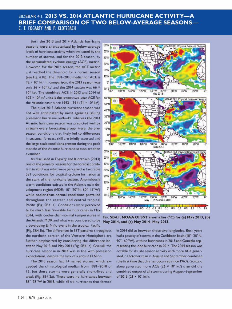
SIDEBAR 4.1: 2013 VS. 2014 ATLANTIC HURRICANE ACTIVITY—A BRIEF COMPARISON OF TWO BELOW-AVERAGE SEASONS— C. T. FOGARTY AND P. KLOTZBACH
Both the 2013 and 2014 Atlantic hurricane seasons were characterized by below-average levels of hurricane activity when evaluated by the number of storms, and for the 2013 season, by the accumulated cyclone energy (ACE) metric. However, for the 2014 season, the ACE metric just reached the threshold for a normal season (see Fig. 4.18). The 1981–2010 median for ACE is 92 × 104 kt2. In comparison, the 2013 season was only 36 × 104 kt2 and the 2014 season was 66 × 104 kt2. The combined ACE in 2013 and 2014 of 102 × 104 kt2 units is the lowest two-year ACE for the Atlantic basin since 1993–1994 (71 × 104 kt2).
The quiet 2013 Atlantic hurricane season was not well anticipated by most agencies issuing preseason hurricane outlooks, whereas the 2014 Atlantic hurricane season was predicted well by virtually every forecasting group. Here, the pre-season conditions that likely led to differences in seasonal forecast skill are briefly assessed and the large-scale conditions present during the peak months of the Atlantic hurricane season are then examined.
As discussed in Fogarty and Klotzbach (2013) one of the primary reasons for the forecast prob-lem in 2013 was what were perceived as favorable SST conditions for tropical cyclone formation at the start of the hurricane season. Anomalously warm conditions existed in the Atlantic main de-velopment region (MDR; 10°–20°N, 60°–15°W) while cooler-than-normal conditions prevailed throughout the eastern and central tropical Pacific (Fig. SB4.1a). Conditions were perceived to be much less favorable for hurricanes in May 2014, with cooler-than-normal temperatures in the Atlantic MDR and what was considered to be a developing El Niño event in the tropical Pacific (Fig. SB4.1b). The differences in SST patterns throughout the northern portion of the Western Hemisphere are further emphasized by considering the difference be-tween May 2013 and May 2014 (Fig. SB4.1c). Overall, the hurricane response in 2014 was in line with preseason expectations, despite the lack of a robust El Niño.
The 2013 season had 14 named storms, which ex-ceeded the climatological median from 1981–2010 of 12, but these storms were generally short-lived and weak (Fig. SB4.2a). There were no hurricanes between 85°–35°W in 2013, while all six hurricanes that formed
in 2014 did so between those two longitudes. Both years had a paucity of storms in the Caribbean basin (10°–20°N, 90°–60°W), with no hurricanes in 2013 and Gonzalo rep-resenting the lone hurricane in 2014. The 2014 season was notable for its late season activity with more ACE gener-ated in October than in August and September combined (the first time that this has occurred since 1963). Gonzalo alone generated more ACE (26 × 104 kt2) than did the combined output of all storms during August–September of 2013 (21 × 104 kt2).
Fig. SB4.1. NOAA OI SST anomalies (°C) for (a) May 2013, (b) May 2014, and (c) May 2014–May 2013.
S104 JULY 2015|
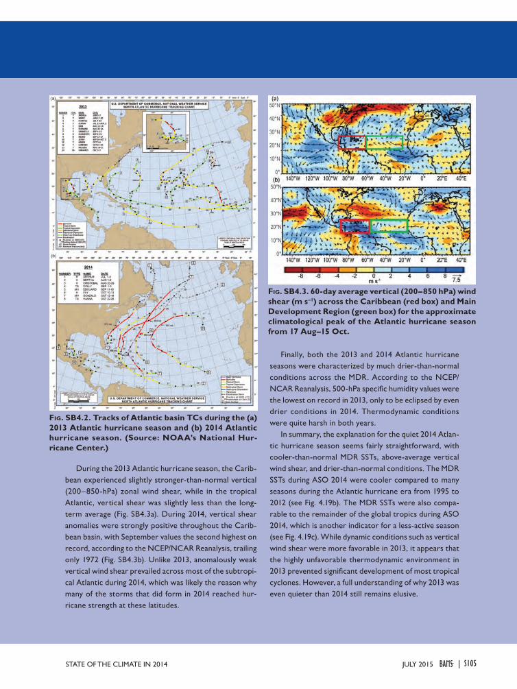
During the 2013 Atlantic hurricane season, the Carib-bean experienced slightly stronger-than-normal vertical (200–850-hPa) zonal wind shear, while in the tropical Atlantic, vertical shear was slightly less than the long-term average (Fig. SB4.3a). During 2014, vertical shear anomalies were strongly positive throughout the Carib-bean basin, with September values the second highest on record, according to the NCEP/NCAR Reanalysis, trailing only 1972 (Fig. SB4.3b). Unlike 2013, anomalously weak vertical wind shear prevailed across most of the subtropi-cal Atlantic during 2014, which was likely the reason why many of the storms that did form in 2014 reached hur-ricane strength at these latitudes.
Finally, both the 2013 and 2014 Atlantic hurricane seasons were characterized by much drier-than-normal conditions across the MDR. According to the NCEP/NCAR Reanalysis, 500-hPa specific humidity values were the lowest on record in 2013, only to be eclipsed by even drier conditions in 2014. Thermodynamic conditions were quite harsh in both years.
In summary, the explanation for the quiet 2014 Atlan-tic hurricane season seems fairly straightforward, with cooler-than-normal MDR SSTs, above-average vertical wind shear, and drier-than-normal conditions. The MDR SSTs during ASO 2014 were cooler compared to many seasons during the Atlantic hurricane era from 1995 to 2012 (see Fig. 4.19b). The MDR SSTs were also compa-rable to the remainder of the global tropics during ASO 2014, which is another indicator for a less-active season (see Fig. 4.19c). While dynamic conditions such as vertical wind shear were more favorable in 2013, it appears that the highly unfavorable thermodynamic environment in 2013 prevented significant development of most tropical cyclones. However, a full understanding of why 2013 was even quieter than 2014 still remains elusive.
Fig. SB4.2. Tracks of Atlantic basin TCs during the (a) 2013 Atlantic hurricane season and (b) 2014 Atlantic hurricane season. (Source: NOAA’s National Hur-ricane Center.)
Fig. SB4.3. 60-day average vertical (200–850 hPa) wind shear (m s–1) across the Caribbean (red box) and Main Development Region (green box) for the approximate climatological peak of the Atlantic hurricane season from 17 Aug–15 Oct.
S105JULY 2015STATE OF THE CLIMATE IN 2014 |
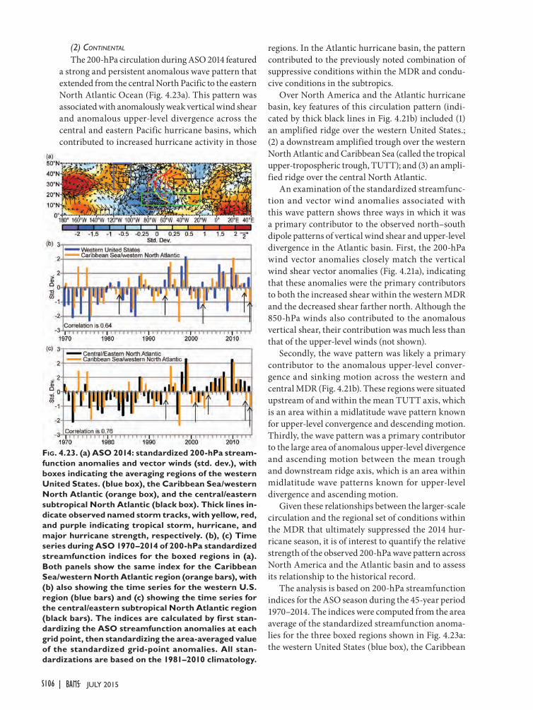
(2) continentAl
The 200-hPa circulation during ASO 2014 featured a strong and persistent anomalous wave pattern that extended from the central North Pacific to the eastern North Atlantic Ocean (Fig. 4.23a). This pattern was associated with anomalously weak vertical wind shear and anomalous upper-level divergence across the central and eastern Pacific hurricane basins, which contributed to increased hurricane activity in those
regions. In the Atlantic hurricane basin, the pattern contributed to the previously noted combination of suppressive conditions within the MDR and condu-cive conditions in the subtropics.
Over North America and the Atlantic hurricane basin, key features of this circulation pattern (indi-cated by thick black lines in Fig. 4.21b) included (1) an amplified ridge over the western United States.; (2) a downstream amplified trough over the western North Atlantic and Caribbean Sea (called the tropical upper-tropospheric trough, TUTT); and (3) an ampli-fied ridge over the central North Atlantic.
An examination of the standardized streamfunc-tion and vector wind anomalies associated with this wave pattern shows three ways in which it was a primary contributor to the observed north–south dipole patterns of vertical wind shear and upper-level divergence in the Atlantic basin. First, the 200-hPa wind vector anomalies closely match the vertical wind shear vector anomalies (Fig. 4.21a), indicating that these anomalies were the primary contributors to both the increased shear within the western MDR and the decreased shear farther north. Although the 850-hPa winds also contributed to the anomalous vertical shear, their contribution was much less than that of the upper-level winds (not shown).
Secondly, the wave pattern was likely a primary contributor to the anomalous upper-level conver-gence and sinking motion across the western and central MDR (Fig. 4.21b). These regions were situated upstream of and within the mean TUTT axis, which is an area within a midlatitude wave pattern known for upper-level convergence and descending motion. Thirdly, the wave pattern was a primary contributor to the large area of anomalous upper-level divergence and ascending motion between the mean trough and downstream ridge axis, which is an area within midlatitude wave patterns known for upper-level divergence and ascending motion.
Given these relationships between the larger-scale circulation and the regional set of conditions within the MDR that ultimately suppressed the 2014 hur-ricane season, it is of interest to quantify the relative strength of the observed 200-hPa wave pattern across North America and the Atlantic basin and to assess its relationship to the historical record.
The analysis is based on 200-hPa streamfunction indices for the ASO season during the 45-year period 1970–2014. The indices were computed from the area average of the standardized streamfunction anoma-lies for the three boxed regions shown in Fig. 4.23a: the western United States (blue box), the Caribbean
Fig. 4.23. (a) ASO 2014: standardized 200-hPa stream-function anomalies and vector winds (std. dev.), with boxes indicating the averaging regions of the western United States. (blue box), the Caribbean Sea/western North Atlantic (orange box), and the central/eastern subtropical North Atlantic (black box). Thick lines in-dicate observed named storm tracks, with yellow, red, and purple indicating tropical storm, hurricane, and major hurricane strength, respectively. (b), (c) Time series during ASO 1970–2014 of 200-hPa standardized streamfunction indices for the boxed regions in (a). Both panels show the same index for the Caribbean Sea/western North Atlantic region (orange bars), with (b) also showing the time series for the western U.S. region (blue bars) and (c) showing the time series for the central/eastern subtropical North Atlantic region (black bars). The indices are calculated by first stan-dardizing the ASO streamfunction anomalies at each grid point, then standardizing the area-averaged value of the standardized grid-point anomalies. All stan-dardizations are based on the 1981–2010 climatology.
S106 JULY 2015|
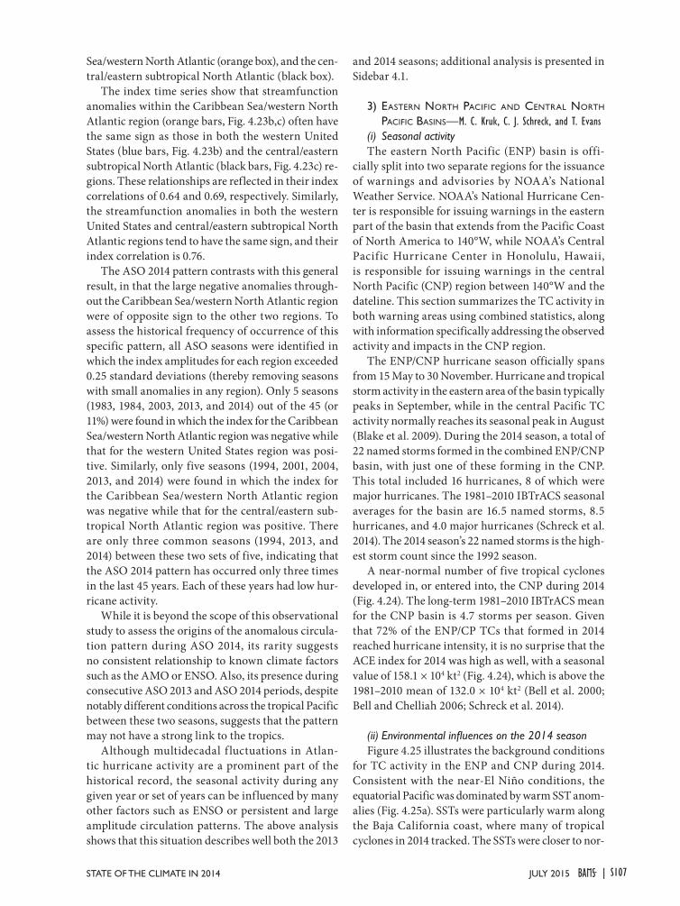
Sea/western North Atlantic (orange box), and the cen-tral/eastern subtropical North Atlantic (black box).
The index time series show that streamfunction anomalies within the Caribbean Sea/western North Atlantic region (orange bars, Fig. 4.23b,c) often have the same sign as those in both the western United States (blue bars, Fig. 4.23b) and the central/eastern subtropical North Atlantic (black bars, Fig. 4.23c) re-gions. These relationships are reflected in their index correlations of 0.64 and 0.69, respectively. Similarly, the streamfunction anomalies in both the western United States and central/eastern subtropical North Atlantic regions tend to have the same sign, and their index correlation is 0.76.
The ASO 2014 pattern contrasts with this general result, in that the large negative anomalies through-out the Caribbean Sea/western North Atlantic region were of opposite sign to the other two regions. To assess the historical frequency of occurrence of this specific pattern, all ASO seasons were identified in which the index amplitudes for each region exceeded 0.25 standard deviations (thereby removing seasons with small anomalies in any region). Only 5 seasons (1983, 1984, 2003, 2013, and 2014) out of the 45 (or 11%) were found in which the index for the Caribbean Sea/western North Atlantic region was negative while that for the western United States region was posi-tive. Similarly, only five seasons (1994, 2001, 2004, 2013, and 2014) were found in which the index for the Caribbean Sea/western North Atlantic region was negative while that for the central/eastern sub-tropical North Atlantic region was positive. There are only three common seasons (1994, 2013, and 2014) between these two sets of five, indicating that the ASO 2014 pattern has occurred only three times in the last 45 years. Each of these years had low hur-ricane activity.
While it is beyond the scope of this observational study to assess the origins of the anomalous circula-tion pattern during ASO 2014, its rarity suggests no consistent relationship to known climate factors such as the AMO or ENSO. Also, its presence during consecutive ASO 2013 and ASO 2014 periods, despite notably different conditions across the tropical Pacific between these two seasons, suggests that the pattern may not have a strong link to the tropics.
Although multidecadal f luctuations in Atlan-tic hurricane activity are a prominent part of the historical record, the seasonal activity during any given year or set of years can be influenced by many other factors such as ENSO or persistent and large amplitude circulation patterns. The above analysis shows that this situation describes well both the 2013
and 2014 seasons; additional analysis is presented in Sidebar 4.1.
3) eastern nOrth pacific and central nOrth pacific Basins—M. C. Kruk, C. J. Schreck, and T. Evans
(i) Seasonal activityThe eastern North Pacific (ENP) basin is offi-
cially split into two separate regions for the issuance of warnings and advisories by NOAA’s National Weather Service. NOAA’s National Hurricane Cen-ter is responsible for issuing warnings in the eastern part of the basin that extends from the Pacific Coast of North America to 140°W, while NOAA’s Central Pacific Hurricane Center in Honolulu, Hawaii, is responsible for issuing warnings in the central North Pacific (CNP) region between 140°W and the dateline. This section summarizes the TC activity in both warning areas using combined statistics, along with information specifically addressing the observed activity and impacts in the CNP region.
The ENP/CNP hurricane season officially spans from 15 May to 30 November. Hurricane and tropical storm activity in the eastern area of the basin typically peaks in September, while in the central Pacific TC activity normally reaches its seasonal peak in August (Blake et al. 2009). During the 2014 season, a total of 22 named storms formed in the combined ENP/CNP basin, with just one of these forming in the CNP. This total included 16 hurricanes, 8 of which were major hurricanes. The 1981–2010 IBTrACS seasonal averages for the basin are 16.5 named storms, 8.5 hurricanes, and 4.0 major hurricanes (Schreck et al. 2014). The 2014 season’s 22 named storms is the high-est storm count since the 1992 season.
A near-normal number of five tropical cyclones developed in, or entered into, the CNP during 2014 (Fig. 4.24). The long-term 1981–2010 IBTrACS mean for the CNP basin is 4.7 storms per season. Given that 72% of the ENP/CP TCs that formed in 2014 reached hurricane intensity, it is no surprise that the ACE index for 2014 was high as well, with a seasonal value of 158.1 × 10⁴ kt2 (Fig. 4.24), which is above the 1981–2010 mean of 132.0 × 10⁴ kt2 (Bell et al. 2000; Bell and Chelliah 2006; Schreck et al. 2014).
(ii)Environmentalinfluencesonthe2014seasonFigure 4.25 illustrates the background conditions
for TC activity in the ENP and CNP during 2014. Consistent with the near-El Niño conditions, the equatorial Pacific was dominated by warm SST anom-alies (Fig. 4.25a). SSTs were particularly warm along the Baja California coast, where many of tropical cyclones in 2014 tracked. The SSTs were closer to nor-
S107JULY 2015STATE OF THE CLIMATE IN 2014 |
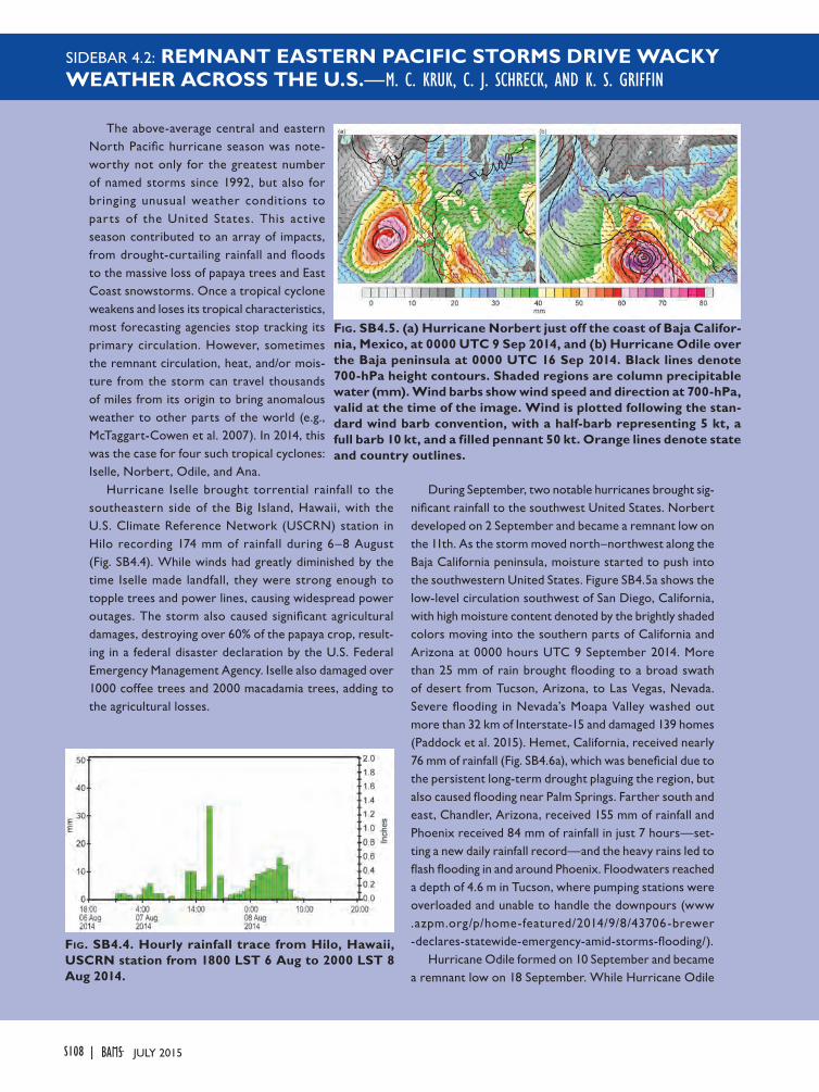
SIDEBAR 4.2: REMNANT EASTERN PACIFIC STORMS DRIVE WACKY WEATHER ACROSS THE U.S.—M. C. KRUK, C. J. SCHRECK, AND K. S. GRIFFIN
The above-average central and eastern North Pacific hurricane season was note-worthy not only for the greatest number of named storms since 1992, but also for bringing unusual weather conditions to parts of the United States. This active season contributed to an array of impacts, from drought-curtailing rainfall and floods to the massive loss of papaya trees and East Coast snowstorms. Once a tropical cyclone weakens and loses its tropical characteristics, most forecasting agencies stop tracking its primary circulation. However, sometimes the remnant circulation, heat, and/or mois-ture from the storm can travel thousands of miles from its origin to bring anomalous weather to other parts of the world (e.g., McTaggart-Cowen et al. 2007). In 2014, this was the case for four such tropical cyclones: Iselle, Norbert, Odile, and Ana.
Hurricane Iselle brought torrential rainfall to the southeastern side of the Big Island, Hawaii, with the U.S. Climate Reference Network (USCRN) station in Hilo recording 174 mm of rainfall during 6–8 August (Fig. SB4.4). While winds had greatly diminished by the time Iselle made landfall, they were strong enough to topple trees and power lines, causing widespread power outages. The storm also caused significant agricultural damages, destroying over 60% of the papaya crop, result-ing in a federal disaster declaration by the U.S. Federal Emergency Management Agency. Iselle also damaged over 1000 coffee trees and 2000 macadamia trees, adding to the agricultural losses.
During September, two notable hurricanes brought sig-nificant rainfall to the southwest United States. Norbert developed on 2 September and became a remnant low on the 11th. As the storm moved north–northwest along the Baja California peninsula, moisture started to push into the southwestern United States. Figure SB4.5a shows the low-level circulation southwest of San Diego, California, with high moisture content denoted by the brightly shaded colors moving into the southern parts of California and Arizona at 0000 hours UTC 9 September 2014. More than 25 mm of rain brought flooding to a broad swath of desert from Tucson, Arizona, to Las Vegas, Nevada. Severe flooding in Nevada’s Moapa Valley washed out more than 32 km of Interstate-15 and damaged 139 homes (Paddock et al. 2015). Hemet, California, received nearly 76 mm of rainfall (Fig. SB4.6a), which was beneficial due to the persistent long-term drought plaguing the region, but also caused flooding near Palm Springs. Farther south and east, Chandler, Arizona, received 155 mm of rainfall and Phoenix received 84 mm of rainfall in just 7 hours—set-ting a new daily rainfall record—and the heavy rains led to flash flooding in and around Phoenix. Floodwaters reached a depth of 4.6 m in Tucson, where pumping stations were overloaded and unable to handle the downpours (www .azpm.org/p/home-featured/2014/9/8/43706-brewer -declares-statewide-emergency-amid-storms-flooding/).
Hurricane Odile formed on 10 September and became a remnant low on 18 September. While Hurricane Odile
Fig. SB4.4. Hourly rainfall trace from Hilo, Hawaii, USCRN station from 1800 LST 6 Aug to 2000 LST 8 Aug 2014.
Fig. SB4.5. (a) Hurricane Norbert just off the coast of Baja Califor-nia, Mexico, at 0000 UTC 9 Sep 2014, and (b) Hurricane Odile over the Baja peninsula at 0000 UTC 16 Sep 2014. Black lines denote 700-hPa height contours. Shaded regions are column precipitable water (mm). Wind barbs show wind speed and direction at 700-hPa, valid at the time of the image. Wind is plotted following the stan-dard wind barb convention, with a half-barb representing 5 kt, a full barb 10 kt, and a filled pennant 50 kt. Orange lines denote state and country outlines.
S108 JULY 2015|
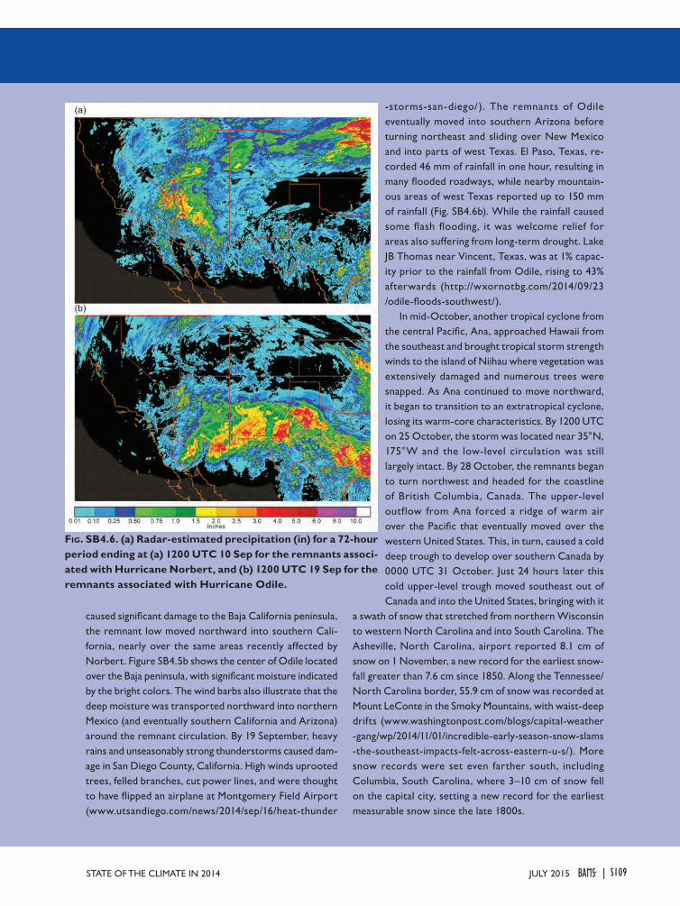
caused significant damage to the Baja California peninsula, the remnant low moved northward into southern Cali-fornia, nearly over the same areas recently affected by Norbert. Figure SB4.5b shows the center of Odile located over the Baja peninsula, with significant moisture indicated by the bright colors. The wind barbs also illustrate that the deep moisture was transported northward into northern Mexico (and eventually southern California and Arizona) around the remnant circulation. By 19 September, heavy rains and unseasonably strong thunderstorms caused dam-age in San Diego County, California. High winds uprooted trees, felled branches, cut power lines, and were thought to have flipped an airplane at Montgomery Field Airport (www.utsandiego.com/news/2014/sep/16/heat-thunder
-storms-san-diego/). The remnants of Odile eventually moved into southern Arizona before turning northeast and sliding over New Mexico and into parts of west Texas. El Paso, Texas, re-corded 46 mm of rainfall in one hour, resulting in many flooded roadways, while nearby mountain-ous areas of west Texas reported up to 150 mm of rainfall (Fig. SB4.6b). While the rainfall caused some flash flooding, it was welcome relief for areas also suffering from long-term drought. Lake JB Thomas near Vincent, Texas, was at 1% capac-ity prior to the rainfall from Odile, rising to 43% afterwards (http://wxornotbg.com/2014/09/23 /odile-floods-southwest/).
In mid-October, another tropical cyclone from the central Pacific, Ana, approached Hawaii from the southeast and brought tropical storm strength winds to the island of Niihau where vegetation was extensively damaged and numerous trees were snapped. As Ana continued to move northward, it began to transition to an extratropical cyclone, losing its warm-core characteristics. By 1200 UTC on 25 October, the storm was located near 35°N, 175°W and the low-level circulation was still largely intact. By 28 October, the remnants began to turn northwest and headed for the coastline of British Columbia, Canada. The upper-level outflow from Ana forced a ridge of warm air over the Pacific that eventually moved over the western United States. This, in turn, caused a cold deep trough to develop over southern Canada by 0000 UTC 31 October. Just 24 hours later this cold upper-level trough moved southeast out of Canada and into the United States, bringing with it
a swath of snow that stretched from northern Wisconsin to western North Carolina and into South Carolina. The Asheville, North Carolina, airport reported 8.1 cm of snow on 1 November, a new record for the earliest snow-fall greater than 7.6 cm since 1850. Along the Tennessee/North Carolina border, 55.9 cm of snow was recorded at Mount LeConte in the Smoky Mountains, with waist-deep drifts (www.washingtonpost.com/blogs/capital-weather -gang/wp/2014/11/01/incredible-early-season-snow-slams -the-southeast-impacts-felt-across-eastern-u-s/). More snow records were set even farther south, including Columbia, South Carolina, where 3–10 cm of snow fell on the capital city, setting a new record for the earliest measurable snow since the late 1800s.
Fig. SB4.6. (a) Radar-estimated precipitation (in) for a 72-hour period ending at (a) 1200 UTC 10 Sep for the remnants associ-ated with Hurricane Norbert, and (b) 1200 UTC 19 Sep for the remnants associated with Hurricane Odile.
S109JULY 2015STATE OF THE CLIMATE IN 2014 |
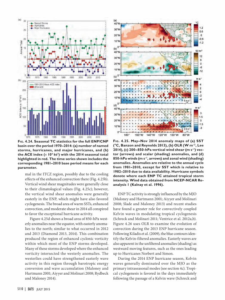
mal in the ITCZ region, possibly due to the cooling effects of the enhanced convection there (Fig. 4.25b). Vertical wind shear magnitudes were generally close to their climatological values (Fig. 4.25c); however, the vertical wind shear anomalies were generally easterly in the ENP, which might have also favored cyclogenesis. The broad area of warm SSTs, enhanced convection, and moderate shear in 2014 all conspired to favor the exceptional hurricane activity.
Figure 4.25d shows a broad area of 850-hPa west-erly anomalies near the equator, with easterly anoma-lies to the north; similar to what occurred in 2012 and 2013 (Diamond 2013, 2014). This combination produced the region of enhanced cyclonic vorticity within which most of the ENP storms developed. Many of these storms developed where the enhanced vorticity intersected the westerly anomalies. The westerlies could have strengthened easterly wave activity in this region through barotropic energy conversion and wave accumulation (Maloney and Hartmann 2001; Aiyyer and Molinari 2008; Rydbeck and Maloney 2014).
ENP TC activity is strongly influenced by the MJO (Maloney and Hartmann 2001; Aiyyer and Molinari 2008; Slade and Maloney 2013) and recent studies have found a greater role for convectively coupled Kelvin waves in modulating tropical cyclogenesis (Schreck and Molinari 2011; Ventrice et al. 2012a,b). Figure 4.26 uses OLR to examine the evolution of convection during the 2013 ENP hurricane season. Following Kiladis et al. (2009), the blue contours iden-tify the Kelvin-filtered anomalies. Easterly waves are also apparent in the unfiltered anomalies (shading) as westward moving features, such as the ones leading up to Hurricanes Norbert and Simon.
During the 2014 ENP hurricane season, Kelvin waves generally dominated over the MJO as the primary intraseasonal modes (see section 4c). Tropi-cal cyclogenesis is favored in the days immediately following the passage of a Kelvin wave (Schreck and
Fig. 4.24. Seasonal TC statistics for the full ENP/CNP basin over the period 1970–2014: (a) number of named storms, hurricanes, and major hurricanes, and (b) the ACE index (× 104 kt2) with the 2014 seasonal total highlighted in red. The time series shown includes the corresponding 1981–2010 base period means for each parameter.
Fig. 4.25. May–Nov 2014 anomaly maps of (a) SST (°C, Banzon and Reynolds 2013), (b) OLR (W m–2, Lee 2014), (c) 200–850-hPa vertical wind shear (m s–1) vec-tor (arrows) and scalar (shading) anomalies, and (d) 850-hPa winds (m s–1, arrows) and zonal wind (shading) anomalies. Anomalies are relative to the annual cycle from 1981–2010, except for SST which is relative to 1982–2010 due to data availability. Hurricane symbols denote where each ENP TC attained tropical storm intensity. Wind data obtained from NCEP-NCAR Re-analysis 1 (Kalnay et al. 1996).
S110 JULY 2015|
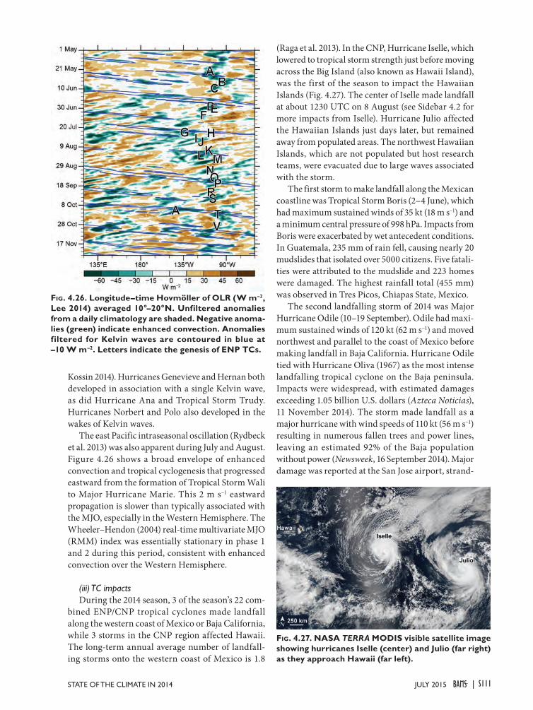
Kossin 2014). Hurricanes Genevieve and Hernan both developed in association with a single Kelvin wave, as did Hurricane Ana and Tropical Storm Trudy. Hurricanes Norbert and Polo also developed in the wakes of Kelvin waves.
The east Pacific intraseasonal oscillation (Rydbeck et al. 2013) was also apparent during July and August. Figure 4.26 shows a broad envelope of enhanced convection and tropical cyclogenesis that progressed eastward from the formation of Tropical Storm Wali to Major Hurricane Marie. This 2 m s−1 eastward propagation is slower than typically associated with the MJO, especially in the Western Hemisphere. The Wheeler–Hendon (2004) real-time multivariate MJO (RMM) index was essentially stationary in phase 1 and 2 during this period, consistent with enhanced convection over the Western Hemisphere.
(iii) TC impactsDuring the 2014 season, 3 of the season’s 22 com-
bined ENP/CNP tropical cyclones made landfall along the western coast of Mexico or Baja California, while 3 storms in the CNP region affected Hawaii. The long-term annual average number of landfall-ing storms onto the western coast of Mexico is 1.8
(Raga et al. 2013). In the CNP, Hurricane Iselle, which lowered to tropical storm strength just before moving across the Big Island (also known as Hawaii Island), was the first of the season to impact the Hawaiian Islands (Fig. 4.27). The center of Iselle made landfall at about 1230 UTC on 8 August (see Sidebar 4.2 for more impacts from Iselle). Hurricane Julio affected the Hawaiian Islands just days later, but remained away from populated areas. The northwest Hawaiian Islands, which are not populated but host research teams, were evacuated due to large waves associated with the storm.
The first storm to make landfall along the Mexican coastline was Tropical Storm Boris (2–4 June), which had maximum sustained winds of 35 kt (18 m s−1) and a minimum central pressure of 998 hPa. Impacts from Boris were exacerbated by wet antecedent conditions. In Guatemala, 235 mm of rain fell, causing nearly 20 mudslides that isolated over 5000 citizens. Five fatali-ties were attributed to the mudslide and 223 homes were damaged. The highest rainfall total (455 mm) was observed in Tres Picos, Chiapas State, Mexico.
The second landfalling storm of 2014 was Major Hurricane Odile (10–19 September). Odile had maxi-mum sustained winds of 120 kt (62 m s−1) and moved northwest and parallel to the coast of Mexico before making landfall in Baja California. Hurricane Odile tied with Hurricane Oliva (1967) as the most intense landfalling tropical cyclone on the Baja peninsula. Impacts were widespread, with estimated damages exceeding 1.05 billion U.S. dollars (Azteca Noticias), 11 November 2014). The storm made landfall as a major hurricane with wind speeds of 110 kt (56 m s−1) resulting in numerous fallen trees and power lines, leaving an estimated 92% of the Baja population without power (Newsweek, 16 September 2014). Major damage was reported at the San Jose airport, strand-
Fig. 4.26. Longitude–time Hovmöller of OLR (W m–2, Lee 2014) averaged 10°–20°N. Unfiltered anomalies from a daily climatology are shaded. Negative anoma-lies (green) indicate enhanced convection. Anomalies filtered for Kelvin waves are contoured in blue at –10 W m–2. Letters indicate the genesis of ENP TCs.
Fig. 4.27. NASA TERRA MODIS visible satellite image showing hurricanes Iselle (center) and Julio (far right) as they approach Hawaii (far left).
S111JULY 2015STATE OF THE CLIMATE IN 2014 |
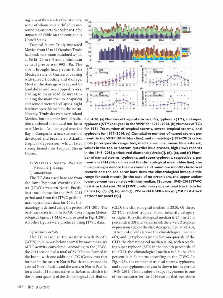
ing tens of thousands of vacationers, some of whom were airlifted to sur-rounding airports. See Sidebar 4.2 for impacts of Odile on the contiguous United States.
Tropical Storm Trudy impacted Mexico from 17 to 19 October. Trudy had peak maximum sustained winds at 56 kt (29 m s−1) and a minimum central pressure of 998 hPa. The storm brought heavy rains to the Mexican state of Guerrero, causing widespread f looding and damage. Most of the damage was caused by landslides and overtopped rivers, leading to many road closures (in-cluding the main road to Acapulco) and some structural collapses. Eight fatalities were blamed on the storm. Notably, Trudy decayed over inland Mexico, but its upper-level circula-tion continued and moved northeast over Mexico. As it emerged over the Bay of Campeche, a new surface low developed and became an Atlantic tropical depression, which later strengthened into Tropical Storm Hanna.
4) we s t e r n n O r t h pa c i f i c Basin—S. J. Camargo
(i) Introduction The TC data used here are from
the Joint Typhoon Warning Cen-ter (JTWC) western North Pacific best-track dataset for the 1945–2013 period and from the JTWC prelimi-nary operational data for 2014. Cli-matology is defined using the period 1971–2010. The best-track data from the RSMC-Tokyo, Japan Meteo-rological Agency (JMA) was also used in Fig. 4.28(b). All other figures were produced using JTWC data.
(ii) Seasonal activityThe TC season in the western North Pacific
(WPN) in 2014 was below normal by most measures of TC activity considered. According to the JTWC, the 2014 season had a total of 23 TCs that formed in the basin, with one additional TC (Genevieve) that formed in the eastern North Pacific and crossed the central North Pacific and the western North Pacific, for a total of 24 storms active in the basin, which is in the bottom quartile of the climatological distribution
(CLD; the climatological median is 28.5). Of these, 22 TCs reached tropical storm intensity category or higher (the climatological median is 26, the 25th percentile is 23) and were named: there were 2 tropical depressions (below the climatological median of 3.5), 10 tropical storms (above the climatological median of 9) and 12 typhoons (in the bottom quartile of the CLD, the climatological median is 16), with 8 reach-ing super typhoon (STY; in the top 5th percentile of the CLD, the climatological median is 3.5, the 75th percentile is 5), status according to the JTWC. In Fig. 4.28a, the number of tropical storms, typhoons, and super typhoons per year is shown for the period 1945–2014. The number of super typhoons is one of the measures for the 2014 season that was above
Fig. 4.28. (a) Number of tropical storms (TS), typhoons (TY), and super typhoons (STY) per year in the WNP for 1945–2014. (b) Number of TCs for 1951–76; number of tropical storms, severe tropical storms, and typhoons for 1977–2014. (c) Cumulative number of named storms per month in the WNP: 2014 (black line), and climatology (1971–2010) as box plots [interquartile range: box, median: red line, mean: blue asterisk, values in the top or bottom quartile: blue crosses, high (low) records in the 1945–2013 period: red diamonds (circles)]. (d), (e), and (f) Num-ber of named storms, typhoons, and super typhoons, respectively, per month in 2014 (black line) and the climatological mean (blue line), the blue plus signs denote the maximum and minimum monthly historical records and the red error bars show the climatological interquartile range for each month (in the case of no error bars, the upper and/or lower percentiles coincide with the median. [Sources: 1945–2013 JTWC best-track dataset, 2014 JTWC preliminary operational track data for panels (a), (c), (d), (e), and (f). 1951–2014 RSMC-Tokyo, JMA best-track dataset for panel (b).]
S112 JULY 2015|
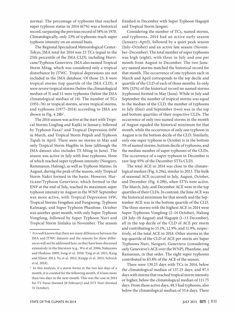
normal. The percentage of typhoons that reached super typhoon status in 2014 (67%) was a historical record, surpassing the previous record of 58% in 1970. Climatologically, only 23% of typhoons reach super typhoon intensity on an annual basis.
The Regional Specialized Meteorological Center-Tokyo, JMA total for 2014 was 23 TCs (equal to the 25th percentile of the JMA CLD), including Hurri-cane/Typhoon Genevieve. JMA also named Tropical Storm Mitag, which was considered only a tropical disturbance by JTWC. Tropical depressions are not included in the JMA database. Of those 23, 8 were tropical storms (top quartile of the JMA CLD), 4 were severe tropical storms (below the climatological median of 5) and 11 were typhoons (below the JMA climatological median of 14). The number of TCs (1951–76) or tropical storms, severe tropical storms, and typhoons (1977–2014) according to JMA are shown in Fig. 4.28b2.
The 2014 season was active at the start with Tropi-cal Storms Lingling and Kajiki in January, followed by Typhoon Faxai3 and Tropical Depression 04W in March, and Tropical Storm Peipah and Typhoon Tapah in April. There were no storms in May and only Tropical Storm Hagibis in June (although the JMA dataset also includes TS Mitag in June). The season was active in July with four typhoons, three of which reached super typhoon intensity (Neogury, Rammasun, Halong), as well as Typhoon Matmo. In August, during the peak of the season, only Tropical Storm Nakri formed in the basin. However, Hur-ricane/Typhoon Genevieve, which formed in the ENP at the end of July, reached its maximum super typhoon intensity in August in the WNP. September was more active, with Tropical Depression 14W, Tropical Storms Fengshen and Fungwong, Typhoon Kalmaegi, and Super Typhoon Phanfone. October was another quiet month, with only Super Typhoon Vongfong, followed by Super Typhoon Nuri and Tropical Storm Sinlaku in November. The season
2 It is well known that there are many differences between the JMA and JTWC datasets and the reasons for these differ-ences will not be addressed here, as they have been discussed extensively in the literature (e.g., Wu et al. 2006; Nakazawa and Hoshino 2009; Song et al. 2010; Ying et al. 2011; Kang and Elsner 2012; Yu et al. 2012; Knapp et al. 2013; Schreck et al. 2014).
3 In this analysis, if a storm forms in the two last days of a month, it is counted for the following month, if it lasts more than two days in the next month. This was the case in 2014 for TY Faxai (formed 28 February) and STY Nuri (formed 31 October).
finished in December with Super Typhoon Hagupit and Tropical Storm Jangmi.
Considering the number of TCs, named storms, and typhoons, 2014 had an active early season (January–April), followed by a quiet peak season (July–October) and an active late season (Novem-ber–December). The total number of super typhoons was high (eight), with three in July and one per month from August to December. The two Janu-ary named storms matched the historical record for that month. The occurrence of one typhoon each in March and April corresponds to the top decile and quartile of the CLD of each of those months. In only 30% (32%) of the historical record no named storms (typhoons) formed in May (June). While in July and September the number of tropical storms was equal to the median of the CLD, the number of typhoons in July (four) and September (two) was in the top and bottom quartiles of their respective CLDs. The occurrence of only two named storms in the month of August equaled the historical minimum for that month, while the occurrence of only one typhoon in August is in the bottom decile of the CLD. Similarly, only one super typhoon in October is in the bottom 5% of named storms, bottom decile of typhoons, and the median number of super typhoons of the CLDs. The occurrence of a super typhoon in December is rare (top 95% of the December STYs CLD).
The total ACE in 2014 was close to the climato-logical median (Fig. 4.29a), similar to 2013. The bulk of seasonal ACE occurred in July, August, October, and December (Fig. 4.29b), when STYs were active. The March, July, and December ACE were in the top quartiles of their CLDs. In contrast, the June ACE was the historical minimum for that month and the Sep-tember ACE was in the bottom quartile of the CLD. The three storms with the highest ACE in 2014 were Super Typhoons Vongfong (2–14 October), Halong (28 July–10 August) and Hagupit (1–13 December), all in the top decile of the CLD of ACE per storm and contributing to 15.1%, 12.9%, and 11.9%, respec-tively, of the total ACE in 2014. Other storms in the top quartile of the CLD of ACE per storm are Super Typhoons Nuri, Neoguri, Genevieve (considering only Genevieve’s ACE over the WNP), Phanfone, and Ramassun, in that order. The eight super typhoons contributed to 83.8% of the ACE of the season.
There were 139.25 days with TCs in 2014, below the climatological median of 157.25 days, and 97.5 days with storms that reached tropical storm intensity or higher, below the climatological median of 111.75 days. From those active days, 48.5 had typhoons, also below the climatological median of 55.6 days. There
S113JULY 2015STATE OF THE CLIMATE IN 2014 |
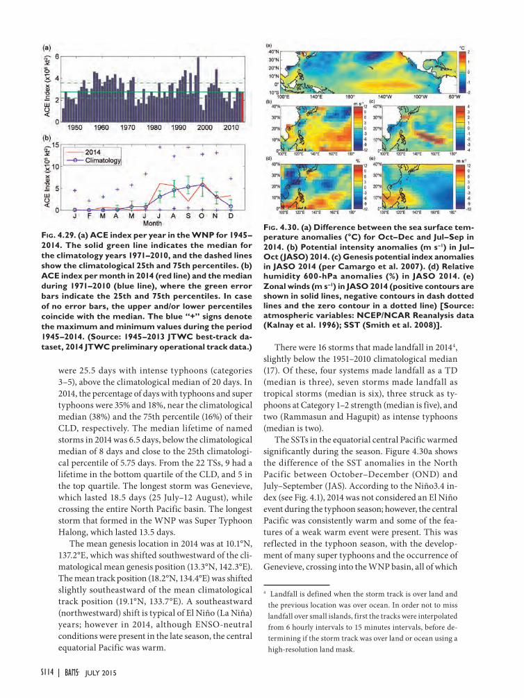
were 25.5 days with intense typhoons (categories 3–5), above the climatological median of 20 days. In 2014, the percentage of days with typhoons and super typhoons were 35% and 18%, near the climatological median (38%) and the 75th percentile (16%) of their CLD, respectively. The median lifetime of named storms in 2014 was 6.5 days, below the climatological median of 8 days and close to the 25th climatologi-cal percentile of 5.75 days. From the 22 TSs, 9 had a lifetime in the bottom quartile of the CLD, and 5 in the top quartile. The longest storm was Genevieve, which lasted 18.5 days (25 July–12 August), while crossing the entire North Pacific basin. The longest storm that formed in the WNP was Super Typhoon Halong, which lasted 13.5 days.
The mean genesis location in 2014 was at 10.1°N, 137.2°E, which was shifted southwestward of the cli-matological mean genesis position (13.3°N, 142.3°E). The mean track position (18.2°N, 134.4°E) was shifted slightly southeastward of the mean climatological track position (19.1°N, 133.7°E). A southeastward (northwestward) shift is typical of El Niño (La Niña) years; however in 2014, although ENSO-neutral conditions were present in the late season, the central equatorial Pacific was warm.
There were 16 storms that made landfall in 20144, slightly below the 1951–2010 climatological median (17). Of these, four systems made landfall as a TD (median is three), seven storms made landfall as tropical storms (median is six), three struck as ty-phoons at Category 1–2 strength (median is five), and two (Rammasun and Hagupit) as intense typhoons (median is two).
The SSTs in the equatorial central Pacific warmed significantly during the season. Figure 4.30a shows the difference of the SST anomalies in the North Pacific between October–December (OND) and July–September (JAS). According to the Niño3.4 in-dex (see Fig. 4.1), 2014 was not considered an El Niño event during the typhoon season; however, the central Pacific was consistently warm and some of the fea-tures of a weak warm event were present. This was reflected in the typhoon season, with the develop-ment of many super typhoons and the occurrence of Genevieve, crossing into the WNP basin, all of which
4 Landfall is defined when the storm track is over land and the previous location was over ocean. In order not to miss landfall over small islands, first the tracks were interpolated from 6 hourly intervals to 15 minutes intervals, before de-termining if the storm track was over land or ocean using a high-resolution land mask.
Fig. 4.30. (a) Difference between the sea surface tem-perature anomalies (°C) for Oct–Dec and Jul–Sep in 2014. (b) Potential intensity anomalies (m s–1) in Jul–Oct (JASO) 2014. (c) Genesis potential index anomalies in JASO 2014 (per Camargo et al. 2007). (d) Relative humidity 600-hPa anomalies (%) in JASO 2014. (e) Zonal winds (m s–1) in JASO 2014 (positive contours are shown in solid lines, negative contours in dash dotted lines and the zero contour in a dotted line) [Source: atmospheric variables: NCEP/NCAR Reanalysis data (Kalnay et al. 1996); SST (Smith et al. 2008)].
Fig. 4.29. (a) ACE index per year in the WNP for 1945–2014. The solid green line indicates the median for the climatology years 1971–2010, and the dashed lines show the climatological 25th and 75th percentiles. (b) ACE index per month in 2014 (red line) and the median during 1971–2010 (blue line), where the green error bars indicate the 25th and 75th percentiles. In case of no error bars, the upper and/or lower percentiles coincide with the median. The blue “+” signs denote the maximum and minimum values during the period 1945–2014. (Source: 1945–2013 JTWC best-track da-taset, 2014 JTWC preliminary operational track data.)
S114 JULY 2015|
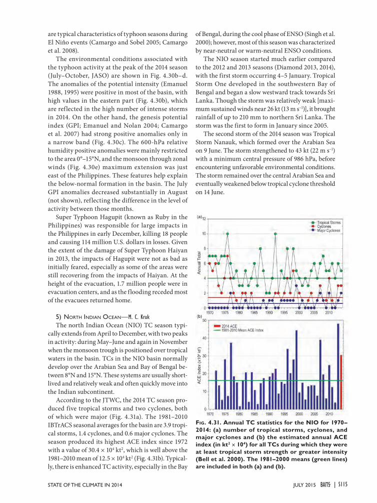
are typical characteristics of typhoon seasons during El Niño events (Camargo and Sobel 2005; Camargo et al. 2008).
The environmental conditions associated with the typhoon activity at the peak of the 2014 season (July–October, JASO) are shown in Fig. 4.30b–d. The anomalies of the potential intensity (Emanuel 1988, 1995) were positive in most of the basin, with high values in the eastern part (Fig. 4.30b), which are reflected in the high number of intense storms in 2014. On the other hand, the genesis potential index (GPI; Emanuel and Nolan 2004; Camargo et al. 2007) had strong positive anomalies only in a narrow band (Fig. 4.30c). The 600-hPa relative humidity positive anomalies were mainly restricted to the area 0°–15°N, and the monsoon through zonal winds (Fig. 4.30e) maximum extension was just east of the Philippines. These features help explain the below-normal formation in the basin. The July GPI anomalies decreased substantially in August (not shown), reflecting the difference in the level of activity between those months.
Super Typhoon Hagupit (known as Ruby in the Philippines) was responsible for large impacts in the Philippines in early December, killing 18 people and causing 114 million U.S. dollars in losses. Given the extent of the damage of Super Typhoon Haiyan in 2013, the impacts of Hagupit were not as bad as initially feared, especially as some of the areas were still recovering from the impacts of Haiyan. At the height of the evacuation, 1.7 million people were in evacuation centers, and as the flooding receded most of the evacuees returned home.
5) nOrth indian Ocean—M. C. KrukThe north Indian Ocean (NIO) TC season typi-
cally extends from April to December, with two peaks in activity: during May–June and again in November when the monsoon trough is positioned over tropical waters in the basin. TCs in the NIO basin normally develop over the Arabian Sea and Bay of Bengal be-tween 8°N and 15°N. These systems are usually short-lived and relatively weak and often quickly move into the Indian subcontinent.
According to the JTWC, the 2014 TC season pro-duced five tropical storms and two cyclones, both of which were major (Fig. 4.31a). The 1981–2010 IBTrACS seasonal averages for the basin are 3.9 tropi-cal storms, 1.4 cyclones, and 0.6 major cyclones. The season produced its highest ACE index since 1972 with a value of 30.4 × 10⁴ kt2, which is well above the 1981–2010 mean of 12.5 × 10⁴ kt2 (Fig. 4.31b). Typical-ly, there is enhanced TC activity, especially in the Bay
of Bengal, during the cool phase of ENSO (Singh et al. 2000); however, most of this season was characterized by near-neutral or warm-neutral ENSO conditions.
The NIO season started much earlier compared to the 2012 and 2013 seasons (Diamond 2013, 2014), with the first storm occurring 4–5 January. Tropical Storm One developed in the southwestern Bay of Bengal and began a slow westward track towards Sri Lanka. Though the storm was relatively weak [maxi-mum sustained winds near 26 kt (13 m s−1)], it brought rainfall of up to 210 mm to northern Sri Lanka. The storm was the first to form in January since 2005.
The second storm of the 2014 season was Tropical Storm Nanauk, which formed over the Arabian Sea on 9 June. The storm strengthened to 43 kt (22 m s−1) with a minimum central pressure of 986 hPa, before encountering unfavorable environmental conditions. The storm remained over the central Arabian Sea and eventually weakened below tropical cyclone threshold on 14 June.
Fig. 4.31. Annual TC statistics for the NIO for 1970–2014: (a) number of tropical storms, cyclones, and major cyclones and (b) the estimated annual ACE index (in kt2 × 104) for all TCs during which they were at least tropical storm strength or greater intensity (Bell et al. 2000). The 1981–2000 means (green lines) are included in both (a) and (b).
S115JULY 2015STATE OF THE CLIMATE IN 2014 |
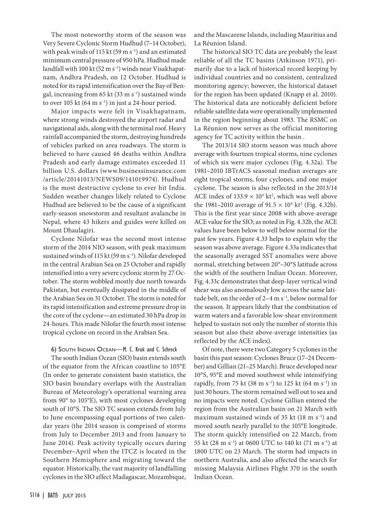
The most noteworthy storm of the season was Very Severe Cyclonic Storm Hudhud (7–14 October), with peak winds of 115 kt (59 m s−1) and an estimated minimum central pressure of 950 hPa. Hudhud made landfall with 100 kt (52 m s−1) winds near Visakhapat-nam, Andhra Pradesh, on 12 October. Hudhud is noted for its rapid intensification over the Bay of Ben-gal, increasing from 65 kt (33 m s−1) sustained winds to over 105 kt (64 m s−1) in just a 24-hour period.
Major impacts were felt in Visakhapatnam, where strong winds destroyed the airport radar and navigational aids, along with the terminal roof. Heavy rainfall accompanied the storm, destroying hundreds of vehicles parked on area roadways. The storm is believed to have caused 46 deaths within Andhra Pradesh and early damage estimates exceeded 11 billion U.S. dollars (www.businessinsurance.com /article/20141013/NEWS09/141019974). Hudhud is the most destructive cyclone to ever hit India. Sudden weather changes likely related to Cyclone Hudhud are believed to be the cause of a significant early-season snowstorm and resultant avalanche in Nepal, where 43 hikers and guides were killed on Mount Dhaulagiri.
Cyclone Nilofar was the second most intense storm of the 2014 NIO season, with peak maximum sustained winds of 115 kt (59 m s−1). Nilofar developed in the central Arabian Sea on 25 October and rapidly intensified into a very severe cyclonic storm by 27 Oc-tober. The storm wobbled mostly due north towards Pakistan, but eventually dissipated in the middle of the Arabian Sea on 31 October. The storm is noted for its rapid intensification and extreme pressure drop in the core of the cyclone—an estimated 30 hPa drop in 24-hours. This made Nilofar the fourth most intense tropical cyclone on record in the Arabian Sea.
6) sOuth indian Ocean—M. C. Kruk and C. SchreckThe south Indian Ocean (SIO) basin extends south
of the equator from the African coastline to 105°E (In order to generate consistent basin statistics, the SIO basin boundary overlaps with the Australian Bureau of Meteorology’s operational warning area from 90° to 105°E), with most cyclones developing south of 10°S. The SIO TC season extends from July to June encompassing equal portions of two calen-dar years (the 2014 season is comprised of storms from July to December 2013 and from January to June 2014). Peak activity typically occurs during December–April when the ITCZ is located in the Southern Hemisphere and migrating toward the equator. Historically, the vast majority of landfalling cyclones in the SIO affect Madagascar, Mozambique,
and the Mascarene Islands, including Mauritius and La Réunion Island.
The historical SIO TC data are probably the least reliable of all the TC basins (Atkinson 1971), pri-marily due to a lack of historical record keeping by individual countries and no consistent, centralized monitoring agency; however, the historical dataset for the region has been updated (Knapp et al. 2010). The historical data are noticeably deficient before reliable satellite data were operationally implemented in the region beginning about 1983. The RSMC on La Réunion now serves as the official monitoring agency for TC activity within the basin .
The 2013/14 SIO storm season was much above average with fourteen tropical storms, nine cyclones of which six were major cyclones (Fig. 4.32a). The 1981–2010 IBTrACS seasonal median averages are eight tropical storms, four cyclones, and one major cyclone. The season is also reflected in the 2013/14 ACE index of 133.9 × 10⁴ kt2, which was well above the 1981–2010 average of 91.5 × 10⁴ kt2 (Fig. 4.32b). This is the first year since 2008 with above-average ACE value for the SIO; as noted in Fig. 4.32b, the ACE values have been below to well below normal for the past few years. Figure 4.33 helps to explain why the season was above average. Figure 4.33a indicates that the seasonally averaged SST anomalies were above normal, stretching between 20°–30°S latitude across the width of the southern Indian Ocean. Moreover, Fig. 4.33c demonstrates that deep-layer vertical wind shear was also anomalously low across the same lati-tude belt, on the order of 2–4 m s−1, below normal for the season. It appears likely that the combination of warm waters and a favorable low-shear environment helped to sustain not only the number of storms this season but also their above-average intensities (as reflected by the ACE index).
Of note, there were two Category 5 cyclones in the basin this past season: Cyclones Bruce (17–24 Decem-ber) and Gillian (21–25 March). Bruce developed near 10°S, 95°E and moved southwest while intensifying rapidly, from 75 kt (38 m s−1) to 125 kt (64 m s−1) in just 30 hours. The storm remained well out to sea and no impacts were noted. Cyclone Gillian entered the region from the Australian basin on 21 March with maximum sustained winds of 35 kt (18 m s−1) and moved south nearly parallel to the 105°E longitude. The storm quickly intensified on 22 March, from 55 kt (28 m s−1) at 0600 UTC to 140 kt (71 m s−1) at 1800 UTC on 23 March. The storm had impacts in northern Australia, and also affected the search for missing Malaysia Airlines Flight 370 in the south Indian Ocean.
S116 JULY 2015|
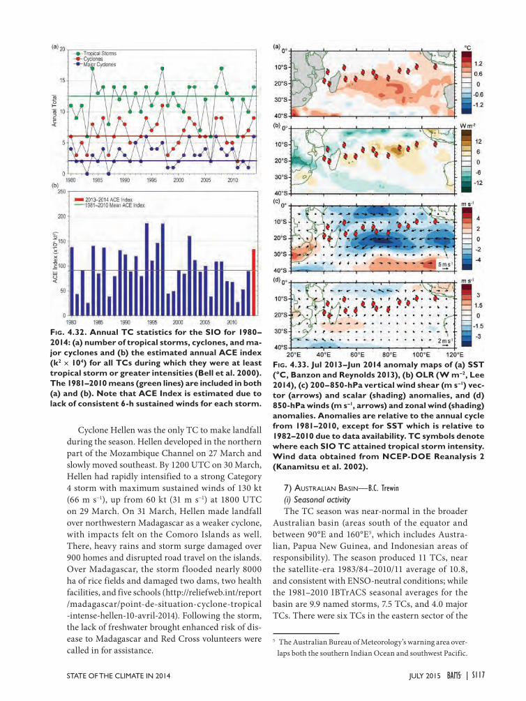
Cyclone Hellen was the only TC to make landfall during the season. Hellen developed in the northern part of the Mozambique Channel on 27 March and slowly moved southeast. By 1200 UTC on 30 March, Hellen had rapidly intensified to a strong Category 4 storm with maximum sustained winds of 130 kt (66 m s−1), up from 60 kt (31 m s−1) at 1800 UTC on 29 March. On 31 March, Hellen made landfall over northwestern Madagascar as a weaker cyclone, with impacts felt on the Comoro Islands as well. There, heavy rains and storm surge damaged over 900 homes and disrupted road travel on the islands. Over Madagascar, the storm f looded nearly 8000 ha of rice fields and damaged two dams, two health facilities, and five schools (http://reliefweb.int/report /madagascar/point-de-situation-cyclone-tropical -intense-hellen-10-avril-2014). Following the storm, the lack of freshwater brought enhanced risk of dis-ease to Madagascar and Red Cross volunteers were called in for assistance.
7) australian Basin—B.C. Trewin(i) Seasonal activityThe TC season was near-normal in the broader
Australian basin (areas south of the equator and between 90°E and 160°E5, which includes Austra-lian, Papua New Guinea, and Indonesian areas of responsibility). The season produced 11 TCs, near the satellite-era 1983/84–2010/11 average of 10.8, and consistent with ENSO-neutral conditions; while the 1981–2010 IBTrACS seasonal averages for the basin are 9.9 named storms, 7.5 TCs, and 4.0 major TCs. There were six TCs in the eastern sector of the
5 The Australian Bureau of Meteorology’s warning area over-laps both the southern Indian Ocean and southwest Pacific.
Fig. 4.32. Annual TC statistics for the SIO for 1980–2014: (a) number of tropical storms, cyclones, and ma-jor cyclones and (b) the estimated annual ACE index (k2 × 104) for all TCs during which they were at least tropical storm or greater intensities (Bell et al. 2000). The 1981–2010 means (green lines) are included in both (a) and (b). Note that ACE Index is estimated due to lack of consistent 6-h sustained winds for each storm.
Fig. 4.33. Jul 2013–Jun 2014 anomaly maps of (a) SST (°C, Banzon and Reynolds 2013), (b) OLR (W m–2, Lee 2014), (c) 200–850-hPa vertical wind shear (m s–1) vec-tor (arrows) and scalar (shading) anomalies, and (d) 850-hPa winds (m s–1, arrows) and zonal wind (shading) anomalies. Anomalies are relative to the annual cycle from 1981–2010, except for SST which is relative to 1982–2010 due to data availability. TC symbols denote where each SIO TC attained tropical storm intensity. Wind data obtained from NCEP-DOE Reanalysis 2 (Kanamitsu et al. 2002).
S117JULY 2015STATE OF THE CLIMATE IN 2014 |

Australian region (east of Australian coast to 160°E and the eastern half of the Gulf of Carpentaria) dur-ing 2013/14, two in the northern sector (125°E east to the western half of the Gulf of Carpentaria), and five in the western sector (between 90°E and 125°E). (One cyclone passed through all three sectors, while another passed through the western and northern sectors.) Six systems made landfall in Australia as tropical cyclones: one in Western Australia, two in the Northern Territory, and three in Queensland.
(ii)LandfallingandothersignificantTCsThe most significant TC of the season in the Aus-
tralian region was Tropical Cyclone Ita. Ita reached tropical cyclone intensity on 5 April southwest of the Solomon Islands. (See www.bom.gov.au/cyclone /about/intensity.shtml for the Australian tropical cy-clone classification system.) It then moved westwards and intensified, passing south of the southeastern tip of Papua New Guinea, before turning southwest to-wards the Queensland coast and intensifying rapidly. The storm reached Category 5 intensity early on 11 April, with maximum sustained winds of 115 kt (59 m s−1). Ita then turned to the south-southeast and weakened slightly, making landfall as a Category 4 system near Cape Flattery (north of Cooktown) on the evening of 11 April. The cyclone weakened rap-idly to Category 1 intensity as it moved inland, then tracked parallel to the coast before re-emerging over the ocean north of Mackay on 13 April. It transitioned into an extratropical cyclone as it moved southeast, with the remnants ultimately reaching New Zealand. A detailed description of the impacts of Ita are noted in section 4f(8).
The other Category 5 cyclone in the Australian region during 2013/14 was Cyclone Gillian. Gillian was a long-lived system which passed through all three sectors of the Australian region, with an iden-tifiable system lasting for 20 days. It first reached cyclone intensity on 8 March in the northern Gulf of Carpentaria, moving southeast and weakening below cyclone intensity before landfall on the west coast of Cape York Peninsula. The remnants re-emerged over water and the system reintensified briefly to cyclone intensity over the central Gulf on 14–15 March be-fore weakening again due to increasing wind shear. Gillian did not exceed Category 1 intensity while over the Gulf. After moving west for several days north of the Australian continent and over or near several Indonesian islands, it reintensified to cyclone intensity for a third time on 21 March, about 400 km south of Jakarta, and moved southwest, passing just north of Christmas Island. This time it intensi-
fied rapidly and reached Category 5 intensity, with maximum sustained winds of 110 kt (57 m s−1) on 23 March near 15°S, 104°E. The system weakened from 24 March onwards as it moved south and was finally downgraded to a tropical low on 26 March [Gillian also discussed in sections 4f(6) and 4f(8)].
Tropical Cyclone Christine was the only landfall-ing TC during the season in the western Australian region. Having formed on 28 December near 15°S, 121°E, it moved generally southwards towards the Pilbara coast, intensified, and made landfall near its peak intensity of 90 kt (46 m s−1) as a Category 4 system near Roebourne late on 30 December, then dissipating as it moved southeast over land on 31 De-cember. There was widespread wind damage, mostly minor to moderate, in the towns of Roebourne and Wickham, some inland f looding, and disruption to mining and offshore oil and gas operations. The relatively quiet season in this area, and the consequent lack of disruption to the resource industry, was cited by the Australian Bureau of Statistics (www.abs.gov .au) as a major contributor to an anomalous increase of 0.9%—equating to about 3 billion in U.S. dol-lars—in Australian gross domestic product in the January–March 2014 quarter.
There were four other landfalling TCs during the season. Cyclone Alessia, a Category 1 system, made landfall near the Daly River Mouth, south of Darwin, on 24 November, then reformed in the Gulf of Car-pentaria on 27 November after moving eastward and made a second landfall near Wollogorang the next day. It was the first November cyclone to affect the Northern Territory since 1975. Dylan made landfall as a Category 2 system south of Bowen, Queensland, early on 31 January, causing some damage, mostly from storm surge inundation and coastal erosion, in the Whitsundays region. An unnamed Category 2 system (upgraded on post-analysis) crossed the coast south of Wadeye, on the west coast of the Northern Territory, on 3 February and caused minor damage in Wadeye. Fletcher made landfall near Karumba, on the Gulf of Carpentaria coast, on 3 February. It was only a short-lived Category 1 cyclone, but the rem-nant low persisted for several days, bringing heavy rain in places. At Kowanyama, daily totals in excess of 150 mm occurred on each of six consecutive days from 4 to 9 February, with a six-day total of 1218 mm. There was significant flooding around the settlement of Kowanyama but only minor impacts elsewhere. Cyclone Bruce (December) and Cyclone Jack (April) both reached Category 3 intensity well off the coast in far western parts of the Australian region but did not affect any land areas.
S118 JULY 2015|
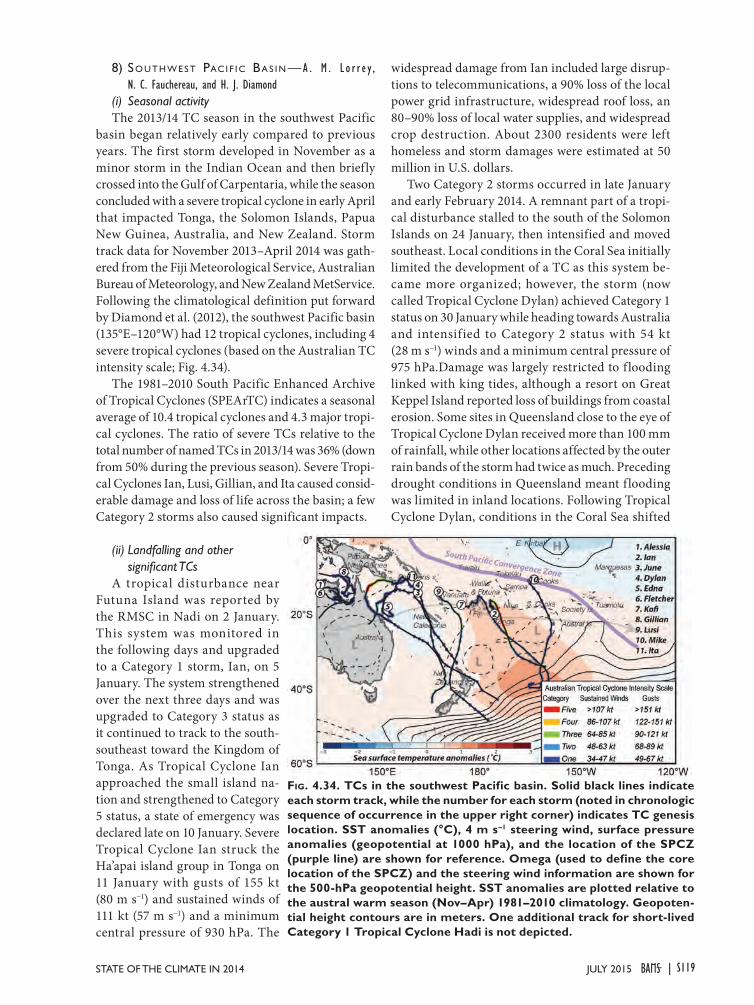
8) sO u th w e s t pac i f i c Ba s i n — A . M . L o r r e y , N. C. Fauchereau, and H. J. Diamond
(i) Seasonal activityThe 2013/14 TC season in the southwest Pacific
basin began relatively early compared to previous years. The first storm developed in November as a minor storm in the Indian Ocean and then briefly crossed into the Gulf of Carpentaria, while the season concluded with a severe tropical cyclone in early April that impacted Tonga, the Solomon Islands, Papua New Guinea, Australia, and New Zealand. Storm track data for November 2013–April 2014 was gath-ered from the Fiji Meteorological Service, Australian Bureau of Meteorology, and New Zealand MetService. Following the climatological definition put forward by Diamond et al. (2012), the southwest Pacific basin (135°E–120°W) had 12 tropical cyclones, including 4 severe tropical cyclones (based on the Australian TC intensity scale; Fig. 4.34).
The 1981–2010 South Pacific Enhanced Archive of Tropical Cyclones (SPEArTC) indicates a seasonal average of 10.4 tropical cyclones and 4.3 major tropi-cal cyclones. The ratio of severe TCs relative to the total number of named TCs in 2013/14 was 36% (down from 50% during the previous season). Severe Tropi-cal Cyclones Ian, Lusi, Gillian, and Ita caused consid-erable damage and loss of life across the basin; a few Category 2 storms also caused significant impacts.
(ii) Landfalling and other significantTCs
A tropical disturbance near Futuna Island was reported by the RMSC in Nadi on 2 January. This system was monitored in the following days and upgraded to a Category 1 storm, Ian, on 5 January. The system strengthened over the next three days and was upgraded to Category 3 status as it continued to track to the south-southeast toward the Kingdom of Tonga. As Tropical Cyclone Ian approached the small island na-tion and strengthened to Category 5 status, a state of emergency was declared late on 10 January. Severe Tropical Cyclone Ian struck the Ha’apai island group in Tonga on 11 January with gusts of 155 kt (80 m s−1) and sustained winds of 111 kt (57 m s−1) and a minimum central pressure of 930 hPa. The
widespread damage from Ian included large disrup-tions to telecommunications, a 90% loss of the local power grid infrastructure, widespread roof loss, an 80–90% loss of local water supplies, and widespread crop destruction. About 2300 residents were left homeless and storm damages were estimated at 50 million in U.S. dollars.
Two Category 2 storms occurred in late January and early February 2014. A remnant part of a tropi-cal disturbance stalled to the south of the Solomon Islands on 24 January, then intensified and moved southeast. Local conditions in the Coral Sea initially limited the development of a TC as this system be-came more organized; however, the storm (now called Tropical Cyclone Dylan) achieved Category 1 status on 30 January while heading towards Australia and intensified to Category 2 status with 54 kt (28 m s−1) winds and a minimum central pressure of 975 hPa.Damage was largely restricted to flooding linked with king tides, although a resort on Great Keppel Island reported loss of buildings from coastal erosion. Some sites in Queensland close to the eye of Tropical Cyclone Dylan received more than 100 mm of rainfall, while other locations affected by the outer rain bands of the storm had twice as much. Preceding drought conditions in Queensland meant f looding was limited in inland locations. Following Tropical Cyclone Dylan, conditions in the Coral Sea shifted
Fig. 4.34. TCs in the southwest Pacific basin. Solid black lines indicate each storm track, while the number for each storm (noted in chronologic sequence of occurrence in the upper right corner) indicates TC genesis location. SST anomalies (°C), 4 m s–1 steering wind, surface pressure anomalies (geopotential at 1000 hPa), and the location of the SPCZ (purple line) are shown for reference. Omega (used to define the core location of the SPCZ) and the steering wind information are shown for the 500-hPa geopotential height. SST anomalies are plotted relative to the austral warm season (Nov–Apr) 1981–2010 climatology. Geopoten-tial height contours are in meters. One additional track for short-lived Category 1 Tropical Cyclone Hadi is not depicted.
S119JULY 2015STATE OF THE CLIMATE IN 2014 |
to become favorable for supporting formation of a tropical low that organized and quickly intensified into Category 1 Tropical Cyclone Edna. The storm system weakened, made a loop, and then reintensi-fied prior to impacting New Caledonia on 4 Febru-ary when it reached Category 2 status with 51 kt (26 m s−1) winds and a minimum central pressure of 985 hPa. Tropical Cyclone Edna deteriorated quickly after 6 February.
Severe Tropical Cyclone Gillian [Australian Cate-gory 5; winds of 111 kt (57 m s−1); MCP of 937 hPa] was unique in that traversed three different TC basins. It began as a tropical low in the Gulf of Carpentaria on 6 March, becoming a Category 1 storm on 8 March as it migrated south along the western Queensland coast before making landfall on the western portion of the Cape York Peninsula. It was during this phase where the influences of Gillian were experienced in the basin, producing 150–250 mm of rainfall over the course of a week. Further impacts of severe TC Gillian are discussed in sections 4f(6) and 4f(7).
A tropical disturbance formed to the west of Nadi, Fiji, on 7 March that would evolve into Severe Tropical Cyclone Lusi [Category 3; 81 kt (28 m s−1); minimum central pressure of 960 hPa], which impacted Vanu-atu, Fiji, and New Zealand after extratropical transi-tion. After initially taking a zonal track westward toward the Coral Sea, Lusi emerged as a Category 1 storm in the northern part of the Vanuatu archipelago in the Torba province. It then crossed Santo Island and veered southeast while traversing Ambrym Island prior to tracking southeast along the f lank of the small island nation as it grew into a Category 2 storm. Severe impacts were felt locally as Tropical Cyclone Lusi passed, with 11 people killed (mostly on Santo) and 20 000 people affected across five provinces. Lusi strengthened further to Category 3 status between 12 and 13 March and then moved due south, taking aim at Cape Reinga, New Zealand. While Tropical Cyclone Lusi had decayed significantly upon tran-sition out of the tropics, it barely missed making landfall in the Far North district. Damage to New Zealand from high winds included uprooted trees and downed power lines that affected more than 2000 people, and local floods cut off parts of major roadways. Ex-Tropical Cyclone Lusi brought severe wind gusts of 65 kt (33 m s−1) to the North Island on approach. As the storm cleared the Taranaki Bight, rainfall exceeded 200 mm in the Nelson ranges on the northern South Island where the core of the remnant storm eventually made landfall.
Severe Tropical Cyclone Ita was the final storm of the season and the strongest one to impact
Queensland, Australia, since Severe Tropical Cyclone Yasi made landfall in 2011. Initially developing as a tropical low in the Solomon Islands area, the system moved south then due west, circumscribing the northern fringe of the Coral Sea while evolving into a Category 1 storm. Ita rapidly intensified into an Aus-tralian Category 5 strength system [116 kt (60 m s−1); minimum central pressure of 930 hPa] as it headed towards Australia’s east coast. It brought >1000 mm of rainfall to the Solomon Islands in less than one week, which caused flash floods and landslides that killed 40 people with additional persons reported missing. Significant health impacts followed from TC Ita in the Solomon Islands where dengue fever and rotavirus outbreaks affected more than 1000 people in the capital of Honiara. There were also two dozen leprosy cases, mostly children, reported within temporary shelters that were set up during the relief effort. Thousands were left homeless in the Solomon Islands from the destruction caused by the storm, with an estimated 50 000 people affected and at least 110 million U.S. dollars in damage. While Severe Tropical Cyclone Ita moved past Papua New Guinea, it brought significant rainfall and damaged buildings and bridges, destroyed power lines, snapped trees, and generated floods that destroyed thousands of homes and some schools. Significant earthquake activity at this time, coincident with the effects of Ita, exacerbated the potential for landslides, resulting in two deaths. Papua New Guinea and the Solomon Islands suffered similar impacts with widespread damage to local infrastructure.
Ita weakened to Category 4 strength upon mak-ing landfall in Queensland, Australia. Many sites recorded >300 mm of rainfall in a 24-hour period. A flash flood was reported in Bowen, Australia, after 110 mm fell in one hour and many of the major rivers in Queensland flooded. There was no reported loss of life from TC Ita in Australia; however, the impacts on Queensland’s regional agriculture included destruc-tion of sugar cane, banana, avocado, and tropical fruit plantations along with other crops, amounting to more than 1 billion U.S. dollars in losses. After making landfall, Ita rapidly decayed to Category 1 strength in less than 18 hours and underwent extra-tropical transition in the north Tasman Sea. The last vestiges of ex-Tropical Cyclone Ita brought gale force winds to much of central and northern New Zealand on 17 April causing widespread power outages, ag-ricultural damage, and destruction and damage to homes that amounted to more than 40 million U.S. dollars in insurance claims.
S120 JULY 2015|
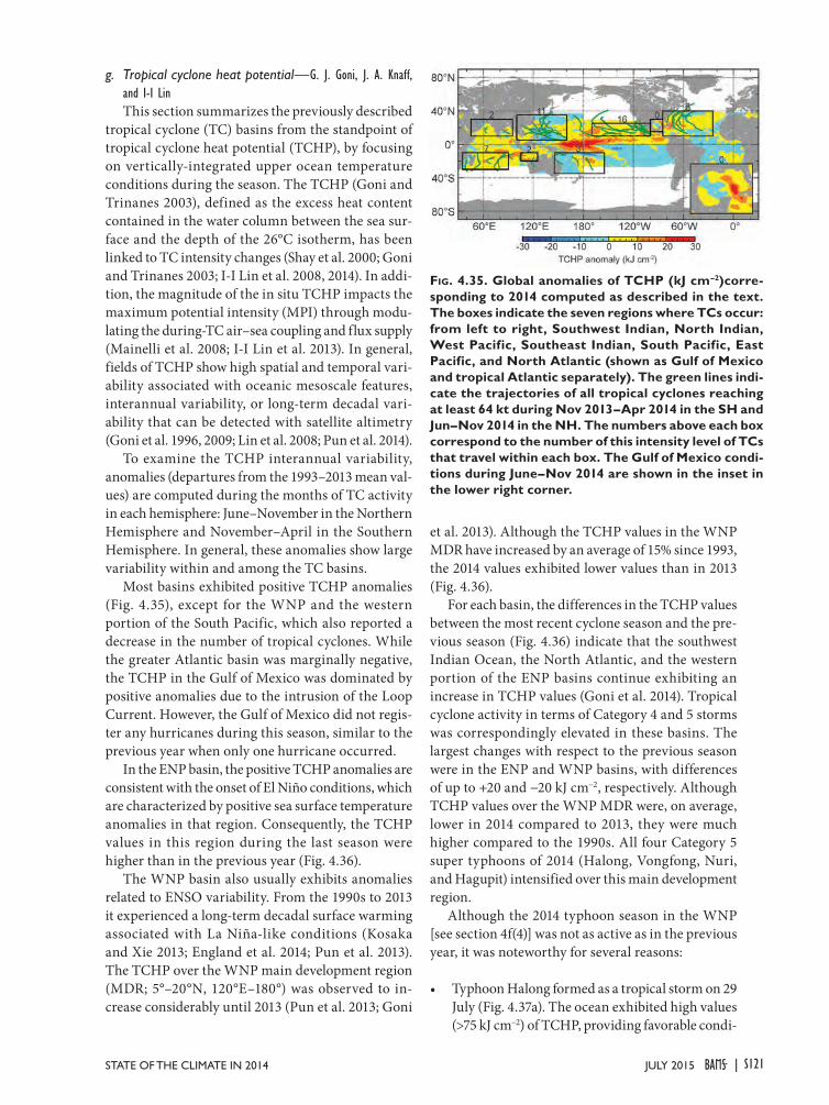
g. Tropical cyclone heat potential—G. J. Goni, J. A. Knaff, and I-I Lin This section summarizes the previously described
tropical cyclone (TC) basins from the standpoint of tropical cyclone heat potential (TCHP), by focusing on vertically-integrated upper ocean temperature conditions during the season. The TCHP (Goni and Trinanes 2003), defined as the excess heat content contained in the water column between the sea sur-face and the depth of the 26°C isotherm, has been linked to TC intensity changes (Shay et al. 2000; Goni and Trinanes 2003; I-I Lin et al. 2008, 2014). In addi-tion, the magnitude of the in situ TCHP impacts the maximum potential intensity (MPI) through modu-lating the during-TC air–sea coupling and flux supply (Mainelli et al. 2008; I-I Lin et al. 2013). In general, fields of TCHP show high spatial and temporal vari-ability associated with oceanic mesoscale features, interannual variability, or long-term decadal vari-ability that can be detected with satellite altimetry (Goni et al. 1996, 2009; Lin et al. 2008; Pun et al. 2014).
To examine the TCHP interannual variability, anomalies (departures from the 1993–2013 mean val-ues) are computed during the months of TC activity in each hemisphere: June–November in the Northern Hemisphere and November–April in the Southern Hemisphere. In general, these anomalies show large variability within and among the TC basins.
Most basins exhibited positive TCHP anomalies (Fig. 4.35), except for the WNP and the western portion of the South Pacific, which also reported a decrease in the number of tropical cyclones. While the greater Atlantic basin was marginally negative, the TCHP in the Gulf of Mexico was dominated by positive anomalies due to the intrusion of the Loop Current. However, the Gulf of Mexico did not regis-ter any hurricanes during this season, similar to the previous year when only one hurricane occurred.
In the ENP basin, the positive TCHP anomalies are consistent with the onset of El Niño conditions, which are characterized by positive sea surface temperature anomalies in that region. Consequently, the TCHP values in this region during the last season were higher than in the previous year (Fig. 4.36).
The WNP basin also usually exhibits anomalies related to ENSO variability. From the 1990s to 2013 it experienced a long-term decadal surface warming associated with La Niña-like conditions (Kosaka and Xie 2013; England et al. 2014; Pun et al. 2013). The TCHP over the WNP main development region (MDR; 5°–20°N, 120°E–180°) was observed to in-crease considerably until 2013 (Pun et al. 2013; Goni
et al. 2013). Although the TCHP values in the WNP MDR have increased by an average of 15% since 1993, the 2014 values exhibited lower values than in 2013 (Fig. 4.36).
For each basin, the differences in the TCHP values between the most recent cyclone season and the pre-vious season (Fig. 4.36) indicate that the southwest Indian Ocean, the North Atlantic, and the western portion of the ENP basins continue exhibiting an increase in TCHP values (Goni et al. 2014). Tropical cyclone activity in terms of Category 4 and 5 storms was correspondingly elevated in these basins. The largest changes with respect to the previous season were in the ENP and WNP basins, with differences of up to +20 and −20 kJ cm−2, respectively. Although TCHP values over the WNP MDR were, on average, lower in 2014 compared to 2013, they were much higher compared to the 1990s. All four Category 5 super typhoons of 2014 (Halong, Vongfong, Nuri, and Hagupit) intensified over this main development region.
Although the 2014 typhoon season in the WNP [see section 4f(4)] was not as active as in the previous year, it was noteworthy for several reasons:
• Typhoon Halong formed as a tropical storm on 29 July (Fig. 4.37a). The ocean exhibited high values (>75 kJ cm−2) of TCHP, providing favorable condi-
Fig. 4.35. Global anomalies of TCHP (kJ cm–2)corre-sponding to 2014 computed as described in the text. The boxes indicate the seven regions where TCs occur: from left to right, Southwest Indian, North Indian, West Pacific, Southeast Indian, South Pacific, East Pacific, and North Atlantic (shown as Gulf of Mexico and tropical Atlantic separately). The green lines indi-cate the trajectories of all tropical cyclones reaching at least 64 kt during Nov 2013–Apr 2014 in the SH and Jun–Nov 2014 in the NH. The numbers above each box correspond to the number of this intensity level of TCs that travel within each box. The Gulf of Mexico condi-tions during June–Nov 2014 are shown in the inset in the lower right corner.
S121JULY 2015STATE OF THE CLIMATE IN 2014 |
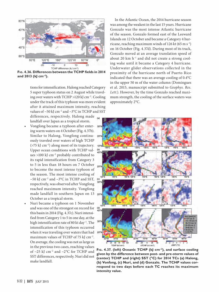
tions for intensification. Halong reached Category 5 super typhoon status on 2 August while travel-ing over waters with TCHP >120 kJ cm−2. Cooling under the track of this typhoon was more evident after it attained maximum intensity, reaching values of −50 kJ cm−2 and −3°C in TCHP and SST differences, respectively. Halong made landfall over Japan as a tropical storm.
• Vongfong became a typhoon after enter-ing warm waters on 4 October (Fig. 4.37b). Similar to Halong, Vongfong continu-ously traveled over waters of high TCHP (>75 kJ cm−2) along most of its trajectory. Upper ocean conditions with TCHP val-ues >100 kJ cm−2 probably contributed to its rapid intensification from Category 3 to 5 in less than 18 hours on 7 October to become the most intense typhoon of the season. The most intense cooling of −50 kJ cm−2 and −3°C in TCHP and SST, respectively, was observed after Vongfong reached maximum intensity. Vongfong made landfall in southern Japan on 13 October as a tropical storm.
• Nuri became a typhoon on 1 November and was one of the strongest on record for this basin in 2014 (Fig. 4.37c). Nuri intensi-fied from Category 1 to 5 in one day, at the high intensification rate of 80 kt day−1. The intensification of this typhoon occurred when it was traveling over waters that had maximum values of TCHP of 75 kJ cm−2. On average, the cooling was not as large as in the previous two cases, reaching values of −25 kJ cm−2 and −2°C for TCHP and SST differences, respectively. Nuri did not make landfall.
In the Atlantic Ocean, the 2014 hurricane season was among the weakest in the last 15 years. Hurricane Gonzalo was the most intense Atlantic hurricane of the season. Gonzalo formed east of the Leeward Islands on 12 October and became a Category 4 hur-ricane, reaching maximum winds of 126 kt (65 m s−1) on 16 October (Fig. 4.37d). During most of its track, Gonzalo moved at an average translation speed of about 20 km h−1 and did not create a strong cool-ing wake until it became a Category 4 hurricane. Underwater glider observations collected in the proximity of the hurricane north of Puerto Rico indicated that there was an average cooling of 0.4°C in the upper 50 m of the water column (Domingues et al. 2015, manuscript submitted to Geophys. Res. Lett.). However, by the time Gonzalo reached maxi-mum strength, the cooling of the surface waters was approximately 2°C.
Fig. 4.36. Differences between the TCHP fields in 2014 and 2013 (kJ cm–2).
Fig. 4.37. (left) Oceanic TCHP (kJ cm–2), and surface cooling given by the difference between post- and pre-storm values of (center) TCHP and (right) SST (°C) for 2014 TCs (a) Halong, (b) Vonfong, (c) Nuri, and (d) Gonzalo. The TCHP values cor-respond to two days before each TC reaches its maximum intensity value.
S122 JULY 2015|
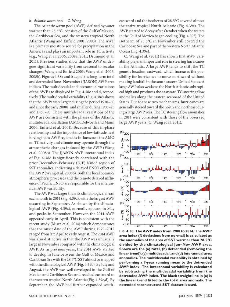
h. Atlantic warm pool—C. WangThe Atlantic warm pool (AWP), defined by water
warmer than 28.5°C, consists of the Gulf of Mexico, the Caribbean Sea, and the western tropical North Atlantic (Wang and Enfield 2001, 2003). The AWP is a primary moisture source for precipitation in the Americas and plays an important role in TC activity (e.g., Wang et al. 2006, 2008a, 2011; Drumond et al. 2011). Previous studies show that the AWP under-goes significant variability from seasonal to secular changes (Wang and Enfield 2003; Wang et al. 2006, 2008b). Figures 4.38a and b depict the long-term total and detrended June–November (JJASON) AWP area indices. The multidecadal and interannual variations of the AWP are displayed in Fig. 4.38c and d, respec-tively. The multidecadal variability (Fig. 4.38c) shows that the AWPs were larger during the period 1930–60 and since the early 2000s, and smaller during 1905–25 and 1965–95. These multidecadal variations of the AWP are consistent with the phases of the Atlantic multidecadal oscillation (AMO; Delworth and Mann 2000; Enfield et al. 2001). Because of this in-phase relationship and the importance of low-latitude heat forcing in the AWP region, the influences of the AMO on TC activity and climate may operate through the atmospheric changes induced by the AWP (Wang et al. 2008b). The JJASON AWP interannual index of Fig. 4.38d is significantly correlated with the prior December–February (DJF) Niño3 region of SST anomalies, indicating a delayed ENSO effect on the AWP (Wang et al. 2008b). Both the local oceanic/atmospheric processes and the remote delayed influ-ence of Pacific ENSO are responsible for the interan-nual AWP variability.
The AWP was larger than its climatological mean each month in 2014 (Fig. 4.39a), with the largest AWP occurring in September. As shown by the climato-logical AWP (Fig. 4.39a), normally appears in May and peaks in September. However, the 2014 AWP appeared early in April. This is consistent with the recent study (Misra et al. 2014) which demonstrates that the onset date of the AWP during 1979–2012 ranged from late April to early August. The 2014 AWP was also distinctive in that the AWP was unusually large in November compared with the climatological AWP. As in previous years, the 2014 AWP started to develop in June between the Gulf of Mexico and Caribbean Sea with the 28.5°C SST almost overlapped with the climatological AWP (Fig. 4.39b). By July and August, the AWP was well developed in the Gulf of Mexico and Caribbean Sea and reached eastward to the western tropical North Atlantic (Fig. 4.39c,d). By September, the AWP had further expanded south-
eastward and the isotherm of 28.5°C covered almost the entire tropical North Atlantic (Fig. 4.39e). The AWP started to decay after October when the waters in the Gulf of Mexico began cooling (Fig. 4.39f). The isotherm of 28.5°C in November still covered the Caribbean Sea and part of the western North Atlantic Ocean (Fig. 4.39e).
C. Wang et al. (2011) has shown that AWP vari-ability plays an important role in steering hurricanes in the Atlantic. A large AWP tends to shift the TC genesis location eastward, which increases the pos-sibility for hurricanes to move northward without making landfall in the southeastern United States. A large AWP also weakens the North Atlantic subtropi-cal high and produces the eastward TC steering flow anomalies along the eastern seaboard of the United States. Due to these two mechanisms, hurricanes are generally steered toward the north and northeast dur-ing a large AWP year. The TC steering flow anomalies in 2014 were consistent with those of the observed large AWP years (C. Wang et al. 2011).
Fig. 4.38. The AWP index from 1900 to 2014. The AWP area index (% deviations from normal) is calculated as the anomalies of the area of SST warmer than 28.5°C divided by the climatological Jun–Nov AWP area. Shown are the (a) total, (b) detrended (removing the linear trend), (c) multidecadal, and (d) interannual area anomalies. The multidecadal variability is obtained by performing a 7-year running mean to the detrended AWP index. The interannual variability is calculated by subtracting the multidecadal variability from the detrended AWP index. The black straight line in (a) is the linear trend fitted to the total area anomaly. The extended reconstructed SST dataset is used.
S123JULY 2015STATE OF THE CLIMATE IN 2014 |
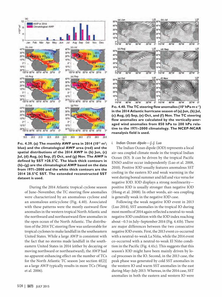
During the 2014 Atlantic tropical cyclone season of June–November, the TC steering flow anomalies were characterized by an anomalous cyclone and an anomalous anticyclone (Fig. 4.40). Associated with these patterns were the mostly eastward flow anomalies in the western tropical North Atlantic and the northward and northeastward flow anomalies in the open ocean of the North Atlantic. The distribu-tion of the 2014 TC steering flow was unfavorable for tropical cyclones to make landfall in the southeastern United States. While a large AWP is consistent with the fact that no storms made landfall in the south-eastern United States in 2014 (either by decaying or moving northward or northeastward), the AWP had no apparent enhancing effect on the number of TCs for the North Atlantic TC season [see section 4f(2)] as a large AWP typically results in more TCs (Wang et al. 2006).
i. Indian Ocean dipole—J.-J. LuoThe Indian Ocean dipole (IOD) represents a local
air–sea coupled climate mode in the tropical Indian Ocean (IO). It can be driven by the tropical Pacific ENSO and/or occur independently (Luo et al. 2008, 2010). Positive IOD usually features anomalous SST cooling in the eastern IO and weak warming in the west during boreal summer and fall and vice versa for negative IOD. IOD displays a strong nonlinearity—positive IOD is usually stronger than negative IOD (Hong et al. 2008). In other words, air–sea coupling is generally weak in the negative IOD case.
Following the weak negative IOD event in 2013 (Luo 2014), SST anomalies in the tropical IO during most months of 2014 again reflected a neutral-to-weak negative IOD condition with the IOD index reaching about −0.5 in July–September 2014 (Fig. 4.41b). There are major differences between the two consecutive negative IOD events. First, the 2013 event co-occurred with a neutral-to-weak La Niña, while the 2014 event co-occurred with a neutral-to-weak El Niño condi-tion in the Pacific (Fig. 4.41c). This suggests that this season’s IOD might have been mainly driven by lo-cal processes in the IO. Second, in the 2013 case, the peak phase was generated by cold SST anomalies in the western IO and warm SST anomalies in the east during May–July 2013. Whereas, in the 2014 case, SST anomalies in both the eastern and western IO were
Fig. 4.39. (a) The monthly AWP area in 2014 (1012 m2; blue) and the climatological AWP area (red) and the spatial distributions of the 2014 AWP in (b) Jun, (c) Jul, (d) Aug, (e) Sep, (f) Oct, and (g) Nov. The AWP is defined by SST >28.5°C. The black thick contours in (b)–(g) are the climatological AWP based on the data from 1971–2000 and the white thick contours are the 2014 28.5°C SST. The extended reconstructed SST dataset is used.
Fig. 4.40. The TC steering flow anomalies (103 hPa m s–1) in the 2014 Atlantic hurricane season of (a) Jun, (b) Jul, (c) Aug, (d) Sep, (e) Oct, and (f) Nov. The TC steering flow anomalies are calculated by the vertically-aver-aged wind anomalies from 850 hPa to 200 hPa rela-tive to the 1971–2000 climatology. The NCEP-NCAR reanalysis field is used.
S124 JULY 2015|
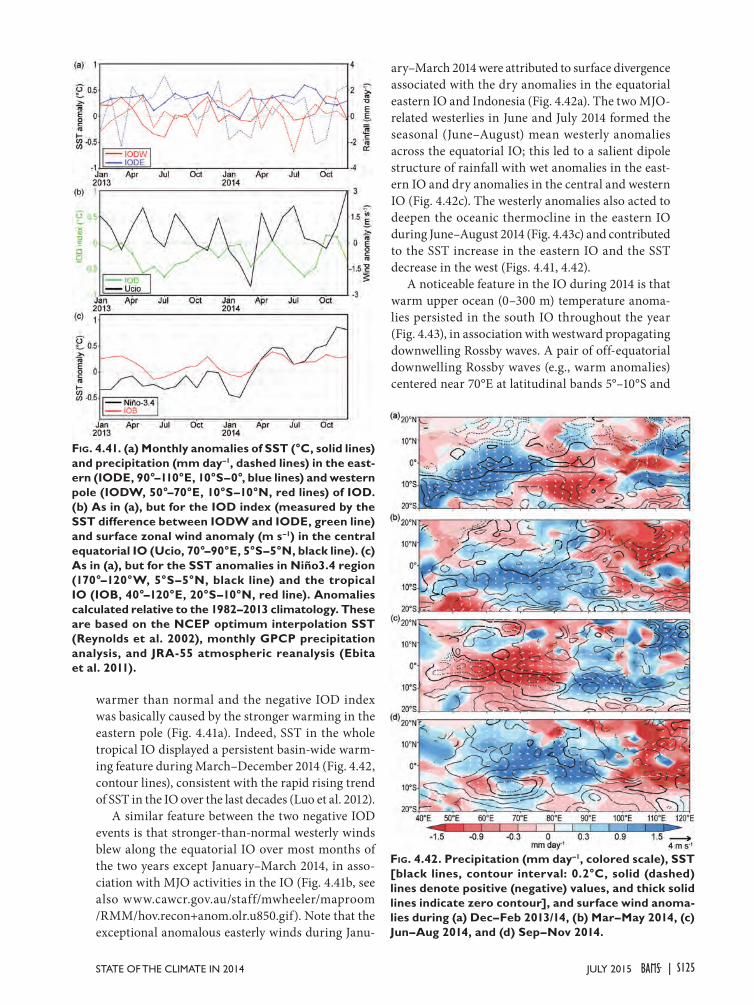
warmer than normal and the negative IOD index was basically caused by the stronger warming in the eastern pole (Fig. 4.41a). Indeed, SST in the whole tropical IO displayed a persistent basin-wide warm-ing feature during March–December 2014 (Fig. 4.42, contour lines), consistent with the rapid rising trend of SST in the IO over the last decades (Luo et al. 2012).
A similar feature between the two negative IOD events is that stronger-than-normal westerly winds blew along the equatorial IO over most months of the two years except January–March 2014, in asso-ciation with MJO activities in the IO (Fig. 4.41b, see also www.cawcr.gov.au/staff/mwheeler/maproom /RMM/hov.recon+anom.olr.u850.gif). Note that the exceptional anomalous easterly winds during Janu-
Fig. 4.41. (a) Monthly anomalies of SST (°C, solid lines) and precipitation (mm day–1, dashed lines) in the east-ern (IODE, 90°–110°E, 10°S–0°, blue lines) and western pole (IODW, 50°–70°E, 10°S–10°N, red lines) of IOD. (b) As in (a), but for the IOD index (measured by the SST difference between IODW and IODE, green line) and surface zonal wind anomaly (m s–1) in the central equatorial IO (Ucio, 70°–90°E, 5°S–5°N, black line). (c) As in (a), but for the SST anomalies in Niño3.4 region (170°–120°W, 5°S–5°N, black line) and the tropical IO (IOB, 40°–120°E, 20°S–10°N, red line). Anomalies calculated relative to the 1982–2013 climatology. These are based on the NCEP optimum interpolation SST (Reynolds et al. 2002), monthly GPCP precipitation analysis, and JRA-55 atmospheric reanalysis (Ebita et al. 2011).
ary–March 2014 were attributed to surface divergence associated with the dry anomalies in the equatorial eastern IO and Indonesia (Fig. 4.42a). The two MJO-related westerlies in June and July 2014 formed the seasonal (June–August) mean westerly anomalies across the equatorial IO; this led to a salient dipole structure of rainfall with wet anomalies in the east-ern IO and dry anomalies in the central and western IO (Fig. 4.42c). The westerly anomalies also acted to deepen the oceanic thermocline in the eastern IO during June–August 2014 (Fig. 4.43c) and contributed to the SST increase in the eastern IO and the SST decrease in the west (Figs. 4.41, 4.42).
A noticeable feature in the IO during 2014 is that warm upper ocean (0–300 m) temperature anoma-lies persisted in the south IO throughout the year (Fig. 4.43), in association with westward propagating downwelling Rossby waves. A pair of off-equatorial downwelling Rossby waves (e.g., warm anomalies) centered near 70°E at latitudinal bands 5°–10°S and
Fig. 4.42. Precipitation (mm day–1, colored scale), SST [black lines, contour interval: 0.2°C, solid (dashed) lines denote positive (negative) values, and thick solid lines indicate zero contour], and surface wind anoma-lies during (a) Dec–Feb 2013/14, (b) Mar–May 2014, (c) Jun–Aug 2014, and (d) Sep–Nov 2014.
S125JULY 2015STATE OF THE CLIMATE IN 2014 |
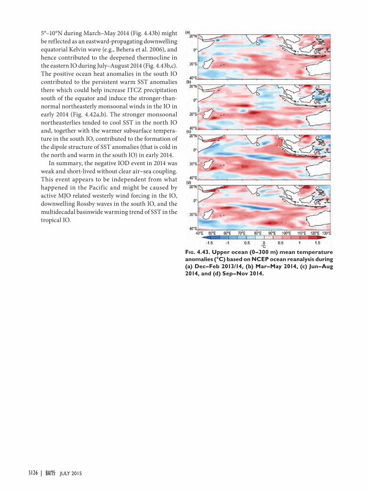
5°–10°N during March–May 2014 (Fig. 4.43b) might be reflected as an eastward-propagating downwelling equatorial Kelvin wave (e.g., Behera et al. 2006), and hence contributed to the deepened thermocline in the eastern IO during July–August 2014 (Fig. 4.43b,c). The positive ocean heat anomalies in the south IO contributed to the persistent warm SST anomalies there which could help increase ITCZ precipitation south of the equator and induce the stronger-than-normal northeasterly monsoonal winds in the IO in early 2014 (Fig. 4.42a,b). The stronger monsoonal northeasterlies tended to cool SST in the north IO and, together with the warmer subsurface tempera-ture in the south IO, contributed to the formation of the dipole structure of SST anomalies (that is cold in the north and warm in the south IO) in early 2014.
In summary, the negative IOD event in 2014 was weak and short-lived without clear air–sea coupling. This event appears to be independent from what happened in the Pacific and might be caused by active MJO related westerly wind forcing in the IO, downwelling Rossby waves in the south IO, and the multidecadal basinwide warming trend of SST in the tropical IO.
Fig. 4.43. Upper ocean (0–300 m) mean temperature anomalies (°C) based on NCEP ocean reanalysis during (a) Dec–Feb 2013/14, (b) Mar–May 2014, (c) Jun–Aug 2014, and (d) Sep–Nov 2014.
S126 JULY 2015|
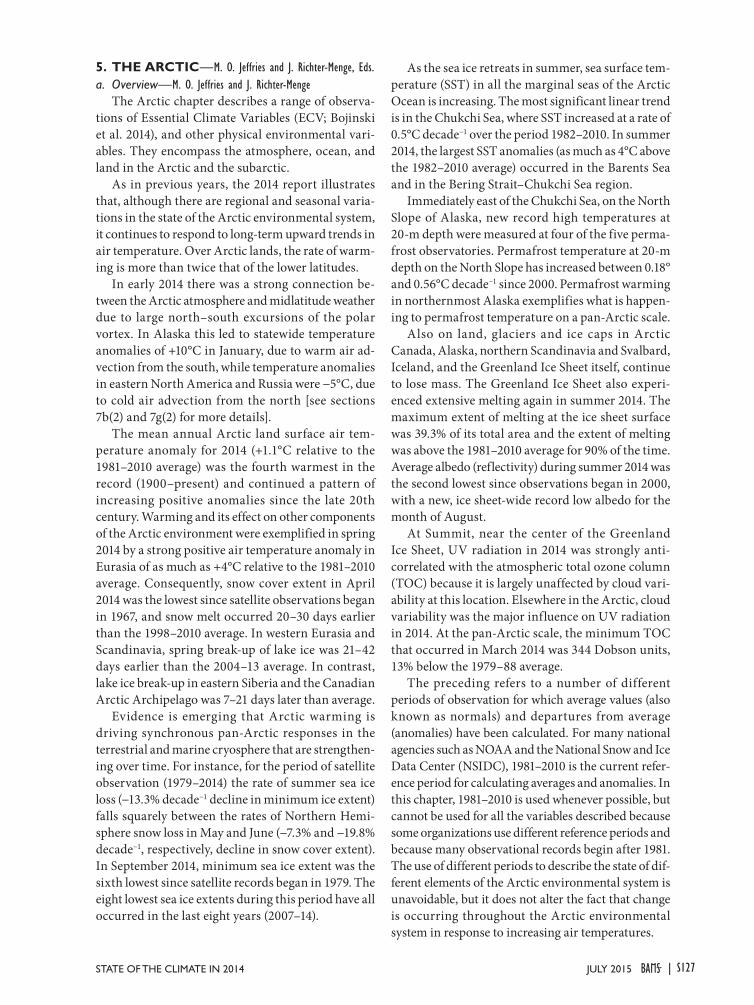
5. THE ARCTIC—M. O. Jeffries and J. Richter-Menge, Eds.a. Overview—M. O. Jeffries and J. Richter-Menge
The Arctic chapter describes a range of observa-tions of Essential Climate Variables (ECV; Bojinski et al. 2014), and other physical environmental vari-ables. They encompass the atmosphere, ocean, and land in the Arctic and the subarctic.
As in previous years, the 2014 report illustrates that, although there are regional and seasonal varia-tions in the state of the Arctic environmental system, it continues to respond to long-term upward trends in air temperature. Over Arctic lands, the rate of warm-ing is more than twice that of the lower latitudes.
In early 2014 there was a strong connection be-tween the Arctic atmosphere and midlatitude weather due to large north–south excursions of the polar vortex. In Alaska this led to statewide temperature anomalies of +10°C in January, due to warm air ad-vection from the south, while temperature anomalies in eastern North America and Russia were −5°C, due to cold air advection from the north [see sections 7b(2) and 7g(2) for more details].
The mean annual Arctic land surface air tem-perature anomaly for 2014 (+1.1°C relative to the 1981–2010 average) was the fourth warmest in the record (1900–present) and continued a pattern of increasing positive anomalies since the late 20th century. Warming and its effect on other components of the Arctic environment were exemplified in spring 2014 by a strong positive air temperature anomaly in Eurasia of as much as +4°C relative to the 1981–2010 average. Consequently, snow cover extent in April 2014 was the lowest since satellite observations began in 1967, and snow melt occurred 20–30 days earlier than the 1998–2010 average. In western Eurasia and Scandinavia, spring break-up of lake ice was 21–42 days earlier than the 2004–13 average. In contrast, lake ice break-up in eastern Siberia and the Canadian Arctic Archipelago was 7–21 days later than average.
Evidence is emerging that Arctic warming is driving synchronous pan-Arctic responses in the terrestrial and marine cryosphere that are strengthen-ing over time. For instance, for the period of satellite observation (1979–2014) the rate of summer sea ice loss (−13.3% decade−1 decline in minimum ice extent) falls squarely between the rates of Northern Hemi-sphere snow loss in May and June (−7.3% and −19.8% decade−1, respectively, decline in snow cover extent). In September 2014, minimum sea ice extent was the sixth lowest since satellite records began in 1979. The eight lowest sea ice extents during this period have all occurred in the last eight years (2007–14).
As the sea ice retreats in summer, sea surface tem-perature (SST) in all the marginal seas of the Arctic Ocean is increasing. The most significant linear trend is in the Chukchi Sea, where SST increased at a rate of 0.5°C decade−1 over the period 1982–2010. In summer 2014, the largest SST anomalies (as much as 4°C above the 1982–2010 average) occurred in the Barents Sea and in the Bering Strait–Chukchi Sea region.
Immediately east of the Chukchi Sea, on the North Slope of Alaska, new record high temperatures at 20-m depth were measured at four of the five perma-frost observatories. Permafrost temperature at 20-m depth on the North Slope has increased between 0.18° and 0.56°C decade−1 since 2000. Permafrost warming in northernmost Alaska exemplifies what is happen-ing to permafrost temperature on a pan-Arctic scale.
Also on land, glaciers and ice caps in Arctic Canada, Alaska, northern Scandinavia and Svalbard, Iceland, and the Greenland Ice Sheet itself, continue to lose mass. The Greenland Ice Sheet also experi-enced extensive melting again in summer 2014. The maximum extent of melting at the ice sheet surface was 39.3% of its total area and the extent of melting was above the 1981–2010 average for 90% of the time. Average albedo (reflectivity) during summer 2014 was the second lowest since observations began in 2000, with a new, ice sheet-wide record low albedo for the month of August.
At Summit, near the center of the Greenland Ice Sheet, UV radiation in 2014 was strongly anti-correlated with the atmospheric total ozone column (TOC) because it is largely unaffected by cloud vari-ability at this location. Elsewhere in the Arctic, cloud variability was the major influence on UV radiation in 2014. At the pan-Arctic scale, the minimum TOC that occurred in March 2014 was 344 Dobson units, 13% below the 1979–88 average.
The preceding refers to a number of different periods of observation for which average values (also known as normals) and departures from average (anomalies) have been calculated. For many national agencies such as NOAA and the National Snow and Ice Data Center (NSIDC), 1981–2010 is the current refer-ence period for calculating averages and anomalies. In this chapter, 1981–2010 is used whenever possible, but cannot be used for all the variables described because some organizations use different reference periods and because many observational records begin after 1981. The use of different periods to describe the state of dif-ferent elements of the Arctic environmental system is unavoidable, but it does not alter the fact that change is occurring throughout the Arctic environmental system in response to increasing air temperatures.
S127JULY 2015STATE OF THE CLIMATE IN 2014 |
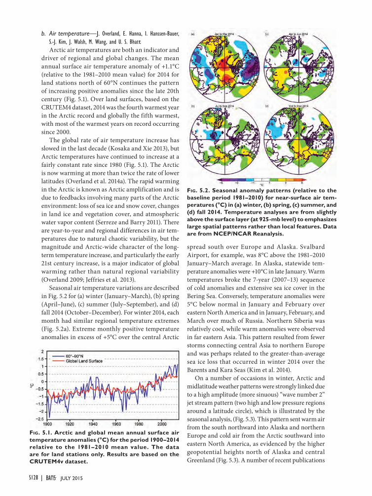
b. Air temperature—J. Overland, E. Hanna, I. Hanssen-Bauer, S.-J. Kim, J. Walsh, M. Wang, and U. S. BhattArctic air temperatures are both an indicator and
driver of regional and global changes. The mean annual surface air temperature anomaly of +1.1°C (relative to the 1981–2010 mean value) for 2014 for land stations north of 60°N continues the pattern of increasing positive anomalies since the late 20th century (Fig. 5.1). Over land surfaces, based on the CRUTEM4 dataset, 2014 was the fourth warmest year in the Arctic record and globally the fifth warmest, with most of the warmest years on record occurring since 2000.
The global rate of air temperature increase has slowed in the last decade (Kosaka and Xie 2013), but Arctic temperatures have continued to increase at a fairly constant rate since 1980 (Fig. 5.1). The Arctic is now warming at more than twice the rate of lower latitudes (Overland et al. 2014a). The rapid warming in the Arctic is known as Arctic amplification and is due to feedbacks involving many parts of the Arctic environment: loss of sea ice and snow cover, changes in land ice and vegetation cover, and atmospheric water vapor content (Serreze and Barry 2011). There are year-to-year and regional differences in air tem-peratures due to natural chaotic variability, but the magnitude and Arctic-wide character of the long-term temperature increase, and particularly the early 21st century increase, is a major indicator of global warming rather than natural regional variability (Overland 2009; Jeffries et al. 2013).
Seasonal air temperature variations are described in Fig. 5.2 for (a) winter (January–March), (b) spring (April–June), (c) summer (July–September), and (d) fall 2014 (October–December). For winter 2014, each month had similar regional temperature extremes (Fig. 5.2a). Extreme monthly positive temperature anomalies in excess of +5°C over the central Arctic
spread south over Europe and Alaska. Svalbard Airport, for example, was 8°C above the 1981–2010 January–March average. In Alaska, statewide tem-perature anomalies were +10°C in late January. Warm temperatures broke the 7-year (2007–13) sequence of cold anomalies and extensive sea ice cover in the Bering Sea. Conversely, temperature anomalies were 5°C below normal in January and February over eastern North America and in January, February, and March over much of Russia. Northern Siberia was relatively cool, while warm anomalies were observed in far eastern Asia. This pattern resulted from fewer storms connecting central Asia to northern Europe and was perhaps related to the greater-than-average sea ice loss that occurred in winter 2014 over the Barents and Kara Seas (Kim et al. 2014).
On a number of occasions in winter, Arctic and midlatitude weather patterns were strongly linked due to a high amplitude (more sinuous) “wave number 2” jet stream pattern (two high and low pressure regions around a latitude circle), which is illustrated by the seasonal analysis, (Fig. 5.3). This pattern sent warm air from the south northward into Alaska and northern Europe and cold air from the Arctic southward into eastern North America, as evidenced by the higher geopotential heights north of Alaska and central Greenland (Fig. 5.3). A number of recent publications
Fig. 5.1. Arctic and global mean annual surface air temperature anomalies (°C) for the period 1900–2014 relative to the 1981–2010 mean value. The data are for land stations only. Results are based on the CRUTEM4v dataset.
Fig. 5.2. Seasonal anomaly patterns (relative to the baseline period 1981–2010) for near-surface air tem-peratures (°C) in (a) winter, (b) spring, (c) summer, and (d) fall 2014. Temperature analyses are from slightly above the surface layer (at 925-mb level) to emphasizes large spatial patterns rather than local features. Data are from NCEP/NCAR Reanalysis.
S128 JULY 2015|
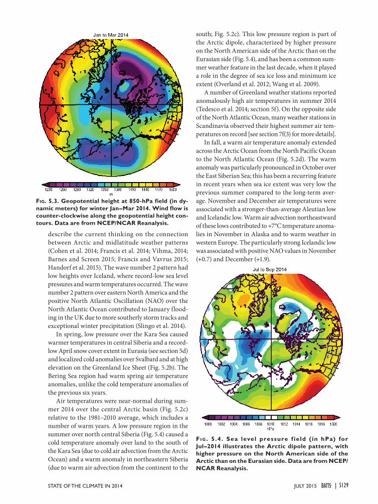
describe the current thinking on the connection between Arctic and midlatitude weather patterns (Cohen et al. 2014; Francis et al. 2014; Vihma, 2014; Barnes and Screen 2015; Francis and Vavrus 2015; Handorf et al. 2015). The wave number 2 pattern had low heights over Iceland, where record-low sea level pressures and warm temperatures occurred. The wave number 2 pattern over eastern North America and the positive North Atlantic Oscillation (NAO) over the North Atlantic Ocean contributed to January flood-ing in the UK due to more southerly storm tracks and exceptional winter precipitation (Slingo et al. 2014).
In spring, low pressure over the Kara Sea caused warmer temperatures in central Siberia and a record-low April snow cover extent in Eurasia (see section 5d) and localized cold anomalies over Svalbard and at high elevation on the Greenland Ice Sheet (Fig. 5.2b). The Bering Sea region had warm spring air temperature anomalies, unlike the cold temperature anomalies of the previous six years.
Air temperatures were near-normal during sum-mer 2014 over the central Arctic basin (Fig. 5.2c) relative to the 1981–2010 average, which includes a number of warm years. A low pressure region in the summer over north central Siberia (Fig. 5.4) caused a cold temperature anomaly over land to the south of the Kara Sea (due to cold air advection from the Arctic Ocean) and a warm anomaly in northeastern Siberia (due to warm air advection from the continent to the
south; Fig. 5.2c). This low pressure region is part of the Arctic dipole, characterized by higher pressure on the North American side of the Arctic than on the Eurasian side (Fig. 5.4), and has been a common sum-mer weather feature in the last decade, when it played a role in the degree of sea ice loss and minimum ice extent (Overland et al. 2012; Wang et al. 2009).
A number of Greenland weather stations reported anomalously high air temperatures in summer 2014 (Tedesco et al. 2014; section 5f). On the opposite side of the North Atlantic Ocean, many weather stations in Scandinavia observed their highest summer air tem-peratures on record [see section 7f(3) for more details].
In fall, a warm air temperature anomaly extended across the Arctic Ocean from the North Pacific Ocean to the North Atlantic Ocean (Fig. 5.2d). The warm anomaly was particularly pronounced in October over the East Siberian Sea; this has been a recurring feature in recent years when sea ice extent was very low the previous summer compared to the long-term aver-age. November and December air temperatures were associated with a stronger-than-average Aleutian low and Icelandic low. Warm air advection northeastward of these lows contributed to +7°C temperature anoma-lies in November in Alaska and to warm weather in western Europe. The particularly strong Icelandic low was associated with positive NAO values in November (+0.7) and December (+1.9).
Fig. 5.3. Geopotential height at 850-hPa field (in dy-namic meters) for winter Jan–Mar 2014. Wind flow is counter-clockwise along the geopotential height con-tours. Data are from NCEP/NCAR Reanalysis.
Fi g. 5.4 . Sea level pressure f ield (in hPa) for Jul–2014 illustrates the Arctic dipole pattern, with higher pressure on the North American side of the Arctic than on the Eurasian side. Data are from NCEP/NCAR Reanalysis.
S129JULY 2015STATE OF THE CLIMATE IN 2014 |
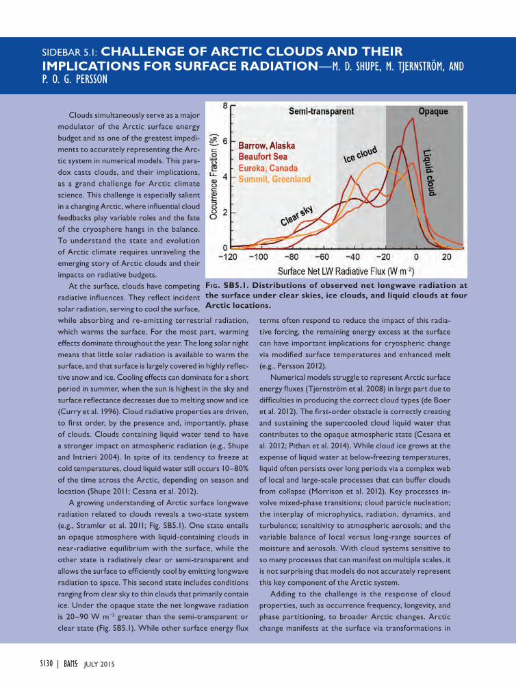
SIDEBAR 5.1: CHALLENGE OF ARCTIC CLOUDS AND THEIR IMPLICATIONS FOR SURFACE RADIATION—M. D. SHUPE, M. TJERNSTRÖM, AND P. O. G. PERSSON
Clouds simultaneously serve as a major modulator of the Arctic surface energy budget and as one of the greatest impedi-ments to accurately representing the Arc-tic system in numerical models. This para-dox casts clouds, and their implications, as a grand challenge for Arctic climate science. This challenge is especially salient in a changing Arctic, where influential cloud feedbacks play variable roles and the fate of the cryosphere hangs in the balance. To understand the state and evolution of Arctic climate requires unraveling the emerging story of Arctic clouds and their impacts on radiative budgets.
At the surface, clouds have competing radiative influences. They reflect incident solar radiation, serving to cool the surface, while absorbing and re-emitting terrestrial radiation, which warms the surface. For the most part, warming effects dominate throughout the year. The long solar night means that little solar radiation is available to warm the surface, and that surface is largely covered in highly reflec-tive snow and ice. Cooling effects can dominate for a short period in summer, when the sun is highest in the sky and surface reflectance decreases due to melting snow and ice (Curry et al. 1996). Cloud radiative properties are driven, to first order, by the presence and, importantly, phase of clouds. Clouds containing liquid water tend to have a stronger impact on atmospheric radiation (e.g., Shupe and Intrieri 2004). In spite of its tendency to freeze at cold temperatures, cloud liquid water still occurs 10–80% of the time across the Arctic, depending on season and location (Shupe 2011; Cesana et al. 2012).
A growing understanding of Arctic surface longwave radiation related to clouds reveals a two-state system (e.g., Stramler et al. 2011; Fig. SB5.1). One state entails an opaque atmosphere with liquid-containing clouds in near-radiative equilibrium with the surface, while the other state is radiatively clear or semi-transparent and allows the surface to efficiently cool by emitting longwave radiation to space. This second state includes conditions ranging from clear sky to thin clouds that primarily contain ice. Under the opaque state the net longwave radiation is 20–90 W m−2 greater than the semi-transparent or clear state (Fig. SB5.1). While other surface energy flux
terms often respond to reduce the impact of this radia-tive forcing, the remaining energy excess at the surface can have important implications for cryospheric change via modified surface temperatures and enhanced melt (e.g., Persson 2012).
Numerical models struggle to represent Arctic surface energy fluxes (Tjernström et al. 2008) in large part due to difficulties in producing the correct cloud types (de Boer et al. 2012). The first-order obstacle is correctly creating and sustaining the supercooled cloud liquid water that contributes to the opaque atmospheric state (Cesana et al. 2012; Pithan et al. 2014). While cloud ice grows at the expense of liquid water at below-freezing temperatures, liquid often persists over long periods via a complex web of local and large-scale processes that can buffer clouds from collapse (Morrison et al. 2012). Key processes in-volve mixed-phase transitions; cloud particle nucleation; the interplay of microphysics, radiation, dynamics, and turbulence; sensitivity to atmospheric aerosols; and the variable balance of local versus long-range sources of moisture and aerosols. With cloud systems sensitive to so many processes that can manifest on multiple scales, it is not surprising that models do not accurately represent this key component of the Arctic system.
Adding to the challenge is the response of cloud properties, such as occurrence frequency, longevity, and phase partitioning, to broader Arctic changes. Arctic change manifests at the surface via transformations in
Fig. SB5.1. Distributions of observed net longwave radiation at the surface under clear skies, ice clouds, and liquid clouds at four Arctic locations.
S130 JULY 2015|

the cryosphere (e.g., sea ice thinning and loss), and within the atmosphere via warming, moistening, and modified large-scale dynamics (Graverson et al. 2008). The seasonal response of clouds to change can have significant and var-ied implications. For example, increases in cloudiness or liquid water occurrence in spring or fall would contribute to enhanced warming, accelerate cryospheric melting, and possibly lengthen melt seasons (Stone et al. 2002; Markus et al. 2009; Persson 2012). On the other hand, increased cloudiness in summer, especially over open water and land areas, would produce a surface cooling effect and slow melt processes. Arctic cloudiness may be increasing in fall and spring, but possibly not in summer (Wang and Key 2003; Kay and Gettelman 2009; Palm et al. 2010), implying that current cloud changes may be amplifying the declines in sea ice, permafrost, and land ice.
Understanding both large-scale and detailed cloud-scale processes, and clarifying the emerging feedbacks be-tween clouds and the evolving Arctic climate system, are
key research objectives for the coming decades. Observa-tions over the sea ice pack and open water areas of the Arctic Ocean will be particularly vital for achieving these objectives. Observational and modeling opportunities to address the Arctic cloud and surface radiation challenge include the Multidisciplinary drifting Observatory for the Study of Arctic Climate (MOSAiC) and the Year of Polar Prediction (YOPP, mid-2017 to mid-2019) of the WMO Polar Prediction Project. MOSAiC aims to observe and characterize coupled atmosphere–ice–ocean–ecosystem processes, including cloud processes and the surface energy budget, at a year-long drifting station on the central Arctic sea ice (www.mosaicobservatory.org). The intensive, process-level observations, along with other enhanced measurements across the Arctic, will serve as a key testbed for coupled-system model development and improving predictive capabilities on a range of time scales during the YOPP.
c. Ozone and UV radiation—G. Bernhard, G. Manney, J.-U. Grooß, R. Müller, K. Lakkala, V. Fioletov, T. Koskela, A. Heikkilä, and B. JohnsenThe minimum Arctic daily total ozone column
(TOC, the total amount of ozone in a column from Earth’s surface to the top of the atmosphere) mea-sured by satellites in March 2014 was 344 Dobson Units (DU). This value was 53 DU (13%) below the average of 397 DU for the period of 1979–88 and 26 DU (7%) below the average for the past decade, 2004–13 (Fig 5.5). The record low was 308 DU in 2011. Figure 5.5 also indicates that the Arctic ozone interannual variability is large: the standard devia-tion for the period 1979–2014 is 36 DU. This large variability is caused by dynamical effects that affect vortex size and longevity, transport of ozone into the lower stratosphere, and stratospheric chemistry via its sensitivity to temperature (e.g., Tegtmeier et al. 2008; WMO 2014).
Figure 5.6 shows the temporal evolution of ozone concentrations measured between 1 December 2013 and 1 April 2014 at approximately 20-km altitude. These measurements are compared with similar data from winter 2010/11 and the mean and range of values observed between winter 2004/05 and winter 2012/13, excluding the 2010/11 winter. That winter had record low ozone due to unusual meteorological
conditions that resulted in a very cold, long-lived vortex with unprecedented chemical ozone loss (e.g., Manney et al. 2011) and weaker-than-usual ozone transport (e.g., Isaksen et al. 2012; Strahan
Fig. 5.5. Time series of area-averaged minimum total ozone for March in the Arctic, calculated as the mini-mum of daily average column ozone poleward of 63° equivalent latitude (Butchart and Remsberg 1986). Open circles represent years in which the polar vor-tex broke up before March. Ozone in those years was relatively high because of mixing with air from lower latitudes and higher altitudes and a lack of significant chemical ozone depletion. Data are adapted from Müller et al. (2008) and WMO (2014), updated using ERA-Interim reanalysis data (Dee et al. 2011a). Ozone data from 1979–2012 are based on the combined to-tal column ozone database version 2.8 produced by Bodeker Scientific (www.bodekerscientific.com/data /total-column-ozone). Data for 2013 and 2014 are from the Ozone Monitoring Instrument aboard the NASA Aura satellite.
S131JULY 2015STATE OF THE CLIMATE IN 2014 |
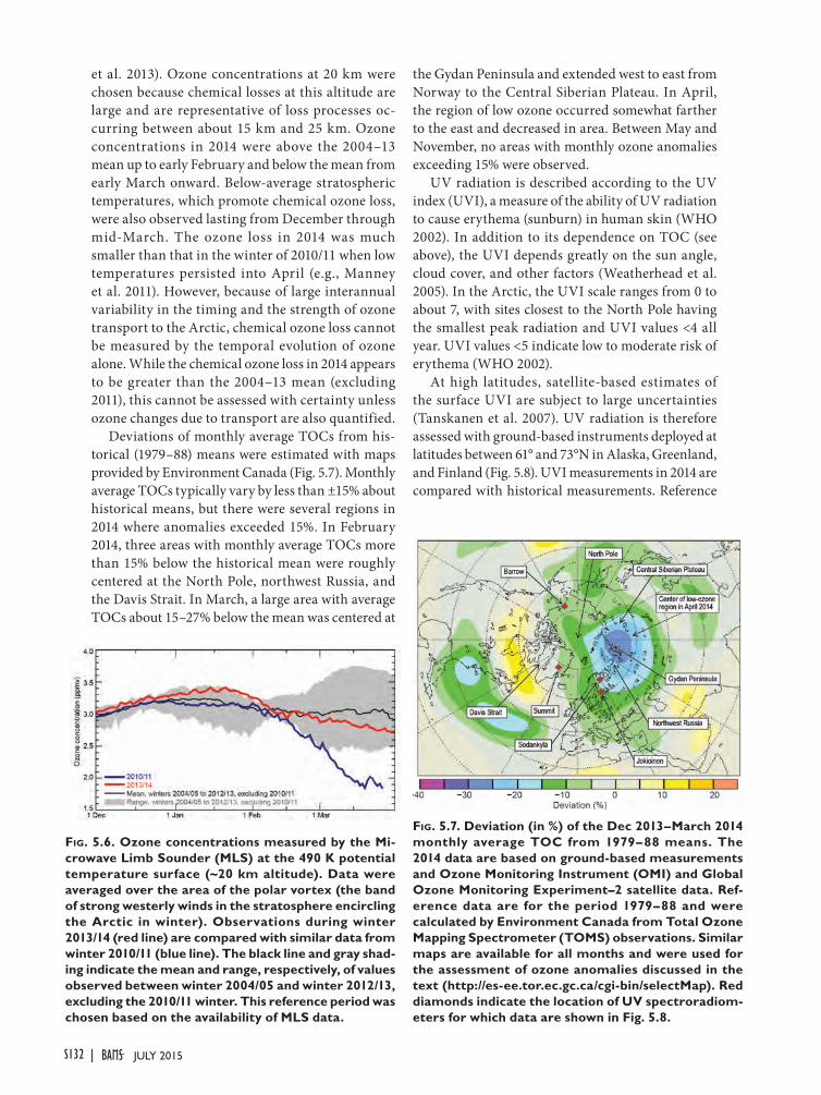
et al. 2013). Ozone concentrations at 20 km were chosen because chemical losses at this altitude are large and are representative of loss processes oc-curring between about 15 km and 25 km. Ozone concentrations in 2014 were above the 2004–13 mean up to early February and below the mean from early March onward. Below-average stratospheric temperatures, which promote chemical ozone loss, were also observed lasting from December through mid-March. The ozone loss in 2014 was much smaller than that in the winter of 2010/11 when low temperatures persisted into April (e.g., Manney et al. 2011). However, because of large interannual variability in the timing and the strength of ozone transport to the Arctic, chemical ozone loss cannot be measured by the temporal evolution of ozone alone. While the chemical ozone loss in 2014 appears to be greater than the 2004–13 mean (excluding 2011), this cannot be assessed with certainty unless ozone changes due to transport are also quantified.
Deviations of monthly average TOCs from his-torical (1979–88) means were estimated with maps provided by Environment Canada (Fig. 5.7). Monthly average TOCs typically vary by less than ±15% about historical means, but there were several regions in 2014 where anomalies exceeded 15%. In February 2014, three areas with monthly average TOCs more than 15% below the historical mean were roughly centered at the North Pole, northwest Russia, and the Davis Strait. In March, a large area with average TOCs about 15–27% below the mean was centered at
the Gydan Peninsula and extended west to east from Norway to the Central Siberian Plateau. In April, the region of low ozone occurred somewhat farther to the east and decreased in area. Between May and November, no areas with monthly ozone anomalies exceeding 15% were observed.
UV radiation is described according to the UV index (UVI), a measure of the ability of UV radiation to cause erythema (sunburn) in human skin (WHO 2002). In addition to its dependence on TOC (see above), the UVI depends greatly on the sun angle, cloud cover, and other factors (Weatherhead et al. 2005). In the Arctic, the UVI scale ranges from 0 to about 7, with sites closest to the North Pole having the smallest peak radiation and UVI values <4 all year. UVI values <5 indicate low to moderate risk of erythema (WHO 2002).
At high latitudes, satellite-based estimates of the surface UVI are subject to large uncertainties (Tanskanen et al. 2007). UV radiation is therefore assessed with ground-based instruments deployed at latitudes between 61° and 73°N in Alaska, Greenland, and Finland (Fig. 5.8). UVI measurements in 2014 are compared with historical measurements. Reference
Fig. 5.6. Ozone concentrations measured by the Mi-crowave Limb Sounder (MLS) at the 490 K potential temperature surface (~20 km altitude). Data were averaged over the area of the polar vortex (the band of strong westerly winds in the stratosphere encircling the Arctic in winter). Observations during winter 2013/14 (red line) are compared with similar data from winter 2010/11 (blue line). The black line and gray shad-ing indicate the mean and range, respectively, of values observed between winter 2004/05 and winter 2012/13, excluding the 2010/11 winter. This reference period was chosen based on the availability of MLS data.
Fig. 5.7. Deviation (in %) of the Dec 2013–March 2014 monthly average TOC from 1979–88 means. The 2014 data are based on ground-based measurements and Ozone Monitoring Instrument (OMI) and Global Ozone Monitoring Experiment–2 satellite data. Ref-erence data are for the period 1979–88 and were calculated by Environment Canada from Total Ozone Mapping Spectrometer (TOMS) observations. Similar maps are available for all months and were used for the assessment of ozone anomalies discussed in the text (http://es-ee.tor.ec.gc.ca/cgi-bin/selectMap). Red diamonds indicate the location of UV spectroradiom-eters for which data are shown in Fig. 5.8.
S132 JULY 2015|
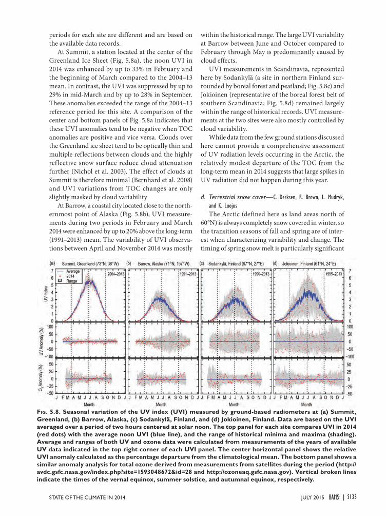
periods for each site are different and are based on the available data records.
At Summit, a station located at the center of the Greenland Ice Sheet (Fig. 5.8a), the noon UVI in 2014 was enhanced by up to 33% in February and the beginning of March compared to the 2004–13 mean. In contrast, the UVI was suppressed by up to 29% in mid-March and by up to 28% in September. These anomalies exceeded the range of the 2004–13 reference period for this site. A comparison of the center and bottom panels of Fig. 5.8a indicates that these UVI anomalies tend to be negative when TOC anomalies are positive and vice versa. Clouds over the Greenland ice sheet tend to be optically thin and multiple reflections between clouds and the highly ref lective snow surface reduce cloud attenuation further (Nichol et al. 2003). The effect of clouds at Summit is therefore minimal (Bernhard et al. 2008) and UVI variations from TOC changes are only slightly masked by cloud variability
At Barrow, a coastal city located close to the north-ernmost point of Alaska (Fig. 5.8b), UVI measure-ments during two periods in February and March 2014 were enhanced by up to 20% above the long-term (1991–2013) mean. The variability of UVI observa-tions between April and November 2014 was mostly
within the historical range. The large UVI variability at Barrow between June and October compared to February through May is predominantly caused by cloud effects.
UVI measurements in Scandinavia, represented here by Sodankylä (a site in northern Finland sur-rounded by boreal forest and peatland; Fig. 5.8c) and Jokioinen (representative of the boreal forest belt of southern Scandinavia; Fig. 5.8d) remained largely within the range of historical records. UVI measure-ments at the two sites were also mostly controlled by cloud variability.
While data from the few ground stations discussed here cannot provide a comprehensive assessment of UV radiation levels occurring in the Arctic, the relatively modest departure of the TOC from the long-term mean in 2014 suggests that large spikes in UV radiation did not happen during this year.
d. Terrestrial snow cover—C. Derksen, R. Brown, L. Mudryk, and K. LuojusThe Arctic (defined here as land areas north of
60°N) is always completely snow covered in winter, so the transition seasons of fall and spring are of inter-est when characterizing variability and change. The timing of spring snow melt is particularly significant
Fig. 5.8. Seasonal variation of the UV index (UVI) measured by ground-based radiometers at (a) Summit, Greenland, (b) Barrow, Alaska, (c) Sodankylä, Finland, and (d) Jokioinen, Finland. Data are based on the UVI averaged over a period of two hours centered at solar noon. The top panel for each site compares UVI in 2014 (red dots) with the average noon UVI (blue line), and the range of historical minima and maxima (shading). Average and ranges of both UV and ozone data were calculated from measurements of the years of available UV data indicated in the top right corner of each UVI panel. The center horizontal panel shows the relative UVI anomaly calculated as the percentage departure from the climatological mean. The bottom panel shows a similar anomaly analysis for total ozone derived from measurements from satellites during the period (http://avdc.gsfc.nasa.gov/index.php?site=1593048672&id=28 and http://ozoneaq.gsfc.nasa.gov). Vertical broken lines indicate the times of the vernal equinox, summer solstice, and autumnal equinox, respectively.
S133JULY 2015STATE OF THE CLIMATE IN 2014 |
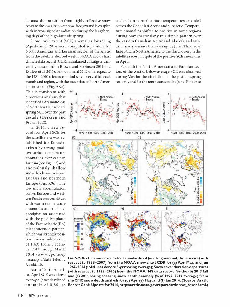
because the transition from highly reflective snow cover to the low albedo of snow-free ground is coupled with increasing solar radiation during the lengthen-ing days of the high-latitude spring.
Snow cover extent (SCE) anomalies for spring (April–June) 2014 were computed separately for North American and Eurasian sectors of the Arctic from the satellite-derived weekly NOAA snow chart climate data record (CDR; maintained at Rutgers Uni-versity; described in Brown and Robinson 2011 and Estilow et al. 2013). Below-normal SCE with respect to the 1981–2010 reference period was observed for each month and region, with the exception of North Amer-ica in April (Fig. 5.9a). This is consistent with a previous analysis that identified a dramatic loss of Northern Hemisphere spring SCE over the past decade (Derksen and Brown 2012).
In 2014, a new re-cord low April SCE for the satellite era was es-tablished for Eurasia, driven by strong posi-tive surface temperature anomalies over eastern Eurasia (see Fig. 5.2) and anomalously shal low snow depth over western Eurasia and northern Europe (Fig. 5.9d). The low snow accumulation across Europe and west-ern Russia was consistent with warm temperature anomalies and reduced precipitation associated with the positive phase of the East Atlantic (EA) teleconnection pattern, which was strongly posi-tive (mean index value of 1.43) from Decem-ber 2013 through March 2014 (w w w.cpc .ncep .noaa.gov/data/teledoc /ea.shtml).
Across North Ameri-ca, April SCE was above average (standardized a noma ly of 0 .86) as
colder-than-normal surface temperatures extended across the Canadian Arctic and subarctic. Tempera-ture anomalies shifted to positive in some regions during May (particularly in a dipole pattern over the eastern Canadian Arctic and Alaska), and were extensively warmer than average by June. This drove June SCE in North America to the third lowest in the satellite record in spite of the positive SCE anomalies in April.
For both the North American and Eurasian sec-tors of the Arctic, below-average SCE was observed during May for the ninth time in the past ten spring seasons, and for the tenth consecutive June. Evidence
Fig. 5.9. Arctic snow cover extent standardized (unitless) anomaly time series (with respect to 1988–2007) from the NOAA snow chart CDR for (a) Apr, May, and Jun 1967–2014 (solid lines denote 5-yr moving average); Snow cover duration departures (with respect to 1998–2010) from the NOAA IMS data record for the (b) 2013 fall and (c) 2014 spring seasons; snow depth anomaly (% of 1999–2010 average) from the CMC snow depth analysis for (d) Apr, (e) May, and (f) Jun 2014. (Source: Arctic Report Card: Update for 2014, http://arctic.noaa.gov/reportcard/snow_cover.html.)
S134 JULY 2015|
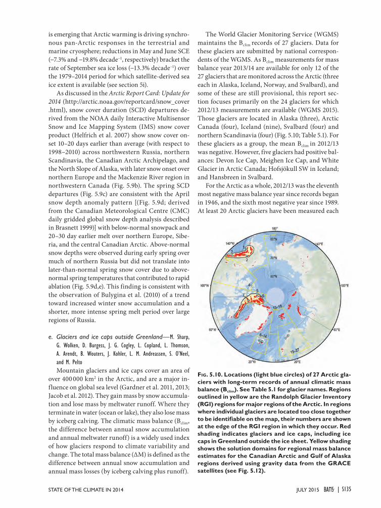
is emerging that Arctic warming is driving synchro-nous pan-Arctic responses in the terrestrial and marine cryosphere; reductions in May and June SCE (−7.3% and −19.8% decade−1, respectively) bracket the rate of September sea ice loss (−13.3% decade−1) over the 1979–2014 period for which satellite-derived sea ice extent is available (see section 5i).
As discussed in the Arctic Report Card: Update for 2014 (http://arctic.noaa.gov/reportcard/snow_cover .html), snow cover duration (SCD) departures de-rived from the NOAA daily Interactive Multisensor Snow and Ice Mapping System (IMS) snow cover product (Helfrich et al. 2007) show snow cover on-set 10–20 days earlier than average (with respect to 1998–2010) across northwestern Russia, northern Scandinavia, the Canadian Arctic Archipelago, and the North Slope of Alaska, with later snow onset over northern Europe and the Mackenzie River region in northwestern Canada (Fig. 5.9b). The spring SCD departures (Fig. 5.9c) are consistent with the April snow depth anomaly pattern [(Fig. 5.9d; derived from the Canadian Meteorological Centre (CMC) daily gridded global snow depth analysis described in Brasnett 1999)] with below-normal snowpack and 20–30 day earlier melt over northern Europe, Sibe-ria, and the central Canadian Arctic. Above-normal snow depths were observed during early spring over much of northern Russia but did not translate into later-than-normal spring snow cover due to above-normal spring temperatures that contributed to rapid ablation (Fig. 5.9d,e). This finding is consistent with the observation of Bulygina et al. (2010) of a trend toward increased winter snow accumulation and a shorter, more intense spring melt period over large regions of Russia.
e. Glaciers and ice caps outside Greenland—M. Sharp, G. Wolken, D. Burgess, J. G. Cogley, L. Copland, L. Thomson, A. Arendt, B. Wouters, J. Kohler, L. M. Andreassen, S. O’Neel, and M. PeltoMountain glaciers and ice caps cover an area of
over 400 000 km2 in the Arctic, and are a major in-fluence on global sea level (Gardner et al. 2011, 2013; Jacob et al. 2012). They gain mass by snow accumula-tion and lose mass by meltwater runoff. Where they terminate in water (ocean or lake), they also lose mass by iceberg calving. The climatic mass balance (Bclim, the difference between annual snow accumulation and annual meltwater runoff) is a widely used index of how glaciers respond to climate variability and change. The total mass balance (ΔM) is defined as the difference between annual snow accumulation and annual mass losses (by iceberg calving plus runoff).
The World Glacier Monitoring Service (WGMS) maintains the Bclim records of 27 glaciers. Data for these glaciers are submitted by national correspon-dents of the WGMS. As Bclim measurements for mass balance year 2013/14 are available for only 12 of the 27 glaciers that are monitored across the Arctic (three each in Alaska, Iceland, Norway, and Svalbard), and some of these are still provisional, this report sec-tion focuses primarily on the 24 glaciers for which 2012/13 measurements are available (WGMS 2015). Those glaciers are located in Alaska (three), Arctic Canada (four), Iceland (nine), Svalbard (four) and northern Scandinavia (four) (Fig. 5.10; Table 5.1). For these glaciers as a group, the mean Bclim in 2012/13 was negative. However, five glaciers had positive bal-ances: Devon Ice Cap, Meighen Ice Cap, and White Glacier in Arctic Canada; Hofsjökull SW in Iceland; and Hansbreen in Svalbard.
For the Arctic as a whole, 2012/13 was the eleventh most negative mass balance year since records began in 1946, and the sixth most negative year since 1989. At least 20 Arctic glaciers have been measured each
Fig. 5.10. Locations (light blue circles) of 27 Arctic gla-ciers with long-term records of annual climatic mass balance (Bclim). See Table 5.1 for glacier names. Regions outlined in yellow are the Randolph Glacier Inventory (RGI) regions for major regions of the Arctic. In regions where individual glaciers are located too close together to be identifiable on the map, their numbers are shown at the edge of the RGI region in which they occur. Red shading indicates glaciers and ice caps, including ice caps in Greenland outside the ice sheet. Yellow shading shows the solution domains for regional mass balance estimates for the Canadian Arctic and Gulf of Alaska regions derived using gravity data from the GRACE satellites (see Fig. 5.12).
S135JULY 2015STATE OF THE CLIMATE IN 2014 |
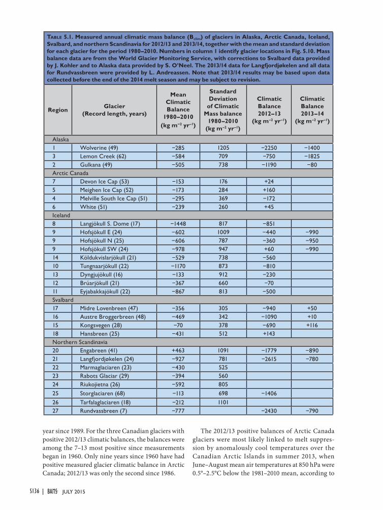
year since 1989. For the three Canadian glaciers with positive 2012/13 climatic balances, the balances were among the 7–13 most positive since measurements began in 1960. Only nine years since 1960 have had positive measured glacier climatic balance in Arctic Canada; 2012/13 was only the second since 1986.
The 2012/13 positive balances of Arctic Canada glaciers were most likely linked to melt suppres-sion by anomalously cool temperatures over the Canadian Arctic Islands in summer 2013, when June–August mean air temperatures at 850 hPa were 0.5°–2.5°C below the 1981–2010 mean, according to
Table 5.1. Measured annual climatic mass balance (Bclim) of glaciers in Alaska, Arctic Canada, Iceland, Svalbard, and northern Scandinavia for 2012/13 and 2013/14, together with the mean and standard deviation for each glacier for the period 1980–2010. Numbers in column 1 identify glacier locations in Fig. 5.10. Mass balance data are from the World Glacier Monitoring Service, with corrections to Svalbard data provided by J. Kohler and to Alaska data provided by S. O’Neel. The 2013/14 data for Langfjordjøkelen and all data for Rundvassbreen were provided by L. Andreassen. Note that 2013/14 results may be based upon data collected before the end of the 2014 melt season and may be subject to revision.
Region Glacier (Record length, years)
Mean Climatic Balance
1980–2010 (kg m–2 yr–1)
Standard Deviation
of Climatic Mass balance
1980–2010 (kg m–2 yr–1)
Climatic Balance 2012–13
(kg m–2 yr–1)
Climatic Balance 2013–14
(kg m–2 yr–1)
Alaska1 Wolverine (49) −285 1205 −2250 −14003 Lemon Creek (62) −584 709 −750 −18252 Gulkana (49) −505 738 −1190 −80Arctic Canada7 Devon Ice Cap (53) −153 176 +245 Meighen Ice Cap (52) −173 284 +1604 Melville South Ice Cap (51) −295 369 −1726 White (51) −239 260 +45Iceland8 Langjökull S. Dome (17) −1448 817 −8519 Hofsjökull E (24) −602 1009 −440 −9909 Hofsjökull N (25) −606 787 −360 −9509 Hofsjökull SW (24) −978 947 +60 −99014 Köldukvislarjökull (21) −529 738 −56010 Tungnaarjökull (22) −1170 873 −81013 Dyngjujökull (16) −133 912 −23012 Brúarjökull (21) −367 660 −7011 Eyjabakkajökull (22) −867 813 −500Svalbard17 Midre Lovenbreen (47) −356 305 −940 +5016 Austre Broggerbreen (48) −469 342 −1090 +1015 Kongsvegen (28) −70 378 −690 +11618 Hansbreen (25) −431 512 +143Northern Scandinavia20 Engabreen (41) +463 1091 −1779 −89021 Langfjordjøkelen (24) −927 781 −2615 −78022 Marmaglaciaren (23) −430 52523 Rabots Glaciar (29) −394 56024 Riukojietna (26) −592 80525 Storglaciaren (68) −113 698 −140626 Tarfalaglaciaren (18) −212 110127 Rundvassbreen (7) −777 −2430 −790
S136 JULY 2015|
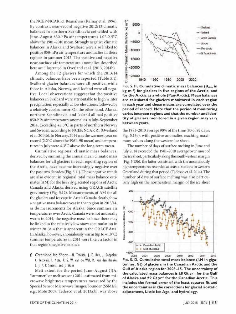
the NCEP-NCAR R1 Reanalysis (Kalnay et al. 1996). By contrast, near-record negative 2012/13 climatic balances in northern Scandinavia coincided with June–August 850-hPa air temperatures 1.0°–2.5°C above the 1981–2010 mean. Strongly negative climatic balances in Alaska and Svalbard were also linked to positive 850-hPa air temperature anomalies in these regions in summer 2013. The positive and negative near-surface air temperature anomalies described here are illustrated in Overland et al. (2013, 2014b).
Among the 12 glaciers for which the 2013/14 climatic balances have been reported (Table 5.1), Svalbard glacier balances were all positive, while those in Alaska, Norway, and Iceland were all nega-tive. Local observations suggest that the positive balances in Svalbard were attributable to high winter precipitation, especially at low elevations, followed by a relatively cool summer. On the other hand, Alaska, northern Scandinavia, and Iceland all had positive 850-hPa air temperature anomalies in July–September 2014, exceeding +2.5°C in parts of northern Norway and Sweden, according to NCEP/NCAR R1 (Overland et al. 2014b). In Norway, 2014 was the warmest year on record (2.2°C above the 1961–90 mean) and tempera-tures in July were 4.3°C above the long-term mean.
Cumulative regional climatic mass balances, derived by summing the annual mean climatic mass balances for all glaciers in each reporting region of the Arctic, have become increasingly negative over the past two decades (Fig. 5.11). These negative trends are also evident in regional total mass balance esti-mates (ΔM) for the heavily glaciated regions of Arctic Canada and Alaska derived using GRACE satellite gravimetry (Fig. 5.12). Measurements of ΔM for all the glaciers and ice caps in Arctic Canada clearly show a negative mass balance year in that region in 2013/14, as do measurements for Alaska. Since summer air temperatures over Arctic Canada were not unusually warm in 2014, the negative mass balance there may be linked to the relatively low snow accumulation in winter 2013/14 that is apparent in the GRACE data. In Alaska, however, anomalously warm (up to +1.0°C) summer temperatures in 2014 were likely a factor in that region’s negative balance.
f. Greenland Ice Sheet—M. Tedesco, J. E. Box, J. Cappelen, X. Fettweis, T. Mote, R. S. W. van de Wal, M. van den Broeke, C. J. P. P. Smeets, and J. WahrMelt extent for the period June–August (JJA,
“summer” or melt season) 2014, estimated from mi-crowave brightness temperatures measured by the Special Sensor Microwave Imager/Sounder (SSMI/S; e.g., Mote 2007; Tedesco et al. 2013a,b), was above
the 1981–2010 average 90% of the time (83 of 92 days; Fig. 5.13a), with positive anomalies reaching maxi-mum values along the western ice sheet.
The number of days of surface melting in June and July 2014 exceeded the 1981–2010 average over most of the ice sheet, particularly along the southwestern margin (Fig. 5.13b), the latter consistent with the anomalously high temperatures recorded at coastal stations in western Greenland during that period (Tedesco et al. 2014). The number of days of surface melting was also particu-larly high on the northeastern margin of the ice sheet
Fig. 5.11. Cumulative climatic mass balances (Bclim in kg m–2) for glaciers in five regions of the Arctic, and for the Arctic as a whole (Pan-Arctic). Mean balances are calculated for glaciers monitored in each region in each year and these means are cumulated over the period of record. Note that the period of monitoring varies between regions and that the number and iden-tity of glaciers monitored in a given region may vary between years.
Fig. 5.12. Cumulative total mass balance (ΔM in giga-tonnes, Gt) of glaciers in the Canadian Arctic and the Gulf of Alaska region for 2003–15. The uncertainty of the calculated mass balances is ±8 Gt yr–1 for the Gulf of Alaska and ±9 Gt yr–1 for the Canadian Arctic. This includes the formal error of the least squares fit and the uncertainties in the corrections for glacial isostatic adjustment, Little Ice Age, and hydrology.
S137JULY 2015STATE OF THE CLIMATE IN 2014 |
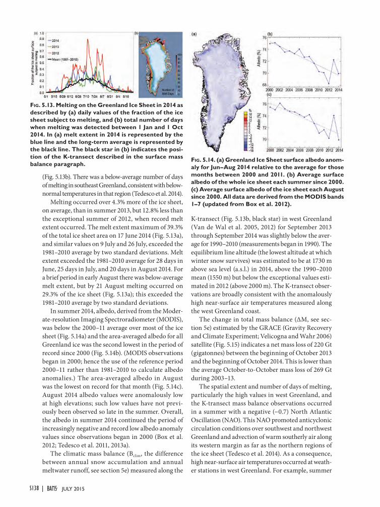
(Fig. 5.13b). There was a below-average number of days of melting in southeast Greenland, consistent with below-normal temperatures in that region (Tedesco et al. 2014).
Melting occurred over 4.3% more of the ice sheet, on average, than in summer 2013, but 12.8% less than the exceptional summer of 2012, when record melt extent occurred. The melt extent maximum of 39.3% of the total ice sheet area on 17 June 2014 (Fig. 5.13a), and similar values on 9 July and 26 July, exceeded the 1981–2010 average by two standard deviations. Melt extent exceeded the 1981–2010 average for 28 days in June, 25 days in July, and 20 days in August 2014. For a brief period in early August there was below-average melt extent, but by 21 August melting occurred on 29.3% of the ice sheet (Fig. 5.13a); this exceeded the 1981–2010 average by two standard deviations.
In summer 2014, albedo, derived from the Moder-ate-resolution Imaging Spectroradiometer (MODIS), was below the 2000–11 average over most of the ice sheet (Fig. 5.14a) and the area-averaged albedo for all Greenland ice was the second lowest in the period of record since 2000 (Fig. 5.14b). (MODIS observations began in 2000; hence the use of the reference period 2000–11 rather than 1981–2010 to calculate albedo anomalies.) The area-averaged albedo in August was the lowest on record for that month (Fig. 5.14c). August 2014 albedo values were anomalously low at high elevations; such low values have not previ-ously been observed so late in the summer. Overall, the albedo in summer 2014 continued the period of increasingly negative and record low albedo anomaly values since observations began in 2000 (Box et al. 2012; Tedesco et al. 2011, 2013a).
The climatic mass balance (Bclim, the difference between annual snow accumulation and annual meltwater runoff, see section 5e) measured along the
K-transect (Fig. 5.13b, black star) in west Greenland (Van de Wal et al. 2005, 2012) for September 2013 through September 2014 was slightly below the aver-age for 1990–2010 (measurements began in 1990). The equilibrium line altitude (the lowest altitude at which winter snow survives) was estimated to be at 1730 m above sea level (a.s.l.) in 2014, above the 1990–2010 mean (1550 m) but below the exceptional values esti-mated in 2012 (above 2000 m). The K-transect obser-vations are broadly consistent with the anomalously high near-surface air temperatures measured along the west Greenland coast.
The change in total mass balance (ΔM, see sec-tion 5e) estimated by the GRACE (Gravity Recovery and Climate Experiment; Velicogna and Wahr 2006) satellite (Fig. 5.15) indicates a net mass loss of 220 Gt (gigatonnes) between the beginning of October 2013 and the beginning of October 2014. This is lower than the average October-to-October mass loss of 269 Gt during 2003–13.
The spatial extent and number of days of melting, particularly the high values in west Greenland, and the K-transect mass balance observations occurred in a summer with a negative (−0.7) North Atlantic Oscillation (NAO). This NAO promoted anticyclonic circulation conditions over southwest and northwest Greenland and advection of warm southerly air along its western margin as far as the northern regions of the ice sheet (Tedesco et al. 2014). As a consequence, high near-surface air temperatures occurred at weath-er stations in west Greenland. For example, summer
Fig. 5.14. (a) Greenland Ice Sheet surface albedo anom-aly for Jun–Aug 2014 relative to the average for those months between 2000 and 2011. (b) Average surface albedo of the whole ice sheet each summer since 2000. (c) Average surface albedo of the ice sheet each August since 2000. All data are derived from the MODIS bands 1–7 (updated from Box et al. 2012).
Fig. 5.13. Melting on the Greenland Ice Sheet in 2014 as described by (a) daily values of the fraction of the ice sheet subject to melting, and (b) total number of days when melting was detected between 1 Jan and 1 Oct 2014. In (a) melt extent in 2014 is represented by the blue line and the long-term average is represented by the black line. The black star in (b) indicates the posi-tion of the K-transect described in the surface mass balance paragraph.
S138 JULY 2015|
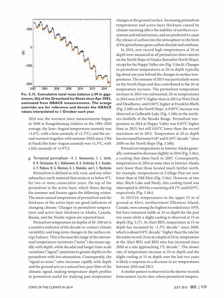
2014 was the warmest since measurements began in 1949 at Kangerlussuaq (relative to the 1981−2010 average, the June–August temperature anomaly was +1.6°C, with a June anomaly of +2.3°C), and the sec-ond warmest (together with summer 2010) since 1784 at Nuuk (the June–August anomaly was +2.3°C, with a July anomaly of +2.9°C).
g. Terrestrial permafrost—V. E. Romanovsky, S. L. Smith, H. H. Christiansen, N. I. Shiklomanov, D. A. Streletskiy, D. S. Drozdov, G. V. Malkova, N. G. Oberman, A. L. Kholodov, and S. S. MarchenkoPermafrost is defined as soil, rock, and any other
subsurface earth material that exists at or below 0°C for two or more consecutive years. On top of the permafrost is the active layer, which thaws during the summer and freezes again the following winter. The mean annual temperature of permafrost and the thickness of the active layer are good indicators of changing climate. Changes in permafrost tempera-tures and active layer thickness in Alaska, Canada, Russia, and the Nordic region are reported here.
Permafrost temperature (at depths of 10–200 m) is a sensitive indicator of the decade-to-century climate variability and long-term changes in the surface en-ergy balance. This is because the range of the interan-nual temperature variations (“noise”) decreases rap-idly with depth, while decadal and longer time-scale variations (“signal”) penetrate to greater depths in the permafrost with less attenuation. Consequently, the “signal-to-noise” ratio increases rapidly with depth and the ground acts as a natural low-pass filter of the climatic signal, making temperature-depth profiles in permafrost useful for studying past temperature
changes at the ground surface. Increasing permafrost temperatures and active layer thickness caused by climate warming affect the stability of northern eco-systems and infrastructure, and are predicted to cause the release of carbon into the atmosphere in the form of the greenhouse gases carbon dioxide and methane.
In 2014, new record high temperatures at 20-m depth were measured at all permafrost observatories on the North Slope of Alaska (hereafter North Slope), except for the Happy Valley site (Fig. 5.16a,b). Changes in permafrost temperatures at 20-m depth typically lag about one year behind the changes in surface tem-peratures. The summer of 2013 was particularly warm on the North Slope and thus contributed to the 20-m temperature increase. The permafrost temperature increase in 2014 was substantial; 20-m temperatures in 2014 were 0.07°C higher than in 2013 at West Dock and Deadhorse, and 0.06°C higher at Franklin Bluffs (Fig. 5.16b) on the North Slope. A 0.09°C increase was observed at Galbraith Lake (Fig. 5.16b) in the north-ern foothills of the Brooks Range. Permafrost tem-perature in 2014 at Happy Valley was 0.03°C higher than in 2013, but still 0.03°C lower than the record maximum set in 2012. Temperature at 20-m depth has increased between 0.18° and 0.56°C decade−1 since 2000 on the North Slope (Fig. 5.16b).
Permafrost temperatures in Interior Alaska gener-ally continued to decrease slightly in 2014 (Fig. 5.16c), a cooling that dates back to 2007. Consequently, temperatures in 2014 at some sites in Interior Alaska were lower than those located much farther north, for example, temperatures at College Peat are now lower than at Old Man (Fig. 5.16c). However, at two sites, Birch Lake and Healy, this cooling trend was interrupted in 2014 by a warming of 0.1°C and 0.05°C, respectively (Fig. 5.16c).
In 2013/14, temperatures in the upper 25 m of ground at Alert, northernmost Ellesmere Island, Canada, were among the highest recorded since 1978, but have remained stable at 24-m depth for the past two years while a slight cooling is observed at 15-m depth (Fig. 5.17). At Alert BH5, temperature at 15-m depth has increased by ~1.3°C decade−1 since 2000, which is about 0.8°C decade−1 higher than the rate for the entire record. Even at a depth of 24 m, temperature at the Alert BH1 and BH2 sites has increased since 2000 at a rate approaching 1°C decade−1. The slower rate of temperature increase at 24-m depth and the slight cooling at 15-m depth over the last two years is likely a response to a decrease in air temperatures between 2010 and 2013.
A similar pattern is observed in the shorter records from eastern Arctic sites, where permafrost tempera-
Fig. 5.15. Cumulative total mass balance (ΔM in giga-tonnes, Gt) of the Greenland Ice Sheet since Apr 2002, estimated from GRACE measurements. The orange asterisks are for reference and denote the GRACE values interpolated to 1 October each year.
S139JULY 2015STATE OF THE CLIMATE IN 2014 |
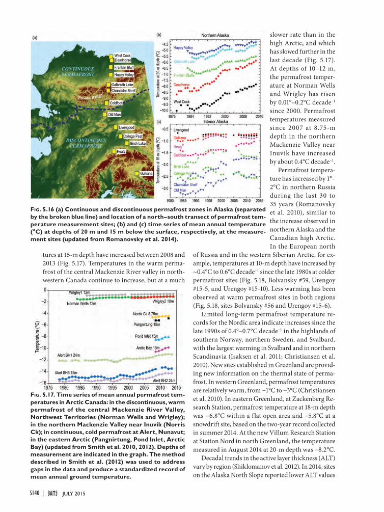
tures at 15-m depth have increased between 2008 and 2013 (Fig. 5.17). Temperatures in the warm perma-frost of the central Mackenzie River valley in north-western Canada continue to increase, but at a much
slower rate than in the high Arctic, and which has slowed further in the last decade (Fig. 5.17). At depths of 10–12 m, the permafrost temper-ature at Norman Wells and Wrigley has risen by 0.01°–0.2°C decade−1 since 2000. Permafrost temperatures measured since 2007 at 8.75-m depth in the northern Mackenzie Valley near Inuvik have increased by about 0.4°C decade−1.
Permafrost tempera-ture has increased by 1°–2°C in northern Russia during the last 30 to 35 years (Romanovsky et al. 2010), similar to the increase observed in northern Alaska and the Canadian high Arctic. In the European north
of Russia and in the western Siberian Arctic, for ex-ample, temperatures at 10-m depth have increased by ~0.4°C to 0.6°C decade−1 since the late 1980s at colder permafrost sites (Fig. 5.18, Bolvansky #59, Urengoy #15-5, and Urengoy #15-10). Less warming has been observed at warm permafrost sites in both regions (Fig. 5.18, sites Bolvansky #56 and Urengoy #15-6).
Limited long-term permafrost temperature re-cords for the Nordic area indicate increases since the late 1990s of 0.4°–0.7°C decade−1 in the highlands of southern Norway, northern Sweden, and Svalbard, with the largest warming in Svalbard and in northern Scandinavia (Isaksen et al. 2011; Christiansen et al. 2010). New sites established in Greenland are provid-ing new information on the thermal state of perma-frost. In western Greenland, permafrost temperatures are relatively warm, from −1°C to −3°C (Christiansen et al. 2010). In eastern Greenland, at Zackenberg Re-search Station, permafrost temperature at 18-m depth was −6.8°C within a flat open area and −5.8°C at a snowdrift site, based on the two-year record collected in summer 2014. At the new Villum Research Station at Station Nord in north Greenland, the temperature measured in August 2014 at 20-m depth was −8.2°C.
Decadal trends in the active layer thickness (ALT) vary by region (Shiklomanov et al. 2012). In 2014, sites on the Alaska North Slope reported lower ALT values
Fig. 5.17. Time series of mean annual permafrost tem-peratures in Arctic Canada: in the discontinuous, warm permafrost of the central Mackenzie River Valley, Northwest Territories (Norman Wells and Wrigley); in the northern Mackenzie Valley near Inuvik (Norris Ck); in continuous, cold permafrost at Alert, Nunavut; in the eastern Arctic (Pangnirtung, Pond Inlet, Arctic Bay) (updated from Smith et al. 2010, 2012). Depths of measurement are indicated in the graph. The method described in Smith et al. (2012) was used to address gaps in the data and produce a standardized record of mean annual ground temperature.
Fig. 5.16 (a) Continuous and discontinuous permafrost zones in Alaska (separated by the broken blue line) and location of a north–south transect of permafrost tem-perature measurement sites; (b) and (c) time series of mean annual temperature (°C) at depths of 20 m and 15 m below the surface, respectively, at the measure-ment sites (updated from Romanovsky et al. 2014).
S140 JULY 2015|
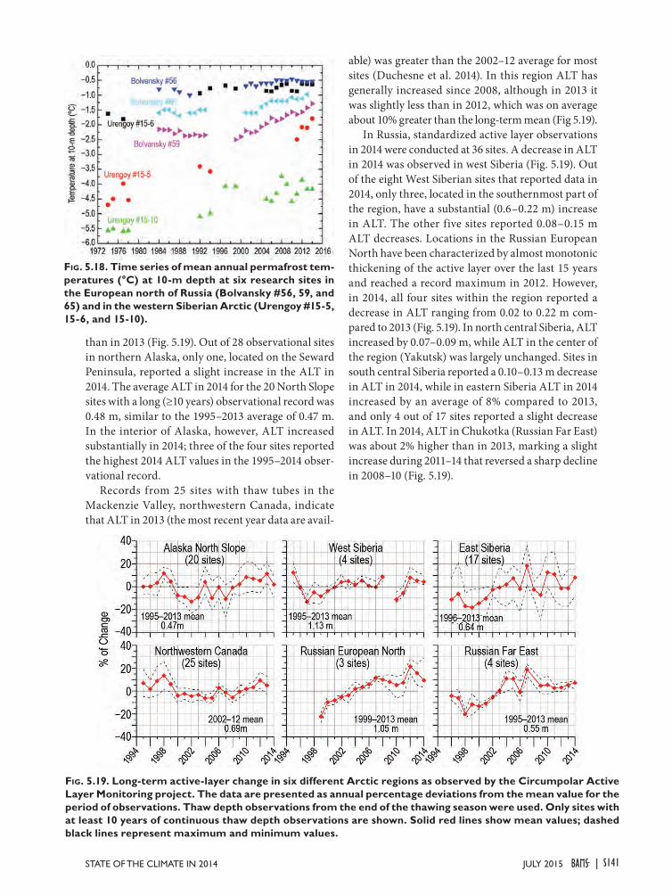
than in 2013 (Fig. 5.19). Out of 28 observational sites in northern Alaska, only one, located on the Seward Peninsula, reported a slight increase in the ALT in 2014. The average ALT in 2014 for the 20 North Slope sites with a long (≥10 years) observational record was 0.48 m, similar to the 1995–2013 average of 0.47 m. In the interior of Alaska, however, ALT increased substantially in 2014; three of the four sites reported the highest 2014 ALT values in the 1995–2014 obser-vational record.
Records from 25 sites with thaw tubes in the Mackenzie Valley, northwestern Canada, indicate that ALT in 2013 (the most recent year data are avail-
able) was greater than the 2002–12 average for most sites (Duchesne et al. 2014). In this region ALT has generally increased since 2008, although in 2013 it was slightly less than in 2012, which was on average about 10% greater than the long-term mean (Fig 5.19).
In Russia, standardized active layer observations in 2014 were conducted at 36 sites. A decrease in ALT in 2014 was observed in west Siberia (Fig. 5.19). Out of the eight West Siberian sites that reported data in 2014, only three, located in the southernmost part of the region, have a substantial (0.6–0.22 m) increase in ALT. The other five sites reported 0.08–0.15 m ALT decreases. Locations in the Russian European North have been characterized by almost monotonic thickening of the active layer over the last 15 years and reached a record maximum in 2012. However, in 2014, all four sites within the region reported a decrease in ALT ranging from 0.02 to 0.22 m com-pared to 2013 (Fig. 5.19). In north central Siberia, ALT increased by 0.07–0.09 m, while ALT in the center of the region (Yakutsk) was largely unchanged. Sites in south central Siberia reported a 0.10–0.13 m decrease in ALT in 2014, while in eastern Siberia ALT in 2014 increased by an average of 8% compared to 2013, and only 4 out of 17 sites reported a slight decrease in ALT. In 2014, ALT in Chukotka (Russian Far East) was about 2% higher than in 2013, marking a slight increase during 2011–14 that reversed a sharp decline in 2008–10 (Fig. 5.19).
Fig. 5.18. Time series of mean annual permafrost tem-peratures (°C) at 10-m depth at six research sites in the European north of Russia (Bolvansky #56, 59, and 65) and in the western Siberian Arctic (Urengoy #15-5, 15-6, and 15-10).
Fig. 5.19. Long-term active-layer change in six different Arctic regions as observed by the Circumpolar Active Layer Monitoring project. The data are presented as annual percentage deviations from the mean value for the period of observations. Thaw depth observations from the end of the thawing season were used. Only sites with at least 10 years of continuous thaw depth observations are shown. Solid red lines show mean values; dashed black lines represent maximum and minimum values.
S141JULY 2015STATE OF THE CLIMATE IN 2014 |
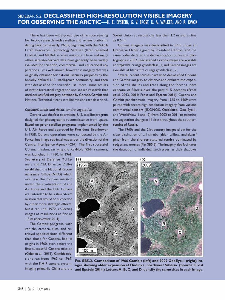
SIDEBAR 5.2: DECLASSIFIED HIGH-RESOLUTION VISIBLE IMAGERY FOR OBSERVING THE ARCTIC—H. E. EPSTEIN, G. V. FROST, D. A. WALKER, AND R. KWOK
There has been widespread use of remote sensing for Arctic research with satellite and sensor platforms dating back to the early 1970s, beginning with the NASA Earth Resources Technology Satellite (later renamed Landsat) and NOAA satellite missions. These and many other satellite-derived data have generally been widely available for scientific, commercial, and educational ap-plications. Less well known, however, is imagery that was originally obtained for national security purposes by the broadly defined U.S. intelligence community, and then later declassified for scientific use. Here, some results of Arctic terrestrial vegetation and sea ice research that used declassified imagery obtained by Corona/Gambit and National Technical Means satellite missions are described.
Corona/Gambit and Arctic tundra vegetationCorona was the first operational U.S. satellite program
designed for photographic reconnaissance from space. Based on prior satellite programs implemented by the U.S. Air Force and approved by President Eisenhower in 1958, Corona operations were conducted by the Air Force, but image retrieval was under the direction of the Central Intelligence Agency (CIA). The first successful Corona mission, carrying the KeyHole (KH-1) camera, was launched in 1960. In 1961, Secretary of Defense McNa-mara and CIA Director Dulles established the National Recon-naissance Office (NRO) which oversaw the Corona mission under the co-direction of the Air Force and the CIA. Corona was intended to be a short-term mission that would be succeeded by other more strategic efforts, but it ran until 1972, collecting images at resolutions as fine as 1.8 m (Berkowitz 2011).
The Gambit program, with vehicle, camera, film, and re-trieval specifications different than those for Corona, had its origins in 1960, even before the first successful Corona mission (Oder et al. 2012). Gambit mis-sions ran from 1963 to 1967, with the KH-7 camera system, imaging primarily China and the
Soviet Union at resolutions less than 1.2 m and as fine as 0.6 m.
Corona imagery was declassified in 1995 under an Executive Order signed by President Clinton, and the same order dictated the declassification of Gambit pho-tographs in 2002. Declassified Corona images are available at https://lta.cr.usgs.gov/declass_1, and Gambit images are available at https://lta.cr.usgs.gov/declass_2.
Several recent studies have used declassified Corona and Gambit imagery to observe and evaluate the expan-sion of tall shrubs and trees along the forest-tundra ecotone of Siberia over the past 4–5 decades (Frost et al. 2013, 2014; Frost and Epstein 2014). Corona and Gambit panchromatic imagery from 1965 to 1969 were paired with recent high-resolution imagery from various commercial sensors (IKONOS, Quickbird, Geo-Eye-1, and WorldView-1 and -2) from 2002 to 2011 to examine the vegetation change at 11 sites throughout the southern tundra of Russia.
The 1960s and the 21st century images allow for the clear distinction of tall shrubs (alder, willow, and dwarf pine) from the shorter-statured tundra dominated by sedges and mosses (Fig. SB5.2). The imagery also facilitates the detection of individual larch trees, as their shadows
Fig. SB5.2. Comparison of 1966 Gambit (left) and 2009 GeoEye-1 (right) im-ages showing alder expansion at Dudinka, northwest Siberia. (Source: Frost and Epstein 2014.) Letters A, B, C, and D identify the same sites in each image.
S142 JULY 2015|
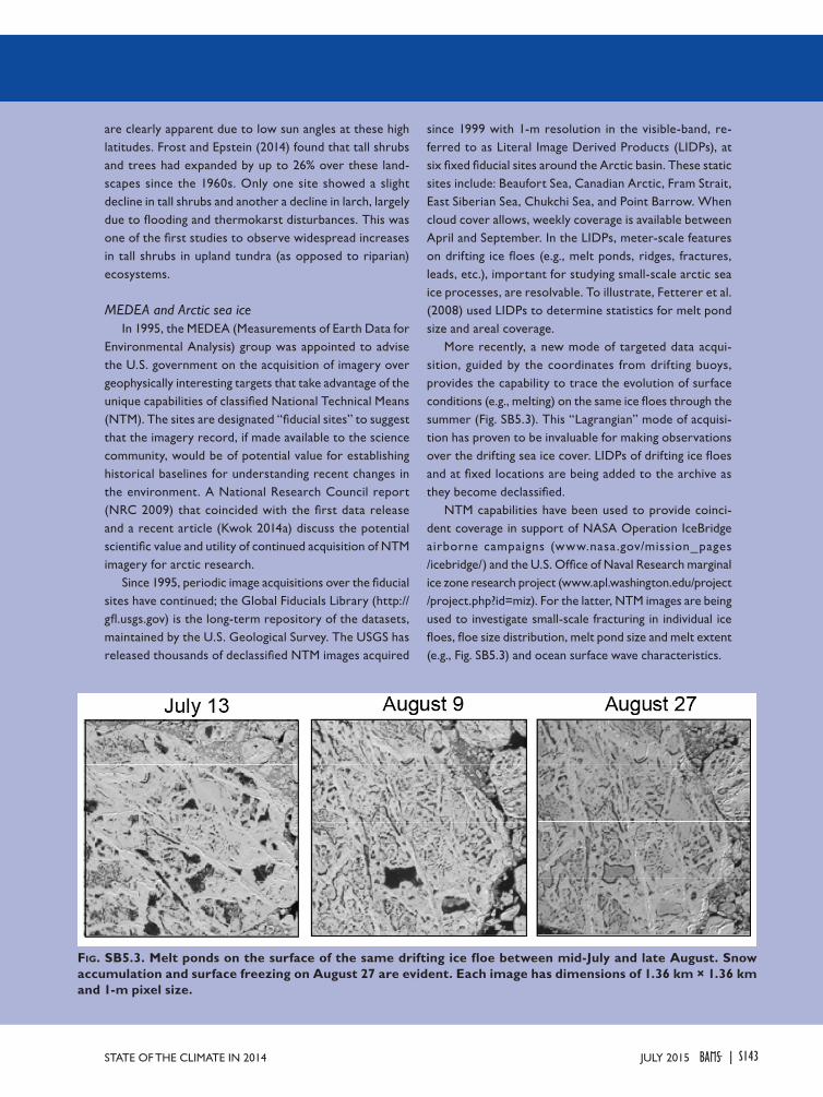
are clearly apparent due to low sun angles at these high latitudes. Frost and Epstein (2014) found that tall shrubs and trees had expanded by up to 26% over these land-scapes since the 1960s. Only one site showed a slight decline in tall shrubs and another a decline in larch, largely due to flooding and thermokarst disturbances. This was one of the first studies to observe widespread increases in tall shrubs in upland tundra (as opposed to riparian) ecosystems.
MEDEA and Arctic sea iceIn 1995, the MEDEA (Measurements of Earth Data for
Environmental Analysis) group was appointed to advise the U.S. government on the acquisition of imagery over geophysically interesting targets that take advantage of the unique capabilities of classified National Technical Means (NTM). The sites are designated “fiducial sites” to suggest that the imagery record, if made available to the science community, would be of potential value for establishing historical baselines for understanding recent changes in the environment. A National Research Council report (NRC 2009) that coincided with the first data release and a recent article (Kwok 2014a) discuss the potential scientific value and utility of continued acquisition of NTM imagery for arctic research.
Since 1995, periodic image acquisitions over the fiducial sites have continued; the Global Fiducials Library (http://gfl.usgs.gov) is the long-term repository of the datasets, maintained by the U.S. Geological Survey. The USGS has released thousands of declassified NTM images acquired
since 1999 with 1-m resolution in the visible-band, re-ferred to as Literal Image Derived Products (LIDPs), at six fixed fiducial sites around the Arctic basin. These static sites include: Beaufort Sea, Canadian Arctic, Fram Strait, East Siberian Sea, Chukchi Sea, and Point Barrow. When cloud cover allows, weekly coverage is available between April and September. In the LIDPs, meter-scale features on drifting ice floes (e.g., melt ponds, ridges, fractures, leads, etc.), important for studying small-scale arctic sea ice processes, are resolvable. To illustrate, Fetterer et al. (2008) used LIDPs to determine statistics for melt pond size and areal coverage.
More recently, a new mode of targeted data acqui-sition, guided by the coordinates from drifting buoys, provides the capability to trace the evolution of surface conditions (e.g., melting) on the same ice floes through the summer (Fig. SB5.3). This “Lagrangian” mode of acquisi-tion has proven to be invaluable for making observations over the drifting sea ice cover. LIDPs of drifting ice floes and at fixed locations are being added to the archive as they become declassified.
NTM capabilities have been used to provide coinci-dent coverage in support of NASA Operation IceBridge airborne campaigns (www.nasa.gov/mission_pages /icebridge/) and the U.S. Office of Naval Research marginal ice zone research project (www.apl.washington.edu/project /project.php?id=miz). For the latter, NTM images are being used to investigate small-scale fracturing in individual ice floes, floe size distribution, melt pond size and melt extent (e.g., Fig. SB5.3) and ocean surface wave characteristics.
Fig. SB5.3. Melt ponds on the surface of the same drifting ice floe between mid-July and late August. Snow accumulation and surface freezing on August 27 are evident. Each image has dimensions of 1.36 km × 1.36 km and 1-m pixel size.
S143JULY 2015STATE OF THE CLIMATE IN 2014 |
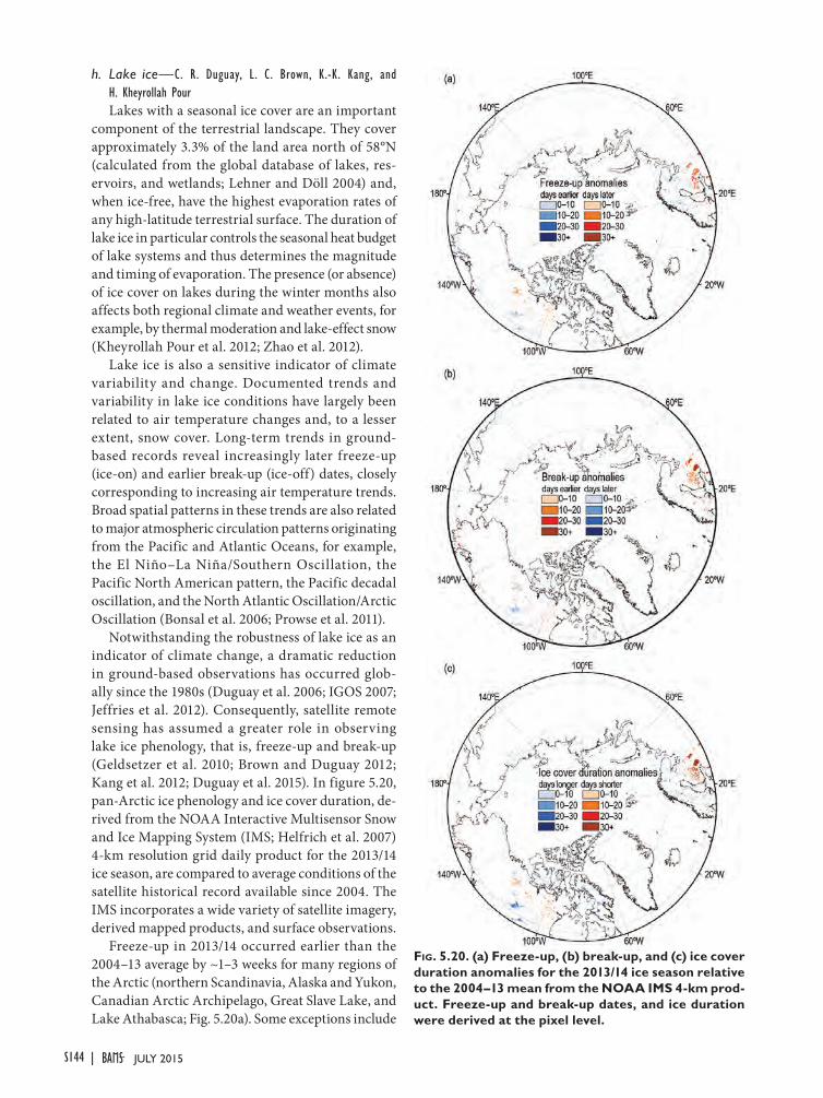
h. Lake ice—C. R. Duguay, L. C. Brown, K.-K. Kang, and H. Kheyrollah PourLakes with a seasonal ice cover are an important
component of the terrestrial landscape. They cover approximately 3.3% of the land area north of 58°N (calculated from the global database of lakes, res-ervoirs, and wetlands; Lehner and Döll 2004) and, when ice-free, have the highest evaporation rates of any high-latitude terrestrial surface. The duration of lake ice in particular controls the seasonal heat budget of lake systems and thus determines the magnitude and timing of evaporation. The presence (or absence) of ice cover on lakes during the winter months also affects both regional climate and weather events, for example, by thermal moderation and lake-effect snow (Kheyrollah Pour et al. 2012; Zhao et al. 2012).
Lake ice is also a sensitive indicator of climate variability and change. Documented trends and variability in lake ice conditions have largely been related to air temperature changes and, to a lesser extent, snow cover. Long-term trends in ground-based records reveal increasingly later freeze-up (ice-on) and earlier break-up (ice-off) dates, closely corresponding to increasing air temperature trends. Broad spatial patterns in these trends are also related to major atmospheric circulation patterns originating from the Pacific and Atlantic Oceans, for example, the El Niño–La Niña/Southern Oscillation, the Pacific North American pattern, the Pacific decadal oscillation, and the North Atlantic Oscillation/Arctic Oscillation (Bonsal et al. 2006; Prowse et al. 2011).
Notwithstanding the robustness of lake ice as an indicator of climate change, a dramatic reduction in ground-based observations has occurred glob-ally since the 1980s (Duguay et al. 2006; IGOS 2007; Jeffries et al. 2012). Consequently, satellite remote sensing has assumed a greater role in observing lake ice phenology, that is, freeze-up and break-up (Geldsetzer et al. 2010; Brown and Duguay 2012; Kang et al. 2012; Duguay et al. 2015). In figure 5.20, pan-Arctic ice phenology and ice cover duration, de-rived from the NOAA Interactive Multisensor Snow and Ice Mapping System (IMS; Helfrich et al. 2007) 4-km resolution grid daily product for the 2013/14 ice season, are compared to average conditions of the satellite historical record available since 2004. The IMS incorporates a wide variety of satellite imagery, derived mapped products, and surface observations.
Freeze-up in 2013/14 occurred earlier than the 2004–13 average by ~1–3 weeks for many regions of the Arctic (northern Scandinavia, Alaska and Yukon, Canadian Arctic Archipelago, Great Slave Lake, and Lake Athabasca; Fig. 5.20a). Some exceptions include
Fig. 5.20. (a) Freeze-up, (b) break-up, and (c) ice cover duration anomalies for the 2013/14 ice season relative to the 2004–13 mean from the NOAA IMS 4-km prod-uct. Freeze-up and break-up dates, and ice duration were derived at the pixel level.
S144 JULY 2015|
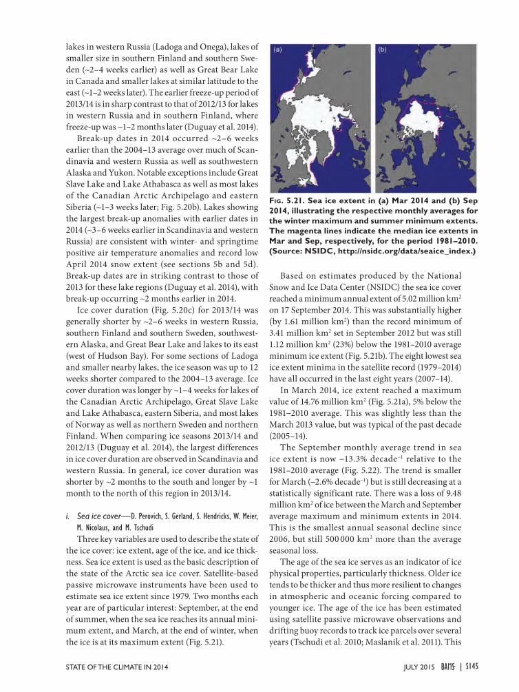
lakes in western Russia (Ladoga and Onega), lakes of smaller size in southern Finland and southern Swe-den (~2–4 weeks earlier) as well as Great Bear Lake in Canada and smaller lakes at similar latitude to the east (~1–2 weeks later). The earlier freeze-up period of 2013/14 is in sharp contrast to that of 2012/13 for lakes in western Russia and in southern Finland, where freeze-up was ~1–2 months later (Duguay et al. 2014).
Break-up dates in 2014 occurred ~2–6 weeks earlier than the 2004–13 average over much of Scan-dinavia and western Russia as well as southwestern Alaska and Yukon. Notable exceptions include Great Slave Lake and Lake Athabasca as well as most lakes of the Canadian Arctic Archipelago and eastern Siberia (~1–3 weeks later; Fig. 5.20b). Lakes showing the largest break-up anomalies with earlier dates in 2014 (~3–6 weeks earlier in Scandinavia and western Russia) are consistent with winter- and springtime positive air temperature anomalies and record low April 2014 snow extent (see sections 5b and 5d). Break-up dates are in striking contrast to those of 2013 for these lake regions (Duguay et al. 2014), with break-up occurring ~2 months earlier in 2014.
Ice cover duration (Fig. 5.20c) for 2013/14 was generally shorter by ~2–6 weeks in western Russia, southern Finland and southern Sweden, southwest-ern Alaska, and Great Bear Lake and lakes to its east (west of Hudson Bay). For some sections of Ladoga and smaller nearby lakes, the ice season was up to 12 weeks shorter compared to the 2004–13 average. Ice cover duration was longer by ~1–4 weeks for lakes of the Canadian Arctic Archipelago, Great Slave Lake and Lake Athabasca, eastern Siberia, and most lakes of Norway as well as northern Sweden and northern Finland. When comparing ice seasons 2013/14 and 2012/13 (Duguay et al. 2014), the largest differences in ice cover duration are observed in Scandinavia and western Russia. In general, ice cover duration was shorter by ~2 months to the south and longer by ~1 month to the north of this region in 2013/14.
i. Sea ice cover—D. Perovich, S. Gerland, S. Hendricks, W. Meier, M. Nicolaus, and M. TschudiThree key variables are used to describe the state of
the ice cover: ice extent, age of the ice, and ice thick-ness. Sea ice extent is used as the basic description of the state of the Arctic sea ice cover. Satellite-based passive microwave instruments have been used to estimate sea ice extent since 1979. Two months each year are of particular interest: September, at the end of summer, when the sea ice reaches its annual mini-mum extent, and March, at the end of winter, when the ice is at its maximum extent (Fig. 5.21).
Based on estimates produced by the National Snow and Ice Data Center (NSIDC) the sea ice cover reached a minimum annual extent of 5.02 million km2 on 17 September 2014. This was substantially higher (by 1.61 million km2) than the record minimum of 3.41 million km2 set in September 2012 but was still 1.12 million km2 (23%) below the 1981–2010 average minimum ice extent (Fig. 5.21b). The eight lowest sea ice extent minima in the satellite record (1979–2014) have all occurred in the last eight years (2007–14).
In March 2014, ice extent reached a maximum value of 14.76 million km2 (Fig. 5.21a), 5% below the 1981−2010 average. This was slightly less than the March 2013 value, but was typical of the past decade (2005–14).
The September monthly average trend in sea ice extent is now −13.3% decade−1 relative to the 1981–2010 average (Fig. 5.22). The trend is smaller for March (−2.6% decade−1) but is still decreasing at a statistically significant rate. There was a loss of 9.48 million km2 of ice between the March and September average maximum and minimum extents in 2014. This is the smallest annual seasonal decline since 2006, but still 500 000 km2 more than the average seasonal loss.
The age of the sea ice serves as an indicator of ice physical properties, particularly thickness. Older ice tends to be thicker and thus more resilient to changes in atmospheric and oceanic forcing compared to younger ice. The age of the ice has been estimated using satellite passive microwave observations and drifting buoy records to track ice parcels over several years (Tschudi et al. 2010; Maslanik et al. 2011). This
Fig. 5.21. Sea ice extent in (a) Mar 2014 and (b) Sep 2014, illustrating the respective monthly averages for the winter maximum and summer minimum extents. The magenta lines indicate the median ice extents in Mar and Sep, respectively, for the period 1981–2010. (Source: NSIDC, http://nsidc.org/data/seaice_index.)
S145JULY 2015STATE OF THE CLIMATE IN 2014 |
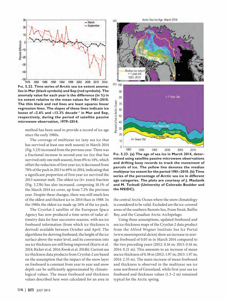
method has been used to provide a record of ice age since the early 1980s.
The coverage of multiyear ice (any sea ice that has survived at least one melt season) in March 2014 (Fig. 5.23) increased from the previous year. There was a fractional increase in second-year ice (ice that has survived only one melt season), from 8% to 14%, which offset the reduction of first-year ice; it decreased from 78% of the pack in 2013 to 69% in 2014, indicating that a significant proportion of first-year ice survived the 2013 summer melt. The oldest ice (4+ years) fraction (Fig. 5.23b) has also increased, composing 10.1% of the March 2014 ice cover, up from 7.2% the previous year. Despite these changes, there was still much less of the oldest and thickest ice in 2014 than in 1988. In the 1980s the oldest ice made up 26% of the ice pack.
The CryoSat-2 satellite of the European Space Agency has now produced a time series of radar al-timetry data for four successive seasons, with sea ice freeboard information (from which ice thickness is derived) available between October and April. The algorithms for deriving freeboard, the height of the ice surface above the water level, and its conversion into sea ice thickness are still being improved (Kurtz et al. 2014; Ricker et al. 2014; Kwok et al. 2014b). Current sea ice thickness data products from CryoSat-2 are based on the assumption that the impact of the snow layer on freeboard is constant from year to year and snow depth can be sufficiently approximated by climato-logical values. The mean freeboard and thickness values described here were calculated for an area in
the central Arctic Ocean where the snow climatology is considered to be valid. Excluded are the ice-covered areas of the southern Barents Sea, Fram Strait, Baffin Bay, and the Canadian Arctic Archipelago.
Using these assumptions, updated freeboard and sea ice thickness maps of the CryoSat-2 data product from the Alfred Wegner Institute Sea Ice Portal (www.meereisportal.de/en) show an increase in aver-age freeboard of 0.05 m in March 2014 compared to the two preceding years (2012: 0.16 m; 2013: 0.16 m; 2014: 0.21 m). This amounts to an increase of mean sea ice thickness of 0.38 m (2012: 1.97 m; 2013: 1.97 m; 2014: 2.35 m). The main increase of mean freeboard and thickness is observed in the multiyear sea ice zone northwest of Greenland, while first-year sea ice freeboard and thickness values (1.5–2 m) remained typical for the Arctic spring.
Fig. 5.22. Time series of Arctic sea ice extent anoma-lies in Mar (black symbols) and Sep (red symbols). The anomaly value for each year is the difference (in %) in ice extent relative to the mean values for 1981–2010. The thin black and red lines are least squares linear regression lines. The slopes of these lines indicate ice losses of –2.6% and –13.3% decade–1 in Mar and Sep, respectively, during the period of satellite passive microwave observation, 1979–2014.
Fig. 5.23. (a) The age of sea ice in March 2014, deter-mined using satellite passive microwave observations and drifting buoy records to track the movement of parcels of ice. The yellow line denotes the median multiyear ice extent for the period 1981–2010. (b) Time series of the percentage of Arctic sea ice in different age categories. The plots are courtesy of J. Maslanik and M. Tschudi (University of Colorado Boulder and the NSIDC).
S146 JULY 2015|
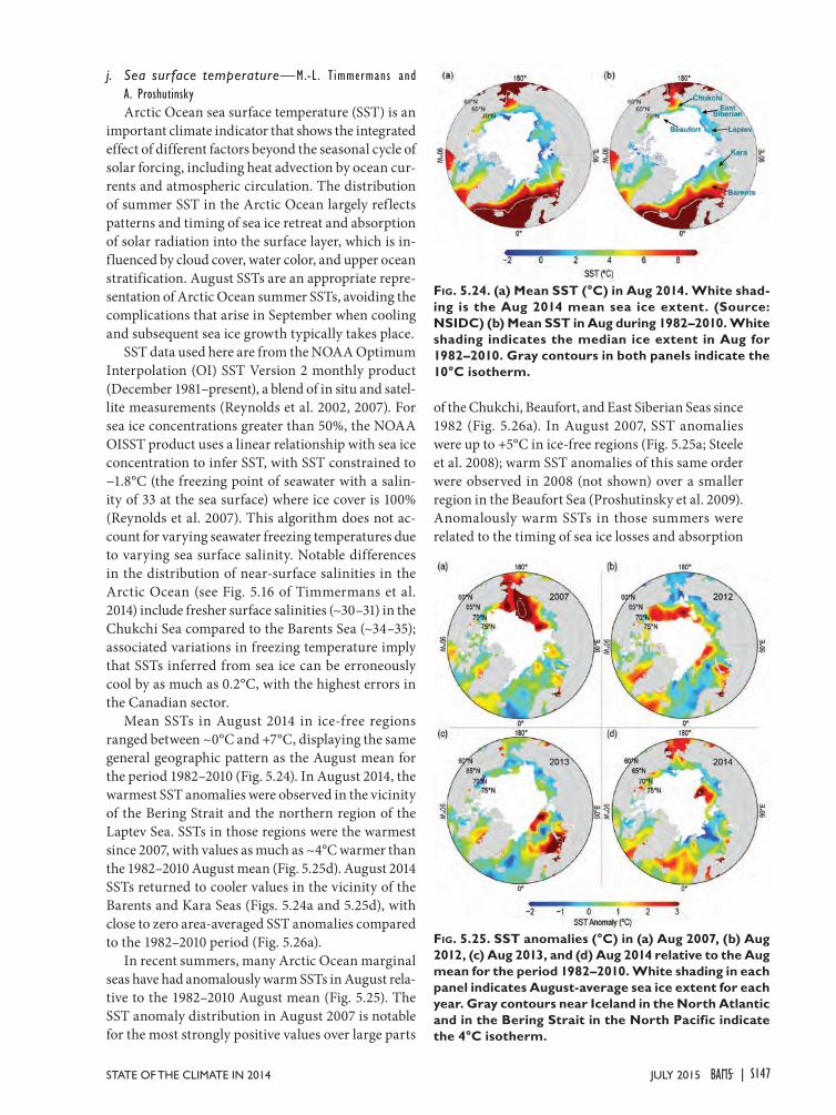
j. Sea surface temperature—M.-L . T immermans and A. ProshutinskyArctic Ocean sea surface temperature (SST) is an
important climate indicator that shows the integrated effect of different factors beyond the seasonal cycle of solar forcing, including heat advection by ocean cur-rents and atmospheric circulation. The distribution of summer SST in the Arctic Ocean largely reflects patterns and timing of sea ice retreat and absorption of solar radiation into the surface layer, which is in-fluenced by cloud cover, water color, and upper ocean stratification. August SSTs are an appropriate repre-sentation of Arctic Ocean summer SSTs, avoiding the complications that arise in September when cooling and subsequent sea ice growth typically takes place.
SST data used here are from the NOAA Optimum Interpolation (OI) SST Version 2 monthly product (December 1981–present), a blend of in situ and satel-lite measurements (Reynolds et al. 2002, 2007). For sea ice concentrations greater than 50%, the NOAA OISST product uses a linear relationship with sea ice concentration to infer SST, with SST constrained to −1.8°C (the freezing point of seawater with a salin-ity of 33 at the sea surface) where ice cover is 100% (Reynolds et al. 2007). This algorithm does not ac-count for varying seawater freezing temperatures due to varying sea surface salinity. Notable differences in the distribution of near-surface salinities in the Arctic Ocean (see Fig. 5.16 of Timmermans et al. 2014) include fresher surface salinities (~30–31) in the Chukchi Sea compared to the Barents Sea (~34–35); associated variations in freezing temperature imply that SSTs inferred from sea ice can be erroneously cool by as much as 0.2°C, with the highest errors in the Canadian sector.
Mean SSTs in August 2014 in ice-free regions ranged between ~0°C and +7°C, displaying the same general geographic pattern as the August mean for the period 1982–2010 (Fig. 5.24). In August 2014, the warmest SST anomalies were observed in the vicinity of the Bering Strait and the northern region of the Laptev Sea. SSTs in those regions were the warmest since 2007, with values as much as ~4°C warmer than the 1982–2010 August mean (Fig. 5.25d). August 2014 SSTs returned to cooler values in the vicinity of the Barents and Kara Seas (Figs. 5.24a and 5.25d), with close to zero area-averaged SST anomalies compared to the 1982–2010 period (Fig. 5.26a).
In recent summers, many Arctic Ocean marginal seas have had anomalously warm SSTs in August rela-tive to the 1982–2010 August mean (Fig. 5.25). The SST anomaly distribution in August 2007 is notable for the most strongly positive values over large parts
of the Chukchi, Beaufort, and East Siberian Seas since 1982 (Fig. 5.26a). In August 2007, SST anomalies were up to +5°C in ice-free regions (Fig. 5.25a; Steele et al. 2008); warm SST anomalies of this same order were observed in 2008 (not shown) over a smaller region in the Beaufort Sea (Proshutinsky et al. 2009). Anomalously warm SSTs in those summers were related to the timing of sea ice losses and absorption
Fig. 5.24. (a) Mean SST (°C) in Aug 2014. White shad-ing is the Aug 2014 mean sea ice extent. (Source: NSIDC) (b) Mean SST in Aug during 1982–2010. White shading indicates the median ice extent in Aug for 1982–2010. Gray contours in both panels indicate the 10°C isotherm.
Fig. 5.25. SST anomalies (°C) in (a) Aug 2007, (b) Aug 2012, (c) Aug 2013, and (d) Aug 2014 relative to the Aug mean for the period 1982–2010. White shading in each panel indicates August-average sea ice extent for each year. Gray contours near Iceland in the North Atlantic and in the Bering Strait in the North Pacific indicate the 4°C isotherm.
S147JULY 2015STATE OF THE CLIMATE IN 2014 |
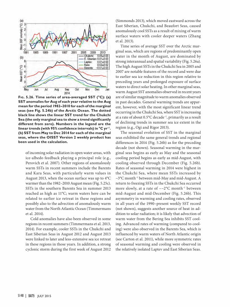
of incoming solar radiation in open water areas, with ice-albedo feedback playing a principal role (e.g., Perovich et al. 2007). Other regions of anomalously warm SSTs in recent summers include the Barents and Kara Seas, with particularly warm values in August 2013, when the ocean surface was up to 4°C warmer than the 1982–2010 August mean (Fig. 5.25c). SSTs in the southern Barents Sea in summer 2013 reached as high as 11°C; warm waters here can be related to earlier ice retreat in these regions and possibly also to the advection of anomalously warm water from the North Atlantic Ocean (Timmermans et al. 2014).
Cold anomalies have also been observed in some regions in recent summers (Timmermans et al. 2013, 2014). For example, cooler SSTs in the Chukchi and East Siberian Seas in August 2012 and August 2013 were linked to later and less-extensive sea ice retreat in these regions in those years. In addition, a strong cyclonic storm during the first week of August 2012
(Simmonds 2013), which moved eastward across the East Siberian, Chukchi, and Beaufort Seas, caused anomalously cool SSTs as a result of mixing of warm surface waters with cooler deeper waters (Zhang et al. 2013).
Time series of average SST over the Arctic mar-ginal seas, which are regions of predominantly open water in the month of August, are dominated by strong interannual and spatial variability (Fig. 5.26a). The high August SSTs in the Chukchi Sea in 2005 and 2007 are notable features of the record and were due to earlier sea ice reduction in this region relative to preceding years and prolonged exposure of surface waters to direct solar heating. In other marginal seas, warm August SST anomalies observed in recent years are of similar magnitude to warm anomalies observed in past decades. General warming trends are appar-ent, however, with the most significant linear trend occurring in the Chukchi Sea, where SST is increasing at a rate of about 0.5°C decade−1, primarily as a result of declining trends in summer sea ice extent in the region (e.g., Ogi and Rigor 2013).
The seasonal evolution of SST in the marginal seas exhibited the same general trends and regional differences in 2014 (Fig. 5.26b) as for the preceding decade (not shown). Seasonal warming in the mar-ginal seas begins as early as May and the seasonal cooling period begins as early as mid-August, with cooling observed through December (Fig. 5.26b). Rates of seasonal warming in 2014 were highest in the Chukchi Sea, where mean SSTs increased by ~3°C month−1 between mid-May and mid-August. A return to freezing SSTs in the Chukchi Sea occurred more slowly, at a rate of ~−2°C month−1 between mid-August and mid-December (Fig. 5.26b). This asymmetry in warming and cooling rates, observed in all years of the 1990–present weekly SST record (not shown), suggests another source of heat in ad-dition to solar radiation; it is likely that advection of warm water from the Bering Sea inhibits SST cool-ing. Advanced rates of warming (compared to cool-ing) were also observed in the Barents Sea, which is influenced by warm waters of North Atlantic origin (see Carton et al. 2011), while more symmetric rates of seasonal warming and cooling were observed in the relatively isolated Laptev and East Siberian Seas.
Fig. 5.26. Time series of area-averaged SST (°C): (a) SST anomalies for Aug of each year relative to the Aug mean for the period 1982–2010 for each of the marginal seas (see Fig. 5.24b) of the Arctic Ocean. The dotted black line shows the linear SST trend for the Chukchi Sea (the only marginal sea to show a trend significantly different from zero). Numbers in the legend are the linear trends (with 95% confidence intervals) in °C yr–1. (b) SST from May to Dec 2014 for each of the marginal seas, where the OISST Version 2 weekly product has been used in the calculation.
S148 JULY 2015|
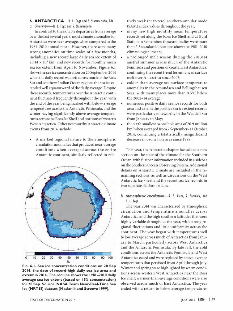
6. ANTARCTICA—R. L. Fogt and S. Stammerjohn, Eds.a. Overview—R. L. Fogt and S. Stammerjohn
In contrast to the notable departures from average over the last several years, most climate anomalies for Antarctica were near-average, when compared to the 1981–2010 annual mean. However, there were many strong anomalies on time scales of a few months, including a new record large daily sea ice extent of 20.14 × 10⁶ km2 and new records for monthly mean sea ice extent from April to November. Figure 6.1 shows the sea ice concentration on 20 September 2014 when the daily record was set; across much of the Ross Sea and southern Indian Ocean regions the sea ice ex-tended well equatorward of the daily average. Despite these records, temperatures over the Antarctic conti-nent fluctuated frequently throughout the year, with the end of the year being marked with below-average temperatures across the Antarctic Peninsula, and the winter having significantly above-average tempera-tures across the Ross Ice Shelf and portions of western West Antarctica. Other noteworthy Antarctic climate events from 2014 include:
• A marked regional nature to the atmospheric circulation anomalies that produced near-average conditions when averaged across the entire Antarctic continent, similarly reflected in rela-
tively weak (near-zero) southern annular mode (SAM) index values throughout the year;
• many new high monthly mean temperature records set along the Ross Ice Shelf and at Byrd Station in September; these anomalies were more than 2.5 standard deviations above the 1981–2010 climatological mean;
• a prolonged melt season during the 2013/14 austral summer across much of the Antarctic Peninsula and portions of coastal East Antarctica, continuing the recent trend for enhanced surface melt over Antarctica since 2005;
• colder-than-average sea surface temperature anomalies in the Amundsen and Bellingshausen Seas, with many places more than 0.5°C below the 2002–14 average;
• numerous positive daily sea ice records for both area and extent; the positive sea ice extent records were particularly noteworthy in the Weddell Sea from January to May;
• the sixth smallest ozone hole area of 20.9 million km2 when averaged from 7 September–13 October 2014, continuing a (statistically insignificant) decrease in ozone hole area since 1998.
This year, the Antarctic chapter has added a new section on the state of the climate for the Southern Ocean, with further information included in a sidebar on the Southern Ocean Observing System. Additional details on Antarctic climate are included in the re-maining sections, as well as discussions on the West Antarctic Ice Sheet and the recent sea ice records in two separate sidebar articles.
b. Atmospheric circulation—K. R. Clem, S. Barreira, and
R. L. FogtThe year 2014 was characterized by atmospheric
circulation and temperature anomalies across Antarctica and the high southern latitudes that were highly variable throughout the year, with strong re-gional fluctuations and little uniformity across the continent. The year began with temperatures well below average across much of Antarctica from Janu-ary to March, particularly across West Antarctica and the Antarctic Peninsula. By late fall, the cold conditions across the Antarctic Peninsula and West Antarctica eased and were replaced by above-average temperatures that persisted from April through July. Winter and spring were highlighted by warm condi-tions across western West Antarctica near the Ross Ice Shelf; warmer-than-average conditions were also observed across much of East Antarctica. The year ended with a return to below-average temperatures
Fig. 6.1. Sea ice concentration conditions on 20 Sep 2014, the date of record-high daily sea ice area and extent in 2014. The red line shows the 1981–2010 daily average sea ice extent (based on 15% concentration) for 20 Sep. Source: NASA Team Near-Real-Time Sea Ice (NRTSI) dataset (Maslanik and Stroeve 1999).
S149JULY 2015STATE OF THE CLIMATE IN 2014 |
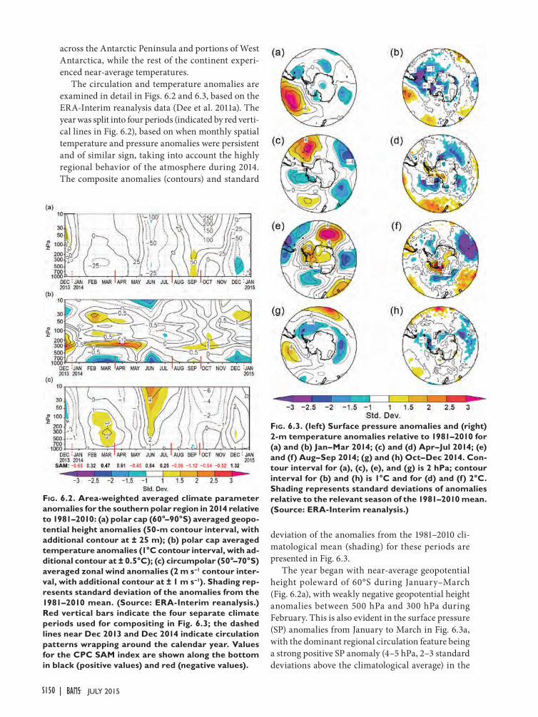
across the Antarctic Peninsula and portions of West Antarctica, while the rest of the continent experi-enced near-average temperatures.
The circulation and temperature anomalies are examined in detail in Figs. 6.2 and 6.3, based on the ERA-Interim reanalysis data (Dee et al. 2011a). The year was split into four periods (indicated by red verti-cal lines in Fig. 6.2), based on when monthly spatial temperature and pressure anomalies were persistent and of similar sign, taking into account the highly regional behavior of the atmosphere during 2014. The composite anomalies (contours) and standard
deviation of the anomalies from the 1981–2010 cli-matological mean (shading) for these periods are presented in Fig. 6.3.
The year began with near-average geopotential height poleward of 60°S during January–March (Fig. 6.2a), with weakly negative geopotential height anomalies between 500 hPa and 300 hPa during February. This is also evident in the surface pressure (SP) anomalies from January to March in Fig. 6.3a, with the dominant regional circulation feature being a strong positive SP anomaly (4–5 hPa, 2–3 standard deviations above the climatological average) in the
Fig. 6.2. Area-weighted averaged climate parameter anomalies for the southern polar region in 2014 relative to 1981–2010: (a) polar cap (60°–90°S) averaged geopo-tential height anomalies (50-m contour interval, with additional contour at ± 25 m); (b) polar cap averaged temperature anomalies (1°C contour interval, with ad-ditional contour at ± 0.5°C); (c) circumpolar (50°–70°S) averaged zonal wind anomalies (2 m s–1 contour inter-val, with additional contour at ± 1 m s–1). Shading rep-resents standard deviation of the anomalies from the 1981–2010 mean. (Source: ERA-Interim reanalysis.) Red vertical bars indicate the four separate climate periods used for compositing in Fig. 6.3; the dashed lines near Dec 2013 and Dec 2014 indicate circulation patterns wrapping around the calendar year. Values for the CPC SAM index are shown along the bottom in black (positive values) and red (negative values).
Fig. 6.3. (left) Surface pressure anomalies and (right) 2-m temperature anomalies relative to 1981–2010 for (a) and (b) Jan–Mar 2014; (c) and (d) Apr–Jul 2014; (e) and (f) Aug–Sep 2014; (g) and (h) Oct–Dec 2014. Con-tour interval for (a), (c), (e), and (g) is 2 hPa; contour interval for (b) and (h) is 1°C and for (d) and (f) 2°C. Shading represents standard deviations of anomalies relative to the relevant season of the 1981–2010 mean. (Source: ERA-Interim reanalysis.)
S150 JULY 2015|
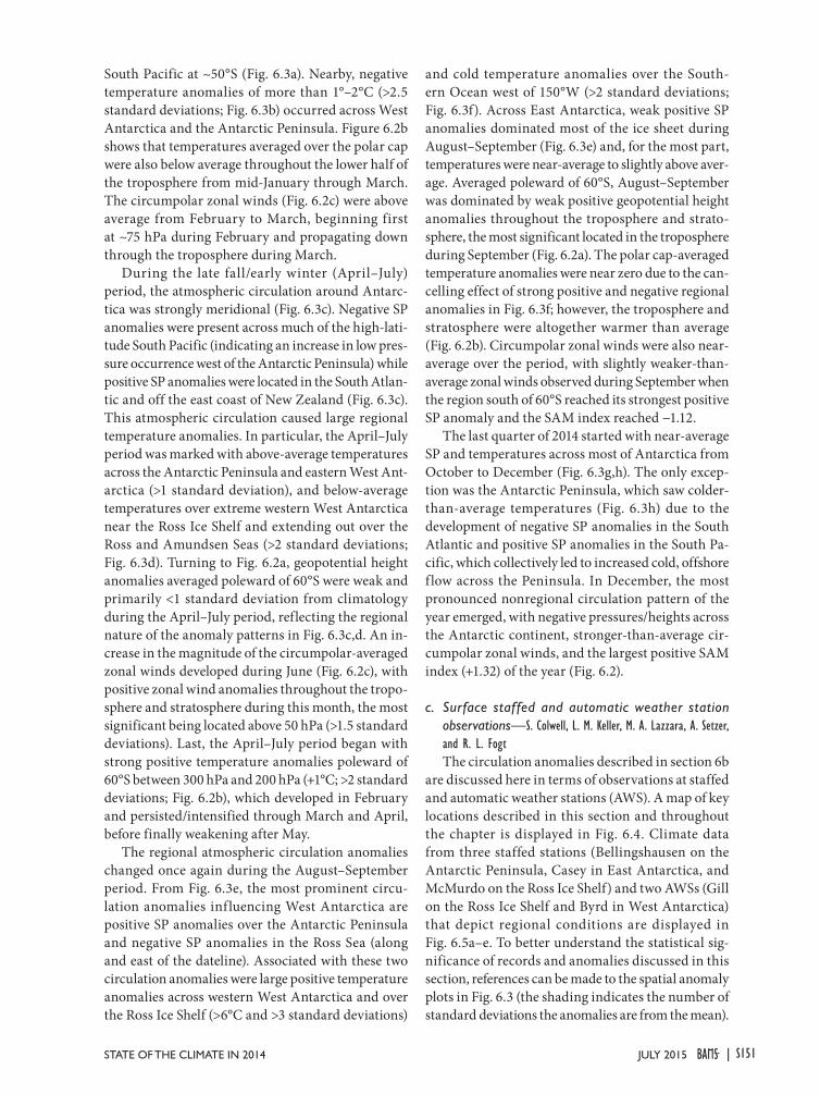
South Pacific at ~50°S (Fig. 6.3a). Nearby, negative temperature anomalies of more than 1°–2°C (>2.5 standard deviations; Fig. 6.3b) occurred across West Antarctica and the Antarctic Peninsula. Figure 6.2b shows that temperatures averaged over the polar cap were also below average throughout the lower half of the troposphere from mid-January through March. The circumpolar zonal winds (Fig. 6.2c) were above average from February to March, beginning first at ~75 hPa during February and propagating down through the troposphere during March.
During the late fall/early winter (April–July) period, the atmospheric circulation around Antarc-tica was strongly meridional (Fig. 6.3c). Negative SP anomalies were present across much of the high-lati-tude South Pacific (indicating an increase in low pres-sure occurrence west of the Antarctic Peninsula) while positive SP anomalies were located in the South Atlan-tic and off the east coast of New Zealand (Fig. 6.3c). This atmospheric circulation caused large regional temperature anomalies. In particular, the April–July period was marked with above-average temperatures across the Antarctic Peninsula and eastern West Ant-arctica (>1 standard deviation), and below-average temperatures over extreme western West Antarctica near the Ross Ice Shelf and extending out over the Ross and Amundsen Seas (>2 standard deviations; Fig. 6.3d). Turning to Fig. 6.2a, geopotential height anomalies averaged poleward of 60°S were weak and primarily <1 standard deviation from climatology during the April–July period, reflecting the regional nature of the anomaly patterns in Fig. 6.3c,d. An in-crease in the magnitude of the circumpolar-averaged zonal winds developed during June (Fig. 6.2c), with positive zonal wind anomalies throughout the tropo-sphere and stratosphere during this month, the most significant being located above 50 hPa (>1.5 standard deviations). Last, the April–July period began with strong positive temperature anomalies poleward of 60°S between 300 hPa and 200 hPa (+1°C; >2 standard deviations; Fig. 6.2b), which developed in February and persisted/intensified through March and April, before finally weakening after May.
The regional atmospheric circulation anomalies changed once again during the August–September period. From Fig. 6.3e, the most prominent circu-lation anomalies inf luencing West Antarctica are positive SP anomalies over the Antarctic Peninsula and negative SP anomalies in the Ross Sea (along and east of the dateline). Associated with these two circulation anomalies were large positive temperature anomalies across western West Antarctica and over the Ross Ice Shelf (>6°C and >3 standard deviations)
and cold temperature anomalies over the South-ern Ocean west of 150°W (>2 standard deviations; Fig. 6.3f). Across East Antarctica, weak positive SP anomalies dominated most of the ice sheet during August–September (Fig. 6.3e) and, for the most part, temperatures were near-average to slightly above aver-age. Averaged poleward of 60°S, August–September was dominated by weak positive geopotential height anomalies throughout the troposphere and strato-sphere, the most significant located in the troposphere during September (Fig. 6.2a). The polar cap-averaged temperature anomalies were near zero due to the can-celling effect of strong positive and negative regional anomalies in Fig. 6.3f; however, the troposphere and stratosphere were altogether warmer than average (Fig. 6.2b). Circumpolar zonal winds were also near-average over the period, with slightly weaker-than-average zonal winds observed during September when the region south of 60°S reached its strongest positive SP anomaly and the SAM index reached −1.12.
The last quarter of 2014 started with near-average SP and temperatures across most of Antarctica from October to December (Fig. 6.3g,h). The only excep-tion was the Antarctic Peninsula, which saw colder-than-average temperatures (Fig. 6.3h) due to the development of negative SP anomalies in the South Atlantic and positive SP anomalies in the South Pa-cific, which collectively led to increased cold, offshore f low across the Peninsula. In December, the most pronounced nonregional circulation pattern of the year emerged, with negative pressures/heights across the Antarctic continent, stronger-than-average cir-cumpolar zonal winds, and the largest positive SAM index (+1.32) of the year (Fig. 6.2).
c. Surface staffed and automatic weather station observations—S. Colwell, L. M. Keller, M. A. Lazzara, A. Setzer, and R. L. FogtThe circulation anomalies described in section 6b
are discussed here in terms of observations at staffed and automatic weather stations (AWS). A map of key locations described in this section and throughout the chapter is displayed in Fig. 6.4. Climate data from three staffed stations (Bellingshausen on the Antarctic Peninsula, Casey in East Antarctica, and McMurdo on the Ross Ice Shelf) and two AWSs (Gill on the Ross Ice Shelf and Byrd in West Antarctica) that depict regional conditions are displayed in Fig. 6.5a–e. To better understand the statistical sig-nificance of records and anomalies discussed in this section, references can be made to the spatial anomaly plots in Fig. 6.3 (the shading indicates the number of standard deviations the anomalies are from the mean).
S151JULY 2015STATE OF THE CLIMATE IN 2014 |
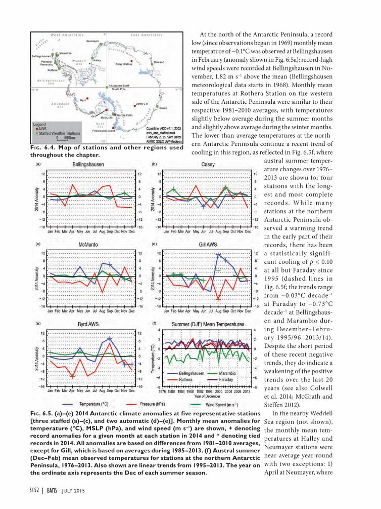
At the north of the Antarctic Peninsula, a record low (since observations began in 1969) monthly mean temperature of −0.1°C was observed at Bellingshausen in February (anomaly shown in Fig. 6.5a); record-high wind speeds were recorded at Bellingshausen in No-vember, 1.82 m s−1 above the mean (Bellingshausen meteorological data starts in 1968). Monthly mean temperatures at Rothera Station on the western side of the Antarctic Peninsula were similar to their respective 1981–2010 averages, with temperatures slightly below average during the summer months and slightly above average during the winter months. The lower-than-average temperatures at the north-ern Antarctic Peninsula continue a recent trend of cooling in this region, as reflected in Fig. 6.5f, where
austral summer temper-ature changes over 1976–2013 are shown for four stations with the long-est and most complete records. W hi le many stations at the northern Antarctic Peninsula ob-served a warming trend in the early part of their records, there has been a stat ist ica l ly signif i-cant cooling of p < 0.10 at all but Faraday since 1995 (dashed l ines in Fig. 6.5f; the trends range from −0.03°C decade−1 at Faraday to −0.73°C decade−1 at Bellingshaus-en and Marambio dur-ing December–Febru-ary 1995/96–2013/14). Despite the short period of these recent negative trends, they do indicate a weakening of the positive trends over the last 20 years (see also Colwell et al. 2014; McGrath and Steffen 2012).
In the nearby Weddell Sea region (not shown), the monthly mean tem-peratures at Halley and Neumayer stations were near-average year-round with two exceptions: 1) April at Neumayer, where
Fig. 6.4. Map of stations and other regions used throughout the chapter.
Fig. 6.5. (a)–(e) 2014 Antarctic climate anomalies at five representative stations [three staffed (a)–(c), and two automatic (d)–(e)]. Monthly mean anomalies for temperature (°C), MSLP (hPa), and wind speed (m s–1) are shown, + denoting record anomalies for a given month at each station in 2014 and * denoting tied records in 2014. All anomalies are based on differences from 1981–2010 averages, except for Gill, which is based on averages during 1985–2013. (f) Austral summer (Dec–Feb) mean observed temperatures for stations at the northern Antarctic Peninsula, 1976–2013. Also shown are linear trends from 1995–2013. The year on the ordinate axis represents the Dec of each summer season.
S152 JULY 2015|
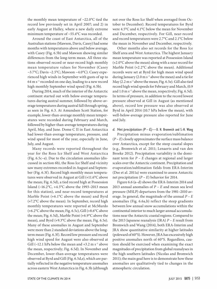
the monthly mean temperature of −22.0°C tied the record low previously set in April 2007; and 2) in early August at Halley, where a new daily extreme minimum temperature of −55.4°C was recorded.
Around the coast of East Antarctica, all of the Australian stations (Mawson, Davis, Casey) had some months with temperatures above and below average, with Casey (Fig. 6.5b) and Mawson showing similar differences from the long-term mean. All three sta-tions observed record or near-record high monthly mean temperature values for November (Casey −3.7°C; Davis −2.5°C; Mawson −4.0°C). Casey expe-rienced high winds in September with gusts of up to 64 m s−1 recorded on one day, leading to a new record high monthly September wind speed (Fig. 6.5b).
During 2014, much of the interior of the Antarctic continent started out with below-average tempera-tures during austral summer, followed by above-av-erage temperatures during austral fall through spring, as seen in Fig. 6.3. At Amundsen Scott Station, for example, lower-than-average monthly mean temper-atures were recorded during February and March, followed by higher-than-average temperatures during April, May, and June. Dome C II in East Antarctica had lower-than-average temperature, pressure, and wind speed for most of the year, especially in June, July, and August.
Many records were reported throughout the year for the Ross Ice Shelf and West Antarctica (Fig. 6.5c–e). Due to the circulation anomalies (dis-cussed in section 6b), the Ross Ice Shelf and vicinity saw many extremes recorded in August and Septem-ber (Fig. 6.3f). Record high monthly mean tempera-tures were observed in August at Gill (+11.6°C above the mean; Fig. 6.5d), a tied record high at Possession Island (−16.2°C, +4.5°C above the 1993–2013 mean for this station), and near-record temperatures at Marble Point (+6.1°C above the mean) and Byrd (+7.2°C above the mean). In September, record high monthly temperatures were reported at McMurdo (+6.2°C above the mean; Fig. 6.5c), Gill (+8.6°C above the mean; Fig. 6.5d), Marble Point (+6.9°C above the mean), and Byrd (+9.3°C above the mean; Fig. 6.5e). Many of these anomalies in August and September were more than 2 standard deviations above the long-term mean (Fig. 6.3f). Record low pressure and record high wind speed for August were also observed at Gill (−12.1 hPa below the mean and +3.2 m s−1 above the mean, respectively; Fig. 6.5d). In November and December, lower-than-average temperatures were observed at Byrd and Gill (Fig. 6.5d,e), which are par-tially reflected in the negative temperature anomalies across eastern West Antarctica in Fig. 6.3h (although
not over the Ross Ice Shelf when averaged from Oc-tober to December). Record temperatures for Byrd were 4.5°C and 4.1°C below the mean for November and December, respectively. For Gill, near-record and record temperatures were 2.7°C and 2.1°C below the mean in November and December, respectively.
Other months also set records for the Ross Ice Shelf area and West Antarctica. The highest January mean temperature was reported at Possession Island (+2.0°C above the mean) along with a near record for Marble Point (+2.2°C above the mean). Additional records were set at Byrd for high mean wind speed during January (2.0 m s−1 above the mean) and a tie for May (2.2 m s−1 above the mean; Fig. 6.5e). Gill also tied record high wind speeds for February and March, (0.9 and 1.0 m s−1 above the mean, respectively; Fig. 6.5d). In terms of pressure, in addition to the record lowest pressure observed at Gill in August (as mentioned above), record low pressure was also observed at Byrd in April 2014 (10.7 hPa below the mean), with well-below-average pressure also reported for June and July.
d. Net precipitation (P – E)—D. H. Bromwich and S.-H. WangPrecipitation minus evaporation/sublimation
(P – E) closely approximates the surface mass balance over Antarctica, except for the steep coastal slopes (e.g., Bromwich et al. 2011; Lenaerts and van den Broeke 2012). Precipitation variability is the domi-nant term for P – E changes at regional and larger scales over the Antarctic continent. Precipitation and evaporation/sublimation fields from ERA-Interim (Dee et al. 2011a) were examined to assess Antarctic net precipitation (P – E) behavior for 2014.
Figure 6.6 (a–d) shows the ERA-Interim 2014 and 2013 annual anomalies of P – E and mean sea level pressure (MSLP) departures from the 1981–2010 av-erage. In general, the magnitude of the annual P – E anomalies (Fig. 6.6a,b) ref lect the steep gradients between low annual snow accumulations within the continental interior to much larger annual accumula-tions near the Antarctic coastal regions. Compared to the 2013 Japanese reanalysis (JRA) P – E result from Bromwich and Wang (2014), both ERA-Interim and JRA show quantitative similarity at higher latitudes (poleward of 60°S). However, JRA has excessively high positive anomalies north of 60°S. Regardless, cau-tion should be exercised when examining the exact magnitudes of precipitation from global reanalyses in the high southern latitudes (Nicolas and Bromwich 2011); the main goal here is to demonstrate how these anomalies are qualitatively tied to changes in the atmospheric circulation.
S153JULY 2015STATE OF THE CLIMATE IN 2014 |
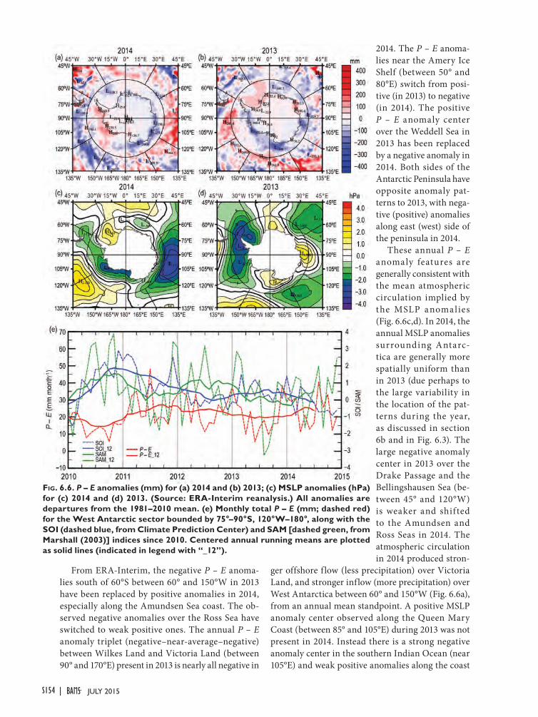
From ERA-Interim, the negative P – E anoma-lies south of 60°S between 60° and 150°W in 2013 have been replaced by positive anomalies in 2014, especially along the Amundsen Sea coast. The ob-served negative anomalies over the Ross Sea have switched to weak positive ones. The annual P – E anomaly triplet (negative–near-average–negative) between Wilkes Land and Victoria Land (between 90° and 170°E) present in 2013 is nearly all negative in
2014. The P – E anoma-lies near the Amery Ice Shelf (between 50° and 80°E) switch from posi-tive (in 2013) to negative (in 2014). The positive P – E anomaly center over the Weddell Sea in 2013 has been replaced by a negative anomaly in 2014. Both sides of the Antarctic Peninsula have opposite anomaly pat-terns to 2013, with nega-tive (positive) anomalies along east (west) side of the peninsula in 2014.
These annual P – E anomaly features are generally consistent with the mean atmospheric circulation implied by the MSLP anomalies (Fig. 6.6c,d). In 2014, the annual MSLP anomalies surrounding Antarc-tica are generally more spatially uniform than in 2013 (due perhaps to the large variability in the location of the pat-terns during the year, as discussed in section 6b and in Fig. 6.3). The large negative anomaly center in 2013 over the Drake Passage and the Bellingshausen Sea (be-tween 45° and 120°W) is weaker and shifted to the Amundsen and Ross Seas in 2014. The atmospheric circulation in 2014 produced stron-
ger offshore f low (less precipitation) over Victoria Land, and stronger inflow (more precipitation) over West Antarctica between 60° and 150°W (Fig. 6.6a), from an annual mean standpoint. A positive MSLP anomaly center observed along the Queen Mary Coast (between 85° and 105°E) during 2013 was not present in 2014. Instead there is a strong negative anomaly center in the southern Indian Ocean (near 105°E) and weak positive anomalies along the coast
Fig. 6.6. P – E anomalies (mm) for (a) 2014 and (b) 2013; (c) MSLP anomalies (hPa) for (c) 2014 and (d) 2013. (Source: ERA-Interim reanalysis.) All anomalies are departures from the 1981–2010 mean. (e) Monthly total P – E (mm; dashed red) for the West Antarctic sector bounded by 75°–90°S, 120°W–180°, along with the SOI (dashed blue, from Climate Prediction Center) and SAM [dashed green, from Marshall (2003)] indices since 2010. Centered annual running means are plotted as solid lines (indicated in legend with “_12”).
S154 JULY 2015|
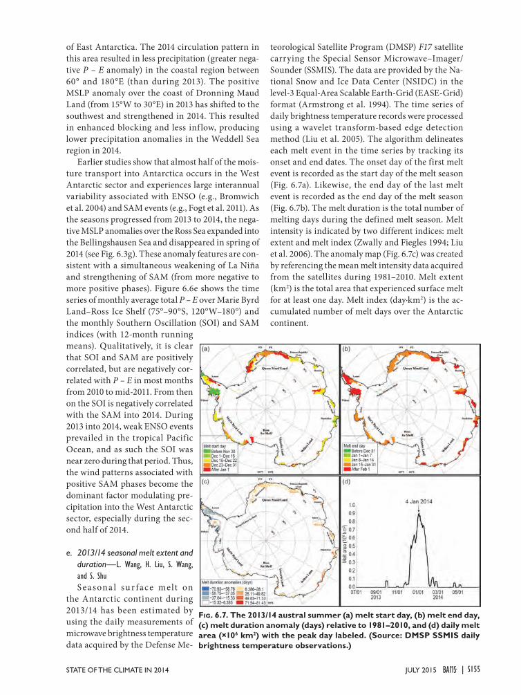
of East Antarctica. The 2014 circulation pattern in this area resulted in less precipitation (greater nega-tive P – E anomaly) in the coastal region between 60° and 180°E (than during 2013). The positive MSLP anomaly over the coast of Dronning Maud Land (from 15°W to 30°E) in 2013 has shifted to the southwest and strengthened in 2014. This resulted in enhanced blocking and less inf low, producing lower precipitation anomalies in the Weddell Sea region in 2014.
Earlier studies show that almost half of the mois-ture transport into Antarctica occurs in the West Antarctic sector and experiences large interannual variability associated with ENSO (e.g., Bromwich et al. 2004) and SAM events (e.g., Fogt et al. 2011). As the seasons progressed from 2013 to 2014, the nega-tive MSLP anomalies over the Ross Sea expanded into the Bellingshausen Sea and disappeared in spring of 2014 (see Fig. 6.3g). These anomaly features are con-sistent with a simultaneous weakening of La Niña and strengthening of SAM (from more negative to more positive phases). Figure 6.6e shows the time series of monthly average total P – E over Marie Byrd Land–Ross Ice Shelf (75°–90°S, 120°W–180°) and the monthly Southern Oscillation (SOI) and SAM indices (with 12-month running means). Qualitatively, it is clear that SOI and SAM are positively correlated, but are negatively cor-related with P – E in most months from 2010 to mid-2011. From then on the SOI is negatively correlated with the SAM into 2014. During 2013 into 2014, weak ENSO events prevailed in the tropical Pacific Ocean, and as such the SOI was near zero during that period. Thus, the wind patterns associated with positive SAM phases become the dominant factor modulating pre-cipitation into the West Antarctic sector, especially during the sec-ond half of 2014.
e. 2013/14 seasonal melt extent and duration—L. Wang, H. Liu, S. Wang, and S. ShuSea sona l su r face melt on
the Antarctic continent during 2013/14 has been estimated by using the daily measurements of microwave brightness temperature data acquired by the Defense Me-
teorological Satellite Program (DMSP) F17 satellite carrying the Special Sensor Microwave–Imager/Sounder (SSMIS). The data are provided by the Na-tional Snow and Ice Data Center (NSIDC) in the level-3 Equal-Area Scalable Earth-Grid (EASE-Grid) format (Armstrong et al. 1994). The time series of daily brightness temperature records were processed using a wavelet transform-based edge detection method (Liu et al. 2005). The algorithm delineates each melt event in the time series by tracking its onset and end dates. The onset day of the first melt event is recorded as the start day of the melt season (Fig. 6.7a). Likewise, the end day of the last melt event is recorded as the end day of the melt season (Fig. 6.7b). The melt duration is the total number of melting days during the defined melt season. Melt intensity is indicated by two different indices: melt extent and melt index (Zwally and Fiegles 1994; Liu et al. 2006). The anomaly map (Fig. 6.7c) was created by referencing the mean melt intensity data acquired from the satellites during 1981–2010. Melt extent (km2) is the total area that experienced surface melt for at least one day. Melt index (day·km2) is the ac-cumulated number of melt days over the Antarctic continent.
Fig. 6.7. The 2013/14 austral summer (a) melt start day, (b) melt end day, (c) melt duration anomaly (days) relative to 1981–2010, and (d) daily melt area (×106 km2) with the peak day labeled. (Source: DMSP SSMIS daily brightness temperature observations.)
S155JULY 2015STATE OF THE CLIMATE IN 2014 |
SIDEBAR 6.1: WAIS-TING AWAY? THE PERILOUS STATE OF THE WEST ANTARCTIC ICE SHEET—R. B. ALLEY
Accelerating mass loss from the West Antarctic Ice Sheet (WAIS) is of special concern. New work suggests that the full distribution of possible behaviors includes faster sea level rise than usually was previously considered, although with large uncertainties.
Glaciers and ice sheets generally shrink with warming, contributing to sea level rise, despite the usual increase in precipitation from warmer air supplying more water vapor (for a longer review, refer to Alley et al. 2015, in press). Mountain glaciers contain only ~0.4 m of sea level equivalent (SLE; Vaughan et al. 2013) and models indicate that shrinkage of the Greenland Ice Sheet (~7 m SLE) will have a multicentennial response time even for large warm-ing (Applegate et al. 2014), whereas the East Antarctic Ice Sheet (>50 m SLE) is less sensitive to initial atmospheric warming than the other ice masses. Large, abrupt sea level rise remains possible from the WAIS (~3.3 m SLE in marine portions; NRC 2013).
Most West Antarctic ice discharges across grounding lines into floating-but-attached ice shelves, which lose mass by basal melting and iceberg calving. Ice thinning at the grounding line causes it to migrate inland, but the bed generally deepens inland, allowing faster ice spreading, further thinning, and potentially unstable retreat. The most important stabilizer is friction between ice shelves and embayment sides or local sea-floor highs. Meltwater wedging from surface warming can disintegrate an ice shelf in weeks (e.g., Rott et al. 1996) and warmer waters
typically increase sub-ice-shelf melting by order 10 m yr–1 °C–1 (e.g., Rignot and Jacobs 2002), with 1°C warming or less sufficient to largely or completely remove many ice shelves.
Recently, ocean warming plus changing winds and, therefore, ocean circulation from some combination of the ozone hole, warming due to greenhouse gas increases, and natural variability (Schmidtko et al. 2014) have in-creased melting beneath the Amundsen Sea ice shelves facing the Pacific Ocean, causing ice-flow acceleration and thinning that dominate Antarctic mass loss (e.g., Sut-terly et al. 2014). Some but not all model results suggest that the threshold for irreversible but probably delayed retreat has already been crossed (Joughin et al. 2014; Parizek et al. 2013).
The paleoclimatic record in and around the ice sheet, and the far-field record of sea level, suggest but do not prove that the ice sheet shrank and likely disappeared one or more times within the last million years, for reasons including response to the rather small additional forcing of the last interglacial (Alley et al. 2015, in press). The far-field record of sea level indicators such as the distribution of well-dated marine deposits now above sea level (e.g., O’Leary et al. 2013), allows inferred deglaciation of West Antarctica to have required centuries or longer, but does not rule out ice loss over shorter times.
The rate of any future “collapse” may depend on the ice cliff dynamics of a “tidewater” glacier. When termi-
This year’s melt can be characterized by its exten-sive melt extent and an anomalously long melt season around most of coastal Antarctica except in the pen-insula and Abbot areas where both positive and nega-tive melt duration anomalies were observed (Fig. 6.7). Areas with intensive melt (>45 day duration) include areas of the Larsen and Wilkins ice shelves along the Antarctic Peninsula, the West and Shackleton ice shelves, and Wilkes Land in coastal East Antarctica. Areas with moderate intensity of melt (14–45 day duration) include much of coastal Queen Maud Land and the Abbot and Amery ice shelves; short-term melt (<14 day duration) occurred on the coast of Marie Byrd Land and portions of Queen Maud Land near the Filchner Ice Shelf. Although the melt duration anomaly was negative in most areas of the Antarctic Peninsula and Wilkins Ice Shelf (Fig. 6.7c) consistent with cooler than normal air temperature (see Fig. 6.3b), an anomalously early melt event (around 1 October 2013) was observed in these areas
(Fig. 6.7a). This melt event only lasted for less than a week however (Fig. 6.7d). Positive melt anomalies can be observed in other regions. The major melt event (Fig. 6.7d) started at the end of November 2013. Melt area reached its peak on 4 January 2014 and the major melt season ended on 6 February 2014. Several minor melt events occurred afterwards and some melt events extended into late April (Fig. 6.7d). These melt events occurred on the Wilkins Ice Shelf (Fig. 6.7b).
Overall, surface melt on the Antarctic continent during the austral summer of 2013/14 was about 25% less in its extent (1 043 750 km2; Fig 6.8) compared to 2012/13 (1 384 375 km2; Wang et al. 2014). The melt index, a measure of the intensity of melting, was also much lower in 2013/14 (39 093 125 day·km2) compared to the 2012/13 melt season (51 335 000 day·km2). In contrast, the 2013/14 melt extent and index numbers were almost equivalent to those observed during austral summer 2010/11 (1 069 375 km2
and 40 280 625 day·km2, respectively). Figure 6.8
S156 JULY 2015|
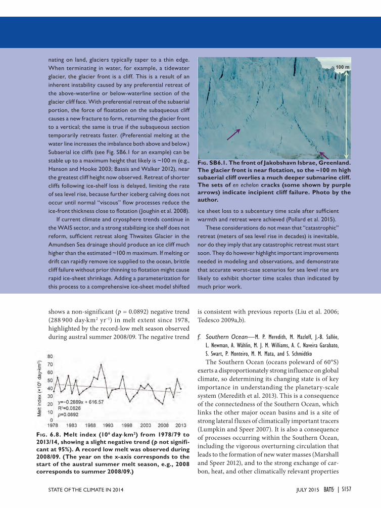
nating on land, glaciers typically taper to a thin edge. When terminating in water, for example, a tidewater glacier, the glacier front is a cliff. This is a result of an inherent instability caused by any preferential retreat of the above-waterline or below-waterline section of the glacier cliff face. With preferential retreat of the subaerial portion, the force of floatation on the subaqueous cliff causes a new fracture to form, returning the glacier front to a vertical; the same is true if the subaqueous section temporarily retreats faster. (Preferential melting at the water line increases the imbalance both above and below.) Subaerial ice cliffs (see Fig. SB6.1 for an example) can be stable up to a maximum height that likely is ~100 m (e.g., Hanson and Hooke 2003; Bassis and Walker 2012), near the greatest cliff height now observed. Retreat of shorter cliffs following ice-shelf loss is delayed, limiting the rate of sea level rise, because further iceberg calving does not occur until normal “viscous” flow processes reduce the ice-front thickness close to flotation (Joughin et al. 2008).
If current climate and cryosphere trends continue in the WAIS sector, and a strong stabilizing ice shelf does not reform, sufficient retreat along Thwaites Glacier in the Amundsen Sea drainage should produce an ice cliff much higher than the estimated ~100 m maximum. If melting or drift can rapidly remove ice supplied to the ocean, brittle cliff failure without prior thinning to flotation might cause rapid ice-sheet shrinkage. Adding a parameterization for this process to a comprehensive ice-sheet model shifted
ice sheet loss to a subcentury time scale after sufficient warmth and retreat were achieved (Pollard et al. 2015).
These considerations do not mean that “catastrophic” retreat (meters of sea level rise in decades) is inevitable, nor do they imply that any catastrophic retreat must start soon. They do however highlight important improvements needed in modeling and observations, and demonstrate that accurate worst-case scenarios for sea level rise are likely to exhibit shorter time scales than indicated by much prior work.
Fig. SB6.1. The front of Jakobshavn Isbrae, Greenland. The glacier front is near flotation, so the ~100 m high subaerial cliff overlies a much deeper submarine cliff. The sets of en echelon cracks (some shown by purple arrows) indicate incipient cliff failure. Photo by the author.
Fig. 6.8. Melt index (106 day·km2) from 1978/79 to 2013/14, showing a slight negative trend (p not signifi-cant at 95%). A record low melt was observed during 2008/09. (The year on the x-axis corresponds to the start of the austral summer melt season, e.g., 2008 corresponds to summer 2008/09.)
shows a non-significant (p = 0.0892) negative trend (288 900 day·km2 yr−1) in melt extent since 1978, highlighted by the record-low melt season observed during austral summer 2008/09. The negative trend
is consistent with previous reports (Liu et al. 2006; Tedesco 2009a,b).
f. Southern Ocean—M. P. Meredith, M. Mazloff, J.-B. Sallée, L. Newman, A. Wåhlin, M. J. M. Williams, A. C. Naveira Garabato, S. Swart, P. Monteiro, M. M. Mata, and S. SchmidtkoThe Southern Ocean (oceans poleward of 60°S)
exerts a disproportionately strong influence on global climate, so determining its changing state is of key importance in understanding the planetary-scale system (Meredith et al. 2013). This is a consequence of the connectedness of the Southern Ocean, which links the other major ocean basins and is a site of strong lateral fluxes of climatically important tracers (Lumpkin and Speer 2007). It is also a consequence of processes occurring within the Southern Ocean, including the vigorous overturning circulation that leads to the formation of new water masses (Marshall and Speer 2012), and to the strong exchange of car-bon, heat, and other climatically relevant properties
S157JULY 2015STATE OF THE CLIMATE IN 2014 |
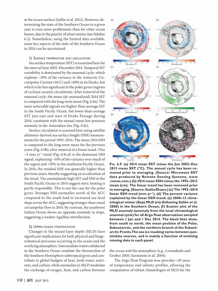
at the ocean surface (Sallée et al. 2012). However, de-termining the state of the Southern Ocean in a given year is even more problematic than for other ocean basins, due to the paucity of observations (see Sidebar 6.2). Nonetheless, using the limited data available, some key aspects of the state of the Southern Ocean in 2014 can be ascertained.
1) Surface temperature and circulation Sea surface temperature (SST) is examined here for
the interval June 2002 –December 2014. Temporal SST variability is dominated by the seasonal cycle, which explains ~30% of the variance in the Antarctic Cir-cumpolar Current (ACC) and >60% in its flanks, but which is far less significant in the polar gyres (regions of cyclonic oceanic circulation). After removal of the seasonal cycle, the mean (de-seasonalized) 2014 SST is compared with the long-term mean (Fig. 6.9a). The most noticeable signals are higher-than-average SST in the South Pacific Ocean, but lower-than-average SST just east and west of Drake Passage during 2014, consistent with the annual mean low-pressure anomaly in the Amundsen Sea (Fig. 6.6c).
Surface circulation is assessed here using satellite altimeter-derived sea surface height (SSH) measure-ments for the period 1993–2014. The mean 2014 SSH is compared to the long-term mean for the previous years (Fig. 6.9b), after removal of a linear trend. This ~3 mm yr−1 trend (Fig. 6.9c,d) is the dominant SSH signal, explaining ~10% of the variance over much of the region and >50% in the southwest Pacific Ocean. In 2014, the residual SSH was generally higher than previous years, thereby suggesting an acceleration of the trend. The anomalously high SST and SSH in the South Pacific Ocean in 2014 suggest steric heating is partly responsible. This is not the case for the polar gyres. Stronger SSH anomalies north of the ACC compared to the south lead to increased sea level slope across the ACC, suggesting stronger-than-usual circumpolar flow in 2014. By contrast, the southwest Indian Ocean shows an opposite anomaly in slope, suggesting a weaker Agulhas retroflection.
2) upper-ocean Stratification
Changes in the mixed-layer depth (MLD) have significant implications for both physical and bioge-ochemical processes occurring in the ocean and the overlying atmosphere. Intermediate waters subducted in the Southern Ocean ventilate the thermocline of the Southern Hemisphere subtropical gyres and con-tribute to global budgets of heat, fresh water, nutri-ents, and carbon, while anomalies in MLD modulate the exchange of oxygen, heat, and carbon between
Fig. 6.9. (a) 2014 mean SST minus the Jun 2002–Dec 2013 mean SST (°C). The annual cycle has been re-moved prior to averaging. (Source: Microwave SST data produced by Remote Sensing Systems, www .remss.com.) (b) 2014 mean SSH minus the 1993–2013 mean (cm). The linear trend has been removed prior to averaging. (Source: Ssalto/Duacs.) (c) The 1993–2014 linear SSH trend (mm yr–1). (d) The percent variance explained by the linear SSH trend. (e) 2000–13 clima-tological winter (Sep) MLD (m) (following Sallée et al. 2006) in the Southern Ocean; (f) Scatter plot of the MLD anomaly (anomaly from the local climatological seasonal cycle) for all Argo float observations sampled between 1 Jan and 1 Dec 2014. The black lines show, from south to north, the mean position of the Polar, Subantarctic, and the northern branch of the Subant-arctic Fronts.The sea ice masking varies between pan-els/data sources, and is mainly a function of omitting missing data in each panel.
the ocean and the atmosphere (e.g., Lovenduski and Gruber 2005; Sarmiento et al. 2004).
The Argo Float Program now provides >10 years of temperature and salinity profiles, allowing the computation of robust climatologies of MLD for the
S158 JULY 2015|
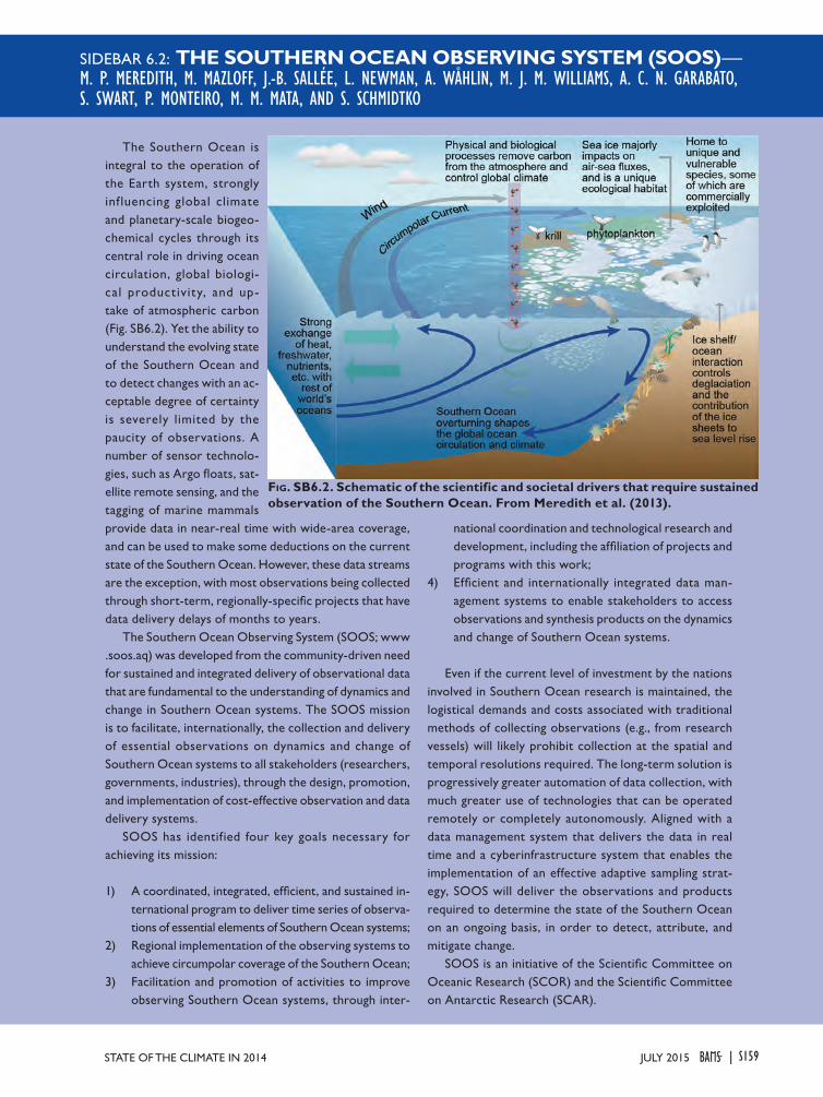
SIDEBAR 6.2: THE SOUTHERN OCEAN OBSERVING SYSTEM (SOOS)—M. P. MEREDITH, M. MAZLOFF, J.-B. SALLÉE, L. NEWMAN, A. WÅHLIN, M. J. M. WILLIAMS, A. C. N. GARABATO, S. SWART, P. MONTEIRO, M. M. MATA, AND S. SCHMIDTKO
The Southern Ocean is integral to the operation of the Earth system, strongly inf luencing global climate and planetary-scale biogeo-chemical cycles through its central role in driving ocean circulation, global biologi-cal productivity, and up-take of atmospheric carbon (Fig. SB6.2). Yet the ability to understand the evolving state of the Southern Ocean and to detect changes with an ac-ceptable degree of certainty is severely limited by the paucity of observations. A number of sensor technolo-gies, such as Argo floats, sat-ellite remote sensing, and the tagging of marine mammals provide data in near-real time with wide-area coverage, and can be used to make some deductions on the current state of the Southern Ocean. However, these data streams are the exception, with most observations being collected through short-term, regionally-specific projects that have data delivery delays of months to years.
The Southern Ocean Observing System (SOOS; www .soos.aq) was developed from the community-driven need for sustained and integrated delivery of observational data that are fundamental to the understanding of dynamics and change in Southern Ocean systems. The SOOS mission is to facilitate, internationally, the collection and delivery of essential observations on dynamics and change of Southern Ocean systems to all stakeholders (researchers, governments, industries), through the design, promotion, and implementation of cost-effective observation and data delivery systems.
SOOS has identified four key goals necessary for achieving its mission:
1) A coordinated, integrated, efficient, and sustained in-ternational program to deliver time series of observa-tions of essential elements of Southern Ocean systems;
2) Regional implementation of the observing systems to achieve circumpolar coverage of the Southern Ocean;
3) Facilitation and promotion of activities to improve observing Southern Ocean systems, through inter-
national coordination and technological research and development, including the affiliation of projects and programs with this work;
4) Efficient and internationally integrated data man-agement systems to enable stakeholders to access observations and synthesis products on the dynamics and change of Southern Ocean systems.
Even if the current level of investment by the nations involved in Southern Ocean research is maintained, the logistical demands and costs associated with traditional methods of collecting observations (e.g., from research vessels) will likely prohibit collection at the spatial and temporal resolutions required. The long-term solution is progressively greater automation of data collection, with much greater use of technologies that can be operated remotely or completely autonomously. Aligned with a data management system that delivers the data in real time and a cyberinfrastructure system that enables the implementation of an effective adaptive sampling strat-egy, SOOS will deliver the observations and products required to determine the state of the Southern Ocean on an ongoing basis, in order to detect, attribute, and mitigate change.
SOOS is an initiative of the Scientific Committee on Oceanic Research (SCOR) and the Scientific Committee on Antarctic Research (SCAR).
Fig. SB6.2. Schematic of the scientific and societal drivers that require sustained observation of the Southern Ocean. From Meredith et al. (2013).
S159JULY 2015STATE OF THE CLIMATE IN 2014 |
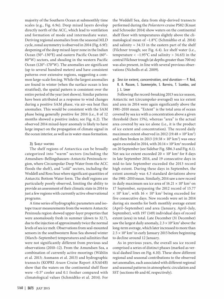
majority of the Southern Ocean at submonthly time scales (e.g., Fig. 6.9e). Deep mixed layers develop directly north of the ACC, which lead to ventilation and formation of mode and intermediate water. Deriving regional anomalies from the seasonal MLD cycle, zonal asymmetry is observed in 2014 (Fig. 6.9f): deepening of the deep mixed-layer zone in the Indian Ocean (50°–130°E) and eastern Pacific Ocean (60°–80°W) sectors, and shoaling in the western Pacific Ocean (120°–170°W). The anomalies are significant (up to several hundred meters) and have consistent patterns over extensive regions, suggesting a com-mon large-scale forcing. While the largest anomalies are found in winter (when the surface ocean is less stratified), the spatial pattern is consistent over the entire period of the year (not shown). Similar patterns have been attributed as a response to wind changes during a positive SAM phase, via air–sea heat flux anomalies. This would be consistent with the SAM phase being generally positive for 2014 (i.e., 8 of 12 months showed a positive index; see Fig. 6.2). The observed 2014 mixed-layer anomaly is likely to have large impact on the propagation of climate signal in the ocean interior, as well as in water-mass formation.
3) Shelf waterS
The shelf regions of Antarctica can be broadly categorized into “warm” sectors (including the Amundsen–Bellingshausen–Antarctic Peninsula re-gion, where Circumpolar Deep Water from the ACC floods the shelf), and “cold” sectors, including the Weddell and Ross Seas where significant quantities of Antarctic Bottom Water form. The shelf regions are particularly poorly observed, limiting the ability to provide an assessment of their climatic state in 2014 to just a few regions with currently active observational programs.
A time series of hydrographic parameters and iso-tope tracer measurements from the western Antarctic Peninsula region showed upper-layer properties that were anomalously fresh in summer (down to 32.7), due to the injection of approximately twice the normal levels of sea ice melt. Observations from seal-mounted sensors in the southwestern Ross Sea showed winter (March–September) temperatures and salinities that were not significantly different from previous seal observations (2010–12). From the Amundsen Sea, a combination of currently active moorings (Wåhlin et al. 2013; Assmann et al. 2013) and hydrographic transects (KOPRI Araon Cruise Report ANA04B) show that the waters on the continental shelf f loor were ~0.5° cooler and 0.1 fresher compared with climatological values (Schmidtko et al. 2014). For
the Weddell Sea, data from ship-derived transects performed during the Polarstern cruise PS82 (Knust and Schroeder 2014) show waters on the continental shelf floor with temperatures slightly above the cli-matological mean of −1.8°C (Schmidtko et al. 2014) and salinity ≈ 34.53 in the eastern part of the shelf (Filchner trough; see Fig. 6.4). Ice shelf water (i.e., temperature < −1.95°C and salinity > 34.63) in the central Filchner trough (at depths greater than 700 m) was also present, in line with several previous obser-vations (Nicholls et al. 2009).
g. Sea ice extent, concentration, and duration— P. Reid, R. A. Massom, S. Stammerjohn, S. Barreira, T. Scambos, and J. L. LieserFollowing the record-breaking 2013 sea ice season,
Antarctic net (circumpolar-averaged) sea ice extent and area in 2014 were again significantly above the 1981–2010 mean. “Extent” is the total area of ocean covered by sea ice with a concentration above a given threshold (here 15%), whereas “area” is the actual area covered by sea ice alone (i.e., it is the product of ice extent and concentration). The record daily maximum extent observed in 2012 (19.48 × 10⁶ km2) and then broken in 2013 (19.58 × 10⁶ km2) was once again exceeded in 2014, with 20.14 × 10⁶ km2 recorded on 20 September (see Sidebar Fig. SB6.3 and Fig. 6.1). Net sea ice extent exceeded 20 × 106 km2 for 8 days in late September 2014, and 19 consecutive days in mid-to-late September exceeded the 2013 record high extent. During these days in September, the extent anomaly was 4.3 standard deviations above the 1981–2010 mean. Similarly, 2014 saw a new record in daily maximum sea ice area of 16.21 × 10⁶ km2 on 17 September, surpassing the 2012 record of 15.77 × 10⁶ km2, with 16 × 106 km2 being exceeded for five consecutive days. New records were set in 2014 during six months for both monthly average extent (April–September) and area (January, April–July, September), with 197 (149) individual days of record extent (area) in total. Late December (31 December) saw the largest daily anomaly, 2.3 × 10⁶ km2 above the long-term average, which later increased to more than 2.5 × 10⁶ km2 in early January 2015 before beginning to decline around 12 January.
As in previous years, the overall sea ice record comprised a series of distinct phases (marked as ver-tical dashed lines on Fig. 6.10). These show different regional and seasonal contributions to the observed net anomalies, each associated with different regional and seasonal patterns in atmospheric circulation and SST (sections 6b and 6f, respectively).
S160 JULY 2015|
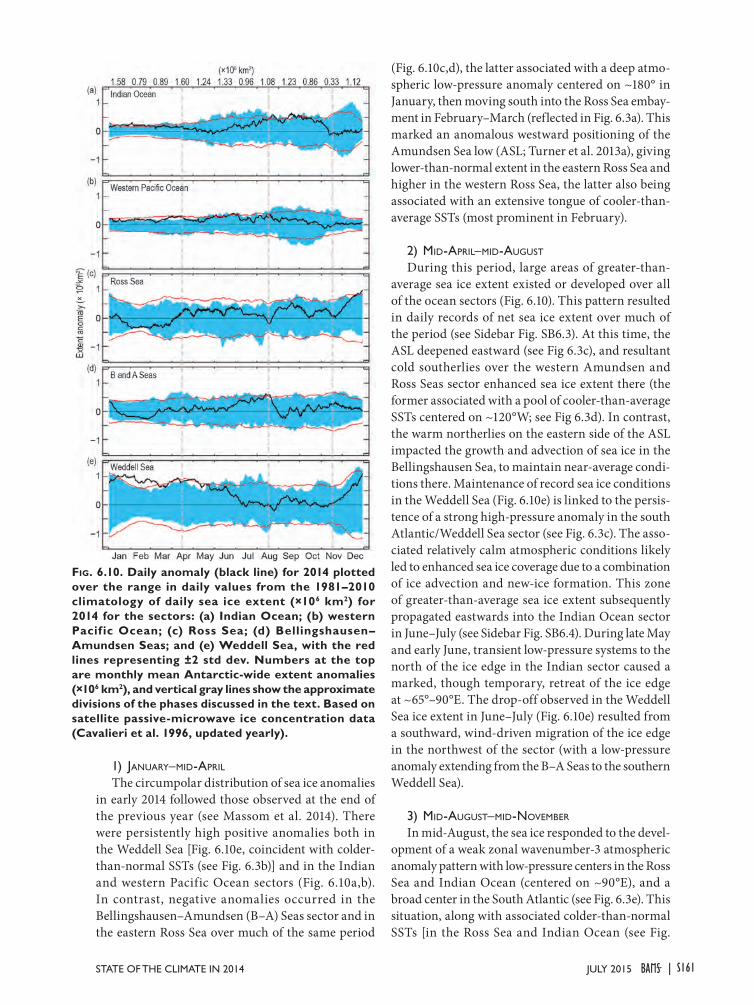
1) January–mid-april
The circumpolar distribution of sea ice anomalies in early 2014 followed those observed at the end of the previous year (see Massom et al. 2014). There were persistently high positive anomalies both in the Weddell Sea [Fig. 6.10e, coincident with colder-than-normal SSTs (see Fig. 6.3b)] and in the Indian and western Pacific Ocean sectors (Fig. 6.10a,b). In contrast, negative anomalies occurred in the Bellingshausen–Amundsen (B–A) Seas sector and in the eastern Ross Sea over much of the same period
Fig. 6.10. Daily anomaly (black line) for 2014 plotted over the range in daily values from the 1981–2010 climatology of daily sea ice extent (×106 km2) for 2014 for the sectors: (a) Indian Ocean; (b) western Pacif ic Ocean; (c) Ross Sea; (d) Bellingshausen–Amundsen Seas; and (e) Weddell Sea, with the red lines representing ±2 std dev. Numbers at the top are monthly mean Antarctic-wide extent anomalies (×106 km2), and vertical gray lines show the approximate divisions of the phases discussed in the text. Based on satellite passive-microwave ice concentration data (Cavalieri et al. 1996, updated yearly).
(Fig. 6.10c,d), the latter associated with a deep atmo-spheric low-pressure anomaly centered on ~180° in January, then moving south into the Ross Sea embay-ment in February–March (reflected in Fig. 6.3a). This marked an anomalous westward positioning of the Amundsen Sea low (ASL; Turner et al. 2013a), giving lower-than-normal extent in the eastern Ross Sea and higher in the western Ross Sea, the latter also being associated with an extensive tongue of cooler-than-average SSTs (most prominent in February).
2) mid-april–mid-auguSt
During this period, large areas of greater-than-average sea ice extent existed or developed over all of the ocean sectors (Fig. 6.10). This pattern resulted in daily records of net sea ice extent over much of the period (see Sidebar Fig. SB6.3). At this time, the ASL deepened eastward (see Fig 6.3c), and resultant cold southerlies over the western Amundsen and Ross Seas sector enhanced sea ice extent there (the former associated with a pool of cooler-than-average SSTs centered on ~120°W; see Fig 6.3d). In contrast, the warm northerlies on the eastern side of the ASL impacted the growth and advection of sea ice in the Bellingshausen Sea, to maintain near-average condi-tions there. Maintenance of record sea ice conditions in the Weddell Sea (Fig. 6.10e) is linked to the persis-tence of a strong high-pressure anomaly in the south Atlantic/Weddell Sea sector (see Fig. 6.3c). The asso-ciated relatively calm atmospheric conditions likely led to enhanced sea ice coverage due to a combination of ice advection and new-ice formation. This zone of greater-than-average sea ice extent subsequently propagated eastwards into the Indian Ocean sector in June–July (see Sidebar Fig. SB6.4). During late May and early June, transient low-pressure systems to the north of the ice edge in the Indian sector caused a marked, though temporary, retreat of the ice edge at ~65°–90°E. The drop-off observed in the Weddell Sea ice extent in June–July (Fig. 6.10e) resulted from a southward, wind-driven migration of the ice edge in the northwest of the sector (with a low-pressure anomaly extending from the B–A Seas to the southern Weddell Sea).
3) mid-auguSt–mid-november In mid-August, the sea ice responded to the devel-
opment of a weak zonal wavenumber-3 atmospheric anomaly pattern with low-pressure centers in the Ross Sea and Indian Ocean (centered on ~90°E), and a broad center in the South Atlantic (see Fig. 6.3e). This situation, along with associated colder-than-normal SSTs [in the Ross Sea and Indian Ocean (see Fig.
S161JULY 2015STATE OF THE CLIMATE IN 2014 |
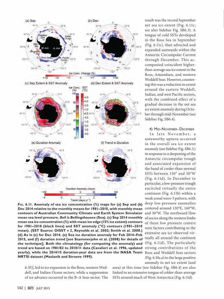
6.3f)], led to ice expansion in the Ross, western Wed-dell, and Indian Ocean sectors, while a suppression of ice advance occurred in the B–A Seas sector. The
Fig. 6.11. Anomaly of sea ice concentration (%) maps for (a) Sep and (b) Dec 2014 relative to the monthly means for 1981–2010, with monthly mean contours of Australian Community Climate and Earth System Simulator mean sea level pressure. Bell is Bellingshausen (Sea). (c) Sep 2014 monthly mean sea ice concentration (%) with mean ice edge (15% ice extent) contours for 1981–2010 (black lines) and SST anomaly (°C) contours (1981–2010 mean). (SST Source: OISST v 2, Reynolds et al. 2002; Smith et al. 2008.) (d) As in (c) for Dec 2014. (e) Sea ice duration anomaly for Feb 2014–Feb 2015, and (f) duration trend [see Stammerjohn et al. (2008) for details of the technique]. Both the climatology (for computing the anomaly) and trend are based on 1981/82 to 2010/11 data (Cavalieri et al. 1996, updated yearly), while the 2014/15 duration-year data are from the NASA Team NRTSI dataset (Maslanik and Stroeve 1999).
result was the record September net sea ice extent (Fig. 6.11c; see also Sidebar Fig. SB6.3). A tongue of cold SSTs developed in the Ross Sea in September (Fig. 6.11c), then advected and expanded eastwards within the Antarctic Circumpolar Current through December. This ac-companied coincident higher-than-average sea ice extent in the Ross, Amundsen, and western Weddell Seas. However, counter-ing this was a reduction in extent around the eastern Weddell, Indian, and west Pacific sectors, with the combined effect of a gradual decrease in the net sea ice extent anomaly during Octo-ber through mid-November (see Sidebar Fig. SB6.4).
4) mid-november–december
I n l a t e N o v e m b e r , a noteworthy upturn occurred in the overall sea ice extent anomaly (see Sidebar Fig. SB6.3.) in response to a deepening of the Antarctic circumpolar trough and associated expansion of the band of cooler-than-normal SSTs between 150° and 30°W (Fig. 6.11d). In December in particular, a low-pressure trough encircled virtually the entire continent (Fig. 6.11b) within a weak zonal wave-3 pattern, with deep low-pressure anomalies centered around 120°E, 140°W, and 30°W. The northward flow of sea ice along the western limbs of these low pressure centers were factors contributing to the extensive sea ice observed vir-tually all around the continent (Fig. 6.11d). The particularly strong contributions of the Ross and Weddell Seas sectors (Fig. 6.10c,e) to the large positive anomaly in net ice extent (and
area) at this time (see Sidebar Fig. SB6.4) are also linked to an extensive tongue of colder-than-average SSTs around much of West Antarctica (Fig. 6.11d).
S162 JULY 2015|
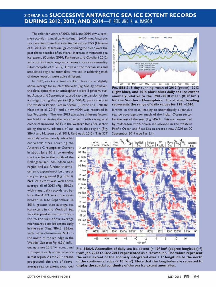
SIDEBAR 6.3: SUCCESSIVE ANTARCTIC SEA ICE EXTENT RECORDS DURING 2012, 2013, AND 2014—P. REID AND R. A. MASSOM
The calendar years of 2012, 2013, and 2014 saw succes-sive records in annual daily maximum (ADM) net Antarctic sea ice extent based on satellite data since 1979 (Massom et al. 2013, 2014; section 6g), continuing the trend over the past three decades of an overall increase in Antarctic sea ice extent (Comiso 2010; Parkinson and Cavalieri 2012) and contributing to regional changes in sea ice seasonality (Stammerjohn et al. 2012). However, the mechanisms and associated regional anomalies involved in achieving each of these records were quite different.
In 2012, sea ice extent tracked close to or slightly above average for much of the year (Fig. SB6.3); however, the development of an atmospheric wave-3 pattern dur-ing August and September caused rapid expansion of the ice edge during that period (Fig. SB6.4), particularly in the western Pacific Ocean sector (Turner et al. 2013b; Massom et al. 2013), and a new ADM was recorded in late September. The year 2013 saw quite different factors involved in achieving the record extent, with a tongue of colder-than-normal SSTs in the western Ross Sea sector aiding the early advance of sea ice in that region (Fig. SB6.4 and Massom et al. 2013; Reid et al. 2015). This SST anomaly subsequently advected eastwards after reaching the Antarctic Circumpolar Current in about June 2013, to envelop the ice edge to the north of the Bellingshausen–Amundsen Seas region and aid further thermo-dynamic expansion of ice there as the year progressed (Fig. SB6.3). Net ice extent was well above average all of 2013 (Fig. SB6.3), with many daily records set be-fore the ADM was once again broken in late September. In 2014, greater-than-average sea ice extent in the Weddell Sea was the predominant contribu-tor to the well-above-average net Antarctic sea ice extent early in the year (Figs. SB6.3, SB6.4), with colder-than-normal SSTs to the north of the ice edge in the Weddell Sea (see Fig. 6.3b) influ-encing a late 2013/14 retreat and subsequent early annual advance in that region. As the 2014 season progressed, the area of above-average sea ice extent expanded
farther to the east, leading to anomalously expansive sea ice coverage over much of the Indian Ocean sector for the rest of the year (Fig. SB6.4). This was augmented by midseason wind-driven ice advance in the western Pacific Ocean and Ross Sea to create a new ADM on 20 September 2014 (see Fig. 6.1).
Fig. SB6.3. 5-day running mean of 2012 (green), 2013 (light blue), and 2014 (dark blue) daily sea ice extent anomaly relative to the 1981–2010 mean (×106 km2) for the Southern Hemisphere. The shaded banding represents the range of daily values for 1981–2010.
Fig. SB6.4. Anomalies of daily sea ice extent [× 103 km2 (degree longitude)–1] from Jan 2012 to Dec 2014 represented as a Hovmöller. The values represent the areal extent of the anomaly integrated over a 1° longitude to the north of the continental edge (× 103 km2). Note that the longitudes are repeated to display the spatial continuity of the sea ice extent anomalies.
S163JULY 2015STATE OF THE CLIMATE IN 2014 |
Consistent with the mostly positive sea ice extent anomalies described for the first half of the year (Fig. 6.10), the timing of the fall/early winter ice-edge advance was earlier than normal (by 10–70 days) in all sectors except: (1) the southern BAS sector; and (2) the Ross Sea sector between 160°E and 160°W, where the ice-edge advance was instead later than normal (by 10 to ~30 days). There was some correspondence between the 2013/14 ice retreat anomaly pattern (Massom et al. 2014) and the 2014 ice advance pattern, particularly for: 1) the western Weddell and Indian Ocean sectors (where the 2013/14 spring retreat was anomalously late, followed by an anomalously early 2014 fall advance); and 2) the outer pack ice of the Bellingshausen Sea (where the 2013/14 spring retreat was anomalously early, followed by an anomalously late 2014 fall advance). Most notable, however, were the strong earlier-than-normal anomalies in the ice edge advance throughout the Weddell Sea sector between 0° and 60°W and the East Antarctic sector between 90°E and 160°E. In contrast, there was a remarkable recovery and acceleration of the ice-edge advance in the outer pack ice of the BAS and
eastern Ross Sea sectors (between 80°W to 160°W) later in the 2014 fall season. This area showed a sharp switch from late to early ice-edge advance anomalies south-to-north. This recovery and acceleration of the ice-edge advance corresponded to the eastward movement of the ASL (described above; see Fig. 6.3c) and strengthening of cold southerly winds in the eastern Ross Sea sector in May–June. Subsequently, a broad band of cold SSTs developed along the advancing ice edge between 90°W and 160°W (see Fig. 6.3d), which may explain the recovery and rapid advance of the ice edge.
The anomaly pattern for the 2014/15 spring–summer sea ice retreat was considerably less striking than the ice advance anomaly pattern just described, showing in general smaller anomalies. There were, however, some interesting contrasts: the outer Weddell Sea and most of the East Antarctic sector showed an earlier retreat (in contrast to the earlier advance previously experienced there), while the Ross Sea sector between 160°E and 160°W showed a later retreat (in contrast to the later advance previously experienced there). Nonetheless, the ice season
Analyses of trends in sea ice extent and seasonality (see Fig. 6.11g) over the last few decades show that the overall increase in Antarctic coverage comprises contrast-ing regional contributions: strong increases in ice extent and duration in the Ross Sea and moderate increases elsewhere except for strong decreases in the western Antarctic Peninsula–Bellingshausen Sea region (WAP–BS). These trends are attributed predominantly to changes in wind patterns (Holland and Kwok 2012; Parkinson and Cavalieri 2012; Stammerjohn et al. 2012), although some research suggests an association with changes in fresh-water fluxes (Liu and Curry 2010; Bintanja et al. 2013). The overall patterns of ice extent anomaly for the last three years (2012–14) are not fully consistent with these regional trends, except in the western Ross Sea where there have been persistent positive anomalies for the last three years (Fig. SB6.4). Ice extent in the WAP–BS was close to or above normal over this three-year period, and was particularly high in 2013 (Fig. SB6.4), in contrast to the long-term trend. The regional anomalies over these last three years are, however, consistent with associated patterns of large-scale drivers of sea ice formation, distri-bution, and retreat, that is, regional atmospheric synoptic patterns and ocean circulation and temperature.
Given that there were three record-breaking years in a row, it is well worth asking: Did the pattern of sea ice extent, and the associated retreat, in one year influence
the pattern of extent and ice advance in the following year? The answer: Quite probably. Several studies have suggested that the pattern of sea ice retreat in one year can influence the advance in the subsequent year (Nihashi and Ohshima 2001; Stammerjohn et al. 2012; Holland 2014), and this appears to be the case, particularly in these last three years. From September 2012 onwards, there is a clear eastward propagation of sea ice extent anomaly stemming from the western Pacific Ocean sector, through the Ross, Bellingshausen, and Amundsen Seas during 2013 and into the Weddell Sea in early 2014 (Fig. SB6.4). The positive ice anomaly in the western Pacific region in August–September 2012, as the result of the deep low pressure in that region, may have slowed the western coastal currents and subsequently caused the cold ocean surface temperatures and hence early advance of sea ice in the western Ross Sea in 2013. Similarly, the anomalous positive extent in sea ice in the WAP–BS sector in late 2013 may have impacted the late retreat and early ad-vance of sea ice in the Weddell Sea in 2013/14. Much of this is speculation, but there is no one specific underlying mechanism that can easily explain these three years of record-breaking sea ice extent. Indeed, Antarctic sea ice continues to behave and respond in a complex fashion by integrating influences from the atmosphere, ocean, and wider cryosphere.
CONT. SIDEBAR 6.3: SUCCESSIVE ANTARCTIC SEA ICE EXTENT RECORDS DURING 2012, 2013, AND 2014—P. REID AND R. A. MASSOM
S164 JULY 2015|
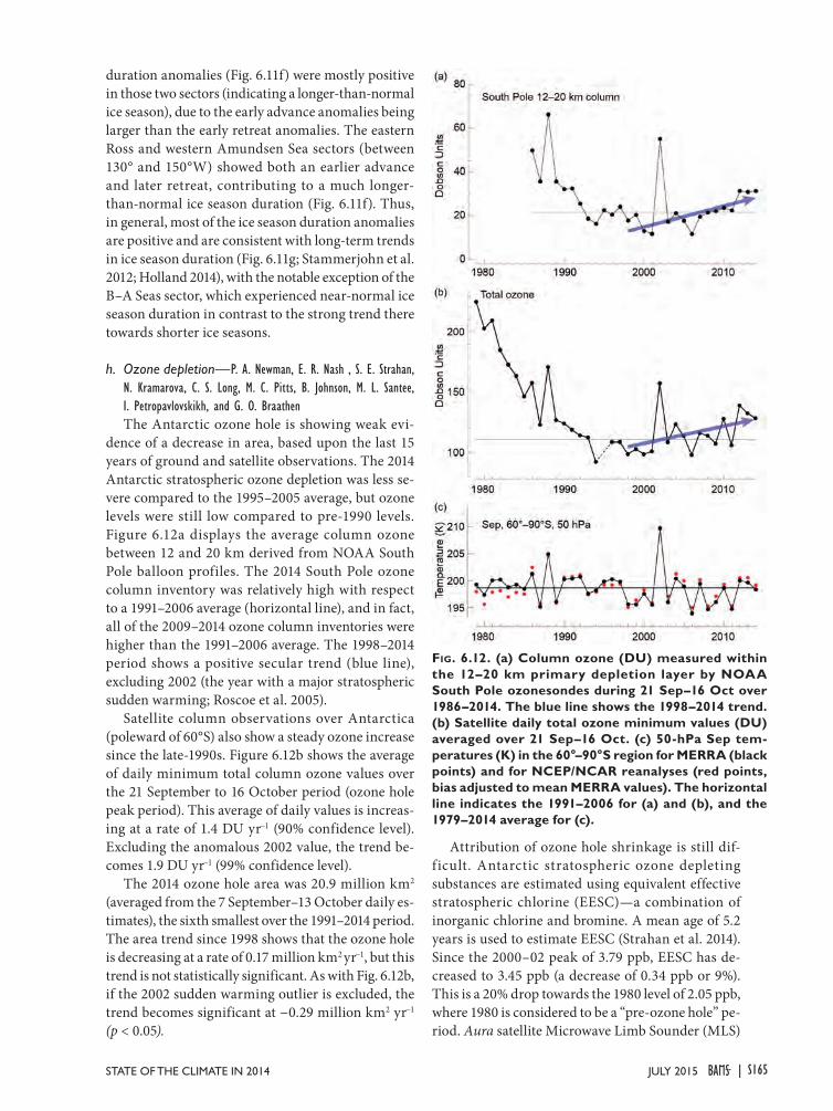
duration anomalies (Fig. 6.11f) were mostly positive in those two sectors (indicating a longer-than-normal ice season), due to the early advance anomalies being larger than the early retreat anomalies. The eastern Ross and western Amundsen Sea sectors (between 130° and 150°W) showed both an earlier advance and later retreat, contributing to a much longer-than-normal ice season duration (Fig. 6.11f). Thus, in general, most of the ice season duration anomalies are positive and are consistent with long-term trends in ice season duration (Fig. 6.11g; Stammerjohn et al. 2012; Holland 2014), with the notable exception of the B–A Seas sector, which experienced near-normal ice season duration in contrast to the strong trend there towards shorter ice seasons.
h. Ozone depletion—P. A. Newman, E. R. Nash , S. E. Strahan, N. Kramarova, C. S. Long, M. C. Pitts, B. Johnson, M. L. Santee, I. Petropavlovskikh, and G. O. BraathenThe Antarctic ozone hole is showing weak evi-
dence of a decrease in area, based upon the last 15 years of ground and satellite observations. The 2014 Antarctic stratospheric ozone depletion was less se-vere compared to the 1995–2005 average, but ozone levels were still low compared to pre-1990 levels. Figure 6.12a displays the average column ozone between 12 and 20 km derived from NOAA South Pole balloon profiles. The 2014 South Pole ozone column inventory was relatively high with respect to a 1991–2006 average (horizontal line), and in fact, all of the 2009–2014 ozone column inventories were higher than the 1991–2006 average. The 1998–2014 period shows a positive secular trend (blue line), excluding 2002 (the year with a major stratospheric sudden warming; Roscoe et al. 2005).
Satellite column observations over Antarctica (poleward of 60°S) also show a steady ozone increase since the late-1990s. Figure 6.12b shows the average of daily minimum total column ozone values over the 21 September to 16 October period (ozone hole peak period). This average of daily values is increas-ing at a rate of 1.4 DU yr−1 (90% confidence level). Excluding the anomalous 2002 value, the trend be-comes 1.9 DU yr−1 (99% confidence level).
The 2014 ozone hole area was 20.9 million km2 (averaged from the 7 September–13 October daily es-timates), the sixth smallest over the 1991–2014 period. The area trend since 1998 shows that the ozone hole is decreasing at a rate of 0.17 million km2 yr−1, but this trend is not statistically significant. As with Fig. 6.12b, if the 2002 sudden warming outlier is excluded, the trend becomes significant at −0.29 million km2 yr−1 (p < 0.05).
Attribution of ozone hole shrinkage is still dif-ficult. Antarctic stratospheric ozone depleting substances are estimated using equivalent effective stratospheric chlorine (EESC)—a combination of inorganic chlorine and bromine. A mean age of 5.2 years is used to estimate EESC (Strahan et al. 2014). Since the 2000–02 peak of 3.79 ppb, EESC has de-creased to 3.45 ppb (a decrease of 0.34 ppb or 9%). This is a 20% drop towards the 1980 level of 2.05 ppb, where 1980 is considered to be a “pre-ozone hole” pe-riod. Aura satellite Microwave Limb Sounder (MLS)
Fig. 6.12. (a) Column ozone (DU) measured within the 12–20 km primary depletion layer by NOAA South Pole ozonesondes during 21 Sep–16 Oct over 1986–2014. The blue line shows the 1998–2014 trend. (b) Satellite daily total ozone minimum values (DU) averaged over 21 Sep–16 Oct. (c) 50-hPa Sep tem-peratures (K) in the 60°–90°S region for MERRA (black points) and for NCEP/NCAR reanalyses (red points, bias adjusted to mean MERRA values). The horizontal line indicates the 1991–2006 for (a) and (b), and the 1979–2014 average for (c).
S165JULY 2015STATE OF THE CLIMATE IN 2014 |
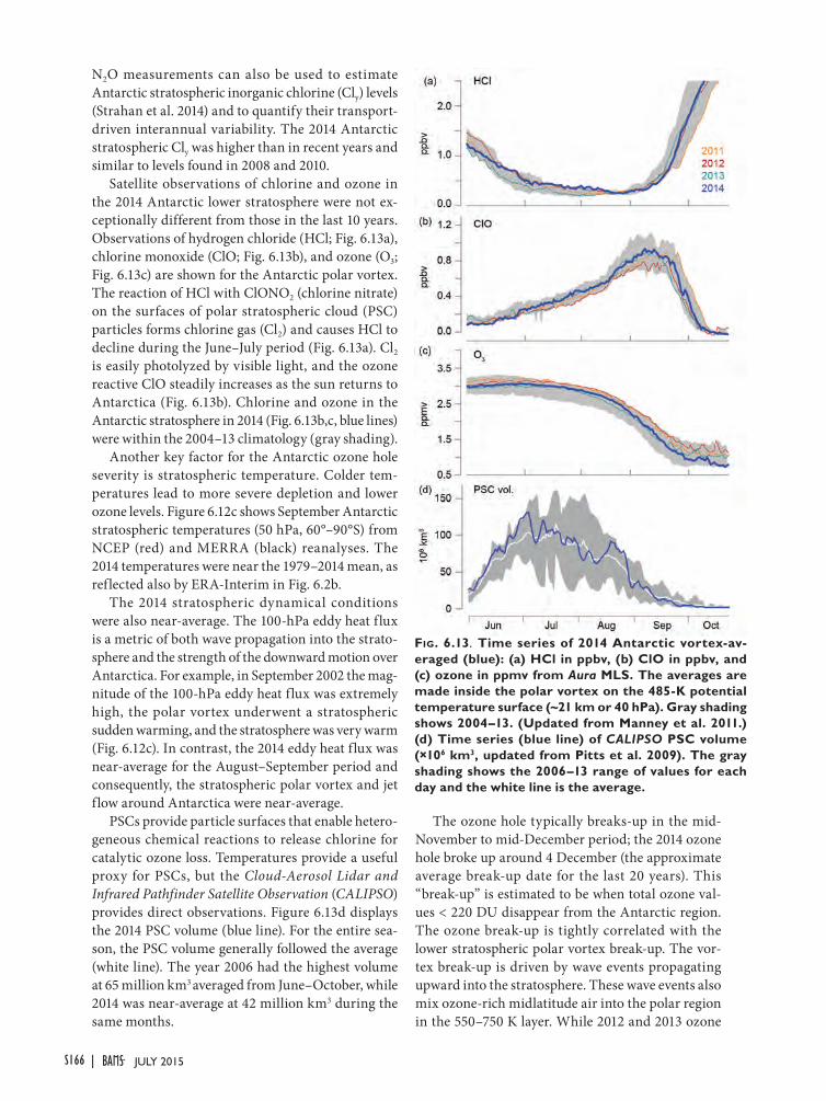
The ozone hole typically breaks-up in the mid-November to mid-December period; the 2014 ozone hole broke up around 4 December (the approximate average break-up date for the last 20 years). This “break-up” is estimated to be when total ozone val-ues < 220 DU disappear from the Antarctic region. The ozone break-up is tightly correlated with the lower stratospheric polar vortex break-up. The vor-tex break-up is driven by wave events propagating upward into the stratosphere. These wave events also mix ozone-rich midlatitude air into the polar region in the 550–750 K layer. While 2012 and 2013 ozone
N2O measurements can also be used to estimate Antarctic stratospheric inorganic chlorine (Cly) levels (Strahan et al. 2014) and to quantify their transport-driven interannual variability. The 2014 Antarctic stratospheric Cly was higher than in recent years and similar to levels found in 2008 and 2010.
Satellite observations of chlorine and ozone in the 2014 Antarctic lower stratosphere were not ex-ceptionally different from those in the last 10 years. Observations of hydrogen chloride (HCl; Fig. 6.13a), chlorine monoxide (ClO; Fig. 6.13b), and ozone (O3; Fig. 6.13c) are shown for the Antarctic polar vortex. The reaction of HCl with ClONO2 (chlorine nitrate) on the surfaces of polar stratospheric cloud (PSC) particles forms chlorine gas (Cl2) and causes HCl to decline during the June–July period (Fig. 6.13a). Cl2 is easily photolyzed by visible light, and the ozone reactive ClO steadily increases as the sun returns to Antarctica (Fig. 6.13b). Chlorine and ozone in the Antarctic stratosphere in 2014 (Fig. 6.13b,c, blue lines) were within the 2004–13 climatology (gray shading).
Another key factor for the Antarctic ozone hole severity is stratospheric temperature. Colder tem-peratures lead to more severe depletion and lower ozone levels. Figure 6.12c shows September Antarctic stratospheric temperatures (50 hPa, 60°–90°S) from NCEP (red) and MERRA (black) reanalyses. The 2014 temperatures were near the 1979–2014 mean, as reflected also by ERA-Interim in Fig. 6.2b.
The 2014 stratospheric dynamical conditions were also near-average. The 100-hPa eddy heat flux is a metric of both wave propagation into the strato-sphere and the strength of the downward motion over Antarctica. For example, in September 2002 the mag-nitude of the 100-hPa eddy heat flux was extremely high, the polar vortex underwent a stratospheric sudden warming, and the stratosphere was very warm (Fig. 6.12c). In contrast, the 2014 eddy heat flux was near-average for the August–September period and consequently, the stratospheric polar vortex and jet flow around Antarctica were near-average.
PSCs provide particle surfaces that enable hetero-geneous chemical reactions to release chlorine for catalytic ozone loss. Temperatures provide a useful proxy for PSCs, but the Cloud-Aerosol Lidar and Infrared Pathfinder Satellite Observation (CALIPSO) provides direct observations. Figure 6.13d displays the 2014 PSC volume (blue line). For the entire sea-son, the PSC volume generally followed the average (white line). The year 2006 had the highest volume at 65 million km3 averaged from June–October, while 2014 was near-average at 42 million km3 during the same months.
Fig. 6.13. Time series of 2014 Antarctic vortex-av-eraged (blue): (a) HCl in ppbv, (b) ClO in ppbv, and (c) ozone in ppmv from Aura MLS. The averages are made inside the polar vortex on the 485-K potential temperature surface (~21 km or 40 hPa). Gray shading shows 2004–13. (Updated from Manney et al. 2011.) (d) Time series (blue line) of CALIPSO PSC volume (×106 km3, updated from Pitts et al. 2009). The gray shading shows the 2006–13 range of values for each day and the white line is the average.
S166 JULY 2015|

holes broke-up earlier than usual due to stronger wave activity that enabled ozone-rich air transport from midlatitudes, the 2014 break-up of the ozone hole occurred close to the average date.
In summary, the Antarctic ozone hole is a severe ozone depletion that regularly appears in austral spring. In the last 14 years, the ozone hole has be-gun to display marginal signs of improvement (i.e., decrease in size). This improvement is statistically significant in observations from both ground and
satellite data, if the year 2002 is treated as an outlier (because of the major stratospheric sudden warming that occurred). Levels of chlorine continue to decline in the stratosphere because of the Montreal Protocol (WMO 2014), and this decline should be manifest in the Antarctic ozone hole. However, unambiguous attribution of the ozone hole improvement to the Montreal Protocol cannot yet be made because of relatively large year-to-year variability and observa-tional uncertainty.
S167JULY 2015STATE OF THE CLIMATE IN 2014 |

S168 JULY 2015|
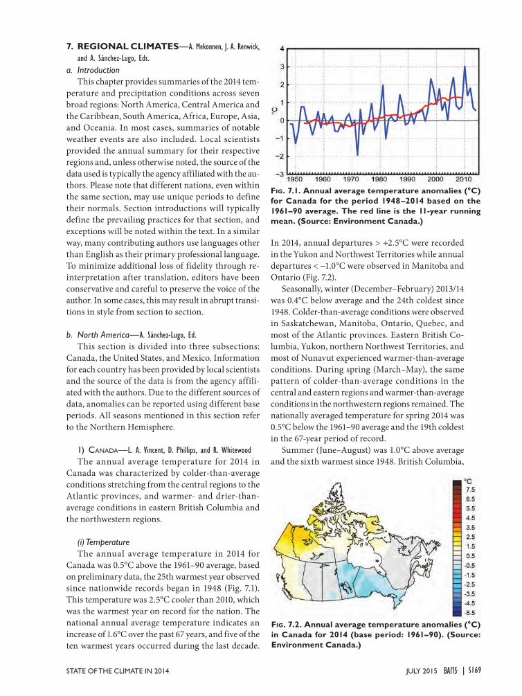
7. REGIONAL CLIMATES—A. Mekonnen, J. A. Renwick, and A. Sánchez-Lugo, Eds.
a. IntroductionThis chapter provides summaries of the 2014 tem-
perature and precipitation conditions across seven broad regions: North America, Central America and the Caribbean, South America, Africa, Europe, Asia, and Oceania. In most cases, summaries of notable weather events are also included. Local scientists provided the annual summary for their respective regions and, unless otherwise noted, the source of the data used is typically the agency affiliated with the au-thors. Please note that different nations, even within the same section, may use unique periods to define their normals. Section introductions will typically define the prevailing practices for that section, and exceptions will be noted within the text. In a similar way, many contributing authors use languages other than English as their primary professional language. To minimize additional loss of fidelity through re-interpretation after translation, editors have been conservative and careful to preserve the voice of the author. In some cases, this may result in abrupt transi-tions in style from section to section.
b. North America—A. Sánchez-Lugo, Ed.This section is divided into three subsections:
Canada, the United States, and Mexico. Information for each country has been provided by local scientists and the source of the data is from the agency affili-ated with the authors. Due to the different sources of data, anomalies can be reported using different base periods. All seasons mentioned in this section refer to the Northern Hemisphere.
1) Canada—L. A. Vincent, D. Phillips, and R. WhitewoodThe annual average temperature for 2014 in
Canada was characterized by colder-than-average conditions stretching from the central regions to the Atlantic provinces, and warmer- and drier-than-average conditions in eastern British Columbia and the northwestern regions.
(i) TemperatureThe annual average temperature in 2014 for
Canada was 0.5°C above the 1961–90 average, based on preliminary data, the 25th warmest year observed since nationwide records began in 1948 (Fig. 7.1). This temperature was 2.5°C cooler than 2010, which was the warmest year on record for the nation. The national annual average temperature indicates an increase of 1.6°C over the past 67 years, and five of the ten warmest years occurred during the last decade.
In 2014, annual departures > +2.5°C were recorded in the Yukon and Northwest Territories while annual departures < −1.0°C were observed in Manitoba and Ontario (Fig. 7.2).
Seasonally, winter (December–February) 2013/14 was 0.4°C below average and the 24th coldest since 1948. Colder-than-average conditions were observed in Saskatchewan, Manitoba, Ontario, Quebec, and most of the Atlantic provinces. Eastern British Co-lumbia, Yukon, northern Northwest Territories, and most of Nunavut experienced warmer-than-average conditions. During spring (March–May), the same pattern of colder-than-average conditions in the central and eastern regions and warmer-than-average conditions in the northwestern regions remained. The nationally averaged temperature for spring 2014 was 0.5°C below the 1961–90 average and the 19th coldest in the 67-year period of record.
Summer (June–August) was 1.0°C above average and the sixth warmest since 1948. British Columbia,
Fig. 7.1. Annual average temperature anomalies (°C) for Canada for the period 1948–2014 based on the 1961–90 average. The red line is the 11-year running mean. (Source: Environment Canada.)
Fig. 7.2. Annual average temperature anomalies (°C) in Canada for 2014 (base period: 1961–90). (Source: Environment Canada.)
S169JULY 2015STATE OF THE CLIMATE IN 2014 |
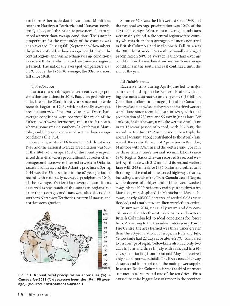
northern Alberta, Saskatchewan, and Manitoba, southern Northwest Territories and Nunavut, north-ern Quebec, and the Atlantic provinces all experi-enced warmer-than-average conditions. The summer temperature for the remainder of the country was near-average. During fall (September–November), the pattern of colder-than-average conditions in the central regions and warmer-than-average conditions in eastern British Columbia and northwestern regions returned. The nationally averaged temperature was 0.5°C above the 1961–90 average, the 33rd warmest fall since 1948.
(ii) PrecipitationCanada as a whole experienced near-average pre-
cipitation conditions in 2014. Based on preliminary data, it was the 22nd driest year since nationwide records began in 1948, with nationally averaged precipitation 98% of the 1961–90 average. Drier-than-average conditions were observed for much of the Yukon, Northwest Territories, and in the far north, whereas some areas in southern Saskatchewan, Mani-toba, and Ontario experienced wetter-than-average conditions (Fig. 7.3).
Seasonally, winter 2013/14 was the 15th driest since 1948 and the national average precipitation was 91% of the 1961–90 average. Most of the country experi-enced drier-than-average conditions but wetter-than-average conditions were observed in western Ontario, eastern Nunavut, and the Atlantic provinces. Spring 2014 was the 22nd wettest in the 67-year period of record with nationally averaged precipitation 104% of the average. Wetter-than-average conditions occurred across much of the southern regions but drier-than-average conditions were also observed in southern Northwest Territories, eastern Nunavut, and northeastern Quebec.
Summer 2014 was the 14th wettest since 1948 and the national average precipitation was 106% of the 1961–90 average. Wetter-than-average conditions were mainly found in the central regions of the coun-try whereas drier-than-average conditions occurred in British Columbia and in the north. Fall 2014 was the 30th driest since 1948 with nationally averaged precipitation 98% of average. Drier-than-average conditions in the northwest and wetter-than-average conditions in the south and east continued until the end of the year.
(iii) Notable eventsExcessive rains during April–June led to major
summer f looding in the Eastern Prairies, caus-ing the most destructive and expensive ($6 billion Canadian dollars in damages) f lood in Canadian history. Saskatoon, Saskatchewan had its third wettest April–June since records began in 1892, with total precipitation of 230 mm and 95 mm in June alone. For Yorkton, Saskatchewan, it was the wettest April–June in its 131-year period of record, with 357 mm; the record wettest June (252 mm or more than triple the normal accumulation) contributed to the April–June record. It was also the wettest April–June in Brandon, Manitoba with 374 mm and the wettest June (252 mm or three times June’s normal accumulation) since 1890. Regina, Saskatchewan recorded its second wet-test April–June with 312 mm and its second wettest June with 208 mm since 1883. Rains and subsequent flooding at the end of June forced highway closures, including a stretch of the TransCanada east of Regina where dozens of bridges and utilities were washed away. About 1000 residents, mainly in southwestern Manitoba, were displaced. In Manitoba and Saskatch-ewan, nearly 405 000 hectares of seeded fields were flooded, and another two million were left unseeded.
In summer 2014, unusually warm and dry con-ditions in the Northwest Territories and eastern British Columbia led to ideal conditions for forest fires. According to the Canadian Interagency Forest Fire Centre, the area burned was three times greater than the 20-year national average. In June and July, Yellowknife had 22 days at or above 25°C, compared to an average of eight. Yellowknife also had only two days in June and three in July with rain, and in a 91-day span—starting from about mid-May—it received only half its normal rainfall. The fires caused highway closures and interruption of the main power supply. In eastern British Columbia, it was the third warmest summer in 67 years and one of the ten driest. Fires caused the third biggest loss of timber in the province
Fig. 7.3. Annual total precipitation anomalies (%) in Canada for 2014 (% departure from the 1961–90 aver-age). (Source: Environment Canada.)
S170 JULY 2015|
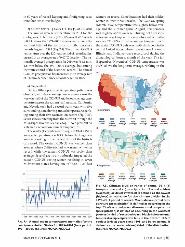
in 60 years of record-keeping and firefighting costs were four times over budget.
2) United StateS—J. Crouch, R. R. Heim Jr., and C. Fenimore The annual average temperature for 2014 for the
contiguous United States (CONUS) was 11.4°C, which is 0.1°C above the 1971–2000 average and among the warmest third of the historical distribution since records began in 1895 (Fig. 7.4). The annual CONUS temperature over the 120-year period of record has in-creased at an average rate of 0.07°C decade−1. The na-tionally averaged precipitation for 2014 was 784.1 mm, 4.8 mm below the 1971–2000 average, but among the wettest third of the historical record. The annual CONUS precipitation has increased at an average rate of 3.6 mm decade−1 since records began in 1895.
(i) TemperatureDuring 2014, a persistent temperature pattern was
observed, with above-average temperatures across the western half of the CONUS and below-average tem-peratures across the eastern half. Arizona, California, and Nevada each had a record warm year, with five surrounding states having annual temperatures rank-ing among their five warmest on record (Fig. 7.5a). Seven states stretching from the Midwest through the Mississippi River valley had a top 10 cold year, but no state had a record low annual temperature.
The winter (December–February) 2013/14 CONUS average temperature was 0.9°C below the long-term average, ranking in the coolest third of the histori-cal record. The western CONUS was warmer than average, where California had its warmest winter on record, while the eastern CONUS was cooler than average. Several arctic-air outbreaks impacted the eastern CONUS during winter, resulting in seven Midwestern states having one of their 10 coldest
winters on record. Some locations had their coldest winter in over three decades. The CONUS spring (March–May) temperature was slightly below aver-age and the summer (June–August) temperature was slightly above average. During both seasons, above-average temperatures were observed across the western CONUS with below-average temperatures in the eastern CONUS. July was particularly cool in the central United States, where three states—Arkansas, Illinois, and Indiana—were record cool during the climatological hottest month of the year. The fall (September–November) CONUS temperature was 0.3°C above the long-term average, ranking in the
Fig. 7.4. Annual mean temperature anomalies for the contiguous United States for 1895–2014 (base period: 1971–2000). (Source: NOAA/NCDC.)
Fig. 7.5. Climate division ranks of annual 2014 (a) temperature and (b) precipitation. Record coldest (warmest) or driest (wettest) is defined as the lowest (highest) annual value for that climate division in the 1895–2014 period of record. Much-above-normal tem-perature (precipitation) is defined as occurring in the top 10% of recorded years. Above-normal temperature (precipitation) is defined as occurring in the warmest (wettest) third of recorded years. Much-below-normal temperature/precipitation falls in the bottom 10% of coolest (driest) years since 1895, and below normal is defined as the coolest (driest) third of the distribution.(Source: NOAA/NCDC.)
S171JULY 2015STATE OF THE CLIMATE IN 2014 |
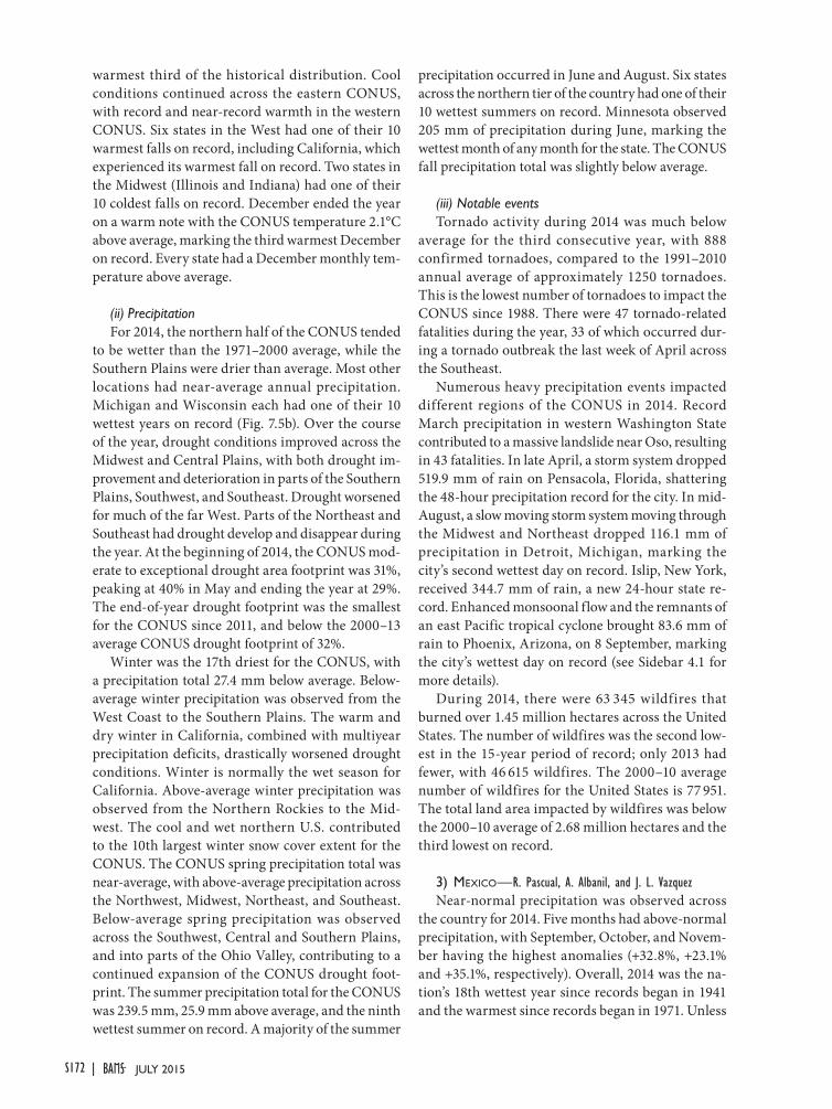
warmest third of the historical distribution. Cool conditions continued across the eastern CONUS, with record and near-record warmth in the western CONUS. Six states in the West had one of their 10 warmest falls on record, including California, which experienced its warmest fall on record. Two states in the Midwest (Illinois and Indiana) had one of their 10 coldest falls on record. December ended the year on a warm note with the CONUS temperature 2.1°C above average, marking the third warmest December on record. Every state had a December monthly tem-perature above average.
(ii) PrecipitationFor 2014, the northern half of the CONUS tended
to be wetter than the 1971–2000 average, while the Southern Plains were drier than average. Most other locations had near-average annual precipitation. Michigan and Wisconsin each had one of their 10 wettest years on record (Fig. 7.5b). Over the course of the year, drought conditions improved across the Midwest and Central Plains, with both drought im-provement and deterioration in parts of the Southern Plains, Southwest, and Southeast. Drought worsened for much of the far West. Parts of the Northeast and Southeast had drought develop and disappear during the year. At the beginning of 2014, the CONUS mod-erate to exceptional drought area footprint was 31%, peaking at 40% in May and ending the year at 29%. The end-of-year drought footprint was the smallest for the CONUS since 2011, and below the 2000–13 average CONUS drought footprint of 32%.
Winter was the 17th driest for the CONUS, with a precipitation total 27.4 mm below average. Below-average winter precipitation was observed from the West Coast to the Southern Plains. The warm and dry winter in California, combined with multiyear precipitation deficits, drastically worsened drought conditions. Winter is normally the wet season for California. Above-average winter precipitation was observed from the Northern Rockies to the Mid-west. The cool and wet northern U.S. contributed to the 10th largest winter snow cover extent for the CONUS. The CONUS spring precipitation total was near-average, with above-average precipitation across the Northwest, Midwest, Northeast, and Southeast. Below-average spring precipitation was observed across the Southwest, Central and Southern Plains, and into parts of the Ohio Valley, contributing to a continued expansion of the CONUS drought foot-print. The summer precipitation total for the CONUS was 239.5 mm, 25.9 mm above average, and the ninth wettest summer on record. A majority of the summer
precipitation occurred in June and August. Six states across the northern tier of the country had one of their 10 wettest summers on record. Minnesota observed 205 mm of precipitation during June, marking the wettest month of any month for the state. The CONUS fall precipitation total was slightly below average.
(iii) Notable eventsTornado activity during 2014 was much below
average for the third consecutive year, with 888 confirmed tornadoes, compared to the 1991–2010 annual average of approximately 1250 tornadoes. This is the lowest number of tornadoes to impact the CONUS since 1988. There were 47 tornado-related fatalities during the year, 33 of which occurred dur-ing a tornado outbreak the last week of April across the Southeast.
Numerous heavy precipitation events impacted different regions of the CONUS in 2014. Record March precipitation in western Washington State contributed to a massive landslide near Oso, resulting in 43 fatalities. In late April, a storm system dropped 519.9 mm of rain on Pensacola, Florida, shattering the 48-hour precipitation record for the city. In mid-August, a slow moving storm system moving through the Midwest and Northeast dropped 116.1 mm of precipitation in Detroit, Michigan, marking the city’s second wettest day on record. Islip, New York, received 344.7 mm of rain, a new 24-hour state re-cord. Enhanced monsoonal flow and the remnants of an east Pacific tropical cyclone brought 83.6 mm of rain to Phoenix, Arizona, on 8 September, marking the city’s wettest day on record (see Sidebar 4.1 for more details).
During 2014, there were 63 345 wildfires that burned over 1.45 million hectares across the United States. The number of wildfires was the second low-est in the 15-year period of record; only 2013 had fewer, with 46 615 wildfires. The 2000–10 average number of wildfires for the United States is 77 951. The total land area impacted by wildfires was below the 2000–10 average of 2.68 million hectares and the third lowest on record.
3) MexiCo—R. Pascual, A. Albanil, and J. L. VazquezNear-normal precipitation was observed across
the country for 2014. Five months had above-normal precipitation, with September, October, and Novem-ber having the highest anomalies (+32.8%, +23.1% and +35.1%, respectively). Overall, 2014 was the na-tion’s 18th wettest year since records began in 1941 and the warmest since records began in 1971. Unless
S172 JULY 2015|
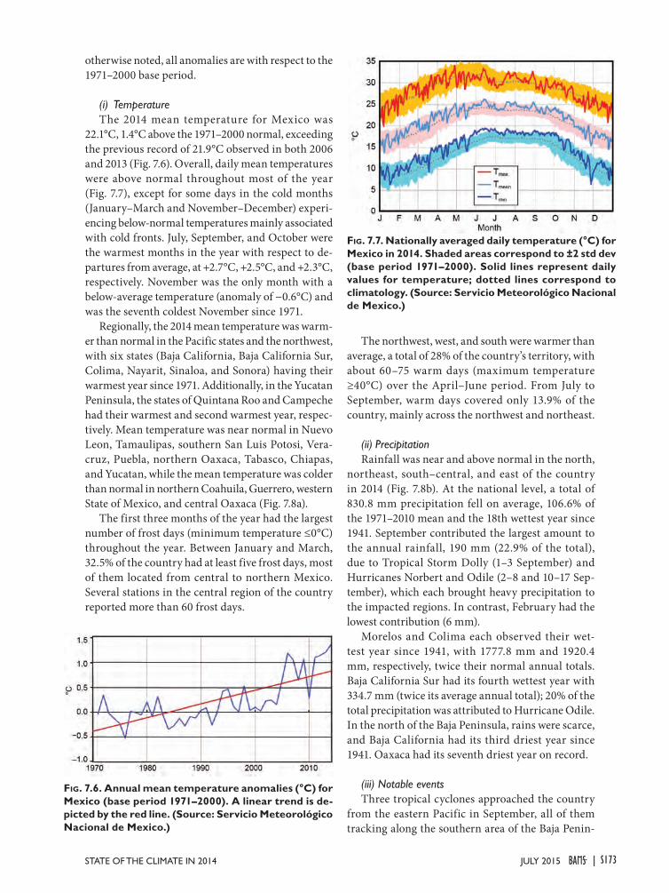
otherwise noted, all anomalies are with respect to the 1971–2000 base period.
(i) TemperatureThe 2014 mean temperature for Mexico was
22.1°C, 1.4°C above the 1971–2000 normal, exceeding the previous record of 21.9°C observed in both 2006 and 2013 (Fig. 7.6). Overall, daily mean temperatures were above normal throughout most of the year (Fig. 7.7), except for some days in the cold months (January–March and November–December) experi-encing below-normal temperatures mainly associated with cold fronts. July, September, and October were the warmest months in the year with respect to de-partures from average, at +2.7°C, +2.5°C, and +2.3°C, respectively. November was the only month with a below-average temperature (anomaly of −0.6°C) and was the seventh coldest November since 1971.
Regionally, the 2014 mean temperature was warm-er than normal in the Pacific states and the northwest, with six states (Baja California, Baja California Sur, Colima, Nayarit, Sinaloa, and Sonora) having their warmest year since 1971. Additionally, in the Yucatan Peninsula, the states of Quintana Roo and Campeche had their warmest and second warmest year, respec-tively. Mean temperature was near normal in Nuevo Leon, Tamaulipas, southern San Luis Potosi, Vera-cruz, Puebla, northern Oaxaca, Tabasco, Chiapas, and Yucatan, while the mean temperature was colder than normal in northern Coahuila, Guerrero, western State of Mexico, and central Oaxaca (Fig. 7.8a).
The first three months of the year had the largest number of frost days (minimum temperature ≤0°C) throughout the year. Between January and March, 32.5% of the country had at least five frost days, most of them located from central to northern Mexico. Several stations in the central region of the country reported more than 60 frost days.
The northwest, west, and south were warmer than average, a total of 28% of the country’s territory, with about 60–75 warm days (maximum temperature ≥40°C) over the April–June period. From July to September, warm days covered only 13.9% of the country, mainly across the northwest and northeast.
(ii) PrecipitationRainfall was near and above normal in the north,
northeast, south–central, and east of the country in 2014 (Fig. 7.8b). At the national level, a total of 830.8 mm precipitation fell on average, 106.6% of the 1971–2010 mean and the 18th wettest year since 1941. September contributed the largest amount to the annual rainfall, 190 mm (22.9% of the total), due to Tropical Storm Dolly (1–3 September) and Hurricanes Norbert and Odile (2–8 and 10–17 Sep-tember), which each brought heavy precipitation to the impacted regions. In contrast, February had the lowest contribution (6 mm).
Morelos and Colima each observed their wet-test year since 1941, with 1777.8 mm and 1920.4 mm, respectively, twice their normal annual totals. Baja California Sur had its fourth wettest year with 334.7 mm (twice its average annual total); 20% of the total precipitation was attributed to Hurricane Odile. In the north of the Baja Peninsula, rains were scarce, and Baja California had its third driest year since 1941. Oaxaca had its seventh driest year on record.
(iii) Notable eventsThree tropical cyclones approached the country
from the eastern Pacific in September, all of them tracking along the southern area of the Baja Penin-
Fig. 7.6. Annual mean temperature anomalies (°C) for Mexico (base period 1971–2000). A linear trend is de-picted by the red line. (Source: Servicio Meteorológico Nacional de Mexico.)
Fig. 7.7. Nationally averaged daily temperature (°C) for Mexico in 2014. Shaded areas correspond to ±2 std dev (base period 1971–2000). Solid lines represent daily values for temperature; dotted lines correspond to climatology. (Source: Servicio Meteorológico Nacional de Mexico.)
S173JULY 2015STATE OF THE CLIMATE IN 2014 |
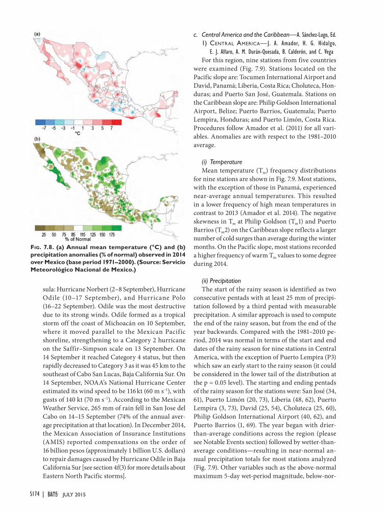
sula: Hurricane Norbert (2–8 September), Hurricane Odile (10–17 September), and Hurricane Polo (16–22 September). Odile was the most destructive due to its strong winds. Odile formed as a tropical storm off the coast of Michoacán on 10 September, where it moved parallel to the Mexican Pacific shoreline, strengthening to a Category 2 hurricane on the Saffir–Simpson scale on 13 September. On 14 September it reached Category 4 status, but then rapidly decreased to Category 3 as it was 45 km to the southeast of Cabo San Lucas, Baja California Sur. On 14 September, NOAA’s National Hurricane Center estimated its wind speed to be 116 kt (60 m s−1), with gusts of 140 kt (70 m s−1). According to the Mexican Weather Service, 265 mm of rain fell in San Jose del Cabo on 14–15 September (74% of the annual aver-age precipitation at that location). In December 2014, the Mexican Association of Insurance Institutions (AMIS) reported compensations on the order of 16 billion pesos (approximately 1 billion U.S. dollars) to repair damages caused by Hurricane Odile in Baja California Sur [see section 4f(3) for more details about Eastern North Pacific storms].
c. Central America and the Caribbean—A. Sánchez-Lugo, Ed.1) Central aMeriCa— J. A. Amador, H. G. Hidalgo,
E. J. Alfaro, A. M. Durán-Quesada, B. Calderón, and C. VegaFor this region, nine stations from five countries
were examined (Fig. 7.9). Stations located on the Pacific slope are: Tocumen International Airport and David, Panamá; Liberia, Costa Rica; Choluteca, Hon-duras; and Puerto San José, Guatemala. Stations on the Caribbean slope are: Philip Goldson International Airport, Belize; Puerto Barrios, Guatemala; Puerto Lempira, Honduras; and Puerto Limón, Costa Rica. Procedures follow Amador et al. (2011) for all vari-ables. Anomalies are with respect to the 1981–2010 average.
(i) TemperatureMean temperature (Tm) frequency distributions
for nine stations are shown in Fig. 7.9. Most stations, with the exception of those in Panamá, experienced near-average annual temperatures. This resulted in a lower frequency of high mean temperatures in contrast to 2013 (Amador et al. 2014). The negative skewness in Tm at Philip Goldson (Tm1) and Puerto Barrios (Tm2) on the Caribbean slope reflects a larger number of cold surges than average during the winter months. On the Pacific slope, most stations recorded a higher frequency of warm Tm values to some degree during 2014.
(ii) PrecipitationThe start of the rainy season is identified as two
consecutive pentads with at least 25 mm of precipi-tation followed by a third pentad with measurable precipitation. A similar approach is used to compute the end of the rainy season, but from the end of the year backwards. Compared with the 1981–2010 pe-riod, 2014 was normal in terms of the start and end dates of the rainy season for nine stations in Central America, with the exception of Puerto Lempira (P3) which saw an early start to the rainy season (it could be considered in the lower tail of the distribution at the p = 0.05 level). The starting and ending pentads of the rainy season for the stations were: San José (34, 61), Puerto Limón (20, 73), Liberia (48, 62), Puerto Lempira (3, 73), David (25, 54), Choluteca (25, 60), Philip Goldson International Airport (40, 62), and Puerto Barrios (1, 69). The year began with drier-than-average conditions across the region (please see Notable Events section) followed by wetter-than-average conditions—resulting in near-normal an-nual precipitation totals for most stations analyzed (Fig. 7.9). Other variables such as the above-normal maximum 5-day wet-period magnitude, below-nor-
Fig. 7.8. (a) Annual mean temperature (°C) and (b) precipitation anomalies (% of normal) observed in 2014 over Mexico (base period 1971–2000). (Source: Servicio Meteorológico Nacional de Mexico.)
S174 JULY 2015|
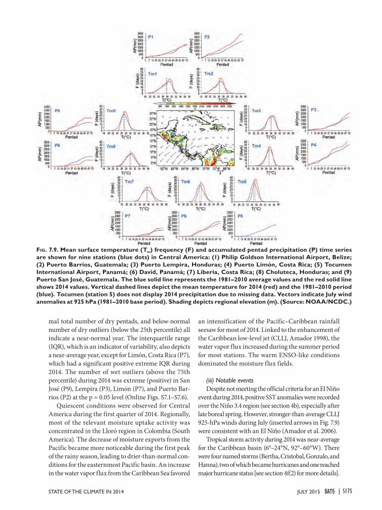
mal total number of dry pentads, and below-normal number of dry outliers (below the 25th percentile) all indicate a near-normal year. The interquartile range (IQR), which is an indicator of variability, also depicts a near-average year, except for Limón, Costa Rica (P7), which had a significant positive extreme IQR during 2014. The number of wet outliers (above the 75th percentile) during 2014 was extreme (positive) in San José (P9), Lempira (P3), Limón (P7), and Puerto Bar-rios (P2) at the p = 0.05 level (Online Figs. S7.1–S7.6).
Quiescent conditions were observed for Central America during the first quarter of 2014. Regionally, most of the relevant moisture uptake activity was concentrated in the Lloró region in Colombia (South America). The decrease of moisture exports from the Pacific became more noticeable during the first peak of the rainy season, leading to drier-than-normal con-ditions for the easternmost Pacific basin. An increase in the water vapor flux from the Caribbean Sea favored
an intensification of the Pacific–Caribbean rainfall seesaw for most of 2014. Linked to the enhancement of the Caribbean low-level jet (CLLJ, Amador 1998), the water vapor flux increased during the summer period for most stations. The warm ENSO-like conditions dominated the moisture flux fields.
(iii) Notable eventsDespite not meeting the official criteria for an El Niño
event during 2014, positive SST anomalies were recorded over the Niño 3.4 region (see section 4b), especially after late boreal spring. However, stronger-than-average CLLJ 925-hPa winds during July (inserted arrows in Fig. 7.9) were consistent with an El Niño (Amador et al. 2006).
Tropical storm activity during 2014 was near-average for the Caribbean basin (6°–24°N, 92°–60°W). There were four named storms (Bertha, Cristobal, Gonzalo, and Hanna), two of which became hurricanes and one reached major hurricane status [see section 4f(2) for more details].
Fig. 7.9. Mean surface temperature (Tm) frequency (F) and accumulated pentad precipitation (P) time series are shown for nine stations (blue dots) in Central America: (1) Philip Goldson International Airport, Belize; (2) Puerto Barrios, Guatemala; (3) Puerto Lempira, Honduras; (4) Puerto Limón, Costa Rica; (5) Tocumen International Airport, Panamá; (6) David, Panamá; (7) Liberia, Costa Rica; (8) Choluteca, Honduras; and (9) Puerto San José, Guatemala. The blue solid line represents the 1981–2010 average values and the red solid line shows 2014 values. Vertical dashed lines depict the mean temperature for 2014 (red) and the 1981–2010 period (blue). Tocumen (station 5) does not display 2014 precipitation due to missing data. Vectors indicate July wind anomalies at 925 hPa (1981–2010 base period). Shading depicts regional elevation (m). (Source: NOAA/NCDC.)
S175JULY 2015STATE OF THE CLIMATE IN 2014 |
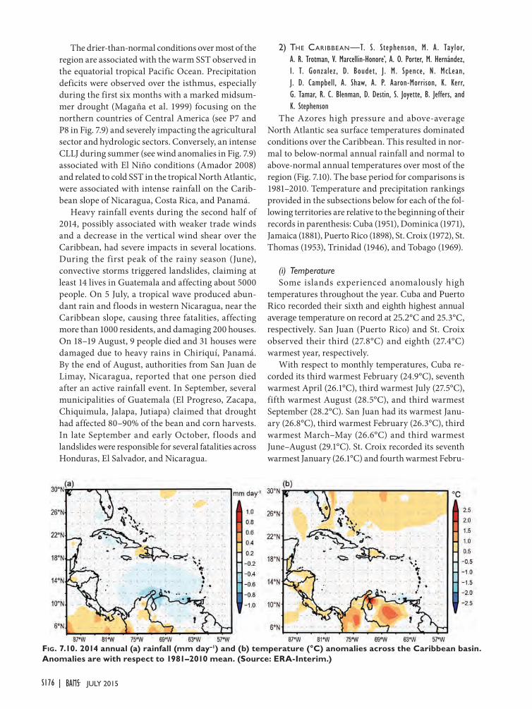
The drier-than-normal conditions over most of the region are associated with the warm SST observed in the equatorial tropical Pacific Ocean. Precipitation deficits were observed over the isthmus, especially during the first six months with a marked midsum-mer drought (Magaña et al. 1999) focusing on the northern countries of Central America (see P7 and P8 in Fig. 7.9) and severely impacting the agricultural sector and hydrologic sectors. Conversely, an intense CLLJ during summer (see wind anomalies in Fig. 7.9) associated with El Niño conditions (Amador 2008) and related to cold SST in the tropical North Atlantic, were associated with intense rainfall on the Carib-bean slope of Nicaragua, Costa Rica, and Panamá.
Heavy rainfall events during the second half of 2014, possibly associated with weaker trade winds and a decrease in the vertical wind shear over the Caribbean, had severe impacts in several locations. During the first peak of the rainy season (June), convective storms triggered landslides, claiming at least 14 lives in Guatemala and affecting about 5000 people. On 5 July, a tropical wave produced abun-dant rain and floods in western Nicaragua, near the Caribbean slope, causing three fatalities, affecting more than 1000 residents, and damaging 200 houses. On 18–19 August, 9 people died and 31 houses were damaged due to heavy rains in Chiriquí, Panamá. By the end of August, authorities from San Juan de Limay, Nicaragua, reported that one person died after an active rainfall event. In September, several municipalities of Guatemala (El Progreso, Zacapa, Chiquimula, Jalapa, Jutiapa) claimed that drought had affected 80–90% of the bean and corn harvests. In late September and early October, f loods and landslides were responsible for several fatalities across Honduras, El Salvador, and Nicaragua.
2) the Caribbean—T. S. Stephenson, M. A . Taylor, A. R. Trotman, V. Marcellin-Honore’, A. O. Porter, M. Hernández, I. T. Gonzalez, D. Boudet , J. M. Spence, N. McLean, J. D. Campbell, A. Shaw, A. P. Aaron-Morrison, K. Kerr, G. Tamar, R. C. Blenman, D. Destin, S. Joyette, B. Jeffers, and K. Stephenson
The Azores high pressure and above-average North Atlantic sea surface temperatures dominated conditions over the Caribbean. This resulted in nor-mal to below-normal annual rainfall and normal to above-normal annual temperatures over most of the region (Fig. 7.10). The base period for comparisons is 1981–2010. Temperature and precipitation rankings provided in the subsections below for each of the fol-lowing territories are relative to the beginning of their records in parenthesis: Cuba (1951), Dominica (1971), Jamaica (1881), Puerto Rico (1898), St. Croix (1972), St. Thomas (1953), Trinidad (1946), and Tobago (1969).
(i) TemperatureSome islands experienced anomalously high
temperatures throughout the year. Cuba and Puerto Rico recorded their sixth and eighth highest annual average temperature on record at 25.2°C and 25.3°C, respectively. San Juan (Puerto Rico) and St. Croix observed their third (27.8°C) and eighth (27.4°C) warmest year, respectively.
With respect to monthly temperatures, Cuba re-corded its third warmest February (24.9°C), seventh warmest April (26.1°C), third warmest July (27.5°C), fifth warmest August (28.5°C), and third warmest September (28.2°C). San Juan had its warmest Janu-ary (26.8°C), third warmest February (26.3°C), third warmest March–May (26.6°C) and third warmest June–August (29.1°C). St. Croix recorded its seventh warmest January (26.1°C) and fourth warmest Febru-
Fig. 7.10. 2014 annual (a) rainfall (mm day–1) and (b) temperature (°C) anomalies across the Caribbean basin. Anomalies are with respect to 1981–2010 mean. (Source: ERA-Interim.)
S176 JULY 2015|
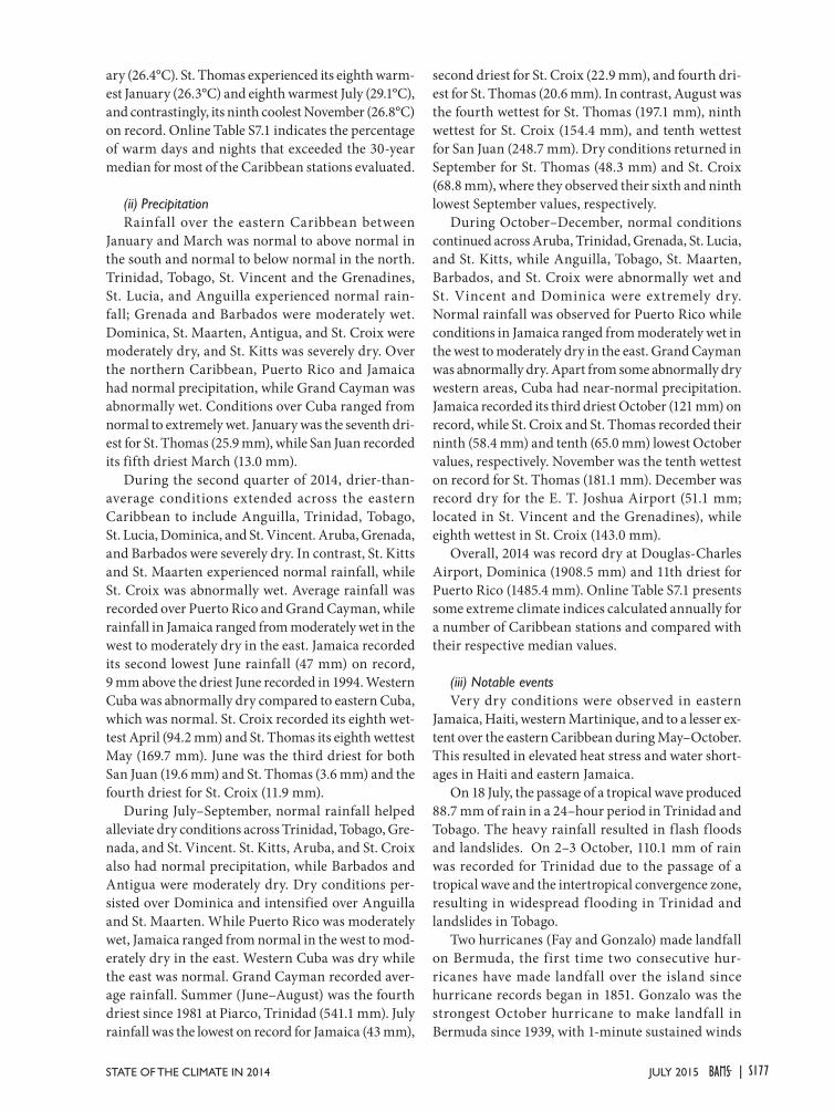
ary (26.4°C). St. Thomas experienced its eighth warm-est January (26.3°C) and eighth warmest July (29.1°C), and contrastingly, its ninth coolest November (26.8°C) on record. Online Table S7.1 indicates the percentage of warm days and nights that exceeded the 30-year median for most of the Caribbean stations evaluated.
(ii) PrecipitationRainfall over the eastern Caribbean between
January and March was normal to above normal in the south and normal to below normal in the north. Trinidad, Tobago, St. Vincent and the Grenadines, St. Lucia, and Anguilla experienced normal rain-fall; Grenada and Barbados were moderately wet. Dominica, St. Maarten, Antigua, and St. Croix were moderately dry, and St. Kitts was severely dry. Over the northern Caribbean, Puerto Rico and Jamaica had normal precipitation, while Grand Cayman was abnormally wet. Conditions over Cuba ranged from normal to extremely wet. January was the seventh dri-est for St. Thomas (25.9 mm), while San Juan recorded its fifth driest March (13.0 mm).
During the second quarter of 2014, drier-than-average conditions extended across the eastern Caribbean to include Anguilla, Trinidad, Tobago, St. Lucia, Dominica, and St. Vincent. Aruba, Grenada, and Barbados were severely dry. In contrast, St. Kitts and St. Maarten experienced normal rainfall, while St. Croix was abnormally wet. Average rainfall was recorded over Puerto Rico and Grand Cayman, while rainfall in Jamaica ranged from moderately wet in the west to moderately dry in the east. Jamaica recorded its second lowest June rainfall (47 mm) on record, 9 mm above the driest June recorded in 1994. Western Cuba was abnormally dry compared to eastern Cuba, which was normal. St. Croix recorded its eighth wet-test April (94.2 mm) and St. Thomas its eighth wettest May (169.7 mm). June was the third driest for both San Juan (19.6 mm) and St. Thomas (3.6 mm) and the fourth driest for St. Croix (11.9 mm).
During July–September, normal rainfall helped alleviate dry conditions across Trinidad, Tobago, Gre-nada, and St. Vincent. St. Kitts, Aruba, and St. Croix also had normal precipitation, while Barbados and Antigua were moderately dry. Dry conditions per-sisted over Dominica and intensified over Anguilla and St. Maarten. While Puerto Rico was moderately wet, Jamaica ranged from normal in the west to mod-erately dry in the east. Western Cuba was dry while the east was normal. Grand Cayman recorded aver-age rainfall. Summer (June–August) was the fourth driest since 1981 at Piarco, Trinidad (541.1 mm). July rainfall was the lowest on record for Jamaica (43 mm),
second driest for St. Croix (22.9 mm), and fourth dri-est for St. Thomas (20.6 mm). In contrast, August was the fourth wettest for St. Thomas (197.1 mm), ninth wettest for St. Croix (154.4 mm), and tenth wettest for San Juan (248.7 mm). Dry conditions returned in September for St. Thomas (48.3 mm) and St. Croix (68.8 mm), where they observed their sixth and ninth lowest September values, respectively.
During October–December, normal conditions continued across Aruba, Trinidad, Grenada, St. Lucia, and St. Kitts, while Anguilla, Tobago, St. Maarten, Barbados, and St. Croix were abnormally wet and St. Vincent and Dominica were extremely dry. Normal rainfall was observed for Puerto Rico while conditions in Jamaica ranged from moderately wet in the west to moderately dry in the east. Grand Cayman was abnormally dry. Apart from some abnormally dry western areas, Cuba had near-normal precipitation. Jamaica recorded its third driest October (121 mm) on record, while St. Croix and St. Thomas recorded their ninth (58.4 mm) and tenth (65.0 mm) lowest October values, respectively. November was the tenth wettest on record for St. Thomas (181.1 mm). December was record dry for the E. T. Joshua Airport (51.1 mm; located in St. Vincent and the Grenadines), while eighth wettest in St. Croix (143.0 mm).
Overall, 2014 was record dry at Douglas-Charles Airport, Dominica (1908.5 mm) and 11th driest for Puerto Rico (1485.4 mm). Online Table S7.1 presents some extreme climate indices calculated annually for a number of Caribbean stations and compared with their respective median values.
(iii) Notable eventsVery dry conditions were observed in eastern
Jamaica, Haiti, western Martinique, and to a lesser ex-tent over the eastern Caribbean during May–October. This resulted in elevated heat stress and water short-ages in Haiti and eastern Jamaica.
On 18 July, the passage of a tropical wave produced 88.7 mm of rain in a 24–hour period in Trinidad and Tobago. The heavy rainfall resulted in flash floods and landslides. On 2–3 October, 110.1 mm of rain was recorded for Trinidad due to the passage of a tropical wave and the intertropical convergence zone, resulting in widespread f looding in Trinidad and landslides in Tobago.
Two hurricanes (Fay and Gonzalo) made landfall on Bermuda, the first time two consecutive hur-ricanes have made landfall over the island since hurricane records began in 1851. Gonzalo was the strongest October hurricane to make landfall in Bermuda since 1939, with 1-minute sustained winds
S177JULY 2015STATE OF THE CLIMATE IN 2014 |
near 95 kt (49 m s−1). Gonzalo was responsible for four fatalities and 200–400 million U.S. dollars in insured damage. Antigua and St. Marteen were also adversely impacted by sustained winds from Gonzalo.
d. South America—A. Sánchez-Lugo, Ed.For the purpose of this publication, South America
is divided into three regions: Northern South America and the tropical Andes, Tropical South America east of the Andes, and Southern South America. Informa-tion for each section is provided by local scientists, and data are typically from the agency affiliated with the authors. Different data sources may use differ-ent base periods to define normal. Unless otherwise noted, normals refer to the 1961–90 base period.
Most of 2014 was characterized by the sustained warmth of the eastern Pacific Ocean, inf luencing South America’s climate (Fig. 7.11). The annual mean temperature was predominantly above normal in South America, with anomalies between +0.5°C and +1.5°C. However, negative anomalies up to −1.0°C occurred over central Bolivia and northern Paraguay (Fig. 7.12a). Precipitation was below normal in west-ern and northern South America and eastern Brazil, while above-normal precipitation was observed over Argentina, Uruguay, Paraguay, and central Bolivia (Fig. 7.12b).
1) northern SoUth aMeriCa and the tropiCal andeS—R. Martínez, J. Arévalo, G. Carrasco, L. Álvarez, J. Bazo, and E. Zambrano
This subsection covers Bolivia, Colombia, Ecua-dor, Peru, and Venezuela.
(i) TemperatureIn Venezuela and Peru, temperatures were near
normal during January–March (JFM) and above normal during April–June (AMJ) and part of July–September (JAS), with anomalies between +1.5°C and +4.0°C. In the highlands, temperatures were warmer than normal during June and July, with below-normal temperatures during August (about 2.5°C below nor-mal). In Colombia, temperatures were above normal across the Andean, Caribbean, and Pacific regions most of the year. Mean temperature anomalies were as high as +2°C, with maximum temperatures as high as 5°C above average. Similarly, in Ecuador, the aver-age temperature for 2014 was predominantly above normal, with anomalies between +0.5° and +1.5°C. Bolivian temperatures were near normal most of the year. However, in the central valley regions, maximum and minimum temperatures surpassed their warmest historical records for June and November, respec-
tively; Oruro (Altiplano) and Cochabamba (valley) set new record maximum temperatures for November.
(ii) PrecipitationIn Venezuela, drier-than-average conditions were
present during JFM and October–December (OND). The lack of precipitation was associated with anoma-lous subsidence over the region. This pattern was par-ticularly strong during JFM when precipitation was 40% of normal in the north and southeast regions. This feature eased during AMJ and JAS, favored by above-normal precipitation. AMJ precipitation in the northwest of the country remained below average, with as little as 60% of normal precipitation, while in north–central and eastern areas, precipitation was 120–130% of normal. In Colombia, precipitation was below normal most of the year, with deficits of up to 60% in the Andean, Caribbean, and Pacific regions. July was the driest month, with 20% of normal pre-cipitation. During the first half of 2014, Ecuador’s
Fig. 7.11. Mean annual sea surface temperature anoma-lies (°C; 1971–2000 base period). Data source: NOAA/NCEP/EMC/CMB/GLOBAL Reyn_Smith OIv2. (Pro-cessed by CIIFEN, 2015.)
S178 JULY 2015|
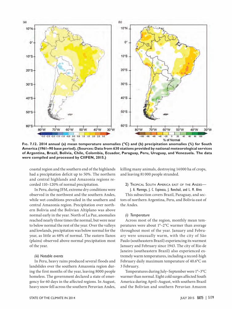
coastal region and the southern end of the highlands had a precipitation deficit up to 50%. The northern and central highlands and Amazonia regions re-corded 110–120% of normal precipitation.
In Peru, during JFM, extreme dry conditions were observed in the northwest and the southern Andes, while wet conditions prevailed in the southern and central Amazonia region. Precipitation over north-ern Bolivia and the Bolivian Altiplano was above normal early in the year. North of La Paz, anomalies reached nearly three times the normal, but were near to below normal the rest of the year. Over the valleys and lowlands, precipitation was below normal for the year, as little as 68% of normal. The eastern llanos (plains) observed above-normal precipitation most of the year.
(iii) Notable eventsIn Peru, heavy rains produced several floods and
landslides over the southern Amazonia region dur-ing the first months of the year, leaving 8000 people homeless. The government declared a state of emer-gency for 60 days in the affected regions. In August, heavy snow fell across the southern Peruvian Andes,
killing many animals, destroying 14 000 ha of crops, and leaving 81 000 people stranded.
2) tropiCal SoUth aMeriCa eaSt of the andeS— J. A. Marengo, J. C. Espinoza, J. Ronchail, and L. M. Alves
This subsection covers Brazil, Paraguay, and sec-tors of northern Argentina, Peru, and Bolivia east of the Andes.
(i) TemperatureAcross most of the region, monthly mean tem-
peratures were about 1°–2°C warmer than average throughout most of the year. January and Febru-ary were unusually warm, with the city of São Paulo (southeastern Brazil) experiencing its warmest January and February since 1943. The city of Rio de Janeiro (southeastern Brazil) also experienced ex-tremely warm temperatures, including a record-high February daily maximum temperature of 40.6°C on 3 February.
Temperatures during July–September were 1°–3°C warmer than normal. Eight cold surges affected South America during April–August, with southern Brazil and the Bolivian and southern Peruvian Amazon
Fig. 7.12. 2014 annual (a) mean temperature anomalies (°C) and (b) precipitation anomalies (%) for South America (1961–90 base period). (Sources: Data from 630 stations provided by national meteorological services of Argentina, Brazil, Bolivia, Chile, Colombia, Ecuador, Paraguay, Peru, Uruguay, and Venezuela. The data were compiled and processed by CIIFEN, 2015.)
S179JULY 2015STATE OF THE CLIMATE IN 2014 |
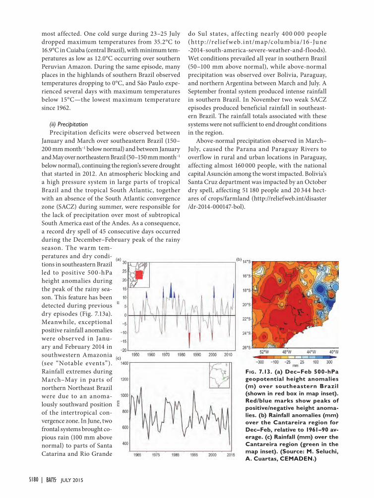
most affected. One cold surge during 23–25 July dropped maximum temperatures from 35.2°C to 16.9°C in Cuiaba (central Brazil), with minimum tem-peratures as low as 12.0°C occurring over southern Peruvian Amazon. During the same episode, many places in the highlands of southern Brazil observed temperatures dropping to 0°C, and São Paulo expe-rienced several days with maximum temperatures below 15°C—the lowest maximum temperature since 1962.
(ii) PrecipitationPrecipitation deficits were observed between
January and March over southeastern Brazil (150– 200 mm month−1 below normal) and between January and May over northeastern Brazil (50–150 mm month−1 below normal), continuing the region’s severe drought that started in 2012. An atmospheric blocking and a high pressure system in large parts of tropical Brazil and the tropical South Atlantic, together with an absence of the South Atlantic convergence zone (SACZ) during summer, were responsible for the lack of precipitation over most of subtropical South America east of the Andes. As a consequence, a record dry spell of 45 consecutive days occurred during the December–February peak of the rainy season. The warm tem-peratures and dry condi-tions in southeastern Brazil led to positive 500-hPa height anomalies during the peak of the rainy sea-son. This feature has been detected during previous dry episodes (Fig. 7.13a). Meanwhile, exceptional positive rainfall anomalies were observed in Janu-ary and February 2014 in southwestern Amazonia (see “Notable events”). Rainfall extremes during March–May in parts of northern Northeast Brazil were due to an anoma-lously southward position of the intertropical con-vergence zone. In June, two frontal systems brought co-pious rain (100 mm above normal) to parts of Santa Catarina and Rio Grande
do Sul states, affecting nearly 400 000 people (ht tp://rel ief web.int /map/columbia/16 -June -2014-south-america-severe-weather-and-f loods). Wet conditions prevailed all year in southern Brazil (50–100 mm above normal), while above-normal precipitation was observed over Bolivia, Paraguay, and northern Argentina between March and July. A September frontal system produced intense rainfall in southern Brazil. In November two weak SACZ episodes produced beneficial rainfall in southeast-ern Brazil. The rainfall totals associated with these systems were not sufficient to end drought conditions in the region.
Above-normal precipitation observed in March–July, caused the Parana and Paraguay Rivers to overflow in rural and urban locations in Paraguay, affecting almost 160 000 people, with the national capital Asunción among the worst impacted. Bolivia’s Santa Cruz department was impacted by an October dry spell, affecting 51 180 people and 20 344 hect-ares of crops/farmland (http://reliefweb.int/disaster /dr-2014-000147-bol).
Fig. 7.13. (a) Dec–Feb 500-hPa geopotential height anomalies (m) over southeastern Brazil (shown in red box in map inset). Red/blue marks show peaks of positive/negative height anoma-lies. (b) Rainfall anomalies (mm) over the Cantareira region for Dec–Feb, relative to 1961–90 av-erage. (c) Rainfall (mm) over the Cantareira region (green in the map inset). (Source: M. Seluchi, A. Cuartas, CEMADEN.)
S180 JULY 2015|
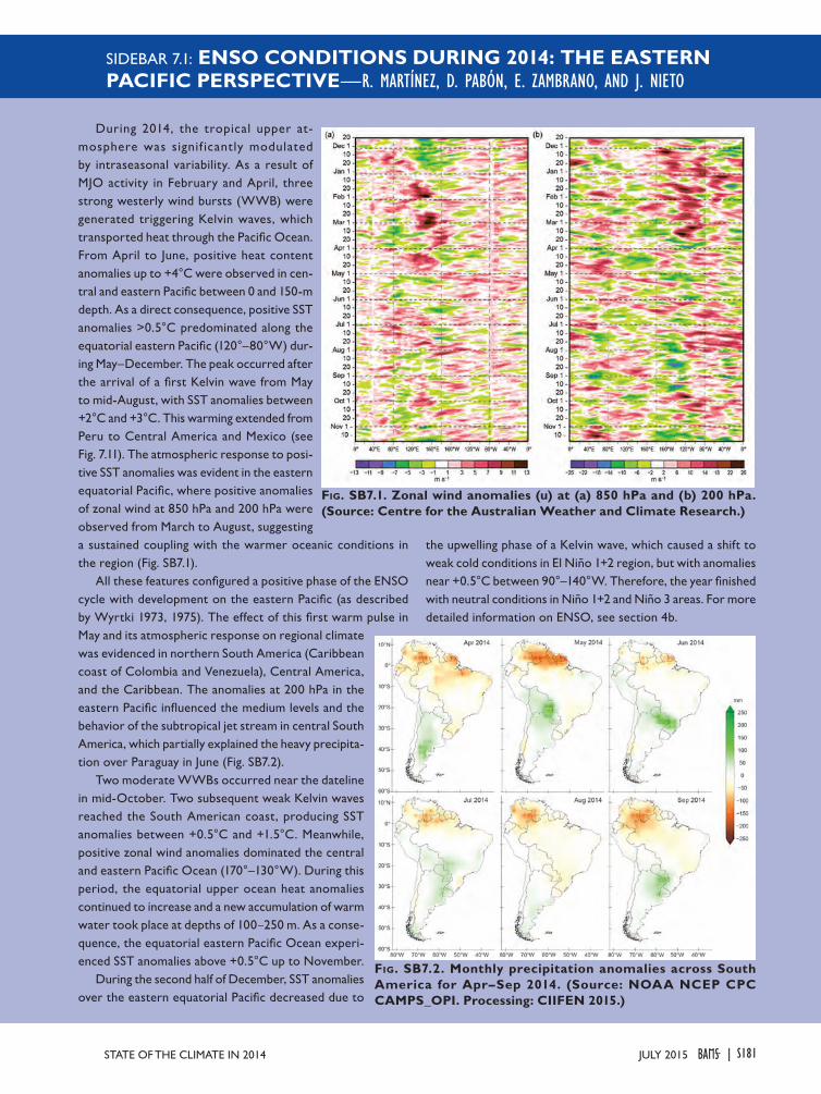
SIDEBAR 7.1: ENSO CONDITIONS DURING 2014: THE EASTERN PACIFIC PERSPECTIVE—R. MARTÍNEZ, D. PABÓN, E. ZAMBRANO, AND J. NIETO
During 2014, the tropical upper at-mosphere was signif icantly modulated by intraseasonal variability. As a result of MJO activity in February and April, three strong westerly wind bursts (WWB) were generated triggering Kelvin waves, which transported heat through the Pacific Ocean. From April to June, positive heat content anomalies up to +4°C were observed in cen-tral and eastern Pacific between 0 and 150-m depth. As a direct consequence, positive SST anomalies >0.5°C predominated along the equatorial eastern Pacific (120°–80°W) dur-ing May–December. The peak occurred after the arrival of a first Kelvin wave from May to mid-August, with SST anomalies between +2°C and +3°C. This warming extended from Peru to Central America and Mexico (see Fig. 7.11). The atmospheric response to posi-tive SST anomalies was evident in the eastern equatorial Pacific, where positive anomalies of zonal wind at 850 hPa and 200 hPa were observed from March to August, suggesting a sustained coupling with the warmer oceanic conditions in the region (Fig. SB7.1).
All these features configured a positive phase of the ENSO cycle with development on the eastern Pacific (as described by Wyrtki 1973, 1975). The effect of this first warm pulse in May and its atmospheric response on regional climate was evidenced in northern South America (Caribbean coast of Colombia and Venezuela), Central America, and the Caribbean. The anomalies at 200 hPa in the eastern Pacific influenced the medium levels and the behavior of the subtropical jet stream in central South America, which partially explained the heavy precipita-tion over Paraguay in June (Fig. SB7.2).
Two moderate WWBs occurred near the dateline in mid-October. Two subsequent weak Kelvin waves reached the South American coast, producing SST anomalies between +0.5°C and +1.5°C. Meanwhile, positive zonal wind anomalies dominated the central and eastern Pacific Ocean (170°–130°W). During this period, the equatorial upper ocean heat anomalies continued to increase and a new accumulation of warm water took place at depths of 100–250 m. As a conse-quence, the equatorial eastern Pacific Ocean experi-enced SST anomalies above +0.5°C up to November.
During the second half of December, SST anomalies over the eastern equatorial Pacific decreased due to
the upwelling phase of a Kelvin wave, which caused a shift to weak cold conditions in El Niño 1+2 region, but with anomalies near +0.5°C between 90°–140°W. Therefore, the year finished with neutral conditions in Niño 1+2 and Niño 3 areas. For more detailed information on ENSO, see section 4b.
Fig. SB7.1. Zonal wind anomalies (u) at (a) 850 hPa and (b) 200 hPa. (Source: Centre for the Australian Weather and Climate Research.)
Fig. SB7.2. Monthly precipitation anomalies across South America for Apr–Sep 2014. (Source: NOAA NCEP CPC CAMPS_OPI. Processing: CIIFEN 2015.)
S181JULY 2015STATE OF THE CLIMATE IN 2014 |
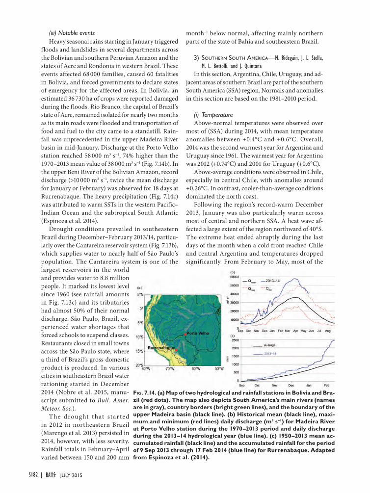
(iii) Notable eventsHeavy seasonal rains starting in January triggered
floods and landslides in several departments across the Bolivian and southern Peruvian Amazon and the states of Acre and Rondonia in western Brazil. These events affected 68 000 families, caused 60 fatalities in Bolivia, and forced governments to declare states of emergency for the affected areas. In Bolivia, an estimated 36 730 ha of crops were reported damaged during the floods. Rio Branco, the capital of Brazil’s state of Acre, remained isolated for nearly two months as its main roads were flooded and transportation of food and fuel to the city came to a standstill. Rain-fall was unprecedented in the upper Madeira River basin in mid-January. Discharge at the Porto Velho station reached 58 000 m3 s−1, 74% higher than the 1970–2013 mean value of 38 000 m3 s−1 (Fig. 7.14b). In the upper Beni River of the Bolivian Amazon, record discharge (>10 000 m3 s−1, twice the mean discharge for January or February) was observed for 18 days at Rurrenabaque. The heavy precipitation (Fig. 7.14c) was attributed to warm SSTs in the western Pacific–Indian Ocean and the subtropical South Atlantic (Espinoza et al. 2014).
Drought conditions prevailed in southeastern Brazil during December–February 2013/14, particu-larly over the Cantareira reservoir system (Fig. 7.13b), which supplies water to nearly half of São Paulo’s population. The Cantareira system is one of the largest reservoirs in the world and provides water to 8.8 million people. It marked its lowest level since 1960 (see rainfall amounts in Fig. 7.13c) and its tributaries had almost 50% of their normal discharge. São Paulo, Brazil, ex-perienced water shortages that forced schools to suspend classes. Restaurants closed in small towns across the São Paulo state, where a third of Brazil’s gross domestic product is produced. In various cities in southeastern Brazil water rationing started in December 2014 (Nobre et al. 2015, manu-script submitted to Bull. Amer. Meteor. Soc.).
The drought t hat star ted in 2012 in northeastern Brazil (Marengo et al. 2013) persisted in 2014, however, with less severity. Rainfall totals in February–April varied between 150 and 200 mm
month−1 below normal, affecting mainly northern parts of the state of Bahia and southeastern Brazil.
3) SoUthern SoUth aMeriCa—M. Bidegain, J. L. Stella, M. L. Bettolli, and J. Quintana
In this section, Argentina, Chile, Uruguay, and ad-jacent areas of southern Brazil are part of the southern South America (SSA) region. Normals and anomalies in this section are based on the 1981–2010 period.
(i) TemperatureAbove-normal temperatures were observed over
most of (SSA) during 2014, with mean temperature anomalies between +0.4°C and +0.6°C. Overall, 2014 was the second warmest year for Argentina and Uruguay since 1961. The warmest year for Argentina was 2012 (+0.74°C) and 2001 for Uruguay (+0.6°C).
Above-average conditions were observed in Chile, especially in central Chile, with anomalies around +0.26°C. In contrast, cooler-than-average conditions dominated the north coast.
Following the region’s record-warm December 2013, January was also particularly warm across most of central and northern SSA. A heat wave af-fected a large extent of the region northward of 40°S. The extreme heat ended abruptly during the last days of the month when a cold front reached Chile and central Argentina and temperatures dropped significantly. From February to May, most of the
Fig. 7.14. (a) Map of two hydrological and rainfall stations in Bolivia and Bra-zil (red dots). The map also depicts South America’s main rivers (names are in gray), country borders (bright green lines), and the boundary of the upper Madeira basin (black line). (b) Historical mean (black line), maxi-mum and minimum (red lines) daily discharge (m3 s–1) for Madeira River at Porto Velho station during the 1970–2013 period and daily discharge during the 2013–14 hydrological year (blue line). (c) 1950–2013 mean ac-cumulated rainfall (black line) and the accumulated rainfall for the period of 9 Sep 2013 through 17 Feb 2014 (blue line) for Rurrenabaque. Adapted from Espinoza et al. (2014).
S182 JULY 2015|
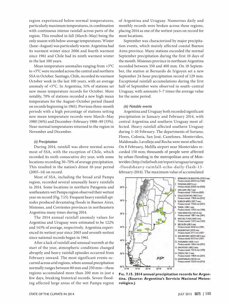
region experienced below-normal temperatures, particularly maximum temperatures, in combination with continuous intense rainfall across parts of the region. This resulted in fall (March–May) being the only season with below-average temperatures. Winter (June–August) was particularly warm: Argentina had its warmest winter since 2006 and fourth warmest since 1961 and Chile had its ninth warmest winter in the last 100 years.
Mean temperature anomalies ranging from +3°C to +5°C were recorded across the central and northern SSA in October. Santiago, Chile, recorded its warmest October week in the last 100 years, with an average anomaly of +5°C. In Argentina, 51% of stations set new mean temperature records for October. More notably, 70% of stations recorded a new high mean temperature for the August–October period (based on records beginning in 1961). Previous three-month periods with a high percentage of stations setting new mean temperature records were March–May 1980 (36%) and December–February 1988–89 (33%). Near-normal temperatures returned to the region in November and December.
(ii) PrecipitationDuring 2014, rainfall was above normal across
most of SSA, with the exception of Chile, which recorded its sixth consecutive dry year, with some locations recording 30–70% of average precipitation. This resulted in the nation’s driest 10-year period (2005–14) on record.
Most of SSA, including the broad arid Pampa region, recorded several unusually heavy rainfalls in 2014. Some locations in northern Patagonia and southeastern wet Pampa region observed their wettest year on record (Fig. 7.15). Frequent heavy rainfall epi-sodes produced devastating floods in Buenos Aires, Misiones, and Corrientes provinces in northeastern Argentina many times during 2014.
The 2014 annual rainfall anomaly values for Argentina and Uruguay were estimated to be 122% and 143% of average, respectively. Argentina experi-enced its wettest year since 2003 and seventh wettest since national records began in 1961.
After a lack of rainfall and unusual warmth at the start of the year, atmospheric conditions changed abruptly and heavy rainfall episodes occurred from February onward. The most significant events oc-curred across arid regions, where annual precipitation normally ranges between 80 mm and 250 mm—these regions accumulated more than 200 mm in just a few days, breaking historical records. Severe flood-ing affected large areas of the wet Pampa region
of Argentina and Uruguay. Numerous daily and monthly records were broken across these regions, placing 2014 as one of the wettest years on record for most locations.
September was characterized by major precipita-tion events, which mainly affected coastal Buenos Aires province. Many stations exceeded the normal September precipitation during the first 10 days of the month. Misiones province in northeast Argentina recorded between 350 and 400 mm. On 18 Septem-ber, the station at Bernardo de Irigoyen set a new September 24-hour precipitation record of 129 mm. Exceptional rainfall accumulations during the first half of September were observed in south–central Uruguay, with amounts 5–7 times the average value for the same period.
(iii) Notable eventsArgentina and Uruguay both recorded significant
precipitation in January and February 2014, with central Argentina and southern Uruguay most af-fected. Heavy rainfall affected southern Uruguay during 1–10 February. The departments of Soriano, Flores, Colonia, San José, Canelones, Montevideo, Maldonado, Lavalleja and Rocha were most affected. On 8 February, Melilla airport near Montevideo re-corded 150 mm; thousands of people were affected by urban flooding in the metropolitan area of Mon-tevideo (http://reliefweb.int/report/uruguay/uruguay -f loodsheav y-ra i n fa l l-echo-da i ly-f la sh-13- february-2014). The maximum value of accumulated
Fig. 7.15. 2014 annual precipitation records for Argen-tina. (Source: Argentina’s Servicio Nacional Meteo-rológico.)
S183JULY 2015STATE OF THE CLIMATE IN 2014 |
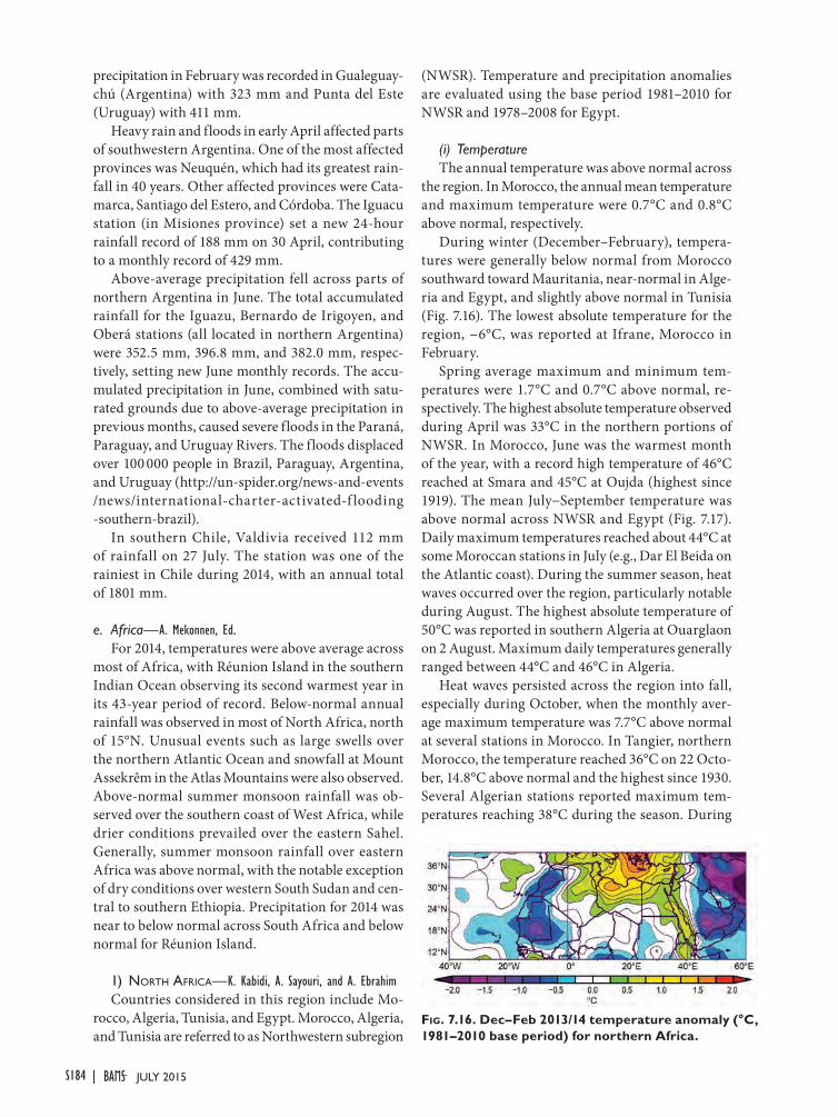
precipitation in February was recorded in Gualeguay-chú (Argentina) with 323 mm and Punta del Este (Uruguay) with 411 mm.
Heavy rain and floods in early April affected parts of southwestern Argentina. One of the most affected provinces was Neuquén, which had its greatest rain-fall in 40 years. Other affected provinces were Cata-marca, Santiago del Estero, and Córdoba. The Iguacu station (in Misiones province) set a new 24-hour rainfall record of 188 mm on 30 April, contributing to a monthly record of 429 mm.
Above-average precipitation fell across parts of northern Argentina in June. The total accumulated rainfall for the Iguazu, Bernardo de Irigoyen, and Oberá stations (all located in northern Argentina) were 352.5 mm, 396.8 mm, and 382.0 mm, respec-tively, setting new June monthly records. The accu-mulated precipitation in June, combined with satu-rated grounds due to above-average precipitation in previous months, caused severe floods in the Paraná, Paraguay, and Uruguay Rivers. The floods displaced over 100 000 people in Brazil, Paraguay, Argentina, and Uruguay (http://un-spider.org/news-and-events /news/international-charter-activated-f looding -southern-brazil).
In southern Chile, Valdivia received 112 mm of rainfall on 27 July. The station was one of the rainiest in Chile during 2014, with an annual total of 1801 mm.
e. Africa—A. Mekonnen, Ed.For 2014, temperatures were above average across
most of Africa, with Réunion Island in the southern Indian Ocean observing its second warmest year in its 43-year period of record. Below-normal annual rainfall was observed in most of North Africa, north of 15°N. Unusual events such as large swells over the northern Atlantic Ocean and snowfall at Mount Assekrêm in the Atlas Mountains were also observed. Above-normal summer monsoon rainfall was ob-served over the southern coast of West Africa, while drier conditions prevailed over the eastern Sahel. Generally, summer monsoon rainfall over eastern Africa was above normal, with the notable exception of dry conditions over western South Sudan and cen-tral to southern Ethiopia. Precipitation for 2014 was near to below normal across South Africa and below normal for Réunion Island.
1) north afriCa—K. Kabidi, A. Sayouri, and A. EbrahimCountries considered in this region include Mo-
rocco, Algeria, Tunisia, and Egypt. Morocco, Algeria, and Tunisia are referred to as Northwestern subregion
(NWSR). Temperature and precipitation anomalies are evaluated using the base period 1981–2010 for NWSR and 1978–2008 for Egypt.
(i) TemperatureThe annual temperature was above normal across
the region. In Morocco, the annual mean temperature and maximum temperature were 0.7°C and 0.8°C above normal, respectively.
During winter (December–February), tempera-tures were generally below normal from Morocco southward toward Mauritania, near-normal in Alge-ria and Egypt, and slightly above normal in Tunisia (Fig. 7.16). The lowest absolute temperature for the region, −6°C, was reported at Ifrane, Morocco in February.
Spring average maximum and minimum tem-peratures were 1.7°C and 0.7°C above normal, re-spectively. The highest absolute temperature observed during April was 33°C in the northern portions of NWSR. In Morocco, June was the warmest month of the year, with a record high temperature of 46°C reached at Smara and 45°C at Oujda (highest since 1919). The mean July−September temperature was above normal across NWSR and Egypt (Fig. 7.17). Daily maximum temperatures reached about 44°C at some Moroccan stations in July (e.g., Dar El Beida on the Atlantic coast). During the summer season, heat waves occurred over the region, particularly notable during August. The highest absolute temperature of 50°C was reported in southern Algeria at Ouarglaon on 2 August. Maximum daily temperatures generally ranged between 44°C and 46°C in Algeria.
Heat waves persisted across the region into fall, especially during October, when the monthly aver-age maximum temperature was 7.7°C above normal at several stations in Morocco. In Tangier, northern Morocco, the temperature reached 36°C on 22 Octo-ber, 14.8°C above normal and the highest since 1930. Several Algerian stations reported maximum tem-peratures reaching 38°C during the season. During
Fig. 7.16. Dec–Feb 2013/14 temperature anomaly (°C, 1981–2010 base period) for northern Africa.
S184 JULY 2015|
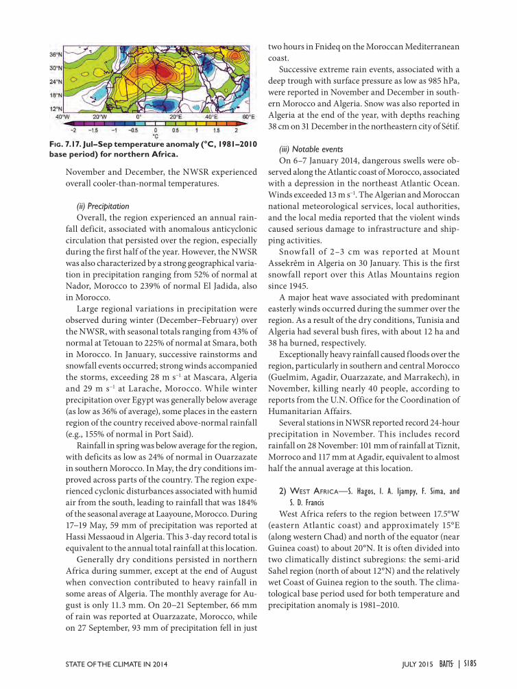
November and December, the NWSR experienced overall cooler-than-normal temperatures.
(ii) PrecipitationOverall, the region experienced an annual rain-
fall deficit, associated with anomalous anticyclonic circulation that persisted over the region, especially during the first half of the year. However, the NWSR was also characterized by a strong geographical varia-tion in precipitation ranging from 52% of normal at Nador, Morocco to 239% of normal El Jadida, also in Morocco.
Large regional variations in precipitation were observed during winter (December−February) over the NWSR, with seasonal totals ranging from 43% of normal at Tetouan to 225% of normal at Smara, both in Morocco. In January, successive rainstorms and snowfall events occurred; strong winds accompanied the storms, exceeding 28 m s−1 at Mascara, Algeria and 29 m s−1 at Larache, Morocco. While winter precipitation over Egypt was generally below average (as low as 36% of average), some places in the eastern region of the country received above-normal rainfall (e.g., 155% of normal in Port Said).
Rainfall in spring was below average for the region, with deficits as low as 24% of normal in Ouarzazate in southern Morocco. In May, the dry conditions im-proved across parts of the country. The region expe-rienced cyclonic disturbances associated with humid air from the south, leading to rainfall that was 184% of the seasonal average at Laayoune, Morocco. During 17−19 May, 59 mm of precipitation was reported at Hassi Messaoud in Algeria. This 3-day record total is equivalent to the annual total rainfall at this location.
Generally dry conditions persisted in northern Africa during summer, except at the end of August when convection contributed to heavy rainfall in some areas of Algeria. The monthly average for Au-gust is only 11.3 mm. On 20−21 September, 66 mm of rain was reported at Ouarzazate, Morocco, while on 27 September, 93 mm of precipitation fell in just
two hours in Fnideq on the Moroccan Mediterranean coast.
Successive extreme rain events, associated with a deep trough with surface pressure as low as 985 hPa, were reported in November and December in south-ern Morocco and Algeria. Snow was also reported in Algeria at the end of the year, with depths reaching 38 cm on 31 December in the northeastern city of Sétif.
(iii) Notable eventsOn 6–7 January 2014, dangerous swells were ob-
served along the Atlantic coast of Morocco, associated with a depression in the northeast Atlantic Ocean. Winds exceeded 13 m s−1. The Algerian and Moroccan national meteorological services, local authorities, and the local media reported that the violent winds caused serious damage to infrastructure and ship-ping activities.
Snowfall of 2–3 cm was reported at Mount Assekrêm in Algeria on 30 January. This is the first snowfall report over this Atlas Mountains region since 1945.
A major heat wave associated with predominant easterly winds occurred during the summer over the region. As a result of the dry conditions, Tunisia and Algeria had several bush fires, with about 12 ha and 38 ha burned, respectively.
Exceptionally heavy rainfall caused floods over the region, particularly in southern and central Morocco (Guelmim, Agadir, Ouarzazate, and Marrakech), in November, killing nearly 40 people, according to reports from the U.N. Office for the Coordination of Humanitarian Affairs.
Several stations in NWSR reported record 24-hour precipitation in November. This includes record rainfall on 28 November: 101 mm of rainfall at Tiznit, Morroco and 117 mm at Agadir, equivalent to almost half the annual average at this location.
2) WeSt afriCa—S. Hagos, I. A. Ijampy, F. Sima, and S. D. Francis
West Africa refers to the region between 17.5°W (eastern Atlantic coast) and approximately 15°E (along western Chad) and north of the equator (near Guinea coast) to about 20°N. It is often divided into two climatically distinct subregions: the semi-arid Sahel region (north of about 12°N) and the relatively wet Coast of Guinea region to the south. The clima-tological base period used for both temperature and precipitation anomaly is 1981–2010.
Fig. 7.17. Jul–Sep temperature anomaly (°C, 1981–2010 base period) for northern Africa.
S185JULY 2015STATE OF THE CLIMATE IN 2014 |
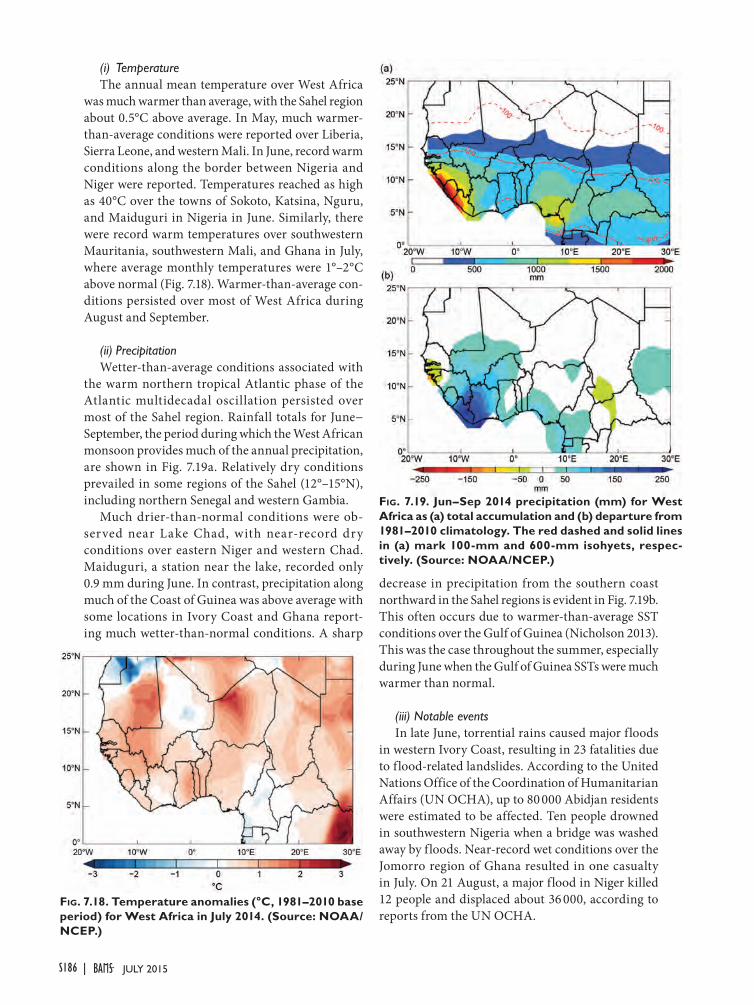
(i) Temperature The annual mean temperature over West Africa
was much warmer than average, with the Sahel region about 0.5°C above average. In May, much warmer-than-average conditions were reported over Liberia, Sierra Leone, and western Mali. In June, record warm conditions along the border between Nigeria and Niger were reported. Temperatures reached as high as 40°C over the towns of Sokoto, Katsina, Nguru, and Maiduguri in Nigeria in June. Similarly, there were record warm temperatures over southwestern Mauritania, southwestern Mali, and Ghana in July, where average monthly temperatures were 1°–2°C above normal (Fig. 7.18). Warmer-than-average con-ditions persisted over most of West Africa during August and September.
(ii) PrecipitationWetter-than-average conditions associated with
the warm northern tropical Atlantic phase of the Atlantic multidecadal oscillation persisted over most of the Sahel region. Rainfall totals for June− September, the period during which the West African monsoon provides much of the annual precipitation, are shown in Fig. 7.19a. Relatively dry conditions prevailed in some regions of the Sahel (12°–15°N), including northern Senegal and western Gambia.
Much drier-than-normal conditions were ob-served near Lake Chad, with near-record dry conditions over eastern Niger and western Chad. Maiduguri, a station near the lake, recorded only 0.9 mm during June. In contrast, precipitation along much of the Coast of Guinea was above average with some locations in Ivory Coast and Ghana report-ing much wetter-than-normal conditions. A sharp
decrease in precipitation from the southern coast northward in the Sahel regions is evident in Fig. 7.19b. This often occurs due to warmer-than-average SST conditions over the Gulf of Guinea (Nicholson 2013). This was the case throughout the summer, especially during June when the Gulf of Guinea SSTs were much warmer than normal.
(iii) Notable eventsIn late June, torrential rains caused major floods
in western Ivory Coast, resulting in 23 fatalities due to flood-related landslides. According to the United Nations Office of the Coordination of Humanitarian Affairs (UN OCHA), up to 80 000 Abidjan residents were estimated to be affected. Ten people drowned in southwestern Nigeria when a bridge was washed away by floods. Near-record wet conditions over the Jomorro region of Ghana resulted in one casualty in July. On 21 August, a major flood in Niger killed 12 people and displaced about 36 000, according to reports from the UN OCHA.
Fig. 7.18. Temperature anomalies (°C, 1981–2010 base period) for West Africa in July 2014. (Source: NOAA/NCEP.)
Fig. 7.19. Jun–Sep 2014 precipitation (mm) for West Africa as (a) total accumulation and (b) departure from 1981–2010 climatology. The red dashed and solid lines in (a) mark 100-mm and 600-mm isohyets, respec-tively. (Source: NOAA/NCEP.)
S186 JULY 2015|
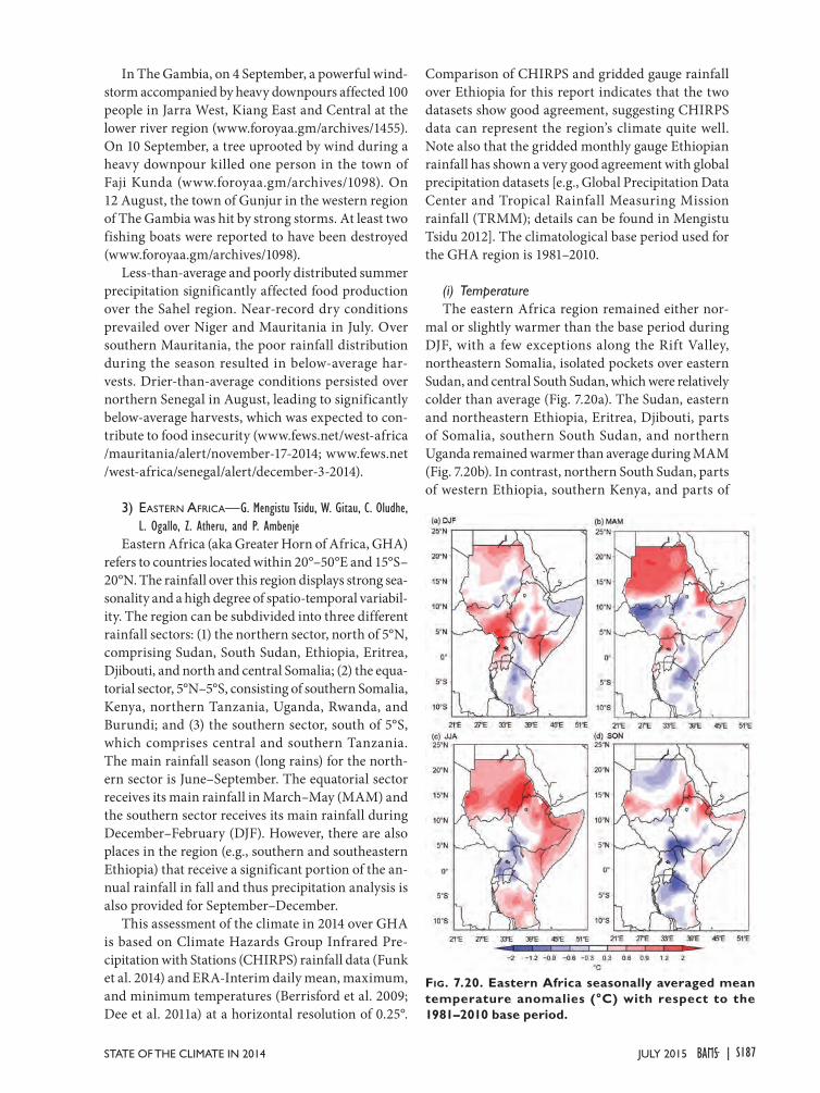
In The Gambia, on 4 September, a powerful wind-storm accompanied by heavy downpours affected 100 people in Jarra West, Kiang East and Central at the lower river region (www.foroyaa.gm/archives/1455). On 10 September, a tree uprooted by wind during a heavy downpour killed one person in the town of Faji Kunda (www.foroyaa.gm/archives/1098). On 12 August, the town of Gunjur in the western region of The Gambia was hit by strong storms. At least two fishing boats were reported to have been destroyed (www.foroyaa.gm/archives/1098).
Less-than-average and poorly distributed summer precipitation significantly affected food production over the Sahel region. Near-record dry conditions prevailed over Niger and Mauritania in July. Over southern Mauritania, the poor rainfall distribution during the season resulted in below-average har-vests. Drier-than-average conditions persisted over northern Senegal in August, leading to significantly below-average harvests, which was expected to con-tribute to food insecurity (www.fews.net/west-africa /mauritania/alert/november-17-2014; www.fews.net /west-africa/senegal/alert/december-3-2014).
3) eaStern afriCa—G. Mengistu Tsidu, W. Gitau, C. Oludhe, L. Ogallo, Z. Atheru, and P. Ambenje
Eastern Africa (aka Greater Horn of Africa, GHA) refers to countries located within 20°–50°E and 15°S–20°N. The rainfall over this region displays strong sea-sonality and a high degree of spatio-temporal variabil-ity. The region can be subdivided into three different rainfall sectors: (1) the northern sector, north of 5°N, comprising Sudan, South Sudan, Ethiopia, Eritrea, Djibouti, and north and central Somalia; (2) the equa-torial sector, 5°N–5°S, consisting of southern Somalia, Kenya, northern Tanzania, Uganda, Rwanda, and Burundi; and (3) the southern sector, south of 5°S, which comprises central and southern Tanzania. The main rainfall season (long rains) for the north-ern sector is June–September. The equatorial sector receives its main rainfall in March–May (MAM) and the southern sector receives its main rainfall during December–February (DJF). However, there are also places in the region (e.g., southern and southeastern Ethiopia) that receive a significant portion of the an-nual rainfall in fall and thus precipitation analysis is also provided for September–December.
This assessment of the climate in 2014 over GHA is based on Climate Hazards Group Infrared Pre-cipitation with Stations (CHIRPS) rainfall data (Funk et al. 2014) and ERA-Interim daily mean, maximum, and minimum temperatures (Berrisford et al. 2009; Dee et al. 2011a) at a horizontal resolution of 0.25°.
Comparison of CHIRPS and gridded gauge rainfall over Ethiopia for this report indicates that the two datasets show good agreement, suggesting CHIRPS data can represent the region’s climate quite well. Note also that the gridded monthly gauge Ethiopian rainfall has shown a very good agreement with global precipitation datasets [e.g., Global Precipitation Data Center and Tropical Rainfall Measuring Mission rainfall (TRMM); details can be found in Mengistu Tsidu 2012]. The climatological base period used for the GHA region is 1981–2010.
(i) Temperature The eastern Africa region remained either nor-
mal or slightly warmer than the base period during DJF, with a few exceptions along the Rift Valley, northeastern Somalia, isolated pockets over eastern Sudan, and central South Sudan, which were relatively colder than average (Fig. 7.20a). The Sudan, eastern and northeastern Ethiopia, Eritrea, Djibouti, parts of Somalia, southern South Sudan, and northern Uganda remained warmer than average during MAM (Fig. 7.20b). In contrast, northern South Sudan, parts of western Ethiopia, southern Kenya, and parts of
Fig. 7.20. Eastern Africa seasonally averaged mean temperature anomalies (°C) with respect to the 1981–2010 base period.
S187JULY 2015STATE OF THE CLIMATE IN 2014 |
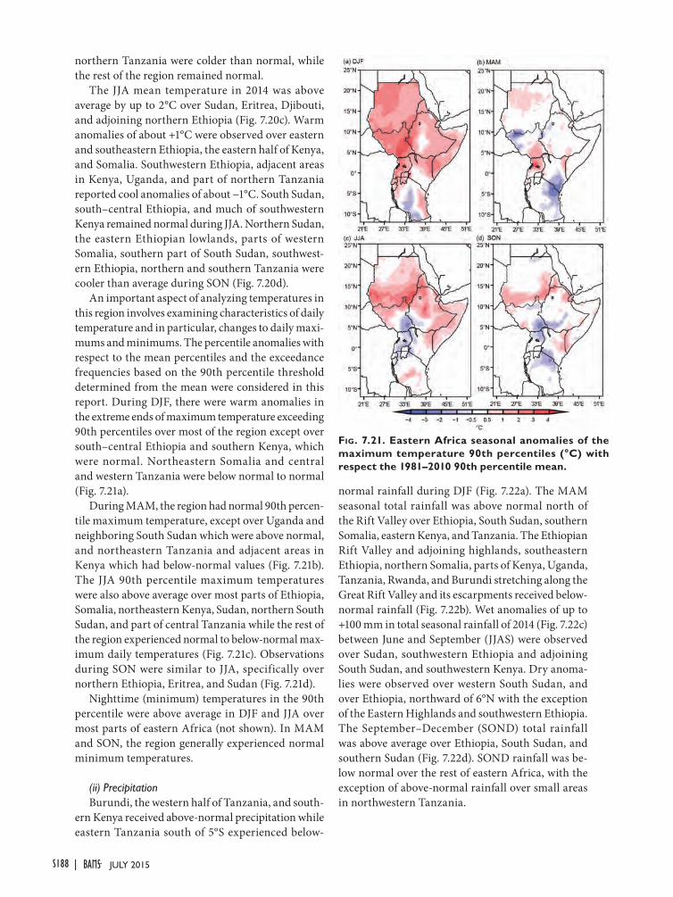
northern Tanzania were colder than normal, while the rest of the region remained normal.
The JJA mean temperature in 2014 was above average by up to 2°C over Sudan, Eritrea, Djibouti, and adjoining northern Ethiopia (Fig. 7.20c). Warm anomalies of about +1°C were observed over eastern and southeastern Ethiopia, the eastern half of Kenya, and Somalia. Southwestern Ethiopia, adjacent areas in Kenya, Uganda, and part of northern Tanzania reported cool anomalies of about −1°C. South Sudan, south–central Ethiopia, and much of southwestern Kenya remained normal during JJA. Northern Sudan, the eastern Ethiopian lowlands, parts of western Somalia, southern part of South Sudan, southwest-ern Ethiopia, northern and southern Tanzania were cooler than average during SON (Fig. 7.20d).
An important aspect of analyzing temperatures in this region involves examining characteristics of daily temperature and in particular, changes to daily maxi-mums and minimums. The percentile anomalies with respect to the mean percentiles and the exceedance frequencies based on the 90th percentile threshold determined from the mean were considered in this report. During DJF, there were warm anomalies in the extreme ends of maximum temperature exceeding 90th percentiles over most of the region except over south–central Ethiopia and southern Kenya, which were normal. Northeastern Somalia and central and western Tanzania were below normal to normal (Fig. 7.21a).
During MAM, the region had normal 90th percen-tile maximum temperature, except over Uganda and neighboring South Sudan which were above normal, and northeastern Tanzania and adjacent areas in Kenya which had below-normal values (Fig. 7.21b). The JJA 90th percentile maximum temperatures were also above average over most parts of Ethiopia, Somalia, northeastern Kenya, Sudan, northern South Sudan, and part of central Tanzania while the rest of the region experienced normal to below-normal max-imum daily temperatures (Fig. 7.21c). Observations during SON were similar to JJA, specifically over northern Ethiopia, Eritrea, and Sudan (Fig. 7.21d).
Nighttime (minimum) temperatures in the 90th percentile were above average in DJF and JJA over most parts of eastern Africa (not shown). In MAM and SON, the region generally experienced normal minimum temperatures.
(ii) PrecipitationBurundi, the western half of Tanzania, and south-
ern Kenya received above-normal precipitation while eastern Tanzania south of 5°S experienced below-
normal rainfall during DJF (Fig. 7.22a). The MAM seasonal total rainfall was above normal north of the Rift Valley over Ethiopia, South Sudan, southern Somalia, eastern Kenya, and Tanzania. The Ethiopian Rift Valley and adjoining highlands, southeastern Ethiopia, northern Somalia, parts of Kenya, Uganda, Tanzania, Rwanda, and Burundi stretching along the Great Rift Valley and its escarpments received below-normal rainfall (Fig. 7.22b). Wet anomalies of up to +100 mm in total seasonal rainfall of 2014 (Fig. 7.22c) between June and September (JJAS) were observed over Sudan, southwestern Ethiopia and adjoining South Sudan, and southwestern Kenya. Dry anoma-lies were observed over western South Sudan, and over Ethiopia, northward of 6°N with the exception of the Eastern Highlands and southwestern Ethiopia. The September–December (SOND) total rainfall was above average over Ethiopia, South Sudan, and southern Sudan (Fig. 7.22d). SOND rainfall was be-low normal over the rest of eastern Africa, with the exception of above-normal rainfall over small areas in northwestern Tanzania.
Fig. 7.21. Eastern Africa seasonal anomalies of the maximum temperature 90th percentiles (°C) with respect the 1981–2010 90th percentile mean.
S188 JULY 2015|
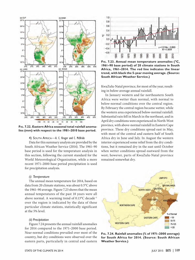
4) SoUth afriCa—A. C. Kruger and C. McBrideData for this summary analysis are provided by the
South African Weather Service (2014). The 1961–90 base period is used for the temperature analysis in this section, following the current standard for the World Meteorological Organization, while a more recent 1971–2000 base period precipitation is used for precipitation analysis.
(i) TemperatureThe annual mean temperature for 2014, based on
data from 20 climate stations, was about 0.5°C above the 1961–90 average. Figure 7.23 shows that the mean annual temperatures of the past 18 years were all above normal. A warming trend of 0.13°C decade−1 over the region is indicated by the data of these particular climate stations, statistically significant at the 5% level.
(ii) PrecipitationFigure 7.24 presents the annual rainfall anomalies
for 2014 compared to the 1971–2000 base period. Near-normal conditions prevailed over most of the country, but dry conditions were observed over the eastern parts, particularly in central and eastern
KwaZulu-Natal province, for most of the year, result-ing in below-average annual rainfall.
In January western and far northeastern South Africa were wetter than normal, with normal to below-normal conditions over the central region. By February the central region became wetter, while the western area experienced below-normal rainfall. Substantial rain fell in March in the northeast, and in April dry conditions were experienced in North-West province, with above-normal rainfall in Eastern Cape province. These dry conditions spread east in May, with most of the central and eastern half of South Africa dry in June and July. In August the western interior experienced some relief from the dry condi-tions, but it remained dry in the east until October when wetter conditions spread eastward from the west; however, parts of KwaZulu-Natal province remained somewhat dry.
Fig. 7.22. Eastern Africa seasonal total rainfall anoma-lies (mm) with respect to the 1981–2010 base period.
Fig. 7.23. Annual mean temperature anomalies (°C, 1961–90 base period) of 20 climate stations in South Africa, 1961–2014. The red line indicates the linear trend, with black the 5-year moving average. (Source: South African Weather Service.)
Fig. 7.24. Rainfall anomalies (% of 1971–2000 average) for South Africa for 2014. (Source: South African Weather Service.)
S189JULY 2015STATE OF THE CLIMATE IN 2014 |
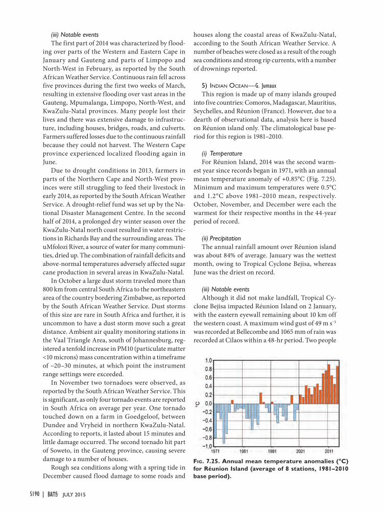
(iii) Notable eventsThe first part of 2014 was characterized by flood-
ing over parts of the Western and Eastern Cape in January and Gauteng and parts of Limpopo and North-West in February, as reported by the South African Weather Service. Continuous rain fell across five provinces during the first two weeks of March, resulting in extensive flooding over vast areas in the Gauteng, Mpumalanga, Limpopo, North-West, and KwaZulu-Natal provinces. Many people lost their lives and there was extensive damage to infrastruc-ture, including houses, bridges, roads, and culverts. Farmers suffered losses due to the continuous rainfall because they could not harvest. The Western Cape province experienced localized f looding again in June.
Due to drought conditions in 2013, farmers in parts of the Northern Cape and North-West prov-inces were still struggling to feed their livestock in early 2014, as reported by the South African Weather Service. A drought-relief fund was set up by the Na-tional Disaster Management Centre. In the second half of 2014, a prolonged dry winter season over the KwaZulu-Natal north coast resulted in water restric-tions in Richards Bay and the surrounding areas. The uMfolozi River, a source of water for many communi-ties, dried up. The combination of rainfall deficits and above-normal temperatures adversely affected sugar cane production in several areas in KwaZulu-Natal.
In October a large dust storm traveled more than 800 km from central South Africa to the northeastern area of the country bordering Zimbabwe, as reported by the South African Weather Service. Dust storms of this size are rare in South Africa and further, it is uncommon to have a dust storm move such a great distance. Ambient air quality monitoring stations in the Vaal Triangle Area, south of Johannesburg, reg-istered a tenfold increase in PM10 (particulate matter <10 microns) mass concentration within a timeframe of ~20–30 minutes, at which point the instrument range settings were exceeded.
In November two tornadoes were observed, as reported by the South African Weather Service. This is significant, as only four tornado events are reported in South Africa on average per year. One tornado touched down on a farm in Goedgeloof, between Dundee and Vryheid in northern KwaZulu-Natal. According to reports, it lasted about 15 minutes and little damage occurred. The second tornado hit part of Soweto, in the Gauteng province, causing severe damage to a number of houses.
Rough sea conditions along with a spring tide in December caused flood damage to some roads and
houses along the coastal areas of KwaZulu-Natal, according to the South African Weather Service. A number of beaches were closed as a result of the rough sea conditions and strong rip currents, with a number of drownings reported.
5) indian oCean—G. JumauxThis region is made up of many islands grouped
into five countries: Comoros, Madagascar, Mauritius, Seychelles, and Réunion (France). However, due to a dearth of observational data, analysis here is based on Réunion island only. The climatological base pe-riod for this region is 1981–2010.
(i) TemperatureFor Réunion Island, 2014 was the second warm-
est year since records began in 1971, with an annual mean temperature anomaly of +0.85°C (Fig. 7.25). Minimum and maximum temperatures were 0.5°C and 1.2°C above 1981–2010 mean, respectively. October, November, and December were each the warmest for their respective months in the 44-year period of record.
(ii) PrecipitationThe annual rainfall amount over Réunion island
was about 84% of average. January was the wettest month, owing to Tropical Cyclone Bejisa, whereas June was the driest on record.
(iii) Notable eventsAlthough it did not make landfall, Tropical Cy-
clone Bejisa impacted Réunion Island on 2 January, with the eastern eyewall remaining about 10 km off the western coast. A maximum wind gust of 49 m s−1 was recorded at Bellecombe and 1065 mm of rain was recorded at Cilaos within a 48-hr period. Two people
Fig. 7.25. Annual mean temperature anomalies (°C) for Réunion Island (average of 8 stations, 1981–2010 base period).
S190 JULY 2015|
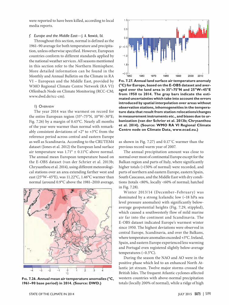
were reported to have been killed, according to local media reports.
f. Europe and the Middle East—J. A. Renwick, Ed.Throughout this section, normal is defined as the
1961–90 average for both temperature and precipita-tion, unless otherwise specified. However, European countries conform to different standards applied by the national weather services. All seasons mentioned in this section refer to the Northern Hemisphere. More detailed information can be found in the Monthly and Annual Bulletin on the Climate in RA VI – European and the Middle East, provided by WMO Regional Climate Centre Network (RA VI) Offenbach Node on Climate Monitoring (RCC-CM; www.dwd.de/rcc-cm).
1) overvieW
The year 2014 was the warmest on record for the entire European region (35°–75°N, 10°W–30°E; Fig. 7.26) by a margin of 0.43°C. Nearly all months of the year were warmer than normal with remark-ably consistent deviations of +2° to +3°C from the reference period across central and eastern Europe as well as Scandinavia. According to the CRUTEM4 dataset (Jones et al. 2012) the European land surface air temperature was 1.71° ± 0.11°C above normal. The annual mean European temperature based on the E-OBS dataset (van der Schrier et al. 2013b; Chrysanthou et al. 2014), using different meteorologi-cal stations over an area extending farther west and east (25°W–45°E), was 11.22°C, 1.46°C warmer than normal (around 0.9°C above the 1981–2010 average,
as shown in Fig. 7.27) and 0.17˚C warmer than the previous record warm year of 2007.
The annual precipitation amount was close to normal over most of continental Europe except for the Balkan region and parts of Italy, where significantly higher totals (>150% of normal) were recorded, and parts of northern and eastern Europe, eastern Spain, South Caucasus, and the Middle East with dry condi-tions (totals <80%, locally <60% of normal; hatched in Fig. 7.28).
Winter 2013/14 (December–February) was dominated by a strong Icelandic low (−18 hPa sea level pressure anomalies) with significantly below-average geopotential heights (Fig. 7.29, stippled), which caused a southwesterly f low of mild marine air far into the continent and Scandinavia. The E-OBS dataset indicated Europe’s warmest winter since 1950. The highest deviations were observed in central Europe, Scandinavia, and over the Balkans, where temperature anomalies exceeded +3°C. Ireland, Spain, and eastern Europe experienced less warming and Portugal even registered slightly below-average temperatures (−0.5°C).
During the season the NAO and AO were in the positive phase which led to an enhanced North At-lantic jet stream. Twelve major storms crossed the British Isles. The frequent Atlantic cyclones affected western countries with above-normal precipitation totals (locally 200% of normal), while a ridge of high
Fig. 7.26. Annual mean air temperature anomalies (°C, 1961–90 base period) in 2014. (Source: DWD.)
Fig. 7.27. Annual land surface air temperature anomaly (°C) for Europe, based on the E-OBS dataset and aver-aged over the land area in 35°–75°N and 25°W–45°E from 1950 to 2014. The gray bars indicate the esti-mated uncertainties which take into account the errors introduced by spatial interpolation over areas without observation stations, inhomogeneities in the tempera-ture data that result from station relocations/changes in measurement instruments etc., and biases due to ur-banization (van der Schrier et al. 2013b; Chrysanthou et al. 2014). (Source: WMO RA VI Regional Climate Centre node on Climate Data, www.ecad.eu.)
S191JULY 2015STATE OF THE CLIMATE IN 2014 |
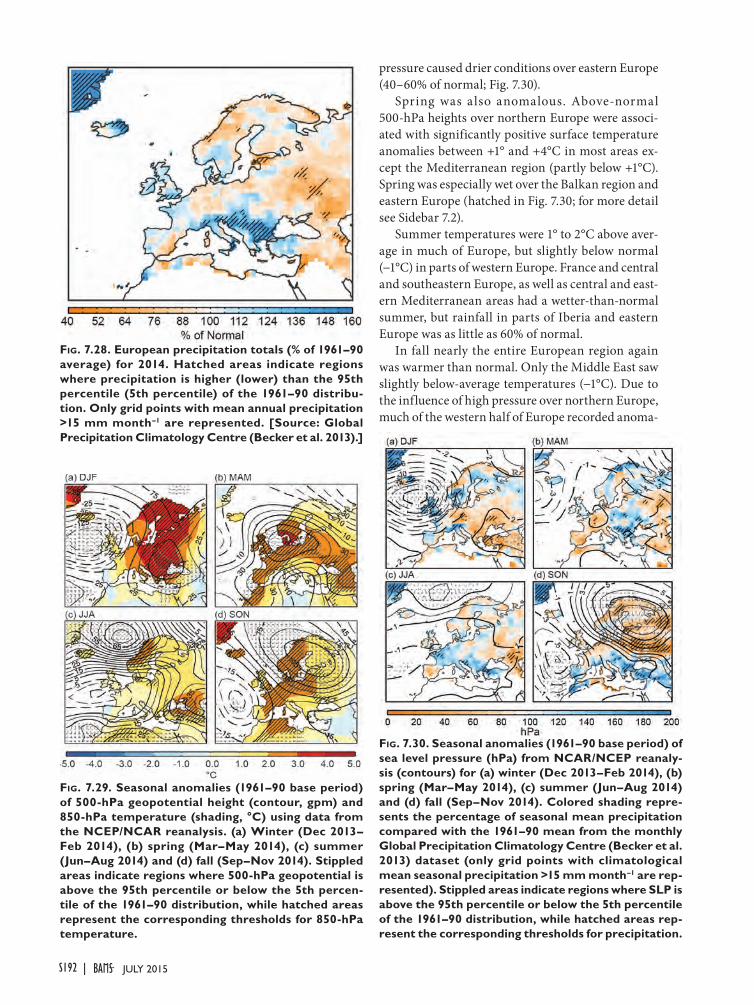
pressure caused drier conditions over eastern Europe (40–60% of normal; Fig. 7.30).
Spring was also anomalous. Above-normal 500-hPa heights over northern Europe were associ-ated with significantly positive surface temperature anomalies between +1° and +4°C in most areas ex-cept the Mediterranean region (partly below +1°C). Spring was especially wet over the Balkan region and eastern Europe (hatched in Fig. 7.30; for more detail see Sidebar 7.2).
Summer temperatures were 1° to 2°C above aver-age in much of Europe, but slightly below normal (−1°C) in parts of western Europe. France and central and southeastern Europe, as well as central and east-ern Mediterranean areas had a wetter-than-normal summer, but rainfall in parts of Iberia and eastern Europe was as little as 60% of normal.
In fall nearly the entire European region again was warmer than normal. Only the Middle East saw slightly below-average temperatures (−1°C). Due to the influence of high pressure over northern Europe, much of the western half of Europe recorded anoma-
Fig. 7.28. European precipitation totals (% of 1961–90 average) for 2014. Hatched areas indicate regions where precipitation is higher (lower) than the 95th percentile (5th percentile) of the 1961–90 distribu-tion. Only grid points with mean annual precipitation >15 mm month–1 are represented. [Source: Global Precipitation Climatology Centre (Becker et al. 2013).]
Fig. 7.29. Seasonal anomalies (1961–90 base period) of 500-hPa geopotential height (contour, gpm) and 850-hPa temperature (shading, °C) using data from the NCEP/NCAR reanalysis. (a) Winter (Dec 2013–Feb 2014), (b) spring (Mar–May 2014), (c) summer (Jun–Aug 2014) and (d) fall (Sep–Nov 2014). Stippled areas indicate regions where 500-hPa geopotential is above the 95th percentile or below the 5th percen-tile of the 1961–90 distribution, while hatched areas represent the corresponding thresholds for 850-hPa temperature.
Fig. 7.30. Seasonal anomalies (1961–90 base period) of sea level pressure (hPa) from NCAR/NCEP reanaly-sis (contours) for (a) winter (Dec 2013–Feb 2014), (b) spring (Mar–May 2014), (c) summer (Jun–Aug 2014) and (d) fall (Sep–Nov 2014). Colored shading repre-sents the percentage of seasonal mean precipitation compared with the 1961–90 mean from the monthly Global Precipitation Climatology Centre (Becker et al. 2013) dataset (only grid points with climatological mean seasonal precipitation >15 mm month–1 are rep-resented). Stippled areas indicate regions where SLP is above the 95th percentile or below the 5th percentile of the 1961–90 distribution, while hatched areas rep-resent the corresponding thresholds for precipitation.
S192 JULY 2015|
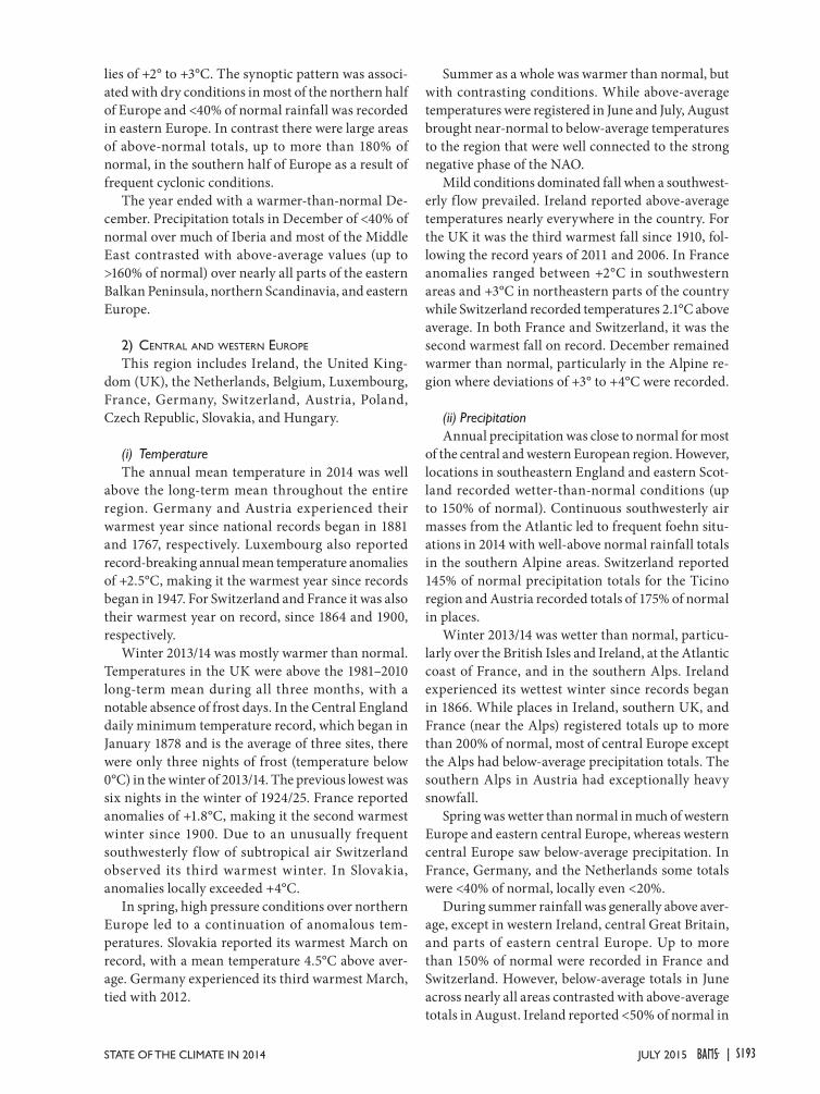
lies of +2° to +3°C. The synoptic pattern was associ-ated with dry conditions in most of the northern half of Europe and <40% of normal rainfall was recorded in eastern Europe. In contrast there were large areas of above-normal totals, up to more than 180% of normal, in the southern half of Europe as a result of frequent cyclonic conditions.
The year ended with a warmer-than-normal De-cember. Precipitation totals in December of <40% of normal over much of Iberia and most of the Middle East contrasted with above-average values (up to >160% of normal) over nearly all parts of the eastern Balkan Peninsula, northern Scandinavia, and eastern Europe.
2) Central and WeStern eUrope
This region includes Ireland, the United King-dom (UK), the Netherlands, Belgium, Luxembourg, France, Germany, Switzerland, Austria, Poland, Czech Republic, Slovakia, and Hungary.
(i) TemperatureThe annual mean temperature in 2014 was well
above the long-term mean throughout the entire region. Germany and Austria experienced their warmest year since national records began in 1881 and 1767, respectively. Luxembourg also reported record-breaking annual mean temperature anomalies of +2.5°C, making it the warmest year since records began in 1947. For Switzerland and France it was also their warmest year on record, since 1864 and 1900, respectively.
Winter 2013/14 was mostly warmer than normal. Temperatures in the UK were above the 1981–2010 long-term mean during all three months, with a notable absence of frost days. In the Central England daily minimum temperature record, which began in January 1878 and is the average of three sites, there were only three nights of frost (temperature below 0°C) in the winter of 2013/14. The previous lowest was six nights in the winter of 1924/25. France reported anomalies of +1.8°C, making it the second warmest winter since 1900. Due to an unusually frequent southwesterly f low of subtropical air Switzerland observed its third warmest winter. In Slovakia, anomalies locally exceeded +4°C.
In spring, high pressure conditions over northern Europe led to a continuation of anomalous tem-peratures. Slovakia reported its warmest March on record, with a mean temperature 4.5°C above aver-age. Germany experienced its third warmest March, tied with 2012.
Summer as a whole was warmer than normal, but with contrasting conditions. While above-average temperatures were registered in June and July, August brought near-normal to below-average temperatures to the region that were well connected to the strong negative phase of the NAO.
Mild conditions dominated fall when a southwest-erly flow prevailed. Ireland reported above-average temperatures nearly everywhere in the country. For the UK it was the third warmest fall since 1910, fol-lowing the record years of 2011 and 2006. In France anomalies ranged between +2°C in southwestern areas and +3°C in northeastern parts of the country while Switzerland recorded temperatures 2.1°C above average. In both France and Switzerland, it was the second warmest fall on record. December remained warmer than normal, particularly in the Alpine re-gion where deviations of +3° to +4°C were recorded.
(ii) PrecipitationAnnual precipitation was close to normal for most
of the central and western European region. However, locations in southeastern England and eastern Scot-land recorded wetter-than-normal conditions (up to 150% of normal). Continuous southwesterly air masses from the Atlantic led to frequent foehn situ-ations in 2014 with well-above normal rainfall totals in the southern Alpine areas. Switzerland reported 145% of normal precipitation totals for the Ticino region and Austria recorded totals of 175% of normal in places.
Winter 2013/14 was wetter than normal, particu-larly over the British Isles and Ireland, at the Atlantic coast of France, and in the southern Alps. Ireland experienced its wettest winter since records began in 1866. While places in Ireland, southern UK, and France (near the Alps) registered totals up to more than 200% of normal, most of central Europe except the Alps had below-average precipitation totals. The southern Alps in Austria had exceptionally heavy snowfall.
Spring was wetter than normal in much of western Europe and eastern central Europe, whereas western central Europe saw below-average precipitation. In France, Germany, and the Netherlands some totals were <40% of normal, locally even <20%.
During summer rainfall was generally above aver-age, except in western Ireland, central Great Britain, and parts of eastern central Europe. Up to more than 150% of normal were recorded in France and Switzerland. However, below-average totals in June across nearly all areas contrasted with above-average totals in August. Ireland reported <50% of normal in
S193JULY 2015STATE OF THE CLIMATE IN 2014 |
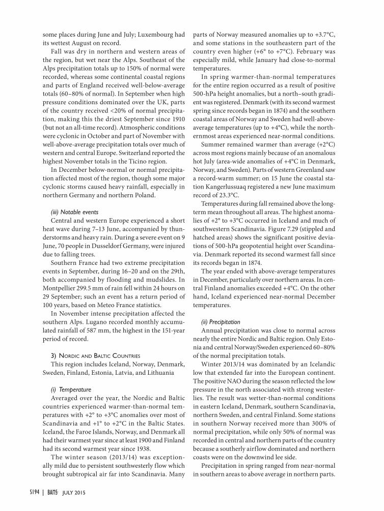
some places during June and July; Luxembourg had its wettest August on record.
Fall was dry in northern and western areas of the region, but wet near the Alps. Southeast of the Alps precipitation totals up to 150% of normal were recorded, whereas some continental coastal regions and parts of England received well-below-average totals (60–80% of normal). In September when high pressure conditions dominated over the UK, parts of the country received <20% of normal precipita-tion, making this the driest September since 1910 (but not an all-time record). Atmospheric conditions were cyclonic in October and part of November with well-above-average precipitation totals over much of western and central Europe. Switzerland reported the highest November totals in the Ticino region.
In December below-normal or normal precipita-tion affected most of the region, though some major cyclonic storms caused heavy rainfall, especially in northern Germany and northern Poland.
(iii) Notable eventsCentral and western Europe experienced a short
heat wave during 7–13 June, accompanied by thun-derstorms and heavy rain. During a severe event on 9 June, 70 people in Dusseldorf Germany, were injured due to falling trees.
Southern France had two extreme precipitation events in September, during 16–20 and on the 29th, both accompanied by f looding and mudslides. In Montpellier 299.5 mm of rain fell within 24 hours on 29 September; such an event has a return period of 100 years, based on Meteo France statistics.
In November intense precipitation affected the southern Alps. Lugano recorded monthly accumu-lated rainfall of 587 mm, the highest in the 151-year period of record.
3) nordiC and baltiC CoUntrieS
This region includes Iceland, Norway, Denmark, Sweden, Finland, Estonia, Latvia, and Lithuania
(i) Temperature Averaged over the year, the Nordic and Baltic
countries experienced warmer-than-normal tem-peratures with +2° to +3°C anomalies over most of Scandinavia and +1° to +2°C in the Baltic States. Iceland, the Faroe Islands, Norway, and Denmark all had their warmest year since at least 1900 and Finland had its second warmest year since 1938.
The winter season (2013/14) was exception-ally mild due to persistent southwesterly flow which brought subtropical air far into Scandinavia. Many
parts of Norway measured anomalies up to +3.7°C, and some stations in the southeastern part of the country even higher (+6° to +7°C). February was especially mild, while January had close-to-normal temperatures.
In spring warmer-than-normal temperatures for the entire region occurred as a result of positive 500-hPa height anomalies, but a north–south gradi-ent was registered. Denmark (with its second warmest spring since records began in 1874) and the southern coastal areas of Norway and Sweden had well-above-average temperatures (up to +4°C), while the north-ernmost areas experienced near-normal conditions.
Summer remained warmer than average (+2°C) across most regions mainly because of an anomalous hot July (area-wide anomalies of +4°C in Denmark, Norway, and Sweden). Parts of western Greenland saw a record-warm summer; on 15 June the coastal sta-tion Kangerlussuaq registered a new June maximum record of 23.3°C.
Temperatures during fall remained above the long-term mean throughout all areas. The highest anoma-lies of +2° to +3°C occurred in Iceland and much of southwestern Scandinavia. Figure 7.29 (stippled and hatched areas) shows the significant positive devia-tions of 500-hPa geopotential height over Scandina-via. Denmark reported its second warmest fall since its records began in 1874.
The year ended with above-average temperatures in December, particularly over northern areas. In cen-tral Finland anomalies exceeded +4°C. On the other hand, Iceland experienced near-normal December temperatures.
(ii) PrecipitationAnnual precipitation was close to normal across
nearly the entire Nordic and Baltic region. Only Esto-nia and central Norway/Sweden experienced 60–80% of the normal precipitation totals.
Winter 2013/14 was dominated by an Icelandic low that extended far into the European continent. The positive NAO during the season reflected the low pressure in the north associated with strong wester-lies. The result was wetter-than-normal conditions in eastern Iceland, Denmark, southern Scandinavia, northern Sweden, and central Finland. Some stations in southern Norway received more than 300% of normal precipitation, while only 50% of normal was recorded in central and northern parts of the country because a southerly airflow dominated and northern coasts were on the downwind lee side.
Precipitation in spring ranged from near-normal in southern areas to above average in northern parts.
S194 JULY 2015|
Some stations in northern Norway recorded 200% of their normal rainfall totals.
During summer most regions received near-normal totals, except northern Norway and central Sweden where 60–80% of normal were registered. In August the NAO was negative and strongly con-nected to the well-above-average rain in southern and eastern areas. Lithuania and Denmark each received totals up to 250% of normal and some places in southwestern Sweden recorded up to 300% of normal.
A mostly drier-than-normal fall followed as a result of a persistent blocking ridge centered over Scandinavia. Figure 7.30 (hatched) shows the signifi-cant positive sea level pressure anomalies of +8 hPa accompanied by the significant below-average pre-cipitation totals. Estonia registered only 20–40% of its normal precipitation during the season.
In December totals were close to normal in the Baltic States. Wetter conditions in northern Scandi-navia and Denmark contrasted with drier conditions in southeastern Norway and southern Sweden in between.
(iii) Notable eventsIn March Norway and Sweden were hit by two
storms within a few days, on 8 March and 11 March, with wind gusts of 38 m s−1 and 44.8 m s−1, respec-tively. The storms brought high tides; the highest wave height of 11.6 m was observed on 9 March in Finnmark, northern Norway.
In summer Finland experienced an exceptionally long heat wave. The country recorded daily maximum temperatures >25°C at one or more stations on 38 days and >30°C on 22 days. This tied 2014 with 1973 for the largest number of such warm days since records began in 1961.
In conjunction with the dry fall, Sweden experi-enced its sunniest September on record, with 243 sun-shine hours observed in southern and central Sweden.
Although fall as a whole was drier than normal, Denmark did record some intense precipitation events: on 15–16 October Lendum, East-Jutland measured 150 mm rain within 32 hours and on 3 November Hvide Sande, Denmark reported 17.7 mm within 30 minutes.
4) iberian peninSUla
This region includes Spain and Portugal. Unless otherwise noted, anomalies refer to a reference period of 1971–2000 in this subsection.
(i) TemperatureThe Iberian Peninsula recorded above-average
annual mean temperatures with mean deviations of +0.54°C in Portugal and +1.33°C in Spain, mostly due to warmer-than-average spring and fall seasons.
Winter 2013/14 over the Iberian Peninsula was only slightly warmer than normal. Positive tempera-ture anomalies of +0.6°C in Portugal and +0.4°C in Spain were mainly due to warmer-than-average temperatures in January and February.
During spring the Iberian Peninsula was warmer than average with anomalies of +1.3°C in Portugal (ninth warmest since records began in 1931) and +1.9°C in Spain (fourth warmest since records be-gan in 1961). During spring the European continent was affected by above-average values of 500-hPa geopotential height (stippled in Fig. 7.29), a pattern often associated with blocking anticyclones over the UK and Scandinavia. This synoptic pattern induced high temperature anomalies over most of the conti-nent, including values above the 95th percentile of the long-term distribution in the Iberian Peninsula (hatched in Fig. 7.29).
The summer mean temperature over the Iberian Peninsula was near-average, with an east–west gra-dient from a slightly negative anomaly in Portugal (−0.4°C) to a positive anomaly in Spain (+0.6°C). The relatively cool summer over Portugal was re-flected in the small number of days with maximum temperature above 30°C and, for the first time since 1996, maximum temperatures above 40°C were not recorded during summer.
The mean temperatures over the Iberian Peninsula in fall were well above normal, particularly in the east. For Portugal, the mean temperature anomaly was +1.4°C, the sixth warmest fall since 1931, while the corresponding minimum temperature was 3°C above normal and the third highest since 1931. In Spain the mean temperature anomaly was +2.3°C. October was record warm in both countries for the month: +2.7°C in Portugal and +3.3°C in Spain.
December was colder than average in Iberia, with negative anomalies particularly notable over Portugal (−1.4°C) but also over Spain (−0.2°C).
(ii) PrecipitationAnnual mean precipitation for the entire Iberian
Peninsula was above normal as a consequence of the wet winter and fall. Spatial mean annual rainfall was ~680 mm in Spain and ~1100 mm in Portugal, 5% and 24% above normal, respectively, in large part due to a wet fall in western Iberia.
S195JULY 2015STATE OF THE CLIMATE IN 2014 |
The mean winter (2013/14) precipitation over the Iberian Peninsula was above average throughout the territory, with the exception of southern Portugal and the Mediterranean coastal region in Spain. Mean seasonal accumulated rainfall for Portugal (Spain) was around 140% (120%) of normal. The North Atlantic storm track was particularly active during winter, with negative sea level pressure anomalies in the winter months (stippled Fig. 7.30) near the British Isles (below the 5th percentile).
In spring, the mean precipitation in Portugal was 90% of normal and 75% of normal in Spain. The summer precipitation was near-average in Portugal, while it was 88% of normal in Spain.
In fall, the mean precipitation on the Iberian Pen-insula was well above average, with roughly 180% of normal precipitation in Portugal and a spatial mean of 449 mm. Spain received 140% of normal with a spatial mean of 255 mm. This wetter-than-average period is well connected to the larger-scale atmospheric circulation with statistically significant negative sea level pressure anomalies (−4 hPa and below the 5th percentile) west of the Iberian Peninsula (stippled in Fig. 7.30).
December 2014 was dry: in Spain, the spatial mean was only 40 mm, about half of normal, and Portugal received only 20% of its normal precipitation. In Por-tugal, this marked the driest December in the last 26 years and the fifth driest on record. In Spain, it was the fourth driest December since 1980.
(iii) Notable eventsIn January and February the western and northern
coasts of the Iberian Peninsula were affected by high swell waves and strong winds associated with the frequent passage of deep low pressure systems in the North Atlantic storm track. Two storms had major impacts on western Iberia: (1) in the first week of January extreme winds generated high waves, with maximum heights of 13.5 m at Leixões (northern coast) and 15 m at Sines (southern coast); (2) on 9 February, a storm developed explosively, the central pressure falling ~29 hPa in 24 hours, and affected the western and northern coast of the Iberian Peninsula with winds higher than 33 m s−1. Again, high waves were recorded at Leixões (12.5 m) and Sines (17 m) with a period of 10 seconds.
Between 11 and 17 June the southern Iberian Pen-insula experienced a heat wave, with temperatures >40°C in southern Spain on 13 and 14 June.
In September, unusually intense precipitation fell in Portugal with some locations recording monthly totals up to eight times higher than their 1971–2000
average. In particular, a new September precipita-tion maximum record of 146.9 mm was set for the Lisbon region.
On 19 October an intense precipitation event oc-curred in Islas Canarias where Santa Cruz de Tenerife recorded a daily accumulation of 125.8 mm, with 102.8 mm in a single hour.
5) Mediterranean, italy, and balkan StateS
This region includes Italy, Malta, Slovenia, Croa-tia, Serbia, Montenegro, Bosnia and Herzegovina, Albania, Macedonia, Greece, Bulgaria, and Turkey.
(i) TemperatureThe annual temperature anomalies in 2014 ranged
from +1°C in areas along the southern Adriatic coast and across Greece and western Turkey to +3°C farther north in the Alpine region. Italy reported its warmest year on record for the last 200 years. Turkey recorded an annual temperature 1.4°C above the 1981–2010 ref-erence period, its second warmest since records began in 1971, and Croatia experienced an extremely warm year with anomalies ranging from +1.1° to +2.5°C.
Winter 2013/14 was dominated by significant positive anomalies of 500-hPa geopotential heights (hatched in Fig. 7.29). Temperature anomalies associ-ated with synoptic conditions ranging from near-zero in eastern Turkey to more than +6°C in southwestern parts of Serbia. February was the primary contributor to the unusual seasonal conditions. Only easternmost Turkey observed below-average values (−0.3°C) as it was affected by polar air masses moving from the northeast.
In spring temperatures were warmer than the long-term mean (up to +3°C in eastern Turkey). Notably, in March above-average values were a result of a high pressure ridge over Europe during the first half of the month. In eastern Turkey March anomalies exceeded +4°C.
During summer, temperatures were mixed across the region, higher than normal in the east (2°−3°C above normal in central Turkey) but lower than nor-mal along the Adriatic coast, in Italy and farther west.
The anomalous warmer temperatures continued during fall in most areas except eastern and southern Turkey. Due to high pressure over northern Europe, polar air masses were transported to the south and slightly colder-than-normal values were recorded in Turkey (anomalies down to −1°C). On the other hand, northern Italy, Sardinia, and Sicily observed temperatures anomalies of +2° to +3°C owing to a southwesterly flow of tropical air masses.
S196 JULY 2015|
December had area-wide positive anomalies; the greatest deviations occurred in the Alpine region and across Turkey (up to more than +4°C).
(ii) PrecipitationAnnual precipitation was mostly close to normal,
except for the Balkans, southern Italy, and the south-ern Alpine region. More than 150% of normal totals were recorded in these regions. Croatia reported precipitation up to 175% of normal, making 2014 an extremely wet year for the country.
During winter 2013/14 the Balkan Peninsula and Turkey were affected by above-average sea level pressure that led to drier-than-normal conditions (40–60% of normal). In contrast the southern Alpine region experienced frequent topographically induced precipitation mainly during January and February; seasonal totals were well above average (200% of normal).
Spring was exceptionally wet in the Balkan coun-tries and southern Italy, but drier than average in the Alpine region and eastern Turkey (locally 40–60% of normal). Most of the Balkan States received anoma-lous rainfalls up to 250% of normal (see Sidebar 7.2).
Summer was wetter than normal in most areas except southernmost Italy and eastern Turkey (where totals as low as 40% of normal were recorded). The highest precipitation was measured in the Bosporus area, up to 200% of normal. The season was domi-nated by below-average sea level pressure associated with repeated westerlies that brought Atlantic cy-clones into the area.
Precipitation totals in fall were below average in some western parts of the region (Corsica, Sicily, central Italy), while the Balkan States and Turkey experienced an exceptionally wet season; more than 180% of normal precipitation was recorded in places. These conditions continued in December 2014, though eastern Turkey became drier.
(iii) Notable eventsAlthough winter as a whole was drier than nor-
mal over the Balkans, during 18–20 January Slo-venia reported heavy rainfall, with 3-day totals of 70–200 mm. On 4−5 January extremely heavy rain in Slovenia brought 48-hour totals of 80–261 mm at various locations, with damage affecting 20% of the country. During 30 January to 3 February Slovenia once again received extremely heavy rain, recording 130–400 mm accumulation over this period. Roma-nia, Croatia, and Montenegro were also affected and reported damage.
Unusual lightning activity (21 recorded events) was reported in Turkey during 23–29 May, 24 July, and 4–11 August. Eleven people lost their lives and 28 were injured.
On 15–16 June record-breaking rainfall with daily totals of 94.4 mm caused severe flooding in north–central regions of Italy.
On 19 June Varna, Bulgaria was flooded as a re-sult of precipitation totals exceeding 50 mm during 14–19 June.
In September Italy was affected by frequent thunderstorms and heavy convective precipitation. The country reported a record-breaking monthly rainfall total of 479.3 mm along the Adriatic coast and a record-breaking daily total of 167.2 mm there on 3 September.
6) eaStern eUrope
This region includes the European part of Russia, Belarus, Ukraine, Moldova, and Romania.
(i) TemperatureThe annual mean temperature anomalies across
eastern Europe in 2014 show a zonal gradient with warmer-than-normal conditions of up to +3°C in western areas and near-normal values in the east.
Winter 2013/14 was 1°–4°C above normal with the exception of easternmost European Russia where it was near-normal. In February, western areas had temperature deviations of more than +4°C, with Be-larus reporting anomalies of +4° to +6°C, while well-below-average values down to −4°C were observed in northeastern European Russia.
During spring widespread anomalous warmth af-fected eastern Europe. The highest positive anomalies occurred in Belarus, northern Ukraine, and western-most Russia (+3° to +4°C). March was exceptionally warm, more than 4°C above average in most of the region. Belarus experienced its second warmest March in more than 100 years.
Temperatures in summer remained warmer than normal, up to +2° to +3°C in the Caucasus region, due to the influence of high pressure. Both the 500-hPa geopotential heights and the 850-hPa temperatures had significant positive anomalies (Fig. 7.29, stippled and hatched areas). In July a blocking pattern ex-tended from the eastern North Atlantic to central Russia. The synoptic circulation induced tempera-tures up to 4°C below average over eastern European Russia, whereas the Ukraine and Belarus experienced anomalies of +2°C to +4°C.
Fall was characterized by significantly above-average 500-hPa heights over northern Europe that
S197JULY 2015STATE OF THE CLIMATE IN 2014 |
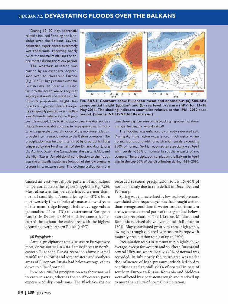
caused an east–west dipole pattern of anomalous temperatures across the region (stippled in Fig. 7.29). Most of eastern Europe experienced warmer-than-normal conditions (anomalies up to +2°C), but a northwesterly flow of polar air masses downstream of the mean ridge brought below-average values (anomalies −1° to −2°C) to easternmost European Russia. In December 2014 positive anomalies oc-curred throughout the entire area with the highest occurring over northern Russia (+4°C).
(ii) PrecipitationAnnual precipitation totals in eastern Europe were
mostly near-normal in 2014. Limited areas in north-eastern European Russia recorded above-normal rainfall (up to 150%) and some western and southern areas of European Russia had below-average values down to 60% of normal.
In winter 2013/14 precipitation was above normal in eastern areas, whereas the southwestern parts experienced dry conditions. The Black Sea region
recorded seasonal precipitation totals 40–60% of normal, mainly due to rain deficit in December and February.
Spring was characterized by low sea level pressure associated with frequent cyclones that brought wetter-than-average conditions to western and northeastern areas, whereas central parts of the region had below-average precipitation. The Ukraine, Moldova, and Romania received above-average rainfall of up to 150%. May contributed greatly to these high totals, owing to a trough centered over eastern Europe with monthly precipitation totals of up to 250%.
Precipitation totals in summer were slightly above average, except for western and southern Russia and central Ukraine, where locally <40% of normal was recorded. In July nearly the entire area was under the inf luence of high pressure, which led to dry conditions and rainfall <20% of normal in part of southern European Russia. Romania and Moldova were affected by a persistent trough and received up to more than 150% of normal precipitation.
SIDEBAR 7.2: DEVASTATING FLOODS OVER THE BALKANS
During 12–20 May, torrential rainfalls induced flooding and land-slides over the Balkans. Several countries experienced extremely wet conditions, receiving nearly twice the normal rainfall for the en-tire month during this 9-day period.
The weather situat ion was caused by an extensive depres-sion over southeastern Europe (Fig. SB7.3). High pressure over the British Isles led polar air masses far into the south where they met subtropical warm and moist air. The 500-hPa geopotential heights fea-tured a trough over central Europe. Its axis quickly pivoted over the Bal-kan Peninsula, where a cut-off pro-cess developed. Due to its location over the Adriatic Sea the cyclone was able to draw in large quantities of mois-ture. Large-scale upward motion of the moisture-laden air brought intense precipitation to the Balkan countries. The precipitation was further intensified by orographic lifting triggered by the local terrain of the Dinaric Alps (along the Adriatic coast), the Carpathians, the eastern Alps, and the High Tatras. An additional contribution to the floods was the unusually stationary location of the low pressure system in its mature stage. The cyclone stalled for more
than three days because of the blocking high over northern Europe, leading to record rainfall.
The flooding was enhanced by already saturated soil. During April the region experienced much wetter-than-normal conditions with precipitation totals exceeding 250% of normal. Serbia reported an especially wet April with totals >350% of normal in southern parts of the country. The precipitation surplus on the Balkans in April was in the top 20% of the distribution during 1981–2010.
Fig. SB7.3. Contours show European mean and anomalous (a) 500-hPa geopotential height (gpdam) and (b) sea level pressure (hPa) for 13–18 May 2014. The shading indicates anomalies relative to the 1981–2010 base period. (Source: NCEP/NCAR Reanalysis.)
S198 JULY 2015|
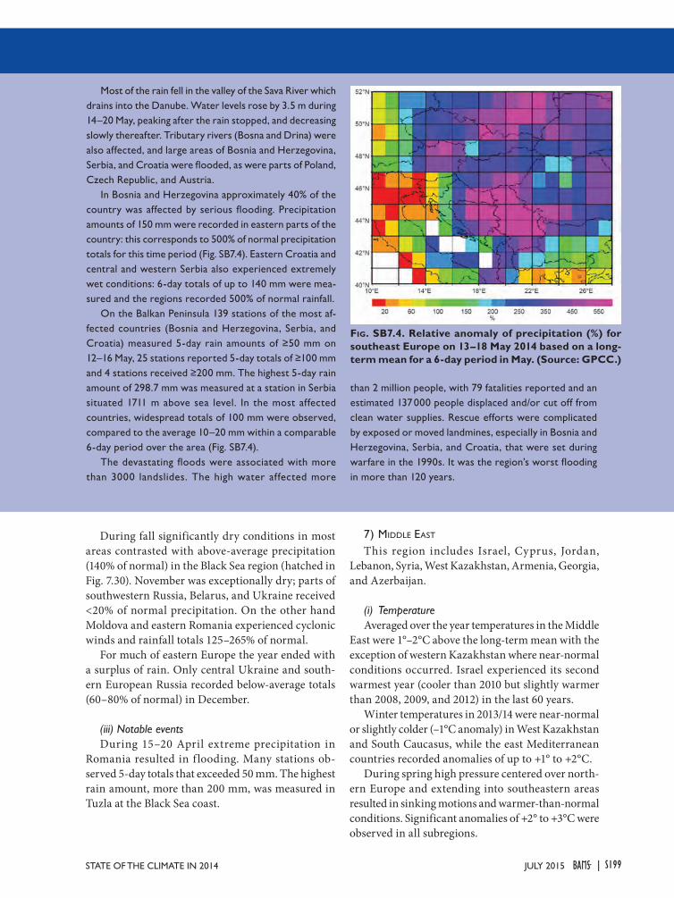
During fall significantly dry conditions in most areas contrasted with above-average precipitation (140% of normal) in the Black Sea region (hatched in Fig. 7.30). November was exceptionally dry; parts of southwestern Russia, Belarus, and Ukraine received <20% of normal precipitation. On the other hand Moldova and eastern Romania experienced cyclonic winds and rainfall totals 125–265% of normal.
For much of eastern Europe the year ended with a surplus of rain. Only central Ukraine and south-ern European Russia recorded below-average totals (60–80% of normal) in December.
(iii) Notable eventsDuring 15–20 April extreme precipitation in
Romania resulted in f looding. Many stations ob-served 5-day totals that exceeded 50 mm. The highest rain amount, more than 200 mm, was measured in Tuzla at the Black Sea coast.
7) Middle eaSt
This region includes Israel, Cyprus, Jordan, Lebanon, Syria, West Kazakhstan, Armenia, Georgia, and Azerbaijan.
(i) TemperatureAveraged over the year temperatures in the Middle
East were 1°–2°C above the long-term mean with the exception of western Kazakhstan where near-normal conditions occurred. Israel experienced its second warmest year (cooler than 2010 but slightly warmer than 2008, 2009, and 2012) in the last 60 years.
Winter temperatures in 2013/14 were near-normal or slightly colder (–1°C anomaly) in West Kazakhstan and South Caucasus, while the east Mediterranean countries recorded anomalies of up to +1° to +2°C.
During spring high pressure centered over north-ern Europe and extending into southeastern areas resulted in sinking motions and warmer-than-normal conditions. Significant anomalies of +2° to +3°C were observed in all subregions.
Most of the rain fell in the valley of the Sava River which drains into the Danube. Water levels rose by 3.5 m during 14–20 May, peaking after the rain stopped, and decreasing slowly thereafter. Tributary rivers (Bosna and Drina) were also affected, and large areas of Bosnia and Herzegovina, Serbia, and Croatia were flooded, as were parts of Poland, Czech Republic, and Austria.
In Bosnia and Herzegovina approximately 40% of the country was affected by serious flooding. Precipitation amounts of 150 mm were recorded in eastern parts of the country: this corresponds to 500% of normal precipitation totals for this time period (Fig. SB7.4). Eastern Croatia and central and western Serbia also experienced extremely wet conditions: 6-day totals of up to 140 mm were mea-sured and the regions recorded 500% of normal rainfall.
On the Balkan Peninsula 139 stations of the most af-fected countries (Bosnia and Herzegovina, Serbia, and Croatia) measured 5-day rain amounts of ≥50 mm on 12–16 May, 25 stations reported 5-day totals of ≥100 mm and 4 stations received ≥200 mm. The highest 5-day rain amount of 298.7 mm was measured at a station in Serbia situated 1711 m above sea level. In the most affected countries, widespread totals of 100 mm were observed, compared to the average 10–20 mm within a comparable 6-day period over the area (Fig. SB7.4).
The devastating floods were associated with more than 3000 landslides. The high water affected more
than 2 million people, with 79 fatalities reported and an estimated 137 000 people displaced and/or cut off from clean water supplies. Rescue efforts were complicated by exposed or moved landmines, especially in Bosnia and Herzegovina, Serbia, and Croatia, that were set during warfare in the 1990s. It was the region’s worst flooding in more than 120 years.
Fig. SB7.4. Relative anomaly of precipitation (%) for southeast Europe on 13–18 May 2014 based on a long-term mean for a 6-day period in May. (Source: GPCC.)
S199JULY 2015STATE OF THE CLIMATE IN 2014 |
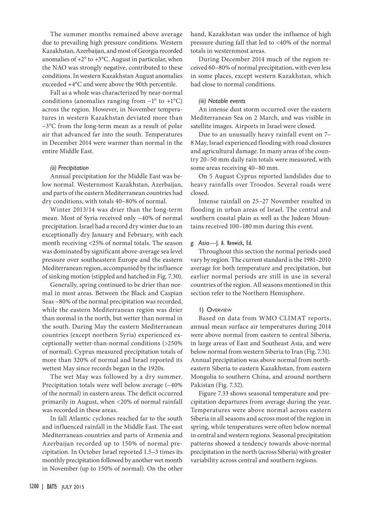
The summer months remained above average due to prevailing high pressure conditions. Western Kazakhstan, Azerbaijan, and most of Georgia recorded anomalies of +2° to +3°C. August in particular, when the NAO was strongly negative, contributed to these conditions. In western Kazakhstan August anomalies exceeded +4°C and were above the 90th percentile.
Fall as a whole was characterized by near-normal conditions (anomalies ranging from −1° to +1°C) across the region. However, in November tempera-tures in western Kazakhstan deviated more than −3°C from the long-term mean as a result of polar air that advanced far into the south. Temperatures in December 2014 were warmer than normal in the entire Middle East.
(ii) PrecipitationAnnual precipitation for the Middle East was be-
low normal. Westernmost Kazakhstan, Azerbaijan, and parts of the eastern Mediterranean countries had dry conditions, with totals 40–80% of normal.
Winter 2013/14 was drier than the long-term mean. Most of Syria received only ~40% of normal precipitation. Israel had a record dry winter due to an exceptionally dry January and February, with each month receiving <25% of normal totals. The season was dominated by significant above-average sea level pressure over southeastern Europe and the eastern Mediterranean region, accompanied by the influence of sinking motion (stippled and hatched in Fig. 7.30).
Generally, spring continued to be drier than nor-mal in most areas. Between the Black and Caspian Seas ~80% of the normal precipitation was recorded, while the eastern Mediterranean region was drier than normal in the north, but wetter than normal in the south. During May the eastern Mediterranean countries (except northern Syria) experienced ex-ceptionally wetter-than-normal conditions (>250% of normal). Cyprus measured precipitation totals of more than 320% of normal and Israel reported its wettest May since records began in the 1920s.
The wet May was followed by a dry summer. Precipitation totals were well below average (~40% of the normal) in eastern areas. The deficit occurred primarily in August, when <20% of normal rainfall was recorded in these areas.
In fall Atlantic cyclones reached far to the south and influenced rainfall in the Middle East. The east Mediterranean countries and parts of Armenia and Azerbaijan recorded up to 150% of normal pre-cipitation. In October Israel reported 1.5–3 times its monthly precipitation followed by another wet month in November (up to 150% of normal). On the other
hand, Kazakhstan was under the influence of high pressure during fall that led to <40% of the normal totals in westernmost areas.
During December 2014 much of the region re-ceived 60–80% of normal precipitation, with even less in some places, except western Kazakhstan, which had close to normal conditions.
(iii) Notable eventsAn intense dust storm occurred over the eastern
Mediterranean Sea on 2 March, and was visible in satellite images. Airports in Israel were closed.
Due to an unusually heavy rainfall event on 7– 8 May, Israel experienced flooding with road closures and agricultural damage. In many areas of the coun-try 20–50 mm daily rain totals were measured, with some areas receiving 40–80 mm.
On 5 August Cyprus reported landslides due to heavy rainfalls over Troodos. Several roads were closed.
Intense rainfall on 25–27 November resulted in f looding in urban areas of Israel. The central and southern coastal plain as well as the Judean Moun-tains received 100–180 mm during this event.
g. Asia—J. A. Renwick, Ed.Throughout this section the normal periods used
vary by region. The current standard is the 1981–2010 average for both temperature and precipitation, but earlier normal periods are still in use in several countries of the region. All seasons mentioned in this section refer to the Northern Hemisphere.
1) overvieW
Based on data from WMO CLIMAT reports, annual mean surface air temperatures during 2014 were above normal from eastern to central Siberia, in large areas of East and Southeast Asia, and were below normal from western Siberia to Iran (Fig. 7.31). Annual precipitation was above normal from north-eastern Siberia to eastern Kazakhstan, from eastern Mongolia to southern China, and around northern Pakistan (Fig. 7.32).
Figure 7.33 shows seasonal temperature and pre-cipitation departures from average during the year. Temperatures were above normal across eastern Siberia in all seasons and across most of the region in spring, while temperatures were often below normal in central and western regions. Seasonal precipitation patterns showed a tendency towards above-normal precipitation in the north (across Siberia) with greater variability across central and southern regions.
S200 JULY 2015|
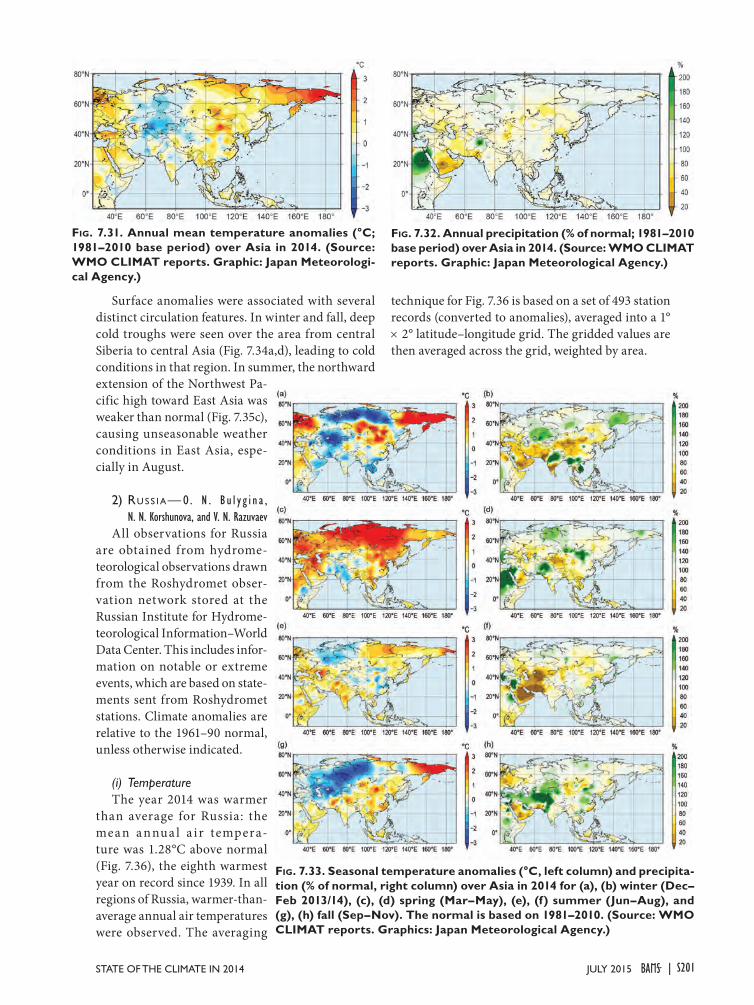
Surface anomalies were associated with several distinct circulation features. In winter and fall, deep cold troughs were seen over the area from central Siberia to central Asia (Fig. 7.34a,d), leading to cold conditions in that region. In summer, the northward extension of the Northwest Pa-cific high toward East Asia was weaker than normal (Fig. 7.35c), causing unseasonable weather conditions in East Asia, espe-cially in August.
2) rU S S i a— O . N . B u l y g i n a , N. N. Korshunova, and V. N. Razuvaev
All observations for Russia are obtained from hydrome-teorological observations drawn from the Roshydromet obser-vation network stored at the Russian Institute for Hydrome-teorological Information–World Data Center. This includes infor-mation on notable or extreme events, which are based on state-ments sent from Roshydromet stations. Climate anomalies are relative to the 1961–90 normal, unless otherwise indicated.
(i) TemperatureThe year 2014 was warmer
than average for Russia: the mea n a nnua l a i r tempera-ture was 1.28°С above normal (Fig. 7.36), the eighth warmest year on record since 1939. In all regions of Russia, warmer-than-average annual air temperatures were observed. The averaging
technique for Fig. 7.36 is based on a set of 493 station records (converted to anomalies), averaged into a 1° × 2° latitude–longitude grid. The gridded values are then averaged across the grid, weighted by area.
Fig. 7.31. Annual mean temperature anomalies (°C; 1981–2010 base period) over Asia in 2014. (Source: WMO CLIMAT reports. Graphic: Japan Meteorologi-cal Agency.)
Fig. 7.32. Annual precipitation (% of normal; 1981–2010 base period) over Asia in 2014. (Source: WMO CLIMAT reports. Graphic: Japan Meteorological Agency.)
Fig. 7.33. Seasonal temperature anomalies (°C, left column) and precipita-tion (% of normal, right column) over Asia in 2014 for (a), (b) winter (Dec–Feb 2013/14), (c), (d) spring (Mar–May), (e), (f) summer (Jun–Aug), and (g), (h) fall (Sep–Nov). The normal is based on 1981–2010. (Source: WMO CLIMAT reports. Graphics: Japan Meteorological Agency.)
S201JULY 2015STATE OF THE CLIMATE IN 2014 |
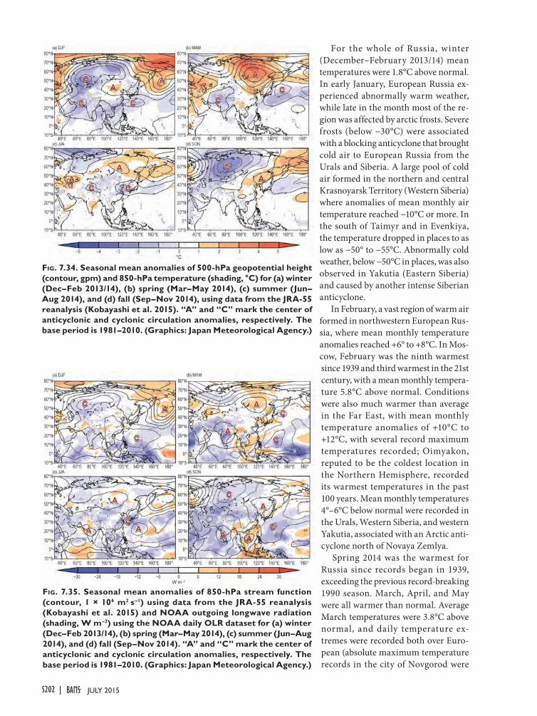
For the whole of Russia, winter (December–February 2013/14) mean temperatures were 1.8°С above normal. In early January, European Russia ex-perienced abnormally warm weather, while late in the month most of the re-gion was affected by arctic frosts. Severe frosts (below −30°С) were associated with a blocking anticyclone that brought cold air to European Russia from the Urals and Siberia. A large pool of cold air formed in the northern and central Krasnoyarsk Territory (Western Siberia) where anomalies of mean monthly air temperature reached −10°С or more. In the south of Taimyr and in Evenkiya, the temperature dropped in places to as low as −50° to −55°С. Abnormally cold weather, below −50°С in places, was also observed in Yakutia (Eastern Siberia) and caused by another intense Siberian anticyclone.
In February, a vast region of warm air formed in northwestern European Rus-sia, where mean monthly temperature anomalies reached +6° to +8°С. In Mos-cow, February was the ninth warmest since 1939 and third warmest in the 21st century, with a mean monthly tempera-ture 5.8°С above normal. Conditions were also much warmer than average in the Far East, with mean monthly temperature anomalies of +10°C to +12°С, with several record maximum temperatures recorded; Oimyakon, reputed to be the coldest location in the Northern Hemisphere, recorded its warmest temperatures in the past 100 years. Mean monthly temperatures 4°–6°С below normal were recorded in the Urals, Western Siberia, and western Yakutia, associated with an Arctic anti-cyclone north of Novaya Zemlya.
Spring 2014 was the warmest for Russia since records began in 1939, exceeding the previous record-breaking 1990 season. March, April, and May were all warmer than normal. Average March temperatures were 3.8°С above normal, and daily temperature ex-tremes were recorded both over Euro-pean (absolute maximum temperature records in the city of Novgorod were
Fig. 7.34. Seasonal mean anomalies of 500-hPa geopotential height (contour, gpm) and 850-hPa temperature (shading, °C) for (a) winter (Dec–Feb 2013/14), (b) spring (Mar–May 2014), (c) summer (Jun–Aug 2014), and (d) fall (Sep–Nov 2014), using data from the JRA-55 reanalysis (Kobayashi et al. 2015). “A” and “C” mark the center of anticyclonic and cyclonic circulation anomalies, respectively. The base period is 1981–2010. (Graphics: Japan Meteorological Agency.)
Fig. 7.35. Seasonal mean anomalies of 850-hPa stream function (contour, 1 × 10⁶ m2 s–1) using data from the JRA-55 reanalysis (Kobayashi et al. 2015) and NOAA outgoing longwave radiation (shading, W m–2) using the NOAA daily OLR dataset for (a) winter (Dec–Feb 2013/14), (b) spring (Mar–May 2014), (c) summer (Jun–Aug 2014), and (d) fall (Sep–Nov 2014). “A” and “C” mark the center of anticyclonic and cyclonic circulation anomalies, respectively. The base period is 1981–2010. (Graphics: Japan Meteorological Agency.)
S202 JULY 2015|
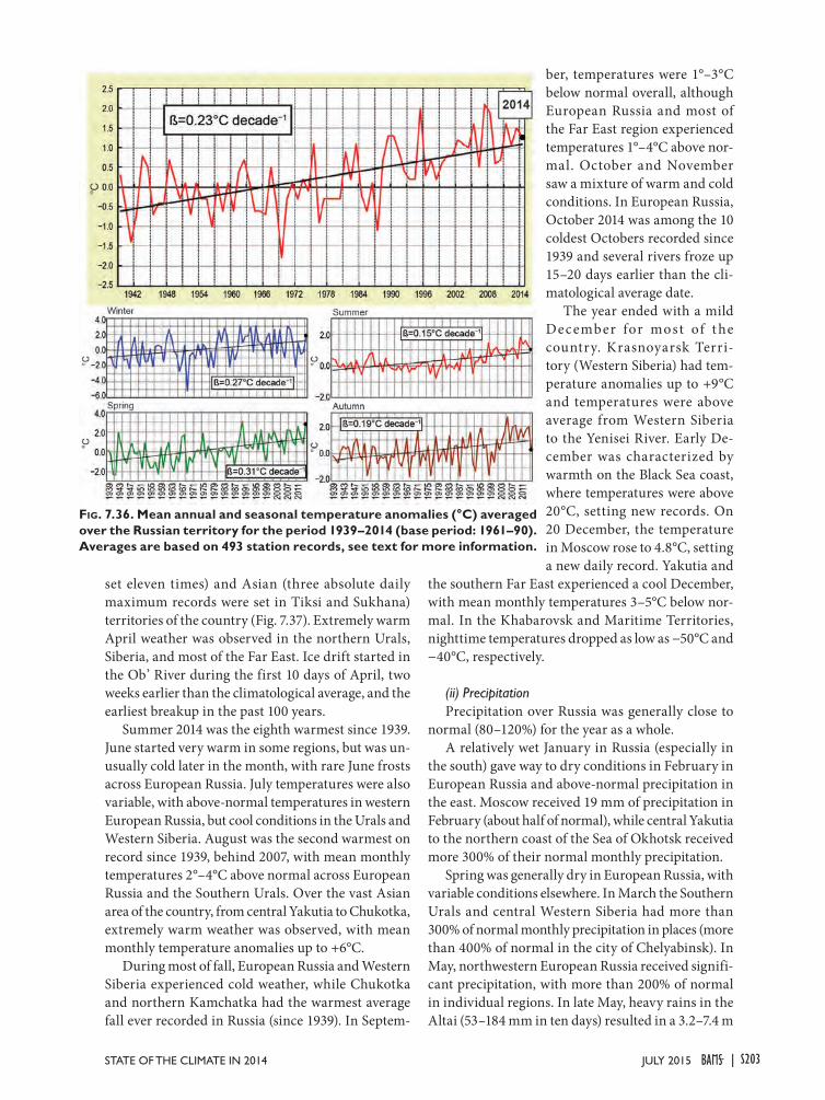
set eleven times) and Asian (three absolute daily maximum records were set in Tiksi and Sukhana) territories of the country (Fig. 7.37). Extremely warm April weather was observed in the northern Urals, Siberia, and most of the Far East. Ice drift started in the Ob’ River during the first 10 days of April, two weeks earlier than the climatological average, and the earliest breakup in the past 100 years.
Summer 2014 was the eighth warmest since 1939. June started very warm in some regions, but was un-usually cold later in the month, with rare June frosts across European Russia. July temperatures were also variable, with above-normal temperatures in western European Russia, but cool conditions in the Urals and Western Siberia. August was the second warmest on record since 1939, behind 2007, with mean monthly temperatures 2°–4°С above normal across European Russia and the Southern Urals. Over the vast Asian area of the country, from central Yakutia to Chukotka, extremely warm weather was observed, with mean monthly temperature anomalies up to +6°С.
During most of fall, European Russia and Western Siberia experienced cold weather, while Chukotka and northern Kamchatka had the warmest average fall ever recorded in Russia (since 1939). In Septem-
ber, temperatures were 1°–3°C below normal overall, although European Russia and most of the Far East region experienced temperatures 1°–4°С above nor-mal. October and November saw a mixture of warm and cold conditions. In European Russia, October 2014 was among the 10 coldest Octobers recorded since 1939 and several rivers froze up 15–20 days earlier than the cli-matological average date.
The year ended with a mild December for most of t he country. Krasnoyarsk Terri-tory (Western Siberia) had tem-perature anomalies up to +9°С and temperatures were above average from Western Siberia to the Yenisei River. Early De-cember was characterized by warmth on the Black Sea coast, where temperatures were above 20°С, setting new records. On 20 December, the temperature in Moscow rose to 4.8°С, setting a new daily record. Yakutia and
the southern Far East experienced a cool December, with mean monthly temperatures 3–5°С below nor-mal. In the Khabarovsk and Maritime Territories, nighttime temperatures dropped as low as −50°С and −40°С, respectively.
(ii) PrecipitationPrecipitation over Russia was generally close to
normal (80–120%) for the year as a whole. A relatively wet January in Russia (especially in
the south) gave way to dry conditions in February in European Russia and above-normal precipitation in the east. Moscow received 19 mm of precipitation in February (about half of normal), while central Yakutia to the northern coast of the Sea of Okhotsk received more 300% of their normal monthly precipitation.
Spring was generally dry in European Russia, with variable conditions elsewhere. In March the Southern Urals and central Western Siberia had more than 300% of normal monthly precipitation in places (more than 400% of normal in the city of Chelyabinsk). In May, northwestern European Russia received signifi-cant precipitation, with more than 200% of normal in individual regions. In late May, heavy rains in the Altai (53–184 mm in ten days) resulted in a 3.2–7.4 m
Fig. 7.36. Mean annual and seasonal temperature anomalies (°C) averaged over the Russian territory for the period 1939–2014 (base period: 1961–90). Averages are based on 493 station records, see text for more information.
S203JULY 2015STATE OF THE CLIMATE IN 2014 |
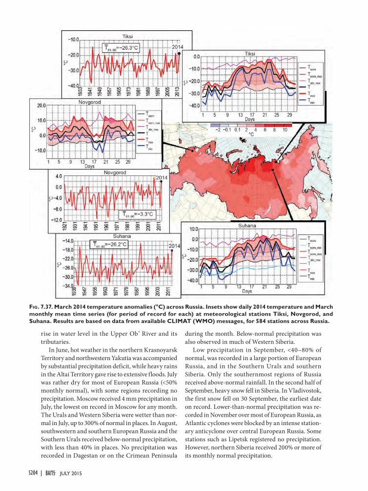
rise in water level in the Upper Ob’ River and its tributaries.
In June, hot weather in the northern Krasnoyarsk Territory and northwestern Yakutia was accompanied by substantial precipitation deficit, while heavy rains in the Altai Territory gave rise to extensive floods. July was rather dry for most of European Russia (<50% monthly normal), with some regions recording no precipitation. Moscow received 4 mm precipitation in July, the lowest on record in Moscow for any month. The Urals and Western Siberia were wetter than nor-mal in July, up to 300% of normal in places. In August, southwestern and southern European Russia and the Southern Urals received below-normal precipitation, with less than 40% in places. No precipitation was recorded in Dagestan or on the Crimean Peninsula
during the month. Below-normal precipitation was also observed in much of Western Siberia.
Low precipitation in September, <40–80% of normal, was recorded in a large portion of European Russia, and in the Southern Urals and southern Siberia. Only the southernmost regions of Russia received above-normal rainfall. In the second half of September, heavy snow fell in Siberia. In Vladivostok, the first snow fell on 30 September, the earliest date on record. Lower-than-normal precipitation was re-corded in November over most of European Russia, as Atlantic cyclones were blocked by an intense station-ary anticyclone over central European Russia. Some stations such as Lipetsk registered no precipitation. However, northern Siberia received 200% or more of its monthly normal precipitation.
Fig. 7.37. March 2014 temperature anomalies (°C) across Russia. Insets show daily 2014 temperature and March monthly mean time series (for period of record for each) at meteorological stations Tiksi, Novgorod, and Suhana. Results are based on data from available CLIMAT (WMO) messages, for 584 stations across Russia.
S204 JULY 2015|
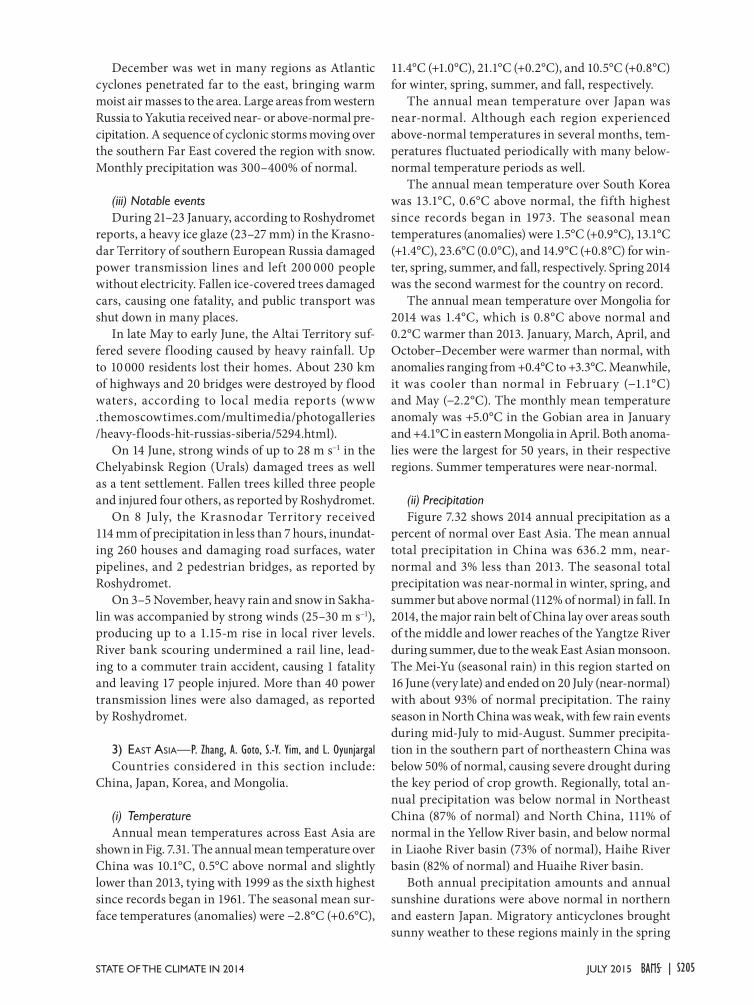
December was wet in many regions as Atlantic cyclones penetrated far to the east, bringing warm moist air masses to the area. Large areas from western Russia to Yakutia received near- or above-normal pre-cipitation. A sequence of cyclonic storms moving over the southern Far East covered the region with snow. Monthly precipitation was 300–400% of normal.
(iii) Notable eventsDuring 21–23 January, according to Roshydromet
reports, a heavy ice glaze (23–27 mm) in the Krasno-dar Territory of southern European Russia damaged power transmission lines and left 200 000 people without electricity. Fallen ice-covered trees damaged cars, causing one fatality, and public transport was shut down in many places.
In late May to early June, the Altai Territory suf-fered severe f looding caused by heavy rainfall. Up to 10 000 residents lost their homes. About 230 km of highways and 20 bridges were destroyed by flood waters, according to local media reports (www .themoscowtimes.com/multimedia/photogalleries /heavy-floods-hit-russias-siberia/5294.html).
On 14 June, strong winds of up to 28 m s−1 in the Chelyabinsk Region (Urals) damaged trees as well as a tent settlement. Fallen trees killed three people and injured four others, as reported by Roshydromet.
On 8 July, the Krasnodar Territory received 114 mm of precipitation in less than 7 hours, inundat-ing 260 houses and damaging road surfaces, water pipelines, and 2 pedestrian bridges, as reported by Roshydromet.
On 3–5 November, heavy rain and snow in Sakha-lin was accompanied by strong winds (25–30 m s−1), producing up to a 1.15-m rise in local river levels. River bank scouring undermined a rail line, lead-ing to a commuter train accident, causing 1 fatality and leaving 17 people injured. More than 40 power transmission lines were also damaged, as reported by Roshydromet.
3) eaSt aSia—P. Zhang, A. Goto, S.-Y. Yim, and L. OyunjargalCountries considered in this section include:
China, Japan, Korea, and Mongolia.
(i) TemperatureAnnual mean temperatures across East Asia are
shown in Fig. 7.31. The annual mean temperature over China was 10.1°C, 0.5°C above normal and slightly lower than 2013, tying with 1999 as the sixth highest since records began in 1961. The seasonal mean sur-face temperatures (anomalies) were −2.8°C (+0.6°C),
11.4°C (+1.0°C), 21.1°C (+0.2°C), and 10.5°C (+0.8°C) for winter, spring, summer, and fall, respectively.
The annual mean temperature over Japan was near-normal. Although each region experienced above-normal temperatures in several months, tem-peratures fluctuated periodically with many below-normal temperature periods as well.
The annual mean temperature over South Korea was 13.1°C, 0.6°C above normal, the fifth highest since records began in 1973. The seasonal mean temperatures (anomalies) were 1.5°C (+0.9°C), 13.1°C (+1.4°C), 23.6°C (0.0°C), and 14.9°C (+0.8°C) for win-ter, spring, summer, and fall, respectively. Spring 2014 was the second warmest for the country on record.
The annual mean temperature over Mongolia for 2014 was 1.4°C, which is 0.8°C above normal and 0.2°C warmer than 2013. January, March, April, and October–December were warmer than normal, with anomalies ranging from +0.4°C to +3.3°C. Meanwhile, it was cooler than normal in February (−1.1°C) and May (−2.2°C). The monthly mean temperature anomaly was +5.0°C in the Gobian area in January and +4.1°C in eastern Mongolia in April. Both anoma-lies were the largest for 50 years, in their respective regions. Summer temperatures were near-normal.
(ii) PrecipitationFigure 7.32 shows 2014 annual precipitation as a
percent of normal over East Asia. The mean annual total precipitation in China was 636.2 mm, near-normal and 3% less than 2013. The seasonal total precipitation was near-normal in winter, spring, and summer but above normal (112% of normal) in fall. In 2014, the major rain belt of China lay over areas south of the middle and lower reaches of the Yangtze River during summer, due to the weak East Asian monsoon. The Mei-Yu (seasonal rain) in this region started on 16 June (very late) and ended on 20 July (near-normal) with about 93% of normal precipitation. The rainy season in North China was weak, with few rain events during mid-July to mid-August. Summer precipita-tion in the southern part of northeastern China was below 50% of normal, causing severe drought during the key period of crop growth. Regionally, total an-nual precipitation was below normal in Northeast China (87% of normal) and North China, 111% of normal in the Yellow River basin, and below normal in Liaohe River basin (73% of normal), Haihe River basin (82% of normal) and Huaihe River basin.
Both annual precipitation amounts and annual sunshine durations were above normal in northern and eastern Japan. Migratory anticyclones brought sunny weather to these regions mainly in the spring
S205JULY 2015STATE OF THE CLIMATE IN 2014 |
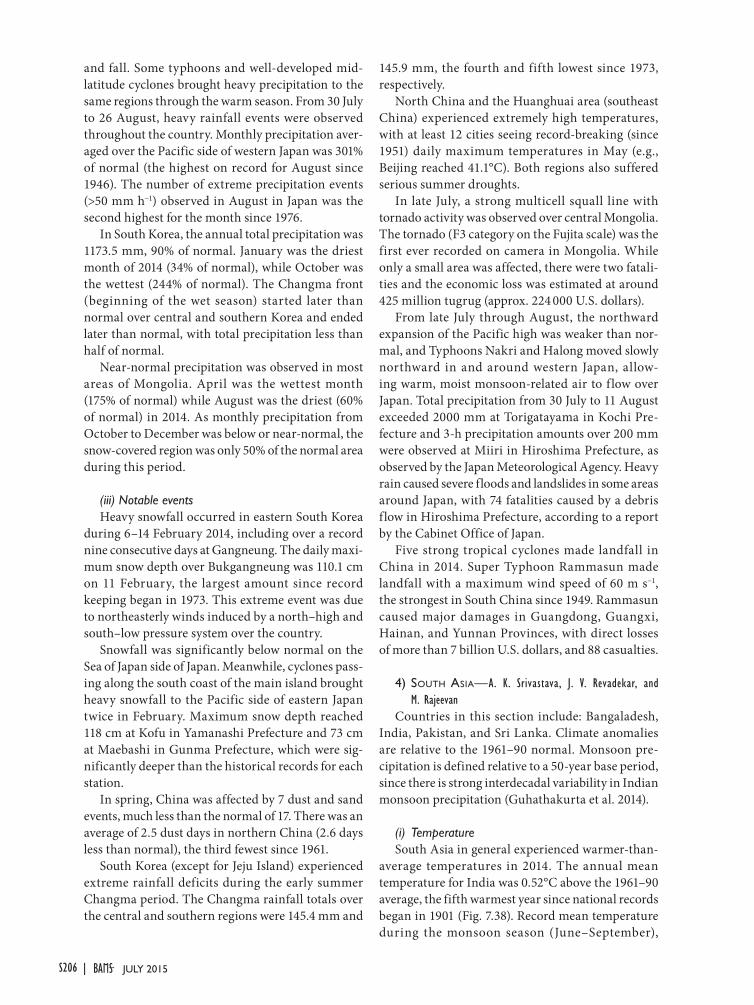
and fall. Some typhoons and well-developed mid-latitude cyclones brought heavy precipitation to the same regions through the warm season. From 30 July to 26 August, heavy rainfall events were observed throughout the country. Monthly precipitation aver-aged over the Pacific side of western Japan was 301% of normal (the highest on record for August since 1946). The number of extreme precipitation events (>50 mm h−1) observed in August in Japan was the second highest for the month since 1976.
In South Korea, the annual total precipitation was 1173.5 mm, 90% of normal. January was the driest month of 2014 (34% of normal), while October was the wettest (244% of normal). The Changma front (beginning of the wet season) started later than normal over central and southern Korea and ended later than normal, with total precipitation less than half of normal.
Near-normal precipitation was observed in most areas of Mongolia. April was the wettest month (175% of normal) while August was the driest (60% of normal) in 2014. As monthly precipitation from October to December was below or near-normal, the snow-covered region was only 50% of the normal area during this period.
(iii) Notable eventsHeavy snowfall occurred in eastern South Korea
during 6–14 February 2014, including over a record nine consecutive days at Gangneung. The daily maxi-mum snow depth over Bukgangneung was 110.1 cm on 11 February, the largest amount since record keeping began in 1973. This extreme event was due to northeasterly winds induced by a north–high and south–low pressure system over the country.
Snowfall was significantly below normal on the Sea of Japan side of Japan. Meanwhile, cyclones pass-ing along the south coast of the main island brought heavy snowfall to the Pacific side of eastern Japan twice in February. Maximum snow depth reached 118 cm at Kofu in Yamanashi Prefecture and 73 cm at Maebashi in Gunma Prefecture, which were sig-nificantly deeper than the historical records for each station.
In spring, China was affected by 7 dust and sand events, much less than the normal of 17. There was an average of 2.5 dust days in northern China (2.6 days less than normal), the third fewest since 1961.
South Korea (except for Jeju Island) experienced extreme rainfall deficits during the early summer Changma period. The Changma rainfall totals over the central and southern regions were 145.4 mm and
145.9 mm, the fourth and fifth lowest since 1973, respectively.
North China and the Huanghuai area (southeast China) experienced extremely high temperatures, with at least 12 cities seeing record-breaking (since 1951) daily maximum temperatures in May (e.g., Beijing reached 41.1°C). Both regions also suffered serious summer droughts.
In late July, a strong multicell squall line with tornado activity was observed over central Mongolia. The tornado (F3 category on the Fujita scale) was the first ever recorded on camera in Mongolia. While only a small area was affected, there were two fatali-ties and the economic loss was estimated at around 425 million tugrug (approx. 224 000 U.S. dollars).
From late July through August, the northward expansion of the Pacific high was weaker than nor-mal, and Typhoons Nakri and Halong moved slowly northward in and around western Japan, allow-ing warm, moist monsoon-related air to f low over Japan. Total precipitation from 30 July to 11 August exceeded 2000 mm at Torigatayama in Kochi Pre-fecture and 3-h precipitation amounts over 200 mm were observed at Miiri in Hiroshima Prefecture, as observed by the Japan Meteorological Agency. Heavy rain caused severe floods and landslides in some areas around Japan, with 74 fatalities caused by a debris flow in Hiroshima Prefecture, according to a report by the Cabinet Office of Japan.
Five strong tropical cyclones made landfall in China in 2014. Super Typhoon Rammasun made landfall with a maximum wind speed of 60 m s−1, the strongest in South China since 1949. Rammasun caused major damages in Guangdong, Guangxi, Hainan, and Yunnan Provinces, with direct losses of more than 7 billion U.S. dollars, and 88 casualties.
4) SoUth aSia—A. K. Srivastava, J. V. Revadekar, and M. Rajeevan
Countries in this section include: Bangaladesh, India, Pakistan, and Sri Lanka. Climate anomalies are relative to the 1961–90 normal. Monsoon pre-cipitation is defined relative to a 50-year base period, since there is strong interdecadal variability in Indian monsoon precipitation (Guhathakurta et al. 2014).
(i) TemperatureSouth Asia in general experienced warmer-than-
average temperatures in 2014. The annual mean temperature for India was 0.52°C above the 1961–90 average, the fifth warmest year since national records began in 1901 (Fig. 7.38). Record mean temperature during the monsoon season (June–September),
S206 JULY 2015|
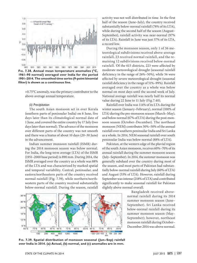
+0.75°C anomaly, was the primary contributor to the above-average annual temperature.
(ii) PrecipitationThe south Asian monsoon set in over Kerala
(southern parts of peninsular India) on 6 June, five days later than its climatological normal date of 1 June, and covered the entire country by 17 July (two days later than normal). The advance of the monsoon over different parts of the country was not smooth and there was a hiatus of about 10 days (20–30 June) in the advancement.
Indian summer monsoon rainfall (ISMR) dur-ing the 2014 monsoon season was below normal. For India, the long-term average (LTA) of the ISMR (1951–2000 base period) is 890 mm. During 2014, the ISMR averaged over the country as a whole was 88% of the LTA and was characterized by marked spatial and temporal variability. Central, peninsular, and eastern/northeastern parts of the country received normal rainfall (Fig. 7.39), while northern/north-western parts of the country received substantially below-normal rainfall. During the season, rainfall
activity was not well distributed in time. In the first half of the season (June–July), the country received substantially below-normal rainfall (78% of its LTA), while during the second half of the season (August–September), rainfall activity was near-normal (97% of its LTA). Rainfall in June was just 57% of its LTA, a record low.
During the monsoon season, only 1 of 36 me-teorological subdivisions received above-average rainfall, 23 received normal rainfall, and the re-maining 12 subdivisions received below-normal rainfall. Of the 615 districts, 223 were affected by moderate meteorological drought (seasonal rainfall deficiency in the range of 26%–50%), while 56 were affected by severe meteorological drought (seasonal rainfall deficiency in the range of 51%–99%). Rainfall averaged over the country as a whole was below normal on most days until the second week of July. National average rainfall was nearly half its normal value during 22 June to 11 July (Fig.7.40).
Rainfall over India was 114% of its LTA during the winter season (January–February), normal (100% of LTA) during the pre-monsoon season (March–May), and below normal (67% of LTA) during the post-mon-soon season (October–December). The northeast monsoon (NEM) contributes 30%–50% of the annual rainfall over southern peninsular India and Sri Lanka as a whole. In 2014, NEM seasonal rainfall over south peninsular India was below normal (88% of LTA).
Pakistan, at the western edge of the pluvial region of the south Asian monsoon, receives 60%–70% of its annual rainfall during the summer monsoon season (July–September). In 2014, the summer monsoon was generally subdued over the country during most of the season, and most parts of Pakistan had substan-tially below-normal rainfall during July (60% of LTA) and August (53% of LTA). However, rainfall during September was intense (218% of LTA) and contributed significantly to make seasonal rainfall for Pakistan slightly above normal overall.
Bangladesh received above-normal rainfall during its 2014 summer monsoon season (June–September). Sri Lanka received below-normal rainfall during its summer monsoon season (May–September); however, northeast monsoon rainfall during October–December 2014 was above normal.
Fig. 7.38. Annual mean temperature anomalies (°C, 1961–90 normal) averaged over India for the period 1901–2014. The smoothed time series (9-point binomial filter) is shown as a continuous line.
Fig. 7.39. Spatial distribution of monsoon seasonal (Jun–Sep) rainfall over India in 2014. (a) Actual, (b) normal, and (c) anomalies are in mm.
S207JULY 2015STATE OF THE CLIMATE IN 2014 |
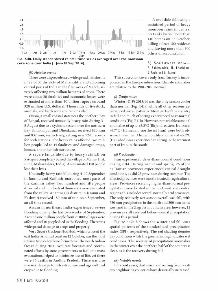
(iii) Notable eventsThere were unprecedented widespread hailstorms
in 28 of 35 districts of Maharashtra and adjoining central parts of India in the first week of March, se-verely affecting two million hectares of crops. There were about 30 fatalities and economic losses were estimated at more than 20 billion rupees (around 320 million U.S. dollars). Thousands of livestock, animals, and birds were injured or killed.
Orissa, a small coastal state near the northern Bay of Bengal, received unusually heavy rain during 3– 5 August due to a cyclonic system over the northern Bay. Sambhalpur and Dhenkanal received 820 mm and 837 mm, respectively, setting new 72-h records for both stations. The heavy rains affected two mil-lion people, led to 45 fatalities, and damaged crops, houses, and other infrastructure.
A severe landslide due to heavy rainfall on 5 August completely buried the village of Malin (Dist. Pune, Maharashtra, India). An estimated 150 people lost their lives.
Unusually heavy rainfall during 4–10 September in Jammu and Kashmir marooned most parts of the Kashmir valley. Two hundred and fifty people drowned and hundreds of thousands were evacuated from the valley. Anantnag (a district in Jammu and Kashmir) received 180 mm of rain on 4 September, an all-time record.
Assam in northeast India experienced severe f looding during the last two weeks of September. Around one million people from 25 000 villages were affected and 40 people died in the flooding. There was widespread damage to crops and property.
Very Severe Cyclone HudHud, which crossed the east India (Andhra) coast on 12 October, was the most intense tropical cyclone formed over the north Indian Ocean during 2014. Accurate forecasts and coordi-nated efforts by state governments to facilitate mass evacuations helped to minimize loss of life, yet there were 46 deaths in Andhra Pradesh. There was also massive damage to infrastructure and agricultural crops due to flooding.
A mudslide following a sustained period of heavy monsoon rains in central Sri Lanka buried more than 140 homes on 22 October, killing at least 100 residents and leaving more than 300 others unaccounted for.
5 ) S o U t h W e S t a S i a — F. Rah imzadeh , M . Khoshkam, S. Fateh, and A. Kazemi
This subsection covers only Iran. Turkey is incor-porated in the Europe subsection. Climate anomalies are relative to the 1981–2010 normal.
(i) TemperatureWinter (DJF) 2013/14 was the only season cooler
than normal (Fig. 7.41a) while all other seasons ex-perienced mixed patterns. Most parts of the country in fall and much of spring experienced near-normal conditions (Fig. 7.41b). However, remarkable seasonal anomalies of up to +5.3°C (Birjand, eastern Iran) and −7.7°C (Hamedan, northwest Iran) were both ob-served in winter. Also, a monthly anomaly of −5.6°C (Haji abad) was experienced in spring in the warmest part of Iran in the south.
(ii) PrecipitationIran experienced drier-than-normal conditions
during 2014. During winter and spring, 26 of the 31 Iranian provinces experienced critical drought conditions, as did 23 provinces during summer. The affected provinces were mostly located in agricultural areas. Provinces receiving higher-than-normal pre-cipitation were located in the northeast and central regions; this includes several normally arid provinces. The only relatively wet season overall was fall, with 750 mm precipitation in the north and 300 mm in the west and in the Zagross mountain area; however, 12 provinces still received below-normal precipitation during this period.
Figure 7.42a,b shows the winter and fall 2014 spatial patterns of the standardized precipitation index (SPI), respectively. The red shading denotes dry conditions while the green shading indicates wet conditions. The severity of precipitation anomalies in the winter over the northern half of the country is clear, as is the recovery during fall.
(iii) Notable eventsIn recent years, dust storms advecting from west-
ern neighboring countries have drastically increased,
Fig. 7.40. Daily standardized rainfall time series averaged over the monsoon core zone over India (1 Jun–30 Sep 2014).
S208 JULY 2015|
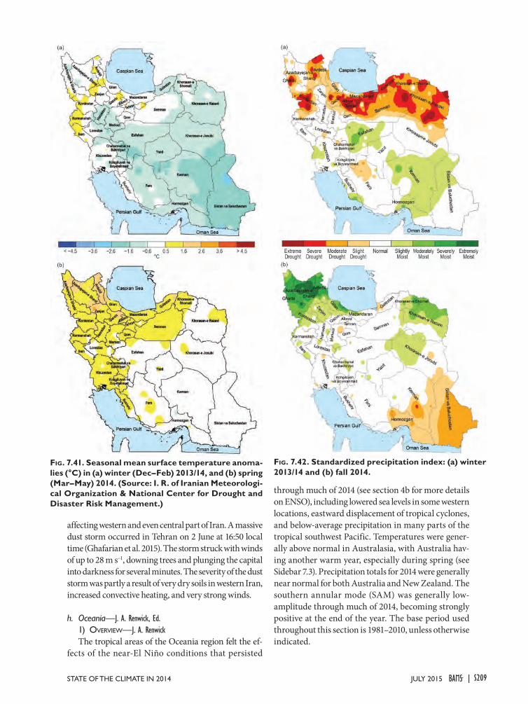
affecting western and even central part of Iran. A massive dust storm occurred in Tehran on 2 June at 16:50 local time (Ghafarian et al. 2015). The storm struck with winds of up to 28 m s−1, downing trees and plunging the capital into darkness for several minutes. The severity of the dust storm was partly a result of very dry soils in western Iran, increased convective heating, and very strong winds.
h. Oceania—J. A. Renwick, Ed.1) overvieW—J. A. RenwickThe tropical areas of the Oceania region felt the ef-
fects of the near-El Niño conditions that persisted
through much of 2014 (see section 4b for more details on ENSO), including lowered sea levels in some western locations, eastward displacement of tropical cyclones, and below-average precipitation in many parts of the tropical southwest Pacific. Temperatures were gener-ally above normal in Australasia, with Australia hav-ing another warm year, especially during spring (see Sidebar 7.3). Precipitation totals for 2014 were generally near normal for both Australia and New Zealand. The southern annular mode (SAM) was generally low-amplitude through much of 2014, becoming strongly positive at the end of the year. The base period used throughout this section is 1981–2010, unless otherwise indicated.
Fig. 7.42. Standardized precipitation index: (a) winter 2013/14 and (b) fall 2014.
Fig. 7.41. Seasonal mean surface temperature anoma-lies (°C) in (a) winter (Dec–Feb) 2013/14, and (b) spring (Mar–May) 2014. (Source: I. R. of Iranian Meteorologi-cal Organization & National Center for Drought and Disaster Risk Management.)
S209JULY 2015STATE OF THE CLIMATE IN 2014 |
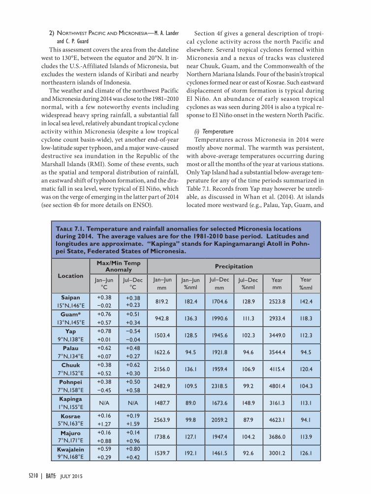
2) northWeSt paCifiC and MiCroneSia—M. A. Lander and C. P. Guard
This assessment covers the area from the dateline west to 130°E, between the equator and 20°N. It in-cludes the U.S.-Affiliated Islands of Micronesia, but excludes the western islands of Kiribati and nearby northeastern islands of Indonesia.
The weather and climate of the northwest Pacific and Micronesia during 2014 was close to the 1981−2010 normal, with a few noteworthy events including widespread heavy spring rainfall, a substantial fall in local sea level, relatively abundant tropical cyclone activity within Micronesia (despite a low tropical cyclone count basin-wide), yet another end-of-year low-latitude super typhoon, and a major wave-caused destructive sea inundation in the Republic of the Marshall Islands (RMI). Some of these events, such as the spatial and temporal distribution of rainfall, an eastward shift of typhoon formation, and the dra-matic fall in sea level, were typical of El Niño, which was on the verge of emerging in the latter part of 2014 (see section 4b for more details on ENSO).
Section 4f gives a general description of tropi-cal cyclone activity across the north Pacific and elsewhere. Several tropical cyclones formed within Micronesia and a nexus of tracks was clustered near Chuuk, Guam, and the Commonwealth of the Northern Mariana Islands. Four of the basin’s tropical cyclones formed near or east of Kosrae. Such eastward displacement of storm formation is typical during El Niño. An abundance of early season tropical cyclones as was seen during 2014 is also a typical re-sponse to El Niño onset in the western North Pacific.
(i) TemperatureTemperatures across Micronesia in 2014 were
mostly above normal. The warmth was persistent, with above-average temperatures occurring during most or all the months of the year at various stations. Only Yap Island had a substantial below-average tem-perature for any of the time periods summarized in Table 7.1. Records from Yap may however be unreli-able, as discussed in Whan et al. (2014). At islands located more westward (e.g., Palau, Yap, Guam, and
Table 7.1. Temperature and rainfall anomalies for selected Micronesia locations during 2014. The average values are for the 1981-2010 base period. Latitudes and longitudes are approximate. “Kapinga” stands for Kapingamarangi Atoll in Pohn-pei State, Federated States of Micronesia.
Location
Max/Min Temp Anomaly Precipitation
Jan–Jun°C
Jul–Dec°C
Jan–Junmm
Jan–Jun%nml
Jul–Decmm
Jul–Dec%nml
Yearmm
Year %nml
Saipan15°N,146°E
+0.38−0.02
+0.38 +0.23 819.2 182.4 1704.6 128.9 2523.8 142.4
Guam*13°N,145°E
+0.76+0.57
+0.51+0.34
942.8 136.3 1990.6 111.3 2933.4 118.3
Yap9°N,138°E
+0.78+0.01
−0.54−0.04
1503.4 128.5 1945.6 102.3 3449.0 112.3
Palau7°n,134°e
+0.62+0.07
+0.48+0.27
1622.6 94.5 1921.8 94.6 3544.4 94.5
Chuuk7°N,152°E
+0.38+0.52
+0.62+0.30
2156.0 136.1 1959.4 106.9 4115.4 120.4
Pohnpei7°N,158°E
+0.38−0.45
+0.50+0.58
2482.9 109.5 2318.5 99.2 4801.4 104.3
Kapinga1°N,155°E
N/A N/A 1487.7 89.0 1673.6 148.9 3161.3 113.1
Kosrae5°N,163°E
+0.16+1.27
+0.19+1.59
2563.9 99.8 2059.2 87.9 4623.1 94.1
Majuro7°N,171°E
+0.16+0.88
+0.14+0.96
1738.6 127.1 1947.4 104.2 3686.0 113.9
Kwajalein9°N,168°E
+0.59+0.29
+0.80+0.42
1539.7 192.1 1461.5 92.6 3001.2 126.1
S210 JULY 2015|
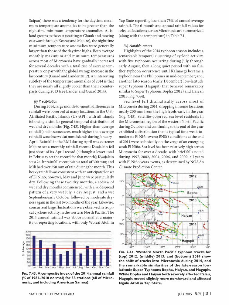
Fig. 7.43. A composite index of the 2014 annual rainfall (% of 1981–2010 normal) for 58 stations (all of Micro-nesia, and including American Samoa).
Saipan) there was a tendency for the daytime maxi-mum temperature anomalies to be greater than the nighttime minimum temperature anomalies. At is-land groups to the east (starting at Chuuk and moving eastward through Kosrae and Majuro), the nighttime minimum temperature anomalies were generally larger than those of the daytime highs. Both average monthly maximum and minimum temperatures across most of Micronesia have gradually increased for several decades with a total rise of average tem-perature on par with the global average increase in the last century (Guard and Lander 2012). An interesting subtlety of the temperature anomalies of 2014 is that they are nearly all slightly cooler than their counter-parts during 2013 (see Lander and Guard 2014).
(ii) PrecipitationDuring 2014, large month-to-month differences in
rainfall were observed at many locations in the U.S.-Affiliated Pacific Islands (US-API), with all islands following a similar general temporal distribution of wet and dry months (Fig. 7.43). Higher-than-average rainfall (and in some cases, much higher-than-average rainfall) was observed at most islands during January–April. Rainfall in the RMI during April was extreme: Majuro set a monthly rainfall record; Kwajalein fell just short of its April record (although a lesser total in February set the record for that month); Kwajalein set a 24-hr rainfall record with a total of 300 mm; and Mili had over 750 mm of rain during the month. This heavy rainfall was consistent with an anticipated onset of El Niño; however, May and June were particularly dry. Following these two dry months, a seesaw of wet and dry months commenced, with a widespread pattern of a very wet July, a dry August, and a wet September/early October followed by moderate dry-ness again in the last two months of the year. Likewise, concurrent large fluctuations were observed in tropi-cal cyclone activity in the western North Pacific. The 2014 annual rainfall was above normal at a major-ity of reporting locations, with only Woleai Atoll in
Yap State reporting less than 75% of annual average rainfall. The 6-month and annual rainfall values for selected locations across Micronesia are summarized (along with the temperature) in Table 7.1.
(iii) Notable eventsHighlights of the 2014 typhoon season include: a
remarkable temporal clustering of cyclone activity, with five typhoons occurring during July through early August, then a long quiet period with no fur-ther typhoon occurrence until Kalmaegi became a typhoon near the Philippines in mid-September; and, another late-season (early December) low-latitude super typhoon (Hagupit) that behaved remarkably similar to Super Typhoons Bopha (2012) and Haiyan (2013; Fig. 7.44).
Sea level fel l dramatica l ly across most of Micronesia during 2014, dropping in some locations nearly 200 mm from the high levels early in the year (Fig. 7.45). Satellite-observed sea level residuals in the Micronesian region of the western North Pacific during October and continuing to the end of the year exhibited a distribution that is typical for a weak-to-moderate El Niño event; ENSO conditions at the end of 2014 were technically on the verge of an emerging weak El Niño. Sea level has been relatively high across Micronesia for over a decade, with brief falls noted during 1997, 2002, 2004, 2006, and 2009, all years with El Niño years events, as determined by NOAA’s Climate Prediction Center.
Fig. 7.44. Western North Pacific typhoon tracks for (top) 2012, (middle) 2013, and (bottom) 2014 show the shift of tracks into Micronesia during 2014, and the remarkable similarities of the late-season low-latitude Super Typhoons Bopha, Haiyan, and Hagupit. While Bopha and Haiyan both severely affected Palau, Hagupit moved slightly more northward and affected Ngulu Atoll in Yap State.
S211JULY 2015STATE OF THE CLIMATE IN 2014 |
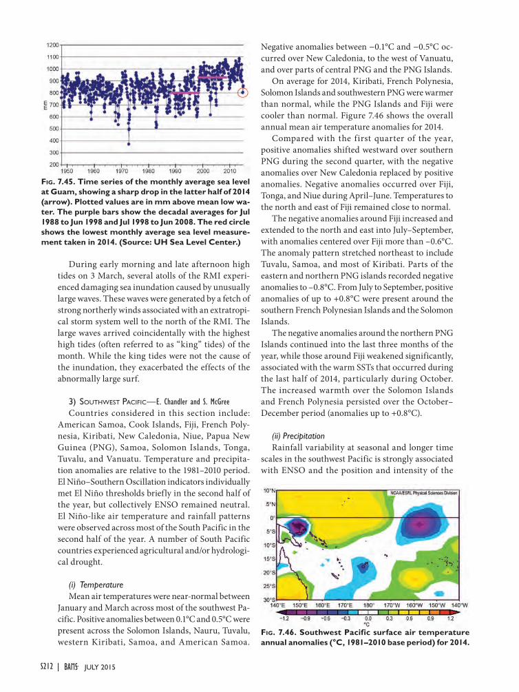
During early morning and late afternoon high tides on 3 March, several atolls of the RMI experi-enced damaging sea inundation caused by unusually large waves. These waves were generated by a fetch of strong northerly winds associated with an extratropi-cal storm system well to the north of the RMI. The large waves arrived coincidentally with the highest high tides (often referred to as “king” tides) of the month. While the king tides were not the cause of the inundation, they exacerbated the effects of the abnormally large surf.
3) SoUthWeSt paCifiC—E. Chandler and S. McGreeCountries considered in this section include:
American Samoa, Cook Islands, Fiji, French Poly-nesia, Kiribati, New Caledonia, Niue, Papua New Guinea (PNG), Samoa, Solomon Islands, Tonga, Tuvalu, and Vanuatu. Temperature and precipita-tion anomalies are relative to the 1981–2010 period. El Niño–Southern Oscillation indicators individually met El Niño thresholds briefly in the second half of the year, but collectively ENSO remained neutral. El Niño-like air temperature and rainfall patterns were observed across most of the South Pacific in the second half of the year. A number of South Pacific countries experienced agricultural and/or hydrologi-cal drought.
(i) TemperatureMean air temperatures were near-normal between
January and March across most of the southwest Pa-cific. Positive anomalies between 0.1°C and 0.5°C were present across the Solomon Islands, Nauru, Tuvalu, western Kiribati, Samoa, and American Samoa.
Negative anomalies between −0.1°C and −0.5°C oc-curred over New Caledonia, to the west of Vanuatu, and over parts of central PNG and the PNG Islands.
On average for 2014, Kiribati, French Polynesia, Solomon Islands and southwestern PNG were warmer than normal, while the PNG Islands and Fiji were cooler than normal. Figure 7.46 shows the overall annual mean air temperature anomalies for 2014.
Compared with the first quarter of the year, positive anomalies shifted westward over southern PNG during the second quarter, with the negative anomalies over New Caledonia replaced by positive anomalies. Negative anomalies occurred over Fiji, Tonga, and Niue during April–June. Temperatures to the north and east of Fiji remained close to normal.
The negative anomalies around Fiji increased and extended to the north and east into July–September, with anomalies centered over Fiji more than –0.6°C. The anomaly pattern stretched northeast to include Tuvalu, Samoa, and most of Kiribati. Parts of the eastern and northern PNG islands recorded negative anomalies to –0.8°C. From July to September, positive anomalies of up to +0.8°C were present around the southern French Polynesian Islands and the Solomon Islands.
The negative anomalies around the northern PNG Islands continued into the last three months of the year, while those around Fiji weakened significantly, associated with the warm SSTs that occurred during the last half of 2014, particularly during October. The increased warmth over the Solomon Islands and French Polynesia persisted over the October–December period (anomalies up to +0.8°C).
(ii) PrecipitationRainfall variability at seasonal and longer time
scales in the southwest Pacific is strongly associated with ENSO and the position and intensity of the
Fig. 7.46. Southwest Pacific surface air temperature annual anomalies (°C, 1981–2010 base period) for 2014.
Fig. 7.45. Time series of the monthly average sea level at Guam, showing a sharp drop in the latter half of 2014 (arrow). Plotted values are in mm above mean low wa-ter. The purple bars show the decadal averages for Jul 1988 to Jun 1998 and Jul 1998 to Jun 2008. The red circle shows the lowest monthly average sea level measure-ment taken in 2014. (Source: UH Sea Level Center.)
S212 JULY 2015|
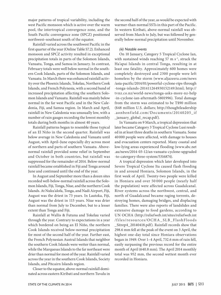
major patterns of tropical variability, including the west Pacific monsoon which is active over the warm pool, the intertropical convergence zone, and the South Pacific convergence zone (SPCZ) positioned northwest–southeast south of the equator.
Rainfall varied across the southwest Pacific in the first quarter of the year (Online Table S7.2). Enhanced monsoon and SPCZ activity resulted in exceptional precipitation totals in parts of the Solomon Islands, Vanuatu, Tonga, and Samoa in January. In contrast, February totals were well below normal in the south-ern Cook Islands, parts of the Solomon Islands, and Vanuatu. In March there was enhanced rainfall activ-ity over the Phoenix Islands, Tokelau, Northern Cook Islands, and French Polynesia, with a second band of increased precipitation affecting the southern Solo-mon Islands and Vanuatu. Rainfall was mainly below normal in the far west Pacific and in the New Cale-donia, Fiji, and Samoa region. In March and April, rainfall in New Caledonia was unusually low, with a number of rain gauges recording the lowest monthly totals during both months in almost 40 years.
Rainfall patterns began to resemble those typical of an El Niño in the second quarter. Rainfall was below average in New Caledonia and Vanuatu until August, with April–June especially dry across most of northern and parts of southern Vanuatu. Above-normal rainfall provided some relief in September and October in both countries, but rainfall was suppressed for the remainder of 2014. Below-normal rainfall became established in Fiji and Tonga around June and continued until the end of the year.
In August and September more than a dozen sites recorded well-below-normal rainfall across the Solo-mon Islands, Fiji, Tonga, Niue, and the northern Cook Islands. At Nuku’alofa, Tonga, and Nadi Airport, Fiji, August was the driest in 73 years. In Lautoka, Fiji, August was the driest in 115 years. Niue was drier than normal from July to December, but to a lesser extent than Tonga and Fiji.
Rainfall at Wallis & Futuna and Tokelau varied through the year. Contrary to expectations in a year which bordered on being an El Niño, the northern Cook Islands received below-normal precipitation for most of the second half of the year. Farther east, the French Polynesian Austral Islands that neighbor the southern Cook Islands were wetter than normal, while the Marquesas Islands to the far northeast were drier than normal for most of the year. Rainfall varied across the year in the southern Cook Islands, Society Islands, and Pitcairn Islands region.
Closer to the equator, above-normal rainfall domi-nated across eastern Kiribati and northern Tuvalu in
the second half of the year, as would be expected with warmer-than-normal SSTs in this part of the Pacific. In western Kiribati, above-normal rainfall was ob-served from March to July, but was followed by gen-erally below-normal precipitation until November.
(iii) Notable eventsOn 10 January, Category 5 Tropical Cyclone Ian,
with sustained winds reaching 57 m s−1, struck the Ha’apai Islands in central Tonga, resulting in at least one fatality. Approximately 600 homes were completely destroyed and 2300 people were left homeless by the storm (www.aljazeera.com/news /asia-pacific/2014/01/powerful-cyclone-rips-through -tonga-islands-201411264930152149.html; http://tvnz.co.nz/world-news/tonga-asks-more-nz-help -in-cyclone-ian-aftermath-5801996). Total damage from the storm was estimated to be T$90 million ($48 million U.S. dollars; http://thoughtleadership . aonben f ie ld .com /Doc u ment s/2014 0205 _ i f _january_global_recap.pdf).
In Vanuatu on 9 March, a tropical depression that later became Category 3 Tropical Cyclone Lusi result-ed in at least three deaths in southern Vanuatu. Some 40 000 people were affected, with damage to houses and evacuation centers reported. Many coastal and low-lying areas experienced flooding (www.abc.net .au/news/2014-03-12/an-vanuatu-cyclone-upgraded -to-catergory-three-system/5316874).
A tropical depression which later developed into Severe Tropical Cyclone Ita caused f lash f looding in and around Honiara, Solomon Islands, in the first week of April. Twenty-two people were killed in Honiara and over 50 000 people (nearly half the population) were affected across Guadalcanal. River systems across the northwest, central, and north of Guadalcanal became raging torrents, de-stroying homes, damaging bridges, and displacing families. There were also reports of landslides and extensive damage to food gardens, according to UN OCHA (http://reliefweb.int/sites/reliefweb.int / f i l e s /re s ou rc e s /O C H A _ SL B _ F l a s h F lo o d s _Sitrep4_20140418.pdf). Rainfall records show that 298.6 mm fell at the peak of the event on 3 April, the highest one-day total since Honiara observations began in 1949. Over 1–4 April, 732.6 mm of rain fell, easily surpassing the previous record for the entire month of April (640.8 mm). The April 2014 monthly total was 952 mm, the second wettest month ever recorded in Honiara.
S213JULY 2015STATE OF THE CLIMATE IN 2014 |
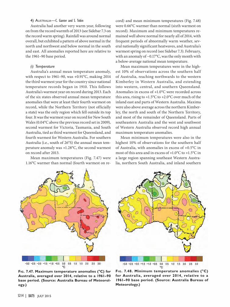
4) aUStralia—C. Ganter and S. TobinAustralia had another very warm year, following
on from the record warmth of 2013 (see Sidebar 7.3 on the record warm spring). Rainfall was around normal overall, but exhibited a pattern of above normal in the north and northwest and below normal in the south and east. All anomalies reported here are relative to the 1961–90 base period.
(i) TemperatureAustralia’s annual mean temperature anomaly,
with respect to 1961–90, was +0.91°C, making 2014 the third warmest year for the country since national temperature records began in 1910. This follows Australia’s warmest year on record during 2013. Each of the six states observed annual mean temperature anomalies that were at least their fourth warmest on record, while the Northern Territory (not officially a state) was the only region which fell outside its top four. It was the warmest year on record for New South Wales (0.04°C above the previous record set in 2009), second warmest for Victoria, Tasmania, and South Australia, tied as third warmest for Queensland, and fourth warmest for Western Australia. For southern Australia (i.e., south of 26°S) the annual mean tem-perature anomaly was +1.28°C, the second warmest on record after 2013.
Mean maximum temperatures (Fig. 7.47) were 1.16°C warmer than normal (fourth warmest on re-
cord) and mean minimum temperatures (Fig. 7.48) were 0.66°C warmer than normal (sixth warmest on record). Maximum and minimum temperatures re-mained well above normal for nearly all of 2014, with frequent periods of abnormally warm weather, sev-eral nationally significant heatwaves, and Australia’s warmest spring on record (see Sidebar 7.3). February, with an anomaly of −0.17°C, was the only month with a below-average national mean temperature.
Mean maximum temperatures were in the high-est 10% of observations across the southern half of Australia, reaching northwards to the western Kimberley in Western Australia, and extending into western, central, and southern Queensland. Anomalies in excess of +1.0°C were recorded across this area, rising to +1.5°C to +2.0°C over much of the inland east and parts of Western Australia. Maxima were also above average across the northern Kimber-ley, the north and south of the Northern Territory, and most of the remainder of Queensland. Parts of southeastern Australia and the west and southwest of Western Australia observed record high annual maximum temperature anomalies.
Mean minimum temperatures were also in the highest 10% of observations for the southern half of Australia, with anomalies in excess of +0.5°C in most of this area and in excess of +1.0°C to +1.5°C in a large region spanning southeast Western Austra-lia, northern South Australia, and inland southern
Fig. 7.48. Minimum temperature anomalies (°C) for Australia , averaged over 2014, relative to a 1961–90 base period. (Source: Australia Bureau of Meteorology.)
Fig. 7.47. Maximum temperature anomalies (°C) for Australia, averaged over 2014, relative to a 1961–90 base period. (Source: Australia Bureau of Meteorol-ogy.)
S214 JULY 2015|
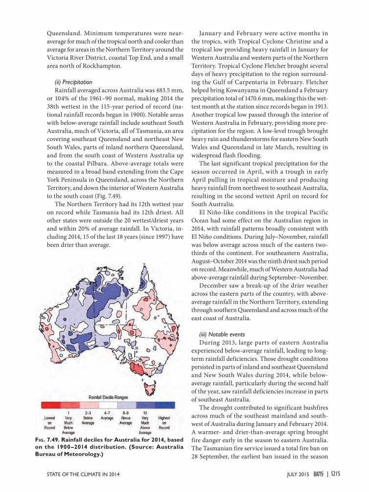
Fig. 7.49. Rainfall deciles for Australia for 2014, based on the 1900–2014 distribution. (Source: Australia Bureau of Meteorology.)
Queensland. Minimum temperatures were near-average for much of the tropical north and cooler than average for areas in the Northern Territory around the Victoria River District, coastal Top End, and a small area north of Rockhampton.
(ii) Precipitation Rainfall averaged across Australia was 483.5 mm,
or 104% of the 1961–90 normal, making 2014 the 38th wettest in the 115-year period of record (na-tional rainfall records began in 1900). Notable areas with below-average rainfall include southeast South Australia, much of Victoria, all of Tasmania, an area covering southeast Queensland and northeast New South Wales, parts of inland northern Queensland, and from the south coast of Western Australia up to the coastal Pilbara. Above-average totals were measured in a broad band extending from the Cape York Peninsula in Queensland, across the Northern Territory, and down the interior of Western Australia to the south coast (Fig. 7.49).
The Northern Territory had its 12th wettest year on record while Tasmania had its 12th driest. All other states were outside the 20 wettest/driest years and within 20% of average rainfall. In Victoria, in-cluding 2014, 15 of the last 18 years (since 1997) have been drier than average.
January and February were active months in the tropics, with Tropical Cyclone Christine and a tropical low providing heavy rainfall in January for Western Australia and western parts of the Northern Territory. Tropical Cyclone Fletcher brought several days of heavy precipitation to the region surround-ing the Gulf of Carpentaria in February. Fletcher helped bring Kowanyama in Queensland a February precipitation total of 1470.6 mm, making this the wet-test month at the station since records began in 1913. Another tropical low passed through the interior of Western Australia in February, providing more pre-cipitation for the region. A low-level trough brought heavy rain and thunderstorms for eastern New South Wales and Queensland in late March, resulting in widespread flash flooding.
The last significant tropical precipitation for the season occurred in April, with a trough in early April pulling in tropical moisture and producing heavy rainfall from northwest to southeast Australia, resulting in the second wettest April on record for South Australia.
El Niño-like conditions in the tropical Pacific Ocean had some effect on the Australian region in 2014, with rainfall patterns broadly consistent with El Niño conditions. During July–November, rainfall was below average across much of the eastern two-thirds of the continent. For southeastern Australia, August–October 2014 was the ninth driest such period on record. Meanwhile, much of Western Australia had above-average rainfall during September–November.
December saw a break-up of the drier weather across the eastern parts of the country, with above-average rainfall in the Northern Territory, extending through southern Queensland and across much of the east coast of Australia.
(iii) Notable eventsDuring 2013, large parts of eastern Australia
experienced below-average rainfall, leading to long-term rainfall deficiencies. Those drought conditions persisted in parts of inland and southeast Queensland and New South Wales during 2014, while below-average rainfall, particularly during the second half of the year, saw rainfall deficiencies increase in parts of southeast Australia.
The drought contributed to significant bushfires across much of the southeast mainland and south-west of Australia during January and February 2014. A warmer- and drier-than-average spring brought fire danger early in the season to eastern Australia. The Tasmanian fire service issued a total fire ban on 28 September, the earliest ban issued in the season
S215JULY 2015STATE OF THE CLIMATE IN 2014 |
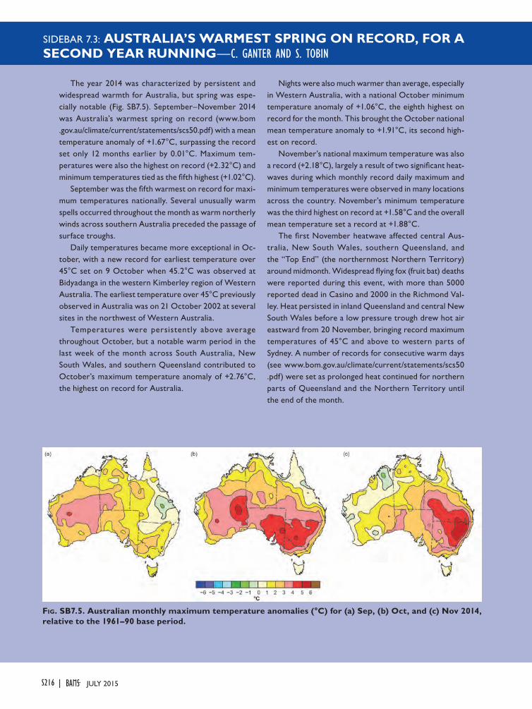
SIDEBAR 7.3: AUSTRALIA’S WARMEST SPRING ON RECORD, FOR A SECOND YEAR RUNNING—C. GANTER AND S. TOBIN
The year 2014 was characterized by persistent and widespread warmth for Australia, but spring was espe-cially notable (Fig. SB7.5). September–November 2014 was Australia’s warmest spring on record (www.bom .gov.au/climate/current/statements/scs50.pdf) with a mean temperature anomaly of +1.67°C, surpassing the record set only 12 months earlier by 0.01°C. Maximum tem-peratures were also the highest on record (+2.32°C) and minimum temperatures tied as the fifth highest (+1.02°C).
September was the fifth warmest on record for maxi-mum temperatures nationally. Several unusually warm spells occurred throughout the month as warm northerly winds across southern Australia preceded the passage of surface troughs.
Daily temperatures became more exceptional in Oc-tober, with a new record for earliest temperature over 45°C set on 9 October when 45.2°C was observed at Bidyadanga in the western Kimberley region of Western Australia. The earliest temperature over 45°C previously observed in Australia was on 21 October 2002 at several sites in the northwest of Western Australia.
Temperatures were persistently above average throughout October, but a notable warm period in the last week of the month across South Australia, New South Wales, and southern Queensland contributed to October’s maximum temperature anomaly of +2.76°C, the highest on record for Australia.
Nights were also much warmer than average, especially in Western Australia, with a national October minimum temperature anomaly of +1.06°C, the eighth highest on record for the month. This brought the October national mean temperature anomaly to +1.91°C, its second high-est on record.
November’s national maximum temperature was also a record (+2.18°C), largely a result of two significant heat-waves during which monthly record daily maximum and minimum temperatures were observed in many locations across the country. November’s minimum temperature was the third highest on record at +1.58°C and the overall mean temperature set a record at +1.88°C.
The first November heatwave affected central Aus-tralia, New South Wales, southern Queensland, and the “Top End” (the northernmost Northern Territory) around midmonth. Widespread flying fox (fruit bat) deaths were reported during this event, with more than 5000 reported dead in Casino and 2000 in the Richmond Val-ley. Heat persisted in inland Queensland and central New South Wales before a low pressure trough drew hot air eastward from 20 November, bringing record maximum temperatures of 45°C and above to western parts of Sydney. A number of records for consecutive warm days (see www.bom.gov.au/climate/current/statements/scs50 .pdf) were set as prolonged heat continued for northern parts of Queensland and the Northern Territory until the end of the month.
Fig. SB7.5. Australian monthly maximum temperature anomalies (°C) for (a) Sep, (b) Oct, and (c) Nov 2014, relative to the 1961–90 base period.
S216 JULY 2015|
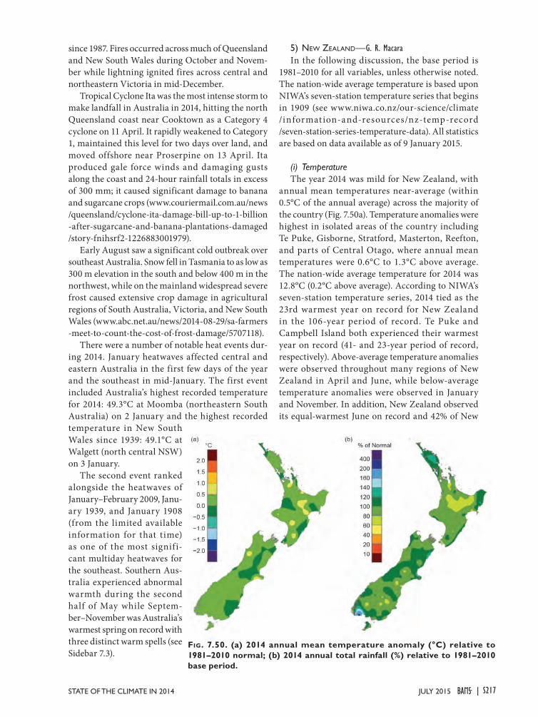
since 1987. Fires occurred across much of Queensland and New South Wales during October and Novem-ber while lightning ignited fires across central and northeastern Victoria in mid-December.
Tropical Cyclone Ita was the most intense storm to make landfall in Australia in 2014, hitting the north Queensland coast near Cooktown as a Category 4 cyclone on 11 April. It rapidly weakened to Category 1, maintained this level for two days over land, and moved offshore near Proserpine on 13 April. Ita produced gale force winds and damaging gusts along the coast and 24-hour rainfall totals in excess of 300 mm; it caused significant damage to banana and sugarcane crops (www.couriermail.com.au/news /queensland/cyclone-ita-damage-bill-up-to-1-billion -after-sugarcane-and-banana-plantations-damaged /story-fnihsrf2-1226883001979).
Early August saw a significant cold outbreak over southeast Australia. Snow fell in Tasmania to as low as 300 m elevation in the south and below 400 m in the northwest, while on the mainland widespread severe frost caused extensive crop damage in agricultural regions of South Australia, Victoria, and New South Wales (www.abc.net.au/news/2014-08-29/sa-farmers -meet-to-count-the-cost-of-frost-damage/5707118).
There were a number of notable heat events dur-ing 2014. January heatwaves affected central and eastern Australia in the first few days of the year and the southeast in mid-January. The first event included Australia’s highest recorded temperature for 2014: 49.3°C at Moomba (northeastern South Australia) on 2 January and the highest recorded temperature in New South Wales since 1939: 49.1°C at Walgett (north central NSW) on 3 January.
The second event ranked alongside the heatwaves of January–February 2009, Janu-ary 1939, and January 1908 (from the limited available information for that time) as one of the most signifi-cant multiday heatwaves for the southeast. Southern Aus-tralia experienced abnormal warmth during the second half of May while Septem-ber–November was Australia’s warmest spring on record with three distinct warm spells (see Sidebar 7.3).
5) neW Zealand—G. R. MacaraIn the following discussion, the base period is
1981–2010 for all variables, unless otherwise noted. The nation-wide average temperature is based upon NIWA’s seven-station temperature series that begins in 1909 (see www.niwa.co.nz/our-science/climate /information-and-resources/nz-temp-record /seven-station-series-temperature-data). All statistics are based on data available as of 9 January 2015.
(i) TemperatureThe year 2014 was mild for New Zealand, with
annual mean temperatures near-average (within 0.5°C of the annual average) across the majority of the country (Fig. 7.50a). Temperature anomalies were highest in isolated areas of the country including Te Puke, Gisborne, Stratford, Masterton, Reefton, and parts of Central Otago, where annual mean temperatures were 0.6°C to 1.3°C above average. The nation-wide average temperature for 2014 was 12.8°C (0.2°C above average). According to NIWA’s seven-station temperature series, 2014 tied as the 23rd warmest year on record for New Zealand in the 106-year period of record. Te Puke and Campbell Island both experienced their warmest year on record (41- and 23-year period of record, respectively). Above-average temperature anomalies were observed throughout many regions of New Zealand in April and June, while below-average temperature anomalies were observed in January and November. In addition, New Zealand observed its equal-warmest June on record and 42% of New
Fig. 7.50. (a) 2014 annual mean temperature anomaly (°C) relative to 1981–2010 normal; (b) 2014 annual total rainfall (%) relative to 1981–2010 base period.
S217JULY 2015STATE OF THE CLIMATE IN 2014 |
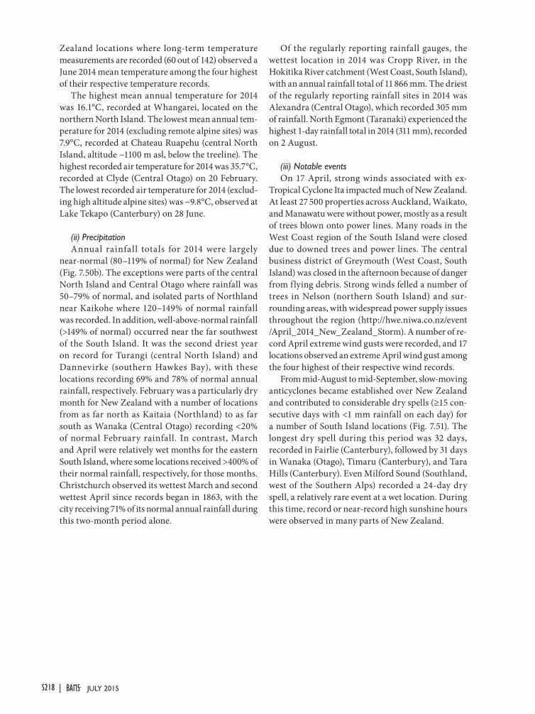
Zealand locations where long-term temperature measurements are recorded (60 out of 142) observed a June 2014 mean temperature among the four highest of their respective temperature records.
The highest mean annual temperature for 2014 was 16.1°C, recorded at Whangarei, located on the northern North Island. The lowest mean annual tem-perature for 2014 (excluding remote alpine sites) was 7.9°C, recorded at Chateau Ruapehu (central North Island, altitude ~1100 m asl, below the treeline). The highest recorded air temperature for 2014 was 35.7°C, recorded at Clyde (Central Otago) on 20 February. The lowest recorded air temperature for 2014 (exclud-ing high altitude alpine sites) was −9.8°C, observed at Lake Tekapo (Canterbury) on 28 June.
(ii) PrecipitationAnnual rainfall totals for 2014 were largely
near-normal (80–119% of normal) for New Zealand (Fig. 7.50b). The exceptions were parts of the central North Island and Central Otago where rainfall was 50–79% of normal, and isolated parts of Northland near Kaikohe where 120–149% of normal rainfall was recorded. In addition, well-above-normal rainfall (>149% of normal) occurred near the far southwest of the South Island. It was the second driest year on record for Turangi (central North Island) and Dannevirke (southern Hawkes Bay), with these locations recording 69% and 78% of normal annual rainfall, respectively. February was a particularly dry month for New Zealand with a number of locations from as far north as Kaitaia (Northland) to as far south as Wanaka (Central Otago) recording <20% of normal February rainfall. In contrast, March and April were relatively wet months for the eastern South Island, where some locations received >400% of their normal rainfall, respectively, for those months. Christchurch observed its wettest March and second wettest April since records began in 1863, with the city receiving 71% of its normal annual rainfall during this two-month period alone.
Of the regularly reporting rainfall gauges, the wettest location in 2014 was Cropp River, in the Hokitika River catchment (West Coast, South Island), with an annual rainfall total of 11 866 mm. The driest of the regularly reporting rainfall sites in 2014 was Alexandra (Central Otago), which recorded 305 mm of rainfall. North Egmont (Taranaki) experienced the highest 1-day rainfall total in 2014 (311 mm), recorded on 2 August.
(iii) Notable eventsOn 17 April, strong winds associated with ex-
Tropical Cyclone Ita impacted much of New Zealand. At least 27 500 properties across Auckland, Waikato, and Manawatu were without power, mostly as a result of trees blown onto power lines. Many roads in the West Coast region of the South Island were closed due to downed trees and power lines. The central business district of Greymouth (West Coast, South Island) was closed in the afternoon because of danger from flying debris. Strong winds felled a number of trees in Nelson (northern South Island) and sur-rounding areas, with widespread power supply issues throughout the region (http://hwe.niwa.co.nz/event /April_2014_New_Zealand_Storm). A number of re-cord April extreme wind gusts were recorded, and 17 locations observed an extreme April wind gust among the four highest of their respective wind records.
From mid-August to mid-September, slow-moving anticyclones became established over New Zealand and contributed to considerable dry spells (≥15 con-secutive days with <1 mm rainfall on each day) for a number of South Island locations (Fig. 7.51). The longest dry spell during this period was 32 days, recorded in Fairlie (Canterbury), followed by 31 days in Wanaka (Otago), Timaru (Canterbury), and Tara Hills (Canterbury). Even Milford Sound (Southland, west of the Southern Alps) recorded a 24-day dry spell, a relatively rare event at a wet location. During this time, record or near-record high sunshine hours were observed in many parts of New Zealand.
S218 JULY 2015|
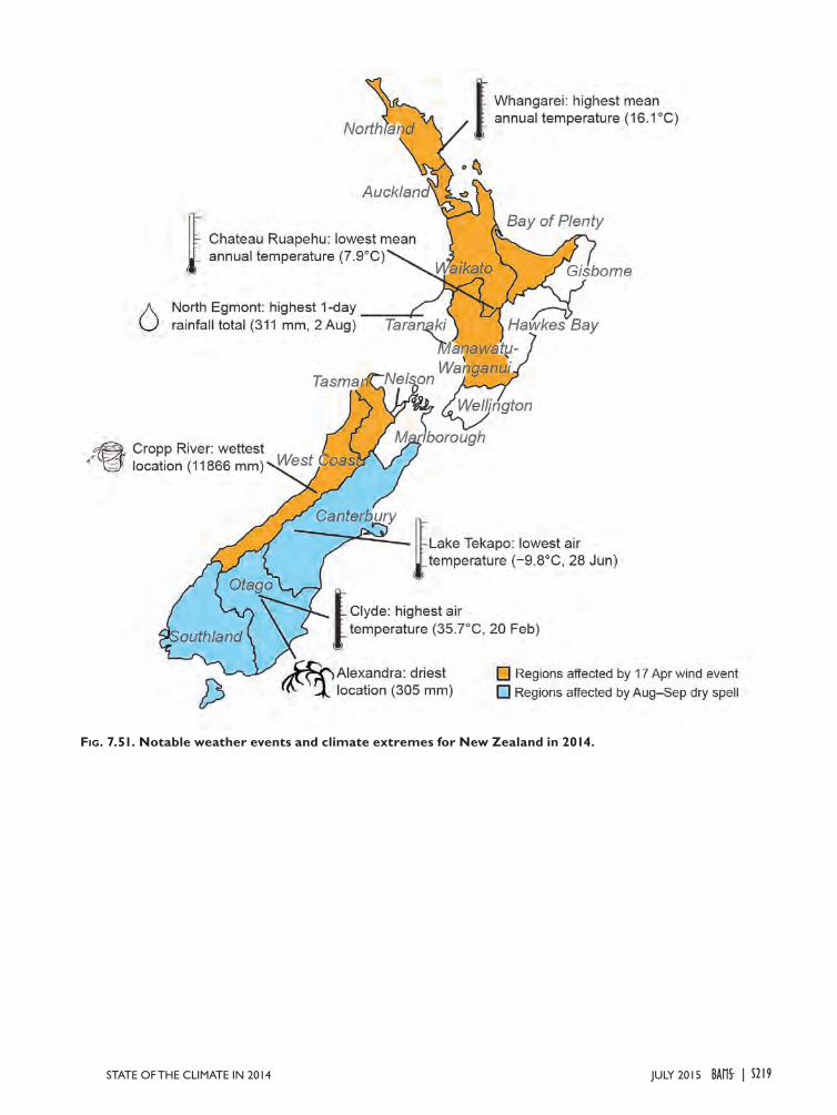
Fig. 7.51. Notable weather events and climate extremes for New Zealand in 2014.
S219JULY 2015STATE OF THE CLIMATE IN 2014 |

S220 JULY 2015|
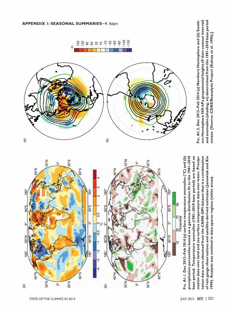
S221JULY 2015STATE OF THE CLIMATE IN 2014 |
APPENDIX 1: SEASONAL SUMMARIES─M. Halpert
Fig
. A1.
1. D
ec 2
013–
Feb
2014
(a)
surf
ace
tem
pera
ture
ano
mal
ies
(°C
) an
d (b
) pr
ecip
itat
ion
perc
enti
les
base
d on
a g
amm
a di
stri
buti
on fi
t to
the
198
1–20
10
base
per
iod.
Tem
pera
ture
ano
mal
ies
(198
1–20
10 b
ase
peri
od)
are
base
d on
st
atio
n da
ta o
ver
land
and
sea
sur
face
tem
pera
ture
dat
a ov
er w
ater
. Pre
cipi
-ta
tion
dat
a w
ere
obta
ined
from
the
CA
MS
-OP
I dat
aset
tha
t is
a co
mbi
nati
on
of r
ain
gaug
e ob
serv
atio
ns a
nd s
atel
lite-
deri
ved
esti
mat
es (
Jano
wia
k an
d X
ie
1999
). A
naly
sis
was
om
itte
d in
dat
a-sp
arse
reg
ions
(w
hite
are
as).
Fig
. A1.
2. D
ec 2
013–
Feb
2014
(a)
Nor
ther
n H
emis
pher
e an
d (b
) So
uth-
ern
Hem
isph
ere
500-
hPa
geop
oten
tial
hei
ghts
(9-d
am c
onto
ur in
terv
al)
and
anom
alie
s (s
hadi
ng, m
) det
erm
ined
from
the
198
1–20
10 b
ase
peri
od
mea
ns. [
Sour
ce: C
DA
S/R
eana
lysi
s P
roje
ct (
Kal
nay
et a
l. 19
96).
]
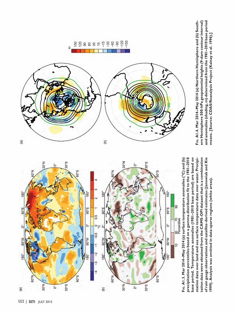
S222 JULY 2015|
Fig
. A1.
3. M
ar 2
014–
May
201
4 (a
) sur
face
tem
pera
ture
ano
mal
ies
(°C
) and
(b)
prec
ipit
atio
n pe
rcen
tile
s ba
sed
on a
gam
ma
dist
ribu
tion
fit
to t
he 1
981–
2010
ba
se p
erio
d. T
empe
ratu
re a
nom
alie
s (1
981–
2010
bas
e pe
riod
) ar
e ba
sed
on
stat
ion
data
ove
r la
nd a
nd s
ea s
urfa
ce t
empe
ratu
re d
ata
over
wat
er. P
reci
pi-
tati
on d
ata
wer
e ob
tain
ed fr
om t
he C
AM
S-O
PI d
atas
et t
hat i
s a
com
bina
tion
of
rai
n ga
uge
obse
rvat
ions
and
sat
ellit
e-de
rive
d es
tim
ates
(Ja
now
iak
and
Xie
19
99).
Ana
lysi
s w
as o
mit
ted
in d
ata-
spar
se r
egio
ns (
whi
te a
reas
).
Fig
. A1.
4. M
ar 2
014
–May
201
4 (a
) N
orth
ern
Hem
isph
ere
and
(b)
Sout
h-er
n H
emis
pher
e 50
0-hP
a ge
opot
enti
al h
eigh
ts (9
-dam
con
tour
inte
rval
) an
d an
omal
ies
(sha
ding
, m) d
eter
min
ed fr
om t
he 1
981–
2010
bas
e pe
riod
m
eans
. [So
urce
: CD
AS
/Rea
naly
sis
Pro
ject
(K
alna
y et
al.
1996
).]
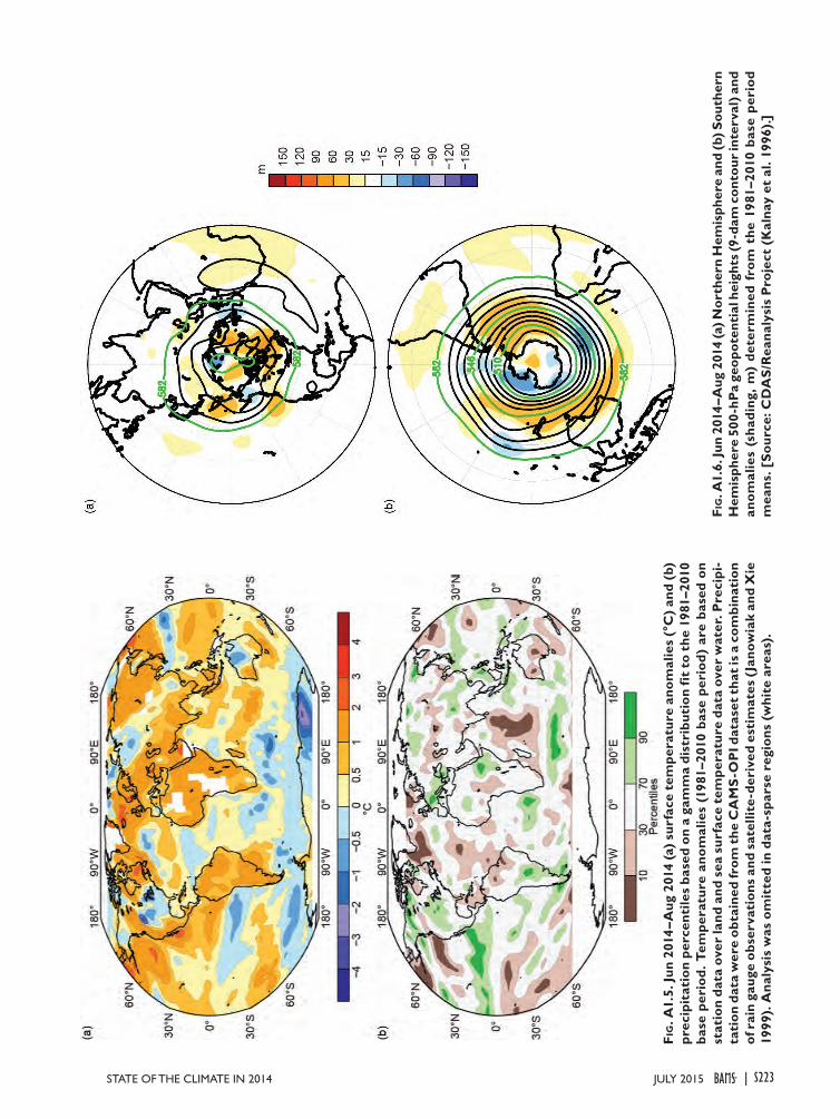
S223JULY 2015STATE OF THE CLIMATE IN 2014 |
Fig
. A1.
5. Ju
n 20
14–A
ug 2
014
(a)
surf
ace
tem
pera
ture
ano
mal
ies
(°C
) an
d (b
) pr
ecip
itat
ion
perc
enti
les
base
d on
a g
amm
a di
stri
buti
on fi
t to
the
198
1–20
10
base
per
iod.
Tem
pera
ture
ano
mal
ies
(198
1–20
10 b
ase
peri
od)
are
base
d on
st
atio
n da
ta o
ver
land
and
sea
sur
face
tem
pera
ture
dat
a ov
er w
ater
. Pre
cipi
-ta
tion
dat
a w
ere
obta
ined
from
the
CA
MS
-OP
I dat
aset
tha
t is
a co
mbi
nati
on
of r
ain
gaug
e ob
serv
atio
ns a
nd s
atel
lite-
deri
ved
esti
mat
es (
Jano
wia
k an
d X
ie
1999
). A
naly
sis
was
om
itte
d in
dat
a-sp
arse
reg
ions
(w
hite
are
as).
Fig
. A1.
6. Ju
n 20
14–A
ug 2
014
(a) N
orth
ern
Hem
isph
ere
and
(b) S
outh
ern
Hem
isph
ere
500-
hPa
geop
oten
tial
hei
ghts
(9-d
am c
onto
ur in
terv
al) a
nd
anom
alie
s (s
hadi
ng,
m)
dete
rmin
ed f
rom
the
198
1–20
10 b
ase
peri
od
mea
ns. [
Sour
ce: C
DA
S/R
eana
lysi
s P
roje
ct (
Kal
nay
et a
l. 19
96).
]
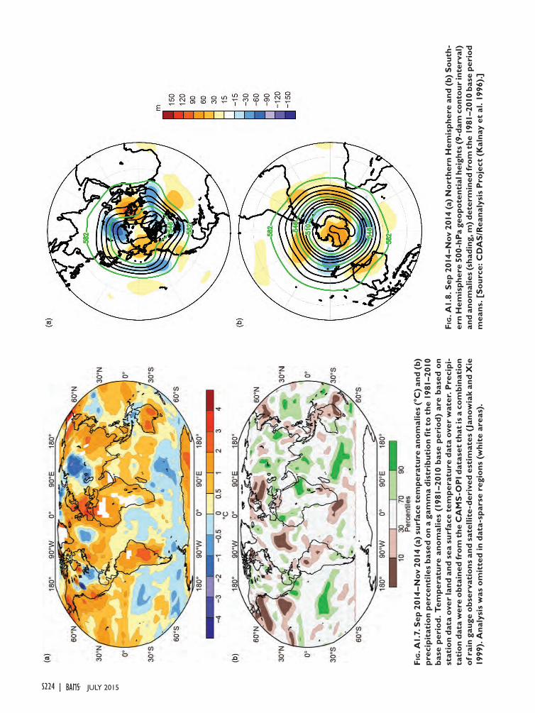
S224 JULY 2015|
Fig
. A1.
7. S
ep 2
014
–Nov
201
4 (a
) sur
face
tem
pera
ture
ano
mal
ies
(°C
) and
(b)
pr
ecip
itat
ion
perc
enti
les
base
d on
a g
amm
a di
stri
buti
on fi
t to
the
198
1–20
10
base
per
iod.
Tem
pera
ture
ano
mal
ies
(198
1–20
10 b
ase
peri
od)
are
base
d on
st
atio
n da
ta o
ver
land
and
sea
sur
face
tem
pera
ture
dat
a ov
er w
ater
. Pre
cipi
-ta
tion
dat
a w
ere
obta
ined
from
the
CA
MS
-OP
I dat
aset
tha
t is
a co
mbi
nati
on
of r
ain
gaug
e ob
serv
atio
ns a
nd s
atel
lite-
deri
ved
esti
mat
es (
Jano
wia
k an
d X
ie
1999
). A
naly
sis
was
om
itte
d in
dat
a-sp
arse
reg
ions
(w
hite
are
as).
Fig
. A1.
8. S
ep 2
014
–Nov
201
4 (a
) N
orth
ern
Hem
isph
ere
and
(b)
Sout
h-er
n H
emis
pher
e 50
0-hP
a ge
opot
enti
al h
eigh
ts (9
-dam
con
tour
inte
rval
) an
d an
omal
ies
(sha
ding
, m) d
eter
min
ed fr
om t
he 1
981–
2010
bas
e pe
riod
m
eans
. [So
urce
: CD
AS
/Rea
naly
sis
Pro
ject
(K
alna
y et
al.
1996
).]
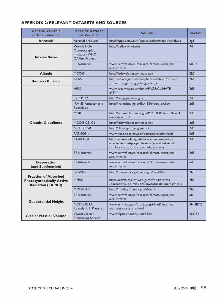
S225STATE OF THE CLIMATE IN 2014 |JULY 2015
General Variable or Phenomenon
Specific Dataset or Variable Source Section
Aerosols Aerosol products http://apps.ecmwf.int/datasets/data/macc-reanalysis 2g3
Air-sea fluxes
Woods Hole Oceanographic Institute (WHOI) OAFlux Project
http://oaflux.whoi.edu 3d
ERA-Interim www.ecmwf.int/en/research/climate-reanalysis /era-interim
SB3.2
Albedo MODIS http://ladsweb.nascom.nasa.gov 2h2
Biomass Burning GFAS https://www.gmes-atmosphere.eu/about/project _structure/global/g_idas/g_idas_2/
2h4
Clouds, Cloudiness
HIRS www.ssec.wisc.edu/~donw/PAGE/CLIMATE .HTM
2d5
ISCCP D2 http://isccp.giss.nasa.gov 2d5
JRA-55 Atmospheric Reanalysis
http://jra.kishou.go.jp/JRA-55/index_en.html 2d5
MISR http://eosweb.larc.nasa.gov/PRODOCS/misr/level3 /overview.html
2d5
MODIS C5, C6 http://ladsweb.nascom.nasa.gov 2d5
NCEP CFSR http://cfs.ncep.noaa.gov/cfsr/ 2d5
PATMOS-x www.ncdc.noaa.gov/cdr/operationalcdrs.html 2d5
CLARA_A1 https://climatedataguide.ucar.edu/climate-data /clara-a1-cloud-properties-surface-albedo-and -surface-radiation-products-based-avhrr
2d5
ERA-Interim www.ecmwf.int/en/research/climate-reanalysis /era-interim
2d5
Evaporation (and Sublimation)
ERA-Interim www.ecmwf.int/en/research/climate-reanalysis /era-interim
6d
Fraction of Absorbed Photosynthetically Active
Radiation (FAPAR)
SeaWIFS http://oceancolor.gsfc.nasa.gov/SeaWiFS 2h3
MERIS https://earth.esa.int/web/guest/missions/esa -operational-eo-missions/envisat/instruments/meris
2h3
MODIS-TIP http://modis.gsfc.nasa.gov/about/ 2h3
Geopotential Height
ERA-Interim www.ecmwf.int/en/research/climate-reanalysis /era-interim
6b
NCEP/NCAR Reanalysis 1: Pressure
www.esrl.noaa.gov/psd/data/gridded/data.ncep .reanalysis.pressure.html
5b, SB7.2
Glacier Mass or Volume World Glacier Monitoring Service
www.wgms.ch/mbb/sum12.html 2c3, 5e
APPENDIX 2: RELEVANT DATASETS AND SOURCES
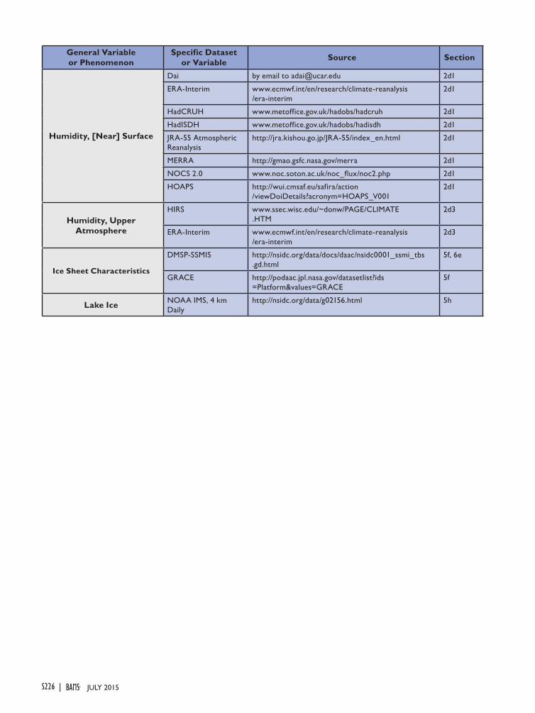
S226 | JULY 2015
General Variable or Phenomenon
Specific Dataset or Variable Source Section
Humidity, [Near] Surface
Dai by email to [email protected] 2d1
ERA-Interim www.ecmwf.int/en/research/climate-reanalysis /era-interim
2d1
HadCRUH www.metoffice.gov.uk/hadobs/hadcruh 2d1
HadISDH www.metoffice.gov.uk/hadobs/hadisdh 2d1
JRA-55 Atmospheric Reanalysis
http://jra.kishou.go.jp/JRA-55/index_en.html 2d1
MERRA http://gmao.gsfc.nasa.gov/merra 2d1
NOCS 2.0 www.noc.soton.ac.uk/noc_flux/noc2.php 2d1
HOAPS http://wui.cmsaf.eu/safira/action /viewDoiDetails?acronym=HOAPS_V001
2d1
Humidity, Upper Atmosphere
HIRS www.ssec.wisc.edu/~donw/PAGE/CLIMATE .HTM
2d3
ERA-Interim www.ecmwf.int/en/research/climate-reanalysis /era-interim
2d3
Ice Sheet Characteristics
DMSP-SSMIS http://nsidc.org/data/docs/daac/nsidc0001_ssmi_tbs .gd.html
5f, 6e
GRACE http://podaac.jpl.nasa.gov/datasetlist?ids =Platform&values=GRACE
5f
Lake Ice NOAA IMS, 4 km Daily
http://nsidc.org/data/g02156.html 5h
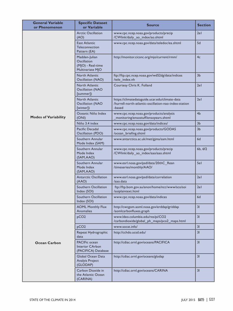
S227STATE OF THE CLIMATE IN 2014 |JULY 2015
General Variable or Phenomenon
Specific Dataset or Variable Source Section
Modes of Variability
Arctic Oscillation (AO)
www.cpc.ncep.noaa.gov/products/precip /CWlink/daily_ao_index/ao.shtml
2e1
East Atlantic Teleconnection Pattern (EA)
www.cpc.ncep.noaa.gov/data/teledoc/ea.shtml 5d
Madden-Julian Oscillation (MJO) - Real-time Multivariate MJO
http://monitor.cicsnc.org/mjo/current/rmm/ 4c
North Atlantic Oscillation (NAO)
ftp://ftp.cpc.ncep.noaa.gov/wd52dg/data/indices /tele_index.nh
3b
North Atlantic Oscillation (NAO [summer])
Courtesy Chris K. Folland 2e1
North Atlantic Oscillation (NAO [winter])
https://climatedataguide.ucar.edu/climate-data /hurrell-north-atlantic-oscillation-nao-index-station -based
2e1
Oceanic Niño Index (ONI)
www.cpc.ncep.noaa.gov/products/analysis _monitoring/ensostuff/ensoyears.shtml
4b
Niño 3.4 index www.cpc.ncep.noaa.gov/data/indices/ 3b
Pacific Decadal Oscillation (PDO)
www.cpc.ncep.noaa.gov/products/GODAS /ocean_briefing.shtml
3b
Southern Annular Mode Index (SAM)
www.antarctica.ac.uk/met/gjma/sam.html 6d
Southern Annular Mode Index (SAM,AAO)
www.cpc.ncep.noaa.gov/products/precip /CWlink/daily_ao_index/aao/aao.shtml
6b, 6f2
Southern Annular Mode Index (SAM,AAO)
www.esrl.noaa.gov/psd/data/20thC_Rean /timeseries/monthly/AAO/
5e1
Antarctic Oscillation (AAO)
www.esrl.noaa.gov/psd/data/correlation /aao.data
2e1
Southern Oscillation Index (SOI)
ftp://ftp.bom.gov.au/anon/home/ncc/www/sco/soi /soiplaintext.html
2e1
Southern Oscillation Index (SOI)
www.cpc.ncep.noaa.gov/data/indices 6d
Ocean Carbon
AOML Monthly Flux Anomalies
http://cwcgom.aoml.noaa.gov/erddap/griddap /aomlcarbonfluxes.graph
3l
pCO2 www.ldeo.columbia.edu/res/pi/CO2 /carbondioxide/global_ph_maps/pco2_maps.html
3l
pCO2 www.socat.info/ 3l
Repeat Hydrographic data
http://cchdo.ucsd.edu/ 3l
PACIFic ocean Interior CArbon (PACIFICA) Database
http://cdiac.ornl.gov/oceans/PACIFICA 3l
Global Ocean Data Analyis Project (GLODAP)
http://cdiac.ornl.gov/oceans/glodap 3l
Carbon Dioxide in the Atlantic Ocean (CARINA)
http://cdiac.ornl.gov/oceans/CARINA 3l
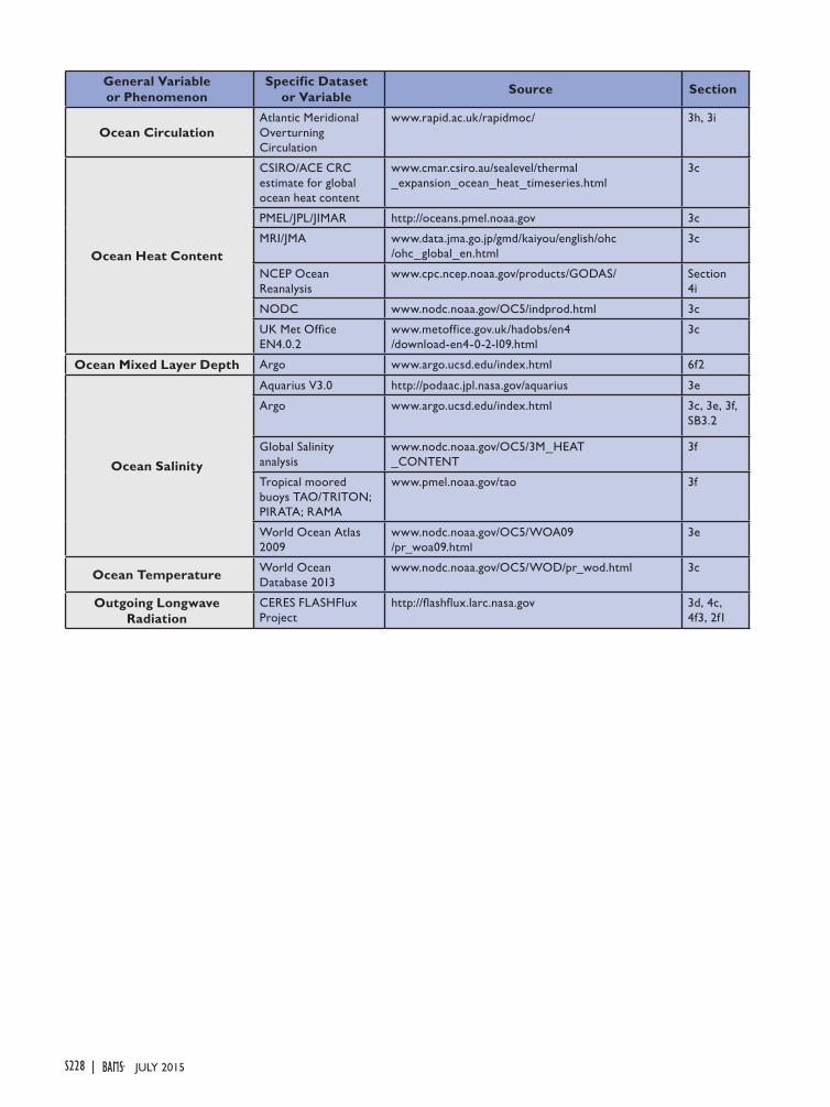
S228 | JULY 2015
General Variable or Phenomenon
Specific Dataset or Variable Source Section
Ocean CirculationAtlantic Meridional Overturning Circulation
www.rapid.ac.uk/rapidmoc/ 3h, 3i
Ocean Heat Content
CSIRO/ACE CRC estimate for global ocean heat content
www.cmar.csiro.au/sealevel/thermal _expansion_ocean_heat_timeseries.html
3c
PMEL/JPL/JIMAR http://oceans.pmel.noaa.gov 3c
MRI/JMA www.data.jma.go.jp/gmd/kaiyou/english/ohc /ohc_global_en.html
3c
NCEP Ocean Reanalysis
www.cpc.ncep.noaa.gov/products/GODAS/ Section 4i
NODC www.nodc.noaa.gov/OC5/indprod.html 3c
UK Met Office EN4.0.2
www.metoffice.gov.uk/hadobs/en4 /download-en4-0-2-l09.html
3c
Ocean Mixed Layer Depth Argo www.argo.ucsd.edu/index.html 6f2
Ocean Salinity
Aquarius V3.0 http://podaac.jpl.nasa.gov/aquarius 3e
Argo www.argo.ucsd.edu/index.html 3c, 3e, 3f, SB3.2
Global Salinity analysis
www.nodc.noaa.gov/OC5/3M_HEAT _CONTENT
3f
Tropical moored buoys TAO/TRITON; PIRATA; RAMA
www.pmel.noaa.gov/tao 3f
World Ocean Atlas 2009
www.nodc.noaa.gov/OC5/WOA09 /pr_woa09.html
3e
Ocean Temperature World Ocean Database 2013
www.nodc.noaa.gov/OC5/WOD/pr_wod.html 3c
Outgoing Longwave Radiation
CERES FLASHFlux Project
http://flashflux.larc.nasa.gov 3d, 4c, 4f3, 2f1

S229STATE OF THE CLIMATE IN 2014 |JULY 2015
General Variable or Phenomenon
Specific Dataset or Variable Source Section
Ozone, Total Column and Stratospheric
Bodeker Scientific www.bodekerscientific.com/data/total -column-ozone
5c
Calipso (Polar Stratospheric Clouds)
http://eosweb.larc.nasa.gov/PRODOCS/calipso /table_calipso.html
6h
GOME/SCIAMACHY/GOME2 (GSG) Merged Total Ozone
www.iup.uni-bremen.de/gome/wfdoas 2g4, 6h
GOZCARDS ozone profiles
https://gozcards.jpl.nasa.gov http://mirador.gsfc.nasa.gov
2g4
GOME/SCIAMACHY/GOME2 (GTO) Merged Total Ozone
http://atmos.eoc.dlr.de/gome/gto-ecv.html www.esa-ozone-cci.org
2g4
KNMI OMI http://ozoneaq.gsfc.nasa.gov 6h
Multi Sensor Reanalysis (MSR) of Total Ozone
www.temis.nl 2g4
NASA Aura Microwave Limb Sounder
http://aura.gsfc.nasa.gov/instruments/mls.html 2g4, 5c, 6h
NASA BUV/SBUV V8.6 (MOD V8.6) Merged Ozone
http://acdb-ext.gsfc.nasa.gov/Data_services/merged /index.html
2g4
NOAA SBUV V8.6 (MOD V8.6) Merged Ozone
ftp://ftp.cpc.ncep.noaa.gov/SBUV_CDR 2g4
Ozone Mapping and Profiler Suite Total Column Nadir Mapper (OMPS TC-NM)
http://ozoneaq.gsfc.nasa.gov/omps 5c, 6h
Ozonesonde www.esrl.noaa.gov/gmd/dv/spo_oz 6h
SAGE II/OSIRIS dataset linked to Bourassa et al. (2014) 2g4
Total Ozone Mapping Spectrometer
http://es-ee.tor.ec.gc.ca/cgi-bin/selectMap 5c
WOUDC Ground-based Ozone
ftp://ftp.tor.ec.gc.ca/pub/woudc/Project-Campaigns /ZonalMeans/
2g4
Ozone, Tropospheric Tropospheric Ozone http://acdb-ext.gsfc.nasa.gov/Data_services/cloud _slice/new_data.html
2g6
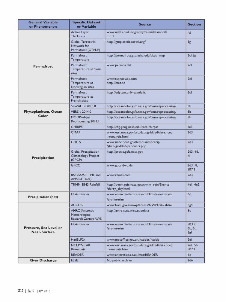
S230 | JULY 2015
General Variable or Phenomenon
Specific Dataset or Variable Source Section
Permafrost
Active Layer Thickness
www.udel.edu/Geography/calm/data/north .html
5g
Global Terrestrial Network for Permafrost (GTN-P)
http://gtnp.arcticportal.org/ 5g
Permafrost Temperature
http://permafrost.gi.alaska.edu/sites_map 2cl,5g
Permafrost Temperature at Swiss sites
www.permos.ch/ 2c1
Permafrost Temperature at Norwegian sites
www.tspnorway.com http://met.no
2c1
Permafrost Temperature at French sites
http://edytem.univ-savoie.fr/ 2c1
Phytoplankton, Ocean Color
SeaWiFS v 2010.0 http://oceancolor.gsfc.nasa.gov/cms/reprocessing/ 3k
VIIRS v 2014.0 http://oceancolor.gsfc.nasa.gov/cms/reprocessing/ 3k
MODIS-Aqua Reprocessing 2013.1
http://oceancolor.gsfc.nasa.gov/cms/reprocessing/ 3k
Precipitation
CHIRPS http://chg.geog.ucsb.edu/data/chirps/ 7e3
CMAP www.esrl.noaa.gov/psd/data/gridded/data.ncep .reanalysis.html
2d3
GHCN www.ncdc.noaa.gov/temp-and-precip /ghcn-gridded-products.php
2d3
Global Precipitation Climatology Project (GPCP)
http://precip.gsfc.nasa.gov 2d3, 4d, 4i
GPCC www.gpcc.dwd.de 2d3, 7f, SB7.2
RSS (SSM/I, TMI, and AMSR-E Data)
www.remss.com 2d3
TRMM 3B43 Rainfall http://trmm.gsfc.nasa.gov/trmm_rain/Events /thirty_day.html
4e1, 4e2
Precipitation (net)ERA-Interim www.ecmwf.int/en/research/climate-reanalysis
/era-interim
6d
Pressure, Sea Level or Near-Surface
ACCESS www.bom.gov.au/nwp/access/NWPData.shtml 6g4
AMRC (Antarctic Meteorological Research Center) AWS
http://amrc.ssec.wisc.edu/data 6c
ERA-Interim www.ecmwf.int/en/research/climate-reanalysis /era-interim
SB3.2, 6b, 6d, 6g1
HadSLP2r www.metoffice.gov.uk/hadobs/hadslp 2e1
NCEP/NCAR Reanalysis
www.esrl.noaa.gov/psd/data/gridded/data.ncep .reanalysis.html
2e1, 5b, SB7.2
READER www.antarctica.ac.uk/met/READER 6c
River Discharge ELSE No public archive 2d6
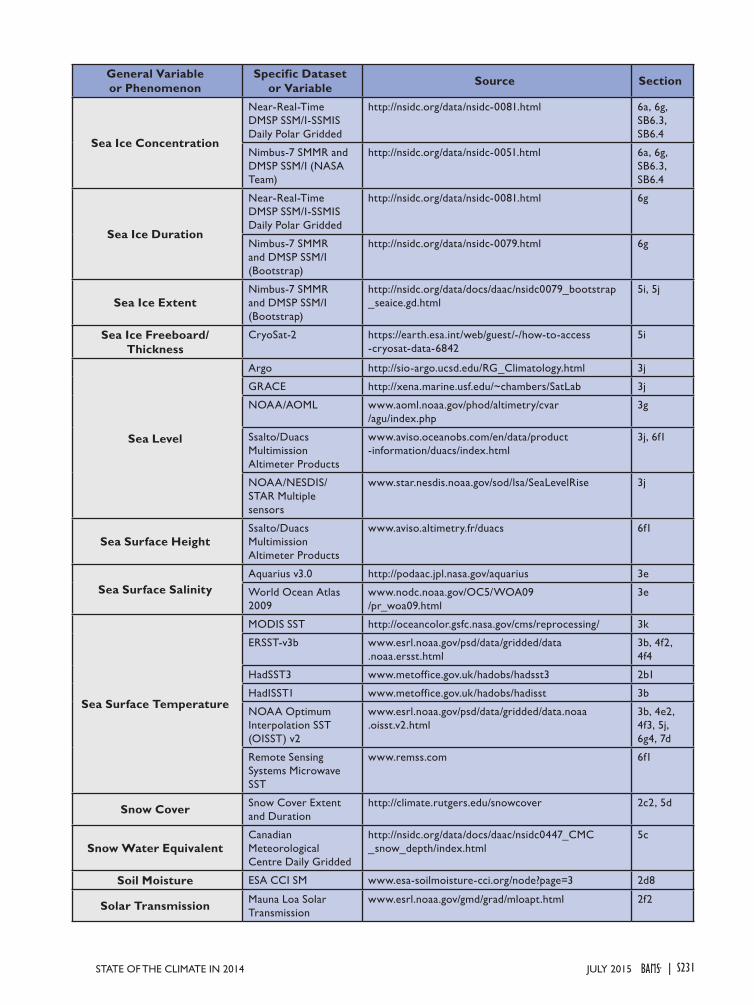
S231STATE OF THE CLIMATE IN 2014 |JULY 2015
General Variable or Phenomenon
Specific Dataset or Variable Source Section
Sea Ice Concentration
Near-Real-Time DMSP SSM/I-SSMIS Daily Polar Gridded
http://nsidc.org/data/nsidc-0081.html 6a, 6g, SB6.3, SB6.4
Nimbus-7 SMMR and DMSP SSM/I (NASA Team)
http://nsidc.org/data/nsidc-0051.html 6a, 6g, SB6.3, SB6.4
Sea Ice Duration
Near-Real-Time DMSP SSM/I-SSMIS Daily Polar Gridded
http://nsidc.org/data/nsidc-0081.html 6g
Nimbus-7 SMMR and DMSP SSM/I (Bootstrap)
http://nsidc.org/data/nsidc-0079.html 6g
Sea Ice ExtentNimbus-7 SMMR and DMSP SSM/I (Bootstrap)
http://nsidc.org/data/docs/daac/nsidc0079_bootstrap _seaice.gd.html
5i, 5j
Sea Ice Freeboard/Thickness
CryoSat-2 https://earth.esa.int/web/guest/-/how-to-access -cryosat-data-6842
5i
Sea Level
Argo http://sio-argo.ucsd.edu/RG_Climatology.html 3j
GRACE http://xena.marine.usf.edu/~chambers/SatLab 3j
NOAA/AOML www.aoml.noaa.gov/phod/altimetry/cvar /agu/index.php
3g
Ssalto/Duacs Multimission Altimeter Products
www.aviso.oceanobs.com/en/data/product -information/duacs/index.html
3j, 6f1
NOAA/NESDIS/STAR Multiple sensors
www.star.nesdis.noaa.gov/sod/lsa/SeaLevelRise 3j
Sea Surface HeightSsalto/Duacs Multimission Altimeter Products
www.aviso.altimetry.fr/duacs 6f1
Sea Surface SalinityAquarius v3.0 http://podaac.jpl.nasa.gov/aquarius 3e
World Ocean Atlas 2009
www.nodc.noaa.gov/OC5/WOA09 /pr_woa09.html
3e
Sea Surface Temperature
MODIS SST http://oceancolor.gsfc.nasa.gov/cms/reprocessing/ 3k
ERSST-v3b www.esrl.noaa.gov/psd/data/gridded/data .noaa.ersst.html
3b, 4f2, 4f4
HadSST3 www.metoffice.gov.uk/hadobs/hadsst3 2b1
HadISST1 www.metoffice.gov.uk/hadobs/hadisst 3b
NOAA Optimum Interpolation SST (OISST) v2
www.esrl.noaa.gov/psd/data/gridded/data.noaa .oisst.v2.html
3b, 4e2, 4f3, 5j, 6g4, 7d
Remote Sensing Systems Microwave SST
www.remss.com 6f1
Snow Cover Snow Cover Extent and Duration
http://climate.rutgers.edu/snowcover 2c2, 5d
Snow Water EquivalentCanadian Meteorological Centre Daily Gridded
http://nsidc.org/data/docs/daac/nsidc0447_CMC _snow_depth/index.html
5c
Soil Moisture ESA CCI SM www.esa-soilmoisture-cci.org/node?page=3 2d8
Solar Transmission Mauna Loa Solar Transmission
www.esrl.noaa.gov/gmd/grad/mloapt.html 2f2
General Variable or Phenomenon
Specific Dataset or Variable Source Section
Permafrost
Active Layer Thickness
www.udel.edu/Geography/calm/data/north .html
5g
Global Terrestrial Network for Permafrost (GTN-P)
http://gtnp.arcticportal.org/ 5g
Permafrost Temperature
http://permafrost.gi.alaska.edu/sites_map 2cl,5g
Permafrost Temperature at Swiss sites
www.permos.ch/ 2c1
Permafrost Temperature at Norwegian sites
www.tspnorway.com http://met.no
2c1
Permafrost Temperature at French sites
http://edytem.univ-savoie.fr/ 2c1
Phytoplankton, Ocean Color
SeaWiFS v 2010.0 http://oceancolor.gsfc.nasa.gov/cms/reprocessing/ 3k
VIIRS v 2014.0 http://oceancolor.gsfc.nasa.gov/cms/reprocessing/ 3k
MODIS-Aqua Reprocessing 2013.1
http://oceancolor.gsfc.nasa.gov/cms/reprocessing/ 3k
Precipitation
CHIRPS http://chg.geog.ucsb.edu/data/chirps/ 7e3
CMAP www.esrl.noaa.gov/psd/data/gridded/data.ncep .reanalysis.html
2d3
GHCN www.ncdc.noaa.gov/temp-and-precip /ghcn-gridded-products.php
2d3
Global Precipitation Climatology Project (GPCP)
http://precip.gsfc.nasa.gov 2d3, 4d, 4i
GPCC www.gpcc.dwd.de 2d3, 7f, SB7.2
RSS (SSM/I, TMI, and AMSR-E Data)
www.remss.com 2d3
TRMM 3B43 Rainfall http://trmm.gsfc.nasa.gov/trmm_rain/Events /thirty_day.html
4e1, 4e2
Precipitation (net)ERA-Interim www.ecmwf.int/en/research/climate-reanalysis
/era-interim
6d
Pressure, Sea Level or Near-Surface
ACCESS www.bom.gov.au/nwp/access/NWPData.shtml 6g4
AMRC (Antarctic Meteorological Research Center) AWS
http://amrc.ssec.wisc.edu/data 6c
ERA-Interim www.ecmwf.int/en/research/climate-reanalysis /era-interim
SB3.2, 6b, 6d, 6g1
HadSLP2r www.metoffice.gov.uk/hadobs/hadslp 2e1
NCEP/NCAR Reanalysis
www.esrl.noaa.gov/psd/data/gridded/data.ncep .reanalysis.html
2e1, 5b, SB7.2
READER www.antarctica.ac.uk/met/READER 6c
River Discharge ELSE No public archive 2d6
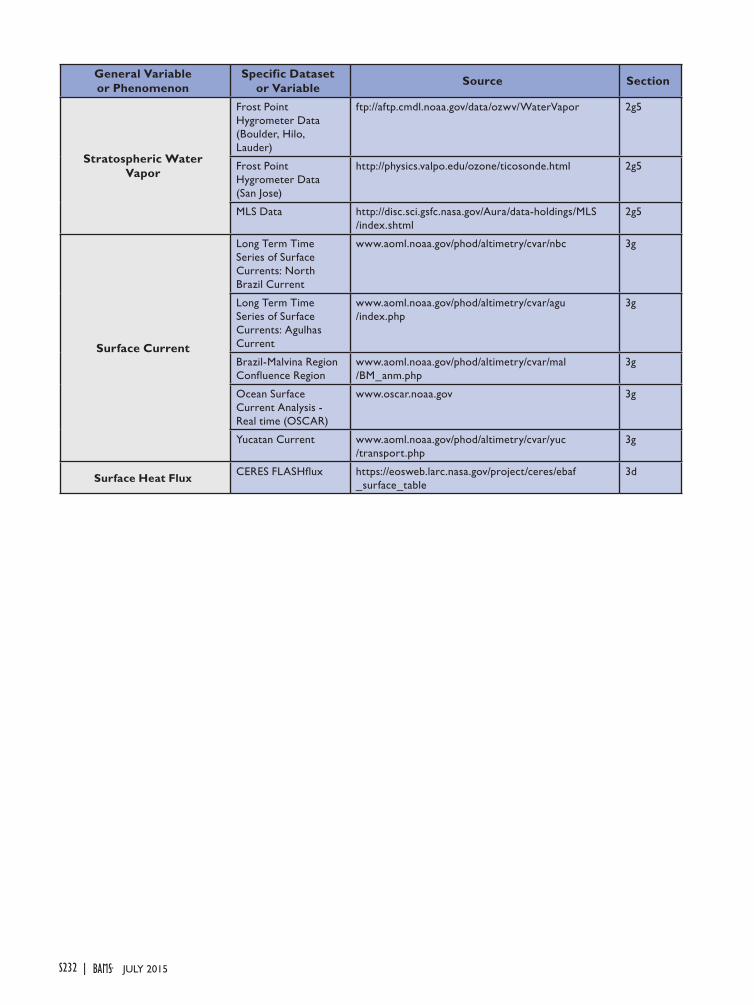
S232 | JULY 2015
General Variable or Phenomenon
Specific Dataset or Variable Source Section
Stratospheric Water Vapor
Frost Point Hygrometer Data (Boulder, Hilo, Lauder)
ftp://aftp.cmdl.noaa.gov/data/ozwv/WaterVapor 2g5
Frost Point Hygrometer Data (San Jose)
http://physics.valpo.edu/ozone/ticosonde.html 2g5
MLS Data http://disc.sci.gsfc.nasa.gov/Aura/data-holdings/MLS /index.shtml
2g5
Surface Current
Long Term Time Series of Surface Currents: North Brazil Current
www.aoml.noaa.gov/phod/altimetry/cvar/nbc 3g
Long Term Time Series of Surface Currents: Agulhas Current
www.aoml.noaa.gov/phod/altimetry/cvar/agu /index.php
3g
Brazil-Malvina Region Confluence Region
www.aoml.noaa.gov/phod/altimetry/cvar/mal /BM_anm.php
3g
Ocean Surface Current Analysis - Real time (OSCAR)
www.oscar.noaa.gov 3g
Yucatan Current www.aoml.noaa.gov/phod/altimetry/cvar/yuc /transport.php
3g
Surface Heat Flux CERES FLASHflux https://eosweb.larc.nasa.gov/project/ceres/ebaf _surface_table
3d
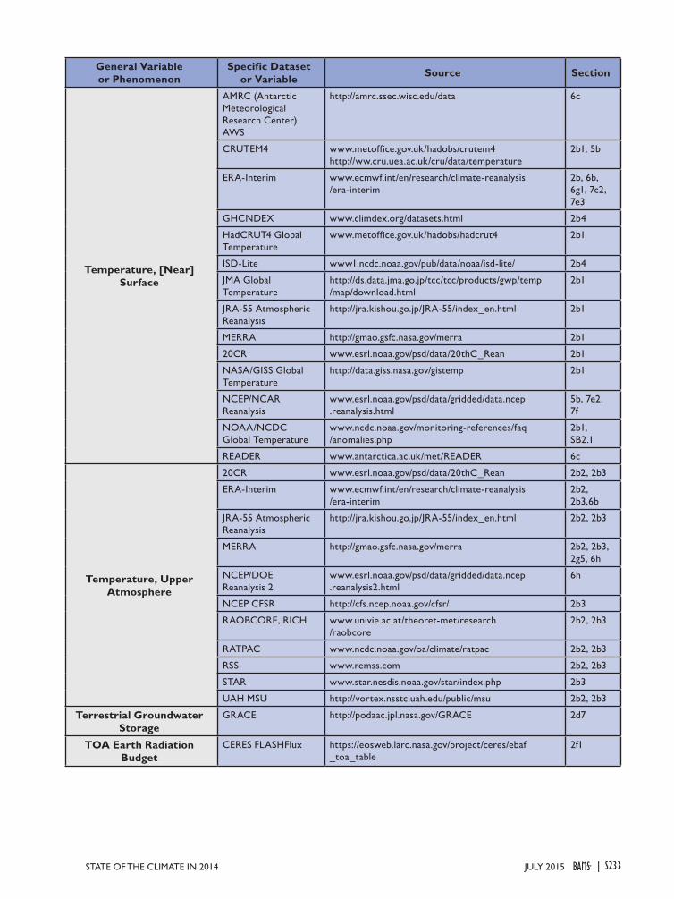
S233STATE OF THE CLIMATE IN 2014 |JULY 2015
General Variable or Phenomenon
Specific Dataset or Variable Source Section
Temperature, [Near] Surface
AMRC (Antarctic Meteorological Research Center) AWS
http://amrc.ssec.wisc.edu/data 6c
CRUTEM4 www.metoffice.gov.uk/hadobs/crutem4 http://ww.cru.uea.ac.uk/cru/data/temperature
2b1, 5b
ERA-Interim www.ecmwf.int/en/research/climate-reanalysis /era-interim
2b, 6b, 6g1, 7c2, 7e3
GHCNDEX www.climdex.org/datasets.html 2b4
HadCRUT4 Global Temperature
www.metoffice.gov.uk/hadobs/hadcrut4 2b1
ISD-Lite www1.ncdc.noaa.gov/pub/data/noaa/isd-lite/ 2b4
JMA Global Temperature
http://ds.data.jma.go.jp/tcc/tcc/products/gwp/temp /map/download.html
2b1
JRA-55 Atmospheric Reanalysis
http://jra.kishou.go.jp/JRA-55/index_en.html 2b1
MERRA http://gmao.gsfc.nasa.gov/merra 2b1
20CR www.esrl.noaa.gov/psd/data/20thC_Rean 2b1
NASA/GISS Global Temperature
http://data.giss.nasa.gov/gistemp 2b1
NCEP/NCAR Reanalysis
www.esrl.noaa.gov/psd/data/gridded/data.ncep .reanalysis.html
5b, 7e2, 7f
NOAA/NCDC Global Temperature
www.ncdc.noaa.gov/monitoring-references/faq /anomalies.php
2b1, SB2.1
READER www.antarctica.ac.uk/met/READER 6c
Temperature, Upper Atmosphere
20CR www.esrl.noaa.gov/psd/data/20thC_Rean 2b2, 2b3
ERA-Interim www.ecmwf.int/en/research/climate-reanalysis /era-interim
2b2, 2b3,6b
JRA-55 Atmospheric Reanalysis
http://jra.kishou.go.jp/JRA-55/index_en.html 2b2, 2b3
MERRA http://gmao.gsfc.nasa.gov/merra 2b2, 2b3, 2g5, 6h
NCEP/DOE Reanalysis 2
www.esrl.noaa.gov/psd/data/gridded/data.ncep .reanalysis2.html
6h
NCEP CFSR http://cfs.ncep.noaa.gov/cfsr/ 2b3
RAOBCORE, RICH www.univie.ac.at/theoret-met/research /raobcore
2b2, 2b3
RATPAC www.ncdc.noaa.gov/oa/climate/ratpac 2b2, 2b3
RSS www.remss.com 2b2, 2b3
STAR www.star.nesdis.noaa.gov/star/index.php 2b3
UAH MSU http://vortex.nsstc.uah.edu/public/msu 2b2, 2b3
Terrestrial Groundwater Storage
GRACE http://podaac.jpl.nasa.gov/GRACE 2d7
TOA Earth Radiation Budget
CERES FLASHFlux https://eosweb.larc.nasa.gov/project/ceres/ebaf _toa_table
2f1
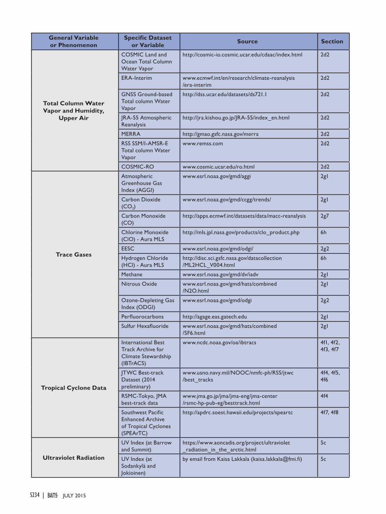
S234 | JULY 2015
General Variable or Phenomenon
Specific Dataset or Variable Source Section
Total Column Water Vapor and Humidity,
Upper Air
COSMIC Land and Ocean Total Column Water Vapor
http://cosmic-io.cosmic.ucar.edu/cdaac/index.html 2d2
ERA-Interim www.ecmwf.int/en/research/climate-reanalysis /era-interim
2d2
GNSS Ground-based Total column Water Vapor
http://dss.ucar.edu/datasets/ds721.1 2d2
JRA-55 Atmospheric Reanalysis
http://jra.kishou.go.jp/JRA-55/index_en.html 2d2
MERRA http://gmao.gsfc.nasa.gov/merra 2d2
RSS SSM/I-AMSR-E Total column Water Vapor
www.remss.com 2d2
COSMIC-RO www.cosmic.ucar.edu/ro.html 2d2
Trace Gases
Atmospheric Greenhouse Gas Index (AGGI)
www.esrl.noaa.gov/gmd/aggi 2g1
Carbon Dioxide (CO2)
www.esrl.noaa.gov/gmd/ccgg/trends/ 2g1
Carbon Monoxide (CO)
http://apps.ecmwf.int/datasets/data/macc-reanalysis 2g7
Chlorine Monoxide (ClO) - Aura MLS
http://mls.jpl.nasa.gov/products/clo_product.php 6h
EESC www.esrl.noaa.gov/gmd/odgi/ 2g2
Hydrogen Chloride (HCl) - Aura MLS
http://disc.sci.gsfc.nasa.gov/datacollection /ML2HCL_V004.html
6h
Methane www.esrl.noaa.gov/gmd/dv/iadv 2g1
Nitrous Oxide www.esrl.noaa.gov/gmd/hats/combined /N2O.html
2g1
Ozone-Depleting Gas Index (ODGI)
www.esrl.noaa.gov/gmd/odgi 2g2
Perfluorocarbons http://agage.eas.gatech.edu 2g1
Sulfur Hexafluoride www.esrl.noaa.gov/gmd/hats/combined /SF6.html
2g1
Tropical Cyclone Data
International Best Track Archive for Climate Stewardship (IBTrACS)
www.ncdc.noaa.gov/oa/ibtracs 4f1, 4f2, 4f3, 4f7
JTWC Best-track Dataset (2014 preliminary)
www.usno.navy.mil/NOOC/nmfc-ph/RSS/jtwc /best_tracks
4f4, 4f5, 4f6
RSMC-Tokyo, JMA best-track data
www.jma.go.jp/jma/jma-eng/jma-center /rsmc-hp-pub-eg/besttrack.html
4f4
Southwest Pacific Enhanced Archive of Tropical Cyclones (SPEArTC)
http://apdrc.soest.hawaii.edu/projects/speartc 4f7, 4f8
Ultraviolet Radiation
UV Index (at Barrow and Summit)
https://www.aoncadis.org/project/ultraviolet _radiation_in_the_arctic.html
5c
UV Index (at Sodankylä and Jokioinen)
by email from Kaisa Lakkala ([email protected]) 5c
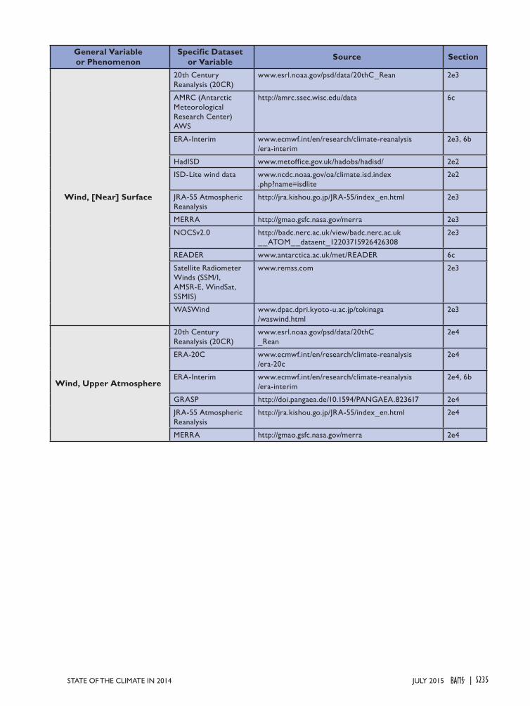
S235STATE OF THE CLIMATE IN 2014 |JULY 2015
General Variable or Phenomenon
Specific Dataset or Variable Source Section
Wind, [Near] Surface
20th Century Reanalysis (20CR)
www.esrl.noaa.gov/psd/data/20thC_Rean 2e3
AMRC (Antarctic Meteorological Research Center) AWS
http://amrc.ssec.wisc.edu/data 6c
ERA-Interim www.ecmwf.int/en/research/climate-reanalysis /era-interim
2e3, 6b
HadISD www.metoffice.gov.uk/hadobs/hadisd/ 2e2
ISD-Lite wind data www.ncdc.noaa.gov/oa/climate.isd.index .php?name=isdlite
2e2
JRA-55 Atmospheric Reanalysis
http://jra.kishou.go.jp/JRA-55/index_en.html 2e3
MERRA http://gmao.gsfc.nasa.gov/merra 2e3
NOCSv2.0 http://badc.nerc.ac.uk/view/badc.nerc.ac.uk __ATOM__dataent_12203715926426308
2e3
READER www.antarctica.ac.uk/met/READER 6c
Satellite Radiometer Winds (SSM/I, AMSR-E, WindSat, SSMIS)
www.remss.com 2e3
WASWind www.dpac.dpri.kyoto-u.ac.jp/tokinaga /waswind.html
2e3
Wind, Upper Atmosphere
20th Century Reanalysis (20CR)
www.esrl.noaa.gov/psd/data/20thC _Rean
2e4
ERA-20C www.ecmwf.int/en/research/climate-reanalysis /era-20c
2e4
ERA-Interim www.ecmwf.int/en/research/climate-reanalysis /era-interim
2e4, 6b
GRASP http://doi.pangaea.de/10.1594/PANGAEA.823617 2e4
JRA-55 Atmospheric Reanalysis
http://jra.kishou.go.jp/JRA-55/index_en.html 2e4
MERRA http://gmao.gsfc.nasa.gov/merra 2e4

S236 | JULY 2015
ACKNOWLEDGMENTS
The report's editors wish to thank the AMS Journals editorial staff, in particular Melissa Fernau, for facilitating the document, and to the NCEI graphics team for laying the document out and executing the countless number of technical edits needed. We also wish to express our sincere and deep gratitude to Dr. Rick Rosen, who served as the AMS special editor for this report. Dr. Rosen's handling of the reviews was at the same time rigor-ous and responsive, and greatly improved the document.
Chapter 2:• The editors thank David Parker for his excellent internal review.• Kate Willett, Robert Dunn, David Parker, Chris Folland, Rob
Allan, and Colin Morice were supported by the Joint UK DECC/Defra Met Office Hadley Centre Climate Programme (GA01101).
• The datasets used for the Total Column Water Vapor and Cloudiness sections [sections 2d(2) and 2d(5)] were provided from the Japanese 55-year Reanalysis (JRA-55) project carried out by the Japan Meteorological Agency (JMA).
• The editors thank Paul Berrisford (European Centre for Medium-Range Weather Forecasts), Mike Bosilovich (NASA), Shinya Kobayashi (Japan Meteorological Agency) and Cathy Smith (NOAA) for timely provision of reanalysis data.
• Additional data were provided by: Environmental Model-ing Center/National Centers for Environmental Prediction/National Weather Service/NOAA/U.S. Department of Com-merce. NCEP Climate Forecast System Reanalysis (CFSR) Monthly Products, January 1979 to December 2010. Research Data Archive at the National Center for Atmospheric Research, Computational and Information Systems Laboratory. http://rda .ucar.edu/datasets/ds093.2/.
Chapter 3:• Acknowledgments: Sandra Bigley (NOAA/Pacific Marine
Environmental Laboratory) provided able editorial assistance.• Simone Alin, Scott Cross, and Dan Siedov provided useful
comments on an early draft of the chapter.• Gregory C. Johnson and John Lyman were supported by NOAA
Research and the NOAA Climate Program Office.• Simon Good was supported by the Joint UK DECC/Defra Met
Office Hadley Centre Climate Programme (GA01101).• Catia M. Domingues was supported by an Australian Research
Council Future Fellowship (FT130101532).• Jeff Dunn provided quality-controlled Argo data (2000–2013)
and Neil White processed altimeter data for the CSIRO/ACE CRCIMAS-UTAS OHCA estimates.
Chapter 4:• Acknowledgements: Mark Lander (University of Guam) and
Charles ‘”Chip” Guard (National Weather Service, Guam Weather Forecast Office) for providing valuable inputs related to the section on Western North Pacific tropical cyclones.
• Bill Ward (NOAA/NWS Pacific Region Headquarters) who was involved with the internal review of the chapter.
Chapter 5:• For support for co-editing the Arctic section, Martin Jeffries
thanks the Office of Naval Research, and Jackie Richter-Menge thanks the NOAA Arctic Research Office. They also thank the authors for their contributions, and the reviewers for their thoughtful and constructive comments.
• Jim Overland’s contribution to the Air Temperature essay was supported by the NOAA Arctic Research Project of the Climate Program Office and by the Office of Naval Research, Code 322.
• Germar Bernhard and co-authors of the Ozone and UV Radia-tion essay acknowledge the support of the U.S. National Sci-ence Foundation (grant ARC-1203250), a Research Council of Norway Centres of Excellence award (project number 223268/F50) to the Norwegian Radiation Protection Authority, and the Academy of Finland for UV measurements by the FARPOCC and SAARA projects in Finland.
• Vladimir Romanovsky and co-authors of the Permafrost essay acknowledge the support of the State of Alaska, the National Science Foundation (grants PLR-0856864 and PLR-1304271 to the University of Alaska Fairbanks; PLR-1002119 and PLR-1304555 to the George Washington University), and by Geologi-cal Survey of Canada and Natural Resources Canada. Support was also provided by the Russian Science Foundation (projects 13-05-41509 RGO, 13-05-00811, 13-08-91001, 14-05-00956, 14-17-00037, and 15-55-71004) and by the government of the Russian Federation.
• Matthew Shupe’s contribution to Sidebar 5.1: Challenge of Arctic Clouds and their Implications for Surface Radiation was supported by the U.S. Department of Energy (DE-SC0011918) and National Science Foundation (PLR1314156).
• Howie Epstein, Gerald Frost and Skip Walker acknowledge the support of the NASA Land Cover Land Use Change Program for their contribution to Sidebar 5.2: Declassified High-Resolution Visible Imagery for Observing the Arctic.
Chapter 6:• Special thanks to Dr. Marilyn Raphael and Dr. Florence Fetterer
for their internal reviews of the chapter.• The work of Rob Massom, Phil Reid, and Jan Lieser was sup-
ported by the Australian Government’s Cooperative Research Centre program through the Antarctic Climate and Ecosystems CRC, and contributes to AAS Project 4116.
• Ted Scambos was supported under NASA grant NNX10AR76G and NSF ANT 0944763, the Antarctic Glaciological Data Center.
• Sharon Stammerjohn was supported under NSF PLR 0823101.
S237JULY 2015STATE OF THE CLIMATE IN 2014 |
ACRONYMS AND ABBREVIATIONS
AAO Antarctic OscillationACE NOAA’s Accumulated Cyclone Energy
IndexAGGI NOAA’s Annual Greenhouse Gas IndexALT active layer thicknessAMO Atlantic Multidecadal OscillationAMSR-E Advanced Microwave Scanning
Radiometer for Earth Observing SystemAMSU Advanced Microwave Sounding UnitAO Arctic OscillationAOD aerosol optical depthAVHRR Advanced Very High Resolution
RadiometerAVISO Archiving, Validating, and
Interpretation of Satellite Oceanographic data
CAMS Climate Anomaly Monitoring SystemCDR climate data recordCERES Clouds and the Earth’s Radiant Energy
SystemCPC NOAA’s Climate Prediction CenterCRU Hadley Centre’s Climate Research UnitDU Dobson UnitE–P evaporation minus precipitationECMWF European Centre for Medium-Range
Weather Forecasts ECV essential climate variableEESC effective equivalent stratospheric
chlorineERB Earth radiation budgetERSST Extended Reconstructed Sea Surface
TemperatureESA European Space AgencyESRL Earth System Research LaboratoryFAPAR Fraction of Absorbed Photosynthetically
Active RadiationFLASHflux Fast Longwave and Shortwave Radiative
FluxesGCOS Global Climate Observing SystemGHCN Global Historical Climatology NetworkGISS NASA’s Goddard Institute of Space
StudiesGOME Global Ozone Monitoring ExperimentGPCC Global Precipitation Climatology
CentreGPCP Global Precipitation Climatology
ProjectGRACE Gravity Recovery and Climate
ExperimentGTN-P Global Terrestrial Network on
Permafrost
HadCRUT Hadley Centre/CRU gridded monthly temperatures dataset
HadISST Hadley Centre’s sea ice and SST datasetHIRS-W High Resolution Infrared SounderIBTrACS International Best Track Archive for
Climate StewardshipIOD Indian Ocean dipoleISCCP International Satellite Cloud
Climatology ProjectJMA Japan Meteorological AgencyJPL Jet Propulsion Laboratory JRA Japanese ReanalysisJTWC U.S. Navy’s Joint Typhoon Warning
CenterLHF latent heat fluxLLGHG long-lived greenhouse gasMDR Main Development RegionMEI multivariate ENSO indexMERIS Medium Resolution Imaging
SpectrometerMISR Multiangle Imaging SpectroRadiometerMLS Microwave Limb SounderMOC meridional overturning circulationMOCHA Meridional Overturning Circulation
Heat Transport Array MODIS Moderate Resolution Imaging
SpectroradiometerMSLP mean sea level pressureMSU Microwave Sounding UnitNAO North Atlantic OscillationNASA National Aeronautics and Space
AdministrationNCAR National Center for Atmospheric
ResearchNCDC NOAA’s National Climatic Data CenterNCEP NOAA’s National Center for
Environmental PredictionNERC National Environmental Research
CouncilNOAA National Oceanic and Atmospheric
AdministrationNSIDC National Snow and Ice Data CenterOAFlux Objectively Analyzed Air-Sea FluxesODGI Ozone Depleting Gas IndexODS ozone depleting substanceOHCA ocean heat content anomalyOISST Optimal Interpolation SSTOLR outgoing longwave radiationOMI Ozone Monitoring InstrumentONI NOAA’s Oceanic Niño Index P–E precipitation minus evaporation
S238 JULY 2015|
PATMOS (-x) Pathfinder Atmospheres (Extended Product)
PDO Pacific decadal oscillationPSC polar stratospheric cloudsPSS practical salinity scaleQBO Quasi-biennial oscillationQuikSCAT Quick ScatterometerRAOBCORE Radiosonde Observation CorrectionRATPAC Radiosonde Atmospheric Temperature
Products for Assessing ClimateRICH Radiosonde Innovation Composite
HomogenizationRSS Remote Sensing SystemsSAM Southern annular modeSCD snow covered durationSCE snow cover extentSCIAMACHY Scanning Imaging Absorption
Spectrometer for Atmospheric Chartography
SeaWiFS Sea-viewing Wide Field of ViewSHF Sensible heat fluxSLP Sea level pressureSOI Southern Oscillation index SPCZ South Pacific convergence zoneSSH Sea surface heightSSM/I Special Sensor Microwave ImagerSSS Sea surface salinitySSTA Sea surface temperature anomalyTCHP Tropical cyclone heat potential TCWV Total column water vaporTOA Top of atmosphereTOMS Total Ozone Mapping SpectrometerTRMM Tropical Rainfall Measuring Missionw.e. water equivalentWGMS World Glacier Monitoring ServiceWMO World Meteorological OrganizationWOA World Ocean Atlas WOCE World Ocean Circulation Experiment
S239JULY 2015STATE OF THE CLIMATE IN 2014 |
REFERENCESAbe, H., and N. Ebuchi, 2014: Evaluation of sea-surface
salinity observed by Aquarius. J. Geophys. Res. Oceans, 119, 8109–8121, doi:10.1002/2014JC010094.
Abraham, J. P., and Coauthors, 2013: A review of global ocean temperature observations: Implications for ocean heat content estimates and climate change. Rev. Geophys., 51, 450–483, doi:10.1002/rog20022.
Ackerman, S. A., R. E. Holz, R. Frey, E. W. Eloranta, B. C. Maddux, and M. McGill, 2008: Cloud detection with MODIS. Part II: Validation. J. Atmos. Oceanic Technol., 25, 1073–1086.
Adler, R. F., and Coauthors, 2003: The version 2 Global Pre-cipitation Climatology Project (GPCP) monthly precipita-tion analysis (1979–present). J. Hydrometeor., 4, 1147–1167.
Ahrens, C. D., 2000: Atmospheric moisture. Meteorology Today: An Introduction to Weather, Climate and the En-vironment. 6th ed. Brooks/Cole, p. 108.
Aiyyer, A., and J. Molinari, 2008: MJO and tropical cyclo-genesis in the Gulf of Mexico and eastern Pacific: Case study and idealized numerical modeling. J. Atmos. Sci., 65, 2691–2704.
Allan, R., and R. D. D’Arrigo, 1999: ‘Persistent’ ENSO se-quences: How unusual was the recent El Niño? Holocene, 9, 101–118.
—, and T. Ansell, 2006: A new globally complete monthly historical gridded mean sea level pressure dataset (Had-SLP2): 1850–2004. J. Climate, 19, 5816–5842.
—, and C. K. Folland, 2014: Mean sea level pressure [in “State of the Climate in 2013”]. Bull. Amer. Meteor. Soc., 95 (7), S26–S28.
—, J. A. Lindesay, and D. E. Parker, 1996: El Niño Southern Oscillation and Climatic Variability. CSIRO Publications, 405 pp.
Allen, R., and S. Sherwood, 2008: Warming maximum in the tropical upper troposphere deduced from thermal winds. Nat. Geosci., 1, 399–403, doi:10.1038/ngeo208.
Alley, R. B., S. Anandakrishnan, K. Christianson, H. J. Horgan, A. Muto, B. R. Parizek, D. Pollard, and R. T. Walker, 2015: Oceanic forcing of ice-sheet retreat: West Antarctica and more. Annu. Rev. Earth Planet. Sci., 43, 207–231, doi:10.1146/annurev-earth-060614-105344.
Alley, W. M., R. W. Healy, J. W. LaBaugh, and T. E. Reilly, 2002: Flow and storage in groundwater systems. Science, 296, 1985–1990.
Alsdorf, D. E., and D. P. Lettenmaier, 2003: Tracking fresh water from space. Science, 301, 1491–1494, doi:10.1126 /science.1089802.
Amador, J., 1998: A climatic feature of the tropical Ameri-cas: The trade wind easterly jet. Top. Meteor. Oceanogr., 5, 91–102.
—, 2008: The Intra-Americas sea low-level jet. Ann. New York Acad. Sci ., 1146 , 153–188, doi:10.1196 /annals.1446.012.
—, E. J. Alfaro, O. G. Lizano, and V. O. Magaña, 2006: Atmospheric forcing of the eastern tropical Pacific: A review. Prog. Oceanogr., 69, 101–142.
—, —, H. G. Hidalgo, and B. Calderón, 2011: Central America [in “State of the Climate 2010”]. Bull. Amer. Meteor. Soc., 92 (6), S182–S183.
—, —, —, A. M. Durán, B. Calderón, I. L. Rivera, and C. Vega, 2014: Central America [in “State of the Climate 2013”]. Bull. Amer. Meteor. Soc., 96 (7), S164–S166.
Andela, N., and G. R. van der Werf, 2014: Recent trends in African fires driven by cropland expansion and El Niño to La Niña transition. Nat. Climate Change, 4, 791–795, doi:10.1038/NCLIMATE2313.
Antonov, J. I., S. Levitus, and T. P. Boyer, 2005: Thermosteric sea level rise, 1955–2003. Geophys. Res. Lett., 32, L12602, doi:10.1029/2005GL023112.
—, and Coauthors, 2010: Salinity. Vol. 2, World Ocean Atlas 2009, NOAA Atlas NESDIS 69, 184 pp.
Applegate, P. J., B. R. Parizek, R. E. Nicholas, R. B. Alley, and K. Keller, 2014: Increasing temperature forcing reduces the Greenland Ice Sheet’s response time scale. Climate Dyn., doi:10.1007/s00382-014-2451-7, in press.
Arguez, A., T. R. Karl, M. F. Squires, and R. S. Vose, 2013: Uncertainty in annual rankings from NOAA’s global tem-perature time series. Geophys. Res. Lett., 40, 5965–5969, doi:10.1002/2013GL057999.
Armstrong, R. L., K. W. Knowles, M. J. Brodzik, and M. A. Hardman, 1994, updated 2014: DMSP SSM/I-SSMIS pathfinder daily EASE-grid brightness temperatures. Version 2. Southern Hemisphere. National Snow and Ice Data Center, Boulder, CO, digital media. [Available online at http://nsidc.org/data/docs/daac/nsidc0032_ssmi_ease _tbs.gd.html.]
Ashok, K., S. K. Behera, S. A. Rao, H. Weng, and T. Yamagata, 2007: El Niño Modoki and its possible teleconnection. J. Geophys. Res., 112, C11007, doi:10.1029/2006JC003798.
Assmann, K. M., A. Jenkins, D. R. Shoosmith, D. P. Walker, S. S. Jacobs, and K. W. Nicholls, 2013: Variability of Cir-cumpolar Deep Water transport onto the Amundsen Sea continental shelf through a shelf break trough. J. Geophys. Res. Oceans, 118, 6603–6620, doi:10.1002/2013JC008871.
Atkinson, G. D., 1971: Forecasters’ guide to tropical meteo-rology. U.S. Air Force Tech. Rep. 240, 360 pp.
Azorin-Molina, C., and Coauthors, 2014: Homogenization and assessment of observed near-surface wind speed trends over Spain and Portugal, 1961–2011. J. Climate, 27, 3692–3712.
S240 JULY 2015|
Baccini, A., and Coauthors, 2012: Estimated carbon diox-ide emissions from tropical deforestation improved by carbon-density maps. Nat. Climate Change, 2, 182–185, doi:10.1038/nclimate1354.
Bakker, D. C. E., and Coauthors, 2014: An update to the Surface Ocean CO2 Atlas (SOCAT version 2). Earth Syst. Sci. Data, 6, 69–90, doi:10.5194/essd-6-69-2014.
Banzon, V. F., and R. W. Reynolds, 2013: Use of WindSat to extend a microwave-based daily optimum interpola-tion sea surface temperature time series. J. Climate, 26, 2557–2562, doi:10.1175/JCLI-D-12-00628.1.
Baringer, M. O., and Coauthors, 2013: Meridional overturn-ing circulation and heat transport observations in the Atlantic [in “State of the Climate in 2012”]. Bull. Amer. Meteor. Soc., 94 (8), S65–S68.
—, W. E. Johns, S. Garzoli, S. Dong, D. Volkov, and W. R. Hobbs, 2014: Meridional oceanic heat transport in the Atlantic Ocean [in “State of the Climate in 2013”]. Bull. Amer. Meteor. Soc., 95 (6), S69–S71.
Barnes, E. A., and J. A. Screen, 2015: The impact of Arctic warming on the midlatitude jet-stream: Can it? Has it? Will it? Wiley Interdiscip. Rev.: Climate Change, 6, 277–286, doi:10.1002/wcc.337.
Bassis, J. N., and C. C. Walker, 2012: Upper and lower limits on the stability of calving glaciers from the yield strength envelope of ice. Proc. Roy. Soc. London, A468, 913–931.
Bastos, A., S. W. Running, C. Gouveia, and R. M. Trigo, 2013: The global NPP dependence on ENSO: La Niña and the extraordinary year of 2011. J. Geophys. Res. Biogeosci., 118, 1247–1255, doi:10.1002/jgrg.20100.
Bauer-Marschallinger, B., W. A. Dorigo, W. Wagner, and A. I. J. M. van Dijk, 2013: How oceanic oscillation drives soil moisture variations over mainland Australia: An analysis of 32 years of satellite observations. J. Climate, 26, 10 159–10 173, doi:10.1175/JCLI-D-13-00149.1.
Baxter, S., S. Weaver, J. Gottschalck, and Y. Xue, 2014: Pentad evolution of wintertime impacts of the Madden–Julian oscillation over the contiguous United States. J. Climate, 27, 7356–7367.
Beal, L. M., V. Hormann, R. Lumpkin, and G. R. Foltz, 2013: The response of the surface circulation of the Arabian Sea to monsoonal forcing. J. Phys. Oceanogr., 43, 2008–2022, doi:10.1175/JPO-D-13-033.1.
Becker, A., P. Finger, A. Meyer-Christoffer, B. Rudolf, K. Schamm, U. Schneider, and M. Ziese, 2013: A description of the global land-surface precipitation data products of the Global Precipitation Climatology Centre with sample applications including centennial (trend) analysis from 1901–present. Earth Syst. Sci. Data, 5, 71–99, doi:10.5194 /essd-5-71-2013.
Behera, K. S., J.-J. Luo, S. Masson, S. A. Rao, H. Sakuma, and T. Yamagata, 2006: A CGCM study on the interaction between IOD and ENSO. J. Climate, 19, 1688–1705.
Behrenfeld, M. J., and Coauthors, 2006: Climate-driven trends in contemporary ocean productivity. Nature, 444, 752–755.
—, K. Halsey, and A. Milligan, 2008: Evolved physiological responses of phytoplankton to their integrated growth environment. Philos. Trans. Roy. Soc., B363, 2687–2703, doi:10.1098/rstb.2008.0019.
Behringer, D. W., M. Ji, and A. Leetmaa, 1998: An improved coupled model for ENSO prediction and implications for ocean initialization. Part I: The ocean data assimilation system. Mon. Wea. Rev., 126, 1013–1021.
Bell, G. D., and M. Chelliah, 2006: Leading tropical modes associated with interannual and multi-decadal fluctua-tions in North Atlantic hurricane activity. J. Climate, 19, 590–612.
—, and Coauthors, 2000: The 1999 North Atlantic and eastern North Pacific hurricane season [in “Climate Assessment for 1999”]. Bull. Amer. Meteor. Soc., 81 (6), S19–S22.
—, and Coauthors, 2011: Atlantic basin [in “State of the Cli-mate in 2010”]. Bull. Amer. Meteor. Soc., 92 (7), S115–S121.
—, and Coauthors, 2012: Atlantic basin [in “State of the Cli-mate in 2011”]. Bull. Amer. Meteor. Soc., 93 (7), S99–S105.
—, and Coauthors, 2014: Atlantic basin [in “State of the Cli-mate in 2013”]. Bull. Amer. Meteor. Soc., 95 (7), S86–S90.
Bellassen, V., and Coauthors, 2011: Reconstruction and at-tribution of the carbon sink of European forests between 1950 and 2000. Global Change Biol., 17, 3274–3292, doi:10.1111/j.1365-2486.2011.02476.x.
Bellucci, A., S. Gualdi, E. Scoccimarro, and A. Navarra, 2008: NAO–ocean circulation interactions in a coupled general circulation model. Climate Dyn., 31, 759–777.
Bergamaschi, P., and Coauthors, 2013: Atmospheric CH4 in the first decade of the 21st century: Inverse model-ing analysis using SCIAMACHY satellite retrievals and NOAA surface measurements. J. Geophys. Res. Atmos., 118, 7350–7369, doi:10.1002/jgrd.50480.
Berkowitz, B., 2011: The National Reconnaissance Office at 50 Years: A Brief History. Center for the Study of National Reconnaissance, 28 pp.
Bernhard, G., C. R. Booth, and J. C. Ehramjian, 2008: Comparison of UV irradiance measurements at Sum-mit, Greenland; Barrow, Alaska; and South Pole, Ant-arctica. Atmos. Chem. Phys., 8, 4799–4810, doi:10.5194 /acp-8-4799-2008.
Berrisford, P., D. Dee, K. Fielding, M. Fuentes, P. Kållberg, S. Kobayashi, and S. Uppala, 2009: The ERA-Interim archive version 1.0. ERA Rep. Series 1, European Centre for Medium Range Weather Forecasts, 16 pp. [Avail-able online at http://old.ecmwf.int/publications/library /ecpublications/_pdf/era/era_report_series/RS_1.pdf.]
S241JULY 2015STATE OF THE CLIMATE IN 2014 |
Berry, D. I., and E. C. Kent, 2009: A new air–sea inter-action gridded dataset from ICOADS with uncer-tainty estimates. Bull. Amer. Meteor. Soc., 90, 645–656, doi:10.1175/2008BAMS2639.1.
—, and —, 2011: Air–sea fluxes from ICOADS: The construction of a new gridded dataset with uncertainty estimates. Int. J. Climatol., 31, 987–1001.
Bichet, A., M. Wild, D. Folini, and C. Schär, 2012: Causes for decadal variations of wind speed over land: sensitiv-ity studies with a global model. Geophys. Res. Lett., 39, L11701, doi:10.1029/2012GL051685.
Bintanja, R., G. J. van Oldenborgh, S. S. Drijfhout, B. Wout-ers, and C. A. Katsman, 2013: Important role for ocean warming and increased ice-shelf melt in Antarctic sea-ice expansion. Nat. Geosci., 6, 376–379.
Blake, E., and Coauthors, 2009: Tropical Cyclones of the Eastern North Pacific Basin, 1949-2006. Historical Cli-matology Series 6-5, NOAA/National Climatic Data Center, 162 pp.
Bockheim, J., G. Vieira, M. Ramos, J. Lopez-Martinez, E. Serrano, M. Guglielmin, K. Wilhelm, and A. Nieuwen-dam, 2013: Climate warming and permafrost dynamics in the Antarctic peninsula region. Global Planet. Change, 100, 215–223.
Bodhaine, B. A, B. G. Mendonca, J. M. Harris, and J. M. Mill-er, 1981: Seasonal variations in aerosols and atmospheric transmission at Mauna Loa Observatory. J. Geophys. Res., 86, 7395–7398, doi:10.1029/JC086iC08p07395.
Boeckli, L., A. Brenning, S. Gruber, and J. Noetzli, 2012: Per-mafrost distribution in the European Alps: Calculation and evaluation of an index map and summary statistics. Cryosphere, 6, 807–820, doi:10.5194/tc-6-807-2012.
Boening, C., J. K. Willis, F. W. Landerer, R. S. Nerem, and J. Fasullo, 2012: The 2011 La Niña: So strong, the oceans fell. Geophys. Res. Lett., 39, L19602, doi:10.1029/2012GL053055.
Bojinski, S., M. Verstraete, T. C. Peterson, C. Richter, A. Simmons, and M. Zemp, 2014: The concept of essential climate variables in support of climate research, applica-tions, and policy. Bull. Amer. Meteor. Soc., 95, 1431–1443, doi:10.1175/BAMS-D-13-00047.1.
Bond, N. A., M. F. Cronin, H. Freeland, and N. Mantua, 2015: Causes and impacts of the 2014 warm anomaly in the NE Pacific. Geophys. Res. Lett., 42, 3414–3420, doi:10.1002/2015GL063306.
Bonjean, F., and G. Lagerloef, 2002: Diagnostic model and analysis of the surface currents in the tropical Pacific Ocean. J. Phys. Oceanogr., 32, 2938–2954.
Bonsal, B. R., T. D. Prowse, C. R. Duguay, and M. P. Lacroix, 2006: Impacts of large-scale teleconnections on freshwa-ter-ice duration over Canada. J. Hydrol., 330, 340–353.
Bopp, L., and Coauthors, 2013: Multiple stressors of ocean ecosystems in the 21st century: Projections with CMIP5 models. Biogeosciences, 10, 6225–6245, doi:10.5194 /bg-10-6225-2013.
Bourassa, A. E., D. A. Degenstein, W. J. Randel, J. M. Za-wodny, E. Kyrölä, C. A. McLinden, C. E. Sioris, and C. Z. Roth, 2014: Trends in stratospheric ozone derived from merged SAGE II and Odin-OSIRIS satellite observa-tions. Atmos. Chem. Phys., 14, 6983–6994, doi:10.5194 /acp-14-6983-2014.
Box, J. E., X. Fettweis, J. C. Stroeve, M. Tedesco, D. K. Hall, and K. Steffen, 2012: Greenland ice sheet albedo feedback: thermodynamics and atmospheric drivers. Cryosphere, 6, 821–839, doi:10.5194/tc-6-821-2012.
Boyer, T., S. Levitus, J. Antonov, R. Locarnini, A. Mishonov, H. Garcia, and S. A. Josey, 2007: Changes in freshwater content in the North Atlantic Ocean 1955–2006. Geophys. Res. Lett., 34, L16603, doi:10.1029/2007GL030126.
—, —, —, J. R. Reagan, C. Schmid, and R. Locarnini, 2012: Subsurface salinity [in “State of the Climate in 2011”]. Bull. Amer. Meteor. Soc., 93 (7), S72–S75.
—, and Coauthors, 2013: World Ocean Database 2013. NOAA Atlas NESDIS 72, 209 pp.
—, S. Levitus, J. I. Antonov, J. R. Reagan, C. Schmid, and R. Locarnini, 2014: Subsurface salinity [in “State of the Cli-mate in 2013”]. Bull. Amer. Meteor. Soc., 95 (8), S62–S65.
Brasnett, B., 1999: A global analysis of snow depth for nu-merical weather prediction. J. Appl. Meteor., 38, 726–740.
Brienen, R. J. W., and Coauthors, 2015: Long-term decline of the Amazon carbon sink. Nature, 519, 344–348, doi:10.1038/nature14283.
Bromwich, D. H., and S.-H. Wang, 2014: Net precipitation (P–E) [in “State of the Climate in 2013”]. Bull. Amer. Meteor. Soc., 95 (7), S147–S149.
—, A. J. Monaghan, and Z. Guo, 2004: Modeling the ENSO modulation of Antarctic climate in the late 1990s with Polar MM5. J. Climate, 17, 109–132.
—, J. P. Nicolas, and A. J. Monaghan, 2011: An assessment of precipitation changes over Antarctica and the Southern Ocean since 1989 in contemporary global reanalyses. J. Climate, 24, 4189–4209, doi:10.1175/2011JCLI4074.1.
Brown, L. C., and C. R. Duguay, 2012: Modelling lake ice phenology with an examination of satellite detected sub-grid cell variability. Adv. Meteor., Article 529064, doi:10.1155/2012/529064.
Brown, R., and D. Robinson, 2011: Northern Hemisphere spring snow cover variability and change over 1922–2010 including an assessment of uncertainty. Cryosphere, 5, 219–229.
Bryden, H. L., B. A. King, G. D. McCarthy, and E. L. McDonagh, 2014: Impact of a 30% reduction in Atlantic meridional overturning during 2009–2010. Ocean Sci., 10, 683–691, doi:10.5194/os-10-683-2014.
S242 JULY 2015|
Bulygina, O. N., P. Ya. Groisman, V. N. Razuvaev, and V. F. Radionov, 2010: Snow cover basal ice layer changes over Northern Eurasia since 1966. Environ. Res. Lett., 5, 015004, doi:10.1088/1748-9326/5/1/015004.
Butchart, N., and E. E. Remsberg, 1986: The area of the strato-spheric polar vortex as a diagnostic for tracer transport on an isentropic surface. J. Atmos. Sci., 43, 1319–1339.
Camargo, S. J., and A. H. Sobel, 2005: Western North Pa-cific tropical cyclone intensity and ENSO. J. Climate, 18, 2996–3006.
—, K. A. Emanuel, and A. H. Sobel, 2007: Use of a genesis potential index to diagnose ENSO effects on tropical cyclone genesis. J. Climate, 20, 4819–4834.
—, A. W. Robertson, A. G. Barnston, and M. Ghil, 2008: Clustering of eastern North Pacific tropical cyclone tracks: ENSO and MJO effects. Geochem. Geophys. Geo-sys., 9, Q06V05, doi:10.1029/2007GC001861.
—, M. C. Wheeler, and A. H. Sobel, 2009: Diagnosis of the MJO modulation of tropical cyclogenesis using an empirical index. J. Atmos. Sci., 66, 3061–3074.
Campbell, J. W., J. M. Blaisdell, and M. Darzi, 1995: Level-3 SeaWiFS data products: Spatial and temporal binning algorithms. NASA Tech. Memo. 104566, Vol. 32, NASA Goddard Space Flight Center, 73 pp.
Carpenter, L. J., S. Reimann, J. B. Burkholder, C. Clerbaux, B. D. Hall, R. Hossaini, J. C. Laube, and S. A. Yvon-Lewis, 2014: Update on ozone-depleting substances (ODSs) and other gases of interest to the Montreal Protocol. Scientific Assessment of Ozone Depletion: 2014, Global Ozone Research and Monitoring Project Rep. 55, World Meteorological Organization, 1.1–1.101. [Available on-line at www.wmo.int/pages/prog/arep/gaw/ozone_2014 /full_report_TOC.html.]
Carton, J. A., G. A. Chepurin, J. Reagan, and S. Häkkinen, 2011: Interannual to decadal variability of Atlantic Water in the Nordic and adjacent seas. J. Geophys. Res., 116, C11035, doi:10.1029/2011JC007102.
Cartus, O., and Coauthors, 2014: A national, detailed map of forest aboveground carbon stocks in Mexico. Remote Sens., 6, 5559–5588, doi:10.3390/rs6065559.
Cassou, C., 2008: Intraseasonal interaction between the Mad-den Julian Oscillation and the North Atlantic Oscillation. Nature, 455, 523–527, doi:10.1038/nature07286.
Cavalieri, D. J., C. L. Parkinson, P. Gloersen, and H. Zwally, 1996, updated yearly: Sea ice concentrations from Nimbus-7 SMMR and DMSP SSM/I-SSMIS passive microwave data (1981-2011). National Snow and Ice Data Center, Boulder, CO, digital media. [Available online at doi:10.5067/8GQ8LZQVL0VL.]
Cazenave, A., H.-B. Dieng, B. Meyssignac, K. von Schuck-mann, B. Descharme, and E. Berthier, 2014: The rate of sea-level rise. Nat. Climate Change, 4, 358–361, doi:10.1038/nclimate2159.
Cesana, G., J. E. Kay, H. Chepfer, J. M. English, and G. de Boer, 2012: Ubiquitous low-level liquid-containing Arctic clouds: New observations and climate model constraints from CALIPSO-GOCCP. Geophys. Res. Lett., 39, L20804, doi:10.1029/2012GL053385.
Chave, J., and Coauthors, 2014: Improved allometric models to estimate the aboveground biomass of tropical trees. Global Change Biol., 20, 3177–3190, doi:10.1111/gcb.12629.
Chehade, W., M. Weber, and J. P. Burrows, 2014: Total ozone trends and variability during 1979–2012 from merged data sets of various satellites. Atmos. Chem. Phys., 14, 7059–7074, doi:10.5194/acp-14-7059-2014.
Chen, J. L., C. R. Wilson, and B. D. Tapley, 2013: Contribution of ice sheet and mountain glacier melt to recent sea level rise. Nat. Geosci., 6, 549–552.
Chen, Y., D. C. Morton, Y. Jin, G. J. Gollatz, P. S. Kasibhatla, G. R. van der Werf, R. S. DeFries, and J. T. Randerson, 2013: Long-term trends and interannual variability of forest, savanna and agricultural fires in South America. Carbon Manage., 4, 617–638, doi:10.4155/CMT.13.61.
Chevallier, F., and Coauthors, 2010: CO2 surface fluxes at grid point scale estimated from a global 21-year reanaly-sis of atmospheric measurements. J. Geophys. Res., 115, D21307, doi:10.1029/2010JD013887.
Chiou, E. W., and Coauthors, 2014: Comparison of profile total ozone from SBUV (v8.6) with GOME-type and ground-based total ozone for a 16-year period (1996 to 2011). Atmos. Meas. Tech., 7, 1681–1692, doi:10.5194 /amt-7-1681-2014.
Christiansen, H. H., and Coauthors, 2010: The thermal state of permafrost in the Nordic area during the international polar year 2007–2009. Permafrost Periglacial Processes, 21, 156–181, doi:10.1002/ppp.687.
Christy, J., 2013: Lower tropospheric temperature [in “State of the Climate in 2012”]. Bull. Amer. Meteor. Soc., 94 (8), S13–S15.
—, 2014: Lower tropospheric temperature [in “State of the Climate in 2013”]. Bull. Amer. Meteor. Soc., 95 (7), S10–S11.
—, R. W. Spencer, and W. B Norris, 2011: The role of remote sensing in monitoring global bulk tropospheric temperatures. Int. J. Remote Sens., 32, 671–685, doi: 10.1080/01431161.2010.517803.
Chrysanthou, A., G. Van der Schrier, E. J. M. Van den Bes-selaar, A. M. G. Klein Tank, and T. Brandsma, 2014: The effects of urbanization on the rise of the European tem-perature since 1960. Geophys. Res. Lett., 41, 7716–7722, doi:10.1002/2014GL061154.
Chung, E.-S., B. J. Soden, B. J. Sohn, and L. Shi, 2014: Upper-tropospheric moistening in response to anthropogenic warming. Proc. Natl. Acad. Sci. USA, 111, 11 636–11 641, doi:10.1073/pnas.1409659111.
S243JULY 2015STATE OF THE CLIMATE IN 2014 |
Church, J. A., and Coauthors, 2010: Ocean temperature and salinity contributions to global and regional sea-level change. Understanding Sea-Level Rise and Variability, J. A. Church et al., Eds., Blackwell, 143–176.
Clerbaux, C., and Coauthors, 2009: Monitoring of atmo-spheric composition using the thermal infrared IASI/MetOp sounder. Atmos. Chem. Phys., 9, 6041–6054, doi:10.5194/acp- 9-6041-2009.
Cohen, J., and Coauthors, 2014: Recent Arctic amplifica-tion and extreme mid-latitude weather. Nat. Geosci., 7, 627–637, doi:10.1038/ngeo2234.
Coldewey-Egbers, M., D. Loyola, P. Braesicke, M. Dam-eris, M. van Roozendael, C. Lerot, and W. Zimmer, 2014: A new health check of the ozone layer at global and regional scales, Geophys. Res. Lett., 41, 4363–4372, doi:10.1002/2014GL060212.
Colwell, S., L. M. Keller, M. A. Lazzara, and A. Setzer, 2014: Surface manned and automatic weather station obser-vations [in “State of the Climate in 2013”]. Bull. Amer. Meteor. Soc., 95, S145–S147.
Comiso, J. C., 2010: Variability and trends of the global sea ice cover. Sea Ice, 2nd ed. D. N. Thomas, and G. S. Dieck-mann, Eds., Wiley-Blackwell, 205–246.
Compo, G. P., and Coauthors, 2011: The Twentieth Century Reanalysis Project. Quart. J. Roy. Meteor. Soc., 137, 1–28, doi:10.1002/qj.776.
Cooper, O., and J. Ziemke, 2013: Tropospheric ozone [in “State of the Climate in 2012”]. Bull. Amer. Meteor. Soc., 94 (8), S38–S39.
—, and Coauthors, 2014: Global distribution and trends of tropospheric ozone: An observation-based review. Elementa: Sci. Anthropocene, 2, 000029, doi:10.12952 /journal.elementa.000029.
Cross, J. N., and Coauthors, 2014: Annual sea-air CO2 fluxes in the Bering Sea: Insights from new autumn and winter observations of a seasonally ice-covered conti-nental shelf. J. Geophys. Res. Oceans, 119, 6693–6708, doi:10.1002/2013JC009579.
Cunningham, S. A., and Coauthors, 2013: Atlantic Me-ridional Overturning Circulation slowdown cooled the subtropical ocean. Geophys. Res. Lett., 40, 6202–6207, doi:10.1002/2013GL058464.
Curry, J. A., J. L. Schramm, W. B. Rossow, and D. Randall, 1996: Overview of Arctic cloud and radiation character-istics. J. Climate, 9, 1731–1764.
Curry, R., R. Dickson, and I. Yashayaev, 2003: A change in the freshwater balance of the Atlantic Ocean over the past four decades. Nature, 426, 826–829.
Curtis, S., and R. Adler, 2000: ENSO indexes based on pat-terns of satellite-derived precipitation. J. Climate, 13, 2786–2793.
Dadaser-Celik, F., and E. Cengiz, 2014: Wind speed trends over Turkey from 1975 to 2006. Int. J. Climatol., 34, 1913–1927, doi:10.1002/joc.3810.
Dai, A., 2006: Recent climatology, variability, and trends in global surface humidity. J. Climate, 19, 3589–3606.
Daniel, J. S., and Coauthors, 2011: A focus on information for policymakers. Scientific Assessment of Ozone Depletion: 2010, Global Ozone Research and Monitoring Project Rep. 52, World Meteorological Organization, 5.1–5.56.
de Boer, G., W. Chapman, J. Kay, B. Medeiros, M. D. Shupe, S. Vavrus, and J. Walsh, 2012: A characterization of the present-day Arctic atmosphere in CCSM4. J. Climate, 25, 2676–2695.
Dee, D. P., and Coauthors, 2011a: The ERA-Interim reanaly-sis: Configuration and performance of the data assimi-lation system. Quart. J. Roy. Meteor. Soc., 137, 553–597, doi:10.1002/qj.828.
—, and Coauthors, 2011b: The use of reanalysis data for monitoring the state of the climate [in “State of the Cli-mate in 2010”]. Bull. Amer. Meteor. Soc., 92 (6), S34–S35.
Deeter, M. N., 2011: MOPITT version 5 product user’s guide. [Available online at www.acd.ucar.edu/mopitt /publications.shtml.]
—, and Coauthors, 2010: The MOPITT version 4 CO product: Algorithm enhancements, validation, and long-term stability. J. Geophys. Res., 115, D07306, doi:10.1029/2009JD013005.
De Jeu, R., W. Dorigo, W. Wagner, and Y. Liu, 2011: Soil moisture [in “State of the Climate in 2010”]. Bull. Amer. Meteor. Soc., 92 (6), S52–S53.
—, —, R. M. Parinussa, W. Wagner, and D. Chung, 2012a: Building a climate record of soil moisture from historical satellite observations [in “State of the Climate in 2011”]. Bull. Amer. Meteor. Soc., 93 (7), S32–S33.
—, —, —, —, and—, 2012b: Soil moisture [in “State of the Climate in 2011”]. Bull. Amer. Meteor. Soc., 93 (7), S30–S34.
Delworth, T. L., and M. E. Mann, 2000: Observed and simulated multi-decadal variability in the Northern Hemisphere. Climate Dyn., 16, 661–676.
DeMaria, M., 1996: The effect of vertical shear on tropical cyclone intensity change. J. Atmos. Sci., 53, 2076–2087.
de Meij, A., A. Pozzer, and J. Lelieveld, 2012: Trend analysis in aerosol optical depths and pollutant emission estimates between 2000 and 2009m. Atmos. Environ., 51, 75–85.
de Pablo, M. A., J. J. Blanco, A. Molina, M. Ramos, A. Quesada, and G. Vieira, 2013: Interannual active layer variability at the Limnopolar Lake CALM site on Byers Peninsula, Livingston Island, Antarctica. Antarctic Sci., 25, 167–180, doi:10.1017/S0954102012000818.
S244 JULY 2015|
Derksen, C., and R. Brown, 2012: Spring snow cover extent reductions in the 2008-2012 period exceeding climate model projections. Geophys. Res. Lett., 39, L19504, doi:10.1029/2012GL053387.
Deser, M., A. Alexander, S. P. Xie, and A. S. Phillips, 2010: Sea surface temperature variability: Patterns and mecha-nisms. Annu. Rev. Mar. Sci., 2, 115–143.
Dessler, A. E., M. R. Schoeberl, T. Wang, S. M. Davis, K. H. Rosenlof, and J.-P. Vernier, 2014: Variations of stratospher-ic water vapor over the past three decades. J. Geophys. Res. Atmos., 119, 12 588–12 598, doi:10.1002/2014JD021712.
Dewitte, S., D. Crommelynck, and A. Joukof, 2004: To-tal solar irradiance observations from DIARAD/VIRGO. J. Geophys. Res. Space Phys., 109, A02102, doi:10.1029/2002JA009694.
Diamond, H. J., Ed., 2013: Tropics [in “State of the Climate in 2012”]. Bull. Amer. Meteor. Soc., 94 (8), S79–S110.
—, Ed., 2014: Tropics [in “State of the Climate in 2013”]. Bull. Amer. Meteor. Soc., 95 (7), S81–S114.
—, A. M. Lorrey, K. R. Knapp, and D. H. Levinson, 2012: Development of an enhanced tropical cyclone tracks database for the southwest Pacific from 1840-2011. Int. J. Climatol., 32, 2240–2250, doi:10.1002/joc.2412.
Di Girolamo, L., A. Menzies, G. Zhao, K. Mueller, C. Moroney, and D. J. Diner, 2010: Multi-angle imaging spectroradiometer level 3 cloud fraction by altitude al-gorithm theoretical basis document. JPL Publ. D-62358, Jet Propulsion Laboratory, 23 pp.
Di Lorenzo, E., and Coauthors, 2008: North Pacific gyre os-cillation links ocean climate and ecosystem change. Geo-phys. Res. Lett., 35, L08607, doi:10.1029/2007GL032838.
Di Michele, S., T. McNally, P. Bauer, and I. Genkova, 2013: Quality assessment of cloud-top height estimates from satellite IR radiances using the CALIPSO lidar. IEEE Trans. Geosci. Remote Sens., 51, 2454–2464, doi:10.1109 /TGRS.2012.2210721.
Dlugokencky, E. J., E. G. Nisbet, R. Fisher, and D. Lowry, 2011: Global atmospheric methane: Budget, changes and dangers. Philos. Trans. Roy. Soc. London, A369, 2058–2072, doi:10.1098/rsta.2010.0341.
Dohan, K., and N. Maximenko, 2010: Monitoring ocean cur-rents with satellite sensors. Oceanography, 23 (4), 94–103.
Doherty, R. M., D. S. Stevenson, C. E. Johnson, W. J. Col-lins, and M. G. Sanderson, 2006: Tropospheric ozone and El Niño–Southern Oscillation: Inf luence of at-mospheric dynamics, biomass burning emissions, and future climate change. J. Geophys. Res., 111, D19304, doi:10.1029/2005JD006849.
Domingues, C. M., J. A. Church, N. J. White, P. J. Gleckler, S. E. Wijffels, P. M. Barker, and J. R. Dunn, 2008: Im-proved estimates of upper-ocean warming and multi-decadal sea-level rise. Nature, 453, 1090–1093, doi:10.1038 /nature07080.
Donat, M. G., L. V. Alexander, H. Yang, I. Durre, R. Vose, and J. Caesar, 2013b: Global land-based datasets for monitoring climatic extremes. Bull. Amer. Meteor. Soc., 94, 997–1006, doi:10.1175/BAMS-D-12-00109.
Doney, S. C., 2006: Oceanography: Plankton in a warmer world. Nature, 444, 695–696.
—, V. J. Fabry, R. A. Feely, and J. A. Kleypas, 2009: Ocean acidification: The other CO2 problem. Annu. Rev. Mar. Sci . , 1, 169–192, doi:10.1146/annurev .marine.010908.163834.
Dorigo, W. A., and Coauthors, 2011: The International Soil Moisture Network: A data hosting facility for global in situ soil moisture measurements. Hydrol. Earth Syst. Sci., 15, 1675–1698.
—, R. De Jeu, D. Chung, R. Parinussa, Y. Liu, W. Wag-ner, and D. Fernandez-Prieto, 2012: Evaluating global trends (1988–2010) in harmonized multi-satellite sur-face soil moisture. Geophys. Res. Lett., 39, L18405, doi:10.1029/2012GL052988.
—, and Coauthors, 2014: Soil moisture [in “State of the Cli-mate in 2013”]. Bull. Amer. Meteor. Soc., 95 (7), S25–S26.
—, and Coauthors, 2015: Evaluation of the ESA CCI soil moisture product using ground-based observa-tions. Remote Sens. Environ., 162, 380–395, doi:10.1016 /j.rse.2014.07.023.
Drumond, A., L. Gimeno, and R. Nieto, 2011: On the contri-bution of the tropical Western Hemisphere Warm Pool source of moisture to the Northern Hemisphere precipi-tation through a Lagrangian approach. J. Geophys. Res., 116, D00Q04, doi:10.1029/2010JD015397.
Duchesne, C., S. Smith, M. Ednie, and J. Chartrand, 2014: 20 years of active layer monitoring in the Mackenzie Val-ley, Northwest Territories. Arctic Change 2014, Ottawa, Canada, ArcticNet, 42–43. [Available online at www .arcticnetmeetings.ca/ac2014/docs/web-posters.pdf.]
Duchez, A., and Coauthors, 2014: A new index for the Atlan-tic meridional overturning circulation at 26°N. J. Climate, 27, 6439–6455, doi:10.1175/JCLI-D-13-00052.1.
Duguay, C. R., T. D. Prowse, B. R. Bonsal, R. D. Brown, M. P. Lacroix, and P. Ménard, 2006: Recent trends in Canadian lake ice cover. Hydrol. Processes, 20, 781–801.
—, L. Brown, K.-K. Kang, and H. Kheyrollah Pour, 2014: Lake ice [in “State of the Climate in 2013”]. Bull. Amer. Meteor. Soc., 95 (7), S138–S139.
—, M. Bernier, Y. Gauthier, and A. Kouraev, 2015: Lake and river ice. Remote Sensing of the Cryosphere, M. Tedesco, Ed., Wiley-Blackwell, 273–306.
Dunn, R. J. H., K. M. Willett, P. W. Thorne, E. V. Woolley, I. Durre, A. Dai, D. E. Parker, and R. S. Vose, 2012: HadISD: A quality-controlled global synoptic report database for selected variables at long-term stations from 1973-2011. Climate Past, 8, 1649–1679.
S245JULY 2015STATE OF THE CLIMATE IN 2014 |
Durack, P. J., and S. E. Wijffels, 2010: Fifty-year trends in global ocean salinities and their relationship to broad-scale warming. J. Climate, 23, 4342–4362.
—, —, and R. J. Matear, 2012: Ocean salinities reveal strong global water cycle intensification during 1950 to 2000. Science, 336, 455–458.
—, —, and P. J. Gleckler, 2014: Long-term sea-level change revisited: The role of salinity. Environ. Res. Lett., 9, 114017, doi:10.1088/1748-9326/9/11/114017.
Dutton, E. G., 1992: A coherence between the QBO and the amplitude of the Mauna Loa atmospheric transmission annual cycle. Int. J. Climatol., 12, 383–396.
—, 2012: Long-term changes of atmospheric solar trans-mission [in “State of the Climate in 2011”]. Bull. Amer. Meteor. Soc., 93 (7), S50.
—, and B. A. Bodhaine, 2001: Solar irradiance anomalies caused by clear-sky transmission variations above Mauna Loa: 1958–1999. J. Climate, 14, 3255–3262.
—, J. J. Deluisi, and A. P. Austring, 1985: Interpretation of Mauna Loa atmospheric transmission relative to aerosols, using photometric precipitable water amounts. J. Atmos. Chem., 3, 53–68.
Dvortsov, V., and S. Solomon, 2001: Response of the strato-spheric temperatures and ozone to past and future in-creases in stratospheric humidity. J. Geophys. Res., 106, 7505–7514, doi:10.1029/2000JD900637.
Ebita, A., and Coauthors, 2011: The Japanese 55-year re-analysis “JRA-55”: An interim report. SOLA, 7, 149–152, doi:10.2151/sola.2011-038.
Eden, C., and J. Willebrand, 2001: Mechanism of interannual to decadal variability of the North Atlantic circulation. J. Climate, 14, 2266–2280.
Ellis, H. T., and R. F. Pueschel, 1971: Solar radiation: Ab-sence of air pollution trends at Mauna Loa. Science, 172, 845–846.
Elverhoi, H., 2014: Glacier length change table 2000–2013. Norwegian Water Resources and Energy Directorate. [Available online at www.nve.no/en/Water/Hydrology /Glaciers/.]
Emanuel, K. A., 1988: The maximum intensity of hurricanes. J. Atmos. Sci., 45, 1143–1155.
—, 1995: Sensitivity of tropical cyclones to surface ex-change coefficients and a revised steady-state model incorporating eye dynamics. J. Atmos. Sci., 52, 3969–3976.
—, and D. S. Nolan, 2004: Tropical cyclone activity and the global climate system. Proc. 26th Conf. on Hurricanes and Tropical Meteor., Miami, Amer. Meteor. Soc., 10A.2, 240–241.
Enfield, D. B., and A. M. Mestas-Nuñez, 1999: Multi-scale variabilities in global sea surface temperatures and their relationships with tropospheric climate patterns. J. Cli-mate, 12, 2719–2733.
—, —, and P. J. Trimble, 2001: The Atlantic Multidecadal Oscillation and its relationship to rainfall and river flows in the continental US. Geophys. Res. Lett., 28, 2077–2080.
England, M. H., and F. Huang, 2005: On the interannual variability of the Indonesian Throughflow and its link-age with ENSO. J. Climate, 18, 1435–1444, doi:10.1175 /JCLI3322.1.
—, and Coauthors, 2014: Recent intensification of wind-driven circulation in the Pacific and the ongoing warm-ing hiatus. Nat. Climate Change, 4, 222–227, doi:10.1038 /nclimate2106.
Eplee, R. E. Jr., K. R. Turpie, G. Meister, F. S. Patt, B. A. Franz, and S. W. Bailey, 2015: On-orbit calibration of the Suomi National Polar-Orbiting Partnership Visible Infrared Radiometer Suite for ocean color applications. Appl. Opt., 54, 1984–2006, doi:10.1364/AO.54.001984.
Esaias, W. E., and Coauthors, 1998: An overview of MODIS capabilities for ocean science observations. IEEE Trans. Geosci. Remote Sens., 36, 1250–1265.
Espinoza, J. C., J. A Marengo, J. Ronchail, J. Molina, L. Noriega, and J. L. Guyot, 2014: The extreme 2014 flood in south-western Amazon basin: The role of tropical-subtropical South Atlantic SST gradient. Environ. Res. Lett., 9, 124007, doi:10.1088/1748 9326/9/12/124007.
Estilow, T. W., and Coauthors, updated 2013: Snow cover extent (Northern Hemisphere) climate data record, by Rutgers. NCAR/UCAR, Boulder, CO, digital data. [Available online at https://climatedataguide.ucar.edu /climate-data/snow-cover-extent-northern-hemisphere -climate-data-record-rutgers.]
European Space Agency, 2012: Report for Mission Selection: Biomass. ESA SP 1324/1, 193 pp. [Available online at https://earth.esa.int/web/guest/document-library/browse -document-library/-/article/biomass-report-for-mission -selection-an-earth-explorer-to-observe-forest-biomass.]
Evans, W., and J. T. Mathis, 2013: The Gulf of Alaska coastal ocean as an atmospheric CO2 sink. Cont. Shelf Res., 65, 52–63, doi:10.1016/j.csr.2013.06.013.
Falkowski, P. G., R. T. Barber, and V. Smetacek, 1998: Bio-geochemical controls and feedbacks on ocean primary production. Science, 281, 200–206.
Famiglietti, J. S., 2014: The global groundwater crisis. Nat. Climate Change, 4, 945–948, doi:10.1038/nclimate2425.
Fasullo, J. T., C. Boening, F. W. Landerer, and R. S. Ner-em, 2013: Australia’s unique inf luence on global sea level in 2010–2011. Geophys. Res. Lett., 40, 4368–4373, doi:10.1002/grl.50834.
Feng, M., H. H. Hendon, S.-P. Xie, A. G. Marshall, A. Schil-ler, Y. Kosaka, N. Caputi, and A. Pearce, 2015: Decadal increase in Ningaloo Niño since the late 1990s. Geophys. Res. Lett., 42, doi:10.1002/2014GL062509.
S246 JULY 2015|
Feng, W., M. Zhong, J.-M. Lemoine, R. Biancale, H.-T. Hsu, and J. Xia, 2013: Evaluation of groundwater depletion in North China using the Gravity Recovery and Climate Experiment (GRACE) data and ground-based measure-ments. Water Resour. Res., 49, 2110–2118, doi:10.1002 /wrcr.20192.
Fetterer, F., S. Wilds, and J. Sloan, 2008: Arctic sea ice melt pond statistics and maps, 1999-2001. National Snow and Ice Data Center, Boulder, CO, digital media. [Available online at http://dx.doi.org/10.7265/N5PK0D32.]
Field, C. B., M. J. Behrenfeld, J. T. Randerson, and P. Falkows-ki, 1998: Primary production of the biosphere: Integrating terrestrial and oceanic components. Science, 281, 237–240, doi:10.1126/science.281.5374.237.
Fioletov, V. E., G. E. Bodeker, A. J. Miller, R. D. McPeters, and R. Stolarski, 2002: Global and zonal total ozone variations estimated from ground-based and satellite measurements: 1964–2000 J. Geophys. Res., 107, 4647, doi:10.1029/2001JD001350.
—, and Coauthors, 2008: The performance of the ground-based total ozone network assessed using satellite data. J. Geophys. Res., 113, D14313, doi:10.1029/2008JD009809.
Flemming, J., A. Inness, H. Flentje, V. Huijnen, P. Moinat, M. G. Schultz, and O. Stein, 2009: Coupling global chem-istry transport models to ECMWF’s integrated forecast system. Geosci. Model Dev., 2, 253–265, doi:10.5194 /gmd-2-253-2009.
—, and Coauthors, 2015: Tropospheric chemistry in the integrated forecasting system of ECMWF. Geosci. Model Dev., 8, 975–1003, doi:10.5194/gmd-8-975-2015.
Fofonoff, N. P., and E. L. Lewis, 1979: A practical salin-ity scale. J. Oceanogr. Soc. Japan, 35, 63–64, doi:10.1007 /BF02108283.
Fogarty, C. T., and P. J. Klotzbach, 2014: The 2013 Atlantic basin hurricane season: Blip or flip? [in “State of the Cli-mate in 2013”]. Bull. Amer. Meteor. Soc., 95 (7), S106–S107.
Fogt, R. L., D. H. Bromwich, and K. M. Hines, 2011: Under-standing the SAM influence on the South Pacific ENSO teleconnection. Climate Dyn., 36, 1555–1576, doi:10.1007 /s00382-010-0905-0.
Folland, C. K., J. Knight, H. W. Linderholm, D. Fereday, S. Ineson, and J. W. Hurrell, 2009: The summer North Atlantic Oscillation: Past, present and future. J. Climate, 22, 1082–1103, doi:10.1175/2008JCLI2459.1.
Foster, M. J., and A. Heidinger, 2013: PATMOS-x: Results from a diurnally corrected 30-yr satellite cloud climatol-ogy. J. Climate, 26, 414–425.
Francis, J. A., and S. J. Vavrus, 2015: Evidence for a wavier jet stream in response to rapid Arctic warming. Environ. Res. Lett., 10, 014005, doi:10.1088/1748-9326/10/1/014005.
—, —, and Q. Tang, 2014: Rapid Arctic warming and midlatitude weather patterns: Are they connected? [in “State of the Climate in 2013”]. Bull. Amer. Meteor. Soc., 95 (7), S118–S119.
Frank, W. M., and P. E. Roundy, 2006: The role of tropical waves in tropical cyclogenesis. Mon. Wea. Rev., 134, 2397–2417.
Franz, B. A., M. J. Behrenfeld, D. A. Siegel, and P. J. Werdell, 2014: Global ocean phytoplankton [in “State of the Cli-mate in 2013”]. Bull. Amer. Meteor. Soc., 95 (7), S78–S80.
Free, M., D. J. Seidel, J. K. Angell, J. R. Lanzante, I. Durre, and T. C. Peterson, 2005: Radiosonde Atmospheric Tempera-ture Products for Assessing Climate (RATPAC): A new dataset of large-area anomaly time series. J. Geophys. Res., 110, D22101, doi:10.1029/2005JD006169.
Friend, A. D., and Coauthors, 2013: Carbon residence time dominates uncertainty in terrestrial vegetation responses to future climate and atmospheric CO2. Proc. Natl. Acad. Sci. USA, 111, 3280–3285, doi:10.1073/pnas.1222477110.
Friis, K., A. Kortzinger, J. Patsch, and D. Wallace, 2005: On the temporal increase of anthropogenic CO2 in the subpolar North Atlantic. Deep-Sea Res. I, 52, 681–698. doi:10.1016/j.dsr.2004.11.017.
Froidevaux, L., and Coauthors, 2015: Global OZone Chem-istry And Related Datasets for the Stratosphere (GOZ-CARDS): Methodology and sample results with a focus on HCl, H2O, and O3. Atmos. Chem. Phys. Discuss., 15, 5849–5957, doi:10.5194/acpd-15-5849-2015.
Frost, G. V., and H. E. Epstein, 2014: Tall shrub and tree expansion in Siberian tundra ecotones since the 1960s. Global Change Biol., 2, 1264–1277.
—, —, D. A. Walker, G. Matyshak, and K. Ermokhina, 2013: Patterned-ground facilitates shrub expansion in Low Arctic tundra. Environ. Res. Lett., 8, 015035, doi:10.1088/1748-9326/8/1/015035.
—, —, and —, 2014: Regional and landscape-scale variability of Landsat-observed vegetation dynamics in northern Siberian tundra. Environ. Res. Lett., 9, 025004, doi:10.1088/1748-9326/9/2/025004.
Funk, C., and Coauthors, 2014: A quasi-global precipitation time series for drought monitoring. U.S. Geological Sur-vey Data Series 832, 4 pp, doi:10.3133/ds832.
Gardelle, J., E. Berthier, Y. Arnaud, and A. Kääb, 2013: Region-wide glacier mass balances over the Pamir-Karakoram-Himalaya during 1999–2011. Cryosphere, 7, 1263–1286, doi:10.5194/tc-7-1263-2013; Corrigendum, 7, 1885–1886, doi:10.5194/tc-7-1885-2013.
Gardner, A. S., and Coauthors, 2011: Sharp acceleration of mass loss from Canadian Arctic Archipelago glaciers and ice caps. Nature, 473, 357–360.
—, and Coauthors, 2013: A consensus estimate of glacier contributions to sea level rise: 2003 to 2009. Science, 340, 852–857.
S247JULY 2015STATE OF THE CLIMATE IN 2014 |
Garzoli, S. L., M. O. Baringer, S. Dong, R. C. Perez, and Q. Yao, 2012: South Atlantic meridional fluxes. Deep-Sea Res. II, 71, 21–32, doi:10.1016/j.dsr.2012.09.003.
Gaveau, D. L. A., and Coauthors, 2014: Major atmospheric emissions from peat fires in Southeast Asia during non-drought years: evidence from the 2013 Sumatran fires. Sci. Rep., 4, 6112, doi:10.1038/srep06112.
GCOS, 2003: The second report on the adequacy of the global observing systems for climate in support of the UNFCCC. GCOS-82 (WMO/TD-1143). World Meteorological Orga-nization, 74 pp. [Available online at www.wmo.int/pages /prog/gcos/Publications/gcos-82_2AR.pdf.]
—, 2010: Implementation plan for the global observing sys-tem for climate in support of the UNFCCC (2010 Update). GCOS-138 (GOOS-184, GTOS-76, WMO/TD-1523). World Meteorological Organization, 180 pp. [Available online at www.wmo.int/pages/prog/gcos/Publications /gcos-138.pdf.]
Geldsetzer, T., J. van der Sanden, and B. Brisco, 2010: Moni-toring lake ice during spring melt using RADARSAT-2 SAR. Can. J. Remote Sens., 36 (S2), S391–S400.
George, M., and Coauthors, 2009: Carbon monoxide distri-butions from the IASI/METOP mission: evaluation with other space-borne remote sensors. Atmos. Chem. Phys., 9, 8317–8330, doi:10.5194/acp-9-8317-2009.
Gergis, J., and A. M. Fowler, 2009: A history of ENSO events since A.D. 1525: Implications for future climate change. Climatic Change, 92, 343–387.
Ghafarian, P., E. Olad, and E. Mobarahosn, 2015: Monitor-ing of dust storm in Tehran on June 2, 2014. Proc. 3rd National Conf. on Air and Noise Pollution Management, Tehran Municipality and Sharif University of Technology, Tehran, Iran.
Giglio, D., and D. Roemmich, 2014: Climatological monthly heat and freshwater f lux estimates on a global scale from Argo. J. Geophys. Res. Oceans, 119, 6884–6899, doi:10.1002/2014JC010083.
Gobron, N., and M. Robustelli, 2013: Monitoring the state of the global terrestrial surfaces. Proc. 2013 ESA Living Planet Symposium, Edinburgh, UK, European Space Agency, SP-722.
—, A. S. Belward, B. Pinty, and W. Knorr, 2010: Monitoring biosphere vegetation 1998-2009. Geophys. Res. Lett., 37, L15402, doi:10.1029/2010GL043870.
Goldenberg, S. B., and L. J. Shapiro, 1996: Physical mecha-nisms for the association of El Niño and west African rainfall with Atlantic major hurricane activity. J. Climate, 9, 1169–1187.
—, C. W. Landsea, A. M. Mestas-Nuñez, and W. M. Gray, 2001: The recent increase in Atlantic hurricane activity: Causes and implications. Science, 293, 474–479.
Goni, G. J., and I. Wainer, 2001: Investigation of the Brazil Current front variability from altimeter data. J. Geophys. Res., 106, 31 117–31 128, doi:10.1029/2000JC000396.
—, and J. A. Trinanes, 2003: Ocean thermal structure monitoring could aid in the intensity forecast of tropical cyclones. Eos, Trans. Amer. Geophys. Union, 84, 573–578.
—, S. Kamholz, S. Garzoli, and D. Olson, 1996: Dynam-ics of the Brazil-Malvinas confluence based on inverted echo sounders and altimetry. J. Geophys. Res., 101, 16 273–16 289, doi:10.1029/96JC01146.
—, and Coauthors, 2009: Applications of satellite-derived ocean measurements to tropical cyclone intensity fore-casting. Oceanography, 22 (3), 176–183.
—, F. Bringas, and P. N. Di Nezio, 2011: Observed low fre-quency variability of the Brazil Current front. J. Geophys. Res., 116, C10037, doi:10.1029/2011JC007198.
—, J. A. Knaff, and I-I Lin, 2013: Tropical cyclone heat potential [in “State of the Climate in 2012”]. Bull. Amer. Meteor. Soc., 94 (8), S99–S101.
—, —, and —, 2014: Tropical cyclone heat potential [in “State of the Climate in 2013”]. Bull. Amer. Meteor. Soc., 95 (7), S99–S100.
Good, S. A., M. J. Martin, and N. A. Rayner, 2013: EN4: Quality controlled ocean temperature and salinity pro-files and monthly objective analyses with uncertainty estimates. J. Geophys. Res. Oceans, 118, 6704–6716, doi:10.1002/2013JC009067.
Gouretski, V., and F. Reseghetti, 2010: On depth and tem-perature biases in bathythermograph data: Development of a new correction scheme based on analysis of a global ocean database. Deep-Sea Res. I, 57, 812–833, doi:10.1016 /j.dsr.2010.03.0111.
Granier, C., and Coauthors, 2011: Evolution of anthropogenic and biomass burning emissions of air pollutants at global and regional scales during the 1980–2010 period. Climatic Change, 109, 163–190, doi:10.1007/s10584-011-0154-1.
Graverson, R., T. Mauritsen, M. Tjernström, E. Källén, and G. Svensson, 2008: Vertical structure of recent Arctic warming. Nature, 451, 53–56.
Gruber, C., and L. Haimberger, 2008: On the homogeneity of radiosonde wind time series. Meteor. Z., 17, 631–643.
Gruber, N., 1998: Anthropogenic CO2 in the Atlan-tic Ocean. Global Biogeochem. Cycles, 12, 165–191, doi:10.1029/97GB03658.
Guglielmin, M., and N. Cannone, 2012: A permafrost warming in a cooling Antarctica? Climatic Change, 111, 177–195.
—, and G. Vieira, 2014: Permafrost and periglacial research in Antarctica: New results and perspectives. Geomorphol-ogy, 225, 1–3, doi:10.1016/j.geomorph.2014.04.005.
S248 JULY 2015|
—, M. R. Worland, F. Baio, and P. Convey, 2014: Permafrost and snow monitoring at Rothera Point (Adelaide Island, Maritime Antarctica): Implications for rock weather-ing in cryotic conditions. Geomorphology, 225, 47–56, doi:10.1016/j.geomorph.2014.03.051.
Guhathakurta, P., M. Rajeevan, D. R. Sikka, and AjitTyagi, 2014: Observed changes in southwest monsoon rainfall over India during 1901–2011. Int. J. Climatol., doi:10.1002 /joc.4095, in press.
Guo, Y., X. Jiang, and D. E. Waliser, 2014: Modulation of the convectively coupled Kelvin waves over South America and the tropical Atlantic Ocean in association with the Madden–Julian oscillation. J. Atmos. Sci., 71, 1371–1388, doi:10.1175/JAS-D-13-0215.1.
Guttman, N. B., 1999: Accepting the standardized precipita-tion index: A calculation algorithm. J. Amer. Water Re-sour. Assoc., 35, 311–322.
Haeberli, W., J. Cihlar, and R. Barry, 2000: Glacier monitor-ing within the Global Climate Observing System. Ann. Glaciol., 31, 241–246.
—, and Coauthors, 2010: Mountain permafrost: Develop-ment and challenges of a young research field. J. Glaciol., 56, 1043–1058, doi:10.3189/002214311796406121.
Haimberger, L., C. Tavolato, and S. Sperka, 2012: Homog-enization of the global radiosonde temperature dataset through combined comparison with reanalysis back-ground series and neighboring stations. J. Climate, 25, 8108–8131, doi:10.1175/JCLI-D-11-00668.1.
Hall, B. D., S. A. Montzka, G. Dutton, and J. W. Elkins, 2014: Ozone-depleting gases [in “State of the Climate in 2013”]. Bull. Amer. Meteor. Soc., 95 (7), S34–S36.
Hamlington, B. D., R. R. Leben, M. W. Strassburg, R. S. Nerem, and K.-Y. Kim, 2013: Contribution of the Pacific decadal oscillation to global mean sea level trends. Geo-phys. Res. Lett., 40, 5171–5175, doi:10.1002/grl.50950.
—, M. W. Strassburg, R. R. Leben, W. Han, R. S. Nerem, and K.-Y. Kim, 2014: Uncovering an anthropogenic sea-level rise signal in the Pacific Ocean. Nat. Climate Change, 4, 782–785, doi:10.1038/nclimate2307.
Handorf, D., R. Jaiser, K. Dethloff, A. Rinke, and J. Cohen, 2015: Impacts of Arctic sea ice and continental snow cover changes on atmospheric winter teleconnections. Geophys. Res. Lett., 42, 2367–2377, doi:10.1002/2015GL063203.
Hansen, J., R. Ruedy, M. Sato, and K. Lo, 2010: Global sur-face temperature change. Rev. Geophys., 48, RG4004, doi:10.1029/2010RG000345.
Hanson, B., and R. LeB. Hooke, 2003: Buckling rate and overhang development at a calving face. J. Glaciol., 49, 577–586.
Harris, I., P. D. Jones, T. J. Osborn, and D. H. Lister, 2014: Up-dated high-resolution monthly grids of monthly climatic observations: the CRU TS 3.10 dataset. Int. J. Climatol., 34, 623–642, doi:10.1002/joc.3711.
Hartmann, D. L., 2015: Pacific sea surface temperature and the winter of 2015. Geophys. Res. Lett., 42, 1894–1902, doi:10.1002/2015GL063083.
—, and Coauthors, 2013: Observations: Atmosphere and surface. Climate Change 2013: The Physical Science Basis. T. F. Stocker et al., Eds., Cambridge University Press, 159–254.
Haverd, V., and Coauthors, 2014: A stand-alone tree demog-raphy and landscape structure module for Earth system models: Integration with inventory data from temper-ate and boreal forests. Biogeosciences, 11, 4039–4055, doi:10.5194/bg-11-4039-2014.
Heidinger, A. K., M. J. Foster, A. Walther, and X. Zhao, 2013: The Pathfinder Atmospheres Extended (PATMOS-x) AVHRR climate data set. Bull. Amer. Meteor. Soc., 95, 909–922, doi:10.1175/BAMS-D-12-00246.1.
Helfrich, S. R., D. McNamara, B. H. Ramsay, T. Baldwin, and T. Kasheta, 2007: Enhancements to, and forthcoming developments in the Interactive Multisensor Snow and Ice Mapping System (IMS). Hydrol. Processes, 21, 1576–1586.
Helm, K. P., N. L. Bindoff, and J. A. Church, 2010: Changes in the global hydrological-cycle inferred from ocean salinity. Geophys. Res. Lett., 37, L18701, doi:10.1029/2010GL044222.
Hendon, H., C. Zhang, and J. Glick, 1999: Interannual variation of the Madden-Julian oscillation during austral summer. J. Climate, 12, 2538–2550.
Hess, P. G., and R. Zbinden, 2013: Stratospheric impact on tropospheric ozone variability and trends: 1990–2009. Atmos. Chem. Phys., 13, 649–674, doi:10.5194/acp-13 -649-2013.
Hilburn, K. A., and F. J. Wentz, 2008: Intercalibrated passive microwave rain products from the unified microwave ocean retrieval algorithm (UMORA). J. Appl. Meteor. Climatol., 47, 778–794.
Hirdman, D., and Coauthors, 2010: Source identification of short-lived air pollutants in the Arctic using statisti-cal analysis of measurement data and particle disper-sion model output. Atmos. Chem. Phys., 10, 669–693, doi:10.5194/acp-10-669-2010.
Hirschi, M., B. Mueller, W. Dorigo, and S. I. Seneviratne, 2014: Using remotely sensed soil moisture for land–at-mosphere coupling diagnostics: The role of surface vs. root-zone soil moisture variability. Remote Sens. Environ., 154, 246–252, doi:10.1016/j.rse.2014.08.030.
Ho, S.-P., Y.-H. Kuo, W. Schreiner, and X. Zhou, 2010a: Using SI-traceable global positioning system radio occultation measurements for climate monitoring [in “State of the Cli-mate in 2009”]. Bull. Amer. Meteor. Sci., 91 (7), S36–S37.
—, X. Zhou, Y.-H. Kuo, D. Hunt, and J.-H. Wang, 2010b: Global evaluation of radiosonde water vapor systematic biases using GPS radio occultation from COSMIC and ECMWF analysis. Remote Sens., 2, 1320–1330.
S249JULY 2015STATE OF THE CLIMATE IN 2014 |
Hobbs, W., and J. K. Willis, 2012: Estimates of North Atlantic heat transport from satellite and drifter data. J. Geophys. Res., 117, C01008, doi:10.1029/2011JC007039.
Hofmann, D. J., and S. A. Montzka, 2009: Recovery of the ozone layer. Eos, Trans. Amer. Geophys. Union, 90, 1–2, doi:10.1029/2009EO010001.
—, J. H. Butler, E. J. Dlugokencky, J. W. Elkins, K. Masarie, S. A. Montzka, and P. Tans, 2006: The role of carbon diox-ide in climate forcing from 1979 to 2004: Introduction of the Annual Greenhouse Gas Index. Tellus, 58B, 614–619.
Hol land, P. R ., 2014: The seasonality of Antarct ic sea ice trends. Geophys. Res. Lett., 41, 4230–4237, doi:10.1002/2014GL060172.
—, and R. Kwok, 2012: Wind-driven trends in Antarc-tic sea-ice drift. Nat. Geosci., 5, 872–875, doi:10.1038 /ngeo1627.
Hollingsworth, A., and Coauthors, 2008: Toward a monitor ing and forecasting system for atmospheric composi-tion: The GEMS project. Bull. Amer. Meteor. Soc., 89, 1147–1164.
Hong, C.-C., T. Li, and J.-J. Luo, 2008: Asymmetry of the Indian Ocean dipole. Part II: Model diagnosis. J. Climate, 21, 4849–4858.
Hu, Z.-Z., A. Kumar, B. Huang, Y. Xue, W. Wang, and B. Jha, 2011: Persistent atmospheric and oceanic anomalies in the North Atlantic from summer 2009 to summer 2010. J. Climate, 24, 5812–5830, doi:10.1175/2011JCLI4213.1.
—, —, H.-L. Ren, H. Wang, M. L’Heureux, and F.-F. Jin, 2013: Weakened interannual variability in the tropi-cal Pacific Ocean since 2000. J. Climate, 26, 2601–2613, doi:10.1175/JCLI-D-12-00265.1.
—, —, B. Huang, J. Zhu, and Y. Guan, 2014: Prediction skill of North Pacific variability in NCEP Climate Fore-cast System Version 2: Impact of ENSO and beyond. J. Climate, 27, 4263–4272, doi:10.1175/JCLI-D-13-00633.1.
Huang, B., M. L’Heureux, J. Lawrimore, C. Liu, H.-M. Zhang, V. Banzon, Z.-Z. Hu, and A. Kumar, 2013: Why did large differences arise in the sea surface temperature datasets across the tropical Pacific during 2012? J. Atmos. Ocean. Tech., 30, 2944–2953, doi:10.1175/JTECH-D-13-00034.1.
Huang, C.-Y., W.-H. Teng, S.-P. Ho, and Y. H. Kuo, 2013: Global variation of COSMIC precipitable water over land: Comparisons with ground-based GPS measurements and NCEP reanalyses. Geophys. Res. Lett., 40, 5327–5331, doi:10.1002/grl.50885.
Huckle, R., and J. Schulz, 2012: Generating a polar wind vec-tor data set from METOP-AVHRR observations. [Avail-able online at http://icr4.org/posters/Huckle_OB-7.pdf.]
—, M. Doutrinaux-Boucher, A. Lattanzio, and J. Schulz, 2014: Atmospheric motion vectors from EUMETSAT for the use in global reanalyses. 2012 IEEE Int. Geoscience and Remote Sensing Symp. (IGARSS), Munich, Institute of Electrical and Electronics Engineers, 4899–4902, doi:10.1109/IGARSS.2012.6352514.
Huffman, G. J., and Coauthors, 2007: The TRMM multi-satellite precipitation analysis: Quasi-global, multi-year, combined-sensor precipitation estimates at fine scale. J. Hydrometeor., 8, 38–55.
—, R. F. Adler, D. T. Bolvin, and G. Gu, 2009: Improving the global precipitation record: GPCP Version 2.1. Geo-phys. Res. Lett., 36, L17808, doi:10.1029/2009GL040000.
Hunt, W. H., D. M. Winker, M. A. Vaughan, K. A. Powell, P. L. Lucker, and C. Weimer, 2009: CALIPSO lidar de-scription and performance assessment. J. Atmos. Oceanic Technol., 26, 1214–1228, doi:10.1175/2009JTECHA1223.1
Hurst, D. F., S. M. Davis, and K. H. Rosenlof, 2014: Strato-spheric water vapor [in “State of the Climate in 2013”]. Bull. Amer. Meteor. Soc., 95 (7), S40–S41.
IGOS, 2007: Integrated Global Observing Strategy for the monitoring of our environment from space and from Earth. Cryosphere Theme Report; WMO/TD-1405, 100 pp.
Inness, A., and Coauthors, 2013: The MACC reanalysis: An 8 yr data set of atmospheric composition. Atmos. Chem. Phys., 13, 4073–4109, doi:10.5194/acp-13-4073-2013.
Isaksen, K., and Coauthors, 2011: Degrading mountain permafrost in southern Norway: Spatial and temporal variability of mean ground temperatures, 1999–2009. Permafrost Periglacial Processes, 22, 361–377, doi:10.1002 /ppp.728.
Ishidoya, S., S. Aoki, D. Goto, T. Nakazawa, S. Taguchi, and P. K. Patra, 2012: Time and space variations of the O2/N2 ratio in the troposphere over Japan and estimation of the global CO2 budget for the period 2000–2010. Tellus, 64B, 18964, doi:10.3402/tellusb.v64i0.18964.
Ishihara, K., 2006: Calculation of global surface temperature anomalies with COBE-SST, (in Japanese). Sokko-jiho [Weather Service Bull.], 73 Special Issue, S19–S25.
Ishii, M., and M. Kimoto, 2009: Revaluation of historical ocean heat content variations with time-varying XBT and MBT depth bias corrections. J. Oceanogr., 65, 287–299, doi:10.1007/s10872-009-0027-7.
Jacob, T., J. Wahr, W. T. Pfeffer, and S. Swenson, 2012: Recent contributions of glaciers and ice caps to sea level rise. Nature, 482, 514–518.
Janowiak, J. E., and P. Xie, 1999: CAMS–OPI: A global satellite-rain gauge merged product for real-time precipi-tation monitoring applications. J. Climate, 12, 3335–3342.
S250 JULY 2015|
Jeffries, M. O., K. Morris, and C. R. Duguay, 2012: Floating ice: Lake ice and river ice. Satellite Image Atlas of Glaciers of the World - State of the Earth’s Cryosphere at the Be-ginning of the 21st Century: Glaciers, Global Snow Cover, Floating Ice, and Permafrost and Periglacial Environments, R. S. Williams Jr. and J. G. Ferrigno, Eds., U.S. Geological Survey Professional Paper 1386-A, A381–A424.
—, J. E. Overland, and D. K. Perovich, 2013: The Arctic shifts to a new normal. Phys. Today, 66 (10), 35–40.
John, V. O., R. P. Allan, and B. J. Soden, 2009: How robust are observed and simulated precipitation responses to tropical ocean warming? Geophys. Res. Lett., 36, L14702, doi:10.1029/2009GL038276.
Johns, W. E., and Coauthors, 2011: Continuous, array-based estimates of Atlantic Ocean heat transport at 26.5°N. J. Climate, 24, 2429–2449.
Johnson, G. C., and J. M. Lyman, 2012: Sea surface salinity [in “State of the Climate in 2011”]. Bull. Amer. Meteor. Soc., 93 (7), S68–S69, S72.
—, and D. P. Chambers, 2013: Ocean bottom pressure sea-sonal cycles and decadal trends from GRACE Release-05: Ocean circulation implications. J. Geophys. Res. Oceans, 118, 4228–4240, doi:10.1002/jgrc.20307.
—, —, G. S. E. Lagerloef, and H.-Y. Kao, 2013: Sea surface salinity [in “State of the Climate in 2012”]. Bull. Amer. Meteor. Soc., 94 (8), S57–S61.
—, —, J. K. Willis, T. Boyer, J. Antonov, S. A. Good, C. M. Domingues, and N. Bindoff, 2014a: Ocean heat content [in “State of the Climate in 2013”]. Bull. Amer. Meteor. Soc., 95 (7), S54–S57.
—, —, G. S. E. Lagerloef, and H.-Y. Kao, 2014b: Sea surface salinity [in “State of the Climate in 2013”]. Bull. Amer. Meteor. Soc., 95 (7), S60–S62.
Jones, P. D., D. H. Lister, T. J. Osborn, C. Harpham, M. Salmon, and C. P. Morice, 2012: Hemispheric and large-scale land surface air temperature variations: An exten-sive revision and an update to 2010. J. Geophys. Res., 117, D05127, doi:10.1029/2011JD017139.
Joshi, M. M., J. M. Gregory, M. J. Webb, D. M. H. Sexton, and T. C. Johns, 2008: Mechanisms for the land/sea warm-ing contrast exhibited by simulations of climate change. Climate Dyn., 30, 455–465.
Joughin, I., and Coauthors, 2008: Ice-front variation and tidewater behavior on Helheim and Kangerdlugssuaq Glaciers, Greenland. J. Geophys. Res., 113, F01004, doi:10.1029/2007JF000837.
—, B. E. Smith, and B. Medley, 2014: Marine ice sheet collapse potentially under way for the Thwaites Glacier Basin, West Antarctica. Science, 344, 735–738.
Kaiser, J. W., and Coauthors, 2012: Biomass burning emis-sions estimated with a global fire assimilation system based on observed fire radiative power. Biogeosciences, 9, 527–554, doi:10.5194/bg-9-527-2012.
Kalnay, E., and Coauthors, 1996: The NCEP/NCAR 40-Year Reanalysis Project. Bull. Amer. Meteor. Soc., 77, 437–471.
Kanamitsu, M., W. Ebisuzaki, J. Woollen, S.-K. Yang, J. J. Hnilo, M. Fiorino, and G. L. Potter, 2002: NCEP–DOE AMIP-II Reanalysis (R-2). Bull. Amer. Meteor. Soc., 83, 1631–1643.
Kang, K.-K., C. R. Duguay, and S. E. L. Howell, 2012: Es-timating ice phenology on large northern lakes from AMSR-E: Algorithm development and application to Great Bear Lake and Great Slave Lake, Canada. Cryo-sphere, 6, 235–254.
Kang, N.-Y., and J. B. Elsner, 2012: Consensus on climate trends in western North Pacific tropical cyclones. J. Cli-mate, 25, 7564–7573.
Kanzow, T., and Coauthors, 2010: Seasonal variability of the Atlantic meridional overturning circulation at 26.5°N. J. Climate, 23, 5678–5698.
Kaplan, A., 2011: Patterns and indices of climate variability [in “State of the Climate in 2010”]. Bull. Amer. Meteor. Soc., 92 (6), S161–S163.
Karlsson, K.-G., and Coauthors, 2013: CLARA-A1: A cloud, albedo, and radiation dataset from 28 yr of global AVHRR data. Atmos. Chem. Phys., 13, 5351–5367, doi:10.5194 /acp-13-5351-2013.
Karnauskas, K. B., 2013: Can we distinguish canonical El Niño from Modoki? Geophys. Res. Lett., 40, 5246–5251, doi:10.1002/grl.51007.
Kawatani, Y., and K. Hamilton, 2013: Weakened stratospheric quasibiennial oscillation driven by increased tropi-cal mean upwelling. Nature, 497, 478–481, doi:10.1038 /nature12140.
Kay, J. E., and A. Gettelman, 2009: Cloud influence on and response to seasonal Arctic sea ice loss. J. Geophys. Res., 114, D18204, doi:10.1029/2009JD011773.
Kayano, M., and V. Kousky, 1999: Intra-seasonal (30-60 day) variability in the global tropics: Principal modes and their evolution. Tellus, 51A, 373–386.
Keegan, K. M., M. R. Albert, J. R. McConnell, and I. Baker, 2014: Climate change and forest fires synergistically drive widespread melt events of the Greenland Ice Sheet. Proc. Natl. Acad. Sci. USA, 111, 7964–7967, doi:10.1073 /pnas.1405397111.
Kennedy, J. J., and Coauthors, 2010: How do we know the world has warmed? [in “State of the Climate in 2009”]. Bull. Amer. Meteor. Soc., 91 (6), S26–S27.
—, N. A. Rayner, R. O. Smith, M. Saunby, and D. E. Parker, 2011a: Reassessing biases and other uncertainties in sea-surface temperature observations since 1850 part 1: Measurement and sampling errors. J. Geophys. Res., 116, D14103, doi:10.1029/2010JD015218.
S251JULY 2015STATE OF THE CLIMATE IN 2014 |
—, —, —, —, and —, 2011b: Reassessing biases and other uncertainties in sea-surface temperature ob-servations since 1850 part 2: Biases and homogenisation. J. Geophys. Res., 116, D14104, doi:10.1029/2010JD015220.
Kheyrollah Pour, H., C. R. Duguay, A. Martynov, and L. C. Brown, 2012: Simulation of surface temperature and ice cover of large northern lakes with 1-D models: A compari-son with MODIS satellite data and in situ measurements. Tellus, 64A, 17614, doi:10.3402/tellusa.v64i0.17614.
Kieke, D., and I. Yashayaev, 2015: Studies of Labrador Sea Water formation and variability in the subpolar North Atlantic in the light of international partnership and collaboration. Prog. Oceanogr., 132, 220–232, doi:10.1016 /j.pocean.2014.12.010.
Kiesewetter, G., B.-M. Sinnhuber, M. Weber, and J. P. Bur-rows, 2010: Attribution of stratospheric ozone trends to chemistry and transport: a modelling study. Atmos. Chem. Phys., 10, 12 073–12 089, doi:10.5194/acp-10-12073-2010.
Kiladis, G., and K. Weickmann, 1992: Circulation anoma-lies associated with tropical convection during northern winter. Mon. Wea. Rev., 120, 1900–1923.
—, M. C. Wheeler, P. T. Haertel, K. H. Straub, and P. E. Roundy, 2009: Convectively coupled equatorial waves. Rev. Geophys., 47, RG2003, doi:10.1029/2008RG000266.
Kim, B.-M., S.-W. Son, S.-K. Min, J.-H. Jeong, S.-J. Kim, X. Zhang, T. Shim, and J.-H. Yoon, 2014: Weakening of the stratospheric polar vortex by arctic sea-ice loss. Nat. Com-mun., 5, 4646, doi:10.1038/ncomms5646.
Kim, H., P. J.-F. Yeh, T. Oki, and S. Kanae, 2009: Role of rivers in the seasonal variations of terrestrial water stor-age over global basins. Geophys. Res. Lett., 36, L17402, doi:10.1029/2009GL039006.
Kim, J.-C., and K. Paik, 2015: Recent recovery of surface wind speed after decadal decrease: A focus on South Korea. Climate Dyn., doi:10.1007/s00382-015-2546-9, in press.
Kinnison, D. E., and Coauthors, 2007: Sensitivity of chemical tracers to meteorological parameters in the MOZART-3 chemical transport model. J. Geophys. Res., 112, D20302, doi:10.1029/2006JD007879.
Kirschke, S., and Coauthors, 2013: Three decades of global methane sources and sinks. Nat. Geosci., 6, 813–823, doi:10.1038/ngeo1955.
Knapp, K. R., M. C. Kruk, D. H. Levinson, H. J. Diamond, and C. J. Neumann, 2010: The International Best Track Archive for Climate Stewardship (IBTrACS). Bull. Amer. Meteor. Soc., 91, 363–376.
—, J. A. Knaff, C. R. Sampson, G. M. Riggio, and A. D. Schnapp, 2013: A pressure-based analysis of the his-torical western North Pacific tropical cyclone inten-sity record. Mon. Wea. Rev., 141, 2611–2631, doi:10.1175 /MWR-D-12-00323.1.
Knust, R., and M. Schröder, Eds., 2014: The Expedition PS82 of the Research Vessel POLARSTERN to the southern Weddell Sea in 2013/2014. Berichte zur Polar- und Meeres-forschung (Reports on polar and marine research) 680, Alfred Wegener Institute for Polar and Marine Research, 155 pp., hdl:10013/epic.44292.
Knutson, T., and K. Weickmann, 1987: 30-60 day atmospher-ic oscillations: Composite life cycles of convection and circulation anomalies. Mon. Wea. Rev., 115, 1407–1436.
Kobayashi, S., and Coauthors, 2015: The JRA-55 reanalysis: General specifications and basic characteristics. J. Meteor. Soc. Japan, 93, 5–48, doi:10.2151/jmsj.2015-001.
Koirala, S., P. J.-F. Yeh, Y. Hirabayashi, S. Kanae, and T. Oki, 2014: Global-scale land surface hydrologic modeling with the representation of water table dynamics. J. Geophys. Res. Atmos., 119, 75–89, doi:10.1002/2013JD020398.
Kolstad, E. W., 2008: A QuikSCAT climatology of ocean surface winds in the Nordic seas: Identification of fea-tures and comparison with the NCEP/NCAR reanalysis. J. Geophys. Res., 113, D11106, doi:10.1029/2007JD008918.
Kopp, G., and J. L. Lean, 2011: A new, lower value of total solar irradiance: Evidence and climate significance. Geophys. Res. Lett., 38, L01706, doi:10.1029/2010GL045777.
Kosaka, Y., and S-P. Xie, 2013: Recent global–warming hiatus tied to equatorial Pacific surface cooling. Nature, 501, 403–407, doi:10.1038/nature12534.
Koumoutsaris, S., I. Bey, S. Generoso, and V. Thouret, 2008: Inf luence of El Niño–Southern Oscillation on the interannual variability of tropospheric ozone in the northern midlatitudes. J. Geophys. Res., 113, D19301, doi:10.1029/2007JD009753.
Kousky, V., and M. Kayano, 1994: Principal modes of outgo-ing longwave radiation and 250-mb circulation for the South American sector. J. Climate, 7, 1131–1143.
Kratz, D. P., P. W. Stackhouse Jr., S. K. Gupta, A. C. Wilber, P. Sawaengphokhai, and G. R. McGarragh, 2014: The Fast Longwave and Shortwave Flux (FLASHFlux) data product: Single scanner footprint fluxes. J. Appl. Meteor. Climatol., 53, 1059–1079, doi:10.1175/JAMC-D-13-061.1.
Krishnamurti, T. N., and D. Subrahmanyam, 1982: The 30–50 day mode at 850 mb during MONEX. J. Atmos. Sci., 39, 2088–2095.
Kumar, A., B. Jha, and H. Wang, 2014: Attribution of SST variability in global oceans and the role of ENSO. Climate Dyn., 43, 209–220.
Kurtz, N. T., N. Galin, and M. Studinger, 2014: An improved CryoSat-2 sea ice freeboard retrieval algorithm through the use of waveform fitting. Cryosphere, 8, 1217–1237, doi:10.5194/tc-8-1217-2014.
Kwok, R., 2014a: Declassified high-resolution visible imagery for Arctic sea ice investigations: An overview. Remote Sens. Environ., 142, 44–56, doi:10.1016/j.rse.2013.11.015.
S252 JULY 2015|
—, 2014b: Simulated effects of a snow layer on retrieval of CryoSat-2 sea ice freeboard. Geophys. Res. Lett., 41, 5014–5020, doi:10.1002/2014GL060993.
Lagerloef, G., R. Lukas, F. Bonjean, J. T. Gunn, G. T. Mitchum, M. Bourassa, and A. J. Busalacchi, 2003: El Niño tropical Pacific Ocean surface current and temperature evolution in 2002 and outlook for early 2003. Geophys. Res. Lett., 30, 1514, doi:10.1029/2003GL017096.
—, R. Schmitt, J. Schanze, and H.-Y. Kao, 2010: The ocean and the global water cycle. Oceanography, 23 (4), 82–93, doi:10.5670/oceanog.2010.07.
Landschützer, P., N. Gruber, D. C. E. Bakker, and U. Schuster, 2014: Recent variability of the global ocean carbon sink. Global Biogeochem. Cycles, 28, 927–949, doi:10.1002/2014gb004853.
Landsea, C. W., and J. L. Franklin, 2013: Atlantic hurricane database uncertainty and presentation of a new database format. Mon. Wea. Rev., 141, 3576–3592.
Lau, W. K.-M., and D. E. Waliser, 2012: Intraseasonal Vari-ability in the Atmosphere-Ocean Climate System. Springer, 642 pp.
Lee, H.-T., 2014: Climate Algorithm Theoretical Basis Docu-ment (C-ATBD): Outgoing Longwave Radiation (OLR) - Daily. NOAA’s Climate Data Record (CDR) Program, CDRP-ATBD-0526, 46 pp. [Available online at http:// w w w1. nc dc . no a a . gov/pu b/d at a /s d s /c d r/C DR s /Outgoing%20Longwave%20Radiation%20-%20Daily /AlgorithmDescription.pdf.]
Lehner, B., and P. Döll, 2004: Development and validation of a global database of lakes, reservoirs and wetlands. J. Hydrol., 296, 1–22.
Lenaerts, J. T. M., and M. van den Broeke, 2012: Model-ing drifting snow in Antarctica with a regional cli-mate model: 2. Results. J. Geophys. Res., 117, D05109, doi:10.1029/2010JD015419.
Le Quéré, C., T. Takahashi, E. T. Buitenhuis, C. Roedenbeck, and S. C. Sutherland, 2010: Impact of climate change and variability on the global oceanic sink of CO2. Global Bio-geochem. Cycles, 24, GB4007, doi:10.1029/2009GB003599.
—, and Coauthors, 2015: Global carbon budget 2014. Earth Syst. Sci. Data, 7, 47–85, doi:10.5194/essd-7-47-2015.
Leung, F.-Y. T., J. A. Logan, R. Park, E. Hyer, E. Kasischke, D. Streets, and L. Yurganov, 2007: Impacts of enhanced biomass burning in the boreal forests in 1998 on tropo-spheric chemistry and the sensitivity of model results to the injection height of emissions. J. Geophys. Res., 112, D10313, doi:10.1029/2006JD008132.
Levitus, S., J. I. Antonov, T. P. Boyer, R. A. Locarnini, H. E. Garcia, and A. V. Mishonov, 2009: Global ocean heat content 1955–2008 in light of recently revealed instru-mentation problems. Geophys. Res. Lett., 36, L07608, doi:10.1029/2008GL037155.
—, and Coauthors, 2012: World ocean heat content and thermosteric sea level change (0–2000 m), 1955–2010. Geo-phys. Res. Lett., 39, L10603, doi:10.1029/2012GL051106.
L’Heureux, M. L., D. C. Collins, and Z.-Z. Hu, 2013: Linear trends in sea surface temperature in the tropical Pacific Ocean and implications for the El Niño-Southern Oscil-lation. Climate Dyn., 40, 1223–1236.
Li, R., L. Zhao, Y. Ding, T. Wu, Y. Xiao, E. Du, G. Liu, and Y. Qiao, 2012: Temporal and spatial variations of the active layer along the Qinghai-Tibet Highway in a permafrost region. Chin. Sci. Bull., 57, 4609–4616, doi:10.1007/s11434 -012-5323-8.
Lin, C., K. Yang, J. Qin, and R. Fu, 2013: Observed coherent trends of surface and upper-air wind speed over China since 1960. J. Climate, 26, 2891–2903.
Lin, H., G. Brunet, and J. Derome, 2009: An observed con-nection between the North Atlantic Oscillation and the Madden–Julian Oscillation. J. Climate, 22, 364–380.
Lin, I-I, C.-C. Wu, I.-F. Pun, and D.-S. Ko, 2008: Upper-ocean thermal structure and the western North Pacific category 5 typhoons. Part I: Ocean features and the category 5 ty-phoons’ intensification. Mon. Wea. Rev., 136, 3288–3306.
—, and Coauthors, 2013: An ocean coupling potential intensity index for tropical cyclones. Geophys. Res. Lett., 40, 1878–1882, doi:10.1002/grl.50091.
—, I.-F. Pun, and C.-C. Lien, 2014: ‘Category-6’ superty-phoon Haiyan in global warming hiatus: Contribution from subsurface ocean warming. Geophys. Res. Lett., 41, 8547–8553, doi:10.1002/2014GL061281.
Lin, M., L.W. Horowitz, S. J. Oltmans, A. M. Fiore, and S. Fan, 2014: Tropospheric ozone trends at Mauna Loa Ob-servatory tied to decadal climate variability. Nat. Geosci., 7, 136–143, doi:10.1038/ngeo2066.
Liu, H., L. Wang, and K. Jezek, 2005: Wavelet-based edge detection approach to derivation of snow-melt onset, duration and extent from satellite passive microwave measurements. Int. J. Remote Sens., 26, 4639–4660.
—, —, and —, 2006: Spatio-temporal variations of snow melt zones in Antarctic Ice Sheet derived from satellite SMMR and SSM/I data (1978-2004). J. Geophys. Res., 111, F01003, doi:10.1029/2005JF000318.
Liu, J., and J. A. Curry, 2010: Accelerated warming of the Southern Ocean and its impacts on the hydrological cycle and sea ice. Proc. Natl. Acad. Sci. USA, 107, 14 987–14 992, doi:10.1073/pnas.1003336107.
Liu, Y. Y., W. A. Dorigo, R. M. Parinussa, R. A. M. De Jeu, W. Wagner, M. F. McCabe, J. P. Evans, and A. I. J. M. Van Dijk, 2012: Trend-preserving blending of passive and active microwave soil moisture retrievals. Remote Sens. Environ., 123, 280–297.
S253JULY 2015STATE OF THE CLIMATE IN 2014 |
—, A. I. J. M. van Dijk, R. A. M. de Jeu, J. G. Canadell, M. F. McCabe, J. P. Evans, and G. Wang, 2015: Recent reversal in losses of global terrestrial biomass. Nat. Climate Change, 5, 470–474, doi:10.1038/nclimate2581, in press.
Llovel, W., J. K. Willis, F. W. Landerer, and I. Fukumori, 2014: Deep-ocean contribution to sea level and energy budget not detectable over the past decade. Nat. Climate Change, 4, 1031–1035, doi:10.1038/nclimate2387.
Loeb, N. G., B. A. Wielicki, D. R. Doelling, G. L. Smith, D. F. Keyes, S. Kato, N. Manalo-Smith, and T. Wong, 2009: Toward optimal closure of the Earth’s Top-of-Atmosphere radiation budget. J. Climate, 22, 748–766.
—, S. Kato, W. Su, T. Wong, F. Rose, D. R. Doelling, and J. Norris, 2012: Advances in understanding Top-of-Atmosphere radiation variability from satellite observa-tions. Surv. Geophys., 33, 359–385, doi:10.1007/s10712-012 -9175-1.
Long, C. S., and J. R. Christy, 2014: Lower stratospheric tem-peratures [in “State of the Climate in 2013”]. Bull. Amer. Meteor. Soc., 95 (7), S14–S15.
Lovenduski, N., and N. Gruber, 2005: Impact of the Southern Annular Mode on the Southern Ocean cir-culation and biology. Geophys. Res. Lett., 32, L11603, doi:10.1029/2005GL022727.
Loyola, D., and Coauthors, 2009: Global long-term monitoring of the ozone layer – a prerequisite for predictions. Int. J. Remote Sens., 30 , 4295–4318, doi:10.1080/01431160902825016.
Lozier, M. S., 2012: Overturning in the North Atlantic. Annu. Rev. Marine Sci., 4, 291–315, doi:10.1146/annurev -marine-120710-100740.
Lumpkin, R., and K. Speer, 2007: Global ocean meridional overturning. J. Phys. Oceanogr., 37, 2550–2562.
—, and S. Garzoli, 2010: Interannual to decadal changes in the southwestern Atlantic’s surface circulation. J. Geophys. Res., 116, C01014, doi:10.1029/2010JC006285.
—, G. Goni, and K. Dohan, 2014: Surface currents [in “State of the Climate in 2013”]. Bull. Amer. Meteor. Soc., 95 (7), S65–S67.
Luo, J.-J., 2014: Indian Ocean dipole [in “State of the Climate in 2013”]. Bull. Amer. Meteor. Soc., 95 (7), S109–S111.
—, S. Behera, Y. Masumoto, H. Sakuma, and T. Yamagata, 2008: Successful prediction of the consecu-tive IOD in 2006 and 2007. Geophys. Res. Lett., 35, L14S02, doi:10.1029/2007GL032793.
—, R. Zhang, S. K. Behera, Y. Masumoto, F.-F. Jin, R. Lukas, and T. Yamagata, 2010: Interaction between El Niño and extreme Indian Ocean dipole. J. Climate, 23, 726–742.
—, W. Sasaki, and Y. Masumoto, 2012: Indian Ocean warming modulates Pacif ic climate change. Proc. Natl. Acad. Sci. USA, 109, 18 701–18 706, doi:10.1073 /pnas.1210239109.
Lyman, J. M., 2012: Estimating global energy f low from the global upper ocean. Surv. Geophys., 33, 387–393, doi:10.1007/s10712-011-9167-6.
—, and G. C. Johnson, 2014: Estimating global ocean heat content changes in the upper 1800 m since 1950 and the influence of climatology choice. J. Climate, 27, 1946–1958, doi:10.1175/ JCLI-D-12-00752.1.
—, S. A. Good, V. V. Gouretski, M. Ishii, G. C. Johnson, M. D. Palmer, D. A. Smith, and J. K. Willis, 2010: Robust warming of the global upper ocean. Nature, 465, 334–337, doi:10.1038/nature09043.
Lyon, B., A. G. Barnston, and D. G. DeWitt, 2014: Tropical Pacific forcing of a 1998–1999 climate shift: Observational analysis and climate model results for the boreal spring season. Climate Dyn., 43, 893–909, doi:10.1007/s00382 -013-1891-9.
MACC-II, 2014: Final report: MACC-II: Monitoring Atmo-spheric Composition and Climate – Interim implementa-tion. [Available online at www.copernicus-atmosphere .eu/documents/maccii/general/MACCII_FinalReport .pdf.]
Macdonald, A., and M. Baringer, 2013: Observed ocean transport of heat. Ocean Circulation and Climate: A 21st Century Perspective, 2nd ed., G. Siedler et al., Eds., Inter-national Geophysics Series, Vol. 103, Elsevier, 759–785.
Madden, R., and P. Julian, 1971: Detection of a 40–50 day oscillation in the zonal wind in the tropical Pacific. J. Atmos. Sci., 28, 702–708.
—, and —, 1972: Description of global-scale circulation cells in the tropics with a 40–50 day period. J. Atmos. Sci., 29, 1109–1123.
—, and —, 1994: Observations of the 40–50 day tropi-cal oscillation: A review. Mon. Wea. Rev., 122, 814–837.
Magaña, V., J. A. Amador, and S. Medina, 1999: The mid-summer drought over México and Central America. J. Climate, 12, 1577–1588.
Magnin, F., P. Deline, L. Ravanel, J. Noetzli, and P. Pogliotti, 2015: Thermal characteristics of permafrost in the steep alpine rockwalls of the Aiguille du Midi (Mont Blanc massif, 3842 m a.s.l). Cryosphere, 9, 109–121, doi:10.5194 /tc-9-109-2015.
Mainelli, M., M. DeMaria, L. Shay, and G. Goni, 2008: Ap-plication of oceanic heat content estimation to operational forecasting of recent Atlantic category 5 hurricanes. Wea. Forecasting, 23, 3–16.
Majkut, J. D., J. L. Sarmiento, and K. B. Rodgers, 2014: A growing oceanic carbon uptake: Results from an inversion study of surface pCO2 data. Global Biogeochem. Cycles, 28, 335–351, doi:10.1002/2013GB004585.
Maloney, E. D., and D. L. Hartmann, 2001: The Madden–Ju-lian oscillation, barotropic dynamics, and North Pacific tropical cyclone formation. Part I: Observations. J. Atmos. Sci., 58, 2545–2558.
S254 JULY 2015|
Manney, G. L., and Coauthors, 2011: Unprecedented Arctic ozone loss in 2011 echoed the Antarctic ozone hole. Na-ture, 478, 469–475.
Mantua, N. J., S. R. Hare, Y. Zhang, J. M. Wallace, and R. C. Francis, 1997: A Pacific interdecadal climate oscillation with impacts on salmon production. Bull. Amer. Meteor. Soc., 78, 1069–1079.
Marécal, V., and Coauthors, 2015: A regional air quality fore-casting system over Europe: The MACC-II daily ensemble production. Geosci. Model Dev. Discuss., 8, 2739–2806, doi:10.5194/gmdd-8-2739-2015.
Marengo, J. A., L. M. Alves, W. R. Soares, D. A. Rodriguez, H. Camargo, M. Paredes Riveros, and A. Diaz Pabló, 2013: Two contrasting seasonal extremes in tropical South America in 2012: Flood in Amazonia and drought in northeast Brazil. J. Climate, 26, 9137–9154.
Markus, T., J. C. Stroeve, and J. Miller, 2009: Recent changes in Arctic sea ice melt onset, freezeup, and melt season length. J. Geophys. Res. Oceans, 114, C12024, doi:10.1029/2009JC005436.
Marshall, G. J., 2003: Trends in the Southern Annular Mode from observations and reanalyses. J. Climate, 16, 4134–4143.
Marshall, J., and K. Speer, 2012: Closure of the meridional overturning circulation through Southern Ocean upwell-ing. Nat. Geosci., 5, 171–180.
Maslanik, J., and J. Stroeve, 1999, updated daily: Near-real-time DMSP SSM/I-SSMIS daily polar gridded sea ice con-centrations. National Snow and Ice Data Center, Boulder, CO, digital media. [Available online at http://nsidc.org /data/docs/daac/nsidc0081_ssmi_nrt_seaice.gd.html.]
—, —, C. Fowler, and W. Emery, 2011: Distribution and trends in Arctic sea ice age through spring 2011. Geophys. Res. Lett., 38, L13502, doi:10.1029/2011GL047735.
Massom, R. A., P. Reid, S. Stammerjohn, S. Barreira, J. Lieser, and T. Scambos, 2013: Sea ice extent and concentration [in “State of the Climate in 2012”]. Bull. Amer. Meteor. Soc., 94 (8), S141–S142.
—, —, —, —, T. Scambos, and J. Lieser, 2014: Sea ice extent and concentration [in “State of the Climate in 2013”]. Bull. Amer. Meteor. Soc., 95 (7), S150–S152.
McCarthy, G., and Coauthors, 2012: Observed interan-nual variability of the Atlantic Meridional Overturning Circulation at 26.5°N. Geophys. Res. Lett., 39, L19609, doi:10.1029/2012GL052933.
—, and Coauthors, 2015: Measuring the Atlantic Meridi-onal Overturning Circulation at 26°N. Prog. Oceanogr., 130, 91–111, doi:10.1016/j.pocean.2014.10.006.
McClain, C. R., 2009: A decade of satellite ocean color ob-servations. Annu. Rev. Marine Sci., 1, 19–42.
McGrath, D., and K. Steffen, 2012: Recent cooler conditions on the northern Antarctic Peninsula [in “State of the Cli-mate in 2011”]. Bull. Amer. Meteor. Soc., 93 (7), S154–S155.
McPeters, R. D., P. K. Bhartia, D. Haffner, G. J. Labow, and L. Flynn, 2013: The version 8.6 SBUV ozone data record: An overview. J. Geophys. Res. Atmos., 118, 8032–8039, doi:10.1002/jgrd.50597.
McTaggart-Cowan, R., L. F. Bosart, J. R. Gyakum, and E. H. Atallah, 2007: Hurricane Katrina (2005). Part II: Evolution and hemispheric impacts of a diabatically generated warm pool. Mon. Wea. Rev., 135, 3927–3949, doi:10.1175/2007MWR2096.1.
McVicar, T. R., and C. Körner, 2013: On the use of elevation, altitude and height in the ecological and climatology literature. Oecologia, 171, 335–337, doi:10.1007/s00442 -012-2416-7.
—, T. G. Van Niel, L. T. Li, M. L. Roderick, D. P. Rayner, L. Ricciardulli, and R. J. Donohue, 2008: Wind speed climatology and trends for Australia, 1975-2006: Cap-turing the stilling phenomenon and comparison with near-surface reanalysis output. Geophys. Res. Lett., 35, L20403, doi:10.1029/2008GL035627.
—, and Coauthors, 2012: Global review and synthesis of trends in observed terrestrial near-surface wind speeds: Implications for evaporation. J. Hydrology, 416/417, 182–205.
—, R. Vautard, J.-N. Thépaut, P. Berrisford, and R. J. H. Dunn, 2013: Land surface winds [in “State of the Climate in 2012”]. Bull. Amer. Meteor. Soc., 94 (8), S27–S29.
Mears, C. A., and F. J. Wentz, 2009: Construction of the RSS V3.2 lower tropospheric temperature records from the MSU and AMSU microwave sounders. J. Atmos. Oceanic Technol., 26, 1492–1509, doi:10.1175/2009JTECHA1237.1
Meehl, G. A., A. Hu, J. M. Arblaster, J. Fasullo, and K. E. Trenberth, 2013: Externally forced and internally gen-erated decadal climate variability associated with the interdecadal Pacific oscillation. J. Climate, 26, 7298–7310. doi:10.1175/JCLI-D-12-00548.1.
Meijers, A. J. S., N. L. Bindoff, and S. R. Rintoul, 2011: Frontal movements and property fluxes: Contributions to heat and freshwater trends in the Southern Ocean. J. Geophys. Res., 116, C08024, doi:10.1029/2010JC006832.
Mengistu Tsidu, G., 2012: High-resolution monthly rainfall database for Ethiopia: Homogenization, reconstruction, and gridding. J. Climate, 25, 8422–8443.
Menne, M. J., I. Durre, B. G. Gleason, T. G. Houston, and R. S. Vose, 2012: An overview of the Global Historical Climatology Network-Daily database. J. Atmos. Oceanic Technol., 29, 897–910.
Meredith, M. P., O. Schofield, L. Newman, E. Urban, and M. D. Sparrow, 2013: The vision for a Southern Ocean Observing System. Curr. Opin. Environ. Sustainability, 5, 306–313, doi:10.1016/j.cosust.2013.03.002.
S255JULY 2015STATE OF THE CLIMATE IN 2014 |
Merrifield, M. A., P. R. Thompson, and M. Lander, 2012: Multidecadal sea level anomalies and trends in the western tropical Pacific. Geophys. Res. Lett., 39, L13602, doi:10.1029/2012GL052032.
—, A. S. Genz, C. P. Kontoes, and J. J. Marra, 2013: Annual maximum water levels from tide gauges: Contributing factors and geographic patterns. J. Geophys. Res. Oceans, 118, 2535–2546, doi:10.1002/jgrc.20173.
Mikaloff-Fletcher, S. E., and Coauthors, 2006: Inverse esti-mates of anthropogenic CO2 uptake, transport, and stor-age by the ocean. Global Biogeochem. Cycles, 20, GB2002, doi:10.1029/2005GB002530.
Miller, B. R., and Coauthors, 2010: HFC-23 (CHF3) emission trend response to HCFC-22 (CHClF2) production and re-cent HFC-23 emission abatement measures. Atmos. Chem. Phys., 10, 7875–7890, doi:10.5194/acp-10-7875-2010.
Miralles, D. G., A. J. Teuling, C. C. van Heerwaarden, and J. Vila-Guerau de Arellano, 2014a: Mega-heatwave tempera-tures due to combined soil desiccation and atmospheric heat accumulation. Nat. Geosci., 7, 345–349, doi:10.1038 /ngeo2141.
—, and Coauthors, 2014b: El Niño–La Niña cycle and recent trends in continental evaporation. Nat. Climate Change, 4, 122–126, doi:10.1038/nclimate2068.
Misra, V., H. Li, and M. Kozar, 2014: The precursors in the Intra-Americas Seas to seasonal climate variations over North America. J. Geophys. Res. Oceans, 119, 2938–2948, doi:10.1002/2014JC009911
Mitchard, E. T. A., and Coauthors, 2014: Markedly divergent estimates of Amazon forest carbon density from ground plots and satellites. Global Ecol. Biogeogr., 23, 935–946, doi:10.1111/geb.12168.
Mo, K. C., 2000: The association between intraseasonal os-cillations and tropical storms in the Atlantic Basin. Mon. Wea. Rev., 128, 4097–4107.
—, and V. E. Kousky, 1993: Further analysis of the re-lationship between circulation anomaly patterns and tropical convection. J. Geophys. Res., 98, 5103–5113, doi:10.1029/92JD02952.
Montzka, S. A., and Coauthors, 2011: Ozone-depleting sub-stances (ODSs) and related chemicals. Scientific Assess-ment of Ozone Depletion: 2010, Global Ozone Research and Monitoring Project Rep. 52, World Meteorological Organization, 1.1–1.108.
—, and Coauthors, 2014: Recent trends in global emissions of hydrochlorofluorocarbons and hydrofluorocarbons: Ref lecting on the 2007 Adjustments to the Montreal Protocol. J. Phys. Chem. A, 119, 4439–4449, doi:10.1021 /jp5097376.
Morcrette, J.-J., A. Benedetti, L. Jones, J. W. Kaiser, M. Razinger, and M. Suttie, 2011: Prognostic aerosols in the ECMWF IFS: MACC vs GEMS aerosols. ECMWF Tech Memo 659. [Available online at www.ecmwf.int/en /research/publications.]
Morice, C. P., J. J. Kennedy, N. A. Rayner, and P. D. Jones, 2012: Quantifying uncertainties in global and regional temperature change using an ensemble of observational estimates: The HadCRUT4 dataset. J. Geophys. Res., 117, D08101, doi:10.1029/2011JD017187.
Morrison, H., G. de Boer, G. Feingold, J. Harrington, M. D. Shupe, and K. Sulia, 2012: Resilience of persistent Arctic mixed-phase clouds. Nat. Geosci., 5, 11–17.
Mote, T., 2007: Greenland surface melt trends 1973-2007: Evidence of a large increase in 2007. Geophys. Res. Lett., 34, L22507, doi:10.1029/GL031976.
Mühle, J., and Coauthors, 2010: Perf luorocarbons in the global atmosphere: Tetraf luoromethane, hexaf luoro-ethane, and octafluoropropane. Atmos. Chem. Phys., 10, 5145–5164, doi:10.5194/acp-10-5145-2010.
Müller, R., J.-U. Grooß, C. Lemmen, D. Heinze, M. Dameris, and G. Bodeker, 2008: Simple measures of ozone depletion in the polar stratosphere. Atmos. Chem. Phys., 8, 251–264, doi:10.5194/acp-8-215-2008.
Münnich, M., and J. D. Neelin, 2005: Seasonal inf lu-ence of ENSO on the Atlantic ITCZ and equato-rial South America. Geophys. Res. Lett., 32, L21709, doi:10.1029/2005GL023900.
Murray, L. T., J. A. Logan, and D. J. Jacob, 2013: Interannual variability in tropical tropospheric ozone and OH: The role of lightning. J. Geophys. Res. Atmos., 118, 11 468–11 480, doi:10.1002/jgrd.50857.
Myhre, G., and Coauthors, 2013: Anthropogenic and natural radiative forcing. Climate Change 2013: The Physical Sci-ence Basis, T. F. Stocker et al., Eds., Cambridge University Press, 659–740.
Nakazawa, T., and S. Hoshino, 2009: Intercomparison of Dvorak parameters in the tropical cyclone datasets over the western North Pacific. SOLA, 5, 33–36, doi:10.2151 /sola.2009-009.
Nerem, R. S., D. P. Chambers, C. Choe, and G. T. Mitchum, 2010: Estimating mean sea level change from the TOPEX and Jason altimeter missions. Mar. Geod., 33, 435–446, doi:10.1080/01490419.2010.4910.
Newman, P. A., J. S. Daniel, D. W. Waugh, and E. R. Nash, 2007: A new formulation of equivalent effective stratospheric chlorine (EESC). Atmos. Chem. Phys., 7, 4537–4552, doi:10.5194/acp-7-4537-2007.
Nicholls, K. W., S. Østerhus, K. Makinson, T. Gam-melsrød, and E. Fahrbach, 2009: Ice‐ocean processes over the continental shelf of the southern Weddell Sea, Antarctica: A review. Rev. Geophys. 47, RG3003, doi:10.1029/2007RG000250.
S256 JULY 2015|
Nicholson, S. E., 2013: The West African Sahel: A review of recent studies on the rainfall regime and its inter-annual variability. ISRN Meteorology, 2013, 453521, doi:10.1155/2013/453521.
Nicolas, J. P., and D. H. Bromwich, 2011: Precipitation changes in high southern latitudes from global reanalyses: A cautionary tale. Surv. Geophys., 32, 475–494, doi:10.1007 /s10712-011-9114-6.
Nihashi, S., and K. I. Ohshima, 2001: Relationship between the sea ice cover in the retreat and advance seasons in the Antarctic Ocean. Geophys. Res. Lett., 28, 3677–3680, doi:10.1029/2001GL012842.
Nobre, P., and J. Shukla, 1996: Variations of sea surface temperature, wind stress and rainfall over the tropical Atlantic and South America. J. Climate, 9, 2464–2479.
NRC, 2009: Scientific Value of Arctic Sea Ice Imagery Derived Products. National Academies Press, 48 pp.
—, 2013: Abrupt Impacts of Climate Change: Anticipating Surprises. National Academies Press, 250 pp.
Ochsner, T. E., and Coauthors, 2013: State of the art in large-scale soil moisture monitoring. Soil Sci. Soc. Amer. J., 77, 1888–1919, doi:10.2136/sssaj2013.03.0093.
Oder, F. C. E., J. C. Fitzpatrick, and P. E. Worthman, 2012: The Gambit Story. J. D. Outzen, Ed., Center for the Study of National Reconnaissance, 258 pp.
Ogi, M., and I. G. Rigor, 2013: Trends in Arctic sea ice and the role of atmospheric circulation. Atmos. Sci. Lett., 14, 97–101, doi:10.1002/asl2.423.
Oki, T., and Y. C. Sud, 1998: Design of Total Runoff Integrat-ing Pathways (TRIP)—A global river channel network. Earth Interact., 2, 1–36.
O’Leary, M. J., P. J. Hearty, W. G. Thompson, M. E. Raymo, J. X. Mitrovica, and J. M. Webster, 2013: Ice sheet collapse following a prolonged period of stable sea level during the last interglacial. Nat. Geosci., 6, 796–800, doi:10.1038 /ngeo1890.
Ordóñez, C., and Coauthors, 2007: Strong inf luence of lowermost stratospheric ozone on lower tropospheric background ozone changes over Europe. Geophys. Res. Lett., 34, L07805, doi:10.1029/2006GL029113.
ORI, 2015: Monitoring and forecasting portal. Okavango Re-search Institute. [Available online at http://168.167.30.198 /ori/.]
Oudrari, H., J. McIntire, X. Xiong, J. Butler, S. Lee, N. Lei, T. Schwarting, and J. Sun, 2014: Prelaunch radiometric characterization and calibration of the S-NPP VIIRS sensor. IEEE Trans. Geosci. Remote Sens., 53, 2195–2210, doi:10.1109/TGRS.2014.2357678.
Overland, J. E., 2009: The case for global warming in the Arctic. Inf luence of Climate Change on the Changing Arctic and Sub-Arctic Conditions, J. C. J. Nihoul and A. G. Kostianoy, Eds., Springer, 13–23.
—, J. A. Francis, E. Hanna, and M. Wang, 2012: The recent shift in early summer Arctic atmospheric circulation. Geo-phys. Res. Lett., 39, L19804, doi:10.1029/2012GL053268.
—, E. Hanna, I. Hanssen-Bauer, B.-M. Kim, S.-J. Kim, J. Walsh, M. Wang, and U. Bhatt, 2013: Air temperature. Arctic Report Card, Update for 2013. [Available online at www.arctic.noaa.gov/report13/air_temperature.html.]
—, —, I. Hanssen-Bauer, S.-J. Kim, J. Walsh, M. Wang, and U. Bhatt, 2014a: Air temperature. Arctic Report Card: Update for 2014. [Available online at www.arctic.noaa.gov /reportcard/air_temperature.html.]
—, and Coauthors, 2014b: The lower atmosphere: Air temperature, clouds and surface radiation [in “State of the Climate for 2013”]. Bull. Amer. Meteor. Soc., 95 (7), S115–S120.
Paddock, M., J. Pullin, and C. Steele, 2015: Southern Nevada impacts associated with tropical moisture from Hurricane Norbert. Major Weather Events and Societal Impacts of 2014, Phoenix, AZ, Amer. Meteor. Soc., Paper 271397.
Palm, S. P., S. T. Strey, J. Spinhirne, and T. Markus, 2010: In-fluence of Arctic sea ice extent on polar cloud fraction and vertical structure and implications for regional climate. J. Geophys. Res., 115, D21209, doi:10.1029/2010JD013900.
Palmer, M. D., and P. Brohan, 2011: Estimating sampling uncertainty in fixed-depth and fixed-isotherm esti-mates of ocean warming. Int. J. Climatol., 31, 980–986, doi:10.1002/joc.2224.
—, K. Haines, S. F. B. Tett, and T. J. Ansell, 2007: Isolating the signal of ocean global warming. Geophys. Res. Lett., 34, L23610, doi:10.1029/2007GL031712.
Palmer, W. C., 1965: Meteorological drought. Weather Bu-reau Res. Paper 45, 58 pp.
Parinussa, R. M., R. De Jeu, W. Wagner, W. Dorigo, F. Fang, W. Teng, and Y. Y. Liu, 2013: Soil moisture [in “State of the Climate in 2012”]. Bull. Amer. Meteor. Soc., 94 (8), S24–S25.
Parizek, B. R., and Coauthors, 2013: Dynamic (in)stability of Thwaites Glacier, West Antarctica. J. Geophys. Res. Earth Surf., 118, 638–655, doi:10.1002/jgrf.20044.
Park, G.-H., and Coauthors, 2010: Variability of global net sea-air CO2 fluxes over the last three decades using em-pirical relationships. Tellus, 62B, 352–368, doi:10.1111 /j.1600-0889.2010.00498.x.
Parkinson, C. L., and D. J. Cavalieri, 2012: Antarctic sea ice variability and trends, 1979–2010. Cryosphere, 6, 871–880, doi:10.5194/tc-6-871-2012.
Parrish, D. D., and Coauthors, 2014: Long-term changes in lower tropospheric baseline ozone concentrations: Comparing chemistry-climate models and observations at northern midlatitudes. J. Geophys. Res. Atmos., 119, 5719–5736, doi:10.1002/2013JD021435.
S257JULY 2015STATE OF THE CLIMATE IN 2014 |
Pelto, M., 2010: Forecasting temperate alpine glacier survival from accumulation zone observations. Cryosphere, 4, 67–75.
Pérez-Hernández, M. D., and T. M. Joyce, 2014: Two modes of Gulf Stream variability revealed in the last two decades of satellite altimeter data. J. Phys. Oceanogr., 44, 149–163, doi:10.1175/JPO-D-13-0136.1.
PERMOS, 2013: Permafrost in Switzerland: 2008/2009 and 2009/2010. Glaciological Rep. (Permafrost) No. 10/11, Cryospheric Commission of the Swiss Academy of Sci-ences, 80 pp.
Perovich, D. K., B. Light, H. Eicken, K. F. Jones, K. Runciman, and S. V. Nghiem, 2007: Increasing solar heating of the Arctic Ocean and adjacent seas, 1979- 2005: Attribution and role in the ice-albedo feedback. Geophys. Res. Lett., 34, L19505, doi:10.1029/2007GL031480.
Persson, P. O. G., 2012: Onset and end of the summer melt season over sea ice: Thermal structure and surface energy perspective from SHEBA. Climate Dyn., 39, 1349–1371.
Peterson, T. C., and R. S. Vose, 1997: An overview of the Global Historical Climatology Network temperature database. Bull. Amer. Meteor. Soc., 78, 2837–2849.
—, R. Vautard, T. R. McVicar, J. N. Thépaut, and P. Berrisford, 2011: Surface winds over land [in “State of the Climate in 2010”]. Bull. Amer. Meteor. Soc., 92 (6), S57.
Petty, A. A., P. R. Holland, and D. L. Feltham, 2014: Sea ice and the ocean mixed layer over the Antarctic shelf seas. Cryosphere, 8, 761–783, doi:10.5194/tc-8-761-2014.
Pfeffer, W. T., and Coauthors, 2014: The Randolph Glacier Inventory: A globally complete inventory of glaciers. J. Glaciol., 60, 537–551, doi:10.3189/2014JoG13J176.
Pinty, B., 2012: Land surface albedo [in “State of the Climate in 2011”]. Bull. Amer. Meteor. Soc., 93 (7), S52–S53.
—, I. Andredakis, M. Clerici, T. Kaminski, M. Taberner, M. M. Verstraete, N. Gobron, and J.-L. Widlowski, 2011a: Exploiting the MODIS albedos with the Two-stream Inversion Package (JRC-TIP) Part I: Effective leaf area index, vegetation and soil properties. J. Geophys. Res., 116, D09105, doi:10.1029/2010JD015372.
—, —, —, —, —, —, —, and —, 2011b: Fractions of transmitted and absorbed f luxes in the vegetation and soil layers. J. Geophys. Res., 116, D09106, doi:10.1029/2010JD015373.
Pithan, F., B. Medeiros, and T. Mauritsen, 2014: Mixed-phase clouds cause climate model biases in Arctic wintertime temperature inversions. Climate Dyn., 43, 289–303.
Pitts, M. C., L. R. Poole, and L. W. Thomason, 2009: CALIPSO polar stratospheric cloud observations: Second-generation detection algorithm and composi-tion discrimination. Atmos. Chem. Phys., 9, 7577–7589, doi:10.5194/acp-9-7577-2009.
Poli, P., and Coauthors, 2013: The data assimilation system and initial performance evaluation of the ECMWF pilot reanalysis of the 20th-century assimilating surface obser-vations only (ERA-20C). ERA report series 14. [Available online at www.ecmwf.int/en/research/publications.]
Pollard, D., R. M. DeConto, and R. B. Alley, 2015: Potential Antarctic Ice Sheet retreat driven by hydrofracturing and ice cliff failure. Earth Planet. Sci. Lett., 412, 112–121, doi:10.1016/j.epsl.2014.12.035.
Proshutinsky, A., and Coauthors, 2009: [Arctic] Ocean [in “State of the Climate in 2008”]. Bull. Amer. Meteor. Soc., 90 (8), S99–S102.
Prowse, T., and Coauthors, 2011: Past and future changes in lake and river ice. Ambio, 40 (S1), 53–62.
Pryor, S. C., and Coauthors, 2009: Wind speed trends over the contiguous United States. J. Geophys. Res., 114, D14105, doi:10.1029/2008JD011416.
Pun, I.-F., I-I Lin, and M.-H. Lo, 2013: Recent increase in high tropical cyclone heat potential area in the Western North Pacific Ocean. Geophys. Res. Lett., 40, 4680–4684, doi:10.1002/grl.50548.
—, —, and D.-S. Ko, 2014: New generation of satellite-derived ocean thermal structure for the western North Pacific typhoon intensity forecasting. Prog. Oceanogr., 121, 109–124.
Purkey, S. G., and G. C. Johnson, 2013: Antarctic Bottom Water warming and freshening: Contributions to sea level rise, ocean freshwater budgets, and global heat gain. J. Climate, 26, 6105–6122, doi:10.1175/JCLI-D-12-00834.1.
Radic, V., A. Bliss, A. C. Beedlow, R. Hock, E. Miles, and J. G. Cogley, 2014: Regional and global projections of twenty-first century glacier mass changes in response to climate scenarios from global climate models. Climate Dyn., 42, 37–58, doi:10.1007/s00382-013-1719-7.
Raga, G. B., B. Bracamontes-Ceballos, L. Farfán, and R. Romero-Centeno, 2013: Landfalling tropical cyclones on the Pacific coast of Mexico: 1850-2010. Atmosfera, 26, 209–220.
Ramella-Pralungo, L., and L. Haimberger, 2014: A Global Radiosonde and tracked-balloon Archive on Sixteen Pres-sure levels (GRASP) going back to 1905. Part 2: Homoge-neity adjustments for pilot balloon and radiosonde wind data Homogeneity adjustments for the global PILOT and radiosonde wind dataset. Earth Syst. Sci. Data, 6, 297–316, 2014, doi:10.5194/essd-6-297-2014.
—, and —, 2015: New estimates of tropical mean temper-ature trend profiles from zonal mean historical radiosonde and pilot balloon wind shear observations. J. Geophys. Res. Atmos., 120, 3700–3713, doi:10.1002/2014JD022664.
S258 JULY 2015|
—, —, A. Stickler, and S. Brönnimann, 2014: A global historical radiosondes and tracked balloons archive on standard pressure levels back to 1905. Part 1: Merging and interpolation to 00:00 and 12:00 GMT. Earth Syst. Sci. Data, 6, 185–200, doi:10.5194/essd-6-185-2014.
Ramos, M., A. Hasler, G. Vieira, C. Hauck, and S. Gruber, 2009: Drilling and installation of boreholes for permafrost thermal monitoring on Livingston Island in the maritime Antarctic. Permafrost Periglacial Processes, 20, 57–64, doi:10.1002/ppp.635.
Rayner, N. A., D. E. Parker, E. B. Horton, C. K. Folland, L. V. Alexander, D. P. Rowell, E. C. Kent, and A. Ka-plan, 2003: Global analyses of sea surface temperature, sea ice, and night marine air temperature since the late nineteenth century. J. Geophys. Res., 108, 4407, doi:10.1029/2002JD002670.
Reid, P., S. Stammerjohn, R. A. Massom, T. Scambos, and J. Lieser, 2015: The record 2013 Southern Hemisphere sea-ice extent maximum. Ann. Glaciol., 56, 99–106, doi:10.3189/2015AoG69A892.
Rémy, S., and Coauthors, 2014: Positive feedback of dust aerosol via its impact on atmospheric stability during dust storms in the Eastern Mediterranean. Atmos. Chem. Phys. Discuss., 14, 28 147–28 201, doi:10.5194/acpd-14 -28147-2014.
Ren, L., E. Hackert, P. Arkin, and A. J. Busalacchi, 2014: Estimating the global oceanic net freshwater flux from Argo and comparing it with satellite-based freshwater flux products. J. Geophys. Res. Oceans, 119, 6884–6899, doi:10.1002/2014JC010083.
Reynolds, R. W., N. A. Rayner, T. M. Smith, D. C. Stokes, and W. Wang, 2002: An improved in situ and satellite SST analysis for climate. J. Climate, 15, 1609–1625.
—, T. M. Smith, C. Liu, D. B. Chelton, K. S. Casey, and M. G. Schlax, 2007: Daily high-resolution-blended analy-ses for sea surface temperature. J. Climate, 20, 5473–5496.
Rhein, M., and Coauthors, 2013: Observations: Ocean. Climate Change 2013: The Physical Science Basis, T. F. Stocker et al., Eds., Cambridge University Press, 255–315, doi:10.1017/CBO9781107415324.010.]
Ricker, R., S. Hendricks, V. Helm, H. Skourup, and M. David-son, 2014: Sensitivity of CryoSat-2 Arctic sea-ice freeboard and thickness on radar-waveform interpretation. Cryo-sphere, 8, 1607–1622, doi:10.5194/tc-8-1607-2014, 2014.
Riddle, E., M. Stoner, N. Johnson, M. L’Heureux, D. Col-lins, and S. Feldstein, 2012: The impact of the MJO on clusters of wintertime circulation anomalies over the North American region. Climate Dyn., 40, 1749–1766, doi:10.1007/s00382-012-1493-y.
Ridley, D. A., and Coauthors, 2014: Total volcanic strato-spheric aerosol optical depths and implications for global climate change. Geophys. Res. Lett., 41, 7763–7769, doi:10.1002/2014GL061541.
Rienecker, M. M., and Coauthors, 2011: MERRA: NASA’s Modern-Era Retrospective Analysis for Research and Applications. J. Climate, 24, 3624–3648.
Rignot, E., and S. Jacobs, 2002: Rapid bottom melting wide-spread near Antarctic ice sheet grounding lines. Science, 296, 2020–2023.
—, S. Jacobs, J. Mouginot, and B. Scheuchl, 2013: Ice-shelf melting around Antarctica. Science, 341, 266–270, doi:10.1126/science.1235798.
Rodell, M., and J. S. Famiglietti, 2001: An analysis of ter-restrial water storage variations in Illinois with implica-tions for the Gravity Recovery and Climate Experiment (GRACE). Wat. Resour. Res., 37, 1327–1340.
—, I. Velicogna, and J. S. Famiglietti, 2009: Satellite-based estimates of groundwater depletion in India. Nature, 460, 999–1002, doi:10.1038/460789a.
Rödenbeck, C., and Coauthors, 2014: Interannual sea–air CO2 flux variability from an observation-driven ocean mixed-layer scheme. Biogeosciences, 11, 4599–4613, doi:10.5194/bg-11-4599-2014.
Roemmich, D., and J. Gilson, 2009: The 2004–2008 mean and annual cycle of temperature, salinity, and steric height in the global ocean from the Argo Program. Progr. Oceanogr., 82, 81–100, doi:10.1016/j.pocean.2009.03.004.
—, and —, 2011: The global ocean imprint of ENSO. Geo-phys. Res. Lett., 38, L13606, doi:10.1029/2011GL047992.
—, and Coauthors, 2009: The Argo Program: Observing the global ocean with profiling floats. Oceanography, 22 (2), 34–43, doi:10.5670/oceanog.2009.36.
Rohde, R., and Coauthors, 2013: A new estimate of the av-erage Earth surface land temperature spanning 1753 to 2011. Geoinfor. Geostat.: Overview, 1 (1), doi:10.4172/2327 -4581.1000101.
Romanovsky, V. E., S. L. Smith, and H. H. Christiansen, 2010: Permafrost thermal state in the polar Northern Hemi-sphere during the International Polar Year 2007–2009: A synthesis. Permafrost Periglacial Processes, 21, 106–116.
—, —, —, N. I. Shiklomanov, D. S. Drozdov, N. G. Oberman, A. L. Kholodov, and S. S. Marchenko, 2013: Permafrost. Arctic Report Card 2013, M. O. Jeffries et al., Eds., NOAA Rep., 132–136. [Available online at www .arctic.noaa.gov/report13/.]
—, and Coauthors, 2014: Terrestrial permafrost [in “State of the Climate in 2013”]. Bull. Amer. Meteor. Soc., 95 (7), S139–S141.
Roscoe, H. K., J. D. Shanklin, and S. R. Colwell, 2005: Has the Antarctic vortex split before 2002? J. Atmos. Sci., 62, 581–588.
Rott, H., P. Skvarca, and T. Nagler, 1996: Rapid collapse of northern Larsen Ice Shelf, Antarctica. Science, 271, 788–792.
S259JULY 2015STATE OF THE CLIMATE IN 2014 |

Roundy, P. E., 2012: Observed structure of convectively coupled waves as a function of equivalent depth: Kelvin waves and the Madden Julian oscillation. J. Atmos. Sci., 69, 2097–2106, doi:10.1175/JAS-D-12-03.1.
Rudolf, B., and F. Rubel, 2005: Global precipitation. Observed Global Climate, Landolt-Börnstein Numer. Data Funct. Relat. New Ser. Vol. 6, M. Hantel et al., Eds., Springer, 11.1–11.53.
Ryan, S., 1997: The wind field around Mauna Loa derived from surface and balloon observations. J. Geophy. Res., 102, 10 711–10 725, doi:10.1029/97JD00646.
Rydbeck, A. V., and E. D. Maloney, 2014: Energetics of east Pacific easterly waves during intraseasonal events. J. Climate, 27, 7603–7621, doi:10.1175/JCLI-D-14-00211.1.
—, —, S.-P. Xie, J. Hafner, and J. Shaman, 2013: Remote Forcing versus local feedback of east Pacific intrasea-sonal variability during boreal summer. J. Climate, 26, 3575–3596, doi:10.1175/JCLI-D-12-00499.1.
Rye, C. D., A. C. Naveira Garabato, P. R. Holland, M. P. Meredith, A. J. G. Nurser, C. W. Hughes, A. C. Coward, and D. J. Webb, 2014: Rapid sea-level rise along the Ant-arctic margins in response to increased glacial discharge. Nat. Geosci., 7, 732–735, doi:10.1038/ngeo2230.
Saatchi, S. S., and Coauthors, 2011: Benchmark map of forest carbon stocks in tropical regions across three continents. Proc. Natl. Acad. Sci. USA, 108, 9899–9904.
—, and Coauthors, 2014: Seeing the forest beyond the trees. Global Ecol. Biogeogr., 24, 606–610, doi:10.1111/geb.12256.
Sabine, C. L., and Coauthors, 2002: Distribution of anthro-pogenic CO2 in the Pacific Ocean. Global Biogeochem. Cycles, 16, 1083, doi:10.1029/2001GB001639.
—, and Coauthors, 2004: The oceanic sink for an-thropogenic CO2. Science, 305, 367–371, doi:10.1126 /science.1097403.
—, R. A. Feely, F. J. Millero, A. G. Dickson, C. Langdon, S. Mecking, and D. Greeley, 2008: Decadal chang-es in Pacific carbon. J. Geophys. Res., 113, C07021, doi:10.1029/2007JC004577.
Saha, S., and Coauthors, 2010: The NCEP climate forecast system reanalysis. Bull. Amer. Meteor. Soc., 91, 1015–1057.
Sallée, J. B., R. Matear, A. Lenton, and S. R. Rintoul, 2012: Lo-calised subduction of anthropogenic carbon dioxide in the Southern Hemisphere oceans. Nat. Geosci., 5, 579–584.
Sarmiento, J., N. Gruber, M. Brzezinski, and J. Dunne, 2004: High-latitude controls of thermocline nutrients and low latitude biological productivity. Nature, 427, 56–60.
Sauvage, B., R. V. Martin, A. van Donkelaar, and J. R. Ziemke, 2007: Quantification of the factors controlling tropical tropospheric ozone and the South Atlantic maximum. J. Geophys. Res., 112, D11309, doi:10.1029/2006JD008008.
Schaaf, C. B., and Coauthors, 2002: First operational BRDF, albedo and nadir ref lectance products from MODIS. Remote Sens. Environ., 83, 135–148.
Schaner, N., N. Voisin, B. Nijssen, and D. Lettenmaier, 2012: The contribution of glacier melt to streamflow. Environ. Res. Lett., 7, 034029, doi:10.1088/1748-9326/7/3/034029.
Schanze, J. J., R. W. Schmitt, and L. L. Yu, 2010: The global oceanic freshwater cycle: A state-of-the-art quantifica-tion. J. Mar. Res., 68, 569–595.
Schauff ler, S. M., and Coauthors, 2003: Chlorine budget and partitioning during the Stratospheric Aerosol and Gas Experiment (SAGE) III Ozone Loss and Valida-tion Experiment (SOLVE). J. Geophys. Res., 108, 4173, doi:10.1029/2001JD002040.
Schmetz, J., S. A. Tjemkes, M. Gube, and L. van de Berg, 1997: Monitoring deep convection and convective overshooting with METEOSAT. Adv. Space Res., 19, 433–441.
Schmidtko, S., K. J. Heywood, A. F. Thompson, and S. Aoki, 2014: Multidecadal warming of Antarctic waters. Science, 346, 1227–1231, doi:10.1126/science.1256117.
Schmitt, R., 2008: Salinity and the global water cycle. Ocean-ography, 21 (1), 12–19.
Schreck, C. J., and J. Molinari, 2011: Tropical cyclogenesis as-sociated with Kelvin waves and the Madden–Julian oscil-lation. Mon. Wea. Rev., 139, 2723–2734, doi:10.1175/MWR -D-10-05060.1.
—, and J. P. Kossin, 2014: A global survey of Kelvin waves and tropical cyclogenesis. 31st Conf. on Hurricanes and Tropical Meteorology, San Diego, CA, Amer. Meteor. Soc., 3D.4. [Available online at https://ams.confex.com /ams/31Hurr/webprogram/Paper243669.html.]
—, —, and A. Aiyyer, 2012: A global view of equatorial waves and tropical cyclogenesis. Mon. Wea. Rev., 140, 774–788, doi:10.1175/MWR-D-11-00110.1.
—, J. M. Cordeira, and D. Margolin, 2013: Which MJO events affect North American temperatures? Mon. Wea. Rev., 141, 3840–3850, doi:10.1175/MWR-D-13-00118.1.
—, K. R. Knapp, and J. P. Kossin, 2014: The impact of best track discrepancies on global tropical cyclone clima-tologies using IBTrACS. Mon. Wea. Rev., 142, 3881–3899, doi:10.1175/MWR-D-14-00021.1.
Schulz, M., M. Chin, and S. Kinne, 2009: The Aerosol Model Comparison Project, AeroCom, Phase II: Clearing up diversity. IGAC Newsletter, 41. [Available online at www .igacproject.org/sites/all/themes/bluemasters/images /NewsletterArchives/Issue_41_May_2009.pdf.
Seager, R., M. Hoerling, S. Schubert, H. Wang, B. Lyon, A. Kumar, J. Nakamura, and N. Henderson, 2014: Causes and predictability of the 2011 to 2014 Califor-nia drought. NOAA/OAR Climate Program Office, 40 pp. [Available online at http://cpo.noaa.gov/MAPP /californiadroughtreport.]
Send, U., M. Lankhorst, and T. Kanzow, 2011: Observation of decadal change in the Atlantic meridional overturning cir-culation using 10 years of continuous transport data. Geo-phys. Res. Lett., 38, L24606, doi:10.1029/2011GL049801.
S260 JULY 2015|
Serreze, M., and R. Barry, 2011: Processes and impacts of Arctic amplification: A research synthesis. Global Planet. Change, 77, 85–96.
Sharkhuu, N., and A. Sharkhuu, 2012: Effects of climate warming and vegetation cover on permafrost of Mon-golian Eurasian steppes: Ecological problems and liveli-hoods in a changing world. Plant Veg., 6, 445–472.
Shay, L. K., G. J. Goni, and P. G. Black, 2000: Effects of a warm oceanic feature on Hurricane Opal. Mon. Wea. Rev., 128, 1366–1383.
Shepherd, T. G., and Coauthors, 2014: Reconciliation of halogen-induced ozone loss with the total-column ozone record. Nat. Geosci., 7, 443–449, doi:10.1038/ngeo2155.
Sherwood, S. C., and N. Nishant, 2015: Atmospheric changes through 2012 as shown by iteratively homogenized ra-diosonde temperature and wind data (IUKv2). Environ. Res. Lett., 10, 054007, doi:10.1088/1748-9326/10/5/054007.
Shi, L., and J. J. Bates, 2011: Three decades of intersatellite-calibrated High-Resolution Infrared Radiation Sounder upper tropospheric water vapor. J. Geophys. Res., 116, D04108, doi:10.1029/2010JD014847.
Shiklomanov, N. I., D. A. Streletskiy, and F. E. Nelson, 2012: Northern Hemisphere component of the global Circum-polar Active Layer Monitoring (CALM) program. Proc. 10th Int. Conf. on Permafrost, Vol. 1, Salekhard, Russia, 377–382.
Shupe, M. D., 2011: Clouds at Arctic atmospheric observa-tories, Part II: Thermodynamic phase characteristics. J. Appl. Meteor. Climate, 50, 645–661.
—, and J. M. Intrieri, 2004: Cloud radiative forcing of the Arctic surface: The influence of cloud properties, surface albedo, and solar zenith angle. J. Climate, 17, 616–628.
Siegel, D. A., and Coauthors, 2012: Global ocean phytoplank-ton [in “State of the Climate in 2011”]. Bull. Amer. Meteor. Soc., 93 (7), S107–S110.
—, and Coauthors, 2013: Regional to global assessments of phytoplankton dynamics from the SeaWiFS mission. Remote Sens. Environ., 135, 77–91.
Simmonds, I., 2013: The extreme storm in the Arctic Basin in August 2012 [in “State of the Climate in 2012”]. Bull. Amer. Meteor. Soc., 94 (8), S114–S115.
Simmons, A. J., and P. Poli, 2014: Arctic warming in ERA-Interim and other analyses. Quart. J. Roy. Meteor. Soc., 141, 1147–1162, doi:10.1002/qj.2422.
—, K. M. Willett, P. D. Jones, P. W. Thorne, and D. Dee, 2010: Low-frequency variations in surface atmospheric humidity, temperature and precipitation: Inferences from reanalyses and monthly gridded observational datasets. J. Geophys. Res., 115, D01110, doi:10.1029/2009JD012442.
—, P. Poli, D. P. Dee, P. Berrisford, H. Hersbach, S. Kobayashi, and C. Peubey, 2014: Estimating low-frequen-cy variability and trends in atmospheric temperature using ERA-Interim. Quart. J. Roy. Meteor. Soc., 140, 329–353, doi:10.1002/qj.2317.
Singh, O. P., T. M. Ali Khan, and S. Rahman, 2000: Changes in the frequency of tropical cyclones over the North In-dian Ocean. Meteor. Atmos. Phys., 75, 11–20.
Skliris, N., R. Marsh, S. A. Josey, S. A. Good, C. Liu, and R. P. Allan, 2014: Salinity changes in the World Ocean since 1950 in relation to changing surface freshwater flux. Climate Dyn., 43, 709–736, doi:10.1007/s00382-014-2131-7.
Slade, S. A., and E. D. Maloney, 2013: An intraseasonal pre-diction model of Atlantic and East Pacific tropical cyclone genesis. Mon. Wea. Rev., 141, 1925–1942.
Slingo, J., and Coauthors, 2014: The Recent Storms and Floods in the UK. Centre for Ecology and Hydrology; UK Met Office, 28 pp.
Smeed, D. A., and Coauthors, 2014: Observed decline of the Atlantic meridional overturning circulation 2004–2012. Ocean Sci., 10, 29–38, doi:10.5194/os-10-29-2014.
Smith, A., N. Lott, and R. S. Vose, 2011: The integrated surface database: Recent developments and part-nerships. Bull . Amer. Meteor. Soc., 92 , 704–708, doi:10.1175/2011BAMS3015.1.
Smith, S. L., V. E. Romanovsky, A. G. Lewkowicz, C. R. Burn, M. Allard, G. D. Clow, K. Yoshikawa, and J. Throop, 2010: Thermal state of permafrost in North America – A contribution to the International Polar Year. Permafrost Periglacial Processes, 21, 117–135.
—, J. Throop, and A. G. Lewkowicz, 2012: Recent changes in climate and permafrost temperatures at forested and polar desert sites in northern Canada. Can. J. Earth Sci., 49, 914–924.
Smith, T. M., and R. W. Reynolds, 1998: A high-resolution global sea surface temperature climatology for the 1961–90 base period. J. Climate, 11, 3320–3323.
—, —, T. C. Peterson, and J. Lawrimore, 2008: Im-provements to NOAA’s Historical Merged Land–Ocean Surface Temperature Analysis (1880–2006). J. Climate, 21, 2283–2296, doi:10.1175/2007JCLI2100.1.
Sobel, A. H., and D. Kim, 2012: The MJO-Kelv in wave transition. Geophys. Res. Lett., 39, L20808, doi:10.1029/2012GL053380.
Solomon, S., K. H. Rosenlof, R. W. Portmann, J. S. Daniel, S. M., Davis, T. J. Sanford, and G.-K. Plattner, 2010: Con-tributions of stratospheric water vapor to decadal changes in the rate of global warming. Science, 327, 1219–1223, doi:10.1126/science.1182488.
—, J. S. Daniel, R. R. Neely III, J.-P. Vernier, E. G. Dutton, and L. W. Thomason, 2011: The persistently variable “background” stratospheric aerosol layer and global climate change. Science, 333, 866–870.
S261JULY 2015STATE OF THE CLIMATE IN 2014 |
Song, J.-J, Y. Wang, and L. Wu, 2010: Trend discrepan-cies among three best track data sets of western North Pacific tropical cyclones. J. Geophys. Res., 115, D12128, doi:10.1029/2009JD013058.
Srokosz, M., M. Baringer, H. Bryden, S. Cunningham, T. Delworth, S. Lozier, J. Marotzke, and R. Sutton, 2012: Past, present and future change in the Atlantic meridi-onal overturning circulation. Bull. Amer. Meteor. Soc., 93, 1663–1676.
Stackhouse, P. W., D. P. Kratz, G. R. McGarragh, S. K. Gupta, and E. B. Geier, 2006: Fast Longwave and Shortwave Radiative Flux (FLASHFlux) products from CERES and MODIS measurements. Proc. 12th Conf. Atmo-spheric Radiation, Madison, WI, Amer. Meteor. Soc., P1.10. [Available online at http://ams.confex.com/ams /pdfpapers/113479.pdf.]
Stammerjohn, S. E., D. G. Martinson, R. C. Smith, X. Yuan, and D. Rind, 2008: Trends in Antarctic annual sea ice re-treat and advance and their relation to El Niño–Southern Oscillation and Southern Annular Mode variability. J. Geophys. Res., 113, C03S90, doi:10.1029/2007JC004269.
—, R. Massom, D. Rind, and D. Martinson, 2012: Re-gions of rapid sea ice change: an inter-hemispheric seasonal comparison. Geophys. Res. Lett., 39, L06501, doi:10.1029/2012GL050874.
Steele, M., W. Ermold, and J. Zhang, 2008: Arctic Ocean surface warming trends over the past 100 years. Geophys. Res. Lett., 35, L02614, doi:10.1029/2007GL031651.
Steinbrecht, W., U. Köhler, H. Claude, M. Weber, J. P. Bur-rows, and R. J. van der A, 2011: Very high ozone columns at northern mid-latitudes in 2010. Geophys. Res. Lett., 38, L06803, doi:10.1029/2010GL046634.
Stickler, A., and Coauthors, 2014: Description of the ERA-CLIM historical upper-air data. Earth Sys. Sci. Data, 6, 29–48, doi:10.5194/essd-6-29-2014.
Stone, R. S., E. G. Dutton, J. M. Harris, and D. Longenecker, 2002: Earlier spring snowmelt in northern Alaska as an indicator of climate change. J. Geophys. Res., 107, 4089, doi:10.1029/2000JD000286.
Strahan, S. E., A. R. Douglass, P. A. Newman, and S. D. Steenrod, 2014: Inorganic chlorine variability in the Antarctic vortex and implications for ozone re-covery. J. Geophys. Res. Atmos., 119, 14 098–14 109, doi:10.1002/2014JD022295.
Stramler, K., A. D. Del Genio, and W. B. Rossow, 2011: Synoptically driven Arctic winter states. J. Climate, 24, 1747–1762.
Straneo, F., and P. Heimbach, 2013: North Atlantic warming and the retreat of Greenland’s outlet glaciers. Nature, 504, 36–43, doi:10.1038/nature12854.
Straub, K. H., G. N. Kiladis, and P. E. Ciesielski, 2006: The role of equatorial waves in the onset of the South China Sea summer monsoon and the demise of El Niño dur-ing 1998. Dyn. Atmos. Oceans, 42, 216–238, doi:10.1016 /j.dynatmoce.2006.02.005.
Sutterley, T. C., I. Velicogna, E. Rignot, J. Mouginot, T. Flament, M. R. van den Broeke, J. M. van Wessem, and C. H. Reijmer, 2014: Mass loss of the Amundsen Sea Embayment of West Antarctica from four indepen-dent techniques. Geophys. Res. Lett., 41, 8421–8428, doi:10.1002/2014GL061940.
Syed, T. H., J. S. Famiglietti, D. P. Chambers, J. K. Willis, and K. Hilburn, 2010: Satellite-based global-ocean mass balance estimates of interannual variability and emerg-ing trends in continental freshwater discharge. Proc. Natl. Acad. Sci. USA, 107, 17 916–17 921, doi:10.1073 /pnas.1003292107.
Takahashi, T., and Coauthors, 2009: Climatological mean and decadal change in surface ocean pCO2, and net sea-air CO2 flux over the global oceans. Deep-Sea Res. II, 56, 554–577, doi:10.1016/j.dsr2.2008.12.009.
—, and Coauthors, 2014: Climatological distributions of pH, pCO2, total CO2, alkalinity, and CaCO3 saturation in the global surface ocean, and temporal changes at selected locations. Mar. Chem., 164, 95–125, doi:10.1016 /j.marchem.2014.06.004.
Tanskanen, A., and Coauthors, 2007: Validation of daily erythemal doses from ozone monitoring instrument with ground-based UV measurement data. J. Geophys. Res., 112, D24S44, doi:10.1029/2007JD008830.
Tapley, B. D., S. Bettadpur, J. C. Ries, P. F. Thompson, and M. M. Watkins, 2004: GRACE measurements of mass variability in the Earth system. Science, 305, 503–505.
Taylor, C. M., R. A. M. De Jeu, F. Guichard, P. P. Harris, and W. A. Dorigo, 2012: Afternoon rain more likely over drier soils. Nature, 489, 282–286, doi:10.1038/nature11377.
Tedesco, M., 2009a: Assessment and development of snow-melt retrieval algorithms over Antarctica from K-band spaceborne brightness temperature (1979-2008). Remote Sens. Environ., 113, 979–997.
—, 2009b: An updated Antarctic melt record through 2009 and its linkages to high-latitude and tropical climate variability. Geophys. Res. Lett., 36, L18502, doi:10.1029/2009GL039186.
—, X. Fettweis, M. R. van den Broeke, R. S. W. van de Wal, W. J. van Berg, M. C. Serreze, and J. E. Box, 2011: The role of albedo and accumulation in the 2010 melt-ing record in Greenland. Environ. Res. Lett., 6, 014005, doi:10.1088/1748-9326/6/1/014005.
S262 JULY 2015|
—, —, T. Mote, J. Wahr, P. Alexander, J. E. Box, and B. Wouters, 2013a: Evidence and analysis of 2012 Greenland records from spaceborne observations, a regional cli-mate model and reanalysis data. Cryosphere, 7, 615–630, doi:10.5194/tc-7-615-2013a.
—, and Coauthors, 2013b: Arctic Greenland ice sheet [in “State of the Climate in 2012”]. Bull. Amer. Meteor. Soc., 94 (8), S121–S123.
—, J. E. Box, J. Cappelen, X. Fettweis, T. Mote, R. S. W. van de Wal, C. J. P. P. Smeets, and J. Wahr, 2014: Greenland ice sheet. Arctic Report Card 2014 [Available online at www .arctic.noaa.gov/reportcard.]
Teng, W.-H., C.-Y. Huang, S.-P. Ho, Y.-H. Kuo, and X.-J. Zhou, 2013: Characteristics of global precipitable water in ENSO events revealed by COSMIC measurements. J. Geophys. Res., 118, 8411–8425, doi:10.1002/jgrd.50371.
Thompson, P. R., and M. A. Merrifield, 2014: A unique asym-metry in the pattern of recent sea level change. Geophys. Res. Lett., 41, 7675–7683, doi:10.1002/2014GL061263.
Thompson, R. L., and Coauthors, 2014: Nitrous oxide emis-sions 1999-2009 from a global atmospheric inversion. Atmos. Chem. Phys., 14, 1801–1817, doi:10.5194/acp-14 -1801-2014.
Timmermans, M.-L., and Coauthors, 2013: Ocean tempera-ture and salinity [in “State of the Climate in 2012”]. Bull. Amer. Meteor. Soc., 94 (8), S128–S130.
—, and Coauthors, 2014: Ocean temperature and salinity [in “State of the Climate in 2013”]. Bull. Amer. Meteor. Soc., 95 (7), S128–S132.
Tiwari, V. M., J. Wahr, and S. Swenson, 2009: Dwindling groundwater resources in northern India, from satellite gravity observations. Geophys. Res. Lett., 36, L18401, doi:10.1029/2009GL039401.
Tjernström, M., J. Sedlar, and M. D. Shupe, 2008: How well do regional climate models reproduce radiation and clouds in the Arctic? An evaluation of ARCMIP simulations. J. Appl. Meteor. Climate, 47, 2405–2422.
Tobin, I., P. Berrisford, R. J. H. Dunn, R. Vautard, and T. R. McVicar, 2014: Land surface winds [in “State of the Cli-mate in 2013”]. Bull. Amer. Meteor. Soc., 95 (7), S28–S29.
Tokinaga, H., and S.-P. Xie, 2011: Wave- and anemometer-based sea surface wind (WASwind) for climate change analysis. J. Climate, 24, 267–285.
Trenberth, K. E., J. T. Fasullo, and J. Mackaro, 2011: Atmo-spheric moisture transports from ocean to land and global energy f lows in reanalyses. J. Climate, 24, 4907–4924, doi:10.1175/2011JCLI4171.1.
—, A. Dai, G. van der Schrier, P. D. Jones, J. Barichivich, K. R. Briffa, and J. Sheffield, 2014: Global warming and changes in drought. Nat. Climate Change, 4, 17–22, doi:10.1038/nclimate2067.
Troccoli, A., K. Muller, P. Coppin, R. Davy, C. Russell, and A. L. Hirsch, 2012: Long-term wind speed trends over Australia. J. Climate, 25,170–183.
Tschudi, M. A., C. Fowler, J. A. Maslanik, and J. A. Stroeve, 2010: Tracking the movement and changing surface characteristics of Arctic sea ice. IEEE J. Selected Top-ics Earth Obs. Remote Sens., 3, 536–540, doi:10.1109 /JSTARS.2010.2048305.
Tummon, F., and Coauthors, 2015: Intercomparison of verti-cally resolved merged satellite ozone data sets: Interan-nual variability and long-term trends. Atmos. Chem. Phys., 15, 3021–3043, doi:10.5194/acp-15-3021-2015.
Turner, J., T. Phillips, J. S. Hosking, G. J. Marshall, and A. Orr, 2013a: The Amundsen Sea low. Int. J. Climatol., 33, 1818–1829, doi:10.1002/joc.3558.
—, J. S. Hosking, T. Phillips, and G. J. Marshall, 2013b: Tem-poral and spatial evolution of the Antarctic sea ice prior to the September 2012 record maximum extent. Geophys. Res. Lett., 40, 5894–5898, doi:10.1002/2013GL058371.
Våge, K., and Coauthors, 2009: Surprising return of deep convection to the subpolar North Atlantic Ocean in winter 2007–2008. Nat. Geosci., 2, 67–72, doi:10.1038 /ngeo382.
Van de Wal, R. S. W., W. Greuell, M. R. van den Broeke, C. H. Reijmer, and J. Oerlemans, 2005: Surface mass-balance observations and automatic weather station data along a transect near Kangerlussuaq, West Greenland. Ann. Glaciol., 42, 311–316.
—, W. Boot, C. J. P. P. Smeets, H. Snellen, M. R. van den Broeke, and J. Oerlemans, 2012: Twenty-one years of mass balance observations along the K-transect, West Greenland. Earth Syst. Sci. Data, 4, 31–35, doi:10.5194 /essd-4-31-2012.
van der A, R. J., M. A. F. Allaart, and H. J. Eskes, 2010: Multi sensor reanalysis of total ozone. Atmos. Chem. Phys., 10, 11 277–11 294, doi:10.5194/acp-10-11277-2010.
—, —, and —, 2015: Extended and refined multi sen-sor reanalysis of total ozone for the period 1970–2012. Atmos. Meas. Tech. Discuss., 8, 3283–3319, doi:10.5194 /amtd-8-3283-2015.
van der Schrier, G., J. Barichivich, K. R. Briffa, and P. D. Jones, 2013a: A scPDSI-based global dataset of dry and wet spells for 1901-2009. J. Geophys. Res. Atmos., 118, 4025–4048, doi:10.1002/jgrd.50355.
—, E. J. M. Van den Besselaar, A. M. G. Klein Tank, and G. Verver, 2013b: Monitoring European averaged tempera-ture based on the E-OBS gridded dataset. J. Geophys. Res. Atmos., 118, 5120–5135, doi:10.1002/jgrd.50444.
van der Werf, G. R., and Coauthors, 2010: Global fire emis-sions and the contribution of deforestation, savanna, for-est, agricultural, and peat fires (1997-2009). Atmos. Chem. Phys., 10, 11 707–11 735, doi:10.5194/acp-10-11707-2010.
S263JULY 2015STATE OF THE CLIMATE IN 2014 |
van Dijk, A. I. J. M., H. E. Beck, R. S. Crosbie, R. A. M. de Jeu, Y. Y. Liu, G. M. Podger, B. Timbal, and N. R. Viney, 2013: The Millennium Drought in southeast Australia (2001–2009): Natural and human causes and implications for water resources, ecosystems, economy, and society. Water Resour. Res., 49, 1040–1057.
Vaughan, D. G., and Coauthors, 2013: Observations: Cryo-sphere. Climate Change 2013: The Physical Sci ence Basis, T. F. Stocker et al., Eds., Cambridge University Press, 317–382.
Vautard, R., J. Cattiaux, P. Yiou, J.-N. Thépaut, and P. Ciais, 2010: Northern Hemisphere atmospheric stilling partly attributed to increased surface roughness. Nat. Geosci., 3, 756–761.
—, T. R. McVicar, J. N. Thépaut, and M. L. Roderick, 2012: Land surface winds and atmospheric evaporative demand [in “State of the Climate in 2011”]. Bull. Amer. Meteor. Soc., 93 (7), S36–S38.
Velicogna, I., and J. Wahr, 2006: Significant acceleration of Greenland ice mass loss in spring, 2004. Nature, 443, 329–331, doi:10.1038/nature05168.
Ventrice, M. J., C. D. Thorncroft, and M. A. Janiga, 2012a: Atlantic tropical cyclogenesis: A three-way interaction between an African easterly wave, diurnally varying con-vection, and a convectively coupled atmospheric Kelvin wave. Mon. Wea. Rev., 140, 1108–1124.
—, —, and C. J. Schreck, 2012b: Impacts of convectively coupled Kelvin waves on environmental conditions for Atlantic tropical cyclogenesis. Mon. Wea. Rev., 140, 2198–2214.
Vernier, J.-P., and Couathors, 2011: Major inf luence of tropical volcanic eruptions on the stratospheric aerosol layer during the last decade. Geophys. Res. Lett., 38, doi:10.1029/2011GL047563.
Vicente-Serrano, S. M., S. Begueria, and J. I. Lopez-Moreno, 2010: A multiscalar drought index sensitive to global warming: The Standardized Precipitation Evapotranspiration Index. J. Climate, 23, 1696–1718, doi:10.1175/2009JCLI2909.1.
Vieira, G., and Coauthors, 2010: Thermal state of permafrost and active-layer monitoring in the Antarctic: Advances during the International Polar Year 2007–2009. Perma-frost Periglacial Processes, 21, 182–197.
Vihma, T., 2014: Effects of Arctic sea ice decline on weather and climate: a review. Surv. Geophys., 35, 1175–1214, doi:10.1007/s10712-014-9284-0.
von Schuckmann, K., J.-B. Sallée, D. Chambers, P.-Y. Le Traon, C. Cabanes, F. Gaillard, S. Speich, and M. Hamon, 2014: Monitoring ocean heat content from the current generation of global ocean observing systems. Ocean Sci., 10, 547–557, doi:10.5194/os-10-547-2012.
Von Storch, H., and F. W. Zwiers, 1999: Statistical Analysis in Climate Research. Cambridge University Press, 484 pp.
Vose, R. S., and Coauthors, 2012: NOAA’s merged land-ocean surface temperature analysis. Bull. Amer. Meteor. Soc., 93, 1677–1685.
Voulgarakis, A., N. H. Savage, O. Wild, P. Braesicke, P. J. Young, G. D. Carver, and J. A. Pyle, 2010: Interannual variability of tropospheric composition: The influence of changes in emissions, meteorology and clouds. Atmos. Chem. Phys., 10, 2491–2506.
—, P. Hadjinicolaou, and J. A. Pyle, 2011: Increases in global tropospheric ozone following an El Niño event: Examining stratospheric ozone variability as a potential driver. Atmos. Sci. Lett., 112, 228–232.
Wåhlin, A., and Coauthors, 2013: The effect of wind forcing on the flow of warm deep water in a submarine trough on the Central Amundsen Shelf. J. Phys. Ocean., 43, 2054–2070.
Waliser, D. E., and C. Gautier, 1993: A satellite-derived cli-matology of the ITCZ. J. Climate, 6, 2162–2174.
Wallace, D. W. R. 1995: Monitoring global ocean carbon inventories. OOSDP Background Rep. 5, 54 pp. [Avail-able online at http://ioc-goos-oopc.org/documents/oosdp /oosdp_br5.pdf.].
Wang, B., and Q. Ding, 2008: Global monsoon: The domi-nant mode of the annual variations of the global tropical precipitation and circulation. Dyn. Atmos. Oceans, 44, 165–183, doi:0.1016/j.dynatmoce.2007.05.002.
—, J. Liu, H. J. Kim, P. J. Webster, and S. Y. Yim, 2012: Recent change of the global monsoon precipitation (1979-2008). Climate Dyn., 39, 1123–1135, doi:10.1007 /s00382-011-1266-z.
Wang, C., and D. B. Enfield, 2001: The tropical Western Hemisphere warm pool. Geophys. Res. Lett., 28, 1635–1638.
—, and —, 2003: A further study of the tropical Western Hemisphere warm pool. J. Climate, 16, 1476–1493.
—, —, S.-K. Lee, and C. W. Landsea, 2006: Influences of the Atlantic warm pool on Western Hemisphere summer rainfall and Atlantic hurricanes. J. Climate, 19, 3011–3028.
—, S.-K. Lee, and D. B. Enfield, 2008a: Climate response to anomalously large and small Atlantic warm pools during the summer. J. Climate, 21, 2437–2450.
—, —, and —, 2008b: Atlantic warm pool acting as a link between Atlantic multidecadal oscillation and Atlan-tic tropical cyclone activity. Geochem. Geophys. Geosyst., 9, Q05V03, doi:10.1029/2007GC001809.
—, S. Dong, and E. Munoz, 2010: Seawater density varia-tions in the North Atlantic and the Atlantic meridional overturning circulation. Climate Dyn., 34, 953–968, doi:10.1007/s00382-009-0560-5.
—, H. Liu, S.-K. Lee, and R. Atlas, 2011: Impact of the At-lantic warm pool on United States landfalling hurricanes. Geophys. Res. Lett., 38, L19702, doi:10.1029/2011GL049265.
S264 JULY 2015|
Wang, J., L. Zhang, A. Dai, T. Van Hove, and J. Van Baelen, 2007: A near-global, 8-year, 2-hourly atmospheric precipitable water dataset from ground-based GPS measurements. J. Geophys. Res. Atmos., 112, D11107, doi:10.1029/2006JD007529.
—, —, E. Watanabe, M. Ikeda, K. Mizobata, J. E. Walsh, X. Bai, and B. Wu, 2009: Is the dipole anomaly a major driver to record lows in Arctic summer sea ice extent? Geo-phys. Res. Lett., 36, L05706, doi:10.1029/2008GL036706.
Wang, L., H. Liu, S. Wang, and S. Shu, 2014: 2012/13 Seasonal melt extent and duration [in “State of the Climate in 2013”]. Bull. Amer. Meteor. Soc., 95 (7), S149.
Wang, W., P. Xie, S. H. Yoo, Y. Xue, A. Kumar, and X. Wu, 2011: An assessment of the surface climate in the NCEP climate forecast system reanalysis. Climate Dyn., 37, 1601–1620, doi:10.1007/s00382-010-0935-7.
Wang, X., and J. R. Key, 2003: Recent trends in surface, cloud, and radiation properties from space. Science, 299, 1725–1728.
Wanninkhof, R., 2014: Relationship between wind speed and gas exchange over the ocean revisited. Limnol. Oceanogr. Methods, 12, 351–362, doi:10.4319/lom.2014.12.351.
—, and Coauthors, 2013: Global ocean carbon uptake: Magnitude, variability and trends. Biogeosciences, 10, 1983–2000, doi:10.5194/bg-10-1983-2013.
Weatherhead, B., A. Tanskanen, and A. Stevermer, 2005: Ozone and ultraviolet radiation. Arctic Climate Impact Assessment, Cambridge University Press, 151–182. [Avail-able online at www.acia.uaf.edu/PDFs/ACIA_Science _Chapters_Final/ACIA_Ch05_Final.pdf.]
Weber, M., S. Dikty, J. P. Burrows, H. Garny, M. Dameris, A. Kubin, J. Abalichin, and U. Langematz, 2011: The Brewer-Dobson circulation and total ozone from seasonal to decadal time scales. Atmos. Chem. Phys., 11, 11 221–11 235, doi:10.5194/acp-11-11221-2011.
Wells, N., S. Goddard, and M. J. Hayes, 2004: A self-cali-brating Palmer Drought Severity Index. J. Climate, 17, 2335–2351.
Wentz, F. J., 1997: A well calibrated ocean algorithm for Spe-cial Sensor Microwave / Imager. J. Geophys. Res. Oceans, 102, 8703–8718.
—, L. Ricciardulli, K. A. Hilburn, and C. A. Mears, 2007: How much more rain will global warming bring? Science, 317, 233–235.
WGMS, 2013: Glacier Mass Balance Bulletin No. 12 (2010–2011). World Glacier Monitoring Service, 106 pp.
—, 2015: Latest glacier mass balance data. [Available online at www.geo.uzh.ch/microsite/wgms/mbb/sum13.html.]
Wheeler, M. C., and G. N. Kiladis, 1999: Convectively coupled equatorial waves: Analysis of clouds and tem-perature in the wavenumber-frequency domain. J. Atmos. Sci., 56, 374–399.
—, and H. H. Hendon, 2004: An all-season real-time mul-tivariate MJO index: Development of an index for moni-toring and prediction. Mon. Wea. Rev., 132, 1917–1932.
Whitney, F. A., 2015: Anomalous winter winds decreases 2014 transition zone productivity in the NE Pacific. Geophys. Res. Lett., 42, 428–431, doi:10.1002/2014GL062634.
WHO, 2002: Global Solar UV Index: A Practical Guide. World Health Organization, 28 pp. [Available online at www .who.int/uv/publications/en/GlobalUVI.pdf.]
Wielicki, B. A., B. R. Barkstrom, E. F. Harrison, R. B. Lee III, G. L. Smith, and J. E. Cooper, 1996: Clouds and the Earth’s Radiant Energy System (CERES): An Earth observing system experiment. Bull. Amer. Meteor. Soc., 77, 853–868.
—, and Coauthors, 1998: Clouds and the Earth’s Radiant Energy System (CERES): Algorithm overview. IEEE Trans. Geosci. Remote Sens., 36, 1127–1141.
Wild, J. D., C. S. Long, P. K. Barthia, and R. D. McPeters, 2012: Constructing a long-term ozone climate data set (1979–2010) from V8.6 SBUV/2 profiles. Quadrennial Ozone Symp. 2012, Toronto, Canada. [Available online at http://larss.science.yorku.ca/QOS2012pdf/6071.pdf.]
Willett, K. M., P. D. Jones, N. P. Gillett, and P. W. Thorne, 2008: Recent changes in surface humidity: Development of the HadCRUH dataset. J. Climate, 21, 5364–5383.
—, R. J. H. Dunn, P. W. Thorne, S. Bell, M. de Podesta, P. D. Jones, D. E. Parker, and C. N. Williams Jr., 2014: HadISDH land surface multi-variable humidity and tem-perature record for climate monitoring. Climate Past, 10, 1983–2006, doi:10.5194/cp-10-1983-2014.
Williams, C. A., and Coauthors, 2014: Impacts of disturbance history on forest carbon stocks and fluxes: Merging satel-lite disturbance mapping with forest inventory data in a carbon cycle model framework. Remote Sens. Environ., 151, 57–71, doi:10.1016/j.rse.2013.10.034.
Williams, N. L., R. A. Feely, C. L. Sabine, A. G. Dickson, J. A. Swift, L .D. Talley, and J. Russell, 2015: Quantifying anthropogenic carbon inventory changes in the Pacific sector of the Southern Ocean. Mar. Chem., in press.
Willis, J. K., 2010: Can in situ floats and satellite altimeters detect long-term changes in Atlantic Ocean overturning? Geophys. Res. Lett., 37, L06602, doi:10.1029/2010GL042372.
—, and L.-L. Fu, 2008: Combining altimeter and subsur-face f loat data to estimate the time-averaged circula-tion in the upper ocean. J. Geophys. Res., 113, C12017, doi:10.1029/2007JC004690.
—, D. Roemmich, and B. Cornuelle, 2004: Interannual variability in upper ocean heat content, temperature, and thermosteric expansion on global scales. J. Geophys. Res., 109, C12036, doi:10.1029/2003JC002260.
S265JULY 2015STATE OF THE CLIMATE IN 2014 |
WMO, 2011: Scientific Assessment of Ozone Depletion: 2010. Global Ozone Research and Monitoring Project Rep. 52, World Meteorological Organization, various paging. [Available online at www.wmo.int/pages/prog/arep/gaw /ozone_2010/ozone_asst_report.html.]
—, 2014: Scientific Assessment of Ozone Depletion: 2014. Global Ozone Research and Monitoring Project Rep. 55, World Meteorological Organization, various paging. [Available online at https://www.wmo.int/pages/prog /arep/gaw/ozone_2014/ozone_asst_report.html.]
—, 2015: WMO statement on the status of the global cli-mate in 2014. WMO 1152, World Meteorological Organi-zation, 24 pp. [Available online at http://library.wmo.int /opac/index.php?lvl=notice_display&id=97.]
Wolter, K., and M. S. Timlin, 1998: Measuring the strength of ENSO—how does 1997/98 rank? Weather, 53, 315–324.
Woolf, D. K., A. G. Shaw, and M. N. Tsimplis, 2003: The influence of the North Atlantic Oscillation on sea-level variability in the North Atlantic region. Global Atmos. Ocean Syst., 9, 145–167.
Worden, H. M., and Coauthors, 2013: Decadal record of satel-lite carbon monoxide observations. Atmos. Chem. Phys., 13, 837–850, doi:10.5194/acp-13-837-2013.
Wright, J. S., and S. Fueglistaler, 2013: Large differences in reanalyses of diabatic heating in the tropical upper tro-posphere and lower stratosphere. Atmos. Chem. Phys., 13, 9565–9576, doi:10.5194/acp-13-9565-2013.
Wu, M.-C., K.-H. Yeung, and W.-L. Chang, 2006: Trends in western North Pacific tropical cyclone intensity. Eos, Trans. Amer. Geophys. Union, 87, 537–548.
Wylie, D. P., D. L. Jackson, W. P. Menzel, and J. J. Bates, 2005: Global cloud cover trends inferred from two decades of HIRS observations. J. Climate, 18, 3021–3031.
Wyrtki, K., 1973: Teleconnections in the equatorial Pacific Ocean. Science, 180, 66–68.
—, 1975: El Niño—The dynamic response of the equatorial Pacific Ocean to atmospheric forcing. J. Phys. Oceanogr., 5, 572–584.
Xie, P., and P. A. Arkin, 1997: Global precipitation: A 17-year monthly analysis based on gauge observations, satellite estimates and numerical model outputs. Bull. Amer. Meteor. Soc., 78, 2539–2558.
Yashayaev, I., and J. W. Loder, 2009: Enhanced production of Labrador Sea Water in 2008. Geophys. Res. Lett., 36, L01606, doi:10.1029/2008GL036162.
—, D. Seidov, and E. Demirov, 2015: A new collective view of oceanography of the Arctic and North At-lantic basins. Prog. Oceanogr., 132, 1–21, doi:10.1016 /j.pocean.2014.12.012.
Yim, S.-Y., B. Wang, J. Liu, and Z.-W. Wu, 2014: A comparison of regional monsoon variability using monsoon indices. Climate Dyn., 43, 1423–1437, doi:10.1007/s00382-013 -1956-9.
Ying, M., E.-J. Cha, and H. J. Kwon, 2011: Comparison of three western North Pacific tropical best track datasets in a seasonal context. J. Meteor. Soc. Japan, 89, 211–224.
Young, P. J., and Coauthors, 2013: Pre-industrial to end 21st century projections of tropospheric ozone from the Atmo-spheric Chemistry and Climate Model Intercomparison Project (ACCMIP). Atmos. Chem. Phys., 13, 2063–2090, doi:10.5194/acp-13-2063-2013.
Yu, H., Y. Lu, P-Y. Chen, and W. C. Zhou, 2012: Intensity change characteristics of tropical cyclones in the western North Pacific as revealed by three different datasets. J. Trop. Meteor., 18, 119–126.
Yu, L., 2011: A global relationship between the ocean water cycle and near-surface salinity. J. Geophys. Res., 116, C10025, doi:10.1029/2010JC006937.
—, 2014: Coherent evidence from Aquarius and Argo for the existence of a shallow low-salinity convergence zone beneath the Pacific ITCZ. J. Geophys. Res. Oceans, 119, 7625–7644, doi:10.1002/2014JC010030.
—, and R. A. Weller, 2007: Objectively Analyzed air-sea heat Fluxes (OAFlux) for the global ocean. Bull. Amer. Meteor. Soc., 88, 527–539.
—, and —, 2009: Global ocean heat fluxes [in “State of the Climate in 2008”]. Bull. Amer. Meteor. Soc., 90 (7), S52–S54.
—, and X. Jin, 2012: Buoy perspective of a high-resolution global ocean vector wind analysis constructed from pas-sive radiometers and active scatterometers (1987–present). J. Geophys. Res., 117, C11013, doi:10.1029/2012JC008069.
—, and —, 2014a: Insights on the OAFlux ocean surface vector wind analysis merged from scatterometers and passive microwave radiometers (1987 onward). J. Geophys. Res. Oceans, 119, 5244–5269, doi:10.1002/2013JC009648.
—, and —, 2014b: Confidence and sensitivity study of the OAFlux multi-sensor synthesis of the global ocean-surface vector wind from 1987 onward. J. Geophys. Res. Oceans, 119, 6842–6862, doi:10.1002/2014JC010194.
—, J. Xin, and R. A. Weller, 2008: Multidecade global flux datasets from the Objectively Analyzed Air-sea Fluxes (OAFlux) Project: Latent and sensible heat fluxes, ocean evaporation, and related surface meteorological variables. OAFlux Project Tech. Rep. OA-2008-01, 64 pp.
Zhang, C., 2005: Madden–Julian oscillation. Rev. Geophys., 43, 1–36.
—, 2013: Madden–Julian oscillation: Bridging weather and climate. Bull. Amer. Meteor. Soc., 94, 1849–1870, doi:10.1175/BAMS-D-12-00026.1.
—, and J. Gottschalck, 2002: SST Anomalies of ENSO and the Madden Julian oscillation in the equatorial Pacific. J. Climate, 15, 2429–2445.
S266 JULY 2015|
Zhang, J., R. Lindsay, A. Schweiger, and M. Steele, 2013: The impact of an intense summer cyclone on 2012 Arctic sea ice retreat. Geophys. Res. Lett., 40, 720–726, doi:10.1002 /grl.50190.
Zhang, X., L. Alexander, G. C. Hegerl, P. Jones, A. Klein Tank, T. C. Peterson, B. Trewin, and F. W. Zwiers, 2011: Indices for monitoring changes in extremes based on daily temperature and precipitation data. Wiley Interdiscip. Rev.: Climate Change, 2, 851–870, doi:10.1002/wcc.147.
Zhao, L., Q. Wu, S. S. Marchenko, and N. Sharkhuu, 2010: Thermal state of permafrost and active layer in Central Asia during the International Polar Year. Permafrost Periglacial Processes, 21, 198–207.
—, J. Jin, S.-Y. Wang, and M. B. Ek, 2012: Integration of remote-sensing data with WRF to improve lake-effect precipitation simulations over the Great Lakes region. J. Geophys. Res., 117, D09102, doi:10.1029/2011JD016979.
Ziemke, J. R., S. Chandra, B. N. Duncan, L. Froidevaux, P. K. Bhartia, P. F. Levelt, and J. W. Waters, 2006: Tropospheric ozone determined from Aura OMI and MLS: Evaluation of measurements and comparison with the Global Model-ing Initiative’s chemical transport model. J. Geophys. Res., 111, D19303, doi:10.1029/2006JD007089.
—, —, G. J. Labow, P. K. Bhartia, L. Froidevaux, and J. C. Witte, 2011: A global climatology of tropospheric and stratospheric ozone derived from Aura OMI and MLS measurements. Atmos. Chem. Phys., 11, 9237–9251.
Zou, C.-Z., and W. Wang, 2010: Stability of the MSU-derived atmospheric temperature trend. J. Atmos. Oceanic Tech-nol., 27, 1960–1971, doi:10.1175/2009JTECHA1333.1.
Zwally, H. J., and S. Fiegles, 1994: Extent and duration of Antarctic surface melting. J. Glaciol., 40, 463–476.
S267JULY 2015STATE OF THE CLIMATE IN 2014 |