state space modeling of dimensional variation...

296 IEEE TRANSACTIONS ON ROBOTICS AND AUTOMATION, VOL. 19, NO. 2, APRIL 2003

State Space Modeling of Dimensional VariationPropagation in Multistage Machining Process

Using Differential Motion VectorsShiyu Zhou, Qiang Huang, and Jianjun Shi

Abstract—In this paper, a state space model is developed to de-scribe the dimensional variation propagation of multistage ma-chining processes. A complicated machining system usually con-tains multiple stages. When the workpiece passes through mul-tiple stages, machining errors at each stage will be accumulatedand transformed onto the workpiece. Differential motion vector, aconcept from the robotics field, is used in this model as the statevector to represent the geometric deviation of the workpiece. Thedeviation accumulation and transformation are quantitatively de-scribed by the state transition in the state space model. A system-atic procedure that builds the model is presented and an experi-mental validation is also conducted. The validation result is satis-factory. This model has great potential to be applied to fault di-agnosis and process design evaluation for complicated machiningprocesses.

Index Terms—Differential motion vector, multistage machiningprocess, state space model, variation propagation.

NOMENCLATURE

FCS, FCS Nominal and actual fixture coordinatesystem.

HTM Homogeneous transformation matrix., Actual and nominal HTM between RCS

and LCS .Deviation HTM defined by and .

, by identity matrix and by zeromatrix, respectively.

LCS th local coordinate system., Total number of key features and ma-

chining stages, respectively.RCS Reference coordinate system.

, Actual and nominal rotational matrix be-tween RCS and LCS.

, Transformation matrices for datum-in-duced error.Transformation matrix for fixture error.

Manuscript received July 23, 2001; revised April 15, 2002. This paper wasrecommended for publication by Associate Editor M. Wang and Editor N.Viswanadham upon evaluation of the reviewers’ comments. This work wassupported by the National Science Foundation Engineering Research Centerfor Reconfigurable Machining Systems under Grant EEC95-92125 at theUniversity of Michigan, and the valuable input from the Center’s industrialpartners.

S. Zhou is with the Department of Industrial Engineering, University of Wis-consin, Madison, WI53706, USA (e-mail: [email protected]).

Q. Huang and J. Shi are with the Department of Industrial and OperationsEngineering, University of Michigan, Ann Arbor, MI 48109 USA (e-mail:[email protected]; [email protected]).

Digital Object Identifier 10.1109/TRA.2003.808852

VD&T Vectorial dimensioning and tolerancing., Position and orientation deviation of LCS

from nominal positions w.r.t. RCS., , Three elements of .

Stage index, .Total number of newly generated feature atstage .

, , Column vectors of a rotational matrix.Skew symmetric matrix obtained fromvector .Extension of a vector . .Feature index for newly generated featureat stage . .Feature index for the primary datum

, secondary datum , and tertiarydatum of the th stage.Feature index for the generated feature upto stage (not include stage ). is aninteger from 1 to total number of generatedfeatures up to stage.

, Actual and nominal vector of the origin ofLCS expressed in RCS.

, , Three elements of .Differential motion vector representing thedeviation of LCS in RCS. It is a stack of

and and is expressed in LCS.State vector.Stack of differential motion vectors ofnewly generated features at stage.

, Differential transformation matrix corre-sponding to and .

, Actual and nominal Euler rotational anglesbetween RCS and LCS.

, , Three elements of .th element of a vector in the bracket.

Cross product of two vectors.

I. INTRODUCTION

PRODUCT variation reduction is an important engineeringobjective in both design and manufacturing. For a mul-

tistage machining process, the product variation at certainstages consists of two components: the variation brought by thevolumetric error of the current machine stage and the variationbrought by the datum feature error produced from previousstages. The second component exists because we have to use

1042-296X/03$17.00 © 2003 IEEE

ZHOU et al.: STATE SPACE MODELING OF DIMENSIONAL VARIATION PROPAGATION IN MULTISTAGE MACHINING PROCESS 297

part features produced by previous stages as the machiningdatum in current operation. The variation from previous stageswill be accumulated onto current operation.

At each single stage, there are many types of volumetricerror sources, such as the geometric and kinematic errors,thermal errors, cutting force induced errors, and fixturingerrors. A huge body of literature can be found on the errormodeling and compensation on a single machining stage. Areview of these papers can be found in Rameshet al. [1], [2].However, due to the complicated interactions between differentvariation errors at different stages, very few attempts have beenmade on the variation propagation analysis for a multistagemachining process. Mantripragada and Whitney [3] adoptedthe concept of output controllability from control theory toevaluate and improve the automotive body structure design.Lawlesset al. [4] and Agrawalet al. [5] investigated variationtransmission in both assembly and machining process byusing an AR(1) model. Jin and Shi [6] proposed a state spacemodel to depict the variation propagation in a multistage bodyassembly process. Their approach cannot be applied directlyto machining processes. Huanget al. [7] proposed a variationpropagation model for multistage machining process. However,that model is an implicit nonlinear model. Djurdjanovic and Ni[8] extended Huang’s formulation to obtain a linear model. Intheir derivation, a norm vector and a position vector are usedto represent the geometric error of the workpiece and Taylorseries expansion is used to linearize the model. Although thefinal model is in linear form, the explicit expression of eachsystem matrix is not given. The physical insights we can obtainare limited.

In this paper, an explicit analytical variation propagationmodel is developed for a multistage machining process. Thismodel is in the state space form. Differential motion vector, aconcept widely used in robotics [9], is used as the state vectorto describe the workpiece geometric deviation. The theory ofhomogeneous transformation is heavily used in the derivationand explicit expressions for all the system matrices are given.The process and production information are quantitativelyintegrated together in the system matrices of this model. Thismodel can be used for process evaluation in design and rootcause identification in manufacturing for multistage machiningprocesses.

The terminologies, representations of part features, and as-sumptions of this model are introduced in Section II. The modelitself is derived in Section III. Section IV presents the experi-mental validation results for this model. Finally, the conclusionsand some discussion of the applications of this model are givenin Section V.

II. WORKPIECEGEOMETRICDEVIATION REPRESENTATION AND

MODEL ASSUMPTIONS

A machining process is used to remove materials from theworkpiece to obtain higher dimensional accuracy, better surfacefinishing, or a more complicated surface form which cannot beobtained by other processes. A complicated machining processis usually a “multistage” machining process, which refers to a

machining process where a part will be machined through dif-ferent setups when it passes through this process. It is not neces-sary that a multistage machining process contains multiple ma-chining stations. If there are different setups on only one ma-chining station, this machining process is still considered as amultistage machining process.

When a workpiece passes through certain stage of a multi-stage machining process, the machining error and fixturing errorof this stage will be accumulated on the workpiece. These errorswill again affect the machining accuracy of the following stagesif the datum used by following stage is produced at current stage.Since the workpiece carries all the machining error information,a representation of accuracy of a workpiece is required to studythe complicated interaction of errors among different stages.

A. Workpiece Geometric Deviation Representation

To regulate the deviations of part features, researchers havedeveloped standards for geometric dimensioning and toler-ancing (ISO 1101 (1983) or ANSI Y14.5(1982)). However,these conventional geometric tolerances are originated fromthe hard gauging practice. They are not suitable for the workingprinciple of Coordinate Measurement Machine (CMM) thatis now a standard measurement equipment for machiningprocess. In addition, the representation of part feature in theconventional geometric tolerances does not conform to the partrepresentations used in CAD/CAM systems.

Recently, some researchers [10] proposed a vectorial dimen-sioning tolerancing (VD&T) strategy. The principle of VD&Tis based on the concept of substitute elements or substitute. Asubstitute feature is an imaginary geometrical ideal feature (e.g.,plane, circle, line) whose location, orientation, and size (if ap-plicable) are calculated from the measurement data points ofthe workpiece surface. Substitute features are represented bythe location vector, orientation vector, and size(s). The locationvector indicates the location of a specified point of the substitutefeature. The substitute orientation vector is a unit vector that isnormal to the substitute plane or parallel to the substitute axis(cylinder, cone, etc). The size is available for some features. Forexample, the diameter is the size of a circular hole. The VD&Tworkpiece feature representation follows the working principleof CMM and CAD/CAM systems. The measurement data fromCMM can be analyzed and compared with the design model di-rectly. The difference between the true feature and the design re-quirement can be fedback to the manufacturing process directly.It is a better tolerancing method for manufacturing process con-trol [11].

In this paper, we adopt a vectorial feature representation pro-posed by Yau [12], [13]. The difference between his represen-tation and the ordinary vectorial representation is in the orien-tation representation. Instead of using a unit direction vector,he used a vector that consists of three Euler rotating angles torepresent the orientation of the substitute feature. The represen-tation of using unit direction vector makes it difficult to desig-nate tolerance on the orientation for a general 3-D geometricelement. Moreover, the direction vector representation violatescertain functional requirements that VD&T intends to capture.Another advantage of angular representation of orientation isthat there are many mathematical tools available in the fields


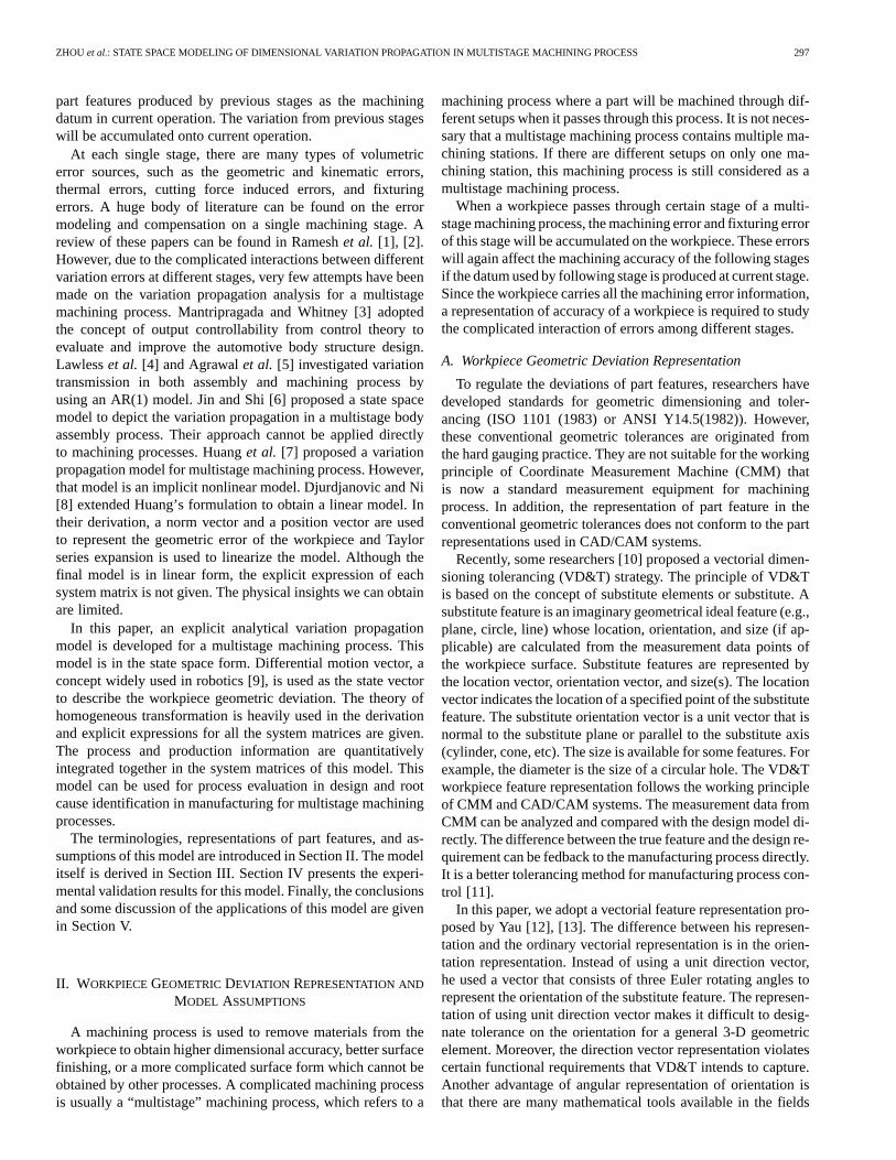
Fig. 1. Illustration of feature representation.

of robotics and kinematics for this representation. Therefore, inthis paper, a location vector and a vector that consists of threerotating Euler angles are used to represent a workpiece feature.Since the size of a feature is usually formed at one machiningstage, it is not considered in the following derivation.

The part representation is illustrated in Fig. 1. OX Y Zis the reference coordinate system (RCS). Plane 1 and Hole 2are represented by the local coordinate systems (LCSs) that areattached on them, respectively. The position and orientation ofPlane 1 can be represented by . is the location vectorthat points to the origin of LCS. is a vector contains roll,pitch, and yaw Euler rotating angles between coordinate systemLCS and RCS. is in Fig. 1. Similarly, Hole 2 canbe represented by . is in Fig. 1.

To describe the accuracy of a machined workpiece, we needto study the relationships between different features. SinceLCS is used to represent each feature, the relationships amongdifferent features can be described by the relationships of cor-responding coordinate systems. Homogeneous transformationmatrix (HTM) as a mathematical tool is used to study the trans-formation between different coordinate systems. Appendix Ilisted the basic notation and results of HTM used in this paper.

If the feature index is, we denote the corresponding LCS asLCS . The deviation of the feature is described by the deviationof the corresponding actual LCS from the corresponding nom-inal LCS. As shown in Appendix I, the deviation of a LCS canbe represented by a differential motion vector . If the

actual location vector for theth element is and the corre-sponding nominal location vector is , then .However, the orientation vector does not have this property, i.e.,in general, . The reason is that the multiplica-tion of rotating matrix does not commute in general cases.

In summary, a location vector and an orientation angularvector are used in this paper to represent a feature in the RCS.The relative position and orientation of a feature is describedas a homogenous transformation matrix. The deviation of afeature from its nominal value is represented by a differentialmotion vector. The rationale of this representation is that itconforms with the working principles of CMM and CAD/CAMmodels. Moreover, many mathematical tools are available foranalyzing this representation.

B. Model Assumptions

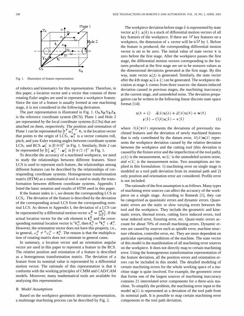
Based on the workpiece geometric deviation representation,a multistage machining process can be described by Fig. 2.

The workpiece deviation before stageis represented by statevector . is a stack of differential motion vectors of allkey features of the workpiece. If there arekey features on aworkpiece, the dimension of vector will be by 1. Beforethe feature is produced, the corresponding differential motionvector is set to be zero. The initial value of state vectoriszero before the first stage. After the workpiece passes the firststage, the differential motion vectors corresponding to the fea-tures produced at the first stage are set to be nonzero values asthe dimensional deviations generated at the first stage. By thisway, state vector is generated. Similarly, the state vectorafter the th stage can be generated. The workpiece de-viation at stage comes from three sources: the datum-induceddeviation caused in previous stages, the machining inaccuracyat the current stage, and unmodeled noise. The deviation propa-gation can be written in the following linear discrete state spaceformat [14]:

(1)

where represents the deviations of previously ma-chined features and the deviation of newly machined featuresthat is only contributed by the datum error, repre-sents the workpiece deviation caused by the relative deviationbetween the workpiece and the cutting tool (this deviation iscaused by the fixture error and the imperfection of the tool path),

is the measurement, is the unmodeled system noise,and is the measurement noise. Two assumptions are im-plied in this formulation: 1) machining error on single stage ismodeled as a tool path deviation from its nominal path and 2)only position and orientation error are considered. Profile erroris not included.

The rationale of the first assumption is as follows. Many typesof machining error sources can affect the accuracy of the work-piece on a single stage. According to Ramesh [1], they canbe categorized as quasistatic errors and dynamic errors. Quasi-static errors are the static or slow varying errors between thetool and the workpiece. They include the geometric and kine-matic errors, thermal errors, cutting force induced errors, toolwear induced error, fixturing error, etc. Quasi-static errors ac-count for about 70% of overall machining errors. Dynamic er-rors are caused by sources such as spindle error, machine struc-ture vibration, controller error, etc. They are more dependent onparticular operating conditions of the machine. The state vectorof this model is the manifestation of all machining error sourceson the workpiece. It does not directly map to certain machiningerror. Using the homogeneous transformation representation ofthe feature deviation, all the position errors and orientation er-rors can be included in this model. The detailed modeling ofcertain machining errors for the whole working space of a ma-chine stage is quite involved. For example, the geometric errorthat forms one of the largest sources of machining inaccuracycontains 21 interrelated error components for a three-axis ma-chine. To simplify the problem, the machining error input to themodel is represented as a deviation of the tool path fromits nominal path. It is possible to map certain machining errorcomponents to the tool path deviation.


Fig. 2. Diagram of a multistage machining process.

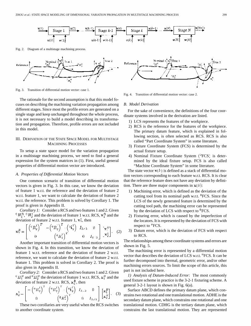
Fig. 3. Transition of differential motion vector: case 1.

The rationale for the second assumption is that this model fo-cuses on describing the machining variation propagation amongdifferent stages. Since most the profile errors are generated on asingle stage and keep unchanged throughout the whole process,it is not necessary to build a model describing its transforma-tion and propagation. Therefore, profile errors are not includedin this model.

III. D ERIVATION OF THESTATE SPACEMODEL FORMULTISTAGE

MACHINING PROCESSES

To setup a state space model for the variation propagationin a multistage machining process, we need to find a generalexpression for the system matrices in (1). First, useful generalproperties of differential motion vector are introduced.

A. Properties of Differential Motion Vectors

One common scenario of transition of differential motionvectors is given in Fig. 3. In this case, we know the deviationof feature 1 w.r.t. the reference and the deviation of feature 2w.r.t. feature 1, we want to calculate the deviation of feature 2w.r.t. the reference. This problem is solved by Corollary 1. Theproof is given in Appendix II.

Corollary 1: Consider a RCS and two features 1 and 2. Given, and the deviation of feature 1 w.r.t. RCS, and the

deviation of feature 2 w.r.t. feature 1, , then

(2)

Another important transition of differential motion vectors isshown in Fig. 4. In this transition, we know the deviation offeature 1 w.r.t. reference and the deviation of feature 2 w.r.t.reference, we want to calculate the deviation of feature 2 w.r.t.feature 1. This problem is solved in Corollary 2. The proof isalso given in Appendix II.

Corollary 2: Consider a RCS and two features 1 and 2. Givenand the deviation of feature 1 w.r.t. RCS, and the

deviation of feature 2 w.r.t. RCS, , then

(3)

These two corollaries are very useful when the RCS switchesto another coordinate system.

Fig. 4. Transition of differential motion vector: case 2.

B. Model Derivation

For the sake of convenience, the definitions of the four coor-dinate systems involved in the derivation are listed.

1) LCS represents the features of the workpiece.2) RCS is the reference for the features of the workpiece.

The primary datum feature, which is explained in fol-lowing section, is often selected as RCS. RCS is alsocalled “Part Coordinate System” in some literature.

3) Fixture Coordinate System (FCS) is determined by theactual fixture setup.

4) Nominal Fixture Coordinate SystemFCS is deter-mined by the ideal fixture setup. FCS is also called“Machine Coordinate System” in some literature.

The state vector is defined as a stack of differential mo-tion vectors corresponding to each feature w.r.t. RCS. It is clearthat the reference feature does not have any deviation by defini-tion. There are three major components in :

1) Machining error, which is defined as the deviation of thecutting tool from its nominal path w.r.t.FCS. Since theLCS of the newly generated feature is determined by thecutting tool path, the machining error can be representedby the deviation of LCS with respect toFCS.

2) Fixturing error, which is caused by the imperfection ofthe locators. It is represented by the deviation of FCS withrespect to FCS.

3) Datum error, which is the deviation of FCS with respectto RCS.

The relationships among these coordinate systems and errors areshown in Fig. 5.

The machining error is represented by a differential motionvector that describes the deviation of LCS w.r.t.FCS. It can befurther decomposed into thermal, geometric error, and/or othermachining errors sources. To limit the scope of this article, thispart is not included here.

1) Analysis of Datum-Induced Error:The most commonlyused fixture scheme in practice is the 3-2-1 fixturing scheme. Ageneral 3-2-1 layout is shown in Fig. 6(a).

Surface ABCD defines the primary datum plane, which con-strains two rotational and one translational motion. ADHE is thesecondary datum plane, which constrains one rotational and onetranslational motion. CDHG is the tertiary datum plane, whichconstrains the last translational motion. They are represented


Fig. 5. Composition of overall feature deviation.

(a)

(b)

Fig. 6. 3-2-1 fixturing setup by a plane and three locators. (a) General 3-2-1setup. (b) Variation of (a).

by LCS of O X Y Z , O X Y Z , and OX Y Z , respec-tively. F , F , and F are the perpendicular projection points ofthe locators P, P , and P on the primary datum. The fixture co-ordinate system (FCS) is shown in Fig. 6 as OX Y Z . F Fis the Y axis of FCS, the line passing Fand perpendicular to

F F is the X axis of FCS, Z axis is perpendicular to the pri-mary datum plane. The LCS of the primary datum plane (sur-face ABCD) is taken as the RCS. The secondary datum plane isdenoted as feature 2 and its deviation is represented as. Thetertiary datum plane is denoted as feature 3 and its deviation isrepresented as . Given and , the deviation of FCS w.r.t.RCS, , can be obtained by

(4)

where and are determined by the nominal positions offeature 2, 3, and the fixture locating pins. and can beobtained by the following general procedure.

Let and be the datum points touching the secondarydatum and be the datum point touching the tertiary datum.The nominal coordinates of these three points in FCS are de-noted as , , and . Denoting , we have

(5)

To guarantee that these points touch with the correspondingpart surface, the coordinates of these points in LCS are zeros(the direction is defined as the normal direction of the sur-face). Consider the first equation. Noting

and, the left-hand side of the first equation

of (5) changes to

(6)

The third element of is zero to guarantee touching, therefore

(7)

Under nominal conditions, , , and should touch withdatum plane. Hence, . Equation (7) changesto

(8)

Denoting

we have

(9)

and

(10)


Similarly, we can get other two equations for and . Fi-nally, we have

(11)

Although there are six parameters in , only three of themare unknown nonzero values. By solving the above equationsystem, we can obtain the differential motion vector andput it in the form of (4) by rearranging the terms. To guaranteethe inverse of the matrix exists, the line passing the two datumpoints on the second datum plane cannot be perpendicular to theprimary datum plane. If so, the first and the second rows of thecoefficient matrix of in the left-hand side of (11) will be thesame.

The expression of and for a general 3-2-1 setup is verycomplicated. However, if datum fixtures 1, 2, and 3 are orthog-onal to each other, which is a very common case in practice,and can be significantly simplified. Given the nominal posi-tions for features 2 and 3 and locating pins in Fig. 6(a) as

, , and ,the solution of (11) can be obtained as (4), where

A very common variation of the general 3-2-1 fixture setup isshown in Fig. 6(b). The six degree of freedoms of the workpieceare constrained by the plane ABCD (two rotational and onetranslational motion), a circular short hole Pand P (two trans-lational motion), and a slot P(one rotational motion). Giventhe nominal positions for features 2 and 3 and locating pins inFig. 6(b) as

, and , the solutionof (11) can be obtained as (4), where

and

The procedure presented in this section can be used to studythe datum-induced error for a general 3-2-1 fixture setup. Fol-lowing the same deviation, similar results can be obtained forother fixture setups, such as that used in turning operations.

2) Analysis of Fixture Errors:In a general 3-2-1 fixturescheme as shown in Fig. 6(a), the workpiece position islocated by six locatorsP P P L L L . Assume thatthe nominal coordinates of these six points in the nominalfixture coordinate systemFCS are , ,

, , , and ,respectively. (Note that we assume that thecoordinates ofP and P are the same to simplify the problem). If there aresmall deviations on these six locators and

, where , the actual fixturecoordinate system FCS will deviate from its nominalFCS.Cai et al. [15] gave an analytical infinitesimal error analysisfor a rigid body locating scheme with general six points.The fixture error can be derived based on their results. InFig. 6, the surface norm vector for L, L , and L is (0, 0,1), for P and P is ( 1, 0, 0), and for P is (0, 1, 0).With the locators’ position vectors, [15, eq. (3.1.6)] canbe applied to obtain the deviation of FCS w.r.t.FCS as

, wherewe have the equation shown at the bottom of the next page, and

.We need to know as well. Note that is

an identity matrix,. On the other hand,

. It is clear that. From (A8), we have

(12)

For the fixture setup shown in Fig. 6(b), the nominal coordi-nates of P, P , and P in FCS are (0, 0, 0), (0, , 0), and (0,0, 0), respectively. Substituting these values into the expressionof , we can obtain another matrix for the particular setupshown in Fig. 6(b) as

The fixture error analysis procedure for a general 3-2-1 fix-ture scheme is presented in this section. For other fixture sys-tems, the analysis can follow a very similar procedure.


Fig. 7. Steps of the derivation of variation propagation model.

3) Procedures for Variation Propagation Modeling:Fig. 7shows the steps of the derivation of the variation propagationmodel. The first step is to re-locate the workpiece at currentstage . The second step calculates the datum-induced error,which is caused by dimensional errors generated in previousstages. The third and fouth steps calculate the contribution offixture error and machining error that are only related with cur-rent stage. The fifth stage combines all errors together to ob-tain the deviation of the newly generated features. Finally, atthe sixth step, the newly generated features are combined withother features to form . The detailed derivations are asfollows.

S1. Using Corollary 2, transform from a stack ofto a stack of , . is the

feature index of the primary datum of stage. Letbe the stack of , then

(13)

where

...

...

...

......

......

......

...

......

......

......

...

......

......

......

...

...

...

...

where is an integer from 1 to the total number of features gen-erated up to stage. In (13), ,

. If primary datum is not changed between stageand stage , equals .

S2. Following the procedure of datum-induced error analysisin Section III, find datum error as

(14)


where . The dimensionof is 6 by .

S3. Denoting the fixture imperfection as , we can obtainthe fixture error following the procedure of fixture error analysisin Section III, , as

(15)

where .S4. Because the machine tool is calibrated based onFCS,

the tool path imperfection is often represented as a deviationw.r.t. FCS. Denoting the machining error of newly generatedfeature , is from 1 to , as and stack them up

as . Using Corollary 1, we can find . Denote

as a stack up of , , yields

(16)

where and

.

In (16), , ,and .

S5. Based on from step 2 and from step 4, wecan use Corollary 1 again to obtain the deviations of the newlygenerated features with respect to RCS, , .

In more detail, denoting as a stack of yields

(17)

Note that in (17) an approximation

(18)

is used because and are both small values. The

details are as follows. First note that

. Since

, ,or see (19), shown at the bottom of the page. Hence

(20)

Substituting (20) into the right-hand side of (18) and neglectingthe second-order small values yields the approximation result of(18).

S6. Adding the newly generated features with the othersyields as follows:

(21)

where A is a selector matrix in the form

......

......

...

......

......

...

......

......

...

......

......

...

Its dimension is by and it places the deviationsof the newly generated features on the corresponding locationwhen they are added to .

Considering (13)–(21), we can get the state transition equa-tion for the state space model

(22)

The detailed derivation can be found in Appendix III. In(1), ,

and .The derivation of the observation equation in (1) is straight-

forward. The measurement stage can be viewed as a special ma-chining stage. Assume that feature is used as the mea-surement reference feature and denote as the stack of

, following the same derivation of Step 1, we can obtain

(23)

where has the same format as in (13) except thatis used in the place of . Hence, the observation

equation can be written as

(24)

where is a selector matrix that is similar to the format ofin (21). selects the measured features among all

the available features. Therefore, in (1), the observation equa-tion is

(25)

The above model describes the deviation propagation amonga multistage machining process. An experimental validation ofthis model is presented in Section IV.

(19)


(a)

(b)

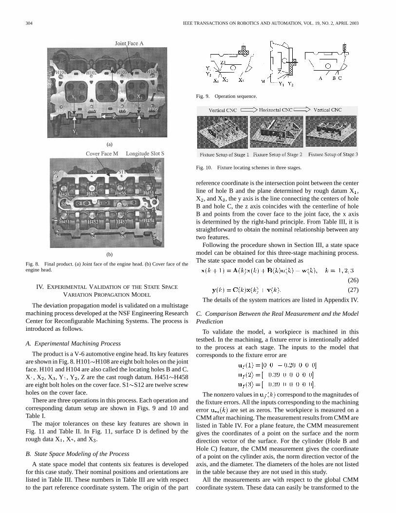
Fig. 8. Final product. (a) Joint face of the engine head. (b) Cover face of theengine head.

IV. EXPERIMENTAL VALIDATION OF THE STATE SPACE

VARIATION PROPAGATION MODEL

The deviation propagation model is validated on a multistagemachining process developed at the NSF Engineering ResearchCenter for Reconfigurable Machining Systems. The process isintroduced as follows.

A. Experimental Machining Process

The product is a V-6 automotive engine head. Its key featuresare shown in Fig. 8. H101H108 are eight bolt holes on the jointface. H101 and H104 are also called the locating holes B and C.X , X , X , Y , Y , Z are the cast rough datum. H451H458are eight bolt holes on the cover face. S1S12 are twelve screwholes on the cover face.

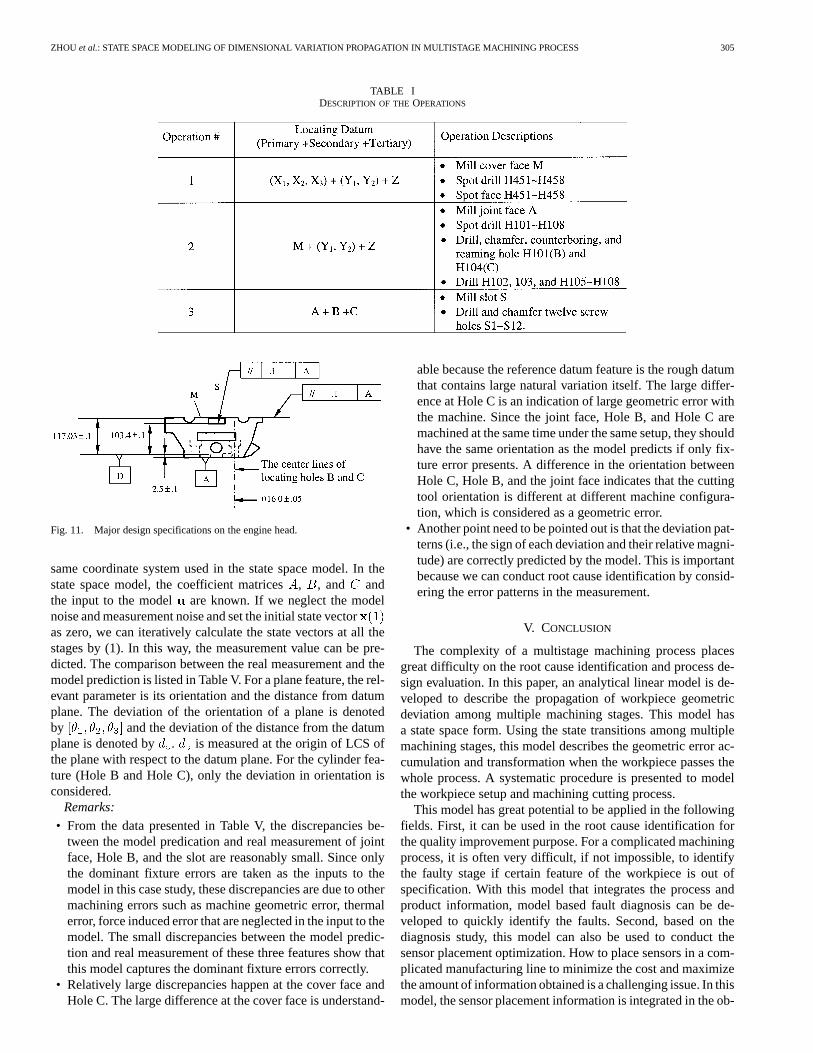
There are three operations in this process. Each operation andcorresponding datum setup are shown in Figs. 9 and 10 andTable I.

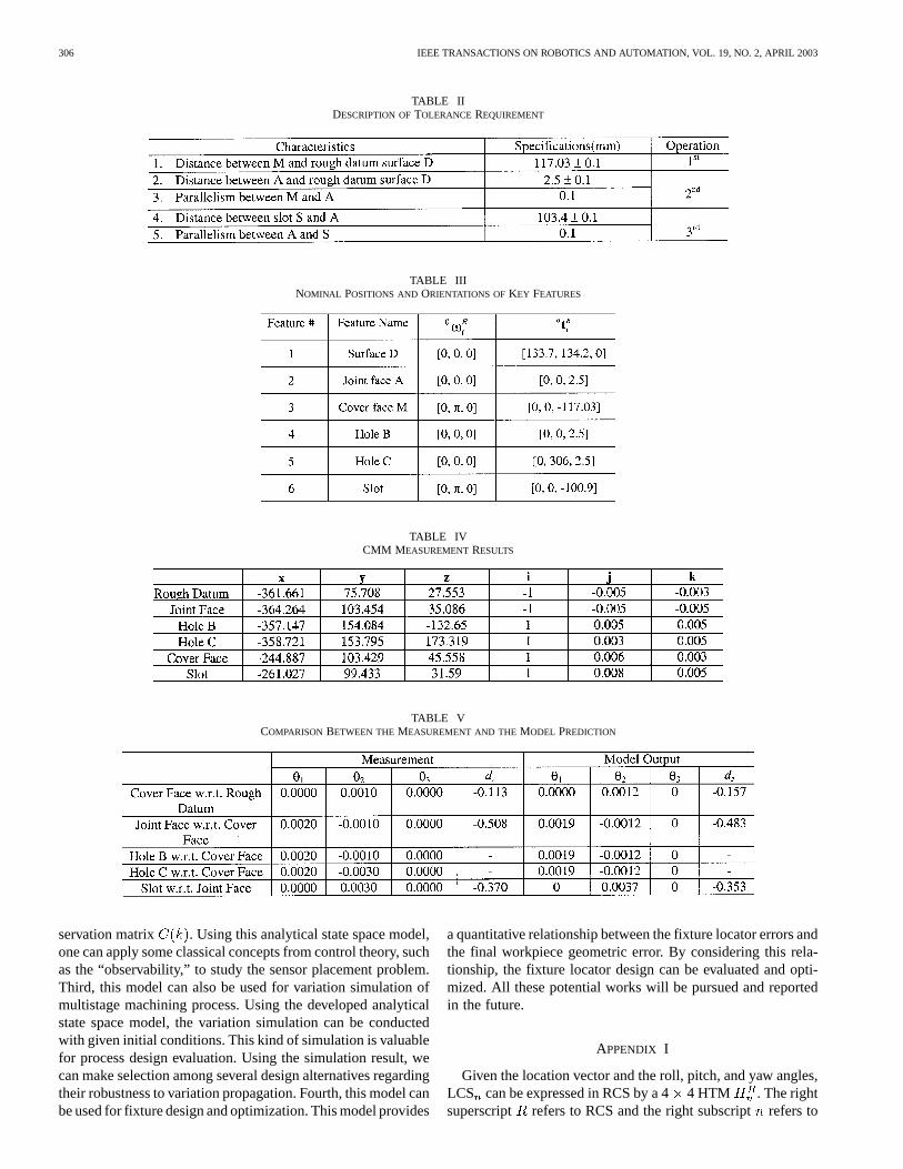
The major tolerances on these key features are shown inFig. 11 and Table II. In Fig. 11, surface D is defined by therough data X, X , and X .

B. State Space Modeling of the Process

A state space model that contents six features is developedfor this case study. Their nominal positions and orientations arelisted in Table III. These numbers in Table III are with respectto the part reference coordinate system. The origin of the part

Fig. 9. Operation sequence.

Fig. 10. Fixture locating schemes in three stages.

reference coordinate is the intersection point between the centerline of hole B and the plane determined by rough datum X,X , and X , the y axis is the line connecting the centers of holeB and hole C, the z axis coincides with the centerline of holeB and points from the cover face to the joint face, the x axisis determined by the right-hand principle. From Table III, it isstraightforward to obtain the nominal relationship between anytwo features.

Following the procedure shown in Section III, a state spacemodel can be obtained for this three-stage machining process.The state space model can be obtained as

(26)

(27)

The details of the system matrices are listed in Appendix IV.

C. Comparison Between the Real Measurement and the ModelPrediction

To validate the model, a workpiece is machined in thistestbed. In the machining, a fixture error is intentionally addedto the process at each stage. The inputs to the model thatcorresponds to the fixture error are

The nonzero values in correspond to the magnitudes ofthe fixture errors. All the inputs corresponding to the machiningerror are set as zeros. The workpiece is measured on aCMM after machining. The measurement results from CMM arelisted in Table IV. For a plane feature, the CMM measurementgives the coordinates of a point on the surface and the normdirection vector of the surface. For the cylinder (Hole B andHole C) feature, the CMM measurement gives the coordinateof a point on the cylinder axis, the norm direction vector of theaxis, and the diameter. The diameters of the holes are not listedin the table because they are not used in this study.

All the measurements are with respect to the global CMMcoordinate system. These data can easily be transformed to the


TABLE IDESCRIPTION OF THEOPERATIONS

Fig. 11. Major design specifications on the engine head.

same coordinate system used in the state space model. In thestate space model, the coefficient matrices, , and andthe input to the model are known. If we neglect the modelnoise and measurement noise and set the initial state vectoras zero, we can iteratively calculate the state vectors at all thestages by (1). In this way, the measurement value can be pre-dicted. The comparison between the real measurement and themodel prediction is listed in Table V. For a plane feature, the rel-evant parameter is its orientation and the distance from datumplane. The deviation of the orientation of a plane is denotedby and the deviation of the distance from the datumplane is denoted by . is measured at the origin of LCS ofthe plane with respect to the datum plane. For the cylinder fea-ture (Hole B and Hole C), only the deviation in orientation isconsidered.

Remarks:

• From the data presented in Table V, the discrepancies be-tween the model predication and real measurement of jointface, Hole B, and the slot are reasonably small. Since onlythe dominant fixture errors are taken as the inputs to themodel in this case study, these discrepancies are due to othermachining errors such as machine geometric error, thermalerror, force induced error that are neglected in the input to themodel. The small discrepancies between the model predic-tion and real measurement of these three features show thatthis model captures the dominant fixture errors correctly.

• Relatively large discrepancies happen at the cover face andHole C. The large difference at the cover face is understand-

able because the reference datum feature is the rough datumthat contains large natural variation itself. The large differ-ence at Hole C is an indication of large geometric error withthe machine. Since the joint face, Hole B, and Hole C aremachined at the same time under the same setup, they shouldhave the same orientation as the model predicts if only fix-ture error presents. A difference in the orientation betweenHole C, Hole B, and the joint face indicates that the cuttingtool orientation is different at different machine configura-tion, which is considered as a geometric error.

• Another point need to be pointed out is that the deviation pat-terns (i.e., the sign of each deviation and their relative magni-tude) are correctly predicted by the model. This is importantbecause we can conduct root cause identification by consid-ering the error patterns in the measurement.

V. CONCLUSION

The complexity of a multistage machining process placesgreat difficulty on the root cause identification and process de-sign evaluation. In this paper, an analytical linear model is de-veloped to describe the propagation of workpiece geometricdeviation among multiple machining stages. This model hasa state space form. Using the state transitions among multiplemachining stages, this model describes the geometric error ac-cumulation and transformation when the workpiece passes thewhole process. A systematic procedure is presented to modelthe workpiece setup and machining cutting process.

This model has great potential to be applied in the followingfields. First, it can be used in the root cause identification forthe quality improvement purpose. For a complicated machiningprocess, it is often very difficult, if not impossible, to identifythe faulty stage if certain feature of the workpiece is out ofspecification. With this model that integrates the process andproduct information, model based fault diagnosis can be de-veloped to quickly identify the faults. Second, based on thediagnosis study, this model can also be used to conduct thesensor placement optimization. How to place sensors in a com-plicated manufacturing line to minimize the cost and maximizethe amount of information obtained is a challenging issue. In thismodel, the sensor placement information is integrated in the ob-


TABLE IIDESCRIPTION OFTOLERANCE REQUIREMENT

TABLE IIINOMINAL POSITIONS AND ORIENTATIONS OFKEY FEATURES

TABLE IVCMM MEASUREMENTRESULTS

TABLE VCOMPARISONBETWEEN THEMEASUREMENT AND THEMODEL PREDICTION

servation matrix . Using this analytical state space model,one can apply some classical concepts from control theory, suchas the “observability,” to study the sensor placement problem.Third, this model can also be used for variation simulation ofmultistage machining process. Using the developed analyticalstate space model, the variation simulation can be conductedwith given initial conditions. This kind of simulation is valuablefor process design evaluation. Using the simulation result, wecan make selection among several design alternatives regardingtheir robustness to variation propagation. Fourth, this model canbe used for fixture design and optimization. This model provides

a quantitative relationship between the fixture locator errors andthe final workpiece geometric error. By considering this rela-tionship, the fixture locator design can be evaluated and opti-mized. All these potential works will be pursued and reportedin the future.

APPENDIX I

Given the location vector and the roll, pitch, and yaw angles,LCS can be expressed in RCS by a 44 HTM . The rightsuperscript refers to RCS and the right subscriptrefers to


the index of LCS. represents the nominal HTM betweenthe RCS and the LCS. A HTM can be written as

is the location vector of the origin of LCSexpressed in RCSand is the rotational matrix. Some useful properties of HTMare listed as follows (see [9] and [16]).

• A point expressed in LCScan be transformed into RCS,i.e., , where the superscript shows in whichcoordinate system the point is expressed.

• A rotational matrix is a special orthogonal matrix.and .

• and it can be obtained as

.

A small deviation of LCS from its nominal position and ori-entation can be described by a differential motion vector

(A1)

where and are asmall position deviation and a small orientation deviation, re-spectively. If we define

and

then the actual HTM and the nominal HTM between the refer-ence and local coordinate systems can be related by

(A2)

is defined as . Hence,

(A3)

can be written as

(A4)

where is called differential transformation matrix (DTM).If a skew symmetric matrix associated with a vectoris defined

as , the DTM can be written as

(A5)

We have

(A6)

One very useful fact can be obtained if we use small motionassumption, i.e.,

(A7)

If we let and , then

(A8)

APPENDIX II

Proof of Corollary 1: Noticeand , we have

. Sincethe deviations are small, we can neglect the second-order smallvalues,

). Noting that ,we have

(A9)

Denoting the differential motion vector associated withas , then the differential motion vector associated with

is

as in [9]. Combining this result with (A9), yields (2).Proof of Corollary 2: Noting , we have

. Then,. Considering (A4) and (A8) yields

(A10)

Therefore,

(A11)

This equation can be further simplified by neglecting thesecond-order small values

(A12)

(A13)

By (A13) and using the result from [9] again, we can get theresult in (3).


APPENDIX III

Derivation of (22): Substituting (13) and (17) into (21), wehave

(A14)

Substituting (14) and (16) into the above equation, we furtherhave

(A15)

Finally, (22) can be obtained by substituting (13) and (15) intothe above equation.

APPENDIX IV

The system matrices for the state space model used in Sec-tion IV:


In the model for experimental validation, the measurementstarts from . The observation matrices , , and

are all selector matrices that only contents zeros andones. The explicit expression of these observation matrices areomitted here.

ACKNOWLEDGMENT

The authors would like to thank the late research scientist atERC, Dr. J. Yuan, who designed the testbed machining processand had many insightful discussions with the authors. Theywould also like to thank the anonymous reviewers for theirenthusiastic efforts in the review process of this paper.

REFERENCES

[1] R. Ramesh, M. A. Mannan, and A. N. Poo, “Error compensation inmachine tools—a review part I: geometric, cutting-force induced andfixture dependent errors,”Int. J. Mach. Tools Manufact., vol. 40, pp.1235–1256, 2000a.

[2] , “Error compensation in machine tools—a review part II: thermalerrors,”Int. J. Mach. Tools Manufact., vol. 40, pp. 1235–1256, 2000b.

[3] R. Mantripragada and D. E. Whitney, “Modeling and controllingvariation propagation in mechanical assemblies using state transitionmodels,”IEEE Trans. Robot. Automat., vol. 15, pp. 124–140, 1999.

[4] J. F. Lawless, R. J. Mackay, and J. A. Robinson, “Analysis of variationtransmission in manufacturing processes—part I,”J. Quality Technol.,vol. 31, no. 2, pp. 131–142, 1999.

[5] R. Agrawal, J. F. Lawless, and R. J. Mackay, “Analysis of variation trans-mission in manufacturing processes—part II,”J. Quality Technol., vol.31, no. 2, pp. 143–154, 1999.

[6] J. Jin and J. Shi, “State space modeling of sheet metal assembly fordimensional control,”J. Manuf. Sci. Eng., vol. 121, pp. 756–762, Nov.1999.

[7] Q. Huang, J. Shi, and J. Yuan, “Part dimensional error and its propaga-tion modeling in multi-operational machining processes,”J. Manuf. Sci.Eng., no. 125, May 2003.

[8] D. Djurdjanovic and J. Ni, “Linear state space modeling of dimensionalmachining errors,”Trans. NAMRI/SME, vol. XXIX, pp. 541–548, 2001.

[9] R. P. Paul,Robot Manipulators: Mathematics, Programming, and Con-trol. Cambridge, MA: MIT Press, 1981.

[10] Handbook of Geometrical Tolerancing: Design, Manufacturing and In-spection, Wiley, New York, 1995.

[11] A. Wirtz, C. Gachter, and D. Wipf, “From unambiguously defined ge-ometry to the perfect quality control loop,”CIRP Ann. Manuf. Technol.,vol. 42, no. 1, pp. 615–618, 1993.

[12] H. Z. Yau, “Evaluation and uncertainty analysis of vectorial tolerances,”Precision Eng., vol. 20, pp. 123–137, 1997.

[13] , “Generalization and evaluation of vectorial tolerances,”Int. J.PROD. RES., vol. 35, no. 6, pp. 1763–1783, 1997.

[14] P. R. Kumar and P. Varaiya,Stochastic Systems: Estimation, Identifi-cation, and Adaptive Control. Englewood Cliffs, NJ: Prentice-Hall,1986.

[15] W. Cai, J. Hu, and J. Yuan, “A variational method of robust fixture con-figuration design for 3-D workpieces,”J. Manuf. Sci. Eng., vol. 119, pp.593–602, Nov. 1997.

[16] J. J. Craig,Introduction to Robotics. Boston, MA: Addison-Wesley,1988.

Shiyu Zhou received the B.S. and M.S. degreesin mechanical engineering from the Universityof Science and Technology of China in 1993 and1996, respectively, and the M.S. degree in industrialengineering and the Ph.D. degree in mechanicalengineering from the University of Michigan, AnnArbor, in 2000.

He is an Assistant Professor in the Departmentof Industrial Engineering at the University ofWisconsin-Madison. His research interests are thequality and productivity improvement methodolo-

gies by information integration based on control theory, advanced statistics,and engineering knowledge.

Dr. Zhou received Distinguished Achievements Award in 2000 at the Univer-sity of Michigan. He is a member of IIE, INFORMS, ASME, and SME.

Qiang Huang received the B.S., M.S., and Ph.D. de-grees in mechanical engineering from Shanghai Jiao-Tong University, Shanghai, China in 1993, 1996, and1998, respectively. He is currently working towardthe Ph.D. degree at the University of Michigan, AnnArbor.

His research interests are centered on variationreduction for complex manufacturing processes, in-tegrated design and manufacturing, and engineeringstatistics.

Dr. Huang is a member of ASME, INFORMS, IIE,and SME.

Jianjun Shi received the B.S. and M.S. degrees inelectrical engineering from Beijing Institute of Tech-nology in 1984 and 1987, respectively, and the Ph.D.degree in mechanical engineering from the Univer-sity of Michigan, Ann Arbor, in 1992.

He currently is an Associate Professor in the De-partment of Industrial and Operations Engineering,University of Michigan. His research interests arethe fusion of advanced statistics and engineeringknowledge to develop in-process quality improve-ment (IPQI) methodologies achieving automatic

process monitoring, diagnosis, compensation, and their implementation invarious manufacturing processes. He received numerous awards and currentlyserves as a Department Editor ofIIE Transactions on Quality and Reliability.

Dr. Shi is a member of ASME, ASQC, IIE, and SME.

state space modeling of dimensional variation...

Documents