statement by author
TRANSCRIPT

2
STATEMENT BY AUTHOR
This thesis has been submitted in partial fulfillment of requirements for an advanceddegree at The University of Arizona and is deposited in the University Library to be madeavailable to borrowers under rules of the Library.
Brief quotations from this thesis are allowable without special permission, provided thataccurate acknowledgment of source is made. Requests for permission for extended quotationfrom or reproduction of this manuscript in whole or in part may be granted by the head ofthe major department or the Dean of the Graduate College when in his or her judgmentthe proposed use of the material is in the interests of scholarship. In all other instances,however, permission must be obtained from the author.
SIGNED:
APPROVAL BY THESIS DIRECTOR
This thesis has been approved on the date shown below:
Dr. Francois E. Cellier DateProfessor of
Electrical and Computer Engineering

3
ACKNOWLEDGMENTS
I would like to express my special appreciation to Dr. Francois E. Cellier, my thesis
advisor, for his guidance, valuable advice and for always devoting his time and patience to
me during this research.
I should also like to thank my friend Michael Schweisguth who reviewed this thesis and
helped me to find formulations in proper English.
Special thanks are due to Dr. Christoph Woernle, Dr. Parviz Nikravesh and the German
Exchange Service (DAAD) for organizing the exchange program between the University of
Stuttgart/Germany and the University of Arizona at Tucson/U.S.A., which allowed me to
make all these precious experiences brought along by an academic year abroad.

4
To my parents

5
TABLE OF CONTENTS
LIST OF FIGURES . . . . . . . . . . . . . . . . . . . . . . . . . . . . . . . . . . 7
LIST OF TABLES . . . . . . . . . . . . . . . . . . . . . . . . . . . . . . . . . . . 9
ABSTRACT . . . . . . . . . . . . . . . . . . . . . . . . . . . . . . . . . . . . . . . 10
1. Introduction . . . . . . . . . . . . . . . . . . . . . . . . . . . . . . . . . . . . . 111.1. Ordinary Differential Equations (ODE) . . . . . . . . . . . . . . . . . . . . 111.2. Numerical methods to solve ODEs . . . . . . . . . . . . . . . . . . . . . . . 121.3. Stability versus accuracy . . . . . . . . . . . . . . . . . . . . . . . . . . . . 15
1.3.1. Introduction . . . . . . . . . . . . . . . . . . . . . . . . . . . . . . . 151.3.2. Errors incurred in numerical integration . . . . . . . . . . . . . . . . 151.3.3. Stability of numerical methods . . . . . . . . . . . . . . . . . . . . . 171.3.4. Spurious eigenvalues . . . . . . . . . . . . . . . . . . . . . . . . . . . 19
1.4. Stiff systems . . . . . . . . . . . . . . . . . . . . . . . . . . . . . . . . . . . 22
2. Derivation of RBDF by regression . . . . . . . . . . . . . . . . . . . . . . . 262.1. Introduction . . . . . . . . . . . . . . . . . . . . . . . . . . . . . . . . . . . 262.2. Formulation and solution of the regression problem . . . . . . . . . . . . . 272.3. Development of an algorithm for the search of RBDF . . . . . . . . . . . . 31
3. Analysis of RBDF . . . . . . . . . . . . . . . . . . . . . . . . . . . . . . . . . 333.1. Introduction . . . . . . . . . . . . . . . . . . . . . . . . . . . . . . . . . . . 333.2. Stability domain . . . . . . . . . . . . . . . . . . . . . . . . . . . . . . . . . 34
3.2.1. Introduction . . . . . . . . . . . . . . . . . . . . . . . . . . . . . . . 343.2.2. Stability domain of RBDF . . . . . . . . . . . . . . . . . . . . . . . 36
3.3. Error constant . . . . . . . . . . . . . . . . . . . . . . . . . . . . . . . . . . 403.4. Damping plot . . . . . . . . . . . . . . . . . . . . . . . . . . . . . . . . . . 423.5. Order star . . . . . . . . . . . . . . . . . . . . . . . . . . . . . . . . . . . . 473.6. Bode plot . . . . . . . . . . . . . . . . . . . . . . . . . . . . . . . . . . . . . 53
4. Implementation of RBDF . . . . . . . . . . . . . . . . . . . . . . . . . . . . 584.1. Startup problem . . . . . . . . . . . . . . . . . . . . . . . . . . . . . . . . . 584.2. Step-size control . . . . . . . . . . . . . . . . . . . . . . . . . . . . . . . . . 59
4.2.1. Introduction . . . . . . . . . . . . . . . . . . . . . . . . . . . . . . . 594.2.2. Newton-Gregory polynomials . . . . . . . . . . . . . . . . . . . . . . 60
6
4.2.3. Calculation of the Nordsieck vector . . . . . . . . . . . . . . . . . . 624.2.4. Step-size control algorithm . . . . . . . . . . . . . . . . . . . . . . . 65
4.3. Integration of nonlinear systems . . . . . . . . . . . . . . . . . . . . . . . . 714.3.1. Startup problem . . . . . . . . . . . . . . . . . . . . . . . . . . . . . 714.3.2. Newton iteration . . . . . . . . . . . . . . . . . . . . . . . . . . . . . 72
4.4. Readout problem . . . . . . . . . . . . . . . . . . . . . . . . . . . . . . . . 73
5. RBDF of 6th order (RBDF6) . . . . . . . . . . . . . . . . . . . . . . . . . . 755.1. Derivation of the algorithms . . . . . . . . . . . . . . . . . . . . . . . . . . 755.2. Analysis . . . . . . . . . . . . . . . . . . . . . . . . . . . . . . . . . . . . . 845.3. Simulation results and comparison of the RBDF6 methods with BDF6 . . 86
6. RBDF of 7th order (RBDF7) . . . . . . . . . . . . . . . . . . . . . . . . . . 1006.1. Derivation of the algorithms . . . . . . . . . . . . . . . . . . . . . . . . . . 1006.2. Analysis . . . . . . . . . . . . . . . . . . . . . . . . . . . . . . . . . . . . . 1016.3. Simulation results . . . . . . . . . . . . . . . . . . . . . . . . . . . . . . . . 107
7. Conclusions . . . . . . . . . . . . . . . . . . . . . . . . . . . . . . . . . . . . . 113
Appendix A. Nordsieck transformation matrices of different order . . . . . 115
Appendix B. Implementation of RBDF61 in MATLAB . . . . . . . . . . . . 119B.1. Main program INT . . . . . . . . . . . . . . . . . . . . . . . . . . . . . . . 119B.2. Procedure DEFINE . . . . . . . . . . . . . . . . . . . . . . . . . . . . . . . 121B.3. Procedure STARTUP . . . . . . . . . . . . . . . . . . . . . . . . . . . . . . 122B.4. Procedure BIN SEARCH H0 . . . . . . . . . . . . . . . . . . . . . . . . . . 123B.5. Procedure RUKU5 . . . . . . . . . . . . . . . . . . . . . . . . . . . . . . . . 126B.6. Procedure RUKU6 . . . . . . . . . . . . . . . . . . . . . . . . . . . . . . . . 127B.7. Procedure COMM . . . . . . . . . . . . . . . . . . . . . . . . . . . . . . . . 127B.8. Function FUNC . . . . . . . . . . . . . . . . . . . . . . . . . . . . . . . . . 128B.9. Function MULT . . . . . . . . . . . . . . . . . . . . . . . . . . . . . . . . . 129B.10.Function NEWTON . . . . . . . . . . . . . . . . . . . . . . . . . . . . . . . 137B.11.Function IMP FUNC . . . . . . . . . . . . . . . . . . . . . . . . . . . . . . 138B.12.Function JAC . . . . . . . . . . . . . . . . . . . . . . . . . . . . . . . . . . 139B.13.Function COMM MULT . . . . . . . . . . . . . . . . . . . . . . . . . . . . 140
REFERENCES . . . . . . . . . . . . . . . . . . . . . . . . . . . . . . . . . . . . . 142
7
LIST OF FIGURES
1.1. Data points used by the Adams-Bashforth algorithms (left) and the Adams-Moulton algorithms (right) . . . . . . . . . . . . . . . . . . . . . . . . . . . 14
1.2. Data points used by the BDF algorithms . . . . . . . . . . . . . . . . . . . 141.3. Stability definitions for numerical integration methods. . . . . . . . . . . . 191.4. Simulation of a stiff linear system. . . . . . . . . . . . . . . . . . . . . . . . 23
3.1. Domain of analytical stability . . . . . . . . . . . . . . . . . . . . . . . . . 343.2. Stability domain of the BE-algorithm . . . . . . . . . . . . . . . . . . . . . 363.3. Stability region of RBDF61 . . . . . . . . . . . . . . . . . . . . . . . . . . . 393.4. Stiffly stable system . . . . . . . . . . . . . . . . . . . . . . . . . . . . . . . 393.5. Stability locus of RBDF69 . . . . . . . . . . . . . . . . . . . . . . . . . . . 403.6. Damping plot of BDF6 . . . . . . . . . . . . . . . . . . . . . . . . . . . . . 443.7. Modified damping plot of the BDF6 method . . . . . . . . . . . . . . . . . 453.8. Stability domain of BDF6 . . . . . . . . . . . . . . . . . . . . . . . . . . . . 463.9. Logarithmic damping plot of BDF6 . . . . . . . . . . . . . . . . . . . . . . 463.10. Order star of the BDF6 method . . . . . . . . . . . . . . . . . . . . . . . . 483.11. Modified damping plot of the BDF6 method . . . . . . . . . . . . . . . . . 493.12. Bode plot of a first order system . . . . . . . . . . . . . . . . . . . . . . . . 543.13. Integration method regarded as a discrete system . . . . . . . . . . . . . . 563.14. Bode plot of a stable system integrated by BDF6 . . . . . . . . . . . . . . 57
5.1. Stability domain of BDF6 . . . . . . . . . . . . . . . . . . . . . . . . . . . . 765.2. Damping plot of BDF6 . . . . . . . . . . . . . . . . . . . . . . . . . . . . . 775.3. Damping plot of a “bad” RBDF . . . . . . . . . . . . . . . . . . . . . . . . 785.4. Stability domain of the “bad” RBDF . . . . . . . . . . . . . . . . . . . . . 785.5. Stability domains of RBDF6 with 8 data points . . . . . . . . . . . . . . . 805.6. Stability domains of RBDF6 with 9 data points . . . . . . . . . . . . . . . 805.7. Damping plots of RBDF6 with 8 data points . . . . . . . . . . . . . . . . . 815.8. Damping plots of RBDF6 with 9 data points . . . . . . . . . . . . . . . . . 815.9. Logarithmic damping plots of RBDF6 with 8 data points . . . . . . . . . . 825.10. Logarithmic damping plots of RBDF6 with 9 data points . . . . . . . . . . 825.11. Order stars of RBDF6 with 8 data points . . . . . . . . . . . . . . . . . . . 835.12. Order stars of RBDF6 with 9 data points . . . . . . . . . . . . . . . . . . . 835.13. Accuracy region of BDF6, RBDF61 and RBDF66 . . . . . . . . . . . . . . 855.14. Integration of system 1 by BDF6 . . . . . . . . . . . . . . . . . . . . . . . . 89
8
5.15. Integration of system 1 by RBDF61 . . . . . . . . . . . . . . . . . . . . . . 905.16. Integration of system 1 by RBDF66 . . . . . . . . . . . . . . . . . . . . . . 915.17. Integration of system 2 by BDF6 . . . . . . . . . . . . . . . . . . . . . . . . 935.18. Integration of system 2 by RBDF61 . . . . . . . . . . . . . . . . . . . . . . 945.19. Integration of system 2 by RBDF66 . . . . . . . . . . . . . . . . . . . . . . 955.20. Bode plot of a stable system integrated by BDF6, RBDF61and RBDF66. . 985.21. Bode plot of a marginally stable system integrated by BDF6, RBDF61 and
RBDF66. . . . . . . . . . . . . . . . . . . . . . . . . . . . . . . . . . . . . . 985.22. Bode plot of an unstable system integrated by BDF6, RBDF61 and RBDF66. 99
6.1. Stability domains of RBDF7 — 1. part . . . . . . . . . . . . . . . . . . . . 1046.2. Stability domains of RBDF7 — 2. part . . . . . . . . . . . . . . . . . . . . 1046.3. Damping plots of RBDF7 — 1. part (RBDF71 through RBDF78) . . . . . 1056.4. Damping plots of RBDF7 — 2. part (RBDF79 through RBDF715) . . . . 1056.5. Logarithmic damping plots of RBDF7 — 1. part (RBDF71 through RBDF78)1066.6. Logarithmic damping plots of RBDF7 — 2. part (RBDF79 through RBDF715)1066.7. Integration of system 1 by RBDF71 . . . . . . . . . . . . . . . . . . . . . . 1096.8. Integration of system 1 by RBDF713 . . . . . . . . . . . . . . . . . . . . . 1106.9. Integration of system 2 by RBDF71 . . . . . . . . . . . . . . . . . . . . . . 1116.10. Integration of system 2 by RBDF713 . . . . . . . . . . . . . . . . . . . . . 112
9
LIST OF TABLES
5.1. Number of 6th order RBDF algorithms satisfying minimum stability require-ments . . . . . . . . . . . . . . . . . . . . . . . . . . . . . . . . . . . . . . . 76
5.2. RBDF6 methods . . . . . . . . . . . . . . . . . . . . . . . . . . . . . . . . . 795.3. BDF6 method . . . . . . . . . . . . . . . . . . . . . . . . . . . . . . . . . . 84
6.1. Number of 7th order RBDF algorithms satisfying minimum stability require-ments . . . . . . . . . . . . . . . . . . . . . . . . . . . . . . . . . . . . . . . 101
6.2. RBDF7 methods — 1. part . . . . . . . . . . . . . . . . . . . . . . . . . . . 1026.3. RBDF7 methods — 2. part . . . . . . . . . . . . . . . . . . . . . . . . . . . 1036.4. Data of RBDF7 algorithms . . . . . . . . . . . . . . . . . . . . . . . . . . . 107

10
ABSTRACT
In the past research has been done to solve stiff systems described by ordinary differen-
tial equations (ODEs). An important result are the famous Backward Difference Formulae
(BDF) [10]. These methods are capable of solving stiff ODE-systems up to accuracy order
six — accuracy order six means that the error made at each integration step is roughly
proportional to the seventh power of the step-size. So far, no BDF algorithms of seventh
order and higher, have been found that are stable.
This thesis proposes the Regression Backward Difference Formulae (RBDF) as new numeri-
cal solution methods for stiff systems described by first order ordinary differential equations.
The RBDF algorithms derived in this thesis, by means of a new regression technique, will
be of sixth and seventh order, and it will be shown that some of the sixth order RBDF
algorithms compare favorably against the sixth order BDF.
The results for the new seventh order RBDF algorithms are shown, but not compared to
BDF since no stable seventh order BDF technique exists.
It can be expected that RBDF methods of order higher than seven may be found by using
the proposed regression approach.
In particular, celestial analysis demands highly accurate calculation and integration. There-
fore, this might be one area where even higher order RBDF techniques than seventh order
RBDF could be applied.

11
CHAPTER 1
Introduction
1.1 Ordinary Differential Equations (ODE)
A first order scalar ODE can be written as
dxdt = x(t) = f(x, u, t) (1.1)
with initial condition
x(t0) = x0. (1.2)
Here t is the independent variable (which usually, but not necessarily, denotes time), u is a
given input, and the function f indicates any explicit functionality between the dependent
variable x and the independent variable t.
Without loss of generality only systems, as shown in equation (1.3), are considered.
x(t) = f(x, u), (1.3)
x(t0) = x0. (1.4)
i.e., systems, where the independent variable t does not appear explicitly in the equations.
In addition to the first-order scalar equation (1.3) it is possible to consider a set of
simultaneous first-order equations, or an equivalent higher-order single equation. Thus we
12
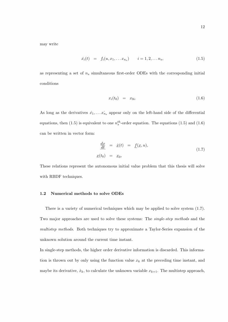
may write
xi(t) = fi(u, x1, . . . xns) i = 1, 2, . . . ns, (1.5)
as representing a set of ns simultaneous first-order ODEs with the corresponding initial
conditions
xi(t0) = x0i. (1.6)
As long as the derivatives x1, . . . ˙xns appear only on the left-hand side of the differential
equations, then (1.5) is equivalent to one nths -order equation. The equations (1.5) and (1.6)
can be written in vector form:
dxdt = x(t) = f(x, u),
x(t0) = x0,
(1.7)
These relations represent the autonomous initial value problem that this thesis will solve
with RBDF techniques.
1.2 Numerical methods to solve ODEs
There is a variety of numerical techniques which may be applied to solve system (1.7).
Two major approaches are used to solve these systems: The single-step methods and the
multistep methods. Both techniques try to approximate a Taylor-Series expansion of the
unknown solution around the current time instant.
In single-step methods, the higher order derivative information is discarded. This informa-
tion is thrown out by only using the function value xk at the preceding time instant, and
maybe its derivative, xk, to calculate the unknown variable xk+1. The multistep approach,

13
however, preserves some of the higher order derivative information by using data of earlier
values xi and xi.
In general a multistep integration algorithm can be expressed as
xk+1 = b−1hfk+1 + a0xk + b0hfk + a1xk−1 + . . . + am−1xk+1−m + bm−1hfk+1−m
=m−1∑i=0
aixk−i +m−1∑i=−1
bihfk−i,
(1.8)
where fi = xi is the derivative of the system variable x at the time instant t = t0 + i∆t.
Note that this method (1.8) is implicit when b−1 �= 0 and it is explicit when b−1 = 0. The
number m denotes the number of steps, so the algorithm shown in (1.8) can be called an
m-step integration algorithm.
Note also that the algorithm depicted in equation (1.8) only uses values of x and x and
not higher derivatives, such as xk. It is also required that (1.8) be applied with equispaced
steps. These restrictions may limit the performance of solutions based on (1.8). However,
(1.8) represents a very important and extensive class of formulas which will be used to
derive RBDF methods.
The two most famous and frequently used multistep integration methods are the Adams
methods and the Backward Difference Formulae (BDF).
The Adams algorithms use the function value xk one time step back and the derivative
values of several of the preceding function values such that they can be written in the form
xk+1 = b−1hfk+1 + a0xk + b0hfk + b1hfk−1 + . . . + bm−1hfk+1−m. (1.9)
If b−1 = 0 then equation (1.9) is reduced to the explicit Adams-Bashforth algorithms.
However, if b−1 �= 0 then equation (1.9) reduces to the implicit Adams-Moulton methods.
14
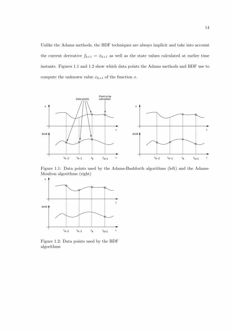
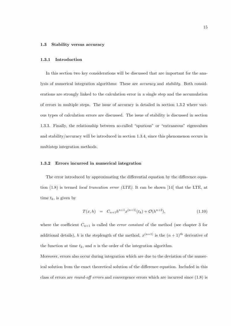
Unlike the Adams methods, the BDF techniques are always implicit and take into account
the current derivative fk+1 = xk+1 as well as the state values calculated at earlier time
instants. Figures 1.1 and 1.2 show which data points the Adams methods and BDF use to
compute the unknown value xk+1 of the function x.
x
dx/dt
t
tk+1kk−1k−2t t t t
Data pointsPoint to becalculated
x
dx/dt
t
tk+1kk−1k−2t t t t
Figure 1.1: Data points used by the Adams-Bashforth algorithms (left) and the Adams-Moulton algorithms (right)
x
dx/dt
t
tk+1kk−1k−2t t t t
Figure 1.2: Data points used by the BDFalgorithms
15
1.3 Stability versus accuracy
1.3.1 Introduction
In this section two key considerations will be discussed that are important for the ana-
lysis of numerical integration algorithms: These are accuracy and stability. Both consid-
erations are strongly linked to the calculation error in a single step and the accumulation
of errors in multiple steps. The issue of accuracy is detailed in section 1.3.2 where vari-
ous types of calculation errors are discussed. The issue of stability is discussed in section
1.3.3. Finally, the relationship between so-called “spurious” or “extraneous” eigenvalues
and stability/accuracy will be introduced in section 1.3.4, since this phenomenon occurs in
multistep integration methods.
1.3.2 Errors incurred in numerical integration
The error introduced by approximating the differential equation by the difference equa-
tion (1.8) is termed local truncation error (LTE). It can be shown [14] that the LTE, at
time tk, is given by
T (x, h) = Cn+1hn+1x(n+1)(tk) + O(hn+2), (1.10)
where the coefficient Cn+1 is called the error constant of the method (see chapter 3 for
additional details), h is the steplength of the method, x(n+1) is the (n + 1)th derivative of
the function at time tk, and n is the order of the integration algorithm.
Moreover, errors also occur during integration which are due to the deviation of the numer-
ical solution from the exact theoretical solution of the difference equation. Included in this
class of errors are round-off errors and convergence errors which are incurred since (1.8) is
16
implicit and must be solved by Newton-iteration.
Another class of errors is called the startup error and it is introduced because a multistep
method requires values of m earlier steps. Typically, a single-step method is used to gen-
erate m starting steps. Hence, an error is introduced into the calculation because of the
numerical approximation of the initial steps.
In work done by Cellier [4], it was shown that the effect of the startup error being accumu-
lated during a simulation is eliminated if the system being integrated is analytically stable
and if the integration method in use is numerically stable.
Hence, the approximated initial conditions of an integration step don’t excessively affect the
result of the overall simulation of an analytically stable system, i.e. the initial conditions of
a m-step method that are produced by a single-step algorithm, are not of large significance
for the resulting accuracy of the overall simulation.
Cellier [4] notes two other classes of errors, the parametric model error and the structural
model error. Parametric model errors occur because the model parameters are inaccurately
estimated, whereas structural model errors are due to the fact that the model fails to de-
scribe important dynamics of the real system.
Thus, these types of errors have nothing to do with the accuracy and stability of the nu-
merical integration technique since they are present in the model already.
The LTE and the startup errors accumulate to produce the global truncation error (GTE)
or accumulated error [14]. The GTE can be expressed as
εk = x(tk) − xk, (1.11)
17
where x(tk) is the exact function value of the analytical solution, and xk is the numerical
approximation of x(tk).
Note that the global truncation error cannot be calculated as the sum of the local errors.
It must be computed as a solution to the linear k-step difference equation
ρ(E)εk + hσ(E)λkεk + Tk + ηk = 0,
which will be derived in section 1.3.4.
While the LTE is proportional to hn+1 for a nth order algorithm, Lambert shows in [14]
that the GTE is roughly proportional to hn for analytically stable systems. Therefore, one
power of h has been lost during the process of accumulation.
1.3.3 Stability of numerical methods
Dahlquist states in [7] that:
Definition 1.3.1 A method is said to be A-stable, if the values h = hλ have negative real
parts, where h is the steplength of the applied numerical method and λ denotes the (complex)
eigenvalue of the test-system x = λx.
The highest order of an A-stable linear multistep method is two [7]. The smallest truncation
error is obtained by using the trapezoidal rule.
In order to be able to apply the definition of A-stability to higher order linear multistep
techniques, the requirements of A-stability have to be relaxed:
The first step is to only regard a wedge in the left half side of the complex λh-plane. This
motivates the definition [20]:

18
Definition 1.3.2 A method is said to be A(α)-stable, α ∈ (0, π/2) if
RA ⊇ {h| − α < π − arg{h} < α},
it is said to be A(0)-stable if it is A(α)-stable for some α ∈ (0, π/2), where RA is the region
of absolute stability, and h = hλ.
Gear proposes in [10] an alternative way of relaxing the requirements of A-stability by using
Cartesian rather than polar coordinates:
Definition 1.3.3 A method is said to be stiffly stable if RA ⊇ R1 ∪ R2, where R1 =
{h|Re{h} < −a} and R2 = {h| − a ≤ Re{h} < 0,−c ≤ Im{h} ≤ c}, a and c are positive
real numbers and h = hλ.
It is characteristic for stiffly stable systems to have eigenvalues which lie far left in the left
half plane. They represent the fast transients of the system. In order to eliminate these
transients a large damping is required as the real part of the eigenvalues goes to −∞. This
results in another definition [2],[8]:
Definition 1.3.4 A one-step method is said to be L-stable if it is A-stable and, in addition,
when applied to the scalar test equation x = λx, λ a complex constant with Re{λ} < 0, it
yields xk+1 = R(hλ)xk, where |R(hλ)| → 0 as Re{hλ} → −∞.
Note that L-stable methods mustn’t be applied to unstable systems since the unstable
behavior would be removed such that the systems would appear stable [14].
Figure 1.3 illustrates the given definitions of stability:
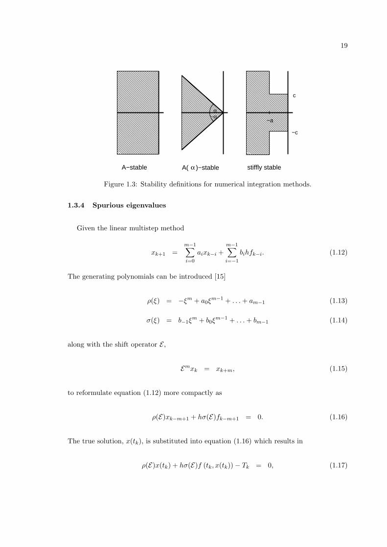
19
A−stable
α−α
c
−c
−a
α stiffly stableA( )−stable
Figure 1.3: Stability definitions for numerical integration methods.
1.3.4 Spurious eigenvalues
Given the linear multistep method
xk+1 =m−1∑i=0
aixk−i +m−1∑i=−1
bihfk−i. (1.12)
The generating polynomials can be introduced [15]
ρ(ξ) = −ξm + a0ξm−1 + . . . + am−1 (1.13)
σ(ξ) = b−1ξm + b0ξ
m−1 + . . . + bm−1 (1.14)
along with the shift operator E ,
Emxk = xk+m, (1.15)
to reformulate equation (1.12) more compactly as
ρ(E)xk−m+1 + hσ(E)fk−m+1 = 0. (1.16)
The true solution, x(tk), is substituted into equation (1.16) which results in
ρ(E)x(tk) + hσ(E)f (tk, x(tk)) − Tk = 0, (1.17)

20
where Tk = T (tk, h).
Note that the index of x has been changed from k − m + 1 to k for convenience.
For the numerical solution the relationship
ρ(E)xk + hσ(E)f(tk, xk) + ηk = 0 (1.18)
holds, where ηk represents the error which results from not having solved the difference
equation exactly.
Subtracting equation (1.17) from equation (1.18) and then applying the mean-value theorem
f(tk, xk) − f (tk, x(tk)) = fx(tk, x) (xk − x(tk)) , (1.19)
where xk ≤ x ≤ x(tk), denoting fx(tk, x) as λk and introducing the accumulated error
εk = xk − x(tk), (1.20)
the m-step difference equation of the accumulated error εk
ρ(E)εk + hσ(E)λkεk + Tk + ηk = 0. (1.21)
is obtained. Assuming that Tk, λk and ηk are constants, equation (1.21) yields
ρ(E)εk + hλσ(E)εk + T + η = 0. (1.22)
Therefore, the accumulated error εk obeys a linear, inhomogeneous, m-step difference equa-
tion with constant coefficients. By solving the characteristic equation of (1.22),
ρ(µ) + hλσ(µ) = 0, (1.23)
the characteristic roots µi, i = 1, 2, . . . m are obtained.
When equation (1.22) is solved and the constant particular solution εkp is ignored, only the
21
homogeneous solution εkh remains as shown in equation (1.24).
εk = εkh + εkp =
≈ εkh =
= c1µk1 + c2µ
k2 + . . . + cmµk
m.
(1.24)
Since the numerical solution xk obeys the same difference equation as the accumulated
error εk, xk can be expressed as
xk = d1µk1 + d2µ
k2 + . . . + dmµk
m. (1.25)
The root µ1, which is called the “principal root,” approximates the Taylor Series expansion
of the true solution. This approximation has a truncation error which corresponds to the
order of the method.
The other m − 1 roots are termed “spurious,” “parasitic,” or “extraneous” roots or eigen-
values.
Lapidus [10] shows that a multistep method, given by (1.12), is absolutely stable if, for
h < h0, where h0 is a real constant, the extraneous solutions in (1.25) vanish as k → ∞
[15].
Alternatively, the method is absolutely stable for those values of hλ where both the prin-
cipal root and the spurious roots are within the unit circle.
The spurious eigenvalues don’t exist in the original system and have been introduced by
the multistep algorithm, that substitutes a first-order differential equation by a mth order
difference equation. Since they bear no connection to the exact solution, they can cause

22
numerical instability [15]. The impact of the extraneous eigenvalues on the stability prop-
erties of a multistep method can also be observed when regarding the stability domain of
the method (see chap. 3).
1.4 Stiff systems
Many physical systems give rise to ordinary differential equations which have eigenvalues
that vary greatly in magnitude. For instance, such situations can arise in studies of chem-
ical kinetics, network analysis and simulation, CAD techniques, and the Method-of-Lines
solution to parabolic partial differential equations.
Practical problems that exhibit such properties include the attitude control system of a
rocket [18], and switched-mode power supplies [19].
An illustrating example of a stiff system (taken from [9]) shall now be discussed.
The analytical solution of the linear system x = Ax with the system-matrix
A =
⎛⎜⎜⎜⎝
998 1998
−999 −1999
⎞⎟⎟⎟⎠
and the initial conditions x1(0) = x2(0) = 1 is
x1(t) = 4e−t − 3e−1000t (1.26)
x2(t) = −2e−t + 3e−1000t. (1.27)
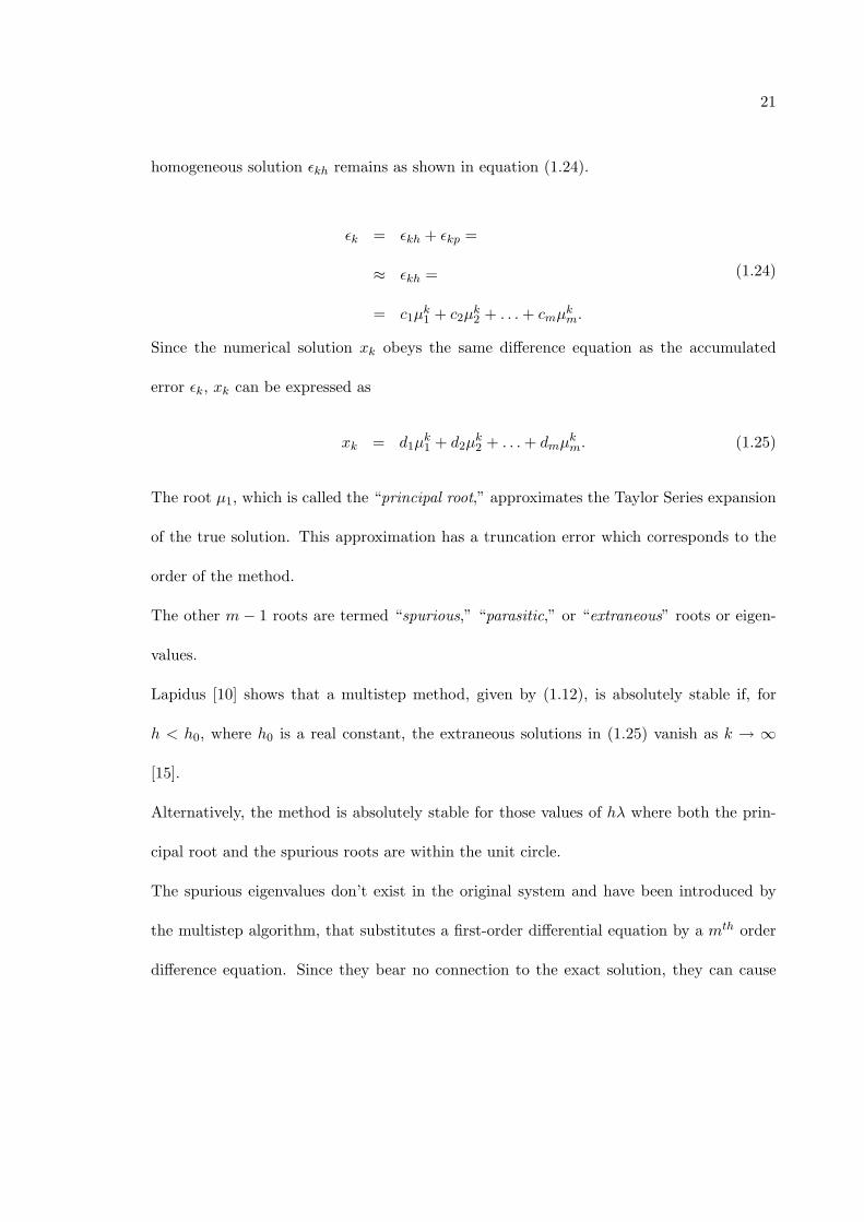
A plot of (1.26) and (1.27) is shown in figure 1.4.
23
0 0.05 0.1 0.15 0.2 0.25 0.3 0.35 0.4-6
-4
-2
0
2
4
6
t
x1,x
2
x1
x2
Figure 1.4: Simulation of a stiff linear system.
After a short time the solution can be closely approximated by the dominant terms as
x1(t) = 4e−t (1.28)
x2(t) = −2e−t, (1.29)
since the fast decaying component vanished. Therefore, an informal definition of a stiff
problem is one in which the solution components of interest are slowly varying but solu-
tions with rapidly changing components are possible [18].
Lambert [14] gives, among others, one essential definition of stiffness in his book:
Definition 1.4.1 (A system is called stiff if a) numerical method with a finite region
of absolute stability, applied to a system with any initial conditions, is forced to use in
a certain interval of integration a steplength which is excessively small in relation to the
smoothness of the exact solution in that interval.
24
Using this definition, an algorithm with finite region of absolute stability (such as explicit
integration methods) used to integrate a stiff system has to apply a very small steplength
which gives rise to long and expensive simulation runs. This is the real problem when
integrating stiff ordinary differential equations.
The statement made above still doesn’t define the term stiffness exactly because of the
fuzzy expression “excessively small.” Therefore, Cellier [4] further specifies the stiffness of
a system in the following manner:
Definition 1.4.2 A system is called stiff if, when integrated with any explicit RKn algo-
rithm and a local error tolerance of 10−n, the step-size of the algorithm is forced down to
below a value indicated by the local error estimate due to constraints imposed on it by the
limited size of the numerically stable region.
This is probably the most exact definition of stiffness available. However, it still has an
inherent drawback, namely that a system may be regarded as stiff when integrated with
one RKn whereas it is not stiff when integrated with another [4].
Although explicit methods — like the explicit RKn algorithms — may be good for checking
the stiffness of a system, they are not capable of integrating stiff systems because their
stability domain in the left half plane is too small.
Dahlquist [14] states that “an explicit linear multistep method cannot be A-stable” and
“the order of an A-stable linear multistep method cannot exceed two.” These statements are
referred to as the “second Dahlquist barrier.” It can also be noted that an “explicit method
cannot be A(0)-stable” [16],[20].
Because of these properties of explicit methods they don’t lend themselves to the integration
25
of stiff systems. Those should be integrated by a method which is at least A(α)-stable.
If the closed instability domain doesn’t intersect with the negative real axis of the complex
(λh)-plane, and if the system being integrated is stable and only has real eigenvalues, then
any steplength may be used to scale the eigenvalues of the system without fear of causing
numerical instability. In this case the steplength is not restricted by stability requirements,
but instead by accuracy requirements. Since explicit methods don’t have this feature,
implicit techniques have to be used to simulate stiff systems [14]. However, a Newton
iteration is required to solve the implicit algebraic equation, since fixed-point iteration
again destroys the stability properties of the stiffly stable method [4]. This causes higher
computation cost.
26
CHAPTER 2
Derivation of RBDF by regression
2.1 Introduction
In chapter 1 it has been shown that linear m-step integration algorithms of order n
use p (p ≥ n + 1) function values or derivatives to calculate the unknown value xk+1.
As a consequence, numerical integration by a multistep method can be considered as an
interpolation procedure where a higher-order interpolation (extrapolation) polynomial is
used to approximate a function g through p given data points and calculate the unknown
point which is represented by xk+1. Note that g is not identical with the function x being
integrated by the multistep technique. It is instead formed by both x and its derivative f
at special time instants.
If there are p = n + 1 (n = accuracy order of the integration method) distinct data points,
then the interpolation problem has a unique solution and the resulting polynomial doesn’t
only approximate the function through the given data points but it interpolates the points
that it passes through [6], [12].
An interesting question arises about using more data points, that is, p > n+1. In practice,
this means that the multistep integration algorithm applies p > n+1 earlier function values
or derivatives to calculate the unknown function value xk+1 with the accuracy order of n.
27
Thus, the order is not increased by using more data points. Instead, the interpolation
results in an nth order method which might have better properties because it uses more
information.
As far as the interpolation problem is concerned, having more data points necessarily means
that we are confronted with an overdetermined system which may be used to attain two
different types of smoothing [6]:
1. A reduction of the effect of random errors in the values of the function.
2. A smoother shape between the net points (even when the function values are perfect).
The solution to this overdetermined system using a regression approach will be discussed
in the next section.
2.2 Formulation and solution of the regression problem
An nth-order multistep algorithm is defined through an nth-order polynomial fitted
through p points which can be either function values or derivatives of the function to
be integrated.
By introducing the auxiliary variable
s =t − tk
h, (2.1)
such that s = 1.0 corresponds to t = tk+1 and s = 0.0 corresponds to t = tk, the interpo-
lating nth-order polynomial can be written in the form
p(s) = a0 + a1s + a2s2 + . . . ansn, (2.2)

28
where the coefficients ai are unknown.
The time derivative of equation (2.2) is given by
hp(s) = a1 + 2a2s + 3a3s2 + . . . + nansn−1. (2.3)
Since the polynomial p(s) interpolates the function x in the data points xk−i, i = 0, 1, . . . , m,
relation (2.2) results in
p(0) = a0 = xk
p(−1) = a0 − a1 + a2 − a3 + . . . + an(−1)n = xk−1
p(−2) = a0 − 2a1 + 4a2 − 8a3 + . . . + an(−2)n = xk−2
......
...
p(−m) = a0 − ma1 + m2a2 + . . . + an(−m)n = xk−m.
(2.4)
Accordingly, it follows from (2.3) that
hp(1) = a1 + 2a2 + 3a3 + . . . + nan = hfk+1
hp(0) = a1 = hfk
hp(−1) = a1 − 2a2 + 3a3 + . . . + nan(−1)n−1 = hfk−1
......
...
hp(−m) = a1 − 2a2m + 3a3m2 + . . . + nan(−m)n−1 = hfk−m.
(2.5)
29
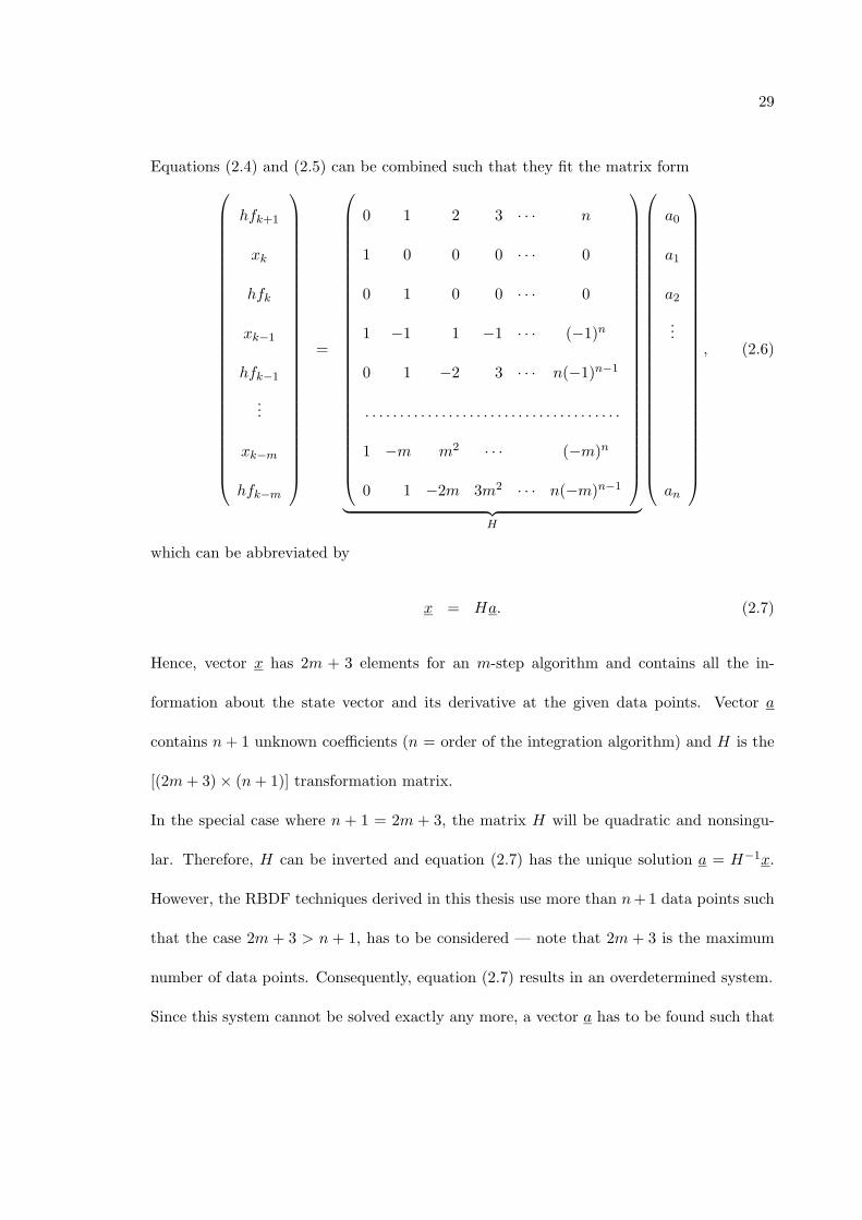
Equations (2.4) and (2.5) can be combined such that they fit the matrix form⎛⎜⎜⎜⎜⎜⎜⎜⎜⎜⎜⎜⎜⎜⎜⎜⎜⎜⎜⎜⎜⎜⎜⎜⎜⎜⎜⎜⎜⎜⎜⎝
hfk+1
xk
hfk
xk−1
hfk−1
...
xk−m
hfk−m
⎞⎟⎟⎟⎟⎟⎟⎟⎟⎟⎟⎟⎟⎟⎟⎟⎟⎟⎟⎟⎟⎟⎟⎟⎟⎟⎟⎟⎟⎟⎟⎠
=
⎛⎜⎜⎜⎜⎜⎜⎜⎜⎜⎜⎜⎜⎜⎜⎜⎜⎜⎜⎜⎜⎜⎜⎜⎜⎜⎜⎜⎜⎜⎜⎝
0 1 2 3 · · · n
1 0 0 0 · · · 0
0 1 0 0 · · · 0
1 −1 1 −1 · · · (−1)n
0 1 −2 3 · · · n(−1)n−1
. . . . . . . . . . . . . . . . . . . . . . . . . . . . . . . . . . . . .
1 −m m2 · · · (−m)n
0 1 −2m 3m2 · · · n(−m)n−1
⎞⎟⎟⎟⎟⎟⎟⎟⎟⎟⎟⎟⎟⎟⎟⎟⎟⎟⎟⎟⎟⎟⎟⎟⎟⎟⎟⎟⎟⎟⎟⎠
︸ ︷︷ ︸H
⎛⎜⎜⎜⎜⎜⎜⎜⎜⎜⎜⎜⎜⎜⎜⎜⎜⎜⎜⎜⎜⎜⎜⎜⎜⎜⎜⎜⎜⎜⎜⎝
a0
a1
a2
...
an
⎞⎟⎟⎟⎟⎟⎟⎟⎟⎟⎟⎟⎟⎟⎟⎟⎟⎟⎟⎟⎟⎟⎟⎟⎟⎟⎟⎟⎟⎟⎟⎠
, (2.6)
which can be abbreviated by
x = Ha. (2.7)
Hence, vector x has 2m + 3 elements for an m-step algorithm and contains all the in-
formation about the state vector and its derivative at the given data points. Vector a
contains n + 1 unknown coefficients (n = order of the integration algorithm) and H is the
[(2m + 3) × (n + 1)] transformation matrix.
In the special case where n + 1 = 2m + 3, the matrix H will be quadratic and nonsingu-
lar. Therefore, H can be inverted and equation (2.7) has the unique solution a = H−1x.
However, the RBDF techniques derived in this thesis use more than n +1 data points such
that the case 2m + 3 > n + 1, has to be considered — note that 2m + 3 is the maximum
number of data points. Consequently, equation (2.7) results in an overdetermined system.
Since this system cannot be solved exactly any more, a vector a has to be found such that

30
H a is the “best” approximation to x [6]. The solution vector a is the least-squares solution
of the overdetermined system.
Definition 2.2.1 The vector a is defined as the vector which minimizes the Euclidean
length of the residual vector, i.e. minimizes
‖r‖2 = (rT r)1/2, r = Ha. (2.8)
In [1] it is stated that when the columns of H are linearly independent, i.e. H has full rank
(ρ(H) = n + 1), then the matrix HT H is nonsingular and can be inverted.
Hence, in order to solve system (2.7) it first has to be shown that the columns of matrix
H are linearly independent. This is done by defining two generating row vectors p and q
shown in equations (2.9) and (2.10).
p = [ 1 −s s2 . . . (−s)n ], (2.9)
q = [ 0 1 −2s 3s2 . . . n(−s)n−1 ]. (2.10)
The rows of H that correspond to xk−s are formed by the components of vector p and
and the rows corresponding to hfk−s are formed by the components of vector q. The
components of these two row vectors (2.9) and (2.10) are elements of polynomials. Such
elements are linearly independent [3] and thus, all the column vectors of H, that are formed
by the components of the generating row vectors p and q when varying the parameter s,
are linearly independent, too, which was to be shown.
Therefore, matrix H can be inverted and it follows from (2.7) that
HT x = HT Ha (2.11)
31
or
a = (HT H)−1HT x. (2.12)
Dahlquist [6] proves that this is the unique solution which solves the overdetermined system
(2.7) in a least-squares sense.
In the literature the matrix
H+ = (HT H)−1HT (2.13)
is referred to as the Penrose-Moore Pseudoinverse.
By using (2.12) to calculate a, the elements of a can be substituted into (2.2) to determine
xk+1.
xk+1 = p(1) = a0 + a1 + . . . + an(2.14)
Note that the coefficients ai are not constants. Each of them represents a linear combination
of the elements of the vector x, given in (2.6) and (2.7).
2.3 Development of an algorithm for the search of RBDF
In the preceding section it has been described how an integration algorithm can be
derived if p data points are chosen out of the possible 2m + 3 points.
Since m and p are free parameters, the search is (theoretically) not restricted, and to get an
nth-order integration algorithm, more data points may be used as long as p ≥ n + 1 holds.
In practice, the search is limited by efficiency considerations. Since the H-matrix becomes
larger as m grows, the integration algorithm is likely to consume more execution time.
Thus there are two questions that have to be answered:
32
1. How many data points should be used?
2. Where should these data points lie to result in an integration algorithm with minimum
stability properties?
In this context, having “minimum stability properties” means that the stability locus of
an implicit method doesn’t intersect with the negative real axis of the complex (λh)-plane
(see chapter 3).
To answer the first question, multiple experiments have been performed with only a few data
points. These experiments have shown that the probability of getting implicit algorithms
with minimum stability properties shrinks as the number of employed data points grows.
Hence, the search starts with pmin = n+2 employed data points and it stops at pmax = 2n
data points. No decent RBDF algorithms have been found for values p > 2n.
Concerning the second question, a lot of calculations with a small number of data points
have shown that most of the data points that yield decent integration algorithms lie within
the time range [tk−n−2, tk+1]. The stability properties of the resulting RBDF algorithms
worsen as the data points get farther away from the defined interval. For this reason the
search is limited to the interval [tk−n−2, tk+1].
This search for RBDF methods can be automated by testing all possible combinations of p
data points within the range [tk−n−2, tk+1] where p is incremented step by step from n + 2
to 2n.

33
CHAPTER 3
Analysis of RBDF
3.1 Introduction
In this chapter some methods will be discussed to analyze integration methods, in par-
ticular RBDF.
These integration methods will be used in chapters 5 and 6 to assess the RBDF methods
that will be derived.
The technique being discussed in the second section of this chapter is the analysis of the
stability domain of the numerical integration method.
In the third section the error constant will be computed.
Another important method for investigating the quality of RBDF is the analysis of the
damping plot which will be described in section four.
The order star will be introduced in the fifth section to make some additional statements
about stability and accuracy. Finally, the Bode plot of the integration algorithm will be
analyzed in section six to see how the algorithm behaves in the frequency domain.
34
3.2 Stability domain
3.2.1 Introduction
In chapter 1, some definitions of numerical stability are given. Chapter 1 also mentions
that the stability properties of the integrator depend strongly on both the steplength used
during the integration, and the eigenvalues of the system.
Before the numerical stability domain is determined, the analytical stability of the system
being integrated can be determined using the following definition:
Definition 3.2.1 The solution of the autonomous, time-invariant linear system
x = Ax (3.1)
with the initial conditions specified by x(t = t0) = x0 is called analytically stable if all the
eigenvalues of A have negative real parts.
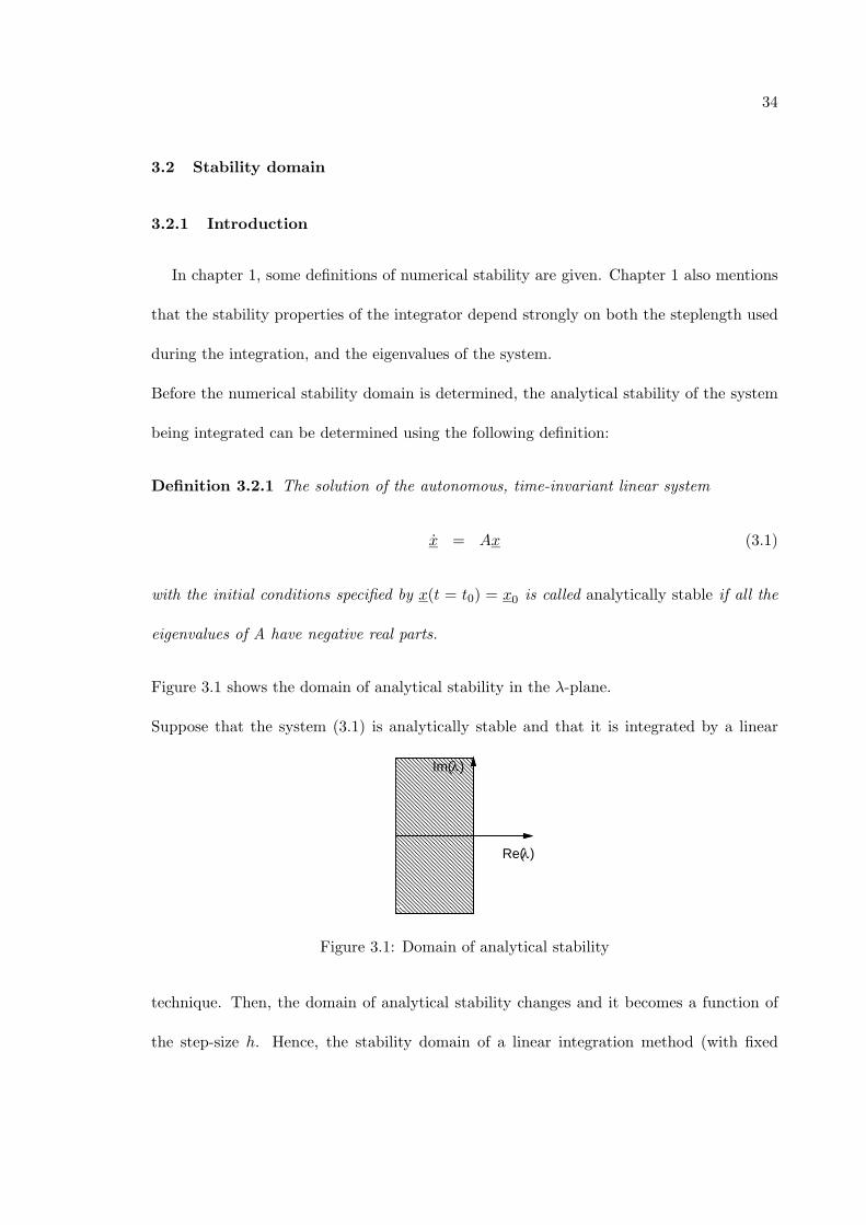
Figure 3.1 shows the domain of analytical stability in the λ-plane.
Suppose that the system (3.1) is analytically stable and that it is integrated by a linear
Im(
Re(λ)
λ)
Figure 3.1: Domain of analytical stability
technique. Then, the domain of analytical stability changes and it becomes a function of
the step-size h. Hence, the stability domain of a linear integration method (with fixed
35
step-size h), when used to integrate the autonomous system (3.1) is defined as the region
in the complex (λh)-plane where the eigenvalues of the equivalent discrete time system all
lie within the unit circle. Note that all the eigenvalues have negative real parts. This is
illustrated by means of the implicit Backward Euler algorithm expressed by:
xk+1 = xk + hfk+1
, (3.2)
where fk+1
= xk+1.
Substituting equation (3.1) into (3.2), equation (3.2) results in
xk+1 = xk + hAxk+1,
or
xk+1 = [I(ns) − Ah]−1xk, (3.3)
where ns is the dimension of system (3.1) and I(ns) is the (ns × ns) identity matrix.
Consequently, the continuous linear system (3.1) has been converted into the equivalent
discrete system (3.3) with the new system matrix
F = [I(ns) − Ah]−1. (3.4)
This discrete system is analytically stable if all of the eigenvalues of F are located within
the unit circle [4].
Since matrix F depends on the steplength h, the eigenvalues of F depend on h, too.
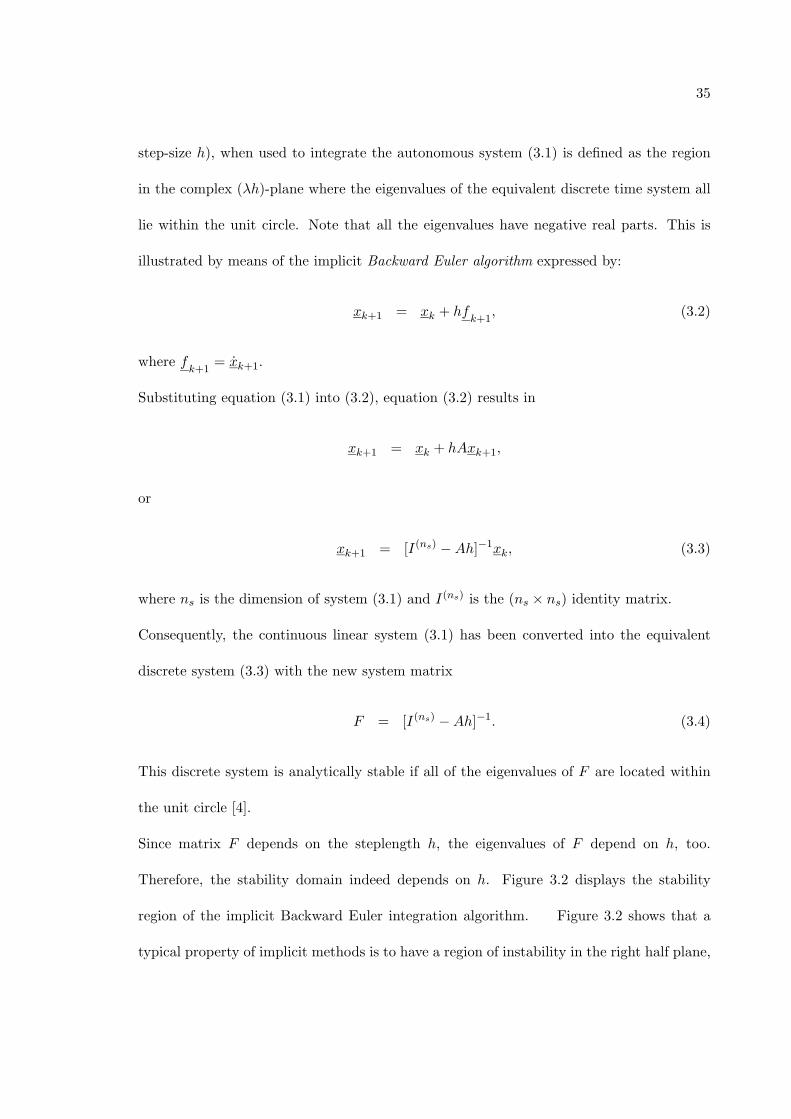
Therefore, the stability domain indeed depends on h. Figure 3.2 displays the stability
region of the implicit Backward Euler integration algorithm. Figure 3.2 shows that a
typical property of implicit methods is to have a region of instability in the right half plane,

36
Im(
Re(λ
λ h)
h)20
Figure 3.2: Stability domain of the BE-algorithm
close to the origin.
When integrating a stable system, whose eigenvalues are in the left half plane, the instability
region shown in figure 3.2 shouldn’t extend into the left half plane. However, this property,
called A-stability in chapter 1, cannot be obtained by linear multistep methods of higher
than second order.
At the very least an implicit integration algorithm must have an instability domain that
doesn’t include the origin. In other words, the stability locus, i.e. the border line of the
stability domain, mustn’t intersect with the negative real axis. Recall that this has been
the main requirement for RBDF algorithms to be good candidates in chapter 2.
3.2.2 Stability domain of RBDF
In order to depict the stability domain, the F -matrix, the discrete time system that
results from applying the RBDF method to system (3.1) is calculated.
The general RBDF algorithm is given by
xk+1 =m−1∑i=0
aixk−i +m−1∑i=−1
bihfk−i
. (3.5)
37
By applying this algorithm to system (3.1), relation (3.5) can be rewritten in the form of
xk+1 = b−1Ahxk+1 + a0xk + b0Ahxk + . . . + am−1xk−m+1 + bm−1Ahxk−m+1,
or
xk+1 = [I(ns) − b−1Ah]−1[(a0I(ns) + b0Ah)xk + (a1I
(ns) + b1Ah)xk−1 + . . .+
+(am−1I(ns) + bm−1Ah)xk−m+1],
(3.6)
where ns is the dimension of system (3.1) and I(ns) is the (ns × ns) identity matrix.
Equation (3.6) is a mth-order difference equation which can be transformed into m first
order difference equations by applying the transformation
z1(tk) = x(tk−m+1)
z2(tk) = x(tk−m+2)
...
zm(tk) = x(tk).
(3.7)
or
z1(tk+1) = x(tk−m+2) = z2(tk)
...
zm(tk+1) = x(tk+1).
(3.8)
By substituting xk+1 from equation (3.6) into (3.8), it follows that
z(tk+1) = Fz(tk), (3.9)
where the mns-vector z is given by
z(ti) =
⎛⎜⎜⎜⎜⎜⎜⎜⎜⎜⎜⎜⎜⎝
z1(ti)
z2(ti)
...
zm(ti)
⎞⎟⎟⎟⎟⎟⎟⎟⎟⎟⎟⎟⎟⎠
, i = k, k + 1, (3.10)
38
and the (mns × mns)-matrix F can be written as
F =
⎛⎜⎜⎜⎜⎜⎜⎜⎜⎜⎜⎜⎜⎜⎜⎜⎜⎝
O(ns) I(ns) O(ns) · · · O(ns)
... O(ns) I(ns). . .
...
... O(ns). . . O(ns)
.... . . I(ns)
Fm,1 Fm,2 · · · Fm,m
⎞⎟⎟⎟⎟⎟⎟⎟⎟⎟⎟⎟⎟⎟⎟⎟⎟⎠
, (3.11)
Fm,1 = Q(ns)[am−1I(ns) + bm−1Ah], (3.12)
Fm,2 = Q(ns)[am−2I(ns) + bm−2Ah], (3.13)
Fm,m = Q(ns)[a0I(ns) + b0Ah], (3.14)
Q(ns) = [I(ns) − b−1Ah]−1. (3.15)
(3.16)
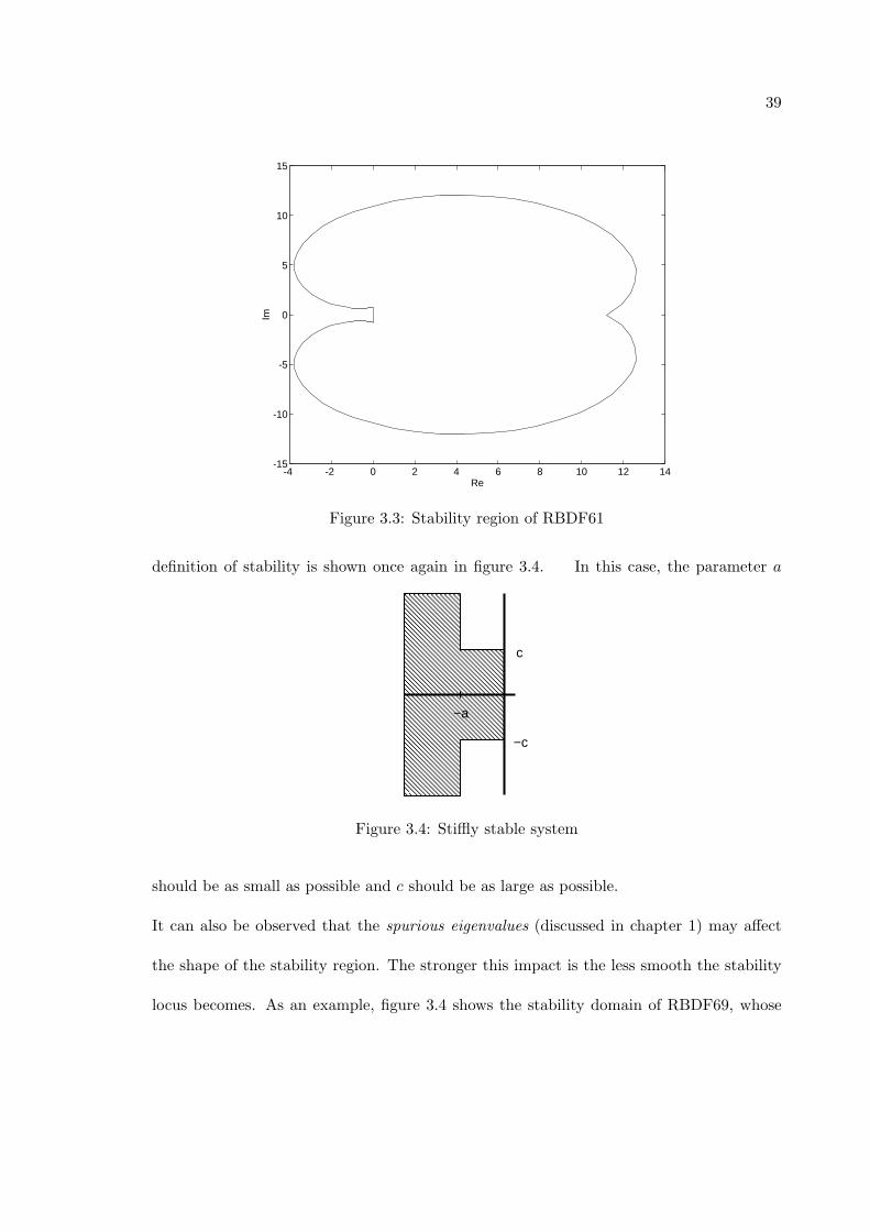
As an example one of the RBDF methods that have been found, RBDF61, is considered:
xk+1 = 5941357hfk+1 + 977
461xk − 1612915 xk−1 + 361
943xk−2
+11711310xk−3 − 3199
3212xk−4 + 257592xk−5 − 389
5370xk−6
(3.17)
Figure 3.3 displays the stability region of RBDF61.
There exist many different ways of assessing the stability domain of implicit methods. One
criteria is the size of the stability region in the left half plane. Since most of the systems
being integrated are stable, this region should be as large as possible. Therefore, the
instability domain shouldn’t extend too far into the left half plane.
By considering the definition of A(α)-stability given in chapter 1, the angle α should be
large.
For stiff systems the definition of stiffly stable algorithms might be even more useful. This
39
-4 -2 0 2 4 6 8 10 12 14-15
-10
-5
0
5
10
15
Re
Im
Figure 3.3: Stability region of RBDF61
definition of stability is shown once again in figure 3.4. In this case, the parameter a
c
−c
−a
Figure 3.4: Stiffly stable system
should be as small as possible and c should be as large as possible.
It can also be observed that the spurious eigenvalues (discussed in chapter 1) may affect
the shape of the stability region. The stronger this impact is the less smooth the stability
locus becomes. As an example, figure 3.4 shows the stability domain of RBDF69, whose

40
formula is given by:
xk+1 = 232533hfk+1 + 2734
1241xk − 414227xk−1 − 211
1164hfk−1
+10071440xk−2 − 985
2009xk−5 + 8715716hfk−5 + 471
1144xk−6 + 1911020hfk−6
(3.18)
Figure 3.5 illustrates that the stability locus of (3.18) has some sharp bends which are
-5 0 5 10 15 20 25 30 35-15
-10
-5
0
5
10
15
Re
Im
Figure 3.5: Stability locus of RBDF69
caused by the spurious eigenvalues described in chapter 1. As noted previously, they
strongly disturb the behavior of integration algorithms in terms of stability and accuracy.
3.3 Error constant
In [14], the Linear Difference Operator L, associated with the linear m-step method
given in standard form as
m∑i=0
αixk+i = hm∑
i=0
βifk+i, (3.19)

41
is defined as
L[z(t); h] =m∑
i=0
[αiz(t + ih) − hβiz(t + ih)], z(t) ∈ C1[a, b]. (3.20)
If z(t) is infinitely differentiable, then z(t + ih) and z(t + ih) can be developed in a Taylor
series around t as shown in the following equation
L[z(t); h] = C0z(t) + C1hz(1)(t) + . . . + Cqhqz(q)(t) + . . . , (3.21)
where z(q)(t) is the qth time derivative of z(t)/.
Now the following statement can be made [14]:
Definition 3.3.1 The linear multistep method (3.19) and the associated difference operator
L are said to be of order n if, in (3.21),
C0 = C1 = . . . = Cn = 0; Cn+1 �= 0.
For the constants Ci the formulae
C0 =m∑
i=0
αi
C1 =m∑
i=0
(iαi − βi)
...
Cq =m∑
i=0
(1q! i
qαi − 1(q−1)! i
q−1βi
), q = 2, 3, . . .
(3.22)
hold. Using the equations shown in (3.22), the error constant can be defined as:
Definition 3.3.2 The linear multistep method of order n is said to have the error constant
Cn+1 given by (3.22).

42
In the first chapter it is shown that the local truncation error T (x, h) is strongly related to
this error constant by
T (x, h) = Cn+1hn+1x(n+1)(tk) + O(hn+2). (3.23)
Hence, a multistep method may integrate more accurately than others if the absolute value
of its error constant is smaller.
3.4 Damping plot
Cellier [4] introduces the damping plot as yet another tool to describe the accuracy of
an integration algorithm. In order to derive the damping plot, the standard linear system
x = Ax, x(t0) = x0 is considered which has the analytical solution xanal = eA(t−t0)x0.
This solution is true for any value of x0, and any value of t. Therefore, if the time instant
t = tk+1 is chosen as well as the initial conditions t0 = tk, and x0 = xk, the analytical result
becomes
xk+1 = eAhxk. (3.24)
This discrete system has the analytical F -matrix Fanal = eAh and the eigenvalues
λdis = eig{Fanal} = eeig{A}h = eλih, i = 1, . . . , ns. (3.25)
The damping of an analytically stable system x = Ax is defined as the smallest magnitude
value of the real parts of its eigenvalues, or
σ = mini
(|σi|) = mini
(|Re{λi}|). (3.26)

43
Since the eigenvalues λi are complex, i.e. λi = −σi + jωi, the eigenvalue λdis can be
rewritten in the form
λdis = eλih = e−σihejωih. (3.27)
The damping of the discrete system (3.24) is defined as the largest magnitude value of the
eigenvalues λdis. Therefore, it follows from equation (3.27) that the damping of the discrete
system can be expressed as
σdis = maxi
(e−σih). (3.28)
Thus, in the case of the continuous system x = Ax, the damping corresponds to the smallest
distance of the eigenvalues from the imaginary axis in the λ-plane, whereas in the case of the
corresponding discrete system xk+1 = eAhxk, the damping refers to the largest distance of
the eigenvalues from the origin in the eλh-plane. This is commonly known as the z-domain,
where z = eλh. Cellier [4] introduces the discrete damping as
σd = hσ. (3.29)
The relationship between σd and Fanal can be derived from the equations (3.25), (3.27) and
(3.28):
σd = −log(maxi
|eig{Fanal}|). (3.30)
In order to come up with an expression for the numerical damping, i.e. the damping of the
numerical integration algorithm applied to the system x = Ax, the analytical Fanal-matrix
needs to be approximated by the matrix Fnum of the numerical integration method.
Thus, by substituting Fanal by Fnum, equation (3.30) yields
σd = −log(maxi
|eig{Fnum}|), (3.31)
44
where σd is the discrete damping of the numerical integration algorithm.
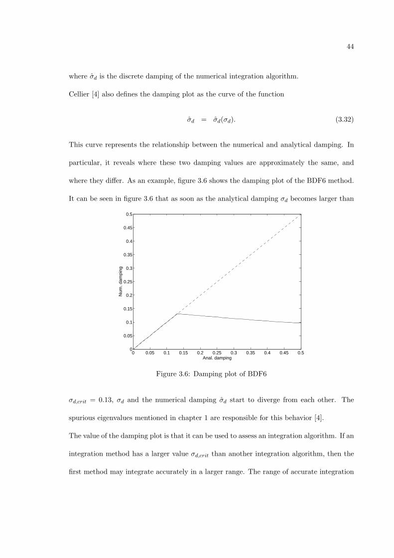
Cellier [4] also defines the damping plot as the curve of the function
σd = σd(σd). (3.32)
This curve represents the relationship between the numerical and analytical damping. In
particular, it reveals where these two damping values are approximately the same, and
where they differ. As an example, figure 3.6 shows the damping plot of the BDF6 method.
It can be seen in figure 3.6 that as soon as the analytical damping σd becomes larger than
0 0.05 0.1 0.15 0.2 0.25 0.3 0.35 0.4 0.45 0.50
0.05
0.1
0.15
0.2
0.25
0.3
0.35
0.4
0.45
0.5
Anal. damping
Num
. dam
ping
Figure 3.6: Damping plot of BDF6
σd,crit = 0.13, σd and the numerical damping σd start to diverge from each other. The
spurious eigenvalues mentioned in chapter 1 are responsible for this behavior [4].
The value of the damping plot is that it can be used to assess an integration algorithm. If an
integration method has a larger value σd,crit than another integration algorithm, then the
first method may integrate accurately in a larger range. The range of accurate integration

45
is often referred to as the asymptotic region in the literature.
To illustrate the relationship between the damping plot and the stability domain of the
integration method (sec. 3.2.2), figure 3.7 shows the modified damping plot for the BDF6
technique where the negative numerical damping −σd is a function of the negative analytical
damping −σd. It can be seen in figure 3.7 that the negative numerical damping −σd
-5 0 5 10 15 20 25 30-1
0
1
2
3
4
5
6
7
Negative anal. damping
Neg
ativ
e nu
m. d
ampi
ng
Figure 3.7: Modified damping plot of the BDF6 method
is zero at −σd = 0 and −σd = 27.72. These points can also be found in figure 3.8 which
displays the stability domain of the BDF6 technique. There, these points are given by the
intersection points of the stability locus with the real axis.
In order to state anything about the behavior of the numerical damping σd as
σd → ∞, Cellier [4] proposes to produce a logarithmic damping plot. Figure 3.9 displays
the logarithmic damping plot of the BDF6 method.
Using this technique, if a numerical integration method is at least A(α)-stable and if σd
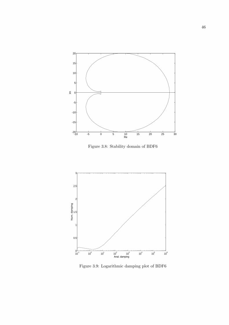
46
-10 -5 0 5 10 15 20 25 30-20
-15
-10
-5
0
5
10
15
20
Re
Im
Figure 3.8: Stability domain of BDF6
10-1
100
101
102
103
104
105
106
0
0.5
1
1.5
2
2.5
3
Anal. damping
Num
. dam
pin
g
Figure 3.9: Logarithmic damping plot of BDF6

47
goes to infinity as σd goes to infinity, then it lends itself to integrate a stiff system because
it is capable of damping out the fast transients. Note that it is not required that the
numerical method integrating a stiff system be L-stable since L-stability is only possible if
the integration technique is A-stable. For instance, the A(α)-stable BDF6 method can be
used to integrate a stiff system although it it not L-stable.
3.5 Order star
Before we derive the order star of a numerical method, we make the following definition:
Definition 3.5.1 A function f is called “essentially analytic” if it is analytical in the
complex plane except at a finite set of singularities.
Assuming that an essentially analytic function f is approximated by a rational function R,
the rational function ρ(z) can be introduced:
ρ(z) =R(z)f(z)
, z ∈ C. (3.33)
In [13], the order star (of the first kind) is defined as the locus where ρ(z) = 1. Thus, a
damping order star can be created by defining z as z = λh and ρ(λh) as
ρ(λh) =σd(λh)σd(λh)
, (3.34)
where the numerical damping σd is an approximation for the analytical damping σd. In
other words, the damping order star is the locus of the points in the complex (λh)-plane
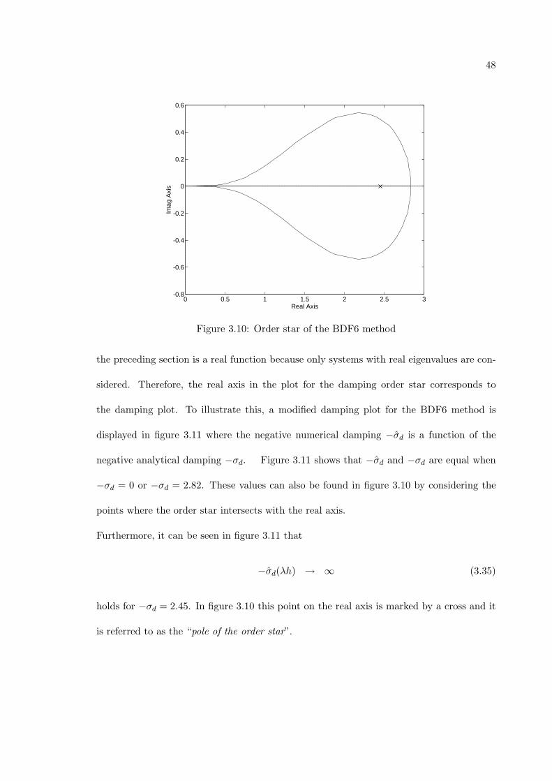
where σd(λh) = σd. In figure 3.10 the order star for the BDF6 algorithm is depicted.
Since the damping order star is produced by integrating a system with two complex eigen-
values, the function ρ(λh) is complex, too. Recall that the damping plot introduced in
48
0 0.5 1 1.5 2 2.5 3-0.8
-0.6
-0.4
-0.2
0
0.2
0.4
0.6
Real Axis
Imag
Axi
s
Figure 3.10: Order star of the BDF6 method
the preceding section is a real function because only systems with real eigenvalues are con-
sidered. Therefore, the real axis in the plot for the damping order star corresponds to
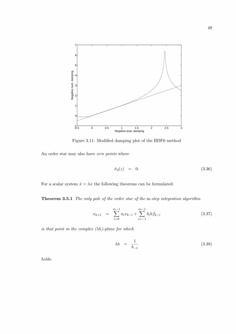
the damping plot. To illustrate this, a modified damping plot for the BDF6 method is
displayed in figure 3.11 where the negative numerical damping −σd is a function of the
negative analytical damping −σd. Figure 3.11 shows that −σd and −σd are equal when
−σd = 0 or −σd = 2.82. These values can also be found in figure 3.10 by considering the
points where the order star intersects with the real axis.
Furthermore, it can be seen in figure 3.11 that
−σd(λh) → ∞ (3.35)
holds for −σd = 2.45. In figure 3.10 this point on the real axis is marked by a cross and it
is referred to as the “pole of the order star”.
49
-0.5 0 0.5 1 1.5 2 2.5 3-1
0
1
2
3
4
5
6
7
Negative anal. damping
Neg
ativ
e nu
m. d
ampi
ng
Figure 3.11: Modified damping plot of the BDF6 method
An order star may also have zero points where
σd(z) = 0. (3.36)
For a scalar system x = λx the following theorems can be formulated:
Theorem 3.5.1 The only pole of the order star of the m-step integration algorithm
xk+1 =m−1∑i=0
aixk−i +m−1∑i=−1
bihfk−i (3.37)
is that point in the complex (λh)-plane for which
λh =1
b−1(3.38)
holds.

50
Proof: The system matrix F of the discrete system (3.37) can be expressed by
F =
⎛⎜⎜⎜⎜⎜⎜⎜⎜⎜⎜⎜⎜⎜⎜⎜⎜⎝
0 1 0 · · · 0
.... . . 1
. . ....
. . . 0
0 · · · 0 1
pm−1 pm−2 pm−3 · · · p0
⎞⎟⎟⎟⎟⎟⎟⎟⎟⎟⎟⎟⎟⎟⎟⎟⎟⎠
, (3.39)
where
pi =ai + biq
1 − b−1q, q = λh. (3.40)
The eigenvalues of F are calculated by solving the characteristic equation:
|λI − F | =
∣∣∣∣∣∣∣∣∣∣∣∣∣∣∣∣∣∣∣∣∣∣
λ −1 0 · · · 0
0. . . . . . . . .
...
.... . . 0
0 · · · 0 λ −1
−pm−1 −pm−2 · · · −p1 λ − p0
∣∣∣∣∣∣∣∣∣∣∣∣∣∣∣∣∣∣∣∣∣∣= λ(λAm−3 + Bm−2) + Bm−1
!= 0,
(3.41)
where
Ai =
∣∣∣∣∣∣∣∣∣∣∣∣∣∣∣∣∣∣∣∣∣∣
λ −1 0 · · · 0
0. . . . . . . . .
...
.... . . 0
0 · · · 0 λ −1
−pi · · · −p1 λ − p0
∣∣∣∣∣∣∣∣∣∣∣∣∣∣∣∣∣∣∣∣∣∣
, (3.42)
51
Bi =
∣∣∣∣∣∣∣∣∣∣∣∣∣∣∣∣∣∣∣∣∣∣
0 −1 0 · · · 0
0 λ. . . . . .
...
.... . . . . . 0
0 · · · 0 λ −1
−pi −pi−2 · · · −p1 λ − p0
∣∣∣∣∣∣∣∣∣∣∣∣∣∣∣∣∣∣∣∣∣∣
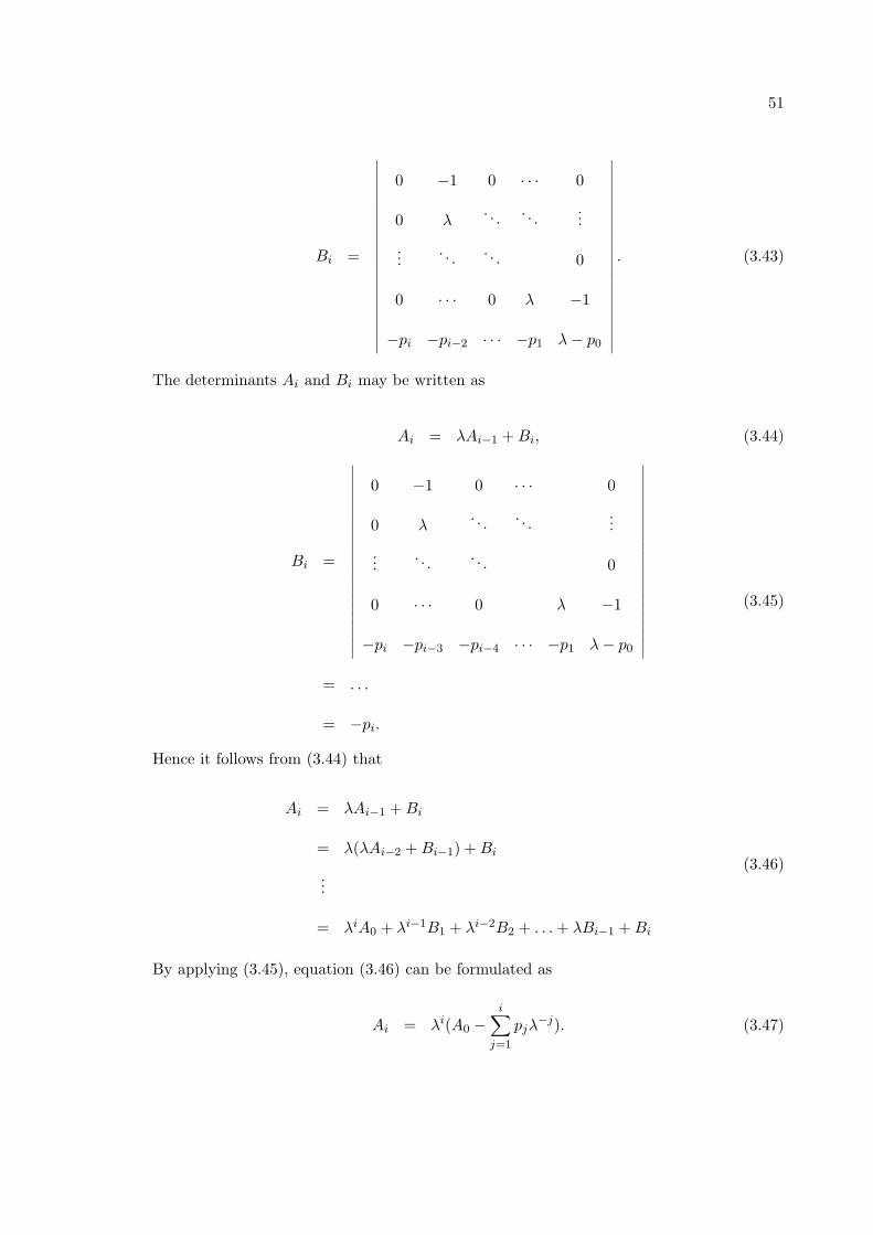
. (3.43)
The determinants Ai and Bi may be written as
Ai = λAi−1 + Bi, (3.44)
Bi =
∣∣∣∣∣∣∣∣∣∣∣∣∣∣∣∣∣∣∣∣∣∣
0 −1 0 · · · 0
0 λ. . . . . .
...
.... . . . . . 0
0 · · · 0 λ −1
−pi −pi−3 −pi−4 · · · −p1 λ − p0
∣∣∣∣∣∣∣∣∣∣∣∣∣∣∣∣∣∣∣∣∣∣= . . .
= −pi.
(3.45)
Hence it follows from (3.44) that
Ai = λAi−1 + Bi
= λ(λAi−2 + Bi−1) + Bi
...
= λiA0 + λi−1B1 + λi−2B2 + . . . + λBi−1 + Bi
(3.46)
By applying (3.45), equation (3.46) can be formulated as
Ai = λi(A0 −i∑
j=1
pjλ−j). (3.47)

52
Since A0 = λ − p0, equation (3.47) yields
Ai = λi(λ −i∑
j=0
pjλ−j). (3.48)
With (3.45) and (3.48), equation (3.41) results in
|λI − F | = λ[λm−2(λ −m−3∑j=0
pjλ−j) − pm−2] − pm−1
= λm−1(λ −m−3∑j=0
pjλ−j) − λpm−2 − pm−1
!= 0, m ≥ 3.
(3.49)
Because of (3.31) and (3.35), a pole requires that the largest eigenvalue λmax of F goes
to infinity. Therefore, relation (3.49) can only be satisfied if pi → ∞ holds for i = 0 or
i = m − 2 or i = m − 1.
From (3.40) it follows that this is identical with the requirement that q = 1b−1
. Since this
is the only pole, the proof is complete.
Theorem 3.5.2 For the zeros of the order star of the m-step integration method (3.37)
the relation
maxi
|λi| = 1, i = 0, 1, . . . , m − 1, (3.50)
holds where λi are the eigenvalues of F and can be calculated with (3.49).
Proof: This theorem follows directly from (3.31) and (3.36).
Theorem 3.5.2 means that all the eigenvalues have to be within the unit circle in the
(λh)-plane while it is required that at least one eigenvalue lies exactly on the unit circle.
53
Hence, the more steps the multistep method uses, the larger the F -matrix becomes, and
the less probable it is that this condition can be satisfied.
Note that the unit circle represents the stability locus of a discrete system. Thus, theorem
3.5.2 shows that the zeros of the damping order star correspond to points on the stability
locus.
To be able to use the order star of an integration method to compare one method with
another, the region around the origin is of particular interest. Basically, the order star,
that is the locus of all those points where the error
∆σd = σd − σd (3.51)
is zero, is not displayed. Instead, the region is determined where
∆|σd| ≤ ∆σd,lim. (3.52)
Statements about the size of the area can be made where an integration method works
accurately with respect to a given error bound ∆σd,lim.
Roughly speaking, the larger this area is, the more accurate is the integration method.
3.6 Bode plot
In this section an alternative way of evaluating an integration algorithm will be intro-
duced. This time, the behavior of the integration method is analyzed in the frequency
domain through the use of a Bode plot. To provide a motivation for this approach, the
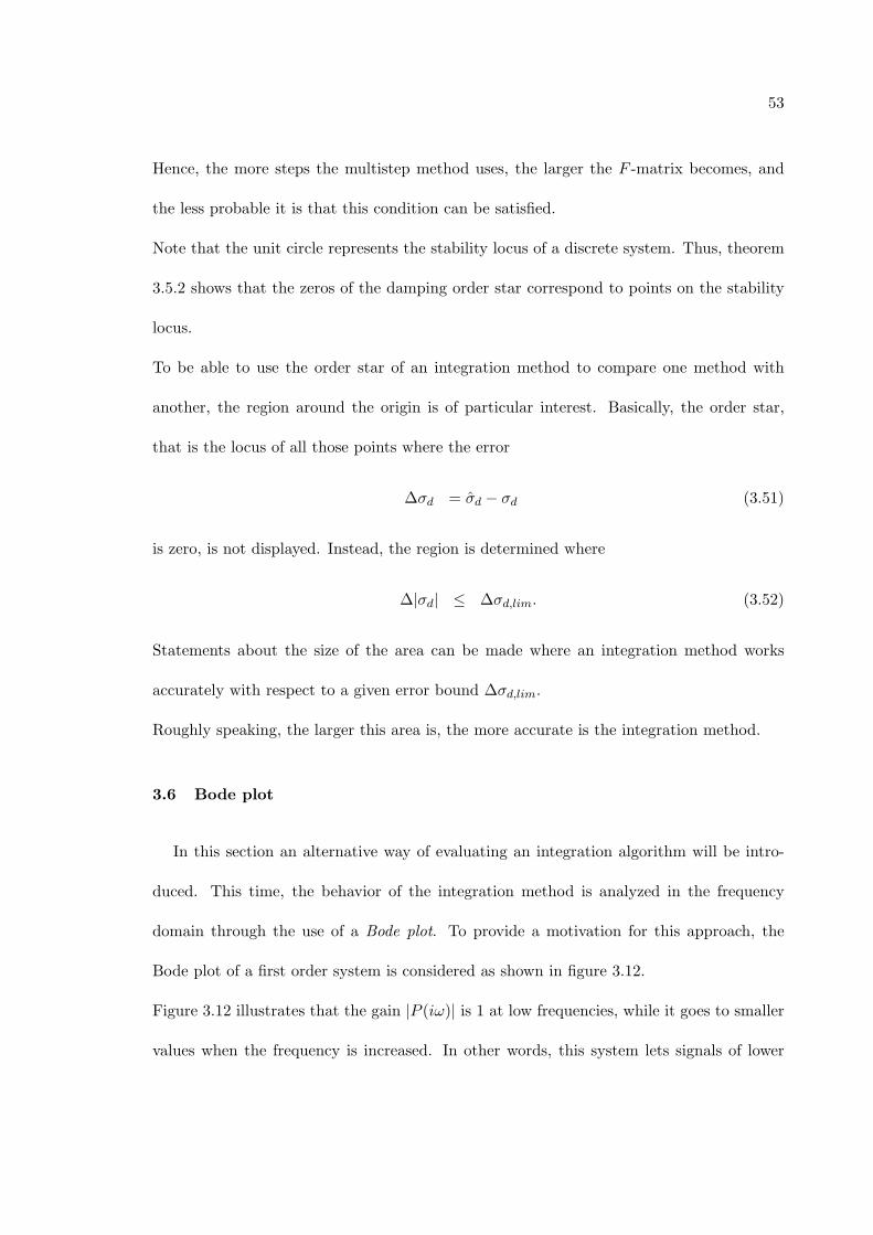
Bode plot of a first order system is considered as shown in figure 3.12.
Figure 3.12 illustrates that the gain |P (iω)| is 1 at low frequencies, while it goes to smaller
values when the frequency is increased. In other words, this system lets signals of lower
54
10-1
100
101
-30
-20
-10
0
Frequency (rad/sec)
Gain
dB
10-1
100
101
-30
-60
-90
0
Frequency (rad/sec)
Phase d
eg
Figure 3.12: Bode plot of a first order system
frequencies pass through whereas it attenuates signals of higher frequencies. Hence, this
system is called a low-pass filter.
When integrating a system whose input signal includes high frequency noise, an integration
method might fail to control the step-size. Instead, the step-size control would follow the
high frequencies such that the step-size would be reduced to an excessively small value.
This effect can be avoided if the integration method is able to damp out high frequencies
(i.e. functions as a low-pass filter).
To look for this property in a RBDF method, a Bode plot is used.
A key result of section 3.2.2 is that the general RBDF method which is formulated as
xk+1 =m−1∑i=0
aixk−i +m−1∑i=−1
bihfk−i
(3.53)
55
can be considered as a discrete system
zk+1 = Fzk, (3.54)
or more generally as
zk+1 = Fzk + Guk,
xk = Hzk + Iuk,
(3.55)
where uk = u(tk) is a given input variable.
This system has a transfer function which is called the pulse transfer function (PTF) in the
discrete case.
For Single-Input Single-Output (SISO) systems, the pulse transfer function P results in
P (ζ) =x(ζ)u(ζ)
, (3.56)
where ζ = e−hs (h = step-size of the discrete system). This function describes how an
input value u is propagated to the output.
Equation (3.56) can be transformed from the ζ-domain to the frequency domain where the
transfer function P (iω) corresponds to P (ζ). Figure 3.13 illustrates how an integration
algorithm can be regarded as a discrete system, and it gives an idea of what P (iω) =
x(iω)/u(iω) means.
By displaying both |P (iω)| and arg{P (iω)} over a logarithmically scaled frequency axis a
Bode plot is obtained.
Three linear test systems — stable, marginally stable, unstable — described by x = Ax, are
chosen that keep their stability properties when being integrated by the considered RBDF
algorithm.
This means that if this system is integrated by the method Φ using the step-size h then

56
dx/dt = Ax + Bu
state space model
Integrator
z−1
u
xk+1
k+1
Figure 3.13: Integration method regarded as a discrete system
the eigenvalues λi = eig{A} should satisfy
Re{λi} < 0 =⇒ λih!∈ S(Φ)
Re{λi} = 0 =⇒ λih!∈ M(Φ)
Re{λi} > 0 =⇒ λih!∈ I(Φ),
(3.57)
where
S = stability domain of method Φ in the (λh)-plane,
M = stability locus of Φ in the (λh)-plane,
I = instability domain of Φ in the (λh)-plane
After the integration algorithm has been chosen such that the conditions (3.57) are satisfied,
the integration technique is described as a discrete system as shown in (3.55). Then the
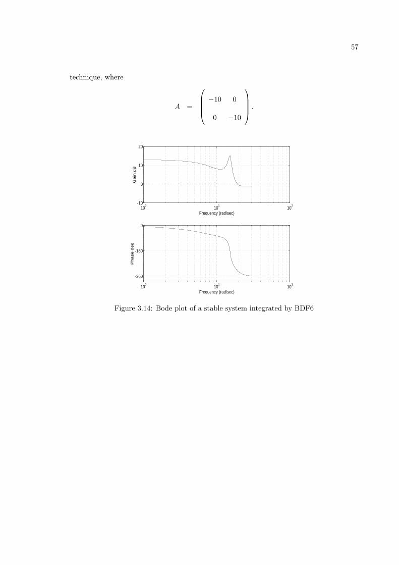
Bode plot can be produced by using the MATLAB-command “DBODE.” As an example,
figure 3.6 shows the Bode plot when the stable system x = Ax is integrated by the BDF6
57
technique, where
A =
⎛⎜⎜⎜⎝
−10 0
0 −10
⎞⎟⎟⎟⎠ .
100
101
102
-10
0
10
20
Frequency (rad/sec)
Gain
dB
100
101
102
-180
-360
0
Frequency (rad/sec)
Phase d
eg
Figure 3.14: Bode plot of a stable system integrated by BDF6

58
CHAPTER 4
Implementation of RBDF
4.1 Startup problem
An m-step integration method needs m initial values of the state variable in order to
get started. These starting values needn’t be accurate as has been described in chapter 1.
Gear [10] proposes to use Runge-Kutta methods for startup purposes. This is specified
more in detail by Cellier [4] who applies n − 1 steps with fixed step-size of a nth order
Runge-Kutta. Thus, the step-size should only be determined once at the beginning of the
simulation. In order to calculate the initial step-size h quickly a binary search technique is
employed that starts at a steplength h0. This starting value of h0 must guarantee a stable
integration of a system with known eigenvalues by a Runge-Kutta algorithm of nth order.
At each step of the binary search, an estimate of the relative error, εrel, is made where,
εrel =|x1 − x2|
max(|x1|, |x2|, δ) . (4.1)
Hence, x1 is the value of the state variable x calculated by a nth order RK-algorithm and
x2 is the value of the state variable x calculated by a (n − 1)th order RK-algorithm. This
result shown in equation (4.1) can be compared to a given error bound tolerance denoted
as tolrel:
If 0.9tolrel ≤ εrel ≤ tolrel, then the binary search is stopped; otherwise, either h is increased
59
(if εrel < 0.9tolrel) or h is decreased before the step is calculated again. If the initial values
vanish (x(0) = 0, f(0) = 0) then the startup with RK-methods fails to compute the initial
values for the multistep technique. In this case, a general RK-method described as
xk+1 = xk + hl∑
i=1
βlixPi−1 , (4.2)
where xPi−1 are the predictors given by
xPi−1 = f(xPi−1 , tk + αi−1h), (4.3)
will always yield the result x = 0. Therefore, relation (4.1) results in εrel = 0, such that
the step-size is never changed. Since the algorithm has been started at the maximum value
of the steplength h0 this might give rise to instability.
This problem can be solved by running one step with an RK-method of nth order to modify
the initial conditions. The time is set back to t = t0 and one step of the startup is executed
to determine the initial step-size h0. By using h0 and the original initial conditions of the
system, the startup procedure is started again at t = t0.
4.2 Step-size control
4.2.1 Introduction
Most of the integration methods can only be applied efficiently if the step-size is adjusted
according to accuracy requirements. For example, when integrating stiff systems without
step-size control a very small steplength would be applied during the whole integration (cf.
chapter 1). Thus, the simulation would last excessively long.
Before the step-size control with multistep methods will be discussed, a mathematical tool,

60
the so-called Newton-Gregory polynomials, is introduced.
Afterwards, it will be shown how this tool is used to calculate Nordsieck vectors of different
order.
Finally, the algorithm for step-size control will be derived that applies the Nordsieck vector
to update the state history vector if the step-size h is changed. This vector contains m
earlier state variables x.
4.2.2 Newton-Gregory polynomials
To make the following calculations more convenient the forward difference operator ∆ is
introduced:
∆g0 = g1 − g0,
∆g1 = g2 − g1,
...
∆gi = gi+1 − gi,
(4.4)
where gi denotes the value of a continuous function g(t) at the point of time ti.
By recursively applying the operator ∆, higher-order forward difference operators are ob-
tained which, in the general case, are given by [4]
∆gp−1i =
⎛⎜⎜⎜⎝
p − 1
0
⎞⎟⎟⎟⎠ gi+p−1 −
⎛⎜⎜⎜⎝
p − 1
1
⎞⎟⎟⎟⎠ gi+p−2 +
⎛⎜⎜⎜⎝
p − 1
2
⎞⎟⎟⎟⎠ gi+p−3
+ . . . ±
⎛⎜⎜⎜⎝
p − 1
p − 1
⎞⎟⎟⎟⎠ gi,
(4.5)

61
where p is the number of earlier data points.
After having defined the backward difference operator ∇ as
∇gi = gi − gi−1, (4.6)
we get the higher-order backward difference operators accordingly:
∇p−1gi =
⎛⎜⎜⎜⎝
p − 1
0
⎞⎟⎟⎟⎠ gi −
⎛⎜⎜⎜⎝
p − 1
1
⎞⎟⎟⎟⎠ gi−1 +
⎛⎜⎜⎜⎝
p − 1
2
⎞⎟⎟⎟⎠ gi−2
+ . . . ±
⎛⎜⎜⎜⎝
p − 1
p − 1
⎞⎟⎟⎟⎠ gi−p+1.
(4.7)
The task is to find a vector polynomial, i.e. a polynomial with scalar argument and vector
coefficients, which interpolates the p distinct data points. This interpolant takes a particu-
larly simple form when the time points ti, where the function values are taken, are equally
spaced [14], i.e.
tk−j = tk − jh, j = 0, 1, 2, . . . , p (h = const.). (4.8)
At this point an auxiliary variable s is introduced as defined in [4],
s =t − t0
h. (4.9)
Hence, the interpolation polynomial can be depicted either as
g(s) ≈
⎛⎜⎜⎜⎝
s
0
⎞⎟⎟⎟⎠ g0 + . . . +
⎛⎜⎜⎜⎝
s
p − 1
⎞⎟⎟⎟⎠∆p−1g0,
(p = number of data points)
(4.10)
or
g(s) ≈ g0 +
⎛⎜⎜⎜⎝
s
1
⎞⎟⎟⎟⎠∇g0 +
⎛⎜⎜⎜⎝
s + 1
2
⎞⎟⎟⎟⎠∇2g0 + . . . +
⎛⎜⎜⎜⎝
s + p − 2
p − 1
⎞⎟⎟⎟⎠∇p−1g0. (4.11)
62
The expression in (4.10) is called the Newton-Gregory forward polynomial whereas (4.11)
is known as the Newton-Gregory backward polynomial (see [4] for the derivation of (4.10)
and (4.11)).
Note that the Newton-Gregory polynomials are only valid if the data points are evenly
spaced, otherwise interpolating polynomials, such as the ones derived by Lagrange [14],
have to be used.
The Newton-Gregory backward polynomial can be employed in a multistep integration by
setting tk = t0 and s = 1.0. Furthermore, the back values need to be substituted by the
corresponding function values x(tk), x(tk−1), . . . etc..
Thus, equation (4.11) automatically calculates an estimate x(tk+1) = g1 which is the un-
known of the multistep algorithm.
4.2.3 Calculation of the Nordsieck vector
In the following it is assumed for convenience that the system being integrated is scalar,
that is: ns = 1.
With the results of the preceding subsection, the Newton-Gregory backward polynomial
for x(t) can be written as
x(t) = xk + s∇xk +
(s2
2+
s
2
)∇2xk +
(s3
6+
s2
2+
s
3
)∇3xk + . . . (4.12)
This equation is differentiated with respect to time which yields
x(t) =1h
[∇xk + (s +12)∇2xk + (
s2
2+ s +
13)∇3xk + . . .]. (4.13)
The higher order derivatives are determined by recursively differentiating (4.13). By trun-
cating the resulting expressions after the nthg term (ng = order of the Nordsieck vector)
63
and expanding the ∇-operator according to (4.4) and evaluating for t = tk (s = 0.0), the
expression
g = Ts, (4.14)
is obtained where
s =
⎛⎜⎜⎜⎜⎜⎜⎜⎜⎜⎜⎜⎜⎝
xk
xk−1
...
xk−m+1
⎞⎟⎟⎟⎟⎟⎟⎟⎟⎟⎟⎟⎟⎠
is the state history vector that contains m state variables of m earlier time instants, T is a
[(ng + 1) × m] transformation matrix, and
g =
⎛⎜⎜⎜⎜⎜⎜⎜⎜⎜⎜⎜⎜⎝
xk
hxk
...
hng
ng!x
(ng)k
⎞⎟⎟⎟⎟⎟⎟⎟⎟⎟⎟⎟⎟⎠
is the (ng + 1)-vector which is similar to the Nordsieck vector N = (xk, hxk, . . . , hngx
(ng)k )
of nthg -order (cf. [4]). However, for convenience we refer to g as the Nordsieck vector in this
section.
In the appendix some transformation matrices are shown for different values of ng and m
if the system being integrated is one-dimensional (ns = 1).
One might get the idea of using the given value hxk as additional information in the state
history vector s. This would require one to substitute the expressions for the last element
64
of s by the expressions dependent on xk. These expressions can be derived by solving
x = . . . + ak−m+1xk−m+1
for xk−m+1. Hence, the last element of s can be rewritten as
xk−m+1 = axk + bhxk + cxk−1 + . . . ,
where the constants a, b, c, . . . need to be determined.
However, multiple simulations which implemented the described step-size control have
shown that the use of hxk is not advantageous. The following quickly describes two key
results:
1. The integration process becomes slower. One reason for this is that the transformation
matrix T , which has to be inverted to calculate the new state history vector after
a change of the step-size, becomes larger. This is explained by the fact that the
formula of the integration algorithm contains the last element of the state history
vector s. Therefore, this element has to be calculated and can only be substituted by
an expression of xk when the Nordsieck vector is computed.
Furthermore, it can be observed that the Nordsieck vector is calculated less accurately:
An error is introduced by replacing x by xk. Therefore, the integration algorithm must
use smaller steplengths to satisfy the accuracy requirements.
2. Although one might think that the integration would become more accurate by using
additional information about the state space model within each integration step, this
is not true. Simulations have proven without any exception that the remaining global
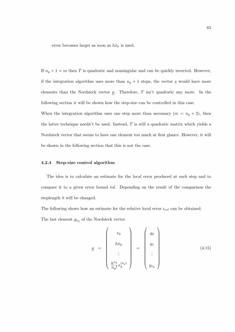
65
error becomes larger as soon as hxk is used.
If ng + 1 = m then T is quadratic and nonsingular and can be quickly inverted. However,
if the integration algorithm uses more than ng + 1 steps, the vector s would have more
elements than the Nordsieck vector g. Therefore, T isn’t quadratic any more. In the
following section it will be shown how the step-size can be controlled in this case.
When the integration algorithm uses one step more than necessary (m = ng + 2), then
the latter technique needn’t be used. Instead, T is still a quadratic matrix which yields a
Nordsieck vector that seems to have one element too much at first glance. However, it will
be shown in the following section that this is not the case.
4.2.4 Step-size control algorithm
The idea is to calculate an estimate for the local error produced at each step and to
compare it to a given error bound tol. Depending on the result of the comparison the
steplength h will be changed.
The following shows how an estimate for the relative local error εrel can be obtained:
The last element gng of the Nordsieck vector
g =
⎛⎜⎜⎜⎜⎜⎜⎜⎜⎜⎜⎜⎜⎝
xk
hxk
...
hng
ng!x
(ng)k
⎞⎟⎟⎟⎟⎟⎟⎟⎟⎟⎟⎟⎟⎠
=
⎛⎜⎜⎜⎜⎜⎜⎜⎜⎜⎜⎜⎜⎝
g0
g1
...
gng
⎞⎟⎟⎟⎟⎟⎟⎟⎟⎟⎟⎟⎟⎠
(4.15)

66
is given by
gng =hngx(ng)
ng!. (4.16)
According to [10], the change ∆gng of gng is an estimate of
∆gng =hng+1x(ng+1)
ng!(4.17)
which can be shown by:
∆gng = hngx
(ng)kng!
− hngx
(ng)k−1ng!
= hng
ng!h
⎛⎝x
(ng)k − x
(ng)k−1
h
⎞⎠
︸ ︷︷ ︸x(ng+1)
k
. (4.18)
As shown in chapter 1, the local truncation error can be estimated by
T = Cn+1hn+1x
(n+1)k + O(hn+2). (4.19)
Only the principal term is considered, and that needs to be smaller than the given error
bound tol:
Cn+1hn+1x
(n+1)k ≤ tol. (4.20)
By choosing ng = n, the equations (4.18) and (4.20) can be combined to formulate
Cn+1n!∆gn ≤ tol. (4.21)
As Gear [10] proposes, relation (4.21) should be tested first. If the test succeeds, the step
is accepted; otherwise it is rejected.
The new step-size is calculated by
hnew = αhold, (4.22)
67
where
Cn+1n!αn+1∆gn = tol. (4.23)
This can be shown by plugging (4.22) into (4.17) which yields
∆gn,new = αn+1hn+1
n!
(x
(n+1)k
)T=
= αn+1∆gn,old.
(4.24)
By plugging relation (4.24) into (4.21) and treating (4.21) as an equality, equation (4.23)
is obtained.
Since ∆gn usually is not constant, a slightly smaller step-size is used in order that (4.21)
can be expected to be satisfied. Thus α is determined by
α =1
1.2
(tol
Cn+1n!∆gn
) 1n+1
. (4.25)
However, calculating α and changing the step-size at each step, the integration algorithm
would be very slow. Therefore, some of the advises given in [11] should be considered:
1. Values for α are only accepted between 0.5 and 2.0.
2. If 1 ≤ α ≤ 1.1, the new step-size is chosen to be hnew = 0.9hold.
3. When the step has failed, the step-size is halved.
As soon as the step-size is changed the state history vector s will have to be adjusted
accordingly. Otherwise the integration method would proceed with wrong initial values.
The adjustment can easily be done by the Nordsieck technique:
The new Nordsieck vector is computed by
gnew
= Hgold
, (4.26)

68
where
H =
⎛⎜⎜⎜⎜⎜⎜⎜⎜⎜⎜⎜⎜⎜⎜⎜⎜⎝
1 0 · · · 0
0 α. . .
...
.... . . α2
. . . 0
0 0 αng
⎞⎟⎟⎟⎟⎟⎟⎟⎟⎟⎟⎟⎟⎟⎟⎟⎟⎠
. (4.27)
In order to obtain the new state history vector snew, equation (4.26) is plugged into the
relation
snew = T−1gnew
, (4.28)
where T is the transformation matrix introduced in (4.14).
So far the only case which has been regarded is where ng = n. This means that the state
history vector s has n + 1 elements if T is quadratic. Therefore, the integration method
uses m = n + 1 steps.
If m = n + 2 steps are applied, then the [(ng + 1) × m] transformation matrix T is still
quadratic. Thus, the last element of the Nordsieck vector becomes
hng
ng!x
ng
k =hn+1
(n + 1)!x
(n+1)k , (4.29)
and it can be directly used in (4.20) without making the approximation (4.17). This saves
computation time.
If the integration algorithm employs more than n + 2 steps then there are two options:
1. The transformation matrix T used in
g = Ts
69
can still be quadratic. However, the Nordsieck vector will have too many elements
since only the (ng + 1)th element of g has to be determined (gng). The state history
vector might be updated after a change of the steplength by applying the relation
s = T−1g. (4.30)
2. The (n + 2)-Nordsieck vector g keeps its size. Therefore, g can still be computed by
g = Ts,
where s is the state history vector containing m components (m > n + 2).
However, to get the new vector snew after a change of the step-size, which results in
a change of g, an overdetermined system has to be solved. As in chapter 2 this sys-
tem is solved in a least-squares sense by calculating the Penrose-Moore Pseudoinverse:
s =(T T T
)−1T T g. (4.31)
In order to decide which of the two options is better the number of applied scalar multipli-
cations (sms) is estimated. To investigate the efficiency of the first option relation (4.14)
has to be solved first where T is a (m × m)-matrix (m > n + 2). This can be done with
q1 = m2 multiplications. For the solution of the inverse problem (4.30) after the change of
the step-size, it is assumed that the computation of the inverse of the asymmetric matrix
T corresponds to q2 multiplications. Therefore
q3 = m2 + q2 (4.32)
70
multiplications are needed to determine s. Thus, after a change of the step-size
qo,1 = q1 + q3
= 2m2 + q2
(4.33)
multiplications have to be executed when choosing the first option.
When choosing the second option, the [(n+2)×m]-matrix T (m > n+2) in equation (4.14)
isn’t quadratic any more. Therefore, equation (4.14) can be calculated with q4 = m(n + 2)
multiplications. Since the matrix
T ∗ = T T T (4.34)
is a (m × m)-matrix, the calculation of its inverse corresponds to q2 multiplications again.
Hence, the inverse problem (4.28) is solved by
q5 = q2 + 2m2(n + 2) + m(n + 2) (4.35)
multiplications. Thus, by choosing the second option, the calculation of new vectors g and
s corresponds to
qo,2 = q4 + q5
= q2 + 2m(n + 2) + 2m2(n + 2)(4.36)
multiplications.
Since m ≥ n + 2, it follows from (4.33) and (4.36) that
qo,2 > qo,1, (4.37)
that is, the first option is faster.
71
4.3 Integration of nonlinear systems
4.3.1 Startup problem
In section 4.1 it has been described how a multistep integration method can be started
quickly by using a binary search technique and RK methods.
In order to search in a binary fashion for the initial step-size h, a starting value h0 is
required. This value can be obtained by determining the largest magnitude |λmax| of the
eigenvalues of the system and using the condition
|λmax|h0 = r0, (4.38)
where r0 is the radius of the largest semicircle around the origin that fits completely into
the part of the stability domain, of the applied nth-order RK-method (n > 2), which is in
the left half plane.
The eigenvalues can be calculated if the system being integrated is linear. However, in
the nonlinear case the eigenvalues of the Jacobian of the system may be determined. The
column vectors J i can be computed as shown in equation (4.39) [4].
J i =δf
δxi≈ f
dev− f
∆xi, (4.39)
where f is the state derivative vector of the nominal state variables and the vector fdev
is
the state derivative vector which results from the perturbation of the state variable xi by
∆xi. Note that all of the other state variables are kept unchanged.
By determining the maximum eigenvalue λmax of the Jacobian J and using relation (4.38)
we obtain the initial step-size h0. The value r0 should be chosen slightly smaller since the
Jacobian can only be approximated and a stable integration has to be ensured in any case.
72
4.3.2 Newton iteration
In this thesis only implicit linear multistep integration methods are of interest. They
are given by
xk+1 =m−1∑i=0
aixk−i +m−1∑i=−1
bihfk−i
. (4.40)
In the case of a linear homogeneous system
x = Ax, x(0) = 0, (4.41)
equation (4.40) results in
xk+1 = [I(ns) − b−1hA]−1m−1∑i=0
(aixk−i + bihfk−i
). (4.42)
However, the matrix inversion cannot be applied to a nonlinear problem. Cellier [4] proposes
to rewrite (4.40) in the form
F(xk+1) = b−1hf(xk+1, tk+1) − xk+1 +m−1∑i=0
(aixk−i + bihfk−i
) = 0 (4.43)
which can be solved by Newton iteration,
xl+1k+1 = xl
k+1 − [Hl]−1[F l], (4.44)
where the Hessian H is given by:
H = b−1Jh − I(ns). (4.45)
In order to save computation time the Jacobian and the Hessian are only computed if it is
necessary, e.g. when the state variables change drastically. This is discussed in more detail
in [4].

73
4.4 Readout problem
At the end of a simulation the results of the simulation need to be displayed. Note that
the points xk calculated by the integration algorithm are most likely not evenly spaced
because the step-size control always changes the step-size.
The problem is that the person who runs the simulation desires values at defined points
called communication points. It is assumed for convenience that these points are equally
spaced.
Within the startup period it is integrated right past the communication point, which is
characterized by the time instant t = tcom. Then an interpolation is made between the
calculated values to obtain the value of xcom at tcom.
As soon as the multistep integration algorithm is applied, the Nordsieck technique is used
again: After having integrated right past tcom, a negative step-size is applied to reach the
communication point. By calculating the Nordsieck vector g at tcom and adding up the
components of g, which represent terms in a Taylor series expansion, an estimate for
xcom = x(tcom).
is obtained (see [4] for more details).

74
From [email protected] Jul 9 14:43:51 1995 Date: Sun, 9 Jul 1995 12:07:59 UTC+0200
From: Francois Cellier ¡[email protected]¿ To: [email protected] Subject:
Kapitel 5 jetzt in Ordnung (nur kleine Aenderungen vorgenommen)
75
CHAPTER 5
RBDF of 6th order (RBDF6)
5.1 Derivation of the algorithms
In this chapter RBDF techniques will be derived that are 6th-order accurate (RBDF6
methods).
The order of 6 is chosen because this is the largest order for which a conventional stable
BDF method can be found. Thus, it is possible to compare the performance of the RBDF6
methods with that of the BDF6 algorithm. The probability of finding RBDF methods in-
creases with the accuracy order of the method due to the increased number of interpolation
points available in the search. However, since there are more possible candidates, the search
also takes longer.
The search method mentioned at the end of chapter 2 is applied to find RBDF6 algorithms
that satisfy minimum stability requirements. In chapter 2 it is discussed that “minimum
stability requirements” means that the stability locus doesn’t intersect with the negative
real axis of the complex (λh)-plane.
Table 5.1 displays the numbers of 6th-order RBDF algorithms that have been found for
different numbers of applied data points. Note that the data points are always given within
the time interval [tk−n−2, tk+1].

76
Number of Number ofdata points RBDF6
algorithms8 719 4510 1511 312 -
Table 5.1: Number of 6th order RBDF al-gorithms satisfying minimum stability re-quirements
The stability domain of these methods is considered and compared to the stability do-
main of BDF6 depicted in figure 5.1.
Out of the 134 RBDF techniques, only 18 algorithms are found whose stability domains
-10 -5 0 5 10 15 20 25 30-20
-15
-10
-5
0
5
10
15
20
Re
Im
Figure 5.1: Stability domain of BDF6
look similar to the one of BDF6.
The next step is to analyze the damping plots of the new methods and compare them with
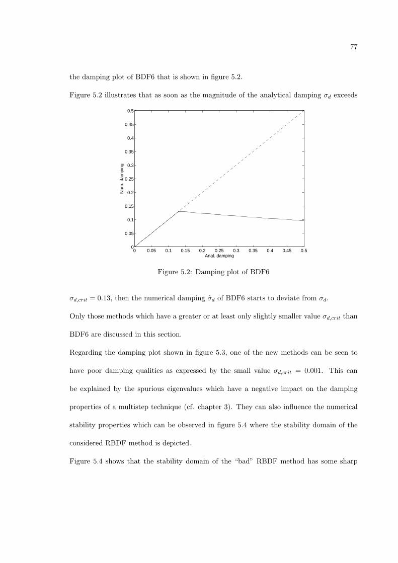
77
the damping plot of BDF6 that is shown in figure 5.2.
Figure 5.2 illustrates that as soon as the magnitude of the analytical damping σd exceeds
0 0.05 0.1 0.15 0.2 0.25 0.3 0.35 0.4 0.45 0.50
0.05
0.1
0.15
0.2
0.25
0.3
0.35
0.4
0.45
0.5
Anal. damping
Num
. dam
ping
Figure 5.2: Damping plot of BDF6
σd,crit = 0.13, then the numerical damping σd of BDF6 starts to deviate from σd.
Only those methods which have a greater or at least only slightly smaller value σd,crit than
BDF6 are discussed in this section.
Regarding the damping plot shown in figure 5.3, one of the new methods can be seen to
have poor damping qualities as expressed by the small value σd,crit = 0.001. This can
be explained by the spurious eigenvalues which have a negative impact on the damping
properties of a multistep technique (cf. chapter 3). They can also influence the numerical
stability properties which can be observed in figure 5.4 where the stability domain of the
considered RBDF method is depicted.
Figure 5.4 shows that the stability domain of the “bad” RBDF method has some sharp
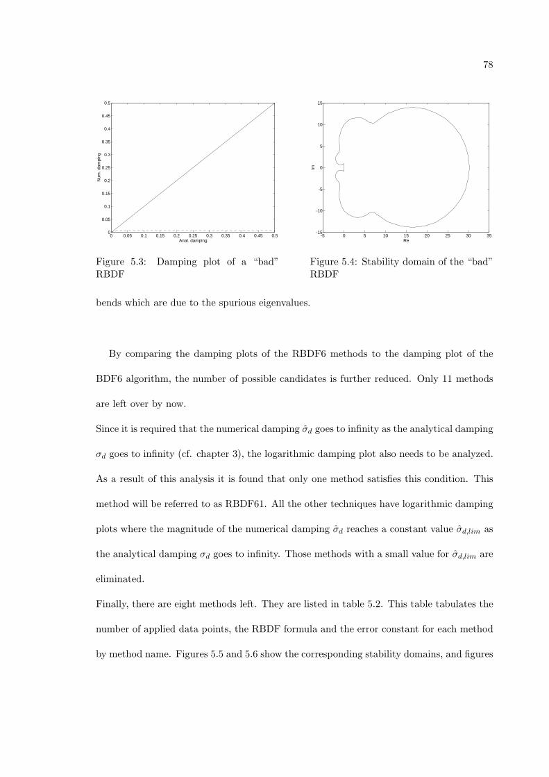
78
0 0.05 0.1 0.15 0.2 0.25 0.3 0.35 0.4 0.45 0.50
0.05
0.1
0.15
0.2
0.25
0.3
0.35
0.4
0.45
0.5
Anal. damping
Num
. dam
ping
Figure 5.3: Damping plot of a “bad”RBDF
-5 0 5 10 15 20 25 30 35-15
-10
-5
0
5
10
15
Re
Im
Figure 5.4: Stability domain of the “bad”RBDF
bends which are due to the spurious eigenvalues.
By comparing the damping plots of the RBDF6 methods to the damping plot of the
BDF6 algorithm, the number of possible candidates is further reduced. Only 11 methods
are left over by now.
Since it is required that the numerical damping σd goes to infinity as the analytical damping
σd goes to infinity (cf. chapter 3), the logarithmic damping plot also needs to be analyzed.
As a result of this analysis it is found that only one method satisfies this condition. This
method will be referred to as RBDF61. All the other techniques have logarithmic damping
plots where the magnitude of the numerical damping σd reaches a constant value σd,lim as
the analytical damping σd goes to infinity. Those methods with a small value for σd,lim are
eliminated.
Finally, there are eight methods left. They are listed in table 5.2. This table tabulates the
number of applied data points, the RBDF formula and the error constant for each method
by method name. Figures 5.5 and 5.6 show the corresponding stability domains, and figures
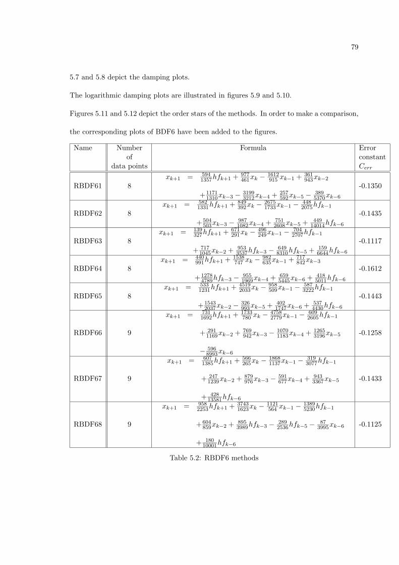
79
5.7 and 5.8 depict the damping plots.
The logarithmic damping plots are illustrated in figures 5.9 and 5.10.
Figures 5.11 and 5.12 depict the order stars of the methods. In order to make a comparison,
the corresponding plots of BDF6 have been added to the figures.
Name Number Formula Errorof constant
data points Cerr
RBDF61 8xk+1 = 594
1357hfk+1 + 977461xk − 1612
915 xk−1 + 361943xk−2
+11711310xk−3 − 3199
3212xk−4 + 257592xk−5 − 389
5370xk−6
-0.1350
RBDF62 8xk+1 = 582
1331hfk+1 + 849392xk − 2675
1733xk−1 − 4482075hfk−1
+504503xk−3 − 987
1082xk−4 + 7512608xk−5 + 449
14014hfk−6
-0.1435
RBDF63 8xk+1 = 139
327hfk+1 + 671291xk − 496
249xk−1 − 7042707hfk−1
+ 7171045xk−2 + 953
3537hfk−3 − 6498310hfk−5 + 159
6644hfk−6
-0.1117
RBDF64 8xk+1 = 440
991hfk+1 + 1538747 xk − 982
635xk−1 + 717842xk−3
+12784789hfk−3 − 955
1969xk−4 + 6595445xk−6 + 418
5011hfk−6
-0.1612
RBDF65 8xk+1 = 533
1231hfk+1 + 45192033xk − 958
509xk−1 − 5873222hfk−1
+15432037xk−2 − 326
993xk−5 + 4021747xk−6 + 537
4430hfk−6
-0.1443
RBDF66 9
xk+1 = 7311692hfk+1 + 1733
780 xk − 47582779xk−1 − 609
2605hfk−1
+ 2911169xk−2 + 769
942xk−3 − 10701183xk−4 + 1265
3196xk−5
− 5968993xk−6
-0.1258
RBDF67 9
xk+1 = 6071385hfk+1 + 566
265xk − 18681137xk−1 − 319
3077hfk−1
+ 2471239xk−2 + 879
976xk−3 − 591677xk−4 + 943
3367xk−5
+ 42813581hfk−6
-0.1433
RBDF68 9
xk+1 = 9582253hfk+1 + 3743
1623xk − 1121564 xk−1 − 1389
5230hfk−1
+604859xk−2 + 895
3989hfk−3 − 2892536hfk−5 − 87
3995xk−6
+ 18010001hfk−6
-0.1125
Table 5.2: RBDF6 methods

80
-10 0 10 20 30 40 50-50
-40
-30
-20
-10
0
10
20
30
40
50
Re
ImRBDF61
RBDF62 RBDF63 BDF6 RBDF64 RBDF65
Figure 5.5: Stability domains of RBDF6 with 8 data points
-10 -5 0 5 10 15 20 25 30-25
-20
-15
-10
-5
0
5
10
15
20
25
Re
Im
RBDF67 RBDF66
RBDF68 BDF6
Figure 5.6: Stability domains of RBDF6 with 9 data points

81
0 0.05 0.1 0.15 0.2 0.25 0.3 0.35 0.4 0.45 0.5-0.1
0
0.1
0.2
0.3
0.4
0.5
Re
Im
BDF6
RBDF65
RBDF61
RBDF64
RBDF63
RBDF62
Figure 5.7: Damping plots of RBDF6 with 8 data points
0 0.05 0.1 0.15 0.2 0.25 0.3 0.35 0.4 0.45 0.5-0.1
0
0.1
0.2
0.3
0.4
0.5
Anal. damping
Num
. dam
ping
BDF6
RBDF67
RBDF68
RBDF66
Figure 5.8: Damping plots of RBDF6 with 9 data points
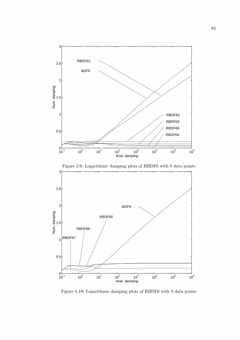
82
10-1
100
101
102
103
104
105
106
0
0.5
1
1.5
2
2.5
3
Anal. damping
Num
. dam
ping
RBDF61
BDF6
RBDF62
RBDF63
RBDF65
RBDF64
Figure 5.9: Logarithmic damping plots of RBDF6 with 8 data points
10-1
100
101
102
103
104
105
106
0
0.5
1
1.5
2
2.5
3
Anal. damping
Num
. dam
ping
RBDF67
RBDF68
RBDF66
BDF6
Figure 5.10: Logarithmic damping plots of RBDF6 with 9 data points

83
0 0.5 1 1.5 2 2.5 3-0.6
-0.4
-0.2
0
0.2
0.4
0.6
Re
Im
RBDF64
RBDF61
RBDF62
RBDF65
RBDF63
BDF6
Figure 5.11: Order stars of RBDF6 with 8 data points
0 0.5 1 1.5 2 2.5 3-0.6
-0.4
-0.2
0
0.2
0.4
0.6
Re
Im
RBDF67
RBDF66
RBDF68
BDF6
Figure 5.12: Order stars of RBDF6 with 9 data points
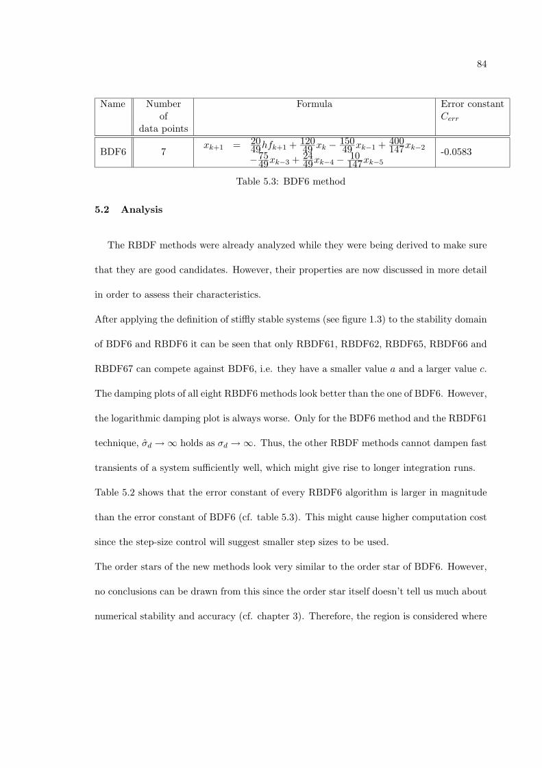
84
Name Number Formula Error constantof Cerr
data points
BDF6 7xk+1 = 20
49hfk+1 + 12049 xk − 150
49 xk−1 + 400147xk−2
−7549xk−3 + 24
49xk−4 − 10147xk−5
-0.0583
Table 5.3: BDF6 method
5.2 Analysis
The RBDF methods were already analyzed while they were being derived to make sure
that they are good candidates. However, their properties are now discussed in more detail
in order to assess their characteristics.
After applying the definition of stiffly stable systems (see figure 1.3) to the stability domain
of BDF6 and RBDF6 it can be seen that only RBDF61, RBDF62, RBDF65, RBDF66 and
RBDF67 can compete against BDF6, i.e. they have a smaller value a and a larger value c.
The damping plots of all eight RBDF6 methods look better than the one of BDF6. However,
the logarithmic damping plot is always worse. Only for the BDF6 method and the RBDF61
technique, σd → ∞ holds as σd → ∞. Thus, the other RBDF methods cannot dampen fast
transients of a system sufficiently well, which might give rise to longer integration runs.
Table 5.2 shows that the error constant of every RBDF6 algorithm is larger in magnitude
than the error constant of BDF6 (cf. table 5.3). This might cause higher computation cost
since the step-size control will suggest smaller step sizes to be used.
The order stars of the new methods look very similar to the order star of BDF6. However,
no conclusions can be drawn from this since the order star itself doesn’t tell us much about
numerical stability and accuracy (cf. chapter 3). Therefore, the region is considered where
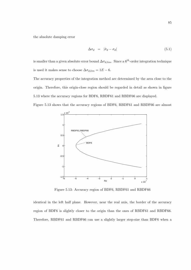
85
the absolute damping error
∆σd = |σd − σd| (5.1)
is smaller than a given absolute error bound ∆σd,lim. Since a 6th-order integration technique
is used it makes sense to choose ∆σd,lim = 1E − 6.
The accuracy properties of the integration method are determined by the area close to the
origin. Therefore, this origin-close region should be regarded in detail as shown in figure
5.13 where the accuracy regions for BDF6, RBDF61 and RBDF66 are displayed.
Figure 5.13 shows that the accuracy regions of BDF6, RBDF61 and RBDF66 are almost
-6 -5 -4 -3 -2 -1 0 1
x 10-7
-1.5
-1
-0.5
0
0.5
1
1.5x 10
-6
Re
Im
BDF6
RBDF61,RBDF66
Figure 5.13: Accuracy region of BDF6, RBDF61 and RBDF66
identical in the left half plane. However, near the real axis, the border of the accuracy
region of BDF6 is slightly closer to the origin than the ones of RBDF61 and RBDF66.
Therefore, RBDF61 and RBDF66 can use a slightly larger step-size than BDF6 when a

86
stable system with real eigenvalues is integrated and a given accuracy condition has to be
satisfied.
5.3 Simulation results and comparison of the RBDF6 methods with BDF6
In this section RBDF6 methods will be used to integrate some stiff systems. The re-
sults will be compared to those obtained when integrating the same systems with BDF6.
Although seven stiff systems have been simulated, the results of only two of these systems
are discussed here since they are representative of the others. One of the two systems is
linear, the other one is nonlinear:
• System 1 (taken from [6]):
x =
⎛⎜⎜⎜⎝
0 1
−1000 −1001
⎞⎟⎟⎟⎠x, (5.2)
x(0) =
⎛⎜⎜⎜⎝
1
−1
⎞⎟⎟⎟⎠ . (5.3)
(5.4)
Eigenvalues: λ1 = −1000; λ2 = −1
Analytical solution:
x1(t) = e−t
x2(t) = −e−t
(5.5)
• System 2:
x + x + 0.01
(x − x3
3
)= 0, (5.6)
87
x(0) = 0.01, (5.7)
x(0) = −4.999875E − 5. (5.8)
Analytical solution:
x(t) = a(t) cos t, (5.9)
where
a(t) =0.01e0.005t(
1 + 0.000025(e0.01t − 1)) 1
2
. (5.10)
Note that system 2 is a special case of the famous Rayleigh-equation and its analytical
solution has been derived by using the Krylov-Bogoliubov-Formulae [?].
All of the eight RBDF6 methods displayed in table 5.1 are tested using these two systems.
Although all of these algorithms perform fairly well in simulating these systems, only the
results of RBDF61 and RBDF66 will be shown. These two algorithms yield the best results
overall. This might be explained by the better damping properties of the two methods (see
chapter 3). Therefore, RBDF61 and RBDF66 are the best RBDF6 methods to compete
against BDF6.
The relative error bound for the step-size control is chosen to be tolrel = 0.001. Hence, the
relative local truncation error (LTE) is compared to this value of tolrel and, the result of
this comparison determines the need for step-size change.
Of course the value of tolrel is chosen to be much smaller in a real simulation —
e.g. tolrel = 1E − 6. However, to be able to more easily compare the different integration
methods, the error is made larger.
In order to assess the simulation results the time functions of the numerical solution x and
88
the global error ε = x− xanal, will be recorded where xanal is the analytical solution of the
system. Furthermore, the time behavior of the step-size h will be displayed.
Eventually, the number of floating-point operations (fop) will be considered to compare the
efficiency of the integration techniques.
At first, system 1 is integrated by BDF6. The simulation results are shown in figure 5.14.
The MATLAB-simulation over 5 time units with BDF6 takes 59026 floating point opera-
tions (fops). Recall that system 1 is stable — both eigenvalues have negative real parts.
Figure 5.14 shows that the integration by BDF6 is stable, too, since the global error is
decreasing with time. This seems to be clear because both eigenvalues being multiplied
with an arbitrary step-size h still lie within the stability domain of BDF6.
Now the same system is simulated with RBDF61 and RBDF66. Figures 5.15 and 5.16
display the results.
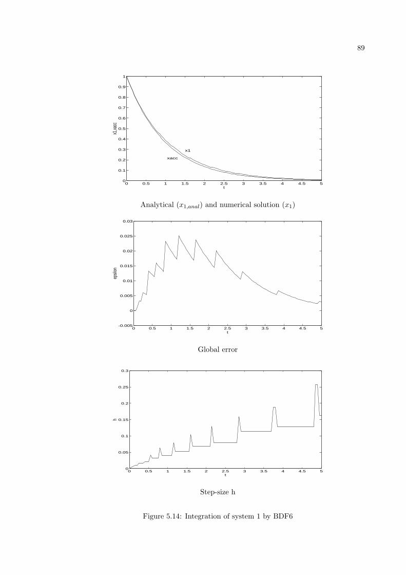
89
0 0.5 1 1.5 2 2.5 3 3.5 4 4.5 50
0.1
0.2
0.3
0.4
0.5
0.6
0.7
0.8
0.9
1
t
x1,xa
cc
x1
xacc
Analytical (x1,anal) and numerical solution (x1)
0 0.5 1 1.5 2 2.5 3 3.5 4 4.5 5-0.005
0
0.005
0.01
0.015
0.02
0.025
0.03
t
epsil
on
Global error
0 0.5 1 1.5 2 2.5 3 3.5 4 4.5 50
0.05
0.1
0.15
0.2
0.25
0.3
t
h
Step-size h
Figure 5.14: Integration of system 1 by BDF6
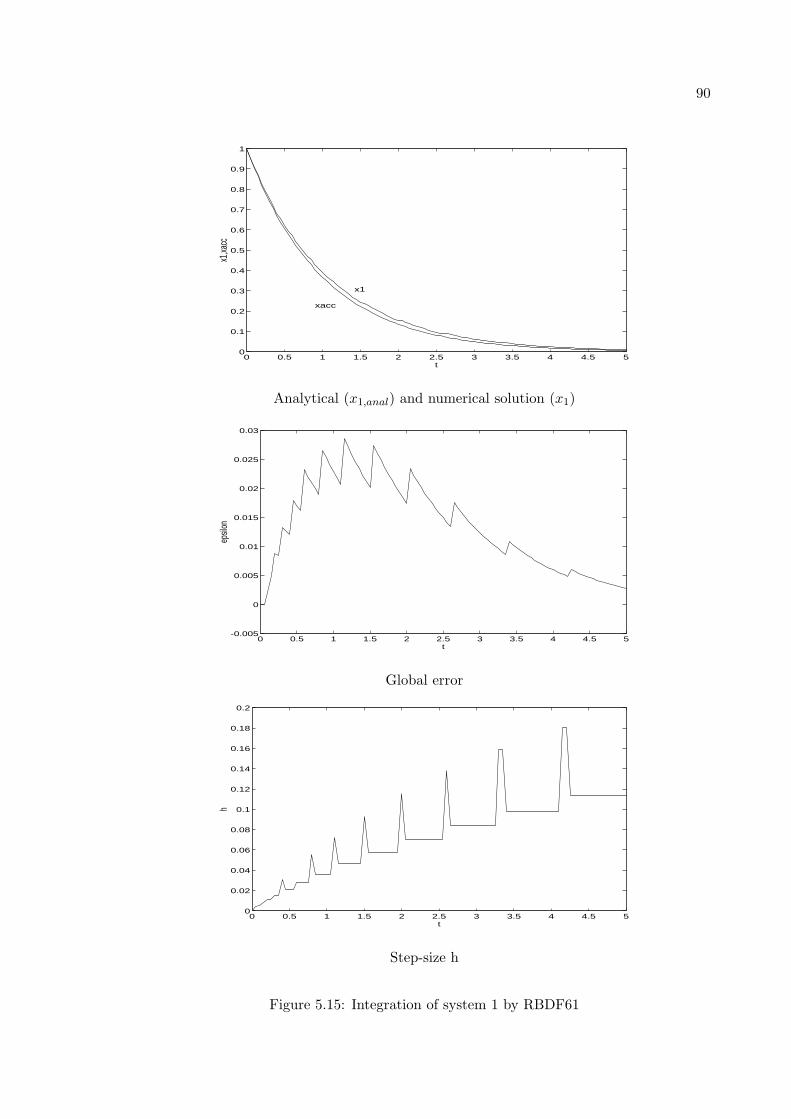
90
0 0.5 1 1.5 2 2.5 3 3.5 4 4.5 50
0.1
0.2
0.3
0.4
0.5
0.6
0.7
0.8
0.9
1
t
x1,xa
cc
x1
xacc
Analytical (x1,anal) and numerical solution (x1)
0 0.5 1 1.5 2 2.5 3 3.5 4 4.5 5-0.005
0
0.005
0.01
0.015
0.02
0.025
0.03
t
epsil
on
Global error
0 0.5 1 1.5 2 2.5 3 3.5 4 4.5 50
0.02
0.04
0.06
0.08
0.1
0.12
0.14
0.16
0.18
0.2
t
h
Step-size h
Figure 5.15: Integration of system 1 by RBDF61

91
0 0.5 1 1.5 2 2.5 3 3.5 4 4.5 50
0.1
0.2
0.3
0.4
0.5
0.6
0.7
0.8
0.9
1
t
x1,xa
cc
x1
xacc
Analytical (x1,anal) and numerical solution (x1)
0 0.5 1 1.5 2 2.5 3 3.5 4 4.5 5-0.5
0
0.5
1
1.5
2
2.5
3x 10
-3
t
epsil
on
Global error
0 0.5 1 1.5 2 2.5 3 3.5 4 4.5 50
0.05
0.1
0.15
0.2
0.25
0.3
0.35
t
h
Step-size h
Figure 5.16: Integration of system 1 by RBDF66

92
When integrating system 1 with RBDF61 over 5 time units 68441 fops are needed,
whereas RBDF66 only needs 48634 fops.
By comparing the results displayed in figures 5.15 and 5.16 it can be seen that RBDF66
integrates much more accurately than RBDF61 and BDF6. Moreover, RBDF66 needs 20%
- 30% less floating point operations than its competitors.
The nonlinear Rayleigh-equation (system 2) is integrated with BDF6, RBDF61 and
RBDF66 which yields the results depicted in figures 5.17 through 5.19.

93
0 0.5 1 1.5 2 2.5 3 3.5 4 4.5 5-0.01
-0.008
-0.006
-0.004
-0.002
0
0.002
0.004
0.006
0.008
0.01
t
x1
xacc
Analytical (x1,anal) and numerical solution (x1)
0 0.5 1 1.5 2 2.5 3 3.5 4 4.5 5-2
-1
0
1
2
3
4
5
6
7
8x 10
-3
t
epsil
on
Global error
0 0.5 1 1.5 2 2.5 3 3.5 4 4.5 50
0.05
0.1
0.15
0.2
0.25
0.3
0.35
0.4
0.45
t
h
Step-size h
Figure 5.17: Integration of system 2 by BDF6

94
0 0.5 1 1.5 2 2.5 3 3.5 4 4.5 5-0.01
-0.008
-0.006
-0.004
-0.002
0
0.002
0.004
0.006
0.008
0.01
t
x1,xa
cc x1
xacc
Analytical (x1,anal) and numerical solution (x1)
0 0.5 1 1.5 2 2.5 3 3.5 4 4.5 5
0
2
4
6
8
x 10-3
t
epsilo
n
Global error
0 0.5 1 1.5 2 2.5 3 3.5 4 4.5 50
0.05
0.1
0.15
0.2
0.25
0.3
0.35
0.4
t
h
Step-size h
Figure 5.18: Integration of system 2 by RBDF61
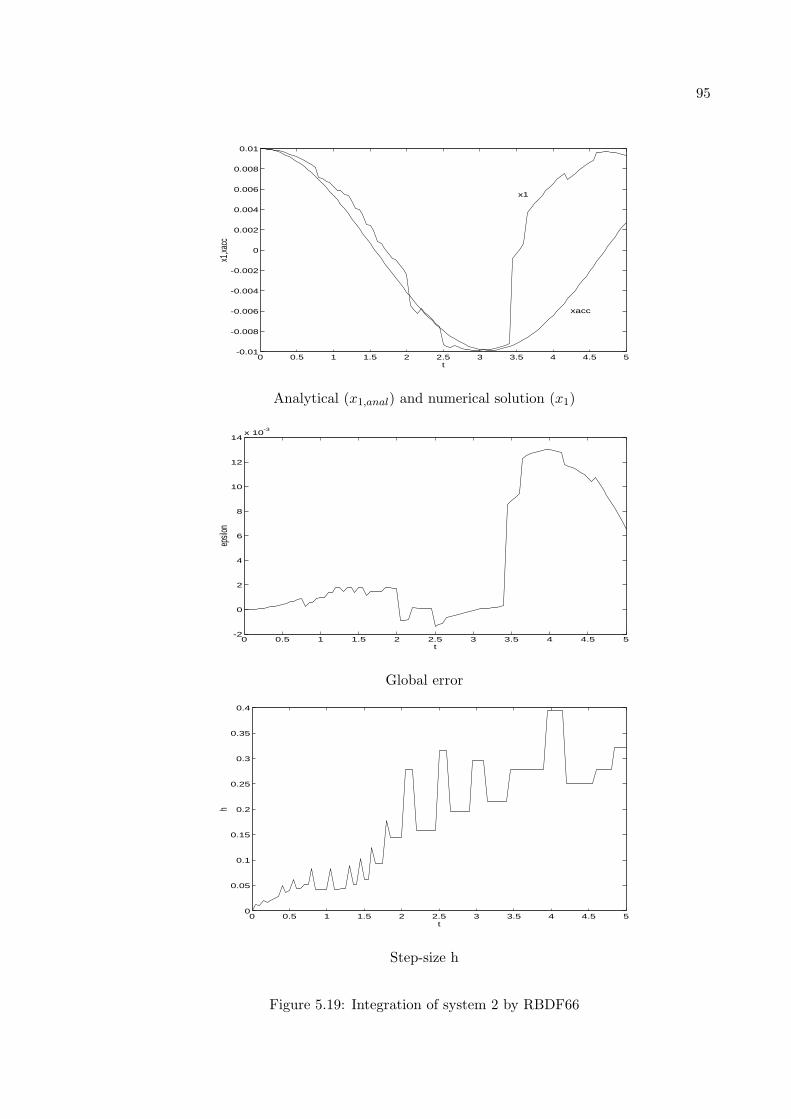
95
0 0.5 1 1.5 2 2.5 3 3.5 4 4.5 5-0.01
-0.008
-0.006
-0.004
-0.002
0
0.002
0.004
0.006
0.008
0.01
t
x1,xa
cc
x1
xacc
Analytical (x1,anal) and numerical solution (x1)
0 0.5 1 1.5 2 2.5 3 3.5 4 4.5 5-2
0
2
4
6
8
10
12
14x 10
-3
t
epsil
on
Global error
0 0.5 1 1.5 2 2.5 3 3.5 4 4.5 50
0.05
0.1
0.15
0.2
0.25
0.3
0.35
0.4
t
h
Step-size h
Figure 5.19: Integration of system 2 by RBDF66
96
This time BDF6 needs 139229 fops, RBDF61 uses 142983 fops and RBDF66 applies
131570 fops. It can be seen that RBDF66 is less accurate than the other two methods but
it is still the fastest one of the three integrators.
These results might be explained by the better stability properties of RBDF61 and RBDF66
in comparison with BDF6 since in terms of all the other properties — e.g. damping, error
constant — the two RBDF6 methods are worse. However, the following chapter will show
that this assumption doesn’t hold.
In figures 5.17 through 5.19 it can be seen that the integration is slightly unstable. This is
due to the fact that the step-size in this implementation is usually changed only after each
(n + 1)th step, where n is the order of the integration method — recall that this has been
done to save computation time. In addition, the bound tolrel for the relative error has been
chosen to be rather large.
Thus, the phenomenon of instability is a problem of the implementation, rather than a
problem of the integration algorithm itself. The unstable behavior can easily be removed
by choosing a smaller value for tolrel and by changing the step-size more frequently.
Finally, the three methods are analyzed in the frequency domain by means of the Bode
plot. As mentioned in chapter 3, three test systems (stable, marginally stable, unstable) of
the kind x = Ax are chosen that don’t change their stability properties when integrated by
the three methods.
97
The system matrix of the stable system is chosen to be
A =
⎛⎜⎜⎜⎝
−10 0
0 −10
⎞⎟⎟⎟⎠ , (5.11)
where the eigenvalues are λ1,2 = −10.
The marginally stable system has the system matrix
A =
⎛⎜⎜⎜⎝
0 1
−1 0
⎞⎟⎟⎟⎠ , (5.12)
which corresponds to the eigenvalues λ1 = −i, λ2 = i.
The unstable system is characterized by the system matrix
A =
⎛⎜⎜⎜⎝
10 0
0 10
⎞⎟⎟⎟⎠ (5.13)
with the eigenvalues λ1,2 = 10.
The stable system is integrated with the step-size h = 1. Note that λih = −10 lies within
the stability region of BDF6, RBDF61 and RBDF66.
Figure 5.20 shows the Bode plots that correspond to this stable integration. They have
been produced using the MATLAB-command “DBODE.”
Figure 5.20 shows that RBDF66 is better than RBDF61 with respect to low-pass filter
characteristics and that RBDF61 is still better than BDF6.
The step-size h = 0.01 is chosen when simulating the marginally stable system. Figure 5.21
displays the corresponding Bode plots.
It can be seen in figure 5.21 that the gain has its maximum at the frequency ω = 1 which
is known as the resonance frequency.
Concerning filter properties this plot doesn’t allow us to make clear statements.

98
100
101
102
-10
0
10
20
Frequency (rad/sec)
Gain
dB
100
101
102
-180
-360
0
Frequency (rad/sec)
Phase d
eg
BDF6
RBDF61
RBDF66
RBDF66
RBDF61
BDF6
Figure 5.20: Bode plot of a stable system integrated by BDF6, RBDF61and RBDF66.
10-2
10-1
100
101
102
0
50
100
Frequency (rad/sec)
Gain
dB
10-2
10-1
100
101
102
-90
-180
0
90
Frequency (rad/sec)
Phase d
eg
BDF6
RBDF61, RBDF66
Figure 5.21: Bode plot of a marginally stable system integrated by BDF6, RBDF61 andRBDF66.
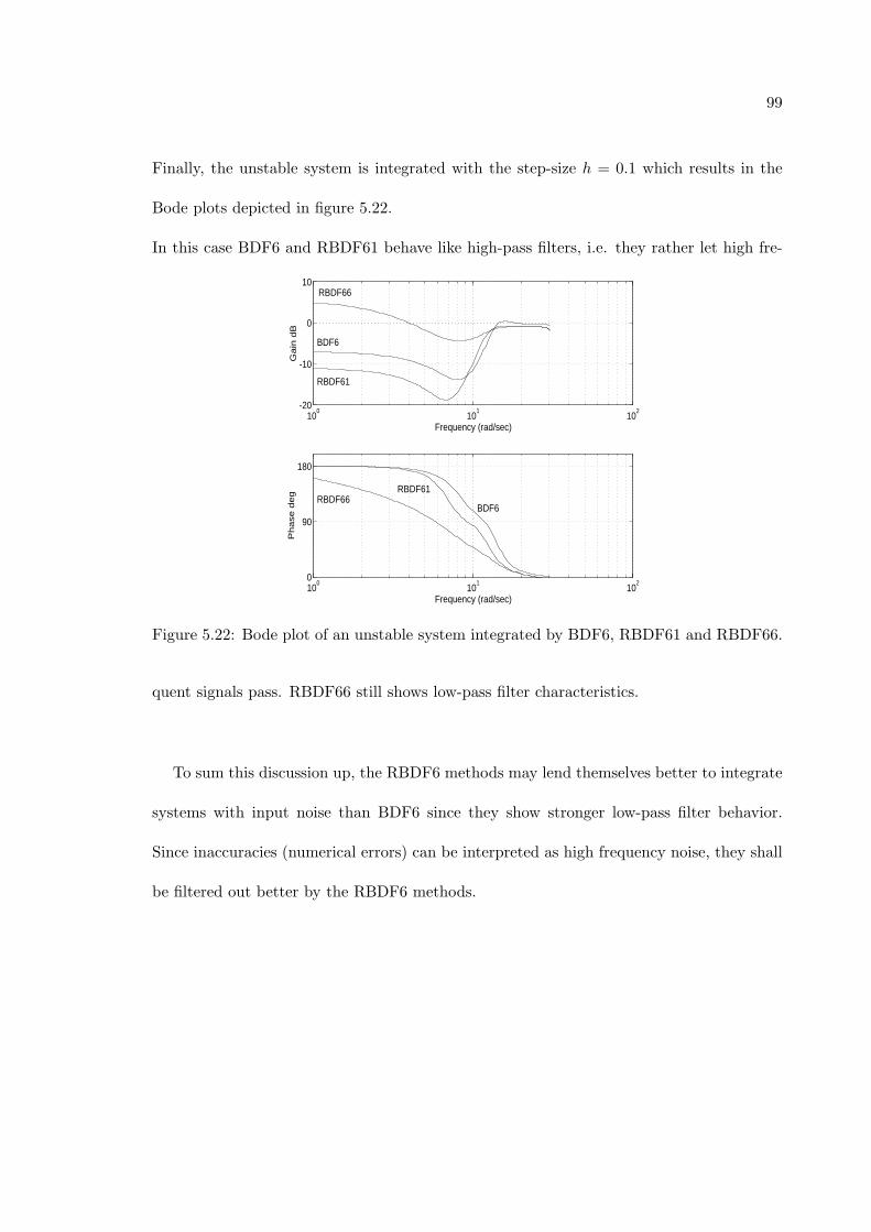
99
Finally, the unstable system is integrated with the step-size h = 0.1 which results in the
Bode plots depicted in figure 5.22.
In this case BDF6 and RBDF61 behave like high-pass filters, i.e. they rather let high fre-
100
101
102
-20
-10
0
10
Frequency (rad/sec)
Gain
dB
100
101
102
0
90
180
Frequency (rad/sec)
Phase d
eg
RBDF66
RBDF61
BDF6
RBDF66BDF6
RBDF61
Figure 5.22: Bode plot of an unstable system integrated by BDF6, RBDF61 and RBDF66.
quent signals pass. RBDF66 still shows low-pass filter characteristics.
To sum this discussion up, the RBDF6 methods may lend themselves better to integrate
systems with input noise than BDF6 since they show stronger low-pass filter behavior.
Since inaccuracies (numerical errors) can be interpreted as high frequency noise, they shall
be filtered out better by the RBDF6 methods.
100
CHAPTER 6
RBDF of 7th order (RBDF7)
6.1 Derivation of the algorithms
The procedure described in section 5.1 is applied to find 7th order RBDF methods. Once
again, the first step is to determine those algorithms that satisfy “minimum stability re-
quirements.”
Table 6.1 shows the number of RBDF7 methods that can be found for different numbers
of applied data points.
Note that there are many more RBDF7 methods with the mentioned requirements than
RBDF6 algorithms (cf. table 5.1).
Unlike the preceding chapter where BDF6 was the competitor, we don’t have any compari-
son within the 7th order range since BDF7 is unstable. Again, only those RBDF7 methods
are accepted that are stiffly stable according to Gear’s definition 1.3.3. 174 RBDF7 were
determined that possess this property.
In chapter 5 it has been shown that it is more restrictive to require the numerical damping
σd to go to infinity as σd goes to infinity than to require a large critical damping σd,crit.
Therefore, the logarithmic damping plot is regarded first and the RBDF methods with the
best damping curves are extracted. This results in 15 RBDF algorithms of 7th order whose
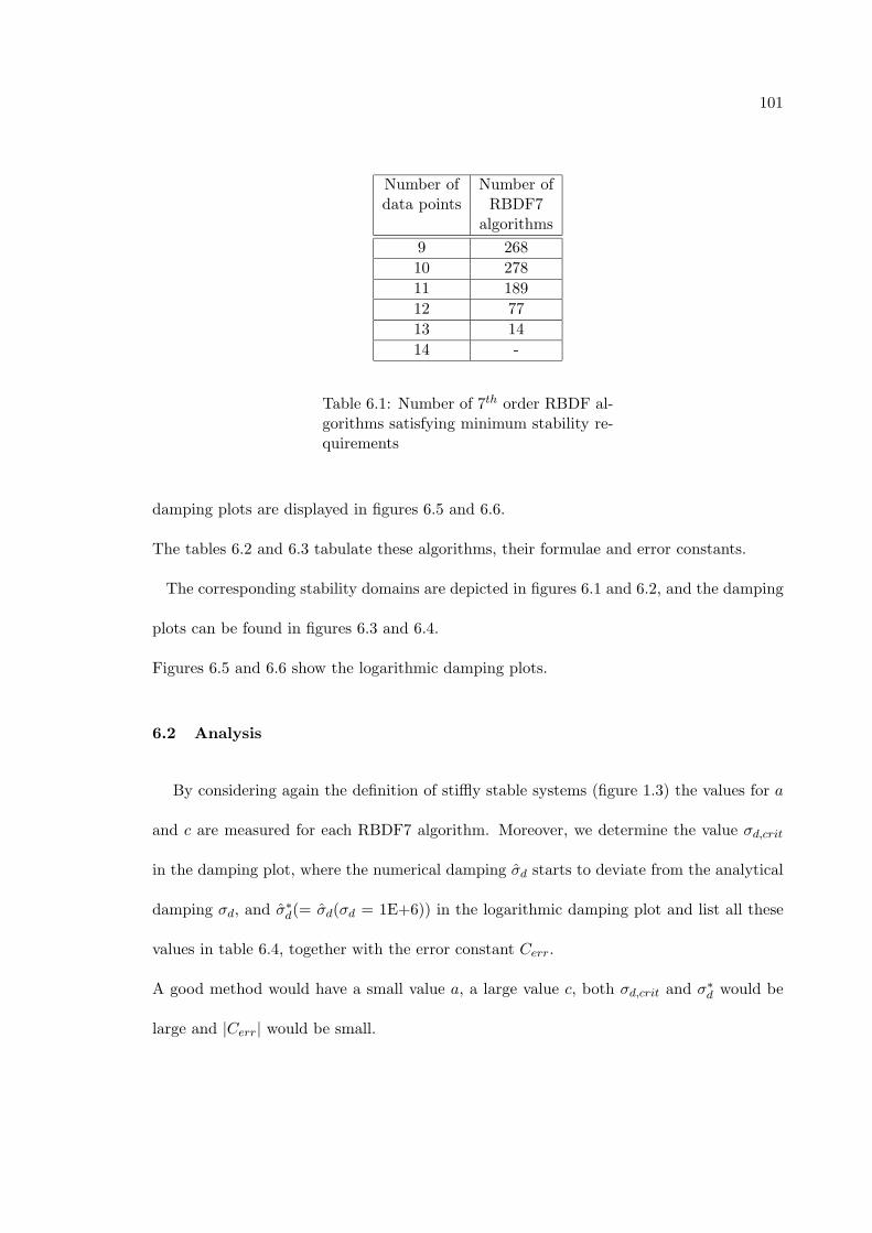
101
Number of Number ofdata points RBDF7
algorithms9 26810 27811 18912 7713 1414 -
Table 6.1: Number of 7th order RBDF al-gorithms satisfying minimum stability re-quirements
damping plots are displayed in figures 6.5 and 6.6.
The tables 6.2 and 6.3 tabulate these algorithms, their formulae and error constants.
The corresponding stability domains are depicted in figures 6.1 and 6.2, and the damping
plots can be found in figures 6.3 and 6.4.
Figures 6.5 and 6.6 show the logarithmic damping plots.
6.2 Analysis
By considering again the definition of stiffly stable systems (figure 1.3) the values for a
and c are measured for each RBDF7 algorithm. Moreover, we determine the value σd,crit
in the damping plot, where the numerical damping σd starts to deviate from the analytical
damping σd, and σ∗d(= σd(σd = 1E+6)) in the logarithmic damping plot and list all these
values in table 6.4, together with the error constant Cerr.
A good method would have a small value a, a large value c, both σd,crit and σ∗d would be
large and |Cerr| would be small.

102
Name Number Formula Errorof constant
data points Cerr
RBDF71 9xk+1 = 948
2257hfk+1 + 454201xk − 1476
683 xk−1 + 653869xk−2
+11511240xk−3 − 452
357xk−4 + 12242285xk−5 − 193
3802xk−7
+ 4210813xk−9
-0.1765
RBDF72 9xk+1 = 372
869hfk+1 + 443204xk − 3349
1814xk−1 + 13454324xk−2
+703648xk−3 − 658
715xk−4 + 298909xk−6 − 845
6228xk−7
+ 8312165xk−9
-0.2249
RBDF73 9xk+1 = 1363
3123hfk+1 + 1022489 xk − 1165
733 xk−1 + 4214469xk−2
+ 8011027xk−3 − 4831
4944xk−5 + 810947xk−6 − 407
1542xk−7
+ 11910830xk−9
-0.2851
RBDF74 9xk+1 = 147
344hfk+1 + 44312014xk − 1295
636 xk−1 + 584647xk−2
+ 9973006xk−4 − 883
967xk−5 + 18852599xk−6 − 417
1900xk−7
+ 15316820xk−9
-0.2433
RBDF75 9xk+1 = 133
305hfk+1 + 675323xk − 1269
808 xk−1 + 11381143xk−3
− 5041777xk−4 − 1065
1417xk−5 + 26683553xk−6 − 337
1399xk−7
+ 474554xk−9
-0.2780
RBDF76 9xk+1 = 503
1187hfk+1 + 322145xk − 2357
1161xk−1 + 6651142xk−2
+13131343xk−3 − 2125
1834xk−4 + 11762749xk−5 − 107
3718xk−8
+ 515581xk−9
-0.2052
RBDF77 9xk+1 = 647
1498hfk+1 + 2005939 xk − 2119
1225xk−1 + 3641983xk−2
+12681165xk−3 − 1254
1511xk−4 + 9254782xk−6 − 53
931xk−8
+ 332065xk−9
-0.2608
RBDF78 9xk+1 = 473
1069hfk+1 + 53262621xk − 709
507xk−1 − 3492482xk−2
+679778xk−3 − 7103
8625xk−5 + 9871849xk−6 − 188
1825xk−8
+ 1314855xk−9
-0.3424
Table 6.2: RBDF7 methods — 1. part
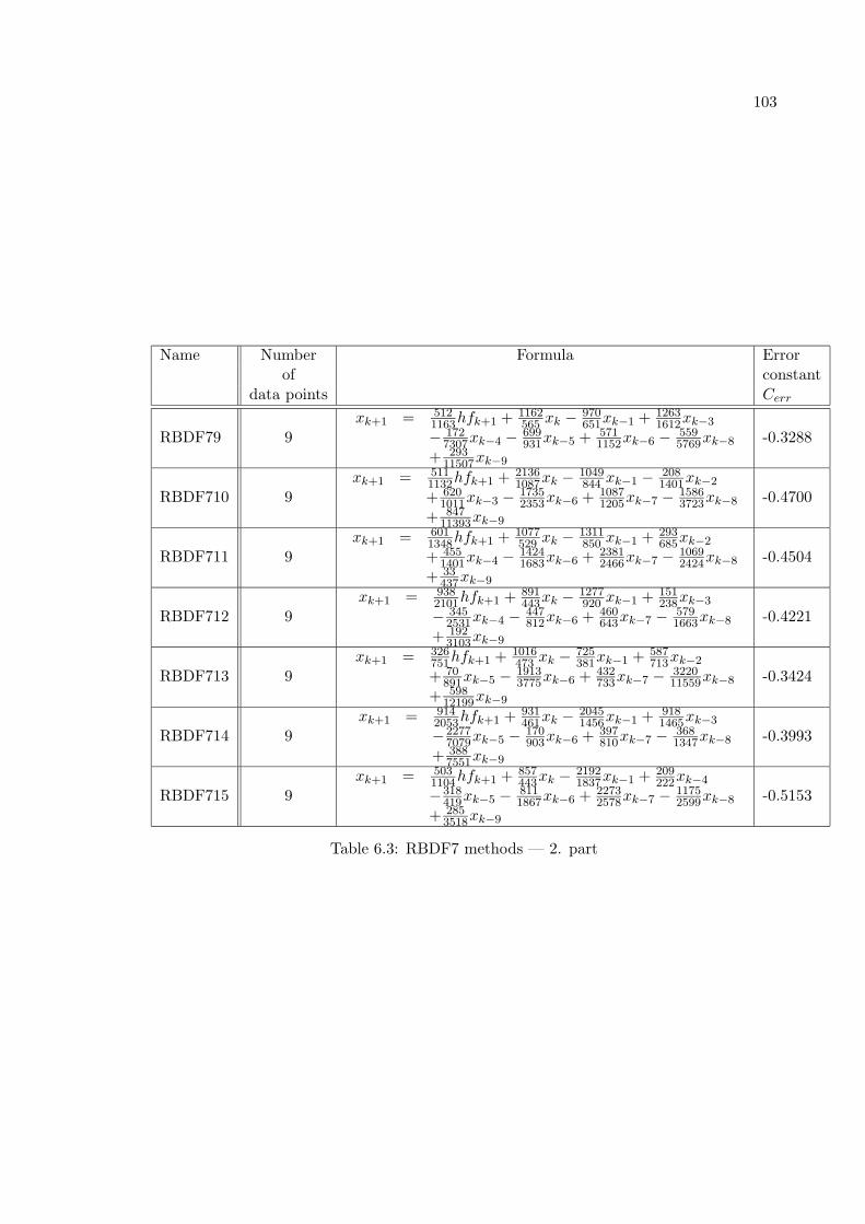
103
Name Number Formula Errorof constant
data points Cerr
RBDF79 9xk+1 = 512
1163hfk+1 + 1162565 xk − 970
651xk−1 + 12631612xk−3
− 1727307xk−4 − 699
931xk−5 + 5711152xk−6 − 559
5769xk−8
+ 29311507xk−9
-0.3288
RBDF710 9xk+1 = 511
1132hfk+1 + 21361087xk − 1049
844 xk−1 − 2081401xk−2
+ 6201011xk−3 − 1735
2353xk−6 + 10871205xk−7 − 1586
3723xk−8
+ 84711393xk−9
-0.4700
RBDF711 9xk+1 = 601
1348hfk+1 + 1077529 xk − 1311
850 xk−1 + 293685xk−2
+ 4551401xk−4 − 1424
1683xk−6 + 23812466xk−7 − 1069
2424xk−8
+ 33437xk−9
-0.4504
RBDF712 9xk+1 = 938
2101hfk+1 + 891443xk − 1277
920 xk−1 + 151238xk−3
− 3452531xk−4 − 447
812xk−6 + 460643xk−7 − 579
1663xk−8
+ 1923103xk−9
-0.4221
RBDF713 9xk+1 = 326
751hfk+1 + 1016473 xk − 725
381xk−1 + 587713xk−2
+ 70891xk−5 − 1913
3775xk−6 + 432733xk−7 − 3220
11559xk−8
+ 59812199xk−9
-0.3424
RBDF714 9xk+1 = 914
2053hfk+1 + 931461xk − 2045
1456xk−1 + 9181465xk−3
−22777079xk−5 − 170
903xk−6 + 397810xk−7 − 368
1347xk−8
+ 3887551xk−9
-0.3993
RBDF715 9xk+1 = 503
1104hfk+1 + 857443xk − 2192
1837xk−1 + 209222xk−4
−318419xk−5 − 811
1867xk−6 + 22732578xk−7 − 1175
2599xk−8
+ 2853518xk−9
-0.5153
Table 6.3: RBDF7 methods — 2. part

104
-4 -2 0 2 4 6 8 10 12-10
-8
-6
-4
-2
0
2
4
6
8
10
RBDF74
RBDF75
RBDF73
RBDF78
RBDF71
RBDF76
RBDF72
RBDF77
Figure 6.1: Stability domains of RBDF7 — 1. part
-2 0 2 4 6 8 10-8
-6
-4
-2
0
2
4
6
8
Re
Im
RBDF710RBDF711
RBDF79
RBDF715
RBDF712
RBDF714RBDF713
Figure 6.2: Stability domains of RBDF7 — 2. part

105
0 0.05 0.1 0.15 0.2 0.25 0.3 0.35 0.4 0.45 0.5-0.1
0
0.1
0.2
0.3
0.4
0.5
Anal. damping
Num
. dam
ping
Figure 6.3: Damping plots of RBDF7 — 1. part (RBDF71 through RBDF78)
0 0.05 0.1 0.15 0.2 0.25 0.3 0.35 0.4 0.45 0.5-0.1
0
0.1
0.2
0.3
0.4
0.5
Anal. damping
Num
. dam
ping
RBDF713
Figure 6.4: Damping plots of RBDF7 — 2. part (RBDF79 through RBDF715)
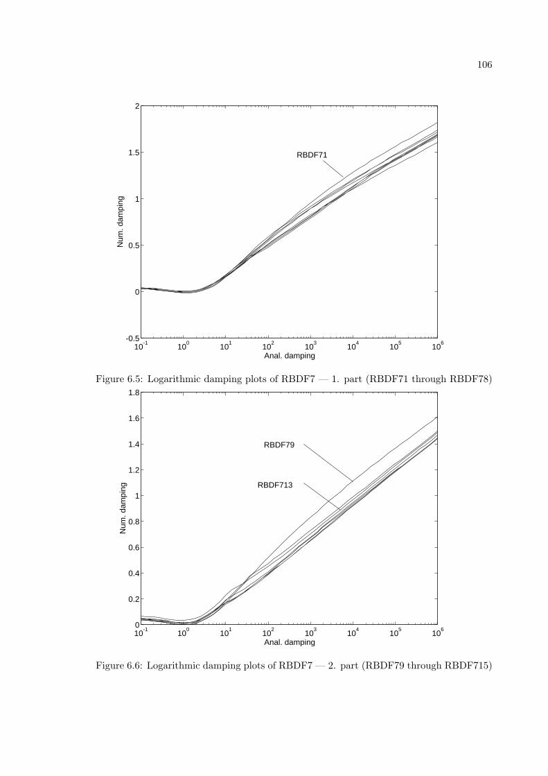
106
10-1
100
101
102
103
104
105
106
-0.5
0
0.5
1
1.5
2
Anal. damping
Num
. dam
ping
RBDF71
Figure 6.5: Logarithmic damping plots of RBDF7 — 1. part (RBDF71 through RBDF78)
10-1
100
101
102
103
104
105
106
0
0.2
0.4
0.6
0.8
1
1.2
1.4
1.6
1.8
Anal. damping
Num
. dam
ping RBDF713
RBDF79
Figure 6.6: Logarithmic damping plots of RBDF7 — 2. part (RBDF79 through RBDF715)
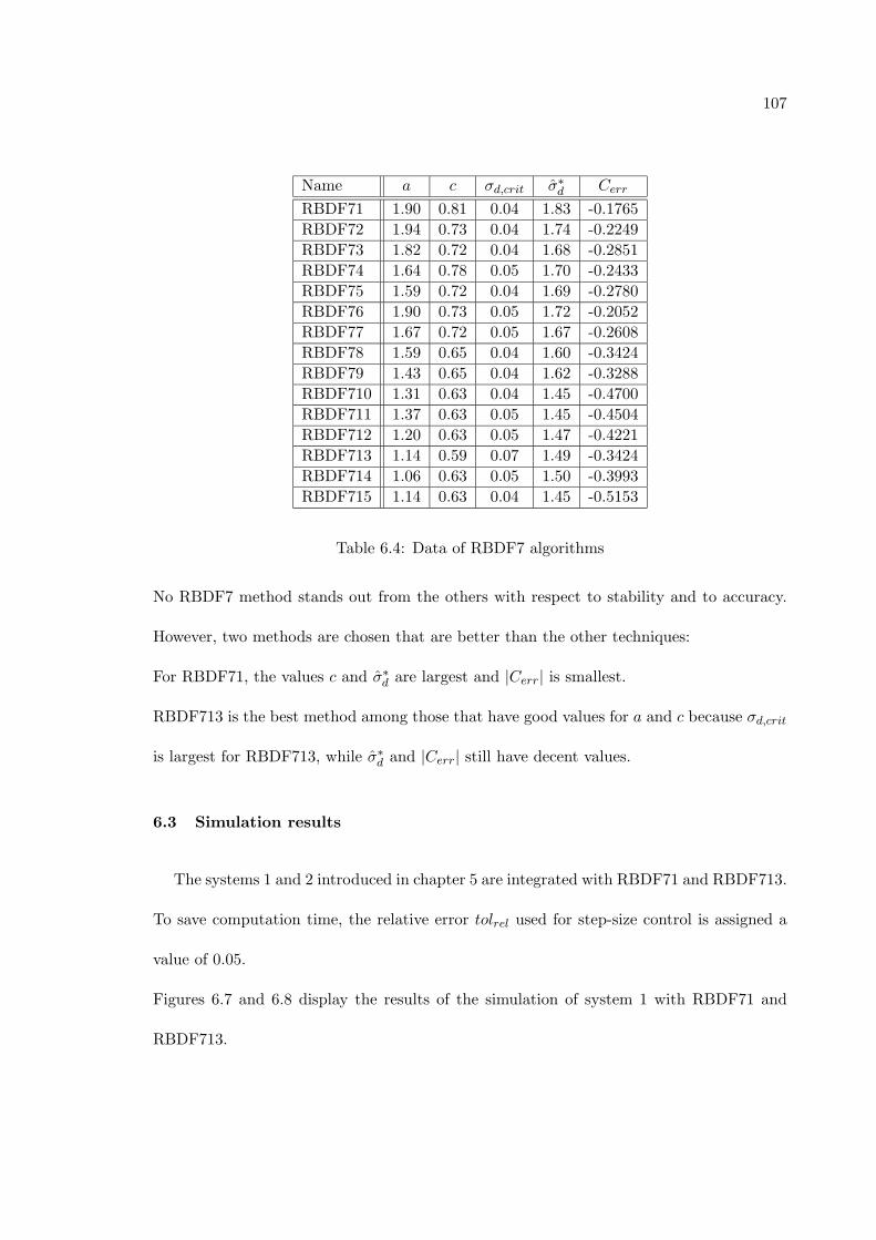
107
Name a c σd,crit σ∗d Cerr
RBDF71 1.90 0.81 0.04 1.83 -0.1765RBDF72 1.94 0.73 0.04 1.74 -0.2249RBDF73 1.82 0.72 0.04 1.68 -0.2851RBDF74 1.64 0.78 0.05 1.70 -0.2433RBDF75 1.59 0.72 0.04 1.69 -0.2780RBDF76 1.90 0.73 0.05 1.72 -0.2052RBDF77 1.67 0.72 0.05 1.67 -0.2608RBDF78 1.59 0.65 0.04 1.60 -0.3424RBDF79 1.43 0.65 0.04 1.62 -0.3288RBDF710 1.31 0.63 0.04 1.45 -0.4700RBDF711 1.37 0.63 0.05 1.45 -0.4504RBDF712 1.20 0.63 0.05 1.47 -0.4221RBDF713 1.14 0.59 0.07 1.49 -0.3424RBDF714 1.06 0.63 0.05 1.50 -0.3993RBDF715 1.14 0.63 0.04 1.45 -0.5153
Table 6.4: Data of RBDF7 algorithms
No RBDF7 method stands out from the others with respect to stability and to accuracy.
However, two methods are chosen that are better than the other techniques:
For RBDF71, the values c and σ∗d are largest and |Cerr| is smallest.
RBDF713 is the best method among those that have good values for a and c because σd,crit
is largest for RBDF713, while σ∗d and |Cerr| still have decent values.
6.3 Simulation results
The systems 1 and 2 introduced in chapter 5 are integrated with RBDF71 and RBDF713.
To save computation time, the relative error tolrel used for step-size control is assigned a
value of 0.05.
Figures 6.7 and 6.8 display the results of the simulation of system 1 with RBDF71 and
RBDF713.

108
It can be seen in these figures that RBDF71 integrates system 1 more accurately than
RBDF713 does.
Moreover, RBDF71 integrates system 1 faster since it only uses 249355 fops during the
simulation while RBDF713 needs to execute 278368 fops.
In figures 6.9 and 6.10 the results of the integration of the nonlinear system 2 are illustrated.
Again, these results show that RBDF71 behaves better than RBDF713, both with respect
to accuracy and to efficiency — RBDF71 needs 599412 fops and RBDF713 uses 672005 fops.
One might be tempted to think that the values σ∗d and Cerr are responsible for this behavior
since RBDF71 has better values σ∗d and Cerr than RBDF713 whereas the values a and σd,crit
are worse (see table 6.4).
However, the results of chapter 5 don’t confirm this assumption. Thus, only by considering
all of the properties of a numerical integration method it can be stated that this method is
better than another technique.
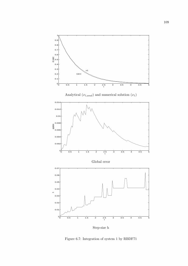
109
0 0.5 1 1.5 2 2.5 3 3.5 4 4.5 50
0.1
0.2
0.3
0.4
0.5
0.6
0.7
0.8
0.9
1
t
x1,xa
cc
x1
xacc
Analytical (x1,anal) and numerical solution (x1)
0 0.5 1 1.5 2 2.5 3 3.5 4 4.5 50
0.002
0.004
0.006
0.008
0.01
0.012
0.014
t
epsil
on
Global error
0 0.5 1 1.5 2 2.5 3 3.5 4 4.5 50
0.01
0.02
0.03
0.04
0.05
0.06
0.07
t
h
Step-size h
Figure 6.7: Integration of system 1 by RBDF71
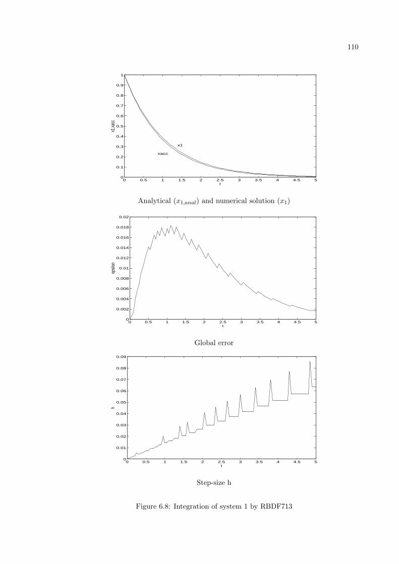
110
0 0.5 1 1.5 2 2.5 3 3.5 4 4.5 50
0.1
0.2
0.3
0.4
0.5
0.6
0.7
0.8
0.9
1
t
x1,xa
cc
xacc
x1
Analytical (x1,anal) and numerical solution (x1)
0 0.5 1 1.5 2 2.5 3 3.5 4 4.5 50
0.002
0.004
0.006
0.008
0.01
0.012
0.014
0.016
0.018
0.02
t
epsil
on
Global error
0 0.5 1 1.5 2 2.5 3 3.5 4 4.5 50
0.01
0.02
0.03
0.04
0.05
0.06
0.07
0.08
0.09
t
h
Step-size h
Figure 6.8: Integration of system 1 by RBDF713
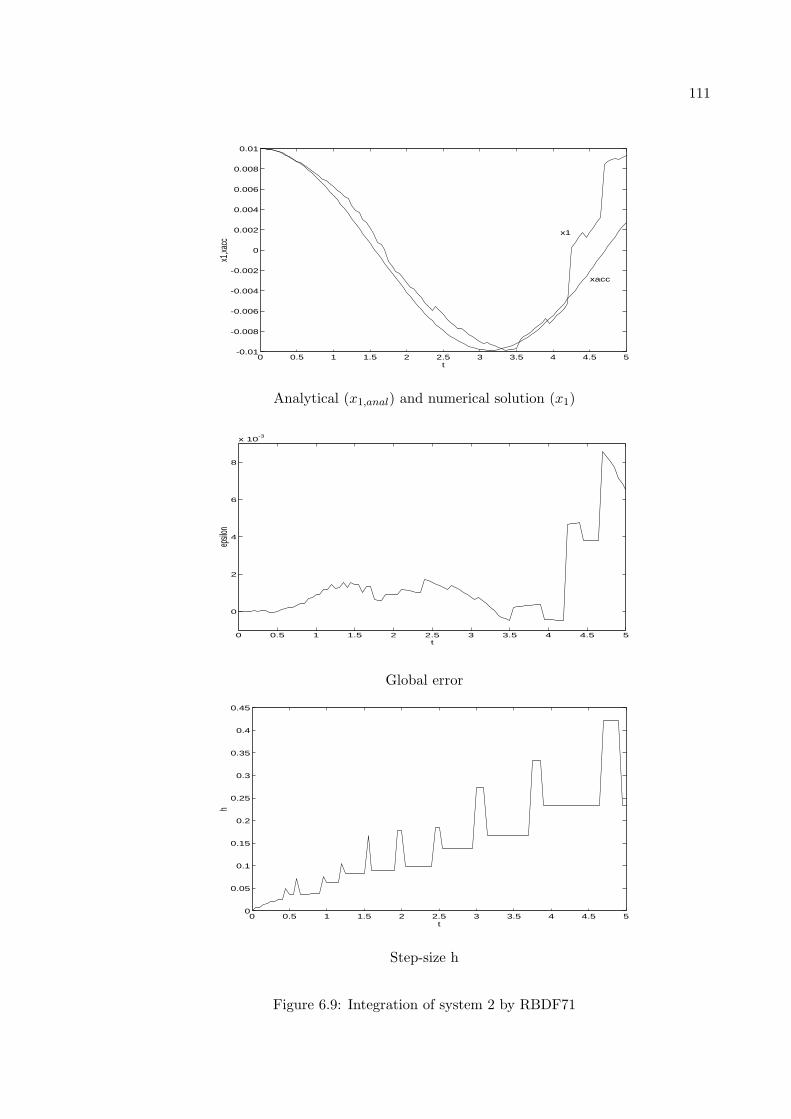
111
0 0.5 1 1.5 2 2.5 3 3.5 4 4.5 5-0.01
-0.008
-0.006
-0.004
-0.002
0
0.002
0.004
0.006
0.008
0.01
t
x1,xa
ccx1
xacc
Analytical (x1,anal) and numerical solution (x1)
0 0.5 1 1.5 2 2.5 3 3.5 4 4.5 5
0
2
4
6
8
x 10-3
t
epsilo
n
Global error
0 0.5 1 1.5 2 2.5 3 3.5 4 4.5 50
0.05
0.1
0.15
0.2
0.25
0.3
0.35
0.4
0.45
t
h
Step-size h
Figure 6.9: Integration of system 2 by RBDF71
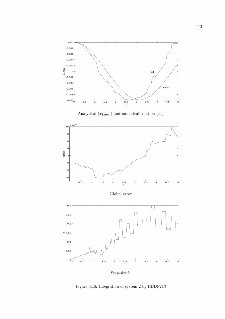
112
0 0.5 1 1.5 2 2.5 3 3.5 4 4.5 5-0.01
-0.008
-0.006
-0.004
-0.002
0
0.002
0.004
0.006
0.008
0.01
t
x1,xa
cc
x1
xacc
Analytical (x1,anal) and numerical solution (x1)
0 0.5 1 1.5 2 2.5 3 3.5 4 4.5 5
-4
-2
0
2
4
6
8
10x 10
-3
t
epsil
on
Global error
0 0.5 1 1.5 2 2.5 3 3.5 4 4.5 50
0.05
0.1
0.15
0.2
0.25
0.3
t
h
Step-size h
Figure 6.10: Integration of system 2 by RBDF713
113
CHAPTER 7
Conclusions
In chapter 3, two new analysis methods for assessing numerical integration algorithms
have been introduced:
1. Order star – accuracy region analysis
2. Bode plot analysis
The RBDF6 techniques presented in chapter 5 can compete with BDF6 in integrating stiff
systems, a fact that has been verified in numerous simulations. In most of the cases con-
sidered in this thesis, the two algorithms RBDF61 and RBDF66 outperform BDF6, and
because of the better shape of their Bode plot it may be concluded that they would do
better than BDF6 when integrating a stiff system with noise input. However, this hasn’t
been proven so far and might be a topic of further research.
As seen in chapter 6, the RBDF7 methods offer a way to integrate stiff systems of
ordinary differential equations with an accuracy order of 7 based on backward difference
formulae. This hasn’t been possible so far since there don’t exist stable BDF methods of
order higher than 6.

114
The regression approach introduced in this thesis to find stiffly stable integration algo-
rithms of accuracy order seven, could be used to identify new stiffly stable RBDF methods
of even higher accuracy orders.
Such methods would be of much interest for use in celestial dynamics where highly
accurate integration of ordinary differential equations is required.

115
Appendix A
Nordsieck transformation matrices of different order
Appendix A contains transformation matrices T of different order that are used to
calculate the Nordsieck vector.
1. m = 2, ng = 1:
T =
⎛⎜⎜⎜⎝
1 0
1 −1
⎞⎟⎟⎟⎠ .
2. m = 3, ng = 2:
T =
⎛⎜⎜⎜⎜⎜⎜⎜⎝
1 0 0
32 −2 1
2
12 −1 1
2
⎞⎟⎟⎟⎟⎟⎟⎟⎠
.
3. m = 4, ng = 3:
T =
⎛⎜⎜⎜⎜⎜⎜⎜⎜⎜⎜⎜⎜⎝
1 0 0 0
116 −3 3
2 −13
1 −52 2 −1
2
16 −1
212 −1
6
⎞⎟⎟⎟⎟⎟⎟⎟⎟⎟⎟⎟⎟⎠
.
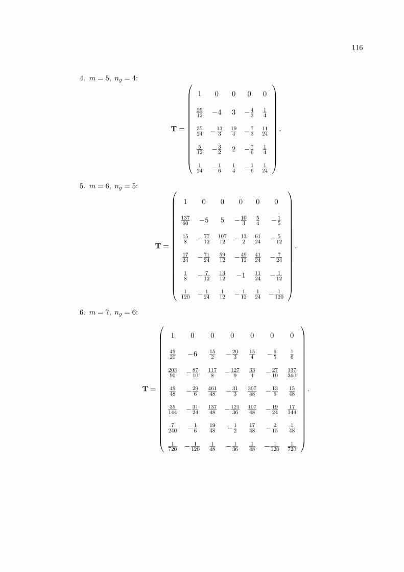
116
4. m = 5, ng = 4:
T =
⎛⎜⎜⎜⎜⎜⎜⎜⎜⎜⎜⎜⎜⎜⎜⎜⎜⎝
1 0 0 0 0
2512 −4 3 −4
314
3524 −13
3194 −7
31124
512 −3
2 2 −76
14
124 −1
614 −1
6124
⎞⎟⎟⎟⎟⎟⎟⎟⎟⎟⎟⎟⎟⎟⎟⎟⎟⎠
.
5. m = 6, ng = 5:
T =
⎛⎜⎜⎜⎜⎜⎜⎜⎜⎜⎜⎜⎜⎜⎜⎜⎜⎜⎜⎜⎜⎜⎝
1 0 0 0 0 0
13760 −5 5 −10
354 −1
5
158 −77
1210712 −13
26124 − 5
12
1724 −71
245912 −49
124124 − 7
24
18 − 7
121312 −1 11
24 − 112
1120 − 1
24112 − 1
12124 − 1
120
⎞⎟⎟⎟⎟⎟⎟⎟⎟⎟⎟⎟⎟⎟⎟⎟⎟⎟⎟⎟⎟⎟⎠
.
6. m = 7, ng = 6:
T =
⎛⎜⎜⎜⎜⎜⎜⎜⎜⎜⎜⎜⎜⎜⎜⎜⎜⎜⎜⎜⎜⎜⎜⎜⎜⎜⎝
1 0 0 0 0 0 0
4920 −6 15
2 −203
154 −6
516
20390 −87
101178 −127
9334 −27
10137360
4948 −29
646148 −31
330748 −13
61548
35144 −31
2413748 −121
3610748 −19
2417144
7240 −1
61948 −1
21748 − 2
15148
1720 − 1
120148 − 1
36148 − 1
1201
720
⎞⎟⎟⎟⎟⎟⎟⎟⎟⎟⎟⎟⎟⎟⎟⎟⎟⎟⎟⎟⎟⎟⎟⎟⎟⎟⎠
.

117
7. m = 8, ng = 7:
T =
⎛⎜⎜⎜⎜⎜⎜⎜⎜⎜⎜⎜⎜⎜⎜⎜⎜⎜⎜⎜⎜⎜⎜⎜⎜⎜⎜⎜⎜⎜⎜⎝
1 0 0 0 0 0 0 0
363140 −7 21
2 −353
354 −21
576 −1
7
469180 −223
2087940 −949
36412 −201
201019360 − 7
20
967720 −319
453929240 −389
182545144 −134
151849720 −29
90
718 −111
487112 −1219
144223 −185
484136 − 7
48
23360 − 59
14498 −247
14411372 −69
801972 − 5
144
1180 − 3
8013120 − 25
14416 − 23
24011360 − 1
240
15040 − 1
7201
240 − 1144
1144 − 1
2401
720 − 15040
⎞⎟⎟⎟⎟⎟⎟⎟⎟⎟⎟⎟⎟⎟⎟⎟⎟⎟⎟⎟⎟⎟⎟⎟⎟⎟⎟⎟⎟⎟⎟⎠
.
8. m = 9, ng = 8:
T =
⎛⎜⎜⎜⎜⎜⎜⎜⎜⎜⎜⎜⎜⎜⎜⎜⎜⎜⎜⎜⎜⎜⎜⎜⎜⎜⎜⎜⎜⎜⎜⎜⎜⎜⎜⎝
1 0 0 0 0 0 0 0 0
761280 −8 14 −56
3352 −56
5143 −8
718
2953110080 −481
3562120 −2003
4569116 −141
52143180 −103
353631120
267160 −349
3618353720 −2391
60145736 −4891
18056148 −527
1804691440
10691920 −329
90152891440 −268
1510993576 −1193
902803480 −67
459675760
980 −115
14417972 −213
4817936 −2581
720138 − 61
1447
144
13960 − 73
720239720 −149
240209288 −391
72061240 − 49
72023
2880
11120 − 1
1441195040 − 231
5040118 − 217
5040148 − 29
50401
1440
140320 − 1
50401
1440 − 1720
1576 − 1
7201
1440 − 15040
140320
⎞⎟⎟⎟⎟⎟⎟⎟⎟⎟⎟⎟⎟⎟⎟⎟⎟⎟⎟⎟⎟⎟⎟⎟⎟⎟⎟⎟⎟⎟⎟⎟⎟⎟⎟⎠
.

118
9. m = 10, ng = 9:
T =
⎛⎜⎜⎜⎜⎜⎜⎜⎜⎜⎜⎜⎜⎜⎜⎜⎜⎜⎜⎜⎜⎜⎜⎜⎜⎜⎜⎜⎜⎜⎜⎜⎜⎜⎜⎜⎜⎜⎜⎜⎝
1 0 0 0 0 0 0 0 0 0
71292520 −9 18 −28 63
2 −1265 14 −36
798 −1
9
65152016 −4609
2805869140 −6289
90649980 −265
46709180 −967
7034071120 − 761
2520
45232268 −14139
112020837560 −72569
1080651980 −3273
48843072160 −4101
2801823560 −29531
90720
95128 −7667
1440249011440 −4013
1201222492880 −5273
14410279480 −2939
360105795760 − 89
480
301317280 −7807
576067871440 −13873
1440367692880 −32773
288098231440 −3817
144034875760 − 1069
17280
5192 − 77
360563720 −401
24033131440 −305
144313240 −373
7203472880 − 1
80
2912096 − 413
20160790 − 31
1803531440 − 67
28853360 − 151
2520287
20160 − 9160480
18064 − 11
1008043
10080 − 7720
412880 − 1
7291
10080 − 195040
3740320 − 1
10080
1362880 − 1
403201
10080 − 14320
12880 − 1
28801
4320 − 110080
140320 − 1
362880
⎞⎟⎟⎟⎟⎟⎟⎟⎟⎟⎟⎟⎟⎟⎟⎟⎟⎟⎟⎟⎟⎟⎟⎟⎟⎟⎟⎟⎟⎟⎟⎟⎟⎟⎟⎟⎟⎟⎟⎟⎠
.

119
Appendix B
Implementation of RBDF61 in MATLAB to integrate (non-)linear
ordinary differential equations of first order
Appendix B contains a complete listing of the MATLAB program ”INT” that represents
the implementation of the RBDF61 method .
By slightly modifying this program, other RBDF techniques introduced in this thesis can
be implemented as well.
B.1 Main program INT
% Program to integrate ordinary differential equations of
% first order
%
flops(0)
define
% order of the integration algorithm
order = 6
steps = order + 1 % number of steps that we go backwards within the state
% history vector
all points = 15
120
algor = 3
load searchmethod7
pick = picks(algor,:)
%
Ms = [ 0 1 2 3 4 5 6; 1 0 0 0 0 0 0; 0 1 0 0 0 0 0; 1 -1 1 -1 1 -1 1; 0 1 -2 3 -4 5 -6; 1 -2 4
-8 16 -32 64; 0 1 -4 12 -32 80 -192; 1 -3 9 -27 81 -243 729; 0 1 -6 27 -108 405 -1458; 1 -4 16
-64 256 -1024 4096; 0 1 -8 48 -256 1280 -6144; 1 -5 25 -125 625 -3125 15625; 0 1 -10 75 -500
3125 -18750; 1 -6 36 -216 1296 -7776 46656; 0 1 -12 108 -864 6480 -46656; 0 1 -12 108 -864
6480 -46656; 1 -7 49 -343 2401 -16807 117649; 0 1 -14 147 -1372 12005 -100842 ]
M = Ms(pick,:)
if rank(M) == order+1
% Penrose-Moore-Pseudoinverse
Minv = inv(M’*M)*M’
s = Minv(1,:)
for k=2:order+1
s = s + Minv(k,:)
end
ss = zeros(1,all points)
ss(pick) = s
end
startup
[xvec,tvec,hvec] = mult(xvec,tvec,hvec,t,tsim,tcom,h,A,B,u,order,...
s,ss,all points,xhist,tolrel,deltat,...
121
delta,pick,found,steps)
fop = flops % number of floating point operations
acc = exp(-tvec)
epsvec = xvec(:,1) – xacc
save 703mo1 xvec tvec hvec fop xacc epsvec
B.2 Procedure DEFINE
tolrelruku = 1E-6 % tolerance for the relative error produced by
% the Runge Kutta startup algorithm
tolrel = 1E-3 % tolerance of the relative error of the multistep algorithm
% stability domain of Ruku 5th order
stab limit = 2.6
deltat = 0.05 % Length of communication interval
tsim = 5.0 % Simulation time
t = 0
tcom = 0
% Definition of the system
A =[ 0 1; -1000 -1001]
B = [0;0]
C = 0
D = 0
max eig = max(abs(eig(A)))

122
% Input
u = 0
% Initial state vector x(0)
x = [1; -1]
n = size(x,1)
delta = ones(1,n)*1E-10
ECHO = 1
xvec = x’
tvec = tcom
hvec = 0
xcom = x’ % state vector that is depicted graphically
xhist = x % whole state history matrix
B.3 Procedure STARTUP
bin search h0
if found == 1
x = x2
t = h
tcom = 0
if t >= tcom + deltat
% communication
comm

123
end
xhist = [x, xhist]
% order–1 times Runge Kutta 6th order with fixed step-size
for i=1:order–1
t = t + h
ruku6
x = x2
xhist = [x, xhist]
if t >= tcom + deltat
comm
end
end
end
B.4 Procedure BIN SEARCH H0
% This program calculates the initial step-size h for the
% multistep algorithm by means of a binary search
%
deltas = delta
ts = t
xs = x
hmin = 0
hmax = stab limit/max eig

124
maxcount = 30 % maximal number of steps of the binary search
count = 0
found = 0 % =1: Initial step-size h is found
% =0: Initial step-size h can’t be found
xlast = x
terminate= -1
% Is hmax the step-size we are searching for?
h = hmax
ruku5
ruku6
eps1 = abs((x1 – x2)’)
v = [x1’;x2’;delta]
epsrel= max(eps1 ./ max(abs(v)))
if epsrel < tolrelruku*1E-6 % too accurate —> change the initial values!
% First step with ruku6 to reevaluate the initial conditions
t = t + 0.5*(hmax+hmin)
ruku6
x = x2
delta = delta*1E-10
else
if epsrel <= tolrelruku
terminate = 1
found = 1
125
end
end
while terminate < 0
h = 0.5*(hmin + hmax)
ruku5
ruku6
eps1 = abs((x1 – x2)’)
v = [x1’;x2’;delta]
epsrel= max(eps1 ./ max(abs(v)))
if epsrel > tolrelruku
hmax = h
else
hmin = h
if epsrel >= 0.9*tolrelruku
terminate = 1
found = 1
else
if count > maxcount
terminate = 1
else
count = count + 1
end
end

126
end
end
if delta < deltas
t = ts
x = xs
ruku6
end
B.5 Procedure RUKU5
% This program executes one step of a Runge Kutta 5th order
%
K1 = h*func(x,t,u)
K2 = h*func(x+0.125*K1,t,u)
K3 = h*func(x+0.25*K2,t,u)
K4 = h*func(x+0.5*K1–K2+K3,t,u)
K5 = h*func(x+0.1875*K1+0.5625*K4,t,u)
K6 = h*func(x+(–5*K1+4*K2+12*K3–12*K4+8*K5)/7,t,u)
x1 = x + (7*K1 + 32*K3 + 12*K4 + 32*K5 + 7*K6)/90

127
B.6 Procedure RUKU6
% This program executes one step of a Runge Kutta 6th order
%
K1 = h*func(x,t,u)
K2 = h*func(x+K1/9,t,u)
K3 = h*func(x+(K1+3*K2)/24,t,u)
K4 = h*func(x+(K1–3*K2+4*K3)/6,t,u)
K5 = h*func(x–0.625*K1+3.375*K2–3.0*K3+6.0*K4,t,u)
K6 = h*func(x+(221*K1–981*K2+867*K3–102*K4+K5)/9,t,u)
K7 = h*func(x+(-783*K1+678*K2–472*K3–66*K4+80*K5+3*K6)/48,t,u)
K8 = h*func(x+(761*K1–2079*K2+1002*K3+834*K4–454*K5–9*K6+72*K7)/82,t,u)
x2 = x + (41*K1 + 216*K2 + 27*K4 + 272*K5 + 27*K6 + 216*K7 + 41*K8)/840
B.7 Procedure COMM
% This procedure calculates the communication state vector that is
% used further to depict the state vector equidistantly
%
ncom = (t – tcom)/deltat – rem(t – tcom,deltat)
deltat1 = tcom + deltat – t + h
% Note that deltat1 > epscom is fulfilled!
deltax = (x–xlast)*deltat1/h

128
xcom = xlast + deltax
xvec = [xvec; xcom]
tcom = tcom + deltat
tvec = [tvec; tcom]
hvec = [hvec; h]
if ncom > 1
ncom = ncom – 1
deltax = (x – xcom)*deltat/h
for i = 1:ncom
xcom = xcom + deltax
tcom = tcom + deltat
xvec = [xvec; xcom]
tvec = [tvec; tcom]
hvec = [hvec; h]
end
end
B.8 Function FUNC
% Implementation of system 3 (Rayleigh equation)
%
function [fu] = func(x,t,u)
%

129
w = 1 – x(1)*x(1) – x(2)*x(2)
fu1 = 0.01*x(2) – x(1)*w
fu2 = -0.01*x(1) – x(2)*w
fu = [fu1;fu2]
B.9 Function MULT
% Multistep algorithm
%
% xhist is now a (n x m) matrix
%
function [xvec,tvec,hvec] = mult(xvec,tvec,hvec,t,tsim,tcom,h,u,n,order,...
s,ss,all points,xhist,tolrel,deltat,...
delta,pick,found,steps)
%
I = eye(n)
toldelta = 0.1 % maximal value of the relative error that keeps the Jacobian unchanged
%
% Factorial of ”order”:
ordfac = 1
for i = 1:order
ordfac = ordfac*i
end
130
%
% Calculation of the error constant C err
%
B1 = 0
p1 = size(pick)p1 = p1(2)
A1 = [zeros(1,p1)]
B1 = [zeros(1,p1)]
for k=p1:-1:1
kk = pick(k)
if (0.5*kk–0.5) == fix(0.5*kk)
B1(steps–0.5*kk+1.5) = s(k)
else
A1(steps–0.5*kk+1)= -s(k)
end
end
A1(steps+1) = 1
C err = 0
for k = 1:p1,
k1 = k–1
Ak = A1(1,k)
Bk = B1(1,k)
C err = C err + (k1ˆ 7)*Ak/5040 – (k1ˆ 6)*Bk/720
end
131
%
factor = 1/1.2
p = 1/(order + 1)
if found == 1
% The first step of the multistep algorithm uses the old step-size
%
% Transformation matrix T to calculate the Nordsieck vector
%
T = [ 1 0 0 0 0 0 0; 2.45 -6 7.5 -20/3 3.75 -1.2 1/6; 20.3/9 -8.7 117/8 -127/9 33/4 -
2.7 137/360; 49/48 -29/6 461/48 -31/3 307/48 -13/6 5/16; 35/144 -31/24 137/48 -121/36
107/48 -19/24 17/144; 7/240 -1/6 19/48 -0.5 17/48 -2/15 1/48; 1/720 -1/120 1/48 -1/36
1/48 -1/120 1/720]
% Note: This matrix T is only valid for the order = 6!
if det(T’) == 0
else
Tinv = inv(T)
%
stepcount = 0
alpha = 1
N old = T*xhist’
n old = N old(order+1,:)
h old = h
chg jacob = 1 % Jacobian is reevaluated
132
epsmultold = delta
x = xhist(:,1) % initial value of x k+1 is x k!
first time = 1
while t < tsim
t = t + h
stepcount = stepcount + 1
finish step = -1
errcount = 0
chgstep = 0
while finish step < 0
one mul = -1
while one mul < 0
f = func(x,t,u)
if chg jacob > 0
% reevaluation of the Jacobian
jacob = jac(x,t,u,f,n)
chg jacob = 0
hess = ss(1)*h*jacob – I % Hesse matrix
inv hess = inv(hess)
else
if chgstep > 0
chgstep = 0
hess = ss(1)*h*jacob – I

133
inv hess = inv(hess)
end
end
% Modified Newton-Raphson iteration
[x,conver] = newton(all points,x,t,u,inv hess,h,conver,delta, ss,...
xhist,0.1*tolrel)
if conver > 0
% convergence of Newton-Raphson
xhist = [x, xhist]
xhist = xhist(:,1:order+1)
%
% Estimation of the relative error
N = T*xhist’ % We have to take the transposed history matrix!
epsmult = C err*ordfac*(N(order+1,:)–n old*alphaˆ order)
epsmult = abs(epsmult)
v = [abs(x’); delta]
xmax = max(v)
epsmultrel = max(epsmult ./ xmax)
deltaeps = (epsmultrel – epsmultold)/epsmultold
epsmultold = epsmultrel
if deltaeps > toldelta
if first time == 1
first time = 0
134
one mul = 1
else
chg jacob = 1
end
else
one mul = 1
end
else
x = xhist(:,1)
one mul = 1
finish step = 1
t = tsim
end % of if conver > 0
end % of while one mul
if conver > 0
% Newton iteration worked fine
if epsmultrel < tolrel
finish step = 1
else
% maybe change of the step-size
errcount = errcount + 1
if errcount >= 3
alpha = 0.5
135
stepcount = 0
chgstep = 1
h old = h
else
stepcount = order + 1
end
end
if stepcount >= order + 1
stepcount = 0
alpha = factor*(tolrel/epsmultrel)ˆp
if alpha >= 1
if alpha > 1.1
chgstep = 1
alpha = min(2,alpha)
else
% step-size is not changed
chgstep = 0
end
else
chgstep = 1
if alpha > 0.9
alpha = 0.9
else

136
alpha = max(alpha,0.5)
end
end % of if alpha >= 1
end % of if stepcount >= order+1
if chgstep > 0
% change of the step-size
chgstep = 0
h = alpha*h old
%Adjustment of the state history matrix
H = [1 0 0 0 0 0 0; 0 alpha 0 0 0 0 0; 0 0 alphaˆ 2 0 0 0 0; 0 0 0 alphaˆ 3 0 0 0; 0 0 0 0
alphaˆ 4 0 0; 0 0 0 0 0 alphaˆ 5 0; 0 0 0 0 0 0 alphaˆ 6]
if epsmultrel < tolrel
N = H*N % Nordsieck matrix
else
N = H*N old
end
xhist = Tinv*N
xhist = xhist’ % We have to transpose the matrix again
end % of if chgstep
end % of if conver > 0
end % of while finish step ..
N old = N
n old = N old(order+1,:)

137
h old = h
if t >= tcom + deltat
% communication point
[xvec,tvec,tcom,hvec] = comm mult(tcom,deltat,t,N,order,h,xvec,...
tvec,hvec,tsim)
end
end % of while t < tsim
end end
B.10 Function NEWTON
% Modified Newton iteration to solve the implicit equation of the
% integration algorithm
%
function [x,conver] = newton(all points,x,t,u,inv hess,h,conver,delta,ss,...
xhist,tolnewton)
%
finish = -1
count = 0
maxcount = 30
conver = 0
while finish < 0
x old = x

138
F = imp func(all points,ss,xhist,x,t,u,h)
x = x – inv hess*F
epsx = abs((x – x old)’)
v = [abs(x’);delta]
xmax = max(v)
epsrel = max(epsx ./ xmax)
if epsrel > tolnewton
if count > maxcount
conver = 0
finish = 1
else
count = count + 1
end
else
finish = 1
conver = 1
end
end
B.11 Function IMP FUNC
%This function calculates the implicit function of the integration algorithm
function [F] = imp func(all points,ss,xhist,x,t,u,h)

139
%
F = 0
for i = 2:all points % all points = size(ss)
if ss(i) == 0
else
if 0.5*i–0.5 == fix(0.5*i)
F = F + ss(i)*h*func(xhist(:,0.5*i–0.5),t,u)
else
F = F + ss(i)*xhist(:,0.5*i)
end
end
end
F = F + ss(1)*h*func(x,t,u) – x
B.12 Function JAC
% This program calculates the Jacobian matrix for the Newton iteration
%
function [J] = jac(x,t,u,f,n)
%
for i = 1:n % columns
xnew = x
if x(i) == 0

140
deltax = 1E-10
else
deltax = x(i)*1E-7
end
xnew(i) = xnew(i) + deltax
fnew = func(xnew,t,u)
J(:,i) = (fnew – f)/deltax
end
B.13 Function COMM MULT
% This function calculates the communication state vector if a
% multistep integration algorithm is used
%
function [xvec,tvec,tcom,hvec] = comm mult(tcom,deltat,t,N,order,...
h,xvec,tvec,hvec,tsim)
finish = -1
while finish < 0
if tcom + deltat <= t
tcom = tcom + deltat % update tcom
if tcom > tsim
finish = 1
else
141
d = tcom – t % negative step-size!
N1 = N
for i = 2:order+1
N1(i,:) = ((d/h)ˆ (i – 1)) * N1(i,:)
end
xcom = N1(1,:)
for i = 2:order+1
xcom = xcom + N1(i,:)
end
xvec = [xvec; xcom]
tvec = [tvec; tcom]
hvec = [hvec; h]
end
else
finish = 1
end
end