static loading test on a 45 m long pipe pile in … sandpoint cgj.pdfpage 1 static loading test on a...

Static Loading Test on a 45 m Long Pipe Pile in Sandpoint, Idaho

Bengt H. Fellenius Bengt Fellenius Consultants Inc.

1905 Alexander Street, Calgary, Alberta, T2G 4J3

Dean E. Harris CH2M Hill

700 Clearwater Lane, Boise, Idaho 83712

Donald G. Anderson CH2M Hill

PO Box 91500, Bellevue, Washington 98009-2050 FELLENIUS, B.H., HARRIS, D., and ANDERSON, D.G., 2003. Static loading test on a 45 m long pipe pile in Sandpoint, Idaho. Canadian Geotechnical Journal, Vol.41, No. 4, pp. 613 - 628..


Bengt H. Fellenius1), Dean E. Harris2), and Donald G. Anderson3)

Summary

Design of piled foundations for bridge structures for the realignment of US95 in Sandpoint, Idaho, required a pre-design static loading test on an instrumented, 406 mm diameter closed-toe pipe pile driven to 45 m depth in soft, compressible soil. The soil conditions at the site consist of a 9 m thick sand layer on normally consolidated, compressible post-glacial alluvial deposits to depths estimated to exceed 200 m. Field explorations included soil borings and CPTU soundings advanced to a depth of 80 m. The clay at the site is brittle and strain-softening, requiring special attention and consideration in geotechnical design of structures in the area. Effective stress parameters back-calculated from the static loading test performed 48 days after driving correspond to beta-coefficients of about 0.8 in the surficial 9 m thick sand layer and 0.15 at the upper boundary of the clay layer below, reducing to 0.07 in the clay layer at the pile toe, and a pile toe-bearing coefficient of 6. The beta-coefficients are low, which is probably due to pore pressures developing during the small shear movements during the test before the ultimate resistance of the clay was reached. The analyses of the results of the static loading test have included correction for residual load caused by fully mobilized negative skin friction down to 10 m depth and fully mobilized positive shaft resistance below 30 m depth with approximately no transfer of load between the pile and the clay from 10 m depth through 30 m depth. Key words

Pile loading test, Residual load, Strain-gage instrumentation, Load distribution, set-up, Pile modulus

_____________________________ 1)…Bengt Fellenius Consultants Inc., 1905 Alexander Street, Calgary, Alberta, T2G 4J3, e-address <[email protected]> 2) …CH2M Hill, 700 Clearwater Lane, Boise, Idaho 83712, e-address: <[email protected]>

3) …CH2M Hill, PO Box 91500, Bellevue, Washington 98009-2050, e-address: <[email protected]>


Bengt H. Fellenius, Dean E. Harris, and Donald G. Anderson

INTRODUCTION

The realigned US95 in Sandpoint, Idaho, will be in an area underlain by soft, compressible soil to depths greater than 80 m, possibly as deep as about 200 m. The design includes a number of embankments and bridges. The bridge structures will be supported on driven, closed-toe pipe piles requiring considerations of axial capacity, dragload, and downdrag (settlement). Detailed geotechnical explorations were made in accordance with the general requirements of the Idaho Transportation Department (ITD). The explorations included drilling and sampling, piezocone penetrometer sounding (CPTU), and laboratory testing. To study the pile response to axial loading, a static loading test was conducted on an instrumented 45 m long steel pipe pile. The test pile was driven on August 29, 2001, and the static loading test was performed on October 17, 2001, 48 days later. The purpose of this paper is to present the results and interpretations of the pile-loading test in terms of load-transfer and distribution of residual load and corresponding soil shear parameters. The results have led to some interesting observations and conclusions regarding the design of pile-supported structures in these very soft soils. SITE AND SOIL DESCRIPTION

Site Description and Soil Profile

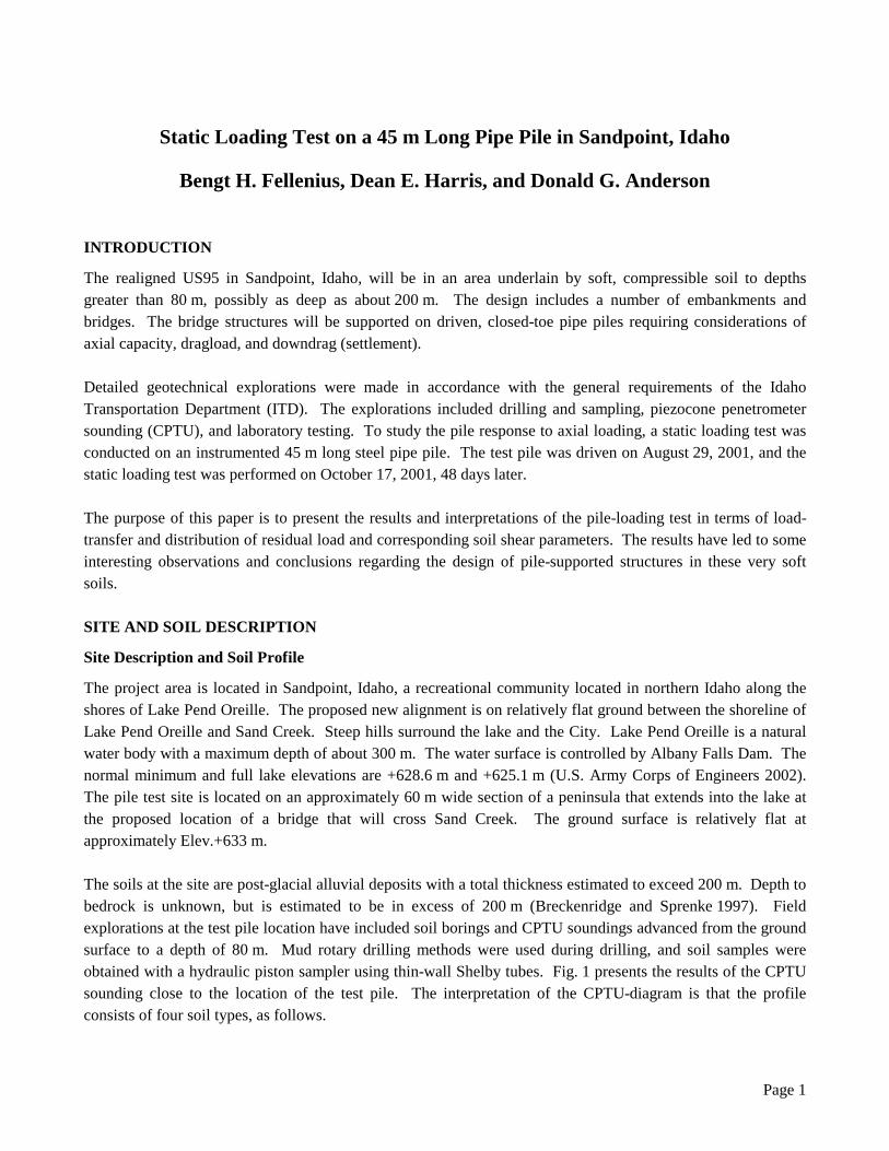
The project area is located in Sandpoint, Idaho, a recreational community located in northern Idaho along the shores of Lake Pend Oreille. The proposed new alignment is on relatively flat ground between the shoreline of Lake Pend Oreille and Sand Creek. Steep hills surround the lake and the City. Lake Pend Oreille is a natural water body with a maximum depth of about 300 m. The water surface is controlled by Albany Falls Dam. The normal minimum and full lake elevations are +628.6 m and +625.1 m (U.S. Army Corps of Engineers 2002). The pile test site is located on an approximately 60 m wide section of a peninsula that extends into the lake at the proposed location of a bridge that will cross Sand Creek. The ground surface is relatively flat at approximately Elev.+633 m. The soils at the site are post-glacial alluvial deposits with a total thickness estimated to exceed 200 m. Depth to bedrock is unknown, but is estimated to be in excess of 200 m (Breckenridge and Sprenke 1997). Field explorations at the test pile location have included soil borings and CPTU soundings advanced from the ground surface to a depth of 80 m. Mud rotary drilling methods were used during drilling, and soil samples were obtained with a hydraulic piston sampler using thin-wall Shelby tubes. Fig. 1 presents the results of the CPTU sounding close to the location of the test pile. The interpretation of the CPTU-diagram is that the profile consists of four soil types, as follows.

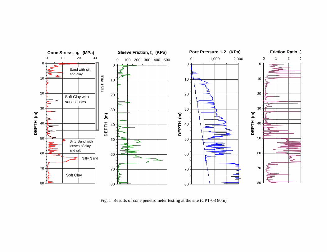
Fig. 1 Results of cone penetrometer testing at the site (CPT-03 80m)

0

10

20

30

40

50

60

70

80

0 10 20 30Cone Stress, qt (MPa)

DEP

TH (

m)

0

10

20

30

40

50

60

70

80

0 100 200 300 400 500

Sleeve Friction, fs (KPa)

DEP

TH (

m)

0

10

20

30

40

50

60

70

80

0 1,000 2,000

Pore Pressure, U2 (KPa)

DEP

TH (

m)

0

10

20

30

40

50

60

70

80

0 1 2 3

Friction Ratio (

DEP

TH (

m)

Sand with silt and clay

Soft Clay with sand lenses

Silty Sand with lenses of clay and silt

Soft Clay

Silty Sand

TES

T P

ILE

(Layer 1) a 9 m thick layer of sandy and silty soil.

(Layer 2) an approximately 40 m thick layer of clay from 9 m to 48 m, containing several approximately 500 mm thick layers or seams of loose to medium dense sandy silt and silt. Five slightly thicker sand zones exist in the clay at depths of 24.6 m (0.90 m thick), 31.9 m (0.20 m thick), 37.1 m (0.40 m thick), 41.8 m (0.20 m thick), and 44.9 m (0.40 m thick).

(Layer 3) a 17 m thick layer of an alternating sequence of silt, silt with sand, and sandy silt and clay to a depth of approximately 65 m. This sequence is referred to collectively as “silt”.

(Layer 4) an approximately 15 m thick layer of silt and clay from 65 m depth to the end of the CPTU sounding at 80 m depth, and probably continuing beyond this depth.

The friction ratio in Layers 2 and 4 ranges from 0.2 % to 0.3 %, which is smaller than usually found for clays. Such a small value is considered indicative for sensitive clay. However, vane shear tests at the site do not indicate any appreciable sensitivity. The results of a soil classification of the CPTU data according to the Eslami-Fellenius CPTU-method (Eslami 1996; Fellenius and Eslami 2000) are presented in Fig. 2. The data points of the CPT sounding have been plotted in four charts, one for each of the four soil layers. For Layer 2, different symbols are used for values classified as clay and for values identifying sand lenses within the clay.

Fig. 2 CPTU soil classification chart according to the Eslami-Fellenius method. The measurements have been plotted separated on the four layers

0.1

1

10

100

1 10 100 1,000Sleeve Friction (KPa)

Con

e St

ress

, qE

(MPa

)

0.1

1

10

100


Con

e St

ress

, qE

(MPa

)

0.1

1

10

100


Con

e St

ress

, qE

(MPa

)

0.1

1

10

100


Con

e St

ress

, qE

(MPa

)

Depth 0m - 9 m

1 = Very Soft Clays, Sensitive, and/or Collapsible Soils. 4a = Sandy Silt 2 = Clay and/or Silt 4b = Silty Sand 3 = Clayey Silt and/or Silty Clay 5 = Sand to Sandy Gravel

1

55

5 5

Depth 9m - 50 m

Depth 50m - 65 m Depth 65m - 80 m

4

4

4

4

3 3

3 3

22

22

1

11

baa

a a

b

bb

LAYER 4

LAYER 1 LAYER 2

LAYER 3

CLAYSAND SEAM

Piezometer Observations

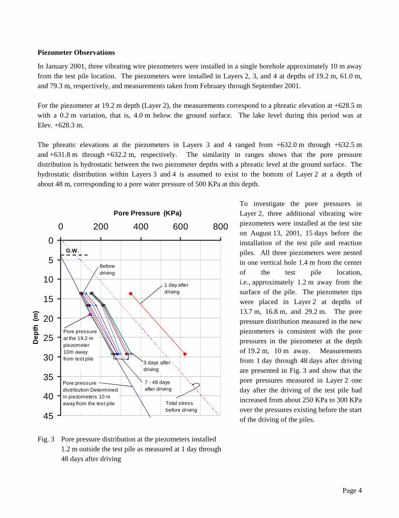
In January 2001, three vibrating wire piezometers were installed in a single borehole approximately 10 m away from the test pile location. The piezometers were installed in Layers 2, 3, and 4 at depths of 19.2 m, 61.0 m, and 79.3 m, respectively, and measurements taken from February through September 2001. For the piezometer at 19.2 m depth (Layer 2), the measurements correspond to a phreatic elevation at +628.5 m with a 0.2 m variation, that is, 4.0 m below the ground surface. The lake level during this period was at Elev. +628.3 m. The phreatic elevations at the piezometers in Layers 3 and 4 ranged from +632.0 m through +632.5 m and +631.8 m through +632.2 m, respectively. The similarity in ranges shows that the pore pressure distribution is hydrostatic between the two piezometer depths with a phreatic level at the ground surface. The hydrostatic distribution within Layers 3 and 4 is assumed to exist to the bottom of Layer 2 at a depth of about 48 m, corresponding to a pore water pressure of 500 KPa at this depth.

To investigate the pore pressures in Layer 2, three additional vibrating wire piezometers were installed at the test site on August 13, 2001, 15 days before the installation of the test pile and reaction piles. All three piezometers were nested in one vertical hole 1.4 m from the center of the test pile location, i.e., approximately 1.2 m away from the surface of the pile. The piezometer tips were placed in Layer 2 at depths of 13.7 m, 16.8 m, and 29.2 m. The pore pressure distribution measured in the new piezometers is consistent with the pore pressures in the piezometer at the depth of 19.2 m, 10 m away. Measurements from 1 day through 48 days after driving are presented in Fig. 3 and show that the pore pressures measured in Layer 2 one day after the driving of the test pile had increased from about 250 KPa to 300 KPa over the pressures existing before the start of the driving of the piles.

Fig. 3 Pore pressure distribution at the piezometers installed 1.2 m outside the test pile as measured at 1 day through 48 days after driving

0

5

10

15

20

25

30

35

40

45

0 200 400 600 800Pore Pressure (KPa)

Dep

th (

m)

1 day after driving

3 days afterdriving

Beforedriving

Pore pressure distribution Determined in piezometers 10 m away from the test pile

Pore pressure at the 19.2 m piezometer 10m away from test pile

7 - 48 days after driving

G.W.

Total stress before driving

The measurements indicate that the pore pressures introduced by the pile driving had essentially dissipated at the time of the static loading test, 48 days after the driving. Laboratory Tests

The results of the laboratory tests on soil samples are compiled in Table 1. The samples were recovered from a borehole advanced about 10 m away from the test pile location and from two other boreholes located adjacent to the test site. The tests determined that the natural water content in the clay layer, Layer 2, ranges from 40 % through 57 %. The consistency limit tests the that the water content is higher than or approximately equal to the Liquid Limit. In the silt and clay layer below 66 m, the average water content is 38 %, a few percentage points higher than the Liquid Limit. Grain-size and hydrometer tests on clay samples were performed in Layers 2 and 4 at depths 28.6 m and 76.4 m, respectively. The results indicate a high percentage of clay size particles in Layer 2, 88 %. In Layer 4, the soil is made up of 42 % clay and 58 % silt size particles. Consolidation (oedometer) tests were performed on samples obtained from Layer 2 at depths of 12.9 m, 18.6 m, and 34.2 m, i.e., within the test pile embedment depth. One test was performed on a sample from Layer 4 at depth 67.4 m. The results from 12.9 m and 18.6 m depths indicate that the Layer 2 clay is slightly overconsolidated with preconsolidation stresses of 200 KPa and 250 KPa, respectively, which are about 50 KPa and 75 KPa, respectively, larger than the effective overburden stress at these depths. The samples from 34.2 m (Layer 2) and 67.4 m (Layer 4) are disturbed and no preconsolidation stress is discernable. The compressibility determined by the consolidometer tests are expressed in terms of Janbu Modulus Number, “m” (Canadian Foundation Engineering Manual, 1992). The tests at depths 12.9 m and 18.6 m indicate modulus numbers of 12 and 14, respectively. These values correspond to Cc and e0 values of 0.44 and 1.28 at 12.9 m depth and 0.40 and 1.36 at 18.6 m depth, respectively. The undrained shear strength in Layer 2 determined from field vane tests close to the test pile location ranges from about 30 KPa at the top of the layer to about 70 KPa at the bottom of the layer. PREVIOUS PILE TESTS IN THE AREA

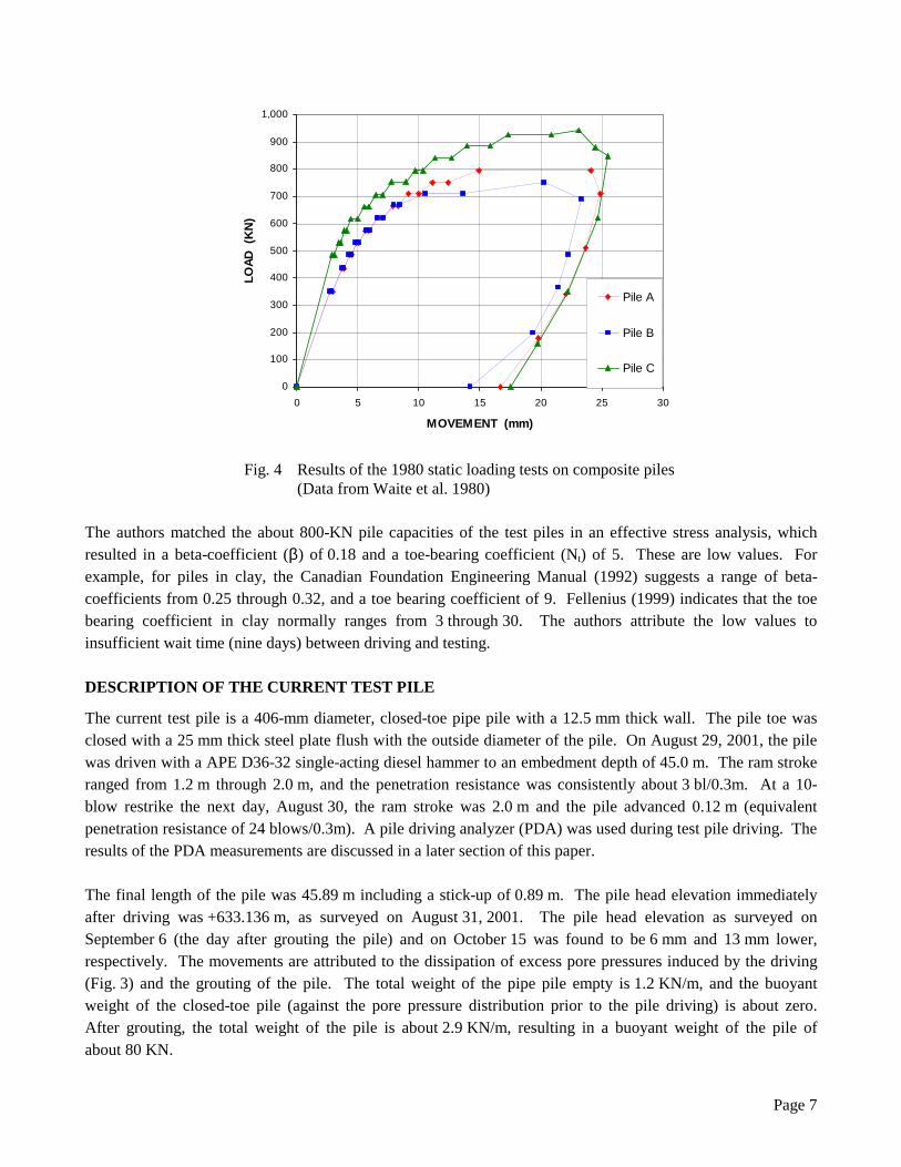
Pile tests were carried out previously in Sandpoint (Waite et al. 1980) about 500 m from the current test site. Three composite piles were driven to a total embedment depth of 30 m. Each pile consisted of an upper 406 mm diameter open steel pipe with a 9.5 mm thick wall spliced to a 15 m long wood pile with a toe diameter ranging from 150 mm through 250 mm. Static loading tests were performed nine days after the driving. The measured load-movement curves are presented in Fig.4. From the shape of the curves, it is estimated that the ultimate resistance for the piles was reached at a pile head movement of about 10 mm to 15 mm. The ultimate resistance ranged from about 700 KN through 900 KN with an average of about 800 KN. As the piles were not instrumented, the resistance distributions cannot be established. However, the ultimate resistance was reached in a plunging mode, indicating that most of the capacity mobilized in the test was shaft resistance. The resistance actually reduced with increasing movement, indicating a strain softening behavior of the clay.

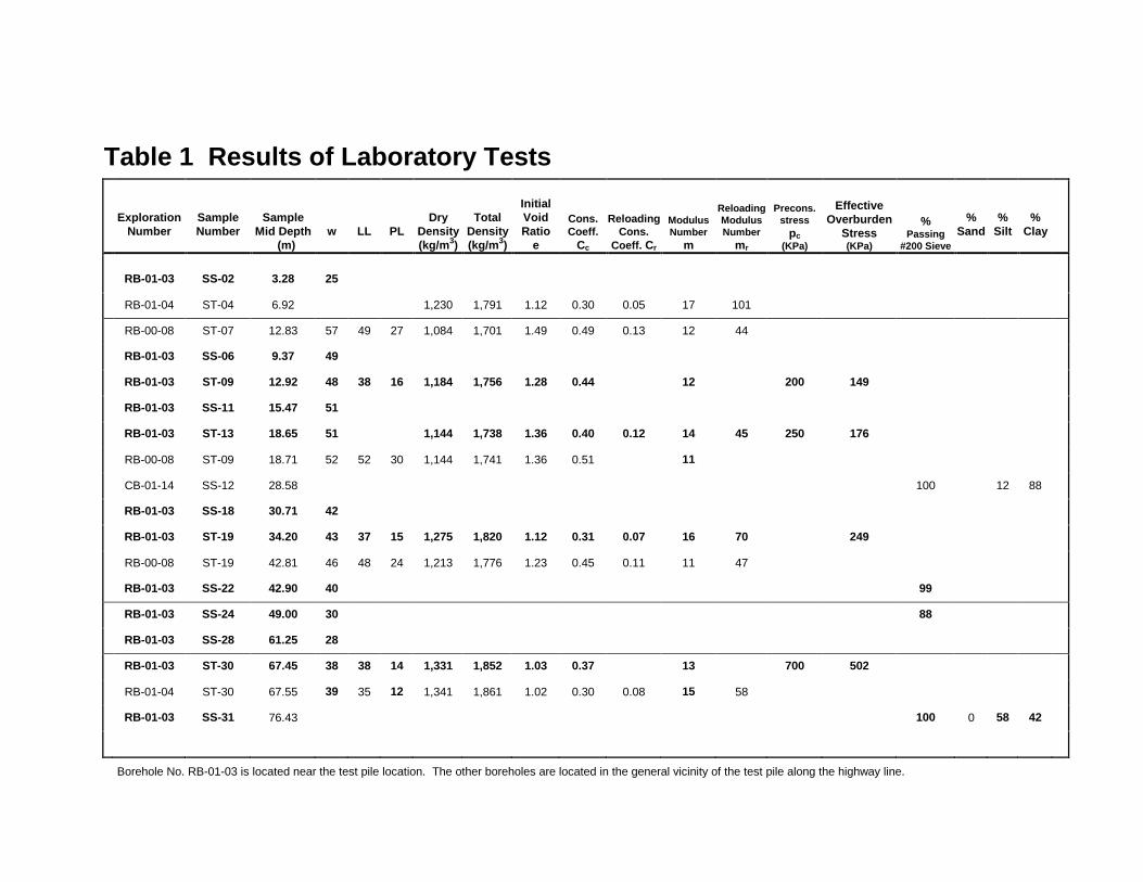
Table 1 Results of Laboratory Tests

Exploration Number

Sample Number

Sample Mid Depth

(m) w

LL

PL

Dry Density (kg/m3)

Total Density (kg/m3)

Initial Void Ratio

e

Cons. Coeff.

Cc

ReloadingCons.

Coeff. Cr

Modulus Number

m

Reloading Modulus Number

mr

Precons. stress

pc (KPa)

Effective Overburden

Stress (KPa)

% Passing

#200 Sieve

% Sand

% Silt

% Clay

RB-01-03 SS-02 3.28 25

RB-01-04 ST-04 6.92 1,230 1,791 1.12 0.30 0.05 17 101

RB-00-08 ST-07 12.83 57 49 27 1,084 1,701 1.49 0.49 0.13 12 44

RB-01-03 SS-06 9.37 49

RB-01-03 ST-09 12.92 48 38 16 1,184 1,756 1.28 0.44 12 200 149

RB-01-03 SS-11 15.47 51

RB-01-03 ST-13 18.65 51 1,144 1,738 1.36 0.40 0.12 14 45 250 176

RB-00-08 ST-09 18.71 52 52 30 1,144 1,741 1.36 0.51 11

CB-01-14 SS-12 28.58 100 12 88

RB-01-03 SS-18 30.71 42

RB-01-03 ST-19 34.20 43 37 15 1,275 1,820 1.12 0.31 0.07 16 70 249

RB-00-08 ST-19 42.81 46 48 24 1,213 1,776 1.23 0.45 0.11 11 47

RB-01-03 SS-22 42.90 40 99

RB-01-03 SS-24 49.00 30 88

RB-01-03 SS-28 61.25 28

RB-01-03 ST-30 67.45 38 38 14 1,331 1,852 1.03 0.37 13 700 502

RB-01-04 ST-30 67.55 39 35 12 1,341 1,861 1.02 0.30 0.08 15 58

RB-01-03 SS-31 76.43 100 0 58 42

Borehole No. RB-01-03 is located near the test pile location. The other boreholes are located in the general vicinity of the test pile along the highway line.

Fig. 4 Results of the 1980 static loading tests on composite piles (Data from Waite et al. 1980) The authors matched the about 800-KN pile capacities of the test piles in an effective stress analysis, which resulted in a beta-coefficient (β) of 0.18 and a toe-bearing coefficient (Nt) of 5. These are low values. For example, for piles in clay, the Canadian Foundation Engineering Manual (1992) suggests a range of beta-coefficients from 0.25 through 0.32, and a toe bearing coefficient of 9. Fellenius (1999) indicates that the toe bearing coefficient in clay normally ranges from 3 through 30. The authors attribute the low values to insufficient wait time (nine days) between driving and testing. DESCRIPTION OF THE CURRENT TEST PILE

The current test pile is a 406-mm diameter, closed-toe pipe pile with a 12.5 mm thick wall. The pile toe was closed with a 25 mm thick steel plate flush with the outside diameter of the pile. On August 29, 2001, the pile was driven with a APE D36-32 single-acting diesel hammer to an embedment depth of 45.0 m. The ram stroke ranged from 1.2 m through 2.0 m, and the penetration resistance was consistently about 3 bl/0.3m. At a 10-blow restrike the next day, August 30, the ram stroke was 2.0 m and the pile advanced 0.12 m (equivalent penetration resistance of 24 blows/0.3m). A pile driving analyzer (PDA) was used during test pile driving. The results of the PDA measurements are discussed in a later section of this paper. The final length of the pile was 45.89 m including a stick-up of 0.89 m. The pile head elevation immediately after driving was +633.136 m, as surveyed on August 31, 2001. The pile head elevation as surveyed on September 6 (the day after grouting the pile) and on October 15 was found to be 6 mm and 13 mm lower, respectively. The movements are attributed to the dissipation of excess pore pressures induced by the driving (Fig. 3) and the grouting of the pile. The total weight of the pipe pile empty is 1.2 KN/m, and the buoyant weight of the closed-toe pile (against the pore pressure distribution prior to the pile driving) is about zero. After grouting, the total weight of the pile is about 2.9 KN/m, resulting in a buoyant weight of the pile of about 80 KN.

0

100

200

300

400

500

600

700

800

900

1,000

0 5 10 15 20 25 30

MOVEMENT (mm)

LOAD

(KN

)

Pile A

Pile B

Pile C

Vibrating Wire Strain Gages

The pile was instrumented at eight levels with Geokon Sister Bar vibrating wire strain gages (Part No. 4911) attached to a “ladder” consisting of two vertically placed U-channels (76 mm x 6.1 mm with a cross sectional area of 7.81 cm2). The cross sectional area of each Sister Bar is 0.71 cm2. The Sister Bars were placed concentrically at a distance of 140 mm from the pile center and at the depths shown in Table 2.

Table 2 Depth to Gages Level # 8 7 6 5 4 3 2 1 Below pile head (m) 1.29 6.50 10.09 16.87 23.85 30.90 37.99 44.86 Below ground (m) 0.4 5.6 9.2 16.0 23.0 30.0 37.1 44.0

The purpose of Level 8 strain gages was to provide data for determining the Young’s modulus of the pile for use when converting the strains measured at Levels 1 through 7 to load in the pile. At Levels 2 through 7, two strain gages were placed diametrically opposed and at equal distance from the pile center. (The strain used to determine the load is the average of the two gages). As Levels 1 and 8 were considered to be the most important gage levels, for redundancy, two gage pairs were placed at 90° at these levels. Each “diameter pair” determines a separate average value of strain in the pile, and the two pairs serve as back-up to each other. Telltales

Before the grouting of the pile, to serve as guides for telltales installed in the pile, two 25-mm outer diameter (OD) pipes were installed inside the pile and all the way to the pile toe by attaching them to the instrumentation ladder. The guide pipe wall thickness is 1.6 mm (cross section area is 1.2 cm2). The telltales consisted of Geokon 10 mm stainless steel rods with threaded connections (Part 1150) and a bayonet fit to lock into the bottom of the guide pipe. One telltale tip was placed at the pile toe (the length between the pile head and the pile toe inside the pile is 45.86 m). The other telltale finished at 39.41 m below the pile head, i.e., 6.45 m above the pile toe. (The values do not include the 25 mm thick toe plate). The purpose of the telltale was to determine the shortening of the pile between the pile head and the pile toe. The pile toe movement was then obtained by subtracting the shortening from the pile head movement. Steel and Concrete Areas

The cross sectional total area and steel area of the test pile are 1,297 cm2 and 154.5 cm2, respectively. The steel area for two U-channels, two Sister Bars, and two telltale guide pipes to add to the cross sectional steel area of the pile is 20.2 cm2. With four Sister Bars, the steel area to add is 21.7 cm2. On September 5, 2001, the instrumentation cage (the “ladder”) was lowered into the test pile, and concrete grout was placed by tremie in the pile. The grout was specified to have a cylinder strength of 28 MPa (4,000 psi). Tests performed on three cylinders on November 1, 2001, 56 days after the grouting of the pile, gave cylinder strengths of 28.7 MPa, 34.6 MPa, and 29.0 MPa (4,160 psi, 5,014 psi, and 4,260 psi). Values of Young’s modulus determined for these cylinders at 40 % of strength were 26 GPa, 27 GPa, and 22 GPa (3.73x106 psi, 3.86x106 psi, and 3.18x106 psi).

ARRANGEMENT OF STATIC LOADING TEST AND PRECISION OF MEASUREMENTS

Six reaction piles were installed at the test site immediately before the driving of the test pile. The reaction piles have the same diameter as the test pile, but were 11.7 m shorter (installed to a depth of 32.3 m). Three reaction piles were placed symmetrically on each side of the test pile in the corners of an equilateral triangle with a 1.5 m long side and the apex pointing away from the test pile. The perpendicular distance of the triangle base from the center of the test pile was 3.1 m. The “apex pile” was 4.3 m away from the test pile. The test load was applied by a 14 MN capacity O-cell jack supplied by Loadtest Inc. weighing 5 KN. Loads were generated by increasing the pressure in the jack by means of an electrically operated pump. The loads were specified to be applied in equal increments of 150 KN. Each load level was maintained for ten minutes, whereupon the pump was activated to raise the load by the next increment. The actual load applied was determined not by the pump reading, but at the O-cell jack itself. The O-cell values were determined to a reading precision of 0.1 KN and are considered true to an accuracy of a few kilonewton. As a back-up to the O-cell reading, the applied loads were also measured by a separate load cell placed on the O-cell. (The O-cell values and the load cell values agreed well in the test). Reading the load level on the pump pressure gage when operating the pump was difficult, and the magnitude of the actually applied load increments deviated slightly from the 150 KN level and ranged from 140 KN through 170 KN with an average of 160 KN. On occasions, the load increment slightly exceeded the intended value. The load level was then always accepted in order not to disturb the test by releasing the pressure in the jack, as this would have reversed the direction of the shear forces along the upper portion of the pile. The movement of the pile head was measured using two Linearly Variable Differential Transducers (LVDT gages) to a precision of 0.001 mm. The telltale measured shortening of the pile was by means of a single LVDT gage also to a precision of 0.001 mm. The pile head movement was also independently recorded with a surveyor’s optical level. The Sister-Bar strain-gage readings were determined to a precision of 0.1 microstrain, corresponding to a load precision of 0.3 KN. The accuracy of a load value determined from the strain-gage readings is a function of the accuracy of the pair of strain gages and the accuracy of the estimated modulus in combination. Therefore, considering the effect of accuracy of the modulus of the composite pile section (see below), the accuracy of the load values determined from the measurements is estimated to be about 5 KN to 10 KN. All measurements were made with a data acquisition system, and the data were displayed in the field and simultaneously stored for later processing. Before starting the test, several readings were taken of all gages to provide baseline values. During the test, readings of applied load, movements, and strains were recorded every 30 seconds and immediately before and after the addition of a load increment. Readings were stored using a data acquisition system. Manual readings were also obtained. RESULTS OF DYNAMIC MONITORING OF THE PILE DRIVING

Dynamic monitoring with the Pile Driving Analyzer (PDA) was carried out during the installation of the test pile, commencing when the pile had reached a depth of 29 m. The driving paused for 72 minutes at 9.4 m depth

and then continued until the final embedment depth of 45 m. A few blows were given to the pile in a restrike the following day, August 30, after a set-up time of 16 hours. A total of four CAPWAP analyses were performed on blow records from the test pile. The blows selected for CAPWAP analysis and the total capacity are indicated in Table 3.

Table 3 CAPWAP Determined Capacities Depth Condition Capacity (m) (- -) (KN)

29 End-of-Drive 190 29 Beginning-of-Restrike 400 45 End-of-Drive 260 45 Beginning-of-16-hour Restrike 980

As shown in Table 3, the capacity of the test pile at 29 m depth increased from 190 KN to 400 KN during a 72-minute set-up time. At the full embedment depth, the End-of-Driving and 16-hour restrike capacities of the test pile were 260 KN and 980 KN, respectively. (As will be presented below, the 980-KN value is about half the capacity, 1,900 KN, found in the static loading test performed 50 days after the driving). At depth 29 m, the 720-KN increase of capacity due to the short-term set-up is mostly along the pile shaft. In soils consisting of mostly clay-size particles, such as at this site, the time for dissipation of pore pressures induced by the driving and full set-up is usually several weeks or months. The test pile was restruck after a set-up time of only 16 hours. That the increase of capacity from 260 KN at End-of-Drive to 980 KN are Beginning-of-Restrike (also evident by the increase in penetration resistance from 3 bl./0.3m to 24 bl./03.m, in the 16-hour period still was significant and could be due to the presence of thin layers of sand and silt which allowed a faster dissipation of pore pressures induced during the driving. The restrike records indicated that the soil resistance diminished within a few blows. The CAPWAP determined capacities for the end-of-drive and at beginning-of-restrike show that the pile toe capacity increased from 30 KN to 90 KN. The increase might be an effect of that, as indicated by the CPTU sounding (Fig. 1), the pile toe is located in a 0.4 m thick sand layer. RESULTS OF THE STATIC LOADING TEST

Initial Load Measurements

The loading test was carried out on October 17, 2001, 48 days after the driving and 42 days after the pile was grouted. The first readings of the vibrating wire gages were taken on October 17, immediately before the start of the static loading test. (The vibrating wire gages can only respond to load in the pile after the grouting, so no load distribution data could be obtained for the six-day period between the driving and the grouting of the pile. For various reasons, no readings of the gages were taken between the grouting and the start of the static loading

test). Those first readings, which are presented in Table 4, are calculated from the factory no-load calibration and show that loads exist in the pile before the start of the test. However, the loads shown are not all of the loads locked-in the pile (“residual loads”) before the start of the test. Residual loads developing from the driving and the grouting of the pile and during the period between grouting and the start of the test are not included in Table 4. Note that even if measurements had been taken during the curing of the grout, strain would have developed or reduced due to temperature changes without involving any transfer of load from the soil to the pile.

Table 4 Loads in Pile Immediately before the Start of the Static Loading Test

Depth below pile head (m) 1.3 6.5 10.1 16.9 23.9 30.9 38.0 44.9 Loads (KN) 0.00 178.1 227.3 326.1 373.5 376.2 312.3 153.3

Pile Head Load-Movement

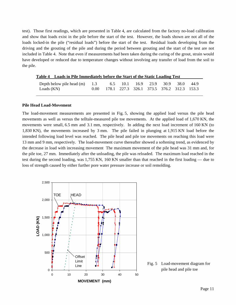
The load-movement measurements are presented in Fig. 5, showing the applied load versus the pile head movements as well as versus the telltale-measured pile toe movements. At the applied load of 1,670 KN, the movements were small, 6.5 mm and 3.1 mm, respectively. In adding the next load increment of 160 KN (to 1,830 KN), the movements increased by 3 mm. The pile failed in plunging at 1,915 KN load before the intended following load level was reached. The pile head and pile toe movements on reaching this load were 13 mm and 9 mm, respectively. The load-movement curve thereafter showed a softening trend, as evidenced by the decrease in load with increasing movement The maximum movement of the pile head was 31 mm and, for the pile toe, 27 mm. Immediately after the unloading, the pile was reloaded. The maximum load reached in the test during the second loading, was 1,755 KN, 160 KN smaller than that reached in the first loading — due to loss of strength caused by either further pore water pressure increase or soil remolding.

Fig. 5 Load-movement diagram for pile head and pile toe 0

500

1,000

1,500

2,000

2,500

0 10 20 30 40 50

MOVEMENT (mm)

LOA

D (K

N)

HEADTOE

OffsetLimitLine

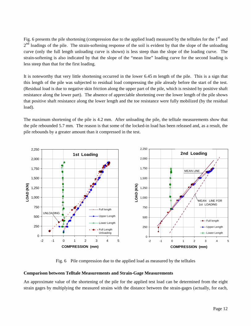
Fig. 6 presents the pile shortening (compression due to the applied load) measured by the telltales for the 1st and 2nd loadings of the pile. The strain-softening response of the soil is evident by that the slope of the unloading curve (only the full length unloading curve is shown) is less steep than the slope of the loading curve. The strain-softening is also indicated by that the slope of the “mean line” loading curve for the second loading is less steep than that for the first loading. It is noteworthy that very little shortening occurred in the lower 6.45 m length of the pile. This is a sign that this length of the pile was subjected to residual load compressing the pile already before the start of the test. (Residual load is due to negative skin friction along the upper part of the pile, which is resisted by positive shaft resistance along the lower part). The absence of appreciable shortening over the lower length of the pile shows that positive shaft resistance along the lower length and the toe resistance were fully mobilized (by the residual load). The maximum shortening of the pile is 4.2 mm. After unloading the pile, the telltale measurements show that the pile rebounded 5.7 mm. The reason is that some of the locked-in load has been released and, as a result, the pile rebounds by a greater amount than it compressed in the test.

Fig. 6 Pile compression due to the applied load as measured by the telltales

Comparison between Telltale Measurements and Strain-Gage Measurements

An approximate value of the shortening of the pile for the applied test load can be determined from the eight strain gages by multiplying the measured strains with the distance between the strain-gages (actually, for each,

0

250

500

750

1,000

1,250

1,500

1,750

2,000

2,250

-2 -1 0 1 2 3 4 5

COMPRESSION (mm)

LOA

D (K

N)

Full length

Upper Length

Lower Length

Full LengthUnloading

0

250

500

750

1,000

1,250

1,500

1,750

2,000

2,250

-2 -1 0 1 2 3 4 5

COMPRESSION (mm)

LOA

D (K

N)

Full length

Upper Length

Lower Length

1st Loading 2nd Loading

MEAN LINE

MEAN LINE FOR 1st LOADING

UNLOADING

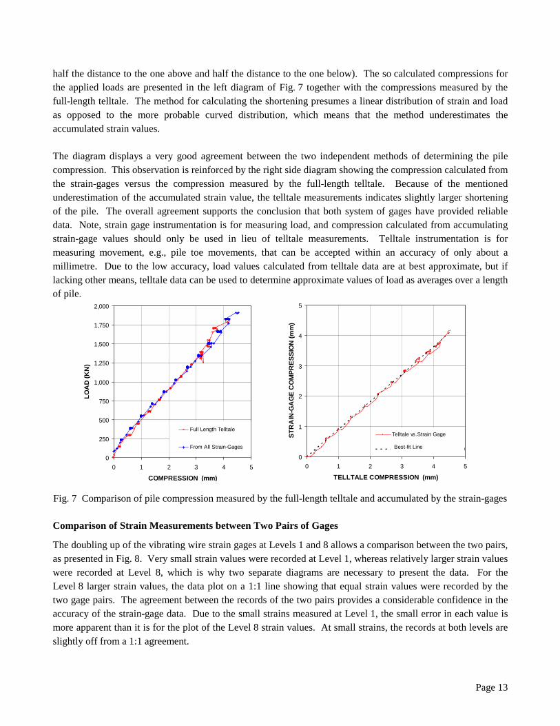
half the distance to the one above and half the distance to the one below). The so calculated compressions for the applied loads are presented in the left diagram of Fig. 7 together with the compressions measured by the full-length telltale. The method for calculating the shortening presumes a linear distribution of strain and load as opposed to the more probable curved distribution, which means that the method underestimates the accumulated strain values. The diagram displays a very good agreement between the two independent methods of determining the pile compression. This observation is reinforced by the right side diagram showing the compression calculated from the strain-gages versus the compression measured by the full-length telltale. Because of the mentioned underestimation of the accumulated strain value, the telltale measurements indicates slightly larger shortening of the pile. The overall agreement supports the conclusion that both system of gages have provided reliable data. Note, strain gage instrumentation is for measuring load, and compression calculated from accumulating strain-gage values should only be used in lieu of telltale measurements. Telltale instrumentation is for measuring movement, e.g., pile toe movements, that can be accepted within an accuracy of only about a millimetre. Due to the low accuracy, load values calculated from telltale data are at best approximate, but if lacking other means, telltale data can be used to determine approximate values of load as averages over a length of pile.

Fig. 7 Comparison of pile compression measured by the full-length telltale and accumulated by the strain-gages Comparison of Strain Measurements between Two Pairs of Gages

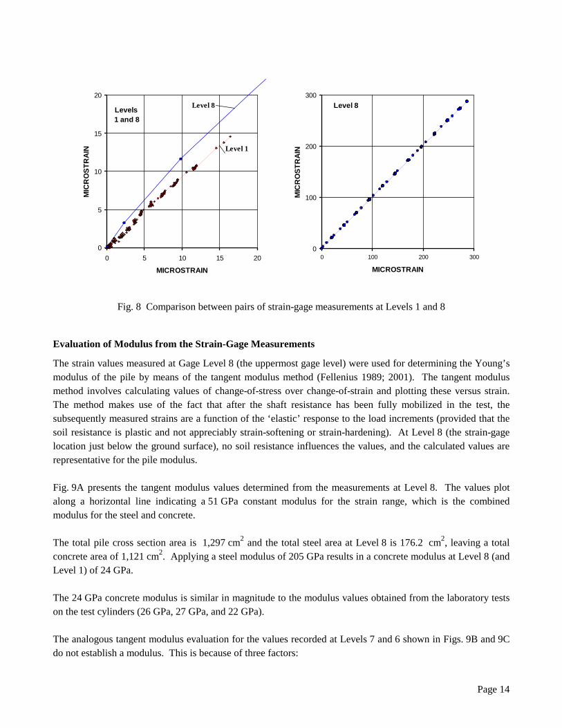
The doubling up of the vibrating wire strain gages at Levels 1 and 8 allows a comparison between the two pairs, as presented in Fig. 8. Very small strain values were recorded at Level 1, whereas relatively larger strain values were recorded at Level 8, which is why two separate diagrams are necessary to present the data. For the Level 8 larger strain values, the data plot on a 1:1 line showing that equal strain values were recorded by the two gage pairs. The agreement between the records of the two pairs provides a considerable confidence in the accuracy of the strain-gage data. Due to the small strains measured at Level 1, the small error in each value is more apparent than it is for the plot of the Level 8 strain values. At small strains, the records at both levels are slightly off from a 1:1 agreement.

0

250

500

750

1,000

1,250

1,500

1,750

2,000

0 1 2 3 4 5

COMPRESSION (mm)

LOA

D (K

N)

Full Length Telltale

From All Strain-Gages

0

1

2

3

4

5

0 1 2 3 4 5

TELLTALE COMPRESSION (mm)

STR

AIN

-GA

GE

CO

MPR

ESSI

ON

(mm

)

Telltale vs.Strain Gage

Linear (Telltale vs.Strain Gage) Best-fit Line

Fig. 8 Comparison between pairs of strain-gage measurements at Levels 1 and 8

Evaluation of Modulus from the Strain-Gage Measurements

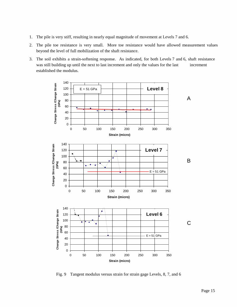
The strain values measured at Gage Level 8 (the uppermost gage level) were used for determining the Young’s modulus of the pile by means of the tangent modulus method (Fellenius 1989; 2001). The tangent modulus method involves calculating values of change-of-stress over change-of-strain and plotting these versus strain. The method makes use of the fact that after the shaft resistance has been fully mobilized in the test, the subsequently measured strains are a function of the ‘elastic’ response to the load increments (provided that the soil resistance is plastic and not appreciably strain-softening or strain-hardening). At Level 8 (the strain-gage location just below the ground surface), no soil resistance influences the values, and the calculated values are representative for the pile modulus. Fig. 9A presents the tangent modulus values determined from the measurements at Level 8. The values plot along a horizontal line indicating a 51 GPa constant modulus for the strain range, which is the combined modulus for the steel and concrete. The total pile cross section area is 1,297 cm2 and the total steel area at Level 8 is 176.2 cm2, leaving a total concrete area of 1,121 cm2. Applying a steel modulus of 205 GPa results in a concrete modulus at Level 8 (and Level 1) of 24 GPa. The 24 GPa concrete modulus is similar in magnitude to the modulus values obtained from the laboratory tests on the test cylinders (26 GPa, 27 GPa, and 22 GPa). The analogous tangent modulus evaluation for the values recorded at Levels 7 and 6 shown in Figs. 9B and 9C do not establish a modulus. This is because of three factors:

0

5

10

15

20

0 5 10 15 20

MICROSTRAIN

MIC

RO

STR

AIN

0

100

200

300

0 100 200 300

MICROSTRAIN

MIC

RO

STR

AIN

Level 8 Levels 1 and 8

Level 8

Level 1

1. The pile is very stiff, resulting in nearly equal magnitude of movement at Levels 7 and 6.

2. The pile toe resistance is very small. More toe resistance would have allowed measurement values beyond the level of full mobilization of the shaft resistance.

3. The soil exhibits a strain-softening response. As indicated, for both Levels 7 and 6, shaft resistance was still building up until the next to last increment and only the values for the last increment established the modulus.

Fig. 9 Tangent modulus versus strain for strain gage Levels, 8, 7, and 6

0

20

40

60

80

100

120

140

0 50 100 150 200 250 300 350

Strain (micro)

Cha

nge

Stre

ss /C

hang

e St

rain

(G

Pa)

E = 51 GPa Level 8

0

20

40

60

80

100

120

140

0 50 100 150 200 250 300 350

Strain (micro)

Cha

nge

Stre

ss /C

hang

e St

rain

(G

Pa)

Level 7

E = 51 GPa

0

20

40

60

80

100

120

140

0 50 100 150 200 250 300 350

Strain (micro)

Cha

nge

Stre

ss /C

hang

e St

rain

(GPa

)

Level 6

E = 51 GPa

A

B

C

Distribution of Measured Loads

The loads determined from the strain values measured at the eight vibrating wire gage levels were calculated with reference to the change of strain from the start of the loading test (i.e., as if assuming the loads in the pile to be zero at the start of the test). These measured load values are presented in Fig. 10 in the form of load-distribution curves showing the load at the each strain gage location along the pile for each load applied to the pile head. Also shown is the similarly calculated loads in the pile after removing the applied load — but for a load of 60 KN left on the pile head to keep jack, load cell, and spacers in compression.

Fig. 10 Measured load distributions for 1st loading with loads in relation to readings at start of test

The loads in the pile after unloading appear to indicate that tension loads developed as result of the loading test. This is false. The tension loads are due to a release of some of the residual load in the pile. As mentioned earlier on, this is also indicated by that the pile rebounded to longer total length than its length before the test. The load distributions of the 2nd loading together with the distributions at maximum load and after unloading of the 1st loading are presented in Fig. 11. The reference of the load values is the same as for the 1st loading; i.e., the strain readings at the start of the 1st loading. A comparison between the distributions for the start and end of 2nd loading shows that some additional increase of the “negative” loads occurred, that is, additional residual load was released. As shown in Fig. 11, between the depths of 10 m and 30 m, the slope of the load distribution curve (at the maximum load) for the 2nd loading is slightly steeper than that for the 1st loading, indicating that the engaged

0

5

10

15

20

25

30

35

40

45

50

-500 0 500 1,000 1,500 2,000

LOAD (KN)

DEP

TH (

m)

1st Loading

At End of1st Loading

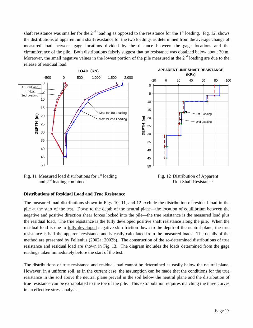
shaft resistance was smaller for the 2nd loading as opposed to the resistance for the 1st loading. Fig. 12. shows the distributions of apparent unit shaft resistance for the two loadings as determined from the average change of measured load between gage locations divided by the distance between the gage locations and the circumference of the pile. Both distributions falsely suggest that no resistance was obtained below about 30 m. Moreover, the small negative values in the lowest portion of the pile measured at the 2nd loading are due to the release of residual load. Fig. 11 Measured load distributions for 1st loading Fig. 12 Distribution of Apparent and 2nd loading combined Unit Shaft Resistance Distributions of Residual Load and True Resistance

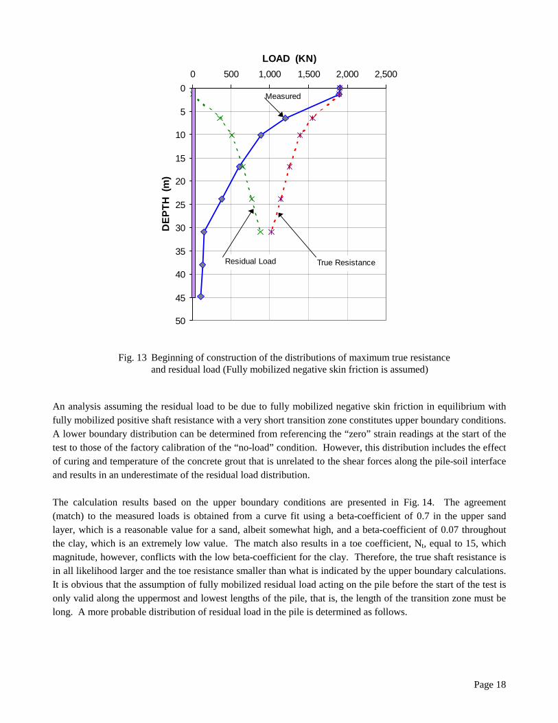
The measured load distributions shown in Figs. 10, 11, and 12 exclude the distribution of residual load in the pile at the start of the test. Down to the depth of the neutral plane—the location of equilibrium between the negative and positive direction shear forces locked into the pile—the true resistance is the measured load plus the residual load. The true resistance is the fully developed positive shaft resistance along the pile. When the residual load is due to fully developed negative skin friction down to the depth of the neutral plane, the true resistance is half the apparent resistance and is easily calculated from the measured loads. The details of the method are presented by Fellenius (2002a; 2002b). The construction of the so-determined distributions of true resistance and residual load are shown in Fig. 13. The diagram includes the loads determined from the gage readings taken immediately before the start of the test. The distributions of true resistance and residual load cannot be determined as easily below the neutral plane. However, in a uniform soil, as in the current case, the assumption can be made that the conditions for the true resistance in the soil above the neutral plane prevail in the soil below the neutral plane and the distribution of true resistance can be extrapolated to the toe of the pile. This extrapolation requires matching the three curves in an effective stress analysis.

0

5

10

15

20

25

30

35

40

45

50

-500 0 500 1,000 1,500 2,000

LOAD (KN)

DEP

TH (

m)

At Start and End of

2nd Loading

Max for 1st Loading

Max for 2nd Loading

0

5

10

15

20

25

30

35

40

45

50

-20 0 20 40 60 80 100

APPARENT UNIT SHAFT RESISTANCE (KPa)

DEP

TH (

m)

2nd Loading

1st Loading

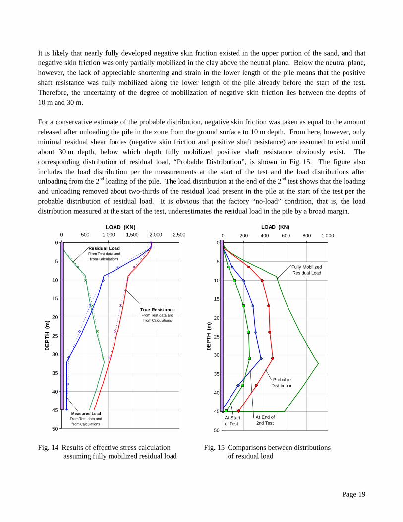
Fig. 13 Beginning of construction of the distributions of maximum true resistance and residual load (Fully mobilized negative skin friction is assumed) An analysis assuming the residual load to be due to fully mobilized negative skin friction in equilibrium with fully mobilized positive shaft resistance with a very short transition zone constitutes upper boundary conditions. A lower boundary distribution can be determined from referencing the “zero” strain readings at the start of the test to those of the factory calibration of the “no-load” condition. However, this distribution includes the effect of curing and temperature of the concrete grout that is unrelated to the shear forces along the pile-soil interface and results in an underestimate of the residual load distribution. The calculation results based on the upper boundary conditions are presented in Fig. 14. The agreement (match) to the measured loads is obtained from a curve fit using a beta-coefficient of 0.7 in the upper sand layer, which is a reasonable value for a sand, albeit somewhat high, and a beta-coefficient of 0.07 throughout the clay, which is an extremely low value. The match also results in a toe coefficient, Nt, equal to 15, which magnitude, however, conflicts with the low beta-coefficient for the clay. Therefore, the true shaft resistance is in all likelihood larger and the toe resistance smaller than what is indicated by the upper boundary calculations. It is obvious that the assumption of fully mobilized residual load acting on the pile before the start of the test is only valid along the uppermost and lowest lengths of the pile, that is, the length of the transition zone must be long. A more probable distribution of residual load in the pile is determined as follows.

0

5

10

15

20

25

30

35

40

45

50

0 500 1,000 1,500 2,000 2,500LOAD (KN)

DEP

TH (

m)

Measured

True ResistanceResidual Load

It is likely that nearly fully developed negative skin friction existed in the upper portion of the sand, and that negative skin friction was only partially mobilized in the clay above the neutral plane. Below the neutral plane, however, the lack of appreciable shortening and strain in the lower length of the pile means that the positive shaft resistance was fully mobilized along the lower length of the pile already before the start of the test. Therefore, the uncertainty of the degree of mobilization of negative skin friction lies between the depths of 10 m and 30 m. For a conservative estimate of the probable distribution, negative skin friction was taken as equal to the amount released after unloading the pile in the zone from the ground surface to 10 m depth. From here, however, only minimal residual shear forces (negative skin friction and positive shaft resistance) are assumed to exist until about 30 m depth, below which depth fully mobilized positive shaft resistance obviously exist. The corresponding distribution of residual load, “Probable Distribution”, is shown in Fig. 15. The figure also includes the load distribution per the measurements at the start of the test and the load distributions after unloading from the 2nd loading of the pile. The load distribution at the end of the 2nd test shows that the loading and unloading removed about two-thirds of the residual load present in the pile at the start of the test per the probable distribution of residual load. It is obvious that the factory “no-load” condition, that is, the load distribution measured at the start of the test, underestimates the residual load in the pile by a broad margin. Fig. 14 Results of effective stress calculation Fig. 15 Comparisons between distributions assuming fully mobilized residual load of residual load

0

5

10

15

20

25

30

35

40

45

50

0 500 1,000 1,500 2,000 2,500LOAD (KN)

DEP

TH (

m)

True ResistanceFrom Test data and from Calculations

Residual LoadFrom Test data and from Calculations

Measured LoadFrom Test data and from Calculations

0

5

10

15

20

25

30

35

40

45

50

0 200 400 600 800 1,000

LOAD (KN)

DEP

TH (

m)

At Start of Test

Fully MobilizedResidual Load

At End of 2nd Test

Probable Distibution

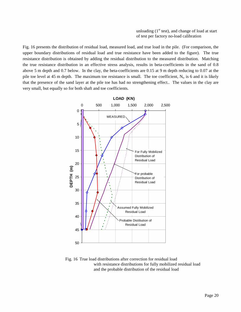
unloading (1st test), and change of load at start of test per factory no-load calibration Fig. 16 presents the distribution of residual load, measured load, and true load in the pile. (For comparison, the upper boundary distributions of residual load and true resistance have been added to the figure). The true resistance distribution is obtained by adding the residual distribution to the measured distribution. Matching the true resistance distribution in an effective stress analysis, results in beta-coefficients in the sand of 0.8 above 5 m depth and 0.7 below. In the clay, the beta-coefficients are 0.15 at 9 m depth reducing to 0.07 at the pile toe level at 45 m depth. The maximum toe resistance is small. The toe coefficient, Nt, is 6 and it is likely that the presence of the sand layer at the pile toe has had no strengthening effect.. The values in the clay are very small, but equally so for both shaft and toe coefficients.

Fig. 16 True load distributions after correction for residual load with resistance distributions for fully mobilized residual load and the probable distribution of the residual load

0

5

10

15

20

25

30

35

40

45

50

0 500 1,000 1,500 2,000 2,500

LOAD (KN)

DEP

TH (

m)

Probable Distibution of Residual Load

MEASURED

For Fully Mobilized Distribution of Residual Load

For probableDistribution of Residual Load

Assumed Fully Mobilized Residual Load

OTHER OBSERVATIONS FROM THE LOADING TEST

Distributions of Resistance in the Pile Determined by Total Stress and CPTU Methods

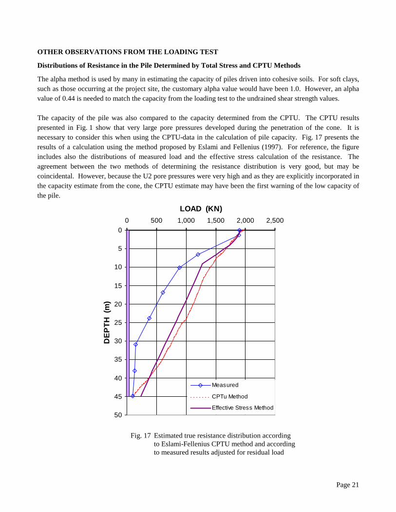
The alpha method is used by many in estimating the capacity of piles driven into cohesive soils. For soft clays, such as those occurring at the project site, the customary alpha value would have been 1.0. However, an alpha value of 0.44 is needed to match the capacity from the loading test to the undrained shear strength values. The capacity of the pile was also compared to the capacity determined from the CPTU. The CPTU results presented in Fig. 1 show that very large pore pressures developed during the penetration of the cone. It is necessary to consider this when using the CPTU-data in the calculation of pile capacity. Fig. 17 presents the results of a calculation using the method proposed by Eslami and Fellenius (1997). For reference, the figure includes also the distributions of measured load and the effective stress calculation of the resistance. The agreement between the two methods of determining the resistance distribution is very good, but may be coincidental. However, because the U2 pore pressures were very high and as they are explicitly incorporated in the capacity estimate from the cone, the CPTU estimate may have been the first warning of the low capacity of the pile.

Fig. 17 Estimated true resistance distribution according to Eslami-Fellenius CPTU method and according to measured results adjusted for residual load

0

5

10

15

20

25

30

35

40

45

50

0 500 1,000 1,500 2,000 2,500LOAD (KN)

DEP

TH (

m)

Measured

CPTu Method

Effective Stress Method

Pore Pressures Measured during the Pile Driving and the Static Loading Test

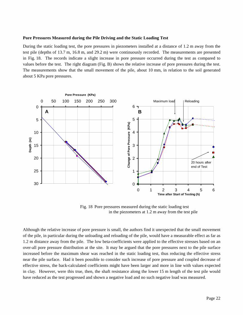
During the static loading test, the pore pressures in piezometers installed at a distance of 1.2 m away from the test pile (depths of 13.7 m, 16.8 m, and 29.2 m) were continuously recorded. The measurements are presented in Fig. 18. The records indicate a slight increase in pore pressure occurred during the test as compared to values before the test. The right diagram (Fig. B) shows the relative increase of pore pressures during the test. The measurements show that the small movement of the pile, about 10 mm, in relation to the soil generated about 5 KPa pore pressures.

Fig. 18 Pore pressures measured during the static loading test in the piezometers at 1.2 m away from the test pile Although the relative increase of pore pressure is small, the authors find it unexpected that the small movement of the pile, in particular during the unloading and reloading of the pile, would have a measurable effect as far as 1.2 m distance away from the pile. The low beta-coefficients were applied to the effective stresses based on an over-all pore pressure distribution at the site. It may be argued that the pore pressures next to the pile surface increased before the maximum shear was reached in the static loading test, thus reducing the effective stress near the pile surface. Had it been possible to consider such increase of pore pressure and coupled decrease of effective stress, the back-calculated coefficients might have been larger and more in line with values expected in clay. However, were this true, then, the shaft resistance along the lower 15 m length of the test pile would have reduced as the test progressed and shown a negative load and no such negative load was measured.

0

5

10

15

20

25

30

0 50 100 150 200 250 300Pore Pressure (KPa)

Dep

th (

m)

0

1

2

3

4

5

6

0 1 2 3 4 5 6Time after Start of Testing (h)

Cha

nge

of P

ore

Pres

sure

(K

Pa)

20 hours after end of Test

Maximum load

A B

Reloading

RESULTS AND CONCLUSIONS

The results of the static loading test on the 45 m long instrumented pile are summarized, as follows. 1. The clay at the site is brittle and strain-softening, requiring special attention and consideration in geotechnical design of structures in the area.

2. The clay at the site provides a very small pile shaft and toe resistances.

3. The restrike testing demonstrates a set-up that develops surprisingly fast.

4. The test pile is affected by residual load. Because the pile was constructed by driving a steel pile that was grouted after the driving, the residual load developing before the concrete grout had cured could not be measured. However, the magnitude and distribution was estimated to be larger than indicated by the values of locked-in load before the start of the test (from reference to the factory calibration of the strain gages) and smaller than corresponding to fully mobilized shear forces along the pile.

5. Consideration of compatibility between toe resistance and shaft resistance resulted in a distribution of residual load that includes almost fully mobilized negative skin friction down to 10 m depth and fully mobilized positive shaft resistance below 30 m depth with minimal transfer of load between the pile and the clay from 10 m depth through 30 m depth. Combining the probable distribution with the distribution of measured load determines the true resistance distribution for the test pile.

6. The back-calculated effective stress parameters corresponding to the resistance distribution are beta-coefficients of about 0.8 in the sand layer and 0.15 at the upper boundary of the clay layer, reducing to 0.07 in the clay layer at the pile toe. The pile toe coefficient is 6.

7. The low beta value of about 0.1 is a unique characteristic of the geology for the area.

8. The effective stress parameters back-calculated from the results of the “old test” of 1980 are similar to those found for the current test pile.

9. Comparison between the results from the “old test” and the current test should consider that the “old” piles were tapered and more axially flexible as opposed to the current test pile.

10. The effective stress parameters established from the results of the static loading test apply also to other piles at the site with diameters and embedment lengths that differ from the test pile.

11. The effective stress parameters established from the test are low. The results of the laboratory tests also indicate a brittle, strain-softening behavior of the clay. The soil conditions at the site are unusual and conventional analysis methods may not adequately model the soil response to loading.

12. For calculation of the capacity of other piles at this site, the CPTU method coupled with an effective stress analysis using a beta-coefficient of 0.1 and a toe coefficient of 6 in the clay is recommended.

13. It is clear from the low beta values recorded during the loading test that pile capacity estimates for this site using conventional methods would not have been very accurate. If no pile loading test had been undertaken, production piles would have been selected on the basis of much higher shaft resistance values. Dynamic testing at the beginning of production pile driving would then have identified a clear discrepancy between design and actual condition. Very quickly it would have been concluded that more piles were needed, and a large change order for the project would have resulted. Fortunately, the uncertainty in soil behavior was

recognized early during the project and this led to performance of the test during design – a situation which is always desirable but usually not done, more often than not causing a capacity problem not to be realized until after start of production pile installation. ACKNOWLEDGEMENTS

Funding for this project was provided by the Idaho Transportation Department (ITD) as part of the US95 Sand Creek Byway Project. The willingness on the part of the ITD, particularly Bill Capaul and Tri Buu, in carrying out the testing programme, rather than relying on conventional approaches, is greatly appreciated. Dewitt Construction of Portland, Oregon, drove the piles, and provided the reaction platform. Installation of gages and execution of the static loading test was carried out by Loadtest Inc., Gainesville, Florida. Dynamic testing and analysis was carried out by Robert Miner Dynamic Testing, Inc., Seattle, Washington. Additional CAPWAP analyses were produced by Urkkada Technology Ltd. The excellent support from each of these organizations contributed to the success of this program. REFERENCES Breckenridge, R.M. and Sprenke, K.F., 1997. An overdeepened glaciated basin, Lake Pend Oreille, Northern Idaho. Glacial Geology and Geomorphology, 1997.

Canadian Geotechnical Engineering Society, 1992, Foundation Engineering Manual, 3rd Edition, BiTech Publishers Ltd., Richmond, BC, 512 p.

Eslami, A., 1996. Bearing capacity of piles from cone penetrometer test data. Ph. D. Thesis, University of Ottawa, Department of Civil Engineering, 516 p.

Eslami A. and Fellenius, B.H., 1997. Pile capacity by direct CPT and CPTU methods applied to 102 case histories. Canadian Geotechnical Journal, 34: 886 – 904.

Fellenius, B. H., 1989. Tangent modulus of piles determined from strain data. The American Society of Civil Engineers, ASCE, Geotechnical Engineering Div., the 1989 Foundation Congress, Edited by F. H. Kulhawy, Vol. 1, pp. 500 – 510.

Fellenius, B.H., 1999. Basics of Foundation Design, 2nd Edition. BiTech Publishers Ltd., Richmond, BC, 164 p.

Fellenius, B. H., 2001. From Strain Measurements to Load in an Instrumented Pile. Geotechnical News Magazine, 19 (1): 35 - 38.

Fellenius, B.H., 2002a. Determining the true distribution of load in piles. American Society of Civil Engineers, ASCE, International Deep Foundation Congress, An International Perspective on Theory, Design, Construction, and Performance, Geotechnical Special Publication No. 116, Edited by M.W. O’Neill, and F.C. Townsend, Orlando, Florida, February 14 - 16, 2002, Vol. 2, pp. 1455 – 1470..

Fellenius, B. H., 2002b. Determining the resistance distribution in piles. Part 1: Notes on shift of no-load reading and residual load. Part 2: Method for Determining the Residual Load. Geotechnical News Magazine, 20 (2): 35 - 38, and 20 (3): 25 - 29.

Fellenius, B. H. and Eslami, A., 2000. Soil profile interpreted from CPTU data. Proceedings of Year 2000 Geotechnics Conference, S-E Asian Geotechnical Society, Asian Institute of Technology, Bangkok, Thailand, November 27 - 30, 30 p.

U.S. Army Corps of Engineers, 2002. Albeni Falls Dam and Pend Oreille Lake. Seattle District, Hydrology & Hydraulics Section, Reservoir Control Center.

Waite, C.A., Narkiewicz, S.A., and Jones, W.V., 1980. Offshore vertical and lateral pile tests on composite friction piles, Pend Oreille Lake, Idaho. The American Society of Civil Engineers, ASCE, Geotechnical Engineering Division, Convention and Exposition, Portland, April 14 – 18, 1980, 19 p.

static loading test on a 45 m long pipe pile in … sandpoint cgj.pdfpage 1 static loading test on a...

Documents