static scheduling algorithms for allocating directed …charm.cs.uiuc.edu/users/arya/docs/6.pdf ·...
TRANSCRIPT
Static Scheduling Algorithms for Allocating Directed Task Graphs to Multiprocessors
Yu-Kwong Kwok1† and Ishfaq Ahmad2
1Department of Electrical and Electronic EngineeringThe University of Hong KongPokfulam Road, Hong Kong
2Department of Computer ScienceThe Hong Kong University of Science and Technology
Clear Water Bay, Hong Kong
Email: [email protected], [email protected]
Revised: July 1998
†. This research was supported by the Hong Kong Research Grants Council under contract numberHKUST 734/96E and HKUST 6076/97E.
Table of Contents
Abstract ..............................................................................................................................................1
1. Introduction..............................................................................................................................2
2. The DAG Scheduling Problem ..............................................................................................6
2.1 The DAG Model.............................................................................................................6
2.2 Generation of a DAG.....................................................................................................8
2.3 Variations in the DAG Model ......................................................................................8
2.4 The Multiprocessor Model .........................................................................................10
3. NP-Completeness of the DAG Scheduling Problem ........................................................10
4. A Taxonomy of DAG Scheduling Algorithms ..................................................................11
5. Basic Techniques in DAG Scheduling ................................................................................14
6. Description of the Algorithms .............................................................................................17
6.1 Scheduling DAGs with Restricted Structures..........................................................18
6.1.1 Hu’s Algorithm for Tree-Structured DAGs ........................................................ 18
6.1.2 Coffman and Graham’s Algorithm for Two-Processor Scheduling ................ 19
6.1.3 Scheduling Interval-Ordered DAGs .................................................................... 20
6.2 Scheduling Arbitrary DAGs without Communication ..........................................21
6.2.1 Level-based Heuristics ........................................................................................... 21
6.2.2 A Branch-and-Bound Approach........................................................................... 22
6.2.3 Analytical Performance Bounds for Scheduling without Communication........................................................................................ 23
6.3 UNC Scheduling ..........................................................................................................25
6.3.1 Scheduling of Primitive Graph Structures .......................................................... 25
6.3.2 The EZ Algorithm ................................................................................................... 26
6.3.3 The LC Algorithm................................................................................................... 27
6.3.4 The DSC Algorithm ................................................................................................ 28
6.3.5 The MD Algorithm ................................................................................................. 30
6.3.6 The DCP Algorithm................................................................................................ 31
6.3.7 Other UNC Approaches......................................................................................... 33
6.3.8 Theoretical Analysis for UNC Scheduling .......................................................... 34
6.4 BNP Scheduling ...........................................................................................................34
6.4.1 The HLFET Algorithm ........................................................................................... 34
6.4.2 The ISH Algorithm ................................................................................................. 36
6.4.3 The MCP Algorithm ............................................................................................... 36
6.4.4 The ETF Algorithm ................................................................................................. 38
6.4.5 The DLS Algorithm................................................................................................. 39
6.4.6 The LAST Algorithm .............................................................................................. 42
6.4.7 Other BNP Approaches.......................................................................................... 42
6.4.8 Analytical Performance Bounds of BNP Scheduling......................................... 45
6.5 TDB Scheduling............................................................................................................45
6.5.1 The PY Algorithm ................................................................................................... 46
6.5.2 The LWB Algorithm ............................................................................................... 47
6.5.3 The DSH Algorithm................................................................................................ 48
6.5.4 The BTDH Algorithm............................................................................................. 49
6.5.5 The LCTD Algorithm ............................................................................................. 50
6.5.6 The CPFD Algorithm.............................................................................................. 51
6.5.7 Other TDB Approaches.......................................................................................... 54
6.6 APN Scheduling...........................................................................................................55
6.6.1 The Message Routing Issue ................................................................................... 55
6.6.2 The MH Algorithm ................................................................................................. 56
6.6.3 The DLS Algorithm................................................................................................. 57
6.6.4 The BU Algorithm................................................................................................... 58
6.6.5 The BSA Algorithm................................................................................................. 59
6.6.6 Other APN Approaches ......................................................................................... 62
6.7 Scheduling in Heterogeneous Environments ..........................................................63
6.8 Mapping Clusters to Processors ................................................................................64
7. Some Scheduling Tools .........................................................................................................66
7.1 Hypertool ......................................................................................................................66
7.2 PYRROS.........................................................................................................................66
7.3 Parallax ..........................................................................................................................67
7.4 OREGAMI.....................................................................................................................67
7.5 PARSA...........................................................................................................................67
7.6 CASCH ..........................................................................................................................68
7.7 Commercial Tools ........................................................................................................68
8. New Ideas and Research Trends .........................................................................................69
8.1 Scheduling using Genetic Algorithms......................................................................70
8.2 Randomization Techniques........................................................................................72
8.3 Parallelizing a Scheduling Algorithm.......................................................................73
8.4 Future Research Directions ........................................................................................75
9. Summary and Concluding Remarks...................................................................................76
References ........................................................................................................................................77
- 1 -
Static Scheduling Algorithms for Allocating Directed Task Graphs to Multiprocessors
Yu-Kwong Kwok1 and Ishfaq Ahmad2
1Department of Electrical and Electronic EngineeringThe University of Hong KongPokfulam Road, Hong Kong
2Department of Computer ScienceThe Hong Kong University of Science and Technology
Clear Water Bay, Hong Kong
Email: [email protected], [email protected]
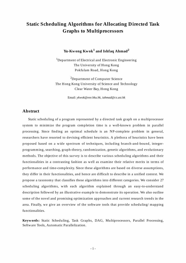
Abstract
Static scheduling of a program represented by a directed task graph on a multiprocessor
system to minimize the program completion time is a well-known problem in parallel
processing. Since finding an optimal schedule is an NP-complete problem in general,
researchers have resorted to devising efficient heuristics. A plethora of heuristics have been
proposed based on a wide spectrum of techniques, including branch-and-bound, integer-
programming, searching, graph-theory, randomization, genetic algorithms, and evolutionary
methods. The objective of this survey is to describe various scheduling algorithms and their
functionalities in a contrasting fashion as well as examine their relative merits in terms of
performance and time-complexity. Since these algorithms are based on diverse assumptions,
they differ in their functionalities, and hence are difficult to describe in a unified context. We
propose a taxonomy that classifies these algorithms into different categories. We consider 27
scheduling algorithms, with each algorithm explained through an easy-to-understand
description followed by an illustrative example to demonstrate its operation. We also outline
some of the novel and promising optimization approaches and current research trends in the
area. Finally, we give an overview of the software tools that provide scheduling/mapping
functionalities.
Keywords: Static Scheduling, Task Graphs, DAG, Multiprocessors, Parallel Processing,Software Tools, Automatic Parallelization.
- 2 -
1 Introduction
Parallel processing is a promising approach to meet the computational requirements of a
large number of current and emerging applications [82], [100], [140]. However, it poses a
number of problems which are not encountered in sequential processing such as designing a
parallel algorithm for the application, partitioning of the application into tasks, coordinating
communication and synchronization, and scheduling of the tasks onto the machine. A large
body of research efforts addressing these problems has been reported in the literature [14],
[33], [65], [82], [111], [115], [116], [117], [137], [140], [148], [170], [172]. Scheduling and
allocation is a highly important issue since an inappropriate scheduling of tasks can fail to
exploit the true potential of the system and can offset the gain from parallelization. In this
paper we focus on the scheduling aspect.
The objective of scheduling is to minimize the completion time of a parallel application
by properly allocating the tasks to the processors. In a broad sense, the scheduling problem
exists in two forms: static and dynamic. In static scheduling, which is usually done at compile
time, the characteristics of a parallel program (such as task processing times, communication,
data dependencies, and synchronization requirements) are known before program execution
[33], [65]. A parallel program, therefore, can be represented by a node- and edge-weighted
directed acyclic graph (DAG), in which the node weights represent task processing times and
the edge weights represent data dependencies as well as the communication times between
tasks. In dynamic scheduling, a few assumptions about the parallel program can be made
before execution, and thus, scheduling decisions have to be made on-the-fly [3], [130]. The
goal of a dynamic scheduling algorithm as such includes not only the minimization of the
program completion time but also the minimization of the scheduling overhead which
constitutes a significant portion of the cost paid for running the scheduler. We address only
the static scheduling problem. Hereafter, we refer to the static scheduling problem as simply
scheduling.
The scheduling problem is NP-complete for most of its variants except for a few
simplified cases (these cases will be elaborated in later sections) [32], [35], [36], [50], [51], [63],
[69], [72], [81], [90], [134], [135], [136], [143], [146], [165]. Therefore, many heuristics with
polynomial-time complexity have been suggested [8], [26], [35], [50], [51], [66], [92], [121],
[132], [139], [149], [156]. However, these heuristics are highly diverse in terms of their
assumptions about the structure of the parallel program and the target parallel architecture,
and thus are difficult to explain in a unified context.
- 3 -
Common simplifying assumptions include uniform task execution times, zero inter-task
communication times, contention-free communication, full connectivity of parallel
processors, and availability of unlimited number of processors. These assumptions may not
hold in practical situations for a number of reasons. For instance, it is not always realistic to
assume that the task execution times of an application are uniform because the amount of
computations encapsulated in tasks are usually varied. Furthermore, parallel and distributed
architectures have evolved into various types such as distributed-memory multicomputers
(DMMs) [82], shared-memory multiprocessors (SMMs) [82], clusters of symmetric
multiprocessors (SMPs) [140], and networks of workstations (NOWs) [82]. Therefore, their
more detailed architectural characteristics must be taken into account. For example, inter-task
communication in the form of message-passing or shared-memory access inevitably incurs a
non-negligible amount of latency. Moreover, a contention-free communication and full
connectivity of processors cannot be assumed for a DMM, a SMP or a NOW. Thus,
scheduling algorithms relying on such assumptions are apt to have restricted applicability in
real environments.
Multiprocessors scheduling has been an active research area and, therefore, many
different assumptions and terminology are independently suggested. Unfortunately, some of
the terms, and assumptions are neither clearly stated nor consistently used by most of the
researchers. As a result, it is difficult to appreciate the merits of various scheduling
algorithms and quantitatively evaluate their performance. To avoid this problem, we first
introduce the directed acyclic graph (DAG) model of a parallel program, and then proceed to
describe the multiprocessor model. This is followed by a discussion about the NP-
completeness of variants of the DAG scheduling problem. Some basic techniques used in
scheduling are introduced. Then we describe a taxonomy of DAG scheduling algorithms and
use it to classify several reported algorithms.
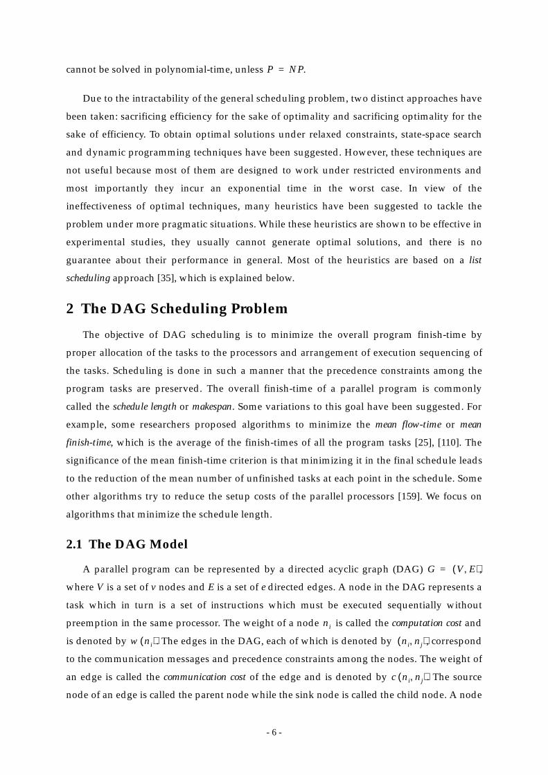
The problem of scheduling a set of tasks to a set of processors can be divided into two
categories: job scheduling and scheduling and mapping (see Figure 1(a)). In the former category,
independent jobs are to be scheduled among the processors of a distributed computing
system to optimize overall system performance [24], [28], [31]. In contrast, the scheduling and
mapping problem requires the allocation of multiple interacting tasks of a single parallel
program in order to minimize the completion time on the parallel computer system [1], [8],
[16], [26], [35], [164]. While job scheduling requires dynamic run-time scheduling that is not a
priori decidable, the scheduling and mapping problem can be addressed in both static [50],
[51], [66], [76], [77], [92], [121], [149] as well as dynamic contexts [3], [129]. When the
- 4 -
characteristics of the parallel program, including its task execution times, task dependencies,
task communications and synchronization, are known a priori, scheduling can be
accomplished off-line during compile-time. On the contrary, dynamic scheduling in the
absence of a priori information is done on-the-fly according to the state of the system.
Two distinct models of the parallel program have been considered extensively in the
context of static scheduling: the task interaction graph (TIG) model and the task precedence graph
(TPG) model (see Figure 1(b) and Figure 1(c)).
The task interaction graph model, in which vertices represent parallel processes and
edges denote the inter-process interaction [23], is usually used in static scheduling of loosely-
Parallel Program Scheduling
Job Scheduling (independent tasks)
Scheduling and Mapping (multiple interacting tasks)
Dynamic Scheduling Static Scheduling
Task Interaction Graph Task Precedence Graph
n2
n1
n3
n4
(a)
(b) (c)
Figure 1: (a) A simplified taxonomy of the approaches to the schedulingproblem; (b) A task interaction graph; (c) A task precedence graph.
- 5 -
coupled communicating processes (since all tasks are considered as simultaneously and
independently executable, there is no temporal execution dependency) to a distributed
system. For example, a TIG is commonly used to model the finite element method (FEM) [22].
The objective of scheduling is to minimize parallel program completion time by properly
mapping the tasks to the processors. This requires balancing the computation load uniformly
among the processors while simultaneously keeping communication costs as low as possible.
The research in this area was pioneered by Stone and Bohkari [22], [158]: Stone [158] applied
network-flow algorithms to solve the assignment problem while Bokhari described the
mapping problem as being equivalent to graph isomorphism, quadratic assignment and
sparse matrix bandwidth reduction problems [23].
The task precedence graph model or simply the DAG, in which the nodes represent the
tasks and the directed edges represent the execution dependencies as well as the amount of
communication, is commonly used in static scheduling of a parallel program with tightly-
coupled tasks on multiprocessors. For example, in the task precedence graph shown in
Figure 1(c), task n4 cannot commence execution before tasks n1 and n2 finish execution and
gathers all the communication data from n2 and n3. The scheduling objective is to minimize
the program completion time (or maximize the speed-up, defined as the time required for
sequential execution divided by the time required for parallel execution). For most parallel
applications, a task precedence graph can model the program more accurately because it
captures the temporal dependencies among tasks. This is the model we use in this paper.
As mentioned above, earlier static scheduling research made simplifying assumptions
about the architecture of the parallel program and the parallel machine, such as uniform
node weights, zero edge weights and the availability of unlimited number of processors.
However, even with some of these assumptions the scheduling problem has been proven to
be NP-complete except for a few restricted cases [63]. Indeed, the problem is NP-complete
even in two simple cases: (1) scheduling tasks with uniform weights to an arbitrary number
of processors [165] and (2) scheduling tasks with weights equal to one or two units to two
processors [165]. There are only three special cases for which there exists optimal polynomial-
time algorithms. These cases are: (1) scheduling tree-structured task graphs with uniform
computation costs on arbitrary number of processors [81], (2) scheduling arbitrary task
graphs with uniform computation costs on two processors [36] and (3) scheduling an interval-
ordered task graph [57] with uniform node weights to an arbitrary number of processors [135].
However, even in these cases, communication among tasks of the parallel program is
assumed to take zero time [35]. Given these observations, the general scheduling problem
- 6 -
cannot be solved in polynomial-time, unless .
Due to the intractability of the general scheduling problem, two distinct approaches have
been taken: sacrificing efficiency for the sake of optimality and sacrificing optimality for the
sake of efficiency. To obtain optimal solutions under relaxed constraints, state-space search
and dynamic programming techniques have been suggested. However, these techniques are
not useful because most of them are designed to work under restricted environments and
most importantly they incur an exponential time in the worst case. In view of the
ineffectiveness of optimal techniques, many heuristics have been suggested to tackle the
problem under more pragmatic situations. While these heuristics are shown to be effective in
experimental studies, they usually cannot generate optimal solutions, and there is no
guarantee about their performance in general. Most of the heuristics are based on a list
scheduling approach [35], which is explained below.
2 The DAG Scheduling Problem
The objective of DAG scheduling is to minimize the overall program finish-time by
proper allocation of the tasks to the processors and arrangement of execution sequencing of
the tasks. Scheduling is done in such a manner that the precedence constraints among the
program tasks are preserved. The overall finish-time of a parallel program is commonly
called the schedule length or makespan. Some variations to this goal have been suggested. For
example, some researchers proposed algorithms to minimize the mean flow-time or mean
finish-time, which is the average of the finish-times of all the program tasks [25], [110]. The
significance of the mean finish-time criterion is that minimizing it in the final schedule leads
to the reduction of the mean number of unfinished tasks at each point in the schedule. Some
other algorithms try to reduce the setup costs of the parallel processors [159]. We focus on
algorithms that minimize the schedule length.
2.1 The DAG Model
A parallel program can be represented by a directed acyclic graph (DAG) ,
where V is a set of v nodes and E is a set of e directed edges. A node in the DAG represents a
task which in turn is a set of instructions which must be executed sequentially without
preemption in the same processor. The weight of a node is called the computation cost and
is denoted by . The edges in the DAG, each of which is denoted by , correspond
to the communication messages and precedence constraints among the nodes. The weight of
an edge is called the communication cost of the edge and is denoted by . The source
node of an edge is called the parent node while the sink node is called the child node. A node
P NP=
G V E,( )=
ni
w ni( ) ni nj,( )
c ni nj,( )
- 7 -
with no parent is called an entry node and a node with no child is called an exit node. The
communication-to-computation-ratio (CCR) of a parallel program is defined as its average edge
weight divided by its average node weight. Hereafter, we use the terms node and task
interchangeably. We summarize in Table 1 the notation used throughout the paper.
The precedence constraints of a DAG dictate that a node cannot start execution before it
gathers all of the messages from its parent nodes. The communication cost between two tasks
assigned to the same processor is assumed to be zero. If node is scheduled to some
processor, then and denote the start-time and finish-time of , respectively.
After all the nodes have been scheduled, the schedule length is defined as
across all processors. The goal of scheduling is to minimize .
The node and edge weights are usually obtained by estimation at compile-time [9], [33],
TABLE 1.
Symbol Definition
The node number of a node in the parallel program task graph
The computation cost of node
An edge from node to
The communication cost of the directed edge from node to
v Number of nodes in the task graph
e Number of edges in the task graph
p The number of processors or processing elements (PEs) in the target system
CP A critical path of the task graph
CPN Critical Path Node
IBN In-Branch Node
OBN Out-Branch Node
sl Static level of a node
b-level Bottom level of a node
t-level Top level of a node
ASAP As soon as possible start time of a node
ALAP As late as possible start time of a node
The actual start time of a node
The possible data available time of on target processor P
The start time of node on target processor P
The finish time of node on target processor P
The parent node of that sends the data arrive last
Pivot_PE The target processor from which nodes are migrated
The processor accommodating node
Lij The communication link between PE i and PE j.
CCR Communication-to-computation Ratio
SL Schedule Length
UNC Unbounded Number of Clusters scheduling algorithms
BNP Bounded Number of Processors scheduling algorithms
TDB Task Duplication Based scheduling algorithms
APN Arbitrary Processors Network scheduling algorithms
ni
w ni( ) ni
ni nj,( ) ni nj
c ni nj,( ) ni nj
TS ni( ) ni
DAT ni P,( ) ni
ST ni P,( ) ni
FT ni P,( ) ni
VIP ni( ) ni
Proc ni( ) ni
ni
ST ni( ) FT ni( ) ni
maxi FT ni( ){ }
maxi FT ni( ){ }
- 8 -
[73], [38], [170]. Generation of the generic DAG model and some of the variations are
described below.
2.2 Generation of a DAG
A parallel program can be modeled by a DAG. Although program loops cannot be
explicitly represented by the DAG model, the parallelism in data-flow computations in loops
can be exploited to subdivide the loops into a number of tasks by the loop-unraveling
technique [18], [108]. The idea is that all iterations of the loop are started or fired together, and
operations in various iterations can execute when their input data are ready for access. In
addition, for a large class of data-flow computation problems and many numerical
algorithms (such as matrix multiplication), there are very few, if any, conditional branches or
indeterminism in the program. Thus, the DAG model can be used to accurately represent
these applications so that the scheduling techniques can be applied. Furthermore, in many
numerical applications, such as Gaussian elimination or fast Fourier transform (FFT), the
loop bounds are known during compile-time. As such, one or more iterations of a loop can be
deterministically encapsulated in a task and, consequently, be represented by a node in a
DAG.
The node- and edge-weights are usually obtained by estimation using profiling
information of operations such as numerical operations, memory access operations, and
message-passing primitives [87]. The granularity of tasks usually is specified by the
programmers [9]. Nevertheless, the final granularity of the scheduled parallel program is to
be refined by using a scheduling algorithm, which clusters the communication-intensive
tasks to a single processor [9], [172].
2.3 Variations in the DAG Model
There are a number of variations in the generic DAG model described above. The more
important variations are: preemptive scheduling vs. non-preemptive scheduling, parallel tasks vs.
non-parallel tasks and DAG with conditional branches vs. DAG without conditional branches.
Preemptive Scheduling vs. Non-preemptive Scheduling: In preemptive scheduling, the
execution of a task may be interrupted so that the unfinished portion of the task can be re-
allocated to a different processor [29], [70], [79], [142]. On the contrary, algorithms assuming
non-preemptive scheduling must allow a task to execute until completion on a single
processor. From a theoretical perspective, a preemptive scheduling approach allows more
flexibility for the scheduler so that a higher utilization of processors may result. Indeed, a
- 9 -
preemptive scheduling problem is commonly reckoned as “easier” than its non-preemptive
counterpart in that there are cases in which polynomial time solutions exist for the former
while the latter is proved to be NP-complete [35], [69]. However, in practice, interrupting a
task and transferring it to another processor can lead to significant processing overhead and
communication delays. In addition, a preemptive scheduler itself is usually more
complicated since it has to consider when to split a task and where to insert the necessary
communication induced by the splitting. We concentrate on the non-preemptive approaches.
Parallel Tasks vs. Non-parallel Tasks: A parallel task is a task that requires more than one
processor at the same time for its execution [167]. Blazewicz et al. investigated the problem of
scheduling a set of independent parallel tasks to identical processors under preemptive and
non-preemptive scheduling assumptions [20], [21]. Du and Leung also explored the same
problem but with one more flexibility: a task can be scheduled to no more than a certain pre-
defined maximum number of processors [47]. However, in Blazewicz et al. ‘s approach, a task
must be scheduled to a fixed pre-defined number of processors. Wang and Cheng further
extended the model to allow precedence constraints among tasks [167]. They devised a list
scheduling approach to construct a schedule based on the earliest completion time (ECT)
heuristic. We concentrate on scheduling DAGs with non-parallel tasks.
DAG with Conditional Branches vs. DAG without Conditional Branches: Towsley [162]
addressed the problem of scheduling a DAG with probabilistic branches and loops to
heterogeneous distributed systems. Each edge in the DAG is associated with a non-zero
probability that the child will be executed immediately after the parent. He introduced two
algorithms based on the shortest path method for determining the optimal assignments of
tasks to processors. El-Rewini and Ali [52] also investigated the problem of scheduling DAGs
with conditional branches. Similar to Towsley’s approach, they also used a two-step method
to construct a final schedule. However, unlike Towsley’s model, they modeled a parallel
program by using two DAGs: a branch graph and a precedence graph. This model differentiates
the conditional branching and the precedence relations among the parallel program tasks.
The objective of the first step of the algorithm is to reduce the amount of indeterminism in the
DAG by capturing the similarity of different instances of the precedence graph. After this
pre-processing step, a reduced branch graph and a reduced precedence graph are generated.
In the second step, all the different instances of the precedence graph are generated according
to the reduced branch graph, and the corresponding schedules are determined. Finally, these
schedules are merged to produce a unified final schedule [52]. Since modeling branching and
looping in DAGs is an inherently difficult problem, little work has been reported in this area.
- 10 -
We concentrate on DAGs without conditional branching in this research.
2.4 The Multiprocessor Model
In DAG scheduling, the target system is assumed to be a network of processing elements
(PEs), each of which is composed of a processor and a local memory unit so that the PEs do
not share memory and communication relies solely on message-passing. The processors may
be heterogeneous or homogeneous. Heterogeneity of processors means the processors have
different speeds or processing capabilities. However, we assume every module of a parallel
program can be executed on any processor even though the completion times on different
processors may be different. The PEs are connected by an interconnection network with a
certain topology. The topology may be fully-connected or of a particular structure such as a
hypercube or mesh.
3 NP-Completeness of the DAG Scheduling Problem
The DAG scheduling problem is in general an NP-complete problem [63], and algorithms
for optimally scheduling a DAG in polynomial-time are known only for three simple cases
[35]. The first case is to schedule a uniform node-weight free-tree to an arbitrary number of
processors. Hu [81] proposed a linear-time algorithm to solve the problem. The second case is
to schedule an arbitrarily structured DAG with uniform node-weights to two processors.
Coffman and Graham [36] devised a quadratic-time algorithm to solve this problem. Both
Hu’s algorithm and Coffman et al.’s algorithm are based on node-labeling methods that
produce optimal scheduling lists leading to optimal schedules. Sethi [146] then improved the
time-complexity of Coffman et al.’s algorithm to almost linear-time by suggesting a more
efficient node-labeling process. The third case is to schedule an interval-ordered DAG with
uniform node-weights to an arbitrary number of processors. Papadimitriou and Yannakakis
[135] designed a linear-time algorithm to tackle the problem. A DAG is called interval-
ordered if every two precedence-related nodes can be mapped to two non-overlapping
intervals on the real number line [57].
In all of the above three cases, communication between tasks is ignored. Ali and El-
Rewini [10] showed that interval-ordered DAG with uniform edge weights, which are equal
to the node weights, can also be optimally scheduled in polynomial time. These optimality
results are summarized in Table 2.
Ullman [165] showed that scheduling a DAG with unit computation to p processors is
NP-complete. He also showed that scheduling a DAG with one or two unit computation
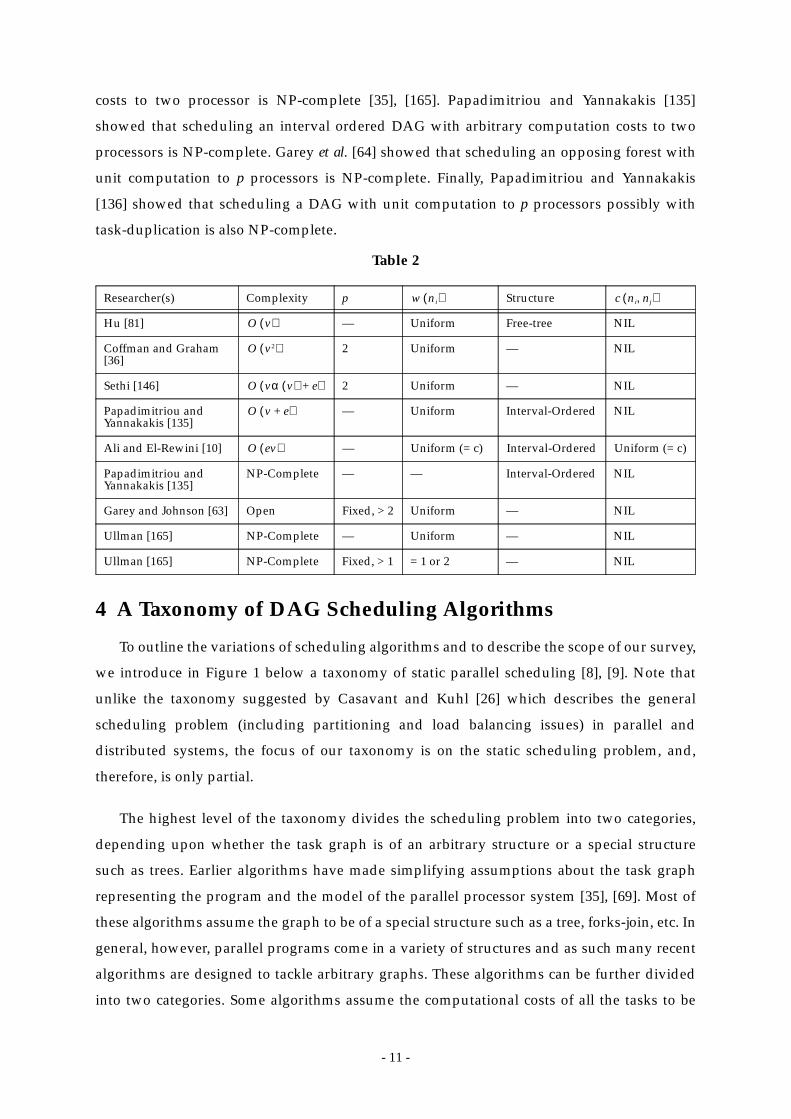
- 11 -
costs to two processor is NP-complete [35], [165]. Papadimitriou and Yannakakis [135]
showed that scheduling an interval ordered DAG with arbitrary computation costs to two
processors is NP-complete. Garey et al. [64] showed that scheduling an opposing forest with
unit computation to p processors is NP-complete. Finally, Papadimitriou and Yannakakis
[136] showed that scheduling a DAG with unit computation to p processors possibly with
task-duplication is also NP-complete.
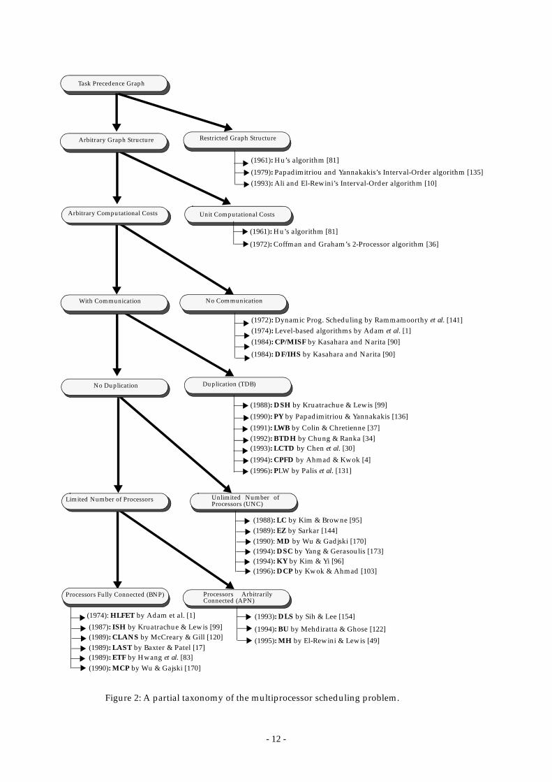
4 A Taxonomy of DAG Scheduling Algorithms
To outline the variations of scheduling algorithms and to describe the scope of our survey,
we introduce in Figure 1 below a taxonomy of static parallel scheduling [8], [9]. Note that
unlike the taxonomy suggested by Casavant and Kuhl [26] which describes the general
scheduling problem (including partitioning and load balancing issues) in parallel and
distributed systems, the focus of our taxonomy is on the static scheduling problem, and,
therefore, is only partial.
The highest level of the taxonomy divides the scheduling problem into two categories,
depending upon whether the task graph is of an arbitrary structure or a special structure
such as trees. Earlier algorithms have made simplifying assumptions about the task graph
representing the program and the model of the parallel processor system [35], [69]. Most of
these algorithms assume the graph to be of a special structure such as a tree, forks-join, etc. In
general, however, parallel programs come in a variety of structures and as such many recent
algorithms are designed to tackle arbitrary graphs. These algorithms can be further divided
into two categories. Some algorithms assume the computational costs of all the tasks to be
Table 2
Researcher(s) Complexity p Structure
Hu [81] — Uniform Free-tree NIL
Coffman and Graham [36]
2 Uniform — NIL
Sethi [146] 2 Uniform — NIL
Papadimitriou and Yannakakis [135]
— Uniform Interval-Ordered NIL
Ali and El-Rewini [10] — Uniform (= c) Interval-Ordered Uniform (= c)
Papadimitriou and Yannakakis [135]
NP-Complete — — Interval-Ordered NIL
Garey and Johnson [63] Open Fixed, > 2 Uniform — NIL
Ullman [165] NP-Complete — Uniform — NIL
Ullman [165] NP-Complete Fixed, > 1 = 1 or 2 — NIL
w ni( ) c ni nj,( )
O v( )
O v2( )
O vα v( ) e+( )
O v e+( )
O ev( )
- 12 -
Figure 2: A partial taxonomy of the multiprocessor scheduling problem.
Task Precedence Graph
Duplication (TDB)No Duplication
Limited Number of Processors Unlimited Number ofProcessors (UNC)
Processors ArbitrarilyConnected (APN)
Processors Fully Connected (BNP)
Arbitrary Computational Costs Unit Computational Costs
Arbitrary Graph Structure Restricted Graph Structure
No CommunicationWith Communication
(1994): BU by Mehdiratta & Ghose [122]
(1993): DLS by Sih & Lee [154]
(1995): MH by El-Rewini & Lewis [49]
(1990): PY by Papadimitriou & Yannakakis [136]
(1993): LCTD by Chen et al. [30]
(1988): DSH by Kruatrachue & Lewis [99]
(1992): BTDH by Chung & Ranka [34](1991): LWB by Colin & Chretienne [37]
(1994): CPFD by Ahmad & Kwok [4](1996): PLW by Palis et al. [131]
(1989): EZ by Sarkar [144] (1990): MD by Wu & Gadjski [170] (1994): DSC by Yang & Gerasoulis [173]
(1996): DCP by Kwok & Ahmad [103]
(1988): LC by Kim & Browne [95]
(1994): KY by Kim & Yi [96]
(1990): MCP by Wu & Gajski [170]
(1989): CLANS by McCreary & Gill [120] (1989): LAST by Baxter & Patel [17] (1989): ETF by Hwang et al. [83]
(1987): ISH by Kruatrachue & Lewis [99]
(1974): HLFET by Adam et al. [1]
(1961): Hu’s algorithm [81]
(1972): Coffman and Graham’s 2-Processor algorithm [36]
(1979): Papadimitriou and Yannakakis’s Interval-Order algorithm [135](1993): Ali and El-Rewini’s Interval-Order algorithm [10]
(1974): Level-based algorithms by Adam et al. [1]
(1984): CP/MISF by Kasahara and Narita [90]
(1984): DF/IHS by Kasahara and Narita [90]
(1972): Dynamic Prog. Scheduling by Rammamoorthy et al. [141]
(1961): Hu’s algorithm [81]
- 13 -
uniform. Others assume the computational costs of tasks to be arbitrary.
Some of the scheduling algorithms which consider the inter-task communication assume
the availability of unlimited number of processors, while some other algorithms assume a
limited number of processors. The former class of algorithms are called the UNC (unbounded
number of clusters) scheduling algorithms [95], [103], [103], [144], [169], [173] and the latter the
BNP (bounded number of processors) scheduling algorithms [1], [15], [96], [104], [120], [131],
[155]. In both classes of algorithms, the processors are assumed to be fully-connected and no
attention is paid to link contention or routing strategies used for communication. The
technique employed by the UNC algorithms is also called clustering [95], [112], [131], [144],
[173]. At the beginning of the scheduling process, each node is considered a cluster. In the
subsequent steps, two clusters are merged if the merging reduces the completion time. This
merging procedure continues until no cluster can be merged. The rationale behind the UNC
algorithms is that they can take advantage of using more processors to further reduce the
schedule length. However, the clusters generated by the UNC need a postprocessing step for
mapping the clusters onto the processors because the number of processors available may be
less than the number of clusters. As a result, the final solution quality also highly depends on
the cluster-mapping step. On the other hand, the BNP algorithms do not need such
postprocessing step. It is an open question as to which of UNC and BNP is better.
We use the term cluster and processor interchangeably since in the UNC scheduling
algorithms, merging a single node cluster to another cluster is analogous to scheduling a
node to a processor.
There have been a few algorithms designed with the most general model in that the
system is assumed to consist of an arbitrary network topology, of which the links are not
contention-free. These algorithms are called the APN (arbitrary processor network) scheduling
algorithms. In addition to scheduling tasks, the APN algorithms also schedule messages on
the network communication links. Scheduling of messages may be dependent on the routing
strategy used by the underlying network. To optimize schedule lengths under such
unrestricted environments makes the design of an APN scheduling algorithm intricate and
challenging.
The TDB (Task-Duplication Based) scheduling algorithms also assume the availability of
an unbounded number of processors but schedule tasks with duplication to further reduce
the schedule lengths. The rationale behind the TDB scheduling algorithms is to reduce the
communication overhead by redundantly allocating some tasks to multiple processors. In
- 14 -
duplication-based scheduling, different strategies can be employed to select ancestor nodes
for duplication. Some of the algorithms duplicate only the direct predecessors while others
try to duplicate all possible ancestors. For a recent quantitative comparison of TDB
scheduling algorithms, the reader is referred to [6].
5 Basic Techniques in DAG Scheduling
Most scheduling algorithms are based on the so called list scheduling technique [1], [8],
[26], [35], [50], [51], [66], [92], [104], [121], [149], [174]. The basic idea of list scheduling is to
make a scheduling list (a sequence of nodes for scheduling) by assigning them some
priorities, and then repeatedly execute the following two steps until all the nodes in the
graph are scheduled:
1) Remove the first node from the scheduling list;
2) Allocate the node to a processor which allows the earliest start-time.
There are various ways to determine the priorities of nodes such as HLF (Highest level
First) [35], LP (Longest Path) [35], LPT (Longest Processing Time) [60], [69] and CP (Critical
Path) [72].
Recently a number of scheduling algorithms based on a dynamic list scheduling approach
have been suggested [103], [154], [173]. In a traditional scheduling algorithm, the scheduling
list is statically constructed before node allocation begins, and most importantly the
sequencing in the list is not modified. In contrast, after each allocation, these recent
algorithms re-compute the priorities of all unscheduled nodes which are then used to
rearrange the sequencing of the nodes in the list. Thus, these algorithms essentially employ
the following three-step approaches:
1) Determine new priorities of all unscheduled nodes;
2) Select the node with the highest priority for scheduling;
3) Allocate the node to the processor which allows the earliest start-time.
Scheduling algorithms which employ this three-step approach can potentially generate
better schedules. However, a dynamic approach can increase the time-complexity of the
scheduling algorithm.
Two frequently used attributes for assigning priority are the t-level (top level) and b-level
(bottom level) [1], [8], [66]. The t-level of a node is the length of a longest path (there can beni
- 15 -
more than one longest path) from an entry node to (excluding ). Here, the length of a
path is the sum of all the node and edge weights along the path. As such, the t-level of
highly correlates with ’s earliest start-time, denoted by , which is determined after
is scheduled to a processor. This is because after is scheduled, its is simply the
length of the longest path reaching it. The b-level of a node is the length of a longest path
from to an exit node. The b-level of a node is bounded from above by the length of a critical
path. A critical path (CP) of a DAG, which is an important structure in the DAG, is a longest
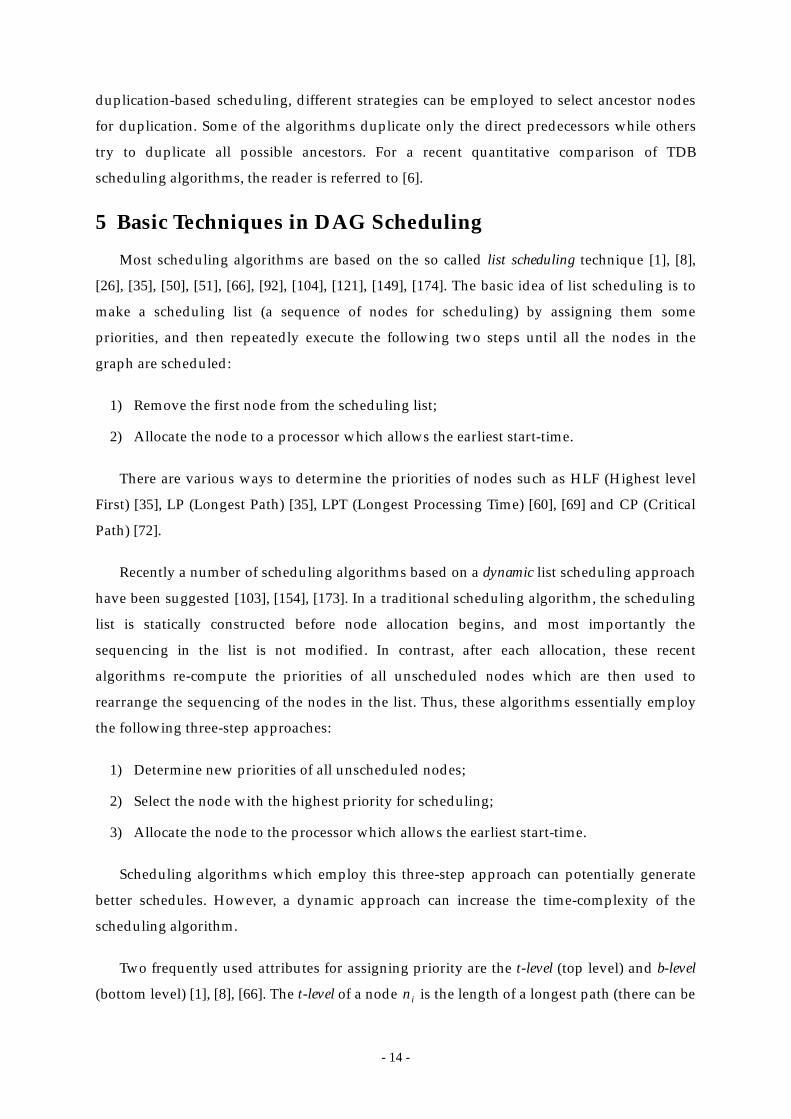
path in the DAG. Clearly a DAG can have more than one CP. Consider the task graph shown
in Figure 3(a). In this task graph, nodes are the nodes of the only CP and are called
CPNs (Critical-Path Nodes). The edges on the CP are shown with thick arrows. The values of
the priorities discussed above are shown in Figure 3(b).
Below is a procedure for computing the t-levels:
Computation of t-level:(1) Construct a list of nodes in topological order. Call it TopList.(2) for each node in TopList do (3) max = 0(4) for each parent of do(5) if t-level( ) + + > max then (6) max = t-level( ) + + (7) endif
ni ni
ni
ni TS ni( ) ni
ni TS ni( )
ni
ni
n1 n7 n9, ,
n1
2
n2
3
n5
5
n9
n3
3
n7
4
n4
4
n8
4
n6
4
1
6
10
1
111
4
1
1
55
(a)
(b)
node sl t-level b-level ALAP* 11 0 23 0
8 6 15 88 3 14 99 3 15 85 3 5 185 10 10 13
* 5 12 11 125 8 10 13
* 1 22 1 22
n1
n2
n3
n4
n5
n6
n7
n8
n9
1
Figure 3: (a) A task graph; (b) The static levels (sls), t-levels, b-levels and ALAPs of the nodes.
ni
nx ninx w nx( ) c nx ni,( )
nx w nx( ) c nx ni,( )
- 16 -
(8) endfor(9) t-level( ) = max(10) endfor
The time-complexity of the above procedure is . A similar procedure, which also
has time-complexity , for computing the b-levels is shown below:
Computation of b-level:(1) Construct a list of nodes in reversed topological order. Call it RevTopList.(2) for each node in RevTopList do(3) max = 0(4) for each child of do(5) if + b-level( ) > max then(6) max = + b-level( )(7) endif(8) endfor(9) b-level( ) = + max(10) endfor
In the scheduling process, the t-level of a node varies while the b-level is usually a
constant, until the node has been scheduled. The t-level varies because the weight of an edge
may be zeroed when the two incident nodes are scheduled to the same processor. Thus, the
path reaching a node, whose length determines the t-level of the node, may cease to be the
longest one. On the other hand, there are some variations in the computation of the b-level of
a node. Most algorithms examine a node for scheduling only after all the parents of the node
have been scheduled. In this case, the b-level of a node is a constant until after it is scheduled
to a processor. Some scheduling algorithms allow the scheduling of a child before its parents,
however, in which case the b-level of a node is also a dynamic attribute. It should be noted
that some scheduling algorithms do not take into account the edge weights in computing the
b-level. In such a case, the b-level does not change throughout the scheduling process. To
distinguish such definition of b-level from the one we described above, we call it the static b-
level or simply static level (sl).
Different algorithms use the t-level and b-level in different ways. Some algorithms assign a
higher priority to a node with a smaller t-level while some algorithms assign a higher priority
to a node with a larger b-level. Still some algorithms assign a higher priority to a node with a
larger (b-level – t-level). In general, scheduling in a descending order of b-level tends to
schedule critical path nodes first, while scheduling in an ascending order of t-level tends to
schedule nodes in a topological order. The composite attribute (b-level – t-level) is a
compromise between the previous two cases. If an algorithm uses a static attribute, such as b-
level or static b-level, to order nodes for scheduling, it is called a static algorithm; otherwise, it
ni
O e v+( )
O e v+( )
ni
ny ni
c ni ny,( ) ny
c ni ny,( ) ny
ni w ni( )
- 17 -
is called a dynamic algorithm.
Note that the procedure for computing the t-levels can also be used to compute the start-
times of nodes on processors during the scheduling process. Indeed, some researchers call the
t-level of a node the ASAP (As-Soon-As-Possible) start-time because the t-level is the earliest
possible start-time.
Some of the DAG scheduling algorithms employ an attribute called ALAP (As-Late-As-
Possible) start-time [103], [170]. The ALAP start-time of a node is a measure of how far the
node’s start-time can be delayed without increasing the schedule length. An time
procedure for computing the ALAP time is shown below:
Computation of ALAP:(1) Construct a list of nodes in reversed topological order. Call it RevTopList.(2) for each node in RevTopList do(3) min_ft = CP_Length(4) for each child of do(5) if alap( ) – < min_ft then(6) min_ft = alap( ) – (7) endif(8) endfor(9) alap( ) = min_ft – (10) endfor
After the scheduling list is constructed by using the node priorities, the nodes are then
scheduled to suitable processors. Usually a processor is considered suitable if it allows the
earliest start-time for the node. However, in some sophisticated scheduling heuristics, a
suitable processor may not be the one that allows the earliest start-time. These variations are
described in detail in Section 6.
6 Description of the Algorithms
In this section, we briefly survey algorithms for DAG scheduling reported in the
literature. We first describe some of the earlier scheduling algorithms which assume a
restricted DAG model, and then proceed to describe a number of such algorithms before
proceeding to algorithms which remove all such simplifying assumptions. The performance
of these algorithms on some primitive graph structures is also discussed. Analytical
performance bounds reported in the literature are also briefly surveyed where appropriate.
We first discuss the UNC class of algorithms, followed by BNP algorithms and TDB
algorithms. Next we describe a few of the relatively unexplored APN class of DAG
scheduling algorithms. Finally we discuss the issues of scheduling in heterogeneous
O e v+( )
ni
ny ni
ny c ni ny,( )ny c ni ny,( )
ni w ni( )
- 18 -
environments and the mapping problem.
6.1 Scheduling DAGs with Restricted Structures
Early scheduling algorithms were typically designed with simplifying assumptions about
the DAG and processor network model [1], [25], [61], [62]. For instance, the nodes in the DAG
were assumed to be of unit computation and communication was not considered; that is,
and . Furthermore, some algorithms were designed for specially
structured DAGs such as a free-tree [35], [81]
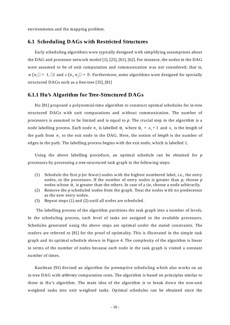
6.1.1 Hu’s Algorithm for Tree-Structured DAGs
Hu [81] proposed a polynomial-time algorithm to construct optimal schedules for in-tree
structured DAGs with unit computations and without communication. The number of
processors is assumed to be limited and is equal to p. The crucial step in the algorithm is a
node labelling process. Each node is labelled where and is the length of
the path from to the exit node in the DAG. Here, the notion of length is the number of
edges in the path. The labelling process begins with the exit node, which is labelled 1.
Using the above labelling procedure, an optimal schedule can be obtained for p
processors by processing a tree-structured task graph in the following steps:
(1) Schedule the first p (or fewer) nodes with the highest numbered label, i.e., the entrynodes, to the processors. If the number of entry nodes is greater than p, choose pnodes whose is greater than the others. In case of a tie, choose a node arbitrarily.
(2) Remove the p scheduled nodes from the graph. Treat the nodes with no predecessoras the new entry nodes.
(3) Repeat steps (1) and (2) until all nodes are scheduled.
The labelling process of the algorithm partitions the task graph into a number of levels.
In the scheduling process, each level of tasks are assigned to the available processors.
Schedules generated using the above steps are optimal under the stated constraints. The
readers are referred to [81] for the proof of optimality. This is illustrated in the simple task
graph and its optimal schedule shown in Figure 4. The complexity of the algorithm is linear
in terms of the number of nodes because each node in the task graph is visited a constant
number of times.
Kaufman [91] devised an algorithm for preemptive scheduling which also works on an
in-tree DAG with arbitrary computation costs. The algorithm is based on principles similar to
those in Hu’s algorithm. The main idea of the algorithm is to break down the non-unit
weighted tasks into unit weighted tasks. Optimal schedules can be obtained since the
w ni( ) 1 i∀,= c ni nj,( ) 0=
ni αi αi xi 1+= xi
ni
αi
- 19 -
resulting DAG is still an in-tree.
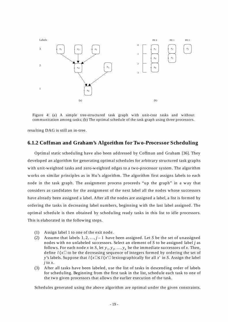
6.1.2 Coffman and Graham’s Algorithm for Two-Processor Scheduling
Optimal static scheduling have also been addressed by Coffman and Graham [36]. They
developed an algorithm for generating optimal schedules for arbitrary structured task graphs
with unit-weighted tasks and zero-weighted edges to a two-processor system. The algorithm
works on similar principles as in Hu’s algorithm. The algorithm first assigns labels to each
node in the task graph. The assignment process proceeds “up the graph” in a way that
considers as candidates for the assignment of the next label all the nodes whose successors
have already been assigned a label. After all the nodes are assigned a label, a list is formed by
ordering the tasks in decreasing label numbers, beginning with the last label assigned. The
optimal schedule is then obtained by scheduling ready tasks in this list to idle processors.
This is elaborated in the following steps.
(1) Assign label 1 to one of the exit node.(2) Assume that labels have been assigned. Let S be the set of unassigned
nodes with no unlabeled successors. Select an element of S to be assigned label j asfollows. For each node x in S, let be the immediate successors of x. Then,define to be the decreasing sequence of integers formed by ordering the set ofy’s labels. Suppose that lexicographically for all in S. Assign the labelj to x.
(3) After all tasks have been labeled, use the list of tasks in descending order of labelsfor scheduling. Beginning from the first task in the list, schedule each task to one ofthe two given processors that allows the earlier execution of the task.
Schedules generated using the above algorithm are optimal under the given constraints.
n1
n4
n2
n6
n5
n3
Labels
3
2
1
n1 n3n2
n4 n5
n6
0
1
2
3
PE 0 PE 1 PE 2
(a) (b)
Figure 4: (a) A simple tree-structured task graph with unit-cost tasks and withoutcommunication among tasks; (b) The optimal schedule of the task graph using three processors.
1 2 … j 1–, , ,
y1 y2 … yk, , ,l x( )
l x( ) l x'( )≤ x'
- 20 -
For the proof of optimality, the reader is referred to [36]. An example is illustrated in Figure 5.
Through counter-examples, Coffman and Graham also demonstrated that their algorithm
can generate sub-optimal solutions when the number of processors is increased to three or
more, or when the number of processors is two and tasks are allowed to have arbitrary
computation costs. This is true even when the computation costs are allowed to be one or two
units. The complexity of the algorithm is because the labelling process and the
scheduling process each takes time.
Sethi [146] reported an algorithm to determine the labels in time and also gave
an algorithm to construct a schedule from the labeling in time, where is
an almost constant function of v. The main idea of the improved labeling process is based on
the observation that the labels of a set of nodes with the same height only depend on their
children. Thus, instead of constructing the lexicographic ordering information from scratch,
the labeling process can infer such information through visiting the edges connecting the
nodes and their children. As a result, the time-complexity of the labeling process is
instead of . The construction of the final schedule is done with the aid of a set data
structure, for which v access operations can be performed in , where is the
inverse Ackermann’s function.
6.1.3 Scheduling Interval-Ordered DAGs
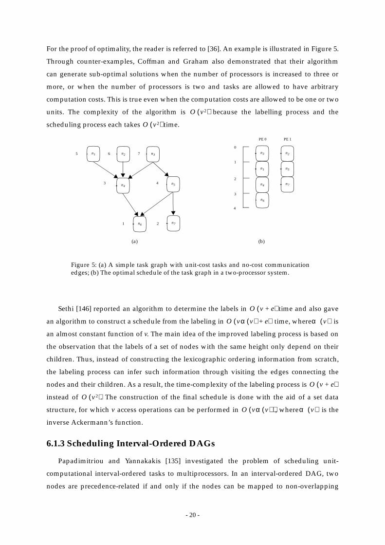
Papadimitriou and Yannakakis [135] investigated the problem of scheduling unit-
computational interval-ordered tasks to multiprocessors. In an interval-ordered DAG, two
nodes are precedence-related if and only if the nodes can be mapped to non-overlapping
O v2( )
n1
n4
n2
n6
n5
n3
n71 2
43
5 6 7 n3 n2
n1 n5
n4 n7
n6
0
1
2
3
4
PE 0 PE 1
(a) (b)
Figure 5: (a) A simple task graph with unit-cost tasks and no-cost communicationedges; (b) The optimal schedule of the task graph in a two-processor system.
O v2( )
O v e+( )
O vα v( ) e+( ) α v( )
O v e+( )
O v2( )
O vα v( )( ) α v( )
- 21 -
intervals on the real line [57]. An example of an interval-ordered DAG is shown in Figure 6.
Based on the interval-ordered property, the number of successors of a node can be used as a
priority to construct a list. An optimal list schedule can be constructed in time.
However, as mentioned earlier, the problem becomes NP-complete if the DAG is allowed to
have arbitrary computation costs. Ali and El-Rewini [10] worked on the problem of
scheduling interval-ordered DAGs with unit computation costs and unit communication
costs. They showed that the problem is tractable and devised an algorithm to generate
optimal schedules. In their algorithm, which is similar to that of Papadimitriou and
Yannakakis, the number of successors is used as a node priority for scheduling.
6.2 Scheduling Arbitrary DAGs without Communication
In this section, we discuss algorithms for scheduling arbitrary structured DAGs in which
computation costs are arbitrary but communication costs are zero.
6.2.1 Level-based Heuristics
Adam et al. [1] performed an extensive simulation study of the performance of a number
of level-based list scheduling heuristics. The heuristics examined are:
• HLFET (Highest Level First with Estimated Times): The notion of level is the sum of
computation costs of all the nodes along the longest path from the node to an exit node.
• HLFNET (Highest Levels First with No Estimated Times): In this heuristic, all nodes
are scheduled as if they were of unit cost.
• Random: The nodes in the DAG are assigned priorities randomly.
n1
n4
n2
n6
n5
n3
n7
Interval 1
Interval 2
Interval 3
Figure 6: (a) A unit-computational interval ordered DAG. (b) An optimal schedule of the DAG.
n3 n2
n1 n5
n4 n7
n6
0
1
2
3
4
PE 0 PE 1
(a) (b)
O v e+( )
O ve( )
- 22 -
• SCFET (Smallest Co-levels First with Estimated Times): A co-level of a node is
determined by computing the sum of the longest path from an entry node to the node.
A node has a higher priority if it has the smaller co-level.
• SCFNET (Smallest Co-levels First with No Estimated Times): This heuristic is the same
as SCFET except that it schedules the nodes as if they were of unit costs.
In [1], an extensive simulation study was conducted using randomly generated DAGs.
The performance of the heuristics were ranked in the following order: HLFET, HLFNET,
SCFNET, Random, and SCFET. The study provided strong evidence that the CP (critical path)
based algorithms have near-optimal performance. In another study conducted by Kohler
[94], the performance of the CP-based algorithms improved as the number of processors
increased.
Kasahara et al. [90] proposed an algorithm called CP/MISF (critical path/ most
immediate successors first), which is a variation of the HLFET algorithm. The major
improvement of CP/MISF over HLFET is that when assigning priorities, ties are broken by
selecting the node with a larger number of immediate successors.
In a recent study, Shirazi et al. [149] proposed two algorithms for scheduling DAGs to
multiprocessors without communication. The first algorithm, called HNF (Heavy Node
First), is based on a simple local analysis of the DAG nodes at each level. The second
algorithm, WL (Weighted Length), considers a global view of a DAG by taking into account
the relationship among the nodes at different levels. Compared to a critical-path-based
algorithm, Shirazi et al. showed that the HNF algorithm is more preferable for its low
complexity and good performance.
6.2.2 A Branch-and-Bound Approach
In addition to CP/MISF, Kasahara et al. [90] also reported a scheduling algorithm based
on a branch-and-bound approach. Using Kohler et al.’s [93] general representation for
branch-and-bound algorithms, Kasahara et al. devised a depth-first search procedure to
construct near-optimal schedules. Prior to the depth-first search process, priorities are
assigned to those nodes in the DAG which may be generated during the search process. The
priorities are determined using the priority list of the CP/MISF method. In this way the
search procedure can be more efficient both in terms of computing time and memory
requirement. Since the search technique is augmented by a heuristic priority assignment
method, the algorithm is called DF/IHS (depth-first with implicit heuristic search). The DF/
- 23 -
IHS algorithm was shown to give near optimal performance.
6.2.3 Analytical Performance Bounds for Scheduling without Communication
Graham [71] proposed a bound on the schedule length obtained by general list
scheduling methods. Using a level-based method for generating a list for scheduling, the
schedule length SL and the optimal schedule length are related by the following:
Rammamoorthy, Chandy, and Gonzalez [141] used the concept of precedence partitions
to generate bounds on the schedule length and the number of processors for DAGs with unit
computation costs. An earliest precedence partition is a set of nodes that can be started in
parallel at the same earliest possible time constrained by the precedence relations. A latest
precedence partition is a set of nodes which must be executed at the same latest possible time
constrained by the precedence relations. For any i and j, and . The
precedence partitions group tasks into subsets to indicate the earliest and latest times during
which tasks can be started and still guarantee minimum execution time for the graph. This
time is given by the number of partitions and is a measure of the longest path in the graph.
For a graph of l levels, the minimum execution time is l units. In order to execute a graph in
the minimum time, the absolute minimum number of processors required is given by
.
Rammamoorthy et al. [141] also developed algorithms to determine the minimum
number of processors required to process a graph in the least possible amount of time, and to
determine the minimum time necessary to process a task graph given k processors. Since a
dynamic programming approach is employed, the computational time required to obtain the
optimal solution is quite considerable.
Fernandez et al. [54] devised improved bounds on the minimum number of processors
required to achieve the optimal schedule length and on the minimum increase in schedule
length if only a certain number of processors are available. The most important contribution
is that the DAG is assumed to have unequal computational costs. Although for such a general
model similar partitions as in Rammamoorthy et al. ‘s work could be defined, Fernandez et al.
[54] used the concepts of activity and load density, defined below.
SLopt
SL 21p---–
SLopt.≤
Ei
Ei Ej φ=∩ Li Lj∩ φ=
max1 i l≤ ≤ Ei Li∩{ }
- 24 -
Definition 1: The activity of a node is defined as:
where is the finish time of .
Definition 2: The load density function is defined by:
Then, indicates the activity of node along time, according to the precedence
constraints in the DAG, and indicates the total activity of the graph as a function of
time. Of particular importance are , the earliest load density function for which all
tasks are completed at their earliest times, and , the load density function for which all
tasks are completed at their latest times. Now let be the load density function of
the tasks or parts of tasks remaining within after all tasks have been shifted to form
minimum overlap within the interval. Thus, a lower bound on the minimum number of
processors to execute the program (represented by the DAG) within the minimum time is
given by:
The maximum value obtained for all possible intervals indicate that the whole
computation graph cannot be executed with a number of processors smaller than the
maximum. Suppose that only p’ processors are available, Fernandez et al. [54] also showed
that the schedule length will be longer than the optimal schedule length by no less than the
following amount:
In a recent study, Jain and Rajaraman [85] reported sharper bounds using the above
expressions. The idea is that the intervals considered for the integration is not just the earliest
and latest start-times but are based on a partitioning of the graphs into a set of disjoint
sections. They also devised an upper bound on the schedule length, which is useful in
determining the worst case behavior of a DAG. Not only are their new bounds easier to
compute but are also tighter in that the DAG partitioning strategy enhances the accuracy of
ni
f τi t,( )1 t τi w ni( ) τi,–[ ] ,∈,
0 otherwise,{=
τi ni
F τ t,( ) f τi t,( ) .i 1=
v
∑=
f τi t,( ) ni
F τ t,( )
F τe t,( )
F τl t,( )
R θ1 θ2 t, ,( )
θ1 θ2,[ ]
pmin max θ1 θ2,[ ]1
θ2 θ1–---------------- R θ1 θ2 t, ,( ) td
θ1
θ2
∫ .=
max w n1( ) w nk( ) CP≤≤ w nk( )–1p'---- F τl t,( ) td
0
w nk( )
∫+ .
- 25 -
the load activity function.
6.3 UNC Scheduling
In this section we survey the UNC class of scheduling algorithms. In particular, we will
describe in more details five UNC scheduling algorithms: the EZ, LC, DSC, MD, and DCP
algorithms. The DAG shown in Figure 3 is used to illustrate the scheduling process of these
algorithms. In order to examine the approximate optimality of the algorithms, we will first
describe the scheduling of two primitive DAG structures: the fork set and the join set. Some
work on theoretical performance analysis of UNC scheduling is also discussed in the last
subsection.
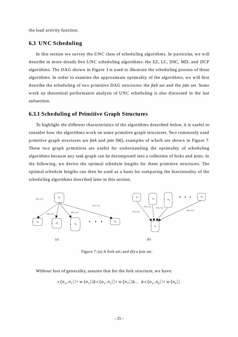
6.3.1 Scheduling of Primitive Graph Structures
To highlight the different characteristics of the algorithms described below, it is useful to
consider how the algorithms work on some primitive graph structures. Two commonly used
primitive graph structures are fork and join [66], examples of which are shown in Figure 7.
These two graph primitives are useful for understanding the optimality of scheduling
algorithms because any task graph can be decomposed into a collection of forks and joins. In
the following, we derive the optimal schedule lengths for these primitive structures. The
optimal schedule lengths can then be used as a basis for comparing the functionality of the
scheduling algorithms described later in this section.
Without loss of generality, assume that for the fork structure, we have:
n1 n2nk
n3
nx
Figure 7: (a) A fork set; and (b) a join set.
c(n1, nx)
n1 n2nk
n3
nx
(a) (b)
c(n2, nx) c(n3, nx)c(nk, nx)
c(nx, n1)
c(nx, n2)c(nx, n3)
c(nx, nk)
c nx n1,( ) w n1( ) c nx n2,( ) w n2( ) … c nx nk,( ) w nk( ) .+≥ ≥+≥+
- 26 -
Then the optimal schedule length is equal to:
where j is given by the following conditions:
In addition, assume that for the join structure, we have:
Then the optimal schedule length for the join is equal to:
where j is given by the following conditions:
From the above expressions, it is clear that an algorithm has to be able to recognize the
longest path in the graph in order to generate optimal schedules. Thus, algorithms which
consider only b-level or only t-level cannot guarantee optimal solutions. To make proper
scheduling decisions, an algorithm has to dynamically examine both b-level and t-level. In the
coming sub-sections, we will discuss the performance of the algorithms on these two
primitive graph structures.
6.3.2 The EZ Algorithm
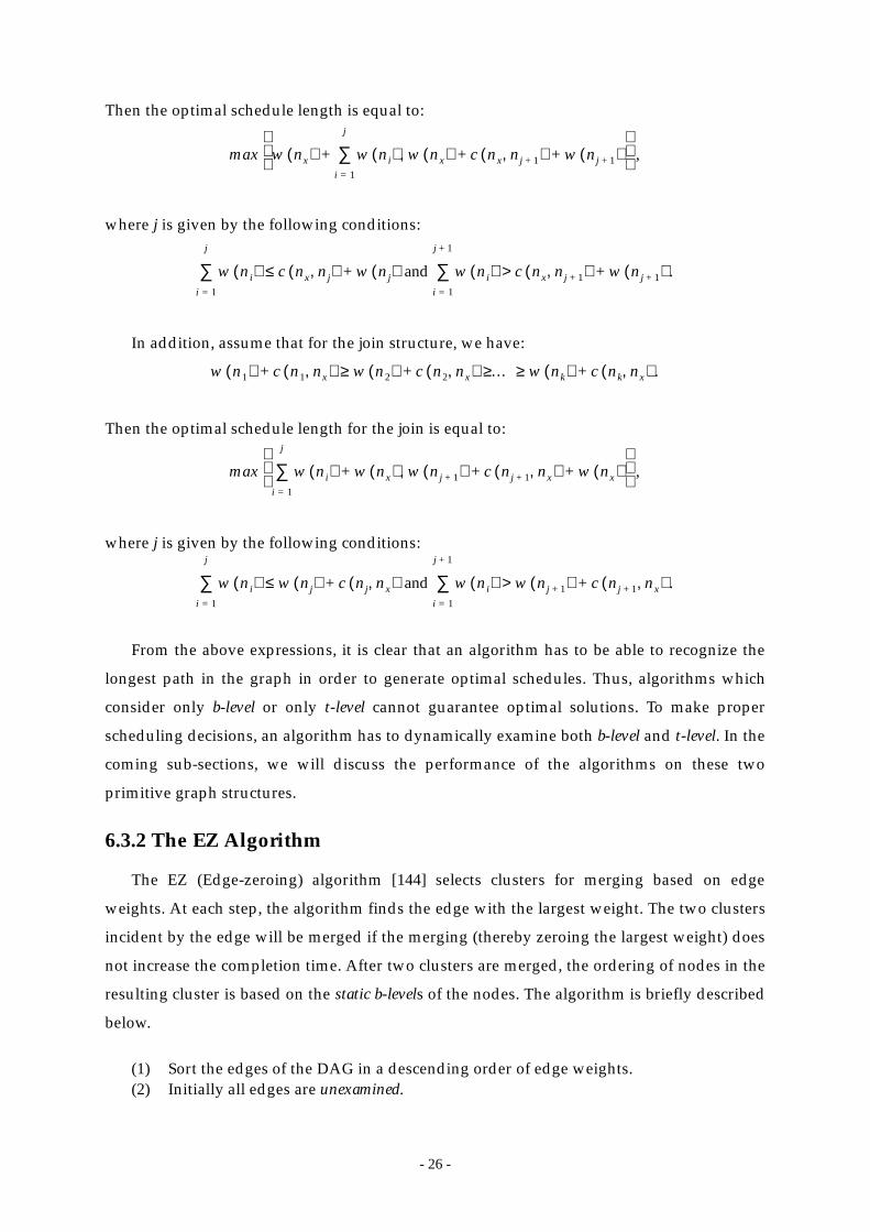
The EZ (Edge-zeroing) algorithm [144] selects clusters for merging based on edge
weights. At each step, the algorithm finds the edge with the largest weight. The two clusters
incident by the edge will be merged if the merging (thereby zeroing the largest weight) does
not increase the completion time. After two clusters are merged, the ordering of nodes in the
resulting cluster is based on the static b-levels of the nodes. The algorithm is briefly described
below.
(1) Sort the edges of the DAG in a descending order of edge weights.(2) Initially all edges are unexamined.
max w nx( ) w ni( ) w nx( ) c nx nj 1+,( ) w nj 1+( )+ +,i 1=
j
∑+
,
w ni( ) c nx nj,( ) w nj( ) and w ni( ) c nx nj 1+,( ) w nj 1+( ) .+>i 1=
j 1+
∑+≤i 1=
j
∑
w n1( ) c n1 nx,( ) w n2( ) c n2 nx,( ) … w nk( ) c nk nx,( ) .+≥ ≥+≥+
max w ni( ) w nx( ) w nj 1+( ) c nj 1+ nx,( ) w nx( )+ +,+i 1=
j
∑
,
w ni( ) w nj( ) c nj nx,( ) and w ni( ) w nj 1+( ) c nj 1+ nx,( ) .+>i 1=
j 1+
∑+≤i 1=
j
∑
- 27 -
Repeat
(3) Pick an unexamined edge which has the largest edge weight. Mark it as examined.Zero the highest edge weight if the completion time does not increase. In thiszeroing process, two clusters are merged so that other edges across these twoclusters also need to be zeroed and marked as examined. The ordering of nodes in theresulting cluster is based on their static b-levels.
Until all edges are examined.
The time-complexity of the EZ algorithm is . For the DAG shown in Figure 3,
the EZ algorithm generates a schedule shown in Figure 8(a). The steps of scheduling are
shown in Figure 8(b).
Performance on fork and join: Since the EZ algorithm considers only the communication
costs among nodes to make scheduling decisions, it does not guarantee optimal schedules for
both fork and join structures.
6.3.3 The LC Algorithm
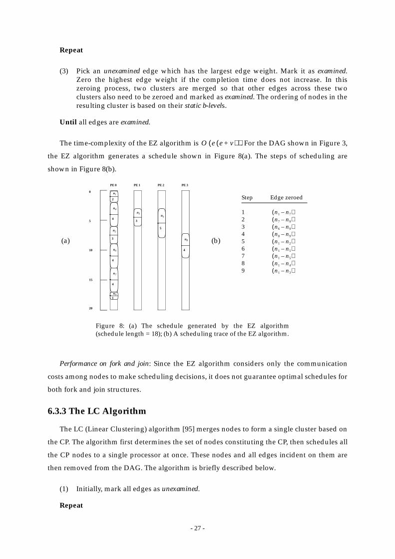
The LC (Linear Clustering) algorithm [95] merges nodes to form a single cluster based on
the CP. The algorithm first determines the set of nodes constituting the CP, then schedules all
the CP nodes to a single processor at once. These nodes and all edges incident on them are
then removed from the DAG. The algorithm is briefly described below.
(1) Initially, mark all edges as unexamined.
Repeat
O e e v+( )( )
PE 0 PE 1 PE 2 PE 3
Step Edge zeroed
123456789
n1 n7–( )n7 n9–( )n6 n9–( )n8 n9–( )n1 n2–( )n1 n5–( )n1 n5–( )n1 n4–( )n1 n3–( )
n1
2
n2
3
n5
5
n91
n3
3
n7
4
n4
4
0
5
10
15
20
n8
4n6
4
Figure 8: (a) The schedule generated by the EZ algorithm(schedule length = 18); (b) A scheduling trace of the EZ algorithm.
(a) (b)
- 28 -
(2) Determine the critical path composed of unexamined edges only.(3) Create a cluster by zeroing all the edges on the critical path.(4) Mark all the edges incident on the critical path and all the edges incident to the
nodes in the cluster as examined.
Until all edges are examined.
The time-complexity of the LC algorithm is . For the DAG shown in Figure 3,
the LC algorithm generates a schedule shown in Figure 9(a). The steps of scheduling are
shown in Figure 9(b).
Performance on fork and join: Since the LC algorithm does not schedule nodes on different
paths to the same processor, it cannot guarantee optimal solutions for both fork and join
structures.
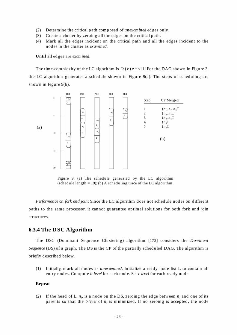
6.3.4 The DSC Algorithm
The DSC (Dominant Sequence Clustering) algorithm [173] considers the Dominant
Sequence (DS) of a graph. The DS is the CP of the partially scheduled DAG. The algorithm is
briefly described below.
(1) Initially, mark all nodes as unexamined. Initialize a ready node list L to contain allentry nodes. Compute b-level for each node. Set t-level for each ready node.
Repeat
(2) If the head of L, ni, is a node on the DS, zeroing the edge between ni and one of itsparents so that the t-level of ni is minimized. If no zeroing is accepted, the node
O v e v+( )( )
PE 0 PE 1 PE 2 PE 3
n1
2
n2
3
n5
5
n91
n3
3
n7
4
n4
4
0
5
10
15
20
n8
4 n6
4
Figure 9: (a) The schedule generated by the LC algorithm(schedule length = 19); (b) A scheduling trace of the LC algorithm.
Step CP Merged
12345
n1 n7 n9, ,( )n4 n8,( )n2 n6,( )n5( )n3( )
PE 4
(a)
(b)
- 29 -
remains in a single node cluster. (3) If the head of L, ni, is not a node on the DS, zeroing the edge between ni and one of
its parents so that the t-level of ni is minimized under the constraint called DominantSequence Reduction Warranty (DSRW). If some of its parents are entry nodes that donot have any child other than ni, merge part of them so that the t-level of ni isminimized. If no zeroing is accepted, the node remains in a single node cluster.
(4) Update the t-level and b-level of the successors of ni and mark ni as examined.
Until all nodes are examined.
DSRW: Zeroing incoming edges of a ready node should not affect the future reduction of t-level( ),where is a not-yet ready node with a higher priority, if t-level( ) is reducible by zeroing anincoming DS edge of .
The time-complexity of the DSC algorithm is . For the DAG shown in
Figure 3, the DSC algorithm generates a schedule shown in Figure 10(a). The steps of
scheduling are given in the table shown in Figure 10(b). In the table, the start-times of the
node on the processors at each scheduling step are given and the node is scheduled to the
PE 0 PE 1 PE 2 PE 3
Step (prio) (prio) Parent PE0 PE1 PE2 PE3
1 (23) NIL NIL 0* N.C. N.C. N.C.2 (21) (23) 2 6* N.C. N.C.3 (23) NIL 5 N.C. N.C. N.C.4 (8) (16) 9 3* N.C. N.C.5 (18) (16) 9 N.C. 3* N.C.6 (17) (18) 9 N.C. N.C. 3*7 (20) (16) 9* N.C. N.C. N.C.8 (18) (19) N.C. N.C. 7* N.C.9 (19) NIL 16* N.C. N.C. N.C.
nx ny
n1
n2 n7 n1
n7 n1
n5 n9 n1
n4 n9 n1
n3 n8 n1
n6 n9 n2
n8 n9 n4
n9 n6
n1
2
n2
3 n5
5
n91
n3
3n7
4
n4
4
0
5
10
15
20
n8
4n6
4
Figure 10: (a) The schedule generated by the DSC algorithm (schedule length = 17);(b) A scheduling trace of the DSC algorithm (N.C. indicates “not considered”).
(a)
(b)
ny
ny ny
ny
O e v+( ) vlog( )

- 30 -
processor on which the start-time is marked by an asterisk.
Performance on fork and join: The DSC algorithm dynamically tracks the critical path in the
DAG using both t-level and b-level. In addition, it schedules each node to start as early as
possible. Thus, for both fork and join structures, the DSC algorithm can guarantee optimal
solutions.
Yang and Gerasoulis [67] also investigated the granularity issue of clustering. They
considered that a DAG consists of fork( ) and join( ) structures such as the two shown in
Figure 7. Suppose we have:
Then the granularity of a DAG is defined as where . A
DAG is called coarse grain if . Based on this definition of granularity, Yang and
Gerasoulis proved that the DSC algorithm has the following performance bound:
Thus, for a coarse grain DAG, the DSC algorithm can generate a schedule length within a
factor of two from the optimal. Yang and Gerasoulis also proved that the DSC algorithm is
optimal for any coarse grain in-tree, and any single-spawn out-tree with uniform
computation costs and uniform communication costs.
6.3.5 The MD Algorithm
The MD (Mobility Directed) algorithm [170] selects a node ni for scheduling based on an
attribute called the relative mobility, defined as:
If a node is on the current CP of the partially scheduled DAG, the sum of its b-level and t-
level is equal to the current CP length. Thus, the relative mobility of a node is zero if it is on
the current CP. The algorithm is described below.
(1) Mark all nodes as unexamined. Initially, there is no cluster.
Repeat
Fx Jx
g Fx( )min w ni( ){ }
max c nx ni,( ){ }------------------------------------------ g Jx( ),min w ni( ){ }
max c ni nx,( ){ }------------------------------------------.= =
g min gx{ }= gx min g Fx( ) g Jx( ),{ }=
g 1≥
SLDSC 11g---+
SLopt.≤
Cur_CP_Length b-levelni( ) t-level ni( )+( )–
w ni( )------------------------------------------------------------------------------------------------------------------ .
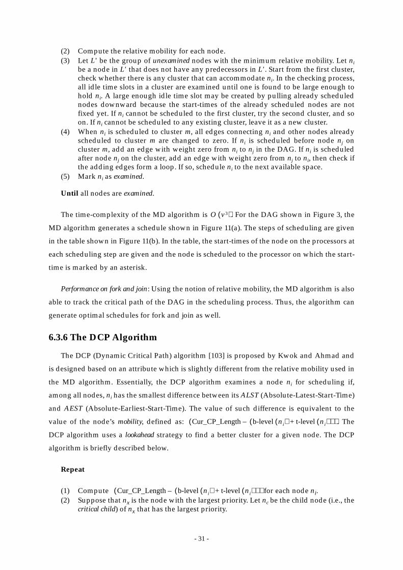
- 31 -
(2) Compute the relative mobility for each node.(3) Let L' be the group of unexamined nodes with the minimum relative mobility. Let ni
be a node in L' that does not have any predecessors in L'. Start from the first cluster,check whether there is any cluster that can accommodate ni. In the checking process,all idle time slots in a cluster are examined until one is found to be large enough tohold ni. A large enough idle time slot may be created by pulling already schedulednodes downward because the start-times of the already scheduled nodes are notfixed yet. If ni cannot be scheduled to the first cluster, try the second cluster, and soon. If ni cannot be scheduled to any existing cluster, leave it as a new cluster.
(4) When ni is scheduled to cluster m, all edges connecting ni and other nodes alreadyscheduled to cluster m are changed to zero. If ni is scheduled before node nj oncluster m, add an edge with weight zero from ni to nj in the DAG. If ni is scheduledafter node nj on the cluster, add an edge with weight zero from nj to ni, then check ifthe adding edges form a loop. If so, schedule ni to the next available space.
(5) Mark ni as examined.
Until all nodes are examined.
The time-complexity of the MD algorithm is . For the DAG shown in Figure 3, the
MD algorithm generates a schedule shown in Figure 11(a). The steps of scheduling are given
in the table shown in Figure 11(b). In the table, the start-times of the node on the processors at
each scheduling step are given and the node is scheduled to the processor on which the start-
time is marked by an asterisk.
Performance on fork and join: Using the notion of relative mobility, the MD algorithm is also
able to track the critical path of the DAG in the scheduling process. Thus, the algorithm can
generate optimal schedules for fork and join as well.
6.3.6 The DCP Algorithm
The DCP (Dynamic Critical Path) algorithm [103] is proposed by Kwok and Ahmad and
is designed based on an attribute which is slightly different from the relative mobility used in
the MD algorithm. Essentially, the DCP algorithm examines a node ni for scheduling if,
among all nodes, ni has the smallest difference between its ALST (Absolute-Latest-Start-Time)
and AEST (Absolute-Earliest-Start-Time). The value of such difference is equivalent to the
value of the node’s mobility, defined as: . The
DCP algorithm uses a lookahead strategy to find a better cluster for a given node. The DCP
algorithm is briefly described below.
Repeat
(1) Compute for each node ni.(2) Suppose that nx is the node with the largest priority. Let nc be the child node (i.e., the
critical child) of nx that has the largest priority.
O v3( )
Cur_CP_Length b-levelni( ) t-level ni( )+( )–( )
Cur_CP_Length b-levelni( ) t-level ni( )+( )–( )

- 32 -
(3) Select a cluster P such that the sum is the smallest among all theclusters holding nx’s parents or children. In examining a cluster, first try not to pulldown any node to create or enlarge an idle time slot. If this is not successful infinding a slot for nx, scan the cluster for suitable idle time slot again possibly bypulling some already scheduled nodes downward.
(4) Schedule nx to P.
Until all nodes are scheduled.
The time-complexity of the DCP algorithm is . For the DAG shown in Figure 3, the
DCP algorithm generates a schedule shown in Figure 12(a). The steps of scheduling are given
in the table shown in Figure 12(b). In the table, the composite start-times of the node (i.e., the
start-time of the node plus that of its critical child) on the processors at each scheduling step
are given and the node is scheduled to the processor on which the start-time is marked by an
asterisk.
PE 0 PE 1 PE 2
Step Rel. Mob. PE0 PE1 PE2 PE3
1 0.0 0* N.C. N.C. N.C.2 0.0 10* N.C. N.C. N.C.3 0.0 2* N.C. N.C. N.C.4 0.0 N.R. 3* N.C. N.C.5 0.0 N.R. 7* N.C. N.C.6 0.0 N.R. N.R. 3* N.C.7 0.0 16* N.C. N.C. N.C.8 0.25 5* N.C. N.C. N.C.9 1.8 N.R. 11* N.C. N.C.
ni
n1
n7
n2
n4
n8
n3
n9
n6
n5
n1
2
n2
3
n5
5
n91
n3
3
n7
4
n4
4
0
5
10
15
20
n8
4
n6
4
Figure 11: (a) The schedule generated by the MD algorithm(schedule length = 17); (b) A scheduling trace of the MD algorithm(N.C. indicates “not considered”, N.R. indicates “no room”).
(a)
(b)
TS nx( ) TS nc( )+
O v3( )
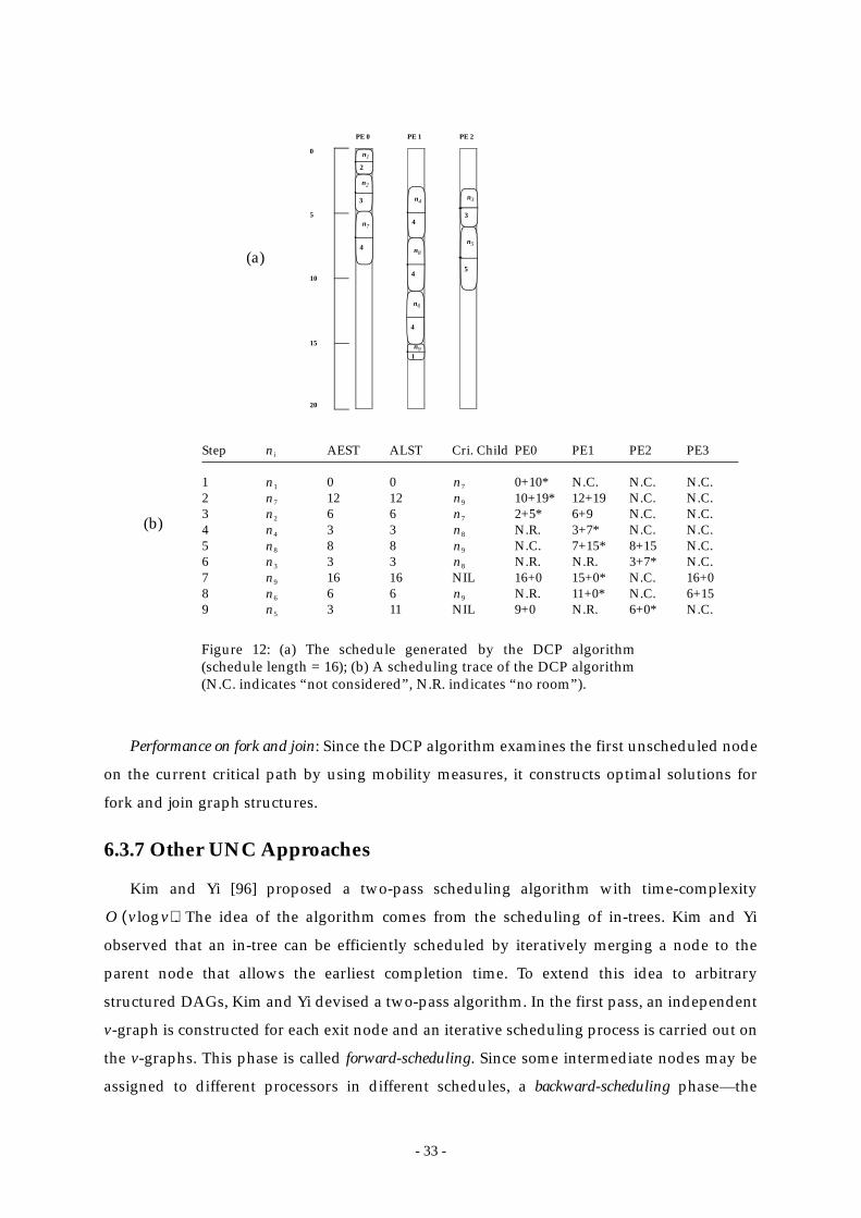
- 33 -
Performance on fork and join: Since the DCP algorithm examines the first unscheduled node
on the current critical path by using mobility measures, it constructs optimal solutions for
fork and join graph structures.
6.3.7 Other UNC Approaches
Kim and Yi [96] proposed a two-pass scheduling algorithm with time-complexity
. The idea of the algorithm comes from the scheduling of in-trees. Kim and Yi
observed that an in-tree can be efficiently scheduled by iteratively merging a node to the
parent node that allows the earliest completion time. To extend this idea to arbitrary
structured DAGs, Kim and Yi devised a two-pass algorithm. In the first pass, an independent
v-graph is constructed for each exit node and an iterative scheduling process is carried out on
the v-graphs. This phase is called forward-scheduling. Since some intermediate nodes may be
assigned to different processors in different schedules, a backward-scheduling phase—the
PE 0 PE 1 PE 2
Step AEST ALST Cri. Child PE0 PE1 PE2 PE3
1 0 0 0+10* N.C. N.C. N.C.2 12 12 10+19* 12+19 N.C. N.C.3 6 6 2+5* 6+9 N.C. N.C.4 3 3 N.R. 3+7* N.C. N.C.5 8 8 N.C. 7+15* 8+15 N.C.6 3 3 N.R. N.R. 3+7* N.C.7 16 16 NIL 16+0 15+0* N.C. 16+08 6 6 N.R. 11+0* N.C. 6+159 3 11 NIL 9+0 N.R. 6+0* N.C.
ni
n1 n7
n7 n9
n2 n7
n4 n8
n8 n9
n3 n8
n9
n6 n9
n5
n1
2
n2
3
n5
5
n91
n3
3n7
4
n4
4
0
5
10
15
20
n8
4
n6
4
Figure 12: (a) The schedule generated by the DCP algorithm(schedule length = 16); (b) A scheduling trace of the DCP algorithm(N.C. indicates “not considered”, N.R. indicates “no room”).
(a)
(b)
O v vlog( )
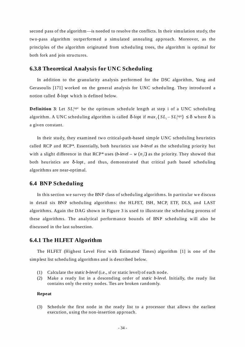
- 34 -
second pass of the algorithm—is needed to resolve the conflicts. In their simulation study, the
two-pass algorithm outperformed a simulated annealing approach. Moreover, as the
principles of the algorithm originated from scheduling trees, the algorithm is optimal for
both fork and join structures.
6.3.8 Theoretical Analysis for UNC Scheduling
In addition to the granularity analysis performed for the DSC algorithm, Yang and
Gerasoulis [171] worked on the general analysis for UNC scheduling. They introduced a
notion called which is defined below.
Definition 3: Let be the optimum schedule length at step i of a UNC scheduling
algorithm. A UNC scheduling algorithm is called if where is
a given constant.
In their study, they examined two critical-path-based simple UNC scheduling heuristics
called RCP and RCP*. Essentially, both heuristics use b-level as the scheduling priority but
with a slight difference in that RCP* uses (b-level – ) as the priority. They showed that
both heuristics are , and thus, demonstrated that critical path based scheduling
algorithms are near-optimal.
6.4 BNP Scheduling
In this section we survey the BNP class of scheduling algorithms. In particular we discuss
in detail six BNP scheduling algorithms: the HLFET, ISH, MCP, ETF, DLS, and LAST
algorithms. Again the DAG shown in Figure 3 is used to illustrate the scheduling process of
these algorithms. The analytical performance bounds of BNP scheduling will also be
discussed in the last subsection.
6.4.1 The HLFET Algorithm
The HLFET (Highest Level First with Estimated Times) algorithm [1] is one of the
simplest list scheduling algorithms and is described below.
(1) Calculate the static b-level (i.e., sl or static level) of each node.(2) Make a ready list in a descending order of static b-level. Initially, the ready list
contains only the entry nodes. Ties are broken randomly.
Repeat
(3) Schedule the first node in the ready list to a processor that allows the earliestexecution, using the non-insertion approach.
δ-lopt
SLilopt
δ-lopt maxi SLi SLilopt–{ } δ≤ δ
w ni( )
δ-lopt
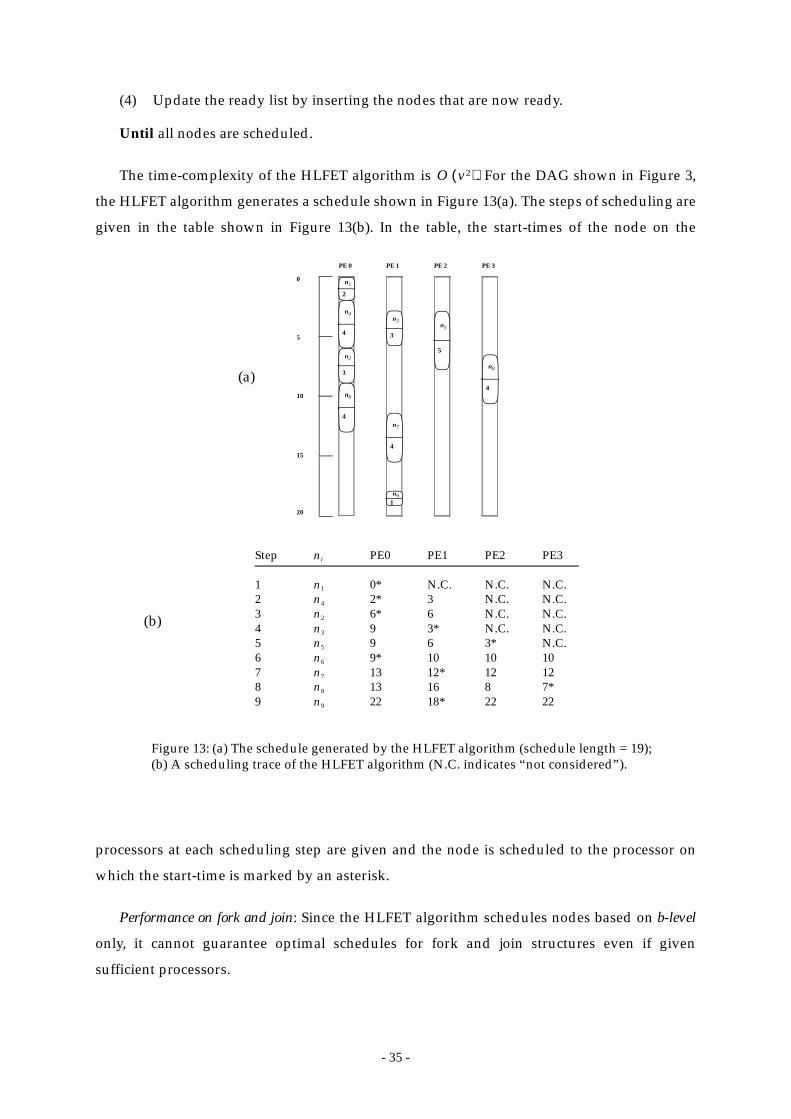
- 35 -
(4) Update the ready list by inserting the nodes that are now ready.
Until all nodes are scheduled.
The time-complexity of the HLFET algorithm is . For the DAG shown in Figure 3,
the HLFET algorithm generates a schedule shown in Figure 13(a). The steps of scheduling are
given in the table shown in Figure 13(b). In the table, the start-times of the node on the
processors at each scheduling step are given and the node is scheduled to the processor on
which the start-time is marked by an asterisk.
Performance on fork and join: Since the HLFET algorithm schedules nodes based on b-level
only, it cannot guarantee optimal schedules for fork and join structures even if given
sufficient processors.
O v2( )
PE 0 PE 1 PE 2 PE 3
Step PE0 PE1 PE2 PE3
1 0* N.C. N.C. N.C.2 2* 3 N.C. N.C.3 6* 6 N.C. N.C.4 9 3* N.C. N.C.5 9 6 3* N.C.6 9* 10 10 107 13 12* 12 128 13 16 8 7*9 22 18* 22 22
ni
n1
n4
n2
n3
n5
n6
n7
n8
n9
n1
2
n2
3
n5
5
n91
n3
3
n7
4
n4
4
0
5
10
15
20
n8
4n6
4
Figure 13: (a) The schedule generated by the HLFET algorithm (schedule length = 19);(b) A scheduling trace of the HLFET algorithm (N.C. indicates “not considered”).
(a)
(b)
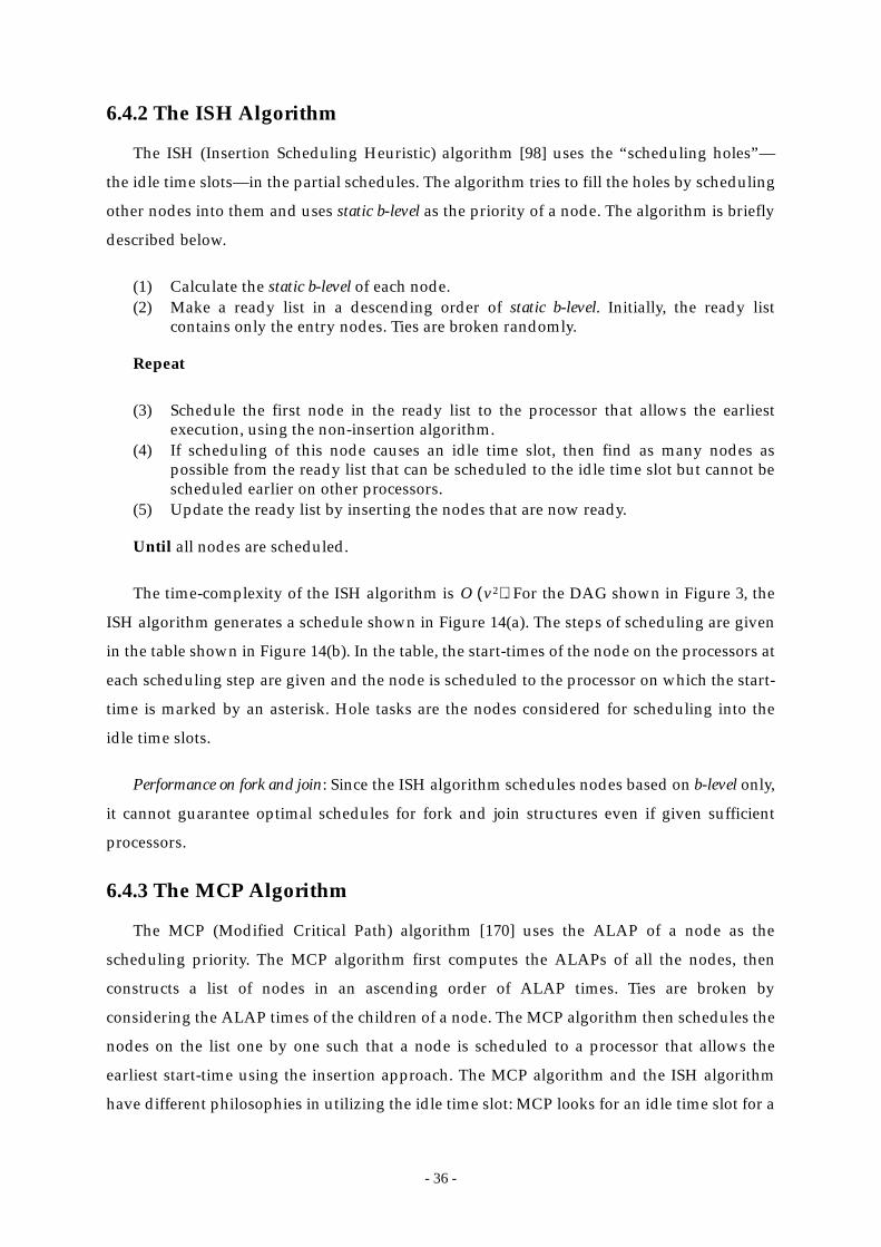
- 36 -
6.4.2 The ISH Algorithm
The ISH (Insertion Scheduling Heuristic) algorithm [98] uses the “scheduling holes”—
the idle time slots—in the partial schedules. The algorithm tries to fill the holes by scheduling
other nodes into them and uses static b-level as the priority of a node. The algorithm is briefly
described below.
(1) Calculate the static b-level of each node.(2) Make a ready list in a descending order of static b-level. Initially, the ready list
contains only the entry nodes. Ties are broken randomly.
Repeat
(3) Schedule the first node in the ready list to the processor that allows the earliestexecution, using the non-insertion algorithm.
(4) If scheduling of this node causes an idle time slot, then find as many nodes aspossible from the ready list that can be scheduled to the idle time slot but cannot bescheduled earlier on other processors.
(5) Update the ready list by inserting the nodes that are now ready.
Until all nodes are scheduled.
The time-complexity of the ISH algorithm is . For the DAG shown in Figure 3, the
ISH algorithm generates a schedule shown in Figure 14(a). The steps of scheduling are given
in the table shown in Figure 14(b). In the table, the start-times of the node on the processors at
each scheduling step are given and the node is scheduled to the processor on which the start-
time is marked by an asterisk. Hole tasks are the nodes considered for scheduling into the
idle time slots.
Performance on fork and join: Since the ISH algorithm schedules nodes based on b-level only,
it cannot guarantee optimal schedules for fork and join structures even if given sufficient
processors.
6.4.3 The MCP Algorithm
The MCP (Modified Critical Path) algorithm [170] uses the ALAP of a node as the
scheduling priority. The MCP algorithm first computes the ALAPs of all the nodes, then
constructs a list of nodes in an ascending order of ALAP times. Ties are broken by
considering the ALAP times of the children of a node. The MCP algorithm then schedules the
nodes on the list one by one such that a node is scheduled to a processor that allows the
earliest start-time using the insertion approach. The MCP algorithm and the ISH algorithm
have different philosophies in utilizing the idle time slot: MCP looks for an idle time slot for a
O v2( )
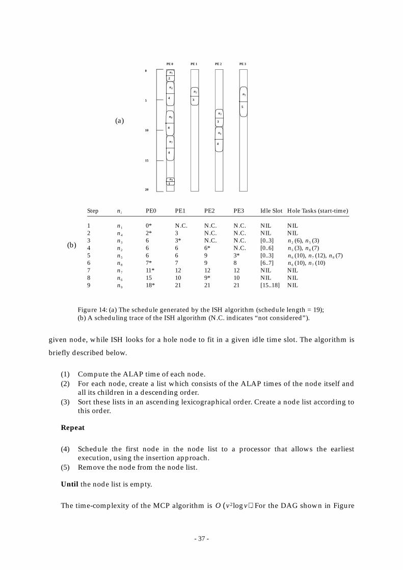
- 37 -
given node, while ISH looks for a hole node to fit in a given idle time slot. The algorithm is
briefly described below.
(1) Compute the ALAP time of each node.(2) For each node, create a list which consists of the ALAP times of the node itself and
all its children in a descending order. (3) Sort these lists in an ascending lexicographical order. Create a node list according to
this order.
Repeat
(4) Schedule the first node in the node list to a processor that allows the earliestexecution, using the insertion approach.
(5) Remove the node from the node list.
Until the node list is empty.
The time-complexity of the MCP algorithm is . For the DAG shown in Figure
PE 0 PE 1 PE 2 PE 3
Step PE0 PE1 PE2 PE3 Idle Slot Hole Tasks (start-time)
1 0* N.C. N.C. N.C. NIL NIL2 2* 3 N.C. N.C. NIL NIL3 6 3* N.C. N.C. [0..3] (6), (3)4 6 6 6* N.C. [0..6] (3), (7)5 6 6 9 3* [0..3] (10), (12), (7)6 7* 7 9 8 [6..7] (10), (10)7 11* 12 12 12 NIL NIL8 15 10 9* 10 NIL NIL9 18* 21 21 21 [15..18] NIL
ni
n1
n4
n3 n2 n5
n2 n5 n8
n5 n6 n7 n8
n8 n6 n7
n7
n6
n9
n1
2
n2
3
n5
5
n91
n3
3
n7
4
n4
4
0
5
10
15
20
n8
4
n6
4
Figure 14: (a) The schedule generated by the ISH algorithm (schedule length = 19);(b) A scheduling trace of the ISH algorithm (N.C. indicates “not considered”).
(a)
(b)
O v2 vlog( )
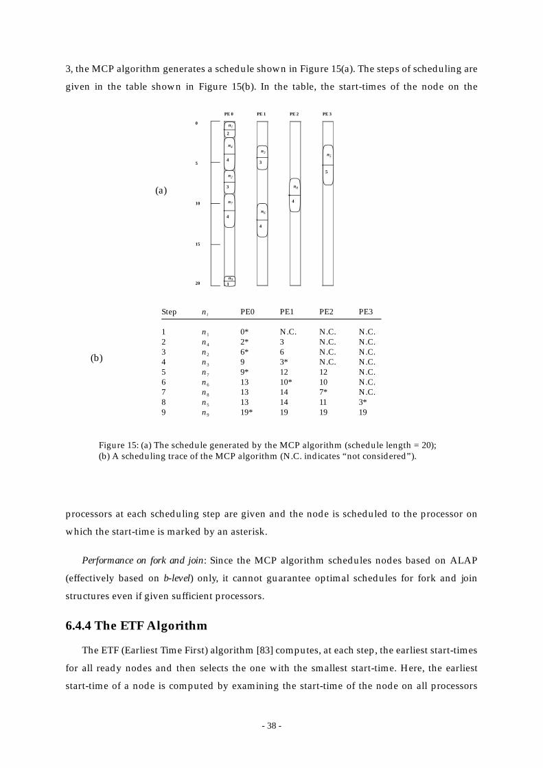
- 38 -
3, the MCP algorithm generates a schedule shown in Figure 15(a). The steps of scheduling are
given in the table shown in Figure 15(b). In the table, the start-times of the node on the
processors at each scheduling step are given and the node is scheduled to the processor on
which the start-time is marked by an asterisk.
Performance on fork and join: Since the MCP algorithm schedules nodes based on ALAP
(effectively based on b-level) only, it cannot guarantee optimal schedules for fork and join
structures even if given sufficient processors.
6.4.4 The ETF Algorithm
The ETF (Earliest Time First) algorithm [83] computes, at each step, the earliest start-times
for all ready nodes and then selects the one with the smallest start-time. Here, the earliest
start-time of a node is computed by examining the start-time of the node on all processors
PE 0 PE 1 PE 2 PE 3
Step PE0 PE1 PE2 PE3
1 0* N.C. N.C. N.C.2 2* 3 N.C. N.C.3 6* 6 N.C. N.C.4 9 3* N.C. N.C.5 9* 12 12 N.C.6 13 10* 10 N.C.7 13 14 7* N.C.8 13 14 11 3*9 19* 19 19 19
ni
n1
n4
n2
n3
n7
n6
n8
n5
n9
n1
2
n2
3
n5
5
n91
n3
3
n7
4
n4
4
0
5
10
15
20
n8
4
n6
4
Figure 15: (a) The schedule generated by the MCP algorithm (schedule length = 20);(b) A scheduling trace of the MCP algorithm (N.C. indicates “not considered”).
(a)
(b)
- 39 -
exhaustively. When two nodes have the same value in their earliest start-times, the ETF
algorithm breaks the tie by scheduling the one with the higher static priority. The algorithm is
described below
(1) Compute the static b-level of each node.(2) Initially, the pool of ready nodes includes only the entry nodes.
Repeat
(3) Calculate the earliest start-time on each processor for each node in the ready pool.Pick the node-processor pair that gives the earliest time using the non-insertionapproach. Ties are broken by selecting the node with a higher static b-level. Schedulethe node to the corresponding processor.
(4) Add the newly ready nodes to the ready node pool.
Until all nodes are scheduled.
The time-complexity of the ETF algorithm is . For the DAG shown in Figure 3, the
ETF algorithm generates a schedule shown in Figure 16(a). The steps of scheduling are given
in the table shown in Figure 16(b). In the table, the start-times of the node on the processors at
each scheduling step are given and the node is scheduled to the processor on which the start-
time is marked by an asterisk.
Performance on fork and join: Since the ETF algorithm schedules nodes based on b-level only,
it cannot guarantee optimal schedules for fork and join structures even if given sufficient
processors.
Hwang et al. also analyzed the performance bound of the ETF algorithm [83]. They
showed that the schedule length produced by the ETF algorithm satisfies the following
relation:
where is the optimal schedule length without considering communication delays and C
is the communication requirements over some parent-parent pairs along a path. An
algorithm is also provided to compute C.
6.4.5 The DLS Algorithm
The DLS (Dynamic Level Scheduling) algorithm [154] uses an attribute called dynamic
level (DL) which is the difference between the static b-level of a node and its earliest start-time
on a processor. At each scheduling step, the algorithm computes the DL for every node in the
ready pool on all processors. The node-processor pair which gives the largest value of DL is
O pv2( )
SLETF
SLETF 21p---–
SLoptnc C,+≤
SLoptnc
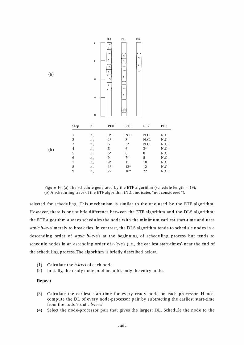
- 40 -
selected for scheduling. This mechanism is similar to the one used by the ETF algorithm.
However, there is one subtle difference between the ETF algorithm and the DLS algorithm:
the ETF algorithm always schedules the node with the minimum earliest start-time and uses
static b-level merely to break ties. In contrast, the DLS algorithm tends to schedule nodes in a
descending order of static b-levels at the beginning of scheduling process but tends to
schedule nodes in an ascending order of t-levels (i.e., the earliest start-times) near the end of
the scheduling process.The algorithm is briefly described below.
(1) Calculate the b-level of each node. (2) Initially, the ready node pool includes only the entry nodes.
Repeat
(3) Calculate the earliest start-time for every ready node on each processor. Hence,compute the DL of every node-processor pair by subtracting the earliest start-timefrom the node’s static b-level.
(4) Select the node-processor pair that gives the largest DL. Schedule the node to the
PE 0 PE 1 PE 2
Step PE0 PE1 PE2 PE3
1 0* N.C. N.C. N.C.2 2* 3 N.C. N.C.3 6 3* N.C. N.C.4 6 6 3* N.C.5 6* 6 8 N.C.6 9 7* 8 N.C.7 9* 11 10 N.C.8 13 12* 12 N.C.9 22 18* 22 N.C.
ni
n1
n4
n3
n5
n2
n8
n6
n7
n9
n1
2
n2
3
n5
5
n91
n3
3
n7
4
n4
4
0
5
10
15
20
n8
4n6
4
Figure 16: (a) The schedule generated by the ETF algorithm (schedule length = 19);(b) A scheduling trace of the ETF algorithm (N.C. indicates “not considered”).
(a)
(b)

- 41 -
corresponding processor.(5) Add the newly ready nodes to the ready pool.
Until all nodes are scheduled.
The time-complexity of the DLS algorithm is . For the DAG shown in Figure 3, the
ETF algorithm generates a schedule shown in Figure 17(a). The steps of scheduling are given
in the table shown in Figure 17(b). In the table, the start-times of the node on the processors at
each scheduling step are given and the node is scheduled to the processor on which the start-
time is marked by an asterisk.
Performance on fork and join: Even though the DLS algorithm schedules nodes based on
dynamic levels, it cannot guarantee optimal schedules for fork and join structures even if
given sufficient processors.
O pv3( )
PE 0 PE 1 PE 2
Step sl PE0 PE1 PE2 PE3 DL
1 11 0* N.C. N.C. N.C. 112 9 2* 3 N.C. N.C. 63 8 6 3* N.C. N.C. 54 8 6* 6 N.C. N.C. 25 5 9 6 3* N.C. 26 5 9 7* 8 N.C. -27 5 9* 11 10 N.C. -48 5 13 12* 12 N.C. -79 1 22 18* 22 N.C. -17
ni
n1
n4
n3
n2
n5
n8
n6
n7
n9
n1
2
n2
3
n5
5
n91
n3
3
n7
4
n4
4
0
5
10
15
20
n8
4n6
4
Figure 17: (a) The schedule generated by the DLS algorithm (schedule length = 19);(b) A scheduling trace of the DLS algorithm (N.C. indicates “not considered”).
(a)
(b)
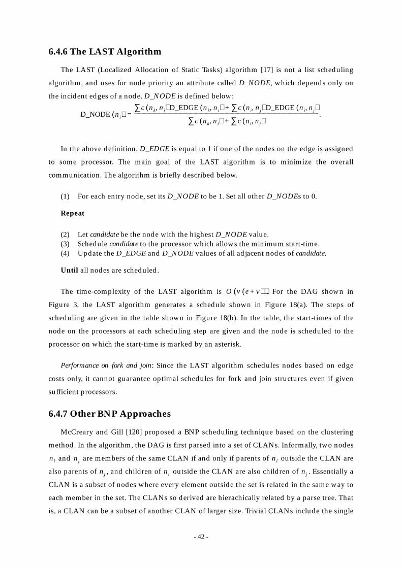
- 42 -
6.4.6 The LAST Algorithm
The LAST (Localized Allocation of Static Tasks) algorithm [17] is not a list scheduling
algorithm, and uses for node priority an attribute called D_NODE, which depends only on
the incident edges of a node. D_NODE is defined below:
In the above definition, D_EDGE is equal to 1 if one of the nodes on the edge is assigned
to some processor. The main goal of the LAST algorithm is to minimize the overall
communication. The algorithm is briefly described below.
(1) For each entry node, set its D_NODE to be 1. Set all other D_NODEs to 0.
Repeat
(2) Let candidate be the node with the highest D_NODE value.(3) Schedule candidate to the processor which allows the minimum start-time.(4) Update the D_EDGE and D_NODE values of all adjacent nodes of candidate.
Until all nodes are scheduled.
The time-complexity of the LAST algorithm is . For the DAG shown in
Figure 3, the LAST algorithm generates a schedule shown in Figure 18(a). The steps of
scheduling are given in the table shown in Figure 18(b). In the table, the start-times of the
node on the processors at each scheduling step are given and the node is scheduled to the
processor on which the start-time is marked by an asterisk.
Performance on fork and join: Since the LAST algorithm schedules nodes based on edge
costs only, it cannot guarantee optimal schedules for fork and join structures even if given
sufficient processors.
6.4.7 Other BNP Approaches
McCreary and Gill [120] proposed a BNP scheduling technique based on the clustering
method. In the algorithm, the DAG is first parsed into a set of CLANs. Informally, two nodes
and are members of the same CLAN if and only if parents of outside the CLAN are
also parents of , and children of outside the CLAN are also children of . Essentially a
CLAN is a subset of nodes where every element outside the set is related in the same way to
each member in the set. The CLANs so derived are hierachically related by a parse tree. That
is, a CLAN can be a subset of another CLAN of larger size. Trivial CLANs include the single
D_NODE ni( )c nk ni,( ) D_EDGE nk ni,( ) c ni nj,( ) D_EDGE ni nj,( )∑+∑
c nk ni,( ) c ni nj,( )∑+∑-----------------------------------------------------------------------------------------------------------------------------------------------------.=
O v e v+( )( )
ni nj ni
nj ni nj
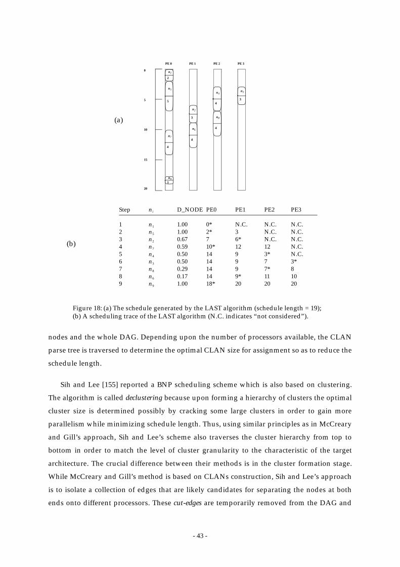
- 43 -
nodes and the whole DAG. Depending upon the number of processors available, the CLAN
parse tree is traversed to determine the optimal CLAN size for assignment so as to reduce the
schedule length.
Sih and Lee [155] reported a BNP scheduling scheme which is also based on clustering.
The algorithm is called declustering because upon forming a hierarchy of clusters the optimal
cluster size is determined possibly by cracking some large clusters in order to gain more
parallelism while minimizing schedule length. Thus, using similar principles as in McCreary
and Gill’s approach, Sih and Lee’s scheme also traverses the cluster hierarchy from top to
bottom in order to match the level of cluster granularity to the characteristic of the target
architecture. The crucial difference between their methods is in the cluster formation stage.
While McCreary and Gill’s method is based on CLANs construction, Sih and Lee’s approach
is to isolate a collection of edges that are likely candidates for separating the nodes at both
ends onto different processors. These cut-edges are temporarily removed from the DAG and
PE 0 PE 1 PE 2 PE 3
Step D_NODE PE0 PE1 PE2 PE3
1 1.00 0* N.C. N.C. N.C.2 1.00 2* 3 N.C. N.C.3 0.67 7 6* N.C. N.C.4 0.59 10* 12 12 N.C.5 0.50 14 9 3* N.C.6 0.50 14 9 7 3*7 0.29 14 9 7* 88 0.17 14 9* 11 109 1.00 18* 20 20 20
ni
n1
n5
n2
n7
n4
n3
n8
n6
n9
n1
2
n2
3
n5
5
n91
n3
3
n7
4
n4
4
0
5
10
15
20
n8
4n6
4
Figure 18: (a) The schedule generated by the LAST algorithm (schedule length = 19);(b) A scheduling trace of the LAST algorithm (N.C. indicates “not considered”).
(a)
(b)

- 44 -
the algorithm designates each remaining connected component as an elementary cluster.
Lee, Hurson, and Feng [108] reported a BNP scheduling algorithm targeted for data-flow
multiprocessors based on a vertical layering method for the DAG. In their scheme, the DAG
is first partitioned into a set of vertical layers of nodes. The initial set of vertical layers is built
around the critical path of the DAG and is then optimized by considering various cases of
accounting for possible inter-processor communication, which may in turn induce new
critical paths. Finally, the vertical layers of nodes are mapped to the given processors in order
to minimize the schedule length.
Zhu and McCreary [176] reported a set of BNP scheduling algorithms for trees. They first
devised an algorithm for finding optimal schedules for trees, in particular, binary trees.
Nonetheless the algorithm is of exponential complexity since optimal scheduling of trees is
an NP-complete problem. They then proposed a number of heuristic approaches that can
generate reasonably good solutions within a much shorter amount of time. The heuristics are
all greedy in nature in that they attempt to minimize the completion times of paths in the tree
and exploit only a small number of possible paths in the search of a good schedule.
Varvarigou, Roychowdhury, Kallath, and Lawler [163] proposed a BNP scheduling
scheme for in-forests and out-forests. However, their algorithm assumes that the trees are
with unit computation costs and unit communication costs. Another distinctive feature of
their algorithm is that the time-complexity is pseudo-polynomial— , which is
polynomial if p is fixed and small. The idea of their algorithm is to first transform the trees
into delay-free trees, which are then scheduled using an optimal merging algorithm. This
transformation step is crucial and is done as follows. For each node, a successor node is
selected to be scheduled immediately after the node. Then, since the communication costs are
unit, the communication costs between the node and all other successors can be dropped.
Only an extra communication free edge is needed to add between the chosen successor and
the other successors. The successor node is so selected that the resulting DAG does not
violate the precedence constraints of the original DAG.
Pande, Agrawal, and Mauney [131] proposed a BNP scheduling scheme using a
thresholding technique. The algorithm first computes the earliest start-times and latest start-
times of the nodes. A threshold for a node is then the difference between its earliest and the
latest start-times. A global threshold is varied between the minimum threshold among the
nodes to the maximum. For a node with threshold less than the global value, a new processor
is allocated for the node, if there is any available. For a node with threshold above the global
O v2p( )
- 45 -
value, the node is then scheduled to the same processor as its parent which allows the earliest
start-time. The rationale of the scheme is that as the threshold of a node represents the
tolerable delay of execution without increasing overall schedule length, a node with smaller
threshold deserves a new processor so that it can start as early as possible. Depending upon
the number of given processors, there is a trade-off between parallelism and schedule length,
and the global threshold is adjusted accordingly.
6.4.8 Analytical Performance Bounds of BNP Scheduling
For the BNP class of scheduling algorithms, Al-Mouhamed [12] extended Fernandez et
al.’s [54] work (described in Section 6.2.3) and devised a bound on the minimum number of
processors for optimal schedule length and a bound on the minimum increase in schedule
length if only a certain smaller number of processor is available. Essentially, Al-Mouhamed
extended the techniques of Fernandez et al. for arbitrary DAGs with communication.
Furthermore, the expressions for the bounds are similar to the ones reported by Fernandez et
al. except that Al-Mouhamed conjectured that the bounds need not be computed across all
possible integer intervals within the earliest completion time of the DAG. However, Jain and
Rajaraman [86] in a subsequent study found that the computation of these bounds in fact
needs to consider all the integer intervals within the earliest completion time of the DAG.
They also reported a technique to partition the DAGs into nodes with non-overlapping
intervals so that a tighter bound is obtained. In addition, the new bounds can take lesser time
to compute. Jain and Rajaraman also found that using such a partitioning facilitates all
possible integer intervals to be considered in order to compute a tighter bound.
6.5 TDB Scheduling
In this section we survey the TDB class of DAG scheduling algorithms. We describe in
detail six TDB scheduling algorithms: the PY, LWB, DSH, BTDH, LCTD, and CPFD
algorithms. The DAG shown in Figure 3 is used to illustrate the scheduling process of these
algorithms.
In the following we do not discuss the performance of the TDB algorithms on fork and
join sets separately because with duplication the TDB scheduling schemes can inherently
produce optimal solutions for these two primitive structures. For a fork set, a TDB algorithm
duplicates the root on every processor so that each child starts at the earliest possible time.
For a join set, although no duplication is needed to start the sink node at the earliest time, all
the TDB algorithms surveyed in this section employ a similar recursive scheduling process to
minimize the start-times of nodes so that an optimal schedule results.
- 46 -
6.5.1 The PY Algorithm
The PY algorithm (named after Papadimitriou and Yannakakis) [136] is an approximation
algorithm which uses an attribute, called e-value, to approximate the absolute achievable
lower bound of the start-time of a node. This attribute is computed recursively beginning
from the entry nodes to the exit nodes. A procedure for computing the e-values is given
below.
(1) Construct a list of nodes in topological order. Call it TopList.(2) for each node in TopList do(3) if has no parent then = 0 (4) else(5) for each parent of do endfor(6) Construct a list of parents in decreasing f. Call it ParentList.(7) Let min_e = the f value of the first parent in ParentList(8) Make as a single node cluster. Call it Cluster( ).(9) for each parent in ParentList do(10) Include Cluster( ) in Cluster( ).(11) Compute the new min_e (i.e., start-time) of in Cluster( ).(12) if new min_e > original min_e then exit this for-loop endif(13) endfor(14) = min_e(15) endif(16) endfor
After computing the e-values, the algorithm inserts each node into a cluster, in which a
group of ancestors are to be duplicated such that the ancestors have data arrival times larger
than the e-value of the node. Papadimitriou and Yannakakis also showed that the schedule
length generated is within a factor of two from the optimal. The PY algorithm is briefly
described below.
(1) Compute e-values for all nodes.(2) for each node do(3) Assign to a new processor PE i.(4) for all ancestors of , duplicate an ancestor if:
(5) Order the nodes in PE i so that a node starts as soon as all its data is available.(6) endfor
The time-complexity of the PY algorithm is . For the DAG shown in
Figure 3, the PY algorithm generates a schedule shown in Figure 19(a). The e-values are also
shown in Figure 19(b).
ni
ni e ni( )
nx ni f nx( ) e nx( ) c nx ni,( )+=
ni ni
nx
nx ni
ni ni
e ni( )
ni
ni
ni nx
e nx( ) w nx( ) c nx ni,( ) e ni( )>+ +
O v2 e v vlog+( )( )
- 47 -
6.5.2 The LWB Algorithm
We call the algorithm the LWB (Lower Bound) algorithm [37] based on its main principle:
it first determines the lower bound start-time for each node, and then identifies a set of
critical edges in the DAG. A critical edge is the one in which a parent’s message-available
time for the child is greater than the lower bound start-time of the child. Colin and
Chrietenne [37] showed in that the LWB algorithm can generate optimal schedules for DAGs
in which node weights are strictly larger than any edge weight.The LWB algorithm is briefly
described below.
(1) For each node , compute its lower bound start-time, denoted by , asfollows:
a) For any entry node , is zero.
b) For any node other than an entry node, consider the set of its parents. Let bethe parent such that is the largest among all parents.Then, the lower bound of , , is given by, with ,
(2) Consider the set of edges in the task graph. An edge is labelled as “critical”if .
(3) Assign each path of critical edges to a distinct processor such that each node isscheduled to start at its lower bound start-time.
The time-complexity of the LWB algorithm is . For the DAG shown in Figure 3, the
LWB algorithm generates a schedule shown in Figure 19(a). The lower bound values are also
shown in Figure 19(b).
PE 0 PE 1 PE 2 PE 3 PE 4 PE 5 PE 6
0222255614
ni e ni( )
n1
n2
n3
n4
n5
n6
n7
n8
n9
n1
2
n2
3n5
5
n91
n3
3
n7
4
n4
4
0
5
10
15
20
n8
4
n6
4
Figure 19: (a) The schedule generated by the PY algorithm (schedulelength = 21); (b) The e-values of the nodes computed by the PY algorithm.
(a) (b)
21
n1
2
n1
2
n1
2
n1
2
n2
3n4
4
n7
4
n8
4
ni lwb ni( )
ni lwb ni( )
ni nxlwb nx( ) w nx( ) c nx ni,( )+ +
ni lwb ni( )MAX lwb nx( ) w nx( ) MAX lwb ny( ) w ny( ) c ny ni,( )+ +{ },+{ }
ny nx≠
ny ni,( )lwb nx( ) w nx( ) c nx ni,( ) lwb ni( )>+ +
O v2( )
- 48 -
6.5.3 The DSH Algorithm
The DSH (Duplication Scheduling Heuristic) algorithm [99] considers each node in a
descending order of their priorities. In examining the suitability of a processor for a node, the
DSH algorithm first determines the start-time of the node on the processor without
duplication of any ancestor. Then, it considers the duplication in the idle time period from the
finish-time of the last scheduled node on the processor and the start-time of the node
currently under consideration. The algorithm then tries to duplicate the ancestors of the node
into the duplication time slot until either until the slot is used up or the start-time of the node
does not improve. The algorithm is briefly described below.
(1) Compute the static b-level for each node.
Repeat
(2) Let ni be an unscheduled node with the largest static b-level.(3) For each processor P, do:
a) Let the ready time of P, denoted by RT, be the finish-time of the last node on P.Compute the start-time of ni on P and denote it by ST. Then the duplication timeslot on P has length . Let candidate be ni.
b) Consider the set of candidate’s parents. Let nx be the parent of ni which is notscheduled on P and whose message for candidate has the latest arrival time. Try toduplicate nx into the duplication time slot.
c) If the duplication is unsuccessful, then record ST for this processor and tryanother processor; otherwise, let ST be candidate’s new start-time and candidate be
PE 0 PE 1 PE 2 PE 3 PE 4
lwb
0222255615
ni
n1
n2
n3
n4
n5
n6
n7
n8
n9
n1
2
n2
3n5
5
n91
n3
3
n7
4
n4
4
0
5
10
15
20
n8
4
n6
4
Figure 20: (a) The schedule generated by the LWB algorithm (schedule length = 16);(b) The lwb (lower bound) values of the nodes computed by the LWB algorithm.
(a) (b)
n1
2
n1
2
n1
2
n1
2
ST RT–( )
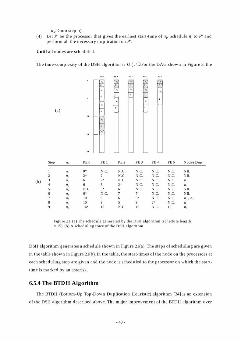
- 49 -
nx. Goto step b).(4) Let P’ be the processor that gives the earliest start-time of ni. Schedule ni to P’ and
perform all the necessary duplication on P’.
Until all nodes are scheduled.
The time-complexity of the DSH algorithm is . For the DAG shown in Figure 3, the
DSH algorithm generates a schedule shown in Figure 21(a). The steps of scheduling are given
in the table shown in Figure 21(b). In the table, the start-times of the node on the processors at
each scheduling step are given and the node is scheduled to the processor on which the start-
time is marked by an asterisk.
6.5.4 The BTDH Algorithm
The BTDH (Bottom-Up Top-Down Duplication Heuristic) algorithm [34] is an extension
of the DSH algorithm described above. The major improvement of the BTDH algorithm over
O v4( )
PE 0 PE 1 PE 2 PE 3 PE 4
Step PE 0 PE 1 PE 2 PE 3 PE 4 PE 5 Nodes Dup.
1 0* N.C. N.C. N.C. N.C. N.C. NIL2 2* 2 N.C. N.C. N.C. N.C. NIL3 6 2* N.C. N.C. N.C. N.C.4 6 5 2* N.C. N.C. N.C.5 N.C. 5* 6 N.C. N.C. N.C. NIL6 6* N.C. 7 7 N.C. N.C. NIL7 10 9 6 5* N.C. N.C. , 8 10 9 5 9 2* N.C.9 14* 15 N.C. 15 N.C. 15
ni
n1
n4
n2 n1
n3 n1
n6
n8
n7 n1 n2
n5 n1
n9 n7
n1
2
n2
3
n5
5
n91
n3
3
n7
4
n4
4
0
5
10
15
20
n8
4
n6
4
Figure 21: (a) The schedule generated by the DSH algorithm (schedule length= 15); (b) A scheduling trace of the DSH algorithm.
(a)
(b)
n1
2
n1
2
n1
2
n1
2
n2
3
n7
4
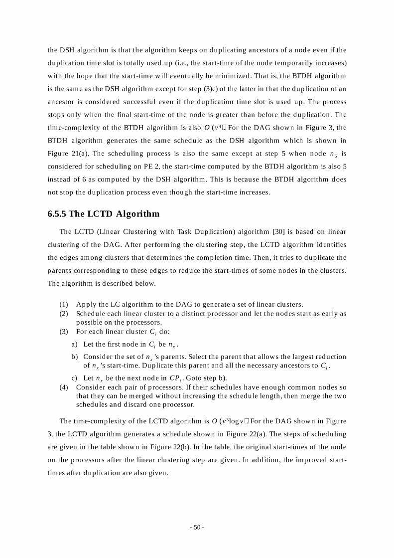
- 50 -
the DSH algorithm is that the algorithm keeps on duplicating ancestors of a node even if the
duplication time slot is totally used up (i.e., the start-time of the node temporarily increases)
with the hope that the start-time will eventually be minimized. That is, the BTDH algorithm
is the same as the DSH algorithm except for step (3)c) of the latter in that the duplication of an
ancestor is considered successful even if the duplication time slot is used up. The process
stops only when the final start-time of the node is greater than before the duplication. The
time-complexity of the BTDH algorithm is also . For the DAG shown in Figure 3, the
BTDH algorithm generates the same schedule as the DSH algorithm which is shown in
Figure 21(a). The scheduling process is also the same except at step 5 when node is
considered for scheduling on PE 2, the start-time computed by the BTDH algorithm is also 5
instead of 6 as computed by the DSH algorithm. This is because the BTDH algorithm does
not stop the duplication process even though the start-time increases.
6.5.5 The LCTD Algorithm
The LCTD (Linear Clustering with Task Duplication) algorithm [30] is based on linear
clustering of the DAG. After performing the clustering step, the LCTD algorithm identifies
the edges among clusters that determines the completion time. Then, it tries to duplicate the
parents corresponding to these edges to reduce the start-times of some nodes in the clusters.
The algorithm is described below.
(1) Apply the LC algorithm to the DAG to generate a set of linear clusters.(2) Schedule each linear cluster to a distinct processor and let the nodes start as early as
possible on the processors.(3) For each linear cluster do:
a) Let the first node in be .
b) Consider the set of ’s parents. Select the parent that allows the largest reductionof ’s start-time. Duplicate this parent and all the necessary ancestors to .
c) Let be the next node in . Goto step b).(4) Consider each pair of processors. If their schedules have enough common nodes so
that they can be merged without increasing the schedule length, then merge the twoschedules and discard one processor.
The time-complexity of the LCTD algorithm is . For the DAG shown in Figure
3, the LCTD algorithm generates a schedule shown in Figure 22(a). The steps of scheduling
are given in the table shown in Figure 22(b). In the table, the original start-times of the node
on the processors after the linear clustering step are given. In addition, the improved start-
times after duplication are also given.
O v4( )
n6
Ci
Ci nx
nxnx Ci
nx CPi
O v3 vlog( )
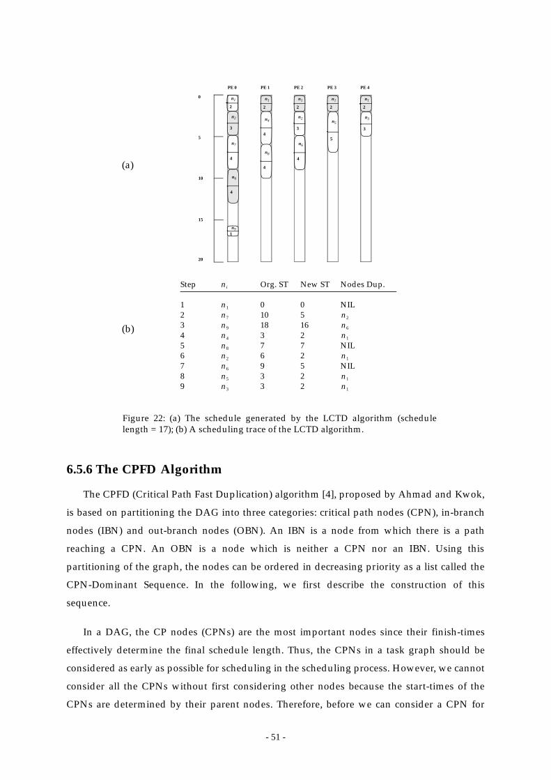
- 51 -
6.5.6 The CPFD Algorithm
The CPFD (Critical Path Fast Duplication) algorithm [4], proposed by Ahmad and Kwok,
is based on partitioning the DAG into three categories: critical path nodes (CPN), in-branch
nodes (IBN) and out-branch nodes (OBN). An IBN is a node from which there is a path
reaching a CPN. An OBN is a node which is neither a CPN nor an IBN. Using this
partitioning of the graph, the nodes can be ordered in decreasing priority as a list called the
CPN-Dominant Sequence. In the following, we first describe the construction of this
sequence.
In a DAG, the CP nodes (CPNs) are the most important nodes since their finish-times
effectively determine the final schedule length. Thus, the CPNs in a task graph should be
considered as early as possible for scheduling in the scheduling process. However, we cannot
consider all the CPNs without first considering other nodes because the start-times of the
CPNs are determined by their parent nodes. Therefore, before we can consider a CPN for
PE 0 PE 1 PE 2 PE 3 PE 4
Step Org. ST New ST Nodes Dup.
1 0 0 NIL2 10 53 18 164 3 25 7 7 NIL6 6 27 9 5 NIL8 3 29 3 2
ni
n1
n7 n2
n9 n6
n4 n1
n8
n2 n1
n6
n5 n1
n3 n1
n1
2
n2
3n5
5
n91
n3
3
n4
4
0
5
10
15
20
n8
4
n6
4
Figure 22: (a) The schedule generated by the LCTD algorithm (schedulelength = 17); (b) A scheduling trace of the LCTD algorithm.
(a)
(b)
n1
2
n1
2
n1
2
n1
2
n2
3
n7
4
n6
4
- 52 -
scheduling, we must first consider all its parent nodes. In order to determine a scheduling
order in which all the CPNs can be scheduled as early as possible, we classify the nodes of the
DAG into three categories given in the following definition.
Definition 4: In a connected graph, an In-Branch Node (IBN) is a node, which is not a CPN,
and from which there is a path reaching a Critical Path Node (CPN). An Out-Branch Node
(OBN) is a node, which is neither a CPN nor an IBN.
After the CPNs, the most important nodes are IBNs because their timely scheduling can
help reduce the start-times of the CPNs. The OBNs are relatively less important because they
usually do not affect the schedule length. Based on this reasoning, we make a sequence of
nodes called the CPN-Dominant sequence which can be constructed by the following
procedure:
Construction of CPN-Dominant Sequence:(1) Make the entry CPN to be the first node in the sequence. Set Position to 2. Let be
the next CPN.
Repeat
(2) If has all its parent nodes in the sequence then (3) Put at Position in the sequence and increment Position. (4) else(5) Suppose is the parent node of which is not in the sequence and has the
largest b-level. Ties are broken by choosing the parent with a smaller t-level. If has all its parent nodes in the sequence, put at Position in the sequence andincrement Position. Otherwise, recursively include all the ancestor nodes of inthe sequence so that the nodes with a larger communication are considered first.
(6) Repeat the above step until all the parent nodes of are in the sequence. Put in the sequence at Position.
(7) endif (8) Make to be the next CPN.
Until all CPNs are in the sequence.
(9) Append all the OBNs to the sequence in a decreasing order of b-level.
The CPN-Dominant sequence preserves the precedence constraints among nodes as the
IBNs reaching a CPN are always inserted before the CPN in the CPN-Dominant sequence. In
addition, the OBNs are appended to the sequence in a topological order so that a parent OBN
is always in front of a child OBN.
The CPN-Dominant sequence of the DAG shown in Figure 3 is constructed as follows.
nx
nx
nx
ny nxny
nyny
nx nx
nx

- 53 -
Since is the entry CPN, it is placed in the first position in the CPN-Dominant sequence.
The second node is because it has only one parent node. After is appended to the CPN-
Dominant sequence, all parent nodes of have been considered and can, therefore, also be
added to the sequence. Now, the last CPN, is considered. It cannot be appended to the
sequence because some of its parent nodes (i.e., the IBNs) have not been examined yet. Since
both and have the same b-level but has a smaller t-level, is considered first.
However, both parent nodes of have not been examined, thus, its two parent nodes,
and are appended to the CPN-Dominant sequence first. Next, is appended followed by
. The only OBN, , is the last node in the CPN-Dominant sequence. The final CPN-
Dominant sequence is as follows: (see Figure 3(b); the CPNs are
marked by an asterisk). Note that using sl (static level) as a priority measure will generate a
different ordering of nodes: .
Based on the CPN-Dominant sequence, the CPFD algorithm is briefly described below.
(1) Determine a critical path. Partition the task graph into CPNs, IBNs, and OBNs. Letcandidate be the entry CPN.
Repeat
(2) Let P_SET be the set of processors containing the ones accommodating the parentsof candidate plus an empty processor.
(3) For each processor P in P_SET, do:
a) Determine candidate’s start-time on P and denote it by ST.
b) Consider the set of candidate’s parents. Let m be the parent which is not scheduledon P and whose message for candidate has the latest arrival time.
c) Try to duplicate m on the earliest idle time slot on P. If the duplication is successfuland the new start-time of candidate is less than ST, then let ST be the new start-timeof candidate. Change candidate to m and goto step a). If the duplication isunsuccessful, then return control to examine another parent of the previouscandidate.
(4) Schedule candidate to the processor P’ that gives the earliest start-time and performall the necessary duplication.
(5) Let candidate be the next CPN.
Until all CPNs are scheduled.
(6) Repeat the process from step (2) to step (5) for each OBN with P_SET containing allthe processors in use together with an empty processor. The OBNs are consideredone by one topologically.
The time-complexity of the CPFD algorithm is . For the DAG shown in Figure 3,
the CPFD algorithm generates a schedule shown in Figure 23(a). The steps of scheduling are
given in the table shown in Figure 23(b). In this table, the start-times of the node on the
n1
n2 n2
n7
n9
n6 n8 n8 n8
n8 n3
n4 n8
n6 n5
n1 n2 n7 n4 n3 n8 n6 n,9
n5, , , , , , ,
n1 n4 n2 n3 n5 n6 n7 n8 n9, , , , , , , ,
O v4( )
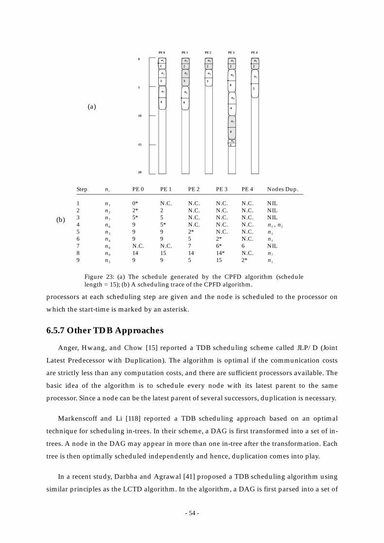
- 54 -
processors at each scheduling step are given and the node is scheduled to the processor on
which the start-time is marked by an asterisk.
6.5.7 Other TDB Approaches
Anger, Hwang, and Chow [15] reported a TDB scheduling scheme called JLP/D (Joint
Latest Predecessor with Duplication). The algorithm is optimal if the communication costs
are strictly less than any computation costs, and there are sufficient processors available. The
basic idea of the algorithm is to schedule every node with its latest parent to the same
processor. Since a node can be the latest parent of several successors, duplication is necessary.
Markenscoff and Li [118] reported a TDB scheduling approach based on an optimal
technique for scheduling in-trees. In their scheme, a DAG is first transformed into a set of in-
trees. A node in the DAG may appear in more than one in-tree after the transformation. Each
tree is then optimally scheduled independently and hence, duplication comes into play.
In a recent study, Darbha and Agrawal [41] proposed a TDB scheduling algorithm using
similar principles as the LCTD algorithm. In the algorithm, a DAG is first parsed into a set of
PE 0 PE 1 PE 2 PE 3 PE 4
Step PE 0 PE 1 PE 2 PE 3 PE 4 Nodes Dup.
1 0* N.C. N.C. N.C. N.C. NIL2 2* 2 N.C. N.C. N.C. NIL3 5* 5 N.C. N.C. N.C. NIL4 9 5* N.C. N.C. N.C. , 5 9 9 2* N.C. N.C.6 9 9 5 2* N.C.7 N.C. N.C. 7 6* 6 NIL8 14 15 14 14* N.C.9 9 9 5 15 2*
ni
n1
n2
n7
n6 n1 n2
n3 n1
n4 n1
n8
n9 n7
n5 n1
n1
2
n2
3n5
5
n91
n3
3
n7
4
n4
4
0
5
10
15
20
n8
4
n6
4
Figure 23: (a) The schedule generated by the CPFD algorithm (schedulelength = 15); (b) A scheduling trace of the CPFD algorithm.
(a)
(b)
n1
2
n1
2
n1
2
n1
2
n2
3
n7
4
- 55 -
linear clusters. Then each cluster is examined to determine the critical nodes for duplication.
Critical nodes are the nodes that determine the data arrival time of the nodes in the cluster
but are themselves outside the cluster. Similar to the LCTD algorithm, the number of
processors required is also optimized by merging schedules with the same set of “prefix”
schedules.
Palis et al. [131] also investigated the problem of scheduling task graphs to processors
using duplication. They proposed an approximation TDB algorithm which produces
schedule lengths at most twice from the optimal. They also showed that the quality of the
schedule improves as the granularity of the task graph becomes larger. For example, if the
granularity is at least 1/2, the schedule length is at most 5/3 times optimal. The time-
complexity of the algorithm is , which is v times faster than the PY
algorithm proposed by Papadimitriou and Yannakakis [136]. In [131], similar algorithms
were also developed that produce: (1) optimal schedules for coarse grain graphs; (2) 2-
optimal schedules for trees with no task duplication; and (3) optimal schedules for coarse
grain trees with no task duplication.
6.6 APN Scheduling
In this section we survey the APN class of DAG scheduling algorithms. In particular we
describe in detail four APN algorithms: the MH (Mapping Heuristic) algorithm [49], the DLS
(Dynamic Level Scheduling) algorithm [154], the BU (Bottom Up) algorithm [122], and the
BSA (Bubble Scheduling and Allocation) algorithm [102]. Before we discuss these algorithms,
it is necessary to examine one of the most important issues in APN scheduling—the message
routing issue.
6.6.1 The Message Routing Issue
In APN scheduling, a processor network is not necessarily fully-connected and
contention for communication channels need to be addressed. This in turn implies that
message routing and scheduling must also be considered. Recent high-performance
architectures (nCUBE-2 [82], iWarp [82], and Intel Paragon [140]) employ wormhole routing
[40] in which the header flit of a message establishes the path, intermediate flits follow the
path, and the tail flit releases the path. Once the header gets blocked due to link contention,
the entire message waits in the network, occupying all the links it is traversing. Hence, it is
increasingly becoming important to take link contention into account as compared to
distance when scheduling computations onto wormhole-routed systems. Routing strategies
can be classified as either deterministic or adaptive. Deterministic schemes, such as the e-cube
O v v v e+log( )( )
- 56 -
routing for hypercube topology, construct fixed routes for messages and cannot avoid
contention if two messages are using the same link even when other links are free. Yet
deterministic schemes are easy to implement and routing decisions can be made efficiently.
On the other hand, adaptive schemes construct optimized routes for different messages
depending upon the current channel allocation in order to avoid link contention. However,
adaptive schemes are usually more complex as they require much state information to make
routing decisions.
Wang [166] suggested two adaptive routing schemes suitable for use in APN scheduling
algorithms. The first scheme is a greedy algorithm which seeks a locally optimal route for
each message to be sent between tasks. Instead of searching for a path with the least waiting
time, the message is sent through a link which yields the least waiting time among the links
that the processor can choose from for sending a message. Thus, the route is only locally
optimal. Using this algorithm, Wang observed that there are two types of possible blockings:
(i) a later message blocks an earlier message (called LBE blocking), and (ii) an earlier message
blocks a later message (called EBL blocking). LBE blocking is always more costly than EBL
blocking. In the case that several messages are competing for a link and blocking becomes
unavoidable, LBE blockings should be avoided as much as possible. Given this observation,
Wang proposed the second algorithm, called the least blocking algorithm, which works by
trying to avoid LBE blocking. The basic idea of the algorithm is to use Dijkstra’s shortest path
algorithm to arrange optimized routes for messages so as to avoid LBE blockings.
Having determined routes for messages, the scheduling of different messages on the links
is also an important aspect. Dixit-Radiya and Panda [46] proposed a scheme for ordering
messages in a link so as to further minimize the extent of link contention. Their scheme is
based on the Temporal Communication Graph (TCG) which, in addition to task precedence,
captures the temporal relationship of the communication messages. Using the TCG model,
the objective of which is to minimize the contention on the link, the earliest start-times and
latest start-times of messages can be computed. These values are then used to heuristically
schedule the messages in the links.
6.6.2 The MH Algorithm
The MH (Mapping Heuristic) algorithm [49] first assigns priorities by computing the sl of
all nodes. A ready node list is then initialized to contain all entry nodes ordered in decreasing
priorities. Each node is scheduled to a processor that gives the smallest start-time. In
calculating the start-time of node, a routing table is maintained for each processor. The table
- 57 -
contains information as to which path to route messages from the parent nodes to the node
under consideration. After a node is scheduled, all of its ready successor nodes are appended
to the ready node list. The MH algorithm is briefly described below.
(1) Compute the sl of each node ni in the task graph.(2) Initialize a ready node list by inserting all entry nodes in the task graph. The list is
ordered according to node priorities, with the highest priority node first.
Repeat
(3) ni ← the first node in the list(4) Schedule ni to the processor which gives the smallest start-time. In determining the
start-time on a processor, all messages from the parent nodes are scheduled androuted by consulting the routing tables associated with each processor.
(5) Append all ready successor nodes of ni, according to their priorities, to the readynode list.
Until the ready node list is empty.
The time-complexity of the MH algorithm is shown to be , where p is the
number of processors in the target system.
For the DAG shown in Figure 3(a), the schedule generated by the MH algorithm for a 4-
processor ring is shown in Figure 24. Here, denotes a communication link between PE i
and PE j. The MH algorithm schedules the nodes in the following order: n1, n4, n3, n5, n2, n8, n7,
n6, n9. Note that the MH algorithm does not strictly schedule nodes according to a descending
order of sls (static levels) in that it uses the sl order to break ties. As can be seen from the
schedule shown in Figure 24, the MH algorithm schedules n4 first before n2 and n7, which are
more important nodes. This is due to the fact that both algorithms rank nodes according to a
descending order of their sls. The nodes n2 and n7 are more important because n7 is a CPN
and n2 critically affects the start-time of n7. As n4 has a larger static level, both algorithms
examine n4 first and schedule it to an early time slot on the same processor as n1. As a result,
n2 cannot start at the earliest possible time—the time just after n1 finishes.
6.6.3 The DLS Algorithm
The DLS (Dynamic Level Scheduling) algorithm [154] described in Section 6.4.5 can also
be used as an APN scheduling algorithm. However, the DLS algorithm requires a message
routing method to be supplied by the user. It then computes the earliest start-time of a node
on a processor by tentatively scheduling and routing all messages from the parent nodes
using the given routing table.
O v p3v e+( )( )
Lij
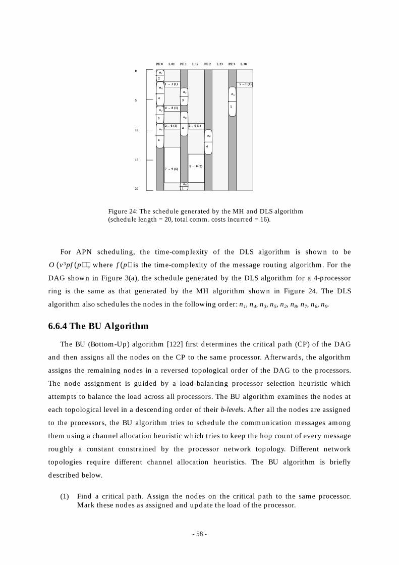
- 58 -
For APN scheduling, the time-complexity of the DLS algorithm is shown to be
, where is the time-complexity of the message routing algorithm. For the
DAG shown in Figure 3(a), the schedule generated by the DLS algorithm for a 4-processor
ring is the same as that generated by the MH algorithm shown in Figure 24. The DLS
algorithm also schedules the nodes in the following order: n1, n4, n3, n5, n2, n8, n7, n6, n9.
6.6.4 The BU Algorithm
The BU (Bottom-Up) algorithm [122] first determines the critical path (CP) of the DAG
and then assigns all the nodes on the CP to the same processor. Afterwards, the algorithm
assigns the remaining nodes in a reversed topological order of the DAG to the processors.
The node assignment is guided by a load-balancing processor selection heuristic which
attempts to balance the load across all processors. The BU algorithm examines the nodes at
each topological level in a descending order of their b-levels. After all the nodes are assigned
to the processors, the BU algorithm tries to schedule the communication messages among
them using a channel allocation heuristic which tries to keep the hop count of every message
roughly a constant constrained by the processor network topology. Different network
topologies require different channel allocation heuristics. The BU algorithm is briefly
described below.
(1) Find a critical path. Assign the nodes on the critical path to the same processor.Mark these nodes as assigned and update the load of the processor.
Figure 24: The schedule generated by the MH and DLS algorithm(schedule length = 20, total comm. costs incurred = 16).
n1
2
2→ 6 (1)
PE 0
n2
3
n5
5
n91
n3
3
n7
4
n4
4
0
5
10
15
20
n8
4
n6
4
5 ←1 (1)
9 ← 6 (5)7 → 9 (6)
4 → 8 (1)
1 → 3 (1)
2→ 6 (1)
L 01 L 12 L 23 L 30PE 1 PE 2 PE 3
O v3pf p( )( ) f p( )
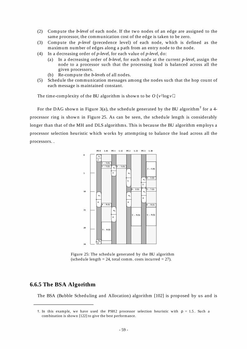
- 59 -
(2) Compute the b-level of each node. If the two nodes of an edge are assigned to thesame processor, the communication cost of the edge is taken to be zero.
(3) Compute the p-level (precedence level) of each node, which is defined as themaximum number of edges along a path from an entry node to the node.
(4) In a decreasing order of p-level, for each value of p-level, do:(a) In a decreasing order of b-level, for each node at the current p-level, assign the
node to a processor such that the processing load is balanced across all thegiven processors.
(b) Re-compute the b-levels of all nodes.(5) Schedule the communication messages among the nodes such that the hop count of
each message is maintained constant.
The time-complexity of the BU algorithm is shown to be .
For the DAG shown in Figure 3(a), the schedule generated by the BU algorithm† for a 4-
processor ring is shown in Figure 25. As can be seen, the schedule length is considerably
longer than that of the MH and DLS algorithms. This is because the BU algorithm employs a
processor selection heuristic which works by attempting to balance the load across all the
processors. .
6.6.5 The BSA Algorithm
The BSA (Bubble Scheduling and Allocation) algorithm [102] is proposed by us and is
†. In this example, we have used the PSH2 processor selection heuristic with . Such acombination is shown [122] to give the best performance.
O v2 vlog( )
ρ 1.5=
n1
2
6← 2 (1)
PE 0
n2
3
n5
5
n91
n3
3
n7
4
n4
4
0
5
10
15
20
n8
4
n6
4
9 ← 8 (5)
4 → 8 (1)
1 → 3 (1)
2→ 7 (1)
L 01 L 12 L 23 L 30PE 1 PE 2 PE 3
24
4 → 8 (1)
6 → 9 (5)6 → 9 (5)
4 ←1 (1)
2 ←1 (4)1 → 5 (1) 1 → 5 (1)
Figure 25: The schedule generated by the BU algorithm(schedule length = 24, total comm. costs incurred = 27).
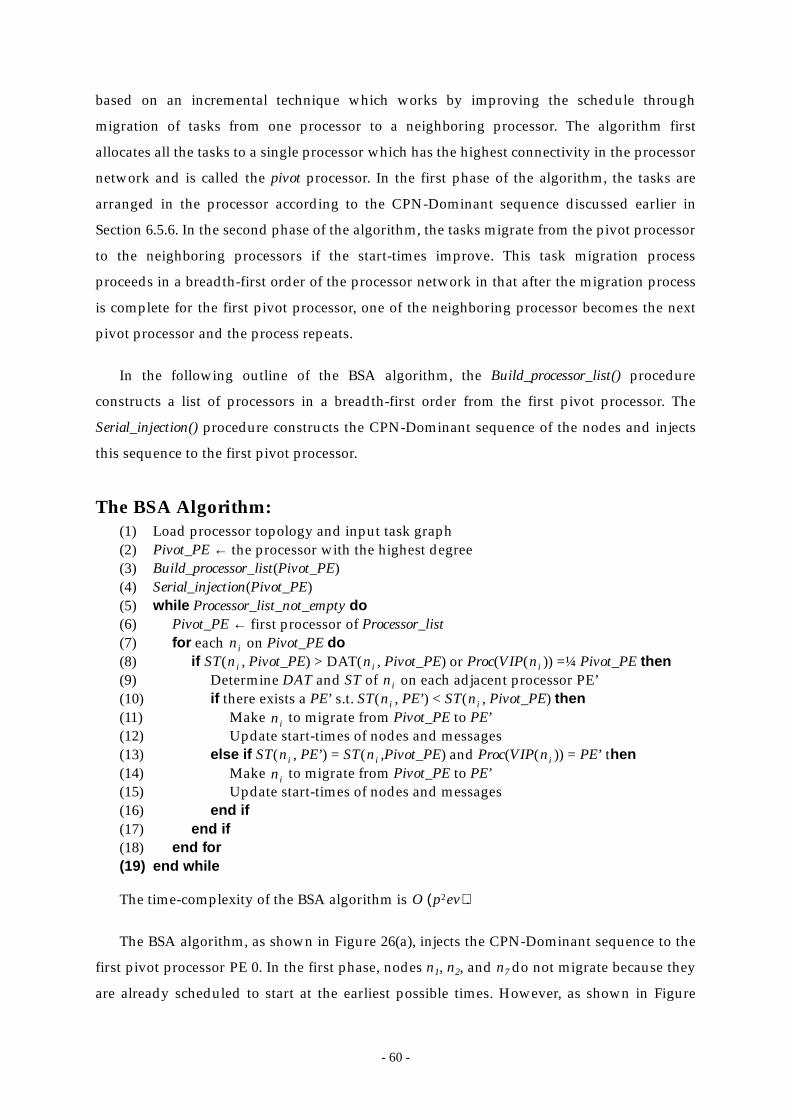
- 60 -
based on an incremental technique which works by improving the schedule through
migration of tasks from one processor to a neighboring processor. The algorithm first
allocates all the tasks to a single processor which has the highest connectivity in the processor
network and is called the pivot processor. In the first phase of the algorithm, the tasks are
arranged in the processor according to the CPN-Dominant sequence discussed earlier in
Section 6.5.6. In the second phase of the algorithm, the tasks migrate from the pivot processor
to the neighboring processors if the start-times improve. This task migration process
proceeds in a breadth-first order of the processor network in that after the migration process
is complete for the first pivot processor, one of the neighboring processor becomes the next
pivot processor and the process repeats.
In the following outline of the BSA algorithm, the Build_processor_list() procedure
constructs a list of processors in a breadth-first order from the first pivot processor. The
Serial_injection() procedure constructs the CPN-Dominant sequence of the nodes and injects
this sequence to the first pivot processor.
The BSA Algorithm:(1) Load processor topology and input task graph(2) Pivot_PE ← the processor with the highest degree(3) Build_processor_list(Pivot_PE)(4) Serial_injection(Pivot_PE)(5) while Processor_list_not_empty do(6) Pivot_PE ← first processor of Processor_list(7) for each on Pivot_PE do(8) if ST( , Pivot_PE) > DAT( , Pivot_PE) or Proc(VIP( )) =¼ Pivot_PE then(9) Determine DAT and ST of on each adjacent processor PE’(10) if there exists a PE’ s.t. ST( , PE’) < ST( , Pivot_PE) then(11) Make to migrate from Pivot_PE to PE’ (12) Update start-times of nodes and messages(13) else if ST( , PE’) = ST( ,Pivot_PE) and Proc(VIP( )) = PE’ then(14) Make to migrate from Pivot_PE to PE’(15) Update start-times of nodes and messages(16) end if(17) end if(18) end for(19) end while
The time-complexity of the BSA algorithm is .
The BSA algorithm, as shown in Figure 26(a), injects the CPN-Dominant sequence to the
first pivot processor PE 0. In the first phase, nodes n1, n2, and n7 do not migrate because they
are already scheduled to start at the earliest possible times. However, as shown in Figure
ni
ni ni ni
ni
ni ni
ni
ni ni ni
ni
O p2ev( )
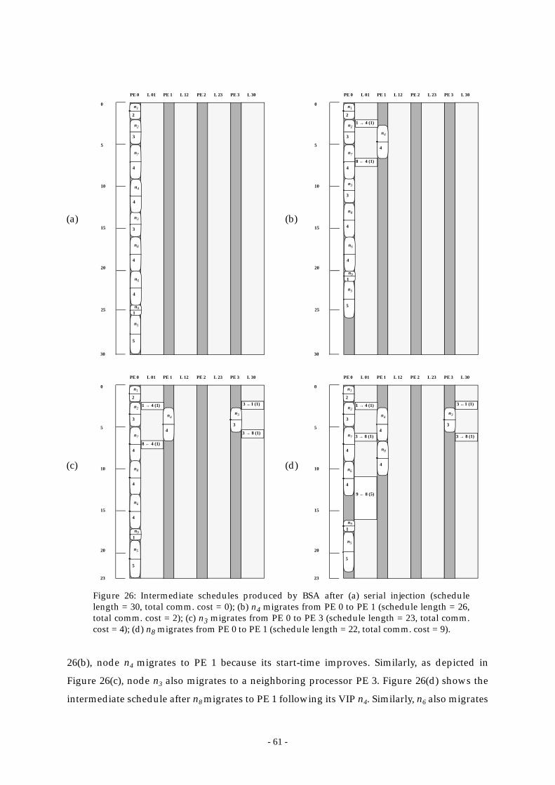
- 61 -
26(b), node n4 migrates to PE 1 because its start-time improves. Similarly, as depicted in
Figure 26(c), node n3 also migrates to a neighboring processor PE 3. Figure 26(d) shows the
intermediate schedule after n8 migrates to PE 1 following its VIP n4. Similarly, n6 also migrates
n1
2
PE 0
n2
3
n5
5
n91
n3
3
n7
4
n4
4
0
5
10
15
20
n8
4
n6
4
L 01 L 12 L 23 L 30PE 1 PE 2 PE 3
25
(c)
30
n1
2
PE 0
n2
3
n5
5
n91
n3
3
n7
4
n4
4
0
5
10
15
20
n8
4
n6
4
L 01 L 12 L 23 L 30PE 1 PE 2 PE 3
25
30
1 → 4 (1)
8 ← 4 (1)
n1
2
PE 0
n2
3
n5
5
n91
n3
3
n7
4
n4
4
0
5
10
15
20
n8
4
n6
4
L 01 L 12 L 23 L 30PE 1 PE 2 PE 3
23
1 → 4 (1)
8 ← 4 (1)
3 ←1 (1)
3 → 8 (1)
n1
2
PE 0
n2
3
n5
5
n9
1
n3
3
n7
4
n4
4
0
5
10
15
20
n8
4n6
4
L 01 L 12 L 23 L 30PE 1 PE 2 PE 3
23
1 → 4 (1) 3 ←1 (1)
3 → 8 (1)3 → 8 (1)
9 ← 8 (5)
(a) (b)
(d)
Figure 26: Intermediate schedules produced by BSA after (a) serial injection (schedulelength = 30, total comm. cost = 0); (b) n4 migrates from PE 0 to PE 1 (schedule length = 26,total comm. cost = 2); (c) n3 migrates from PE 0 to PE 3 (schedule length = 23, total comm.cost = 4); (d) n8 migrates from PE 0 to PE 1 (schedule length = 22, total comm. cost = 9).
- 62 -
to PE 3 following its VIP n3, as shown in Figure 27(a). The last CPN, n9, migrates to PE 1 to
which its VIP n8 is scheduled. Such migration allows the only OBN n5 to bubble up. The
resulting schedule is shown in Figure 27(b). This is the final schedule as no more nodes can
improve the start-time through migration.
6.6.6 Other APN Approaches
Kon’ya and Satoh [97] reported an APN scheduling algorithm for the hypercube
architectures. Their algorithm, called the LST (Latest Starting Time) algorithm, works by
using a list scheduling approach in that the priorities of nodes are first computed and a list is
constructed based on these priorities. The priority of a node is defined as its latest starting
time, which is determined before scheduling starts. Thus, the list is static and does not
capture the dynamically changing importance of nodes, which is crucial in APN scheduling.
In a later study, Selvakumar and Murthy [145] reported an APN scheduling scheme
which is an extension of Sih and Lee’s DLS algorithm. The distinctive new feature in their
algorithm is that it exploits schedule holes in processors and communication links in order to
produce better schedules. Essentially, it differs from the DLS algorithm in two respects: (i) the
way in which the priority of a task with respect to a processor in a partial schedule; and (ii)
the way in which a task and all communications from its parents are scheduled. The priority
(b)(a)
Figure 27: (a) Intermediate schedule produced by BSA after n6 migrates from PE 0 to PE 3(schedule length = 22, total comm. cost = 15); (b) final schedule produced by BSA after n9migrates from PE 0 to PE 1 and n5 is bubbled up (schedule length = 16, total comm. cost = 21).
n1
2
PE 0
n2
3
75
5
n9
1
n3
3
n7
4
n4
4
0
5
10
15
20
n8
4
n6
4
L 01 L 12 L 23 L 30PE 1 PE 2 PE 3
23
1 → 4 (1) 3 ←1 (1)
3 → 8 (1)3 → 8 (1)
9 ← 8 (5)
6 ← 2 (1)
6 → 9 (5)
n1
2
PE 0
n2
3
n5
5
n9
1
n3
3
n7
4
n4
4
0
5
10
15
16
n8
4
n6
4
L 01 L 12 L 23 L 30PE 1 PE 2 PE 3
1 → 4 (1) 3 ←1 (1)
3 → 8 (1)3 → 8 (1)
7 → 9 (6)
6 ← 2 (1)
9 ← 6 (5)9 ← 6 (5)
- 63 -
of a node is modified to be the difference between the static level and the earliest finish-time.
During the scheduling of a node, a router is used to determine the best possible path between
the processors that need communication. In their simulation study, the improved scheduling
algorithm outperformed both the DLS algorithm and the MH algorithm.
6.7 Scheduling in Heterogeneous Environments
Heterogeneity has been shown to be an important attribute in improving the
performance of multiprocessors [53], [59], [123], [151], [153], [168]. In parallel computations,
the serial part is the bottleneck, according to Amhdal’s law [14]. In homogeneous
multiprocessors, if one or more faster processors are used to replace a set of cost-equivalent
processors, the serial computations and other critical computations can be scheduled to such
faster processors and performed at a greater rate so that speedup can be increased.
As we have seen in earlier parts of this section, most DAG scheduling approaches assume
the target system is homogeneous. Introducing heterogeneity into the model inevitably
makes the problem more complicated to handle. This is because the scheduling algorithm has
to take into account the different execution rate of different processors when computing the
potential start-times of tasks on the processors. Another complication is that the resulting
schedule for a given heterogeneous system immediately becomes invalid if some of the
processing elements are replaced even though the number of processors remain the same.
This is because the scheduling decisions are made not only on the number of processors but
also on the capability of the processors.
Static scheduling targeted for heterogeneous environments was unexplored until
recently. Menasce et al. [124], [125], [126], [127] investigated the problem of scheduling
computations to heterogeneous multiprocessing environments. The heterogeneous
environment was modeled as a system with one fast processor plus a number of slower
processors. In their study, both dynamic and static scheduling schemes were examined but
nevertheless DAGs without communication are used to model computations [13]. Markov
chains were used to analyze the performance of different scheduling schemes. In their
findings, out of all the static scheduling schemes, the LTF/MFT (Largest Task First/
Minimizing finish-time) significantly outperformed all the others including WL (Weighted
Level), CPM (Critical Path Method) and HNF (Heavy Node First). The LTF/MFT algorithm
works by picking the largest task from the ready tasks list and schedules it to the processor
which allows the minimum finish-time, while the other three strategies select candidate
processor based on the execution time of the task. Thus, based on their observations, an
- 64 -
efficient scheduling algorithm for heterogeneous systems should concentrate on reducing the
finish-times of tasks. Nonetheless, if communication delays are also considered, different
strategies may be needed.
6.8 Mapping Clusters to Processors
As discussed earlier, mapping of clusters to physical processors is necessary for UNC
scheduling when the number of clusters is larger than the number of physical processors.
However, the mapping of clusters to processors is a relatively unexplored research topic
[109]. In the following we discuss a number of approaches reported in the literature.
Upon obtaining a schedule by using the EZ algorithm, Sarkar [144] used a list-scheduling
based method to map the clusters to physical processors. In the mapping algorithm, each task
is considered in turn according to the static level. A processor is allocated to the task if it
allows the earliest execution, then the whole cluster containing the task is also assigned to
that processor and all the member tasks are marked as assigned. In this scheme, two clusters
can be merged to a single processor but a cluster is never cracked. Furthermore, the allocation
of channels to communication messages was not considered.
Kim and Browne [95] also proposed a mapping scheme for the UNC schedules obtained
from their LC algorithm. In their scheme, the linear UNC clusters are first merged so that the
number of clusters is at most the same as the number of processors. Two clusters are
candidates for merging if one can start after another finishes, or the member tasks of one
cluster can be merged into the idle time slots of another cluster. Then a dominant request tree
(DRT) is constructed from the UNC schedule which is a cluster graph. The DRT consists of
the connectivity information of the schedule and is, therefore, useful for the mapping stage in
which two communicating UNC clusters attempt to be mapped to two neighboring
processors, if possible. However, if for some clusters this connectivity mapping heuristic fails,
another two heuristics, called perturbation mapping and foster mapping, are invoked. For both
mapping strategies, a processor is chosen which has the most appropriate number of
channels among currently unallocated processors. Finally, to further optimize the mapping, a
restricted pairwise exchange step is called for.
Wu and Gajski [170] also suggested a mapping scheme for assigning the UNC clusters
generated in scheduling to processors. They realized that for best mapping results, a
dedicated traffic scheduling algorithm that balances the network traffic should be used.
However, traffic scheduling requires flexible-path routing, which incurs higher overhead.
Thus, they concluded that if network traffic is not heavy, a simpler algorithm which
- 65 -
minimizes total network traffic can be used. The algorithm they used is a heuristic algorithm
designed by Hanan and Kurtzberg [74] to minimize the total communication traffic. The
algorithm generates an initial assignment by a constructive method and the assignment is
then iteratively improved to obtain a better mapping.
Yang and Gerasoulis [171] employed a work profiling method for merging UNC clusters.
The merging process proceeds by first sorting the clusters in an increasing order of aggregate
computational load. Then a load balancing algorithm is invoked to map the clusters to the
processors so that every processor has about the same load. To take care of the topology of
the underlying processor network, the graph of merged clusters are then mapped to the
network topology using Bokhari’s algorithm.
Yang, Bic, and Nicolau [175] reported an algorithm for mapping cluster graphs to
processor graphs which is suitable for use as the post-processing step for BNP scheduling
algorithms. The mapping scheme is not suitable for UNC scheduling because it assumes the
scheduling algorithm has already produced a number of clusters which is less than or equal
to the number of processors available. The objective of the mapping method is to reduce
contention and optimize the schedule length when the clusters are mapped to a topology
which is not fully-connected as assumed by the BNP algorithms. The idea of the mapping
algorithm is based on determining a set of critical edges, each of which is assigned a single
communication link. Substantial improvement over random mapping was obtained in their
simulation study.
In a recent study, Liou and Palis [113] investigated the problem of mapping clusters to
processors. One of the major objectives of their study was to compare the effectiveness of
one-phase scheduling (i.e., BNP scheduling) to that of the two-phase approach (i.e., UNC
scheduling followed by clusters mapping). To this end, they proposed a new UNC algorithm
called CASS-II (Clustering And Scheduling System II), which was applied to randomly
generated task graphs in an experimental study using three clusters mapping schemes,
namely, the LB (load-balancing) algorithm, the CTM (communication traffic minimizing)
algorithm and the RAND (random) algorithm. The LB algorithm uses processor workload as
the criterion of matching clusters to processors. By contrast, the CTM algorithm tries to
minimize the communication costs between processors. The RAND algorithm simply makes
random choices at each mapping step. To compare the one-phase method with the two-phase
method, in one set of test cases the task graphs were scheduled using CASS-II with the three
mapping algorithms while in the other set using the mapping algorithms alone. Liou and
Palis found that two-phase scheduling is better than one-phase scheduling in that the
- 66 -
utilization of processors in the former is more efficient than the latter. Furthermore, they
found that the LB algorithm finds significantly better schedules than the CTM algorithm.
7 Some Scheduling Tools
Software tools providing automated functionalities for scheduling/mapping can the
parallel programming task easier. Despite a vast volume of research on scheduling exists,
building useful scheduling tools is only recently addressed. A scheduling tool should allow a
programmer to specify a parallel program in certain textual or graphical form, and then
perform automatic partitioning and scheduling of the program. The tool should also allow
the user to specify the target architecture. Performance evaluation and debugging functions
are also highly desirable. Some tools provide interactive environments for performance
evaluation of various popular parallel machines but do not generate an executable scheduled
code [137]. Under the above definition, such tools provide other functionalities but cannot be
classified as scheduling tools.
In the following we survey some of the recently reported prototype scheduling tools.
7.1 Hypertool
Hypertool takes a user-partitioned sequential program as input and automatically
allocates and schedules the partitions to processors [170]. Proper synchronization primitives
are also automatically inserted. Hypertool is a code generation tool since the user program is
compiled into a parallel program for the iPSC/2 hypercube computer using parallel code
synthesis and optimization techniques. The tool also generates performance estimates
including execution time, communication and suspension times for each processor as well as
network delay for each communication channel. Scheduling is done using the MD algorithm
or the MCP algorithm.
7.2 PYRROS
PYRROS is a compile-time scheduling and code generation tool [172]. Its input is a task
graph and the associated sequential C code. The output is a static schedule and a parallel C
code for a given architecture (the iPSC/2). PYRROS consists of a task graph language with an
interface to C, a scheduling system which uses only the DSC algorithm, a X-Windows based
graphic displayer, and a code generator. The task graph language lets user define partitioned
programs and data. The scheduling system is used for clustering the task graph, performing
load balanced mapping, and computation/communication ordering. The graphic displayer
is used for displaying task graphs and scheduling results in the form of Gantt charts. The
- 67 -
code generator inserts synchronization primitives and performs parallel code optimization
for the target parallel machine.
7.3 Parallax
Parallax incorporates seven classical scheduling heuristics designed in the seventies [111],
providing an environment for parallel program developers to find out how the schedulers
affect program performance on various parallel architectures. Users must provide the input
program as a task graph and estimate task execution times. Users must also express the target
machine as an interconnection topology graph. Parallax then generates schedules in the form
of Gantt charts, speedup curves, processor and communication efficiency charts using X-
Windows interface. In addition, an animated display of the simulated running program to
help developers to evaluate the differences among the scheduling heuristics provided.
Parallex, however, is not reported to generate an executable code.
7.4 OREGAMI
OREGAMI is designed for use in conjunction with parallel programming languages that
support a communication model, such as OCCAM, C*, or C and FORTRAN with
communication extension [115]. As such, it is a set of tools that includes a LaRCS compiler to
compile textual user task descriptions into specialized task graphs, which are called TCG
(Temporal Communication Graphs) [114]. In addition, OREGAMI includes a mapper tool for
mapping tasks on a variety of target architectures, and a metrics tools for analyzing and
displaying the performance. The suite of tools are implemented in C for SUN workstations
with an X-Windows interface. However, precedence constraints among tasks are not
considered in OREGAMI. Moreover, no target code is generated. Thus, like Parallax,
OREGAMI is rather a design tool for parallel program development.
7.5 PARSA
PARSA is a software tool developed for automatic scheduling and partitioning of
sequential user programs [148]. PARSA consists of four components: an application
specification tool, an architecture specification tool, a partitioning and scheduling tool, and a
performance assessment tool. PARSA does not generate any target code. The application
specification tool accepts a sequential program written in the SISAL functional language and
converts it into a DAG, which is represented in textual form by the IF1 (Intermediate Form 1)
acyclic graphical language. The architecture specification tool allows the user to interactively
specify the target system in graphical form. The execution delay for each task is also
generated based on the architecture specification. The partitioning and scheduling tool
- 68 -
consists of the HNF algorithm, the LC algorithm, and the LCTD algorithm. The performance
assessment tool displays the expected run-time behavior of the scheduled program. The
expected performance is generated by the analysis of the scheduled program trace file, which
contains the information on where each task is assigned for execution and exactly where each
task is expected to start execution, stop execution, or send a message to a remote task.
7.6 CASCH
CASCH (Computer-Aided SCHeduling) tool [9] is aimed to be a complete parallel
programming environment including parallelization, partitioning, scheduling, mapping,
communication, synchronization, code generation, and performance evaluation.
Parallelization is performed by a compiler that automatically converts sequential
applications into parallel codes. The parallel code is optimized through proper scheduling
and mapping, and is executed on a target machine. CASCH provides an extensive library of
state-of-the-art scheduling algorithms from the recent literature. The library of scheduling
algorithms is organized into different categories which are suitable for different architectural
environments.
The scheduling and mapping algorithms are used for scheduling the task graph
generated from the user program, which can be created interactively or read from disk. The
weights on the nodes and edges of the task graph are computed using a database that
contains the timing of various computation, communication, and I/O operations for different
machines. These timings are obtained through benchmarking. An attractive feature of
CASCH is its easy-to-use GUI for analyzing various scheduling and mapping algorithms
using task graphs generated randomly, interactively, or directly from real programs. The best
schedule generated by an algorithm can be used by the code generator for generating a
parallel program for a particular machine—the same process can be repeated for another
machine.
7.7 Commercial Tools
There is only a few commercially available tools for scheduling and program
parallelization. Examples include ATEXPERT by Cray Research [39], PARASPHERE by DEC
[45], IPD by Intel [84], MPPE by MasPar [119], and PRISM by TMC [161]. Most of these tools
provide software development and debugging environments. Some of them also provide
performance tuning tools and other program development facilities.
- 69 -
8 New Ideas and Research Trends
With the advancements in processors and networking hardware technologies, parallel
processing can be accomplished in a wide spectrum of platforms ranging from tightly-
coupled MPPs to loosely-coupled network of autonomous workstations. Designing an
algorithm for such diverse platforms makes the scheduling problem even more complex and
challenging. In summary, in the design of scheduling algorithms for efficient parallel
processing, we have to address four fundamental aspects: performance, time-complexity,
scalability, and applicability. These aspects are elaborated below.
Performance: A scheduling algorithm must exhibit high performance and be robust. By
high performance we mean the scheduling algorithm should produce high quality solutions.
A robust algorithm is one which can be used under a wide range of input parameters (e.g.,
arbitrary number of available processors and diverse task graph structures).
Time-complexity: The time-complexity of an algorithm is an important factor insofar as the
quality of solution is not compromised. As real workload is typically of a large size [9], a fast
algorithm is necessary for finding good solutions efficiently.
Scalability: A scheduling algorithms must possess problem-size scalability, that is, the
algorithm has to consistently give good performance even for large input. On the other hand,
a scheduling algorithm must also possess processing-power scalability, that is, given more
processors for a problem, the algorithm should produce solutions with comparable quality in
a shorter period of time.
Applicability: A scheduling algorithm must be applicable in practical environments. To
achieve this goal, it must take into account realistic assumptions about the program and
multiprocessor models such as arbitrary computation and communication weights, link
contention, and processor network topology.
It is clear that the above mentioned goals are conflicting and thus pose a number of
challenges to researchers. To combat these challenges, several new ideas have been suggested
recently. These new ideas, which include genetic algorithms, randomization approaches, and
parallelization techniques, are employed to enhance the solution quality, or to lower the time-
complexity, or both. In the following, we briefly outline some of these recent advancements.
At the end of this section, we also indicate some current research trends in scheduling.
- 70 -
8.1 Scheduling using Genetic Algorithms
Genetic algorithms (GAs) [42], [56], [58], [68], [78], [157] have recently found many
applications in optimization problems including scheduling [11], [19], [27], [44], [80], [147].
GAs use global search techniques to explore different regions of the search space
simultaneously by keeping track of a set of potential solutions of diverse characteristics,
called a population. As such, GAs are widely reckoned as effective techniques in solving
numerous optimization problems because they can potentially locate better solutions at the
expense of longer running time. Another merit of a genetic search is that its inherent
parallelism can be exploited to further reduce its running time. Thus, a parallel genetic search
technique in scheduling is a viable approach in producing high quality solutions using short
running times.
Ali, Sait, and Benten [11] proposed a genetic algorithm for scheduling a DAG to a limited
number of fully-connected processors with a contention-free communication network. In
their scheme, each solution or schedule is encoded as a chromosome containing v alleles,
each of which is an ordered pair of task index and its assigned processor index. With such
encoding the design of genetic operators is straightforward. Standard crossover is used
because it always produces valid schedules as offsprings and is computationally efficient.
Mutation is simply a swapping of the assigned processors between two randomly chosen
alleles. For generating an initial population, Ali et al. use a technique called “pre-scheduling”
in which random permutations of numbers from 1 to v are generated. The number in each
random permutation represents the task index of the task graph. The tasks are then assigned
to the PEs uniformly: the first tasks in a permutation are assigned to PE 0, the next tasks
to PE 1, and so on. In their simulation study using randomly generated task graphs with a
few tenths of nodes, their algorithm was shown to outperform the ETF algorithm proposed
by Hwang et al. [83].
Hou, Ansari, and Ren [80] also proposed a scheduling algorithm using genetic search in
which each chromosome is a collection of lists, and each list represents the schedule on a
distinct processor. Thus, each chromosome is not a linear structure but a two-dimensional
structure instead. One dimension is a particular processor index and the other is the ordering
of tasks scheduled on the processor. Using such an encoding scheme poses a restriction on
the schedules being represented: the list of tasks within each processor in a schedule is
ordered in ascending order of their topological height, which is defined as the largest number
of edges from an entry node to the node itself. This restriction also facilitates the design of the
crossover operator. In a crossover, two processors are selected from each of two
Np
vp--- v
p---
- 71 -
chromosomes. The list of tasks on each processor is cut into two parts and then the two
chromosomes exchange the two lower parts of their task lists correspondingly. It is shown
that this crossover mechanism always produces valid offsprings. However, the height
restriction in the encoding may cause the search to be incapable of obtaining the optimal
solution because the optimal solution may not obey the height ordering restriction at all.
Hou et al. incorporated a heuristic technique to lower the likelihood of such pathological
situation. Mutation is simpler in design. In a mutation, two randomly chosen tasks with the
same height are swapped in the schedule. As to the generation of the initial population,
randomly permuted schedules obeying the height ordering restriction are generated. In their
simulation study using randomly generated task graphs with a few tenths of nodes, their
algorithm was shown to produce schedules within 20 percent degradation from optimal
solutions.
Ahmad and Dhodhi [2] proposed a scheduling algorithm using a variant of genetic
algorithm called simulated evolution. They employ a problem-space neighborhood
formulation in that a chromosome represents a list of task priorities. Since task priorities are
dependent on the input DAG, different set of task priorities represent different problem
instances. First, a list of priorities is obtained from the input DAG. Then the initial population
of chromosomes are generated by randomly perturbing this original list. Standard genetic
operators are applied to these chromosomes to determine the fittest chromosome which is the
one giving the shortest schedule length for the original problem. The genetic search, therefore,
operates on the problem-space instead of the solution-space as is commonly done. The
rationale of this approach is that good solutions of the problem instances in the problem-
space neighborhood are expected to be good solutions for the original problem as well [160].
Recently, we have proposed a parallel genetic algorithm for scheduling [104], called the
Parallel Genetic Scheduling (PGS) algorithm, using a novel encoding scheme, an effective initial
population generation strategy, and computationally efficient genetic search operators. The
major motivation of using a genetic search approach is that the recombinative nature of a
genetic algorithm can potentially determine an optimal scheduling list leading to an optimal
schedule. As such, a scheduling list (i.e., a topological ordering of the input DAG) is encoded
as a genetic string. Instead of generating the initial population totally randomly, Kwok and
Ahmad generate the initial set of strings based on a number of effective scheduling lists such
as ALAP list, b-level list, t-level list, etc. They use a novel crossover operator, which is a variant
of the order crossover operator, in the scheduling context. The proposed crossover operator
has the potential to effectively combine the good characteristics of two parent strings in order
Np
- 72 -
to generate a scheduling string leading to a schedule with shorter schedule length. The
crossover operator is easy to implement and is computationally efficient.
In our experimental studies [104], we have found that the PGS algorithm generates
optimal solutions for more than half of all the cases in which random task graphs were used.
In addition, the PGS algorithm demonstrates an almost linear speedup and is therefore
scalable. While the DCP algorithm [103] has already been shown to outperform many leading
algorithms, the PGS algorithm is even better since it generates solutions with comparable
quality while using significantly less time due to its effective parallelization. The PGS
algorithm outperforms the well-known DSC algorithm in terms of both the solution quality
and running time. An extra advantage of the PGS algorithm is scalability, that is by using
more parallel processors, the algorithm can be used for scheduling larger task graphs.
8.2 Randomization Techniques
The time-complexity of an algorithm and its solution quality are in general conflicting
goals in the design of efficient scheduling algorithms. Our previous study [106] indicates that
not only does the quality of existing algorithms differ considerably but their running times
can vary by large margins. Indeed, designing an algorithm which is fast and can produce
high quality solutions requires some low-complexity algorithmic techniques. One promising
approach is to employ randomization. As indicated by Karp [89], Motwani and Raghavan
[128], and other researchers, an optimization algorithm which makes random choices can be
very fast and simple to implement. However, there has been very little work done in this
direction.
Recently, Kwok et al. [101], [105], [107] proposed a BNP scheduling algorithm based on a
random neighborhood search technique [88], [133]. The algorithm is called the Parallel Fast
Assignment with Search Technique (PFAST) algorithm which has time-complexity of only
where e is the number of edges in the DAG [105]. The PFAST algorithm first constructs an
initial schedule quickly in linear-time and then refines it by using multiple physical
processors, each of which operates on a disjoint subset of blocking-nodes as a search
neighborhood. The physical processors communicate periodically to exchange the best
solution found thus far. As the number of search steps required is a small constant which is
independent of the size of the input DAG, the algorithm effectively takes linear-time to
determine the final schedule.
In their performance study, Kwok et al. [101], [105] have compared the PFAST algorithm
with a number of well-known efficient scheduling algorithms. The PFAST algorithm has been
O e( )
- 73 -
shown to be better than the other algorithms in terms of both solution quality and running
time. Since the algorithm takes linear-time, it is the fastest algorithm to our knowledge. In
experiments using random task graphs for which optimal solutions are known, the PFAST
algorithm generates optimal solutions for a significant portion of all the test cases, and close-
to-optimal solutions for the remaining cases. The PFAST algorithm also exhibits good
scalability in that it gives a consistent performance when applied to large task graphs. An
interesting finding of the PFAST algorithm is that parallelization can sometimes improve its
solution quality. This is due to the partitioning of the blocking-nodes set, which implies a
partitioning of the search neighborhood. The partitioning allows the algorithm to explore the
search space simultaneously, thereby enhancing the likelihood of getting better solutions.
8.3 Parallelizing a Scheduling Algorithm
Parallelizing a scheduling algorithm is a novel as well as natural way to reduce the time-
complexity. This approach is novel in that no previous work has been done in the
parallelization of a scheduling algorithm. Indeed, as indicated by Norman and Thanisch
[129], it is strange that there has been hardly any attempt to parallelize a scheduling and
mapping process itself. Parallelization is natural in that parallel processing is realized only
when a parallel processing platform is available. Furthermore, parallelization can be utilized
not only to speed up the scheduling process further but also to improve the solution quality.
Recently there have been a few parallel algorithms proposed for DAG scheduling [5], [101],
[104].
In a recent study [7], we have proposed two parallel state-space search algorithms for
finding optimal or bounded solutions. The first algorithm which is based on the A* search
technique uses a computationally efficient cost function for quickly guiding the search. The
A* algorithm is also parallelized using static and dynamic load-balancing schemes to evenly
distribute the search states to the processors. A number of effective state-pruning techniques
are also incorporated to further enhance the efficiency of the algorithm. The proposed
algorithm outperforms a previously reported branch-and-bound algorithm by using
considerable less computation time. The second algorithm is an approximate algorithm that
guarantees a bounded deviation from the optimal solution but executes in a considerably
shorter turnaround time. Based on both theoretical analysis and experimental evaluation [7]
using randomly generated task graphs, we have found that the approximate algorithm is
highly scalable and is an attractive choice if slightly degraded solutions are acceptable.
We have also proposed [5], [101] a parallel APN scheduling algorithm called the Parallel
- 74 -
Bubble Scheduling and Allocation (PBSA) algorithm. The proposed PBSA algorithm is based on
considerations such as a limited number of processors, link contention, heterogeneity of
processors, and processor network topology. As a result, the algorithm is useful for
distributed systems including clusters of workstations. The major strength of the PBSA
algorithm lies in its incremental strategy of scheduling nodes and messages together. It first
uses the CPN-Dominant sequence to serialize the task graph to one PE, and then allows the
nodes to migrate to other PEs for improving their start-times. In this manner, the start-times
of the nodes, and hence, the schedule length, are optimized incrementally. Furthermore, in
the course of migration, the routing and scheduling of communication messages between
tasks are also optimized. The PBSA algorithm first partitions the input DAG into a number of
disjoint subgraphs. The subgraphs are then scheduled independently in multiple physical
processors, each of which runs a sequential BSA algorithm. The final schedule is constructed
by concatenating the subschedules produced. The proposed algorithm is, therefore, the first
attempt of its kind in that it is a parallel algorithm and it also solves the scheduling problem
by considering all the important scheduling parameters.
We have evaluated the PBSA algorithm [5], [101] by testing it in experiments using
extensive variations of input parameters including graph types, graph sizes, CCRs, and
target network topologies. Comparisons with three other APN scheduling algorithms have
also been made. Based on the experimental results, we find that the PBSA algorithm can
provide a scalable schedule, and can be useful for scheduling large task graphs which are
virtually impossible to schedule using sequential algorithms. Furthermore, the PBSA
algorithm exhibits superlinear speedup in that given q physical processors, the algorithm can
produce solutions with comparable quality with a speedup of roughly over the
sequential case.
Other researchers have also suggested techniques for some restricted forms of the
scheduling problem. Recently, Pramanick and Kuhl [138] proposed a paradigm, called
Parallel Dynamic Interaction (PDI), for developing parallel search algorithms for many NP-
hard optimization problems. The PDI method is applied to the job-shop scheduling problem
in which a set of independent jobs are scheduled to homogeneous machines. De Falco et al.
[43] have suggested to use parallel simulated annealing and parallel tabu search algorithms
for the task allocation problem, in which a Task Interaction Graph (TIG), representing
communicating processes in a distributed systems, is to be mapped to homogeneous
processors. As mentioned earlier, a TIG is different from a DAG in that the former is an
undirected graph with no precedence constraints among the tasks. Parallel branch-and-
O q2( )
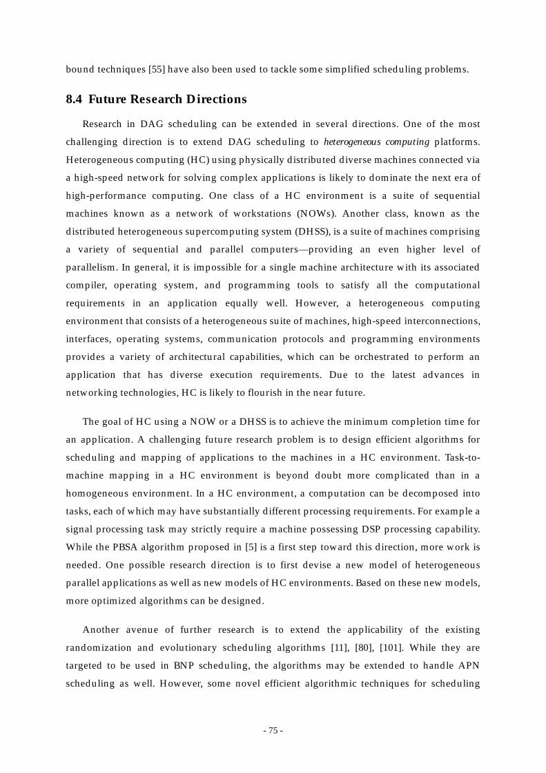
- 75 -
bound techniques [55] have also been used to tackle some simplified scheduling problems.
8.4 Future Research Directions
Research in DAG scheduling can be extended in several directions. One of the most
challenging direction is to extend DAG scheduling to heterogeneous computing platforms.
Heterogeneous computing (HC) using physically distributed diverse machines connected via
a high-speed network for solving complex applications is likely to dominate the next era of
high-performance computing. One class of a HC environment is a suite of sequential
machines known as a network of workstations (NOWs). Another class, known as the
distributed heterogeneous supercomputing system (DHSS), is a suite of machines comprising
a variety of sequential and parallel computers—providing an even higher level of
parallelism. In general, it is impossible for a single machine architecture with its associated
compiler, operating system, and programming tools to satisfy all the computational
requirements in an application equally well. However, a heterogeneous computing
environment that consists of a heterogeneous suite of machines, high-speed interconnections,
interfaces, operating systems, communication protocols and programming environments
provides a variety of architectural capabilities, which can be orchestrated to perform an
application that has diverse execution requirements. Due to the latest advances in
networking technologies, HC is likely to flourish in the near future.
The goal of HC using a NOW or a DHSS is to achieve the minimum completion time for
an application. A challenging future research problem is to design efficient algorithms for
scheduling and mapping of applications to the machines in a HC environment. Task-to-
machine mapping in a HC environment is beyond doubt more complicated than in a
homogeneous environment. In a HC environment, a computation can be decomposed into
tasks, each of which may have substantially different processing requirements. For example a
signal processing task may strictly require a machine possessing DSP processing capability.
While the PBSA algorithm proposed in [5] is a first step toward this direction, more work is
needed. One possible research direction is to first devise a new model of heterogeneous
parallel applications as well as new models of HC environments. Based on these new models,
more optimized algorithms can be designed.
Another avenue of further research is to extend the applicability of the existing
randomization and evolutionary scheduling algorithms [11], [80], [101]. While they are
targeted to be used in BNP scheduling, the algorithms may be extended to handle APN
scheduling as well. However, some novel efficient algorithmic techniques for scheduling
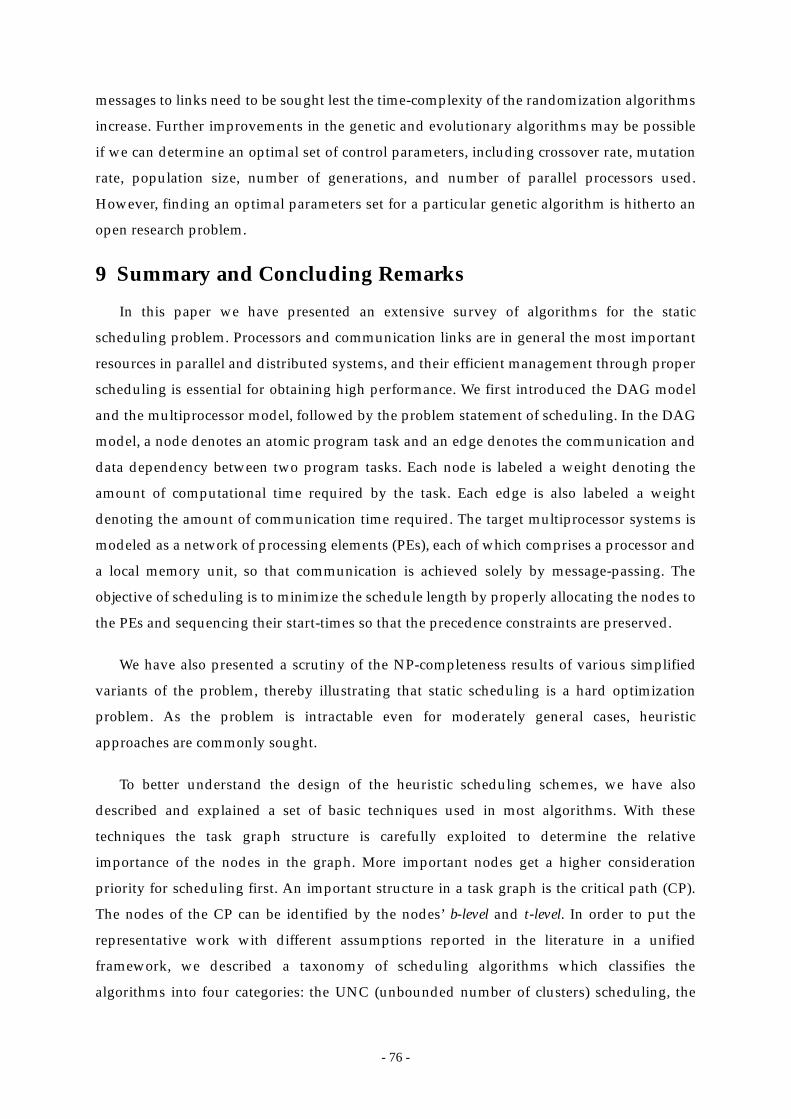
- 76 -
messages to links need to be sought lest the time-complexity of the randomization algorithms
increase. Further improvements in the genetic and evolutionary algorithms may be possible
if we can determine an optimal set of control parameters, including crossover rate, mutation
rate, population size, number of generations, and number of parallel processors used.
However, finding an optimal parameters set for a particular genetic algorithm is hitherto an
open research problem.
9 Summary and Concluding Remarks
In this paper we have presented an extensive survey of algorithms for the static
scheduling problem. Processors and communication links are in general the most important
resources in parallel and distributed systems, and their efficient management through proper
scheduling is essential for obtaining high performance. We first introduced the DAG model
and the multiprocessor model, followed by the problem statement of scheduling. In the DAG
model, a node denotes an atomic program task and an edge denotes the communication and
data dependency between two program tasks. Each node is labeled a weight denoting the
amount of computational time required by the task. Each edge is also labeled a weight
denoting the amount of communication time required. The target multiprocessor systems is
modeled as a network of processing elements (PEs), each of which comprises a processor and
a local memory unit, so that communication is achieved solely by message-passing. The
objective of scheduling is to minimize the schedule length by properly allocating the nodes to
the PEs and sequencing their start-times so that the precedence constraints are preserved.
We have also presented a scrutiny of the NP-completeness results of various simplified
variants of the problem, thereby illustrating that static scheduling is a hard optimization
problem. As the problem is intractable even for moderately general cases, heuristic
approaches are commonly sought.
To better understand the design of the heuristic scheduling schemes, we have also
described and explained a set of basic techniques used in most algorithms. With these
techniques the task graph structure is carefully exploited to determine the relative
importance of the nodes in the graph. More important nodes get a higher consideration
priority for scheduling first. An important structure in a task graph is the critical path (CP).
The nodes of the CP can be identified by the nodes’ b-level and t-level. In order to put the
representative work with different assumptions reported in the literature in a unified
framework, we described a taxonomy of scheduling algorithms which classifies the
algorithms into four categories: the UNC (unbounded number of clusters) scheduling, the
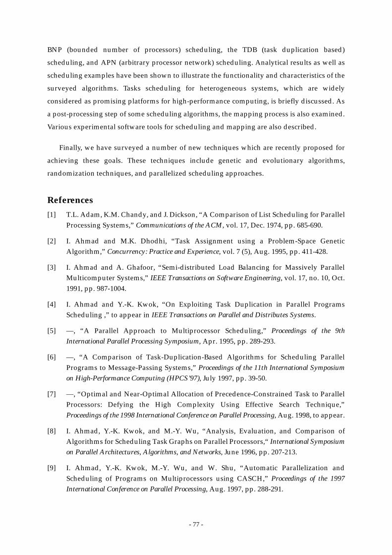
- 77 -
BNP (bounded number of processors) scheduling, the TDB (task duplication based)
scheduling, and APN (arbitrary processor network) scheduling. Analytical results as well as
scheduling examples have been shown to illustrate the functionality and characteristics of the
surveyed algorithms. Tasks scheduling for heterogeneous systems, which are widely
considered as promising platforms for high-performance computing, is briefly discussed. As
a post-processing step of some scheduling algorithms, the mapping process is also examined.
Various experimental software tools for scheduling and mapping are also described.
Finally, we have surveyed a number of new techniques which are recently proposed for
achieving these goals. These techniques include genetic and evolutionary algorithms,
randomization techniques, and parallelized scheduling approaches.
References
[1] T.L. Adam, K.M. Chandy, and J. Dickson, “A Comparison of List Scheduling for ParallelProcessing Systems,” Communications of the ACM, vol. 17, Dec. 1974, pp. 685-690.
[2] I. Ahmad and M.K. Dhodhi, “Task Assignment using a Problem-Space GeneticAlgorithm,” Concurrency: Practice and Experience, vol. 7 (5), Aug. 1995, pp. 411-428.
[3] I. Ahmad and A. Ghafoor, “Semi-distributed Load Balancing for Massively ParallelMulticomputer Systems,” IEEE Transactions on Software Engineering, vol. 17, no. 10, Oct.1991, pp. 987-1004.
[4] I. Ahmad and Y.-K. Kwok, “On Exploiting Task Duplication in Parallel ProgramsScheduling ,” to appear in IEEE Transactions on Parallel and Distributes Systems.
[5] —, “A Parallel Approach to Multiprocessor Scheduling,” Proceedings of the 9thInternational Parallel Processing Symposium, Apr. 1995, pp. 289-293.
[6] —, “A Comparison of Task-Duplication-Based Algorithms for Scheduling ParallelPrograms to Message-Passing Systems,” Proceedings of the 11th International Symposiumon High-Performance Computing (HPCS’97), July 1997, pp. 39-50.
[7] —, “Optimal and Near-Optimal Allocation of Precedence-Constrained Task to ParallelProcessors: Defying the High Complexity Using Effective Search Technique,”Proceedings of the 1998 International Conference on Parallel Processing, Aug. 1998, to appear.
[8] I. Ahmad, Y.-K. Kwok, and M.-Y. Wu, “Analysis, Evaluation, and Comparison ofAlgorithms for Scheduling Task Graphs on Parallel Processors,“ International Symposiumon Parallel Architectures, Algorithms, and Networks, June 1996, pp. 207-213.
[9] I. Ahmad, Y.-K. Kwok, M.-Y. Wu, and W. Shu, “Automatic Parallelization andScheduling of Programs on Multiprocessors using CASCH,” Proceedings of the 1997International Conference on Parallel Processing, Aug. 1997, pp. 288-291.
- 78 -
[10] H.H. Ali and H. El-Rewini, “The Time Complexity of Scheduling Interval Orders withCommunication is Polynomial,” Parallel Processing Letters, vol. 3, no. 1, 1993, pp. 53-58.
[11] S. Ali, S.M. Sait, and M.S.T. Benten, “GSA: Scheduling and Allocation using GeneticAlgorithm,” Proceedings of EURO-DAC’94, 1994, pp. 84-89.
[12] M.A. Al-Mouhamed, “Lower Bound on the Number of Processors and Time forScheduling Precedence Graphs with Communication Costs,” IEEE Transactions onSoftware Engineering, vol. 16, no. 12, Dec. 1990, pp. 1390-1401.
[13] V.A.F. Almeida, I.M. Vasconcelos, J.N.C. Arabe, and D.A. Menasce, “Using RandomTask Graphs to Investigate the Potential Benefits of Heterogeneity in Parallel Systems,”Proceedings of Supercomputing‘92, 1992, pp. 683-691.
[14] G. Amdahl, “Validity of the Single Processor Approach to Achieving Large ScaleComputing Capability,” Proceedings of AFIPS Spring Joint Computer Conference 30,Reston, VA., 1967, pp. 483-485.
[15] F.D. Anger, J.J. Hwang, and Y.C. Chow, “Scheduling with Sufficiently Loosely CoupledProcessors,” Journal of Parallel and Distributed Computing, 9, 1990, pp. 87-92.
[16] A.F. Bashir, V. Susarla, and K. Vairavan, “A Statistical Study of the Performance of aTask Scheduling Algorithm,” IEEE Transactions on Computers, vol. C-32, no. 8, Aug. 1983,pp. 774-777.
[17] J. Baxter and J.H. Patel, “The LAST Algorithm: A Heuristic-Based Static Task AllocationAlgorithm,” Proceedings of International Conference on Parallel Processing, vol. II, Aug.1989, pp. 217-222.
[18] M. Beck, K.K. Pingali, and A. Nicolau, “Static scheduling for dynamic dataflowmachines,” Journal of Parallel and Distributed Computing, 10, 1990, pp. 279-288.
[19] M.S.T. Benten and S.M. Sait, “Genetic Scheduling of Task Graphs,” International Journalof Electronics, vol. 77, no. 4, Oct. 1994, pp. 401-415.
[20] J. Blazewicz, M. Drabowski, and J. Weglarz, “Scheduling Multiprocessor Tasks toMinimize Schedule length,” IEEE Transactions on Computers, vol. C-35, no. 5, May 1986,p. 389-393.
[21] J. Blazewicz, J. Weglarz, and M. Drabowski, “Scheduling Independent 2-processorTasks to Minimize Schedule Length,” Information Processing Letters, 18, 1984, pp. 267-273.
[22] S.H. Bokhari, “Dual Processor Scheduling with Dynamic Reassignment,” IEEETransactions on Software Engineering, vol. SE-5, no. 4, July 1979, pp. 341-349.
[23] —, “On the Mapping Problem”, IEEE Transactions on Computers, vol. C-30, 1981, pp. 207-214.
[24] G. Bozoki and J.P. Richard, “A Branch-and-Bound Algorithm for Continuous-processTask Shop Scheduling Problem,” AIIE Transactions, 2, 1970, pp. 246-252.
- 79 -
[25] J. Bruno, E.G. Coffman, and R. Sethi, “Scheduling Independent Tasks to Reduce MeanFinishing Time,”, Communications of the ACM, vol. 17, no. 7, July 1974, pp. 382-387.
[26] T.L. Casavant and J.G. Kuhl, “A Taxonomy of Scheduling in General-PurposeDistributed Computing Systems,” IEEE Transactions on Software Engineering, vol. 14, no.2, Feb. 1988, pp. 141-154.
[27] R. Chandrasekharam, S. Subhramanian, and S. Chaudhury, “Genetic Algorithm forNode Partitioning Problem and Applications in VLSI Design,” IEE Proceedings, vol. 140,no. 5, Sep. 1993, pp. 255-260.
[28] G. Chen and T.H. Lai, “Scheduling Independent Jobs on Hypercubes,” Proceedings ofConference on Theoretical Aspects of Computer Science, 1988, pp. 273-280.
[29] —, “Preemptive Scheduling of Independent Jobs on a Hypercube,” InformationProcessing Letters, 28, 1988, pp. 201-206.
[30] H. Chen, B. Shirazi, and J. Marquis, “Performance Evaluation of A Novel SchedulingMethod: Linear Clustering with Task Duplication,” Proceedings of InternationalConference on Parallel and Distributed Systems, Dec. 1993, pp. 270-275.
[31] R. Cheng, M. Gen, and Y. Tsujimura, “A Tutorial Survey of Job-Shop SchedulingProblems using Genetic Algorithms. I. Representation,” Computers and IndustrialEngineering, vol. 30, no. 4, Sep. 1986, pp. 983-997.
[32] P. Chretienne, “A Polynomial Algorithm to Optimally Schedule Tasks on a VirtualDistributed System under Tree-like Precedence Constraints”, European Journal ofOperational Research, 43, 1989, pp. 225-230.
[33] W.W. Chu, M.-T. Lan, and J. Hellerstein, “Estimation of Intermodule Communication(IMC) and Its Applications in Distributed Processing Systems,” IEEE Transactions onComputers, vol. C-33, no. 8, Aug. 1984, pp. 691-699.
[34] Y.C. Chung and S. Ranka, “Application and Performance Analysis of a Compile-TimeOptimization Approach for List Scheduling Algorithms on Distributed-MemoryMultiprocessors,” Proceedings of Supercomputing’92, Nov. 1992, pp. 512-521.
[35] E.G. Coffman, Computer and Job-Shop Scheduling Theory, Wiley, New York, 1976.
[36] E.G. Coffman and R.L. Graham, “Optimal Scheduling for Two-Processor Systems,” ActaInformatica, vol. 1, 1972, pp. 200-213.
[37] J.Y. Colin and P. Chretienne, “C.P.M. Scheduling with Small Computation Delays andTask Duplication,” Operations Research, 1991, pp. 680-684.
[38] M. Cosnard and M. Loi, “Automatic Task Graph Generation Techniques,” ParallelProcessing Letters, vol. 5, no. 4, Dec. 1995, pp. 527-538.
[39] Cray Research Inc., UNICOS Performance Utilities Reference Manual, SR2040 Edition 6.0,1991.
- 80 -
[40] W.J. Dally, “Virtual-channel Flow Control,” IEEE Transactions on Parallel and DistributedSystems, vol. 3, Mar. 1992, pp. 194-205.
[41] S. Darbha and D.P. Agrawal, “A Fast and Scalable Scheduling Algorithm for DistributedMemory Systems,” Proceedings of Symposium of Parallel and Distributed Processing, Oct.1995, pp. 60-63.
[42] L.D. Davis (Ed.), The Handbook of Genetic Algorithms, New York, Van Nostrand Reinhold,1991.
[43] I. De Falco, R. Del Balio, E. Tarantino, “An Analysis of Parallel Heuristics for TaskAllocation in Multicomputers,” Computing: Archiv fur Informatik und Numerik, vol. 59, no.3, 1997, pp. 259-75.
[44] M.K. Dhodhi, Imtiaz Ahmad, and Ishfaq Ahmad, “A Multiprocessor SchedulingScheme using Problem-Space Genetic Algorithms,” Proceedings of IEEE InternationalConference on Evolutionary Computation, 1995, vol. 1, pp. 214-219.
[45] Digital Equipment Corp., PARASPHERE User’s Guide.
[46] V.A. Dixit-Radiya and D.K. Panda, “Task Assignment on Distributed-Memory Systemswith Adaptive Wormhole Routing,” Proceedings of International Symposium of Parallel andDistributed Systems, Dec. 1993, pp. 674-681.
[47] J. Du and J.Y.T. Leung, “Complexity of Scheduling Parallel Task Systems,” SIAM Journalon Discrete Mathematics, vol. 2, no. 4, Nov. 1989, pp. 473-487.
[48] R. Duncan, “A Survey of Parallel Computer Architectures,” IEEE Computer, Feb. 1990,pp. 5-16.
[49] H. El-Rewini and T.G. Lewis, “Scheduling Parallel Programs onto Arbitrary TargetMachines,” Journal of Parallel and Distributed Computing, vol. 9, no. 2, June 1990, pp. 138-153.
[50] H. El-Rewini, H.H. Ali, and T.G. Lewis, “Task Scheduling in Multiprocessing Systems,”IEEE Computer, Dec. 1995, pp. 27-37.
[51] H. El-Rewini, T.G. Lewis, and H.H. Ali, Task Scheduling in Parallel and DistributedSystems, Prentice Hall, Englewood Cliffs, 1994.
[52] H. El-Rewini and H.H. Ali, “Static Scheduling of Conditional Branches in ParallelPrograms,” Journal of Parallel and Distributed Computing, 24, 1995, pp. 41-54.
[53] M.D. Ercegovac, “Heterogeneity in Supercomputer Architectures,” Parallel Computing,7, 1988, pp. 367-372.
[54] E.B. Fernadez and B. Bussell, “Bounds on the Number of Processors and Time forMultiprocessor Optimal Schedules,” IEEE Transactions on Computers, vol. C-22, no. 8,Aug. 1973, pp. 745-751.
[55] A. Ferreira and P. Pardalos (Eds.), Solving Combinatorial Optimization Problems in Parallel:
- 81 -
Methods and Techniques, Lecture Notes in Computer Science 1054, Springer, 1996.
[56] J.L.R. Filho, P.C. Treleaven, and C. Alippi, “Genetic-Algorithm ProgrammingEnvironments,” IEEE Computer, June 1994, pp. 28-43.
[57] P.C. Fishburn, Interval Orders and Interval Graphs, John Wiley & Sons, New York, 1985.
[58] S. Forrest and M. Mitchell, “What Makes a Problem Hard for a Genetic Algorithm? SomeAnomalous Results and Their Explanation,” Machine Learning, 13, 1993, pp. 285-319.
[59] R.F. Freund and H.J. Siegel, “Heterogeneous Processing,” IEEE Computer, June 1993, pp.13-17.
[60] D.K. Friesen, “Tighter Bounds for LPT Scheduling on Uniform Processors,” SIAMJournal on Computing, vol. 16, no. 3, June 1987, pp. 554-560.
[61] M. Fujii, T. Kasami, and K. Ninomiya, “Optimal Sequencing of Two EquivalentProcessors,” SIAM Journal Applied Mathematics, 17, no. 1, 1969.
[62] H. Gabow, “An Almost Linear Algorithm for Two-Processor Scheduling,” Journal of theACM, 29, 3, 1982, pp. 766-780.
[63] M.R. Garey and D.S. Johnson, Computers and Intractability: A Guide to the Theory of NP-Completeness, W.H. Freeman and Company, 1979.
[64] M.R. Garey, D. Johnson, R. Tarjan, and M. Yannakakis, “Scheduling Opposing Forests,”SIAM Journal on Algebraic Discrete Methods, 4, 1, 1983, pp. 72-92.
[65] D.D. Gajski and J. Peir, “Essential Issues in Multiprocessors,” IEEE Computer, 18, 6, June1985.
[66] A. Gerasoulis and T. Yang, “A Comparison of Clustering Heuristics for SchedulingDAG’s on Multiprocessors,” Journal of Parallel and Distributed Computing, vol. 16, no. 4,Dec. 1992, pp. 276-291.
[67] —, “On the Granularity and Clustering of Directed Acyclic Task Graphs,” IEEETransactions on Parallel and Distributed Systems, vol. 4, no. 6, June 1993, pp. 686-701.
[68] D.E. Goldberg, Genetic Algorithms in Search, Optimization and Machine Learning, Addison-Wesley, Reading, Mass., 1989.
[69] M.J. Gonzalez, Jr., “Deterministic Processor Scheduling,” ACM Computing Surveys, vol.9, no. 3, Sep. 1977, pp. 173-204.
[70] T. Gonzales and S. Sahni, “Preemptive scheduling of uniform processor systems,”Journal of the ACM, 25, 1978, pp. 92-101.
[71] R.L. Graham, “Bounds for Certain Multiprocessing Anomalies,” Bell System TechnicalJournal, 45, 1966, pp. 1563-1581.
[72] R.L. Graham, E.L. Lawler, J.K. Lenstra, and A.H.G. Rinnoy Kan, “Optimization andApproximation in Deterministic Sequencing and Scheduling: A Survey,” Annals of
- 82 -
Discrete Mathematics, no. 5, 1979, pp. 287-326.
[73] S. Ha and E.A. Lee, “Compile-Time Scheduling and Assignment of Data-Flow ProgramGraphs with Data-Dependent Iteration,” IEEE Transactions on Computers, vol. 40, no. 11,Nov. 1991, pp. 1225-1238.
[74] M. Hanan and J. Kurtzberg, “A Review of the Placement and Quadratic AssignmentProblems,” SIAM Review, vol. 14, Apr. 1972, pp. 324-342.
[75] J.P. Hayes and T. Mudge, “Hypercube Supercomputers,” Proceedings of the IEEE, vol. 77,no. 12, Dec. 1989.
[76] D.S. Hochbaum and D.B. Shmoys, “Using Dual Approximation Algorithms forScheduling Problems: Theoretical and Practical Results,” Journal of the ACM, 34 (1), Jan.1987, pp. 144-162.
[77] —, “A Polynomial Approximation Scheme for Scheduling on Uniform Processors:Using the Dual Approximation Approach,” SIAM Journal on Computing, vol. 17, no. 3,June 1988, pp. 539-551.
[78] J.H. Holland, Adaptation in Natural and Artificial Systems, University of Michigan Press,Ann Arbor, Mich., 1975.
[79] E.C. Horvath, S. Lam, and R. Sethi, “A Level Algorithm for Preemptive Scheduling,”Journal of the ACM, 24, 1977, pp. 32-43.
[80] E.S.H. Hou, N. Ansari, and H. Ren, “A Genetic Algorithm for MultiprocessorScheduling,” IEEE Transactions on Parallel and Distributed Systems, vol. 5, no. 2, Feb. 1994,pp. 113-120.
[81] T.C. Hu, “Parallel Sequencing and Assembly Line Problems,” Operations Research, vol.19, no. 6, Nov. 1961, pp. 841-848.
[82] Kai Hwang, Advanced Computer Architecture: Parallelism, Scalability, Programmability,McGraw Hill, 1993.
[83] J.J. Hwang, Y.C. Chow, F.D. Anger, and C.Y. Lee, “Scheduling Precedence Graphs inSystems with Interprocessor Communication Times,” SIAM Journal on Computing, vol.18, no. 2, Apr. 1989, pp. 244-257.
[84] Intel Supercomputer Systems Division, iPSC/2 and iPSC/860 Interactive Parallel DebuggerManual, Apr. 1991.
[85] K.K. Jain and V. Rajaraman, “Lower and Upper Bounds on Time for MultiprocessorOptimal Schedules,” IEEE Transactions on Parallel and Distributed Systems, vol. 5, no. 8,Aug. 1994, pp. 879-886.
[86] —, “Improved Lower Bounds on Time and Processors for Scheduling PrecedenceGraphs on Multicomputer Systems,” Journal of Parallel and Distributed Computing, 28,1995, pp. 101-108.
- 83 -
[87] H. Jiang, L.N. Bhuyan, and D. Ghosal, “Approximate Analysis of Multiprocessing TaskGraphs,” Proceedings of International Conference on Parallel Processing, 1990, vol. III, pp.228-235.
[88] D.S. Johnson, C.H. Papadimitriou and M. Yannakakis, “How Easy Is Local Search?,”Journal of Computer and System Sciences, vol. 37, no. 1, Aug. 1988, pp. 79-100.
[89] R.M. Karp, “Introduction to Randomized Algorithms,” Discrete Applied Mathematics, vol.34, no. 1-3, Nov. 1991, pp. 165-201.
[90] H. Kasahara and S. Narita, “Practical Multiprocessor Scheduling Algorithms forEfficient Parallel Processing,” IEEE Transactions on Computers, vol. C-33, Nov. 1984, pp.1023-1029.
[91] M. Kaufman, “An Almost-Optimal Algorithm for the Assembly Line SchedulingProblem,” IEEE Transactions on Computers, vol. C-23, no. 11, 1974, pp. 1169-1174.
[92] A.A. Khan, C.L. McCreary, and M.S. Jones, “A Comparison of MultiprocessorScheduling Heuristics,” Proceedings of International Conference on Parallel Processing, vol.II, Aug. 1994, pp. 243-250.
[93] W.H. Kohler and K. Steiglitz, “Characterization and theoretical comparison of branch-and-bound algorithms for permutation problems,” Journal of the ACM, vol. 21, Jan. 1974,pp. 140-156.
[94] W.H. Kohler, “A Preliminary Evaluation of the Critical Path Method for SchedulingTasks on Multiprocessor Systems,” IEEE Transactions on Computers, Dec. 1975, pp. 1235-1238.
[95] S.J. Kim and J.C. Browne, “A General Approach to Mapping of Parallel Computationupon Multiprocessor Architectures,” Proceedings of International Conference on ParallelProcessing, vol. II, Aug. 1988, pp. 1-8.
[96] D. Kim and B.G. Yi, “A Two-Pass Scheduling Algorithm for Parallel Programs,” ParallelComputing, 20, 1994, pp. 869-885.
[97] S. Kon’ya and T. Satoh, “Task Scheduling on a Hypercube with Link Contentions,”Proceedings of International Parallel Processing Symposium, Apr. 1993, pp. 363-368.
[98] B. Kruatrachue and T.G. Lewis, “Duplication Scheduling Heuristics (DSH): A NewPrecedence Task Scheduler for Parallel Processor Systems,” Technical Report, OregonState University, Corvallis, OR 97331, 1987.
[99] —, “Grain Size Determination for Parallel Processing,” IEEE Software, Jan. 1988, pp. 23-32.
[100] V. Kumar, A. Grama, A. Gupta, and G. Karypis, Introduction to Parallel Computing: Designand Analysis of Algorithms, The Benjamin/Cummings, 1994.
[101] Y.-K. Kwok, High-Performance Algorithms for Compile-Time Scheduling of Parallel
- 84 -
Processors, PhD. Thesis, HKUST, Hong Kong, 1997.
[102] Y.-K. Kwok and I. Ahmad, “Bubble Scheduling: A Quasi Dynamic Algorithm for StaticAllocation of Tasks to Parallel Architectures,” Proceedings of the 7th Symposium on Paralleland Distributed Processing, Oct. 1995, pp. 36-43.
[103] —, “Dynamic Critical-Path Scheduling: An Effective Technique for Allocating TaskGraphs onto Multiprocessors,” IEEE Transactions on Parallel and Distributed Systems, vol.7, no. 5, May 1996, pp. 506-521.
[104] —, “Efficient Scheduling of Arbitrary Task Graphs to Multiprocessors using A ParallelGenetic Algorithm,” Journal of Parallel and Distributed Computing, vol. 47, no. 1, Nov.1997, pp. 58-77.
[105] —, “A Parallel Algorithm for Compile-Time Scheduling of Parallel Programs onMultiprocessors,” Proceedings of the 1997 International Conference on Parallel Architecturesand Compilation Techniques (PACT’97), Nov. 1997, pp. 90-101.
[106] —, “Benchmarking the Task Graph Scheduling Algorithms,” Proceedings of the FirstMerged IPPS/SPDP’98 (the 12th International Parallel Processing Symposium & the 9theSymposium on Parallel and Distributed Processing), Mar. 1998, pp. 531-537.
[107] Y.-K. Kwok, I. Ahmad, and J. Gu, “FAST: A Low-Complexity Algorithm for EfficientScheduling of DAGs on Parallel Processors,” Proceedings of 25th International Conferenceon Parallel Processing, Aug. 1996, vol. II, pp. 150-157.
[108] B. Lee, A.R. Hurson, and T.Y. Feng, “A Vertically Layered Allocation Scheme for DataFlow Systems,” Journal of Parallel and Distributed Computing, vol. 11, 1991, pp. 175-187.
[109] S.Y. Lee and J.K. Aggarwal, “A Mapping Strategy for Parallel Processing,” IEEETransactions on Computers, vol. C-36, April 1987, pp. 433-442.
[110] J.Y.-T. Leung and G.H. Young, “Minimizing Schedule Length subject to Minimum FlowTime,” SIAM Journal on Computing, vol. 18, no. 2, April 1989, pp. 314-326.
[111] T.G. Lewis and H. El-Rewini, “Parallax: A Tool for Parallel Program Scheduling,” IEEEParallel and Distributed Technology, May 1993, vol. 1, no. 2, pp. 64-76.
[112] J.-C. Liou and M.A. Palis, “An Efficient Task Clustering Heuristic for Scheduling DAGson Multiprocessors,” Workshop on Resource Management, Symposium of Parallel andDistributed Processing, 1996.
[113] —, “A Comparison of General Approaches to Multiprocessor Scheduling,” Proceedingsof 11th International Parallel Processing Symposium, Apr. 1997, pp. 152-156.
[114] V.M. Lo, “Temporal Communication Graphs: Lamport’s Process-Time GraphsAugmented for the Purpose of Mapping and Scheduling,” Journal of Parallel andDistributed Computing, 16, 1992, pp. 378-384.
[115] V.M. Lo, S. Rajopadhye, S. Gupta, D. Keldsen, M.A. Mohamed, B. Nitzberg, J.A. Telle,and X. Zhong, “OREGAMI: Tools for Mapping Parallel Computations to Parallel
- 85 -
Architectures,” International Journal of Parallel Programming, vol. 20, no. 3, 1991, pp. 237-270.
[116] R.E. Lord, J.S. Kowalik, and S.P. Kumar, “Solving Linear Algebraic Equations on anMIMD Computer,” Journal of the ACM, 30(1), Jan. 1983, pp. 103-117.
[117] S. Manoharan and N.P. Topham, “An Assessment of Assignment Schemes forDependency Graphs,” Parallel Computing, 21, 1995, pp. 85-107.
[118] P. Markenscoff and Y.Y. Li, “Scheduling a Computational DAG on a Parallel Systemwith Communication Delays and Replication of Node Execution,” Proceedings ofInternational Parallel Processing Symposium, 1993, pp. 113-117.
[119] MasPar Computer, MPPE User’s Guide.
[120] C. McCreary and H. Gill, “Automatic Determination of Grain Size of Efficient ParallelProcessing,” Communications of ACM, vol. 32, no. 9, Sep. 1989, pp. 1073-1078.
[121] C. McCreary, A.A. Khan, J.J. Thompson, and M.E. McArdle, “A Comparison ofHeuristics for Scheduling DAG’s on Multiprocessors,” Proceedings of InternationalParallel Processing Symposium, 1994, pp. 446-451.
[122] N. Mehdiratta and K. Ghose, “A Bottom-Up Approach to Task Scheduling onDistributed Memory Multiprocessor,” Proceedings of International Conference on ParallelProcessing, vol. II, Aug. 1994, pp. 151-154.
[123] D.A. Menasce and V.A.F. Almeida, “Cost-performance Analysis of Heterogeneity inSupercomputer Architectures,” Proceedings of ACM-IEEE Supercomputing’90, New York,1990.
[124] D.A. Menasce and S.C. Porto, “Scheduling on Heterogeneous Message PassingArchitectures,” Journal of Computer and Software Engineering, 1, 3, 1993.
[125] D.A. Menasce, S.C. Porto, and S.K. Tripathi, “Static Heuristic Processor Assignment inHeterogeneous Message Passing Architectures,” International Journal of High SpeedComputing, 6, 1, Mar. 1994, pp. 115-137.
[126] —, “Processor Assignment in Heterogeneous Parallel Architectures,” Proceedings ofInternational Parallel Processing Symposium, 1992.
[127] D.A. Menasce, D. Saha, S.C. Porto, V.A.F. Almeida, and S.K. Tripathi, “Static andDynamic Processor Scheduling Disciplines in Heterogeneous Parallel Architectures,”Journal of Parallel and Distributed Computing, 28, 1995, pp. 1-18.
[128] R. Motwani and P. Raghavan, Randomized Algorithms, Cambridge University Press,1995.
[129] M.G. Norman and P. Thanisch, “Models of Machines and Computation for Mapping inMulticomputers,” ACM Computing Surveys, vol. 25, no. 3, Sep. 1993, pp. 263-302.
[130] M.A. Palis, J.-C. Liou, S. Rajasekaran, S. Shende and D.S.L. Wei, “Online Scheduling of
- 86 -
Dynamic Trees,” Parallel Processing Letters, vol. 5, no. 4, Dec. 1995, pp. 635-646.
[131] M.A. Palis, J.-C. Liou, and D.S.L. Wei, “Task Clustering and Scheduling for DistributedMemory Parallel Architectures,” IEEE Transactions on Parallel and Distributed Systems,vol. 7, no. 1, Jan. 1996, pp. 46-55.
[132] S.S. Pande, D.P. Agrawal, and J. Mauney, “A Threshold Scheduling Strategy for Sisal onDistributed Memory Machines,” Journal of Parallel and Distributed Computing, 21, 1994,pp. 223-236.
[133] C.H. Papadimitriou and K. Steiglitz, Combinatorial Optimization: Algorithms andComplexity, Prentice-Hall, Englewood Cliffs, NJ, 1982.
[134] C.H. Papadimitriou and J.D. Ullman, “A Communication-Time Tradeoff”, SIAM Journalon Computing, vol. 16, no. 4, Aug. 1987, pp. 639-646.
[135] C.H. Papadimitriou and M. Yannakakis, “Scheduling Interval-Ordered Tasks,” SIAMJournal on Computing, 8, 1979, pp. 405-409.
[136] —, “Towards an Architecture-Independent Analysis of Parallel Algorithms,” SIAMJournal on Computing, vol. 19, no. 2, Apr. 1990, pp. 322-328.
[137] D. Pease, A. Ghafoor, I. Ahmad, D.L. Andrews, K. Foudil-Bey, T.E. Karpinski, M.A.Mikki, and M. Zerrouki, “PAWS: A Performance Evaluation Tool for ParallelComputing Systems,” IEEE Computer, Jan. 1991, pp. 18-29.
[138] I. Pramanick and J.G. Kuhl, “An Inherently Parallel Method for Heuristic Problem-Solving: Part I—General Framework,” IEEE Transactions on Parallel and DistributedSystems, vol. 6, no. 10, Oct. 1995, pp. 1006-1015.
[139] M. Prastein, Precedence-Constrained Scheduling with Minimum Time and Communication,M.S. Thesis, University of Illinois at Urbana-Champaign, 1987.
[140] M.J. Quinn, Parallel Computing: Theory and Practice, McGraw-Hill, 1994.
[141] C.V. Ramamoorthy, K.M. Chandy and M.J. Gonzalez, “Optimal Scheduling Strategiesin a Multiprocessor System,” IEEE Transactions on Computers, vol. C-21, Feb. 1972, pp.137-146.
[142] V.J. Rayward-Smith, “The Complexity of Preemptive Scheduling Given InterprocessorCommunication Delays,” Information Processing Letters, 25, 1987, pp. 123-125.
[143] —, “UET Scheduling with Unit Interprocessor Communication Delays,” Discrete AppliedMathematics, 18, 1987, pp. 55-71.
[144] V. Sarkar, Partitioning and Scheduling Parallel Programs for Multiprocessors, MIT Press,Cambridge, MA, 1989.
[145] S. Selvakumar and C.S.R. Murthy, “Scheduling Precedence Constrained Task Graphswith Non-Negligible Intertask Communication onto Multiprocessors,” IEEETransactions on Parallel and Distributed Systems, vol. 5, no. 3, Mar. 1994, pp. 328-336.
- 87 -
[146] R. Sethi, “Scheduling Graphs on Two Processors,” SIAM Journal on Computing, vol. 5,no.1, Mar. 1976, pp. 73-82.
[147] M. Schwehm, T. Walter, B. Buchberger, and J. Volkert, “Mapping and Scheduling byGenetic Algorithms,” Proceedings of the 3rd Joint International Conference on Vector andParallel Processing (CONPAR’94), 1994, pp. 832-841.
[148] B. Shirazi, K. Kavi, A.R. Hurson, and P. Biswas, “PARSA: A Parallel ProgramScheduling and Assessment Environment,” Proceedings of International ConferenceParallel Processing, 1993, vol. II, pp. 68-72.
[149] B. Shirazi, M. Wang, and G. Pathak, “Analysis and Evaluation of Heuristic Methods forStatic Scheduling,” Journal of Parallel and Distributed Computing, no. 10, 1990, pp. 222-232.
[150] H.J. Siegel, Interconnection Networks for Large-Scale Parallel Processing: Theory and CaseStudies, 2nd Ed., McGraw-Hill, New York, 1990.
[151] H.J. Siegel, J.B. Armstrong and D.W. Watson, “Mapping Computer-Vision-RelatedTasks onto Reconfigurable Parallel Processing Systems,” IEEE Computer, Feb. 1992, pp.54-63.
[152] H.J. Siegel and C.B. Srunkel, “Inside Parallel Computers: Trends in InterconnectionNetworks,” IEEE Computational Science and Engineering, vol. 3, no. 3, Fall 1996, pp. 69-71.
[153] H.J. Siegel, H.G. Dietz, and J.K. Antonio, “Software Support for HeterogeneousComputing,” ACM Computing Surveys, vol. 28, no. 1, Mar. 1996, pp. 237-239.
[154] G.C. Sih and E.A. Lee, “A Compile-Time Scheduling Heuristic for Interconnection-Constrained Heterogeneous Processor Architectures,” IEEE Transactions on Parallel andDistributed Systems, vol. 4, no. 2, Feb. 1993, pp. 75-87.
[155] —, “Declustering: A New Multiprocessor Scheduling Technique,” IEEE Transactions onParallel and Distributed Systems, vol. 4, no. 6, June 1993, pp. 625-637.
[156] B.B. Simons and M.K. Warmuth, “A Fast Algorithm for Multiprocessor Scheduling ofunit-length jobs,” SIAM Journal on Computing, vol. 18, no. 4, Aug. 1989, pp. 690-710.
[157] M. Srinivas and L.M. Patnaik, “Genetic Algorithms: A Survey,” IEEE Computer, June1994, pp. 17-26.
[158] H.S. Stone, “Multiprocessor Scheduling with the Aid of Network Flow Algorithms,”IEEE Transactions on Software Engineering, vol. SE-3, no. 1, Jan. 1977, pp. 85-93.
[159] R.T. Sumichrast, “Scheduling Parallel Processors to Minimize Setup Time,” Computersand Operations Research, vol. 14, no. 4, 1987, pp. 305-313.
[160] R.H. Storer, S.D. Wu, and R. Vaccari, “New Search Spaces for Sequencing Problems withApplication to Job Shop Scheduling,” Management Science, vol. 38, no. 10, Oct. 1992, pp.1495-1509.
[161] Thinking Machines Corp., PRISM User’s Guide, Version 1.1, Dec. 1991.
- 88 -
[162] D. Towsley, “Allocating Programs Containing Branches and Loops Within a MultipleProcessor System,” IEEE Transactions on Software Engineering, vol. SE-12, no. 10, Oct.1986, pp. 1018-1024.
[163] T.A. Varvarigou, V.P. Roychowdhury, T. Kallath and E. Lawler, “Scheduling in and outForests in the Presence of Communication Delays,” IEEE Transactions on Parallel andDistributed Systems, vol. 7, no. 10, Oct. 1996, pp. 1065-1074.
[164] B. Veltman, B.J. Lageweg, and J.K. Lenstra, “Multiprocessor scheduling withcommunication delays,” Parallel Computing, 16, 1990, pp. 173-182.
[165] J. Ullman, “NP-Complete Scheduling Problems,” Journal of Computer and System Sciences,10, 1975, pp. 384-393.
[166] M.-F. Wang, “Message Routing Algorithms for Static Task Scheduling,” Proceedings ofthe 1990 Symposium on Applied Computing, 1990, pp. 276-281.
[167] Q. Wang and K.H. Cheng, “List Scheduling of Parallel Task,” Information ProcessingLetters, 37, 1991, pp. 291-297.
[168] L. Wang, H.J. Siegel, and V.P. Roychowdhury, “A Genetic-Algorithm-Based Approachfor Task Matching and Scheduling in Heterogeneous Computing Environments,”Proceedings of 5th Heterogeneous Computing Workshop, 1996, pp. 72-85.
[169] W.S. Wong and R.J.T. Morris, “A New Approach to Choosing Initial Points in LocalSearch,” Information Processing Letters, vol. 30, no. 2, Jan. 1989, pp. 67-72.
[170] M.-Y. Wu and D.D. Gajski, “Hypertool: A Programming Aid for Message-PassingSystems,” IEEE Transactions on Parallel and Distributed Systems, vol. 1, no. 3, July 1990, pp.330-343.
[171] T. Yang and A. Gerasoulis, “List Scheduling with and without Communication Delays,”Parallel Computing, 19, 1992, pp. 1321-1344.
[172] —, “PYRROS: Static Task Scheduling and Code Generation for Message PassingMultiprocessors,” Proceedings of 6th ACM International Conference on Supercomputing,1992, pp. 428-443.
[173] —, “DSC: Scheduling Parallel Tasks on an Unbounded Number of Processors,” IEEETransactions on Parallel and Distributed Systems, vol. 5, no. 9, Sep. 1994, pp. 951-967.
[174] C.-Q. Yang and B.P. Miller, “Critical Path Analysis for the Execution of Parallel andDistributed Programs,” Proceedings of International Conference on Distributed ComputingSystems, June 1988, pp. 366-373.
[175] J. Yang, L. Bic, and A. Nicolau, “A Mapping Strategy for MIMD Computers,”International Journal of High Speed Computing, vol. 5, no. 1, 1993, pp. 89-103.
[176] Y. Zhu and C.L. McCreary, “Optimal and Near Optimal Tree Scheduling for ParallelSystems,” Proceedings of Symposium on Parallel and Distributed Processing, 1992, pp. 112-119.