* Department of Economics, Bar-Ilan University, Ramat Gan 5290002, Israel igal.milchtaich@biu.ac.il http://faculty.biu.ac.il/~milchti

Static Stability in Symmetric and Population Games

Igal Milchtaich*

November 2016

Static stability in strategic games differs from dynamic stability in only considering the

players’ incentives to change their strategies. It does not rely on any assumptions about the

players’ reactions to these incentives and it is thus independent of the law of motion (e.g.,

whether players move simultaneously or sequentially). This paper presents a general notion

of static stability in symmetric 𝑁-player games and population games, of which

evolutionarily stable strategy (ESS) and continuously stable strategy (CSS) are essentially

special cases. Unlike them, the proposed stability concept does not depend on the existence

of special structures in the game such as multilinear payoff functions or unidimensional

strategy spaces. JEL Classification: C72.

Keywords: Static stability, evolutionarily stable strategy, continuously stable strategy, risk

dominance, potential games.

1 Introduction A strategic game is at equilibrium when the players do not have any incentives to act

differently than they do. In other words, at an equilibrium point, no player can increase his

payoff by unilaterally changing his strategy. Stability differs in referring to the effects – either

on the players’ incentives or on the actual strategy choices – of starting at another, typically

close-by, point. Notions of stability that only examine incentives may be broadly classified as

static, and those that look at the consequent changes of strategies may be referred to as

dynamic. (For a brief review of some additional notions of stability in strategic games, which

fit neither of these categories, see Appendix A.) Dynamic stability necessarily concerns a

specific law of motion, such as the replicator dynamics. It thus depends both on the game

itself, that is, on the payoff functions, and on the choice of dynamics. Static stability, by

contrast, depends only on intrinsic properties of the game, and is hence arguably the more

basic, fundamental concept. This is not an assessment of the relative importance of the two

kinds of stability but of the logical relation between them.

This paper introduces a notion of static stability in symmetric 𝑁-player games and

population games that is universal in that it does not depend on structures or properties

that only certain kinds of games have, such as multilinearity of the payoff function. Stability

may be local or global. The former refers to a designated topology on the strategy space,

which gives a meaning to a neighborhood of a strategy. In this paper, there are no

restrictions on the choice of topology, which may in particular be the trivial topology, where

the only neighborhood of any strategy is the entire strategy space. The latter choice

corresponds to global stability, and it is most natural in the case of finite strategy spaces.

2

The definition of (static) stability in this paper is based on a very simple idea, namely,

examination of the incentive to switch to a strategy 𝑥 from another strategy 𝑦 in all states in

which only these two strategies are used, that is, every player uses either 𝑥 or 𝑦. The effect

on a player’s payoff of moving from the group of 𝑦 users to that of 𝑥 users normally varies

with the relative sizes of the two groups. Strategy 𝑦 is said to be stable if the condition that

the change of payoff is on average negative holds for all strategies 𝑥 in some neighborhood

of 𝑦. This stability condition represents minimal divergence from the (Nash) equilibrium

concept. However, the latter does not imply stability and, in general, the reverse implication

also does not hold. The paper’s focus is on stable equilibrium strategies, which satisfy both

conditions. For a number of large, important classes of symmetric and population games, it

examines the specific meaning of stability (in the above sense) in the class. In some cases,

the latter turns out to be equivalent, or essentially so, to an established “native” notion of

stability. Evolutionary stability for symmetric 𝑛 × 𝑛 games and continuous stability for

games with unidimensional strategy spaces are examples of this. The definition outlined

above thus turns static stability from a generic notion to a concrete, well-defined one.

The reliance of static stability solely on incentives makes it particularly suitable for

comparative statics analysis, in particular, study of the welfare effects of altruism and spite.

Whether people in a group where everyone shares such sentiments are likely to fare better

or worse than where people are indifferent to the others’ payoffs turns out to depend on

the static stability or instability of the corresponding equilibrium strategies (Milchtaich

2012). If the strategies are stable, welfare tends to increase with increasing altruism or

decreasing spite, but if they are (definitely) unstable, the effect may go in the opposite

direction. Thus, Samuelson’s (1983) “correspondence principle”, which maintains that

conditions for stability coincide with those under which comparative statics analysis leads to

what are usually regarded as “normal” conclusions, holds. However, this is so only if

‘stability’ refers to the notion of static stability presented in this paper. The principle may

not hold for other kinds of stability. In particular, dynamic stability under the continuous-

time replicator dynamics (Hofbauer and Sigmund 1998) does not guarantee a positive

relation between altruism and welfare. Even in a symmetric 3 × 3 game, a continuously

increasing degree of altruism may actually lower the players’ (identical material) payoffs if

the equilibria involved are dynamically stable, which, as indicated, cannot happen if the

equilibrium strategies are statically stable.

2 Symmetric and population games A symmetric 𝑁-player game (𝑁 ≥ 1) is a real-valued (payoff1) function 𝑔: 𝑋𝑁 → ℝ that is

defined on the 𝑁-times Cartesian product of a (finite or infinite nonempty) set 𝑋, the

players’ common strategy space, and is invariant under permutations of its second through

𝑁th arguments. If one player uses strategy 𝑥 and the others use 𝑦, 𝑧, … , 𝑤, in any order, the

first player’s payoff is 𝑔(𝑥, 𝑦, 𝑧, … , 𝑤). A strategy 𝑦 is a (symmetric Nash) equilibrium

strategy in 𝑔, with the equilibrium payoff 𝑔(𝑦, 𝑦, … , 𝑦), if it is a best response to itself, that

is, for every other strategy 𝑥,

1 In this paper, the payoff function and the game itself are identified.

3

𝑔(𝑦, 𝑦, … , 𝑦) ≥ 𝑔(𝑥, 𝑦, … , 𝑦).

A population game, as defined in this paper, is formally a symmetric two-player game 𝑔

such that the strategy space 𝑋 is a convex set in a (Hausdorff real) linear topological space

(for example, the unit simplex in a Euclidean space) and 𝑔(𝑥, 𝑦) is continuous in 𝑦 for all

𝑥 ∈ 𝑋. However, the game is interpreted not as representing an interaction between two

specific players but as one involving an (effectively) infinite2 population of individuals who

are “playing the field”. This means that an individual’s payoff 𝑔(𝑥, 𝑦) depends only on his

own strategy 𝑥 and on the population strategy 𝑦. The latter may, for example, be the

population’s mean strategy with respect to some nonatomic measure, which attaches zero

weight to each individual. In this case, the meaning of the equilibrium condition,

𝑔(𝑦, 𝑦) = max𝑥∈𝑋

𝑔(𝑥, 𝑦),

is that, in a monomorphic population, where everyone plays 𝑦, single individuals cannot

increase their payoff by choosing any other strategy. Alternatively, a population game 𝑔 may

describe a dependence of an individual’s payoff on the distribution of strategies in the

population (Bomze and Pötscher 1989), with the latter expressed by the population strategy

𝑦. In this case, 𝑋 consists of mixed strategies, that is, probability measures on some

underlying space of allowable actions or (pure3) strategies, and 𝑔(𝑥, 𝑦) is linear in 𝑥 and

expresses the expected payoff for an individual whose choice of strategy is random with

distribution 𝑥. Provided the space 𝑋 is rich enough, the equilibrium condition (2) now means

that the population strategy 𝑦 is supported in the collection of all best response pure

strategies. In other words, the (possibly) polymorphic population is in an equilibrium state.

Example 1. Random matching in a symmetric multilinear game (Bomze and Weibull 1995;

Broom et al. 1997). The 𝑁 players in a symmetric 𝑁-player game 𝑔 are picked up

independently and randomly from an infinite population of potential players. The strategy

space 𝑋 is a convex set in a linear topological space, and 𝑔 is continuous and is linear in each

of its arguments. (This assumption may be relaxed by dropping the linearity requirement for

the first argument.) Because of the multilinearity of 𝑔, a player’s expected payoff only

depends on his own strategy 𝑥 and on the population’s mean strategy 𝑦. Specifically, the

expected payoff is given by

�̅�(𝑥, 𝑦) ≝ 𝑔(𝑥, 𝑦, … , 𝑦).

This defines a population game �̅�: 𝑋2 → ℝ. Clearly, a strategy 𝑦 is an equilibrium strategy

in �̅� if and only if it is an equilibrium strategy in the underlying 𝑁-player game 𝑔.

Another example of a population game is a nonatomic congestion game with a continuum of

identical users (Milchtaich 2012, Example 4).

2 An infinite population may represent the limiting case of an increasingly large population, with the possible effect of each player’s actions on each of the other players correspondingly decreasing. Alternatively, it may represent all possible characteristics of players, or potential players, when the number of actual players is finite. 3 “Pure” and “mixed” are relative terms. In particular, a pure strategy may itself be a probability vector.

(1)

(2)

(3)

4

3 Static stability By far the most well-known kind of static stability in symmetric two-player games and

population games is evolutionary stability (Maynard Smith 1982).

Definition 1. A strategy 𝑦 in a symmetric two-player game or population game 𝑔 is an

evolutionarily stable strategy (ESS) or a neutrally stable strategy (NSS) if, for every strategy

𝑥 ≠ 𝑦, for sufficiently small4 𝜖 > 0 the inequality

𝑔(𝑦, 𝜖𝑥 + (1 − 𝜖)𝑦) > 𝑔(𝑥, 𝜖𝑥 + (1 − 𝜖)𝑦)

or a similar weak inequality, respectively, holds. An ESS or NSS with uniform invasion

barrier satisfies the stronger condition obtained by interchanging the two logical quantifiers.

That is, for sufficiently small 𝜖 > 0 (which cannot vary with 𝑥), (4) or a similar weak

inequality, respectively, holds for all 𝑥 ≠ 𝑦.

Continuous stability (Eshel and Motro 1981; Eshel 1983) is another kind of static stability,

which is applicable to games with a unidimensional strategy space.

Definition 2. In a symmetric two-player game or population game 𝑔 with a strategy space

that is a (finite or infinite) interval in the real line ℝ, an equilibrium strategy 𝑦 is a

continuously stable strategy (CSS) if it has a neighborhood where, for every strategy 𝑥 ≠ 𝑦,

for sufficiently small 𝜖 > 0 the inequality

𝑔(𝑥 + 𝜖(𝑦 − 𝑥), 𝑥) > 𝑔(𝑥, 𝑥)

holds and a similar inequality with 𝜖 replaced by – 𝜖 does not hold.

In other words, a strategy 𝑦 that satisfies the “global” condition of being an equilibrium

strategy5 is a CSS if it also satisfies the “local” condition (known as m-stability or convergence

stability; Taylor 1989; Christiansen 1991) that every nearby strategy 𝑥 is not a best response

to itself, specifically, any small deviation from 𝑥 towards 𝑦, but not in the other direction,

increases the payoff.

Yet another static notion of stability in symmetric and (with 𝑁 = 2) population games is

local superiority (or strong uninvadability; Bomze 1991).

Definition 3. A strategy 𝑦 in a symmetric 𝑁-player game or population game 𝑔 is locally

superior if it has a neighborhood where, for every strategy 𝑥 ≠ 𝑦,

𝑔(𝑦, 𝑥, … , 𝑥) > 𝑔(𝑥, 𝑥, … , 𝑥).

Local superiority is applicable to any symmetric or population game in which the strategy

space is a topological space, so that the notion of neighborhood is well defined.6 It does not

rely on any other properties of the strategy space or of the payoff function – unlike ESS and

4 A condition holds for “sufficiently small” 𝜖 > 0 if there is some 𝛿 > 0 such that the condition holds for all 0 < 𝜖 < 𝛿. 5 The original definition of CSS differs slightly from the version given here in requiring a stronger global condition, which is a version of ESS. 6 A subset of 𝑋 is said to be a neighborhood of a strategy 𝑥 if its interior includes 𝑥 (Kelley 1955).

(4)

(5)

(6)

5

CSS, which would not be meaningful without a linear structure. It is well known (see

Section ‎6) that in the special case of symmetric 𝑛 × 𝑛 games local superiority is in fact

equivalent to the ESS condition. However, for games with a unidimensional strategy space

(Section ‎7) local superiority and CSS are not equivalent.

The next section presents a universal notion of static stability, that is, one which is applicable

to all symmetric and population games. It (essentially) gives ESS and CSS as special cases

when applied to specific, suitable classes of games.

4 A general framework Inequality (1) in the equilibrium condition and inequality (6) in the definition of local

superiority both concern a player’s lack of incentive to use a particular alternative 𝑥 to his

strategy 𝑦. In the equilibrium condition, all the other players are using 𝑦, and in local

superiority, they all use 𝑥. Stability, as defined below, differs from both concepts in

considering not only the incentives to be first or last to move to 𝑥 from 𝑦 but also all the

intermediate cases. In the simplest version, described by the followings definition (and

extended in Section ‎4.2), the same weight is attached to all cases. Put differently, stability

requires that, when the players move one-by-one to 𝑥 from 𝑦, the corresponding changes of

payoff are negative on average.

Definition 4. A strategy 𝑦 in a symmetric 𝑁-player game 𝑔: 𝑋𝑁 → ℝ is stable, weakly stable

or definitely unstable if it has a neighborhood where, for every strategy 𝑥 ≠ 𝑦, the inequality

1

𝑁∑(𝑔(𝑥, 𝑥, … , 𝑥⏟ ,

𝑗−1 times

𝑦,… , 𝑦⏟ 𝑁−𝑗 times

) − 𝑔(𝑦, 𝑥, … , 𝑥⏟ ,𝑗−1 times

𝑦,… , 𝑦⏟ 𝑁−𝑗 times

))

𝑁

𝑗=1

< 0,

a similar weak inequality or the reverse (strict) inequality, respectively, holds.

Stability, as defined here, is a local concept. It refers to neighborhood systems of strategies,

or equivalently to a topology on the strategy space 𝑋. The topology may be explicitly

specified or it may be understood from the context. The latter applies when it is natural to

view 𝑋 as a subspace of a Euclidean space or some other standard topological space, so that

its topology is the relative one. For example, if the strategy space is an interval in the real

line ℝ, so that strategies are simply (real) numbers, a set of strategies is a neighborhood of a

strategy 𝑦 if and only if, for some 휀 > 0, every 𝑥 ∈ 𝑋 with |𝑥 − 𝑦| < 휀 is in the set. In a game

with a finite number of strategies, it may seem natural to consider the discrete topology,

that is, to view strategies as isolated. However, as discussed in Section ‎5 below, a more

useful choice of topology in a finite game is the trivial, or indiscrete, topology. This choice

effectively puts topology out of the way, since it means that the only neighborhood of any

strategy is the entire strategy space. The trivial topology may be used also with an infinite 𝑋.

Stability, weak stability or definite instability of a stategy 𝑦 with respect to the trivial

topology automatically implies the same with respect to any other topology. Such a strategy

𝑦 will be referred to as globally stable, weakly stable or definitely unstable, respectively.

Note that there can be at most one globally stable strategy.

(7)

6

In some classes of games (see Sections ‎6, ‎8 and ‎9), stability of a strategy automatically

implies that it is an equilibrium strategy. In other games, the reverse implication holds. In

particular, an equilibrium strategy is automatically globally stable in every symmetric game

satisfying symmetric substitutability (see Milchtaich 2012, Section 6), which is the condition

that for all strategies 𝑥, 𝑦, 𝑧, … , 𝑤 with 𝑥 ≠ 𝑦

𝑔(𝑥, 𝑥, 𝑧, … , 𝑤) − 𝑔(𝑦, 𝑥, 𝑧, … , 𝑤) < 𝑔(𝑥, 𝑦, 𝑧, … , 𝑤) − 𝑔(𝑦, 𝑦, 𝑧, … , 𝑤).

The condition implies that the expression in parentheses in (7) strictly decreases as 𝑗

increases from 1 to 𝑁. If 𝑦 is an equilibrium strategy, then by (1) the expression is

nonpositive for 𝑗 = 1, which means that the whole sum is negative, which proves that 𝑦 is

globally stable.

In general, however, the equilibrium and stability conditions are incomparable: neither of

them implies the other. The incomparability is partially due to equilibrium being a global

condition: all alternative strategies, not only nearby ones, are considered. However, it holds

also with ‘equilibrium’ replaced by ‘local equilibrium’ (with the obvious meaning) or if the

strategy space has the trivial topology, which obviates the distinction between local and

global. A stable equilibrium strategy is a strategy that satisfies both conditions. It is not

difficult to see that in the special case of symmetric two-player games, where the

equilibrium condition can be written as (2) and inequality (7) can be rearranged to read

1

2(𝑔(𝑥, 𝑥) − 𝑔(𝑦, 𝑥) + 𝑔(𝑥, 𝑦) − 𝑔(𝑦, 𝑦)) < 0,

a strategy 𝑦 is a stable equilibrium strategy if and only if it has a neighborhood where, for

every 𝑥 ≠ 𝑦, the inequality

𝑝𝑔(𝑥, 𝑥) + (1 − 𝑝)𝑔(𝑥, 𝑦) < 𝑝𝑔(𝑦, 𝑥) + (1 − 𝑝)𝑔(𝑦, 𝑦)

holds for all 0 < 𝑝 ≤ 1/2. This condition means that the alternative strategy 𝑥 affords a

lower expected payoff than 𝑦 against an uncertain strategy that may be 𝑥 or 𝑦, with the

former no more likely than the latter.

Local superiority is similar to stability in being a local condition. Moreover, for equilibrium

strategies in symmetric two-player games, locally superiority implies stability, since (with

𝑁 = 2) inequality (8) can be obtained by averaging (1) and (6). The same implication holds

also for certain kinds of symmetric games with more than two players (see Section ‎9). The

reverse implication does not hold even for equilibrium strategies in symmetric two-player

games (see Section ‎7).

4.1 Stability in population games Stability in population games can be defined by a variant of Definition 4 that replaces the

number of players using strategy 𝑥 or 𝑦 with the size of the subpopulation to which the

strategy applies, 𝑝 or 1 − 𝑝 respectively. Correspondingly, the sum in (7) is replaced with an

integral.

Definition 5. A strategy 𝑦 in a population game 𝑔:𝑋2 → ℝ is stable, weakly stable or

definitely unstable if it has a neighborhood where, for every strategy 𝑥 ≠ 𝑦, the inequality

(8)

(9)

7

∫ (𝑔(𝑥, 𝑝𝑥 + (1 − 𝑝)𝑦) − 𝑔(𝑦, 𝑝𝑥 + (1 − 𝑝)𝑦)) ⅆ𝑝1

0

< 0,

a similar weak inequality or the reverse (strict) inequality, respectively, holds.

The difference between stability in the sense of Definition 5 and in the sense of (the two

versions of) ESS (Definition 1) boils down to a different meaning of proximity between

population strategies. The definition of ESS reflects the view that a population strategy is

close to 𝑦 if the latter applies to a large subpopulation, of size 1 − 𝜖, and another strategy 𝑥

applies to a small subpopulation, of size 𝜖. By contrast, in Definition 5, the subpopulation to

which 𝑥 applies need not be small, but 𝑥 itself is assumed close to 𝑦. The significance of this

difference between the definitions is examined in Sections ‎6 and ‎9.

If a population game �̅� is derived from a symmetric multilinear game 𝑔 as in Example 1,

then, depending on whether 𝑦 is viewed as a strategy in 𝑔 or �̅�, Definition 4 or 5 applies.

However, the point of view turns out to be immaterial.

Proposition 1. A strategy 𝑦 in a symmetric multilinear 𝑁-player game 𝑔 is stable, weakly

stable or definitely unstable if and only if it has the same property in the population game �̅�

defined by (3).

Proof. For 0 ≤ 𝑝 ≤ 1, and for strategies 𝑥, 𝑦 and

𝑥𝑝 = 𝑝𝑥 + (1 − 𝑝)𝑦,

the linearity of 𝑔 in each of its second through 𝑁th arguments and its invariance to

permutations of these arguments give

�̅�(𝑥, 𝑥𝑝) − �̅�(𝑦, 𝑥𝑝) = 𝑔(𝑥, 𝑥𝑝, … , 𝑥𝑝) − 𝑔(𝑦, 𝑥𝑝, … , 𝑥𝑝)

=∑𝐵𝑗−1,𝑁−1(𝑝)(𝑔(𝑥, 𝑥, … , 𝑥⏟ ,𝑗−1 times

𝑦,… , 𝑦⏟ 𝑁−𝑗 times

) − 𝑔(𝑦, 𝑥, … , 𝑥⏟ ,𝑗−1 times

𝑦,… , 𝑦⏟ 𝑁−𝑗 times

))

𝑁

𝑗=1

,

where

𝐵𝑗−1,𝑁−1(𝑝) = (𝑁−1

𝑗−1) 𝑝𝑗−1(1 − 𝑝)𝑁−𝑗 , 𝑗 = 1,2, … , 𝑁

are the Bernstein polynomials. These polynomials satisfy the equalities

∫ 𝐵𝑗−1,𝑁−1(𝑝) ⅆ𝑝 1

0

=1

𝑁, 𝑗 = 1,2, … , 𝑁.

It therefore follows from (11) by integration that the expression obtained by replacing 𝑔 on

the left-hand side of (10) by �̅� is equal to the expression on the left-hand side of (7). ∎

In the subsequent sections, Definitions 4 and 5 are applied, or restricted, to a number of

specific classes of symmetric and population games and the results are compared with

certain “native” notions of stability for these games. The rest of the present section is

concerned with an extension of the above framework, which facilitates the capturing of

some additional native notions of stability.

(10)

(11)

(12)

8

4.2 �̅�-stability Stability as defined above in a sense occupies the midpoint between equilibrium and local

superiority. It takes into consideration a player’s incentive to be the first or last to switch to

a particular alternative strategy, but attaches to these extreme cases the same weight it

attaches to each of the intermediate ones. This uniform distribution of weights may be

interpreted as expressing a particular belief of the player about the total number of players

who will be using the alternative strategy after he switches to it, with the rest using the

original strategy. Namely, the probabilities 𝑝1, 𝑝2, … , 𝑝𝑁 that the number in question is

1,2, … , 𝑁 are all equal,

𝑝𝑗 =1

𝑁, 𝑗 = 1,2, … , 𝑁.

Thus, unlike local superiority, in which the gain from switching from strategy 𝑦 to the

alternative strategy 𝑥 is computed under the belief that all the other players are using 𝑥, in

stability the expected gain is with respect to the probabilities (13), which give the expression

on the left-hand side of (7). A straightforward generalization of both concepts is to allow any

beliefs.

Definition 6. For a probability vector �̅� = (𝑝1, 𝑝2, … , 𝑝𝑁), a strategy 𝑦 in a symmetric 𝑁-

player game 𝑔: 𝑋𝑁 → ℝ �̅�-stable, weakly �̅�-stable or definitely �̅�-unstable if it has a

neighborhood where, for every strategy 𝑥 ≠ 𝑦, the inequality

∑𝑝𝑗(𝑔(𝑥, 𝑥, … , 𝑥⏟ ,𝑗−1 times

𝑦,… , 𝑦⏟ 𝑁−𝑗 times

) − 𝑔(𝑦, 𝑥, … , 𝑥⏟ ,𝑗−1 times

𝑦,… , 𝑦⏟ 𝑁−𝑗 times

))

𝑁

𝑗=1

< 0,

a similar weak inequality or the reverse (strict) inequality, respectively, holds.

If each of the other players switches to 𝑥 with probability 𝑝 and stays with 𝑦 with probability

1 − 𝑝, then, depending on whether the choices are, respectively, perfectly correlated (i.e.,

identical) or independent,

𝑝𝑗 = {

1 − 𝑝, 𝑗 = 10 , 1 < 𝑗 < 𝑁𝑝 , 𝑗 = 𝑁

or

𝑝𝑗 = (𝑁−1

𝑗−1) 𝑝𝑗−1(1 − 𝑝)𝑁−𝑗 = 𝐵𝑗−1,𝑁−1(𝑝), 𝑗 = 1,2, … , 𝑁.

A strategy 𝑦 is dependently- or independently-stable if it is �̅�-stable with �̅� = (𝑝1, 𝑝2, … , 𝑝𝑁)

given by (15) or (16), respectively, for all 0 < 𝑝 < 1.

The number of other players using strategy 𝑥 and the number using 𝑦 have a symmetric joint

distribution if the two numbers are equally distributed (hence, have an equal expectation of

(𝑁 − 1)/2), that is,

𝑝𝑗 = 𝑝𝑁−𝑗+1, 𝑗 = 1,2, … , 𝑁.

For �̅� = (𝑝1, 𝑝2, … , 𝑝𝑁) satisfying (17), the left-hand side of (14) is equal to the more

symmetrically-looking expression

(13)

(14)

(15)

(16)

(17)

9

𝐺�̅�(𝑥, 𝑦) ≝∑𝑝𝑗(𝑔(𝑥, … , 𝑥⏟ ,𝑗 times

𝑦, … , 𝑦) − 𝑔(𝑦,… , 𝑦⏟ ,𝑗 times

𝑥,… , 𝑥)).

𝑛

𝑗=1

Thus, for such �̅�, a strategy 𝑦 is �̅�-stable if and only if it has a neighborhood where it is the

unique best response to itself in the symmetric two-player zero-sum game 𝐺�̅�: 𝑋2 → ℝ. As a

special case, this characterization applies to stability, that is, to �̅� given by (13). A strategy 𝑦

is symmetrically-stable if it is �̅�-stable for all �̅� satisfying (17).

For single-player games (𝑁 = 1), stability and �̅�-stability of a strategy mean the same thing,

namely, strict local optimality: switching to any nearby alternative strategy reduces the

payoff. For 𝑁 = 2, stability does not generally imply �̅�-stability (or vice versa) but the

implication does partially hold (specifically, holds whenever 0 < 𝑝2 ≤ 1/2) in the special

case of an equilibrium strategy (see (9)). A full appreciation of the differences between

stability in the sense of Definition 4 and the varieties based on �̅�-stability requires looking at

multiplayer games. One class of such games is examined in Section ‎9.

5 Finite games and risk dominance In every symmetric or population game, every isolated strategy is trivially stable. Therefore,

if the strategy space 𝑋 has the discrete topology, that is, all singletons are open sets, then all

strategies are stable. The definition of stability is therefore of interest only for games with

non-discrete strategy spaces. This includes games with a finite number of strategies where

the topology on 𝑋 is the trivial one, so that stability and definite instability mean global

stability and definite instability (see Section ‎4). The simplest (interesting) such game is a

finite symmetric two-player game with only two strategies, strategy 1 and strategy 2, for

example, the game with payoff matrix

1 212

(3 41 5

)

(where the rows correspond to the player’s own strategy and the columns to the opponent’s

strategy). In this example, both strategies are equilibrium strategies. Strategy 1 is globally

stable and strategy 2 is globally definitely unstable, because (using the form (7) of (8))

1

2(5 − 4 + 1 − 3) < 0 <

1

2(3 − 1 + 4 − 5).

The two inequalities, which are clearly equivalent, have an additional meaning. Namely, they

express the fact that (1,1) is the risk dominant equilibrium (Harsanyi and Selten 1988). It is

not difficult to see that this coincidence of global stability and risk dominance holds in

general – it is not a special property of the payoffs in this example.

Proposition 2. In a finite symmetric two-player game with two strategies, an equilibrium

strategy 𝑦 is globally stable if and only if the equilibrium (𝑦, 𝑦) is risk dominant.

For a pure equilibrium strategy 𝑦, risk dominance of (𝑦, 𝑦) is equivalent also to global

stability of 𝑦 in the mixed extension 𝑔 of the finite game, that is, when mixed strategies are

allowed. This follows from the fact that global stability of 𝑦 in the finite game implies that

10

inequality (9) holds for all 0 < 𝑝 ≤ 1/2, where 𝑥 is the other pure strategy. Because of the

bilinearity of 𝑔, the same is then true with 𝑥 replaced by any convex combination of 𝑥 and 𝑦

other than 𝑦 itself, which proves that 𝑦 is globally stable in 𝑔. However, since in the mixed

extension of the finite game, which is a symmetric 2 × 2 game, the strategy space 𝑋 is

essentially the unit interval, the natural topology on 𝑋 is not the trivial topology but the

usual one. Stability with respect to the latter is a weaker condition than global stability. For

example, as shown in the next section, it holds for both pure strategies if (as in the above

example) the corresponding strategy profiles are strict equilibria.

6 Symmetric 𝒏 × 𝒏 games and evolutionary stability A symmetric 𝑛 × 𝑛 game is given by a (square) payoff matrix 𝐴 with these dimensions. The

strategy space 𝑋, whose elements are referred to as mixed strategies, is the unit simplex in

ℝ𝑛. The interpretation is that there are 𝑛 possible actions, and a strategy 𝑥 = (𝑥1, 𝑥2, … , 𝑥𝑛)

is a probability vector specifying the probability 𝑥𝑖 with which each action 𝑖 is used

(𝑖 = 1,2, … , 𝑛). The set of all actions 𝑖 with 𝑥𝑖 > 0 is the support of 𝑥. A strategy is pure or

completely mixed if its support contains only a single action 𝑖 (in which case the strategy

itself may also be denoted by 𝑖) or all 𝑛 actions, respectively. The game (i.e., the payoff

function) 𝑔:𝑋2 → ℝ is defined by

𝑔(𝑥, 𝑦) = 𝑥T𝐴𝑦

(where superscript T denotes transpose and strategies are viewed as column vectors). Thus,

𝑔 is bilinear, and 𝐴 = (𝑔(𝑖, 𝑗))𝑖,𝑗=1

𝑛.

A symmetric 𝑛 × 𝑛 game may be viewed either as a symmetric two-player game or as a

population game. In the former case, Definition 4 applies, and in the latter, Definition 5

applies. However, by Proposition 1, the two definitions of stability in fact coincide, and the

same is true for weak stability and for definite instability. Moreover, as the next two results

show, stability is also equivalent to evolutionary stability and to local superiority (see

Section ‎3). It also follows from these results that every (even weakly) stable strategy in a

symmetric 𝑛 × 𝑛 game is an equilibrium strategy, and every strict equilibrium strategy is

stable.

The following proposition is rather well known (Bomze and Pötscher 1989; van Damme

1991, Theorem 9.2.8; Weibull 1995, Propositions 2.6 and 2.7; Bomze and Weibull 1995).

Proposition 3. For a strategy 𝑦 in a symmetric 𝑛 × 𝑛 game 𝑔, the following conditions are

equivalent:7

(i) Strategy 𝑦 is an ESS.

(ii) Strategy 𝑦 is an ESS with uniform invasion barrier.

(iii) For every strategy 𝑥 ≠ 𝑦 in some neighborhood of 𝑦,

𝑔(𝑦, 𝑥) > 𝑔(𝑥, 𝑥).

7 Note that condition (iii) means that 𝑦 is locally superior and that the first part of (iv) means that it is an equilibrium strategy.

(18)

11

(iv) For every 𝑥 ≠ 𝑦, the (weak) inequality 𝑔(𝑦, 𝑦) ≥ 𝑔(𝑥, 𝑦) holds, and if it holds as

equality, then (18) also holds.

An NSS is characterized by similar equivalent conditions, in which the strict inequality (18) is

replaced by a weak one.

A completely mixed equilibrium strategy 𝑦 in a symmetric 𝑛 × 𝑛 game 𝑔 is said to be

definitely evolutionarily unstable (Weissing 1991) if the reverse of inequality (18) holds for all

𝑥 ≠ 𝑦.

Theorem 1. A strategy 𝑦 in a symmetric 𝑛 × 𝑛 game 𝑔 is stable or weakly stable if and only if

it is an ESS or NSS, respectively. A completely mixed equilibrium strategy is definitely

unstable if and only if it is definitely evolutionarily unstable.

Proof. The two inequalities in (iii) and (iv) of Proposition 3 together imply (8), and the same is

true with the strict inequalities (8) and (18) both replaced by their weak versions. This

proves that a sufficient condition for stability or weak stability of a strategy 𝑦 is that it is an

ESS or NSS, respectively. For a completely mixed equilibrium strategy 𝑦, the inequality in (iv)

automatically holds as equality for all 𝑥, and therefore a similar argument proves that a

sufficient condition for definite instability of 𝑦 is that it is definitely evolutionarily unstable.

In remains to prove necessity. For a stable strategy 𝑦, inequality (8) holds for all nearby

strategies 𝑥 ≠ 𝑦. Therefore, 𝑦 has the property that, for every strategy 𝑥 ≠ 𝑦, for sufficiently

small 휀 > 0

𝑔(휀𝑥 + (1 − 휀)𝑦, 휀𝑥 + (1 − 휀)𝑦) − 𝑔(𝑦, 휀𝑥 + (1 − 휀)𝑦)

+ 𝑔(휀𝑥 + (1 − 휀)𝑦, 𝑦) − 𝑔(𝑦, 𝑦) < 0.

It follows from the bilinearity of 𝑔 that (19) is equivalent to

(2 − 휀)(𝑔(𝑦, 𝑦) − 𝑔(𝑥, 𝑦)) + 휀(𝑔(𝑦, 𝑥) − 𝑔(𝑥, 𝑥)) > 0.

Therefore, the above property of 𝑦 is equivalent to (iv) in Proposition 3, which proves

that 𝑦 is an ESS. Similar arguments show that a weakly stable strategy is an NSS and that a

definitely unstable completely mixed equilibrium strategy is definitely evolutionarily

unstable. In the first case, the proof needs to be modified only by replacing the strict

inequalities in (18), (19) and (20) by weak inequalities, and in the second case (in which the

first term in (20) vanishes for all 𝑥), they need to be replaced by the reverse inequalities. ∎

7 Games with a unidimensional strategy space and continuous

stability In a symmetric two-player game or population game where the strategy space is an interval

in the real line ℝ, stability or instability of an equilibrium strategy, in the sense of either

Definition 4 or 5, has a simple, familiar meaning. As shown below, if the payoff function is

twice continuously differentiable, and with the possible exception of certain borderline

cases, the equilibrium strategy is stable or definitely unstable if, at the (symmetric)

equilibrium point, the graph of the best-response function, or reaction curve, intersects the

(19)

(20)

12

forty-five degree line from above or below, respectively. This geometric characterization of

stability and its differential counterpart are also shared by continuous stability (Section ‎3),

which shows that these two notions of static stability are essentially equivalent.

Theorem 2. Let 𝑔 be a symmetric two-player game or population game with a strategy space

𝑋 that is a (finite or infinite) interval in the real line ℝ, and 𝑦 an interior equilibrium strategy

(that is, one lying in the interior of 𝑋) such that 𝑔 has continuous second-order partial

derivatives8 in a neighborhood of the equilibrium point (𝑦, 𝑦). If

𝑔11(𝑦, 𝑦) + 𝑔12(𝑦, 𝑦) < 0,

then 𝑦 is stable and a CSS. If the reverse inequality holds, then 𝑦 is definitely unstable and

not a CSS.

Proof. Using Taylor’s theorem, it is not difficult to show that, for 𝑥 tending to 𝑦, the left-hand

sides of both (8) and (10) can be expressed as

𝑔1(𝑦, 𝑦)(𝑥 − 𝑦) +1

2(𝑔11(𝑦, 𝑦) + 𝑔12(𝑦, 𝑦))(𝑥 − 𝑦)

2 + 𝑜((𝑥 − 𝑦)2).

Since 𝑦 is an interior equilibrium strategy, the first term in (22) is zero. Therefore, a sufficient

condition for (22) to be negative or positive for all 𝑥 ≠ 𝑦 in some neighborhood of 𝑦 (hence,

for 𝑦 to be stable or definitely unstable, respectively) is that 𝑔11(𝑦, 𝑦) + 𝑔12(𝑦, 𝑦) has that

sign.

Next, consider the CSS condition in Definition 2. It may be possible to determine whether

this condition holds by looking at the sign of

ⅆ

ⅆ𝜖|𝜖=0

(𝑔(𝑥, 𝑥) − 𝑔(𝑥 + 𝜖(𝑦 − 𝑥), 𝑥)) = 𝑔1(𝑥, 𝑥)(𝑥 − 𝑦).

For 𝑥 tending to 𝑦, (23) is given by an expression that is similar to (22) except that it lacks the

factor 1/2. Therefore, if (21) or the reverse inequality holds, then (23) is negative or positive,

respectively, for all 𝑥 ≠ 𝑦 in some neighborhood of 𝑦. In the first or second case, (5) holds or

does not hold, respectively, for 𝜖 > 0 sufficiently close to 0 and the converse is true for

𝜖 < 0. Therefore, in the first case, 𝑦 is a CSS, and in the second case, it is not a CSS. ∎

The connection between inequality (21) and the slope of the reaction curve can be

established as follows (Eshel 1983). If 𝑦 is an interior equilibrium strategy, then it follows

from the equilibrium condition (2) that 𝑔1(𝑦, 𝑦) = 0 and 𝑔11(𝑦, 𝑦) ≤ 0. If the last inequality

is in fact strict, then by the implicit function theorem there is a continuously differentiable

function 𝑓 from some neighborhood of 𝑦 to the strategy space, with 𝑓(𝑦) = 𝑦, such that

𝑔1(𝑓(𝑥), 𝑥) = 0 and 𝑔11(𝑓(𝑥), 𝑥) < 0 for all strategies 𝑥 in the neighborhood. Thus,

strategy 𝑓(𝑥) is a local best response to 𝑥. By the chain rule, at the point 𝑦

𝑓′(𝑦) = −𝑔12(𝑦, 𝑦)

𝑔11(𝑦, 𝑦).

8 Partial derivatives are denoted by subscripts. For example, 𝑔12 is the mixed second-order partial derivative of 𝑔.

(21)

(22)

(23)

13

Therefore, (21) holds (so that 𝑦 is stable) or the reverse inequality holds (𝑦 definitely

unstable) if and only if the slope of the function 𝑓 at 𝑦 is less or greater than 1, respectively.9

In the first case, the reaction curve (see Figure 1), which is the graph of 𝑓, intersects the

forty-five degree line from above (which means that the (local) fixed point index is +1; see

Dold 1980). In the second case, the intersection is from below (and the fixed point index is

−1).

In a population or symmetric two-player game with a unidimensional strategy space, an

equilibrium strategy 𝑦 that is locally superior is said to be a neighborhood invader strategy

(Apaloo 1997). As shown (see Section ‎4), such a strategy is necessarily stable. However,

unlike for symmetric 𝑛 × 𝑛 games (Section ‎6), the converse is false. This can be seen most

easily by considering the differential condition for local superiority of an equilibrium strategy

𝑦, which differs from (21) in that the second term 𝑔12(𝑦, 𝑦) is multiplied by 2 (Oechssler and

Riedel 2002). Since, by the equilibrium condition, the first term 𝑔11(𝑦, 𝑦) is necessarily

nonpositive, this makes the condition more demanding than (21).

8 Potential games A symmetric 𝑁-player game 𝑔: 𝑋𝑁 → ℝ is called an (exact) potential game if it has an (exact)

potential, which is a symmetric function (that is, a function that is invariant under

permutations of its 𝑁 arguments) 𝐹: 𝑋𝑁 → ℝ such that, whenever a single player changes

his strategy, the change in the player’s payoff is equal to the change in 𝐹. Thus, for any

𝑁 + 1 (not necessarily distinct) strategies 𝑥, 𝑥′, 𝑦, 𝑧, … , 𝑤,

𝐹(𝑥, 𝑦, 𝑧, … , 𝑤) − 𝐹(𝑥′, 𝑦, 𝑧, … , 𝑤) = 𝑔(𝑥, 𝑦, 𝑧, … , 𝑤) − 𝑔(𝑥′, 𝑦, 𝑧, … , 𝑤).

It follows immediately from the definition that the potential is unique up to an additive

constant. It also follows that a necessary condition for the existence of a potential is that the

total change of payoff of any two players who change their strategies one after the other does

not depend on the order of their moves: for any 𝑁 + 2 strategies 𝑥, 𝑥′, 𝑦, 𝑦′, 𝑧, … , 𝑤,

𝑔(𝑥, 𝑦, 𝑧, … , 𝑤) − 𝑔(𝑥′, 𝑦, 𝑧, … , 𝑤) + 𝑔(𝑦, 𝑥′, 𝑧, … , 𝑤) − 𝑔(𝑦′, 𝑥′, 𝑧, … , 𝑤)

= 𝑔(𝑦, 𝑥, 𝑧, … , 𝑤) − 𝑔(𝑦′, 𝑥, 𝑧, … , 𝑤) + 𝑔(𝑥, 𝑦′, 𝑧, … , 𝑤) − 𝑔(𝑥′, 𝑦′, 𝑧, … , 𝑤). 9 This geometric condition for static stability is weaker than the corresponding one for dynamic stability, which requires the absolute value of slope to be less than 1 (Fudenberg and Tirole 1995).

(24)

Unstable Stable

Strategy

Best response

Figure 1. An equilibrium strategy is stable (and a CSS) or definitely unstable (and not a CSS) if, at the equilibrium point, the reaction curve (thick line) intersects the forty-five degree line (thin) from above or below, respectively.

14

It is not difficult to show that this condition is also sufficient (see Monderer and Shapley

1996, Theorem 2.8, which however refers to general, not necessarily symmetric, games, for

which the potential function is also not symmetric). Moreover, if 𝑔 is the mixed extension of

a finite game (which means that it is a symmetric 𝑛 × 𝑛 game; see Section ‎6 for definition

and notation), then 𝑔 is a potential game if and only if the above condition holds for (any

𝑁 + 2) pure strategies (Monderer and Shapley 1996, Lemma 2.10). In this case, the

potential, like the game 𝑔 itself, is multilinear.

Example 2. Symmetric 2 × 2 games. Every symmetric 2 × 2 game 𝑔, with pure strategies 1

and 2, is a potential game, since it is easy to see that it satisfies the above condition for pure

strategies. It is moreover not difficult to check that the following bilinear function is a

potential for 𝑔:

𝐹(𝑥, 𝑦) = (𝑔(1,1) − 𝑔(2,1))𝑥1𝑦1 + (𝑔(2,2) − 𝑔(1,2))𝑥2𝑦2.

The potential 𝐹 of a symmetric potential game 𝑔 may itself be viewed as a symmetric 𝑁-

player game, indeed, a doubly symmetric one.10 It follows immediately from (24) that 𝐹 and

𝑔 have exactly the same equilibrium strategies, stable and weakly stable strategies, and

definitely unstable strategies. Stability and instability in this case have a strikingly simple

characterization, which follows immediately from the observation that the sum in (7) is

equal the difference 𝐹(𝑥, 𝑥, … , 𝑥) − 𝐹(𝑦, 𝑦, … , 𝑦) divided by 𝑁.

Theorem 3. In a symmetric 𝑁-player game with a potential 𝐹, a strategy 𝑦 is stable, weakly

stable or definitely unstable if and only if it is a strict local maximum point, a local maximum

point or a strict local minimum point, respectively, of the function 𝑥 ↦ 𝐹(𝑥, 𝑥, … 𝑥).11

The following simple result illustrates the theorem. It also makes use of Theorem 1 and

Example 2.

Corollary 1. In a symmetric 2 × 2 game 𝑔 with pure strategies 1 and 2, a (mixed) strategy is

an ESS or an NSS if and only if it is a strict local maximum point or a local maximum point,

respectively, of the quadratic function 𝛷:𝑋 → ℝ defined by

𝛷(𝑥) =1

2(𝑔(1,1) − 𝑔(2,1))𝑥1

2 +1

2(𝑔(2,2) − 𝑔(1,2))𝑥2

2.

8.1 Potential in population games For population games, which represent interactions involving many players whose individual

actions have negligible effects on the other players, the definition of potential may be

naturally adapted by replacing the difference on the left-hand side of (24) with a derivative.

Definition 7. For a population game 𝑔: 𝑋2 → ℝ, a continuous function 𝛷:𝑋 → ℝ is a

potential if for all 𝑥, 𝑦 ∈ 𝑋 and 0 < 𝑝 < 1 the derivative on the left-hand side of the

following equality exists and the equality holds:

10 A symmetric game is doubly symmetric if it has a symmetric payoff function, in other words, if the players’ payoffs are always equal. 11 Of course, if (𝑦, 𝑦, … , 𝑦) is a global maximum point of 𝐹 itself, then 𝑦 is in addition an equilibrium strategy.

(25)

(26)

15

ⅆ

ⅆ𝑝𝛷(𝑝𝑥 + (1 − 𝑝)𝑦) = 𝑔(𝑥, 𝑝𝑥 + (1 − 𝑝)𝑦) − 𝑔(𝑦, 𝑝𝑥 + (1 − 𝑝)𝑦).

Example 3. Symmetric 2 × 2 games, viewed as population games. It is easy to check that, for

every such game 𝑔, with pure strategies 1 and 2, the function 𝛷 defined by (26) is a

potential. Note that, unlike the function 𝐹 defined in (25), 𝛷 is a function of one variable

only.

Example 3 and Corollary 1 hint at the following general result.12 As for symmetric games,

stability and instability (here, in the sense of Definition 5) of a strategy 𝑦 in a population

game with a potential 𝛷 is related to 𝑦 being a local extremum point of the potential.

Theorem 4. In a population game 𝑔 with a potential 𝛷, a strategy 𝑦 is stable, weakly stable

or definitely unstable if and only if it is a strict local maximum point, local maximum point or

strict local minimum point of 𝛷, respectively. In the first two cases, 𝑦 is in addition an

equilibrium strategy. If the potential 𝛷 is strictly concave, an equilibrium strategy is also a

strict global maximum point of 𝛷, and necessarily the game’s unique stable strategy.

Proof. By (27), the left-hand side of (10) can be written as

∫ⅆ

ⅆ𝑝𝛷(𝑝𝑥 + (1 − 𝑝)𝑦) ⅆ𝑝

1

0

.

This integral equals 𝛷(𝑥) − 𝛷(𝑦), which proves the first part of the theorem. It also follows

from (27), in the limit 𝑝 → 0, that for all 𝑥 and 𝑦

ⅆ

ⅆ𝑝|𝑝=0+

𝛷(𝑝𝑥 + (1 − 𝑝)𝑦) = 𝑔(𝑥, 𝑦) − 𝑔(𝑦, 𝑦).

If 𝑦 is a local maximum point of 𝛷, then the left-hand side of (28) is nonpositive, which

proves that 𝑦 is an equilibrium strategy.

To prove the last part of the theorem, consider an equilibrium strategy 𝑦. For any strategy

𝑥 ≠ 𝑦, the right-, and therefore also the left-, hand side of (28) is nonpositive. If 𝛷 is strictly

concave, this implies that the left-hand side of (27) is negative for all 0 < 𝑝 < 1, which

proves that 𝑦 is a strict global maximum point of 𝛷. ∎

Since by definition a potential is a continuous function, an immediate corollary of Theorem 4

is the following result, which concerns the existence of strategies that are (at least) weakly

stable. The result sheds light on the difference in this respect between symmetric 2 × 2

games and, for example, 3 × 3 games. The former, which as indicated are potential games,

always have at least one NSS, whereas for the latter, it is well known that this is not so (a

counterexample is a variant of the rock–scissors–paper game where a draw yields a small

positive payoff for both players; see Maynard Smith 1982, p. 20).

12 Conversely, Example 3 and Theorem 4 below together provide an alternative proof for Corollary 1.

(27)

(28)

16

Corollary 2. If a population game 𝑔 with a potential 𝛷 has a compact strategy space, then it

has at least one weakly stable strategy. If in addition the number of such strategies is finite,

they are all stable.

The term potential is borrowed from physics, where it refers to a scalar field whose gradient

gives the force field. Force is analogous to incentive here. The analogy can be taken one step

further by presenting the payoff function 𝑔 as the differential of the potential 𝛷. This

requires 𝛷 to be defined not only on the strategy space 𝑋 (which by definition is a convex

set in a linear topological space) but on its cone �̂�, which is the collection of all space

elements that can be written as a strategy 𝑥 multiplied by a positive number 𝑡. For example,

if strategies are probability measures, 𝛷 needs to be defined for all positive, non-zero finite

measures. The differential of the potential can then be defined as its directional derivative,

that is, as the function ⅆ𝛷: �̂�2 → ℝ given by13

ⅆ𝛷(�̂�, �̂�) =ⅆ

ⅆ𝑡|𝑡=0+

𝛷(𝑡�̂� + �̂�).

The differential exists if the (right) derivative in (29) exists for all �̂�, �̂� ∈ �̂�.

Proposition 4. Let 𝑔: 𝑋2 → ℝ be a population game and 𝛷: �̂� → ℝ a continuous function (on

the cone of the strategy space). A sufficient condition for the restriction of 𝛷 to 𝑋 to be a

potential for 𝑔 is that the differential ⅆ𝛷: �̂�2 → ℝ exists, is continuous in the second

argument and satisfies

ⅆ𝛷(𝑥, 𝑦) = 𝑔(𝑥, 𝑦), 𝑥, 𝑦 ∈ 𝑋.

If this condition holds, then 𝑔 is necessarily linear in the first argument 𝑥.

Proof (an outline). Using elementary arguments, the following can be established.

Fact. A continuous real-valued function defined on an open real interval is continuously

differentiable if and only if it has a continuous right derivative.

Suppose that ⅆ𝛷 satisfies the specified condition. Replacing �̂� in (29) with 𝑝�̂� + �̂� gives

ⅆ𝛷(�̂�, 𝑝�̂� + �̂�) =ⅆ

ⅆ𝑡|𝑡=𝑝+

𝛷(𝑡�̂� + �̂�), �̂�, �̂� ∈ �̂�, 𝑝 ≥ 0.

By the above Fact and the continuity properties of 𝛷 and ⅆ𝛷, for 0 < 𝑝 < 1 the right

derivative in (31) is actually a two-sided derivative and it depends continuously on �̂�.

Therefore, by (30), the right-hand side of (27) is equal to the expression

ⅆ

ⅆ𝑡|𝑡=𝑝

𝛷(𝑡𝑥 + (1 − 𝑝)𝑦) −ⅆ

ⅆ𝑡|𝑡=1−𝑝

𝛷(𝑝𝑥 + 𝑡𝑦),

which by the chain rule is equal to the derivative on the left-hand side of (27). Hence, that

equality holds. Another corollary of (31) is the identity

13 Note that, in the directional derivative ⅆ𝛷, the direction is specified by the first argument.

(29)

(30)

(31)

17

∫ⅆ𝛷(�̂�, 𝑝�̂� + �̂�) ⅆ𝑝

𝑡

0

= 𝛷(𝑡�̂� + �̂�) − 𝛷(�̂�), �̂�, �̂� ∈ �̂�, 𝑡 > 0,

which, used twice, gives

∫(ⅆ𝛷(�̂�, 𝑝�̂� + 𝜆𝑡�̂� + �̂�) + ⅆ𝛷(�̂�, 𝑝�̂� + �̂�)) ⅆ𝑝

𝜆𝑡

0

= 𝛷(𝜆𝑡�̂� + 𝜆𝑡�̂� + �̂�) − 𝛷(𝜆𝑡�̂� + �̂�)

+𝛷(𝜆𝑡�̂� + �̂�) − 𝛷(�̂�) = 𝛷(𝜆𝑡�̂� + 𝜆𝑡�̂� + �̂�) − 𝛷(�̂�), �̂�, �̂�, �̂� ∈ �̂�, 𝜆, 𝑡 > 0.

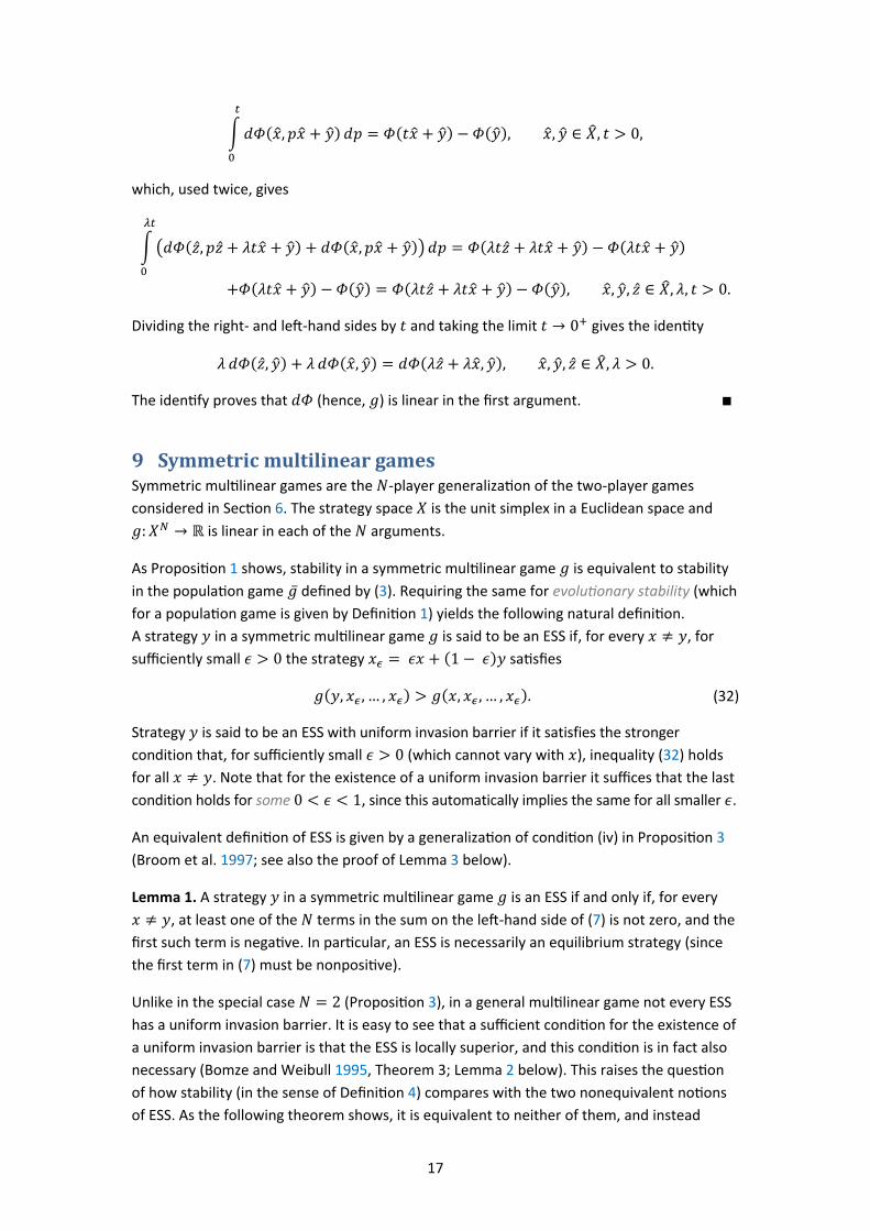
Dividing the right- and left-hand sides by 𝑡 and taking the limit 𝑡 → 0+ gives the identity

𝜆 ⅆ𝛷(�̂�, �̂�) + 𝜆 ⅆ𝛷(�̂�, �̂�) = ⅆ𝛷(𝜆�̂� + 𝜆�̂�, �̂�), �̂�, �̂�, �̂� ∈ �̂�, 𝜆 > 0.

The identify proves that ⅆ𝛷 (hence, 𝑔) is linear in the first argument. ∎

9 Symmetric multilinear games Symmetric multilinear games are the 𝑁-player generalization of the two-player games

considered in Section ‎6. The strategy space 𝑋 is the unit simplex in a Euclidean space and

𝑔: 𝑋𝑁 → ℝ is linear in each of the 𝑁 arguments.

As Proposition 1 shows, stability in a symmetric multilinear game 𝑔 is equivalent to stability

in the population game �̅� defined by (3). Requiring the same for evolutionary stability (which

for a population game is given by Definition 1) yields the following natural definition.

A strategy 𝑦 in a symmetric multilinear game 𝑔 is said to be an ESS if, for every 𝑥 ≠ 𝑦, for

sufficiently small 𝜖 > 0 the strategy 𝑥𝜖 = 𝜖𝑥 + (1 − 𝜖)𝑦 satisfies

𝑔(𝑦, 𝑥𝜖 , … , 𝑥𝜖) > 𝑔(𝑥, 𝑥𝜖 , … , 𝑥𝜖).

Strategy 𝑦 is said to be an ESS with uniform invasion barrier if it satisfies the stronger

condition that, for sufficiently small 𝜖 > 0 (which cannot vary with 𝑥), inequality (32) holds

for all 𝑥 ≠ 𝑦. Note that for the existence of a uniform invasion barrier it suffices that the last

condition holds for some 0 < 𝜖 < 1, since this automatically implies the same for all smaller 𝜖.

An equivalent definition of ESS is given by a generalization of condition (iv) in Proposition 3

(Broom et al. 1997; see also the proof of Lemma 3 below).

Lemma 1. A strategy 𝑦 in a symmetric multilinear game 𝑔 is an ESS if and only if, for every

𝑥 ≠ 𝑦, at least one of the 𝑁 terms in the sum on the left-hand side of (7) is not zero, and the

first such term is negative. In particular, an ESS is necessarily an equilibrium strategy (since

the first term in (7) must be nonpositive).

Unlike in the special case 𝑁 = 2 (Proposition 3), in a general multilinear game not every ESS

has a uniform invasion barrier. It is easy to see that a sufficient condition for the existence of

a uniform invasion barrier is that the ESS is locally superior, and this condition is in fact also

necessary (Bomze and Weibull 1995, Theorem 3; Lemma 2 below). This raises the question

of how stability (in the sense of Definition 4) compares with the two nonequivalent notions

of ESS. As the following theorem shows, it is equivalent to neither of them, and instead

(32)

18

occupies an intermediate position: weaker than one and stronger than the other. The two

ESS conditions are also comparable with the stronger stability conditions derived from

�̅�-stability (see Section ‎4.2). In fact, two of the latter turn out to be equivalent to ESS with

uniform invasion barrier.

Theorem 5. In a symmetric multilinear game, with 𝑁 ≥ 2 players, the following implications

and equivalences among the possible properties of a strategy hold:

ESS ⇐ stable ⇐ ESS with uniform invasion barrier ⇔ locally superior ⇔ dependently-

stable ⇔ independently-stable ⇐ symmetrically-stable.

Each of the three implications is actually an equivalence in the special case of two-player

games, but not in general.

The proof of Theorem 5 uses the following two lemmas, which hold for every game 𝑔 as in

the theorem. The first lemma uses the following terminology. A strategy 𝑦 in 𝑔 is

conditionally locally superior if it has a neighborhood where inequality (6) holds for every

strategy 𝑥 ≠ 𝑦 that satisfies the reverse of inequality (1).

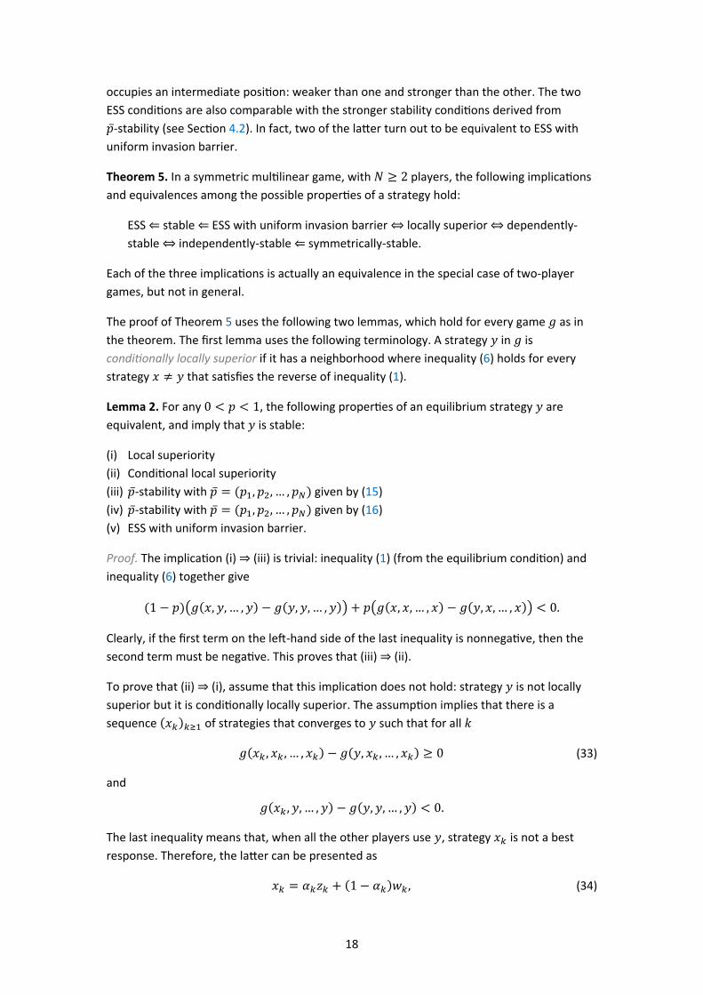
Lemma 2. For any 0 < 𝑝 < 1, the following properties of an equilibrium strategy 𝑦 are

equivalent, and imply that 𝑦 is stable:

(i) Local superiority

(ii) Conditional local superiority

(iii) �̅�-stability with �̅� = (𝑝1, 𝑝2, … , 𝑝𝑁) given by (15)

(iv) �̅�-stability with �̅� = (𝑝1, 𝑝2, … , 𝑝𝑁) given by (16)

(v) ESS with uniform invasion barrier.

Proof. The implication (i) ⇒ (iii) is trivial: inequality (1) (from the equilibrium condition) and

inequality (6) together give

(1 − 𝑝)(𝑔(𝑥, 𝑦, … , 𝑦) − 𝑔(𝑦, 𝑦, … , 𝑦)) + 𝑝(𝑔(𝑥, 𝑥, … , 𝑥) − 𝑔(𝑦, 𝑥, … , 𝑥)) < 0.

Clearly, if the first term on the left-hand side of the last inequality is nonnegative, then the

second term must be negative. This proves that (iii) ⇒ (ii).

To prove that (ii) ⇒ (i), assume that this implication does not hold: strategy 𝑦 is not locally

superior but it is conditionally locally superior. The assumption implies that there is a

sequence (𝑥𝑘)𝑘≥1 of strategies that converges to 𝑦 such that for all 𝑘

𝑔(𝑥𝑘 , 𝑥𝑘 , … , 𝑥𝑘) − 𝑔(𝑦, 𝑥𝑘 , … , 𝑥𝑘) ≥ 0

and

𝑔(𝑥𝑘 , 𝑦, … , 𝑦) − 𝑔(𝑦, 𝑦, … , 𝑦) < 0.

The last inequality means that, when all the other players use 𝑦, strategy 𝑥𝑘 is not a best

response. Therefore, the latter can be presented as

𝑥𝑘 = 𝛼𝑘𝑧𝑘 + (1 − 𝛼𝑘)𝑤𝑘 ,

(33)

(34)

19

where 0 < 𝛼𝑘 ≤ 1, 𝑧𝑘 is a strategy whose support includes only pure strategies that are not

best responses when everyone else uses the equilibrium strategy 𝑦, and 𝑤𝑘 is a strategy that

is a best response, i.e.,

𝑔(𝑤𝑘 , 𝑦, … , 𝑦) − 𝑔(𝑦, 𝑦, … , 𝑦) = 0.

Since there are only finitely many pure strategies, there is some 𝛿 > 0 such that for all 𝑘

𝑔(𝑧𝑘 , 𝑦, … , 𝑦) − 𝑔(𝑦, 𝑦, … , 𝑦) < −2𝛿.

By (33), (34), (35) and (36), for all 𝑘

(𝑔(𝑥𝑘 , 𝑥𝑘 , … , 𝑥𝑘) − 𝑔(𝑥𝑘 , 𝑦, … , 𝑦)) − (𝑔(𝑦, 𝑥𝑘 , … , 𝑥𝑘) − 𝑔(𝑦, 𝑦, … , 𝑦)) > 2𝛿𝛼𝑘 .

As 𝑘 → ∞, the two expressions in parentheses tend to zero, since 𝑥𝑘 → 𝑦. Therefore,

𝛼𝑘 → 0, which by (34) implies that 𝑤𝑘 → 𝑦. Since 𝑦 is conditionally locally superior and (35)

holds for all 𝑘, for almost all 𝑘 (that is, all 𝑘 > 𝐾, for some integer 𝐾)

𝑔(𝑤𝑘 , 𝑤𝑘 , … , 𝑤𝑘) − 𝑔(𝑦, 𝑤𝑘 , … , 𝑤𝑘) ≤ 0.

Therefore, for almost all 𝑘

∑𝐵𝑗−1,𝑁−1(𝛼𝑘)

𝛼𝑘(𝑔(𝑤𝑘 , 𝑧𝑘 , … , 𝑧𝑘⏟ ,

𝑗−1 times

𝑤𝑘 , … , 𝑤𝑘⏟ 𝑁−𝑗 times

) − 𝑔(𝑦, 𝑧𝑘 , … , 𝑧𝑘⏟ ,𝑗−1 times

𝑤𝑘 , … , 𝑤𝑘⏟ 𝑁−𝑗 times

))

𝑁

𝑗=2

=1

𝛼𝑘((𝑔(𝑤𝑘 , 𝑥𝑘 , … , 𝑥𝑘) − 𝑔(𝑦, 𝑥𝑘 , … , 𝑥𝑘)) − (1 − 𝛼𝑘)

𝑁−1(𝑔(𝑤𝑘 , 𝑤𝑘 , … , 𝑤𝑘) − 𝑔(𝑦, 𝑤𝑘 , … , 𝑤𝑘)))

≥1

𝛼𝑘(𝑔(𝑤𝑘 , 𝑥𝑘 , … , 𝑥𝑘) − 𝑔(𝑦, 𝑥𝑘 , … , 𝑥𝑘)).

The sum on the left-hand side tends to zero as 𝑘 → ∞, since 𝑤𝑘 → 𝑦. Therefore, for almost

all 𝑘 the expression on the right-hand side is less than 𝛿, so that

𝑔(𝑤𝑘 , 𝑥𝑘 , … , 𝑥𝑘) − 𝑔(𝑦, 𝑥𝑘 , … , 𝑥𝑘) < 𝛼𝑘𝛿.

On the other hand, by (36) and since 𝑥𝑘 → 𝑦, for almost all 𝑘

𝛼𝑘 ((𝑔(𝑦, 𝑦, … , 𝑦) − 𝑔(𝑧𝑘 , 𝑦, … , 𝑦)) + (𝑔(𝑧𝑘 , 𝑦, … , 𝑦) − 𝑔(𝑧𝑘 , 𝑥𝑘 , … , 𝑥𝑘))

+ (𝑔(𝑤𝑘 , 𝑥𝑘 , … , 𝑥𝑘) − 𝑔(𝑤𝑘 , 𝑦, … , 𝑦))) > 𝛼𝑘𝛿.

By (34) and (35), the left-hand side is equal to 𝑔(𝑤𝑘 , 𝑥𝑘 , … , 𝑥𝑘) − 𝑔(𝑥𝑘 , 𝑥𝑘 , … , 𝑥𝑘), which by

(33) is less than or equal to

𝑔(𝑤𝑘 , 𝑥𝑘 , … , 𝑥𝑘) − 𝑔(𝑦, 𝑥𝑘 , … , 𝑥𝑘).

This contradicts (37). The contradiction proves that (ii) ⇒ (i).

To prove that (i) ⇒ (iv), assume that 𝑦 is locally superior, and thus has a convex

neighborhood 𝑈 where (6) holds for every strategy 𝑥 ≠ 𝑦. By the convexity of 𝑈 and the

linearity of 𝑔 in the first argument, for every 𝑥 ∈ 𝑈 ∖ {𝑦}

(35)

(36)

(37)

20

𝑔(𝑥, 𝑥𝑝, … , 𝑥𝑝) − 𝑔(𝑦, 𝑥𝑝, … , 𝑥𝑝) < 0,

where 𝑥𝑝 = 𝑝𝑥 + (1 − 𝑝)𝑦 . By the second equality in (11), inequality (38) is equivalent to

(14), with (𝑝1, 𝑝2, … , 𝑝𝑁) given by (16). Thus, 𝑦 has property (iv).

Clearly, the above arguments also apply with 𝑝 replaced by any other number in (0,1).

Integration over this interval therefore gives that, for every 𝑥 ∈ 𝑈 ∖ {𝑦}, (14) holds also with

𝑝1, 𝑝2, … , 𝑝𝑁 given (not by (16) but) by the left-hand side of the corresponding equality in

(12). The equalities in (12) therefore prove that the locally superior strategy 𝑦 is stable.

The proof of the reverse implication, (iv) ⇒ (i), is rather similar. As shown above, 𝑦 has

property (iv) if and only if it has a neighborhood 𝑈 such that (38) holds for all strategies

𝑥 ≠ 𝑦 in 𝑈, or equivalently (6) holds for all 𝑥 ≠ 𝑦 in the set

𝑈𝑝 = { 𝑝𝑧 + (1 − 𝑝)𝑦 ∣∣ 𝑧 ∈ 𝑈 }.

In this case, 𝑦 is locally superior, since 𝑈𝑝 is also a neighborhood of 𝑦. Indeed, for any

neighborhood 𝑈 of any strategy 𝑦, {𝑈𝜖}0<𝜖<1 is a base for the neighborhood system of 𝑦

(see Bomze and Pötscher 1989, Lemma 42; Bomze 1991, Lemma 6).

The special case 𝑈 = 𝑋 of the last topological fact gives the equivalence (i) ⇔ (v). A strategy

𝑦 has a neighborhood where (6) holds for all 𝑥 ≠ 𝑦 if and only if it has such a neighborhood

of the form 𝑋𝜖, for some 0 < 𝜖 < 1. ∎

Lemma 3. For a probability vector �̅� = (𝑝1, 𝑝2, … , 𝑝𝑁) with 𝑝𝑁 > 0, every �̅�-stable strategy 𝑦

is an ESS.

Proof. Let �̅� be a probability vector as above. For distinct strategies 𝑥 and 𝑦 and 0 < 𝜖 < 1,

∑𝑝𝑘(𝑔(𝑥𝜖 , 𝑥𝜖 , … , 𝑥𝜖⏟ ,𝑘−1 times

𝑦,… , 𝑦⏟ 𝑁−𝑘 times

) − 𝑔(𝑦, 𝑥𝜖 , … , 𝑥𝜖⏟ ,𝑘−1 times

𝑦,… , 𝑦⏟ 𝑁−𝑘 times

))

𝑁

𝑘=1

= ∑𝑝𝑘𝜖∑𝐵𝑗−1,𝑘−1(ϵ)(𝑔(𝑥, 𝑥, … , 𝑥⏟ ,𝑗−1 times

𝑦, … , 𝑦⏟ 𝑁−𝑗 times

) − 𝑔(𝑦, 𝑥, … , 𝑥⏟ ,𝑗−1 times

𝑦,… , 𝑦⏟ 𝑁−𝑗 times

))

𝑘

𝑗=1

𝑁

𝑘=1

=∑(∑(𝑘−1

𝑗−1) (1 − ϵ)𝑘−𝑗𝑝𝑘

𝑁

𝑘=𝑗

)

𝑁

𝑗=1

(𝑔(𝑥, 𝑥, … , 𝑥⏟ ,𝑗−1 times

𝑦,… , 𝑦⏟ 𝑁−𝑗 times

) − 𝑔(𝑦, 𝑥, … , 𝑥⏟ ,𝑗−1 times

𝑦,… , 𝑦⏟ 𝑁−𝑗 times

)) ϵ𝑗 .

The expression on the right-hand side is negative for sufficiently small 𝜖 > 0 if and only if at

least one of its 𝑁 terms is not zero and the first such term (that is, the nonzero term ending

with the smallest power of 𝜖) is negative. Observe that the sign of each term is completely

determined by the sign of the second expression in parentheses (the difference). The first

term (the inner sum) is necessarily positive, since 𝑝𝑁 > 0. This observation proves that if 𝑦 is

�̅�-stable, then the condition in Lemma 1 holds. Note, parenthetically, that in the special case

𝑝𝑁 = 1 the observation also proves Lemma 1 itself. ∎

Proof of Theorem 5. By Lemma 3, a strategy that has any of the seven properties in the

theorem is an ESS, and hence (by Lemma 1) an equilibrium strategy. An immediate corollary

(38)

21

of Lemma 2 is that, for an equilibrium strategy, the properties of local superiority,

dependent- and independent stability, and ESS with uniform invasion barrier are all

equivalent, and imply stability. The special case 𝑝 = 1/2 of the same lemma (specifically, of

the implication (iii) ⇒ (i)) shows that symmetric-stability implies local superiority.

With only two players (𝑁 = 2), there is no difference between stability and symmetric-

stability, and thus the equivalence of all the properties in the theorem follows from the first

part of the proof and Proposition 3. The counterexamples in Example 4 below (where 𝑁 =

4) complete the proof. ∎

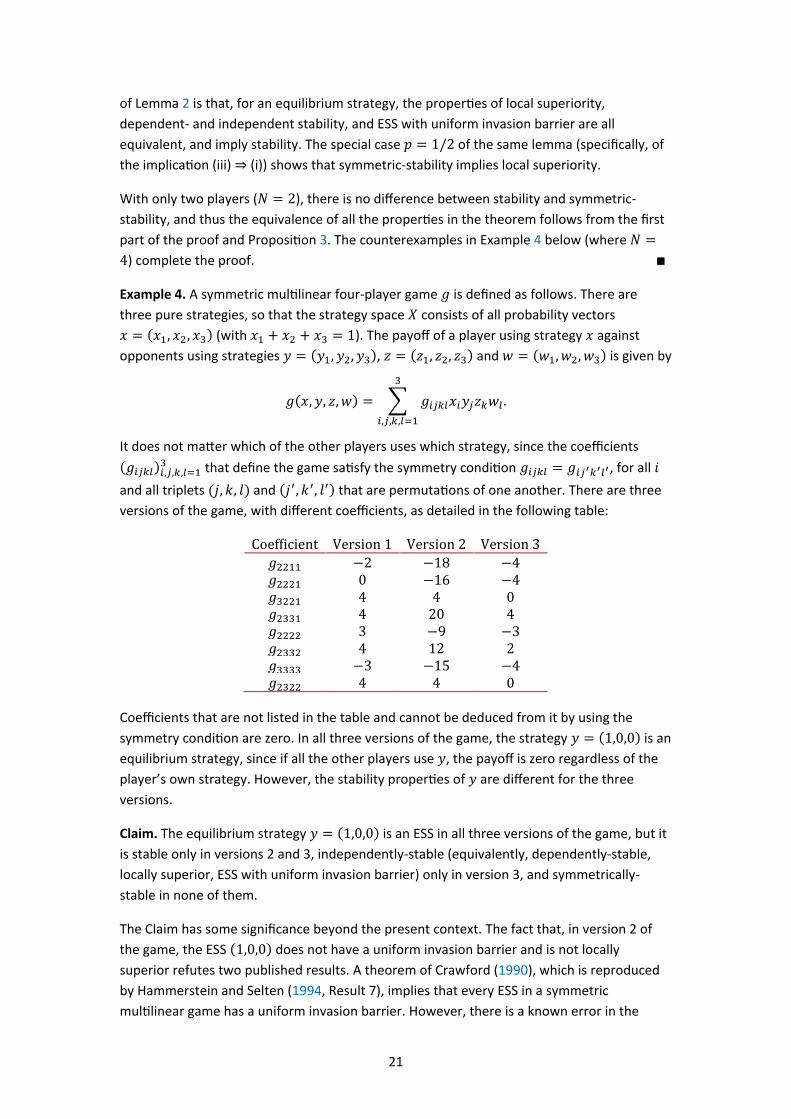
Example 4. A symmetric multilinear four-player game 𝑔 is defined as follows. There are

three pure strategies, so that the strategy space 𝑋 consists of all probability vectors

𝑥 = (𝑥1, 𝑥2, 𝑥3) (with 𝑥1 + 𝑥2 + 𝑥3 = 1). The payoff of a player using strategy 𝑥 against

opponents using strategies 𝑦 = (𝑦1, 𝑦2, 𝑦3), 𝑧 = (𝑧1, 𝑧2, 𝑧3) and 𝑤 = (𝑤1, 𝑤2, 𝑤3) is given by

𝑔(𝑥, 𝑦, 𝑧, 𝑤) = ∑ 𝑔𝑖𝑗𝑘𝑙𝑥𝑖𝑦𝑗𝑧𝑘𝑤𝑙

3

𝑖,𝑗,𝑘,𝑙=1

.

It does not matter which of the other players uses which strategy, since the coefficients

(𝑔𝑖𝑗𝑘𝑙)𝑖,𝑗,𝑘,𝑙=13 that define the game satisfy the symmetry condition 𝑔𝑖𝑗𝑘𝑙 = 𝑔𝑖𝑗′𝑘′𝑙′, for all 𝑖

and all triplets (𝑗, 𝑘, 𝑙) and (𝑗′, 𝑘′, 𝑙′) that are permutations of one another. There are three

versions of the game, with different coefficients, as detailed in the following table:

Coefficient Version 1 Version 2 Version 3

𝑔2211 −2 −18 −4 𝑔2221 0 −16 −4 𝑔3221 4 4 0 𝑔2331 4 20 4 𝑔2222 3 −9 −3 𝑔2332 4 12 2 𝑔3333 −3 −15 −4 𝑔2322 4 4 0

Coefficients that are not listed in the table and cannot be deduced from it by using the

symmetry condition are zero. In all three versions of the game, the strategy 𝑦 = (1,0,0) is an

equilibrium strategy, since if all the other players use 𝑦, the payoff is zero regardless of the

player’s own strategy. However, the stability properties of 𝑦 are different for the three

versions.

Claim. The equilibrium strategy 𝑦 = (1,0,0) is an ESS in all three versions of the game, but it

is stable only in versions 2 and 3, independently-stable (equivalently, dependently-stable,

locally superior, ESS with uniform invasion barrier) only in version 3, and symmetrically-

stable in none of them.

The Claim has some significance beyond the present context. The fact that, in version 2 of

the game, the ESS (1,0,0) does not have a uniform invasion barrier and is not locally

superior refutes two published results. A theorem of Crawford (1990), which is reproduced

by Hammerstein and Selten (1994, Result 7), implies that every ESS in a symmetric

multilinear game has a uniform invasion barrier. However, there is a known error in the

22

proof of that theorem (Bomze and Pötscher 1993). Theorem 2 of Bukowski and Miekisz

(2004) asserts that local superiority and the ESS condition are equivalent even for 𝑁 > 2.

However, these authors employ a definition of ESS that is different from that used here (and

in other papers) in that it requires the existence of a uniform invasion barrier.

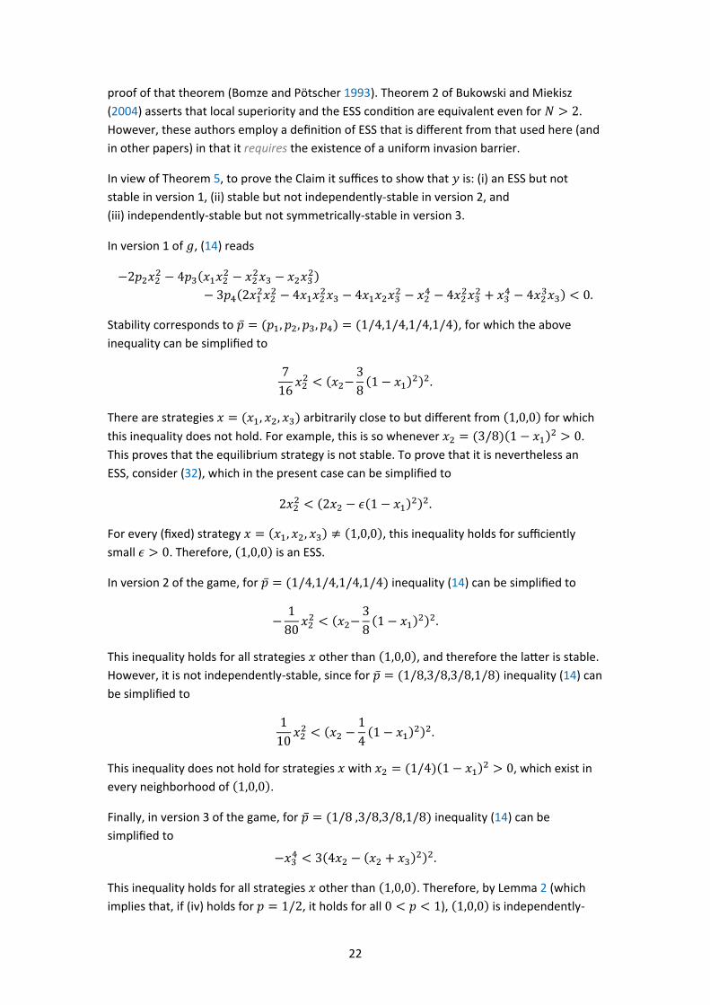
In view of Theorem 5, to prove the Claim it suffices to show that 𝑦 is: (i) an ESS but not

stable in version 1, (ii) stable but not independently-stable in version 2, and

(iii) independently-stable but not symmetrically-stable in version 3.

In version 1 of 𝑔, (14) reads

−2𝑝2𝑥22 − 4𝑝3(𝑥1𝑥2

2 − 𝑥22𝑥3 − 𝑥2𝑥3

2)

− 3𝑝4(2𝑥12𝑥22 − 4𝑥1𝑥2

2𝑥3 − 4𝑥1𝑥2𝑥32 − 𝑥2

4 − 4𝑥22𝑥32 + 𝑥3

4 − 4𝑥23𝑥3) < 0.

Stability corresponds to �̅� = (𝑝1, 𝑝2, 𝑝3, 𝑝4) = (1/4,1/4,1/4,1/4), for which the above

inequality can be simplified to

7

16𝑥22 < (𝑥2−

3

8(1 − 𝑥1)

2)2.

There are strategies 𝑥 = (𝑥1, 𝑥2, 𝑥3) arbitrarily close to but different from (1,0,0) for which

this inequality does not hold. For example, this is so whenever 𝑥2 = (3/8)(1 − 𝑥1)2 > 0.

This proves that the equilibrium strategy is not stable. To prove that it is nevertheless an

ESS, consider (32), which in the present case can be simplified to

2𝑥22 < (2𝑥2 − 𝜖(1 − 𝑥1)

2)2.

For every (fixed) strategy 𝑥 = (𝑥1, 𝑥2, 𝑥3) ≠ (1,0,0), this inequality holds for sufficiently

small 𝜖 > 0. Therefore, (1,0,0) is an ESS.

In version 2 of the game, for �̅� = (1/4,1/4,1/4,1/4) inequality (14) can be simplified to

−1

80𝑥22 < (𝑥2−

3

8(1 − 𝑥1)

2)2.

This inequality holds for all strategies 𝑥 other than (1,0,0), and therefore the latter is stable.

However, it is not independently-stable, since for �̅� = (1/8,3/8,3/8,1/8) inequality (14) can

be simplified to

1

10𝑥22 < (𝑥2 −

1

4(1 − 𝑥1)

2)2.

This inequality does not hold for strategies 𝑥 with 𝑥2 = (1/4)(1 − 𝑥1)2 > 0, which exist in

every neighborhood of (1,0,0).

Finally, in version 3 of the game, for �̅� = (1/8 ,3/8,3/8,1/8) inequality (14) can be

simplified to

−𝑥34 < 3(4𝑥2 − (𝑥2 + 𝑥3)

2)2.

This inequality holds for all strategies 𝑥 other than (1,0,0). Therefore, by Lemma 2 (which

implies that, if (iv) holds for 𝑝 = 1/2, it holds for all 0 < 𝑝 < 1), (1,0,0) is independently-

23

stable. However, it is not symmetrically-stable. There are probability vectors �̅� satisfying (17)

for which (14) does not hold for some strategies 𝑥 arbitrarily close to (1,0,0). For examples,

for �̅� = (1/20,9/20,9/20,1/20), inequality (14) can be simplified to

24𝑥22 −

1

3𝑥34 < (8𝑥2 − (1 − 𝑥1)

2)2.

For strategies 𝑥 with 𝑥2 = (1/8)(1 − 𝑥1)2, this inequality is equivalent to (1 − 𝑥1)

4 −

32(1 − 𝑥1)3 + 384(1 − 𝑥1)

2 − 2048(1 − 𝑥1) > 512. Hence, it does not hold if 𝑥1 is

sufficiently close to 1. This completes the proof of the Claim.

Appendix A. Other notions of stability Static and dynamic stability are not the only kinds of stability in strategic games considered

in the game-theoretic literature. For completeness, some of the other categories are briefly

reviewed below.

One kind of stability refers to the effects of perturbations of the players’ strategy spaces

(e.g., allowing only completely mixed strategies) or a combination of perturbations of the

strategy spaces and of the strategies themselves. The requirement that a strategy profile in a

strategic game is stable against these kinds of perturbations gives the notions of (trembling-

hand) perfect equilibrium (Selten 1975), proper equilibrium (Myerson 1978), strict

perfection (Okada 1981) and (strategic) stability and full stability (Kohlberg and Mertens

1986). Stability may also refer to the effects on a given equilibrium of perturbations of the

payoff functions. Essentiality (Wu and Jiang 1962) and strong stability (Kojima et al. 1985)

are examples of this kind of stability, which has interesting links with some of the other

kinds. For example, in a multilinear game, every essential equilibrium is strictly perfect (van

Damme 1991, Theorem 2.4.3), and in a symmetric 𝑛 × 𝑛 game, every regular ESS is essential

(Selten 1983). Another example of a link between different kinds of stability is the finding

that, in several classes of games, the (local) degree of an equilibrium (or of a connected

component of equilibria) is equal to its index (Govindan and Wilson 1997; Demichelis and

Germano 2000). The index of an equilibrium is related to its asymptotic stability or instability

with respect to a large class of natural dynamics, which determine how strategies in the

game change over time. The degree, by contrast, expresses a topological property of the

equilibrium when viewed as a point in a manifold that includes the various equilibria of

different games (Ritzberger 2002). The index (= degree) of an equilibrium is connected with

stability also in that, in a nondegenerate bimatrix game, it determines whether the

equilibrium can be made the unique equilibrium by extending the game: adding one or more

pure strategies to one of the players (von Schemde and von Stengel 2008).

Whether any of these alternative notions can be linked with statics stability is yet to be

determined.

24

References Apaloo, J., 1997. Revisiting strategic models of evolution: The concept of neighborhood

invader strategies. Theoretical Popul. Biol. 52, 71–77.

Bomze, I. M., 1991. Cross entropy minimization in uninvadable states of complex

populations. J. Math. Biol. 30, 73–87.

Bomze, I. M., Pötscher, B. M., 1989. Game Theoretical Foundations of Evolutionary Stability.

Springer, Berlin.

Bomze, I. M., Pötscher, B. M., 1993. “On the definition of an evolutionarily stable strategy in

the playing the field model” by V. P. Crawford. J. Theoretical Biol. 161, 405.

Bomze, I. M., Weibull, J. W., 1995. Does neutral stability imply Lyapunov stability? Games

Econ. Behav. 11, 173–192.

Broom, M., Cannings, C., Vickers, G. T., 1997. Multi-player matrix games. Bull. Math. Biol. 59,

931–952.

Bukowski, M., Miekisz, J., 2004. Evolutionary and asymptotic stability in symmetric multi-

player games. Internat. J. Game Theory 33, 41–54.

Christiansen, F. B., 1991. On conditions for evolutionary stability for a continuously varying

character. Am. Nat. 138, 37–50.

Crawford, V.P., 1990. On the definition of an evolutionarily stable strategy in the “playing

the field” model. J. Theoretical Biol. 143, 269–273.

Demichelis, S., Germano, F., 2000. On the indices of zeros of Nash fields. J. Econ. Theory 94,

192–217. (An extended version: Discussion paper, CORE, Louvain-la-Neuve, 2000).

Dold, A., 1980. Lectures on Algebraic Topology, Second Edition. Springer-Verlag, Berlin.

Eshel, I., 1983. Evolutionary and continuous stability. J. Theoretical Biol. 103, 99–111.

Eshel, I., Motro, U., 1981. Kin selection and strong evolutionary stability of mutual help.

Theoretical Popul. Biol. 19, 420–433.

Fudenberg, D., Tirole, J., 1995. Game Theory. MIT Press, Cambridge, MA.

Govindan, S., Wilson, R., 1997. Equivalence and invariance of the index and the degree of

Nash equilibria. Games Econ. Behav. 21, 56–61.

Hammerstein, P., Selten, R., 1994. Game theory and evolutionary biology. In: Aumann, R. J.,

Hart, S. (Eds.), Handbook of Game Theory with Economic Applications, Vol. 2, pp. 929–993.

Elsevier Science, Amsterdam.

Harsanyi, J., Selten, R., 1988. A General Theory of Equilibrium Selection in Games. MIT Press,

Cambridge, MA.

Hofbauer, J., Sigmund, K., 1998. Evolutionary Games and Population Dynamics. Cambridge

University Press, Cambridge, UK.

Kelley, J. L., 1955. General Topology. Springer, New York.

25

Kohlberg, E., Mertens, J.-F., 1986. On the strategic stability of equilibria. Econometrica 54,

1003–1037.

Kojima, M., Okada, A., Shindoh, S., 1985. Strongly stable equilibrium points of n-person

noncooperative games. Math. Oper. Res. 10, 650–663.

Maynard Smith, J., 1982. Evolution and the Theory of Games. Cambridge University Press,

Cambridge, UK.

Milchtaich, I., 2012. Comparative statics of altruism and spite. Games Econ. Behav. 75, 809–

831.

Monderer, D., Shapley, L. S., 1996. Potential games. Games Econ. Behav. 14, 124–143.

Myerson, R. B., 1978. Refinements of the Nash Equilibrium Concept. Internat. J. Game

Theory 7, 73–80.

Oechssler, J., Riedel, F., 2002. On the dynamic foundation of evolutionary stability in

continuous models. J. Econ. Theory 107, 223–252.

Okada, A., 1981. On the stability of perfect equilibrium points. Internat. J. Game Theory 10,

67–73.

Ritzberger, K., 2002. Foundations of Non-Cooperative Game Theory. Oxford University Press,

Oxford.

Samuelson, P. A., 1983. Foundations of Economic Analysis, Enlarged Edition. Harvard

University Press, Cambridge, MA.

Selten, R., 1975. A reexamination of the perfectness concept for equilibrium points in

extensive games. Internat. J. Game Theory 4, 25–55.

Selten, R., 1983. Evolutionary stability in extensive two-person games. Math. Social Sci. 5,

269–363.

Taylor, P. D., 1989. Evolutionary stability in one-parameter models under weak selection.

Theoretical Popul. Biol. 36, 125–143.

van Damme, E., 1991. Stability and Perfection of Nash Equilibria, Second Edition. Springer-

Verlag, Berlin.

von Schemde, A., von Stengel, B., 2008. Strategic characterization of the index of an

equilibrium. In: Monien, B., Schroeder, U.-P. (Eds.), Symposium on Algorithmic Game Theory

(SAGT) 2008, Lecture Notes in Computer Science 4997, pp. 242–254, Springer-Verlag, Berlin.

Weibull, J. W., 1995. Evolutionary Game Theory. MIT Press, Cambridge, MA.

Weissing, F. J., 1991. Evolutionary stability and dynamic stability in a class of evolutionary

normal form games. In: Selten, R. (Ed.), Game Equilibrium Models, pp. 29–97. Springer-

Verlag, Berlin.

Wu, W.-T., Jiang, J.-H., 1962. Essential equilibrium points of n-person non-cooperative

games. Sci. Sinica 11, 1307–1322.