statics and dynamics ch 1

8/12/2019 Statics and Dynamics Ch 1

http://slidepdf.com/reader/full/statics-and-dynamics-ch-1 1/23

© Copyright 2006, S.B. Biggers, for Clemson University students currently in ME 201 only, no distribution

permitted without permission of author.11

Chapter 1: Introduction to Newton’s Laws

1-1 Governing Equations for Dynamics and Statics

Prior to Sir Isaac Newton’s formulation of his three famous laws in 1687, scientists were notcompletely successful in explaining the motion or lack of motion of bodies. Newton’s laws

allow us to be successful in both areas as long as the velocities are much less than the speed of

light and the bodies are much larger than individual atoms. In such extreme cases, Einstein’srelativistic mechanics, published in 1905, and other complex theories of physics would have to

be used. Therefore, in the vast majority of cases, Newton’s laws serve perfectly well as the

foundation for applications of mechanics to practical situations. Newton’s second law states that

the sum of all forces acting on a body equals the product of its mass times its acceleration.

∑ G F = m a (1.1)

This governing equation will be the starting point for our study of Dynamics. Later we will seethat the acceleration in this equation must be the acceleration of the center of gravity ( CG) of the

body, thus the subscript “G” on the acceleration. This equation will be integrated in two special

ways to yield the governing equations two additional methods, i.e. the work-energy method (Chapter 9) or the impulse-momentum method (Chapter 10). When the body is restrained so

that it cannot move, or at least has a zero acceleration (i.e., constant velocity), Newton’s first law

is the result. This simplified version of the second law says simply that if the sum of all forces

acting on a body equals zero, the body is either (a) in static equilibrium, i.e. has no motion

at all, or (b) moves with constant velocity. In either case, equation (1.1) reduces to

∑F = 0 (1.2)

which is Newton’s first law. It is simply a special case of the second law and it forms thestarting point for our study of Statics. These two simple but important laws clearly show the

close relationship of Dynamics and Statics. These equations refer to lack of motion or motion

Statics vs. Dynamics

photo courtesy of: www.la-magic.com/ladyann/space/shuttle.html





along a straight or curved line, motion referred to as translation, which we will define more

precisely later. We will show how to modify these equations to describe rotational motion orlack of such rotation as follows:

α ∑ G G M = I (1.3)

and

∑ M = 0 (1.4)

The terms in these equations will be defined later as required, but for now, equations (1.3 – 1.4)can be interpreted as Newton’s Second and First Laws for rotational motion or lack of such

motion, respectively. Motion involving both translation and rotation is referred to as general

motion and will require satisfaction of the dynamic form of both the translational and rotationalequations (1.1 and 1.3). Static equilibrium implies the lack of all motion and therefore requires

that the zero forms of both equations (1.2 and 1.4) are satisfied. You will see that pure

translation requires satisfaction of the dynamic form of the translational equation (1.1) along

with the zero form (static form) of the rotational equation (1.4). Conversely, you will see that pure rotational motion about the center of gravity of a rigid body requires satisfaction of the

opposite forms of the equations (1.2 and 1.3).

Newton also developed a third law that is equally important in Dynamics and in Statics. This

states that when two separate bodies contact each other or attract each other, the

interacting forces are equal in magnitude and opposite in direction. You can feel this easily by pushing two fingers together or linking them and pulling on them.

You may be surprised to learn that the foundation for this integrated course has now been statedin terms of equations (1.1 – 1.4) comprising the static form (zero form) and the dynamic form

(nonzero form) of Newton’s Second Law for translation and rotation. We still need to define the

terms in the rotational equations. We also must define the physical point on the body known as

the “center of gravity”, and will do so very soon.

In Dynamics the governing kinetics equations introduced above will be supplemented with

additional equations of kinematics which describe the relationships between translational and

rotational motions and how they relate to time and position . In Dynamics we will sometimes

use integrated forms of Newton’s Second Law to formulate problems in terms of Work-

Energy and/or Impulse-Momentum principles. However, with only a very few exceptions, Newton’s Second Laws for translation and rotation can be used for any static or dynamic

situation. In some cases, however, the other methods may lead to simpler formulations and

quicker solutions.

1-2 Force of Gravity

Newton formulated his universal law of gravitation when he discovered that any two masses

have equal and opposite attractive forces on each other. This is actually a quantitative version of

his third law. Our weight is simply the attractive force that the mass of the earth has on our bodymass. As discussed in the introduction, weight is a force and it will be measured in N or lb.





Newton’s law of gravitation states that the attractive force F between two stationary masses m1 and m2 whose centers are a

distance r apart as shown at right is given by

(1.5)

where the gravitational constant G is given by

G = 6.673 x 10-11

m3/(kg-sec

2) in SI, and G = 3.439 x 10

-8 ft

4/(lb-sec

4) in USC.

Since the earth is notspherical (radius larger

at equator than poles),

the distance r varieswith latitude, as well as

elevation. Since theearth rotates, there is a

slight tendency for bodies to be thrown off

the surface due to this

rotation. This effectalso varies from

maximum at the equator

to minimum at the poles.Therefore, the total

effective interactiveforce between any body

and the earth is a

function of position(latitude and elevation).

So the measured weight of any body is maximized at the poles and minimized at the equator.

Since weight is also defined as mass times the so called “acceleration of gravity”, g , themagnitude of g also varies in the same way as weight. The chart in Figure 1.1 summarizes the

acceleration of gravity at sea level at different locations on the earth. If the earth did not rotate,

the curve with higher values would apply. The effect of earth’s rotation is included in the lowercurve. In this course, we will always assume an average value of g = 9.81 m/s

2 in the SI system

or 32.2 ft/s2 in the USC system, unless a different value can be justified by additional given

information. Given the values of g at the equator and the poles for a nonrotating earth in

Figure 1.1 and the mass of the earth = 5.976 x 1024

kg, find the earth’s radius at the equator

and at the poles.

F = (G) (m1 m2 )/( r

2

)

Figure 1.1 “Acceleration” of Gravity. (from Meriam & Kraige)

m1

F m2

r





1-3 Free Body Diagrams and Kinetic Diagrams

The most important step in formulating and solving dynamics and statics problems is to draw

simple sketches that represent the two sides of the equation stating Newton’s second law.

On the left hand side, we need to represent all forces acting on the body so they can be summed.

The sketch that shows the body and all known and unknown forces acting on it is called the freebody diagram (FBD). The magnitude and direction of known forces are shown. Unknown

forces are shown with an assumed direction and an identifying name. The term free simply

means the body has been cut free from all supports or connections to other bodies and thoseunknown reaction or connection forces are shown with names and directions as they are known

to act or are assumed to act on the body. If a support prevents motion in a particular direction,

there is a reaction force opposite to that direction. The kinetic diagram (KD) is drawn torepresent the right hand side of Newton’s second law when modeling a dynamic condition. It

shows the magnitude and directions of known accelerations or the assumed magnitudes and

identifying names of unknown accelerations. In static equilibrium, the kinetic diagram is simplya zero and can be omitted.

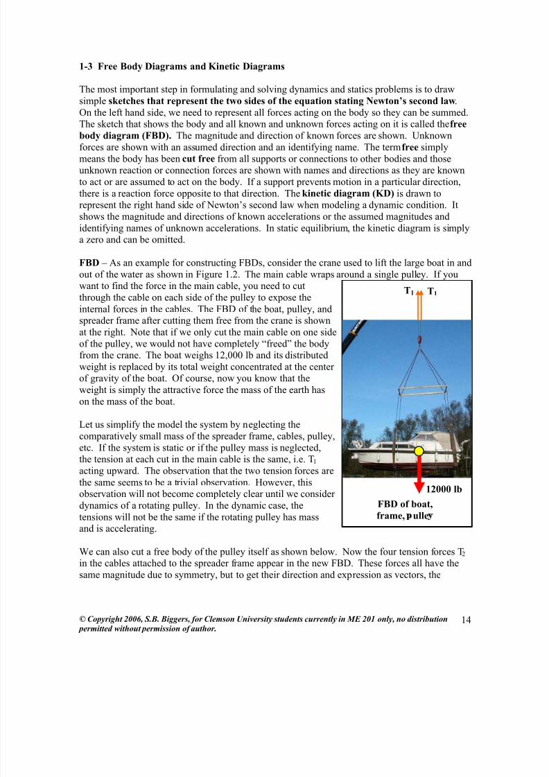
FBD – As an example for constructing FBDs, consider the crane used to lift the large boat in and

out of the water as shown in Figure 1.2. The main cable wraps around a single pulley. If youwant to find the force in the main cable, you need to cut

through the cable on each side of the pulley to expose the

internal forces in the cables. The FBD of the boat, pulley, andspreader frame after cutting them free from the crane is shown

at the right. Note that if we only cut the main cable on one side

of the pulley, we would not have completely “freed” the bodyfrom the crane. The boat weighs 12,000 lb and its distributed

weight is replaced by its total weight concentrated at the centerof gravity of the boat. Of course, now you know that the

weight is simply the attractive force the mass of the earth has

on the mass of the boat.

Let us simplify the model the system by neglecting the

comparatively small mass of the spreader frame, cables, pulley,

etc. If the system is static or if the pulley mass is neglected,the tension at each cut in the main cable is the same, i.e. T1

acting upward. The observation that the two tension forces are

the same seems to be a trivial observation. However, thisobservation will not become completely clear until we consider

dynamics of a rotating pulley. In the dynamic case, the

tensions will not be the same if the rotating pulley has massand is accelerating.

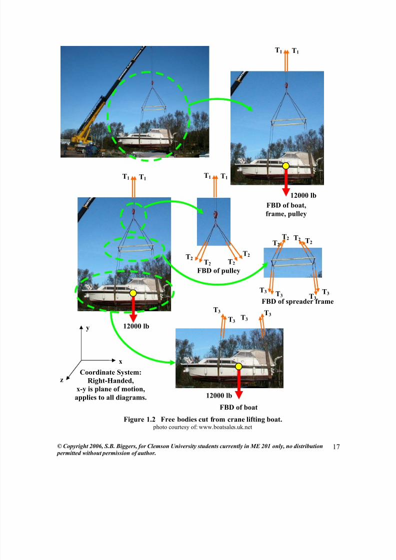
We can also cut a free body of the pulley itself as shown below. Now the four tension forces T2 in the cables attached to the spreader frame appear in the new FBD. These forces all have the

same magnitude due to symmetry, but to get their direction and expression as vectors, the

T1 T1

FBD of boat,

frame, ulle

12000 lb





geometry of the spreader frame is needed. We will return to this

problem in Chapter 5 after discussing ways to define vectors in 3-D space in the Chapter 2.

Next, we can cut a free body of only the spreader frame as shown.

Now the four equal tension forces T3 in the nearly vertical strapssurrounding the boat appear in the new FBD. Finally, the FBD of

the boat alone is shown in Figure 1.2 as supported by the T3 forces

in the straps.

Note that in all cases, tension forces “pull” on the body on which

they act. Internal forces on either side of a cut are always equal inmagnitude and opposite in direction (Newton’s Third Law). It is

very important to note that the internal forces are not shown on a

FBD unless there has been a cut made in the support (cable in thisinstance) on that particular FBD. Then the internal force is shown

as it acts on the cut surface. There are many other FBDs thatcould be cut and drawn from the original photo and later we will

do some of these. It is a good practice to actually indicate on theoriginal body exactly where the FBD is being cut free. This has

been done with the dashed green lines on the photo in Figure 1.2.

The FBD is only what is inside the dashed line and internal forcesare shown only where the dashed line cuts through a supporting

element. Your instructor will ask you to practice drawing FBDs

for a number of situations. You will be expected to do thiscorrectly as the first step in formulating the governing equations

using Newton’s Second Law for dynamics or statics. You will also be given some FBDs that

are incomplete or include mistakes that students often make and you will be asked to find and

correct the mistakes.

A complete FBD shows:

• A simple sketch of the body that has been cut free and all forces acting on that particular body including:

o The weight, located at the CG, with magnitude and direction shown

o The magnitude and direction of any other known forces tending to cause, restrict,

or prevent motion

o Any unknown forces in members that were cut to free the body but tending to

cause, restrict, or prevent motion – an assumed direction and a unique name

should be shown.

• A coordinate system identifying directions used in vector expressions

• Important geometric information needed to solve the problem. If this information is tooextensive, sometimes it is best to show it on a separate diagram.

KD – The kinetic diagram is much simpler than the FBD. It represents the termG

m a on the

right hand side of Newton’s Second Law for forces and translation, and the term α G

for

T1 T1

T2T2 T2

T2

FBD of pulley

T2

T2 T2 T2

T3T3T3

T3

FBD of spreaderframe





moments and rotation (to be examined later). Sometimes the KD is so simple students bypass

drawing it because it seems to be trivial. However, this tendency must be avoided in formulatingthe governing equations for dynamics. Drawing the KD forces you to make a conscious decision

about which mass or masses you are considering and which ones are actually accelerating. You

are also forced to make a first estimate or assumption of the direction(s) of the acceleration(s)

and to show the point to which the acceleration applies. It aids in making observations aboutrelationships of motions of different points on the body and in recording any assumptions about

these accelerations.

A complete KD shows:

• A simple sketch of the body under consideration and the accelerations that particular body may be experiencing including:

o The linear acceleration vector at the CG with the given, assumed, or observeddirection(s) shown and the vector or vector components named.

o The angular acceleration of the body with the given, assumed, or observed

direction(s) shown and the vector or vector component(s) named. In cases of 2-D

motion, only a vector component normal to the plane of motion will be present.• Any support or connection to another element that restricts the motion in any way, be thatzero motion or nonzero motion. (Note this is quite different from the FBD which must be

shown free from all supports, and shows forces not motion.)

Some students attempt to combine the FBD and KD into a single diagram. This should never

be done. Some examples of FBDs and KDs a successful student would create for the boatlifting problem are shown in Figure 1.3. You will be expected to do this correctly as the

second step in formulating the governing equations using Newton’s Second Law for

dynamics.





T1 T1

T2T2 T2

T2

T2

T2 T2 T2

T3T3T3

T3

T1 T1

T1 T1

12000 lb

12000 lb

T3

T3

T3

T3

12000 lb

FBD of boat

FBD of spreader frame

FBD of pulley

FBD of boat,

frame, pulley

Figure 1.2 Free bodies cut from crane lifting boat. photo courtesy of: www.boatsales.uk.net

Coordinate System:

Right-Handed,

x-y is plane of motion,

applies to all diagrams.

y

x

z





FBD of pulley

Figure 1.3 Student FBDs and KDs.

KD of pulley

KD of boat,

frame, pulley

FBD of boat,

frame, pulley

KD of boatFBD of boat

Coord

System

FBD of frame KD of frame





EXAMPLE 1.1 – Statics and Dynamics of Lifting: If the boat is held by the crane but notmoved up or down, its velocity is a constant (i.e. zero) and therefore the vertical acceleration of

the mass of the boat is zero. In fact, if the crane is lifting the boat at a constant vertical speed,

the same can be said. The case of no motion at all is clearly a case of static equilibrium. The

constant speed case is referred to as quasi-static since the governing equation and its solution arethe same as for the truly static case. As your first quantitative exercise, use the diagrams in

Figure 1.2 and the guide given for problem solving to model lifting the boat. Apply Newton’s

Second Law for forces in the vertical direction to find the tension T 1 in the main cables in the

following conditions:

(1) the boat is being held motionless

(2) the boat is being lifted straight up with an acceleration of 5 ft/sec2

(3) the boat is being lowered straight down with an acceleration of 5 ft/sec2

(4) the boat is being lifted straight up with a deceleration of 5 ft/sec2

(5) the boat is being lowered straight down with a deceleration of 5 ft/sec2

(6) the boat is lifted with a constant cable tension from the static position to achieve a

vertical speed of 4 ft/sec in a period of 0.5 sec.(7) after 0.5 sec, the crane continues to lift the boat at a constant speed of 4 ft/sec.

(a) In which of the seven cases above could the velocity become instantaneously equal to zero

assuming the accelerations or decelerations remain as stated. (b) What happens to the values

of the cable tension at the instant when the velocity becomes zero? (c) What happens to the

values of the cable tension just after that instant of zero velocity when motion resumes?

(d) In case (2), is there an upper limit to the magnitude of the acceleration could achieve

given no limit to the power of the crane winch or strength of the cables? (e) What about case

(3)? (f) What can you say about the magnitude of the cable tensions as the accelerations in

cases (2) and (3) increase?

From these simple examples, you can easily see how closely static and dynamic conditions are

related. The importance of showing the directions of forces and accelerations or decelerationsin the FBD and KD and using these in the governing equations should also be evident.

Hopefully, the effects of the direction and magnitude of velocity vector and changes in the

velocity vector have also been noted.

1-4 Types of Motion: Pure Translation

We have already dealt with translation in the example above since it is the simplest type ofmotion. Motion in a straight line is the simplest type of translation. If the boat above is lifted or

lowered vertically with no swinging, it is undergoing straight line translation. For a moregeneral definition, we say the body is moving in pure translation when it moves such that all

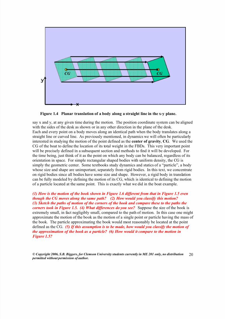
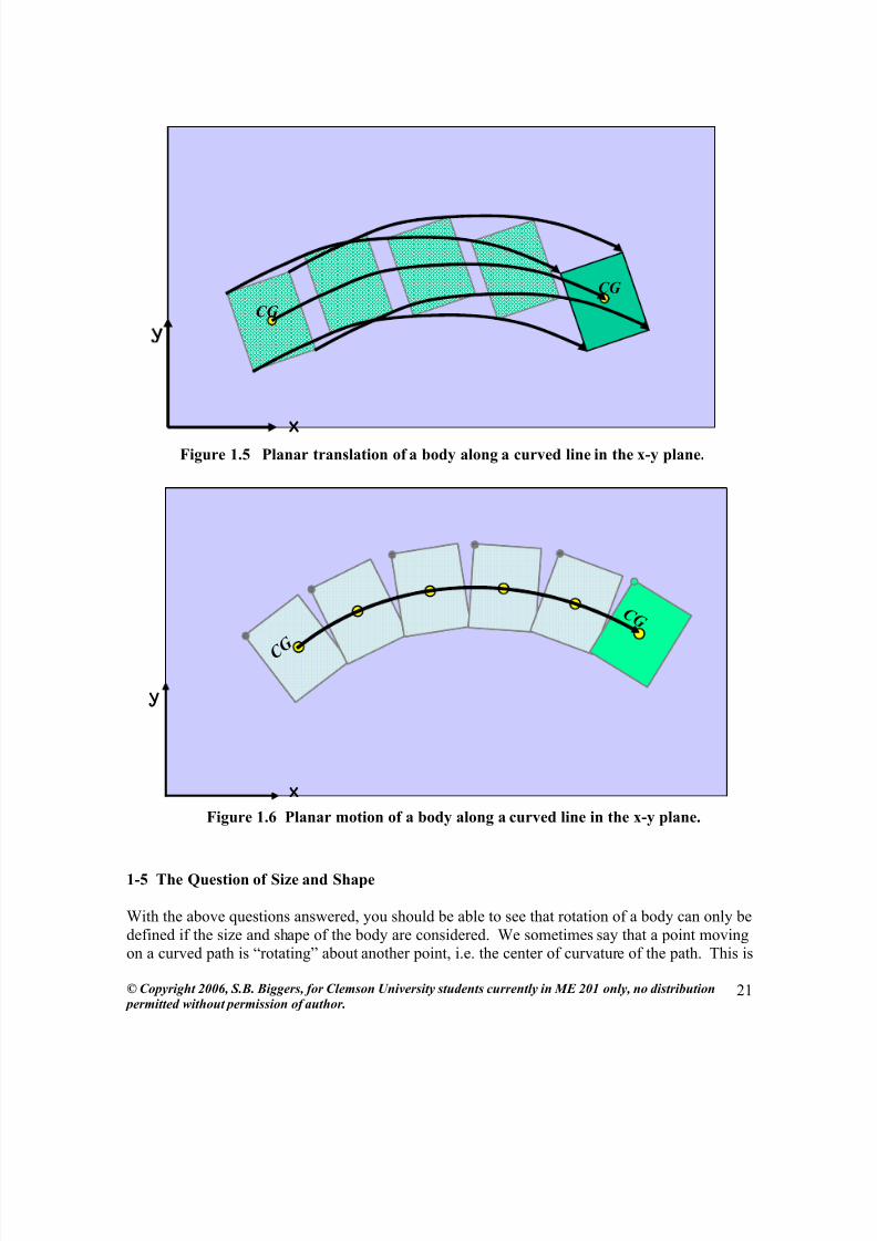
points on it travel along paths that have the same length and shape. Figures 1.4 and 1.5 below

illustrate such motion, first along a straight line and then along a curved line. Envision a book

lying flat on a horizontal desk and being moved as shown. Even though the book is a 3-D body,this motion is called planar translation since it can be fully defined by two position coordinates,





say x and y, at any given time during the motion. The position coordinate system can be aligned

with the sides of the desk as shown or in any other direction in the plane of the desk.

Each and every point on a body moves along an identical path when the body translates along astraight line or curved line. As previously mentioned, in dynamics we will often be particularly

interested in studying the motion of the point defined as the center of gravity, CG. We used the

CG of the boat to define the location of its total weight in the FBDs. This very important point

will be precisely defined in a subsequent section and methods to find it will be developed. For

the time being, just think of it as the point on which any body can be balanced, regardless of itsorientation in space. For simple rectangular shaped bodies with uniform density, the CG is

simply the geometric center. Some textbooks study dynamics and statics of a “particle”, a bodywhose size and shape are unimportant, separately from rigid bodies. In this text, we concentrate

on rigid bodies since all bodies have some size and shape. However, a rigid body in translation

can be fully modeled by defining the motion of its CG, which is identical to defining the motionof a particle located at the same point. This is exactly what we did in the boat example.

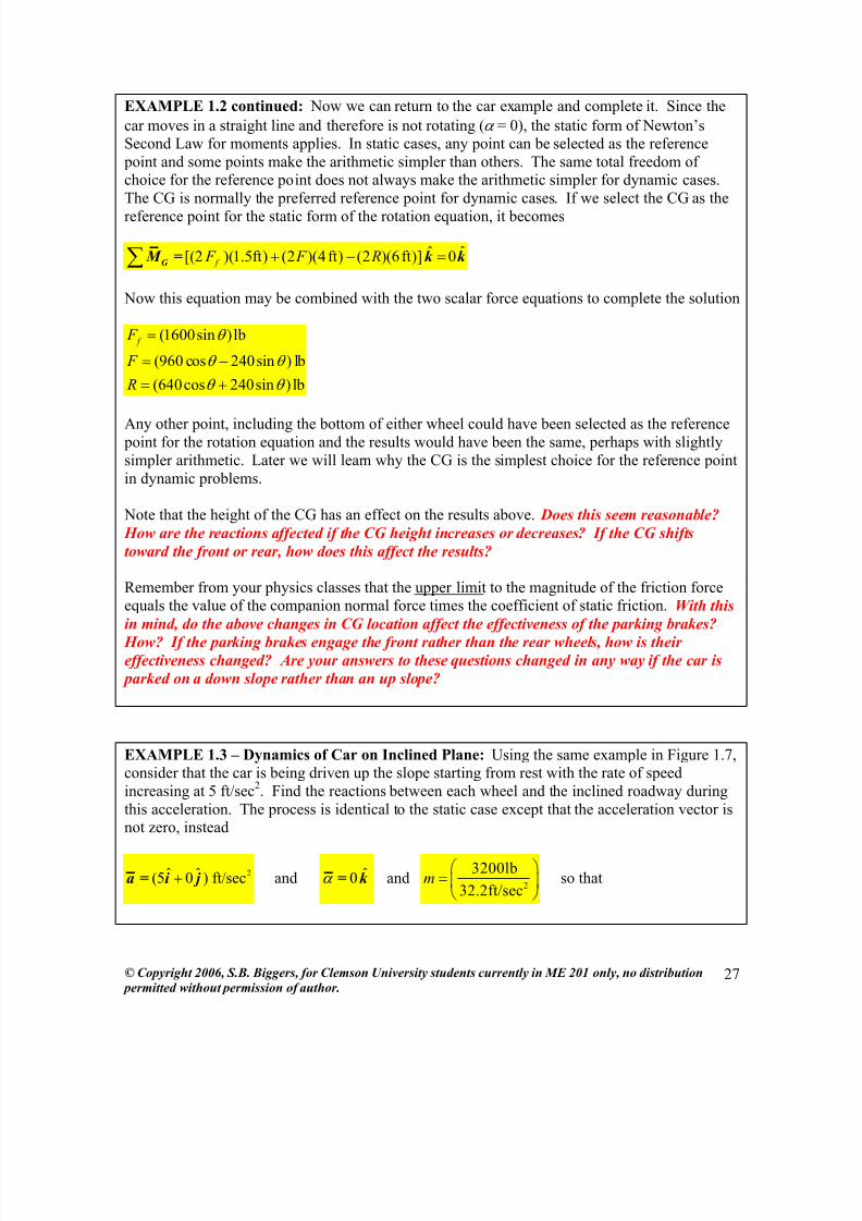
(1) How is the motion of the book shown in Figure 1.6 different from that in Figure 1.5 even

though the CG moves along the same path? (2) How would you classify this motion?

(3) Sketch the paths of motion of the corners of the book and compare these to the paths the

corners took in Figure 1.5. (4) What differences do you see? Suppose the size of the book is

extremely small, in fact negligibly small, compared to the path of motion. In this case one mightapproximate the motion of the book as the motion of a single point or particle having the mass of

the book. The particle approximating the book would most reasonably be located at the point

defined as the CG. (5) If this assumption is to be made, how would you classify the motion of

the approximation of the book as a particle? (6) How would it compare to the motion in

Figure 1.5?

x

Figure 1.4 Planar translation of a body along a straight line in the x-y plane.

CG CG





1-5 The Question of Size and Shape

With the above questions answered, you should be able to see that rotation of a body can only be

defined if the size and shape of the body are considered. We sometimes say that a point movingon a curved path is “rotating” about another point, i.e. the center of curvature of the path. This is

x

Figure 1.5 Planar translation of a body along a curved line in the x-y plane.

CG

CG

y

x

C G

C G

Figure 1.6 Planar motion of a body along a curved line in the x-y plane.





technically true. However using the language of dynamics, this motion of a point or particle is

actually only translation along a curved path and equations (1.3) and (1.4) are of no use. Oncethe body has significant size and shape, then one of these two equations will be required to

model the motion of the body in addition to equation (1.1) or (1.2).

EXAMPLE 1.2 – Statics of Car on Inclined Plane: Questions of accelerations of a rigid bodyor a particle moving along a curved path require special attention and this will be addressed in

Chapter 2 and afterwards. But for the time being, let us examine this question of size on a

simpler, straight-line translational motion problem. Consider the motion of a car, along astraight inclined roadway as shown in Figure 1.7. The car weighs a total of 3200 lb, is

symmetric left to right, and has a CG located as shown. Due to symmetry, the wheel reactions

will be identical left to right. The car is rear wheel drive and the roadway provides sufficientfriction to prevent slipping of the tires. Effects of rotation of the wheels and axles as the car

translates are neglected for the present. First find the reactions between each wheel and the road

if the car is parked with the parking brakes engaged (lock rear wheels only). Anothersimplifying assumption made here is that the so called “rolling resistance”, associated with

rolling of flexible tires and imperfect wheel bearings, is negligible. This rolling resistance can beaccounted for rather easily and will be considered in later examples. But it should not be

confused with the contact friction between the tires and roadway that allows the car to remainstationary or to accelerate.

First, free the car from the roadway and draw the FBD. The KD is zero in this static case but is

shown here for consistency with examples to follow.

FBD of car KD of car

Right-Handed Coordinate System:

x- is lane of motion.

y

x

z

CG

2F

2R

W = 3200 lb

2F f

=

a x = 0

Photo courtesy of

http://forums.beyond.ca/showthread/t-50075.html

Figure 1.7 Static Equilibrium of a Car Parked on an Incline.

Car Geometry

6 ft 4 ft

1.5 ft

θ





The friction reaction prevents the car from sliding down the incline and acts parallel to the slope.

Friction preventing sliding or resulting from sliding will always be tangent to the surface of potential sliding. The factors of 2.0 are present on the unknown reactions due to the left-to-right

symmetry. Note that the coordinate system is oriented along the incline for simplicity in writing

the force vectors since the three unknown reactions are in these directions. Because such choices

are possible but not necessary, it is essential to show a sketch of the chosen coordinate systemalong with each FBD. A vertical and horizontal system could have been used if desired. Unit

vectors ˆ ˆ ˆi, j,k are defined in the given x,y,z directions, respectively. Using this coordinate

system, the weight must be resolved into components in the coordinate directions. Then the

static form of Newton’s Second Law for the forces is written as

ˆ ˆ ˆ ˆ[2 (3200lb)sin ] [2 2 (3200lb)cos ] 0 0θ θ − + + − = +∑ f F R F F = i j i j

Separating the scalar equations for the forces in the x- and y-directions, we get the sum of forces

in the x- and the y-directions shown below. In many simple problems, we will write these two

scalar equations direction without first writing the combined vector equation.

ˆ : 2 (3200lb)sin 0

ˆ : 2 2 (3200lb)cos 0

θ

θ

− =

+ − =

f F

R F

i

j

The first equation shows that the friction force at each rear wheel needed to keep the car static is

simply equal and opposite to half the x-component of the weight,

(1600sin )lbθ = f F

acting up the slope as assumed on the FBD. It should seem reasonable that as the angle θ goestoward zero, the required friction force also approaches zero. The opposite is true as the angle

increases. This is a rather obvious example of examining limiting cases to ensure your solution

is reasonable.

The scalar equation for the y-direction has two unknowns. Therefore, unless we make a

simplifying assumption, we cannot solve for the unknown normal reaction forces R and F . If thecar were to be treated as a particle and its size neglected, the front and rear wheel reactions

would become equal, would be located at the CG, and the simplified problem could be solved.

The normal wheel reactions would each be one fourth of the y-component of the car’s weight.The friction reaction is not affected by this simplification. However, it is hard to justify treating

such a sizable body as a particle and the simplified solution must be treated as a crudeapproximation.

If a more realistic solution is required, we are forced to find another governing equation.

Equation (1.4), the static form of Newton’s Second Law for rotation, is available. But first we

must define the concept of a moment. After this important development, the car example will be

revisited.





1-6 Moment of a Force about a Point and Definition of a Couple

When Newton and his predecessors were trying to come to a firm understanding of what forces

are and how they affect static and dynamic bodies, they finally came to recognize that the

position of a force on a body was important, as well as its magnitude and direction of the force.Forces applied to an unrestrained body along a line in any direction but passing through the

balance point (CG) produced pure translation. Other forces along any line not passing throughthe CG produced translation AND ROTATION. One meaning of the word “moment” in the

dictionary is “importance” and we often speak of “momentous” occasions as those of special

importance. Therefore, Newton came to talk to his colleagues about the “moment” orimportance of a force, some having more moment or importance than others depending on how

the line along which they acted was located relative to the CG and how much the force tended to

rotate the body. The moment of a force about any given point was defined as the strength anddirection of that tendency to rotate the body about that point.

They also found that pairs of equal and opposite forces that are parallel but not collinear, produced only rotation and no translation of the CG since the sum of the force vectors is zero.This special set of forces obviously creates a moment since the pair produces rotation. Their

moment is given the special name of “couple.” They might have used the word “pair” and we

would still be using it in that way. Instead of pair, we use couple. Special properties of a couplewill be examined and used in later chapters.

In solid mechanics we have come to use the single word moment to represent “moment of aforce”. Whereas a force always tends to push or pull (i.e. translate) a body, a moment of a force

tends to rotate a body. The moment must be defined for a given force as being relative to agiven point since the tendency to rotate will change as the position of the force changes relative

to the point. When you use a wrench, you are applying a force to create rotation of a nut or bolt.

The force you apply is also pushing or pulling on the nut, but rotation is the objective. Thedistance of your hand’s force from the nut and the direction of the force are equally important.

In vector terms, a moment M of a force about a point is defined very precisely as the cross

product

× M = r F (1.6)

where r is the position vector from the reference point to any point on the line of action of the

force vector F . The given order of the terms in the cross-product is critical and the position

vector must originate at the reference point. Note that the moment is a vector that is

perpendicular to the plane formed by the vectors r and F . The line through the moment vectoris parallel to the axis about which the body tends to rotate. In plane motion in the x-y plane,moments will always be in the plus or minus z-direction and the axis of rotation or tendency to

rotate will always be perpendicular to the x-y plane of the body’s motion. In 3-D motion,

moments can have components in all three coordinate directions just as force and positionvectors can. The corresponding axis of rotation will be a line in 3-D space oriented according to

the components of the moment vector.





Recall from your math courses that the magnitude of a cross product ( M in this case) of twovectors can be written in scalar for as

( ) ( ) sin M r F θ = (1.7)

where θ is the angle between the two vectors. The sign (direction) of the cross-product isdetermined by the right-hand-rule. In your math courses, you saw various geometric

interpretations of the cross product, especially when both vectors are position vectors havingunits of length. The moment is a physical interpretation of the cross product.

By regrouping the terms as shown in equation (1.8) and

recognizing that (r sinθ ) is the perpendicular distance

d p in the plane of the two vectors from the force vectorto the reference point, the magnitude of the moment can

be determined using a more physical scalar approach

( ) ( sin ) ( )( ) p F r F d θ = = (1.8)

The perpendicular distance is shown in the figure to the

right. When geometric information is two-dimensionaland given in a form so that d p is obvious, some prefer to

obtain the magnitude of the moment using equation

(1.8). The sign (direction) of the moment must then be determined by observation. Whengeometric information is 3-dimensional, it will almost always be preferable to use the more

formal vector approach to finding moments since the vector approach provides both the

magnitude and direction of the moment. Convince yourself that either of equations (1.6), (1.7),

or (1.8) yields the same magnitude of the moment and your observation gives the same direction

as the vector approach.

Figure 1.8 shows a wrench with several forces that are attempting to tighten the lug nut on thewheel. The wrench is horizontal. Think about how effective these forces are in doing this and

qualitatively rank them without computation. Then compute the moment of the force about

the nut. Do some by hand and some on your calculator, some with scalars and some with

cross-products, and a few with both methods for verification. Compare your computed values

to your qualitative ranking. Try to justify any differences from your qualitative rankings.

Recompute the moments about the center of the wheel, i.e. what tendency do the forces have to

rotate the wheel assuming the nut is tight. If the wheel is raised off the ground, with no

brakes applied and transmission out of gear, would the wheel rotate? If so, in which

direction?

You should have found the results for cases (a) and (i) are the same. Cases (b) and (d) should

also be the same. This illustrates a useful idea known as the “transmissibility of a force”. Put

this idea into words based on these examples?

If the wheel is in firm contact with the ground (center is 14 inches above ground) with the

transmission in neutral and no brakes applied and sufficient friction to keep the wheel from

F

r θ

pd

pd

reference

point





rotating, find the friction force for case (d). Draw the FBD of the wheel with wrench in place

to solve for the friction force. Then draw separate FBDs of the wrench and then the wheel so

that you get the same results.

The FBD of the wrench should show the applied force and the reaction the nut places on the left

end of the wrench. This illustrates that the wrench by itself is in static equilibrium and that thereactions from the nut on the wrench allow this equilibrium.

The FBD of the wheel alone illustrates another useful idea known as equivalent force-couple

system. The wheel with the “equivalent force and couple moment from the wrench, applied on

the nut, is still in static equilibrium. Observe the relationship between the reactions of the nut

on the wrench and the wrench on the nut. Observe how these relate to the equivalent force-

couple system. Also, remember Newton’s Third Law about bodies in contact with each other.

Right-Handed System:

x-y is plane of motion.

y

x

z

a

g

fed

cb

h

Fi ure 1.8 Effect of force location and direction on Moment about a oint.

2 2 4

0.8

(lengths in inches)

55o

F = 20 lb





EXAMPLE 1.2 continued: Now we can return to the car example and complete it. Since the

car moves in a straight line and therefore is not rotating (α = 0), the static form of Newton’sSecond Law for moments applies. In static cases, any point can be selected as the reference

point and some points make the arithmetic simpler than others. The same total freedom ofchoice for the reference point does not always make the arithmetic simpler for dynamic cases.

The CG is normally the preferred reference point for dynamic cases. If we select the CG as thereference point for the static form of the rotation equation, it becomes

ˆ ˆ[(2 )(1.5ft) (2 )(4ft) (2 )(6ft)] 0 f F F R+ − =∑ G M = k k

Now this equation may be combined with the two scalar force equations to complete the solution

(1600sin )lb

(960 cos 240sin ) lb

(640cos 240sin ) lb

f F

F

R

θ

θ θ

θ θ

=

= −

= +

Any other point, including the bottom of either wheel could have been selected as the reference

point for the rotation equation and the results would have been the same, perhaps with slightly

simpler arithmetic. Later we will learn why the CG is the simplest choice for the reference point

in dynamic problems.

Note that the height of the CG has an effect on the results above. Does this seem reasonable?

How are the reactions affected if the CG height increases or decreases? If the CG shifts

toward the front or rear, how does this affect the results?

Remember from your physics classes that the upper limit to the magnitude of the friction force

equals the value of the companion normal force times the coefficient of static friction. With thisin mind, do the above changes in CG location affect the effectiveness of the parking brakes?

How? If the parking brakes engage the front rather than the rear wheels, how is their

effectiveness changed? Are your answers to these questions changed in any way if the car is

parked on a down slope rather than an up slope?

EXAMPLE 1.3 – Dynamics of Car on Inclined Plane: Using the same example in Figure 1.7,consider that the car is being driven up the slope starting from rest with the rate of speed

increasing at 5 ft/sec2. Find the reactions between each wheel and the inclined roadway during

this acceleration. The process is identical to the static case except that the acceleration vector isnot zero, instead

2ˆ ˆ(5 0 ) ft/sec+a = i j and ˆ0α = k and2

3200lb

32.2ft/sec

=

m so that





2

2

3200 lbˆ ˆ ˆ ˆ[2 (3200 lb)sin ] [2 2 (3200 lb) cos ] (5 0 ) ft/sec32.2 ft/sec

θ θ

− + + − = +

∑ f F R F F = i j i j

ˆ ˆ[(2 )(1.5 ft) (2 )(4 ft) (2 )(6 ft)] 0 f F F R+ − =∑ G M = k k

Again, separating the scalar equations as follows:

2

2

3200 lbˆ : 2 (3200lb)sin (5 ft/sec )32.2 ft/sec

ˆ : 2 2 (3200lb)cos 0

ˆ : (2 )(1.5 ft) (2 )(4 ft) (2 )(6 ft) 0

f

f

F

R F

F F R

θ

θ

− =

+ − =

+ − =

i

j

k

the reactions are found to be

(1600sin 248.4) lb

(960 cos 240sin 37.27) lb

(640cos 240sin 37.27) lb

f F

F

R

θ

θ θ

θ θ

= +

= − −

= + +

As expected, the friction force required to accelerate the car is greater than that required to hold

it static. The y-direction and z-direction equations are unchanged from the static case, but thefront normal reaction is decreased and rear normal reaction is increased compared to the static

case. Intuition might or might not lead you to think the normal reactions should change from the

static case since the normal direction equation is unchanged.

Is it reasonable for the front reaction to get smaller as the acceleration increases, the

inclination angle increases, the CG moves toward the rear, and/or height of the CG increases?

Do the results confirm these expectations based on common sense? Can you think of a

similar case you have seen where the front reaction goes to zero? What conclusions could you

make if any of the above parameters changed sufficiently to yield a negative value of the front

reaction?

Can you modify the above three equations for the dynamic case to create the governing

equations for the static case? Can you use these equations to produce static and dynamic

solutions for the case where the car is facing down the incline? Using a slope of 20 degrees,

compare the static and dynamic solutions for an upward slope to those for a downward slope.





1-7 Friction and the Limits on Friction

Friction plays an important part in most dynamics and many statics problems. Sometimes

friction prevents, limits, or resists motion; but sometimes it enables motion. The latter is the case

in the accelerating car example or when you start walking across the floor. The former is the

case in the parked car example or while you are bring your walking to a halt. In both carexamples, it was assumed that there was sufficient friction to prevent the wheels from slipping or

spinning regardless of the other parameters in the problem. If the roadway or tires are slick, thismay not be true. As you were reminded in the above example, friction forces that resist sliding

between two dry, unlubricated surfaces have upper limits. Before sliding starts, the friction force

can take any value between zero, when there is no tendency to slide, up to the static limit atwhich point sliding starts. That upper limit on the friction force for static behavior is

( ) µ f s nmax staticF = ( ) (F ) (1.9)

where µ s is the coefficient of static friction and

nF is the force normal to the sliding surfaces. It

is very important not to simply use this limiting value for every static friction force and to

recognize that it gives only the largest value possible before sliding starts. If this limit is

eventually reached and sliding begins, the friction force can be approximated as a constant valueuntil such time as sliding stops. The dynamic friction force is

( ) µ f k ndynamic

F = ( ) (F ) (1.10)

where µ k is the coefficient of kinetic friction. Both coefficients of friction are physical

properties that must be determined experimentally. They are functions of both surfaces in

contact. Some typical ranges for values of static and kinetic coefficients of friction are given inTable 1.1 below. The condition of the surfaces can make a big difference in the exact value.

To ensure you understand the above discussion, consider the simple case shown in Figure 1.9.

A horizontal force F x is applied to a 100 lb box with negligible size in an attempt to slide it

across the horizontal surface. The static and kinetic coefficients are shown. If F x is applied

starting from zero and increases gradually up to 100 lb, graph the friction force versus the

applied force F x in the space to the right of the figure.





Table 1.1 Typical Ranges of Coefficients of Dry Friction

Contact Surfaces Static Kinetic

Metal on Metal 0.15 – 0.60 0.12 - .0.50Metal on Wood 0.20 – 0.60 0.15 – 0.45

Metal on Stone 0.30 – 0.70 0.25 – 0.60

Wood on Wood 0.25 – 0.50 0.20 – 0.45

Stone on Stone 0.40 – 0.70 0.35 – 0.60

Rubber on Concrete 0.60 – 0.90 0.50 – 0.75

EXAMPLE 1.3 continued: Now that friction forces are understood to be limited by the

coefficients of static and kinetic friction and the associated normal forces, other questions can be

examined for the car on the inclined roadway. For example, the maximum acceleration that carcan achieve can now be found. (a) Decide whether this would occur with the rear driving

wheels spinning or not spinning. (b) Then find the maximum possible acceleration if s = 0.30

and k = 0.20 and with a 20 degree inclination angle. (c) If the car were all wheel drive, how

fast could it accelerate?

Another question might be to ask whether, for the above values of the parameters, the parked car

can remain static or will it slide down the incline. (d) If you decide it is in static equilibrium,

find the angle at which the parked car would start sliding backward if the slope of the incline

were increased. (e) Find the acceleration the car would experience at an angle just greater

than that limiting value as it slides backward down the increased slope.

1-8 Parametric Formulation

Fx

Ff

0 1000

Figure 1.9 Variation of Friction Force

during Static and Dynamic Response.

Fx

100 lb

= 0.30 and k = 0.20





In Examples 1.2 and 1.3, many questions were asked as a way of examining the governingequations and their solution. Some of these questions were “what-if” questions similar to those

that might be asked in a design situation. The governing equations were formulated with only

one variable parameter, i.e. the inclination angle θ . This allowed some of the questions to beanswered easier than others. Often in real-world engineering work, it is preferable to formulate

the governing equations in terms of many parameters that could take on ranges of values. This isa particularly important approach when a system is being designed rather than simply analyzedIt also allows critical examination of the equations and the solution to be obtained and used with

relative ease.

EXAMPLES 1.2 and 1.3 reformulated: Let us reformulate the car on incline problem using

the parametric approach. The only numbers that will appear are due to the restriction that the car

has four wheels and is symmetric left to right. The wheels are assumed to remain in contact withthe roadway and rotational effects of the wheels and axles are neglected as before. The system

parameters are defined in Figure 1.10.

The FBD shows that the possibility of 4-wheel drive, rear-wheel drive, or front-wheel drive is

allowed due to the presence of friction forces on the front and/or rear wheels. Either friction

forces may be set to zero, or to limiting values to investigate different scenarios. In addition, theKD shows a positive x-direction acceleration. This is a good practice in complex problems if the

direction cannot be observed but must be determined. The acceleration can be set to zero for the

parked car problem. Negative computed values of acceleration will indicate the car is sliding backward down the slope. While the algebra associated with solving the parametric equations is

y

x

z Fi ure 1.10 Parametric Formulation for a Car on an Incline.

Variable Parameters: b, c, h, W, F, R, F f , θ, a x

FBD of carKD of car

b c

h

θ

CG

2F

2R

W

2F f

=

Car Geometry

a x

m=W/g

Photo courtesy ofhttp://forums.beyond.ca/showthread/t-50075.html





not too complex in this case, symbolic math programs such as Maple or MathCad are quiteuseful in finding a parametric solution. MATLAB can also be used with the symbolic toolbox.

Units will not be shown in the equations because units are associated with each parameter. The

combinations of parameters in each term must produce units consistent with the other terms. The

FBD is drawn as before showing known and unknown parameters. Observations of zero andnonzero accelerations are made and shown on the KD, i.e.

ˆ ˆ0 xa +a = i j and ˆ0α = k along with ( )/m W g =

Then using the FBD and KD along with Newton’s Second Law as before, the governing

equations are

( )ˆ ˆ ˆ ˆ[2( ) sin ] [2 2 cos ] / ( 0 ) fR fF x F F W R F W W g aθ θ + − + + − = +∑F = i j i j

ˆ ˆ[2( + ) (2 ) (2 ) ] 0 fR fF

F F h F c R b+ − =∑ G M = k k

Separating the scalar equations yields

( )ˆ : 2( ) sin /

ˆ : 2 2 cos 0

ˆ : 2( ) (2 ) (2 ) 0

fR fF x

fR fF

F F W W g a

R F W

F F h F c R b

θ

θ

+ − =

+ − =

+ + − =

i

j

k

After some algebra, or using a symbolic math program, the reactions are found to be

( )( )

( )

( ) 0.5 / sin

cos sin /0.5

cos sin /0.5

fR fF x

x

x

F F W a g

b h a g F W

b c

c h a g R W

b c

θ

θ θ

θ θ

+ = +− +

= +

+ + =

+

You may want to practice with your chosen math program to see if you can duplicate these

results. You can see that all terms added together in any part of any equation have like units.

Units are consistent on the left and right hand sides of the equations. The parametric solution

can be specialized to produce the solutions to both the parked car and accelerating car examples.Furthermore, all of the questions you were asked to answer concerning effects of changes in

values such as location of the CG, angle of inclination, which wheels drive the car, etc. can be

easily answered by simply observing where the quantities are in the solution, what signs theyhave or by assigning numerical over a range of values. Math programs are also good ways to

numerically evaluate at range of parameter values or even to plot results as a function of the

parameters. If a 4-wheel drive arrangement is selected, and if neither front nor rear wheelfriction forces are at their static limit or either pair of wheels is spinning, it is the sum of the 4



© Copyright 2006 S B Biggers for Clemson University students currently in ME 201 only no distribution 33

friction forces than can be determined. To evaluate either pair individually would require

consideration of the rotational effects associated with the wheels and axles, a subject to beconsidered later. Modern day all-wheel-drive systems with traction control carefully monitor

tendencies of each wheel toward slipping and redirect power to other wheels as required, not

allowing any one wheel to exceed the static friction limit, except perhaps for a fraction of a

second after which time the power to the slipping wheel is reduced.

1-9 Summary

• In many static and in some dynamic situations, Newton’s Second Law for forces

(translation) and moments (rotation) are sufficient to solve for external reactions (forcesand moments) and internal reactions as well. Later we will see that some static problems

require knowledge of how a body deforms in order to find the external and internal

reactions. Dynamic problem will often require development of kinematic relationships to

supplement Newton’s Second Law.

• If friction is involved, you must recognize how it differs between cases having no motion,

those being on the verge of motion, and those having motion. You must also recognizethe difference between friction that resists motion and friction that enables motion.

• In all cases, a complete and correct FBD is critical for formulating the governing statics

equations. It is just as important for dynamics cases, but the KD plays an equally

important role here. The correct direction must be shown for any friction force.

• It is also critical that you understand the relationship of mass to weight and use the

correct one of these in formulating the governing equations. Parametric formulation isoften very useful, particularly in the evaluation stage of your problem solution in whichyou consider limiting cases and decide if your solution makes good sense.

statics and dynamics ch 1

Documents