1

IPN Progress Report 42-190 • August 15, 2012

Station-Specific Errors in Mars Ranging Measurements

Petr Kuchynka,* William M. Folkner,* and Alex S. Konopliv*

* Mission Design and Navigation Section.

The research described in this publication was carried out by the Jet Propulsion Laboratory, California Institute of Technology, under a contract with the National Aeronautics and Space Administration. © 2012 California Institute of Technology. U.S. Government sponsorship acknowledged.

abstract. — Measurements of the round-trip light time (range) from Earth to planetary spacecraft are important for the estimation of the orbits of the planets. The range measure-ment accuracy is thought to be limited by the calibration of radio signal delays within the Earth tracking antennas. By fitting range measurements to the planetary ephemeris, we find that the average measurement residuals are under 1 m except for measurements from a few tracking stations that show larger systematic effects for several years before 2008. By delet-ing the small number of measurements that exhibit systematic trends, and estimating a bias for each station, the accuracy of the range measurements is improved by up to 30 percent to a root-mean-square between 55 cm and 80 cm (depending on spacecraft).

I. Introduction

Since 1999, the tracking of Mars orbiting spacecraft by the Deep Space Network (DSN) provides almost continuous observations of the Earth–Mars distance with an accuracy on the order of a meter. Among the NASA-operated missions, range measurements with 1-m accuracy are provided by the tracking of Mars Global Surveyor (MGS, 1999–2007), Mars Odyssey (ODY, 2002–now), and Mars Reconnaissance Orbiter (MRO, 2006–now). These observations impose strong constraints on the orbits of both Earth and Mars, as well as on other solar system parameters. In consequence, ranging data not only allow the construc-tion of an accurate Earth and Mars ephemeris, they also contribute significantly to our knowledge of parameters such as asteroid masses. The quality of the estimated parameters depends directly on the accuracy of the range data. The current limit of about 1 m is usu-ally attributed to systematic errors introduced at each DSN station by imperfect calibration of delays within the station electronics [1,2]. In this article, we show that station-specific errors appear distinctly in the Mars range residuals of the JPL planetary ephemeris [3]. We use the patterns observed in the residuals to investigate the station-specific errors and to mitigate their impact on the range observations.

2

II. Planetary Range Observations

Range measurements rely on the modulation of a range signal onto a carrier sine wave. For MGS, ODY, and MRO, the carrier frequencies are near 8.4 GHz (X-band). Each spacecraft uses a different frequency channel within the band. The modulated carrier is emitted from a DSN antenna towards the spacecraft. At the spacecraft, a transponder first demodulates the range signal and then modulates it back on a downlink carrier that it emits to Earth. The downlink frequency is coherently related to the uplink frequency by a known ratio (usu-ally 880/749 for X-band). This prevents interference of the transmitted and received signals at the spacecraft or at the Deep Space Station (DSS). The downlink signal is received by a DSS back at Earth. The range measurement is the round-trip light-time (RTLT) of the range signal, that is, the difference between the time of reception of the range signal at a DSS and the time of its emission by the DSS. For further details, we refer the reader to [4] or to [5]. In the following, range measurements will always be reported as one-way and in units of m using /RTLTc 2# where c is the speed of light.

The RTLT depends mostly on the Earth–Mars distance, but other effects are involved as well. Geometric effects include the Earth Orientation Parameters (EOP), the positions of the DSN antennas with respect to Earth, and the spacecraft positions with respect to Mars. Delays are introduced in the RTLT by the interaction of the range signal with the ionosphere and troposphere of Earth and the interaction with the solar plasma. Additional delays are due to the signal processing within the spacecraft and within the DSN stations. The RTLT also con-tains random thermal noise introduced by the spacecraft transponder and the station track-ing receiver. Before being used to constrain the model parameters of a planetary ephemeris, the range measurements are preprocessed in order to remove several of the previous effects. Spacecraft orbits around Mars are determined from Doppler tracking and their contribution to the measurements is subtracted [2,6]. Based on measurements provided by the tracking of the Global Positioning System (GPS), the delays due to the ionosphere and the tropo-sphere are also removed. Finally, the RTLT is corrected by removing best estimates of the delays within the spacecraft electronics and the delays within each DSN station. The station delays have two components [4]. One component accounts for the transit time between the ranging coupler that emits/receives radio signals and the signal processing center. This delay is station and configuration dependent and is calibrated before each ranging pass. The second component, the Z-correction, is determined about once a year and corresponds to the delay between the range coupler and the antenna’s reference location. The preprocess-ing of the range data thus involves the contribution, often uncredited, of several radio and orbit determination specialists.

III. Range Residuals

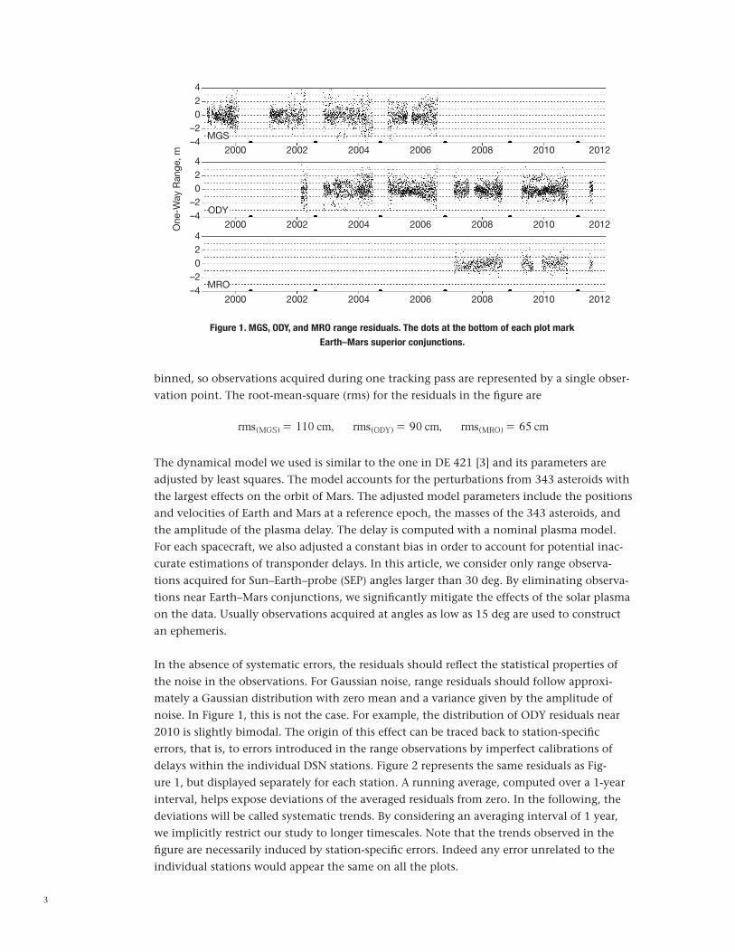
Station locations, the EOPs, and the ionospheric and tropospheric delays are known with a precision of a few cm. The preprocessed range data, besides any calibration imperfections, depends mainly on the plasma delay and the orbits of Earth and Mars. Figure 1 shows Mars range residuals obtained with a work version of the JPL planetary ephemeris. The residuals correspond to differences between the range observations and the predictions of a dynami-cal model adjusted to the same observations. Range data used throughout this study are

3

Figure 1. MGS, ODY, and MRO range residuals. The dots at the bottom of each plot mark

Earth–Mars superior conjunctions.

2000

2000

2000

MGS

ODY

MRO

2002

2002

2002

2004

2004

2004

2006

2006

2006

2008

2008

2008

2010

2010

2010

2012

2012

2012

4

4

4

2

2

2

0

0

0

–2

–2

–2

–4

–4

–4

One

-Way

Ran

ge, m

binned, so observations acquired during one tracking pass are represented by a single obser-vation point. The root-mean-square (rms) for the residuals in the figure are

, ,rms cm rms cm rms cm110 09 65( ) ( ) ( )MGS ODY MRO= = =

The dynamical model we used is similar to the one in DE 421 [3] and its parameters are adjusted by least squares. The model accounts for the perturbations from 343 asteroids with the largest effects on the orbit of Mars. The adjusted model parameters include the positions and velocities of Earth and Mars at a reference epoch, the masses of the 343 asteroids, and the amplitude of the plasma delay. The delay is computed with a nominal plasma model. For each spacecraft, we also adjusted a constant bias in order to account for potential inac-curate estimations of transponder delays. In this article, we consider only range observa-tions acquired for Sun–Earth–probe (SEP) angles larger than 30 deg. By eliminating observa-tions near Earth–Mars conjunctions, we significantly mitigate the effects of the solar plasma on the data. Usually observations acquired at angles as low as 15 deg are used to construct an ephemeris.

In the absence of systematic errors, the residuals should reflect the statistical properties of the noise in the observations. For Gaussian noise, range residuals should follow approxi-mately a Gaussian distribution with zero mean and a variance given by the amplitude of noise. In Figure 1, this is not the case. For example, the distribution of ODY residuals near 2010 is slightly bimodal. The origin of this effect can be traced back to station-specific errors, that is, to errors introduced in the range observations by imperfect calibrations of delays within the individual DSN stations. Figure 2 represents the same residuals as Fig-ure 1, but displayed separately for each station. A running average, computed over a 1-year interval, helps expose deviations of the averaged residuals from zero. In the following, the deviations will be called systematic trends. By considering an averaging interval of 1 year, we implicitly restrict our study to longer timescales. Note that the trends observed in the figure are necessarily induced by station-specific errors. Indeed any error unrelated to the individual stations would appear the same on all the plots.

4

Figure 2. Mars range residuals plotted for each DSN station separately. Observations from MGS, ODY, and

MRO are displayed in blue, gray, and black, respectively. The red dots represent

a running average computed over a 1-year interval.

2000 2002 2004 2006 2008 2010 2012 2000 2002 2004 2006 2008 2010 2012

DSS-14 DSS-43

DSS-15 DSS-45

DSS-24 DSS-54

DSS-25 DSS-55

DSS-26 DSS-63

DSS-34 DSS-65

2

2

2

2

2

2

0

0

0

0

0

0

–2

–2

–2

–2

–2

–2

2

2

2

2

2

2

0

0

0

0

0

0

–2

–2

–2

–2

–2

–2

One

-Way

Ran

ge, m

5

For the majority of stations, the systematic trends stay below 1 m. On stations 26, 43, 54, and 55, the trends are larger and can reach up to 2 m. The trends on these four stations contribute significantly to the overall dispersion in the range residuals. In particular, the constant bias on station 55 is responsible for the bimodal distribution mentioned earlier. To a first order, the trends in the residuals are reproduced in a consistent way by the three spacecraft. On some stations (e.g., station 55), there is a small discrepancy between the residuals from MRO and from ODY.

IV. Station Errors

We established that the systematic trends in Figure 2 are a consequence of station-specific errors. The relation between the trends and the underlying station errors can be expressed simply, if we assume that the distribution of the observations is the same on all 12 stations. Then, for a trend ri observed on a particular station i and for a systematic error zi intro-duced by the same station, we have

r z Pzi i m= -

where P represents the projection matrix on the vector space spanned by the partials of the observations. The vector zm represents the average station error, computed over the 12 sta-tions involved in the acquisition of the data:

...z

z z z12m

1 2 12=+ + +

The formula is derived in the Appendix. If the dynamical model is adjusted to range data from only one single station, we empirically observe that no systematic trend is present in the residuals on timescales larger than 1 year. The property is observed for all 12 stations. Thus, for any station i , we have Pz zi i= and the relation between the trends and the un-derlying station errors simplifies to

r z zi i m= -

We stress that the property Pz zi i= is observed empirically and is not general. It is specific to our dynamical model and the observational dataset. In the Appendix, we show that the parameters determined from range data are not sensitive to the individual station errors, but only to the average error Pz zm m= . Note that the average error corresponds exactly to the part of the station errors that does not appear in the residuals. Only the part of a systematic error that is not absorbed into the parameters of a model can appear in the re-siduals. The part that corrupts the adjusted parameters is absorbed and will remain hidden. Systematic trends in the residuals should be interpreted as a potential “tip of an iceberg”: an imperfection in the model or in the observations, insignificant by itself, but that may be a part of a larger systematic effect corrupting the estimated parameters.

Although the distribution of the range observations is in practice different from station to station, we will use the previous results as an approximation in order to interpret the trends of Figure 2 in terms of the actual station errors. As the residuals on the various stations cor-respond to the differences between the station errors and the average error, the individual

6

station errors are a priori undetermined. The observed trends provide only 11 indepen-dent relations between the 12 variables. The indeterminacy can be overcome only with an additional hypothesis. The stations involve various equipment and various geographic locations so a reasonable hypothesis consists in assuming that most of the station errors evolve independently and do not share a common trend. With this hypothesis, the residu-als on Figure 2 suggest that the average station error zm must be smaller than 1 m. Indeed, the residuals on most stations stay below 1 m; the errors for these stations stay then within 1 m of the average error and any variation of the average error larger than 1 m would cor-respond to a common trend among the stations (thus contradicting the hypothesis). In a way, the 1 m limit acts similar to noise. Trends in the residuals that rise above its amplitude represent actual station errors. Smaller trends do not represent individual station errors and should not be interpreted as such. An alternative hypothesis consists in assuming that, at any given date, the station-specific errors are distributed normally among the 12 stations. A conservative estimate for the amplitude of the average error zm is then given by the qua-dratic mean of the maxima of the 12 individual trends ri divided by the square root of the number of stations ( 12 ). This approach estimates the amplitude of zm at 40 cm.

Based on the previous considerations, significant trends in the individual station errors ap-pear only for stations 26, 43, 54, and 55. On station 55, the error corresponds to a constant bias. For the other three stations, the errors correspond to biases and ramps spanning parts of the interval between 1999 and 2012.

V. Reducing the Impact of the Station Errors

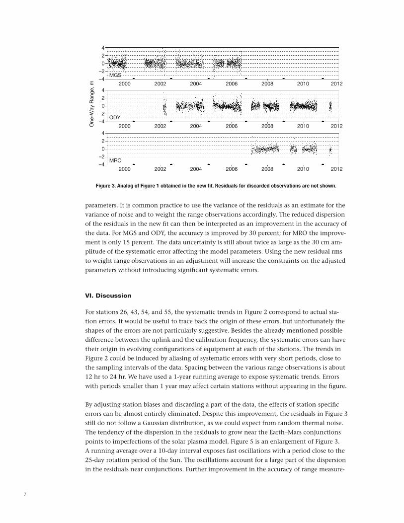
In order to reduce the station-specific errors, we include in the set of adjusted model pa-rameters two constant biases per station: one for MGS/ODY data and one for MRO data. We do not consider two separate biases for MGS and ODY, because in Figure 2, the systematic trends are reproduced consistently by both spacecraft. The adjusted biases can account for any constant imperfection in the calibration process. For example, the Z-correction is frequency dependent. According to [4], a difference between the calibration frequency and the uplink frequency on a given station may cause a constant delay of up to 10 ns (1.5 m in terms of one-way range). The estimation of constant biases will have only a small impact on the trends observed for stations 26, 43, and 54. In order to further reduce systematic errors in the range data, we partially discard observations from these stations. Data acquired by stations 26 and 43 before the 2005 conjunction are removed. Data from station 54 are re-moved up to October 2008. The discarded observations correspond to less than one tenth of all the available observations. Adjusting the model parameters, including the station biases, on the new dataset leads to the residuals shown in Figure 3. The rms of the residuals are

, ,rms cm rms cm rms cm0 580 6 5( ) ( ) ( )MGS ODY MRO= = =

Figure 4 shows range residuals obtained in the new fit on each of the DSN stations. All the systematic trends are smaller than 1 m. It follows then that, if we assume a normal distribu-tion of station errors among the 12 stations, the amplitude of the average error zm is 30 cm. By including station biases in the model and discarding a part of the observations, we reduced the dispersion of the residuals as well as the systematic error affecting the adjusted

7

Figure 3. Analog of Figure 1 obtained in the new fit. Residuals for discarded observations are not shown.

2000

2000

2000

MGS

ODY

MRO

2002

2002

2002

2004

2004

2004

2006

2006

2006

2008

2008

2008

2010

2010

2010

2012

2012

2012

4

4

4

2

2

2

0

0

0

–2

–2

–2

–4

–4

–4

One

-Way

Ran

ge, m

parameters. It is common practice to use the variance of the residuals as an estimate for the variance of noise and to weight the range observations accordingly. The reduced dispersion of the residuals in the new fit can then be interpreted as an improvement in the accuracy of the data. For MGS and ODY, the accuracy is improved by 30 percent; for MRO the improve-ment is only 15 percent. The data uncertainty is still about twice as large as the 30 cm am-plitude of the systematic error affecting the model parameters. Using the new residual rms to weight range observations in an adjustment will increase the constraints on the adjusted parameters without introducing significant systematic errors.

VI. Discussion

For stations 26, 43, 54, and 55, the systematic trends in Figure 2 correspond to actual sta-tion errors. It would be useful to trace back the origin of these errors, but unfortunately the shapes of the errors are not particularly suggestive. Besides the already mentioned possible difference between the uplink and the calibration frequency, the systematic errors can have their origin in evolving configurations of equipment at each of the stations. The trends in Figure 2 could be induced by aliasing of systematic errors with very short periods, close to the sampling intervals of the data. Spacing between the various range observations is about 12 hr to 24 hr. We have used a 1-year running average to expose systematic trends. Errors with periods smaller than 1 year may affect certain stations without appearing in the figure.

By adjusting station biases and discarding a part of the data, the effects of station-specific errors can be almost entirely eliminated. Despite this improvement, the residuals in Figure 3 still do not follow a Gaussian distribution, as we could expect from random thermal noise. The tendency of the dispersion in the residuals to grow near the Earth–Mars conjunctions points to imperfections of the solar plasma model. Figure 5 is an enlargement of Figure 3. A running average over a 10-day interval exposes fast oscillations with a period close to the 25-day rotation period of the Sun. The oscillations account for a large part of the dispersion in the residuals near conjunctions. Further improvement in the accuracy of range measure-

8

Figure 4. Analog of Figure 2 obtained in the new fit. Residuals for discarded observations are not shown.

2000 2002 2004 2006 2008 2010 2012 2000 2002 2004 2006 2008 2010 2012

DSS-14 DSS-43

DSS-15 DSS-45

DSS-24 DSS-54

DSS-25 DSS-55

DSS-26 DSS-63

DSS-34 DSS-65

2

2

2

2

2

2

0

0

0

0

0

0

–2

–2

–2

–2

–2

–2

2

2

2

2

2

2

0

0

0

0

0

0

–2

–2

–2

–2

–2

–2

One

-Way

Ran

ge, m

9

ments could be achieved by accounting for a plasma structure corotating with the Sun. The current model of the plasma delay is based on a stationary electron distribution, unable to reproduce the observed oscillations.

VII. Conclusion

For Sun–Earth–probe angles higher than 30 deg, up to 30 percent of the dispersion in Mars range residuals is due to station calibration imperfections evolving at timescales of 1 year or longer. The imperfections translate as systematic trends in the range residuals and as systematic errors in the adjusted model parameters. By discarding less than one tenth of the range data and accounting for a constant bias on each station, the imperfections can be almost entirely eliminated.

Acknowledgments

This research was supported by an appointment to the NASA Postdoctoral Program at the Jet Propulsion Laboratory, administered by Oak Ridge Associated Universities through a contract with NASA.

Figure 5. Range residuals, obtained with the new fit, near the 2001 and 2007 conjunctions. The left and right plots

are based on MGS and ODY data, respectively. The gray lines correspond to a

running average computed over a 10-day interval.

1999.6 2006.11999.8 2006.32000.0 2006.5

2 2

1 1

0 0

–1 –1

–2 –2One

-Way

Ran

ge, m

One

-Way

Ran

ge, m

10

References

[1] J. S. Border and M. Paik, “Station Delay Calibrations for Ranging Measurements,” The

Interplanetary Network Progress Report, vol. 42-177, Jet Propulsion Laboratory, Pasadena, California, pp. 1–14, May 15, 2009. http://ipnpr.jpl.nasa.gov/progress_report/42-177/177C.pdf

[2] A. S. Konopliv, S. W. Asmar, W. M. Folkner, Ö. Karatekin, D. C. Nunes, S. E. Smrekar, C. F. Yoder, and M. T. Zuber, “Mars High-Resolution Gravity Fields from MRO, Mars Sea-sonal Gravity, and Other Dynamical Parameters,” Icarus, vol. 211, no. 1, pp. 401–428, January 2011.

[3] W. M. Folkner, J. G. Williams, and D. H. Boggs, “The Planetary and Lunar Ephemeris DE 421,” The Interplanetary Network Progress Report, vol. 42-178, Jet Propulsion Labora-tory, Pasadena, California, pp. 1–34, August 15, 2009. http://ipnpr.jpl.nasa.gov/progress_report/42-178/178C.pdf

[4] P. W. Kinman, “Sequential Ranging,” Station Data Processing: 203C, in DSN Telecommu-

nications Link Design Handbook, DSN No. 810-005, Jet Propulsion Laboratory, Pasadena, California, March 22, 2012. http://eis.jpl.nasa.gov/deepspace/dsndocs/810-005/

[5] C. L. Thornton and J. S. Border, Radiometric Tracking Techniques for Deep-Space Naviga-

tion, DESCANSO Monograph Series, Pasadena, California: NASA Jet Propulsion Labora-tory, 2000. http://descanso.jpl.nasa.gov/Monograph/series1/Descanso1_all.pdf

[6] A. S. Konopliv, C. F. Yoder, E. M. Standish, D.-N. Yuan, and W. L. Sjogren, “A Global So-lution for the Mars Static and Seasonal Gravity, Mars Orientation, Phobos and Deimos Masses, and Mars Ephemeris,” Icarus, vol. 182, no. 1, pp. 23–50, May 2006.

11

Appendix

In the following, we assume that range observations are acquired simultaneously on all DSN stations. The hypothesis is equivalent to considering that the partials of the observa-tions with respect to model parameters are exactly identical from station to station. Using this simplifying hypothesis, we determine the relation between systematic trends in residu-als and the underlying station-specific errors. We also show that model parameters are not sensitive to the individual station errors, but only to their average. The computations are presented for n = 3 stations, but they extend naturally to any number of stations.

In a least-squares fit, the range residuals rg due to any systematic error zg are given by

( )r z M M M M zg g g gTg g

Tg

1= - -

where Mg represents the matrix of the partials of all the range observables with respect to the adjusted parameters. We implicitly assume that Mg is full rank. Expanding the equation in terms of measurements acquired at each station, we obtain

where

r

r

r

z

z

z

M M M M

z

z

z

M

M

M

Mg g

Tg g

Tg

1

2

3

1

2

3

11

2

3

1

2

3

= - =-

J

L

KKK

J

L

KKK

J

L

KKK

J

L

KKK

`N

P

OOO

N

P

OOO

N

P

OOO

N

P

OOO

j

The vectors r1, r2, r3 and z1, z2, z3 represent residuals and station-specific error on each of the n stations. M1,M2,M3 represent the matrices of partials for each individual station. The sim-plifying hypothesis guarantees that the matrices are identical. With M = M1 = M2 = M3, we verify that the residuals on any station i can be expressed as

( )where andr z Pz P M M M M zn

z1

i i mT T

m ii

n1

1

= - = =-

=

/

Note that the matrix P operates a projection on the vector space spanned by the columns of M. The relation may be used to interpret the systematic trends observed in the residuals in terms of the individual station errors. The systematic errors bD induced by zg on the estimated parameters are

M M M zgTg g

Tg

1bD =

-` j

Expressing Mg and zg in terms of z1, z2, z3 and M, we obtain directly

( )M M M zT Tm

1bD = -

In terms of systematic errors, the parameters are indeed sensitive only to the average station error zm. Note that in the above equation, zm can be replaced by Pzm without any loss of generality. The parameters are sensitive to exactly the part of the observations that is absent from the residuals.

JPL CL#12-2220