statistcs university of calwornia berkeley, californis
TRANSCRIPT

A Practleal Perspective on III-Posed Inverse Problems:
A Review with Some New Developments*
by
Finbarr O'Sulivan
Department of StatistcsUniversity of CalWorniaBerkeley, Californis
Technical Report No. 62
November 1985
*Research Supported by the National Science Foundationunder Grant No. MCS-8403239.
Department of StasttlesUnlversiy of CaliorniaBerkley, Caliornia

A Practical Perspective on III-Poned Inverse Problems:A Review with Some New Developments
Finbsrr O'SulivanDepartment of StatisticsUniversity of CaliforniaBerkeley. CA 94720.
ABSTRACT
IIl-posed inverse problems rise in many branches of wience and engineer-ing. In the typical situation one is interested in recovering a whole functiongiven a finite number of noisy measurements on functionals. Performancecharacteristics of an inversion algorithm are studied via the mean square errorwhich is decomposed into bias and variability. Variability calculations are oftenstraightforward, but useful bias measures are more difficult to obtain. Anappropriate definition of what geophysicists call the Backus-Gilbert averagingkernel leads to a natural way of measuring bias characteristics. Moreover, theideas give rise to some important experimental design criteria. It can be shownthat the optimal inversion algorithms are methods of regularization procedures,but to completely specify these algorithms the signal to noise ratio must be sup-plied. Statistical approaches to the empirical determination of the signal to noiseratio are discussed; cross-validation and unbiased risk methods are reviewed andsome extensions, which seem particularly appropriate in the inverse problem con-text, are indicated. Linear and non-linear examples from medicine, meteorologyand geophysics are used for illustration.
Key-words: ill-posed inverse problems, mean square error, averaging kernel, bias,variability, optimal inversion algorithm, experimental design, B-splines, crossvalidation, unbiased risk, predictive mean square error, estimable loss, randomspheres, integral equations, radiative transfer, distributed parameteridentification.
This work was supported by the National Science Foundation under GrantNumber MCS-8403239.

A Practieal Perspective on Il-Posed Inverse Problems:
A Revlew with Some New Developments
Finbarr O'SuUIvan
Department of Statistics
University of California
Berkeley. CA 94720.
1. Introductlon
Inverse problems have got to do with situations where one is interested in making inferences
about a phenomenon from partial or incomplete information. Accordingly, statistical estimation
and model building are both inverse problems. In modern science there is an increasingly impor-
tant clas of inverse problems which are not amenable to clasical statistical estimation procedures
and such problems are termed ill-posed. The notion of ill-posedness is due to Tikhonovl221 and
an extended treatment of the concept appears in Tikhonov and Arsenin[231. In an ill-posed
inverse problem, a classical least squares, minimum distance or maximum likelihood solution may
not be uniquely defined, moreover the sensitivity of such solution to slight perturbations in the
data is often unacceptably large.
A typical example of an ill-posed inverse problem is described by Nychka et al.[l91. Here
one is interested in the estimation of a 3-dimensional tumor size distribution in liver tissue, from
measurements on cross-sectional slices. A schematic for the experiment is given in Figure 1.1.
Figure 1.1 ABOUT HERE

- 2 -
Modeling tumors as spheres randomly distributed in the tissue an approximate integral relation-
ship between the 3-dimensional distribution of tumor radii and the 2-dimensional distribution of
radii observed in cros-sectional slices may be derived. Letting z, be the observed proportion of
2-dimensional slices with radii in the interval k ,z +tl one bas that
Z, = fK(2,,r)If r)dr + e, i =1,2, P,m
where e, are measurement/modeling errors. f 3 is the density of 3-dimensional tumor radii and
the kernels K (z, ,r ) are given by
0 e<r <z,
K (Z, ,r V77 zt<:r< z,+1rm/;z, Fr_X +1T ,+,<r <R
Physically, e is the smallest detectable tumor radius and R is the largest possible tumor radius in
the given section of tissue. Since e<=-1<z2< <**z,,<R, the estimation of fJ must be
restricted to the interval le,R 1. It is easy to to appreciate the ill-posednes of this inverse prob-
lem. The kernels K (Z. ,) are smooth, and as a result relatively large perturbations in f 3 can give
rise to very slight perturbations in the data and conversely. It follows from this that least
squares, minimum X2, or maximum likelihood solutions will be very sensitive to slight changes in
the data.
Ill-posed inverse problems have become recurrent theme in modern science, see for example
Crystallographyj231, Geophysics(2, 8, 251, Medical Electrocardiograms[l19, Meteorology(46, 471,
M1croffuroimagery1351, Radio Astronomy [241, Reservoir Engineeringj27, 371, and Tomogra-
phy|1O, SS|. Corresponding to this broad spectrum of fields of application, there is a wide litera-
ture on different kinds of inversion algorithms, that is, techniques for solving the inverse problem.
The basic principle common to all such methods is as follows; seek a solution that is consistent
both with the observed data and pnor notions about the phyrsical behavior of the phenomenon
under study. Different practical problems have led to unique strategies for implementation of this
principle, such as the Method of Regularization[531, Maximum Entropy[241 and Quasi-
Reversibility[281. Understanding the performance characteristics of a given inversion method is

- 3-
an important issue: Firstly, such information has obvious intrinsic value and secondly, it can criti-
cally influence the choice of experimental design, see section 2.
The primary goal of this paper is to identify some tools for assessing the finite sample per-
formance characteristics of an inversion algorithm. These tools, most of which can be found scat-
tered throughout the diverse inverse problem literature, are considered in the context of the fol-
lowing generalized non-linear regression model: Measurements, z,, are of the form are of the form:
z,= 7(sz,,) + (, i =1,2, * - - ,m
where O is in e ( the nominal parameter space), (z,, are linear or non-linear functionals of U,
and the E, are measurement errors assumed to have mean zero. In all that we discuss, there will
be an underlying assumption that the unknown true function, 9, is well approxAmated by a smooth
function. Though this assumption does not allow Us talk about highly discontinuous functions,
such as those that arise in typical pattern recognition problems, the model is still quite general,
and includes for example linear and non-linear integral equations of the first kind. Examples used
later on include the temperature retrieval problem in satellite meteorology, and the system
identification problem of reservoir engineering.
1.1. Iuvwslon Algorithms and the Method of Regulrlsatlon
An inversion algorithm, S, is a mapping that takes data into parameter estimates.
a= S.When S is linear then 0 can be written as a linear combination of impulse response functions, O,
i.e.
O(t) Ea,()z
where s, =So,, and *, is the i 'th unit vector in R . In statistical terms, an inversion algorithm
would be simply called an estimator, but here the terms estimator and inversion algorithm are
used interchangeably.

- 4-
One of the most useful techniques for generating inversion algorithms or estimators is the
Method of Regularization (MOR), see Titterington[541. The MOR procedure is due to Tikho.
nov(52, 531. There are various possible implementations of the method but they all amount to
choosing 0 to be the minimizer of a weighted combination of two functionals: The first functional
measures lack of fit to the observed data and the second measures physical plausibility of the esti-
mate. For example, we might choose 0 to be the minimizer of a criterion of the form
[Z[Z - i1(:, ,e)j2 + Al(O) , X > 0. (1.1)
The functional J is chosen so that highly irregular or physicall implausible O's have large values.
Statisticians will recognize this method as a version of Penalized Likelihood Estimation described
by Good and Gaskins[211; the sum of squares is the likelihood part and the functional J the
penalty term. The method is equivalent to the Method of Sieves introduced by Grenander(221.
Also, if J is chosen by some information principle such as entropy, J(0) = -f (t )logO(t )dt, then
the method of regularization yields a procedure equivalent to the Method of Maximum Entropy
pioneered by Jaynes, see Jaynes[241 and Chapter 4 of McLaughlin[341.
When the functionals, (;')are linear in 0, and J is quadratic with J(9) 2 0 ( 0 for
O = 0 ) then the solution to (1.1) is linear in the observed data. Nforeover, in this case the MOR
has an interesting Bayesian interpretation. To see this, first suppose that e is finite dimensional,
i.e. 0= uSon(ta with Ok linearly independent. The elements of 0 can be written as
#O for 5 = (Ol,2 * * - #K in RK, so that 0 can be identified with RK. Since J isk
quadratic and J(0) = 0, J(0) can be expressed as a quadratic form in .0, J() = n,, for some
positive semi-definite matrix nl. It follows that the MOR estimator is t,'k t where j minimizes
>2[z, -X, 012+Xi no
Here X is a design matrix, X,k = v(z, 0k). Thus j is given by
-= Ss where S = [X' X + m)xnljlX'

- -
Obviously, the MOR estimator is linear in the observed data. A Bayesian interpretation for 0. is
obtained by specifying a Gaussian prior with mean zero and covariance matrix proportional to
0'. Then, if the e, 's are independent and identically distributed Gaussian random variables with
mean zero, the MOR estimator, p, is the posterior mean of p given the data.
The foregoing statements carry through to more general settings. If e is a Ifilbert space
with inner product <, >, the 'i(;,j are bounded linear functionals and J is quadratic,
1(0) = <9,W9>, where W is positive semi-definite, then it can be shown, see Cox[131 for exam-
ple, that the MOR estimators have the form
9>= Ss where S =[X' X + mX\WIlX'
where the design matnx, X, is an operator derived from the the functionals i(: ,-. Thus S is a
linear operator from the data space into 0. General Bayesian interpretations for the method are
also available, these are discussed by Kimeldorf and Wahba[261. Further results on the optimality
of the MOR are described in section 2.
1.2. Outilne
Performance characteristics of an inversion algorithm are studied via the mean square error
which can be split into bias and variability components. Bias measures the systematic error while
variability measures the random error. In section 2 we consider linear inversion algorithms and
describe some ways of measuring bias and variability. Variability is calculated in a direct
manner. For bias it is convenient to introduce a generalized version of what geophysicists call the
Backus-Gilbert averaging kernel, see Backus and Gilbert[6, 71. The generalized notion of the
averaging kernel allows one compute the maximum or average expected bias and also leads to
some natural design criteria. These are described and illustrated in section 2.4. Optimal inver-
sion algorithms can be found and these turn out to be MOR procedures. The use of B-splines for
obtaining numerically convenient and accurate approximations to the averaging kernel and bias is
described in section 3. Though the theory of linear inverse problems is fairly well established, the
field of non-linear inverse problems is in its infancy. There are many exciting and challenging

- 6-
problers that need to be tackled in this area. The performance of MOR estimators when applied
to two interesting non-linear inverse problems is discussed in section 4. One of these problems
arises in satellite meteorology and is concerned with the estimation of atmospheric characteristics
such as temperature form upwelling radiance measurements. The second problem is of major
interest in reservoir engineering. It concerns the estimation of reservoir characteristics, such as
the easy of flow of fluid in the reservoir, from pressure-history data measured at distributed well
sites. As described in section 2, optimal inversion algorithms though MOR procedures are not
fully specified without supplying the signal-to-noise ratio. For a given problem this will not be
known and so has to be empirically determined. The final section of the paper deals with this
issue; the methods of cros validation and unbiased risk are described and some relevant exten-
sions to ill-posed inverse problems are developed.

2. Finite Sample Performance of an Inversion Algorithm
The quality of an inversion algorithm at some point, t, is measured by comparing the esti-
mate, O(t ), to the true value, O(t ). This difference can be decomposed into systematic and ran-
dom components as
e(#O(t) = O(t)-EO(I ) + EO(t)-O(t)
where the expectation is over the distribution of possible errors. The average performance of the
inversion at t is measured by the mean square error (MSE).
MSE(t E[O(te) O-t )12 1[(e ) - EG(t )12 + E[9(t ) - EO(t )12
=ise.2(t,) + var(t,9)
The mean square error depends both on O and the asumed error distribution. It is sum of the
squared bias, bias 2(t ,G), and the variance, var (t ,O). It the inversion algorithm is designed solely
to minimize bias then the variance dominates the mean square error and vice-versa. Thus a good
inversion algorithm must balance bias and variability, i.e. unbiasness may be a desirable property
in classical statistical estimation, but in the context of ill-pred inverse problems it is not.
Mean square error performance of an inversion algorithm can, in principle, be found by
Monte-Carlo simulation. Modern computing resources are making this a very viable and practical
approach. For linear problems one can avoid direct Monte-Carlo simulation and in the process
obtain some useful insights which can be applied to more complex situations.
2.1. Linar Problems
By a linear problem we shall mean that both the functionals, vi(z, ,), are linear in O, and the
inversion algorithm, S, is linear in the data.
2.1.1. VariabilIty
Variability computations for a linear inversion algorithms are very straightforward. Here,
variability does not depend on O and

- 8-
var(t,e) - var(t ) var ( u,(t)ej
where u, is the impulse response function. Thus if the errors, e,, have covariance ES, then
rar(t) .(ty e(g)
where r(t) (ul(t ),t2(t), ,u, (S()Y . In particular, if the errors are independent with con-
stant variance a2, then the variability is simply
var(t) a2 (t ys(t
2.1.2. Bl.
Bias properties are best understood by introducing the notion of the Averaging Kernel. In
certain circumstances the averaging kernel yields a representation of the form
Ee(t)= A(ts)O(u)du , (2.1)
for the systematic part of the estimate. The function A (t, ) is known as the averaging kernel at
t and A (l ,) determines the nature of the bias incurred at t. The averaging kernel is related to
what engineers and astronomers call the pointspread function. The point-spread function at t
is defined to be the solution obtained by the inversion algorithm when the true function is a Dirac
6-function at S and there is no measurement error. Thus from (2.1) if the averaging kernel at t is
A (t ,) then the point-spread at t is the function A ( ,t ).
The representation in (2.1) is an L2 representation for the averaging kernel. In the Geophy-
sics literature this representation is known as the Backus-Gilbert averaging kernel, after two geo-
physicists Backus and Gilbert[6, 71. Alternative representations for the averaging kernel are also
possible and these alternative representations are more useful when it comes to computing bias.
The averaging kernel and its generalizations are described next.

2.2. Averaging Kernel
2.2.1. Backus-Glibert Formulation
Backus and Gilbert worked in an integral equation context.
i(2 ,) = Ks (a)()d. =12 m
and the kernels K, ( ) are known smooth functions. For a linear inversion algorithm the E&(t) can
be written as
EO(t )- s (t f|Ks (o )(s )do
So, taking the summation inside the integral sign, we have
EB(t = A(tu )U(* )duwhere
A(t,) 2,(e)K,()t
The function A (t, ) is the Backus-Gilbert averaging kernel for the inversion algorithm S at t.
For illustration, an averaging kernel corresponding to a method or regularization procedure
applied to the tumor size distribution problem, described in section 1, is given in Figure 2.1.
Figure 2.1 ABOUT HERE
One can see that the kernel is well centered about the point or interest, r =.4. Moreover the ker-
nel seems fairly symmetric so that if the 3-dimensional tumor radius density were locally linear in
the neighborhood of this point then the inversion algorithm would be locally unbiased. Properties
of the averaging kernel can be varied by changing the regularization parameter, X - large values
of X cause the averaging kernel to be more spread out. Techniques for empirically selecting this
parameter are discussed in section 5.

- 10-
The center, spread and skewness of the averaging kernel give a rough appreciation for its
behavior. Assuming they exist, these are defined to be the first, second and third moment of the
absolute value of the averaging kernel when suitably normalized. Letting
= ,~~~~thenfIIAx(t,)I dt
Characterlstles of the Averaging Kernel
center: c()=f I Xx(t,*)I d.
spread: 8p(1)= If IAx(t,u)I(e-c(t))2d.
skewns: ek (t f IXx(,)v ('C(3t))Isdo
The skewnes is dimensionless while the center and spread are in t -units. Skewnesis important
since a symmetric averaging kernel ( uk (t )=O.) will exactly pas a linear trend.
Intuitively, the bias at a point, t, is determined by the how close the averaging kernel is to
a Dirac 6-function at t. Backus and Gilbert tried to develop some direct meaures of the nearness
of the averaging kernel to a Dirac 6-function - "6-ness of the averaging kernel". By choosing the
inversion algorithm, so that the averaging kernel is as 6-like as possible, subject to some upper
bound on the size of the standard error, one obtains so called Backus-Gilbert inversion algorithms.
The idea seems perfectly reasonable, however, there is some degree of arbitrariness in the 6-ness
criteria defined by Backus and Gilbert, moreover in general it is not true that the function max-
imizing a 6-nes criterion will necesarily be the Dirac 6-function. Problems with the 6-ness cri-
teria really arise because the Backus-Gilbert calculus takes place in an L2 setting where evalua-
tion is not a continuous linear functional. If we work in a space where evaluation is continuous,
we can derive a more reflned formulation of the averaging kernel and use a straightforward cal-
culus to assess 6-ness. The reflned definition of the averaging kernel also allows one deal with

- 11 -
more general linear functionals q(z,,O).
2.2.2. Reained Formulation of the Avera g Kernel
Prellmlnarles: Llnar Functionals and Representer
We shall need the notion of a representer of a continuous linear functional. To motivate
this concept, consider first the cue where 0 = spSnif (t} and the Ot are linealy independent.1<k<K
Here, elements of 0 are identified by a K -vector of coefficients, t in RK. Moreover the usual
inner product on R K determines an inner product on 0 by
<91,92> = .'6>2
K Kwhere 1 = O91k 4k, and °2 = S2t Ot. If i(,s,)i linear then for any 9 in 0
u(z .°)-X,' p (2.2)
Kwhere O= O and X, =-(i(,,AI,02), ** ,(Z,tK )f . X, determines an element,
ICK
St E X,t t . in 0 with the property that for all 9 in 0
ii(,,fl)=,,0
In functional analysis terms, *, is the representer of the linear functional i(,). An important
linear functional is evaluation at point. The representer in 0 of evaluation at t is given by
ICet = o2 (t )ok
One can easily verified that
0(t < et< re,> , fIor all in e.
The notion of a representer can be extended to more elaborate function spaces. The level of
functional analysis needed to understand this is very elementary and the interested reader might
consult Rudin[451. It is important to realize that, in general, the form of the representer depends

- 12-
on which inner product is used. Let 0 be a real Hilbert space with inner product <, > and
norm 11[11. A linear functional I is continuous if there is a constant M such that
1I(0)1 M Olell forall 9 in 0
Corresponding to any continuous linear functional, I, there exists a representer f in 0 such that
l(O) =- <C,9> tor all in 0
This is known as the Riesz representation theorem, Rudin(451. A Hilbert space of real valued
functions in which evaluation is continuous is known as Reproducing Kernel Hilbert Space
(RKHS). Reproducing kernel Hilbert spaces play an important role in applied mathematics. The
importance of RKHS in the study of ill-posed inverse problems has long been emphasisd by Pro.
lesor Wahba, see Wahbaj6g| and the references cited therein. Evaluation is not continuous in
L2, but is continuous in the space of functions whose fint derivatives are square integrable.
Represntr of the Averaging Kernel
Given the notion of a representer, the generalization of the averaging kernel is very simple.
Let 0 be a real Hilbert space with inner product <, > and suppose that the functionals (Z, ,)
are continuous with representers *,. Since
Ee(t ) ,(t )q(Z, ,e)
the representer of the averaging kernel, A (t ), is given by
Thus the averaging kernel is a linear combination of the representers of the functional v(s,).
The linear combination is determined by the impulse response functions of the inversion algo-
rithm.

- 13-
2.3. BIas Measures and Some Design Criteria
The more general formulation of the averaging kernel leads to natural ways of measuring
bias and this in turn motivates some useful design criteria. Let 0 be such that evaluation at t is
continuous and let et denote the corresponding representer. From the averaging kernel, the bias
at I may be written as
O(t)-~~ett_c-A (t)PO>
Average Blas
The representation, <et-A (t ),6>, can be used to compute the expected squared bias with
respect to a prior distribution on possible O values. Thus, if 0 = opan (0i) and a prior mean
and covariance for 6 is be specified by means of the coefficients of the *k 's, O,
E#10-Oo= , Var,[jSJ
then the average expected bias is
bl(t) = E[6(t )-E(t)2= Eo< et -A (t),>2= CttsoCt + <et-A (t ),9o>2K
wherect =(<et -A(t),tj>,<et -A(t),42>..-p,<et- A(t ),OK>Y andO0= EfO k k.
Maximum Bias
A less sophisticated measure of bias is the maximum bias over all functions in 0 whose
norm is less than some specified value, p. From the averaging kernel representation for bias and
the Cauchy-Schwartz inequality, this is given by
8up 1[(1 )EG(s )12 8=up <et-A (t ) 9>2 tIl-A (t )II22Ils10<0,2 iim 2<,,2
Thus letting bM,(t) = Ict-A (t )JI, bJ(t) is proportional to the maximum bias over any ball in 0.
Figure 2.2 plots the maximum bia, bM(S ), and standard error, square root of variability, for
a MOR inversion applied to the tumor size distribution problem. Both the bias and standard
error have poor behavior for small radii, suggesting that there is dificulty in getting reliable

- 14 -
estimates of the size distribution for small radii. This is largely a consequence of the fact that
small tumors are hard to detect, see Nychka et al.1381 for more discussion. The ripples in the plot
are due to the finite sample size, m =50, in this illustration. The vertical scales on the bias and
variability plots are left unspecified. If particular values for the g and a are asigned then an
appropriate scaling can be setup.
Figure 2.2 ABOUT HERE
Design Criteria
Combining bias with variability gives an overall asessment of the performance of the inver-
sion algorithm which can be used for design purposes. The average bias measure gives rise to a
an Average Mean Square Error design criterion (AMSE):
AMSE(t )P(t ) + var (t)
Also, from the maximum bias measure, we obtain the Maximum Mean Square Error design cri-
terion (MMSE):
MMSE(t) =2b2(a)+ var(t)
2.4. OptImal Inversion Algorithms and Experimental Design
Since both the average and maximum mean square errors depend on the inversion algo-
rithm, we can select the algorithm which perfornm best with respect to either of these criteria.
Interestingly, the solution one obtains in each case is a MOR procedure. This analysis can be car-
ried out in a very general setting, however the structure of these results becomes most clear when
0 is finite dimensional and the measurement errors are mean zero uncorrelated with constant
variance a.

- 1S-
Mllmlsang the Average Mean Squar Error
Let s() =(l(t ),u (t), * * , K(t)). For simplicity suppose that the prior for P ha zero
mean and covariance 12 E. The average mean square error can be written as
AMSE(t )=2(Xt-Xe(i )f E (X-Xi )) +a9(Iy e(t)
where Xt = (01(0),4(t), * K* (t )f and the i 'th row of X is given in equation (2.2). MInim-
izing with respect to (t ) we have
a2IX'P OX + 7 1 i(t )=X' EoXt
This holds for any 1. If Ep is invertible, then, by straightforward algebra, the optimal inversion
algorithm can be expremed as
S-=X' X + 7E-11-7XI
Comparing this with the forms given in section 1.1, it can be seen that the optimal algorithm
corresponds to a MIOR estimator with X =2
and J (0) = Pj'p. X-1 is interpreted as the
signal-to-noise ratio.
Malmlsug the Maxlmum Mean Square Error
The maximum mean square error in a ball of radius A is given by
MMSE(t) = p2jXt _ S (t )X 1' IXt - EV.(t)X, I + c2s(t)' (t)
Minimizing with respect to s(1 ), we get that the optimal vector satisfies
tx' x + 42i11Q)=- X' xt
Thus the optimal inversion algorithm is given by
02S1- X'X +yIIX'
Again, this is a MOR inversion algorithm with X = 22 and J(0)= I11011. X-1 is againmpis

- 16 -
interpreted as a signal-to-noise ratio.
Versions of the above results have appeared at several times in the literature. Weinreb and
CrosbylOOI credit Foster[18j, see also Strand and Westwater[SI|. The optimal inversion algorithm
from the point of view of average mean square error is called the minimum-rms solution while the
optimal solution for maximum mean square error is the minimum information solution. Generali-
zations of these results have appeared in the statistics literature. Kimeldorf and Wahba[261 show
that the minimum-rms solution is sometimes interpretable a an optimal Bayesian procedure.
Minimum information solutions are also been termed minimax. Results on the minimaxity of the
MOR are given by Li[291, and also Speckman[481. In practice the signal-to-noise ratio is not
known so that the parameter X needs to be set empirically. Some statistical methods available for
doing this are given in section S.
Expwlmental Design
The MMSE and the AMSE are also functions of the the design points, z, i =1,2 * * * ,m,
and an optimal experimental design can be defined as the design making the MMSE or the AMSE
minimum. Since one may not be interested in performance at just a single point, l, an integrated
AMSE or MMSE over some region of interest is often more appropriate. Crosby and Weinrebl[Olhave carried out a program of this kind in connection with the selection of spectral wavelengths
for satellite radiometers. Their criterion is reduced to a simple trace criterion, see eqn. (10) of
their paper. More recently, Wahba[581 has also discussed the design issue. She presents two
design criterion: one of which is akin to Weinreb and Crosby's criterion, see eqn. (13), and a
second which is termed the "degrees of freedom for signal" criterion. The use of integrated mean
square error as a design criterion is not new to statisticians. Box and Draperl9g proposed this as a
design criterion for model-robust response surface designs. Further discussion of this literature can
be found in section 5 of the recent paper by Steinberg and Hunter[60.

- 17-
3. Numerical Approximatlon of the Averaging Kernel with B-spilne
Exact computation of averaging kernels requires the manipulation of the representers of the
functionals q(z, ,) for i = 1,2, * * ,m. In reproducing kernel Hilbert spaces there are theoretical
formulas available for the evaluation of representers, see Nychka et al.[381 for example. However,
direct evaluation of averaging kernels by means of such formula is extremely inefficient, compu-
tationally, and other approaches are needed. Approximating the elements of 0 by simpler forms,
it is often possible to obtain highly efficient methods for evaluating the averaging kernels at a
negligible loss in accuracy. To illustrate this we consider one very popular MOR procedure for
estimating a one-dimensional real valued function, U defined on an interval [a ,b |: ° is the minim-
izer over the Sobolev space W2 [a ,b jIe of
[lZs .(I 0j)12 + Xf[(t)12ds X > .
W?2 [a,b I is an infinite dimensional Hilbert space with inner product
<0,> @=fe(e )0te )di + fe(s )O(t )dt 0,0 in W2 l[a b
Sobolev spaces are discussed at length in the book by Adams11l. It is well known that the ele-
ments of e can be approximated to arbitrarily high degree of accuracy by cubic B-splines and we
can make good advantage of this in the computation of the averaging kernels. Before describing
this we pause briefly to describe cubic B-splines. The standard reference on B-splines is the book
by de Boorlf161. Throughout this section we continue to assume that the functionals 11(Z,) are
linear.
3.1. Bmspfles
Consider a set of distinct knot points [t1<t2<....<tK441 with t3<a and b <tz4. (Multi-
ple knots are also allowed, see de Boor[161 for more details). A cubic spline on a ,b I is a cubic
polynomial between successive knot points joined up at the knots so as to have continuous second
derivative over the interval la ,b 1. By increasing the knot density in [a ,b 1, functions in
W22 [a,b I can be very closely approximated by cubic splines. Cubic splines can be expremed as a

- 18 -
Klinear combination of basis elements (Bk )k-. The elements, Bk, of the basis are called B-splines
(B stands for basis) and the entire basis is called the B-spline basis. Each element of the basis is
non-negative and has very local support: in fact Bk is zero outside of the interval [tktwkk+4J Over
[tk,tk+41. Bk is proportional to the probability density for the sum or four independent uniform
random variables, U, , i -1,2,3,4, where U, is defined on [tk+-a,l-k..I. The local support pro-
perty or B-splines can be used to great advantage in computations. de Boor[|lB has developed a
set of Fortran prograns for manipulating B-splines and these are now available in most modern
mathematical software libraries.
3.2. ComputatIon of the Averaging Kernel In a B-splln basis
Let 0K = ( Bk )f.... The MOR estimate ON is approximated as 09 #m t Bk wherek
,& IX' X + mX021-'X' s (3.1)
b
and X,k =- (:, ,B ) and 2(j, k)f )B, (s)Bk(t )dt:.
K KThree inner product, on 0K will be defined. For 9 = °t Bk, and E- tk Bt in 0,
we have
Eucildean Inner Products
K
<84>5 rVO*kk = V where *=(Ul,°2,** - KY and t ,4'KY
L 2 Inner Products
<4>2 J =fe(t)O(t)ds = e 00* where Ila(j,k) = fB,(t)Bk(t)dt,
Sobol.v Inner Product:
<eO>s = fe(t)O(t)di + fe(t)-()dt = [no+ n2J1Corresponding to each inner product there is an approximate representation for the averag-
ing kernel at t . Let these be denoted A,(i ), A (t ), and As(t ),

E6) (t)<A,(t),@> r-<A2(t),9>2= <As(t),O>s
AE(t1) is most easily computed; from (3.1), its B-spline coefficients are given by
a,(t)=X' X[XI X + mXf2I-1S(t)
where .(t) = (B1(t),B4A 1), ,Bx(t )) are the B-spline coeficients of the representer of
evaluation at t ( with respect to the Euclidean inner product). The B-spline coefficients, a2(t)
and a, (t ), of A 2(t ) and As (t ) are directly obtained from the a, (t ).
A40) =o',(&#) ; as (t)[flO +o l[1a(t )
A word of caution: The matrices 0O and |l0O + 021 are poorly conditioned for K large. As a
result a very stable method such as a singularvalue decomposition, see Dongarra et al.[171, should
be used to compute the inverses. From the L2 representation, we have that the Backus-Gilbert
averaging kernel at t is approximately given by
K
The Sobolev representation for the averaging kernel is
KA, (t, ast(I)Bk(k
Bia Computations
The average and maximum bias can be approximated directly in terms of the Euclidean
Krepresentation for the averaging kernel in (Bk )k.. For example, the maximum bias in a ball
of radius s in 0e W2 [a ,b I is M2b2(I) where
b2(t ) [.(t -a&, (t )j' [o + n2l-ll'e( ) . (t )I

- 20-
4. AppilcatIon to Non-Linear Invere Problems
We shall now apply the techniques described in section 2 and 3 to the study of two non-
linear ill-posed inverse problerm taken from satellite meteorology and reservoir engineering. In
both cases the function, O, of interest is restricted to be one-dimensional and we consider the fol-
lowing MOR procedure: O is the minimizer in W2 [ b of
Z - q(z 90)12 + XfI(- )12 X >0°
In order to study performance characteristics, we linearize the tunctionals q(;,,) about some
value OO
(s.,G)A mg((sg o) + v77(z:,° oXU-°o) ,
and consider the properties Of a modified MOR procedure: O is the minimizer of
1 [z'. - Vi,X(Z, 'go) j12 + lf[(t)2d X>
where z z= - v1(z ,fo) + v'(z ,0o)0o. The averaging kernel calculus can be applied to the
modified MOR procedure and the results of this linearized analysis are presented below. A
rigorous justification for the linearization is not attempted. (This is a very challenging problem
and even an asymptotic analysis seems to be quite difficult. The theory presented in Cox and
O'Sullivan[141 may provide a starting point for further investigation of this topic). It is asumed
that the analysis will give reliable results whenever the degree of non-linearity in the functionals v
is low.
To compute averaging kernels, bias and variability for the linearized problem, we use a B-
spline basis and rollow the development in section 3. The number of basis elements is chosen so
that any plots of averaging kernels, and bia and variability characteristics, are Visually
unchanged by the addition of extra basis elements. The design matrix, X, has the form
X.k = vl(z.,,o)Bt i=1,2,...M
where Bt is the k'th element of the B-spline basis. Two sets of system libraries were employed:

- 21 -
computations for the satellite meteorology example were carried out on a DEC VAX 11/750
machine using the Bspline and Linpack routines which are part of the publicly available CMLIB;
computations for the reservoir engineering example, required repeated numerical solutions Of a
diffusion equation, and these were carried out on a Boeing Computer Serices Cray 1 machine
using routines available in the BCSLIB.
4.1. Temperature Retrevalfrom Stlolte Radiance Data
Intensities of radiation measured by modern meteorological satellites provide information
about atmospheric characteristics such u temperature and moisture. This new database is
becoming an increasingly important tool in the proces of nowcauting, i.e. specifying the current
state of the atmosphere, and forecasting, i.e. describing the future states of the atmosphere.
Smith ct at 1471 and SmithI461 describe the basic features of these measurement systems. A typi-
cal climatological temperature profile is given in Figure 4.1. The vertical axis is decreasing in
pressure while the horizontal axis gives temperature. It is standard practice for meteorologists to
plot things in this way because moving up the vertical axis then corresponds to going higher up in
the atmosphere. The plot shows a temperature inversion near 20 mb, the temperature is generally
increaing as one moves away from this point. Inversions are a characteristic feature of atmos-
pheric temperature profiles. The location of this upper atmosphere temperature inversion is
known as the tropopause height.
Figure 4.1 ABOUT HERE
The processing of radiance data to get temperature estimates involves the solution of an
interesting inverse problem. The radiative transfer equations, LiouI311, are used to model how the
intensity of radiation, z,, at frequency v,a, depends on the temperature profile T, temperature as
a function of premure, in the column beneath the satellite;

where
R,(T) = BV(T(xs))r(. ) - fB,1T(x))IT,(*)dzSo
and : is some monotone transformation of pressure p; 2, corresponds to the surface and zo
corresponds to the top of the atmosphere. Meteorologists usually work in kappa -units, i.e.
z (p ) - p 6/, because atmospheric variations are believed to be slowly varying in this scale. rT(z)is the transmittance of the atmosphere above : at wavenumber v, and B, is Planck's function
given by:
B,(T = c 1a/[ezp (c2v/TT)-IIwhere
C i.g9o6XlO4erg -cm2-sec1and
C 2 1.43868cm -dec (K).
The measurement errors, c,, are roughly mean zero and uncorrelated, however, different channels
have different noise levels so by dividing through by relative noise levels in channels we obtain a
generalized non-linear regression model as in section 1. The TIROS-N system, see Smith ct
at 1471, has fifteen channels (m =15). Linearizing the RV, (T) about the climatological profile,
TO, given in Figure 4.1, we get
s.
vrR,,(T4T = k. (v. )T(z,)+ fk(v,,z)T(z)dz
where k, (v) = B,[ T. (:, )1rV(z ) and k (V,S) = - BV| T, (z )]j*s ). Since the linearized functionals
have an explicit form, the linearized design matrix is very easy to compute by numerical integra-
tion.
X,k TvR,(T. )Bk = k(v.)Bk(;) + fk(v. ,2 )Bt(z )dzI'

- 23 -
where Bk is the k'th element of the B-spline basis.
An averaging kernel at 700 millibars for the MOR inversion is given in Figure 4.2. The
corresponding bias and variability characteristics are given in Figure 4.3. Again these plots
correspond to a particular value for the regularization parameter X. Larger values for the smooth-
ing result in broader averaging kernels, more bias and less variance.
Figure 4.2 ABOUT HERE
Figure 4.3 ABOUT HERE
Notice that the averaging kernel has sharp behavior near the surface. This is attributable to the
microwave channels. The data obtained from these are nearly direct measurements of the surface
okin temperature, T (z, ). As a result the L 2 representers of the functionals corresponding to
these channels are very spiked at the surface and since the averaging kernel is a linear combina-
tion of these representers, the behavior at the surface is to be expected. The effect of the
microwave channels on the bias is is also quite dramatic. The variability profile indicates regions
near 600mb and 200 mb where sampling density might be improved. However, there are physical
constraints on selection of spectral wavelengths which make it difficult to get good coverage
throughout the atmosphere, see pp 250 ff of Liou[311. The operating characteristics given in Fig-
ure 4.3 relate to maximum bias. In a meteorological setting, where there is a huge database of
prior information on atmospheric variation, an average bias measure with respect to a climatologi-
cal prior would be more appropriate. In spite of the fact that there is a dependence on the initial
climatology, T,, the retrieval characteristics predicted by the averaging kernel calculus is largely
in agreement with those found by Monte-Carlo simulation in O'Sullivan and Wahba[391.

- 24
4.2. The History Matching Problem of Reervolr Englneerng
The dynamic flow of fluid through a porous medium is usually modeled by a diffusion equa-
tion
au(X,t) - d (x)u(x,I)) = q(x,t) x in n ,p
in [O,TI
subject to prescribed initial and boundary conditions. Here u is pressure, q accounts for the
withdrawal or injection of fluid into the region 0, and a is the transmiivity or conductance
which determines the ease with which fluid flows through the medium. The initial condition is
u (x,O) = v. (x) and a typical boundary condition is no fluid flow acros the boundary of the
region, i.e. -df = 0, where w represents the direction normal to the boundary. The history
matching problem arises as one tries to use scattered well data on (x, ,t,) and q (xs,),
i-1,2, * ,m, j-1,2, * ,x, to infer the diffusion parameter, a, see Cooley[11, 121, Kravaris
and Seinfeld[271 and Neuman and Yakowitz[371. This problem is an example of a broad clas of
inverse problems which arise in connection with partial differential equations. These problems
have attracted an amount of pure mathematical interest. See Anger[41, Lionsl301, McLaugh-
lin[341, and especially Payne[411.
For a simplified version of the history matching problem let n-10,11 and T =1. Assume
there is no injection or withdrawal of fluid and that there is no flow across the boundary. Sup-
pose that we have 10 measurement sites at; = (Si 3)/49 , i 1,2, * - ,10, and readings on v
are made for t, - 0.0(.007)0.5. These data are modeled by a non-linear regression
Z,) = va(Z.,t,;e)+a E
where the errors are mean zero with constant variance.
The dependence of u (z, ,t, ;a ) on a is again non-linear. By linearizing u (z, ,t, ;a ) about a
plausible transmissivity profile, ao, such as the one given in Figure 4.4, we can compute averaging
kernels, etc. The true pressure history plays a significant role in determining the information
recovered about transmissivity. Roughly speaking, gradients in the pressure history generate

- 25 -
information about the transmissivity. A pressure history corresponding to the transmissivity
profile in Figure 4.4 is given in Figure 4.5. This pressure history is driven by an initial pressure
distribution which ranges from 10 at =0. to 100 at =1.
Figure 4.4 ABOUT HERE
Figure 4.5 ABOUT HERE
Computatlon of the LLnearlzed Desin Matrix
Unlike the temperature retrieval problem, we do not have an explicit analytical representa-
tion for the observed functionals, and this makes the computation of the design matrix a bit more
complicated.
x =]t=VV(z'st,u o)B = ,aa(tU;.o)Olak
Kwhere the gradient is taken in the direction of functions of the form a () =- ak Bt (x) and u
is the solution to
d9u a (=z)au (z,t) with (z,t) in I0,1IX[l,.51
subject to for z _ Oil
Let D (a): U- Q X U.xBOxBI denote the mapping
D(a)t. =[I ag-a daaa)u )au(0) au(1,)D (av7s (-ox, ' I

- 26 -
Under regularity, by applying the implicit function theorem, the inverse of D (a), denoted G (a),
exists and is differentiable in a neighborhood of Go.
G (a ) f ,u. ,O,O I (-,-;)
The relation G (a )D (a) = I may be used to obtain - (z, ,t, ;.0). Differentiating, we have
a0( (a )D(. OG(a)clak a~~~akas
Thus
G(a - _G(a aD(a)GaOcGak ask
which implies
OD _ - (G) _ u Os
But OaD ( -8 )Bk (X )L9-.) 000,O J, and the expression simplifies to
Clak ____ ____ 0 O
au = G(ao) [ - (Bk()-)a ,OO,Oj
Hence X,,k can be round by solving the original diffusion equation with the forcing term, q,
replaced by O-{Bk (z ) @u!) and the initial pressure distribution, u,, replaced by the constant 0.
By this method, the computation of the entire linearized design matrix requires K separate
numerical solutions of the diffusion equation (K being the number of basis elements). Although
this is a generally applicable technique, it is rather inelegant. Since the solution corresponding to
Bk is likely to be "near" the solution corresponding to Bk+ it may be possible to improve com-
putational efficiency by using some form of relaxation. This is currently being investigated. For
the time invariant problem, Neuman and Yakowitz[371 use properties of a particular finite
difference scheme to develop a fast method for computing the analogue of the design matrix. A
further approach to this problem, relying on an optimal control formulation, is employed by Kra-
varis and Seinfeld[271.

- 27-
Llnearised Averaging Kerneb and Retrieval Characteritis
Figures 4.6 and 4.7 give linearized averaging kernels and retrieval characteristics.
Figure 4.6 ABOUT HERE
Figure 4.7 ABOUT HERE
One would suspect that information about a should depend critically on the true presure history.
If the initial pressure were constant, then, since there would be no presure gradients, there would
be no lateral flow. However, the functional parameter is a transmisivity and information about
transmisivity can only be generated by lateral flow. The averaging kernel and the bias and vari-
ability characteristics show that for the given pressure history, the greatest detail on transmis-
sivity is recovered near the middle of the z-range. Changing the presure history results in
different retrieval properties - the bias and variability calculus seems to make very good physical
sense.

- 28 -
5. Empirical Selection of Smoothing Parameters
Nearly all inversion algorithms, and in particular the MOR, have explicit or implicit
smoothing/tuning parameters, corresponding to the signal-to-noise ratio which, in a practical set-
ting, have to be selected by the user. Two of the more popular techniques to emerge from the
statistical literature on this problem are the methods of crow-validation and unbiased risk estima-
tion. Typically, these techniques try to find that value of the smoothing parameter which minim-
izes the predictive mean square error (PMSE).
PMSE(X) = 2.. [, ,0) -i(; ,a)j2m,
where 0 and Ox are the true and estimated functions. (Throughout this section we will use X to
denote the smoothing/tuning parameters of the inversion algorithm). The predictive mean square
(PMSE) is a convenient criterion but not necessarily a criterion of real intrinsic interest. Inverse
problens are focused on a particular function, so it seenm more appropriate to phrase a loss
directly in terms of that function. Thus it might be of interest to consider a loss of the form
L (X) _ E l°(t, )_jx(t, )12
where the t,'s are some points of direct interest to the investigator. For certain loss functions,
which are cstimable in the sense described below, it is ponsible to develop refined versions of the
cross-validation and unbiased risk assessments. It should be pointed out that the PMSE has a
certain robustness property; it is often the case that the best choice of the smoothing parameter,
from the point of view of PMSE loss, is very nearly optimal from the point of view of other loss
functions also, see Cox [131, Lukas[321, Ragozin[421 and WahbaI571. Thus the practical need for
refined procedures will only arise in situations where the PMEE and the loss function of interest
have very different minimizers.
We assume throughout that we are dealing with linear inversion algorithms and that the
functionals p(z,,0) are themselves linear in 0. For some extensions to non-linear inversion algo-
rithms, see O'Sullivan and Wahba[391, O'Sullivan et al.1401, Villalobos and WahbaISBI and

- 29-
Wahbaj5gj. A brief review of crosrvalidation and unbiased risk in the standard predictive mean
square error context is given next. For a more detailed discusson of these methods see the recent
review of Titterington[541.
5.1. Empirlcal Assesment of PMSE
The Hat-matri, H(X), is defined to be the matrix that maps data s into predictions l,
-= H(\)s
For a linear inversion algorithm the Hat-matrix is obtained from the impulse response functions,
*I(k), via
H,, (X) -o- t(z, v*,(N))
Here the dependence of the inversion on the smoothing/tuning parameters X is highlighted- the
impulse response functions are functions of X. The trace of the Hat-matrix occurs in both the
crosvalidation and unbiased risk assessments of the PMSE. We begin with the unbiased risk
method, which is easier to describe.
Unblased Rlsk
This procedure assumes that one has a reliable estimate of the noise level a. Given a, the
procedure uses the residual sum of squares (RSS) to construct an unbiased estimate of the PMSE
risk. The basic steps are as follows:
PMSE(X)= 1 1 ,
i.e. =( (vq(zj,,vi(z2,j), 4)(z')r . By linearity, the expected value of the predictive mean
square error is
mE(PMSE(X)) = 111-H(X)! (I)II2 + etrIH(X\ H(A)I
BL4S2(X) + o2tr H(Xf H(X)I
Meanwhile,

- 30-
RSS(A)-, IZ_z i, 12 [|I _H-] (X)ISII 2RSS(X\) = az- 2nII-()5I
So the expected value is
E(RSS (X)) = II' -H (X)I;(O)II 2 + Ml,r IjI-H ()1'II-H(X)IJ
BIAS X) + 2tr [[I-H(X)j' [I-H(X)jJ
Combining these formulae we have that
PMSE(X) =-RSS(X) - o + 2a2 tr jH(,)Im m
is an unbiased estimate of the predictive mean square error. In the standard regression context
H = X(X' X)-'X' , and PMSE reduces to Mallows' C, statistic, see[331.
Croin-Vaildatlon
In cross-validation one considers, I., which is defined to be the prediction of "(:, ,) from
an estimator constructed from data with the i'th data point, z,, omitted. The idea being that if
the prediction rule is really good, that is, X well chosen, then i, should be reasonably close to z,
on average. Ordinary cross-validation or Allen's predictive sum of squares (PRESS), see Allenj31,is defined to be
vo(A FSIZ,-z 1
For the MOR estimators in section 1.1, where H(X) X[X' X+mXW[1'X' , a rank one
update formula, can be used to show that
(z,-i, )
(1-,, (X))
where h,, (X) is the i'th diagonal element of the Hat-matrix, also known as the i'th leverage
value. It follows that the ordinary cross-validation assessment is a weighted residual sum of
squares
I n2
Zs -ZsVs (x) = -E 0
m I ad I-As$ (x)

- 31-
If instead of dividing residuals by 1-h,, (X) we divide by the mean value, 1-h,, (X), then we obtain
the Generalized Cross Validation (GCV) of Craven and Wahba[ISI. The GCV score is usually
written as
[Zs 4'Jr,1
I,i2
1-- trH (X)12m
We point out that, since
V(X) - RSS(X)m [I--L trH(X)j2m
in a regreuion context, where H = X(X' X)"X' , the GCV score is proportional to the resi-
dual mean square divided by the degrees of freedom for error. So in this context, the GCV score
reduces to a model selection statistic proposed by Anscombe[SJ and simplified by Tukey, see pp.
388 ff Mosteller and Tukey[361.
A great deal is known about the asymptotic behavior of the above empirical asessments
methods. The typical result says that the minimizer of the empirical assessment tends to minim-
ize the PMSE, in large samples; Monte carlo simulation results show that a similar property tends
to hold in finite samples, see for example Craven and Wahba[1S], Golub Heath and Wahba[201,
Nychka et a&1381, RiceI431, and Speckman[491.
5.2. Emplilcal Assessment of Estimable Looe
Borrowing from the terminology of the standard linear model we can characterize an estim-
able functional as follows
Definition: A continuout linear functional < , > iu estimable if there ezists c in RI such that
Ec s= < ,C> forall 9 in 0 .
Clearly, since q(z,, ) are continuous linear functionals, <f, > is estimable iff c in R such
that

- 32 -
where C, are representers of v(:, ,) in e. With this we say that a loss function is eutimablC if it
defined in terms of eutimable functionals.
To illustrate how to empirically asses estimable loses we consider a particular estimable
los of the form
rL (X) 2<C,9->2
where C, are all estimable. Let ec be such that
rC, = SCJC,1. j=1, ,T .
A simple modification of the crosvalidation and unbiaed risks techniques can be formulated to
directly asess the loss L (X).
Unbised RIsk Asseoment of L (X)
By a development similar to that used in RiceI44l, the expected value of L (X) as
E[L(X)l = <C, ,-EO9,>2+ v2Se,' [I-H(X)' I1I-H(X)Ie,1 )~~~~-
= BIAS2(X) + a2 I-H(Xy I[I-H(X)Ic
The sum of squares
SS= e[C] s - C]' U12has expected value
E[SSI = BIAS2(X) + av2,'H(efH(H)c,
Thus
r (L (A) =SS - o,2 e/ elc + 2o2E C] ' (xr el
,_=,_M

- 33-
is an unbiased estimate of L (X). Again note that a reliable estimate of a is necessary in order to
be able to use this assessment.
CrosValidatlon ment of L (X)
The cros-validation procedure is sligbtly more complicated to derive. Instead of leaving
out one data point, we now omit the c, 'th component of the data and use the remaining data to
develop a prediction, cs.,, of <., 9>. The cros-validation asessment then compares c, ' s to
es-,, i.e.
rvs (X) E ICe,' s - cu_,l
In the context of MOR estimators the situation becomes clearer. To make the notation less com-
plicated, suppose the e are normalized so that c} ce = 1 for j =1,2, ... , T. Let
Pi =I--e,,
PI is a projection onto the space orthogonal to el. The estimator obtained by removing the
c,'th component minimizes
I [ip (s-0())1' P:-IP% (a-(9))j + X< o,WG>
where P,_ is the generalized inverse of P, . Since P, P,-P, = P, , it follows that
cis_. = cl IX[' P,X + mxW['X' P,s .
Again, using a rank one update formula and some algebra we have that
c I-t IlewH(scwlI
where H(X) =XXX' X + m XW j-'X' . Thus the ordinary cross-validation score is
r 2
C,iI-Cl'H £ 12
and the GCV extension is
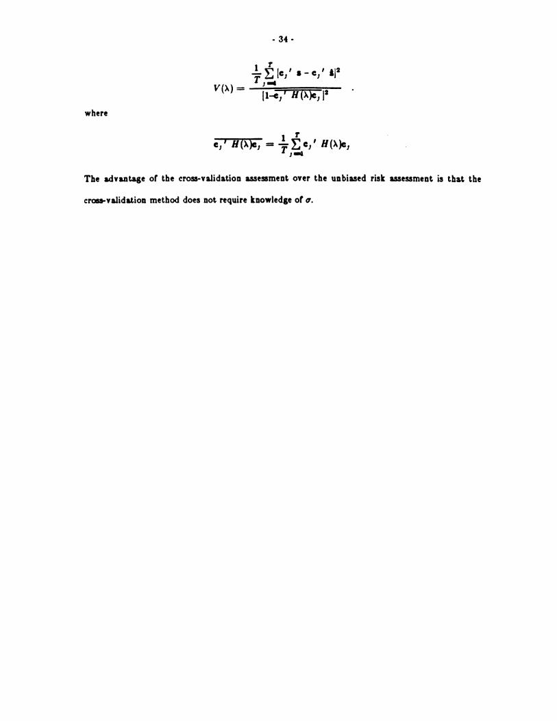
- 34-
I 1 1I] s - eljV(A)-~ ~~~(,)e
where
re,' H(X)c, T Eel' H(,\),
j =I
The advantage of the cros-validation assemment over the unbiased risk assessment is that the
cross-validation method does not require knowledge of a.

- 35-
Acknowledgements
The motivation for this article arose out of a series of presentations I gave in a seminar on
"Inverse Problems and Statistical Signal Models" jointly organized with David Donoho at Berke-
ley in the Spring of 1985. I would like to thank the participants in the seminar and also D. L.
Banks, B. A. Bolt, D. R. Brillinger, M. H. DeGroot, J. A. Rice, G. Wahba, and two referees for
many useful comments which have lead to substantial improvements in the paper.

Adams, R. (1975). Sobolev Spaces, Academic Pres.New York.
121 Aki, K. and Richards, G. (1980). Quantitative Seismology: Theory and Method, W.
H. Freeman.San Francisco.
[31 Allen, D. M. (1974). "The relationship between variable selection and data augmen-
tation and a method of prediction," Technometrics 1, pp. 125-127.
[41 Anger, G. (1979). Inverse and Improperly Posed Problem. in Differential Equation:
Proceedings of a Conference on Mathematicl and Numerical Methods, Akademie.
Verlag.Berlin.
[51 Anscombe, F. J. (1967). "Topics in the investigation of linear relations fitted by least
squares," J. Roy. Statist. Soc. B 29, pp. 1-62.
161 Backus, G. and Gilbert, F. (198). "The resolving power of gross earth data," Geo-
physics Journal of the Royal Astronomical Society 255, pp. 18206.
[71 Backus, G. and Gilbert, F. (1970). "Uniqueness in the inversion of inaccurate gross
earth data," Philos. Trans. Royal Soc. Ser. A. 255, pp. 123-192.
[81 Bolt, B. A. (1980). "What can inverse problems do for applied mathematics and the
sciences," Search 11, 8,
[91 Box, G. E. P. and Draper, N. R. (1959). "A bas for the selection of a response sur-
race design," Amer. Statist. Assoc. 54, pp. 622-853.
[101 Budinger, T. F. (1980). "Physical attributes of single-photon tomography," J. NucI.
Med. 21, 6,
[11j Cooley, R. L. (1982). "Incorporation of prior information on parameters into non-
linear regression groundwater flow models, 1 Theory,' Water Resour. Re#. 18, pp.
[11

- 37 -
965-g76.
1121 Cooley, R. L. (1983). "Incorporation of prior information on parameters into non-
linear regression groundwater flow models, 2 Applications,' Water Reoovr. Rev. 19,
pp. 682-478.
[131 Cox, D. D. (1983). 'Approximation of the method of regulaization estimators." Tech.
Rep. No. 723, Statistics Dept., Universty of Wisconsin-Madison .
1141 Cox, D. D. and O'Sullivan, F., (1985). Analysis of penalized likelihood type estimators
wib application to generalized smoothing in Sololev Spaces, Manuscript.
[151 Craven, P. and Wahba, G. (1979). "Smoothing noisy data with spline functions:
estimating the correct degree of smoothing by the method of generalized cros-
validation," Numer. Math. 91, pp. 377-403.
1181 DeBoor, C. (1978). A Prcetical Gvide to B-Splineu, Springer-Verlag.New York.
[171 Dongarra, J. J., Bunch, J. R., Moler, C. B., and Stewart, G. W. (1979). Linpack
User's Guide, SIAM.Philladelphia.
[181 Foster, M. R. (1961). "An application of the Weiner-Kolmogorov smoothing theory
to matrix inversion," J. SIAM 9, pp. 387-392.
[191 Franzone, P. Colli, Taccardi, B., and Viganotti, C. (1977). "An approach to inverse
calculation of epi-cardial potentials from body surface maps," Adv. Cardiol. *1, pp.
167-170.
[201 Golub, G., Heath, M., and Wahba, G. (1979). "Generalized cross validation as a
method for choosing a good ridge parameter," Technometrico 51, pp. 316-224.
- 38 -
1211 Good, 1. J. and Gaskins, R. A. (1971). 'Non-parametric roughness penalties for pro-
bability densities,' Biometriks 58, pp. 255-277.
[221 Grenander, U. (1981). Abstract Inference, J. Wiley.
[231 Grunbaum, F. A. (1975). 'Remark on the phue problem in Crystallography,' Proc.
Nat. Acad. Sci. USA 72, 5, pp. 1699gl701.
[241 Jaynes, E. T. (1983). Papers on Probability, Statittice and Statitical Physics, Syn-
these Library.
[251 Jeffreys, H. (1976). The Earth, Cambridge University Press.
[261 Kimeldorf, G. S. and Wahba, G. (1971). 'Some results on Tchebychefflan Spline
Functions,' Mathematical Analysis and Application. 99, pp. 824-95.
[271 Kravaris, C. and Seinfeld, J. H. (1g85). 'Identification of parameters in distributed
parameter systems by regularization,' SIAM J. Control and Optimization 19, 2, pp.
217-241.
j281 Lattes, R. and Lions, J. L. (1969). The Method of Quasi-reversibility, Applications to
Partial Differentil Equation., American Elsevier.New York.
[291 Li, K. C. (1982). 'Mfinimaxity of the metbod of regularization on stochastic
processes," Ann. Statist. 10, pp. 937-942.
[301 Lions, J. L. (1971). Optimal Control of System, Governed by Partial Differential
Equations, Springer-Verlag.Berlin.
Liou, K. (1979). Introduction to Atmospheric Radiation, Academic Press.London.1311

- 39 -
1321 Lukas, M. (1981). "Regularization of linear operator equations.." Unpublished Ph.D.
thesis, Australian National University .
1331 Mallows, C. L. (1973). "Some comments on C,," Technometrics 15, PP. 661-675.
1341 McLaughlin, D. W. (1983). Inverse Problems: Proceedings ofa Symposium in Applied
Mathematics, American Mathematical Society.
[351 Mendelsohn, J. and Rice, J. (1983). "Deconvolution of Micro-furometric histogruas
with B.splines," J. Amer. St.ti.t. Assoc. 77, pp. 748-753.
[381 Mosteller, F. and Tukey, J. W. (1977). Data Analysi and Regression, Addison-
Wesley.Reading, MA.
[371 Neuman, S. P. and Yakowitz, S. (1979). "A statistical approach to the inverse prob-
lem of aquifier hydrology 1. Theory," Water Regour. Res. 15, pp. 845-880.
[381 Nychka, D., Wahba, G., Goldfarb, S., and Pugh, T. (1984). "Cross-validated spline
methods for the estimation of three-dimensional tumor size distributions from observa-
tions on two dimensional cross sections," 1. Amer. Statiet. Assoc. 79, 388,
[391 O'Sullivan, F. and Wahba, G. (1985). "A cros validated Bayesian retrieval algo-
rithm for non-linear remote sensing experiments," Journal of Computat. Physics 59, 3,
pp. 441-455.
[401 O'Sullivan, F., Yandell, B., and Raynor, W. J. (1986 (in press)). "Automatic smooth-
ing of regression functions in generalized linear models," Amer. Statist. Assoc.,
[411 Payne, L. E. (1975). "Improperly Posed Problems in Partial Differential Equations,"
In Regional Conference Series in Applied Mathematics, SIAM.

- 40-
1421 Ragozin, D. (1981). "Error bounds ror derivative estimates based on spline smoothing
of exact or noisy data." Tech. Rep. No. GN-50, Statistics Dept., University of
Washington-Seattle.
[431 Rice, J. A. (1984). "Bandwidth choice for nonparametric regression," Ann. Statist.
1*, pp. 1215-1230.
1441 Rice, J. A. (1984). "Bandwidth choice for differentiation.' Manuscript .
1451 Rudin, W. (1976). Principles of MatIematicd Analsi, McGraw-Hill.New York.
1461 Smith, W. (1983). "The retrieval of atmospheric profiles from VAS geotationary
radiance observations," 1. Atmotpheric Sciences 40, pp. 2025-2035.
[471 Smith, W. L., Woolf, H. M., Hayden, C. NM, Wark, D. Q., and McMillin, L. M.
(October 1979). "The TIROS-N operational vertical sounder," Bull. Amer. Meteor.
Soc. 50, 10, pp. 1177-1187.
[481 Speckman, P. (1979). Minima estimates of linear functional. in Hilbert space,
Department of Mathematics, University of Oregon.
[491 Speckman, P. (1982). "Efficient nonparametric regression with cross-validated smooth-
ing splines." Tech. Rep. No. 45, Statistics Dept., University of Missouri-Columbia .
[501 Steinberg, D. M. and Hunter, W. G. (1984). "Experimental design: review and com-
ment (with discussion)," Technometrics £5, 2, pp. 71-130.
[511 Strand, 0. N. and Westwater, E. R. (1988). "Minimum-rms estimation of the numer-
ical solution of a Fredholm integral equation of the first kind," SIAM J. Numer. Anal.
5, pp. 287-295.

- 41-
1521 Tikhonov, A. (1963). "Solution of incorrectly formulated problems and the regulari-zation method," Soviet Math Dokl 5, pp. 1036-1038.
[531 Tikhonov, A. and Arenin, V. (1977). Solutions oflU-Posed Problems, Wiley.New
York.
[541 Titterington, D. M. (1985). "Common structure of smoothing techniques in statis-
tics.," Intenational Statistical Review 55, pp.. 141-170.
(SSI Vardi, Y., Shepp, L. A., and Kaufman, L. (1985). "A statistical model for positron
emision tomography," J. Amer Stastt. Autoc. 80, 389,
(561 Villalobos, M. and Wahba, G. (1983). Commun. Statist. A 12, pp. 1449.1480.
[571 Wahba, G. (1979). "Smoothing and ill-posed problems," pp. 183.194. In Solution
Method for Integral Equations with Applications, ed. M. Goldberg,Plenum Prem .
[581 Wahba, G. (1983). "Design criteria and eigensequence plot, for satellite computed
tomography." Tech. Rep. No. 732, Statistics Dept., University of Wisconsin-Madison .
1591 Wahba, G. (1984). "Cros-validated spline methods for the estimation of multivariate
functions from data on functionals," pp. 205-233. In Statistic.: An Appraisal, ed. H.
A. David and H. T. David,The Iowa State University Prem .
[60l Weinreb, M. P. and Crosby, D. S. (1972). "Optimization of spectral intervals for
remote sensing of atmospheric temperature profiles," Remote Sensing of the Environ-
ment 2, pp. 193.201.

Figure Legends
Figure 1.1: Reconstruction of the Tumor Size Distribution from data on cross
sectional slices
Figure 2.1 Sample Averaging Kernel for a MOR procedure applied to the Tumor
Problem
Figure 2.2 Maximum Bias and Standard Error for a MOR procedure applied to the
Tumor Problem. The ripples are due to the finite sampling (m =50).
Figure 4.1: Typical climatological profile, T.. Vertical axis is pre3ure in kappa scale.
Horizontal aXis is in degrees Kelvin. Note the temperature inversion high up in the
atmosphere.
Figure 4.2: Averaging Kernel at 700mb for the Temperature Retrieval Problem.
Vertical axis is pressure in kappa scale. Horizontal axis is in degrees Kelvin. The
sharp behavior near the surface is attributable to the microwave channels.
Figure 4.3 : Inversion Characteristics of a MOR procedure applied to the Temperature
Retrieval Problem
Figure 4.4: A Transmissivity Distribution, a0, for the History Miatching Problem
Figure 4.5: True Presure History.

Figure 4.8: Sample Avenging Kernels for a MOR procedure applied to the History
Matching Problem.
Figure 4.7: Inversion Characteristics of a MOR procedure applied to the History
Miatching Problem. Retrieval properties are best near the middle of the z range.

Figure 1.1
Section of Timue
<
Crow Sectional Slices
A3distribution oftumor radii
K
distribution oftumor radii(cdt F2 )
DATA:
= F4z32,)-F42(z) , z, < z,+.
MODEL:R
Zs m fK(z,,r)fs(r)dr + e,c
xi x;,p

Averaging Kernel at r = .4 (Figure 2. 1)
.I
\I
\I\
I.
II
0.0 0.2 0.4 0.60.8 1.0~~~~~~~~~~~~~~~~~~~~~~~~~~~~~~~~~~~~~~~.11I
0.0 0.2 0.4 0.6 0.8 1.0

Inversion Characteristics (Figure 2.2)
0.0 0.2 0.4 0.6 0.8
Standard Error
0.0 0.2 0.4 0.6 0.8 1.0
Maximum Bias
1.0

Climatological Temperature Profile (Figure 4.1)
N.~~~~~~~~~~~~~~~~NN
.NL
xi
.I

Averaging Kernel at 700 millibars (Figure 4.2)
'I
Ii
/
. ._. _ . _ . _ .-~~~

Inversion Characteristics (Figure 4.3)
Standard ErrorMaximum Bias

Transmissivity Profile (Figure 4.4)
0.2 0.4. 0.6 0.8
x
000
0r-0
0
0
000.0 1.0

True Pressure History (Figure 4.5)
//47 -.Wk...

Sample Averaging Kernels (Figure 4.6)
0OD
4o
eq
0
eo
0
0O
I I
I II'' I1
i I; - /"
N. Il 7 ~ 1
%W. I %01". .
p~~~~~~
0.0 0.2 0.4 0.6 0.8 1.0
x=.2
0.0 0.2 0.4 0.6 0.8 1.0
x=.4
NAI II II II II I
I II I
I
0'-4
0
0'-4
00
N
1
04.
0LA
\
_-J -
\ I
/
0.0 0.2 0.4 0.6 0.8 1.0
x=.8
/ \,
I
0'-4
0
0'-4
00
0
m
I
l
_,
I., -- --
I %
II
- II
I
I
I
i-1
III
I I I
0
OD
o
(40
0.0 0.2 0.4 0.6 0.8 1.0
x=.6
I" f
I
. 0
1

Inversion Characteristics (Figure 4.7)
0.0 0.2 0.4 0.6 0.8 1.0 0.0 0.2 0.4 0.6 0.8 1.0
Standard ErrorMaximum Bias
TECHNICAL REPORTSStatistics Department
University of Califoria, Berkeley
1. BREIMAN, L and FREEDMAN, D. (Nov. 1981, revised Feb. 1982). How many varables should be entaed in aregression e Jour. Amer. Statist Assoc., Marchi 1983, 78, No. 381, 131-136.
2. BRILLINGER, D. R. (Jan. 1982). Some contasting exwamples of the time and fequency domain approaches to time seriesanalysis. Time Series Methods in Hydrosciences, (A. H. E1-Shaarawi and S. R. Esterby, eds.) Elsevier ScientificPublishing Co., Amsterdam, 1982, pp. 1-15.
3. DOKSUM, K. A. (Jan. 1982). On the performance of estimates in proportional hazard and log-linear models. SurvivalAnalysis, (John Crowley and Richard A. Johnson, eds.) IMS Lectre Notes - Monograph Series, (Shanti S. upta, seriesed.) 1982, 74-84.
4. BICKEL, P. J. and BREIMAN, L. (Feb. 1982). Sums of functions of nearest neighbor distances, moment bounds, limittheorans and a goodness of fit test. Ann. Prob., Feb. 1982, 11. No. 1, 185-214.
5. BRILIJNGER, D. R. and TUKEY, J. W. (March 1982). Spectrum estimation and system identification relying on aFourier transform. The Collected Works of J. W. Tukey, vol. 2, Wadsworth, 1985, 1001-1141.
6. BERAN, R. (May 1982). Jackknife approximation to bootstrap estimates. Am. Statist, March 1984, 12 No. 1, 101-118.
7. BICKEL, P. J. and FREEDMAN, D. A. (June 1982). Bootstrapping resion models with many parameters.Lehmann Festschrift, (P. J. Bickel, K. Doksum and J. L. Hodges, Jr., eds.) Wadsworth Press, Belmont, 1983, 2848.
8. BICKEL, P. J. and COLLINS, J. (March 1982). Minimizing Fisher information over mixtures of distributions. S1983, 45, Series A, Pt. 1, 1-19.
9. BREIMAN, L. and FRIEDMAN, J. (July 1982). Estimating optinal transformations for multiple regression and correlation.
10. FREEDMAN, D. A. and PETERS, S. (July 1982 revised Aug. 1983). Bootstrapping a regression equation: someempircal results. JASA, 1984, 79, 97-106.
11. EATON, M. L. and FREEDMAN, D. A. (Sept. 1982). A remark on adjusting for covariates in multiple regrssion.12. BICKEL, P. J. (April 1982). Minimax estimation of the mean of a mean of a nonnal distribution subject to doing weil
at a poinL Recent Advances in Statistics, Academic Press, 1983.
14. FREEDMAN, D. A., ROTHENBERG, T. and SUTCH, R. (Oct. 1982). A review of a residential energy end use model.
15. BRILLINGER, D. and PREISLER, H. (Nov. 1982). Maximum likelihood estimation in a latent variable problem. Studiesin Econometrics, Time Series, and Multivariate Statistics, (eds. S. Karlin, T. Amemiya, L. A. Goodman). AcademicPress, New Yor, 1983, pp. 31-63?
16. BICKEL, P. J. (Nov. 1982). Robust regression based on infinitesimal neighborhoods. Ann. Statist., Dec. 1984, 12,1349-1368.
17. DRAPER, D. C. (Feb. 1983). Rank-based robust analysis of linear models. I. Exposition and review. Statistical Science,1988, Vol.3 No. 2 239-271.
18. DRAPER, D. C. (Feb 1983). Rank-based robust inference in regression models with several observations per cell.
19. FREEDMAN, D. A. and FENBERG, S. (Feb. 1983, revised April 1983). Statistics and the scientific method, Commentson and reactions to Freedman A rejoinder to Fienberg's comments. Springer New York 1985 Cohort Analysis in SocialResearch, (W. M. Mason and S. E. Fienberg, eds.).
20. FREEDMAN, D. A. and PETERS, S. C. (March 1983, revised Jan. 1984). Using the bootstrap to evaluate forecastingequations. J. of Forecasting. 1985, Vol. 4, 251-262.
21. FREEDMAN, D. A. and PETERS, S. C. (March 1983, revised Aug. 1983). Bootstrapping an econometric model: someempircal results. JBES, 1985, 2, 150-158.
22. FREEDMAN, D. A. (March 1983). Structral-equation models: a case study.
23. DAGGETT, R. S. and FREEDMAN, D. (April 1983, revised Sept 1983). Econometrics and the law: a case study in theproof of antitrust damages. Proc. of the Berkeley Conference, in honor of Jerzy Neyman and Jack Kiefer. Vol I pp.123-172. (L. Le Cam, R. Olshen eds.) Wadsworth, 1985.

- 2 -
24. DOKSUM, K. and YANDELL, B. (April 1983). Tests for exponentiality. Handbook of Statstics, (P. R. Krishnaiah andP. K. Sae, eds.) 4, 1984, 579-611.
25. FREEDMAN, D. A. (May 1983). Comments on a paper by Markus.
26. FREEDMAN, D. (Oct 1983, revised March 1984). On bootsaping two-stage least-squares estimates in stationary linearmodels. Amn. S 1984, 12, 827-842.
27. DOKSUM, K. A. (Dec. 1983). An extension of partial likelihood methods for proportional hazard models to generaltransformation models. Ann. Statist., 1987, 15, 325-345.
28. BICKEL, P. J., GOETZE, F. and VAN ZWET, W. R. (Jan. 1984). A simple analysis of third order efficiency of estimateProc. of the Neyman-Kiefer Conference, (L. Le Cam, ed.) Wadsworth, 1985.
29. BICKEL, P. J. and FREEDMAN, D. A. Asymptotic normality and the bootstrap in stratifed sampling. Arm. Statist12 470482.
30. FREEDMAN, D. A. (Jan. 1984). The mean vs. the median: a case sdy in 4-R Act litigation. JBES. 1985 Vol 3pp. 1-13.
31. STONE, C. J. (Feb. 1984). An asymptotically optimal window selection rule for kemel density estimates. Ann. SDec. 1984, 12, 1285-1297.
32. BREIMAN, L. (May 1984). Nail finders, edifices, and Oz.
33. STONE, C. J. (Oct. 1984). Additive regression and othe nonparametric models. Ann. Statist., 1985, 13, 689-705.
34. STONE, C. J. (June 1984). An asymptotically optimal histogram selection rule. Proc. of the Berley Conf. in Honor ofJerzy Neyman and Jack Kiefer (L Le Cam and R. A. Olshen, eds.), , 513-520.
35. FREEDMAN, D. A. and NAVIDL W. C. (Sept. 1984, revised Jan. 1985). Regression models for adjusdng the 1980Census. Statistical Science. Feb 1986, Vol. 1, No. 1, 3-39.
36. FREEDMAN, D. A. (Sept. 1984, revised Nov. 1984). De Finetti's theorem in continuous time.
37. DIACONIS, P. and FREEDMAN, D. (Oct. 1984). An elementary proof of Stirling's formula. Amer. Math Monthly. Feb1986, Vol. 93, No. 2, 123-125.
38. LE CAM, L. (Nov. 1984). Sur l'approximation de familles de mesures par des familles Gaussienes. Ann. InsLHenri Poincar6, 1985, 21, 225-287.
39. DIACONIS, P. and FREEDMAN, D. A. (Nov. 1984). A note on weak star uniformities.
40. BREIMAN, L. and IHAKA, R. (Dec. 1984). Nonlinear discriminant analysis via SCALING and ACE.
41. STONE, C. J. (Jan. 1985). The dimensionality reduction principle for generalized additive models.
42. LE CAM, L. (Jan. 1985). On the normal approximation for sums of independent variables.
43. BICKEL, P. J. and YAHAV, J. A. (1985). On estimating the number of unseen species: how many executions werethere?
44. BRILLINGER, D. R. (1985). The natural variability of vital rates and associated statistics. Biometrics, to appear.
45. BRILLINGER, D. R. (1985). Fourier inference: some methds for the analysis of aray and nonGaussian series dataWater Resources Bulletin, 1985, 21, 743-756.
46. BREIMAN, L and STONE, C. J. (1985). Broad spectrum estimates and confidence intervals for tail quantiles.
47. DABROWSKA, D. M. and DOKSUM, K. A. (1985, revised March 1987). Partial likelihood in transformation modelswith censored data. Scandinavian J. Statist., 1988, 15, 1-23.
48. HAYCOCK, K. A. and BRILLINGER, D. R. (November 1985). LIBDRB: A subroutine library for elemntary timeseries analysis.
49. BRILLINGER, D. R. (October 1985). Fitting cosines: some procedures and some physical examples. Joshi Festschrift,1986. D. Reidel.
50. BRILLIJGER, D. R. (November 1985). What do seismology and neurophysiology have in common? - StadsticslComptes Rendus Math. p Acad. Sci. Canada. January, 1986.
51. COX, D. D. and O'SULLIVAN, F. (October 1985). Analysis of penalized likelihood-type estimators with application togeneralized smoothing in Sobolev Spaces.

- 3 -
52. O'SULLIVAN, F. (November 1985). A practical pespective on ill-posed inverse problems: A review with somenew developnmnts. To appear in Journal of Statistical Science.
53. LE CAM, L and YANG, G. L (November 1985, revised March 1987). On the preservation of local asymptotic normalityunder infonnation loss.
54. BLACKWEL1 D. (November 1985). Approximate normality of large products.
55. FREEDMAN, D. A. (June 1987). As others see us: A case study in path analysis. Jounal of EducatonalStatistics. 12, 101-128.
56. LE CAM, L. and YANG, G. L. (January 1986). Replaced by No. 68.
57. LE CAM, L (February 1986). On the Berstein - von Mises theorem.
58. O'SULLIVAN, F. (January 1986). Estimation of Densities and Hazards by the Method of Penalized likelihood.
59. ALDOUS, D. and DIACONIS, P. (February 1986). Strong Uniform Times and Finite Random Walks.
60. ALDOUS, D. (March 1986). On the Markov Chain simulation Method for Unifonn Combinatorial Distributions andSimulated Annealing.
61. CHENG, C-S. (April 1986). An Optimization Problem with Applications to Optimal Design Teory.
62. CHENG, C-S., MAJUMDAR, D., STUFKEN, J. & TURE, T. E. (May 1986, revised Jan 1987). Optimal step typedesign for comparing test treatments with a controL
63. CHENG, C-S. (May 1986, revised Jan. 1987). An Application of the Kiefer-Wolfowitz Equivalence Theorem.
64. O'SULUIVAN, F. (May 1986). Nonparametic Esimation in the Cox ProporIonal Hazards Model.
65. ALDOUS, D. (JUNE 1986). Finite-Time Implications of Relaxation Times for Stochastically Monotone Processs.
66. PITMAN, J. (JULY 1986, revised November 1986). Stationary Excursions.
67. DABROWSKA, D. and DOKSUM, K. (July 1986, revised November 1986). Estimates and confidence intervals formedian and mean life in the proportional hazard model with censored data. Biometrika, 1987, 74, 799-808.
68. LE CAM, L and YANG, G.L. (July 1986). Distinguished Statistics, Loss of information and a theorem of Robert B.Davies (Fourth edition).
69. STONE, C.J. (July 1986). Asymptotic properties of logspline density estimation.
71. BICKEL, PJ. and YAHAV, J.A. (July 1986). Richardson Extrapolation and the Bootstrap.
72. LEHMANN, E.L. (July 1986). Statistics - an overview.
73. STONE, C.J. (August 1986). A norparametric framework for statistical modelling.
74. BIANE, PH. and YOR, M. (August 1986). A relation between Lcvy's stochastic area fornula, Legendre polynomial,and some continued fractions of Gauss.
75. LEHMANN, EL. (August 1986, revised July 1987). Comparing Location Experiments.
76. O'SULLIVAN, F. (September 1986). Relative risk estimation.
77. O'SULLIVAN, F. (Sepember 1986). Deconvolution of episodic hormone data.
78. PiTMAN, J. & YOR, M. (September 1987). Further asymptotic laws of planar Brownian motion.
79. FREEDMAN, D.A. & ZEISEL, H. (November 1986). From mouse to man: The quantitative assessment of cancer risks.To appear in Statistical Science.
80. BRILLIJGER, D.R. (October 1986). Maxmum likelihood analysis of spike trains of interacting nerve cells.
81. DABROWSKA, D.M. (November 1986). Nonparametric regression with censored survival time data.
82. DOKSUM, K.J. and LO, A.Y. (Nov 1986, revised Aug 1988). Consistent and robust Bayes Procedures forLocation based on Partial Information.
83. DABROWSKA, D.M., DOKSUM, KA. and MIURA, R. (November 1986). Rank estimates in a class of semiparametrictwo-samplc models.

- 4 -
84. BRILLINGER, D. (December 1986). Some statistical methods for random process data from seismology andneurophysiology.
85. DIACONIS, P. and FREEDMAN, D. (December 1986). A dozen de Finetti-style results in search of a theory.Ann. Ist. Here P Sia6, 1987, 23, 397-423.
86. DABROWSKA, D.M. (January 1987). Uniforn consistency of nearest neighbour and kernel conditional Kaplan- Meier estimate.
87. FREEDMAN, DA., NAVIDI, W. and PETERS, S.C. (February 1987). On the impact of variable selection infitting regression equations.
88. ALDOUS, D. (February 1987, revised April 1987). Hashing with linear probing, under non-uniform probabilities.89. DABROWSKA, D.M. and DOKSUM, KA. (March 1987, revised January 1988). Estimating and tsting in a two
sample generalized odds rate model. J. Amer. Statist. Asoc., 1988, 83, 744-749.
90. DABROWSKA, D.M. (March 1987). Rank tests for matched pair experiments with censored data.
91. DlACONIS, P and FREEDMAN, D.A. (April 1988). Conditional limit theorems for exponential families and finiteversions of de Finetti's theorem. To appear in the Jounal of Applied Probability.
92. DABROWSKA, D.M. (April 1987, revised September 1987). Kaplan-Meier estimate on the plane.
92a. ALDOUS, D. (April 1987). The Harmonic mean formula for probabilities of Unions: Applications to sparse randomgraphs.
93. DABROWSKA, D.M. (June 1987, revised Feb 1988). Nonparamnetric quantile regression with censored data.
94. DONOHO, D.L & STARK, PJB. (June 1987). Uncertainty principles and sipal recovery.
95. CANCELLED
96. BRILLINGER, D.R. (June 1987). Some examples of the statistical analysis of seismological data To appear inProce Centnnial Anniversary Symposium, Seismographic Stations, University of California Berkeley.
97. FREEDMAN, DA. and NAVIDI, W. (June 1987). On the multi-stage model for carcinogenesis. To appear inEnvironmental Health Perspectives.
98. O'SULLIVAN, F. and WONG, T. (June 1987). Detrmining a function diffusion coefficient in the heat equation.99. O'SULLIVAN, F. (June 1987). Constrained non-linear regularization with application to some system identification
problems.100. LE CAM, L. (July 1987, revised Nov 1987). On the standard asymptotic confidence ellipsoids of Wald.
101. DONOHO, D.L. and LIU, R.C. (July 1987). Pathologies of some minimnm distance estimators. Annals ofStatistcs, June, 1988.
102. BRILLINGER, D.R., DOWNING, K.H. and GLAESER, R.M. (July 1987). Some statistical aspects of low-doseelectron imaging of crystals.
103. LE CAM, L. (August 1987). Harald Cram6r and sums of independent random variables.
104. DONOHO, A.W., DONOHO, D.L. and GASKO, M. (August 1987). Macspin: Dynamic graphics on a desktopcomputer. IEEE Computer Graphics and applications, June, 1988.
105. DONOHO, D.L. and LIU, R.C. (August 1987). On minimax estimation of linear functionals.
106. DABROWSKA, D.M. (August 1987). Kaplan-Meier estimate on the plane: weak convergence, LIL and the bootstrap.
107. CHENG, C-S. (Aug 1987, revised Oct 1988). Some orthogonal main-effect plans for asymmetrical factorials.
108. CHENG, C-S. and JACROUX, M. (August 1987). On the construction of trend-free run orders of two-level factorialdesigns.
109. KLASS, M.J. (August 1987). Maximizing E max S+/ES'?: A prophet inequality for sums of I.I.D. mean zeO variates.
110. DONOHO, D.L. and LIU, R.C. (August 1987). The "automatic" robustns of minimum distance furctionals.Annal of Statistics, June, 1988.
111. BICKEL PJ. and GHOSH, J.K. (August 1987, revised June 1988). A decomposition for the likelihood ratio statisticand the Bartlett correction- a Bayesian argument.

- 5 -
112. BURDZY. K., PrIMAN, J.W. and YOR, M. (September 1987). Some asymptotic laws for crossings and excurions.
113. ADHIKARL A. and PTMMA, J. (September 1987). The shortest planar arc of width 1.
114. RITOV, Y. (September 1987). Estimation in a linear regression model with censored data.
115. BICKEL, PJ. and RlTOV, Y. (SepL 1987, revised Aug 1988). Large sample theory of estimation in biased sanplingregression models .
116. RXTOV, Y. and BICKEL. P.J. (Sept1987, revised Aug. 1988). Achieving information bounds in non andsemiparametric models.
117. RITOV, Y. (October 1987). On the convergence of a maximal correlation algorithun with alternating projections.
118. ALDOUS, D.J. (October 1987). Meeting times for independet Markov chains.
119. HESSE, C.H. (October 1987). An asymptotic expansion for the mean of the passage-time distribution of integratedBrownian Motion.
120. DONOHO, D. and LIU, R. (Oct. 1987, revised Mar. 1988, Oct 1988). Geometrizing rates of convergence, U.
121. BRILLINGER, D.R. (October 1987). Estimating the chances of large earthquakes by radiocarbon dating and statisticalmodeling. To appear in Statistics a Guide to the Unknown.
122. ALDOUS, D., FLANNERY, B. and PALACIOS, J.L. (November 1987). Two applications of um process: The fringeanalysis of search trees and the simulation of quasi-stationary distributions of Markov chains.
123. DONOHO, D.L., MACGIBBON, B. and LIU, R.C. (Nov.1987, revised July 1988). Minimax risk for hyperectangles.
124. ALDOUS, D. (November 1987). Stopping times and tightness IL
125. HESSE, C.H. (November 1987). The present state of a stochastic model for sedimentation.
126. DALANG, R.C. (December 1987, revised June 1988). Optimal stopping of two-parameter processes onnonstandard probability spaces.
127. Same as No. 133.
128. DONOHO, D. and GASKO, M. (December 1987). Multivariate generalizations of the median and trimmed mean II.
129. SMITH, D.L. (December 1987). Exponential bounds in Vapnik-tervonenkis classes of index 1.
130. STONE, C.J. (Nov.1987, revised Sept. 1988). Uniform error bounds involving logspline models.
131. Same as No. 140
132. HESSE, C.H. (December 1987). A Bahadur - Type representation for empirical quantiles of a large class of stationary,possibly infinite - variance, linear processes
133. DONOHO, D.L. and GASKO, M. (December 1987). Multivariate generalizations of the median and timmed mean, L.
134. DUBINS, L.E. and SCHWARZ, G. (December 1987). A sharp inequality for martingales and stopping-times.
135. FREEDMAN, DA. and NAVIDI, W. (December 1987). On the risk of lung cancer for ex-smokers.
136. LE CAM, L. (January 1988). On some stochastic models of the effects of radiation on cell survival.
137. DIACONIS, P. and FREEDMAN, DA. (April 1988). On the uniform consistency of Bayes estimates for multinomialprobabilities.
137a. DONOHO, D.L. and LIU, R.C. (1987). Geometrizing rates of convergence, I.
138. DONOHO, DL. and LIU, R.C. (January 1988). Geometrizing rates of convergence, m.
139. BERAN, R. (January 1988). Refining simultaneous confidence sets.
140. HESSE, C.H. (December 1987). Numerical and statistical aspects of neural networks.
141. BRILLJNGER, D.R. (Mar. 1989). a) A study of second- and third-order spectral procedures and maximum likelihoodidentification of a bilinear system. b) Some statistical aspects of NMR spectroscopy, Actas del 2° congreso lantinceri-cano de probabilidad y estadistica matematica, Caracas, 1985.
142. DONOHO, D.L. (Jan. 1985, revised Jan. 1988). One-sided inference about functionals of a density.

- 6 -
143. DALANG, R.C. (Feb. 1988, revised Nov. 1988). Randomization in the two-anned bandit problem.144. DABROWSKA, D.M., DOKSUM, K.A. and SONG, J.K. (February 1988). Graphical comparisons of cumulative hazards
for two populations.145. ALDOUS, D.J. (February 1988). Lower bounds for covering times for reversible Markov Chains and random walks on
graphs.146. BICKEL, PJ. and R1TOV, Y. (Feb.1988, revised August 1988). Estimating integrated squared density derivatives.
147. STARK, P.B. (March 1988). Strict bounds and applications.
148. DONOHO, D.L. and STARK, P.B. (March 1988). Rearrangements and smoothing.
149. NOLAN, D. (March 1988). Asymptotics for a multivariate location estimator.
150. SEILLIER, F. (March 1988). Sequential probability forecasts and the probability integral transfonn.
151. NOLAN, D. (March 1988). Limit theorems for a random convex set.
152. DIACONIS, P. and FREEDMAN, DA. (April 1988). On a theorem of Kuchler and Lauritzen.
153. DIACONIS, P. and FREEDMAN, DA. (April 1988). On the problem of types.
154. DOKSUM, KA. (May 1988). On the correspondence between models in binary regression analysis and survival analysis.
155. LEHMANN, E.L. (May 1988). Jerzy Neyman, 1894-1981.
156. ALDOUS, D.J. (May 1988). Stein's method in a two-dimensional coverage problem.
157. FAN, J. (June 1988). On the optimal rates of convergence for nonparametric deconvolution problem.
158. DABROWSKA, D. (June 1988). Signed-rank tests for censored matched pairs.
159. BERAN, R.J. and MILLAR, P.W. (June 1988). Multivariate symmetry models.
160. BERAN, R.J. and MILLAR, P.W. (June 1988). Tests of fit for logistic models.
161. BREIMAN, L. and PETERS, S. (June 1988). Comparing automatic bivariate smoothers (A public service e ise).
162. FAN, J. (June 1988). Optimal global rates of convergence for nonparametric deconvolution problem.
163. DIACONIS, P. and FREEDMAN, DA. (June 1988). A singular measure which is locally unifonn. (Revised byTech Report No. 180).
164. BICKEL, P.J. and KRIEGER, A.M. (July 1988). Confidence bands for a distribution function using the bootstrap.
165. HESSE, C.H. (July 1988). New methods in the analysis of economic time series I.
166. FAN, JIANQING (July 1988). Nonparametric estimation of quadratic functionals in Gaussian white noise.
167. BREIMAN, L., STONE, C.J. and KOOPERBERG, C. (August 1988). Confidence bounds for extreme quantiles.
168. LE CAM, L. (August 1988). Maximum likelihood an introduction.
169. BREIMAN, L. (Aug.1988, revised Feb. 1989). Submodel selection and evaluation in regression I. The X-fixed caseand little bootstrap.
170. LE CAM, L. (September 1988). On the Prokhorov distance between the empirical process and the associated Gaussianbridge.
171. STONE, C.J. (September 1988). Large-sample inference for logspline models.
172. ADLER, R.J. and EPSTEIN, R. (September 1988). Intersection local times for infinite systems of planar brownianmotions and for the brownian density process.
173. MILLAR, P.W. (October 1988). Optimal estimation in the non-parametric multiplicative intensity model.
174. YOR, M. (October 1988). Interwinings of Bessel processes.
175. ROJO, J. (October 1988). On the concept of tail-heaviness.
176. ABRAHAMS, D.M. and RIZZARDI, F. (September 1988). BLSS - The Berkeley interactive statistical system:An overview.

177. MIILAR, P.W. (October 1988). Gamma-funls in the domain of a probability, with statistical implications.
178. DONOHO, DL. and LIU, R.C. (October 1988). Hardest one-dimsonal subfamilies.
179. DONOHO, D.L and STARK. P.B. (October 1988). Recovery of sparse signals from data missing low frequencies.
180. FREEDMAN, DA. amd PITMAN, JA. (Nov. 1988). A measure which is singular and uniformly locally uniform.(Revision of Tech Report No. 163).
181. DOKSUM, K.A. and HOYLAND, ARNLJOT (Nov. 1988, revised Jan. 1989). A model for step-stress accelerated lifetesting cxpeiments based on Wiener processes and the inverse Gaussian distribution.
182. DALANG, R.C., MORTON, A. and WILLINGER, W. (November 1988). Equivalent martingale measures andno-arbitrage in stochastic securities market models.
183. BERAN, R. (November 1988). Calibrating prediction regions.
184. BARLOW, M.T., PrlMAN, L. and YOR, M. (Feb. 1989). On Walsh's Brownian Motions.
185. DALANG, R.C. and WALSH, J.B. (Dec. 1988). Almost-equivalence of the germ-field Markov property and the sharpMarkov pperty of the Brownian sheet.
186. HESSE, C.H. (Dec. 1988). Level-Crossing of integrated Ornstein-Uhlenbeck processes
187. NEVEU, J. and PriMAN, J.W. (Feb. 1989). Renewal propet of the extrenia and tree prpert of the excsionof a one-dimensional brownian motion.
188. NEVEU, J. and Pr1MAN, J.W. (Feb. 1989). The branching proces in a brownian excursion.
189. PrlMAN, J.W. and YOR, M. (Mar. 1989). Some extensions of the arcsine law.
190. STARK, PB. (Dec. 1988). Duality and discretization in linear inverse problems.
191. LEHMANN, E.L. and SCHOLZ, F.W. (Jan. 1989). Ancillarity.
192. PEMANTLE, R. (Feb. 1989). A time-dependent version of P6lya's um.
193. PEMANTLE, R. (Feb. 1989). Nonconvergence to unstable points in urn models and stochastic aprximations.
194. PEMANTLE, R. (Feb. 1989). When are touchpoints limits for generalized P6lya ums.
195. PEMANTLE, R. (Feb. 1989). Random walk in a random environment and first-passage percolation on trees.
196. BARLOW, M., PH'MAN, J. and YOR, M. (Feb. 1989). Une extension multidimensionnele de la loi de I'arc sinus.
197. BREIMAN, L. and SPECTOR, P. (Mar. 1989). Submodel selection and evaluation in regression - the X-radom case.
198. BREIMAN, L., TSUR, Y. and ZEMEL, A. (Mar. 1989). A simple estimation procedure for censoredregression models with known error distibution.
Copies of these Reports plus the most recent additions to the Technical Report series are available from the Statistics Depart-ment technical typist in room 379 Evans Hall or may be requested by mail from:
Department of StatisticsUniversity of CalifomiaBerkeley, Califomia 94720
Cost: S1 per copy.