1

SSttaattiissttiiccaall AAnnaallyyssiiss PPrroocceedduurreess

Version 9.3

Copyright

Information in this document is subject to change without notice and does not represent a

commitment on the part of Sanitas Technologies. The software described in this

document is furnished under a license agreement and may be used only in accordance

with the terms of the agreement. No part of this manual may be reproduced or

transmitted in any form or by any means, electronic or mechanical, including

photocopying, recording, or information storage or retrieval systems, for any purpose

other than the purchaser’s personal use without the permission of Sanitas Technologies.

© 1992-2012 SANITAS TECHNOLOGIES. All rights reserved.

User Guide Version 9.3 designed by Sanitas Technologies.

SANITAS TECHNOLOGIES

22052 W 66th Street

Suite 133

Shawnee, KS 66226

www.sanitastech.com

2

TABLE OF CONTENTS

INTRODUCTION ................................................................................................................ 2

DESCRIPTIVE STATISTICS ................................................................................................. 5

Time Series Plot .......................................................................................................... 5

Box and Whiskers Plot ................................................................................................ 5

Histogram ................................................................................................................... 6

Probability Plot ........................................................................................................... 9

Seasonality Plot ........................................................................................................ 10

Statistical Outlier Tests ............................................................................................. 10

Rank Von Neumann................................................................................................... 17

Normality Report ...................................................................................................... 19

Stiff Diagram ............................................................................................................. 19

Piper Diagram .......................................................................................................... 20

DETECTION MONITORING STATISTICS ........................................................................... 21

Shewhart-CUSUM Control Chart............................................................................. 21

Intrawell Rank Sum ................................................................................................... 37

Mann-Whitney / Wilcoxon Rank Sum ....................................................................... 38

Welch's t-test ............................................................................................................. 39

One-Way Analysis of Variance (ANOVA) ................................................................. 41

Parametric ANOVA .................................................................................................. 41

Nonparametric ANOVA ............................................................................................ 47

Tolerance Limits ....................................................................................................... 48

Prediction Limits (or Intervals): EPA Standards ..................................................... 52

Prediction Limits (or Intervals): EPA Draft Unified Guidance (UG) Standards ..... 56

California Non-statistical Analysis of VOCs ............................................................ 62

Verification Retest Procedure – California .............................................................. 63

Intrawell ASTM Approach (ASTM Standards Only) ................................................ 64

Interwell ASTM Approach (ASTM Standards Only) ................................................. 70

EVALUATION MONITORING STATISTICS ......................................................................... 77

Trend Analysis .......................................................................................................... 77

Sen’s Slope Estimator ............................................................................................... 80

Seasonal Kendall Test ............................................................................................... 82

COMPLIANCE OR CORRECTIVE ACTION MONITORING STATISTICS ................................. 83

Confidence Intervals ................................................................................................. 83

Tolerance Intervals ................................................................................................... 87

APPENDIX I: GLOSSARY OF SELECTED STATISTICAL TERMS ................... 89

BIBLIOGRAPHY ........................................................................................................... 92

INDEX .............................................................................................................................. 94

Introduction

This section describes the statistical methods incorporated into the Sanitas for Ground

Water and Environmental Media software developed and used by SANITAS

3

TECHNOLOGIES to evaluate environmental data. These methods are proposed for use

in the monitoring and response programs of Subtitle C & D facilities and incorporate the

ground water statistical analysis requirements of:

� 40 CFR Part 264;

� 40 CFR Part 257 and 258;

� the EPA “Statistical Analysis of Ground Water Monitoring Data at RCRA Facilities -

Interim Final Guidance”, 1989;

� the EPA “Addendum to the Interim Final Guidance”, 1992;

� articles 5 and 10, Chapter 15, Title 23 of the California Code of Regulations; and

� the ASTM “Standard Guide for Developing Appropriate Statistical Approaches for

Ground-Water Detection Monitoring Programs” D 6312-98.

� the EPA Statistical Analysis of Groundwater Monitoring Data at RCRA Facilities,

Unified Guidance, March 2009.

Specifically, the descriptive statistics described in this document include:

� Time Series;

� Box and Whiskers Plot (including annual and seasonal);

� Histogram;

� Skewness;

� Kurtosis;

� Probability Plot;

� Seasonality Plot;

� Statistical Outlier Tests;

� Normality Report;

� Rank Von Neumann;

� Normality Report;

� Stiff Diagram; and

� Piper Diagram.

The distributional statistics described include:

� Shapiro-Wilk Test;

� Coefficient-of-Variation Test;

� Shapiro-Francia Test;

� Chi-Squared Test; and

� Levene’s Test.

The censored data substitution functions described include:

4

� Detection Limit Substitution;

� Cohen’s Adjustment;

� Aitchison’s Adjustment, and;

� Kaplan-Meier.

The detection monitoring statistical tests described include:

� Combined Shewhart-CUSUM Control Charts;

� Intrawell Rank Sum:

− Exact Test;

− Large Sample Approximation Test;

� Mann-Whitney;

� Welch's t-test;

� Parametric Analysis of Variance;

� Bonferroni t-statistics (Multiple comparisons procedure);

� Nonparametric Analysis of Variance:

− Kruskal-Wallis;

� Tolerance Limits:

− Parametric;

− Nonparametric;

� Prediction Limits:

− Parametric;

− Nonparametric;

− With Retesting (Unified Guidance method)

� California Non-Statistical Analysis of VOCs;

� Poisson Prediction Limits;

� Intrawell ASTM Method; and

� Interwell ASTM Method.

The evaluation/assessment monitoring statistical tests described include:

� Mann-Kendall:

− Exact Test;

− Normal Approximation Test; and

� Sen’s Slope Estimator and Plot.

� Seasonal Kendall Slope Estimator and Plot

The compliance and corrective action statistical tests described include:

� Confidence Intervals:

5

− Parametric;

− Nonparametric; and

� Tolerance Intervals:

− Parametric;

− Nonparametric.

Moreover, this document describes the analysis decision logic and which pre- and post-

analysis tests are required to ensure that the data do not violate any size, distribution, or

seasonality assumptions of the relevant statistical tests. In general, the behavior

described herein is based on the default settings, and many of the details are subject to

alteration by the user.

Descriptive Statistics

Time Series Plot

Description:

Time Series plots provide a graphical method to view changes in data at a particular well

(monitoring point) or wells over time. Time Series plots display the variability in

concentration levels over time and can be used to indicate possible outliers. More than

one well can be compared on the same plot to look for differences between wells. They

can also be used to examine the data for trends.

Procedures:

Order the well measurements by sampling date. Number the sampling dates starting with

"O" for the initial date of collection. All subsequent dates will be numbered as the days

elapsed relative to this initial date. Plot the analyte measurement on the y-axis by

sampling date on the x-axis. The x-axis is labeled with intermittent month/year on the

Sanitas time series plots.

Box and Whiskers Plot

Description:

A quick way to visualize the distribution of data in a given data set is to construct a Box

and Whiskers plot. The basic box plot graphically locates the median, 25th

and 75th

percentiles of the data set; the "whiskers" extend to the minimum and maximum values of

the data set. The range between the ends of a box plot represents the Interquartile Range,

which can be used as a quick estimate of spread or variability. The mean is denoted by

a"+".

6

When comparing multiple wells or well groups, box plots for each well can be lined up

on the same axes to roughly compare the variability in each well. This may be used as a

quick exploratory screening for the test of homogeneity of variance across multiple wells.

If two or more boxes are very different in length, the variances in those well groups may

be significantly different.

Note that depending on the length of the well names and similar considerations, only

about 10 or 12 wells can fit on a Sanitas Box & Whiskers report without overcrowding.

For standard box plots, Sanitas will prompt the user for a maximum per page, but for

Grouped/Seasonal etc. box plots the user may have to divide the wells manually. To

keep the scale consistent among multiple subsets of a given View, leave all wells selected

in the well list on the left-hand side, and deselect the observations for specific wells on

the right-hand side. The deselected values will still be used in calculating the scale.

Procedures:

The data are first ordered from lowest to highest. The 25th

(lower quartile), 50th

(median),

and 75th

(upper quartile) percentile values from the data set are then computed. To

compute the pth

percentile, find the data point with rank position equal to:

p n( )++++ 1

100

Where:

n = number of samples;

p = the percentile of interest.

In the case of sparse data, the following logic is applied:

When n = 1, minimum value = 25th

percentile value = median = 75th

percentile

value = maximum value;

When n = 2, minimum value = 25th

percentile value, maximum value = 75th

percentile value, and median = ½ (minimum + maximum values);

When n = 3, minimum value = 25th

percentile value, maximum value = 75th

percentile value, and median = middle value.

Histogram

Description:

A frequency distribution may be visually displayed in the form of a histogram.

Procedure:

The analyte measurements are plotted on the x-axis and the frequencies of these

measurements are plotted on the y-axis. Values are collapsed within class intervals, each

7

represented by a rectangular bar on the plot. The height of each bar corresponds with the

respective frequencies. Coefficients of skewness and kurtosis are computed from the data

to give an indication of normality.

Skewness:

Skewness is a measure of the symmetry of the frequency distribution. The coefficient of

skewness, γγγγ, is computed as follows:

−

Χ−Χ

=

∑

3

2/3

3

1

)(

Sn

n

n

i

γ

Where:

Xi = the value for the i th observation;

X = the mean of the n observations;

S = the standard deviation; and

n = the number of observations.

The mean, X , and the standard deviation, s, are computed as follows:

n

mf

X

k

i

ii∑== 1

( )

1

2

1

−

Χ−Χ

=∑

=

nS

n

i

i

Where:

fi = the frequency of the ith observation;

mi = the value of the ith observation; and

k = the number of distinct values.

A right skewed distribution has a positive skewness value, and a left skewed distribution

has a negative skewness value. A large absolute skewness value can be an indication of

the presence of outliers. A normally distributed frequency distribution would have a

skewness absolute value of less than 1.

8

Kurtosis:

Kurtosis is a measure of flatness or peakedness of the frequency distribution. The

coefficient of kurtosis, K, is computed as follows:

( )( )( )( )

( )( )( )32

13

321

12

4

−−

−−

Χ−Χ

−−−

+=Κ ∑

nn

n

Snnn

nn i

Where:

Xi = the value for the i th observation;

X = the mean of the n observations;

S = the standard deviation; and

n = the number of observations.

A normal distribution has a kurtosis absolute value of less than 1. A negative kurtosis

value indicates a flatter curve than the normal distribution. A positive kurtosis value

indicates a curve that is more peaked than the normal distribution.

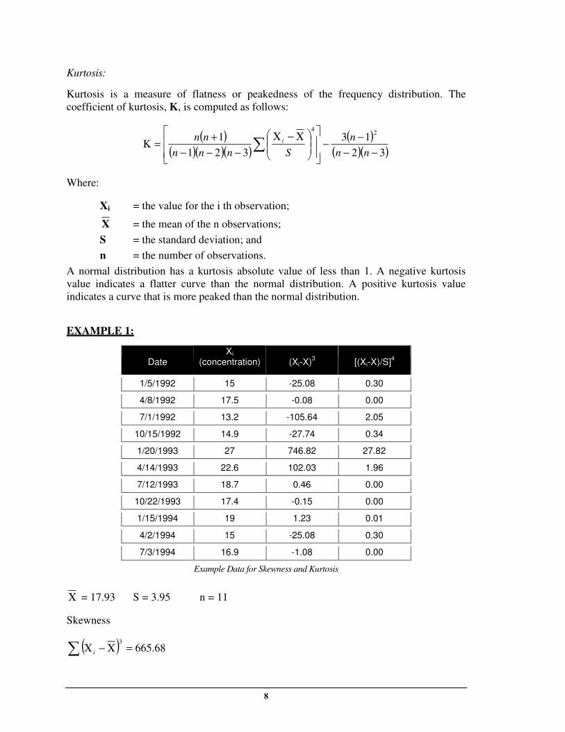
EXAMPLE 1:

Date Xi

(concentration) (Xi-X)3 [(Xi-X)/S]

4

1/5/1992 15 -25.08 0.30

4/8/1992 17.5 -0.08 0.00

7/1/1992 13.2 -105.64 2.05

10/15/1992 14.9 -27.74 0.34

1/20/1993 27 746.82 27.82

4/14/1993 22.6 102.03 1.96

7/12/1993 18.7 0.46 0.00

10/22/1993 17.4 -0.15 0.00

1/15/1994 19 1.23 0.01

4/2/1994 15 -25.08 0.30

7/3/1994 16.9 -1.08 0.00

Example Data for Skewness and Kurtosis

Χ = 17.93 S = 3.95 n = 11

Skewness

( ) 68.6653

=Χ−Χ∑ i

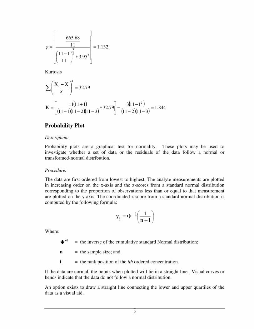
9

132.1

95.311

111

11

68.665

32

3=

∗

−

=γ

Kurtosis

79.32

4

=

Χ−Χ∑

S

i

( )( )( )( )

( )( )( )

844.1311211

111379.32

311211111

11111 2

=−−

−−

∗

−−−

+=Κ

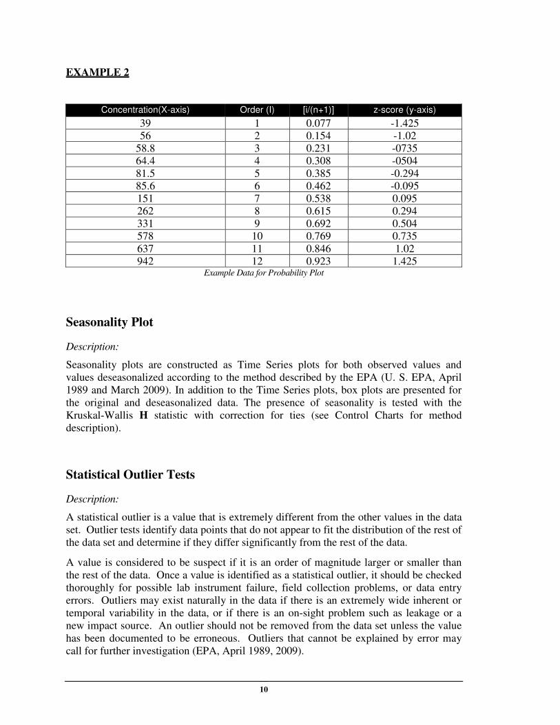
Probability Plot

Description:

Probability plots are a graphical test for normality. These plots may be used to

investigate whether a set of data or the residuals of the data follow a normal or

transformed-normal distribution.

Procedure:

The data are first ordered from lowest to highest. The analyte measurements are plotted

in increasing order on the x-axis and the z-scores from a standard normal distribution

corresponding to the proportion of observations less than or equal to that measurement

are plotted on the y-axis. The coordinated z-score from a standard normal distribution is

computed by the following formula:

+−Φ=

1n

i1i

y

Where:

ΦΦΦΦ −−−−1 = the inverse of the cumulative standard Normal distribution;

n = the sample size; and

i = the rank position of the ith ordered concentration.

If the data are normal, the points when plotted will lie in a straight line. Visual curves or

bends indicate that the data do not follow a normal distribution.

An option exists to draw a straight line connecting the lower and upper quartiles of the

data as a visual aid.

10

EXAMPLE 2

Concentration(X-axis) Order (I) [i/(n+1)] z-score (y-axis)

39 1 0.077 -1.425

56 2 0.154 -1.02

58.8 3 0.231 -0735

64.4 4 0.308 -0504

81.5 5 0.385 -0.294

85.6 6 0.462 -0.095

151 7 0.538 0.095

262 8 0.615 0.294

331 9 0.692 0.504

578 10 0.769 0.735

637 11 0.846 1.02

942 12 0.923 1.425 Example Data for Probability Plot

Seasonality Plot

Description:

Seasonality plots are constructed as Time Series plots for both observed values and

values deseasonalized according to the method described by the EPA (U. S. EPA, April

1989 and March 2009). In addition to the Time Series plots, box plots are presented for

the original and deseasonalized data. The presence of seasonality is tested with the

Kruskal-Wallis H statistic with correction for ties (see Control Charts for method

description).

Statistical Outlier Tests

Description:

A statistical outlier is a value that is extremely different from the other values in the data

set. Outlier tests identify data points that do not appear to fit the distribution of the rest of

the data set and determine if they differ significantly from the rest of the data.

A value is considered to be suspect if it is an order of magnitude larger or smaller than

the rest of the data. Once a value is identified as a statistical outlier, it should be checked

thoroughly for possible lab instrument failure, field collection problems, or data entry

errors. Outliers may exist naturally in the data if there is an extremely wide inherent or

temporal variability in the data, or if there is an on-sight problem such as leakage or a

new impact source. An outlier should not be removed from the data set unless the value

has been documented to be erroneous. Outliers that cannot be explained by error may

call for further investigation (EPA, April 1989, 2009).

11

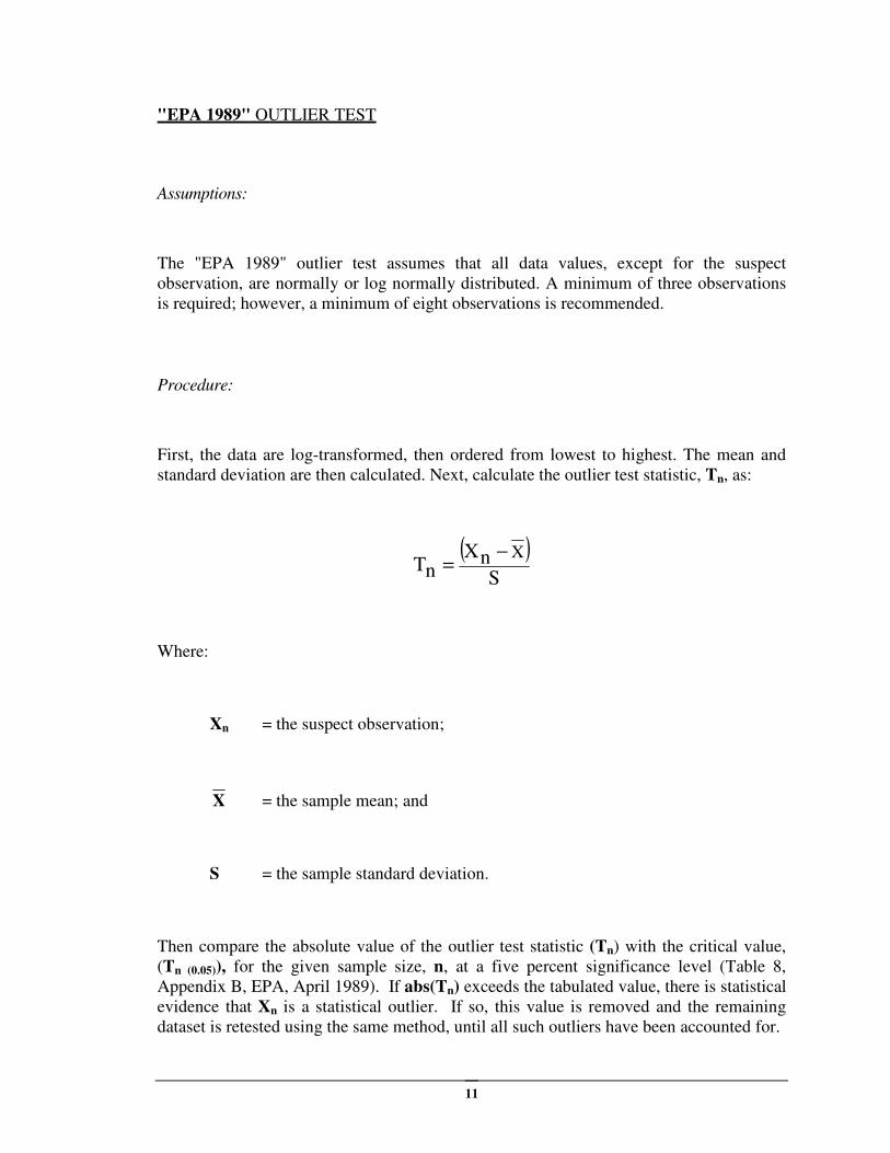
"EPA 1989" OUTLIER TEST

Assumptions:

The "EPA 1989" outlier test assumes that all data values, except for the suspect

observation, are normally or log normally distributed. A minimum of three observations

is required; however, a minimum of eight observations is recommended.

Procedure:

First, the data are log-transformed, then ordered from lowest to highest. The mean and

standard deviation are then calculated. Next, calculate the outlier test statistic, Tn, as:

( )S

nXnT

X−=

Where:

Xn = the suspect observation;

X = the sample mean; and

S = the sample standard deviation.

Then compare the absolute value of the outlier test statistic (Tn) with the critical value,

(Tn (0.05)), for the given sample size, n, at a five percent significance level (Table 8,

Appendix B, EPA, April 1989). If abs(Tn) exceeds the tabulated value, there is statistical

evidence that Xn is a statistical outlier. If so, this value is removed and the remaining

dataset is retested using the same method, until all such outliers have been accounted for.

12

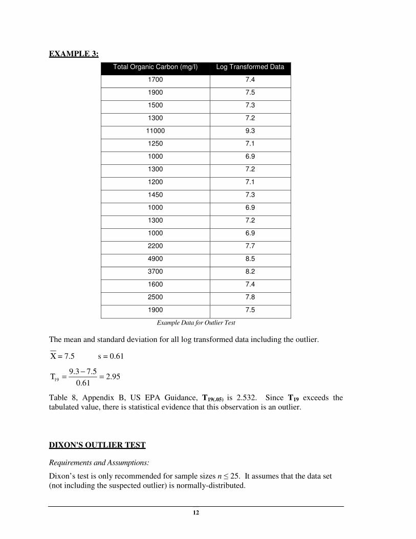
EXAMPLE 3:

Total Organic Carbon (mg/I) Log Transformed Data

1700 7.4

1900 7.5

1500 7.3

1300 7.2

11000 9.3

1250 7.1

1000 6.9

1300 7.2

1200 7.1

1450 7.3

1000 6.9

1300 7.2

1000 6.9

2200 7.7

4900 8.5

3700 8.2

1600 7.4

2500 7.8

1900 7.5

Example Data for Outlier Test

The mean and standard deviation for all log transformed data including the outlier.

Χ = 7.5 s = 0.61

95.261.0

5.73.919 =

−=Τ

Table 8, Appendix B, US EPA Guidance, T19(.05) is 2.532. Since T19 exceeds the

tabulated value, there is statistical evidence that this observation is an outlier.

DIXON'S OUTLIER TEST

Requirements and Assumptions:

Dixon’s test is only recommended for sample sizes n ≤ 25. It assumes that the data set

(not including the suspected outlier) is normally-distributed.

13

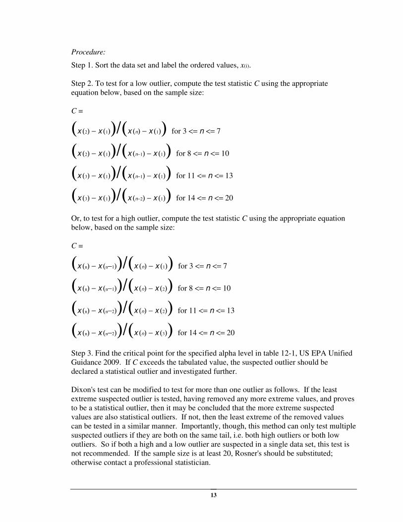
Procedure:

Step 1. Sort the data set and label the ordered values, x(i).

Step 2. To test for a low outlier, compute the test statistic C using the appropriate

equation below, based on the sample size:

C =

(x (2) − x (1))/(x (n) − x (1)) for 3 <= n <= 7

(x (2) − x (1))/(x (n−1) − x (1)) for 8 <= n <= 10

(x (3) − x (1))/(x (n−1) − x (1)) for 11 <= n <= 13

(x (3) − x (1))/(x (n−2) − x (1)) for 14 <= n <= 20

Or, to test for a high outlier, compute the test statistic C using the appropriate equation

below, based on the sample size:

C =

(x (n) − x (n−1))/(x (n) − x (1)) for 3 <= n <= 7

(x (n) − x (n−1))/(x (n) − x (2)) for 8 <= n <= 10

(x (n) − x (n−2))/(x (n) − x (2)) for 11 <= n <= 13

(x (n) − x (n−2))/(x (n) − x (3)) for 14 <= n <= 20

Step 3. Find the critical point for the specified alpha level in table 12-1, US EPA Unified

Guidance 2009. If C exceeds the tabulated value, the suspected outlier should be

declared a statistical outlier and investigated further.

Dixon's test can be modified to test for more than one outlier as follows. If the least

extreme suspected outlier is tested, having removed any more extreme values, and proves

to be a statistical outlier, then it may be concluded that the more extreme suspected

values are also statistical outliers. If not, then the least extreme of the removed values

can be tested in a similar manner. Importantly, though, this method can only test multiple

suspected outliers if they are both on the same tail, i.e. both high outliers or both low

outliers. So if both a high and a low outlier are suspected in a single data set, this test is

not recommended. If the sample size is at least 20, Rosner's should be substituted;

otherwise contact a professional statistician.

14

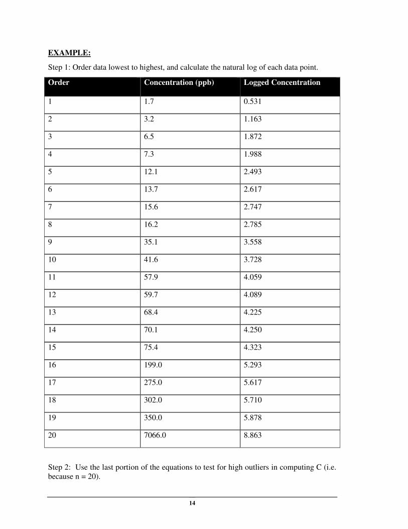
EXAMPLE:

Step 1: Order data lowest to highest, and calculate the natural log of each data point.

Order Concentration (ppb) Logged Concentration

1 1.7 0.531

2 3.2 1.163

3 6.5 1.872

4 7.3 1.988

5 12.1 2.493

6 13.7 2.617

7 15.6 2.747

8 16.2 2.785

9 35.1 3.558

10 41.6 3.728

11 57.9 4.059

12 59.7 4.089

13 68.4 4.225

14 70.1 4.250

15 75.4 4.323

16 199.0 5.293

17 275.0 5.617

18 302.0 5.710

19 350.0 5.878

20 7066.0 8.863

Step 2: Use the last portion of the equations to test for high outliers in computing C (i.e.

because n = 20).

15

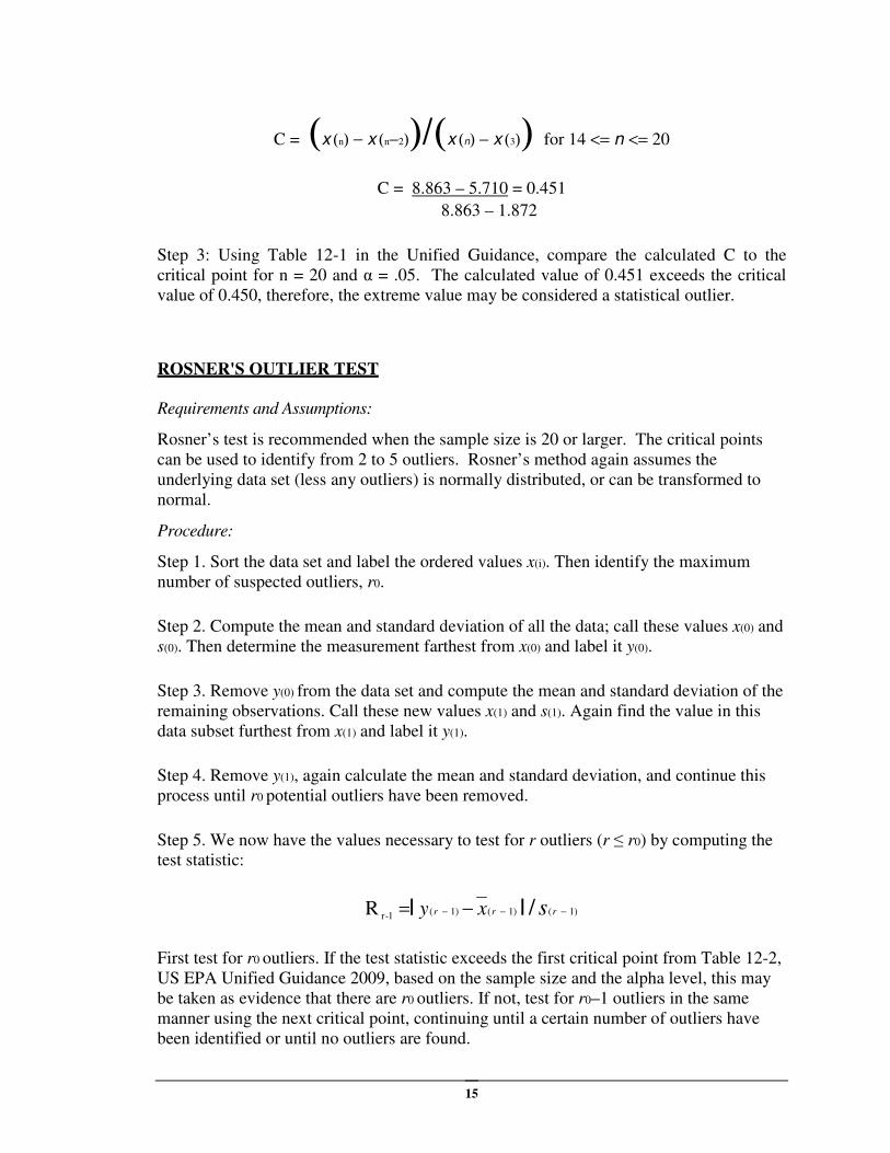
C = (x (n) − x (n−2))/(x (n) − x (3)) for 14 <= n <= 20

C = 8.863 – 5.710 = 0.451

8.863 – 1.872

Step 3: Using Table 12-1 in the Unified Guidance, compare the calculated C to the

critical point for n = 20 and α = .05. The calculated value of 0.451 exceeds the critical

value of 0.450, therefore, the extreme value may be considered a statistical outlier.

ROSNER'S OUTLIER TEST

Requirements and Assumptions:

Rosner’s test is recommended when the sample size is 20 or larger. The critical points

can be used to identify from 2 to 5 outliers. Rosner’s method again assumes the

underlying data set (less any outliers) is normally distributed, or can be transformed to

normal.

Procedure:

Step 1. Sort the data set and label the ordered values x(i). Then identify the maximum

number of suspected outliers, r0.

Step 2. Compute the mean and standard deviation of all the data; call these values x(0) and

s(0). Then determine the measurement farthest from x(0) and label it y(0).

Step 3. Remove y(0) from the data set and compute the mean and standard deviation of the

remaining observations. Call these new values x(1) and s(1). Again find the value in this

data subset furthest from x(1) and label it y(1).

Step 4. Remove y(1), again calculate the mean and standard deviation, and continue this

process until r0 potential outliers have been removed.

Step 5. We now have the values necessary to test for r outliers (r ≤ r0) by computing the

test statistic:

)1()1()1(1-r /R −−− −= rrr sxy ||

First test for r0 outliers. If the test statistic exceeds the first critical point from Table 12-2,

US EPA Unified Guidance 2009, based on the sample size and the alpha level, this may

be taken as evidence that there are r0 outliers. If not, test for r0–1 outliers in the same

manner using the next critical point, continuing until a certain number of outliers have

been identified or until no outliers are found.

16

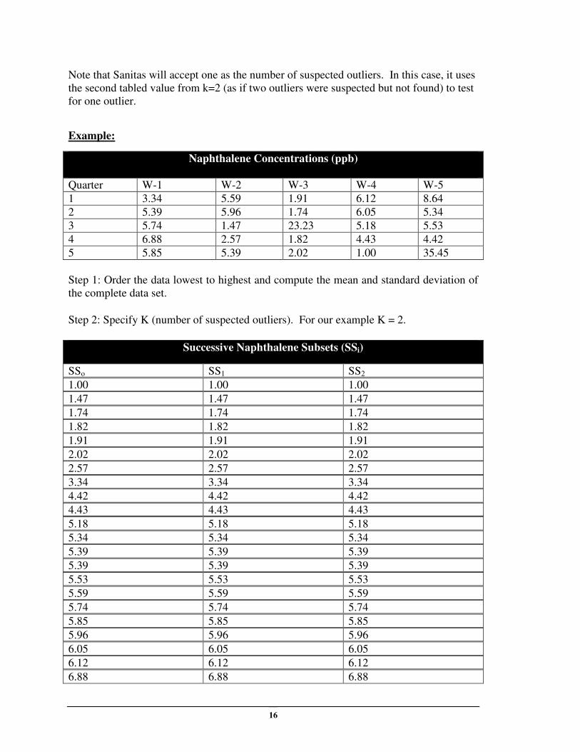
Note that Sanitas will accept one as the number of suspected outliers. In this case, it uses

the second tabled value from k=2 (as if two outliers were suspected but not found) to test

for one outlier.

Example:

Step 1: Order the data lowest to highest and compute the mean and standard deviation of

the complete data set.

Step 2: Specify K (number of suspected outliers). For our example K = 2.

Successive Naphthalene Subsets (SSi)

SSo SS1 SS2

1.00 1.00 1.00

1.47 1.47 1.47

1.74 1.74 1.74

1.82 1.82 1.82

1.91 1.91 1.91

2.02 2.02 2.02

2.57 2.57 2.57

3.34 3.34 3.34

4.42 4.42 4.42

4.43 4.43 4.43

5.18 5.18 5.18

5.34 5.34 5.34

5.39 5.39 5.39

5.39 5.39 5.39

5.53 5.53 5.53

5.59 5.59 5.59

5.74 5.74 5.74

5.85 5.85 5.85

5.96 5.96 5.96

6.05 6.05 6.05

6.12 6.12 6.12

6.88 6.88 6.88

Naphthalene Concentrations (ppb)

Quarter W-1 W-2 W-3 W-4 W-5

1 3.34 5.59 1.91 6.12 8.64

2 5.39 5.96 1.74 6.05 5.34

3 5.74 1.47 23.23 5.18 5.53

4 6.88 2.57 1.82 4.43 4.42

5 5.85 5.39 2.02 1.00 35.45

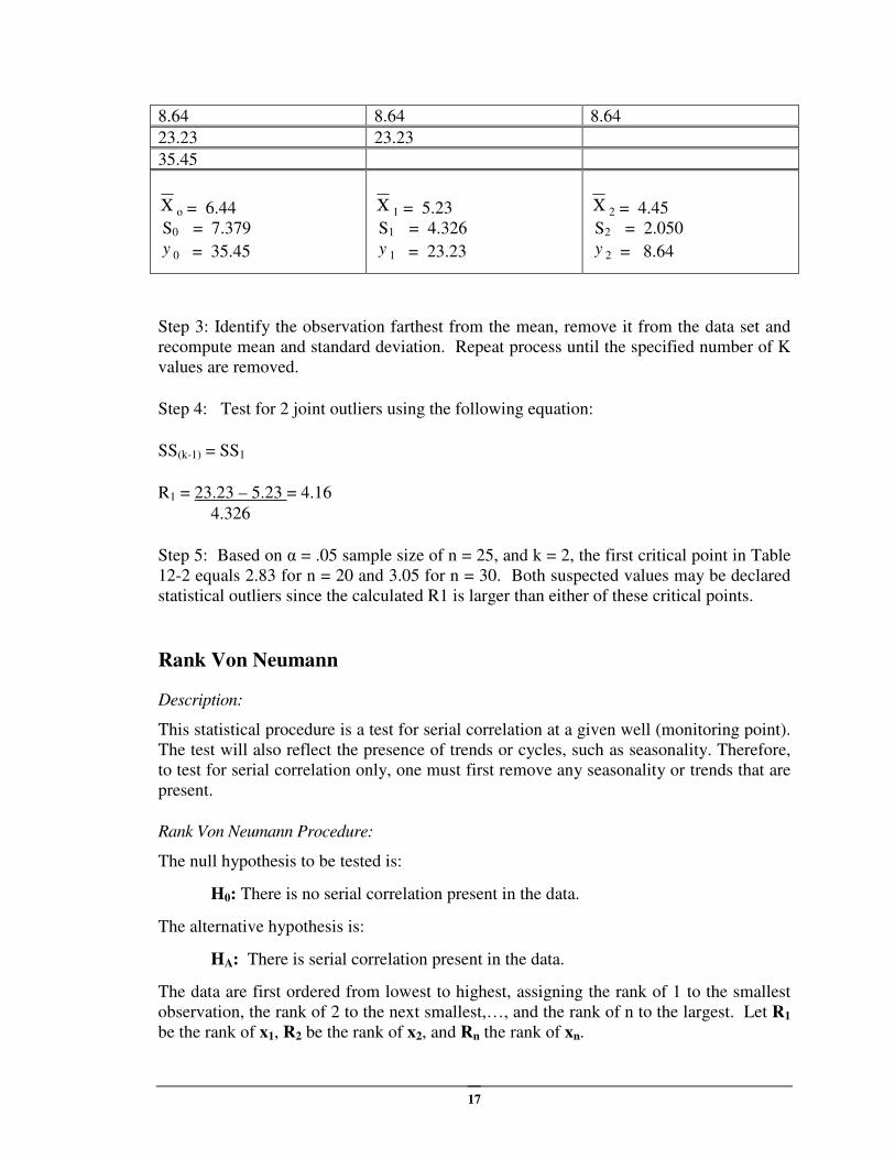
17

8.64 8.64 8.64

23.23 23.23

35.45

Χ o = 6.44

S0 = 7.379

y 0 = 35.45

Χ 1 = 5.23

S1 = 4.326

y 1 = 23.23

Χ 2 = 4.45

S2 = 2.050

y 2 = 8.64

Step 3: Identify the observation farthest from the mean, remove it from the data set and

recompute mean and standard deviation. Repeat process until the specified number of K

values are removed.

Step 4: Test for 2 joint outliers using the following equation:

SS(k-1) = SS1

R1 = 23.23 – 5.23 = 4.16

4.326

Step 5: Based on α = .05 sample size of n = 25, and k = 2, the first critical point in Table

12-2 equals 2.83 for n = 20 and 3.05 for n = 30. Both suspected values may be declared

statistical outliers since the calculated R1 is larger than either of these critical points.

Rank Von Neumann

Description:

This statistical procedure is a test for serial correlation at a given well (monitoring point).

The test will also reflect the presence of trends or cycles, such as seasonality. Therefore,

to test for serial correlation only, one must first remove any seasonality or trends that are

present.

Rank Von Neumann Procedure:

The null hypothesis to be tested is:

H0: There is no serial correlation present in the data.

The alternative hypothesis is:

HA: There is serial correlation present in the data.

The data are first ordered from lowest to highest, assigning the rank of 1 to the smallest

observation, the rank of 2 to the next smallest,…, and the rank of n to the largest. Let R1

be the rank of x1, R2 be the rank of x2, and Rn the rank of xn.

18

Compute the Rank Von Neumann statistic as:

( )2

1n

1i 1iR

iR

12nn

12Rv ∑

−

= +−

−=

Where:

Ri = the rank of the ith observation in the sequence; and

Ri+1 = the rank of the (i+1)st observation in the sequence (the following

observation).

If the sample size n is greater than or equal to ten, or less than or equal to 100, the

calculated value Rv is compared to the tabulated Rvαααα (Table A5, Gilbert). The null

hypothesis is rejected if the computed value Rv is less than the tabulated critical value.

If the sample size, n, is greater than 100, compute:

( )2

2vRn

RZ

−=

Reject the null hypothesis if ZR is negative and the absolute value of ZR is greater than

the tabulated Z1-αααα value (Table A1, Gilbert).

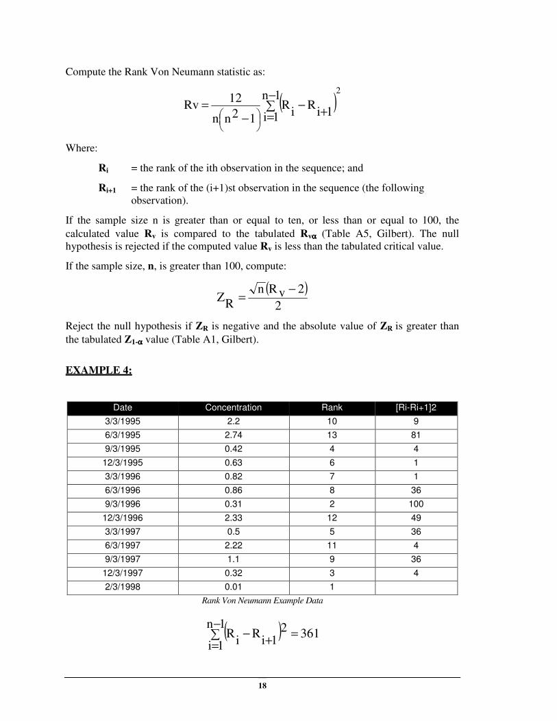
EXAMPLE 4:

Date Concentration Rank [Ri-Ri+1]2

3/3/1995 2.2 10 9

6/3/1995 2.74 13 81

9/3/1995 0.42 4 4

12/3/1995 0.63 6 1

3/3/1996 0.82 7 1

6/3/1996 0.86 8 36

9/3/1996 0.31 2 100

12/3/1996 2.33 12 49

3/3/1997 0.5 5 36

6/3/1997 2.22 11 4

9/3/1997 1.1 9 36

12/3/1997 0.32 3 4

2/3/1998 0.01 1

Rank Von Neumann Example Data

( )∑−

==

+−

1n

1i361

21i

Ri

R

19

( ) 1.984361

121313

12vR =

−=

The tabled critical value at an alpha of .05 is 1.14. Since Rv is greater than the tabled

critical value, we cannot reject H0.

Normality Report

Description:

The Normality Test report is a textual report of normality test results for each well

(monitoring point) selected in the current data set. Either the Shapiro-Wilk/Shapiro

Francia method, the Chi-Squared method or the Coefficient of Variation (see descriptions

elsewhere in this statistical write-up) may be used, and optionally the normality results

after each transformation in the Ladder of Powers (see the User Guide) may be detailed.

Stiff Diagram

Description:

Stiff Diagrams are a graphical method devised to portray water compositions and

facilitate in the interpretation and presentation of chemical analysis. They may be used to

visually compare the chemical composition of water quality across wells, and aid in

determining whether the aquifer is heterogeneous or homogenous. Stiff Diagrams are

calculated in terms of equivalents per million, more commonly referred to as

milliequivalents; and they take into account the ionic charge and the formula weight for

selected constituents, specifically (sodium+potassium), magnesium, calcium, chloride,

sulfate, and bicarbonate.

Procedure:

Milliequivalents per liter for each of the above constituents are calculated as

Weight/Charge.

The resulting values determine the relative distances from the center line for the

respective vertices of the diagram.

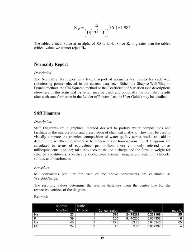
Example :

Atomic

Number

Ionic

Charge Concentration meq % meq %

Na 23 1 570 24.78261 0.251108 25

K 39 1 250 6.410256 0.064952 6

Ca 40 2 1275 63.75 0.645943 65

Mg 24 2 45 3.75 0.037997 4

20

Total 98.69287 100

Cl 35.5 1 5000 140.8451 0.803372 80

SO4 96 2 155 3.229167 0.018419 2

Bicarbonate 61 1 635 10.40984 0.059377 6

Carbonate 60 2 625 20.83333 0.118832 12

Total 175.3174 100

Discussion, focusing on Sodium:

A sample of water contains 570 mg/l of sodium (Na). The concentration of Na, in terms

of milliequivalents, in the water sample may be computed as follows:

Atomic Weight of Na: 23

Ionic Charge (volume): 1

Combining Weight (milliequivallent):

23/1 = 23

eq/l = 570 x 1/23 = 24.78 (the relative distance to the left from the center line on the

diagram)

%: 24.78 /98.69 = .25 or 25%.

To run a Stiff Diagram report, choose a sampling date from the drop down list, and

optionally extend this to a range if the sampling event occupied multiple days. Select the

wells to analyze, and click Run.

The following options are available:

Label Axes: Adds a scale (in milliequivalents) to the x-axis of each Stiff Diagram drawn.

Label Constituents: Adds abbreviated constituent names on the vertices.

Compare Dates: Replaces the Date ComboBox (single date selection) with a scrolling list

of dates (multiple date selection). Allows the comparison of data not only by well, but

also by date.

Piper Diagram

Description:

Piper diagrams are a form of tri-linear diagram, which provide a visual representation of

the ion concentration of groundwater. A piper diagram has two triangular plots on the

right and left side of a 4-sided center field. The three major cations are plotted in the left

triangle and anions in the right. Each of the three cation/anion variables, in

milliequivalents, is divided by the sum of the three values, to produce a percent of total

cation/anions. These percentages determine the location of the associated symbol. The

21

data points in the center field are located by extending the points in the lower triangles to

the point of intersection.

In order for a Piper diagram to be produced, the selected data file must contain the

following constituents: Sodium (or Na), Potassium (or K), Calcium (or Ca), Magnesium

(or Mg), Chloride (or Cl), Bicarbonate (or HCO3), Carbonate (or CO3) and Sulfate (or

SO4). The units should be mg/l, ppm, ug/l or ppb, and must be consistent.

If the Note Cation-Anion Balance option is selected (in Configure Sanitas) the report will

also show the Cation-Anion Balance, which is the absolute value of the difference

between the total cations and the total anions, both expressed in milliequivalents, divided

by their sum.

Detection Monitoring Statistics

Shewhart-CUSUM Control Chart

Description:

The combined Shewhart-Cumulative Sum (CUSUM) Control Charts are useful graphical

tools for evaluating detection-monitoring data because they monitor the inherent

statistical variation of data collected within a single well (monitoring point) and/or

between background and compliance wells, and flag anomalous results.

Control Charts are a form of a time-series graph, on which a parametric statistical

representation of concentrations of a given constituent are plotted at intervals over time.

The statistics are computed and plotted together with upper and/or lower control limits on

a chart where the x-axis represents time. If a result falls outside the predetermined control

limits, then the process is considered “out of control” and may indicate potentially

impacted ground water. Otherwise, the process is considered “in control.”

Assumptions:

The standard assumptions in the use of Control Charts are that the data are independent

and normally distributed with a constant mean, X , and constant variance, s2, and that the

background data haven’t been previously impacted by the facility. In addition, it is

assumed that seasonality in the data is sufficiently accounted for to minimize the chance

of mistaking seasonal effects for evidence of water quality degradation due to release

from a nearby waste management unit (WMU). Another assumption is that a sufficient

number of background data points exists to provide reliable estimates of the mean and

standard deviation of the constituent’s concentration values for a given well.

22

Independence:

Prior to construction of the Control Charts, the assumption of data independence should

be considered. The monitoring data should be collected to ensure physical independence

of the samples, and a specified rigorous field sampling protocol should be followed.

Distribution:

The distribution of the data is evaluated by applying the Shapiro-Wilk or Shapiro-Francia

test for normality to the raw data or, when applicable, to the transformed data. The null

hypothesis, H0, to be tested is:

H0: The population has a normal (or transformed-normal) distribution.

The alternative hypothesis, HA, is:

HA: The population does not have a normal (or transformed-normal)

distribution.

Shapiro-Wilk Test Procedure:

Calculation of the Shapiro-Wilk W-statistic to test the null hypothesis is presented in

detail on page 158 of Statistical Methods for Environmental Pollution Monitoring

(Gilbert, 1987). This test will be used when there are 49 or fewer observations to test.

Beyond 49 observations, the Shapiro-Francia test will be used.

The denominator, d, of the W test statistic, using n data is computed as follows:

( )2

1 1 1

22 1∑ ∑ ∑

= = =

Χ−Χ=Χ−Χ=

n

i

n

i

n

i

iiin

d

Where:

Xi = the value for the i th observation;

X = the mean of the n observations; and

n = the number of observations.

Order the n data from smallest to largest (e.g. X[1] < X[2] < ... < X[n]). Then compute k

where:

2k

n= if n is even

2

1-nk = if n is odd

The coefficients a1, a2, ..., ak for the observed n data can be found in Table A6 (Gilbert,

1987).

23

The W test statistic is then computed as follows:

[ ] [ ]( )2

k

1i

i1iiad

1W

Χ−Χ= ∑

=

+−n

The data are tested at the α = 0.05 significance level. The significance level represents

the probability of rejecting the null hypothesis when it is true (i.e. the percent of false

positives). It is customary to set α at 0.05 (corresponding to a 95 percent confidence

level) or at .01 (corresponding to a 99 percent confidence level).

α - This is also known as "Type I error." Reject Ho at the α significance level if W is

less than the quantile given in Table A7 (Gilbert, 1987).

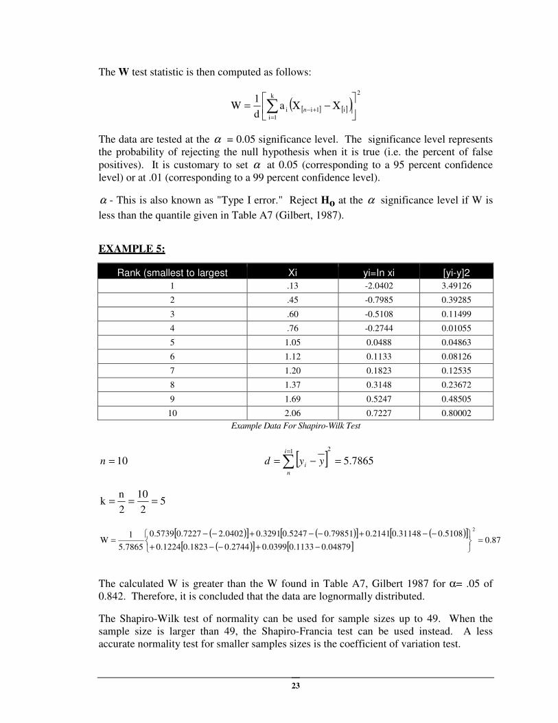
EXAMPLE 5:

Example Data For Shapiro-Wilk Test

10=n [ ] 7865.5

21

=−=∑=i

n

i yyd

52

10

2

nk ===

( )[ ] ( )[ ] ( )[ ]( )[ ] [ ]

87.004879.01133.00399.02744.01823.01224.0

5108.031148.02141.079851.05247.03291.00402.27227.05739.0

7865.5

1W

2

=

−+−−+

−−+−−+−−=

The calculated W is greater than the W found in Table A7, Gilbert 1987 for α= .05 of

0.842. Therefore, it is concluded that the data are lognormally distributed.

The Shapiro-Wilk test of normality can be used for sample sizes up to 49. When the

sample size is larger than 49, the Shapiro-Francia test can be used instead. A less

accurate normality test for smaller samples sizes is the coefficient of variation test.

Rank (smallest to largest Xi yi=In xi [yi-y]2

1 .13 -2.0402 3.49126

2 .45 -0.7985 0.39285

3 .60 -0.5108 0.11499

4 .76 -0.2744 0.01055

5 1.05 0.0488 0.04863

6 1.12 0.1133 0.08126

7 1.20 0.1823 0.12535

8 1.37 0.3148 0.23672

9 1.69 0.5247 0.48505

10 2.06 0.7227 0.80002

24

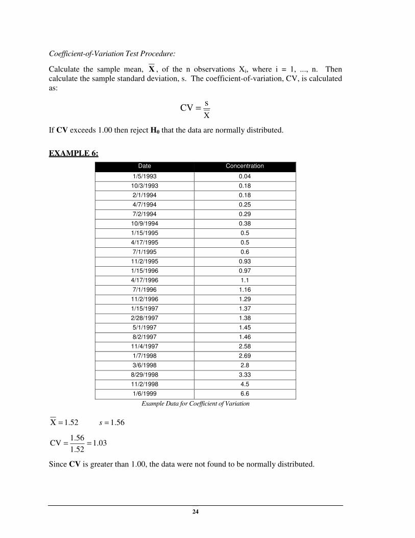
Coefficient-of-Variation Test Procedure:

Calculate the sample mean, X , of the n observations Xi, where i = 1, ..., n. Then

calculate the sample standard deviation, s. The coefficient-of-variation, CV, is calculated

as:

X

sCV =

If CV exceeds 1.00 then reject H0 that the data are normally distributed.

EXAMPLE 6:

Date Concentration

1/5/1993 0.04

10/3/1993 0.18

2/1/1994 0.18

4/7/1994 0.25

7/2/1994 0.29

10/9/1994 0.38

1/15/1995 0.5

4/17/1995 0.5

7/1/1995 0.6

11/2/1995 0.93

1/15/1996 0.97

4/17/1996 1.1

7/1/1996 1.16

11/2/1996 1.29

1/15/1997 1.37

2/28/1997 1.38

5/1/1997 1.45

8/2/1997 1.46

11/4/1997 2.58

1/7/1998 2.69

3/6/1998 2.8

8/29/1998 3.33

11/2/1998 4.5

1/6/1999 6.6

Example Data for Coefficient of Variation

52.1=Χ 56.1=s

03.11.52

1.56CV ==

Since CV is greater than 1.00, the data were not found to be normally distributed.

25

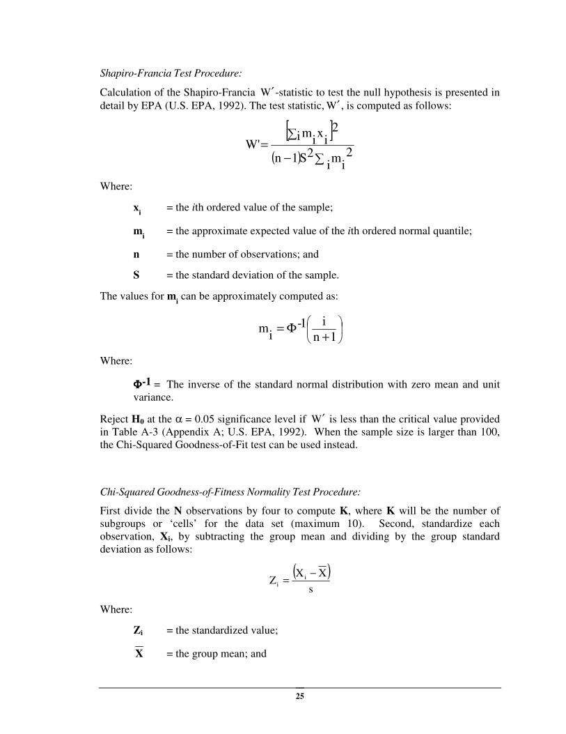
Shapiro-Francia Test Procedure:

Calculation of the Shapiro-Francia W′ -statistic to test the null hypothesis is presented in

detail by EPA (U.S. EPA, 1992). The test statistic, W′ , is computed as follows:

[ ]( ) 2

im

i2S1n

2i i

xi

mW'

∑−

∑=

Where:

xi = the ith ordered value of the sample;

mi = the approximate expected value of the ith ordered normal quantile;

n = the number of observations; and

S = the standard deviation of the sample.

The values for mi can be approximately computed as:

+Φ=

1n

i1-i

m

Where:

ΦΦΦΦ-1 = The inverse of the standard normal distribution with zero mean and unit

variance.

Reject H0 at the α = 0.05 significance level if W′ is less than the critical value provided

in Table A-3 (Appendix A; U.S. EPA, 1992). When the sample size is larger than 100,

the Chi-Squared Goodness-of-Fit test can be used instead.

Chi-Squared Goodness-of-Fitness Normality Test Procedure:

First divide the N observations by four to compute K, where K will be the number of

subgroups or ‘cells’ for the data set (maximum 10). Second, standardize each

observation, Xi, by subtracting the group mean and dividing by the group standard

deviation as follows:

( )s

XXZ i

i

−=

Where:

Zi = the standardized value;

X = the group mean; and

26

s = the group standard deviation.

Once the standardized values and K have been calculated, the third step is to subgroup

the Zi according to the cell boundaries designated for K cells in Table 4-3 (EPA, April

1989). The Chi-Squared statistic, ΧΧΧΧ2, may be calculated as follows:

( )∑=

−=

K

1i iE

2i

Ei

N2X

Where:

Ni = the number of observations in the ith cell; and

Ei = N/K, The expected number of observations in the ith cell.

Last, compare the calculated ΧΧΧΧ2 to a table of the chi-squared distribution (Table 1,

Appendix B; U.S. EPA, 1989) with α = 0.05 and K=3 degrees of freedom. If the

calculated value exceeds the tabulated value, then reject H0 that the data are normally

distributed.

The following example data represent the residuals from an analysis of variance on

dioxin concentrations. The standardization process has been applied to the residuals,

resulting in the data in the third column, the standardized residuals or Zi.

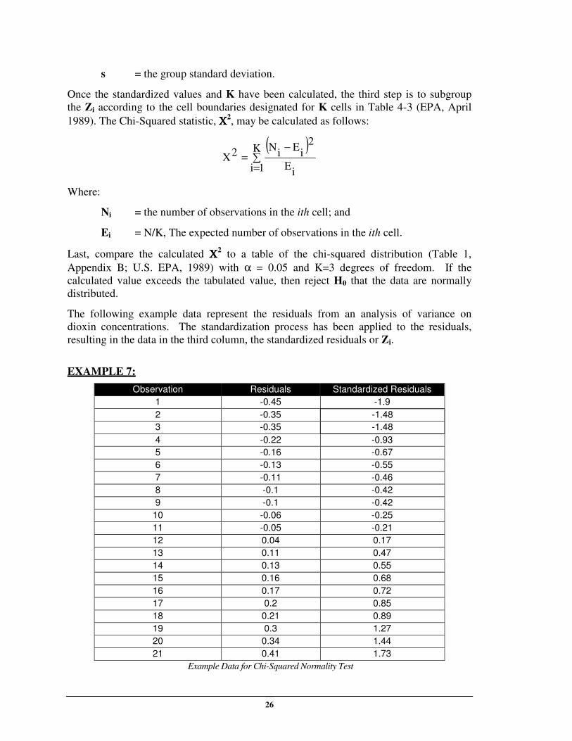
EXAMPLE 7:

Observation Residuals Standardized Residuals

1 -0.45 -1.9

2 -0.35 -1.48

3 -0.35 -1.48

4 -0.22 -0.93

5 -0.16 -0.67

6 -0.13 -0.55

7 -0.11 -0.46

8 -0.1 -0.42

9 -0.1 -0.42

10 -0.06 -0.25

11 -0.05 -0.21

12 0.04 0.17

13 0.11 0.47

14 0.13 0.55

15 0.16 0.68

16 0.17 0.72

17 0.2 0.85

18 0.21 0.89

19 0.3 1.27

20 0.34 1.44

21 0.41 1.73

Example Data for Chi-Squared Normality Test

27

21=Ν

54

21==Κ

The standardized residuals are then grouped according to the cell boundaries designated

for 5 cells in Table 4-3 (EPA, April 1989). The cell boundaries for K=5 are -0.84, -0.25,

0.25 and 0.84. Applying these boundaries to the above Zi, there are 4 observations in the

first cell, 6 in the second cell, 2 in the third, 4 in the fourth, and 5 in the fifth. These

counts represent the Ni in the above equation that is used to calculate the ΧΧΧΧ2 statistic. The

expected number in each cell, Ei, is N/K or 4.2. The ΧΧΧΧ2 statistic for these data is

calculated as:

( ) ( ) ( ) ( ) ( )10.2

2.4

2.45

2.4

2.44

2.4

2.42

2.4

2.46

2.4

2.4422222

2 =−

+−

+−

+−

+−

=Χ

The critical value at α = 0.05 for a chi-squared test with 2 (K - 3 = 5-3 = 2) degrees of

freedom is 5.99 (Table 1, Appendix B; U.S. EPA, 1989). Since the calculated chi-

squared value is less than the tabulated value, we fail to reject H0 that the data are

normally distributed.

Seasonality:

Prior to constructing the Control Charts, the significance of data seasonality is evaluated

using the nonparametric Kruskal- Wallis test (U.S. EPA, April 1989) at the α = 0.05

significance level. The null hypothesis to be tested is:

H0: The populations from which the quarterly data sets have been drawn have

the same median.

The alternative hypothesis is:

HA: At least one population has a median larger or smaller than at least one

other population’s median.

Where there are no ties, the Kruskal-Wallis statistic, H, is calculated:

( )( )1N3

N

R

1NN

12H

k

1i i

2

i +−

+= ∑

=

Where:

Ri = the sum of the ranks of the ith group;

Ni = the number of observations in the ith group (station);

N = the total number of observations; and

k = the number of groups (seasons).

28

If there are tied values (more than one data point having the same value) present in the

data, the Kruskal-Wallis Η′ statistic is calculated:

( )

Ν−Ν−

Η=Η

∑=3

g

1i

iT

1

'

Where:

g = the number of groups of distinct tied observations; and

N = the total number of observations

Ti is computed as:

( )i

3

ii ttT −=

Where:

ti = the number of observations in tie group i.

The calculated value H (or Η′ if ties are present) is compared to the tabulated chi-

squared value with (K-1) degrees of freedom, (Table A-1, Appendix B; U.S. EPA, April

1989) where K is the number of seasons. The null hypothesis is rejected if the computed

value exceeds the tabulated critical value.

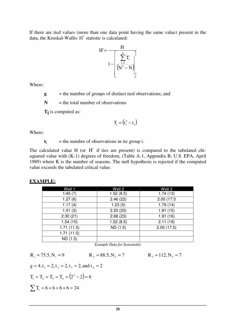
EXAMPLE:

Well 1 Well 2 Well 3 1/45 (7) 1.52 (8.5) 1.74 (13)

1.27 (6) 2.46 (22) 2.00 (17.5

1.17 (4) 1.23 (5) 1.79 (14)

1.01 (3) 2.20 (20) 1.81 (15)

2.30 (21) 2.68 (23) 1.91 (16)

1.54 (10) 1.52 (8.5) 2.11 (19)

1.71 (11.5) ND (1.5) 2.00 (17.5)

1.71 (11.5)

ND (1.5)

Example Data for Seasonality

9N75.5,R ii == 7N88.5,R 22 == 7N112,R 33 ==

2 tand2,t2,t2,t4,g 4321 =====

( ) 6223

4321 =−=Τ=Τ=Τ=Τ

246666i =+++=Τ∑

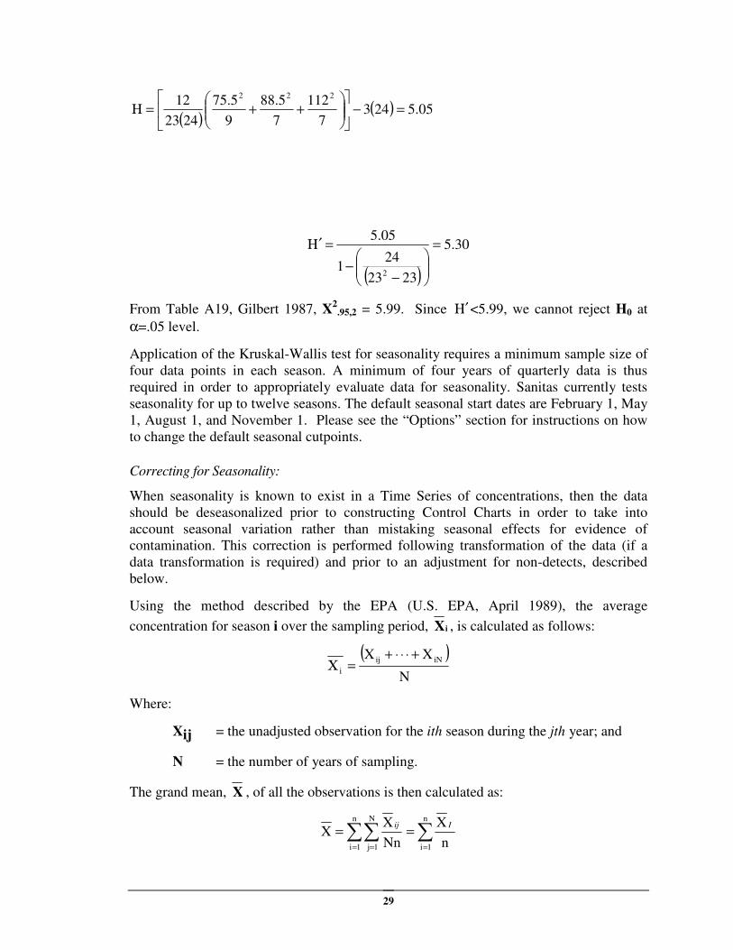
29

( )( ) 05.5243

7

112

7

5.88

9

5.75

2423

12 222

=−

++=Η

( )

30.5

2323

241

05.5

2

=

−−

=Η′

From Table A19, Gilbert 1987, X2

.95,2 = 5.99. Since Η′<5.99, we cannot reject H0 at

α=.05 level.

Application of the Kruskal-Wallis test for seasonality requires a minimum sample size of

four data points in each season. A minimum of four years of quarterly data is thus

required in order to appropriately evaluate data for seasonality. Sanitas currently tests

seasonality for up to twelve seasons. The default seasonal start dates are February 1, May

1, August 1, and November 1. Please see the “Options” section for instructions on how

to change the default seasonal cutpoints.

Correcting for Seasonality:

When seasonality is known to exist in a Time Series of concentrations, then the data

should be deseasonalized prior to constructing Control Charts in order to take into

account seasonal variation rather than mistaking seasonal effects for evidence of

contamination. This correction is performed following transformation of the data (if a

data transformation is required) and prior to an adjustment for non-detects, described

below.

Using the method described by the EPA (U.S. EPA, April 1989), the average

concentration for season i over the sampling period, Xi , is calculated as follows:

( )N

XX iNij

i

+⋅⋅⋅+=Χ

Where:

Xij = the unadjusted observation for the ith season during the jth year; and

N = the number of years of sampling.

The grand mean, X , of all the observations is then calculated as:

∑ ∑∑= ==

==n

1i

n

1i

N

1j n

X

Nn

XX

Iij

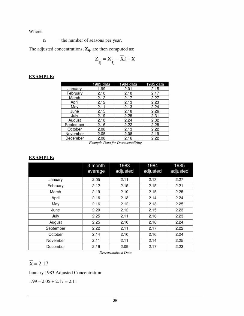
30

Where:

n = the number of seasons per year.

The adjusted concentrations, Zij, are then computed as:

XXij

Xij

Z +−= i

EXAMPLE:

1983 data 1984 data 1985 data January 1.99 2.01 2.15 February 2.10 2.10 2.17

March 2.12 2.17 2.27 April 2.12 2.13 2.23 May 2.11 2.13 2.24 June 2.15 2.18 2.26 July 2.19 2.25 2.31

August 2.18 2.24 2.32 September 2.16 2.22 2.28

October 2.08 2.13 2.22 November 2.05 2.08 2.19 December 2.08 2.16 2.22

Example Data for Deseasonalizing

EXAMPLE:

3 month average

1983 adjusted

1984 adjusted

1985 adjusted

January 2.05 2.11 2.13 2.27

February 2.12 2.15 2.15 2.21

March 2.19 2.10 2.15 2.25

April 2.16 2.13 2.14 2.24

May 2.16 2.12 2.13 2.25

June 2.20 2.12 2.15 2.23

July 2.25 2.11 2.16 2.23

August 2.25 2.10 2.16 2.24

September 2.22 2.11 2.17 2.22

October 2.14 2.10 2.16 2.24

November 2.11 2.11 2.14 2.25

December 2.16 2.09 2.17 2.23

Deseasonalized Data

2.17X =

January 1983 Adjusted Concentration:

1.99 – 2.05 + 2.17 = 2.11

31

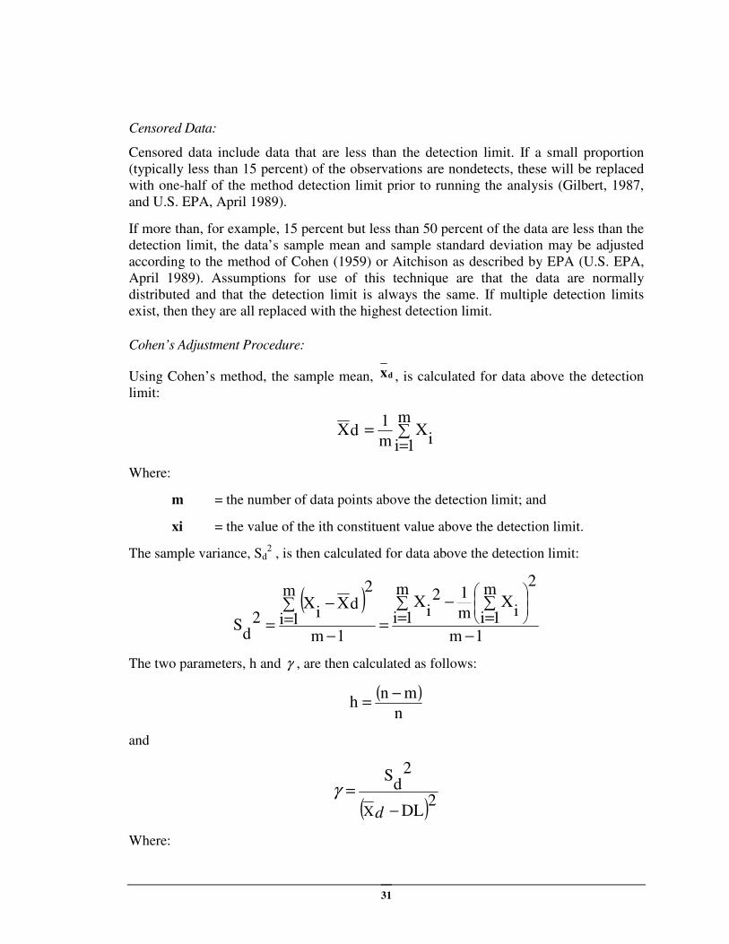
Censored Data:

Censored data include data that are less than the detection limit. If a small proportion

(typically less than 15 percent) of the observations are nondetects, these will be replaced

with one-half of the method detection limit prior to running the analysis (Gilbert, 1987,

and U.S. EPA, April 1989).

If more than, for example, 15 percent but less than 50 percent of the data are less than the

detection limit, the data’s sample mean and sample standard deviation may be adjusted

according to the method of Cohen (1959) or Aitchison as described by EPA (U.S. EPA,

April 1989). Assumptions for use of this technique are that the data are normally

distributed and that the detection limit is always the same. If multiple detection limits

exist, then they are all replaced with the highest detection limit.

Cohen’s Adjustment Procedure:

Using Cohen’s method, the sample mean, xd , is calculated for data above the detection

limit:

∑=

=m

1i iX

m

1dX

Where:

m = the number of data points above the detection limit; and

xi = the value of the ith constituent value above the detection limit.

The sample variance, Sd2 , is then calculated for data above the detection limit:

( )1m

m

1i

2m

1i iX

m

12i

X

1m

2m

1idX

iX

2d

S−

∑=

∑=

−

=−

∑=

−

=

The two parameters, h and γ , are then calculated as follows:

( )n

mnh

−=

and

( )2DL

2d

S

X −

=

d

γ

Where:

32

n = the total number of observations (i.e., above and below the detection

limit); and

DL = the detection limit.

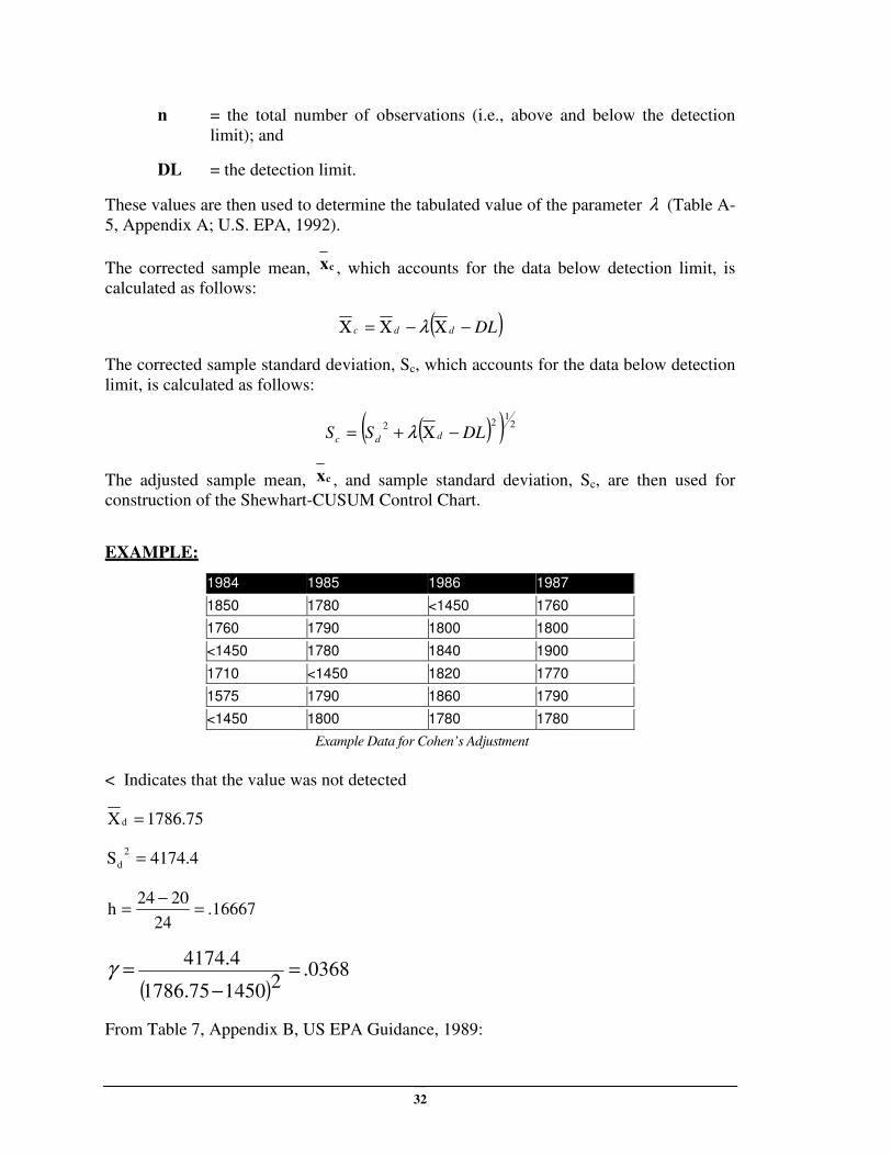
These values are then used to determine the tabulated value of the parameter λ (Table A-

5, Appendix A; U.S. EPA, 1992).

The corrected sample mean, xc , which accounts for the data below detection limit, is

calculated as follows:

( )DLddc −Χ−Χ=Χ λ

The corrected sample standard deviation, Sc, which accounts for the data below detection

limit, is calculated as follows:

( )( ) 21

22DLSS ddc −Χ+= λ

The adjusted sample mean, xc , and sample standard deviation, Sc, are then used for

construction of the Shewhart-CUSUM Control Chart.

EXAMPLE:

1984 1985 1986 1987

1850 1780 <1450 1760

1760 1790 1800 1800

<1450 1780 1840 1900

1710 <1450 1820 1770

1575 1790 1860 1790

<1450 1800 1780 1780

Example Data for Cohen’s Adjustment

< Indicates that the value was not detected

1786.75X d =

4174.4S2

d =

.1666724

2024h =

−=

( ).0368

214501786.75

4174.4=

−=γ

From Table 7, Appendix B, US EPA Guidance, 1989:

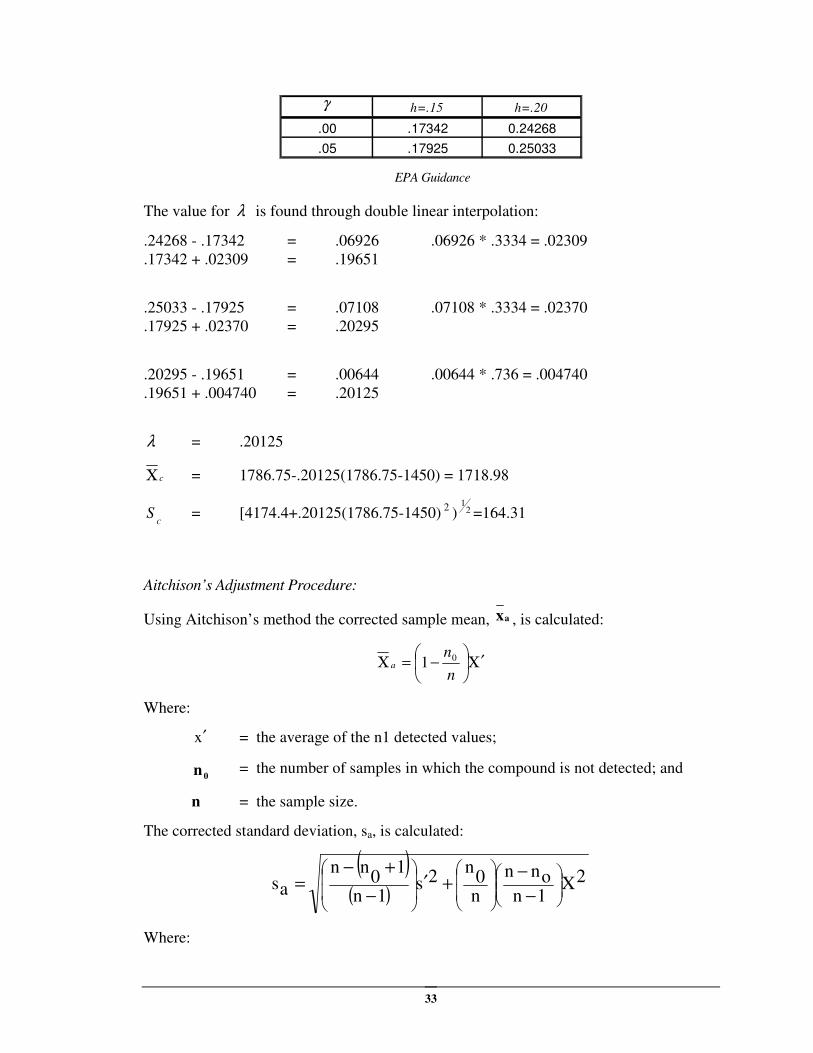
33

h=.15 h=.20

.00 .17342 0.24268

.05 .17925 0.25033

γ

EPA Guidance

The value for λ is found through double linear interpolation:

.24268 - .17342 = .06926 .06926 * .3334 = .02309

.17342 + .02309 = .19651

.25033 - .17925 = .07108 .07108 * .3334 = .02370

.17925 + .02370 = .20295

.20295 - .19651 = .00644 .00644 * .736 = .004740

.19651 + .004740 = .20125

λ = .20125

cΧ = 1786.75-.20125(1786.75-1450) = 1718.98

CS = [4174.4+.20125(1786.75-1450)

2 ) 2

1

=164.31

Aitchison’s Adjustment Procedure:

Using Aitchison’s method the corrected sample mean, xa , is calculated:

Χ′

−=Χ

n

na

01

Where:

x′ = the average of the n1 detected values;

0n = the number of samples in which the compound is not detected; and

n = the sample size.

The corrected standard deviation, sa, is calculated:

( )( )

2X1nonn

n0

n2s

1n

10

nn

as

−

−+′

−

+−=

Where:

34

s′ = the standard deviation of the n1 detected measurements.

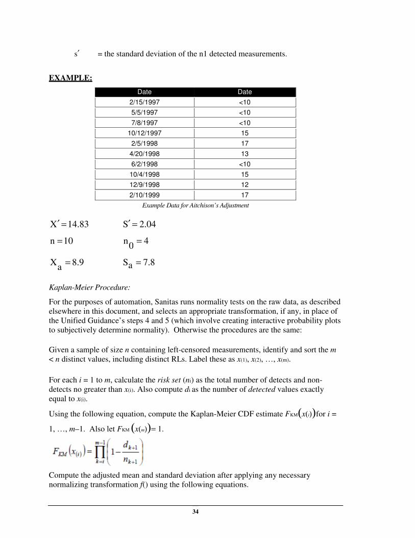
EXAMPLE:

Date Date

2/15/1997 <10

5/5/1997 <10

7/8/1997 <10

10/12/1997 15

2/5/1998 17

4/20/1998 13

6/2/1998 <10

10/4/1998 15

12/9/1998 12

2/10/1999 17

Example Data for Aitchison’s Adjustment

14.83X =′ 2.04S =′

10n = 40

n =

8.9a

X = 7.8aS =

Kaplan-Meier Procedure:

For the purposes of automation, Sanitas runs normality tests on the raw data, as described

elsewhere in this document, and selects an appropriate transformation, if any, in place of

the Unified Guidance’s steps 4 and 5 (which involve creating interactive probability plots

to subjectively determine normality). Otherwise the procedures are the same:

Given a sample of size n containing left-censored measurements, identify and sort the m

< n distinct values, including distinct RLs. Label these as x(1), x(2), …, x(m).

For each i = 1 to m, calculate the risk set (ni) as the total number of detects and non-

detects no greater than x(i). Also compute di as the number of detected values exactly

equal to x(i).

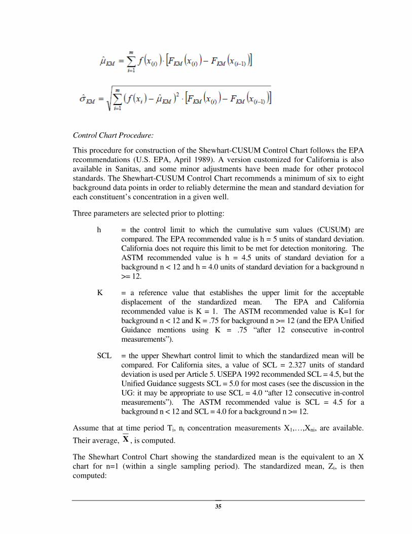
Using the following equation, compute the Kaplan-Meier CDF estimate FKM(x(i))for i =

1, …, m–1. Also let FKM (x(m))= 1.

Compute the adjusted mean and standard deviation after applying any necessary

normalizing transformation f() using the following equations.

35

Control Chart Procedure:

This procedure for construction of the Shewhart-CUSUM Control Chart follows the EPA

recommendations (U.S. EPA, April 1989). A version customized for California is also

available in Sanitas, and some minor adjustments have been made for other protocol

standards. The Shewhart-CUSUM Control Chart recommends a minimum of six to eight

background data points in order to reliably determine the mean and standard deviation for

each constituent’s concentration in a given well.

Three parameters are selected prior to plotting:

h = the control limit to which the cumulative sum values (CUSUM) are

compared. The EPA recommended value is h = 5 units of standard deviation.

California does not require this limit to be met for detection monitoring. The

ASTM recommended value is h = 4.5 units of standard deviation for a

background n < 12 and h = 4.0 units of standard deviation for a background n

>= 12.

K = a reference value that establishes the upper limit for the acceptable

displacement of the standardized mean. The EPA and California

recommended value is K = 1. The ASTM recommended value is K=1 for

background n < 12 and K = .75 for background n >= 12 (and the EPA Unified

Guidance mentions using K = .75 “after 12 consecutive in-control

measurements”).

SCL = the upper Shewhart control limit to which the standardized mean will be

compared. For California sites, a value of SCL = 2.327 units of standard

deviation is used per Article 5. USEPA 1992 recommended SCL = 4.5, but the

Unified Guidance suggests SCL = 5.0 for most cases (see the discussion in the

UG: it may be appropriate to use SCL = 4.0 “after 12 consecutive in-control

measurements”). The ASTM recommended value is SCL = 4.5 for a

background n < 12 and SCL = 4.0 for a background n >= 12.

Assume that at time period Ti, ni concentration measurements X1,…,Xni, are available.

Their average, X , is computed.

The Shewhart Control Chart showing the standardized mean is the equivalent to an X

chart for n=1 (within a single sampling period). The standardized mean, Zi, is then

computed:

36

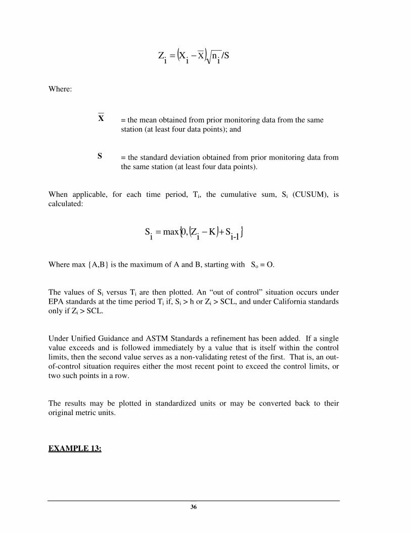
( ) /Si

ni

Xi

Z X−=

Where:

X = the mean obtained from prior monitoring data from the same

station (at least four data points); and

S = the standard deviation obtained from prior monitoring data from

the same station (at least four data points).

When applicable, for each time period, Ti, the cumulative sum, Si (CUSUM), is

calculated:

( ){ }1-i

SKi

Z0,maxi

S +−=

Where max {A,B} is the maximum of A and B, starting with So = O.

The values of Si versus Ti are then plotted. An “out of control” situation occurs under

EPA standards at the time period Ti if, Si > h or Zi > SCL, and under California standards

only if Zi > SCL.

Under Unified Guidance and ASTM Standards a refinement has been added. If a single

value exceeds and is followed immediately by a value that is itself within the control

limits, then the second value serves as a non-validating retest of the first. That is, an out-

of-control situation requires either the most recent point to exceed the control limits, or

two such points in a row.

The results may be plotted in standardized units or may be converted back to their

original metric units.

EXAMPLE 13:

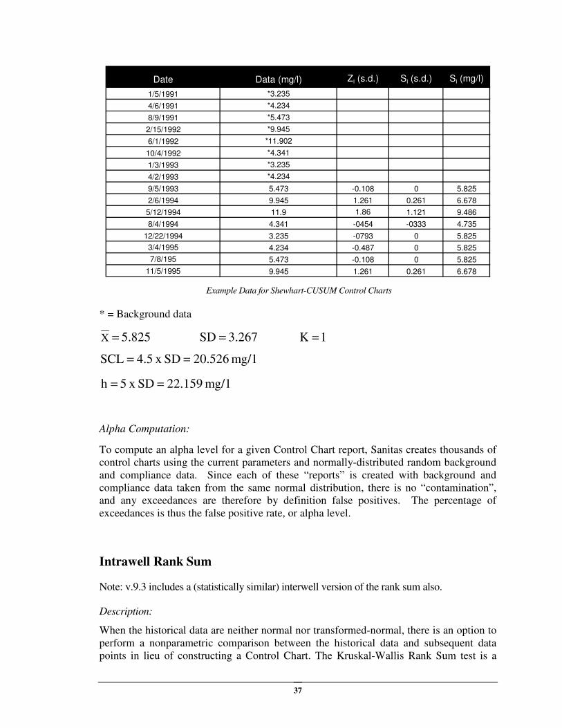
37

Date Data (mg/l) Zi (s.d.) Si (s.d.) Si (mg/l)

1/5/1991 *3.235

4/6/1991 *4.234

8/9/1991 *5.473

2/15/1992 *9.945

6/1/1992 *11.902

10/4/1992 *4.341

1/3/1993 *3.235

4/2/1993 *4.234

9/5/1993 5.473 -0.108 0 5.825

2/6/1994 9.945 1.261 0.261 6.678

5/12/1994 11.9 1.86 1.121 9.486

8/4/1994 4.341 -0454 -0333 4.735

12/22/1994 3.235 -0793 0 5.825

3/4/1995 4.234 -0.487 0 5.825

7/8/195 5.473 -0.108 0 5.825

11/5/1995 9.945 1.261 0.261 6.678

Example Data for Shewhart-CUSUM Control Charts

* = Background data

5.825X = 3.267SD = 1K =

mg/1 20.526SD x 4.5SCL ==

mg/1 22.159SD x 5h ==

Alpha Computation:

To compute an alpha level for a given Control Chart report, Sanitas creates thousands of

control charts using the current parameters and normally-distributed random background

and compliance data. Since each of these “reports” is created with background and

compliance data taken from the same normal distribution, there is no “contamination”,

and any exceedances are therefore by definition false positives. The percentage of

exceedances is thus the false positive rate, or alpha level.

Intrawell Rank Sum

Note: v.9.3 includes a (statistically similar) interwell version of the rank sum also.

Description:

When the historical data are neither normal nor transformed-normal, there is an option to

perform a nonparametric comparison between the historical data and subsequent data

points in lieu of constructing a Control Chart. The Kruskal-Wallis Rank Sum test is a

38

nonparametric procedure where the sums of ranked data sets are compared. Subsequent

sample data are compared with sampling data from the initial monitoring period of the

same well. It is assumed that during the initial monitoring period the well has shown no

evidence of contamination nor an increasing trend. This test does not require a normal

distribution of the data.

The null hypothesis to be tested is:

H0: The historical (background) data and the compliance data have the same

median constituent concentration.

The alternative hypothesis is:

HA: The compliance data have a greater median constituent concentration than

the historical data.

Procedure:

The Kruskal-Wallis test procedure is used to evaluate whether the historical (background

data) and the compliance data have the same median constituent concentration (see

Control-Chart Seasonality test for method description and example).

Mann-Whitney / Wilcoxon Rank Sum

Description:

The Mann-Whitney test, also known as Wilcoxon Rank Sum, may be used to test whether

the measurements from one population are significantly higher or lower than another

population. This test is available for both interwell and intrawell analyses.

The null hypothesis that is being tested is:

HO: The two data sets are equivalent.

The alternative hypothesis is:

HA: There is a statistically significant difference between the two data sets.

Procedure:

Sanitas uses the normal approximation of the Mann-Whitney test as follows.

First divide the data into two groups where

n1 = the number of observations in sample one,

n2 = the number of observations in sample two,

and 21 nnN += .

39

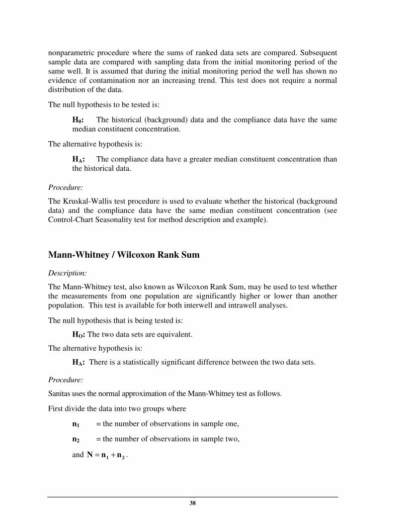
Order the measurements for group 1 and group 2 from the lowest value to the highest

value.

Calculate the Mann-Whitney statistic as:

Or, if ties are present:

Where:

111

21 R2

1)(nnnnU −

++=

R1 = The sum of the ranks of the observations in sample one.

And:

A statistically significant finding is declared if the absolute value of Z is greater than the

tabled value Z1-α/2. Significance is tested at the following alpha levels: .10, .05, .025, and

.01.

Welch's t-test

Assumptions:

All t-tests assume independence of the individual sample values. It is left to the user to

ensure that the time span between subsequent samples allows for independence of the

data. This assumption can be further tested by means of the Rank Von Neumann test,

described elsewhere in this document, if desired.

The hypothesis tests with Welch's t-test assume that errors (residuals) are normally

distributed. The normal distribution can be checked using the multiple group Shapiro-

12

1)(Nnn

2

nnU

Z

21

21

+

−=

∑ ∑ −= )t(tt i

3

i

12

tNN*

NN

nn

2

nnU

Z3

2

21

21

∑−−

−

−=

40

Wilk test, described below. Two groups (1 background and 1 compliance well in the

case of Interwell; time ranges in the case of Intrawell) are to be compared, and the

minimum sample size requirement is 4 samples per group. If the data normality

assumption is not met after attempted transformation(s) (depending on user settings), then

the Wilcoxon Rank Sum, described elsewhere in this document, is substituted.

In addition, the Wilcoxon Rank Sum will be substituted in cases in which > 20% of the

data are censored values.

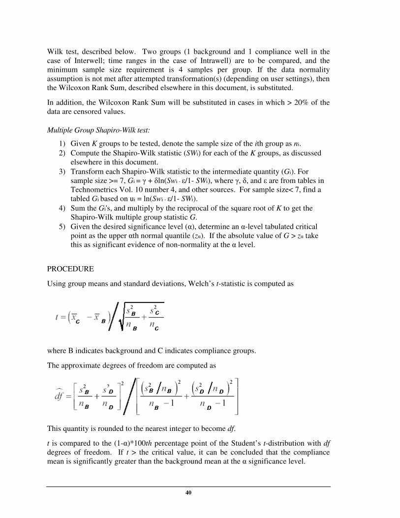
Multiple Group Shapiro-Wilk test:

1) Given K groups to be tested, denote the sample size of the ith group as ni.

2) Compute the Shapiro-Wilk statistic (SWi) for each of the K groups, as discussed

elsewhere in this document.

3) Transform each Shapiro-Wilk statistic to the intermediate quantity (Gi). For

sample size >= 7, Gi = γ + δln(Swi - ε/1- SWi), where γ, δ, and ε are from tables in

Technometrics Vol. 10 number 4, and other sources. For sample size< 7, find a

tabled Gi based on ui = ln(Swi - ε/1- SWi).

4) Sum the Gi's, and multiply by the reciprocal of the square root of K to get the

Shapiro-Wilk multiple group statistic G.

5) Given the desired significance level (α), determine an α-level tabulated critical

point as the upper αth normal quantile (zα). If the absolute value of G > zα take

this as significant evidence of non-normality at the α level.

PROCEDURE

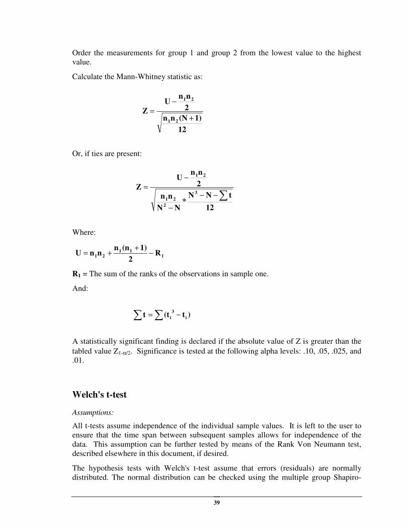
Using group means and standard deviations, Welch’s t-statistic is computed as

where B indicates background and C indicates compliance groups.

The approximate degrees of freedom are computed as

This quantity is rounded to the nearest integer to become df.

t is compared to the (1-α)*100th percentage point of the Student’s t-distribution with df

degrees of freedom. If t > the critical value, it can be concluded that the compliance

mean is significantly greater than the background mean at the α significance level.

41

One-Way Analysis of Variance (ANOVA)

Description:

Analysis of variance (ANOVA) is the name given to a variety of similar statistical

procedures. These similar procedures all compare the means or median values of

different groups of observations to determine if a statistical difference exists among

groups. The procedure is an interwell procedure that can be used to compare compliance

well data to background well data. Two types of analysis of variance are presented:

parametric and nonparametric one-way analysis of variance. Both methods are

appropriate when the only factor of concern is the spatial variability of constituent

measurements in a given sampling period. For statistically meaningful results, at least

three observations should be present in each well. Prior to statistical analysis, the

assumption of data independence should be considered. A specified rigorous field

sampling protocol should be followed.

Parametric ANOVA

Assumptions:

The hypothesis tests with parametric ANOVA assume that errors (residuals) are normally

distributed with equal variances across all wells and a single detection limit is used for

the analyte of interest. The normal distribution can be checked by testing the distribution

of the residuals (the difference between the observations and the values predicted by the

ANOVA model). At least p > 2 groups (wells) are to be compared, and the total sample

size, N, should be large enough so that N - p > 5. Under CA standards, the minimum

sample size requirement is 4 samples per well. If the data normality assumption is not

met, then nonparametric ANOVA is performed.

Normality of Residuals:

The residuals are the differences between each observation and its predicted value. In the

case of one-way analysis of variance, the predicted value for each observation is the

group (well) mean. Thus the residuals, Rij, are given by:

iXij

Xij

R −=

Where:

Xij = the jth observation in the ith well; and

Xi = the mean of the observations in the ith well.

42

Once the residuals have been computed, the Shapiro-Wilk test for normality (previously

described) is performed on the absolute values of the residuals. If the residuals are not

found to be normally distributed, the data are transformed and the normality test of the

residuals is repeated. If the residuals are not found to be transformed-normal,

nonparametric ANOVA is performed (subsequently described).

Equality of Variance Test:

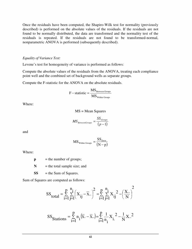
Levene’s test for homogeneity of variance is performed as follows:

Compute the absolute values of the residuals from the ANOVA, treating each compliance

point well and the combined set of background wells as separate groups.

Compute the F-statistic for the ANOVA on the absolute residuals.

GroupsWithin

GroupsBetween

MS

MSstatisticF =−

Where:

MS = Mean Squares

( )1−=

p

SSMS

Groups

upsBetweenGro

and

( )pN

SSMS Error

GroupsWithin −

=

Where:

p = the number of groups;

N = the total sample size; and

SS = the Sum of Squares.

Sum of Squares are computed as follows:

∑=∑=

−∑=∑=

=−=

p

1i

2i

n

1j N

X..2ij

Xp

1i

in

1j

2..

ijX

totalSS X

( ) 2X..N

1p

1i

2i.

X

in

1p

1i..

in

StationsSS XX i −∑

=∑=

=−=

43

and

StationsSS

totalSS

ErrorSS −=

Where:

X.. = the sum of the total observations;

X.. = the mean of the total observations; Xi. = the sum of all ni observations in group i;

.X i = the mean of the observations at group i; and

ni = the number observations at group i.

If the calculated F-statistic exceeds the tabulated F-statistic (α = 0.05) for (p - 1) and (N -

p) degrees of freedom found in Table 2, (Appendix B; U.S. EPA, April 1989), conclude

that the variances among the groups are not equal. In this case, Sanitas will (by default)

transform the original data and perform the equality of variance test again. If the

calculated F-statistic does not exceed the tabulated F-statistic, conclude that the variances

are equal and perform ANOVA on the original observations. If the calculated F-statistic

still exceeds the tabulated F-statistic, conclude that the variances among the groups are

not equal and perform a nonparametric analysis of variances. If the calculated F-statistic

is less than the tabulated F-statistic, conclude that the variances among the groups are

equal and perform ANOVA on the transformed data.

EXAMPLE:

Date Well 1 Well 2 Well 3

1/3/1995 22.9 2.0 2.0

2/5/1995 3.09 1.25 109.4

4/5/1995 35.7 7.8 4.5

6/10/1995 4.18 52 2.5

Group mean 16.47 15.76 29.6

Example Data for Levene’s Equality of Variance Test

Date

Well 1

(residuals)

Well 2

(residuals)

Well 3

(residuals)

1/3/1995 6.43 13.76 27.6

2/5/1995 13.38 14.51 79.8

4/5/1995 19.23 7.96 25.1

6/10/1995 12.29 36.23 27.1

Group mean 12.83 18.12 39.9

Overall Mean 23.62

Table 8.1:Residuals of Data

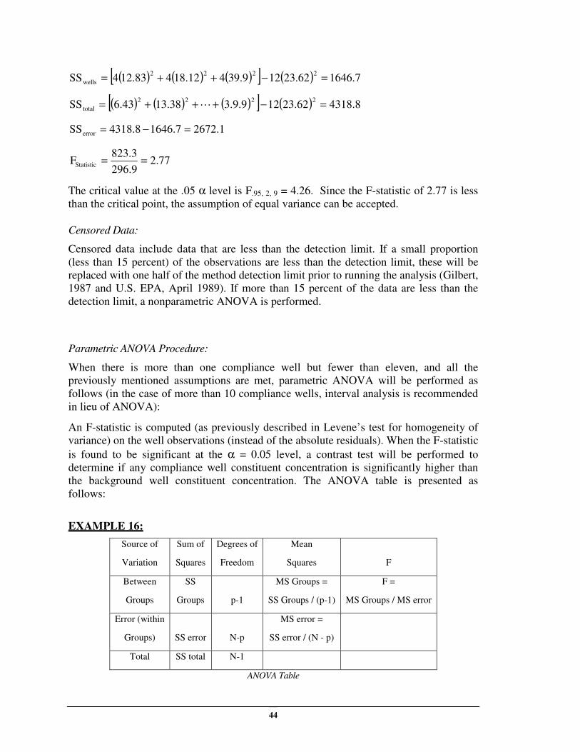
44

( ) ( ) ( )[ ] ( ) 1646.723.621239.9418.12412.834SS2222

wells =−++=

( ) ( ) ( )[ ] ( ) 4318.823.62123.9.913.386.43SS2222

total =−+++= L

2672.11646.74318.8SSerror =−=

2.77296.9

823.3FStatistic ==

The critical value at the .05 α level is F.95, 2, 9 = 4.26. Since the F-statistic of 2.77 is less

than the critical point, the assumption of equal variance can be accepted.

Censored Data:

Censored data include data that are less than the detection limit. If a small proportion

(less than 15 percent) of the observations are less than the detection limit, these will be

replaced with one half of the method detection limit prior to running the analysis (Gilbert,

1987 and U.S. EPA, April 1989). If more than 15 percent of the data are less than the

detection limit, a nonparametric ANOVA is performed.

Parametric ANOVA Procedure:

When there is more than one compliance well but fewer than eleven, and all the

previously mentioned assumptions are met, parametric ANOVA will be performed as

follows (in the case of more than 10 compliance wells, interval analysis is recommended

in lieu of ANOVA):

An F-statistic is computed (as previously described in Levene’s test for homogeneity of

variance) on the well observations (instead of the absolute residuals). When the F-statistic

is found to be significant at the α = 0.05 level, a contrast test will be performed to

determine if any compliance well constituent concentration is significantly higher than

the background well constituent concentration. The ANOVA table is presented as

follows:

EXAMPLE 16:

Source of

Variation

Sum of

Squares

Degrees of

Freedom

Mean

Squares

F

Between

Groups

SS

Groups

p-1

MS Groups =

SS Groups / (p-1)

F =

MS Groups / MS error

Error (within

Groups)

SS error

N-p

MS error =

SS error / (N - p)

Total SS total N-1

ANOVA Table

45

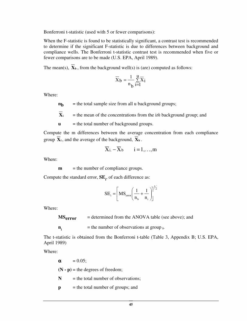
Bonferroni t-statistic (used with 5 or fewer comparisons):

When the F-statistic is found to be statistically significant, a contrast test is recommended

to determine if the significant F-statistic is due to differences between background and

compliance wells. The Bonferroni t-statistic contrast test is recommended when five or

fewer comparisons are to be made (U.S. EPA, April 1989).

The mean(s), Xb , from the background well(s) is (are) computed as follows:

∑=

=u

1iiX

bn

1bX

Where:

nb = the total sample size from all u background groups;

Xi = the mean of the concentrations from the ith background group; and

u = the total number of background groups.

Compute the m differences between the average concentration from each compliance

group Xi , and the average of the background, Xb .

bi. XX − m,1,i K=

Where:

m = the number of compliance groups.

Compute the standard error, SEi, of each difference as:

21

ib

errorin

1

n

1MSSE

+=

Where:

MSerror = determined from the ANOVA table (see above); and

ni = the number of observations at group i.

The t-statistic is obtained from the Bonferroni t-table (Table 3, Appendix B; U.S. EPA,

April 1989)

Where:

αααα = 0.05;

(N - p) = the degrees of freedom;

N = the total number of observations;

p = the total number of groups; and

46

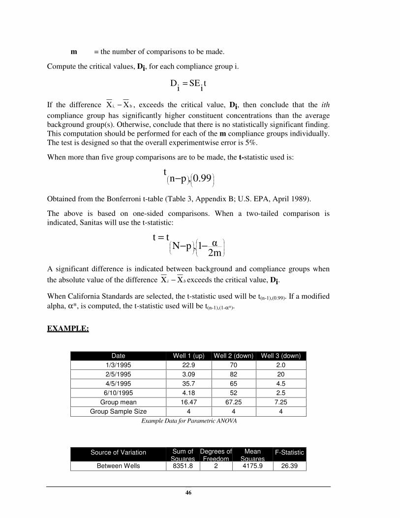
m = the number of comparisons to be made.

Compute the critical values, Di, for each compliance group i.

ti

SEi

D =

If the difference bi. XX − , exceeds the critical value, Di, then conclude that the ith

compliance group has significantly higher constituent concentrations than the average

background group(s). Otherwise, conclude that there is no statistically significant finding.

This computation should be performed for each of the m compliance groups individually.

The test is designed so that the overall experimentwise error is 5%.

When more than five group comparisons are to be made, the t-statistic used is:

− 0.99,pn

t

Obtained from the Bonferroni t-table (Table 3, Appendix B; U.S. EPA, April 1989).

The above is based on one-sided comparisons. When a two-tailed comparison is

indicated, Sanitas will use the t-statistic:

−−=

2mα1,pN

tt

A significant difference is indicated between background and compliance groups when

the absolute value of the difference bi Χ−Χ exceeds the critical value, Di.

When California Standards are selected, the t-statistic used will be t(n-1),(0.99). If a modified

alpha, α*, is computed, the t-statistic used will be t(n-1),(1-α*).

EXAMPLE:

Date Well 1 (up) Well 2 (down) Well 3 (down)

1/3/1995 22.9 70 2.0

2/5/1995 3.09 82 20

4/5/1995 35.7 65 4.5

6/10/1995 4.18 52 2.5

Group mean 16.47 67.25 7.25

Group Sample Size 4 4 4

Example Data for Parametric ANOVA

Source of Variation Sum of Squares

Degrees of Freedom

Mean Squares

F-Statistic

Between Wells 8351.8 2 4175.9 26.39

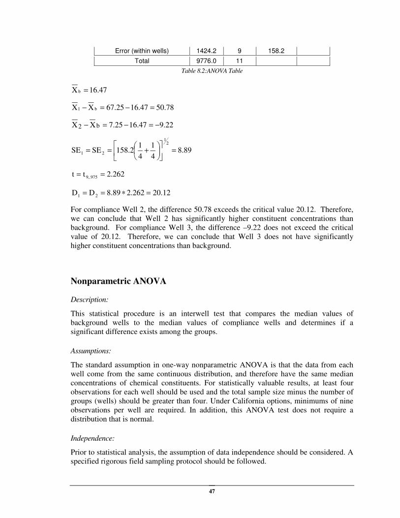
47

Error (within wells) 1424.2 9 158.2

Total 9776.0 11

Table 8.2:ANOVA Table

16.47X b =

50.7816.4767.25XX b1 =−=−

9.2216.477.25XX b2 −=−=−

8.894

1

4

1158.2SESE

21

21 =

+==

2.262tt 9,.975 ==

20.122.2628.89DD 21 =∗==

For compliance Well 2, the difference 50.78 exceeds the critical value 20.12. Therefore,

we can conclude that Well 2 has significantly higher constituent concentrations than

background. For compliance Well 3, the difference –9.22 does not exceed the critical

value of 20.12. Therefore, we can conclude that Well 3 does not have significantly

higher constituent concentrations than background.

Nonparametric ANOVA

Description:

This statistical procedure is an interwell test that compares the median values of

background wells to the median values of compliance wells and determines if a

significant difference exists among the groups.

Assumptions:

The standard assumption in one-way nonparametric ANOVA is that the data from each

well come from the same continuous distribution, and therefore have the same median

concentrations of chemical constituents. For statistically valuable results, at least four

observations for each well should be used and the total sample size minus the number of

groups (wells) should be greater than four. Under California options, minimums of nine

observations per well are required. In addition, this ANOVA test does not require a

distribution that is normal.

Independence:

Prior to statistical analysis, the assumption of data independence should be considered. A

specified rigorous field sampling protocol should be followed.

48

Procedure:

The Kruskal-Wallis test procedure (see Control Chart-Seasonality test for method

description) is used to evaluate the data sets at the α = 0.05 significance level when there

are two or more wells being compared. This test is performed on the ranked values, and

the null hypothesis to be tested is:

H0: The populations from which the quarterly data sets have been drawn have

the same median concentrations.

The alternative hypothesis to be tested is:

HA: At least one population has a median larger or smaller than the

background population.

The calculated value, H (or H′ , if ties are present) is compared to the tabulated chi-

squared value with (k-1) degrees of freedom (U.S. EPA, April 1989) where k is the

number of groups. The null hypothesis is rejected if the calculated value exceeds the

tabulated critical value. Application of the Kruskal-Wallis test requires a minimum

sample size of four data points for each well.

Censored Data:

Censored data include data that are less than the detection limit. These data will be

replaced with one half of the method detection limit prior to running the analysis (U.S.

EPA, 1992).

Tolerance Limits

Description:

An alternative approach to analysis of variance (to determine whether there is statistically

significant evidence of an impact) is to use Tolerance Limits. A tolerance limit is

constructed from the data on unimpacted background wells (or in the case of intrawell

Tolerance Limits, from non-trending historical data – this discussion will focus on the

interwell case). The concentrations from compliance wells are then compared to the

upper limit of the tolerance interval. With the exception of pH, if the compliance

concentrations fall above the upper limit of the tolerance interval (Tolerance Limit), this

provides statistically significant evidence of a difference. For pH and other constituents

in which low values as well as high values may be indicative of a facility impact, the

lower limit of the tolerance interval is also used. Compliance concentrations that fall

outside the bounds of the tolerance interval provide evidence of a statistical difference.

Assumptions:

Tolerance Limits are most appropriate for use at facilities that do not exhibit high degrees

of spatial variation between background wells and compliance wells. In addition, for a

Parametric Tolerance Limit, the background data must be normally or transformed

49

normally distributed, with at least three observations, but preferably eight or more

observations.

Distribution:

The distribution of data is evaluated using the Shapiro-Wilk test for normality (see

Control Chart-Distribution for method description) for samples with 50 or fewer

observations. The Shapiro-Francia test is used for sample sizes greater than 50 (see

Control Chart-Distribution for method description). Parametric intervals with background

sample sizes over 50 are only applicable for interwell tests.

Parametric Tolerance Limit Procedure:

To construct the upper tolerance limit, the mean, X , and the standard deviation, S, are

calculated from the background data. The one-sided upper tolerance limit, TL, is

constructed as follows:

KSXTL +=

Where:

X = the mean of the background observations;

K = the one-sided normal tolerance factor found in Table 5 (Appendix B;

U.S. EPA, April 1989); and

S = the standard deviation of the background observations.

Each observation from the compliance wells is compared to the upper tolerance limit. If

any observation exceeds the tolerance limit, that is statistically significant evidence of an

impact. In the case of transformed-normal background data, the tolerance interval is

constructed on the transformed background data, and the transformed compliance well

observations are compared to the upper tolerance limit.

In the case of a two-tailed test, both an upper and a lower tolerance limit are constructed.

The upper tolerance limit, UTL, is constructed as follows:

KSXUTL +=

Where:

K = the two-tailed normal tolerance factors (Eisenhart, C., Hastay, M.W.,

and Wallis, W.A., 1947) for 95% (default for interwell) or 99% (default

for intrawell) confidence and 95% coverage.

The lower tolerance limit, LTL, is constructed as follows:

KSLTL X −=

Where:

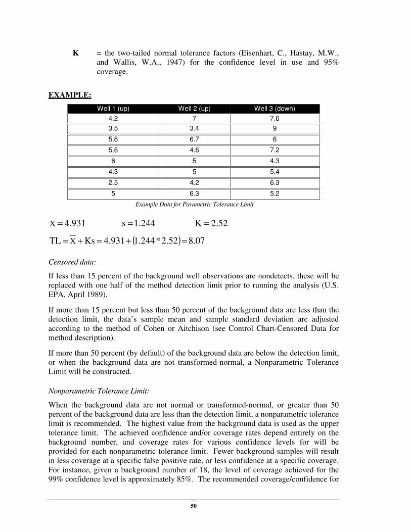
50

K = the two-tailed normal tolerance factors (Eisenhart, C., Hastay, M.W.,

and Wallis, W.A., 1947) for the confidence level in use and 95%

coverage.

EXAMPLE:

Well 1 (up) Well 2 (up) Well 3 (down)

4.2 7 7.6

3.5 3.4 9

5.6 6.7 6

5.6 4.6 7.2

6 5 4.3

4.3 5 5.4

2.5 4.2 6.3

5 6.3 5.2

Example Data for Parametric Tolerance Limit

4.931X = 1.244s = 2.52K =

( ) 8.072.52*1.2444.931KsTL X =+=+=

Censored data:

If less than 15 percent of the background well observations are nondetects, these will be

replaced with one half of the method detection limit prior to running the analysis (U.S.

EPA, April 1989).

If more than 15 percent but less than 50 percent of the background data are less than the

detection limit, the data’s sample mean and sample standard deviation are adjusted

according to the method of Cohen or Aitchison (see Control Chart-Censored Data for

method description).

If more than 50 percent (by default) of the background data are below the detection limit,

or when the background data are not transformed-normal, a Nonparametric Tolerance

Limit will be constructed.

Nonparametric Tolerance Limit:

When the background data are not normal or transformed-normal, or greater than 50

percent of the background data are less than the detection limit, a nonparametric tolerance

limit is recommended. The highest value from the background data is used as the upper

tolerance limit. The achieved confidence and/or coverage rates depend entirely on the

background number, and coverage rates for various confidence levels for will be

provided for each nonparametric tolerance limit. Fewer background samples will result

in less coverage at a specific false positive rate, or less confidence at a specific coverage.

For instance, given a background number of 18, the level of coverage achieved for the

99% confidence level is approximately 85%. The recommended coverage/confidence for

51

interwell tests is generally 95% coverage/95% confidence, and for intrawell is 95%

coverage/99% confidence.

Procedure:

When there is at least one detectable observation, the highest value for the background

data is used to set the upper limit of the tolerance interval. When all the data are

censored (i.e., nondetects or trace values) the behavior will depend on the user choice in

the Configure Sanitas window: the tolerance limit is either the most recent or highest

detection limit, or a “substitution” such as ½ of that value (again, depending on settings).

Coverage values for a given alpha have been shown to be at least the nth

root of alpha.

For example, if the desired confidence is 99% (alpha = 0.01) and the n is 18, the coverage

is the 18th

root of 0.01, or 0.774.

.

52

Prediction Limits (or Intervals): EPA Standards

Description:

A prediction limit is used to determine whether a single observation is statistically

representative of a group of observations. It is a statistical interval calculated to include

one or more observations from the same population with a specified confidence. In

ground water monitoring, a prediction limit approach may be used to make comparisons

between background and compliance data. The interval is constructed from a

background set of observations such that it will contain K future compliance observations

with stated confidence. If any observation exceeds the bounds of the prediction limit, this

is statistically significant evidence that that observation is not representative of the

background group.

Assumptions:

The parametric prediction limit is constructed if the background data all follow a normal

or transformed-normal distribution. A minimum of four background values should be

used in constructing the interval. The estimate of the standard deviation (S) that is used

should be an unbiased estimator. The usual estimate assumes that there is only one source

of variation. If there are other sources of variation, such as time effects, or spatial

variation in the data used for the background, then the parametric Prediction Limit is

inappropriate. In these situations, a multivariate statistical procedure is suggested.

Distribution:

In order to determine whether a parametric or nonparametric prediction limit should be

used, the distribution of the data is evaluated by applying the Shapiro-Wilk or Shapiro-

Francia tests for normality to the raw data or, when applicable to the ladder of powers

(Helsel & Hirsch, 1992) transformed data. The null hypothesis, Ho, to be tested is:

H0: The population has a normal (or transformed-normal) distribution.

The alternative hypothesis, HA, is:

HA: The population does not have a normal (or transformed-normal)

distribution.

Parametric Prediction Limits Procedure:

The mean, X , and the standard deviation, S, are calculated for the raw or transformed

background data. The number of comparison observations, K, is specified to be included

in the interval. If K will be different from the default in Sanitas™ which assumes K=1

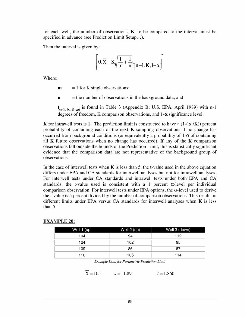
53

for each well, the number of observations, K, to be compared to the interval must be

specified in advance (see Prediction Limit Setup…).

Then the interval is given by:

−−++

αK,11,nt

n

1

m

1S0,X

Where:

m = 1 for K single observations;

n = the number of observations in the background data; and

t(n-1, K, (1-αααα))

is found in Table 3 (Appendix B; U.S. EPA, April 1989) with n-1

degrees of freedom, K comparison observations, and 1-αααα significance level.

K for intrawell tests is 1. The prediction limit is constructed to have a (1-(α /K)) percent

probability of containing each of the next K sampling observations if no change has

occurred from background conditions (or equivalently a probability of 1-α of containing

all K future observations when no change has occurred). If any of the K comparison

observations fall outside the bounds of the Prediction Limit, this is statistically significant

evidence that the comparison data are not representative of the background group of

observations.

In the case of interwell tests when K is less than 5, the t-value used in the above equation

differs under EPA and CA standards for interwell analyses but not for intrawell analyses.

For interwell tests under CA standards and intrawell tests under both EPA and CA

standards, the t-value used is consistent with a 1 percent α-level per individual

comparison observation. For interwell tests under EPA options, the α-level used to derive

the t-value is 5 percent divided by the number of comparison observations. This results in

different limits under EPA versus CA standards for interwell analyses when K is less

than 5.

EXAMPLE 20:

Well 1 (up) Well 2 (up) Well 3 (down)

104 94 112

124 102 95

109 86 87

116 105 114

Example Data for Parametric Prediction Limit

105=Χ 89.11=s 860.1=t

54

128.911.898

1

1

11.860105

n

1

m

1sPL X =++=++=

t

For a two-tailed test, t(n-1,K,(1-( α /2))) is substituted for t(n-1, K, (1-α)) in the above formula.

Statistically significant evidence of an impact is noted when compliance observations fall

outside the bounds of the upper and lower prediction limits.

When a modified alpha, α*, is computed, t(n-1,K,1-α*) will be substituted for t(n-1, K, (1- α)) in

the above formula.

Censored data:

If less than 15 percent of the background observations are nondetects, these will be

replaced with one half of the method detection limit prior to running the analysis (U.S.

EPA, April 1989).

If more than 15 percent but less than 50 percent of the background data are less than the

detection limit, the data’s sample mean and sample standard deviation are adjusted

according to the method of Cohen, Aitchison or Kaplan-Meier (see Control Charts for

method description).

If more than 50 percent of the background data are less than the detection limit, a

nonparametric prediction limit will be computed. Poisson-based prediction limits are

available as an alternative method when greater than 90 percent of the background data

are less than the detection limit.

Nonparametric Prediction Limits:

Distribution:

When the background data are not transformed-normal, or greater than 50 percent of the

background data are less than the detection limit, there is an option to construct a

nonparametric prediction limit. The highest value from the background data is used as

the upper limit of the prediction limit. Minimums of 19 background samples are required

for a 5% false positive rate when comparing a single compliance observation (k=1) to the

prediction limit. Fewer than the required minimum background sample size will result in

an inflated false positive rate that can be computed as (1-(n/(n+k))). Since the highest

background value is always used as the upper prediction limit, the actual significance

level decreases with increasing background sample size. In the case of a two-tailed test,

the lowest value from the background data is used to set the lower limit of the prediction

limit.

The false positive rate is based upon the formula:

( )( )knn/1 +−

Where:

n = the background sample size; and

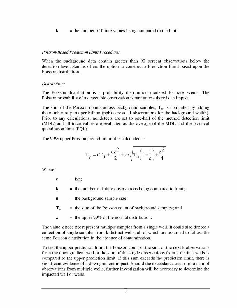
55

k = the number of future values being compared to the limit.

Poisson-Based Prediction Limit Procedure:

When the background data contain greater than 90 percent observations below the

detection level, Sanitas offers the option to construct a Prediction Limit based upon the

Poisson distribution.

Distribution:

The Poisson distribution is a probability distribution modeled for rare events. The

Poisson probability of a detectable observation is rare unless there is an impact.

The sum of the Poisson counts across background samples, Tn, is computed by adding

the number of parts per billion (ppb) across all observations for the background well(s).

Prior to any calculations, nondetects are set to one-half of the method detection limit

(MDL) and all trace values are evaluated as the average of the MDL and the practical

quantitation limit (PQL).

The 99% upper Poisson prediction limit is calculated as:

4

2z

c

11nTcz

2

2czncT

kT ++++=

Where:

c = k/n;

k = the number of future observations being compared to limit;

n = the background sample size;

Tn = the sum of the Poisson count of background samples; and

z = the upper 99% of the normal distribution.

The value k need not represent multiple samples from a single well. It could also denote a

collection of single samples from k distinct wells, all of which are assumed to follow the

same Poisson distribution in the absence of contamination.

To test the upper prediction limit, the Poisson count of the sum of the next k observations

from the downgradient well or the sum of the single observations from k distinct wells is

compared to the upper prediction limit. If this sum exceeds the prediction limit, there is

significant evidence of a downgradient impact. Should the exceedance occur for a sum of

observations from multiple wells, further investigation will be necessary to determine the

impacted well or wells.

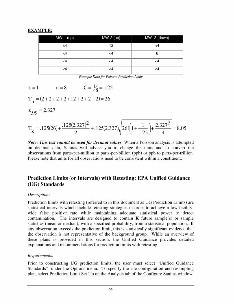
56

EXAMPLE:

MW-1 (up) MW-2 (up) MW -3 (down)

<4 12 <4

<4 <4 6

<4 <4 <4

<4 <4 <4

Example Data for Poisson Prediction Limits

1k = 8n = .1258

1C ==

( ) 26222122222n

T =+++++++=

2.327.99

z =

( )( )

( ) 05.84

2327.2

125.

11261327.2125.

2

2327.2125.26125.

kT =++++=

Note: This test cannot be used for decimal values. When a Poisson analysis is attempted

on decimal data, Sanitas will advise you to change the units and to convert the

observations from parts-per-million to parts-per-billion (ppb) or ppb to parts-per-trillion.

Please note that units for all observations need to be consistent within a constituent.

Prediction Limits (or Intervals) with Retesting: EPA Unified Guidance

(UG) Standards

Description:

Prediction limits with retesting (referred to in this document as UG Prediction Limits) are

statistical intervals which include retesting strategies in order to achieve a low facility-

wide false positive rate while maintaining adequate statistical power to detect

contamination. The intervals are designed to contain K future sample(s) or sample

statistics (mean or median), with a specified probability, from a statistical population. If

any observation exceeds the prediction limit, this is statistically significant evidence that

the observation is not representative of the background group. While an overview of

these plans is provided in this section, the Unified Guidance provides detailed

explanations and recommendations for prediction limits with retesting.

Requirements:

Prior to constructing UG prediction limits, the user must select “Unified Guidance

Standards” under the Options menu. To specify the site configuration and resampling

plan, select Prediction Limit Set Up on the Analysis tab of the Configure Sanitas window.

57

Enter the number of statistical evaluation periods per year (nE), number of constituents

(c), and number of monitoring wells (w). The annual target facility-wide false positive

rate should be no greater than 10% (cumulative throughout the year). If a facility

samples semi-annually, for instance, the overall target rate is distributed evenly among

each sampling event for a 5% target rate (α = .10/2 = .05 = 5%). The individual test

alpha (α*) then equals the targeted per-event false positive rate divided by the total

number of statistical tests (r) in a given sampling event.

For example, a site which samples semi-annually for 15 constituents at 7 wells would

have the following per-test alpha levels:

Semi-annual target rate: α = .10/2 = .05 = 5%

Total # of tests: r = c ● w = 15 x 7 = 105

Per-test alpha level: α* = α/r = .05/105 = .0004

Resample Plans:

Complete the site configuration by specifying whether prediction limits will be

constructed based on future observations, means of order 2, or means of order 3. If

prediction limits will be constructed for future observations, a resample program must be

selected (1 of 2, 1 of 3, 1 of 4, or 2 of 4 Modified CA Plan). The first number in each of

the plans indicates how many resamples must pass the predicted limit in order to declare

an initial exceedance a false finding. The second number indicates the “total” number of

samples required (i.e. the initial sample plus all resamples). When the resample is within

its predicted limit, it should replace the exceeded value in any future statistical analyses.

For instance, the 1 of 3 plan means that when an initial exceedance is noted, two

resamples are collected and one of them must pass the limit in order to declare the initial

exceedance a false finding. The exceedance would then be retained in the data file, but

assigned a user-specified flag so that it may be easily deselected in future statistical

analyses.

The “means of order 2 and 3” resample programs require 4 or 6 independent

measurements from each well. For instance, the “means of order 2” requires collection of

two samples so that the mean may be calculated and compared to a background limit. If

the mean exceeds the prediction limit, two additional samples are averaged and compared

to the limit.

Assumptions:

The parametric prediction limit is constructed if the background data follow a normal or

transformed-normal distribution. A minimum of four background values are required to

construct the interval, however, generally eight or more background samples are

recommended. The estimate of the standard deviation (S) that is used should be an

unbiased estimator. The usual estimate assumes that there is only one source of variation.

If there are other sources of variation, such as time effects, or spatial variation in the data

used for the background, then the parametric prediction limit is inappropriate. In these

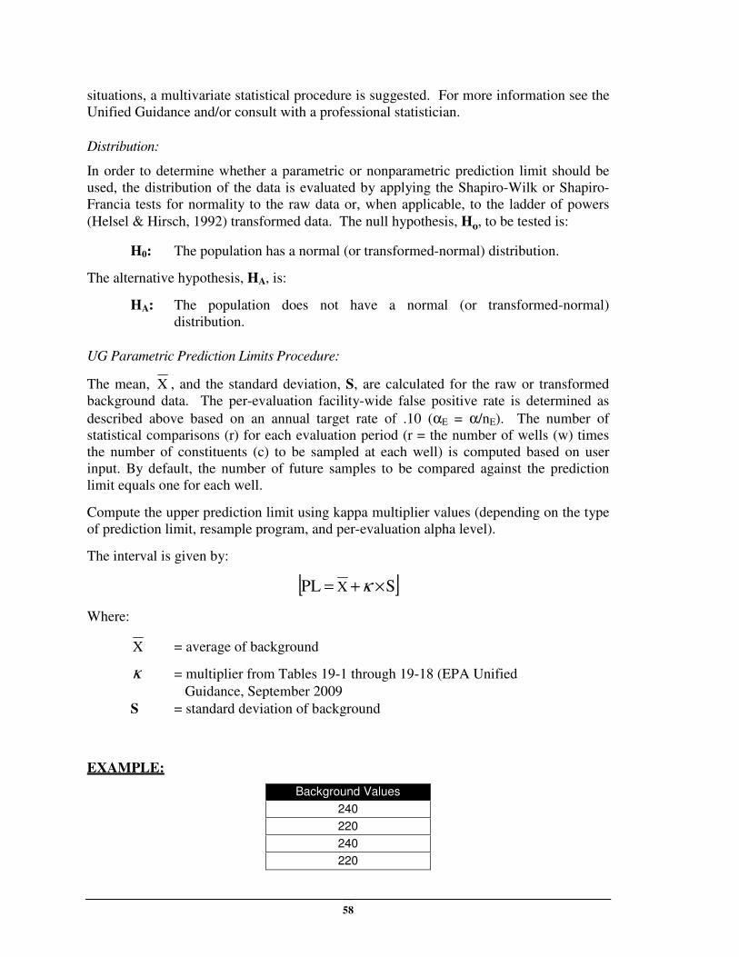
58

situations, a multivariate statistical procedure is suggested. For more information see the

Unified Guidance and/or consult with a professional statistician.

Distribution:

In order to determine whether a parametric or nonparametric prediction limit should be

used, the distribution of the data is evaluated by applying the Shapiro-Wilk or Shapiro-

Francia tests for normality to the raw data or, when applicable, to the ladder of powers

(Helsel & Hirsch, 1992) transformed data. The null hypothesis, Ho, to be tested is:

H0: The population has a normal (or transformed-normal) distribution.

The alternative hypothesis, HA, is:

HA: The population does not have a normal (or transformed-normal)

distribution.

UG Parametric Prediction Limits Procedure:

The mean, X , and the standard deviation, S, are calculated for the raw or transformed

background data. The per-evaluation facility-wide false positive rate is determined as

described above based on an annual target rate of .10 (αE = α/nE). The number of

statistical comparisons (r) for each evaluation period (r = the number of wells (w) times

the number of constituents (c) to be sampled at each well) is computed based on user

input. By default, the number of future samples to be compared against the prediction

limit equals one for each well.

Compute the upper prediction limit using kappa multiplier values (depending on the type

of prediction limit, resample program, and per-evaluation alpha level).

The interval is given by:

[ ]S PL X ×+= κ

Where:

X = average of background

κ = multiplier from Tables 19-1 through 19-18 (EPA Unified

Guidance, September 2009

S = standard deviation of background

EXAMPLE:

Background Values

240

220

240

220

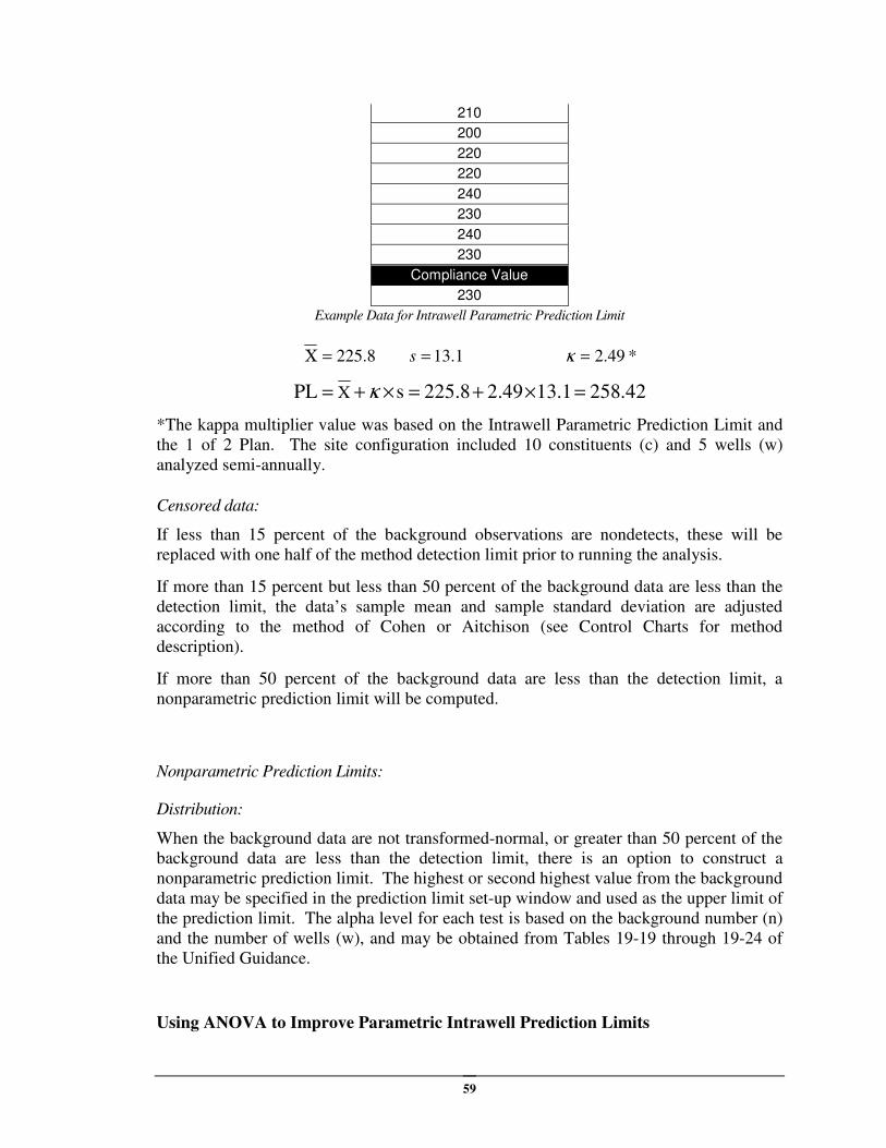
59

210

200

220

220

240

230

240

230

Compliance Value

230

Example Data for Intrawell Parametric Prediction Limit

8.225=Χ 1.13=s 49.2=κ *

42.2581.1349.2225.8sPL X =×+=×+= κ

*The kappa multiplier value was based on the Intrawell Parametric Prediction Limit and

the 1 of 2 Plan. The site configuration included 10 constituents (c) and 5 wells (w)

analyzed semi-annually.

Censored data:

If less than 15 percent of the background observations are nondetects, these will be

replaced with one half of the method detection limit prior to running the analysis.

If more than 15 percent but less than 50 percent of the background data are less than the

detection limit, the data’s sample mean and sample standard deviation are adjusted

according to the method of Cohen or Aitchison (see Control Charts for method

description).

If more than 50 percent of the background data are less than the detection limit, a

nonparametric prediction limit will be computed.

Nonparametric Prediction Limits:

Distribution:

When the background data are not transformed-normal, or greater than 50 percent of the

background data are less than the detection limit, there is an option to construct a

nonparametric prediction limit. The highest or second highest value from the background

data may be specified in the prediction limit set-up window and used as the upper limit of

the prediction limit. The alpha level for each test is based on the background number (n)

and the number of wells (w), and may be obtained from Tables 19-19 through 19-24 of

the Unified Guidance.

Using ANOVA to Improve Parametric Intrawell Prediction Limits

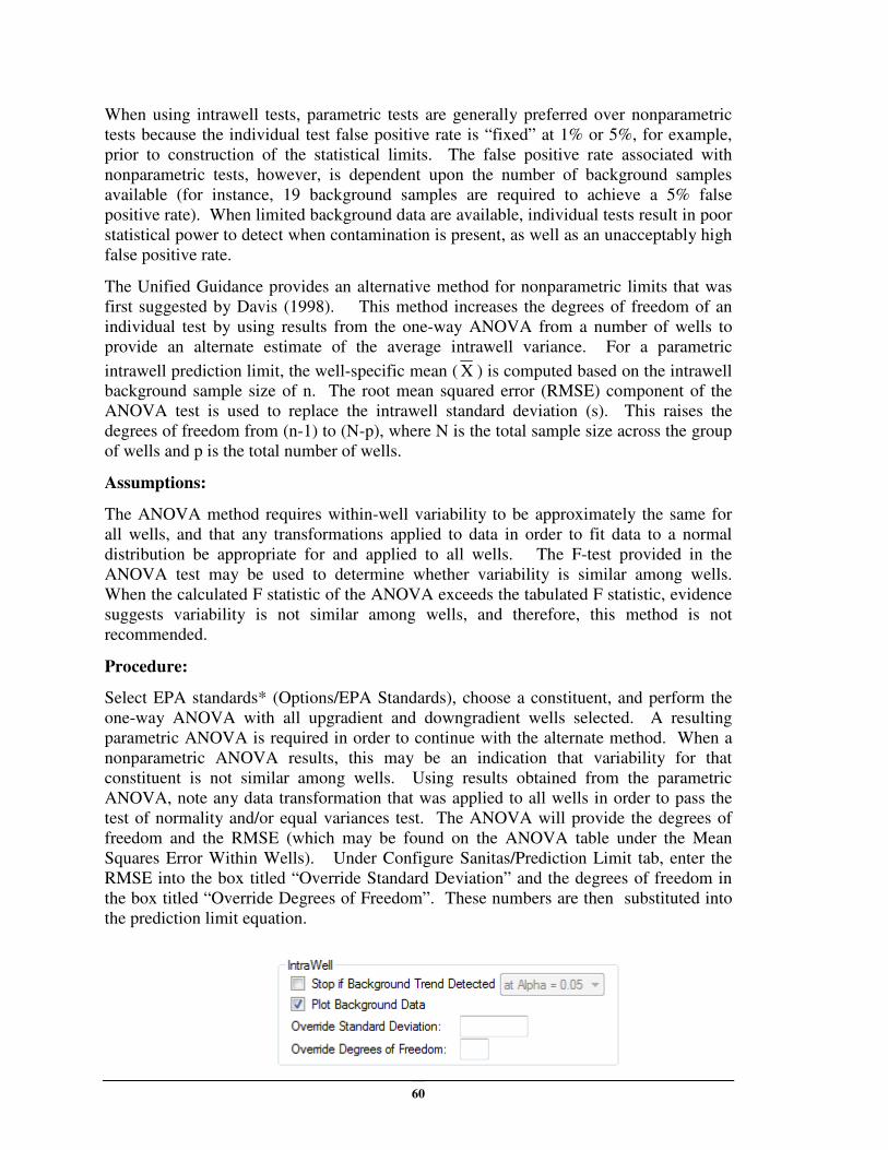
60

When using intrawell tests, parametric tests are generally preferred over nonparametric

tests because the individual test false positive rate is “fixed” at 1% or 5%, for example,

prior to construction of the statistical limits. The false positive rate associated with

nonparametric tests, however, is dependent upon the number of background samples

available (for instance, 19 background samples are required to achieve a 5% false

positive rate). When limited background data are available, individual tests result in poor

statistical power to detect when contamination is present, as well as an unacceptably high

false positive rate.

The Unified Guidance provides an alternative method for nonparametric limits that was

first suggested by Davis (1998). This method increases the degrees of freedom of an

individual test by using results from the one-way ANOVA from a number of wells to

provide an alternate estimate of the average intrawell variance. For a parametric

intrawell prediction limit, the well-specific mean ( X ) is computed based on the intrawell

background sample size of n. The root mean squared error (RMSE) component of the

ANOVA test is used to replace the intrawell standard deviation (s). This raises the

degrees of freedom from (n-1) to (N-p), where N is the total sample size across the group

of wells and p is the total number of wells.

Assumptions:

The ANOVA method requires within-well variability to be approximately the same for

all wells, and that any transformations applied to data in order to fit data to a normal

distribution be appropriate for and applied to all wells. The F-test provided in the

ANOVA test may be used to determine whether variability is similar among wells.

When the calculated F statistic of the ANOVA exceeds the tabulated F statistic, evidence

suggests variability is not similar among wells, and therefore, this method is not

recommended.

Procedure:

Select EPA standards* (Options/EPA Standards), choose a constituent, and perform the

one-way ANOVA with all upgradient and downgradient wells selected. A resulting

parametric ANOVA is required in order to continue with the alternate method. When a

nonparametric ANOVA results, this may be an indication that variability for that

constituent is not similar among wells. Using results obtained from the parametric

ANOVA, note any data transformation that was applied to all wells in order to pass the

test of normality and/or equal variances test. The ANOVA will provide the degrees of

freedom and the RMSE (which may be found on the ANOVA table under the Mean

Squares Error Within Wells). Under Configure Sanitas/Prediction Limit tab, enter the

RMSE into the box titled “Override Standard Deviation” and the degrees of freedom in

the box titled “Override Degrees of Freedom”. These numbers are then substituted into

the prediction limit equation.

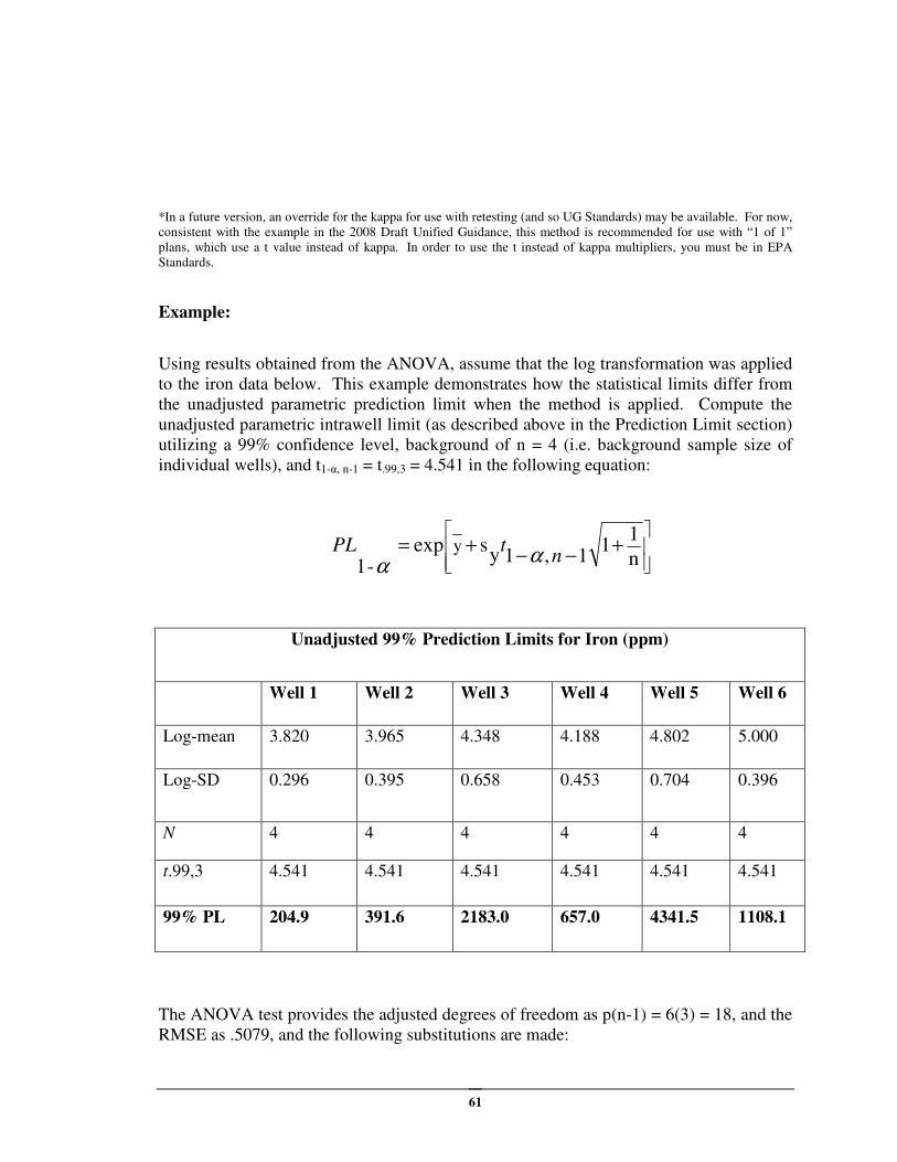
61

*In a future version, an override for the kappa for use with retesting (and so UG Standards) may be available. For now,

consistent with the example in the 2008 Draft Unified Guidance, this method is recommended for use with “1 of 1”

plans, which use a t value instead of kappa. In order to use the t instead of kappa multipliers, you must be in EPA

Standards.

Example:

Using results obtained from the ANOVA, assume that the log transformation was applied

to the iron data below. This example demonstrates how the statistical limits differ from

the unadjusted parametric prediction limit when the method is applied. Compute the

unadjusted parametric intrawell limit (as described above in the Prediction Limit section)

utilizing a 99% confidence level, background of n = 4 (i.e. background sample size of

individual wells), and t1-α, n-1 = t.99,3 = 4.541 in the following equation:

The ANOVA test provides the adjusted degrees of freedom as p(n-1) = 6(3) = 18, and the

RMSE as .5079, and the following substitutions are made:

Unadjusted 99% Prediction Limits for Iron (ppm)

Well 1 Well 2 Well 3 Well 4 Well 5 Well 6

Log-mean 3.820 3.965 4.348 4.188 4.802 5.000

Log-SD

0.296 0.395 0.658 0.453 0.704 0.396

N 4 4 4 4 4 4

t.99,3 4.541 4.541 4.541 4.541 4.541 4.541

99% PL 204.9 391.6 2183.0 657.0 4341.5 1108.1

+

−−+=

n

11

1,1ysexp

-1y

ntPL

αα

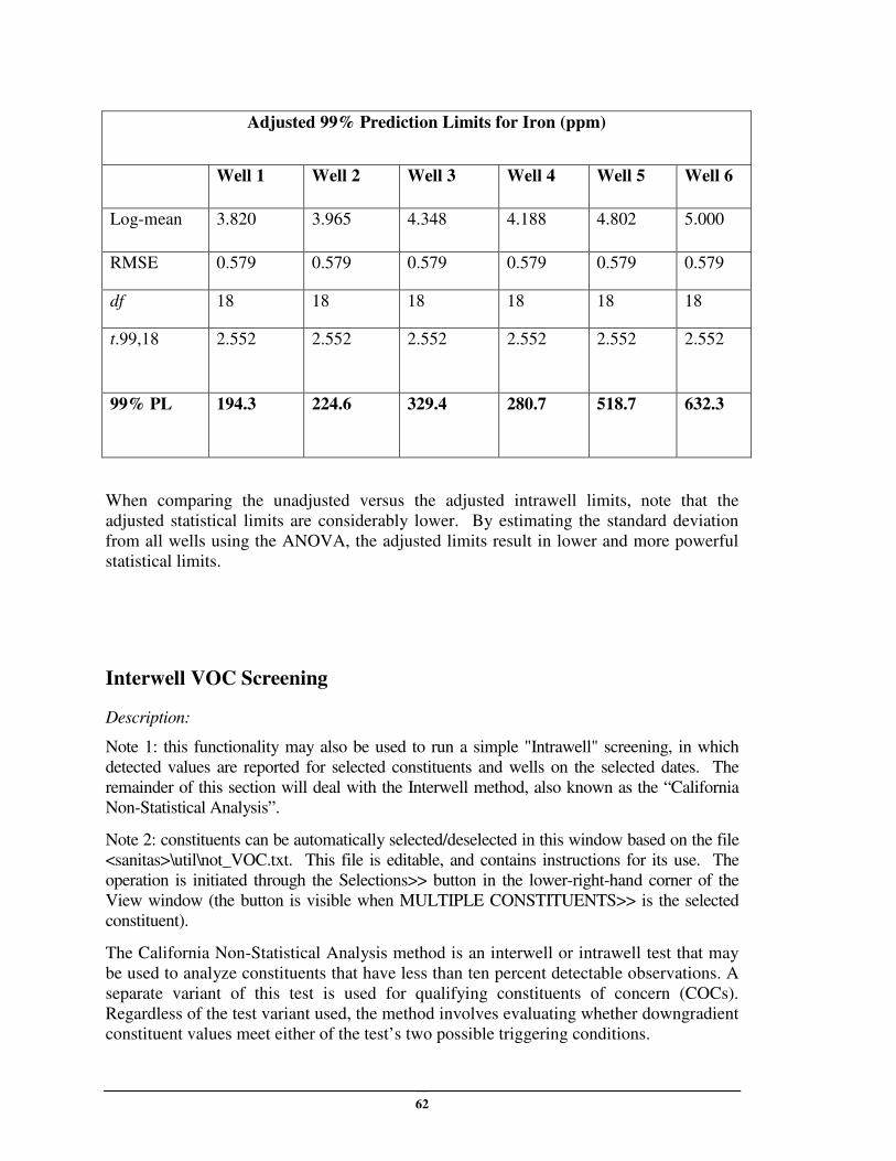
62

When comparing the unadjusted versus the adjusted intrawell limits, note that the

adjusted statistical limits are considerably lower. By estimating the standard deviation

from all wells using the ANOVA, the adjusted limits result in lower and more powerful

statistical limits.

Interwell VOC Screening

Description:

Note 1: this functionality may also be used to run a simple "Intrawell" screening, in which

detected values are reported for selected constituents and wells on the selected dates. The

remainder of this section will deal with the Interwell method, also known as the “California

Non-Statistical Analysis”.

Note 2: constituents can be automatically selected/deselected in this window based on the file

<sanitas>\util\not_VOC.txt. This file is editable, and contains instructions for its use. The

operation is initiated through the Selections>> button in the lower-right-hand corner of the

View window (the button is visible when MULTIPLE CONSTITUENTS>> is the selected

constituent).

The California Non-Statistical Analysis method is an interwell or intrawell test that may

be used to analyze constituents that have less than ten percent detectable observations. A

separate variant of this test is used for qualifying constituents of concern (COCs).

Regardless of the test variant used, the method involves evaluating whether downgradient

constituent values meet either of the test’s two possible triggering conditions.

Adjusted 99% Prediction Limits for Iron (ppm)

Well 1 Well 2 Well 3 Well 4 Well 5 Well 6

Log-mean 3.820 3.965 4.348 4.188 4.802 5.000

RMSE 0.579 0.579 0.579 0.579 0.579 0.579

df 18 18 18 18 18 18

t.99,18 2.552 2.552 2.552 2.552 2.552 2.552

99% PL 194.3 224.6 329.4 280.7 518.7 632.3

63

Assumption:

The background samples have less than ten percent detectable values for the given

parameters. This assumption is automatically enforced in the case of interwell analysis.

The intrawell case is more flexible, but requires the user to specify which constituent/well

pairs will be analyzed. For CA intrawell use, it is recommended that the View be

restricted to those Constituent/Well pairs containing <10% detects (for example,

Selections->Uncheck All, and then Selections->Check Where->Constituent/Well Pair->Is

Detect->Less than 10%) and then can be further restricted by removing cases that will be

analyzed statistically or via the interwell non-statistical approach. This View (which can

be saved specifically for this purpose) is then used to control the data included in

subsequent intrawell VOC analyses.

Procedure:

In the interwell case, the background well observations are checked to determine which

VOCs have less than ten percent detectable values, i.e. are eligible for the Non-Statistical

test. VOCs that have greater than or equal to ten percent detectable values must be

analyzed with a statistical analysis and are referred to as “orphans”.

Of the VOCs that are eligible for a non-statistical analysis (or for all selected constituents

and wells in the intrawell case) the compliance data are checked for the presence of either

three* VOCs exceeding their method detection limit or one VOC exceeding its practical

quantitation limit.

When either of the two possible triggering conditions has been met, VOC contamination

is suspected and a verification retest is indicated (see Verification Retest Procedure

section).

*This value can be user-adjusted in the .ini file.

Verification Retest Procedure – California

The following verification procedure is intended to meet the special performance

standards under Subsection 2550.7(e)(8)(E) in addition to the statistical performance

standards under Subsection 2550.7(e)(9) for detection monitoring.

The proposed verification procedure consists of discrete retests, in which rejection of the

null hypothesis for any one of the retests will be considered confirmation of significant

evidence of an impact. The discrete retest consists of collecting two new suites of

samples for the constituent(s) exceeding the concentration limit from the indicating

monitoring points.

The statistical test method used to evaluate the retest results will be the same as the

method used in the initial statistical comparison. For the original indication to be ignored,

both new analyses must contradict the original indication.

In the case of a Non-Statistical VOC analysis retest, two discrete samples are taken from

the suspected well(s) and a VOC suite chemical analysis is performed to identify

detectable constituents. The same triggering conditions hold for the retest as for the

64

original test; however, the parameters triggering a significant finding may be different

than those triggering the original indication.

Intrawell ASTM Approach (ASTM Standards Only)

This intrawell approach to detection monitoring is described in the Standard Guide for

Developing Appropriate Statistical Approaches for Ground-Water Detection Monitoring

Programs D 6312-98.

Censored Data:

If less than 75 percent of the observations are nondetects, an Intrawell Shewhart-CUSUM

Control Chart will be used. All nondetects will be replaced with the quantification limit

prior to running the analysis. If there are multiple detection limits, the median

quantification limit will be used.

If more than 75 percent but less than 100 percent of the data are less than the detection

limit, an Intrawell Poisson Prediction limit will be computed unless a sufficient number

of data points are available to compute an Intrawell Nonparametric Prediction limit that

will provide 99% confidence.

If 100 percent of the data are less than the detection limit, a Nonparametric Prediction

Limit or a Poisson Prediction Limit will be computed, depending on user selection.

Distribution:

If less than 75 percent of the observations are nondetects, the distribution of the data is

evaluated by applying the Shapiro-Wilk or Shapiro-Francia test for normality to the raw

data or, when applicable, to the transformed data. For a description of both the Shapiro-

Wilk and Shapiro-Francia tests please see the Distribution subsection of the Control

Chart Section.

If the distribution of the data is not found to be Normal, you can continue to run a

Shewhart-CUSUM Control Chart in ASTM Standards.

Seasonality:

Prior to constructing the Control Charts, the significance of data seasonality is evaluated

using the nonparametric Kruskal-Wallis test (U.S. EPA, April 1989). For a description,

please see earlier subsection on Seasonality under the Control Chart section.

When seasonality is known to exist, the data are deseasonalized prior to constructing

Control Charts in order to take into account seasonal variation rather than mistaking

seasonal effects for evidence of contamination. The data are deseasonalized using the

method described by EPA (U.S. EPA, April 1989). For a description, please see earlier

subsection on “Correcting for Seasonality” under the Control Chart Section.

65

Outliers:

To remove the possibility of either a high or low outlier in the historical data set, the

historical data are screened for the existence of outliers. See subsection “Outlier

Procedure” under the Descriptive Statistics Section for a method description. Note that if

the user has manually flagged values with an "O" (or "o") then the outlier test will not be

run, and the manually flagged outliers will instead be treated as confirmed outliers.

Existing Trends:

Prior to constructing a control chart, the background data are tested for the existence of

trends. If any trend exists (positive or negative) Sanitas will not run a control chart. The

ASTM Provisional Standards restrict trend testing to increasing trends. Sanitas tests for

both increasing and decreasing trends to prevent the possibility of a significant trend

confusing the statistical results. Both increasing and decreasing trends may lead to

inflated control limits. The provisional ASTM standards state that when significant

trends in background are present and these trends are not due to an impact, that an

alternative indicator constituent may be required for that well or all wells at the facility.

The Mann-Kendall test is used to test for significant trends in the background data. For a

method description please see the “Trend Analysis” subsection of the Evaluation

Monitoring Section.

Control Chart Procedure:

This procedure for construction of the Shewhart-CUSUM Control Chart follows the

ASTM recommendations (1996). The Shewhart-CUSUM Control Chart requires a

minimum of eight historical data points in order to reliably determine the mean and

standard deviation for each constituent’s concentration in a given well.

Three parameters are selected by the system prior to plotting:

h = the control limit to which the cumulative sum values (CUSUM) are

compared. ASTM (1996) recommends the value h = 4.5 units of

standard deviation for a background n < 12. When the background n >

12 the h is adjusted to = 4.0.

SCL = the upper Shewhart Control Limit to which the standardized mean

will be compared. ASTM (1996) recommends a value of SCL = 4.5

when background n < 12. When the background n > 12 ASTM

recommends SCL = 4.0.

c = a parameter related to the displacement that should be quickly

detected. ASTM (1996) recommends c = 1 for background n < 12. For

background n > 12, ASTM recommends c = 0.75.

The Shewhart CUSUM Control Chart is constructed as the method description describes

in the “Control Chart Procedure” section.

The results are plotted in their original metric units rather than standard deviation units.

For background, sample sizes less than 12:

66

4.5sSCLh +== X

For background sample sizes greater than or equal to 12:

4.0sSCLh +== X

and the Si are converted to the metric concentration by the transformation:

X+∗si

S

Censored Data:

If less than 75 percent of the background data are less than the quantification limit, the

data’s sample mean and standard deviation are adjusted according to the method of

Cohen or Aitchison. Please see previous section for a description of Cohen’s and

Aitchison’s adjustment.

If more than 75 percent of the background data are less than the quantification limit, a

nonparametric prediction limit will be computed. As an option to the nonparametric

prediction limit, a Poisson-based prediction limit may be computed.

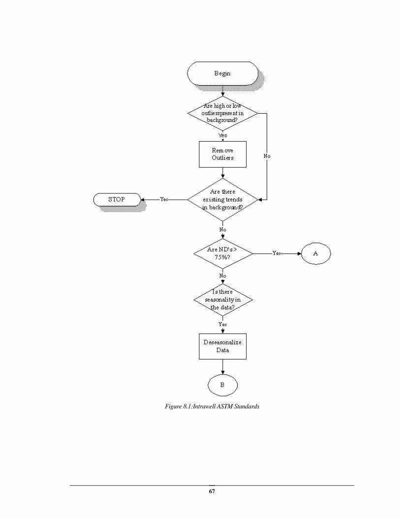
67

Figure 8.1:Intrawell ASTM Standards

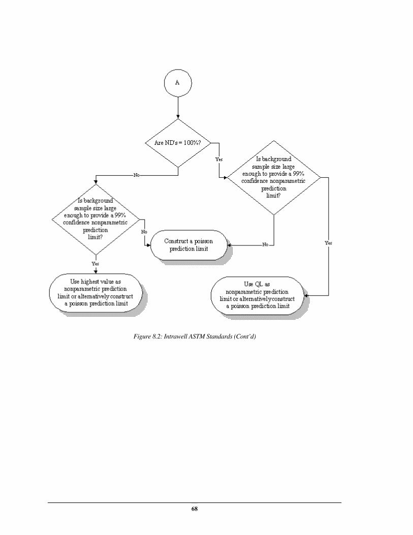
68

Figure 8.2: Intrawell ASTM Standards (Cont’d)

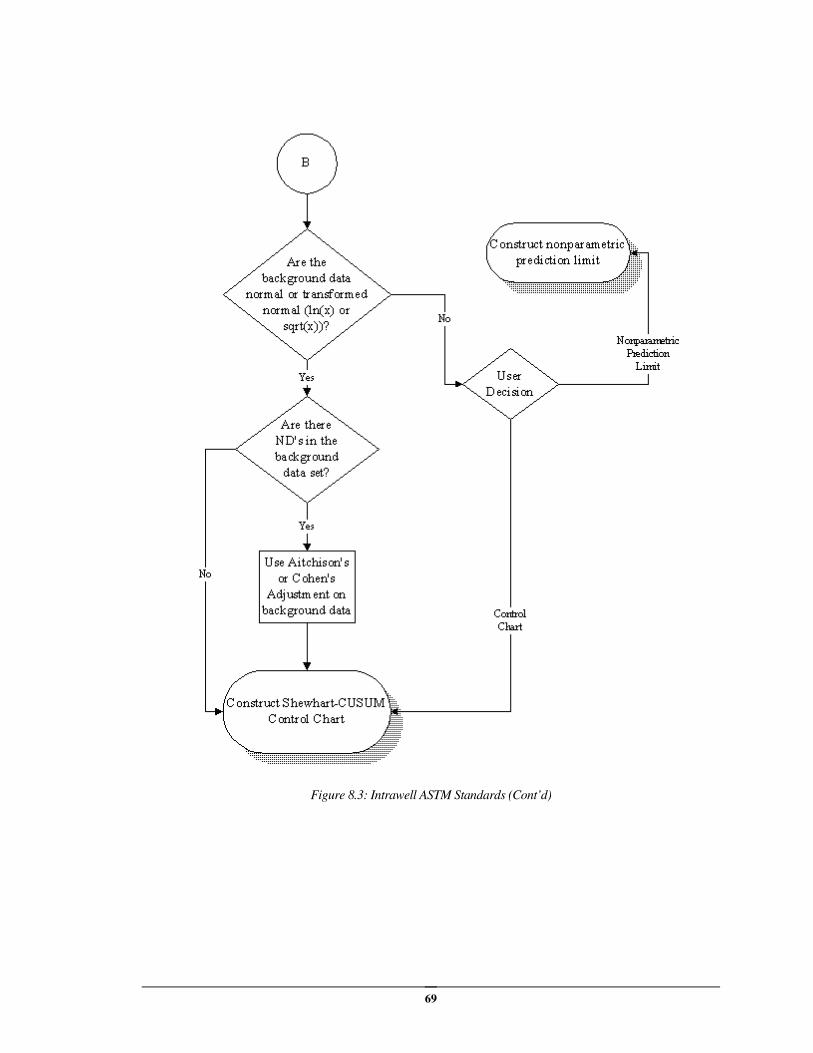
69

Figure 8.3: Intrawell ASTM Standards (Cont’d)

70

Interwell ASTM Approach (ASTM Standards Only)

This Interwell approach to detection monitoring is described in the Standard Guide for

Developing Appropriate Statistical Approaches for Ground-Water Detection Monitoring

Programs D 6312-98.

Distribution:

The distribution of the data is evaluated by applying the multiple group version of the

Shapiro-Wilk test for normality to the raw data or, when applicable, to the log

transformed data.

The null hypothesis, H0, to be tested is:

H0: The population has a normal (or transformed-normal) distribution.

The alternative hypothesis, HA, is:

HA: The population does not have a normal (or transformed-normal)

distribution.

Multiple Group Version Shapiro-Wilk Procedure:

The multiple group version of the Shapiro-Wilk test takes into consideration that

upgradient measurements are nested within different upgradient monitoring wells.

First, calculate the Shapiro-Wilk W-statistic (see prior section for method description) for

each compliance well and denote as Wi. Calculation of the multiple group version of the

Shapiro Wilk G-statistic to test the null hypothesis is presented in detail in

Technometrics, 10 (Wilk, Shapiro, 1968).

For sample size Ni, ≥ equal to seven, calculate G

i for each well. G

i is the percentage

point of the standard normal distribution corresponding to α α α αi. Under the null

assumptions, the quantities G1,...,G

K may be considered to be a random sample from a

standard normal distribution:

iW1

εi

Wδln

iG

−

−+= γ

Where the values γγγγ, δδδδ, εεεε are given in the Shapiro-Wilk (1968) table.

For sample sizes between three and six, use the value for Gi obtained from Table 2 of

Shapiro-Wilk (1968) by linear interpolation on the tabulated quantities:

71

−

−=

iW1

εi

Wln

iu

Then, compute G, the normalized value of Gi:

( )K

G2

G1

GK

1G +++=

K

Where:

K = number of wells.

Refer the normalized mean, G, to a standard table of the normal integral. If the

probability of G is greater than .01, accept the null hypothesis that the population has a

normal (or transformed normal) distribution.

Outliers:

To remove the possibility of either a high or low outlier in the historical data set, the

historical data are screened for the existence of outliers. See subsection “Outlier

Procedure” under the Descriptive Statistics Section for a method description. Note that if

the user has manually flagged values with an "O" (or "o") then the outlier test will not be

run, and the manually flagged outliers will instead be treated as confirmed outliers.

Censored data:

If less than 50 percent of the background data are less than the detection limit, the data’s

sample mean and sample standard deviation are adjusted according to the method of

Aitchison or Cohen. The use of Cohen’s or Aitchison’s adjustment is a user-selected

option. The user has the choice to select between these two approaches for adjusting non-

detects. The U.S. EPA (1992) provides a useful approach to help select which method to

use.

If more than 50 percent of the background data are less than the detection limit, a

nonparametric prediction limit will be computed. As an option to the nonparametric

prediction limit, a poisson-based prediction limit may be computed.

Parametric Prediction Limit Procedure:

The mean, X , and the standard deviation, S, are calculated for the raw or transformed

background data. Then the interval is given by:

n

11S

α1,ntX +

−+

if the data are normal, and the interval is given by:

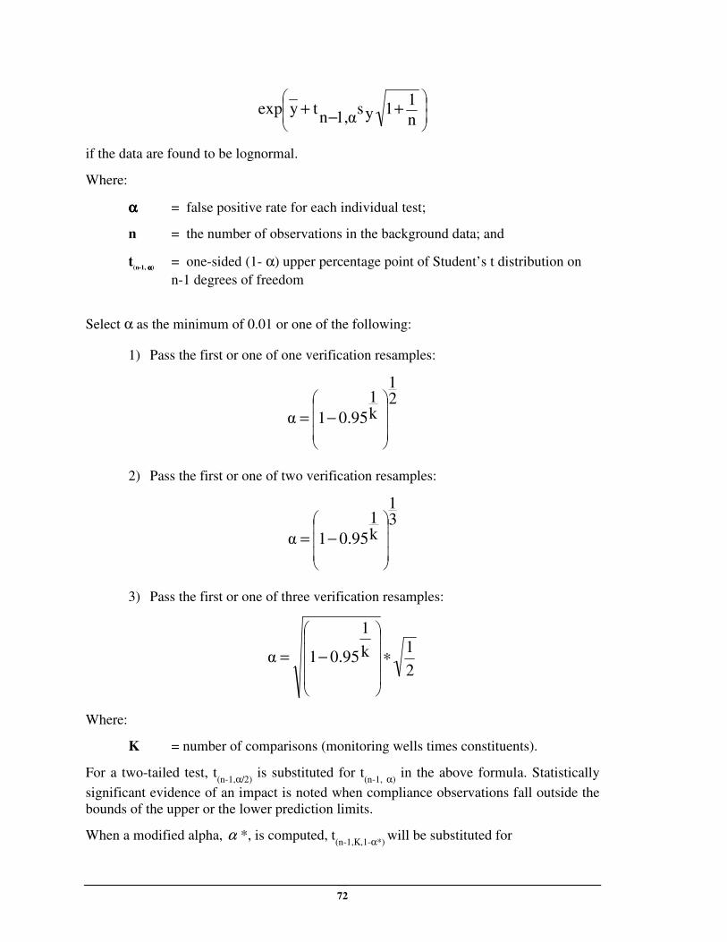
72

+

−+

n

11ys

α1,ntyexp

if the data are found to be lognormal.

Where:

αααα = false positive rate for each individual test;

n = the number of observations in the background data; and

t(n-1, αααα)

= one-sided (1- α) upper percentage point of Student’s t distribution on

n-1 degrees of freedom

Select α as the minimum of 0.01 or one of the following:

1) Pass the first or one of one verification resamples:

21

k1

0.951α

−=

2) Pass the first or one of two verification resamples:

31

k1

0.951α

−=

3) Pass the first or one of three verification resamples:

2

1k

1

0.951α ∗−=

Where:

K = number of comparisons (monitoring wells times constituents).

For a two-tailed test, t(n-1,α/2)

is substituted for t(n-1, α)

in the above formula. Statistically

significant evidence of an impact is noted when compliance observations fall outside the

bounds of the upper or the lower prediction limits.

When a modified alpha, α *, is computed, t(n-1,K,1-α*)

will be substituted for

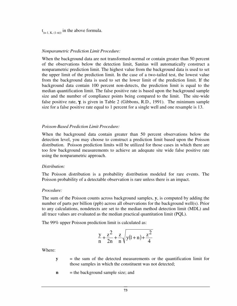
73

t(n-1, K, (1-α))

in the above formula.

Nonparametric Prediction Limit Procedure:

When the background data are not transformed-normal or contain greater than 50 percent

of the observations below the detection limit, Sanitas will automatically construct a

nonparametric prediction limit. The highest value from the background data is used to set

the upper limit of the prediction limit. In the case of a two-tailed test, the lowest value

from the background data is used to set the lower limit of the prediction limit. If the

background data contain 100 percent non-detects, the prediction limit is equal to the

median quantification limit. The false positive rate is based upon the background sample

size and the number of compliance points being compared to the limit. The site-wide

false positive rate, γγγγ, is given in Table 2 (Gibbons, R.D., 1991). The minimum sample

size for a false positive rate equal to 1 percent for a single well and one resample is 13.

Poisson-Based Prediction Limit Procedure:

When the background data contain greater than 50 percent observations below the

detection level, you may choose to construct a prediction limit based upon the Poisson

distribution. Poisson prediction limits will be utilized for those cases in which there are

too few background measurements to achieve an adequate site wide false positive rate

using the nonparametric approach.

Distribution:

The Poisson distribution is a probability distribution modeled for rare events. The

Poisson probability of a detectable observation is rare unless there is an impact.

Procedure:

The sum of the Poisson counts across background samples, y, is computed by adding the

number of parts per billion (ppb) across all observations for the background well(s). Prior

to any calculations, nondetects are set to the median method detection limit (MDL) and

all trace values are evaluated as the median practical quantitation limit (PQL).

The 99% upper Poisson prediction limit is calculated as:

( )4

2zn1y

n

z

2n

2z

n

y++++

Where:

y = the sum of the detected measurements or the quantification limit for

those samples in which the constituent was not detected;

n = the background sample size; and

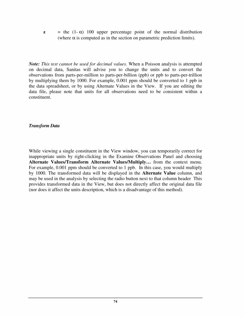
74

z = the (1- α) 100 upper percentage point of the normal distribution

(where α is computed as in the section on parametric prediction limits).

Note: This test cannot be used for decimal values. When a Poisson analysis is attempted

on decimal data, Sanitas will advise you to change the units and to convert the

observations from parts-per-million to parts-per-billion (ppb) or ppb to parts-per-trillion

by multiplying them by 1000. For example, 0.001 ppm should be converted to 1 ppb in

the data spreadsheet, or by using Alternate Values in the View. If you are editing the

data file, please note that units for all observations need to be consistent within a

constituent.

Transform Data

While viewing a single constituent in the View window, you can temporarily correct for

inappropriate units by right-clicking in the Examine Observations Panel and choosing

Alternate Values/Transform Alternate Values/Multiply… from the context menu.

For example, 0.001 ppm should be converted to 1 ppb. In this case, you would multiply

by 1000. The transformed data will be displayed in the Alternate Value column, and

may be used in the analysis by selecting the radio button next to that column header This

provides transformed data in the View, but does not directly affect the original data file

(nor does it affect the units description, which is a disadvantage of this method).

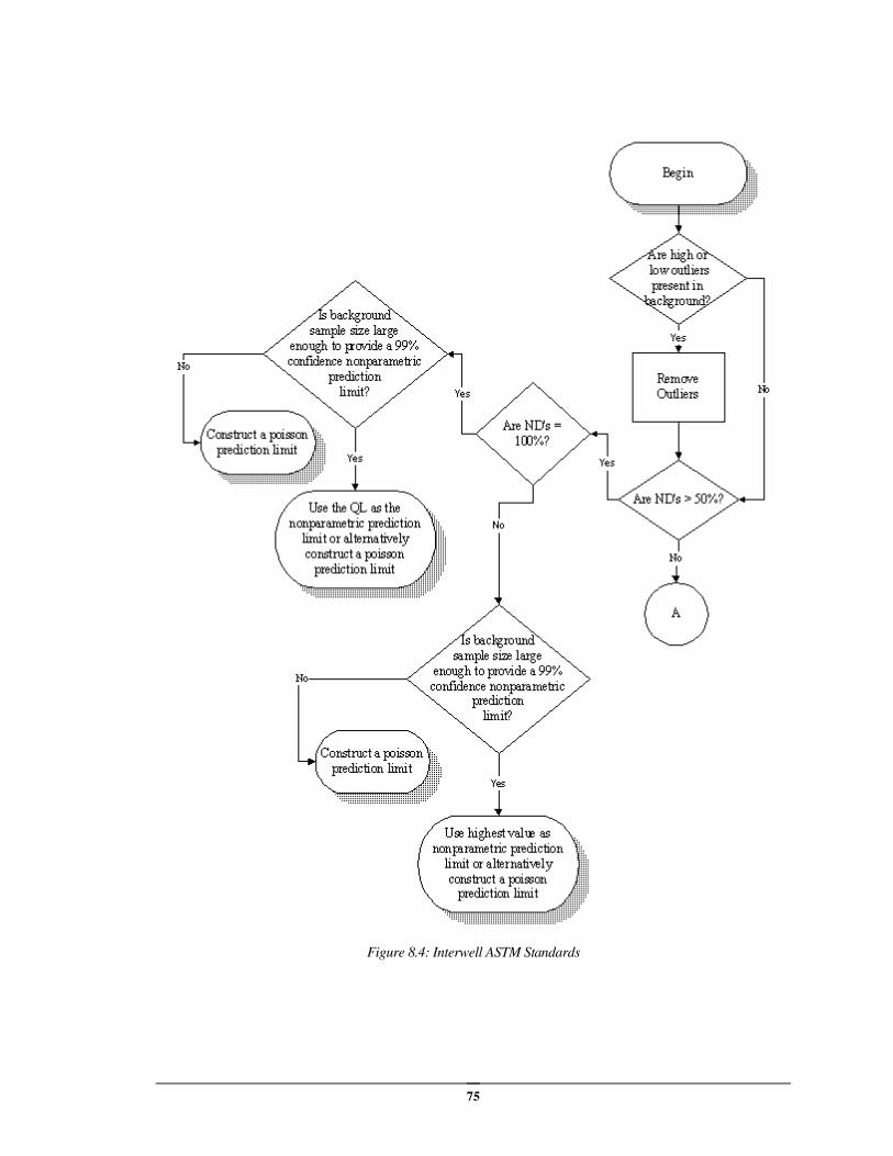
75

Figure 8.4: Interwell ASTM Standards

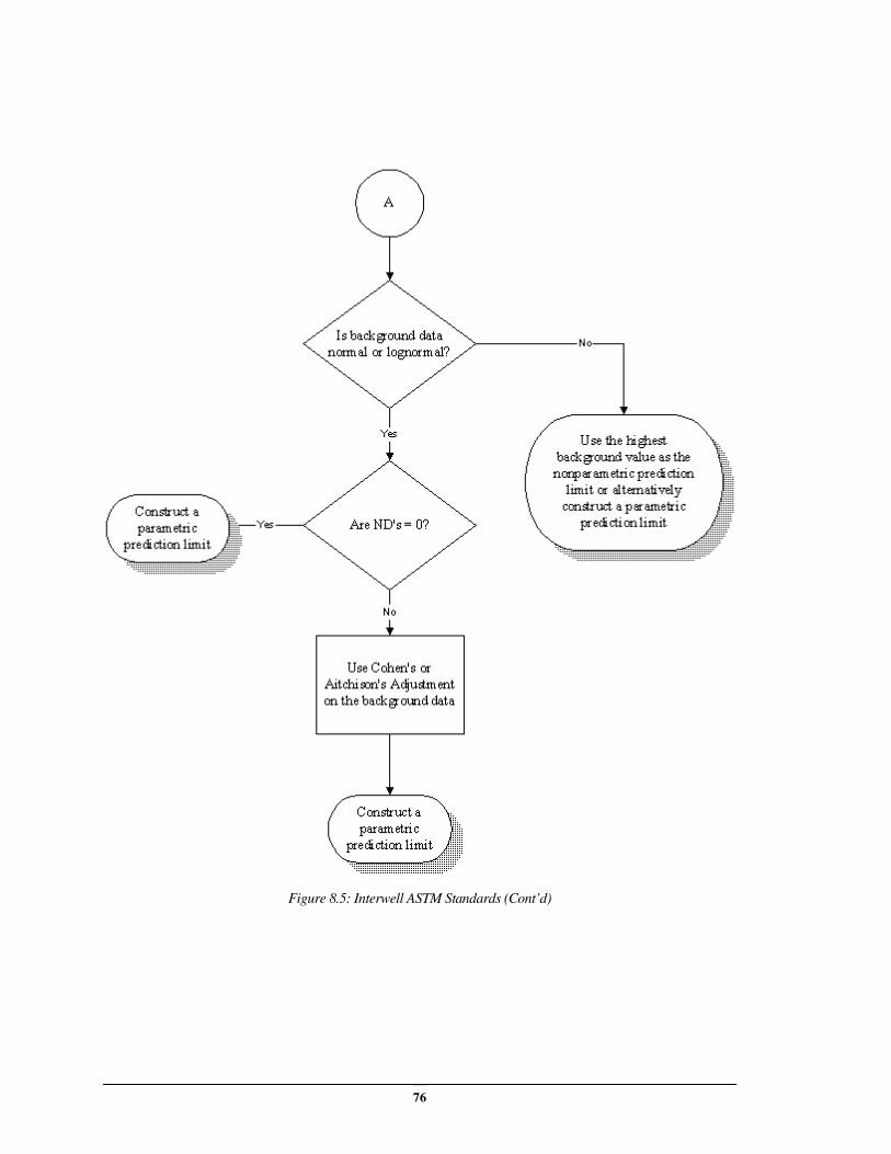
76

Figure 8.5: Interwell ASTM Standards (Cont’d)

77

Evaluation Monitoring Statistics

Trend Analysis

Description and Procedure:

A trend is the general increase or decrease in observed values of some random variable

over time. A trend analysis can be used to determine the significance of an apparent trend

and to estimate the magnitude of that trend. The Mann-Kendall test for temporal trend

(Hollander & Wolfe, 1973) and Sen’s slope estimate (Gilbert, 1987) were chosen for the

site evaluation (or assessment) monitoring program to evaluate the correlation of selected

constituent concentrations with time.

The Mann-Kendall test is nonparametric, meaning that it does not depend on an

assumption of a particular underlying distribution. The test uses only the relative

magnitude of data rather than actual values. Therefore, missing values are allowed, and

values that are recorded as non-detects by the laboratory can still be used in the statistical

analysis by assigning values equal to half their detection limits (Gilbert, 1987).

The null hypothesis, H0, to be tested is:

H0: No significant trend of a constituent exists over time.

The alternative hypothesis, HA, is:

HA: A significant upward (or downward) trend of a constituent concentration

exists over time.

For groups having fewer than 41 data points, an exact test is performed. If 41 or more

data points are available, the normal approximation test is used (Gilbert, 1987).

- Exact Test (n <= 40):

The Mann-Kendall method assigns a positive or negative score based on the differences

between the data points. The first step is to list the data in the order in which they were

collected over time, and then determine the sign of all possible differences xj - xk, where

j > k:

−

kx

jxsgn = 0

kx

j xif 1 >−

= 0k

xj

xif 0 =−

= 0k

xj

xif 1 <−−

Where:

xj = the value of the jth observation; and

78

xk = the value of the kth observation.

The Mann-Kendall statistic, S, is then computed, which is the number of positive

differences minus the number of negative differences.

∑−

=∑

+=−=

1n

1k

n

1kj kx

jxsgnS

Where:

n = the total number of observations.

If S (noted on the plot as the Mann-Kendall Statistic) is a large positive number,

measurements taken later in time tend to be larger than those taken earlier, i.e., an upward

trend. Similarly, if S is a large negative number, measurements taken later in time tend to

be smaller, i.e., a downward trend.

For a two-tailed test to detect either an upward or downward trend, the tabulated

probability level corresponding to the absolute value of S (Gilbert, 1987) is doubled and

H0 is rejected if that doubled value is less than or equal to the a priori α significance level

of the test. In other words, the Mann-Kendall Statistic (S) is compared to the Critical

value (or threshold for accepting H0) on the plot, and a trend is statistically significant if

the absolute value of S is greater than the tabulated Critical Value.

A minimum of 4 samples is required to perform the test. However, with a sample size of

only 4, the only meaningful information that can be obtained from this test is the value of

the Sen's slope, which gives the average rate of change in concentration over time. The

Mann Kendall test for significance of trend will always indicate no trend at the 95%

confidence level since the largest possible value of the test statistic, S, with four data

points is 6, and that value is not significant at any available alpha level.

- Normal Approximation Test (n > 40):

The Mann-Kendall test statistic, S, is calculated using the same method of the exact test.

When there are no tied values, the variance of VAR(S) is computed:

18

5)1)(2nn(nVAR(S)

+−=

S and VAR(S) are then used to compute the test statistic, Z, as follows:

79

[ ]

[ ]

0S if

VAR(S)

1SZ

0S if0Z

0S if

VAR(S)

1SZ

2

1

2

1

<+

=

==

>−

=

When tied values (data points having equal values) are present, the variance of S is

computed:

+−∑

=−+−= 5)p1)(2tp(t

g

1ppt5)1)(2nn(n

18

1VAR(S)

Where:

g = the number of tied groups; and

tp = the number of observations in the pth group.

To test for an upward or a downward trend (a two-tailed test), a level of significance, α ,

must first be chosen. The level of significance is the probability of rejecting the null

hypothesis, (Ho) no trend, when no trend actually exists (Type I error). In general, α is

chosen to be 0.05. The split Type I error probability, or α / 2, for a two-tailed test is

then 0.025.

The Z-value associated with the 0.025 significance level is 1.96, from Table A-1

(Hollander and Wolfe, 1973), corresponding to an α -level of 0.05, 95 percent (1-α ) of

the area under the normal curve lies between -Zα = -1.96 and Zα = 1.96.

A positive or negative value of Z can indicate an upward or downward trend,

respectively. With an α -value of 0.05, any Z-value above 1.96 indicates a statistically

significant upward trend, and any value below -1.96 indicates a statistically significant

downward trend. In such cases, the Ho of no trend would be rejected. For values, which

fall between -1.96 and 1.96, the null hypothesis cannot be rejected.

To reject H0, the probability corresponding to the Z-value must be less than the specified

α -value. The smaller the probability value, the greater the likelihood that a trend is

occurring and the greater the likelihood the constituent concentration (the dependent

variable) is an increasing or decreasing function of time.

80

Sen’s Slope Estimator

Description:

This simple nonparametric procedure was developed by Sen (1968) and presented in

Gilbert (1987) to estimate the true slope. The advantage of this method over linear

regression is that it is not greatly affected by gross data errors or outliers, and can be

computed when data are missing.

The N′ individual slope estimates, Q, are computed for each time period:

ii'i

X'i

XQ

−

−=

Where:

ii X and X′

= the data values at time i′ and i (in days), respectively, i′ ’> I; and

N′ = the number of data pairs for which i′ > i.

A value of one half of the detection limit will be substituted for Xi values below the

detection limit.

Sen’s Slope estimator is the median slope, obtained by ranking the N′ values of Q from

smallest to largest, and choosing the middle-ranked slope as follows.

( )[ ] odd is N' if/21nnN'Q −=

even is N' if/22N'

Q/2N'

Q2

1

++

Where:

n = the number of time periods.

This value is multiplied by 365 to give the yearly slope value.

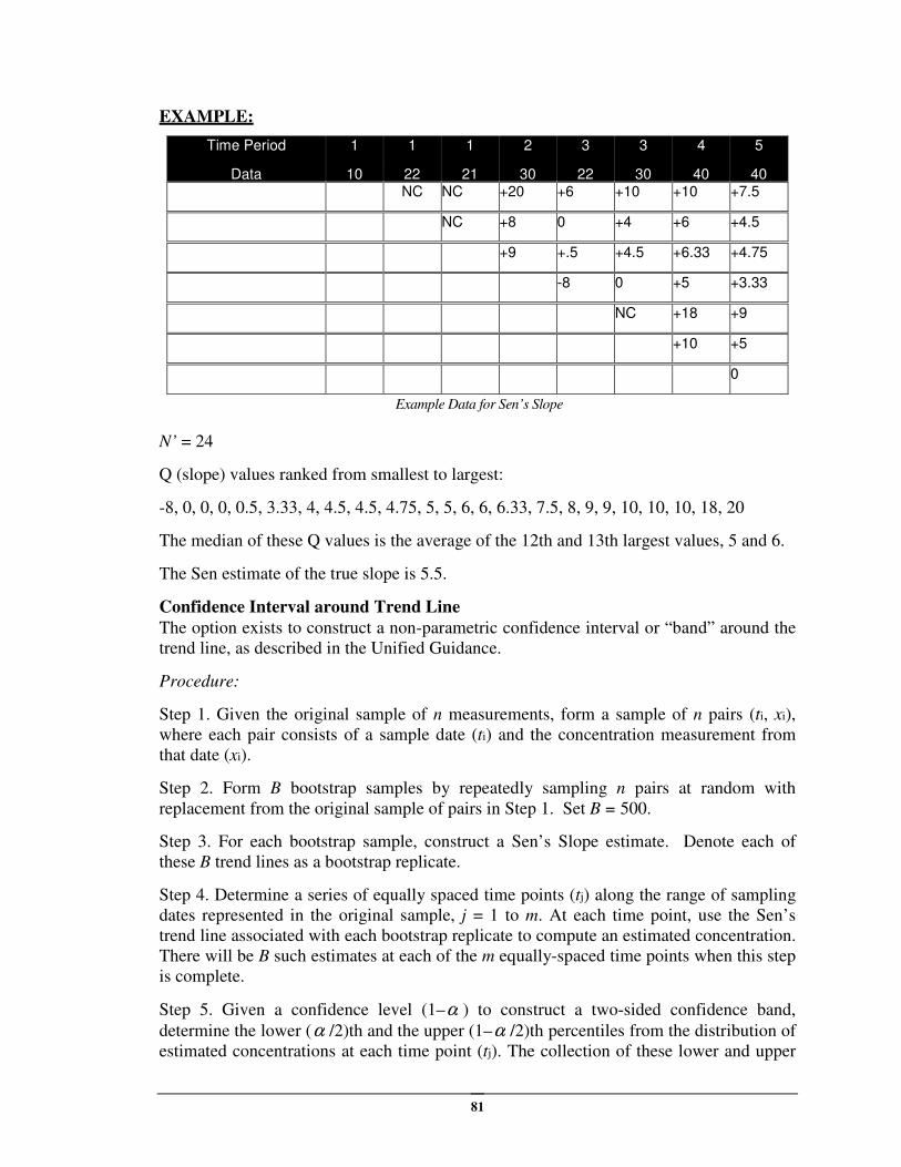
81

EXAMPLE:

Time Period

Data

1

10

1

22

1

21

2

30

3

22

3

30

4

40

5

40 NC NC +20 +6 +10 +10 +7.5

NC +8 0 +4 +6 +4.5

+9 +.5 +4.5 +6.33 +4.75

-8 0 +5 +3.33

NC +18 +9

+10 +5

0

Example Data for Sen’s Slope

N’ = 24

Q (slope) values ranked from smallest to largest:

-8, 0, 0, 0, 0.5, 3.33, 4, 4.5, 4.5, 4.75, 5, 5, 6, 6, 6.33, 7.5, 8, 9, 9, 10, 10, 10, 18, 20

The median of these Q values is the average of the 12th and 13th largest values, 5 and 6.

The Sen estimate of the true slope is 5.5.

Confidence Interval around Trend Line

The option exists to construct a non-parametric confidence interval or “band” around the

trend line, as described in the Unified Guidance.

Procedure:

Step 1. Given the original sample of n measurements, form a sample of n pairs (ti, xi),

where each pair consists of a sample date (ti) and the concentration measurement from

that date (xi).

Step 2. Form B bootstrap samples by repeatedly sampling n pairs at random with

replacement from the original sample of pairs in Step 1. Set B = 500.

Step 3. For each bootstrap sample, construct a Sen’s Slope estimate. Denote each of

these B trend lines as a bootstrap replicate.

Step 4. Determine a series of equally spaced time points (tj) along the range of sampling

dates represented in the original sample, j = 1 to m. At each time point, use the Sen’s

trend line associated with each bootstrap replicate to compute an estimated concentration.

There will be B such estimates at each of the m equally-spaced time points when this step

is complete.

Step 5. Given a confidence level (1–α ) to construct a two-sided confidence band,

determine the lower (α /2)th and the upper (1–α /2)th percentiles from the distribution of

estimated concentrations at each time point (tj). The collection of these lower and upper

82

percentiles along the range of sampling dates (tj, j = 1 to m) forms the bootstrapped

confidence band.

Seasonal Kendall Test

Description:

The Seasonal Kendall Test is an extension of the Mann-Kendall test that removes

seasonal cycles and tests for trend.

Seasonal Kendall Procedure:

Compute the Mann-Kendall statistic, S, for each season. Let Si denote this statistic for

the ith season, that is:

∑ ∑−

= +=

−=1n

1k

n

1kl

ikil

i i

)xsgn(xSi

Where l > k, ni is the number of data for season i, and:

0 x-x if -1

0 x-x if 0

0 x-x if 1)xsgn(x

ikil

ikil

ikilikil

<=

==

>=−

VAR(Si) is computed as follows:

1)(n2n

1)(uu1)(tt

2)1)(n(n9n

2)1)(u(uu2)1)(t(tt

5)1)(2u(uu5)1)(2t(tt5)1)(2n(nn18

1)VAR(S

ii

g

1p

h

1q

iqiqipip

iii

g

1p

h

1q

iqiqiqipipip

g

1p

h

1q

iqiqiqipipipiiii

i ii i

i i

−

−−

+−−

−−−−

+

+−−+−−+−=

∑ ∑∑ ∑

∑ ∑

= == =

= =

Where:

gi = The number of groups of tied data in season I;

tip = The number of tied data in the pth group for season I;

hi = The number of sampling times(or time periods) in season i that

contain multiple data; and

uiq = The number of multiple data in the qth time period in season i.

After Si and VAR(Si) are computed, we pool across the K seasons:

∑=

=K

1i

iSS'

and

83

∑=

=K

1i

i )VAR(S)VAR(S'

Next compute:

[ ]0 S' if

)VAR(S'

1)(S'Z

0 S' if 0 Z

0 S' if )][VAR(S'

1)(S'Z

1/2

1/2

<+

=

==

>−

=

For a two tailed test, we reject Ho of no trend if the absolute value of Z is greater than Z1-

α/2. Sanitas tests at the 80%, 90% and 95% confidence levels.

Seasonal Kendall Slope Estimator Procedure:

First compute individual Ni slope estimates for the ith season:

kl

xxQi ikil

−

−=

Where:

xil = The datum for the ith season of the lth year; and

xik = The datum for the ith season of the kth year, where l > k.

Do this for each of the K seasons. Then rank the N’1 + N’2 + …+ N’K = N’ individual

slope estimates and find their median. This median is the seasonal Kendall slope

estimator.

Compliance or Corrective Action Monitoring Statistics

Confidence Intervals

Description:

A Confidence Interval is constructed from sample data and is designed to contain the

mean concentration of a well analyte in ground water monitoring, with a designated level

of confidence. A Confidence Interval generally should be used when specified by permit

or when downgradient samples are being compared to the maximum concentration limit

84

(MCL) or alternate concentration limit (ACL). In this situation, the MCL or ACL is a

specified concentration limit or determined by the background concentrations.

Assumptions:

The sample data used to construct the intervals must be normally or transformed-

normally distributed. In the case of a transformed-normal distribution, the Confidence

Interval must be constructed on the transformed sample concentration values. In addition

to the interval construction, the comparison must be made to the transformed MCL or

ACL value. When none of the transformed models can be justified, a nonparametric

version of each interval may be utilized. If the entire Confidence Interval exceeds the

compliance limit, there is statistically significant evidence that the mean concentration

exceeds the compliance limit.

Distribution:

The distribution of the data is evaluated by applying the Shapiro-Wilk or Shapiro-Francia

test for normality to the raw data or, when applicable to the Ladder of Powers (Helsel &

Hirsch, 1992) transformed data.

The null hypothesis, H0, to be tested is:

H0: The population has a normal (or transformed-normal) distribution.

The alternative hypothesis, HA, is:

HA: The population does not have a normal (or transformed-normal)

distribution.

Censored Data:

If less than 15 percent of the observations are nondetects, these will be replaced with one

half the method detection limit prior to running the normality test and constructing the

Confidence Interval.

If more than 15 percent but less than 50 percent of the data are less than the detection

limit, the data’s sample mean and standard deviation are adjusted according to the

method of Cohen or Aitchison (U.S. EPA, April 1989). This adjustment is made prior to

construction of the Confidence Interval.

If more than 50 percent of the data are less than the detection limit, these values are

replaced with one half the method detection limit and a nonparametric Confidence

Interval is constructed.

Parametric Confidence Interval Procedures:

A minimum of four sample values is required for the construction of the parametric

Confidence Interval. The mean, X , and standard deviation, S, of the sample

concentration values are calculated separately for each compliance well (monitoring

point). For each well, the Confidence Interval is calculated as:

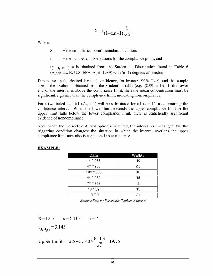
85

n

S1)nα,(1

tX−−

±

Where:

S = the compliance point’s standard deviation;

n = the number of observations for the compliance point; and

t(1-αααα, n-1) = is obtained from the Student’s t-Distribution found in Table 6

(Appendix B; U.S. EPA, April 1989) with (n -1) degrees of freedom.

Depending on the desired level of confidence, for instance 99% (1-α), and the sample

size n, the t-value is obtained from the Student’s t-table (e.g. t(0.99, n-1)). If the lower

end of the interval is above the compliance limit, then the mean concentration must be

significantly greater than the compliance limit, indicating noncompliance.

For a two-tailed test, t(1-α/2, n-1) will be substituted for t(1-α, n-1) in determining the

confidence interval. When the lower limit exceeds the upper compliance limit or the

upper limit falls below the lower compliance limit, there is statistically significant

evidence of noncompliance.

Note: when the Corrective Action option is selected, the interval is unchanged, but the

triggering condition changes: the situation in which the interval overlaps the upper

compliance limit now also is considered an exceedance.

EXAMPLE:

Date Well#3

1/1/1988 10

4/1/1988 2.5

10/1/1988 16

4/1/1989 15

7/1/1989 8

10/1/89 15

1/1/90 21

Example Data for Parametric Confidence Interval

12.5X = 6.103s = 7n =

3.143.99,6

t =

75.197

6.1033.14312.5 Limit Upper =∗+=

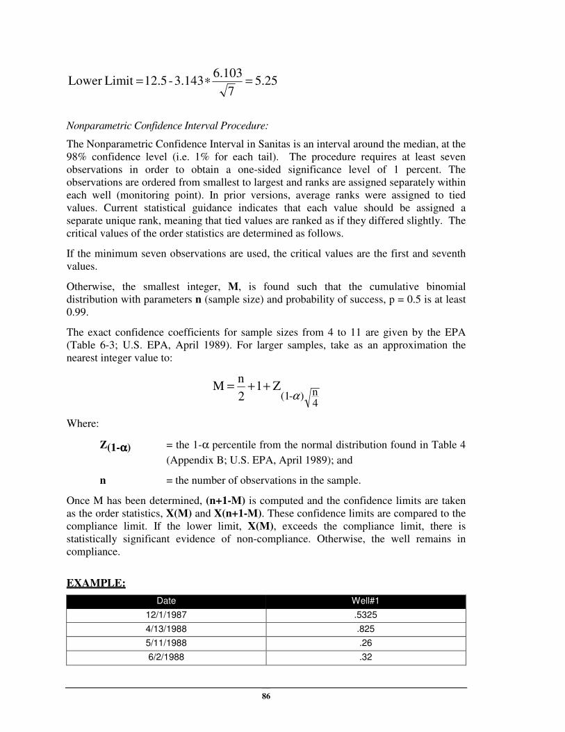
86

25.57

6.1033.143-12.5 Limit Lower =∗=

Nonparametric Confidence Interval Procedure:

The Nonparametric Confidence Interval in Sanitas is an interval around the median, at the

98% confidence level (i.e. 1% for each tail). The procedure requires at least seven

observations in order to obtain a one-sided significance level of 1 percent. The

observations are ordered from smallest to largest and ranks are assigned separately within

each well (monitoring point). In prior versions, average ranks were assigned to tied

values. Current statistical guidance indicates that each value should be assigned a

separate unique rank, meaning that tied values are ranked as if they differed slightly. The

critical values of the order statistics are determined as follows.

If the minimum seven observations are used, the critical values are the first and seventh

values.

Otherwise, the smallest integer, M, is found such that the cumulative binomial

distribution with parameters n (sample size) and probability of success, p = 0.5 is at least

0.99.

The exact confidence coefficients for sample sizes from 4 to 11 are given by the EPA

(Table 6-3; U.S. EPA, April 1989). For larger samples, take as an approximation the

nearest integer value to:

4n)-(1

Z12

nM

α++=

Where:

Z(1-αααα) = the 1-α percentile from the normal distribution found in Table 4

(Appendix B; U.S. EPA, April 1989); and

n = the number of observations in the sample.

Once M has been determined, (n+1-M) is computed and the confidence limits are taken

as the order statistics, X(M) and X(n+1-M). These confidence limits are compared to the

compliance limit. If the lower limit, X(M), exceeds the compliance limit, there is

statistically significant evidence of non-compliance. Otherwise, the well remains in

compliance.

EXAMPLE:

Date Well#1

12/1/1987 .5325

4/13/1988 .825

5/11/1988 .26

6/2/1988 .32

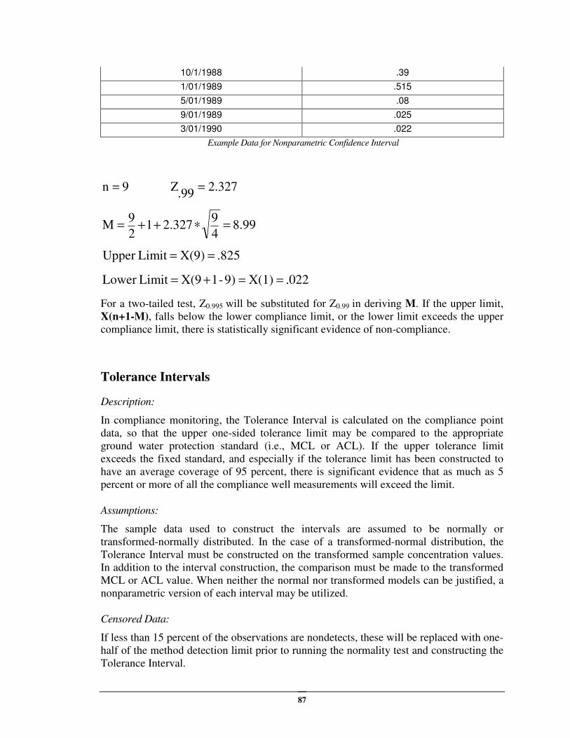
87

10/1/1988 .39

1/01/1989 .515

5/01/1989 .08

9/01/1989 .025

3/01/1990 .022

Example Data for Nonparametric Confidence Interval

2.327.99

Z9n ==

8.994

92.3271

2

9M =∗++=

.825X(9)Limit Upper ==

.022X(1)9)-1X(9Limit Lower ==+=

For a two-tailed test, Z0.995 will be substituted for Z0.99 in deriving M. If the upper limit,

X(n+1-M), falls below the lower compliance limit, or the lower limit exceeds the upper

compliance limit, there is statistically significant evidence of non-compliance.

Tolerance Intervals

Description:

In compliance monitoring, the Tolerance Interval is calculated on the compliance point

data, so that the upper one-sided tolerance limit may be compared to the appropriate

ground water protection standard (i.e., MCL or ACL). If the upper tolerance limit

exceeds the fixed standard, and especially if the tolerance limit has been constructed to

have an average coverage of 95 percent, there is significant evidence that as much as 5

percent or more of all the compliance well measurements will exceed the limit.

Assumptions:

The sample data used to construct the intervals are assumed to be normally or

transformed-normally distributed. In the case of a transformed-normal distribution, the

Tolerance Interval must be constructed on the transformed sample concentration values.

In addition to the interval construction, the comparison must be made to the transformed

MCL or ACL value. When neither the normal nor transformed models can be justified, a

nonparametric version of each interval may be utilized.

Censored Data:

If less than 15 percent of the observations are nondetects, these will be replaced with one-

half of the method detection limit prior to running the normality test and constructing the

Tolerance Interval.

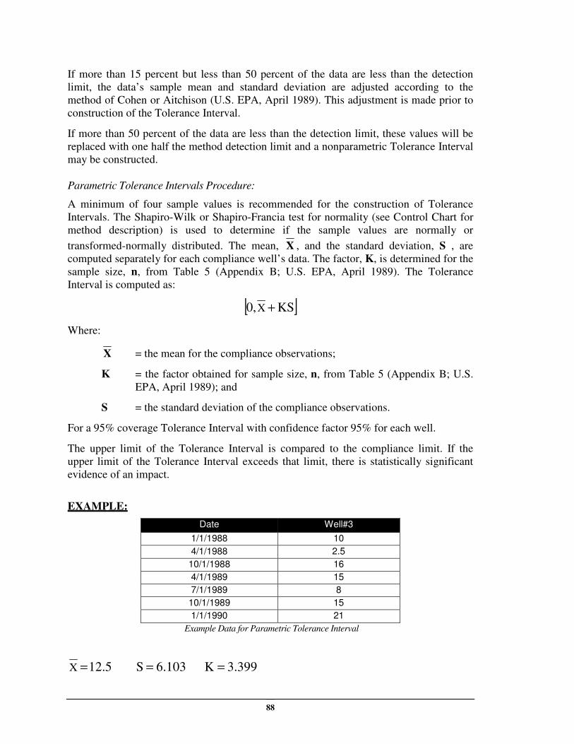
88

If more than 15 percent but less than 50 percent of the data are less than the detection

limit, the data’s sample mean and standard deviation are adjusted according to the

method of Cohen or Aitchison (U.S. EPA, April 1989). This adjustment is made prior to

construction of the Tolerance Interval.

If more than 50 percent of the data are less than the detection limit, these values will be

replaced with one half the method detection limit and a nonparametric Tolerance Interval

may be constructed.

Parametric Tolerance Intervals Procedure:

A minimum of four sample values is recommended for the construction of Tolerance

Intervals. The Shapiro-Wilk or Shapiro-Francia test for normality (see Control Chart for

method description) is used to determine if the sample values are normally or

transformed-normally distributed. The mean, X , and the standard deviation, S , are

computed separately for each compliance well’s data. The factor, K, is determined for the

sample size, n, from Table 5 (Appendix B; U.S. EPA, April 1989). The Tolerance

Interval is computed as:

[ ]KS0,X +

Where:

X = the mean for the compliance observations;

K = the factor obtained for sample size, n, from Table 5 (Appendix B; U.S.

EPA, April 1989); and

S = the standard deviation of the compliance observations.

For a 95% coverage Tolerance Interval with confidence factor 95% for each well.

The upper limit of the Tolerance Interval is compared to the compliance limit. If the

upper limit of the Tolerance Interval exceeds that limit, there is statistically significant

evidence of an impact.

EXAMPLE:

Date Well#3

1/1/1988 10

4/1/1988 2.5

10/1/1988 16

4/1/1989 15

7/1/1989 8

10/1/1989 15

1/1/1990 21

Example Data for Parametric Tolerance Interval

12.5X = 6.103S = 3.399K =

89

33.253.399)(6.10312.5 Interval Tolerance =∗+=

Nonparametric Tolerance Interval Procedure: For a Tolerance Interval the highest

compliance observation is used to set the upper limit of the tolerance interval. This upper

limit is compared to the compliance limit. If the upper limit of the Tolerance Interval

exceeds that limit, there is statistically significant evidence of an impact.

A minimum of 19 sample values is recommended for the construction of a 95%

Confidence/95% Coverage Tolerance Interval. The highest background value is used to

set the upper limit of the Tolerance Interval. This upper limit is compared to the

compliance limit. If the upper limit of the Tolerance Interval exceeds that limit, there is

statistically significant evidence of an impact.

APPENDIX I: GLOSSARY OF SELECTED STATISTICAL

TERMS

2-tailed Mode - The option used when there is a concern that compliance values can be

both too low as well as too high relative to background values. Sanitas automatically

evaluates pH for high and low exceedances, requiring this option to be checked only if

this feature is needed for other parameters.

95% Confidence Interval - Each time a test is performed, there is a 5% chance that it

will result in a false positive conclusion.

95% Coverage - 95% of the population is intended to be contained within the tolerance

interval.

99% Confidence Level - Each time a test is performed, there is a 1% chance that it will

result in a false positive conclusion.

Alpha Level - The false positive rate, or fraction of the results that will show and

exceedance when in fact none exists. The confidence level associated with each test is 1-

α.

Analysis of Variance (ANOVA) - An interwell analysis that compares either well

means or average ranks among wells. This test is typically recommended in detection

monitoring for determining whether intrawell or interwell tests are most appropriate.

The ANOVA, when run on upgradient wells only, will indicate whether variation exists

among the background wells. When spatial variation is present among upgradient wells,

intrawell tests are recommended in the absence of a historical release at the facility.

Box and Whiskers Plots - A concentration plot depicting the mean, median, minimum,

maximum, and 25th

and 75th

percentiles of a data set. This test is useful in detection

monitoring as a method for visualizing the variation within and among wells.

90

California Non-statistical Analysis of VOCs - An interwell analysis for a suite of

VOCs when nondetects comprise 90% or more of the background data.

Central Tendency - A statistical indicator of the average or middle value of a data set.

Confidence Interval (CI) - A concentration range that is designed to contain the mean

concentration level with a designated level of confidence (e.g., 99%). Confidence

Intervals are useful at sites in corrective action where remediation efforts need to be

evaluated.

Intrawell Limit-Based Tests – Within well comparisons. In the case of limit-based

tests, historical data from within a given well for a given constituent is used to construct a

limit. Compliance points are compared to the limit to determine whether a change is

occurring on a per-well/per-constituent basis. Intrawell limit-based tests are

recommended when there is evidence of spatial variation in the ground water, particularly

among upgradient wells, as it is inappropriate to pool those data across wells for the

purpose of creating interwell limits for comparison with compliance well data. Intrawell

tests may be used at both new and existing facilities. When performing intrawell limit-

based tests at existing facilities, ground water must not be impacted by the facility, and

proposed “background” data must be carefully screened for trends, outliers, and

seasonality prior to constructing limits.

Interwell Tests – Between well comparisons. Interwell limit-based tests use pooled

upgradient well data to construct limits. Individual downgradient well data are compared

to the limits to determine if the facility is impacting ground water. Interwell tests may be

used when there is a continuous aquifer at both new and existing facilities.

Lower Confidence Limit (LCL) - Lower limit to a confidence interval.

Log Transformation – In Sanitas, as is typical in the Guidance documents referenced

below, the term log transformation is synonymous with natural log transformation.

Mann-Kendall Statistical Evaluation - A nonparametric statistical analysis typically

used in detection and assessment monitoring. The Mann-Kendall portion of the Sen’s

Slope/Mann-Kendall trend test determines whether suspected increasing or decreasing

trends are statistically significant. In detection monitoring, this test is useful for

screening proposed background data while in assessment monitoring it may be used to

evaluate the ongoing condition of the trends.

Nondetect Data – Also referred to as “censored” measurements, these data fall between

0 and the quantitation limit (QL) as determined by the laboratory. There is much

uncertainty associated with values falling below the QL due to the difficult in

distinguishing the signal characteristic of the analyte from background noise associated

with laboratory equipment. Because of this, these concentrations are reported as

nondetects to represent “undetected” data.

Non-normal Data - The distribution of the population of data from which the sample has

been drawn is unknown; therefore no assumptions about or estimations of the population

parameters (e.g., mean) can be made.

91

Normally Distributed Data - Data (constituent concentration values) follow a normal

(Gaussian) or bell-shaped curve; the majority of values (95%) are within two standard

deviations from the mean of the concentration values.

Outlier - An observation that is at least an order of magnitude different from the rest of

the group of observations.

Power - The power of a statistical test is the probability that the test will reject a false

null hypothesis, or in other words that it will not make a Type II error. The higher the

power, the greater the chance of obtaining a statistically significant result when the null

hypothesis is false.

Precision - The extent to which a given set of sample measurements of the same

population of values agree with a measure of their central tendency.

Prediction Limit Analysis - An interwell or intrawell analysis that compares one or

more future observations to a limit established by background data. These limit-based

tests are recommended for sites in detection monitoring to determine whether changes are

occurring at compliance wells. In the case of both intra- and inter-well prediction limits,

it is recommended that only one future compliance point (referred to as the “K” value)

from each well be compared to a background limit. By default, Sanitas sets K=1. When

combined with retesting, these tests prove to be the most powerful among the EPA-

recommended methodologies, while minimizing the chance of false exceedances at a site.

Poisson Distributed Data - Data (constituent concentration values) follow a model of

rare events, where the probability of detection is low but stays constant from sampling

period to sampling period (U.S. EPA, 1992).

Sen’s Slope Trend Analysis - A nonparametric statistical analysis of the increase or

decrease in concentration levels over time; calculation of the slope of the linear

relationship of concentration level and time. In Sanitas, this test is combined with the

Mann Kendall test which determines whether the calculated slope is statistically

significant. In detection monitoring, this test is useful for screening proposed background

data while in assessment monitoring it may be used to evaluate the ongoing condition of

the trends.

Shewhart-CUSUM Control Charts – Measure both rapid releases as well as long-term,

gradual trends within a given well for a given constituent. Control Charts are

recommended for sites in detection monitoring and may be used as an alternative to

intrawell prediction limits. These tests used screened background data from within a well

to establish a baseline for comparison of future comparisons.

Site-Wide False Positive Rate (SWFPR) - The probability that at least one parameter

for at least one well will result in a statistically significant finding for each sampling

event at a facility. EPA recommends an annual SWFPR of 10% or less (which equals 5%

for each semi-annual sampling event or 2.5% for each quarterly sampling event)>

Skewness - A measure of the degree of asymmetry of a data distribution.

Testwise Alpha – The overall alpha (or false positive) level for a given test.

92

Time Series Plot - A graphic plot of time ( i.e.: days, months, years) versus

concentration levels.

Tolerance Interval (TI) - A concentration range that is constructed to contain a specified

proportion (e.g., 95%) of the population of observations with a specified confidence (i.e.,

confidence level).

Tolerance Limit - An interwell or intrawell analysis that compares compliance

observations to a limit established by background data that is constructed to contain a

specified proportion (e.g., coverage of 95%) of the population of observations. This test

has historically been one of the tests recommended for sites in detection monitoring for

detection releases. However, more recent EPA recommendations discuss the uncertainty

of the false positive rate associated with this test due to the coverage and confidence

levels.

Transformed-normally Distributed Data - The raw data are not normally distributed;

however the natural logarithms (or some other transformation in the Ladder of Powers

[Helsel & Hirsch]) of the data are normally distributed and parametric procedures may be

used.

Upper Confidence Limit (UCL) - Upper limit to a confidence interval.

Variability - A measure of divergence from the mean of a data set.

BIBLIOGRAPHY

93

ASTM, December 1998. Standard Guide for Developing Appropriate Statistical Approaches

for Ground-Water Detection Monitoring Programs. American Society For Testing and

Materials, West Conshocken, PA.

Cohen, A.C., Jr., 1959. Simplified Estimators for the Normal Distribution When Samples Are

Singly Censored or Truncated, Technometrics, 1: 217-237.

Davis, C. B. and McNichols, R. J., 1994. Ground Water Monitoring Statistics Update: Part II:

Nonparametric Prediction Limits, Ground Water Monitoring Review, Fall: 159.

Eisenhart, C., Hastay, M.W., and Wallis, W.A., 1947. Techniques of Statistical Analysis.

McGraw-Hill Book Company, Inc.

Gibbons, R.D., 1991. Some Additional Prediction Limits for Groundwater Detection

Monitoring at Waste Disposal Facilities, Groundwater, 29:5.

Gilbert, R.O., 1987. Statistical Methods for Environmental Pollution Monitoring. Van

Nostrand Reinhold

Helsel, D.R. and Hirsch, R.M., 1992. Statistical Methods in Water Resources. Elsevier.

Hollander, M. and Wolfe, D.A., 1973. Nonparametric Statistical Methods. John Wiley &

Sons.

Sen, P.K., 1968. Estimates of the Regression Coefficient based on Kendall’s Tau, Journal of

the American Statistical Association, 63 : 1379-1389.

U.S. EPA, April 1989. Statistical Analysis of Ground-Water Monitoring Data at RCRA

Facilities, Interim Final Guidance. Office of Solid Waste Management Division, U.S.

Environmental Protection Agency, Washington, DC.

U.S. EPA, July 1992. Statistical Analysis of Ground-Water Monitoring Data at RCRA

Facilities, Addendum to Interim Final Guidance. Office of Solid Waste Management

Division, U.S. Environmental Protection Agency, Washington, DC.

U.S. EPA, March, 2009. Statistical Analysis of Groundwater Monitoring Data at RCRA

Facilities, Unified Guidance. Office of Resource Conservation and Recovery Program

Implementation and Information Division, U.S. Environmental Protection Agency,

Washington, DC.

Wilk, M.B., and Shapiro, S.S., Technometrics, 10, No. 4, 1968, p 825-839

Willits, N., 1994. Personal Communication between Henry R. Horsey and Neil Willits,

statistical consultant to the California State Water Resources Control Board, Use of

nonparametric prediction limits including retests.

Zar, Jerrold H., 1996. Biostatistical Analysis. 3rd

edition (p112) Prentice Hall.

94

INDEX

2-tailed Mode ...................................... 89

Aitchison’s Adjustment ................ 33, 34

Alpha ................................................... 89

Alternate Value ................................... 74

Analysis of Variance ........................... 41

ANOVA ... 39, 41, 42, 43, 44, 45, 46, 47,

89

ASTM ............................... 36, 64, 70, 93

Bonferroni t-statistic ........................... 45

Box & Whiskers Plot .......................... 89

Box and Whiskers Plot.......................... 5

California ................................ 46, 62, 63

California standards ............................ 36

Censored Data ..................................... 31

Central Tendency ................................ 90

Chi-Squared ........................................ 25

Coefficient of-Variation ...................... 24

Cohen’s Adjustment...................... 31, 32

Compliance or Corrective Action ....... 83

Confidence .......................................... 89

Confidence Interval ............................. 90

Confidence Interval around Trend Line

......................................................... 81

Confidence Intervals ........................... 83

Control Chart ................................ 21, 91

Control Chart Procedure ............... 35, 65

Coverage ............................................. 89

Deseasonalizing .................................. 30

Detection Monitoring .......................... 21

Dixon's OutLier Test ........................... 12

EPA ..................................................... 93

EPA 1989 Outlier Test ........................ 11

Equality of Variance Test ............. 42, 43

Evaluation Monitoring ........................ 77

Histogram .............................................. 6

Interwell .............................................. 90

Intrawell .............................................. 90

Kaplan-Meier ...................................... 34

Kruskal-Wallis test............ 29, 38, 48, 64

Kurtosis ............................................. 7, 9

Ladder of Powers .......................... 52, 58

Levene’s test ....................................... 42

Log Transformation ............................ 90

Mann-Kendall ................... 65, 77, 78, 90

Mann-Whitney .............................. 38, 39

Multiple Group Shapiro-Wilk ....... 40, 70

Non-Detects ........................................ 90

Nonparametric..................................... 93

Nonparametric ANOVA ..................... 47

Non-Statistical Analysis................ 62, 90

Normality ............................................ 91

Normality Report ................................ 19

Outlier ........................................... 10, 91

Parametric ..................................... 41, 74

Parametric ANOVA ...................... 41, 44

Piper Diagram ..................................... 20

Poisson ........................ 55, 64, 66, 73, 91

Power .................................................. 91

Precision .............................................. 91

Prediction Limit ...................... 52, 71, 91

Prediction Limits

EPA ................................................. 52

UG Standards .................................. 56

Probability Plot ..................................... 9

Rank Sum ............................................ 37

Rank Von Neumann ............................ 17

Rosner’s Outlier Test .......................... 15

Seasonal Kendall Test ......................... 82

Seasonality ........................ 27, 28, 38, 64

Seasonality Adjustment ...................... 29

Seasonality Plot ................................... 10

Sen’s Slope.......................................... 91

Sen’s Slope Estimator ......................... 80

Shapiro-Francia ................................... 25

Shapiro-Wilk ....................................... 22

Shapiro-Wilk, Multiple Group ...... 40, 70

Shewhart-CUSUM 21, 32, 35, 37, 64, 65

Skewness ......................................... 8, 91

standard deviation ................................. 7

Statistical Outlier ................................ 10

Stiff Diagram ...................................... 19

SWFPR ............................................... 91

Time Series ..................................... 5, 29

Tolerance Intervals.............................. 87

Tolerance Limit ................................... 49

Tolerance Limit ................................... 92

Tolerance Limits ................................. 48

Transformations .................................. 92

95

Trend Analysis .................................... 77

Two-tailed ........................................... 79

Unified Guidance ................................ 56

Unified Guidance ................................ 36

Unified Guidance ................................ 93

Variability ........................................... 92

Verification Retest Procedure ............. 63

Welch's t-test ....................................... 39

Wilcoxon Rank Sum ........................... 38

W-statistic ........................................... 22