statistical analysis of high sample rate time-series data

University of VermontScholarWorks @ UVM

Graduate College Dissertations and Theses Dissertations and Theses

2015

Statistical Analysis of High Sample Rate Time-series Data for Power System Stability AssessmentGoodarz GhanavatiUniversity of Vermont

Follow this and additional works at: https://scholarworks.uvm.edu/graddis

Part of the Electrical and Electronics Commons

This Dissertation is brought to you for free and open access by the Dissertations and Theses at ScholarWorks @ UVM. It has been accepted forinclusion in Graduate College Dissertations and Theses by an authorized administrator of ScholarWorks @ UVM. For more information, please [email protected].

Recommended CitationGhanavati, Goodarz, "Statistical Analysis of High Sample Rate Time-series Data for Power System Stability Assessment" (2015).Graduate College Dissertations and Theses. 333.https://scholarworks.uvm.edu/graddis/333

https://scholarworks.uvm.edu?utm_source=scholarworks.uvm.edu%2Fgraddis%2F333&utm_medium=PDF&utm_campaign=PDFCoverPages

https://scholarworks.uvm.edu/graddis?utm_source=scholarworks.uvm.edu%2Fgraddis%2F333&utm_medium=PDF&utm_campaign=PDFCoverPages

https://scholarworks.uvm.edu/etds?utm_source=scholarworks.uvm.edu%2Fgraddis%2F333&utm_medium=PDF&utm_campaign=PDFCoverPages

https://scholarworks.uvm.edu/graddis?utm_source=scholarworks.uvm.edu%2Fgraddis%2F333&utm_medium=PDF&utm_campaign=PDFCoverPages

http://network.bepress.com/hgg/discipline/270?utm_source=scholarworks.uvm.edu%2Fgraddis%2F333&utm_medium=PDF&utm_campaign=PDFCoverPages

https://scholarworks.uvm.edu/graddis/333?utm_source=scholarworks.uvm.edu%2Fgraddis%2F333&utm_medium=PDF&utm_campaign=PDFCoverPages

mailto:[email protected]

STATISTICAL ANALYSIS OF HIGH SAMPLE RATE TIME-SERIES DATA FORPOWER SYSTEM STABILITY ASSESSMENT

A Dissertation Presented

by

Goodarz Ghanavati

to

The Faculty of the Graduate College

of

The University of Vermont

In Partial Fullfillment of the Requirementsfor the Degree of Doctor of PhilosophySpecializing in Electrical Engineering

May, 2015

Defense date: Nov 20, 2014Dissertation Examination Committee:

Paul D. H. Hines, Ph.D., Co-AdvisorTaras I. Lakoba, Ph.D., Co-AdvisorPeter S. Dodds, Ph.D., Chairperson

Kurt E. Oughstun, Ph.D.Mads Almassalkhi, Ph.D.

Cynthia J. Forehand, Ph.D., Dean of the Graduate College

ABSTRACT

The motivation for this research is to leverage the increasing deployment of thephasor measurement unit (PMU) technology by electric utilities in order to improve situa-tional awareness in power systems. PMUs provide unprecedentedly fast and synchronizedvoltage and current measurements across the system. Analyzing the big data provided byPMUs may prove helpful in reducing the risk of blackouts, such as the Northeast blackoutin August 2003, which have resulted in huge costs in past decades.

In order to provide deeper insight into early warning signs (EWS) of catastrophicevents in power systems, this dissertation studies changes in statistical properties of high-resolution measurements as a power system approaches a critical transition. The EWS un-der study are increases in variance and autocorrelation of state variables, which are genericsigns of a phenomenon known as critical slowing down (CSD).

Critical slowing down is the result of slower recovery of a dynamical system fromperturbations when the system approaches a critical transition. CSD has been observed inmany stochastic nonlinear dynamical systems such as ecosystem, human body and powersystem. Although CSD signs can be useful as indicators of proximity to critical transitions,their characteristics vary for different systems and different variables within a system.

The dissertation provides evidence for the occurrence of CSD in power systems us-ing a comprehensive analytical and numerical study of this phenomenon in several powersystem test cases. Together, the results show that it is possible extract information regard-ing not only the proximity of a power system to critical transitions but also the locationof the stress in the system from autocorrelation and variance of measurements. Also, asemi-analytical method for fast computation of expected variance and autocorrelation ofstate variables in large power systems is presented, which allows one to quickly identifylocations and variables that are reliable indicators of proximity to instability.

CITATIONS

Material from this dissertation has been published in the following form:

Ghanavati, G., Hines, P. D. H., Lakoba, T. I. and Cotilla-Sanchez, E.. (2014) Understand-ing early indicators of critical transitions in power systems from autocorrelation functions.IEEE Trans. Circuits Syst. I, vol. 61, no. 9, 2747–2760.

AND

Material from this dissertation has been published in the following form:

Ghanavati, G., Hines, P. D. H. and Lakoba, T. I.. (2014) Investigating early warning signsof oscillatory instability in simulated phasor measurements. Proc. IEEE Power and EnergySoc. General Meeting, 1–5.

AND

Material from this dissertation has been submitted for publication in IEEE Trans. PowerSystem on 10/04/2014 in the following form:

Ghanavati, G., Hines, P. D. H. and Lakoba, T. I.. (2014) Identifying useful statistical indi-cators of proximity to instability in stochastic power systems. IEEE Trans. Power System.

ii

Dedicated to my parents, Mohammadali and Mahvash and my sister, Gildafor their love and support.

iii

ACKNOWLEDGEMENTS

I would like to thank my advisor Dr. Paul D. H. Hines for his excellent mentoring and sup-

port. During the whole time that we have been working together, he has been tremendously

resourceful, supportive and encouraging. Also, I am grateful for Dr. Taras I. Lakoba’s

help. His help contributed immensely to the successful completion of this work. Working

with Paul and Taras has been a very valuable, fulfilling and enjoyable experience for me.

They are both great researchers and also very nice and kind. I also would like to express

my gratitude to the other members of my thesis committee Dr. Kurt E. Oughstun, Dr. Pe-

ter S. Dodds and Dr. Mads Almassalkhi for their helpful feedback. I also wish to thank

Dr. Eduardo Cotilla-Sanchez and Dr. Christopher Danforth for helpful contributions to this

research. Thank you also to my friends Pooya Rezaei and Dr. Mert Korkali for valuable dis-

cussions and their assistance. Finally, I wish to thank my family and friends who supported

me during my Ph. D. studies.

iv

TABLE OF CONTENTS

Page

CITATIONS . . . . . . . . . . . . . . . . . . . . . . . . . . . . . . . . . . . . . . . . . . . . . ii

DEDICATION . . . . . . . . . . . . . . . . . . . . . . . . . . . . . . . . . . . . . . . . . . . iii

ACKNOWLEDGEMENTS . . . . . . . . . . . . . . . . . . . . . . . . . . . . . . . . . . . iv

LIST OF TABLES . . . . . . . . . . . . . . . . . . . . . . . . . . . . . . . . . . . . . . . . . ix

LIST OF FIGURES . . . . . . . . . . . . . . . . . . . . . . . . . . . . . . . . . . . . . . . . x

ABBREVIATIONS . . . . . . . . . . . . . . . . . . . . . . . . . . . . . . . . . . . . . . . . xiv

CHAPTER 1: INTRODUCTION . . . . . . . . . . . . . . . . . . . . . . . . . . . . . . . . . 1

1.1 Abstract . . . . . . . . . . . . . . . . . . . . . . . . . . . . . . . . . . . . . . . . . . . . . 1

1.2 Motivation . . . . . . . . . . . . . . . . . . . . . . . . . . . . . . . . . . . . . . . . . . . 1

1.2.1 Blackout Mitigation . . . . . . . . . . . . . . . . . . . . . . . . . . . . . . . . . . . 2

1.2.2 Synchronized Phasor Measurement Systems . . . . . . . . . . . . . . . . . . . 3

1.3 Critical Slowing Down . . . . . . . . . . . . . . . . . . . . . . . . . . . . . . . . . . . 3

1.4 Stochastic Dynamics of Power Systems . . . . . . . . . . . . . . . . . . . . . . . . . 4

1.5 Critical Bifurcations in Power System . . . . . . . . . . . . . . . . . . . . . . . . . . 6

1.5.1 Voltage Stability . . . . . . . . . . . . . . . . . . . . . . . . . . . . . . . . . . . . . 7Voltage stability time scales . . . . . . . . . . . . . . . . . . . . . . . . . . . . . . 8Voltage stability monitoring . . . . . . . . . . . . . . . . . . . . . . . . . . . . . . 9

1.5.2 Oscillatory Stability . . . . . . . . . . . . . . . . . . . . . . . . . . . . . . . . . . . 11Oscillatory stability monitoring . . . . . . . . . . . . . . . . . . . . . . . . . . . . 12

1.6 Dissertation outline . . . . . . . . . . . . . . . . . . . . . . . . . . . . . . . . . . . . . . 13

v

CHAPTER 2:UNDERSTANDING EARLY INDICATORS OF CRITICAL TRANSI-TIONS IN POWER SYSTEMS FROM AUTOCORRELATION FUNC-TIONS . . . . . . . . . . . . . . . . . . . . . . . . . . . . . . . . . . . . . . . . . 15

2.1 Abstract . . . . . . . . . . . . . . . . . . . . . . . . . . . . . . . . . . . . . . . . . . . . . 15

2.2 Introduction . . . . . . . . . . . . . . . . . . . . . . . . . . . . . . . . . . . . . . . . . . 15

2.3 Solution Method for Autocorrelation Functions . . . . . . . . . . . . . . . . . . . . 19

2.3.1 The Model . . . . . . . . . . . . . . . . . . . . . . . . . . . . . . . . . . . . . . . . . 19

2.3.2 Autocorrelation and Variance of Differential Variables . . . . . . . . . . . . . 22

2.3.3 Autocorrelation and Variance of Algebraic Variables . . . . . . . . . . . . . . 23

2.3.4 Numerical Simulation . . . . . . . . . . . . . . . . . . . . . . . . . . . . . . . . . 25

2.4 Single Machine Infinite Bus System . . . . . . . . . . . . . . . . . . . . . . . . . . . 25

2.4.1 Stochastic SMIB System Model . . . . . . . . . . . . . . . . . . . . . . . . . . . 26

2.4.2 Autocorrelation and Variance . . . . . . . . . . . . . . . . . . . . . . . . . . . . 27

2.4.3 Discussion . . . . . . . . . . . . . . . . . . . . . . . . . . . . . . . . . . . . . . . . . 32

2.5 Single Machine Single Load System . . . . . . . . . . . . . . . . . . . . . . . . . . . 36

2.5.1 Stochastic SMSL System Model . . . . . . . . . . . . . . . . . . . . . . . . . . 36

2.5.2 Discussion . . . . . . . . . . . . . . . . . . . . . . . . . . . . . . . . . . . . . . . . . 38

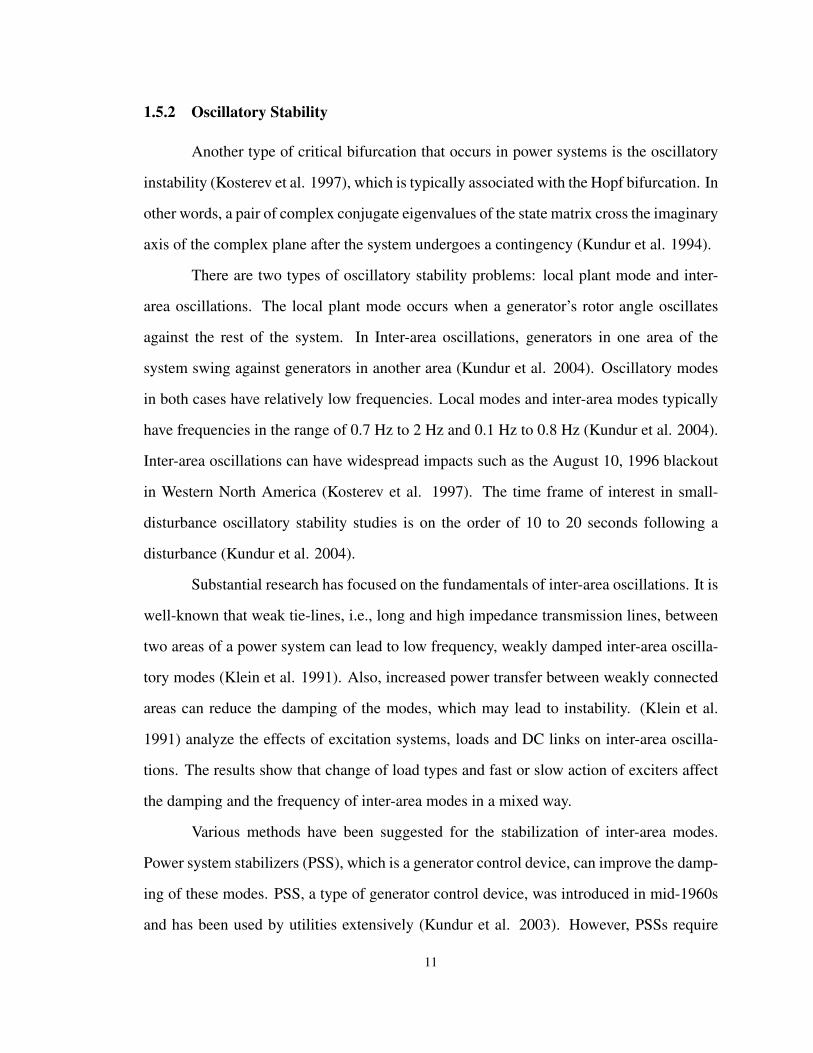
2.6 Three-Bus System . . . . . . . . . . . . . . . . . . . . . . . . . . . . . . . . . . . . . . 41

2.6.1 Model and Results . . . . . . . . . . . . . . . . . . . . . . . . . . . . . . . . . . . . 41

2.6.2 Discussion . . . . . . . . . . . . . . . . . . . . . . . . . . . . . . . . . . . . . . . . . 44

2.7 CSD in multi-machine systems . . . . . . . . . . . . . . . . . . . . . . . . . . . . . . 46

2.8 Conclusion . . . . . . . . . . . . . . . . . . . . . . . . . . . . . . . . . . . . . . . . . . . 50

2.9 Appendix A . . . . . . . . . . . . . . . . . . . . . . . . . . . . . . . . . . . . . . . . . . 51

2.10 Appendix B . . . . . . . . . . . . . . . . . . . . . . . . . . . . . . . . . . . . . . . . . . 53

Bibliography . . . . . . . . . . . . . . . . . . . . . . . . . . . . . . . . . . . . . . . . . . . . . 55

vi

CHAPTER 3: INVESTIGATING EARLY WARNING SIGNS OF OSCILLATORYINSTABILITY IN SIMULATED PHASOR MEASUREMENTS . . . . 59

3.1 Abstract . . . . . . . . . . . . . . . . . . . . . . . . . . . . . . . . . . . . . . . . . . . . . 59

3.2 Introduction . . . . . . . . . . . . . . . . . . . . . . . . . . . . . . . . . . . . . . . . . . 59

3.3 Simulation and results . . . . . . . . . . . . . . . . . . . . . . . . . . . . . . . . . . . . 60

3.3.1 Test Case and Simulation . . . . . . . . . . . . . . . . . . . . . . . . . . . . . . . 60

3.3.2 Autocorrelations and variances of the system variables . . . . . . . . . . . . . 62

3.4 Discussion . . . . . . . . . . . . . . . . . . . . . . . . . . . . . . . . . . . . . . . . . . . 63

3.5 Conclusion . . . . . . . . . . . . . . . . . . . . . . . . . . . . . . . . . . . . . . . . . . . 67

3.6 System data . . . . . . . . . . . . . . . . . . . . . . . . . . . . . . . . . . . . . . . . . . 67

Bibliography . . . . . . . . . . . . . . . . . . . . . . . . . . . . . . . . . . . . . . . . . . . . . 70

CHAPTER 4: IDENTIFYING USEFUL STATISTICAL INDICATORS OF PROX-IMITY TO INSTABILITY IN STOCHASTIC POWER SYSTEMS . . . 72

4.1 Abstract . . . . . . . . . . . . . . . . . . . . . . . . . . . . . . . . . . . . . . . . . . . . . 72

4.2 Introduction . . . . . . . . . . . . . . . . . . . . . . . . . . . . . . . . . . . . . . . . . . 72

4.3 Calculation of Autocorrelation and Variance in Multimachine Power Systems 73

4.3.1 System Model . . . . . . . . . . . . . . . . . . . . . . . . . . . . . . . . . . . . . . 73

4.3.2 Solution Method . . . . . . . . . . . . . . . . . . . . . . . . . . . . . . . . . . . . . 74

4.4 Useful early warning signs: voltage magnitudes and line currents . . . . . . . . 77

4.4.1 Autocorrelation and Variance of Voltages . . . . . . . . . . . . . . . . . . . . . 77

4.4.2 Autocorrelation and Variance of Line Currents . . . . . . . . . . . . . . . . . 78

4.5 Detectability after measurement noise . . . . . . . . . . . . . . . . . . . . . . . . . . 79

4.5.1 Impact of Measurement Noise on Variance and Autocorrelation . . . . . . . 79

4.5.2 Spread of Statistics . . . . . . . . . . . . . . . . . . . . . . . . . . . . . . . . . . . 80

vii

4.5.3 Filtering Measurement Noise . . . . . . . . . . . . . . . . . . . . . . . . . . . . 82

4.6 Detecting Locations of Increased Stress . . . . . . . . . . . . . . . . . . . . . . . . . 87

4.6.1 Transmission line tripping . . . . . . . . . . . . . . . . . . . . . . . . . . . . . . . 87

4.6.2 Capacitor tripping . . . . . . . . . . . . . . . . . . . . . . . . . . . . . . . . . . . . 88

4.6.3 Discussion . . . . . . . . . . . . . . . . . . . . . . . . . . . . . . . . . . . . . . . . . 90

4.7 Conclusions . . . . . . . . . . . . . . . . . . . . . . . . . . . . . . . . . . . . . . . . . . 90

4.8 Appendix A . . . . . . . . . . . . . . . . . . . . . . . . . . . . . . . . . . . . . . . . . . 91

Bibliography . . . . . . . . . . . . . . . . . . . . . . . . . . . . . . . . . . . . . . . . . . . . . 93

CHAPTER 5: CONCLUSIONS AND FUTURE DIRECTIONS . . . . . . . . . . . . . . 97

5.1 Conclusions . . . . . . . . . . . . . . . . . . . . . . . . . . . . . . . . . . . . . . . . . . 97

5.2 Future directions . . . . . . . . . . . . . . . . . . . . . . . . . . . . . . . . . . . . . . . 98

5.2.1 Modeling renewable energy sources . . . . . . . . . . . . . . . . . . . . . . . . . 100

APPENDIX A: SIMULATION SCRIPTS . . . . . . . . . . . . . . . . . . . . . . . . . . . . 101

A.1 Dynamic simulation driver . . . . . . . . . . . . . . . . . . . . . . . . . . . . . . . . . 101

A.2 Perturbation function . . . . . . . . . . . . . . . . . . . . . . . . . . . . . . . . . . . . 104

Bibliography . . . . . . . . . . . . . . . . . . . . . . . . . . . . . . . . . . . . . . . . . . . . . 106

viii

LIST OF TABLES

Table Page

Table 2.1: Three-bus system parameters . . . . . . . . . . . . . . . . . . . . . . . 42

Table 2.2: The largest indices q 8020

(for variance) and the relative activity in thedominant mode for bus voltage magnitudes . . . . . . . . . . . . . . . . . . . 49

Table 3.1: Relative activity of differential and algebraic variables in dominant mode67

ix

LIST OF FIGURES

Figure Page

Figure 1.1: A radial power system. A distribution line connects a generator andseveral loads. . . . . . . . . . . . . . . . . . . . . . . . . . . . . . . . . . . . 4

Figure 1.2: A single machine single load system. The system model consists of agenerator, a transmission line and a constant power load. . . . . . . . . . . . . 8

Figure 1.3: Load voltage versus its power. The vertical line represents the loadpower for a normal operating condition. The circles show the system equilibria. 9

Figure 2.1: Stochastic single machine infinite bus system used in Sec. 2.4. Thenotation Vg θg represents Vg exp [jθg]. . . . . . . . . . . . . . . . . . . . . . 27

Figure 2.2: The decrease of ω′ with Pm in the SMIB system. Near the bifurcation,ω′ is very sensitive to changes in Pm. In this figure, and most that follow, b isthe value of the bifurcation parameter (Pm in this system) at the bifurcation. . . 29

Figure 2.3: Autocorrelation function of ∆δ. ∆t = 0.1s is close to 1/4 of the small-est period of the function for all values of Pm. . . . . . . . . . . . . . . . . . . 30

Figure 2.4: Panels a,b show the variances of ∆δ,∆δ versus mechanical power (Pm)

values. Panels c,d show the autocorrelations of ∆δ,∆δ versus mechanicalpower (Pm) values. The autocorrelation values are normalized by dividing bythe variances of the variables. . . . . . . . . . . . . . . . . . . . . . . . . . . 32

Figure 2.5: Panels a,b show the variances of ∆Vg and ∆θg versus mechanical power(Pm) levels. The two terms comprising the variances in (2.21) are also shown.Panels c,d show the autocorrelations of ∆Vg and ∆θg versus Pm. . . . . . . . . 33

Figure 2.6: Eigenvalues of the first system as the bifurcation parameter (mechan-ical power) is increased. The arrows show the direction of the eigenvalues’movement in the complex plane as Pm is increased. The values of Pm and δ0

are given for several eigenvalues. . . . . . . . . . . . . . . . . . . . . . . . . 34

Figure 2.7: Single machine single load system. . . . . . . . . . . . . . . . . . . . 37

Figure 2.8: Variances of ∆δ−∆θl and ∆Vl for different load levels. Both variancesincrease with Pd as the system approaches the bifurcation. . . . . . . . . . . . 39

Figure 2.9: A sample trajectory of the rotor angle of (a) the SMIB system (b) theSMSL system. . . . . . . . . . . . . . . . . . . . . . . . . . . . . . . . . . . 40

Figure 2.10: The load bus voltage as a function of load power. The load bus voltagemagnitude becomes increasingly sensitive to power fluctuations as the systemapproaches the bifurcation. This increased sensitivity raises the voltage mag-nitude’s variance. . . . . . . . . . . . . . . . . . . . . . . . . . . . . . . . . . 40

Figure 2.11: Three–bus system. . . . . . . . . . . . . . . . . . . . . . . . . . . . . 41x

Figure 2.12: Three variables C6, C7 and C27/C6 derived by linearizing the Three-bus

system model. The left panel shows the variables versus Pd for Case B. Theright panel shows a close-up view of the variables near the bifurcation. Notethat as Pd → Pd,cr, C6 → 0 while C7 approaches a finite value of ∼ 0.6.C2

7/C6 →∞, as Pd → Pd,cr. . . . . . . . . . . . . . . . . . . . . . . . . . . 43

Figure 2.13: Panels a,b show the variances of ∆δ,∆δ versus load power (Pd). Panelsc,d show the autocorrelations of ∆δ,∆δ versus Pd. The ratios q 80

20(1), q 80

20(2)

are for case A, case B respectively. CaseA(N), CaseA(A) denote numericaland analytical solutions for case A. . . . . . . . . . . . . . . . . . . . . . . . 44

Figure 2.14: Panels a,b show the variances of ∆Vl,∆θl versus Pd. Panels c,d showthe autocorrelations of ∆Vl,∆θl versus Pd. . . . . . . . . . . . . . . . . . . . 45

Figure 2.15: Autocorrelation of ∆δ for two machines in the Three-bus system withtwo generators. G1 is the same generator as in the Three-bus system and G2 isthe new generator. . . . . . . . . . . . . . . . . . . . . . . . . . . . . . . . . 46

Figure 2.16: The variances and autocorrelations of five bus voltage magnitudes andfive generator rotor angles of the 39-bus system. Load level is the ratio of thevalues of the system’s loads to their nominal values. . . . . . . . . . . . . . . 48

Figure 2.17: Variances of three bus voltages versus load level. For three load levels,variances for 100 realizations are shown. For other load levels, only mean ofthe variances are shown. . . . . . . . . . . . . . . . . . . . . . . . . . . . . . 50

Figure 3.1: Three-bus test system . . . . . . . . . . . . . . . . . . . . . . . . . . . 61

Figure 3.2: PV curve for the Three-bus system. The vertical dotted line shows thenominal load power (9pu). . . . . . . . . . . . . . . . . . . . . . . . . . . . . 63

Figure 3.3: Trajectory of the three pairs of dominant eigenvalues of the Three-bus system as the load is increased. The arrows show the direction of theeigenvalues’ movement in the complex plane as the load is increased. Theincrement of bifurcation parameter Pd is 0.9pu. Near the bifurcation, the next(fourth) smallest real part of eigenvalues is approximately −0.7. . . . . . . . . 64

Figure 3.4: Variance and autocorrelation of the voltage magnitude of the load busversus load level. Note that the autocorrelation 〈∆V (t)∆V (t+ ∆t)〉 is shownonly for ∆V3; it is similar for the other two voltages. . . . . . . . . . . . . . . 65

Figure 3.5: Variance and autocorrelation of the voltage angle of the load bus versusload level. Note that the autocorelation 〈∆θ(t)∆θ(t+ ∆t)〉 is shown only for∆θ3; it is similar for the other two angles. . . . . . . . . . . . . . . . . . . . . 66

Figure 3.6: Variances and autocorrelations of the generators rotor angles versusload level. Note that the autocorelation 〈∆δ(t)∆δ(t + ∆t)〉 is shown only for∆δ1; it is similar for the other generator angle. . . . . . . . . . . . . . . . . . 67

xi

Figure 3.7: Variances and autocorrelations of the generators speed deviations ver-sus load level. Variances of ∆δ1 and ∆δ2 are very close, so their differenceis not observable in the left-hand side panel. Note that the autocorelation〈∆δ(t)∆δ(t+ ∆t)〉 is shown only for ∆δ1; it is similar for the other generatorspeed. . . . . . . . . . . . . . . . . . . . . . . . . . . . . . . . . . . . . . . . 68

Figure 4.1: Variance and autocorrelation of voltage magnitudes for five buses inthe 39-bus test case versus load level. Load level is the ratio of the systemloads to their nominal values. b denotes the bifurcation point. The bus numberassociated with each curve is shown next to it. Here and everywhere below theautocorrelation time lag t− s = 0.2s. . . . . . . . . . . . . . . . . . . . . . . 78

Figure 4.2: Variance and autocorrelation of current of two lines. The numbers inbrackets are bus numbers at two ends of the lines. . . . . . . . . . . . . . . . 79

Figure 4.3: Variances and autocorrelations of voltage magnitudes of five buses inthe 39-bus test case versus load level, accounting for measurement noise. . . . 81

Figure 4.4: The left panel shows the empirical pdfs ofX , which can be σ2 orR (∆t)of measurements for two load levels. Measure q95/80 is equal to the sum of thehatched areas. The dash-dot line shows the mean of X versus load level. Theright panel shows an alternative view of the pdfs. . . . . . . . . . . . . . . . . 82

Figure 4.5: Power spectral density of the current of line [6 31] for several loadlevels listed in the legend. Bifurcation is at load level=2.12. . . . . . . . . . . 83

Figure 4.6: Variance and autocorrelation of voltage magnitude of buses 7,36 versusthe load level after filtering the measurement noise. In this and subsequentfigures, the lines show the mean and the discrete symbols (∗,4) represent5th, 25th, 75th, 95th percentiles of values of σ2, R (∆t) for 100 realizations ateach load level. The vertical dash-dot lines show Load level = 80%b, 95%b. . 84

Figure 4.7: Variance and autocorrelation of currents of lines [6 31], [4 14] afterfiltering the measurement noise. . . . . . . . . . . . . . . . . . . . . . . . . . 85

Figure 4.8: Index q95/80 for σ2∆V of bus voltages across the 39-bus test case. Here,

and in Fig. 4.9, each rectangle represents the index q95/80 for σ2∆V of the bus

next to it. In order to illustrate the results more clearly, we show q95/80 =0.3 for measurements with q95/80 > 0.3, because quantities with this spreadbecome indistinguishable. . . . . . . . . . . . . . . . . . . . . . . . . . . . . 85

Figure 4.9: Index q95/80 for R∆I (∆t) of lines across the 39-bus test case. Eachrectangle represents index q95/80 for R∆I (∆t) of the line next to it. . . . . . . 86

Figure 4.10: Panel (a) shows Ratio (σ2∆V ) after disconnecting the two lines con-

nected to bus 4. The mean of the Ratio (σ2∆V ) for the 5 buses that show the

highest increases in variance, as well as the 5th, 25th, 75th, 95th percentilesof their values, are shown. Panel (b) shows Diff (R∆I (∆t)) for 5 lines thatexhibit the largest increases in R∆I (∆t). The results are shown after filteringof measurement noise. . . . . . . . . . . . . . . . . . . . . . . . . . . . . . . 88

Figure 4.11: PV curve for the three cases described in Sec. 4.6.2. The vertical linecorresponds to the base load level. . . . . . . . . . . . . . . . . . . . . . . . . 89

xii

Figure 4.12: Panel (a) shows σ2∆I,caseC/σ2

∆I,caseA for 5 lines that exhibit the largest in-crease in σ2

∆I among all lines. Panel (b) showsR∆I,,caseC (∆t)−R∆I,,caseA (∆t)for 5 lines that exhibit the largest increase in R∆I (∆t). . . . . . . . . . . . . . 90

xiii

ABBREVIATIONS

A/D Analog to digital

ANN Artificial neural network

ARMA Autoregressive moving average

CSD Critical slowing down

CTMC Continuous-time Markov chain

DAE Differential algebraic equation

emf Electromotive force

EWS Early warning sign

GPS Global positioning system

PDF Probability density function

PMU Phasor measurement unit

PSAT Power system analysis toolbox

PSD Power spectral density

PSS Power system stabilizer

SCADA Supervisory control and data acquisition

SDAE Stochastic differential algebraic equations

SDE Stochastic differential equation

SMIB Single machine infinite bus

SMSL Single machine single load

TCSC Thyristor-controlled series capacitor

ULTC Under-load tap changer

xiv

CHAPTER 1: INTRODUCTION

1.1 Abstract

This dissertation presents the study of two early warning signs (EWS) of critical bi-

furcations in power system. These EWS are variance and autocorrelation of state variables,

which are signs of a phenomenon known as critical slowing down. The thesis presents an

analytical and numerical study of changes in autocorrelation and variance of the variables

in the proximity of Saddle-node and Hopf bifurcations. These two bifurcations are associ-

ated with two types of catastrophic events in power grids known as voltage and oscillatory

instability. The contributions of this dissertation can be useful in developing novel power

system stability monitoring methods, which subsequently can help towards a more reliable

electric grid.

1.2 Motivation

The primary motivation of this research is to help reduce the likelihood of black-

outs in power grids by improving the understanding about early warning signs of such

events. EWS can be obtained from high-sample rate measurements, which are becom-

ing more and more available via the deployment of the phasor measurement unit (PMU)

technology by utilities. PMUs provide many more measurements (30 or 60 Hz) relative

to traditional supervisory control and data acquisition (SCADA) systems (with maximum

sampling rates between 0.1 Hz to 0.5 Hz), which are widely used by utilities at present.

Also, PMU measurements are time synchronized using the GPS technology, which allows

one to reconstruct blackout and near-blackout events with precision. Older SCADA sys-

tems frequently had clocks that would drift, making it difficult to reconstruct the order of

events after complicated disturbances.

1

1.2.1 Blackout Mitigation

Blackouts have caused significant economic and social costs worldwide in the past

three to four decades. For example, estimates of total costs of the August 14, 2003 blackout

in the United States range between $4 billion and $10 billion and in Canada, gross domestic

product was down 0.7% in August 2003 (Abraham and Efford 2004). The July 30, 2012

blackout in India affected more than 600 million people (Romero 2012).

A variety of factors are common among major blackouts, e.g., contact of conductors

with trees, insufficient reactive power generation, inadequate system visibility tools, system

operation beyond safe limits, etc. (Abraham and Efford 2004). Also, large blackouts are

usually caused by a combination of events such as voltage problems, transmission line

tripping and undamped electromechanical oscillations.

Investigation of some widespread blackouts has shown that signs of stress were

present minutes to hours before large-scale cascading began. For example, the report of the

August 14, 2003 blackout states that (Abraham and Efford 2004):

During the days before August 14 and throughout the morning and mid-day on

August 14, voltages were depressed across parts of northern Ohio because of

high air conditioning demand and other loads, and power transfers into and to a

lesser extent across the region.

Clearly, advanced monitoring algorithms and tools could help operators to avert widespread

outages in situations like the above by giving them warning of the increased system stress

with sufficient early warning to take timely action. One of the practices deemed to be very

effective for blackout mitigation is to turn high-resolution, synchronized measurements

provided by PMUs into useful information to improve situational awareness of system

operators (FERC and NERC 2012).

2

1.2.2 Synchronized Phasor Measurement Systems

Phasor measurement units provide high-resolution synchronized measurements of

currents and voltages (magnitude and phase) across power grid. PMUs are equipped with

analog to digital (A/D) converters, which transform current and voltage measurements into

digital signals. The synchronization is achieved by using a sampling clock that receives the

signal provided by a GPS receiver (De La Ree et al. 2010).

After the invention of the PMU in the late 80’s (Phadke 1993), utilities have been

gradually deploying them to create wide area measurement systems. In power systems,

phasor data concentrators collect data from a number of PMUs and use time-stamps to

correlate them by time in order to create a system-wide measurement set (Gómez-Expósito

et al. 2011).

Prior studies have proposed various applications for PMU data (Centeno et al.

1993), (Gou and Abur 2001), (Zhong et al. 2005). (De La Ree et al. 2010) describe

several applications of PMU in power system monitoring, protection and control. This dis-

sertation examines the transformation of data from PMU systems into information about

grid stress, making use of the theory of "critical slowing down".

1.3 Critical Slowing Down

Prior research suggests that signs of a phenomenon known as critical slowing down

(CSD) can provide early warning of critical bifurcations (Boettiger et al. 2013). CSD is

the slower recovery of a dynamical system from perturbations as it approaches a critical

bifurcation. CSD has been observed in various dynamical systems such as ecosystems

(Scheffer et al. 2001) and climate (Lenton et al. 2012).

Critical slowing down has several indicators. The two most generic ones are in-

creases in variance and autocorrelation of state variables. As the system slows down,

the impact of shocks decay slower, which results in increased variance for state variables

(Scheffer et al. 2009). Also, the intrinsic rates of change in the system decrease due to

CSD and the state of the system becomes more and more like its past state, which leads to

3

increased autocorrelation (Scheffer et al. 2009). Other indicators such as flickering, spatial

patterns and increases in skewness have also been suggested as CSD signs (Scheffer et al.

2009). However, they are not as generic as the increase in variance and autocorrelation.

Recent research has shown that not all systems that undergo regime shifts exhibit

CSD (Boettiger et al. 2013), (Boerlijst et al. 2013). (Boerlijst et al. 2013) show that

even in cases where a system exhibits CSD, its signs may not be observable in all of the

system variables. These findings show that CSD is not a strictly universal phenomenon and

it is necessary to analyze a particular system in order to understand the conductions under

which CSD does occur for that system. Earlier research has shown that CSD does occur in

power system (Cotilla-Sanchez et al. 2012). (Chertkov et al. 2011) study a radial power

system (see Fig. 1.1 ) and shows that voltage variations at the end of a distribution line

increase as the system approaches voltage instability (saddle-node bifurcation). (Podolsky

and Turitsyn 2013b) derive an approximate analytical autocorrelation function (from which

autocorrelation and variance can be found) for state variables in a power system model in

proximity of the saddle-node bifurcation and shows that CSD occurs in the system near this

type of bifurcation.

P1+jQ1&

P2+jQ2&

P3+jQ3&

P4+jQ4&

P5+jQ5&

Figure 1.1: A radial power system. A distribution line connects a generator and several loads.

In order to study CSD mathematically, the use of stochastic models is necessary.

The next section discusses the stochastic modeling and dynamics of power systems.

1.4 Stochastic Dynamics of Power Systems

A power system is a stochastic dynamical system in nature. Random sources such as

load switching, and changes in renewable energy sources such as wind and solar excite the4

system constantly. The majority of existing studies on power grid dynamics have focused

on the dynamics of deterministic models. However, increasing integration of renewable

energy sources has directed attention to the analysis of stochastic power system dynamics

(Odun-Ayo and Crow 2012).

Power system dynamics are typically modeled with differential-algebraic equations.

The differential equations model the dynamics of equipment such as generator, exciter1 and

turbine-governor2. The algebraic equations model the flow of power through the transmis-

sion system. The dynamics within the transmission system are much faster than the equip-

ment dynamics. That is why power flows in the system are assumed to be instantaneous

and described using algebraic equations (Dobson et al. 2002).

Considering random changes in power system such as load perturbations requires

the use of stochastic differential algebraic equations (SDAE) for modeling the system dy-

namics. In (Milano and Zarate–Minano 2013), a general approach to model power systems

as continuous SDAEs is proposed. The paper presents a systematic approach to include

stochastic terms in power system models. It also presents a tool for evaluating the weight

of stochastic perturbations on the power system transient behavior.

A number of researchers have used stochastic methods to study the impact of load

and generation perturbations on power system dynamic stability. (Wang and Crow 2013)

study the stability of the stochastic single machine infinite bus system3 by analyzing the

probability density function of state variables. The results show that addition of noise (load

perturbations) may improve dynamic stability under some conditions. In (Dhople et al.

2013), a framework is proposed to study the impact of stochastic active/reactive power in-

jections (power generation sources and loads) on power system dynamics with a focus on

time scales involving electromechanical phenomena. In their framework, active/reactive

power injections evolve according to a continuous-time Markov chain (CTMC), while the

standard differential algebraic equation (DAE) model describes the power system dynam-1Exciter controls the output voltage of a generator.2Turbine-governor controls the output power of a generator.3A system that consists of a generator that is connected to a large power grid such that the generator can not impact the grid’s

dynamics.

5

ics. The paper presents the application of the framework to calculation of long-term power

system state statistics, and to short-term probabilistic dynamic performance/reliability as-

sessment.

(Dong et al. 2012) propose a framework for assessment of power system transient

stability (stability after a large disturbance). The framework models load level as well as

discrete random events such as system faults (or any event that results in network recon-

figuration) using stochastic processes. (Odun-Ayo and Crow 2012) propose a new method

for analyzing stochastic transient stability using the transient energy function. It presents

a method to integrate the transient energy function and recloser4 probability distribution

function to provide a quantitative measure of probability of stability.

(Perninge et al. 2010) present a method for calculation of the probability distribu-

tion of the time to voltage instability (See Sec. 1.5.) with uncertain future loading scenar-

ios, which are modeled with the Brownian motion random process. (De Marco and Bergen

1987) propose a security measure indicating the vulnerability to voltage instability driven

by small disturbances in load. The measure is based on the expected exit time from the

region of attraction for the stable equilibrium point of the underlying deterministic system.

This dissertation uses a stochastic approach in order to study the CSD phenomenon

for two common types of critical bifurcations in power system, which will be discussed in

the next section.

1.5 Critical Bifurcations in Power System

In this dissertation, a critical bifurcation is defined to be a bifurcation where a

slowly-varying parameter moves the system towards a catastrophic regime change. Voltage

instability and oscillatory instability are two types of critical bifurcations that are known to

occur in power system models and have contributed to large blackouts in recent years.4A circuit breaker that is equipped with an automatic closing mechanism after disconnection of a transmission line.

6

1.5.1 Voltage Stability

Voltage stability refers to the ability of a power system to maintain steady voltages

at all buses (system nodes) in the system after being subjected to a disturbance from a given

initial operating condition. Instability that may result occurs in the form of a progressive

fall or rise of voltages of some buses. A possible outcome of voltage instability is loss

of load in an area, or tripping of transmission lines and other elements by their protective

systems leading to cascading outages (Kundur et al. 2004). Voltage instability has caused

or contributed to many large blackouts, e.g., August 2003 blackout in the US & Canada

(Abraham and Efford 2004).

Loads and reactive power sources play important roles in voltage stability of power

grid. Increase in load puts stress on the transmission network and limits its capability to

transfer power and support voltage (Kundur et al. 2004). Insufficient reactive power gener-

ation also reduces the ability of the system to provide voltage support. Voltage stability is

threatened when a disturbance increases the reactive power demand beyond the sustainable

capacity of the available reactive power resources (Kundur et al. 2004).

Voltage stability is associated with the saddle-node bifurcation, i.e., two equilibria

of a power system model collide and annihilate each other. Figs. 1.2 and 1.3 illustrate how

voltage stability is related to saddle-node bifurcation. Fig. 1.2 shows a simple power system

model consisting of a generator, a transmission line and a constant power load (Pd + jQd).

The generator is modeled with a voltage sourceE ′a and a reactanceX ′d and the transmission

line is modeled with a resistance rl and a reactance Xl. δ is angle of the generator’s rotor

relative to a synchronously rotating reference frame. Vg, Vd, θg, θd represent the voltage

magnitudes and angles of generator and load nodes. Fig. 1.3 shows that as the load power

increases, its voltage decreases. When the equivalent impedance of the load matches the

value of the line impedance, then the system reaches its critical loading. Before this point,

for each load power value, there are two equilibria. The equilibrium located in the upper

branch of the curve is stable while the other one is unstable. As the load power increases,

7

E0a/"

X 0d

gVg/"rl Xl

Vd d/"

Pd + jQd

Figure 1.2: A single machine single load system. The system model consists of a generator, a transmissionline and a constant power load.

these two equilibria approach each other and coalesce at the critical loading. Therefore, a

saddle-node bifurcation occurs at the critical loading.

Several control actions can be used for mitigating voltage instability. A common

method is switching on capacitor banks near load centers to meet the reactive power de-

mand. This action helps with the voltage stability of the system either by relieving stress on

transmission lines (since less reactive power will flow through the lines) or compensating

for the lack of sufficient reactive power generation. Other methods such as load shedding

and generation rescheduling can also be used to improve the voltage stability of the system.

Voltage stability time scales

Voltage stability may be either a short-term or a long-term phenomenon. The time

frame of interest for voltage stability problems ranges from a few seconds to tens of minutes

(Kundur et al. 2004). Short term voltage stability is associated with electromechanical

transients on transmission lines and synchronous generators and voltage collapse may occur

in the time range of seconds (Dobson et al. 2002). Long term voltage stability involves

slower acting equipment such as tap-changing transformers and generator current limiters.

The disturbance could also be in the form of sustained load buildup (Kundur et al. 2004).

The time-scale of long term voltage collapse ranges from tens of seconds to several minutes.8

0 0.5 1 1.5 2 2.5 30

0.2

0.4

0.6

0.8

1

1.2

Pd(pu)

Vd(p

u)

pf = 0.95 leadpf = 0.95 lag

Figure 1.3: Load voltage versus its power. The vertical line represents the load power for a normal operatingcondition. The circles show the system equilibria.

This dissertation focuses on using CSD for monitoring long term voltage stability of a

power system.

Voltage stability monitoring

The first step in the prevention of voltage instability is monitoring. Fig. 1.3 il-

lustrates the necessity of voltage stability monitoring. In this figure, the system becomes

unstable at very distinctly different points for two load power factor5 values. Therefore,

for a given load power, distance of the system from the bifurcation is very different for two

cases. This example shows that changes in system parameters can have a significant impact

on voltage stability of the system. Since many other parameters, e.g., voltage dependence

of loads, reactive power generation capacity, etc., can also impact the voltage stability of

a large power system, it is necessary to develop methods for estimating the distance to the

saddle-node bifurcation.

Numerous studies have focused on the voltage stability monitoring problem. Var-

ious methods such as the methods based on the maximum power transfer theorem (or the5Load power factor is: pf = Pd/

√P2d

+Q2d

9

Thevenin circuit) (Milosevic and Begovic 2003), monitoring reactive power reserves (Bao

et al. 2003) and artificial neural networks (ANN) (Zhou et al. 2010) are suggested for

monitoring of voltage stability.

In the maximum power transfer method, a circuit consisting of a Thevenin equiv-

alent voltage source and impedance, model the network as seen from a node (except the

load connected to that node). Based on the maximum power transfer theorem, the maxi-

mum power is transferred when the load impedance equals the complex conjugate of the

Thevenin equivalent impedance. This fact is the basis of the maximum power transfer

method for voltage stability monitoring. The voltage stability indices calculated based on

this method give an estimate of the local voltage stability. (Milosevic and Begovic 2003)

present a local voltage stability indicator based on local voltage and current phasor mea-

surements and load characteristics. In reference (Smon et al. 2006), a method for calcula-

tion of Thevenin parameters from two consecutive phasor measurements is presented using

the Tellegen’s theorem.

Another class of voltage stability monitoring methods is based on monitoring gener-

ator reactive power reserves. The correlation between the generator reactive power reserves

and the system voltage stability margin has been observed by system operators for many

years (Bao et al. 2003). Using this relationship, (Bao et al. 2003) develops a method for

online voltage stability monitoring. (Milosevic and Begovic 2003) use information on re-

active power reserves of the system along with the maximum power transfer theorem to

develop an online voltage stability monitoring indicator.

Voltage stability monitoring methods based on ANN use analytical (i.e. model-

based) studies to train their networks. The network inputs are some of the system mea-

surements such as voltage magnitudes and angles of system buses and the output is the

calculated voltage stability index (Zhou et al. 2010), (Popovic et al. 1998).

10

1.5.2 Oscillatory Stability

Another type of critical bifurcation that occurs in power systems is the oscillatory

instability (Kosterev et al. 1997), which is typically associated with the Hopf bifurcation. In

other words, a pair of complex conjugate eigenvalues of the state matrix cross the imaginary

axis of the complex plane after the system undergoes a contingency (Kundur et al. 1994).

There are two types of oscillatory stability problems: local plant mode and inter-

area oscillations. The local plant mode occurs when a generator’s rotor angle oscillates

against the rest of the system. In Inter-area oscillations, generators in one area of the

system swing against generators in another area (Kundur et al. 2004). Oscillatory modes

in both cases have relatively low frequencies. Local modes and inter-area modes typically

have frequencies in the range of 0.7 Hz to 2 Hz and 0.1 Hz to 0.8 Hz (Kundur et al. 2004).

Inter-area oscillations can have widespread impacts such as the August 10, 1996 blackout

in Western North America (Kosterev et al. 1997). The time frame of interest in small-

disturbance oscillatory stability studies is on the order of 10 to 20 seconds following a

disturbance (Kundur et al. 2004).

Substantial research has focused on the fundamentals of inter-area oscillations. It is

well-known that weak tie-lines, i.e., long and high impedance transmission lines, between

two areas of a power system can lead to low frequency, weakly damped inter-area oscilla-

tory modes (Klein et al. 1991). Also, increased power transfer between weakly connected

areas can reduce the damping of the modes, which may lead to instability. (Klein et al.

1991) analyze the effects of excitation systems, loads and DC links on inter-area oscilla-

tions. The results show that change of load types and fast or slow action of exciters affect

the damping and the frequency of inter-area modes in a mixed way.

Various methods have been suggested for the stabilization of inter-area modes.

Power system stabilizers (PSS), which is a generator control device, can improve the damp-

ing of these modes. PSS, a type of generator control device, was introduced in mid-1960s

and has been used by utilities extensively (Kundur et al. 2003). However, PSSs require

11

regular retuning in order to perform suitably. Another device for damping inter-area oscil-

lations is thyristor controlled series capacitor (TCSC) (Yang et al. 1998). Impedance of the

tie-line between two areas of a system has significant impact on the damping of inter-area

modes. TCSC can modulate the line impedance rapidly (Yang et al. 1998). As a result, it

can be used to increase the damping of inter-area modes. (Huang et al. 2011) take a dif-

ferent approach to damping inter-area modes. Their approach adjusts the system operating

conditions (like generators dispatch) to increase the system damping.

Oscillatory stability monitoring

Several methods have been proposed for monitoring inter-area oscillations (Cai

et al. 2013), (Peng and Nair 2012) and (Browne et al. 2008). The typical method for

monitoring oscillatory stability is to use modal identification methods to estimate the sys-

tem’s dominant modes from measurements.

There are two approaches to the estimation of dominant modes from measurement

data: 1) ringdown, 2) ambient (Zhou et al. 2012). The ambient detection refers to moni-

toring the network under an equilibrium condition with small-amplitude random load vari-

ations. On the other hand, ringdown detection methods track the oscillatory behavior after

the system has experienced some major disturbances (Peng and Nair 2012). Ambient data,

which are the measured response of the system to small perturbations, is a random pro-

cess. Stochastic models such as auto-regressive model, auto-regressive moving-average

(ARMA) model, and stochastic state-space model have been used in this case (Ghasemi

and Cañizares 2008). The Prony method, which uses a deterministic model, has been

widely used to analyze ring-down data in power systems (Ghasemi and Cañizares 2008).

From another perspective, the algorithms for identification of dominant oscillatory

modes can be classified into two categories: block processing and recursive processing

(Cai et al. 2013). Block processing algorithms process a set of data belonging to a sin-

gle sliding data window simultaneously. On the contrary, recursive algorithms update the

mode estimates based upon a new time sample and the previous estimate (Cai et al. 2013).

12

Prony analysis, Hilbert transform and ARMA are examples of block processing algorithms

suggested in literature (Cai et al. 2013), (Browne et al. 2008). Kalman filter is the most

widely used recursive processing algorithm (Peng and Nair 2012).

The block processing algorithms for modal identification have limitations with re-

gard to measurement noise, accuracy and discriminating between similar modes (Cai et al.

2013), (Browne et al. 2008). The challenge with recursive processing algorithms is that

prior knowledge of the system is essential for these methods. Also, inadequate selection

of initial conditions may cause the latter algorithms to produce biased results or lead to

convergence errors (Peng and Nair 2012).

1.6 Dissertation outline

This research takes a different approach to monitoring power system stability by

using the statistics of phasor measurements. Until recent years, it was not possible to use

statistics of measured quantities for monitoring some phenomena in power system since

the resolution of measurements in the timescale associated with those events was so low

that data statistics could not represent the true statistics of variables.

One motivation for the present approach is to use measurements’ statistics for sig-

naling an impending critical transition. Merely measuring the mean values of measured

quantities, which is widely used in stability monitoring algorithms, does not provide such

information sometimes. Another reason for pursuing this method is to form the basis of

algorithms that are less dependent on system models and more on data characteristics. The

reason for this is that any model has some inherent error. Also, detailed dynamic parame-

ters for power system models are frequently imprecise, or unavailable.

The remainder of the dissertation is organized as follows. Chapter 2 presents an

analytical study of CSD for various power system test cases. It presents analytical auto-

correlation functions of state variables for three small power systems. Using the functions,

it examines changes in variance and autocorrelation of state variables as the systems ap-

proach a saddle-node bifurcation. The chapter also includes a numerical study of CSD for

a larger multimachine power system test case.13

Chapter 3 presents a numerical study of CSD in proximity of a Hopf bifurcation in

a small power system model. Also, the chapter examines the reason that CSD signs are

better observable in some variables compared to others.

Chapter 4 presents a semi-analytical method for fast calculation of variance and

autocorrelation of state variables in large power systems to quickly identify variables and

locations that are better indicators of system stability. It also analyzes the impact of mea-

surement noise on observability of CSD signs. Lastly, the chapter presents a method for

detection of stressed areas in a power system using variance and autocorrelation of phasor

measurements.

Chapter 5 summarizes the conclusions and the contributions of the dissertation. It

also presents the future directions for this research.

Appendix A presents some MATLAB scripts for simulating a dynamic power sys-

tem model with stochastic changes in load using power system analysis toolbox (PSAT)

(Milano 2005).

14

CHAPTER 2: UNDERSTANDING EARLY INDICATORS OF CRITICAL

TRANSITIONS IN POWER SYSTEMS FROM AUTOCORRELATION

FUNCTIONS

2.1 Abstract

In order to better understand the extent to which critical slowing down (CSD) can

be used as an indicator of proximity to bifurcation in power systems, this chapter derives

autocorrelation functions for three small power system models, using the stochastic dif-

ferential algebraic equations (SDAE) associated with each. The analytical results, along

with numerical results from a larger system, show that, although CSD does occur in power

systems, its signs sometimes appear only when the system is very close to transition. On

the other hand, the variance in voltage magnitudes consistently shows up as a good early

warning of voltage collapse.

2.2 Introduction

There is increasing evidence that time-series data taken from stochastically forced

dynamical systems show statistical patterns that can be useful in predicting the proximity of

a system to critical transitions (Scheffer et al. 2009), (Lenton et al. 2012). Collectively this

phenomenon is known as Critical Slowing Down, and is most easily observed by testing for

autocorrelation and variance in time-series data. Increases in autocorrelation and variance

have been shown to give early warning of critical transitions in climate models (Dakos

et al. 2008), ecosystems (Dakos et al. 2011), the human brain (Litt et al. 2001) and electric

power systems (Cotilla-Sanchez et al. 2012, Podolsky and Turitsyn 2013b, Podolsky and

Turitsyn 2013a).

Scheffer et al. (Scheffer et al. 2009) provide some explanation as to why increasing

variance and autocorrelation can indicate proximity to a critical transition. They illustrate

that increasing autocorrelation results from the system returning to equilibrium more slowly

after perturbations, and that increased variance results from state variables spending more15

time further away from equilibrium. Reference (Kuehn 2011) uses the mathematical theory

of the stochastic fast-slow dynamical systems and the Fokker–Planck equation to explain

the use of autocorrelation and variance as indicators of CSD.

While CSD is a general property of critical transitions (Boerlijst et al. 2013), its

signs do not always appear early enough to be useful as an early warning, and do not

universally appear in all variables (Boerlijst et al. 2013, Hastings and Wysham 2010).

References (Boerlijst et al. 2013) and (Hastings and Wysham 2010) both show, using

ecological models, that the signs of CSD appear only in a few of the variables, or even not

at all.

Several types of critical transitions in deterministic power system models have been

explained using bifurcation theory. Reference (Dobson 1992) explains voltage collapse as

a saddle-node bifurcation. Reference (Dobson et al. 2002) describes voltage instability

caused by the violation of equipment limits using limit-induced bifurcation theory. Some

types of oscillatory instability can be explained as a Hopf bifurcation (Ajjarapu and Lee

1992),(Cañizares et al. 2004). Reference (Avalos et al. 2009) describes an optimization

method that can find saddle-node or limit-induced bifurcation points. Reference (Revel

et al. 2010) shows that both Hopf and saddle-node bifurcations can be identified in a

multi-machine power system, and that their locations can be affected by a power system

stabilizer.

Substantial research has focused on estimating the proximity of a power system to

a particular critical transition. References (Dobson et al. 2002), (Chiang et al. 1990), (Be-

govic and Phadke 1992) and (Glavic and Van Cutsem 2009) describe methods to measure

the distance between an operating state and voltage collapse with respect to slow-moving

state variables, such as load. Although these methods provide valuable information about

system stability, they are based on the assumption that the current network model is accu-

rate. However, all power system models include error, both in state variable estimates and

network parameters, particularly for areas of the network that are outside of an operator’s

immediate control.16

An alternate approach to estimating proximity to bifurcation is to study the response

of a system to stochastic forcing, such as fluctuations in load, or variable production from

renewable energy sources. To this end, a growing number of papers study power system

stability using stochastic models (De Marco and Bergen 1987), (Nwankpa et al. 1992),

(Anghel et al. 2007), (Dong et al. 2012), (Wang and Crow 2013) and (Dhople et al. 2013).

Reference (De Marco and Bergen 1987) models power systems using Stochastic Differen-

tial Equations (SDEs) in order to develop a measure of voltage security. In (Dong et al.

2012), numerical methods are used to assess transient stability in power systems, given

fluctuating loads and random faults. Reference (Wang and Crow 2013) uses the Fokker–

Planck equation to calculate the probability density function (PDF) for state variables in a

single machine infinite bus system (SMIB), and uses the time evolution of this PDF to show

how random load fluctuations affect system stability. In (Dhople et al. 2013), an analytical

method to compute bounds on the distribution of system states or bounds on probabilities

of different events of interest in stochastic power systems is presented. Reference (Mi-

lano and Zarate–Minano 2013) proposes a systematic approach to model power systems as

continuous stochastic differential-algebraic equations.

The results above clearly show that power system stability is affected by stochas-

tic forcing. However, they provide little information about the extent to which CSD can

be used as an early warning of critical transitions given fluctuating measurement data.

Given the increasing availability of high-sample-rate synchronized phasor measurement

unit (PMU) data, and the fact that insufficient situational awareness has been identified as a

critical contributor to recent large power system failures (e.g., (Abraham and Efford 2004),

(FERC and NERC 2012)) there is a need to better understand how statistical phenomena,

such as CSD, might be used to design good indicators of stress in power systems.

Results from the literature on CSD suggest that autocorrelation and variance in

time-series data increase before critical transitions. Empirical evidence for increasing au-

tocorrelation and variance is provided for an SMIB and a 9-bus test case in (Cotilla-Sanchez

et al. 2012). Reference (Chertkov et al. 2011) shows that voltage variance at the end of17

a distribution feeder increases as it approaches voltage collapse. However, the results do

not provide insight into autocorrelation. To our knowledge, only (Podolsky and Turitsyn

2013a), (Podolsky and Turitsyn 2013b) derive approximate analytical autocorrelation func-

tions (from which either autocorrelation or variance can be found) for state variables in a

power system model, which is applied to the New England 39 bus test case. However, the

autocorrelation function in (Podolsky and Turitsyn 2013a), (Podolsky and Turitsyn 2013b)

is limited to the operating regime very close to the threshold of system instability. Fur-

thermore, there is, to our knowledge, no existing research regarding which variables show

the signs of CSD most clearly in power system, and thus which variables are better indica-

tors of proximity to critical transitions. In (Ghanavati et al. 2013), the authors derived the

general autocorrelation function for the stochastic SMIB system. This chapter extends the

SMIB results in (Ghanavati et al. 2013), and studies two additional power system models

using the same analytical approach. Also, this chapter includes new numerical simulation

results for two multi-machine systems, which illustrate insights gained from the analytical

work.

Motivated by the need to better understand CSD in power systems, the goal of this

chapter is to describe and explain changes in the autocorrelation and variance of state vari-

ables in several power system models, as they approach bifurcation. To this end, we derive

autocorrelation functions of state variables for three small models. We use the results to

show that CSD does occur in power systems, explain why it occurs, and describe condi-

tions under which autocorrelation and variance signal proximity to critical transitions. The

remainder of this chapter is organized as follows. Section 2.3 describes the general math-

ematical model and the method used to derive autocorrelation functions in this chapter.

Analytical solutions and illustrative numerical results for three small power systems are

presented in Secs. 2.4, 2.5 and 2.6. In Sec. 2.7, the results of numerical simulations on

two multi-machine power system models including the New England 39 bus test case are

presented. Finally, Sec. 3.5 summarizes the results and contributions of this chapter.

18

2.3 Solution Method for Autocorrelation Functions

In this section, we present the general form of the Stochastic Differential Algebraic

Equations (SDAEs) used to model the three systems studied in this chapter. Then, the

solution of the SDAEs and the expressions for autocorrelations and variances of both alge-

braic and differential variables of the systems are presented. Finally, the method used for

simulating the SDAEs numerically is described.

2.3.1 The Model

All three models studied analytically in this chapter include a single second-order

synchronous generator. These systems can be described by the following SDAEs:

δ + 2γδ + F1

(δ, y, η

)= 0 (2.1)

F2

(δ, y, η

)= 0 (2.2)

where δ is angle of the synchronous generator’s rotor relative to a synchronously

rotating reference axis, y is the vector of algebraic variables, γ is the damping coefficient,

F1, F2 form a set of nonlinear algebraic equations of the systems, and η is a Gaussian

random variable. η has the following properties:

E [η (t)] = 0 (2.3)

E [η (t) η (s)] = σ2η · δI (t− s) (2.4)

where t, s are two arbitrary times, σ2η is the intensity of noise, and δI represents the unit

impulse (delta) function (which should not be confused with the rotor angle δ).

Equation (2.4) implies that we model the noise as having zero correlation time.

In practical power systems, such noise originates from stochastic changes from loads and

generators, as well as electromagnetic interferences, which occur over many time scales.

To our knowledge, no empirical studies have quantified the spectral density, or correlation

time, of fluctuations in power systems. In this chapter, we assume that the spectral density19

of noise sources is flat over a certain frequency range, while acknowledging that this model

is likely to have limitations. The higher end of the frequency range of interest is set by

the sampling rate of the PMU, which is commonly 30 Hz. (Note that this is higher than

the highest frequency of the system oscillations, which in our examples is in the range 1–

10 Hz.) The lower end of the frequency range is set by the length of our simulated time

window, which is 2 minutes, corresponding to a frequency of about 0.01 Hz. If one were

to measure for CSD in a practical power system one would want to look at the statistical

properties of data with a similar window length. Following the methods in (Dakos et al.

2008), the window of data would be initially low-pass filtered to remove slow trends. This

would ensure that the resulting data stream has zero mean, as does η in (2.3). The detrended

dataset would retain the important oscillations that might indicate instability (typically well

above 0.01 Hz), but discard slower trends. Thus, the noise model described by (2.3) and

(2.4) is based on the assumption that the spectral density of noise sources is nearly constant

over the frequency range of 0.01 Hz to 30 Hz. For this model to be accurate, the correlation

time of the noise needs to be somewhat smaller than 1/30s. Our numerical simulations,

which use a time step size of 0.01s, inject noise at each time step, thus implicitly assuming

that the correlation time of the noise is 0.01s (see the discussion after (2.20) and Sec. 2.3.4).

It should be noted that other studies (Milano and Zarate–Minano 2013), (Hauer et al. 2007)

have used noise models in which the noise spectral density falls off at frequencies above

approximately 1 Hz, rather than our value of 30 Hz. It is likely that, as assumed in (Milano

and Zarate–Minano 2013) and (Hauer et al. 2007), there is some frequency dependence in

the spectral density of empirical measurements from power systems. However, the exact

structure of the noise is yet to be verified empirically. Future work is needed to determine

the impact of frequency dependence (or, equivalently, the noise’s finite correlation time) on

the results presented in this chapter.

In order to solve (2.1) and (2.2) analytically, we linearized F1 and F2 around the sta-

ble equilibrium point. Then (2.1) and (2.2) were combined into a single damped harmonic

oscillator equation with stochastic forcing:20

∆δ + 2γ∆δ + ω20∆δ = −fη (2.5)

where ω0 is the undamped angular frequency of the oscillator, f is a constant, and ∆δ = δ−

δ0 is the deviation of the rotor angle from its equilibrium value. Both ω0 and f change with

the system’s equilibrium operating state. Equation (2.5) can be written as a multivariate

Ornstein–Uhlenbeck process (Gardiner 2010):

z (t) = Az (t) +B

0

η (t)

(2.6)

where z =[

∆δ ∆δ]T

is the vector of differential variables, ∆δ is the deviation of the

generator speed from its equilibrium value, and A and B are constant matrices:

A =

0 1

−ω20 −2γ

(2.7)

B =

0 0

0 −f

(2.8)

Given (2.7), the eigenvalues of A are −γ ±√γ2 − ω2

0 . At ω0 = 0, one of the eigenvalues

of matrix A becomes zero, and the system experiences a saddle-node bifurcation.

Equation (2.5) can be interpreted in two different ways: using either Ito SDE and

Stratonovich SDEs. Here, we use the Stratonovich interpretation (Stratonovich 1963),

where noise has finite, albeit very small, correlation time (Gardiner 2010). The reason

why we chose the Stratonovich interpretation is that it allows the use of ordinary calculus,

which is not possible with the Ito interpretation.

If γ < ω0 (which holds until very close to the bifurcation in two of our systems),

the solution of (2.6) is (Blanchard et al. 2006):

21

∆δ(t) = f ·ˆ t

−∞exp (γ (t′ − t)) η (t′) · (2.9)

sin (ω′(t′ − t))ω′

dt′

∆δ (t) = − f ·ˆ t

−∞exp (γ (t′ − t)) η (t′) · (2.10)

sin (ω′(t′ − t) + φ)ω0

ω′dt′

where ω′ =√ω2

0 − γ2 and φ = arctan(ω′/γ).

In the system in Sec. 2.5, ω0 = 0 for all system parameters, so the condition γ < ω0

does not hold. Therefore, the solution of (2.5) in that system is different from (2.9), (2.10):

∆δ = −fˆ t

−∞exp (−2γ (t− t′)) η (t′) dt′ (2.11)

2.3.2 Autocorrelation and Variance of Differential Variables

Given that the eigenvalues of A have negative real part (because γ > 0), one can

calculate the stationary variances and autocorrelations of ∆δ and ∆δ using (2.3), (2.4),

(2.9) and (2.10). The variances of the differential variables are as follows:

σ2∆δ =

f 2σ2η

4γω20

(2.12)

σ2∆δ

=f 2σ2

η

4γ(2.13)

If γ < ω0, their normalized autocorrelation functions are:

E [∆δ (t) ∆δ (s)]

σ2∆δ

= exp (−γ∆t)ω0

ω′· (2.14)

sin (ω′∆t+ φ)

E[∆δ (t) ∆δ (s)

]σ2

∆δ

= exp (−γ∆t)−ω0

ω′· (2.15)

sin (ω′∆t− φ)

where ∆t = t− s and ω′ =√ω2

0 − γ2 as above.22

If ω0 = 0, the variance of ∆δ can be calculated from (2.13) and the autocorrelation

of ∆δ is as follows:

E[∆δ (t) ∆δ (s)

]σ2

∆δ

= exp (−2γ∆t) (2.16)

2.3.3 Autocorrelation and Variance of Algebraic Variables

In order to compute the autocorrelation functions of the algebraic variables, we

calculated the algebraic variables as linear functions of the differential variable ∆δ and the

noise η, by linearizing F2 in (2.2):

∆yi (t) = Ci,1∆δ (t) + Ci,2η (2.17)

where yi is an algebraic variable, and Ci,1, Ci,2 are constants. Then, the autocorrelation of

∆yi for t ≥ s is:

E [∆yi (t) ∆yi (s)] = C2i,1 · E [∆δ (t) ∆δ (s)] + (2.18)

Ci,1Ci,2·E [∆δ (t) η (s)] +

C2i,2 · E [η (t) η (s)]

In deriving (2.18), we used the fact that E [∆δ (s) η (t)] = 0 since the system is causal.

Equation (2.18) shows that, in order to calculate the autocorrelation of ∆yi (t), it is neces-

sary to calculate E [∆δ (t) η (s)], which can be found from (2.9):

E [∆δ (t) η (s)] = − exp (−γ∆t) · fω′· (2.19)

sin (ω′∆t)σ2η

This shows that cov (∆δ, η) = 0.

In order to use (2.18) to compute the variance of ∆yi, we need to carefully consider

our model of noise in numerical computations. According to (2.4), the variance of η is23

infinite, because the delta function is infinite at t = s, which would mean that the variance

of ∆yi could be infinite. However, the noise in numerical simulations must have a finite

variance. To determine it, we rewrite (2.6) as follows:

dz (t) = Az (t) dt+BdW (t) (2.20)

where dW (t) = ηdt is the Wiener process. It is well-known that the variance of dW (t) is

σ2ηdt (Gardiner 2010). In numerical simulations, dt = τint, where τint is the integration time

step. Thus, E [dW 2num] = E

[(ηnumτint)

2] = σ2ητint. Hence, E [η2

num] = σ2η/τint. Then from

(2.17),

σ2∆yi

= C2i,1σ2

∆δ + C2i,2

σ2η

τint(2.21)

Combining (2.12) and (2.21) results in the following:

σ2∆yi

=

(C2i,1f

2

4γω20

+C2i,2

τint

)σ2η (2.22)

Combining (2.12), (2.14), (2.18) , (2.19) and (2.22), we calculated the normalized autocor-

relation function of ∆yi:

E [∆yi (t) ∆yi (s)]

σ2∆yi

= exp (−γ∆t) sin (ω′∆t+ φ∆yi) ·

Ci,1fω0

√λ

ω′(C2i,1f 2 + 4C2

i,2γω2

0

) (2.23)

where λ =√Ci,1f

(Ci,1f − 8Ci,2γ

2)

+(4Ci,2ω0γ

)2, φ∆yi =

arctan

(Ci,1fω

′

(Ci,1fγ−4Ci,2γω20)

).

24

2.3.4 Numerical Simulation

We numerically solved (2.1) and (2.2) using a trapezoidal ordinary differential

equation solver, as follows. First, (2.1) was written as:

z = F1 ≡

z2

−2γz2 − F1

(2.24)

where z = (z1, z2)Twas defined after (2.6). Then, (2.1) and (2.2) were discretized:

z(n+1) − z(n) =τint2

(F1

(n) + F1(n+1)

)(2.25)

0 = F2(n+1) (2.26)

where τint is a fixed integration time step, z(n), z(n+1) are the solutions at times t(n) =

nτint and t(n+1) = (n+ 1) τint, F(n+1)2 ≡ F2

(z(n+1), y(n+1), η(n+1)

), and similarly

for F1(n),F1

(n+1). The nonlinear algebraic system (2.25), (2.26) was solved by Newton’s

method for z(n+1) and y(n+1), with values z(n) and y(n) being known from the previous

step and η(n+1) being a random variable generated at t(n+1). Note that η(n) and η(n+1) are

uncorrelated, and, according to the discussion after (2.20), the variance of η(n) was σ2η/τint.

The integration time step τint was chosen to be 0.01s, which is about ten times smaller than

∆t, where ∆t is the time lag for calculation of the autocorrelation.

In order to determine numerical mean values in this chapter, each set of SDEs was

simulated 100 times. In each case the resulting averages were compared with analytical

means.

2.4 Single Machine Infinite Bus System

Analysis of small power system models can be helpful for understanding the con-

cepts of power system stability. The single machine infinite bus system has long been

used to understand the behavior of a generator connected to a larger system through a long

transmission line. It has also been used to explore the small signal stability of synchronous

25

machines (Demello and Concordia 1969) and to evaluate control techniques to improve

transient stability and voltage regulation (Wang et al. 1993). Recently, there has been in-

creased interest in stochastic behavior of power systems, in part due to the integration of

renewable energy sources. A few of these papers use stochastic SMIB models. For exam-

ple, references (Wang and Crow 2013), (Wei and Luo 2009) studied stability in a stochastic

SMIB system.

2.4.1 Stochastic SMIB System Model

Fig. 2.1 shows the stochastic SMIB system. Equation (2.27), which combines

the mechanical swing equation and the electrical power produced by the generator, fully

describes the dynamics of this system:

Mδ +Dδ +(1 + η)E ′a

Xsin (δ) = Pm (2.27)

where (η ∼ N (0, 0.01)) is a white Gaussian random variable added to the voltage magni-

tude of the infinite bus to account for the noise in the system, M and D are the combined

inertia constant and damping coefficient of the generator and turbine, and E ′a is the tran-

sient emf. The reactance X is the sum of the generator transient reactance (X′

d) and the

line reactance (Xl), and Pm is the input mechanical power. The values of parameters used

in this section are given below:

D = 0.03 purad/s

, H = 4MW.sMV A

, X ′d = 0.15pu,

Xl = 0.2pu, ωs = 2π · 60rad/s

Note that M = 2H/ωs, where H is the inertia constant in seconds, and ωs is the rated

speed of the machine. The generator and the system base voltage levels are 13.8kV and

115kV, and both the generator and system per unit base are set to 100MVA. The generator

transient reactance X ′

d = 0.15 · (13.8/115)2 pu, on the system pu base. The third term on

the left-hand side of (2.27) is the generator’s electrical power (Pg).

26

In order to test the system at various load levels, we solved the system for different

equilibria, with the generator’s mechanical and electrical power equal at each equilibrium:

Pm = Pg0 =E

′a

Xsin (δ0) (2.28)

where δ0 is the equilibrium value of the generator’s rotor angle.

gVg/"XlX 0

d

E0a/"

(1 + )/"0

Figure 2.1: Stochastic single machine infinite bus system used in Sec. 2.4. The notation Vg θg representsVg exp [jθg].

2.4.2 Autocorrelation and Variance

In this section, we calculate the autocorrelation and variance of the algebraic and

differential variables of this system using the method in Sec. 2.3. Equations (2.1) and (2.2)

describe this system for which the following equalities hold:

γ =D

2M; ω0 =

√E ′a cos δ0

MX; y =

[Vg θg

]T(2.29)

f =Pg0M

; F1

(z, y, η

)=

((1+η)E

′a

Xsin δ − Pm

)M

(2.30)

27

where ∆Vg = Vg − Vg0,∆θg = θg − θg0 are the deviations of, respectively, the generator

terminal busbar’s voltage magnitude and angle from their equilibrium values. Equations

(2.29) and (2.30) show that f increases, while ω0 decreases, with δ0.

In order to calculate the algebraic equations, which form F2 (δ, y, η) in (2.2), we

wrote Kirchhoff’s current law at the generator’s terminal:

E ′aejδ − VgejθgjX ′d

+1 + η − Vgejθg

jXl

= 0 (2.31)

Separating the real and imaginary parts in (2.31) gives:

Vg sin (θg) = αE′

a sin (δ) (2.32)

Vg cos (θg) = αE′

a cos (δ) (2.33)

+ (1 + η) (1− α)

where α = Xl/(Xl + X′

d). Equations (2.32) and (2.33) combine to make F2 (δ, y, η) in

(2.2).

Linearizing (2.32) and (2.33) yields the coefficients in (2.17), which are necessary

for calculating the autocorrelation and variance of the algebraic variables (y1 = ∆Vg, y2 =

∆θg):

C1,1 = αE′

a sin (θg0 − δ0) (2.34)

C1,2 = (1− α) cos (θg0) (2.35)

C2,1 = αE′

a cos (θg0 − δ0) (2.36)

C2,2 = − (1− α) sin (θg0) (2.37)

Fig. 2.2 shows the decrease of ω′, which is the imaginary part of the eigenvalues

of A in (2.7), with Pm. Note that the bifurcation occurs at b = 5pu. This figure illustrates

how it can be difficult to accurately foresee a bifurcation by computing the eigenvalues of a

system (as in, e.g., (Chiang et al. 1990)), if there is noise in the measurements feeding the

28

0 0.5 1 1.5 2 2.5 3 3.5 4 4.5 b

3

6

9

12

15

Pm(pu)

t’

Figure 2.2: The decrease of ω′ with Pm in the SMIB system. Near the bifurcation, ω′ is very sensitive tochanges in Pm. In this figure, and most that follow, b is the value of the bifurcation parameter (Pm in thissystem) at the bifurcation.

calculation. The value of ω′ ∼ (Pm − b)1/4 does not decrease by a factor of two (compared

to its value at Pm = 1.0pu) until Pm = 4.83pu (only < 3.4% away from the bifurcation). It

decreases by another factor of two at Pm = 4.99pu (0.2% away from the bifurcation). Also,

note that the real part of the eigenvalues equals−γ until very close to the bifurcation (0.1%

away from the bifurcation), so it does not provide a useful indication of proximity to the

bifurcation either, Thus, one can confidently predict from ω′ the imminent occurrence of the

bifurcation only very near it, which may be too late to avert it. On the other hand, we will

demonstrate below that for this system, autocorrelation functions can provide substantially

more advanced warning of the bifurcation.

Using autocorrelation as an early warning sign of a bifurcation requires one to care-

fully select a time lag, ∆t = t− s, such that changes in autocorrelation are observable. To

understand the impact of different time lags, we computed the autocorrelation function of

∆δ (see Fig. 2.3). From (2.14), the autocorrelation of ∆δ crosses zero at ∆t0 = 2π−φω′ . We

note that choosing ∆t close to, but below, ∆t0 allows one to observe a monotonic increase

of autocorrelation as Pm increases. Indeed, for ∆t > ∆t0, autocorrelation may not increase

29

0 0.1 0.2 0.3 0.4 0.5−1

−0.5

0

0.5

1

Au

toco

rrela

tion o

f ∆

δ

∆t(sec)

Pm

= 0.1pu

Pm

= 2pu

Pm

= 4pu

Pm

= 4.75pu

Figure 2.3: Autocorrelation function of ∆δ. ∆t = 0.1s is close to 1/4 of the smallest period of the functionfor all values of Pm.

monotonically, or the autocorrelation for some values of Pm may be negative. For example,

in Fig. 2.3 for ∆t = 0.3s, the autocorrelation decreases first and then increases with Pm.

On the other hand, for ∆t considerably smaller than ∆t0, the increase of the autocorrelation

may not be large enough to be measurable. In Fig. 2.3, the curves converge as ∆t → 0.

Given that the smallest period of oscillation (T = 2π/ω′) in this system is 0.41s, we chose

∆t = 0.1s for the autocorrelation calculations in this section.

Using (2.12)–(2.15), we calculated the variance and autocorrelation of ∆δ, ∆δ at

different operating points. In Fig. 2.4, these analytical results are compared with the numer-

ical ones. To initialize the numerical simulations, we assumed that Vg0 = 1pu and solved

for E ′a in (2.32), (2.33) to obtain Vg = Vg0 (for η = 0). We chose the integration step size

τint = 0.01s, which is much shorter than the the smallest period of oscillation (T = 0.41s)

and the time lag ∆t. The numerical results are shown for the range of bifurcation parameter

values for which the numerical solutions were stable.

In order to determine if variance and autocorrelation measurably increase as load

approaches the bifurcation, we compared a base load level (the normal operating condition

of the system) with a load level that is high, and closer to the bifurcation, but still some

30

distance from the bifurcation (far enough that an operator would have time to take precau-

tionary control actions). Since our aim is to study early warning signs of the bifurcation, we

use the differences between these two states as an indication of whether particular variables

provide observable early warning. While different load values for these two points could

be chosen for different systems, in this chapter we assume that the base level is 20% of the

load at the bifurcation point , and the high load level is at 80%. Therefore, we computed

the ratio of each statistic when load is at 80% of the bifurcation value to the value when

load is at 20% of b. This ratio, q 8020

in Fig. 2.4, is defined as follows:

q 8020

=Autocorrelation of u or σ2

u|Pm=0.8b

Autocorrelation of u or σ2u|Pm=0.2b

(2.38)

where u is the plot’s variable. In subsequent figures, q 8020

is defined similarly.

Fig. 2.4 shows that the variance of both ∆δ and ∆δ increases substantially with Pm,

and thus appears to be a good warning sign of the bifurcation. However, the two variances

grow with different rates. (This becomes clear when comparing the ratios q 8020

for ∆δ and

∆δ.) The difference becomes even more noticeable near the bifurcation where the variance

of ∆δ increases much faster than the variance of ∆δ. This is caused by the term ω20 in the

denominator of the expression for the variance of ∆δ in (2.12). In Fig. 2.4, the autocor-

relation of ∆δ and ∆δ increases with Pm. Similar to the variance, the autocorrelation is

a good early warning sign of the bifurcation. Comparing Fig. 2.4 with Fig. 2.2 (where an

equivalent q 8020

would be 1.28) shows that the autocorrelations and variances of ∆δ and ∆δ

provide a substantially stronger early warning sign, relative to using eigenvalues to estimate

the distance to bifurcation in this system.

The results for the algebraic variables are mainly similar. Fig. 2.5 show the variance

and autocorrelation of ∆Vg,∆θg as a function of load. In Fig. 2.5, the variance of ∆Vg

decreases with Pm until the system gets close to the bifurcation, while the variance of ∆θg

increases with Pm even if the system is far from the bifurcation. The autocorrelations of

both ∆Vg and ∆θg in Fig. 2.5 increase with Pm. However, the ratio q 8020

in (2.38) is much

31

0

100

200

σ2 ∆

δ/σ

2 η

NumericalAnalytical

0

0.5

1

1.5

σ2 ∆

δ

NumericalAnalytical

1 2 3 4 b0

0.5

1

Auto

corr

.of

∆δ

Pm(pu)

NumericalAnalytical

1 2 3 4 b0

0.5

1

Auto

corr

.of

∆δ

Pm(pu)

NumericalAnalytical

(a)

q 8020

= 26.2

(b)

q 8020

= 15.9

q 8020

= 4.1

(c) (d)

q 8020

= 22.5

Figure 2.4: Panels a,b show the variances of ∆δ,∆δ versus mechanical power (Pm) values. Panels c,dshow the autocorrelations of ∆δ,∆δ versus mechanical power (Pm) values. The autocorrelation values arenormalized by dividing by the variances of the variables.

larger for ∆Vg than for ∆θg. This is caused by the autocorrelation of ∆Vg being very close

to zero for small values of Pm.

2.4.3 Discussion

These results can be better understood by observing the trajectory of the eigenvalues

of the SMIB system (Fig. 2.6). Near the bifurcation, the eigenvalues are very sensitive

to changes in the bifurcation parameter. As a result, the system is in the overdamped

regime (ω0 < γ) for much less than 0.1% distance in terms of Pm to the critical transition.

This implies that, at least for this system, the autocorrelation function in (Podolsky and

Turitsyn 2013a) and (Podolsky and Turitsyn 2013b), is valid only when the system is within

0.1% of the saddle-node bifurcation. By considering a range of system parameters, we

observed that the region where one eigenvalue determines the system dynamics is within

1.5% of the bifurcation point at most. The width of this region scales approximately with

D2, Xl and 1/H. Because the method in (Podolsky and Turitsyn 2013a) and (Podolsky and

32

0

0.1

0.2

σ2 ∆

Vg/σ

2 η

NumericalAnalyticalFirst termSecond term

0

100

200

σ2 ∆

θg/σ

2 η

NumericalAnalyticalFirst termSecond term

1 2 3 4 b0

0.5

1

Auto

corr

.of

∆V

g

Pm(pu)

NumericalAnalytical

1 2 3 4 b0

0.5

1

Auto

corr

.of

∆θ

g

Pm(pu)

NumericalAnalytical

(a)

q 8020

= 0.7

(b)

q 8020

= 26.4

q 8020

= 76.7

(c) (d)

q 8020

= 4.0

Figure 2.5: Panels a,b show the variances of ∆Vg and ∆θg versus mechanical power (Pm) levels. The twoterms comprising the variances in (2.21) are also shown. Panels c,d show the autocorrelations of ∆Vg and∆θg versus Pm.

Turitsyn 2013b), can provide a good estimate of the autocorrelations and variances of state

variables only for a very short range of the bifurcation parameter, it may not be particularly

useful as an early warning sign of bifurcation.

From Figs. 2.4,2.5, we can observe that, except for the variance of ∆Vg, the vari-

ances and autocorrelations of all state variables increase when the system is more loaded.

This demonstrates that CSD occurs in this system as it approaches bifurcation, as suggested

both by general results (Kuehn 2011), and prior work for power systems (Cotilla-Sanchez

et al. 2012, Podolsky and Turitsyn 2013b). As an example, we calculated the variances of

∆δ and ∆δ as a function of the system parameters using (2.12), (2.13) and (2.29):

σ2∆δ =

E ′aσ2η

2X2D· sin2 δ0

cos δ0

(2.39)

σ2∆δ

=E

′2a σ

2η

2MX2D· sin2 δ0 (2.40)

33

−1.4 −1.2 −1 −0.8 −0.6 −0.4 −0.2 0−15

−10

−5

0

5

10

15

Im

Re

b0 = 69.32Pm = 4.66

b0 = 0.57Pm = 0.05

b0 = 0.57Pm = 0.05

b0 = 69.32Pm = 4.66

b0 = 89.78Pm = 5.00 b0 = 90

Pm = 5.00b0 = 89.95Pm = 5.00

b0 = 89.78Pm = 5.00

b0 = 90Pm = 5.00

b0 = 89.95Pm = 5.00

Figure 2.6: Eigenvalues of the first system as the bifurcation parameter (mechanical power) is increased. Thearrows show the direction of the eigenvalues’ movement in the complex plane as Pm is increased. The valuesof Pm and δ0 are given for several eigenvalues.

It can be observed from these expressions that as the system approaches the bifurca-

tion (δ0 −→ 90), the variable terms sin2 δ0cos δ0

, sin2 δ0 also increase. As a result, variance of

∆δ,∆δ both increase under all conditions.

In addition to validating these prior results, several new observations can be made.

For example, the signs of CSD are more clearly observable in some variables than in others.

While all of the variables show some increase in autocorrelation and variance, they are

less clearly observable in ∆Vg. The variance of ∆Vg decreases with Pm slightly until the

vicinity of the bifurcation. In comparison, the variance of ∆θg always increases with Pm.

Fig. 2.5 shows the two terms of the expressions for the variances of ∆Vg and ∆θg in (2.21).

The second term of the variance of ∆θg is very small compared to the first term, and the

first term is always dominant and growing. On the other hand, the second term of the

variance of ∆Vg is more significant for small Pm. This term decreases with Pm, which can

be observed from the expression for C1,2 in (2.35). Accordingly, decrease of C1,2 with Pm

causes the the variance of ∆Vg to decrease with Pm until the vicinity of the bifurcation.

34

In conclusion, the variance of ∆θg is a better indicator of proximity to the bifurcation.

Because the variables ∆δ and ∆δ are highly correlated with ∆θg, their variances are also

good indicators of proximity to the bifurcation.

The rate at which autocorrelation increases with Pm differs significantly in Figs. 2.4

and 2.5. In Fig. 2.4, the ratio q 8020

in (2.38) is 5.5 times larger for ∆δ than for ∆δ. The

normalized autocorrelation functions of ∆δ and ∆δ are as follows:

E [∆δ (t) ∆δ (s)] /σ2∆δ = exp (−γ∆t)

ω0

ω′(2.41)

· sin (ω′∆t+ φ)

E[∆δ (t) ∆δ (s)

]/σ2

∆δ= exp (−γ∆t)

ω0

ω′(2.42)

· sin (ω′∆t+ π − φ)

The difference between the two functions is in the phase of the sine function which causes

the values of the two autocorrelations to be different. q 8020

is so much larger for ∆δ than for

∆δ because of the time lag (∆t) used to compute autocorrelation. ∆t = 0.1s is close to the

zero crossing of the autocorrelation function of ∆δ, causing the large q 8020

. This difference

illustrates the importance of choosing an appropriate time lag.

It is important to note that although the growth ratio of the autocorrelation for ∆δ is

not large compared to ∆δ, it can be increased by subtracting a bias value from the autocor-

relation values for Pm = 0.2b(pu) and Pm = 0.8b(pu). For example, if the value of 0.075

is subtracted from the autocorrelation values, the ratio q 8020

increases from 4.1 to 13.0.

The results also show the nonlinearity of F1 in (2.30), causes the changes in auto-

correlation and variance of the system variables. In (Gardiner 2010), it is shown that the

stationary time correlation matrix of (2.6) can be calculated using the following equation:

E[Z (t)ZT (s)

]= exp [−A∆t]σ (2.43)

where σ is the covariance matrix of the state variables. Thus, the normalized autocor-

relation matrix depends only on A and the time lag. One of the elements of the state35

matrix (−ω20) in (2.7) changes with Pm because of the nonlinear relationship between the

electrical power (Pg) and the rotor angle in F1. Thus, in this system, CSD is caused by the

nonlinearity of F1.

2.5 Single Machine Single Load System

The single machine infinite bus system illustrates how CSD can occur in a generator

connected to a large power grid, through a long line. In this section we use a generator to

represent the bulk grid, and look for signs of CSD caused by a stochastically varying load.

Some form of the single machine single load (SMSL) model used in this section has been

used extensively to study voltage collapse (e.g., (Dobson et al. 2002, Kundur et al. 1994)).

2.5.1 Stochastic SMSL System Model

The second system (shown in Fig. 2.7) consists of one generator, one load and

a transmission line between them. The random variable η defined in (2.3) and (2.4), is

added to the load to model its fluctuations. The load consists of both active and reactive

components. In order to stress the system, the baseline load Sd is increased, while keeping

the noise intensity (Sd0) and the load’s power factor constant. The reason for keeping the

noise intensity constant was to ensure that the increase of variables’ variances is not due to

the increase of the noise level.

A set of differential-algebraic equations comprising the swing equation and power

flow equations describe this system. The swing equation and the generator’s electrical

power equation are given below:

Mδ +Dδ = Pm − Pg (2.44)

Pg = E′

aVlGgl cos (δ − θl) (2.45)

+E′

aVlBgl sin (δ − θl) + E′2a Ggg

36

/"X 0

d Xlrl

Sd + Sd0

Vl lgVg/"

E0a/"

Figure 2.7: Single machine single load system.

where Vl, θl are voltage magnitude and angle of the load busbar, Ggl, Ggg and Bgl are as

follows:

Ggg = −Ggl = Re

(1

rl + jXl

)(2.46)

Bgl = −Im(

1

rl + jXl

)(2.47)

The power flow equations at the load bus are as follows:

−Pd − Pd0η = E′

aVlGgl cos (θl − δ) (2.48)

+E′

aVlBgl sin (θl − δ) + V 2l Gll

−Qd −Qd0η = E′

aVlGgl sin (θl − δ) (2.49)

−E ′

aVlBgl cos (θl − δ)− V 2l Bll

where Gll = Ggg, Bll = −Bgl, and Pd0, Qd0 are constant values. The parameters of this

system are similar to the SMIB system, with the following additional parameters: rl =

0.025Ω, Pd0 = 1pu, pf = 0.95lead, where rl is the line’s resistance and pf is the load’s

power factor.

37

In this system, Vl, θl − δ are the algebraic variables, and δ, δ are the differential

variables. The algebraic equations (2.48) and (2.49) define Vl and θl − δ, which then drive

δ through (2.44) and (2.45). By linearizing (2.45) and the power flow equations around the

equilibrium, we simplified (2.44) to the following:

∆δ +D

M∆δ = −C5

Mη (2.50)

where C5 is a function of the system state at the equilibrium point. The derivation of (2.50)

and the expression for C5 are presented in Appendix 2.9. Comparing (2.5) with (2.50)

yields:

γ =D

2M,ω0 = 0, f =

C5

M(2.51)

The expression for the autocorrelation of ∆δ is given in (2.16). Note that the nor-

malized autocorrelation of ∆δ does not change with the bifurcation parameter (Pd), as it

did for the SMIB system. In Appendix 2.9, it is shown that ∆Vl and ∆δ − ∆θl are pro-

portional to η (see (2.59) and (2.60)). As a result, they are memoryless; the variables have

zero autocorrelation.

Fig. 2.8 shows the analytical and numerical solutions of the variances of ∆Vl and

∆δ−∆θl. The results also show that the variance of ∆δ increases modestly with Pd as the

system approaches the bifurcation. Unlike the SMIB system, the variance of ∆Vl is a good

early warning sign of the bifurcation. It is also much more sensitive to the increase of Pd

compared to ∆δ −∆θl and ∆δ.

2.5.2 Discussion

As was the case with the SMIB system, when the power flowing on the transmission

line in this system reaches its transfer limit, the algebraic equations become singular. How-

ever, unlike the previous system, the differential equations of this system do not become

singular at the bifurcation point of the algebraic equations. Fig. 2.9 shows the sample tra-

jectories of the two systems’ rotor angles. Both signals are Gaussian stochastic processes.38

0.5 1 1.5 2 2.5 b 0

5

10

15

20

25

30

35

40

σ2 ∆

δ−

∆θ

l/σ

2 η

Pd(pu)

NumericalAnalytical

0.5 1 1.5 2 2.5 b 0

5

10

15

σ2 ∆

Vl/

σ2 η

Pd(pu)

NumericalAnalytical

q 8020

= 2.4 q 8020

= 50.3

Figure 2.8: Variances of ∆δ −∆θl and ∆Vl for different load levels. Both variances increase with Pd as thesystem approaches the bifurcation.

The rotor angle in the SMIB system is an Ornstein–Uhlenbeck process while the rotor an-

gle in the SMSL system varies like the position of the brownian particle (Horsthemke and

Lefever 2006). The existence of the infinite bus in the former system causes this difference.

One difference between the SMSL system and the SMIB system is the absence of the term

comprising ∆δ in (2.50) compared with (2.5). This causes the linearized state matrix to be

independent of the bifurcation parameter. From (2.43), one can show that the normalized

autocorrelation of ∆δ depends only on A and the time lag. Since A is state-independent in

this system, the autocorrelation of ∆δ will be constant for a specific ∆t.

The increase of the variances of both differential and algebraic variables is due

to the non-linearity of the algebraic equations. Fig. 2.10 shows that as the load power

increases, the perturbation of the load power causes a larger deviation in the load busbar

voltage magnitude. Consequently, variance of this algebraic variable increases with Pd.

Likewise, this nonlinearity causes the coefficient C5 in (2.50) to increase as the load power

is increased, increasing the variance of ∆δ.

While voltage variance increases with load, this system does not technically show

CSD before the bifurcation, since increases in both variance and autocorrelation are essen-

tial to conclude that CSD has occurred (Kuehn 2011). Also, the eigenvalues of the state39

0 50 1000.7

0.8

0.9

1

1.1

1.2

1.3

1.4

δ(r

ad)

t(s)0 50 100

−8

−6

−4

−2

0

2

δ(r

ad)

t(s)

a b

Figure 2.9: A sample trajectory of the rotor angle of (a) the SMIB system (b) the SMSL system.

0 0.25 0.5 0.75 1 1.25 1.5 1.75 2 2.25 2.5 2.75 330.8

0.85

0.9

0.95

1

1.05

1.1

1.15

1.2

Pd(pu)

Vl(

pu)

0 5−0.04

0.04

∆V

l(pu)

t(s)

0 5−0.04

0.04

t(s)

∆V

l(pu)

Figure 2.10: The load bus voltage as a function of load power. The load bus voltage magnitude becomes in-creasingly sensitive to power fluctuations as the system approaches the bifurcation. This increased sensitivityraises the voltage magnitude’s variance.

40

matrix of this system do not vary with load. This confirms that CSD does not occur in this

system, since the poles of the dynamical system do not move toward the right-half plane as

the bifurcation parameter increases (Scheffer et al. 2009), (Kuehn 2011).

2.6 Three-Bus System

Real power systems have properties that are common to both the SMIB in Sec. 2.4

and the SMSL in Sec. 2.5. In order to explore CSD for a system that has both an infinite

bus, and the potential for voltage collapse case, this section looks at the three-bus system

in Fig. 2.11.

2.6.1 Model and Results

The three-bus system consists of a generator connected to a load bus through a

transmission line, which is connected to an infinite bus through another transmission line.

In the SMIB system, the bifurcation occurred in the differential equations. Increasing the

load in the three-bus system causes a saddle-node bifurcation in the algebraic equations

F1

(δ, y, 0

)= 0, F2

(δ, y, 0

)= 0 (in terms of (2.1), (2.2)), as in the SMSL system. How-

ever, unlike in the SMSL system, the bifurcation in these algebraic equations also causes a

bifurcation in the differential equation (2.5).

E0a/"

gVg/" /"Vl lX 0

d

Pd + Pd0

Xl1 Xl2

1 0/"

Figure 2.11: Three–bus system.

41

Table 2.1: Three-bus system parameters

Case no. Xl1(pu) Xl2(pu) X ′d(pu) D

(pu

rad/s

)A 0.1 0.35 0.1 0.03

B 0.3 0.35 0.1 0.001

We studied this system for two different cases. Our goal in studying these two cases

was to show that the CSD signs for some variables can vary differently with changing the

system parameters. Table. 2.1 shows the system parameters for two cases. The rest of the

parameters are similar to those in the SMIB system.

The algebraic equations of the three-bus system are as follows:

(E ′aVlX

sin (δ − θl)−2

3Pd

)/M = 0 (2.52)

E ′aVlX

sin (δ − θl)−VlXl2

sin (θl)− Pd0η = Pd (2.53)

E ′aVlX

cos (δ − θl) +VlXl2

cos (θl) = V 2l ·(

1

X+

1

Xl2

)(2.54)

where X = X′

d + Xl1, Vl, θl are voltage magnitude and angle of the load busbar. Equa-

tion (2.52) is equivalent to F1

(δ, y, 0

)in (2.1), and (2.53), (2.54), which are the simplified

active and reactive power flow equations at the load busbar, are equivalent to F2

(δ, y, 0

)in

(2.2). We assumed that Pg0 = 2Pd/3, which is reflected in (2.52).

The following equalities relate this system to the general model in (2.5):

γ =D

2M;ω2

0 =−C6

M; f =

−C7

M(2.55)

where C6 and C7 are functions of the system state at the equilibrium point. The derivation

and expressions for C6, C7 are presented in Appendix 2.10. Fig. 2.12 shows C6, C7 versus

Pd. When the load increases, C6 approaches 0, and a bifurcation in the differential equation

(2.5) and (2.55) occurs.

Using (2.55), the expressions in Sec. 2.3.2, and (2.76), (2.77) in Appendix 2.10,

we calculated the variances and autocorrelations of ∆δ,∆δ,∆Vl and ∆θl. We chose the

autocorrelation time lag ∆t of the variables to be equal to 0.14s taking a similar approach42

0 1 2 b−3

−2

−1

0

1

Pd(pu)

C6,C

7&

C2 7/C

6

C6

C7

C7

2/C

6

2.8 2.9 b −3

−2

−1

0

1

C6,C

7&

C2 7/C

6

Pd(pu)

C6

C7

C7

2/C

6

Figure 2.12: Three variables C6, C7 and C27/C6 derived by linearizing the Three-bus system model. The left

panel shows the variables versus Pd for Case B. The right panel shows a close-up view of the variables nearthe bifurcation. Note that as Pd → Pd,cr, C6 → 0 whileC7 approaches a finite value of∼ 0.6. C2

7/C6 →∞,as Pd → Pd,cr.

as in Sec. 2.4.2. Although the chosen ∆t may not be optimal for all of the variables, it rep-

resents a reasonable compromise between simplicity (choosing just one ∆t) and usefulness

as early warning signs. Figs. 2.13,2.14 compare the analytical solutions with the numerical

solutions of the variances and autocorrelations of ∆δ, ∆δ, ∆Vl and ∆θl.

Fig. 2.13 shows that although the growth rates of the autocorrelations of ∆δ,∆δ

are not large, the autocorrelations increase monotonically in both cases. As mentioned in

Sec. 2.4.3, it is possible to have larger indicators (growth ratios) by subtracting a bias value

from the autocorrelations. On the other hand, the variances of ∆δ,∆δ in Fig. 2.13, do not

monotonically increase for case B. We will explain this behavior in the next subsection. As

a result, they are not reliable indicators of proximity to the bifurcation.

Fig. 2.14 shows that although both variances of ∆Vl and ∆θl increase with Pd,

increase of the variance of ∆Vl is more significant. Also, the variance of ∆θl does not

increase monotonically with Pd for case B. As a result, the variance of ∆Vl seems to be a

better indicator of the system stability.

43

In Fig. 2.14, the autocorrelation of ∆Vl until very near the bifurcation is small

compared to those in Fig. 2.13. This is caused by C26 being very small in (2.76), so ∆Vl is

tied to the differential variables weakly. As a result, ∆Vl behaves in part like η—the white

random variable, and hence its autocorrelation is not a good indicator of proximity to the

bifurcation. In addition, nonmonotonicity of the autocorrelations of ∆Vl, ∆θl for case B in

Fig. 2.14 shows that they are not good early warning signs of bifurcation.

0

10

20

30

σ2 ∆

δ/σ

2 η

Case A (N)

Case A (A)

Case B

0

0.05

0.1

σ2 ∆

δ

Case A (N)

Case A (A)

Case B

0 1 2 3 4 5 b0

0.5

1

Auto

corr

.of

∆δ

Pd(pu)

Case A (N)

Case A (A)

Case B

0 1 2 3 4 5 b0

0.5

1A

uto

corr

.of

∆δ

Pd(pu)

Case A (N)

Case A (A)

Case B

q 8020

(1) = 1.6

q 8020

(2) = 0.9(a) q 80

20(1) = 1.2

q 8020

(2) = 0.8(b)

q 8020

(1) = 1.9

q 8020

(2) = 1.3

(c) q 8020

(1) = 3.3

q 8020

(2) = 1.3

(d)

Figure 2.13: Panels a,b show the variances of ∆δ,∆δ versus load power (Pd). Panels c,d show the auto-correlations of ∆δ,∆δ versus Pd. The ratios q 80

20(1), q 80

20(2) are for case A, case B respectively. CaseA(N),

CaseA(A) denote numerical and analytical solutions for case A.

2.6.2 Discussion

After studying this system with a range of different parameters, we found that au-

tocorrelations of the differential variables and variance of the voltage magnitude are con-

sistently good indicators of proximity to the bifurcation.

On the other hand, as shown in Fig. 2.13, variance in the differential variables is

not a reliable indicator. Namely, variances change non-monotonically (i.e., they do not

always increase) and, importantly, may exhibit very abrupt changes. Fig. 2.12 provides44

0

1

2

3

σ2 ∆

Vl/σ

2 η

Case A (N)

Case A (A)

Case B

0

5

10

15

20

σ2 ∆

θl/σ

2 η

Case A (N)

Case A (A)

Case B

0 1 2 3 4 5 b0

0.1

0.2

Auto

corr

.of

∆V

l

Pd(pu)

Case A (N)

Case A (A)

Case B

0 1 2 3 4 5 b0

0.2

0.4

Auto

corr

.of

∆θ

l

Pd(pu)

Case A (N)

Case A (A)

Case B

q 8020

(1) = 45.0

q 8020

(2) = 47.1(a) q 80

20(1) = 2.0

q 8020

(2) = 1.0(b)

q 8020

(1) = 1.7

q 8020

(2) = 1.2

(c) q 8020

(1) = 1.6

q 8020

(2) = 0.9

(d)

Figure 2.14: Panels a,b show the variances of ∆Vl,∆θl versus Pd. Panels c,d show the autocorrelationsof ∆Vl,∆θl versus Pd.

some clues as to the reason for this latter phenomenon. In this figure, the absolute value

of C7 decreases with Pd and becomes zero very close to the bifurcation point, at Pd|C7=0.

Therefore, the variances of ∆δ and ∆δ, which are proportional to C27 , decrease and vanish

at Pd|C7=0. Past this point, |C7| increases, while C6 continues to decrease and vanishes at b.

Therefore, the variances of ∆δ and ∆δ, which are proportional to C27/C6, increase to infinity

in the very narrow interval(Pd|C7=0, b

); see Fig. 2.12. This explains the sharp features in

Figs. 2.13(a), 2.13(b); a similar explanation can be given to such a feature in Figs. 2.14(c),

2.14(d). Therefore, neither the variances of ∆δ,∆δ or the autocorrelations of ∆Vl,∆θl are

good indicators of proximity to bifurcation.

The results for this system clearly show that not all of the variables in a power

system will show CSD signs long before the bifurcation. Although autocorrelations and

variances of all variables increase before the bifurcation, some of them increase only very

near the bifurcation or the increase is not monotonic. Hence, these variables are not useful

indicators of proximity to the bifurcation. In the three-bus system, autocorrelation in the

differential equations was a better indicator of proximity than autocorrelation in ∆Vl or

∆θl, which are not directly associated with the differential equations. Also, ∆Vl was the

45

0 0.5 1 1.5 2 2.5 b 0.78

0.79

0.8

0.81

0.82

0.83

0.84

Auto

corr

elat

ion

of∆

δ

Load level

G1G2

Figure 2.15: Autocorrelation of ∆δ for two machines in the Three-bus system with two generators. G1 is thesame generator as in the Three-bus system and G2 is the new generator.

only variable whose variance shows a gradual and monotonic increase with the bifurcation

parameter.

2.7 CSD in multi-machine systems

In order to compare these analytical results to results from more practical power

system, this section presents numerical results for two multi-machine systems.

The first system was similar to the Three-bus system (case B in Sec. 2.6). The only

difference was that instead of infinite bus, a generator similar to the other generator was

used. The numerical simulation results were similar to the Three-bus system, except for

the autocorrelation of ∆δ. Fig. 2.15 shows that the autocorrelation of ∆δ increases for one

of the machines, while it decreases for the other one. This shows that the autocorrelation

of ∆δ is not a reliable indicator of the proximity to the bifurcation in this system.

The second system we studied was the New England 39-bus system, using the sys-

tem data from (Pai 1989) We simulated this system for different load levels using the power

system analysis toolbox (PSAT) (Milano 2005). In order to change the system loading, each

load was multiplied by the same factor. At each load level, we added white noise to each

46

load. As one would expect, increasing the loads moves the system towards voltage col-

lapse. For solving the stochastic DAEs, we used the fixed-step trapezoidal solver of PSAT

with the step size of 0.01s. The noise intensity was kept constant for all load levels.

The simulation results show that the variances and autocorrelations of bus voltage

magnitudes increase with load. However, similar to the Three-bus system, the autocorre-

lations of voltage magnitudes are very small, indicating that in practice, these variables

would not be good indicators of proximity. The variances and autocorrelations of genera-

tor rotor angles and speeds and bus voltage angles did not consistently show an increasing

pattern. Fig. 2.16 shows the variances and autocorrelations of the voltage magnitudes of

five buses and the rotor angles of five generators of the system. The buses and generators

were arbitrarily chosen. As in previous results, the autocorrelation time lag was chosen to

be 0.1s.

Exciters, governors and frequency-dependent loads were not included in the results

shown here. However, tests with exciters and governors indicated that that adding these

elements to the simulations did not substantially change the conclusions. Considering the

frequency-dependence of loads raised the rate at which the autocorrelation of voltage mag-

nitudes increased. On the other hand, it decreased the rate of increase of the variance of

voltage magnitudes. Nevertheless, the rate of increase of variance still remained signifi-

cant. In this case, variance and autocorrelation of voltage magnitudes provide useful early

warning of the bifurcation. In contrast, variances and autocorrelations of other variables do

not provide a consistent early warning.

The results in this section suggest that autocorrelations of differential variables

show nonmonotonic behavior in some cases, which limits their application as early waning

signs of bifurcation.

Comparing the measure q 8020

for variances and autocorrelations of voltage magni-

tudes shows that some variables at some buses have larger growth ratios than others. As

suggested in (Podolsky and Turitsyn 2013a) and (Podolsky and Turitsyn 2013b), this may

be associated with the contribution of the variables to the leading mode near the threshold47

0

2

4x 10−4

σ2 ∆

V

0

0.02

0.04

0.06

Auto

corr

.of

∆V

0 0.5 1 b 2

4

6

x 10−8

σ2 ∆

δ

Load level 0 0.5 1 b 0.6

0.8

1

Auto

corr

.of

∆δ

Load level

Figure 2.16: The variances and autocorrelations of five bus voltage magnitudes and five generator rotor anglesof the 39-bus system. Load level is the ratio of the values of the system’s loads to their nominal values.

of collapse. However, except for cases that are very close to (~1% away) the bifurcation,

eigenvalue analysis shows that there are several simultaneously dominant modes. The re-

sults indicate that the mode whose damping decreases the fastest is most strongly connected

to the variance of bus voltages. Table 2.2 shows that, in general, the buses with the largest

increases in variances have larger activity in the dominant mode. On the other hand, auto-

correlations do not show a similar pattern. While the exact reasons for this are not yet clear,

Fig. 2.3 and the analytical results indicate that the autocorrelation functions of variables can

take many different shapes, which affects the growth ratio of their autocorrelations.

Table 2.2 shows the buses with the highest q 8020

indices for bus voltage variance,

as well as the relative activity of these bus voltage magnitudes in the dominant mode. In

order to calculate the relative activity of the bus voltages in the dominant mode, we first

calculated the right modal matrix of the state matrix. Then, using a matrix which relates

the differential and algebraic variables, we calculated the matrix that relates the algebraic

variables and the system modes (For further details, see Sec. 3.4). The entries of each

column of this matrix gives the relative activity of the algebraic variables in one of the

modes. It should be noted that the entries shown in Table 2.2 are a small subset of the48

Table 2.2: The largest indices q 8020

(for variance) and the relative activity in the dominant mode for bus voltagemagnitudes

Bus q 8020

(Variance) relative activity

38 11.5944 0.0135

29 9.9317 0.0147

28 9.0663 0.0147

33 8.5141 0.0101

37 8.3509 0.007

entries of the column corresponding to the dominant mode, which is why their values are

so small.

In many ways, this test case is a multi-machine version of the SMSL system. As

with the SMSL and Three-bus systems, variances of bus voltage magnitudes are good early

warning signs. However, unlike in the SMSL system, autocorrelation in voltage magnitudes

increases, albeit only slightly in some cases, with system load. Unlike in the SMSL system,

voltage magnitudes in the 39-bus case have non-zero autocorrelation for ∆t > 0. This

results from the fact that voltage magnitudes are coupled to the differential variables in this

system.

Results from this system, as with the SMSL system, suggest that variance in voltage

magnitudes is a useful early warning sign of voltage collapse. It is less clear from these

results if changes in autocorrelation will be sufficiently large to provide a reliable early

warning of criticality.

One important point about the numerical results presented in this chapter is that

these results are averages over many simulations with randomly chosen sequences of η.

This averaging is different from the quantities observed by power system operators. One

should take this into account when using CSD signs for monitoring system stability. For ex-

ample, Fig. 2.17 shows the variances of the voltage magnitudes of three buses in the 39-bus

system. For each bus, mean variances (for 100 realizations) are shown for all load levels.

For three load levels (low, medium and high load level), the actual measured variance from

each of the 100 realizations (one minute windows) is also shown. The increases in volt-

age magnitude variance are significant in that there is no overlap between the variances at49

0 0.5 1 b 0

0.2

0.4

0.6

0.8

1

1.2

1.4x 10

−4

σ2 ∆V

Load level

Bus3

Bus16

Bus25

Figure 2.17: Variances of three bus voltages versus load level. For three load levels, variances for 100realizations are shown. For other load levels, only mean of the variances are shown.

these three load levels even for a single realization. Therefore, we conclude that, at least

given the assumptions underlying these simulations, it is possible to accurately estimate the

distance to bifurcation based on the variance of a one-minute stream of voltage magnitude

data.

2.8 Conclusion

In this chapter, we analytically and numerically solve the stochastic differential

algebraic equations for three small power system models in order to understand critical

slowing down in power systems. The results from the single machine infinite bus system

and the Three-bus system models show that critical slowing down does occur in power sys-

tems, and illustrate that autocorrelation and variance in some cases can be good indicators

of proximity to criticality in power systems. The results also show that the way in which

the bifurcation parameter changes the system state matrix (A) importantly influences the

observed changes in autocorrelation and variance. For example, the constant state matrix

in the single machine single load system (see (2.7),(2.51)) caused the autocorrelation of

the differential variable to be constant. On the other hand, in the SMIB and Three-bus

systems, the state matrix changed with the the bifurcation parameter; that is, the coefficient

50

ω0 in (2.7) changed with the bifurcation parameter Pm (for SMIB, see (2.28),(2.29)) or Pd

(Three-bus, see (2.55)). As a result, the variance and autocorrelation of the differential

variables changed with the bifurcation parameter, and in some cases indicate proximity to

bifurcation.

Although the signs of critical slowing down do consistently appear as the systems

approach bifurcation, only in a few of the variables did the increases in autocorrelation

appear sufficiently early to give a useful early warning of potential collapse. On the other

hand, variance in load bus voltages consistently showed substantial increases with load,

indicating that variance in bus voltages can be a good indicator of voltage collapse in multi-

machine power system models. This was verified for the New England 39-bus system.

Determining intuitive analytical or physical explanations for why some variables show the

signs of CSD better than others requires additional investigation, and is a subject for future

research.

Together these results suggest that it is possible to obtain useful information about

system stability from high-sample rate time-series data, such as that produced by synchro-

nized phasor measurement units. Future research will focus on developing an effective

power system stability indicator based on these results.

2.9 Appendix A

The derivation of (2.50) is presented in this section. By linearizing (2.45) around the

equilibrium and replacing the obtained equation for Pg in (2.44), we obtained the following:

M∆δ +D∆δ = −C12∆Vl − C13 (∆δ −∆θl) (2.56)

where C12 and C13 are:=

C12 = E′

a |Ygl| sin (θl0 − δ0 − π/2 + φgl) (2.57)

C13 = Vl0E′

a |Ygl| cos (θl0 − δ0 − π/2 + φgl) (2.58)

51

where |Ygl| =√G2gl +B2

gl, φgl = arctan (Bgl/Ggl). By linearizing (2.48) and (2.49) around

the equilibrium and solving for ∆Vl and ∆δ −∆θl, we obtained the following:

∆Vl = C14η (2.59)

∆δ −∆θl = C15η (2.60)

where C14 and C15 are: C14

C15

=

C19Pd0 − C17Qd0

C18Pd0 − C16Qd0

/(C17C18 − C16C19) (2.61)

where C16 − C19 are given below:

C16 = E′

a |Ygl| sin (θl0 − δ0 + π/2− φgl) (2.62)

+2GllVl0

C17 = Vl0E′

a |Ygl| cos (θl0 − δ0 + π/2− φgl) (2.63)

C18 = −E ′

a |Ygl| cos (θl0 − δ0 + π/2− φgl) (2.64)

−2BllVl0

C19 = Vl0E′

a |Ygl| sin (θl0 − δ0 + π/2− φgl) (2.65)

Using (2.59) and (2.60), we rewrote (2.56) as (2.50) where C5 is:

C5 =(C13C18 + C12C19)Pd0 − (C13C16 + C12C17)Qd0

C16C19 − C17C18

(2.66)

52

2.10 Appendix B

The derivation of C6, C7 is presented in this section. By using (2.1) and lineariz-

ing (2.52)-(2.54) around the equilibrium, we have the following:

∆δ = −(D∆δ + C20∆Vl + C21 (∆δ −∆θl)

)/M (2.67)

0 = −Pd0η + C22∆Vl + C21∆δ + C23∆θl (2.68)

0 = −∆Vl + C24∆δ + C25∆θl (2.69)

where C20 through C25 are as follows:

C20 =E ′aX

sin (δ0 − θl0) (2.70)

C21 =E ′aVl0X

cos (δ0 − θl0) (2.71)

C22 = C20 − sin(θl0)/Xl2 (2.72)

C23 = −C21 −Vl0Xl2

cos (θl0) (2.73)

C24 = −βE ′a sin (δ0 − θl0) (2.74)

C25 = −C24 − (1− β) · sin (θl0) (2.75)

where β = Xl2/(X +Xl2). Using (2.68) and (2.69), we solved for ∆Vl and ∆θl:

∆Vl = C26∆δ + C27η (2.76)

∆θl = C28∆δ + C29η (2.77)

where C26 through C29 are as follows:

C26

C27

C28

C29

=

C23C24 − C21C25

C25Pd0

−C21 − C22C24

Pd0

/(C22C25 + C23) (2.78)

53

Equations (2.67), (2.76) - (2.78) lead to the following expressions:

C6 = C21C28 − C20C26 − C21 (2.79)

C7 = C21C29 − C20C27 (2.80)

54

BibliographyAbraham, S. and J. Efford (2004). Final report on the August 14, 2003 blackout in the

United states and Canada: causes and recommendations. Technical report, US–CanadaPower Syst. Outage Task Force.

Ajjarapu, V. and B. Lee (1992, Feb.). Bifurcation theory and its application to nonlineardynamical phenomena in an electrical power system. IEEE Trans. Power Syst. 7(1),424–431.

Anghel, M., K. A. Werley, and A. E. Motter (2007, Jan.). Stochastic model for power griddynamics. In 40th Annual Hawaii Intl. Conf. Syst. Sci. IEEE.

Avalos, R., C. Canizares, F. Milano, and A. Conejo (2009, Jan.). Equivalency of continua-tion and optimization methods to determine saddle-node and limit-induced bifurcationsin power systems. IEEE Trans. Circuits Syst. I, Reg. Papers 56(1), 210 –223.

Ayasun, S., C. Nwankpa, and H. Kwatny (2004, Aug.). Computation of singular and sin-gularity induced bifurcation points of differential-algebraic power system model. IEEETrans. Circuits Syst. I, Reg. Papers 51(8), 1525 – 1538.

Begovic, M. M. and A. G. Phadke (1992). Control of voltage stability using sensitivityanalysis. IEEE Trans. Power Syst. 7(1), 114–123.

Bergen, A. and V. Vittal (1999). Power systems analysis (2nd ed.). New Jersey: PrenticeHall.

Blanchard, P., R. L. Devaney, and G. R. Hall (2006). Differential Equations. ThomsonBrooks/Cole.

Boerlijst, M. C., T. Oudman, and A. M. de Roos (2013). Catastrophic collapse can occurwithout early warning: examples of silent catastrophes in structured ecological models.PLOS ONE 8(4), e62033.

Canizares, C. A. (1995, February). On bifurcations, voltage collapse and load modeling.IEEE Trans. Power Syst. 10(1), 512–522.

Canizares, C. A. et al. (2002). Voltage stability assessment: concepts, practices and tools.Power Syst. Stability Subcommittee Special Publication IEEE/PES.

Cañizares, C. A., N. Mithulananthan, F. Milano, and J. Reeve (2004, May.). Linear perfor-mance indices to predict oscillatory stability problems in power systems. IEEE Trans.Power Syst. 19(2), 1104–1114.

Chertkov, M., S. Backhaus, K. Turtisyn, V. Chernyak, and V. Lebedev (2011). Voltage col-lapse and ODE approach to power flows: Analysis of a feeder line with static disorderin consumption/production. arXiv preprint arXiv:1106.5003.

Chiang, H. D., I. Dobson, R. J. Thomas, J. S. Thorp, and L. Fekih-Ahmed (1990). Onvoltage collapse in electric power systems. IEEE Trans. Power Syst. 5(2), 601–611.

Coffey, W., Y. Kalmykov, and J. Waldron (2004). The Langevin Equation: With Appli-cations in Physics, Chemistry, and Electrical Engineering (2nd ed.). World Scientificseries in contemporary physics. Singapore: World Scientific.

Cotilla-Sanchez, E., P. D. H. Hines, and C. Danforth (2012, Dec.). Predicting criticaltransitions from time series synchrophasor data. IEEE Trans. Smart Grid 3(4), 1832–1840.

55

Dakos, V., S. Kéfi, M. Rietkerk, E. H. van Nes, and M. Scheffer (2011). Slowing downin spatially patterned ecosystems at the brink of collapse. Amer. Natur. 177(6), E153–E166.

Dakos, V., M. Scheffer, E. H. Van Nes, V. Brovkin, V. Petoukhov, and H. Held (2008,Sep.). Slowing down as an early warning signal for abrupt climate change. Proc. Natl.Acad. Sci. 105(38), 14308–14312.

De Marco, C. and A. Bergen (1987, Dec.). A security measure for random load distur-bances in nonlinear power system models. IEEE Trans. Circuits Syst. 34(12), 1546–1557.

Demello, F. P. and C. Concordia (1969). Concepts of synchronous machine stability asaffected by excitation control. IEEE Trans. Power Apparatus Syst. (4), 316–329.

Dhople, S., Y. Chen, L. DeVille, and A. Dominguez-Garcia (2013, Dec.). Analysis ofpower system dynamics subject to stochastic power injections. IEEE Trans. CircuitsSyst. I, Reg. Papers 60(12), 3341–3353.

Dobson, I. (1992, Mar.). Observations on the geometry of saddle node bifurcation andvoltage collapse in electrical power systems. IEEE Trans. Circuits Syst. I, Fundam.Theory Appl. 39(3), 240–243.

Dobson, I. (1994). The irrelevance of load dynamics for the loading margin to voltagecollapse and its sensitivities. In Bulk Power Syst. Voltage Phenom. III, Voltage stability,Security, Control, Proc. ECC/NSF workshop, Davos, Switzerland.

Dobson, I. and H. D. Chiang (1989, Sep). Towards a theory of voltage collapse in electricpower systems. Syst. Control Lett. 13(3), 253–262.

Dong, Z. Y., J. H. Zhao, and D. Hill (2012, Nov.). Numerical simulation for stochastictransient stability assessment. IEEE Trans. Power Syst. 27(4), 1741 –1749.

FERC and NERC (2012, Apr.). Arizona–Southern California outages on September 8,2011: Causes and recommendations. Technical report.

Gardiner, C. W. (2010). Stochastic Methods: A Handbook for the Natural and SocialSciences (4th ed.). Berlin, Germany: Springer.

Ghanavati, G., P. D. H. Hines, T. I. Lakoba, and E. Cotilla-Sanchez (2013, Sep.). Calcula-tion of the autocorrelation function of the stochastic single machine infinite bus system.In North American Power Symposium.

Glavic, M. and T. Van Cutsem (2009, Aug.). Wide-area detection of voltage instabil-ity from synchronized phasor measurements. Part I: Principle. IEEE Trans. PowerSyst. 24(3), 1408 –1416.

Hastings, A. and D. B. Wysham (2010). Regime shifts in ecological systems can occurwith no warning. Ecology Lett. 13(4), 464–472.

Hauer, A. J. F., D. J. Trudnowski, and J. G. DeSteese (2007, Jun.). A perspective onWAMS analysis tools for tracking of oscillatory dynamics. In IEEE Power and EnergySoc. General Meeting (PES), pp. 1–10.

Hines, P. D. H., E. Cotilla-Sanchez, B. O’hara, and C. Danforth (2011). Estimating dy-namic instability risk by measuring critical slowing down. In Power Energy Soc. Gen-eral Meeting, pp. 1–5. IEEE.

56

Horsthemke, W. and R. Lefever (2006). Noise-induced Transitions (2nd. ed.). Berlin, Ger-many: Springer.

Hou, G. and V. Vittal (2012, Nov.). Trajectory sensitivity based preventive control of volt-age instability considering load uncertainties. IEEE Trans. Power Syst. 27(4), 2280 –2288.

Kuehn, C. (2011, Jun.). A mathematical framework for critical transitions: Bifurcations,fast-slow systems and stochastic dynamics. Phys. D: Nonlinear Phen. 240(12), 1020–1035.

Kundur, P., N. J. Balu, and M. G. Lauby (1994). Power system stability and control (1sted.). New York: McGraw-hill.

Kundur, P., J. Paserba, V. Ajjarapu, G. Andersson, A. Bose, C. Canizares, N. Hatziar-gyriou, D. Hill, A. Stankovic, C. Taylor, T. Van Cutsem, and V. Vittal (2004, Aug.).Definition and classification of power system stability IEEE/CIGRE joint task force onstability terms and definitions. IEEE Trans. Power Syst. 19(3), 1387 – 1401.

Kwatny, H. G., R. F. Fischl, and C. O. Nwankpa (1995, Nov.). Local bifurcation in powersystems: Theo. compu. appl. Proc. IEEE 83(11), 1456–1483.

Lenton, T., V. Livina, V. Dakos, E. Van Nes, and M. Scheffer (2012). Early warning ofclimate tipping points from critical slowing down: comparing methods to improverobustness. Philos. Trans. Royal Soc. A: Math., Phys. Eng. Sci. 370(1962), 1185–1204.

Litt, B., R. Esteller, J. Echauz, M. D’Alessandro, R. Shor, T. Henry, P. Pennell, C. Epstein,R. Bakay, M. Dichter, et al. (2001). Epileptic seizures may begin hours in advance ofclinical onset: a report of five patients. Neuron 30(1), 51–64.

Mannella, R. and V. Peter (2012, Mar.). Itô versus Stratonovich: 30 years later. Fluct.Noise Lett. 11(01), 1240010.

Milano, F. (2005). An open source power system analysis toolbox. IEEE Trans. PowerSyst. 20(3), 1199–1206.

Milano, F. and R. Zarate-Minano (2013, Nov.). A systematic method to model powersystems as stochastic differential algebraic equations. IEEE Trans. Power Syst. 28(4),4537–4544.

Nwankpa, C., S. Shahidehpour, and Z. Schuss (1992, Nov.). A stochastic approach tosmall disturbance stability analysis. IEEE Trans. Power Syst. 7(4), 1519–1528.

Pai, M. (1989). Energy function analysis for power system stability (1st ed.). MA, USA:Kluwer Academic Publishers.

Podolsky, D. and K. Turitsyn (2013a, Jul.). Critical slowing-down as indicator of approachto the loss of stability. arXiv preprint arXiv:1307.4318.

Podolsky, D. and K. Turitsyn (2013b). Random load fluctuations and collapse probabilityof a power system operating near codimension 1 saddle-node bifurcation. In IEEEPower and Energy Soc. General Meeting (PES).

Revel, G., A. Leon, D. Alonso, and J. Moiola (2010, Apr.). Bifurcation analysis on amultimachine power system model. IEEE Trans. Circuits Syst. I, Reg. Papers 57(4),937 –949.

57

Rümelin, W. (1982). Numerical treatment of stochastic differential equations. SIAM J.Numer. Anal., 604–613.

Scheffer, M., J. Bascompte, W. A. Brock, V. Brovkin, S. R. Carpenter, V. Dakos, H. Held,E. H. Van Nes, M. Rietkerk, and G. Sugihara (2009, Sep.). Early–warning signals forcritical transitions. Nature 461(7260), 53–59.

Stratonovich, R. L. (1963). Introduction to the Theory of Random Noise. Gordon andBreach.

Susuki, Y. and I. Mezic (2012). Nonlinear koopman modes and a precursor to powersystem swing instabilities. IEEE Trans. Power Syst. 27(3), 1182–1191.

Van Cutsem, T. (2000, Feb.). Voltage instability: phenomena, countermeasures, and anal-ysis methods. Proc. IEEE 88(2), 208 –227.

Veraart, A. J., E. J. Faassen, V. Dakos, E. H. van Nes, M. Lürling, and M. Scheffer (2011).Recovery rates reflect distance to a tipping point in a living system. Nature 481(7381),357–359.

Wang, K. and M. L. Crow (2013, Aug.). The Fokker–Planck equation for power systemstability probability density function evolution. IEEE Trans. Power Syst. 28(3), 2994–3001.

Wang, Y., D. J. Hill, R. H. Middleton, and L. Gao (1993). Transient stability enhancementand voltage regulation of power systems. IEEE Trans. Power Syst. 8(2), 620–627.

Wei, D. and X. Luo (2009). Noise-induced chaos in single-machine infinite-bus powersystems. Europhys. Lett. 86(5), 50008, 6 pp.

58

CHAPTER 3: INVESTIGATING EARLY WARNING SIGNS OF

OSCILLATORY INSTABILITY IN SIMULATED PHASOR MEASUREMENTS

3.1 Abstract

Chapter 2 examined critical slowing down (CSD) in power system in the vicinity

of a saddle-node bifurcation. This chapter investigates the occurrence of CSD as a power

system approaches a Hopf bifurcation. The results for a small power system test case

show that the variance of load bus voltage magnitude increases measurably as the system

approaches a Hopf bifurcation, which is similar to the findings in the previous chapter

for the saddle-node bifurcation. This property can potentially be used as a method for

monitoring oscillatory stability in power grid using high-resolution phasor measurements.

Also, this chapter examines why some variables show the signs of CSD better than others

using the eigenvalue analysis of the system’s state matrix.

3.2 Introduction

One of the most important grid conditions that operators need to monitor for is

oscillatory stability. Oscillatory stability problems are typically associated with a pair of

complex eigenvalues crossing the imaginary axis of the complex plane after a system un-

dergoes a contingency (Kundur et al. 1994).

Numerous methods are proposed for monitoring inter-area oscillations such as

(Browne et al. 2008), (Cañizares et al. 2004) and (Kakimoto et al. 2006) (For more

information, see Sec. 1.5.2). In this chapter, we show that changes of statistics of some of

system variables can be a potentially helpful complement to existing methods.

Prior research (Cotilla-Sanchez et al. 2012), (Podolsky and Turitsyn 2013a),

(Ghanavati et al. 2013) and (Podolsky and Turitsyn 2013b) has shown that the signs of

CSD occur in power systems, in the vicinity of saddle-node bifurcations. However, the

results in chapter 2 showed that CSD signs do not appear in all variables in the vicinity of

a saddle-node bifurcation, in several power system models.59

In this chapter, we investigate changes in autocorrelation and variance of system

variables as a power system model approaches a Hopf bifurcation. The results show that

increasing variance of bus voltage magnitudes is a good early warning sign of Hopf bifurca-

tion. Thus, monitoring for this value could potentially be used as an indicator of oscillatory

stability problems in power system. Sec. 3.3 presents the simulation and results of study

of changes in autocorrelation and variance of a Three-bus test case in the vicinity of Hopf

bifurcation. Sec. 3.4 examines why some variables show the signs of CSD better than

others by calculation of the activity of variables in the system’s dominant mode. Sec. 3.5

highlights the results and contributions made in this chapter.

3.3 Simulation and results

This section presents the simulation of a small power system test case, with which

we study the occurrence of CSD in the vicinity of a Hopf bifurcation. First, we present the

test case and the simulation method used. Then, the changes of variances and autocorrela-

tions of system variables in the vicinity of Hopf bifurcation are shown.

3.3.1 Test Case and Simulation

Fig. 3.1 shows the single-line diagram of a Three-bus test system model (Ghasemi

2006) under study. The two generators in this system are modeled with a standard sixth

order generator model (Kundur et al. 1994), and are equipped with exciters. A governor

is connected to the first generator. The system data are given in Appendix A. We simu-

lated this system using the power system analysis toolbox (PSAT) (Milano 2005). Here,

we assume that the load power varies stochastically, with normally distributed fluctuations.

However, since the variance of white noise is infinite, we assumed that the load perturba-

tions have finite correlation time. We also assumed that the correlation time of noise is

negligible relative to the response-time of the system. Numerically, this correlation time is

assumed to be equal to the integration time step of (3.1) below. Adding noise to the system

load adds randomness to the system. Therefore, a set of stochastic differential-algebraic

60

G1######1# 3# 2# G2#

Pd + jQd + (Pd0 + jQd0)

Figure 3.1: Three-bus test system

equations (SDAEs) describe this system:

x = f(x, y)

(3.1)

0 = g(x, y, η

)(3.2)

where x, y represent the vector of differential and algebraic variables respectively, η is

the gaussian random variable added to the load η ∼ N (0, 0.01), f, g represent the set

of differential and algebraic equations of the system, respectively. A subset of algebraic

equations are power flow equations, into which the noise is added:

Pk − Pk0η = Vk ·n∑

m=1

(GkmVm cos θkm +BkmVm sin θkm) (3.3)

Qk −Qk0η = Vk ·n∑

m=1

(GkmVm sin θkm −BkmVm cos θkm) (3.4)

where n = 3; Pk and Qk are injected active and reactive power at each bus; Pk0, Qk0 are

constant values; Gkm and Bkm are the conductance and the susceptance of the line between

bus k and bus m; Vm is the voltage magnitude of bus m; θkm = θk − θm, where θk, θm

are voltage angles of buses k,m. The differential and algebraic equations that describe the

generator, exciter and turbine governor are available in (Milano 2008).

61

We solved the resulting SDAEs using a fixed-step trapezoidal differential-algebraic

equations solver for different load levels. For each load level, we simulated the system

around the equilibrium. Each load’s active and reactive powers fluctuate around their mean

values. The time for each simulation was 120s and the integration step size was 0.01s. We

assumed that the noise level is constant (i.e. Pk0, Qk0 are constant in (3.3), (3.4)) when

the load is varied, so as to make sure that the increase of variables’ variances is not due

to the increase of the noise level. At the end of the simulation, we subtracted means of

the time-series of the algebraic and differential variables before calculating their variances

and autocorrelations. For each load level, we ran simulations 100 times, and calculated

the average of variances and autocorrelations of variables. In this work, we vary P and Q

proportionally, so that the power factor remains constant.

As the load increases, the system passes through a Hopf bifurcation. Fig. 3.2 shows

the PV curve for this system. Hopf bifurcation occurs before the maximum power transfer

limit (the nose point of the PV curve). Fig. 3.3 shows the trajectory of the eigenvalues of

the system as the load increases. Only the three pairs of eigenvalues closest to the right-half

plane are shown. In this and subsequent figures, the dotted line shows a point close to the

bifurcation at which we did eigenvalue analysis (see Sec. 3.4) to find out why variances and

autocorrelations of the variables show different patterns in the vicinity of the bifurcation.

3.3.2 Autocorrelations and variances of the system variables

Figs. 3.4–3.7 show variance and autocorrelation of several variables that can be

measured in real time. Before calculating the variances and autocorrelations, the variables’

means were subtracted from their values. Horizontal axis is the ratio of Pd to the nominal

load (Pdn). These figures demonstrate that the bus voltage magnitudes are the only variables

whose variances show a monotonic and, importantly, gradual increase over the entire range

of load values. Among the angle variables, only the variance of θ3 shows a monotonic and

gradual increase starting with Pd/Pdn ≈ 0.6, and its increase is less pronounced than that

of σ2∆V . In contrast to the variances, the autocorrelations of the voltage magnitudes increase

62

0 5 10 15 200

0.2

0.4

0.6

0.8

1

Pd(pu)

V3(p

u)

HopfSaddle−node

Figure 3.2: PV curve for the Three-bus system. The vertical dotted line shows the nominal load power (9pu).

conspicuously only very near the bifurcation, while variances and autocorrelations of other

variables (Figs. 3.5–3.7) are not even monotonic over most of the range of the load level.

Therefore, among all the measurable quantities in the Three-bus system, only the load bus

voltage variance is a reliable early sign of the bifurcation.

3.4 Discussion

From the description in Sec. 3.3.2, we conclude that a good early warning sign

of a Hopf bifurcation in power systems is the same as for saddle-node bifurcation (see

chapter 2). We emphasize the word “early”. Indeed, it is well-known that variance and

autocorrelation of most variables increases according to certain universal laws near a bi-

furcation (Kuehn 2011). However, our results demonstrate that only a small subset of such

variables - namely, the bus voltage magnitudes’ variance - exhibits a consistent increase

sufficiently far from the bifurcation. Therefore, only these variables can serve as a useful

warning sign, which can potentially be detected early enough to avert a system collapse.

Let us point out that this conclusion is supported by the eigenvalue analysis. It

is well-known that right eigenvectors of the state matrix give the relative activity of state

(i.e. differential) variables when the corresponding mode is excited (Kundur et al. 1994).63

−0.3 −0.25 −0.2 −0.15 −0.1 −0.05 0 0.05−1

−0.5

0

0.5

1

Re

Im

h1h2h3

Figure 3.3: Trajectory of the three pairs of dominant eigenvalues of the Three-bus system as the load isincreased. The arrows show the direction of the eigenvalues’ movement in the complex plane as the loadis increased. The increment of bifurcation parameter Pd is 0.9pu. Near the bifurcation, the next (fourth)smallest real part of eigenvalues is approximately −0.7.

Eigenvectors are obtained from linearization of (3.1), (3.2), whereby these equations reduce

to:

∆x = A∆x (3.5)

where A is:

A = fx − fyg−1y gx (3.6)

where fx, fy, gx, gy are matrices of partial derivatives of (3.1) and (3.2) with respect to the

differential and algebraic variables. Note that gy is nonsingular before the saddle-node

point. The solution of (3.5) is represented as:

∆x = φz (3.7)

where φ is a matrix whose columns are right eigenvectors of the state matrix, z is the time-

dependent vector of transformed state variables such that each variable is associated with

only one mode (Kundur et al. 1994). In order to determine the relative activity of algebraic

64

0 0.5 1 b 0

1

2

3x 10−4

σ2 ∆

V

Pd/Pdn

0 0.5 1 b 0

0.05

0.1

0.15

0.2

0.25

0.3

Aut

ocor

rela

tion

of∆

V3

Pd/Pdn

6t = 0.16t = 0.26t = 0.3

6V1

6V2

6V3

Figure 3.4: Variance and autocorrelation of the voltage magnitude of the load bus versus load level. Note thatthe autocorrelation 〈∆V (t)∆V (t+ ∆t)〉 is shown only for ∆V3; it is similar for the other two voltages.

variables, we linearized (3.2) (with no noise in the load):

∆y = −g−1y gx∆x (3.8)

Then (3.7) and (3.8) yield:

∆y = Cz (3.9)

where C = −g−1y gxφ. The columns of C give the relative activity of algebraic variables in

corresponding modes.

To identify the most “active” variables, one looks for a group of the entries of the

eigenvectors (columns of φ) for the state variables, or the columns of matrix C for the

algebraic variables. Strictly speaking, one should do so for all the dominant modes, whose

eigenvalues have the smallest real part, because their response to an external disturbance

(e.g. noise in the load) would decay most slowly. However, out of the three dominant modes

shown in Fig. 3.3 we have focused only on the one with the smallest real part for the specific

value of load Pd = 10.4pu (see the vertical dotted line in Fig. 3.3), and demonstrate that

even such restricted analysis agrees with the results provided by Figs. 3.4–3.7. In Table 3.1

we show the magnitudes of only those entries of the corresponding column of φ and of C65

0 0.5 1 b 0

1

2

3

4

5

6x 10−4

σ2 ∆

θ

Pd/Pdn

0 0.5 1 b 0

0.02

0.04

0.06

0.08

0.1

0.12

Aut

ocor

rela

tion

of∆

θ 3

Pd/Pdn

6t = 0.16t = 0.26t = 0.3

6e1

6e2

6e3

Figure 3.5: Variance and autocorrelation of the voltage angle of the load bus versus load level. Note that theautocorelation 〈∆θ(t)∆θ(t+ ∆t)〉 is shown only for ∆θ3; it is similar for the other two angles.

which can be directly measured. There are other entries as well, which explains why the

displayed entries do not satisfy the conventional normalization:

|u1|2 + |u2|2 + .... = 1 (3.10)

where ui is the i-th entry of a column of φ or C. We see that the “activity” of the state

variables δ1,2, ˙δ1,2 is too small compared to that of other state variables. This is reflected

in Figs. 3.6 and 3.7 by the fact that these variables do not show any substantial increase in

variance except perhaps very near the bifurcation point. The “activity” of voltage magni-

tudes V1,2,3 and angles θ1,2,3 is also not very high (in light of the normalization (3.10)). Yet,

the “activity” of V1,2,3 relative to other variables is, apparently, high enough for the variance

of V1,2,3 to exhibit conspicuous increase near the bifurcation. Note that of the three angles,

θ3 has the largest “activity”, and its variance’s increase is comparable to that of V1,2,3. The

other two angles have too small “activities”, and their variances do not show monotonic

growth as Pd approaches the Hopf bifurcation value.

66

0 0.5 1 b 0

0.5

1

1.5

2

2.5x 10−5

σ2 ∆

δ

Pd/Pdn

0 0.5 1 b 0

0.2

0.4

0.6

0.8

1

Aut

ocor

rela

tion

of∆

δ 1

Pd/Pdn

6t = 0.16t = 0.26t = 0.3

6b2

6b1

Figure 3.6: Variances and autocorrelations of the generators rotor angles versus load level. Note that theautocorelation 〈∆δ(t)∆δ(t+ ∆t)〉 is shown only for ∆δ1; it is similar for the other generator angle.

Table 3.1: Relative activity of differential and algebraic variables in dominant mode

θ1 θ2 θ3 V1 V2 V3

0.0081 0.0631 0.0946 0.1525 0.1476 0.1664

δ1 δ2 δ1 δ2

0.0661 0.0254 1e− 4 4e− 5

3.5 Conclusion

In this chapter, we showed that critical slowing down occurs in power system for

Hopf bifurcation. As shown in chapter 2 for the saddle-node bifurcation, the results show

that CSD signs for the Hopf bifurcation are better observable in some variables than others

as well. We showed that this occurs because fluctuations of some variables are more aligned

with the direction of dominant mode. Specifically, we found that variance of load bus

voltage magnitude is a good early warning sign of Hopf bifurcation. This property along

with the availability of fast PMU measurements can potentially help in developing a method

for monitoring of oscillatory stability in power grid using phasor measurements.

3.6 System data

System base power is 100 MVA.

67

0 0.5 1 b 6

6.5

7

7.5x 10−7

σ2 ∆

δ

Pd/Pdn

0 0.5 1 b 0.9

0.92

0.94

0.96

0.98

1

Auto

corr

elat

ion

of∆

δ 1

Pd/Pdn

6t = 0.16t = 0.26t = 0.3

Figure 3.7: Variances and autocorrelations of the generators speed deviations versus load level. Variances of∆δ1 and ∆δ2 are very close, so their difference is not observable in the left-hand side panel. Note that theautocorelation 〈∆δ(t)∆δ(t+ ∆t)〉 is shown only for ∆δ1; it is similar for the other generator speed.

Nominal load and generation:

Pd = 900MW, Qd = 300MVAR, Pg2 = 400MW

Synchronous generator:

68

Bus no. Base MVA r(pu) Xd(pu) X ′d(pu)

1 555.5 0 1.81 0.3

2 700 0 1.81 0.3

X”d(pu) T ′do(s) T”do(s) Xq(pu)

1 0.217 7.8 0.022 1.76

2 0.217 7.8 0.022 1.76

X ′q(pu) X”q(pu) T ′qo(s) T”qo(s)

1 0.61 0.217 0.9 0.074

2 0.61 0.217 0.9 0.074

M (s) D(pu)

1 9.06 0

2 13.06 0

Exciter:

Exciter model is PSAT’s Type III model (Milano 2008).

Gen. no. vfmax vfmin K0 T2 T1

1 40 -40 20 12 1

2 40 -40 20 12 1

vf0 S0 Te Tr

1 0 0 0.04 0.05

2 0 0 0.04 0.05

Turbine Governor:

Turbine Governor model is PSAT’s Type II model (Milano 2008).

Gen. no. R Pmax Pmin T2 T1

1 0.2 10 0.3 5 0

69



Ajjarapu, V. and B. Lee (1992, Feb.). Bifurcation theory and its application to nonlineardynamical phenomena in an electrical power system. IEEE Trans. Power Syst. 7(1),424–431.

Bacher, R., U. Naf, M. Renggli, W. Buhlmann, and H. Glavitsch (2003, Nov.). Report onthe blackout in Italy on 28 september 2003. Technical report, Swiss Federal Office ofEnergy.

Boerlijst, M. C., T. Oudman, and A. M. de Roos (2013). Catastrophic collapse can occurwithout early warning: examples of silent catastrophes in structured ecological models.PloS one 8(4), e62033.

Browne, T. J., V. Vittal, G. T. Heydt, and A. R. Messina (2008). A comparative assessmentof two techniques for modal identification from power system measurements. IEEETrans. Power Syst. 23(3), 1408–1415.

Cañizares, C. A., N. Mithulananthan, F. Milano, and J. Reeve (2004). Linear performanceindices to predict oscillatory stability problems in power systems. IEEE Trans. PowerSyst. 19(2), 1104–1114.

Cotilla-Sanchez, E., P. D. H Hines, and C. M. Danforth (2012). Predicting critical transi-tions from time series synchrophasor data. IEEE Trans. Smart Grid 3(4), 1832–1840.

FERC and NERC (2012, Apr.). Arizona–Southern California outages on September 8,2011: causes and recommendations. Technical report.

Ghanavati, G., P. D. Hines, T. Lakoba, and E. Cotilla-Sanchez (2013a). Calculation of theautocorrelation function of the stochastic single machine infinite bus system. In Proc.North Amer. Power Symp., 1–6.

Ghanavati, G., P. D. Hines, T. I. Lakoba, and E. Cotilla-Sanchez (2013b). Understandingearly indicators of critical transitions in power systems from autocorrelation functions.IEEE Trans. Circuits Syst. I. 61(9), 2747–2760.

Ghasemi, H. (2006). On-line monitoring and oscillatory stability margin prediction inpower systems based on system identification. Ph. D. thesis, University of Waterloo.

Hastings, A. and D. B. Wysham (2010). Regime shifts in ecological systems can occurwith no warning. Ecology Lett. 13(4), 464–472.

Kakimoto, N., M. Sugumi, T. Makino, and K. Tomiyama (2006). Monitoring of interareaoscillation mode by synchronized phasor measurement. IEEE Trans. Power Syst. 21(1),260–268.

Klein, M., G. Rogers, and P. Kundur (1991, Aug.). A fundamental study of inter-areaoscillations in power systems. IEEE Trans. Power Syst. 6(3), 914–921.

Kosterev, D., S. Yirga, and V. Venkatasubramanian (1997, Mar.). Validation report of theaugust 10, 1996 WSCC disturbance. Technical report, Western Systems CoordinatingCouncil.

70

Kuehn, C. (2011, Jun.). A mathematical framework for critical transitions: Bifurcations,fast-slow systems and stochastic dynamics. Phys. D: Nonlinear Phen. 240(12), 1020–1035.

Kundur, P. (1994). Power system stability and control. Tata McGraw-Hill Education.Kundur, P., J. Paserba, V. Ajjarapu, G. Andersson, A. Bose, C. Canizares, N. Hatziar-

gyriou, D. Hill, A. Stankovic, C. Taylor, et al. (2004). Definition and classification ofpower system stability IEEE/CIGRE joint task force on stability terms and definitions.IEEE Trans. Power Syst. 19(3), 1387–1401.

Mantzaris, J. C., A. Metsiou, and C. D. Vournas (2013, Nov.). Analysis of interarea oscil-lations including governor effects and stabilizer design in south-eastern europe. IEEETrans. Power Syst. 28(4), 4948–4956.


Milano, F. (2008, June). Power System Analysis Toolbox Quick Reference Manual forPSAT version 2.1. 2.

Podolsky, D. and K. Turitsyn (2013). Random load fluctuations and collapse probability ofa power system operating near codimension 1 saddle-node bifurcation. Power EnergySoc. Gen. Meeting, 1–5.

Podolsky, D. and K. Turitsyn (2013). Critical slowing-down as indicator of approach tothe loss of stability. arXiv preprint arXiv:1307.4318.

Scheffer, M., J. Bascompte, W. A. Brock, V. Brovkin, S. R. Carpenter, V. Dakos, H. Held,E. H. Van Nes, M. Rietkerk, and G. Sugihara (2009). Early-warning signals for criticaltransitions. Nature 461(7260), 53–59.

71

CHAPTER 4: IDENTIFYING USEFUL STATISTICAL INDICATORS OF

PROXIMITY TO INSTABILITY IN STOCHASTIC POWER SYSTEMS

4.1 Abstract

The results in chapters 2 and 3 show that autocorrelation and variance in voltage

measurements tend to increase as power systems approach instability. To determine the

practical implications of such results, this chapter seeks to identify the conditions under

which these statistical indicators provide reliable early warning of instability in power sys-

tems. First, the chapter derives and validates a semi-analytical method for quickly cal-

culating the expected variance and autocorrelation of all voltages and currents in an arbi-

trary power system model. Building on this approach, the chapter describes the conditions

under which filtering can be used to detect these signs in the presence of measurement

noise. Finally, several experiments show which types of measurements are good indicators

of proximity to instability for particular types of state changes. For example, increased

variance in voltages can reliably indicate the location of increased stress, while growth of

autocorrelation in certain line currents is a reliable indicator of system-wide instability.

4.2 Introduction

The goal of this chapter is to present a general method for estimating the autocorre-

lation and variance of state variables from a power system model and to use the results to

determine which variables in a power system provide useful early warning of critical transi-

tions in the presence of measurement noise. To this end, Sec. 4.3 presents a semi-analytical

method for calculating the variance and autocorrelation of algebraic and differential vari-

ables. This method enables the fast calculation of voltage and current statistics for many

potential operating scenarios in large power systems, and unlike the method in (Podolsky

and Turitsyn 2013b), is not limited to the immediate vicinity of a bifurcation. Sec. 4.4

illustrates the method using the 39-bus test case and shows that some variables are better

indicators of proximity to instability than others. Sec. 4.5 extends the analysis to systems72

with measurement noise and presents a method for detecting CSD in the presence of mea-

surement noise. Sec. 4.6 uses this approach to identify stressed areas in a power network.

Finally, the conclusions of the chapter are presented in Sec. 4.7.

4.3 Calculation of Autocorrelation and Variance in Multimachine Power Systems

This section presents a semi-analytical method for the fast calculation of variance

(σ2) and autocorrelation (R (∆t)) of bus voltage magnitudes and line currents in power

system. Fluctuations of load and generation are well known sources of stochasticity in

power systems. While this section models only randomness in load, the method can be

readily extended to the case of stochasticity in power injections.

4.3.1 System Model

Adding stochastic load to the set of general differential-algebraic equations (DAE)

that model a power system gives (similar to 3.1 and 3.2):

x = f(x, y)

(4.1)

0 = g(x, y, u

)(4.2)

where f, g represent differential and algebraic equations, x, y are vectors of differential

and algebraic variables (generator rotor angles, bus voltage magnitudes, etc.), and u is the

vector of load fluctuations. The algebraic equations consist of nodal power flow equations

and static equations for components such as generator, exciter, and turbine governor. The

differential equations describe the dynamic behavior of the equipment. In this chapter, for

modeling load fluctuations, we take an approach similar to (Perninge et al. 2010), (Hauer

et al. 2007) and assume that load fluctuations u follow the Ornstein–Uhlenbeck process:

u = −Eu+ ξ (4.3)

73

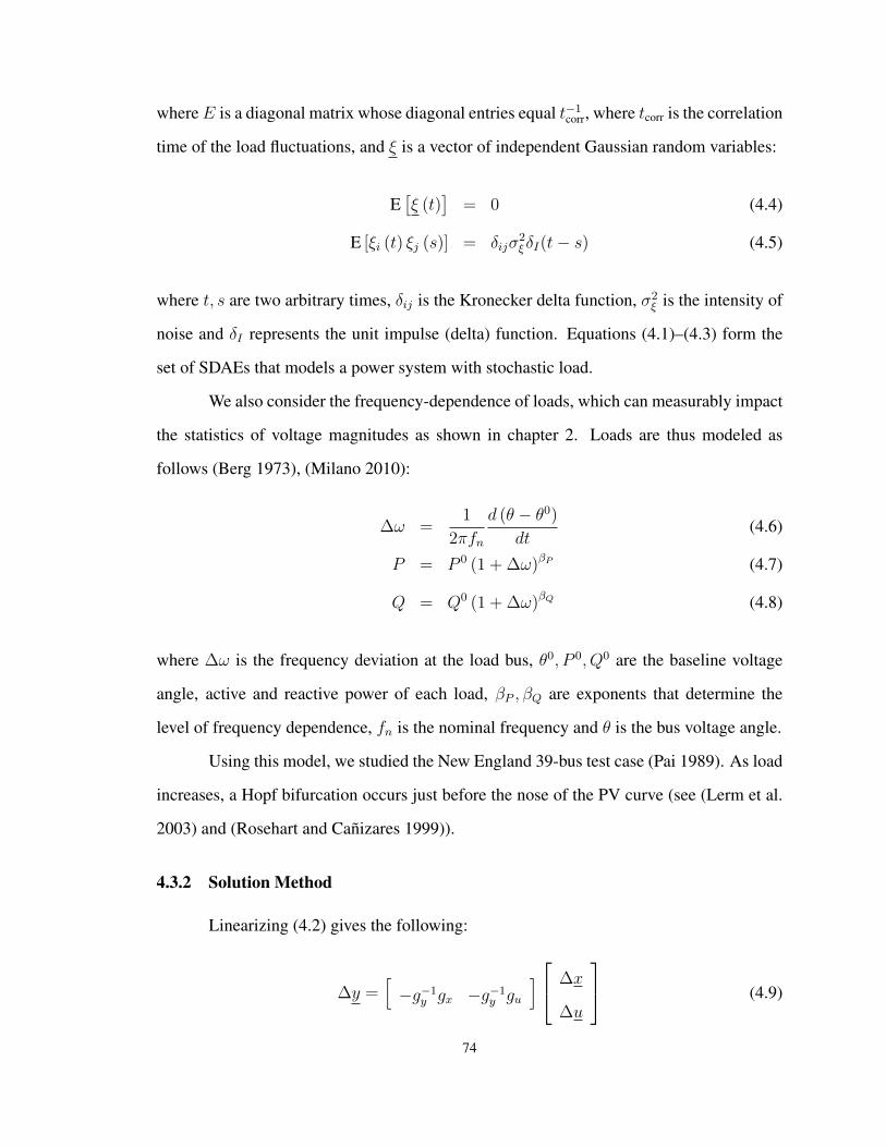
whereE is a diagonal matrix whose diagonal entries equal t−1corr, where tcorr is the correlation

time of the load fluctuations, and ξ is a vector of independent Gaussian random variables:

E[ξ (t)

]= 0 (4.4)

E [ξi (t) ξj (s)] = δijσ2ξδI(t− s) (4.5)

where t, s are two arbitrary times, δij is the Kronecker delta function, σ2ξ is the intensity of

noise and δI represents the unit impulse (delta) function. Equations (4.1)–(4.3) form the

set of SDAEs that models a power system with stochastic load.

We also consider the frequency-dependence of loads, which can measurably impact

the statistics of voltage magnitudes as shown in chapter 2. Loads are thus modeled as

follows (Berg 1973), (Milano 2010):

∆ω =1

2πfn

d (θ − θ0)

dt(4.6)

P = P 0 (1 + ∆ω)βP (4.7)

Q = Q0 (1 + ∆ω)βQ (4.8)

where ∆ω is the frequency deviation at the load bus, θ0, P 0, Q0 are the baseline voltage

angle, active and reactive power of each load, βP , βQ are exponents that determine the

level of frequency dependence, fn is the nominal frequency and θ is the bus voltage angle.

Using this model, we studied the New England 39-bus test case (Pai 1989). As load

increases, a Hopf bifurcation occurs just before the nose of the PV curve (see (Lerm et al.

2003) and (Rosehart and Cañizares 1999)).

4.3.2 Solution Method

Linearizing (4.2) gives the following:

∆y =[−g−1

y gx −g−1y gu

] ∆x

∆u

(4.9)

74

where gx, gy, gu are the Jacobian matrices of g with respect to x, y, u. Linearizing (4.1)

and (4.3) and eliminating ∆y via (4.9) gives the following:

∆x

∆u

=

As −fyg−1y gu

0 −E

∆x

∆u

+ (4.10)

0

In

ξwhere fx, fy are the Jacobian matrices of f with respect to x, y and As = fx − fyg−1

y gx; In

is an identity matrix, with n being the length of u. If we let z =[

∆x ∆u]T

, (4.10) can

be re-written in the standard form:

z = Az +Bξ (4.11)

The covariance matrix of z (σz) satisfies the Lyapunov equation (Gardiner 2010):

Aσz + σzAT = −BBT (4.12)

which can be solved efficiently in O (n3) operations using MATLAB’s lyap function. To

stress the difference between the solution from (4.12) and the results of direct numerical

simulation of (4.1)–(4.3), we will refer to the former solution as semi-analytical. The rea-

son why we refer to it as semi-analytical is that we solve the Lyapunov equation using a

numerical algorithm to calculate the covariance matrix rather than deriving explicit expres-

sions for covariance and correlations matrices as in chapter 2. Therefore, our method is

not entirely analytical. It is not completely numerical either since it is not based on solving

SDAEs numerically.

The stationary autocorrelation matrix can be computed given σz and an equation

from (Gardiner 2010):

E[z (t) zT (s)

]= exp [−A |∆t|]σz (4.13)

75

where ∆t = t − s. From (4.12) and (4.13) the normalized autocorrelation function of zi

can be calculated:Rzi (∆t) = E

[zi (t) z

Ti (s)

]/σ2

zi(4.14)

The covariance matrix of the algebraic variables, σ∆y, is found from (4.9) and (4.12):

σ∆y = KσzKT (4.15)

where K is the matrix from (4.9). Similarly, the autocorrelation function of ∆y(t) is:

E[∆y (t) ∆yT (s)

]= K · E

[z (t) zT (s)

]KT (4.16)

Finally, the covariance and autocorrelation matrices for voltage magnitudes are a subset of

the matrices from (4.15) and (4.16).

Fluctuation-induced deviations of the current magnitudes, ∆Iik, in a line between

buses i and k can be found by linearizing the following:

Iik = YiiViej(φik−φik+θi−θk) + YikVk (4.17)

where Iik is the magnitude of the current of the line between buses i, k; Vi, θi are the voltage

magnitude and angle of bus i; Yii, φii and Yik, φik are magnitudes and angles of the diagonal

and off-diagonal elements of the YBUS matrix. By linearizing (4.17) one can find ∆I from

∆y and then compute the covariance and autocorrelation matrices of ∆I from equations

similar to (4.15) and (4.16).

Comparing the semi-analytical method with the numerical solution shows that the

former is significantly more time-efficient. For the numerical simulations in this chapter,

we solved (4.1)–(4.3) using the trapezoidal DAE solver in the Power System Analysis

Toolbox (PSAT) (Milano 2005). To find numerical values for σ2 and R(∆t) we ran 100

240s simulations, with an integration step size of 0.01s, and then computed the statistics.

For the 39-bus case with 140 variables, solving for σ2z using the semi-analytical method

76

took approximately 0.08s, whereas calculating the variances using numerical simulations

took about 24 hours.

4.4 Useful early warning signs: voltage magnitudes and line currents

This section applies the method in Sec. 4.3 to calculate the autocorrelation and

variance of voltages and currents in the 39-bus test case. These results are subsequently

used to identify particular locations and variables in which the statistical early-warning

signs are most clearly observable.

4.4.1 Autocorrelation and Variance of Voltages

Using the methods described in Sec. 4.3, we calculated σ2, R (∆t) of bus voltage

magnitudes in the 39-bus test case both semi-analytically and numerically using PSAT. In

order to see how these statistics change as the system state moves toward the bifurcation, we

increased all loads uniformly, multiplying each load by the same factor. For the correlation

time and intensity of noise we used: tcorr = 1s and σ2u = 10−4 pu. The values of βP , βQ in

(A.2), (A.3) were chosen randomly from within [2, 3] and [1, 2], respectively (Berg 1973).

For all results in this chapter, we chose the autocorrelation time lag ∆t = 0.2s, based on

the criteria for choosing an optimal ∆t described in chapter 2.

Fig. 4.1 shows several typical, illustrative examples of how σ2, R (∆t) of bus volt-

age magnitudes depend on load level in the 39-bus case. These results show that, as antici-

pated from CSD theory, both σ2 and R (∆t) of voltage magnitudes increase as the system

approaches the bifurcation. However, not all of these signs appear sufficiently early to

detect the bifurcation and take mitigating actions. For example, σ2∆V in buses 7, 14, and

26 exhibits a conspicuous increase when the load level is 10–15% below the bifurcation.

These variables are good early warning signs (EWS) of the impending bifurcation. In con-

trast, σ2∆V in buses 20 and 36 is not a useful warning sign as its increase occurs too close

to the bifurcation. The situation with autocorrelation is reversed, as shown in the second

panel of Fig. 4.1.

77

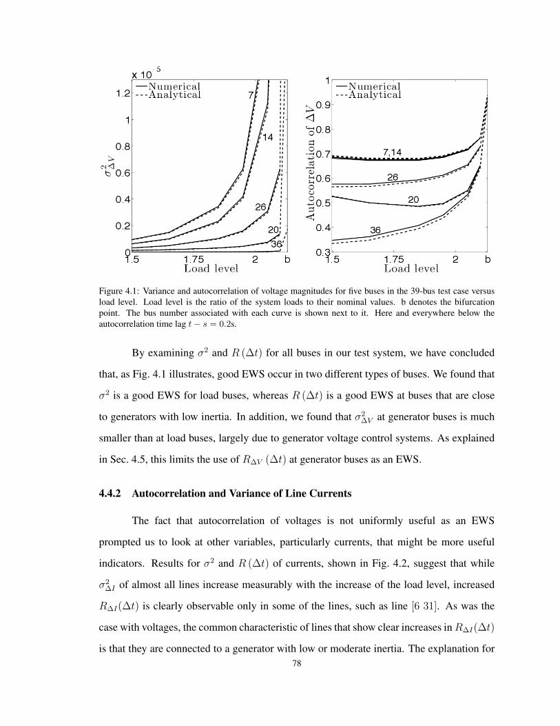
Figure 4.1: Variance and autocorrelation of voltage magnitudes for five buses in the 39-bus test case versusload level. Load level is the ratio of the system loads to their nominal values. b denotes the bifurcationpoint. The bus number associated with each curve is shown next to it. Here and everywhere below theautocorrelation time lag t− s = 0.2s.

By examining σ2 and R (∆t) for all buses in our test system, we have concluded

that, as Fig. 4.1 illustrates, good EWS occur in two different types of buses. We found that

σ2 is a good EWS for load buses, whereas R (∆t) is a good EWS at buses that are close

to generators with low inertia. In addition, we found that σ2∆V at generator buses is much

smaller than at load buses, largely due to generator voltage control systems. As explained

in Sec. 4.5, this limits the use of R∆V (∆t) at generator buses as an EWS.

4.4.2 Autocorrelation and Variance of Line Currents

The fact that autocorrelation of voltages is not uniformly useful as an EWS

prompted us to look at other variables, particularly currents, that might be more useful

indicators. Results for σ2 and R (∆t) of currents, shown in Fig. 4.2, suggest that while

σ2∆I of almost all lines increase measurably with the increase of the load level, increased

R∆I(∆t) is clearly observable only in some of the lines, such as line [6 31]. As was the

case with voltages, the common characteristic of lines that show clear increases inR∆I(∆t)

is that they are connected to a generator with low or moderate inertia. The explanation for78

this appears to be that increasedR∆I (∆t) is closely tied to the way that generators respond

to perturbations as the system approaches bifurcation. Increases inR∆I(∆t) are not clearly

observable in lines that are close to load centers, such as line [4 14] in Fig. 4.2.

Figure 4.2: Variance and autocorrelation of current of two lines. The numbers in brackets are bus numbers attwo ends of the lines.

Examining changes in σ2, R (∆t) of several state variables showed that only mag-

nitudes of voltages and line currents signal the proximity to the bifurcation well under

certain conditions mentioned above. Other variables such as voltage angle, current angle,

generator rotor angle and generator speed did not show measurable or clear monotonically

increasing patterns in σ2, R (∆t) that can indicate proximity to a bifurcation.

4.5 Detectability after measurement noise

This section examines the detectability of increases in σ2 and R (∆t) of voltages

and currents given the presence of measurement noise. In addition, we present a method

for reducing the impact of measurement noise using a band-pass filter.

4.5.1 Impact of Measurement Noise on Variance and Autocorrelation

Clearly, measurement noise will adversely impact the observability of increases

in σ2, R (∆t) of voltages and currents. In order to model this impact, we assumed that

79

measurement noise at each bus is normally distributed with a standard deviation that is

proportional to the steady-state mean voltage for this load level: ση = 0.01 〈V 〉. As a result

the measured variance, σ2∆Vm

, of a bus voltage increases to:

σ2∆Vm = σ2

∆V + σ2η (4.18)

where σ2∆V is the variance before adding measurement noise.

Applying this method, Fig. 4.3 shows σ2 and R (∆t) for the voltage magnitudes

of the same five buses used in Sec. 4.4.1, but after adding measurement noise. The re-

sults show that measurement noise causes the increases in σ2∆Vm

to occur only close to the

bifurcation, except for bus 36. In fact, σ2∆Vm

decreases for most buses, until close to the

bifurcation. The reason for this decrease is that, based on (4.18), σ2η decreases with 〈V 〉,

and 〈V 〉 decreases as the system moves toward the nose of the PV curve. Also, because of

the 1% measurement noise, σ2η > σ2

∆V until close to the bifurcation for most buses. For bus

36, which is a generator bus, σ2 is almost constant since 〈V 〉 (and as a result of σ2η) is held

constant by the exciter; σ2η σ2

∆V for generator buses.

Fig. 4.3 also shows that R∆Vm (∆t) increases significantly near the bifurcation for

buses 7, 14 and, to a lesser extent, for bus 26. Appendix 4.8 demonstrates that the increase

in R∆Vm (∆t) of these buses is largely an artifact of adding measurement noise: it is pri-

marily due to increases in σ2 rather than that of R (∆t). Autocorrelation of ∆Vm is almost

zero for buses 20, 36 since the uncorrelated measurement noise dominates the voltage of

buses near generators.

Thus, measurement noise essentially washes out the useful EWS that we reported

in Sec. 4.4.1. In addition, there is another issue impacting the detectability of EWS, which

we discuss in the next subsection.

4.5.2 Spread of Statistics

One important point regarding the detection of increased σ2 and R (∆t) is that the

measured statistics of a sample of a variable’s measurement data (which an operator can80

Figure 4.3: Variances and autocorrelations of voltage magnitudes of five buses in the 39-bus test case versusload level, accounting for measurement noise.

observe in finite time) are different from the mean statistical properties of that variable over

infinitely many measurements. Although the mean of these statistics typically grows as the

system approaches a bifurcation, the variance (spread) of these statistics that results from

finite sample sizes can cause difficulty in estimating the distance to the bifurcation.

In order to quantify the detectability of an increase in σ2 orR (∆t), we introduce an

index q95/80 (see Fig. 4.4):

q95/80 =

ˆ ∞a

fX(80%)dx+

ˆ a

−∞fX(95%)dx (4.19)

where X is the statistic of interest (σ2 orR (∆t)), fX(80%) and fX(95%) are the probability

density functions (pdfs) of X for load levels of 80% and 95% of the bifurcation, and a is

the point where the two distributions intersect. This measure ranges from 0 to 1, where

0 suggests that there is no overlap between the two distributions, such that detectability

is unimpeded by the statistic’s spread, while q95/80 = 1 means that the two distributions

completely overlap—i.e. the statistic does not increase. When the statistic has a decreasing

81

Figure 4.4: The left panel shows the empirical pdfs of X , which can be σ2 orR (∆t) of measurements fortwo load levels. Measure q95/80 is equal to the sum of the hatched areas. The dash-dot line shows the meanof X versus load level. The right panel shows an alternative view of the pdfs.

trend, we declare q95/80 = NA. q95/80 roughly corresponds to the probability of being able

to correctly distinguish between the measured statistics at 80% and 95% load levels.

4.5.3 Filtering Measurement Noise

In this section, we explore the use of a band-pass filter to reduce the impact of

measurement noise on the statistics of voltage and current measurements. The reason for

filtering out the high frequency content of measurements is that the power spectral density

(PSD) of voltages and currents (see Fig. 4.5) shows that the power of the system noise

(i.e., voltage or current magnitude variations in response to load fluctuations) is concen-

trated mostly in its low frequencies. This appears to be typical for Hopf and saddle-node

bifurcations in power systems. On the other hand, in order to detect CSD, it is necessary

to remove slow trends that result not from CSD but from other factors, such as gradual

changes in the system’s operating point (Dakos et al. 2008). By experimentation, we found

that a band-pass filter with a pass-band of [0.1, 2] Hz reduces the impact of measurement

noise in this system optimally. The rationale for these bounds can be seen from Fig. 4.5,

82

Figure 4.5: Power spectral density of the current of line [6 31] for several load levels listed in the legend.Bifurcation is at load level=2.12.

which shows the PSD of a typical current magnitude in our system. We use this filter for

all “filtered” results reported subsequently.

Fig. 4.6 shows σ2∆V , R∆V (∆t) of buses 7, 36 after filtering measurement noise.

Comparing Fig. 4.6 with Fig. 4.3 shows that using the band-pass filter significantly im-

proves the detectability of increases in σ2∆V7

, which is close to load centers, but is not effec-

tive for bus 36, which is connected to a generator. The reason is that, even with filtering, it

is still necessary that σ2 without measurement noise be sufficiently large so that measure-

ment noise does not dominate it. σ2 of measurement noise after filtering will approximately

be:

σ2ηf = σ2

η ·fH − fL

(fs/2)(4.20)

where σ2ηf is the variance of measurement noise after filtering; fH , fL are upper and lower

cut-off frequencies of the filter; and fs is the sampling frequency of measurements. As-

suming σ2η = 1e− 4 and fs = 60Hz, we get σ2

ηf = 6.3× 10−6. From Fig. 4.1, one can see

that only σ2∆V of the load buses exceeds this value near the bifurcation.

Fig. 4.6 also shows that after filtering out measurement noise, the increase in

R∆V7 (∆t) is detectable near the bifurcation. However, as mentioned in Sec. 4.5.1, in-

83

Figure 4.6: Variance and autocorrelation of voltage magnitude of buses 7,36 versus the load level after filter-ing the measurement noise. In this and subsequent figures, the lines show the mean and the discrete symbols(∗,4) represent 5th, 25th, 75th, 95th percentiles of values of σ2, R (∆t) for 100 realizations at each loadlevel. The vertical dash-dot lines show Load level = 80%b, 95%b.

creases inR(∆t) primarily result from increases in σ2∆V , and thus do not provide additional

information regarding the proximity of the system to the bifurcation. Since σ2η σ2

∆V for

generator buses, R∆V36 (∆t) also does not increase measurably as the system approaches

the bifurcation, even after filtering.

Similar to the case without measurement noise,R (∆t) of line currents close to gen-

erators increase more clearly than that of lines near load centers. Fig. 4.7 shows σ2, R (∆t)

of currents of lines [6 31] and [4 14] after filtering the noise.

In general, filtering noise from line currents is easier than from voltages since the

ratio of σ2 of the system noise (defined above) to σ2 of measurement noise is larger for

currents.

Fig. 4.8 shows the index q95/80 for σ2∆V across the 39-bus test case after filtering

measurement noise. The results in Fig. 4.8 illustrate our earlier statement that σ2∆V of

buses near load centers are good EWS of the bifurcation while σ2∆V of generator buses are

not.

84

1.45 1.65 1.85 2.05 b

0.01

0.02

0.03

0.04

0.05

0.06σ

2 ∆I

Load level

Line [6 31]

Line [4 14]

1.45 1.65 1.85 2.05 b 0

0.2

0.4

0.6

0.8

1

Auto

corr

ela

tion

of

∆I

Load level

Line [6 31]

Line [4 14]

q95/80(1) = 0.0q95/80(2) = 0.0

q95/80(1) = 0.0q95/80(2) = 0.2

Figure 4.7: Variance and autocorrelation of currents of lines [6 31], [4 14] after filtering the measurementnoise.

0

0.1

0.2

0.3

Figure 4.8: Index q95/80 for σ2∆V of bus voltages across the 39-bus test case. Here, and in Fig. 4.9, each

rectangle represents the index q95/80 for σ2∆V of the bus next to it. In order to illustrate the results more

clearly, we show q95/80 = 0.3 for measurements with q95/80 > 0.3, because quantities with this spreadbecome indistinguishable.

85

0

0.1

0.2

0.3

Figure 4.9: Index q95/80 for R∆I (∆t) of lines across the 39-bus test case. Each rectangle represents indexq95/80 for R∆I (∆t) of the line next to it.

Fig. 4.9 shows the index q95/80 for R∆I (∆t) of lines across the 39-bus test case

after filtering the measurement noise. The results in Fig. 4.9 show that R∆I (∆t) of the

lines near generators provide good EWS of the bifurcation while R∆I (∆t) of the rest of

the lines do not provide useful EWS.

Note that while filtering of measurement noise can be helpful in detecting the in-

crease in σ2∆V of buses near load centers, it is not helpful in detecting an increase in

R∆V (∆t) of these buses. This is because the R∆V (∆t) of such buses are not inherently

good indicators of the proximity to the bifurcation; See Sec. 4.4.1. Also, filtering mea-

surement noise will not be helpful in retrieving the statistics of the bus voltages close to

generators since their variances are small compared to that of measurement noise. On the

contrary, R∆I (∆t) of lines near generators provide good EWS for the bifurcation, while

σ2∆I of almost all lines provide good EWS.

86

4.6 Detecting Locations of Increased Stress

This section examines the potential to use statistical properties of measurements to

detect the locations of increased stress in a power system. By studying two scenarios, we

investigated whether patterns of change in σ2 and R (∆t) in a stressed area are different

from the rest of the grid, so they can be helpful in identifying the location of the stressed

area.

4.6.1 Transmission line tripping

In the first scenario, we disconnected lines between buses 4, 14 and buses 4, 5 in or-

der to increase stress in the area close to bus 4. For this experiment, the load level was held

constant at 1.45 times the nominal (Note that the system stress due to this load level does

not cause the disconnection of the two lines). We calculated the ratio of σ2∆V and σ2

∆I for the

stressed case to the variances at the normal operating condition (Ratio (σ2)). We also cal-

culated the difference between R∆V (∆t) and R∆I (∆t) for the two cases (Diff (R (∆t))).

Values of Ratio (σ2) , Diff (R (∆t)) that are sufficiently larger than 1 or 0 indicate signif-

icant increase in σ2 or R (∆t), respectively. Fig. 4.10(a) shows Ratio (σ2∆V ) after adding

measurement noise and filtering. The five bus voltages shown have the highest mean of

Ratio (σ2) among all buses. The figure shows that the voltage of the buses near bus 4 have

the largest Ratio (σ2∆V ) among the system buses. As with voltages, σ2

∆I close to bus 4

showed more growth than σ2∆I in the rest of the system. These results suggest that larger

increases in σ2∆V and σ2

∆I in one area of the system, relative to the rest of the system, can

indicate that this area is stressed.

Our results from Sec. 4.5 identified certain lines whose autocorrelation of currents

can be good EWS of bifurcation. We now comment on what behavior these autocorrela-

tions exhibit in this experiment. It turns out that not all of these autocorrelations show a

measurable increase; the five lines whose currents’ autocorrelations show the largest in-

creases are shown in Fig. 4.10(b). While it is not possible to pinpoint the location of the

disturbance based only on these statistical characteristics, it is possible to tell, based on the87

4 3 18 17 270

0.5

1

1.5

2

2.5

3

3.5

4

Bus No.

Rat

io(σ

2 ∆V)

Percentiles

Mean

[6 5] [2 30] [10 13] [13 14] [2 3]0

0.05

0.1

0.15

0.2

0.25

0.3

0.35

0.4

0.45

0.5

Diff

(R∆

I(∆

t))

Line No.

(a) (b)Percentiles

Mean

Figure 4.10: Panel (a) shows Ratio(σ2

∆V

)after disconnecting the two lines connected to bus 4. The mean

of the Ratio(σ2

∆V

)for the 5 buses that show the highest increases in variance, as well as the 5th, 25th, 75th,

95th percentiles of their values, are shown. Panel (b) shows Diff (R∆I (∆t)) for 5 lines that exhibit the largestincreases in R∆I (∆t). The results are shown after filtering of measurement noise.

statistics, that the disturbance has occurred in a certain area of the network. This knowledge

would reinforce the information obtained from monitoring variances of voltages and cur-

rents. As explained in Sec. 4.5.1, R∆V (∆t) does not provide useful information regarding

which areas in the grid are most stressed.

4.6.2 Capacitor tripping

This section provides an example in which the statistical measures, σ2 and R (∆t),

(at least partially) indicate the location of stress in the network, but the mean voltages

〈V 〉 do not change enough to be good indicators. This example was designed to test the

hypothesis that σ2 and R (∆t) can provide information that is not readily available from

the mean values.

For this example, we added a new bus (bus 40) and an under-load tap changing

(ULTC) transformer that connects bus 40 with bus 15. We also transferred the load of

bus 15 to bus 40. Fig. 4.11 shows the P-V curve of bus 40 for three cases. In Case A,

the system is in normal operating condition. In Case B, a 3-MVAR capacitor at bus 40

88

Figure 4.11: PV curve for the three cases described in Sec. 4.6.2. The vertical line corresponds to the baseload level.

is disconnected and in Case C, the tap changer changes the tap from 1 to 1.1 in order to

return the voltage to the normal operating range ([0.95 1.05] pu). Fig. 4.11 shows that the

disconnection of the capacitor reduces the stability margin significantly, which manifests

itself in lower voltage at bus 40. However, the increase in the ULTC’s tap ratio to 1.1

returns the voltage to a value close to its normal level.

Fig. 4.12(a) shows Ratio (σ2∆I) = σ2

∆I,caseC/σ2∆I,caseA for five lines, after filtering the

measurement noise. These five line currents show the largest increase in σ2∆I among all

lines. The first three highest Ratio (σ2∆I) occur in lines that are close to the stressed area.

However, some of the lines that are close to that area do not show significant or any increase

in σ2∆I . For example, σ2

∆I of line[

14 15]

decreases. Nevertheless, considering lines

with the highest growth in σ2∆I can clearly be helpful in identifying the location of the area

of the system under excessive stress. As was the case for line currents, the results show that

buses that exhibit the largest increases in σ2∆V are close to the stressed area. Fig. 4.12(b)

shows Diff (R∆I (∆t)) = R∆I,,caseC (∆t)−R∆I,,caseA (∆t) for 5 lines. The positive values

indicate the increase in R∆I (∆t). The results in Fig. 4.12(b) show that lines that exhibit

the largest increase in R∆I (∆t) are close to the stressed area.

89

[40 15] [15 16] [16 24] [12 11] [22 35]0

0.5

1

1.5

2

2.5

3

3.5

Line No.

Rati

o(σ

2 ∆I)

Percentiles

Mean

[14 15] [16 24] [15 16] [10 13] [2 30]0

0.05

0.1

0.15

0.2

Line No.

Diff

(R∆

I(∆

t))

Percentiles

Mean(a) (b)

Figure 4.12: Panel (a) shows σ2∆I,caseC/σ2

∆I,caseA for 5 lines that exhibit the largest increase in σ2∆I among

all lines. Panel (b) shows R∆I,,caseC (∆t) − R∆I,,caseA (∆t) for 5 lines that exhibit the largest increase inR∆I (∆t).

4.6.3 Discussion

The results presented in this section show that comparing σ2∆V and σ2

∆I for a stressed

operating condition with their variances for the normal operating condition can be useful

in detecting stressed areas of a power system. The reason for this is that the variances of

voltage and current magnitudes show larger increases near the stressed area of a power sys-

tem, compared to variances in the rest of the system. The results also show that R∆I (∆t)

can be helpful in detecting the stressed area’s approximate location, although it may not

be helpful in pinpointing the exact location of the stress. Autocorrelation of bus voltages

were not found to be useful for pinpointing the stressed location for the reason explained

in Appendix 4.8.

4.7 Conclusions

Building upon theoretical aspects of the CSD phenomenon in power system dis-

cussed in chapters 2 and 3, this chapter investigates the application of CSD for monitoring

power system stability.

90

In this chapter, we first derived a semi-analytical method for quickly computing the

expected autocorrelation and variance for any voltage or current in a dynamic power system

model. Computing the statistics in this way was shown to be orders of magnitude faster

than obtaining the same result by simulation, and allows one to quickly identify locations

and variables that are reliable indicators of proximity to instability. Using this method, we

showed that the variance of voltage magnitudes near load centers, the autocorrelation of line

currents near generators, and the variance of almost all line currents increased measurably

as the 39-bus test case approached bifurcation. We found that these trends persist, even in

the presence of measurement noise, provided that the data are band-pass filtered. Finally,

the chapter provides results suggesting that the statistics of voltage and current data can

be helpful in identifying not only whether a system is seeing increased stress, but also the

location of the stress.

Together, these results suggest that, under certain conditions, these easily measured

statistical quantities in synchrophasor data can be useful indicators of stability. However,

it is necessary to take further steps to use these results for stability monitoring of a power

system. First, it is essential to take into account the impact of filtering measurement noise

in the semi-analytical method. Also, it is crucial to have a realistic estimate of measurement

noise characteristics.

4.8 Appendix A

The equation for R∆Vm (∆t) before band-pass filtering is:

E[∆Vm(t)∆Vm(s)]/σ2∆Vm

= E[∆V (t)∆V (s)]/(σ2∆V +σ2

η) (4.21)

If σ2∆V σ2

η , R∆Vm (∆t) will be almost zero. This is the case for generator buses or buses

close to generators such as buses 20, 36. However, if σ2∆V increases such that σ2

∆V ∼ σ2η

and R∆V (∆t) is sufficiently larger than 0 (> 0.2), then R∆Vm (∆t) will rise significantly

with load level, in part because of increase in R∆V (∆t) and in part because of increase

in σ2∆V . This happens for buses close to load centers such as 7, 14. Comparing R (∆t) of

91

voltage of buses 7, 14 in Fig. 4.1 with those in Fig. 4.3 shows that these quantities increase

significantly after adding measurement noise while their increase without measurement

noise is much smaller. This shows that the increase in R∆Vm (∆t) for load buses is more

due to the increase in σ2∆V than due to the increase in R∆V (∆t).

92

BibliographyAlvarado, F., I. Dobson, and Y. Hu (1994, May). Computation of closest bifurcations in

power systems. IEEE Trans. Power Syst. 9(2), 918–928.Anderson, P. M. and A. Bose (1983, Aug.). A probabilistic approach to power system

stability analysis. IEEE Trans. Power Apparatus Syst. 102(8), 2430–2439.Anghel, M., K. A. Werley, and A. E. Motter (2007, Jan.). Stochastic model for power grid

dynamics. In 40th Annual Hawaii Intl. Conf. Syst. Sci.Avalos, R. J., C. A. Cañizares, F. Milano, and A. J. Conejo (2009, Jan.). Equivalency

of continuation and optimization methods to determine saddle-node and limit-inducedbifurcations in power systems. IEEE Trans. Circuits Syst. I 56(1), 210–223.

Berg, G. (1973, Mar.). Power system load representation. In Proc. IEE, Volume 120, pp.344–348.

Boerlijst, M. C., T. Oudman, and A. M. de Roos (2013). Catastrophic collapse can occurwithout early warning: examples of silent catastrophes in structured ecological models.PLOS ONE 8(4), e62033, 6 pp.

Browne, T. J., V. Vittal, G. T. Heydt, and A. R. Messina (2008, Aug.). A comparative as-sessment of two techniques for modal identification from power system measurements.IEEE Trans. Power Syst. 23(3), 1408–1415.

Bu, S., W. Du, H. Wang, Z. Chen, L. Xiao, and H. Li (2012, May). Probabilistic analysis ofsmall-signal stability of large-scale power systems as affected by penetration of windgeneration. IEEE Trans. Power Syst. 27(2), 762–770.

Chertkov, M., S. Backhaus, K. Turtisyn, V. Chernyak, and V. Lebedev (2011, Jun.). Volt-age collapse and ODE approach to power flows: Analysis of a feeder line with staticdisorder in consumption/production. arXiv preprint arXiv:1106.5003.


Dakos, V., M. Scheffer, E. H. van Nes, V. Brovkin, V. Petoukhov, and H. Held (2008,Sep.). Slowing down as an early warning signal for abrupt climate change. Proc. Natl.Acad. Sci. 105(38), 14308–14312.


Dhople, S., Y. Chen, L. DeVille, and A. Dominguez-Garcia (2013, Dec.). Analysis ofpower system dynamics subject to stochastic power injections. IEEE Trans. Circ. Syst.I 60(12), 3341–3353.

Dong, Z. Y., J. H. Zhao, and D. Hill (2012, Nov.). Numerical simulation for stochastictransient stability assessment. IEEE Trans. Power Syst. 27(4), 1741–1749.


Ghanavati, G., P. D. H. Hines, T. I. Lakoba, and E. Cotilla-Sanchez (2014, Sep.). Under-standing early indicators of critical transitions in power systems from autocorrelationfunctions. IEEE Trans. Circuits Syst. I 61(9), 2747–2760.

93

Ghasemi, H. and C. A. Cañizares (2008). Confidence intervals estimation in the identifica-tion of electromechanical modes from ambient noise. IEEE Trans. Power Syst. 23(2),641–648.

Grijalva, S. (2012, Feb.). Individual branch and path necessary conditions for saddle-nodebifurcation voltage collapse. IEEE Trans. Power Syst. 27(1), 12–19.

Haesen, E., C. Bastiaensen, J. Driesen, and R. Belmans (2009, May). A probabilisticformulation of load margins in power systems with stochastic generation. IEEE Trans.Power Syst. 24(2), 951–958.

Haque, M. (2003, Jan.). On-line monitoring of maximum permissible loading of a powersystem within voltage stability limits. IEE Proc. Gen. Trans. Dist. 150(1), 107–112.

Hauer, A. J. F., D. J. Trudnowski, and J. G. DeSteese (2007, Jun.). A perspective onWAMS analysis tools for tracking of oscillatory dynamics. In IEEE Power and EnergySoc. General Meeting, pp. 1–10.

Hou, G. and V. Vittal (2012, Nov.). Trajectory sensitivity based preventive control of volt-age instability considering load uncertainties. IEEE Trans. Power Syst. 27(4), 2280–2288.

Huang, H. and C. Chung (2012, Nov.). Coordinated damping control design for DFIG-based wind generation considering power output variation. IEEE Trans. PowerSyst. 27(4), 1916–1925.

Huang, H., C. Chung, K. W. Chan, and H. Chen (2013, Aug.). Quasi-Monte Carlo basedprobabilistic small signal stability analysis for power systems with plug-in electric ve-hicle and wind power integration. IEEE Trans. Power Syst. 28(3), 3335–3343.

Kakimoto, N., M. Sugumi, T. Makino, and K. Tomiyama (2006, Feb.). Monitoring ofinterarea oscillation mode by synchronized phasor measurement. IEEE Trans. PowerSyst. 21(1), 260–268.

Kamwa, I., A. K. Pradhan, and G. Joós (2011, Feb.). Robust detection and analysis ofpower system oscillations using the Teager-Kaiser energy operator. IEEE Trans. PowerSyst. 26(1), 323–333.

Kataoka, Y. (2003, Nov.). A probabilistic nodal loading model and worst case solutionsfor electric power system voltage stability assessment. IEEE Trans. Power Syst. 18(4),1507–1514.


Lerm, A. A. P., C. A. Cañizares, and A. S. Silva (2003, May). Multiparameter bifurcationanalysis of the South Brazilian power system. IEEE Trans. Power Syst. 18(2), 737–746.

Lim, J. M. and C. L. DeMarco (2013, Aug.). Model-free voltage stability assessments viasingular value analysis of PMU data. In Bulk Pow. Syst. Dyn. Cont.-IX Optim. Secu.Cont. Emer. Pow. Grid Symp., pp. 1–10.


94

Milano, F. (2010, May). Power System Analysis Toolbox Quick Reference Manual forPSAT version 2.1. 6.

Milano, F. and R. Zarate-Minano (2013, Nov.). A systematic method to model powersystems as stochastic differential algebraic equations. IEEE Trans. Power Syst. 28(4),4537–4544.

Mori, H. (1963). On the relaxation processes near the second order phase transition point.Prog. Theor. Phys. 30(4), 576–578.

Munoz, J., C. Canizares, K. Bhattacharya, and A. Vaccaro (2013, Nov.). An affinearithmetic-based method for voltage stability assessment of power systems with in-termittent generation sources. IEEE Trans. Power Syst. 28(4), 4475–4487.


Odun-Ayo, T. and M. L. Crow (2012). Structure-preserved power system transient stabilityusing stochastic energy functions. IEEE Trans. Power Syst. 27(3), 1450–1458.


Perninge, M., V. Knazkins, M. Amelin, and L. Soder (2010, Aug.). Risk estimation ofcritical time to voltage instability induced by saddle-node bifurcation. IEEE Trans.Power Syst. 25(3), 1600–1610.

Podolsky, D. and K. Turitsyn (2013a, Jul.). Critical slowing-down as indicator of approachto the loss of stability. arXiv preprint:1307.4318.

Podolsky, D. and K. Turitsyn (2013b, Jul.). Random load fluctuations and collapse prob-ability of a power system operating near codimension 1 saddle-node bifurcation. InIEEE Power and Energy Soc. Gen. Meeting, pp. 1–5.

Rosehart, W. D. and C. A. Cañizares (1999, Mar.). Bifurcation analysis of various powersystem models. Intl. J. Elec. Pow. Energy Syst. 21(3), 171–182.

Scheffer, M., J. Bascompte, W. A. Brock, V. Brovkin, S. R. Carpenter, V. Dakos, H. Held,E. H. Van Nes, M. Rietkerk, and G. Sugihara (2009). Early–warning signals for criticaltransitions. Nature 461(7260), 53–59.

Scheffer, M., S. R. Carpenter, T. M. Lenton, J. Bascompte, W. Brock, V. Dakos, J. van deKoppel, I. A. van de Leemput, S. A. Levin, E. H. van Nes, M. Pascual, and J. Vander-meer (2012, Oct.). Anticipating critical transitions. Science 338(6105), 344–348.

Schellenberg, A., W. Rosehart, and J. A. Aguado (2006, May). Cumulant-based stochasticnonlinear programming for variance constrained voltage stability analysis of powersystems. IEEE Trans. Power Syst. 21(2), 579–585.

Verdejo, H., L. Vargas, and W. Kliemann (2012, Jul.). Stability of linear stochastic sys-tems via Lyapunov exponents and applications to power systems. Appl. Math. Com-put. 218(22), 11021–11032.

Wang, K., C. Chung, C. Tse, and K. Tsang (2000, Jan.). Improved probabilistic methodfor power system dynamic stability studies. In IEE Proc. Gen. Trans. Dist., Volume147, pp. 37–43.

95



Yuan, B., M. Zhou, G. Li, and X.-P. Zhang (to be published). Stochastic small-signalstability of power systems with wind power generation. IEEE Trans. Power Syst..

96

CHAPTER 5: CONCLUSIONS AND FUTURE DIRECTIONS

5.1 Conclusions

This dissertation aims to improve our understanding of early warning signs (EWS)

of critical bifurcations such as saddle-node and Hopf in power systems, which can lead to

catastrophic failures (i.e. a blackout) if they are not detected sufficiently early. The EWS

under study are increases in variance and autocorrelation of state variables, which are due

to a phenomenon in dynamical systems known as critical slowing down (CSD). The results

of this research provide new methods for extracting information regarding the proximity of

a power system to critical bifurcations as well as for identifying stressed locations of the

system.

Starting with analytical studies, the results (see chapter 2) from calculation of au-

tocorrelation function of state variables in three small power systems demonstrate that the

CSD phenomenon does indeed occur in power systems. Numerical simulation of stochas-

tic differential equations that model these systems confirms the findings from the analytical

results. Together, numerical and analytical results show that this phenomenon occurs for

both saddle-node and Hopf bifurcations.

The results also show that although CSD signs do consistently appear as the sys-

tems approach bifurcation, only in a few of the variables such as voltage magnitudes do

the increases in autocorrelation and variance appear sufficiently early to give a useful early

warning of potential collapse. Eigenvalue analysis presented in chapter 3 provides some

explanation as to why CSD signs are better observable in some variables than others. In-

vestigation of a system for which a Hopf bifurcation occurs as a result of increase in system

loading, shows that fluctuations of the variables that show well observable increase in the

statistics, are more aligned with the direction of the system’s dominant mode.

The dissertation also presents (see chapter 4) a semi-analytical method for quickly

computing the expected autocorrelation and variance for state variables in a dynamic power97

system model. The results show that computing the statistics using this method is much

faster than obtaining them by simulation, and allows one to quickly identify locations and

variables that are reliable indicators of proximity to instability.

The results obtained using the semi-analytical method, show that not only is in-

crease in autocorrelation and variance more clearly measurable in some variables than in

others, but also CSD signs are better observable in some areas of a power system. Af-

ter considering measurement noise, the results for a test system suggest that the variance

of voltage magnitudes near load centers, the autocorrelation of line currents near genera-

tors, and the variance of almost all line currents show measurable increase as the system

approaches a Hopf bifurcation, provided that the data are band-pass filtered.

Finally, the results from a couple of experiments show that it is possible to extract

information about the location of the stress in the system from the statistics of voltages and

currents. Comparing variances of voltages and currents for stressed operating conditions

with their variances for the normal operating condition shows that variances of voltage

and current magnitudes exhibit larger increases near the stressed area of a power system,

which can be useful in detecting such an area. The results also show that autocorrelation

of currents can be helpful in detecting the stressed area’s approximate location, although it

may not be helpful in pinpointing the exact location of the stress.

5.2 Future directions

A natural expansion upon the current work is to develop a power system stabil-

ity indicator using statistics of measurements. Considering factors such as inaccuracy in

power system parameters and models, calculating distance to a critical bifurcation using

only deterministic models and mean values of measurements may not provide true risk or

likelihood of failures. It might be possible to get a more accurate estimate about distance

to a bifurcation by combining information from mean values with variance and autocor-

relation of measurements. To this end, it would be helpful to expand the semi-analytical

method so that it takes into account the impact of filtering measurement noise. There will

also be other challenges for achieving a reliable statistics-based stability indicator, e.g.,98

changes in load variations intensity and inaccurate modeling of measurement noise, which

can impact measurements’ statistics.

Considering the above, it might be worthwhile to investigate the impacts of more

detailed models of measurement noise on the results presented in this work. Measurement

noise can come from various elements of a measurement system such as current or volt-

age transformers, cables, and sensors or A/D converters (Zhu et al. 2006). Modeling each

source in sufficient detail could help with better understanding of implications of measure-

ment noise on measurements’ statistics.

Also, studying patterns of change in statistics of power system variables that are

not included in this work, might uncover helpful EWS. In this work, we studied statistical

patterns of magnitude and angle of node voltages and line currents, and rotor angle and

speed of generators. The results showed that statistics of voltage and current magnitudes

in some cases provide helpful EWS for saddle-node and Hopf bifurcations. There are,

however, other variables whose statistical properties might worth exploring in the future;

one example here is the frequency of load nodes.

An additional research direction stems from stochastic methods used to analyze

power system dynamics in this dissertation. In the current literature, there is little infor-

mation regarding modeling renewable energy sources using stochastic calculus (Yuan et al.

2014). Building upon this work, one could develop a comprehensive stochastic framework

for modeling and analysis of a power system with renewable sources, such as wind tur-

bines and solar panels. Developing such a framework would enable the study of the impact

of renewable sources on power system stability. Moreover, stochastic modeling of renew-

able sources could also be helpful for stability analysis of low voltage distribution systems,

which might be of importance in the future due to increase in penetration of distributed

generation in these systems (Cardell and Ilic 2004), (Nguyen and Turitsyn 2014). The

following subsection briefly discusses some aspects of stochastic modeling of renewable

energy sources.

99

5.2.1 Modeling renewable energy sources

Recently, some research has focused on development of stochastic models of wind

and solar generation and examining their impact on power system dynamics. (Ajala and

Sauer 2014) propose a stochastic model for a grid-connected three-phase photovoltaic sys-

tem. (Bu et al. 2012) present an analytical method for calculation of the probability density

function (PDF) of critical eigenvalues of a large-scale power system from the PDF of multi-

ple grid-connected sources of wind power generation. (Yuan et al. 2014) present a method

for calculation of steady-state expectation and variance of state variables of a power system

model with stochastic wind excitation after a small disturbance. However, the current mod-

eling approaches seem to be in an early stage and the results obtained using these models

are sometimes significantly different. For example, (Bu et al. 2012) conclude that "stochas-

tic variation of grid-connected wind generation can cause the system to lose stability even

though the system is stable deterministically". On the contrary, (Yuan et al. 2014) state

that stochastic excitation due to wind generation only leads to bounded fluctuations of the

power system.

Various methods have been used for modeling stochastic excitation of renewable

generation by wind and solar energy. (Ajala and Sauer 2014) model solar irradiance and

temperature using the Wiener process. (Bu et al. 2012) use the Weibull distribution for

modeling wind speed. (Yuan et al. 2014) model the input mechanical power of wind using

the Wiener process. Further investigation is necessary to verify these methods.

100

APPENDIX A: SIMULATION SCRIPTS

The MATLAB scripts in this appendix can be used for running a dynamic simula-

tion with stochastic changes in load using power system analysis toolbox (PSAT). In the

simulations, loads vary randomly at each time-step and their values at any point of time

are correlated to their values at previous times. Loads fluctuations follow the Ornstein–

Uhlenbeck process (Perninge et al. 2010), (Hauer et al. 2007), which is a mean-reverting

Gaussian process. Also, loads are assumed to be frequency-dependent:

∆ω =1

2πfn

d (θ − θ0)

dt(A.1)

P = P 0 (1 + ∆ω)βP (A.2)

Q = Q0 (1 + ∆ω)βQ (A.3)

A.1 Dynamic simulation driver

The script below (run_sim.m) is the driver for running dynamic simulations. It

employs PSAT through a set of commands. First it loads data and perturbation files. Then

it runs power flow. After initialization, time-domain simulation is performed. At the end

output variables are saved in "output.mat". The script d039.m includes 39-bus test case

data (Pai 1989).

run_sim.m

clear all;close all;clc;

tstart=tic;

global intstep VP_nos VQ_nos tcorr PQ Varout Varname P0 Q0;

RandStream.setDefaultStream(RandStream(’mt19937ar’,’seed’,...

101

sum(100*clock)));

intstep = 0.01; % Integration Step Size

tbegin = 0; % Initial Simulation time

tfinal = 120; % Final Simulation time

tcorr = 1; % Correlation time of noise

d039;

npq = size(PQ.con,1);

P0 = PQ.con(:,4); % Initial value of loads’ active power

Q0 = PQ.con(:,5); % Initial value of loads’ reactive

power

initpsat; % Initialize PSAT global variables

datafile = ’d039’; % Test case data file

runpsat(datafile,’data’);

runpsat(’perturb’,’pert’); % "Perturb": Perturbation file

Settings.freq = 60;

clpsat.readfile = 1; % Read data file before running power

flow

runpsat(’pf’); % Run power flow

%% SETTINGS FOR TIME DOMAIN SIMULATION

Settings.coi = 1; % Use center of inertia for synchronous

machines

Settings.t0 = tbegin;

Settings.tf = tfinal;

Settings.pq2z = 0; % Do not convert PQ loads to constant

102

% impedance loads after power flow

Settings.fixt = 1; % Enable fixed time-step solver

Settings.tstep = intstep;

%%

VP_nos = zeros(npq,1); % Vector of noise for load active

powers, see "perturb.m"

VQ_nos = zeros(npq,1);

nL = Line.n + Ltc.n + Phs.n + Hvdc.n + Lines.n;

Varname.idx = 1:DAE.n + DAE.m + 2*Bus.n + 5*nL;

runpsat(’td’); % Running time domain (dynamic)

simulation

%% OUTPUT VARIABLES

%Index of output variables

ix_Va = DAE.n+1:DAE.n+Bus.n; % Index of voltage angles

ix_Vm = DAE.n+Bus.n + ... % Index of voltage magnitudes

1:DAE.n+2*Bus.n;

ix_I = DAE.n + DAE.m +... % Index of line currents

2*Bus.n + 4*nL + 1:DAE.n + DAE.m + 2*Bus.n + 5*nL;

ix_P = DAE.n + DAE.m + ... % Index of line active powers

2*Bus.n + 1:DAE.n + DAE.m + 2*Bus.n+nL;

ix_Q = DAE.n + DAE.m + ... % Index of line reactive

powers

2*Bus.n +2*nL + 1:DAE.n + DAE.m + 2*Bus.n+3*nL;

ix_de = Syn.delta; % Index of generator rotor

angles

ix_om = Syn.omega; % Index of generator speed

103

%Output variable values

Va = Varout.vars(:,ix_Va); % Va: Bus voltage angles

Vm = Varout.vars(:,ix_Vm); % Vm: Bus voltage magnitudes

time = Varout.t;

deltas = Varout.vars(:,ix_de);

omegas = Varout.vars(:,ix_om);

Il = Varout.vars(:,ix_I);

Pl = Varout.vars(:,ix_P);

Ql = Varout.vars(:,ix_Q);

%%

save(’output’,’Va’,’Vm’,’deltas’,’omegas’,’time’,’Pl’,’Ql’,’Il’);

close all;

stime = toc(tstart)

A.2 Perturbation function

The following is the perturbation function (Perturb.m) for introducing disturbances

such as opening a line, load changes, fault, etc. In this file, values of P 0 and Q0 in A.2, A.3

are modified at each time step according to the Ornstein–Uhlenbeck process.

perturb.m

function perturb(t)

% Adding correlated noise (Ornstein-Uhlenbeck process) to

% load active and reactive powers

global intstep VP_nos VQ_nos tcorr Fl P0 Q0;

gamma = 1/tcorr;

nos_std = 0.01*sqrt(2*gamma);

rnd_vec = randn(size(Fl.con,1),1);104

VP_nos = VP_nos*(1 - gamma * intstep) + nos_std * ...

sqrt(intstep) * rnd_vec;

VQ_nos = VQ_nos*(1 - gamma * intstep) + nos_std *...

sqrt(intstep) * rnd_vec;

Fl.con(:,2) = P0 .*(1+VP_nos); % Fl.con(:,2) will be

% multiplied later by (1+Delta omega)^beta_p to give load

% active power values at each time step

Fl.con(:,5) = Q0 .*(1+VQ_nos); % Fl.con(:,5) will be

% multiplied by (1+Delta omega)^beta_q

105



Ajala, O. and P. Sauer (2014). Stochastic processes in a grid-connected three-phase pho-tovoltaic system. In Power Energy Conf. Illinois, pp. 1–8. IEEE.

Anghel, M., K. A. Werley, and A. E. Motter (2007, Jan.). Stochastic model for power griddynamics. In 40th Annual Hawaii Intl. Conf. Syst. Sci.

Avalos, R. J., C. A. Cañizares, F. Milano, and A. J. Conejo (2009, Jan.). Equivalencyof continuation and optimization methods to determine saddle-node and limit-inducedbifurcations in power systems. IEEE Trans. Circuits Syst. I 56(1), 210–223.

Bao, L., Z. Huang, and W. Xu (2003). Online voltage stability monitoring using var re-serves. IEEE Trans. Power Syst. 18(4), 1461–1469.

Begovic, M. M. and A. G. Phadke (1992). Control of voltage stability using sensitivityanalysis. IEEE Trans. Power Syst. 7(1), 114–123.

Berg, G. (1973, Mar.). Power system load representation. In Proc. IEE, Volume 120, pp.344–348.

Blanchard, P., R. L. Devaney, and G. R. Hall (2006). Differential Equations. ThomsonBrooks/Cole.

Boerlijst, M. C., T. Oudman, and A. M. de Roos (2013). Catastrophic collapse can occurwithout early warning: examples of silent catastrophes in structured ecological models.PLOS ONE 8(4), e62033, 6 pp.

Boettiger, C., N. Ross, and A. Hastings (2013). Early warning signals: the charted anduncharted territories. Theoretical Ecology, 1–10.

Browne, T. J., V. Vittal, G. T. Heydt, and A. R. Messina (2008, Aug.). A comparative as-sessment of two techniques for modal identification from power system measurements.IEEE Trans. Power Syst. 23(3), 1408–1415.

Bu, S., W. Du, H. Wang, Z. Chen, L. Xiao, and H. Li (2012, May). Probabilistic analysis ofsmall-signal stability of large-scale power systems as affected by penetration of windgeneration. IEEE Trans. Power Syst. 27(2), 762–770.

Cai, D., P. Regulski, M. Osborne, and V. Terzija (2013, Sep.). Wide area inter-areaoscillation monitoring using fast nonlinear estimation algorithm. IEEE Trans. SmartGrid 4(3), 1721–1731.

Cañizares, C. A., N. Mithulananthan, F. Milano, and J. Reeve (2004, May). Linear perfor-mance indices to predict oscillatory stability problems in power systems. IEEE Trans.Power Syst. 19(2), 1104–1114.

Cardell, J. and M. Ilic (2004, Jun.). Maintaining stability with distributed generation in arestructured industry. In Power Engineering Society General Meeting, pp. 2142–2149.IEEE.

Centeno, V., J. De La Ree, A. Phadke, G. Michel, R. Murphy, and R. Burnett Jr (1993,Oct.). Adaptive out-of-step relaying using phasor measurement techniques. IEEE Com-put. Appl. Pow. 6(4), 12–17.

106

Chertkov, M., S. Backhaus, K. Turtisyn, V. Chernyak, and V. Lebedev (2011, Jun.). Volt-age collapse and ODE approach to power flows: Analysis of a feeder line with staticdisorder in consumption/production. arXiv preprint arXiv:1106.5003.

Chiang, H., I. Dobson, R. J. Thomas, J. S. Thorp, and L. Fekih-Ahmed (1990). On voltagecollapse in electric power systems. IEEE Trans. Power Syst. 5(2), 601–611.


Dakos, V., S. Kéfi, M. Rietkerk, E. H. van Nes, and M. Scheffer (2011). Slowing downin spatially patterned ecosystems at the brink of collapse. The American Natural-ist 177(6), E153–E166.

Dakos, V., M. Scheffer, E. H. van Nes, V. Brovkin, V. Petoukhov, and H. Held (2008,Sep.). Slowing down as an early warning signal for abrupt climate change. Proc. Natl.Acad. Sci. 105(38), 14308–14312.

De La Ree, J., V. Centeno, J. S. Thorp, and A. G. Phadke (2010). Synchronized phasormeasurement applications in power systems. IEEE Trans. Smart Grid 1(1), 20–27.


Demello, F. P. and C. Concordia (1969, Apr.). Concepts of synchronous machine stabilityas affected by excitation control. IEEE Trans. Power Apparatus Syst. 88(4), 316–329.

Dhople, S., Y. Chen, L. DeVille, and A. Dominguez-Garcia (2013, Dec.). Analysis ofpower system dynamics subject to stochastic power injections. IEEE Trans. Circ. Syst.I 60(12), 3341–3353.

Dobson, I. (1992, Mar.). Observations on the geometry of saddle node bifurcation andvoltage collapse in electrical power systems. IEEE Trans. Circ. Syst. I: Fund. Theo.App. 39(3), 240 –243.

Dobson, I., T. Van Cutsem, C. D. Vournas, C. L. DeMarco, M. Venkatasubramanian,T. Overbye, and C. A. Canizares (2002). Voltage stability assessment: concepts, prac-tices and tools. Power System Stability Subcommittee Special Publication IEEE/PES.

Dong, Z. Y., J. H. Zhao, and D. Hill (2012, Nov.). Numerical simulation for stochastictransient stability assessment. IEEE Trans. Power Syst. 27(4), 1741–1749.

FERC and NERC (2012, Apr.). Arizona–Southern California outages on September 8,2011: causes and recommendations. Technical report.


Ghanavati, G., P. D. H. Hines, T. Lakoba, and E. Cotilla-Sanchez (2013, Sep.). Calculationof the autocorrelation function of the stochastic single machine infinite bus system. InProc. North Amer. Power Symp., pp. 1–6.

Ghasemi, H. (2006). On-line monitoring and oscillatory stability margin prediction inpower systems based on system identification. Ph. D. thesis, University of Waterloo.

107

Ghasemi, H. and C. A. Cañizares (2008, May). Confidence intervals estimation in theidentification of electromechanical modes from ambient noise. IEEE Trans. PowerSyst. 23(2), 641–648.

Glavic, M. and T. Van Cutsem (2009, Aug.). Wide-area detection of voltage instabil-ity from synchronized phasor measurements. part I: Principle. IEEE Trans. PowerSyst. 24(3), 1408 –1416.

Gómez-Expósito, A., A. Abur, P. Rousseaux, A. de la Villa Jaén, and C. Gómez-Quiles(2011). On the use of PMUs in power system state estimation. In Proc. 17th PowerSyst. Compu. Conf., pp. 22–26.

Gou, B. and A. Abur (2001, Nov.). An improved measurement placement algorithm fornetwork observability. IEEE Trans. Power Syst. 16(4), 819–824.

Hastings, A. and D. B. Wysham (2010). Regime shifts in ecological systems can occurwith no warning. Ecol. Lett. 13(4), 464–472.

Hauer, A. J. F., D. J. Trudnowski, and J. G. DeSteese (2007, Jun.). A perspective onWAMS analysis tools for tracking of oscillatory dynamics. In IEEE Power Energy Soc.Gen. Meeting, pp. 1–10.

Horsthemke, W. and R. Lefever (2006). Noise-induced Transitions (2nd. ed.). Berlin:Springer.

Huang, Z., N. Zhou, F. Tuffner, and D. Trudnowski (2011). Use of modal sensitivity tooperating conditions for damping control in power systems. In 44th Hawaii Intl. Conf.Syst. Sci., pp. 1–9.

Kakimoto, N., M. Sugumi, T. Makino, and K. Tomiyama (2006, Feb.). Monitoring ofinterarea oscillation mode by synchronized phasor measurement. IEEE Trans. PowerSyst. 21(1), 260–268.

Klein, M., G. Rogers, and P. Kundur (1991, Aug.). A fundamental study of inter-areaoscillations in power systems. IEEE Trans. Power Syst. 6(3), 914–921.

Kosterev, D., S. Yirga, and V. Venkatasubramanian (1997, Mar.). Validation report of theAugust 10, 1996 WSCC disturbance. Technical report, Western Systems CoordinatingCouncil.

Kundur, P., N. J. Balu, and M. G. Lauby (1994). Power system stability and control, Vol-ume 4. New York: McGraw-hill.

Kundur, P., G. Berube, L. Hajagos, and R. Beaulieu (2003, Jul.). Practical utility experi-ence with and effective use of power system stabilizers. In IEEE Power Energy Soc.Gen. Meeting, Volume 3, pp. 1777–1785. IEEE.


Lenton, T., V. Livina, V. Dakos, E. Van Nes, and M. Scheffer (2012). Early warning ofclimate tipping points from critical slowing down: comparing methods to improverobustness. Philos. Trans. Royal Soc. A: Math., Phys. Eng. Sci. 370(1962), 1185–1204.

Lerm, A. A. P., C. A. Cañizares, and A. S. Silva (2003, May). Multiparameter bifurcationanalysis of the South Brazilian power system. IEEE Trans. Power Syst. 18(2), 737–746.

108

Litt, B., R. Esteller, J. Echauz, M. D’Alessandro, R. Shor, T. Henry, P. Pennell, C. Epstein,R. Bakay, M. Dichter, et al. (2001). Epileptic seizures may begin hours in advance ofclinical onset: a report of five patients. Neuron 30(1), 51–64.


Milano, F. (2010, May). Power System Analysis Toolbox Quick Reference Manual forPSAT version 2.1. 6.

Milano, F. and R. Zarate–Minano (2013, Nov.). A systematic method to model powersystems as stochastic differential algebraic equations. IEEE Trans. Power Syst. 28(4),4537–4544.

Milosevic, B. and M. Begovic (2003). Voltage-stability protection and control using awide-area network of phasor measurements. IEEE Trans. Power Syst. 18(1), 121–127.

Nguyen, H. D. and K. Turitsyn (2014, Jul.). Voltage multistability and pulse emergencycontrol for distribution system with power flow reversal. arXiv:1407.1355.


Odun-Ayo, T. and M. L. Crow (2012, Aug.). Structure-preserved power system transientstability using stochastic energy functions. IEEE Trans. Power Syst. 27(3), 1450–1458.


Peng, J. H. and N. K. Nair (2012). Enhancing Kalman filter for tracking ringdown elec-tromechanical oscillations. IEEE Trans. Power Syst. 27(2), 1042–1050.

Perninge, M., V. Knazkins, M. Amelin, and L. Soder (2010, Aug.). Risk estimation ofcritical time to voltage instability induced by saddle-node bifurcation. IEEE Trans.Power Syst. 25(3), 1600–1610.

Phadke, A. (1993, Apr.). Synchronized phasor measurements in power systems. IEEEComput. Appl. Pow. 6(2), 10–15.

Podolsky, D. and K. Turitsyn (2013a, Jul.). Critical slowing-down as indicator of approachto the loss of stability. arXiv preprint:1307.4318.

Podolsky, D. and K. Turitsyn (2013b, Jul.). Random load fluctuations and collapse prob-ability of a power system operating near codimension 1 saddle-node bifurcation. InIEEE Power Energy Soc. Gen. Meeting, pp. 1–5.

Popovic, D., D. Kukolj, and F. Kulic (1998, Jul.). Monitoring and assessment of voltagestability margins using artificial neural networks with a reduced input set. IEE Proc.Gen. Trans. Dist. 145(4), 355–362.

Revel, G., A. Leon, D. Alonso, and J. Moiola (2010, Apr.). Bifurcation analysis on amultimachine power system model. IEEE Trans. Circ. Syst. I 57(4), 937 –949.

Romero, J. J. (2012, Oct.). Blackouts illuminate India’s power problems. IEEE Spec-trum 49(10), 11–12.

Rosehart, W. D. and C. A. Cañizares (1999, Mar.). Bifurcation analysis of various powersystem models. Intl. J. Elec. Pow. Energy Syst. 21(3), 171–182.

109

Scheffer, M., J. Bascompte, W. A. Brock, V. Brovkin, S. R. Carpenter, V. Dakos, H. Held,E. H. Van Nes, M. Rietkerk, and G. Sugihara (2009, Sep.). Early-warning signals forcritical transitions. Nature 461(7260), 53–59.

Scheffer, M., S. Carpenter, J. A. Foley, C. Folke, and B. Walker (2001). Catastrophic shiftsin ecosystems. Nature 413(6856), 591–596.

Smon, I., G. Verbic, and F. Gubina (2006, Aug.). Local voltage-stability index using Tel-legen’s theorem. IEEE Trans. Power Syst. 21(3), 1267–1275.

Stratonovich, R. L. (1963). Introduction to the Theory of Random Noise. Gordon andBreach.


Wang, Y., D. J. Hill, R. H. Middleton, and L. Gao (1993, May). Transient stability en-hancement and voltage regulation of power systems. IEEE Trans. Power Syst. 8(2),620–627.


Yang, N., Q. Liu, and J. D. McCalley (1998, Nov.). TCSC controller design for dampinginterarea oscillations. IEEE Trans. Power Syst. 13(4), 1304–1310.

Yuan, B., M. Zhou, G. Li, and X. Zhang (2014). Stochastic small-signal stability of powersystems with wind power generation. IEEE Trans. Power Syst. ( to be published.).

Zhong, Z., C. Xu, B. J. Billian, L. Zhang, S. Tsai, R. W. Conners, V. A. Centeno, A. G.Phadke, and Y. Liu (2005, Nov.). Power system frequency monitoring network (FNET)implementation. IEEE Trans. Power Syst. 20(4), 1914–1921.

Zhou, D. Q., U. Annakkage, and A. D. Rajapakse (2010). Online monitoring of volt-age stability margin using an artificial neural network. IEEE Trans. Power Syst. 25(3),1566–1574.

Zhou, N., J. W. Pierre, and D. Trudnowski (2012). A stepwise regression method forestimating dominant electromechanical modes. IEEE Trans. Power Syst. 27(2), 1051–1059.

Zhu, J., A. Abur, M. Rice, G. Heydt, and S. Meliopoulos (2006, Nov.). Enhanced stateestimators. Technical report, PSERC.

110

statistical analysis of high sample rate time-series data

Documents