STATISTICAL ANALYSIS OF PHARMACOKINETIC DATA---BIOEQUIVALENCE STUDY

By

Qingmin Guo

A THESIS

Submitted to Michigan State University

in partial fulfillment of the requirements for the degree of

Biostatistics—Master of Science

2015

ABSTRACT

STATISTICAL ANALYSIS OF PHARMACOKINETIC DATA--BIOEQUIVALENCE STUDY

By

Qingmin Guo

Bioequivalence (BE) studies are widely carried out in the pharmaceutical industry. The assessment

of BE adopted by the Food and Drugs Administration (FDA) is a moment-based criterion

evaluating log-transformed pharmacokinetic responses such as Area Under the Curve (AUC),

Maximum Concentration ( maxC ), which are usually estimated from drug plasma time profiles.

Average BE (ABE) is based solely on the comparison of population averages but not on the

variances, while Population BE (PBE) and individual BE (IBE) approaches include comparisons of

both averages and variances. The objective of this thesis is to review the standard approaches to

statistical analyses of pharmacokinetic data. It also covers estimation of AUC, maxC and other

pharmacokinetic (PK) parameters as introduced in a Non-Compartmental Analysis (NCA)

approach and Compartmental Models Analysis approach. Widely cited data sets from the published

literature are used to illustrate these two approaches. They show the benefits of parameter

estimation and subsequent statistical inference with an appropriate compartmental model, even

though the model fitting could be a little complicated.

iii

ACKNOWLEDGEMENTS

I would never have been able to finish my thesis without the guidance of my committee members

Dr. Joseph Gardiner, Dr. Zhehui Luo and Dr. Dorothy Pathak, help from friends, and support from

my family.

iv

TABLE OF CONTENTS LIST OF TABLES . . . . . . . . . . . . . . . . . . . . . . . . . . . . . . . . . . . . . . . . . vi

LIST OF FIGURES . . . . . . . . . . . . . . . . . . . . . . . . . . . . . . . . . . . . . . . . vii

CHAPTER 1 INTRODUCTION . . . . . . . . . . . . . . . . . . . . . . . . . . . . . . . . 1 1.1 Pharmacokinetics (PK) . . . . . . . . . . . . . . . . . . . . . . . . . . . . . . . . . . 1 1.2 Area Under the Curve (AUC) . . . . . . . . . . . . . . . . . . . . . . . . . . . . . . 1 1.3 Peak Concentration ( maxC ). . . . . . . . . . . . . . . . . . . . . . . . . . . . . . . 2 1.4 Bioequivalence (BE) . . . . . . . . . . . . . . . . . . . . . . . . . . . . . . . . . . . 2 1.5 Crossover Design . . . . . . . . . . . . . . . . . . . . . . . . . . . . . . . . . . . . . 3

1.5.1 Treatment Effect . . . . . . . . . . . . . . . . . . . . . . . . . . . . . . . . . . 4 1.5.2 Period Effect . . . . . . . . . . . . . . . . . . . . . . . . . . . . . . . . . . . . . 4 1.5.3 Carryover Effect . . . . . . . . . . . . . . . . . . . . . . . . . . . . . . . . . . 4

1.6 Statistical Model . . . . . . . . . . . . . . . . . . . . . . . . . . . . . . . . . . . . . . 5 1.7 Average Bioequivalence (ABE) . . . . . . . . . . . . . . . . . . . . . . . . . . . . . 7 1.8 Population Bioequivalence (PBE) . . . . . . . . . . . . . . . . . . . . . . . . . . . 9 1.9 Individual Bioequivalence (IBE) . . . . . . . . . . . . . . . . . . . . . . . . . . . . 10

CHAPTER 2 BIOEQUIVALENCE . . . . . . . . . . . . . . . . . . . . . . . . . . . . . . 12 2.1 ABE . . . . . . . . . . . . . . . . . . . . . . . . . . . . . . . . . . . . . . . . . . . . . 12 2.2 Sample Size Calculation . . . . . . . . . . . . . . . . . . . . . . . . . . . . . . . . . 18

2.2.1 Formula for sample size. . . . . . . . . . . . . . . . . . . . . . . . . . . . . . 18

CHAPTER 3 AUC ESTIMATION . . . . . . . . . . . . . . . . . . . . . . . . . . . . . . . 20 3.1 Definition of PK Parameters. . . . . . . . . . . . . . . . . . . . . . . . . . . . . . . . 20

3.1.1 Elimination Rate Constant. . . . . . . . . . . . . . . . . . . . . . . . . . . . . 20 3.1.2 Absorption Rate Constant. . . . . . . . . . . . . . . . . . . . . . . . . . . . . . 21 3.1.3. Half-life . . . . . . . . . . . . . . . . . . . . . . . . . . . . . . . . . . . . . . . . 21 3.1.4. Bioavailability . . . . . . . . . . . . . . . . . . . . . . . . . . . . . . . . . . . . 21 3.1.5. Volume of Distribution. . . . . . . . . . . . . . . . . . . . . . . . . . . . . . . 21 3.1.6. Clearance . . . . . . . . . . . . . . . . . . . . . . . . . . . . . . . . . . . . . . . 22

3.2 Non-Compartmental Analysis (NCA) . . . . . . . . . . . . . . . . . . . . . . . . . . 22 3.3 One Compartment Model. . . . . . . . . . . . . . . . . . . . . . . . . . . . . . . . . . 24

3.3.1 AUC estimation . . . . . . . . . . . . . . . . . . . . . . . . . . . . . . . . . . . 26 3.3.2 Tmax and Cmax . . . . . . . . . . . . . . . . . . . . . . . . . . . . . . . . . . . . . 26 3.3.3 T1/2 (half life) estimation. . . . . . . . . . . . . . . . . . . . . . . . . . . . . . 27 3.3.4 Application. . . . . . . . . . . . . . . . . . . . . . . . . . . . . . . . . . . . . . 28 3.3.5. Model for C(t) . . . . . . . . . . . . . . . . . . . . . . . . . . . . . . . . . . . 28

CHAPTER 4 DISCUSSION . . . . . . . . . . . . . . . . . . . . . . . . . . . . . . . . . . . 33

v

BIBLIOGRAPHY . . . . . . . . . . . . . . . . . . . . . . . . . . . . . . . . . . . . . . . . . 37

vi

LIST OF TABLES

Table 1 The standard 2×2 crossover design . . . . . . . . . . . . . . . . . . . . . . . . . . . 3

Table 2 Expected Cell Means for Model (1) . . . . . . . . . . . . . . . . . . . . . . . . . . 6

Table 3 Expected Means and Effects for Model (1) . . . . . . . . . . . . . . . . . . . . . . 6

Table 4 Bioequivalence Types and Evaluation Criteria . . . . . . . . . . . . . . . . . . . 9

Table 5 Expected Cell Means for log(AUC) . . . . . . . . . . . . . . . . . . . . . . . . . . 13

Table 6 Expected Means and Effects for log(AUC) . . . . . . . . . . . . . . . . . . . . . . 13

Table 7 TTEST output for log(AUC) . . . . . . . . . . . . . . . . . . . . . . . . . . . . . . . 14

Table 8 GLIMMIX output for log(AUC) . . . . . . . . . . . . . . . . . . . . . . . . . . 15

Table 9 Expected Cell Means for log (Cmax) . . . . . . . . . . . . . . . . . . . . . . . . . . 15

Table 10 Expected Means and Effects for log (Cmax) . . . . . . . . . . . . . . . . . . . . . . 15

Table 11 TTEST output for log (Cmax) . . . . . . . . . . . . . . . . . . . . . . . . . . . . . . . 17

Table 12 GLIMMIX output for log (Cmax) . . . . . . . . . . . . . . . . . . . . . . . . . . 17

Table 13 Comparison of AUC by NCA and compartment model based estimates . . . . . . . 30 Table 14 Comparison of Cmax by NCA and compartment model based estimates . . . . . . . 31 Table 15 Comparison of Tmax by NCA and compartment model based estimates . . . . . . . 31

vii

LIST OF FIGURES

Figure 1 Schema of plasma concentration-vs.-time curve . . . . . . . . . . . . . . . . 2

Figure 2 Profiles over Treatment A and B for log(AUC) in two periods . . . . . . . . 13

Figure 3 Treatment A vs. B Agreement of log(AUC) in two periods . . . . . . . . . . . . 14

Figure 4 Profiles over Treatment A and B for log(Cmax) in two periods . . . . . . . . 16

Figure 5 Treatment A vs. B Agreement of log(Cmax) in two periods . . . . . . . . . . . . 16

Figure 6 One compartmental model with i.v. administration . . . . . . . . . . . . . . . . . 24

Figure 7 One compartmental model with extravascular administration . . . . . . . . 25

Figure 8 Individual concentration profiles by NCA . . . . . . . . . . . . . . . . . . . . 30

1

CHAPTER 1 INTRODUCTION

1.1 Pharmacokinetics (PK)

PK is the study of the movement of drugs in the body, involving the processes of absorption,

distribution, metabolism, and excretion (ADME), including the rate and extent of each of these

processes. The science of PK concerns on how the body converts an active drug molecule into

metabolites, the time course of drugs in the body, and what the body does to the drug. PK data

are often derived from blood (serum or plasma) samples in small to medium-size datasets of

individuals over time.

From a PK profile, pharmacokinetic parameters can be estimated such as Area Under the Curve

(AUC), Maximum Concentration ( maxC ), Time to Maximum Concentration ( maxT ), Half Life

( 1/2T ), Bioavailability, Clearance, Volume of Distribution, etc. These PK parameters are very

useful in optimization of the dosage form and dose interval.

1.2 Area Under the Curve (AUC)

AUC has units of concentration×time (e.g., /mg hr L× ), is a measure of the total systemic

exposure of a drug integrated over time. AUC is usually estimated from concentration-time data.

There are two major approaches to estimation of AUC: one is Non-Compartmental Analysis

(NCA), which calculates the AUC following the trapezoidal rule by adding up the area under the

curve between consecutive time points, the requirement of the Food and Drugs Administration

(FDA)[1][2] for AUC estimation; the other is compartmental modeling analysis, which will be

discussed in chapter 3.

2

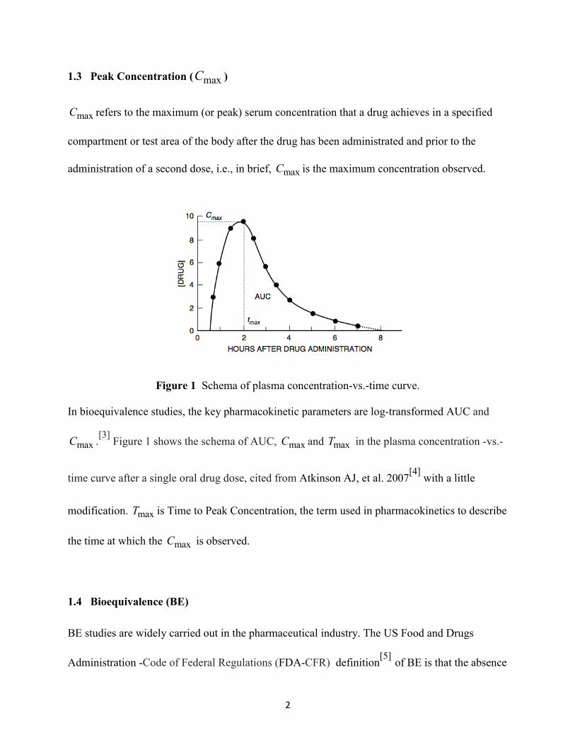
1.3 Peak Concentration ( maxC )

maxC refers to the maximum (or peak) serum concentration that a drug achieves in a specified

compartment or test area of the body after the drug has been administrated and prior to the

administration of a second dose, i.e., in brief, maxC is the maximum concentration observed.

Figure 1 Schema of plasma concentration-vs.-time curve.

In bioequivalence studies, the key pharmacokinetic parameters are log-transformed AUC and

maxC .[3] Figure 1 shows the schema of AUC, maxC and maxT in the plasma concentration -vs.-

time curve after a single oral drug dose, cited from Atkinson AJ, et al. 2007[4] with a little

modification. maxT is Time to Peak Concentration, the term used in pharmacokinetics to describe

the time at which the maxC is observed.

1.4 Bioequivalence (BE)

BE studies are widely carried out in the pharmaceutical industry. The US Food and Drugs

Administration -Code of Federal Regulations (FDA-CFR) definition[5] of BE is that the absence

3

of a significant difference in the rate and extent to which the active ingredient in pharmaceutical

equivalents or pharmaceutical alternatives becomes available at the site of drug action when

administered at the same molar dose under similar conditions in an appropriately designed study.

Although it is seen sometimes that measures used in BE study are pharmacological or clinical

end-points, the most sensitive measures used in BE studies[6] are drug concentrations in the

blood. From subject-level time and concentration data, subject-level AUC and maxC can be

estimated, which form the BE outcome data for statistical analyses. If the drugs' plasma

concentration curves are superimposable, then these drugs are considered as bioequivalent in

extent and rate of absorption.

The FDA guidelines for BE studies recommend a minimum of 12 samples collected over time

following drug administration with an additional sample prior to dosing.[2] These investigations

on BE are best made through randomized clinical trials, and BE of two drugs is assessed by

analysis of logarithmic transformed AUC and maxC typically obtained from a crossover design.

1.5 Crossover Design

Crossover Design is probably the most commonly used statistical design for comparing

bioequivalence between two formulations of a drug. We shall refer to a two-sequence, two-

period, crossover design as the standard 2×2 crossover design, also called AB|BA design.

Table 1 The standard 2×2 crossover design Crossover Designs for Two Formulations Period 1 Period 2 Sequence AB = 1 A B Sequence BA = 2 B A

A standard 2 2× crossover study will generate paired outcomes 1 2( , )Y Y in two sequences of

subjects: (a) In sequence AB subjects receive drug A in period 1 and are crossed over to drug B

4

in period 2; (b) In sequence BA subjects receive drug B in period 1 and are crossed over to drug

A in period 2, as shown in Table 1. The dosing periods are separated by a washout period of

sufficient length for the drug received in the first period to be completely metabolized or

excreted from the body. Now, let's discuss here treatment effect, period effect and carry-over

effect.

1.5.1 Treatment Effect. The objective of a cross-over trial is to focus attention on within-

patient treatment differences, the difference between different measurements in the same subject,

also called within-subject difference. The difference between these measurements removes any

component that is related to the differences between the subjects, which is called ‘subject-effect’,

from the comparison.

1.5.2 Period Effect. The within-subject difference could also be thought of as a comparison

between the two treatment periods, which is the reason why usually one group of subjects

received the treatments in the order AB and the other group received the treatments in the order

BA.

1.5.3 Carryover Effect. A carryover effect is defined as effect of the treatment from the

previous time period on the response at the current time period. The presence of carryover is an

empirical matter.[7] It depends on the design, the setting, the treatment, and the response. The

washout periods are usually included in the design, to allow the active effects of a treatment

given in one period to be washed out of the body before each subject begins the next period of

treatment. The disadvantage of the 2 2× crossover trial is that several important effects, such as

5

carryover effect and interaction effect are aliased with each other. Therefore, the carryover effect

cannot be removed just by randomization alone in 2 2× crossover design. Washout period has to

be clarified, usually 5 Half-life time ( 1/2 T ) is necessary.

The objective of crossover design is to estimate the treatment effect, the expected difference in

mean of logarithm transformed AUC and maxC of drug A versus drug B obtained from each

subject. In each sequence, Treatment A and Treatment B produce a difference measure, provided

that the period effect can be assumed to be constant, the information from both sequences can be

combined to obtain the estimate of expected difference. Since the difference measure is within

one subject, the difference removes any ‘subject-effect’ from the comparison.

1.6 Statistical Model

Consider a statistical model without considering carryover effect used by Byron Jones and

Michael G. Kenward.[7] Let ijkY =response in k-th patient, in j-th period for i-th treatment. There

is implied ‘nesting’ of treatment in period.

The model is:

ijk i j k ijkY µ τ π α ε= + + + + (1)

where

µ is effect of an overall mean;

iτ is effect of i-th treatment effect, i=1, 2, ..., t;

jπ is effect of the j-th period effect, k=1, 2, ..., p;

kα is random effect associated with the k-th subject.

6

ijkε is random error associated with the k-th subject who received the i-th treatment in the j-th

period, k=1, 2, ..., ni.

( )2~ 0,k N αα σ , 2~ (0, )ijk N εε α , kα and ijkε are independent.

( ) ( ) 2 2 2 ijk k ijkVar Y Var α εα ε σ α σ= + = + = , and 2, ' )( ijk ij kCov Y Y ασ= for all j j≠ ′ .

In this random subject-effects model, 2ασ is the inter-subject variability and 2

εα is the within-

subject variability.

In Table 2, there are only four sample means 11 12 21., ., .,y y y and 22.y . 11y ⋅ represents the mean

of samples of treatment 1 and period 1, ..., 21.y represents the mean of samples of treatment 2

and period 1; Table 3 lists the mean of treatment and period, period effect and treatment effect

with regard to this 2 2× crossover design.

Table 2 Expected Cell Means for Model (1) Sequence Period

1 2 1 11 1 1.y µ τ π= + + 22 2 2.y µ τ π= + + 2 21 2 1.y µ τ π= + + 12 1 2.y µ τ π= + +

Table 3 Expected Means and Effects for Model (1)

Mean of Treatment A 11 12 1 1 2½( . .)= ½ ½y y µ τ π π+ + + +

Mean of Treatment B 21 22 2 1 2½( . .)= ½ ½y y µ τ π π+ + + +

Mean of Period 1 11 21 1 1 2½( . .) ½ ½y y µ π τ τ+ = + + +

Mean of Period 2 12 22 2 1 2½( . .) ½ ½y y µ π τ τ+ = + + +

Treatment (A-B) Effect 1 2τ τ−

Period (1-2) Effect 1 2π π−

7

It is known from empirical studies that after logarithmic transformation, AUC and maxC are

normally distributed or may be assumed to be approximately normally distributed. The core

modeling component of SAS proc GLIMMIX can be illustrated for both fixed and random

subject-effects models.[7] Suppose there are variates including subject, period, direct treatment

and response variables in the dataset, model fitting and inference for fixed subject-effect models

follow conventional ordinary least squares (OLS) procedures and for random subject-effect

models Restricted Maximum Likelihood (REML) analyzes are used.[7]

The benefit of crossover design is that each subject serves as their own control, and statistical

efficiencies are gained with respect to power and precision. Although crossover design has great

advantages, it also brings a potential disadvantage: (1) Carryover may be confounded with direct

treatment effects. (2) There are at least 2 periods, patients may withdraw from the trial, or

become "lost to follow-up".

Special consideration is needed while doing statistical analysis for the crossover design. The

typical method of Null Hypothesis Significance Testing (NHST) is designed to assess the

evidence against the null hypothesis. The null hypothesis is rejected if the observed p-value is

less than the stated significance level α; if not rejected, the null hypothesis will be retained.

However, equivalence is not concluded just because we do not reject null. Here, the Two One-

Sided Tests (TOST) is applied to assessing bioequivalence.

1.7 Average Bioequivalence (ABE)

ABE is a conventional method for the BE study, which solely compares the population averages

of a BE measure of interest but not the variances of the measures for the T and R products,

8

following the FDA 1992 guidance on Statistical Procedures for Bioequivalence Studies.[3][8]

TOST has been used to determine whether the ratio of the logarithm transformed averages of the

measures for the test and reference products were comparable.[9]

The two null hypotheses of TOST: (1) the mean difference is larger than the upper value of the

BE limit ∆; and (2) the mean difference is below the lower bound of the BE limit -∆, versus the

alternative hypothesis of the difference falls within the range of the BE limit.

where T is Test, and R is Reference.

BE is established at significance level of α if a t-interval of confidence ( )1 2 100%α− × is

contained in the interval ( , )−∆ ∆ , which is called Westlake’s Confidence Interval.[10] Therefore,

to establish BE at significant level of 0.05α = , a 90% confidence interval should fall within the

BE limit ( , )−∆ ∆ . For PK measures after logarithmic transformation, ln 1.25∆ = , ln 1.25−∆ = −

,[3] while for PK measures without logarithmic transformation, the BE limit is a little different. For the case of no logarithmic transformation, let T R/D µ µ= be the ratio of the averages of the

measures for the Test and Reference products.

01 T 02: / , : / : / µ µ ε µ µ ε ε µ µ ε≥ ≤ < <R U T R L a L T R UH H H

4 / 5 0.8Lε = = , and 5 / 4 1.25Uε = = on /µ µ= T RD that define the region of equivalence.[3]

To establish BE at significant level of 0.05α = , a 90% confidence interval should fall within the

BE limit ( , )ε εL U .

01 02: , :T R T RH Hµ µ µ µ− ≥ ∆ − ≤ −∆ :a T RH µ µ−∆ < − < ∆

9

ABE only compares the population averages of a BE measure, assesses no comparison between

variances of the measure for T and R products, therefore, there are some limitations on ABE.

FDA (2001)[3] recommends Population Bioequivalence (PBE) and Individual Bioequivalence

(IBE), which include comparisons of both averages and variances of the measure. In Table 4, the

evaluation criteria are listed for ABE, PBE and IBE.

Table 4 Bioequivalence Types and Evaluation Criteria Bioequivalence/Parameters Evaluation Criteria ABE Population averages( T R;µ µ )

2 2T R( ) Aµ µ θ− ≤

PBE Population averages ( T R;µ µ )

Total variances ( 2 2;TT TRσ σ )

2 2 2 2 T R P[( ) ( )] /TT TR TRµ µ σ σ σ θ− + − ≤ or

2 2 2 2 T R 0 P[( ) ( )] /TT TR Tµ µ σ σ σ θ− + − ≤

IBE Population averages ( T R;µ µ )

Intra-subject variances ( 2 2 ,WT WRσ σ ) Subject-by-formulation interaction variance ( 2

Dσ )

2 2 2 2 2 T R I[( ) ( )] /D WT WR WRµ µ σ σ σ σ θ− + + − ≤

or 2 2 2 2 2

T R 0 I[( ) ( )] /D WT WR Wµ µ σ σ σ σ θ− + + − ≤

, ,A P Iθ θ θ : specified bounds by the FDA; 20 Tσ , 2

0Wσ :specified threshold value by the FDA.

1.8 Population Bioequivalence (PBE)

PBE approach uses both the mean and the variance of log(AUC) and maxlog(C ) , to assess total

variability of the measure in the population.[3][11]

For PBE, the parameter of interest is:

2 2 2

2

2 2 2

20

( )

( )

T R TT TR

TRPBE

T R TT TR

T

µ µ σ σσ

µ µ σ σσ

− + −

Θ = − + −

when 2 20TR Tσ σ> (Reference-scaled criterion)

when 2 20TR Tσ σ≤ (Constant-scaled criterion)

10

In the equation, T Rµ µ− is still the mean difference between the test and reference. 2TTσ is the

total variance of test, and 2TRσ is the total variance of reference. 2

0 Tσ is the FDA specified

threshold value, currently the values recommended by the FDA is 20 0.04Tσ = .[11] When the

total variance of Reference 2TRσ is greater than the FDA specified threshold value 2

0 Tσ ,

Reference-scaled criterion is to be applied. Otherwise, Constant-scaled criterion is to be used.

Currently FDA recommended value for Pθ is 1.7448,[11] if PBE pθΘ < , and ABE is concluded,

then PBE is also concluded.

1.9 Individual Bioequivalence (IBE)

IBE approach uses the means and variances of T and R, and the subject-by-formulation

interaction to assess within-subject variability for the T and R products, as well as the subject-by-

formulation interaction.

when 2 2

0WR Wσ σ> ( Reference-scaled criterion)

when 2 20WR Wσ σ≤ (Constant-scaled criterion)

Here, 2

WTσ is within-subject variance for test drug, and 2WRσ is within- subject variance for

reference drug. 2BTσ is between-subject variance for test drug, 2

BRσ is between-subject variance

for reference drug. ( )22 2 (1 )σ σ σ ρ σ σ= − + −D BT BR BT BR , assesses the subject-by-

formulation interaction. ρ is the correlation coefficient between individual average test and

reference formulation, they both contribute to the IBE determination.[3][11]

2 2 2 2

2

2 2 2 2

20

( )

( )

T R D WT WR

WRIBE

T R D WT WR

W

µ µ σ σ σσ

µ µ σ σ σσ

− + + −

Θ = − + + −

11

20Wσ is specified threshold value, currently the FDA recommended 2

0 0.04Wσ = .When the

within variance of reference 2 20 WR Wσ σ> , Reference-scaled criterion is to be applied.

Otherwise, Constant-scaled criterion is to be used. FDA recommended value for Iθ is

2.4948[11], if IBE IθΘ < , and ABE is concluded, then IBE is also concluded.

The two-period two-treatment crossover design is the simplest prototype, which is not enough

for PBE and IBE. When additional periods and/or treatments are considered, the possible

configurations would increase. Some examples of a three-period two-treatment crossover design

are (i) Sequences ABA and BAB; (ii) Sequences AAB, ABA and BAA; (iii) Sequences ABB and

BAA.[3] Just as in the AB|BA design, we note that the treatment difference can be estimated in

each period from any of these three designs. The benefit of having additional periods and/or

treatments contributes to detecting if there is carryover effect in crossover design. Moreover, the

IBE can be estimated with high order crossover design in addition to ABE and PBE.

12

CHAPTER 2 BIOEQUIVALENCE

A data set called "pkdata" from STATA documentation[12] is used here for our illustration. The

data comprises two concentrations CONCA, CONCB in the same n=16 subjects assesses at 13

time points, including t=0. At baseline the concentration is zero. Eight patients are randomly

assigned to sequence 1, which means they take the drug A in the period 1, and then take the drug

B in the period 2; the other 8 patients are assigned to sequence 2, take the drug B in the period 1,

and then take the drug A in the period 2. Assume the Drug B is the reference drug (R), and Drug

A is the test drug (T). We will calculate AUC and maxC by Non Compartmental Analysis

approach. Take the logarithmic transformation of AUC and maxC as the variables for the ABE

study.

2.1 ABE

Consider the parameter AUC. Let BRµ µ= be the reference group population mean, T Aµ µ=

be the test group population mean. Let D T Rµ µ µ= − be the treatment difference, ln1.25−∆ = −

be the lower bound, and ln1.25∆ = (=0.2231) be the upper bounds on D T Rµ µ µ= − that define

the region of equivalence. ABE involves the calculation of a 90% CI for D T Rµ µ µ= − , the

difference in the means of log-transformed AUC. The ABE will be concluded based on the

calculated 90% confidence limits falling within 0.2231 0.2231T Rµ µ− ≤ − ≤ . First, the expected

cell means for ( )log AUC in Table 5 are listed following notations used in Table 2.

13

Table 5 Expected Cell Means for ( )log AUC Sequence Period

1 2 1 11. 5.0069y = 22. 4.9270y = 2 21. 5.0077y = 12. 4.8740y =

Similarly, the expected means and effects for ( )log AUC in Table 6 are listed following notations

used in Table 3.

Table 6 Expected Means and Effects for ( )log AUC Mean of Treatment T 11 12½( . .)= 4.9404+y y Mean of Treatment R 21 22½( . .)= 4.9673+y y Mean of Period 1 11 21½( . .) 5.0073y y+ = Mean of Period 2 12 22½( . .) 4.9005y y+ = Treatment (T-R) Effect -0.0269

Period (1-2) Effect 0.1067

Figure 2 Profiles over treatment A and B for ( )log AUC in two periods.

The objective of this study with cross-over design is to focus attention on within-subject

treatment differences. Figure 2 shows profiles over treatment for crossover designs. The subject-

14

profiles in Figure 2 are plotted for each sequence the change in each subject’s response over the

two treatment periods, which show no strong treatment effect or period effect.

Figure 3 Treatment A vs. B Agreement of ( )log AUC in two periods.

The treatment agreement in Figure 3 is plotted for the response associated with the second

treatment against the response associated with the first treatment. The figure indicates the

strength of the treatment effect is small, and the treatment effect A-B is negative. The spread of

points within sequence AB being wider indicates the bigger between-subject variability.

Table 7 TTEST output for ( )log AUC

Treatment Method Mean Lower Bound

90% CL Mean Upper Bound

Assessment

Diff (1-2) Pooled -0.0269 -0.2231 < -0.1462 0.0924 < 0.2231 Equivalent Diff (1-2) Satterthwaite -0.0269 -0.2231 < -0.1503 0.0965 < 0.2231 Equivalent

For crossover design, TOST option of PROC TTEST requests Schuirman’s TOST equivalence

test, with the option of specifying the equivalence bounds. After log - transformation of PK data,

given the BE limit is (-0.2231, 0.2231), the assessment of BE is finally shown in Table 7.

Exactly the same calculations can be carried out in PROC GLIMMIX with LSMEANS statement

(1) compute least squares (LS) means of fixed effects (2) compute the 90% CI for LS-mean

15

difference, and (3) see if 90% CI falls in the stated BE limits (-∆, ∆). The BE limits are (-0.2231,

0.2231) in ABE evaluation.

Table 8 GLIMMIX output for ( )log AUC

Estimates Label Estimate Standard

Error DF t Value Pr> |t| Lower Upper

T-R -0.02690 0.06774 14 -0.40 0.6973 -0.1462 0.09241 In Table 8, the PROC GLIMMIX output shows that the 90% CI (-0.1462, 0.09241) falls within

the range (-0.2231, 0.2231), the ABE is concluded for ( )log AUC at significance level 0.05α =

Table 9 Expected Cell Means for ( )maxlog C Sequence Period

1 2 1 11. 1.9763y = 22. 2.5126y = 2 21. 2.0101y = 12. 2.4469y =

Similarly, the expected cell means for ( )maxlog C in Table 9 are listed following notations used

in Table 2. ( )maxlog C of Drug T and Drug R are estimated by PROC TTEST and PROC

GLIMMIX procedures.

Table 10 Expected Means and Effects for ( )maxlog C Mean of Treatment T 11 12½( . .) = 2.2116+y y

Mean of Treatment R 21 22½( . .)= 2.2614+y y Mean of Period 1 11 21½( . .) 1.9932y y+ = Mean of Period 2 12 22½( . .) 2.4798y y+ = Treatment (T-R) Effect -0.0498

Period (1-2) Effect -0.4866

Similarly, the expected means and effects for ( )maxlog C in Table 10 are listed following

notations used in Table 3.

16

Figure 4 shows profiles over treatment for crossover designs. The subject-profiles in Figure 4 are

plotted for each sequence the change in each subject’s response over the two treatment periods,

which show no strong treatment effect but maybe a period effect.

Figure 4 Profiles over treatment A and B for ( )maxlog C in two periods.

Figure 5 Treatment A vs. B Agreement of ( )maxlog C in two periods.

The treatment agreement in Figure 5 is plotted for the response associated with the second

treatment against the response associated with the first treatment. The figure indicates the

17

strength of the treatment effect is small, and the treatment effect of A-B is negative. Substantial

location differences between the two sequences indicate a strong period effect.

Table 11 TTEST output for ( )maxlog C

Treatment Method Mean Lower Bound

90% CL Mean Upper Bound

Assessment

Diff (1-2) Pooled -0.0498 -0.2231 < -0.1280 0.0285 < 0.2231 Equivalent Diff (1-2) Satterthwaite -0.0498 -0.2231 < -0.1285 0.0290 < 0.2231 Equivalent

For crossover design, TOST option of PROC TTEST requests Schuirman’s TOST equivalence

test, with the option of specifying the equivalence bounds. After logarithmic transformation of

PK data, given the BE limit is (-0.2231, 0.2231), the assessment of bioequivalence is finally

shown in Table 11.

Table 12 GLIMMIX output for ( )maxlog C

Estimates Label Estimate Standard

Error DF t Value Pr> |t| Lower Upper

T-R -0.04976 0.04379 14 -1.14 0.2749 -0.1269 0.02737

Similarly use PROC GLIMMIX with LSMEANS statement: (1) compute LS means of fixed

effects, (2) compute the 90% CI for LS-mean difference, and (3) see if 90% CI falls in the stated

BE limits (-∆, ∆), here the BE limits are (-0.2231, 0.2231).

In Table 12, PROC GLIMMIX output shows that the 90% CI (-0.1269, 0.02737) falls within the

range (-0.2231, 0.2231), the ABE is concluded for ( )maxlog C at significance level 0.05α = .

Therefore, summarizing the two primary response variables for BE study, ( )log AUC and

( )maxlog C , the ABE is concluded for T and R at the significance level 0.05α = .

18

2.2 Sample Size Calculation

Sample size calculation for crossover design in bioavailability and bioequivalence study is an

essential question, which establishes bioequivalence within meaningful limits in the case of

logarithm transformed AUC and maxC .[13] A minimum number of 12 evaluable subjects should

be included in any BE study according to FDA guidelines.[3]

Based on Schuirmann’s TOST procedure for interval hypothesis, use the data D T Rµ µ µ= − as

the expected mean difference after logarithmic transformation. If the 100(1-2α )% CI

( ),2 2 ,2 2ˆ ˆ ˆ ˆ,D n D nt tα αµ σ µ σ− −− ⋅ + ⋅ of the mean µD is entirely within the BE limit (-ln1.25,

ln1.25), then 0H is rejected at significance level α and no drug-drug interaction is concluded;

otherwise, 0H fails to be rejected.

The type-I error α of the TOST procedure is often set as 5%.Total number of subjects should

provide adequate power for BE demonstration, and the adequate power means at least 80%

power to detect a 20% difference in products’ BE. In practice the power usually is about 80% -

90%.

2.2.1 Formula for sample size. Let n = number of subjects required per sequence. α is the

significant level, β is the type ΙΙ error, CV = coefficient of variation, / 100%e RCV σ µ= ⋅ , δ =

the BE limit, ∇ is the expected difference compared to expected mean of Reference ,

100T R

R

µ µµ−

∇ = ⋅ ; σ̂ is the intra-subject standard deviation. Assuming a normal distribution of

logarithm transformed PK data (AUC, maxC ), for 0∇ = , n can be estimated[13][14] by

19

2 2,2 2 /2,2 2 ˆ2[ ] [ / ]n nn t tα β σ δ− −≥ +

The approximate sample size calculation for the TOST tests for ∇ > 0, the equation is:

2 2,2 2 ,2 2 ˆ2[ ] [ / ( )]α β σ δ− −≥ + −∇n nn t t

The n on the right hand side is unknown (in the degrees of freedom). Start with an initial value

n0, the n1 is calculated. The calculation is iterative until n is almost unchangeable.

As an illustration, consider the STATA dataset described at the beginning of this chapter.

Let α =0.05, β =0.2; For ( )log AUC , 0.2231δ = , σ̂ =0.1355, use the initial value 0 8n =

2 2/2 2 22 2

[ (2 2) (2 2)] [1.761 1.345]ˆ2 2 0.1355 80.2231

t n t nn α β σ

δ

− + − +≥ ≥ ≅

So n per group = 8, and total n = 16.

The n per group =8 is also estimated from PROC POWER. The example is for ABE study. The

number of subjects for PBE or IBE studies can be estimated by simulation according to the FDA

guideline,[3] which will not be discussed here.

20

CHAPTER 3 AUC ESTIMATION

There are two representative examples of one compartmental pharmacokinetic models:[15][16]

(A) One compartmental model with i.v. administration; (B) One compartmental model with

extravascular administration.

One compartmental model with i.v. dosing means administering a dose of drug over a very short

time period, there is no absorption rate constant ( ak ) considered. A one compartmental model

with extravascular administration means absorption phase is involved in the whole process. As

shown in Chapter 1, the maxC and maxT are simple measures for summarizing the absorption

process. In one compartment model, assessment of maxT depends on the value of both

elimination rate constant ( ek ) and absorption rate constant ( ak ).

( )max

log /a e

a e

k kT

k k=

−.

Let us look into the concepts of ek and ak , and how they appear in a pharmacokinetic model.

3.1 Definition of PK Parameters

3.1.1 Elimination Rate Constant ( ek , units are h-1) describes the rate of decrease in

concentration per unit time, usually the time unit is hour. It is estimated from the log-linear

terminal part of the concentration-time curve, ek slope= − .

3.1.2 Absorption Rate Constant ( ak , units are h-1) is the rate of absorption of a drug absorbed

from its site of application according to assumption of first-order kinetics, which is for a drug

21

administered by a route (for example, oral) other than the intravenous. The first-order differential

equation that governs the drug amount remained ( )X t : ( ) ( )adX t k X t

dt= − . (0)D X= is the actual

dose (mg) that is available to the body for kinetics, whereas the oral dose is given in mg/kg.

Next we define the four most useful PK parameters characterizing the in vivo disposition of a

drug.[15][16]

3.1.3 Half-life ( 1/2T ) is given by ( )1/2 log 2 / keT = , that is, the time from maxT to reach one-

half of the maximum concentration maxC .

3.1.4 Bioavailability (F , has no unit) is described as the fraction of the extravascular dose of

the administered drug that reaches the absorption depot. If the drug is injected intravenously, it is

assumed that bioavailability F =100%. Bioavailability generally decreases when a medication is

administered via other routes (such as orally), such as oral iv

iv oral

AUC DoseF

AUC Dose×

=×

, F is often

measured by quantifying the "AUC".

3.1.5 Volume of Distribution (V , the units of volume, e.g., L) or apparent volume of

distribution is a pharmacological, theoretical volume that the total amount of administered drug

would have to occupy (if it were uniformly distributed), to provide the same concentration as it

currently is in blood plasma. There are two quantities: the concentration ( )C t in plasma and the

amount of drug ( )X t in tissue. It is assumed that ( ) / ( )X t C t V= is constant.

22

3.1.6 Clearance (CL , the units are volume per time, e.g., L/hr) is called the drug clearance rate,

can be defined as the volume of plasma which is completely cleared of drug per unit time. CL is

calculated using the dose administered divided by the subsequent measured AUC,

( ) (0) e

Oral dose F XCL V kAUC AUC

×= = = × , where F is the bioavailability. Unless we have

information on F, the parameter CL/F is only identified, this is called the apparent clearance.

With the drug plasma concentration-time profile, AUC can be estimated by NCA, and also by

compartmental modeling analysis.

3.2 Non-Compartmental Analysis (NCA)

Based on the theory of statistical moments, the moments of a function are used in the analysis of

pharmacokinetic data.[17] Suppose drug concentration ( )C t is a real-valued function defined on

the interval [0, ∞); the zeroth moment of ( )C t is 0S : 0 0( )S C t dt AUC

∞= =∫ , “the area under the

curve from time zero to infinity”; and the first moment of ( )C t is 1S : 1 0( )S t C t dt AUMC

∞= ⋅ =∫

, “the area under the first moment curve”, is the area under the curve of concentration-time

versus time curve from time zero to infinity, AUMC can be used to estimate some other PK

parameters.

Non-compartmental Analysis estimate AUC using the trapezoidal rule without making any

assumption concerning the number of compartments. Following the trapezoidal rule,

concentration-time curve is considered as a series of trapezoids and the AUC estimate is the total

area of all the trapezoids.

23

For non-compartment model, (0 ) tAUC − is AUC from 0 h to the last quantifiable concentration

to be calculated; (0 ) (0 ) ( )t tAUC AUC AUC−∞ − −∞= + , represents the total drug exposure over

time. (0 )AUC −∞ requires extrapolation of the elimination-phase curve beyond the last measurable

plasma concentration. The extrapolation of AUC from t to infinity requires several assumptions:

(1) At low concentrations, drug usually declines in mono exponential fashion; (2) The terminal

elimination rate constant does not change over time or with different concentrations of

circulating drug; (3) other processes such as absorption and distribution do not play a significant

role in the terminal phase of the pharmacokinetic profile. These assumptions usually are valid in

almost all PK applications. Therefore, (0 )AUC −∞ can be calculated as

(0 ) (0 ) C /t last eAUC AUC k−∞ −= + , where lastC is the last observed quantifiable concentration

and ek is the terminal phase rate constant, ek slope= − (units: h-1). When a regression line is

fitted to terminal phase data points on log-scale, then elimination half-life 1/2 log(2) / eT k= can

be estimated. With NCA, the observed maxC and maxT are obtained directly from the data

without interpolation.

Non-compartmental analysis allows a simple estimation of AUC. It basically summarizes the

concentration-time profile without modeling assumptions. However, non-compartmental

methods are unable to visualize or predict plasma concentration‐ time profile for other dosing

regimens. It assumes the kinetics to be linear and stationary (i.e., time‐independent) for simple

applications. In more sophisticated analyses of PK data, the one compartment model or multi-

compartment analysis with nonlinear mixed effects models (NLMEM) are increasingly used in

drug development.[18]

24

We will use the widely cited example of drug theophylline,[19][20][21] which has serum

concentrations measured at 11 time points over a 25 hour period in 12 subjects to illustrate the

NCA method and compare the results with that of a one compartment model.

3.3 One Compartment Model

Compartmental modeling in pharmacokinetics estimate the concentration- time curve using

kinetic models that depend on the rate of drug distribution to the different parts of the body.[15]

In a one compartment model, the drug is considered to be distributed instantaneously into all

parts of the body. The simplest case, if i.v. drug is received, it instantaneously equilibrates within

the compartment and is eliminated at a constant rate ek . For a concentration measure ( )C t , first-

order kinetics is assumed: ( ) ( )edC t k C t

dt= − where 0ek > is the elimination rate constant. We

get ( ) (0)exp( )eC t C k t= − where C(0) is the initial concentration. The elimination rate is h-1, per

hour. (0) (0) /C X V= is the initial amount of dose in mg per unit volume in L, where V is the

volume distribution.

Figure 6 One compartmental model with i.v. administration.

i.v. ek Central Compartment

25

Figure 7 One compartmental model with extravascular administration.

For extravascular (such as oral) administration, the body receives the drug and is absorbed at

constant rate ak proportional to the amount of drug available for absorption. The drug

instantaneously equilibrates within the compartment and is eliminated at a constant rate ek . The

first-order differential equations that govern the amounts 1( )X t : 11

( ) ( )adX t k X t

dt= − , and 2( )X t :

21 2

( ) ( ) ( )a edX t k X t k X t

dt= − .The initial amounts are 1(0)X D= and 2(0) 0X = ; at time t, the

drug amount in the absorption depot is: 1 1( ) (0)exp( )aX t X k t= − , as shown in Figure 6; and the

drug amount in the central compartment is ( )12

(0)( ) exp( ) exp( )a

e aa e

k XX t k t k t

k k= − − −

−, as shown

in Figure 7. Note that this equation makes sense only when a ek k> . The focus is on the equation

of central compartment, which can be expressed as the concentration equation:

( )( ) exp( ) exp( )( )

ae a

a e

k DC t k t k t

V k k= − − −

−.

From the equations /ek CL V= and (0) ( )X Oral dose F= × , an operational expression of drug

concentration in the central compartment at time t is

( )( )( ) exp( ) exp( )

( )a e

e aa e

k k oral dose FC t k t k t

CL k k×

= − − −−

.

input ak ek Absorption depot, 1( )X t

Central compartment,

2( )X t

26

The unknown parameters are ,ak ,ek CL that must be estimated from observed concentrations

{ ( ) : 0,1, , }C t t m= … in individuals over a grid of time points.

3.3.1 AUC estimation. From the equation of the drug concentration, the AUC is defined as

0( )AUC C t dt

∞= ∫ and also denoted by (0 )AUC −∞ . From the formula for ( )C t we get

( )0

( ) exp( ) exp( )( )

( ) 1 1 ( ) .( )

a ee a

a e

a e

a e e a

k k oral dose FAUC k t k t dtCL k k

k k oral dose F oral dose FCL k k k k CL

∞×= − − −

−

× ×= − = −

∫

Only if the underlying pharmacokinetic model is identified, can the parameters be accurately

estimated, otherwise this method of estimation is not to be recommended.[22]

3.3.2 maxT and maxC estimation.. Since maxT is the time to maximum concentration we

obtain the maximum value of ( )C t by solving ( ) 0dC tdt

= and showing that the unique solution is

indeed the maximum value.

( )( )( ) exp( ) exp( )( )

a ee e a a

a e

k k oral dose FdC t k k t k k tdt CL k k

×= − − + −

−.

The derivative is a continuous function; at t=0 it is positive; as t → +∞, the derivative approaches

zero. When a ek k> , the solution maxT is given by ( )

maxlog /a e

a e

k kT

k k=

−.

To obtain maxC :

27

( )max max max( )

( ) exp( ) exp( )( )

a ee a

a e

k k oral dose FC T k T k T

CL k k×

= − − −−

.

Although we defined 0

( )AUC C t dt∞

= ∫ , another quantity of interest is

maxmax

( )(0, ) 0TAUC C t dtT = ∫ .

Using the formula maxmax0

1 exp( )exp( )T a

aa

k Tk t dt

k− −

− =∫ and repeating the previous calculation

gives

( )max(0, )max 0

max max

max

( )exp( ) exp( )

( )

( ) exp( ) exp( )1 1( )

( ) exp( ) exp( )( )

Ta eT e a

a e

a e e a

a e e a e a

a e e

a e e

k k oral dose FAUC k t k t dt

CL k k

k k oral dose F k T k TCL k k k k k k

k k oral dose F k Toral dose FCL CL k k k

×= − − −

−

× − −= − − − −

× −×= − −

−

∫

max( )a

a

k Tk

−

The first term on the right hand side is (0, )AUC ∞ that was calculated previously.

3.3.3 1/2T (half life) estimation. The half-life 1/2T is the time from maxT to reach one-half of

the maximum concentration maxC . Initially at t=0 the concentration is zero. With the passage of

time the concentration ( )C t increases to a peak maxC at time maxT and then ( )C t declines to

zero asymptotically.

The relationship between elimination rate constant ( ek ) and half-life ( 1/2T ) is:

1/2

log 2ek

t= .

The half-life ( 1/2T ) is determined by clearance ( CL ) and volume of distribution (V):

28

1/2log 2 VT

CL×

= .

An objective of PK studies is to obtain estimates of parameters from observations of

concentrations { ( ) : 0,1, , }C t t m= … in individuals over a grid of time points. The

parameterization may allow for some parameters to be individual-specific which makes them

random effects instead of pure constants.

3.3.4 Application. Take the widely cited example of drug theophylline,[19][20][21] serum

concentrations measured at 11 time points over a 25 hour period in 12 subjects. First the NCA

method is used to estimate the PK parameters, comparing the results from the one compartment

model. As described above, the one compartment model is used to estimate the PK parameters,

and then estimates of AUC, maxC and maxT are derived from the formulas. Among the benefits

of the one compartment model analysis is that the PK parameters are estimated together with

their standard errors and 95% confidence intervals. In addition individual (subject-specific)

prediction of drug concentration can be made.

3.3.5 Model for ( )C t . Assume normal distribution for ( )C t given ( , , )a ek k CL . The parameters

( , )ak CL are subject-specific, i.e., random effects, but ek is a fixed parameter. All parameters

are transformed to their logged form: ( )alog k , ( )elog k and ( )log CL ;and the random effects

are jointly normal and independent of the error term in ( )C t .

Therefore, formally the model is described by the equation (for one subject)

( )( )( ) exp( ) exp( ) ( )( )

ε×

= − − − +−

a ee a

a e

k k oral dose FC t k t k t tCL k k

29

where

(i) the error term(s) ( )ε t are serially independent (within subject), normally distributed, mean

zero and variance 2εσ .

(ii) 1 1( ) ,CLl g bo β= + ( ) 2 2 ,a blog k β= + ( ) 3,elog k β= with 1β , 2β , 3β as fixed parameters,

1,b 2b as subject-specific random effects — means 0, covariance matrix Σ (3-parameters

2 21 2 12, ,σ σ σ ).

(iii) 1 2( , )b b independent of the error term.

Across subjects independence is assumed. Hence we can construct a joint likelihood for the

sample data { ( ) : 0 ,1 }τ≤ ≤ ≤ ≤iC t t i n for the n=12 subjects with 11 concentrations assessed at

the same grid of time points from (0, 25hr).

Maximum likelihood estimation (MLE) provides estimates of all model parameters and their

covariance matrix. There are 7 parameters: 1β , 2β , 3β , 21 ,σ 2

2 ,σ 12σ , 2εσ .The formulas for

AUC, maxC and maxT for the compartment model now give their estimates. Because ( , )ak CL

is individual-specific, we will get individual- specific estimates for the PK parameters. The

additional big advantage of the compartment model is the calculation of standard errors of these

estimates.

Table 13 shows the 0 infAUC − calculation by NCA approach, and AUC estimates by

compartment model. It shows the values estimated by these two approaches are very similar

except subject 1 and subject 10.

30

Table 13 Comparison of AUC by NCA and compartment model based estimates

NCA Compartment model based estimates

Obs subject 0 infAUC − AUC Stderr AUC

Lower 95% CI

Upper 95% CI

1 1 270.004 144.816 7.00102 129.217 160.416 2 2 95.050 110.005 5.87935 96.905 123.105 3 3 107.599 111.415 5.95405 98.148 124.681 4 4 121.926 118.535 6.25209 104.604 132.465 5 5 146.878 137.689 6.62215 122.934 152.444 6 6 87.877 87.023 5.54399 74.670 99.376 7 7 115.931 106.554 6.28655 92.547 120.561 8 8 104.732 102.774 5.87002 89.695 115.853 9 9 96.641 95.818 5.34297 83.914 107.723

10 10 207.536 154.629 7.40864 138.122 171.137 11 11 85.472 96.932 5.54048 84.587 109.277 12 12 126.815 141.073 6.77517 125.977 156.169

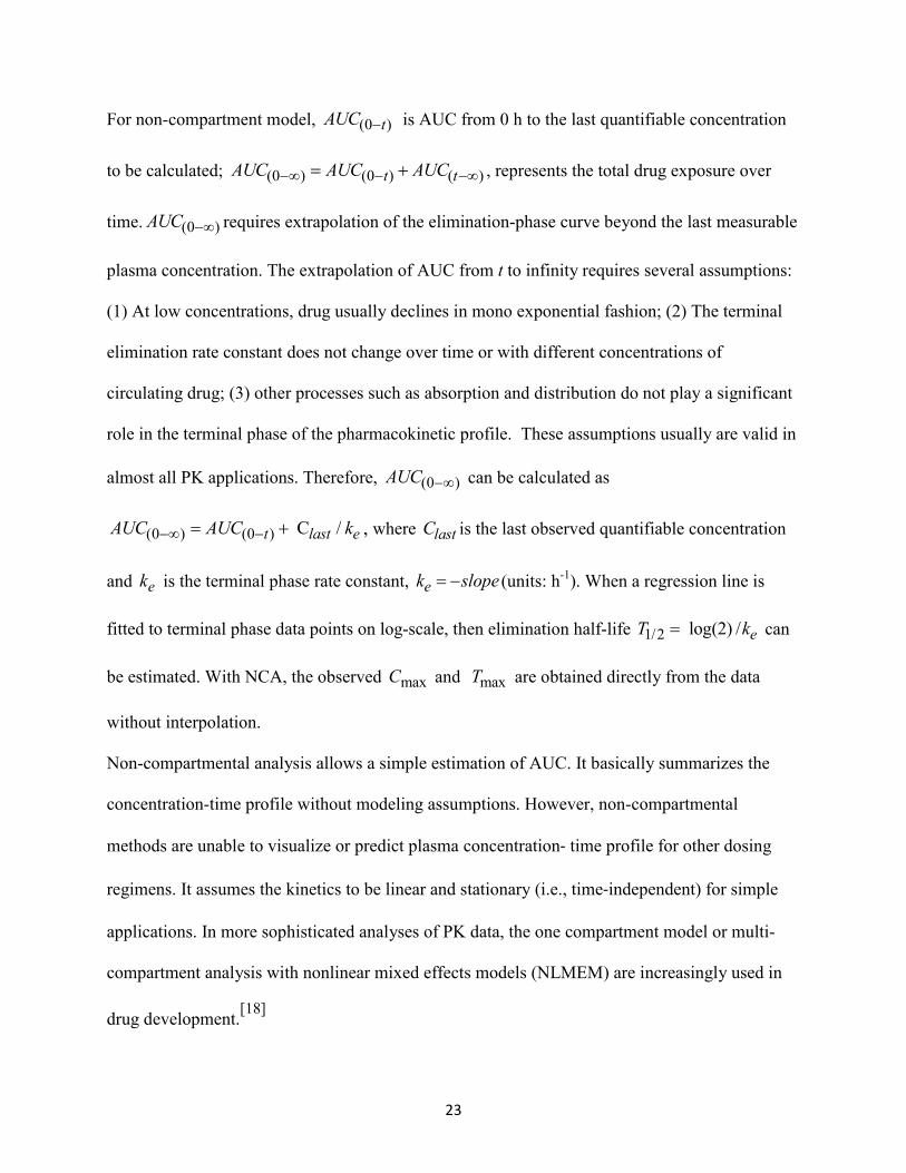
Figure 8 Individual concentration profiles by NCA.

Figure 8 shows individual concentration profiles by NCA, AUC of subject 1 and subject10by

NCA are higher than AUC of most subjects. Higher lastC of these 2 subjects explains the higher

AUC by NCA, and furthermore, explains the discrepancy of AUC by NCA and compartment

model analysis.

AUC=270

AUC=207

31

Table 14 Comparison of maxC by NCA and compartment model based estimates NCA Compartment model based estimates

Obs subject maxC maxC Stderr maxC

Lower 95% CI

Upper 95% CI

1 1 10.50 10.3420 0.33180 9.60273 11.0813 2 2 8.33 8.2205 0.32169 7.50370 8.9372 3 3 8.20 8.3918 0.32066 7.67732 9.1063 4 4 8.60 8.2855 0.31677 7.57966 8.9913 5 5 11.40 9.8981 0.32666 9.17026 10.6259 6 6 6.44 6.1226 0.30897 5.43414 6.8110 7 7 7.09 6.9453 0.31625 6.24068 7.6500 8 8 7.56 7.3470 0.31939 6.63534 8.0586 9 9 9.03 7.7379 0.31140 7.04408 8.4318

10 10 10.21 9.7244 0.31813 9.01554 10.4332 11 11 8.00 7.5903 0.32118 6.87468 8.3060 12 12 9.75 9.5540 0.32690 8.82562 10.2824

Table 15 Comparison of maxT by NCA and compartment model based estimates

NCA Compartment model based estimates

Obs subject maxT maxT StderrmaxT

Lower 95% CI

Upper 95% CI

1 1 1.12 2.10624 0.18124 1.70241 2.51008 2 2 1.92 1.57581 0.16126 1.21650 1.93511 3 3 1.02 1.48354 0.17806 1.08680 1.88028 4 4 1.07 2.35712 0.21209 1.88455 2.82969 5 5 1.00 2.02911 0.15872 1.67545 2.38277 6 6 1.15 2.28098 0.27775 1.66212 2.89984 7 7 3.48 3.17439 0.32442 2.45154 3.89723 8 8 2.02 2.09445 0.22878 1.58470 2.60420 9 9 0.63 0.66861 0.13729 0.36270 0.97452

10 10 3.55 3.59319 0.26621 3.00003 4.18634 11 11 0.98 1.02902 0.15033 0.69407 1.36397 12 12 3.52 2.72684 0.20907 2.26101 3.19268

Similarly, the maxC and maxT estimates by NCA approach and compartment model are shown in

Table 14 and 15. It indicates the values estimated by these two approaches are very similar.

Our analysis shows the benefits of parameter estimation and subsequent statistical inference with

an appropriate compartmental model, even though the model fitting could be a little complicated.

32

This pharmacokinetic model is well identified; the parameters can be accurately estimated. If it

failed AUC estimation is recommended by NCA.[22] Failure to fit a compartment model to a

given data set could be due to many factors. As seen the statistical model is highly non-linear,

introduction of too many random effects can be problematic if the data set cannot support a

complex structure. A good approach would start with a ‘fixed’ parameters model to obtain initial

parameter values for building a more complex model. A few attempts might be needed before a

stable model can be obtained.

Extension beyond a one compartment model is possible. Two-compartment models view the

body as a central compartment that receives the drug with transfer from the central compartment

to a peripheral blood compartment that absorbs the drug. Transfer in the opposite direction from

peripheral to central is also possible. Elimination occurs from the central compartment.

33

CHAPTER 4 DISCUSSION

The objective of this thesis is to review the standard approaches to statistical analyses of

pharmacokinetic (PK) data. It covers estimation of Area Under the Curve (AUC), Peak

Concentration ( maxC ) and other PK parameters and how a bioequivalence (BE) study can be

conducted with crossover design. Parameters such as AUC and maxC are the key parameters in a

PK study and used for bioavailability and bioequivalence. They are identified as population

parameters and estimated from observed drug concentration-time profiles.

The assessment of AUC adopted by the Food and Drugs Administration (FDA) is the Non-

Compartmental Analysis (NCA) approach that estimates AUC using the trapezoidal rule without

making any assumption concerning the number of compartments. Following the trapezoidal rule,

concentration-time curve is considered as a series of trapezoids and the AUC estimate is the total

area of all the trapezoids. The other approach is based on compartmental models.

The one compartment model is used to estimate the PK parameters, such as Absorption Rate

Constant ( ak ), Elimination Rate Constant ( ek ) and Clearance (CL). They can be estimated from

observed concentrations { ( ) : 0,1, , }C t t m= … in individuals over a grid of time points, and then

estimates of AUC, maxC and maxT are derived from formulas. They show the benefits of

parameter estimation and subsequent statistical inference with an appropriate compartmental

model, even though the model fitting could be a little complicated. Among the benefits of the

one compartment model analysis is that the PK parameters are estimated together with their

34

standard errors and 95% confidence intervals. In addition individual (subject-specific) prediction

of drug concentration can be made. For Pharmacokinetic/Pharmacodynamic modeling, the

compartmental pharmacokinetic models are widely used, providing continuous description of the

drug concentration that can serve as the input of pharmacodynamic models.[23]

Fitting of compartmental models can be a complex and lengthy process. As seen the statistical

model is highly non-linear, introduction of too many random effects can be problematic if the

data set cannot support a complex structure. A good approach would start with a ‘fixed’

parameters model to obtain initial parameter values for building a more complex model. A few

attempts might be needed before a stable model can be obtained. If it failed AUC estimation is

recommended by NCA.[22]

The widely cited example of drug "theophylline" data[19][20][21] is used to illustrate these two

approaches. Comparison of the PK parameters by NCA and one compartmental model shows

the parameters estimated from these two methods are very close, the model is identified. Only

when the underlying pharmacokinetic model parameters are identified, can AUC be accurately

estimated, otherwise AUC estimation is recommended by the NCA.

BE studies are widely carried out in the pharmaceutical industry. For small molecule drug

products, a bioavailability and bioequivalence study are required by FDA for approval of generic

drug products, which contain the exact same active ingredient as the innovator drug. Biosimilars

are large molecule biological drug products made via living systems. As generic forms of

35

biological products instead of the classical generic drugs, biosimilars are only similar to the

reference product; with no exactly the same active ingredient as the innovator drug. The more

stringent assessment include safety, purity, and potency, to show that a follow-on biologic is not

clinically different from the reference biological product.[24]

Average bioequivalence (ABE) is based solely on the comparison of population averages but not

on the variances, while population bioequivalence (PBE) and individual bioequivalence (IBE)

approaches include comparisons of both averages and variances. For statistical analyses in a

bioequivalence study, we used the "pkdata" example with AB|BA design to illustrate how the

crossover design is applied and ABE is tested. SAS procedures PROC TTEST and PROC

GLIMMIX are applied to the logarithm-transformed AUC and maxC to estimate ABE. Available

from a public resource even though there are quality issues in this data, the "pkdata" example is

the reasonable example of data with blood concentration time profiles, from which we can

estimate AUC and maxC , the two key parameters to compare in the BE study.

The deficit of the data for BE study includes: (1) For a AB/BA design, since there are only 4

combinations of periods and treatments, the period effect in this particular parameterization is

aliased with the carryover effect.[25] Our results show that there is period effect when comparing

maxlog( )C for A and B. There is no information available if there is carryover effect, therefore,

it is not clear if the period effect is a real period effect. The purpose of this thesis is to illustrate

how a bioequivalence (BE) study can be conducted with crossover design, so we claim there is

no carryover effects. (2) For the AB/BA design, it is not well-suited for comparison of the

36

within-unit variance 2Aσ and 2

Bσ[25] in the statistical model, we have only have one common

variance 2εσ for treatment A and treatment B. Therefore, total variance of A and B cannot be

calculated. The "pkdata" example cannot be used for Population BE and individual BE study.

We will need a replicated crossover design.[3]

In recent years statisticians in the pharmaceutical industry have given attention to developing

strategies for statistical analyses for Biosimilars and Biobetters. The FDA recently (April 2015)

issued guidance on the scientific issues to be considered in demonstrating biosimilarity to a

reference product.[26] The FDA’s definition states: Biosimilar or biosimilarity means that “the

biological product is highly similar to the reference product notwithstanding minor differences in

clinically inactive components,” and that “there are no clinically meaningful differences between

the biological product and the reference product in terms of the safety, purity, and potency of the

product.”

Therefore, the role that crossover designs have in bioequivalence demonstration on a single

endpoint or outcome measures must now be expanded in ways to assess multiple endpoints and

measures. It will bring biostatisticians and methodologists in pharmacology together to craft the

statistical designs and studies for clinical evaluations that can answer these questions.

37

BIBLIOGRAPHY

38

BIBLIOGRAPHY

[1] Guidance for Industry--- Exposure-Response Relationships --- Study Design, Data Analysis, and Regulatory Applications. U.S. Department of Health and Human Services Food and Drug Administration, Center for Drug Evaluation and Research (CDER), Center for Biologics Evaluation and Research (CBER) April 2003.

[2] Guidance for Industry --- Bioavailability and Bioequivalence Studies Submitted in NDAs or INDs --- General Considerations. U.S. Department of Health and Human Services Food and Drug Administration Center for Drug Evaluation and Research (CDER) March 2014. [3] Guidance for Industry ---Statistical Approaches to Establishing Bioequivalence. U.S. Department of Health and Human Services Food and Drug Administration Center for Drug Evaluation and Research (CDER) January 2001. [4] Atkinson AJ, Abernethy DR, Daniels CE, et al. Principles of clinical pharmacology. Second edition. Academic Press, 2007. [5] FDA-CFR. Title 21---Food and Drugs chapter 1--- Food and drug administration department of health and human services Subchapter D---Drugs and human use. Part 320 Bioavailability and Bioequivalence, 2014. [6] Niazi SK. Handbook of Bioequivalence Testing. Second Edition.CRC Press 2014. [7] Jones B, Kenward MG. Design and Analysis of Cross-Over Trials. Third Edition. Chapman and Hall/CRC, 2014. [8] CENTER FOR DRUG EVALUATION AND RESEARCH --- Guidance for Industry. The FDA published Good Guidance Practices in February 1997. [9] Schuirmann DJ. A comparison of the two one-sided tests procedure and the power approach for assessing the equivalence of average bioavailability. J Pharmacokinet Biopharm. 1987; 15: 657-80. [10] Westlake WJ. Symmetrical confidence intervals for bioequivalence trials. Biometrics. 1976; 32: 741-4. [11] McNally RJ, Iyer H, Mathew T. Tests for individual and population bioequivalence based on generalized p-values. Stat Med. 2003; 22: 31-53. [12] StataCorp. Stata 14 Base Reference Manual. College Station, TX: Stata Press. Datasets for Stata Base Reference Manual, Release 14. 2015.

39

[13] Chow SC, Jen-pei Liu, JP. Design and Analysis of Bioavailability and Bioequivalence Studies. Third edition. Chapman and Hall/CRC, 2008. [14] Statistical Approaches To Establishing Bioequivalence. Appendix 1: statistical issues --- Food and Drug Administration. 2002. [15] Hedaya MA. Basic pharmacokinetics. Second edition.CRC Press, 2011.

[16] Benet LZ, Zia-Amirhosseini P. Basic principles of pharmacokinetics.ToxicolPathol.1995; 23: 115-123.

[17] Chow SC, Hsieh TC, Chi E, and Yang J.A comparison of moment-based and probability-based criteria for assessment of follow-on biologics. Journal of Biopharmaceutical Statistics. 2010; 20: 31-45. [18] Wang Z, Kim S, Quinney S, Zhou J, Li L. Non-compartment model to compartment model pharmacokinetics transformation meta-analysis – a multivariate nonlinear mixed model.BMC Systems Biology. 2010; 4: S8. [19] Pinheiro JC and Bates DM. Approximations to the Loglikelihood Function in the Nonlinear Mixed Effects Model. Journal of Computational and Graphical Statistics.1995; 4: 12-35 [20] Wolfinger RD. Fitting Nonlinear Mixed Models with the New NLMIXED Procedure. SUGI Proceedings, 1999. [21] Russek-Cohen E, Martinez MN, Nevius AB. A SAS/IML program for simulating pharmacokinetic data. Computer Methods and Programs in Biomedicine.2005; 78: 39-60. [22] Buncher CR. Statistics in the Pharmaceutical Industry. Second edition. Marcel Dekker Inc, 2006. [23] Derendorf H, Meibohm B. Modeling of pharmacokinetic/pharmacodynamic (PK/PD) relationships: concepts and perspectives. Pharm Res. 1999; 16: 176-85. [24] Chow SC, Ju C. Assessing biosimilarity and interchangeability of biosimilar products under the Biologics Price Competition and Innovation Act. Generics and Biosimilars Initiative Journal.2013; 2: 20-5.

[25] Vonesh, EF and Chinchilli, VM. Linear and Nonlinear Models for the Analysis of Repeated Measurements. First edition. Marcel Dekker Inc, 1997. [26] Scientific Considerations in Demonstrating Biosimilarity to a Reference Product Guidance for Industry. U.S. Department of Health and Human Services Food and Drug Administration Center for Drug Evaluation and Research (CDER), Center for Biologics Evaluation and Research (CBER).April 2015 Biosimilarity.