statistical approaches for classifying and defining …
TRANSCRIPT

STATISTICAL APPROACHES FOR CLASSIFYING AND DEFINING AREAS IN SOUTH AFRICA AS “URBAN” OR “RURAL” Sharthi Laldaparsad
A research report submitted to the Faculty of Science, University of the Witwatersrand,
Johannesburg, in partial fulfillment of the requirements for the degree of Master of
Science
Johannesburg, 2006

ii
DECLARATION I declare that this research report is my own, unaided work. It is being submitted for
the Degree of Master of Science in the University of the Witwatersrand, Johannesburg.
It has not been submitted before for any degree or examination in any other University.
_______________________________________
(Signature of candidate)
_______________ day of ______________________ 20_________

iii
ABSTRACT
The purpose of this research report is to utilise appropriate statistical (both non-spatial
and spatial) techniques to classify areas in the country into urban and rural. These
areas, as derived by means of each statistical method, are profiled and common
characteristics amongst them are summarised for classification and definition of urban
and rural areas. Population data for these areas were aggregated to determine the
overall urbanisation for the country.
The methodology utilised was that of supervised classification. Two sample data sets
of areas that are known with certainty to be urban or rural were derived and used
consistently throughout the study. The importance of utilising areas of known urban
and rural status was firstly to identify essential patterns or predominant characteristics
from areas that are known, and thereafter to apply similar characteristics to areas that
are not known or are ambiguous, in order to classify them as either urban or rural.
Sample 1 comprises all areas in the country with formal and informal urban
settlements, as well as formal rural areas, i.e. farms. Sample 2 is similar to sample 1,
but in addition it includes areas falling under the jurisdiction of traditional authorities,
known as tribal areas, which were classed as known rural. Non-spatial techniques,
namely linear logistic regression, classification trees and discriminant analysis, as well
as spatial techniques, namely straight-majority-rule and iterated conditional modes
(ICM), were researched, applied and analysed for both samples, for each province and
for South Africa as a whole, using the 2001 South African population census data.
Comparisons were made with the 1996 census information.
All three non-spatial statistical methods gave insight into those census variables and
their combinations that best describe the subject under research, i.e. urban and rural.
All three methods identified significant variables that clearly separate urban and rural
areas. The results of all three non-spatial statistical methods showed similarities within
each sample, but differences were noted between the two samples. All three non-
spatial statistical methods applied to sample 1 classified the majority of the tribal EAs
(Enumeration Areas) as urban, whilst the results from sample 2 are very similar to
those obtained from both censuses, since both censuses and sample 2 predefine tribal
settlements as rural.

iv
Of the two spatial statistical methodologies, ICM performed best. In general, ICM,
performed better than the non-spatial statistical methodologies. Thus for this problem,
applying the Bayesian spatial methodology does improve the classifications.
Comparing the results of the analyses across the two samples yielded the conclusion
that the various statistical methods do not impact as much on the study as the
constitution of the two samples. Thus, including tribal areas as known rural, instead of
allowing them to be classified by the statistical methodologies, has influenced the
results far more strongly than have the differences between the methodologies
themselves.

v
DEDICATION
To my ever-loving children
Mishka and Yarika Laldaparsad

vi
ACKNOWLEDGEMENTS
I wish to acknowledge the guidance received from my study leader, Professor Paul
Fatti, also the assistance received from Professor Jacky Galpin, both from the School
of Statistics and Actuarial Science and Dr. Teresa Dirsuweit from the School of
Geography, Archaeology and Environmental Studies.
My appreciation and gratitude to Statistics South Africa’s Statistician-General and
Deputy Director-Generals for this opportunity and financial assistance.
Thank you for your technical advice and support Helene, Ilse, Nick, Denzyl, Annelie,
Anné-Marie, Piet, Jean-Marie and all my other colleagues in the Geography Division of
Statistics South Africa.
Thank you to Kashmira from DataWorld for the spatial programming.
Lastly, my sincere gratitude to my husband, Rabin and children, Mishka and Yarika, for
their support and encouragement throughout this period of my studies.

vii
CONTENTS PAGE DECLARATION ...................................................................................................................... ii ABSTRACT ........................................................................................................................... iii DEDICATION ......................................................................................................................... v ACKNOWLEDGEMENTS ...................................................................................................... vi LIST OF TABLES .................................................................................................................. xi
CHAPTER 1 - Introduction and Problem Statement .................................................. 1 1.1 Introduction ............................................................................................................ 1 1.2 Objectives of the study .......................................................................................... 2 1.3 Motivation for the study ......................................................................................... 3 1.4 Background of South Africa’s spatial framework and its impact on definitions for
urban and rural ..................................................................................................... 3 1.4.1 Impact of apartheid legislature on South Africa’s urban landscape ........................ 3 1.4.2 Historical classifications of urban and rural in South Africa .................................... 6 1.5 Research methodology .......................................................................................... 7 1.6 Structure of research report ................................................................................... 9
CHAPTER 2 - Methodology and Literature Review ................................................. 11 2.1 Introduction ............................................................................................................ 11
2.1.1 Statistical methods .............................................................................................. 11 2.1.2 The geographer’s viewpoint on urban and rural classifications ............................ 12
2.2 Linear Logistic Regression .................................................................................... 14 2.2.1 Introduction .......................................................................................................... 14 2.2.2 Fitting the logistic regression model .................................................................... 14 2.2.3 Multiple logistic regression .................................................................................. 15 2.2.4 Interpreting the fit and the odds ratio ................................................................... 15
2.3 Classification Trees ............................................................................................... 17 2.3.1 Introduction .......................................................................................................... 17 2.3.2 Tree method of SAS ............................................................................................ 17 2.3.3 Splitting rules and pruning ................................................................................... 18
2.4 Discriminant Analysis ............................................................................................ 20 2.4.1 Introduction .......................................................................................................... 20 2.4.2 Allocation rules .................................................................................................... 20 2.4.3 Linear discriminant functions ............................................................................... 21
2.5 Markov Random Fields, ICM and Gibbs Sampler .................................................. 22 2.5.1 Markov random fields .......................................................................................... 22 2.5.2 Iterated Conditional Modes (ICM) ........................................................................ 25 2.5.3 Gibbs sampler ..................................................................................................... 26
2.6 The Geographer’s Viewpoint on Urban and Rural Classifications .......................... 26

viii
2.7 Chapter Summary and Conclusion ........................................................................ 31 CHAPTER 3 - Non-Spatial Data Application and Results ....................................... 33
3.1 Introduction ............................................................................................................ 33 3.2 Methodology .......................................................................................................... 33
3.2.1 Rationale for utilising areas of known urban and rural status in the study............ 33 3.2.2 Description of the two sample data sets of known urban and rural status ............ 34 3.2.3 Selecting Census 2001 variables ........................................................................ 35 3.2.4 Process Followed ................................................................................................ 37 3.2.5 Weighting the data with prior information ............................................................. 39
3.3 Results .................................................................................................................. 42 3.3.1 Results from linear logistic regression ................................................................. 42 3.3.2 Results from classification trees .......................................................................... 47 3.3.3 Results from discriminant analysis ...................................................................... 52 3.3.4 Confusion matrices .............................................................................................. 58 3.3.5 Overall results in terms of aggregated population totals ...................................... 64 3.3.6 Map analysis ....................................................................................................... 68
3.4 Chapter summary and conclusion ......................................................................... 86 CHAPTER 4 - Spatial Data Application and Results ................................................ 88
4.1 Introduction ............................................................................................................ 88 4.2 Methodology .......................................................................................................... 88
4.2.1 Straight-majority-rule ........................................................................................... 88 4.2.2 Markov Random Fields ........................................................................................ 89
4.3 Results .................................................................................................................. 91 4.3.1 Results for Straight-majority-rule ......................................................................... 91 4.3.2 Results for ICM .................................................................................................. 113
4.4 Chapter summary and conclusion ....................................................................... 130 CHAPTER 5 -Discussion, Recommendations and Conclusions .......................... 131
5.1 Introduction .......................................................................................................... 131 5.2 Discussion ........................................................................................................... 131
5.2.1 Discussion on the non-spatial statistical methods, i.e. linear logistic regression,
classification trees and discriminant analysis ................................................... 131 5.2.2 Discussion on the spatial statistical methods, i.e. straight-majority-rule and iterated
conditional modes ............................................................................................ 133 5.2.3 Discussion on both non-spatial and spatial statistical methodologies ................ 134 5.2.4 Discussion on both sample 1 and sample 2 ...................................................... 134 5.2.5 Discussion on the application and analysis per province and for South Africa as a
whole ................................................................................................................ 136 5.3 Meeting the study objectives ............................................................................... 136
ix
5.4 Utilising the results of the study ........................................................................... 137 5.5 Limitations of the study ........................................................................................ 138 5.6 Taking the study further ....................................................................................... 138 5.7 Chapter summary and conclusion ....................................................................... 139
REFERENCES ........................................................................................................... 142 APPENDICES ............................................................................................................ 145

x
LIST OF FIGURES
Figure 2.6.1: The urban system can be considered structured by several subsystems (Adapted
from Reif 1973) ...................................................................................................... 30
xi
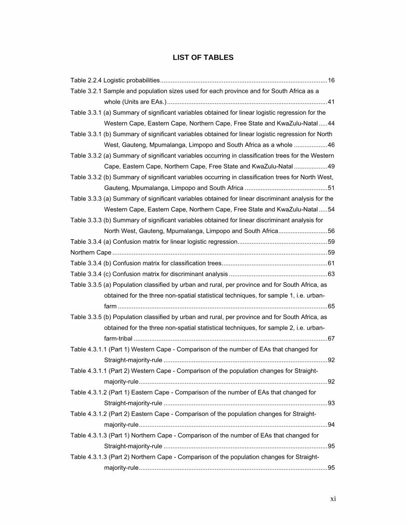
LIST OF TABLES Table 2.2.4 Logistic probabilities ............................................................................................... 16
Table 3.2.1 Sample and population sizes used for each province and for South Africa as a
whole (Units are EAs.) ........................................................................................... 41
Table 3.3.1 (a) Summary of significant variables obtained for linear logistic regression for the
Western Cape, Eastern Cape, Northern Cape, Free State and KwaZulu-Natal ..... 44
Table 3.3.1 (b) Summary of significant variables obtained for linear logistic regression for North
West, Gauteng, Mpumalanga, Limpopo and South Africa as a whole ................... 46
Table 3.3.2 (a) Summary of significant variables occurring in classification trees for the Western
Cape, Eastern Cape, Northern Cape, Free State and KwaZulu-Natal ................... 49
Table 3.3.2 (b) Summary of significant variables occurring in classification trees for North West,
Gauteng, Mpumalanga, Limpopo and South Africa ............................................... 51
Table 3.3.3 (a) Summary of significant variables obtained for linear discriminant analysis for the
Western Cape, Eastern Cape, Northern Cape, Free State and KwaZulu-Natal ..... 54
Table 3.3.3 (b) Summary of significant variables obtained for linear discriminant analysis for
North West, Gauteng, Mpumalanga, Limpopo and South Africa ............................ 56
Table 3.3.4 (a) Confusion matrix for linear logistic regression ................................................... 59
Northern Cape .......................................................................................................................... 59
Table 3.3.4 (b) Confusion matrix for classification trees ............................................................ 61
Table 3.3.4 (c) Confusion matrix for discriminant analysis ........................................................ 63
Table 3.3.5 (a) Population classified by urban and rural, per province and for South Africa, as
obtained for the three non-spatial statistical techniques, for sample 1, i.e. urban-
farm ....................................................................................................................... 65
Table 3.3.5 (b) Population classified by urban and rural, per province and for South Africa, as
obtained for the three non-spatial statistical techniques, for sample 2, i.e. urban-
farm-tribal .............................................................................................................. 67
Table 4.3.1.1 (Part 1) Western Cape - Comparison of the number of EAs that changed for
Straight-majority-rule ............................................................................................. 92
Table 4.3.1.1 (Part 2) Western Cape - Comparison of the population changes for Straight-
majority-rule ........................................................................................................... 92
Table 4.3.1.2 (Part 1) Eastern Cape - Comparison of the number of EAs that changed for
Straight-majority-rule ............................................................................................. 93
Table 4.3.1.2 (Part 2) Eastern Cape - Comparison of the population changes for Straight-
majority-rule ........................................................................................................... 94
Table 4.3.1.3 (Part 1) Northern Cape - Comparison of the number of EAs that changed for
Straight-majority-rule ............................................................................................. 95
Table 4.3.1.3 (Part 2) Northern Cape - Comparison of the population changes for Straight-
majority-rule ........................................................................................................... 95
xii
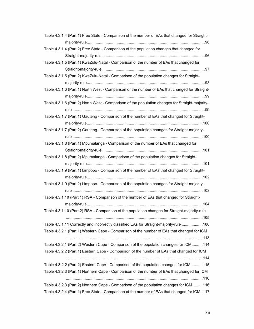
Table 4.3.1.4 (Part 1) Free State - Comparison of the number of EAs that changed for Straight-
majority-rule ........................................................................................................... 96
Table 4.3.1.4 (Part 2) Free State - Comparison of the population changes that changed for
Straight-majority-rule ............................................................................................. 96
Table 4.3.1.5 (Part 1) KwaZulu-Natal - Comparison of the number of EAs that changed for
Straight-majority-rule ............................................................................................. 97
Table 4.3.1.5 (Part 2) KwaZulu-Natal - Comparison of the population changes for Straight-
majority-rule ........................................................................................................... 98
Table 4.3.1.6 (Part 1) North West - Comparison of the number of EAs that changed for Straight-
majority-rule ........................................................................................................... 99
Table 4.3.1.6 (Part 2) North West - Comparison of the population changes for Straight-majority-
rule ........................................................................................................................ 99
Table 4.3.1.7 (Part 1) Gauteng - Comparison of the number of EAs that changed for Straight-
majority-rule ......................................................................................................... 100
Table 4.3.1.7 (Part 2) Gauteng - Comparison of the population changes for Straight-majority-
rule ...................................................................................................................... 100
Table 4.3.1.8 (Part 1) Mpumalanga - Comparison of the number of EAs that changed for
Straight-majority-rule ........................................................................................... 101
Table 4.3.1.8 (Part 2) Mpumalanga - Comparison of the population changes for Straight-
majority-rule ......................................................................................................... 101
Table 4.3.1.9 (Part 1) Limpopo - Comparison of the number of EAs that changed for Straight-
majority-rule ......................................................................................................... 102
Table 4.3.1.9 (Part 2) Limpopo - Comparison of the population changes for Straight-majority-
rule ...................................................................................................................... 103
Table 4.3.1.10 (Part 1) RSA - Comparison of the number of EAs that changed for Straight-
majority-rule ......................................................................................................... 104
Table 4.3.1.10 (Part 2) RSA - Comparison of the population changes for Straight-majority-rule
............................................................................................................................ 105
Table 4.3.1.11 Correctly and incorrectly classified EAs for Straight-majority-rule ................... 106
Table 4.3.2.1 (Part 1) Western Cape - Comparison of the number of EAs that changed for ICM
............................................................................................................................ 113
Table 4.3.2.1 (Part 2) Western Cape - Comparison of the population changes for ICM .......... 114
Table 4.3.2.2 (Part 1) Eastern Cape - Comparison of the number of EAs that changed for ICM
............................................................................................................................ 114
Table 4.3.2.2 (Part 2) Eastern Cape - Comparison of the population changes for ICM ........... 115
Table 4.3.2.3 (Part 1) Northern Cape - Comparison of the number of EAs that changed for ICM
............................................................................................................................ 116
Table 4.3.2.3 (Part 2) Northern Cape - Comparison of the population changes for ICM ......... 116
Table 4.3.2.4 (Part 1) Free State - Comparison of the number of EAs that changed for ICM .. 117

xiii
Table 4.3.2.4 (Part 2) Free State - Comparison of the population changes for ICM ............... 117
Table 4.3.2.5 (Part 1) KwaZulu-Natal - Comparison of the number of EAs that changed for ICM
............................................................................................................................ 118
Table 4.3.2.5 (Part 2) KwaZulu-Natal - Comparison of the population changes for ICM ......... 118
Table 4.3.2.6 (Part 1) North West - Comparison of the number of EAs that changed for ICM 119
Table 4.3.2.6 (Part 2) North West - Comparison of the population changes for ICM ............... 119
Table 4.3.2.7 (Part 1) Gauteng - Comparison of the number of EAs that changed for ICM ..... 120
Table 4.3.2.7 (Part 2) Gauteng - Comparison of the population changes for ICM ................... 120
Table 4.3.2.8 (Part 1) Mpumalanga - Comparison of the number of EAs that changed for ICM
............................................................................................................................ 121
Table 4.3.2.8 (Part 2) Mpumalanga - Comparison of the population changes for ICM ............ 121
Table 4.3.2.9 (Part 1) Limpopo - Comparison of the number of EAs that changed for ICM ..... 122
Table 4.3.2.9 (Part 2) Limpopo - Comparison of the population changes for ICM ................... 122
Table 4.3.2.10 (Part 1) RSA - Comparison of the number of EAs that changed for ICM ......... 123
Table 4.3.2.10 (Part 2) RSA - Comparison of the population changes for ICM ....................... 124
Table 4.3.2.11 Correctly and incorrectly classified EAs for ICM .............................................. 125
Table 5.1 (a) Summary table for sample 1: Population percentages for urban and rural for each
statistical method for each province and South Africa ......................................... 140
Table 5.1 (b) Summary table for sample 2: Population percentages for urban and rural for each
statistical method for each province and South Africa ......................................... 141

1
CHAPTER 1 - Introduction and Problem Statement
1.1 Introduction Statistics South Africa1 (Stats SA) conducts population censuses at regularly
defined intervals. This is a mammoth exercise with the aim to count all South
Africans. In order to cover the entire country in a specified period, Stats SA divides
the country into manageable units called Enumeration Areas2 (EAs). For the 2001
population census, South Africa was divided into approximately 80 000 EAs. These
EAs form the basis for dividing work by assigning an enumerator to each EA to
administer the census questionnaire. Nowadays, the EA as a unit has become
more than an administrative workload to conduct the census. Being the smallest
unit against which information is collected, the EA is aggregated to other
administrative units such as provinces, municipalities, electoral wards, etc. to
produce meaningful information for planning and decision-making.
Stats SA has for several censuses now, published data on the classification of
South Africa in terms of urban and rural or non-urban (We will use rural for ease of
writing.) The definition or classification for urban and rural came from attribute
information attached to each EA, namely the classification of EAs into EA-types.
EA-types were, and still are, based on town planning concepts such as proclaimed
town area (i.e. cadastral information). Each EA has a unique EA-type. There are
ten EA-types defined for the 2001 population census. Assigning EA-types to each
EA, can become very subjective. Based on a rule set, an operator assigns the EA-
type. Sometimes this decision is very difficult, due to the nature of the area.
Currently, in South Africa, the classification of the country into urban and rural has
changed radically due to the implementation of the new demarcation of municipal
1 Statistics South Africa (Stats SA) is a national Government department accountable to the Minister of Finance. The activities of the department are regulated by the Statistics Act (6 of 1999). Stats SA’s tasks are to coordinate, collect, process, analyse and disseminate official statistics in support of economic growth, socio-economic development and the promotion of democracy and good governance. 2 An Enumeration Area (EA) is defined as a manageable area consisting of approximately 120 households to be visited by an enumerator during the period of the census.

2
areas as defined by the Municipal Demarcation Board (MDB)3. The new
demarcation has moved away from classifying the municipality in terms of urban
and rural but rather to an all-inclusive municipality.
However, the concept of urban and rural is still in the minds of South Africans who
want to know how much of the country is urban, or how much urbanisation is taking
place as urbanisation or urban areas are most frequently associated with having
improved service delivery, more institutional facilities and infrastructure, thus better
living standards. On the other side of the coin, these areas are also associated with
higher levels of unemployment, high levels of crime, etc.
The problem, and thus the research contained in this report, is around the
classification of areas in the country into urban and rural, as well as determining
appropriate definitions for urban and rural. To elaborate further, definitions of urban
and rural have traditionally followed the aggregations of EA-types from previous
censuses to the 1996 population census. For the 2001 population census, owing to
the redemarcation of new municipal areas and the subjectiveness of the EA-types,
together with the EA-type definition, an attempt was made by Stats SA to
investigate the use of population density as a proxy for conceptually defining urban
and rural.
This research report’s main focus is to follow scientific approaches (a move away
from subjective definitions) by utilising non-spatial and spatial statistical methods to
classify and define urban and rural in South Africa.
1.2 Objectives of the study
The main objective of the study is to classify areas using appropriate statistical
methods to determine urban and rural areas in the country. These areas, as
derived by means of each statistical method, are profiled and common
characteristics amongst them are summarised for classification and for the
definitions of urban and rural areas. Population data are aggregated to determine
the overall urbanisation for the country.
3 The Municipal Demarcation Board (MDB) is responsible for the redetermination of municipal boundaries in South Africa.
3
1.3 Motivation for the study The first motivation for this study comes from the need to know by South Africans,
Government and various other planners and decision-makers, in their everyday life
and in their attempts to redress inequalities of the country’s past, just how urban (or
rural) South Africa is. In the recent 2005 budget speech by the Finance Minister,
Mr. Manuel said “this social intent also embodies our commitment to build a more
just, more equal society, in which steady progress is made in reducing the gulfs
that divide rich and poor, black and white, men and women, rural and urban”.
The second motivation comes from the need for evidence-based statistical
information required by users of official statistics. The methodological statistical
techniques that are investigated in this study and applied for defining urban and
rural, will in the first place reduce the subjectivity associated with such definitions.
The approach can be extended to various other concepts and definitions that are
needed by users of statistical data.
The third motivation comes from the approaches this study takes with respect to
definitions and classifications for official statistics. The study incorporates both non-
spatial and spatial methodologies. The study introduces new perspectives and new
ways of thinking that incorporate the spatial side to defining concepts used in
official statistics. In this way, the close links between South Africa’s spatial
frameworks and its statistics become evident.
1.4 Background of South Africa’s spatial framework and its impact on definitions for urban and rural
1.4.1 Impact of apartheid legislature on South Africa’s urban landscape Historically, South Africa’s urban and rural classification is impacted by the
country’s apartheid past. As a result of this, South Africa’s urban and rural
classifications are different from such classifications of other countries. In fact it has
resulted in characteristics that can be considered as classically South African and
not shared by other countries. Such characteristics have also emerged in the
results of this study. Smit (1979) states, “Without homeland urbanisation many
cities and towns in the White sector would have a far larger Black urban
population.”

4
SPP (1983) reports on the mass forced removals or population relocation in South
Africa since the early 1960s. These relocations were a result of farm removals,
clearance of informal areas, removals under the Group Areas Act and influx control.
Large scale removals were that of Africans. They were relocated out of cities, towns
and farming areas falling in the 87% of the country designated for white ownership
into the 13% allocated for African occupation.
Smit (1979) reported on the “suggestion that ‘rural villages’ be established for
Blacks employed in industry and other sectors, which was accepted for the first
time in 1945 by the General Council of the Ciskei and the Transkei (Rogers, 1949,
in Smit, 1979).” SPP (1983) mentions about the Bantu Authorities Act of 1951
which provided for the establishment of tribal, regional and territorial authorities.
This Act coopted tribalism and traditional institutions of Government, such as
chieftainship into the administration of apartheid. In 1959 eight national units were
demarcated under the Promotion of Bantu Self-Government Act, and the Bantustan
(or homeland or independent national states) era in South African politics was
launched.
Fair (1982) talks about the 1913 Land Act which “ … in particular sought to
underdevelop the African peasantry by inhibiting its productive capacity and by
limiting its access to land and to markets. Moreover, the Native Reserves to which
the peasantry was then largely confined, became a ‘vast reservoir of migrant
labour’ – ‘a sponge that absorbs, and returns when required, the reserve army of
African labour’ (Bundy, 1979, in Fair, 1982). Production in the reserves was
preserved at a low, mainly subsistence, level which ‘conferred direct benefits upon
urban employers – particularly in the mines in the form of low wages, cheap
housing, the avoidance of welfare considerations for workers’ dependents, and a
brake on the growth of an urban proletariat’ “ (Bundy, 1979, in Fair, 1982).
Yawitch (1982) discusses the schedule attached to the 1913 Land Act listing all
existing native reserves, locations and African-owned farms as areas that were
reserved for African land-holding only. A trust fund, administered by the South
African Native Trust, was set up to buy land, hence the term ‘trust land’. According
to Yawitch (1982) even before 1936 these areas had a substantial African

5
population, which “… included ‘black spots’, land already owned by Africans,
already carrying a huge African population.”
Yawitch (1982) talks about the betterment schemes, which can be traced to the
Glen Grey Act of 1894, “… even through betterment schemes, Government was
seeking the most convenient way in which to organise the reserves so that they
could ultimately feed themselves, govern themselves and still provide the labour
base to the functioning of the central South African economy. … Betterment had
come to actually mean control. … The South African working class was divided in a
fundamental way into an urban privileged group and a poor and unemployed rural
group. The way that the entire system of labour control operated was to export
these ‘excess’ rural people out of urban areas to places where their unemployment
and poverty was not visible. This was the main reason for the non-workability of
betterment schemes.”
“The first Black ‘town’ was laid out in the forties at Zwelitsha (in the Ciskei) near
King William’s Town where the Industrial Development Corporation established a
textile factory. At more or less the same time Temba was laid out in
Bophuthatswana to accommodate squatters from the PWV complex. … In about
1950 the notation began to gain ground that towns in the homelands ‘should not
only become dumping grounds for the surplus rural population but should also
provide accommodation for those working in adjacent White areas’ (Henning, 1969,
in Smit, 1979). Umlazi was the first Black town established in a homeland (in 1949 -
50) to alleviate the housing shortage in a large White city (Durban).” (Rogers, 1949,
in Smit, 1979)
Murray (1987) states that “what has happened, in summary, is massive
‘urbanisation’ in the Bantustans, in terms of the sheer density of population now
concentrated there. … 56% of the population of the Bantustans are now
‘urbanised’. … Some of the concentration has taken place in ‘proclaimed’ (officially
planned) towns in the Bantustans, whose population was 33 500 in 1960, 595 000
in 1970 and 1.5 million by 1981. But most of the concentration has taken place in
huge rural slums which are ‘urban’ in respect of their population densities but ‘rural’
in respect of the absence of proper urban infrastructure or services.”

6
“In the 1980s the South African Government made a number of significant
changes, both constitutionally and with respect to urban development policy. …
Another significant change in the 1980s was the abandonment of policies designed
to prevent Blacks from migrating to the towns. … Bureaucratic momentum, effective
segregation and racial discrimination are but part of the inheritance of urban
apartheid” (Christopher, 1992).
1.4.2 Historical classifications of urban and rural in South Africa The discussion that follows is intended to give some understanding of the country’s
historical classifications of urban and rural. It also provides the context with respect
to the evolution of South Africa’s spatial frameworks and space economy, and the
role it played in urban and rural areas in the country.
Davies (1967) and Davies and Cook (1968) postulated an urban hierarchy for
South Africa. The hierarchy refers to conditions in 1960. It was based on an index
method using a series of twelve index central functions, which was considered
significant for different degrees of urban importance. Data were extracted from
various sources such as government and provincial departments, commercial and
financial institutions, and newspapers, supplemented by reference to commercial
and telephone directories and by field checks. Davies (1967) describes how data
for the 601 places classified as urban in the 1960 population census was used. He
further describes “all places without an independent post office, which was the
baseline of central functions in South African towns, were excluded from the
analysis. These included places such as isolated collieries and other small mining
settlements and resorts. Punctiform settlements not listed in the 1960 census had
also been excluded. … No exact nomenclature to describe the status of urban
places had yet evolved in South Africa beyond the use of such terms as
metropolitan area, city and town in English and metropolitaanse gebied, stad, dorp
and dorpie in Afrikaans. Terms such as village, hamlet or sub-town have never
formed a part of customary usage.” Davies (1967) suggested that South African
urban areas be classified under the following eight orders of towns:
Order 1: Primate Metropolitan Area (The Witwatersrand concurbation)
Order 2: Major Metropolitan Areas (Cape Town and Durban)
Order 3: Metropolitan Areas (Pretoria, Bloemfontein, Pietermaritzburg, East
London, Kimberley)
7
Order 4: Major country towns
Order 5: Country towns
Order 6: Minor country towns
Order 7: Local service centres
Order 8: Low-order service centres
Davies (1967) then tested the validity of the classification of using the twelve index
functions against a hierarchy based upon fifty central functions. These included
aspects such as administrative, educational, financial, professional, commercial,
service industry, accommodation, social services, transport, newspaper,
entertainment and utility services. Davies and Cook (1968) concluded that there “
… is a high degree of correlation between the index hierarchy and the hierarchy
based on more comprehensive methods. This has obvious benefits in that an urban
hierarchy may be established rapidly using simple methods with a considerable
degree of reliability, and may be easily updated periodically.”
According to Fair (1982) South Africa’s spatial system then was regarded as
comprising three main elements:
The core – comprising the major metropolitan areas of the PWV, Cape Town and
Durban-Pinetown, the minor metropolitan areas of Port Elizabeth, East London,
Pietermaritzburg, Bloemfontein and Kimberley all considered together as the non-
contiguous urban core of the South African space economy
The inner periphery – comprising the rest of South Africa in White, Coloured and
Asian ownership
The outer periphery – comprising the African homelands or Black national states
1.5 Research methodology
The study also covers the geographer’s perspective with regard to classifications
and definitions for urban and rural. However, a recent trend amongst geographers
is a move away from the concept of urban and rural. This is due to the difficulty in
practically separating the two, due to movement on the ground and the existence of
rural areas within urban areas. Rather, the concept of regional geography is being
pursued again. According to Hoekveld (1990) “regional geography is about places,
which means areas; it is not about objects, which have spatial attributes.” Regional
geography refers to classes of areas with common attributes and therefore can be

8
compared to other areas in the same class. The concepts of urban and rural from
the geographer’s perspective are covered in Chapter 2.
Non-spatial and spatial statistical methodologies are investigated for solutions to
our classification problem, in particular that of supervised classifications.
Supervised classification techniques best suit this study since we want to classify
into two groups, i.e. urban and rural, using sample data sets of areas that are
known with certainty to be urban or rural. Supervised statistical techniques, i.e.
linear logistic regression, discriminant analysis and classification trees, were
applied to sample data sets of known urban and rural areas for each province and
for South Africa as a whole. The unknown areas were thereafter scored with the
results obtained from the sample. The methodology and results are presented in
Chapter 3.
While the non-spatial methodologies provide information as to how combinations of
input variables contribute to the classifications, it nevertheless also is important not
to neglect their spatial association, i.e. the association between variables
distributed over space. Since EAs are adjacent to one another, this aspect cannot
be ignored. The subject under research is most definitely a spatially affected
phenomenon and it might be wrong to apply only non-spatial statistics to spatial
data. Owing to this, some spatial techniques for grouping, based on conditional
probabilities and adjacency, are researched and applied as a means to label an EA
as either urban or rural, based on its spatial distribution.
Spatial methods researched and applied to EA level data are straight-majority-rule
and iterated conditional modes (ICM). In the case of straight-majority-rule, each
unknown status EA, namely an EA where the urban or rural status is not known, is
classified according to the majority classification rule, based on its neighbours. The
process is iterated throughout the province (or in the case of South Africa as a
whole, throughout South Africa) until stability is reached. The initial classification is
taken from the best results as determined by the non-spatial methodologies, i.e.
logistic regression, discriminant analysis or classification trees. The methodology
and results are discussed in Chapter 4.

9
For ICM, which is based on Markov random fields, a prior and posterior probability
per EA is calculated and applied, in order to determine the urban/rural status of an
unknown status EA. The prior probability is based on the number of urban and rural
EAs in the neighbourhood of the unknown status EA. The posterior probability is
the prior probability multiplied by the density function from the non-spatial
discriminant analysis, using the significant census 2001 variables. The process is
iterated until stability is reached. The initial classification is based on the urban/rural
classifications as obtained for discriminant analysis. The methodology and results
are discussed in Chapter 4.
The selection of the sample data sets of areas where the urban/rural status is
known is important to this study. All statistical methods made use of the same
sample data sets so that outcomes can be compared. The selection of the sample
data sets of knowns is explained in Chapter 3. The chapter explains why and how
two sample data sets (per province and for South Africa as a whole) were selected,
i.e. Sample 1 (urban-farm) and Sample 2 (urban-farm-tribal).
The attribute data from the 2001 population census was used.
1.6 Structure of research report
This research report consists of five chapters.
Chapter 1: Introduction and Problem Statement
In this introductory chapter an explanation of the problem under research is
presented, i.e. classifying and defining areas in South Africa as urban or rural
through statistical approaches, as well as details of the objectives and relevance
of the research. In order to put some context with regard to urban and rural in this
country, a background review with respect to South Africa’s spatial framework and
the influence it has on urban and rural, are also discussed in this chapter. Also
included is an overview of the research methodology used in the study, as well as
the research report structure.

10
Chapter 2: Methodology and Literature Review
The chapter provides a theoretical literature review of the statistical methods used,
and also discusses the concepts urban and rural from the geography discipline
point of view.
Chapter 3: Non-spatial Data Application and Results
In this chapter the non-spatial statistical techniques, i.e. linear logistic regression,
classification trees and discriminant analysis, are applied to selected census 2001
demographic and household data. The application methodology is described. The
rationale and selection of the two sample data sets are explained. The
methodology for weighting the data with prior information from census 2001 for
each statistical method is described. The selection of census 2001 variables is also
discussed and results for each method are presented and analysed. Confusion
matrices are also presented and the results are spatially presented on maps.
Chapter 4: Spatial Data Application and Results
In this chapter the spatial statistical techniques, i.e. straight-majority-rule and
iterated conditional modes (ICM) are explained and applied. Results from each
method are presented and analysed. Confusion matrices are presented, and the
results are spatially presented on maps.
Chapter 5: Discussion, Recommendations and Conclusion
This chapter discusses the results from both the non-spatial and spatial
methodologies holistically and makes final recommendations and conclusions to
the study.

11
CHAPTER 2 - Methodology and Literature Review
2.1 Introduction 2.1.1 Statistical methods This chapter contains a theoretical discussion of the various statistical techniques
selected for classifying the country into urban and rural areas. Its purpose is to provide
the theoretical understanding needed before applying the methodology to data in the
following chapters. The selected statistical techniques incorporate both non-spatial and
spatial techniques.
The following non-spatial statistical techniques are discussed in this chapter:
• Linear logistic regression
• Classification trees
• Discriminant analysis
These non-spatial statistical techniques are also referred to as supervised classification
techniques. Hastie, Tibshirani and Friedman (2001) describe supervised classification
as predicting the values of one or more outputs or response variables for a given set of
input or predictor variables. Supervised classification techniques are applicable to this
study since we want to classify into two groups, i.e. urban and rural, using sample data
sets of areas that are known with certainty to be urban or rural.
Regression tells us how one variable is related to another – or to several others
(Wonnacott & Wonnacott 1981). Regression models are used for several purposes,
including the following: data description, parameter estimation, prediction and
estimation and control (Montgomery & Peck 1992). Hosmer and Lemeshow (2000)
discuss logistic regression, where the outcome variable is binary or dichotomous.
Logistic regression is appropriate for this study, since the outcome variable is either
urban or rural.
Classification trees were chosen as an alternative strategy for selecting appropriate
variables that can describe the features of urban and rural. This is mainly due to its
non-linear approach, i.e. ‘instead of using the complete set of features jointly to make a

12
decision, different subsets of the features are used at different levels of the tree’ (Webb
1999).
McLachlan (1992) argues that discriminant analysis has to do with the assignment of
the entity to one of a number of possible groups on the basis of its associated
measurements, where the group membership of the entity is unknown. Thus this
technique was selected to assign enumeration areas (EAs) based on the outcome of
the sample data set of known urban and rural areas into two groups, i.e. urban and
rural.
The following spatial statistical techniques are discussed:
• Straight-majority-rule
• Markov Random Fields (i.e. ICM and the Gibbs Sampler)
While the non-spatial methodologies described above provide more information as to
how combinations of input variables contribute to the classifications, it is nevertheless
also important not to neglect their spatial association, i.e. the association between
variables distributed over space. Since EAs are adjacent to one another this aspect
cannot be ignored. The subject under research is most definitely a spatially effected
phenomenon and it might be wrong to apply only non-spatial statistics to spatial data.
According to Besag (1989) nearby values (he uses pixels, we can link to EAs) tend to
be similar, adjacent labels are usually the same, and boundaries around objects are
generally continuous. Thus the spatial contribution to this study is important.
2.1.2 The geographer’s viewpoint on urban and rural classifications The other key aspect of this chapter is a discussion of urban-rural as defined
traditionally by statistical agencies and by selected geography researchers and
specialists. The relevance of this section is to get an understanding of current
classifications, definitions and possible variables that describe urban and rural which
can be used in the statistical analysis that follows in the next chapter. As Clarke (1972)
says, the distinction between urban and rural is a “thorny problem for the population
geographer.”
Statistics South Africa (2003), identifies possible reasons for the differences in urban
and rural figures for census 1996 and census 2001 by means of

13
• Reclassification of the 1996 EA-types in terms of urban and rural to correspond
with the cadastral features on which census 2001 was based
• Reclassification of specific EAs from urban to rural in 2001 for comparison
purposes between census 1996 and census 2001
Statistics South Africa (2003), further applies international definitions for urbanisation
based on population density. The methodology employed, comprises calculations and
comparisons of population densities for main places and sub places in South Africa at
density cut-offs of 500 per km2 and 1000 per km2. The results showed that many urban
informal areas (squatter areas) with a high population, concentrated in smaller areas,
have a high population density. Interestingly some of the larger tribal areas of South
Africa, which are regarded as rural are, based on this definition, actually urban. The
older smaller so-called white dorpies (towns), as classified on the basis of a cadastral
definition, are no longer classified as urban. The implications of some of these findings
are profound and will require a change in the mindset of many people and leaders of
the country. However, it is clear that a definition for urban and rural cannot be based on
population density alone, and further investigations are needed to include other social,
economic and institutional attributes such as number of public facilities, e.g. schools,
police stations, health care, etc. in a given area to determine functionality or even
human activities that can classify an area as urban or rural.

14
2.2 Linear Logistic Regression 2.2.1 Introduction
Christensen (1997) says that all of logistic regression can be viewed as an extension of
standard regression analysis. In logistic regression, there is a binary or dichotomous
response of interest, and predictor variables are used to model the probability of that
response.
The specific form of the logistic regression model according to Hosmer and Lemeshow
(2000) is
( )e
ex
xx
10
10
1 ββ
ββ
+
+
+=Π . (1)
The quantity ( ) ( )xYx /Ε=Π represents the conditional mean of Y given x when the
logistic distribution is used, where Y denotes the outcome variable and x denotes a
value of the independent variable.
A transformation of ( )xΠ that is central to logistic regression is the logit transformation.
This transformation is defined, in terms of ( )xΠ , as
( ) ( )( ) .
1ln 10 x
xxxg ββ +=⎥
⎦
⎤⎢⎣
⎡Π−
Π=
The importance of this transformation is that ( )xg has many of the desirable properties
of a linear regression model. The logit, ( )xg , is linear in its parameters, may be
continuous, and may range from ∞− to ∞+ , depending on the range of .x
2.2.2 Fitting the logistic regression model To fit the logistic regression model in equation (1) to a set of data requires that we need
to estimate the values of β 0 and β1 , the unknown parameters. Maximum likelihood is
the method that forms the foundation for estimation with the logistic regression model.
The likelihood function is essentially the joint density of the data, expressed as a
15
function of the unknown parameters. The likelihood is based on the Bernoulli
distribution.
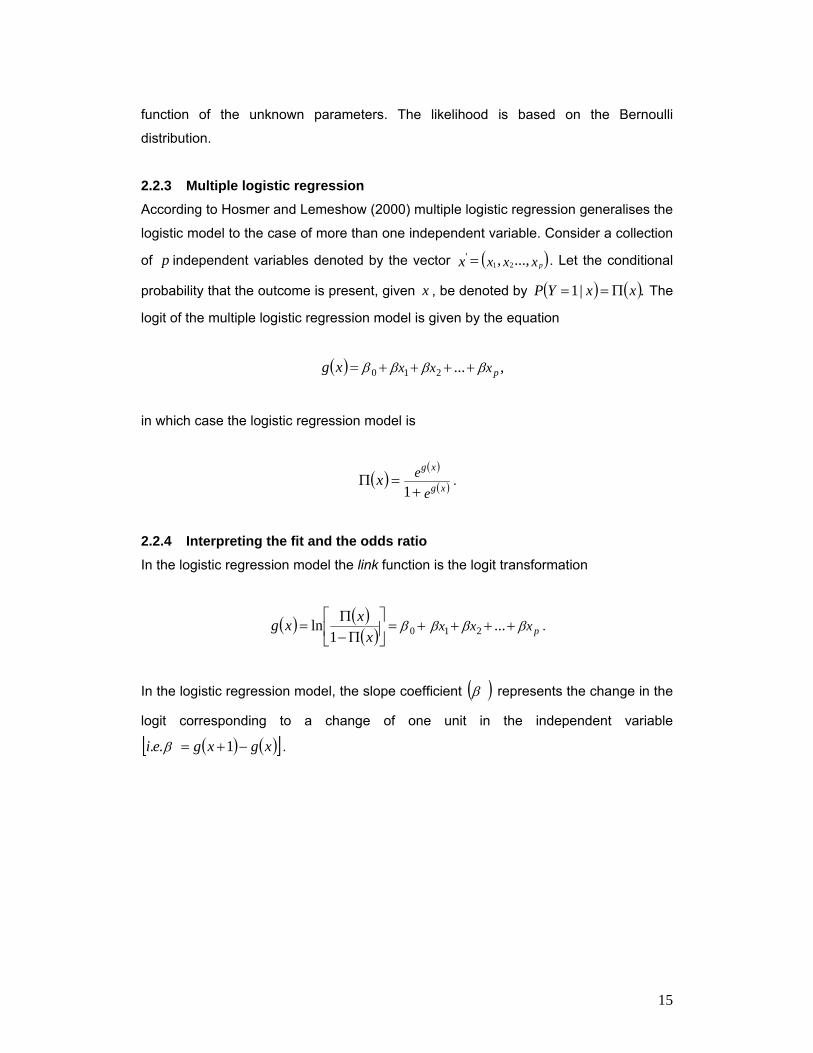
2.2.3 Multiple logistic regression According to Hosmer and Lemeshow (2000) multiple logistic regression generalises the
logistic model to the case of more than one independent variable. Consider a collection
of p independent variables denoted by the vector ( )xxx px ...,, 21' = . Let the conditional
probability that the outcome is present, given x , be denoted by ( ) ( ).|1 xxYP Π== The
logit of the multiple logistic regression model is given by the equation
( ) ,...210 xxx pxg ββββ ++++=
in which case the logistic regression model is
( )( )
( )ee
xg
xgx
+=Π
1.
2.2.4 Interpreting the fit and the odds ratio In the logistic regression model the link function is the logit transformation
( ) ( )( ) +=⎥
⎦
⎤⎢⎣
⎡Π−
Π= β 01
lnx
xxg xxx pβββ +++ ...21 .
In the logistic regression model, the slope coefficient ( )β represents the change in the
logit corresponding to a change of one unit in the independent variable
( ) ( )[ ]xgxgei −+= 1.. β .

16
Hosmer and Lemeshow (2000) explains odds using a dichotomous independent
variable, x , coded as either zero or one. The possible values of the logistic
probabilities may be conveniently displayed in a 2 x 2 table as shown in table 2.2.4.
The odds of the outcome being present among individuals with 1=x , is defined as
( )( )⎥⎦⎤
⎢⎣
⎡Π−
Π11
1. Similarly, the odds of the outcome being present amongst individuals with
0=x , is defined as ( )( )⎥⎦
⎤⎢⎣
⎡Π−
Π01
0. The odds ratio, denoted by OR, is defined as the ratio
of the odds for 1=x to the odds for 0=x , and is given by the equation
OR =
( )( )
( )( ) ⎥
⎥⎥⎥
⎦
⎤
⎢⎢⎢⎢
⎣
⎡
Π−ΠΠ−
Π
010
111
. (2)
Table 2.2.4 Logistic probabilities
Outcome variable Independent variable
1=x
Independent variable
0=x
1=y ( )e
e10
10
11
ββ
ββ
+
+
+=Π ( )
ee
0
0
10
β
β
+=Π
0=y ( )e 101
11 1ββ ++
=Π− ( )e 01
01 1β+
=Π−
Total 0.1 0.1
Substituting the expression for the logistic regression model shown in table 2.2.4 into
(2) we obtain
OR = e 1β ,
which shows the relationship between the odds ratio and the regression coefficient for
logistic regression with a dichotomous independent variable coded 1 and 0.

17
2.3 Classification Trees 2.3.1 Introduction Webb (1999) says that classification trees or decision trees are capable of modelling
complex non-linear decision boundaries. A classification tree or a decision tree is an
example of a multistage decision process. Instead of using the complete set of features
jointly to make a decision, different subsets of features are used at different levels of
the tree. Classification trees break up the decision into a series of simpler decisions at
each node. Associated with each internal node of the tree is a variable and a threshold.
Associated with each leaf or terminal node is a class label. The top node is the root of
the tree. The number of decisions required to classify a pattern depends on the pattern.
Generally the outcome of a decision could be one of 2≥m possible categories.
Fatti (2003) discusses Automatic Interaction Detection (AID). AID comprises a family of
methods for reducing a large data set consisting of
1) a dependent variable Y which is either categorical or continuous
2) a (possibly large) number of predictor variables
into relatively homogeneous (in Y ) subsets defined by different combinations of
categories of the predictor variables.
The strength of an AID analysis is that it imposes little structure on the data (such as
the linearity required by multiple regression), and the categorical dependent variable
version (CHAID: χ2 - AID) requires few distributional assumptions. The continuous
dependent variable version (XAID – extended AID) is based on normality of Y .
2.3.2 Tree method of SAS Since SAS Enterprise Miner Tree Node was used in the study, a brief description of the
Tree Method follows.
The SAS implementation of decision trees finds multiway splits based on nominal,
ordinal and interval inputs. There are options to include features such as CHAID (Chi-
squared automatic interaction detection). The criterion for evaluating a splitting rule
may be based on either a statistical significance test, namely an F test or a Chi-
square test, or on the reduction in variance, entropy or gini impurity measure.

18
SAS Enterprise Miner Tree Node differs from the CHAID algorithm, in that the Tree
Node seeks the split minimising the adjusted p-value, whereas the original KASS
algorithm does not. CHAID discretises interval inputs, while the Tree Node sometimes
consolidates observations into groups.
2.3.3 Splitting rules and pruning Webb (1999) mentions that the construction involves three (3) steps:
1. Selecting a splitting rule for each internal node. This means determining the
features, together with a threshold, that will be used to partition the data set
at each node.
2. Determining which nodes are terminal nodes. This means that for each
node, we must decide whether to continue splitting or to make the node a
terminal node and assign a class label to it. If we continue splitting until
every terminal node has pure class membership (all samples in the design
set that arrive at that node belong to the same class), then we are likely to
end up with a large tree that overfits the data and gives a poor error rate on
an unseen test set. Alternatively, relatively impure terminal nodes (nodes for
which the corresponding subset of the design set has mixed class
membership) lead to small trees that may underfit the data. Several
stopping rules have been proposed in the literature, but the approach
suggested by Breiman, Friedman, Olshen and Stone (1984, in Webb, 1999)
is to successfully grow and selectively prune the tree, using cross-validation
to choose the subtree with the lowest estimated misclassification rate.
3. Assigning class labels to terminal nodes. This is straightforward and labels
can be assigned by minimising the estimated misclassification rate.
A splitting rule, according to Webb (1999), is a prescription for deciding which variable,
or combination of variables, should be used at each node to divide the samples into
subgroups, and for deciding what the thresholds on these variables should be. A split
consists of a condition on the coordinates of a vector ℜ∈ px .
19
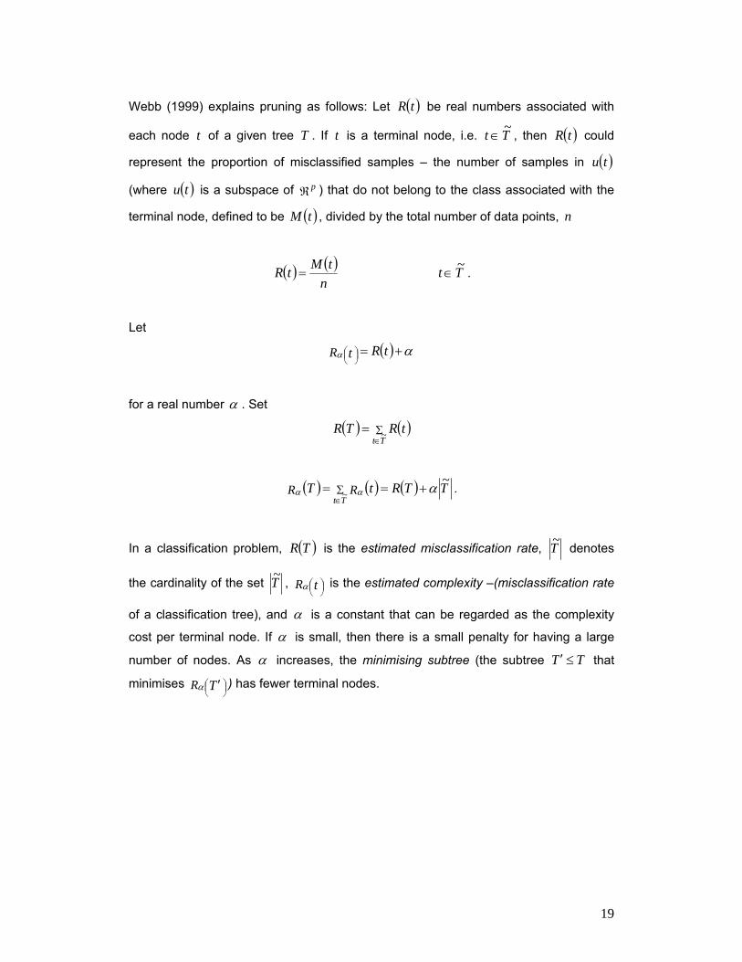
Webb (1999) explains pruning as follows: Let ( )tR be real numbers associated with
each node t of a given tree T . If t is a terminal node, i.e. Tt ~∈ , then ( )tR could
represent the proportion of misclassified samples – the number of samples in ( )tu
(where ( )tu is a subspace of ℜp ) that do not belong to the class associated with the
terminal node, defined to be ( )tM , divided by the total number of data points, n
( ) ( )n
tMtR = Tt ~∈ .
Let
( ) αα +=⎟⎠⎞⎜
⎝⎛ tRtR
for a real number α . Set
( ) ( )tRTRTtΣ∈
= ~
( ) ( ) ( ) TTRtT RRTt
~~ ααα +== Σ
∈.
In a classification problem, ( )TR is the estimated misclassification rate, T~ denotes
the cardinality of the set T~ , R t ⎟⎠⎞⎜
⎝⎛α is the estimated complexity –(misclassification rate
of a classification tree), and α is a constant that can be regarded as the complexity
cost per terminal node. If α is small, then there is a small penalty for having a large
number of nodes. As α increases, the minimising subtree (the subtree TT ≤′ that
minimises R T ⎟⎠⎞⎜
⎝⎛ ′α ) has fewer terminal nodes.

20
2.4 Discriminant Analysis 2.4.1 Introduction McLachlan (1992) describes discriminant analysis as follows: Suppose there is a finite
number, say g , of distinct populations, categories, classes or groups, denoted by
GG g,...,1 (refer to Gi as groups). In discriminant analysis, the existence of the groups is
known a priori. An entity of interest is assumed to belong to one (and only one) of the
groups. Let the categorical variable z denote the group membership of the entity,
where iz = implies that it belongs to group Gi ( )gi ,...,1= . Let the p-dimensional
vector ( )′= xx px ,...,1 contain the measurements on p available features of the entity.
In this framework, discriminant analysis is concerned with the relationship between the
group-membership label z and the feature vector x . At the decision end of the scale,
the group membership of the entity is unknown and the intent is to make an outright
assignment of the entity to one of the g possible groups on the basis of its associated
measurements. That is, in terms of our present notation, the problem is to estimate z
solely on the basis of x .
At the other extreme end of the spectrum, no assignment or allocation of the entity to
one of the possible groups is intended. Rather, the problem is to draw inferences about
the relationship between z and the feature variables in x .
Between these extremes lie most of the everyday situations in which discriminant
analysis is applied. Typically, the problem is to make a prediction or tentative allocation
for an unclassified entity.
2.4.2 Allocation rules McLachlan (1992) describes a classified entity as an entity whose group of origin is
known. A rule for the assignment of an unclassified entity to one of the groups is
referred to as a discriminant or allocation rule.
Webb (1999) says that a discriminant function is a function of the pattern x that leads
to a classification rule. The p-dimensional data vector ( )′= xx px ,...,1 , denotes the p
measurements of the features of an object, which are thought to be important for

21
classification. In discrimination assume that there exist C groups or classes, denoted
by ωω c,...,1 , with a priori probabilities (the probability of each class occurring)
( ) ( )ωω cpp ,...,1 such that ( ) 11
=∑=
c
iip ω and associated with each pattern x is a
categorical variable z that denotes the class or group membership; that is , if iz = ,
then the pattern belongs to ω i , Ci ,...,1∈ .
2.4.3 Linear discriminant functions Webb (1999) considered a family of discriminant functions that are linear combinations
of the components of ( )′= xx px ,...,1 ,
( ) .00 wxww ip
iixwxg +=+′= ∑
This is a linear discriminant function, a complete specification of which is achieved by
prescribing the weight vector w and threshold weight .0w
A linear discriminant function can arise through assumptions of normal distributions for
the class densities, with equal covariance matrices. Alternatively, without making
distributional assumptions, we may impose the form of the discriminant function to be
linear and determine its parameters.
The most widely used classifier is that based on the normal distribution,
( )( )
( ) ( )⎭⎬⎫
⎩⎨⎧ −′−−= Σ
ΣΠ− μμω iiipi xxxp
i
12/12/ 2
1exp1|2
.
Classification is achieved by assigning a pattern to a class for which the posterior
probability, ( )xp i |ω , is the greatest, or equivalently ( )[ ]xp i |log ω . Using Bayes’ rule
and the normal assumption for the conditional densities above, we have
( )[ ] ( ) ( )( ) ( )( )[ ]xppxpxp iii loglog|log|log −+= ωωω
( ) ( ) ( ) ( ) ( )( ) ( )( )xpppxx iiiii loglog2log2
log21
21 1 −+Π−−−′−−= ΣΣ − ωμμ .

22
Since ( )xp is independent of class, the discriminant rule is: assign x to ωi if gg ji > ,
for all ij ≠ , where
( ) ( )( ) ( ) ( ) ( )μμω iiiiii xxpxg −′−−−= ΣΣ −1
21log
21log .
Classifying a pattern x on the basis of the values of ( )xgi , ,,...,1 ci = gives the normal-
based quadratic discriminant function. When the covariance matrices are equal, i.e.
∑∑ = ,i ,,...,1 ci = the normal-based quadratic discriminant function becomes the
linear discriminant function, i.e. ( ) ( ),21)( 1 μμμμ cicixxLDF −
′⎟⎠⎞
⎜⎝⎛ +−= Σ− .1,...,1 −= ci
2.5 Markov Random Fields, ICM and Gibbs Sampler 2.5.1 Markov random fields Besag (1986) talks about Markov random fields by associating them with satellite
imagery. Each picture element, or pixel, has a particular colour. The colours may be
unordered, and represent the value per pixel of some underlying variable, such as
intensity. Besag (1986) states that “… there is supposed to be a true but unknown
colouring of the pixels … the aim is to reconstruct the scene from two imperfect
sources of information.”
With each pixel there is a possible multivariate record, which provides data on the
colour of the pixel. By assuming that the records for any particular scene follow a
known statistical distribution and that pixels close together tend to have the same
colour, Besag (1986) aims to construct a scene of unknown colouring of pixels with
additional knowledge that pixels close together tend to have the same colours, by using
non-degenerate Markov random field, which represents the local characteristics of the
underlying scene. Besag (1986) states that such an approach enables the two
assumptions to be “combined by Bayes’ theorem and the true scene to be estimated
according to standard criteria”.

23
In developing his methodologies, Besag (1986) uses the following notation and makes
the following assumptions. Suppose a two-dimensional region S is partitioned into n
pixels, labelled in some manner by the integers i = 1, 2, …, n. Each pixel can take one
of c colours, labelled 1, 2, …, c, with c finite. Assume there is no deterministic
exclusions, so that the minimal sample space is Ω = 1, 2, …, cn. An arbitrary colouring
of S will be denoted by x = (x1, x2, …, xn), where xi is the corresponding colour of
pixel i . x* is used to denote the true but unknown scene and interpret this as a
particular realisation of a random vector X = (X1, X2, …, Xn) where X i assigns colour
to pixel i . yi denotes the observed record at i and y is the corresponding vector,
interpreted as the realisation of the random vector, Y = (Y1, Y2, …, Yn). P(.) and PT(.)
denote probabilities of named events.
Besag (1986) makes two assumptions:
Assumption 1: Given any particular scene x , the random variables Y1, Y2, …, Yn are
conditionally independent and each Yi has the same known conditional density function
( )i x|iyf , dependent only on xi . Thus, the conditional density of the observed records
y , given x , is simply
( ) ( )i1
x|x| in
iyfyl ∏
== .
Two modifications to Assumption 1 are made:
(1) There may be overlaps between records, in that yi may contain information not
only from pixel i but also from adjacent pixels. The conditioning set in f must then be
expanded to include the x j `s at these pixels.
(2) The assumption of conditional independence is not always valid: for example, the
reflectance from adjacent pixels may be noticeably more alike than those from pixels
further apart.
Assumption 2: the true colouring x* is a realisation of a locally dependent Markov
random field with specified distribution ( ) xp .
( ) xp is a probability distribution which assigns colourings to S. Denote by xA a
colouring of the subset A of S and, in particular, by x is| a colouring of all pixels other

24
than pixel i ; xs = x and x i = xi . Consider the conditional probability ( )xx isiP \| of
colour xi occurring at pixel i , given the colouring x is| elsewhere. Viewed through its
conditional distribution at each pixel, ( ) xp is termed a Markov random field.
Focusing on fields whose conditional distributions are locally dependent, that is
dependent only on the colours of pixels in the immediate vicinity of pixel i . Thus,
suppose that for every x ,
( ) ( )xxpxx iiiisiP ∂≡ || \ ,
where pi is specific to the pixel i and ∂i is a subset of S\ i . The members of the set ∂i
are termed the neighbours of pixel i . In practice, the problem is approached from the
other end, by first naming the neighbours ∂i of each pixel i and then selecting ( ) xp
from among the corresponding class of probability distributions. ( ) xp is to be viewed
merely as our prior distribution for the true scene x* .
Besag (1986) considers some connected probabilistic methods of estimating the true
scene x* . The estimate ∧x is chosen to have maximum probability, given the vector of
records y. Thus, by Bayes’ thereom, ∧x maximises
( ) ( ) ( )xpxylyxP || ∝
with respect to x . In a Bayesian framework, ∧x is the maximum a posteriori estimate of
x* , being the mode of its posterior distribution. Besag (1989) explains this, in the
context of Bayesian Image Analysis, as combining the prior density and the likelihood
by Bayes’ theorem to form the posterior density ( )yxP | of x given y , as shown
above. A major strength of the Bayesian approach is that an interval estimate
(Bayesian confidence interval) can be attached to each pixel.

25
Besag (1986) says that an important requirement is to maximise the expected
proportion of correctly classified pixels, that is, to estimate *ix , for each i , by ix∧
which
maximises
( ) ( ) ( )xpxylyxP isxi || |∑∝ ,
the marginal (posterior) probability of xi at i , given the records y . ( )yxP i | depends on
all the records for (almost) any ( ) xp .
2.5.2 Iterated Conditional Modes (ICM)
According to Besag (1986) if we want to update the colour ix∧
at pixel i , (∧x denotes a
provisional estimate of the true scene x* ), using all available information, the colour
with maximum conditional probability is chosen, given the record y and the current
reconstruction isx |∧
elsewhere; that is, the new ix∧
maximises ⎟⎠
⎞⎜⎝
⎛ ∧isi xyP x |,| with respect
to xi . It follows from Bayes’ theorem that
( ) ⎟⎠⎞⎜
⎝⎛∝⎟
⎠
⎞⎜⎝
⎛∂
∧∧
iiiiiisi xxpxyx fxyP ||,| | ,
so that implementation is trivial for any locally dependent ( ) xp . Note that, because of
the assumption of local dependency of the colours we need only condition on ix∂∧
, the
colours of the neighbouring pixels. When applied to each pixel in turn, the procedure
defines a single cycle of an iterative algorithm for estimating x* . The algorithm is
applied for a fixed number of cycles or until convergence, to produce the final estimate
of x* . Note that
( ) ( )yxyPyxP xPx isisi |,|| || ⎟⎟⎠
⎞⎜⎜⎝
⎛= ,
26
so that ⎟⎠⎞⎜
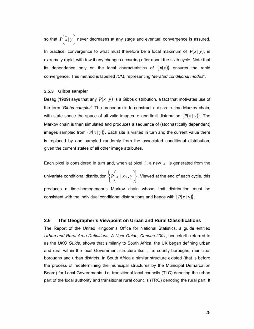
⎝⎛ ∧ yP x | never decreases at any stage and eventual convergence is assured.
In practice, convergence to what must therefore be a local maximum of ( )yxP | , is
extremely rapid, with few if any changes occurring after about the sixth cycle. Note that
its dependence only on the local characteristics of ( ) xp ensures the rapid
convergence. This method is labelled ICM, representing “iterated conditional modes”.
2.5.3 Gibbs sampler
Besag (1989) says that any ( )yxP | is a Gibbs distribution, a fact that motivates use of
the term ‘Gibbs sampler’. The procedure is to construct a discrete-time Markov chain,
with state space the space of all valid images x and limit distribution ( ) yxP | . The
Markov chain is then simulated and produces a sequence of (stochastically dependent)
images sampled from ( ) yxP | . Each site is visited in turn and the current value there
is replaced by one sampled randomly from the associated conditional distribution,
given the current states of all other image attributes.
Each pixel is considered in turn and, when at pixel i , a new xi is generated from the
univariate conditional distribution ⎭⎬⎫
⎩⎨⎧
⎟⎟⎠
⎞⎜⎜⎝
⎛∂ yxP iix ,| . Viewed at the end of each cycle, this
produces a time-homogeneous Markov chain whose limit distribution must be
consistent with the individual conditional distributions and hence with ( ) yxP | .
2.6 The Geographer’s Viewpoint on Urban and Rural Classifications The Report of the United Kingdom’s Office for National Statistics, a guide entitled
Urban and Rural Area Definitions: A User Guide, Census 2001, henceforth referred to
as the UKO Guide, shows that similarly to South Africa, the UK began defining urban
and rural within the local Government structure itself, i.e. county boroughs, municipal
boroughs and urban districts. In South Africa a similar structure existed (that is before
the process of redetermining the municipal structures by the Municipal Demarcation
Board) for Local Governments, i.e. transitional local councils (TLC) denoting the urban
part of the local authority and transitional rural councils (TRC) denoting the rural part. It

27
was not until the local Government reforms in the UK in the early 1970s that different
approaches to defining urban and rural areas became necessary.
From the UKO Guide it is evident that there are a number of different urban/ rural
definitions in use, for different needs, mainly as a result of different policies.
Methods for defining an urban or rural area that were deployed over the years in the
UK are the following:
• Groupings of about four Enumeration Districts (EDs), (called Enumeration Areas,
i.e. EAs in South Africa) within the urban land.
• Making use of the population weighted centroids where an ED was defined as
‘urban’ if its centroid was either wholly within the area of urban land or within a 150
metre buffer of the boundary.
• The Scottish 1991 Census made use of geographically contiguous groups of
postcodes and densities of addresses to designate localities. The use of addresses
to create population estimates has advantages in the sense that the exercise can
be repeated outside census years. In fact, the favoured single criterion definition of
‘urban’ has been based on land use, whether measured directly as land parcels or
by proxy as (residential and commercial) address densities.
Another approach suggested in the UKO Guide is to classify places based on their
social and economic characteristics. The approach requires that data be collected for a
consistent place geography and the use of sophisticated statistical techniques. Stats
SA has developed an area based place name geographical frame for South Africa. The
frame was developed by aggregating EAs into places. Although the EA-types are
attached to each EA, the aggregation of EAs into places did not take EA-types into
consideration and thus gives no clear indication of urban and rural.
The problems of defining rural areas are more intractable than those of defining urban
areas, leading one observer to suggest that what constitutes rurality is largely a matter
of convenience (Newby, 1986, in the UKO Guide). The problem with this approach of
defining areas like small settlements on the fringes of large towns and cities to remote
villages and hamlets to large farming areas as rural, is the economic and social
changes that have taken place in rural areas that resemble an urban style of life and
work.
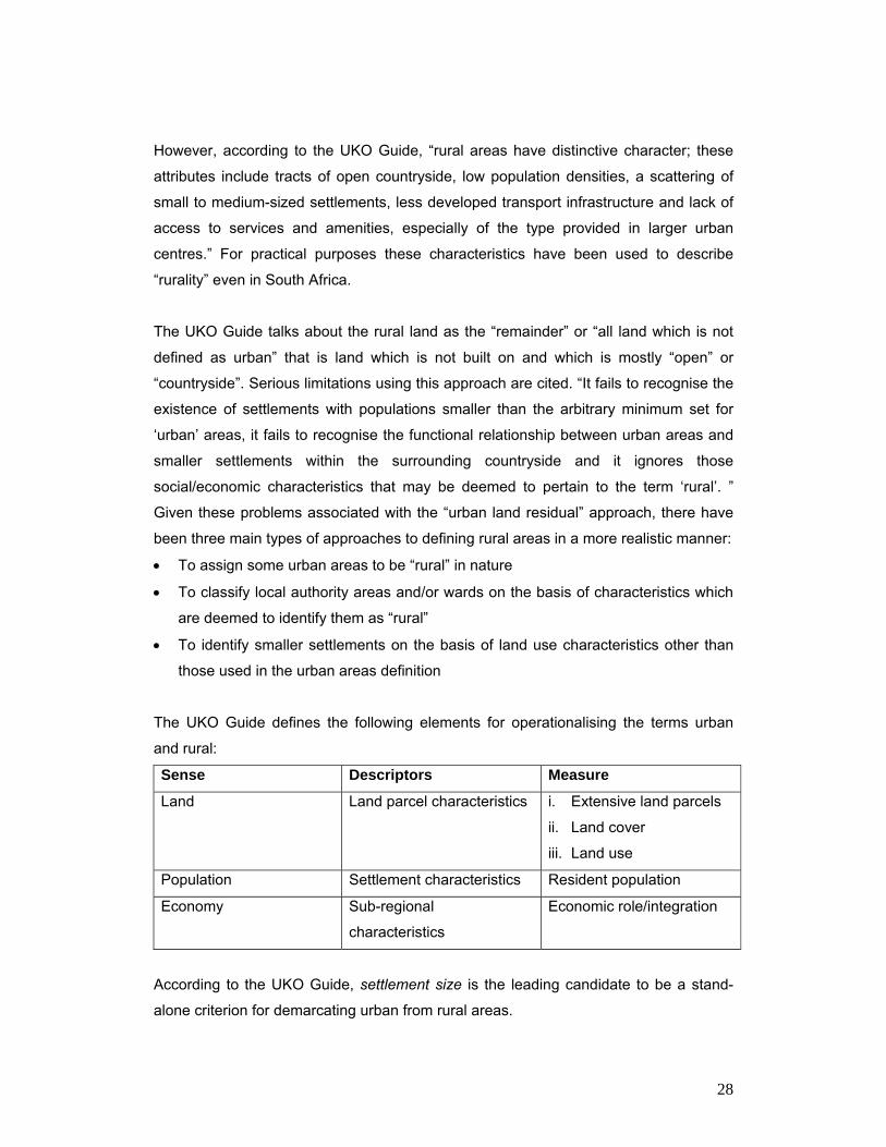
28
However, according to the UKO Guide, “rural areas have distinctive character; these
attributes include tracts of open countryside, low population densities, a scattering of
small to medium-sized settlements, less developed transport infrastructure and lack of
access to services and amenities, especially of the type provided in larger urban
centres.” For practical purposes these characteristics have been used to describe
“rurality” even in South Africa.
The UKO Guide talks about the rural land as the “remainder” or “all land which is not
defined as urban” that is land which is not built on and which is mostly “open” or
“countryside”. Serious limitations using this approach are cited. “It fails to recognise the
existence of settlements with populations smaller than the arbitrary minimum set for
‘urban’ areas, it fails to recognise the functional relationship between urban areas and
smaller settlements within the surrounding countryside and it ignores those
social/economic characteristics that may be deemed to pertain to the term ‘rural’. ”
Given these problems associated with the “urban land residual” approach, there have
been three main types of approaches to defining rural areas in a more realistic manner:
• To assign some urban areas to be “rural” in nature
• To classify local authority areas and/or wards on the basis of characteristics which
are deemed to identify them as “rural”
• To identify smaller settlements on the basis of land use characteristics other than
those used in the urban areas definition
The UKO Guide defines the following elements for operationalising the terms urban
and rural:
Sense Descriptors Measure
Land Land parcel characteristics i. Extensive land parcels
ii. Land cover
iii. Land use
Population Settlement characteristics Resident population
Economy Sub-regional
characteristics
Economic role/integration
According to the UKO Guide, settlement size is the leading candidate to be a stand-
alone criterion for demarcating urban from rural areas.

29
Clarke (1972) states that urban populations differ strongly from rural populations in
distribution, density, ways of life, structure and growth. Distinction between urban and
rural is a “thorny problem for the population geographer”. Urban population is
considered in terms of town living, that is to say the concentration of dwellings in a
recognisable street pattern, where people live in some social and economic
interdependence, enjoying common administrative, cultural and social amenities. But
such a definition is too vague for statistical analysis.
Clarke (1972) argues that there are certain inherent difficulties in the urban-rural
classification of population.
• Firstly, it is no easy task to draw a line between what is urban and what is rural.
There exists a wide range of settlement patterns between the two, especially in
advanced countries. There towns are increasingly tentacular and large
communities exist in the urban-rural fringe, where urban and rural cultures merge.
• Secondly, towns vary enormously in character and function.
• Thirdly, population data are normally available only for administrative units, whose
boundaries may not coincide at all with the limits between town and country.
• Fourthly, there are wide national variations in urban-rural classification, which inhibit
international comparisons.
Goodall (1972) gives an economic definition of urban, comprising complex markets,
where the spatial extent can be defined. He mentions that it has been customary to
define urban in terms of physical characteristics, reflecting the spatial agglomeration of
population and activities. Common to such definitions are
• A physical element, which emphasizes the high-density settlement of the
continuous built-up area and its separation from other urban centres by a much
greater area of thinly settled land
• An occupational element, which recognises the concentration of employment in
secondary and tertiary industries
The economic definition of urban comprises complex markets such as labour, land,
housing, capital, goods and services, where the spatial extents can be defined. The
spatial extents of each market are not necessarily coincident, but they overlap and
interlock is such a way as to form an urban economy.

30
Reif (1973) summarises the basic entities of the urban system in terms of its
• Objects: population, goods, vehicles
• Activities: residential, working, retail trade, education, production of goods and
services, recreation
• Land: land in different uses
• Infrastructure: Buildings: houses, schools, shops, factories, offices; Transport
facilities: roads, railway lines, airports, ports, etc.
The urban population system can be broken down into activities such as
• Residential activity
• Industrial activity
• Retail trade (shopping) activity
• Recreational activity, etc.
Each unit of population (person or family) can be additionally classified according to its
age, sex, income level, car ownership, etc. The urban economic system is built around
the entities ‘goods and services’.
In the diagram below, Reif (1973) shows that the urban system can be considered
structured by several subsystems.
Populationsubsystem
Administrativesubsystem
ETC.
Soci
al s
ubsy
stem
Economic
subsystem
Political
subsystem
Interactions
URBAN SYSTEM
Figure 2.6.1: The urban system can be considered structured by several subsystems (Adapted from Reif 1973)

31
White (1987) describes neighbourhoods and urban society, and states that where
people live is also partly determined by the location of jobs and industry, by the
technology of transportation and communication, and by the availability (and selection
preference for) local public services.
In general, geographers are moving away from the concept of urban and rural. This is
due to the difficulty in practically separating the two, due to movement on the ground
and the evidence of rural areas within urban areas. Rather, the concept of regional
geography is being pursued again. According to Hoekveld (1990) “regional geography
is about places, which means areas; it is not about objects, which have spatial
attributes.” Regional geography refers to classes of areas with common attributes and
therefore can be compared to other areas in the same class.
Hoekveld (1990) discusses the new regional realities, which are different from the
traditional conceptual frameworks, “relationships between site, national resource
bases, and society are mediated by an international economy, a nation state, world-
cities, and national city or settlement systems, in addition to wide institutional and
communication networks and financing organisations such as banks, pension funds,
etc. On the basis of these new regional realities, regional geographers might try to hew
new building blocks and assemble a new general conceptual framework to replace the
redundant ones.”
2.7 Chapter Summary and Conclusion In this chapter a literature review is conducted of the statistical techniques to be used in
the classifications and definitions for urban and rural, i.e. non-spatial techniques,
namely logistic regression, discriminant analysis, classification trees, and spatial
techniques, namely Markov random fields, i.e. iterated conditional modes and the
Gibbs sampler. The non-spatial statistical techniques will be applied and analysed in
Chapter 3. Thereafter, in Chapter 4, the spatial statistical techniques which take
advantage of common attributes due to spatial adjacencies, will be applied, hopefully to
improve the classifications obtained from the non-spatial techniques.
The chapter also contains a discussion of the geographer’s perspective with respect to
urban and rural. From the literature it is evident that the classification and definition of

32
urban and rural is certainly not straightforward in fact the literature gives an excellent
overview of the variety of approaches that are available and can be explored and even
combined. The literature does not provide a single classification or definition that can
be adapted as the standard, which makes the direct application from the literature
difficult. Further, the literature gives little or no indication of variables that can be
attributed to urban or rural that could be used in the statistical analysis. United Nations
(2006) states that due to “national differences in the characteristics that distinguish
urban from rural areas, the distinction between the urban and the rural population is not
yet amenable to a single definition …”. The diagram by Reif (1973) (Figure 2.6.1)
shows that the urban system can be made up by several subsystems namely political,
economic, administrative, social and population. This suggests that the classification of
urban and rural can take several aspects into consideration, some of which might be
difficult to consistently monitor across time. This study only made use of available
information from the 2001 Population Census of South Africa to classify areas as urban
and rural.
Geographers are moving away from classifying areas into urban and rural, rather
towards the concept of regional geography. Despite this, the study is relevant since the
concept of urban and rural plays an important role in shaping our society, as it provides
fundamental information needed for government allocations and service provision. In
the recent 2005 budget speech by the Finance Minister, Mr. Manuel said “this social
intent also embodies our commitment to build a more just, more equal society, in which
steady progress is made in reducing the gulfs that divide rich and poor, black and
white, men and women, rural and urban”.
In the next two chapters, the above mentioned statistical techniques are applied and
analysed with data from census 2001, to classify areas as urban and rural.

33
CHAPTER 3 - Non-Spatial Data Application and Results
3.1 Introduction In this chapter selected non-spatial statistical techniques are applied to selected 2001
population census data, to obtain estimates of the urban and rural population for each
province and the country as a whole, by classifying areas (enumeration areas) as
urban or rural. This chapter gives a detailed description of the non-spatial statistical
techniques applied, namely linear logistic regression, classification trees and
discriminant analysis.
In this chapter the non-spatial statistical application methodology is explained. It makes
use of areas in the country that are known to be urban and rural. Due to the importance
of using such areas (with known urban and rural status) in the study, the requirements
and compilation of these areas are explained. The selection of 2001 population census
data and the rationale for choosing these are also discussed. The results from the data
applications are presented.
3.2 Methodology 3.2.1 Rationale for utilising areas of known urban and rural status in the study An important aspect of the methodology is the use of areas in the country where the
classification of urban and rural is known with certainty. For example, large cities such
as Johannesburg, Cape Town and other clusters of built-up areas in the country, are
known to be urban, whilst farms or areas falling under the jurisdiction of traditional
authorities, are generally known to be rural and even as deep-rural in South Africa. The
rationale behind this was to firstly identify essential patterns or predominant
characteristics from areas that are known to be urban and rural, and thereafter apply
(or score) areas that are not known (or ambiguous) with similar characteristics, in order
to classify them as either urban or rural.

34
3.2.2 Description of the two sample data sets of known urban and rural status Two different sample data sets were generated. The application of the statistical
techniques and the analyses were performed utilising both sample data sets. In order
to systematically identify areas where the classifications of urban and rural are known,
the EA-types as defined for the 2001 population census of South Africa, were used.
EA-types are classifications of the country based on both settlement patterns and legal
proclamations. There are ten categories of EA-types across the country, i.e. vacant,
tribal settlement, farm, small-holding, urban settlement, informal settlement,
recreational area, industrial area, institution and hostel. Each of the 80 000 odd
enumeration areas was assigned with a unique EA-type for the 2001 population
census. (See Appendix A.)
The first sample data set comprises all areas in the country, where the EA-type is
urban settlement, labelled as known urban areas, and all areas in the country where
the EA-type is purely farm, labelled as known rural areas.
The second sample data set included the above two types of areas, but in addition all
areas within the country falling under the jurisdiction of traditional authorities, known as
tribal areas, were also included, and labelled as known rural areas.
For both sample data sets, note that no subsampling was done within the selected EA-
types, that is, all areas within the selected EA-types were utilised.
The main reason for utilising two sample data sets was that in the first data set a
common geographical definition of rural, indicative from the research conducted in
Chapter 2, i.e. farm, was strictly applied. Tribal areas (and other unknown areas) were
later scored with the characteristics obtained from the sample. Utilising this sample
data set to score the unknown areas, especially the tribal areas in the country, gives us
the opportunity to determine their classification statistically. The second sample reflects
South Africa more realistically, where tribal areas are considered as rural, mainly due
to the lack of services as a result of their previous exclusion from serviced areas.

35
The results obtained from the two sample data sets are very different and gives rise to
an interesting analysis.
For ease of writing, the first sample data set will be referred to as urban-farm or sample
1 and the second as urban-farm-tribal or sample 2.
To clarify the definitions of urban and rural used in the following sections and
forthcoming chapters, the definitions are repeated below:
• urban-farm or sample 1 comprises the urban settlement (as urban) and farm (as
rural) EA-types.
• urban-farm-tribal or sample 2, similar to urban-farm or sample 1, in addition
consists of the tribal (as rural) EA-type.
• In addition to the above two definitions, some tables in the following sections
will make use of the urban-rural population figures as published for the
censuses (i.e. 2001 and 1996).
o For census 2001, urban-rural figures are aggregations of geography-
types (different from EA-types). During the EA demarcation phase of
census 2001 each EA was assigned a unique geography-type. There
are four geography-types for the country, i.e. urban-formal, urban-
informal, tribal and farm. The urban-rural definition used for the census
classified urban-formal and urban-informal as urban and tribal and farm
as rural. (See Appendix A for a more detailed classification of urban-
rural for census 2001.)
o For census 1996, urban-rural figures were aggregations of EA-types (as
defined for census 1996, different to those used in census 2001),
comprising three categories, namely urban, semi-urban and rural. In
1996, rural and semi-urban comprised rural and was known as non-
urban. (See Appendix A for a more detailed classification of urban-rural
for census 1996.)
3.2.3 Selecting Census 2001 variables The census endeavoured to enumerate every person present in South Africa on
census night, 9-10 October 2001. The census data covers both household and person
information, i.e. information about the household and each person present in the
household on census night, as well as about services available to the household.

36
The study made use of selected household and person census information, with a
person weighting for person as well as for the household data, i.e. the number of
persons related to that household’s information, e.g. the number of persons with
access to piped water in the household. Variables were selected on the basis that they
have some relevance to the subject matter, i.e. urban and rural. Since the literature
review did not explicitly reveal variables that classify urban and rural, in this study we
are essentially searching for variables that could classify or indicate urban and rural.
When in doubt or uncertain about a variable it was added to the process, thus over 100
census variables were selected and applied to all provinces, and to South Africa as a
whole by EA. The use of certain census variables is limiting, as they are relatively
unstable and as such might be difficult to monitor across time, thus their inclusion in the
analysis might be a weakness in the study. These include variables such as
employment status, level of education and work status. Changes in these variables
could render a rural EA urban (and vice versa). Nevertheless the study is limited to
exploring the relevance of census variables for classifying urban and rural and forms
the framework for the analysis.
The following categories of person data were selected:
• Language
• Employment status
• Work status
• Total births
• Level of education
The following categories of household data were selected:
• Household size (the number of persons in a household)
• Type of housing unit (the type of dwelling, e.g. house or brick structure,
traditional dwelling, etc.)
• Rooms (number of rooms that the household utilises)
• Access to water (type of access to water the household has, e.g. piped water)
• Toilet facilities (main type of toilet facilities, e.g. flush toilet)
• Energy source for cooking (type of energy/fuel the household mainly uses for
cooking, e.g. electricity)
• Gender of head of household

37
• Population group of head of household
• Occupation of head of household
• Annual household income
3.2.4 Process Followed
3.2.4.1 Study conducted for each province Due to the different socio-economic characteristics and varying settlement patterns of
each province in South Africa, the study was conducted separately for each province
as well as for South Africa as a whole. Two sample data sets, described above, were
drawn for each province as well as for the country as a whole (details given in Table
3.2.1) and each statistical technique was performed for each province and for South
Africa, separately.
3.2.4.2 Partitioning the data set of known areas into training and validation data sets Since the methodology required that part of the sample data (that is urban and rural
areas that are known) be used to estimate the model and part be used to test the fitted
model, each sample data set for each province and for South Africa as a whole was
partitioned, using random sampling, into two independent data sets, i.e. the training
and the validation data sets. Each data set contained more or less 50% of the sample
data sets. The training data set was used to estimate the model and the validation data
set was used to test the fitted model by analysing the confusion matrix and assessing
the misclassification rate. According to Fernandez (2003) the training data provides the
predictive model with a chance to identify essential patterns that are specific to the
entire database. After training, the fitted model must be validated with data
independent of the training set to provide a way to measure the ability of the model to
distinguish between urban and rural areas. Unknown areas were thereafter scored with
the predictive model to classify them as either urban or rural. Section 3.3.4 shows the
confusion matrix for each statistical technique applied.
SAS Enterprise Miner was used to partition the data sets as well as to perform the
analyses. The same data sets, i.e. training and validation, were used to apply linear
logistic regression, classification trees and discriminant analysis.

38
3.2.4.3 Applying linear logistic regression Stepwise linear logistic regression was applied to the training data set to select
variables to include in the model and to obtain the estimates. The validation data set
was used to test the fitted model. Table 3.3.4 (a) shows the confusion matrix. The
model obtained from the training data set was applied to the unknown areas in order to
classify the unknowns as urban or rural. The results were weighted, as described in
section 3.2.5.1.

39
3.2.4.4 Applying classification trees Classification trees were applied to the training data set and the validation data set was
used for testing. Table 3.3.4 (b) shows the confusion matrix. Final nodes were
weighted as described in section 3.2.5.2. The model was applied to the unknown
areas.
3.2.4.5 Applying discriminant analysis Significant variables were selected using stepwise discrimination. These variables were
used to obtain the linear discriminant functions for urban and rural. The validation data
set was used to test the model. Table 3.3.4 (c) shows the confusion matrix. The results
were weighted as described in section 3.2.5.3 and applied to the data set of unknown
areas.
3.2.5 Weighting the data with prior information Adjustments based on the 2001 population census classifications of EAs into urban
and rural areas were applied. Table 3.2.1 shows the sample sizes (i.e. units in terms of
EAs, not persons) for both samples and the total population, broken down by urban
and rural. The methodology applied for adjusting the predictions for linear logistic
regression, classification trees and discriminant analysis is briefly explained below.
3.2.5.1 Weighting the data with prior information for logistic regression Adjusting the predictions from a linear logistic model, to correct for sampling that is
non-representative of the population:
⎟⎠⎞
⎜⎝⎛−
−⎟⎟⎠
⎞⎜⎜⎝
⎛−
+=P
PQ
Qxy1
ln1
ln'^β
where Q is the proportion of the population in Group 1 (urban), P is the proportion of
the sample in Group 1 (urban), x is the significant census variable and β is the
derived estimate.

40
Thereafter the classification rule,
if 0≥y then classify the EA in Group 1 (urban), if 0<y then classify the EA as rural,
was applied.
3.2.5.2 Weighting the data with prior information for classification trees All final nodes in the tree were converted to either urban or rural by correcting them
with the population proportion. Urban totals for all final nodes in the tree were multiplied
by the factor PQ / where Q is the urban proportion of the population and P is the
urban proportion of the sample. Similarly, the rural totals for all final nodes were
multiplied by the factor )1/()1( PQ −− where Q−1 is the rural proportion of the
population and P−1 is the rural proportion of the sample.
3.2.5.3 Weighting the data with prior information for linear discriminant analysis The following classification rule was used:
If ( ) ( ) ⎟⎟⎠
⎞⎜⎜⎝
⎛−
≥−Q
QxLDFxLDF1
log21
then classify the EA in Group 1 (urban),
if ( ) ( ) ⎟⎟⎠
⎞⎜⎜⎝
⎛−
<−Q
QxLDFxLDF1
log21
then classify the EA in Group 2 (rural),
where Q is the prior probability of Group 1 (urban) and Q−1 is the prior for Group 2
(rural) in the population.

41
Table 3.2.1 Sample and population sizes used for each province and for South Africa as a whole
(Units are EAs.)
Sample 1 Sample 2 Population*
(Urban-Farm) %
(Urban-Farm-Tribal)
% (2001 Census) %
W. Cape Rural 707 12 707 12 810 11 Urban 5265 88 5265 88 6291 89 Total 5972 100 5972 100 7101 100
E. Cape Rural 582 16 10284 78 14208 77 Urban 2968 84 2968 22 4162 23 Total 3550 100 13252 100 18370 100
N. Cape Rural 374 28 395 30 406 27 Urban 941 72 941 70 1103 73 Total 1315 100 1336 100 1509 100
F. State Rural 828 22 1415 32 1486 29 Urban 2991 78 2991 68 3697 71 Total 3819 100 4406 100 5183 100
KZN Rural 800 17 6445 62 6834 54 Urban 3957 83 3957 38 5919 46 Total 4757 100 10402 100 12753 100
N. West Rural 614 27 3797 69 4318 67 Urban 1680 73 1680 31 2159 33 Total 2294 100 5477 100 6477 100
Gauteng Rural 257 3 257 3 356 3 Urban 9424 97 9424 97 12846 97 Total 9681 100 9681 100 13202 100
MP Rural 724 29 3096 64 3336 58 Urban 1749 71 1749 36 2392 42 Total 2473 100 4845 100 5728 100
Limpopo Rural 451 37 8753 92 9481 91 Urban 761 63 761 8 984 9 Total 1212 100 9514 100 10465 100
S. Africa Rural 5337 15 35149 54 41235 51 (Sum-Parts) Urban 29736 85 29736 46 39553 49
Total 35073 100 64885 100 80788 100
S.Africa Rural 5337 15 35149 54 41235 51 (as a whole) Urban 29736 85 29736 46 39552 49
Total 35073 100 64885 100 80787 100
* The population sizes (units in terms of EAs) used here make use of geography-types
as defined during Census 2001. (See section 3.2.2 and Appendix A for definitions.)

42
Table 3.2.1 shows the number of EAs in each sample as well as the total number of
EAs for Census 2001. The difference between Sample 1 and Sample 2 is the inclusion
of the tribal communities in Sample 2. This difference is evident for provinces such as
the Eastern Cape, the Free State, KwaZulu-Natal, North West, Mpumalanga and
Limpopo, whilst provinces such as the Western Cape and Gauteng have similar
sample sizes since they do not have tribal areas.
3.3 Results The results obtained from linear logistic regression, classification trees and discriminant
analysis are presented below. Thereafter overall results are discussed in terms of the
aggregated population for the classifications of urban and rural as derived by means of
each statistical technique. The best classifications were selected for the map analyses.
3.3.1 Results from linear logistic regression The estimated logistic regression model for estimating the log (odds of urban) for each
province and South Africa as a whole, for both samples, is given in detail in Appendix
B. Regression parameter estimates were selected using a stepwise procedure with 5%
inclusion probability. Tables 3.3.1 (a) and (b) show a summary of some significant
variables occurring amongst the provinces and South Africa. In the case where the
variable increases the odds of urban, 1 denotes it and in the case where the variable
decreases the odds of urban, 0 denotes it. The confusion matrix is given in section
3.3.4.
Generally, examining the results from linear logistic regression, for sample 1, important
variables such as population density, unemployed persons, flush toilets connected to
sewer system, number of children ever born i.e. 0-5, and white headed households,
increase the odds of urban, whilst persons with no schooling, households using wood
as the main source of energy for cooking, head of household occupation is skilled
agricultural and fishery workers, increase the odds of rural.
Generally, for sample 2 important variables such as population density, unemployed
persons, flush toilet connected to sewer system, number of children ever born i.e. 0-5,
and persons who have completed primary schooling, increase the odds of urban, whilst
persons with no schooling, persons living in traditional/hut structures, households using
wood as the main source of energy for cooking, head of household occupation is

43
skilled agricultural and fishery workers, persons whose employment status is
homemaker or housewife, larger household sizes i.e. 10 persons and more,
households with no annual income, Black African headed households and households
with chemical toilets or pit latrines, increase the odds of rural.
Comparing sample 1 and sample 2, common variables are population density,
unemployed persons, households with flush toilets connected to sewer system, smaller
number of children ever born i.e. 0-5, that increase the odds of urban, whilst persons
with no schooling, households that use wood as the main source of energy for cooking,
skilled agricultural or fishery or elementary workers, increase the odds of rural.
Comparing sample 1 and sample 2 for variables that are not common between both,
sample 1 contains a variable such as White headed households, which increases the
odds of urban, whilst sample 2 contains a variable such as persons with complete
primary schooling, which increases the odds of urban. In addition, sample 2 contains
variables such as persons whose employment status is homemaker/ housewife, larger
household size i.e. 10+ persons, households with no annual income, households using
chemical toilets or pit latrines (with or without) ventilation, persons living in
traditional/hut structures and Black African head of household, which all increase the
odds of rural.
Therefore we can assume that since urban settlements and farms are common EA-
types in both samples, that variables such as population density, unemployed persons,
households with flush toilets connected to sewer system, smaller number of children
ever born i.e. 0-5, White headed households and persons with complete primary
schooling, separate urban settlements from rural, whilst persons with no schooling,
households that use wood as the main source of energy for cooking, skilled agricultural
or fishery or elementary workers separate farm (rural) settlements. An even further
assumption can be made that tribal settlements, which are only contained in sample 2,
can be separated from urban and farm (rural) settlements by variables such as persons
whose employment status is homemaker/housewife, larger household sizes i.e. 10+
persons, households with no annual income, households using chemical toilets or pit
latrines (with or without ventilation), persons living in traditional/hut structures and
Black African head of household.

44
Table 3.3.1 (a) Summary of significant variables obtained for linear logistic regression for the
Western Cape, Eastern Cape, Northern Cape, Free State and KwaZulu-Natal
W. Cape E. Cape N. Cape F. State KZN
Sample 1
Sample 2
Sample 1
Sample 2
Sample 1
Sample 2
Sample 1
Sample 2
Sample 1
Sample 2
Person
X1 Population density 1 1 1 1 1 1 1 1 1
Employment Status
(Employment status of each person)
X13 Employed 0 0
X14 Unemployed 1
X16 Home-maker or housewife 0
Total Births
(Total children ever born)
X27 0-5 children 1 1
Level of Education
(Highest level of education the person completed)
X30 No schooling 0 0 0 0
X32 Complete primary 1 1
Household Household Size
(Total number of persons in a household)
X37 6-10 persons 0
X38 More than 10 persons 0
Housing Unit
(Type of living quarters)
X40
Traditional dwelling/ hut/ structure made of traditional materials
0
X44
Informal dwelling/ shack, in backyard
1 1 1 0
Access to Water
(Type of access to water)
X62 Water vendor 1
Toilet facilities
(Main type of toilet facilities)
X63
Flush toilet (connected to sewerage system)
1 1 1 1 1
X65 Chemical toilet 0
X67
Pit latrine without ventilation
0
Energy source
(Type of energy/fuel mainly used for cooking)
X73 Wood 0 0 0

45
W. Cape E. Cape N. Cape F. State KZN
Sample 1
Sample 2
Sample 1
Sample 2
Sample 1
Sample 2
Sample 1
Sample 2
Sample 1
Sample 2
Gender of Head of Household
X78 Female 1 0 Population Group of Head of Household
X82 White 1 1 1 Occupation of Head of Household
X88
Skilled agricultural and fishery workers
0
Annual Household Income
X93 No income 0
X94 R 1 - R 4 800 1 1
“1” denotes increasing the odds of urban; “0” denotes decreasing the odds of urban

46
Table 3.3.1 (b) Summary of significant variables obtained for linear logistic regression for North
West, Gauteng, Mpumalanga, Limpopo and South Africa as a whole
N. West Gauteng MP Limpopo S. Africa
Sample 1
Sample 2
Sample 1
Sample 2
Sample 1
Sample 2
Sample 1
Sample 2
Sample 1
Sample 2
Person
X1 Population density 1 1 1 1 1 1 1 1 1
Employment
Status
(Employment status of each person)
X13 Employed 1 1
X14 Unemployed 1 1
X16 Home-maker or housewife 0
X17 Pensioner or retired person 1 1
Work Status
(Main activity or work status of person)
X24 Self-employed 1
Total Births
(Total children ever born)
X27 0-5 children 1 1 1 1
Level of Educati
on
(Highest level of education the person completed)
X30 No schooling 0
Household
Household Size
(Total number of persons in a household)
X37 6-10 persons 0
X38 More than 10 persons 0 0
Housing Unit
(Type of living quarters)
X39
House or brick structure on a separate stand or yard 0
X40
Traditional dwelling/ hut/ structure made of traditional materials 0
X44
Informal dwelling/ shack, in backyard 1
X45
Informal dwelling/ shack, not in backyard, informal/ squatter 1 1
X47 Caravan or tent 1 1
Access to Water
(Type of access to water)
X53 Piped water (tap) inside dwelling 1 1

47
N. West Gauteng MP Limpopo S. Africa
Sample 1
Sample 2
Sample 1
Sample 2
Sample 1
Sample 2
Sample 1
Sample 2
Sample 1
Sample 2
X54 Piped water (tap) inside yard 1 1
X57 Borehole 0
X60 Dam/ pool/ stagnant water 0
X62 Water vendor 1 0
Toilet facilities
(Main type of toilet facilities)
X63
Flush toilet (connected to sewerage system) 1 1 1 1 1
X64 Flush toilet (with septic tank) 1 1
X66 Pit latrine with ventilation (VIP) 0
X67 Pit latrine without ventilation 0
Energy source
for cooking
(Type of energy/ fuel mainly used for cooking)
X70 Electricity 1
X72 Paraffin 0
X73 Wood 0 0 0 0 0 0 0 0
X74 Coal 0 Population Group of Head of Household
X79 Black African 0 Occupation of Head of Household
X83
Legislators, senior officials and managers 1 1
X88
Skilled agricultural and fishery workers 0 0
X91 Elementary occupations 0
“1” denotes increasing the odds of urban; “0” denotes decreasing the odds of urban
3.3.2 Results from classification trees Tree diagrams, showing the main variables and how they split, for each province and
South Africa, for both samples, are presented in Appendix C. Tables 3.3.2 (a) and (b)
analyse the significant variables occurring for each province and South Africa for each
sample. The confusion matrix is given in section 3.3.4.
For sample 1 common variables amongst provinces that appear in the tree are
population density, households with flush toilets connected to sewer system,

48
households that use wood as the main source of energy for cooking, skilled agricultural
or fishery or elementary workers, persons with some primary schooling.
For sample 2 common variables amongst provinces that appear in the tree are
population density, households with flush toilets connected to sewer system,
households that use wood as the main source of energy for cooking, skilled agricultural
or fishery or elementary workers, persons with no schooling, persons whose main
language at home is Xitsonga, households using flush toilets with septic tanks,
chemical toilets, pit latrines (with or without ventilation) or bucket latrines.
Comparing sample 1 and sample 2, common variables between them are population
density, households with flush toilets connected to sewer system, households that use
wood as the main source of energy for cooking, skilled agricultural or fishery or
elementary workers.
In addition, comparing sample 1 and sample 2 for variables that are not common
between them, sample 1 contains variables such as persons with some primary
schooling. Sample 2 contains variables such as persons with no schooling, persons
whose main language at home is Xitsonga, households using flush toilets with septic
tanks, chemical toilets, pit latrines (with or without ventilation) or bucket latrines.
Therefore we can assume, since urban settlements and farms are common EA-types in
both samples, that population density, households with flush toilets connected to sewer
system, households that use wood as the main source of energy for cooking, skilled
agricultural or fishery or elementary workers, and persons with some primary
schooling, separate the urban and farm settlements. An even further assumption can
be made that tribal settlements, which are only contained in sample 2 can be separated
by variables such as persons with no schooling, persons whose main language at
home is Xitsonga, households using flush toilets with septic tanks, chemical toilets, pit
latrines (with or without ventilation) or bucket latrines.

49
Table 3.3.2 (a) Summary of significant variables occurring in classification trees for the Western
Cape, Eastern Cape, Northern Cape, Free State and KwaZulu-Natal
W. Cape E. Cape N. Cape F. State KZN
Sample
1 Sample
2 Sample
1 Sample
2 Sample
1 Sample
2 Sample
1 Sample
2 Sample
1 Sample
2 Person
X1 Population density √ √ √ √ √ √ √ √ √ √
Language
(Language most often spoken at home)
X9 Setswana √
Employment Status
(Employment status of each person)
X14 Unemployed √ √
Level of Education
(Highest level of education the person completed)
X30 No schooling √
X31 Some primary √ √
X34 Grade 12/ Std 10 √
Household
Household Size
(Total number of persons in a household)
X36 1-5 persons √
Rooms
(Number of rooms that the household utilises)
X49 1-3 rooms √
Toilet facilities
(Main type of toilet facilities)
X63
Flush toilet (connected to sewerage system)
√ √
√
X64 Flush toilet (with septic tank) √
X65 Chemical toilet √
X67 Pit latrine without ventilation √
Energy source for cooking
(Type of energy/ fuel mainly used for cooking)
X73 Wood √ √ √ √ √ Gender of Head of Household
X77 Male √ Population Group of Head of Household
X82 White √

50
W. Cape E. Cape N. Cape F. State KZN
Sample
1 Sample
2 Sample
1 Sample
2 Sample
1 Sample
2 Sample
1 Sample
2 Sample
1 Sample
2 Occupation of Head of Household
X88
Skilled agricultural and fishery workers
√ √
√
X91 Elementary occupations √ √

51
Table 3.3.2 (b) Summary of significant variables occurring in classification trees for North West,
Gauteng, Mpumalanga, Limpopo and South Africa
N. West Gauteng MP Limpopo S. Africa
Sample
1 Sample
2 Sample
1 Sample
2 Sample
1 Sample
2 Sample
1 Sample
2 Sample
1 Sample
2 Person
X1 Population Density √ √ √ √ √ √ √ √ √ √
Language
(Language most often spoken at home)
X2 Afrikaans √
X12 Xitsonga √ √ Level of Education
(Highest level of education the person completed)
X30 No schooling √
Household
Housing Unit
(Type of living quarters)
X45
Informal dwelling/ shack, not in backyard, informal/ squatter
√
Access to Water
(Type of access to water)
X56
Piped water on community stand: > 200 metres
√ √
Toilet facilities
(Main type of toilet facilities)
X63
Flush toilet (connected to sewerage system)
√
√
√
√
X64
Flush toilet (with septic tank)
√
X68 Bucket latrine √
Energy source for cooking
(Type of energy/ fuel mainly used for cooking)
X73 Wood √ √ Occupation of Head of Household
X88
Skilled agricultural and fishery workers
√ √
√
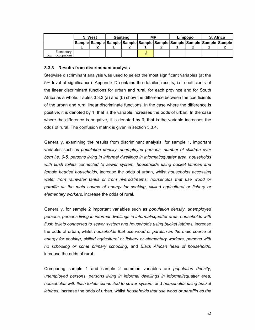
52
N. West Gauteng MP Limpopo S. Africa
Sample
1 Sample
2 Sample
1 Sample
2 Sample
1 Sample
2 Sample
1 Sample
2 Sample
1 Sample
2
X91 Elementary occupations √
3.3.3 Results from discriminant analysis Stepwise discriminant analysis was used to select the most significant variables (at the
5% level of significance). Appendix D contains the detailed results, i.e. coefficients of
the linear discriminant functions for urban and rural, for each province and for South
Africa as a whole. Tables 3.3.3 (a) and (b) show the difference between the coefficients
of the urban and rural linear discriminate functions. In the case where the difference is
positive, it is denoted by 1, that is the variable increases the odds of urban. In the case
where the difference is negative, it is denoted by 0, that is the variable increases the
odds of rural. The confusion matrix is given in section 3.3.4.
Generally, examining the results from discriminant analysis, for sample 1, important
variables such as population density, unemployed persons, number of children ever
born i.e. 0-5, persons living in informal dwellings in informal/squatter area, households
with flush toilets connected to sewer system, households using bucket latrines and
female headed households, increase the odds of urban, whilst households accessing
water from rainwater tanks or from rivers/streams, households that use wood or
paraffin as the main source of energy for cooking, skilled agricultural or fishery or
elementary workers, increase the odds of rural.
Generally, for sample 2 important variables such as population density, unemployed
persons, persons living in informal dwellings in informal/squatter area, households with
flush toilets connected to sewer system and households using bucket latrines, increase
the odds of urban, whilst households that use wood or paraffin as the main source of
energy for cooking, skilled agricultural or fishery or elementary workers, persons with
no schooling or some primary schooling, and Black African head of households,
increase the odds of rural.
Comparing sample 1 and sample 2 common variables are population density,
unemployed persons, persons living in informal dwellings in informal/squatter area,
households with flush toilets connected to sewer system, and households using bucket
latrines, increase the odds of urban, whilst households that use wood or paraffin as the

53
main source of energy for cooking and skilled agricultural or fishery or elementary
workers, increase the odds of rural.
In addition, comparing sample 1 and sample 2 for variables that are not common to
both, sample 1 contains the variable female head of households, which increases the
odds of urban. Sample 1 contains the variable households with main source of water
from rainwater tanks or rivers/streams, which increases the odds of rural, whilst sample
2 contains variables such as persons with no schooling or some primary schooling, and
Black African head of household, which increase the odds of rural.
Therefore we can assume, since urban settlements and farms are common EA-types in
both samples, that population density, unemployed persons, smaller number of
children ever born i.e. 0-5, persons living in informal dwellings in informal/squatter area,
households with flush toilets connected to sewer system, households using bucket
latrines and female headed households, separate urban settlements from rural, whilst
households that use wood or paraffin as the main source of energy for cooking and
skilled agricultural or fishery or elementary workers, separate the farm (rural)
settlements. An even further assumption can be made that tribal settlements, which are
only contained in sample 2, can be separated from urban and farm (rural) settlements
by variables such as persons with no schooling or some primary schooling, households
accessing water from rainwater tanks or rivers/streams, and Black African head of
household.

54
Table 3.3.3 (a) Summary of significant variables obtained for linear discriminant analysis for the
Western Cape, Eastern Cape, Northern Cape, Free State and KwaZulu-Natal
W. Cape E. Cape N. Cape F. State KZN
Sample
1 Sample
2 Sample
1 Sample
2 Sample
1 Sample
2 Sample
1 Sample
2 Sample
1 Sample
2 Person
X1 Population density 1 1 1 1 1 1
Language
(Language most often spoken at home)
X2 Afrikaans 1
X3 English 1
X9 Setswana 1
Employment Status
(Employment status of each person)
X13 Employed 0 0
X14 Unemployed 1 1 1 1
X15 Scholar or student 1
Work Status
(Main activity or work status of person)
X22 Paid employee 0 Total Births
(Total children ever born)
X27 0-5 children 1 1 1
Level of Education
(Highest level of education the person completed)
X30 No schooling 0 0 0
X31 Some primary 0 0 0
X33 Some secondary 1
Household
Household Size
(Total number of persons in a household)
X36 1-5 persons 1 Housing Unit
(Type of living quarters)
X40
Traditional dwelling/ hut/ structure made of traditional materials 0
X41 Flat in a block of flats 0
X45
Informal dwelling/ shack, not in backyard, informal/ squatter 1 1 1 1 1 1
X47 Caravan or tent 0
Access to Water
(Type of access to water)
X53 Piped water (tap) inside dwelling 1
X54 Piped water (tap) inside yard 1
X57 Borehole 0
X59 Rainwater tank 0 0
X60 Dam/ pool/ stagnant water 0

55
W. Cape E. Cape N. Cape F. State KZN
Sample
1 Sample
2 Sample
1 Sample
2 Sample
1 Sample
2 Sample
1 Sample
2 Sample
1 Sample
2 X61 River/ stream 0 0
Toilet facilities
(Main type of toilet facilities)
X63
Flush toilet (connected to sewerage system) 1 1 1 1 1
X64 Flush toilet (with septic tank) 1 1 1
X65 Chemical toilet 0
X66 Pit latrine with ventilation (VIP) 0
X67 Pit latrine without ventilation 0
X68 Bucket latrine 1 1 0 0
Energy source for cooking
(Type of energy/ fuel mainly used for cooking)
X70 Electricity 1 1
X72 Paraffin 1
X73 Wood 0 0 0 0 0 0 0
X75 Animal dung 0 0
Gender of Head of Household
X77 Male 1
X78 Female 1 1 1 Population Group of Head of Household
X79 Black African 1 Occupation of Head of Household
X88 Skilled agricultural and fishery workers 0 0 0 0 0 0 0 0 0
X89 Craft and related trades workers 1 1
X90
Plant and machine operators and assemblers 0 0
X91 Elementary occupations 0 0 0 0 0 0 0
Annual Household Income
X94 R 1 - R 4 800 1 “1” denotes increasing the odds of urban; “0” denotes decreasing the odds of urban

56
Table 3.3.3 (b) Summary of significant variables obtained for linear discriminant analysis for North
West, Gauteng, Mpumalanga, Limpopo and South Africa
N. West Gauteng MP Limpopo S. Africa
Sample
1 Sample
2 Sample
1 Sample
2 Sample
1 Sample
2 Sample
1 Sample
2 Sample
1 Sample
2 Person
X1 Population density 1 0 1 1 1
Language
(Language most often spoken at home)
X2 Afrikaans 1 1
X3 English 1
X4 IsiNdebele 1 1 1
X6 IsiZulu 1
X12 Xitsonga 0
Employment Status
(Employment status of each person)
X14 Unemployed 1
X21 Could not find work 1
Work Status
(Main activity or work status of person)
X22 Paid employee 0
X24 Self-employed 1 1
Total Births
(Total children ever born)
X27 0-5 children 1
Household
Household Size
(Total number of persons in a household)
X37 6-10 persons 1
Housing Unit
(Type of living quarters)
X40
Traditional dwelling/ hut/ structure made of traditional materials 0 1
X44
Informal dwelling/ shack, in backyard 1 1
X45 Informal dwelling/ 1 1 1 1 1 1
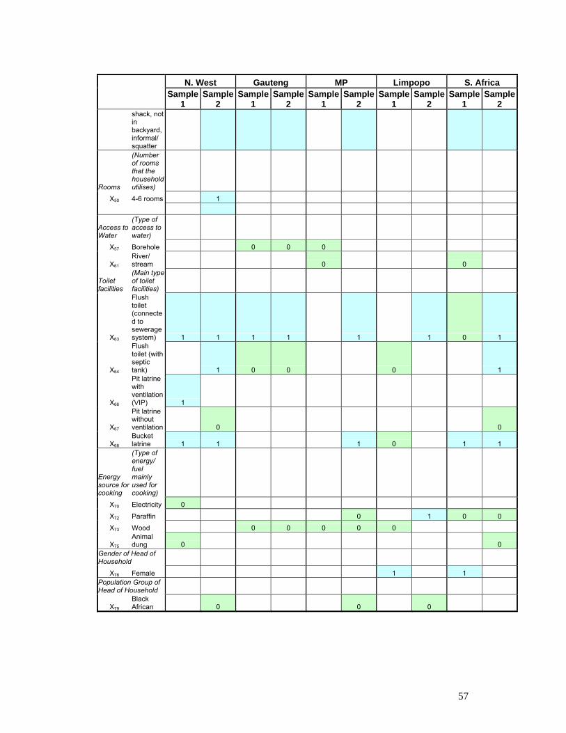
57
N. West Gauteng MP Limpopo S. Africa
Sample
1 Sample
2 Sample
1 Sample
2 Sample
1 Sample
2 Sample
1 Sample
2 Sample
1 Sample
2 shack, not in backyard, informal/ squatter
Rooms
(Number of rooms that the household utilises)
X50 4-6 rooms 1
Access to Water
(Type of access to water)
X57 Borehole 0 0 0
X61 River/ stream 0 0
Toilet facilities
(Main type of toilet facilities)
X63
Flush toilet (connected to sewerage system) 1 1 1 1 1 1 0 1
X64
Flush toilet (with septic tank) 1 0 0 0 1
X66
Pit latrine with ventilation (VIP) 1
X67
Pit latrine without ventilation 0 0
X68 Bucket latrine 1 1 1 0 1 1
Energy source for cooking
(Type of energy/ fuel mainly used for cooking)
X70 Electricity 0
X72 Paraffin 0 1 0 0
X73 Wood 0 0 0 0 0
X75 Animal dung 0 0
Gender of Head of Household
X78 Female 1 1 Population Group of Head of Household
X79 Black African 0 0 0

58
N. West Gauteng MP Limpopo S. Africa
Sample
1 Sample
2 Sample
1 Sample
2 Sample
1 Sample
2 Sample
1 Sample
2 Sample
1 Sample
2 Occupation of Head of Household
X86 Clerks 1
X88
Skilled agricultural and fishery workers 0 0 0 0 0 0 0 0
X89
Craft and related trades workers 0
X90
Plant and machine operators and assemblers 0 0 0
X91
Elementary occupations 0 0 0 0 0 0 0
X92
Occupations unspecified or not elsewhere classified 0
Annual Household Income
X93 No income 1 1
X99 R 76 801 - R 153 600 1 1
“1” denotes increasing the odds of urban; “0” denotes decreasing the odds of urban
3.3.4 Confusion matrices Table 3.3.4 (a) is the confusion matrix for linear logistic regression for both samples, for
the validation data sets only, for each province and for South Africa as a whole.
Noticeable misclassifications, i.e. over 10%, where rural EAs (farms) have been
wrongly classified as urban (urban settlements), for sample 1 occur for Gauteng,
Eastern Cape, North West and Mpumalanga, whilst for sample 2, these only occur for
Gauteng. Misclassifications over 10%, where urban EAs (urban settlements) have
been wrongly classified as rural (farm or tribal settlements) for sample 2 occur for
Limpopo and Mpumalanga.

59
Table 3.3.4 (a) Confusion matrix for linear logistic regression
Sample 1 Sample 2 1 0 Total 1 0 Total
Western Cape 1 2631 99% 21 1% 2652 2627 99% 22 1% 2649 0 21 6% 313 94% 334 23 7% 314 93% 337
Total 2652 334 2986 2650 336 2986
Eastern Cape 1 1445 98% 27 2% 1472 1274 95% 70 5% 1344 0 50 17% 253 83% 303 44 1% 5238 99% 5282
Total 1495 280 1775 1318 5308 6626 Northern Cape
1 464 97% 12 3% 476 465 96% 18 4% 483 0 11 6% 170 94% 181 11 6% 174 94% 185
Total 475 182 657 476 192 668
Free State 1 1482 99% 9 1% 1491 1508 98% 29 2% 1537 0 18 4% 400 96% 418 30 5% 636 95% 666
Total 1500 409 1909 1538 665 2203
KwaZulu-Natal 1 1971 99% 15 1% 1986 1849 95% 93 5% 1942 0 31 8% 361 92% 392 55 2% 3204 98% 3259
Total 2002 376 2378 1904 3297 5201
North West 1 808 98% 20 2% 828 812 94% 50 6% 862 0 42 13% 277 87% 319 42 2% 1834 98% 1876
Total 850 297 1147 854 1884 2738
Gauteng 1 4708 100% 15 0% 4723 4708 100% 15 0% 4723 0 25 21% 92 79% 117 25 21% 92 79% 117
Total 4733 107 4840 4733 107 4840
Mpumalanga 1 867 97% 28 3% 895 741 88% 99 12% 840 0 37 11% 304 89% 341 71 4% 1511 96% 1582
Total 904 332 1236 812 1610 2422
Limpopo 1 373 95% 19 5% 392 284 76% 88 24% 372 0 2 1% 212 99% 214 68 2% 4317 98% 4385
Total 375 231 606 352 4405 4757
RSA 1 14836 99% 108 1% 14944 14318 96% 623 4% 14941 0 225 9% 2367 91% 2592 397 2% 17104 98% 17501
Total 15061 2475 17536 14715 17727 32442 “1” = urban and “0” = rural

60
Table 3.3.4 (b) is the confusion matrix for classification trees for both samples, for the
validation data sets only, for each province and for South Africa as a whole. Noticeable
misclassifications, i.e. over 10%, where rural EAs (farms) have been wrongly classified
as urban (urban settlements), for sample 1 occur for Gauteng, RSA and Western Cape,
whilst for sample 2, they occur only for Gauteng. Misclassifications over 10%, where
urban EAs (urban settlements) have been wrongly classified as rural (farm or tribal
settlements), for sample 2 occur for Limpopo and Mpumalanga.

61
Table 3.3.4 (b) Confusion matrix for classification trees
Sample 1 Sample 2 1 0 Total 1 0 Total
Western Cape 1 2642 100% 10 0% 2652 2632 99% 17 1% 2649 0 37 11% 297 89% 334 24 7% 313 93% 337
Total 2679 307 2986 2656 330 2986
Eastern Cape 1 1447 98% 25 2% 1472 1253 93% 91 7% 1344 0 12 4% 291 96% 303 46 1% 5236 99% 5282
Total 1459 316 1775 1299 5327 6626
Northern Cape 1 468 98% 8 2% 476 450 93% 33 7% 483 0 16 9% 165 91% 181 3 2% 182 98% 185
Total 484 173 657 453 215 668
Free State 1 1484 100% 7 0% 1491 1488 97% 49 3% 1537 0 16 4% 402 96% 418 32 5% 634 95% 666
Total 1500 409 1909 1520 683 2203
KwaZulu-Natal 1 1973 99% 13 1% 1986 1832 94% 110 6% 1942 0 41 10% 351 90% 392 60 2% 3199 98% 3259
Total 2014 364 2378 1892 3309 5201
North West 1 814 98% 14 2% 828 814 94% 48 6% 862 0 9 3% 310 97% 319 26 1% 1850 99% 1876
Total 823 324 1147 840 1898 2738
Gauteng 1 4712 100% 11 0% 4723 4718 100% 5 0% 4723 0 35 30% 82 70% 117 42 36% 75 64% 117
Total 4747 93 4840 4760 80 4840 Mpumalanga
1 848 95% 47 5% 895 680 81% 160 19% 840 0 8 2% 333 98% 341 17 1% 1565 99% 1582
Total 856 380 1236 697 1725 2422
Limpopo 1 371 95% 21 5% 392 293 79% 79 21% 372 0 1 0% 213 100% 214 66 2% 4319 98% 4385
Total 372 234 606 359 4398 4757
RSA 1 14862 99% 82 1% 14944 13976 94% 965 6% 14941 0 313 12% 2279 88% 2592 425 2% 17076 98% 17501
Total 15175 2361 17536 14401 18041 32442 “1” = urban and “0” = rural

62
Table 3.3.4 (c) is the confusion matrix for discriminant analysis for both samples, for
the validation data sets only, for each province. Noticeable misclassifications, i.e. over
10%, where rural EAs (farms) have been wrongly classified as urban (urban
settlements), for sample 1 occur for Gauteng, RSA, KwaZulu-Natal and Mpumalanga,
whilst for sample 2, they occur only for Gauteng. Misclassifications over 10%, where
urban EAs (urban settlements) have been wrongly classified as rural (farm or tribal
settlements), for sample 2 occur for Limpopo and Mpumalanga.

63
Table 3.3.4 (c) Confusion matrix for discriminant analysis
Sample 1 Sample 2 1 0 Total 1 0 Total
Western Cape 1 2615 99% 37 1% 2652 2612 99% 37 1% 2649 0 34 10% 300 90% 334 35 10% 302 90% 337
Total 2649 337 2986 2647 339 2986
Eastern Cape 1 1442 98% 30 2% 1472 1243 92% 101 8% 1344 0 26 9% 277 91% 303 46 1% 5236 99% 5282
Total 1468 307 1775 1289 5337 6626
Northern Cape 1 463 97% 13 3% 476 469 97% 14 3% 483 0 19 10% 162 90% 181 16 9% 169 91% 185
Total 482 175 657 485 183 668
Free State 1 1486 100% 5 0% 1491 1476 96% 61 4% 1537 0 29 7% 389 93% 418 40 6% 626 94% 666
Total 1515 394 1909 1516 687 2203
KwaZulu-Natal 1 1972 99% 14 1% 1986 1812 93% 130 7% 1942 0 45 11% 347 89% 392 62 2% 3197 98% 3259
Total 2017 361 2378 1874 3327 5201
North West 1 811 98% 17 2% 828 814 94% 48 6% 862 0 22 7% 297 93% 319 32 2% 1844 98% 1876
Total 833 314 1147 846 1892 2738
Gauteng 1 4715 100% 8 0% 4723 4715 100% 8 0% 4723 0 31 26% 86 74% 117 32 27% 85 73% 117
Total 4746 94 4840 4747 93 4840 Mpumalanga
1 871 97% 24 3% 895 721 86% 119 14% 840 0 36 11% 305 89% 341 66 4% 1516 96% 1582
Total 907 329 1236 787 1635 2422
Limpopo 1 369 94% 23 6% 392 309 83% 63 17% 372 0 14 7% 200 93% 214 173 4% 4212 96% 4385
Total 383 223 606 482 4275 4757
RSA 1 14843 99% 101 1% 14944 14032 94% 909 6% 14941 0 352 14% 2240 86% 2592 537 3% 16964 97% 17501
Total 15195 2341 17536 14569 17873 32442 “1” = urban and “0” = rural

64
3.3.5 Overall results in terms of aggregated population totals Tables 3.3.5 (a) and 3.3.5 (b) show the overall results in terms of aggregated urban
and rural population per province and for South Africa as a whole, based on the
classifications as derived by means of the three statistical techniques discussed in the
previous sections, for sample 1 urban-farm and sample 2 urban-farm-tribal,
respectively. Two results were calculated for South Africa 1) by adding the urban and
rural population as obtained for each province (sum-parts), and 2) by applying the
statistical techniques for South Africa as a whole. For comparison purposes the census
2001 and 1996 figures for urban and rural for each province and for South Africa, as
published in the discussion document, Investigations into appropriate definitions of
urban and rural areas for South Africa, report no. 03-02-20 (2001), are included in the
table.

65
Table 3.3.5 (a) Population classified by urban and rural, per province and for South Africa, as
obtained for the three non-spatial statistical techniques, for sample 1, i.e. urban-farm
Linear
Logistic Regression
% Classi-fication Trees
% Discrim-
inant Analysis
% Census 2001 % Census
1996 %
W. Cape Rural 447266 10 438204 10 461325 10 435626 10 418918 11 Urban 4077053 90 4086115 90 4062994 90 4088709 90 3537956 89 Total 4524319 100 4524319 100 4524319 100 4524335 100 3956874 100
E. Cape Rural 226942 4 414973 6 2142188 33 3936529 61 3897080 62 Urban 6209759 96 6021728 94 4294513 67 2500234 39 2405446 38 Total 6436701 100 6436701 100 6436701 100 6436763 100 6302526 100
N. Cape Rural 147035 18 147134 18 150115 18 142267 17 208694 25 Urban 675681 82 675582 82 672601 82 680460 83 631627 75 Total 822716 100 822716 100 822716 100 822727 100 840321 100
F. State Rural 401221 15 396563 15 1006248 37 654660 24 822353 31 Urban 2305544 85 2310202 85 1700517 63 2052115 76 1811151 69 Total 2706765 100 2706765 100 2706765 100 2706775 100 2633504 100
KZN Rural 4307050 46 2950704 31 3864930 41 5091375 54 4700589 56 Urban 5118976 54 6475322 69 5561096 59 4334642 46 3716432 44 Total 9426026 100 9426026 100 9426026 100 9426017 100 8417021 100
N. West Rural 1203270 33 391706 11 1338751 36 2135581 58 1896267 57 Urban 2466093 67 3277657 89 2330612 64 1533768 42 1458558 43 Total 3669363 100 3669363 100 3669363 100 3669349 100 3354825 100
Gauteng Rural 321637 4 220221 2 270820 3 246380 3 221932 3 Urban 8515498 96 8616914 98 8566315 97 8590798 97 7126491 97 Total 8837135 100 8837135 100 8837135 100 8837178 100 7348423 100
MP Rural 923972 30 559882 18 932602 30 1834556 59 1690666 60 Urban 2199038 70 2563128 82 2190408 70 1288434 41 1110046 40 Total 3123010 100 3123010 100 3123010 100 3122990 100 2800712 100
Limpopo Rural 1104205 21 379662 7 1427330 27 4573183 87 4364169 88 Urban 4169433 79 4893976 93 3846308 73 700459 13 565199 12 Total 5273638 100 5273638 100 5273638 100 5273642 100 4929368 100
S. Africa Rural 9082598 20 5899049 13 11594309 26 19050159 43 18220668 45 (Sum-Parts) Urban 35737075 80 38920624 87 33225364 74 25769619 58 22362906 55
Total 44819673 100 44819673 100 44819673 100 44819778 100 40583574 100
S.Africa Rural 15165764 34 4534509 10 12625836 28 (All) Urban 29653909 66 40285164 90 32193837 72
Total 44819673 100 44819673 100 44819673 100

66
It is evident from Table 3.3.5 (a), for some provinces and even for South Africa as a
whole that there are large differences between the results obtained from the statistical
techniques and the published figures for urban and rural from census 2001 and census
1996. The results obtained from the statistical techniques, especially for provinces such
as the Eastern Cape, Limpopo, Mpumalanga, North West and even for South Africa,
show an astoundingly greater number of urban dwellers than there are rural dwellers,
compared to the two census figures, where these provinces show mainly rural dwellers.
Urban and rural populations for the provinces of the Western Cape, Northern Cape and
Gauteng remain similar to those of the two censuses. These provinces do not have
tribal settlements. Therefore it can be deduced that the differences in population figures
for provinces such as the Eastern Cape, Limpopo, Mpumalanga and North West and
even for South Africa as a whole, are the result of the classification of many tribal
settlements as urban, that is, generally all three statistical techniques have classified
the majority of the tribal EAs as urban. (See section 3.3.6 for map analysis.)

67
Table 3.3.5 (b) Population classified by urban and rural, per province and for South Africa, as
obtained for the three non-spatial statistical techniques, for sample 2, i.e. urban-farm-tribal
Linear logistic
regression %
Classi-fication
trees %
Discrim-inant
analysis % Census
2001 % Census 1996 %
W. Cape Rural 448204 10 437331 10 461325 10 435626 10 418918 11 Urban 4076115 90 4086988 90 4062994 90 4088709 90 3537956 89 4524319 100 4524319 100 4524319 100 4524335 100 3956874 100
E. Cape Rural 4039533 63 4055575 63 4118876 64 3936529 61 3897080 62 Urban 2397168 37 2381126 37 2317825 36 2500234 39 2405446 38 6436701 100 6436701 100 6436701 100 6436763 100 6302526 100
N. Cape Rural 159996 19 154942 19 156871 19 142267 17 208694 25 Urban 662720 81 667774 81 665845 81 680460 83 631627 75 822716 100 822716 100 822716 100 822727 100 840321 100
F. State Rural 673831 25 681059 25 675801 25 654660 24 822353 31 Urban 2032934 75 2025706 75 2030964 75 2052115 76 1811151 69 2706765 100 2706765 100 2706765 100 2706775 100 2633504 100
KZN Rural 5419969 58 5473047 58 5619984 60 5091375 54 4700589 56 Urban 4006057 42 3952979 42 3806042 40 4334642 46 3716432 44 9426026 100 9426026 100 9426026 100 9426017 100 8417021 100
N. West Rural 2290511 62 2309291 63 2299995 63 2135581 58 1896267 57 Urban 1378852 38 1360072 37 1369368 37 1533768 42 1458558 43 3669363 100 3669363 100 3669363 100 3669349 100 3354825 100
Gauteng Rural 321637 4 213793 2 270820 3 246380 3 221932 3 Urban 8515498 96 8623342 98 8566315 97 8590798 97 7126491 97 8837135 100 8837135 100 8837135 100 8837178 100 7348423 100
MP Rural 1887983 60 1923295 62 1918009 61 1834556 59 1690666 60 Urban 1235027 40 1199715 38 1205001 39 1288434 41 1110046 40 3123010 100 3123010 100 3123010 100 3122990 100 2800712 100
Limpopo Rural 4724887 90 4766208 90 4694302 89 4573183 87 4364169 88 Urban 548751 10 507430 10 579336 11 700459 13 565199 12 5273638 100 5273638 100 5273638 100 5273642 100 4929368 100
S. Africa Rural 19966551 45 20014541 45 20215983 45 19050159 43 18220668 45 (Sum-Parts) Urban 24853122 55 24805132 55 24603690 55 25769619 58 22362906 55
44819673 100 44819673 100 44819673 100 44819778 100 40583574 100
S.Africa Rural 19816920 44 20200678 45 20678423 46 (All) Urban 25002753 56 24618995 55 24141250 54
44819673 100 44819673 100 44819673 100

68
Results from table 3.3.5 (b) are very different from those presented in table 3.3.5 (a)
but follow a similar trend as the results for the 2001 and 1996 censuses. This is due to
the sampling methodology that predefines the classification of tribal settlements as
rural, similar to the censuses.
3.3.6 Map analysis What follows is a map analysis for the Eastern Cape, Free State, KwaZulu-Natal, North
West, Mpumalanga, Limpopo and for South Africa based on the statistical technique
that results in the best classifications (lowest misclassification rates) for samples 1 and
2. (The Western Cape, Northern Cape and Gauteng are not presented below, since
these provinces have similar map analyses for both the samples and the census.) For
comparison purposes census 2001 classifications are mapped for each province (see
Appendix E).
Urban areas are shown in blue on the maps and rural areas in green.
3.3.6.1 Maps for the Eastern Cape For sample 1, the non-spatial statistical technique resulting in the best classification is
that of classification trees. According to classification trees only 6% of the population in
the Eastern Cape is classified as rural and 94% as urban, when compared to Census
2001, 61% is classified as rural and 39% as urban, and similarly for Census 1996, 62%
as rural and 38% as urban. Map 3.3.6.1 (a) shows that previous township areas such
as Ibhayi and Motherwell, Port Elizabeth and East London city and tribal areas such as
Makaula, Quakeni, Mhlanga, Imizizi, and others are some of the highest population
urban areas in the Eastern Cape. Map 3.3.6.1 (b) shows sample 2 where the technique
that results in the best classification is linear logistic regression. Comparing both maps
shows that for sample 1 the statistical technique has classified most tribal areas as
urban. The sampling methodology used for sample 2 predefines tribal areas as rural.

69
3.3.6.2 Maps for the Free State For sample 1, the non-spatial statistical technique resulting in the best classification is
that of linear logistic regression. According to linear logistic regression 15% of the
population in the Free State is classified as rural and 85% as urban, when compared to
Census 2001, 24% is classified as rural and 76% as urban, and similarly for Census
1996, 31% as rural and 69% as urban. Map 3.3.6.2 (a) shows that previous township
areas such as Mangaung, Botshabelo and Thabong, Bloemfontein city and tribal areas
such as Namahadi, Kutlwanong, Monontsha, Bolata, and others are some of the
highest population urban areas in the Free State. Map 3.3.6.2 (b) shows sample 2
where the technique that results in the best classification is linear logistic regression.
Comparing both maps shows that for sample 1 the statistical technique has classified
most tribal areas as urban. The sampling methodology used for sample 2 predefines
tribal areas as rural.
3.3.6.3 Maps for KwaZulu-Natal For sample 1, the non-spatial statistical technique resulting in the best classification is
that of linear logistic regression. According to linear logistic regression 46% of the
population in KwaZulu-Natal is classified as rural and 56% as urban, when compared
to Census 2001, 54% is classified as rural and 46% as urban, and similarly for Census
1996, 56% as rural and 44% as urban. Map 3.3.6.3 (a) shows that cities such as
Durban, Pietermaritzburg and Pinetown, towns such as Chatsworth, Phoenix,
Madadeni and Stanger, previous township areas such as Umlazi, Kwa-Mashu, Inanda,
Ntuzuma and Edendale, tribal areas such as Hlubi and Dube, and others are some of
the highest populated urban areas in KwaZulu-Natal. Map 3.3.6.3 (b) shows sample 2
where the technique that results in the best classification is linear logistic regression.
Comparing both maps shows that for sample 1 the statistical technique has classified
most tribal areas as urban. The sampling methodology used for sample 2 predefines
tribal areas as rural.

70
3.3.6.4 Maps for North West For sample 1, the non-spatial statistical technique resulting in the best classification is
that of classification trees. According to classification trees, 11% of the population in
North West is classified as rural and 89% as urban, when compared to Census 2001,
58% is classified as rural and 42% as urban, and similarly for Census 1996, 57% as
rural and 43% as urban. Map 3.3.6.4 (a) shows that parts of towns such as Mabopane,
Ga-Rankuwa, Rustenburg, Klerksdorp, Temba, Mmabatho and Potchefstroom,
previous township areas such as Jouberton, Kanana, Ikageng, Khuma and Lethlabile,
tribal areas such as Bafukeng, Bathlaping Ba Ga Phuduhutswana, Bakgatla Ba Ga
Kgafela, Tirisano, Amandebele A Lebelo, Bakgatla Ba Mmakau, Batlharo Ba
Lotlhwareand Dube and others are some of the highest population urban areas in
North West. Map 3.3.6.4 (b) shows sample 2 where the technique that results in the
best classification is classification trees. Comparing both maps shows that for sample 1
the statistical technique has classified most tribal areas as urban. The sampling
methodology used for sample 2 predefines tribal areas as rural.
3.3.6.5 Maps for Mpumalanga For sample 1, the non-spatial statistical technique resulting in the best classification is
that of classification trees. According to classification trees, 18% of the population in
Mpumalanga is classified as rural and 82% as urban, when compared to Census 2001,
59% is classified as rural and 41% as urban, and similarly for Census 1996, 60% as
rural and 40% as urban. Map 3.3.6.5 (a) shows that towns such as Witbank,
Middelburg, Matsulu and Kanyamazane, previous township areas such as Embalenhle,
KwaGuqa, Mhluzi, Sakhile and Ekangala, tribal areas such as Moretele, Mkobola,
Matsamo, Moutse, Msogwaba, KwaMhlanga, Siboshwa and others are some of the
highest population urban areas in Mpumalanga. Map 3.3.6.5 (b) shows sample 2 where
the technique that results in the best classification is linear logistic regression.
Comparing both maps shows that for sample 1 the statistical technique has classified
most tribal areas as urban. The sampling methodology used for sample 2 predefines
tribal areas as rural. The Kruger Park is shown as rural when classification trees is
applied to sample 1, and when linear logistic regression is applied to sample 2 although
some camps are shown as rural, the larger EAs (in terms of area) are shown as urban,
although generally speaking, the effects of the different techniques does not effect the
results as much as the sample constitution, in this case, due to the differences in
71
census variables applied for both techniques, it can lead to anomalous results, in
retrospect parks and recreation EAs should not be included in the analysis.
3.3.6.6 Maps for Limpopo For sample 1, the non-spatial statistical technique resulting in the best classification is
that of linear logistic regression. According to linear logistic regression, 21% of the
population in Limpopo is classified as rural and 79% as urban, when compared to
Census 2001, 87% is classified as rural and 13% as urban, and similarly for Census
1996, 88% as rural and 12% as urban. Map 3.3.6.6 (a) shows that parts of the city of
Pietersburg, towns such as Mahwelereng, Giyani, Thohoyandou and Lebowakgomo,
previous township areas such as Seshego, Belabela, Phagameng, Nancefield and
Regorogile, tribal areas such as Tshivhase, Modjadji, Moletji, Bankuna,
Sekhukhuneland, Bakenberg, Zebediela and others are some of the highest population
urban areas in Limpopo. Map 3.3.6.6 (b) shows sample 2 where the technique that
results in the best classification is linear logistic regression. Comparing both maps
shows that for sample 1 the statistical technique has classified most tribal areas as
urban. The sampling methodology used for sample 2 predefines tribal areas as rural.
3.3.6.7 Maps for South Africa as a whole For sample 1, the non-spatial statistical technique resulting in the best classification is
that of linear logistic regression. According to linear logistic regression, 34% of the
population in the RSA is classified as rural and 66% as urban, when compared to
Census 2001, 43% is classified as rural and 58% as urban, and similarly for Census
1996, 45% as rural and 55% as urban. Map 3.3.6.7 (a) shows that cities such as
Johannesburg, Cape Town, Durban, Pretoria, Port Elizabeth, Pietermaritzburg,
Roodepoort, towns such as Chatsworth, Mdantsane, Phoenix and Mabopane, previous
township areas such as Soweto, Mitchell's Plain, Umlazi, Tembisa, Katlehong and
Khayelitsha, tribal areas such as Bafokeng, Tshivhase, Moletji, Mkobola, Hlubi,
Namahadi, Msogwaba and others are some of the highest population urban areas in
the RSA. Map 3.3.6.7 (b) shows sample 2 where the technique that results in the best
classification is linear logistic regression. Comparing both maps shows that for sample
1 the statistical technique has classified most tribal areas as urban. The sampling
methodology used for sample 2 predefines tribal areas as rural.

72

73

74

75

76
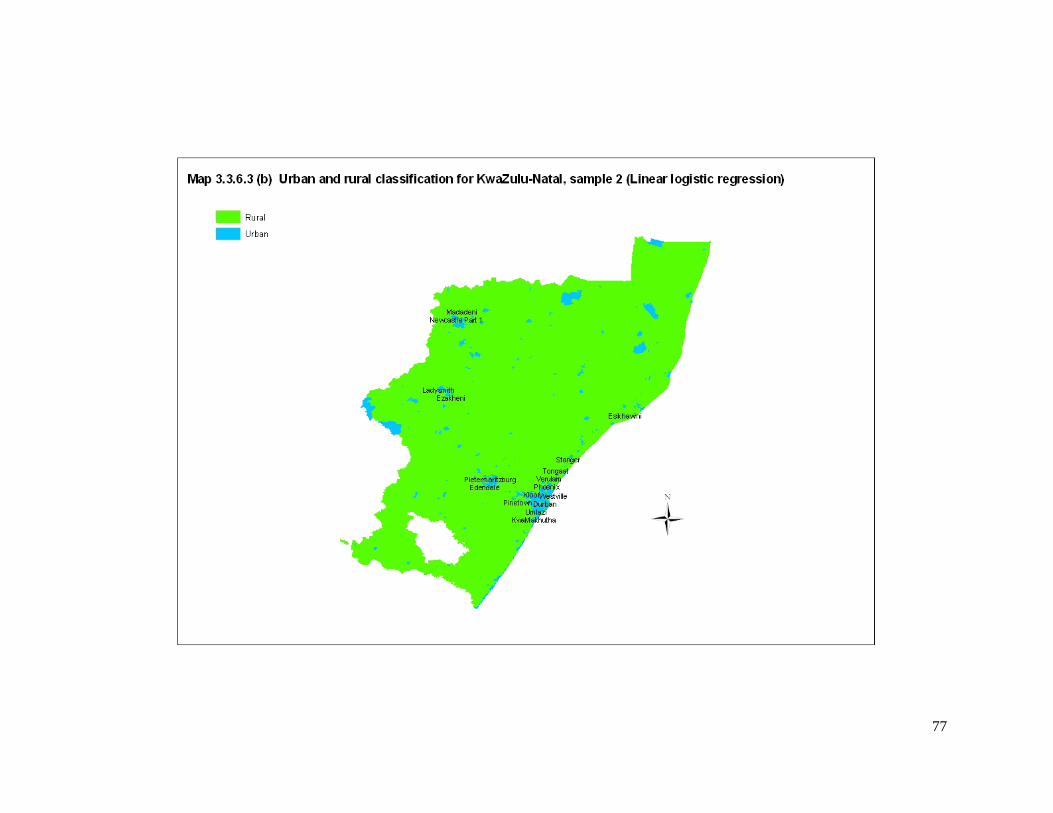
77

78

79

80

81
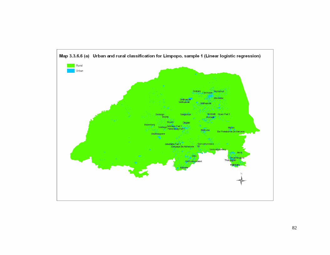
82
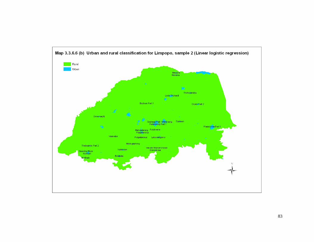
83

84

85

86
3.4 Chapter summary and conclusion In this chapter detailed discussions of the applications, methodologies and results were
presented for the non-spatial statistical techniques, namely linear logistic regression,
classification trees and discriminant analysis.
Generally, the results (i.e. significant variables, misclassification rates and population
aggregates) obtained for all three statistical techniques for both samples, are more or
less similar within each sample, but differ between the two samples.
From the three statistical techniques, classification trees provide combinations of
significant variables for assigning areas into urban and rural, whilst linear logistic
regression and discriminant analysis give more information, that is, both are able to
separate significant variables more clearly for urban and rural. Thus combining the
results obtained from linear logistic regression and discriminant analysis for sample 1
shows that variables such as population density, unemployed persons, number of
children ever born i.e. 0-5, persons living in informal dwellings in informal/ squatter
areas, households with flush toilets connected to sewer, households using bucket
latrines and female or White headed households, separate the urban from the rural
settlements, whilst variables such as persons with no schooling, households accessing
water from rainwater tanks or rivers/streams, households using wood or paraffin as the
main source of energy for cooking, and head of household occupation is skilled
agriculture and fishery workers or elementary occupations, separate rural, i.e. farm
settlements. For sample 2 variables such as population density, unemployed persons,
number of children ever born i.e. 0-5, persons living in informal dwellings in
informal/squatter areas, households with flush toilets connected to sewer, households
using bucket latrines and persons who have completed primary schooling, separate the
urban settlements, whilst variables such as persons with no or some primary schooling,
households using wood or paraffin as the main source of energy for cooking, head of
household occupation is skilled agriculture and fishery workers or elementary
occupations, persons living in traditional/hut structures, African headed households,
households with chemical toilets or pit latrines, larger household sizes i.e. 10 or more,
households with no annual income and persons whose employment status is
homemaker or housewife, separate rural i.e. farm and tribal settlements. Combining all
the significant variables obtained from both samples for urban settlement, can be

87
assumed to separate urban settlements from rural, and common significant variables
obtained between both samples for rural, can separate rural, i.e. farm settlements,
whilst variables that are not common for rural between the two samples, can be
assumed to separate out rural, i.e. tribal settlements. Such variables are persons living
in traditional/hut structures, African headed households, households with chemical
toilets or pit latrines, larger household sizes i.e. 10 or more, households with no annual
income and persons whose employment status is homemaker or housewife.
Results from the confusion matrices, section 3.3.4, show that there are provinces for
both samples that have large misclassifications (above 10%), however, looking at
these more critically, their actual figures are relatively small when compared to the total
number of EAs in the samples.
Generally, the population figures obtained, based on the classifications produced by
the models for sample 1, are very different from the population totals for both censuses
(and sometimes differ markedly amongst themselves), whilst in contrast, those
produced by the models based on sample 2 generally agree amongst themselves and
with the population figures obtained from the censuses. This is due to the sampling
methodology for sample 2 that predefines the classification of tribal settlements as
rural, which is the same classification for both censuses, whilst for sample 1, large
parts of tribal areas are classified as urban.
The next chapter contains the analysis using spatial statistical techniques.

88
CHAPTER 4 - Spatial Data Application and Results
4.1 Introduction The previous chapter discussed in detail the classification of areas into urban and rural
using non-spatial statistical techniques, i.e. linear logistic regression, classification
trees and discriminant analysis. In this chapter, spatial statistical techniques, namely 1)
straight-majority-rule, and 2) Iterated Conditional Modes (ICM) based on the principles
of Markov Random Fields, are applied to the classification of urban and rural.
The motivation for making use of spatial statistical techniques is mainly because the
classification of areas into urban and rural is a spatial matter; this was included to
explore the impact of similarities amongst adjacent areas in the urban and rural
classification.
In this chapter the spatial statistical application is explained. The results from the
spatial data applications are summarised and presented.
4.2 Methodology 4.2.1 Straight-majority-rule Straight-majority-rule is an iterative procedure for determining the urban or rural status
of a particular enumeration area (say X) based on the urban or rural status of its
neighbouring enumeration areas. As the name implies, the urban or rural classification
for X is based on the status of the majority of its neighbouring or surrounding
enumeration areas. For the process, a neighbourhood (say Z) was defined as all
enumeration areas touching (topologically connected to) that particular enumeration
area (i.e. X). Each enumeration area was initially (iteration 0) assigned an urban or
rural status based on the results with the lowest misclassification rates obtained from
the non-spatial statistical techniques discussed in Chapter 3. Subsequent iterations
made use of the results of previous iterations to determine the urban/rural status of
each X, until stability was reached, i.e. no further changes to X based on Z, occurred.
The enumeration areas that changed for each iteration were recorded and the
population totals were aggregated. In order to compare the results with those obtained
in the non-spatial statistical techniques, the areas of known urban or rural status, as

89
defined in Chapter 3, remained unchanged, and were used in the procedure to
determine the status of unknown areas.
Finally a misclassification rate for each province and for South Africa as a whole was
calculated, based on the results of the final iteration. Areas of known urban and rural
status were iterated once to redetermine their urban and rural status based on the
results of the final iteration. A misclassification rate was calculated by taking the known
areas that changed urban or rural status, divided by the total number of known areas.
The correctly and incorrectly classified EAs are shown in Table 4.3.1.11. This method
to calculate the misclassification rate was used since the areas of known urban and
rural status were excluded from each iteration.
Straight-majority-rule was applied for each province and for South Africa. The results
are presented in Section 4.3.1.
4.2.2 Markov Random Fields Based on the principles of Markov Random Fields and Bayesian analysis, ICM was
used. The method made use of a likelihood and a prior probability to produce a
posterior probability. For the likelihood, the density function obtained from the non-
spatial statistical technique, i.e. discriminant analysis, was used. That is, using a
Multivariate Normal model,
( )( )
( ) ( )( ) ( ) ( )( )''1| 12/112/12/2
xye xiyixye xiyixy iiiipiif μμ μμ −∝−Σ
= ∑∑Π
−⎟⎠⎞⎜
⎝⎛ −−−⎟
⎠⎞⎜
⎝⎛ −−
where ),...,( 1 yyy piii = are the significant census variables from the discriminant
analysis for each enumeration area, ( )xiμ is the mean vector of the class xi (i.e.
urbanxi = or rural ) and ∑ is the common covariance matrix of the .'sy
For the prior probability, the Markov Random Field model as stated in Besag (1986)
was adapted for our application,
( )( )
( )∑=
=⋅ c
l
lu
ku
ii
i
e
ekp
1
|β
β
.

90
This assigns conditional probability to the class k at pixel i , given the classes in the
neighbouring pixels, where ( )lui denotes the number of neighbours of i having colour
,l and β is a fixed parameter. According to Besag (1986) 5.1=β works well and was
used in the calculations.
Thus the conditional prior probability in the case of urban is
[ ]ee
eoodneighbourhinEAsruralofnumberoodneighbourhinEAsurbanofnumber
oodneighbourhinEAsurbanofnumberclassesngneighbouriUrbanP _____*5.1_____*5.1
_____*5.1_|
+∝
and for rural is
[ ]ee
eoodneighbourhinEAsruralofnumberoodneighbourhinEAsurbanofnumber
oodneighbourhinEAsruralofnumberclassesngneighbouriRuralP
_____*5.1_____*5.1
_____*5.1_|
+∝
.
The likelihood and prior probabilities were multiplied by each other to give a posterior
probability. EAs were assigned an urban or rural classification based on the larger of
the two probabilities, i.e. if the urban probability was larger than the rural probability
then the EA was classified as urban, similarly if the rural probability was larger, the EA
was classified as rural.
The process was iterated until no further changes to X based on Z, occurred. The
enumeration areas that changed for each iteration were recorded and population totals
were aggregated. In order to compare results with those obtained in the non-spatial
statistical techniques, the areas of known urban or rural status, as defined in Chapter 3,
remained unchanged, and were used in the simulation to determine the status of
unknown areas.
Finally a misclassification rate for each province and for South Africa as a whole was
estimated in a similar manner as for straight-majority-rule.
ICM was run for each province and for South Africa. The results are presented in
Section 4.3.2.

91
4.3 Results 4.3.1 Results for Straight-majority-rule Based on the methodology described in Chapter 2, straight-majority-rule was applied
for each province and for South Africa as a whole. The tables in this section are shown
in two parts. Tables 4.3.1.1-10 (Part 1) show the number of EAs that changed from the
original classification for each province and for South Africa. Iteration 0 gives the
number of EAs classified as rural and urban for the original (un-iterated) classification.
The number of EAs that changed for each iteration is expressed as a percentage of the
number of rural and urban EAs of the original classification (iteration 0). Table 4.3.1.1-
10 (Part 2) shows the aggregated population for the original classification (iteration 0)
and for other iterations as a result of the changes in EA classification. Please note that
the population figures are slightly different from those given in Chapter 3; this is a result
of the random rounding used by Statistics South Africa in SuperCross4. Table 4.3.1.11
shows the estimated number (and percent) of correctly and incorrectly classified EAs
for straight-majority-rule, for each province and for South Africa.
In general, most provinces show that many EAs, i.e. unknown status EAs, have
changed urban/rural status, mainly in the first iteration. Although some provinces such
as the Western Cape, Northern Cape, Free State and Gauteng show large changes in
the EA classification, these changes have little or no impact on the population
aggregations. This is mainly due to changes of low population rural EAs to urban. The
Eastern Cape on the other hand shows the opposite; there smaller changes in EA
classification, have a larger impact on the population aggregates. Similar results are
evident for KwaZulu-Natal and Limpopo. Although there are changes in the EA
classification, these changes have little or no impact on the population aggregates for
sample 2.
4 SuperCross is the software used by Statistics South Africa to disseminate census data. To prevent disclosure of information that is less than 5, random rounding is used.

92
Table 4.3.1.1 (Part 1) Western Cape - Comparison of the number of EAs that changed for Straight-
majority-rule
Iterations 0 1 2 3 4
Western Cape (Sample 1 - Urban-Farm) No. of EAs that changed: Rural to Urban 150 97 2 0 0 Urban to Rural 979 94 5 1 0 TOTAL 1129 191 7 1 0 % EAs that changed: Rural to Urban % 65 1 0 0 Urban to Rural % 10 1 0 0 TOTAL % 17 1 0 0 Western Cape (Sample 2 - Urban-Farm-Tribal) No. of EAs that changed: Rural to Urban 83 49 2 0 0 Urban to Rural 1046 113 5 1 0 TOTAL 1129 162 7 1 0
% EAs that changed: Rural to Urban % 59 2 0 0 Urban to Rural % 11 0 0 0 TOTAL % 14 1 0 0
Table 4.3.1.1 (Part 2) Western Cape - Comparison of the population changes for Straight-majority-
rule
Iterations 0 1 2 3 4 Western Cape (Sample 1 - Urban-Farm) Rural 447271 463016 463135 463603 463603 Urban 4077044 4061299 4061180 4060712 4060712 TOTAL 4524315 4524315 4524315 4524315 4524315 Rural % 10 10 10 10 10 Urban % 90 90 90 90 90 TOTAL % 100 100 100 100 100 Western Cape (Sample 2 - Urban-Farm-Tribal) Rural 437329 462473 463135 463603 463603 Urban 4086986 4061842 4061180 4060712 4060712 TOTAL 4524315 4524315 4524315 4524315 4524315 Rural % 10 10 10 10 10 Urban % 90 90 90 90 90
TOTAL % 100 100 100 100 100

93
Table 4.3.1.2 (Part 1) Eastern Cape - Comparison of the number of EAs that changed for Straight-
majority-rule
Iterations 0 1 2 3 4 5 6 7 8 9 10 11 12 13
Eastern Cape (Sample 1 - Urban-Farm) No. of EAs that changed: Rural to Urban 4986 1030 303 54 14 11 4 0 0 0 0 0 0 0 Urban to Rural 9834 5544 676 270 170 80 67 34 19 16 20 5 4 0 TOTAL 14820 6574 979 324 184 91 71 34 19 16 20 5 4 0 % EAs that changed: Rural to Urban % 21 6 1 0 0 0 0 0 0 0 0 0 0 Urban to Rural % 56 7 3 2 1 1 0 0 0 0 0 0 0 TOTAL % 44 7 2 1 1 0 0 0 0 0 0 0 0 Eastern Cape (Sample 2 - Urban-Farm-Tribal) No. of EAs that changed: Rural to Urban 4229 170 22 4 2 2 0 Urban to Rural 889 158 7 0 0 0 0 TOTAL 5118 328 29 4 2 2 0 % EAs that changed: Rural to Urban % 4 1 0 0 0 0 Urban to Rural % 18 1 0 0 0 0 TOTAL % 6 1 0 0 0 0

94
Table 4.3.1.2 (Part 2) Eastern Cape - Comparison of the population changes for Straight-majority-rule
Iterations 0 1 2 3 4 5 6 7 8 9 10 11 12 13 Eastern Cape (Sample 1 - Urban-Farm) Rural 415002 2497810 2603600 2673286 2722777 2743139 2761762 2771487 2778071 2782259 2787555 2789863 2790579 2790579 Urban 6021694 3938885 3833095 3763410 3713919 3693557 3674934 3665209 3658625 3654437 3649140 3646833 3646117 3646117 TOTAL 6436696 6436696 6436696 6436696 6436696 6436696 6436696 6436696 6436696 6436696 6436696 6436696 6436696 6436696 Rural % 6 39 40 42 42 43 43 43 43 43 43 43 43 43 Urban % 94 61 60 58 58 57 57 57 57 57 57 57 57 57 TOTAL % 100 100 100 100 100 100 100 100 100 100 100 100 100 100 Eastern Cape (Sample 2 - Urban-Farm-Tribal) Rural 4039569 4055956 4049901 4049188 4049185 4048393 4048393 Urban 2397126 2380740 2386795 2387507 2387510 2388302 2388302 TOTAL 6436696 6436696 6436696 6436696 6436696 6436696 6436696 Rural % 63 63 63 63 63 63 63 Urban % 37 37 37 37 37 37 37 TOTAL % 100 100 100 100 100 100 100

95
Table 4.3.1.3 (Part 1) Northern Cape - Comparison of the number of EAs that changed for Straight-
majority-rule
Iterations 0 1 2 3
Northern Cape (Sample 1 - Urban-Farm) No. of EAs that changed: Rural to Urban 40 23 2 0 Urban to Rural 154 53 2 0 TOTAL 194 76 4 0 % EAs that changed: Rural to Urban % 58 5 0 Urban to Rural % 34 1 0 TOTAL % 39 2 0 Northern Cape (Sample 2 - Urban-Farm-Tribal) No. of EAs that changed: Rural to Urban 77 43 4 0 Urban to Rural 96 24 0 0 TOTAL 173 67 4 0 % EAs that changed: Rural to Urban % 56 5 0 Urban to Rural % 25 0 0 TOTAL % 39 2 0
Table 4.3.1.3 (Part 2) Northern Cape - Comparison of the population changes for Straight-majority-
rule
Iterations 0 1 2 3 Northern Cape (Sample 1 - Urban-Farm) Rural 147038 158365 156435 156435 Urban 675681 664354 666284 666284 TOTAL 822719 822719 822719 822719 Rural % 18 19 19 19 Urban % 82 81 81 81 TOTAL % 100 100 100 100 Northern Cape (Sample 2 - Urban-Farm-Tribal) Rural 159997 162528 160107 160107 Urban 662722 660191 662612 662612 TOTAL 822719 822719 822719 822719 Rural % 19 20 19 19 Urban % 81 80 81 81 TOTAL % 100 100 100 100

96
Table 4.3.1.4 (Part 1) Free State - Comparison of the number of EAs that changed for Straight-
majority-rule
Iterations 0 1 2 3 4
Free State (Sample 1 - Urban-Farm) No. of EAs that changed: Rural to Urban 206 154 22 1 0 Urban to Rural 1158 106 13 0 0 TOTAL 1364 260 35 1 0 % EAs that changed: Rural to Urban % 75 11 0 0 Urban to Rural % 9 1 0 0 TOTAL % 19 3 0 0 Free State (Sample 2 - Urban-Farm-Tribal) No. of EAs that changed: Rural to Urban 135 81 10 1 0 Urban to Rural 642 70 8 2 0 TOTAL 777 151 18 3 0 % EAs that changed: Rural to Urban % 60 7 1 0 Urban to Rural % 11 1 0 0 TOTAL % 19 2 0 0
Table 4.3.1.4 (Part 2) Free State - Comparison of the population changes that changed for Straight-
majority-rule
Iterations 0 1 2 3 4 Rural 401239 431336 431001 430802 430802 Urban 2305526 2275429 2275764 2275963 2275963 TOTAL 2706765 2706765 2706765 2706765 2706765 Rural % 15 16 16 16 16 Urban % 85 84 84 84 84 TOTAL % 100 100 100 100 100 Rural 673832 674583 677720 679023 679023 Urban 2032932 2032182 2029045 2027742 2027742 TOTAL 2706765 2706765 2706765 2706765 2706765 Rural % 25 25 25 25 25 Urban % 75 75 75 75 75 TOTAL % 100 100 100 100 100

97
Table 4.3.1.5 (Part 1) KwaZulu-Natal - Comparison of the number of EAs that changed for Straight-majority-rule
Iterations
0 1 2 3 4 5 6 7 8 9 10 11 12KwaZulu-Natal (Sample 1 - Urban-Farm) No. of EAs that changed: Rural to Urban 5263 351 51 7 2 0 0 0 0 0 0 0 0 Urban to Rural 2732 434 84 36 8 6 3 3 3 4 2 6 0 TOTAL 7995 785 135 43 10 6 3 3 3 4 2 6 0 % EAs that changed: Rural to Urban % 7 1 0 0 0 0 0 0 0 0 0 0 Urban to Rural % 16 3 1 0 0 0 0 0 0 0 0 0 TOTAL % 10 2 1 0 0 0 0 0 0 0 0 0 KwaZulu-Natal (Sample 2 - Urban-Farm-Tribal) No. of EAs that changed: Rural to Urban 938 325 32 13 1 0 0 0 0 0 Urban to Rural 1412 167 18 8 9 6 5 4 1 0 TOTAL 2350 492 50 21 10 6 5 4 1 0 % EAs that changed: Rural to Urban % 35 3 1 0 0 0 0 0 0 Urban to Rural % 12 1 1 1 0 0 0 0 0 TOTAL % 21 2 1 0 0 0 0 0 0

98
Table 4.3.1.5 (Part 2) KwaZulu-Natal - Comparison of the population changes for Straight-majority-rule
Iterations 0 1 2 3 4 5 6 7 8 9 10 11 12 KwaZulu-Natal (Sample 1 - Urban-Farm) Rural 4307043 4570182 4602660 4629297 4635344 4639790 4641194 4642844 4644672 4647187 4648260 4651991 4651991Urban 5118948 4855809 4823331 4796694 4790647 4786201 4784797 4783147 4781319 4778804 4777731 4774000 4774000TOTAL 9425991 9425991 9425991 9425991 9425991 9425991 9425991 9425991 9425991 9425991 9425991 9425991 9425991 Rural % 46 48 49 49 49 49 49 49 49 49 49 49 49 Urban % 54 52 51 51 51 51 51 51 51 51 51 51 51 TOTAL % 100 100 100 100 100 100 100 100 100 100 100 100 100 KwaZulu-Natal (Sample 2 - Urban-Farm-Tribal) Rural 5419941 5400010 5396923 5393442 5398616 5403147 5406929 5409219 5409897 5409897 Urban 4006050 4025981 4029068 4032549 4027375 4022844 4019062 4016772 4016094 4016094 TOTAL 9425991 9425991 9425991 9425991 9425991 9425991 9425991 9425991 9425991 9425991 Rural % 57 57 57 57 57 57 57 57 57 57 Urban % 43 43 43 43 43 43 43 43 43 43 TOTAL % 100 100 100 100 100 100 100 100 100 100

99
Table 4.3.1.6 (Part 1) North West - Comparison of the number of EAs that changed for Straight-majority-rule
Iterations
0 1 2 3 4 5 6 North West (Sample 1 - Urban-Farm) No. of EAs that changed: Rural to Urban 632 273 164 17 6 0 0 Urban to Rural 3551 635 57 12 2 1 0 TOTAL 4183 908 221 29 8 1 0 % EAs that changed: Rural to Urban % 43 26 3 1 0 0 Urban to Rural % 18 2 0 0 0 0 TOTAL % 22 5 1 0 0 0 North West (Sample 2 - Urban-Farm-Tribal) No. of EAs that changed: Rural to Urban 756 105 27 3 2 0 Urban to Rural 244 78 15 3 3 0 TOTAL 1000 183 42 6 5 0 % EAs that changed: Rural to Urban % 14 4 0 0 0 Urban to Rural % 32 6 1 1 0 TOTAL % 18 4 1 1 0
Table 4.3.1.6 (Part 2) North West - Comparison of the population changes for Straight-majority-rule
Iterations 0 1 2 3 4 5 6 North West (Sample 1 - Urban-Farm) Rural 391725 673916 640804 641912 642675 643880 643880 Urban 3277611 2995420 3028532 3027424 3026662 3025456 3025456TOTAL 3669336 3669336 3669336 3669336 3669336 3669336 3669336 Rural % 11 18 17 17 18 18 18 Urban % 89 82 83 83 82 82 82 TOTAL % 100 100 100 100 100 100 100
North West (Sample 2 - Urban-Farm-Tribal) Rural 2309290 2308127 2299833 2299972 2301475 2301475 Urban 1360046 1361209 1369503 1369364 1367861 1367861 TOTAL 3669336 3669336 3669336 3669336 3669336 3669336 Rural % 63 63 63 63 63 63 Urban % 37 37 37 37 37 37 TOTAL % 100 100 100 100 100 100

100
Table 4.3.1.7 (Part 1) Gauteng - Comparison of the number of EAs that changed for Straight-majority-rule
Iterations
0 1 2 3 4 Gauteng (Sample 1 - Urban-Farm) No. of EAs that changed: Rural to Urban 320 162 16 1 0 Urban to Rural 3201 90 8 0 0 TOTAL 3521 252 24 1 0
% EAs that changed: Rural to Urban % 51 5 0 0 Urban to Rural % 3 0 0 0 TOTAL % 7 1 0 0 Gauteng (Sample 2 - Urban-Farm-Tribal) No. of EAs that changed: Rural to Urban 320 158 21 1 0 Urban to Rural 3201 91 8 0 0 TOTAL 3521 249 29 1 0
% EAs that changed: Rural to Urban % 49 7 0 0 Urban to Rural % 3 0 0 0 TOTAL % 7 1 0 0
Table 4.3.1.7 (Part 2) Gauteng - Comparison of the population changes for Straight-majority-rule
Iterations 0 1 2 3 4 Gauteng (Sample 1 - Urban-Farm) Rural 321624 328264 326083 325725 325725 Urban 8515456 8508816 8510997 8511355 8511355 TOTAL 8837080 8837080 8837080 8837080 8837080 Rural % 4 4 4 4 4 Urban % 96 96 96 96 96 TOTAL % 100 100 100 100 100 Gauteng (Sample 2 - Urban-Farm-Tribal) Rural 321624 332204 326083 325725 325725 Urban 8515456 8504877 8510997 8511355 8511355 TOTAL 8837080 8837080 8837080 8837080 8837080 Rural % 4 4 4 4 4 Urban % 96 96 96 96 96 TOTAL % 100 100 100 100 100

101
Table 4.3.1.8 (Part 1) Mpumalanga - Comparison of the number of EAs that changed for Straight-majority-rule
Iterations
0 1 2 3 4 5 6 7 8 Mpumalanga (Sample 1 - Urban-Farm) No. of EAs that changed: Rural to Urban 451 266 86 13 4 0 0 0 0 Urban to Rural 2804 279 41 16 11 2 2 1 0 TOTAL 3255 545 127 29 15 2 2 1 0 % EAs that changed: Rural to Urban % 59 19 3 1 0 0 0 0 Urban to Rural % 10 1 1 0 0 0 0 0 TOTAL % 17 4 1 0 0 0 0 0 Mpumalanga (Sample 2 - Urban-Farm-Tribal) No. of EAs that changed: Rural to Urban 270 70 13 3 0 Urban to Rural 613 204 14 4 0 TOTAL 883 274 27 7 0 % EAs that changed: Rural to Urban % 26 5 1 0 Urban to Rural % 33 2 1 0 TOTAL % 31 3 1 0
Table 4.3.1.8 (Part 2) Mpumalanga - Comparison of the population changes for Straight-majority-rule
Iterations 0 1 2 3 4 5 6 7 8Mpumalanga (Sample 1 - Urban-Farm) Rural 559846 690720 676808 679365 681743 683080 684366 685595 685595 Urban 2563107 2432233 2446145 2443588 2441210 2439873 2438587 2437358 2437358 TOTAL 3122953 3122953 3122953 3122953 3122953 3122953 3122953 3122953 3122953 Rural % 18 22 22 22 22 22 22 22 22 Urban % 82 78 78 78 78 78 78 78 78 TOTAL % 100 100 100 100 100 100 100 100 100 Mpumalanga (Sample 2 - Urban-Farm-Tribal) Rural 1887935 1902785 1900620 1900371 1900371 Urban 1235018 1220168 1222333 1222582 1222582 TOTAL 3122953 3122953 3122953 3122953 3122953 Rural % 60 61 61 61 61 Urban % 40 39 39 39 39 TOTAL % 100 100 100 100 100

102
Table 4.3.1.9 (Part 1) Limpopo - Comparison of the number of EAs that changed for Straight-majority-rule
Iterations
0 1 2 3 4 5 6 7 8 9 10 Limpopo (Sample 1 - Urban-Farm) No. of EAs that changed:
Rural to Urban 2512 555 242 34 13 4 0 0 0 0 0 Urban to Rural 6741 1866 261 95 50 16 3 9 2 1 0 TOTAL 9253 2421 503 129 63 20 3 9 2 1 0
% EAs that changed: Rural to Urban % 22 10 1 1 0 0 0 0 0 0 Urban to Rural % 28 4 1 1 0 0 0 0 0 0 TOTAL % 26 5 1 1 0 0 0 0 0 0 Limpopo (Sample 2 - Urban-Farm-Tribal) No. of EAs that changed: Rural to Urban 804 51 7 1 0 Urban to Rural 147 69 6 0 0 TOTAL 951 120 13 1 0
% EAs that changed: Rural to Urban % 6 1 0 0 Urban to Rural % 47 4 0 0 TOTAL % 13 1 0 0

103
Table 4.3.1.9 (Part 2) Limpopo - Comparison of the population changes for Straight-majority-rule
Iterations
0 1 2 3 4 5 6 7 8 9 10 Limpopo (Sample 1 - Urban-Farm)
Rural 1104155 2021332 2047635 2080534 2097822 2101968 2103214 2108775 2109960 2110712 2110712
Urban 4169405 3252227 3225924 3193025 3175738 3171592 3170346 3164784 3163600 3162847 3162847
TOTAL 5273559 5273559 5273559 5273559 5273559 5273559 5273559 5273559 5273559 5273559 5273559
Rural % 21 38 39 39 40 40 40 40 40 40 40
Urban % 79 62 61 61 60 60 60 60 60 60 60
TOTAL % 100 100 100 100 100 100 100 100 100 100 100
Limpopo (Sample 2 - Urban-Farm-Tribal)
Rural 4724829 4747178 4747431 4747431 4747431
Urban 548730 526381 526129 526129 526129
TOTAL 5273559 5273559 5273559 5273559 5273559
Rural % 90 90 90 90 90
Urban % 10 10 10 10 10
TOTAL % 100 100 100 100 100

104
Table 4.3.1.10 (Part 1) RSA - Comparison of the number of EAs that changed for Straight-majority-rule
Iterations
0 1 2 3 4 5 6 7 8 9 10 11 12 RSA (Sample 1 - Urban-Farm) No. of EAs that changed:
Rural to Urban 30310 2096 406 79 16 4 2 0 0 0 0 0 0
Urban to Rural 15404 3831 534 196 84 41 17 7 12 7 5 6 0
TOTAL 45714 5927 940 275 100 45 19 7 12 7 5 6 0
% EAs that changed:
Rural to Urban % 7 1 0 0 0 0 0 0 0 0 0 0
Urban to Rural % 25 3 1 1 0 0 0 0 0 0 0 0
TOTAL % 13 2 1 0 0 0 0 0 0 0 0 0
RSA (Sample 2 - Urban-Farm-Tribal) No. of EAs that changed:
Rural to Urban 7857 1249 144 19 4 4 0 0 0
Urban to Rural 8045 853 113 25 9 6 2 1 0
TOTAL 15902 2102 257 44 13 10 2 1 0
% EAs that changed:
Rural to Urban % 16 2 0 0 0 0 0 0
Urban to Rural % 11 1 0 0 0 0 0 0
TOTAL % 13 2 0 0 0 0 0 0

105
Table 4.3.1.10 (Part 2) RSA - Comparison of the population changes for Straight-majority-rule
Iterations
0 1 2 3 4 5 6 7 8 9 10 11 12 RSA (Sample 1 - Urban-Farm) Rural 15165704 16883147 17006880 17094838 17128266 17145887 17153330 17157021 17162879 17167083 17169756 17173487 17173487
Urban 29653710 27936267 27812534 27724576 27691148 27673527 27666085 27662394 27656535 27652332 27649658 27645927 27645927
TOTAL 44819414 44819414 44819414 44819414 44819414 44819414 44819414 44819414 44819414 44819414 44819414 44819414 44819414
Rural % 34 38 38 38 38 38 38 38 38 38 38 38 38
Urban % 66 62 62 62 62 62 62 62 62 62 62 62 62
TOTAL % 100 100 100 100 100 100 100 100 100 100 100 100 100
RSA (Sample 2 - Urban-Farm-Tribal) Rural 19816833 19993842 19986709 19989986 19995653 19998151 19999568 20000033 20000033 Urban 25002581 24825572 24832705 24829428 24823761 24821263 24819846 24819381 24819381 TOTAL 44819414 44819414 44819414 44819414 44819414 44819414 44819414 44819414 44819414 Rural % 44 45 45 45 45 45 45 45 45 Urban % 56 55 55 55 55 55 55 55 55 TOTAL % 100 100 100 100 100 100 100 100 100
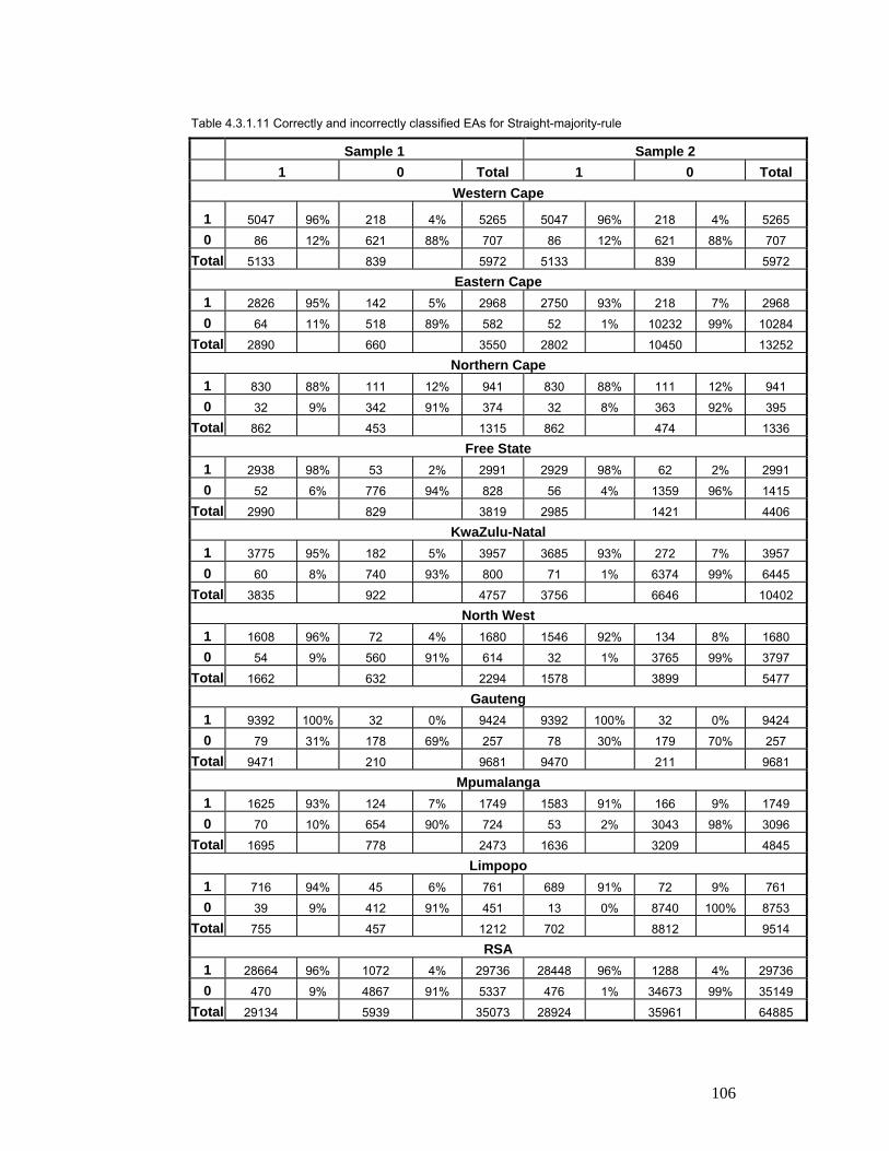
106
Table 4.3.1.11 Correctly and incorrectly classified EAs for Straight-majority-rule
Sample 1 Sample 2 1 0 Total 1 0 Total
Western Cape
1 5047 96% 218 4% 5265 5047 96% 218 4% 5265
0 86 12% 621 88% 707 86 12% 621 88% 707
Total 5133 839 5972 5133 839 5972
Eastern Cape 1 2826 95% 142 5% 2968 2750 93% 218 7% 2968
0 64 11% 518 89% 582 52 1% 10232 99% 10284
Total 2890 660 3550 2802 10450 13252
Northern Cape 1 830 88% 111 12% 941 830 88% 111 12% 941
0 32 9% 342 91% 374 32 8% 363 92% 395
Total 862 453 1315 862 474 1336
Free State 1 2938 98% 53 2% 2991 2929 98% 62 2% 2991
0 52 6% 776 94% 828 56 4% 1359 96% 1415
Total 2990 829 3819 2985 1421 4406
KwaZulu-Natal 1 3775 95% 182 5% 3957 3685 93% 272 7% 3957
0 60 8% 740 93% 800 71 1% 6374 99% 6445
Total 3835 922 4757 3756 6646 10402
North West 1 1608 96% 72 4% 1680 1546 92% 134 8% 1680
0 54 9% 560 91% 614 32 1% 3765 99% 3797
Total 1662 632 2294 1578 3899 5477
Gauteng 1 9392 100% 32 0% 9424 9392 100% 32 0% 9424
0 79 31% 178 69% 257 78 30% 179 70% 257
Total 9471 210 9681 9470 211 9681
Mpumalanga 1 1625 93% 124 7% 1749 1583 91% 166 9% 1749
0 70 10% 654 90% 724 53 2% 3043 98% 3096
Total 1695 778 2473 1636 3209 4845
Limpopo 1 716 94% 45 6% 761 689 91% 72 9% 761
0 39 9% 412 91% 451 13 0% 8740 100% 8753
Total 755 457 1212 702 8812 9514
RSA 1 28664 96% 1072 4% 29736 28448 96% 1288 4% 29736
0 470 9% 4867 91% 5337 476 1% 34673 99% 35149
Total 29134 5939 35073 28924 35961 64885

107
Represented in the maps below is a selection of a few provinces, where the changes in
EA classification have a large impact on the population aggregates. The final iteration
for each province is mapped. The red polygons on the map show areas that have
changed.
Eastern Cape – Map 4.3.1 (a)
For the Eastern Cape for sample 1, straight-majority-rule iterates 13 times before
reaching stability. In the first iteration 44% of EAs changed classifications, 21%
changed from rural to urban and 56% from urban to rural. The largest difference in
population occurs in the first iteration where the rural population increases from 6% at
the initial un-iterated setting to 39% in the first iteration, whilst the urban population
drops from 94% to 61%. For the other iterations smaller changes in population occur.
This has mainly occurred in the tribal and vacant areas of the Eastern Cape. For
sample 2, the process iterates 6 times before reaching stability. The population
percentages remain unchanged.
North West – Map 4.3.1 (b) For the North West for sample 1, straight-majority-rule iterates 6 times before reaching
stability. In the first iteration 22% of EAs changed classifications, 43% changed from
rural to urban and 18% from urban to rural. The largest difference in population occurs
in the first iteration where the rural population increases from 11% at the initial un-
iterated setting to 18% in the first iteration, whilst the urban population drops from 89%
to 82%. For the other iterations smaller changes in population occur. These occur
mainly in the tribal and vacant areas, as well as areas with informal settlements in the
North West. For sample 2, the process iterates 5 times before reaching stability. The
population percentages remain unchanged.
Mpumalanga – Map 4.3.1 (c)
For Mpumalanga for sample 1, straight-majority-rule iterates 8 times before reaching
stability. In the first iteration 17% EAs changed classifications, 59% changed from rural
to urban and 10% from urban to rural. The largest difference in population occurs in the
first iteration where the rural population increases from 18% at the initial un-iterated
setting to 22% in the first iteration, whilst the urban population drops from 82% to 78%.
For the other iterations smaller changes in population occur. These occur mainly in the
tribal and vacant areas of Mpumalanga. For sample 2, the process iterates 4 times

108
before reaching stability. The population percentages change slightly in iteration 1
thereafter remain unchanged.
Limpopo – Map 4.3.1 (d) For Limpopo for sample 1, straight-majority-rule iterates 10 times before reaching
stability. In the first iteration 26% EAs changed classifications, 22% changed from rural
to urban and 28% from urban to rural. The largest difference in population occurs in the
first iteration where the rural population increases from 21% at the initial un-iterated
setting to 38% in the first iteration, whilst the urban population drops from 79% to 62%.
For the other iterations smaller changes in population occur. These occur mainly in the
tribal and vacant areas of Limpopo. For sample 2, the process iterates 4 times before
reaching stability. The population percentages remain unchanged.

109

110

111

112

113
4.3.2 Results for ICM Based on the methodology described in Chapter 2, ICM was applied for each province and for
South Africa as a whole. The tables below are similar to those presented in section 4.3.1. Tables
4.3.2.1-10 (Part 1) show the number of EAs that changed from the original classification for each
province and for South Africa, in this case the original classification was the results as obtained
from the non-spatial statistical method, that is discriminant analysis. Tables 4.3.2.1-10 (Part 2)
show the aggregated population for the original classification (iteration 0) and for other iterations as
a result of the changes in EA classification. Table 4.3.2.11 shows the number (and percentage) of
correctly and incorrectly classified EAs for ICM, for each province and for South Africa.
In general, the results are very similar to those obtained for straight-majority-rule. However,
comparing Tables 4.3.1.11 and 4.3.2.11 there are more correctly classified EAs for ICM for all
provinces than for straight-majority-rule. In some cases, for example the Eastern Cape, KwaZulu-
Natal, Limpopo and Mpumalanga, the number of iterations is less for ICM than straight-majority-
rule.
Table 4.3.2.1 (Part 1) Western Cape - Comparison of the number of EAs that changed for ICM
Iterations 0 1 2 3
Western Cape (Sample 1 - Urban-Farm)
No. of EAs that changed:
Rural to Urban 249 113 3 0
Urban to Rural 880 3 0 0
TOTAL 1129 116 3 0
% EAs that changed:
Rural to Urban % 45 1 0
Urban to Rural % 0 0 0
TOTAL % 10 0 0
Western Cape (Sample 2 - Urban-Farm-Tribal)
No. of EAs that changed:
Rural to Urban 249 114 3 0
Urban to Rural 880 2 0 0
TOTAL 1129 116 3 0
% EAs that changed:
Rural to Urban % 46 1 0
Urban to Rural % 0 0 0
TOTAL % 10 0 0

114
Table 4.3.2.1 (Part 2) Western Cape - Comparison of the population changes for ICM
Iterations 0 1 2 3 Western Cape (Sample 1 - Urban-Farm)
Rural 461328 444663 443501 443501
Urban 4062987 4079652 4080814 4080814
TOTAL 4524315 4524315 4524315 4524315
Rural % 10 10 10 10
Urban % 90 90 90 90
TOTAL % 100 100 100 100
Western Cape (Sample 2 - Urban-Farm-Tribal)
Rural 461328 443185 442023 442023
Urban 4062987 4081130 4082292 4082292
TOTAL 4524315 4524315 4524315 4524315
Rural % 10 10 10 10
Urban % 90 90 90 90
TOTAL % 100 100 100 100
Table 4.3.2.2 (Part 1) Eastern Cape - Comparison of the number of EAs that changed for ICM
Iterations 0 1 2 3 4 5 6 7 8 9
Eastern Cape (Sample 1 - Urban-Farm) No. of EAs that changed:
Rural to Urban 8962 412 85 19 6 5 5 2 1 0
Urban to Rural 5858 1322 130 27 4 1 0 0 0 0
TOTAL 14820 1734 215 46 10 6 5 2 1 0
% EAs that changed:
Rural to Urban % 5 1 0 0 0 0 0 0 0
Urban to Rural % 23 2 0 0 0 0 0 0 0
TOTAL % 12 1 0 0 0 0 0 0 0
Eastern Cape (Sample 2 - Urban-Farm-Tribal) No. of EAs that changed:
Rural to Urban 4379 34 1 0
Urban to Rural 739 30 1 0
TOTAL 5118 64 2 0
% EAs that changed:
Rural to Urban % 1 0 0
Urban to Rural % 4 0 0
TOTAL % 1 0 0

115
Table 4.3.2.2 (Part 2) Eastern Cape - Comparison of the population changes for ICM
Iterations 0 1 2 3 4 5 6 7 8 9 Eastern Cape (Sample 1 - Urban-Farm)
Rural 2142233 2561230 2593625 2603517 2603499 2603040 2601321 2600840 2600620 2600620
Urban 4294463 3875466 3843070 3833179 3833197 3833656 3835375 3835856 3836076 3836076
TOTAL 6436696 6436696 6436696 6436696 6436696 6436696 6436696 6436696 6436696 6436696
Rural % 33 40 40 40 40 40 40 40 40 40
Urban % 67 60 60 60 60 60 60 60 60 60
TOTAL % 100 100 100 100 100 100 100 100 100 100
Eastern Cape (Sample 2 - Urban-Farm-Tribal)
Rural 4118891 4113315 4112133 4112133
Urban 2317805 2323381 2324563 2324563
TOTAL 6436696 6436696 6436696 6436696
Rural % 64 64 64 64
Urban % 36 36 36 36
TOTAL % 100 100 100 100
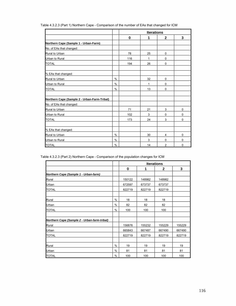
116
Table 4.3.2.3 (Part 1) Northern Cape - Comparison of the number of EAs that changed for ICM
Iterations 0 1 2 3
Northern Cape (Sample 1 - Urban-Farm)
No. of EAs that changed:
Rural to Urban 78 25 0
Urban to Rural 116 1 0
TOTAL 194 26 0
% EAs that changed:
Rural to Urban % 32 0
Urban to Rural % 1 0
TOTAL % 13 0
Northern Cape (Sample 2 - Urban-Farm-Tribal)
No. of EAs that changed:
Rural to Urban 71 21 3 0
Urban to Rural 102 3 0 0
TOTAL 173 24 3 0
% EAs that changed:
Rural to Urban % 30 4 0
Urban to Rural % 3 0 0
TOTAL % 14 2 0
Table 4.3.2.3 (Part 2) Northern Cape - Comparison of the population changes for ICM
Iterations 0 1 2 3 Northern Cape (Sample 1 - Urban-farm)
Rural 150122 148982 148982
Urban 672597 673737 673737
TOTAL 822719 822719 822719
Rural % 18 18 18
Urban % 82 82 82
TOTAL % 100 100 100
Northern Cape (Sample 2 - Urban-farm-tribal)
Rural 156876 155232 155229 155229
Urban 665843 667487 667490 667490
TOTAL 822719 822719 822719 822719
Rural % 19 19 19 19
Urban % 81 81 81 81
TOTAL % 100 100 100 100

117
Table 4.3.2.4 (Part 1) Free State - Comparison of the number of EAs that changed for ICM
Iterations
0 1 2 3 Free State (Sample 1 - Urban-Farm)
No. of EAs that changed:
Rural to Urban 1364 1280 23 0
Urban to Rural 0 0 0 0
1364 1280 23 0
% EAs that changed:
Rural to Urban % 94 2 0
Urban to Rural % 0 0 0
TOTAL % 94 2 0
Free State (Sample 2 - Urban-Farm-Tribal)
No. of EAs that changed:
Rural to Urban 121 50 3 0
Urban to Rural 656 28 0 0
777 78 3 0
% EAs that changed:
Rural to Urban % 41 2 0
Urban to Rural % 4 0 0
TOTAL % 10 0 0
Table 4.3.2.4 (Part 2) Free State - Comparison of the population changes for ICM
Iterations 0 1 2 3 Free State (Sample 1 - Urban-Farm)
Rural 1006256 391114 387569 387569
Urban 1700509 2315651 2319196 2319196
TOTAL 2706765 2706765 2706765 2706765
Rural % 37 14 14 14
Urban % 63 86 86 86
TOTAL % 100 100 100 100
Free State (Sample 2 - Urban-Farm-Tribal)
Rural 675802 661685 660876 660876
Urban 2030963 2045080 2045889 2045889
TOTAL 2706765 2706765 2706765 2706765
Rural % 25 24 24 24
Urban % 75 76 76 76
TOTAL % 100 100 100 100

118
Table 4.3.2.5 (Part 1) KwaZulu-Natal - Comparison of the number of EAs that changed for ICM
Iterations 0 1 2 3 4
KwaZulu-Natal (Sample 1 - Urban-Farm)
No. of EAs that changed:
Rural to Urban 4465 105 9 0 0
Urban to Rural 3530 264 25 3 0
TOTAL 7995 369 34 3 0
% EAs that changed:
Rural to Urban % 2 0 0 0
Urban to Rural % 7 1 0 0
TOTAL % 5 0 0 0
KwaZulu-Natal (Sample 2 - Urban-Farm-Tribal)
No. of EAs that changed:
Rural to Urban 1141 174 16 0 0
Urban to Rural 1209 115 6 1 0
TOTAL 2350 289 22 1 0
% EAs that changed:
Rural to Urban % 15 1 0 0
Urban to Rural % 10 0 0 0
TOTAL % 12 1 0 0
Table 4.3.2.5 (Part 2) KwaZulu-Natal - Comparison of the population changes for ICM
Iterations 0 1 2 3 4 KwaZulu-Natal (Urban-Farm)
Rural 3864900 3981392 3994462 3996523 3996523
Urban 5561091 5444599 5431529 5429468 5429468
TOTAL 9425991 9425991 9425991 9425991 9425991
Rural % 41 42 42 42 42
Urban % 59 58 58 58 58
TOTAL % 100 100 100 100 100
KwaZulu-Natal (Urban-Farm-Tribal)
Rural 5619928 5617604 5614250 5614436 5614436
Urban 3806063 3808387 3811741 3811555 3811555
TOTAL 9425991 9425991 9425991 9425991 9425991
Rural % 60 60 60 60 60
Urban % 40 40 40 40 40
TOTAL % 100 100 100 100 100
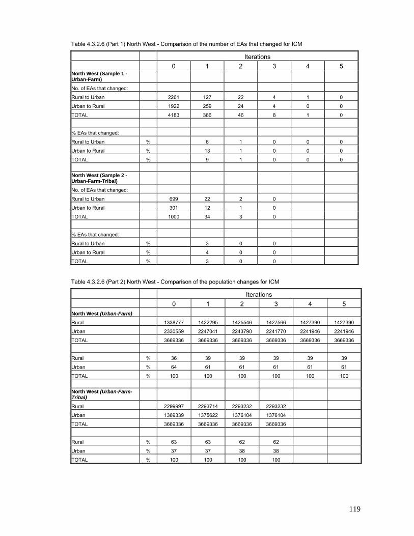
119
Table 4.3.2.6 (Part 1) North West - Comparison of the number of EAs that changed for ICM
Iterations 0 1 2 3 4 5
North West (Sample 1 - Urban-Farm)
No. of EAs that changed:
Rural to Urban 2261 127 22 4 1 0
Urban to Rural 1922 259 24 4 0 0
TOTAL 4183 386 46 8 1 0
% EAs that changed:
Rural to Urban % 6 1 0 0 0
Urban to Rural % 13 1 0 0 0
TOTAL % 9 1 0 0 0
North West (Sample 2 - Urban-Farm-Tribal)
No. of EAs that changed:
Rural to Urban 699 22 2 0
Urban to Rural 301 12 1 0
TOTAL 1000 34 3 0
% EAs that changed:
Rural to Urban % 3 0 0
Urban to Rural % 4 0 0
TOTAL % 3 0 0
Table 4.3.2.6 (Part 2) North West - Comparison of the population changes for ICM
Iterations 0 1 2 3 4 5
North West (Urban-Farm)
Rural 1338777 1422295 1425546 1427566 1427390 1427390
Urban 2330559 2247041 2243790 2241770 2241946 2241946
TOTAL 3669336 3669336 3669336 3669336 3669336 3669336
Rural % 36 39 39 39 39 39
Urban % 64 61 61 61 61 61
TOTAL % 100 100 100 100 100 100
North West (Urban-Farm-Tribal)
Rural 2299997 2293714 2293232 2293232
Urban 1369339 1375622 1376104 1376104
TOTAL 3669336 3669336 3669336 3669336
Rural % 63 63 62 62
Urban % 37 37 38 38
TOTAL % 100 100 100 100

120
Table 4.3.2.7 (Part 1) Gauteng - Comparison of the number of EAs that changed for ICM
Iterations 0 1 2 3
Gauteng (Sample 1 - Urban-Farm)
No. of EAs that changed:
Rural to Urban 242 42 0
Urban to Rural 3279 3 0
TOTAL 3521 45 0
% EAs that changed:
Rural to Urban % 17 0
Urban to Rural % 0 0
TOTAL % 1 0
Gauteng (Sample 2 - Urban-Farm-Tribal)
No. of EAs that changed:
Rural to Urban 235 70 5 0
Urban to Rural 3286 2 0 0
TOTAL 3521 72 5 0
% EAs that changed:
Rural to Urban % 30 2 0
Urban to Rural % 0 0 0
TOTAL % 2 0 0
Table 4.3.2.7 (Part 2) Gauteng - Comparison of the population changes for ICM
Iterations 0 1 2 3 Gauteng (Urban-Farm)
Rural 272071 256844 256844
Urban 8565009 8580236 8580236
TOTAL 8837080 8837080 8837080
Rural % 3 3 3
Urban % 97 97 97
TOTAL % 100 100 100
Gauteng (Urban-Farm-Tribal)
Rural 270812 253146 251838 251838
Urban 8566268 8583934 8585242 8585242
TOTAL 8837080 8837080 8837080 8837080
Rural % 3 3 3 3
Urban % 97 97 97 97
TOTAL % 100 100 100 100

121
Table 4.3.2.8 (Part 1) Mpumalanga - Comparison of the number of EAs that changed for ICM
Iterations 0 1 2 3 4 5
Mpumalanga (Sample 1 - Urban-Farm)
No. of EAs that changed:
Rural to Urban 901 143 13 4 0
Urban to Rural 2354 144 18 4 0
TOTAL 3255 287 31 8 0
% EAs that changed:
Rural to Urban % 16 1 0 0
Urban to Rural % 6 1 0 0
TOTAL % 9 1 0 0
Mpumalanga (Sample 2 - Urban-Farm-Tribal)
No. of EAs that changed:
Rural to Urban 318 57 9 5 1 0
Urban to Rural 565 128 5 2 0 0
TOTAL 883 185 14 7 1 0
% EAs that changed:
Rural to Urban % 18 3 2 0 0
Urban to Rural % 23 1 0 0 0
TOTAL % 21 2 1 0 0
Table 4.3.2.8 (Part 2) Mpumalanga - Comparison of the population changes for ICM
Iterations 0 1 2 3 4 5 Mpumalanga (Urban-Farm)
Rural 932572 925193 928789 928899 928899
Urban 2190381 2197760 2194164 2194054 2194054
TOTAL 3122953 3122953 3122953 3122953 3122953
Rural % 30 30 30 30 30
Urban % 70 70 70 70 70
TOTAL % 100 100 100 100 100
Mpumalanga (Urban-Farm-Tribal)
Rural 1917959 1905090 1903043 1901531 1900952 1900952
Urban 1204995 1217863 1219910 1221422 1222001 1222001
TOTAL 3122953 3122953 3122953 3122953 3122953 3122953
Rural % 61 61 61 61 61 61
Urban % 39 39 39 39 39 39
TOTAL % 100 100 100 100 100 100

122
Table 4.3.2.9 (Part 1) Limpopo - Comparison of the number of EAs that changed for ICM
Iterations 0 1 2 3 4 5 6 7
Limpopo (Sample 1 - Urban-Farm)
No. of EAs that changed:
Rural to Urban 2822 389 113 19 1 1 0 0
Urban to Rural 6431 1393 199 48 25 5 2 0
TOTAL 9253 1782 312 67 26 6 2 0
% EAs that changed:
Rural to Urban % 14 4 1 0 0 0 0
Urban to Rural % 22 3 1 0 0 0 0
TOTAL % 19 3 1 0 0 0 0
Limpopo (Sample 2 - Urban-Farm-Tribal)
No. of EAs that changed:
Rural to Urban 710 14 1 0
Urban to Rural 241 76 2 0
TOTAL 951 90 3 0
% EAs that changed:
Rural to Urban % 2 0 0
Urban to Rural % 32 1 0
TOTAL % 9 0 0
Table 4.3.2.9 (Part 2) Limpopo - Comparison of the population changes for ICM
Iterations 0 1 2 3 4 5 6 7 Limpopo (Sample 2 - Urban-Farm)
Rural 1427287 2021314 2056172 2066039 2076695 2079677 2081413 2081413
Urban 3846272 3252245 3217387 3207521 3196865 3193882 3192146 3192146
TOTAL 5273559 5273559 5273559 5273559 5273559 5273559 5273559 5273559
Rural % 27 38 39 39 39 39 39 39
Urban % 73 62 61 61 61 61 61 61
TOTAL % 100 100 100 100 100 100 100 100
Limpopo (Sample 2 - Urban-Farm-Tribal)
Rural 4694252 4720839 4721862 4721862
Urban 579307 552720 551697 551697
TOTAL 5273559 5273559 5273559 5273559
Rural % 89 90 90 90
Urban % 11 10 10 10
TOTAL % 100 100 100 100
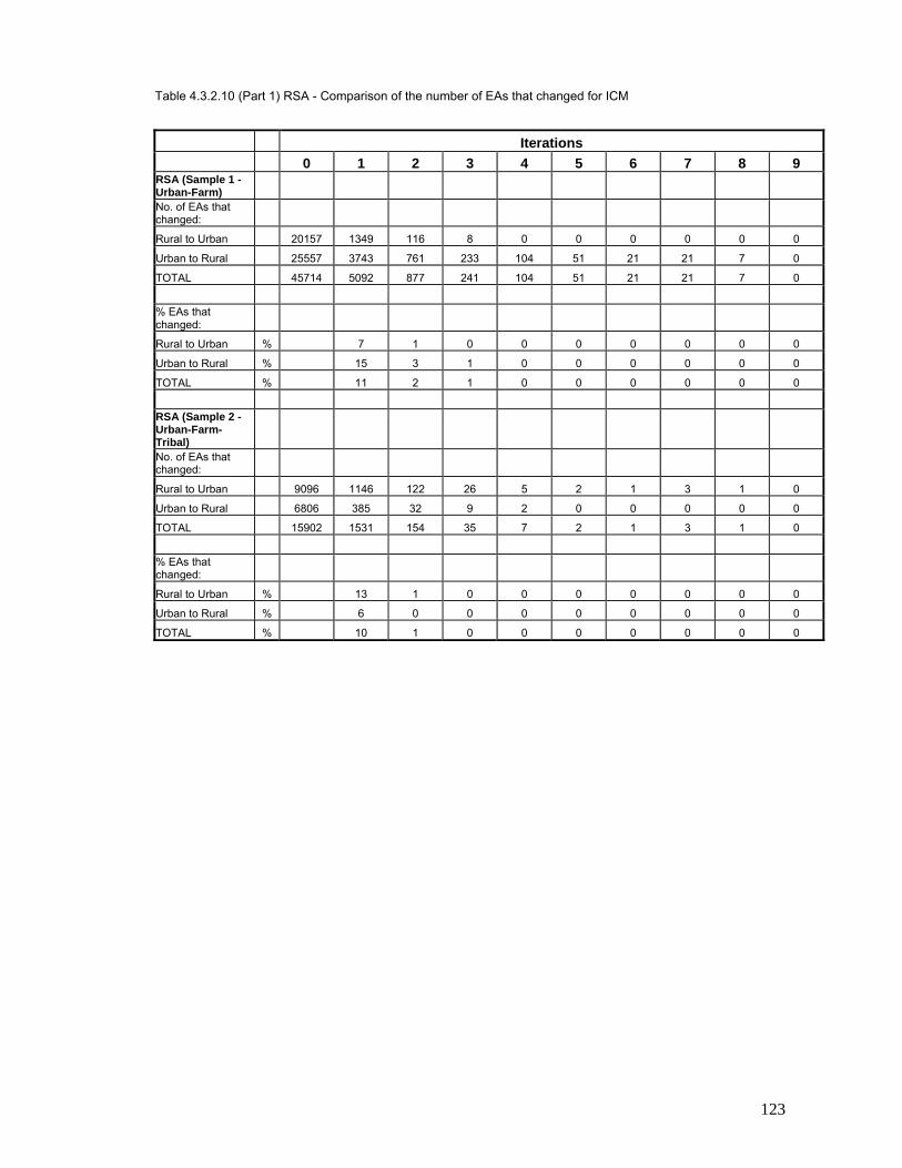
123
Table 4.3.2.10 (Part 1) RSA - Comparison of the number of EAs that changed for ICM
Iterations
0 1 2 3 4 5 6 7 8 9 RSA (Sample 1 - Urban-Farm) No. of EAs that changed:
Rural to Urban 20157 1349 116 8 0 0 0 0 0 0
Urban to Rural 25557 3743 761 233 104 51 21 21 7 0
TOTAL 45714 5092 877 241 104 51 21 21 7 0
% EAs that changed:
Rural to Urban % 7 1 0 0 0 0 0 0 0
Urban to Rural % 15 3 1 0 0 0 0 0 0
TOTAL % 11 2 1 0 0 0 0 0 0
RSA (Sample 2 - Urban-Farm-Tribal) No. of EAs that changed:
Rural to Urban 9096 1146 122 26 5 2 1 3 1 0
Urban to Rural 6806 385 32 9 2 0 0 0 0 0
TOTAL 15902 1531 154 35 7 2 1 3 1 0
% EAs that changed:
Rural to Urban % 13 1 0 0 0 0 0 0 0
Urban to Rural % 6 0 0 0 0 0 0 0 0
TOTAL % 10 1 0 0 0 0 0 0 0

124
Table 4.3.2.10 (Part 2) RSA - Comparison of the population changes for ICM
Iterations 0 1 2 3 4 5 6 7 8 9
Rural 12656536 12701563 12823510 12863972 12879666 12888390 12890721 12894204 12895054 12895054
Urban 32162878 32117851 31995904 31955442 31939748 31931024 31928693 31925210 31924360 31924360
TOTAL 44819414 44819414 44819414 44819414 44819414 44819414 44819414 44819414 44819414 44819414
Rural % 28 28 29 29 29 29 29 29 29 29
Urban % 72 72 71 71 71 71 71 71 71 71
TOTAL % 100 100 100 100 100 100 100 100 100 100
Rural 20678304 20464948 20426137 20416000 20414364 20413695 20413401 20412440 20412124 20412124
Urban 24141111 24354466 24393277 24403414 24405050 24405719 24406013 24406974 24407290 24407290
TOTAL 44819414 44819414 44819414 44819414 44819414 44819414 44819414 44819414 44819414 44819414
Rural % 46 46 46 46 46 46 46 46 46 46
Urban % 54 54 54 54 54 54 54 54 54 54
TOTAL % 100 100 100 100 100 100 100 100 100 100
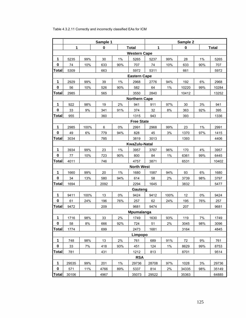
125
Table 4.3.2.11 Correctly and incorrectly classified EAs for ICM
Sample 1 Sample 2 1 0 Total 1 0 Total
Western Cape 1 5235 99% 30 1% 5265 5237 99% 28 1% 5265 0 74 10% 633 90% 707 74 10% 633 90% 707
Total 5309 663 5972 5311 661 5972 Eastern Cape
1 2929 99% 39 1% 2968 2776 94% 192 6% 2968 0 56 10% 526 90% 582 64 1% 10220 99% 10284
Total 2985 565 3550 2840 10412 13252 Northern Cape
1 922 98% 19 2% 941 911 97% 30 3% 941 0 33 9% 341 91% 374 32 8% 363 92% 395
Total 955 360 1315 943 393 1336 Free State
1 2985 100% 6 0% 2991 2968 99% 23 1% 2991 0 49 6% 779 94% 828 45 3% 1370 97% 1415
Total 3034 785 3819 3013 1393 4406 KwaZulu-Natal
1 3934 99% 23 1% 3957 3787 96% 170 4% 3957 0 77 10% 723 90% 800 84 1% 6361 99% 6445
Total 4011 746 4757 3871 6531 10402 North West
1 1660 99% 20 1% 1680 1587 94% 93 6% 1680 0 34 13% 580 94% 614 58 2% 3739 98% 3797
Total 1694 2092 2294 1645 3832 5477 Gauteng
1 9411 100% 13 0% 9424 9412 100% 12 0% 9424 0 61 24% 196 76% 257 62 24% 195 76% 257
Total 9472 209 9681 9474 207 9681 Mpumalanga
1 1716 98% 33 2% 1749 1630 93% 119 7% 1749 0 58 8% 666 92% 724 51 2% 3045 98% 3096
Total 1774 699 2473 1681 3164 4845 Limpopo
1 748 98% 13 2% 761 689 91% 72 9% 761 0 33 7% 418 93% 451 124 1% 8629 99% 8753
Total 781 431 1212 813 8701 9514 RSA
1 29535 99% 201 1% 29736 28708 97% 1028 3% 29736 0 571 11% 4766 89% 5337 814 2% 34335 98% 35149
Total 30106 4967 35073 29522 35363 64885

126
Similar to section 4.3.1, the maps below represent a selection of a few provinces,
where the changes in EA classification have a large impact on the population
aggregates. The final iteration for each province is mapped. The red polygons on the
map show areas that have changed.
Eastern Cape – Map 4.3.2 (a)
For the Eastern Cape for sample 1, ICM iterates 9 times before reaching stability. In
the first iteration 12% of EAs changed classifications, 5% changed from rural to urban
and 23% from urban to rural. The largest difference in population occurs in the first
iteration where the rural population increases from 33% at the initial un-iterated setting
to 40% in the first iteration, whilst the urban population drops from 67% to 60%. For the
other iterations there are smaller or no changes in population aggregates. Changes
have mainly occurred in the tribal and vacant areas of the Eastern Cape. For sample 2,
the process iterates 3 times before reaching stability. The population percentages
remain unchanged.
Free State – Map 4.3.2 (b)
For the Free State for sample 1, ICM iterates 3 times before reaching stability. In the
first iteration 94% of EAs changed from rural to urban. The largest difference in
population occurs in the first iteration where the rural population decreases from 37%
at the initial un-iterated setting to 14% in the first iteration, whilst the urban population
rises from 63% to 86%. For the other iterations there are smaller or no changes in
population aggregates. This has mainly occurred in the tribal and vacant areas of the
Free State. For sample 2, the process iterates 3 times before reaching stability. The
population percentages show small changes or remain unchanged.
Limpopo – Map 4.3.2 (c)
For Limpopo for sample 1, ICM iterates 7 times before reaching stability. In the first
iteration 9% of EAs changed classification, 2% changed from rural to urban and 32%
from urban to rural. The largest difference in population occurs in the first iteration
where the rural population increases from 27% at the initial un-iterated setting to 38%
in the first iteration, whilst the urban population drops from 73% to 62%. For the other
iterations there are smaller or no changes in population aggregates. This has mainly
occurred in the tribal and vacant areas of Limpopo. For sample 2, the process iterates
3 times before reaching stability. The population percentages show small changes or
remain unchanged.

127

128

129

130
4.4 Chapter summary and conclusion In this chapter the spatial statistical techniques, i.e. straight-majority-rule and ICM, are
applied to each province and South Africa for both samples. The changes in EA
classifications, the correctly and incorrectly classified EAs and changes in aggregated
population as a result of changes in the EA classification are tabled. Maps showing
areas of change are also presented.
In general, for both methods and both samples, most provinces show that many EAs,
i.e. unknown status EAs, have changed urban/rural status, mainly in the first iteration.
Although some provinces show large changes in the EA classification, these changes
have little or no impact on the population aggregations. This is mainly due to changes
of low population rural EAs to urban. Some provinces, on the other hand, show the
opposite, where smaller changes in EA classification have a larger impact on the
population aggregates. Although sample 2 shows changes in the EA classifications
these changes have little or no impact on the population aggregates.
Comparing the misclassified EAs for both spatial methods, shows that there are fewer
misclassified EAs for ICM than for straight-majority-rule, therefore ICM has performed
better. Comparing the misclassified EAs for the spatial classification, i.e. ICM, with
those obtained for the non-spatial classification namely discriminant analysis, for
Sample 1, shows that for six provinces, that is Western Cape, Free State, Kwazulu-
Natal, Gauteng, Mpumalanga and Limpopo as well as for South Africa, there are fewer
or the same number of misclassified EAs for ICM, therefore in these cases the spatial
classifications have improved the results. In the cases of the Eastern Cape and North
West for the rural classifications, there are more misclassified EAs for ICM, i.e. the
non-spatial classifications performed better, whilst ICM performed better for the urban
classifications. Northern Cape shows the opposite. For Sample 2, ICM i.e. the spatial
classification, shows better results for all provinces and South Africa, implying that the
application of spatial methods does improve the classifications.
Comparing the misclassified EAs for the spatial classification, i.e. straight-majority-rule,
with those obtained for the non-spatial classifications (i.e. the best classifications as
obtained from linear logistic regression, classification trees or discriminant analysis), for
both samples, shows that for most provinces the non-spatial classifications have
performed slightly better.
131
CHAPTER 5 -Discussion, Recommendations and Conclusions
5.1 Introduction The main objective of this study was to utilise appropriate statistical techniques to
classify areas in South Africa into urban and rural. Both non-spatial, i.e. linear logistic
regression, classification trees and discriminant analysis, and spatial, i.e. straight-
majority-rule and iterated conditional modes (ICM), statistical methodologies were
investigated and applied to selected 2001 census data. These areas, as derived from
each statistical method, were profiled and common characteristics amongst them were
summarised for classification and definitions of urban and rural areas. Population data
were aggregated to determine the overall urbanisation for the country.
Both methodologies, i.e. non-spatial and spatial, made use of areas in the country that
are known with certainty to be urban and rural. The importance of utilising areas of
known urban and rural status was to firstly identify essential patterns or predominant
characteristics from areas that are known, and thereafter apply similar characteristics
to areas that are not known or are ambiguous, in order to classify them as either urban
or rural. Two different sample data sets were generated and used for all statistical
analyses. Stats SA’s 2001 census EA-types were used to generate the samples of
knowns. The first sample data set, known as Sample 1 or urban-farm, comprised the
urban settlements (as urban) and farm (as rural) EA-types. The second sample data
set was known as Sample 2 or urban-farm-tribal. It comprised, in addition to that
mentioned for sample 1, the tribal settlements (as rural).
5.2 Discussion 5.2.1 Discussion on the non-spatial statistical methods, i.e. linear logistic
regression, classification trees and discriminant analysis
Stepwise linear logistic regression, classification trees and stepwise discrimination
were applied to both samples’ training data sets of knowns, and their validation data
sets of knowns were used to test the models, from which the numbers of correctly and
incorrectly classified EAs were estimated and analysed. Results were weighted with
data as obtained from the 2001 census to produce population figures. Results were
presented for both samples, for each province and for South Africa as a whole.

132
All three non-spatial statistical methods gave insight into those census variables or
combinations thereof that best describe the subject under research, i.e. urban and
rural. Of these three methods, linear logistic regression and discriminant analysis
clearly identified significant variables for urban (increasing the odds of urban) and for
rural (decreasing the odds of urban), whilst classification trees provide sets of
quantitative rules for assigning areas to the two classes. In this regard linear logistic
regression and discriminant analysis are preferred. The results of all three methods
showed similarities within the samples. Differences were, however, noted between the
samples. This was evident in the significant variables, aggregated population figures
and to some extent in the misclassification rates obtained (see chapter 3). Thus one
can deduce that the various statistical methods did not impact as much on the final
results as the constitution of the two samples.
The results obtained for the two samples are very different. Sample 1 contained a
smaller number of known EAs and more unknown status EAs than sample 2 (see
Table 3.2.1). The only difference between the two samples was the inclusion of tribal
settlements as known rural in sample 2. This implies that tribal settlements for sample
1 were scored from the characteristics of sample 1 (urban and farm settlements).
Analysing the results further shows that many tribal settlements have been classified
as urban. (See Chapter 3 Section 3.3.6 Map analysis. For example, for South Africa,
approximately 40% of the tribal population, which was rural in the 2001 census
classification, was classified as urban when linear logistic regression was applied.)
Generally all three statistical methods applied to sample 1 have classified the majority
of the tribal EAs as urban.
The results obtained for sample 2, classify fewer unknown status EAs, and the results
are very similar to those obtained for both censuses, since both censuses and sample
2 predefine tribal settlements as rural. This implies to some extent that the
classifications of unknown status EAs for sample 2, as scored from the statistical
methods, are similar to the classifications assigned by the censuses (which were
termed in the beginning of the study as being subjective). Since the classification of
tribal settlements can swing the results drastically (which is evident from the study
results), more attention should be given to correctly classifying important EA-types
such as urban and tribal settlements, more especially the tribal settlements.

133
5.2.2 Discussion on the spatial statistical methods, i.e. straight-majority-rule and iterated conditional modes
Since the classification of areas into urban and rural is a spatial matter, it was important
to explore the impact of similarities amongst adjacent areas on the classifications. Two
statistical methods were investigated and applied, i.e. straight-majority-rule and iterated
conditional modes (ICM). Straight-majority-rule is an iterated procedure that makes use
of the majority urban/rural status of neighbouring EAs to determine the urban or rural
status of an unknown status EA. Whilst ICM is similar, the method is fully Bayesian.
The density function from the non-spatial statistical technique, i.e. discriminant
analysis, was used for the likelihood function. For the prior probability the Markov
Random Field model, as stated in Besag (1986), was adapted for this application. All
known status EAs were kept fixed during the iterations. Their status was, however,
used to calculate the class of unknown status EAs. In order to get a sense of the
number of correctly and incorrectly classified EAs, the EAs of known urban/rural status
were iterated once after the final iteration to recalculate their new (iterated) status.
Comparisons were made with their original known status and misclassification rates
were inferred. Results were presented for both samples, for each province and for
South Africa as a whole.
The results obtained for both spatial methods were similar. For both methods most
changes in classifications occurred in the first iteration. For sample 1, although some
provinces show large changes in EA classification, these changes have almost no
impact on the aggregated population totals. This is mainly the result of low population
rural EAs changing status. On the other hand, in some provinces the opposite is true;
smaller changes in classifications result in a large impact on the population aggregates.
EAs that changed classifications mainly occurred for tribal settlements and vacant
areas. Sample 2, for both methods, shows that although there are substantial changes
in classifications, these changes have in most cases no impact on the population
aggregates; in fact the population totals for each iteration remained stable.
It is, however, noticeable that the numbers of correctly classified EAs are improved
when ICM is applied. This is mainly the result of utilising more information through the
Bayesian approach. ICM also resulted in fewer iterations.

134
5.2.3 Discussion on both non-spatial and spatial statistical methodologies Classifications of areas into urban or rural were accomplished with both methodologies.
In addition, the non-spatial statistical methods provided more information on the census
variables that describe or characterise (or even define) urban and rural. The spatial
statistical methods further refine (or smooth) the classifications by utilising similarities
of adjacent classifications. As is evident from the results obtained in Chapter 4,
comparing the misclassified EAs for both spatial methods with those of the non-spatial
methodologies for both samples, shows fewer misclassified EAs for ICM than for
straight-majority-rule. Of the two spatial methods, ICM has therefore performed best.
Thus the conclusion can be made that applying spatial methodologies that are fully
Bayesian does improve the classifications.
5.2.4 Discussion on both sample 1 and sample 2 Basing all applications and analyses on the two training samples, afforded us the
opportunity to compare outcomes. These comparisons have enabled us to conclude
that the various statistical methods do not impact on the study as much as the
constitution of the two training samples. The results for the two sets of analysis
therefore differ mainly as a result of the sample selection.
The only difference between sample 1 and sample 2 is the inclusion of the tribal areas
in sample 2, classified as known rural. For sample 1, the classification of tribal areas is
not predefined, as in the case of sample 2; but is based on the characteristics of urban
settlements and farms. When sample 1 is used, a large proportion of tribal areas are
classified statistically as urban areas, a typical example is the case of the Eastern
Cape province which shows drastic changes from mainly rural to largely urban, when
changing from sample 2 to sample 1. This implies that these tribal areas are not in the
same profile as farms where typically agricultural activities are the main source of
income and livelihood. Some tribal areas tend to resemble townships since they are
more formal in layout, dwellings are constructed from brick and corrugated iron, with
basic services (such as electricity and water) and limited infrastructure (such as roads,
but untarrred), and they are high in density. However, since tribal areas fall within the
jurisdiction of tribal authorities and under traditional leadership, in the RSA these areas
are classed as rural and it might be incorrect to class them as urban. The trend by the
younger generation from traditional areas to move to more urban or built up areas to
find employment, also affects urbanisation in the traditional areas i.e. rural-urban

135
migration. Since in most cases urban areas are developed for “commercial or
administrative purposes” (Smit 1979) and currently tribal areas have little or no
commercial development (in fact they still remain largely unintegrated with the urban
hierarchy) implies that such areas are still predominantly rural. Smit (1979) also noted
the long distances of such areas from cities or towns. United Nations (2006) mentions
that urban areas are usually “a higher standard of living than are found in rural areas”.
The impact of South Africa’s apartheid past was captured by SPP (1983) “ … even if
the relocation were suddenly to come to an end, it would not alter the position of
millions of people already relocated, nor undermine, substantially the major
restructuring of South Africa into a ‘white’ core and ten ethnic Bantustans on the
periphery that is already far advanced.” According to Murray (1987) such tribal areas
maybe considered ‘urban’ due to the “sheer density of population concentrated there …
‘urban’ in respect of their population densities but ‘rural’ in respect of the absence of
proper urban infrastructure or services”. This is certainly observable from the results of
the study. When sample 1 was applied large proportions of tribal areas were classified
as urban, ‘urban’ mainly as a result of large population densities and ‘rural’ due to its
poor infrastructure and services, described by SPP (1983) as “… a place to stay with
no economic base …”, in areas that were previously reserved to relocate several
hundred thousand people during the apartheid era. South Africa’s previous apartheid
‘”reserve” areas still suffers from lack of development that can classify them as urban in
the normal sense of the word.
Utilising the two samples, it is evident from the results that the classification of tribal
settlements can swing the results drastically, it can be argued that due to this, there is
opportunity to include a third classification category for tribal areas, in addition to urban
and farm settlements.
Taking the above statements of Smit and SPP into consideration, it can be accepted
that sample 2, with tribal areas predefined as rural, more realistically depicts the
situation in this country, and thus provides more realistic classifications and definitions
for urban and rural.

136
For sample 1, although tribal areas show the most significant change in classification
from rural to urban, smaller changes are noted for EA types such as institutions,
hostels and smallholdings. These changes are mainly attributed to high densities.
5.2.5 Discussion on the application and analysis per province and for South Africa as a whole
At the beginning of the study it was decided to apply the statistical techniques and
analyse the results per province and for South Africa as a whole. The motivation for
this was that South Africa’s provinces have varying characteristics and it was hoped
that the study could highlight these.
Here again the constitution of the samples dominated the results, that is the statistical
methods in most cases showed very similar results for any particular province, the
differences being mainly between the samples.
Observing the results from Chapters 3 and 4 shows that, in general, within each of the
samples the classifications for the RSA as a whole performs more or less similarly
compared to the separate provincial classifications, with the exception of Gauteng,
where the rural misclassifications are very high.
5.3 Meeting the study objectives The objectives of the study as mentioned above and in Chapter 1 can be broken down
as follows:
• Classification of areas using appropriate statistical methods to determine urban
and rural areas in the country
• Definitions for urban and rural by investigating common characteristics from the
results obtained from the statistical methods
• The overall urbanisation for the country
Has the study met the objectives?
• Classification of areas using appropriate statistical methods to determine urban
and rural areas in the country
The classifications were achieved and are strictly that of the chosen approach
for this research study, that is, supervised classifications applying both non-
spatial and spatial statistical methods. For the non-spatial statistical

137
methodologies, the unknown status areas were classified into urban or rural
based on the models derived from the sample data sets of known areas. The
spatial statistical methodologies classified unknown status areas into urban or
rural based on their neighbourhoods and probabilities. In other words, this
research study includes five different classifications (classifications were done
per province and for South Africa as a whole, as well as for each sample, i.e.
sample 1 and 2).
• Definitions for urban and rural by investigating common characteristics from
results obtained from statistical methods
The study approaches did not explicitly derive definitions for urban and rural.
Census attributes (from a selection of those available from the census) that
have significance on the classifications, can in general be used to describe the
characteristics of urban and rural (see Chapter 3). Studying the coefficients
obtained from the linear logistic regression and discriminant analysis models to
help infer new definitions of urban and rural, would be a useful extension of this
study.
• The overall urbanisation for the country
With this objective it was envisaged that aggregating population data from the
2001 census, based on the various classifications, could approximate the
overall urbanisation. Fair (1982) describes urbanisation as the geographic
concentration of population and non-agricultural activities in urban
environments of varying size and form. Clarke (1972) states amongst the six
definitions that urbanisation is the proportion of the total population living in
urban centres. In line with the above, Tables 5.1 (a) and (b) show a summary of
the population percentages for urban and rural, for each statistical method, for
each province and South Africa as a whole, for sample 1 and 2.
5.4 Utilising the results of the study The study approach (the utilisation of areas of known urban and rural status to model
other areas that are not known) and methodologies (supervised classifications, non-
spatial, i.e. linear logistic regression, classification trees and discriminant analysis, and
spatial, i.e. straight-majority-rule and ICM) form the basis of this study and its results.

138
In general, the results of the study can be utilised to derive the following information on
the subject:
• Comparisons of three different non-spatial statistical methods, applied to urban
and rural classifications for each province and for South Africa for two samples.
This is seen in the aggregations of population figures based on the
classifications in tables 3.3.5 (a) and (b).
• Further refinement of classifications derived from the non-spatial methods by
applying spatial methods.
• Comparisons of misclassifications.
• Comparisons of results with those obtained from the censuses.
• Census 2001 attributes that describe characteristics of urban, farm and tribal
settlements.
• Spatial distributions of urban and rural (map analysis).
• Comparative outcomes of sampling methods on the study topic or generally the
impact of sampling methodologies on statistical results.
• Finally, actual classification of each EA in South Africa as urban or rural.
5.5 Limitations of the study The main limitation of the study was the method of drawing the samples of known
areas, i.e. the use of census 2001 EA-types. This resulted in sample 1 covering 43%
and sample 2 80% of the total number of EAs in South Africa. Therefore sample 2
covered a very small proportion of unknown areas that required classification.
5.6 Taking the study further The study can be taken further in the following ways:
• Explore the opportunity of including a third classification for tribal areas, in
addition to urban and farm settlements.
• Since this study explored only supervised methods of classification, the
unsupervised methodologies might be explored as a different approach.
• Appropriate methodologies can be explored that can break down urban and
rural into subcomponents or segments.
• The possibility can be explored of utilising other data sources, e.g. deeds,
municipal and property value data, with census information in the
classifications.
139
5.7 Chapter summary and conclusion The study was about classifying and defining urban and rural in South Africa by means
of different statistical approaches. This was achieved by applying supervised
classifications, i.e. non-spatial and spatial statistical methodologies. The study has
generated at least five different classifications, with aggregated population figures for
each province and for South Africa as a whole for two sample data sets, and has
identified significant census variables that are important in classifications into urban
and rural.

140
Table 5.1 (a) Summary table for sample 1: Population percentages for urban and rural for each statistical method for each province and South Africa
Western
Cape Eastern
Cape Northern
Cape Free State KwaZulu-Natal
North West Gauteng Mpumalan
ga Limpopo RSA
Non-spatial
Linear logistic regression
% Rural 10 4 18 15 46 33 4 30 21 34
% Urban 90 96 82 85 54 67 96 70 79 66
TOTAL 100 100 100 100 100 100 100 100 100 100
Classification trees
% Rural 10 6 18 15 31 11 2 18 7 10
%Urban 90 94 82 85 69 89 98 82 93 90
TOTAL 100 100 100 100 100 100 100 100 100 100
Discriminant analysis
% Rural 10 33 18 37 41 36 3 30 27 28
% Urban 90 67 82 63 59 64 97 70 73 72
TOTAL 100 100 100 100 100 100 100 100 100 100
Spatial
Straight-majority-rule
% Rural 10 43 19 16 49 18 4 22 40 38
% Urban 90 57 81 84 51 82 96 78 60 62
TOTAL 100 100 100 100 100 100 100 100 100 100
ICM
% Rural 10 40 18 14 42 39 3 30 39 29
% Urban 90 60 82 86 58 61 97 70 61 71
TOTAL 100 100 100 100 100 100 100 100 100 100

141
Table 5.1 (b) Summary table for sample 2: Population percentages for urban and rural for each statistical method for each province and South Africa
Western
Cape Eastern
Cape Northern
Cape Free State KwaZulu-Natal
North West Gauteng Mpumalan
ga Limpopo RSA
Non-spatial
Linear logistic regression
% Rural 10 63 19 25 58 62 4 60 90 44
% Urban 90 37 81 75 42 38 96 40 10 56
TOTAL 100 100 100 100 100 100 100 100 100 100
Classification trees
% Rural 10 63 19 25 58 63 2 62 90 45
% Urban 90 37 81 75 42 37 98 38 10 55
TOTAL 100 100 100 100 100 100 100 100 100 100
Discriminant analysis
% Rural 10 64 19 25 60 63 3 61 89 46
% Urban 90 36 81 75 40 37 97 39 11 54
TOTAL 100 100 100 100 100 100 100 100 100 100
Spatial
Straight-majority-rule
% Rural 10 63 19 25 57 63 4 61 90 45
% Urban 90 37 81 75 43 37 96 39 10 55
TOTAL 100 100 100 100 100 100 100 100 100 100
ICM
% Rural 10 64 19 24 60 62 3 61 90 46
% Urban 90 36 81 76 40 38 97 39 10 54
TOTAL 100 100 100 100 100 100 100 100 100 100

142
REFERENCES
Agresti, A. (1990). Categorical data analysis. John Wiley & Sons. USA.
Besag, J. (1986). On the statistical analysis of dirty pictures. Royal Statistical Society.
48, No. 3, pp. 259 – 302.
Besag, J. (1989). Digital Image Processing. Towards Bayesian image analysis.
Journal of Applied Statistics, vol. 16, No. 3.
Bundy, C. (1979). The rise and fall of the South African peasantry. London:
Heinemann.
Cacoullos, T. (1973). Discriminant analysis and applications. Academic Press. New
York and London.
Clarke, J. I. (1972). Population Geography. 2nd Edition. Pergamon Press. England.
Cressie, N. A. C. (1993). Statistics for spatial data. Revised edition. United States of
America. John Wiley & Sons, Inc.
Christensen, R. (1997). Log-linear models and Logistic regression. 2nd Edition. Springer
text in Statistics.
Christopher, A. J. (1992). The final phase of urban apartheid zoning in South Africa.
South African Geographical Journal.
Davies, R. J. (1967). The South African urban hierarchy. South African Geographical Journal. Vol. 49: 9-19.
Davies, R. J. & Cook, G. P. (1968). Reappraisal of the South African urban hierarchy.
South Africa Geographical Journal. Vol. 50: 116-132.
Davies, R. J. & Young, B. S. (1969) The economic structure of South African cities.
South African Geographical Journal. Vol. 51: 19-37.

143
Fatti, P. (2003). Automatic interaction detection (AID). (Unpublished paper).
Fernandez, G. (2003). Data mining using SAS Applications. Chapman & Hall/CRC.
Fair, T. J. D. (1982). South Africa: Spatial frameworks for development. South African
Geographies and Environment Studies Series. Juta & Co, LTD.
Goodall, B. (1972). The economics of urban areas. Pergamon Press. Oxford.
Hastie, T., Tibshirani, R. & Friedman J. (2001). The elements of statistical learning.
Springer Series.
Hoekveld, G. A. (1990). Regional geography must adjust to new realities. In Regional
Geography, current developments and future prospects. Routledge series in
Geography and Environment.
Hosmer, D. W. & Lemeshow, S. (2000). Applied logistic regression. 2nd Edition. Wiley
Series in Probability and Statistics.
Isaaks, E. H. & Srivastava, R. M. (1989). An introduction to applied geostatistics.
Oxford University Press.
Kass. SAS System Help, Tree Node. SAS Enterprise Miner. SAS Institute Inc., Cary,
NC 27513, USA.
Manuel, T. A. (2005). Budget Speech 2005. ISBN: 0-621-35493-7.
www.treasury.gov.za.
McLachlan, G. (1992). Discriminant analysis and statistical pattern recognition. John
Wiley & Sons, Inc. Canada.
Montgomery, D. C. & Peck, E. A. (1992). Introduction to linear regression analysis.
Wiley-Interscience, John Wiley & Sons, Inc. Canada.

144
Murray, C. (1987). Displaced urbanization: South Africa’s rural slums. African Affairs
86, (344); 311-329.
Reif, B. (1973). Models in urban and regional planning. Leonard Hill Books. Great
Britain.
SAS Enterprise Miner. SAS Institute Inc., Cary, NC 27513, USA.
Smit, P. (1979). Urbanisation in Africa: lessons for urbanisation in the homelands.
South African Geographical Journal. Vol. 61: 3-28.
SPP. (1983). Forced Removals in South Africa, Vol. 1-4. The Surplus People’s Project.
Cape Town.
Statistics South Africa. (2003). Investigations into appropriate definitions of urban and
rural areas for South Africa (discussion document).
SuperCross. Version 4.2. Space Time Research, Australia.
UKO Guide: United Kingdom Office for National Statistics. (2001). Urban and Rural
Area Definitions: A User Guide for their Census 2001.
United Nations. (2006). Principals and recommendations for population and housing
censuses (draft). Revision 2.
Webb, A. (1999). Statistical Pattern Recognition. Newnes. Great Britain.
White, M. J. (1987). American neighbourhoods and residential differentiation. A Census
Monograph Series. Russell Sage Foundation. New York.
Wonnacott, T. H. & Wonnacott, R. J. (1981). Regression: a second course in statistics.
John Wiley & Sons. USA.
Yawitch, J. (1982). Betterment: the Myth of Homeland Agriculture. Johannesburg,
SAIRR.

145
APPENDICES
APPENDIX A .............................................................................................................. 146 Census 1996 EA-type classification ........................................................................... 146 Census 2001 EA-type classification ........................................................................... 147 APPENDIX B .............................................................................................................. 148 (Part 1) Results from linear logistic regression for the Western Cape, Eastern Cape,
Northern Cape, Free State and KwaZulu-Natal .................................................. 149 (Part 2) Results from linear logistic regression for North West, Gauteng, Mpumalanga,
Limpopo and South Africa .................................................................................. 153 APPENDIX C .............................................................................................................. 157 Tree diagram for the Western Cape (sample 1) ......................................................... 158 Tree diagram for the Western Cape (sample 2) ......................................................... 159 Tree diagram for the Eastern Cape (sample 1) .......................................................... 160 Tree diagram for the Eastern Cape (sample 2) .......................................................... 161 Tree diagram for the Northern Cape (sample 1) ......................................................... 162 Tree diagram for the Northern Cape (sample 2) ......................................................... 162 Tree diagram for the Free State (sample 1) ............................................................... 163 Tree diagram for the Free State (sample 2) ............................................................... 164 Tree diagram for KwaZulu-Natal (sample 1) ............................................................... 165 Tree diagram for KwaZulu-Natal (sample 2) ............................................................... 166 Tree diagram for North West (sample 1) .................................................................... 167 Tree diagram for North West (sample 2) .................................................................... 167 Tree diagram for Gauteng (samples 1 & 2) ................................................................ 168 Tree diagram for Mpumalanga (sample 1) ................................................................. 169 Tree diagram for Limpopo (sample 1) ........................................................................ 171 Tree diagram for Limpopo (sample 2) ........................................................................ 172 Tree diagram for the RSA (sample 1) ......................................................................... 172 Tree diagram for the RSA (sample 2) ......................................................................... 173 APPENDIX D .............................................................................................................. 174 (Part 1) Coefficients of significant variables for the linear discriminant functions for the
Western Cape and the Eastern Cape ................................................................. 175 (Part 2) Coefficients of significant variables for the linear discriminant functions for the
Northern Cape and the Free State...................................................................... 180 (Part 3) Coefficients of significant variables for the linear discriminant functions for
KwaZulu-Natal and North West .......................................................................... 185 (Part 4) Coefficients of significant variables for the linear discriminant functions for
Gauteng and Mpumalanga ................................................................................. 190 (Part 5) Coefficients of significant variables for the linear discriminant functions for
Limpopo and South Africa as a whole ................................................................ 194 APPENDIX E .............................................................................................................. 198

146
APPENDIX A Census EA-types for 1996 and 2001
Census 1996 EA-type classification EA-Type Urban/ Semi-urban/ Rural Urban/ Non-urban
11 Urban: formal
12 Urban: informal
13 Urban: hostels
14 Urban: institutions
Urban
Urban
21 Semi-urban: formal
22 Semi-urban: informal
23 Semi-urban: hostels
24 Semi-urban: institutions
Semi-urban
Non-urban 31 Rural: formal
32 Rural: formal/semi-formal
33 Rural: tribal villages
34 Rural: informal
35 Rural: hostels
36 Rural: institutions
37 Rural: farms
38 Rural: tribal excl. villages
Rural

147
Census 2001 EA-type classification EA-Type Geography Type Urban/Rural
0 Vacant
3 Small-holding
4 Urban settlement
6 Recreational
7 Industrial area
8 Institution
9 Hostel
Urban Formal
Urban
5 Informal settlement Urban Informal
2 Farm
3 Small-holding
6 Recreational
7 Industrial area
8 Institution
9 Hostel
Rural Formal
Rural 0 Vacant
1 Tribal settlement
6 Recreational
7 Industrial area
8 Institution
9 Hostel
Tribal area
148
APPENDIX B Results from linear logistic regression
The table below shows the coefficients of the estimates as obtained for both samples,
i.e. Sample 1 (urban-farm) and Sample 2 (urban-farm-tribal), for each province. The
table is split into two parts. Part 1 shows the results for the Western Cape, Eastern
Cape, Northern Cape, Free State and KwaZulu-Natal, and Part 2 shows the results for
North West, Gauteng, Mpumalanga, Limpopo and South Africa as a whole.
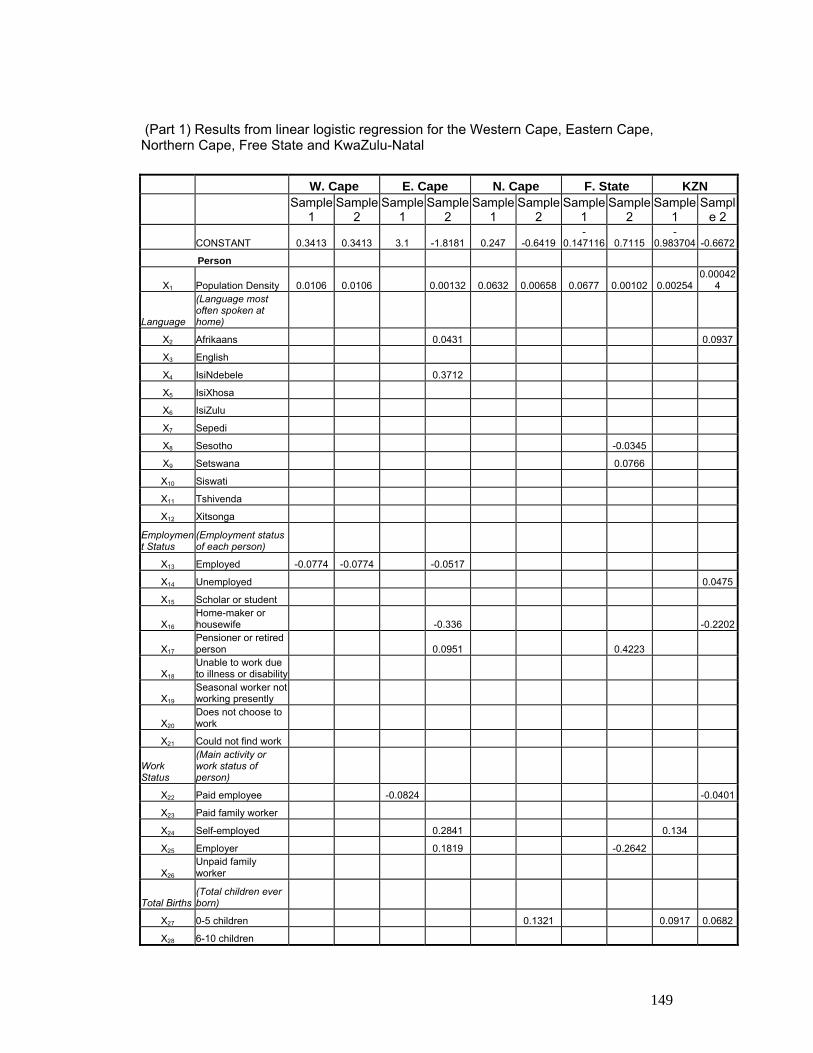
149
(Part 1) Results from linear logistic regression for the Western Cape, Eastern Cape, Northern Cape, Free State and KwaZulu-Natal W. Cape E. Cape N. Cape F. State KZN
Sample
1 Sample
2 Sample
1 Sample
2 Sample
1 Sample
2 Sample
1 Sample
2 Sample
1 Sampl
e 2
CONSTANT 0.3413 0.3413 3.1 -1.8181 0.247 -0.6419-
0.147116 0.7115 -
0.983704 -0.6672
Person
X1 Population Density 0.0106 0.0106 0.00132 0.0632 0.00658 0.0677 0.00102 0.002540.00042
4
Language
(Language most often spoken at home)
X2 Afrikaans 0.0431 0.0937
X3 English
X4 IsiNdebele 0.3712
X5 IsiXhosa
X6 IsiZulu
X7 Sepedi
X8 Sesotho -0.0345
X9 Setswana 0.0766
X10 Siswati
X11 Tshivenda
X12 Xitsonga
Employment Status
(Employment status of each person)
X13 Employed -0.0774 -0.0774 -0.0517
X14 Unemployed 0.0475
X15 Scholar or student
X16 Home-maker or housewife -0.336 -0.2202
X17 Pensioner or retired person 0.0951 0.4223
X18 Unable to work due to illness or disability
X19 Seasonal worker not working presently
X20 Does not choose to work
X21 Could not find work
Work Status
(Main activity or work status of person)
X22 Paid employee -0.0824 -0.0401
X23 Paid family worker
X24 Self-employed 0.2841 0.134
X25 Employer 0.1819 -0.2642
X26 Unpaid family worker
Total Births (Total children ever born)
X27 0-5 children 0.1321 0.0917 0.0682
X28 6-10 children

150
W. Cape E. Cape N. Cape F. State KZN
Sample
1 Sample
2 Sample
1 Sample
2 Sample
1 Sample
2 Sample
1 Sample
2 Sample
1 Sampl
e 2
X29 more than 10 children
Level of Education
(Highest level of education the person completed)
X30 No schooling -0.1875 -0.1875 -0.2064 -0.0792
X31 Some primary 0.0728
X32 Complete primary 0.3104
X33 Some secondary 0.0414
X34 Grade 12/ Std 10 0.068
X35 Higher
Household
Household Size
(Total number of persons in a household)
X36 1-5 persons
X37 6-10 persons -0.0512 -0.0372
X38 More than 10 persons -0.1632
Housing Unit
(Type of living quarters)
X39
House or brick structure on a separate stand or yard
X40
Traditional dwelling/ hut/ structure made of traditional materials -0.054
X41 Flat in a block of flats -0.0229
X42 Town/ cluster/ semi-detached house
X43 House/ flat/ room, in backyard
X44 Informal dwelling/ shack, in backyard 0.1651 0.1651 0.0416 0.0299
X45
Informal dwelling/ shack, not in backyard, informal/ squatter
X46
Room/ flatlet not in backyard but on shared property
X47 Caravan or tent
X48 Private ship/ boat
Rooms
(Number of rooms that the household utilises)
X49 1-3 rooms 0.1033
X50 4-6 rooms
X51 7-10 rooms
X52 More than 10 rooms 0.131 -0.0583
Access to Water
(Type of access to water)
X53 Piped water (tap) inside dwelling 0.0414
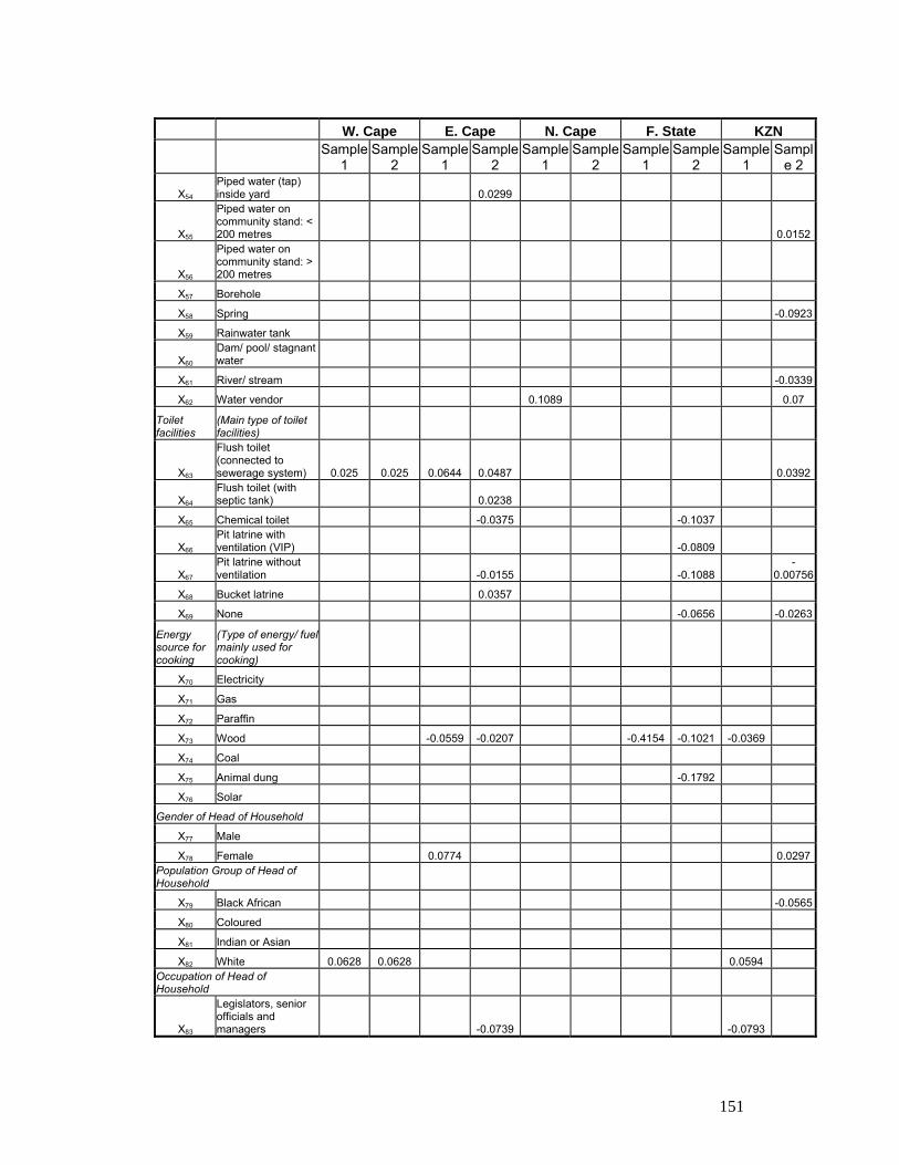
151
W. Cape E. Cape N. Cape F. State KZN
Sample
1 Sample
2 Sample
1 Sample
2 Sample
1 Sample
2 Sample
1 Sample
2 Sample
1 Sampl
e 2
X54 Piped water (tap) inside yard 0.0299
X55
Piped water on community stand: < 200 metres 0.0152
X56
Piped water on community stand: > 200 metres
X57 Borehole
X58 Spring -0.0923
X59 Rainwater tank
X60 Dam/ pool/ stagnant water
X61 River/ stream -0.0339
X62 Water vendor 0.1089 0.07
Toilet facilities
(Main type of toilet facilities)
X63
Flush toilet (connected to sewerage system) 0.025 0.025 0.0644 0.0487 0.0392
X64 Flush toilet (with septic tank) 0.0238
X65 Chemical toilet -0.0375 -0.1037
X66 Pit latrine with ventilation (VIP) -0.0809
X67 Pit latrine without ventilation -0.0155 -0.1088
-0.00756
X68 Bucket latrine 0.0357
X69 None -0.0656 -0.0263
Energy source for cooking
(Type of energy/ fuel mainly used for cooking)
X70 Electricity
X71 Gas
X72 Paraffin
X73 Wood -0.0559 -0.0207 -0.4154 -0.1021 -0.0369
X74 Coal
X75 Animal dung -0.1792
X76 Solar
Gender of Head of Household
X77 Male
X78 Female 0.0774 0.0297Population Group of Head of Household
X79 Black African -0.0565
X80 Coloured
X81 Indian or Asian
X82 White 0.0628 0.0628 0.0594 Occupation of Head of Household
X83
Legislators, senior officials and managers -0.0739 -0.0793

152
W. Cape E. Cape N. Cape F. State KZN
Sample
1 Sample
2 Sample
1 Sample
2 Sample
1 Sample
2 Sample
1 Sample
2 Sample
1 Sampl
e 2 X84 Professionals
X85
Technicians and associate professionals
X86 Clerks 0.1948
X87
Service workers, shop and market sales workers
X88 Skilled agricultural and fishery workers -0.1858 -0.0613 -0.3647 -0.4028 -0.2525
X89 Craft and related trades workers
X90
Plant and machine operators and assemblers
X91 Elementary occupations -0.0361 -0.0361 -0.088 -0.0859 -0.0446
X92
Occupations unspecified or not elsewhere classified
Annual Household Income
X93 No income -0.1545
X94 R 1 - R 4 800 0.1187 0.1187 0.0335
X95 R 4 801 - R 9 600
X96 R 9 601 - R 19 200 0.0338
X97 R 19 201 - R 38 400 -0.0391
X98 R 38 401 - R 76 800
X99 R 76 801 - R 153 600 0.0809
X100 R 153 601 - R 307 200 -0.0587 0.0766
X101 R 307 201 - R 614 400
X102 R 614 401 - R 1 228 800
X103 R 1 228 801 - R 2 457 600
X104 R 2 457 601 or more

153
(Part 2) Results from linear logistic regression for North West, Gauteng, Mpumalanga, Limpopo and South Africa
N. West Gauteng MP Limpopo S. Africa
Sample
1 Sample
2 Sample
1 Sampl
e 2 Sample
1 Sample
2 Sample
1 Sample
2 Sample
1 Sample
2
CONSTANT -
1.598801 -2.2532 1.5435 1.5435-
0.523451 0.5784-
4.083585 -0.7982 0.2338 -0.7516
Person
X1 Population density 0.000439 0.00238 0.00238 0.00259 0.000425 0.0157 0.000359 0.00311 0.00057
Language
(Language most often spoken at home)
X2 Afrikaans
X3 English -0.0171
X4 IsiNdebele -0.0411 0.076 0.0124
X5 IsiXhosa
X6 IsiZulu 0.0332
X7 Sepedi -0.0127
X8 Sesotho -0.0103
X9 Setswana -0.043 -0.043 -0.0116
X10 Siswati
X11 Tshivenda -0.0146
X12 Xitsonga -0.1053 0.047 -0.0302 -0.0484 -0.0507
Employment Status
(Employment status of each person)
X13 Employed
X14 Unemployed 0.075 0.1512 0.0402 0.0415
X15 Scholar or student
X16 Home-maker or housewife -0.1309
X17 Pensioner or retired person 0.1055 0.0904
X18
Unable to work due to illness or disability
X19
Seasonal worker not working presently
X20 Does not choose to work
X21 Could not find work
Work Status
(Main activity or work status of person)
X22 Paid employee 0.0275
X23 Paid family worker 0.0722
X24 Self-employed 0.1284
X25 Employer
X26 Unpaid family worker
Total Births (Total children ever born)
X27 0-5 children 0.2052 0.0793 0.0682 0.023
X28 6-10 children

154
N. West Gauteng MP Limpopo S. Africa
Sample
1 Sample
2 Sample
1 Sampl
e 2 Sample
1 Sample
2 Sample
1 Sample
2 Sample
1 Sample
2
X29 More than 10 children
Level of Education
(Highest level of education the person completed)
X30 No schooling -0.0254
X31 Some primary -0.1348
X32 Complete primary
X33 Some secondary
X34 Grade 12/ Std 10 0.0199
X35 Higher 0.0619
Household
Household Size
(Total number of persons in a household)
X36 1-5 persons
X37 6-10 persons -0.0139
X38 More than 10 persons -0.0585 -0.0253 -0.0279
Housing Unit
(Type of living quarters)
X39
House or brick structure on a separate stand or yard -0.0317 -0.0117
X40
Traditional dwelling/ hut/ structure made of traditional materials -0.0195
X41 Flat in a block of flats 0.0237
X42
Town/ cluster/ semi-detached house
X43 House/ flat/ room, in backyard
X44 Informal dwelling/ shack, in backyard
X45
Informal dwelling/ shack, not in backyard, informal/ squatter 0.0352 0.0333 0.0285
X46
Room/ flatlet not in backyard but on shared property
X47 Caravan or tent 0.4339 0.4339
X48 Private ship/ boat
Rooms
(Number of rooms that the household utilises)
X49 1-3 rooms
X50 4-6 rooms 0.0563 0.0194
X51 7-10 rooms
X52 More than 10 rooms
Access to Water
(Type of access to water)

155
N. West Gauteng MP Limpopo S. Africa
Sample
1 Sample
2 Sample
1 Sampl
e 2 Sample
1 Sample
2 Sample
1 Sample
2 Sample
1 Sample
2
X53 Piped water (tap) inside dwelling 0.0153 0.0107
X54 Piped water (tap) inside yard 0.0126 0.0084
X55
Piped water on community stand: < 200 metres
X56
Piped water on community stand: > 200 metres
X57 Borehole -0.2193
X58 Spring
X59 Rainwater tank
X60 Dam/ pool/ stagnant water -0.1254 -0.1561
X61 River/ stream
X62 Water vendor 0.0225 -0.0334
Toilet facilities
(Main type of toilet facilities)
X63
Flush toilet (connected to sewerage system) 0.0492 0.0184 0.0184 0.0459 0.0449 0.016 0.0358
X64 Flush toilet (with septic tank) -0.069 -0.069 0.0381 0.015
X65 Chemical toilet 0.0677
X66 Pit latrine with ventilation (VIP) -0.0321
X67 Pit latrine without ventilation -0.0121
X68 Bucket latrine 0.0568 0.0363 0.0169 0.0366
X69 None
Energy source for cooking
(Type of energy/ fuel mainly used for cooking)
X70 Electricity 0.0266 -0.0265
X71 Gas
X72 Paraffin -0.0244
X73 Wood -0.1034 -0.0463 -0.0463 -0.0252 -0.0273 -0.0794 -0.0392 -0.0147 -0.015
X74 Coal -0.0908
X75 Animal dung
X76 Solar
Gender of Head of Household
X77 Male
X78 Female 0.0503 Population Group of Head of Household
X79 Black African -0.031 -0.0362 -0.0187 -0.02
X80 Coloured
X81 Indian or Asian
X82 White Occupation of Head of Household
X83 Legislators, senior 0.1747 0.1747

156
N. West Gauteng MP Limpopo S. Africa
Sample
1 Sample
2 Sample
1 Sampl
e 2 Sample
1 Sample
2 Sample
1 Sample
2 Sample
1 Sample
2 officials and managers
X84 Professionals
X85
Technicians and associate professionals 0.0549
X86 Clerks
X87
Service workers, shop and market sales workers
X88 Skilled agricultural and fishery workers -0.4575 -0.4575 -0.1695 -0.1545 -0.1655 -0.1096
X89 Craft and related trades workers
X90
Plant and machine operators and assemblers -0.0329
X91 Elementary occupations -0.1405 -0.0357 -0.0357 -0.0534 -0.0371 -0.0357
X92
Occupations unspecified or not elsewhere classified 0.0601
Annual Household Income
X93 No income -0.0223 -0.0205
X94 R 1 - R 4 800
X95 R 4 801 - R 9 600
X96 R 9 601 - R 19 200 0.0137
X97 R 19 201 - R 38 400 -0.025
X98 R 38 401 - R 76 800
X99 R 76 801 - R 153 600 0.0585
X100 R 153 601 - R 307 200
X101 R 307 201 - R 614 400
X102 R 614 401 - R 1 228 800
X103 R 1 228 801 - R 2 457 600
X104 R 2 457 601 or more
157
APPENDIX C
Results from classification trees Tree diagrams, showing the significant variables and how they split, for each province
and for South Africa as a whole, are given below for both samples. Urban final nodes
are indicated in blue (vertical lines) and rural final nodes in green (horizontal lines).
Units for all variables are persons (standardised by total population), with the exception
of the variable population density where persons per square kilometre, is used.

158
Tree diagram for the Western Cape (sample 1)
Population Density
< 65 >= 65
Persons with some primaryschooling
< 20 >= 20
Head of household occupation:elementary occupations
< 48.5 >= 48.5
Head of household occupation:skilled agricultural and fishery
workers
< 48 >= 48
Employment status:unemployed
< 5.5 >= 5.5
N 5972Urban 88%Rural 12%
N 748Urban 17%Rural 83%
N 151Urban 72%Rural 28%
N 597Urban 3%
Rural 97%
N 5224Urban 98%
Rural 2%
N 5167Urban 99%
Rural 1%
N 57Urban 16%Rural 84%
N 5163Urban 99%
Rural 1%
N 4Urban 0%Rural 100%
N 48Urban 2%
Rural 98%
N 9Urban 89%Rural 11%

159
Tree diagram for the Western Cape (sample 2)
Population Density
< 54 >= 54
Persons with no schooling
< 4.5 >= 4.5
Head of household occupation:elementary occupations
< 48.5 >= 48.5
Head of household occupation:skilled agricultural and fishery
workers
>= 23 >= 48
Employment status: unemployed
< 5.5 >= 5.5
Persons with higher than Grade12/ std 10 schooling
< 23 < 48
N 9Urban 89%Rural 11%
N 5187Urban 99%
Rural 1%
N 5Urban 0%Rural 100%
N 60Urban 2%
Rural 98%
N 10Urban 80%Rural 20%
N 578Urban 2%
Rural 98%
N 5972Urban 88%Rural 12%
N 710Urban 15%Rural 85%
N 5262Urban 98%
Rural 2%
N 123Urban 70%Rural 30%
N 587Urban 3%
Rural 97%
N 5192Urban 99%
Rural 1%
N 70Urban 13%Rural 87%

160
Tree diagram for the Eastern Cape (sample 1)
Population Density
< 59 >= 59
Persons with some primaryschooling
< 13.5 >= 13.5
>= 11.5
Households with flush toiletconnected to sewerage system
< 11.5
N 3550Urban 84%Rural 16%
N 2916Urban 99%
Rural 1%
N 634Urban 11%Rural 89%
N 532Urban 4%
Rural 96%
N 102Urban 48%Rural 52%
N 83Urban 39%Rural 61%
N 19Urban 89%Rural 11%

161
Tree diagram for the Eastern Cape (sample 2)
Households with flush toiletconnected to sewerage system
< 25.5 >= 25.5
Population density
< 2997.5 >= 2997.5
< 63
Households with flush toiletconnected with septic tank
< 63
Population density
< 115.5 >= 115.5
< 62
Households that use wood forcooking
< 62
N 13252Urban 22%Rural 78%
N 10676Urban 5%
Rural 95%
N 268Urban 91%
Rural 9%
N 10408Urban 2%
Rural 98%
N 10347Urban 2%
Rural 98%
N 61Urban 75%Rural 25%
N 116Urban 41%Rural 59%
N 2453Urban 99%
Rural 1%
N 7Urban 0%Rural 100%

162
Tree diagram for the Northern Cape (sample 1)
Population Density
< 76.5 >= 76.5
Households that use wood forcooking
< 2.5 >= 2.5
N 1315Urban 72%Rural 28%
N 892Urban 100%Rural 0%
N 362Urban 4%
Rural 96%
N 61Urban 59%Rural 41%
N 423Urban 12%Rural 88%
Tree diagram for the Northern Cape (sample 2)
Persons who speak Setswanamost often in the household
< 95.5 >= 95.5
Population Density
< 93.5 >= 93.5
N 1336Urban 70%Rural 30%
N 444Urban 12%Rural 88%
N 891Urban 99%
Rural 1%
N 1Urban 0%Rural 100%
N 892Urban 99%
Rural 1%

163
Tree diagram for the Free State (sample 1)
Population Density
< 49 >= 49
Households that use wood forcooking
< 1.5 >= 1.5
N 3819Urban 78%Rural 22%
N 2946Urban 100%Rural 0%
N 807Urban 1%
Rural 99%
N 66Urban 61%Rural 39%
N 873Urban 5%Rural 95%
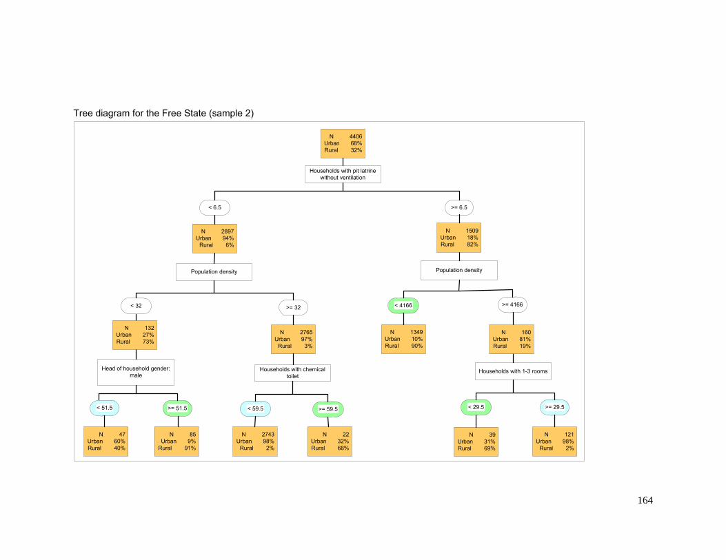
164
Tree diagram for the Free State (sample 2)
Households with pit latrinewithout ventilation
< 6.5 >= 6.5
Population density
< 32 >= 32
Population density
< 4166 >= 4166
>= 59.5
Households with 1-3 rooms
< 29.5 >= 29.5
Households with chemicaltoilet
< 59.5
Head of household gender:male
>= 51.5< 51.5
N 47Urban 60%Rural 40%
N 85Urban 9%
Rural 91%
N 2743Urban 98%
Rural 2%
N 22Urban 32%Rural 68%
N 39Urban 31%Rural 69%
N 121Urban 98%
Rural 2%
N 1349Urban 10%Rural 90%
N 4406Urban 68%Rural 32%
N 2897Urban 94%
Rural 6%
N 132Urban 27%Rural 73%
N 2765Urban 97%
Rural 3%
N 1509Urban 18%Rural 82%
N 160Urban 81%Rural 19%

165
Tree diagram for KwaZulu-Natal (sample 1)
Population Density
< 101.5 >= 101.5
Households that use wood forcooking
< 80.5 >= 80.5
>= 3.5
Head of household occupation:skilled agricultural and fishery
workers
< 3.5
N 4757Urban 83%Rural 17%
N 828Urban 11%Rural 89%
N 16Urban 19%Rural 81%
N 3849Urban 99%
Rural 1%
N 64Urban 70%Rural 30%
N 3929Urban 98%
Rural 2%
N 3913Urban 99%
Rural 1%

166
Tree diagram for KwaZulu-Natal (sample 2)
Households with flush toiletsconnected to a sewerage system
< 101.5 >= 33.5
Population Density
< 108.5 >= 108.5
>= 51
Head of household populationgroup: White
< 51
Households that use wood forcooking
< 1.5 >= 1.5
>= 39.5
Household size from 1-5 persons
< 39.5
N 10402Urban 38%Rural 62%
N 6036Urban 2%
Rural 98%
N 281Urban 17%Rural 83%
N 412Urban 70%Rural 30%
N 156Urban 15%Rural 85%
N 25Urban 88%Rural 12%
N 3492Urban 99%
Rural 1%
N 3673Urban 95%
Rural 5%
N 6729Urban 7%
Rural 93%
N 181Urban 25%Rural 75%
N 693Urban 48%Rural 52%

167
Tree diagram for North West (sample 1)
Population Density
< 61.5 >= 61.5
N 2294Urban 73%Rural 27%
N 1672Urban 99%
Rural 1%
N 622Urban 4%
Rural 96%
Tree diagram for North West (sample 2)
Households with flush toiletsconnected to a sewerage system
< 57.5 >= 57.5
Population Density
< 66.5 >= 66.5
Households with bucket latrines
< 39 >= 39
N 5477Urban 31%Rural 69%
N 3864Urban 3%
Rural 97%
N 185Urban 98%
Rural 2%
N 35Urban 29%Rural 71%
N 1393Urban 98%
Rural 2%
N 1428Urban 96%
Rural 4%
N 4049Urban 8%
Rural 92%

168
Tree diagram for Gauteng (samples 1 & 2)
Population Density
< 54.5 >= 54.5
Head of household occupation:skilled agricultural and fishery
workers
< 0.5 >= 0.5
>= 1.5
Piped water on community stand:distance greater than 200m
< 1.5
N 9681Urban 97%
Rural 3%
N 9385Urban 100%Rural 0%
N 296Urban 25%Rural 75%
N 197Urban 4%
Rural 96%
N 99Urban 67%Rural 33%
N 74Urban 77%Rural 23%
N 25Urban 36%Rural 64%

169
Tree diagram for Mpumalanga (sample 1)
Population Density
< 79 >= 79
Head of household occupation:elementary occupations
< 38.5 >= 38.5
N 2473Urban 71%Rural 29%
N 794Urban 11%Rural 89%
N 1668Urban 99%
Rural 1%
N 11Urban 18%Rural 82%
N 1679Urban 99%
Rural 1%

170
Tree diagram for Mpumalanga (sample 2)
Households with flush toiletsconnected to a sewerage system
< 46.5 >= 46.5
Population Density
< 72 >= 108.5
>= 43
Persons who speak Afrikaansmost often in the household
< 43
Households that use wood forcooking
< 5.5 >= 5.5
>= 41
Informal dwelling/ shack, not inbackyard, in an informal/ squatter
settlement
< 41
N 4845Urban 36%Rural 64%
N 2603Urban 5%
Rural 95%
N 1329Urban 99%
Rural 1%
N 738Urban 30%Rural 70%
N 64Urban 83%Rural 17%
N 94Urban 14%Rural 86%
N 17Urban 88%Rural 12%
N 3405Urban 12%Rural 88%
N 1440Urban 94%
Rural 6%
N 111Urban 25%Rural 75%
N 802Urban 34%Rural 66%

171
Tree diagram for Limpopo (sample 1)
Population Density
< 75 >= 75
Head of household occupation:skilled agricultural and fishery
workers
< 8.5 >= 8.5
N 1212Urban 63%Rural 37%
N 481Urban 7%
Rural 93%
N 728Urban 100%Rural 0%
N 3Urban 0%Rural 100%
N 731Urban 99%
Rural 1%

172
Tree diagram for Limpopo (sample 2)
Households with flush toiletsconnected to a sewerage system
< 54.5 >= 54.5
Persons who speak Xitsongasmost often in the household
< 27 >= 27
>= 22.5
Population Density
< 22.5
Households with flush toilets withseptic tank
< 54 >= 54
N 9514Urban 8%
Rural 92%
N 8566Urban 2%
Rural 98%
N 39Urban 54%Rural 46%
N 8605Urban 2%
Rural 98%
N 909Urban 65%Rural 35%
N 204Urban 16%Rural 84%
N 31Urban 3%
Rural 97%
N 674Urban 83%Rural 17%
N 705Urban 79%Rural 21%
Tree diagram for the RSA (sample 1)
Population Density
< 78.5 >= 78.5
N 35073Urban 85%Rural 15%
N 5773Urban 11%Rural 89%
N 29300Urban 99%
Rural 1%

173
Tree diagram for the RSA (sample 2)
Households with flushtoilets connected to a
sewerage system
< 53.5 >= 53.5
Households that use woodfor cooking
< 6.5 >= 6.5
Population density
< 57.5 >= 57.5
>= 3368.5
Persons who speakXitsonga most often in the
household
< 56.5 >= 56.5
Population Density
< 3368.5
Population Density
>= 3839.5< 3839.5
Persons with no schooling
< 6.5 >= 6.5
N 64885Urban 46%Rural 54%
N 5504Urban 32%Rural 68%
N 2198Urban 87%Rural 13%
N 30501Urban 2%
Rural 98%
N 642Urban 51%Rural 49%
N 207Urban 68%Rural 32%
N 468Urban 16%Rural 84%
N 25168Urban 99%
Rural 1%
N 197Urban 30%Rural 70%
N 38845Urban 12%Rural 88%
N 26040Urban 96%
Rural 4%
N 7702Urban 48%Rural 52%
N 31143Urban 3%
Rural 97%
N 675Urban 32%Rural 68%
N 25365Urban 98%
Rural 2%

174
APPENDIX D Results from discriminant analysis
Stepwise discriminant analysis was used to select the most significant variables (at the
5% level of significance). Thereafter the linear discriminate functions were generated.
The table that follows shows the coefficients of the significant variables for the linear
discriminant functions, for urban and rural, per province for each sample; only the first
10 most significant variables are shown. The table is in 5 parts, i.e. Part 1 for the
Western Cape and the Eastern Cape, Part 2 for the Northern Cape and the Free State,
Part 3 for KwaZulu-Natal and North West, Part 4 for Gauteng and Mpumalanga and
Part 5 for Limpopo and South Africa as a whole.

175
(Part 1) Coefficients of significant variables for the linear discriminant functions for the Western Cape and the Eastern Cape W. Cape E. Cape Sample 1 Sample 2 Sample 1 Sample 2 LDF (Urban) LDF (Rural) LDF (Urban) LDF (Rural) LDF (Urban) LDF (Rural) LDF (Urban) LDF (Rural)
CONSTANT -44.18537 -43.94055 -44.26657 -43.96753 -25.6351 -21.49215 -31.14049 -12.32054
Person
X1 Population density 0.0004511 0.0000332
Language
(Language most often spoken at home)
X2 Afrikaans
X3 English
X4 IsiNdebele
X5 IsiXhosa
X6 IsiZulu
X7 Sepedi
X8 Sesotho
X9 Setswana
X10 Siswati
X11 Tshivenda
X12 Xitsonga
Employment Status
(Employment status of each person)
X13 Employed 0.08611 0.28733 0.08288 0.2878
X14 Unemployed 0.15839 0.02106 0.1615 0.02374
X15 Scholar or student
X16 Home-maker or housewife
X17 Pensioner or retired person
X18
Unable to work due to illness or disability
X19
Seasonal worker not working presently
X20 Does not choose to work
X21 Could not find work
Work Status
(Main activity or work status of person)
X22 Paid employee
X23 Paid family worker
X24 Self-employed
X25 Employer
X26 Unpaid family worker

176
W. Cape E. Cape Sample 1 Sample 2 Sample 1 Sample 2 LDF (Urban) LDF (Rural) LDF (Urban) LDF (Rural) LDF (Urban) LDF (Rural) LDF (Urban) LDF (Rural)
Total Births (Total children ever born)
X27 0-5 children
X28 6-10 children
X29 More than 10 children
Level of Education
(Highest level of education the person completed)
X30 No schooling
X31 Some primary 0.01691 0.22204 0.015 0.22028
X32 Complete primary
X33 Some secondary
X34 Grade 12/ Std 10
X35 Higher
Household
Household Size
(Total number of persons in a household)
X36 1-5 persons
X37 6-10 persons
X38 More than 10 persons
Housing Unit
(Type of living quarters)
X39
House or brick structure on a separate stand or yard
X40
Traditional dwelling/ hut/ structure made of traditional materials
X41 Flat in a block of flats
X42
Town/ cluster/ semi-detached house
X43
House/ flat/ room, in backyard
X44
Informal dwelling/ shack, in backyard
X45
Informal dwelling/ shack, not in backyard, informal/ squatter 0.02535 0.00447 0.02518 0.00378 0.16608 0.05604
X46
Room/ flatlet not in backyard but on shared property
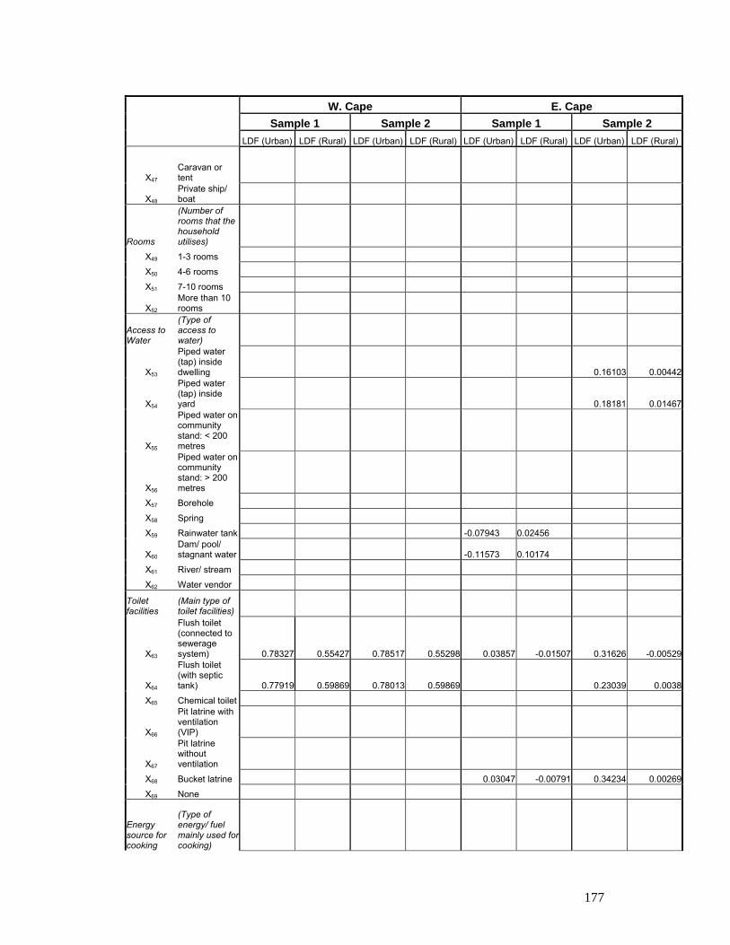
177
W. Cape E. Cape Sample 1 Sample 2 Sample 1 Sample 2 LDF (Urban) LDF (Rural) LDF (Urban) LDF (Rural) LDF (Urban) LDF (Rural) LDF (Urban) LDF (Rural)
X47 Caravan or tent
X48 Private ship/ boat
Rooms
(Number of rooms that the household utilises)
X49 1-3 rooms
X50 4-6 rooms
X51 7-10 rooms
X52 More than 10 rooms
Access to Water
(Type of access to water)
X53
Piped water (tap) inside dwelling 0.16103 0.00442
X54
Piped water (tap) inside yard 0.18181 0.01467
X55
Piped water on community stand: < 200 metres
X56
Piped water on community stand: > 200 metres
X57 Borehole
X58 Spring
X59 Rainwater tank -0.07943 0.02456
X60 Dam/ pool/ stagnant water -0.11573 0.10174
X61 River/ stream
X62 Water vendor
Toilet facilities
(Main type of toilet facilities)
X63
Flush toilet (connected to sewerage system) 0.78327 0.55427 0.78517 0.55298 0.03857 -0.01507 0.31626 -0.00529
X64
Flush toilet (with septic tank) 0.77919 0.59869 0.78013 0.59869 0.23039 0.0038
X65 Chemical toilet
X66
Pit latrine with ventilation (VIP)
X67
Pit latrine without ventilation
X68 Bucket latrine 0.03047 -0.00791 0.34234 0.00269
X69 None
Energy source for cooking
(Type of energy/ fuel mainly used for cooking)

178
W. Cape E. Cape Sample 1 Sample 2 Sample 1 Sample 2 LDF (Urban) LDF (Rural) LDF (Urban) LDF (Rural) LDF (Urban) LDF (Rural) LDF (Urban) LDF (Rural)
X70 Electricity
X71 Gas
X72 Paraffin
X73 Wood -0.06447 0.0729 0.04324 0.07901
X74 Coal
X75 Animal dung
X76 Solar Gender of Head of Household
X77 Male 0.43008 0.25324
X78 Female 0.09552 -0.004 0.0977 -0.00341 0.42503 0.2408 Population Group of Head of Household
X79 Black African
X80 Coloured
X81 Indian or Asian
X82 White Occupation of Head of Household
X83
Legislators, senior officials and managers
X84 Professionals
X85
Technicians and associate professionals
X86 Clerks
X87
Service workers, shop and market sales workers
X88
Skilled agricultural and fishery workers -0.00269 0.29326 -0.00188 0.2967 -0.21188 0.08882 -0.19771 0.00345
X89
Craft and related trades workers 0.17792 -0.14739 0.18053 -0.14745
X90
Plant and machine operators and assemblers -0.11163 0.02233
X91 Elementary occupations -0.12806 0.16806 -0.1271 0.1703 -0.17588 0.07788
X92
Occupations unspecified or not elsewhere classified
Annual Household Income
X93 No income
X94 R 1 - R 4 800 0.08731 -0.04259
X95 R 4 801 - R 9 600
X96 R 9 601 - R 19 200
X97 R 19 201 - R 38 400
X98 R 38 401 - R

179
W. Cape E. Cape Sample 1 Sample 2 Sample 1 Sample 2 LDF (Urban) LDF (Rural) LDF (Urban) LDF (Rural) LDF (Urban) LDF (Rural) LDF (Urban) LDF (Rural)
76 800
X99 R 76 801 - R 153 600
X100 R 153 601 - R 307 200
X101 R 307 201 - R 614 400
X102 R 614 401 - R 1 228 800
X103 R 1 228 801 - R 2 457 600
X104 R 2 457 601 or more

180
(Part 2) Coefficients of significant variables for the linear discriminant functions for the Northern Cape and the Free State N. Cape F. State Sample 1 Sample 2 Sample 1 Sample 2 LDF (Urban) LDF (Rural) LDF (Urban) LDF (Rural) LDF (Urban) LDF (Rural) LDF (Urban) LDF (Rural)
CONSTANT -26.54567 -25.32 -15.29096 -11.39335 -39.20981 -52.00485 -20.33756 -22.60671
Person
X1 Population density 0.0001050 -0.0001029 0.0002617 0.0001686 0.0000968 -0.0005273 0.000715 0.0003026
Language
(Language most often spoken at home)
X2 Afrikaans 0.01637 -0.00832 0.25373 0.16133
X3 English 0.26631 0.18647
X4 IsiNdebele
X5 IsiXhosa
X6 IsiZulu
X7 Sepedi
X8 Sesotho
X9 Setswana 0.04927 -0.01901
X10 Siswati
X11 Tshivenda
X12 Xitsonga
Employment Status
(Employment status of each person)
X13 Employed
X14 Unemployed 0.06852 -0.03531
X15 Scholar or student 0.33588 0.15295
X16 Home-maker or housewife
X17 Pensioner or retired person
X18
Unable to work due to illness or disability
X19
Seasonal worker not working presently
X20
Does not choose to work
X21 Could not find work
Work Status
(Main activity or work status of person)
X22 Paid employee
X23 Paid family worker
X24 Self-employed
X25 Employer
X26 Unpaid family
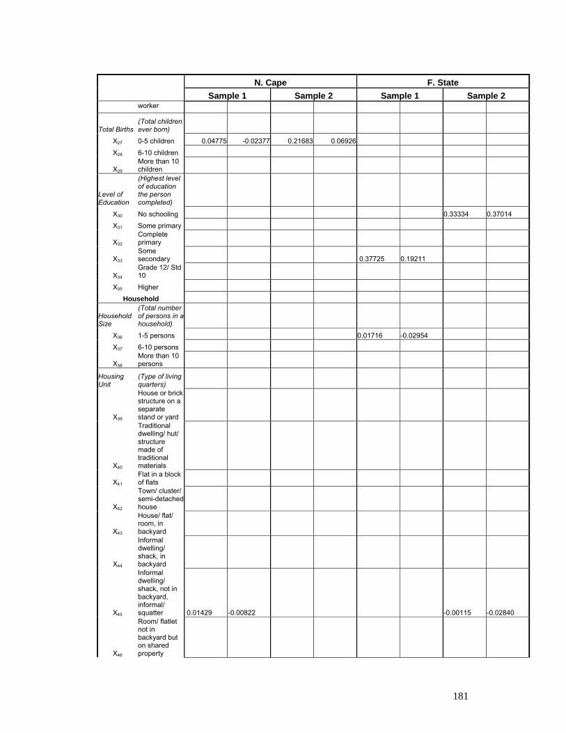
181
N. Cape F. State Sample 1 Sample 2 Sample 1 Sample 2
worker
Total Births (Total children ever born)
X27 0-5 children 0.04775 -0.02377 0.21683 0.06926
X28 6-10 children
X29 More than 10 children
Level of Education
(Highest level of education the person completed)
X30 No schooling 0.33334 0.37014
X31 Some primary
X32 Complete primary
X33 Some secondary 0.37725 0.19211
X34 Grade 12/ Std 10
X35 Higher
Household
Household Size
(Total number of persons in a household)
X36 1-5 persons 0.01716 -0.02954
X37 6-10 persons
X38 More than 10 persons
Housing Unit
(Type of living quarters)
X39
House or brick structure on a separate stand or yard
X40
Traditional dwelling/ hut/ structure made of traditional materials
X41 Flat in a block of flats
X42
Town/ cluster/ semi-detached house
X43
House/ flat/ room, in backyard
X44
Informal dwelling/ shack, in backyard
X45
Informal dwelling/ shack, not in backyard, informal/ squatter 0.01429 -0.00822 -0.00115 -0.02840
X46
Room/ flatlet not in backyard but on shared property

182
N. Cape F. State Sample 1 Sample 2 Sample 1 Sample 2
X47 Caravan or tent -0.20142 0.22181
X48 Private ship/ boat
Rooms
(Number of rooms that the household utilises)
X49 1-3 rooms
X50 4-6 rooms
X51 7-10 rooms
X52 More than 10 rooms
Access to Water
(Type of access to water)
X53
Piped water (tap) inside dwelling
X54
Piped water (tap) inside yard
X55
Piped water on community stand: < 200 metres
X56
Piped water on community stand: > 200 metres
X57 Borehole
X58 Spring
X59 Rainwater tank -0.2028 0.17718
X60 Dam/ pool/ stagnant water
X61 River/ stream -0.14207 0.09631
X62 Water vendor
Toilet facilities
(Main type of toilet facilities)
X63
Flush toilet (connected to sewerage system)
X64
Flush toilet (with septic tank)
X65 Chemical toilet -0.02266 0.10086
X66
Pit latrine with ventilation (VIP) -0.01476 0.05248
X67
Pit latrine without ventilation -0.04376 0.04348 -0.01795 0.13842
X68 Bucket latrine
X69 None -0.00333 0.05968
Energy source for cooking
(Type of energy/ fuel mainly used for cooking)
X70 Electricity

183
N. Cape F. State Sample 1 Sample 2 Sample 1 Sample 2
X71 Gas
X72 Paraffin 0.04203 -0.05148
X73 Wood -0.03138 0.03066 -0.02760 0.01929 -0.05808 0.27686 -0.07729 -0.0078
X74 Coal
X75 Animal dung -0.01613 0.17468 -0.10623 -0.01745
X76 Solar Gender of Head of Household
X77 Male
X78 Female Population Group of Head of Household
X79 Black African 0.22019 0.15547
X80 Coloured
X81 Indian or Asian
X82 White Occupation of Head of Household
X83
Legislators, senior officials and managers
X84 Professionals
X85
Technicians and associate professionals
X86 Clerks
X87
Service workers, shop and market sales workers
X88
Skilled agricultural and fishery workers -0.15278 0.10651 -0.10779 0.10002 -0.17093 0.31814
X89
Craft and related trades workers
X90
Plant and machine operators and assemblers -0.14137 0.24485
X91 Elementary occupations -0.10029 0.09497 -0.12539 0.06625 -0.12855 0.28095
X92
Occupations unspecified or not elsewhere classified
Annual Household Income
X93 No income
X94 R 1 - R 4 800
X95 R 4 801 - R 9 600
X96 R 9 601 - R 19 200
X97 R 19 201 - R 38 400
X98 R 38 401 - R 76 800
X99 R 76 801 - R 153 600
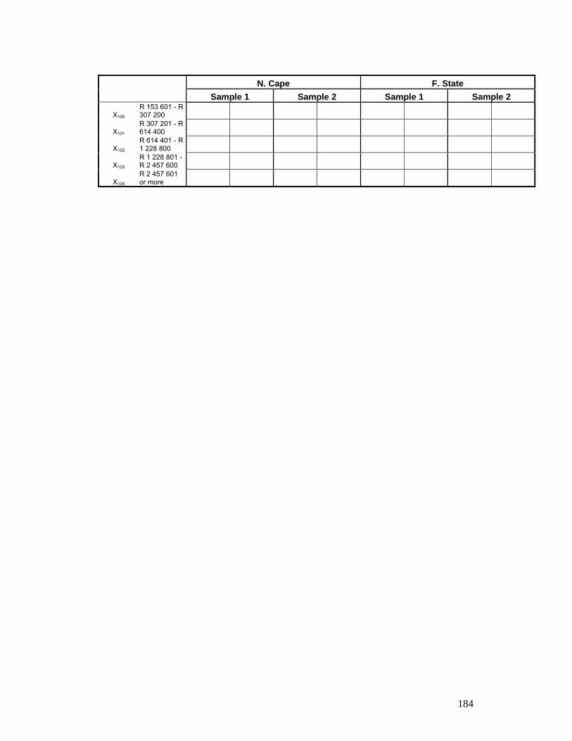
184
N. Cape F. State Sample 1 Sample 2 Sample 1 Sample 2
X100 R 153 601 - R 307 200
X101 R 307 201 - R 614 400
X102 R 614 401 - R 1 228 800
X103 R 1 228 801 - R 2 457 600
X104 R 2 457 601 or more

185
(Part 3) Coefficients of significant variables for the linear discriminant functions for KwaZulu-Natal and North West KZN N. West Sample 1 Sample 2 Sample 1 Sample 2 LDF (Urban) LDF (Rural) LDF (Urban) LDF (Rural) LDF (Urban) LDF (Rural) LDF (Urban) LDF (Rural)
CONSTANT -45.85524 -53.32265 -40.6216 -33.63047 -48.66572 -39.00236 -27.87796 -15.30619
Person
X1 Population density 0.0000849 -0.0000969 0.0002281 -0.0001053 0.0000304 0.0007397
Language
(Language most often spoken at home)
X2 Afrikaans
X3 English
X4 IsiNdebele
X5 IsiXhosa
X6 IsiZulu
X7 Sepedi
X8 Sesotho
X9 Setswana
X10 Siswati
X11 Tshivenda
X12 Xitsonga
Employment Status
(Employment status of each person)
X13 Employed
X14 Unemployed 0.19626 0.11307
X15 Scholar or student
X16 Home-maker or housewife
X17 Pensioner or retired person
X18
Unable to work due to illness or disability
X19
Seasonal worker not working presently
X20
Does not choose to work
X21 Could not find work
Work Status
(Main activity or work status of person)
X22 Paid employee -0.00266 0.25304
X23 Paid family worker
X24 Self-employed
X25 Employer
X26 Unpaid family

186
KZN N. West Sample 1 Sample 2 Sample 1 Sample 2
worker
Total Births (Total children ever born)
X27 0-5 children 0.1584 -0.01491
X28 6-10 children
X29 More than 10 children
Level of Education
(Highest level of education the person completed)
X30 No schooling 0.06859 0.2421 0.34962 0.48961
X31 Some primary 0.61286 0.79096
X32 Complete primary
X33 Some secondary
X34 Grade 12/ Std 10
X35 Higher
Household
Household Size
(Total number of persons in a household)
X36 1-5 persons
X37 6-10 persons
X38 More than 10 persons
Housing Unit
(Type of living quarters)
X39
House or brick structure on a separate stand or yard
X40
Traditional dwelling/ hut/ structure made of traditional materials 0.03566 0.08137
X41 Flat in a block of flats 0.02498 0.05933
X42
Town/ cluster/ semi-detached house
X43
House/ flat/ room, in backyard
X44
Informal dwelling/ shack, in backyard 0.10448 0.00115
X45
Informal dwelling/ shack, not in backyard, informal/ squatter 0.11895 -0.01373 0.07987 0.00460
X46
Room/ flatlet not in backyard but on shared property

187
KZN N. West Sample 1 Sample 2 Sample 1 Sample 2
X47 Caravan or tent
X48 Private ship/ boat
Rooms
(Number of rooms that the household utilises)
X49 1-3 rooms
X50 4-6 rooms 0.10847 0.06954
X51 7-10 rooms
X52 More than 10 rooms
Access to Water
(Type of access to water)
X53
Piped water (tap) inside dwelling
X54
Piped water (tap) inside yard
X55
Piped water on community stand: < 200 metres
X56
Piped water on community stand: > 200 metres
X57 Borehole -0.00958 0.22663
X58 Spring
X59 Rainwater tank
X60 Dam/ pool/ stagnant water
X61 River/ stream -0.03528 0.09776
X62 Water vendor
Toilet facilities
(Main type of toilet facilities)
X63
Flush toilet (connected to sewerage system) 0.21796 0.00824 0.09316 -0.04421 0.33024 0.03722
X64
Flush toilet (with septic tank) 0.20664 0.0481 0.27736 0.11931
X65 Chemical toilet
X66
Pit latrine with ventilation (VIP) 0.03258 -0.01551
X67
Pit latrine without ventilation 0.01818 0.05084
X68 Bucket latrine 0.06057 -0.02716 0.31094 0.03748
X69 None
Energy source for cooking
(Type of energy/ fuel mainly used for cooking)
X70 Electricity 0.79634 0.64658 0.09024 0.06435 -0.12828 0.0671

188
KZN N. West Sample 1 Sample 2 Sample 1 Sample 2
X71 Gas
X72 Paraffin
X73 Wood 0.70859 0.72466
X74 Coal
X75 Animal dung -0.58017 0.29937
X76 Solar Gender of Head of Household
X77 Male
X78 Female Population Group of Head of Household 0.17357 0.22767
X79 Black African
X80 Coloured
X81 Indian or Asian
X82 White Occupation of Head of Household
X83
Legislators, senior officials and managers
X84 Professionals
X85
Technicians and associate professionals
X86 Clerks
X87
Service workers, shop and market sales workers
X88
Skilled agricultural and fishery workers -0.10151 0.28302 -0.23064 -0.07783
X89
Craft and related trades workers -0.19415 0.09833
X90
Plant and machine operators and assemblers -0.12408 0.06510
X91 Elementary occupations -0.08997 0.00981 -0.184 0.09419 -0.07648 -0.02976
X92
Occupations unspecified or not elsewhere classified -0.24023 0.12628
Annual Household Income
X93 No income
X94 R 1 - R 4 800
X95 R 4 801 - R 9 600
X96 R 9 601 - R 19 200
X97 R 19 201 - R 38 400
X98 R 38 401 - R 76 800
X99 R 76 801 - R 153 600
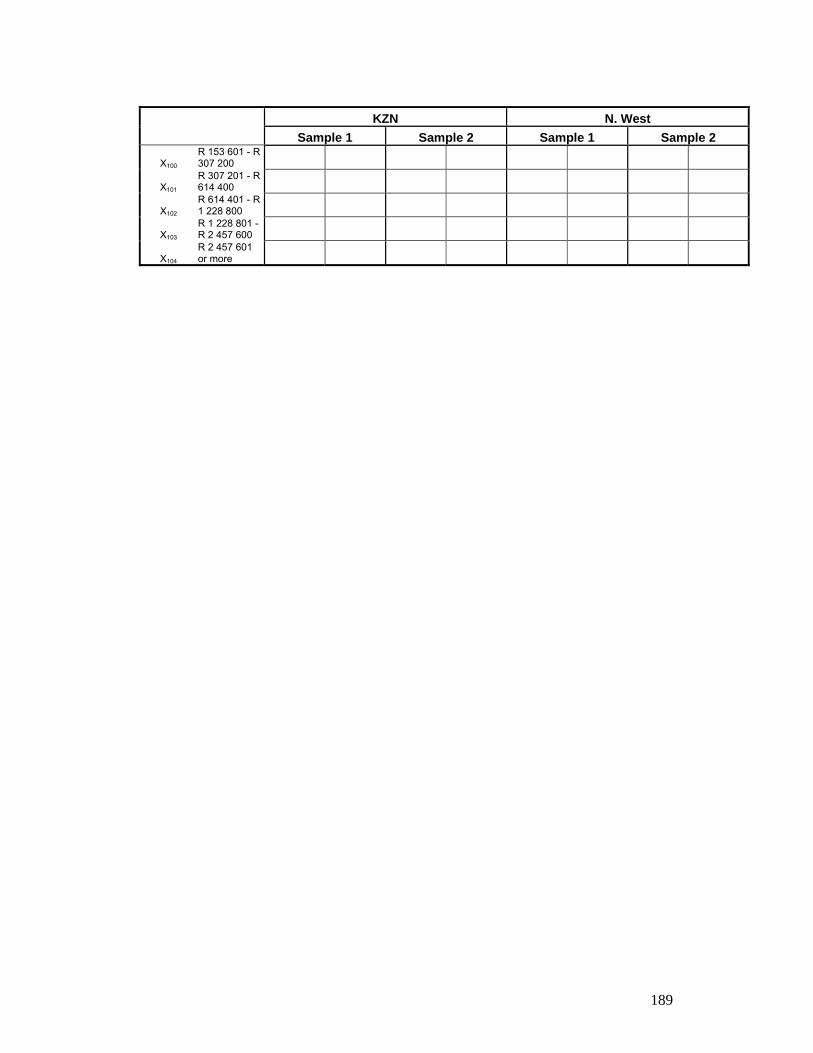
189
KZN N. West Sample 1 Sample 2 Sample 1 Sample 2
X100 R 153 601 - R 307 200
X101 R 307 201 - R 614 400
X102 R 614 401 - R 1 228 800
X103 R 1 228 801 - R 2 457 600
X104 R 2 457 601 or more

190
(Part 4) Coefficients of significant variables for the linear discriminant functions for Gauteng and Mpumalanga Gauteng MP Sample 1 Sample 2 Sample 1 Sample 2 LDF (Urban) LDF (Rural) LDF (Urban) LDF (Rural) LDF (Urban) LDF (Rural) LDF (Urban) LDF (Rural)
CONSTANT -69.05159 -99.19904 -69.05159 -99.19904 -14.45368 -17.58319 -12.77307 -14.24335
Person
X1 Population density 0.0002469 -0.0001784 -0.0002347 -0.0005404
Language
(Language most often spoken at home)
X2 Afrikaans
X3 English
X4 IsiNdebele 0.10901 -0.20477 0.1131 -0.15830
X5 IsiXhosa
X6 IsiZulu -0.01113 -0.03646
X7 Sepedi
X8 Sesotho
X9 Setswana
X10 Siswati
X11 Tshivenda
X12 Xitsonga
Employment Status
(Employment status of each person)
X13 Employed
X14 Unemployed
X15 Scholar or student
X16 Home-maker or housewife
X17 Pensioner or retired person
X18
Unable to work due to illness or disability
X19
Seasonal worker not working presently
X20 Does not choose to work
X21 Could not find work
Work Status
(Main activity or work status of person)
X22 Paid employee 0.1212 0.15877
X23 Paid family worker
X24 Self-employed -0.32926 -0.61633 -0.33510 -0.75026
X25 Employer
X26 Unpaid family worker

191
Gauteng MP Sample 1 Sample 2 Sample 1 Sample 2
Total Births (Total children ever born)
X27 0-5 children 0.18874 0.07598
X28 6-10 children
X29 More than 10 children
Level of Education
(Highest level of education the person completed)
X30 No schooling
X31 Some primary
X32 Complete primary
X33 Some secondary
X34 Grade 12/ Std 10
X35 Higher
Household
Household Size
(Total number of persons in a household)
X36 1-5 persons
X37 6-10 persons
X38 More than 10 persons
Housing Unit
(Type of living quarters)
X39
House or brick structure on a separate stand or yard
X40
Traditional dwelling/ hut/ structure made of traditional materials 0.00353 0.04373
X41 Flat in a block of flats
X42
Town/ cluster/ semi-detached house
X43
House/ flat/ room, in backyard
X44
Informal dwelling/ shack, in backyard
X45
Informal dwelling/ shack, not in backyard, informal/ squatter 0.11308 0.03723 0.11709 0.04646 0.02669 -0.01261
X46
Room/ flatlet not in backyard but on shared property
X47 Caravan or tent
X48 Private ship/ boat
Rooms
(Number of rooms that the household
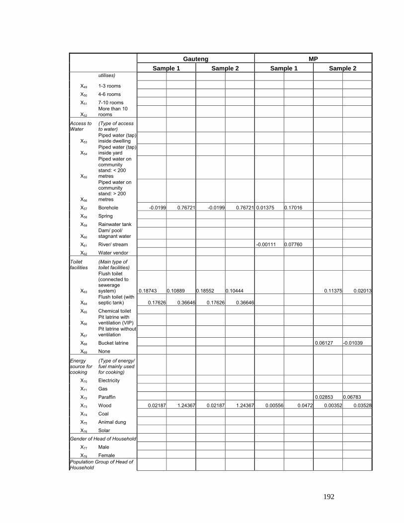
192
Gauteng MP Sample 1 Sample 2 Sample 1 Sample 2
utilises)
X49 1-3 rooms
X50 4-6 rooms
X51 7-10 rooms
X52 More than 10 rooms
Access to Water
(Type of access to water)
X53 Piped water (tap) inside dwelling
X54 Piped water (tap) inside yard
X55
Piped water on community stand: < 200 metres
X56
Piped water on community stand: > 200 metres
X57 Borehole -0.0199 0.76721 -0.0199 0.76721 0.01375 0.17016
X58 Spring
X59 Rainwater tank
X60 Dam/ pool/ stagnant water
X61 River/ stream -0.00111 0.07760
X62 Water vendor
Toilet facilities
(Main type of toilet facilities)
X63
Flush toilet (connected to sewerage system) 0.18743 0.10889 0.18552 0.10444 0.11375 0.02013
X64 Flush toilet (with septic tank) 0.17626 0.36646 0.17626 0.36646
X65 Chemical toilet
X66 Pit latrine with ventilation (VIP)
X67 Pit latrine without ventilation
X68 Bucket latrine 0.06127 -0.01039
X69 None
Energy source for cooking
(Type of energy/ fuel mainly used for cooking)
X70 Electricity
X71 Gas
X72 Paraffin 0.02853 0.06783
X73 Wood 0.02187 1.24367 0.02187 1.24367 0.00556 0.0472 0.00352 0.03528
X74 Coal
X75 Animal dung
X76 Solar
Gender of Head of Household
X77 Male
X78 Female Population Group of Head of Household

193
Gauteng MP Sample 1 Sample 2 Sample 1 Sample 2
X79 Black African 0.1742 0.22222
X80 Coloured
X81 Indian or Asian
X82 White Occupation of Head of Household
X83
Legislators, senior officials and managers
X84 Professionals
X85
Technicians and associate professionals
X86 Clerks
X87
Service workers, shop and market sales workers
X88
Skilled agricultural and fishery workers -0.12886 2.58179 -0.12886 2.58179 -0.06524 0.10064 -0.19090 -0.08819
X89 Craft and related trades workers
X90
Plant and machine operators and assemblers 0.0126 0.0935
X91 Elementary occupations -0.15157 0.21927 -0.15157 0.21927 0.00376 0.05354
X92
Occupations unspecified or not elsewhere classified
Annual Household Income
X93 No income 0.11775 0.09273 0.13855 0.11880
X94 R 1 - R 4 800
X95 R 4 801 - R 9 600
X96 R 9 601 - R 19 200
X97 R 19 201 - R 38 400
X98 R 38 401 - R 76 800
X99 R 76 801 - R 153 600 -0.00844 -0.07137
X100 R 153 601 - R 307 200
X101 R 307 201 - R 614 400
X102 R 614 401 - R 1 228 800
X103 R 1 228 801 - R 2 457 600
X104 R 2 457 601 or more

194
(Part 5) Coefficients of significant variables for the linear discriminant functions for Limpopo and South Africa as a whole Limpopo RSA Sample 1 Sample 2 Sample 1 Sample 2 LDF (Urban) LDF (Rural) LDF (Urban) LDF (Rural) LDF (Urban) LDF (Rural) LDF (Urban) LDF (Rural)
CONSTANT -16.62465 -13.68195 -64.25581 -57.37735 -34.07552 -34.71215 -29.12101 -23.46501
Person
X1 Population density 0.0006189 -0.0005445
Language
(Language most often spoken at home)
X2 Afrikaans 0.15033 0.08441 1.17996 1.05291
X3 English 1.30677 1.12542
X4 IsiNdebele 0.14797 -0.01982
X5 IsiXhosa
X6 IsiZulu
X7 Sepedi
X8 Sesotho
X9 Setswana
X10 Siswati
X11 Tshivenda
X12 Xitsonga -0.01369 0.00405
Employment Status
(Employment status of each person)
X13 Employed
X14 Unemployed 0.32901 0.15108
X15 Scholar or student
X16 Home-maker or housewife
X17 Pensioner or retired person
X18
Unable to work due to illness or disability
X19
Seasonal worker not working presently
X20 Does not choose to work
X21 Could not find work 0.48525 0.19063
Work Status
(Main activity or work status of person)
X22 Paid employee
X23 Paid family worker
X24 Self-employed
X25 Employer
X26 Unpaid family worker

195
Limpopo RSA Sample 1 Sample 2 Sample 1 Sample 2
Total Births (Total children ever born)
X27 0-5 children
X28 6-10 children
X29 More than 10 children
Level of Education
(Highest level of education the person completed)
X30 No schooling
X31 Some primary
X32 Complete primary
X33 Some secondary
X34 Grade 12/ Std 10
X35 Higher
Household
Household Size
(Total number of persons in a household)
X36 1-5 persons
X37 6-10 persons 0.07952 0.0005374
X38 More than 10 persons
Housing Unit
(Type of living quarters)
X39
House or brick structure on a separate stand or yard 0.01002 0.00181
X40
Traditional dwelling/ hut/ structure made of traditional materials
X41 Flat in a block of flats
X42
Town/ cluster/ semi-detached house
X43
House/ flat/ room, in backyard
X44
Informal dwelling/ shack, in backyard 0.07004 0.00412
X45
Informal dwelling/ shack, not in backyard, informal/ squatter 0.04097 -0.0000317 0.10551 0.02211
X46
Room/ flatlet not in backyard but on shared property
X47 Caravan or tent
X48 Private ship/ boat
Rooms
(Number of rooms that the household

196
Limpopo RSA Sample 1 Sample 2 Sample 1 Sample 2
utilises)
X49 1-3 rooms
X50 4-6 rooms
X51 7-10 rooms
X52 More than 10 rooms
Access to Water
(Type of access to water)
X53 Piped water (tap) inside dwelling
X54 Piped water (tap) inside yard
X55
Piped water on community stand: < 200 metres
X56
Piped water on community stand: > 200 metres
X57 Borehole
X58 Spring
X59 Rainwater tank
X60 Dam/ pool/ stagnant water
X61 River/ stream -0.03509 0.08867
X62 Water vendor
Toilet facilities
(Main type of toilet facilities)
X63
Flush toilet (connected to sewerage system) 0.16491 0.00852 0.00482 0.05628 0.21709 0.06066
X64 Flush toilet (with septic tank) 0.01816 0.07992 0.18751 0.09307
X65 Chemical toilet
X66 Pit latrine with ventilation (VIP)
X67 Pit latrine without ventilation 0.03325 0.05721
X68 Bucket latrine -0.15112 0.05774 0.05972 0.01552 0.16831 0.02298
X69 None Energy source for cooking
(Type of energy/ fuel mainly used for cooking)
X70 Electricity
X71 Gas
X72 Paraffin 0.06726 -0.02421 -0.00683 0.14897 0.02675 0.06034
X73 Wood -0.03418 0.06317
X74 Coal
X75 Animal dung 0.03831 0.07508
X76 Solar
Gender of Head of Household
X77 Male
X78 Female 0.15381 0.08890 0.53218 0.42717 Population Group of Head of Household
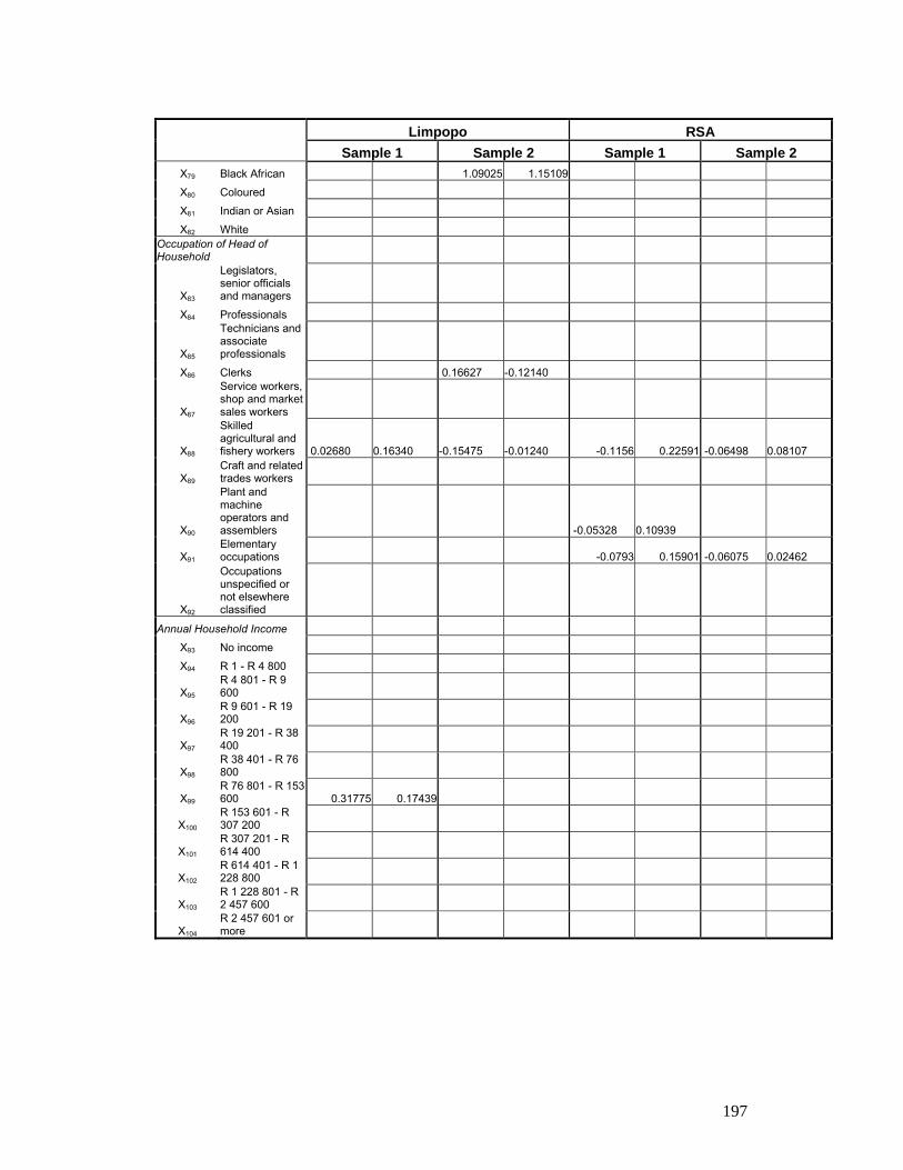
197
Limpopo RSA Sample 1 Sample 2 Sample 1 Sample 2
X79 Black African 1.09025 1.15109
X80 Coloured
X81 Indian or Asian
X82 White Occupation of Head of Household
X83
Legislators, senior officials and managers
X84 Professionals
X85
Technicians and associate professionals
X86 Clerks 0.16627 -0.12140
X87
Service workers, shop and market sales workers
X88
Skilled agricultural and fishery workers 0.02680 0.16340 -0.15475 -0.01240 -0.1156 0.22591 -0.06498 0.08107
X89 Craft and related trades workers
X90
Plant and machine operators and assemblers -0.05328 0.10939
X91 Elementary occupations -0.0793 0.15901 -0.06075 0.02462
X92
Occupations unspecified or not elsewhere classified
Annual Household Income
X93 No income
X94 R 1 - R 4 800
X95 R 4 801 - R 9 600
X96 R 9 601 - R 19 200
X97 R 19 201 - R 38 400
X98 R 38 401 - R 76 800
X99 R 76 801 - R 153 600 0.31775 0.17439
X100 R 153 601 - R 307 200
X101 R 307 201 - R 614 400
X102 R 614 401 - R 1 228 800
X103 R 1 228 801 - R 2 457 600
X104 R 2 457 601 or more

198
APPENDIX E Maps illustrating the provincial urban and rural classification

199

200

201

202
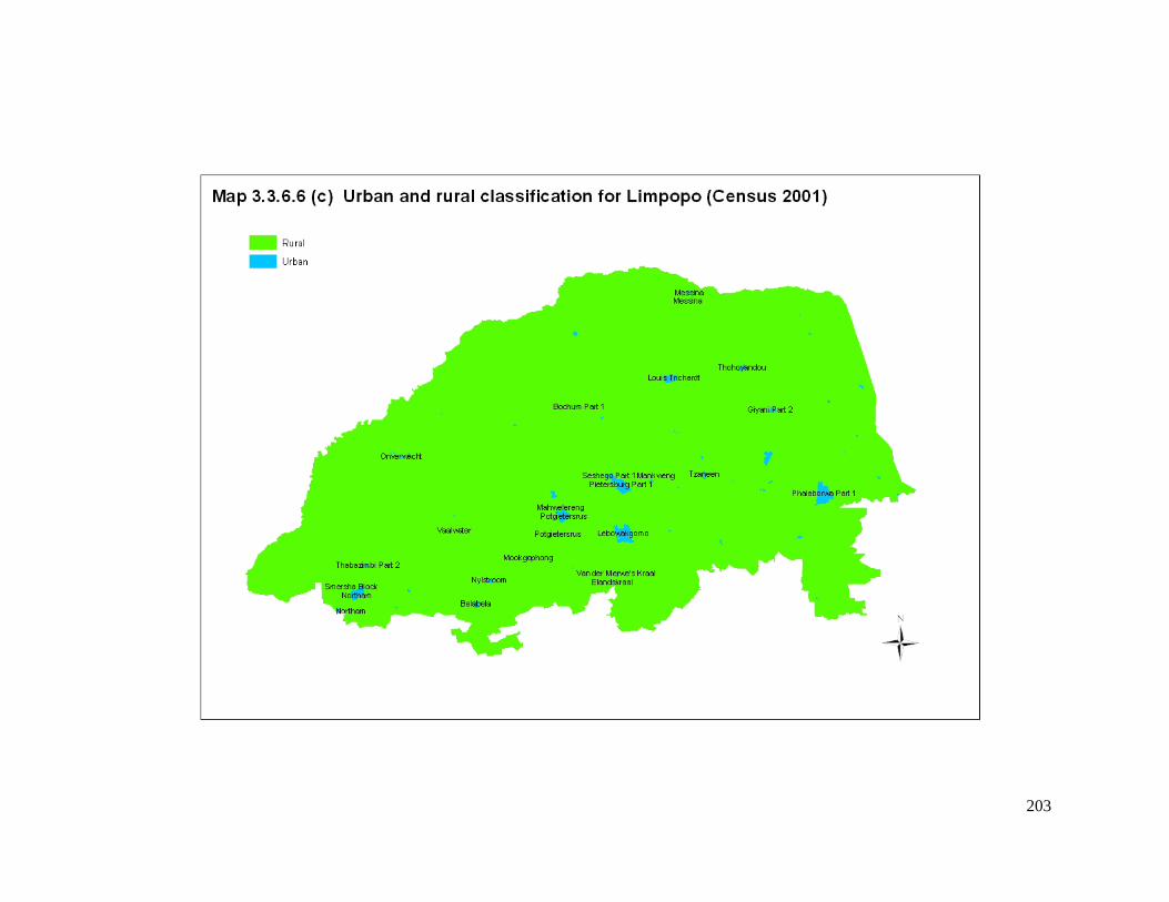
203

204