Statistical Arbitrage: Asset clustering, market-exposure minimization, and

high-frequency explorations.

Aniket Inamdar(ainamdar@stanford.edu), Blake Jennings(bmj@stanford.edu), BernardoRamos(bramos@stanford.edu), Yiwen Chen(yiwen15@stanford.edu), Ben

Etringer(etringer@stanford.edu)

Stanford University

MS&E 448, Spring 2016

Abstract

In this paper we describe and implement two statistical arbitrage trading strategies. The first strategy models themean-reverting residual of a cluster of assets whose weights are selected so as to minimize market exposure. The secondstrategy maintains a portfolio of pairs, each weighted proportional to a measure of mean-reversion speed. We presentperformance metrics for each strategy, discuss the difficulties of their application into high-frequency trading, and suggesta direction where future research could focus.

1 Introduction

The technique of statistical arbitrage is the systematic exploitation of perceived mispricings of similar assets. A tradingstrategy built around statistical arbitrage involves three fundamental pillars: (1) a measure of similarity of assets, (2) ameasure of pricing mismatch, and (3) a confidence metric for each mismatch. Traditional statistical arbitrage techniques, like“Pairs Trading”, employ these three pillars, holding long-short positions in a pair of strongly “similar” assets. The covariance(or correlation) between two assets is a widely used metric of their “similarity”. However, recent studies have used additionalattributes such as co-integration tests to select asset pairs that are better suited for a statistical arbitrage trading strategy.

We base our signal generation strategy on the seminal paper [3], whose theory is briefly described in Sec. 2. Next, Sec.3.1 describes a strategy to select assets to perform statistical arbitrage on. Sec. 3.2 introduces a mechanism by which weattempt to achieve market neutrality. Sec. 4.1 shows the efficacy of our asset selection procedure, and Sec. 4.2, 4.3 containa detailed discussion on the performance of the strategy across a wide range of sectors for up to 9 years of out-of-sampletesting. Section 5 presents a multiple pairs trading strategy and the idiosyncrasies involved with mean reversion at differentfrequencies. Section 6 compares the strategy’s performance in both low and high-frequency. Section 7 presents the conclusionand final remarks.

2 Model Basics - Signal Generation

Consider the returns of two correlated assets. We can express the relationship between the returns as a linear relationship,

dQ

Q= α+ β

dP

P+ ε (2.1)

Since dPP and dQ

Q are correlated returns for a given lookback period (from the literature, this lookback time is 60 days

for daily signal generation, which makes sense intuitively for correlated assets with quarterly earnings reporting [3]), we canexpress their residuals ε as a mean reverting process dXt. That is, we can express dXt as the instantaneous mismatch in thereturns of the assets we are considering by performing a simple linear regression. In practice, α ≈ 0, so we will set α = 0here for simplification. Note, problems can arise when we take on this assumption for assets with drift α 6= 0 (explained indepth in Section 5). We then have the following model,

dXt =dQ

Q− β dP

P(2.2)

In traditional single-pairs trading, dXt could be interpreted as a 2-asset portfolio with the weight of one asset proportionalto the regression coefficient of its returns with the returns of the other asset, but it could also model the residual of a general

1

cluster of assets. The principle hypothesis of statistical arbitrage is that the mismatch between any two correlated assets ismean-reverting and may be modeled as a stochastic mean reverting process. In [3], the choice of the mean reverting process- which also seems to be the conventional wisdom - is the Ornstein-Uhlenbeck (OU) process,

dXt = κ(m−Xt) + σdWt (2.3)

where

dXt = κ︸︷︷︸Mean Reversion Speed

(

Mean︷︸︸︷m −Xt) + σ︸︷︷︸

V olatility

Brownian Motion︷︸︸︷dWt (2.4)

Noting that the Autoregressive (AR-1) model is the discretized version of the OU-process, where {a, b, ξ} are as in equation(2.6), we can regress to obtain {a, b,Var{ξ}} and back out the parameters {κ,m, σ2}.

Xn+1 = a+ bXn + ξn+1 (2.5)

b = exp (−κdt) a = m(1− exp (−κdt)) Var(ξ) = σ2 1−exp (−2κdt)2κ

(2.6)

where the trading signal is defined by

s = −m√

2κ

σ, (2.7)

where s is a normalized signal that indicates the number of units of mismatch in terms of the volatility of the OU processand dt is the frequency of the signal generation. In subsequent sections, we present results for several dt. Consider a pairposition to hold −β units of asset P and 1 unit of asset Q. Then a negative value for s suggests the pair is underpricedwhile a positive value suggests the pair is overpriced. Clearly, a signal within ±1 standard deviation is expected roughly 66%of the time if we take on the convention that normalized returns are i.i.d. Gaussian, and hence is not reasonable to tradeon. Thus, the signal resulting from the mismatch is not a statistical anomaly if it only fluctuates ±1 standard deviation. A“significantly” negative (corr. positive) value suggests that there is statistically significant underpricing (corr. overpricing)of the pair. Thus, it is reasonable to expect gains if we enter into a long (corr. short) position as the signal is expected tomean-revert. We inherit the signal thresholds from [3], see equation 2.8. We enter a long position when the signal crossesslong,enter and hold the position until the signal crosses slong,exit. We follow an identical process for a short position (seefigure 1). We establish a stop-loss rule in Section 5.3.1.

slong,enter = −1.25 slong,exit = −0.5 sshort,enter = 1.25 sshort,exit = 0.75 (2.8)

Figure 1: An example of a trading signal generated from daily returns of XLF and JPM in 2014

2

3 Strategy 1: Cluster Trading

In this section we describe a generalized statistical arbitrage strategy that minimizes exposure to market factors. Theasset universe is projected onto its first three orthogonal principle components and clustered based on their mutual proximityin this orthogonal sub-space. Two distinct linear combinations of cluster members (cluster residuals) are obtained that aremarket neutral under the assumption of being portfolios with either positive or negative expected bank-excess returns. Thesecluster residuals are amenable to being modeled as mean reverting stochastic processes on which a recent arbitrage strategyis implemented. The feasibility and performance of this strategy are discussed in detail.

3.1 Asset Selection - Subtractive Clustering in Orthogonal Eigenspace

Now that we have a methodology to generate a trading signal, the logical next step is selecting assets from a given universeto trade on. For this we employ a combination of Principle Component Analysis (PCA) and subtractive clustering.

Let RT×M be the daily bank excess returns (henceforth the term “return” describes bank-excess return) of M assets forT days, and define ~rm to be the daily returns of asset m. Define ~ym = ~rm−µm

σmand YT×M = [~y1~y2...~yM ] ,where µm = E(~rm)

and σm =√Var(~rm). Now, using singular value decomposition for Y , we get,

YT×M = UT×MΣM×MVTM×M = F̃T×M β̃M×M ≈ UT×KΣK×KV

TM×K = FT×KβK×M︸ ︷︷ ︸

K-factor approximation

Note that ~fk’s are orthonormal. Thus, the columns of β, ~bm may be considered the coordinates of the mth asset inthe K-dimensional orthogonal factor space. Now that we have a “measure” for each asset, we have access to a plethora ofalgorithms to group based on proximity. One such algorithm is the subtractive clustering algorithm that is used here tofind clusters of assets that have their ~bm’s within an ellipsoid in the K-dimensional factor space. We define the radii of thisellipsoid as follows:

ri =

(1

σsvdi

)2∑Kj=1

(1

σsvdj

)2 ∣∣ i ∈ [1, 2, ..,K]

This accounts for the relative importance of each principle component as indicated by its corr. singular value. The higherthe singular value, the closer the assets must be in the direction of the component, since the contribution of the corr. principlecomponent to systematic part of the variance is greater. Note, this process needs no heuristic thresholds!

3.2 Cluster Signal Generation

In section 3.1 we described how to obtain a set of clusters of assets that are expected to behave similarly. For us to usethe signal generation strategy described in Sec. 2, we now have to generate dXt needed therein. We simultaneously espouseto keep our exposure to the K principle components (and by extension, to the systematic part of market variance) to aminimum. In the case of pairs trading, we know

Xt = drP − βdrQ = [1 − β]

[drPdrQ

]i.e. the dXt is a linear combination of the returns of the asset pair or equivalently, dXt are the returns of a portfolio

containing assets {P,Q}.Let us consider a cluster with P assets and define our dXt = YT×P ~w as a linear combination of the returns of the assets

in the cluster (or the returns of a portfolio consisting of the cluster assets) . A naive way to minimize market exposure wouldbe to minimize ~wTCov(Y )~w such that ~wT1 = 1 (normalizing weights). But this puts no restriction on the expected returnof the portfolio. If we were to short (corr. long) this portfolio, we would desire for its expected return to be non-positive(corr. non-negative). This is a natural way to minimize stop losses! Hence, we consider two distinct linear combinations(portfolios) of the cluster assets - one with weights ~wl for when we wish to enter a long position and one with ~ws when wewish to short the portfolio.

min~wl/s∈RP

~wTl/sCov(YT×P )~wl/s = ‖βT×P ~wl/s‖22

s.t. ~wTl/s1 = 1

and ~wTl ~µ ≥ 0 ~wTl ~µ ≤ 0

(3.1)

where µi = E(~yi)∣∣ i ∈ [1, 2, ..., P ].

We now have two measures of mismatch in the pricing of the cluster as a whole and use them to find the correspondingtrading signals sl, ss. We enter a long (corr. short) position in the cluster iff sl < slong,enter (corr. ss > sshort,enter).

3

4 Cluster Trading: Results and Discussion

Before we discuss the performance of the clustering and trading strategies, it is important to note the underlying assump-tions that have gone into the strategies:

1. Look-Back Period : The clustering and signal generation are both based on a moving window look-back of 60 days.It is assumed that this period is long enough for any market event at the beginning of the period to have been accountedfor.

2. Systematic Principle Components : All through our simulations, the PCA was truncated to K = 3. It is assumedthat the first 3 principle components are sufficient to describe the systematic part of the market. In other words, theyaccount for ∼ 50% of the observed variance.

3. Signal Thresholding : We use the thresholds from [3] given in eqn. 2.8. That is, we consider the signal has deviated“significantly” iff its different form zero with 90% confidence (Φ(slong,enter) ≈ 0.1, 1−Φ(sshort,enter) ≈ 0.1).

4. Risk-Free (Bank) Returns: We assume that the bank rate is constant and equal to 5% annualized.

Besides the above, the algorithm requires no external inputs. No other heuristic is implemented. The objective is toobserve the PDF of trade gains using this strategy and whether the strategy has any inherent merit. If it does (i.e. if itsPDF is skewed to the right of zero), it can then be improved upon by heuristics designed to sample from the favorable halfof the aforementioned PDF. A large number of datasets were used to perform our simulations. These are listed in table 1.

Name Size Duration(# of assets)

S&P 500 422 2 yrs.NYSE 599 9 yrs.

Random(Russel 2000) 1661 9 yrs.XLB 24 9 yrs.XLE 33 9 yrs.XLF 85 9 yrs.XLFS 57 9 yrs.XLI 61 9 yrs.XLK 64 9 yrs.XLP 32 9 yrs.

XLRE 28 9 yrs.XLU 28 9 yrs.XLV 52 9 yrs.XLY 77 9 yrs.

Concatenated ETFs 456 9 yrs.All Traded(ongoing) variable 9 yrs.

Table 1: List of Datasets

4.1 Clustering Efficiency

Here we wish to examine whether the clustering algorithm selects groups of assets that are indeed related. For thispurpose, we find clusters in the concatenated ETFs and check which ETF the members of each cluster come from. Theclustering algorithm produces 30 clusters from the 456 assets in the concatenated ETF universe. In table 2 the breakdownof each of the 30 clusters is shown. It is clear that the clustering algorithm groups together assets primarily from one majorETF.

It is also able to detect that XLF(Finance) and XLFS(Finance) are similar ETFs. Similarly, the clustering is suggestiveof the ETFs XLP(Consumer) and XLV(Health) to have some assets that are strongly similar - e.g. Cluster 30 has Coca-Cola, CVS, Mondelez(food & beverage), McCormick(spices & herbs) and Merc. & Co.(pharma). In cluster 11 we haveDanaher(design & manufacturing), Minnesota Mining & Manufacturing, Parker Hannifin (hi tech. manufacturing), RockwellAutomation, Stanley Black & Decker (hardware & tools manufacturing) and Walt Disney. While Disney doesn’t quite fit thegroup, it is a fortune 100 company that helps hedge the rest of the portfolio against the market.

The large cardinality of clusters is a consequence of the underlying universe being well defined (and hopefully related)assets from market ETFs. In fig. 2, the clusters for the “Random” dataset are shown. Clearly, the size of the clusters increaseand the number of clusters decrease as the underlying universe is random and weakly correlated. Another observation to bemade is the fact that the clustering is the most sensitive to PC1 and almost agnostic to PC2 and PC3. This is to be expectedfor a random collection of assets as they don’t necessarily belong to a well defined sector/industry.

4

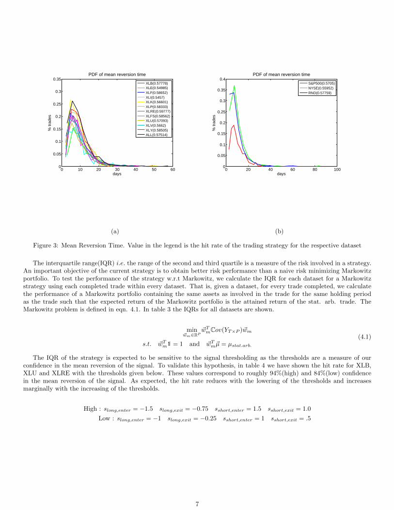
4.2 Trading Signal Statistics

An ex-post sanity check of our look-back period would be to check if the mean reversion times of the OU processes observedby the traded clusters are less than ∼ 30(= 60

2 ) days. In the absence of dealiasing, only half the frequencies contained ina dataset with equispaced sampling are uncontaminated (Nyquist sampling theorem). In fig. 3, histogram plots for meanreversion times for all datasets is shown. Clearly, an overwhelming majority of the trades are seen to have a mean reversiontime of about 8-10 days.

Cluster Number Cluster Breakdown Total

1 3(3), 2(4), 7(5), 1(7), 2(8), 2(11) 142 1(1), 2(3), 3(4), 3(5), 2(8), 2(11) 113 1(4), 5(5), 1(10), 1(11) 84 1(1), 1(3), 4(5), 1(8) 65 4(3), 2(4), 4(8) 66 6(10) 67 1(3), 4(5), 1(7), 1(10) 68 3(4), 2(5) 59 1(3), 1(4), 4(5), 1(6), 1(8), 1(10) 810 1(6), 2(11) 311 5(4), 1(11) 612 1(3), 1(5), 1(7), 1(10) 313 8(2) 814 1(3), 2(4), 1(8), 1(11) 415 3(3), 2(7), 1(8) 316 2(6), 2(10) 417 4(6) 418 1(1), 1(3), 2(4), 1(8) 419 2(5), 1(11) 320 3(3), 3(8) 321 1(6), 3(10) 422 3(9) 323 2(9), 1(10) 324 2(9) 225 1(6), 2(10) 326 3(10) 327 1(5), 1(11) 228 1(1), 2(4) 329 3(3), 1(7), 2(8) 330 4(6), 1(10) 5

ETF Key

XLB 1XLE 2XLF 3XLI 4XLK 5XLP 6

XLRE 7XLFS 8XLU 9XLV 10XLY 11

Table 2: Performance of the Clustering Algorithm. Value in brackets is the key of the ETF

4.3 Trade Statistics

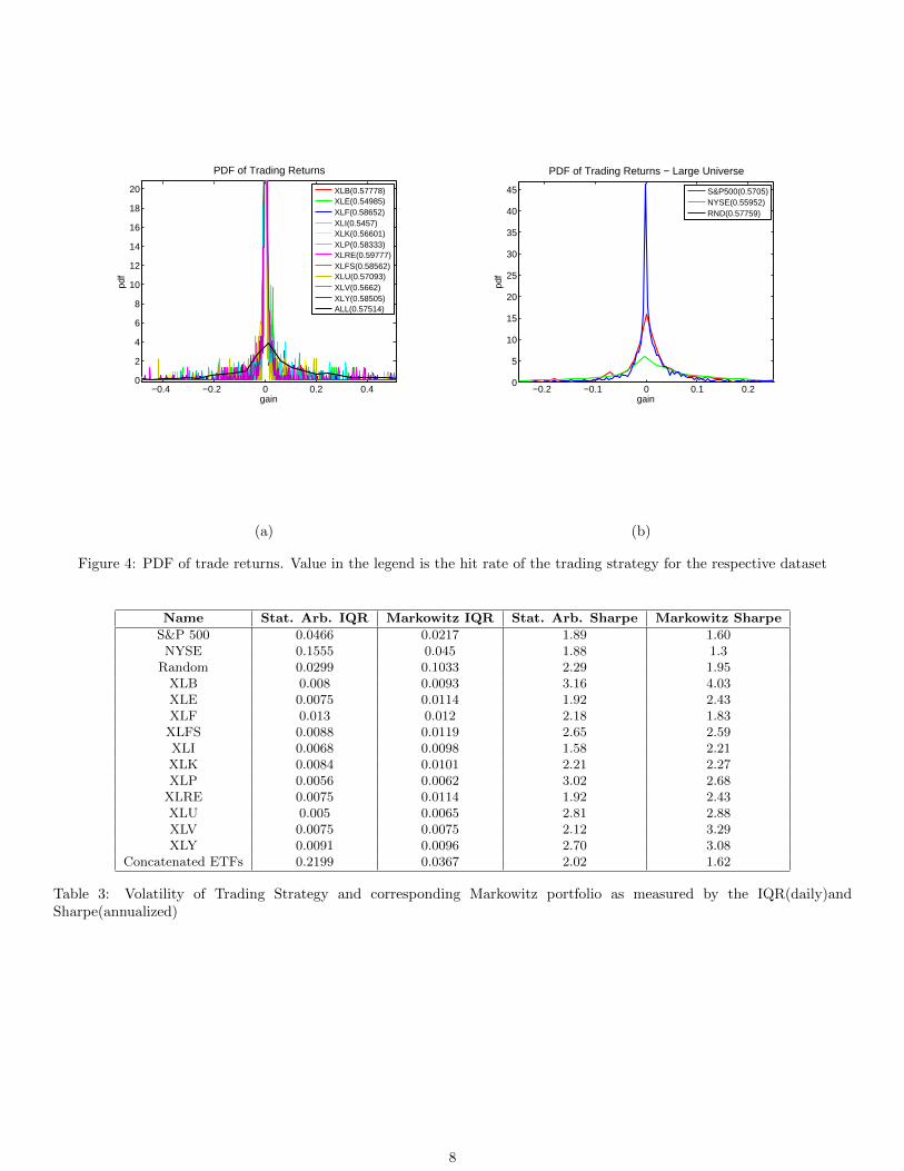
In this section, we discuss the performance of the raw (no heuristics) trading strategy. We desire a PDF of bank excessreturns that is positively skewed. In fig. 6 the PDFs for all the datasets are shown. All PDFs, regardless of the dataset,show a characteristic distribution - peak around zero with a narrow negative tail and thicker positive tail - resulting in a hitrate of ∼ 57% across all datasets. This behavior is clearly visible in the PDF of the concatenated ETFs (fig. 5).

5

−60

−40

−20

0

20

40

−20

−10

0

10

20

30−25

−20

−15

−10

−5

0

5

10

15

PC1PC2

PC

3

−60 −50 −40 −30 −20 −10 0 10 20 30 40−20

−15

−10

−5

0

5

10

15

20

25

30

PC1

PC

2

(a) Isometric View (b) PC1 - PC2

−60 −50 −40 −30 −20 −10 0 10 20 30 40−25

−20

−15

−10

−5

0

5

10

15

PC1

PC

3

−20 −15 −10 −5 0 5 10 15 20 25−25

−20

−15

−10

−5

0

5

10

15

PC

3

(c) PC1-PC3 (b) PC2 - PC3

Figure 2: Clusters for the “Random” dataset

6

0 10 20 30 40 50 600

0.05

0.1

0.15

0.2

0.25

0.3

0.35

days

% tr

ades

PDF of mean reversion time

XLB(0.57778)XLE(0.54985)XLF(0.58652)XLI(0.5457)XLK(0.56601)XLP(0.58333)XLRE(0.59777)XLFS(0.58562)XLU(0.57093)XLV(0.5662)XLY(0.58505)ALL(0.57514)

0 20 40 60 80 1000

0.05

0.1

0.15

0.2

0.25

0.3

0.35

0.4

days

% tr

ades

PDF of mean reversion time

S&P500(0.5705)NYSE(0.55952)RND(0.57759)

(a) (b)

Figure 3: Mean Reversion Time. Value in the legend is the hit rate of the trading strategy for the respective dataset

The interquartile range(IQR) i.e. the range of the second and third quartile is a measure of the risk involved in a strategy.An important objective of the current strategy is to obtain better risk performance than a naive risk minimizing Markowitzportfolio. To test the performance of the strategy w.r.t Markowitz, we calculate the IQR for each dataset for a Markowitzstrategy using each completed trade within every dataset. That is, given a dataset, for every trade completed, we calculatethe performance of a Markowitz portfolio containing the same assets as involved in the trade for the same holding periodas the trade such that the expected return of the Markowitz portfolio is the attained return of the stat. arb. trade. TheMarkowitz problem is defined in eqn. 4.1. In table 3 the IQRs for all datasets are shown.

min~wm∈RP

~wTmCov(YT×P )~wm

s.t. ~wTm1 = 1 and ~wTm~µ = µstat.arb.

(4.1)

The IQR of the strategy is expected to be sensitive to the signal thresholding as the thresholds are a measure of ourconfidence in the mean reversion of the signal. To validate this hypothesis, in table 4 we have shown the hit rate for XLB,XLU and XLRE with the thresholds given below. These values correspond to roughly 94%(high) and 84%(low) confidencein the mean reversion of the signal. As expected, the hit rate reduces with the lowering of the thresholds and increasesmarginally with the increasing of the thresholds.

High : slong,enter = −1.5 slong,exit = −0.75 sshort,enter = 1.5 sshort,exit = 1.0

Low : slong,enter = −1 slong,exit = −0.25 sshort,enter = 1 sshort,exit = .5

7

−0.4 −0.2 0 0.2 0.40

2

4

6

8

10

12

14

16

18

20

gain

pdf

PDF of Trading Returns

XLB(0.57778)XLE(0.54985)XLF(0.58652)XLI(0.5457)XLK(0.56601)XLP(0.58333)XLRE(0.59777)XLFS(0.58562)XLU(0.57093)XLV(0.5662)XLY(0.58505)ALL(0.57514)

−0.2 −0.1 0 0.1 0.20

5

10

15

20

25

30

35

40

45

gain

pdf

PDF of Trading Returns − Large Universe

S&P500(0.5705)NYSE(0.55952)RND(0.57759)

(a) (b)

Figure 4: PDF of trade returns. Value in the legend is the hit rate of the trading strategy for the respective dataset

Name Stat. Arb. IQR Markowitz IQR Stat. Arb. Sharpe Markowitz Sharpe

S&P 500 0.0466 0.0217 1.89 1.60NYSE 0.1555 0.045 1.88 1.3

Random 0.0299 0.1033 2.29 1.95XLB 0.008 0.0093 3.16 4.03XLE 0.0075 0.0114 1.92 2.43XLF 0.013 0.012 2.18 1.83

XLFS 0.0088 0.0119 2.65 2.59XLI 0.0068 0.0098 1.58 2.21XLK 0.0084 0.0101 2.21 2.27XLP 0.0056 0.0062 3.02 2.68

XLRE 0.0075 0.0114 1.92 2.43XLU 0.005 0.0065 2.81 2.88XLV 0.0075 0.0075 2.12 3.29XLY 0.0091 0.0096 2.70 3.08

Concatenated ETFs 0.2199 0.0367 2.02 1.62

Table 3: Volatility of Trading Strategy and corresponding Markowitz portfolio as measured by the IQR(daily)andSharpe(annualized)

8

−1 −0.5 0 0.5 10

0.5

1

1.5

2

2.5

3

3.5

4

gain

pdf

PDF of Trading Returns − ALL

Figure 5: Nature of PDF of trade returns.

Thresholds XLB XLU XLRELower 56.9% 55.6% 58.7%

Baseline 58% 57% 60%Higher 59% 58% 60.5%

Table 4: Sensitivity of Hit Rate to Signal Thresholding

5 Strategy 2: Combinatorial Pairs Trading at Different Frequencies

In this section we present a strategy built on a generalization of the single-pair framework. Unlike the eigenportfoliocontributions from Avellaneda and Lee or the clustering approach presented above, similarity between assets here is notmeasured via a multi-factor regression model [3]. Instead, we consider all

(N2

)pairs a stock universe of N assets - perhaps the

holdings of ETF or a set generated by the subtractive clustering algorithm. At each time-step, single-factor regression andAR(1) model parameters are fit for each pair. We then rank the pairs according to the F -score1 and correlation coefficientfrom the OU model, as well as the drift of the residual process.

The F -score is set to 0 if correlation and F -score thresholds are not met, or the drift of the residual process is too large.Since the F -score is related to the amount of times the signal is expected to revert to its mean, it is also set to zero if theF -score is not higher than a certain amount. Before checking if a pair’s signal crossed a threshold in the previous time-step,capital is allocated in proportion to signal strength of the remaining pairs with non-zero F -scores. This step is essential tokeep cash on reserve for the other pairs with qualifying F -scores, whose signals are imminently expected to cross. Finally,trades are placed only on the pairs that crossed a signal threshold, with the traditional (1,−β) weights, but now with scaledwith respect to the pair’s allocation.

1For a pair p, lookback period ` and frequency window ∆t, we define the F -score as

Fscore(p) = κp`∆t = Expected #reversions in [t, t+ `].

9

5.1 Simulation

We utilize two distinct backtesting frameworks to simulate our strategy, the first of which we designed to represent asimplified market environment without limit order book considerations. Additionally, only daily trades are supported at theAdj. Close price. All feeds are obtained from Yahoo Finance.

The second simulator is much more robust and is provided by Thesys Technologies. In addition to clean timeseries, itfeatures limit order book data from multiple exchanges at a frequency on the order of microseconds. Additionally, marketliquidity is accurately modeled. Accordingly, our strategy is equipped with an order management system for rebalancing andtracking unfilled and partially filled orders. These considerations do not typically arise when trading at a daily frequency,and are addressed in the upcoming high-frequency section.

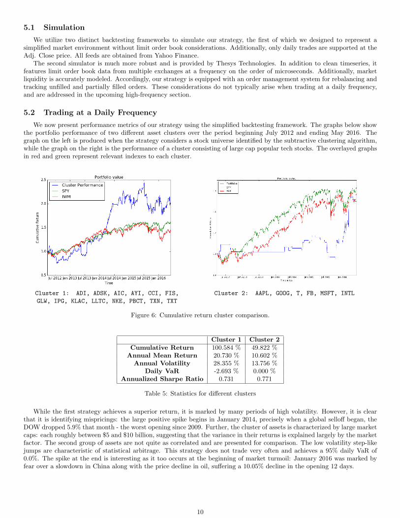
5.2 Trading at a Daily Frequency

We now present performance metrics of our strategy using the simplified backtesting framework. The graphs below showthe portfolio performance of two different asset clusters over the period beginning July 2012 and ending May 2016. Thegraph on the left is produced when the strategy considers a stock universe identified by the subtractive clustering algorithm,while the graph on the right is the performance of a cluster consisting of large cap popular tech stocks. The overlayed graphsin red and green represent relevant indexes to each cluster.

Cluster 1: ADI, ADSK, AIC, AYI, CCI, FIS, Cluster 2: AAPL, GOOG, T, FB, MSFT, INTL

GLW, IPG, KLAC, LLTC, NKE, PBCT, TXN, TXT

Figure 6: Cumulative return cluster comparison.

Cluster 1 Cluster 2Cumulative Return 100.584 % 49.822 %

Annual Mean Return 20.730 % 10.602 %Annual Volatility 28.355 % 13.756 %

Daily VaR -2.693 % 0.000 %Annualized Sharpe Ratio 0.731 0.771

Table 5: Statistics for different clusters

While the first strategy achieves a superior return, it is marked by many periods of high volatility. However, it is clearthat it is identifying mispricings: the large positive spike begins in January 2014, precisely when a global selloff began, theDOW dropped 5.9% that month - the worst opening since 2009. Further, the cluster of assets is characterized by large marketcaps: each roughly between $5 and $10 billion, suggesting that the variance in their returns is explained largely by the marketfactor. The second group of assets are not quite as correlated and are presented for comparison. The low volatility step-likejumps are characteristic of statistical arbitrage. This strategy does not trade very often and achieves a 95% daily VaR of0.0%. The spike at the end is interesting as it too occurs at the beginning of market turmoil: January 2016 was marked byfear over a slowdown in China along with the price decline in oil, suffering a 10.05% decline in the opening 12 days.

10

5.3 High Frequency

Limit Order Book Dynamics (potential limits)

We now explore statistical arbitrage in the high frequency domain. If we can make consistent small profits on a smalltime interval, we can theoretically generate large profits from the accrued small returns. We obtain strong signals (see figure7), however we find that we cannot easily profit them. The predominant issue is that the expected returns of each trade inthe high frequency domain is on the same order as the spreads of the returns (more on this in section 6). In addition, thereis a large trade-off between quick order executions and spread-associated costs. Thus, without the guarantee that we tradeat the desired price given by the signal, we will lose money on the trade. Furthermore, there is a $0.01 minimum tick size,which is too large for our strategy to make a profit on. Even if we could overcome these issues, we would need to generatesubstantial profits from each trade due to transaction costs. In essence, even though we generate strong signals in the highfrequency domain, we are unable to make a profit from them.

(a) Frequency=1 minute. (b) Frequency=30 seconds.

(c) Frequency=10 seconds.

Figure 7: Example of signal behavior for different trading frequencies.

In order to profit from the signal there must be sufficient time in between peaks for the price of the underlying assets inthe pair to move. The signal in the first plot is precisely what we want to see. Our strategy can seemingly detect reversionat a smaller precision than $0.01, but is unable to trade on this. In order to get filled when the spread is at $0.01, we mustbid at ask, and so we lose any possible profit.

5.3.1 Trading rules

In this section we explain some trading rules we considered in our strategy. They are designed so that we take high-frequency idiosyncrasies into account.

1. Stop-loss criterion: In order to minimize risk from a single pair, we block both assets in that pair from being tradedif we currently hold a position on the asset, unless the order corresponds to an exit in the position (e.g. if the signal isnot strong anymore). We do this both for minimizing transaction costs and setting the maximum loss of a single pairto be the amount of cash we allotted based on the F -score.

2. Liquidity constraint: As we discuss in the following sections, high-frequency orders must be performed in a timelymanner in order to ensure the expected gains from signal movements. Since orders are not necessarily filled at mid-price,

11

we propose to introduce a parameter α ∈ [−1, 1] from order prices are determined as follows:

OrderPrice = α (Ask−Mid) + Mid (buy side),

OrderPrice = Mid− α (Mid− Bid) (sell side), (5.1)

so for α = 0 we would trade at the mid-price, and at α = 1 we would pay the whole spread. This trick will let us havea balance between not paying the full spread and getting orders quickly filled. In our tests we used alpha ranging from0.2 to 0.5; that is, we always trade higher than the mid-price, but not as much so to pay for the whole spread.

3. Unfilled order management: Our strategy is very highly dependent on trading a particular pair at the right timewith the correct weights. Having an exposure from unfilled orders is unwanted since portfolio values can vary wildlyin the high-frequency setting. Therefore, we set out the following rule for dealing with unfilled pairs: if we submit anorder at time i∆t, then at time (i+ 1)∆t:

• If the signal strength is still within the desired bounds (i.e. it has not crossed any exit bar), then we recalibratethe model, compute the desired proportion (1 to -β), and submit an order so to rebalance the pair with the currentposition.

• If the signal is not strong anymore, submit orders so to cancel the current position. Since there is no expectedgain from it, we assume the loss arising from having held an unbalanced pair.

When using the previous rules, we see that the strategy performs reasonably well for low and mid-frequencies. As anillustration, figure 8 shows the behavior of holding returns2 at a trading frequency of 3 hours. We see that the returns areskewed to the right, which is indicative of a hit rate greater than 50%. In the following section we will evaluate how returnsand other statistics behave when we trade at higher frequencies.

Figure 8: Distribution of annualized holding returns from 2015/06/15 to 2015/12/15 on a 3-hour frequency setting. Assetstraded are (JPM, XLF).

6 Results

In this section we assess the performance of pairs strategy in high frequency. To draw sound conclusions about thedifferences between high and low frequencies, we take the single pair (JPM, XLF)3 and run the strategy over different tradingwindows. The following visualizations will then be based on this pair. While the results look similar for the multiple-paircase, the interaction between some measures –e.g. portfolio value progression vs. trading signal tracking– is explained in amore straightforward manner for the single-pair case.

2Throughout, by holding return we mean the instantaneous returns of when holding a non-zero position on the pair. In the case where weuninterruptedly hold a position over [0, T], it is computed as the annualized version of

Ret(0, T ) =1

T

T∑t=1

pt − pt−1

pt−1,

where pt is the value of the portfolio at time t and T is the total number of steps. In pairs trading, we expect this holding return to be skewed tothe right, since the residual signal is expected to return to its mean, thus having instantaneous pair profits until exiting the position.

3We took this pair as the ‘canonical’ example, where we can safely assume the cointegration relationship holds.

12

6.1 Transaction costs versus gains

First, let us look at how the portfolio values progresses. Figure 9 shows an example of the portfolio value dynamics forboth low and high frequencies. Whenever the portfolio value stays flat, the strategy does not hold a pair position. Thefirst difference to spot is how many non-flat periods Figure 9b (high-frequency) shows. The result is as expected: the high-frequency trades a larger number of times, even if the test period is smaller. However, the fact that positions are beingevaluated at higher frequencies, the overall portfolio value will be highly volatile relative to the gains. See, for example, howcontinuous changes scale to the gains of exiting the position in the 9a versus 9b.

As we will later see, this effect is a source of hardship for the strategy to make profits. On the one hand, more tradingcosts have to be paid the more frequently we trade. Second, the timing of exiting the position is fairly influential on theoutcome of the trade. Indeed, changing the bid (ask) price even a few cents can drive the outcome from profits to losses hadthe trade been performed a few seconds (or minutes) earlier. Since profits drawn for the high-frequency setting are of theorder of the spread (a few –or even one– cents per trade, versus whole dollars in low frequencies), the timing for enteringor clearing positions must be quick. This effect is pervasive for any trading frequencies on the sub-hour, and is our mainmotivation to believe that the model can become robust if it included predictions about ominous changes in the order book.

(a) Portfolio values at frequency=3-hours. (b) Portfolio values at frequency=1-minute.

Figure 9: Examples of portfolio value progressions for different frequencies. The dates selected were 2015/06/15 to 2015/12/15for low frequency and 2015/06/15 to 2015/07/15 for high-frequency.

Figure 10 shows another example of the progression of cumulative clearance (i.e. non-spread related) costs in a high-frequency setting. The number of steps reconfirm the observation that we trade a fairly high number of times in a singletrading day. For the particular period shown, cumulative trading costs amount to 10% of the total gains, and that particularday experienced an outstanding return. While bearing in mind that no conclusion is valid for all possible trading seasonsand regimes, this illustrates how trading costs can scale to undermine a potentially alarming proportion of gains.

Figure 10: Example of cumulative trading costs in high-frequency.

13

6.2 Performance and risk measures

While per-trade costs do not increase with frequency (they scale linearly to the number of trades performed), the proportionof trading costs (of a few cents) relative to per-trade gains can increase up to the point where gains are overwhelmed. Anexample of this effect is shown in Table 6, where we show performance measure as well as risk indicators of the strategy overdifferent frequencies. For this example –all trades start on the same day, but frequencies change–, we can see the annualizedcumulative and holding returns being consistently drawn down the higher the frequency. While this is not the case for alltrading periods (some test periods do have a stable return behavior), this illustrates how either (a) signals generated athigher frequencies are spurious (cf. figure 7), which generates negative returns, or (b) transaction costs overwhelm expectedgain on each trade.

Frequency Return Vol. Cum. return Daily 95% VaR Max Drawdown ` Horizon3 hours 61.55% 17.25% 7.89% -2.85% 60 6 months2 hours 41.26% 17.93% 5.15% -4.8% 60 6 months1 hour 89.27% 19.98% 7.71% -6.03% 60 4 months

30 minutes -16.7% 12.28% -0.7% -6.8% 120 2 months1 minute -8.92% 9.21% -0.19% -0.32% 240 1 month

30 seconds -1.54% 14.31% -3.19% -54.43% 240 1 month10 seconds -113.9% 8.53% -2.35% -55.66% 240 1 month

Table 6: Statistics for different frequencies. The start date was randomly picked to be 06/15/2015. The strategy trades fora period determined by the horizon, with a lookback period determined by `.

Annualized volatility, on the other hand, shows a fairly stable behavior throughout frequencies, so that Sharpe ratios arecompletely determined by expected returns. This observation shows surprising to us given the belief that high-frequency seriescontain strong non-continuous behavior, microstructure noise and jumps that undermine the usual estimator of the volatility.The (normalized) maximum drawdown is another measure whose magnitude does not vary enough across frequencies. Thedecreasing behavior stems for a higher volatility –hence dividing the maximum value drop by a larger amount. However,having a 2.88% 10-second drawdown in a single is indicative of a very highly risky position. In the same line, the sharpincrease in Daily 95% Value at Risk indicates that strategies become riskier the more frequently we trade.

Table 6 showed an illustration over one particular period in H2-2015, which one can very well judge as unrepresentative.To show more robust results on the strategy’s performance in high-frequency, we performed thirty independent simulations ofthe strategy at a 1-minute frequency, where each of the dates was picked at random between 2011 and 2015 and the tradingwindow was four days. The cumulative returns–that is, the return over the 4-day period– density estimation is shown inFigure 11. Note the difference of Fig. 11 with the shape when compared to Fig. 8, where a smooth right-skewed graph ispresented.4 While the high-frequency strategy can achieve significant returns (seemingly with a high probability), there is anon-negligible possibility that returns are catastrophic (cf. the left clump in figure Fig. 11).

The non-smoothness of the return curve about a mean can also indicative of a high sensitivity of the strategy to modelparameters. As we pointed earlier, the presence of microstucture noise and jumps can undermine the confidence on themean-reverting model. For illustration, Figure 12 shows the behavior of the estimator of β in equation (2.2). We can clearlysee that jumps in the data introduce strong discontinuities in one of the model’s most crucial parameters. We would beinterested in performing research on this respect –that is, getting jump-robust estimators or modeling the residual as asemi-martingale with a jump component.–

4The scale, however, is not comparable.

14

Figure 11: Distribution of returns based on 30 independent simulations of the strategy.

Figure 12: Distribution of returns based on 30 independent simulations of the strategy.

For a final assessment on the shape of the density of returns, Figure 13 shows the distribution of the annualized holdingreturns at different frequencies. The fact that higher frequencies have a lower holding returns is no surprise –most of the timesthe portfolio value will not vary too much for very small time windows. However, we wish to highlight how the smoothnessof the curve changes as the frequency becomes lower. In particular, low-frequency lines are clearly skewed to the right, thuswe are more confident about the model for generating profits. This is not to mean that pairs trading at high frequencies isunreliable; rather, we should be careful in implementing low-frequency strategies to any time window without adjusting forimportant idiosyncrasies of high-frequency.

15

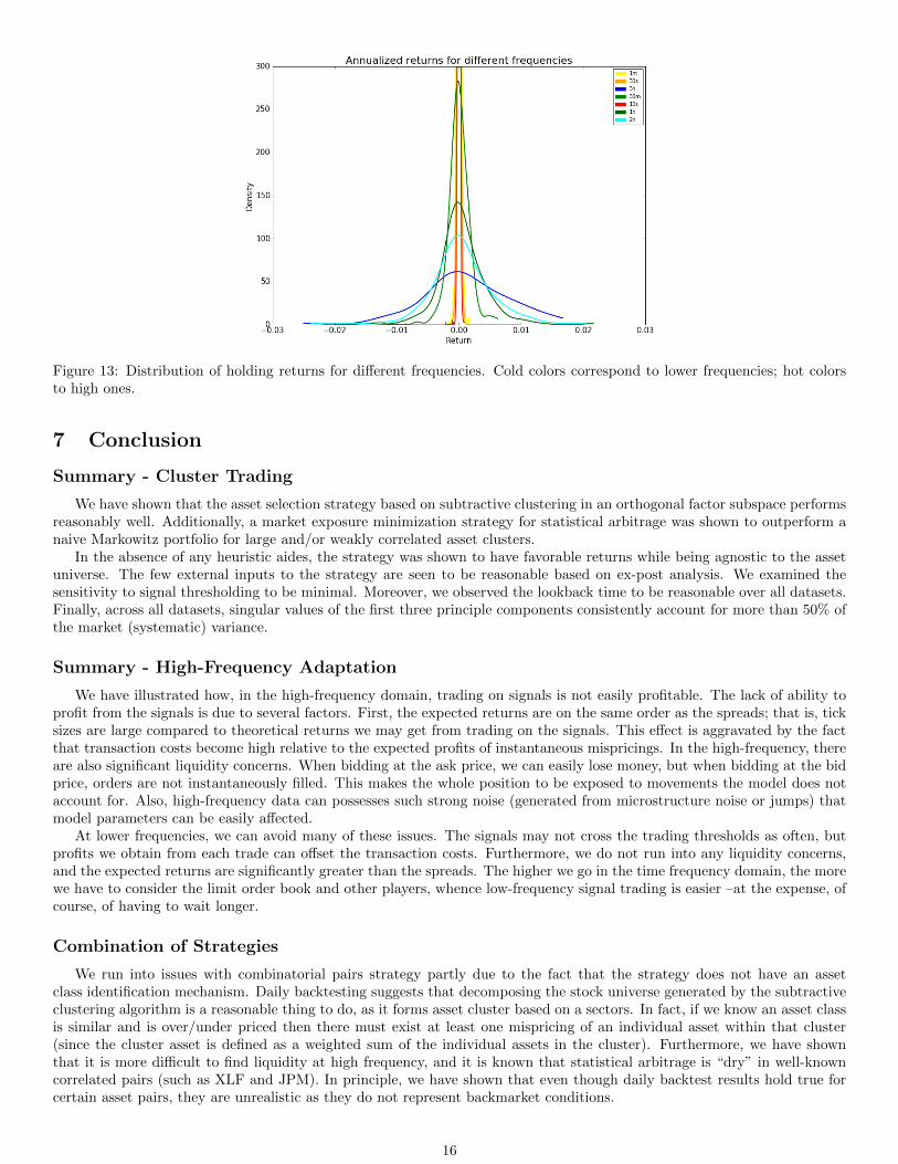
Figure 13: Distribution of holding returns for different frequencies. Cold colors correspond to lower frequencies; hot colorsto high ones.

7 Conclusion

Summary - Cluster Trading

We have shown that the asset selection strategy based on subtractive clustering in an orthogonal factor subspace performsreasonably well. Additionally, a market exposure minimization strategy for statistical arbitrage was shown to outperform anaive Markowitz portfolio for large and/or weakly correlated asset clusters.

In the absence of any heuristic aides, the strategy was shown to have favorable returns while being agnostic to the assetuniverse. The few external inputs to the strategy are seen to be reasonable based on ex-post analysis. We examined thesensitivity to signal thresholding to be minimal. Moreover, we observed the lookback time to be reasonable over all datasets.Finally, across all datasets, singular values of the first three principle components consistently account for more than 50% ofthe market (systematic) variance.

Summary - High-Frequency Adaptation

We have illustrated how, in the high-frequency domain, trading on signals is not easily profitable. The lack of ability toprofit from the signals is due to several factors. First, the expected returns are on the same order as the spreads; that is, ticksizes are large compared to theoretical returns we may get from trading on the signals. This effect is aggravated by the factthat transaction costs become high relative to the expected profits of instantaneous mispricings. In the high-frequency, thereare also significant liquidity concerns. When bidding at the ask price, we can easily lose money, but when bidding at the bidprice, orders are not instantaneously filled. This makes the whole position to be exposed to movements the model does notaccount for. Also, high-frequency data can possesses such strong noise (generated from microstructure noise or jumps) thatmodel parameters can be easily affected.

At lower frequencies, we can avoid many of these issues. The signals may not cross the trading thresholds as often, butprofits we obtain from each trade can offset the transaction costs. Furthermore, we do not run into any liquidity concerns,and the expected returns are significantly greater than the spreads. The higher we go in the time frequency domain, the morewe have to consider the limit order book and other players, whence low-frequency signal trading is easier –at the expense, ofcourse, of having to wait longer.

Combination of Strategies

We run into issues with combinatorial pairs strategy partly due to the fact that the strategy does not have an assetclass identification mechanism. Daily backtesting suggests that decomposing the stock universe generated by the subtractiveclustering algorithm is a reasonable thing to do, as it forms asset cluster based on a sectors. In fact, if we know an asset classis similar and is over/under priced then there must exist at least one mispricing of an individual asset within that cluster(since the cluster asset is defined as a weighted sum of the individual assets in the cluster). Furthermore, we have shownthat it is more difficult to find liquidity at high frequency, and it is known that statistical arbitrage is “dry” in well-knowncorrelated pairs (such as XLF and JPM). In principle, we have shown that even though daily backtest results hold true forcertain asset pairs, they are unrealistic as they do not represent backmarket conditions.

16

8 Future work

There are many dimensions to consider in order to overcome the difficulties discovered in our work. As we pointed insection 6.1, the incorporation of the volume in the order book could be highly useful for predicting when is the best timeto trade on a pair. Incorporating knowledge about mispricing signal behavior paired with fundamental analysis could bepromising for taking advantage on the spreads. Additionally, having a dynamic liquidity parameter α (cf. equation 5.1)based on fundamental data could also reduce transaction costs.

Another direction we could take is to let signal thresholds to vary. In theory we would expect to have potentially highermispricings –thus returns– in periods of high volatility. We could then set thresholds based on measures of future volatility.

We observed in section 6.2 that high-frequency estimators can alarmingly undermine the variance of estimated parameters.In particular, jumps (Figure 12) can be an important source of estimation error. We contemplate the incorporation of jumpbehavior into the residual dXt as a possibility for making the model more robust. As an alternative, we could imagineestimators of the OU parameters to include thresholding to neglect jumps, similar to what recent developments in high-frequency econometrics have developed. For a survey on this literature, see [1].

Acknowledgments

The authors would like to thank Dr. Lisa Borland and Enzo Bussetti for providing their insight into the world ofmathematical finance in the age of large data and guiding us through the hurdles we faced during this project.

References

[1] Yacine Aı̈t-Sahalia and Jean Jacod. High-frequency financial econometrics. Princeton University Press, 2014.

[2] Ghazi Al-Naymat. Mining pairs-trading patterns: A framework. International Journal of Database Theory and Applica-tion, 6(6):19–28, 2013.

[3] Marco Avellaneda and Jeong-Hyun Lee. Statistical arbitrage in the us equities market. Quantitative Finance, 10(7):761–782, 2010.

[4] Evan Gatev, William N Goetzmann, and K Geert Rouwenhorst. Pairs trading: Performance of a relative-value arbitragerule. Review of Financial Studies, 19(3):797–827, 2006.

[5] George J Miao. High frequency and dynamic pairs trading based on statistical arbitrage using a two-stage correlationand cointegration approach. International Journal of Economics and Finance, 6(3):96, 2014.

[6] Merton H Miller, Jayaram Muthuswamy, and Robert E Whaley. Mean reversion of standard & poor’s 500 index basischanges: Arbitrage-induced or statistical illusion? The Journal of Finance, 49(2):479–513, 1994.

[7] Jesus Otero and Jeremy Smith. Testing for cointegration: power versus frequency of observation—further monte carloresults. Economics Letters, 67(1):5–9, 2000.

17