statistical assessment of the potential factors affecting
TRANSCRIPT
The Pennsylvania State University
The Graduate School
Department of Energy and Mineral Engineering
STATISTICAL ASSESSMENT OF THE POTENTIAL FACTORS AFFECTING
DELAYED INCIDENT REPORTING IN THE OIL AND GAS INDUSTRY
A Thesis in
Energy and Mineral Engineering
by
Osahon Ighodaro Abbe
2012 Osahon Ighodaro Abbe
Submitted in Partial Fulfillment
of the Requirements
for the Degree of
Master of Science
May 2012

The thesis of Osahon Ighodaro Abbe was reviewed and approved* by the following:
Samuel A. Oyewole
Assistant Professor
Environmental Health and Safety Engineering
Thesis Advisor
Larry Grayson
Professor Energy and Mineral Engineering
George H., Jr., and Anne B. Deike Chair in Mining Engineering
Graduate Program Officer of Energy and Mineral Engineering
Li Li
Assistant Professor
Petroleum and Natural Gas Engineering
Yaw Yeboah
Professor and Department Head of Energy and Mineral Engineering
*Signatures are on file in the Graduate School

iii
ABSTRACT
Safety in the workplace has an ever-growing audience; even so safety in the workplace in
the oil and gas industry. The Occupational Safety and Health Administration (OSHA) enforces
and regulates safety rules through federal-approved and state-approved programs that must be
met by businesses. In this thesis, safety records from an undisclosed company in the oil and gas
industry were used to study factors that potentially contribute to having an effect on the health of
humans in areas where there have been oil spills. The safety records from the study included
chemical spills, explosions and safety incidents over a 21-year period. The objective of this
research was to develop the most feasible model to help in identifying the significant
independent factors such as nature of spill, delay time, incident type, population, yearly effect
and seasonal effect in delayed incident reporting. In this study, the various models were
developed based on the previous spills which can be used to predict potential health effects of
future spills and effectively manage the effects or eliminate them. A dependent variable (deaths
per state) was regressed against the significant independent factors which were converted from
qualitative to quantitative data points using analytical hierarchy process (AHP) technique.
Additional transformational analyses were performed using the square root, cube, square, inverse
and natural logarithm of the dependent variable. From the transformational analyses, the most
feasible model was the cube transformation model of the dependent variable which had the
highest R-squared value while still maintaining its normality. The cube transformation of the
dependent variable had an F-value of 985.13 and R-square value of 79.6% compared to the base
model which had an F-value of 375.14 and R-square value of 51.9%. The cube model used the
independent factors to predict the potential health effects from the dependent variables and the
significant factors that proved to be helpful in reducing the negative effects of the incidents were

iv
the delayed reporting and the nature of the chemical spilled. However, with the data set lacking
some critical information pertaining to the corresponding injuries and economical cost per
incident, adequate analyses on the direct impact of each incident was limited.
v
TABLE OF CONTENTS
LIST OF FIGURES ............................................................................................................ VIII
LIST OF TABLES ................................................................................................................. IX
ACKNOWLEDGEMENTS ................................................................................................... XI
CHAPTER 1 ..............................................................................................................................1
INTRODUCTION .....................................................................................................................1
OCCUPATIONAL HEALTH AND SAFETY ....................................................................1
OBJECTIVES OF STUDY .................................................................................................2
PROBLEMS ENCOUNTERED .........................................................................................3
ASSOCIATED RISKS AND HAZARDS IN THE OIL AND GAS INDUSTRY ...............5
PHYSICAL EFFECTS OF HAZARDS ..............................................................................7
PSYCHOSOCIAL EFFECTS .............................................................................................7
CHEMICAL AND ENVIRONMENTAL EFFECTS OF HAZARDS ...............................8
NEED FOR ORGANIZATION-SPECIFIC ASSESSMENT AND PREDICTION
MODELS ....................................................................................................................9
CHAPTER 2 ............................................................................................................................ 11
BACKGROUND ..................................................................................................................... 11
SAFETY MANAGEMENT ............................................................................................... 11
DECISION-MAKING ....................................................................................................... 12
STRATEGIC DECISION-MAKING PROCESS ............................................................. 13
MULTI-CRITERIA DECISION MAKING ..................................................................... 14
ANALYTICAL HIERARCHY PROCESS ....................................................................... 15

vi
PAIRWISE COMPARISON ............................................................................................. 16
CHAPTER 3 ............................................................................................................................ 17
LITERATURE REVIEW ....................................................................................................... 17
DECISION-MAKING FACTORS AFFECTING INCIDENTS IN THE WORKPLACE
................................................................................................................................... 17
FACTORS INFLUENCING DELAYED INCIDENT REPORTING .............................. 18
PERIODIC (YEAR) EFFECT .......................................................................................... 19
NATURAL FACTORS...................................................................................................... 19
POPULATION OF LOCATION ...................................................................................... 19
CURRENT SAFETY MANAGEMENT ADOPTION STRATEGIES IN THE OIL AND
GAS INDUSTRY ...................................................................................................... 20
CHAPTER 4 ............................................................................................................................ 22
METHODOLOGY AND RESEARCH DESIGN .................................................................. 22
DATA SOURCE AND ANALYSIS TECHNIQUE .......................................................... 22
EXPERIMENTAL DESIGN PROCEDURE .................................................................... 23
THE DEPENDENT VARIABLE ...................................................................................... 24
FACTOR A: NATURE OF SPILL .................................................................................... 24
FACTOR B: INCIDENT TYPE ........................................................................................ 29
FACTOR C: POPULATION ............................................................................................ 32
FACTOR D: DELAY TIME ............................................................................................. 32
FACTOR E: YEAR EFFECT ........................................................................................... 32
FACTOR F: NATURAL FACTORS ................................................................................ 33

vii
CHAPTER 5 ............................................................................................................................ 35
ANALYSIS AND RESULTS .................................................................................................. 35
REGRESSION ANALYSIS .............................................................................................. 35
TRANSFORMATIONS .................................................................................................... 40
SQUARE ROOT TRANSFORMATION ......................................................................... 40
INVERSE TRANSFORMATION .................................................................................... 45
SQUARE TRANSFORMATION...................................................................................... 49
NATURAL LOG TRANSFORMATION ......................................................................... 53
CUBE TRANSFORMATION ........................................................................................... 58
CHAPTER 6 ............................................................................................................................ 63
CONCLUSIONS ..................................................................................................................... 63
DISCUSSION .................................................................................................................... 63
LIMITATIONS OF STUDY ............................................................................................. 64
SUGGESTIONS FOR FUTURE WORK ......................................................................... 64
APPENDIX A: ORIGINAL MODEL .................................................................................... 69
APPENDIX B: SQUARE ROOT MODEL ............................................................................ 72
APPENDIX C: INVERSE MODEL ....................................................................................... 75
APPENDIX D: SQUARED MODEL ..................................................................................... 78
APPENDIX E: NATURAL LOG MODEL ............................................................................ 81
APPENDIX F: CUBIC MODEL ............................................................................................ 84
viii
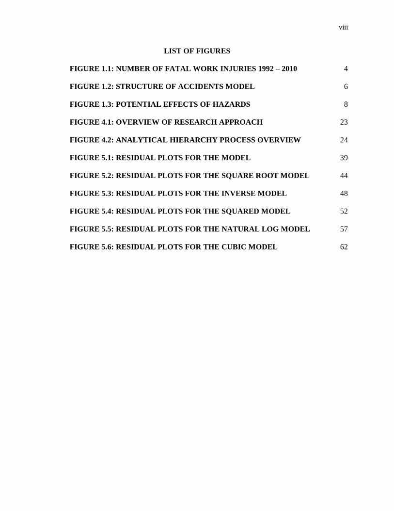
LIST OF FIGURES
FIGURE 1.1: NUMBER OF FATAL WORK INJURIES 1992 – 2010 4
FIGURE 1.2: STRUCTURE OF ACCIDENTS MODEL 6
FIGURE 1.3: POTENTIAL EFFECTS OF HAZARDS 8
FIGURE 4.1: OVERVIEW OF RESEARCH APPROACH 23
FIGURE 4.2: ANALYTICAL HIERARCHY PROCESS OVERVIEW 24
FIGURE 5.1: RESIDUAL PLOTS FOR THE MODEL 39
FIGURE 5.2: RESIDUAL PLOTS FOR THE SQUARE ROOT MODEL 44
FIGURE 5.3: RESIDUAL PLOTS FOR THE INVERSE MODEL 48
FIGURE 5.4: RESIDUAL PLOTS FOR THE SQUARED MODEL 52
FIGURE 5.5: RESIDUAL PLOTS FOR THE NATURAL LOG MODEL 57
FIGURE 5.6: RESIDUAL PLOTS FOR THE CUBIC MODEL 62

ix
LIST OF TABLES
TABLE 4.1: ALTERNATIVE RANKS .................................................................................. 25
TABLE 4.2: RELATIVE IMPORTANCE OF ONE CRITERION OVER ANOTHER ..... 25
TABLE 4.3: PAIRWISE COMPARISON IN TERMS OF EFFECT ON THE
ENVIRONMENT .............................................................................................. 27
TABLE 4.4: PAIRWISE COMPARISON IN TERMS OF EFFECT ON THE HUMANS . 28
TABLE 4.5: WEIGHTS ASSIGNED TO THE DIFFERENT CLASSES OF FACTOR A . 29
TABLE 4.6: PAIRWISE COMPARISON FOR THE VARIOUS INCIDENT TYPES ....... 30
TABLE 4.7: WEIGHTS ASSIGNED TO THE DIFFERENT CLASSES OF FACTOR B . 31
TABLE 4.8: DUMMY VARAIBLES PER TIMEFRAME ................................................... 33
TABLE 4.9: DUMMY VARAIBLES PER SEASON ............................................................ 34
TABLE 5.1: REGRESSION COEFFICIENT STATISTICS ................................................ 36
TABLE 5.2: CORRELATION MATRIX FOR MODEL ...................................................... 37
TABLE 5.3: ANALYSIS OF VARIANCE FOR THE REGRESSION MODEL ................. 37
TABLE 5.4: SEQUENTIAL SUM OF SQUARES FOR THE REGRESSION MODEL .... 38
TABLE 5.5: REGRESSION COEFFICIENT STATISTICS ................................................ 41
TABLE 5.6: CORRELATION MATRIX FOR SQUARE ROOT MODEL......................... 42
TABLE 5.7: ANALYSIS OF VARIANCE FOR THE REGRESSION MODEL ................. 43
TABLE 5.8: SEQUENTIAL SUM OF SQUARES FOR THE REGRESSION MODEL .... 43
TABLE 5.9: REGRESSION COEFFICIENT STATISTICS ................................................ 45
TABLE 5.10: CORRELATION MATRIX FOR INVERSE MODEL .................................. 46
TABLE 5.11: ANALYSIS OF VARIANCE FOR THE REGRESSION MODEL ............... 47
TABLE 5.12: SEQUENTIAL SUM OF SQUARES FOR THE REGRESSION MODEL... 47
x
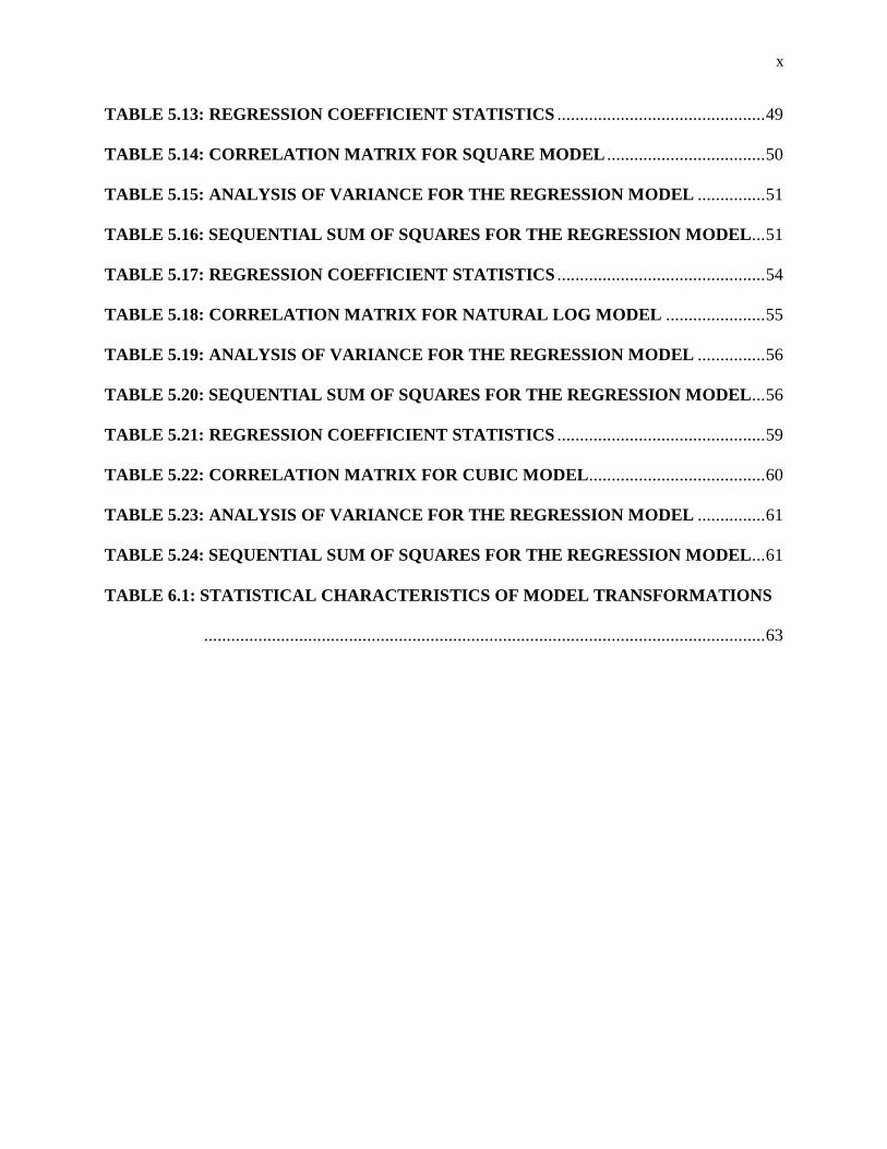
TABLE 5.13: REGRESSION COEFFICIENT STATISTICS .............................................. 49
TABLE 5.14: CORRELATION MATRIX FOR SQUARE MODEL ................................... 50
TABLE 5.15: ANALYSIS OF VARIANCE FOR THE REGRESSION MODEL ............... 51
TABLE 5.16: SEQUENTIAL SUM OF SQUARES FOR THE REGRESSION MODEL... 51
TABLE 5.17: REGRESSION COEFFICIENT STATISTICS .............................................. 54
TABLE 5.18: CORRELATION MATRIX FOR NATURAL LOG MODEL ...................... 55
TABLE 5.19: ANALYSIS OF VARIANCE FOR THE REGRESSION MODEL ............... 56
TABLE 5.20: SEQUENTIAL SUM OF SQUARES FOR THE REGRESSION MODEL... 56
TABLE 5.21: REGRESSION COEFFICIENT STATISTICS .............................................. 59
TABLE 5.22: CORRELATION MATRIX FOR CUBIC MODEL....................................... 60
TABLE 5.23: ANALYSIS OF VARIANCE FOR THE REGRESSION MODEL ............... 61
TABLE 5.24: SEQUENTIAL SUM OF SQUARES FOR THE REGRESSION MODEL... 61
TABLE 6.1: STATISTICAL CHARACTERISTICS OF MODEL TRANSFORMATIONS
............................................................................................................................ 63

xi
ACKNOWLEDGEMENTS
First I want to thank my lord and savior Jesus Christ for giving me life and making it
possible for me to get this far. I am nothing without Him. I would love to thank everyone who
made it possible for me to complete my thesis. I am grateful to Dr. Samuel Oyewole, who took
me under his wings when I entered the master’s program in the department and has made
available his support in a number of ways throughout my thesis with his patience and knowledge
whilst allowing me the room to work in my own way. This work will not have been possible
without his complete devotion and guidance all the way to the end. I am also grateful to Dr.
Larry Grayson, Dr. Antonio Nieto and Dr. Li Li for taking time out of their busy schedules to
encourage me and to check on the progress of my work. I truly appreciate you all.
My family has shown me support throughout my educational career and their undying
love and devotion has kept me going through difficult spurs along the way and I will not be who
I am today if not for my family. I would like to thank Engr. Ighodaro Olusegun Abbe of blessed
memories who showed me the importance of hard work early in my childhood and Itohan Mercy
Abbe for instilling in me the character and morals of a man beyond my years. I love you mom.
And to my three angels who have guided me for 25 years from afar and nearby; thank you and I
appreciate all that you have been in my life. I love you Efe Abbe, Eseosa Abbe and Izoduwa
Abbe. Thank you for being lovely and beautiful sisters to me.
Finally, I would like to thank everybody who was important to the successful realization
of my thesis, the beautiful Ikponmwosa, Chux (the American dream), Rytchad (the American
life), Chris, Tunde, Olaide, Jae and a host of others I did not mention. My Penn State experience
would not have been the same without your friendship and help. Thank you.

CHAPTER 1
INTRODUCTION
OCCUPATIONAL HEALTH AND SAFETY
Occupational health and safety is always a vital component of many if not all engineering
processes and it encompasses a broad array of factors based on decisions made. Successes of
engineering processes are mainly determined mostly by the efficiency and the ability to be
pragmatic at the same time. Without safety the previously mentioned assessment factors would
be meaningless. Decisions made every day will result in the increase or decrease of efficiency
and overall safety in an organization. Certain areas or decisions are deemed more critical than
others based on different demographics such as the level of education of the decision maker,
experience, age and many other factors. This in turn plays a huge role in determining the incident
rate in an engineering process. Occupational health and safety should always be the primary
concern for organizations and society in general. Data obtained from the United States Bureau of
Labor Statistics (USBLS) shows that among the employers in the private industry in the United
States there were 3,277,700 total recordable cases of non-fatal injuries and illnesses in 2009 of
which 965,000 were cases involving days away from work (USBLS, 2009). Also in that same
year there were 4551 fatal work injuries recorded (USBLS, 2009). Even though these numbers
may have slightly reduced from the previous year, there is still the need to maintain the steady
decline or improve on the much achieved decrease in numbers. One reason for this is the fact that
occupational injuries and illnesses constitute a very legitimate source of decrease in profits for
organizations due to the high costs that are incurred. A study done on the costs associated with
occupational injuries and illnesses suggest that the financial costs associated with those injuries
in the United States are over a billion dollars (Leigh et al., 2000). This cost range is however
2
probably conservative and does not include future earnings or productivity from the workers
being killed or permanently injured; also it does not account for the economic impact on the
families and dependents of those workers affected by injuries or fatalities. This in turn only calls
for increased research in identifying ways in which incident rates can be reduced.
A lot of incidents that occur in the workplace, about nine out of ten events, can be
predicted (Grimaldi, 1980). This statement sheds light on the fact that there exists information
and knowledge to stop most incidents from occurring, but the fact that this is not the case is
evident in the yearly totals; hence, the need for legislation and enforcement of that legislation.
The Occupational Safety and Health Administration (OSHA) is the body in charge of enforcing
safe and healthful working conditions for working men and women in the United States. OSHA
does this also by providing training, outreach, education and assistance through the Occupational
Safety and Health Act of 1970.
OBJECTIVES OF STUDY
This research highlights the factors that potentially play a role in increased negative
health effects alongside the delay of incident reporting and explores how significant they are in
the oil and gas company under review. These incidents mostly stem from bad or poor decision-
making and result in days away from work, job transfers and even fatalities. The environment is
also at the peril of the oil and gas industry due to the nature of the activities carried out at every
job site; from drilling of wells to closing or abandonment of the wells, environmental hazards
happen at every stage of the entire process. The objective of this research proposal is to develop
a model which will look into and predict the potential effects of delayed accident reporting and
analyze the significance of each factor in the model. This would enable the implementation of

3
certain safety and health management programs to suit the specific need of reducing and possibly
eliminating delay time in reporting observed incidents in the workplace, which could decrease
consequences and injuries in the oil and gas industry. By evaluating the various incidents that
have occurred over the years based on the causes of incidents and risks involved with the
operation as well as presenting an assessment and possible prevention techniques, a model is
developed using decision-making techniques, that would help to achieve this objective.
PROBLEMS ENCOUNTERED
In 2010, there was a huge oil spill in the Gulf of Mexico which flowed for 3 months. It
has been deemed the largest incidental marine oil spill in the history of the petroleum industry
(Jervis and Levin 2010). Eleven men were killed in the explosion and several others injured. This
explosion resulted from the failure of a pressure-controlled system operated by BP which was
known as the Macondo Prospect. The effects of this explosion are still felt to this day from the
damage of marine and wildlife habitats to the fishing and tourism industries in the area. There
have been reports of dissolved oil under water which is not visible at the surface (Gillis 2010)
and a kill zone surrounding the blown well (Gutman and Netter 2011). These features could have
tremendous exponential effects over the years not only to the residents of the affected area but to
most people who come in contact with the food and tourism in the area.
The current situation in the Niger Delta is similar to the Lower Mississippi region in that
a lot of oil spills take place yearly, but due to the lack of exposure of the country internationally,
these events for the most part go unreported (Vidal 2010). Oil spills are a result of poor decisions
made in different contexts. The most prominent reason for oil spills is usually associated with the
oil and gas companies; when they neglect certain maintenance or overhaul of equipment. There

4
are other factors like pipeline vandalism by the locals and militant groups in the area;
unintentional impacts such as that from excavations also play a role in oil spill incidents. A lot of
media coverage occurs when catastrophic events happen, but what is lost in all the noise are the
injuries and/or fatalities that occurred along with the event and also the ripple effects of these
events on humans and the environment. Figure 1.1 shows the trend of the number of fatal work
injuries in the United States (U.S. Bureau of Labor Statistics n.d.).
FIGURE 1.1: NUMBER OF FATAL WORK INJURIES 1992 – 2010
*Data from 2001 exclude fatal work injuries resulting from September 11 terrorist attacks
From Figure 1.1, it can be seen that there is a gradual decline in the total number of
fatalities over the years. However, that number stays about the same in 2009 and 2010. Is this an
arbitrary deviation from the trend or does this mean that the safety measures that have been taken
in the workplace have plateaued? That cannot be a conclusion from Figure 1.1 but it must be
clear that to continue the decline in workplace injuries and fatalities, more safety measures and
efficient ways of implementing them must be taken into account. A suitable prediction model

5
becomes imperative in an attempt to continue the downward slope of fatal injuries and mitigate
the human and environmental effects of these spilled chemicals.
ASSOCIATED RISKS AND HAZARDS IN THE OIL AND GAS INDUSTRY
In every work setting there are a number of risks that will be associated with activities
being performed; and the oil and gas industry is no stranger to these risks. Exposure to risk can
be referred to as the possibility of loss or injury; someone or something that creates a suggested
hazard (Merriam-Webster). Risk has connotations in different aspects of society such as the
stock market’s volatility, public health and safety management. All these connotations are
similar and usually translate to potentially negative events. In the oil and gas industry the risks
that are observed are direct results of hazards in the workplace. A hazard is any event or set of
events that have a harmful outcome. Risk of an event can be derived from a hazard by coupling
the probability of the event happening with the extent or severity of the harm (British Medical
Association, 1987). Risk expresses the likelihood or probability that the harm from a particular
hazard will be realized. This is shown in equation 1.1.
Risk=Probability ×Severity………………………. (1.1)
In the oil and gas industry, risk encompasses the likelihood of loss which is not limited to
injury to workers and property damage but also includes damages done to the environment.
Despite the knowledge of risk and its probability of occurrence, it is very difficult to eliminate it
and on most accounts impossible to eliminate it. This raises a question of how risk eventually
turns into an incident. There have been various studies looking into this process with one of the

6
more famous basic concepts being the domino theory. The domino theory was developed in the
1930’s from research in accident causation theory in which the researcher suggested that one
unsafe act or risk leads to another, then to another and so on. This goes on until an incident
finally occurs (Heinrich, 1959). More complex theories have been proposed to proffer a solution
as to the cause of incidents in the workplace. The structure of accidents model is one of the more
complex models shown in Figure 1.2 (Encyclopedia of Occupational Health and Safety n.d.).
The structure of accidents model first identifies the immediate cause of accidents, like unsafe
acts and conditions. In addition to that it later identifies contributing cases which may not pose
any threat alone but add and contribute to the scenario resulting in accidents.
FIGURE 1.2: STRUCTURE OF ACCIDENTS MODEL

7
PHYSICAL EFFECTS OF HAZARDS
These are the effects of hazards physically when they come to fruition. These include
traumatic injuries which can be further classified as fatal or non-fatal injuries. Fatal injuries as
the name suggests result in death and are mostly caused by explosions, fires, electrocution and
falling objects. Some other causes include overexertion, suffocation/inhalation, drowning and
faulty/lack of expertise while using machinery. A lot of safety measures have been taken in
recent years to reduce the amount of fatalities in the oil and gas industry and kudos should be
given to the various technological advancements which have brought about a decline in the
number of fatalities in this industry over the years. Extraction of minerals in the oil and gas
industry involves the use of heavy and gigantic equipment for the various processes involved;
and these processes are often accompanied by noise which is detrimental to the health of workers
with respect to partial and complete hearing losses.
PSYCHOSOCIAL EFFECTS
Psychophysical impairments which are difficult to measure are developed from the use of
illicit drugs and alcohol in the oil and gas industry due to many issues encountered by the
workers. However, there has been an improvement in drug and alcohol policies in the industry.
Aside from this problem, another psychosocial hazard involves the placement of expatriates in
remote locations which may or may not be favorable to their psychological balance. The effect of
similar hazards is dangerous to the general well-being of workers placed in charge of heavy
equipment on site. Different levels of post-traumatic stress disorders, legal actions, fear of injury
and guilt of injury to others are significant hazards that need to be looked into with great caution.

8
CHEMICAL AND ENVIRONMENTAL EFFECTS OF HAZARDS
Various exposures to chemicals hazards through air, water, food or soil have different
adverse effects on humans and the environment. These effects range from cancer to lung disease
in humans, and global warming to acid rain on the environment. Some of the effects are direct
while some are suggestive at best. Simple effects of chemical hazards can be traced and limited;
however, there are effects which take decades to come to fruition and still may not be conclusive
when diagnosed due to the weakening of the ability of the body to fight certain illnesses. The
potential effects of hazards based on the activities are shown in Figure 1.3.
FIGURE 1.3: POTENTIAL EFFECTS OF HAZARDS

9
NEED FOR ORGANIZATION-SPECIFIC ASSESSMENT AND PREDICTION MODELS
The goal of business is simple; to make profit. However, when profit margins get high
there is room for error and others to profit from those errors. This gets even more complex when
it involves forecasting market trends, keeping and attracting new customers, maintaining
productive assets, and the list goes on. In all these processes of business, there will be mishaps
due to the intricate nature and one of the mishaps happens to be accidents. Accidents could range
from minor incidents to serious injury and sometimes fatalities all which inevitably will cost
money and put a dent in the profit margins. When incidents occur an investigation takes place
which ultimately affects the productivity and efficiency of the business being investigated. The
overlooked solution to this issue is safety; however, how can the modern era of risk-taking and
aggressive entrepreneurship balance the act of safety management and profit?
Having an idea of what lies ahead makes it easier to handle the situation when it arises; in
modern tongues this is known as prediction. Also knowing what to look for plays an important
role in finding what the detractors are that lie ahead; this is also known as assessing the
significance of a situation. An organization that will adopt or follow these two steps will be in
much better shape to equip themselves to handle safety hazards. In safety analysis, the factors
responsible for a near-miss incident, like someone avoiding tripping over a cable in a plant, are
no different from the factors responsible for an oil rig blowing up offshore. Identifying a
combination of factors that lead to an incident will provide adequate information in predicting
the outcome of an observation, which in turn provides room for avoidance. An example of
factors that can lead to an incident can be seen in the Clapham Junction disaster in which there
was a collision of trains that left thirty-five people dead, five hundred more injured and sixty-
nine seriously injured. The incident resulted from the failure to remove a wire during alterations

10
to the existing signaling system. This wire made contact with the new wire in place enabling the
flow of current into the old circuit, which prevented the signal from turning red (Hartley 2001).
The immediate cause of the incident was the uncut wire, and evidently so. However, how does
an experienced electrician do such a poor job that goes unnoticed? This question gives a larger
picture to the combination of factors that resulted in the incident coming to fruition. There was
failure by the management to acknowledge what goes into the job and communicate that to the
electrician or the person in charge of the electrician. There was no established safety system
checklist procedure to follow and there was a failure to do a routine audit on the work done to
assess the performance and quality of the job. Had all these tasks been adequately performed, the
incident would have been averted. The same holds through in the oil and gas industry for
prevention of incidents. Finding factors that are most important in the trend of incidents will shed
light on schemes to incorporate into the safety management procedures. This will ensure the
efficiency and productivity of the organization stays at a high level and profit margins are
maintained.

CHAPTER 2
BACKGROUND
SAFETY MANAGEMENT
Safety management interest is a concept that generally can be perceived to be very old
and very new at the same time. The inception of manufacturing and mining legislation in the
early 19th century brought about an obligation on management in companies to be responsible for
their workers’ safety. Simple rules and regulations were set up in the early days of safety
management which were geared towards land management with respect to the people living
around the manufacturing companies. These regulations protected the people from nuisances
such as noise, stench and water pollution. The simple rules and regulations changed with time to
encompass the activities on the company premises which could potentially yield accidents. Most
of the early policies on safety management focused on technical issues in the workplace and
failed to impose organizational or managerial requirements for industrial safety. This led to the
addition of human factors to the scope of safety management and has led to many studies of
workplace and procedures, and the management of primary work groups. One of such studies
showed that a combination of two group routines, one group being a review group and the other
an accident investigation group led to better accident statistics from heightened accident
prevention activities at a company (Carter and Menckel 1990). This type of study paved the way
for incorporation of feedback communication in safety information systems which was reported
to have facilitated greater individual acceptance of responsibility with respect to safety (Kjellen
and Baneryd 1983).

12
DECISION-MAKING
Decisions can be said to be the resultant action taken from much or less deliberation of
the action taker. Decisions made can be easily classified based on the outcome of the resultant
action; which are mostly good or bad. On a broader note, decision makers are faced with the task
of optimizing their decisions to suit the required outcome and face a wide array of factors that
influence the decisions to be made; hence there is need to understand the various heuristics that
are involved in each decision to be made and how the biases can be eliminated to make a well
informed decision. Qualitative research has been done that examines different factors that
influence high-level decision-making such as environmental antecedents, organizational
antecedents, decision-specific antecedents and individual managerial characteristics (Simons and
Thompson 1998).
The process of decision-making is pertinent to understanding the outcomes of decisions
and can be subdivided into different tasks; information acquisition, evaluation, action and
feedback/learning (Einhorn and Hogarth 1981). These processes are understood to interact with
each other and their interaction is very important in the process of decision-making. There are
two major types of decisions; rational decisions and intuitive decisions. Making decisions in such
a way that the outcomes convey the preferences, idioms and traits of a person or people making a
joint decision is referred to as a rational decision. These decisions are based on the acquired and
influenced nature of the people or people making the decisions from societal experiences, norms
and expectations and also economic prevalence surrounding the decisions to be made. The
alternatives that constitute the criterion of preference are limited to the decision makers’ desires;
hence yielding a rational or preferential structure for decision-making. In essence, decisions
made based on pre-conceived notions from past experiences and critical assessment are known

13
as rational decisions, and the outcome of the decsion confirms the decision maker’s preference
(Raiffa, 1968). Decisions made on impulses which rarely involve any type of analysis or
deliberations are often referred to as intuitive decisions. These decisions although spontaneous,
are based on holistic thinking and provide immediate insight to decision-making. An example of
an intuitive decision can be derived from a quarterback in a football game responding to a game
situation by eluding an oncoming opponent’s tackle and fitting a pass into a narrow window
between defenders for the game-winning touchdown in what looks like seconds. The two
mentioned types of decisions are different but not opposite of each other; there is still a certain
amount of development that needs to take place in intuitive decision-making to be able to carry
out the decision while rational decisions are based on quantitative and qualitative analysis but
also are influenced by pre-conceived notions.
STRATEGIC DECISION-MAKING PROCESS
Competition and failure to succeed are motivating factors in the day-to-day activities in
any business organization. And the ability to make rapid choices plays a role in the direction of
an organization in a dynamically changing environment. Strategic decisions critically influence
the success or lack thereof within an organization. An external constraint imposed on an
organization due to the environment in which it exists has an effect on the internal activities that
organization will decide to go ahead with, hence fitting the conditions under which the
organization can operate. The decision to fit the external constraints may involve a choice from
some alternatives. This choice is critical in achieving a set goal and can be made from
experience, intuition, judgment or from a number of complex analyses. Making this decision
strategically involves fitting the activities of the organization to external constraints by choosing

14
the best possible or available alternative. During the strategic decision-making process, one of
the major problems is uncertainty which arises from derisory knowledge (Bhushan and Rai
2004). To overcome this problem, a model to forecast or predict future scenarios and a technique
or methodology to choose between alternatives will be optimal.
MULTI-CRITERIA DECISION MAKING
There are four dominant words often used in multi-criteria decision-making; attributes,
criteria, goals and objectives. Different literature and contexts have various explanations for the
meanings of these words. In the context of this research, attributes refer to the different qualities
used to rank an alternative; criteria refers to the collection of attributes an alternative possesses;
goals are a priori values that a decision maker aims to achieve (Simon 1964) and objectives are
the inputs of a desired outcome. Multi-criteria decision-making usually refers to making
decisions in the presence of different (usually more than two) criteria. These criteria are often
conflicting in nature and pose a very arduous task of selecting or ranking between each of them.
Multi-criteria decision-making problems come in different forms and sizes and are faced on a
day-to-day basis. For example, buying a car or a house may involve deciding amongst price,
style, location, gas mileage, school district, color and/or some other criteria. In engineering, the
multi-criteria decision-making problems are usually on a much larger scale and involve much
complexity in their approach. An example will be deciding what material to use for metal pipes
in a highly corrosive manufacturing plant due to the season of the year, profitability, type of
product and many more factors. Although multi-criteria decision-making has a wide spread and
can be seen to have been existent as far back as three centuries ago with Benjamin Franklin using
a paper scheme for his decisions (Koksalan, Wallenius and Zionts 2011) its history as a
15
discipline is relatively short and can be traced back thirty years (Xu and Yang 2001). This recent
development of multi-criteria decision-making as a discipline can be attributed to the advent of
technology which has made it possible for systematic analysis of large volumes of data, which is
also a result of technology.
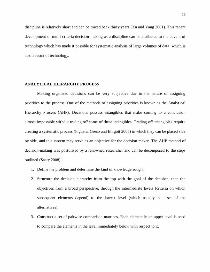
ANALYTICAL HIERARCHY PROCESS
Making organized decisions can be very subjective due to the nature of assigning
priorities to the process. One of the methods of assigning priorities is known as the Analytical
Hierarchy Process (AHP). Decisions possess intangibles that make coming to a conclusion
almost impossible without trading off some of these intangibles. Trading off intangibles require
creating a systematic process (Figuera, Greco and Ehrgott 2005) in which they can be placed side
by side, and this system may serve as an objective for the decision maker. The AHP method of
decision-making was postulated by a renowned researcher and can be decomposed to the steps
outlined (Saaty 2008)
1. Define the problem and determine the kind of knowledge sought.
2. Structure the decision hierarchy from the top with the goal of the decision, then the
objectives from a broad perspective, through the intermediate levels (criteria on which
subsequent elements depend) to the lowest level (which usually is a set of the
alternatives).
3. Construct a set of pairwise comparison matrices. Each element in an upper level is used
to compare the elements in the level immediately below with respect to it.

16
4. Use the priorities obtained from the comparisons to weigh the priorities in the level
immediately below. Do this for every element. Then for each element in the level below
add its weighed values and obtain its overall or global priority. Continue this process of
weighing and adding until the final priorities of the alternatives in the bottom-most level
are obtained.
PAIRWISE COMPARISON
Pairwise comparisons are used in the Analytical Hierarchy Process (AHP) to compare
attributes of alternatives. It aids in the elimination of the trading off process when decision
makers are faced with highly complex issues. Comparing attributes develops weights that can be
associated with each attribute based on preference at each level of hierarchy. This helps to
eliminate inconsistency and shed light on the reasons behind a preference.
CHAPTER 3
LITERATURE REVIEW
DECISION-MAKING FACTORS AFFECTING INCIDENTS IN THE WORKPLACE
There has been a lot of research on factors affecting incidents in the workplace and a
good number of these known factors depend on managerial practices. One of the important
studies conducted in this area was a ten-study review which looked to establish a relationship
between organizational factors and injury rates. For a factor to be considered to have a
relationship with injury rate it had to be statistically significant in one direction in at least two
thirds of the studies in which it was examined, and not found to be significant in the opposite
direction in any other study. Variables were categorized into joint health and safety committee,
management style and culture, organizational philosophy on OHS, post-injury factors, work
force characteristics, and other factors (Shannon, Mayr and Haines 1997). Seventeen factors
were identified that met the criteria of which was; the amount of training the joint health and
safety committee received, good relations between management and workers, monitoring of
unsafe work behaviors, low turnover of staff, and safety controls on machinery (Shannon, Mayr
and Haines 1997). Another study identified two organizational factors that contribute to reducing
the level of occupational risk: the implementation of quality management tools and the fostering
of worker empowerment. It was suggested in the literature that intensive occupational risk
prevention is of prime importance to reduce occupational accidents (Arocena, Nunez and
Villanueva 2007). Of the literature that examined human behavioral factors it was generally seen
to be an effective factor in reducing injury rates in the workplace when it was coupled with a
structured safety program and most times resulted in a substantial reduction of accidents and
sizable estimated financial savings (Reber, Wallin and Chhoker 2008). The examination of
18
behavioral factors and the positive correlation to reduced injury rates raises an important concept
in safety management of worker inclusion and participation. A study reports that an active top-
management practice in occupational health and safety that includes workers in their decision-
making were significantly associated with lower injury rates (Butler and Park 2005). It is
important to note that joint structured safety programs helped reduce injury rates and was
reiterated in most studies (Havlovic and McShane 2000).
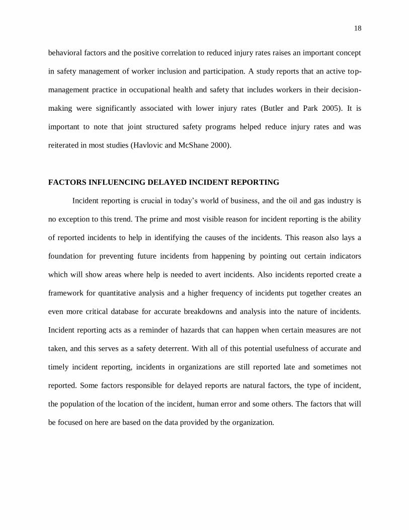
FACTORS INFLUENCING DELAYED INCIDENT REPORTING
Incident reporting is crucial in today’s world of business, and the oil and gas industry is
no exception to this trend. The prime and most visible reason for incident reporting is the ability
of reported incidents to help in identifying the causes of the incidents. This reason also lays a
foundation for preventing future incidents from happening by pointing out certain indicators
which will show areas where help is needed to avert incidents. Also incidents reported create a
framework for quantitative analysis and a higher frequency of incidents put together creates an
even more critical database for accurate breakdowns and analysis into the nature of incidents.
Incident reporting acts as a reminder of hazards that can happen when certain measures are not
taken, and this serves as a safety deterrent. With all of this potential usefulness of accurate and
timely incident reporting, incidents in organizations are still reported late and sometimes not
reported. Some factors responsible for delayed reports are natural factors, the type of incident,
the population of the location of the incident, human error and some others. The factors that will
be focused on here are based on the data provided by the organization.

19
PERIODIC (YEAR) EFFECT
Organizations that have a safety management program in place aim for better safety
numbers from year to year. However if the safety numbers do not improve from the inception of
the safety management program or after a bad safety period, then there needs to be an evaluation
of the program. This factor will help to portray the effect of a particular timeframe on the
dependent variable.
NATURAL FACTORS
There is increasing knowledge about the effect of natural hazards in the oil and gas
industry. The threat of natural hazards impacting chemical facilities and infrastructure has
become more of a focus due to the negative change of climate in this industrial age. Incidents
triggered by natural hazards such as earthquakes, hurricanes, floods and lightning strikes are
extremely dangerous and may lead to environmental pollution, economic effects, serious injuries
and fatalities. It has been noted that about five percent of all recorded chemical incidents
reported are a result of natural events (Campedel 2008).
POPULATION OF LOCATION
When an incident occurs in a densely populated location, there is a higher risk value
associated with that type of occurrence. Also there is a much higher probability that the incident
will be reported and adequate measures will be taken to curtail the effects. Likewise in a remote
location, when an incident occurs it can go unnoticed depending on the magnitude of the
incident, and this could increase the risk value of the incident due to the delay. Remote areas
tend to be under-manned and under-equipped to handle certain incidents, and the time it would

20
take to assemble the man-power and equipment to get there can also contribute to increasing the
risk value of the incident. This factor aims to find the effect of the population size on the
dependent variable.
CURRENT SAFETY MANAGEMENT ADOPTION STRATEGIES IN THE OIL AND
GAS INDUSTRY
In recent years, there have been a few high-profile incidents resulting in a lot of damage
and in some cases fatal injuries. This has been met by a gradual shift in the overall approach to
safety management in organizations, especially in the oil and gas industry. This shift from
obvious factors that can be seen as organizational weaknesses have generated a lot of buzz due to
the eye-opening issues that have come forward. Although it is almost impossible to associate
individual incidents to organizational failures, the use of technology and analytic processes give
a broader picture and enable hindsight to be very effective in a deterministic way (Reason 1997).
A review of studies done that examined forty-eight different variables representing management
practices revealed that the practices associated with performance of the organizations under
review are important (Shannon, Mayr and Haines 1997). Some of the practices included joint
health and safety committees in which longer tenure for the committee members resulted in
better performances of the workers; and managerial style and culture where a direct
communication with employees about the organization’s goals and a good relationship between
management and the workers also produced better performances. Incorporating the findings in
the study above with safety practices that have worked in the past (DePasquale and Geller 1999)
have brought about distinct themes of strategies in today’s safety management approach.
Genuine and continuous commitment to safety by management including high-profile safety

21
meetings, periodization of safety initiatives and work environments which include safety
contracts are evident in organizations more than ever. Adequate communication between
management, supervisors and workers about safety issues are becoming regular, and employee
involvement in safety initiatives is gaining ground through empowerment and delegation of tasks
(Mearns, Whitaker and Flin 2003).

CHAPTER 4
METHODOLOGY AND RESEARCH DESIGN
DATA SOURCE AND ANALYSIS TECHNIQUE
The data used in this analysis is based on the records kept by the environmental health
and safety group in the company where these incidents occurred. The data was taken in the
United States only and was reported based on the company’s standards which are compliant with
OSHA and NIOSH standards in the United States. The incident data was collected over a period
of 21 years (1990 – 2010). Each of the years in the data set was sorted using the Excel
spreadsheet and considered separately. Some of the categories of data obtained from the reports
include: date of incident, date incident was reported, description of incident, nearest city to
incident, material spilled and medium affected. This approach to safety management identifies
significant factors that are responsible for increasing the potential health effects of delayed
incidents and focuses on the severity of each incident in assessing the significant relationships
using a detailed model and analysis tools.
For this research, the various incident causes recognized by the description of the incident
given in the data were identified to be; earthquake, equipment failure, explosion, flood,
hurricane, natural phenomenon, operator error, over pressuring and transport accident. The data
obtained from the company will be grouped into dependent and independent factors as
mentioned above. Figure 4.1 gives an overview of the research including the establishment of
variables to be used for analysis.

23
EXPERIMENTAL DESIGN PROCEDURE
FIGURE 4.1: OVERVIEW OF RESEARCH APPROACH
Literature Review
Problem definition
Expert critical Review Preliminary variable
establishment
Thesis plan and method
Quantitative analysis
and results
Discussion and
conclusion

24
THE DEPENDENT VARIABLE
The dependent variable for this research will be the number of deaths recorded in each
state by the census bureau of the United States of America. The nature of the chemicals spilled
tend to be highly hazardous and a variable that modeled health effects that best fit this criteria is
the number of deaths.
FACTOR A: NATURE OF SPILL
In any complex system, especially the systems operated by humans, incidents that occur
can be attributed to a number of factors. One of the most common factors that affects the
reporting of incidents in the oil and gas industry is the nature of the incident. Based on the data
obtained, the various incidents were grouped and weighted as shown in Table 4.5. The weights
are assigned using AHP and begin with an objective which will be picking the worst-case
scenario in this situation. The relevant criteria for obtaining this objective are effect on the
environment and effect on humans. Figure 4.2 shows the different hierarchies in the AHP
process.
- Carcinogenic - Carcinogenic
- Flammable - Flammable
FIGURE 4.2: ANALYTICAL HIERARCHY PROCESS OVERVIEW
WORST CASE
SCENARIO
Humans Environment
25
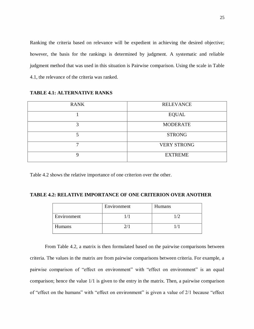
Ranking the criteria based on relevance will be expedient in achieving the desired objective;
however, the basis for the rankings is determined by judgment. A systematic and reliable
judgment method that was used in this situation is Pairwise comparison. Using the scale in Table
4.1, the relevance of the criteria was ranked.
TABLE 4.1: ALTERNATIVE RANKS
RANK RELEVANCE
1 EQUAL
3 MODERATE
5 STRONG
7 VERY STRONG
9 EXTREME
Table 4.2 shows the relative importance of one criterion over the other.
TABLE 4.2: RELATIVE IMPORTANCE OF ONE CRITERION OVER ANOTHER
Environment Humans
Environment 1/1 1/2
Humans 2/1 1/1
From Table 4.2, a matrix is then formulated based on the pairwise comparisons between
criteria. The values in the matrix are from pairwise comparisons between criteria. For example, a
pairwise comparison of “effect on environment” with “effect on environment” is an equal
comparison; hence the value 1/1 is given to the entry in the matrix. Then, a pairwise comparison
of “effect on the humans” with “effect on environment” is given a value of 2/1 because “effect

26
on humans is subjectively preferred twice to “effect on environment” for the worst-case scenario.
The resultant matrix is given:
A = [
]
To obtain ranking priorities from this vector, there are several methods that can be used.
However the preferred and one of the best approaches is the Eigenvector solution (T. Saaty
1990). The steps in finding the eigenvector are given:
1. Square the matrix
2. Sum up the rows of the new matrix
3. Normalize each value
The square of the matrix will give
A2 = [
]
Summing the rows up will give
A2 = [
]
Normalizing the values is achieved by dividing the sums by the total of the sums. The sum of the
values of the rows is 9. Therefore,

27
A2 = [
]
[
]
Next the pairwise comparisons are performed for each of the observed situations to rank
each of the situations in order of the worst for this analysis based on the criteria identified and
ranked. The ranks applied to this comparison are from Table 4.1.
TABLE 4.3: PAIRWISE COMPARISON IN TERMS OF EFFECT ON THE
ENVIRONMENT
EFFECT ON THE
ENVIRONMENT
CARCINOGENIC FLAMMABLE
CARCINOGENIC 1/1 1/4
FLAMMABLE 4/1 1/1
E = [
]
E2 = [
]
Summing up the rows
E2 = [
]
Normalizing

28
E2 = [
]
[
]
The same approach is carried out in terms of effect on humans and one more set of
eigenvectors are produced from the iteration.
TABLE 4.4: PAIRWISE COMPARISON IN TERMS OF EFFECT ON THE HUMANS
EFFECT ON HUMANS CARCINOGENIC FLAMMABLE
CARCINOGENIC 1/1 2/1
FLAMMABLE 1/2 1/1
H = [
]
H2 = [
]
Summing up the rows
H2 = [
]
Normalizing
H2 = [
]
[
]

29
The individual eigenvectors are then put together to form a matrix of eigenvectors. The
eigenvector solution is then calculated by multiplying the matrix of the eigenvectors of the
alternatives with the eigenvector of the selection criteria.
[
] * [
] = [
]
To make sure the solution for the weights is accurate; the sum of the weights must be
approximately equal 1. (0.515 + 0.485 = 1). Table 4.5 shows the weights that will be assigned to
the alternatives that give the worst-case scenario for factor A.
TABLE 4.5: WEIGHTS ASSIGNED TO THE DIFFERENT CLASSES OF FACTOR A
TYPE OF CHEMICAL
SPILLED
WEIGHT LEVEL
CARCINOGENIC 0.515
FLAMMABLE 0.485
FACTOR B: INCIDENT TYPE
There are different types of incidents that occur in the oil and gas industry. In the case of
spills, these incidents can also be classified into different types. The various types of occurrences
bring about different responses in reporting, stemming from overlooking a supposed minor
incident to not having knowledge of the occurrence. This factor will classify some observed
incident types and assign weights to them in an attempt to analyze the significance it exhibits on
the dependent factor.

30
Following a similar procedure, Table 4.6 shows the pairwise comparison based on the
ranks in Table 4.1 of one two alternatives at a time. One example is the pairwise comparison of
“mobile” and “fixed”. The given value if 2/1 which means a mobile incident is preferred twice as
much to a fixed incident to produce a worst-case scenario.
TABLE 4.6: PAIRWISE COMPARISON FOR THE VARIOUS INCIDENT TYPES
INCIDENT
TYPES
FIXED MOBILE CONTINUOUS STORAGE
TANK/
VESSEL
OTHER
FIXED 1/1 1/2 1/4 2/1 4/1
MOBILE 2/1 1/1 1/2 4/1 8/1
CONTINUOUS 4/1 2/1 1/1 8/1 9/1
STORAGE
TANK/ VESSEL
1/2 1/4 1/8 1/1 2/1
OTHER 1/4 1/8 1/9 1/2 1/1
Following the steps that were given earlier for factor A, the AHP process is carried out as
follows:
First the matrix,
B =
[
]
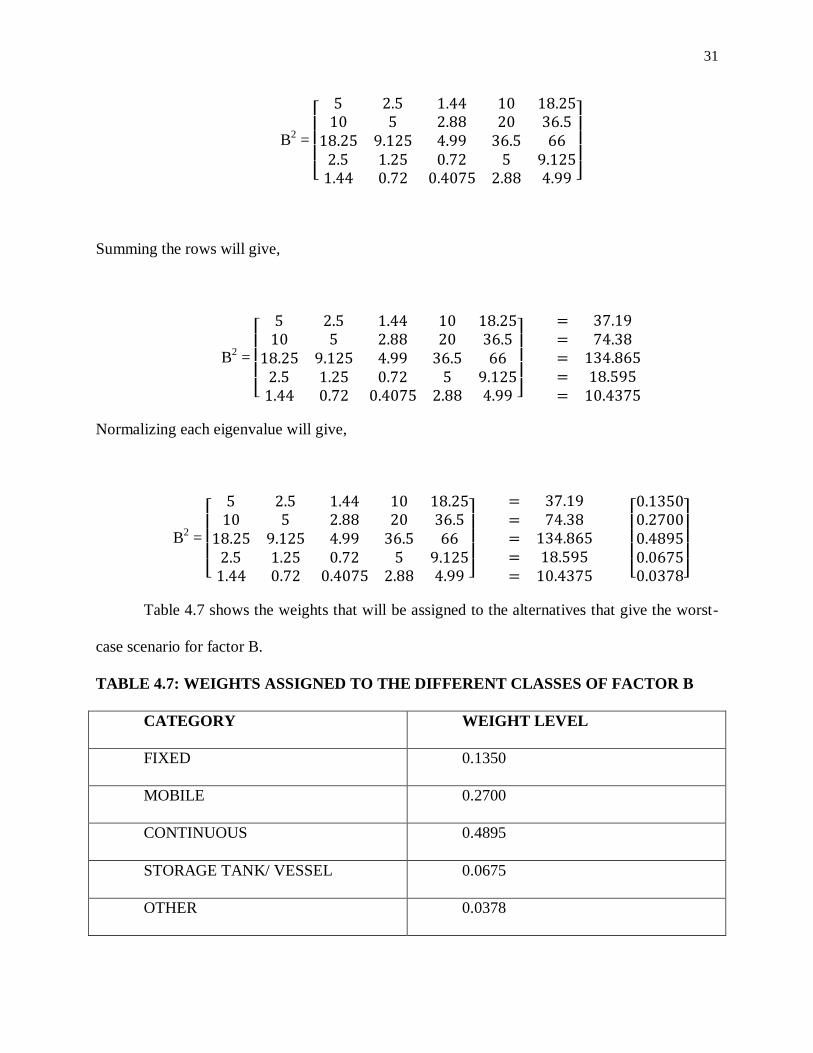
Squaring the matrix will give,
31
B2 =
[
]
Summing the rows will give,
B2 =
[
]
Normalizing each eigenvalue will give,
B2 =
[
]
[ ]
Table 4.7 shows the weights that will be assigned to the alternatives that give the worst-
case scenario for factor B.
TABLE 4.7: WEIGHTS ASSIGNED TO THE DIFFERENT CLASSES OF FACTOR B
CATEGORY WEIGHT LEVEL
FIXED 0.1350
MOBILE 0.2700
CONTINUOUS 0.4895
STORAGE TANK/ VESSEL 0.0675
OTHER 0.0378

32
FACTOR C: POPULATION
Incidents that were reported in the data set occurred at different locations and an accurate
measure of the health effects is needed. The number of people any spilled chemical affects is
dependent on the number of people in contact with the spilled chemical. The number of people
living in the county of the oil spill was used to model this factor.
FACTOR D: DELAY TIME
The time of exposure to a chemical is crucial in determining or modeling the health
effects attributed to that particular chemical. Some chemicals are more hazardous than others and
this can be noted by the recommended exposure limit (REL) regulated by OSHA and NIOSH in
the form of ceiling concentrations, short-term exposures (ST) and time-weighted averages
(TWA) (Department of Health and Human Services 2007).
FACTOR E: YEAR EFFECT
This factor will be modeled based on the assumption that a safety program has been in
place at the organization from which the data was collected and weights were assigned based on
the fact that the earliest timeframe should have the largest weight on the dependent variable.
However to best implement this variable, a dummy variable system or method will be used to be
able to assess the health effects of each timeframe on the dependent variable. Table 4.8 shows
the way the dummy variable will be modeled.

33
TABLE 4.8: DUMMY VARAIBLES PER TIMEFRAME
DUMMY VARIABLES
YEARS Y1 Y2 Y3 Y4 Y5
1990 – 1994 1 0 0 0 0
1995 – 1998 0 1 0 0 0
1999 – 2002 0 0 1 0 0
2003 – 2006 0 0 0 1 0
2007 - 2010 0 0 0 0 1
FACTOR F: NATURAL FACTORS
Natural hazards have become a primary focus due to the effect of technological advances
on the climate. There have been a number of high profiled incidents resulting from natural
hazards over the last ten years including hurricanes, tsunamis, earthquakes and floods. The oil
and gas industry is no stranger to natural hazards and its effects. This also has an effect on the
timely reporting of the occurrence. Incidents that happen at specific times of the year may create
a problem for the requirements of reporting to be put together. This factor aims to represent
natural occurrences and assess the significance it has on the dependent variable. A dummy
variable method is also used for this factor.

34
TABLE 4.9: DUMMY VARAIBLES PER SEASON
DUMMY VARIABLES
SEASON NF1 NF2 NF3 NF4 NF5
SUMMER 1 0 0 0 0
WINTER 0 1 0 0 0
SPRING 0 0 1 0 0
FALL 0 0 0 1 0
ACROSS
SEASONS
0 0 0 0 1

CHAPTER 5
ANALYSIS AND RESULTS
REGRESSION ANALYSIS
The Minitab 16 Statistical Software was used for the statistical analysis of the sorted data.
Regression analysis is frequently used as an analytical method for finding relationships between
variables. Mostly there are two types of variables involved in regression analysis; they are a
dependent variable and independent variables. Regression analysis was carried out on the sorted
data based on a confidence level of 95%. The effect of each of the factors on this analysis
corresponds to x1, x2, x3, x4, x5 … xi. The variables “x1, x2, x3, x4, x5 … xi” are considered as
the independent variables. The dependent variable is the number of deaths in each of the states
the incidents took place over the 21-year period and is denoted as (X’). The mathematical
representation for the interactive relationship between the independent and dependent variables
is given in equation 5.1 as:
…………………………… (5.1)
β0 – β5 are all regression coefficients and E denotes the various errors which may be due to
uncontrollable and nuisance factors including but not limited to human error and sabotage. This
analysis aimed at describing how each of the various factors varies with the other and how
multiple factors play roles in increasing the potential health effects of oil spills (All analyses and
methodologies used are shown in the appendices).
36
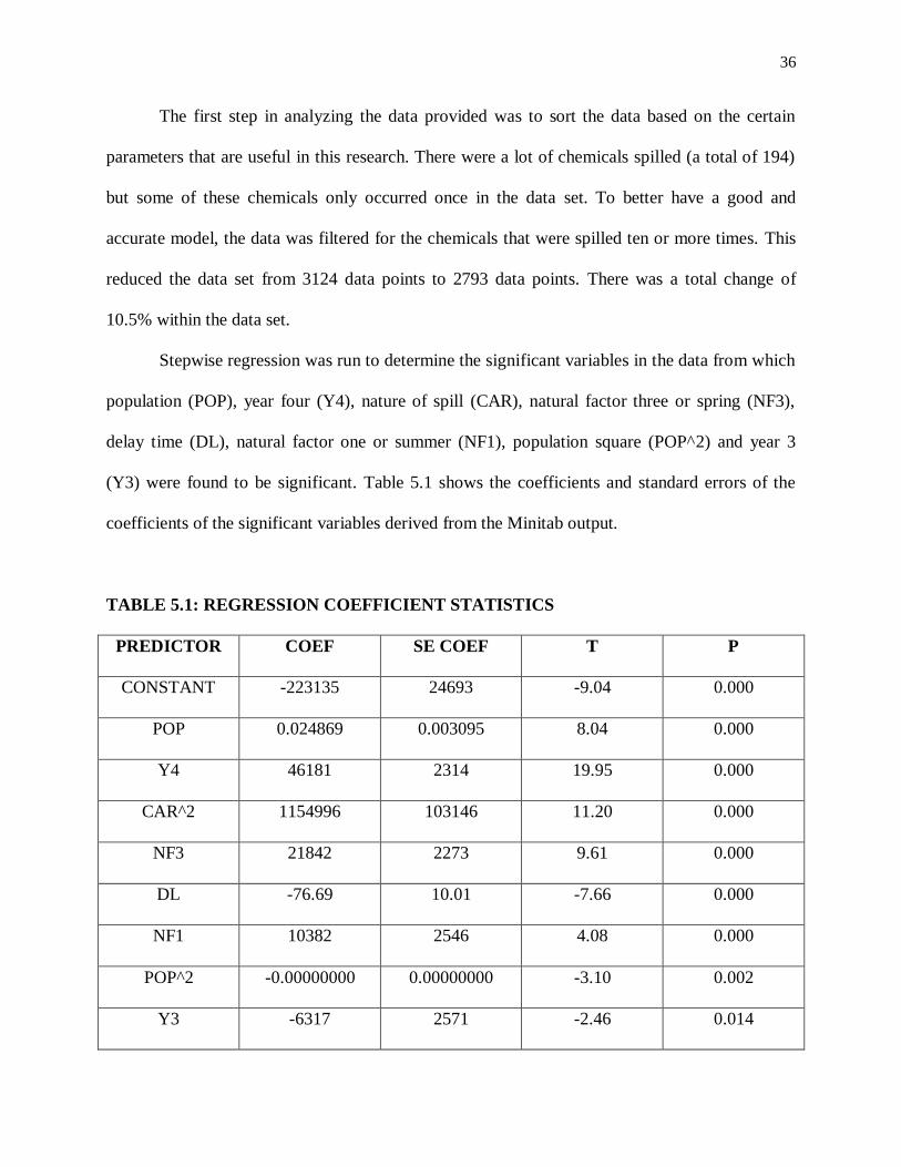
The first step in analyzing the data provided was to sort the data based on the certain
parameters that are useful in this research. There were a lot of chemicals spilled (a total of 194)
but some of these chemicals only occurred once in the data set. To better have a good and
accurate model, the data was filtered for the chemicals that were spilled ten or more times. This
reduced the data set from 3124 data points to 2793 data points. There was a total change of
10.5% within the data set.
Stepwise regression was run to determine the significant variables in the data from which
population (POP), year four (Y4), nature of spill (CAR), natural factor three or spring (NF3),
delay time (DL), natural factor one or summer (NF1), population square (POP^2) and year 3
(Y3) were found to be significant. Table 5.1 shows the coefficients and standard errors of the
coefficients of the significant variables derived from the Minitab output.
TABLE 5.1: REGRESSION COEFFICIENT STATISTICS
PREDICTOR COEF SE COEF T P
CONSTANT -223135 24693 -9.04 0.000
POP 0.024869 0.003095 8.04 0.000
Y4 46181 2314 19.95 0.000
CAR^2 1154996 103146 11.20 0.000
NF3 21842 2273 9.61 0.000
DL -76.69 10.01 -7.66 0.000
NF1 10382 2546 4.08 0.000
POP^2 -0.00000000 0.00000000 -3.10 0.002
Y3 -6317 2571 -2.46 0.014

37
Pearson correlation was performed for the filtered data points for all the variables. This
was to decipher if there were relationships within the variables and Table 5.2 shows the results
TABLE 5.2: CORRELATION MATRIX FOR MODEL
X POP Y4 CAR^2 NF3 DL NF1 POP^2
POP 0.589
Y4 0.403 0.110
CAR^2 0.127 -0.083 0.071
NF3 0.126 -0.049 0.079 0.006
DL -0.090 -0.032 0.156 -0.039 -0.107
NF1 0.037 0.045 -0.050 0.002 -0.295 -0.087
POP^2 0.585 0.993 0.110 -0.073 -0.040 -0.049 0.037
Y3 -0.220 -0.015 -0.535 -0.036 -0.034 -0.075 0.031 -0.010
Equation 5.2 shows the prediction model for the associated health effects by way of the
number of deaths based on the significant variables mentioned earlier.
–
– – ………………………(5.2)
The Analysis of Variance (ANOVA) of the model is given in Table 5.3.
TABLE 5.3: ANALYSIS OF VARIANCE FOR THE REGRESSION MODEL

38
SOURCE DF SS MS F P
REGRESSION 8 7.51851E+12 9.39814E+11 375.14 0.000
RESIDUAL
ERROR
2783 6.97209E+12 2505241605
TOTAL 2791 1.44906E+13
The sequential sum of squares was derived from the Minitab output and are shown in
Table 5.4.
TABLE 5.4: SEQUENTIAL SUM OF SQUARES FOR THE REGRESSION MODEL
SOURCE DF SEQ SS
POP 1 5.03356E+12
Y4 1 1.68212E+12
CAR^2 1 3.25127E+11
NF3 1 2.33675E+11
DL 1 1.56336E+11
NF1 1 45731374434
POP^2 1 26838489011
Y3 1 15119961051
The R2 value of the regression model was 51.9% and the adjusted R
2 value, which is
expected to be less, was 51.7%. This means that 51.9% of the variations in X’ can be explained
by the model given in equation (5.2). The normal probability plot in the top right of Figure 5.1
shows the normality of the residuals. The left top graph shows the residuals versus the fitted

39
values which is not funnel shaped, curved or skewed. The histogram in the bottom left corner
shows a bell-shaped curve of the distribution of the residuals while the bottom right graph of
versus order shows how well the residuals are spread.
2000001000000-100000-200000
99.99
99
90
50
10
1
0.01
Residual
Pe
rce
nt
4000003000002000001000000
200000
100000
0
-100000
Fitted Value
Re
sid
ua
l
150000
100000
500000
-50000
-100000
400
300
200
100
0
Residual
Fre
qu
en
cy
2600
2400
2200
2000
1800
1600
1400
1200
100080
0600
400
2001
200000
100000
0
-100000
Observation Order
Re
sid
ua
l
Normal Probability Plot Versus Fits
Histogram Versus Order
Residual Plots for Deaths by State
FIGURE 5.1: RESIDUAL PLOTS FOR THE MODEL

40
TRANSFORMATIONS
Most quantitative analyses require tools that can help in giving a clearer picture of
relationships between variables. Data transformations are commonly used for many other
functions in quantitative analysis. One use of data transformations is for solving the issue of non-
homogenous variances. This transformational analysis will focus on commonly used data
transformations in statistics: square root, inverse, square, natural log and cube of the dependent
variable which will aim to improve upon the normality of the variable. These transformations are
usually referred to as variance-stabilizing transformations because they reduce and sometimes
eliminate uneven variances and also normalize distributions. The characteristics of the various
transformed models were compared to the original model to determine the best result based on
the analysis of variance, R2 value and the normal plots of residuals.
SQUARE ROOT TRANSFORMATION
The square root transformation of the dependent variable can be expressed
mathematically as shown in equation (5.3).
X’ = √X……………………………………………… (5.3)
Stepwise regression was run to determine the significant variables in the data from which
population (POP), year four (Y4), nature of spill squared (CAR^2), natural factor three or spring
(NF3), year 3 (Y3), population square (POP^2), natural factor one or summer (NF1) and delay
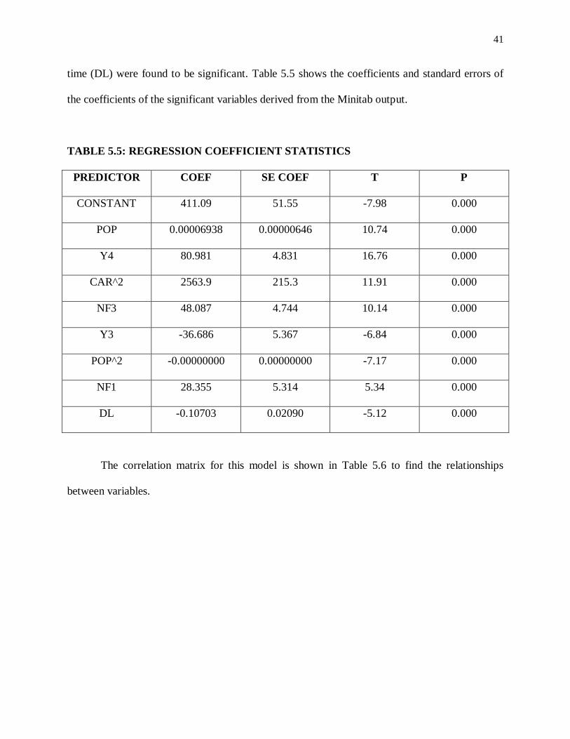
41
time (DL) were found to be significant. Table 5.5 shows the coefficients and standard errors of
the coefficients of the significant variables derived from the Minitab output.
TABLE 5.5: REGRESSION COEFFICIENT STATISTICS
PREDICTOR COEF SE COEF T P
CONSTANT 411.09 51.55 -7.98 0.000
POP 0.00006938 0.00000646 10.74 0.000
Y4 80.981 4.831 16.76 0.000
CAR^2 2563.9 215.3 11.91 0.000
NF3 48.087 4.744 10.14 0.000
Y3 -36.686 5.367 -6.84 0.000
POP^2 -0.00000000 0.00000000 -7.17 0.000
NF1 28.355 5.314 5.34 0.000
DL -0.10703 0.02090 -5.12 0.000
The correlation matrix for this model is shown in Table 5.6 to find the relationships
between variables.
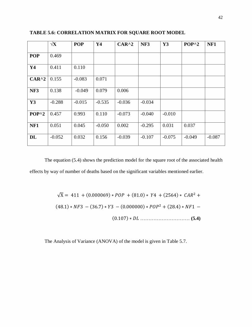
42
TABLE 5.6: CORRELATION MATRIX FOR SQUARE ROOT MODEL
√X POP Y4 CAR^2 NF3 Y3 POP^2 NF1
POP 0.469
Y4 0.411 0.110
CAR^2 0.155 -0.083 0.071
NF3 0.138 -0.049 0.079 0.006
Y3 -0.288 -0.015 -0.535 -0.036 -0.034
POP^2 0.457 0.993 0.110 -0.073 -0.040 -0.010
NF1 0.051 0.045 -0.050 0.002 -0.295 0.031 0.037
DL -0.052 0.032 0.156 -0.039 -0.107 -0.075 -0.049 -0.087
The equation (5.4) shows the prediction model for the square root of the associated health
effects by way of number of deaths based on the significant variables mentioned earlier.
√
………………………… (5.4)
The Analysis of Variance (ANOVA) of the model is given in Table 5.7.

43
TABLE 5.7: ANALYSIS OF VARIANCE FOR THE REGRESSION MODEL
SOURCE DF SS MS F P
REGRESSION 8 22823907 2852988 261.35 0.000
RESIDUAL
ERROR
2783 30379845 10916
TOTAL 2791 53203752
The sequential sum of squares was derived from the Minitab output and are shown in
Table 5.8
TABLE 5.8: SEQUENTIAL SUM OF SQUARES FOR THE REGRESSION MODEL
SOURCE DF SEQ SS
POP 1 11701408
Y4 1 6959837
CAR^2 1 1464224
NF3 1 916686
Y3 1 591853
POP^2 1 505429
NF1 1 398317
DL 1 286153
The R2 value of the regression model was 42.9% and the adjusted R
2 value which is
expected to be less was 42.7%. This means that 42.9% of the variations in √X can be explained
by the model given in equation (5.4). The normal probability plot in the top right of Figure 5.2
shows the normality of the residuals. The left top graph shows the residuals versus the fitted
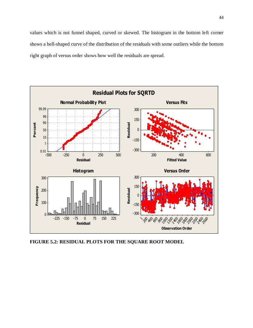
44
values which is not funnel shaped, curved or skewed. The histogram in the bottom left corner
shows a bell-shaped curve of the distribution of the residuals with some outliers while the bottom
right graph of versus order shows how well the residuals are spread.
5002500-250-500
99.99
99
90
50
10
1
0.01
Residual
Pe
rce
nt
600400200
300
150
0
-150
-300
Fitted Value
Re
sid
ua
l
225150750-75-150-225
300
200
100
0
Residual
Fre
qu
en
cy
2600
2400
2200
2000
1800
1600
1400
1200
100080
0600
400
2001
300
150
0
-150
-300
Observation Order
Re
sid
ua
l
Normal Probability Plot Versus Fits
Histogram Versus Order
Residual Plots for SQRTD
FIGURE 5.2: RESIDUAL PLOTS FOR THE SQUARE ROOT MODEL

45
INVERSE TRANSFORMATION
The inverse transformation of the dependent variable can be expressed mathematically as
shown in equation (5.5).
X’ = 1/X……………………..…………………… (5.5)
Stepwise regression was run to determine the significant variables in the data from which
year 3 (Y3), population (POP), population square (POP^2), nature of spill squared (CAR^2),
year 4 (Y4), natural factor three or spring (NF3), natural factor one or summer (NF1), incident
type square (TYPE^2) and incident type (TYPE) were found to be significant. Table 5.9 shows
the coefficients and standard errors of the coefficients of the significant variables derived from
the Minitab output.
TABLE 5.9: REGRESSION COEFFICIENT STATISTICS
PREDICTOR COEF SE COEF T P
CONSTANT 0.00053902 0.00005619 9.59 0.000
Y3 0.00007339 0.00000560 13.10 0.000
POP -0.00000000 0.00000000 -13.79 0.000
POP^2 0.00000000 0.00000000 12.60 0.000
CAR^2 -0.0023466 0.0002245 -10.45 0.000
Y4 -0.00004150 0.00000499 -8.32 0.000
NF3 -0.00004177 0.00000490 -8.53 0.000
NF1 -0.00003367 0.00000551 -6.11 0.000
TYPE^2 -0.0023864 0.0002448 -9.75 0.000
TYPE 0.0013634 0.0001460 9.34 0.000
46
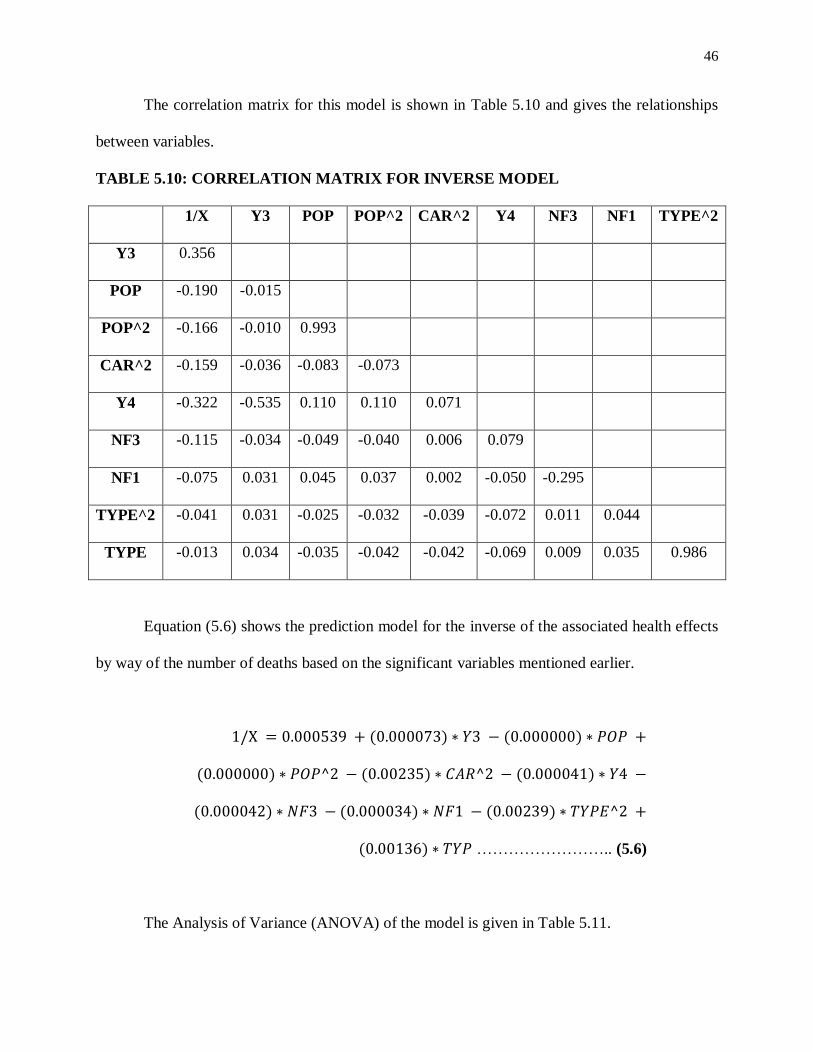
The correlation matrix for this model is shown in Table 5.10 and gives the relationships
between variables.
TABLE 5.10: CORRELATION MATRIX FOR INVERSE MODEL
1/X Y3 POP POP^2 CAR^2 Y4 NF3 NF1 TYPE^2
Y3 0.356
POP -0.190 -0.015
POP^2 -0.166 -0.010 0.993
CAR^2 -0.159 -0.036 -0.083 -0.073
Y4 -0.322 -0.535 0.110 0.110 0.071
NF3 -0.115 -0.034 -0.049 -0.040 0.006 0.079
NF1 -0.075 0.031 0.045 0.037 0.002 -0.050 -0.295
TYPE^2 -0.041 0.031 -0.025 -0.032 -0.039 -0.072 0.011 0.044
TYPE -0.013 0.034 -0.035 -0.042 -0.042 -0.069 0.009 0.035 0.986
Equation (5.6) shows the prediction model for the inverse of the associated health effects
by way of the number of deaths based on the significant variables mentioned earlier.
…………………….. (5.6)
The Analysis of Variance (ANOVA) of the model is given in Table 5.11.

47
TABLE 5.11: ANALYSIS OF VARIANCE FOR THE REGRESSION MODEL
SOURCE DF SS MS F P
REGRESSION 9 1.35854E-05 1.50949E-06 127.11 0.000
RESIDUAL
ERROR
2782 3.30365E-05 1.18751E-08
TOTAL 2791 4.66219E-05
The sequential sum of squares was derived from the Minitab output and are shown in
Table 5.12.
TABLE 5.12: SEQUENTIAL SUM OF SQUARES FOR THE REGRESSION MODEL
SOURCE DF SEQ SS
Y3 1 5.91999E-06
POP 1 1.59554E-06
POP^2 1 1.45656E-06
CAR^2 1 1.48353E-06
Y4 1 7.93441E-07
NF3 1 6.31737E-07
NF1 1 5.43095E-07
TYPE^2 1 1.26449E-07
TYPE 1 1.03507E-06
The R2 value of the regression model was 29.1% and the adjusted R
2 value, which is
expected to be less, was 28.9%. This means that 29.1% of the variations in 1/X can be explained
by the model given in the equation (5.6). The normal probability plot in the top right of Figure
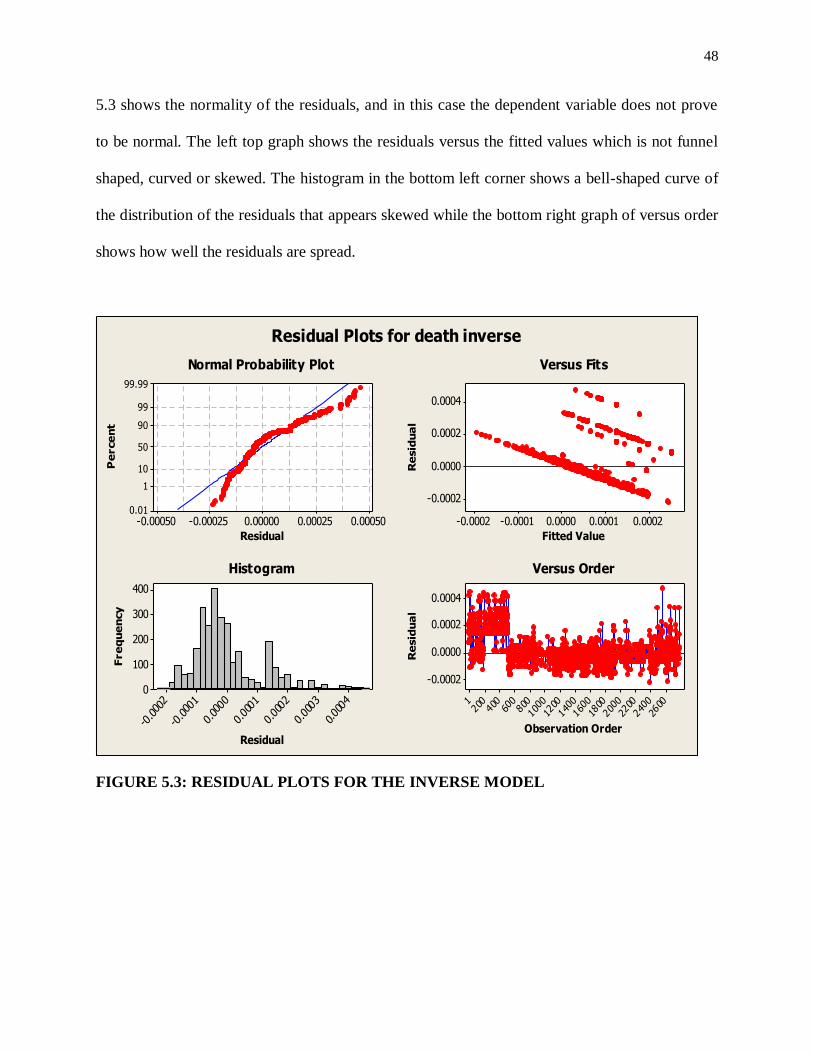
48
5.3 shows the normality of the residuals, and in this case the dependent variable does not prove
to be normal. The left top graph shows the residuals versus the fitted values which is not funnel
shaped, curved or skewed. The histogram in the bottom left corner shows a bell-shaped curve of
the distribution of the residuals that appears skewed while the bottom right graph of versus order
shows how well the residuals are spread.
0.000500.000250.00000-0.00025-0.00050
99.99
99
90
50
10
1
0.01
Residual
Pe
rce
nt
0.00020.00010.0000-0.0001-0.0002
0.0004
0.0002
0.0000
-0.0002
Fitted Value
Re
sid
ua
l
0.0004
0.0003
0.0002
0.0001
0.0000
-0.0001
-0.0002
400
300
200
100
0
Residual
Fre
qu
en
cy
2600
2400
2200
2000
1800
1600
1400
1200
100080
0600
400
2001
0.0004
0.0002
0.0000
-0.0002
Observation Order
Re
sid
ua
l
Normal Probability Plot Versus Fits
Histogram Versus Order
Residual Plots for death inverse
FIGURE 5.3: RESIDUAL PLOTS FOR THE INVERSE MODEL

49
SQUARE TRANSFORMATION
The square transformation of the dependent variable can be expressed mathematically as
shown in equation (5.5);
X’ = X2……………………………..…………… (5.5)
Stepwise regression was run to determine the significant variables in the data from which
population square (POP^2), year 4 (Y4), delay time (DL), nature of spill (CAR), natural factor
three or spring (NF3), population (POP), natural factor four or fall (NF4), year one (Y1), delay
time square (DL^2) and natural factor five of across seasons (NF5) were found to be significant.
Table 5.13 shows the coefficients and standard errors of the coefficients of the significant
variables derived from the Minitab output.
TABLE 5.13: REGRESSION COEFFICIENT STATISTICS
PREDICTOR COEF SE COEF T P
CONSTANT -7.93839E+10 9188020292 -8.64 0.000
POP^2 0.00017329 0.00005668 3.06 0.002
Y4 8795700809 377992445 23.27 0.000
DL -55598863 12072424 -4.61 0.000
CAR 1.75296E+11 18802592477 9.32 0.000
NF3 2723800926 419897223 6.49 0.000
POP 2770.9 561.0 4.94 0.000
NF4 -1261164266 439550190 -2.87 0.004
Y1 -1426178288 559068091 -2.55 0.011
DL^2 35458 10929 3.24 0.001
NF5 6982752560 2934656634 2.38 0.017

50
The correlation matrix for this model is shown in Table 5.14 and shows the relationships
between variables.
TABLE 5.14: CORRELATION MATRIX FOR SQUARE MODEL
X
2 POP^2 Y4 DL CAR NF3 POP NF4 Y1 DL^2
POP^2 0.760
Y4 0.355 0.110
DL -0.110 -0.049 0.156
CAR 0.069 -0.073 0.071 -0.039
NF3 0.087 -0.040 0.079 -0.107 0.006
POP 0.757 0.993 0.110 -0.032 -0.083 -0.049
NF4 -0.021 0.052 -0.049 -0.097 -0.026 -0.332 0.058
Y1 -0.193 -0.109 -0.339 -0.053 -0.003 -0.013 -0.106 -0.008
DL^2 -0.093 -0.041 0.141 0.936 -0.042 -0.084 -0.027 -0.076 -0.048
NF5 -0.105 -0.047 0.112 0.873 -0.005 -0.123 -0.032 -0.111 -0.037 0.684
Equation (5.6) shows the prediction model for the square of the associated health effects
by way of number of deaths based on the significant variables mentioned earlier.
–
…………. (5.6)
The Analysis of Variance (ANOVA) of the model is given in Table 5.15.

51
TABLE 5.15: ANALYSIS OF VARIANCE FOR THE REGRESSION MODEL
SOURCE DF SS MS F P
REGRESSION 10 5.04571E+23 5.04571E+22 610.75 0.000
RESIDUAL
ERROR
2781 2.29754E+23 8.26156E+19
TOTAL 2791 7.34324E+23
The sequential sum of squares was derived from the Minitab output and are shown in
Table 5.16.
TABLE 5.16: SEQUENTIAL SUM OF SQUARES FOR THE REGRESSION MODEL
SOURCE DF SEQ SS
POP^2 1 4.24221E+23
Y4 1 5.44531E+22
DL 1 1.03670E+22
CAR 1 6.81179E+21
NF3 1 4.90862E+21
POP 1 1.76479E+21
NF4 1 6.44387E+20
Y1 1 5.24491E+20
DL^2 1 4.07287E+20
NF5 1 4.67736E+20
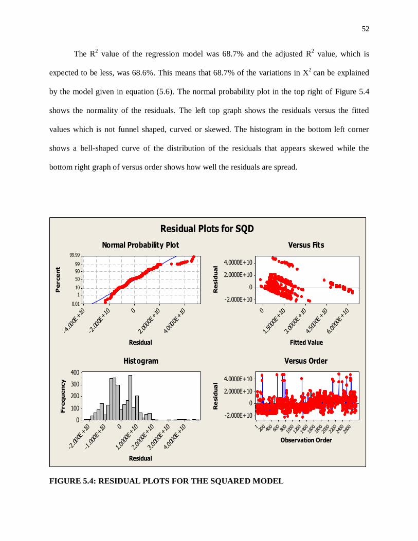
52
The R2 value of the regression model was 68.7% and the adjusted R
2 value, which is
expected to be less, was 68.6%. This means that 68.7% of the variations in X2
can be explained
by the model given in equation (5.6). The normal probability plot in the top right of Figure 5.4
shows the normality of the residuals. The left top graph shows the residuals versus the fitted
values which is not funnel shaped, curved or skewed. The histogram in the bottom left corner
shows a bell-shaped curve of the distribution of the residuals that appears skewed while the
bottom right graph of versus order shows how well the residuals are spread.
4.0000E+10
2.0000E+100
-2.000E+10
-4.000E+10
99.99
99
90
50
10
1
0.01
Residual
Pe
rce
nt
6.0000E+10
4.5000E+10
3.0000E+10
1.5000E+100
4.0000E+10
2.0000E+10
0
-2.000E+10
Fitted Value
Re
sid
ua
l
4.0000E+10
3.0000E+10
2.0000E+10
1.0000E+100
-1.000E+10
-2.000E+10
400
300
200
100
0
Residual
Fre
qu
en
cy
2600
2400
2200
2000
1800
1600
1400
1200
100080
0600
400
2001
4.0000E+10
2.0000E+10
0
-2.000E+10
Observation Order
Re
sid
ua
l
Normal Probability Plot Versus Fits
Histogram Versus Order
Residual Plots for SQD
FIGURE 5.4: RESIDUAL PLOTS FOR THE SQUARED MODEL

53
NATURAL LOG TRANSFORMATION
The natural log transformation of the dependent variable can be expressed
mathematically as shown in equation (5.7).
X’ = ln X………………………………………… (5.7)
Stepwise regression was run to determine the significant variables in the data from which
year 3 (Y3), population (POP), population square (POP^2), nature of spill squared (CAR^2),
year 4 (Y4), natural factor three or spring (NF3), natural factor one or summer (NF1), incident
type square (TYPE^2) and incident type (TYPE) were found to be significant. Table 5.17 shows
the coefficients and standard errors of the coefficients of the significant variables derived from
the Minitab output.

54
TABLE 5.17: REGRESSION COEFFICIENT STATISTICS
PREDICTOR COEF SE COEF T P
CONSTANT -2.838 1.206 -2.35 0.019
Y4 0.78392 0.06518 12.03 0.000
POP 0.00000097 0.00000007 13.22 0.000
Y3 -0.59596 0.07053 -8.45 0.000
CAR 29.174 2.436 11.98 0.000
POP^2 -0.00000000 0.00000000 -10.87 0.000
NF3 0.52389 0.05392 9.72 0.000
NF1 0.35083 0.06065 5.78 0.000
TYPE^2 22.750 2.657 8.56 0.000
TYPE -13.137 1.585 -8.29 0.000
NF5 -0.2589 0.1194 -2.17 0.030
Y1 0.17655 0.08455 2.09 0.037
The correlation matrix for this model is shown in Table 5.18 to reveal the relationships
between variables.
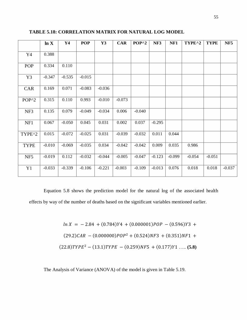
55
TABLE 5.18: CORRELATION MATRIX FOR NATURAL LOG MODEL
ln X Y4 POP Y3 CAR POP^2 NF3 NF1 TYPE^2 TYPE NF5
Y4 0.388
POP 0.334 0.110
Y3 -0.347 -0.535 -0.015
CAR 0.169 0.071 -0.083 -0.036
POP^2 0.315 0.110 0.993 -0.010 -0.073
NF3 0.135 0.079 -0.049 -0.034 0.006 -0.040
NF1 0.067 -0.050 0.045 0.031 0.002 0.037 -0.295
TYPE^2 0.015 -0.072 -0.025 0.031 -0.039 -0.032 0.011 0.044
TYPE -0.010 -0.069 -0.035 0.034 -0.042 -0.042 0.009 0.035 0.986
NF5 -0.019 0.112 -0.032 -0.044 -0.005 -0.047 -0.123 -0.099 -0.054 -0.051
Y1 -0.033 -0.339 -0.106 -0.221 -0.003 -0.109 -0.013 0.076 0.018 0.018 -0.037
Equation 5.8 shows the prediction model for the natural log of the associated health
effects by way of the number of deaths based on the significant variables mentioned earlier.
….. (5.8)
The Analysis of Variance (ANOVA) of the model is given in Table 5.19.
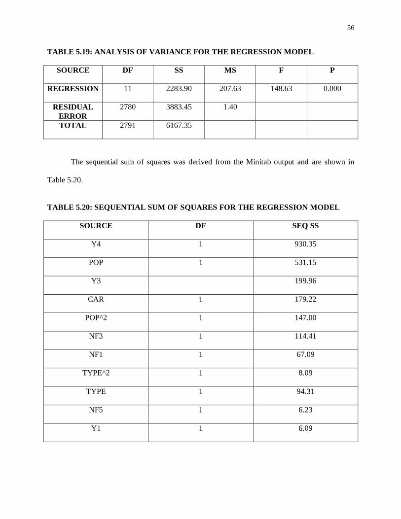
56
TABLE 5.19: ANALYSIS OF VARIANCE FOR THE REGRESSION MODEL
SOURCE DF SS MS F P
REGRESSION 11 2283.90 207.63 148.63 0.000
RESIDUAL
ERROR
2780 3883.45 1.40
TOTAL 2791 6167.35
The sequential sum of squares was derived from the Minitab output and are shown in
Table 5.20.
TABLE 5.20: SEQUENTIAL SUM OF SQUARES FOR THE REGRESSION MODEL
SOURCE DF SEQ SS
Y4 1 930.35
POP 1 531.15
Y3 199.96
CAR 1 179.22
POP^2 1 147.00
NF3 1 114.41
NF1 1 67.09
TYPE^2 1 8.09
TYPE 1 94.31
NF5 1 6.23
Y1 1 6.09
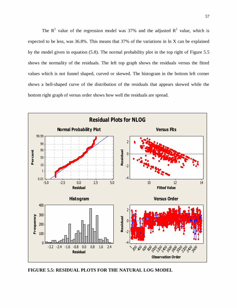
57
The R2 value of the regression model was 37% and the adjusted R
2 value, which is
expected to be less, was 36.8%. This means that 37% of the variations in ln X can be explained
by the model given in equation (5.8). The normal probability plot in the top right of Figure 5.5
shows the normality of the residuals. The left top graph shows the residuals versus the fitted
values which is not funnel shaped, curved or skewed. The histogram in the bottom left corner
shows a bell-shaped curve of the distribution of the residuals that appears skewed while the
bottom right graph of versus order shows how well the residuals are spread.
5.02.50.0-2.5-5.0
99.99
99
90
50
10
1
0.01
Residual
Pe
rce
nt
141210
2
0
-2
-4
Fitted Value
Re
sid
ua
l
2.41.60.80.0-0.8-1.6-2.4-3.2
400
300
200
100
0
Residual
Fre
qu
en
cy
2600
2400
2200
2000
1800
1600
1400
1200
100080
0600
400
2001
2
0
-2
-4
Observation Order
Re
sid
ua
l
Normal Probability Plot Versus Fits
Histogram Versus Order
Residual Plots for NLOG
FIGURE 5.5: RESIDUAL PLOTS FOR THE NATURAL LOG MODEL

58
CUBE TRANSFORMATION
The cube transformation of the dependent variable can be expressed mathematically as
shown in equation (5.9).
X’ = X3…………………………………..……… (5.9)
Stepwise regression was run to determine the significant variables in the data from which
year 3 (Y3), population (POP), population square (POP^2), nature of spill squared (CAR^2),
year 4 (Y4), natural factor three or spring (NF3), natural factor one or summer (NF1), incident
type square (TYPE^2) and incident type (TYPE) were found to be significant. Table 5.21 shows
the coefficients and standard errors of the coefficients of the significant variables derived from
the Minitab output.

59
TABLE 5.21: REGRESSION COEFFICIENT STATISTICS
PREDICTOR COEF SE COEF T P
CONSTANT -1.20352E+16 1.69143E+15 -7.12 0.000
POP^2 78.80 10.45 7.54 0.000
Y4 1.83424E+15 8.89953E+13 20.61 0.000
DL -9.52126E+12 2.22051E+12 -4.29 0.000
CAR 2.56399E+16 3.45785E+15 7.41 0.000
NF3 4.14705E+14 7.72497E+13 5.37 0.000
Y3 4.43070E+14 9.62009E+13 4.61 0.000
POP 378386637 103478598 3.66 0.000
NF4 -2.03896E+14 8.08632E+13 -2.52 0.012
DL^2 6055530581 2010020947 3.01 0.003
Y5 2.65404E+14 1.24020E+14 2.14 0.032
NF5 1.12417E+15 5.39927E+14 2.08 0.037
The correlation matrix for this model is shown in Table 5.22 and depict the relationships
between variables.
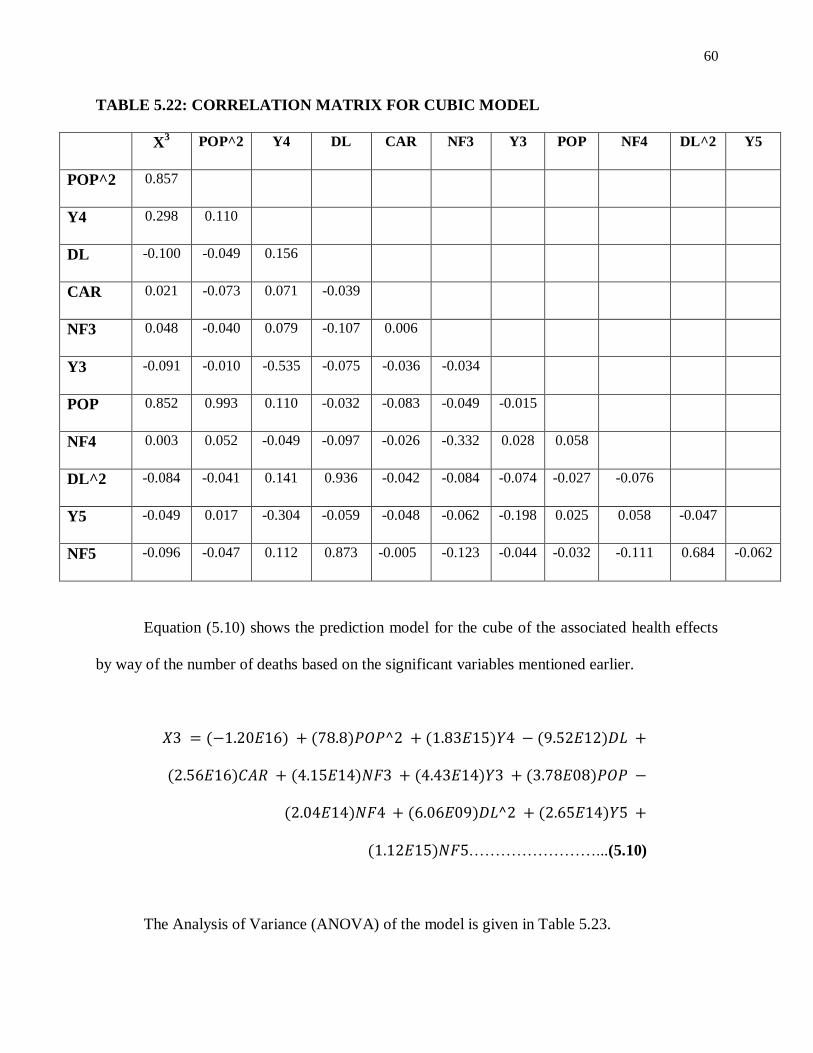
60
TABLE 5.22: CORRELATION MATRIX FOR CUBIC MODEL
X3 POP^2 Y4 DL CAR NF3 Y3 POP NF4 DL^2 Y5
POP^2 0.857
Y4 0.298 0.110
DL -0.100 -0.049 0.156
CAR 0.021 -0.073 0.071 -0.039
NF3 0.048 -0.040 0.079 -0.107 0.006
Y3 -0.091 -0.010 -0.535 -0.075 -0.036 -0.034
POP 0.852 0.993 0.110 -0.032 -0.083 -0.049 -0.015
NF4 0.003 0.052 -0.049 -0.097 -0.026 -0.332 0.028 0.058
DL^2 -0.084 -0.041 0.141 0.936 -0.042 -0.084 -0.074 -0.027 -0.076
Y5 -0.049 0.017 -0.304 -0.059 -0.048 -0.062 -0.198 0.025 0.058 -0.047
NF5 -0.096 -0.047 0.112 0.873 -0.005 -0.123 -0.044 -0.032 -0.111 0.684 -0.062
Equation (5.10) shows the prediction model for the cube of the associated health effects
by way of the number of deaths based on the significant variables mentioned earlier.
……………………...(5.10)
The Analysis of Variance (ANOVA) of the model is given in Table 5.23.

61
TABLE 5.23: ANALYSIS OF VARIANCE FOR THE REGRESSION MODEL
SOURCE DF SS MS F P
REGRESSION 11 3.02805E+34 2.75277E+33 985.13 0.000
RESIDUAL
ERROR
2780 7.76819E+33 2.79431E+30
TOTAL 2791 3.80487E+34
The sequential sum of squares was derived from the Minitab output and are shown in
Table 5.24.
TABLE 5.24: SEQUENTIAL SUM OF SQUARES FOR THE REGRESSION MODEL
SOURCE DF SEQ SS
POP^2 1 2.79637E+34
Y4 1 1.59562E+33
DL 1 3.25533E+32
CAR 1 1.48079E+32
NF3 1 1.17340E+32
Y3 1 4.06772E+31
POP 1 3.48119E+31
NF4 1 1.62697E+31
DL^2 1 1.41904E+31
Y5 1 1.21153E+31
NF5 1 1.21134E+31

62
The R2 value of the regression model was 79.6% and the adjusted R
2 value, which is
expected to be less, was 79.5%. This means that 79.6% of the variations in X3 can be explained
by the model given in equation (5.10). The normal probability plot in the top right of Figure 5.6
shows the normality of the residuals. The left top graph shows the residuals versus the fitted
values which is not funnel shaped, curved or skewed. The histogram in the bottom left corner
shows a bell-shaped curve of the distribution of the residuals while the bottom right graph of
versus order shows how well the residuals are spread.
1.0000E+165.0000E+150-5.000E+15
99.99
99
90
50
10
1
0.01
Residual
Pe
rce
nt
1.6000E+16
1.2000E+16
8.0000E+15
4.0000E+150
1.0000E+16
5.0000E+15
0
-5.000E+15
Fitted Value
Re
sid
ua
l
1.0000E+16
7.5000E+15
5.0000E+15
2.5000E+150
-2.500E+15
-5.000E+15
480
360
240
120
0
Residual
Fre
qu
en
cy
2600
2400
2200
2000
1800
1600
1400
1200
100080
0600
400
2001
1.0000E+16
5.0000E+15
0
-5.000E+15
Observation Order
Re
sid
ua
l
Normal Probability Plot Versus Fits
Histogram Versus Order
Residual Plots for cube
FIGURE 5.6: RESIDUAL PLOTS FOR THE CUBIC MODEL
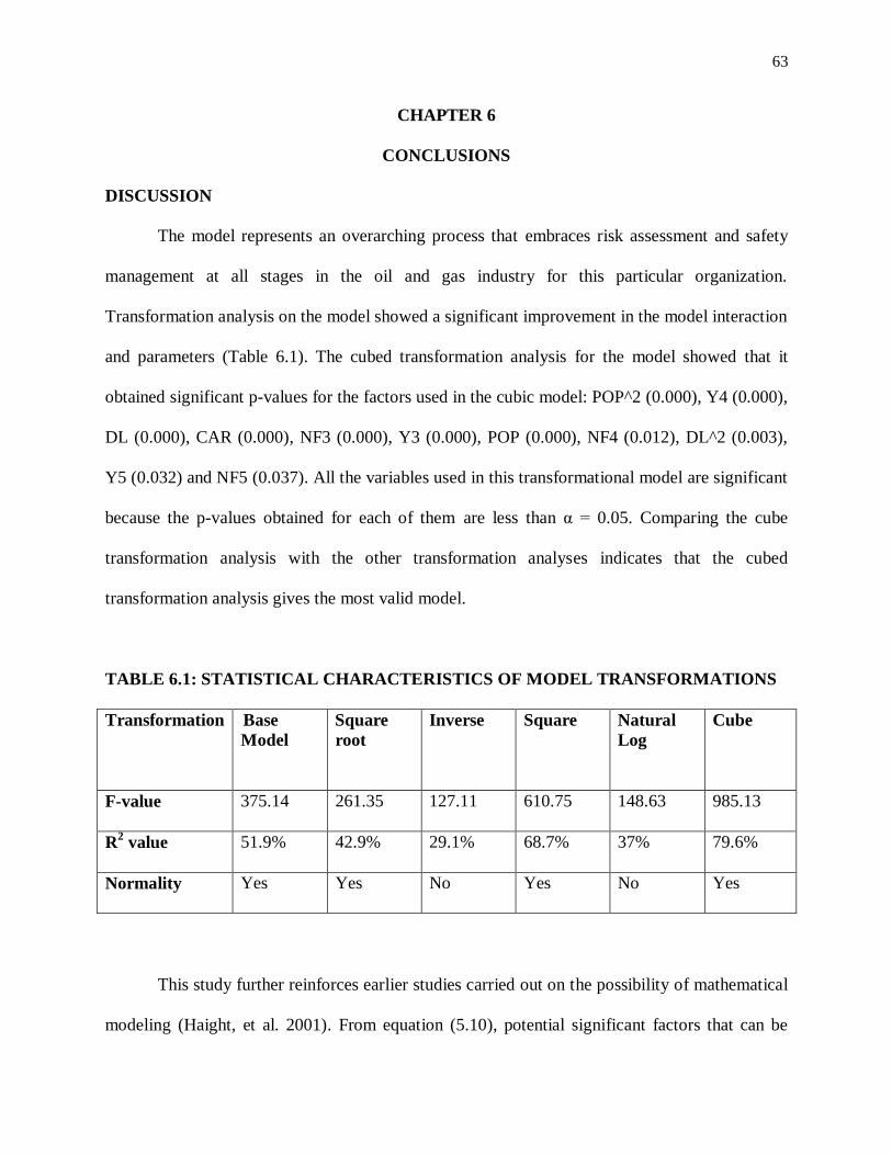
63
CHAPTER 6
CONCLUSIONS
DISCUSSION
The model represents an overarching process that embraces risk assessment and safety
management at all stages in the oil and gas industry for this particular organization.
Transformation analysis on the model showed a significant improvement in the model interaction
and parameters (Table 6.1). The cubed transformation analysis for the model showed that it
obtained significant p-values for the factors used in the cubic model: POP^2 (0.000), Y4 (0.000),
DL (0.000), CAR (0.000), NF3 (0.000), Y3 (0.000), POP (0.000), NF4 (0.012), DL^2 (0.003),
Y5 (0.032) and NF5 (0.037). All the variables used in this transformational model are significant
because the p-values obtained for each of them are less than α = 0.05. Comparing the cube
transformation analysis with the other transformation analyses indicates that the cubed
transformation analysis gives the most valid model.
TABLE 6.1: STATISTICAL CHARACTERISTICS OF MODEL TRANSFORMATIONS
Transformation Base
Model
Square
root
Inverse Square Natural
Log
Cube
F-value 375.14 261.35 127.11 610.75 148.63 985.13
R2 value 51.9% 42.9% 29.1% 68.7% 37% 79.6%
Normality Yes Yes No Yes No Yes
This study further reinforces earlier studies carried out on the possibility of mathematical
modeling (Haight, et al. 2001). From equation (5.10), potential significant factors that can be

64
affected by safety management include the incident delay and the nature of spill. Reducing these
two controllable significant factors will eventually reduce the number of deaths occurring from
incidents. This also aligns with a study that shows that relationship that exists between safety
management activities or the lack thereof and incidents in the workplace (Iyer, et al. 2004).
LIMITATIONS OF STUDY
Complete information regarding each of the incidents is needed for comprehensive safety
management and statistical modeling. The data collected lacked the magnitude of each
occurrence and resulted in the generation of quantitative data points from qualitative
information. The inclusion of the number of casualties per incident broken down into fatalities,
non-fatal accidents, incidents resulting in days away from work, incidents resulting in job
transfer and the economic cost of each incident will provide a better basis for quantitative
analysis and mathematical modeling to suit safety management prevention techniques. Also
functional dependencies between factors will be evident in the event of a broader data collection
technique.
SUGGESTIONS FOR FUTURE WORK
More investigations should be carried out in a study to clearly indicate that, for complex
or multiple-factored safety management analysis, the interaction effects are quite significant.
Hence, isolating each factor and studying its direct effects on incidents will not be adequate.
There is a wide range of opportunities presented by this company in applying this concept of
modeling for future work in different safety areas specific to desired goals such as surveying or
locating a plant to limit potential hazards. Opportunities for future work also exist in
65
incorporating the already designed factors into model building and investigating measures to
determine how applicable a single model can be to all their strategic business units in the
organization. With continual collection of data from different companies, future studies will
result in a more generalized model that can be applicable to several companies within the oil and
gas industry with a unique standard or common safety management factors. This may be
achieved by building a computer program capable of restructuring the mathematical model by
selecting a combination of variables. This research forms a strong base for future development in
creating more generalized dynamic models. The current state of this study forms an empirical
basis to support intuition.

66
REFERENCES
Arocena, Pablo, Imanol Nunez, and Mikel Villanueva. "The impact of prevention measures and
organisationa lfactors on occupational injuries." Safety Science, 2007.
Bhushan, Navneet, and Kanwal Rai. Strategic Decision Making: Applying the Analytical
Hierarchy Process. London: Springer-Verlag, 2004.
Boesch, Donald F, Nancy N Rabalais, and Jerry M Neff. Long-term environmental effects of
offshore oil and gas development. New York: Elsevier Applied Science, 1987.
British Medical Association. Living with Risk. Chichester: John Wiley and Sons, 1987.
Butler, Richard J, and Yong-Seung Park. Safety practices, firm culture, and workplace injuries.
2005.
Campedel, M. "Analysis of major industrial accidents triggered by natural events reported in the
principal available chemical accident databases." 2008.
Carter, Ned, and Ewa Menckel. Group Routines for Improving Accident Prevention Activities
and Accident Statistics. Sweden: National Institute of Occupational Health, Social
Psychology Unit, 1990.
Department of Health and Human Services. NIOSH pocket guide to chemical hazards. DHHS
(NIOSH), 2007.
DePasquale, J P, and E Geller. Critical success factors for behavior-based safety: a study of
twenty industry-wide applications. Journal of Safety Research, 1999.
Einhorn, H, and R Hogarth. Behavioral decision theory: Processes of Judgement. Annual
Review of Psychology, 1981.
Encyclopedia of Occupational Health and Safety. Vol. II. International Labor Organization, n.d.
Figuera, J, S Greco, and M Ehrgott. Multiple Criteria Decision Analysis, State of the Art Surveys.
New York: Springer, 2005.
Gillis, Justin. Giant Plumes of Oil Forming Under the Gulf. New York: The New York Times,
2010.
Grimaldi, J V. "Hazards, Harms and Hegemony." Professional Safety, 1980: 28.
Gutman, Matt, and Sarah Netter. Submarine Dive Finds Oil, Dead Sea Life at Bottom of Gulf of
Mexico. ABC News, 2011.

67
Haight, J M, R E Thomas, L A Smith, R L Bulfin Jr, and B K Hopkins. Intervention
Effectiveness Research: Phase 1 Developing a Mathematical Relationship between
Interventions and Incident Rates for the Design of a Loss Prevention System. American
Society of Safety Engineers, 2001.
Hartley, Hazel J. Exploring Sport and Leisure Disasters: a socio-legal perspective. Cavendish,
2001.
Havlovic, S, and S McShane. The Effectiveness of Joint Health and Safety Committees and
Safety Training in Reducing Fatalities and Injuries in British Columbia Forest Product
Mills. Workplace Gazette, 2000.
Heinrich, H W. Industrial Accident Prevention. New York: McGraw-Hill, 1959.
Iyer, P S, J M Haight, E Del Castillo, B W Tink, and P W Hawkins. Intervention Effectiveness
Research: Understanding and Optimizing Industrial Safety Programs Using Leading
Indicators. Division of Chemical health and Safety of the American Chemical Society,
2004.
Jervis, Rick, and Alan Levin. USA Today. May 28, 2010.
http://www.usatoday.com/news/nation/2010-05-27-oil-spill-news_N.htm?csp=34news
(accessed November 11, 2011).
Kjellen, Urban, and K Baneryd. Changing the local health and safety practices at work within
the explosives industry. Ergonomics, 1983.
Koksalan, M, J Wallenius, and S Zionts. MULTIPLE CRITERIA DECISION MAKING - From
Early History to the 21st Century. Singapore: World Scientific Publishing Co. Pte. Ltd.,
2011.
Labor, U.S. Department of. U.S. Bureau of Labor Statistics. 2011. www.bls.gov (accessed 2011).
Mearns, Kathryn, Sean M Whitaker, and Rhona Flin. Safety climate, safety management practice
and safety performance in offshore environments. Elsevier, 2003.
Merriam-Webster. n.d. http://www.merriam-
webster.com/dictionary/risk?show=0&t=1316020603 (accessed September 14, 2011).
Reason, J. "Managing the Risks of Organizational Accidents." 1997.
Reber, Robert A, Jerry A Wallin, and Jagdeep S Chhoker. "Reducing Industrial Accidents: A
Behavioral Experiment." Industrial Relations: A Journal of Economy and Society, 2008.
Saaty. Decision making with the analytical hierarchy process. Int. J. Services Sciences, 2008.
68
Saaty, Thomas. THE ANALYTIC HIERARCHY PROCESS. Pittsburgh: Int. J. Services Sciences,
1990.
Shannon, H S, J Mayr, and T Haines. Overview of the relationship between organizational and
workplace factors and injury rates. Safety Science, 1997.
Shannon, Harry S, Janet Mayr, and Ted Haines. "Overview of the relationship between
organizational and workplace factors and injury rates." Safety Science, 1997: 201-217.
Simon, Herbert A. On the Concept of Organizational Goal. Johnson Graduate School of
Management, Cornell University, 1964.
Simons, R, and B Thompson. Strategic determinants: the context of managerial decision making.
Journal of Managerial Psychology, 1998.
U.S. Bureau of Labor Statistics. "Databases & Tools." n.d. http://bls.gov/iif/ (accessed
September 6, 2011).
Vidal, John. The Guardian. May 29, 2010. http://www.guardian.co.uk/world/2010/may/30/oil-
spills-nigeria-niger-delta-shell (accessed November 12, 2011).
Xu, Ling, and Jian-Bo Yang. Introduction to Multi-Criteria Decision Making and the Evidential
Reasoning Approach. Manchester: Manchester School of Management, 2001.
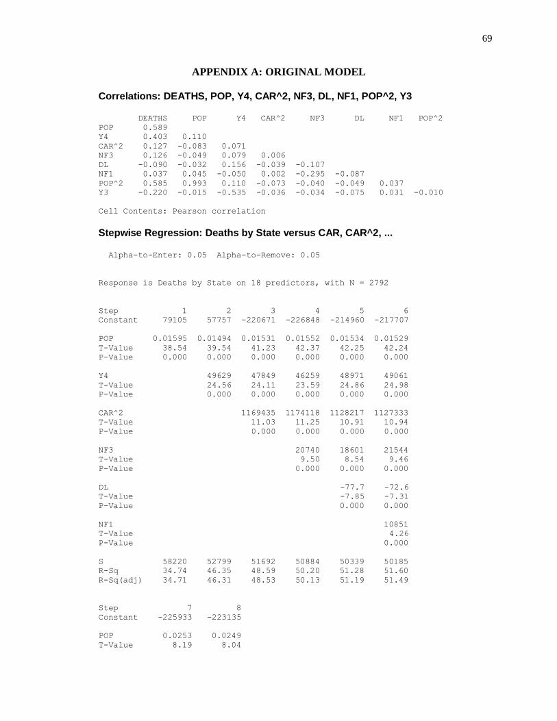
69
APPENDIX A: ORIGINAL MODEL
Correlations: DEATHS, POP, Y4, CAR^2, NF3, DL, NF1, POP^2, Y3 DEATHS POP Y4 CAR^2 NF3 DL NF1 POP^2
POP 0.589
Y4 0.403 0.110
CAR^2 0.127 -0.083 0.071
NF3 0.126 -0.049 0.079 0.006
DL -0.090 -0.032 0.156 -0.039 -0.107
NF1 0.037 0.045 -0.050 0.002 -0.295 -0.087
POP^2 0.585 0.993 0.110 -0.073 -0.040 -0.049 0.037
Y3 -0.220 -0.015 -0.535 -0.036 -0.034 -0.075 0.031 -0.010
Cell Contents: Pearson correlation
Stepwise Regression: Deaths by State versus CAR, CAR^2, ... Alpha-to-Enter: 0.05 Alpha-to-Remove: 0.05
Response is Deaths by State on 18 predictors, with N = 2792
Step 1 2 3 4 5 6
Constant 79105 57757 -220671 -226848 -214960 -217707
POP 0.01595 0.01494 0.01531 0.01552 0.01534 0.01529
T-Value 38.54 39.54 41.23 42.37 42.25 42.24
P-Value 0.000 0.000 0.000 0.000 0.000 0.000
Y4 49629 47849 46259 48971 49061
T-Value 24.56 24.11 23.59 24.86 24.98
P-Value 0.000 0.000 0.000 0.000 0.000
CAR^2 1169435 1174118 1128217 1127333
T-Value 11.03 11.25 10.91 10.94
P-Value 0.000 0.000 0.000 0.000
NF3 20740 18601 21544
T-Value 9.50 8.54 9.46
P-Value 0.000 0.000 0.000
DL -77.7 -72.6
T-Value -7.85 -7.31
P-Value 0.000 0.000
NF1 10851
T-Value 4.26
P-Value 0.000
S 58220 52799 51692 50884 50339 50185
R-Sq 34.74 46.35 48.59 50.20 51.28 51.60
R-Sq(adj) 34.71 46.31 48.53 50.13 51.19 51.49
Step 7 8
Constant -225933 -223135
POP 0.0253 0.0249
T-Value 8.19 8.04

70
P-Value 0.000 0.000
Y4 49206 46181
T-Value 25.09 19.95
P-Value 0.000 0.000
CAR^2 1154163 1154996
T-Value 11.18 11.20
P-Value 0.000 0.000
NF3 21764 21842
T-Value 9.57 9.61
P-Value 0.000 0.000
DL -77 -77
T-Value -7.71 -7.66
P-Value 0.000 0.000
NF1 10304 10382
T-Value 4.04 4.08
P-Value 0.000 0.000
POP^2 -0.00000 -0.00000
T-Value -3.27 -3.10
P-Value 0.001 0.002
Y3 -6317
T-Value -2.46
P-Value 0.014
S 50098 50052
R-Sq 51.78 51.89
R-Sq(adj) 51.66 51.75
Regression Analysis: Deaths by State versus POP, Y4, ... The regression equation is
Deaths by State = - 223135 + 0.0249 POP + 46181 Y4 + 1154996 CAR^2 + 21842 NF3
- 76.7 DL + 10382 NF1 - 0.000000 POP^2 - 6317 Y3
Predictor Coef SE Coef T P
Constant -223135 24693 -9.04 0.000
POP 0.024869 0.003095 8.04 0.000
Y4 46181 2314 19.95 0.000
CAR^2 1154996 103146 11.20 0.000
NF3 21842 2273 9.61 0.000
DL -76.69 10.01 -7.66 0.000
NF1 10382 2546 4.08 0.000
POP^2 -0.00000000 0.00000000 -3.10 0.002
Y3 -6317 2571 -2.46 0.014
S = 50052.4 R-Sq = 51.9% R-Sq(adj) = 51.7%
Analysis of Variance

71
Source DF SS MS F P
Regression 8 7.51851E+12 9.39814E+11 375.14 0.000
Residual Error 2783 6.97209E+12 2505241605
Total 2791 1.44906E+13
Source DF Seq SS
POP 1 5.03356E+12
Y4 1 1.68212E+12
CAR^2 1 3.25127E+11
NF3 1 2.33675E+11
DL 1 1.56336E+11
NF1 1 45731374434
POP^2 1 26838489011
Y3 1 15119961051
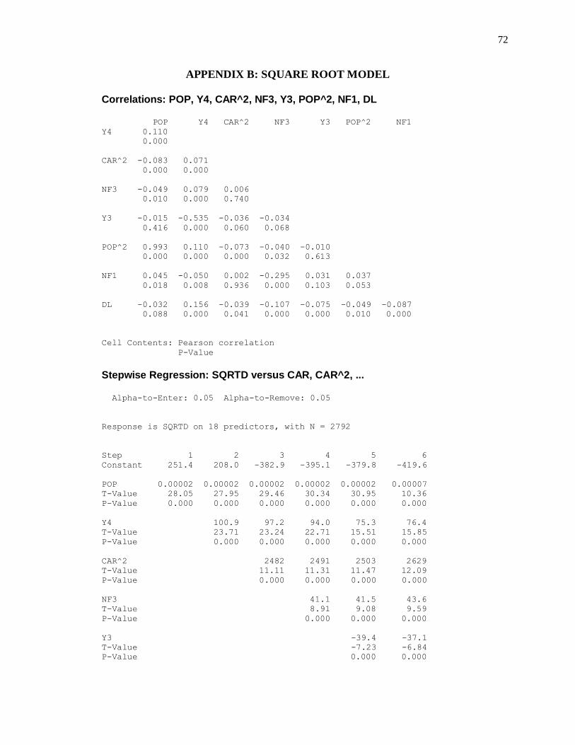
72
APPENDIX B: SQUARE ROOT MODEL
Correlations: POP, Y4, CAR^2, NF3, Y3, POP^2, NF1, DL POP Y4 CAR^2 NF3 Y3 POP^2 NF1
Y4 0.110
0.000
CAR^2 -0.083 0.071
0.000 0.000
NF3 -0.049 0.079 0.006
0.010 0.000 0.740
Y3 -0.015 -0.535 -0.036 -0.034
0.416 0.000 0.060 0.068
POP^2 0.993 0.110 -0.073 -0.040 -0.010
0.000 0.000 0.000 0.032 0.613
NF1 0.045 -0.050 0.002 -0.295 0.031 0.037
0.018 0.008 0.936 0.000 0.103 0.053
DL -0.032 0.156 -0.039 -0.107 -0.075 -0.049 -0.087
0.088 0.000 0.041 0.000 0.000 0.010 0.000
Cell Contents: Pearson correlation
P-Value
Stepwise Regression: SQRTD versus CAR, CAR^2, ... Alpha-to-Enter: 0.05 Alpha-to-Remove: 0.05
Response is SQRTD on 18 predictors, with N = 2792
Step 1 2 3 4 5 6
Constant 251.4 208.0 -382.9 -395.1 -379.8 -419.6
POP 0.00002 0.00002 0.00002 0.00002 0.00002 0.00007
T-Value 28.05 27.95 29.46 30.34 30.95 10.36
P-Value 0.000 0.000 0.000 0.000 0.000 0.000
Y4 100.9 97.2 94.0 75.3 76.4
T-Value 23.71 23.24 22.71 15.51 15.85
P-Value 0.000 0.000 0.000 0.000 0.000
CAR^2 2482 2491 2503 2629
T-Value 11.11 11.31 11.47 12.09
P-Value 0.000 0.000 0.000 0.000
NF3 41.1 41.5 43.6
T-Value 8.91 9.08 9.59
P-Value 0.000 0.000 0.000
Y3 -39.4 -37.1
T-Value -7.23 -6.84
P-Value 0.000 0.000
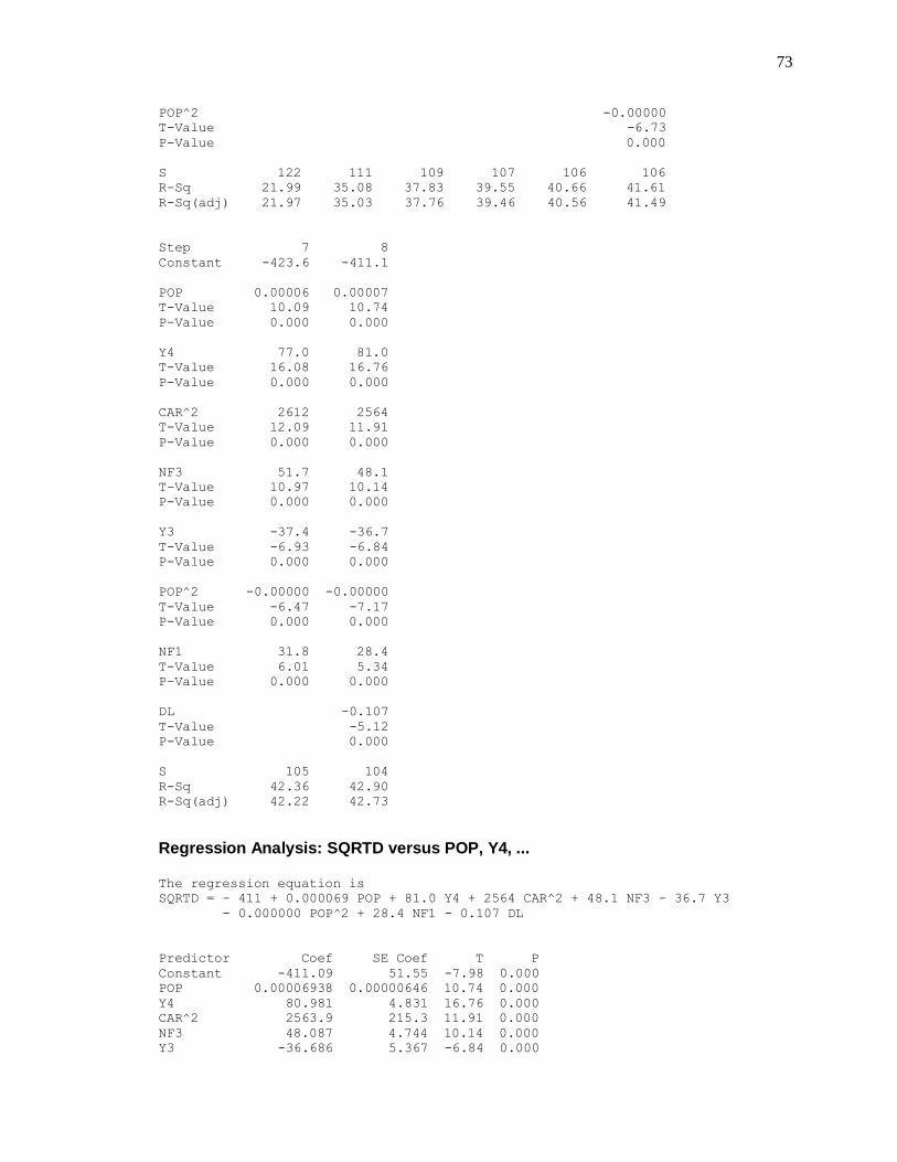
73
POP^2 -0.00000
T-Value -6.73
P-Value 0.000
S 122 111 109 107 106 106
R-Sq 21.99 35.08 37.83 39.55 40.66 41.61
R-Sq(adj) 21.97 35.03 37.76 39.46 40.56 41.49
Step 7 8
Constant -423.6 -411.1
POP 0.00006 0.00007
T-Value 10.09 10.74
P-Value 0.000 0.000
Y4 77.0 81.0
T-Value 16.08 16.76
P-Value 0.000 0.000
CAR^2 2612 2564
T-Value 12.09 11.91
P-Value 0.000 0.000
NF3 51.7 48.1
T-Value 10.97 10.14
P-Value 0.000 0.000
Y3 -37.4 -36.7
T-Value -6.93 -6.84
P-Value 0.000 0.000
POP^2 -0.00000 -0.00000
T-Value -6.47 -7.17
P-Value 0.000 0.000
NF1 31.8 28.4
T-Value 6.01 5.34
P-Value 0.000 0.000
DL -0.107
T-Value -5.12
P-Value 0.000
S 105 104
R-Sq 42.36 42.90
R-Sq(adj) 42.22 42.73
Regression Analysis: SQRTD versus POP, Y4, ... The regression equation is
SQRTD = - 411 + 0.000069 POP + 81.0 Y4 + 2564 CAR^2 + 48.1 NF3 - 36.7 Y3
- 0.000000 POP^2 + 28.4 NF1 - 0.107 DL
Predictor Coef SE Coef T P
Constant -411.09 51.55 -7.98 0.000
POP 0.00006938 0.00000646 10.74 0.000
Y4 80.981 4.831 16.76 0.000
CAR^2 2563.9 215.3 11.91 0.000
NF3 48.087 4.744 10.14 0.000
Y3 -36.686 5.367 -6.84 0.000
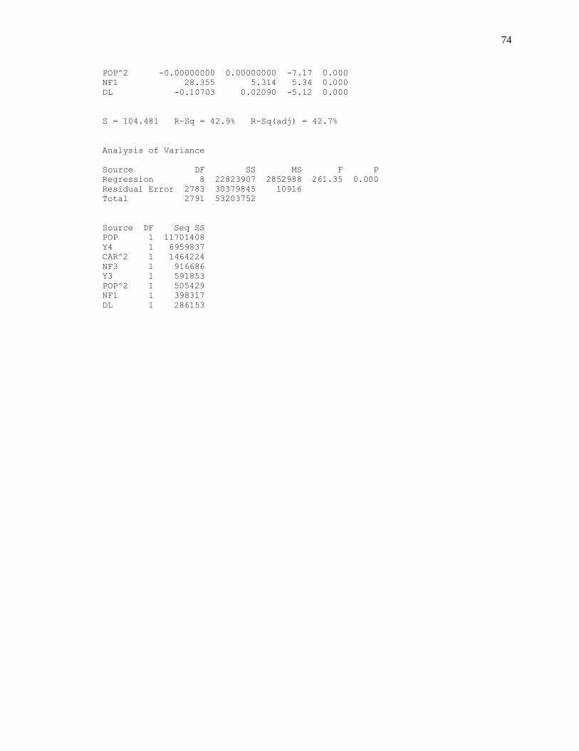
74
POP^2 -0.00000000 0.00000000 -7.17 0.000
NF1 28.355 5.314 5.34 0.000
DL -0.10703 0.02090 -5.12 0.000
S = 104.481 R-Sq = 42.9% R-Sq(adj) = 42.7%
Analysis of Variance
Source DF SS MS F P
Regression 8 22823907 2852988 261.35 0.000
Residual Error 2783 30379845 10916
Total 2791 53203752
Source DF Seq SS
POP 1 11701408
Y4 1 6959837
CAR^2 1 1464224
NF3 1 916686
Y3 1 591853
POP^2 1 505429
NF1 1 398317
DL 1 286153
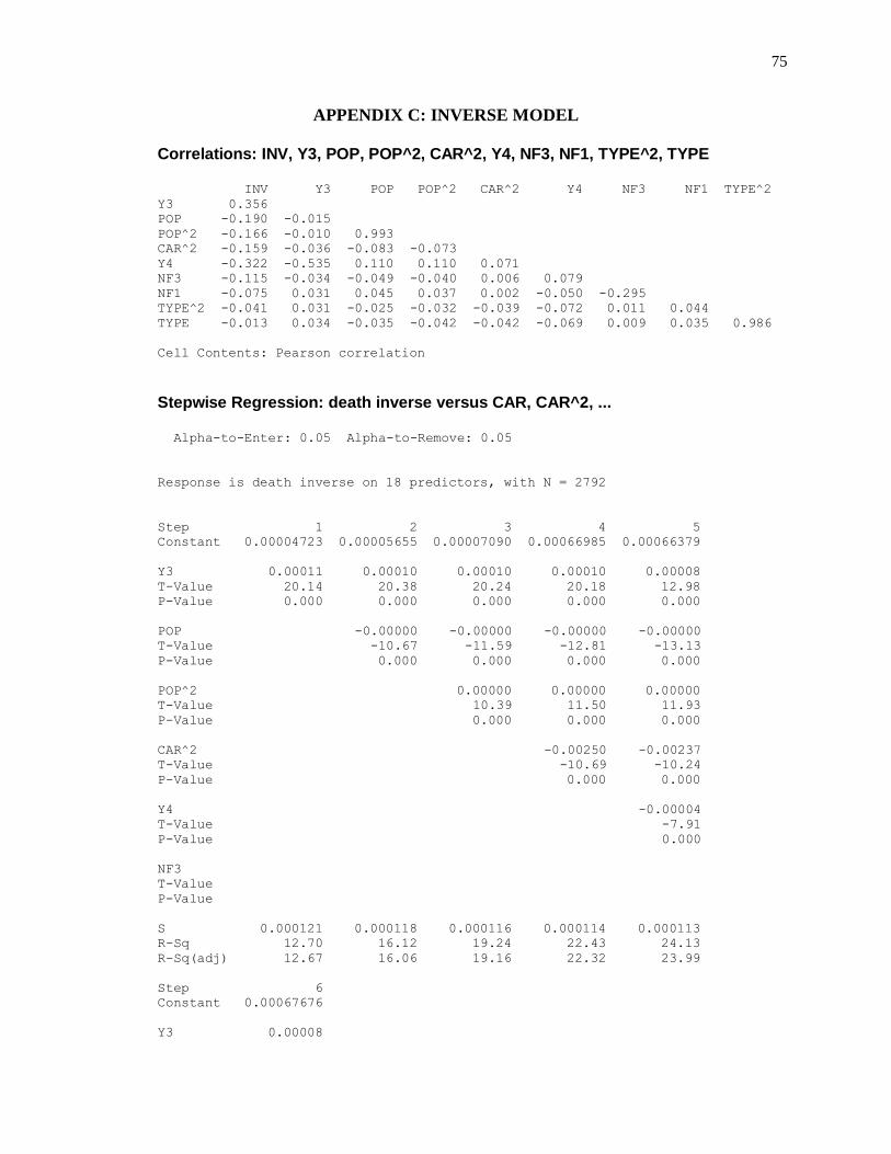
75
APPENDIX C: INVERSE MODEL
Correlations: INV, Y3, POP, POP^2, CAR^2, Y4, NF3, NF1, TYPE^2, TYPE INV Y3 POP POP^2 CAR^2 Y4 NF3 NF1 TYPE^2
Y3 0.356
POP -0.190 -0.015
POP^2 -0.166 -0.010 0.993
CAR^2 -0.159 -0.036 -0.083 -0.073
Y4 -0.322 -0.535 0.110 0.110 0.071
NF3 -0.115 -0.034 -0.049 -0.040 0.006 0.079
NF1 -0.075 0.031 0.045 0.037 0.002 -0.050 -0.295
TYPE^2 -0.041 0.031 -0.025 -0.032 -0.039 -0.072 0.011 0.044
TYPE -0.013 0.034 -0.035 -0.042 -0.042 -0.069 0.009 0.035 0.986
Cell Contents: Pearson correlation
Stepwise Regression: death inverse versus CAR, CAR^2, ... Alpha-to-Enter: 0.05 Alpha-to-Remove: 0.05
Response is death inverse on 18 predictors, with N = 2792
Step 1 2 3 4 5
Constant 0.00004723 0.00005655 0.00007090 0.00066985 0.00066379
Y3 0.00011 0.00010 0.00010 0.00010 0.00008
T-Value 20.14 20.38 20.24 20.18 12.98
P-Value 0.000 0.000 0.000 0.000 0.000
POP -0.00000 -0.00000 -0.00000 -0.00000
T-Value -10.67 -11.59 -12.81 -13.13
P-Value 0.000 0.000 0.000 0.000
POP^2 0.00000 0.00000 0.00000
T-Value 10.39 11.50 11.93
P-Value 0.000 0.000 0.000
CAR^2 -0.00250 -0.00237
T-Value -10.69 -10.24
P-Value 0.000 0.000
Y4 -0.00004
T-Value -7.91
P-Value 0.000
NF3
T-Value
P-Value
S 0.000121 0.000118 0.000116 0.000114 0.000113
R-Sq 12.70 16.12 19.24 22.43 24.13
R-Sq(adj) 12.67 16.06 19.16 22.32 23.99
Step 6
Constant 0.00067676
Y3 0.00008

76
T-Value 13.15
P-Value 0.000
POP -0.00000
T-Value -13.75
P-Value 0.000
POP^2 0.00000
T-Value 12.49
P-Value 0.000
CAR^2 -0.00239
T-Value -10.40
P-Value 0.000
Y4 -0.00004
T-Value -7.41
P-Value 0.000
NF3 -0.00003
T-Value -7.12
P-Value 0.000
S 0.000112
R-Sq 25.48
R-Sq(adj) 25.32
Step 7 8 9
Constant 0.0006814 0.0006910 0.0005390
Y3 0.00008 0.00008 0.00007
T-Value 13.31 13.32 13.10
P-Value 0.000 0.000 0.000
POP -0.00000 -0.00000 -0.00000
T-Value -13.48 -13.31 -13.79
P-Value 0.000 0.000 0.000
POP^2 0.00000 0.00000 0.00000
T-Value 12.24 12.07 12.60
P-Value 0.000 0.000 0.000
CAR^2 -0.00237 -0.00240 -0.00235
T-Value -10.40 -10.51 -10.45
P-Value 0.000 0.000 0.000
Y4 -0.00004 -0.00004 -0.00004
T-Value -7.61 -7.80 -8.32
P-Value 0.000 0.000 0.000
NF3 -0.00004 -0.00004 -0.00004
T-Value -8.78 -8.69 -8.53
P-Value 0.000 0.000 0.000
NF1 -0.00004 -0.00004 -0.00003
T-Value -6.65 -6.51 -6.11
P-Value 0.000 0.000 0.000
TYPE^2 -0.00013 -0.00239
T-Value -3.21 -9.75
P-Value 0.001 0.000

77
TYPE 0.00136
T-Value 9.34
P-Value 0.000
S 0.000111 0.000111 0.000109
R-Sq 26.65 26.92 29.14
R-Sq(adj) 26.46 26.71 28.91
Regression Analysis: death inverse versus Y3, POP, ... The regression equation is
death inverse = 0.000539 + 0.000073 Y3 - 0.000000 POP + 0.000000 POP^2
- 0.00235 CAR^2 - 0.000041 Y4 - 0.000042 NF3 - 0.000034 NF1
- 0.00239 TYPE^2 + 0.00136 TYPE
Predictor Coef SE Coef T P
Constant 0.00053902 0.00005619 9.59 0.000
Y3 0.00007339 0.00000560 13.10 0.000
POP -0.00000000 0.00000000 -13.79 0.000
POP^2 0.00000000 0.00000000 12.60 0.000
CAR^2 -0.0023466 0.0002245 -10.45 0.000
Y4 -0.00004150 0.00000499 -8.32 0.000
NF3 -0.00004177 0.00000490 -8.53 0.000
NF1 -0.00003367 0.00000551 -6.11 0.000
TYPE^2 -0.0023864 0.0002448 -9.75 0.000
TYPE 0.0013634 0.0001460 9.34 0.000
S = 0.000108973 R-Sq = 29.1% R-Sq(adj) = 28.9%
Analysis of Variance
Source DF SS MS F P
Regression 9 1.35854E-05 1.50949E-06 127.11 0.000
Residual Error 2782 3.30365E-05 1.18751E-08
Total 2791 4.66219E-05
Source DF Seq SS
Y3 1 5.91999E-06
POP 1 1.59554E-06
POP^2 1 1.45656E-06
CAR^2 1 1.48353E-06
Y4 1 7.93441E-07
NF3 1 6.31737E-07
NF1 1 5.43095E-07
TYPE^2 1 1.26449E-07
TYPE 1 1.03507E-06
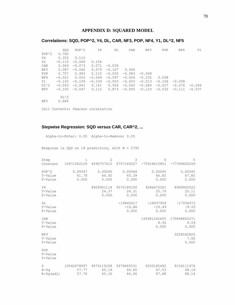
78
APPENDIX D: SQUARED MODEL
Correlations: SQD, POP^2, Y4, DL, CAR, NF3, POP, NF4, Y1, DL^2, NF5 SQD POP^2 Y4 DL CAR NF3 POP NF4 Y1
POP^2 0.760
Y4 0.355 0.110
DL -0.110 -0.049 0.156
CAR 0.069 -0.073 0.071 -0.039
NF3 0.087 -0.040 0.079 -0.107 0.006
POP 0.757 0.993 0.110 -0.032 -0.083 -0.049
NF4 -0.021 0.052 -0.049 -0.097 -0.026 -0.332 0.058
Y1 -0.193 -0.109 -0.339 -0.053 -0.003 -0.013 -0.106 -0.008
DL^2 -0.093 -0.041 0.141 0.936 -0.042 -0.084 -0.027 -0.076 -0.048
NF5 -0.105 -0.047 0.112 0.873 -0.005 -0.123 -0.032 -0.111 -0.037
DL^2
NF5 0.684
Cell Contents: Pearson correlation
Stepwise Regression: SQD versus CAR, CAR^2, ... Alpha-to-Enter: 0.05 Alpha-to-Remove: 0.05
Response is SQD on 18 predictors, with N = 2792
Step 1 2 3 4 5
Constant 10471562129 6595757612 6707166527 -75918615851 -77399605269
POP^2 0.00047 0.00045 0.00044 0.00045 0.00045
T-Value 61.78 64.92 65.39 66.82 67.85
P-Value 0.000 0.000 0.000 0.000 0.000
Y4 8929901114 9570180100 9286672261 8999905522
T-Value 24.37 26.31 25.79 25.11
P-Value 0.000 0.000 0.000 0.000
DL -19845417 -18937928 -17206972
T-Value -10.86 -10.49 -9.55
P-Value 0.000 0.000 0.000
CAR 169381242605 170898805271
T-Value 8.92 9.09
P-Value 0.000 0.000
NF3 3028562820
T-Value 7.65
P-Value 0.000
POP
T-Value
P-Value
S 10542678997 9574115208 9379665531 9250165492 9156111976
R-Sq 57.77 65.19 66.60 67.53 68.19
R-Sq(adj) 57.76 65.16 66.56 67.48 68.14

79
Step 6
Constant -81724138479
POP^2 0.00019
T-Value 3.40
P-Value 0.001
Y4 9012857803
T-Value 25.23
P-Value 0.000
DL -18264011
T-Value -10.09
P-Value 0.000
CAR 178666746643
T-Value 9.50
P-Value 0.000
NF3 3136368082
T-Value 7.94
P-Value 0.000
POP 2587
T-Value 4.60
P-Value 0.000
S 9123092275
R-Sq 68.43
R-Sq(adj) 68.37
Step 7 8 9 10
Constant -80746469384 -80837467494 -81091262538 -79383922794
POP^2 0.00019 0.00018 0.00018 0.00017
T-Value 3.27 3.19 3.10 3.06
P-Value 0.001 0.001 0.002 0.002
Y4 9010516029 8701347031 8714384758 8795700809
T-Value 25.26 23.08 23.13 23.27
P-Value 0.000 0.000 0.000 0.000
DL -18993623 -19035383 -29520169 -55598863
T-Value -10.40 -10.43 -5.83 -4.61
P-Value 0.000 0.000 0.000 0.000
CAR 177449647168 178292669666 178927506462 175296315752
T-Value 9.45 9.50 9.54 9.32
P-Value 0.000 0.000 0.000 0.000
NF3 2738405044 2743019429 2681422850 2723800926
T-Value 6.53 6.54 6.39 6.49
P-Value 0.000 0.000 0.000 0.000
POP 2665 2699 2750 2771
T-Value 4.74 4.81 4.90 4.94
P-Value 0.000 0.000 0.000 0.000
NF4 -1223448714 -1246906213 -1309623572 -1261164266
T-Value -2.79 -2.84 -2.98 -2.87
P-Value 0.005 0.005 0.003 0.004
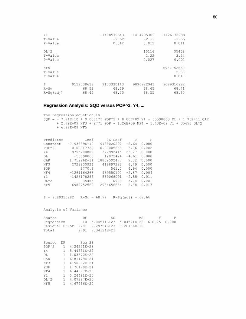
80
Y1 -1408579643 -1414705309 -1426178288
T-Value -2.52 -2.53 -2.55
P-Value 0.012 0.012 0.011
DL^2 15116 35458
T-Value 2.22 3.24
P-Value 0.027 0.001
NF5 6982752560
T-Value 2.38
P-Value 0.017
S 9112038618 9103330143 9096922941 9089310982
R-Sq 68.52 68.59 68.65 68.71
R-Sq(adj) 68.44 68.50 68.55 68.60
Regression Analysis: SQD versus POP^2, Y4, ... The regression equation is
SQD = - 7.94E+10 + 0.000173 POP^2 + 8.80E+09 Y4 - 55598863 DL + 1.75E+11 CAR
+ 2.72E+09 NF3 + 2771 POP - 1.26E+09 NF4 - 1.43E+09 Y1 + 35458 DL^2
+ 6.98E+09 NF5
Predictor Coef SE Coef T P
Constant -7.93839E+10 9188020292 -8.64 0.000
POP^2 0.00017329 0.00005668 3.06 0.002
Y4 8795700809 377992445 23.27 0.000
DL -55598863 12072424 -4.61 0.000
CAR 1.75296E+11 18802592477 9.32 0.000
NF3 2723800926 419897223 6.49 0.000
POP 2770.9 561.0 4.94 0.000
NF4 -1261164266 439550190 -2.87 0.004
Y1 -1426178288 559068091 -2.55 0.011
DL^2 35458 10929 3.24 0.001
NF5 6982752560 2934656634 2.38 0.017
S = 9089310982 R-Sq = 68.7% R-Sq(adj) = 68.6%
Analysis of Variance
Source DF SS MS F P
Regression 10 5.04571E+23 5.04571E+22 610.75 0.000
Residual Error 2781 2.29754E+23 8.26156E+19
Total 2791 7.34324E+23
Source DF Seq SS
POP^2 1 4.24221E+23
Y4 1 5.44531E+22
DL 1 1.03670E+22
CAR 1 6.81179E+21
NF3 1 4.90862E+21
POP 1 1.76479E+21
NF4 1 6.44387E+20
Y1 1 5.24491E+20
DL^2 1 4.07287E+20
NF5 1 4.67736E+20

81
APPENDIX E: NATURAL LOG MODEL
Correlations: NLOG, Y4, POP, Y3, CAR, POP^2, NF3, NF1, TYPE^2, TYPE, NF5, Y1 NLOG Y4 POP Y3 CAR POP^2 NF3 NF1 TYPE^2
Y4 0.388
POP 0.334 0.110
Y3 -0.347 -0.535 -0.015
CAR 0.169 0.071 -0.083 -0.036
POP^2 0.315 0.110 0.993 -0.010 -0.073
NF3 0.135 0.079 -0.049 -0.034 0.006 -0.040
NF1 0.067 -0.050 0.045 0.031 0.002 0.037 -0.295
TYPE^2 0.015 -0.072 -0.025 0.031 -0.039 -0.032 0.011 0.044
TYPE -0.010 -0.069 -0.035 0.034 -0.042 -0.042 0.009 0.035 0.986
NF5 -0.019 0.112 -0.032 -0.044 -0.005 -0.047 -0.123 -0.099 -0.054
Y1 -0.033 -0.339 -0.106 -0.221 -0.003 -0.109 -0.013 0.076 0.018
TYPE NF5
NF5 -0.051
Y1 0.018 -0.037
Cell Contents: Pearson correlation
Stepwise Regression: NLOG versus CAR, CAR^2, ... Alpha-to-Enter: 0.05 Alpha-to-Remove: 0.05
Response is NLOG on 18 predictors, with N = 2792
Step 1 2 3 4 5 6
Constant 10.303 10.180 10.516 -2.876 -4.074 -4.307
Y4 1.160 1.063 0.720 0.675 0.697 0.660
T-Value 22.26 21.39 12.48 11.92 12.51 11.97
P-Value 0.000 0.000 0.000 0.000 0.000 0.000
POP 0.00000 0.00000 0.00000 0.00000 0.00000
T-Value 17.74 18.68 19.97 12.22 13.02
P-Value 0.000 0.000 0.000 0.000 0.000
Y3 -0.725 -0.730 -0.689 -0.694
T-Value -11.12 -11.43 -10.96 -11.18
P-Value 0.000 0.000 0.000 0.000
CAR 27.5 29.6 29.8
T-Value 10.74 11.73 11.99
P-Value 0.000 0.000 0.000
POP^2 -0.00000 -0.00000
T-Value -9.90 -10.62
P-Value 0.000 0.000
NF3 0.460
T-Value 8.85
P-Value 0.000
S 1.37 1.30 1.27 1.25 1.22 1.21

82
R-Sq 15.09 23.70 26.94 29.85 32.23 34.08
R-Sq(adj) 15.05 23.64 26.86 29.74 32.11 33.94
Step 7 8 9 10 11
Constant -4.305 -4.427 -2.861 -2.832 -2.838
Y4 0.668 0.676 0.695 0.709 0.784
T-Value 12.21 12.34 12.84 13.01 12.03
P-Value 0.000 0.000 0.000 0.000 0.000
POP 0.00000 0.00000 0.00000 0.00000 0.00000
T-Value 12.75 12.61 13.00 13.18 13.22
P-Value 0.000 0.000 0.000 0.000 0.000
Y3 -0.698 -0.697 -0.675 -0.671 -0.596
T-Value -11.34 -11.33 -11.10 -11.03 -8.45
P-Value 0.000 0.000 0.000 0.000 0.000
CAR 29.6 29.8 29.3 29.3 29.2
T-Value 12.00 12.08 12.03 12.02 11.98
P-Value 0.000 0.000 0.000 0.000 0.000
POP^2 -0.00000 -0.00000 -0.00000 -0.00000 -0.00000
T-Value -10.35 -10.21 -10.64 -10.84 -10.87
P-Value 0.000 0.000 0.000 0.000 0.000
NF3 0.566 0.562 0.548 0.529 0.524
T-Value 10.51 10.44 10.31 9.83 9.72
P-Value 0.000 0.000 0.000 0.000 0.000
NF1 0.413 0.407 0.381 0.363 0.351
T-Value 6.83 6.73 6.37 6.00 5.78
P-Value 0.000 0.000 0.000 0.000 0.000
TYPE^2 1.05 22.58 22.56 22.75
T-Value 2.38 8.49 8.49 8.56
P-Value 0.018 0.000 0.000 0.000
TYPE -13.0 -13.0 -13.1
T-Value -8.21 -8.22 -8.29
P-Value 0.000 0.000 0.000
NF5 -0.25 -0.26
T-Value -2.11 -2.17
P-Value 0.035 0.030
Y1 0.177
T-Value 2.09
P-Value 0.037
S 1.20 1.20 1.18 1.18 1.18
R-Sq 35.17 35.30 36.83 36.93 37.03
R-Sq(adj) 35.01 35.12 36.63 36.71 36.78
Regression Analysis: NLOG versus Y4, POP, ... The regression equation is
NLOG = - 2.84 + 0.784 Y4 + 0.000001 POP - 0.596 Y3 + 29.2 CAR - 0.000000 POP^2
+ 0.524 NF3 + 0.351 NF1 + 22.8 TYPE^2 - 13.1 TYPE - 0.259 NF5 + 0.177 Y1
Predictor Coef SE Coef T P
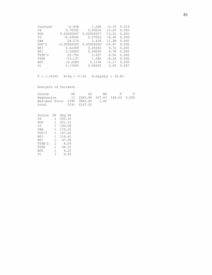
83
Constant -2.838 1.206 -2.35 0.019
Y4 0.78392 0.06518 12.03 0.000
POP 0.00000097 0.00000007 13.22 0.000
Y3 -0.59596 0.07053 -8.45 0.000
CAR 29.174 2.436 11.98 0.000
POP^2 -0.00000000 0.00000000 -10.87 0.000
NF3 0.52389 0.05392 9.72 0.000
NF1 0.35083 0.06065 5.78 0.000
TYPE^2 22.750 2.657 8.56 0.000
TYPE -13.137 1.585 -8.29 0.000
NF5 -0.2589 0.1194 -2.17 0.030
Y1 0.17655 0.08455 2.09 0.037
S = 1.18192 R-Sq = 37.0% R-Sq(adj) = 36.8%
Analysis of Variance
Source DF SS MS F P
Regression 11 2283.90 207.63 148.63 0.000
Residual Error 2780 3883.45 1.40
Total 2791 6167.35
Source DF Seq SS
Y4 1 930.35
POP 1 531.15
Y3 1 199.96
CAR 1 179.22
POP^2 1 147.00
NF3 1 114.41
NF1 1 67.09
TYPE^2 1 8.09
TYPE 1 94.31
NF5 1 6.23
Y1 1 6.09

84
APPENDIX F: CUBIC MODEL
Correlations: CUBE, POP^2, Y4, DL, CAR, NF3, Y3, POP, NF4, DL^2, Y5, NF5 CUBE POP^2 Y4 DL CAR NF3 Y3 POP NF4
POP^2 0.857
Y4 0.298 0.110
DL -0.100 -0.049 0.156
CAR 0.021 -0.073 0.071 -0.039
NF3 0.048 -0.040 0.079 -0.107 0.006
Y3 -0.091 -0.010 -0.535 -0.075 -0.036 -0.034
POP 0.852 0.993 0.110 -0.032 -0.083 -0.049 -0.015
NF4 0.003 0.052 -0.049 -0.097 -0.026 -0.332 0.028 0.058
DL^2 -0.084 -0.041 0.141 0.936 -0.042 -0.084 -0.074 -0.027 -0.076
Y5 -0.049 0.017 -0.304 -0.059 -0.048 -0.062 -0.198 0.025 0.058
NF5 -0.096 -0.047 0.112 0.873 -0.005 -0.123 -0.044 -0.032 -0.111
DL^2 Y5
Y5 -0.047
NF5 0.684 -0.062
Cell Contents: Pearson correlation
Stepwise Regression: cube versus CAR, CAR^2, ... Alpha-to-Enter: 0.05 Alpha-to-Remove: 0.05
Response is cube on 18 predictors, with N = 2792
Step 1 2 3
Constant 1496030715970441 832569683144713 852311676915360
POP^2 120.1 116.9 116.1
T-Value 87.96 92.74 93.63
P-Value 0.000 0.000 0.000
Y4 1528622351720234 1642081707290097
T-Value 22.90 24.74
P-Value 0.000 0.000
DL -3516667396001
T-Value -10.54
P-Value 0.000
CAR
T-Value
P-Value
NF3
T-Value
P-Value
Y3
T-Value
P-Value
S 1901230228602616 1744666117751950 1711195323908276

85
R-Sq 73.49 77.69 78.54
R-Sq(adj) 73.49 77.67 78.52
Step 4 5 6
Constant -11330067541113566 -11559046834509920 -11653935121384388
POP^2 116.8 117.3 117.0
T-Value 94.74 95.64 95.46
P-Value 0.000 0.000 0.000
Y4 1600281195272768 1555943508224480 1712450744967065
T-Value 24.24 23.61 22.07
P-Value 0.000 0.000 0.000
DL -3382866892333 -3115239538563 -3135371304059
T-Value -10.22 -9.40 -9.48
P-Value 0.000 0.000 0.000
CAR 24973639830427104 25208273800645388 25092734523320136
T-Value 7.18 7.29 7.28
P-Value 0.000 0.000 0.000
NF3 468253294827734 464317583720509
T-Value 6.43 6.39
P-Value 0.000 0.000
Y3 327007245969501
T-Value 3.80
P-Value 0.000
S 1695909173520878 1683752464906696 1679712630993364
R-Sq 78.93 79.24 79.35
R-Sq(adj) 78.90 79.20 79.30
Step 7 8 9
Constant -12267727787273260 -12113076560122540 -12162341126628398
POP^2 80 79 78
T-Value 7.70 7.59 7.49
P-Value 0.000 0.000 0.000
Y4 1723028032353843 1723474267192902 1728466424645180
T-Value 22.23 22.26 22.33
P-Value 0.000 0.000 0.000
DL -3285228458748 -3401321387405 -5359402261295
T-Value -9.88 -10.13 -5.75
P-Value 0.000 0.000 0.000
CAR 26179261880830332 25985629978481532 26102787791976052
T-Value 7.58 7.53 7.57
P-Value 0.000 0.000 0.000
NF3 479266195900822 416013475625838 404453264279892
T-Value 6.60 5.39 5.24
P-Value 0.000 0.000 0.000
Y3 345299651049937 347008218089076 351824546130151
T-Value 4.01 4.03 4.09
P-Value 0.000 0.000 0.000
POP 363944003 376504341 386367242
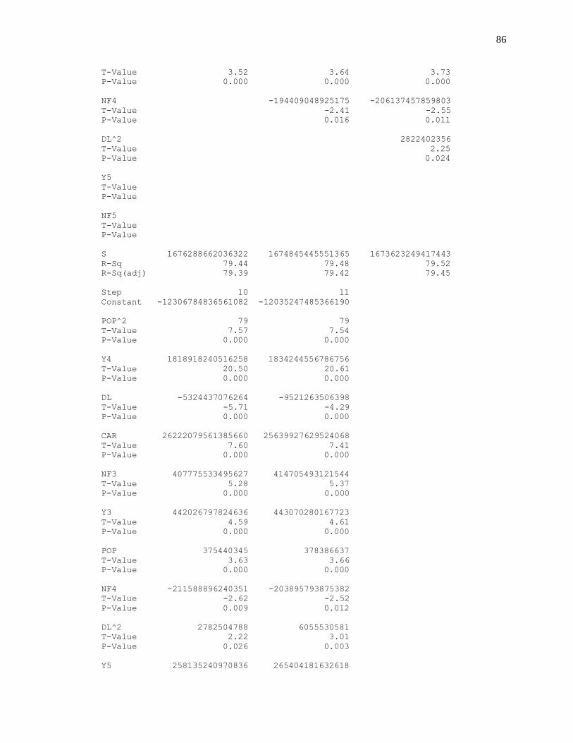
86
T-Value 3.52 3.64 3.73
P-Value 0.000 0.000 0.000
NF4 -194409048925175 -206137457859803
T-Value -2.41 -2.55
P-Value 0.016 0.011
DL^2 2822402356
T-Value 2.25
P-Value 0.024
Y5
T-Value
P-Value
NF5
T-Value
P-Value
S 1676288662036322 1674845445551365 1673623249417443
R-Sq 79.44 79.48 79.52
R-Sq(adj) 79.39 79.42 79.45
Step 10 11
Constant -12306784836561082 -12035247485366190
POP^2 79 79
T-Value 7.57 7.54
P-Value 0.000 0.000
Y4 1818918240516258 1834244556786756
T-Value 20.50 20.61
P-Value 0.000 0.000
DL -5324437076264 -9521263506398
T-Value -5.71 -4.29
P-Value 0.000 0.000
CAR 26222079561385660 25639927629524068
T-Value 7.60 7.41
P-Value 0.000 0.000
NF3 407775533495627 414705493121544
T-Value 5.28 5.37
P-Value 0.000 0.000
Y3 442026797824636 443070280167723
T-Value 4.59 4.61
P-Value 0.000 0.000
POP 375440345 378386637
T-Value 3.63 3.66
P-Value 0.000 0.000
NF4 -211588896240351 -203895793875382
T-Value -2.62 -2.52
P-Value 0.009 0.012
DL^2 2782504788 6055530581
T-Value 2.22 3.01
P-Value 0.026 0.003
Y5 258135240970836 265404181632618

87
T-Value 2.08 2.14
P-Value 0.038 0.032
NF5 1124167750780872
T-Value 2.08
P-Value 0.037
S 1672622350863856 1671620331729146
R-Sq 79.55 79.58
R-Sq(adj) 79.48 79.50
Regression Analysis: cube versus POP^2, Y4, ... The regression equation is
cube = - 1.20E+16 + 78.8 POP^2 + 1.83E+15 Y4 - 9.52E+12 DL + 2.56E+16 CAR
+ 4.15E+14 NF3 + 4.43E+14 Y3 + 3.78E+08 POP - 2.04E+14 NF4
+ 6.06E+09 DL^2 + 2.65E+14 Y5 + 1.12E+15 NF5
Predictor Coef SE Coef T P
Constant -1.20352E+16 1.69143E+15 -7.12 0.000
POP^2 78.80 10.45 7.54 0.000
Y4 1.83424E+15 8.89953E+13 20.61 0.000
DL -9.52126E+12 2.22051E+12 -4.29 0.000
CAR 2.56399E+16 3.45785E+15 7.41 0.000
NF3 4.14705E+14 7.72497E+13 5.37 0.000
Y3 4.43070E+14 9.62009E+13 4.61 0.000
POP 378386637 103478598 3.66 0.000
NF4 -2.03896E+14 8.08632E+13 -2.52 0.012
DL^2 6055530581 2010020947 3.01 0.003
Y5 2.65404E+14 1.24020E+14 2.14 0.032
NF5 1.12417E+15 5.39927E+14 2.08 0.037
S = 1.671620E+15 R-Sq = 79.6% R-Sq(adj) = 79.5%
Analysis of Variance
Source DF SS MS F P
Regression 11 3.02805E+34 2.75277E+33 985.13 0.000
Residual Error 2780 7.76819E+33 2.79431E+30
Total 2791 3.80487E+34
Source DF Seq SS
POP^2 1 2.79637E+34
Y4 1 1.59562E+33
DL 1 3.25533E+32
CAR 1 1.48079E+32
NF3 1 1.17340E+32
Y3 1 4.06772E+31
POP 1 3.48119E+31
NF4 1 1.62697E+31
DL^2 1 1.41904E+31
Y5 1 1.21153E+31
NF5 1 1.21134E+31