statistical characterization of interfacial waves in
TRANSCRIPT

Statistical characterization of interfacial waves in
turbulent stratified gas-liquid pipe flows
A.A. Ayatia, J.N.E. Carneirob
aDepartment of Mathematics, University of Oslo, N-0316 Oslo, NorwaybInstituto SINTEF do Brasil, 22290-160, Rio de Janeiro, RJ, Brazil
Abstract
This study presents a statistical analysis of interfacial waves in a turbu-lent stratified air-water flow inside a 10 cm diameter pipe. Wave elevationmeasurements were acquired using conductance probes with high samplingrate, Sr = 500Hz. Local wave parameters (elevation, crest height, troughheight, etc.) were extracted using a zero-crossing technique. The evolutionof their corresponding statistical distributions and statistical moments wasinvestigated for varying flow conditions.
The main goal of this study is to offer an alternative method for dis-tinguishing between various wavy flow patterns. The proposed approach isbased on the Gaussian model, which is widely used in the characterizationof ocean waves. Instead of the traditional sub-regime categorization whichis based on a combination of visual observations and qualitative spectraldescription, this method categorizes a wave field depending on its degreeof non-linearity and statistics of elevation parameters. This approach alsoallows parametrization of the interfacial structure. As a first step, this ap-proach was carried out only for a selected set of flow rate combinations, inwhich the liquid superficial velocity was kept constant at Usl = 0.10 m/swhilst the superficial velocity was increased from 1.0 m/s to 4.0 m/s withincrements of 0.25 m/s. Subsequently, statistical moments of the interfaceelevation were computed and compared to literature data, for varying Usland Usg. Based on the detailed statistical description of wave data, twoflow regimes are categorized: wave amplitude growth and saturation. Theseregimes were also identified as quasi-Gaussian and non-Gaussian, respec-
Email addresses: [email protected] (A.A. Ayati),[email protected] (J.N.E. Carneiro)
Preprint submitted to Int. Journal of Multiphase Flow February 15, 2018

tively, based on comparisons of exceedence distributions. For Usl = 0.10m/s, the saturation regime occurs for Froude numbers (based on the rela-tive bulk velocity) Fr > 4. Finally, analysis of data for various Usl and Usgsuggests that the critical Froude number for the transition to the saturationregime decreases with increasing liquid flow rate, and that the ratio of modeheight to mean liquid height is nearly constant (H ' 0.2hL) in this regime,i.e. depth limited mode.
Keywords: Gas-liquid flow; pipe flow; interfacial waves; Gaussian wavemodel.
1. Introduction
Gas-liquid flow in pipes is relevant to a variety of industrial applications,ranging from nuclear and petroleum industries to waste water mains (Lake-hal et al., 2003; Pothof & Clemens, 2011; Bratland, 2010). The flow insidepipelines that transport natural gas often consists of both a gaseous and aliquid phase, in the form of gas-water or gas-condensate combination, seeMokhatab & Poe (2012) for an overview of gas-liquid pipe flow in the natu-ral gas industry. In general, both phases flow co-currently and the gaseousphase flows significantly faster than the liquid phase. Under a wide range ofconditions, stratified flow is the predominant flow regime in horizontal andnear-horizontal pipelines.
At low flow rates, the interface is usually kept smooth by the action ofgravity and surface tension. As inertial forces increase with increasing gasflow rate, shear-waves appear on the interface. Within a range of gas flowrates, below the threshold of onsetting intermittent flow, the waves may growand interact both linearly and non-linearly with each other. It is widelyknown that waves at the interface significantly enhance the drag betweenthe phases, see Andritsos & Hanratty (1987); Biberg (2007); Berthelsen &Ytrehus (2005). This has an important impact on the overall pressure dropand liquid hold-up of the system, which are key parameters in the design ofpipelines and supporting infrastructure.
Under constant flow rate conditions and at sufficient distance from thepipe inlet, the wavy interface reaches a stationary state in which energy in-put from the gas flow and energy dissipation due to non-linear processessuch as wave breaking or interaction with the turbulent base flow, reachesan equilibrium. This state is often referred to as fully developed stratified
2

wavy flow. Depending on the characteristics of the waves, this regime may befurther divided into a range of sub-regimes. In laboratory studies, such sub-division has traditionally been based on a combination of visual observationand qualitative spectral analysis (Ayati et al., 2015; Espedal, 1998; Strand,1993). Meanwhile, mathematical models yielding sub-regime transition cri-teria have mainly been based on linear stability analysis, see for instanceTzotzi & Andritsos (2013) for a review. Tzotzi & Andritsos (2013) listed thefollowing stratified flow sub-regimes: i) smooth interface, occurring at verylow gas and liquid velocities. ii) Small amplitude regular 2D waves. Transi-tion to this sub-regime is predicted using the sheltering model proposed byJeffreys (1925). ii) Large amplitude irregular 3D waves, also called Kelvin-Helmholtz waves, as their onset is modelled by a viscous Kelvin-Helmholtzcriteria.
The state of affairs in describing interfacial waves in pipes is rather poorwhen compared to advances in ocean waves. The reason for this is two-fold:i) Like in the ocean, interfacial waves in pipes are most of the time within thenon-linear regime, exhibiting more or less random behaviour. This impliesthat any deterministic attempt to describe them accurately is very com-plicated. ii) Industrial flow simulators such as OLGA (Bendiksen et al.,1991) cannot afford to resolve waves in their attempt to simulate multiphaseflow inside very long pipes due to enormous computational costs required toperform such simulations. Thus, the engineering motivation has not beenquite high enough for such detailed studies of interfacial waves in two-phasepipe flows. Their presence is usually taken into account through augmen-tation of friction forces, which must often be adjusted to match real data.Nevertheless, the next generation of flow simulators are expected to include”regime-capturing” approaches which rely on finer grid resolution (Issa &Kempf, 2003; Carneiro et al., 2011; Danielson et al., 2012; Nieckele et al.,2011; Nieckele & Carneiro, 2017). Furthermore, recent developments in ex-perimental investigation of this system (Birvalski et al., 2014, 2015, 2016;Ayati et al., 2014, 2015, 2016, 2017; Andre & Bardet, 2017), have shownthat the overall bulkflow is strongly coupled with wavy interface. To thisend, detailed description of measured interfacial waves is expected to be ofvaluable use with respect to validation of models and CFD simulations. Forthese reasons, one of the goals of this study is to provide distributions ofwave parameters for validation measures.
By contemplating literature on ocean waves, one may find a number ofalternative methods to characterize waves on the sea surface, one of which is
3

the application of statistical tools in the assessment of extreme wave events,i.e. so-called rogue waves, see for instance Sobey (1992); Onorato et al. (2009,2013); Petrova & Soares (2014). In this approach, the seemingly random seasurface elevation is modelled, to the leading order (linear theory), as a su-perposition of independent planar waves, i.e. Fourier components, wherethe wave phases are uniformly distributed between 0 and 2π. The surfaceelevation is then considered as a stochastic process which obeys Gaussianstatistics. Deviations from Gaussian statistics, quantified by higher orderstatistical moments, i.e. skewness and kurtosis, are often attributed to non-linearity. For second order non-linearity (2nd order Stokes waves), Tayfun(1980) derived an analytical expression for the distribution of the wave en-velope, i.e. the so-called Tayfun distribution.
In ongoing work, we aim to transfer methodologies found in air-sea lit-erature to gas-liquid flow in pipes. This approach is in line with the shortnote published by Prosperetti (2003). In this particular study, the Gaussianmodel will be used to distinguish between linear and non-linear wave regimesin a system with waves that are purely shear-induced. However, it should benoted that no further assessment of non-linear interactions will be addressedhere as this is viewed to be outside the scope of this paper. Such analysis isintended to feature in future publications.
This manuscript is structured as follows; i) first, we introduce the exper-imental setup and methodology, ii) secondly, we provide a brief summary ofthe Gaussian wave model, iii) the main results are then presented in terms ofprobability distributions of wave parameters. Here, exceedence probabilityplots are used to illustrate the departure from linear theory. iv) Higher orderstatistical moments are compared with additional data from the literatureand wave regimes are categorized v) Finally, concluding remarks are given.
2. Experimental set-up and methodology
The data under investigation was acquired during an experimental cam-paign conducted at the Hydrodynamic Laboratory at the University of Oslo.The experimental techniques PIV, conductance probing and hot-wire anemom-etry were combined to study of air-water flow in pipes (Ayati et al., 2014,2015, 2016). In this paper, we will only focus on the data stemming from thewave gauge, i.e. conductance probes.
The experiments were conducted in a 31 m long horizontal acrylic pipewith internal diameter D = 10cm. Air and water at atmospheric pressure
4

were used as test-fluids. Both fluids were introduced at the pipe inlet usingfrequency-regulated pump and fan, for the water and gas, respectively. Thewater and air mass flow rates were measured with an Endress Hauser Promassand an Emerson MicroMotion Coriolis flow meter with 0.2% and 0.05% ofmaximal measured values in accuracy, respectively. A schematic view of thepipe-loop is shown in Fig. 1.
An interface elevation measurement gauge was placed approximately 270Ddownstream from the pipe inlet. The gauge consisted of two double-wireprobes made of platina wires of 0.3mm diameter and separated by 4 mm.Both probes were placed in the center of the pipe with a distance d = 6cmin the stream-wise direction, allowing to extract wave speeds through cross-correlation methods. Interface elevation, ηi(t), with the subscript i depictingeach probe, was measured with a relatively high temporal resolution of 500Hz.For more details about the experimental setup and methodology, the readeris referred to Ayati et al. (2015) as well as appendix A.
2.1. Zero-crossing analysis
The wave parameters of interest in this study are; wave elevation (η),crest height (ηc), trough height (ηt), wave height (H) and the hilbert up-per envelope Aup. Local values of each parameters were computed for eachwave cycle, wn, by means of the zero-crossing method, as illustrated in Fig.2. First, the mean elevation was subtracted from the raw signal given byeach probe η′i(t) = ηi(t) − ηi. A zero-down-crossing is then defined as thelocation at which the signal changes sign from positive to negative. Wavecrests and troughs are defined as the global maxima and minima in between
Figure 1: Schematic view of the experimental setup in use.
5

t, [s]0 0.2 0.4 0.6 0.8 1 1.2 1.4 1.6 1.8
η, [m
m]
-5
-4
-3
-2
-1
0
1
2
3
4
d2d wave
Crest height
Trough heightWave height
Wave period
Trough period
Crest period
Figure 2: Zero crossing method with a full wave cycle defined as the region between twoconsecutive zero-down-crossings (large cirles).
two subsequent zero down-crossings, respectively. Thus, for the probabil-ity analysis (section 3.2), local elevation parameters correspond to globalmaxima/minima. However, for the purpose of the qualitative analysis (sec-tion 3.1), one may define an irregularity factor α as the ratio between thenumber of zero-crossings (Nzc) and total number of maxima and minima(Nmax +Nmin):
α =Nzc
Nmax +Nmin
(1)
For a time series that is long enough, one should expect α → 1 for aregular wave filed and 0 < α < 1 if the waves are irregular. Thus, α is a wayof quantifying the degree of irregularity displayed by the waves.
2.2. Gaussian wave model
In the linear approximation of random water waves, the surface elevationη(x, t) can be written as a superposition of Fourier modes,
η(x, t) =N∑n=1
an cos(knx− ωnt+ φn) (2)
6

where an, kn, ωn and φn represent the amplitude, wave number, angularfrequency and phase, respectively, for a given mode n. The phases φn, areassumed to be independent, stochastic variables uniformly distributed within[0, 2π). Thus, as a result of the central limit theorem, the surface elevationmay be regarded as a stochastic process, which has a Gaussian distribution:
p(η) =1√
2πσ2exp
[−(η − µ)2
2σ2
], (3)
where µ and σ are the mean and standard deviation of η. Longuet-Higgins(1952) showed that in this approximation, the probability distribution of thewave envelope A(t) is Rayleigh distributed. This can easily be shown bywriting η(t) as a modulated signal (see also Onorato et al. (2013)):
η(t) = A(t) cos[θ(t)
]. (4)
The analytic signal of the wave elevation is then defined as
ζ[η(t)
]= η(t) + iη(t) (5)
where,η(t) = A(t) sin
[θ(t)
], (6)
is the Hilbert transform of η(t). Thus, the envelope is given by
A(t) =∣∣∣ζ [η(t)
]∣∣∣ =√η2(t) + η2(t), (7)
and the instantaneous phase,
θ(t) = arctan
[η(t)
η(t)
], (8)
consists of both the signal phase and carrier phase.Since η is considered a stochastic process, it follows that its Hilbert trans-
form η must be a stochastic process also. The two processes are by definitiondecorrelated and have identical variance σ2. The joint probability functionof two independent stochastic processes with identical variance is:
p(η, η) =1
2πσ2exp
[−η
2 + η2
2σ2
]. (9)
7

This distribution is related to the joint PDF of the envelope and instanta-neous phase, p(A, θ), through a transformation to polar coordinates [η, η]→[A, θ] such that dηdη = AdAdθ, where A is the Jacobian. Thus, p(A, θ) isgiven by
p(A, θ) =A
2πσ2exp
[− A2
2σ2
]. (10)
Finally, the probability distribution of the wave envelope alone is obtainedby integrating eq.(10) over all phases,
p(A) =
∫ 2π
0
A
2πσ2exp
[− A2
2σ2
]dθ =
A
σ2exp
[− A2
2σ2
], (11)
which is the Rayleigh distribution. In the limit of spectral bandwidth ap-proaching zero, the Hilbert envelope is half the wave height, or the same asthe crest or trough height, such that under this condition, these parameteralso obey the Rayleigh distribution.
Considering the Stokes expansion of surface waves (eq.12),
η(x, t) = a cos(kx− ωt+ φ) + γa2 cos 2(kx− ωt+ φ), (12)
where γ = kp/2 is half the peak wave number, Tayfun (1980) derived theprobability distribution function for second order non-linear waves. In thisexpansion, the upper envelope can be written as
Aup = |a|+ γ|a|2, (13)
Assuming that |a| is Rayleigh distributed, it follows that the probabilitydensity distribution of the second order non-linear upper envelope takes theform
pAup(x) =1
2γσ2
1− 1√1 + 4γx
exp
[√1 + 4γx− 1− 2γx
(2γσ)2
] (14)
here, we use the expression derived by Socquet-Juglard et al. (2005).In the present analysis, direct comparison of measured distributions with
the analytic expressions presented in this section will be done through theassessment of exceedence distribution functions (EDF). The EDF is defined
8

as E(X ≤ x) = 1−P (X ≤ x), where P (X ≤ x) is the cumulative distributionfunction. Table 1 provides an overview of the exceedence functions that willbe addressed in this study.
Table 1: Exceedence probability functions used in this study.
Wave parameter Linear approximation 2nd order non-linearity
Surface elevation, η 1− 12
[1 + erf
(y−µ√2σ
)]-
(Gaussian)
Upper envelope, Aup exp[−y22σ2
]exp
[− 1α2
(αy + 1−
√2αy + 1
)](Rayleigh) (Tayfun; Socquet-Juglard et al. (2005))
For the second order exceedence distribution, we use the expression pre-sented by Socquet-Juglard et al. (2005), with α = kpση.
According to this approach, deviations from Gaussian statistics, i.e. eq.(3)for the elevation and eq.(11) for the envelope, are attributed to non-linearities.Whereas deviations from Tayfun distribution are attributed to higher ordernon-linearities. These results will be primarily used to distinguish betweenlinear and non-linear regime of interfacial wave propagation.
2.3. Statistical moments
The interface structure can also be characterized in a straight forwardmanner through the statistical moments of the interfacial displacement. Themean value is given by the first moment of the time series of the interfacedisplacement:
µ = limT→∞
1
T
∫ T
0
ηdt ≈ 1
Nt
Nt∑j=1
ηj, (15)
where Nt denotes the total number of occurrences considered in the timetraces of the liquid height, ηj. The general expression for the central momentsis given by:
Mi = limT→∞
1
T
∫ T
0
(η − µ)idt ≈ 1
Nt
Nt∑j=1
(ηj − µ)i, i ≥ 2 (16)
9

The second central moment, or variance, is given by σ = M2 and represents ameasure of the data spread in relation to the average value, (µ). The sampleskewness indicates the degree of symmetry of a given distribution and is givenin the non-dimensional form as:
b1(Skewness) =M3
σ3(17)
A symmetric distribution (e.g. Gaussian) has a null skewness. The normal-ized fourth central moment is the kurtosis, and can be determined by:
b2(Kurtosis) =M4
σ4(18)
The excess kurtosis (b2 − 3) is also used as a measure of the spread in thedata, in relation to a Gaussian distribution with the same mean and variance(i.e., b2 = 3). A common interpretation of the kurtosis is that a positiveexcess kurtosis implies higher peaks and wider tails, while a negative valueimplies shorter tails and wider peaks. For this reason, the kurtosis is oftenreferred to as ”flatness” parameter Andritsos & Hanratty (1987); Strand(1993). According to DeCarlo (1997), in fact the relative importance of tails,peaks and shoulders are all aspects of kurtosis. DeCarlo (1997) pointed outthat a strong negative excess kurtosis might also be used as indicator of PDFbi-modality DeCarlo (1997). However, as pointed out by Hildebrand (1971),although this interpretation may be true, there are counter examples (such asthe family of double-Gamma distributions) which oppose this view. A moregeneral interpretation for symmetric distributions could be that a movementof probability mass from or into the shoulders of a distribution into or fromits centre or tails implies in changes of its kurtosis. The changes in kurtosisand other statistical moments, reflecting changes in the PDF shape, havebeen used for example by Barghi et al. (2004) as indicators of flow regimetransitions in bubble columns, and by Andritsos & Hanratty (1987) andStrand (1993) to identify different wave patterns in stratified flows.
3. Results
The experimental cases investigated in the first part of this paper arelisted in Table 2. In all cases, the liquid superficial velocity was constantat Usl = 0.1m/s, while the gas superficial velocity was gradually increasedwith increments of 0.25m/s. The table also shows bulk velocities Ubl and
10

Ubg, Froude numbers Fr, mean liquid heights hl and characteristic amplitudeAc =
√2ση, where ση is the standard deviation of the wave elevation time
series η(t). Here the bulk velocity of a each fluid Ub,f is computed as follows
Ub,f =mf
Afρf(19)
where, mf is the measured mass flow rate, ρf is the fluid density and Af isthe local cross-sectional area occupied by a the fluid. Af is computed usingthe measured mean liquid height hl. Furthermore, the Froude number isdefined as the ratio between slip velocity and shallow water wave celerity
Fr =Ubg − Ubl√
ghL(20)
The six cases which are highlighted with bold characters in the table willbe analysed in detail (distribution of wave parameters will be shown explic-itly). Note that additional cases with varying liquid superficial velocitiesUsl =0.08, 0.12 and 0.14 m/s will also be assessed in section 3.2.1.
Table 2: Experimental Matrix
Usl = 0.10 m/s
Ubl, [m/s] Usg, [m/s] Ubg, [m/s] Fr =Ubg−Ubl√
ghLhl ± Ac, [mm] Case #
0.24 0.96 1.71 2.2 45.09 ± 0.40 -0.24 1.30 2.25 3.1 43.79 ± 0.47 10.26 1.50 2.44 3.4 41.00 ± 0.90 20.24 1.54 2.70 3.7 44.45 ± 1.45 30.24 1.77 3.06 4.3 43.84 ± 2.96 40.24 2.03 3.40 4.9 42.26 ± 3.14 -0.25 2.29 3.83 5.6 42.30 ± 3.41 -0.26 2.55 4.13 6.1 40.66 ± 3.37 -0.27 2.78 4.46 6.7 40.28 ± 3.46 -0.29 3.08 4.93 7.4 40.11 ± 3.54 50.28 3.32 5.11 7.9 38.06 ± 3.35 -0.29 3.58 5.44 8.5 37.40 ± 3.33 -0.27 3.78 6.07 9.2 40.29 ± 3.31 -0.32 4.09 6.17 9.7 37.01 ± 3.52 6
11

3.1. Time traces and evolution of rms elevation
Prior to discussing probability and exceedence distributions, it is insight-ful to carry out a simple qualitative analysis of the waves under investigation.Fig. 3a shows the evolution of rms elevation normalised by the pipe diameter(ση/D), while Fig. 3b shows the irregularity factor (α), which was definedin sec. 2.1. Both parameters are plotted as functions of the Froude numberdefined in Table 2. Furthermore, Fig. 4 shows segments of the wave elevationtime traces of the six focus cases. In addition, the Hilbert envelope is plottedin order to demonstrate the modulation of the signal (wave grouping). Notethat the shown envelope was subjected to a low-pass filter. Each time tracesegment was chosen to include the highest recorded wave.
Both Figures 3a and 4 reveal that average wave amplitude grows as afunction of gas velocity up to Usg = 1.77m/s (Fr = 4.3). Above this value,the average wave amplitude stays more or less constant, fluctuating between2 and 2.5% of the pipe diameter (3 ≤ Ac ≤ 3.5mm). In addition, it canbe seen from the time traces that, as the gas velocity increases, the wavesbecome increasingly more irregular. This is quantified by the decreasingirregularity factor shown in Fig.3b. It should be recalled from section 2.1,that α decreases with increasing degree of irregularity.
Thus, based on these observations, it is possible to distinguish betweentwo wave regimes; i) a wave growth regime, in which the average wave eleva-tion depends on the gas flow rate. In this region of flow rates, the wave field isfairly regular, quantified irregularity factor close to unity, 0.9 < α < 1. ii) Awave stagnation regime, where the average wave elevation is independent ofthe gas velocity. In this region, the waves are strongly modulated and becomeincreasingly more irregular with increasing gas velocity (0.75 < α < 0.9).These observations will be discussed further throughout the paper.
12

2 3 4 5 6 7 8 9 10
Fr
0
0.005
0.01
0.015
0.02
0.025
0.03/D
a) rms elevation.
2 3 4 5 6 7 8 9 10
Fr
0.7
0.75
0.8
0.85
0.9
0.95
1
1.05
b) irregularity factor.
Figure 3: Evolution of RMS wave elevation ση normalised by the pipe diameter (a) andirregularity factor α (b) as a function of Froude number. Red squares represent the casesin focus.
3.2. Distribution of wave elevation
Figure 5 shows the evolution of the probability density distribution offour wave parameters; interface elevation η, crest height ηc, trough heightηt and wave height H, for the six highlighted cases in Table 2. The associ-ated Gaussian distribution of each parameter is plotted in dotted lines as areference distribution.
For gas velocities below 1.77 m/s (Fr < 4.3), i.e, Cases 1-3, the distri-bution of η is fairly Gaussian. Furthermore, the distributions of ηc and ηthave peaks (modes) at approximately the same y/D values, indicating thatthe interface displacement is symmetric about its mean level. Case 3 has aslightly narrower and taller ηt distribution in comparison to its correspondingcrest height distribution. This means that the wave field has higher degree ofirregularity relative to the two preceding cases. For all three cases, the waveheight distributions are slightly right-skewed (positive skewness), whilst theopposite trend is seen at gas velocities above 1.77m/s, where the skewnessis negative, see Fig. 6 (right plot). Fig. 6 also shows that the mode heightjumps from 2.5% to 7% of the pipe diameter between Cases 3 and 4. Thisjump represents the transition between the wave growth and wave stagnationregimes.
The distributions of Cases 4-6 are completely different from the first threecases. The distribution of η deviates significantly from the Gausian distri-bution. The exceedence plots (Fig. 7) show that η starts deviating from the
13

510 512 514 516 518 520 522
t, [s]
-5
0
5
, [m
m]
Usg=1.30m/s; Ac=0.5mm
Hmax
/D = 0.024
658 660 662 664 666 668 670 672 674
t, [s]
-5
0
5
, [m
m]
Usg=1.50m/s; Ac=0.9mm
Hmax
/D = 0.052
510 512 514 516 518 520 522 524 526 528 530
t, [s]
-5
0
5
, [m
m]
Usg=1.54m/s; Ac=1.5mm
Hmax
/D = 0.084
1528 1530 1532 1534 1536 1538 1540 1542 1544 1546 1548
t, [s]
-5
0
5
, [m
m]
Usg=1.77m/s; Ac=3.0mm
Hmax
/D = 0.11
750 755 760 765 770 775 780
t, [s]
-5
0
5
, [m
m]
Usg=3.08m/s; Ac=3.5mm
Hmax
/D = 0.12
560 565 570 575 580 585
t, [s]
-5
0
5
, [m
m]
Usg=4.09m/s; Ac=3.5mm
Hmax
/D = 0.11
Figure 4: Time trace of wave signal containing the largest wave. Low-pass filtered Hilbertupper and lower envelopes are also shown for all cases.
14

normal distribution at y < 2σ. Meanwhile, distributions of ηc and ηt arewider than in Cases 1-3 and they are no longer symmetric. The crest heightsare more narrowly distributed than the trough heights and they have highermode values. This means that the wave field is irregular and consists mainlyof waves with tall crests and shallow troughs, i.e. typical for non-linear waves.
Figure 7 shows the exceedence distributions of η and the upper enve-lope Aup, ηt. In addition, the associated Gaussian, Rayleigh and Tayfundistributions (see section 2.2) are plotted for direct comparison. The overallobservation is that, between Case 1 to 3, the waves seem to evolve towardsa Gaussian wave state. Case 3 is an interesting case because it agrees withthe Gaussian model, presented in section 2.2, with an upper envelope thatis distributed according to the second order distribution of Tayfun (1980).Meanwhile, in the stagnation regime (Usg > 1.77), the Gaussian model over-predicts the measurements considerably from y > 2σ. Put in other words,large amplitude waves predicted by the Gaussian model, appear to be sup-pressed in the wave field.
Based on the presented statistical analysis, the investigated cases may bedivided into two regimes; i) a quasi-Gaussian regime (Usg < 1.77; Fr < 4.3)in which the interface displacement to a large degree obeys Gaussian statis-tics, with some small deviations at the tails, and where crest- and troughamplitudes are symmetrically distributed. The waves are regular and incre-ment of momentum input from the gas flow rate is effectively converted intowave growth. ii) A non-Gaussian regime (Usg <= 1.77; Fr > 4.3), in whichthe Gaussian distribution over-predicts the interface displacement, and crestsand troughs are asymmetrically distributed. In this regime, the waves areirregular and strongly modulated as seen in Fig. 4. The largest waves arenot as large one would expect in a randomly distributed Gaussian wave field,such as on the ocean surface. This means that energy input stemming fromincreasing the gas flow is either not efficiently converted into wave growth,or that dissipative mechanisms are of equal importance as the input.
The quasi-Gaussian regime is the same as what has been referred to asthe growth regime earlier. Here, the dominant Fourier components of thewave field are amplified as a result of “wind-forcing” by the gas flow. It iswidely recognized that in the problem of turbulent airflow above propagatingwaves, momentum is transferred from the airflow to the waves by the actionof interfacial stresses, i.e. form drag acting in the normal direction and shearstresses acting in the tangential direction. Grare et al. (2013) and Andre &Bardet (2017) pointed out that whilst the form drag is mainly responsible
15

-0.01 0 0.01 0.020
50
100
150
200
250
pd
f
Usg=1.30m/s; Ac=0.5mm
c
t
H
G
-0.02 0 0.02 0.040
20
40
60
80
100Usg=1.50m/s; Ac=0.9mm
-0.04 -0.02 0 0.02 0.04 0.06 0.080
10
20
30
40
50
60
70Usg=1.54m/s; Ac=1.5mm
-0.05 0 0.05 0.1
y/D
0
10
20
30
40
50
pd
f
Usg=1.77m/s; Ac=3.0mm
-0.05 0 0.05 0.1
y/D
0
10
20
30
40Usg=3.08m/s; Ac=3.5mm
-0.05 0 0.05 0.1
y/D
0
5
10
15
20
25
30
35Usg=4.09m/s; Ac=3.5mm
Figure 5: Probability distribution of η, ηc, ηt and H, here normalized by the pipe diameterD. Gaussian distributions (black dots) are plotted for comparison.
0.5 1 1.5 2 2.5 3 3.5 4 4.5
Usg, [m/s]
0
0.01
0.02
0.03
0.04
0.05
0.06
0.07
0.08
Hm
od
/D
0.5 1 1.5 2 2.5 3 3.5 4 4.5
Usg, [m/s]
-1
-0.8
-0.6
-0.4
-0.2
0
0.2
0.4
0.6
0.8
1
b1 (
skew
ness)
Figure 6: Evolution of mode (left), skewness (right) of H/D with increasing Usg
16

Figure 7: Exceedence distribution of the wave elevation η and Hilbert upper envelopeAup, here normalized by the elevation standard deviation. The associated Gaussian (- -),Rayleigh (-.) and Tayfun (blue -) distributions are plotted for comparison.
17

for wave amplification, shear stresses induce surface currents. Grare et al.(2013) also showed that the rate at which momentum is transferred fromthe airflow to the waves depends on the wave steepness ak for values upto ak = 0.2. Above this steepness, intermittent airflow separation takesplace, reducing the efficiency of momentum transfer. This happens becausethe contact plane between the airflow and the wave surface is reduced andstrong turbulence occurs at the separation region. This process has also beendiscussed Buckley & Veron (2016) (PIV measurements) and Yang & Shen(2010) (DNS simulations).
The question on whether airflow separation takes place in the systemunder investigation cannot be answered directly solely based on wave ele-vation data. However, one may assess this question indirectly by studyingthe evolution of wave steepness, see Fig. 8. Note that the local steepnesswas determined by means of the method described in Appendix A. It can beseen from the figure that the steepness exhibits similar behaviour as the rmsamplitude shown in Fig. 3; it increases up to ε ∼ 0.15 at Usg = 1.77m/s, thenbeyond the transition to wave stagnation, it remains more or less constant.Although the maximum steepness does not exceed 0.15, which is below thevalue at which Grare et al. (2013) observed airflow separation, it is still possi-ble that intermittent separation takes place in the present system. It shouldbe emphasized that both studies by Grare et al. (2013) and Buckley & Veron(2016) were carried out in large wind-wave tanks. Furthermore, since thewave probes were placed at the pipe centreline in our set-up, the measuredsteepness does not provide the full picture of the shape of the waves. Dueto the pipe geometry, the waves are considerably steeper at the pipe wallthan in the mid-plane where the present measurements are taken. Thus, theaverage steepness of each wave is expected to be larger than the values shownin Fig. 8. To this end, it is possible that airflow separation contributes tothe wave stagnation observed in the non-Gaussian regime, by lowering therate at which momentum is transferred from the gas flow to the waves.
Besides airflow separation, there are obviously other dissipative mecha-nisms such as wave breaking, non-linear wave-wave interaction or interactionwith the bulk flow (which is both turbulent and sheared), that may explainthe stagnation of wave growth observed in the non-Gaussian regime. Inreality, the observed stagnation may be caused by a combination of all men-tioned mechanisms. It should be stated that strong wave breaking with air-entrainment was not observed during the experimental acquisition. However,weak or micro-breaking might have taken place, as this form of breaking is
18

0.5 1 1.5 2 2.5 3 3.5 4 4.5
Usg, [m/s]
0
0.05
0.1
0.15
Figure 8: Evolution of steepness
harder to spot visually. Nevertheless, it is emphasized that the investigationof these mechanisms and their effects is not the scope of this study.
3.2.1. Statistical moments and comparison with literature data
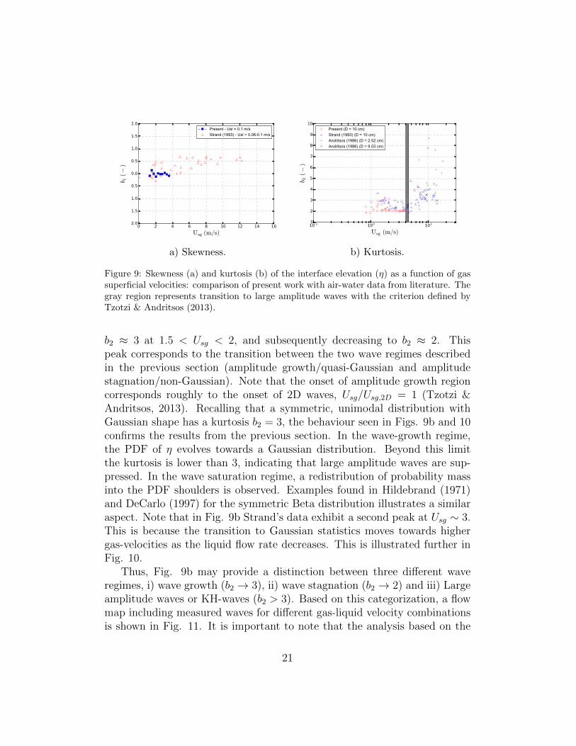
In Figure 9, skewness and kurtosis of interface elevation data collectedfrom the literature (Strand, 1993; Andritsos, 1986) are plotted together withmeasured data. Fig. 9a shows the evolution of skewness (b1) with increasingUsg and includes data acquired by Strand (1993) in the same laboratory(same pipe diameter and length). Strand varied the liquid superficial velocitywithin the range Usl = 0.06 − 0.1m/s. The figure shows that there is ageneral tendency towards larger positive skewness values as the gas increasesbeyond the range presented in the detailed analysis above. This behaviouris interpreted in the following manner; as the gas flow rate increases whileUsl is kept below 0.1m/s (below onset of slugs), the most probable waveamplitude is bounded by the amount of liquid available in the system, i.e.there is a depth-limited mode amplitude (see section 3.3). Large amplitudewaves may still be present in the flow as a result of either linear or non-linearwave-wave interaction, as demonstrated by Sanchis et al. (2011). However,the shedding probability of these large waves is low in comparison to thedominant depth-limited waves. Thus for a given Usl and increasing Usg, thePDFs of η are expected to have more or less constant modes (depth-limited),and increasingly longer tails towards higher η values, i.e. positive skewness.
Figure 9b shows the evolution of kurtosis of η with increasing Usg. Itincludes two datasets provided by Andritsos (1986); i) one set measured ina pipe with diameter D = 2.52cm and superficial liquid velocities varying
19

within the range Usl = 0.01 − 0.06m/s, ii) the second set was acquired in apipe with diameter D = 9.53cm and Usl = 0.01−0.1m/s. Note that the figurealso includes a grey region indicating the transition to large amplitude waves(also called roll-waves or Kelvin Helmholtz (KH) waves by other investiga-tors). Andritsos & Hanratty (1987) observed that the velocity combinationthat led to this transition coincided with the Kelvin-Helmholtz instabilitycriteria. Tzotzi & Andritsos (2013) included the effect of fluid propertiesand revised the previous criteria. According to Tzotzi & Andritsos (2013),for 0.08 < Usl < 0.1m/s, the critical velocity for KH-waves is around 4 - 4.5m/s, calculated with Eq. (21) below:
Usg,KH ≥1
0.65
(ρWρL
)−0.5(ρGρA
)−0.5(σWσL
)−0.33ln[ 1.39
Usl,KH
( µLµW
)−0.15](21)
In the above equation, ρL, µL, σL, ρG are the liquid density, liquid vis-cosity, liquid/gas interfacial tension and gas density, respectively; water andair are taken as reference fluids, with ρW , µW , σW the water density, wa-ter viscosity and water/air superficial tension, and ρA is the air density; allreference properties are taken at standard conditions (20 C and 1 atm).
From Fig 9b one may notice that irrespective of liquid flow rate or pipediameter, above a critical value for the gas superficial velocity of 5 m/s,the Kurtosis is predominantly higher than 3. A strongly positive excessKurtosis is an indicator of transition to large amplitude waves, as alreadypointed out in previous works (Andritsos & Hanratty, 1987; Strand, 1993).Furthermore, below the transition to large amplitude waves, the Kurtosis liespredominantly between the values 2 and 3.
Figure 10 also presents the variation of kurtosis with Usg/Usg,2D, for thepresent data set, for different values of Usl. Here, Usg,2D represents the veloc-ity at which small amplitude 2D waves appear at the liquid surface Tzotzi& Andritsos (2013). This transition velocity is based on Jeffreys’s shelteringmodel (Jeffreys, 1925), and modified by Tzotzi & Andritsos (2013), accordingto the following relation:
Usg,2D ≥1
1.95
(ρWρL
)−0.1(ρGρA
)−0.5( µLµW
)0.35ln[ 0.8
Usl,2D
( µLµW
)0.2](22)
The figure reveals that, in the region prior to KH-waves (Usg < 4m/s),the kurtosis has a non-monotonic behaviour, with local maxima reaching
20
0 2 4 6 8 10 12 14 16
Usg�(m/s)
−2.0
−1.5
−1.0
−0.5
0.0
0.5
1.0
1.5
2.0b 1
�(−)
Present - Usl = 0.1 m/sStrand (1993) - Usl = 0.06-0.1 m/s
a) Skewness.
10-1 100 101
Usg (m/s)
1
2
3
4
5
6
7
8
9
10
b 2 (−)
Present (D = 10 cm)Strand (1993) (D = 10 cm)Andritsos (1986) (D = 2.52 cm)Andritsos (1986) (D = 9.53 cm)
b) Kurtosis.
Figure 9: Skewness (a) and kurtosis (b) of the interface elevation (η) as a function of gassuperficial velocities: comparison of present work with air-water data from literature. Thegray region represents transition to large amplitude waves with the criterion defined byTzotzi & Andritsos (2013).
b2 ≈ 3 at 1.5 < Usg < 2, and subsequently decreasing to b2 ≈ 2. Thispeak corresponds to the transition between the two wave regimes describedin the previous section (amplitude growth/quasi-Gaussian and amplitudestagnation/non-Gaussian). Note that the onset of amplitude growth regioncorresponds roughly to the onset of 2D waves, Usg/Usg,2D = 1 (Tzotzi &Andritsos, 2013). Recalling that a symmetric, unimodal distribution withGaussian shape has a kurtosis b2 = 3, the behaviour seen in Figs. 9b and 10confirms the results from the previous section. In the wave-growth regime,the PDF of η evolves towards a Gaussian distribution. Beyond this limitthe kurtosis is lower than 3, indicating that large amplitude waves are sup-pressed. In the wave saturation regime, a redistribution of probability massinto the PDF shoulders is observed. Examples found in Hildebrand (1971)and DeCarlo (1997) for the symmetric Beta distribution illustrates a similaraspect. Note that in Fig. 9b Strand’s data exhibit a second peak at Usg ∼ 3.This is because the transition to Gaussian statistics moves towards highergas-velocities as the liquid flow rate decreases. This is illustrated further inFig. 10.
Thus, Fig. 9b may provide a distinction between three different waveregimes, i) wave growth (b2 → 3), ii) wave stagnation (b2 → 2) and iii) Largeamplitude waves or KH-waves (b2 > 3). Based on this categorization, a flowmap including measured waves for different gas-liquid velocity combinationsis shown in Fig. 11. It is important to note that the analysis based on the
21

10-1 100 101
Usg
Usg, 2D�(− )
1.0
1.5
2.0
2.5
3.0
3.5
4.0
4.5
5.0
b 2�(−)
Usl = 0.08 m/sUsl = 0.1 m/sUsl = 0.12 m/s
Figure 10: Kurtosis of the interface elevation (η) as a function of gas superficial velocities,normalized by the transitional velocity to 2D waves (Usg/Usg,2D).
wave data statistics (previous sections) also allow the same categorization.
3.3. Short note on the depth limited mode height
For the different flow conditions investigated in the present study, thewave height is considered to be a function of gas and liquid velocities, themean liquid height and the gravitational acceleration, neglecting the effectof surface tension in the leading order. Note that the fluid properties areconstant (air and water at atmospheric conditions) for all experiments. Asan assumption, the effect of phase velocities will be given by the relativevelocity, Ubr = Ubg − Ubl, and the wave height will be taken as the mode ofthe probability density functions of H. A dimensional analysis gives rise tothe following relation (Lilleleht & Hanratty, 1961):
gH
U2br
= Φ(ghLU2br
) (23)
The relation above may be rewritten as H∗ = Φ(Fr−2), where the non-dimensional height, H∗, is given by: H∗ = H
U2br/g
. Figure 12 shows H∗ as
a function of Fr for different liquid superficial velocities (Usl = 0.08 − 0.14m/s). For all liquid superficial velocities considered, the data corresponding
22

0 1 2 3 4 5 6
Usg�(m/s)
0.06
0.08
0.10
0.12
0.14
0.16
Usl
�(m/s)
LASA wave growth wave saturation LASA wave growth wave saturation
Figure 11: Flow map indicating transition to small amplitude (SA) 2D waves (blackdashed line) and to large amplitude (LA) waves (gray line). Both transitions are basedon criteria proposed by Tzotzi & Andritsos (2013). The black line between the SA andLA region distinguishes between the wave growth and wave saturation regimes reportedin the present study.
23

0 2 4 6 8 10 12 14
Fr (− )
0.000
0.005
0.010
0.015
0.020
0.025
0.030
H∗ (−)
∝Fr−2
Usl = 0.08 m/sUsl = 0.1 m/sUsl = 0.12 m/sUsl = 0.14 m/s
Figure 12: Non-dimensional height versus Froude number.
to the region of wave saturation seem to be well correlated by a quadraticexpression of the form H∗ ∝ Fr−2. This gives rise to the following relation:
H ≈ 0.2hL (24)
indicating that under present flow conditions, the depth-limited mode heightis approximately 20% of the mean liquid depth for the wave saturation region.Hence, in this wave regime, the characteristic wave heights are observed hereto grow predominantly by increase in the liquid flow rate, but depend weaklyon the gas flow rates.
On the other hand, in the region corresponding to wave growth, thewaves may grow both due to increase in the gas or liquid flow rates. Themechanisms of energy transfer between waves and the bulk flow, as well asinteraction between the different wave components still needs further inves-tigation. Changes in the wave structure in the different wavy flow regimes,as given by changes in the frequency (or wave length) spectra, for example,will also be investigated in a forthcoming study.
3.4. Concluding remarks
We present a statistical analysis of interfacial waves in stratified gas-liquidflow in a horizontal pipe. The analysis builds on the Gaussian wave model
24

which is widely applied in the ocean waves community in the assessment ofrogue waves (Onorato et al., 2013). The main goal is to use this model todifferentiate between linear and non-linear wave regimes in gas-liquid pipeflow. Note that the waves under investigation were purely wind-induced,i.e., they developed as result of gas-liquid interaction, as opposed to themechanically induced waves described by Ayati et al. (2017).
A zero-crossing method was applied on measured wave elevation time se-ries, yielding local interfacial displacement parameters. The evolution of theprobability distributions of wave elevation (η), crest height (ηc), trough height(ηt) and wave height (H) were investigated for increasing gas superficial ve-locities (Usg ∼ 1 − 4) at constant superficial liquid velocity (Usl = 0.1m/s).Exceedence distributions of η and the upper Hilbert envelope Aup were com-pared to their associated Gaussian and Tayfun distributions, where the latterincludes effects of second-order non-linearities. The results showed that thewaves under (detailed) investigation could be classified into two regimes; i)A quasi-Gaussian or quasi-linear regime for Fr < 4. In this region, thePDFs and EDFs evolved towards Gaussian statistics with second order non-linearity at Fr = 3.7 or Usg = 1.54m/s. This regime corresponds to theregion in which the waves grow with increasing gas velocity, i.e. wave growthregime (Ayati et al., 2015) or gas flow dependent regime (with reference towind-dependent regime in ocean literature). ii) A non-Gaussian or non-linearregime where Gaussian statistics considerably overpredict the distributionsof both η and Aup. This regime corresponds to what has been called thestagnation or saturation regime (Ayati et al., 2015), or the equilibrium rangein the ocean wave literature Phillips (1958). Mechanisms that possibly couldexplain the stagnation of wave growth, encompassing amongst others airflowseparation and micro-breaking were briefly discussed. No conclusions regard-ing these processes could be drawn based on the present data set. Furtherwork shall include detailed spectral analysis of the liquid height signals undervarious flow conditions, as well as interaction with the bulk flow through flowfield measurements.
Higher order moments (skewness and kurtosis) acquired from literaturewere included in the analysis in order to put the observed wave regimes intoa wider context. Variations on higher order moments also indicate changesin the interfacial structures according to the different regimes, which supportand complement the interpretation of wave data statistics. Finally, analysisof a range of cases for various Usl and Usg suggests that the transition to thesaturation regime occurs at lower Froude numbers, for increasing Usl, and
25

that the ratio of the equilibrium wave height to the mean liquid height isapproximately constant H = 0.2hL, i.e. depth-limited mode height.
Appendix A
The conductance probing technique, described in more details in Ay-ati et al. (2015), was performed using a Field Programmable Gate Array(FPGA). This system has the advantage of performing complex combina-tional functions at a high sampling rate. A low-pass filter with cut-off fre-quency of 500Hz was set to match the frequency of a 4mm wave propagatingat 1m/s, taking into account the Nyquist criteria. The length scale of 4mmis corresponds to the distance between two parallel wires. Nonetheless, thesignificant portion of the frequency spectrum lies between 0 and 60 Hz, seefig. 13, after which the spectral power flattens at S(60Hz) ∼ 10−4mm2s andthe noise becomes dominant. This corresponds to a minimum amplitudeAmin =
√S(60Hz) × 60Hz ≈ 0.6mm, which twice the probe wire thickness
(0.3mm).
4 8 16 60
f [Hz]
10 -4
10 -3
10 -2
10 -1
100
PS
D [
mm
2s]
Figure 13: Typical example of a power spectrum without smoothing.
Appendix B
The wave celerity of a given wave, cj, was computed by cross-correlating ofthe elevation signals from probe 1 and probe 2, see Fig 14. In order to extract
26

the value of c, the full signal was partitioned into short segments starting froma given wave wj and including its neighbouring N waves [wj+1, wj+2, ..., wj+N ].The value N varied between 10 and 50. An initial value of N was set based onthe average number of wave cycles per wave group as seen from Fig. 4. Thefinal value of N was chosen by iteration, until the value for the correlationcoefficient, C(η1, η2; τ), converged. Here, τ is the time lag that correspondsto the maximum value of the correlation coefficient. Typically, large values ofN were chosen in the low gas flow rate cases. Note that our use of the term”local wave celerity” implies an assumption that the phase speed remainsconstant within the interval of N waves.
Local wave lengths and crest steepness are given as λj = cjTj and εc,j =πηc,j/λc,j, respectively. Here, Tj is the local wave period and λc,j = cjTc,jis the local crest length. The crest steepness was chosen instead of the fullwave steepness, εj = 2πAj/λj because it was found to be more informative,especially at gas flow rates above 1.77m/s. At these conditions, the waveprofile displayed typical non-linear characteristics, that is, tall and narrowcrests and long and shallow troughs.
27

1.5 2 2.5 3 3.5 4
t, [sec]
-4
-2
0
2
4
610
-3
1(t)
2(t)
1.5 2 2.5 3 3.5 4
t, [sec]
-4
-2
0
2
4
610
-3
-2 -1.5 -1 -0.5 0 0.5 1 1.5 2
, [sec]
-0.5
0
0.5
1
Xcorr
Figure 14: An illustration of how the local wave speed was computed for a given wave, wj .Here, only 10 wave cycles were required to achieve a converged value of the correlationcoefficient. The upper plate shows the raw elevation signals. The middle plate shows ashifted signal from probe 2 (η2(t − τ)), where τ is the time lag that corresponds to thepeak of the correlation coefficient.
28

Acknowledgements
The authors acknowledge funding from the SIU/CAPES joint programUTFORSK2016 (grant UTF.2016-CAPES-SIU/10012) as well as the Akademiaprogram at the Faculty of Mathematics and Natural Sciences, University ofOslo.
References
Andre, Matthieu A & Bardet, Philippe M 2017 Viscous stress dis-tribution over a wavy gas–liquid interface. International Journal of Multi-phase Flow 88, 1–10.
Andritsos, Nikos 1986 Effect of pipe diameter and liquid viscosity onhorizontal stratified flow. PhD thesis, Univ. Illinois, Urbana.
Andritsos, N. & Hanratty, T.J. 1987 Influence of interfacial waves instratified gas-liquid flows. AIChE Journal 33, 444–454.
Ayati, A.A., Kolaas, J., Jensen, A. & Johnson, G.W. 2014 A {PIV}investigation of stratified gasliquid flow in a horizontal pipe. InternationalJournal of Multiphase Flow 61, 129 – 143.
Ayati, A.A., Kolaas, J., Jensen, A. & Johnson, G.W. 2015 Combinedsimultaneous two-phase {PIV} and interface elevation measurements instratified gas/liquid pipe flow. International Journal of Multiphase Flow74, 45 – 58.
Ayati, A.A., Kolaas, J., Jensen, A. & Johnson, G.W. 2016 The effectof interfacial waves on the turbulence structure of stratified air/water pipeflow. International Journal of Multiphase Flow 78, 104 – 116.
Ayati, A. A., Farias, P. S. C., Azevedo, L. F. A. & de Paula,I. B. 2017 Characterization of linear interfacial waves in a turbu-lent gas-liquid pipe flow. Physics of Fluids 29 (6), 062106, arXiv:http://dx.doi.org/10.1063/1.4985717.
Barghi, S, Prakash, A, Margaritis, A & Bergougnou, MA 2004Flow regime identification in a slurry bubble column from gas holdup andpressure fluctuations analysis. The Canadian Journal of Chemical Engi-neering 82 (5), 865–870.
29

Bendiksen, Kjell H, Maines, Dag, Moe, Randi, Nuland, Sven &others 1991 The dynamic two-fluid model olga: Theory and application.SPE production engineering 6 (02), 171–180.
Berthelsen, P.A. & Ytrehus, T. 2005 Calculations of stratified wavytwo-phase flow in pipes. International Journal of Multiphase Flow 31, 571–592.
Biberg, D 2007 A mathematical model for two-phase stratified turbulentduct flow. Multiphase Science and Technology 19, 1–48.
Birvalski, M., Tummers, M.J., Delfos, R. & Henkes, R.A.W.M.2014 Piv measurements of waves and turbulence in stratified horizontaltwo-phase pipe flow. International Journal of Multiphase Flow 62, 161–173.
Birvalski, M, Tummers, MJ & Henkes, RAWM 2016 Measurements ofgravity and gravity-capillary waves in horizontal gas-liquid pipe flow usingpiv in both phases. International Journal of Multiphase Flow 87, 102–113.
Birvalski, M., Tummers, M. J., Delfos, R. & Henkes, R. A. W. M.2015 Laminarturbulent transition and waveturbulence interaction in strat-ified horizontal two-phase pipe flow. Journal of Fluid Mechanics 780,439456.
Bratland, Ove 2010 Pipe flow 2 multi-phase flow assurance. Chapt 18,274–284.
Buckley, Marc P & Veron, Fabrice 2016 Structure of the airflowabove surface waves. Journal of Physical Oceanography 46 (5), 1377–1397.
Carneiro, J.N.E., Fonseca Jr, R., Ortega, A.J., Chucuya, R.C.,Nieckele, A.O. & Azevedo, L.F.A. 2011 Statistical characterizationof the two phase slug flow in a horizontal pipe. Journal of the BrazilianSociety of Mechanical Sciences and Engineering 33, 251 – 258.
Danielson, T.J., Bansal, K.M., Djoric, B., Larrey, D., Johansen,S.T., De Leebeeck, A. & Kjølaas, J. 2012 Simulation of slug flow inoil and gas pipelines using a new transient simulator. In Offshore Technol-ogy Conference 2012, Texas, USA.
30

DeCarlo, Lawrence T 1997 On the meaning and use of kurtosis. Psy-chological methods 2 (3), 292.
Espedal, M 1998 An experimental investigation of stratified two-phase pipeflow at small inclinations. PhD thesis, The Norwegian University of Scienceand Technology (NTNU).
Grare, Laurent, Peirson, William L, Branger, Hubert, Walker,James W, Giovanangeli, Jean-Paul & Makin, Vladimir 2013Growth and dissipation of wind-forced, deep-water waves. Journal of FluidMechanics 722, 5–50.
Hildebrand, David K 1971 Kurtosis measures bimodality? The AmericanStatistician 25 (1), 42–43.
Issa, R.I. & Kempf, M.H.W. 2003 Simulation of slug flow in horizontaland nearly horizontal pipes with the twofluid model. International Journalof Multiphase Flow 29, 69 – 95.
Jeffreys, H. 1925 On the formation of waves by wind ii. Proc. Roy. Soc.110A, 341–347.
Lakehal, D., Fulgosi, M., Banerjee, S. & Angelis., De 2003 Directnnumerical simulation of turbulence in a sheared air water flow with adeformable interface. Journal of Fluid Mechanics 482, 319–345.
Lilleleht, Lembit U & Hanratty, Thomas J 1961 Measurement ofinterfacial structure for co-current air–water flow. Journal of Fluid Me-chanics 11 (1), 65–81.
Longuet-Higgins, Michael S 1952 On the statistical distributions of seawaves. Journal of Marine Research 11 (3), 245–265.
Mokhatab, Saeid & Poe, William A 2012 Handbook of natural gastransmission and processing . Gulf Professional Publishing.
Nieckele, A.O. & Carneiro, J.N.E. 2017 On the numerical modeling ofslug and intermittent flows in oil and gas production. In Proceedings of theASME 2017 36th International Conference on Ocean, Offshore and ArcticEngineering OMAE2017 June 25-30, 2017, Trondheim, Norway .
31

Nieckele, A.O., Carneiro, J.N.E., Chucuja, R.C. & Azevedo,J.H.P. 2011 Initiation and statistical evolution of horizontal slug flowwith a two-fluid model. ASME Journal of Fluids Engineering 135 (12),121302.
Onorato, M., Residori, S., Bortolozzo, U., Montina, A. & Arec-chi, F.T. 2013 Rogue waves and their generating mechanisms in differentphysical contexts. Physics Reports 528 (2), 47 – 89, rogue waves and theirgenerating mechanisms in different physical contexts.
Onorato, M, Waseda, T, Toffoli, A, Cavaleri, L, Gramstad, O,Janssen, PAEM, Kinoshita, T, Monbaliu, Jaak, Mori, N, Os-borne, AR & others 2009 Statistical properties of directional oceanwaves: the role of the modulational instability in the formation of extremeevents. Physical Review Letters 102 (11), 114502.
Petrova, PG & Soares, C Guedes 2014 Distributions of nonlinear waveamplitudes and heights from laboratory generated following and crossingbimodal seas. Natural Hazards and Earth System Sciences 14 (5), 1207.
Phillips, O.M. 1958 The equilibrium range in the spectrum of wind-generated waves. Journal of Fluid Mechanics 4, 426–434.
Pothof, I.W.M. & Clemens, F.H.L.R. 2011 Experimental study of air-water flow in downward sloping pipes. International Journal of MultiphaseFlow 37 (3), 278 – 292.
Prosperetti, A 2003 Two questions concerning ”fully developed gas-liquidflows”. Multiphase Science and Technology 15 (1-4).
Sanchis, A., Johnson, G.W. & Jensen, A. 2011 The formation of hy-drodynamic slugs by the interaction of waves in gas-liquid two-phase pipe.International Journal of Multiphase Flow 37, 358–368.
Sobey, R.J. 1992 The distribution of zero-crossing wave heights and periodsin a stationary sea state. Ocean Engineering 19 (2), 101 – 118.
Socquet-Juglard, Herve, Dysthe, Kristian, Trulsen, Karsten,Krogstad, Harald E & Liu, Jingdong 2005 Probability distribu-tions of surface gravity waves during spectral changes. Journal of FluidMechanics 542, 195–216.
32
Strand, O. 1993 An experimental investigation of stratified two-phase flowin horizontal pipes. PhD thesis, University of Oslo.
Tayfun, M Aziz 1980 Narrow-band nonlinear sea waves. Journal of Geo-physical Research: Oceans 85 (C3), 1548–1552.
Tzotzi, C. & Andritsos, N. 2013 Interfacial shear stress in wavy stratifiedgasliquid flow in horizontal pipes ”. International Journal of MultiphaseFlow 54, 43 – 54.
Yang, Di & Shen, Lian 2010 Direct-simulation-based study of turbulentflow over various waving boundaries. Journal of Fluid Mechanics 650,131–180.
33