STATISTICAL CONTRIBUTION

TO THE ANALYSIS

OF METABONOMIC DATA IN1H-NMR SPECTROSCOPY.

These presentee en vue de l’obtention du grade deDocteur en Sciences (orientation statistique) par :

Rejane Rousseau

Membres du jury:Prof. Bernadette Govaerts (Co-promoteur)Prof. Michel Verleysen (Co-promoteur)Dr. Bruno Boulanger (Arlenda, Charge de Cours ULg)Dr. Pascal de Tullio (ULg)Prof. Paul H.C. Eilers (Erasmus Mc)Prof. Philippe Lambert (UCL, ULg)Prof. Rainer von Sachs (President du jury)

Louvain-la-Neuve, 2011

Acknowledgements

Je voudrais remercier tous ceux qui ont contribue, de pres ou de loin, al’elaboration de ma these.

Mes premiers remerciements vont a ma promotrice, le ProfesseurBernadette Govaerts, qui a cru en moi et n’a jamais cesse de m’encourager.Je la remercie tout particulierement pour le partage de connaissancesainsi que son immense implication et ses nombreuses suggestions autout au long du developpement de ma these de doctorat. Je tiens aussia la remercier pour tous les bons moments passes en dehors du travailet l’enrichissement humain que j’ai acquis a son contact.

Je remercie egalement mon co-promoteur, le Professeur Michel Ver-leysen, pour sa disponibilite, ses conseils. Je souhaite egalement ex-primer toute ma gratitude aux membres du jury, qui ont accepte delire ma these avec autant de soin. Je voudrais exprimer tout ma recon-naissance au Dr. Bruno Boulanger pour m’avoir propose de travaillersur ce sujet ainsi qu’au Professeur Paul HC Eilers pour ses nombreusessources d’inspiration. Je remercie egalement Pascal de Tullio et MichelFrederich pour leur collaboration motivee et dynamique.

Mes remerciements vont egalement a tous les membres de l’Institut,personnel administratif, academique, scientifique et SMCS, qui ont con-tribue a une atmosphere de travail tres agreable. Je tiens a remercierparticulierement Angelique, Astrid, Bianca, Celine B., Celine L., Maria,Nancy, Oana pour leurs encouragements et amities depuis le debut dece doctorat. Je remercie egalement Alain, Anne, Catherine R., Cather-ine T., Cedric, Diane, Fabian, Louis, Marco, Mathieu pour leurs ecoutes,bons conseils et bons moments partages au cours de ces dernieres annees.

Je tiens finalement a remercier ma famille et mes amis pour leursoutien continu.

Contents

List of Figures 7

Introduction 1

0.1 Context: metabonomics . . . . . . . . . . . . . . . . . . . 1

0.2 History of metabonomics and literature review . . . . . . 5

0.3 Presentation of a metabonomic study . . . . . . . . . . . . 8

0.3.1 Definition of the goals of the study . . . . . . . . . 9

0.3.2 Study design . . . . . . . . . . . . . . . . . . . . . 10

0.3.3 Experiments and sampling . . . . . . . . . . . . . 11

0.3.4 Spectral data acquisition . . . . . . . . . . . . . . 12

0.3.5 Data pre-treatments . . . . . . . . . . . . . . . . . 12

0.3.6 Data analysis . . . . . . . . . . . . . . . . . . . . . 12

0.3.7 Molecular interpretation of spectral biomarkers . . 12

0.4 Conventional statistical analysis of metabonomic data . . 14

0.5 Contents and contribution of this thesis . . . . . . . . . . 18

1 The 1H-NMR spectroscopy and metabonomic data pre-treaments 25

1.1 Introduction . . . . . . . . . . . . . . . . . . . . . . . . . . 25

1.2 Proton Nuclear Magnetic Resonancespectroscopy . . . . . . . . . . . . . . . . . . . . . . . . . 26

1.2.1 Principles of Proton Nuclear Magnetic Resonancespectroscopy . . . . . . . . . . . . . . . . . . . . . 27

1.2.2 The original data: the Free Induction Decay . . . . 32

1.2.3 An 1H-NMR analysis . . . . . . . . . . . . . . . . . 38

1.2.4 A typical 1H-NMR spectrum . . . . . . . . . . . . 41

1.3 Metabonomic data pre-treatments . . . . . . . . . . . . . 45

1.3.1 Advised pre-treatments procedure . . . . . . . . . 47

1.3.2 Summary of the advised pre-treatments procedure 80

1.4 Conclusions . . . . . . . . . . . . . . . . . . . . . . . . . . 82

2 CONTENTS

2 The metabonomic databases used in this thesis 852.1 Introduction . . . . . . . . . . . . . . . . . . . . . . . . . . 852.2 The semi-artificial database . . . . . . . . . . . . . . . . . 86

2.2.1 Motivations for creating this database . . . . . . . 862.2.2 The placebo data . . . . . . . . . . . . . . . . . . . 862.2.3 Simulation of alterations . . . . . . . . . . . . . . . 872.2.4 The final database . . . . . . . . . . . . . . . . . . 882.2.5 Notes-remarks . . . . . . . . . . . . . . . . . . . . 88

2.3 The urine experimental database . . . . . . . . . . . . . . 892.3.1 Motivations for creating this database . . . . . . . 892.3.2 Statistical experimental design . . . . . . . . . . . 892.3.3 Sample preparation and acquisition of the 1H-NMR

data . . . . . . . . . . . . . . . . . . . . . . . . . . 912.3.4 The pre-treatments . . . . . . . . . . . . . . . . . . 912.3.5 The final urine database . . . . . . . . . . . . . . . 92

2.4 The serum experimental database . . . . . . . . . . . . . . 932.4.1 Motivations for creating this database . . . . . . . 932.4.2 Study design . . . . . . . . . . . . . . . . . . . . . 932.4.3 Sample preparation . . . . . . . . . . . . . . . . . 982.4.4 Spectral acquisition . . . . . . . . . . . . . . . . . 992.4.5 The pre-treatments . . . . . . . . . . . . . . . . . . 992.4.6 The final database . . . . . . . . . . . . . . . . . . 99

2.5 The human serum database . . . . . . . . . . . . . . . . . 992.5.1 Motivations for creating this database . . . . . . . 992.5.2 Statistical design . . . . . . . . . . . . . . . . . . . 1002.5.3 Sample preparation . . . . . . . . . . . . . . . . . 1012.5.4 The pre-treatments . . . . . . . . . . . . . . . . . . 1012.5.5 The final database . . . . . . . . . . . . . . . . . . 101

3 Evaluation of stability, repeatability and reproducibilityproperties of 1H-NMR spectra in metabonomic studies 1033.1 Introduction . . . . . . . . . . . . . . . . . . . . . . . . . . 1033.2 Sources of variability . . . . . . . . . . . . . . . . . . . . . 1053.3 Research questions and notations . . . . . . . . . . . . . . 1063.4 Data and contextual variability questions . . . . . . . . . 106

3.4.1 Datasets . . . . . . . . . . . . . . . . . . . . . . . . 1073.4.2 Contextual questions studied on the datasets . . . 108

3.5 Proposed methodologies . . . . . . . . . . . . . . . . . . . 1103.5.1 PCA with group identification and inertia compu-

tation . . . . . . . . . . . . . . . . . . . . . . . . . 1103.5.2 Pointwise summary statistics and global coefficient

of variation . . . . . . . . . . . . . . . . . . . . . . 116

CONTENTS 3

3.5.3 Pointwise mixed modelling . . . . . . . . . . . . . 124

3.6 Conclusions about contextual questions . . . . . . . . . . 138

3.6.1 Question for the experimental serum dataset . . . 138

3.6.2 Question for the human serum dataset . . . . . . . 138

3.6.3 Question for the urine dataset . . . . . . . . . . . . 139

3.7 Conclusions . . . . . . . . . . . . . . . . . . . . . . . . . . 139

4 Comparison of some chemometric tools for metabonomicbiomarkeridentification 143

4.1 Introduction . . . . . . . . . . . . . . . . . . . . . . . . . . 143

4.2 Methods . . . . . . . . . . . . . . . . . . . . . . . . . . . . 144

4.2.1 Multiple hypothesis testing (MHT) . . . . . . . . . 144

4.2.2 Supervised principal component analysis (s-PCA) . 146

4.2.3 Supervised independent component analysis (s-ICA)147

4.2.4 Discriminant Partial Least Squares (PLS-DA) . . . 148

4.2.5 Linear logistic regression (LLR) . . . . . . . . . . . 149

4.2.6 Classification and regression trees (CART) . . . . 150

4.2.7 Implementation . . . . . . . . . . . . . . . . . . . . 151

4.3 Description of the data . . . . . . . . . . . . . . . . . . . . 151

4.4 Illustration of the methods . . . . . . . . . . . . . . . . . 152

4.5 Method comparison . . . . . . . . . . . . . . . . . . . . . 158

4.5.1 Number of identifications . . . . . . . . . . . . . . 158

4.5.2 ROC curves . . . . . . . . . . . . . . . . . . . . . . 160

4.5.3 Variability of the results . . . . . . . . . . . . . . . 164

4.6 Conclusions . . . . . . . . . . . . . . . . . . . . . . . . . . 165

5 Combination of IndependentComponent Analysis and statisticalmodelling for the search ofmetabonomic biomarkers in 1H-NMR spectroscopy 167

5.1 Introduction . . . . . . . . . . . . . . . . . . . . . . . . . . 167

5.2 Data description . . . . . . . . . . . . . . . . . . . . . . . 170

5.3 First step of the methodology: ICA . . . . . . . . . . . . . 171

5.3.1 The ICA theoretical principles . . . . . . . . . . . 171

5.3.2 Independent Component Analysis on metabonomicdata . . . . . . . . . . . . . . . . . . . . . . . . . . 173

5.3.3 Choice of the number of sources to estimate . . . 174

5.3.4 Measure of the information contained in ICA sources. . . . . . . . . . . . . . . . . . . . . . . . . . . . 175

5.3.5 Example . . . . . . . . . . . . . . . . . . . . . . . . 176

5.3.6 Comparison between ICA and PCA . . . . . . . . 179

4 CONTENTS

5.4 Step II: Statistical modelling . . . . . . . . . . . . . . . . 182

5.4.1 Goals and principle . . . . . . . . . . . . . . . . . . 182

5.4.2 Linear mixed model specification and estimation . 182

5.4.3 Example . . . . . . . . . . . . . . . . . . . . . . . . 183

5.5 Step III: Biomarker identification . . . . . . . . . . . . . 184

5.5.1 Goals and principle . . . . . . . . . . . . . . . . . . 184

5.5.2 Selection of significant sources . . . . . . . . . . . 185

5.5.3 Example . . . . . . . . . . . . . . . . . . . . . . . . 186

5.6 Step IV: Visualization of biomarkers and factor effects . . 188

5.6.1 Goal and principle . . . . . . . . . . . . . . . . . . 188

5.6.2 Contrast calculation . . . . . . . . . . . . . . . . . 188

5.6.3 Example . . . . . . . . . . . . . . . . . . . . . . . . 189

5.7 Application to more complex data . . . . . . . . . . . . . 192

5.8 Conclusions . . . . . . . . . . . . . . . . . . . . . . . . . . 195

6 Example: metabonomic study of Age related MacularDegeneration (AMD) 197

6.1 Introduction . . . . . . . . . . . . . . . . . . . . . . . . . . 197

6.2 Study setting up . . . . . . . . . . . . . . . . . . . . . . . 198

6.2.1 Definition of the goals of the study . . . . . . . . . 198

6.2.2 Study design . . . . . . . . . . . . . . . . . . . . . 198

6.3 Acquisition of the data . . . . . . . . . . . . . . . . . . . . 200

6.3.1 Experiment and sampling . . . . . . . . . . . . . . 200

6.3.2 Data acquisition . . . . . . . . . . . . . . . . . . . 200

6.3.3 Pre-treatments . . . . . . . . . . . . . . . . . . . . 201

6.3.4 The AMD database in the end of the data acquisition201

6.4 Data analysis . . . . . . . . . . . . . . . . . . . . . . . . . 202

6.4.1 Evaluation of the data . . . . . . . . . . . . . . . . 202

6.4.2 Search for biomarkers . . . . . . . . . . . . . . . . 210

6.4.3 Molecular interpretation . . . . . . . . . . . . . . . 218

6.4.4 Conclusions . . . . . . . . . . . . . . . . . . . . . . 220

7 Conclusion 221

Appendices 229

7.1 Appendix 1: the warping function . . . . . . . . . . . . . 230

7.2 Appendix 2: the probability density plot and boxplots ofthe σf vectors. . . . . . . . . . . . . . . . . . . . . . . . . 233

7.3 Appendix 3: the probability density plot of the ICCfvectors. . . . . . . . . . . . . . . . . . . . . . . . . . . . . 235

7.4 Appendix 4: the probability density plot and boxplots ofthe SNR vectors. . . . . . . . . . . . . . . . . . . . . . . . 237

CONTENTS 5

7.5 Appendix 5: the scatterplot matrix and coefficients ofcorrelation of the ten sources. . . . . . . . . . . . . . . . . 239

7.6 Appendix 6: spectral misalignment shown in ICA sources. 2407.7 Appendix 7: the sources and contrasts with q=4 and q=8. 2427.8 Appendix 8: the AIC of the LLR variable selection ap-

plied to the AMD dataset. . . . . . . . . . . . . . . . . . . 2457.9 Appendix 9: AMD, the eighteen estimated ICA sources

and their weights. . . . . . . . . . . . . . . . . . . . . . . . 2467.10 Appendix 10: AMD, comparisons of means on the vectors

of weights of the 18 sources. . . . . . . . . . . . . . . . . . 250

Abbreviations 251

Bibliography 253

6 CONTENTS

List of Figures

1 The general scheme of a metabonomic study. . . . . . . . 3

2 The different steps of a metabonomic study. . . . . . . . . 8

3 The conventional methods for metabonomic data analysis. 15

4 Conventional Principal Components Analysis for metabo-nomic data analysis. . . . . . . . . . . . . . . . . . . . . . 16

5 The metabonomic study steps concerned in the chaptersof the thesis. . . . . . . . . . . . . . . . . . . . . . . . . . 19

1.1 A nuclear spin and its magnetic moment . . . . . . . . . . 27

1.2 The spins orientations . . . . . . . . . . . . . . . . . . . . 28

1.3 The spin and magnetic moment precessions. . . . . . . . . 28

1.4 The net magnetization at equilibrium. . . . . . . . . . . . 30

1.5 The rotation of the net magnetization into the xy plan. . 30

1.6 FID induction . . . . . . . . . . . . . . . . . . . . . . . . . 31

1.7 The evolution of the magnetization over time. . . . . . . . 32

1.8 The x and y components of the signal . . . . . . . . . . . 33

1.9 The characteristics of the FID component. . . . . . . . . . 34

1.10 An FID. . . . . . . . . . . . . . . . . . . . . . . . . . . . . 35

1.11 Examples of FIDs and their spectra. . . . . . . . . . . . . 36

1.12 The relation between T2 and LB. . . . . . . . . . . . . . . 37

1.13 The three periods of a pulse-acquire experiment and theparameters of acquisition. . . . . . . . . . . . . . . . . . . 38

1.14 The 1H-NMR spectrum of para-xylen. . . . . . . . . . . . 42

1.15 The high resolution 1H-NMR spectra of urine and serum. 43

1.16 The usual and the advised pre-treatment procedures. . . . 46

1.17 An FID and its group delay. . . . . . . . . . . . . . . . . . 49

1.18 The absorptive and dispersive modes. . . . . . . . . . . . 50

1.19 An FID after first order phase correction. . . . . . . . . . 52

1.20 The spectrum before and after the water suppression. . . 53

1.21 The FID before and after the water suppression. . . . . . 54

1.22 The FID before apodization and the exponential apodiza-tion function. . . . . . . . . . . . . . . . . . . . . . . . . . 56

8 LIST OF FIGURES

1.23 The Real part of the FID before and after apodization. . . 58

1.24 The spectrum after Fourier Transform: the Real and Imag-inary parts. . . . . . . . . . . . . . . . . . . . . . . . . . . 60

1.25 The Real part of the resulting zero order phased spectrum. 62

1.26 The spectrum before the baseline correction. . . . . . . . 64

1.27 The spectrum after the baseline correction. . . . . . . . . 65

1.28 Spectra before and after warping. . . . . . . . . . . . . . . 68

1.29 The spectrum and the different scales units. . . . . . . . . 70

1.30 The spectrum after spectral window selection. . . . . . . . 71

1.31 A same spectrum without bucketing, in a resolution of750 buckets and of 250 buckets. . . . . . . . . . . . . . . . 72

1.32 The principle of the new bucketing methodology. . . . . . 73

1.33 An urine spectrum after the removal between 4.5 and 6.00ppm. . . . . . . . . . . . . . . . . . . . . . . . . . . . . . . 75

1.34 A serum spectrum after the removal from 4.5 to 5.04 ppmand from 1.36 to 1.28. . . . . . . . . . . . . . . . . . . . . 76

1.35 A urine spectrum after citrate aggregation with the initialmethodology. . . . . . . . . . . . . . . . . . . . . . . . . . 77

1.36 A urine spectrum after citrate aggregation with the newmethodology. . . . . . . . . . . . . . . . . . . . . . . . . . 78

1.37 Zooms on two urine spectra before and after normalization. 79

2.1 The alterations added to the placebo spectra. . . . . . . . 87

2.2 The urine experimental design. . . . . . . . . . . . . . . . 90

2.3 A typical urine spectrum with spiked citrate and hippurate. 90

2.4 The full experimental design of the serum experimentaldatabase. . . . . . . . . . . . . . . . . . . . . . . . . . . . 94

2.5 The preparation procedure of the experimental serum database. 96

2.6 The twenty four spectra obtained with each of the threemethods to remove peaks of proteins. . . . . . . . . . . . . 97

3.1 The sources of spectral variabilities. . . . . . . . . . . . . 105

3.2 The experimental design of the ”experimental serum dataset”.108

3.3 The experimental design of the ”urine dataset”. . . . . . . 109

3.4 The PCA scoreplot of the two first PCs for the experi-mental serum dataset. . . . . . . . . . . . . . . . . . . . . 112

3.5 The PCA scoreplot of the two first PCs for the humanserum dataset. . . . . . . . . . . . . . . . . . . . . . . . . 113

3.6 The PCA scoreplots of the two first PCs for the urinedataset. . . . . . . . . . . . . . . . . . . . . . . . . . . . . 114

3.7 The differences of three spectra to the mean spectrum. . . 117

LIST OF FIGURES 9

3.8 The spectra of xj , sj , cvj for the 24 CPMG and the 24STE spectra. . . . . . . . . . . . . . . . . . . . . . . . . . 118

3.9 The curves of the ordered sg. . . . . . . . . . . . . . . . . 119

3.10 The curves of the ordered cvg. . . . . . . . . . . . . . . . . 119

3.11 The probability density plot of sg and cvg. . . . . . . . . . 121

3.12 The boxplots of cvg. . . . . . . . . . . . . . . . . . . . . . 122

3.13 The boxplots of cvg. . . . . . . . . . . . . . . . . . . . . . 122

3.14 The scatterplots of s vs x. . . . . . . . . . . . . . . . . . . 123

3.15 The spectra of the five σf vectors from the human serumdataset. . . . . . . . . . . . . . . . . . . . . . . . . . . . . 128

3.16 The curves of the ordered σf vectors. . . . . . . . . . . . . 129

3.17 The spectra of the five ICC vectors. . . . . . . . . . . . . 131

3.18 The curves of the ordered ICCf vectors. . . . . . . . . . . 132

3.19 The boxplots of the ICCf vectors. . . . . . . . . . . . . . 133

3.20 The spectra of the SNR vector in each pre-treatments case.136

3.21 The ordered curves of the SNR vectors. . . . . . . . . . . 137

4.1 Biomarker scores for all tested methods. . . . . . . . . . . 153

4.2 Projection of the spectra on the principal componentswhich best discriminate between normal and altered spec-tra. . . . . . . . . . . . . . . . . . . . . . . . . . . . . . . . 156

4.3 The ten ICA sources which best discriminate betweennormal and altered spectra. . . . . . . . . . . . . . . . . . 157

4.4 Classification tree before and after pruning. . . . . . . . . 158

4.5 Proportions of occurrences of true and false biomarkeridentification in simulations. . . . . . . . . . . . . . . . . . 160

4.6 Mean ROC curves for the six methods. . . . . . . . . . . . 162

4.7 Standard deviation of FDR or sensitivity versus numberof identifications for the six methods. . . . . . . . . . . . . 165

5.1 Methodology steps of ICA with mixed models. . . . . . . 169

5.2 Experimental design of the first dataset used in example. 170

5.3 A typical urine spectrum with spiked citrate and hippurate.170

5.4 Screeplot of the % of variance explained by the q first PCsfrom the PCA-whitening. . . . . . . . . . . . . . . . . . . 176

5.5 The q = 6 sources from ICA. . . . . . . . . . . . . . . . . 178

5.6 The mixing coefficients for sources 2 and 3. . . . . . . . . 179

5.7 Component directions ideally chosen by PCA and ICA onillustrative experimental design. . . . . . . . . . . . . . . . 180

5.8 The PCA loadings and the ICA sources resulting fromapplication on illustrative experimental data. . . . . . . . 181

5.9 The p-values corresponding to each sources. . . . . . . . . 187

10 LIST OF FIGURES

5.10 The relationship between the hippurate dose and the vec-tor of mixing weights a3. . . . . . . . . . . . . . . . . . . . 189

5.11 The three contrasts obtained when y1 is introduced as acontinuous variable in the model. . . . . . . . . . . . . . . 190

5.12 The three contrasts obtained when y1 is introduced as acategorical variable in the model. . . . . . . . . . . . . . . 190

5.13 Experimental design of the more complex dataset dividedin three groups of disease. . . . . . . . . . . . . . . . . . . 192

5.14 The q = 5 sources for the complex data example. . . . . . 193

5.15 The three contrasts in the complex data example. . . . . . 195

6.1 The AMD metabonomic study steps. . . . . . . . . . . . . 199

6.2 Outliers detection in the scoreplot of the two first princi-pal components. . . . . . . . . . . . . . . . . . . . . . . . 202

6.3 Outliers detection in the scoreplot of the two first princi-pal components from the group centered PCA. . . . . . . 203

6.4 The four detected outliers. . . . . . . . . . . . . . . . . . . 204

6.5 Projections of the spectra on the two first principal com-ponents. . . . . . . . . . . . . . . . . . . . . . . . . . . . . 206

6.6 The spectra of xj , sj , cvj for the AMD and the controlspectra. . . . . . . . . . . . . . . . . . . . . . . . . . . . . 208

6.7 The curves of the ordered coefficients of variation. . . . . 209

6.8 Projections of the spectra on the two first principal com-ponents. . . . . . . . . . . . . . . . . . . . . . . . . . . . . 210

6.9 The six biomarker score vectors and the biomarkers onthe mean of control spectra. . . . . . . . . . . . . . . . . . 212

6.10 Projections of the spectra on the principal componentswhich best discriminate between control and AMD spectra.213

6.11 Screeplot of the % of variance explained by the q = 189first PCs from the PCA-whitening. . . . . . . . . . . . . . 214

6.12 The contrasts between: AMD inactive cases and controls(top), AMD active cases and controls (middle), AMD ac-tive and AMD inactive cases (bottom). Colored spectralzones represent the lactate and lipoproteins zones. . . . . 218

6.13 A control and a ADML spectrum with the lactate andlipoproteins spectral zones. . . . . . . . . . . . . . . . . . 219

7.1 Leftmost panel: the warping function, ω(ν), estimatedfor the serum spectrum illustrating Section 1.3.1. Mid-dle panel: its differences, with the unwarped frequencies,ω(ν)− ν. Rightmost panel: the derivative of the warpingfunction, ω(νi)− ω(νi−1). . . . . . . . . . . . . . . . . . . 230

LIST OF FIGURES 11

7.2 The spectrum before warping (uppest panel) and the dif-ferences ω(ν)− ν (lowest panel) in the spectral zone keptin the spectral window selection. . . . . . . . . . . . . . . 231

7.3 Histogram of the size of the frequency shifts performedby the warping function in the selected spectral window. . 232

7.4 The probability density plot of the σf vectors. The vol-unteer factor curve is in black, the sampling one in red,the tube one in green, the time in blue and the residualsin pink. . . . . . . . . . . . . . . . . . . . . . . . . . . . . 233

7.5 The boxplots of the σf vectors. . . . . . . . . . . . . . . . 2347.6 The probability density plot of the ICCf vectors. The

volunteer factor curve is in black, the sampling one in red,the tube one in green, the time in blue and the residualsin pink. . . . . . . . . . . . . . . . . . . . . . . . . . . . . 235

7.7 Zoom on the probability density plot of the ICCf vectors.The volunteer factor curve is in black, the sampling onein red, the tube one in green, the time in blue and theresiduals in pink. . . . . . . . . . . . . . . . . . . . . . . . 236

7.8 The probability density plot of the SNR vectors. . . . . . 2377.9 The boxplots of the SNR vectors. . . . . . . . . . . . . . . 2387.10 The scatterplot matrix and coefficients of correlation of

the ten sources. . . . . . . . . . . . . . . . . . . . . . . . . 2397.11 Spectral misalignments presented in an ICA source. . . . 2407.12 After bucketing in 3000 buckets, the spectral zone be-

tween 6.74 and 5.97 ppms for spectrum ”M1C02D5R1”(spectra 3 in black) and the spectrum ”M1C44D5R2”(spectra 26 in red) . . . . . . . . . . . . . . . . . . . . . . 241

7.13 The q=4 sources. . . . . . . . . . . . . . . . . . . . . . . . 2427.14 The q=8 sources. . . . . . . . . . . . . . . . . . . . . . . . 2437.15 The three contrasts obtained when y1 is introduced as a

categorical variable in the model, with q=4 sources. . . . 2447.16 The three contrasts obtained when y1 is introduced as a

categorical variable in the model, with q=8 sources. . . . 244

12 LIST OF FIGURES

Introduction

0.1 Context: metabonomics

Metabonomics is the study of endogenous metabolites 1 changes in var-ious biological states [68]. This new science offers very promising toolsin many health care fields: a metabonomic study provides knowledgeabout metabolites fluctuations usable to detect and understand biolog-ical reactions of the organism in a fast, low cost and low invasive way.

Physicians need to be able to discover if an individual has developeda pathological reaction. The pharmaceutical industry needs to evaluateif toxicological reactions are developed after the administration of a newdrug candidate. Until now, these biological reactions of an organismare usually examined through the occurrence of external endpoints. Forexample, the development of a disease can be observed through the ex-amination of fever. But these external biological endpoints come late andfollow earlier changes in metabolites. Actually, any complex organism isformed by several interlinked levels of biomolecular organization (genes,proteins, metabolites). Throughout life, when an organism meets stres-sors, it affects the equilibrium of its different biomolecular levels withdifferent time courses. If these disturbances are of sufficient magnitude,they cannot be controlled. This established molecular disequilibriumconducts to perturbations of the efficient working of the whole organ-ism, only then translated by external endpoints. A metabonomic studyaims to identify the metabolites altered when the biological reactionsof the organism occur. Based on this knowledge, the examination ofbiological reactions of an organism can be moved in the measurement ofchanges of endogenous metabolites, what represents a gain of time.

More generally, metabonomics belongs to a new kind of biologicalfield, the Omics, which studies the biological events through the differentbiomolecular levels of an organism. The Omics recently appeared con-sequently to progress in analytical techniques realized since the 1990’s.

1any molecule less than 1KDa in size contained in biofluids.

2 Introduction

The Omics are formed by several technological platforms (genomics, pro-teomics, metabonomics) using multiparametric biochemical informationderived from the different levels of biomolecular organization (respec-tively the genes, proteins and metabolites). All of these Omics sciencesrely on analytical chemistry methods, providing in complex multivariatedatasets which require a large variety of statistical and bioinformaticaltools to be interpretated.

Metabonomics, the most recent technology in the world of Omics, an-alyzes the entire pool of endogenous metabolites in biofluids and is thenparticularly indicated to extract biochemical information reflecting thebiological events. Indeed, genomic and proteomic information describetranscriptional effects and protein synthesis, which does not provide acomplete description of the reaction caused by a pathological agent ora xenobiotic on an organism. Alternatively, endogenous metabolites inbiofluids analyzed in metabonomics have a central place in organizationof living systems. Metabonomics gives then a more complete biologicalsummary of these perturbations and also closest to the phenotype.

Figure 1 presents a general scheme of a metabonomic study leadingto the discovery of the endogenous metabolites modified in a specificbiological reaction. It is decomposed in three parts.

First, the biological reaction to study is chosen and clearly defined.For example, it can be chosen to study a specific disease already knownto be caused by the exposure to a specific pathological agent. The goalof the study is thus to discover which metabolites are altered when theorganism produces this disease.

Secondly, the data have to be collected. These data are obtainedfrom samples of biofluids giving rise to 1H-NMR spectra. The samplesof biofluids are collected from subjects presenting different states of thebiological reaction of interest. For example, samples can be collectedfrom animals with and without the contact with the pathological agent.Only these first ones are assumed to have biologically reacted by thedisease. In some studies, the gold standard diagnostic is used to ensurethat these subjects present the searched state of the biological reaction(see Section 0.4). The concentration of metabolites in biofluid samples issupposed to be altered according to the presence or the degree of the bio-logical reaction of the subject at the sample time. Analytical technologyis then used to reveal the composition of metabolites in the samples. Pro-ton Nuclear Magnetic Resonance (1H-NMR) or mass (MS) spectroscopygenerate spectral profiles describing the structure and concentration ofmetabolites contained in collected biofluid samples. The MS ionizeschemical compounds to generate charged molecules and measurement of

0.1 Context: metabonomics 3

Figure 1: The general scheme of a metabonomic study.

their mass-to-charge ratios from which the elemental composition of asample is determined [83]. The nuclear magnetic resonance spectroscopyis the name given to a technique that exploits the magnetic properties ofcertain nuclei: in a magnetic field, NMR active nuclei absorb energy at afrequency characteristic of the isotope and radiate this energy back out.1H-NMR spectroscopy is the application of nuclear magnetic resonancewith respect to proton 2 within the molecules of a substance, in order todetermine from the irradiated energy the structure and concentration ofits molecules [81]. In this thesis, the 1H-NMR spectroscopy is the cho-sen analytical technology. The 1H-NMR technology is non-destructive,non-selective, cost-effective and typically takes only a few minutes persample requiring little or no sample preparation.

Thirdly, the spectral data are compared in order to discover biomark-ers or altered metabolites in the biological reaction. Actually,each resulting spectrum offers an overview of the metabolic state of theorganism at the moment of the biofluid sampling. In the presence of

2The proton is a subatomic particle with an electric charge of +1. The nucleusof the most common isotope of the hydrogen atom is a lone proton. Therefore, theword ”proton” is commonly used as a synonym for hydrogen nucleus.

4 Introduction

the biological reaction, the concentrations of some metabolites in sam-ples are altered and the spectral profiles are consequently modified. Onthis basis, a comparison of spectra in various specific states al-lows us to detect the spectral alterations corresponding to thebiochemical changes existing in case of the biological reaction.Finally, these spectral alterations are translated in term of molecules.

A distinction in vocabulary has to be made between the recordedspectral alterations and its molecular structure interpretation. They arehere respectively named ”spectral biomarker” and ”molecular biomarker”.As this thesis is focused on the methodology to discover spectral biomarker,we use with more extend the term ”biomarker” to designate the spec-tral zones changing in relation to the biological reaction.

The biomarkers resulting from the metabonomic study canbe used for two objectives: they can be mapped by biologiststo quickly build hypotheses about biochemical mechanisms.Anyway, the principal opportunity provided by the resultingmetabonomic biomarkers is the development of detection toolsof the biological reaction: viewing the recorded spectral changes asfingerprints of the reaction, the concerned regions of the spectrum canbe inspected on a new spectral profile to declare if this new observa-tion has developed the reaction. Eventually, predictive models based onthese biomarkers can also be used on 1H-NMR spectra to provide theprobability to present the biological reaction.

Nevertheless, in order to discover metabonomic biomarkers, a typical1H-NMR metabonomic study generates numerous biofluid samples andrelated complex 1H-NMR spectra. This makes impossible, even for atrained 1H-NMR-spectroscopist, to reveal the searched spectral changesby a visual inspection. Moreover, systematic differences between spectraare often hidden in biological noise. Adequate data pre-treatments andchemometric methodologies are then required to extract regions withstable differences between spectra obtained in various conditions.

More precisely, each spectrum domain is first transformed in a setof regions called descriptors corresponding to the averaged intensity ofthe signal in a given spectral region. The observed values of all spectragive rise to a multivariate 1H-NMR database, typically characterized bya large number of variables (the descriptors). Discovery of metabonomicbiomarker is then realized by the application of multivariate statisticaltools to mine typical differences between spectral data in different biolog-ical states. The resulting spectral regions or ”spectral biomarkers” areassumed to be associated to the alterations of an endogenous metabolitein the biological reaction studied.

0.2 History of metabonomics and literature review 5

The aim of this thesis is to propose and evaluate a panel of sta-tistical techniques to prepare and analyze 1H-NMR metabonomic data.The next section of this introduction presents a short history of metabo-nomics and gives a review of the literature. The general course of actionof a metabonomic study is given in Figure 1. Section 0.3 details theconcrete steps of this kind of study. Section 0.4 concerns the conven-tional statistical analysis of metabonomic data. The last section givesthe contents of this thesis.

0.2 History of metabonomics and literature review

Historically, but not by default, metabonomics has been 1H-NMR based.

The concept that individuals might have a ”metabolic profile” thatcan be reflected in the composition of their biological fluids was intro-duced by Roger Williams in the late 1940s [34] and revisited in 1971by Horning [40]. However, it was only by the end of the 1970s, that1H-NMR spectroscopy was sensitive enough to identify metabolites inbiological samples.

The 1H-NMR-based metabonomics was pioneered by a group of sci-entists headed by Jeremy Nicholson at Birkbeck College, University ofLondon and later at Imperial College London. The foundation studiesfirst involving 1H-NMR spectroscopy of biological fluids date from themid 1980s [71]. But the 1H-NMR technological platform is only nowstarting to be recognized as a tool of major importance.

This approach was, from the beginning, combined with the use ofpattern recognition and multivariate statistic investigation of the com-plex 1H-NMR-generated datasets [3] [32] [72].

The term metabonomics was not coined until much later and was for-mally defined in 1999 by Nicholson and colleagues [70] as the ”quantita-tive measurement of the dynamic multiparametric metabolic response ofliving systems to pathophysiological stimuli or genetic modifications”. Alittle later, in 2001, the term ”metabolomics” was introduced by OliverFiehn and somewhat differently as ”a comprehensive and quantitativeanalysis of all metabolites of a cell” [30]. Now, the two terms are of-ten used interchangeably by scientists and organizations with disagree-ment over the exact differences between ”metabolomics” and ”metabo-nomics”. The difference is not related to the choice of the analyticalplatform: although metabonomics is more associated with NMR spec-troscopy and metabolomics with mass spectrometry-based techniques,this is simply because of usages amongst different groups that have pop-ularized the different terms. The term ”metabonomics” is rarely usedto describe research not directly related to human disease or nutrition.

6 Introduction

In practice, even within the field of human disease research, there is stilla large degree of overlap in the way both terms are used.

Although metabonomics was based on analytical methods initiallydeveloped and applied in academic laboratories, advances in NMR spec-troscopic and chemometric technologies have quickly resulted in theadoption of this technology in the pharmaceutical industry, joining upthe other ”Omics”.

Metabonomics presents several advantages in comparison to others”Omics”. In many cases, genomic and proteomic responses are likely tobe ineffective at predicting drug toxicity: xenobiotics may act only atthe pharmacological level and hence may not affect gene regulation orexpression. On the contrary, every perturbation creates altered biofluidcompositions that could be followed in metabonomics. Metabonomicsdoesn’t have to preselect analytes and is also potentially less expensiveand labor-intensive than genomics and proteomics. Being made throughthe use of biofluids, metabonomics is also minimally invasive.

The pharmaceutical areas where metabonomics is impacting includepreclinical evaluation of candidate drugs in safety studies, assessmentof safety in humans in clinical trials and after product launch, quantifi-cation or ranking of the beneficial effects of pharmaceuticals, improvedunderstanding of the causes of highly sporadic idiosyncratic toxicity ofmarketed drugs, and patient stratification for clinical trials and drugtreatment (”pharmacometabonomics”). Metabonomic preclinical toxic-ity drug candidate assessment is of particular relevance. The selectionof robust candidate drugs based on minimizing drug adverse effects isone of the most important aims of pharmaceutical Research and Devel-opment. In this goal, metabolic profiling (especially of urine or bloodsamples) can be used to detect the physiological changes caused by toxicinsult of a chemical. In many cases, the observed changes can be relatedto specific syndromes, e.g. a specific lesion in liver or kidney. In thisway, a potential drug compound candidate can be eliminated before itreaches clinical trials on the ground of adverse toxicity and it saves theenormous expense of the trials [76].

The usefulness of metabonomics for evaluating toxicity reaction inpreclinical toxicological screening of candidate drugs was explored bythe Consortium for Metabonomic Toxicology (COMET)[58]. This con-sortium was formed in 2001 between 6 pharmaceutical companies andImperial College London, UK. The project generated comprehensivemetabonomic databases (around 35000 NMR spectra). They gener-ated metabonomic data for a wide range of toxins (147 in total) using1H-NMR spectroscopy of urine and blood serum from rats and mice.

0.2 History of metabonomics and literature review 7

COMET studies designs were planified according to a typical design forstudy searching for biomarkers in metabonomics (see Section 0.3.2): 10rats or 8 mice per group were randomly assigned to control, low or highdose treatment groups. Blood was sampled at 24h, 48h and 168h post-dosing, and urine was collected over a period of 8 days which included a1 day baseline collection. The liver and kidneys toxicity onset and pro-gression were also followed using histopathology to provide a definitiveclassification of the toxicity state relating to each sample. The NMR in-strument manufacturer Bruker provided access to software and technicalbackup. After three years, this project has been achieved and databaseshave been transferred to the sponsoring companies. Feasibility studiesrevealed the high degree of robustness expected for NMR [49] and a highdegree of consistency between samples from the various companies [67].

COMET showed that it is possible to use these biomarkers in multi-variate statistical models (expert systems) to predict the liver and kidneytoxicity in the rat and mouse and concluded that new methodologies toidentify metabonomic biomarkers of toxicity had to be developed.

More recently, applications of metabonomic technology have expendedin both academic and commercial areas to include clinical diagnosis,monitoring efficacy of therapeutic intervention and investigation of phys-iological status.

Metabonomics is playing a role in improving differential diagnosis ofhuman diseases, particularly for chronic and degenerative diseases andfor diseases caused by genetic effects. Many examples exist in the litera-ture on the use of NMR-based metabolic profiling to aid human diseasediagnosis, such as the use of serum to study diabetes, cerebro-spinalfluid (CSF) for investigating Alzheimer’s disease and meningitis, syn-ovial fluid for osteoarthritis, seminal fluid for male infertility and urinein the investigation of various renal diseases. Another promising use ofNMR spectroscopy metabonomics of urine and serum, as evidenced bythe number of publications, is in the diagnosis of children with ”inbornerrors of metabolism” [65][39][4]. One area of disease where progressis also being made using NMR-based metabonomic studies is cancer,as already shown by a publication on epithelial ovarian cancer [52]. Amethod for diagnosis of coronary artery disease noninvasively throughthe analysis of blood serum sample is also proposed in [12].

Metabonomics has also shown its efficiency for monitoring liver andrenal transplantations [54]. Changes of metabolites linked to diet werealso investigated by metabonomics [75].

Beyond an important work realized in botanical sciences, metabo-

8 Introduction

nomic technology has made significant inroads into the environmentalresearch community [92]. Some of the most interesting work in this areahas been conducted in earthworms [16] and for monitoring physiologicdispersion or exposure to environmental chemicals [15] [95]. Recently,better understandings of large-scale human population differences wereobtained through metabolic profiling of stored biofluids in an epidemio-logical study [7].

Metabonomics is now recognized as a successful technology to studydrug toxicity, diagnoze pathology, unterstand pathological mechanismsand perform quality control. A Metabonomic society, constituted in2004 is dedicated to promoting the growth, use and understanding ofmetabonomics in the life sciences. The society also supports a dedicatedjournal ”Metabolomics” to serve as a platform to communicate newscientific findings and developments in metabonomics.

0.3 Presentation of a metabonomic studyThe general structure of a metabonomic study was given in Figure 1.This section details it in seven different steps. Figure 2 presents themwith their respective outputs.

Figure 2: The different steps of a metabonomic study.

0.3 Presentation of a metabonomic study 9

Two steps (the definition of the goals and the study design) areneeded to set up the study. The acquisition of the data is performedin three steps: one for experiments and sampling, a second one for 1H-NMR spectral acquisition, and a last one of pre-treatment of the spectraldata. The search for biomarkers is then realized in two steps: a first oneconsists into a statistical analysis. The resulting biomarkers are thenin the last step translated into molecular biomarkers. The final list ofbiomarkers will be subsequently used as detection tool or to supportbiological hypotheses.

0.3.1 Definition of the goals of the study

As the goal of the study is to discover the spectral areas and the cor-responding metabolites which are consistently altered in a biologicalreaction, samples should be collected in a way to ensure the presence ofthe relevant information in the data. Therefore, it is important to starta metabonomic study by a clear definition of the biological reaction ofinterest. A number of related questions have to be taken in considera-tion in both the design of the study and the evaluation of the outcomes.For example, what is previously known? What additional informationis needed? Where could we observe subjects presenting the biologicalreaction? In a laboratory with an experimental setting or in a hospitalwith an observational setting? This step must be realized through acareful description in a protocol.

Each spectrum that will be obtained must be characterized by thestate of the studied biological reaction from its corresponding subject.The outcome measured to describe this state depends on the biologicalreaction to study and has also to be defined in this step. More generally,the outcome can be described in a qualitative or a quantitative way.

When the outcome is qualitative, biomarkers will be spectral ar-eas allowing to discriminate between groups of subjects. A distinctioncan be made between two main categories of metabonomic studies withqualitative outcomes:

• ”Two-class problem” studies in which biomarkers are searched toseparate two groups of subjects.• ”Multiple-class problem” studies in which biomarkers are searched

to discriminate between three or more groups of subjects.

Two frequently asked biological questions by the metabonomic studiesare the disease state and the toxicity of a new drug or molecule. Inthe disease context, ”Two-class problem” and ”Multiple-class problem”respectively correspond to:

• the search for biomarkers to separate healthy and diseased sub-jects.

10 Introduction

• the situation in which biomarkers are needed to discriminate be-tween groups of subjects characterized by different degrees of ill-ness severity and/or a group of healthy subjects.

In the drug toxicity context, ”Two-class problem” and ”Multiple-class problem” respectively correspond to:

• the search for biomarkers to separate subjects developing or not atoxicity.• the situations in which biomarkers are used to separate subjects

developing a toxicity with different degrees of severity.

Quantitative outcomes are continuous measures from an another diag-nosis tool (e.g.: clinical chemistry or immunological analysis). In thiscase, the data analysis will show the areas of the spectrum evolving ac-cording to the description of the biological reaction given by the otherdiagnosis tool.

The choice of a qualitative or a quantitative outcome is limited bythe available means to describe the biological reaction. Anyway, themajority of the metabonomic studies are aimed to discover biomarkerswith discriminant perspectives. Qualitative outcomes to describe thebiological reaction are thus most of the time used.

0.3.2 Study design

Statistical design of experiments (”DOE”) can then be used to optimizethe experimental protocol and to select representative samples, relatedto the biological question of interest. DOE is the methodology [61] [9] ofhow to conduct experiments to extract the maximum amount of infor-mation in the fewest number of experimental runs. The basic idea is toset up a small set of experiments in which all the pertinent factors arevaried systematically. A design data matrix, YA is already recorded dur-ing this planning stage. This design matrix describes the experimentalconditions underlying each available spectrum. Typical design factorsare: subject (animal or human), ID, disease state or treatment, dose,time of sampling.

However, the degree of control of the experimental conditions of thestudy depends on the question of interest. The number of samples issometimes limited by the possibilities to find diseased subject (in thedisease state application) or financial means. Indeed, a metabonomicstudy leading to the discovery of biomarkers for a disease will oftentake an observational form: patients already affected by the disease areinvolved in the study and collections of their biofluid are compared tobiofluids of healthy subjects. In this case, the possibilities to use DOEare restricted. On the contrary, the toxicity of a drug is usually studied incontrolled experimental context similar to typical clinical studies. In this

0.3 Presentation of a metabonomic study 11

situation, a metabonomic study usually involves about 30 to 200 spectraor sample measurements. One group of subjects typically involves 5 to10 subjects evaluated up to 10 time periods. The COMET study design(see Section 0.2) are a good example of typical organization of a drugtoxicity experiment.

0.3.3 Experiments and sampling

In this step, samples are collected, stored and prepared in order to belater analyzed in the 1H-NMR spectrometer.

Metabonomic studies use biofluids or tissue extracts. This makes oneof the biggest advantages of these studies: they are often easy to obtainand, for mammalian biofluids, can provide an integrated view of thewhole biological system. Urine and blood serum are essentially obtainednoninvasively and hence can be easily used for disease diagnosis and, inclinical trial setting, for monitoring drug therapy. Nevertheless, there isa wide range of fluids that have been studied, including seminal fluid,amniotic fluid, cerebrospinal fluid (CSF), synovial fluid, digestive fluids,blister and cyst fluids, lung aspirates and dialysis fluids. A number ofmetabonomic studies have also used the analysis of tissue biopsy samplesand their lipid and aqueous extracts, such as from vascular tissue inartherosclerosis.

In contrast to other analytical techniques or clinical chemistry meth-ods, metabolite profiling of biofluids by 1H-NMR requires in generalless sophisticated sample preparation procedures. However, several fac-tors are known to influence the sample quality as microbial or chemicaldegradation and unequal treatment or storage of individual samples ofthe study. Sample preparation can be used in order to reduce chemicalshift variations in 1H-NMR spectra what may influence the data analysisand/or interpretation. Attention should particularly be paid to controlthe pH of the sample with buffer.

During the sample collection, two kinds of information may be col-lected for each sample in a ”covariate data” matrix YB and in a ”clinicaldata” matrix YC . Covariate data variables offer a description of thesubject involved in the study (e.g. the age, sex of the subject). Thesevariables can be controlled in the study planning by the setting of specificinclusion or exclusion criteria for the study, or just be observed. Clin-ical data give a biological description of the subject. These data canbe, for instance, the results of an histopathological analysis or chemicalchemistry (e.g.: glycemia).

12 Introduction

0.3.4 Spectral data acquisition

Samples are analyzed by 1H-NMR spectroscopy, a technology describedin Chapter 1, resulting in a time signal, called Free Induction decay(FID) (see Section 1.2.2). Typically, an 1H-NMR plate contains 96 sam-ples. Currently, approximately 100 samples per day can be measured onone spectrometer, each taking a total acquisition time of only around 5minutes.

0.3.5 Data pre-treatments

In order to chemically interpret the signals, each FID is converted by aFourier Transform (FT) in a spectral or frequency domain signal.

The goal of metabonomics is to study the biological responses causedby a factor of interest. The statistical comparison is then concerned bya specific biological variation in the spectra. However, original metabo-nomic data also contain undesired variations caused by the instrumentalacquisition (ex: instrumental noise), by environmental or unfocused bi-ological factors (ex: influence of pH, intersubject diuretic fluctuationswith urine samples). Therefore, before the statistical analysis, this unde-sired variability should be as much as possible removed from the acquireddata.

For this purpose, a combination of operations can be applied on bothtime and frequency metabonomic data. Their efficiency is then an im-portant issue for the performances of the analysis and its interpretation.These operations, called data pre-treatments are described in Chapter1. The classical pre-treatment procedure remains basic. In Chapter 1,we propose new approaches.

0.3.6 Data analysis

In a majority of the publications, Principal Component Analysis (”PCA”)is the only tool applied for statistical analysis and remains a highly ques-tionable procedure. Conventional data analysis is described in Section0.4. Several other approaches are discussed and compared further in thisthesis.

0.3.7 Molecular interpretation of spectral biomarkers

Once spectral biomarkers regions are determined, spectral libraries areused to identify the corresponding specific compounds. The creation ofmetabolite libraries is now underway by a limited number of companies,including Bruker 3 and Chemomx Inc 4, by some initiatives in the public

3www.bruker-biospin.com4www.chemomx.com

0.3 Presentation of a metabonomic study 13

sector including the Canadian Human Metabolome Project 5 and also acollaboration between Sigma-Aldrich and the University of Birmingham,UK 6. In January 2007, the Human Metabolome Project completed thefirst draft of the human metabolome library, consisting of a database ofapproximately 2500 metabolites, 1200 drugs and 3500 food components.

5www.genomeprairie.ca/metabolomics/index.htm6www.cancerstudies.bham.ac.uk/research/nmr

14 Introduction

0.4 Conventional statistical analysis of metabonomicdata

The ”biomarker discovery” by metabonomic data analysis aims to find,in the frequency range covered by the 1H-NMR spectrum, the descrip-tor(s) which is (are) consistently altered by a given biological reactionof interest (e.g.: disease, toxicity).

As presented above (Section 0.3), a typical experimental database isformed by two sets of data:

• an 1H-NMR spectral data matrix named X of dimensions (n ×m). X contains n spectra, each of them described by m values ordescriptors.

• a metadata matrix Y . Y typically identifies controls and treatedsamples but also includes additional knowledge as for example thedose of a drug received by the subject, its age, its gender, the timeof sample collection. All this information is contained in matri-ces YA (”Design data matrix”), YB (”Covariate data matrix”), YC(”Clinical data matrix”). Let Y be the (n× l) datamatrix formedby the regrouping of YA, YB, YC . Variables in Y can be both quan-titative (e.g. dose of a drug) and qualitative (e.g. control/diseasestatus). One of these variables describes the state of the biologicalreaction related to the searched biomarker: yk.

This variable yk can be qualitative or quantitative. The definition of theinformation given in yk depends on the biological reaction under study.In a metabonomic study of a human disease, yk is typically the goldstandard diagnosis (an another technological diagnosis or the diagnosisrealized by a physician). yk is thus given in YC . In a metabonomic studyof disease realized on animals, yk could be the exposure to a pathologicalagent and is provided in YA. In a metabonomic study of toxicity of a newdrug candidate, yk is more often an histopathological examination of anorgan. It can also be the result of an another technological diagnosis.Variable yk can certify the presence of the toxicity or give informationabout the severity of the toxicity in a qualitative or a quantitative way.As explained in Section 0.3.1, the majority of metabonomic studies usea qualitative yk, with the goal to further use the resulting biomarker todiscriminate between subjects (detection tool).

A metabonomic study usually involves about 30 to 200 spectra orsample measurements. The resulting matrix X is thus typically char-acterized by a larger number m of variables than the number n of ob-servations. Another important characteristic of 1H-NMR spectra is the

0.4 Conventional statistical analysis of metabonomic data 15

strong association (dependency) existing between some descriptors, dueto the fact that each molecule can have more than one spectral peak andhence contribute to a lot more than one descriptor. As a large varietyof dynamic biological systems and processes are reflected in spectra, arange of physiological conditions, as for example the nutritional status,can also modify spectra. Noise or biological fluctuations are thus alsonatural in the spectral data.

Due to the field of application, chemometric rather than statisticalmethods are commonly considered in order to discover in the multivari-ate spectral data matrix X which variables (descriptors) are the morealtered in relation to yk.

Figure 3 provides a summary of the different methods used for metabo-nomic data analysis, the oldest only being Principal Component Analysis(”PCA”), Hierarchical cluster analysis (”HCA”) and Nonlinear mapping(”NLM”)[33] [2] [69].

Figure 3: The list of the conventional methods for metabonomic dataanalysis.

16 Introduction

Usually, multivariate unsupervised analysis based on projection meth-ods constitutes a first step in the metabonomic data analysis. Withoutassuming any previous knowledge of sample classes, these methods en-able the visualization of the data in a reduced dimensional space builton the dissimilarities between samples with respect to their biochemicalcomposition. In this step, biomarkers are identified in a pertinent spaceof reduced dimensions. For this purpose, PCA is extensively used inmetabonomics [89], [47]. The data are presented on a two dimensionalplot (”scoreplot”) where the coordinate axes correspond to the two firstprincipal components (see Figure 4).

Figure 4: Conventional Principal Components Analysis for metabo-nomic data analysis.

If spectra differ according to a characteristic yk, the plot may revealclustering of the data. Examination of the loadings conducts to discoverbiomarkers or key portions of the 1H-NMR spectra giving rise to theseregroupings.

Sometimes, the variation within groups is larger than the variationbetween groups, resulting in a scoreplot with clusters that overlap ordo not directly correlate to the characteristics under study. In thesecases, other data decomposition methods such as Partial Least Squares(”PLS”), Discriminant PLS (”PLS-DA”) or Orthogonal Partial LeastSquares (”O-PLS”) can be used to extract more efficiently the infor-mation available in the data. As PCA, these methods look for sys-tematic variability between samples but are called ”supervised” becausethey use the information about samples given by the variable of interest

0.4 Conventional statistical analysis of metabonomic data 17

yk. Biomarkers are then discovered from the coefficients of the mod-els. Therefore, these methods often allow a better separation of samplesand a clearer identification of significant biomarker variables, but arebiased in contrast to PCA. PCA and PLS-DA are discussed extensivelyin Chapter 4. The OPLS method is a recent modification of the PLSmethod that is still rarely used in metabonomics and is not further dis-cussed in this thesis. The OPLS [88] separates the systematic variationin X into two parts, one that is linearly related to Y and one that is un-related (orthogonal) to Y in order to facilitate model interpretation andapplication on new samples. Only the first one is used for Y modelling.OPLS can, analogously to PLS-DA, be used for discrimination (OPLS-DA) [17]. The orthogonal loading matrix provides the opportunity tointerpret the structured noise.

Beyond the scope of biomarker discovery, these multiparametric mod-elling methods can be used for prediction on the basis of a training setcontaining spectra of known origin or class. The interest is then nomore turned to the discovery of metabolites involved into the biolog-ical response developed towards the stressors. Predictive models arelimited to the classification of subjects with respect to yk but do notalways allow to go further into the understanding of biological phenom-ena or biological hypotheses. Predictive models are mainly used in themetabonomic application field of drug toxicity research. For example,the major goal in terms of data analysis of the COMET consortium (seeSection 0.2) was to build a predictive expert system for liver and kidneytoxicity. Discovery of the endogenous metabolites responsible for theclassification was only placed as a secondary objective. The COMETconsortium has developed a classification method to predict the class oftoxicity based on all 1H-NMR data. Named Classification Of Unknownsby Density Superposition (CLOUDS), CLOUDS is a novel non-neuralimplementation developed from probabilistic neural networks. As pre-dictive models, Soft Independent Modelling of Class Analogy (SIMCA)models are also often used. Other nonlinear approaches (Genetic al-gorithm, Bayesian modelling, artificial neural networks) have also beentested but rarely employed.

Nevertheless, in most applications of metabonomics, data analysis isturned towards the goal of biomarkers discovery. In this thesis, we willfocus most of our research on this goal.

In spite of the variety of methods presented above, in a majorityof metabonomic works the PCA is the only tool applied and remainsa highly questionable procedure. Halouska and Powers have underlinedthe negative impact of the PCA sensitivity to noise for the analysis of

18 Introduction

1H-NMR data [37]: very small and random fluctuations within noiseof the 1H-NMR spectrum can result in irrelevant clusters in the scoreplot formed by the two first principal components, what may inhibitproper interpretation of the data. They propose to remove the noiseregions by only using in the PCA the signals above a chosen peak inten-sity threshold. Moreover in the traditional metabonomic PCA, spectralbiomarkers are identified from the loadings of the two first principalcomponents, while the two first components do not necessarily containthe most relevant variations between altered and normal spectra.

Despite apparent satisfying published results with PCA, improve-ments are expected with more robust methods to identify biomarkers innoisy data.

0.5 Contents and contribution of this thesis

Metabonomics provides an enormous amount of data interesting for di-versified and increasing fields of applications. Understanding these datalets foreseeing opportunities for biological and pathological mechanismsdiscoveries as for clinical diagnosis and for solutions to speed up the drugdiscovery process.

Nevertheless, potential limitations exist arising from whether or notthe statistical analysis of these data are implemented properly. Eventhough improvements in the 1H-NMR analytical technology may mini-mize measurement problems, each step of the metabonomic study facesquestions influencing the quality of the final statistical analysis. Statis-tical methods can also help to solving these problems before the properstatistical evaluation of the metabonomic data.

This thesis presents several data processing and statistical tools use-ful along the different steps of a metabonomic study. The impact pointsof the research presented in the different chapters of this thesis are pre-sented in Figure 5.

In Chapter 1, we introduce the principles of 1H-NMR spectroscopyand we suggest an 1H-NMR metabonomic data pre-treatment procedure.

The output of the 1H-NMR spectrometer is not directly exploitable.The Free Induction Decay generated by the spectrometer needs to beFourier transformed. Instrumental 1H-NMR parameters and limitationsare also sources of noise and artifacts. The biological nature of the sam-ples studied in metabonomics further modifies 1H-NMR spectra underthe influence of pH and diuretic fluctuations. Additionally some metabo-lites are out of interest as biomarker (ex: the water solvent) but prepon-derant in the spectrum and hide informative peaks for the biomarker

0.5 Contents and contribution of this thesis 19

Fig

ure

5:T

he

met

ab

onom

icst

ud

yst

eps

con

cern

edin

the

chap

ters

ofth

eth

esis

.

20 Introduction

search. All these problems of instrumental or biological nature modifythe quality of the spectral description of metabolites and/or create artifi-cial spectral variations, which might greatly interfere with the statisticaldata analysis. Pre-treatment methods are operations based on statisticaland/or mathematical principles attempting to control these variations,noise, and any bias. Up to now, no guideline or standard pre-treatmentsare referenced for 1H-NMR metabonomic data. Many 1H-NMR practi-tioners currently perform common pre-treatments for the 1H-NMR nonmetabonomic data. These pre-treatments generally use thoughtless con-cepts and are most of the time performed ”by hand”, which is tediousand extremely user-dependent for success.

Selecting an efficient 1H-NMR data pre-treatment procedure in ade-quacy with the biological nature of the samples is crucial for the metabo-nomic statistical analysis. In 2006, Eli Lilly and P.Eilers developed anautomated 1H-NMR pre-treatment procedure for metabonomic data.In collaboration with the spectroscopists of the University of Liege, wetested this procedure and brought improvements and additional oper-ations to it. From this work, we advice a pre-treatment procedure in15 steps executable in an automated way, in a free open source softwarecombining Matlab and R functions. In this procedure, some of the usualpre-treatments have been revisited with more accurate methods as thephase correction and the baseline correction now performed with asym-metric weighting least squares. With regards to the usual procedure,the advised procedure includes new pre-treatments to reduce noise, ar-tifacts and spectral problems specific to metabonomic data: diureticperturbations, misalignment created by pH, presence of non informativemetabolite peaks. The quality of the metabonomic data is thus expectedto be improved as the procedure discards confounding variations for thestatistical search for metabonomic biomarker. Additionally, an innovat-ing pre-treatment step, the ”parametric-time warping” is proposed forpeak shifts correction. Combined with peak aggregation, this new stepoffers the possibility to avoid an important data reduction, what resultsinto spectra describing more compounds and giving more chances todiscover biomarkers.

Chapter 2 presents the metabonomic databases used in this thesis.Two of them use urine biofluid; the others ones use serum biofluid.The two urine databases have been artificially or experimentally cre-ated in order to control the spectral positions of the biomarkers to find.This property allows us to evaluate performances of various statisti-cal methods presented in Chapters 4 and 5. The urine experimentaldatabase is also designed in order to explore the influence on spectra of

0.5 Contents and contribution of this thesis 21

diuretic fluctuations, intra-sample 1H-NMR replications and inter-day1H-NMR measurements. The diuretic spectral variations observed inthis database permits to study normalization pre-treatment methodol-ogy in Chapter 1. The two serum databases have been experimentallycreated in order to elaborate an adequate model for metabonomic dataacquisition. These data do not involve biomarker signal but spectra wereobtained in different biological or analytical conditions. The methodsproposed in Chapter 3 evaluate the impact of these conditions on thequality of the metabonomic data and give information to choose themore adequate.

In Chapter 3, we propose statistical tools to study the spectral vari-ability sources. The aim of metabonomic analyses is to extract spectralvariations specific to a biological situation. Nevertheless, metabonomicdata also contain many confounding variations caused by various sourcesencountered in all study steps preceding the analysis. These variationsout of interest often dominate the metabolite profile hindering the abilityof statistical analysis to discover metabonomic biomarkers. The successof metabonomic studies is thus really dependent on keeping the analyt-ical and biological variations as low as possible. Prevention measuresas adequate study designs, experimental protocols, spectral acquisitionmodes and data pre-treatments have to be elaborated in this goal. Thischapter provides means to evaluate spectral variability sources and theimpact of the prevention measures. We establish a list of three generalresearch topics about metabonomic spectral variability: the quantifica-tion of the variability caused by the choice of a modality of a factor influ-encing the spectral variability, the quantification and comparison of thevariability created by different factors sources of variability, the spectralexpression of biomarker variability relatively to the spectral expressionof confounding variations. Several statistical tools are proposed to an-swer to these questions. They are based on the three following methods:PCA, pointwise descriptive statistics and pointwise mixed modelling.The results of all methods are presented visually or through global in-dices. These tools are illustrated on several datasets designed with ULgin order to study the problematic of specific sources of biological and an-alytical spectral variabilities. In these data, our proposed tools provideimportant conclusions for the setting of a metabonomic study relativeto the choice of a protein suppression method, to the presence of an im-portant inter-individual effect and the necessity of a water suppressionpre-treatment.

Chapter 4 is dedicated to the choice of an appropriate statistical

22 Introduction

method for the analysis of metabonomic data. As explained in Section0.4, metabonomic spectral biomarker discovery is traditionally realizedwith some limitations by the examination of the two first components ofa PCA. Nonetheless more robust methods are needed to analyze thesenoisy and correlated data. Chapter 4 explores the respective effective-ness of six multivariate methods in order to identify spectral biomarkersdiscriminant between two kinds of spectra: multiple hypotheses testing,supervised extensions of principal (s-PCA) and independent componentanalysis (ICA), discriminant partial least squares, linear logistic regres-sion and classification trees. Each method is adapted in order to providea biomarker score for each zone of the spectrum. These scores aim atgiving to the biologist indications on which metabolites of the analyzedbiofluid are potentially affected in a situation of interest (e.g. toxicityof a drug, presence of a given disease or therapeutic effect of a drug).The application of the six methods to samples of 60 and 200 spectraissued from a semi-artificial database allowed us to evaluate their re-spective properties. In particular, their sensitivities and false discoveryrates (FDR) are illustrated through receiver operating characteristicscurves (ROC) and the resulting identifications are used to show theirspecificities and relative advantages. We conclude by the recommenda-tions to use with caution the s-PCA showing a general low efficiency andto discard the CART which is very sensitive to noise. The other fourmethods give promising results, each having its own specificities.

Chapter 5 goes deeper in the use of ICA for the analysis of metabo-nomic data. It presents a new methodology in four steps providing twokinds of knowledge on 1H-NMR metabonomics biomarkers: the discov-ery of spectral biomarkers and the visualization of the effects on thespectral biomarkers caused by external changes of interest. A first stepemploys Independent Component Analysis in order to decompose thespectral data into statistically independent components or sources. Theindependent pure or composite metabolites contained in the biofluid arediscovered through the sources and their quantity through the mixingweights. The advantages of independent components to overview thedata are described comparatively to the usual PCA analysis. Solutionsto questions specific to ICA like the choice of the number of componentsand their ordering have been developed. The second step consists ina statistical modelling applied to the ICA results. Statistical hypoth-esis tests on the parameters of the estimated models lead in the thirdstep, to select sources presenting biomarkers or spectral regions chang-ing significantly according to the factor of interest. A panel of statisticalmodels is considered adaptively to the possible nature of the biomarker

0.5 Contents and contribution of this thesis 23

question. Finally, the last step proposes the computation of contrasts tovisualize changes on the spectral biomarkers caused by different changesof a factor of interest. The methodology and its efficiency are illustratedon two experimental datasets.

Chapter 6 illustrates the content of this thesis through an applica-tion on a metabonomic study about Age-related Macular Degeneration(AMD).

Finally, Chapter 7 concludes the dissertation with some remarks andperspectives.

24 Introduction

CHAPTER 1

The 1H-NMR spectroscopy andmetabonomic data pre-treaments

1.1 Introduction

The main analytical techniques employed for metabonomic studies areProton Nuclear Magnetic Resonance (1H-NMR) spectroscopy and mass(MS) spectroscopy. Other more specialized techniques such as FourierTransform infra-red (FTIR) spectroscopy and arrayed electrochemicaldetection have been used in some cases [48] [31]. MS is more sen-sitive than 1H-NMR spectroscopy but it requires a pre-separation ofthe metabolic components using either gas chromatography (GC) af-ter chemical derivatisation, liquid chromatography (LC), or the newermethod of ultra-high-pressure LC (UPLC). For the FTIR, the main lim-itation is the low level of molecular identification that can be achieved.

In this thesis, we focus on 1H-NMR spectroscopy that has advantagesin terms of minimal sampling processing, quantitative calibration andminimally invasiveness [56].

An 1H-NMR analysis results into a time signal called ”Free Induc-tion Decay” (FID). Pre-treatments transform the FID in a frequencyspectrum with the aim to render subsequent analysis easier, robust andaccurate. These methods reduce sources of variation, noise, artifactswhich are not of interest or which might interfere with statistical dataanalysis.

Section 1.2 of this chapter introduces the 1H-NMR techniques. Thefirst subsection gives a brief overview of the 1H-NMR theoretical princi-ples. The next subsection describes the resulting FID. Subsection 1.2.3presents a typical 1H-NMR analysis. The last subsection describes a typ-

26The 1H-NMR spectroscopy and metabonomic data

pre-treaments

ical 1H-NMR spectrum. Section 1.3 concerns pre-treatments. Metabo-nomic 1H-NMR practitioners currently perform the common pre-treatmentsfor standard 1H-NMR data with optionally some additional operationsto take into account the biological nature of the data. This classicalprocedure poorly exploits the statistical opportunities. In this context,Eli Lilly and Paul Eilers developed an automated free Matlab packagewith innovating methods for thepre-treatment (”Bubble”)[91]. Together with the University of Liege,we tested Bubble and made a list of some characteristics of good pre-treatments that could lead to improvements of the methodology. Fromthis research, improvements and additional operations were brought toBubble resulting in the procedure proposed in this chapter. The differentsteps of this procedure are described and illustrated on the subsectionsof Section 1.3.

1.2 Proton Nuclear Magnetic Resonancespectroscopy

Proton Nuclear Magnetic Resonance spectroscopy is an analytical tech-nique that exploits the magnetic properties of hydrogen-1 nuclei (1H orproton): in a magnetic field, these nuclei absorb energy from appliedpulse of adequate frequency and radiate this energy back out. 1H-NMRspectroscopy uses the energy radiated back out in order to study thephysical, chemical and biological properties of matter. The theoreticalbases of NMR were proposed by Pauli in 1924. It was only in 1946 thatBlack and Purcell independently showed that 1H nuclei absorb electro-magnetic radiation in a strong magnetic field. They shared the NobelPrize in Physics for this work in 1952. In 1953, the first high-resolutionspectrometer was presented although it was not until about 1970 thatthe Fourier Transform (FT) 1H-NMR instrument was available on themarket.

The 1H-NMR spectroscopy finds applications in several areas ofsciences as the structural determination of organic compounds. Two-dimensional techniques are used to determine the structure of morecomplicated molecules, as proteins. Time domain 1H-NMR spectro-scopic techniques are used to probe molecular dynamics in solutions.This thesis uses the simple one-dimensional 1H-NMR spectroscopy thatis routinely used by chemists to study chemical structures. The use of1H-NMR for metabolic studies was described as early as 1977 when itwas shown that proton signals could be observed from a range of com-pounds in a suspension of red blood cells, including lactate, pyruvate,alanine and creatine [13].

1.2 Proton Nuclear Magnetic Resonancespectroscopy 27

1.2.1 Principles of Proton Nuclear Magnetic Resonance spec-troscopy

As all nuclei of atoms with odd mass numbers, a 1H nucleus rotatesaround a given axis in a movement called spin. Since it is a movingcharge, the spin generates a magnetic field along its spin axis, called the”magnetic moment” (Figure 1.1).

Figure 1.1: A nuclear spin and its magnetic moment [74].

In the absence of an external magnetic field B0, these spins are randomlyoriented. During an 1H-NMR experiment, an artificial magnetic fieldB0 is applied and the spin axis aligns to the field. In this case, eachmagnetic moment can only take two spatial orientations: aligned in thefield (parallel) or against it (anti-parallel) (see Figure 1.2).

Each of these orientations corresponds to a discrete energy level ofthe proton. The parallel orientation has a lower energy and is morestable. Transitions to the less favorable higher energy state take placethrough absorption of energy. In 1H-NMR spectroscopy, this energy isprovided in resonance condition through radio frequency (RF) pulse.Actually, the rotational axis of spinning nucleus cannot be oriented ex-actly parallel or anti-parallel with the direction of the applied field B0:the spin precesses (motion similar to a gyroscope) around B0 at an angleθ (see Figure 1.3), with a precession rate called ”Larmor frequency”: ν.

28The 1H-NMR spectroscopy and metabonomic data

pre-treaments

Figure 1.2: The spins orientations: random in absence of a magneticfield (left), parallel or anti-parallel in presence of an external magneticfield B0 (right) [19].

Figure 1.3: Left: in the presence of an externally applied magnetic field,B0, nuclei are constrained to adopt one of two orientations with respectto B0. As the nuclei possess spin, these orientations are not exactly at0 and 180 degrees to B0. Right: a magnetic moment precessing aroundB0. Its path describes the surface of a cone. (Figure from [19].)

1.2 Proton Nuclear Magnetic Resonancespectroscopy 29

If the frequencies of the applied RF and of the precession movementcoincide, a resonance phenomenon is created. The spin absorbsthe energy and is promoted to a higher energy state. This transitionenergy can be found from:

4E = hν. (1.1)

with:

• 4 E the energy difference between the two states.

• h the Planck constant.

• ν the Larmor frequency and frequency of the absorbed radiation(in Hertz).

This higher energy state is less favorable what makes the nucleus relaxesor returns to its initial low level of energy. Doing this, the previously ab-sorbed energy is rendered through a current at a frequency also equal toν. Knowledge about the frequency of the emission allows us to discoverthe belonging of the proton to a specific chemical group. For example,a 1H can be said to be involved in a C − CH3 or in CH3 − O− groupaccording to the value of ν. Actually, ν depends on the neighborhood ofthe 1H: it increases with the density of electrons belonging to the atomsand the bindings surrounding the proton.

In an 1H-NMR experiment, not just one nucleus but a very largenumber of nuclei are observed. Among them, several kinds of protonsare distinguished according to their Larmor frequency ν or in otherwords their belonging to a specific kind of chemical group. For eachkind of proton, a total or net magnetic moment M0 is observed. Thisone is the sum of all individual nuclear magnetic moments of the protonsnuclei with the same neighborhood. At equilibrium, vector M0 lies alongthe direction of the applied magnetic field B0. Viewed in a 3-D space,the z component of magnetization Mz equals M0. Mz is referred toas the longitudinal magnetization. There is no transverse (Mx or My)magnetization here (see Figure 1.4).

If enough energy is put into the system, it is possible to make Mz= 0.To put this energy into the system, a radio frequency (RF) pulse at theLarmor frequency ν of the observed 1H kind is applied perpendicularto B0 (along the x-axis). The system achieves a resonant condition andabsorbs energy (4 E ) and M0 is rotated away from the z-axis into thexy plan.

30The 1H-NMR spectroscopy and metabonomic data

pre-treaments

Figure 1.4: At equilibrium, a sample has a net magnetization along themagnetic field direction (the z axis) [74].

Figure 1.5: The net magnetization is rotated into the xy plan [74].

When the M0 is placed in the xy plan, it rotates about the z-axis atthe Larmor frequency (see Figure 1.5). This motion induces a periodiccurrent measured over time in the xy plan: a Free Induction Decaycomponent (see Figure 1.6). This current has a frequency equal to theLarmor frequency of the protons nuclei entered in resonance.

When the RF pulse ends, the nuclei relax and return to their equi-librium positions, and the signal decays. This relaxation combines twodifferent mechanisms: a longitudinal relaxation corresponding to longi-tudinal magnetization recovery and a transverse relaxation correspond-ing to transverse magnetization decay. Longitudinal and transverse re-laxation are each one described by one exponential curve, respectivelycharacterized by time constants T1 and T2. After time T2, transversemagnetization has lost 63 % of its original value. Characteristics of theFID component allow us to discover the presence in the sample of thespecific chemical group in which the emitting protons nuclei are involved,and their concentrations (see Section 1.2.2).

Actually, during a 1H-NMR experiment not one but several RFpulses of different frequencies are applied. Several FID components are

1.2 Proton Nuclear Magnetic Resonancespectroscopy 31

Figure 1.6: The precessing magnetization induces a current in the coil.This current can be amplified, digitized and recorded. For clarity, thecoil has only been shown on one side of the x-axis [74].

then produced from protons of different Larmor frequencies correspond-ing to one of the frequencies of pulses. The recorded current, calledthe Free Induction Decay (”FID”) is thus the sum of the FID compo-nents emitted by the protons involved in different groups and entered inresonance.

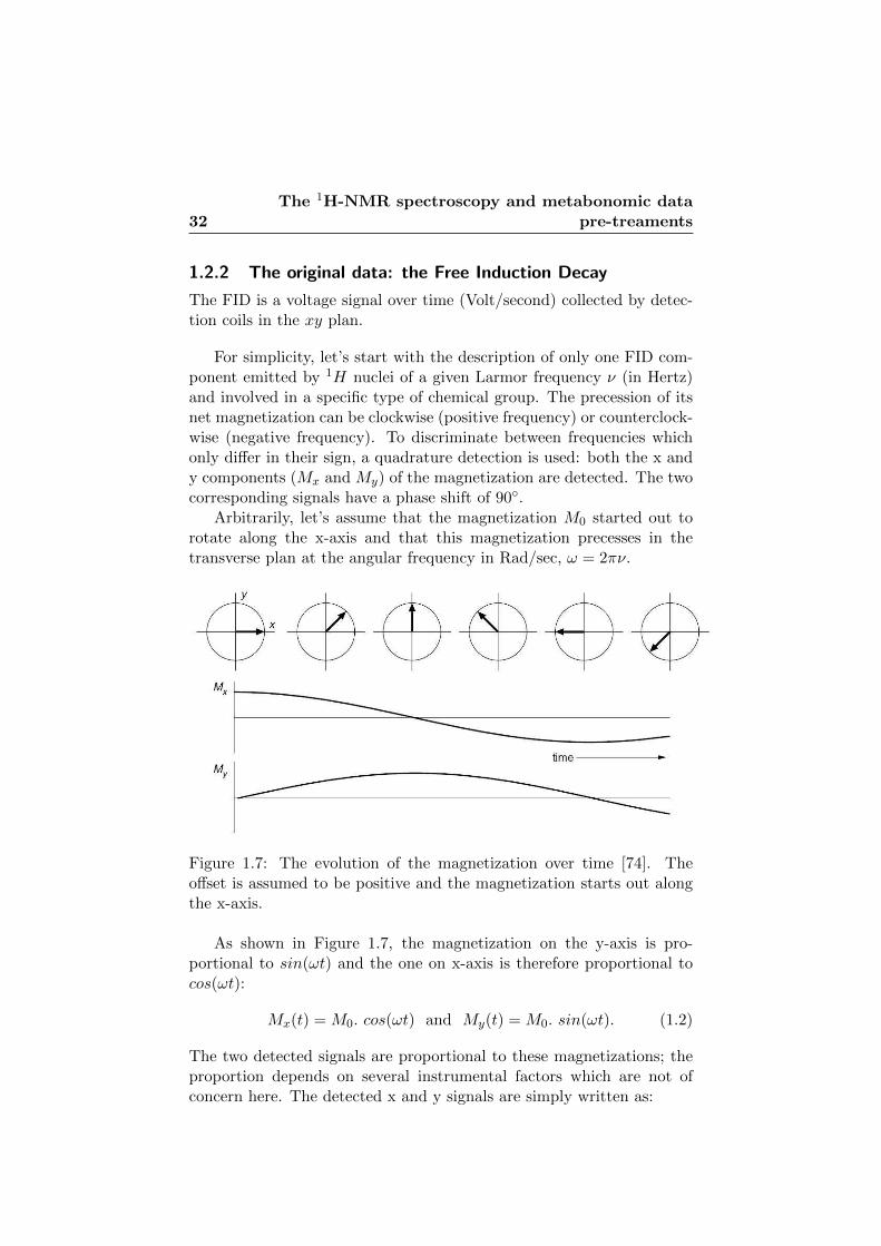
32The 1H-NMR spectroscopy and metabonomic data

pre-treaments

1.2.2 The original data: the Free Induction Decay

The FID is a voltage signal over time (Volt/second) collected by detec-tion coils in the xy plan.

For simplicity, let’s start with the description of only one FID com-ponent emitted by 1H nuclei of a given Larmor frequency ν (in Hertz)and involved in a specific type of chemical group. The precession of itsnet magnetization can be clockwise (positive frequency) or counterclock-wise (negative frequency). To discriminate between frequencies whichonly differ in their sign, a quadrature detection is used: both the x andy components (Mx and My) of the magnetization are detected. The twocorresponding signals have a phase shift of 90◦.

Arbitrarily, let’s assume that the magnetization M0 started out torotate along the x-axis and that this magnetization precesses in thetransverse plan at the angular frequency in Rad/sec, ω = 2πν.

Figure 1.7: The evolution of the magnetization over time [74]. Theoffset is assumed to be positive and the magnetization starts out alongthe x-axis.

As shown in Figure 1.7, the magnetization on the y-axis is pro-portional to sin(ωt) and the one on x-axis is therefore proportional tocos(ωt):

Mx(t) = M0. cos(ωt) and My(t) = M0. sin(ωt). (1.2)

The two detected signals are proportional to these magnetizations; theproportion depends on several instrumental factors which are not ofconcern here. The detected x and y signals are simply written as:

1.2 Proton Nuclear Magnetic Resonancespectroscopy 33

sx(t) = s0. cos(ωt). e−(t/T2) = s0. cos(2πνt). e

−(t/T2). (1.3)

sy(t) = s0. sin(ωt). e−(t/T2) = s0. sin(2πνt). e−(t/T2). (1.4)

where s0 is the overall amplitude of the signal. It is convenient to thinkof this signal as arising from a vector of length s0 rotating at frequencyω. The x and y components of the vector give sx and sy, as is illustratedon Figure 1.8.

Figure 1.8: The x and y components of the signal can be thought of asarising from the rotation of a vector s0 at frequency ω [74].

34The 1H-NMR spectroscopy and metabonomic data

pre-treaments

Additionally, the transverse magnetization decays over time, what isrepresented in the Equations 1.3 and 1.4 by an exponential decay witha time constant T2 (of the order of a second).

As a consequence of the way the Fourier Transform works, it is alsoconvenient to consider sx(t) and sy(t) as the Real and Imaginary partsof a complex signal s(t). The FID component is then written as follow:

s(t) = sx(t) + i. sy(t) (1.5)

= s0. cos(ωt). e−(t/T2) + i. s0. sin(ωt). e−(t/T2) (1.6)

= s0. e(iωt). e−(t/T2) (1.7)

= s0. e(i2πνt). e−(t/T2). (1.8)

An FID component is thus characterized by its frequency ν, amplitudes0 and decay T2 (see Figure 1.9). The frequency ν corresponds to the

Figure 1.9: The characteristics of the FID component.

Larmor frequency of the 1H nuclei emitting the FID component andattests of the presence of a given chemical group in the sample. Theconcentration of the 1H nuclei involved in this chemical group is pro-portional to s0, the amplitude of s(t). In the 1H-NMR experiment,several kinds of 1H nuclei with different Larmor frequencies emit s(t)

1.2 Proton Nuclear Magnetic Resonancespectroscopy 35

with specific values of ν, s0 and T2. Being the sum of all these compo-nents, the recorded FID has a complicated form (see Figure 1.10) thatwe here simply describe as a function of time with a Real and Imaginaryparts:

S(t) = Sx(t) + i. Sy(t). (1.9)

0.5 1 1.5 2 2.5 3

x 104

−1

−0.8

−0.6

−0.4

−0.2

0

0.2

0.4

0.6

0.8

1x 10

6

time

inte

nsity

Figure 1.10: An FID. Time units are second × 10−4.

36The 1H-NMR spectroscopy and metabonomic data

pre-treaments

A Fourier Transform (FT) is used to recover from the FID the dif-ferent FID components involved in its formation. The FT representseach recovered FID component by a peak in a frequency domain spec-trum. The aspect of a spectral peak is determined by the followingcharacteristics of its corresponding FID component:

• the frequency:As shown in Figure 1.11, the FID frequency is decomposed by theFT to recover the frequencies of each FID component. Concretely,the FID component frequency determines the positions of peaksin the frequency scale spectrum. Figure 1.11 gives an example:

Figure 1.11: Examples of FIDs and their spectra [19].

the frequency of the second FID is the sum of the frequencies ofits two components presented below. The frequencies of these twocomponents are separated and illustrated by two peaks in differ-ent positions. In the pre-treatment, the spectral frequency scaleis translated in a chemical shift scale expressed in parts per mil-lion or ppm (see Section 1.3.1.10). More precisely, each frequencypoint of a spectrum is converted in a shift from a specific frequencycorresponding to the peak position of a reference proton. Conse-quently, in a prepared spectrum, the FID components observeddeterminate the appearance of peaks with specific chemical shifts.

1.2 Proton Nuclear Magnetic Resonancespectroscopy 37

• the amplitude:The area under a spectral peak reflects the intensity of the FIDcomponent. The intensity at the first time point also determinesthe phase of the peak.• the shape of the decay:

The decay is described by a time constant of transverse relaxationT2: the lower T2 is, the faster the decay is. The shape of thedecay of the FID component is translated into the broadening ofthe spectral peaks. Indeed, the broadening at the half height of itspeak (”Line Broadening” or LB) is inversely proportional to theT2 of the FID component (see Figure 1.12).

Figure 1.12: The relation between T2 and LB [19].

Generally speaking, the more an FID component decays (T2 low),the larger the LB of the spectral peak is. But the areas underthe spectral peak remain constant and so as it gets broader, thepeak height will decrease. A faster decaying FID component witha same intensity results then in a smaller but broader peak, whatis undesirable as it corresponds to a low signal to noise ratio.

38The 1H-NMR spectroscopy and metabonomic data

pre-treaments

1.2.3 An 1H-NMR analysis

Before FID acquisition, several products are added to each sample:• a reference compound, 3-(trimethylsilyl)propionate-2,2,3,3 (”TMSP”).• a buffer to control pH.• a deuterated water solvent.

Typical volumes for normal 1H-NMR tubes are from 0.5 to 0.7 ml. Thesolution is contained in a glass tube with thin wall. The samples areorganized in standard 96 plate-size tube racks. Automated sample han-dling systems are used to transfer the tubes to the magnet.

Figure 1.13: The three periods of a pulse-acquire experiment and theparameters of acquisition.

A pulse-acquire experiment comes in three periods (see Figure 1.13):

1. the application of the magnetic field B0 (P1): the sample is led tocome to equilibrium.

2. the transfer of energy (P2): radio frequency (RF) power is switchedon for a sufficient time to rotate the net magnetizations through90◦ in the xy plan.

3. the recording (P3): after the RF power is switched off, the netmagnetizations have a decaying rotation returning to the equilib-rium. The resulting voltage is detected.

The duration of P1 and P2 typically are a few microseconds.Several parameters of acquisition (see Figure 1.13) determine the FIDpresented in the previous section:

1.2 Proton Nuclear Magnetic Resonancespectroscopy 39

1. the number of complex data points recorded (mt).The data are digitalized in order to save the data on the computer.A device, the ”Analogue Digital Converter” or ADC is used toconvert the signal from a voltage to a binary number which canbe stored in computer memory. The ADC samples the signal atregular intervals, resulting in a representation of the FID as datapoints. Each of these time points is complex consisting in a Realand an Imaginary part (quadrature detection). Because the FastFourier Transform (FFT) is usually used, mt must be a power of2. The number of spectral points (mf ) equals the number of timepoints (mt) in the FID and the spectral resolution expressed inDigital Resolution (see Section 1.2.4) is inversely proportional tomf or to mt.

2. the Dwell Time (DW): the time interval between two pointssampled in the FID.If the DW is too long, crucial features of the FID are missed.DW is related to the frequency of sampling (Fsampling) in the fol-lowing way:

Fsampling = 1/DW. (1.10)

The Nyquist theorem states that an efficient rate of sampling is atleast twice the frequency of the highest frequency that is containedin the spectrum (Fmax):

Fsampling ≥ 2 Fmax. (1.11)

In this condition, DW = 12Fmax

.

3. the Acquisition time (AQ): the time spent to record the signal.AQ is the number of recorded points multiplied by the time neededto record one point:

AQ = mt ×DW = mt/Fsampling. (1.12)

For a given Fmax, the value of mt determines AQ, what must becarefully chosen to obtain a good signal to noise ratio (SNR) in theFID. Inevitably when the FID is recorded, noise is also recorded atthe same time. Some of the noise is issued from electronics in thespectrometer, but the major contributor is the thermal noise fromthe coil used to detect the signal. By its nature, the FID decaysover time but in contrast the noise remains constant. The SNR

40The 1H-NMR spectroscopy and metabonomic data

pre-treaments

(amplitude of the FID divided by the noise level) is thus muchlower in the tail part of the FID that in the beginning. Therefore,if AQ is too long, by recording the FID for long after it has decayed,only noise and no signal are recorded in the final part, reducing theSNR. On the opposite, if the AQ is too short, the FID is missedwhat also results in a reduction of the SNR.

In practice, the spectroscopist fixes the values of mt and of the Fmax.The other parameters are deduced from these lasts. A typical situationis the following: the spectroscopist fixes the number of complex datapoints to 32768. Fmax is 5122.95Hz. The Fsampling is then twice theFmax: 10245.9Hz. Finally, the AQ is computed as 32768/10245.9 = 3.20seconds.

1.2 Proton Nuclear Magnetic Resonancespectroscopy 41

1.2.4 A typical 1H-NMR spectrum

The spectrum is the translation in a frequency domain of the FID timedomain signal performed by the Fourier Transform. As mentioned above,this allows separating the FID components represented through spectralpeaks with position that are specific to their frequencies. The differentfrequencies in the spectrum correspond to the different kinds of 1H ac-cording to the fact that they emit at different frequencies under theinfluence of their surroundings.The information contained in the spectrum is represented by the follow-ing spectral features:

• the positions of peaks:The position of a peak is the expression of a specific frequency ofemission and attests the presence in the sample of a kind of protonwith specific electron surrounding. Note that small interactions(couplings) between the different groups of protons involved in asame molecule can lead to the appearance of several peaks for asame group of proton (”multiplicity of peaks”). Based on estab-lished couplings of peaks, the molecules contained in the sampleare deduced from the observation of several peaks in specific posi-tions, in other words of several kind of protons groups.

• the area under the peaks:The area under a peak in a specific position is proportional to theconcentration in the sample of the kind of proton emitting at thisfrequency. Consequently, the concentration of a molecule in thesample is obtained from the areas under its corresponding spectralpeaks.

A simple example is given in Figure 1.14 showing the spectrum of asample containing only para-xylen [38].It must be noted that in this spectrum, the Hertz frequency scale istranslated in “part per million” (ppm) in order to be independent ofthe kind of spectrometer used (see Section 1.3.1.10). The para-xylenmolecule presents two different kinds of protons: a first kind are 1Hinvolved in methyl (CH3) and a second kind are 1H involved in anaromatic group. As expected, the spectrum presents then two peaksin different positions corresponding to the two different frequencies ofemission of the two kinds of protons: one at 2.20 ppm and the otherat 6.95 ppm. A peak at 2.20 ppm is known to correspond to a methylgroup and a peak at 6.95 ppm to a 1H involved in an aromatic group.Together, these two information allow us to deduce the presence of para-xylen. The concentration of this molecule is then determined from the

42The 1H-NMR spectroscopy and metabonomic data

pre-treaments

Figure 1.14: The 1H-NMR spectrum of para-xylen.

areas under these peaks. Peak areas estimation is realized by integrals.Two principal methods may be used for quantification in 1H-NMR: theabsolute method with reference to an internal standard compound andthe calibration method with reference to a calibration model.

1.2 Proton Nuclear Magnetic Resonancespectroscopy 43

Figure 1.15: The high resolution 1H-NMR spectrum of urine (top) andof serum (bottom) on a ppm scale.

A typical 1H-NMR spectrum of urine contains thousands of sharplines from predominantly low molecular weight metabolites (see Figure1.15). Blood serum contains low and high molecular weight components,and this gives a wide range of signal line widths (see Figure 1.15). Broadbands from protein and lipoprotein signals contribute strongly to these1H-NMR spectra, with sharp peaks from small molecules superimposedon them. Spectral databases respectively exist to identify molecules inurine and blood spectra according to the positions of spectral peaks.Technical characteristics of a spectrum are the following:

• the spectral windows (SW ) or the total spectral width.

• the number of frequency points contained in SW: mf .

44The 1H-NMR spectroscopy and metabonomic data

pre-treaments

• the spectral resolution expressed by the Digital Resolution (DR):DR is the space between two points of the spectrum expressed inHertz. The larger the spectral resolution is, the lower the DR isand the opposite [60]. For a given SW, DR is defined :

DR = SW/mf . (1.13)

A spectrum of high DR has a small number of points mf and showssharp peaks for which the maximum can be not well determined.A low DR or a low mf is then not favorable.

1.3 Metabonomic data pre-treatments 45

1.3 Metabonomic data pre-treatments

The FID is not directly exploitable. Basically, the Free Induction Decay(FID) generated by the spectrometer needs to be Fourier transformed.Additionally, due to instrumental 1H-NMR parameters and limitations,the original metabonomic data also contains noise, artifacts (peak distur-bances or ”phase shift”, artifacts in the baseline). Due to the biologicalcharacter of the samples studied in metabonomics, 1H- spectra are alsomodified under the influence of pH, and diuretic fluctuations.

All these problems modify the quality of the spectral description ofmetabolites and/or create spectral variations that are non informative asspectral biomarker, which might greatly interfere with the metabonomicstatistical data analysis. Data pre-treatments aim at removing this un-desired variability, noise and artifacts. A data pre-treatment procedureconsists in a combination of operations based on statistical and/or math-ematical principles, performed on time or frequency 1H-NMR data.

While the statistical analysis of the data is called ”processing”, theseoperations in the literature are interchangeably called by ”pre-treatment”,”pre- or post-processing”. Recent literature [36] introduces a distinc-tion between two categories of treatments: ”Pre-processing” proceduresrepresent the methods going from raw instrumental data to data onwhich statistical analysis can be applied (”cleaned data”). The termpre-treatment designates further transformations (ex: scaling, center-ing) of the ”cleaned data” before the statistical analysis. For simplicity,in this chapter, the term ”pre-treatment” is used for both kinds of op-erations.

The efficiency of the data pre-treatments is an important issue forthe performance of the metabonomic statistical analysis and the in-terpretation of the biomarkers. Up to now, no guideline or standardpre-treatments are referenced for 1H-NMR metabonomic data. Many1H-NMR metabonomic practitioners currently perform the classical pre-treatments for the standard 1H-NMR. Sometimes, they add pre-treatmentsacquired from their experience in the field of metabonomic to controlproblems specific to the nature of metabonomic samples. In the COMETstudies (see Section 0.2), the data pre-treatment procedure took intoaccount the problematic of pH and diuretic variations by the involve-ment of two pre-treatments: the bucketing and the normalization. ThisCOMET pre-treatment procedure is in this thesis referred as the usualmetabonomic 1H-NMR pre-treatment procedure and is represented inthe left part of Figure 1.16.

46The 1H-NMR spectroscopy and metabonomic data

pre-treaments

Figure 1.16: The usual and the advised pre-treatment procedures.

1.3 Metabonomic data pre-treatments 47

This procedure presents some weaknesses: bucketing corrects pHinduced misalignment but at the price of a large decrease of spectralresolution, what corresponds to a loss of information. The correctionof the diuretic spectral variation by the COMET normalization remainsimperfect due to the presence of the water peak particularly sensitive tothe dilution of metabonomic biofluid. Moreover this peak is predominantand occults the lowest spectral peaks. On the operational side of thisprocedure, the pre-treatment steps are successively applied using a com-bination of several pre-treatment softwares, most of the time developedby spectrometer sellers. Common softwares are the Bruker Topspin andAMIX 1 2 softwares. Such non-automated classical pre-treatment proce-dures are long and fastidious, some steps being individually applied oneach spectrum (Phase correction, Baseline correction). Moreover, mostof them involve a lot of human interventions what exposes to the risk ofa quality depending of the user expertise.

Aware of the impact of the weaknesses of spectral data preparedwith the usual procedure on the conclusions of their metabonomic stud-ies, Eli Lilly developed with Paul Eilers in 2006 a new tool for 1H-NMRmetabonomic data pre-treatments: ”Bubble”[91], a free library in Mat-lab in which all the 1H-NMR data operations are automatized. Bubbleincludes new kinds of pre-treatment for the water suppression and toalign spectra (”Parametric Time Warping”). Bubble also offers innovat-ing methods for pre-treatments already included in the usual procedure,the phase and baseline corrections.

1.3.1 Advised pre-treatments procedure

Since the early work of this thesis, Bubble was used to prepare the data.From this experience, good practices were defined with the spectro-scopists of the University of Liege (ULg). On this basis, a pre-treatmentprocedure is here proposed combining a step by step use of Bubble withsome additional operations that we developed independently. Figure1.16, on its right part, illustrates our advised procedure. The steps thatwere already proposed in Bubble are surrounded.

In comparison to the Bubble procedure, the advised procedure pro-poses two categories of additional operations.

A first category has the goal to improve the Bubble procedure. In-deed, from our investigations of the performances of Bubble to prepare1H-NMR metabonomic data, it appeared that the use of the Bubblemethods, on one hand, allows us to solve specific data problems but, on

1http://www.bruker-biospin.com/topspin3-dir.html2http://www.bruker-biospin.com/amix.html

48The 1H-NMR spectroscopy and metabonomic data

pre-treaments

the other hand, sometimes also creates new ones. Consequently, someoperations are added here to correct the imperfections of Bubble. Forexample, the Bubble phase and baseline corrections can induce negativevalues. As negative values have no sense and create problems in thefollowing steps, we set these descriptors to zero.

Bubble is, in the advised procedure, also completed by other op-erations: a new bucketing, the removal of undesired regions, a citrateaggregation for urine samples and a normalization. The normalizationwas already included in the typical procedure but the removal of unde-sired regions and a citrate aggregation for urine sample were advised bythe experience of spectroscopists. The bucketing already involved in theusual procedure has been improved with a more effective interpolationalgorithm. Moreover, for urine samples, the inclusion of the citrate ag-gregation advised by spectroscopists has been improved to be includedin the advised procedure.

The advised procedure involves 15 steps. Five of them are realizedon the FID.

The 15 steps are described in the following subsections; each of themis illustrated on the same serum metabonomic observation. Finally,Subsection 1.3.2 gives a summary of the procedure and Table 1.1 presentsthe mathematical formulation of the output in each pre-treatment step.

1.3.1.1 Step 0: the initial FID

The input data of the pre-treatment procedure is a FID function on mt

complex time points, t = 1, ...,mt.To the FID description given in Section 1.2.2, it must be added that

the FID presents a group delay at its beginning. Actually, when an FIDis recorded, the instrument also takes into account signal components offrequencies higher or lower than the ones focused in the spectral window.Their presences produce in the spectrum a folding effect: ghost peaksappear in the spectrum. To avoid this effect, the 1H-NMR manufactorBruker automatically applies a digital filter during the recording. Unfor-tunately, this digital filter contributes to the presence of a ”group delay”at the beginning of the stored initial FID, S(t)step 0. The intensities ofS(t)step 0 do not start as expected at its maximum followed by a decay:the Real part intensity is now starting from zero at the first data pointand rises to a maximum after the 60 first data points (see Figure 1.17).

1.3 Metabonomic data pre-treatments 49

0 1 2 3 4

x 104

−1

0

1

2

3x 10

6 Real part

inte

nsity

0 50 100 150 200−1

0

1

2

3x 10

6

0 1 2 3 4

x 104

−3

−2

−1

0

1x 10

6

time

inte

nsity

Imaginary part

0 50 100 150 200−3

−2

−1

0

1x 10

6

time

Figure 1.17: An FID. Left figures show the total FID. Right figures showa zoom on the beginning of the FID illustrating the group delay.

1.3.1.2 Step 1: first order phase correction

The general goal of a phase correction is to correct the appearance ofthe spectrum what depends on the position of the FID at time zero(”phase”). In an ideal or ”phased” 1H-NMR spectrum, all the peaks ofthe Real spectrum have positive values (”absorptive mode” - see Fig-ure 1.18 [19]) while the peaks of the Imaginary spectrum have positiveand negative parts (”dispersive mode”). These spectral configurationsare only observed for an FID function with characteristics of a phasesituation S(t)phased: at time zero, the recorded Real part of the FID,Sx(t)phased is a maximum and the recorded Imaginary part of the FID,Sy(t)phased is zero.In practice, due to several factors, the initial complex FID, S(t)step 0,presents thus a ”phase shift or error”: at time zero the recorded Sx(t)step 0

is not a maximum and Sy(t)step 0 is not zero. Indeed, the initial complexFID is:

S(t)step 0 = S(t)phased .e(iφ). (1.14)

where φ is the phase error.Due to this phase error, the FT of S(t)step 0 results in a spectrum

with impure Real part Re(ν) and impure Imaginary part Im(ν) which

50The 1H-NMR spectroscopy and metabonomic data

pre-treaments

Figure 1.18: The absorptive and dispersive modes.

are mixtures of absorptive and dispersive modes, with proportions thatvary with ν.

If there is a phase error of magnitude φ, this can be corrected byusing the impure Re(ν) and Im(ν) in the equations:

Re′(ν) = Re(ν) .cos(φ) + Im(ν) .sin(φ) . (1.15)

Im′(ν) = Re(ν) .sin(φ)− Im(ν) .cos(φ) . (1.16)

where Re′(ν) and Im′(ν) are the Real and Imaginary spectra correctedfor the phase error. The objective of this correction is to obtain an pureabsorptive Re′(ν).

The problem of phase correction then consists in finding the correctangle φ. Two kinds of phase errors are to take into account:

1. Those causing an equal amount of phase error on all the frequenciesof the spectrum. They are called zero order phase error. They canarise for instance from the inability of the spectrometer to detectthe exact Mx(t) and My(t).

2. Those who are frequency dependent or first order phase error. Onecause of such phase error is the delay between the end of the RFpulse and the start of acquisition. The presence of a ”group delay”,explained in step 0, is thus equivalent to the application of a phaseshift, depending on the frequency of the domain of frequencies(first order phase shift)[96].

The total phase error φ is the sum of a frequency-independent term anda linear frequency-dependent term:

φ = ϕ0 + ϕ1(ν). (1.17)

In the usual pre-treatments, the spectroscopist visually chooses thevalue of φ in two successive stages of one pre-treatment step: one for

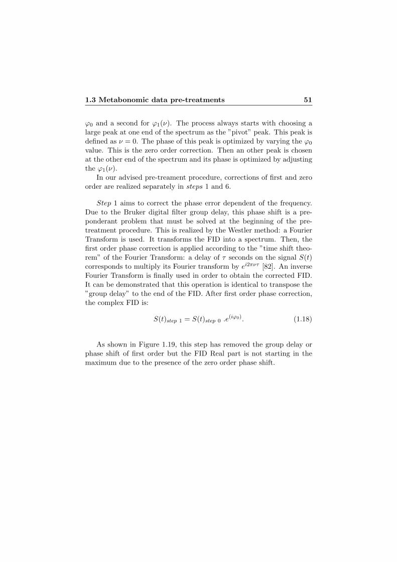
1.3 Metabonomic data pre-treatments 51

ϕ0 and a second for ϕ1(ν). The process always starts with choosing alarge peak at one end of the spectrum as the ”pivot” peak. This peak isdefined as ν = 0. The phase of this peak is optimized by varying the ϕ0

value. This is the zero order correction. Then an other peak is chosenat the other end of the spectrum and its phase is optimized by adjustingthe ϕ1(ν).

In our advised pre-treament procedure, corrections of first and zeroorder are realized separately in steps 1 and 6.

Step 1 aims to correct the phase error dependent of the frequency.Due to the Bruker digital filter group delay, this phase shift is a pre-ponderant problem that must be solved at the beginning of the pre-treatment procedure. This is realized by the Westler method: a FourierTransform is used. It transforms the FID into a spectrum. Then, thefirst order phase correction is applied according to the ”time shift theo-rem” of the Fourier Transform: a delay of τ seconds on the signal S(t)corresponds to multiply its Fourier transform by ei2πντ [82]. An inverseFourier Transform is finally used in order to obtain the corrected FID.It can be demonstrated that this operation is identical to transpose the”group delay” to the end of the FID. After first order phase correction,the complex FID is:

S(t)step 1 = S(t)step 0 .e(iϕ0). (1.18)

As shown in Figure 1.19, this step has removed the group delay orphase shift of first order but the FID Real part is not starting in themaximum due to the presence of the zero order phase shift.

52The 1H-NMR spectroscopy and metabonomic data

pre-treaments

0 1 2 3 4

x 104

−4

−3

−2

−1

0

1x 10

6 Real part

inte

nsity

0 50 100 150 200−4

−3

−2

−1

0

1x 10

6 Real part

0 1 2 3

x 104

−1.5

−1

−0.5

0

0.5

1

1.5x 10

6 Imaginary part

time

inte

nsity

0 50 100 150 200−1.5

−1

−0.5

0

0.5

1

1.5x 10

6 Imaginary part

time

Figure 1.19: An FID after first order phase correction. Figures on the leftshow the total FID. Figures on the right show a zoom on the beginningof the FID. The group delay is deleted.

1.3.1.3 Step 2: suppression of the solvent signal

The solvent is by definition the major component into the solution whichresults in an intense peak in the spectrum. In metabonomics, the solventis the water and the peaks of the water molecules are consequently moreintense. During the 1H-NMR experiment, the water signal has alreadybeen reduced by techniques of water pre-saturation. However, residualsof water remains in the spectrum. In comparison to all the other peaks,the residuals of water are less stable and stills higher, risking to hideother peaks from informative compounds (see Figure 1.20).

This thesis proposes to suppress the water resonance directly fromthe FID. The FID signal component corresponding to the water S(t)water,is modelled and substracted from the original FID. The FT of the mod-ified FID then produces a spectrum without the water-solvent peak.

The solvent signal being generally a strong and predominant com-ponent of the recorded FID, S(t)water is simply modelled as a smoothedfunction of the FID (see Figure 1.21 a and b).

1.3 Metabonomic data pre-treatments 53

0.9 1 1.1 1.2 1.3 1.4 1.5 1.6 1.7 1.8 1.9

x 104

0

5

10

x 107

inte

nsity

0.9 1 1.1 1.2 1.3 1.4 1.5 1.6 1.7 1.8 1.9

x 104

0

5

10

x 107

time

inte

nsity

Figure 1.20: The spectrum before (on top) and after (below) the watersuppression.

In practice, S(t)water is fitted separately on the Real and Imaginary partsof the FID with a Whittaker smoother with second-order differences [25],a smoother based on penalized least squares. Let us consider an FID asa series y and the water FID component to fit as a series z, each oneof mt values. To fit the smooth series z to y, the Whittaker smoothersearches the series z that minimizes:

Q = V + λR. (1.19)

where:

• V =∑mt

j=1(yj − zj)2. This term measures the lack of fit of to thedata.

• R =∑(mt−2)

j=1 (42j )

2 where 42j = (zj−zj−1)−(zj−1−zj−2). Squar-

ing and summing the second-order differences gives us a simpleand effective measure of the roughness of z.

• λ is a penalty on roughness. The larger λ is, the stronger theinfluence of R on the goal Q and the smoother z will be. Thedefault value in Bubble is 105.

54The 1H-NMR spectroscopy and metabonomic data

pre-treaments

0 1000 2000 3000 4000 5000−1.5

−1

−0.5

0

0.5

1x 10

6 Real part

inte

nsity

0 1000 2000 3000 4000 5000−1

−0.5

0

0.5

1x 10

6 Imaginary part

time

0 1000 2000 3000 4000 5000−1.5

−1

−0.5

0

0.5

1x 10

6

inte

nsity

time0 1000 2000 3000 4000 5000

−1

−0.5

0

0.5

1x 10

6

time

(a) (b)

(d)(c)

Figure 1.21: The two upper figures, (a) and (b), show the FID partsbefore water suppression and the estimations of the water signal in red.The two lower figures, (c) and (d), are the FID parts after water removal.

The minimization of Equation 1.19 is achieved by solving the followingsystem of equation:

z = (I + λD′D)−1y . (1.20)

where D is a ((mt − 2)×mt) matrix such that Dz = 42z.The two fitted series on Real and Imaginary FID, Sx(t)water and

Sy(t)water, are respectively substracted:

Sx(t)step 2 = Sx(t)step 1 − Sx(t)water . (1.21)

Sy(t)step 2 = Sy(t)step 1 − Sy(t)water . (1.22)

S(t)step 2 is the FID function after water suppression, defined for amt time points t = 1, ...,mt. It can be seen in Figure 1.20 that the waterpeak (near the point 1.6 × 104) has been removed by this operation.

1.3 Metabonomic data pre-treatments 55

Unfortunately, water residuals and negative values have been created inthis spectral region.

56The 1H-NMR spectroscopy and metabonomic data

pre-treaments

1.3.1.4 Step 3 and 4: apodizations

The apodization (or window processing) aims at increasing the SNR ofthe spectrum by multiplying the FID by a function which emphasizesthe initial portion of the FID and understates the later noisy portion.Multiplying an FID by a function results in changing the shape of thespectrum but not the frequencies (FT similarity theorem). Differentapodization functions can be chosen.

We suggest to combine two apodizations:

• an apodization by a ”scale function” giving a weight of 1 to the firsthalf of the FID and a weight of 0 to the second half. Consequently,the end of the FID is deleted assuming that this part is only madeof noise. The resulting FID is:

S(t)step 3 =

{S(t)step 2 if 0 ≤ t≤ mt/2,

0 if mt/2 < t≤ mt.(1.23)

• an apodization by an ”negative exponential function”: the FID ismultiplied by a negative exponential function (see Figure 1.22):

h(t) = e−t/a. (1.24)

As h(t) distributes a lower weight to the data at the end of the

0 0.5 1 1.5 2 2.5 3 3.5

x 104

−2.5

−2

−1.5

−1

−0.5

0

0.5

1

1.5x 10

6

time

intensity

Figure 1.22: The FID before apodization (in black) and the exponentialapodization function h(t) (in red).

1.3 Metabonomic data pre-treatments 57

FID, in S(t)step 4 the contribution from the noisy right-hand sideis suppressed and the resulting spectrum presents less noise (seeFigure 1.23).When the apodization is applied on S(t)step 3, for (mt/2 < t ≤mt), S(t)step 4 = 0 . For (0 ≤ t ≤ mt/2), this results in a newtime function S(t)step 4 with a faster decay. This change of decayis illustrated on Figure 1.23: after apodization the FID decreasesfaster.

The h(t) decay constant, a needs to be carefully chosen for tworeasons:

1. If a is to small, the decay can be strong enough to delete theleft hand side of the FID which contains mainly the signal.

2. As the apodized FID has a new stronger decay, the T2 decayconstants of the FID components can then be reduced whatresults in taller and broader spectral peaks (see Section 1.2.2).

The decay constant a should then be sufficiently big to suppressthe noise in the tail of S(t)step 3 but not too large to avoid thesetwo problems. The same function h(t) can be used to performapodization of all the spectra of a study. Apodization is providedin the usual softwares by a default value a. In Bubble a constantof 1Hz is used.

It can be seen in Figure 1.23 that the exponential apodizationfunction with a = 1Hz does not significantly affect the signal atshort times, does not create broader peaks but greatly reduces thenoise at later times.

58The 1H-NMR spectroscopy and metabonomic data

pre-treaments

0 1 2 3 4

x 104

−2

−1

0

1x 10

6

inte

nsity

0 1 2 3 4

x 104

−2

−1

0

1x 10

6

0.8 1 1.2 1.4 1.6 1.8 2

x 104

−2

0

2

4

6

8x 10

7

inte

nsity

0.8 1 1.2 1.4 1.6 1.8 2

x 104

−2

0

2

4

6

8x 10

7

1.4 1.45 1.5 1.55

x 104

0

1

2

3

4x 10

7

frequency

inte

nsity

1.4 1.45 1.5 1.55

x 104

0

1

2

3

4x 10

7

frequency

Figure 1.23: The two upper figures show the Real part of the FID before(left) and after (right) apodization. The two figures in the middle arethe corresponding spectra. The two lower figures show a zoom on thesespectra.

1.3.1.5 Step 5: Fourier Transform

The Fourier Transform (FT) is used on this composite signal to discoverthe frequencies of the different nuclei in the sample. More precisely,the FT extracts from the composite FID each signal component andtranslates this component into a peak in a spectrum. This peak hasa position that is specific to the frequency of the corresponding signalcomponent. The peak height depends on the amplitude of the signalcomponent and its width at half height is determined by its decay rate.

The FT decomposes a periodical function into an infinite sum ofa sinusoidal signals. As the FID is a complex function, it could besubmitted to the FT to produce a complex function of frequency F (ν)

1.3 Metabonomic data pre-treatments 59

with a Real and an Imaginary spectrum. The FT is:

F (ν) =

∫ +∞

0f(t) e−i2πνt dt (1.25)

=

∫ +∞

0f(t) [cos(2πνt)− i sin(2πνt)] dt. (1.26)

where:

• F (ν) is the Fourier transformed owning as argument, ν, the fre-quency.

• f(t) is the periodical function with argument, t, the times.

In our case, we work with discrete data and a discrete version of thisformula is used, which is for a signal S(t) of mt complex data points:

F (ν)step 5 =

mt−1∑t=0

S(t)step 4 e−2iπkt/mt . (1.27)

where S(t)step 4 and F (ν)step 5 are complex functions. The DiscreteFourier Transform (DFT) requires data sampling at regular time inter-vals until the signal is close to zero, and truncation of the FID will leadto artifacts.

After FT, the data is a complex spectral function F (ν)step 5 on mf

frequency points ν = 1, ...,mf . mf is equal to mt, the number of FIDtime points. Figure 1.24 shows the Real and the Imaginary parts, Re(ν)and Im(ν), of F (ν)step 5.Before FT, the FID presented a phase shift of zero order what results indispersive peaks (see Section 1.3.1.2) on both the Real and Imaginaryspectra of Figure 1.24.

60The 1H-NMR spectroscopy and metabonomic data

pre-treaments

0 0.5 1 1.5 2 2.5 3 3.5

x 104

−6

−4

−2

0

2x 10

7

inte

nsity

0 0.5 1 1.5 2 2.5 3 3.5

x 104

−4

−2

0

2

4x 10

7

frequency

inte

nsity

Figure 1.24: The spectrum after Fourier Transform: the Real and Imag-inary parts.

1.3.1.6 Step 6: zero order phase correction

Step 5 has performed a FT of the FIDstep 4 which involves a zero orderphase shift: e(iϕ0). The resulting F (ν)step 5 is thus a spectrum witha phase shift assumed to be equal at all the frequency points of thespectrum (see Section 1.3.1.2): F (ν)step 5 = F (ν)phased. e

(iϕ0) whereF (ν)phased is the phased spectrum and ϕ0 the independent phase error.The correction is realized as described in Equation 1.16 and 1.17 withφ corresponding to the independent phase error:

φ = ϕ0. (1.28)

The optimal φ angle is found in an automatic way which do not requirethe intervention of the spectroscopist. Based on the fact that an idealspectrum is positive, Bubble tries a zero order correction with all theangles between −180 ◦ and +180 ◦ and keeps the angle that gives the”most positive” spectrum. The criterion used to measure positiveness isrms, the ratio of the sum of squares of the negative parts to the total ofthe sum of squares of the spectrum. For a tested angle φ, the spectrumobtained with this correction is F

′φ(ν) described by mf values. The rms

1.3 Metabonomic data pre-treatments 61

is computed as:rms = ssa/ssb . (1.29)

ssa =

√√√√mf∑j=1

(F′φ(νj)− a)2 × indj . (1.30)

ssb =

mf∑j=1

(F′φ(νj)− b)2 . (1.31)

where:• indj is a binary vector with indj = 1 if νj < 0 and indj = 0

otherwise.• a represents the mean intensity of the frequencies which are neg-

ative after correction

a =

∑mf

j=1(F′φ(νj)× indj)∑mf

j=1 indj. (1.32)

• b represents the mean intensity for all the frequencies after correc-tion

b =

∑mf

j=1 F′φ(νj)

mf. (1.33)

This correction results in a phased function, F (ν)phased with a Realpart Re′(ν) and an Imaginary part Im′(ν). In the following of themetabonomic study, the Real part of F (ν)phased will be the onlyspectrum used. At the end of step 6, the data are thus:F (ν)step 6 = Re′(ν).

As shown by the comparison between the upper graph in Figure 1.24and Figure 1.25, F (ν)step 6 spectrum is more absorptive than the Realpart of F (ν)step 5and then presents more peaks. Besides this improve-ment, Figure 1.25 illustrates that the phase correction also creates neg-ative values. Anyway these negative values are few in proportion, lowerthan with some classical phase correction methods for which the perfor-mances depend on the experiment of the spectroscopist. In a metabo-nomic study involving several spectra, the usual as the Bubble phasecorrection requires to define the angle φ individually for each spectrum.The automated method of Bubble represents an important benefit oftime.

62The 1H-NMR spectroscopy and metabonomic data

pre-treaments

0 0.5 1 1.5 2 2.5 3 3.5

x 104

−1

0

1

2

3

4

5

6x 10

7

frequency

inte

nsity

Figure 1.25: The Real part of the resulting zero order phased spectrum,F (ν)step 6.

1.3.1.7 Step 7: baseline correction

In the spectrum, frequencies in which no signal was emitted by thesample are supposed to be equal to zero. Nevertheless, even when thephasing is completed, some of these νj still exhibit baseline artifacts(values different from zero) due to imperfections and non linearities ofthe electronic detection process. Baseline correction aims to suppressbaseline artifacts.

A good baseline correction is important for several reasons:

• The baseline artifacts are values having no molecular interpreta-tion. Consequently, they could alter the subsequent statisticalanalysis.• The efficiency of the warping (see Section 1.3.1.9) will be reduced

on spectra with a bad baseline: in this situation, the warpingfunction would try to match the artifacts instead of the interestingparts of the spectrum.• Poor baseline suppression would also change the peak heights and

integrals which are important for the statistical analysis.

The most convenient way to correct baseline distortions is to constructa model of the baseline in the frequency domain and subtract it fromthe spectrum [35]. Traditional 1H-NMR desktop softwares allow theuser to choose points belonging to the baseline manually and interpolate

1.3 Metabonomic data pre-treatments 63

between them a polynomial function to be subtracted from the spectrum.Bubble subtracts for each spectrum point a baseline Z(ν) estimated

by an algorithm developed by Paul Eilers in cooperation with HansBoelens [27]:

F (ν)step 7 = F (ν)step 6 − Z(ν). (1.34)

The baseline estimator is obtained by the combination of a Whittakersmoother (see Section 1.3.1.3) with asymmetric least squares (AsLS).Asymmetric least squares assigns different weights to the data pointsthat are above and below the trend.

Z(ν) is found by minimizing:

Q =

mf∑j

wj(F (νj)− Z(νj))2 + λ

mf∑j

(∆2Z(νj))2. (1.35)

where:

• F (ν) is the spectral function with F (νj), the intensity at frequencyνj .

• Z(ν) is the smoothed baseline function.

• wj a weight for the νj . wj = p if F (νj) > Z(νj) and wj = (1− p)if F (νj) ≤ Z(νj). The default value of p in Bubble is 0.05.

• λ is a positive parameter setting the weight of the second term,the roughness penalty; the larger λ, the smoother Z(νj) will be.The default value of λ in Bubble is 106.

• ∆2Z(νj) = (Z(νj)− Z(νj−1))− (Z(νj−1)− Z(νj−2)).

The first term measures the fit to the data by least squares. Asymmetricweighting is used in order to create a positive corrected signal: the pos-itive deviations ((F (νj)− Z(νj)) > 0) with respect to baseline estimateare weighted less than negative ones.

The second term penalizes the non smoothness of Z(ν). Parameterλ tunes the balance between the two terms.

The first graph in Figure 1.26 shows the spectrum before the baselinecorrection with the estimated baseline Z(ν) in red. In order to obtain abaseline equal to zero after correction, spectral regions presenting a neg-ative baseline distortions (as the water region) correspond to a negativeestimated baseline and inversely.

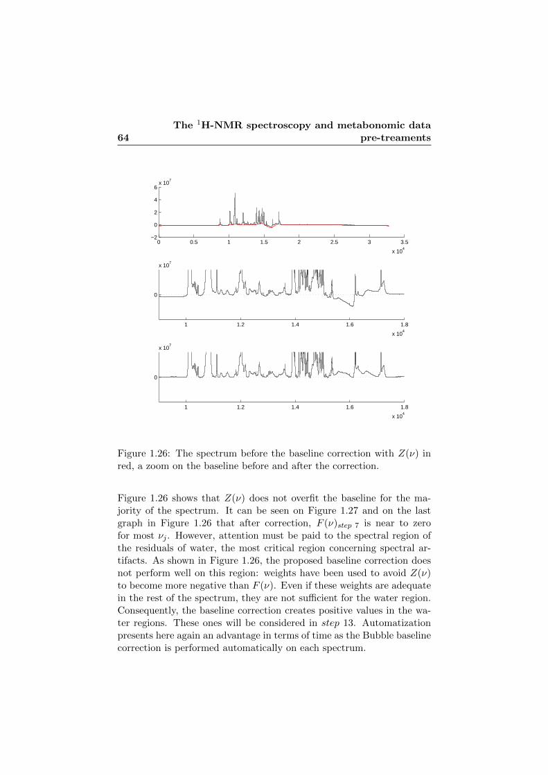
64The 1H-NMR spectroscopy and metabonomic data

pre-treaments

0 0.5 1 1.5 2 2.5 3 3.5

x 104

−2

0

2

4

6x 10

7

1 1.2 1.4 1.6 1.8

x 104

0

x 107

1 1.2 1.4 1.6 1.8

x 104

0

x 107

Figure 1.26: The spectrum before the baseline correction with Z(ν) inred, a zoom on the baseline before and after the correction.

Figure 1.26 shows that Z(ν) does not overfit the baseline for the ma-jority of the spectrum. It can be seen on Figure 1.27 and on the lastgraph in Figure 1.26 that after correction, F (ν)step 7 is near to zerofor most νj . However, attention must be paid to the spectral region ofthe residuals of water, the most critical region concerning spectral ar-tifacts. As shown in Figure 1.26, the proposed baseline correction doesnot perform well on this region: weights have been used to avoid Z(ν)to become more negative than F (ν). Even if these weights are adequatein the rest of the spectrum, they are not sufficient for the water region.Consequently, the baseline correction creates positive values in the wa-ter regions. These ones will be considered in step 13. Automatizationpresents here again an advantage in terms of time as the Bubble baselinecorrection is performed automatically on each spectrum.

1.3 Metabonomic data pre-treatments 65

0 0.5 1 1.5 2 2.5 3 3.5

x 104

−1

0

1

2

3

4

5x 10

7

frequency

inte

nsity

Figure 1.27: The spectrum after the baseline correction.

1.3.1.8 Step 8: setting negative values to zero

Some frequencies still have negative values due to an imperfect phase orbaseline correction. Since negative values have no meaning, they can allbe set to zero.

F (ν)step 8 = F (ν)step 7 × h(ν)step 8. (1.36)

where

h(ν)step 8 =

{1 if F (ν)step 7 ≥ 0,

0 if F (ν)step 7 < 0.(1.37)

1.3.1.9 Step 9: warping

The 1H-NMR biofluid spectra are rarely perfectly aligned (see Figure1.28 on the top). Peak positions may be affected by variations in exper-imental conditions such as temperature and pH [57]. In this situation,the spectral intensity at a given frequency may be due to both changes inmolecular concentrations as well as shifts in resonance positions, makingthe interpretation of statistical analysis difficult.

The usual method to correct misalignment is the ”bucketing”: theresolution of spectra is decreased to hide the differences (see Section1.3.1.12).

66The 1H-NMR spectroscopy and metabonomic data

pre-treaments

More refined alignment methods for 1H-NMR data are proposed inthe literature. One example is partial linear fit (PLF), a method outlinedby Vogels [93]. PLF automatically picks out segments in an 1H-NMRspectrum of size d and shift them s points left and right. Every possibleand relevant combination of d and s is tried until the sum of squareddifferences between the spectrum and the target for alignment is mini-mized. Another approach, outlined by Brown and Stoyanova, removesboth frequency and phase shifts in 1H-NMR spectra by using PCA todetermine the misalignment in a single peak appearing across a series ofspectra.

The Bubble software proposes a new alignment correction beforedata reduction: the Parametric Time Warping [26]. The warping isa registration method: the idea is to match peaks in two spectra bycomputing a function to transform the horizontal frequency axis. Thewarping function w(ν) must then represent the distortions of the fre-quency axis and the warped spectrum is computed as:

Fstep 9(ν) = F (w(ν))step 8. (1.38)

Suppose that we have two spectra, represented as two series fj =F (ν) and vj = V (ν) with j = 1, ...,mf . A sum of third order polynomialand a set of B-splines is used to model the warping function:

w(ν) =

K∑k=0

βkνk +

L∑l=0

αlBl(ν). (1.39)

where

•∑K

k=0 βkνk is a polynomial of degree K (K = 3), βk the coefficient

of degree k.

•∑L

l=0 αlBl(ν) is a set of L B-splines (L= 40), and αl is the warpingcoefficient for the lth B-spline Bl.

Quite complex patterns of forward and backward shifting of peaks canoccur and can not be captured by just polynomials, even if high ordersare used, like quadratic polynomials and beyond. This is why the poly-nomial is here extended with scaled local basis functions, B-splines. TheB-splines look like normal distributions but they consist in polynomialsegments (quadratic or cubic) joined together.

A warping function w(ν) is built such that F (w(ν)) is close to V (ν).A natural measure of nearness is the integral of squares of differences.

1.3 Metabonomic data pre-treatments 67

As the spectrum is discretized, the following approximation is used:

S =

mf∑j=1

[V (νj)− F (w(νj))]2. (1.40)

The flexibility of the warping function can be controlled by changingwith the number of B-splines. However in order to obtain a more accu-rate warping function, this approximation is improved by the introduc-tion of two penalty terms on the B-splines coefficients:

1. a “Roughness penalty” having the objective to control the smooth-ness: λ

∑l(42αl)

2

(λ = 0.01)

2. a “Ridge penalty” because the roughness penalty can lead to ratherstrong swings of the warping function in parts of signal withoutpeak: κ

∑α2l

(κ = 0.0001).

The function w(ν) is then found by minimizing by iterations the follow-ing objective function:

S∗ =

mf∑j

[V (νj)− F (w(νj))]2 + λ

L∑l

(42αl)2 + κ

L∑l

α2l . (1.41)

Appendix 1 presents the warping function estimated for the serum spec-trum used in all the illustrations of the pre-treatment steps described inSection 1.3.1.

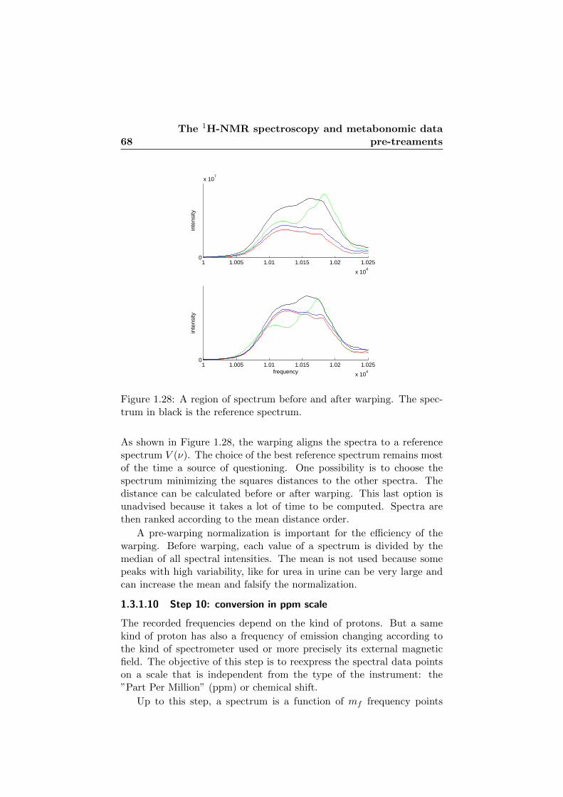
68The 1H-NMR spectroscopy and metabonomic data

pre-treaments

1 1.005 1.01 1.015 1.02 1.025

x 104

0

x 107

inte

nsity

1 1.005 1.01 1.015 1.02 1.025

x 104

0

frequency

inte

nsity

Figure 1.28: A region of spectrum before and after warping. The spec-trum in black is the reference spectrum.

As shown in Figure 1.28, the warping aligns the spectra to a referencespectrum V (ν). The choice of the best reference spectrum remains mostof the time a source of questioning. One possibility is to choose thespectrum minimizing the squares distances to the other spectra. Thedistance can be calculated before or after warping. This last option isunadvised because it takes a lot of time to be computed. Spectra arethen ranked according to the mean distance order.

A pre-warping normalization is important for the efficiency of thewarping. Before warping, each value of a spectrum is divided by themedian of all spectral intensities. The mean is not used because somepeaks with high variability, like for urea in urine can be very large andcan increase the mean and falsify the normalization.

1.3.1.10 Step 10: conversion in ppm scale

The recorded frequencies depend on the kind of protons. But a samekind of proton has also a frequency of emission changing according tothe kind of spectrometer used or more precisely its external magneticfield. The objective of this step is to reexpress the spectral data pointson a scale that is independent from the type of the instrument: the”Part Per Million” (ppm) or chemical shift.

Up to this step, a spectrum is a function of mf frequency points

1.3 Metabonomic data pre-treatments 69

(typically 32768) expressed on a frequency scale in Hz. A referencecompound is used, the Trimethylsilyl-propionate (TMSP). Its peak hasthe higher frequency in the spectral width, found between the frequencypoints 7400 and 9400. Changes of its position according to the externalmagnetic field are minimal and do not really influence the followingcomputations. For each data point j, the conversion of its frequencyin ppm is computed as the difference between its frequency νj and thefrequency of the reference compound νTMSP , divided by a frequencyfixed by the type of spectrometer used.

ppmj = (νj − νTMSP

νspectrometer)× 106. (1.42)

By convention, the TMSP peak corresponds to 0 ppm.Figure 1.29 presents a spectrum in term of data points indices, Hz

scale and ppm scale. The TMSP peak is here found at the datapoint8728 and corresponds to the 0 ppm. The 32768 points are in a 20.49ppms range, going from -5.56 to 14.93 ppm.

At the end of step 10, spectral intensities remain unchanged and thespectrum is a function on mf ppms:

F (ppm)step 10 = F (ν)step 9. (1.43)

70The 1H-NMR spectroscopy and metabonomic data

pre-treaments

0 0.5 1 1.5 2 2.5 3 3.5

x 104

−1

0

1

2

3

4

5x 10

7

inte

nsity

−5122.95 0 5122.95

−5.56 0 14.93

TMSPpeak

Hz scale

ppmscale

points

Selection:0.2 − 10 ppms

Figure 1.29: The spectrum and the different scales units.

1.3.1.11 Step 11: spectral window selection

Inside the 20.49 ppms range, not all the zones present peaks. The spec-tral window, ppmSW is then restricted to the frequency range by thechoice of an inferior (e.g.: 0.2 ppm) and a superior borders (e.g.: 10ppm). This typical spectral window is shown on Figure 1.29 (dubblearrow in red).

The selected domain of definition of F (ppmSW )step 11 is also re-versed: the spectrum is now read from the right to the left in a rangefrom 10 to 0.2 ppm involving mSW

f values. In the spectral illustration,

mSWf = 15677.

1.3 Metabonomic data pre-treatments 71

012345678910−1

0

1

2

3

4

5x 10

7

ppms

intensity

Figure 1.30: The spectrum after spectral window selection.

1.3.1.12 Step 12: bucketing

Data reduction also called bucketing is the commonly used method tosolve the problem already considered by warping: the presence of shiftsin resonance position.

The spectrum is integrated within m predetermined spectral regions,called ”bins” or ”buckets”. Subsequent data analysis procedures are nomore influenced by peak shifts, as long as these shifts remain within theborders of bins. Along with decreasing the dimension of the spectra, thebucketing also reduces the computation in the statistical data analysis.

Firstly, the number of buckets to form, m is defined. The widthof each bucket is then computed as: mSW

f /m. Each of these bucket

has a minimal, a maximal and a middle ppm value: ppmSWmin, ppmSW

max,ppmSW

mid. For each bucket, the spectral function F (ppmSW )step 11 is in-tegrated between ppmSW

min and ppmSWmax. This results into a vector of m

values. After reduction, a spectrum is described as a (1 × m) vector.Each spectral value corresponds to a bucket or variable xj labeled by itsppmSW

mid value.

Usually, the spectra, restricted to the frequency range of 0.2 - 10

72The 1H-NMR spectroscopy and metabonomic data

pre-treaments0

1030

50

15677 ppms points

Inte

nsity

10 8.91 7.82 6.73 5.64 4.56 3.47 2.38 1.29 0.2

010

2030

40

750 buckets

Inte

nsity

9.99 8.9 7.82 6.72 5.64 4.56 3.48 2.38 1.3 0.21

05

1015

2025

30

250 buckets

Inte

nsity

9.98 8.88 7.82 6.73 5.63 4.57 3.47 2.38 1.32 0.22

Figure 1.31: A same spectrum without bucketing, in a resolution of 750buckets and of 250 buckets.

ppm, are covered with approximatively 250 buckets of equidistant binwidth of 0.04 ppm. The more the resolution decreases, the more thepeaks become aligned between spectra.

Figure 1.31 shows that unfortunately an important data reductioncould occult information by the assimilation of several peaks in a samebucket.

The bucketing is here proposed with a new interpolation routine.The principle of the new bucketing is illustrated in Figure 1.31. For eachof the m buckets to create, a series of k initial coordinates ppmSW

i areconsidered. Each coordinate ppmSW

i corresponds to the spectral inten-sities F (ppmSW

i ). The borders of the bucket fixed at ppmSWmin=ppmSW

2

and ppmSWmax=ppmSW

k−1. The value of the bucket is the area under thespectral intensities between these borders. In this goal the spectral zone

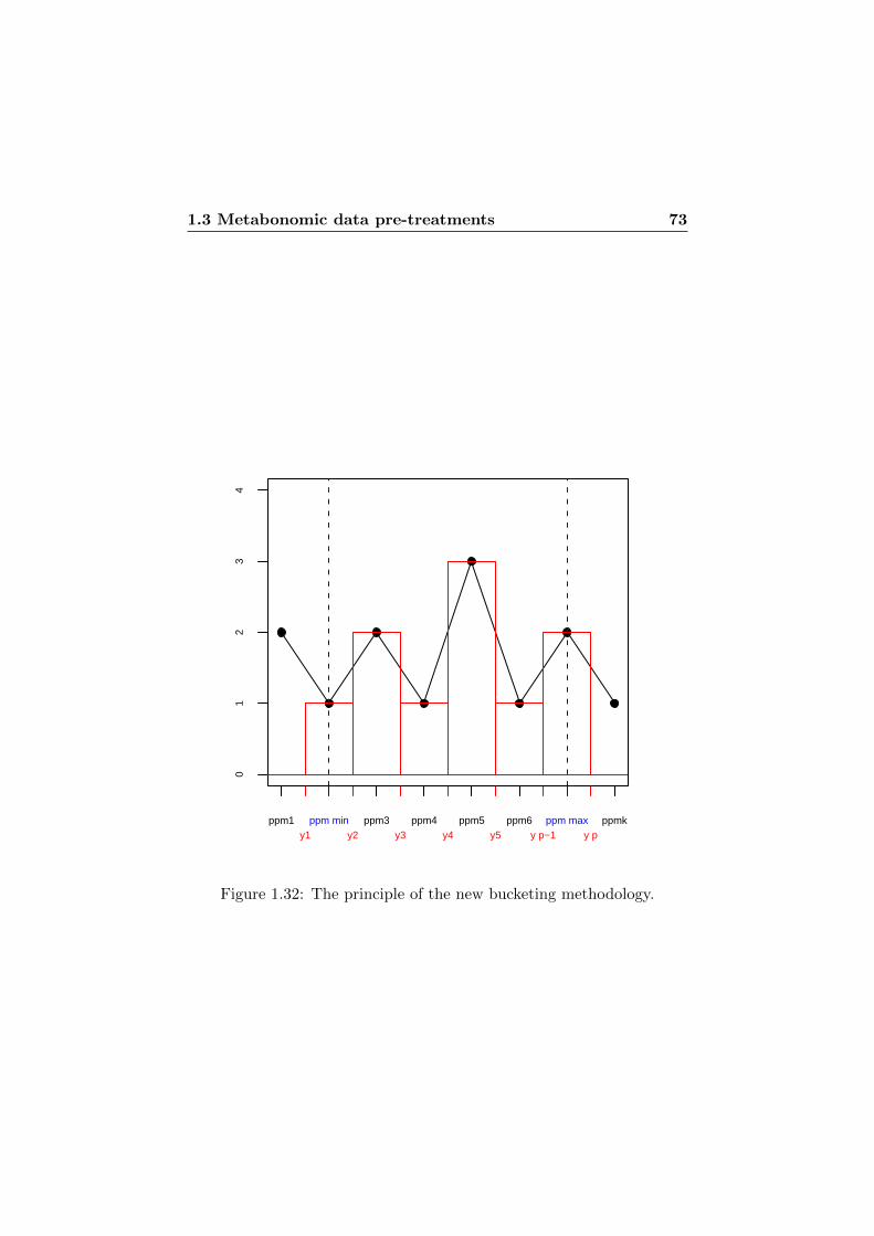
1.3 Metabonomic data pre-treatments 730

12

34

y1 y2 y3 y4 y5 y p−1 y pppm min ppm maxppm1 ppm3 ppm4 ppm5 ppm6 ppmk

Figure 1.32: The principle of the new bucketing methodology.

74The 1H-NMR spectroscopy and metabonomic data

pre-treaments

between ppmSW1 and ppmSW

k is decomposed in a series y of p new coor-dinates yi computed as:

yi =

(k−1)∑i=1

ppmSW(i+1) − ppm

SWi

2. (1.44)

Let r be the difference between two consecutive values of y: r = yi+1 −yi = ppmSW

i+1 − ppmSWi . The value of the bucket is:

xj = (r/2× F (ppmSWmin)) +

(k−2)∑i=3

(r × F (ppmSWi )) + (r/2× F (ppmSW

max)).

(1.45)This value is the sum of the areas of rectangles drawn in red betweenppmSW

m in and ppmSWm ax in Figure 1.32.

In our advised pre-treatments procedure, as a previous warping stephas already corrected the small variations of the chemical shifts and at-tenuates the problem, a weakest data reduction is sufficient to suppressthe remaining variations. These spectra have finally much more peaksthan spectra reduced to 250 buckets. Consequently, they allow to studymore compounds than usual spectra. The number of buckets to formin the advised pre-treatments procedure is wished to be the largest aspossible. Bucketings into 3000 or 1000 buckets were tested and wereinsufficient to suppress the spectral variations remaining after the warp-ing. We recommend a bucketing into 500 spectral variables for the urinespectra and 750 spectral variables for the serum spectra. These efficientnumbers of buckets already allows to double or triple the usual numberof 250 buckets.

In the end of step 12, the spectrum is a (1×m) vector x of m bucketsvalues xj labeled by a ppm value.

1.3 Metabonomic data pre-treatments 75

1.3.1.13 Step 13: removal of undesired regions

Some spectral regions contain resonances that are not of interest butmay strongly bias the subsequent statistical analysis. These regions canbe excluded or replaced by zeros. One important peak to exclude is theresonances of the solvent water. In many recent publications, this zone isreplaced by zeros. In the presented procedure, the solvent suppressionwas already considered in the step 2 but remaining solvent residualsand the artificial positive values created by the baseline correction hasbe removed.

For urine spectra, the region from 5.5 to 6.0 ppm corresponds to ahigh and non quantitative peak of urea. In this procedure, the removalof regions of water and urea are combined by a setting to zero of thespectral region between 4.5 and 6.00 ppm (see Figure 1.34).

For serum spectra, the lactate region (from 1.36 to 1.28 ppm) is alsooften set to zero because the lactate peak intensity is so high that ithides other informative peaks. In the case of serum samples, the onlyanalyzed spectral ranges are between 0.2 and 1.27, between 1.37 and 4.5and between 5.04 to 10 ppm.

In some studies, resonances corresponding to drug metabolites alsoneed to be excluded.

050

150

250

ppm

Inte

nsity

10 8.9 7.83 6.73 5.65 4.56 3.48 2.39 1.31 0.21

Figure 1.33: An urine spectrum after the removal between 4.5 and 6.00ppm.

1.3.1.14 Step 14: spectral zone aggregation

Even with the use of buffer in urine samples, the two peaks of citrate(between 2.5 and 2.7 ppm) shows a pronounced pH dependent chemicalshift variation. This problem does not occur in serum spectra wherecitrate peaks are more stable. A data reduction of urine spectra with

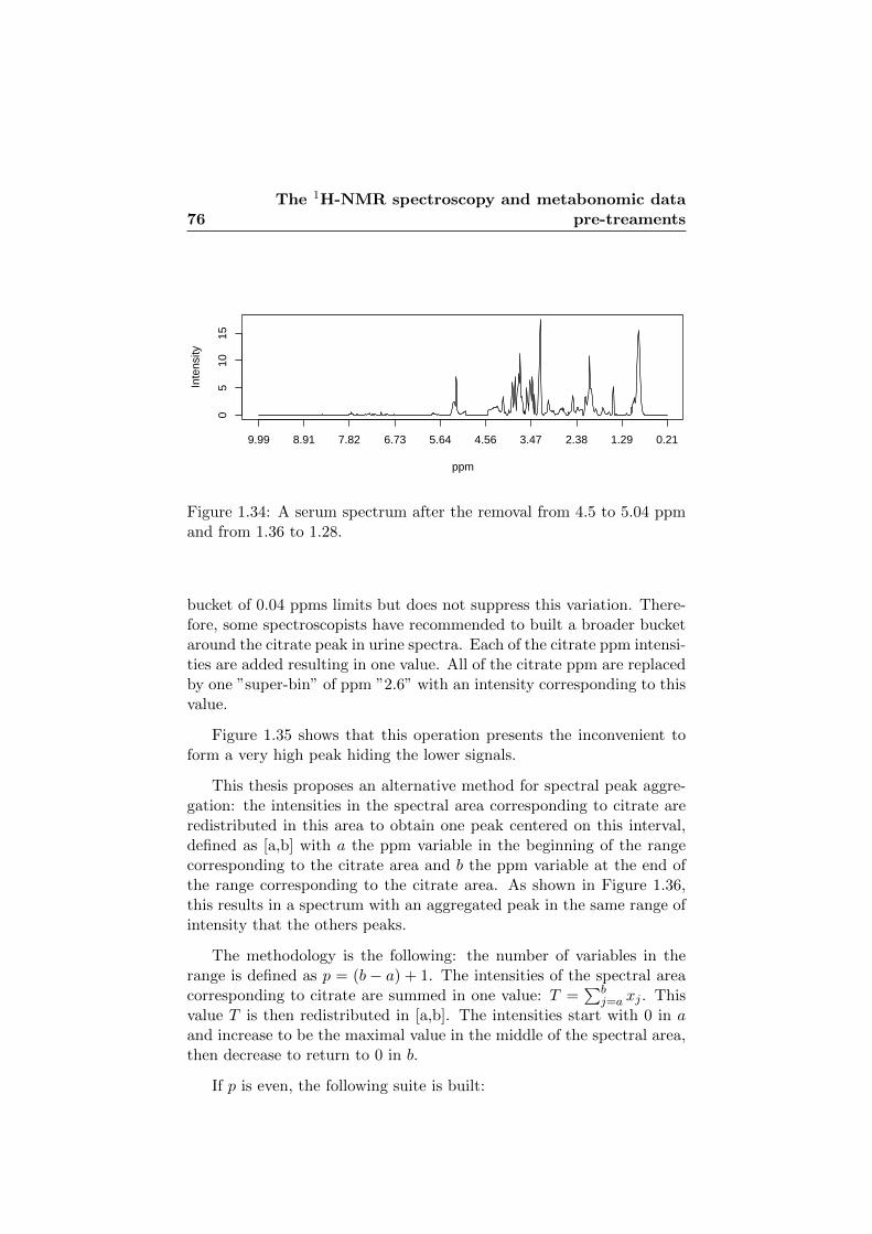
76The 1H-NMR spectroscopy and metabonomic data

pre-treaments0

510

15

ppm

Inte

nsity

9.99 8.91 7.82 6.73 5.64 4.56 3.47 2.38 1.29 0.21

Figure 1.34: A serum spectrum after the removal from 4.5 to 5.04 ppmand from 1.36 to 1.28.

bucket of 0.04 ppms limits but does not suppress this variation. There-fore, some spectroscopists have recommended to built a broader bucketaround the citrate peak in urine spectra. Each of the citrate ppm intensi-ties are added resulting in one value. All of the citrate ppm are replacedby one ”super-bin” of ppm ”2.6” with an intensity corresponding to thisvalue.

Figure 1.35 shows that this operation presents the inconvenient toform a very high peak hiding the lower signals.

This thesis proposes an alternative method for spectral peak aggre-gation: the intensities in the spectral area corresponding to citrate areredistributed in this area to obtain one peak centered on this interval,defined as [a,b] with a the ppm variable in the beginning of the rangecorresponding to the citrate area and b the ppm variable at the end ofthe range corresponding to the citrate area. As shown in Figure 1.36,this results in a spectrum with an aggregated peak in the same range ofintensity that the others peaks.

The methodology is the following: the number of variables in therange is defined as p = (b − a) + 1. The intensities of the spectral areacorresponding to citrate are summed in one value: T =

∑bj=a xj . This

value T is then redistributed in [a,b]. The intensities start with 0 in aand increase to be the maximal value in the middle of the spectral area,then decrease to return to 0 in b.

If p is even, the following suite is built:

1.3 Metabonomic data pre-treatments 770

200

400

600

ppm

Inte

nsity

9.99 8.9 7.82 6.72 5.65 4.55 3.47 2.38 1.3 0.21

Figure 1.35: A urine spectrum after citrate aggregation with the initialmethodology.

{0, d, 2d, K,

(p2− 1)d,(p

2− 1)d, K, 2d, d, 0

}(1.46)

where d = 4T(p−2)p .

If p is odd, we construct the suite:

{0, d, 2d, ...,

(p+ 1

2− 2)d,(p+ 1

2− 1)d,(p+ 1

2− 2)d, ..., 2d, 0

}(1.47)

where d = 4T(p−1)2 .

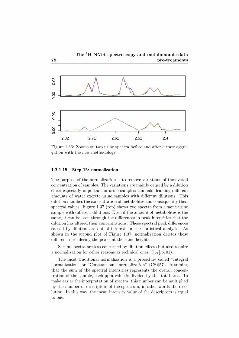
78The 1H-NMR spectroscopy and metabonomic data

pre-treaments

0.00

0.03

0.00

0.03

2.82 2.71 2.61 2.51 2.4

Figure 1.36: Zooms on two urine spectra before and after citrate aggre-gation with the new methodology.

1.3.1.15 Step 15: normalization

The purpose of the normalization is to remove variations of the overallconcentration of samples. The variations are mainly caused by a dilutioneffect especially important in urine samples: animals drinking differentamounts of water excrete urine samples with different dilutions. Thisdilution modifies the concentration of metabolites and consequently theirspectral values. Figure 1.37 (top) shows two spectra from a same urinesample with different dilutions. Even if the amount of metabolites is thesame, it can be seen through the differences in peak intensities that thedilution has altered their concentrations. These spectral peak differencescaused by dilution are out of interest for the statistical analysis. Asshown in the second plot of Figure 1.37, normalization deletes thesedifferences rendering the peaks at the same heights.

Serum spectra are less concerned by dilution effects but also requirea normalization for other reasons as technical ones. ([57],p101).

The most traditional normalization is a procedure called ”Integralnormalization” or ”Constant sum normalization” (CS)[57]. Assumingthat the sum of the spectral intensities represents the overall concen-tration of the sample, each ppm value is divided by this total area. Tomake easier the interpretation of spectra, this number can be multipliedby the number of descriptors of the spectrum, in other words the reso-lution. In this way, the mean intensity value of the descriptors is equalto one.

1.3 Metabonomic data pre-treatments 790.

0 e+

001.

5 e+

07

ppms

Inte

nsity

9.99 8.9 7.8 6.71 5.61 4.52 3.43 2.33 1.24

010

20

ppms

Inte

nsity

9.99 8.9 7.8 6.71 5.61 4.52 3.43 2.33 1.24

Figure 1.37: Zooms on two urine spectra before and after normalization.

xCSj =xj∑mj=1 xj

×m. (1.48)

where:

• xCSj is the normalized intensity for descriptor j.

• m is the resolution or number of descriptors in the spectrum.

• xj is the intensity for descriptor j before normalization.

Spectra are sometimes normalized to an endogenous metabolite witha presumed constant concentration level ([57], p104). For example, inurine, the creatinine excretion is considered as constant thus creatininecan be taken as an indicator of the concentration of urine. Each spectralvalue is then divided by the creatinine concentration, determined by itspeaks in the spectra (at 3.05 and 4.05 ppm). Creatinine normalizationis not of general use in metabonomics as it faces technical and biologicaldifficulties. Metabolites with overlapping peaks can interfere with thedetermination of the creatinine concentration. In addition, the chemi-cal shift of creatinine at 4.05 ppm depends on the pH of the sampling.Moreover, several studies have shown changes of the concentration ofcreatinine due to metabonomic responses [80]. In that case, the nor-malization by creatinine is worthless. Poor results in PCA and variance

80The 1H-NMR spectroscopy and metabonomic data

pre-treaments

component approaches (see Chapter 3) were obtained from our tests ofthe following others normalizations: by the median, the first quartile,the logarithm of the sum of the spectral intensities [18]. Note that, nor-malization in Section 1.3.2.9 was used to suppress systematic differencesbetween spectra before warping to ensure its efficiency. However, theeffect of this median normalization has been deleted by the data reduc-tion and the removal of undesired spectral regions. This is why a secondnormalization is needed.

1.3.2 Summary of the advised pre-treatments procedure

Table 1 gives for each pre-treatment step the mathematical representa-tion of one 1H-NMR output. From step 0 to step 4, the signal is an FIDor a complex function giving intensities for each of the mt time pointst. In step 5, the FT results in a complex function of spectral intensi-ties for frequencies values ν. From step 6, only the phased Real partis considered. In step 10, frequencies are translated into ppm units. Instep 11, the domain of definition of this function is restricted. SignalF (ppm)step11 is a function of spectral intensities with ppms values argu-ments. In step 12, the function is transformed in a function giving forbuckets, or zones of ppms, the area under the function F (ppm)step11 ineach bucket. The data are then represented by the resulting vector ofthis function, x.Some steps are aimed to suppress artifacts:

• the first and zero order phase corrections (step 1 and step 6).

• the baseline correction (step 7).

• the setting to zero of negative values (step 8).

Low signal to noise ratio is eliminated in apodizations (step 3 and step 4).Several steps correct problems in relation to the biological nature ofsamples and objectives of metabonomic study:

• Spectral variations due to peak shifts are treated in the warp-ing (step 9), bucketing (step 12) and spectral zones aggregation(step 14).

• Spectral dilution variations are removed in the suppression of thesolvent (step 2 and step 13) and the normalization (step 15).

• Selection of metabonomic informative spectral regions is realizedthrough the suppression of the solvent (step 2), the removal ofundesired regions (step 13), and the spectral window selection(step 11).

1.3 Metabonomic data pre-treatments 81

Ste

pN

am

eS

ign

alw

ith

0O

rigin

alF

IDS

(tj) step0

j=

1,...,mt

1F

irst

ord

erp

has

eco

rrec

tion

S(tj) step1

j=

1,...,mt

2S

up

pre

ssio

nof

the

solv

ent

S(tj) step2

j=

1,...,mt

3A

pod

izati

on

by

asc

ale

fun

ctio

nS

(tj) step3

j=

1,...,mt

4A

pod

izat

ion

by

anex

pon

enti

alfu

nct

ion

S(tj) step4

j=

1,...,mt

5F

ou

rier

Tra

nsf

orm

F(νj) step5

=Re(ν j

)+i.Im

(νj)

j=

1,...,mf

6Z

ero

ord

erp

hase

corr

ecti

on

F(νj) step6

=Re′

(νj)

j=

1,...,mf

7B

asel

ine

corr

ecti

onF

(νj) step7

=F

(νj) step6−Z

(νj)

j=

1,...,mf

8S

etti

ng

toze

roof

neg

ativ

eva

lues

F(νj) step8

=F

(νj) step7×h

(νj) step8

j=

1,...,mf

9W

arp

ing

F(νj) step9

=F

(w(νj))step

8j

=1,...,mf

10

Con

vers

ion

inp

pm

scale

F(ppmj) step10

=F

(νj) step9

j=

1,...,mf

11

Sp

ectr

al

win

dow

sele

ctio

nF

(ppmSW

j) step11

j=

1,...,mSW

f

12

Bu

cket

ing

xstep

12

xstep

12

=(1×m

)

13

Rem

oval

of

un

des

ired

regio

ns

xstep

13

xstep

13

=(1×m

)

14

Sp

ectr

al

zon

esagg

regati

on

xstep

14

xstep

14

=(1×m

)

15

Norm

aliz

atio

nxstep

15

xstep

15

=(1×m

)

Tab

le2.

Su

mm

ary

ofp

re-t

reat

men

ts.

82The 1H-NMR spectroscopy and metabonomic data

pre-treaments

1.4 Conclusions

This chapter has described and investigated the steps of a metabonomicstudy leading from prepared samples of collected biofluids to data readyfor the search of biomarkers: the spectral acquisition and the data pre-treatments.

At first, we have described the analytical technology used to acquirethe data, the 1H-NMR spectroscopy and the resulting recorded signalthe FID.

Secondly, we have presented a procedure of data pre-treatments.This new procedure is an improvement over a software named Bub-ble. The 15 steps procedure have proposed new pre-treatments withregards to the classical procedure and innovating methods for the phaseand baseline corrections, already included in the usual procedure.

Comparatively to the data prepared with the usual pre-treatmentprocedure, spectra from the advised procedure are expected to present:

• less noise due to the two apodization steps. These steps are meth-ods already existing in the field of 1H-NMR pre-treatments butunfortunately they were not included in the usual procedure.• less artifacts due to accurate methods of phase and baseline correc-

tions combined with a setting to zero of negative values artifacts.Phase and baseline corrections were already involved in the usualprocedure but they are here performed with innovating methods.Additionally, the advised procedure proposes a new step to deletetheir imperfections with the setting to zero of negative values.• less spectral metabolites out of interest for the biomarker search

due to a new methodology for water suppression on the FID anda new step of setting to zero of non informative peaks selected bythe spectroscopists.• less diuretic perturbations as a careful water peak suppression is

combined with an efficient normalization method, the constantsum normalization. This improvement is particularly importantfor urine biofluid metabonomic studies.• less misalignment created by pH thanks to the new steps of warping

and peak aggregation combined with a new efficient method ofbucketing.

All these points improve the quality of the metabonomic data as theydiscard confounding variations for the statistical search of metabonomicbiomarkers. In the current situation, the procedure used by spectro-scopists mainly requires development to better take into account theproblems related to the biological nature of the metabonomic study. Theadvised procedure answers to this need, offering several solutions to re-

1.4 Conclusions 83

move from the data confounding variations of biological sources throughsome new steps (warping, citrate aggregation, FID water suppression,and removal of non informative values) and new methods (bucketing).

The innovation in the correction of spectral misalignments also givesto our advised procedure the important advantage to provide exploitablespectral data in a higher resolution. The warping step is expected tohave partially corrected small variations of the chemical shift of peaksbetween spectra. Some metabonomic practitioners already take into ac-count the problematic of peak shifts in a bucketing. But if the bucketingis realized after warping, the problem requires a less important data re-duction: the number of buckets can be dubble or triple in comparison toclassically pre-treated spectra. Consequently, spectra pre-treated by ouradvised procedure allow to study more compounds, giving more chancesto discover biomarkers.

A major advantage of the procedure proposed here is its automatedaspect. New methodology has allowed to automate several steps with re-gards to the classical procedure as the phase correction and the baseline.Performances are thus faster and no more exposed to depend on the userskills, what warranties an improvement on reproducibility. However, inour vision, the automation is not synonymous of a black box behaviour.The advised procedure is a combination of a collection of Matlab M-filesand R functions, available as an open source software so that peoplecan freely download them and have access to the source codes. Thischaracteristic enables users to monitor the pre-treatment.

Criteria and methodology are required to assess the efficiency of theadvised pre-treatments procedure and to compare them with the clas-sical ones. Chapter 3 is dedicated to the development of methods toevaluate the quality of spectra: tools are proposed to study the spec-tral variability through the ”signal to noise ratio”. These tools are usedin Section 3.5.3.5 to evaluate some steps of the advised pre-treatmentsprocedure.

84The 1H-NMR spectroscopy and metabonomic data

pre-treaments

CHAPTER 2

The metabonomic databases usedin this thesis

2.1 Introduction

This chapter presents the databases used in this thesis and their con-struction. These databases were designed with spectroscopists from EliLilly and/or the University of Liege (ULg). The five databases used inthis thesis are:

• the semi-artificial urine database used in Chapter 4.• the urine experimental database used in Chapters 3 and 5.• the serum experimental database used in Chapter 3.• the human serum database used in Chapter 3.• the human AMD database.

Contrarily to the three others databases, the two serum databases donot involve biomarker signal. These spectra were obtained in differentbiological or analytical conditions in order to evaluate the impact ofthese conditions on the spectral variability of the metabonomic data.

The two urine databases have been artificially or experimentally cre-ated in order to control the spectral locations of the biomarkers to find.This property allows us to evaluate the performances of the data anal-ysis of the various statistical methods presented in Chapters 4 and 5.The last database results from a typical metabonomic study: spectralalterations related to the disease are expected for samples from diseasedsubjects but their spectral locations are unknown. The AMD databaseis presented in Chapter 6.

The urine experimental database is also designed in order to explorethe influence on spectra of diuretic fluctuations, intra-sample 1H-NMRreplications, and inter-day 1H-NMR measurements.

86 The metabonomic databases used in this thesis

The subsamples of the databases used in each chapter are detailed ineach of them. The emphasis is put here on the collection or preparationof the whole database.Each database is formed by two sets of data:

• X(n×m), the spectral data matrix,

• Y(n×l), the metadata matrix.

The latter contains one variable yk describing the information of interestrelated to the searched biomarker.

2.2 The semi-artificial database

2.2.1 Motivations for creating this database

To explore the capabilities of various multivariate statistical methodsto discover biomarkers, a semi-artificial database was built in which thedescriptors to be identified by the methods are controlled. Knowingthe positions of biomarkers to be found allows us to evaluate importantcharacteristics of the methods as their sensitivity and specificity. Theprinciple of this construction lays on the addition of random artificialalterations to normal or placebo real rat urine spectra.

2.2.2 The placebo data

The placebo data are composed of more than 800 spectra supposed toreflect a situation of physiological stability in rat urine. Each of spectrumis issued from the COMET [58] database (for COMET design see Section0.2) and corresponds to the spectral profile obtained from a ”control”rat (which did not received any treatment). All spectra were measuredat a 1H-NMR frequency of 600 MHZ at the Imperial College London,using a flow injection process.

After acquisition, spectral FID signals were automatically treatedand converted to spectral data using the Bubble Matlab library devel-oped at Eli Lilly (see Section 1.3)[91]. Bubble automatically performed,in sequence, the suppression of the water resonance, an apodization, abaseline correction, and a warping to align shifted peaks. The last stepreduces, by simple integration, the part of the spectrum between 0.2 and10 ppm to 500 descriptors.

Finally, some statistical tools (Euclidian and Mahalanobis distancesand PCA) were used to find outliers in the set of spectra and some ofthem were removed (less than 20). A typical urine spectrum coming outof this process is given in Figure 2.1.a.

2.2 The semi-artificial database 87

Typ

ical

urin

e sp

ectr

um0

510

1520

Index

Mea

n al

tera

tions

0 100 200 300 400 500

05

10

Figure 2.1: (Top) Typical rat urine 1H-NMR spectrum, (Below) thepositions and mean amplitude of alterations added to urine spectra.

2.2.3 Simulation of alterations

Among the 500 descriptors, 46 were chosen to become altered. These46 descriptors were altered for half of the spectra according to the de-scription below, in order to simulate the response of an organism to astressor or treatment. The 46 descriptors are chosen in ten consecutiveregions of the spectra as shown in Figure 2.1. Half of these 46 descriptorsand five regions are localized in a first part (index from 7.26 to 6.48)of the spectra containing a low level of noise. The other descriptorsand regions are localized in a second part (index from 3.37 to 2.56) ofthe spectra, where the level of noise is higher. The principle consistsin adding to the placebo spectra peaks with random heights accord-ing to Gamma distributions. Their means take the form of ten peakswith different widths localized in the ten regions as shown in Figure 2.1.Note also that four peaks have a width of seven descriptors and the sixother peaks have a smaller width of three descriptors, for a total of 46descriptors or biomarkers. Moreover, some pairs (see arrows in Figure2.1) of alterations were designed to be correlated, by using the sameGamma distribution to generate peaks, so that only six independentGamma distributions have been used instead of ten. This last featureallows us to test if the biomarker search methods are able or not todiscover correlated biomarkers. The six sets of three to fourteen single

88 The metabonomic databases used in this thesis

descriptors or biomarkers generated independently will be called belowthe ”independent” biomarkers. Note finally that each placebo spectrumwas only altered by two (randomly chosen) from the six possible inde-pendent biomarkers. This simulates the fact that each organism do notnecessarily respond the same way to a stimulus. A dataset of 400 al-tered spectra (randomly chosen from the 800 placebos) was built withthis methodology.

2.2.4 The final database

The spectral matrix X(800×500) therefore consists in 400 placebo spectraand 400 ”altered” spectra. To decrease the inter-sample variability, aconstant sum normalization was applied after the addition of the alter-ations. The metadata matrix Y only contains a variable giving the nameof the spectra and a variable declaring if the spectrum has received ornot the alterations (disease/control status). This last binary variable,yk, is the variable of interest for the biomarker search.

Subsamples of sizes 60 (2× 30) and 200 (2× 100) are extracted fromthe database in order to explore how the statistical methods are able toidentify the altered descriptors in different sample sizes.

2.2.5 Notes-remarks

Chronologically, these spectral data were used in the earliest part ofthe research presented in the thesis. In this period, the pre-treatmentscheme was not yet investigated. Consequently, the citrate peak was notaggregated, and the water area was not set to zero.

2.3 The urine experimental database 89

2.3 The urine experimental database

2.3.1 Motivations for creating this database

These urine database was collected according an experimental plan de-signed with three objectives.

The first one was to study the ability of statistical methods to find asbiomarkers the descriptors of the spectra for which a variability was ex-perimentally controlled. In this experiment homogenized medium urinesamples were spiked with two products at different levels of concentra-tion and analyzed by spectroscopy. The “concentrations” factor of eachadded product has to mimic the variability focused in a biomarker searchstudy.

The second objective was to study the quality of normalization tech-niques. Two dilutions in water of a same pool of urine were consideredin these experiments.

The third objective was to study the natural variability of spectrarelated to several factors: the day of analysis, and the repetition of aspectral acquisition (replication).

2.3.2 Statistical experimental design

Four factors of variability were considered in the experimental designand described in a matrix YA:

1. the medium: two media are considered: the urine from a pool(“B04-331, fisher 344 rats, female”) and the urine coming fromthe same pool but diluted with a dilution rate of 50 %.

2. the concentration of each of the two products into the samples:hippuric acid and citric acid were added to the samples in differentconcentrations described in Figure 2.2. The maximal concentra-tions are 8mM for the citric acid (QC) and 4mM for the hippuricacid (Qh). Four levels of each acid were considered, determinatingfourteen experimental conditions.

As shown in Figure 2.3, the peaks corresponding to each productare located in distant ppm domains. The hippurate has threepeaks with two in the region of high ppms containing a low noiselevel. On the contrary, citrate peaks are located in the noisy regionof low ppms. Note that in the spectral pre-treatments the citratepeaks are aggregated in one peak to avoid alignment problems (seeSection 1.3.1.14).

3. the replicates: each mixture or experimental condition describedin Figure 2.2. was repeated twice. Consequently, 28 samples were

90 The metabonomic databases used in this thesis

Figure 2.2: The urine experimental design.

Figure 2.3: A typical urine spectrum with spiked citrate and hippurate.

prepared for each medium.

4. the day of 1H-NMR measurement: for each medium, the prepara-tion of the 28 mixtures (14 experimental conditions × 2 replicates)were performed in three series. The two media samples of each se-ries correspond to a plate. Each day, a plate was defrosted in orderto be analyzed by the 1H-NMR spectrometer. Additionally, plate1 was analyzed twice: the plate was analyzed on day 1, refrost,then defrost and analyzed again on day 5. Values for the day ofmeasurement factor are: day 1, day 2, day 3, day 5.

2.3 The urine experimental database 91

In each plate, according to the previous description, we have 56 samples(2 media × 14 experimental conditions × 2 replicates). In this way, overthe four days, we obtained 224 samples to analyze. A design matrix YAgives for each spectrum the name of the corresponding sample and theconditions of each of the four factors.

2.3.3 Sample preparation and acquisition of the 1H-NMR data

Each sample had a final volume of 1200 µl. For each sample prepared, amixture of 600 µl was added to 600 µl of media. The media was eitherurine coming from a pool of 344 female Fischer rats or the same urinediluted at 50%. The mixture included the two products (citrate andhippurate) in the chosen concentrations and phosphate buffer containingTMSP. The volume of the phosphate buffer was adapted in order toobtain a volume of 600 µl to add to the 600 µl of urine. For example, afinal urine media sample contains 600 µl of urine and 600 µl of mixturecomposed of 150 µl of citrate, 150 µl of hippurate and 300 µl of buffer.The corresponding diluted media sample was obtained by taking half ofthe citrate volume, half of the hippurate and a larger volume of buffer tokeep the mixture volume at 600 µl. In the example, the correspondingfinal diluted urine media sample contains 600 µl of the diluted urinemedia and 600 µl of the mixture, here composed by 75 µl of citrate, 75µl of hippurate and 450 µl of buffer. In each preparation, the mixturewas added to the urine, centrifuged, frozen at − 80◦C and unfrozen at4◦C the day before the 1H-NMR analysis.

Sample tubes were analyzed within each day of experiment with aNOESY presaturation sequence (see Section 2.4.4.1).

The spectra were coded as follows: ”Mm−Cxy−Dd−Rr” wherem isthe code for the medium (1 or 2 for urine and diluted urine respectively),xy are the product proportions of the maximal concentrations, d is theday, r is the replicate index.

2.3.4 The pre-treatments

Each spectrum was processed using the pre-treatment procedure advisedin Section 1.3.1. The part of the spectrum between 0.2 and 10 ppm hasbeen reduced to 600 descriptors. Attention must be paid to the factsthat:

• the ppm values corresponding to the large non-informative ureaand to the water peak (4.5 - 6.0 ppm) were set to zero.• the region around the citrate resonances (2.56 - 2.72 ppm) was

integrated into one peak to suppress the high shifts of the citratepeaks.• the data were normalized by a constant sum normalization.

92 The metabonomic databases used in this thesis

2.3.5 The final urine database

The database finally contains a spectral data matrix X of dimensions(224 × 600). Among the 224 samples analyzed, three present prob-lems during the spectral acquisition (”M1C04D1R2”, ”M2C00D1R7”,”M2C48D1R1”). The metadata matrix Y corresponds to the YA matrixof dimensions (224 × 9). The variables contained in Y are: the nameof the spectrum, the medium, the combined level of hippurate and cit-rate (qualitative variable), the level of hippurate separately (qualitativevariable), the level of only citrate (qualitative variable), the volume ofadded hippurate (quantitative variable), the volume of added citrate(quantitative variable), the index of the replicate and the day.

Subsamples of these database are used in Chapter 3 and Chapter 5.

2.4 The serum experimental database 93

2.4 The serum experimental database

2.4.1 Motivations for creating this database

This database was created in order to study the impact of several factorsof 1H-NMR acquisition procedure on the variability of serum spectra.In this objective, eighteen samples containing only serum were preparedfrom a same pool of rat serum. They were analyzed by 1H-NMR follow-ing a procedure in which the same studied factors were changed accord-ing to an experimental design.

2.4.2 Study design

Five factors of variability were considered in the experimental design:

1. the day of 1H-NMR analysis (day 1, day 2, day 3).

2. the method of to remove protein peaks. Three methods (see Sec-tion 2.4.4.1) were considered: NOESY, CPMG, STE.

3. the sample. Eighteen samples were used what corresponds to twosamples per day and method.

4. the time of analysis in the day: for each suppression method, oneach day, samples were analyzed at two different times after de-frozing.

5. the replicate: for each method removing the protein peaks, on eachday, at each of the two considered times, the sample was analyzedtwice.

Figure 2.4 presents the design of experiments.A design matrix YA gives for each spectrum the name of the corre-

sponding sample, the method of protein peaks removing, the day of the1H-NMR analysis, the time after defrozing and the replicate number.

94 The metabonomic databases used in this thesis

Figure 2.4: The full experimental design of the serum experimentaldatabase.

2.4 The serum experimental database 95

2.4.2.1 The three methods to remove peaks of proteins

In these data, we consider three methods to remove the spectral proteinpeaks. The aim of these methods is to avoid high peaks of proteinsocculting the peaks of other molecules. The peaks of proteins can beremoved by a physical elimination of protein from the sample or by asuppression of their signal with the use of an adequate pulse sequenceduring the acquisition. The here considered methods (see Figure 2.5)are: a physical elimination of the proteins before acquisition, the use ofa protein suppression CPMG sequence, and the use of a protein sup-pression STE sequence.

Whatever the chosen proteins peaks removing method, a sample is1H-NMR analyzed with a long presaturation pulse called ”Noesypresat”[94]. This pulse allows to suppress the high intensity signal caused bythe water molecules. In the first method, proteins have been physicallyeliminated during the sample preparation, according to a methodologydescribed in Section 2.4.4, before the analysis with the Noesypresat se-quence. On the contrary, for the two others methods, no sample prepa-ration to eliminate proteins are realized before the analysis with theNoesypresat sequence. In these methods, the proteins signal are sup-pressed by other pulses following the Noesypresat sequence. The mostcurrent protein suppression sequence is the ”Carr Purcell Meiboom Gill”pulse sequence. However, this method creates some distortions of thebaseline and the phase. According to Lucas [59], these drawbacks couldbe avoided by the use of a pulsed filter of gradient instead of the ”CarrPurcell Meiboom Gill” sequence. This pulse gradient filter is called”Stimulated Echo”.

96 The metabonomic databases used in this thesis

Figure 2.5: The three methods to remove protein peaks and the prepa-ration procedure.

2.4 The serum experimental database 97

Spectra obtained with the physical elimination of proteins followedby the Noesypresat sequence are here named ”NOESY spectra”. Spectranamed ”CPMG spectra” are the ones obtained without physical elim-ination of proteins and with the Noesypresat sequence followed by theCarr Purcell Meiboom Gill pulse. Spectra named ”STE spectra” arethe ones obtained without physical elimination of proteins and with theNoesypresat sequence followed by the Stimulated Echo pulse.

Figure 2.6. shows the spectra obtained for each of the three methodsto remove peaks of proteins, after pre-treatments. It can be seen that:• the peak intensities between 4 and 3 ppm, corresponding to the

proteins, are higher in the NOESY spectra.• the intensity of the two large peaks between 1.5 and 0.5 ppm is

clearly larger for the CPMG and STE than the NOESY spectra.

05

1020

30

NOESY

X_9_993855 X_8_909242 X_7_824629 X_6_726897 X_5_642285 X_4_557977 X_3_473364 X_2_375632 X_1_291019 X_0_206712

Day 1Day 2Day 3

05

1020

30

CPMG

X_9_993855 X_8_909242 X_7_824629 X_6_726897 X_5_642285 X_4_557977 X_3_473364 X_2_375632 X_1_291019 X_0_206712

Day 1Day 2Day 3

05

1020

30

STE

X_9_993855 X_8_909242 X_7_824629 X_6_726897 X_5_642285 X_4_557977 X_3_473364 X_2_375632 X_1_291019 X_0_206712

Day 1Day 2Day 3

Figure 2.6: The twenty four spectra obtained with each of the threemethods to remove peaks of proteins.

98 The metabonomic databases used in this thesis

2.4.3 Sample preparation

The preparation of the samples and the spectral acquisition were realizedat the Laboratoire de Chimie Pharmaceutique of ULg, Belgium. Thepreparation procedure is presented in Figure 2.5. The serum was boughtfrom the SIGMA firm and conserved at minus 22 C◦.

Before the preparation of the samples, a physical protein eliminationwas applied to a part of this serum: during the first day of experiment,100 ml of this serum was defrosted. 15 ml of this defrosted serum wereisolated in a tube of 50 ml in order to suppress the proteins. The pro-teins were eliminated by precipitation by the help of 2.25 ml of 20 %trichoracetic acid (TCA). Then the tube was shaken and set into a icebath during ten minutes. After the ice bath, the tube was centrifugedat 4 C◦ at 10000 rpm during fifteen minutes. The supernatant wastransferred into another tube. A second centrifugation identical to thefirst one was operated on the supernatant in order to obtain a higherdegree of purity. As TCA is an acid, it also causes a fall of pH. This fallis corrected by the addition of NaOH (10%) until the neutralisation ofthe solution (pH 7). Then, the pH of the solution is stabilized by theaddition of a phosphate buffer. The remaining defrosted serum is notsubmitted to a physical protein elimination.

Eighteen Ependorff tubes were filled with the serum. Six of themwere filled with serum without protein. The twelve others contain serumwith proteins. The eighteen tubes were stocked at - 22 C◦. The experi-ments were realized over three days. Each day of experiment, six Epen-dorff tubes were defrosted: two without protein and four with proteins.Each day, the six defrosted samples were submitted to an addition ofphosphate buffer and of TMSP.

2.5 The human serum database 99

2.4.4 Spectral acquisition

Each day, two Ependorff tubes for which the proteins have been phys-ically eliminated were analyzed in 1H-NMR with only the Noesypresatpulse sequence [94]. This sequence suppresses the water signal. The halfof the four Ependorff tubes in which the proteins were not physicallyeliminated were analyzed with the Carr Purcell Meiboom Gill pulse se-quence. The other half of the tubes was analyzed with the StimulatedEcho pulse sequence. In this database, with the two samples by day fora method processed twice, over the three days, we have 24 spectra foreach protein removing method.

2.4.5 The pre-treatments

Each acquired spectrum was pre-treated according to the procedure pro-posed in Section 1.3.1. Each spectrum has 750 ppms and is normalizedto have a sum equal to 750.

2.4.6 The final database

According to this design, a total number of 72 spectra were acquired: 3days × 3 methods × 2 samples × 2 times × 2 replicates. The spectraldata matrix X is then of dimension (72 × 750). The metadata matrixY corresponds to the matrix YA described in Section 2.4.2. These dataare used in Chapter 3.

2.5 The human serum database

2.5.1 Motivations for creating this database

The second serum database is dedicated to the exploration of the impactof biological factors on the spectral variability.

Actually, the biological variability is issued from several components.The first one is the variability between healthy people. Another sourceof variability is the fluctuations within a given individual. An exampleof this kind of fluctuation is given by the glucose. The glucose levelsare usually lower in the morning, before the breakfast, and rise by a fewgrams during an hour or two after meals. A third source of variabilityis the systematic difference between spectra of healthy and non healthypeople. The diabetic person, for instance, has higher glucose level in hisblood than a healthy person. The goal of this database is not to describeall the biological variance components in detail. The aim instead is to geta reasonable idea of the global amplitude of natural biological variabilitydue to inter- and intra-individual sources.

Another purpose of this database is to compare the analytical vari-ability and the biological one. For various further use of the discovered

100 The metabonomic databases used in this thesis

metabonomic biomarkers, it is very crucial to have an analytical variabil-ity lower than the biological one. If a discovered metabonomic spectralbiomarker corresponds to a spectral zone presenting a systematicallyhigher intensity but also a huge variability due to the acquisition or thepre-treatments of data, detection tools built with this biomarker willhave a low sensitivity and specificity.

This database was created from the collection of blood samples takenfrom volunteers. Samplings were organized following a procedure allow-ing to observe the biological factors of interest. The resulting bloodsamples were then prepared and measured in order to explore some an-alytical factor.

2.5.2 Statistical design

Four factors of variability were considered in the experimental design:

1. the volunteer (from 1 to 12): the blood of twelve volunteers wascollected. Since the alterations of the spectra due to diseases isoutside the scope of the current analysis, all selected volunteerswere healthy. Among the volunteers, seven were women and fivewere men. By controlling the sex balance, sex is not a confoundingfactor in the study.

2. the sampling for a given volunteer (from 1 to 3): the blood sam-pling was performed on three non consecutive days under similarconditions. Similar conditions means that the three blood sam-plings were all carried out the morning around 10 o’clock. Thevolunteers were encouraged to have fasted. Thanks to these mea-sures, the fluctuation and the variability between the individualswas controlled.

3. the tube for a given volunteer and a given sampling (from 1 to2): each blood sampling day, two tubes were collected. Since twosamples are available for a given volunteer the experimental vari-ance can be estimated. By experimental variance, we mean thevariability due to the laboratory operations.

4. the time of measurement: each tube was measured twice the sameday with a couple of hours between the two measurements. Thereplication allows determining whether the sample can be con-served after defrozing. Actually this has been already consideredin the previous serum database. The only difference is the use ofhuman serum instead of commercial serum from rats.

The two first factors are biological sources of variability while the twolasts are analytical sources.

2.5 The human serum database 101

A design matrix YA gives for each spectrum: the number of thevolunteer, the day of sampling, the number of the tube and the timeof measurement after defrozing. A covariate matrix YB gives for eachspectrum the sex of the volunteer.

2.5.3 Sample preparation

The preparation of the samples and the spectral acquisition were real-ized at the Laboratoire de Chimie Pharmaceutique of ULg, Belgium.Once the blood sample had been collected, it was processed into serum.Then phosphate buffer was added to control the pH. The trimethylsi-lyl propanoate (TMSP) was finally put in as internal reference. Theprotein signals were eliminated thanks to the pulse sequence CPMG.Serum samples were conserved frozen. The spectra were coded as fol-low: ”V v − Pp − Tt − Rr” where v is the code for the volunteer, p isthe code for the day of sampling, t is the tube number, r is the time ofmeasurement number.

2.5.4 The pre-treatments

Each acquired spectrum was pre-treated according to the procedure pro-posed in Section 1.3.1. Each spectrum has 750 ppms and is normalizedto have a sum equal to 750.

2.5.5 The final database

According to this design, a total number of 144 spectra were acquired: 12volunteers × 3 sampling × 2 tubes × 2 times of measurement. Amongthe 144 samples analyzed, four presents problems during the spectralacquisition: V 4P2T2R1, V 8P2T2R2, V 11P1T2R1, V 11P1T2R2. Thedatabase contains a spectral data matrix X (140× 750). The metadatamatrix Y (140× 5) corresponds to the matrices YA and YB.

These data are used in Chapter 3.

102 The metabonomic databases used in this thesis

CHAPTER 3

Evaluation of stability,repeatability and reproducibility

properties of 1H-NMR spectra inmetabonomic studies

3.1 Introduction

Beside the variability of interest focused in the biomarker search, ametabonomic study involves numerous other sources of variability. In-deed, in relation with the biological context, spectra face biological vari-ations involuntary produced in the metabonomic study: for example,spectral profiles can be influenced by physiological factors which are notof interest for the biomarker search as diet and hormonal status [8].Non-biological variations (ex: sample instability or analytical artifact)can also affect spectra.

Searched biomarkers are metabolites with concentration changes stea-

dily occurring in specific biological situations. Metabonomic data anal-ysis needs thus to extract in the spectral data matrix the variationslinked to a change indicated in a factor of interest. If the other sourcesof variability are predominant, they can hide the spectral variability tar-geted in the biomarker search. This stresses the importance to discoverthe sources of variability of the spectral metabonomic data and to de-velop methods to control them (e.g. by experimental designs and/orpre-treatment procedures).

In the literature, several papers treat the question of the variabilityof the spectral metabonomic data. The stability of several urine spec-

104Evaluation of stability, repeatability and reproducibilityproperties of 1H-NMR spectra in metabonomic studies

tral regions was assessed by computation of means, standard deviationsand coefficients of variations [23]. But most of the papers focus on theeffect of specific chosen factors and the methodology used to analyzethe spectral variabilities due to the factor(s) of interest is, in most ofthe cases, limited to a principal components scoreplot [8] [50] [87] [51].Little methodology exists to go further than a simple statement of theexistence of a variability and to quantify it.

This chapter proposes statistical tools to study, quantify and com-pare the spectral variability.

The initial goal of the research presented in this chapter was to an-swer to specific questions about the spectral variability caused by spe-cific factors in urine and serum metabonomic data. Experiments weredesigned to supply data allowing us to answer these specific questions.This initial context is enlarged to more general concepts in this chapter:a classification of potential sources of variability is presented in Section3.2 and three kinds of research questions that can be addressed in thestudy of spectral variability are discussed in Section 3.3. Several toolsare proposed to answer these general questions. They allow us to studythe spectral variability due to different factors or to different modalitiesof a factor through several visual or quantitative supports. These arebased on PCA and inertia calculation, on simple summary statistics andon mixed linear modelling. In the objective to obtain the best spectrafor metabonomic biomarkers discovery, the spectral variability is alsostudied through the ”signal to noise ratio”: the ratio of the useful vari-ability due to the factor of interest and the undesired variability due toother factors. Section 3.5 describes these tools. They are illustrated onurine and serum datasets in Section 3.4, with their specific variabilityquestions. Finally, Section 3.6 summarizes the answers obtained to theinitial questions about serum and urine metabonomic data.

3.2 Sources of variability 105

3.2 Sources of variability

The variability sources in metabonomic studies are issued from the differ-ent steps of data acquisition and can be classified in different categories(see Figure 3.1)

Figure 3.1: The sources of spectral variabilities.

A first distinction is made between the ”factors of variability of in-terest” yk and the ”factors of undesired variability”. Factor yk is theone for which the biomarkers are going to be searched as the diseasestatus or the drug dose. Factors of undesired variability are related tobiological, experimental or analytical contexts that influence metabo-nomic data but for which biomarkers are not searched. It can be for e.g.the subject who has personal particularities in his metabolism or thepreparation characteristics of a 1H-NMR tube as instrumental artifacts.Note that even if pre-treatments are operations aiming to suppress theundesired variability accumulated in the spectral data, they can alsocreate new undesired variabilities.

A second distinction is done between ”controlled” and ”uncontrolled”factors. A factor is controlled when its value can be imposed in the studydesign or maintained by an appropriate operation. For instance, the age

106Evaluation of stability, repeatability and reproducibilityproperties of 1H-NMR spectra in metabonomic studies

of the subject involved in the study is usually controlled by the design.By opposition, ”uncontrolled” factors are those factors that we suffer inthe metabonomic studies, as the differences between samples preparedwith the same methodology or between measurements taken on differentdays.

Finally, from a statistical point of view, the uncontrolled factors canbe classified as ”fixed” or ”random”. Even if the effect of variabilitysources is uncontrolled, some uncontrolled sources are fixed factors.

3.3 Research questions and notationsThe tools presented in this chapter aim to explore the influence of thefactors of spectral variability through a here established list of threepossible research questions:

1. Research question of type 1: Comparison of the variability ofgroups of spectra.The goal is to discover for a controlled factor of interest, whichlevel provides the more similar spectra.

2. Research question of type 2: Identification and quantification ofthe spectral sources of variability.This question can be declined in two sub-objectives:

• to discover if spectral variabilities are created by a factor(other than the one of interest).

• to quantify and to compare the spectral variabilities createdby different factors.

3. Research question of type 3: Comparison of groups of spectra withrespect to their ”signal” to noise ratio.The objective is to discover which group of spectra both maximizesthe variability related to the factor of interest and minimizes thevariability due to noise factors.

In the next sections, X will denote the (n×m) matrix of spectra and Ythe (n× l) metadata matrix with factor of variability sources. Let y∗ beone of these factors with G levels: y1, ..., yG. These levels form G groupsof spectra dividing the spectral matrix X in G submatrices: X1, ..., XG

of sizes (ng ×m) with g = 1...G. xgi is the ith spectrum (line) of matrixXg and xgij the intensity of this spectrum for descriptor xj .

3.4 Data and contextual variability questionsThe developments in this chapter were motivated by specific needs ofknowledge about the sources variability affecting typical 1H-NMR metabo-

3.4 Data and contextual variability questions 107

nomic data. Firstly, in the previous chapter, a set of pre-treatmentoperations have been proposed to transform the acquired signal intoinformative data. Well controlled data and tools were then needed toverify if the proposed pre-treatments are efficient to highlight biomarkerinformation and reduce noise. Secondly, working on data acquisitionwith spectroscopists showed that the design and setup of metabonomicstudies imply several experimental or biological choices. Each choicemay potentially impact the final spectrum quality and must then bedone on the basis of objective information. These questions have led tothe creation of three experimental datasets aimed at answering precisequestions about spectral variability or repeatability.

This section presents the three datasets and three related questionsthat will be explored to illustrate this chapter. Each of these contex-tual questions can be classified as one of the general research questionpresented in Section 3.3.

3.4.1 Datasets

A first serum dataset, called here ”experimental serum dataset”, hasno variability caused by a factor of interest. These data have beenobtained according to an experimental design, described in Section 2.4.Only 48 spectra, the 24 ”CPMG spectra” and the 24 ”STE spectra”acquired with the two pulse methods to suppress protein signals areconsidered here. Figure 3.2 presents the part of the experimental designcorresponding to these spectra.

Spectral variabilities can be explained according to three randomfactors (day of measurement, sample, replication) and two controlledfactors (time of measurement after defrozing and protein suppressionmethod - CPMG or STE). Each spectrum was pre-treated with the pro-cedure described in Section 1.3.1, has 750 ppms and is normalized tohave a sum equal to 750. The second serum dataset, called here ”hu-

man serum dataset”, is the whole database described in Section 2.5.The spectral data matrix X contains 140 spectra of 750 descriptors,pre-treated with the procedure described in Section 1.3.1. Spectral vari-ations can be explained by three randoms factors (volunteer, blood sam-pling for a given volunteer, blood tube for a given volunteer and a givensampling) and one fixed factor (time of measurement after defrozing).

The ”urine database” was built from mixtures of urine with citrateand hippurate (see Section 2.3). The 32 spectra, here used, are a sub-sample of this database corresponding to the samples at the vertices ofthe experimental domain as shown by the black points in Figure 3.3.

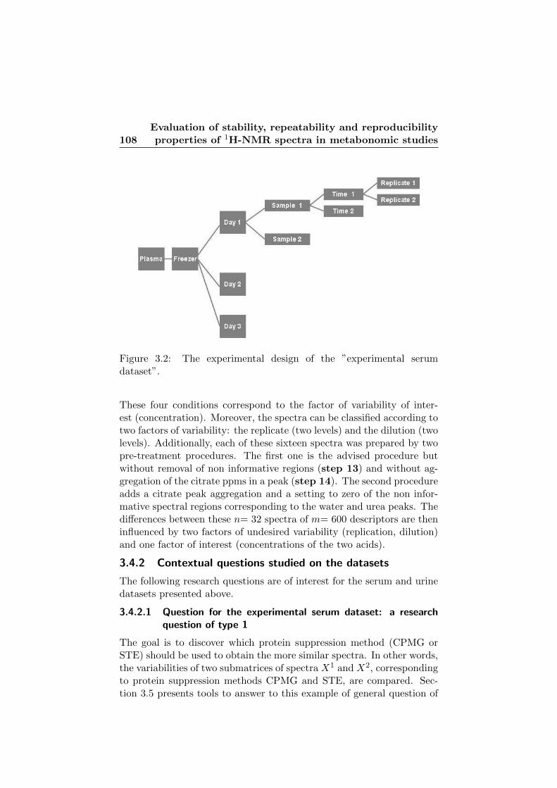
108Evaluation of stability, repeatability and reproducibilityproperties of 1H-NMR spectra in metabonomic studies

Figure 3.2: The experimental design of the ”experimental serumdataset”.

These four conditions correspond to the factor of variability of inter-est (concentration). Moreover, the spectra can be classified according totwo factors of variability: the replicate (two levels) and the dilution (twolevels). Additionally, each of these sixteen spectra was prepared by twopre-treatment procedures. The first one is the advised procedure butwithout removal of non informative regions (step 13) and without ag-gregation of the citrate ppms in a peak (step 14). The second procedureadds a citrate peak aggregation and a setting to zero of the non infor-mative spectral regions corresponding to the water and urea peaks. Thedifferences between these n= 32 spectra of m= 600 descriptors are theninfluenced by two factors of undesired variability (replication, dilution)and one factor of interest (concentrations of the two acids).

3.4.2 Contextual questions studied on the datasets

The following research questions are of interest for the serum and urinedatasets presented above.

3.4.2.1 Question for the experimental serum dataset: a researchquestion of type 1

The goal is to discover which protein suppression method (CPMG orSTE) should be used to obtain the more similar spectra. In other words,the variabilities of two submatrices of spectra X1 and X2, correspondingto protein suppression methods CPMG and STE, are compared. Sec-tion 3.5 presents tools to answer to this example of general question of

3.4 Data and contextual variability questions 109

Figure 3.3: The experimental design of the ”urine dataset”.

type 1: PCA with group identification and inertia calculus, pointwisecomputation of mean, standard deviations, coefficients of variation andglobal coefficients of variation.

3.4.2.2 Question for the human serum dataset: a research questionof type 2

In this dataset, four factors influence the spectra variability. We wantto understand and quantify the variability due to these sources as wellas from other sources and compare them. This contextual question cor-responds to a research question of type 2. The proposed methodologiesto answer to this question are PCA with group identification and iner-tia calculus, standard deviations and intraclass correlation coefficientsestimated from pointwise mixed models.

3.4.2.3 Question studied on the urine dataset: a research questionof type 3

The urine dataset asks a specific question about pre-treatments corre-sponding to a general research question of type 3. The objective hereis to discover which pre-treatments procedure (1 or 2) maximizes thefactor to noise ratio: in other words, which pre-treatments proceduremaximizes the heterogeneity between groups of spectra of the differentcategories of the factor of interest (concentration), while minimizing theheterogeneity into the groups of spectra of a same level of this factorof interest. PCA with group identification and inertia calculus, Signalto Noise Ratio estimated from pointwise mixed models are proposed toanswer this question.

110Evaluation of stability, repeatability and reproducibilityproperties of 1H-NMR spectra in metabonomic studies

3.5 Proposed methodologies

This section presents tools offering solutions for each of the three re-search questions of Section 3.3. These tools are based on three classes ofstatistical methods: the Principal Component Analysis (PCA), simpledescriptive summary statistics and pointwise mixed modelling. Fromthe results of these methods, numerical indices and visual representa-tions are extracted to answer the research questions. These tools aresummarized in Table 3.1 with the research questions they aim to an-swer.

Method Tools Question

PCA - Graphic with group identification Q1 Q2 Q3- Inertia Q1 Q2 Q3

Descriptive - Differences to the mean spectrum Q1statistics - ”Spectra” of mean, s and cv Q1

- Sorted s and cv Q1- Global coefficient of variation Q1

Pointwise - Variance components Q2Mixed Modelling - Interclass correlation coefficient (ICC) Q2

- Signal to Noise Ratio (SNR) Q3

Table 3.1: The proposed tools to study spectral variability. (s are stan-dard deviations and cv coefficients of variations)

3.5.1 PCA with group identification and inertia computation

PCA [47] is the most commonly used method in metabonomics and 1H-NMR data exploration. For the study of the spectral variability of amatrix of spectra, PCA can be applied in the same way as for usualbiomarker search. The projections of the (centered) spectra on the twofirst components are plotted and different symbols or colors are used tohighlight the levels of the factor(s) of interest. Information about thevariability is reported through the global positions and separation of thedifferent symbols for each level of the factor.

As a complement to PCA, inertia using euclidean distances and amass of 1 for each spectrum can also be computed in order to quantifythe dispersion of groups of spectra in the spectral space. According tothe Huygens theorem [77], the total inertia of a cloud of n spectra witha barycenter u is the sum of the intraclass and interclass inertias:

ITot =n∑i=1

d2(xi, u) = IW + IB. (3.1)

3.5 Proposed methodologies 111

The interclass inertia is: IB =∑G

g=1 ngd2(ug, u) where ug is the

barycenter of the spectra of the submatrix Xg defined from the levels of aconsidered factor y. The intraclass inertia is computed as: Iw =

∑Gg=1 I

gw

where Igw is the inertia of the group g containing ng spectra: IgW =∑ng

i=1 d2(xgi , ug). The IB, IW and Igw are expressed in proportion of ITot

in order to appreciate the responsibility of a factor or of its levels in thedispersion of spectra. Different Euclidean based distances may be chosenbut the non-weighted one has the advantage to be simple and to respectall initial sources of variability. Also, the inertia can be calculated inthe initial spectral space or in its projection on the plane of the twofirst principal components. We recommend the first approach in orderto keep all the information available concerning spectral dissimilarities.

The PCA with group identification and inertia computation is usefulfor each of the three research questions as illustrated below on the threedatasets.

In order to answer the question about experimental serum data, aPCA was performed on the 48 CPMG and STE spectra (see Figure 3.4).Beside the clear difference between the two protein suppression methods,the PCA scoreplot shows a very larger dispersion or variability for STEspectra.

112Evaluation of stability, repeatability and reproducibilityproperties of 1H-NMR spectra in metabonomic studies

Figure 3.4: The PCA scoreplot of the two first PCs.

In this plan, the inertias within each of the two groups of spectra con-firm this conclusion: the intraclass inertias within the group of CPMGspectra and within the group of STE spectra are respectively 0.89% and49.32% of the ITot. Table 3.2 gives the intraclass inertias within thegroup of CPMG spectra and within the group of STE spectra computedin the initial space.

CPMG STE

IW 3.44% 16.88%

Table 3.2: The intraclass inertias within the group of CPMG and STEspectra in the initial space.

3.5 Proposed methodologies 113

For the question on human serum data, a PCA was performed on the140 spectra. The spectra were projected on the two first PCs labeled bytheir identification codes: ”V v−Pp−Tt−Rr” where v is the volunteernumber, p is the day of sampling, t is the tube number, r is the time ofmeasurement. Attributing successively different colors to the projectionsof spectra according to the levels of one of the four factors (volunteer,sampling, tube, time) allows us to visualize the presence of differencesbetween the spectra related to this factor. In this data, the clearestseparation is observed for symbols corresponding to the levels of thefactor ”volunteer” (see Figure 3.5). This observation is confirmed in

−0.10 −0.05 0.00 0.05 0.10 0.15 0.20

−0.

10.

00.

10.

2

PC1 ( 30.58 %)

PC

2 (

10.4

2 %

)

V10P1T1R1V10P1T1R2

V10P1T2R1V10P1T2R2

V10P2T1R1V10P2T1R2V10P2T2R1V10P2T2R2

V10P3T1R1V10P3T1R2

V10P3T2R1V10P3T2R2

V1P1T1R1

V11P1T1R2V11P1T1R2

V1P1T1R2V1P1T2R1

V11P2T1R1V11P2T1R2

V1P1T2R2

V11P2T2R1V11P2T2R2

V11P3T1R1

V11P3T1R2V11P3T2R1V11P3T2R2V1P2T1R1

V12P1T1R1V12P1T1R2

V1P2T1R2

V12P1T2R1V12P1T2R2

V1P2T2R1

V12P2T1R1

V12P2T1R2

V1P2T2R2

1V12P2T2R1V12P2T2R2

V12P3T1R1V12P3T1R2V12P3T2R1V12P3T2R2

V1P3T1R1V1P3T1R2V1P3T2R1V1P3T2R2V2P1T1R1V2P1T1R2V2P1T2R1V2P1T2R2

V2P2T1R1V2P2T1R2

V2P2T2R1V2P2T2R2

V2P3T1R1V2P3T1R2V2P3T2R1V2P3T2R2

V3P1T1R1V3P1T1R2V3P1T2R1V3P1T2R2

V3P2T1R1V3P2T1R2V3P2T2R1V3P2T2R2

V3P3T1R1V3P3T1R2

V3P3T2R1V3P3T2R2

V4P1T1R1V4P1T1R2

V4P1T2R1V4P1T2R2

V4P2T1R1V4P2T1R2

V4P2T2R2

V4P3T1R1V4P3T1R2V4P3T2R1

V4P3T2R2 V5P1T1R1V5P1T1R2V5P1T2R1

V5P1T2R2

V5P2T1R1V5P2T1R2V5P2T2R1V5P2T2R2

V5P3T1R1V5P3T1R2V5P3T2R1V5P3T2R2

V6P1T1R1V6P1T1R2V6P1T2R1V6P1T2R2

V6P2T1R1V6P2T1R2V6P2T2R1V6P2T2R2

V6P3T1R1V6P3T1R2V6P3T2R1V6P3T2R2

V7P1T1R17V7P1T1R2V7P1T2R1V7P1T2R2

V7P2T1R1V7P2T1R2V7P2T2R1V7P2T2R2

V7P3T1R1V7P3T1R2V7P3T2R1V7P3T2R2

V8P1T1R1V8P1T1R2V8P1T2R1V8P1T2R2V8P2T1R1V8P2T1R2V8P2T2R1V8P3T1R1V8P3T1R2

V8P3T2R1V8P3T2R2

V9P1T1R1V9P1T1R2V9P1T2R1V9P1T2R2

V9P2T1R1V9P2T1R2

V9P2T2R1V9P2T2R2

V9P1T1R1V9P1T1R2V9P1T2R1V9P1T2R2

Figure 3.5: The projections of 140 spectra on the PCA scoreplot of thetwo first PCs. Labels are the identification code of the spectra and colorsvary according to the volunteer.

114Evaluation of stability, repeatability and reproducibilityproperties of 1H-NMR spectra in metabonomic studies

Table 3.3 which gives the interclass inertias in the initial space betweengroups defined by the levels of the four factors of variability. The morea factor has a high interclass inertia, the more this factor represents aimportant source of variability between spectra.

Volunteer Sampling Tube Time

IB 16.14 % 3.11% 0.10% 0.03%

Table 3.3: The interclass inertias in % of ITot for each of the four sourcesof variability.

For the urine data, Figures 3.6 left and right, respectively present thescoreplots formed by the two first principal components of a PCA real-ized on the 16 urine spectra prepared with the pre-treatments 1 and 2.The colors represent the four concentrations of the two analytes, lettersAa and Bb the two dilutions and cases ab or AB the two replicates.

Figure 3.6: The PCA scoreplots of the two first PCs for the pre-treatments 1 (left) and 2 (right).

This figure shows clearly that the second pre-treatment has strongly im-proved the reproducibility of spectra and reduced the effect of dilution.As a consequence, with this pre-treatment, the experimental design isclearly visible in the space of the two first principal components whichrepresents a larger part of the total variability of the data (45.21% to62.57%).

Table 3.4 shows that, in the initial space, the inertia between groupsof spectra of different dilutions and of different replications decrease:

3.5 Proposed methodologies 115

Concentration Dilution Replicate

Pre− treatments 1 59.88 % 2.72% 31.55%

Pre− treatments 2 86.19 % 0.22% 10.78%

Table 3.4: The interclass inertias in % of ITot for each of the three factorsin the different pre-treatments.

spectra are more similar with regards to the undesired variability sources.Inertia between groups of spectra of different conditions increases: thespectral variability caused by the factor of interest is better highlighted.Note from these inertias that the best improvement obtained with thesecond pre-treatment concerns the reduction of the spectral variabilitycaused by the dilution: its interclass inertia in pre-treatments 2 is lessthan a tenth of its interclass inertia in pre-treatments 1. This is explain-able by the suppression of the water regions.

This PCA methodology is often informative but has the drawback toneglect the variability in higher dimensions. Inertia computation in theinitial space can help to solve this lacuna. PCA is also a visual method,without any quantification of the variability caused by the factor or thelevels of a factor. This limitation to a visual aspect makes PCA withgroup identification not really interesting when the variability is tight.Moreover, the PCA scoreplot becomes complicated to explore if thereare several sources of variability to study.

116Evaluation of stability, repeatability and reproducibilityproperties of 1H-NMR spectra in metabonomic studies

3.5.2 Pointwise summary statistics and global coefficient ofvariation

The tools presented in this section are addressed to answer the ques-tion of research of type 1 and are illustrated on the contextual questionstudied in the experimental serum dataset. They consist simply to sum-marize a set of spectra through the calculation, descriptor by descriptor,of summary statistics and to represent the resulting series with differ-ent approaches. For Xg, a given group of spectra, the mean, standarddeviation and coefficient of variation can be computed descriptor bydescriptor what results in the following summary vectors:• the mean spectra: xg = (xg1, ..., x

gj , ...x

gm)′.

• the vector of standard deviations: sg = (sg1, ..., sgj , ..., s

gm)′.

• the vector of coefficients of variation: cvg = (cvg1 , ..., cvgj , ..., cv

gm)′.

where:

xgj =1

ng

ng∑i=1

xgij . (3.2)

sgj =

√√√√ 1

(ng − 1)

ng∑i=1

(xgij − xgj )

2. (3.3)

cvgj =sgjxgj. (3.4)

These vectors are the basis of four approaches to visualize and quantifythe variability between spectra in matrix Xg or compare the variabilitiesbetween groups of spectra.

3.5.2.1 Differences to the mean spectra

For each spectrum xgi of a matrix of spectra Xg, the difference betweenthe spectrum and the mean spectrum dgi = (xgi−xg) is computed and thedifferences represented on a graph. The graph allows us to localize partsof the spectra with larger variability and compare variabilities betweendifferent groups of spectra. In Figure 3.7, three differences to the meanspectra are represented for the two protein suppression method CPMGand STE in the serum dataset. It shows that CPMG and STE spectrapresent different variability properties with a largest overall variabilityfor STE spectra.

3.5 Proposed methodologies 117

−3

−1

12

3

CPMG

X_9_993855 X_7_824629 X_5_642285 X_3_473364 X_1_291019

−3

−1

12

3

STE

X_9_993855 X_7_824629 X_5_642285 X_3_473364 X_1_291019

Figure 3.7: The differences of three spectra to the mean spectrum of the24 CPMG (upper) and the 24 STE (lower).

3.5.2.2 Pointwise mean, standard deviation and coefficient of vari-ation plots

The summary ”spectra” of means, standard deviations and coefficientsof variation can simply be drawn to visualize the mean behavior of thespectra and their variability in real and relative values. Figure 3.8 illus-trates such graphs for the CPMG and STE protein suppression methodsin the serum experimental dataset. They allow us to discover the zonesin the spectrum presenting a high variability. It can be observed thatthey are not the same for both methods what confirms that STE methodleads to more variable spectra than the CPMG method.

Figure 3.8. shows that both sg and cvg have drawback to study thelocal variability. As shown by the dotted red lines in the STE case,the standard deviations commonly increase when the descriptor meanincreases. Consequently, the standard deviations are not really com-parable among the descriptors. The cv spectra allows us to avoid thisproblem by highlighting spectral zones where the variability is propor-tionally large to the mean. cv spectra unfortunately have the drawbackthat high cv’s often correspond to descriptors with a mean close to zero.This default can be by-passed by removing from the graph all cvj ’s forwhich xj is beyond a threshold. Note also that, when graphs of different

118Evaluation of stability, repeatability and reproducibilityproperties of 1H-NMR spectra in metabonomic studies

05

1015

2025

CPMG

Means

05

1015

2025

STE

Means

0.0

0.5

1.0

1.5

2.0

Standard deviations0.

00.

51.

01.

52.

0

Standard deviations

0.0

1.0

2.0

3.0

9.993855 7.824629 5.642285 3.473364 1.291019

Coefficients of variation

0.0

1.0

2.0

3.0

Coefficients of variation

9.993855 7.824629 5.642285 3.473364 1.291019

Figure 3.8: The spectra of xj , sj , cvj for the 24 CPMG (left) and the24 STE spectra (right).

groups of spectra are represented, their comparisons is not easy.

3.5.2.3 Sorted standard deviations and coefficients of variation

If the aim is to compare more globally the variabilities of several groupsof spectra, a solution consists in plotting the vector of standard devia-tions sgj sorted in increasing order (see Figure 3.9 for the example). Theupper the curve is, the higher is the variability of the group of spectra.This approach is particularly informative when the number of groups tocompare is high.

The same procedure is applicable to vectors of coefficients of variation.Nevertheless, attention must be paid to the fact that these have some-times different lengths due to the fact that the cv is not defined when thesignal is null (sgj = 0 and xgj = 0). This situation appears, for example,with the application of spectral pre-treatments such as the suppressionof spectral zones and zero setting of negative values. In the serum exam-ple, 108 cv’s are undefined for CPMG spectra and only 76 for STE ones.Superimposing on the same graph ordered vectors of different lengthsmight erroneously give the impression that the variability of one groupof spectra is higher than another due to a shift in the abscissa axis. Forthis reason, sorted cvg vectors should only be realized on the descrip-tors where both cv’s are available. This is illustrated on Figure 3.10 for

3.5 Proposed methodologies 119

0 200 400 600

0.0

0.5

1.0

1.5

2.0

2.5

s

Figure 3.9: The curves of the ordered sg in black for the CPMG and inred for the STE spectra.

the serum example and confirms the larger (relative) variability of STEspectra compared to CPMG ones for the common non null descriptors.

0 100 200 300 400 500 600

0.0

0.5

1.0

1.5

2.0

2.5

3.0

cv

Figure 3.10: The curves of the ordered cvg computed on the descriptorsdifferent from zero in both the CPMG and STE cases. The black curverepresents the CPMG and the red curve, the STE.

Note that, in ordered curves, the information about the descriptor in-dices (or bucket) is lost. Pointwise comparison between the values of

120Evaluation of stability, repeatability and reproducibilityproperties of 1H-NMR spectra in metabonomic studies

two curves should then be done with caution keeping in mind that theycorrespond to different ppms.

Two kinds of alternative visual supports are also possible to performa more detailed comparison:

• the plots of the probability density functions estimated for thevector of standard deviations sgj (see Figure 3.11 upper plot) orfor the vector of coefficients of variation cvg (see Figure 3.11 lowerplot).

• the boxplots of the vector of standard deviations sgj (see Figure3.12) or for the vector of coefficients of variation cvg (see Figure3.13).

3.5 Proposed methodologies 121

0.0 0.2 0.4 0.6 0.8 1.0 1.2

02

46

810

12

Den

sity

of p

roba

bilit

y

0.0 0.5 1.0 1.5 2.0

0.0

0.5

1.0

1.5

2.0

2.5

3.0

Den

sity

of p

roba

bilit

y

Figure 3.11: The upper figure presents the probability density plot of sg

and the lower figure of cvg. The black curves represent the CPMG andthe red curves, the STE.

122Evaluation of stability, repeatability and reproducibilityproperties of 1H-NMR spectra in metabonomic studies

CPMG STE

0.0

0.5

1.0

1.5

2.0

Figure 3.12: The boxplots of cvg. The grey one represents the CPMGcase and the red one the STE.

CPMG STE

0.0

1.0

2.0

3.0

Figure 3.13: The boxplots of cvg. The grey one represents the CPMGand the red one the STE case.

3.5 Proposed methodologies 123

3.5.2.4 Global coefficient of variation

Eilers [22] proposed an index to summarize the individual coefficient ofvariation of a group of spectra. This global index solves the problem ofsummarizing series of cv’s where big cv’s are due to low means. Thisindex, the global coefficient of variation, is defined as the slope of aregression line through the origin fitted in a scatterplot of sgj ’s versusxgj ’s:

CV =

∑mj=1 s

gj xgj∑m

j=1 xg2

j

(3.5)

To answer to the contextual question of the experimental serum dataset,two global coefficients of variation were computed: one for the 24 CPMGspectra and one for the 24 STE spectra (see Table 3.5 ).

CPMG STE

CV 2.86 % 7.14%

Table 3.5: The global coefficients of variation.

The global CV (slope of the regression line through the origin in Figure3.14) is more than twice larger for the STE.

Figure 3.14: The scatterplots of s vs x. The dotted lines representedthe regression lines.

This tool confirms once more that the CPMG protein suppression methodimproves the repeatability of the spectra.

124Evaluation of stability, repeatability and reproducibilityproperties of 1H-NMR spectra in metabonomic studies

3.5.3 Pointwise mixed modelling

The basis of this method is to perform for each descriptor an analysis ofvariance aimed at explaining the spectral values variations as a functionof the different factors of variability present in the study design.

In this ANOVA approach, the fixed or random character of the fac-tors of variability is taken into account by considering it as fixed orrandom in a mixed linear model. Independent variables whose levelsare determined or set by the experimenter are said to have fixed ef-fects. The random effects are classification effects where the levels ofthe effects are assumed to be a randomly selected sample from a largerpopulation of possible effects. Many variables of research interest arenot fully amenable to experimental manipulation and have random ef-fects. One important example is the inter-individual effect which cannotbe experimentally manipulated. Usual fixed consideration are thus in-sufficiently to evaluate the inter-individual effect. However, in biologicalareas as the metabonomics, the individual contribution to variation canbe important and it is of great interest to assess it accurately as a ran-dom effect. The statistical analysis of random effects is accomplished byusing random effect model, if all of the independent factors are assumedto have random effects, or by using the mixed model, if some of them areassumed to have random effects and others are assumed to have fixedeffects.

The resulting models give three quantitative indices to quantify theeffect of the sources of variabilities: the standard deviation, the intraclasscoefficients of correlation and the signal to noise ratio. These tools aimto answer to research questions of type 2 and 3.

The sections below present the methodology and illustrate it on thehuman serum and urine datasets.

3.5.3.1 Mixed linear model specification

Let xj be the (n × 1) vector of intensities for the jth descriptor in thespectral matrix X and Y the (n×l) experimental design matrix. Amongthe l factors yf included in Y , suppose that the factor of interest forbiomarker search is y1. Other factors are factors of variability. In orderto specify the mixed model to be estimated, two model matrices arebuilt from Y :

• Z1, an (n×p1) incidence matrix containing the fixed effects of themodel. This matrix contains the coded factors of variability withfixed effects and possibly interactions or other high-order terms.These factors of variability typically include the factor of inter-est and the controlled undesired variability factors. Categorical

3.5 Proposed methodologies 125

factors are coded through dummy variables in this matrix.

• Z2, an (n × p2) incidence matrix containing the random effectsof the model. It contains coded uncontrolled random factors ofvariability and interactions between fixed and random variables.

3.5.3.2 Model estimation

For each of the m descriptors xj , the following linear mixed model isthen fitted to the data:

xj = µj + Z1βj + Z2γj + εj . (3.6)

where µj is the overall mean, Z1 and Z2 have been defined in Section3.5.3.1, βj is a (p1× 1) vector of fixed parameters, γj is a (p2× 1) vectorof random effects distributed as a multivariate normal N(0, G) and εj isa (n×1) vector of residuals distributed as a multivariate normal N(0, R)[14]. G and R are diagonal matrices in typical metabonomic studies.

3.5.3.3 Information obtained from the models

For each xj and for each factor yf , the variance σ2jf of the estimated

factor effects is estimated from the model. For the random factors, σ2jfis directly available from the model estimation outputs. For the fixedfactor yf , we define σ2jf as:

σ2jf =1

G

G∑g=1

β2jfg (3.7)

where βjfg is the parameter corresponding to the gth level of the fixed

factor yf with¯βjf = 0.

These variances can then be used to compute three statistics for eachfactor yf and each spectral descriptor xj :

• the standard deviation of the factor effect (σjf ):√σ2jf .

The squared root of the variance of the factor effect provides in-formation about the variability of the descriptor j caused by theconsidered factor. Answers to the research question of type 2 isthus given by comparing σ2j between the different factors.

• the Intraclass Correlation Coefficient (ICCjf ): σ2jf/∑l

f=1 σ2jf .

The ICCjf of a factor yf expresses for the descriptor j the vari-ability caused by this factor with respect to the overall variabilityof xj , answering to the second type of research question.

126Evaluation of stability, repeatability and reproducibilityproperties of 1H-NMR spectra in metabonomic studies

• the Signal to Noise Ratio (SNRj): σ2j1/∑l

f=2 σ2jf .

The SNRj opposes the variation of the descriptor xj caused bythe factor of interest (yf = y1) to its variation caused by other(noise) factors. For a biomarker metabonomic study, variation ofdata are expected to be only caused by the factor of interest: thelarger the SNR is, the more this objective is reached. The SNRjcorresponding the different groups of spectra Xg (e.g. spectra pre-pared by different pre-treatment methods) can then be comparedto answer the research question of type 3.

As the model is performed on each of the m descriptors of the spectra,each factor yf is then described by three (1 × m) vectors: σf , ICCf ,SNRf . In order to give an answer for the whole spectral descriptors tothe research questions, these vectors can be explored in three ways:

1. Spectral representations : each vector is plotted in the originalorder giving rise to a spectrum.

2. Sorted curves: the vector is sorted in increasing order and plotted.3. A global statistic: the vector is summarized in a global value for

the whole spectrum.Examples of such vectors are presented below on the human serum andurine data.

3.5.3.4 Pointwise mixed modelling tools for the research questionof type 2: σj and ICC

In the human serum dataset, the following model is fitted to explaineach xj by fixed and random factors:

xjklpq = µj + αjk + β(α)jkl + γ(αβ)jklp + ϕjq + εjklpq. (3.8)

where:• µj is the overall spectra mean for descriptor j.• αjk is the random effect of the volunteer k with k = 1 to 12.• β(α)jkl is the random effect of the sampling l for the volunteer k

with l = 1 to 3.• γ(αβ)jklp is the random effect of the tube p for the volunteer k

and the sampling l with p going from 1 to 2.• ϕjq is the fixed effect of the time with q = 1,2.• εjklpq are the residuals.

For these factors, the variance of their estimated effects are obtained:

σ2j(α), σ2j(β(α)), σ2j(γ(αβ)), σ2j(ϕ), σ2j(ε).

Each of these variances gives rise to a standard deviation and an ICC.For each spectral descriptor j, σjf gives the importance of its variability

3.5 Proposed methodologies 127

created by the factor yf . The larger σjf is, the more the descriptorintensity varies between spectra with different conditions of yf . ICCjfgives the proportion of the total variability of the descriptor j caused bythe factor yf . This indicates the influence of the factor on the variabilityof the descriptor intensity. Note that a descriptor can then have a lowvalue of σf and a large value of ICCf as its total variability is low but theinfluence of the factor on its variability is large. The variability causedby the factor represents the largest part of its low total variability.

The five (1×m) vectors of standard deviations of an effect obtainedfrom the m fitted models are: σ(volunteer), σ(sampling), σ(tube), σ(time),σ(residuals). These vectors are firstly represented as spectra (see Figure3.15). The σf spectrum of a factor yf reveals descriptors presenting animportant variability caused by the factor.

Only spectra of the volunteer and sampling factors present high val-ues. The volunteer appears to be the factor that creates the largestvariability between 1H-NMR spectra. Some descriptors also present animportant variability between the spectra of the different samplings ofa same volunteer. The variability between spectra of the different tubesfor a same sampling of one volunteer is moderate. The time of measure-ment of a tube does not seem to influence the descriptor variabilities.The weak values in the residuals spectrum indicate that the model fac-tors explain together almost all the variabilities of the descriptors.

Colored dotted lines indicate the descriptors that maximize each σfvector. The transpositions of these lines on the spectrum of the µj allowto discover the overall mean intensities of these descriptors for which thefactor creates a large variability. Note that with the exception of thetube, the dotted lines of all the factors correspond to descriptors (0.86,0.87 ppms) involved in a high peak for which the total variability is thusmore naturally high. The descriptor (3.25 ppm) indicated for the tubealso belongs to a high overall mean peak.

128Evaluation of stability, repeatability and reproducibilityproperties of 1H-NMR spectra in metabonomic studies

010

2030

mu

01

23

4

sigm

a vo

lunt

eer

01

23

4

sigm

a sa

mpl

ing

01

23

4

sigm

a tu

be

01

23

4

sigm

a tim

e

01

23

4

sigm

a re

sidu

als

9.994 8.909 7.825 6.727 5.643 4.558 3.474 2.376 1.292 0.207

Figure 3.15: The spectrum of the overall means and spectra of the fiveσf vectors.

3.5 Proposed methodologies 129

To compare them globally the vectors of σf are sorted in increasingorder and plotted in Figure 3.16.

0 200 400 600

01

23

4

Figure 3.16: The curves of the ordered σf vectors: the volunteer factorcurve is in black, the sampling one in red, the tube one in green, thetime in blue and the residuals in pink.

The upper the curve is, the larger is the global spectral variability causedby the factor. According to these curves, global variabilities of the dif-ferent factors are ranked in decreasing importance in the following way:the volunteer, the sampling, the tube, the residuals and the time. Theuppermost positions of their curves clearly attest that volunteer andsampling are the two causes at the origin of the largest variabilities inthese data. Due to the clearly inferior position of its curve, time is againnot to be considered as a source of spectral variability.

Probability density plots and boxplots of the σf vectors were consid-ered but are more tricky to interpret because of large scale differencesbetween the σf values of the different factors (see Appendix 2).

Each vector σf of a factor is also summarized in one statistic, the

130Evaluation of stability, repeatability and reproducibilityproperties of 1H-NMR spectra in metabonomic studies

global coefficient of variation of the factor effect:

CVf =

∑mj=1 σjf × µj∑m

f=1 µ2j

. (3.9)

The CVf is the slope of a regression line through the origin fitted ina scatterplot of σjf vs µj . It expresses the importance of the wholespectral variability caused by the factor relatively to the overall mean.Table 3.6 presents the global CVf ’s for the factors studied on the humanserum dataset. These values lead to the same conclusions than the ones

Volunteer Sampling Tube Time Residuals

CVf 12.75% 9.0% 2.55% 0.26% 1.8%

Table 3.6: The global coefficient of variations of the different sources ofvariability.

taken with the ordered curves but with the advantage that comparisonsof CVf ’s are not based on visual support; this can help in situations thatare less clear than with these data.

From each variance of estimated factors effects, five (1×m) vectorsof ICCf are obtained:

ICCvolunteer, ICCsampling, ICCtube, ICCtime, ICCresiduals.

Spectra of the ICCf vectors are given in Figure 3.17. Comparison be-tween the values in a ICCf spectrum reveals the descriptors presentinga large proportion of their variability created by the factor yf ; in otherwords the descriptors suffering from a large influence of the factor ontheir variability. For a given descriptor, its values in the different spectraallow to compare the influences of the different sources on its variability.The sum of its values in the different spectra is equal to 1.

ICC spectrum of the time factor presents a lot of low values, in-dicating a low influence of the time. The more informative 1H-NMRspectral zones are mainly influenced by the volunteer and the sampling.Indeed, the spectra of these factors have a lot of large ICC values in theright hand part, the one presenting high intensities in the overall meanspectrum. On the opposite, the volunteer, the sampling and the tubehave weak ICC values in the left hand part which corresponds to lowintensities in the overall mean spectrum. The high values of the spec-trum of the ICCresiduals shows that the left hand part of the spectrum

3.5 Proposed methodologies 1310

1020

30

mu

0.0

0.4

0.8

ICC

vol

unte

er

0.0

0.4

0.8

ICC

sam

plin

g

0.0

0.4

0.8

ICC

tube

0.0

0.4

0.8

ICC

tim

e

0.0

0.4

0.8

ICC

res

idua

ls

9.994 8.909 7.825 6.727 5.643 4.558 3.474 2.376 1.292 0.207

Figure 3.17: The spectrum of the overall means and spectra of the fiveICC vectors.

only contains white noise. Colored lines are drawn on the spectrum ofthe overall means, on the descriptors that have the largest ICC for afactor: in black for the volunteer factor, red for the sampling, green forthe tube, blue for the time and pink for the residuals. It shows that thedifferent sources of variability have their maximal influence on differentbuckets. The concerned buckets for the volunteer and the sampling are

132Evaluation of stability, repeatability and reproducibilityproperties of 1H-NMR spectra in metabonomic studies

in high spectral peaks. With their ppm values, it can be concluded thatthe 3.52 ppm bucket is the one with the variability that is the most in-fluenced by the volunteer. The bucket which has the largest proportionof its variability due to the different samplings of a same volunteer isthe 0.91 ppm. Different tubes of a same blood sampling of a volunteerhave their largest influence on the variability of the 1.76 ppm bucket.

To compare more globally the influences of the different factors onthe spectral variabilities, the ICC vectors are sorted in increasing orderand plotted in Figure 3.18. The upper the curve of a factor is, themore this factor influences the variability of the 1H-NMR spectra. The

0 200 400 600

0.0

0.2

0.4

0.6

0.8

1.0

Ord

ered

ICC

Figure 3.18: The curves of the ordered ICCf vectors: the volunteerfactor curve is in black, the sampling one in red, the tube one in greenand the time in blue, residuals in pink.

positions of the curves indicate the volunteer as the most influent sourceof variability. Sampling is also an influent source, more than the tube.Time has a weak influence as attested by the low position of its curve.Interpretation of the residuals must be done keeping in mind that theuppermost values in its curve correspond to buckets of intensities close

3.5 Proposed methodologies 133

to zero (see the spectrum of the ICC residuals vector). This underlinesthat the ordered curves must be interpreted with caution as they presentvalues corresponding to different buckets. Boxplots of the ICCf vectors(see Figure 3.19) offer a more detailed visual support for comparison.Probability density plots of the ICCf vectors were considered but are

Volunteer Sampling Tube Replication Residuals

0.0

0.2

0.4

0.6

0.8

1.0

Figure 3.19: The boxplots of the ICCf vectors: the volunteer factorboxplot is in grey, the sampling one in red, the tube one in green, thetime in blue and the residuals in pink.

tricky to compare due to a high variation of scale between the curves ofthe different factors (see Appendix 3).

134Evaluation of stability, repeatability and reproducibilityproperties of 1H-NMR spectra in metabonomic studies

Finally, global comparison are completed by a numerical support.Each ICC vector of an effect is summarized by a global statistic:

Global ICCf =

∑mj=1 σ

2jf × σ2j tot∑m

j=1(σ2j tot)

2. (3.10)

where σ2j tot = σ2j volunteer + σ2j sampling + σ2j tube + σ2j time + σ2j residuals.Table 3.7 gives the resulting Global ICCf . A decreasing ranking of the

Volunteer Sampling Tube Time Residuals

Global ICCf 70.28% 27.23% 1.64% 0.02% 0.83%

Table 3.7: The Global ICCf for the different sources of variability.

Global ICCf provides the same conclusion than the ordered curves. TheGlobal ICCf describes the volunteer as a much more influent source ofspectral variability. Note that their sum is equal to 1 so that they canbe seen as a way to decompose the total variability in components.

3.5 Proposed methodologies 135

3.5.3.5 Pointwise mixed modelling tools for the research questionof type 3: SNR

This tool was applied on each submatrix of the urine dataset, respec-tively containing the 16 spectra after pre-treatments with procedures 1and 2. The following model was fitted for each descriptor j, to explainits intensity xj from fixed factors of interest:

xijkl = µj + αjk + γjl + εijkl (3.11)

where :

• µj is the spectral mean for descriptor j.

• αjk is the fixed effect of the factor of interest concentration withk= 1 to 4.

• γjl is the fixed effect of the factor dilution with l with p= 1 to 2.

• εijkl is the residual representing the replications.

For each descriptor xj , the model procures an estimated effect for eachfactor translated as the variance of this effect (σ2j concentration, σ2j dilution,

σ2j replication) used to compute the factor to noise ratio of the descriptor:

SNRj =σ2j concentration

σ2j dilution + σ2j replication. (3.12)

The SNRj gives the ratio between the variability caused by the factor ofinterest with respect to the total variance due to other (undesired/noise)factors. For example, a SNRj= 2 indicates that the variability of inter-est is twice the undesired variability of the descriptor. A SNRj below1 indicates that the corresponding descriptor is mainly affected by thepointless variability in the metabonomic study.

Two (1×m) SNR vectors are obtained: one from the models fitted onthe spectra with the first pre-treatments and a second from the modelsfitted on the spectra with the second pre-treatments. Three methodsare used to compare these two SNR vectors.

The first one is the spectra of the SNR.Actually, the concentration of hippurate is translated in a spectrumthrough the total of the values of the four peaks in positions correspond-ing to the four first peaks shown in the SNR spectra. Variability causedby the factor of interest is already well transcribed in pre-treatments 1:the SNR’s of the hippurate peaks are over 1. Spectrum 2 shows an in-crease of the SNR for the subset of spectral zones corresponding to the

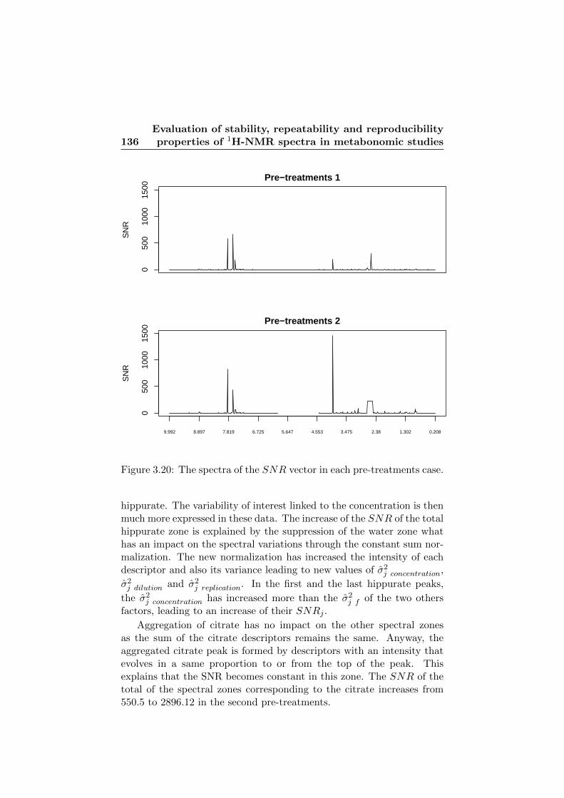
136Evaluation of stability, repeatability and reproducibilityproperties of 1H-NMR spectra in metabonomic studies

050

010

0015

00

Pre−treatments 1

SN

R

050

010

0015

00

Pre−treatments 2

SN

R

9.992 8.897 7.819 6.725 5.647 4.553 3.475 2.38 1.302 0.208

Figure 3.20: The spectra of the SNR vector in each pre-treatments case.

hippurate. The variability of interest linked to the concentration is thenmuch more expressed in these data. The increase of the SNR of the totalhippurate zone is explained by the suppression of the water zone whathas an impact on the spectral variations through the constant sum nor-malization. The new normalization has increased the intensity of eachdescriptor and also its variance leading to new values of σ2j concentration,

σ2j dilution and σ2j replication. In the first and the last hippurate peaks,

the σ2j concentration has increased more than the σ2j f of the two othersfactors, leading to an increase of their SNRj .

Aggregation of citrate has no impact on the other spectral zonesas the sum of the citrate descriptors remains the same. Anyway, theaggregated citrate peak is formed by descriptors with an intensity thatevolves in a same proportion to or from the top of the peak. Thisexplains that the SNR becomes constant in this zone. The SNR of thetotal of the spectral zones corresponding to the citrate increases from550.5 to 2896.12 in the second pre-treatments.

3.6 Conclusions about contextual questions 137

Ordered curves are the second way to summarize the informationpresented in the spectra. Spectral zones corresponding to the water arenot taken into account for building both curves.

0 100 200 300 400 500

050

010

0015

00

SN

R

Figure 3.21: The ordered curves of the SNR vectors. The blackcurve corresponds to pre-treatments procedure 1; the red one to pre-treatments procedure 2.

The curves show that pre-treatments procedure 2 gives a better highlightof the effect of the concentration factor (upper curves). Appendix 4presents the probability density plots and the boxplots of the two SNRvectors.

Finally, for each pre-treatment procedure, the vector of the m SNRjcan be summarized by a global statistic:

SNRstat =1

m

m∑j=1

(σ2j1∑lf=2 σ

2jf

). (3.13)

with y1 is the factor of interest (the concentration in this example).

Table 3.8 presents the SNRstat computed for each factor in eachpre-treatments procedure. Values indicate that the pre-treatments pro-cedure 2 maximizes the heterogeneity between spectra of different acidsconcentration levels, while minimizing the heterogeneity between spec-tra from different dilution levels or replications.

138Evaluation of stability, repeatability and reproducibilityproperties of 1H-NMR spectra in metabonomic studies

Pre-treatments procedure SNRstat1 540.32

2 867.74

Table 3.8: The global statistics of the SNR in the 2 pre-treatmentprocedures.

3.6 Conclusions about contextual questionsThe use of the proposed tools on the designed datasets provides impor-tant conclusions for the setting of a metabonomic study.

Between STE and CPMG protein suppression method, the CPMGis the one to recommend to warranty spectral repeatability.

In human serum data two studied biological sources of spectral vari-ability, the volunteer and blood sampling, affect much more the qualityof metabonomic data than two studied analytical sources of spectralvariability, the tube preparation and the time of measurement after de-frozing. This last source has a very weak impact on the metabonomicdata variability.

The removal of water and urea with citrate aggregation in a peakwere demonstrated to provide data with a better expression of biomarkersignals relatively to the undesired variability.

The next subsections summarize the results obtained for each ques-tion.

3.6.1 Question for the experimental serum dataset

All the proposed tools indicate that STE protein suppression methodcreates a larger spectral variability. The global variability of STE isevaluated to be more than twice larger than the CPMG by the globalCV ’s, and four times larger by the inertias. These conclusions are main-tained even when attention is paid to the fact that STE spectra presenta largest proportion of descriptors susceptible to vary (not set to zero)than the CPMG spectra (global CV ’s and ordered curves were also re-alized for the descriptors not set to zero in both protein suppressionmethods). For the two protein suppression methods, different spectralparts with a large variability relative to their mean intensities are iden-tified in the spectra of the coefficients of variation vectors.

3.6.2 Question for the human serum dataset

In the human serum dataset, the three proposed tools result in thefollowing decreasing ranking of the four studied sources of spectral vari-ability: the volunteer, the blood sampling of a volunteer, the tube of

3.7 Conclusions 139

a sampling for a volunteer, the time of measurement. All the resultsagree to conclude that the differences between spectra from differentvolunteers are predominant. The spectral variations caused by the vol-unteer are the most important ones and ICCvolunteer also tells us thatthey correspond to a huge proportion of the total variability of the af-fected buckets. Spectra also meet considerable variations from one toanother blood sampling for a volunteer and these variations represent alarge proportion of the variability of many of the influenced buckets bythis source. Spectral variations between spectra of different tubes of ablood sampling from a volunteer are present but weak in comparison tothe ones created by the volunteer and the blood sampling. Variationsbetween spectra of a same tube measured at different times are nearlyzero. The time of measurement after defrozing does not impact on thequality of metabonomic data. Note that analysis of the residuals fromthe pointwise models have shown that there exist sources of variabilityunconsidered, or even interactions between the studied sources. But ifthey create spectral variations larger than the ones caused by the timeof measurement they remain weak.

3.6.3 Question for the urine dataset

In the urine datasets, the PCA scoreplots and inertias have shown thatthe second procedure accentuates differences between spectra from sam-ples with different concentrations of hippurate and citrate and reducesdifferences between spectra from samples of different dilutions or dif-ferent replicates. The SNR global statistics and ordered curves havedemonstrated that proportionally to the spectral variability caused bythe dilution and replication, the spectral variability linked to changesof metabolites concentration is better expressed in procedure 2. Theimprovement by procedure 2 is explained by the effect of the water zonesuppression through the normalization. Citrate aggregation has only aneffect on the citrate zone what also contributes to improve some results(inertia, global statistics, ordered curves).

3.7 Conclusions

The success of metabonomic data analysis crucially depends on keepingthe biological, experimental and analytical variabilities at a minimum.This chapter presented methodologies to evaluate spectral variabilitysources and the performances of tools that can minimize these undesiredvariations as study designs, experimental protocols, acquisition modesand data pre-treatments.

Starting from the elaboration of a list of three general research ques-tions about metabonomic spectral variability, we proposed several solu-

140Evaluation of stability, repeatability and reproducibilityproperties of 1H-NMR spectra in metabonomic studies

tion tools.

The PCA was naturally considered due to its broadcasting in themetabonomic field and its previous use in the literature for the spectralvariability study. The PCA offers, on the scoreplot of the two first PCs,a general solution for the three questions about spectral variability. Butif its visual support is on one hand an advantage, on the other hand itrenders PCA insufficient to study the repeatability of the spectral data.Even if some useful information can be given, spectral variabilities arenot limited to the variability present in the two first components.

By contrast with PCA, the other proposed tools offer an examinationof the complete spectral variability. A distinction can be made amongthem between inertias and pointwise approaches.

Inertia computed in the initial space can complete PCA and alsooffers solutions to the three research questions. The inertia tool resultsinto global values which are quickly comparable. The decomposition ofthe total inertia in interclass and intraclass inertias is a decompositionof the total variability in the variability caused by a factor and theresidual variability. Inertia is thus similar to an ANOVA decompositionin several dimensions. Nevertheless, inertia decomposition cannot beengeneralized for more than one factor in unbalanced design.

Two kinds of pointwise approaches were presented: simple pointwisesummary statistics and pointwise mixed models. Pointwise summarystatistics are typically used to compare the different levels of a givensource of variability. Pointwise mixed models provide variance compo-nents of different factors in order to compare variability sources. Thesetwo pointwise approaches have the advantage to result in variabilityinformation detailed for the different spectral descriptors. In each situ-ation, additional solutions were brought to summarize the results overthe set the different descriptors.

Based on simple concepts, the pointwise summary statistics locallymeasure the variability in absolute way or relatively to the mean 1H-NMR intensity. The buckets with a large variability are revealed by theirspectral representations. To find the levels of the variability source thatminimizes the global spectral variabilities, we proposed ordered curvesand Global CV ’s to summarize and compare the pointwise statistics. Ascurves comparison are tricky (the ppm information is lost and in somecases, curves can be only compared for a restricted number descriptors),we recommend the use of the Global CV ’s.

3.7 Conclusions 141

To explore and compare several sources of undesired spectral vari-ability, we presented two indices computed from the pointwise variancecomponents. These ones locally measure the importance of the vari-ability created by the source in an absolute way and relatively to thetotal variability. Thanks to the pointwise approach, buckets the morevarying and the more influenced for a given source can be discovered ona spectral representation of these indices. Visual supports and globalvalue computation were presented to summarize the pointwise indicesover the whole spectrum. The sources of variability can thus be rankedand appreciated through the importance of the variability created andthe proportion of the total variability that it represents. Additionally,the modelling approach provides models residuals giving insight aboutthe existence of unconsidered sources of variability.

To evaluate the spectral expression of the biomarker signal compar-atively to other signals, we proposed an index, the SNR, formed onthe basis of the pointwise variance components. Comparison of SNRbetween several datasets gives the possibility to choose the more in-formative dataset. This can be applied to evaluate performances of apre-treatment. The comparisons can be realized with SNR spectral rep-resentations or more globally by ordered curves and global indices. Butthis last is not scaled what presents a disadvantage to evaluate the qual-ity of a single dataset. In this situation, the spectral representation ofthe SNR is more informative.

Contrarily to the inertia tool, pointwise tools based on mixed modelsare able to treat several factors in complex unbalanced design dataset.Additionally, the random character of a source of variability can betaken into account. Some perspectives could be to consider the gen-eralization of ANOVA to multiple variables. The multivariate-ANOVA(MANOVA) is the classical generalization [62]. But for large number ofmeasured variables, as in metabonomics, MANOVA breaks down owingto problems of singularity of the covariance matrices [84]. The possibil-ity for generalization of ANOVA could be found with a recent method,the ANOVA-simultaneous component analysis (ASCA) [46].

142Evaluation of stability, repeatability and reproducibilityproperties of 1H-NMR spectra in metabonomic studies

CHAPTER 4

Comparison of some chemometrictools for metabonomic biomarker

identification

Part of this chapter comes from: Rousseau R., Govaerts B., VerleysenM., Boulanger B., Comparison of some chemometric tools for metabo-nomic biomarker identification, published in Chemometric and intelli-gent laboratory systems 91 (2008) 54-66.

4.1 Introduction

This chapter aims at investigating the relative properties of advancedstatistical methods for the discovery of metabonomic spectral biomark-ers from 1H-NMR data. The searched biomarkers are in this chapterthe spectral areas allowing to discriminate between two groups of sub-jects (”Two-class problem” study). All methods covered in this chapterare based on published statistical tools. Nevertheless, some of them areextended in order to fit with the spectral metabonomic biomarker discov-ery goal. Some of the methods are used solely for spectral metabonomicbiomarker search; others may be used as predictive models too. All arecompared based on both qualitative and quantitative considerations.

Chapter 4 is organized as follows. Section 4.2 presents six possi-ble methods to discover spectral biomarkers. The first one (MHT) isbased on traditional descriptor-wise multiple hypothesis testing. Thenext two (s-PCA and s-ICA) are extensions of corresponding traditionalmultivariate data reduction tools. The final three methods (PLS, lin-ear logistic regression and CART classification trees) provide predictivemodels from which spectral biomarkers can be extracted.

144

Comparison of some chemometric tools for metabonomicbiomarker

identification

The next sections are devoted to the illustration and comparisonof these methods. Section 4.3 presents the data used for this pur-pose. These data are subsamples from the semi-artificial metabonomicdatabase presented in Section 2.2. Section 4.4 illustrates the methodson one dataset and emphasizes their particular characteristics. Finally,Section 4.5 tests systematically the six methods on several data sam-ples and compares their performances in terms of various criteria suchas sensitivity, specificity and stability. This comparison will show thatall methods, except s-PCA and CART, give promising results. Each ofthem has its own advantages and provides specific information.

4.2 Methods

In this section, six methods considered for spectral biomarker discov-ery and/or prediction are described, after the presentation of unifiednotations. All methods are described both in an intuitive way and analgorithmic form.

As explained in Section 0.4, two sets of data are used in the search ofspectral metabonomic biomarkers: X, the (n×m) spectral data matrixand Y , the (n× l) metadata matrix. Y contains yk, a variable of interestfor which the spectral biomarkers are searched. In this part of the thesisresearch, yk is a binary vector. This vector yk of size n identifies theclass of each of the n spectra; n0 are normal spectra (yk = 0) and n1(yk = 1) are altered ones. Section 4.3 will detail the difference betweennormal and altered spectra.

The goal here is to find among the m descriptors of the spectrumthose which are associated to the concept of class membership, i.e.those which show systematic differences between the normal and alteredclasses. Concretely, each method provides so-called ”biomarker scores”for all spectral descriptors in a vector b of size (m× 1). The descriptorswith the highest scores will be considered as potential biomarkers. Thenumber mb of potential biomarkers is chosen either by the biologist orrecommended based on statistical criterion included in the method.

4.2.1 Multiple hypothesis testing (MHT)

4.2.1.1 Presentation

In the emerging -Omics techniques, multiple hypothesis testing (MHT)has become a very popular technique to determine simultaneously ifsome descriptors, of a large set of possible ones, are altered by a (biolog-ical) factor of interest. Micro-array data analysis has been the privilegedarea of application of such methods.

4.2 Methods 145

MHT consists in calculating, for each descriptor, a test statistic mea-suring the effect of the factor of interest; in our case, this factor is yk, thealtered and normal spectral class identifier. The multiple test procedureaims then at giving a rule to decide which of the calculated statisticsare statistically significant in controlling the total error rate of the test.When the number of tests is very high, the false discovery rate (FDR),i.e. the number of false discoveries over the number of discoveries, isusually taken as the error factor to be controlled. Several methods havebeen developed in an attempt to control the FDR under independent ordependent hypotheses [6] [90] [85] [86].

In this work, MHT is applied in two steps. First, for each descrip-tor, a classical t statistic is calculated to compare the mean spectralintensities of the two groups. The p-values attached to each statistic arethen calculated and transformed to build biomarker scores. The Ben-jamini and Yekutieli [6] rule for multiple testing under dependency isthen applied to set up a cut point between significant descriptors andnon-significant ones.

4.2.1.2 Algorithm

• From the spectral matrix X, calculate, for each descriptor j =1, ...,m, the following t statistic :

tj =x1j − x0j√s21jn1

+s20jn0

. (4.1)

where

– x0j = 1n0

∑{i:yki=0}Xij

– x1j = 1n1

∑{i:yki=1}Xij

– s20j = 1n0−1

∑{i:yki=0}(Xij − x0j)2

– s21j = 1n1−1

∑{i:yki=1}(Xij − x1j)2

• Calculate the individual p-values attached to these t statistics as

pj = 2P (tνj > |tj |). (4.2)

where tνj is a Student t random variable with νj degrees of free-dom. νj is defined by the Welch formula as the closest integer to

(s21n1

+s20n0

)2

(s41

n21(n1−1)

+s40

n20(n0−1)

).

146

Comparison of some chemometric tools for metabonomicbiomarker

identification

• Define the vector of signed biomarker scores b = (b1, b2, ..., bm)from the following transformation of the pj ’s :

bj = sign(tj)(log(1/pj)). (4.3)

• Choice as potential biomarkers the mb descriptors with the highestbj ’s. mb can be chosen by the analyst or by the Benjamini-YekutieliFDR controlling rule [6]: mb = max{i : pi ≤ iα

m∑m

i=11i

} where α

is the maximum expected FDR desired for the multiple testingprocedure.

4.2.2 Supervised principal component analysis (s-PCA)

4.2.2.1 Presentation

In metabonomics and 1H-NMR data exploration, the Principal Compo-nent Analysis (PCA) [47] is the most commonly used method by prac-titioners. However, as discussed in previous chapters, the traditionaluse of PCA in metabonomics remains questionable, notably due to theuse of the two first principal components. As PCA is here presented asa reference tool for spectral biomarker search, some improvements aresuggested through a method called s-PCA.

s-PCA is performed as follows. A PCA is first applied to the matrixof centered by columns spectra Xc. The normalized score matrix isthen used to find the two components which discriminate best betweenthe two groups. This is an unusual, but effective way of using PCA.Indeed, PCA is an unsupervised method: the principal components arecomputed without taking the class information into account. The twofirst directions, which are usually selected, are therefore not necessarilythose that maximize the discrimination. Here all directions are firstcomputed, and only the two ones that discriminate the most the classesare kept. Then, in the plane defined by these two principal components,the direction that maximizes the discrimination is calculated and thecorresponding loadings are chosen as biomarker scores.

4.2.2.2 Algorithm

• Center X by columns: Xc = X − 1n · XT where X is the (m× 1)vector of column means and 1n a (n× 1) vector of ones.• Perform a PCA on Xc : Xc = TP T where T is the (n× q) scores

matrix and P is the (m× q) loadings matrix (q = min(n,m)).• Normalize the score matrix as C = TΓ−1/2 where Γ is the diagonal

matrix with the q nonnull eigenvalues of (XcTXc).

4.2 Methods 147

• By applying formula (4.1) to C (instead of X), calculate t statisticsto compare, for each principal component, the normalized scoresof both groups.• Search the two components j1 and j2 that maximize |tj |, i.e. which

discriminate the best between the two groups.• In the space of components j1 and j2, find the direction which max-

imizes the distance between the two groups centroids and evaluatethe contribution of loadings to this direction:

p∗ = pj1 c1j1 − pj2 c0j2 . (4.4)

where c1j1 is the coordinate on j1 of the mean c1 of spectra scoresfrom class 1 and c0j2 is defined in the same way.• Define the biomarkers scores as b = p∗.• Choose a predefined number of descriptors with highest (absolute)

scores as candidate biomarkers.

4.2.3 Supervised independent component analysis (s-ICA)

4.2.3.1 Presentation

Independent component analysis (ICA) [45] is a method that originallyaimed in recovering unobserved signals or sources from linear mixtures ofthem. In the context of metabonomic 1H-NMR data, the media analyzed(e.g. serum, urine) can be seen as a mixture of individual metabolitesand 1H-NMR spectra may then be interpreted as weighted sums of 1H-NMR spectra of these single metabolites. If the matrix X of 1H-NMRspectra is rich enough, the application of ICA to 1H-NMR data shouldthen ideally recover source products included in the analyzed media, inparticular those that are biomarkers of the causal factor of interest inthe study.

ICA is applied in this context as follows. First ICA is applied tothe matrix of spectra. t statistics are then calculated from the mixingcoefficients and used to identify sources that are able to discriminatethe two groups of interest. Identified sources can ideally be interpretedas spectra of pure or complex metabolites whose quantities have beenaltered by the factor of interest. Mean 1H-NMR spectra for both alteredand normal groups are then reconstructed from the identified sourcesand the differences between these mean spectra are used as biomarkerscores.

4.2.3.2 Algorithm

• Transpose X and center it by columns: XTc = XT −1m · X whereX is the (1 × n) vector of columns (spectra) means and 1m a

148

Comparison of some chemometric tools for metabonomicbiomarker

identification

(m× 1) unit vector.• Apply ICA to XTc. e.g. the FastICA algorithm with parallel

extraction of components proceeds in three steps:

– Reduce by PCA the (m×n) matrix XTc to a (m× q) matrixof scores T (q ≤ min(n,m)): XTc = TP T +E where E is theerror.

– Apply ICA to T : T = SW where S is the (m× q) matrix ofsources and W is the (q × q) unmixing matrix.

– Derive the mixing matrix A such that XTc = SA.

• Search for the sources that discriminate the most normal and al-tered spectra.

– Calculate t statistics to compare, for each source, the mixingcoefficients in both groups. The t statistics are derived byapplying formula (4.1) to AT , the transposed mixing matrix.

– Choose the r sources with the highest tj as those that discrim-inate the most the two groups. r can be chosen either visuallyor with a Bonferroni correction or a FDR based method ap-plied on the tj ’s.

– Build S∗ and A∗ the subset matrices of S and A correspondingto these r sources.

• Calculate the biomarker scores as

b = S∗A∗Z. (4.5)

where Z is a (n × 1) vector with Zi = −1/n0 if yk = 0 and 1/n1otherwise.• Choose a predefined number of descriptors with highest (absolute)

scores as candidate biomarkers.More details about the ICA are given in Chapter 5.

4.2.4 Discriminant Partial Least Squares (PLS-DA)

4.2.4.1 Presentation

Partial least squares discriminant analysis (PLS-DA)[5][63] is a partialleast squares regression aiming at predicting one (or several) binary re-sponses(s) Y from a set X of descriptors. PLS-DA implements a compro-mise between the usual discriminant analysis and a discriminant analysison the significant principal components of the descriptor variables. It isspecifically suited to deal with problems where the number of predictorsis large (compared to the number of observations) and collinear, twomajor challenges encountered with 1H-NMR data.

4.2 Methods 149

This research suggests to apply PLS-DA for spectral biomarker dis-covery as follows. First, a PLS-DA prediction model is estimated [21];the number of significant components is then chosen according to a cross-validation based criterion. The model provides regression parametersthat can be used as biomarker scores b. The descriptors with the high-est (absolute) coefficients are candidate biomarkers.

4.2.4.2 Algorithm

• Center X by columns: Xc = X − 1n · XT .• Choose the optimal number of components of the PLS model us-

ing an adequate validation technique and criterion. The RMSEP(Root mean square error of prediction)[64] is a traditional criterionused in this context. It can be calculated for each size of model onan external validation set or, when no validation set is available,by k-fold cross-validation.• Build the PLS regression prediction equation Y = Xcb using the

previously chosen number of components.• Define b as the vector of biomarker scores.• Choose a predefined number of descriptors with highest (absolute)

scores as candidate biomarkers.

4.2.5 Linear logistic regression (LLR)

4.2.5.1 Presentation

Linear logistic regression (LLR) [41] generalizes classical multiple regres-sion to binary responses. It aims at predicting the probability of classmembership π = P (Y = 1) as a function of a set of exploratory variablesx = (x1, x2, ...xk)

′. In order to get a model response in the [0, 1] inter-val, the π is transformed with the logistic transformation: η = log( π

1−π )and η is expressed as a linear combination of x as η = α + δ′x. Theparameters are estimated by maximum likelihood to take into accountthe Bernouilli distribution of the response yk.

Several points must be discussed when applying LLR to biomarkersearch. As the number of potential regressors (descriptors) m is highand, in most cases, larger than the number of spectra (n << m), adimension reduction or variable selection technique must be first appliedto allow model estimation. Variable selection is privileged in this paperbecause the variables (descriptors) selected in the model can directly beseen as potential biomarkers. Forward selection (a technique that addsdescriptors and never deletes them) and stepwise-forward (which startswith an empty set and adds or removes a single predictor variable ateach step of the procedure) have been tested. Forward selection has

150

Comparison of some chemometric tools for metabonomicbiomarker

identification

demonstrated to be adequate in this context. The Akaike AIC criterion[1] is commonly used to select the variables to be entered into the model.The AIC criterion is defined as AIC = −2log(L) + 2(k + 1) where L isthe likelihood of the estimated model, and k is the number of variablesincluded. When a model has been set up, biomarkers scores may bederived from the p-values of the regression coefficients.

4.2.5.2 Algorithm

• Estimate a model with the constant term only and calculate thecorresponding AIC.• Repeat for k = 1, ...,mb:

– Try to enter each descriptor xj (j = 1, ...,m) as a supplemen-tary variable in the model and calculate the correspondingAICj .

– enter in the model variable xj such that AICj is minimum.

• Stop either when a predefined maximum number mb of descriptoris reached or when the AIC criterion can not be decreased anymore.• Take as biomarker scores bj = 0 if descriptor j is not chosen in the

model and bj = sign(δj)(1/pj) for the other descriptors. pj is thep-value of the Wald test on the regression parameter δj .

4.2.6 Classification and regression trees (CART)

4.2.6.1 Presentation

The CART tree classifier [11] implements a strategy where a complexproblem is divided into simplest sub-problems, with the advantage thatit becomes possible to follow the classification process through each nodeof the decision tree. In the context of this research, CART is proposedto realize recursive and iterative binary segmentations of the descriptorspace in order to direct spectra to smaller and smaller groups that aremore and more homogeneous with regards to the class. When lookingfor biomarkers, the tree is not developed for its capacity to predict theclass membership but for its stepwise selection of a subset of featuresrelevant for class discrimination: the construction of the tree highlightsin segmentation rules the descriptors with a good discriminant powerbetween the two classes of spectra.

4.2.6.2 Algorithm

• Build the maximal tree model Tmax by repeating segmentationuntil the number of spectra in each subgroup is less or equal than5 as suggested by Breinman ([11] p82):

4.3 Description of the data 151

– Define a binary segmentation rule by a descriptor xj and its

threshold x(t)j chosen as to maximize the decrease of the Gini

impurity criterion ( [11] p38).

– based on the value of xij , direct each spectrum i of the nodeto the left or the right child-node according to the chosen

segmentation rule (xij ≤ or > x(t)j ).

• If a fixed mb is required, take as biomarkers the descriptors xj ’scorresponding to the mb segmentation rules with the highest num-ber of spectra in the branch under the corresponding node. Thebiomarker score bj is this number when xj is in this biomarker listand 0 otherwise. Note that the number of segmentation rules inthe tree may be smaller than mb.

• If one wants to choose automatically the number of biomarkersmb, the tree Tmax may be reduced to a smaller (and optimal) treeTopt by cost-complexity pruning [29]. This method cuts stepwisethe branches of the initial tree which minimize the increase of errorrate. In this sequence of nested trees, the optimal one is chosenwith respect to its predictive accuracy (measured by a deviance)on an external data set or k-fold cross-validation ones.

4.2.7 Implementation

All algorithms have been implemented in the R language. Links to theused libraries are available onwww.cran.r-project.org/src/contrib/Descriptions/. The following librarieswere used: for PCA, the pcurve library, for ICA: the fastICA library,for PLS-DA: the pls-pcr library, for LLR: the Design library, for CART:the tree library. The MHT method has been implemented specificallyfor this study.

4.3 Description of the dataThe goal of the next sections is to show that the methods are able to iden-tify the altered descriptors. For this purpose, a semi-artificial database,presented in Section 2.2, was constructed. Each of the used urine spec-tra has a resolution of 500 buckets. This part of the thesis researchhas been realized before the study of the pre-treatment scheme. Conse-quently, the spectra were only pre-teated by Bubble. This correspondsto the pre-treatment procedure advised in Section 1.3.1 but without zerosetting of negative values, removal of non informative regions and ag-gregation of the citrate ppms. However a final normalization has beenapplied.

152

Comparison of some chemometric tools for metabonomicbiomarker

identification

Subsamples of size 60 (2×30) and 200 (2×100) have been extractedout this database to simulate typical metabonomic sample sizes. InSection 4.4, one sample of 200 spectra was drawn randomly to illustratethe methods. In Section 4.5, 20 samples for each size were drawn tocompare the performances of the methods. Note that validation setswere not used when needed in the methods (PSL and CART); k-foldcross validation was preferred instead.

The variable of interest for the biomarker search, yk, is here a bi-nary variable describing the fact that the spectrum is or not an alteredspectrum. By convention, the terms ”biomarkers” and ”identifications”are here used to make a distinction between respectively the ”real alter-ations that we want to detect” and ”the results or selection of descriptorsindicated by the method as biomarker”.

4.4 Illustration of the methodsThe purpose of this section is to illustrate the six methods on a sub-sample of 200 (100 normal and 100 altered) spectra extracted from thesemi-artificial database described in Section 4.3. The main results avail-able from the six methods are reported graphically in Figures 4.1 to 4.4.Figure 4.1 provides the biomarker scores calculated for each one. Fig-ures 4.2, 4.3 and 4.4 present intermediate outputs for s-PCA, s-ICA andCART that offer additional support to visualize the identified descrip-tors and/or some specific features of these procedures. All these graphsserve below to describe qualitative behaviour resulting from the designof the methods; systematic performance method evaluation is the topicof Section 4.5.

4.4 Illustration of the methods 153

MHT

s−PCA

s−ICA

PLS−DA

LLR

Index0 100 200 300 400 500

CART

Figure 4.1: Biomarker scores for all tested methods.

154

Comparison of some chemometric tools for metabonomicbiomarker

identification

Let’s first interpret the score plot figure.

• Four methods (MHT, s-PCA, s-ICA and PLS-DA) provide non nullscores for all descriptors leading to possible complex score profiles.Score profiles for the LLR and CART methods are simpler sincethey come from variable selection procedures and non null scorevalues only exist when a descriptor is selected.• The vertical lines on the graph show the locations of the 46 ”real”

biomarkers. High positive scores in these regions denote that themethod was able to identify them. High (positive or negative)scores elsewhere must be interpreted as false discoveries.• The sign of each score has also a meaning: a positive score indicates

that the corresponding descriptor has potentially a positive effecton the intensity of the altered spectra. A negative score leads toa decrease of intensity from normal to altered spectra.• Three methods (MHT, LLR, CART) provide criteria to select au-

tomatically ”significant” scores. These have been applied here.The threshold of selection, drawn by an horizontal line in the MHTgraph, is calculated from the Benjamini Yekutieli (B-Y) FDR rulewith α = 0.05. The descriptors in LLR are those selected by min-imizing AIC and in CART by applying the pruning algorithm.This example shows that LLR and CART seem to be very selec-tive methods but, on the contrary, the B-Y does not seem to reallycontrol FDR since many false discoveries appear (much more than5%). The horizontal lines drawn for the three other methods (s-PCA, s-ICA and PLS-DA) have no statistical interpretation andare there only for visual purpose. They have been drawn such thatthe number of scores appearing out of the interval is 23, the halfof the 46 ”real” biomarkers.• The MHT method identifies well all biomarkers but is also the

method that generates the noisiest score vector leading to manyfalse identifications. It may be shown that this behaviour increaseswhen the sample size decreases.• s-PCA, s-ICA and PLS-DA methods have quite similar score pro-

files: they are all able to identify some (s-PCA and PLS-DA) orall (s-ICA) biomarkers and display reasonable noise in the otherregions. s-ICA is specially able to extract signal from noise. PLS-DA seems, as it is a predictive tool, to privilege biomarkers fromthe less noisy spectral region. More curiously, s-PCA performsbetter in the noisy biomarker region. This may be due to the factthat the t statistic privileges high signal even in a noisy area ofthe spectrum.• For LLR and CART methods, one can observe that true discoveries

4.4 Illustration of the methods 155

are all coming from independent biomarkers. When one descrip-tor from an independent biomarker is selected by the procedure,all others are discarded because they constitute redundant (andcorrelated) information. This behaviour is typical in a forward re-gression selection technique and in decision trees. Figure 4.1 showsthat LLR identifies five (of the six) independent biomarkers witha little sensitivity to noise while CART identifies only the three inthe first part of the spectra. The CART method presents indeeda high sensitivity to noise, as illustrated by the lack of identifica-tion of biomarkers in the second (noisy) part of the spectra. Manyother simulations have confirmed that basic CART can be efficientin situations without or with low noise but is not able to find signalin presence of higher noise.

The following comments can be made from Figure 4.2 to 4.4:

• Figure 4.2 presents, for s-PCA, the projection of the 200 spectrain the space of the two principal components which discriminatebest normal and altered spectra. This graph is certainly helpfulfor most biologists very used to PCA methods. It shows how wellspectra are separated and can detect outliers. Note that, in thisexample, the two best components are the 8th and the 7th. Biol-ogists used to work with first components should then figure outthat high variance explained does not mean high discriminationas the classification factor is not taken into account in a PCA.More precisely, the space of the 7th and 8th components explainsan amount of variance smaller than the space formed by the PC1and PC2 (7,9% with respect to 14,8%). However, components 7and 8 contain the part of the variance that is informative for thesearch for biomarkers, as illustrated by the distinction between thetwo kinds of spectra in Figure 4.2.• Among the 100 estimated sources in s-ICA, 10 independent sources

were selected (by a FDR based procedure applied to the t statis-tics) to be significantly discriminant. Each of these independentsources is illustrated on Figure 4.3. The graphic is impressive:sources s1, s2, s3, s4, s7 and s8 correspond nearly perfectly to thesix independent biomarkers added to highly variable urine spectrain the artificial database. ICA is therefore able to extract these in-dependent multi-descriptor biomarkers without prior informationon their number and characteristics. The ”purity” of the sources(especially s1, s2 and s7) must also be highlighted: the signal canreally be extracted from the noise. Sources s5, s6, s9 and s10 areunfortunately less useful: these represent correct biomarkers but

156

Comparison of some chemometric tools for metabonomicbiomarker

identification

−0.2 −0.1 0.0 0.1

−0.

2−

0.1

0.0

0.1

0.2

PC8

PC

7

Figure 4.2: Projection of the spectra on the principal components whichbest discriminate between normal and altered spectra. A 4 symbolrepresents a projection of a normal spectrum and a ◦ of a altered one.The two ∗ indicate the centroids of the clouds respectively formed byeach kind of spectra.

are only parts of the multi-peak independent biomarkers. Theorthogonality of the ten sources is confirmed by scatterplots andPearson coefficients of correlation in Appendix 5. The occurrenceof s5, s6, s9 and s10 as independent sources is explained by the factthat they present random variations observable between the initialplacebo spectra and not the artificial alterations added. Addition-ally, a close examination of s9 and s10 shows that these sourcesrespectively present a peak reaching its top in two different andconsecutive descriptors. The same observation is made for s5 ands6. The two couple of sources (s5-s6, s9-s10) give insight abouttwo peak shifts. These shift problems are easily understandablein these data as the bucketing interpolation method (see Section1.3.1.12) was not used in the pre-treatment.Note that the authors realized similar graphs with the loadingsof the principal components calculated from s-PCA or PLS-DA.They are not shown here because they do not reveal any usefulinformation about independent biomarkers and are much noisier.

4.4 Illustration of the methods 157

S1 S2

S3 S4

S5 S6

S7 S8

Index

S9

0 100 200 300 400 500Index

0 100 200 300 400 500

S10

Figure 4.3: The ten ICA sources which best discriminate between normaland altered spectra.

• The CART tree representation shown in Figure 4.4 presents thesequence of descriptors issued from the recursive segmentation,providing supplementary information on the order of descriptorselection and the exact segmentation rules. The horizontal lineshows where the tree was cut by the pruning algorithm.

158

Comparison of some chemometric tools for metabonomicbiomarker

identification

|X291 < 0.857045

X214 < 24.6104

X221 < 2.32421

X75 < 0.36807

X169 < 0.353421

X139 < 1.14923

X179 < 0.439958

X72 < 0.111282

1 10

0

0 01

1

1

Figure 4.4: Classification tree before and after pruning. Horizontal barsindicate where the tree is pruned.

4.5 Method comparison

The six methods described in this paper have been illustrated using asingle dataset in Section 4.4. The present section compares their perfor-mances on several datasets of different sample sizes. For this purpose,20 samples of 200 spectra (100 altered and 100 placebo ones) and of 60spectra (30 altered and 30 placebo ones) were drawn at random fromthe semi-artificial database described in Section 4.3. The six methodswere then applied to each of these 40 datasets. Different samples sizesare used to test the robustness of the methods to small (but realistic inreal-life situations) samples. In addition, generating 20 samples elim-inates possible effects of a particular draw while the variability of theresults can also be studied too.

4.5.1 Number of identifications

The first results concern the identifications obtained from each method.Figure 4.5 provides for the 200 spectra datasets and for each method,the proportion of simulations where each descriptor has been identifiedas a biomarker. The positive bars represent the correct identifications;the negative bars indicate false discoveries. Results for the 60 spectradatasets are not given because they are very similar and only accentuate

4.5 Method comparison 159

the observations coming out of Figure 4.5.For three methods (s-PCA, s-ICA and PLS-DA), the number of de-

scriptors mb that the method identifies as biomarkers has to be fixed bythe analyst. As a method can be supposed to have a limited numberof correct detections, the number mb for these methods has been fixedhere at 23, the half of the total 46 biomarkers randomly added to the al-tered spectra. For the three other algorithms (MHT, LLR and CART),the number of identifications mb is chosen automatically by a statisticalcriteria as detailed in Section 4.2.

These results will be interpreted together with the ROC curves afterthe next subsection.

160

Comparison of some chemometric tools for metabonomicbiomarker

identification

MHT

−1.0

−0.5

0.0

0.5

1.0

s−PCA

−1.0

−0.5

0.0

0.5

1.0

s−ICA

−1.0

−0.5

0.0

0.5

1.0

PLS−DA

−1.0

−0.5

0.0

0.5

1.0

LLR

−1.0

−0.5

0.0

0.5

1.0

Index

CART

0 100 200 300 400 500

−1.0

−0.5

0.0

0.5

1.0

Figure 4.5: Proportions of occurrences of true (positive bars) and false(negative bars) biomarker identification in simulations.

4.5.2 ROC curves

As the performances of a method strongly depend on the total numberof identifications mb (both false identifications and biomarkers correctlyidentified), it is sometimes difficult to compare several methods which donot deliver the same number of identifications. The receiver operating

4.5 Method comparison 161

characteristic curve (ROC [24]) provides a way to visualize the perfor-mances of a method for a whole range of possible mb. It must be noticedthat in the presented ROC curves the performances evolve according toan experimental condition (the value of mb) and not according to a pa-rameter of the method as in the traditional ROC curves. Consequently,the ROC curves here shown can be non-monotonic. More precisely,it gives for each number mb of identifications, in a chosen range, themethod sensitivity and FDR (false discovery rate). The sensitivity isdefined as the proportion of biomarkers correctly identified (among allbiomarkers); the FDR is the percentage of false identifications (amongall the mb identifications).

As explained in Section 2.2, there are only six independent (multi-ple) biomarkers among the 46 ones. The sensitivity may thus be definedwith respect to the proportion of correct identifications among the 46biomarkers, or with respect to the proportion of correct identificationsfound among the six independent ones. These two definitions of sensi-tivity (therefore of ROC curves) give the four diagrams of Figure 4.6,two for the 200 spectra case and two for the 60 spectra one. Each curverepresents the mean of the 20 ROC curves obtained from the applica-tion of one method to the 20 datasets. Each curve presents a methodperformance in a range of 1 to 46 numbers of identifications.

Good methods are those whose curves are mostly concentrated in orat least reach the upper left part of the ROC diagrams.

162

Comparison of some chemometric tools for metabonomicbiomarker

identificationS

ensi

tivity

MHTs−PCAPLS−DAs−ICALLRCART

0.0

0.5

1.0

All biomarkers − n=200

False discovery rate

Sen

sitiv

ity0.

00.

51.

0

0.0 0.5 1.0

Independant biom − n=200

All biomarkers − n=60

False discovery rate0.0 0.5 1.0

Independant biom − n=60

Figure 4.6: Mean ROC curves (sensitivity versus false discovery rate)for the six methods. For clarity, curves only show symbols representingeven number of identifications.

The following comments can be made from Figures 4.5 and 4.6.

The MHT method, with its FDR based threshold criterion, selectsa higher number of descriptors as potential biomarkers (75 in averagefor the 200 spectra case). It is thus natural that this method has a highsensitivity, but this it is at the price of a high FDR. This confirms thepoor performance of the B-Y decision rule in this context. The MHT tscores are able to discover biomarkers in both low and high noise regionsof the spectra but loose clearly its performance in small samples. TheMHT method has also the tendency to make false discoveries in the mostnosy part of the spectra. The main advantage of MHT is then certainlyits simplicity coupled with overall acceptable performances especially inlarge samples. However, as other methods do not require it, the nor-mality of the present 1H-NMR data do not have be taken into account.A possible lack of normality can then have consequences on the MHTscore and its performance.

4.5 Method comparison 163

The s-PCA method, traditionally used in this context, is performingvery poorly. As explained in Section 4.4, s-PCA only provides correctidentifications in presence of high alterations in an ideal unoisy spec-trum. This is why in the presented more likely natural case with largestbiomarkers in a noisy part of the spectra, s-PCA is the second worstmethod (after CART): even if the number of biomarkers was chosen ad-equately (which would require a well-defined criterion), an increase ofthe sensitivity would be accompanied by a high FDR.

The ICA method is more natural than methods based on PCA: in-deed, the independence statistical criterion corresponds to the notionof independent biomarkers, contrarily to the decorrelation as in PCA-based algorithms. This is certainly the main advantage of ICA; theconsequence is that the independent biomarkers can be retrieved andplotted in the form of a spectrum (see Section 4.4) and the metabolitesplaying a role as biomarker can thus potentially be identified.

Besides this interpretation power, the ICA method also gives goodbiomarker identification performances. As it can be seen in Figure 4.5,biomarkers are correctly identified even in the noisy part of the spectra.ROC curves go also in the upper left corners of the diagrams, showingthat sensitivity can become high when increasing the number of iden-tifications without deteriorating too much the FDR. In the case of thesearch for independent biomarkers, the method is even more efficient.In terms of the mean number of biomarkers found, only the PLS-DAmethod can compete with the ICA one.

From Figure 4.5, it is however visible that the good performances ofPLS-DA mostly come from the less-noisy regions of the spectra, while theICA method is more robust in the strongly noisy regions. At comparableperformances in terms of ROC curves, it can be concluded that ICA ismore robust to noise than PLS-DA. The PLS-DA method is however veryefficient in recovering independent biomarkers (it is the only method thatfinds always all of them in the 20 experiments with 200 spectra).

The LLR method is not adequate to find all biomarkers. As a pureprediction tool, it stops selecting potential biomarkers once the predic-tive performances are acceptable. This means that once a biomarkeris found, all other ones that are dependent to the first one will notbe identified. Indeed, the method gives much better performances whenlooking for independent biomarkers only. It is the method which reachesthe highest sensitivity with the smallest mean number of identifications(0.8 with five identifications for n=200). Nevertheless, from Figure 4.5,

164

Comparison of some chemometric tools for metabonomicbiomarker

identification

it appears that in the 20 runs, different biomarkers are selected amongeach set of dependent ones. Building different models (from slightly dif-ferent samples) can thus lead the biologist to find several biomarkersinfluenced by a single metabolite, what can be interesting in some cases.

The CART method does not lead to good performances. As a pre-dictive tool, it identifies only independent biomarkers. Moreover, CARTonly succeeds to identify independent biomarkers in low-noise regions.The advantage of the CART method resides in its tree representationthat is easily interpretable, but coupled to low performances and to beused in non-noisy problems only, i.e. non realistic situation.

Finally, let us remind that PLS-DA, LLR and CART are the onlypredictive methods among the six ones, providing them a further advan-tage when prediction is also an objective of the study.

4.5.3 Variability of the results

In addition to the comparison of the mean performances of the methodsover 20 runs, it is important to characterize the variability of the resultsamong the runs. A high variability can be considered as a drawbackas it makes results less repeatable, but can also be exploited to extractadditional information (as detailed for instance in the LLR paragraphabove).

Figure 4.7 shows the standard deviations of the sensitivity and ofthe FDR (top and bottom respectively), in the 200 and 60 spectra cases(left and right respectively) among the 20 datasets. As it can be seen,the standard deviation of both the sensitivity and the FDR are high inthe MHT and s-PCA methods. In the MHT case, it even increases inthe 60-spectra case, proving a low robustness to small samples. On theother hand, PLS-DA and LLR are the more stable methods, LLR beingclearly the winner in small sample. In the ICA case, the surprising resultthat the variance is higher in the 200-spectra case than in the 60-spectraone comes from the difficulty that the ICA method has to handle high-dimensional signals [44]. Coupled to the fact that the ICA method ismore robust to noise than other ones, it can be concluded that the bestsituation to use ICA is with noisy small samples.

4.6 Conclusions 165S

tand

ard

devi

atio

n

MHTs−PCAPLS−DAs−ICALLRCART

0.0

0.1

0.2

0.3

0.4

0.5

FDR − n=200

Number of identifications

Sta

ndar

d de

viat

ion

0.00

0.04

0.08

0.12

0 10 20 30 40

Sensitivity − n=200

FDR − n=60

Number of identifications0 10 20 30 40

Sensitivity − n=60

Figure 4.7: Standard deviation of FDR(top) or sensitivity (bottom) ver-sus number of identifications for the six methods. For clarity, curves onlyshow symbols representing odd number of identifications.

4.6 Conclusions

Metabonomics is emerging as a valuable tool in a number of biologi-cal applications. Although, the choice of efficient chemometric methodsfor biomarkers discovery in 1H-NMR based metabonomics remains animportant research topic. This chapter proposes to revisit the tradition-ally used PCA method and to explore more advances chemometrics andstatistical tools to discover biomarkers from 1H-NMR spectra classifiedin two groups according to a factor of interest. Each proposed methoddelivers biomarker scores to indicate which spectral parts are altered inthe presence of a biological reaction. The application of each method tosamples of 60 and 200 spectra issued from a semi-artificial database hasallowed to observe the following properties: easiness of interpretationof the results, robustness to noise and ability to discover biomarkers.ROC curves have been used to represent method false discovery rates

166

Comparison of some chemometric tools for metabonomicbiomarker

identification

and sensitivities.

Due to their high sensitivities to noise, the CART and the improvedPCA methods have shown bad performances in comparison to the othermethods. In spectral databases where the signal to noise ratio andthe number of spectra are low, CART is not recommended and s-PCAmust be used with caution. ROC curves of PLS-DA and s-ICA meth-ods have shown good and competitive biomarker identification perfor-mances. Nevertheless, each of them presents specific relevant character-istics.

The s-ICA method is robust to noise and more interpretable as itis able to recover independent metabolites from complex spectra. ThePLS-DA method is very easy to apply and is efficient in recovering inde-pendent biomarkers. As it identifies only independent biomarkers, theLLR method can not be directly compared to the others. Nevertheless,it has shown to be very efficient in the context by providing automat-ically the smallest number of identifications for an already satisfyingproportion of correct independent biomarkers. The main advantage ofthe last tested method, the MHT method, is its simplicity coupled withoverall acceptable performances especially in large samples.

Some perspectives could be to consider the exploration of the per-formances of two tools: the Penalized Logistic Regression [28] and theLLR-PLS [66]. The high sensitivity to noise of CART suggests explor-ing more robust related methods as the Random Forests [10]. The FDRbased criterion used in MHT must clearly be improved.

Results from this work are encouraging to go deeper in the study oftwo methods that are very promising to discover spectral metabonomicbiomarkers: the PLS and the ICA based method. The Partial LeastRegression method is an already frequently used method in the field. Inthe next chapter, we propose to go deeper in the study of ICA methodfor the search for metabonomic biomarkers. We will provide a morecomplete description and propose solutions for here unaddressed pointsof discussion as the choice of the number of components. In Chapter 4,s-ICA was tested on semi-artificial data. Illustrations of Chapter 5 willverify the ability of s-ICA to recover independent biomarkers on realdata. Additionally, we will enlarge its use for the search of biomarkersdiscriminant for more than two categories and propose to add to theICA components a statistical modelling approach.

CHAPTER 5

Combination of IndependentComponent Analysis and statistical

modelling for the search ofmetabonomic biomarkers in

1H-NMR spectroscopy

This work constitutes the discussion paper DP0941 by Rousseau R.,Govaerts B. and Verleysen M. (2009) of the Institute of Statistics, Uni-versite catholique de Louvain, Belgium.

5.1 Introduction

This chapter proposes to expand the use of Independent ComponentsAnalysis (ICA) for the identification of 1H-NMR spectral metabonomicbiomarkers. The searched biomarkers are here the spectral variablessteadily altered according to changes indicated by a variable which canbe either qualitative or continuous. If the biological reaction of interestis described by a factor, the searched biomarkers are here discriminantfor two or but also more categories of spectra (”Multiple-class problem”study), by contrast to Chapter 4.

The previous promising results are a first motivation to go furtherinto the study of the use of ICA for the analysis of metabonomic data.Additionally, applications of ICA in contexts similar to metabonomics,as genomics [55] [53] and even in Mass spectroscopy metabonomics [78],have shown that ICA outperforms PCA. ICA has also the advantageto have similitudes to usual PCA: both of them are projection meth-

168

Combination of IndependentComponent Analysis and statistical

modelling for the search ofmetabonomic biomarkers in 1H-NMR spectroscopy

ods linearly decomposing the dataset into components. As for PCA,the ICA results can then be supported by visual representations. Any-way, the ICA components have a more stringent nature than principalcomponents: PCA decomposes the data into uncorrelated componentsof maximal variance when ICA attempts to achieve a more ambitiousobjective by modelling the data as a linear mixture of maximally inde-pendent components. For non-gaussian data, the structure of the datacan be more naturally explained and ICA is likely to be successful in thiscontext because most biological variance sources have non-gaussian dis-tributions. The independence of the components is also adequate for thebiological interpretation because the media analyzed (e.g. serum, urine)can be seen as a mixture of unrelated metabolites and 1H-NMR spectramay then be interpreted as weighted sums of 1H-NMR spectra of theseindependent metabolites. The application of ICA should then ideally re-cover components representing the independent metabolites containedin the media.

The chapter presents a methodology for the study of 1H-NMR metabo-nomic biomarkers in four steps (Figure 5.1). The first step applies In-dependent Component Analysis in order to reduce the dimension anddecompose the multivariate spectral data into statistically independentcomponents. The second step of this methodology consists in a statisti-cal modelling of the ICA results. In a third step, the model coefficientsand appropriate multiplicity corrected statistical tests are used to de-cide which ICA sources can be considered as biomarkers of a biologicalcondition of interest. Finally, in a fourth step, a method is proposed tovisualize the changes on the 1H-NMR spectra caused by the biologicalreaction.

This chapter is organized as follows: Section 5.2 provides a presentationthe experimental data used in this chapter. Section 5.3 presents thefirst step of the methodology, the ICA dimension reduction. Subsec-tions 5.3.1 and 5.3.2 respectively expose the ICA theoretical principlesand the ICA application on metabonomic data. The third subsectionproposes a criterion to measure the amount of information contained inthe resulting components. This measure allows us to order the com-ponents in a similar way to the percentage of explained variance inPCA and also to select the number of components to estimate. Sub-section 5.3.4 demonstrates the usefulness of independent componentsto overview data and to search for outliers, comparatively to the usualPCA analysis. In Section 5.4, the mixing weights resulting from ICA areused in combination of a panel of various mixed linear statistical modelsadapted to the nature of the question. Section 5.5 exposes the third step

5.1 Introduction 169

Figure 5.1: Methodology steps.

of the methodology. In Section 5.6, corresponding to the fourth step ofthe methodology, several contrasts are proposed on the basis of the se-lected sources to visualize the effect of a change of a factor of intereston the spectra. All the concepts presented from Section 5.2 to Section5.6 are illustrated on a simple experimental dataset. Finally, Section 5.7illustrates the proposed methodology through an application to a morecomplex 1H-NMR metabonomic dataset.

170

Combination of IndependentComponent Analysis and statistical

modelling for the search ofmetabonomic biomarkers in 1H-NMR spectroscopy

5.2 Data descriptionData used in this chapter are extracted from the urine experimentaldatabase (Section 2.3). The spectral data matrix X is formed by n = 28spectra of m = 600 ppms. These 28 spectra are the two replicates ofthe fourteen points designed on one day of experiment in only one waterdilution (see Figure 5.2).

Figure 5.2: Experimental design.

As described in Section 2.3.4, the spectra have been pre-treated ac-cording to the pre-treatment methodology advised in Section 1.3.1. Fig-ure 5.3 presents the peaks corresponding to hippurate and citrate prod-ucts. Note that in the spectral pre-treatments the citrate peaks areaggregated to avoid alignment problems (see Section 1.3.2.14).

Figure 5.3: A typical urine spectrum with spiked citrate and hippurate.

In the corresponding metadata matrix Y (28 × 10), four variables are

5.3 First step of the methodology: ICA 171

the citrate and hippurate concentrations defined in a qualitative andquantitative way.

The spectra obtained are here used to mimic a typical metabonomicstudy. We will suppose that 28 subjects of four different ages (the fourlevels of citrate) have received four different doses of a drug (the fourlevels of hippurate). The hypothetical goal of the study is to find abiomarker of the effect of the drug dose on the urine. The ”discovered”spectral biomarker will hopefully have the shape and position of thehippurate peaks but of course no information on these peaks is providedin the methodology.

5.3 First step of the methodology: ICA

5.3.1 The ICA theoretical principles

The basic idea of Independent Component Analysis (ICA) is to recon-struct from observation sequences original sequences that are assumedto be independent. ICA is a multivariate analysis technique which aimsat separating or recovering unobserved multidimensional independentsignals from linearly mixed observed ones [45].

ICA was originally developed for signal processing to solve the prob-lem of blind source separation (BSS) [20]. The aim of BSS is the recoveryof a number of original signals when only a mixture of them is available.

In the basic noiseless ICA model, each observed signal is a mixtureof unknown statistically independent signals (named sources or compo-nents):

XT = SAT . (5.1)

with XT denoting the (m × n) matrix that contains n original signalvectors of m observed values, S denoting the (m × q) matrix that con-tains q unknown sources vectors sj . The relative contribution of eachcomponent to the expression profile for a given sample is determined bythe coefficients of the unknown (q×n) mixing matrix AT . The ”unmix-ing” problem considered by ICA is to recover S. The goal of ICA is tofind a demixing matrix W such that the sources can be estimated byS = XT .W where S is the matrix that contains as columns q estimationsof scaled independent sources vectors sj .

The ICA model introduces an ambiguity in the scale of the recoveredsources. It results from the fact that scaling a source by a factor λ isexactly compensated by dividing the corresponding column of the mixingmatrix by λ. A natural way of fixing the magnitudes of independentcomponents is thus to assume that each component has unit variance.It should be noted that the ambiguity of the sign remains as we canmultiply any independent component by -1 without affecting the model.

172

Combination of IndependentComponent Analysis and statistical

modelling for the search ofmetabonomic biomarkers in 1H-NMR spectroscopy

The key assumption of ICA is that the sources are statistically in-dependent. Under the ICA model, the observed data tend to be moregaussian than the independent sources components due to the CentralLimit Theorem (the distribution of a sum of independent random vari-ables is generally more normal than the summands). Thus the indepen-dence of random variables can be reflected by non-gaussianity. Solvingthe ICA problem aims then at finding a matrix W maximizing the non-gaussianity of the estimated sources, under the constraint that theirvariances are constant.

Two classical measures of non-gaussianity are the kurtosis (the fourth-order cumulant) and the negentropy. Although the idea of maximizingthe kurtosis is more simple, it can be very sensitive to outliers [42]. Analgorithm based on the maximization of the negentropy, the FastICAalgorithm proposed by Hyvarinen [43] is used here. The entropy of arandom variable Y , which is the basic concept of information theory, isdefined as:

H(Y ) = −∫fY (y)log(fY (y))dy. (5.2)

A result of information theory is that, among all random variables ofequal variance, the normal one has the largest entropy. The FastICAalgorithm uses a contrast function called the negentropy J , defined by:

J(Y ) = H(Ygauss)−H(Y ). (5.3)

where Ygauss is a gaussian random variable with the same covariancematrix as Y . The main disadvantage of using negentropy is that it iscomputationally intensive because it requires to estimate a probabilitydensity function. Therefore, a simpler approximation of negentropy isused in FastICA [45].

Before applying this algorithm to the data, some pre-processing isnecessary. First, to simplify the theory and the algorithm, one assumes,without loss of generality, that both the mixture variables and the in-dependent components have zero mean. This assumption is achieved bycentering each observed signal vector. The second pre-processing step,called ”Whitening” allows the ICA algorithm to transform and reducethe dimension of the signal matrix to a (m × q) matrix of orthogonalvectors T in order to reduce the number of parameters to be estimatedin the next step. Columns of T are linear combinations of original signalvectors and are obtained by PCA with variances equal to unity. Thenumber q of sources to be computed can be fixed in this processing stepby a method discussed in Section 5.3.3.

5.3 First step of the methodology: ICA 173

5.3.2 Independent Component Analysis on metabonomic data

In the context of metabonomic 1H-NMR data, the media analyzed (e.g.serum, urine) can be seen as a mixture of individual metabolites and1H-NMR spectra may then be interpreted as weighted sums of 1H-NMRspectra of these single metabolites. If the matrix X of 1H-NMR spec-tra is rich enough, the application of ICA to 1H-NMR data should thenideally recover source products included in the analyzed media, inter-pretable as spectra of pure or complex metabolites.

5.3.2.1 Algorithm application

The ICA analysis with the FastICA algorithm is applied to the matrixof spectra as follows:• Preprocessing step 1: transpose the X(n×m) spectral matrix and

center it by columns:

XTc = XT − 1m · X (5.4)

where X is the (1× n) vector of columns (spectra) means and 1m

a (m× 1) unit vector.• Preprocessing step 2 (”Whitening”): reduce by PCA the (m× n)

matrix XTc to a (m× q) matrix of scores T (q ≤ min(n,m)):

XTc = T ?P ? = TP + E. (5.5)

The column vectors of the full score matrix T ? are centered, un-correlated and their variances are equal to one. In other words,the variance-covariance matrix of T ? equals the identity matrix:V ar(T ?) = In. P ? is a (n × n) matrix defined according to thebasis of the eigenvectors of the covariance matrix ((XTc)TXTc)/n.Note that this PCA differs from the usual PCA for metabonomicbiomarkers discovery as the created components are linear com-binations of observations (spectra) not of variables (spectral de-scriptors) and centering is done by spectra and not by descriptor.The number of sources q to be estimated can be fixed to less thanmin(m,n). This is performed by selecting the q first scores vectors(columns) of T ? to build the matrix T of dimension (m× q). P isthen defined as the q first lines of P ∗ and E is the error matrix.The choice of q is discussed in Section 5.3.3.• Application of ICA to T and calculation of S andAT . The FastICA

algorithm, with parallel extraction of components, proceeds in thefollowing steps:

– compute a (q × q) unmixing matrix W such that TW = Swhere S is the (m × q) matrix of independent sources. W

174

Combination of IndependentComponent Analysis and statistical

modelling for the search ofmetabonomic biomarkers in 1H-NMR spectroscopy

is chosen to maximize the negentropy of the columns of S.As the variance of TW must be constrained to unity, for thewhitened data this is equivalent to constrain the norm of Wto be unity.

– define the mixing matrix A from AT = W−1P in order toobtain the ICA decomposition:

XTc = SAT + E. (5.6)

The (m×q) matrix S contains q estimated independent components (IC),sj . Each sj has a zero mean and a unit variance and at least (q − 1)sources are non gaussian distributed. The pr-processing step of centeringleading to the estimation of zero mean sj is made solely to simplify theICA algorithms. Nevertheless, after estimating the mixing matrix AT

with centered data, the mean vector of each source is given by AT−1m,

where m is the mean that was subtracted in the pre-processing. Notethat the estimation of S is not complete here by adding the mean vectorof each source back and the transposed uncentered spectral matrix is:

XT = XTc + 1m · X = SAT + E + 1m · X. (5.7)

The A mixing matrix, the transposed matrix of AT = W−1P , is of di-mension (n×q). Each column of A, aj is then a (n×1) vector containingthe weights or contributions of the corresponding source sj in the con-struction of the n observed spectra. A source sj playing a major role inthe contribution of an observed spectrum xi has then a large absolutevalue |aij |.5.3.3 Choice of the number of sources to estimate

One important parameter that can change the results of ICA is thenumber q of estimated components. The real number of independentsources contributing to the signal is unknown and has to be guessed.The ICA theory supposes that the number of sources is less than or equalto the number of observed mixtures: q ≤ n. This is a required conditionto avoid overlearning effects. Moreover, to make the implementation ofthe FastICA algorithm effective, the maximal value for q is the smallestdimension of its input matrix. Indeed, the data matrix used as input forthe FastICA algorithm is the whitened matrix. The maximal number ofsources to be computed is then fixed by the scores matrix T of dimensions(m × q) with q ≤ min(m,n). In 1H-NMR metabonomic datasets, theresolution of the spectrum m is typically higher than the number ofspectra n. The maximal value q will then be the number n of observedspectra: q ≤ n. Anyway, when n is large, the choice of q = n can

5.3 First step of the methodology: ICA 175

produce convergence problems or very high computational cost. Onthe other hand, q should be large enough to allow sufficient freedom orrichness of choice for the feature selection algorithms.

To avoid convergence problems, the number of sources must be lim-ited to a chosen value q < n by discarding some score vectors obtained inthe whitening matrix T ?. The selection of these vectors is based on thePCA natural ordering of the columns of T ? according to the eigenvaluesλj of ((XTc)TXTc). The q first vectors of scores associated with thelargest eigenvalues are selected to form the matrix T of reduced dimen-sions (m × q) with q < n. This keeps only components which explainmost of the variance in the data and discards those describing noise. Letus define Dq as the proportion of the variation of XTc explained by thefirst q principal components:

Dq =

∑qj=1 λj∑nj=1 λj

. (5.8)

We propose to choose q on the basis of a screeplot in order to be quitesure to keep enough information from the original data.

5.3.4 Measure of the information contained in ICA sources

In ICA, there is no natural ordering of the computed sources. Thissection presents a possible solution. Given a set of q estimated sourcessj , we can reconstruct the data as XTc = SAT . Let’s define the error inthe reconstruction of XTc obtained with only the source sj by:

Ej = (XTc − sj .aTj ) = S 6=jAT6=j . (5.9)

This error is equivalent to the data reconstructed with all the othersources contained in the (m × (q − 1)) matrix S 6=j . For independentsources with zero mean and unit variance, it can be shown that a measureof the proportion of the variation in T explained by sj is:

R2j = 1−

tr(ETj Ej)

tr((XTc)T XTc)=

∑ni=1 a

2ij

tr(ATA). (5.10)

The proportion of the variance of signals in XTc explained by a sourcesj is then defined by:

Cj =

∑ni=1 a

2ij

tr(ATA)×Dq. (5.11)

withDq the proportion of variance explained by the q scores in T . Below,the sj are ordered according to their Cj .

176

Combination of IndependentComponent Analysis and statistical

modelling for the search ofmetabonomic biomarkers in 1H-NMR spectroscopy

5.3.5 Example

This section applies this ICA procedure on the data set described inSection 5.2. The dataset involves n=28 spectra with m=600 ppms eachcorresponding to the two replicated samples of each of the fourteen mix-tures of urine.

As samples are mixtures of three products, we expected to find threeindependent sources of variation in the spectra: the variation of theurine spectra, the variation due to the citrate and hippurate peaks.Anyway, we supposed that we do not know that data come from anexperimental design, and have based the number of calculated sourceson the percentage of explained variance of the principal components(PCs) in the whitening stage. Based on the screeplot (Figure 5.4), wechose to calculate q = 6 sources. The percentage of explained varianceby these six first PCs is D6= 97.96%.

0 5 10 15 20 25

020

4060

8010

0

Number of principal components

Dj (

%)

97.96 %

Figure 5.4: Screeplot of the % of variance explained by the q first PCsfrom the PCA-whitening.

The FastICA algorithm was then applied to the (600× 6) T matrix.Figure 5.5 presents the six computed ICA sources; one can directly seethat the goal is reached. Source 1 (39.18% of information) represents atypical urine spectrum, source 2 (29.62%) the spectrum of pure citrate

5.3 First step of the methodology: ICA 177

and source 3 (27.86%) the spectrum of pure hippurate. The three lastsources explain a very low amount of information and may be attributedto noise and/or a remaining problem of misalignmnt between spectra(see Appendix 6). Note that, out of product peaks, sources 2 and 3present very low noise. This is a characteristic of ICA compared toPCA (see Section 3.5.6).

Figure 5.6 presents, on a x-y plot, the values of the mixing weightsvectors aj for sources 2 and 3 and for the (14×2) experiments. The shapeof the experimental design can directly be recognized and illustrateshow mixing weights give a direct idea of the amount of each metabolitepresent in the mixture. The diamond shape of the design is due to thefact that citrate and hippurate quantities have been added to a constantquantity of urine and are then not real proportions in the mixture. Thepositive values of all weights take in account the fact that pure urinealready contains a certain amount of citrate and hippurate.

178

Combination of IndependentComponent Analysis and statistical

modelling for the search ofmetabonomic biomarkers in 1H-NMR spectroscopy

02

46

810

9.9917004 8.897418 7.8194544 6.7249886 5.647086 4.5528036 3.4749012 2.3804354 1.302472 0.2082506

39.18 %

02

46

810

9.9917004 8.897418 7.8194544 6.7249886 5.647086 4.5528036 3.4749012 2.3804354 1.302472 0.2082506

29.62 %

05

1015

9.9917004 8.897418 7.8194544 6.7249886 5.647086 4.5528036 3.4749012 2.3804354 1.302472 0.2082506

27.86 %

−5

05

1015

9.9917004 8.897418 7.8194544 6.7249886 5.647086 4.5528036 3.4749012 2.3804354 1.302472 0.2082506

0.9 %

−10

−5

05

10

9.9917004 8.897418 7.8194544 6.7249886 5.647086 4.5528036 3.4749012 2.3804354 1.302472 0.2082506

0.37 %

−6

−4

−2

02

46

9.9917004 8.897418 7.8194544 6.7249886 5.647086 4.5528036 3.4749012 2.3804354 1.302472 0.2082506

0.03 %

Figure 5.5: The q = 6 sources from ICA.

5.3 First step of the methodology: ICA 179

0.0018 0.0020 0.0022 0.0024 0.0026

0.00

180.

0020

0.00

220.

0024

0.00

26

Mixing weights for source 2

Mix

ing

wei

ghts

for

sour

ce 3

Figure 5.6: The mixing coefficients for sources 2 and 3.

5.3.6 Comparison between ICA and PCA

ICA and PCA are methods allowing to reduce the dimension but eachone uses a different principle to choose the directions of their compo-nents. PCA results in uncorrelated axes with directions computed fromthe second order statistics while ICA provides statistically independentaxes with directions actually based on the second and higher orders.The statistical independence of the ICA sources is a stronger conceptthan the non-correlation of the principal components from PCA. If thevariables are independent, they are uncorrelated, while uncorrelatednessdoes not imply independence. For this reason, ICA can then be seen asa generalization of PCA which leans the high-order dependencies in theinput in addition to the correlations.

This weakness of PCA is solved by ICA that also provides morenatural and biologically meaningful representations of the data. The in-dependent components are not only more meaningful than uncorrelatedcomponents but also more suitable for our concern: in metabonomicdata the component (metabolites) of interest are not always in the di-rection of the maximum variance.

Figure 5.7 (left) shows a design of experiments allowing to illus-

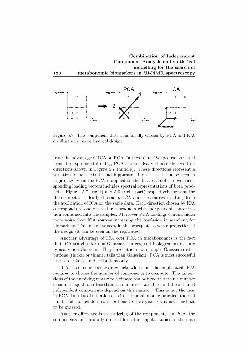
180

Combination of IndependentComponent Analysis and statistical

modelling for the search ofmetabonomic biomarkers in 1H-NMR spectroscopy

Figure 5.7: The component directions ideally chosen by PCA and ICAon illustrative experimental design.

trate the advantage of ICA on PCA. In these data (24 spectra extractedfrom the experimental data), PCA should ideally choose the two firstdirections shown in Figure 5.7 (middle). These directions represent avariation of both citrate and hippurate. Indeed, as it can be seen inFigure 5.8, when the PCA is applied on the data, each of the two corre-sponding loading vectors includes spectral representations of both prod-ucts. Figures 5.7 (right) and 5.8 (right part) respectively present thethree directions ideally chosen by ICA and the sources resulting fromthe application of ICA on the same data. Each direction chosen by ICAcorresponds to one of the three products with independent concentra-tion contained into the samples. Moreover PCA loadings contain muchmore noise than ICA sources increasing the confusion in searching forbiomarkers. This noise induces, in the scoreplots, a worse projection ofthe design (it can be seen on the replicates).

Another advantage of ICA over PCA in metabonomics is the factthat ICA searches for non-Gaussian sources, and biological sources aretypically non-Gaussian. They have either sub- or super-Gaussian distri-butions (thicker or thinner tails than Gaussian). PCA is most successfulin case of Gaussian distributions only.

ICA has of course some drawbacks which must be emphasized. ICArequires to choose the number of components to compute. The dimen-sions of the unmixing matrix to estimate can be fixed to obtain a numberof sources equal to or less than the number of variables and the obtainedindependent components depend on this number. This is not the casein PCA. In a lot of situations, as in the metabonomic practice, the realnumber of independent contributions to the signal is unknown and hasto be guessed.

Another difference is the ordering of the components. In PCA, thecomponents are naturally ordered from the singular values of the data

5.3 First step of the methodology: ICA 181

Figure 5.8: The PCA loadings (left)- the ICA sources (right) resultingfrom application on illustrative experimental data.

182

Combination of IndependentComponent Analysis and statistical

modelling for the search ofmetabonomic biomarkers in 1H-NMR spectroscopy

matrix and used to decrease the dimensions of the problem by consid-ering only the first components which explain most of the variance inthe data. In ICA, the sources have no order and the order in whichthe sources in S are listed by the algorithm is irrelevant to their in-dependence. In Section 5.3.4, we propose a measure of the amount ofinformation contained in each estimated source, giving rise to a ranking.

Finally, in contrast to principal component analysis (PCA), all ICAalgorithms face the problem of convergence to local optima, thus slightlydifferent components will be produced when the same dataset is reana-lyzed. It is then recommended to run the ICA algorithm several timesand check the stability of the results for different values of q.

5.4 Step II: Statistical modelling

5.4.1 Goals and principle

The second step of the methodology consists in fitting a statistical modelaiming at identifying metabonomic biomarkers from ICA results. Moreprecisely, the model will search for a link between the ICA mixing weightmatrix A and the design factors of the metabonomic study.

The logic underlying this approach is the following. An 1H-NMRspectrum reflects the concentrations of pure or complex metabolites con-tained in the analyzed sample. The design factors, as for example thedose of an administrated drug, can influence these concentrations andconsequently modify the spectra in a specific way. The methodology pre-sented in this paper supposes that the q sources recovered by ICA arethe spectral images of pure or complex metabolites that are influencedby the (observed or unobserved) variables underlying the metabonomicstudy. Under this hypothesis, the mixing weights aij should be propor-tional to the concentrations of the identified metabolites in the studysamples.

The statistical models will then search for an effect of the design vari-ables of interest on the concentrations quantified by the mixing weights.

5.4.2 Linear mixed model specification and estimation

Let aj be the (n× 1) vector of mixing weights corresponding to the jth

ICA source and Y the (n× l) metadata matrix. In order to specify themodel to be estimated, two model matrices must be built from Y :

• Z1, a (n× p1) incidence matrix containing the fixed effects of themodel. This matrix contains typically a constant term, coded cat-egorical variables, continuous variables and interactions or otherhigh-order terms.• Z2, a (n × p2) incidence matrix containing the random effects of

5.4 Step II: Statistical modelling 183

the model. It contains typically coded random design variablesas subject, batch, day and interactions between fixed and randomvariables.

For each of the q sources sj , the following linear mixed model is thendefined:

aj = Z1βj + Z2γj + εj . (5.12)

where βj is a (p1 × 1) vector of constant parameters to be estimated,γj is a (p2 × 1) vector of random effects distributed as a multivariatenormal N(0, G) and εj is a (n × 1) vector of residuals distributed as amultivariate normal N(0, R) [14].

Different particular cases of this general model are possible accordingto the inclusion of both Z1 and Z2, only Z1 or only Z2 in the model.

Models using only Z1 can be declined into two categories accordingto the nature of the fixed effects covariates. In the case of categoricalcovariates, the model is an ANOVA model. In the case of quantitativecovariates, a linear regression model is defined and when both types ofvariables are included a (fixed) GLM model is concerned. A quantitativevariable is typically the dose of a drug and a categorical variable can bea treatment type (e.g. placebo versus a low and a high dose of a drug).Note that, in many medical studies, quantitative variables are oftencategorized before being introduced in statistical models.

Models using only Z2 are variance components models includingonly random factors. This arises when one is interested by the effectof various populations or analytical factors on the spectrum variability(e.g. subject, operator, batch,...) but this is not yet commonly donein metabonomic studies. Advantages of models using random factors(random and mixed models) for metabonomics are discussed in Section3.5.3. Complex metabonomic studies typically include both fixed andrandom effects as for example in longitudinal studies where n subjectsbelonging to p categories of treatments are followed over time. The nextsubsection will illustrate the simple ANOVA and regression cases on thehypothetical metabonomic study data.

Section 5.7 will illustrate the complete methodology with ANOVAmodel on a more complex metabonomic dataset.

5.4.3 Example

This section illustrates the modelling step on the experimental data inthe case where only fixed effects are present. In Section 5.3.5, six ICAsources were identified from the spectral matrix and the mixing weightsgathered in a (28×6) matrix A. The design matrix Y contains two fixedcovariates: the drug dose y1 (or hippurate) and the age of the subject

184

Combination of IndependentComponent Analysis and statistical

modelling for the search ofmetabonomic biomarkers in 1H-NMR spectroscopy

y2 (or citrate). y1 is the covariate of interest for which biomarkers aresearched.

These variables can be introduced either as continuous or as cate-gorical variables in the linear model. In the first case, matrix Z1 willbe, at least, a (28× 3) matrix with a constant term as first column andy1 and y2 as second and third columns and one obtains, for each sourcesj , the following linear model:

aj = Z1βj + εj = βj0 + βj1y1 + βj2y2 + εj . (5.13)

The β’s estimated by linear regression for the six sources are given inTable 5.1. We will interpret these coefficients in the next step. Notethat higher order terms (quadratic or interaction terms) could also havebeen introduced in this model.

If the two covariates are introduced as categorical variables in themodel, Z1 becomes a (28×7) matrix with a constant term as first columnand two blocks of three columns corresponding to the binary coding ofthe four levels categorical variables. Such model can then be estimatedby regression but corresponds also to a two ways ANOVA model whichcan be fitted through classical ANOVA formulae when the design isbalanced [79]. The model would be written in the ANOVA literature as:

ajlh = β0 + βlj1 + βhj2 + εjlh. (5.14)

where indices i and h refer to the levels of the two variables y1 and y2and βlj1 and βhj2 to the corresponding main effects for source sj . Notethat one could also introduce an interaction term in the model but thisis not done in this work. ANOVA model results will be provided in thenext section.

5.5 Step III: Biomarker identification

5.5.1 Goals and principle

The third step of the procedure aims at finding which of the q ICAsources vary significantly in the observed spectra when the values ofthe covariates of interest in the study are modified. These sources orcombinations of them will be taken as candidate biomarkers.

Practically, the choice of the significant sources is based on the sta-tistical significance of the terms or effects included in the mixed modelsestimated in Step II. The adequate statistical tests depending on themodel structure and effect classes must include a multiplicity correctionwhen the number of sources and effects of interest are large.

This step produces rk significant sources for each covariate or morecomplex effect of interest in the model. These sources are the input ofthe next step of the procedure.

5.5 Step III: Biomarker identification 185

5.5.2 Selection of significant sources

In general mixed models, common procedures exist to test the signifi-cance of model terms. They are different for fixed and random effects,depend on the method applied to estimate the model and may be con-treversed when complex random effects are concerned. To keep thingssimple, only some simple cases are here treated and the reader is invitedto consult related literature [14] and software for general situations ( e.g.PROC MIXED in SAS or function lme in R).

Let us suppose first that the model contains only fixed continuousand categorical effects and that the effect of interest is the main effectof a continuous covariate yk. The significance of yk is derived for eachsource sj through the p-value related to a t-statistic and calculated asfollows:

pjk = 2× P (t(n−p)) ≥ |t(j, k)|). (5.15)

with

t(j, k) = βjk/s(βjk). (5.16)

and where βjk is the coefficient of yk in the fitted model on aj , s(βjk)

is the standard error of βjk, n is the number of observations (spectra),p is the number of parameters of the model and t(n−p) is a t randomvariable with (n− p) degrees of freedom.

If one supposes now that the effect of interest is a categorical co-variate with p levels, the significance of yk is derived for each source sjthrough a F statistic as follows:

pjk = P (Fp−1,n−p ≥ F (j, k)). (5.17)

with

F (j, k) = MSykj /MSRj . (5.18)

and where MSRj is the mean square of model residuals for source sj ,MSykj the mean square related to yk effect and Fp−1,n−p a F randomvariable with (p− 1) and (n− p) degrees of freedom.

If such procedure is applied on K variables or more complex effectsof interest in the model and for each of the q sources, (K × q) tests areperformed and the decision of significance of the p-values must take intoaccount the multiplicity situation. If (K × q) remains reasonably small,a simple Bonferroni correction is applicable and the significance of theeffect of yk for source sj is declared if pjk ≤ α/(K × q) where α is achosen total error rate (e.g. α=0.05). For large (K × q) procedures likeFalse Discovery Rate (FDR) could used [6].

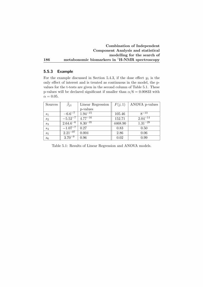
186

Combination of IndependentComponent Analysis and statistical

modelling for the search ofmetabonomic biomarkers in 1H-NMR spectroscopy

5.5.3 Example

For the example discussed in Section 5.4.3, if the dose effect y1 is theonly effect of interest and is treated as continuous in the model, the p-values for the t-tests are given in the second column of Table 5.1. Thesep-values will be declared significant if smaller than α/6 = 0.00833 withα = 0.05.

Sources βj1 Linear Regressionp-values

F (j, 1) ANOVA p-values

s1 −6.6−7 1.94−15 105.46 8−13

s2 −5.52−7 4.77−16 152.71 2.04−14

s3 2.64.6−6 8.30−35 4468.90 1.31−29

s4 −1.07−7 0.27 0.83 0.50

s5 2.21−07 0.004 2.86 0.06

s6 3.70−9 0.96 0.02 0.99

Table 5.1: Results of Linear Regression and ANOVA models.

5.5 Step III: Biomarker identification 187

05

1015

2025

3035

−lo

g(p−

valu

es)

s1 s2 s3 s4 s5 s6

05

1015

2025

3035

s1 s2 s3 s4 s5 s6

Figure 5.9: The p-values corresponding to each sources for the regressionmodels (left) and for the ANOVA models (right). P-values are expressedas -log(p-value) in these plots. Significant p-values are over the dottedlines represent the levels of significance after Bonferroni corrections withthe -log transformation.

Table 5.1 and Figure 5.9 (left) show that four sources are significant.The most significant one is source s3 corresponding to the hippuratespectrum (as expected).

If y1 is introduced as a categorical variable in the model (see Equation5.14), the two last columns of Table 5.1 provides the F -statistics andrelated p-values for the six sources and Figure 5.9 (right) shows thatthree sources are significant, the most significant still being source s3.

Regression and ANOVA approaches select then the same more sig-nificant source: s3.

Spectral regions represented in s3 present then the biomarkers orspectral expression of metabolites significantly affected by a change ofthe factor of interest y1. As expected in this example with y1 beingthe hippurate dose, s3 presents as biomarkers the peaks in a spectralpositions of the hippurate molecule.

Additionally, both Linear Regression and ANOVA models select s1(spectral profile of pure urine) and s2 (spectral profile of pure citrate).In the Linear Regression models, the signs of each estimated βj1 effectof y1 on the modellized vector of weight can also be inspected. For aselected source, a positive βj1 indicates that the contribution of this

188

Combination of IndependentComponent Analysis and statistical

modelling for the search ofmetabonomic biomarkers in 1H-NMR spectroscopy

source to the observed spectra significantly increase when y1 increases.In other words, biomarkers peaks presented in this source increase wheny1 increases.

Table 5.1 shows that β31 is positive and the β11, β21 are negative: anincrease in y1 is followed by an increase in the spectral peaks of hippurate(regions presented in s3), while an increase of y1 results in a decrease inthe spectrum of peaks corresponding to natural urine (regions presentedin s1) and peaks corresponding to citrate (regions presented in s2). Thiscan be easily explained by the fact that each observed spectrum is nor-malized to have a sum equal to one (constant sum normalization).

Comparisons between Linear Regression and ANOVA p-values showsthat source s5 is only selected in Linear Regression. Although ANOVAanalysis has the advantage to account for slightly more of the variation,the ANOVA method is evaluated on more degrees of freedom than thethe regression method and has larger p-values. This can lead to the riskof missing significant effects as for s5. Treating independent variable ascontinuous ones should then be the method of choice in the first instance,with ANOVA being used if regression analysis is not appropriate (e.g. ifthe relationship between the variables is not linear). Figure 5.10 showsthat in this example, the relationship between the weight vectors andy1 can be considered as linear and this for each of the level of the othercovariate y2.

5.6 Step IV: Visualization of biomarkers and factoreffects

5.6.1 Goal and principle

For each covariate of interest in the metabonomic study, Step III pro-vides a list of r significant sources. Step IV proposes finally a simpletool to interpret visually these sources as biomakers.

The tool aims to answer the following question: which average changeis expected in the spectrum when the covariate of interest changes fromone level to another (e.g. if a patient is or is not affected by an illnessor if the dose of a drug is increased)?

5.6.2 Contrast calculation

Let us define S∗ as the (m × r) matrix of significant sources identifiedin Step III. Let y1k and y2k be two levels of interest for covariate yk (e.g.two drug doses). Let us finally define ∆a2−1∗ = a2∗ − a1∗ as the vector ofdifferences of model predictions for these two covariate levels and for ther identified sources. For models without interactions, these differencesare only influenced by the terms in yk in the model. For models with

5.6 Step IV: Visualization of biomarkers and factor effects189

0 50 100 150 200 250 300

0.00

180.

0022

0.00

26

y1

a3

Figure 5.10: The relationship between the hippurate dose (y1) and thevector of mixing weights a3. Each of the four lines represents the esti-mated Linear Regression models for one fixed value of y2.

interactions, the values of the other factors should be fixed to chosenlevels.

From this difference of predictions, the expected changes in spectracan simply be obtained as the following contrast

C2−1 = S∗∆a∗ . (5.19)

where C2−1 is a (m × 1) vector and can be drawn as a spectrum tovisualize the spectral regions affected by the covariate.

In particular, if yk is introduced as a continuous variable in the modeland β∗k is the vector of regression coefficients for yk and the r identifiedsources, the expected change between the spectra at the levels y1k and

y2k is given by: C2−1 = S∗β∗k(y2k − y1k).

If yk is introduced as a categorical variable in the model and β1∗k and

β2∗k are the vectors of the estimated effects for the two levels of interest

for the r sources, the change in spectra is given by C2−1 = S∗(βk∗2− βk∗1).

5.6.3 Example

In the design matrix Y , the hippurate dose y1 is observed at the followingvalues: 0, 75, 150 and 300 mg. Three contrasts C2−1, C3−1, C4−1

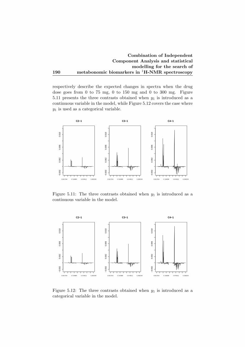
190

Combination of IndependentComponent Analysis and statistical

modelling for the search ofmetabonomic biomarkers in 1H-NMR spectroscopy

respectively describe the expected changes in spectra when the drugdose goes from 0 to 75 mg, 0 to 150 mg and 0 to 300 mg. Figure5.11 presents the three contrasts obtained when y1 is introduced as acontinuous variable in the model, while Figure 5.12 covers the case wherey1 is used as a categorical variable.

−0.

002

0.00

20.

006

0.01

0

C2−1

9.9917004 6.7249886 3.4749012 0.2082506

−0.

002

0.00

20.

006

0.01

0

C3−1

9.9917004 6.7249886 3.4749012 0.2082506

−0.

002

0.00

20.

006

0.01

0

C4−1

9.9917004 6.7249886 3.4749012 0.2082506

Figure 5.11: The three contrasts obtained when y1 is introduced as acontinuous variable in the model.

−0.

002

0.00

20.

006

0.01

0

C2−1

9.9917004 6.7249886 3.4749012 0.2082506

−0.

002

0.00

20.

006

0.01

0

C3−1

9.9917004 6.7249886 3.4749012 0.2082506

−0.

002

0.00

20.

006

0.01

0

C4−1

9.9917004 6.7249886 3.4749012 0.2082506

Figure 5.12: The three contrasts obtained when y1 is introduced as acategorical variable in the model.

5.6 Step IV: Visualization of biomarkers and factor effects191

As the dose goes from 0 to a larger value in each of the three con-trasts, the hippurate peaks increase. On the contrary, the rest of thespectrum shows negative values. It indicates that when the drug doseincreases, peaks corresponding to other metabolites decrease. This canbe explained by the fact that each spectrum is normalized to have anequal sum or total concentration.

Comparisons between C2−1, C3−1, C4−1 show also that when thedrug dose is increased by a factor of two (75 to 150 mg, 150 to 300 mg),hippurate peaks are expected to increase in the same proportion.

Step I to IV were also applied on these data with the estimation of re-spectively four and height sources. The three contrasts obtained in eachsituation (see Appendix 7) demonstrate the stability of the contrasts fordifferent number of sources estimated.

192

Combination of IndependentComponent Analysis and statistical

modelling for the search ofmetabonomic biomarkers in 1H-NMR spectroscopy

5.7 Application to more complex data

In this section, data extracted from the experimental design described inSection 2.3.2 will allow to illustrate the methodology presented in thispaper in a more complex hypothetical situation. As shown in Figure5.13, nine experimental mixtures will be considered and grouped in threeclasses corresponding, for example, to three hypothetical disease states:group 0 corresponds to spectra from subjects with no disease, group 1to spectra from subjects with a first kind of disease, group 2 to subjectswith a second kind of disease.

Figure 5.13: Experimental design of the more complex dataset dividedin three groups of disease.

For each experimental condition, the spiked urine samples were analyzedat eight times: as such or in diluted water (1/1), over two consecutivedays and with two replicates per day per media. 72 spectra were thenused and can be described in the design matrix according to the followingcategorical factors:

• y1: disease group (G1, G2, G3).• y2: media (diluted or non diluted urine).• y3: day of measurement (day1 or day2).• y4: replicate within each day (1 or 2).

The pre-treatments described in Section 2.3.4 were applied on the spec-tral data and produced a (72 × 600) spectral matrix X. ICA was thenapplied, as described in Section 5.3.2, in order to obtain q = 5 sources(Dj = 89%) and their mixing weight vectors aj (see Figure 5.14).

A mixed model was then fitted on each vector aj with y1, y2, y3 asfixed factors and with all possible interactions of first and second order.Table 5.2 provides the F statistics and p-values corresponding to themain effects of these three factors on the mixing weights. Interaction

5.7 Application to more complex data 193

02

46

810

12

9.9917004 8.897418 7.8194544 6.7249886 5.647086 4.5528036 3.4749012 2.3804354 1.302472 0.2082506

36.8 %

02

46

810

12

9.9917004 8.897418 7.8194544 6.7249886 5.647086 4.5528036 3.4749012 2.3804354 1.302472 0.2082506

25.82 %

05

1015

9.9917004 8.897418 7.8194544 6.7249886 5.647086 4.5528036 3.4749012 2.3804354 1.302472 0.2082506

25.76 %

−5

05

10

9.9917004 8.897418 7.8194544 6.7249886 5.647086 4.5528036 3.4749012 2.3804354 1.302472 0.2082506

0.5 %

−4

−2

02

46

8

9.9917004 8.897418 7.8194544 6.7249886 5.647086 4.5528036 3.4749012 2.3804354 1.302472 0.2082506

0.1 %

Figure 5.14: The q = 5 sources from ICA.

194

Combination of IndependentComponent Analysis and statistical

modelling for the search ofmetabonomic biomarkers in 1H-NMR spectroscopy

effects are not reported in the table because they are all non signifi-cant. The Bonferonni corrected p-value threshold was taken as 0.05/15= 0.0033.

Sources F (j, 1) pj,1 F (j, 2) pj,2 F (j, 3) pj,3s1 35.51 6.67−11 0.09 0.77 0.01 0.92

s2 17.55 9.98−7 0.22 0.64 0.07 0.79

s3 18.70 4.87−7 0.02 0.90 0.07 0.79

s4 0.12 0.89 269.35 1.07−30 0.59 0.44

s5 1.17 0.32 0 0.994 0.50 0.48

Table 5.2: The results of Linear Regression and ANOVA models.

This table shows that the experimental group has a very significant ef-fect on the three first ICA sources. These sources were then used tocompute three contrasts in order to illustrate the effect on the spec-tra when passing from one group to the other (see Figure 5.15). C1−0

presents the average change expected in the spectrum when a subjectwith no disease gets disease 1: citrate peak increases. C2−0 illustratesthe fact that, for a subject without disease that becomes a subject withdisease 2, hippurate peaks increase. Finally, C1−2 shows that evolvingfrom disease 2 to disease 1 leads to a decrease of hippurate peaks andan increase of the citrate peak. All these results are of course expected.

Table 5.2 shows also that the sources do not significantly changefrom one day to the other (y3) but that the media (water dilution -y2) has a significant effect on source 4. This source is characterizedby a peak on the left side of the water peak region (set to zero in thepre-treatments). This peak is in fact a side effect of the original waterpeak but the percentage of variation of the source (0.5%) shows thatthe different pre-treatment steps used to remove media systematic effectwere efficient.

None of the factors has a significant effect on source 5 but its mixingweights vector indicates that this source is mainly influenced by oneoutlier spectrum.

It is also interesting to compare the ICA results obtained in thisexample and in the example of Section 5.3. Here, 89% of the totalvariance of X is explained by the five first sources. In the previousexample, 98% of the variation was explained by the same number ofsources. This difference can be explained by the fact that replicatingthe measures over several days and with different dilutions introducesrandom noise in the data which can not be catched by ICA sources.

5.8 Conclusions 195

−0.

005

0.00

00.

005

0.01

0

9.9917004 6.7249886 3.4749012 0.2082506

−0.

005

0.00

00.

005

0.01

0

9.9917004 6.7249886 3.4749012 0.2082506

−0.

005

0.00

00.

005

0.01

0

9.9917004 6.7249886 3.4749012 0.2082506

Figure 5.15: The three contrasts C1−0, C2−0, C1−2

5.8 Conclusions

In this chapter, we presented a four steps methodology providing threekinds of knowledge on 1H-NMR metabonomic data: the visualizationof biomarkers, a statistical confirmation of the significance of the foundbiomarkers and the visualization of the effects on the biomarkers causedby changes of the factor of interest.

The methodology involves a dimension reduction by ICA followedby a statistical modelling approach.

We first presented a process to decompose by ICA the spectral datainto statistically independent components. We proposed solutions forquestions specific to ICA concerning the number of components to esti-mate and their ordering. We exposed, on experimental data, that ICAallows us to visualize, through the resulting sources, the spectral profileof independent metabolites contained in the studied biofluid and theirquantity through the corresponding mixing weights. From Steps II andIII, various linear mixed statistical models were applied on ICA resultsto select the sources. These sources present the biomarkers, spectralregions changing significantly according to the factors of interest. Inthe final step, the selected sources were used to reconstruct the spectraand to compute contrasts presenting the alterations in biomarker regionscaused by different changes of the factor of interest.

As exposed on experimental data, the ICA solves the weaknessesof the PCA dimension reduction by providing more natural and alsomore biologically meaningful representations of the data. Additionally,

196

Combination of IndependentComponent Analysis and statistical

modelling for the search ofmetabonomic biomarkers in 1H-NMR spectroscopy

the combination of ICA with statistical models has the advantage tobase the component selection on an inferential criterion: biomarkers areidentified from components for which the covariate of interest showsa significant effect. In the usual PCA, biomarkers are identified fromthe component with the largest percentage of variance, without anyinferential information.

In Chapter 4, source selection was based on t-statistics computed onthe weight vectors without using their significance levels. In Chapter5, we provided a more accurate source selection due to its inferentialcharacter but also to the fact that models give the possibility to in-clude all the design covariates jointly with the covariate of interest. Thelarge diversity of statistical models accepted by this methodology allowsto apply it to a large variety of metabonomic situations: models caninclude quantitative and qualitative design variables as well as combi-nations of fixed and random effects. As a result, additionally to theproposed biomarker search, the methodology provides information onspectral regions affected by other factors of the study.

Finally, the methodology goes further than the usual search formetabonomic biomarkers: beside their discovery, contrasts also allowto visualize the alterations of biomarkers expected for defined changesof covariate conditions.

CHAPTER 6

Example: metabonomic study ofAge related Macular Degeneration

(AMD)

6.1 IntroductionThis chapter illustrates the content of this thesis through an applicationon a study about Age-related Macular Degeneration (AMD) realizedin collaboration with ULg 12. Figure 6.1 gives a scheme of the differ-ent steps of the AMD study presented in the different sections of thischapter. The pre-treatment procedure presented in Chapter 1 is usedto prepare the data. The quality of the data is evaluated with outliersdetection procedure, statistical descriptive analysis and some statisti-cal tools for the study the spectral variability proposed in Chapter 3.The dataset submitted to the statistical search of biomarkers involves189 spectra including 93 spectra from AMD subjects. The six statisti-cal methods presented in Chapter 4 are applied to search for spectralbiomarkers discriminant between AMD and healthy subjects. Combi-nation of ICA with statistical models is used in the objective to explorethe spectral changes related to the activity state of the disease.

The resulting spectral biomarkers for this disease correspond to ametabolite supporting biological explanations of the setting of AMD.

1Department of Ophthalmology, CHU ULg.2CIRM, Drug Research Center, ULg.

198Example: metabonomic study of Age related Macular

Degeneration (AMD)

6.2 Study setting up

6.2.1 Definition of the goals of the study

Age-related macular degeneration is a leading cause of vision loss in thewestern world among people aged fifty or older. As less is known aboutthe metabolic changes in patients with AMD, the ULg decided to usemetabonomic and to collaborate with the Ucl to prepare and analyzethe data.

This study has been realized on serum samples due to vascular hy-pothesis about the AMD. Indeed, ninety percent of all vision loss dueto AMD results from the exudative form, which is characterized bychoroidal neovascularization, defined as newly formed blood vessels aris-ing from choriocapillaries. Age-related changes that induce pathologicneovascularization are incompletely understood.

The goal of this research is to discover metabonomic biomarkersmaking the distinction between healthy and diseased subjects. Thesemolecular biomarkers will be used to develop knowledge about the AMDpathological mechanisms. Subsequently, their corresponding spectralbiomarkers could be used in the future as diagnostic tool.

The AMD study is a qualitative outcome two class problemdisease metabonomic study. In this study, each spectrum is charac-terized by the AMD status of its corresponding subject through a binaryqualitative outcome: a medical examination declares if the subject hasor not the AMD.

6.2.2 Study design

This observational case-control study was designed according to a pro-tocol approved by the ethical committee of the University Hospital ofLiege, Belgium. Cases for the study were defined as patients of theUniversity Hospital of Liege Belgium affected by AMD over the age ofsixty. Controls are age-matched patients in the same hospital withoutany sign of macular disease and not having a known family history ofAMD. Cases as controls were said eligible on the basis of an examinationrealized by a trained ophthalmologist. Informed consent was requiredfrom all study subjects before participation.

The protocol also foresaw the additional biochemical and health stateinformation to collect on the serum samples and subjects. Additionally,AMD patients had to be categorized into active or not active phenotypiccategories depending of the bleeding of lesions on the basis of the OpticalCoherence Tomography (OCT) examination.

A design matrix YA was formed during the study design step. Thismatrix contains the following information:

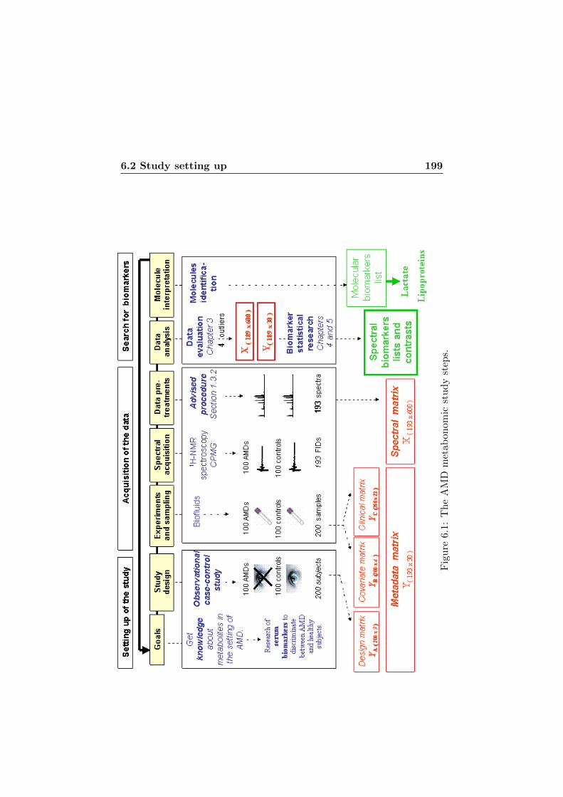
6.2 Study setting up 199

Fig

ure

6.1:

Th

eA

MD

met

abon

omic

stud

yst

eps.

200Example: metabonomic study of Age related Macular

Degeneration (AMD)

• an identifiant for each blood sample providing a spectrum:”MH + number” for a AMD case and ”MC + number” for acontrol.• the qualitative outcome describing the presence or not of AMD

according to the medical examination: 0 = yes, 1 = no.• the activity phenotypic character of the AMD: 0 = AMD subject

in active phase, 1 = AMD subject in inactive phase, 2 = control(no phase of activity).

6.3 Acquisition of the data

6.3.1 Experiment and sampling

Enrolment of study subjects was stopped on the first October 2008 when100 AMD patients (mean age = 77.36, sd = 7.6 years) and 100 controlpatients (mean age = 70.92, sd = 9.1 years) were involved.

For each individual, 30 ml of blood was collected on the day of en-rolment and distributed in the following way:

• 10 ml in an auto-separation blood collection tube gel for the sep-aration of the serum. This tube of serum is used for the 1H-NMRmeasurement.• 10 ml in a K2 EDTA blood collection tube to use for blood cells

accounts and CRP measurement.• 10 ml in a sodium/K3 EDTA blood collection tube to use for a

biochemical analysis.

For each study subject, additional information were collected in a matrixYB: sex, age, BMI, tabagism (yes, no, before). A biological descriptionof each subject was reported in a clinical data matrix YC . This matrixincludes the following information:

• health problems (yes or no): cholesterol, articular troubles, asthma,haemolysis.• antecedent of AMD or not.• blood cells accounts: white and red blood cells, platelets (in 103

cell/ µ), % of neutrocytes, lymphocytes, monocytes, eosinophilsand basophils.• biochemical measurement of CRP (C-reactive Protein).

A descriptive analysis of matrices YB and YC is presented in Section6.4.1.2 for all the subjects involved in the statistical analysis.

6.3.2 Data acquisition

After defrosting, 500 µl of serum were added with 100 µl of D2O phos-phate buffer (0,1 M, pH = 7.4). After centrifugation (3000 rpm, 10min.), the supernatant was supplemented with 30 µl of a TMSP solu-

6.3 Acquisition of the data 201

tion in D2O (10 mg/ml) and placed in a 5 mm NMR capillary for dataacquisition.

All one-dimensional 1H-NMR spectra were acquired on a Bruker Ad-vance spectrometer operating at 500.13 MHz with a Broad Band Inverseprobe. A CPMG sequence with water pre-saturation was applied toattenuate broad signals arising from proteins and water. Acquisitionparameters included a 90 ◦ pulse, 64K time domain points, a spectralwidth of 10000 Hz, an acquisition time of 3.277 s.

Problems were met during the spectral acquisition for seven samples:”MH12”, ”MH24”,”MH27”, ”MH49”, ”MH50”,”MH100” and ”MC83”.

6.3.3 Pre-treatments

Each FID was pre-treated according to the advised procedure describedin Section 1.3.1. Each spectrum is reduced into 600 buckets of 0.016ppms length in a spectral window going from 10 to 0.2 ppms. Values setto zero are negative values, the spectral zones from 4.5 to 5.5 and from0.5 to 0.2 ppms. Note that the lactate zone (1.36 to 1.31 ppm) is notset to zero in these data. Each spectrum was normalized to have a sumequal to one. Figure 6.13 presents one of these pre-treated spectra froman AMD subject and one from a control subject.

6.3.4 The AMD database in the end of the data acquisition

Due to spectral acquisition problems for seven samples, the spectral datamatrix X involves 193 spectra; 94 FIDs from AMD subjects and 99 FIDsfrom control subjects. The corresponding (193 × 30) metadata matrixY is formed by the groupment of matrices YA, YB, YC .

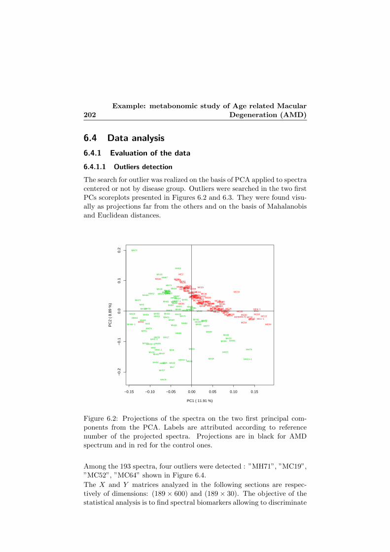
202Example: metabonomic study of Age related Macular

Degeneration (AMD)

6.4 Data analysis

6.4.1 Evaluation of the data

6.4.1.1 Outliers detection

The search for outlier was realized on the basis of PCA applied to spectracentered or not by disease group. Outliers were searched in the two firstPCs scoreplots presented in Figures 6.2 and 6.3. They were found visu-ally as projections far from the others and on the basis of Mahalanobisand Euclidean distances.

−0.15 −0.10 −0.05 0.00 0.05 0.10 0.15

−0.

2−

0.1

0.0

0.1

0.2

PC1 ( 11.91 %)

PC

2 (

8.89

%)

MH1

MH2

MH3−1

MH4−1

MH5

MH6

MH7

MH8

MH9

MH10

MH11

MH13

MH14

MH15−1

MH16

MH17

MH18MH19

MH20

MH21−1MH22

MH23−1

MH25

MH26

MH28

MH29

MH30

MH31

MH32

MH33

MH34

MH35

MH36

MH37−1

MH38

MH39

MH40

MH41MH42

MH43MH44

MH45

MH46

MH47

MH48

MH51

MH52

MH53−1

MH54

MH55

MH56

MH57

MH58

MH59

MH60

MH61

MH62

MH63

MH64

MH65

MH66−1

MH67

MH68

MH69

MH70

MH71

MH72

MH73

MH74

MH75MH76

MH77

MH78

MH79

MH80

MH81

MH82MH83

MH84

MH85

MH86

MH87

MH88

MH89

MH90

MH91

MH92

MH93

MH94

MH95MH96

MH97MH98

MH99

MC1−1

MC2

MC3MC4−1

MC5

MC6MC7MC8

MC9

MC100

MC10MC11

MC12

MC13

MC14

MC15

MC16MC17

MC18

MC19

MC20

MC21

MC22

MC23

MC24 MC25

MC26

MC27

MC28

MC29

MC30

MC31

MC32

MC33

MC34

MC35

MC36

MC37

MC38

MC39

MC40

MC41

MC42

MC43MC44

MC45

MC46MC47

MC48

MC49 MC50

MC51

MC52

MC53

MC54

MC55MC56

MC57MC58

MC59

MC60

MC61

MC62

MC63

MC64

MC65

MC66

MC67

MC68

MC69

MC70

MC71

MC72

MC73

MC74

MC75MC76

MC77

MC78

MC79

MC80

MC81

MC82MC84

MC85MC86

MC87

MC88MC89

MC90

MC91MC92

MC93

MC94

MC95

MC96

MC97

MC98

MC99

Figure 6.2: Projections of the spectra on the two first principal com-ponents from the PCA. Labels are attributed according to referencenumber of the projected spectra. Projections are in black for AMDspectrum and in red for the control ones.

Among the 193 spectra, four outliers were detected : ”MH71”, ”MC19”,”MC52”, ”MC64” shown in Figure 6.4.

The X and Y matrices analyzed in the following sections are respec-tively of dimensions: (189 × 600) and (189 × 30). The objective of thestatistical analysis is to find spectral biomarkers allowing to discriminate

6.4 Data analysis 203

−0.2 −0.1 0.0 0.1 0.2

−0.

2−

0.1

0.0

0.1

0.2

PC1 ( 11.27 %)

PC

2 (

8.35

%)

MH1

MH2

MH3−1

MH4−1

MH5

MH6

MH7MH8

MH9

MH10

MH11

MH13

MH14

MH15−1

MH16MH17

MH18

MH19

MH20

MH21−1

MH22

MH23−1

MH25

MH26

MH28

MH29

MH30

MH31

MH32

MH33

MH34

MH35

MH36

MH37−1

MH38

MH39

MH40

MH41

MH42

MH43

MH44

MH45

MH46MH47

MH48

MH51

MH52

MH53−1

MH54

MH55

MH56

MH57

MH58

MH59

MH60

MH61

MH62

MH63

MH64

MH65

MH66−1

MH67

MH68

MH69

MH70

MH71

MH72

MH73

MH74

MH75

MH76MH77

MH78

MH79

MH80MH81

MH82

MH83MH84 MH85

MH86

MH87

MH88

MH89

MH90

MH91

MH92MH93

MH94

MH95MH96

MH97

MH98

MH99

MC1−1

MC2

MC3MC4−1

MC5

MC6

MC7 MC8MC9

MC100 MC10MC11

MC12

MC13

MC14

MC15

MC16MC17

MC18

MC19

MC20

MC21MC22

MC23

MC24

MC25

MC26MC27

MC28

MC29MC30

MC31

MC32

MC33

MC34

MC35

MC36MC37

MC38 MC39MC40

MC41MC42

MC43

MC44MC45

MC46

MC47

MC48

MC49

MC50

MC51

MC52

MC53

MC54

MC55

MC56

MC57

MC58

MC59

MC60

MC61MC62

MC63

MC64

MC65

MC66

MC67MC68

MC69

MC70

MC71 MC72

MC73MC74

MC75

MC76MC77MC78

MC79

MC80

MC81MC82MC84 MC85MC86MC87

MC88MC89

MC90

MC91MC92

MC93

MC94

MC95

MC96

MC97MC98

MC99

Figure 6.3: Projections of the spectra on the two first principal com-ponents from the PCA applied to spectra centered by disease statusgroup. Labels are attributed according to reference number of the pro-jected spectra. Projections are in black for AMD spectrum and in redfor the control ones.

between AMD and control subjects. This information is contained inthe variable of interest y2, the ”disease status”: 93 spectra correspondto AMD subjects and the 96 others to control subjects.

204Example: metabonomic study of Age related Macular

Degeneration (AMD)

0.00

0.02

0.04

MH71

0.00

0.04

0.08

0.12

MC19

0.00

0.02

0.04

MC52

0.00

0.02

0.04

MC64

9.99 8.9 7.82 6.73 5.65 4.55 3.47 2.38 1.3 0.21

Figure 6.4: The four outliers (in red) superimposed to the mean of allthe others spectra of their disease group (in black).

6.4.1.2 Statistical descriptive analysis of the metadata matrix

On the basis of information contained in Y , Table 6.1 presents a de-scription of the subjects, samples or spectra. The mean and standarddeviation are given for quantitative variables and frequencies for quali-tative variables. Note that the values of some variables are not availablefor some subjects. The numbers of cases and controls on which thesedescriptive statistics are computed are respectively referred as n1 andn2. Hypothesis tests were used to compare AMD cases and controls.P-values of homogeneity Chi square or Exact Fisher tests are reportedfor qualitative variables. For quantitative variables, the p-values resultfrom Welch’s t-test or t-test with equal variances.

Additionally to variables presented in Table 6.1, a variable “AMDactivity” describes the state of the disease. Patients in inactive phasehave stationary lesions while patients in active phase have evolving le-sions presenting bleeding and neovascularization. The AMD activity

6.4 Data analysis 205

description is available for 75 AMD spectra, including 51 active phase(58 %) and 24 inactive phase.

Due to problems of acquisition and outliers, the number of cases andcontrols are no more equal in this dataset. AMD spectra are thus nomore matched with control spectra by the age. However, the p-value ofthe Student t-test does not indicate a significant difference for the agebetween AMD and controls (α = 0.05).

206Example: metabonomic study of Age related Macular

Degeneration (AMD)

6.4.1.3 Evaluation of the data variability

This subsection compares the intra-variability of the AMD spectra groupand the control spectra group. In this aim, the tools presented in Chap-ter 3 for the first type of question about spectral variability (see Section3.3) are used.

A PCA was performed on the 189 AMD and control spectra. Figure6.5 presents the projections of the spectra on the two first components.Different symbols and colors are used according to the disease status.

−0.15 −0.10 −0.05 0.00 0.05 0.10 0.15

−0.

2−

0.1

0.0

0.1

PC1 ( 12.36 %)

PC

2 (

9.22

%)

Figure 6.5: Projections of the spectra on the two first principal compo-nents. A green 4 symbol represents a projection of AMD spectrum anda red ◦ of a control one.

Beside the separation between the AMD and control spectra, the PCAscoreplot shows a very larger dispersion or variability for the AMD spec-tra. Inertias were computed in the initial space in order to confirm thisconclusion with the variability in higher dimensions. The initial spaceinertia between the AMD and control group is equal to 21.16 %. Table6.2 gives the the intraclass inertias within the group of AMD spectra

6.4 Data analysis 207

Gro

up

n1

n2

AM

Dsu

bje

cts

Con

trol

sub

ject

sp

-val

ues

Sex

=F

9296

64%

69%

0.60

Age

9396

75.

28(7.9

8)

72.9

8(9.

26)

0.07

BM

I92

9526.

75(4.3

3)

26.7

5(4.

45)

0.99

Ante

ced

ent

9296

23.0

0%11.4

6%0.

04

Tab

agis

m92

96ye

s=13.0

4%

bef

ore

=34.7

8%ye

s=14.5

8%b

efor

e=38.5

4%0.

77

Ch

oles

tero

l92

969.

78%

8.3

3%0.

73

Art

icu

lar

pro

ble

ms

9296

53.2

6%61.4

6%0.

26

Ast

hm

a92

964.

35%

2.0

8%0.

38

Hae

mol

ysi

s92

960.

00%

1.0

4%0.

33

Baso

ph

il92

960.

74(0.5

4)0.8

2(0.

45)

0.24

Eos

inop

hil

9296

2.80

(2.0

7)2.5

8(1.

84)

0.43

Mon

ocy

te92

966.

45(1.8

3)5.8

6(1.

79)

0.03

Lym

ph

ocy

te92

9624.

89(7.1

5)

25.8

8(9.

36)

0.42

Neu

trop

hil

9296

63.

16(8.9

9)

62.9

1(10.2

1)0.

86

Pla

tele

t92

9626

5.68

(62.

87)

270.

8(67.6

0)0.

59

Red

blo

od

cell

9296

4.64

(0.4

7)4.6

2(0.

48)

0.77

Wh

ite

blo

od

cell

9296

7.24

(1.9

4)8.1

3(6.

80)

0.22

CR

P93

943.

65(7.8

6)3.2

9(4.

42)

0.74

Tab

le6.

1:T

he

des

crip

tive

anal

ysi

sof

the

stu

dy

sub

ject

s.

208Example: metabonomic study of Age related Macular

Degeneration (AMD)

and within the group of control spectra computed in the initial space.

AMD Control

IW 53.84% 25.00%

Table 6.2: The intraclass inertias within the group of AMD and controlspectra in the initial space.

For each disease status group, the summary ”spectra” of means, stan-dard deviations and coefficients of variation are drawn in Figure 6.6 tovisualize the mean behavior of the spectra and their variability in realand relative values. Note that the coefficients of variation for whichxj is beyond a threshold (indicated by the horizontal red dotted linein the spectra of the means) are not drawn in order to avoid high cv’scorresponding to a mean close to zero.

0.00

0.02

0.04

0.06

AMD

Means

0.00

0.02

0.04

0.06

Control

Means

0.00

00.

010

0.02

0

Standard deviations

0.00

00.

010

0.02

0

Standard deviations

02

46

810

9.99 8.9 7.82 6.73 5.65 4.55 3.47 2.38 1.3 0.21

Coefficients of variation

02

46

810

Coefficients of variation

9.99 8.9 7.82 6.73 5.65 4.55 3.47 2.38 1.3 0.21

Figure 6.6: The spectra of xj , sj , cvj for the 93 AMD (left) and the 96control spectra (right).

The spectra allow us to discover the zones in the spectrum presenting ahigh variability.

To compare more globally the variability of the two groups of spectra,their vector of coefficients of variation were sorted in increasing orderand plotted (see Figure 6.7 ).

6.4 Data analysis 209

0 50 100 150 200 250 300 350

02

46

810

orde

red

cv

Figure 6.7: The curves of the ordered coefficients of variation, in blackfor the AMD and in red for the control spectra.

The comparison of the ordered curves of the coefficients of variationattests of a slightly higher variability in the group of AMD spectra.

In order to clarify this last comparison, two global coefficients ofvariation were computed: one for the 93 AMD spectra and one for the 96control spectra (see Table 6.3). Global coefficients of variations indicate

AMD Control

CV 39.84 % 25.84%

Table 6.3: The global coefficients of variation.

a higher variability for the AMD spectra.All the results agree to conclude that the spectral variability is higher

into the group of AMD spectra than into the group of control spectra.The AMD disease presents stationary or evolving states (see Section

6.4.1.2). The activity state of the disease is thus a potential factor toexplain the high variability of the AMD spectra. In order to verify thishypothesis, the PCA scoreplot presented in Figure 6.5 is modified inFigure 6.8 by the use of different colors and symbols according to theactivity of AMD. Note that some spectra are no more projected on theplan as their activity state is unknown. In this plan, no clear distinctionis observed between the positions of the projections of AMD active andinactive spectra.

210Example: metabonomic study of Age related Macular

Degeneration (AMD)

−0.15 −0.10 −0.05 0.00 0.05 0.10 0.15

−0.

2−

0.1

0.0

0.1

PC1 ( 12.36 %)

PC

2 (

9.22

%)

Figure 6.8: Projections of the spectra on the two first principal compo-nents. A blue 4 symbol represents a projection of AMD active spec-trum, a black × of AMD inactive spectrum and a red ◦ of a controlone.

6.4.2 Search for biomarkers

The six methods presented in Chapter 4 were applied on the AMD data.

Figure 6.9 presents on its left part the vectors of 600 biomarkerscores values obtained with each of these methods. Due to variableselection, LLR and CART methods result in non null score only for thedescriptors proposed as biomarker. LLR has been implemented to selectin a forward procedure twenty biomarkers represented by the twentynon null score values (see Appendix 8 for the AIC values of the variableselection). The CART biomarker score is not represented as this method

6.4 Data analysis 211

only proposes one descriptor, the bucket ′′3.8178′′, as spectral biomarker.For the MHT, s-PCA, s-ICA and PLS-DA methods, the descriptors witha score out of the dotted black lines are the twenty ones with the highestscores for the method. These twenty descriptors are kept as biomarkersdiscovered by the method.

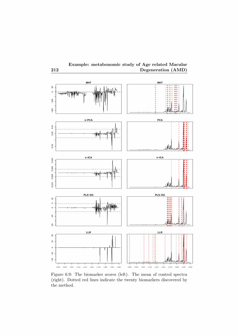
212Example: metabonomic study of Age related Macular

Degeneration (AMD)

−20

0−

100

050

MHT MHT

−0.

020.

000.

01

s−PCA PCA

−0.

015

−0.

005

0.00

50.

015 s−ICA s−ICA

−20

−10

05

10

PLS−DA PLS−DA

−20

−10

010

20

LLR

9.9923 8.8976 7.8197 6.7254 5.6472 4.5531 3.4749 2.3805 1.3026 0.2082

LLR

9.9923 8.8976 7.8197 6.7254 5.6472 4.5531 3.4749 2.3805 1.3026 0.2082

Figure 6.9: The biomarker scores (left). The mean of control spectra(right). Dotted red lines indicate the twenty biomarkers discovered bythe method.

6.4 Data analysis 213

The red dotted lines on the right part of Figure 6.9 show on themean of control spectra the locations of the twenty descriptors selectedas biomarkers by the method. This allows us to verify if the methodproposes as biomarker a descriptor for which a spectral signal exists.

The MHT declares a very large number of biomarkers: 419 of the600 descriptors according to a threshold of selection computed by theBenjamini-Yekutieli FDR rule with α = 0.0001.

The PCA scoreplot formed by the first and the third PCs (see Figure6.10) is the one offering the best discrimination between projections ofAMD case and control spectra. These PCs respectively explain 12.36%and 6.51% of the variance in X. In this plan, the intergroup inertia is

−0.2 −0.1 0.0 0.1 0.2

−0.

2−

0.1

0.0

0.1

0.2

PC3

PC

1

Figure 6.10: Projections of the spectra on the principal componentswhich best discriminate between control and AMD spectra. A green4 symbol represents a projection of AMD spectrum and a red ◦ of acontrol one. The two ∗ indicate the centroids of the clouds respectivelyformed by each kind of spectra.

32.91%. Note that the intragroup Inertia is 39, 87% in AMD group and27, 22% in the control group.

The PLS-DA model was fitted with ten latent variables according to

214Example: metabonomic study of Age related Macular

Degeneration (AMD)

the RMSEP computed by k-fold cross validation.

Eighteen sources were estimated in the s-ICA. This number of esti-mated sources q was chosen based on the percentage of explained vari-ance of the PCs in the whitening step: the 18th PC is the last one witha % of explained variance over 0.1% (see screeplot in Figure 6.11). Thecumulated percentage of explained variance of the eighteen first PCsis Dq = 75.94 % (see Section 5.3.3). The eighteen sources and their

0 50 100 150

020

4060

8010

0

Number of principal components

Dj (

%)

75.94 %

Figure 6.11: Screeplot of the % of variance explained by the q = 189first PCs from the PCA-whitening.

weights are presented in Appendix 9 in increasing order of p-values at-tached to the t-statistics computed on their weights. Their percentagesof explained variance Cj (see Section 5.3.4) are given in these graphs.

Levene tests for homogeneity of variance were applied on each vectorof weights (see Appendix 10). The p-values obtained either from t-tests with equal variances or from Welch’s t-tests are given for eachsource in Appendix 10. Fourteen sources have a significant p-value at

6.4 Data analysis 215

the level α= 0.05/18 = 0.003 or even with the FDR Benjamini-Yekuteliselection. However, we decided to select the ten more significant sourcesto compute the biomarker score. This decision was based on the factthat the next significant sources give with more noise the informationalready involved in the ten selected sources. The ten selected sourcesare: s2, s11, s10, s13, s16, s12, s5, s8, s3, s1 (see Appendix 10).

Table 6.4 presents the lists of the twenty biomarkers of each methodthat we transferred to the spectroscopists of the ULg.

From this table and the right part of Figure 6.9, it can be seen thats-ICA and s-PCA propose quite similar biomarkers (17 in common). Alot of them are in the regions from 0.89 to 0.55 ppms and from 1.36to 1.17 ppms. The LLR also finds one biomarker in the region from0.89 to 0.55 ppms and seven in the region from 1.36 to 1.17 ppms. ThePLS-DA only proposes one biomarker in these regions (”1.2861”). Notethat these regions have high peaks.

s-ICA and s-PCA also propose two peaks in upper regions with theppms ”2.0702” and ”3.2461”. With exception to the CART, all themethods also propose these peaks. Biomarkers from PLS-DA particu-larly cover this spectral zone.

PLS-DA also finds many biomarkers in the next medium intensitypeaks from 3.39 to 3.94 ppms. Biomarkers of the MHT are more disper-sive but six of them are common with the PLS-DA in this last region.The only biomarker of CART is also found in this region.

The LLR makes propositions of biomarkers in the right spectral part,often common to those of s-PCA, s-ICA and PLS-DA. However, the LLRis the only method proposing biomarkers in the high ppms zones wherethe signal is very low.

216Example: metabonomic study of Age related Macular

Degeneration (AMD)

Rank MHT s-PCA s-ICA PLS-DA LLR CART

1 2.6585 1.3026 1.3026 2.0702 3.2952 3.817816

2 2.6908 1.3679 1.2208 3.2299 4.2755

3 2.0702 0.7797 1.2044 3.2952 5.4839

4 3.2952 0.7635 1.2373 3.8996 5.9413

5 2.6746 1.3191 1.1882 3.8508 6.9051

6 2.3805 1.3514 1.3514 3.8669 2.4784

7 3.9484 0.7962 3.2461 3.2461 1.6782

8 5.8433 0.7473 1.2535 3.5237 5.8433

9 3.5893 3.2461 0.7797 3.9161 7.6889

10 2.7073 2.0702 0.7635 2.0049 6.2189

11 3.5237 0.5673 0.8944 2.0376 1.2861

12 3.8669 0.8126 0.8779 1.2861 1.3026

13 2.7237 0.8779 1.3191 3.7199 1.2044

14 2.3643 0.5512 1.172 3.4749 3.2461

15 3.0667 1.2044 2.0702 1.5967 2.0702

16 2.4784 1.1882 0.7962 3.769 1.3679

17 4.1607 0.8944 1.2861 3.9484 1.2208

18 3.9161 1.172 0.7473 3.5893 1.2373

19 2.4949 1.2861 1.1556 3.3931 0.7797

20 5.8595 1.2208 0.5673 1.662 1.1882

Table 6.4: The ranking of descriptors proposed as biomarker by thedifferent methods.

6.4 Data analysis 217

Descriptor Number ofmethods

MHT s-PCA s-ICA PLS-DA LLR

2.0702 5 3 10 15 1 15

3.2461 4 0 9 7 7 14

1.2861 4 0 19 17 12 11

3.2952 3 4 0 0 3 1

1.3026 3 0 1 1 0 12

0.7797 3 0 3 9 0 19

1.1882 3 0 16 5 0 20

Table 6.5: The seven more common descriptors proposed as biomarkersby the different methods and their ranks in the biomarker list of eachmethod.

Table 6.5 presents the more common biomarkers for the differentmethods. One of them, the ”2.0702” is common to five methods. Twoare common to four methods and four are to three methods.

Combination of ICA with statistical models was finally used in the ob-jective to explore the spectral changes related to the activity state ofthe disease.

Stationary or evolving states of AMD is described by the variable“AMD activity” (see Section 6.4.1.2). Available values of this variableallow us to list 171 of the 189 spectra in the three following categories:AMD active phase (51 spectra), AMD inactive phase (24 spectra), nophase or control (96 spectra). The ICA with statistical models wereapplied on the basis of the eighteen sources recovered above and themixing weights of the 171 spectra.

An ANOVA model involving one fixed factor, the “AMD activity”was fitted on each weight vector corresponding to one of the the q = 18recovered sources. Appendix 10 gives the p-values of the disease statuseffect for the different sources.

The phase of activity has a significant effect on fourteen sources witha Bonferonni corrected p-value threshold taken as 0.05/18 = 0.0028.These fourteen sources were then used to compute the contrasts pre-sented in Figure 6.12. The first graph represents the changes occurringin the spectra when an healthy or control subject becomes an AMDsubject in inactive phase. The second graph is the contrast computedbetween AMD subject in active phase and control. Last graph shows thechanges occurring in the spectra when the stationary or inactive AMDdisease turns to an active or evolving disease.

218Example: metabonomic study of Age related Macular

Degeneration (AMD)

−0.

010

0.00

00.

010

0.02

0−

0.01

00.

000

0.01

00.

020

0.00

00.

005

0.01

00.

015

0.02

0

9.9923 8.8976 7.8197 6.7254 5.6472 4.5531 3.4749 2.3805 1.3026 0.2082

Figure 6.12: The contrasts between: AMD inactive cases and controls(top), AMD active cases and controls (middle), AMD active and AMDinactive cases (bottom). Colored spectral zones represent the lactateand lipoproteins zones.

6.4.3 Molecular interpretation

Spectroscopists have identified the metabolites corresponding to the pro-posed spectral biomarkers of the lists. Among these lists, they found de-scriptors corresponding to two metabolites of interest, the lipoproteins(LDL, VLDL, HDL) and the lactate. The biomarker lipoprotein discov-ery supports previous published biological hypothesis about their role inthe onset of AMD [73]. The biomarker lactate has generated from theULg researchers a theory about AMD pathological mechanisms involv-ing an increase of lactate.

The Figure 6.13 presents the lactate and the lipoprotein zones on acontrol and a ADML spectrum. The lipoproteins (LDL, VLDL, HDL)are represented by the descriptors in the zones from 1.31 to 1.2 ppms andfrom 0.90 et 0.74 ppms. The first lipoprotein spectral zone, between 1.31and 1.2 ppms, is covered by nine descriptors in the data. The secondlipoprotein spectral zones, between 0.90 and 0.74 ppms is covered bytwelve descriptors.

6.4 Data analysis 219

0.00

0.01

0.02

0.03

0.04

0.05

0.00

0.01

0.02

0.03

0.04

0.05

9.9923 8.8976 7.8197 6.7254 5.6472 4.5531 3.4749 2.3805 1.3026 0.2082

Figure 6.13: A control and a ADML spectrum. Spectral zones in yellowindicate the lactate and the two lipoproteins spectral zones.

The descriptor “1.2861” situated in the first zone was proposed byfour methods: s-PCA, s-ICA, PLS-DA and LLR. Moreover, the s-ICAhas also proposed six of the eight others descriptors in the first zone.The LLR has also proposed in this zone four of the eight others de-

220Example: metabonomic study of Age related Macular

Degeneration (AMD)

scriptors and the s-PCA three. Descriptors of the second zone wereproposed by the s-PCA, the s-ICA and LLR; respectively seven, six andone descriptor proposed.

The lactate corresponds to five descriptors ′′1.3679′′, ′′1.3514′′, ′′1.3353′′′′1.3191′′ and ′′1.3076′′ ppms, just before the first lipoprotein zone. Thedescriptors ′′1.3076′′ was proposed by three methods: the s-PCA, s-ICAand the LLR. The descriptor ′′1.3514′′ and ′′1.3191′′ were respectivelyonly by the s-PCA and the s-ICA. The descriptor ′′1.3076′′ was rankedin first position of the biomarker list for the s-PCA, s-ICA but in twelfthposition in the LLR list.

The evolution of the lipoproteins and lactate spectral zones in thedifferent state of the disease is viewable in the ICA contrasts (Figure6.12), indicated by the yellow zones. The lactate increases with theemergence of the disease as in the transition from an inactive to anactive state of the disease. On the opposite, the lipoproteins decrease inthese situations.

6.4.4 Conclusions

This chapter illustrated the application of the tools proposed in this the-sis. It appears that metabonomics can help the understanding of AMD.Subsequent experiments are now required in order to better define theexact structure and changes of the discovered metabolites biomarkers.

CHAPTER 7

Conclusion

This thesis provides a complete methodology in R and Matlab routinesto lead a metabonomic study from the data acquisition to the discoveryof biomarkers. The whole methodology has been applied with successto a real metabonomic study for the search of AMD disease biomarkers.The relevance of the resulting biomarkers, the lactate and the lipopro-teins, in pathological mechanism theories attests of the efficiency of ourmethodology.

The use of statistics in metabonomics is commonly restricted to thedata analysis. This thesis underlines that statistical methodologies havealso a role to play in the data acquisition steps. The success of a metabo-nomic study does not only depend on the choice of a statistical dataanalysis method but also depends on the information contained in thedata. Beside the biomarker information, spectral data inevitably involveinformation in relation with the biological context, sample handling andinstrumental measurement. Data acquisition operational modes, whichavoid, limit or reduce the information out of interest, rely on statisti-cal principles for elaboration. From this perspective, the methodologypresented in this thesis brings statistical contributions to metabonomicdata analysis on two axes. On one hand statistical tools and databaseswere developed to improve the quality of the data. On the other hand,statistical methods are proposed to search for biomarkers.

The following contributions were brought in this thesis:

• The creation of databases useful to evaluate the performances ofpre-treatments and statistical analysis methods or to study thespectral repeatability due to several factors.

The inter-day, intra-day and general 1H-NMR repeatability areevaluable on the urine and serum experimental databases. Ef-fects of laboratory operations and of the sample conservation after

222 Conclusion

defrozing are observable in the experimental urine, experimentalserum and human serum databases. The inter- and intra- indi-vidual spectral repeatability can be assessed in the human serumdatabase.

• An automated 1H-NMR data pre-treatment procedure involvingthoughtful statistical methods and taking into account the biolog-ical nature of the samples.

Spectral misalignments due to pH are considered with new solu-tions (warping, citrate aggregation) and improved bucketing. Theyoffer the possibility to work with spectral data in higher resolutionand give more chances to discover biomarkers. The FID waterremoval opens new perspectives for a better control of the di-uretic effect, a major problem in urine metabonomic study. Anevaluation of several normalization methods allowed us to recom-mend the simple but efficient constant sum normalization. Twoapodization solutions are brought to reduce noise in the data andinstrumental artifacts are treated by improved phase and baselinecorrections followed by a setting to zero of negative values. Statis-tical methods are integrated in the pre-treatment procedure: theWhittaker smoother used for the FID solvent removal and com-bined with asymmetric least squares for the baseline correction,the parametric time warping, the rms criterion for the zero orderphase correction. A major advantage of the procedure is the possi-bility to automate the tasks, what represents advantages in termsof reproducibility and human time.

• A panel of methods to evaluate the variability of spectra and definean adequate operational mode of sample collection, preparation,1H-NMR measurement and pre-treatments.

These study steps must ideally maximize spectral variability dueto the biological reaction of interest and the spectral repeatabilitycaused by others factors. We propose to evaluate the spectral vari-ability having as sources factors involved in the data acquisition.The resulting information gives the possibility to choose the moreadequate level for a source of variability, to quantify the effects ofdifferent sources of spectral variability and to compare the qualityof the data after different pre-treatments. To reach these threeobjectives, we propose several tools based on three approaches:PCA, inertia and pointwise consideration. Each approach has itsown specificity and also weakness. The two first components PCAscoreplot gives a partial representation of the variability. The in-

223

ertia are not generalizable to study several sources in complexunbalanced dataset. Ordered curves of pointwise approaches aresometimes difficult to compare and the accuracy of the summarystatistics is to put in relation to the adequacy of a linear regres-sion. However, each tool gives a different and complementary wayto grasp and understand the spectral variability. We recommendto find answers to a given objective by a combined use of differenttools. Used in this way, the tools have provided important con-clusions for the setting of a metabonomic study on the databasescreated in the thesis. The CPMG protein suppression methodmust be used in disfavor to the STE one. We have shown that thespectral repeatability is strongly affected by the inter- and intra-individual factor while the tube preparation and time of conserva-tion after defrozing have low impact. It was demonstrated that theproposed water and urea suppression, the citrate aggregation andthe constant normalization pre-treatments increase the quality ofthe data.

• A battery of six methods as alternatives to the common and ques-tionable PCA for the search of biomarkers which discriminate be-tween two groups of spectra.

The six methods are distinguishable on the basis of their princi-ples in three categories: the methods which do not use an associa-tion criterion (Multiple Hypothesis Testing - MHT), the methodswhich extract the more altered descriptors in each unassociated setof variables (Classification and regression tree - CART and LinearLogistic Regression), and the methods which extract the more al-tered associated set of variables (supervised Principal ComponentAnalysis - s-PCA, supervised Independent Component Analysis- s-ICA, Partial Least Squares Discriminant Analysis PLS-DA).Taking into account the associations between descriptors has itsimportance as a metabolite can correspond to several descriptorsand the fluctuations of a given metabolite is chemically expectedto influence the fluctuations of some others metabolites. An ade-quate method to find biomarkers must also be robust to noise andnot propose a high rate of false discovery.

The MHT controlled on the false discovery rate (FDR) by theBenjamini-Yekutieli rule under dependency does not provide anaccomplished answer to the biomarker search. The resulting listof biomarkers is questionably large. True biomarkers are conse-quently hidden in a lot of false discoveries especially in noisy spec-tral regions and small samples. As the CART does not suit to

224 Conclusion

the robustness to noise condition, we recommend to discard thismethod. Due to the AIC forward variable selection, the LLR ef-ficiently provides a small list of uncorrelated biomarkers. On theopposite associated biomarkers are visuable as spectral profile onthe loadings or components of s-PCA, s-ICA and PLS-DA. Theserepresentations are attractive for biologists, especially the s-ICAone, for their interpretations. The s-PCA and the PLS-DA usecorrelation and are supervised. The PLS-DA uses the spectralgroup information to form its components while the s-PCA usesit in the selection of two components. The PLS-DA has a highpower of true biomarker discovery but specifically performs wellin low noise spectral regions while the s-PCA is more able to findbiomarkers in noisy regions but conducts to more false discoveries.The s-ICA combines these advantages. It finds biomarkers in noisyand unoisy regions and makes few false biomarker propositions.

The s-ICA is very attractive for metabonomic biomarker search.Anyway, each method presents specific relevant characteristics ifnot by its robustness or low rate of false biomarkers (s-ICA, PLS-DA, LLR), by its simplicity (MHT), easiness of use (MHT, s-PCA,LLR) or visual representation (s-PCA, PLS-DA, s-ICA, CART).We recommend to confront the information provided by the resultsof the different methods. As shown in the AMD study, severallists of biomarkers and the establishment of their similarities giveto the biologist more certitude in the interpretation of biomarkermetabolites.

225

• A four steps methodology combining ICA and statistical modellingto discover the biomarkers in various kinds of metabonomic studies(Two- and multiple-class qualitative as quantitative outcomes).

The main advantage of this method is to result into selected sources,each ones interpretable as a spectral profile of an independentbiomarker metabolites. Thanks to these visual supports, a re-searcher easily understands the biomarkers in terms of molecules.With the solutions proposed in the thesis for the choice of thenumber of sources and their ranking, ICA is now a performantalternative to the PCA due to its advantage of interpretation butalso by being more suitable for metabonomics as the directions ofmaximal variance are not always the ones of interest.

The selection of sources is realized in an inferential way by theuse of linear models fitted on the weight vectors. The models givethe possibility to include all the design covariates jointly with thecovariate of interest. Sources presenting a significant effect for adesign covariate have underlined that metabonomic data analysisgains in accuracy by the consideration of the design covariate, whatis not done in traditional methods.

The ICA four steps method goes further than the usual searchfor biomarkers. Firstly, beside the biomarker discovery, contrastsallow to visualize the alterations of biomarkers expected for definedchanges of the studied biological reaction. Secondly, the methodalso provides information not related to the biomarker but leadingto a more complete understanding of the data. The set of all therecovered sources gives the possibility to understand the biofluidcomposition. A biologist discovers not only the biomarkers butalso all the independent metabolites contained into the biofluidand their mixing weights give him insights on their concentrationsin samples. Sources with a significant effect for a design covariateare also of interest to understand the metabonomic context.

Those different tools constitute our statistical contribution to metabo-nomics. Firstly, methodologies are proposed to avoid that spectral vari-ations out of interest disturb the biomarker search analysis. Proposedpre-treatments offer solutions to decrease instrumental and biologicalvariations out of interest. Databases and methods to study variabilityare usable to define a data acquisition step which avoids variations outof interest. Secondly, several statistical data analysis methods were de-veloped and evaluated. Model-based ICA sources selection have shownthat biomarker search analysis gains accuracy by controlling the spectral

226 Conclusion

variations out of interest through the consideration of design covariates.

The methodology developed on the basis of these contributions suf-ficiently improves the quality of the data to permit to the statisticalmethods proposed an efficient biomarker discovery.

Some additional work can be done to improve the proposed method-ology:

• Each pre-treatment step needs to be evaluated individually andthe tuning parameters of some pre-treatments should be adaptedmore accurately.

• New databases can be created in order to study the spectral vari-ability due to not already considered sources. The possibilitiesof multivariate decomposition of variance can be investigated toquantify the spectral variability caused by a source and to discoverthe spectral zones affected. The ANOVA-simultaneous componentanalysis (ASCA) is a method which could be considered.

• Some adaptations of the proposed biomarker search methods arepossible as the Random Forest based regression trees, the Penal-ized or Lasso based logistic regression. The data normality shouldbe explored in order to understand the results of MHT.

• Our study of the inter- and intra- individual spectral repeatabilityhave shown that the data still contains important variations out ofinterest of biological nature. Metabonomic data are biofluid dataand contain consequently a very important amount of biologicalinformation. In one hand this richness is an advantage to searchfor biomarkers but on the other hand it will always imposes im-portant biological spectral variations out of interest complicatingthe biomarker search. These unavoidable non-biomarker biologi-cal variations are numerous, complex and very dependent on thecontext as they reflect the state of the entirety of an organism.

Taking into account design covariates, as the age or the sex, intothe analysis will already help to control some of the inter-individualbiological variations out of interest and lead to a more accuratebiomarker discovery. Additionally, biological processes are dy-namic, progressing over time at different speed according to thesubject. Sequential sampling will make it possible to evaluate andhandle separately some biological intra-individual biological vari-ations out of interest as the circadian rhythm. However, the bi-ological variations out of interest may still be difficult to control.

227

This conducts us to think that if further developments of statis-tical methods are needed, the methods searching for biomarkersshould be able to filter the biological information out of interest.The Orthogonal Signal Correction Partial Least Square Discrimi-nate Analysis (OPLS) is a possible method to enhance the focuson the variations of interest, while filtering other variations. TheOPLS separates the systematic variation in the spectral data intotwo parts, one that is linearly related and one that is unrelated(orthogonal) to the outcome variable describing the biological re-action of interest. Only the first one is used for modelling theoutcome variable. The OPLS can, analogously to PLS-DA, beused for discrimination (OPLS-DA).

An efficient collaboration in an interdisciplinary team is the key factor ofsuccess for a metabonomic study. Several experts must work together tocontrol each study step, from the design to the data analysis, throughthe data acquisition. The statistical tool to search for metabonomicbiomarkers has its importance but cannot palliate to data quality insuf-ficiency.

228 Conclusion

Appendices

230 Introduction

7.1 Appendix 1: the warping functionThe warping function presented here was estimated for a serum spec-trum of 32768 frequency points (in Hz), used in all the illustrations ofthe successive steps of the advised pre-treatment procedure (see Section1.3.1).

0 1 2 3

x 104

0

0.5

1

1.5

2

2.5

3

3.5x 10

4

Frequency (v)

w(v

)

0 1 2 3

x 104

−100

−80

−60

−40

−20

0

20

40

Frequency (v)

w(v

)− v

0 1 2 3

x 104

0.85

0.9

0.95

1

1.05

1.1

1.15

1.2

Frequency (v)

w(v

i)−w

(vi−

1)

Figure 7.1: Leftmost panel: the warping function, ω(ν), estimated forthe serum spectrum illustrating Section 1.3.1. Middle panel: its differ-ences, with the unwarped frequencies, ω(ν) − ν. Rightmost panel: thederivative of the warping function, ω(νi)− ω(νi−1).

7.1 Appendix 1: the warping function 231

Smoothness of the warping function can be appreciated from thedifferences presented in the rightmost panel.

The differences with the unwarped frequencies (middle panel) showthe size of the frequency shifts performed by the warping function. Fig-ure 7.2 presents for the spectral zone kept in the spectral window selec-tion (see Section 1.3.11- step 11), the spectrum before warping (uppestpanel) and the differences ω(ν) − ν (lowest panel). The largest shift

0 2000 4000 6000 8000 10000 12000 14000 16000−20

0

20

40

60

0 2000 4000 6000 8000 10000 12000 14000 16000−100

−50

0

50

Frequency, v

w(v

)−v

Figure 7.2: The spectrum before warping (uppest panel) and the differ-ences ω(ν) − ν (lowest panel) in the spectral zone kept in the spectralwindow selection.

performed in this zone is 82 frequency points, what corresponds to 4buckets of the final spectrum.

232 Introduction

Figure 7.3 presents an histogram of the size of shifts in this zone. In

−100 −80 −60 −40 −20 0 200

1000

2000

3000

4000

5000

6000

7000

8000

w(v)−v

Figure 7.3: Histogram of the size of the frequency shifts performed bythe warping function in the selected spectral window.

this zone, the mean size of shifts is of 31 frequency units (or 1.5 bucket)with a standard deviation equal to 27.66 frequency units (or 1.4 bucket).

7.2 Appendix 2: the probability density plot and boxplots ofthe σf vectors. 233

7.2 Appendix 2: the probability density plot andboxplots of the σf vectors.

0 1 2 3 4

050

100

150

Den

sity

Figure 7.4: The probability density plot of the σf vectors. The volunteerfactor curve is in black, the sampling one in red, the tube one in green,the time in blue and the residuals in pink.

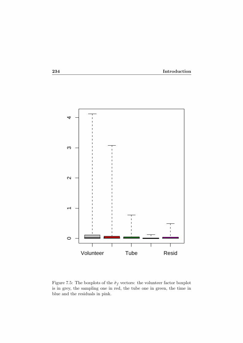
234 Introduction

Volunteer Tube Resid

01

23

4

Figure 7.5: The boxplots of the σf vectors: the volunteer factor boxplotis in grey, the sampling one in red, the tube one in green, the time inblue and the residuals in pink.

7.3 Appendix 3: the probability density plot of the ICCfvectors. 235

7.3 Appendix 3: the probability density plot of theICCf vectors.

Large differences in scale for the densities of probability for the differentfactors make the comparison impossible. Figure 7.7 presents the sameplot with a y-axis restricted from 0 to 20.

0.0 0.2 0.4 0.6 0.8 1.0

010

020

030

040

050

060

0

Den

sity

Figure 7.6: The probability density plot of the ICCf vectors. Thevolunteer factor curve is in black, the sampling one in red, the tube onein green, the time in blue and the residuals in pink.

236 Introduction

0.0 0.2 0.4 0.6 0.8 1.0

05

1015

20

Den

sity

Figure 7.7: Zoom on the probability density plot of the ICCf vectors.The volunteer factor curve is in black, the sampling one in red, the tubeone in green, the time in blue and the residuals in pink.

7.4 Appendix 4: the probability density plot and boxplots ofthe SNR vectors. 237

7.4 Appendix 4: the probability density plot andboxplots of the SNR vectors.

0 500 1000 1500

05

1015

20

Den

sity

Figure 7.8: The probability density plot of the SNR vectors.

238 Introduction

SNR1 SNR2

050

010

0015

00

Figure 7.9: The boxplots of the SNR vectors.

7.5 Appendix 5: the scatterplot matrix and coefficients ofcorrelation of the ten sources. 239

7.5 Appendix 5: the scatterplot matrix and coeffi-cients of correlation of the ten sources.

col1

−12 −2

5.5e−15 2.2e−16

−5 10

7.6e−15 3.4e−14

−5 10

5.8e−15 7.5e−15

0 15

4.9e−15 4.8e−15

−20 0

−15

0

4.4e−15

−12

−2

col2 1.3e−15 3.9e−14 3.5e−14 1.4e−15 8.8e−15 1.0e−14 1.4e−14 1.5e−14

col3 9.1e−14 2.2e−14 3.4e−13 5.1e−15 1.6e−13 4.7e−14

−10

0

1.6e−14

−5

10 col4 1.0e−13 1.6e−13 9.5e−14 3.1e−13 2.1e−13 3.2e−13

col5 1.3e−13 7.4e−14 1.5e−13 5.4e−14

−20

0

1.0e−13

−5

10 col6 1.3e−13 2.4e−13 8.3e−14 8.9e−14

col7 6.0e−15 3.9e−15

06

7.9e−16

015 col8 2.0e−13 4.6e−13

col9

0153.6e−13

−15 0

−20

0

−10 0 −20 0 0 6 0 15

col10

Figure 7.10: The scatterplot matrix and coefficients of correlation of theten sources.

240 Introduction

7.6 Appendix 6: spectral misalignment shown inICA sources.

The upper plot of Figure 7.11 presents the source s5 from Figure 5.5.Upside down peaks in the zone between the two red dotted lines indi-cate a misalignment between spectra, remaining even after warping andbucketing. The middle plot shows the twenty-eight spectra in this zone.Shifts of peak positions are observable between spectra. The misalign-ment is more highlighted in the lower plot which presents the same zonefor two spectra, the spectrum ”M1C02D5R1” (spectra 3 in black) andthe spectrum ”M1C44D5R2” (spectra 26 in red). These two spectra arethe two ones with the more different weight a5 for the source s5.

−10

−5

05

10

s5

9.992 8.897 7.819 6.725 5.647 4.553 3.475 2.38 1.302 0.208

0.00

00.

004

0.00

8

spec

tra

6.741 6.66 6.578 6.48 6.398 6.317 6.235 6.137 6.055 5.974

0.00

00.

004

0.00

8

spec

tra

3 an

d 26

6.741 6.66 6.578 6.48 6.398 6.317 6.235 6.137 6.055 5.974

Figure 7.11: Spectral misalignments presented in an ICA source.

7.6 Appendix 6: spectral misalignment shown in ICA sources.241

Between 6.578 ppm and 6.48 ppm, spectrum 26 presents a dubblepeak while spectrum 3 presents a single and width peak. This differencecan be explained by the combinaison of the misalignment and the buck-eting. As it can been seen in a higher resolution (see Figure 7.12), bothspectra present in this zone peaks of the same shape but misaligned.

0.00

000.

0005

0.00

100.

0015

spec

tra

3 an

d 26

6.673 6.594 6.519 6.441 6.363 6.287 6.209 6.13 6.055 5.977

Figure 7.12: After bucketing in 3000 buckets, the spectral zone between6.74 and 5.97 ppms for spectrum ”M1C02D5R1” (spectra 3 in black)and the spectrum ”M1C44D5R2” (spectra 26 in red)

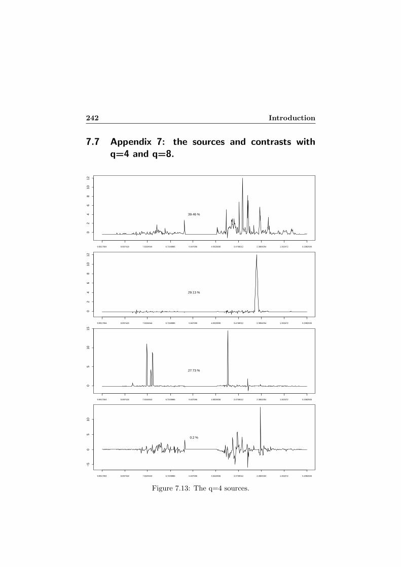
242 Introduction

7.7 Appendix 7: the sources and contrasts withq=4 and q=8.

02

46

810

12

9.9917004 8.897418 7.8194544 6.7249886 5.647086 4.5528036 3.4749012 2.3804354 1.302472 0.2082506

39.46 %

02

46

810

12

9.9917004 8.897418 7.8194544 6.7249886 5.647086 4.5528036 3.4749012 2.3804354 1.302472 0.2082506

29.13 %

05

1015

9.9917004 8.897418 7.8194544 6.7249886 5.647086 4.5528036 3.4749012 2.3804354 1.302472 0.2082506

27.73 %

−5

05

10

9.9917004 8.897418 7.8194544 6.7249886 5.647086 4.5528036 3.4749012 2.3804354 1.302472 0.2082506

0.2 %

Figure 7.13: The q=4 sources.

7.7 Appendix 7: the sources and contrasts with q=4 and q=8.243

04

812

9.9917004 8.897418 7.8194544 6.7249886 5.647086 4.5528036 3.4749012 2.3804354 1.302472 0.2082506

39.41 %

04

812

9.9917004 8.897418 7.8194544 6.7249886 5.647086 4.5528036 3.4749012 2.3804354 1.302472 0.2082506

29.76 %

05

1015

9.9917004 8.897418 7.8194544 6.7249886 5.647086 4.5528036 3.4749012 2.3804354 1.302472 0.2082506

26.2 %

−5

05

10

9.9917004 8.897418 7.8194544 6.7249886 5.647086 4.5528036 3.4749012 2.3804354 1.302472 0.2082506

1.64 %

−5

515

9.9917004 8.897418 7.8194544 6.7249886 5.647086 4.5528036 3.4749012 2.3804354 1.302472 0.2082506

1.2 %

−6

−2

26

9.9917004 8.897418 7.8194544 6.7249886 5.647086 4.5528036 3.4749012 2.3804354 1.302472 0.2082506

0.14 %

−10

05

15

9.9917004 8.897418 7.8194544 6.7249886 5.647086 4.5528036 3.4749012 2.3804354 1.302472 0.2082506

0.07 %

0.07 %

−5

05

10

9.9917004 8.897418 7.8194544 6.7249886 5.647086 4.5528036 3.4749012 2.3804354 1.302472 0.2082506

0.02 %

Figure 7.14: The q=8 sources.

244 Introduction

−0.

002

0.00

00.

002

0.00

40.

006

0.00

80.

010

C2−1

9.9917004 6.7249886 3.4749012 0.2082506

−0.

002

0.00

00.

002

0.00

40.

006

0.00

80.

010

C3−1

9.9917004 6.7249886 3.4749012 0.2082506

−0.

002

0.00

00.

002

0.00

40.

006

0.00

80.

010

C4−1

9.9917004 6.7249886 3.4749012 0.2082506

Figure 7.15: The three contrasts obtained when y1 is introduced as acategorical variable in the model, with q=4 sources.

−0.

002

0.00

00.

002

0.00

40.

006

0.00

80.

010

C2−1

9.9917004 6.7249886 3.4749012 0.2082506

−0.

002

0.00

00.

002

0.00

40.

006

0.00

80.

010

C3−1

9.9917004 6.7249886 3.4749012 0.2082506

−0.

002

0.00

00.

002

0.00

40.

006

0.00

80.

010

C4−1

9.9917004 6.7249886 3.4749012 0.2082506

Figure 7.16: The three contrasts obtained when y1 is introduced as acategorical variable in the model, with q=8 sources.

7.8 Appendix 8: the AIC of the LLR variable selectionapplied to the AMD dataset. 245

7.8 Appendix 8: the AIC of the LLR variable se-lection applied to the AMD dataset.

Selection AIC

1 4.006525

2 239.8081

3 241.7860

4 243.7860

5 245.7858

6 247.7854

7 249.3052

8 251.0029

9 252.9996

10 254.9996

11 256.9996

12 254.1854

13 239.4771

14 230.2833

15 223.5777

16 218.0535

17 212.5977

18 210.0387

19 208.0730

20 206.595

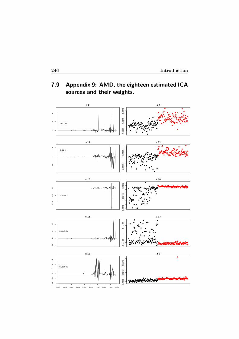
246 Introduction

7.9 Appendix 9: AMD, the eighteen estimated ICAsources and their weights.

05

10

s 2

10.71 %0.

0010

0.00

200.

0030

a 2

−5

05

s 11

1.49 %

−0.

0015

−0.

0005

a 11

−10

−5

0

s 10

2.41 %

−0.

0030

−0.

0015

0.00

00

a 10

−5

05

10

s 13

0.4445 %

0 e

+00

1 e

−03

a 13

−4

−2

02

46

s 16

0.2898 %

9.9923 8.8976 7.8197 6.7254 5.6472 4.5531 3.4749 2.3805 1.3026 0.2082

0.00

000.

0010

0.00

20

a 6

7.9 Appendix 9: AMD, the eighteen estimated ICA sourcesand their weights. 247

05

10

s 12

0.76 %

0.00

000.

0010

a 12

−15

−10

−5

0

s 5

8.08 %

−0.

004

−0.

002

0.00

0a 5

−6

−4

−2

02

s 8

3.51 %

−0.

0020

−0.

0010

a 8

05

1015

20

s 3

9.37 %

0.00

050.

0015

0.00

25

a 3

05

1015

20

s 1

17 %

9.9923 8.8976 7.8197 6.7254 5.6472 4.5531 3.4749 2.3805 1.3026 0.2082

0.00

10.

003

0.00

5

a 1

248 Introduction

05

1015

20

s 7

4.18 %

0.00

000.

0010

0.00

20

a 7

−20

−15

−10

−5

05

s 6

4.75 %

−0.

0025

−0.

0010

0.00

00a 6

05

1015

20

s 17

0.1828 %

0 e

+00

1 e

−03

a 17

−10

−5

05

s 9

3.25 %

−0.

0020

−0.

0010

a 9

−5

05

10

s 15

0.3587 %

9.9923 8.8976 7.8197 6.7254 5.6472 4.5531 3.4749 2.3805 1.3026 0.2082

−0.

0005

0.00

050.

0015

a 15

7.9 Appendix 9: AMD, the eighteen estimated ICA sourcesand their weights. 249

−2

02

46

s 18

0.143 %

−0.

0005

0.00

000.

0005

0.00

100.

0015

0.00

200.

0025

a 18

−2

02

46

8

s 14

0.4029 %

0 50 100 150

0.00

000.

0010

0.00

200.

0030

a 14

−5

05

1015

s 4

8.59 %

9.9923 8.8976 7.8197 6.7254 5.6472 4.5531 3.4749 2.3805 1.3026 0.2082 0 50 100 150

0.00

10.

002

0.00

30.

004

0.00

5

a 4

250 Introduction

7.10 Appendix 10: AMD, comparisons of meanson the vectors of weights of the 18 sources.

The left part of the table gives the p-values from t-tests comparing AMDand controls weights. The right part gives the p-values obtained fromAnova comparison of active, inactive cases and controls. In both partof the table, a × in the variance columns indicates a p-value inferior to0.05 for the Levene test of homogeneity of variances.

Sources p-values Variances 6= p-values Variances 6=2 1.093−34 × 2.545−28

11 7.11−28 × 2.542−26 ×10 7.34−21 × 3.679−18 ×13 2.13−15 × 1.709−18 ×16 1.82−14 1.972−12

12 4.96−13 × 5.311−15 ×5 8.80−12 × 3.356−11 ×8 6.70−12 8.656−14

3 1.04−10 1.541−09

1 1.37−10 2.408−09

7 1.20−08 × 2.238−08 ×6 2.28−08 × 5.969−07 ×17 0.0002 × 0.0026 ×9 0.0004 × 0.001 ×15 0.012 × 0.0463 ×18 0.042 × 0.041 ×14 0.509 × 0.800 ×4 0.636 × 0.536 ×

Abbreviations

• ADC: Analog Digital Converter.• AIC: Akaike Information Criterion.• AQ: Acquisition Time.• AMD: Age-related Macular Degeneration.• ANOVA: ANalysis Of VAriance• ASCA: ANOVA-Simultaneous Component Analysis.• B-Y rule: Benjamini-Yekutieli FDR rule.• CART: Classification and Regression Tree.• COMET: Consortium for Metabonomic Toxicology.• CLOUDS: Classification Of Unknowns by Density Superposition.• CPMG: Carr Purcell Meiboom Gill pulse sequence.• CS: Constant Sum normalization.• CSF: Cerebro-Spinal Fluid.• DOE: Statistical design of experiments.• DR: Digital Resolution.• DW: Dwell Time.• FFT: Fast Fourier Transform.• FID: Free Induction Decay.• FDR: False discovery Rate.• FT: Fourier Transform.• GLM: General Linar Model.• 1H: Proton.• 1H-NMR spectroscopy: Proton Nuclear Magnetic Resonance spec-

troscopy.• HCA: Hierarchical Cluster Analysis.• ICA: Independent Component Analysis.• ICC: Intraclass Correlation Coefficient.• LB: Line Broadening.• LLR: Linear Logistic Regression.• MHT: Multiple Hypothesis Testing.• MS spectroscopy: Mass spectroscopy.• NLM: Nonlinear mapping.

252 Introduction

• NOESY: Noesypresat pulse.• O-PLS: Orthogonal - Partial Least Squares.• PC: Principal Component.• PCA: Principal Component Analysis.• PLS: Partial Least Squares.• PLS-DA: Partial Least Squares - Discriminant Analysis.• Ppm: Part per million.• RF: Radio Frequency.• RMSEP: Root Mean Square Error of Prediction.• ROC curves: Receiver Operating Characteristics curves.• SIMCA: Soft Independent Modelling of Class Analogy.• SNR: Signal to Noise Ratio (different measurements on the FID

and the spectrum).• s-ICA: supervised - Independent Component Analysis.• s-PCA: supervised - Principal Component Analysis.• STE: Stimulated Echo pulse sequence.• SW: Spectral Window.• TMSP: 3-(trimethylsilyl)propionate-2,2,3,3.

Bibliography

[1] H Akaike. A new look at the statistical model identification. Auto-matic Control IEEE Transactions, 19(6):716–23, 1974.

[2] ML Anthony, BC Sweatman, CR Beddell, JC Lindon, andJK Nicholson. Pattern recognition classification of the site ofnephrotoxicity based on metabolic data derived from proton nu-clear magnetic resonance spectra of urine. Molecular Pharmacology,46(1):199–211, 1994.

[3] JR Bales, DP Higham, I Howe, JK Nicholson, and PJ Sadler. Useof high resolution proton nuclear magnetic resonance spectroscopyfor rapid multi-component analysis of urine. Clinical Chemistry,30(3):426–432, 1984.

[4] FJ Bamforth. Diagnosis of inborn errors of metabolism using h-nmr spectroscopic analysis of urine. Journal of Inherited MetabolicDisease, 22:297–301, 1999.

[5] M Barker and W Rayens. Partial least squares for discrimination.Journal of Chemometrics, 17(3):166–173, 2003.

[6] Y Benjamini and D Yekutieli. The control of the false discoveryrate in multiple testing under dependency. The Annals of Statistics,29(4):1165–1188, 2001.

[7] M Bictash, TM Ebbels, Q Chan, RL Loo, IK Yap, IJ Brown,M de Iorio, and ML Daviglus. Opening up the ”black box”:Metabolic phenotyping and metabolome-wide association studies inepidemiology. Journal of Clinical Epidemiology, 63(9):970–9, 2000.

[8] ME Bollard and E Holmes. Nmr-based metabonomic approaches forevaluating physiological influences on biofluid composition. NMRin Biomedicine, 18:143–162, 2005.

254 BIBLIOGRAPHY

[9] GEP Box, WG Hunter, and JS Hunter. Statistics for Experi-menters. John Wiley and Sons, New-York, 1978.

[10] LJ Breiman. Random forests. Machine Learnings, 45:5–32, 2001.

[11] LJ Breinman, R Friedman, R Olsen, and C Stone. Classificationand Regression Trees. Wadsworth Pacific Grove, CA, 1984.

[12] JT Brindle, H Antii, and E Holmes. Rapid and non-invasive diag-nosis of the presence and severity of coronary heart disease using1h-nmr based metabonomics. Nature Medicine, 8:1439–1445, 2002.

[13] FF Brown, ID Camplell, PW Kuchel, and DC Rabenstein. Humanerythrocyte metabolism studies by 1h spin echo nmr. FEBS Letters,82(1):12–16, 1977.

[14] H Brown and R Prescott. Applied Mixed Models in Medicine. JohnWiley and Sons, 2006.

[15] JG Bundy, EM Lenz, NJ Bailey, CL Gavaghan, C Svendsen,D Spurgeon, PK Hankard, and D Osborn. Metabonomic assess-ment of toxicity of 4-fluoroaniline, 3,5-difluoroaniline and 2-fluoro-4-methylaniline: identification of new endogenous biomarkers. En-vironmental Toxicology and Chemistry, 21(9):1966–1972, 2002.

[16] JG Bundy, D Osbornb, JM Weeks, JC Lindon, and JK Nichol-son. An nmr based metabonomics approach to the investigation ofcoelomic fluid biochemistry in earthworms under toxic stress. FEBSLetters, 500(1):31–35, 2001.

[17] M Bylesjo, O Cloarec, JK Nicholson, E Holmes, and J Trygg. Oplsdiscriminant analysis - combining the strengths of pls-da and simcaclassification. Journal of Chemometrics, 77(20):1282–1289, 2006.

[18] MA Chabot. Etude de l’effet du prtraitement et de la methode denormalization sur la qualite informative des spectres H-NMR enmetabonomique. Master’s thesis in statistics, Universite catholiquede Louvain, 2007.

[19] TDW Claridge. High-Resolution NMR Techniques in OrganicChemistry. Elsevier, 2009.

[20] P Common. Independent component analysis, a new concept? Sig-nal Processing, 36(3):287–314, 1994.

BIBLIOGRAPHY 255

[21] S de Jong. Simpls: An alternative approach to partial leastsquares regression. Chemometrics and Intelling Laboratory Sys-tems, 18(3):251–253, 1993.

[22] M de Noo, A Tollenaar, P Kuppen, M Bladergroen, PHC Eilers,and A Deelder. Reliability of human serum protein profiles gener-ated with c8 magnetic beads assisted maldi-tof mass spectrometry.Analytical Biochemistry, 77:7232–7241, 2005.

[23] ME Dumas. Assessment of analytical reproducibility of h-nmr spec-troscopy based metabonomics for large-scale epidemiological re-search; the intermap study. Analytical Chemistry, 78:2199–2208,2006.

[24] JP Egan. Signal Detection Theory and ROC Analysis. AcademicPress: New York, 1975.

[25] PHC Eilers. A perfect smoother. Analytical Chemistry, 75:3631–3636, 2003.

[26] PHC Eilers. Parametric time warping. Analytical Chemistry,76(2):404–411, 2004.

[27] PHC Eilers and HFM Boelens. Baseline correction with asymmetricleast squares smoothing. Leiden University Medical Centre report,2005.

[28] PHC Eilers, J Boer, G VanOmmen, and H VanHouwelingen.Classification of microarray data with penalized logistic regres-sion. Progress in Biomedical Optics and Images, 4266(187):187–198,2001.

[29] F Esposito, D Malerba, and G Semeraro. A comparative analysis ofmethods for pruning decision trees. IEEE Transactions of patternanalysis and machine intelligence, 19(5):476–491, 1997.

[30] O Fiehn. Combining genomics, metabolome analysis, and biochem-ical modelling to understand metabolic networks. Comparative andFunctional Genomics, 2(3):155–168, 2001.

[31] PH Gamache, DF Meyer, MC Granger, and IN Acworth.Metabolomic applications of electrochemistry/mass spectrome-try. Journal of the American Society for Mass Spectrometry,15(12):1717–1726, 2004.

256 BIBLIOGRAPHY

[32] KPR Gartland, F Bonner, and JK Nicholson. Investigations intothe biochemical effects of region-specific nephrotoxins. MolecularPharmacology, 35(2):242–251, 1989.

[33] KPRG Gartland, C Beddell, JC Lindon, and JK Nicholson. Theapplication of pattern recognition methods to the analysis and clas-sification of toxicological data. Molecular Pharmacology, 39(5):629–642, 1991.

[34] SC Gates and CC Sweeley. Quantitative metabolic profiling basedon gas chromatography. Clinical Chemistry, 24(10):1663–73, 1978.

[35] S Golotvin and A Williams. Improved baseline recognition andmodeling of ft nmr spectra. Journal of Magnetic Resonance,146(1):122–125, 2000.

[36] R Goodacre, D Broadhurst, AK Smilde, B Kristal, JD Baker,R Beger, C Bessant, S Connor, G Capuani, A Craig, T Ebbels,J Trygg, and F Wulfert. Proposed minimum reporting standardsfor data analysis in metabolomics. Metabolomics, 3(3):231–241,2007.

[37] S Halouska and R Powers. Negative impact of noise on the principalcomponents analysis of nmr data. Journal of Magnetic Resonance,178(1):88–95, 2006.

[38] H Hart and JM Conia. Introduction a la chimie organique. Dunod,2000.

[39] E Holmes. H-nmr spectroscopy characterization of the complexmetabolic pattern of urine from patients with inborn errors ofmetabolism. Journal of Pharmaceutical and Biomedical Analysis,15:1647–1657, 1997.

[40] KG Horning. Analysis of phospholipids, ceramides, and cerebro-sides by gas chromatography and gas chromatography-mass spec-trometry. American Journal of Clinical Nutrition, 24(9):1086–1096,1971.

[41] DW Hosmer and S Lemeshow. Applied Logistic Regression. Wiley:New York, 1989.

[42] P Hubber. Projection pursuit. The Annals of Statistics, 13:435–475,1985.

BIBLIOGRAPHY 257

[43] A Hyvarinen. Fast and robust fixed-point algorithms for indepen-dent component analysis. IEEE Transactions on Neural Networks,10:626–634, 1999.

[44] A Hyvarinen, J Karhunen, and E Oja. Independent ComponentAnalysis. Wiley: USA, 2001.

[45] A Hyvarinen and E Oja. Independent component analysis: algo-rithms and applications,. Neural Networks, 13(4):411–430, 2000.

[46] J Jansen, J Hoefsloot, J van der Greef, M Timmerman, J West-erhuis, and AK Smilde. Asca: analysis of multivariate data ob-tained from an experimental design. Journal of Chemometrics,9(9):469481, 2005.

[47] I Jolliffe. Principal Component Analysis. Springer-Verlag: NewYork, 1986.

[48] NN Kaderbhai, DI Broadhurst, DI Ellis, and DB Kell. Functionalgenomics via metabolite footprinting: monitoring metabolite secre-tion by escherichia coli tryptophan metabolism mutants using ft-irand direct injection electrospray mass spectrometry. Comparativeand Functional Genomics, 4(4):376–391, 2003.

[49] H Keun, TMD Ebbels, H Antti, ME Bollard, O Beckonert,G Schlotterbeck, H Senn, U Niederhauser, E Holmes, JC Lindon,and JK Nicholson. Physiological variations and analytical repro-ducibility in metabonomics urinalysis. Chemical Research in Toxi-cology, 15(11):1380–1386, 2002.

[50] HC Keun, TMD Ebbels, and JK Nicholson. Analytical reproducibil-ity in h-nmr-based metabonomics urinalysis. Chemical research intoxicology, 15:1380–1386, 2002.

[51] S Kochlar, DM Jacobs, and LB Fay. Probing gender-specificmetabolism differences in human by nuclear magnetic resonance-based metabonomics. Analytical Biochemistry, 352:274–281, 2006.

[52] Kodunsi and Wollman. Detection of epithelial ovarian cancer us-ing 1h-nmr based metabonomics. International Journal of Cancer,113(5):782–788, 2005.

[53] S Lee and S Batzoglou. Application of independent componentanalysis to microarrays. Genome Biology, 4:76.1–76.21, 2003.

258 BIBLIOGRAPHY

[54] C Legido-Quigley, O Cloarec, E Holmes, JC Lindon, and JK Nichol-son. First example of hepatocyte transplantation to alleviateornithine transcarbamylase deficiency, monitored by nmr-basedmetabonomics. Bioanalysis, 1:1527–1535, 2009.

[55] W Liebermeister. Linear modes of gene expression determined byindependent component analysis. Bioinformatics, 18:51–60, 2002.

[56] JC Lindon, E Holmes, and JK Nicholson. Metabonomics-techniques and applications. Business Briefing-Futur Drug Dis-covery, 23(6):1075–1088, 2004.

[57] JC Lindon, JK Nicholson, and E Holmes. The Handbook of Metabo-nomics and Metabolomics. Elsevier: Imperial College London, 2007.

[58] JC Lindon, JK Nicholson, E Holmes, H Antti, ME Bollard, H Keun,O Beckonert, TM Ebbels, MD Reily, D Robertson, GJ Stevens,P Luke, AP Breau, GH Cantor, RH BiblE, U Niederhauser, H Senn,G Schlotterbeck, UG Sidelmann, SM Laursen, A Tymiak, BD Car,L Lehman-McKeeman, JM Colet, A Loukaci, and C Thomas. Con-temporary issues in toxicology: the role of metabonomics in tox-icology and its evaluation by the comet project. Toxicology andApplied Pharmacology, 187(3):137–146, 2002.

[59] LH Lucas. Progress toward automated metabolic profiling of hu-man serum: comparison of cpmg and gradient-filterred nmr analyt-ical methods. Journal of Pharmaceutical and Biomedical Analysis,39(1):156–163, 2005.

[60] M Luhmer. Mesure et traitement du signal en rmn du h 1 dimen-sion. First Belgian Symposium on Metabolomics and Metabonomics,Mons: FNRS:41–61, 2009.

[61] T Lundstedt, E Seifert, L Abramo, B Thelin, A Nystrm, J Pet-tersen, and R Bergman. Experimental design and optimiza-tion. Chemometrics and Intelligent Laboratory Systems, 42(1):3–40,1998.

[62] KV Mardia, JT Kent, and JM Bibby. Multivariate Analysis. Lon-don Academic Press, 1979.

[63] H Martens and T Naes. Multivariate Calibration. Wiley: ChichesterUK, 1989.

BIBLIOGRAPHY 259

[64] B Mevik and HR Cederkvist. Mean squared error of prediction(msep) estimates for principal component regression (pcr) andpartial least squares regression (plsr). Journal of Chemometrics,18(9):422–429, 2004.

[65] Moolenaar, UFH Engelke, and RA Wevers. Proton nuclear mag-netic resonance spectroscopy of body fluids in the field of inbornerrors of metabolism. Annals of Clinical Biochemistry, 40:16–24,2003.

[66] V Nguyen and D Rocke. Tumor classification by partial leastsquares using microarray gene expression data. Bioinformatics,18:39–50, 2002.

[67] AW Nicholls, E Holmes, JC Lindon, and JK Nicholson. Metabo-nomic investigations into hydrazine toxicity in the rat. ChemicalResearch in Toxicology, 14(8):975–987, 2002.

[68] J Nicholson, J Connelly, JC Lindon, and E Holmes. Metabonomics:a generic platform for the study of drug toxicity and gene function.Nature Reviews Drug Discovery, 1:153–161, 2002.

[69] JK Nicholson, PJD Foxall, M Spraul, RD Farrant, and JC Lindon.750 mhz 1h and 13c nmr spectroscopy of human blood plasma.Analytical Chemistry, 67(5):793–811, 1995.

[70] JK Nicholson, JC Lindon, and E Holmes. Metabonomics: under-standing the metabolic responses of living systems to pathophysio-logical stimuli via multivariate statistical analysis of biological nmrspectroscopic data. Xenobiotica, 29(11):1181–1189, 1999.

[71] JK Nicholson, JA Timbrell, and PJ Sadler. Proton nmr spectra ofurine as indicators of renal damage. mercury-induced nephrotoxic-ity in rats. Molecular Pharmacology, 27(6):644–651, 1985.

[72] JK Nicholson and ID Wilson. High resolution proton nmr spec-troscopy of biological fluids. Progress in NMR Spectroscopy, 21:449–501, 1989.

[73] M Nowak. Changes in lipid metabolism in women with age-relatedmacular degeneration. Clinical and Experimental Medicine, 4:183–7, 2005.

[74] J Keeler University of Cambridge Department ofChemistry. Understanding 1h-nmr spectroscopy.www.chem.queensu.ca/facilities/nmr/nmr/webcourse/, 2004.

260 BIBLIOGRAPHY

[75] AN Phipps, J Stewart, and B Wright. Effect of diet on the urinaryexcretion of hippuric acid and other dietary-derived aromatics inrat. a complex interaction between diet, gut microflora and sub-strate specificity. Xenobiotica, 5:527–537, 1998.

[76] DG Robertson. Metabonomics in toxicology: a review. ToxicologicalSciences, 85(2):809–822, 2005.

[77] G Saporta. Probabilites, analyses des donnees et statistiques. Edi-tions TECHNIP, 2006.

[78] M Scholz, S Gatzek, A Sterling, O Fiehn, and J Selbig. Metabolitefingerprint: detecting biological features by independent componentanalysis. Bioinformatics, 15:2447–2454, 2004.

[79] SR Searle and CR Henderson. Dispersion matrices for variancecomponents models. Journal of American Statististics Association,74:465–547, 1979.

[80] JP Shockor and E Holmes. Current opinion in drug discovery anddevelopment. Analytical Chemistry, 3(1):72–78, 2000.

[81] RM Silverstein, GC Bassler, and TC Morrill. Spectrometric Identi-fication of Organic Compounds. Wiley, 1991.

[82] J Smith. Shift theorem, center for computer researchin music and acoustics (ccrma), standford university.https://ccrma.stanford.edu/ jos/sasp/Shift Theorem DTFT.html,2010.

[83] OD Sparkman. Mass spectrometry desk reference. Global ViewPublishing,Pittsburgh, 2000.

[84] L Stahle and S Wold. Multivariate analysis of variance (manova).Chemometrics and Intelligent Laboratory Systems, 9(2):127–141,1990.

[85] J Storey. A direct approach to false discovery rates. Journal of theRoyal Statistical Society Series B, 64(3):479–498, 2001.

[86] J Storey and D Siegmund. Strong control, conservative point es-timation, and simultaneous conservative consistency of false dis-covery rates: a unified approach. Journal of the Royal StatisticalSociety Series B, 66:187–205, 2004.

BIBLIOGRAPHY 261

[87] O Teahan. Impact of analytical bias in metabonomic studies ofhuman blood serum and plasma. Analytical Chemistry, 78:4307–4318, 2006.

[88] J Trygg. Orthogonal projections to latent structures (o-pls). Jour-nal of Chemometrics, 16(3):119–128, 2002.

[89] J Trygg, E Holmes, and T Lundstedt. Chemometrics in metabo-nomics. Journal of Proteome Research, 6(2):469–479, 2007.

[90] V Tusher, R Tibshiriani, and G Chu. Significant analysis of microar-ray applied to the ionising radiation response. PNAS, 98(9):5116–5121, 2001.

[91] J Vanwinsberghe. Bubble: development of a matlab tool for auto-mated 1H-NMR data processing in metabonomics. Master’s thesisStrasbourg University, 2005.

[92] MR Viant. Improved methods for the acquisition and interpretationof nmr metabolomic data. Biochemical and Biophysical ResearchCommunications, 310(3):934–948, 2003.

[93] JTWE Vogels, AC Tas, J Venekamp, and J van der Greef. Partiallinear fit: A new nmr spectroscopy preprocessing tool for patternrecognition applications. Journal of Chemometrics, 10(5-6):425–438, 1996.

[94] F Wang. NMR-based Metabolomics for Biomarker Discovery, Meth-ods in pharmacology and toxicology: biomarker Methods in drugdiscovery and development. Hamana Press, 2008.

[95] MA Warne, EM Lenz, D Osborn, JM Weeks, and JK Nicholson.An nmr-based metabonomics investigation of the toxic effects of 3-trifluoromethyl-aniline on the earthworm eisenia veneta. Biomark-ers, 5(1):56–72, 2000.

[96] WM Westler and F Abilgdaard. Dmx digital filters and non brukerofline processing iii. Falculty of Science: the website of ResearchGroup Bio-Organic Chemistry, 2004.