statistical description of the wireless channeltoker/ele492/3... · statistical description of the...

Statistical Description of the Wireless Channel

Spring 2017 ELE 492 – FUNDAMENTALS OF WIRELESS COMMUNICATIONS 1

Path Loss + Small/Large Scale Fading


Time-Invariant Two-Path Model


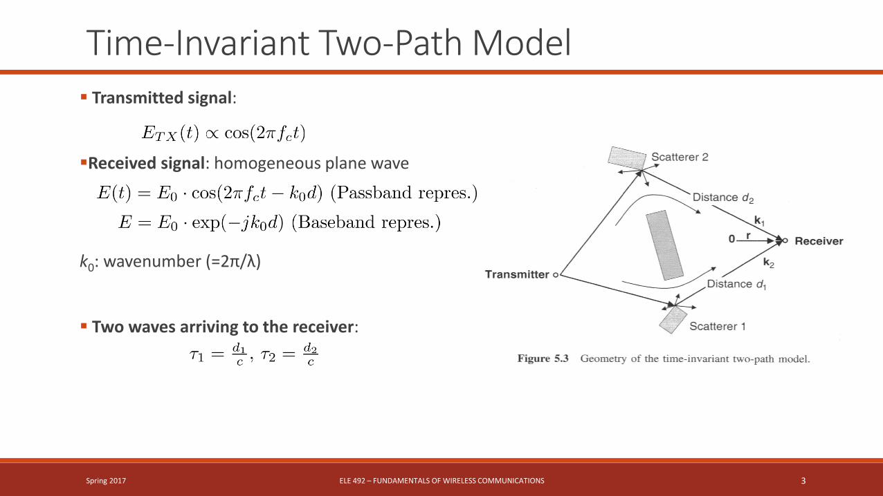
Transmitted signal:

Received signal: homogeneous plane wave

k0: wavenumber (=2π/λ)

Two waves arriving to the receiver:

Time-Invariant Two-Path Model Two waves arriving to the receiver:

Note the deep fades in amplitude (E1 = E2) (WHY?)

Destructive/constructive interference!


* deep fades!

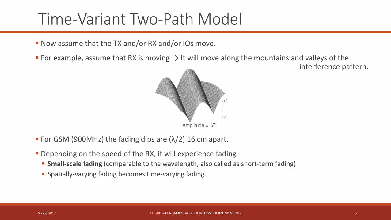
Time-Variant Two-Path Model Now assume that the TX and/or RX and/or IOs move.

For example, assume that RX is moving → It will move along the mountains and valleys of the interference pattern.

For GSM (900MHz) the fading dips are (λ/2) 16 cm apart.

Depending on the speed of the RX, it will experience fading Small-scale fading (comparable to the wavelength, also called as short-term fading)

Spatially-varying fading becomes time-varying fading.


Time-Variant Two-Path Model Motion in the channel introduces Doppler shift

Doppler shift:


When the direction of motion and direction of propagation are aligned!

Time-Variant Two-Path Model When all MPCs experience the same Doppler shift, the receiver can compensate the distortion (by shifting the LO frequency.)

If the MPCs experience difference Doppler shifts, the superposition will create a sequence of fading dips.

For two MPCs → beating of two oscillations with slightly different frequencies.

This behaviour is equivalent to the fast fading (small scale fading) created by passing through the «mountains and valleys» of the field strength plot.


2

Time-Variant Two-Path Model Fading rate can be obtained by two approaches:

1. Plot the interference pattern («mountains and valleys») and count the number of fading dips per second that the RX experiences when passing through the pattern.

2. Superimpose two signals with different Doppler shifts at the RX antenna and determine the fading rate from the beat frequency.

Doppler frequency is a measure for the rate of change of the channel.

Superposition of many slightly Doppler-shifted signals leads to phase shifts of the received signal impairment in the reception of angle/phase-modulated signals (FM, FSK, PSK)

(What happens for >2 signals?)


Small-Scale Fading Without a LOS (Line-of-Sight) component

With a LOS component


Small-Scale Fading without a Dominant Component

There are many IOs in the channel and the RX is moving. many IOs → Almost impossible to track with ray-tracing.

Example: 8 plane waves incident onto the RX.

|ai|: absolute amplitude

ϕi : angle of incidence (wrt x-axis, horizontal plane)

φi : phase of the received signal




Central Limit Theorem:N →∞ => pdf → Gaussian



real, imag pdf → independent Gaussian magnitude pdf → Rayleigh phase pdf → uniform


Statistics of Amplitude and Phase N homogeneous plane waves (MPCs)

Absolute amplitudes of the MPCs do not change over the region of observation, i.e.

but the phases ψi vary → consider them as r.v.s with uniform pdf (ψi [0,2π))

Received signal:

I-Q components in the passband


Sum of many r.v.s, non dominating (|ai|<<CP)Central Limit Theorem → I(t) has zero-mean

Gaussian pdfSame for Q(t).

I(t) and Q(t) are independent.We do not need to know the distribution of ais.

Rayleigh Distribution

pdf of the I and Q components: N(0,σ2)

complex envelope (I(t)+jQ(t)) has the amplitude and phase pdf.s

Rayleigh distribution:


← pI(I(t)) and pQ(Q(t))

Rayleigh pdf

uniform pdf

Rayleigh Distribution Cumulative distribution function, cdf


r

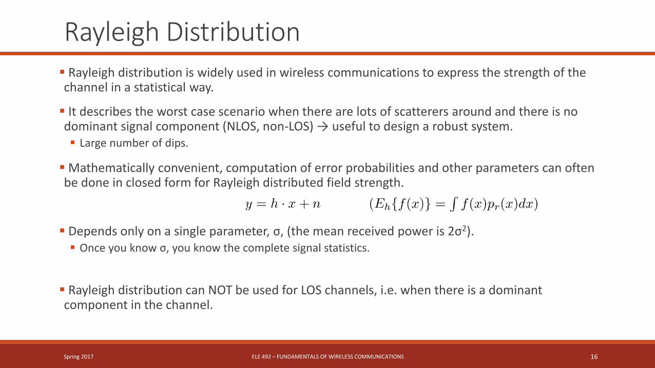
Rayleigh Distribution Rayleigh distribution is widely used in wireless communications to express the strength of the channel in a statistical way.

It describes the worst case scenario when there are lots of scatterers around and there is no dominant signal component (NLOS, non-LOS) → useful to design a robust system. Large number of dips.

Mathematically convenient, computation of error probabilities and other parameters can often be done in closed form for Rayleigh distributed field strength.

Depends only on a single parameter, σ, (the mean received power is 2σ2). Once you know σ, you know the complete signal statistics.

Rayleigh distribution can NOT be used for LOS channels, i.e. when there is a dominant component in the channel.


Fading Margin for NLOS Channels Even if the field strength is large, it does not guarantee successful communications at all times.

Given a minimum receive power or field strength required forsuccessful communications, how large does the mean power haveto be in order to ensure that communications fail in no more thanx% of all situations.

In order to achieve an x% outage probability

What should the minimum field strength be to achieve x% outage probability? minimum mean power:


(see slide 15, definition of Rayleigh cdf.)

Fading Margin for NLOS ChannelsExample: For a signal with Rayleigh-distributed amplitude, what is the probability that the received signal power is at least 20, 6 and 3 dB below the mean power.

A power level 20 dB below the mean power level:

Probability for 6 dB is 0.221 and for 3 dB is 0.393.

If we use the approximate cdf expression ◦ for 20 dB, probability is 0.01 (approx. works)

◦ for 6 dB, probability is 0.25 (approx. works)

◦ for 3 dB, probability is 0.5 (approx. fails)


Small-Scale Fading with a Dominant Component

What happens if we have an additional «dominant» MPC also?


Small-Scale Fading with a Dominant Component


Observe the contributionfrom the dominant component.

Probability of deep fades is much smaller than theRayleigh distribution.

sine wave from 0o

dominates the others.

This is the Rician distributionwith Rician factor:

Rician Distribution

w.l.o.g. assume that the dominant component is purely real. Then, I(t) α N(A,σ2) and Q(t) α N(0,σ2). I(t) and Q(t) are independent, but r and ψ are not.

Joint pdf of r and ψ is

pdf of amplitude r (Rician distribution):

Rician factor: Kr→0 : pr → Rayleigh , Kr ↗ : pr → Gaussian with mean A

rms value of r:

Phase is NOT uniform. Dominant term dominates the phase as Kr ↗.


Modified Bessel func. of the first kind and order zero.

Fading Margin for LOS ChannelsExample: Compute the fading margin for a Rician distribution with Kr = 0.3, 3 and 20 dB so thatthe outage probability is less than 5%.

We need the cdf of Rician distribution:

Then, the outage probability is

And the fading margin is given by

The required fading margins: Kr = 0.3 dB → 11.5 dB

Kr = 3 dB → 9.7 dB

Kr = 20 dB → 1.1 dB


Marcum Q function

Nakagami m-distribution Another widely used pdf is the Nakagami m-distribution:

For m>1

Rician and Nakagami-m have similar shape. The main difference is the behaviour around r = 0.

Main difference: Rician distribution: Exact distribution of the amplitude when there is one dominant component, and a large number of

non-dominant components.

Nakagami-m: Approximate distribution of the amplitude where the central limit theorem is not necessarily valid. (e.g. UWB channels.)


Gamma function

𝑚 =Ω2

𝑟2 − ഥΩ2

Doppler Spectrum and Temporal Channel Variations

Remember that moving RX experiences a Doppler shift (if there is a single wave incident onto it)

Max. Doppler shift (in the + or –ve direction) occurs when the RX approaches the wavefront directly from the front, or receives wavefront right from the behind.

When there are multiple MPCs in the channel, angle of arrivals of the wavefronts from these MPCs maydiffer. There is a density of Doppler shifts depending on the spatial angle g.

We need to know the distribution of power of the incident waves. Let us call this distribution pg (g).

Furthermore, the RX antenna has a gain dependent on the angle g, then the received power spectrum is

This relation gives the dependency on the angle g.

What about the distribution wrt the Doppler freq ν? (This is more meaningful communications-wise)


We cannot distinguish the difference between g and – g.JakesModel

Mean power of the arriving field.

Doppler Spectrum To find the distribution wrt the Doppler freq ν, apply a change of variable g → ν:

nth order moment of the Doppler Spectrum:

Jakes model: MPCs are incident uniformly from all azimuthal directions:

Bathtub shape! Recall the singularities at ±νmax (Why?).


Jakes Model

Autocorrelation of the channel Describes the frequency dispersion caused by the channel. A single tone is spread overfrequency. May cause problem in narrowband communications, and OFDM.

Gives a measure about the temporal variability of the channel.

Statistical measure: autocorrelation function of the fading: For the inphase component:

Covariance function of the envelope:


𝐼 𝑡 𝐼(𝑡 + ∆𝑡)

𝐼(𝑡)2= 𝐽𝑜 2𝜋νmax∆𝑡

Inverse Fourier transformof the Doppler Spectrum

Valid for the Jakes model!

𝑟 𝑡 𝑟(𝑡 + ∆𝑡) − 𝑟(𝑡)2

𝑟(𝑡)2= 𝐽0

2 2𝜋νmax∆𝑡

𝐼 𝑡 𝑄 𝑡 + ∆𝑡 = 0, ∀∆𝑡(I and Q are independent)

Autocorrelation of the channelExample: Assume that an MS is located in a fading dip. On average, what minimum distanceshould the MS move, so that it is no longer influenced by this fading dip?


0.18 λ 0.38 λ

Level Crossing Rate LCR gives the number of deep fades per second. Define a deep fade? We will derive LCR for an arbitrary level:

NR(r) is the expected value of the rate at which thereceived field strength crosses a certain level r in thepositive direction.

For the Jakes Doppler Spectrum

Ω0, Ω2: 0th and 2nd moments of the Jakes spectrum.

: rms value of the amplitude.


Average Duration of Fades ADF: Ratio of the rate of field strength going below a threshold (LCR), and the percentage of time the field strength is lower than this threshold (cdf of the field strength):


r

CDF

LCR

Average Duration of Fades Example: Assume a multipath environment where the received signal has a Rayleigh distribution and the Doppler spectrum has the classical bathtub (Jakes) shape. Compute the LCR and ADF for a maximum Doppler frequency νmax = 50Hz, and amplitude thresholds

2nd moment of the Jakes spectrum is

And, the Rayleigh cdf is:

Then, LCR is

And, ADF is


Large Scale Fading Small-scale fading: Caused by the interference pattern of the MPCs

Channel changes within couple of wavelengths, fading is relatively rapid.

Large-scale fading: Caused by the obstacles in the medium. The path goes into the «shadow» of these obstacles.

Small Scale Averaged (SSA) field strength, F: averaged over a small area (e.g. 10λ x 10λ) For small-scale fading, SSA field strength is roughly constant,

For large-scale fading, SSA field strength may vary.

shows a Gaussian distribution around a mean μ when considered on a logarithmic scale:

SSA power:


μdB: mean of F in dBσF: std of F

μP, dB = μdB + 10 log10(4/π) dBσP = σF

Log-

no

rmal

dis

trib

uti

on

:

Small + Large Scale Fading To take both small and also large scale fading into account when calculating the fading margin, you may consider both separately, i.e. Calculate fading margins for the Rayleigh and log-normal distributions separately.

Simple approach but may overestimate the required fading margin.

Instead, you may consider the effect of both together: Suzuki distribution. Small scale fading over a small area: Rayleigh distributed

Large scale fading over a large area: Log-normal distributed

Find the expected value of small-scale fading over the large-scale fading (?).


Small + Large Scale Fading Mean of SSA field strength is (Slide 14):

Distribution of the local value of the field strength conditioned on

is log-normal distributed. Then, pr(r) gives the Suzuki distribution

and the distribution of power is


(Rayleigh pdf)

(Rayleigh pdf)

Fading MarginExample: Consider a channel with σF = 6 dB and µ = 0 dB. Compute the fading margin for a Suzuki distribution relative to the mean-dB value of the shadowing so that the outageprobability is smaller than 5%.

Also compute the fading margin for Rayleigh fading and shadow fading separately.

Fading margin is

For the Suzuki distribution, substitute σF = 6 dB and µ = 0 dB and numerically calculate

For the plot of Pout(rmin) see the next slide:


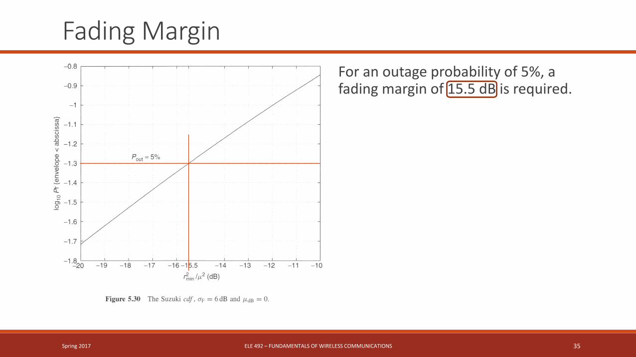
Fading Margin

For an outage probability of 5%, a fading margin of 15.5 dB is required.


Fading Margin Fading margin for small-scale fading only is (Rayleigh pdf)

Then,

Fading margin for large-scale fading only is (log-normal pdf)

Then


statistical description of the wireless channeltoker/ele492/3... · statistical description of the...

Documents