statistical distributions byu james b. mcdonald. statistical distributions james b. mcdonald brigham...
TRANSCRIPT

Statistical DistributionsBYU
James B. McDonald

Statistical Distributions
James B. McDonald
Brigham Young University
May 2013
The research assistance of Brad Larsen, Patrick Turley, and Sean Kerman is gratefully acknowledged as are comments from
Richard Michelfelder and Panayiotis Theodossiou.


Statistical Distributions
1. Introduction
2. Some families of statistical distributions
3. Regression applications
4. Censored regression
5. Qualitative response models
6. Option pricing
7. VaR (value at risk)
8. Conclusion
Statistical Distributions
1. Introduction 2. Some families of statistical distributions
a. Families
3. Regression applications4. Censored regression5. Qualitative response models6. Option pricing 7. VaR (value at risk)8. Conclusion
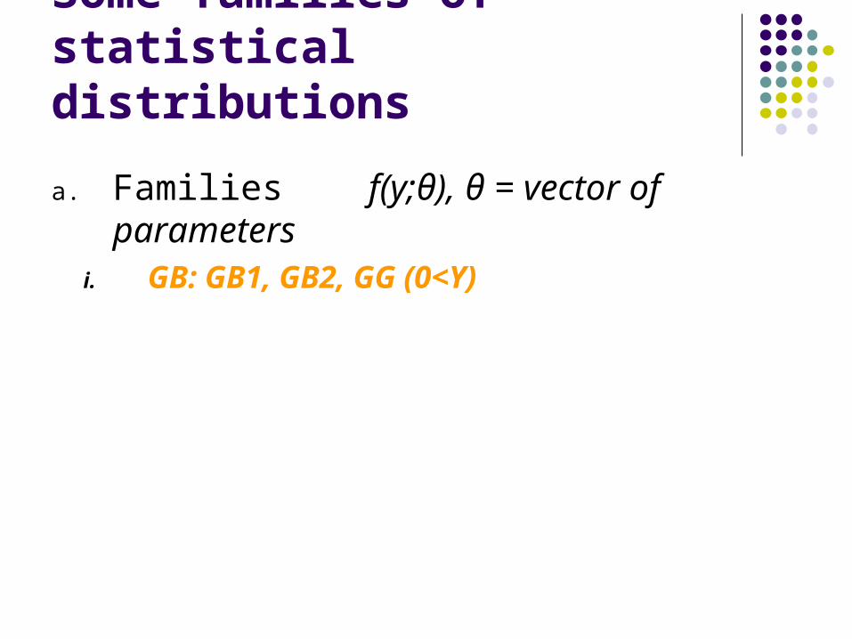
Some families of statistical distributions
a. Families f(y;θ), θ = vector of parameters i. GB: GB1, GB2, GG (0<Y)

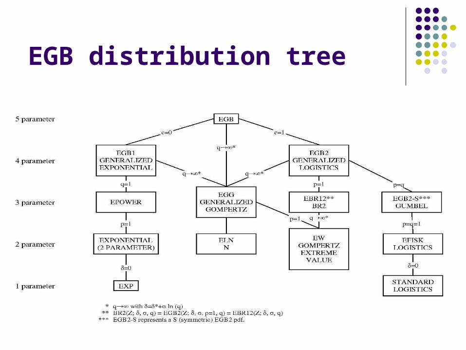
GB distribution tree

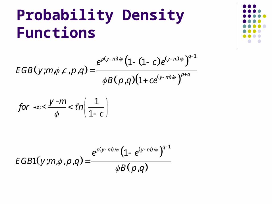
Probability Density Functions
11 1 1 /
; , , , , , 0 / 1, 1 /
qaap
a ap qaap
a y c y bGB y a b c p q y b c
b B p q c y b
11 1 /
1 ; , , , ; , , 0, ,,
qaap
ap
a y y bGB y a b p q GB y a b c p q
b B p q

Probability Density Functions
1
2 ; , , , ; , , 1, ,, 1 /
ap
p qaap
a yGB y a b p q GB y a b c p q
b B p q y b
/1
; , ,
ayap
ap
a y eGG y a p
p
0 / 1
,
a a
a controls peakedness
b is a scale parameter
c domain y b c
p q shape parameters
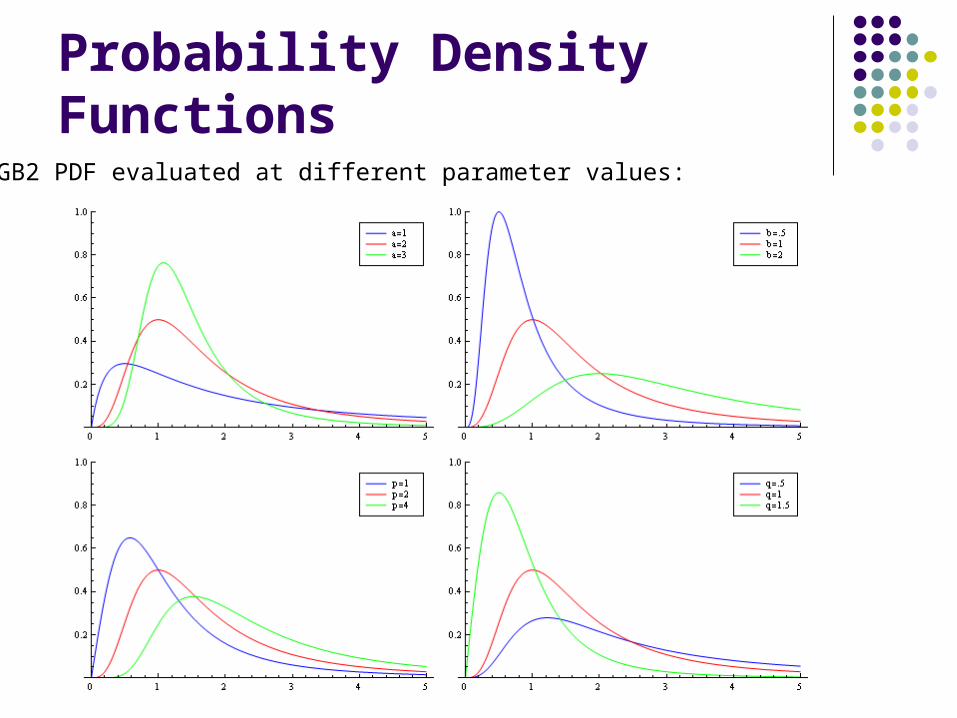
Probability Density FunctionsGB2 PDF evaluated at different parameter values:

Some families of statistical distributions
a. Families i. GB: GB1, GB2, GG
ii. EGB: EGB1, EGB2, EGG (Y is real valued)
EGB distribution tree
Probability Density Functions
1/ /
/
1 1; , , , ,
, 1
qp y m y m
p qy m
e c eEGB y m c p q
B p q ce
- 1 - <
1
y mfor n
c
1/ /1
1 ; , , ,,
qp y m y me e
EGB y m p qB p q

Probability Density Functions
/
/2 ; , , ,
, 1
p y m
p qy m
eEGB y m p q
B p q e
//
; , ,y mp y m ee e
EGG y m pp
,
m controls location
is a scale parameter
c defines the domain
p q are shape parameters

Probability Density FunctionsEGB2 PDF evaluated at different parameter values:

Some families of statistical distributions
a. Families i. GB: GB1, GB2, GG
ii. EGB: EGB1, EGB2, EGG
iii. SGT (Skewed generalized t): SGED, GT, ST, t, normal (Y is real valued)

SGT distribution tree
SGT5 parameter
SGED GT
SLaplace SNormal t SCauchy
Laplace Uniform Normal Cauchy
4 parameter
3 parameter
2 parameter
λ=0 p=2q→∞
ST
GED
λ=0λ=0
λ=0 λ=0λ=0
p=2 p=2
p=2
p=1
p=1
q→∞ q→∞
q=1/2
q→∞ q=1/2p→∞
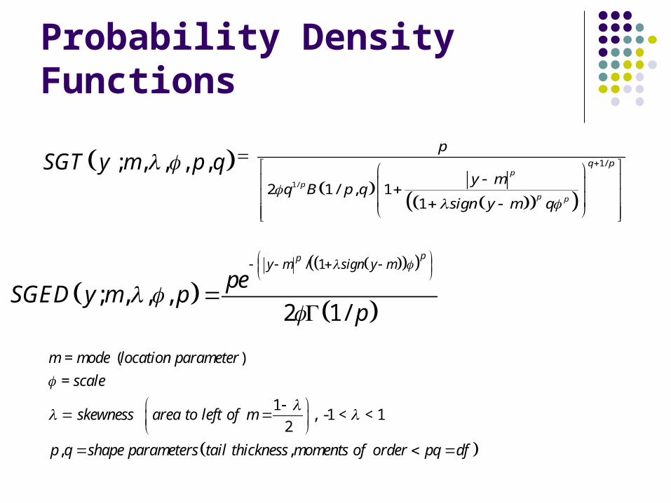
Probability Density Functions
; , , , ,SGT y m p q
1/
1/
2 1/ , 11
p
p
p p
q p
p
y mq B p q
sign y m q
/ 1
; , , ,2 1/
ppy m sign y m
peSGED y m p
p
= ( )
=
1 , -1 < < 1
2
, ,
m mode location parameter
scale
skewness area to left of m
p q shape parameters tail thickness moments of order pq df

Probability Density FunctionsSGT PDF evaluated at different parameter values:

Some families of statistical distributions
a. Families i. GB: GB1, GB2, GG
ii. EGB: EGB1, EGB2, EGG
iii. SGT (Skewed generalized t): SGED, GT, ST, t, normal
iv. IHS

Probability Density Functions
sinh 0,1 /Y a b N k
22 22 2ln / / ln
2
22 2 2; , , ,
2 /
ky y
keIHS y k
y
2 2 2 2.5 .5.5 2 21/ , / , .5 , and .5 2 1k k k k
w w w w we e e e e e
2
k
mean
variance
skewness parameter
tail thickness
; , lim ; , , , 0kN y IHS y k
where
IHS

Probability Density FunctionsIHS PDF evaluated at different parameter values:

Some families of statistical distributions
a. Families i. GB: GB1, GB2, GG
ii. EGB: EGB1, EGB2, EGG
iii. SGT (Skewed generalized t): SGED, GT, ST, t, normal
iv. IHS
v. g-and-h distribution (Y is real valued)

g-and-h distribution
Definition:
where Z ~ N[0,1]
2 / 2,
1gZhZ
g h
eY Z a b e
g
h>0 h<0

g-and-h distribution
2 20,0 ~ ,Y Z a bZ N a b
, 0
1gZ
g h
eY Z a b
g
2 / 20,
gZg hY Z a bZe
Is known as the g distribution where the parameter g allows for skewness.
Is known as the h distribution
• Symmetric
• Allows for thick tails

Probability Density Functionsg-and-h PDF evaluated at different parameter values with h>0:

Probability Density Functionsg-and-h PDF evaluated at different parameter values with h<0:

Some families of statistical distributions
a. Families f(y;θ)i. GB: GB1, GB2, GG
ii. EGB: EGB1, EGB2, EGG
iii. SGT (Skewed generalized t): SGED, GT, ST, t, normal
iv. IHS
v. g-and-h distribution
vi. Other distributions: extreme value, Pearson family, …

Some families of statistical distributions
a. Families f(y;θ)i. GB: GB1, GB2, GGii. EGB: EGB1, EGB2, EGG iii. SGT (Skewed generalized t): SGED, GT, ST, t,
normaliv. IHSv. g- and h-distributionvi. Other distributions: extreme value, Pearson
family, …vii. Extensions: 1. x , 2. Multivariate

Statistical Distributions
1. Introduction 2. Some families of statistical distributions
a. Families b. Properties
3. Regression applications4. Censored regression5. Qualitative response models6. Option pricing 7. VaR (value at risk)8. Conclusion

Some families of statistical distributions
b. Propertiesi. Moments
1. GB family
2 1
/ , / ; / , F
/ ;,
hh
GB
p h a h a cb B p h a qE Y
p q h aB p q
for h < aq with c=1

Some families of statistical distributions
b. Propertiesi. Moments
1. GB family
a. GB1
1
/ ,
,
hh
GB
b B p h a qE Y
B p q
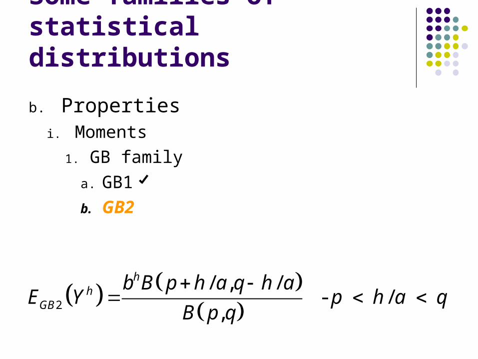
Some families of statistical distributions
b. Propertiesi. Moments
1. GB family
a. GB1
b. GB2
2
/ , / - /
,
hh
GB
b B p h a q h aE Y p h a q
B p q

Some families of statistical distributions
b. Propertiesi. Moments
1. GB family
a. GB1
b. GB2
c. GG
/ /
hh
GG
p h aE Y for h a p
p


Some families of statistical distributions
b. Propertiesi. Moments
1. GB family
2. EGB family
2 1
, ; c,
p+q+t,
tty
EGB
p t te B p t qM t E e F
B p q
/ σ with 1for t q c

EGB moments
p p p q p q
2 ' p 2 ' 'p p q 2 ' 'p q
3 '' p 3 '' ''p p q 3 '' ''p q
4 ''' p 4 ''' '''p p q 4 ''' '''p q
EGG EGB1 EGB2
Mean
Variance
Skewness
Excess kurtosis
d n ss
ds

EGB2 moment space

Some families of statistical distributions
b. Propertiesi. Moments
1. GB family
2. EGB family
3. SGT family

SGT family
/
1 1
1,
1 1 12 1
,
h p
hh h h h
SGT
h hq B q
p pE y m
B qp
1 1
1
1 1 12 1
hh h h h
SGED
hp
E y m
p
for h < pq=d.f.

SGT moment space

SGT family moment space

Some families of statistical distributions
a. Families
b. Propertiesi. Moments
1. GB family
2. EGB family
3. SGT family
4. IHS

IHS moment space

Some families of statistical distributions
a. Families
b. Propertiesi. Moments
1. GB family
2. EGB family
3. SGT family
4. IHS
5. g-and-h family
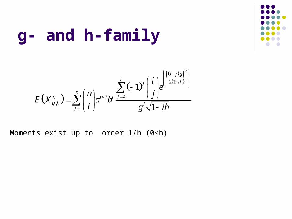
g- and h-family
2
2 1
0,
1
1
i j gi ihj
njn n i i
g h ii
ie
n jE X a b
i g ih
Moments exist up to order 1/h (0<h)

g-and-h moment space (h>0)(visually equivalent to the IHS)

Moment space for g-and-h (h>0) and g-and-h (h real)

Moment space of SGT, EGB2, IHS, and g-and-h

Some families of statistical distributions
b. Propertiesi. Moments
ii. Cumulative distribution functions (see appendix)
• Involve the incomplete gamma and beta functions

Some families of statistical distributions
b. Propertiesi. Moments
ii. Cumulative distribution functions (see appendix)• Involve the incomplete gamma and beta functions
iii. Gini coefficients (G)

Gini Coefficients (G)
Definition:
0 0
1: :
2G x y f x f y dxdy
2
0
0
11
1
F y dy
F y dy
G
(Dorfman, 1979, RESTAT)

Gini Coefficients
Interpretation:
G = 2A

Gini Coefficients
Application:
Stochastic Dominance
Measures of income and wealth inequality

Some families of statistical distributions
b. Propertiesi. Moments
ii. Cumulative distribution functions (see appendix)
iii. Gini coefficients (G)
iv. Incomplete moments

Incomplete moments
Definition:
;
yh
h
s f s ds
y hE Y
Applications:
Option pricing formulas
Lorenz Curves

Incomplete moments
Convenient theoretical results:
;y h
2 2; ,LN y h
; , , /GG y a p h a
2 ; , , / , /GB y a b p h a q h a
Distribution
LN
GG
GB2

Some families of statistical distributions
b. Propertiesi. Moments
ii. Cumulative distribution functions (see appendix)
iii. Gini coefficients (G)
iv. Incomplete moments
v. Mixture models

Mixture Models
Let denote a structural or conditional density of the random variable Y where and denote vectors of distributional parameters. Let the density of be given by the mixing distribution . The observed or mixed distribution can be written as
; ,f y
;g
; , ; , ;h y f y g d
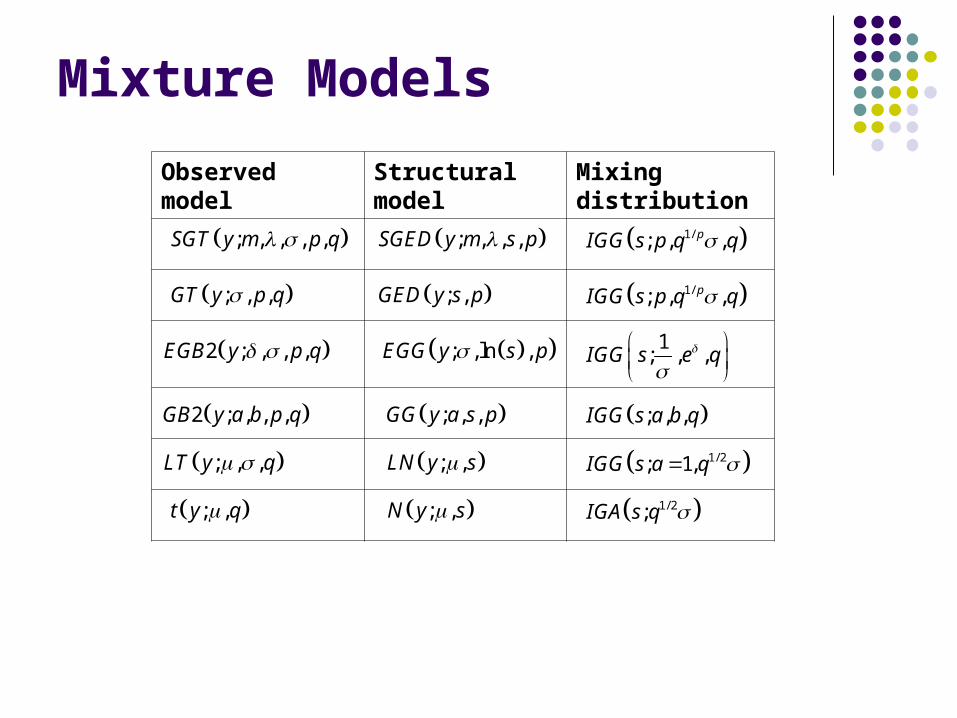
Mixture Models
Observed model Structural model
Mixing distribution
; , , , ,SGT y m p q
; , ,GT y p q
2 ; , , ,EGB y p q
2 ; , , ,GB y a b p q
; , ,LT y q
; ,t y q
; , , ,SGED y m s p
; ,GED y s p
; , ln ,EGG y s p
; , ,GG y a s p
; ,LN y s
; ,N y s
1/; , ,pIGG s p q q
1/; , ,pIGG s p q q
1; , ,IGG s e q
; , ,IGG s a b q
1/ 2; 1,IGG s a q
1/ 2;IGA s q

Some families of statistical distributions
b. Propertiesi. Moments
ii. Cumulative distribution functions (see appendix)
iii. Gini coefficients (G)
iv. Incomplete moments
v. Mixture models
vi. Hazard functions (Duration dependence)

Hazard functions
Definition:
Let denote the pdf of a spell (S) or duration of an event.
is the probability that that S>s.The corresponding hazard function is defined by
which can be thought of as representing the rate or likelihood that a spell will be completed after surviving s periods.
f s
1 F s
( )1
f sh s
F s

Hazard functions
Applications:
Does the probability of ending a strike, unemployment spell, expansion, or stock run depend on the length of the strike, unemployment spell, or of the run?
With unemployment, A job seeker might lower their reservation wage and become more likely to find a
job Increasing hazard function However, if being out of work is a signal of damaged goods, the longer they are
out of work might decrease employment opportunities Decreasing hazard function.
An alternative example might deal with attempts to model the time between stock trades. Engle and Russell (1998) Autoregressive conditional duration: a new model for
irregularly spaced transaction data. Econometrica 66: 1127-1162 Hazard function of time between trades is decreasing as t increases or the
longer the time between trades the less likely the next trade will occur.

Hazard functions
Applications:
Bubbles McQueen and Thorley (1994) Bubbles, stock returns, and duration dependence.
Journal of Financial and Quantitative Analysis, 29:379-401 Efficient markets hypothesis, stock runs should not exhibit duration dependence
(constant hazard function) McQueen and Thorley argue that asset prices may contain “bubbles” which grow
each period until they “burst” causing the stock market to crash. Hence, bubbles cause runs of positive stock returns to exhibit duration dependence—the longer the run the less likely it will end (decreasing hazard function), but runs of negative stock returns exhibit no duration dependence
Grimshaw, McDonald, McQueen, and Thorley. 2005, Communications in Statistics—Simulation and Computation, 34: 451-463.
What model should we use to characterize duration dependence? Exponential—constant Gamma—the hazard function can increase, decrease, or be constant Weibull—the hazard function can increase, decrease, or be constant Generalized Gamma: the hazard function can be increasing, decreasing, constant,
-shaped, or -shaped

Hazard functions
Possible shapes for the GG hazard functions
Statistical Distributions
1. Introduction 2. Some families of statistical distributions
a. Families b. Propertiesc. Model selection
3. Regression applications4. Censored regression5. Qualitative response models6. Option pricing 7. VaR (value at risk)8. Conclusion

Some families of statistical distributionsc. Model selection
i. Goodness of fit statistics• Log-likelihood values
o for individual data
o for grouped data
Partition the data into g groups,
Empirical frequency:
Theoretical frequency:
1
:n
ii
n f y
1
!g
i i ii
n n n n p n n
1, , 1, 2,...,i i iI Y Y i g
1
/ , g
i i ii
p n n n n
;
i
i
I
p f y dy

Model Selection
i. Goodness of fit statistics• Log-likelihood values• Possible Measures
1
g
i ii
SAE p p
21
g
i ii
SSE p p
2
2 2
1
/ ~ # 1g
ii i
i
nn p p g parameters
n

Model Selection
i. Goodness of fit statistics• Log-likelihood values• Possible Measures• Akaike Information Criterion (AIC)
• A tool for model selection• Attaches a penalty to over-fitting a model
2AIC k

Model Selection
i. Goodness of fit statistics
ii. Testing nested models
Examples:1.
2.
: 0OH g
: : 0O OH SGT GT H
: : 2, 0, O OH SGT Normal H p and q

Testing nested models
Likelihood ratio tests
where r denotes the number
of independent restrictions
Wald test
22 * ~aLR r
21 2 * ~ 1a
SGT GTLR
22 2 * ~ 3a
SGT NormalLR
1 2' var ~a
MLE MLE MLEW g g g r
1
21
ˆ ˆ ˆ0 0 ~ 1aW Var

Statistical Distributions1. Introduction 2. Some families of statistical distributions
a. Families b. Propertiesc. Model selectiond. An example: the distribution of stock returns
3. Regression applications4. Qualitative response models5. Option pricing 6. VaR (value at risk)7. Conclusion

An example: the distribution of stock returns
1 11/ ~ 1t t t
t t tt t
P P Py n P P
P P
Daily, weekly, and monthly excess returns (1/2/2002 – 12/29/2006) from CRSP database (NYSE, AMEX, and NASDAQ)— 4547 companies
H0: skewness = 0
H0: excess kurtosis = 0
H0: returns ~ N(μ, σ2)
JB =
.95 2 6 / , 2 6 /CI n n
.95 2 24 / , 2 24 /CI n n
22
2.05
~ 2 5.99
6 24
excess kurtosisskewn
.95 0 5.99CI JB
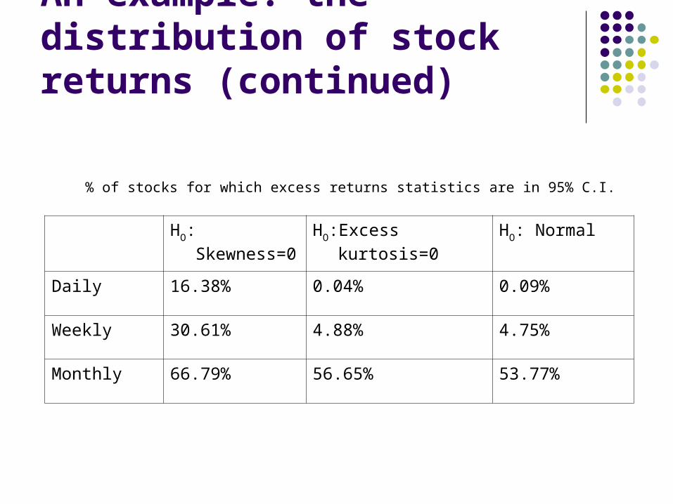
An example: the distribution of stock returns (continued)
% of stocks for which excess returns statistics are in 95% C.I.
HO: Skewness=0 HO:Excess kurtosis=0 HO: Normal
Daily 16.38% 0.04% 0.09%
Weekly 30.61% 4.88% 4.75%
Monthly 66.79% 56.65% 53.77%

An example: the distribution of stock returns (continued)
Daily excess returns plotted with admissible moment space of flexible distributions
-4 -3 -2 -1 0 1 2 3 40
10
20
30
40
50
60
Skewness
Kur
tosi
s
CRSP daily stocks--excess returns
CRSP stock
EGB2
SGTIHS
bound

An example: the distribution of stock returns (continued)
Weekly excess returns plotted with admissible moment space of flexible distributions
-4 -3 -2 -1 0 1 2 3 40
10
20
30
40
50
60
Skewness
Kur
tosi
s
CRSP weekly stocks--excess returns
CRSP stock
EGB2
SGTIHS
bound

An example: the distribution of stock returns (continued)
Monthly excess returns plotted with admissible moment space of flexible distributions
-4 -3 -2 -1 0 1 2 3 40
10
20
30
40
50
60
Skewness
Kur
tosi
s
CRSP monthly stocks--excess returns
CRSP stock
EGB2
SGTIHS
bound

An example: the distribution of stock returns (continued)
Fraction of stocks in the admissible skewness-kurtosis space
daily weekly monthly
EGB2 15.48% 43.81% 50.80%
IHS 83.92% 84.39% 61.97%
SGT 87.62% 89.00% 95.10%
g-and-h 100.00% 99.98% 98.99%

An example: the distribution of stock returns (continued)
Fitting a PDF to normal excess returns
Company Name Skew Kurtosis Jb Stat
US Steel 0.06 3.308 5.62
Estimated PDF logL SSE SAE Chi^2
Normal 2753.52 0.001 0.12 27.81
EGB2 2756.83 0.001 0.11 23.38
IHS 2756.76 0.001 0.11 23.46
SGT 2758.78 0.001 0.12 28.19
-0.15 -0.1 -0.05 0 0.05 0.1 0.15 0.20
2
4
6
8
10
12
14
16
18
20
Excess returns
Estimated PDFs for US Steel daily excess returns
Returns
Normal
EGB2IHS
SGT

An example: the distribution of stock returns (continued)
Company Name Skew Kurtosis Jb Stat
iShares -29.06 965.09 48733899.02
Fitting a PDF to leptokurtic excess returns
Estimated PDF logL SSE SAE Chi^2
Normal 2516.86 0.099 0.93 1433.33
EGB2 3713.99 0.002 0.13 43.47
IHS 3795.21 0.001 0.12 33.43
SGT 3810.07 0.003 0.21 79.35
-0.06 -0.04 -0.02 0 0.02 0.04 0.06 0.080
5
10
15
20
25
30
35
40
45
50
Excess returns
Estimated PDFs for iShares daily excess returns
Returns
Normal
EGB2IHS
SGT
Statistical Distributions
1. Introduction 2. Some families of statistical distributions3. Regression applications4. Censored regression5. Qualitative response models6. Option pricing 7. VaR (value at risk)8. Conclusion

Statistical Distributions
1. Introduction 2. Some families of statistical distributions3. Regression applications
a. Background
4. Censored regression models5. Qualitative response models6. Option pricing 7. VaR (value at risk)8. Conclusion

Regression applications--background
Model:
1xK vector of observations on the explanatory variables
Kx1 vector of unknown coefficients
independently and identically distributed random disturbances with pdf
t t tY X
tX
t ;f

Regression applications--background
If the errors are normally distributed OLS will be unbiased and minimum variance
However, if the errors are not normally distributed OLS will still be BLUE There may be more efficient nonlinear estimators

Statistical Distributions
1. Introduction 2. Some families of statistical distributions3. Regression applications
a. Backgroundb. Alternative estimators
4. Censored regression5. Qualitative response models6. Option pricing 7. VaR (value at risk)8. Conclusion

Alternative Estimators
i. Estimation
OLS
LAD
Lp
21
arg minn
OLS t tt
Y X
1
arg minn
LAD t tt
Y X
1
arg minp
pn
L t tt
Y X

Alternative Estimators (continued)
i. Estimation (continued)M-estimators:
Includes OLS, LAD, and Lp as special cases Includes MLE (QMLE or partially adaptive estimators) as a
special case where
SGT SGED EGB2 IHS
; ;n f
,1
arg min ;n
MLE t tt
Y X
1
arg minn
M t tt
Y X

Alternative Estimators (continued)
i. Estimation
ii. Influence functions: ( ) '( )
OLS LADRedescending
influence function


Alternative Estimators (continued)
i. Estimation
ii. Influence functions
iii. Asymptotic distribution of extremum
estimators
where
min H
1 1ˆ ~ ;asandwichN A BA
2
and ' '
d H dH dHA E B E
d d d d

Alternative Estimators (continued)
i. Estimation ii. Influence functionsiii. Asymptotic distribution of extremum estimatorsiv. Other estimators
Semiparametric (Kernel estimator, Adaptive MLE)
where
denotes a kernel, and h is the window width
1
arg min n
SP K t tt
n f Y X
1
1 ni
Ki
ef K
nh h
i i i OLSe Y X
K
Regression applications (continued)
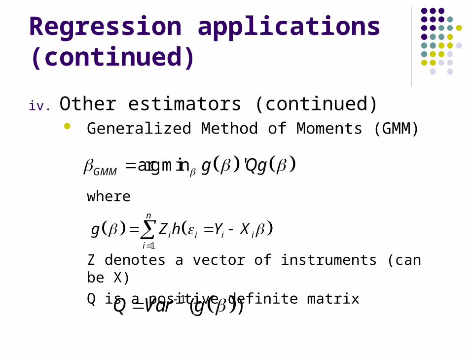
iv. Other estimators (continued) Generalized Method of Moments (GMM)
where
Z denotes a vector of instruments (can be X)
Q is a positive definite matrix
arg min 'GMM g Qg
1
n
i i i ii
g Z h Y X
1( )Q Var g

Statistical Distributions
1. Introduction 2. Some families of statistical distributions3. Regression applications
a. Backgroundb. Alternative estimatorsc. A Monte Carlo comparison of alternative estimators
4. Censored regression models5. Qualitative response models6. Option pricing 7. VaR (value at risk)8. Conclusion

A Monte Carlo comparison of alternative estimatorsc. A Monte Carlo comparison of alternative estimators
Model:
Error distributions: (zero mean and unitary variance)
Normal:
Mixture:
Skewness =0Kurtosis =24.3
Skewed:
Skewness=6.18Kurtosis=113.9
0;1N
.9* 0,1/ 9 .1* 0,9N N
.50,1 / 1LN e e e
1t t ty X
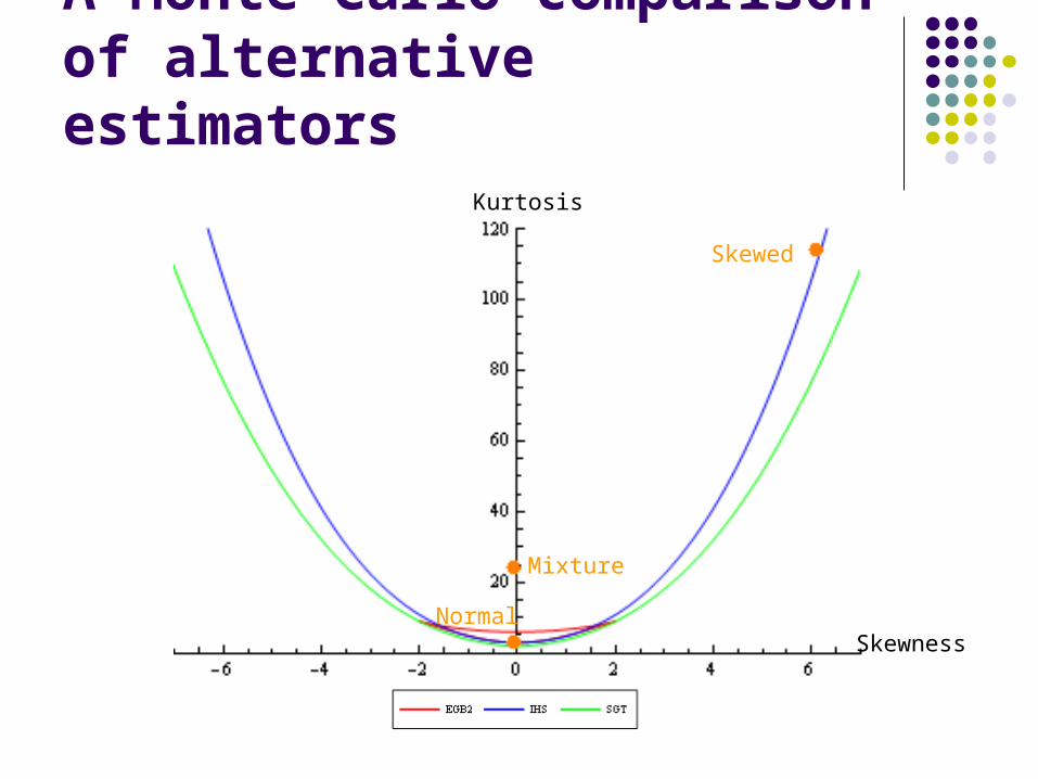
A Monte Carlo comparison of alternative estimators
Skewness
Kurtosis
Skewed
Mixture
Normal

A Monte Carlo comparison of alternative estimators
Estimators Normal Mixture-thick tails Skewed
OLS .275 .287 .280
LAD .332 .122 .159
SGED .335 .128 .060
ST .293 .112 .054
GT .314 .133 .135
SGT .335 .125 .073
EGB2 .287 .125 .049
IHS .285 .119 .054
SP = AML .285 .114 .128
GMM .319 .115 .088
Sample size = 50, T=1000 replicationsRMSE for slope estimators

Statistical Distributions
1. Introduction 2. Some families of statistical distributions3. Regression applications
a. Backgroundb. Alternative estimatorsc. A Monte Carlo comparison of alternative estimatorsd. An application: CAPM
i. Error distribution effectsii. ARCH effects
4. Censored regression5. Qualitative response models6. Option pricing 7. VaR (value at risk)8. Conclusion

An application: CAPM
i. CAPM and the error distribution
Daily, weekly, and monthly excess returns (1/2/2002 – 12/29/2006) from CRSP database (NYSE, AMEX, and NASDAQ)— 4547 companies
HO: Skewness=0 HO:Excess kurtosis=0 HO: Normal (JB)
Daily 14.14% 0.02% 0%
Weekly 28.13% 3.91% 3.43%
Monthly 67.56% 57.14% 54.76%
Percent of stocks for which OLS residual statistics are in 95% C.I.

An application: CAPM with and without ARCH effects (ST)
i. CAPM and the error distribution
Daily, weekly, and monthly excess returns (1/2/2002 – 12/29/2006) from CRSP database (NYSE, AMEX, and NASDAQ)— 4547 companies
HO: Skewness=0 HO:Excess kurtosis=0 HO: Normal (JB)
Daily 14.05% 0.02% 0%
Weekly 28.82% 3.83% 3.39%
Monthly 64.04% 54.72% 51.48%
Percent of stocks for which ST residual statistics are in 95% C.I.

An application: CAPM with and without ARCH effects (IHS)
i. CAPM and the error distribution
Daily, weekly, and monthly excess returns (1/2/2002 – 12/29/2006) from CRSP database (NYSE, AMEX, and NASDAQ)— 4547 companies
HO: Skewness=0 HO:Excess kurtosis=0 HO: Normal (JB)
Daily 13.99% 0.02% 0%
Weekly 27.89% 3.83% 3.36%
Monthly 65.54% 55.71% 52.32%
Percent of stocks for which IHS residual statistics are in 95% C.I.

An application: CAPM with alternative error distributions
Company Name Skewness Kurtosis JB stat
UNITED NATURAL FOODS INC -0.074 2.8004 0.1543
99 CENTS ONLY STORES 1.7541 7.6594 85.0456
Statistics of OLS residuals
Company Name OLS T GT SGED EGB2 IHS ST SGT
UNITED NATURAL FOODS INC 0.313 0.313 0.335 0.334 0.303 0.302 0.314 0.335
99 CENTS ONLY STORES 0.184 0.125 0.125 0.110 0.109 0.106 0.110 0.110
Estimated Betas

An application: CAPM with and without ARCH effects
i. CAPM and the error distribution
ii. CAPM: how about ARCH effects? Review:
If errors are normal and no ARCH effects, OLS is MLE If errors are not normal and no ARCH effects OLS is
BLUE, but not MLE nor efficient If errors are normal and have ARCH effects OLS is
BLUE, but not efficient If errors are not normal and have ARCH effects OLS is
BLUE,but not efficient

An application: CAPM with and without ARCH effects
ii. CAPM: ARCH effects (continued)
Model:
Percent of stocks exhibiting ARCH(1) effects (OLS) (% rejecting )1: 0OH
0.10 level 0.05 level
Daily 63.2% 60.0%
Weekly 29.2% 24.1%
Monthly 18.7% 13.7%
t t tY X .52
0 1 1t t tu

An application: CAPM with and without ARCH effects
Percent of stocks exhibiting ARCH(1) effects (ST) (% rejecting )
Percent of stocks exhibiting ARCH(1) effects (IHS) (% rejecting )
0.10 level 0.05 level
Daily 63.2% 59.9%
Weekly 29.1% 23.9%
Monthly 16.9% 12.3%
1: 0OH
0.10 level 0.05 level
Daily 63.3% 60.0%
Weekly 29.3% 24.1%
Monthly 18.9% 13.9%
1: 0OH
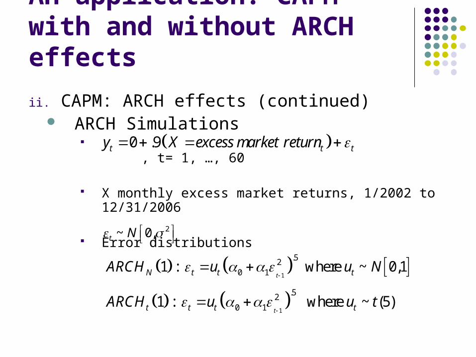
An application: CAPM with and without ARCH effects
ii. CAPM: ARCH effects (continued) ARCH Simulations
, t= 1, …, 60
X monthly excess market returns, 1/2002 to 12/31/2006
Error distributions
0 .9 t t ty X excess market return
2~ 0,t N
1
.520 11 : where ~ 0,1
tN t t tARCH u u N
1
.520 11 : where ~ (5)
tt t t tARCH u u t

An application: CAPM with and without ARCH effects
ARCH Simulations (continued)
Errors
Estimation Non-ARCH ARCH Non-ARCH ARCH Non-ARCH ARCH
OLS/Normal 0.352 0.356 0.347 0.291 0.353 0.300
LAD 0.444 0.446 0.397 0.369 0.315 0.297
T 0.358 0.363 0.338 0.293 0.283 0.265
GED 0.381 0.389 0.357 0.318 0.306 0.285
GT 0.387 0.396 0.362 0.322 0.306 0.286
SGED 0.406 0.417 0.374 0.341 0.318 0.297
EGB2 0.371 0.376 0.352 0.312 0.300 0.281
IHS 0.368 0.377 0.348 0.319 0.291 0.275
ST 0.375 0.382 0.350 0.310 0.293 0.277
SGT 0.409 0.420 0.376 0.344 0.316 0.297
Root Mean Square Error (RMSE) for 10,000 replications
N(0,σ 2) N(0,1), Arch(1) t(5), Arch(1)

Statistical Distributions
1. Introduction 2. Some families of statistical distributions3. Regression applications4. Censored regression models
a. Basic frameworkb. Simulation study
5. Qualitative response models6. Option pricing 7, VaR (value at risk)8. Conclusion
*i i iY X

Censored Regression a. Basic Framework
Model:
Log-likelihood function:
*i i iy X
* *
*
if y 0
= 0 if y < 0
i i i
i
y y
* 00
, ; ;ii
i i iyy
n f y X n F X

b. Censored regression: non-normality and heteroskedasticity

Qualitative Response Models

Statistical Distributions
1. Introduction 2. Some families of statistical distributions3. Regression applications4. Censored Regression models5. Qualitative response models
a. Basic framework
6. Option pricing 7. VaR (value at risk)8. Conclusion

Qualitative Response—Basic Framework
Model:
if and 0 otherwise
Log-likelihood function:
*i i iy X
1 iy * 0iy
*Pr 1 Pri i i i i iy X y X X
Pr ; ;iX
i i iX f s ds F X
1
, ; 1 1 ;n
i i i ii
y n F X y n F X

Qualitative Response—Basic Framework (continued)
MLE of will be consistent and asymptotically distributed as
if the model is correctly specified.
Probit and logit estimators will be inconsistent if The error distribution is incorrectly specified heteroskedasticity exists, e.g. unmeasured heterogeneity is
present relevant variables have been omitted The index appears in a nonlinear form
Similar results are associated with Censored & Truncated regression models
12
ˆ ~ ;'
a dN E
d d

Statistical Distributions
1. Introduction 2. Some families of statistical distributions3. Regression applications4. Censored regression 5. Qualitative response models
a. Basic frameworkb. An application: fraud detection
6. Option pricing 7. VaR (value at risk)8. Conclusion

Prediction of corporate fraud (Y=1 fraud) Compare financial ratios of companies with averages
of five largest companies (“virtual” firm) 228 companies (114 fraud and 114 non-fraud) Variables: accruals to assets, asset quality, asset
turnover, days sales in receivables, deferred charges to assets, depreciation, gross margin, increase in intangibles, inventory growth, leverage, operating performance margin, percent uncollectables, receivables growth, sales growth, working capital turnover.
SGT, EGB2, & IHS formulations improve predictions
Qualitative response—An application: fraud detection

Statistical Distributions
1. Introduction 2. Some families of statistical distributions3. Regression applications4. Censored regression5. Qualitative response models
a. Basic frameworkb. An applicationc. Some related issues
6. Option pricing 7. VaR (value at risk)8. Conclusion

Qualitative response—Some related issues
Cost of misclassification Choice-based sampling Heterogeneity Semi-parametric estimation procedures

Statistical Distributions
1. Introduction 2. Some families of statistical distributions3. Regression applications4. Censored regression5. Qualitative response models6. Option pricing: European call option 7. VaR (value at risk)8. Conclusion

Statistical Distributions
1. Introduction 2. Some families of statistical distributions3. Regression applications4. Qualitative response models5. Option pricing: European call option
a. The Black-Scholes option pricing formula
6. VaR (value at risk)7. Conclusion
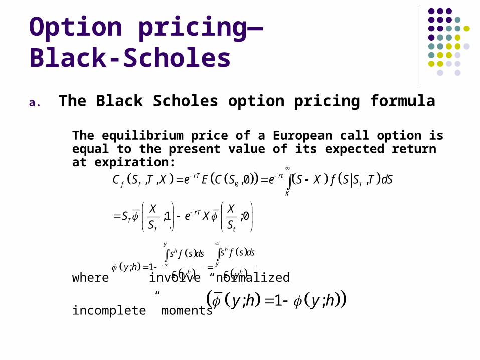
Option pricing—Black-Scholes
a. The Black Scholes option pricing formula
The equilibrium price of a European call option is equal to the present value of its expected return at expiration:
where involve “normalized
incomplete” moments
0, , ,0 ,
;1 ;0
rT rtf T T
X
rTT
T t
C S T X e E C S e S X f S S T dS
X XS e X
S S
; 1
yhh
y
h h
s f s dss f s ds
y hE y E y
; 1 ;y h y h
.

Statistical Distributions
1. Introduction 2. Some families of statistical distributions3. Regression applications4. Qualitative response models5. Option pricing: European call option
a. The Black-Scholes option pricing formulab. Some background and alternative formulations
6. VaR (value at risk)7. Conclusion

Option pricing– Some background and alternative formulations
The Black Scholes (1973) option pricing formula corresponds to being the lognormal
, the cdf for the lognormal
The Black Scholes formula (Bookstaber and McDonald, 1991) corresponding to the Generalized Gamma is obtained from
, the cdf for the GG
The Black Scholes formula ( Bookstaber and McDonald, 1991) corresponding to the GB2 is obtained from
, the cdf for the GB2
Rebonato (1999) applied to the Deutschemark
f s
2 2; ; ,LN y h LN y h
; ; , ,GG
hy h GG y a p
a
2 ; 2 ; , , ,GB
h hy h GB y a b p q
a a
2 , ,GB TC S T X
Option pricing– Some background and alternative formulations
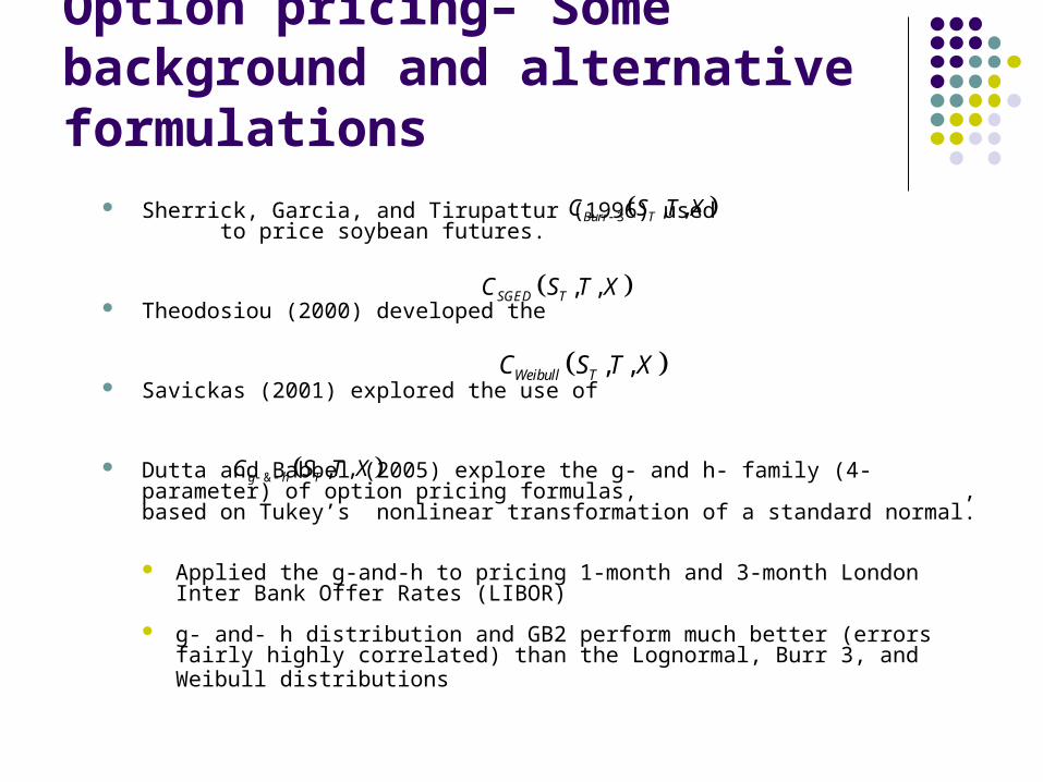
Sherrick, Garcia, and Tirupattur (1996) used to price soybean futures.
Theodosiou (2000) developed the
Savickas (2001) explored the use of
Dutta and Babbel (2005) explore the g- and h- family (4-parameter) of option pricing formulas, , based on Tukey’s nonlinear transformation of a standard normal.
Applied the g-and-h to pricing 1-month and 3-month London Inter Bank Offer Rates (LIBOR)
g- and- h distribution and GB2 perform much better (errors fairly highly correlated) than the Lognormal, Burr 3, and Weibull distributions
& , ,g h TC S T X
, ,SGED TC S T X
, ,Weibull TC S T X
3 , ,Burr TC S T X

Statistical Distributions
1. Introduction 2. Some families of statistical distributions3. Regression applications4. Qualitative response models5. Option pricing: European call option
a. The Black-Scholes option pricing formulab. Some background and alternative formulationsc. A comparison of pricing behavior
6. VaR (value at risk)7. Conclusion
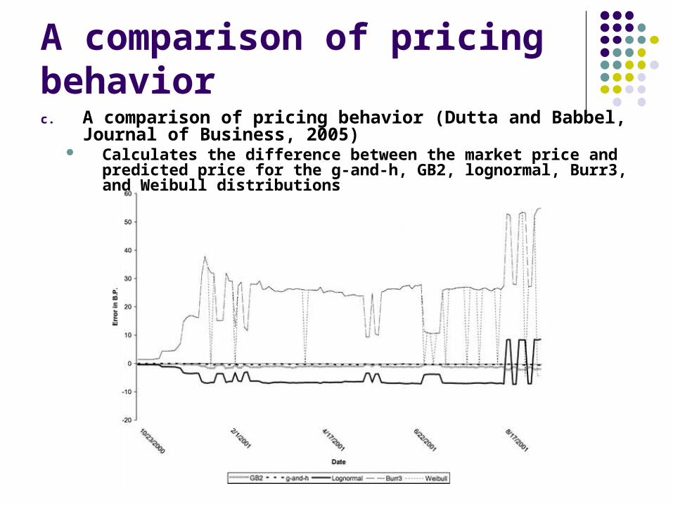
A comparison of pricing behaviorc. A comparison of pricing behavior (Dutta and Babbel, Journal of
Business, 2005) Calculates the difference between the market price and predicted price
for the g-and-h, GB2, lognormal, Burr3, and Weibull distributions

Option Pricing
Statistical Distributions
1. Introduction 2. Some families of statistical distributions3. Regression applications4. Qualitative response models5. Option pricing: European call option 6. VaR (value at risk)7. Conclusion
Statistical Distributions
1. Introduction 2. Some families of statistical distributions3. Regression applications4. Censored regression5. Qualitative response models6. Option pricing: European call option 7. VaR (value at risk)
a. Background and definitions
8. Conclusion

VaR—Background and definitions
i. Value at risk (VaR) is the maximum expected loss on a portfolio of assets over a certain time period for a given probability level.
R is the return on the asset
θ denotes the distributional parameters
α is the predetermined confidence level or coverage probability
is the corresponding maximum expected loss or conditional threshold
;R
f R dR
1 :RR F
R

VaR—Background and definitions
R z
1 :; ,
R
Z Z
ZFf z dz Z
1 :ZR F
ii. Standardized returns

VaR—Background and definitions
iii. Unconditional VaR formulation
Estimate f(R;θ)

VaR—Background and definitions
iv. Conditional VaR formulation (AR(1) ABS-GARCH(1,1))
0 1 1t t t t t t tR R Z z
0 1 1 1 2 1t t t tz 1 :t t t ZR F

Statistical Distributions
1. Introduction 2. Some families of statistical distributions3. Regression applications4. Censored regression5. Qualitative response models6. Option pricing: European call option 7. VaR (value at risk)
a. Background and definitionsb. Models and applications
8. Conclusion

VaR—Models and applications
i. Unconditional VaR formulation Exponential: (Hogg, R. V. and S. A. Klugman (1983)) Gamma: (Cummins, et al. 1990) Log-gamma: (Ramlau-Hansen (1988)), (Hogg, R. V. and
S. A. Klugman (1983)) Lognormal: (Ramlau-Hansen (1988)) Stable: (Paulson and Faris (1985) Pareto: (Hogg, R. V. and S. A. Klugman (1983)) Log-t: (Hogg, R. V. and S. A. Klugman (1983)) Weibull: (Cummins et al. (1990))

VaR—Models and applications
i. Unconditional VaR formulation (continued) Burr: (Hogg, R. V. and S. A. Klugman (1983)) Generalized Pareto: (Hogg, R. V. and S. A.
Klugman (1983)) GB2: (Cummins (1990, 1999, 2007) Pearson family: Aiuppa (1988) Extreme value distribution: Bali (2003), Bali and
Theodossiou (2008) IHS: Bali and Theodossiou (2008)

VaR—Models and applications
ii. Conditional VaR formulations (Bali and Theodossiou, JRI, 2008)
Data: S&P500 composite index, 1/4/50 – 12/29/2000 (n=12,832) Daily percentage log-returns: (Sample mean = .0341,
maximum=8.71, minimum=-22.90 standard deviation = .874 skewness =1.622 kurtosis=45.52

VaR—Models and applications
ii. Conditional distributions (Bali and Theodossiou, JRI, 2008) (continued)
Models Generalized extreme value EGB2 SGT IHS
Findings Out of sample VaR estimates are rejected for most unconditional
specifications Thresholds exhibit time varying behavior Out of sample VaR estimates for the conditional specifications
corresponding to the SGT, IHS, and EGB2 perform better than the extreme value distributions

Selected references for option pricing and VaR
Aiuppa, T. A. 1988. “Evaluation of Pearson curves as an approximation of the maximum probable annual aggregate loss.” Journal of Risk and Insurance 55, 425-441
Bali, T. G., 2003. “An Extreme Value Approach to Estimating Volatility and Value at Risk,” Journal of Business, 76:83-108 Bali, T. G. and P. Theodossiou, 2007. “A Conditional-SGT-VaR Approach with Alternative GARCH Models,” Annals of
Operations Research, 151: 241-267. Bali, T. G. and P. Theodossiou, 2008. “Risk Measurement Performance of Alternaitve Distribution Functions,” Journal of Risk
and Insurance, 75: 411-437. Black, F (1976). The Pricing of Commodity Contracts. Journal of Financial Economics 3:169-179. Cummins, J. D., G. Dionne, J. B. McDonald, and B. M. Pritchett 1990. “Applications of the GB2 family of distributions in
modeling insurance loss processes.” Insurance: Mathematics and Economics 9, 257-272. Cummins, J. D., C. Merrill, and J. B. McDonald, 2007. “Risky Loss Distributions and Modeling the Loss Reserve Pay-out Tail,”
Review of Applied Economics 3. Cummins, J. D., R. D. Phillips, and S. D. Smith 2001. “Pricing Excess of Loss Reinsurance Contracts against catastrophic
loss.” In Kenneth Froot, ed., The Financing of Catastrophe Risk (Chicago: University of Chicago Press) Dutta, K. K. and D. F. Babbel 2005. “Extracting Probabilistic Information from the Prices of Interest Rate Options: Tests of
Distributional Assumptions.” Journal of Business 78:841-870 Hogg, R. V. and S. A. Klugman, 1983. “On the Estimation of Long Tailed Skewed Distributions with Actuarial Applications.”
Journal of Econometrics 23, 91-102. McDonald, J. B. and R. M. Bookstaber (1991). “Option Pricing for Generalized Distributions.” Communications in Statistics:
Theory and Methods, 20(12), 4053-4068. Rebonato, R. (1999). Volatility and correlations in the pricing of equity. FX and interest-rate options. New York: John Wiley. Paulson, A. S. and N. J. Faris (1985). “A Practical Approach to Measuring the Distribuiton of Total Annual Claims.” In J. D.
Cummins, ed., Strategic Planning and Modeling in Property-Liability Insurance. Norwell, MA: Kluwer Academic Publishers. Ramlau-Hansen, H. (1988). “A Solvency Study in Non-life Insurance. Part 1. Analysis of Fire, Windstorm, and Glass Claims.”
Scandinavian Actuarial Journal, pp. 3-34. Rebonato, R. 1999. Volatility and correlations in the pricing of equity, FX and interest-rate options. New York: John Wiley. Reid, D. H. (1978). “Claim Reserves in General Insurance,” Journal of the Institute of Actuaries 105: 211-296 Savickas, R. (2001). A Simple option-pricing formula. Working paper, Department of Finance, George Washington University,
Washington, DC. Sherrick, B. J., P. Garcia, and V. Tirupattur (1996). Recovering probabilistic information for options markets: Tests of
distributional assumptions. Journal of Futures Markets 16:545-560. Theodossiou, Panayiotis, “Skewed Generalized Error Distribution of Financial Assets and Option Pricing,”

Statistical Distributions
1. Introduction 2. Some families of statistical distributions3. Regression applications4. Censored regression5. Qualitative response models6. Option pricing: European call option 7. VaR (value at risk)8. Conclusion
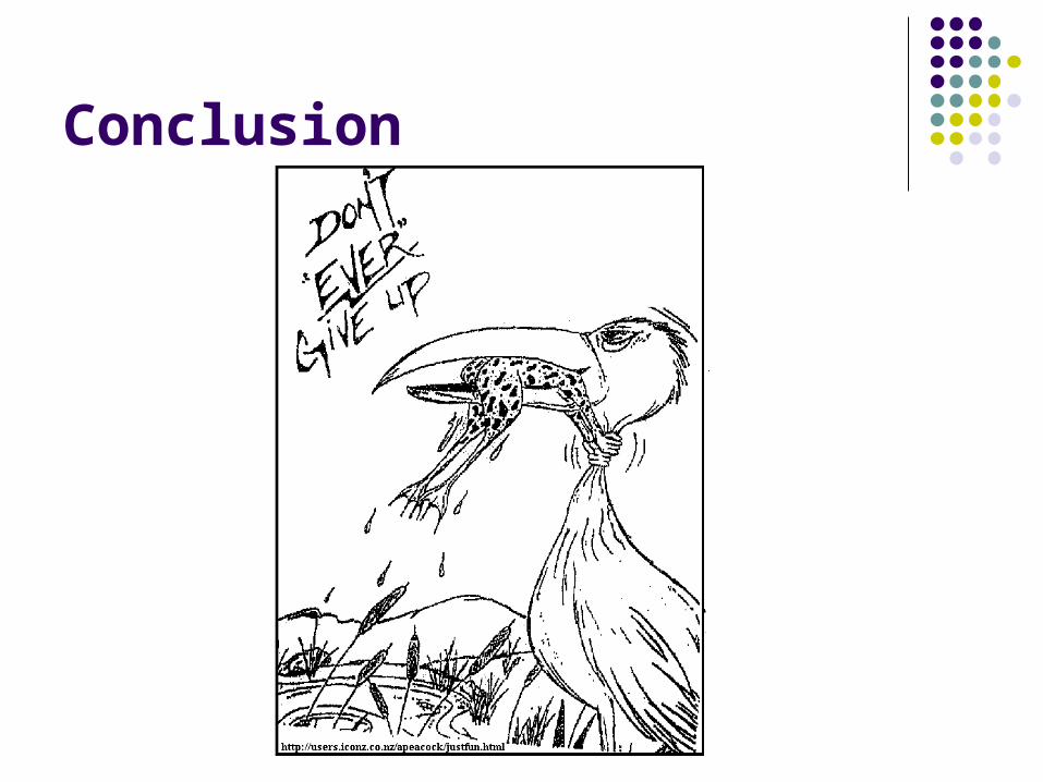
Conclusion


END OF PRESENTATION

Appendices
Cumulative distribution functions1. GB, GB1, GB2, GG2. EGB23. SGT4. SGED5. IHS6. g-and-h distribution
Option pricing basics VaR—Models and applications discussion

Appendices—Cumulative distribution functions
1. GB, GB1, GB2, and GG
where and
denotes the incomplete beta function
2 1 ,1 ; 1;1 ; , , ,
,
,
p
z
z F p q p zGB y a b p q
pB p q
B p q
/a
z y b
11
0
1
,,
zqp
z
s s ds
B p qB p q

Appendices—Cumulative distribution functions
1. GB, GB1, GB2, and GG (continued)
where
2 1 ,1 ; 1;2 ; , , ,
,
,
p
z
z F p q p zGB y a b p q
pB p q
B p q
/
1 /
a
a
y bz
y b

Appendices—Cumulative distribution functions
1. GB, GB1, GB2, and GG (continued)
where
and
denotes the incomplete gamma function
Abramowitz and Stegun (1970, p. 932), McDonald (1984), and Rainville (1960,p. 60 and 125)
/
1 1
/; , , 1; 1; /
1
a apyae y
GG y a b p F p yp
z p
/a
z y
1
0
zp s
z
s e ds
pp

Appendices—Cumulative distribution functions
2. EGB2
where
3. SGT
where
2 ; , , , ,zEGB y m p q B p q
/
/1
y m
y m
ez
e
11
; , , , , 1/ ,2 2 z
sign y mSGT y m p q sign y m B p q
1
p
pp p
y mz
y m q sign y m

Appendix—Cumulative distribution functions
4. SGED
where
11; , , , 1/
2 2 z
sign y mSGED y m p sign y m p
1
p
pp
y mz
sign y m

Appendices—Cumulative distribution functions
5. IHS
where
; , , , Pr PrIHS y k Y y Z z
2; 0, 1 PrN z Z z 2
1 1
1 1 3 ; ;
2 2 2 22
z zF
2 / 2
1 1
2 2 2z
sign z
2
1y a y a
z k n kb b
/ wb 2 2 2.5 .52 2/ .5 2 1k k ke e e
2.5.5 kwa b b e e e
and with

Appendices—Cumulative distribution functions
6. g- and h-distribution Numeric procedures, based on the use of order statistics as
outlined in Exploring Data Tables, Trends, and Shapes by Hoaglin,, Mosteller, and Tukey (1985), Wiley.
For h > 0, the transformation
is one-to-one, (Martinez, J. and B. Iglewicz . 1984. “Some Properties of Tukey g and h family of distributions,” Communications in Statistics—Theory and Methods 13, 353-369). Even without an explicit functional form for the inverse, numerical “MLE” estimates” can be obtained.
2 / 2,
1gZhZ
g h
eY Z a b e
g

Appendices
Cumulative distribution functions Option pricing basics
1. European call option
2. Put option
3. Definitions of terms
4. Assumptions
5. Volatility
6. The Greeks
VaR—Models and applications discussion

Appendices—Option pricing basics
1. European call option
2. Put option
0
T 1 2
, , , ,0, , ,
;1 ;0 BS: S d
rT rtf T T
X
rT rTT
T t
C S T X r e E C S X r e S X f S S T dS
X XS e X e X d
S S
2 1 : -rTTBS Put formula e X d S d

Appendices—Option pricing basics
3. Definitions of terms: T = time to expiration ST = Current market price r = interest rate (risk free rate) X = strike price (or exercise price)
call options: price at which the instrument can be purchased up to expiration profit per share gained upon exercising or selling the option >0 in the money <0 out of the money
put options: price at which the instrument can be sold up to expiration
TS X
TS X
TS X

Appendices—Option pricing basics
4. Assumptions: Can short sell the underlying instrument No arbitrage opportunities Continuous trading in the instrument No taxes or transaction costs Securities are perfectly divisible Can borrow or lend at a constant risk free rate The instrument does not pay a dividend
5. Volatility (in the BS option pricing formula—based on the LN)

Appendices—Option pricing basics6. The Greeks:
(delta) measures the change in value of the instrument to a change in the current market price
(kappa or vega) measures the responsiveness of the value of the instrument in response to a change in volatility
(theta) responsiveness of the value of the instrument to T (time to expiration)
(rho) responsiveness to changes in the risk free rate
, , ,;1
f T
T T
C S T X r X
S S
, , ,
( )f TC S T X r
volatility
, , ,f TC S T X r
T
, , ,f TC S T X r
r
Appendices
Cumulative distribution functions Option pricing basics VaR—Models and applications
discussion

Appendices—VaR: Models and applications discussion
Paulson and Faris (1985) used the stable family and Aiuppa (1988) used the Pearson family to model insurance losses
Ramlau-Hansen (1988) modeled fire, windstorm, and glass claims using the log-gamma and lognormal
Cummins, et al. (1990) modeled fire losses using the GB2 Cummins, Lewis, and Phillips (1999) used the LN, Burr 12, and GB2 to
model hurricane and earthquake losses. Hogg, R. V. and S. A. Klugman, 1983. “On the Estimation of Long Tailed
Skewed Distributions with Actuarial Applications.” Journal of Econometrics 23, 91-102
Models loss distributions (a. Hurricaines (1949-1980), b. malpractice claims paid for insured hospitals in 1975)
Considers exponential, pareto (mixture of an exponential and inverse gamma), generalized pareto (mixture of gamma and inverse gamma), Burr distribution (mixture of a Weibull and inverse gamma), log-t (mixture of a lognormal and inverse gamma) and a log-gamma.
Consider alternative estimation procedures: maximum likelihood and minimum distance estimators
Many loss distributions are characterized by skewness and long tails such as associated with the flexible distributions coming from mixtures.

Appendices—VaR: Models and applications discussion
Cummins, J. D., G. Dionne, J. B. McDonald, and B. M. Pritchett, 1990. “Applications of the GB2 family of distributions in modeling insurance loss processes.” Insurance: Mathematics and Economics 9, 257-272. Models fire losses Considers the GB2 and special cases GG, BR3, BR12, LN, W, and
GA to model the fire loss data. MLE estimates of distributional parameters and Maximum Probably Yearly Aggregate Loss (MPY) were obtained at the .01 level.
Important to use distributions which permit thick tails Bali, T. G., 2003. “An Extreme Value Approach to Estimating
Volatility and Value at Risk,” Journal of Business, 76:83-108

Appendices—VaR: Models and applications discussion
Cummins, J. D., C. Merrill, and J. B. McDonald, 2007. “Risky Loss Distributions and Modeling the Loss Reserve Pay-out Tail,” Review of Applied Economics 3. Estimate aggregate loss distribution associated with claims incurred
in a given year, but settled in different years Data: U.S. products liability insurance paid claims (Insurance Services
Office (ISO)) Mixture model:
Consider different GB2 distributions for each cell (year) Multinomial distribution for fraction of claims settled at different lags
Single aggregate GB2 distribution for each year GB2 provides a significantly better fit to severity data than the LN, gamma, Weibull, Burr12, or generalized gamma
The Aggregate GB2 distribution has a thicker tail than does the mixture distribution

Appendices—VaR: Models and applications discussion
Bali, T. G. and P. Theodossiou, 2008. “Risk Measurement Performance of Alternative Distribution Functions,” Journal of Risk and Insurance, 75: 411-437. Models: Unconditional formulations
Generalized Pareto Generalized extreme value Box-Cox extreme value SGED SGT EGB2 IHS
Models: Conditional formulations (model time-varying VaR thresholds)
0 1 1t t t t t t tR R z z 0 1 1 1 2 1t t t tz
tL
Appendices—VaR: Models and applications discussion
Bali, T. G. and P. Theodossiou, 2008. “Risk Measurement Performance of Alternative Distribution Functions,” Journal of Risk and Insurance, 75: 411-437. (continued) Data
S&P500 composite index (1/4/1950 to 12/29/2000) Daily percentage log-returns: (n=12,832 maximum=8.71 minimum=-22.90 skewness =1.622 kurtosis=45.52
Findings Out of sample VaR estimates are rejected for most unconditional
specifications Thresholds exhibit time varying behavior Out of sample VaR estimates for the conditional specifications
corresponding to the SGT, IHS, and EGB2 perform better than the extreme value distributions

END OF APPENDICES