statistical distributions of poisson voronoi cells in …...statistical distributions of poisson...

221

Original Paper ________________________________________________________ Forma, 18, 221–247, 2003

Statistical Distributions of Poisson Voronoi Cellsin Two and Three Dimensions

Masaharu TANEMURA

The Institute of Statistical Mathematics, 4-6-7 Minami-Azabu, Minato-ku, Tokyo 106-8569, JapanE-mail address: [email protected]

(Received December 2, 2002; Accepted November 29, 2003)

Keywords: Delaunay Triangles, Generalized Gamma Distribution, Kiang’s Conjecture,Maximum Likelihood Estimates, Voronoi Tessellation

Abstract. Statistical distributions of geometrical characteristics concerning the PoissonVoronoi cells, namely, Voronoi cells for the homogeneous Poisson point processes, arenumerically obtained in two- and three-dimensional spaces based on the computerexperiments. In this paper, ten million and five million independent samples of Voronoicells in two- and three-dimensional spaces, respectively, are generated. Geometricalcharacteristics such as the cell volume, cell surface area and so on, are fitted to thegeneralized gamma distribution. Then, maximum likelihood estimates of parameters ofthe generalized gamma distribution are given.

1. Introduction

Tessellations of space for a given set of points into non-overlapping cells play animportant role in the fields of science on form and stochastic geometry.

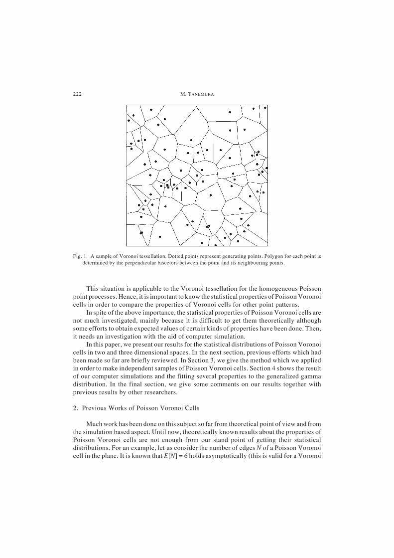
Among many possibilities of tessellations, the Voronoi tessellation might be the mostpopular and the most useful (see Fig. 1). The shape of cells of Voronoi tessellations clearlyreflects the manner of configuration of points. Namely, some of the statistical propertiesof spatial point patterns are reflected into the properties of geometrical structure of thecorresponding Voronoi tessellation. Thus, the Voronoi tessellation is playing an importantrole in the science on form.

From a point of view of application, the Voronoi cells are very useful as a geometricalmodel of crystal grains, biological cells, and so on. Voronoi cells are also useful as a toolfor numerical computations.

We define the Poisson Voronoi cells as the typical Voronoi cell based on thehomogeneous Poisson point processes. Recall that the homogeneous Poisson point processplays a role as the standard model for point patterns. Namely, statistical properties ofPoisson point process are often used as the null hypothesis against the correspondingproperties of competitive point process models.

222 M. TANEMURA

This situation is applicable to the Voronoi tessellation for the homogeneous Poissonpoint processes. Hence, it is important to know the statistical properties of Poisson Voronoicells in order to compare the properties of Voronoi cells for other point patterns.

In spite of the above importance, the statistical properties of Poisson Voronoi cells arenot much investigated, mainly because it is difficult to get them theoretically althoughsome efforts to obtain expected values of certain kinds of properties have been done. Then,it needs an investigation with the aid of computer simulation.

In this paper, we present our results for the statistical distributions of Poisson Voronoicells in two and three dimensional spaces. In the next section, previous efforts which hadbeen made so far are briefly reviewed. In Section 3, we give the method which we appliedin order to make independent samples of Poisson Voronoi cells. Section 4 shows the resultof our computer simulations and the fitting several properties to the generalized gammadistribution. In the final section, we give some comments on our results together withprevious results by other researchers.

2. Previous Works of Poisson Voronoi Cells

Much work has been done on this subject so far from theoretical point of view and fromthe simulation based aspect. Until now, theoretically known results about the properties ofPoisson Voronoi cells are not enough from our stand point of getting their statisticaldistributions. For an example, let us consider the number of edges N of a Poisson Voronoicell in the plane. It is known that E[N] = 6 holds asymptotically (this is valid for a Voronoi

Fig. 1. A sample of Voronoi tessellation. Dotted points represent generating points. Polygon for each point isdetermined by the perpendicular bisectors between the point and its neighbouring points.

Statistical Distributions of Poisson Voronoi Cells in Two and Three Dimensions 223

cell of any stochastic point processes). But the probability density which N for PoissonVoronoi cells should obey is not theoretically known yet. The situation is similar for othercharacteristic (let it be X) of Poisson Voronoi cells and, in most cases, its statisticalproperties are partly known through the few lower moments such as E[X], E[X2] and so on(see MØLLER (1994), for instance, as a review of mainly the theoretical aspect).

In order to investigate the spatial statistics of point patterns by using Voronoi cells, itis desirable to know all of the statistical properties of Poisson Voronoi cells as the standard.For that purpose, we inevitably take a computer simulation approach. There are manyefforts in this direction, but we mention here only a few. HINDE and MILES (1980) haveconducted a computer simulation of Poisson Voronoi cells in two dimensional space. Thenumber of samples of their simulation was two million, which has been a record until now.As the characteristics of Poisson Voronoi polygons, HINDE and MILES (1980) reported thenumber of edges N, the area A, the perimeter S and the internal angle θ of a typical cell. Theyobtained the first four moments of N, A, S and θ, and then fitted their histograms to the three-parameter generalized gamma density.

In case of three-dimensional Poisson Voronoi cells, TANEMURA (1988) reported thestatistical properties such as the distribution of the volume V and the number of faces Fbased on a hundred thousand sample of Voronoi polyhedra. More recently, KUMAR et al.(1992) presented the results of properties of three-dimensional Poisson Voronoi tessellationbased on 358,000 simulated cells. They reported on the statistical properties of F, V, S(surface area), B (total edge length) of a Poisson Voronoi polyhedron and fitted theirhistograms to the two-parameter generalized gamma density. Note the term “density” usedhere is meant by the “probability density function”. We often use this notation throughoutthis paper.

3. Methods

In order to make independent samples of Voronoi cells for homogeneous Poissonprocesses, we use the following method. Although the two-dimensional terminology isused, the extension to other dimensions will be easy.

First, let R be the region where the generating points are distributed, |R| be the area ofthe region. Let ρ be the intensity of the Poisson point process. We generate a homogeneousPoisson point pattern inside R with intensity ρ. Then, the number of points inside R willobey the Poisson distribution with mean ρ|R|. Next, we select a point at random among thedistributed points and construct a Voronoi cell of the selected point. Details of theprocedure are the following:

(1) Letting n be the total number of independent samples, we set the number of points,m, inside R according to the Poisson distribution with mean ρ|R| theoretically for eachsampling. Then, we generate m points inside R uniformly at random.

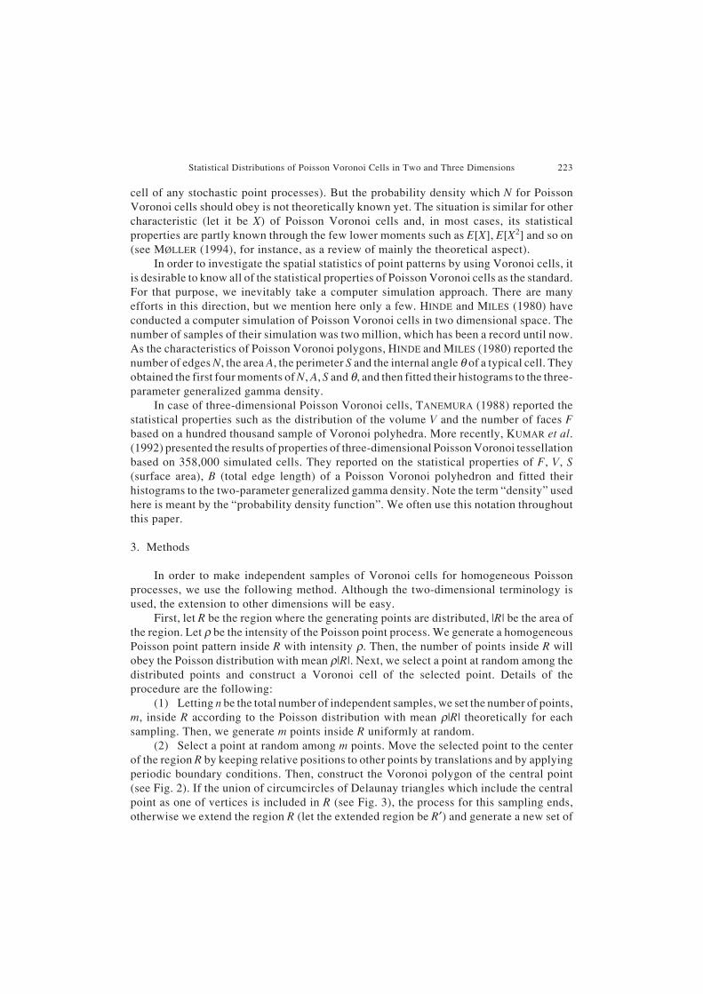
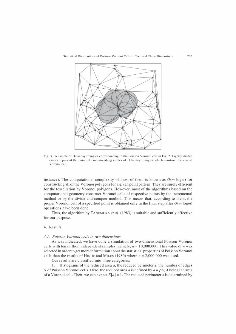
(2) Select a point at random among m points. Move the selected point to the centerof the region R by keeping relative positions to other points by translations and by applyingperiodic boundary conditions. Then, construct the Voronoi polygon of the central point(see Fig. 2). If the union of circumcircles of Delaunay triangles which include the centralpoint as one of vertices is included in R (see Fig. 3), the process for this sampling ends,otherwise we extend the region R (let the extended region be R′) and generate a new set of

224 M. TANEMURA

points with the same intensity ρ, select a central point, move other points such that theselected point is at the center of R′ by applying the same procedure as above, and thenconstruct the Voronoi polygon of central point. Repeat the process until the union ofcircumcircles of Delaunay triangles satisfy the above condition.

This procedure is basically due to HINDE and MILES (1980). In the paper of HINDE andMILES (1980), they have set ρ = 100 in two-dimensional case. In the present simulations,we set ρ = 200 for two-dimensional space, and ρ = 500 for three-dimensional space. Bythese settings, the process of extension of the region R in the second step of the aboveprocedure did not actually happen.

Algorithm for constructing Voronoi cell of the central pointLet us mention about the details of the algorithm for constructing the central Voronoi

cell by using the example of two-dimensional space. Let us remind, for each realization ofhomogeneous Poisson point patterns, we are interested to construct a Voronoi polygon fora single central point as indicated by the shaded area in Fig. 2.

For that purpose, the algorithm devised by TANEMURA et al. (1983) is the mostsuitable. In their algorithm, all of the Delaunay triangles which include the central point asa vertex are efficiently constructed (see Fig. 3, for example). The computational complexityof this algorithm for constructing a single Voronoi polygon is O(m), where m is the existingnumber of points in the current point pattern.

Here, we recall a set of efficient algorithms which are based on the results of the fieldof ‘computational geometry’ (see, for the existing algorithms OKABE et al. (2000), for

Fig. 2. A sample of Poisson Voronoi cell. Shaded polygon is the Voronoi polygon which is successfully made.


instance). The computational complexity of most of them is known as O(m logm) forconstructing all of the Voronoi polygons for a given point pattern. They are surely efficientfor the tessellation by Voronoi polygons. However, most of the algorithms based on thecomputational geometry construct Voronoi cells of respective points by the incrementalmethod or by the divide-and-conquer method. This means that, according to them, theproper Voronoi cell of a specified point is obtained only in the final step after O(m logm)operations have been done.

Thus, the algorithm by TANEMURA et al. (1983) is suitable and sufficiently effectivefor our purpose.

4. Results

4.1. Poisson Voronoi cells in two dimensionsAs was indicated, we have done a simulation of two-dimensional Poisson Voronoi

cells with ten million independent samples, namely, n = 10,000,000. This value of n wasselected in order to get more information about the statistical properties of Poisson Voronoicells than the results of HINDE and MILES (1980) where n = 2,000,000 was used.

Our results are classified into three categories:1. Histograms of the reduced area a, the reduced perimeter s, the number of edges

N of Poisson Voronoi cells. Here, the reduced area a is defined by a = ρA, A being the areaof a Voronoi cell. Then, we can expect E[a] = 1. The reduced perimeter s is determined by

Fig. 3. A sample of Delaunay triangles corresponding to the Poisson Voronoi cell in Fig. 2. Lightly shadedcircles represent the union of circumscribing circles of Delaunay triangles which construct the centralVoronoi cell.

226 M. TANEMURA

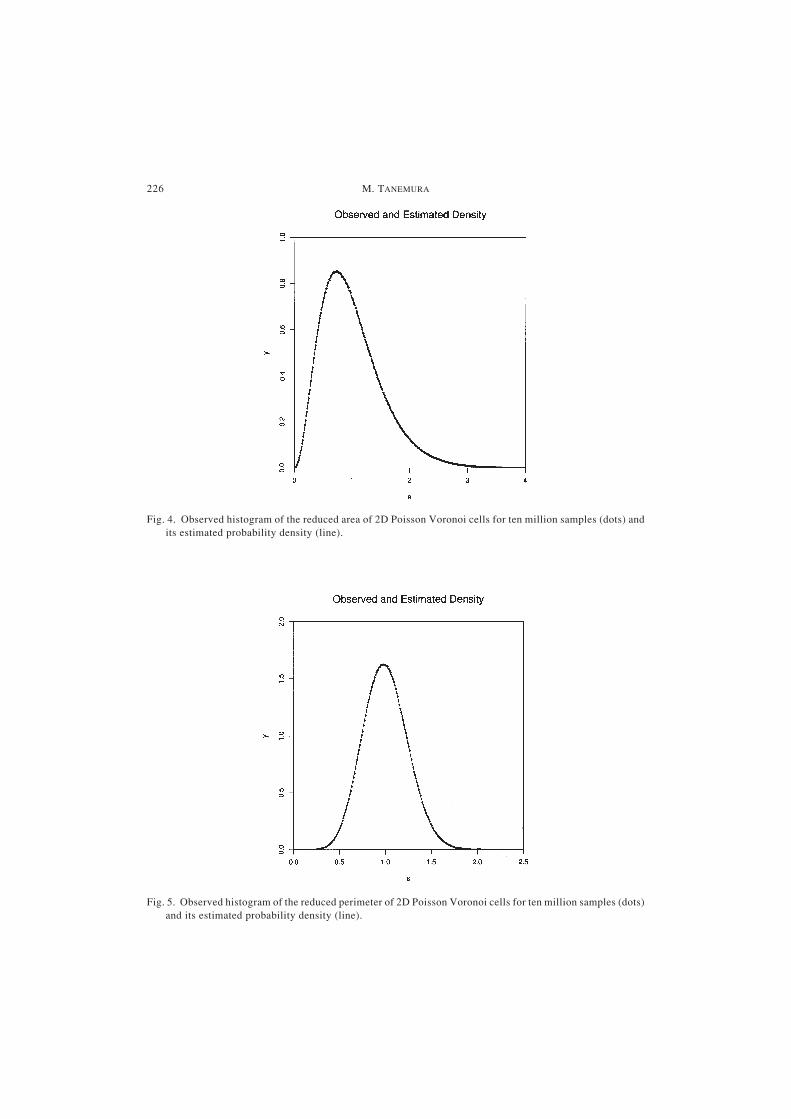
Fig. 4. Observed histogram of the reduced area of 2D Poisson Voronoi cells for ten million samples (dots) andits estimated probability density (line).

Fig. 5. Observed histogram of the reduced perimeter of 2D Poisson Voronoi cells for ten million samples (dots)and its estimated probability density (line).


the relation s = ρ S/4, where S is the perimeter of a Voronoi cell. In this case, we canexpect also E[s] = 1, since it is known that, for a homogeneous Poisson point process, E[S]

= 4/ ρ holds (MILES, 1970).Also histograms of the area aN and the perimeter sN of Poisson Voronoi cells for a given

number of edges are given.2. Moments of a, s, N, and aN.3. Parameters a, b, c of generalized Gamma distribution

f x a b cab

c ax bx a b c

c ac a, ,

/exp , ,

/

( ) =( )

−( ) >( ) ( )−

Γ1 0 1

fitted to the histograms of a, s, N, aN and sN.

HistogramsDotted points in Figs. 4 and 5 represent the observed histograms of, respectively, the

area a and the perimeter s of two-dimensional Poisson Voronoi cells. The class intervalsfor a and s were chosen as 0.01 which gave 700 classes for a and 300 classes for s. It isbecause the observed minimum and the maximum values of a and s were, respectively, amin= 0.002059 and amax = 6.265011 and smin = 0.059381 and smax = 2.439198.

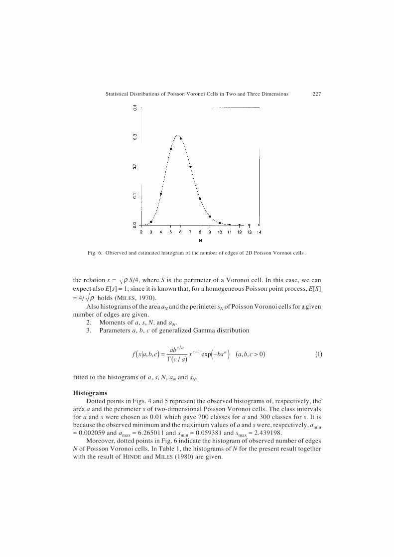
Moreover, dotted points in Fig. 6 indicate the histogram of observed number of edgesN of Poisson Voronoi cells. In Table 1, the histograms of N for the present result togetherwith the result of HINDE and MILES (1980) are given.

Fig. 6. Observed and estimated histogram of the number of edges of 2D Poisson Voronoi cells .

228 M. TANEMURA

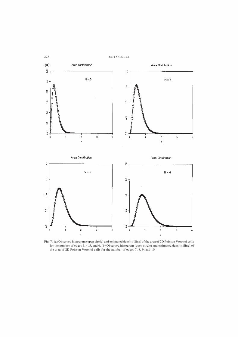
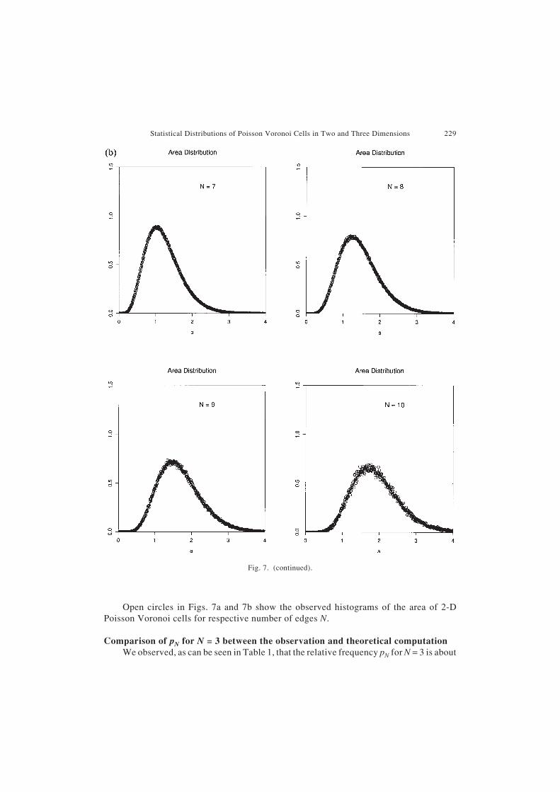
Fig. 7. (a) Observed histogram (open circle) and estimated density (line) of the area of 2D Poisson Voronoi cellsfor the number of edges 3, 4, 5, and 6. (b) Observed histogram (open circle) and estimated density (line) ofthe area of 2D Poisson Voronoi cells for the number of edges 7, 8, 9, and 10.


Open circles in Figs. 7a and 7b show the observed histograms of the area of 2-DPoisson Voronoi cells for respective number of edges N.

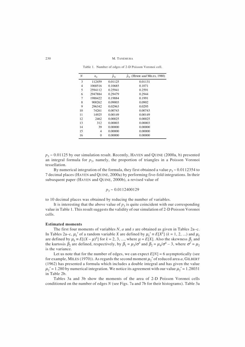
Comparison of pN for N = 3 between the observation and theoretical computationWe observed, as can be seen in Table 1, that the relative frequency pN for N = 3 is about

Fig. 7. (continued).

230 M. TANEMURA

p3 ~ 0.01125 by our simulation result. Recently, HAYEN and QUINE (2000a, b) presentedan integral formula for p3, namely, the proportion of triangles in a Poisson Voronoitessellation.

By numerical integration of the formula, they first obtained a value p3 ~ 0.0112354 to7 decimal places (HAYEN and QUINE, 2000a) by performing five-fold integrations. In theirsubsequent paper (HAYEN and QUINE, 2000b), a revised value of

p3 ~ 0.0112400129

to 10 decimal places was obtained by reducing the number of variables.It is interesting that the above value of p3 is quite coincident with our corresponding

value in Table 1. This result suggests the validity of our simulation of 2-D Poisson Voronoicells.

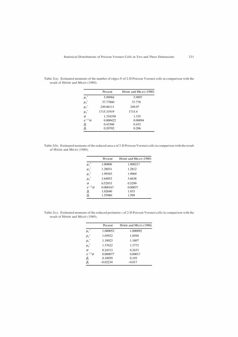
Estimated momentsThe first four moments of variables N, a and s are obtained as given in Tables 2a–c.

In Tables 2a–c, µk′ of a random variable X are defined by µk′ ≡ E[Xk] (k = 1, 2, ...) and µkare defined by µk ≡ E[(X – µ)k] for k = 2, 3, ..., where µ = E[X]. Also the skewness β1 andthe kurtosis β2 are defined, respectively, by β1 = µ3/σ3 and β2 = µ4/σ4 – 3, where σ2 = µ2is the variance.

Let us note that for the number of edges, we can expect E[N] = 6 asymptotically (seefor example, MILES (1970)). As regards the second moment µ2′ of reduced area a, GILBERT

(1962) has presented a formula which includes a double integral and has given the valueµ2′ = 1.280 by numerical integration. We notice its agreement with our value µ2′ = 1.28031in Table 2b.

Tables 3a and 3b show the moments of the area of 2-D Poisson Voronoi cellsconditioned on the number of edges N (see Figs. 7a and 7b for their histograms). Table 3a

Table 1. Number of edges of 2-D Poisson Voronoi cell.

N nN pN pN (HINDE and MILES, 1980)

3 112459 0.01125 0.011314 1068516 0.10685 0.10715 2594112 0.25941 0.25916 2947884 0.29479 0.29447 1988422 0.19884 0.19918 900262 0.09003 0.09029 296342 0.02963 0.0295

10 74261 0.00743 0.0074311 14925 0.00149 0.0014912 2462 0.00025 0.0002513 312 0.00003 0.0000314 39 0.00000 0.0000015 4 0.00000 0.0000016 0 0.00000 0.00000


Table 2(a). Estimated moments of the number of edges N of 2-D Poisson Voronoi cells in comparison with theresult of HINDE and MILES (1980).

Table 2(b). Estimated moments of the reduced area a of 2-D Poisson Voronoi cells in comparison with the resultof HINDE and MILES (1980).

Table 2(c). Estimated moments of the reduced perimeter s of 2-D Poisson Voronoi cells in comparison with theresult of HINDE and MILES (1980).

Present HINDE and MILES (1980)

µ1′ 5.99984 5.9997

µ2′ 37.77860 37.778

µ3′ 249.06111 249.07

µ4′ 1715.31919 1715.4

σ 1.334350 1.335n–1.2σ 0.000422 0.00094β1 0.43360 0.432β2 0.20702 0.206


µ1′ 1.00006 1.000217

µ2′ 1.28031 1.2812

µ3′ 1.99303 1.9969

µ4′ 3.64852 3.6638

σ 0.52933 0.5299n–1.2σ 0.000167 0.00037β1 1.02640 1.033β2 1.55980 1.599


µ1′ 1.000052 1.000092

µ2′ 1.05922 1.0594

µ3′ 1.18023 1.1807

µ4′ 1.37622 1.3772

σ 0.24313 0.2433n–1.2σ 0.000077 0.00017β1 0.18959 0.193β2 –0.02234 –0.017

232 M. TANEMURA

N 3 4 5 6

nN 112459 1068516 2594112 2947884µ1′ 0.34479 0.55810 0.77420 0.99621

µ2′ 0.16325 0.40137 0.73723 1.18061

µ3′ 0.09883 0.35501 0.83592 1.62589

µ4′ 0.07324 0.37380 1.10209 2.55601

σ 0.21063 0.29982 0.37128 0.43379n–1.2σ 0.00063 0.00029 0.00023 0.00025β1 1.27827 1.13780 1.01056 0.91678β2 2.58398 1.99061 1.57440 1.30334

N 7 8 9 10

nN 1988422 900262 296342 74261µ1′ 1.22181 1.45418 1.68690 1.92214

µ2′ 1.73336 2.40957 3.19728 4.10391

µ3′ 2.80500 4.48590 6.73178 9.64369

µ4′ 5.10613 9.27567 15.59465 24.74464

σ 0.49043 0.54307 0.59301 0.63977n–1.2σ 0.00035 0.00057 0.00109 0.00235β1 0.84271 0.77537 0.72819 0.69470β2 1.10344 0.90388 0.78615 0.71529

Table 3(a). Estimated moments of the area aN of 2-D Poisson Voronoi cells for given number of edges N.

Table 3(b). Estimated moments of the area aN of 2-D Poisson Voronoi cells for given number of edges N.

is for aN where N = 3, 4, 5 and 6, while Table 3b is the moments of aN for N = 7, 8, 9 and10.

Fitting the generalized gamma distribution to the histogramsWe tried to fit the observed histograms of various geometrical quantities of 2-D

Poisson Voronoi cells to a certain flexible density function with a few parameters. Amonga vast possibilities, we have selected the three-parameter generalized gamma distribution(1) since it will represent a wide range of distribution with a single mode and with anexponential decay for a large value. Moreover, that the range of its variable is limited to(0, ∞) is suitable for our purpose, since we are concerned with variables which take onlypositive values.

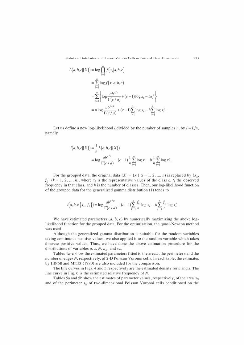
In order to estimate the parameters of the three-parameter generalized gammadistribution, we adapted the maximum likelihood estimation. Let L(a, b, c |{X}) be the log-likelihood of parameters a, b and c for the observed data {X}. Then, we get for thegeneralized gamma distribution,


L a b c X f x a b c

f x a b c

ab

c ac x bx

nab

c ac x b x

ii

n

ii

n

c a

i ia

i

n

c a

ii

n

ia

i

, , log , ,

log , ,

log/

log

log/

log log

/

/

{ }( ) = ( )

= ( )

=( )

+ −( ) −

=( )

+ −( ) −

=

=

=

= =

∏

∑

∑

∑

1

1

1

1

1

1

Γ

Γ 11

n

∑ .

Let us define a new log-likelihood l divided by the number of samples n, by l = L/n,namely

l a b c Xn

L a b c X

ab

c ac

nx b

nx

c a

ii

n

ia

i

n

, , , ,

log/

log log ./

{ }( ) = { }( )

=( )

+ −( ) −= =∑ ∑

1

11 1

1 1Γ

For the grouped data, the original data {X} = {xi} (i = 1, 2, ..., n) is replaced by {xk,fk} (k = 1, 2, ..., h), where xk is the representative values of the class k, fk the observedfrequency in that class, and h is the number of classes. Then, our log-likelihood functionof the grouped data for the generalized gamma distribution (1) tends to

l a b c x fab

c ac

f

nx b

f

nxk k

c ak

kk

hk

ka

k

h

, , , log/

log log ./

{ }( ) =( )

+ −( ) −= =

∑ ∑Γ1

1 1

We have estimated parameters (a, b, c) by numerically maximizing the above log-likelihood function for the grouped data. For the optimization, the quasi-Newton methodwas used.

Although the generalized gamma distribution is suitable for the random variablestaking continuous positive values, we also applied it to the random variable which takesdiscrete positive values. Thus, we have done the above estimation procedure for thedistributions of variables a, s, N, aN, and sN.

Tables 4a–c show the estimated parameters fitted to the area a, the perimeter s and thenumber of edges N, respectively, of 2-D Poisson Voronoi cells. In each table, the estimatesby HINDE and MILES (1980) are also included for the comparison.

The line curves in Figs. 4 and 5 respectively are the estimated density for a and s. Theline curve in Fig. 6 is the estimated relative frequency of N.

Tables 5a and 5b show the estimates of parameter values, respectively, of the area aNand of the perimeter sN of two-dimensional Poisson Voronoi cells conditioned on the

234 M. TANEMURA

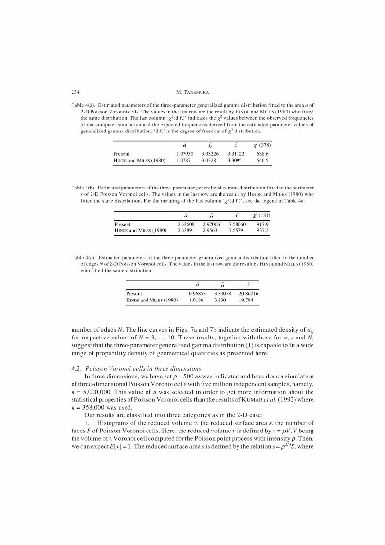
Table 4(a). Estimated parameters of the three-parameter generalized gamma distribution fitted to the area a of2-D Poisson Voronoi cells. The values in the last row are the result by HINDE and MILES (1980) who fittedthe same distribution. The last column ‘χ2(d.f.)’ indicates the χ2 values between the observed frequenciesof our computer simulation and the expected frequencies derived from the estimated parameter values ofgeneralized gamma distribution. ‘d.f.’ is the degree of freedom of χ2 distribution.

Table 4(b). Estimated parameters of the three-parameter generalized gamma distribution fitted to the perimeters of 2-D Poisson Voronoi cells. The values in the last row are the result by HINDE and MILES (1980) whofitted the same distribution. For the meaning of the last column ‘χ2(d.f.)’, see the legend in Table 4a.

Table 4(c). Estimated parameters of the three-parameter generalized gamma distribution fitted to the numberof edges N of 2-D Poisson Voronoi cells. The values in the last row are the result by HINDE and MILES (1980)who fitted the same distribution.

a b c χ2 (378)

Present 1.07950 3.03226 3.31122 638.6HINDE and MILES (1980) 1.0787 3.0328 3.3095 646.5

a b c χ2 (181)

Present 2.33609 2.97006 7.58060 917.9HINDE and MILES (1980) 2.3389 2.9563 7.5579 937.3

a b c

Present 0.96853 3.80078 20.86016HINDE and MILES (1980) 1.0186 3.130 19.784

number of edges N. The line curves in Figs. 7a and 7b indicate the estimated density of aNfor respective values of N = 3, ..., 10. These results, together with those for a, s and N,suggest that the three-parameter generalized gamma distribution (1) is capable to fit a widerange of propability density of geometrical quantities as presented here.

4.2. Poisson Voronoi cells in three dimensionsIn three dimensions, we have set ρ = 500 as was indicated and have done a simulation

of three-dimensional Poisson Voronoi cells with five million independent samples, namely,n = 5,000,000. This value of n was selected in order to get more information about thestatistical properties of Poisson Voronoi cells than the results of KUMAR et al. (1992) wheren = 358,000 was used.

Our results are classified into three categories as in the 2-D case:1. Histograms of the reduced volume v, the reduced surface area s, the number of

faces F of Poisson Voronoi cells. Here, the reduced volume v is defined by v = ρV, V beingthe volume of a Voronoi cell computed for the Poisson point process with intensity ρ. Then,we can expect E[v] = 1. The reduced surface area s is defined by the relation s = ρ2/3S, where


S is the surface area of a Voronoi cell for the Poisson point process with intensity ρ. In thiscase, we can expect also E[s] ~ 5.821, since it is known that, for a homogeneous Poissonpoint process, E[S] = (256π/3)1/3Γ(5/3)ρ–2/3 holds (MEIJERING, 1953).

Also histograms of the volume vF and the surface area sF of Poisson Voronoi cells fora given number of faces are given.

2. Moments of v, s, F, and vF.3. Parameters a, b, c of generalized Gamma distribution

f x a b cab

c ax bx a b c

c ac a, ,

/exp , ,

/

( ) =( )

−( ) >( )−

Γ1 0

fitted to the histograms of v, s, F, vF and sF.

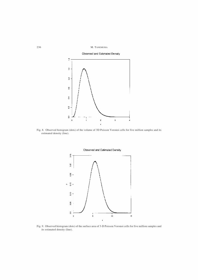
HistogramsDotted points in Figs. 8 and 9 show the observed histograms of, respectively, the

volume v and the surface area s of three-dimensional Poisson Voronoi cells. The class

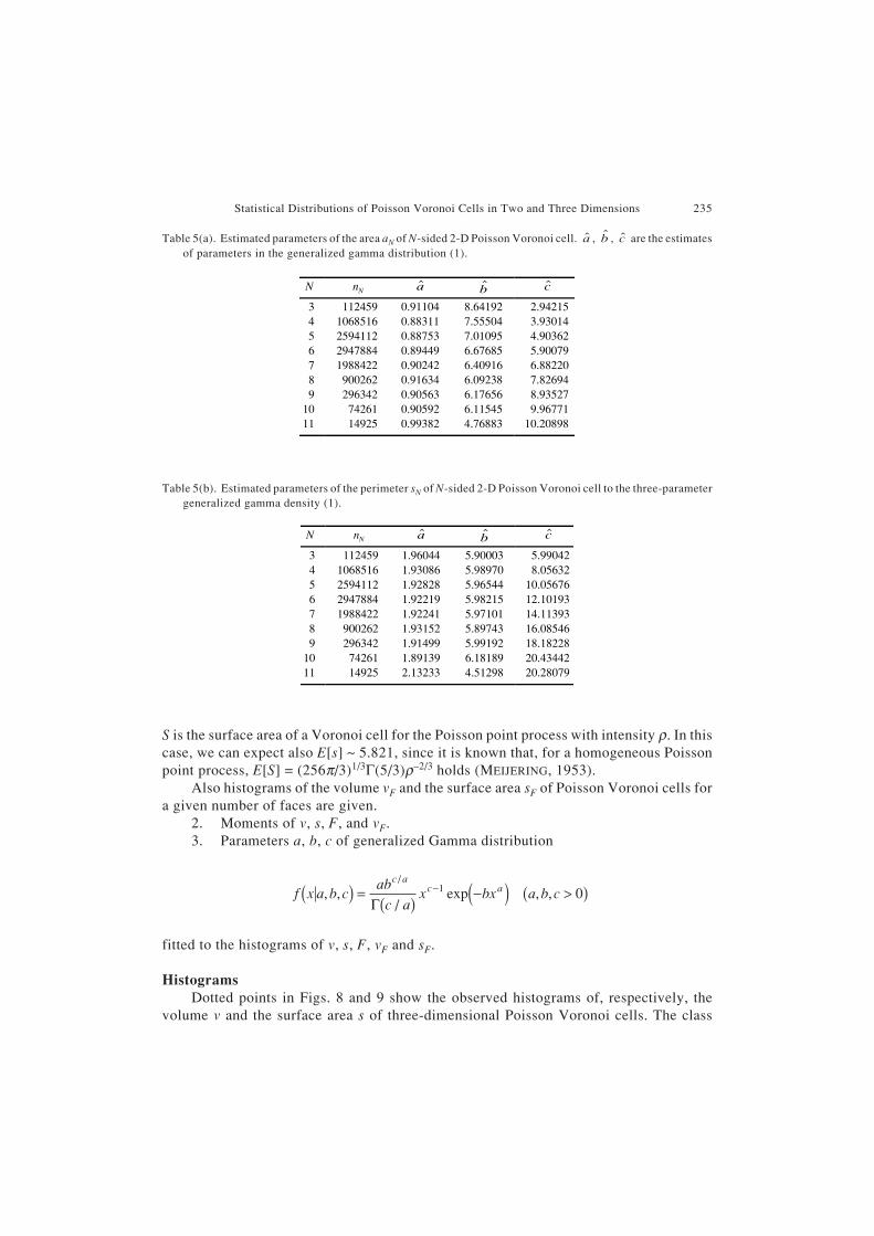
Table 5(a). Estimated parameters of the area aN of N-sided 2-D Poisson Voronoi cell. a , b , c are the estimatesof parameters in the generalized gamma distribution (1).

Table 5(b). Estimated parameters of the perimeter sN of N-sided 2-D Poisson Voronoi cell to the three-parametergeneralized gamma density (1).

N nN a b c

3 112459 0.91104 8.64192 2.942154 1068516 0.88311 7.55504 3.930145 2594112 0.88753 7.01095 4.903626 2947884 0.89449 6.67685 5.900797 1988422 0.90242 6.40916 6.882208 900262 0.91634 6.09238 7.826949 296342 0.90563 6.17656 8.93527

10 74261 0.90592 6.11545 9.9677111 14925 0.99382 4.76883 10.20898

N nN a b c

3 112459 1.96044 5.90003 5.990424 1068516 1.93086 5.98970 8.056325 2594112 1.92828 5.96544 10.056766 2947884 1.92219 5.98215 12.101937 1988422 1.92241 5.97101 14.113938 900262 1.93152 5.89743 16.085469 296342 1.91499 5.99192 18.18228

10 74261 1.89139 6.18189 20.4344211 14925 2.13233 4.51298 20.28079

236 M. TANEMURA

Fig. 8. Observed histogram (dots) of the volume of 3D Poisson Voronoi cells for five million samples and itsestimated density (line).

Fig. 9. Observed histogram (dots) of the surface area of 3-D Poisson Voronoi cells for five million samples andits estimated density (line).


intervals of v and s were respectively chosen to be 0.01 and 0.04, which gave 500 and 400classes for v and s, respectively. It is because the observed minimum and maximum valuesof v and s were, respectively, vmin = 0.015622 and vmax = 4.623616, and smin = 0.558396 andsmax = 14.812654.

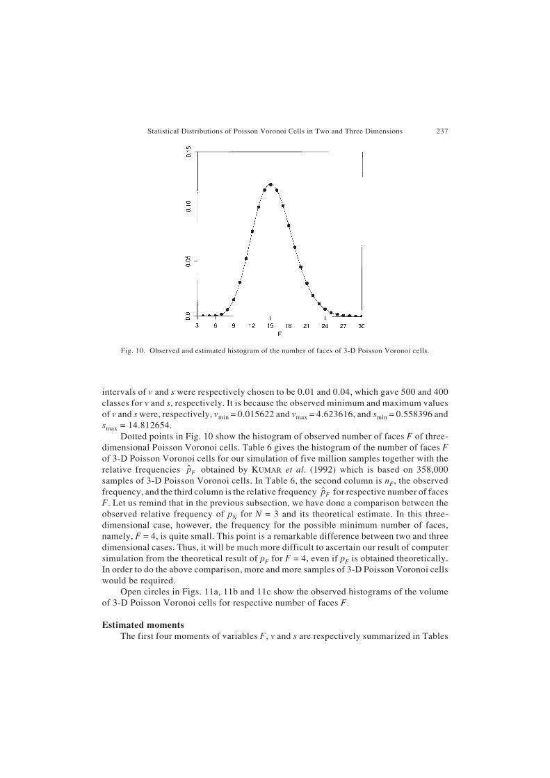
Dotted points in Fig. 10 show the histogram of observed number of faces F of three-dimensional Poisson Voronoi cells. Table 6 gives the histogram of the number of faces Fof 3-D Poisson Voronoi cells for our simulation of five million samples together with therelative frequencies pF obtained by KUMAR et al. (1992) which is based on 358,000samples of 3-D Poisson Voronoi cells. In Table 6, the second column is nF, the observedfrequency, and the third column is the relative frequency pF for respective number of facesF. Let us remind that in the previous subsection, we have done a comparison between theobserved relative frequency of pN for N = 3 and its theoretical estimate. In this three-dimensional case, however, the frequency for the possible minimum number of faces,namely, F = 4, is quite small. This point is a remarkable difference between two and threedimensional cases. Thus, it will be much more difficult to ascertain our result of computersimulation from the theoretical result of pF for F = 4, even if pF is obtained theoretically.In order to do the above comparison, more and more samples of 3-D Poisson Voronoi cellswould be required.

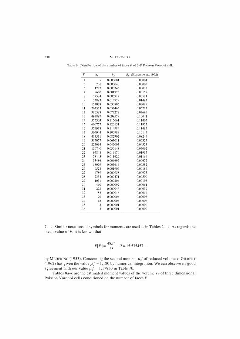
Open circles in Figs. 11a, 11b and 11c show the observed histograms of the volumeof 3-D Poisson Voronoi cells for respective number of faces F.

Estimated momentsThe first four moments of variables F, v and s are respectively summarized in Tables

Fig. 10. Observed and estimated histogram of the number of faces of 3-D Poisson Voronoi cells.

238 M. TANEMURA

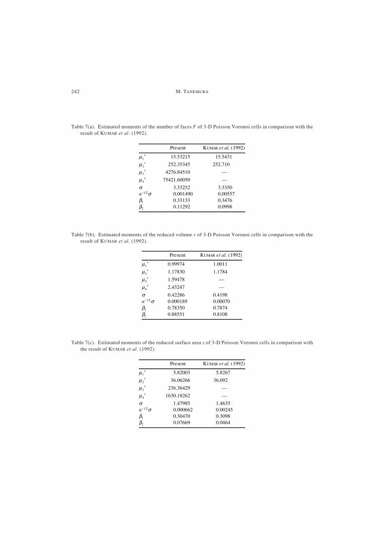
7a–c. Similar notations of symbols for moments are used as in Tables 2a–c. As regards themean value of F, it is known that

E F[ ] = + =48

352 15 535457

2π. K

by MEIJERING (1953). Concerning the second moment µ2′ of reduced volume v, GILBERT

(1962) has given the value µ2′ = 1.180 by numerical integration. We can observe its goodagreement with our value µ2′ = 1.17830 in Table 7b.

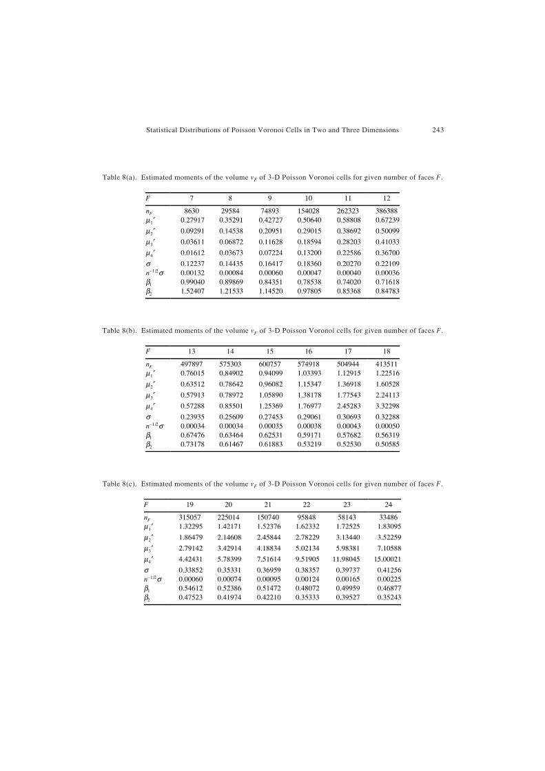
Tables 8a–c are the estimated moment values of the volume vF of three dimensionalPoisson Voronoi cells conditioned on the number of faces F.

Table 6. Distribution of the number of faces F of 3-D Poisson Voronoi cell.

F nF pF pF (KUMAR et al., 1992)

4 5 0.000001 0.000015 201 0.000040 0.000036 1727 0.000345 0.000337 8630 0.001726 0.001598 29584 0.005917 0.005819 74893 0.014979 0.01494

10 154028 0.030806 0.0308911 262323 0.052465 0.0521212 386388 0.077278 0.0769513 497897 0.099579 0.1004114 575303 0.115061 0.1146515 600757 0.120151 0.1192716 574918 0.114984 0.1148517 504944 0.100989 0.1014418 413511 0.082702 0.0824419 315057 0.063011 0.0632520 225014 0.045003 0.0452321 150740 0.030148 0.0306222 95848 0.019170 0.0193523 58143 0.011629 0.0116424 33486 0.006697 0.0067225 18079 0.003616 0.0038226 9528 0.001906 0.0018627 4789 0.000958 0.0097528 2354 0.000471 0.0050029 1031 0.000206 0.0019830 460 0.000092 0.0006131 228 0.000046 0.0003932 82 0.000016 0.0001433 29 0.000006 0.0000334 15 0.000003 0.0000635 3 0.000001 0.0000036 3 0.000001 0.00000


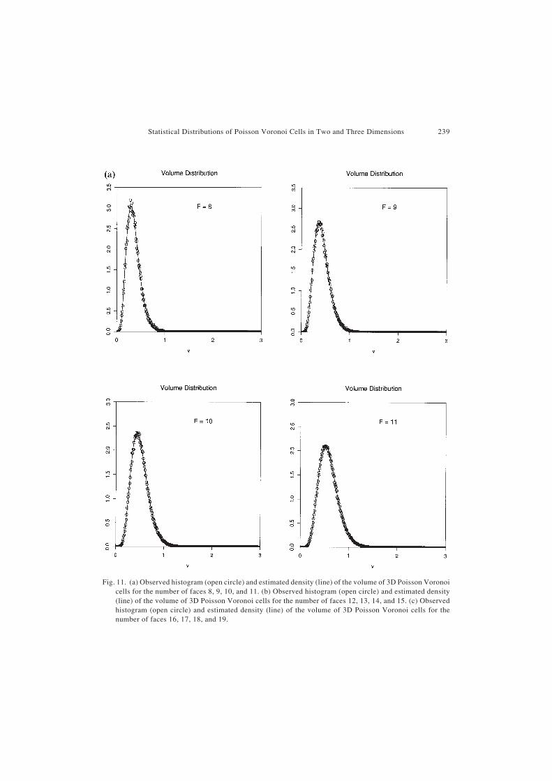
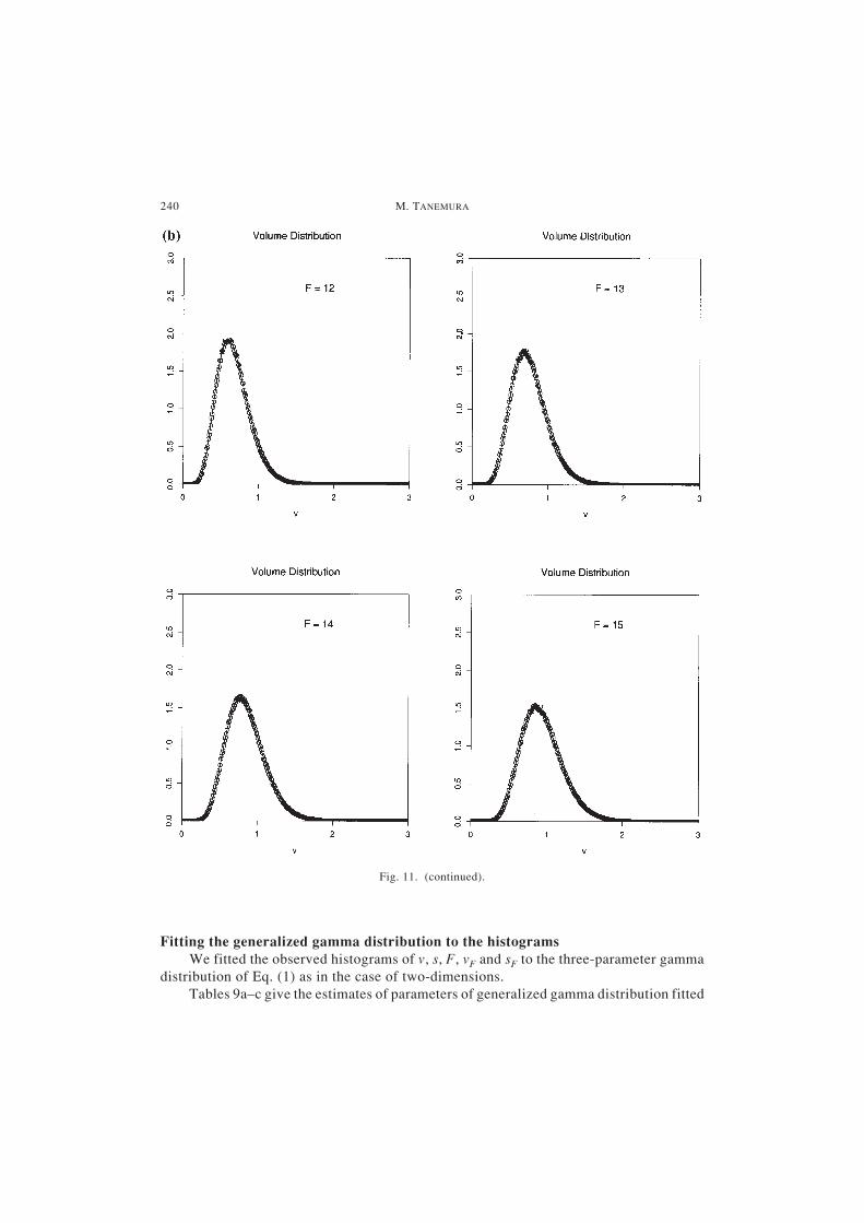
Fig. 11. (a) Observed histogram (open circle) and estimated density (line) of the volume of 3D Poisson Voronoicells for the number of faces 8, 9, 10, and 11. (b) Observed histogram (open circle) and estimated density(line) of the volume of 3D Poisson Voronoi cells for the number of faces 12, 13, 14, and 15. (c) Observedhistogram (open circle) and estimated density (line) of the volume of 3D Poisson Voronoi cells for thenumber of faces 16, 17, 18, and 19.

240 M. TANEMURA

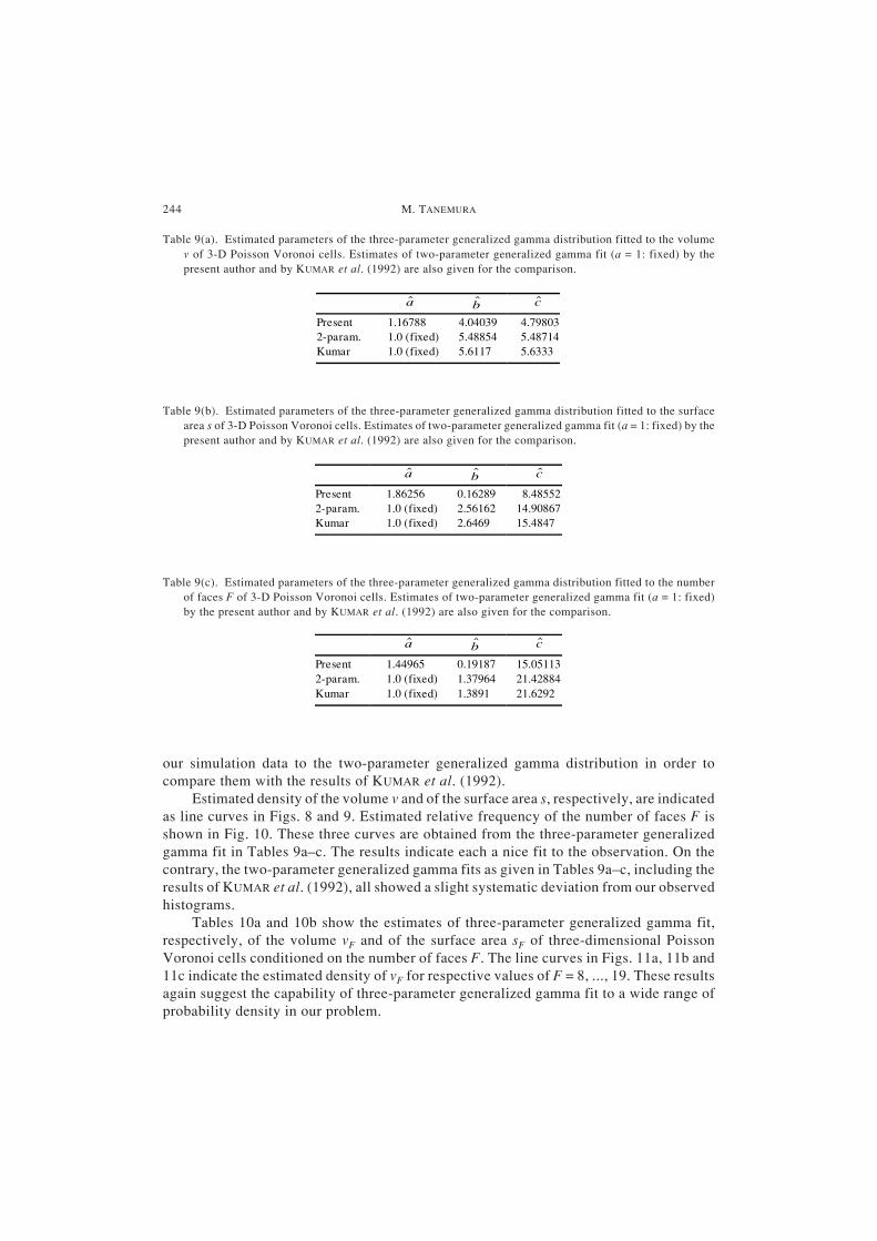
Fitting the generalized gamma distribution to the histogramsWe fitted the observed histograms of v, s, F, vF and sF to the three-parameter gamma

distribution of Eq. (1) as in the case of two-dimensions.Tables 9a–c give the estimates of parameters of generalized gamma distribution fitted




to the volume v, the surface area s and the number of faces F, respectively, of 3-D PoissonVoronoi cells. In each table, the estimates by KUMAR et al. (1992) are also included. Noticethat KUMAR et al. (1992) have adopted the two-parameter generalized gamma fit (they usedb and c as variable parameters by fixing a = 1 in our Eq. (1)). Then, we independently fitted

242 M. TANEMURA

Table 7(a). Estimated moments of the number of faces F of 3-D Poisson Voronoi cells in comparison with theresult of KUMAR et al. (1992).

Table 7(b). Estimated moments of the reduced volume v of 3-D Poisson Voronoi cells in comparison with theresult of KUMAR et al. (1992).

Table 7(c). Estimated moments of the reduced surface area s of 3-D Poisson Voronoi cells in comparison withthe result of KUMAR et al. (1992).

Present KUMAR et al. (1992)

µ1′ 15.53215 15.5431

µ2′ 252.35345 252.710

µ3′ 4276.84510 —

µ4′ 75421.60050 —

σ 3.33252 3.3350n–1/2σ 0.001490 0.00557β1 0.33133 0.3476β2 0.11292 0.0998


µ1′ 0.99974 1.0011

µ2′ 1.17830 1.1784

µ3′ 1.59478 —

µ4′ 2.43247 —

σ 0.42286 0.4198n–1/2σ 0.000189 0.00070β1 0.78350 0.7874β2 0.88551 0.8108


µ1′ 5.82003 5.8267

µ2′ 36.06266 36.092

µ3′ 236.36429 —

µ4′ 1630.18262 —

σ 1.47985 1.4635n–1/2σ 0.000662 0.00245β1 0.30470 0.3098β2 0.07669 0.0464


Table 8(a). Estimated moments of the volume vF of 3-D Poisson Voronoi cells for given number of faces F.

Table 8(b). Estimated moments of the volume vF of 3-D Poisson Voronoi cells for given number of faces F.

Table 8(c). Estimated moments of the volume vF of 3-D Poisson Voronoi cells for given number of faces F.

F 7 8 9 10 11 12

nF 8630 29584 74893 154028 262323 386388µ1′ 0.27917 0.35291 0.42727 0.50640 0.58808 0.67239

µ2′ 0.09291 0.14538 0.20951 0.29015 0.38692 0.50099

µ3′ 0.03611 0.06872 0.11628 0.18594 0.28203 0.41033

µ4′ 0.01612 0.03673 0.07224 0.13200 0.22586 0.36700

σ 0.12237 0.14435 0.16417 0.18360 0.20270 0.22109n–1/2σ 0.00132 0.00084 0.00060 0.00047 0.00040 0.00036β1 0.99040 0.89869 0.84351 0.78538 0.74020 0.71618β2 1.52407 1.21533 1.14520 0.97805 0.85368 0.84783

F 13 14 15 16 17 18

nF 497897 575303 600757 574918 504944 413511µ1′ 0.76015 0.84902 0.94099 1.03393 1.12915 1.22516

µ2′ 0.63512 0.78642 0.96082 1.15347 1.36918 1.60528

µ3′ 0.57913 0.78972 1.05890 1.38178 1.77543 2.24113

µ4′ 0.57288 0.85501 1.25369 1.76977 2.45283 3.32298

σ 0.23935 0.25609 0.27453 0.29061 0.30693 0.32288n–1/2σ 0.00034 0.00034 0.00035 0.00038 0.00043 0.00050β1 0.67476 0.63464 0.62531 0.59171 0.57682 0.56319β2 0.73178 0.61467 0.61883 0.53219 0.52530 0.50585

F 19 20 21 22 23 24

nF 315057 225014 150740 95848 58143 33486µ1′ 1.32295 1.42171 1.52376 1.62332 1.72525 1.83095

µ2′ 1.86479 2.14608 2.45844 2.78229 3.13440 3.52259

µ3′ 2.79142 3.42914 4.18834 5.02134 5.98381 7.10588

µ4′ 4.42431 5.78399 7.51614 9.51905 11.98045 15.00021

σ 0.33852 0.35331 0.36959 0.38357 0.39737 0.41256n–1/2σ 0.00060 0.00074 0.00095 0.00124 0.00165 0.00225β1 0.54612 0.52386 0.51472 0.48072 0.49959 0.46877β2 0.47523 0.41974 0.42210 0.35333 0.39527 0.35243

244 M. TANEMURA

our simulation data to the two-parameter generalized gamma distribution in order tocompare them with the results of KUMAR et al. (1992).

Estimated density of the volume v and of the surface area s, respectively, are indicatedas line curves in Figs. 8 and 9. Estimated relative frequency of the number of faces F isshown in Fig. 10. These three curves are obtained from the three-parameter generalizedgamma fit in Tables 9a–c. The results indicate each a nice fit to the observation. On thecontrary, the two-parameter generalized gamma fits as given in Tables 9a–c, including theresults of KUMAR et al. (1992), all showed a slight systematic deviation from our observedhistograms.

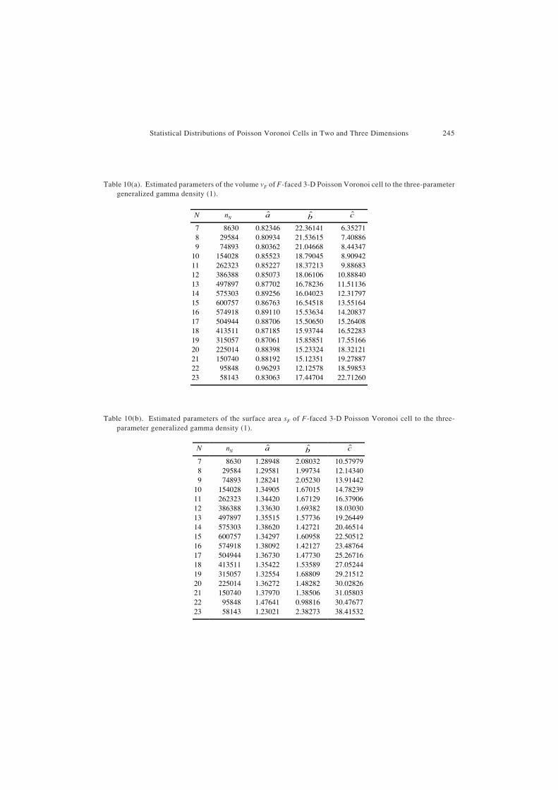
Tables 10a and 10b show the estimates of three-parameter generalized gamma fit,respectively, of the volume vF and of the surface area sF of three-dimensional PoissonVoronoi cells conditioned on the number of faces F. The line curves in Figs. 11a, 11b and11c indicate the estimated density of vF for respective values of F = 8, ..., 19. These resultsagain suggest the capability of three-parameter generalized gamma fit to a wide range ofprobability density in our problem.

Table 9(a). Estimated parameters of the three-parameter generalized gamma distribution fitted to the volumev of 3-D Poisson Voronoi cells. Estimates of two-parameter generalized gamma fit (a = 1: fixed) by thepresent author and by KUMAR et al. (1992) are also given for the comparison.

Table 9(b). Estimated parameters of the three-parameter generalized gamma distribution fitted to the surfacearea s of 3-D Poisson Voronoi cells. Estimates of two-parameter generalized gamma fit (a = 1: fixed) by thepresent author and by KUMAR et al. (1992) are also given for the comparison.

Table 9(c). Estimated parameters of the three-parameter generalized gamma distribution fitted to the numberof faces F of 3-D Poisson Voronoi cells. Estimates of two-parameter generalized gamma fit (a = 1: fixed)by the present author and by KUMAR et al. (1992) are also given for the comparison.

a b c

Present 1.16788 4.04039 4.798032-param. 1.0 (fixed) 5.48854 5.48714Kumar 1.0 (fixed) 5.6117 5.6333

a b c


a b c



Table 10(b). Estimated parameters of the surface area sF of F-faced 3-D Poisson Voronoi cell to the three-parameter generalized gamma density (1).

Table 10(a). Estimated parameters of the volume vF of F-faced 3-D Poisson Voronoi cell to the three-parametergeneralized gamma density (1).

N nN a b c

7 8630 0.82346 22.36141 6.352718 29584 0.80934 21.53615 7.408869 74893 0.80362 21.04668 8.44347

10 154028 0.85523 18.79045 8.9094211 262323 0.85227 18.37213 9.8868312 386388 0.85073 18.06106 10.8884013 497897 0.87702 16.78236 11.5113614 575303 0.89256 16.04023 12.3179715 600757 0.86763 16.54518 13.5516416 574918 0.89110 15.53634 14.2083717 504944 0.88706 15.50650 15.2640818 413511 0.87185 15.93744 16.5228319 315057 0.87061 15.85851 17.5516620 225014 0.88398 15.23324 18.3212121 150740 0.88192 15.12351 19.2788722 95848 0.96293 12.12578 18.5985323 58143 0.83063 17.44704 22.71260

N nN a b c

7 8630 1.28948 2.08032 10.579798 29584 1.29581 1.99734 12.143409 74893 1.28241 2.05230 13.91442

10 154028 1.34905 1.67015 14.7823911 262323 1.34420 1.67129 16.3790612 386388 1.33630 1.69382 18.0303013 497897 1.35515 1.57736 19.2644914 575303 1.38620 1.42721 20.4651415 600757 1.34297 1.60958 22.5051216 574918 1.38092 1.42127 23.4876417 504944 1.36730 1.47730 25.2671618 413511 1.35422 1.53589 27.0524419 315057 1.32554 1.68809 29.2151220 225014 1.36272 1.48282 30.0282621 150740 1.37970 1.38506 31.0580322 95848 1.47641 0.98816 30.4767723 58143 1.23021 2.38273 38.41532

246 M. TANEMURA

5. Discussion

In the present paper, we have done computer simulations of Poisson Voronoi cells intwo and three dimensional spaces. The numbers of independent samples generated were n= 10,000,000 and n = 5,000,000 for two-dimensions and for three-dimensions, respectively.These sample sizes are the biggest among the computer simulations so far reported.

Computer simulations of Poisson Voronoi cells of such a big size of random samplesare now becoming possible to perform because of the recent increase of computer power.This circumstance is becoming obvious not only in the high-end computer environments,but also in the level of personal computers with lower cost.

One of the points which became clear from the results of the present computersimulation is the good coincidence between the observed relative frequency of triangles forthe two-dimensional Poisson Voronoi cells and its theoretical estimate given by HAYEN

and QUINE (2000a, b). This coincidence shows not only the validity of our simulationprocedure, but also the necessity of large number of independent samples in the MonteCarlo simulation of Poisson Voronoi cells. Such a coincidence would not be obtained if thenumber of samples is less. This point shows, at the same time, the difficulty of performingtheoretically the derivation of the distribution of the number of edges of Poisson Voronoicells, even in two-dimensions.

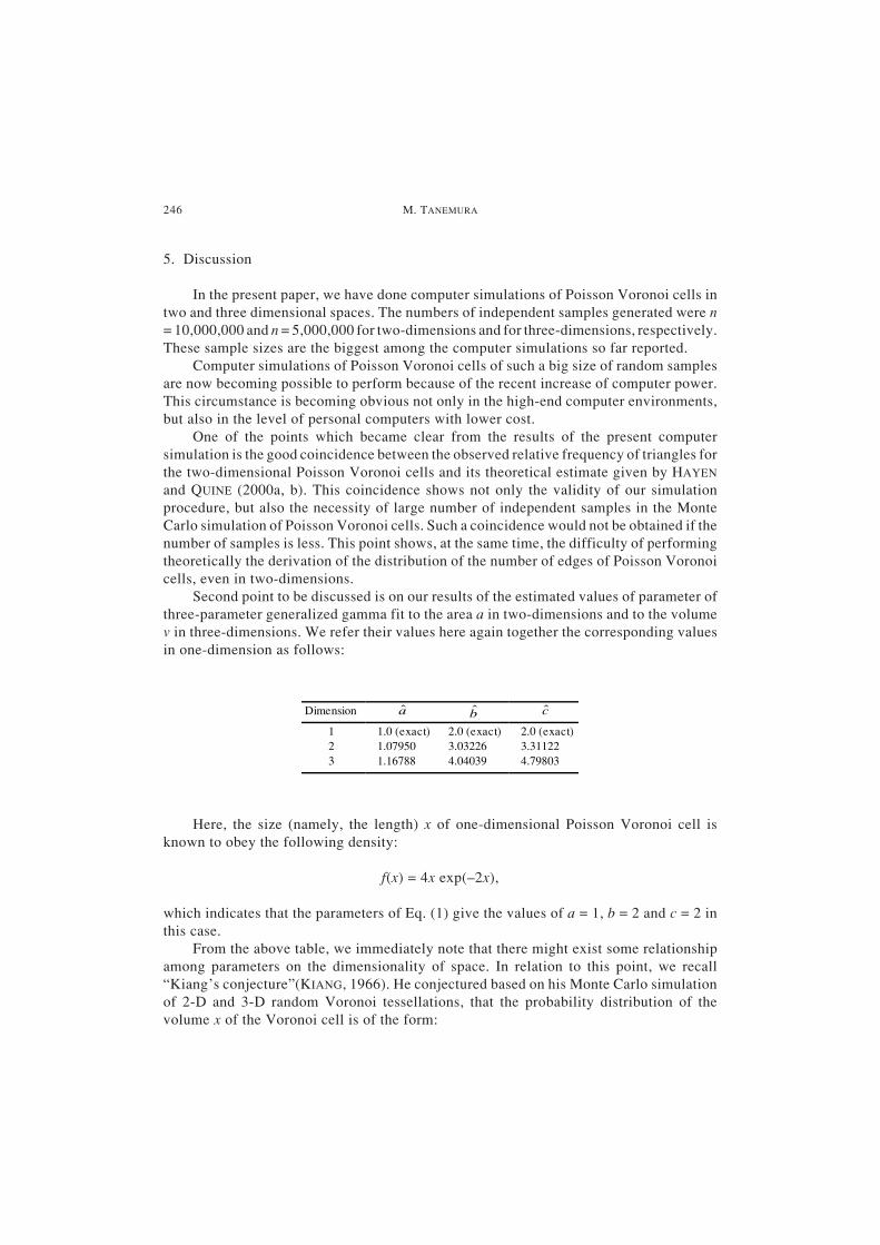
Second point to be discussed is on our results of the estimated values of parameter ofthree-parameter generalized gamma fit to the area a in two-dimensions and to the volumev in three-dimensions. We refer their values here again together the corresponding valuesin one-dimension as follows:

Dimension a b c

1 1.0 (exact) 2.0 (exact) 2.0 (exact)2 1.07950 3.03226 3.311223 1.16788 4.04039 4.79803

Here, the size (namely, the length) x of one-dimensional Poisson Voronoi cell isknown to obey the following density:

f(x) = 4x exp(–2x),

which indicates that the parameters of Eq. (1) give the values of a = 1, b = 2 and c = 2 inthis case.

From the above table, we immediately note that there might exist some relationshipamong parameters on the dimensionality of space. In relation to this point, we recall“Kiang’s conjecture”(KIANG, 1966). He conjectured based on his Monte Carlo simulationof 2-D and 3-D random Voronoi tessellations, that the probability distribution of thevolume x of the Voronoi cell is of the form:


f x x x d( ) =( ) ( ) −( ) =−αα

α α αα

Γ1 2exp ;

where d is the dimension of space. Later, the Kiang’s conjecture was denied by TANEMURA

(1988) through his computer simulation of 3-D Poisson Voronoi tessellation. In TANEMURA

(1988), n = 100,000 Voronoi cells are randomly sampled from fifty independent realizationsof 4000 point Poisson point processes. Then, the empirical distribution of the volume ofVoronoi cells was fitted to the three-parameter generalized gamma distribution (1) usinga non-linear least-squares method. The estimated values of parameters were a = 1.409, b= 2.813 and c = 4.120, which showed a discrepancy from the Kiang’s conjecture, namely,a = 1, b = 4 and c = 4. It will be clear that the above estimated values of present investigationagain reject Kiang’s conjecture. However, we note there might be a certain tendencybetween the parameter values and the dimension of space as was stated. Thus, it will beinteresting to investigate the Poisson Voronoi cells in higher dimensions.

This research was partly supported by the Grant-in-Aid for Scientific Research (C) No.10680326 and No. 13680379 from the Ministry of Education, Science, Sports and Culture of Japan.The author is also grateful to the referee whose comments were helpful to improve the manuscript.

REFERENCES

GILBERT, E. N. (1962) Random subdivision of space into crystals, Annals of Math. Statist., 33, 958–972.HAYEN, A. and QUINE, M. (2000a) The proportion of triangles in a Poisson-Voronoi tessellation of the plane,

Advances in Appl. Prob. (SGSA), 32, 67–74.HAYEN, A. and QUINE, M. (2000b) Calculating the proportion of triangles in a Poisson-Voronoi tessellation of

the plane, J. Statist. Comput. Simul., 67, 351–358.HINDE, A. L. and MILES, R. E. (1980) Monte Carlo estimates of the distributions of the random polygons of the

Voronoi tessellation with respect to a Poisson process, J. Statist. Comput. Simul., 10, 205–223.KIANG, T. (1966) Random fragmentation in two and three dimensions, Z. Astrophys., 64, 433–439.KUMAR, S., KURTZ, S. K., BANAVAR, J. R. and SHARMA, M. G. (1992) Properties of a three-dimensional Poisson-

Voronoi tessellation: a Monte Carlo study, J. Statist. Phys., 67, 523–551.MEIJERING, J. L. (1953) Interface area, edge length, and number of vertices in crystal aggregates with random

nucleation, Philips Research Rep., 8, 270–290.MILES, R. E. (1970) On the homogeneous planar Poisson point process, Mathematical Biosciences, 6, 85–127.MØLLER, J. (1994) Lectures on Random Voronoi Tessellations, Springer, New York.OKABE, A., BOOTS, B. SUGIHARA, K. and CHIU, S. N. (2000) Spatial Tessellations: Concepts and Applications

of Voronoi Diagrams, 2nd Ed., John Wiley & Sons, Chichester.TANEMURA, M. (1988) Random packing and random tessellation in relation to the dimension of space, J.

Microscopy, 151, 247–255.TANEMURA, M., OGAWA, T. and OGITA, N. (1983) A new algorithm for three-dimensional Voronoi tessellation,

J. Computational Phys., 51, 191–207.

statistical distributions of poisson voronoi cells in …...statistical distributions of poisson...

Documents