statistical geometrical features for texture classification

8/11/2019 Statistical Geometrical Features for Texture Classification

http://slidepdf.com/reader/full/statistical-geometrical-features-for-texture-classification 1/16

Pattern Recognition, Vol. 28, No. 4, pp. 537-552, 1995

Elsevier Science Ltd

Copyright @ 1995 Pattern Recognition Society

Printed in Great Britain. All rights reserved

0031-3203/95 $9.50 + 03

0031-3203 94)00116-2

STATISTICAL GEOMETRICAL FEATURES FOR

TEXTURE CLASSIFICATION

YAN QIU CHEN,* MARK S. NIXON and DAVID W. THOM AS

Department of Electronics and Comp uter Science, University of Southampto n, U.K.

(Received 9 Februar y 1994; i n evi sedform 24 August 1994; recei ved or publ i cati on 1 Sept ember 1994)

Abstract-This paper proposes a novel set of 16 features based on the statistics of geometrical attributes of

connected regions in a sequence of binary imag es obtained from a texture image. Systematic comparison

using a l l the Brodatz textures shows that the new set achieves a higher correct classification rate than the

well-known Statistical Gray Level Dependence Matrix method, the recently proposed Statistical Feature

Matrix, and Liu ’s features. The deterioration in performance with the increase in the number of textures in

the set is less with the new SGF features than with the other methods, indicating that SG F is capable of

handling a larger texture population. The new method’s performance under additive n oise is also shown to

be the best of the four.

Texture analvsis

Feature extraction

Statistical features

Geometrical features

Additive noise

1. INTRODUCTION

Texture plays an important role in image analysis and

understanding. Its potential applications range from

remote sensing, quality control, to medical diagnosis

etc. As a front end in a typical classification system,

texture feature extraction is of key significance to the

overall system performance. Many papers have been

published in this area, proposing a number of various

approaches.

Structural approaches(rm3’ are based on the theory

of formal languages: a texture image is regarded as

generated from a set of texture primitives using a set

of placement rules. These approaches work well on

“ deterministic” textures but most natural textures, un-

fortunately, are not of this type.

From a statistical point of view, texture images are

complicated pictorial patterns, on which, sets of statis-

tics can be obtained to characterize these patterns. The

most popularly used one is the Spatial Grey Level

Dependence Matrix (SGLDM ) method,‘435 ) which con-

structs m atrices by counting the number of occur-

rences of pixel pa irs of given gray levels at a given

displacement. Statistics like contrast, energy, entropy

and so forth are then applied to the matrices to obtain

texture features. These statistics are largely heuristic,

although Julesz’s conjectureC6) about the human eyes’

inability to discriminate-between textures differing only

in third or higher order statistics is an indication of the

appropriateness of the method. Other schemes include

the Statistical Feature Matrix” ) and the Texture Spec-

trum.(8.g)

A two-dimensional power spectrum of a texture

image often reveals the periodicity and directionality

* Author to whom all correspondence should be addressed.

of the texture. For example, a coarse texture tends to

generate low frequency components in its spectrum

while a fine texture will have high frequency compo-

nents. Stripes in one direction cause the power spec-

trum to concentrate near the line through the origin

and perpendicular to the direction. Fourier transform

based methodsoO~“) usually perform well on textures

showing strong periodicity, their performance signifi-

cantly deteriorates, though, when the periodicity

weakens.

Stochastic models such as two-dimensional ARM A,

Marko v random fields etc. can also be used for texture

feature extraction via parameter estimation.(‘2-15) These

approaches consider textures as realizations of a ran-

dom process. Structural and geometrical features ap-

pearing in textures are largely ignored. Other difti-

culties such as that in choosing an appropriate order

for a model have also been reported.

This paper proposes a novel set of sixteen texture

features based on the statistics of geometrical pro-

perties of connected regions in a sequence of binary

images obtained from a texture image. Th e first step

of the approach is to decompose a texture image into

a stack of binary images. Th is decomposition has been

proven to have the advantage of causing no informa-

tion loss, and resulting in binary images that are easier

to deal with geometrically. For each binary im age,

geometrical attributes such as the number of con-

nected regions and their irregularity are statistically

considered. Sixteen such statistical geo metrical fea-

tures are proposed in this paper.

2. THE STATISTICAL GEOMETRICAL FEATURES

An n, x nY digital image with n, grey levels can

be modelled by a 2D function f(x. y). where (x, y)~

531



538

Y. Q. CHEN et a [.

(O,l,..., n,-1)x (0,1,..., n,--l}, and f(x,Y)~

0, 1,. . , n, - l}. f(x, Y ) is termed the intensity of the

pixel at (x, y).

When an image f(x,Y) is thresholded with a thresh-

oldvaluecc,ccE{l,...,

nl - l}, a corresponding binary

image is obtained, that is

1

fb(% Y; x) =

if f(x,y) 2 c(

0 otherwise .

1)

where fb(x,Y; a) denotes the binary image obtained

with threshold a.

For a given original image, there are n, - 1 potenti-

ally different binary images, i.e. fb x, ; ), fb(x, y; 2), ,

f c, y; n, -

1). This set of binary images shall be termed

a binary image stack. For images of a given size and

of a given number of grey levels, the above defined

mapping (of the space of images into the space of

binary image stacks) is bijective (one-to-one and onto),

which guarantees that no loss of information is en-

tailed by this transform. This is true because

VI- 1

f(%Y) = 1 f&Y; a)

I=1

v(x,y)E{o,1)...) n,-l}{O,l,...) n,-1). (2 )

For each binary image, all l-valued pixels are grouped

into a set of connected pixel groups termed connected

regions. The same is done to all O-valued pixels. (Ap-

pendix A presents formal definition and an algorithm.)

Let the number of connected regions of l-valued pixels

in the binary image fb(x, y; LZ) e denoted by NOC,(a),

and that of O-valued pixels in the same binary image

by NOC,(a). Both NOC,(a) and NOC,(a) are func-

tions of a, c(E{ ~,. ..,n, - 1).

To each of the connected regions (of either l-valued

pixels or O-valued pixels), a measure of irregularity

(un-compactness) is applied, which is defined to be

l+,/;;mlJ(xi-x)~+(yi-)i)~

irregularity =

Y/TV

- 1,

(3)

where

cxi

g4.i

x _ lEZ ) -

14

y=II’

(4)

I is the set of indices to all pixels in the connected

region con cerned, 111 enotes the cardinality of the set

I (the num ber of elements in I). (2, Y) Can be thought

of as the centre of mass of the connected region under

the assumption that all the pixels in the region are of

equal weight.

Alternatively, the usual measure of compactness

(circularity) can be used, which is defined as

4&i

where

compactness = ~

perimeter’

(5)

perimeter1 [fbCxi 13Yi)

Ofb Xi,

Yi +

.fbfxi 12

i)

ieZ

0 fbtxi> Yi + fbtxi Yi - ‘1O.fbCxi Yi)

+btXi2Yi + l)Ob XiiYi)lr

6)

@ denotes the logic XOR op erator, that is

I

ifx Y

xoy= ^

[U

x=y

(Appendix B discusses the properties of the irregularity

measure and the compactness measure in detail.)

As stated, a digital image corresponds to n, - 1

binary images, each of which, in turn, comprises a few

connected regions (of l-valued pixels and of O-valued

pixels). Let the irregularity of the ith connected region

of l-valued pixels (O-valued pixels, respectively) of the

binary image

fb x, y;

a) be denoted by IRGL,(i,a)

[IRGL,(i, a), respectively]. The average (weighted by

size) of irregularity of the regions of l-valued pixels in

the binary image fb(x, y; a) is defined to be

IRGL, a) = CiEzCNOPl i, ).ZRGhk 4

Ci,,NOPl i, 4

’

@I

where

NOP,(i,a)

is the numbe r of pixels in the ith

connected region of l-valued pixels of the binary image

fb(x, y; r). ZRGL,(cr) is similarly defined.

By now, four functions of cI, i.e., NOC i(a), NOC ,(a),

ZRGL,(a), ZRGL,(x), have been obtained, each of which,

is further characterized using the following four statis-

tics

max

vaue

max s a),

(9)

l<lr<?l-1

(10)

verage val ue =

“;I s(a):

1 a

sample mean =

x”llll &) y$; u. dx)

11)

a 1

sample S.D. =

J

12)

where g(z) is one of the four functions: NOC ,(a),

NO&(a), ZRGL,(a), ZRGZ ).

The same procedures apply if the alternative com-

pactness measure is to be used. In all, there are 16

feature measures for a texture image, four obtained from

NOCl(a), four from NO&(a), four from ZRGL,(x), and

another four from ZRGL,(a).

3. EXPERIMENTAL EVALUATION

3.1. The

dat abase

The set of all 112 texture pictures in the Brodatz’s

photographic atlas of textures was organized into three

groups. The first group comprises four sets with each

having 28 pictures, that is, the first set includes pictures

Dl through D28 , the second set includes pictures D2 9



Statistical g eometrical features for texture classification

539

through D56 , and so on. The second group consists of

two sets, the first set contains pictures Dl through

D56 , the second set contains pictures D57 through

D11 2. The third group is made up of the whole set,

namely, pictures D l through D11 2. The database was

arranged to ensure a systematic comparison of algo-

rithms.

Each texture picture in the atlas was scanned by an

HP flat bed scanner to produce a 256 x 256 x 8 digital

image, from which, sixteen 64 x 64 x 8 sub-images

were obtained using perfectly aligned 64 x 64 win-

dows. Nine of them were then randomly chosen as

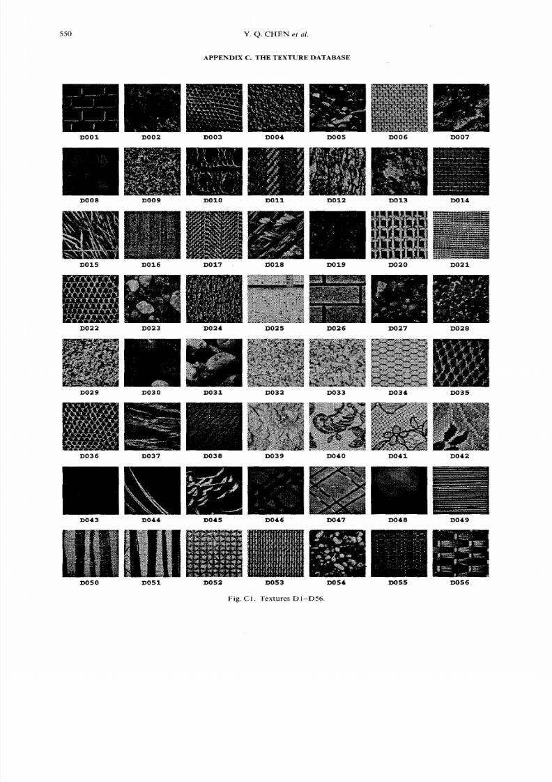
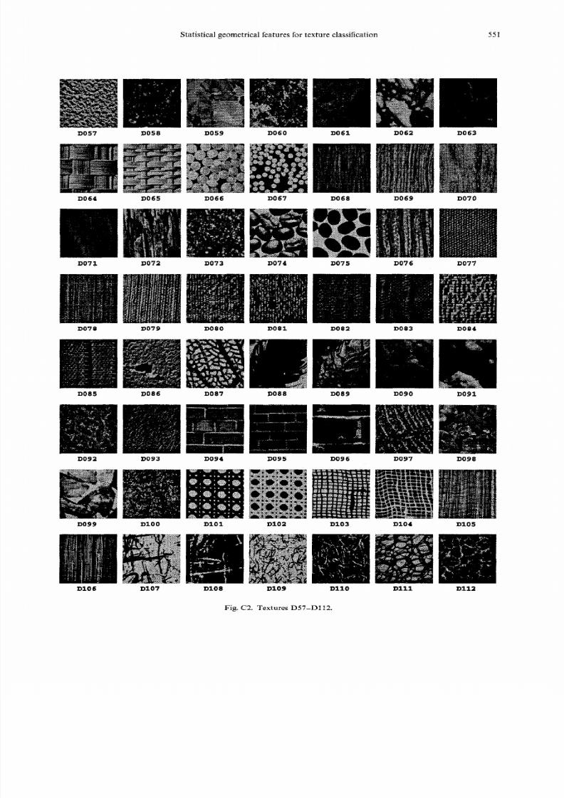
samples. One sub-image for each texture is shown in

Fig. Cl and C2 in appendix C.

3.2. Three other techniques for compar i son

Three other methods along with the Statistical Geo-

metrical Features (SGF) proposed in this paper were

tested on the same aforementioned database under the

same conditions for comparison.

(1) The Spatial G rey Level Dependence Matrix

(SGLD M) approach (4) is popularly used for extract-

ing texture features. Five commonly used features as

suggested in (5): energy, entropy, correlation, local

homogeneity and inertia were computed in our experi-

ments.

(2) Liu’s features (11) are one of the many methods

based on the Fourier Transform. Eight optimal fea-

tures (as proposed by the authors) fl, f2, f5, fi7, fro,

fZ1.fZ5,

f z 6 e r e s e d

(3) The recently proposed Statistical Feature Ma-

trix (SFM) method (7) was claimed to have superior

performance over SGLD M and Liu’s features and

therefore was considered in our experiments. The ma-

trices M,,,

of size 4 x 4 and 8 x 8 were used.

There are 255 binary images obtainable from an

S-bit grey level digital image. T o reduce computation al

costs, 63 binary images (evenly spaced thresholds, i.e.

CI= 4, 8, 12,. ,252) were used in the experiments.

3.3. Feature normalization

All the features were standardized (normalized) by

their sample m eans a nd S.D.‘s which amou nts to say-

ing that every component was normalized using the

following equation

f:=fi-q i=l2,

, , ..,n,

(13)

0

where

p = ’ i it

(14)

Izi=l

(15)

n is the number of samples.

The k-nearest neighbour rule using the Euclidean

distance and the “ leave one out” estimate”@ were then

adopted for feature evaluation (k = 3). The k-nearest

neighbour rule is popularly used in cases where the

underlying probability distribution is unknow n, and

the “ leave one out” estimate is unbiased and generally

desirable when the number of available samples for

each class is relatively small.

3.4. Classifi cati on result s and discussions

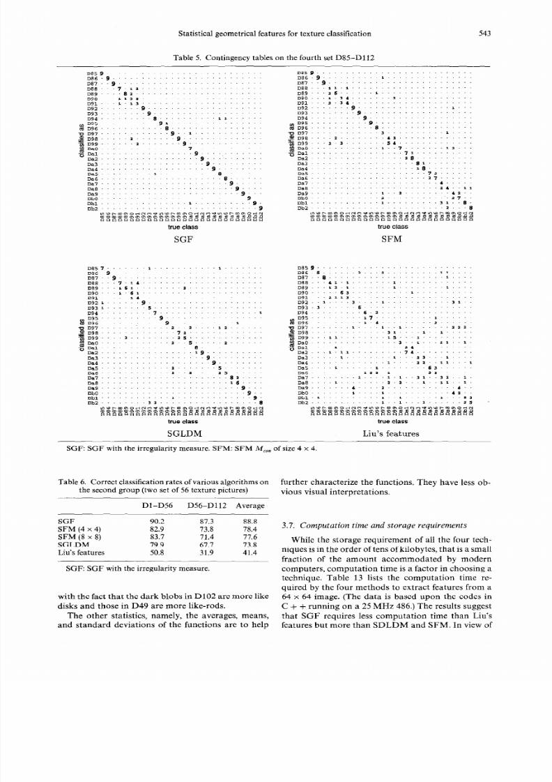
On the first group of the four sets Dl-D28 , D29 9D5 6,

D57-D84 and D85-D112, it is seen from Table 1 that

SGF’s average correct classification rate is 92.1x , wh ich

is substantially higher than tha t of the other three

techniques. A further look at the contingency tables

(confusion matrices) as shown in Tables 2-5 gives

more detailed information:

On the first set Dl-D28 , classification with SGF is

accurate with the exception of misclassification on

some rock/stone textures (D2, D5, D7, D23, D27 and

D28 ) and tree bark textures (D12 , D13). This is under-

standable because these rock/stone/tree bark images

are non-stationary and its texture properties vary con-

siderably with the location of the window; see Figure

Cl in appendix. SFM’s correct classification rate is a

little higher than that of SGF on this set but it mis-

classifies nine textures into 1 2 wrong classes as against

SGF’s misclassifying eight textures into nine wrong

classes. SGLD M’s performance is poorer tha n the

previous two. Liu’s features can only correctly classify

Dl, D4, D8, Dll and D21.

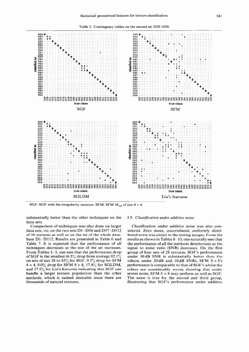
On the second set D29 9D5 6, SGF correctly classi-

fies the textures with the exceptio n of some m isclassifi-

cation between two similar pebbles D3 0 and D31 one

on D50, and some misclassification among D43, D44

and D45 which is also understandable since D43 , D44

and D4 5 contain patterns much larger than the win-

dow hence information obtainable within the window

is inadequate. SFM’s performance is considerably worse.

It misclassifies several textures that are considerably

Table 1. Correct classification rates of various algorithms on the first group(four sets of 28 texture pictures)

SGF

SFM (4 x 4)

SFM (8 x 8)

SGLDM

Liu’s features

Dl-D28 D29-D56 D57-D84

D85-D112

Average

90.8

92.6 93.5

91.5 92.1

93.5 78.3 83.7 72.5 82.0

93.1

80.8 81.7

70.1 81.4

88.4

83.9 76.6

79.2 82.0

62.3

57.4 38.8

42.4 50.2

SGF: SGF with the irregularity measure.



Y. Q. CHEN et al.

Table 2 . Contingency tables on the first set Dl-D28

SGF: SG F with the irregularity measure. SFM: SF M M,,, of size 4 x 4

different, e.g. D30/D 46 and D33/D4 0/D42. SGLDM ’s

discriminating ability is also considerably lower than

that of SGF. Liu’s features can only correctly classify

D29, D37, D47 and D48.

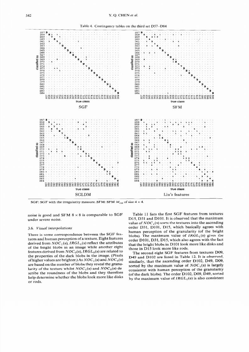
On the third set D57 -D84, SGF’s discrimination

ability is considerably better than the other three tech-

niques in terms of correct classification rates and num-

bers of textures misclassified. Misclassification with

SGF happens on textures that contain very large pat-

terns or appear severely non-stationary. The same is

true on the fourth data set D85 -D11 2.

An alternative assessment of feature vectors is based

on their within-class and inter-class distance distribu-

tions. We wish that the within-class distances of a

feature vector are small and the inter-class distances

are large, thus giving a small overlapping area, ideally

zero, since the smaller the area the less possibly pat-

terns are to be misclassified although the ordering

might not be strict.

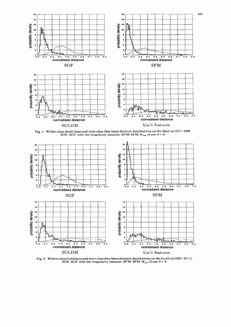
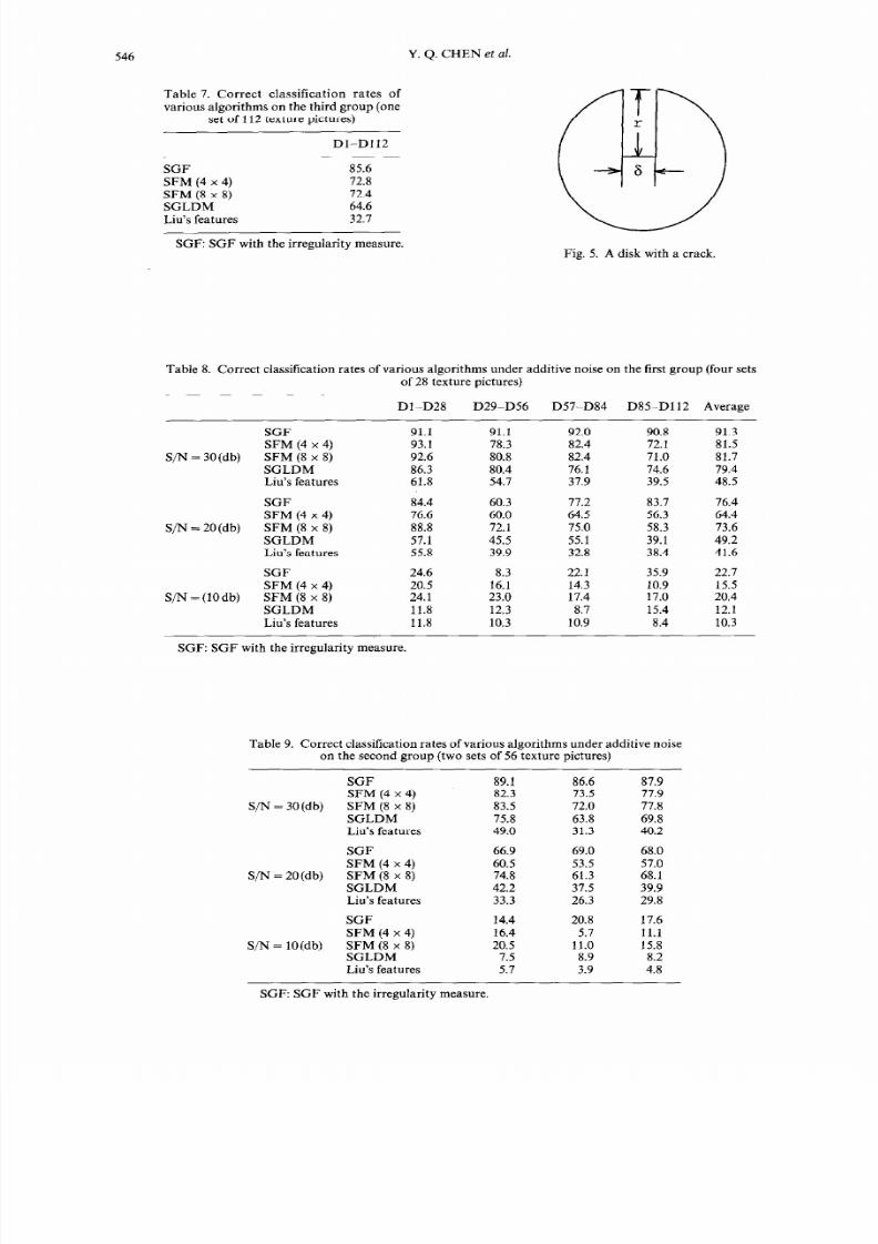
Figures l-4 show the distance distributions with the

four techniques on the four data sets. It is seen from

Fig. 1 that, o n the first data set Dl-D28 , the over-

lapping area with SGF is the smallest, and that SFM

gives the second smallest overlapping area (slightly

larger than that with SGF), indicating that SGF and

SFM should be the best two

for’

this data set. Figures

2-4 show that the overlapping areas with SGF are

considerably smaller than that with the other tech-

niques on the data sets D29-D56, D57-D84 and D85-

D11 2, indicating that SGF’s performance should be



Statistical geometrical features for texture classification

Table 3. Contingency tables on the second set D29-D56

541

.............

....

..I ......

.............

&Tgg ...........................

D),J.,~.........................

c~l.ng .........................

mz...g ........................

~~3....~... . .1

.................

D34.....9 ......................

~~S.... . .S.,

...................

D36.... . . .g

....................

037. . . . . .1 .6

...................

D3 j.. . . . . . . .5

..................

~~~.........lb...1.............

~MO...........,..~

.............

DDd1.. .......... . ................

~w2,...........I.s

..............

‘1 m: : : : :

..1...12~...........

......

.I..,,2 ...........

U”~...............~,

...........

D46..................g

..........

c~,..........l....l~.~

.........

~&...................g

........

c4g....................g

.......

C~O.....................S...~

..

~~~.............~........~

.....

oyJ.........l.............,

....

Ds)........................g

...

DSP.....................~...,

..

MS.........1 .......... ..a..g.

o~~.........................l .9

~O_NOI~~Prn~O_NOI~~Frn~~_~~~~~

N~~~O~~~OO~~~~~~~~~~~~~~~~~~

~~~~~~~O~~~~OP~~~~~~~~~~~~~~

true class

SGLDM

~~~~...........~...~

...........

~.j().,i..............r

..........

C~1..,

..................

h ......

c32...gr

.......................

~?_3....,......).1.1..

..........

~~~.....g..........l...........

~~~.... . .~

.....................

D36

..... ..g......l

.............

D37 ....... .g ...................

D3&........g1.....1

...........

D39

......... .,....~~

...........

~W~....I......I.6r.1......~.~

..

-oorl............*..l........,

....

ED42

......... ..,.iI

.............

3

~~3..............1~............

D~~..............rl............

~c~5...........1....1=

..........

~~6.,I.............lb

..........

047..............1...g

.........

~~8..........1...~....~

........

~~s....................g

.......

~~~...............~.....g

......

D~~......................~

.....

DQ

............

..l........s

....

DS)

.....................

.g ...

~~4.............r...........~

..

~~~................l.........~.

DS6

.........................

..g

~03Nn~~~Pm~O_NOI~~Pm~~-~~~~~

N~~nn~~O~~Olllllllll~~~~~~~~

~~~~~P~~~~~~~~~~~~P~~~~~~~~~

true class

SFM

~~.gg...........>

...............

~2_l).&I..................~

......

D?+1.1S.... . .1... . ..I

..........

~32...b~.......~...............

~~3...11.......)

...............

~~~.... .* .2.1r..1

..............

c~s......rl..,~

................

D36......~r....II

..............

D3y

....... g.....r

.............

D3s..1......I.I...~~

...........

D3~......r...rlr..11......1....

gMfJ.........rl,...ll........,

..

no~~...1,..~.li.1...............

.p 012 .

....... .11.

.s...........1..

~~~3..............,5,

...........

t$~~*.........~....3.1

...........

OD~s...........r..I

.............

c46.r...............*

..........

D~7.....1............g

.........

~~s...................g

........

odg....................8.1

.....

DScJ.11... ............

..d..) ...

~~l.,.............I....l.s

.....

~~2.......................,..~.

~yj.~...................r..,

...

D54.......r...,.~...........s

..

D~~.........~...........I.r..~ 2

~~~..l.......................~ s

~O-N~~~~Pm~O-NnC~~Pm~~-~~~~~

N~0~0n~~~0011CC11111~~~~~~~~

~~~~~~~P~O~~~~~~OO~~~~~~~~~~

true class

Liu’s features

SGF: SGF with the irregularity measure. SFM: SFM M,,, of size 4 x 4.

substantially better than the other techniques on the

data sets.

3.5. Classif icati on under addit iv e noise

Comparison of techniques was also done on larger

Classification under additive noise was also con-

data sets, viz. on the two sets Dl-D56 and D57 -D11 2

sidered. Zero mean, uncorrelated, uniformly distri-

of 56 textures as well as on the set of the w hole data-

buted noise was added to the testing images. From the

base Dl-D1 12. Results are presented in Table 6 and results as shown in Tables 8-10, one naturally sees that

Table 7. It is expected that the performance of all the performance of all the methods deteriorates as the

techniques decreases as the size of the set increases.

signal to noise ratio (SNR ) decreases. On the first

From Tables 1-3, one sees that the performance drop

group of four sets of 28 textures, SGF’s performance

of SGF is the smallest (6.5% drop from av erage 92.1%

under 30dB SN R is substantially better than the

on sets of size 28 to 85% for SGF, 9.2% drop for SFM others; under 20dB and 1OdB SNRs, SFM 8 x 8’s

4 x 4, 9.0% drop for SFM 8 x 8, 17.4% for SGLD M, performance is comparable to that of SGF’s whilst the

and 17.5% for Liu’s features) indicating that SGF can others are considerably worse, showing that und er

handle a larger texture population than the other severe noise, SFM 8 x 8 may perform as well as SGF.

methods, which is indeed desirable since there are

The same is true for the second and third group,

thousands of natural textures.

illustrating that SGF’s performance under additive



Y. Q. CHEN et al.

Table 4. Contingency tables on the third set D57-D84

SGF SFM

true class

noise is good and SFM 8 x 8 is comparable to SGF

under severe noise.

3.6.

Visual interpolations

There is some correspondence between the SGF fea-

tures and human perception of a texture. Eight features

derived from NOC ,(a), IRGL,(cc) reflect the attributes

of the bright blobs in an image while another eight

features derived from NO& (a), ZRG L,(a) are related to

the properties of the dark blobs in the image. (Pixels

of higher values are brighter.) As NOC , (CX)nd NOC,(a)

are based on the number of blobs they reveal the granu-

larity of the texture whilst NOC ,(5r) and NO& (a) de-

scribe the roundness of the blobs and they therefore

help determine whether the blobs look more like disks

or rods.

Table 11 lists the first SGF features from textures

D15, D31 and DlOl. It is observed that the maximum

value of NOC ,(cr) sorts the textures into the ascending

order D3 1, DlOl, D15 , which basically agrees with

human perception of the granularity (of the bright

blobs). The maxim um value of IRGL l(a) gives the

order DlOl, D31 , D15 , which also agrees with the fact

that the bright blobs in DlOl look mo re like disks and

those in D15 look more like rods.

The second eight SGF features from textures D09 ,

D49 and D10 2 are listed in Table 12. It is observed,

similarly, tha t the ascending order D10 2, D49 , D09 ,

sorted by the maximu m value of NOC ,(x) is largely

consistent with human perception of the granularity

(of the dark blobs). The order D10 2, D0 9, D49, sorted

by the maxim um value of IRGL,(a) is also consistent




Table 5. Contingency tables on the fourth set D85-D112

SFM

Table 6. Correct classification rates of various algorithms on

further characterize the functions. They have less ob-

the second group (two set of 56 texture pictures)

vious visual interpretations.

Dl-D56

D56-D112 Average

SGF

90.2 87.3 88.8

SFM (4 x 4)

82.9 73.8 78.4

SFM (8 x 8)

83.7 71.4 77.6

SGLDM

79.9 67.7 73.8

Liu’s features

50.8 31.9 41.4


with the fact that the dark blobs in D1 02 are more like

disks and those in D49 are more like-rods.

The other statistics, namely, the averages, means,

and standard deviations of the functions are to help

3.7. omputation time and storage requirements

While the storage requirement of all the four tech-

niques is in the order of tens of kilobytes, that is a small

fraction of the amou nt accommod ated by modern

computers, computation time is a factor in choosing a

technique. Table 13 lists the computation time re-

quired by the four methods to extract features from a

64 x 64 image. (The data is based upon the codes in

C + f running on a 25 MHz 486.) The results suggest

that SGF requires less computation time than Liu’s

features but more than SD LDM and SFM. In view of



normalised distance

SGLDM

0

0.0 0.1 0.1 0.3 0.1

0.1

0.6 0.7 0.1

0.9

normalised distance

SFM

0

0.0 0.1 0.2

0.3 0.1 0.5

0.c 0.1

0.8 0.9

normalised distance

Liu’s features

Fig. 1. Within-class (bold lines) and inter-class (tine lines) distance distributions on the first set Dl-D28.


normalised distance

SGF

-0.0 0.1 0.1

0.3 0.1 0.5 0.6

0.1 0.. 0.9

normalised distance

SGLDM

0

0.0 0.1 0.1 0.3 0.4

0.5 0.6 0.7 0.s

0.9

normalised distance

Liu’s features

Fig. 2. Within-class (bold lines) and inter-class (fine lines) distance distributions on the second set D299D56.




normalised distance

SGLDM

normalised distance

Liu’s features

Fig. 3. Within-class (bold lines) and inter-class (tine lines) distance distributions on the third set D57-D84.


normalised distance

SGF

0

0.0 0.1 0.1 0.3 0.1 0.5 o. 0.7 0.1 0.9

normalised distance

SGLDM

0.0 0.1 0.1 0.3 0.. 0.5 0.6 0.7 o.* 0.9

normalised distance

Liu’s features

Fig. 4. Within-class (bold lines) and inter-class (fine lines) distance distributions on the fourth set D85-D112.

SGF: SGF with the irregularity measure. SFM: SFM

M

of size 4 x 4.



546

Y. Q. CHEN et al.

Table 7. Correct classification rates of

various algorithms on the third group (one

set of 112 texture pictures)

Dl-D112

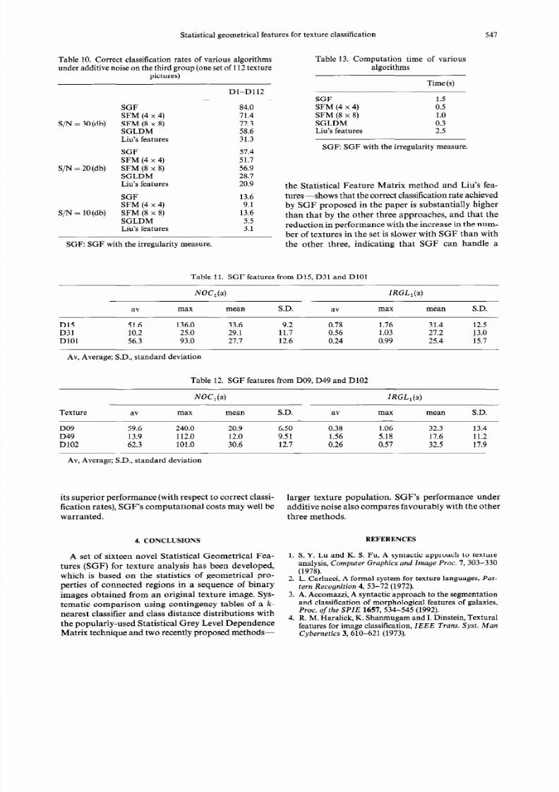
SGF 85.6

SFM (4 x 4)

72.8

SFM (8 x 8)

72.4

SGLDM 64.6

Liu’s features 32.7


c

Fig. 5. A disk with a crack.

Table 8. Correct classification rates of various algorithms under additive noise on the first group (four sets

of 28 texture pictures)

Dl-D28 D29-D56 D57-D84

D85-D112 Average

SGF 91.1 91.1 92.0 90.8 91.3

SFM (4 x 4) 93.1 78.3 82.4 72.1 81.5

S/N = 30(db) SFM (8 x 8) 92.6 80.8 82.4 71.0 81.7

SGLDM 86.3 80.4 76.1 74.6 79.4

Liu’s features 61.8 54.7 37.9 39.5 48.5

SGF 84.4 60.3

SFM (4 x 4) 76.6 60.0

S/N = 20 (db) SFM (8 x 8) 88.8 72.1

SGLDM 57.1 45.5

Liu’s features 55.8 39.9

SGF 24.6 8.3

SFM (4 x 4) 20.5 16.1

S/‘N=(lOdb) SFM (8 x 8) 24.1 23.0

SGLDM 11.8 12.3

Liu’s features 11.8 10.3


17.2

64.5

75.0

55.1

32.8

22.1

14.3

17.4

8.7

10.9

83.7 76.4

56.3 64.4

58.3 73.6

39.1 49.2

38.4 41.6

35.9 22.7

10.9 15.5

17.0 20.4

15.4 12.1

8.4 10.3

Table 9. Correct classification rates of various algorithms under additive noise

on the second group (two sets of 56 texture pictures)

SGF 89.1

SFM (4 x 4)

82.3

S/N = 30 (db) SFM (8 x 8)

83.5

SGLDM 75.8


SGF 66.9

SFM (4 x 4) 60.5

S/N = 20 (db) SFM (8 x 8)

74.8

SGLDM 42.2


SGF 14.4

SFM (4 x 4) 16.4

S/N = lO(db) SFM (8 x 8)

20.5

SGLDM 7.5



86.6 87.9

73.5 77.9

72.0 77.8

63.8 69.8

31.3 40.2

69.0 68.0

53.5 57.0

61.3

68.1

37.5 39.9

26.3 29.8

20.8 17.6

5.7 11.1

11.0 15.8

8.9

8.2

3.9

4.8



Statistical geometrical features for texture classification 541

Table 10 . Correct classification rates of various algorithms

under additive noise on the third g roup (one set of 112 texture

pictures)

Dl-D112

SGF

84.0

SFM (4 x 4)

71.4

S/N = 30 (db) SFM (8 x 8)

72.3

SGLDM

58.6


SGF

57.4

SFM (4 x 4) 51.7

S/N = 20 (db) SFM (8 x 8) 56.9

SGLDM 28.7

Liu’s features

20.9

SGF

SFM (4 x 4)

13.6

9.1

13.6

5.5

3.1

S/N = 10 (db)

SFM (8 x 8)

SGLDM

Liu’s features


Table 13. Comp utation time of various

algorithms

Time(s)

SGF 1.5

SFM (4 x 4) 0.5

SFM (8 x 8) 1.0

SGLDM 0.3



the Statistical Feature Matrix method and Liu’s fea-

tures-shows that the correct classification rate achieved

by SGF proposed in the paper is substantially higher

than that by the other three approaches, and that the

reduction in performance with the increase in the num-

ber of textures in the set is slower with SGF than with

the other three, indicating that SGF can handle a

Table 11. SGF features from D15, D31 and DlOl

av

NGb)

lRGL, a)

max mean S.D.

av

max mean S.D.

D15 51.6 136.0 33.6 9.2 0.78 1.76 31.4 12.5

D31 10.2 25.0 29.1 11.7 0.56 1.03 27.2 13.0

DlOl 56.3 9 3.0 27.7 12.6 0.24 0.99 25.4 15.7

Av, Average; S.D., standard deviation

Table 12. SGF features from D09, D49 and D102

Texture

av

NOCl 4

lRGL, a)

max

mean

S.D.

av

max

mean S.D.

DO9 59.6 240.0 20.9 6.50 0.38 1.06 32.3 13.4

D49 13.9 112.0 12.0 9.51 1.56 5.18 17.6 11.2

D102 62.3 101.0 30.6 12.7 0.26 0.57 32.5 17.9

Av, Average; S.D., standard deviation

its superior performance (with respect to correct classi- larger texture po pulation. SGF’s performance under

fication rates), SGF’s compu tational costs may well be additive noise also compares favourably with the other

warranted. three methods.

4. CONCLUSIONS

REFEREN ES

A set of sixteen no vel Statistical Geometrical Fea-

1. S. Y. Lu and K. S. Fu, A syntactic approach to texture

tures (SGF) for texture analysis has been developed,

analysis, Computer Graphics and Image Proc. I, 303-330

which is based on the statistics of geometrical pro-

(1978).

perties of connected regions in a sequence of binary

2. L . Carlucci, A formal system for texture lang uages, Pat-

tern Recognition 4, 53-72 (1972).

images obtained from an original texture im age. Sys- 3. A. Accomazzi, A syntactic approach to the segmentation

tematic comparison using contingency tables of a k-

and classification of morphological features of galaxies,

nearest classifier and class distance distributions with

Proc. oft he SPl E 1657, 534-545 (1992).

the popularly-used Statistical Grey Level Dependence

4. R . M. Haralick, K. Shanm ugam and I. Dinstein, Tex tural

Matrix technique and two recently proposed methods-

features for image classification, I EEE Trans. Syst. M an

Cybernetics 3,610-621 (1973).



548

Y. Q. CHEN et al.

5

6.

7.

8.

9.

10.

11.

12.

13.

14.

15.

16.

R. W. Conners and C. A. Harlow, A theoretical com-

parison of texture algorithms, IEEE Trans. Patt ern Ana-

l ysi s M ach. I nt el l. 2, 204-222 (1980).

B. Julesz, Visual pattern discrimination, IR E Trans. Inf

Theory 8,84-92 (1962).

C.

M. Wu and Y. C. Chen, Statistical feature matrix for

texture analysis,

CVGIP: Graphi cal M odels Image Proc.

54,407-419 (1992).

D. C. He and L. Wang, Texture unit, texture spectrum

and textute analysis, I EEE Trans. Geosci . Remot e Sensing

28,509-512 (1990).

D. C. He and L. Wang, Texture features based on texture

spectrum,

Pat tern Recognit i on 24, 391-399 (1991).

C.

H. Chen, A study of texture classification using spec-

tral features, Proc. Sixth Int. Conf. Pattern Recognition

1074-1077 (1982).

S. S. Liu and M. E. Jernigan, Texture analysis and dis-

crimination in additive noise, Computer Visi on Graphi cs

Image Proc. 49,52-67 (1990).

M. Hassner and J. Sklansky, The use of markov random

fields as models of texture,

Computer Graphics Image

Proc. 12,357-370 (1980).

H. Derin and.W. Cole, Segmentation of textured images

using gibbs random fields. Computer Visi on Graphi cs

Image Proc. 35,72-98 (1986).

F. S. Cohen, Z. Fan and M. A. Patel, Classification of

rotated and scaled textured images using gaussian

markov random field models.

ZEEE Trans. Patt ern A na-

l ysi s M ach. I nt el l. 13, 192-202 (1991).

C. S. Won and H. Derin, Unsupervised segmentation of

noisy and textured images using markov random fields.

CVGI P: G raph ical M odels Image Proc. 54308-328 (1992).

P. A. Devijver and J. Kittler, Patt ern Recognit ion: a Sta-

ti stical A pproach. Prentice Hall International, Eagle Cliffs,

New Jersey (1982).

APPENDIX A CONNECTIVITY

Dejni t ion 1. For a given coordinate pair (x, y), the 4-neigh-

bourhood is defined to be the set

N, x, y)

= {(x + l,y),

(x - 1, y), x, Y+ l b (x, Y l)}.

Def in i t ion 2. A pixel p1 at (x,,y,) is said to be a 4-neighbour

of pz at (x,,Y,) if and onl y i f x,,~,)~N,(x,,y,).

Def in i t ion 3. Two pixels p and p’ are 4-connected if and only

if p is a 4-neighbour of p’ and both the grey level 1of p and

the grey level I’ satisfy some condition. e.g. they should be

equal.

Defin i t ion 4. A 4-connecting path between p1 and p. is a

sequence of pixels

(pi );, 1

uch that

pi

and

pi+ 1

or 15

i I

n

1

are 4-connected.

Defin i t ion 5. A 4-connected region is a set of pixels such that

there is at least one 4-connecting path for each pair of pixels

in this set.

A recursive algorithm for traversing a 4-connected region

of gl-valued

gl

= 0 or gl 1) pixels around (x. y) is given as

follows:

getConnectedRegion(int x, int y)

r

if (imageArray[x] [y] = gl) return;

imageArray[x] [y] = 1 - gl;

addPixel (x. y);

getConnectedRegion (x + 1, y);

get ConnectedRegion (x - 1, y);

getConnectedRegion (x, y + );

getConnectedRegion (x, y - 1);

return;

where imageArray [] [] is a two dimensional image array,

addPixel(int, int) is a function to store the pixels in a con-

nected region for analysis.

To obtain all the connected regions from a binary image,

one simply need to sequentially apply the above algorithm to

every pixel of the image. It is easy to see that the computa-

tional complexity for

obtain ing al l

the connected regions in

an image is

o(n)

where n is the number of pixels in the image.

In fact, no more than 6 x n times accesses to f x, y) (an

element of a two-dimensional array), arithmetic comparisons,

and function calls are needed.

APPENDIX B. SHAPE MEASURES

Given a connected region A in the plane, the extent of its

irregularity can be measured by the ratio of its maximum

radius to the square root of its area, where the maximum

radius is defined to be

x=

lxdx, j= lydy. (B2)

A A

where sup is supremum (the least upper bound).

Equation (3) (in main text) is for measuring the irregularity

of a connected region in a digital image, where the factor &

and

two

additive 1s are

introduced

to make the measure

approximate to zero when the region is a disk (the most

compact and hence least irregular region in the usual sense).

This can be seen as

(1) If there is only one pixel in the region, equation (3)

becomes

1+&o

l=.

irregulari ty = ~ -

1

(2) As the space e of the sampling grid [at spacing (E,E)]

approaches 0 the irregularity of a disk becomes

i

1 + ntxJ(xi-a)~+(Y,-j)*

irregulari ty = lim

-1

e-0

fi

1

(B4)

=o

(111 approaches infinity as E approaches 0.)

An alternative shape measure of a connected region in the

plane is the ratio of the square root of its area to its perimeter,

termed compactness or circularity. (The reciprocal of this

measure constitutes a regularity measure that has the same

properties to be discussed later.) Equation 5 (in main text) is

given for measuring the compactness of a region in a digital

image.

It is observed that the two measures, when applied to

digital images, have their respective advantages and dis-

advantages as follows

(1) The irregularity measure is invariant to rotation while

the compactness measure is not.

Proof. For a connected region A in the plane, a spatial

sampling process using a grid of spacing (E,E) gives rise to a

corresponding region A, in a digital image. With moderate

conditions upon A that are satisfied by most natural images,

it is easy to see that as E -to the following independent of the

rotation of

A.

(The area of a pixel is

Ed

the height and width

is E.)




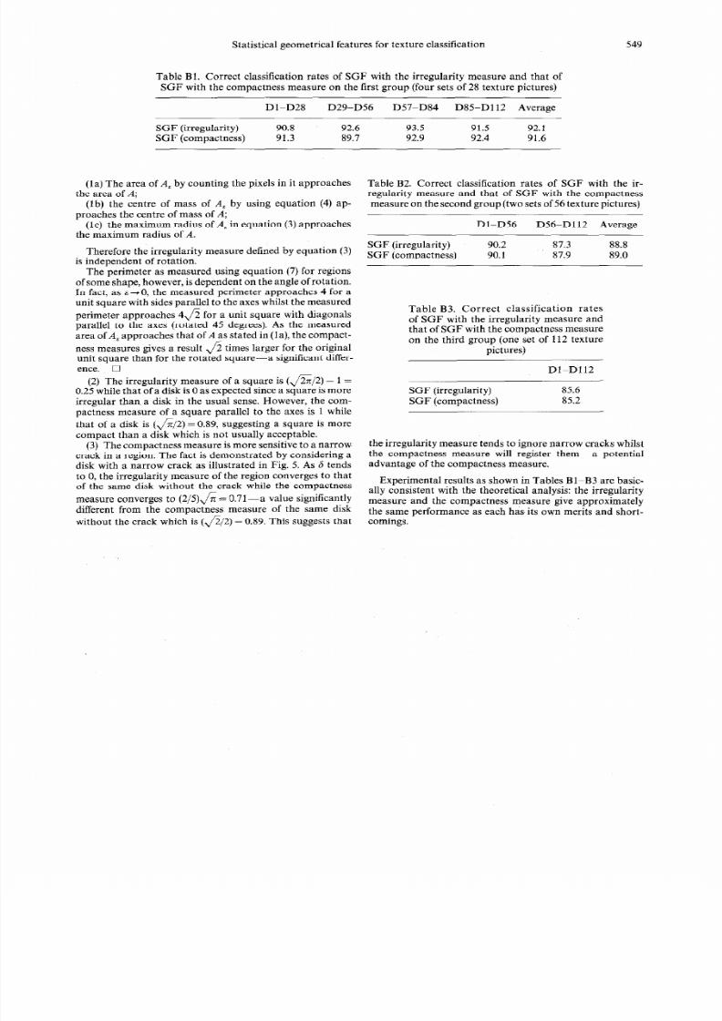
Table Bl. Correct classification rates of SGF with the irregularity measure and that of

SGF with the compactness measure on the first group (four sets of 28 texture pictures)

549

DlLD28 D29-D56

D577D84 D85-D112 Average

SGF (irregularity) 90.8 92.6 93.5 91.5 92.:

SGF (compactness) 91.3 89.7 92.9 92.4 91.6

(la) The area of A, by counting the pixels in it approaches

the area of A;

(lb) the centre of mass of

A

by using equation (4) ap-

proaches the centre of mass of

A;

(lc) the maximum radius of

A

in equation (3) approaches

the maximum radius of

A.

Therefore the irregularity measure defined by equation (3)

is independent of rotation.

The perimeter as measured using equation (7) for regions

ofsome shape, however, is dependent on the angle ofrotation.

In fact, as E + 0, the measured perimeter approaches 4 for a

unit square with sides parallel to the axes whilst the measured

perimeter approaches 4$ for a unit square with diagonals

parallel to the axes (rotated 45 degrees). As the measured

area of A approaches that of A as stated in (la), the compact-

ness measures gives a result fi times larger for the original

unit square than for the rotated square-a significant differ-

ence. 0

(2) The irregularity measure of a square is (@/2) - 1 =

0.25 while that of a disk is 0 as expected since a square is more

irregular than a disk in the usual sense. However, the com-

pactness measure of a square parallel to the axes is 1 while

that of a disk is (,/%/2) = 0.89, suggesting a square is more

compact than a disk which is not usually acceptable.

(3) The compactness measure is more sensitive to a narrow

crack in a region. The fact is demonstrated by considering a

disk with a narrow crack as illustrated in Fig. 5. As 6 tends

to 0, the irregularity measure of the region converges to that

of the same disk without the crack while the compactness

measure converges to (2/5)J;f = 0.71-a value significantly

different from the compactness measure of the same disk

without the crack which is (G/2) = 0.89. This suggests that

Table B2. Correct classification rates of SGF with the ir-

regularity measure and that of SGF with the compactness

measure on the second group (two sets of 56 texture pictures)

SGF (irregularity)

SGF (compactness)

Dl-D56 D56-D112 Average

90.2

87.3

88.8

90.1 87.9 89.0

Table B3. Correct classification rates

of SGF with the irregularity measure and

that of SGF with the compactness measure

on the third group (one set of 112 texture

pictures)

DlpD112

SGF (irregularity)

85.6

SGF (compactness)

85.2

the irregularity measure tends to ignore narrow cracks whilst

the compactness measure will register them-a potential

advantage of the compactness measure.

Experimental results as shown in Tables BlLB3 are basic-

ally consistent with the theoretical analysis: the irregularity

measure and the compactness measure give approximately

the same performance as each has its own merits and short-

comings.



Y. Q. CHE N et al.

APPENDIX C THE TEXTURE DATABASE

DO01 DO02 DO03

DO04 DO05 DO06 DO07

DO08

DO09 DO10 DO11 DO12 DO13 DO14

DO15 DO16 DO17 riO18 DO19

DO20 DO21

DO22 DO23 DO24 DO25 DO26 DO27 DO28

DO29


DO36

DO37

DO38

DO39 DO40 DO41

DO42

DO43 DO44 DO45

DO46

DO47 DO48 DO49

DO50 DO51

DO52 DO53 DO54 DO55 DO56

Fig Cl. Textures Dl-D56.



Statistical geometrical features for texture classification 551

DO57

DO58 DO59 DO6 DO61

DO62 DO63

-___- _.. ..-... _ .-.. -.._ ..__- _

DO64 DO65 DO66

DO67 DO68 DO69 DO7

DO71

DO72

DO73

DO74 DO75 DO76

DO77


DO84

DO65

DO86

DO87 Do88 DO89 DO9

DO91

DO92

DO93

DO94 DO95 DO96 DO97

DO98

DO99

DloO DlOl DlO2 D1 3 DlO4

D1 5

D1 6

D1 7

DlOB D1 9 DllO

Dlll

Dll2

Fig. C2. Textures D57-D112.



552 Y. Q. CHEN et al.

About the Author YAN QIU CHEN received his B.Eng and M.Eng in 1985 and 1988, respectively, from

the Department of Electrical Engineering at Tongji University, Shanghai, P.R. China. He joined the

Shanghai Maritime University in 1988, where he later became a research team leader in the Institute of

Nautical Science and Technology. Mr Chen is currently a research student studying for a Ph.D. in the Vision

Speech and Signal Processing (VSSP) research group in the Department of Electronics and Computer

Science at Southampton University, U.K. His main research interests are in pattern recognition and neural

networks.

About the Author MARK NIXON

is a lecturer in Electronics in Computer Science and is a member of

the VSSP group. His research interests include computer vision and image processing with particular

interests in feature extraction.

About the Author DAVID THOM AS’s

research interests include signal processing both in 1 and 2D. His

research has included vehicle identification, speech signal processing and image processing, including

reconstruction and analysis.

statistical geometrical features for texture classification

Documents