Statistical Inference for Lorenz Curves with Censored Data

by

Frank A Cowell STICERD, London School of Economics and Political Science

and

Maria-Pia Victoria-Feser

Université de Genève

The Toyota Centre Suntory and Toyota International Centres for Economics and Related Disciplines London School of Economics and Political Science Discussion Paper Houghton Street No.DARP/35 London WC2A 2AE June 1998 Tel.: 020-7955 6678 The first author is partially supported by ESRC grants R000235725 and R5550XY8. The second author is partially supported by the 'Fond National Suisse pour la Recherche Scientifique. We are grateful to Elvezio Ronchetti and Christian Schluter for helpful comments, and to Kaspar Richter and Hung Wai Wong for research assistance.

Abstract

Lorenz curves and associated tools for ranking income distributions are commonly

estimated on the assumption that full, unbiased samples are available. However, it is

common to find income and wealth distributions that are routinely censored or

trimmed. We derive the sampling distribution for a key family of statistics in the case

where data have been modified in this fashion.

Keywords: Lorenz curve; sampling errors.

JEL Nos.: C13, D63.

© by Frank A Cowell. All rights reserved. Short sections of text, not to exceed two paragraphs, may be quoted without explicit permission provided that full credit, including © notice, is given to the source. Contact address: Contact address: Professor Frank Cowell, STICERD, London School of Economics and Political Science, Houghton Street, London WC2A 2AE, UK. Email: f.cowell@lse.ac.uk

1 Introduction

The use of Lorenz comparisons in distributional analysis is viewed by many as

fundamental. In order to be able to implement the principles of such comparisons

in practice it is necessary to have appropriate statistical tools. Building on a

classic paper by Beach and Davidson it has become standard practice to apply

statistical tests to distributional comparisons and to construct con¯dence bands

for Lorenz curves and associated tools (Beach and Davidson 1983) (Beach and

Kaliski 1986) (Beach and Richmond 1985).1 However, although the results in

this literature are \distribution-free", in that they impose few restrictions on the

assumed underlying distribution in the population, they do rest upon some fairly

demanding assumptions about the sample - which may be systematically violated

in many practical applications to income- and wealth-distributions. In this paper

we establish results for a more general approach which takes into account some

of these di±culties.

It is now commonly recognised that income and wealth data may have been

censored or trimmed for reasons of con¯dentiality or convenience (Fichtenbaum

and Shahidi 1988). This treatment of the data means that the conventional

analysis - reviewed in Section 3 below - is not applicable. Section 4 derives

analogous results for censored data and shows their relationship to the standard

1For other applications of classical hypothesis testing to ranking criteria see, for example,Beach et al. (1994), ? (?, ?, ?, ?), Bishop et al. (1991), ?), Davidson and Duclos (1997), Steinet al. (1987).

1

literature.

Of course it should be recognised that deriving asymptotic distributions and

moments is just one possible way of providing the statistical tools for testing

distributional comparisons. So, before presenting our results, a word should be

said about other ways of making inference from sample data. An alternative

approach would be to use the bootstrap (Efron 1979, Efron and Tibshirani 1993)

which is particularly suitable in the case of small samples. However, the bootstrap

does not work in every case, especially when the statistic to be bootstrapped is

bounded, as Schenker (1985) and Andrews (1997) have shown. Applications to

Lorenz curves might fail in these special cases, but to prove this is beyond the

scope of the present paper.

2 Terminology and Notation

Let F be the set of all continuous probability distributions and F¤ the subset of

F which is twice di®erentiable with ¯nite mean and variance. Let income be a

continuous random variable X with probability distribution F 2 F and support

on the interval [x; ¹x] µ <, where < is the real line. Write the mean of the

distribution as the functional ¹(F ).

We require three fundamental functionals from F £ [0; 1] to <. Let q 2 [0; 1]

2

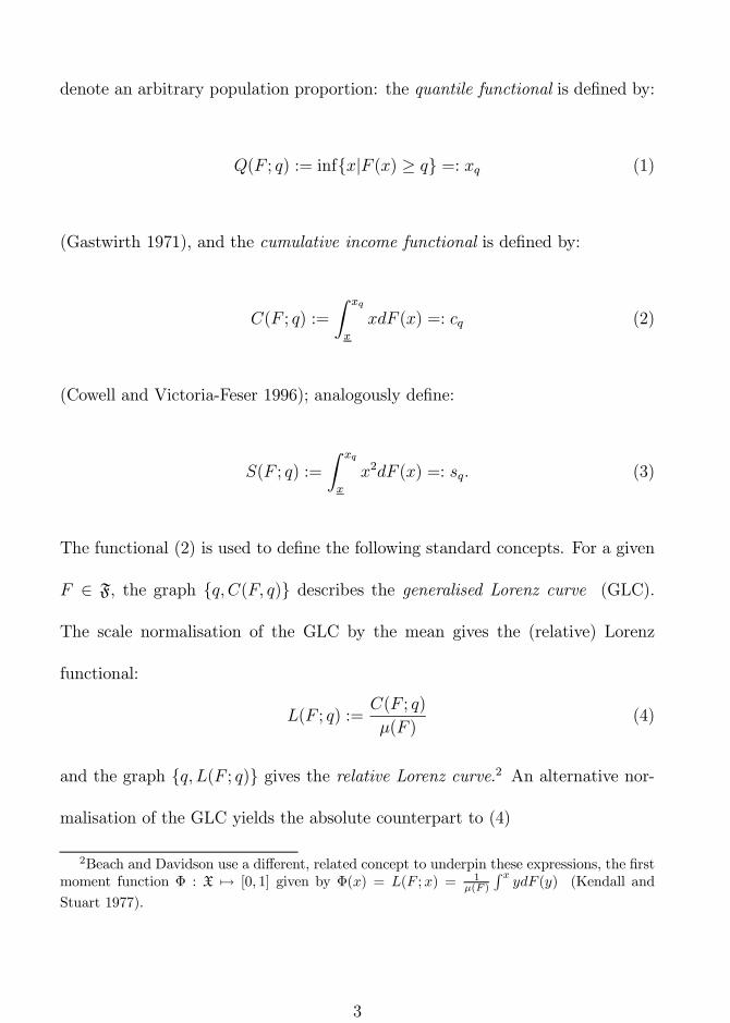
denote an arbitrary population proportion: the quantile functional is de¯ned by:

Q(F ; q) := inffxjF (x) ¸ qg =: xq (1)

(Gastwirth 1971), and the cumulative income functional is de¯ned by:

C(F ; q) :=

Z xq

x

xdF (x) =: cq (2)

(Cowell and Victoria-Feser 1996); analogously de¯ne:

S(F ; q) :=

Z xq

x

x2dF (x) =: sq: (3)

The functional (2) is used to de¯ne the following standard concepts. For a given

F 2 F, the graph fq; C(F; q)g describes the generalised Lorenz curve (GLC).

The scale normalisation of the GLC by the mean gives the (relative) Lorenz

functional:

L(F ; q) :=C(F ; q)

¹(F )(4)

and the graph fq; L(F ; q)g gives the relative Lorenz curve.2 An alternative nor-

malisation of the GLC yields the absolute counterpart to (4)

2Beach and Davidson use a di®erent, related concept to underpin these expressions, the ¯rstmoment function © : X 7! [0; 1] given by ©(x) = L(F ;x) = 1

¹(F )

R xydF (y) (Kendall and

Stuart 1977).

3

A(F ; q) := C(F ; q)¡ q¹(F ) (5)

and the graph fq;A(F ; q)g is the absolute Lorenz Curve (Moyes 1987).

In estimating the quantiles and income cumulations one uses F (n), a sample of

size n drawn from the distribution F ; this is a distribution consisting of n point-

masses 1n, one at each observation in the sample. Denote the order statistics of

the sample by©x[i] : i = 1; :::; n

ª. How these are to be implemented appropriately

depends upon the nature of the sample as we discuss in Sections 3 and 4.

3 Empirical Implementation: Uncensored Sam-

ples

Choose a ¯nite collection of population proportions £ ½ [0; 1]; then for each

q 2 £ on can compute the sample quantiles and cumulants. Let int(z) be the

largest integer less than or equal to z, and let

¶(n; q) := int[(n¡ 1)q + 1] (6)

denote the order of the observation corresponding to the quantile q. Then we

have

xq := Q¡F (n); q

¢= x[¶(n;q)] (7)

4

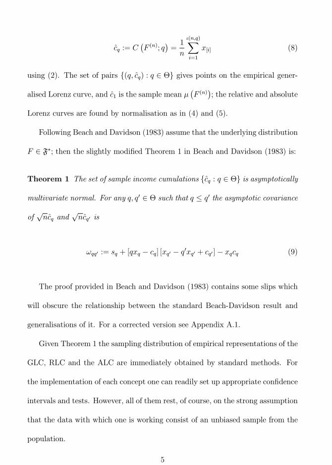
cq := C¡F (n); q

¢=1

n

¶(n;q)X

i=1

x[i] (8)

using (2). The set of pairs f(q; cq) : q 2 £g gives points on the empirical gener-

alised Lorenz curve, and c1 is the sample mean ¹¡F (n)

¢; the relative and absolute

Lorenz curves are found by normalisation as in (4) and (5).

Following Beach and Davidson (1983) assume that the underlying distribution

F 2 F¤; then the slightly modi¯ed Theorem 1 in Beach and Davidson (1983) is:

Theorem 1 The set of sample income cumulations fcq : q 2 £g is asymptotically

multivariate normal. For any q; q0 2 £ such that q · q0 the asymptotic covariance

ofpncq and

pncq0 is

!qq0 := sq + [qxq ¡ cq] [xq0 ¡ q0xq0 + cq0 ]¡ xqcq (9)

The proof provided in Beach and Davidson (1983) contains some slips which

will obscure the relationship between the standard Beach-Davidson result and

generalisations of it. For a corrected version see Appendix A.1.

Given Theorem 1 the sampling distribution of empirical representations of the

GLC, RLC and the ALC are immediately obtained by standard methods. For

the implementation of each concept one can readily set up appropriate con¯dence

intervals and tests. However, all of them rest, of course, on the strong assumption

that the data with which one is working consist of an unbiased sample from the

population.

5

4 Censored Data

One major departure from the unbiased-sample case is that where the sample has

been censored. Censored data are commonly encountered in practical applications

to income and wealth distributions, for several reasons.

As noted in the introduction the data may have been censored by the data

providers. This usually a®ects extreme values - the problem of \top-coding" and

\bottom-coding". Some high-income observations may have been removed from

the sample because of concern for con¯dentiality - in the sparse upper tail it

might not be too di±cult from a skilful data-detective to identify the individ-

uals or households corresponding to individual observations. Some low-income

observations may have been removed or modi¯ed for reasons of convenience: it

has been known for zero or negative income values to be ¯ltered from a sample

before releasing it; the tax authorities may not ¯nd it practical or worthwhile to

collect data from those of modest means. Sometimes extreme values have been

modi¯ed because it was inconvenient to store large numbers in the data set.

Furthermore, because income cumulations are inherently non-robust statistics

(Cowell and Victoria-Feser 1996) the prudent user of income or wealth statistics

may selectively \trim" the sample data in order to obtain Lorenz-type compar-

isons that are not driven by extreme values (?).

We treat the problem of trimming or censoring by supposing that a given pro-

portion of the observations has been removed from each end of the distribution.

6

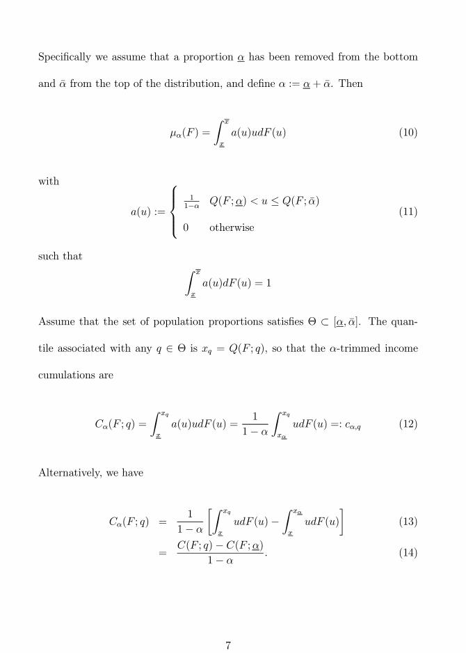
Speci¯cally we assume that a proportion ® has been removed from the bottom

and ¹® from the top of the distribution, and de¯ne ® := ®+ ¹®. Then

¹®(F ) =

Z x

x

a(u)udF (u) (10)

with

a(u) :=

8>><>>:

11¡® Q(F ;®) < u · Q(F ; ¹®)

0 otherwise

(11)

such thatZ x

x

a(u)dF (u) = 1

Assume that the set of population proportions satis¯es £ ½ [®; ¹®]. The quan-

tile associated with any q 2 £ is xq = Q(F ; q), so that the ®-trimmed income

cumulations are

C®(F ; q) =

Z xq

x

a(u)udF (u) =1

1¡ ®

Z xq

x®

udF (u) =: c®;q (12)

Alternatively, we have

C®(F ; q) =1

1¡ ®

·Z xq

x

udF (u)¡Z x®

x

udF (u)

¸(13)

=C(F ; q)¡ C(F ;®)

1¡ ® : (14)

7

Also de¯ne

S®(F ; q) :=

Z xq

x

a(u)u2dF (u) =1

1¡ ®

Z xq

x®

u2dF (u) =: s®;q: (15)

The sample version is obtained by considering the sample quantiles (7) with

n being the untrimmed sample size, and the ¯rst moment sample cumulants

c®;q := C®¡F (n); q

¢=

1

n [1¡ ®]

¶(n;q)X

i=¶(n;®)+1

x[i] =cq ¡ c®1¡ ® (16)

=cq ¡ c®1¡ ®

- see (6). Note that x[¶(n;®)+1] is the ¯rst observation in the trimmed sample. It

is easy to show that

E[c®;q] =c® ¡ cq1¡ ® (17)

For the covariance, we need to ¯nd [1¡ ®]¡2 times

cov¡pn [cq ¡ c®] ;

pn [cq0 ¡ c®]

¢(18)

Expression (18) is equivalent to

n [ cov (cq; cq0)¡ cov (cq; c®)¡ cov (cq0 ; c®) + cov (c®; c®)]

= !qq0 ¡ s® + x®c®

8

+ [®x® ¡ c®] [x® ¡ xq ¡ xq0 ¡ ®x® + qxq + q0xq0 + c® ¡ cq ¡ cq0 ] (19)

where !qq0 is given by (9).

However the expression (19) is unsatisfactory, because an estimate of it would

have to be based on the sample analogues of cq, cq0 and sq which would need to

be calculated using the whole sample (before censoring). We therefore need an

expression that depends only on c®;q and s®;q. We can do that by calculating

directly (up to the multiplicative constant of [1¡ ®]¡2)

cov¡pnc®;q;

pnc®;q0

¢: (20)

As with the untrimmed case (see 33 in the Appendix), this covariance (20)

can be expressed as

Z xq

x®

[1¡ F (y)]Z y

x®

F (u)dudy +

Z xq

x®

F (y)

Z xq0

y

[1¡ F (u)] dudy: (21)

and (21) may then be rearranged to give (see 39 to 40 in the Appendix):

xqZ

x®

F (y)dy

xq0Z

x®

[1¡ F (u)] du¡®x® [xq ¡ x®]¡xqZ

x®

yZ

x®

udF (u)dy+x®

xqZ

x®

F (y)dy (22)

9

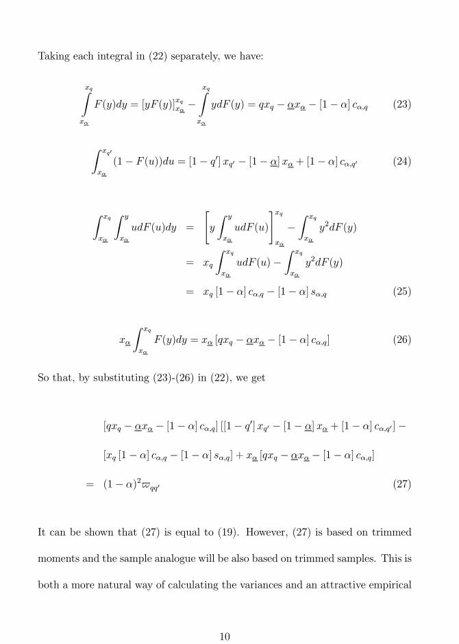
Taking each integral in (22) separately, we have:

xqZ

x®

F (y)dy = [yF (y)]xqx® ¡xqZ

x®

ydF (y) = qxq ¡ ®x® ¡ [1¡ ®] c®;q (23)

Z xq0

x®

(1¡ F (u))du = [1¡ q0] xq0 ¡ [1¡ ®]x® + [1¡ ®] c®;q0 (24)

Z xq

x®

Z y

x®

udF (u)dy =

"y

Z y

x®

udF (u)

#xq

x®

¡Z xq

x®

y2dF (y)

= xq

Z xq

x®

udF (u)¡Z xq

x®

y2dF (y)

= xq [1¡ ®] c®;q ¡ [1¡ ®] s®;q (25)

x®

Z xq

x®

F (y)dy = x® [qxq ¡ ®x® ¡ [1¡ ®] c®;q] (26)

So that, by substituting (23)-(26) in (22), we get

[qxq ¡ ®x® ¡ [1¡ ®] c®;q] [[1¡ q0]xq0 ¡ [1¡ ®] x® + [1¡ ®] c®;q0]¡

[xq [1¡ ®] c®;q ¡ [1¡ ®] s®;q] + x® [qxq ¡ ®x® ¡ [1¡ ®] c®;q]

= (1¡ ®)2$qq0 (27)

It can be shown that (27) is equal to (19). However, (27) is based on trimmed

moments and the sample analogue will be also based on trimmed samples. This is

both a more natural way of calculating the variances and an attractive empirical

10

construct in that it is independent of detailed information censored from the

distribution. So we may state:3

Theorem 2 Given a sample of size n and lower and upper trimming proportions

®; ¹® 2 [0; 1] the set of sample income cumulations fc®;q : q 2 £g is asymptotically

multivariate normal. For any q; q0 2 £ such that q · q0 the asymptotic covariance

ofpnc®;q and

pnc®;q0 is given by $qq0 de¯ned in (27).

Theorem 2 can immediately be applied to the construction of practical tools

for distributional comparisons. For example the 95% con¯dence interval for or-

dinates of the GLC will be given by

c®;q § 1:96n¡1=2$qq (28)

where $qq are the sample analogues of $qq.

For the relative Lorenz curves, we need to specify the following quantities.

First note that

¹® = c®;1 = c®;1¡® (29)

Therefore, the asymptotic variance of ¹® and the covariances between ¹® and c®;q

are found using (19) or (27). Let the latter be denoted respectively by $11 and

$q1. Using the standard result on limiting distributions of di®erentiable functions

3Asymptotic normality follows from the fact that the required statistics are linear functionsof order statistics - see Moore (1968), Shorack (1972), Stigler (1969, 1974).

11

of random variables (Rao 1973), the asymptotic covariances of the RLC ordinates

are then given by

vRLCqq0 =1

¹2®[$qq0 + c®;qc®;q0$11 ¡ c®;q$q01 ¡ c®;q0$q1] :

Therefore, a 95% con¯dence interval for the ordinates of the RLC is given by

L(F (n); q)§ 1:96n¡1=2vRLCqq

where vRLCqq is the sample analogue of vRLCqq .

For absolute Lorenz curves, following the same argument, we ¯nd that the

asymptotic covariances of the ALC ordinates are then given by

vALCqq0 = $qq0 + qq0$11 ¡ q$q01 ¡ q0$q1 :

Therefore, a 95% con¯dence interval for the ordinates of the ALC is given by

A(F (n); q)§ 1:96n¡1=2vALCqq :

5 Concluding Remarks

Statistical inference with trimmed or censored Lorenz curves should be part of

the standard repertoire of applied economists and statisticians working with in-

12

come and wealth data. Our approach makes relatively few demands on the data:

all that one needs to know is the amount by which the sample has been trimmed

in each tail before the data are analysed. Furthermore the main result requires

only modest (but important) extensions to the standard procedures in the liter-

ature. The analysis is straightforward to interpret and to translate into practical

algorithms.

13

References

Andrews, D. W. K. (1997). A simple counterpart to the bootstrap. Discus-

sion Paper 1157, Cowles Foundation for Research in Economics at Yale

University, New Haven, Connecticut 06520-8281.

Beach, C. M., K. Chow, J. Formby, and G. Slotsve (1994). Statistical inference

for decile means. Economics Letters 45, 161{167.

Beach, C. M. and R. Davidson (1983). Distribution-free statistical inference

with Lorenz curves and income shares. Review of Economic Studies 50,

723{725.

Beach, C. M. and S. F. Kaliski (1986). Lorenz Curve inference with sample

weights: an application to the distribution of unemployment experience.

Applied Statistics 35 (1), 38{45.

Beach, C. M. and J. Richmond (1985). Joint con¯dence intervals for income

shares and Lorenz curves. International Economic Review 26 (6), 439{450.

Bishop, J. A., J. P. Formby, and W. P. Smith (1991). International comparisons

of income inequality: Tests for Lorenz dominance across nine countries.

Economica 58, 461{477.

Cowell, F. A. and M.-P. Victoria-Feser (1996). Welfare judgements in the pres-

ence of contaminated data. Distributional Analysis Discussion Paper 13,

STICERD, London School of Economics, London WC2A 2AE.

14

Davidson, R. and J.-Y. Duclos (1997). Statistical inference for the measurement

of the incidence of taxes and transfers. Econometrica 65. forthcoming.

Efron, B. (1979). Bootstrap methods: Another look at the jackknife. The An-

nals of Statistics 7, 1{26.

Efron, B. and R. Tibshirani (1993). An Introduction to the Bootstrap. London:

Chapman and Hall.

Fichtenbaum, R. and H. Shahidi (1988). Truncation bias and the measurement

of income inequality. Journal of Business and Economic Statistics 6, 335{

337.

Gastwirth, J. L. (1971). A general de¯nition of the Lorenz curve. Economet-

rica 39, 1037{1039.

Kendall, M. and A. Stuart (1977). The Advanced Theory of Statistics. London:

Gri±n.

Moore, D. S. (1968). An elementary proof of asymptotic normality of linear

functions of order statistics. Annals of Mathematical Statistics 39, 263{265.

Moyes, P. (1987). A new concept of Lorenz domination. Economics Letters 23,

203{207.

Rao, C. R. (1973). Linear Statistical Inference and Its Applications. New York:

Wiley.

15

Schenker, N. (1985). Qualms about bootstrap con¯dence intervals. Journal of

the American Statistical Association 80, 360{361.

Shorack, G. R. (1972). Functions of order statistics. Annals of Mathematical

Statistics 43, 412{427.

Stein, W. E., R. C. Pfa®enberger, and D. W. French (1987). Sampling error

in ¯rst-order stochastic dominance. Journal of Financial Research 10, 259{

269.

Stigler, S. M. (1969). Linear functions of order statistics. Annals of Mathemat-

ical Statistics 40, 770{788.

Stigler, S. M. (1974). Linear functions of order statistics with smooth weight

functions. Annals of Statistics 2, 676{693. "Correction", 7, 466.

16

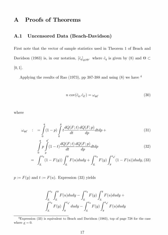
A Proofs of Theorems

A.1 Uncensored Data (Beach-Davidson)

First note that the vector of sample statistics used in Theorem 1 of Beach and

Davidson (1983) is, in our notation, [cq]q2£. where cq is given by (8) and £ ½

[0; 1].

Applying the results of Rao (1973), pp 387-388 and using (8) we have 4

n cov(cq; cq0) = !qq0 (30)

where

!qq0 : =

qZ

0

(1¡ p)pZ

0

tdQ(F ; t)

dt

dQ(F ; p)

dpdtdp+ (31)

qZ

0

p

q0Z

p

(1¡ t)dQ(F ; t)dt

dQ(F ; p)

dpdtdp (32)

=

Z xq

x

(1¡ F (y))Z y

x

F (u)dudy +

Z xq

x

F (y)

Z xq0

y

(1¡ F (u))dudy; (33)

p := F (y) and t := F (u). Expression (33) yields

Z xq

x

Z y

x

F (u)dudy ¡Z xq

x

F (y)

Z y

x

F (u)dudy +

Z xq

x

F (y)

Z xq0

y

dudy ¡Z xq

x

F (y)

Z xq0

y

F (u)dudy

4Expression (33) is equivalent to Beach and Davidson (1983), top of page 728 for the casewhere x = 0.

17

=

Z xq

x

Z y

x

F (u)dudy +

Z xq

x

F (y)

Z xq0

y

dudy ¡Z xq

x

F (y)

Z xq0

x

F (u)dudy

=

Z xq

x

Z y

x

F (u)dudy +

Z xq

x

F (y)

Z xq0

y

dudy +

Z xq

x

F (y)dy

Z xq0

x

(1¡ F (u))du¡Z xq

x

F (y)dy

Z xq0

x

du

=

Z xq

x

F (y)dy

Z xq0

x

(1¡ F (u))du¡Z xq

x

F (y)

Z y

x

dudy +

Z xq

x

Z y

x

F (u)dudy

=

Z xq

x

F (y)dy

Z xq0

x

(1¡ F (u))du¡Z xq

x

F (y) [y ¡ x] dy +Z xq

x

½[uF (u)]yx ¡

Z y

x

udF (u)

¾dy

=

Z xq

x

F (y)dy

·Z xq0

x

(1¡ F (u))du+ x¸

¡Z xq

x

Z y

x

udF (u)dy (34)

Evaluating the three main components of (34) we have:

Z xq

x

F (y)dy = [yF (y)]xqx ¡Z xq

x

ydF (y) = qxq ¡ cq (35)

Z xq0

x

(1¡ F (u))du+ x = xq0(1¡ q0) + cq0 (36)

Z xq

x

Z y

x

udF (u)dy =

24y

yZ

x

udF (u)

35xq

x

¡xqZ

x

y2dF (y) = xqcq ¡ sq (37)

Substituting from (35)-(37) into (34) we ¯nd

!qq0 := [qxq ¡ cq] [xq0(1¡ q0) + cq0 ]¡ [xqcq ¡ sq]

18

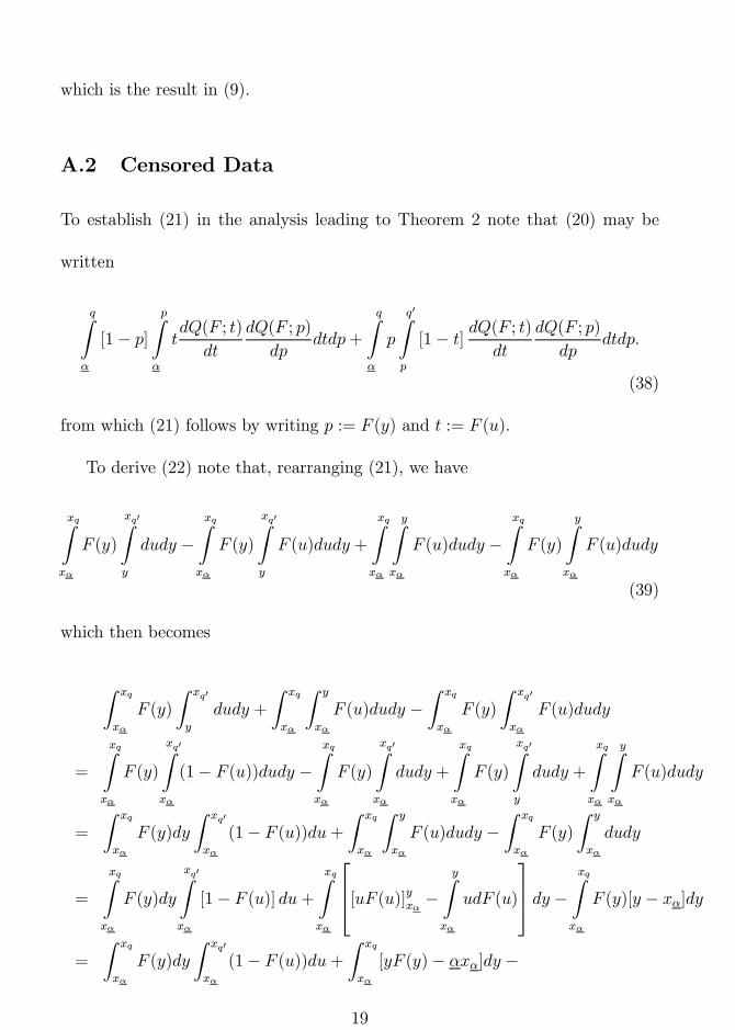
which is the result in (9).

A.2 Censored Data

To establish (21) in the analysis leading to Theorem 2 note that (20) may be

written

qZ

®

[1¡ p]pZ

®

tdQ(F ; t)

dt

dQ(F ; p)

dpdtdp+

qZ

®

p

q0Z

p

[1¡ t] dQ(F ; t)dt

dQ(F ; p)

dpdtdp:

(38)

from which (21) follows by writing p := F (y) and t := F (u).

To derive (22) note that, rearranging (21), we have

xqZ

x®

F (y)

xq0Z

y

dudy ¡xqZ

x®

F (y)

xq0Z

y

F (u)dudy +

xqZ

x®

yZ

x®

F (u)dudy ¡xqZ

x®

F (y)

yZ

x®

F (u)dudy

(39)

which then becomes

Z xq

x®

F (y)

Z xq0

y

dudy +

Z xq

x®

Z y

x®

F (u)dudy ¡Z xq

x®

F (y)

Z xq0

x®

F (u)dudy

=

xqZ

x®

F (y)

xq0Z

x®

(1¡ F (u))dudy ¡xqZ

x®

F (y)

xq0Z

x®

dudy +

xqZ

x®

F (y)

xq0Z

y

dudy +

xqZ

x®

yZ

x®

F (u)dudy

=

Z xq

x®

F (y)dy

Z xq0

x®

(1¡ F (u))du+Z xq

x®

Z y

x®

F (u)dudy ¡Z xq

x®

F (y)

Z y

x®

dudy

=

xqZ

x®

F (y)dy

xq0Z

x®

[1¡ F (u)] du+xqZ

x®

264[uF (u)]yx® ¡

yZ

x®

udF (u)

375 dy ¡

xqZ

x®

F (y)[y ¡ x®]dy

=

Z xq

x®

F (y)dy

Z xq0

x®

(1¡ F (u))du+Z xq

x®

[yF (y)¡ ®x®]dy ¡

19

Z xq

x®

Z y

x®

udF (u)dy ¡Z xq

x®

F (y)ydy + x®

Z xq

x®

F (y)dy (40)

from which (22) follows.

A.3 Equivalence of trimmed-variance expresssions

Equations (19) and (27) can be shown to be equivalent. Using

[1¡ ®] c®;q = cq ¡ c®

[1¡ ®] s®;q = sq ¡ s®

expression (27) becomes

[qxq ¡ ®x® ¡ [cq ¡ c®]] [[1¡ q0]xq0 + ®x® + [cq0 ¡ c®]]

¡ [xq [cq ¡ c®]¡ [sq ¡ s®]]¡ ®x® [xq ¡ x®]

= sq + [qxq ¡ cq ¡ [®x® ¡ c®]] [[1¡ q0] xq0 + cq0 + ®x® ¡ c®]¡ xqcq

+ [xqc® ¡ s®]¡ ®x® [xq ¡ x®]

= sq + [qxq ¡ cq] [[1¡ q0] xq0 + cq0]¡ xqcq

¡ [®x® ¡ c®] [[1¡ q0] xq0 + cq0 + ®x® ¡ c®] + [qxq ¡ cq] [®x® ¡ c®]

+ [xqc® ¡ s®]¡ ®x® [xq ¡ x®]

= sq + [qxq ¡ cq] [[1¡ q0] xq0 + cq0]¡ xqcq

+ [®x® ¡ c®] [qxq ¡ cq ¡ [1¡ q0] xq0 ¡ cq0 ¡ ®x® + c®]

20

¡s® + [®x® ¡ c®] [x® ¡ xq] + x®c®

which becomes (19) in one step.

21