Statistical Inference in Nonparametric Frontier

Models: Recent Developments and

Perspectives

Leopold Simar1

Institut de StatistiqueUniversite Catholique de Louvain

Louvain-la-Neuve, Belgiumsimar@stat.ucl.ac.be

Paul W. Wilson

The John E. Walker Department of Economics222 Sirrine Hall

Clemson UniversityClemson, South Carolina 29634 USA

pww@clemson.edu

1Research support from the “Inter-university Attraction Pole”, Phase V (No.P5/24) sponsored by the Belgian Government (Belgian Science Policy) is gratefullyacknowledged.

Contents

4 Statistical Inference in Nonparametric Frontier Models: Re-cent Developments and Perspectives 14.1 Frontier Analysis and The Statistical Paradigm . . . . . . . . 1

4.1.1 The Frontier Model: Economic Theory . . . . . . . . . 14.1.2 The Statistical Paradigm . . . . . . . . . . . . . . . . . 3

4.2 The Nonparametric Envelopment Estimators . . . . . . . . . . 8

4.2.1 The Data Generating Process (DGP) . . . . . . . . . . 84.2.2 The FDH Estimator . . . . . . . . . . . . . . . . . . . 10

4.2.3 The DEA Estimators . . . . . . . . . . . . . . . . . . . 124.2.4 An Alternative Probabilistic Formulation of the DGP . 154.2.5 Properties of FDH/DEA Estimators . . . . . . . . . . 19

4.3 Bootstrapping DEA and FDH Efficiency Scores . . . . . . . . 304.3.1 General principles . . . . . . . . . . . . . . . . . . . . . 304.3.2 Bootstrap confidence intervals . . . . . . . . . . . . . . 32

4.3.3 Bootstrap bias corrections . . . . . . . . . . . . . . . . 354.3.4 Bootstrapping DEA in action . . . . . . . . . . . . . . 36

4.3.5 Practical Considerations for the Bootstrap . . . . . . . 454.3.6 Bootstrapping FDH efficiency scores . . . . . . . . . . 604.3.7 Extensions of the bootstrap ideas . . . . . . . . . . . . 62

4.4 Improving the FDH estimator . . . . . . . . . . . . . . . . . . 674.4.1 Bias-corrected FDH . . . . . . . . . . . . . . . . . . . . 67

4.4.2 Linearly interpolated FDH: LFDH . . . . . . . . . . . 684.5 Robust Nonparametric Frontier Estimators . . . . . . . . . . . 71

4.5.1 Order-m frontiers . . . . . . . . . . . . . . . . . . . . . 73

4.5.2 Order-α quantile frontiers . . . . . . . . . . . . . . . . 854.5.3 Outlier Detection . . . . . . . . . . . . . . . . . . . . . 92

4.6 Explaining Efficiencies . . . . . . . . . . . . . . . . . . . . . . 95

i

ii CONTENTS

4.6.1 Two-stage regression approach . . . . . . . . . . . . . . 974.6.2 Conditional Efficiency Measures . . . . . . . . . . . . . 102

4.7 Parametric Approximations of Nonparametric Frontier . . . . 1054.7.1 Parametric v. nonparametric models . . . . . . . . . . 1054.7.2 Formalization of the problem and two-stage procedure 109

4.8 Open Issues and Conclusions . . . . . . . . . . . . . . . . . . . 1134.8.1 Allowing for noise in DEA/FDH . . . . . . . . . . . . . 1134.8.2 Inference with DEA/FDH estimators . . . . . . . . . . 1144.8.3 Results for CRS case . . . . . . . . . . . . . . . . . . . 1144.8.4 Tools for dimension reduction . . . . . . . . . . . . . . 1144.8.5 Final conclusions . . . . . . . . . . . . . . . . . . . . . 115

Chapter 4

Statistical Inference inNonparametric FrontierModels: Recent Developmentsand Perspectives

4.1 Frontier Analysis and The Statistical

Paradigm

4.1.1 The Frontier Model: Economic Theory

As discussed in Chapter 1, the economic theory underlying efficiency analysisdates to the work of Koopmans (1951), Debreu (1951), and Farrell (1957),who made the first attempt at empirical estimation of efficiencies for a set ofobserved production units.

In this section, the basic concepts and notation used in this chapter areintroduced. The production process is constrained by the production set Ψ,which is the set of physically attainable points (x, y); i.e.,

Ψ = (x, y) ∈ RN+M+ | x can produce y, (4.1)

where x ∈ RN+ is the input vector and y ∈ RM

+ is the output vector.For purposes of efficiency measurement, the upper boundary of Ψ is of

interest. The efficient boundary (frontier) of Ψ is the locus of optimal pro-duction plans (e.g., minimal achievable input level for a given output, or

1

maximal achievable output given the level of the inputs). The boundary ofΨ,

∂Ψ = (x, y) ∈ Ψ | (θx, y) 6∈ Ψ, ∀ 0 < θ < 1, (x, λy) /∈ Ψ, ∀ λ > 1, (4.2)

is sometimes referred to as the technology or the production frontier, and isgiven by the intersection of Ψ and the closure of its complement. Firms thatare technically inefficient operate at points in the interior of Ψ, while thosethat are technically efficient operate somewhere along the technology definedby ∂Ψ.

It is often useful to describe the production set Ψ by its sections. Forinstance, the input requirement set is defined for all y ∈ RM

+ by

X(y) = x ∈ RN+ | (x, y) ∈ Ψ. (4.3)

The (input-oriented) efficiency boundary ∂X(y) is defined for a given y ∈ RM+

by

∂X(y) = x | x ∈ X(y), θx /∈ X(y), ∀ 0 < θ < 1. (4.4)

Finally, the Debreu-Farrell input measure of efficiency for a given point(x, y) is given by

θ(x, y) = infθ | θx ∈ X(y)= infθ | (θx, y) ∈ Ψ. (4.5)

Given an output level y, and an input mix (a direction) given by thevector x, the efficient level of input is determined by

x∂(y) = θ(x, y)x, (4.6)

which is the projection of (x, y) onto the efficient boundary ∂Ψ, along theray x and orthogonal to the vector y. Hence θ(x, y) is the proportionatereduction of inputs a unit located at (x, y) could undertake to become tech-nically efficient. By construction, for all (x, y) ∈ Ψ, θ(x, y) ≤ 1 and (x, y)is efficient if and only if θ(x, y) = 1. This measure is the reciprocal of theShephard (1970) input distance function.

The efficient boundary of Ψ can also be described in terms of outputefficiency scores. The production set Ψ is characterized by output feasibilitysets defined for all x ∈ RN

+ as

Y (x) = y ∈ RM+ | (x, y) ∈ Ψ. (4.7)

2

Then the (output-oriented) efficiency boundary ∂Y (x) is defined for a givenx ∈ RN

+ as

∂Y (x) = y | y ∈ Y (x), λy /∈ Y (x), ∀ λ > 1, (4.8)

and the Debreu-Farrell output measure of efficiency for a production unitlocated at (x, y) ∈ RN+M

+ is

λ(x, y) = supλ | (x, λy) ∈ Ψ. (4.9)

Analogous to the input-oriented case described above, λ(x, y) is the pro-portionate, feasible increase in outputs for a unit located (x, y) that wouldachieve technical efficiency. By construction, for all (x, y) ∈ Ψ, λ(x, y) ≥ 1and (x, y) is technically efficient if and only if λ(x, y) = 1. The outputefficiency measure λ(x, y) is the reciprocal of the Shephard (1970) outputdistance function. The efficient level of output, for the input level x and forthe direction of the output vector determined by y is given by

y∂(x) = λ(x, y)y. (4.10)

Thus the efficient boundary of Ψ, can be described in either of two ways,either in terms of the input direction or in terms of the output direction.In other words, the unit at (x, y) in the interior of Ψ can achieve technicalefficiency either (i) by moving from (x, y) to (x∂(y), y), or (ii) by movingfrom (x, y) to (x, y∂(x)). Note, however, that there is only one well-definedefficient boundary of Ψ.

A variety of assumptions on Ψ are found in the literature (e.g., free dis-posability, convexity, etc.; see Shephard (1970) for examples). The assump-tions about Ψ determine the appropriate estimator that should be used toestimate ∂Ψ, θ(x, y), or λ(x, y). This issue will be discussed below in detail.

4.1.2 The Statistical Paradigm

In any interesting application, the attainable set Ψ as well as X(y), ∂X(y),Y (x), and ∂Y (x) are unknown. Consequently, the efficiency scores θ(x, y)and λ(x, y) of a particular unit operating at input, output levels are alsounknown.

Typically, the only information available to the analyst is a sample

Xn = (xi, yi), i = 1, . . . , n (4.11)

3

of observations on input and output levels for a set of production units en-gaged in the activity of interest.1 The statistical paradigm poses the followingquestion that must be answered: what can be learned by observing Xn? Inother words, how can the information in Xn be used to estimate θ(x, y) andλ(x, y), or Ψ and hence X(y), ∂X(y), Y (x), and ∂Y (x)?

Answering these questions involves much more than writing a linear pro-gram and throwing the data in Xn into a computer to compute a solutionto the linear program. Indeed, one could ask, “what is learned from an es-timate of θ(x, y) or λ(x, y) (i.e., numbers computed from Xn by solving alinear program)?” The answer is clear: almost nothing. One might learn,for example, that unit A uses less input quantities while producing greateroutput quantities than unit B, but little else can be learned from estimatesof θ(x, y) and λ(x, y) alone.

Before anything can be learned about θ(x, y) or λ(x, y), or by extensionabout Ψ and its various characterizations, one must use methods of statisti-cal analysis to understand the properties of whatever estimators have beenused to obtain estimates of the things of interest.2 This raises the followingquestions:

• is the estimator consistent?

• is the estimator biased?

• if the estimator is biased, does the bias disappear as the sample sizetends toward infinity?

• if the estimator is biased, can the bias be corrected, and at what cost?

• can confidence intervals for the values of interest be estimated?

• can interesting hypotheses about the production process be tested, andif so, how?

1In oder to simplify notation, a random sample is denoted by the lower-case letters(xi, yi) and not, as in standard textbooks, by the upper-case (Xi, Yi). The context willdetermine whether the (xi, yi) are random variables or their realized, observed values,which are real numbers.

2Note that an estimator is a random variable, while an estimate is a realization of anestimator (random variable). An estimator can take perhaps infinitely many values withdifferent probabilities, while an estimate is merely a known, non-random value.

4

Notions of statistical consistency, etc. are discussed below in Section 4.2.5.Before these questions can be answered, indeed before it can be known

what is estimated, a statistical model must be defined. Statistical modelsconsist of two parts: (i) a probability model, which in the present case in-cludes assumptions on the production set Ψ and the distribution of input,output vectors (x, y) over Ψ; and (ii) a sampling process. The statisticalmodel describes the process that yields the data in the sample Xn, and issometimes called the data-generating process (DGP).

In cases where a group of productive units are observed at the same pointin time, i.e., where cross-sectional data are observed, it is convenient and of-ten reasonable to assume the sampling process involves independent drawsfrom the probability distribution defined in the DGP’s probability model.With regard to the probability model, one must attempt reasonable assump-tions. Of course, there are trade-offs here; the assumptions on the probabilitymodel must be strong enough to permit estimation using estimators that havedesirable properties, and to allow those properties to be deduced, yet not sostrong as to impose conditions on the DGP that do not reflect reality. Thegoal should be, in all cases, to make flexible, minimal assumptions in orderto let the data reveal as much as possible about the underlying DGP, ratherthan making strong, untested assumptions that have potential to influenceresults of estimation and inference in perhaps large and misleading ways.The assumptions defining the statistical model are of crucial importance,since any inference that might be made will typically be valid only if theassumptions are in fact true.

The above considerations apply equally to the parametric approach de-scribed in Chapter 2 as well as to the nonparametric approaches to esti-mation discussed in this chapter. It is useful to imagine a spectrum ofestimation approaches, ranging from fully parametric (most restrictive) tofully non-parametric (least restrictive). Fully parametric estimation strate-gies necessarily involve stronger assumptions on the probability model, whichis completely specified in terms of a specific probability distribution function,structural equations, etc. Semi-parametric strategies are less restrictive; inthese approaches, some (but not all) features of the probability model areleft unspecified (for example, in a regression setting one might specify para-metric forms for some, but not all, of the moments of a distribution functionin the probability model). Fully non-parametric approaches assume no para-metric forms for any features of the probability model. Instead, only (rela-tively) mild assumptions on broad features of the probability distribution are

5

made, usually involving assumptions of various types of continuity, degreesof smoothness, etc.

With nonparametric approaches to efficiency estimation, no specific an-alytical function describing the frontier is assumed. In addition, (too) re-strictive assumptions on the stochastic part of the model, describing theprobabilistic behavior of the observations in the sample with respect to theefficient boundary of Ψ, are also avoided.

The most general nonparametric approach would assume that observa-tions (xi, yi) on input, output vectors are drawn randomly, independentlyfrom a population of firms whose input, output vectors are distributed on theattainable set Ψ according to some unknown probability law described by aprobability density function f(x, y) or the corresponding distribution func-tion F (x, y) = Prob(X ≤ x, Y ≤ y). This chapter focuses on deterministicfrontier models where all observations are assumed to be technically attain-able.

Formally,

Prob((xi, yi) ∈ Ψ) = 1. (4.12)

The most popular nonparametric estimators are based on the idea ofestimating the attainable set Ψ by the smallest set Ψ within some class ofsets that envelop the observed data. Depending on assumptions made onΨ, this idea leads to the Free Disposal Hull (FDH) estimator of Deprins etal. (1984), which relies only on an assumption of free disposability, and theData Envelopment Analysis (DEA) estimators which incorporate additionalassumptions. Farrell (1957) was the first to use a DEA estimator in anempirical application, but the idea remained obscure until it was popularizedby Charnes et al. (1978) and Banker et al. (1984). Charnes et al. (1978)estimated Ψ by the convex cone of the FDH estimator of Ψ, thus imposingconstant returns to scale, while Banker et al. (1984) used the convex hull ofthe FDH estimator of Ψ, thereby allowing for variable returns to scale.

Among deterministic frontier models, the primary advantage of nonpara-metric models and estimators lies in their great flexibility (as opposed toparametric, deterministic frontier models). In addition, the nonparametricestimators are easy to compute, and today most of their statistical propertiesare well-established. As will be discussed below, inference is available usingbootstrap methods.

The main drawbacks of deterministic frontier models—both non-parametric as well as parametric models—is that they are very sensitive to

6

outliers and extreme values, and that noisy data are not allowed. As discussedlater in this chapter (see Section 4.8.1), a fully nonparametric approach whennoise is introduced into the DGP leads to identification problems. Some al-ternative approaches will be described later.

It should be noted that allowing for noise in frontier models presentsdifficult problems, even in a fully parametric framework where one can relyon the assumed parametric structure. In fully parametric models where theDGP involves a one-sided error process reflecting inefficiency and a two-sided error process reflecting statistical noise, numerical identification of thestatistical model’s features is sometimes highly problematic even with large(but finite) samples; see Ritter and Simar (1997) for examples.

Apart from the issue of numerical identification, fully parametric, stochas-tic frontier models present other difficulties. Efficiency estimates in thesemodels are based on residual terms that are unidentified. Researchers insteadbase efficiency estimates on an expectation, conditional on a composite resid-ual; estimating an expected inefficiency is rather different from estimating ac-tual inefficiency. An additional problem arises from the fact that, even if thefully parametric, stochastic frontier model is correctly specified, there is typi-cally a non-trivial probability of drawing samples with the “wrong” skewness(e.g., when estimating cost functions, one would expect composite residualswith right-skewness, but it is certainly possible to draw finite samples withleft-skewness—the probability of doing so depends on the sample size and themean of the composite errors). Since there are apparently no published stud-ies, and also apparently no working papers in circulation, where researchersreport composite residuals with the “wrong” skewness when fully parametric,stochastic frontier models are estimated, it appears that estimates are some-times, perhaps often, conditioned (i) on either drawing observations until thedesired skewness is obtained or (ii) on model specifications that result in thedesired skewness. This raises formidable questions for inference.

The remainder of this chapter is organized as follows. Section 4.2 presentsin a unified notation the basic assumptions needed to define the DGP andshow how the nonparametric estimators (FDH and DEA) can be describedeasily in this framework. Section 4.2.4 is particularly appealing: it showshow the Debreu-Farrell concepts of efficiency can be formalized in an in-tuitive probabilistic framework. All the available statistical properties ofFDH/DEA estimators are then summarized and the basic ideas for perform-ing consistent inference using bootstrap methods are described. Section 4.3discusses bootstrap methods for inference based on DEA and FDH estimates.

7

Section 4.3.7 illustrates how the bootstrap can be used to solve relevant test-ing issues: comparison of groups of firms, testing returns to scale, and testingrestrictions (specification tests).

Section 4.4 discusses two ways FDH estimators can be improved, usingbias-corretions and interpolation. As noted above, the envelopment estima-tors are very sensitive to outliers and extreme values; Section 4.5 proposesa way for defining robust nonparametric estimators of the frontier, based ona concept of “partial frontiers” (order-m frontiers or order-α quantile fron-tiers). These robust estimators are particularly easy to compute, and areuseful for detecting outliers.

An important issue in efficiency analysis is the explanation of the ob-served inefficiency. Often researchers seek to explain (in)efficiency in termsof some environmental factors. Section 4.6 surveys the most recent tech-niques allowing investigation of the effects of these external factors on effi-ciency. Parametric and nonparametric methods have often been viewed aspresenting paradoxes in the literature. In Section 4.7, the two approaches arereconciled with each other, and a nonparametric method is is shown to beparticularly useful even if in end a parametric model is desired. This mixed“semi-parametric” approach seems to outperform the usual parametric ap-proaches based on regression ideas. Section 4.8 concludes with a discussionof still-important, open issues and questions for future research.

4.2 The Nonparametric Envelopment Esti-

mators

4.2.1 The Data Generating Process (DGP)

They assumptions listed below are adapted from Kneip et al. (1998), Parket al. (2000) and Kneip et al. (2003). These assumptions define a statisticalmodel (i.e., a DGP), are very flexible, and seem quite reasonable in manypractical situations. The first assumption reflects the deterministic frontiermodel defined in (4.12). In addition, for sake of simplicity, the standardindependence hypothesis is assumed, meaning that the observed firms areconsidered as being drawn randomly and independently from a populationof firms.

Assumption 4.2.1. The sample observations (xi, yi) in Xn are realizations

8

of identically, independently distributed (iid) random variables (X, Y ) withprobability density function f(x, y), which has support over Ψ ⊂ RN+M

+ , theproduction set as defined in (4.1); i.e. Prob((X, Y ) ∈ Ψ) = 1.

The next assumption is a regularity condition sufficient for proving theconsistency of all the nonparametric estimators described in this chapter. Itsays that the probability of observing firms in any open neighborhood of thefrontier is strictly positive—quite a reasonable property since microeconomictheory indicates that with competitive input and output markets, firms whichare inefficient will, in a long run, be driven from the market.

Assumption 4.2.2. The density f(x, y) is strictly positive on the boundary∂Ψ of the production set Ψ and is continuous in any direction toward theinterior of Ψ.

The next assumptions regarding Ψ are standard in microeconomic theoryof the firm; see, for example, Shephard (1970) and Fare (1988).

Assumption 4.2.3. All production requires use of some inputs: (x, y) /∈ Ψif x = 0 and y ≥ 0, y 6= 0.

Assumption 4.2.4. Both inputs and outputs are freely disposable: if (x, y) ∈Ψ, then for any (x′, y′) such that x′ ≥ x and y′ ≤ y, (x′, y′) ∈ Ψ.

Assumption 4.2.3 means that there are no “free lunches”. The disposabil-ity assumption is sometimes called strong disposability and is equivalent toan assumption of monotonicity of the technology. This property also char-acterizes the technical possibility of wasting resources (i.e., the possibility ofproducing less with more resources).

Assumption 4.2.5. Ψ is convex: if (x1, y1), (x2, y2) ∈ Ψ, then (x, y) ∈ Ψfor (x, y) = α(x1, y1) + (1 − α)(x2, y2), for all α ∈ [0, 1].

This convexity assumption may be really questionable in many situations.Several recent studies focus on the convexity assumption in frontier models(e.g., Bogetoft, 1996; Bogetoft et al., 2000; Briec et al., 2004). Assumption4.2.5 will be relaxed at various points below.

Assumption 4.2.6. Ψ is closed.

9

Closedness of the attainable set Ψ is a technical condition, avoiding math-ematical problems for infinite production plans.

Finally, in order to prove consistency of the estimators, the productionfrontier must be sufficiently smooth.

Assumption 4.2.7. For all (x, y) in the interior of Ψ, the function θ(x, y)and λ(x, y) are differentiable in both their arguments.

The characterization of smoothness in Assumption 4.2.7 is stronger thanrequired for the consistency of the nonparametric estimators. Kneip etal. (1998) require only Lipschitz continuity of the efficiency scores, whichis implied by the simpler, but stronger requirement presented here. How-ever, derivation of limiting distributions of the nonparametric estimators hasbeen obtained only with the stronger assumption made here.

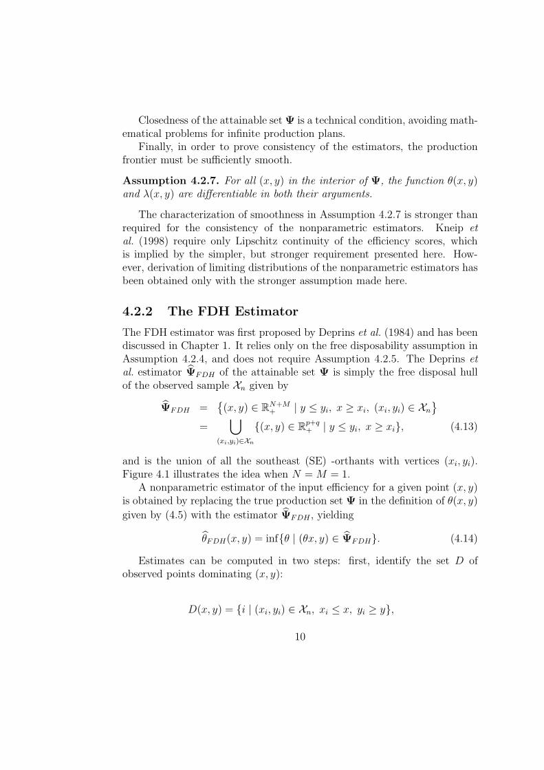
4.2.2 The FDH Estimator

The FDH estimator was first proposed by Deprins et al. (1984) and has beendiscussed in Chapter 1. It relies only on the free disposability assumption inAssumption 4.2.4, and does not require Assumption 4.2.5. The Deprins etal. estimator ΨFDH of the attainable set Ψ is simply the free disposal hullof the observed sample Xn given by

ΨFDH =(x, y) ∈ RN+M

+ | y ≤ yi, x ≥ xi, (xi, yi) ∈ Xn

=⋃

(xi,yi)∈Xn

(x, y) ∈ Rp+q+ | y ≤ yi, x ≥ xi, (4.13)

and is the union of all the southeast (SE) -orthants with vertices (xi, yi).Figure 4.1 illustrates the idea when N = M = 1.

A nonparametric estimator of the input efficiency for a given point (x, y)is obtained by replacing the true production set Ψ in the definition of θ(x, y)

given by (4.5) with the estimator ΨFDH , yielding

θFDH(x, y) = infθ | (θx, y) ∈ ΨFDH. (4.14)

Estimates can be computed in two steps: first, identify the set D ofobserved points dominating (x, y):

D(x, y) = i | (xi, yi) ∈ Xn, xi ≤ x, yi ≥ y,

10

0 2 4 6 8 10 120

1

2

3

4

5

6

7

8

9

10

input: x

outp

ut: y

FDH estimator

Free Disposability

ΨFDH

(xi,y

i)

Figure 4.1: FDH estimator ΨFDH of the production set Ψ.

then θ(x, y) is computed simply by evaluating

θFDH(x, y) = mini∈D(x,y)

maxj=1,...,N

(xj

i

xj

), (4.15)

where for a vector a, aj denotes the jth element of a. The estimator in (4.15)can be computed quickly and easily, since it involves only simple sortingalgorithms.

An estimate of the efficient levels of inputs for a given output levels y anda given input direction determined by the input vector x is obtained by

x∂(y) = θFDH(x, y)x. (4.16)

By construction, ΨFDH ⊆ Ψ, and so ∂X(y) is an upward-biased estimator

11

of ∂X(y). Therefore, for the efficiency scores, θFDH(x, y) is an upward-biased

estimator of θ(x, y); i.e., θFDH(x, y) ≥ θ(x, y).Things work similarly in the output-orientation. The FDH estimator of

λ(x, y) is defined by

λFDH(x, y) = supλ | (x, λy) ∈ ΨFDH. (4.17)

This is computed quickly and easily by evaluating

λFDH(x, y) = maxi∈D(x,y)

minj=1,...,M

(yj

i

yj

), (4.18)

Efficient output levels for given input levels x and given an output mix (di-rection) described by the vector y are estimated by

y∂(x) = λFDH(x, y)y. (4.19)

By construction, λFDH(x, y) is an downward-biased estimator of λ(x, y); for

all (x, y) ∈ Ψ, λFDH(x, y) ≤ λ(x, y).

4.2.3 The DEA Estimators

Although DEA estimators were first used by Farrell (1957) to measure techni-cal efficiency for a set of observed firms, the idea did not gain wide acceptanceuntil the paper by Charnes et al. (1978) appeared 21 years later. Charnes et

al. used the convex cone (rather than the convex hull) of ΨFDH to estimateΨ, which would be appropriate if returns to scale are everywhere constant.Later, Banker et al. (1984) used the convex hull of ΨFDH to estimate Ψ,thus allowing variable returns to scale. Here, “DEA” refers to both of theseapproaches, as well as others that involve using linear programs to define aconvex set enveloping the FDH estimator ΨFDH .

The most general DEA estimator of the attainable set Ψ is simply theconvex hull of the FDH estimator, i.e.,

ΨV RS = (x, y) ∈ RN+M | y ≤n∑

i=1

γiyi; x ≥n∑

i=1

γixi for (γ1, . . . , γn)

such that

n∑

i=1

γi = 1; γi ≥ 0, i = 1, . . . , n. (4.20)

12

Alternatively, the conical hull of the FDH estimator, used by Charnes etal. (1978), is obtained by dropping the constraint in (4.20) requiring the γsto sum to one:

ΨCRS = (x, y) ∈ RN+M | y ≤n∑

i=1

γiyi; x ≥n∑

i=1

γixi for (γ1, . . . , γn)

such that γi ≥ 0, i = 1, . . . , n. (4.21)

Other estimators can be defined by modifying the constraint on the sum ofthe γs in (4.20). For example, the estimator

ΨNIRS = (x, y) ∈ RN+M | y ≤n∑

i=1

γiyi; x ≥n∑

i=1

γixi for (γ1, . . . , γn)

such that

n∑

i=1

γi ≤ 1; γi ≥ 0, i = 1, . . . , n (4.22)

incorporates an assumption of non-increasing returns to scale. In otherwords, returns to scale along the boundary of ΨNIRS are either constantor decreasing, but not increasing. By contrast, returns to scale along theboundary of ΨV RS are either increasing, constant, or decreasing, while re-turns to scale along the boundary of ΨCRS are constant everywhere.

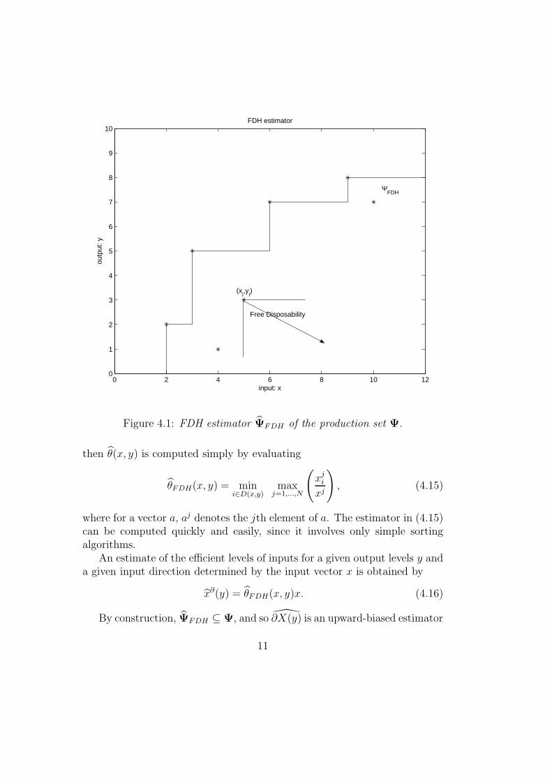
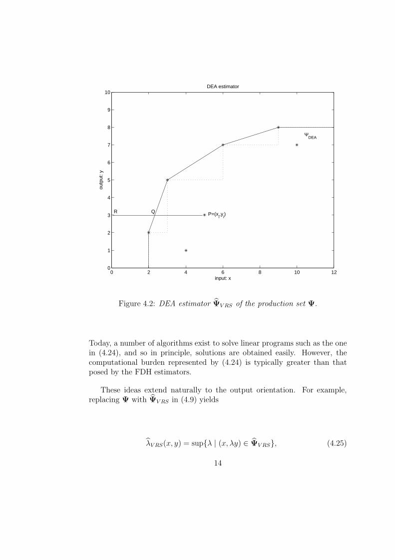
Figure 4.2 illustrates the DEA estimator ΨV RS for the case of one inputand one output (N = M = 1).

As with the FDH estimators, DEA estimators of the efficiency scoresθ(x, y) and λ(x, y) defined in 4.5 and (4.9) can be obtained by replacing

the true, but unknown, production set Ψ with one of the estimators ΨV RS,ΨCRS , or ΨNIRS. For example, in the input-orientation, with varying returnsto scale, using ΨV RS to replace Ψ in (4.5) leads to the estimator

θV RS(x, y) = infθ | (θx, y) ∈ ΨV RS. (4.23)

As a practical matter, θV RS(x, y) can be computed by solving the linearprogram

θV RS(x, y) = minθ > 0 | y ≤n∑

i=1

γiyi; θx ≥n∑

i=1

γixi for (γ1, . . . , γn)

such that

n∑

i=1

γi = 1; γi ≥ 0, i = 1, . . . , n. (4.24)

13

0 2 4 6 8 10 120

1

2

3

4

5

6

7

8

9

10

input: x

outp

ut: y

DEA estimator

R Q

ΨDEA

P=(xi,y

i)

Figure 4.2: DEA estimator ΨV RS of the production set Ψ.

Today, a number of algorithms exist to solve linear programs such as the onein (4.24), and so in principle, solutions are obtained easily. However, thecomputational burden represented by (4.24) is typically greater than thatposed by the FDH estimators.

These ideas extend naturally to the output orientation. For example,replacing Ψ with ΨV RS in (4.9) yields

λV RS(x, y) = supλ | (x, λy) ∈ ΨV RS, (4.25)

14

which can be computed by solving the linear program

λV RS(x, y) = supλ | λy ≤n∑

i=1

γiyi; x ≥n∑

i=1

γixi for (γ1, . . . , γn)

such that

n∑

i=1

γi = 1; γi ≥ 0, i = 1, . . . , n. (4.26)

In the input orientation, the technically efficient level of inputs, for agiven level of outputs y, is estimated by (θV RS(x, y)x, y). Similarly, in theoutput orientation the technically efficient level of outputs for a given levelof inputs x is estimated by (x, λV RS(x, y)y).

All of the FDH and DEA estimators are biased by construction sinceΨFDH ⊆ ΨV RS ⊆ Ψ. Moreover, ΨV RS ⊆ ΨNIRS ⊆ ΨCRS. If the tech-nology ∂Ψ exhibits constant returns to scale everywhere, then ΨCRS ⊆Ψ; otherwise, ΨCRS will not be a statistically consistent estimator ofΨ (of course, if Ψ is not convex, then ΨV RS will also be inconsistent).

These relations further imply that θFDH(x, y) ≥ θV RS(x, y) ≥ θ(x, y) and

θV RS(x, y) ≥ θNIRS(x, y) ≥ θCRS(x, y). Alternatively, in the output orien-

tation, λFDH(x, y) ≤ λV RS(x, y) ≤ λ(x, y) and λV RS(x, y) ≤ λNIRS(x, y) ≤λCRS(x, y).

4.2.4 An Alternative Probabilistic Formulation of the

DGP

The presentation of the DGP in Section 4.2.1 is traditional. However, itis also possible to present the DGP in a way that allows a probabilisticinterpretation of the Debreu-Farrell efficiency scores, providing a new way ofdescribing the nonparametric FDH estimators. This new formulation will beuseful for introducing extensions of the FDH and DEA estimators describedabove. The presentation here follows that of Daraio and Simar (2005a), whoextend the ideas of Cazals et al. (2002).

The stochastic part of the DGP introduced in Section 4.2.1 through theprobability density function f(x, y) (or the corresponding distribution func-tion F (x, y)) is completely characterized by the following probability func-tion:

HXY (x, y) = Prob(X ≤ x, Y ≥ y). (4.27)

15

Note that this is not a standard distribution function, since the cumulativeform is used for the inputs x and the survival form is used for the outputs y.The function has a nice interpretation and interesting properties:

• HXY (x, y) gives the probability that a unit operating at input, outputlevels (x, y) is dominated, i.e., that another unit produces at least asmuch output while using no more of any input than the unit operatingat (x, y).

• HXY (x, y) is monotone, non-decreasing in x and monotone non-increasing in y.

• The support of the distribution function HXY (·, ·) is the attainable setΨ; i.e.,

HXY (x, y) = 0 ∀ (x, y) 6∈ Ψ. (4.28)

The joint probability HXY (x, y) can be decomposed using Bayes’ rule bywriting

HXY (x, y) = Prob(X ≤ x|Y ≥ y)︸ ︷︷ ︸=FX|Y (x|y)

Prob(Y ≥ y)︸ ︷︷ ︸=SY (y)

(4.29)

= Prob(Y ≥ y|X ≤ x)︸ ︷︷ ︸=SY |X(y|x)

Prob(X ≤ x)︸ ︷︷ ︸=FX(x)

, (4.30)

where SY (y) = Prob(Y ≥ y) denotes the survivor function of Y , SY |X(y|x) =Prob(Y ≥ y | X ≤ x) denotes the conditional survivor function of Y , and theconditional distribution and survivor functions are assumed to exist wheneverused (i.e., when needed, SY (y) > 0 and FX(x) > 0). Since the support ofthe joint distribution is the attainable set, boundaries of Ψ can be definedin terms of the conditional distributions defined above by (4.29) and (4.30).This allows definition of some new concepts of efficiency.

For the input-oriented case, assuming SY (y) > 0, define

θ(x, y) = infθ |FX|Y (θx|y) > 0 = infθ |HXY (θx, y) > 0. (4.31)

Similarly, for the output-oriented case, assuming FX(x) > 0, define

λ(x, y) = supλ |SY |X(λy|x) > 0 = supλ |HXY (x, λy) > 0. (4.32)

16

The input efficiency score θ(x, y) may be interpreted as the proportionate re-duction of inputs (holding output levels fixed) required for a unit operatingat (x, y) ∈ Ψ to achieve zero probability of being dominated. Analogously,

the output efficiency score λ(x, y) gives the proportionate increase in out-puts required for the same unit to have zero probability of being dominated,holding input levels fixed. Note that in a multivariate framework, the radialnature of the Debreu-Farrell measures is preserved.

From the properties of the distribution function HXY (x, y), it is clear thatthe new efficiency scores defined in (4.31) and (4.32) have some interesting(and reasonable) properties. In particular,

• θ(x, y) is monotone, non-increasing with x and monotone, non-decreasing with y.

• λ(x, y) is monotone non-decreasing with x and monotone non-increasing with y.

Most importantly, if Ψ is free disposal (an assumption that will be maintainedthroughout this chapter), it is trivial to show that

θ(x, y) ≡ θ(x, y) and λ(x, y) ≡ λ(x, y).

Therefore, under the assumption of free disposability of inputs and outputs,the probabilistic formulation presented here leads to a new representation ofthe traditional Debreu-Farrell efficiency scores.

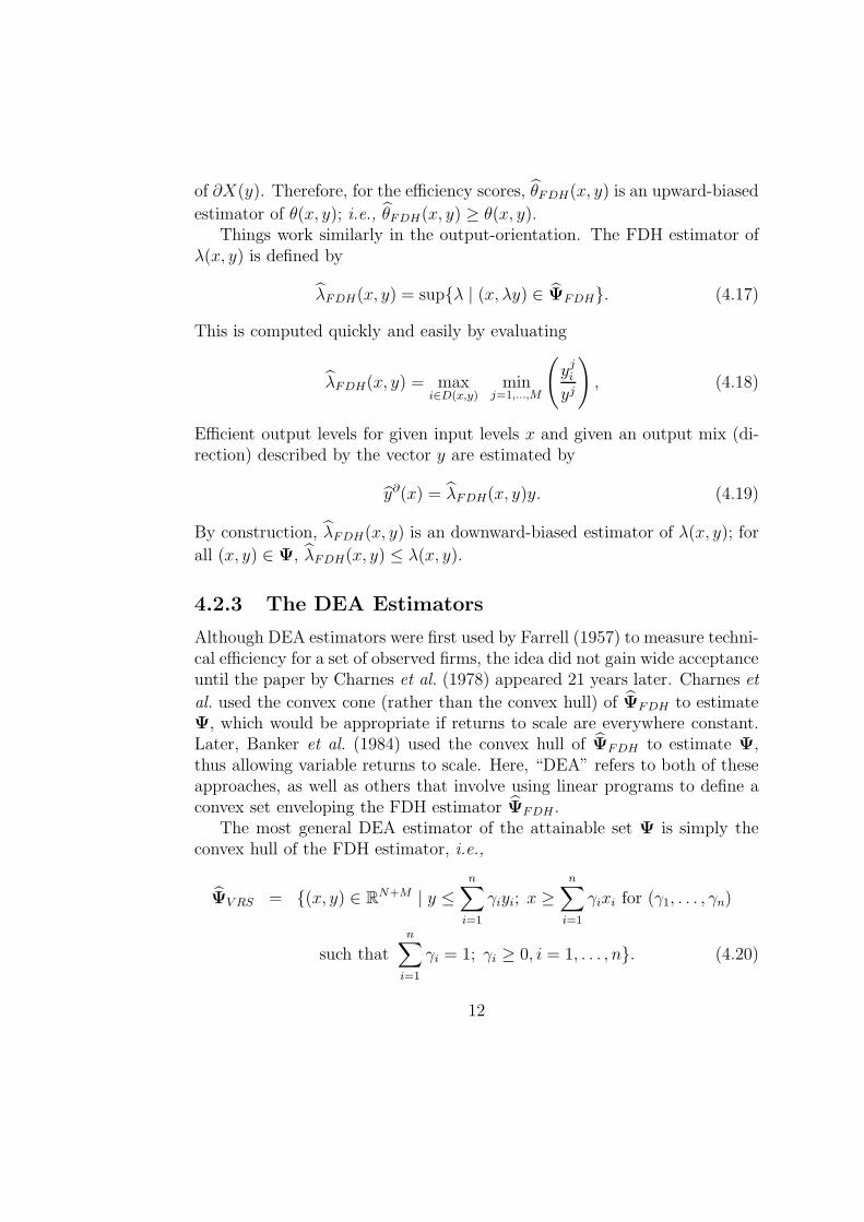
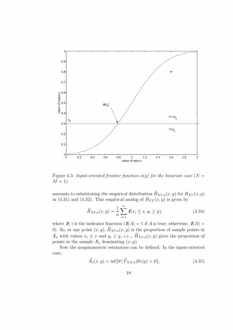
For a given y, the efficient frontier of Ψ can be characterized as notedabove by x∂(y) defined in (4.6). If x is univariate, x∂(y) determines a frontierfunction φ(y) as a function of y, where

φ(y) = infx|FX(x|y) > 0 ∀ y ∈ RM+ . (4.33)

(this was called a factor requirements set in Chapter 1). This function isillustrated in Figure 4.3. The intersection of the horizontal line at outputlevel y0 and the curve representing φ(y) gives the minimum input level φ(y0)than can produce output level y0. Similarly, working in the output direction,a production function is obtained if y is univariate.

Nonparametric estimators of the efficiency scores θ(x, y) and λ(x, y) (andhence also of θ(x, y) and λ(x, y), can be obtained using the same plug-inapproach that was used to define DEA estimators. In the present case, this

17

0 0.2 0.4 0.6 0.8 1 1.2 1.4 1.6 1.8 20

0.1

0.2

0.3

0.4

0.5

0.6

0.7

0.8

0.9

1

value of input x

valu

e of

out

put y

y0

φ(y0)

Ψ

Y>=y0

Y<y0

Figure 4.3: Input-oriented frontier function φ(y) for the bivariate case (N =M = 1).

amounts to substituting the empirical distribution HXY,n(x, y) for HXY (x, y)in (4.31) and (4.32). This empirical analog of HXY (x, y) is given by

HXY,n(x, y) =1

n

n∑

i=1

1I(xi ≤ x, yi ≥ y), (4.34)

where 1I(·) is the indicator function (1I(A) = 1 if A is true; otherwise, 1I(A) =

0). So, at any point (x, y), HXY,n(x, y) is the proportion of sample points in

Xn with values xi ≤ x and yi ≥ y, i.e.,, HXY,n(x, y) gives the proportion ofpoints in the sample Xn dominating (x, y).

Now the nonparametric estimators can be defined. In the input-orientedcase,

θn(x, y) = infθ | FX|Y,n(θx|y) > 0, (4.35)

18

where FX|Y,n(x|y) is the empirical conditional distribution function:

FX|Y,n(x|y) =HXY,n(x, y)

HXY,n(∞, y)(4.36)

For the output-oriented case,

λn(x, y) = supλ | SY |X,n(λy|x) > 0, (4.37)

where SY |X,n(y|x) is the empirical conditional survival function:

SY |X,n(y|x) =HXY,n(x, y)

HXY,n(x, 0). (4.38)

It is easy to show that these estimators coincide with the FDH estimatorsof the Debreu-Farrell efficiency scores. Indeed,

θn(x, y) = mini|Yi≥y

maxj=1,...,p

xji/x

j ≡ θFDH(x, y) (4.39)

andλn(x, y) = max

i|Xi≤xmin

j=1,...,qyj

i /yj ≡ λFDH(x, y). (4.40)

Here, the FDH estimators are presented as intuitive, empirical versions of theDebreu-Farrell efficiency scores, without explicit reference to the free disposalhull of the observed cloud of points.

The presentation in this section is certainly appealing for the FDH es-timators since they appear as the most natural nonparametric estimator ofthe Debreu-Farrell efficiency scores by using the plug-in principle.

The probabilistic, plug-in presentation in this section will be very usefulfor providing extensions of the FDH estimators later in this chapter. InSection 4.4.1 below, a useful bias-corrected FDH estimator is derived. Thenin Section 4.5, definitions are given for some robust nonparametric estimators,while Section 4.6.2 shows how this framework can be used to investigate theeffect of environmental variables on the production process.

4.2.5 Properties of FDH/DEA Estimators

It is necessary to investigate the statistical properties of any estimator beforeit can be known what, if anything, the estimator may be able to reveal

19

about the underlying quantity that one wishes to estimate. An understandingof the properties of an estimator is necessary in order to make inference.Earlier, the FDH and DEA estimators were shown to be biased. Here, weconsider whether, and to what extent, these estimators can reveal usefulinformation about efficiency, and under what conditions. Simar and Wilson(2000a) surveyed the statistical properties of FDH and DEA estimators, butmore recent results have been obtained.

Stochastic convergence and rates of convergence

Perhaps the most fundamental property that an estimator should possessis that of consistency. Loosely speaking, if an estimator βn of an unknownparameter β is consistent, then the estimator converges (in some sense) to βas the sample size n increases toward infinity (a subscript n is often attachedto notation for estimators to remind the reader that one can think of aninfinite sequence of estimators, each based on a different sample size). Inother words, if an estimator is consistent, then more data should be helpful—quite a sensible property. If an estimator is inconsistent, then in general evenan infinite amount of data would offer no particular hope or guarantee ofgetting “close” to the true value that one wishes to estimate. It is this sensein which consistency is the most fundamental property that an estimatormight have; if an estimator is not consistent, there is no reason to considerwhat other properties the estimator might have, nor is there typically be anyreason to use such an estimator.

To be more precise, first consider the notion of convergence in probability,denoted βn

p−→ β. Convergence in probability occurs whenever

limn→∞

Prob(|βn − β| < ε) = 1 for any ε > 0.

An estimator that converges in probability (to the quantity of interest) issaid to be weakly consistent; other types of consistency can also be defined(e.g., see Serfling, 1980). Convergence in probability means that, for anyarbitrarily small (but strictly positive) ε, the probability of obtaining anestimate different from β by more than ε in either direction tends to 0 asn → ∞.

Note that consistency does not mean that it is impossible to obtain anestimate very different from β using a consistent estimator with a very largesample size. Rather, consistency is an asymptotic property; it only describes

20

what happens in the limit. Although consistency is a fundamental property,it is also a minimal property in this sense. Depending on the rate, or speed,with which βn converges to β, a particular sample size may or may not offermuch hope of obtaining an accurate, useful estimate.

In nonparametric statistics, it is often difficult to prove convergence ofan estimator and to obtain its rate of convergence. Often, convergence andits rate are expressed in terms of the stochastic order of the error of estima-tion. The weakest notion of the stochastic order is related to the notion of“bounded in probability”. A sequence of random variables An is said to bebounded in probability if there exists Bε and nε such that for all n > nε andε > 0, Prob(An > Bε) < ε; such cases are denoted by writing An = Op(1).This means that when n is large, the random variable An is bounded, withprobability tending to one. The notation An = Op(n

−α), where α > 0, de-notes that the sequence An/n−α = nαAn is Op(1). In this case, An is saidto converge to a small quantity of order n−α. With some abuse of language,one can say also that An converges at the rate nα because even multipliedby nα (which can be rather large if n is large and if α is not too small), thesequence nαAn remains bounded in probability. Consequently, if α is small(near zero), the rate of convergence is very slow, because n−α is not so smalleven when n is large.

This type of convergence is weaker than convergence in probability. If An

converges in probability at the rate nα (α > 0), then An/n−α = nαAn

p−→ 0,which can be denoted by writing An = op(n

−α) or nαAn = op(1) (this issometimes called big-O, little-o notation). Writing An = Op(n

−α) meansthat nαAn remains bounded when n → ∞ but writing An = op(n

−α) means

that nαAnp−→ 0 when n → ∞.

In terms of the convergence of an estimator βn of β, writing βn − β =op(n

−α) means that βn converges in probability at rate nα. Writing βn −β =Op(n

−α) implies the weaker form of convergence, but the rate is still said to benα. Standard, parametric estimation problems usually yield estimators thatconverge in probability at the rate

√n (corresponding to α = 1/2) and are

said to be root-n consistent in such cases; this provides a familiar benchmarkto which the rates of convergence of other, nonparametric estimators can becompared.

In all cases, the value of α plays a crucial role by indicating the “stochasticorder” of the error of estimation. Since in many nonparametric problems αwill be small (i.e., smaller than 1/2), it is illuminating to look at Table 4.1

21

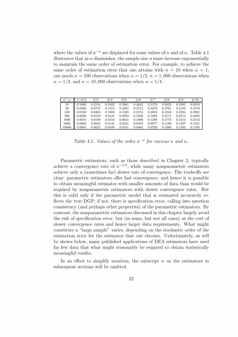
where the values of n−α are displayed for some values of n and of α. Table 4.1illustrates that as α diminishes, the sample size n must increase exponentiallyto maintain the same order of estimation error. For example, to achieve thesame order of estimation error that one attains with n = 10 when α = 1,one needs n = 100 observations when α = 1/2, n = 1, 000 observations whenα = 1/3, and n = 10, 000 observations when α = 1/4.

n \ α 1=2/2 2/3 2/4 2/5 2/6 2/7 2/8 2/9 2/10

10 0.1000 0.2154 0.3162 0.3981 0.4642 0.5179 0.5623 0.5995 0.631050 0.0200 0.0737 0.1414 0.2091 0.2714 0.3270 0.3761 0.4192 0.4573100 0.0100 0.0464 0.1000 0.1585 0.2154 0.2683 0.3162 0.3594 0.3981500 0.0020 0.0159 0.0447 0.0833 0.1260 0.1694 0.2115 0.2513 0.28851000 0.0010 0.0100 0.0316 0.0631 0.1000 0.1389 0.1778 0.2154 0.25125000 0.0002 0.0034 0.0141 0.0331 0.0585 0.0877 0.1189 0.1507 0.182110000 0.0001 0.0022 0.0100 0.0251 0.0464 0.0720 0.1000 0.1292 0.1585

Table 4.1: Values of the order n−α for various n and α.

Parametric estimators, such as those described in Chapter 2, typicallyachieve a convergence rate of n−1/2, while many nonparametric estimatorsachieve only a (sometimes far) slower rate of convergence. The tradeoffs areclear: parametric estimators offer fast convergence, and hence it is possibleto obtain meaningful estimates with smaller amounts of data than would berequired by nonparametric estimators with slower convergence rates. Butthis is valid only if the parametric model that is estimated accurately re-flects the true DGP; if not, there is specification error, calling into questionconsistency (and perhaps other properties) of the parametric estimators. Bycontrast, the nonparametric estimators discussed in this chapter largely avoidthe risk of specification error, but (in some, but not all cases) at the cost ofslower convergence rates and hence larger data requirements. What mightconstitute a “large sample” varies, depending on the stochastic order of theestimation error for the estimator that one chooses. Unfortunately, as willbe shown below, many published applications of DEA estimators have usedfar few data that what might reasonably be required to obtain statisticallymeaningful results.

In an effort to simplify notation, the subscript n on the estimators insubsequent sections will be omitted.

22

Consistency of DEA/FDH estimators

This section summarizes the consistency results for the nonparametric en-velopment estimators under the Assumptions 4.2.1 to 4.2.7 given above. Forthe DEA estimators, convexity of Ψ (Assumption 4.2.5) is needed, but forthe FDH case, the results are valid with or without this assumption

Research on consistency and rates of convergence of efficiency estimatorsfirst examined the simpler cases where either inputs or outputs were unidi-mensional. For N = 1 and M ≥ 1, Banker (1993) showed consistency of the

input efficiency estimator θV RS for convex Ψ, but obtained no informationon the rate of convergence.

The first systematic analysis of the convergence properties of the envel-opment estimators (ΨFDH and ΨV RS) appeared in Korostelev et al. (1995a,1995b). For for the case N = 1 and M ≥ 1, they found that when Ψ satisfiesfree disposability, but not convexity,

d∆(ΨFDH ,Ψ) = Op(n− 1

M+1 ), (4.41)

and when Ψ satisfies both free disposability and convexity,

d∆(ΨV RS ,Ψ) = Op(n− 2

M+2 ), (4.42)

where d∆(·, ·) is the Lebesgue measure (giving the volume) of the differencebetween the two sets.

The rates of convergence for ΨFDH and ΨV RS are not very different;however, for all M ≥ 1, n−1/(M+1) > n−2/(M+2). Moreover, the difference islarger for small values of M as revealed by Table 4.1. Hence, incorporationof the convexity assumption into the estimator of Ψ (as done by ΨV RS)improves the rate of convergence. But, as noted earlier, if the true set in non-convex, the DEA estimator is not consistent and hence does not converge,whereas the FDH estimator converges regardless of whether Ψ is convex. Therates of convergence depend on the dimensionality of the problem, i.e., onthe number of outputs M (when N = 1). This is yet another manifestationof the “curse of dimensionality” shared by most nonparametric approachesin statistics and econometrics; additional discussion on this issue is givenbelow.

Despite the curse of dimensionality, Korostelev et al. (1995a, 1995b) showthat the FDH and DEA estimators share some optimality properties. Inparticular, under free disposability (but not convexity), ΨFDH is the most

23

efficient estimator of Ψ (in term of the minimax risk over the set of estimatorssharing the free disposability assumption, where the loss function is d∆).

Where Ψ is both free-disposal and convex, ΨV RS becomes the most efficientestimator over the class of all the estimators sharing the free disposal andthe convexity assumption. These are quite important results and suggest theinherent quality of the envelopment estimators, even if imprecise in smallsamples where M large.

The full multivariate case, where both N and M are greater than one, wasinvestigated later; results were established in terms of the efficiency scoresthemselves. Kneip et al. (1998) obtained results for DEA estimators, andPark et al. (2000) obtained results for FDH estimators. To summarize,

θFDH(x, y) − θ(x, y) = Op(n− 1

N+M ) (4.43)

and

θV RS(x, y) − θ(x, y) = Op(n− 2

N+M+1 ). (4.44)

The rates obtained above when N = 1 are a special case of the results here.The curse of dimensionality acts symmetrically in both input and outputspaces; i.e., the curse of dimensionality is exacerbated, to the same degree,regardless of whether N or M is increased. The same rates of convergencecan be derived for the output-oriented efficiency scores.

The convergence rate for θV RS(x, y) is slightly faster than for θFDH(x, y),

provided Assumption 4.2.5 is satisfied; otherwise, θV RS(x, y) is inconsistent.The faster convergnce rate for the DEA estimator is due to the fact thatΨFDH ⊆ ΨDEA ⊆ Ψ To date, the convergence rate for θCRS(x, y) has notbeen establshed, but we can imagine that its convergence rate would be fasterthan the rate achieved by θCRS(x, y) if ∂Ψ displays globally constant returnsto scale for similar reasons.

Curse of dimensionality: parametric v. nonparametric inference

Returning to Table 4.1, it is clear that if M + N increases, a much largersample size is needed to reach the precision obtained in the simplest casewhere M = N = 1, where the parametric rate n1/2 is obtained by theFDH estimator, or where an even better rate n2/3 is obtained by the DEAestimator. When M + N is large, unless a very large quantity of data are

24

available, the resulting imprecision will manifest itself in the form of largebias, large variance, and very wide confidence intervals.

This has been confirmed in Monte-Carlo experiments. In fact, as thenumber of outputs is increased, the number of observations must increase atan exponential rate to maintain a given mean-square error with the nonpara-metric estimators of Ψ. General statements on the number of observationsrequired to achieve a given level of mean-square error are not possible, sincethe exact convergence of the nonparametric estimators depends on unknownconstants related to the features of the unobserved Ψ. Nonetheless, for esti-mation purposes, it is always true that more data are better than fewer data(recall that this is a consequence of consistency). In the case of nonparamet-

ric estimators such as ΨFDH and ΨV RS, this statement is more than doublytrue—it is exponentially true! To illustrate this fact, from Table 4.1 it can beseen that, ceteris paribus, inference with n = 10, 000 observations when thenumber of inputs and outputs is above or equal to 9, is less accurate than withn = 10 observations with one input and one output! In fact, with N +M = 9,one would need not 10,000 observations, but 10×10, 000 = 100, 000 observa-tions to achieve the same estimation error as with n = 10 observations whenN = M = 1. A number of applied papers using relatively small numbersof observations with many dimensions have appeared in the literature, buthopefully no more will appear.

The curse of dimensionality results from the fact that as a given set of nobservations are projected in an increasing number of orthogonal directions,the Euclidean distance between the observations necessarily must increase.Moreover, for a given sample size, increasing the number of dimensions willresult in more observations lying on the boundaries of the estimators ΨFDH

and ΨV RS . The FDH estimator is particularly affected by this problem.The DEA estimator is also affected, often times to a lesser degree due to itsincorporation of the convexity assumption (recall that ΨV RS is merely the

convex hull of ΨFDH; consequently, fewer points will lie on the boundaryof ΨV RS than on the boundary of ΨFDH). Wheelock and Wilson (2003)and Wilson (2004) have found cases where all or nearly all observations in

samples of several thousand observations lie on the boundary of ΨFDH, whilerelatively few observations lie on the boundary of ΨV RS. Both papers arguethat the FDH estimator should be used as a diagnostic to check whether itmight be reasonable to employ the DEA estimator in a given application;large numbers of observations falling on the boundary of ΨFDH may indicate

25

problems due to the curse of dimensionality.Parametric estimators suffer little from this phenomenon in the sense

that their rate of convergence typically does not depend on dimensionalityof the problem. The parametric structure incorporates information from allof the observations in a sample, regardless of the dimensionality of Ψ. Thisalso explains why parametric estimators are usually (but not always) moreefficient in a statistical sense than their nonparametric counterparts—theparametric estimators extract more information from the data, assuming ofcourse, that the parametric assumptions that have been made are correct.This is frequently a big assumption.

Additional insight is provided by comparing parametric maximum like-lihood estimators and nonparametric FDH and DEA estimators. Paramet-ric maximum likelihood estimation is the most frequently used parametricestimation method. Under some regularity conditions that do not involvedimensionality of the problem at hand (see, for example, Spanos 1999), max-imum likelihood estimators are root-n consistent. Maximum likelihood esti-mation involves maximizing a likelihood function in which each observationis weighted equally. Hence, maximum likelihood estimators are global esti-mators, as opposed to FDH and DEA estimators, which are local estimators.With FDH or DEA estimators of the frontier, only observations near thepoint where the frontier is being estimated contribute to the estimate at thatpoint; far-away observations contribute little or nothing to estimation at thepoint of interest.

It remains true, however, that when data are projected in an increasingnumber of orthogonal directions, Euclidean distance between the observa-tions necessarily increases. This is problematic for FDH and DEA estima-tors, because it means that increasing dimensionality results in fewer near-byobservations that can impart information about the frontier at a particularpoint of interest. But increasing distance between observations means alsothat parametric, maximum likelihood estimators are combining information,and weighting it equally, from observations that are increasingly far apart(with increasing dimensionality). Hence, increasing dimensionality meansthat the researcher must rely increasingly on the parametric assumptions ofthe model. Again, these are often big assumptions, and should be tested,though often they are not.

The points made here go to the heart of the tradeoff between nonpara-metric and parametric estimators. Parametric estimators incur the risk ofmisspecification, which typically results in inconsistency, but are almost al-

26

ways statistically more efficient than nonparametric estimators if properlyspecified. Nonparametric estimators avoid the risk of misspecification, butusually involve more noise than parametric estimators. Lunch is not free,and the world is full of tradeoffs, which creates employment opportunitiesfor economists and statisticians.

Asymptotic sampling distributions

As discussed above, consistency is an essential property for any estimator.However, consistency is a minimal theoretical property. The preceding dis-cussion indicates that DEA or FDH efficiency estimators converge as thesample size increases (although at perhaps a slow rate), but by themselves,these results have little practical use other than to confirm that the DEA orFDH estimators are possibly reasonable to use for efficiency estimation.

For empirical applications, more is needed—in particular, the appliedresearcher must have some knowledge of the sampling distributions in orderto make inferences about the true levels of efficiency or inefficiency (correctionfor the bias and construction of confidence intervals, for instance). This isparticularly important in situations where point estimates of efficiency mightbe highly varialbe due to the curse of dimensionality or other problems. Inthe nonparametric framework of FDH and DEA , as is often the case, onlyasymptotic results are available. For FDH estimators, a rather general resultis available, but for DEA estimators, useful results have been obtained onlyfor the case of one input and one output (M = N = 1). A general result isalso available, but it is of little practical use.

• FDH with N, M ≥ 1: Park et al. (2000) obtained a well-known lim-iting distribution for the error of estimation for this case:

n1

N+M

(θFDH(x, y) − θ(x, y)

)d−→ Weibull(µx,y, N + M) (4.45)

where µx,y is a constant depending on the DGP. The constant is pro-portional to the probability of observing a firm dominating a point onthe ray x, in a neighborhood of the frontier point x∂(y). This con-stant µx,y is larger (smaller) as the density f(x, y) provides more (less)mass in the neighborhood of the frontier point. The bias and standarddeviation of the FDH estimator are of the order n−1/(N+M), and areproportional to µ

−1/(N+M)x,y . Also, the ratio of the mean to the standard

deviation of θFDH(x, y)− θ(x, y) does not depend on µx,y or on n, and

27

increases as the dimensionality M + N increases. Thus, the curse ofdimensionality here is two-fold: not only does the rate of convergenceworsen with increasing dimensionality, but bias also worsens. Theseresults suggest a strong need for a bias-corrected version of the FDHestimator; such an improvement is proposed later in this chapter.

Park et al. propose a consistent estimator of µx,y in order to obtain abias-corrected estimator and asymptotic confidence intervals. However,Monte-Carlo studies indicate that the noise introduced by estimatingµx,y reduces the quality of inference when N+M is large with moderatesample sizes (say, n ≤ 1000 with M +N ≥ 5). Here again the bootstrapmight provide a useful alternative, but some smoothing of the FDHestimator might even be more appropriate than it is in the case of thebootstrap with DEA estimators (Jeong and Simar, 2006). This pointis briefly discussed below, in Sections 4.3.6 and 4.4.2.

• DEA with M = N = 1: In this case, the efficient boundary can berepresented by a function, and Gijbels et al. (1999) obtain the asymp-totic result

n2/3(θV RS(x, y) − θ(x, y)

)d−→ Q1(·) (4.46)

as well as an analytical form for the limiting distribution Q1(·). Thelimiting distribution is a regular distribution function known up to someconstants. These constants depends on features of the DGP involvingthe curvature of the frontier and the magnitude of the density f(x, y) atthe true frontier point (θ(x, y)x, y). Expressions for the asymptotic biasand variance are also provided. As expected for the DEA estimator, thebias is of the order n−2/3 and is larger for greater curvature of the truefrontier (DEA is a piecewise linear estimator, and so increasing curva-ture of the true frontier makes estimation more difficult) and decreaseswhen the density at the true frontier point increases (large density at(θ(x, y)x, y) implies greater chances of observing observations near thepoint of interest that can impart useful information; recall again thatDEA is a local estimator). The variance of the DEA estimator behavessimilarly. It appears also that in most cases, the bias will be muchlarger than the variance.

Using simple estimators of the two constants in Q1(·), Gijbels et al. pro-vide a bias-corrected estimator and a procedure for building confidence

28

intervals for θ(x, y). Monte-Carlo experiments indicates that even formoderate sample size (n = 100), the procedure works reasonably well.

Although the results of Gijbels et al. are limited to the case whereN = M = 1, their use extends beyond this simple case. The resultsprovide insight for inference by identifying which features of the DGPaffect the quality of inference-making. One would expect that in a moregeneral multivariate setting, the same features should play similar roles,but perhaps in a more complicated fashion.

• DEA with N, M ≥ 1: Deriving analytical results for DEA estimatorsin multivariate settings is necessarily more difficult, and consequentlythe results are less satisfying. Kneip et al. (2003) have obtained animportant key result, namely

n2

N+M+1

(θV RS(x, y)

θ(x, y)− 1

)d−→ Q2(·) (4.47)

where Q2(·) is a regular distribution function known up to some con-stants. However, in this case, no closed analytical from for Q2(·) isavailable, and hence the result is of little practical use for inference. Inparticular, the moments and the quantiles of Q2(·) are not available,so that neither bias-correction nor confidence intervals can be providedeasily using only the result in (4.47). Rather, the importance of thisresult lies in the fact that it is needed for proving the consistency ofthe bootstrap approximation (see below). The bootstrap remains theonly practical tool for inference here.

To summarize, where limiting distributions are available and tractable, onecan estimate the bias of FDH or DEA estimators and build confidence in-tervals. However, additional noise is introduced by estimating unknown con-stants appearing in the limiting distributions. Hence the bootstrap remainsan attractive alternative and is, to date, the only practical way of makinginference in the multivariate DEA case.

29

4.3 Bootstrapping DEA and FDH Efficiency

Scores

The bootstrap provides an attractive alternative to the theoretical resultsdiscussed in the previous section. The essence of the bootstrap idea (Efron,1979, 1982; Efron and Tibshirani, 1993) is to approximate the samplingdistributions of interest by simulating, or mimicking, the DGP. The firstuse of the bootstrap in frontier models dates to Simar (1992). Its use fornonparametric envelopment estimators was developed by Simar and Wilson(1998, 2000a). Theoretical properties of the bootstrap with DEA estimatorsis provided in Kneip et al. (2003), and for FDH estimators in Jeong andSimar (2006).

The presentation below is in terms of the input oriented case, but it caneasily be translated to the output oriented case. The bootstrap is intendedto provide approximations of the sampling distributions of θ(x, y) − θ(x, y)

orθ(x, y)

θ(x, y), which may be used as an alternative to the asymptotic results

described above.

4.3.1 General principles

The presentation in this section follows Simar and Wilson (2000a). The orig-inal data Xn are generated from the DGP, which is completely characterizedby knowledge of Ψ and of the probability density function f(x, y). Let P de-

note the DGP. Then P = P(Ψ, f(·, ·)). Let P(Xn) be a consistent estimatorof the DGP P, where

P(Xn) = P(Ψ, f(·, ·)

)(4.48)

In the true world, P, Ψ and θ(x, y) are unknown ((x, y) is a given, fixedpoint of interest). Only the data Xn are observed, and these must be usedto construct estimates of P, Ψ and θV RS(x, y).

Now consider a virtual, simulated world, i.e., the bootstrap world. Thisbootstrap world is analogous to the true world, but in the bootstrap world,estimates P, Ψ, and θV RS(x, y) take the place of P, Ψ, and θ(x, y) in the

true world. In other words, in the true world P is the true DGP while Pis an estimate of P, but in the bootstrap world, P is the true DGP. In the

30

bootstrap world, a new dataset Xn∗ = (x∗

i , y∗i ), i = 1, . . . , n can be drawn

from P , since P is a known estimate. Within the bootstrap world, Ψ is thetrue attainable set, and the union of the free disposal and the convex hullsof Xn

∗ gives an estimator of Ψ, namely

Ψ∗

= Ψ(Xn∗) = (x, y) ∈ RN+M | y ≤

n∑

i=1

γiy∗i , x ≥

n∑

i=1

γix∗i

n∑

i=1

γi = 1, γi ≥ 0 ∀ i = 1, . . . , n. (4.49)

For the fixed point (x, y), an estimator of θV RS(x, y) is provided by

θ∗V RS(x, y) = infθ | (θx, y) ∈ Ψ∗ (4.50)

(recall that in the bootstrap world, θV RS(x, y) is the quantity estimated,

analogous to θ(x, y) in the true world). The estimator θ∗V RS(x, y) may becomputed by solving the linear program

θ∗V RS(x, y) = minθ > 0 | y ≤

n∑

i=1

γiy∗i , θx ≥

n∑

i=1

γix∗i ,

n∑

i=1

γi = 1, γi ≥ 0 ∀ i = 1, . . . , n. (4.51)

The key relation here is that within the true world, θV RS(x, y) is anestimator of θ(x, y), based on the sample Xn generated from P; whereas in

the bootstrap world, θ∗V RS(x, y) is an estimator of θV RS(x, y), based on the

pseudo-sample Xn∗ generated from P(Xn). If the bootstrap is consistent,

then(θ∗V RS(x, y) − θV RS(x, y)

)| P(Xn)

approx.∼(θV RS(x, y) − θ(x, y)

)| P,(4.52)

or equivalently,

θ∗V RS(x, y)

θV RS(x, y)

∣∣∣P(Xn)approx.∼ θV RS(x, y)

θ(x, y)

∣∣∣P. (4.53)

Within the bootstrap world and conditional on the observed data Xn,the sampling distribution of θ∗V RS(x, y) is (in principle) completely known

31

since P(Xn) is known. However, in practice, it is impossible to compute thisanalytically. Hence Monte-Carlo simulations are necessary to approximatethe left-hand sides of (4.52) or (4.53).

Using P(Xn) to generate B samples Xn∗b of size n, b = 1, . . . , B, and

applying the original estimator to these pseudo samples, yields a set of Bpseudo estimates θ∗V RS,b(x, y), b = 1, . . . , B. The empirical distribution ofthese bootstrap values gives a Monte Carlo approximation of the samplingdistribution of θ∗V RS(x, y), conditional on P(Xn), i.e., the left-hand side of(4.52) (or of (4.53) if the ratio formulation is used). The quality of theapproximation relies in part on the value of B: by the law of large num-bers, when B → ∞, the error of this approximation due to the bootstrapresampling (i.e., drawing from P) tends to zero. The practical choice of Bis limited by the speed of one’s computer; for confidence intervals, values of2000 or more may be needed to give a reasonable approximation.

The issue of computational constraints continues to diminish in impor-tance as computing technology advances. For many problems, however, asingle desktop system may be sufficient. Given the independence of each ofthe B replications in the Monte Carlo approximation, the bootstrap algo-rithm is easily adaptable to parallel computing environments or by using aseries of networked personal computers; the price of these machines continuesto decline while processor speeds increase.

The bootstrap is an asymptotic procedure, as indicated by the condi-tioning on the left-hand-side of (4.52) or of (4.53). Thus the quality of thebootstrap approximation depends on both the number of replications B andand the sample size n. When the bootstrap is consistent, the approximationbecomes exact as B → ∞ and n → ∞.

4.3.2 Bootstrap confidence intervals

The procedure described in Simar and Wilson (1998) for constructing theconfidence intervals depends on using bootstrap estimates of bias to correctfor the bias of the DEA estimators; in addition, the procedure described thererequires using these bias estimates to shift obtained bootstrap distributionsappropriately. Use of bias estimates introduces additional noise into theprocedure.

Simar and Wilson (1999c) propose an improved procedure outlined be-low which automatically corrects for bias without explicit use of a noisybias estimator. The procedure is presented below in terms of the difference

32

θV RS(x, y) − θ(x, y); in Kneip et al. (2003), the procedure is adapted to the

ratio θV RS(x, y)/θ(x, y).For practical purposes, it is advantageous to parameterize the input effi-

ciency scores in term of the Shephard (1970) input distance function

δ(x, y) ≡ 1

θ(x, y). (4.54)

The corresponding estimator (allowing for variable returns to scale) is definedby

δV RS(x, y) ≡ 1

θV RS(x, y). (4.55)

In some cases, failure to re-parameterize the problem may result in estimatedlower bounds for confidence intervals that are negative; this results becauseof the boundary at zero. With the re-parameterization, only the boundaryat one need be considered.

If the distribution of (δV RS(x, y)− δ(x, y)) were known, then it would betrivial to find values cα/2 and c1−α/2 such that

Prob(cα/2 ≤ δV RS(x, y) − δ(x, y) ≤ c1−α/2

)= 1 − α, (4.56)

where ca denotes the ath-quantile of the sampling distribution of (δV RS(x, y)−δ(x, y)). Note that ca ≥ 0 for all a ∈ [0, 1]. Then

δV RS(x, y) − c1−α/2 ≤ δ(x, y) ≤ δV RS(x, y) − cα/2 (4.57)

would give a (1− α)× 100-percent confidence interval for δ(x, y), and hence

1

δV RS(x, y) − cα/2

≤ θ(x, y) ≤ 1

δV RS(x, y) − c1−α/2

(4.58)

would give a (1−α)× 100-percent confidence interval for θ(x, y), due to thereciprocal relation in (4.54).

Of course, the quantiles ca are unknown, but from the empirical bootstrapdistribution of the pseudo estimates δ∗V RS,b, b = 1, . . . , B, estimates of ca

can be found for any value of a ∈ [0, 1]. For example, if ca is the ath

33

sample quantile of the empirical distribution of (δ∗V RS,b(x, y) − δV RS(x, y)),b = 1, . . . , B, then

Prob(cα/2 ≤ δ∗V RS(x, y) − δV RS(x, y) ≤ c1−α/2 | P(Xn)

)= 1 − α. (4.59)

In practice, finding cα/2 and c1−α/2 involves sorting the values (δ∗V RS,b(x, y)−δV RS(x, y)), b = 1, . . . , B in increasing order, and then deleting (α

2× 100)-

percent of the elements at either end of the sorted list. Then set cα/2 andc1−α/2 equal to the endpoints of the truncated, sorted array.

The bootstrap approximation of (4.56) is then

Prob(cα/2 ≤ δV RS(x, y) − δ(x, y) ≤ c1−α/2

)≈ 1 − α, (4.60)

and the estimated (1 − α) × 100-percent confidence interval for δ(x, y) is

δV RS(x, y) − c1−α/2 ≤ δ(x, y) ≤ δV RS(x, y) − cα/2, (4.61)

or1

δV RS(x, y) − cα/2

≤ θ(x, y) ≤ 1

δV RS(x, y) − c1−α/2

. (4.62)

Since 0 ≤ cα/2 ≤ c1−α/2, the estimated confidence interval will include the

original estimate δV RS(x, y) on its upper boundary only if cα/2 = 0. Thismay seem strange until one recalls that the boundary of support of f(x, y) isbeing estimated; under the assumptions, distance from (x, y) to the frontier

can be no less than the distance indicated by δV RS(x, y), but is likely more.The procedure outlined here can be used for any point (x, y) ∈ RN+M

+

for which θV RS(x, y) exists. Typically, the applied researcher is interested inthe efficiency scores of the observed units themselves; in this case, the aboveprocedure can be repeated n times, with (x, y) taking values (xi, yi), i =1, . . . , n, producing a set of n confidence intervals of the form (4.62) foreach firm in the sample. Alternatively, in cases where the computationalburden is large due to large numbers of observations, one might select afew representative firms, or perhaps a small number of hypothetical firms.For example, rather than reporting results for several thousand firms, onemight report results for a few hypothetical firms represented by the means(or medians) of input and output levels for observed firms in quintiles ordeciles determined by size or some other feature of the observed firms.

34

4.3.3 Bootstrap bias corrections

DEA (and FDH) estimators were shown above to be biased, by construction.By definition,

BIAS(θV RS(x, y)

)≡ E

(θV RS(x, y)

)− θ(x, y). (4.63)

The bootstrap bias estimate for the original estimator θV RS(x, y) is the em-pirical analog of (4.63):

BIASB

(θV RS(x, y)

)= B−1

B∑

b=1

θ∗V RS,b(x, y) − θV RS(x, y). (4.64)

It is tempting to construct a bias-corrected estimator of θ(x, y) by com-puting

θV RS(x, y) = θV RS(x, y) − BIASB

(θV RS(x, y)

)

= 2θV RS(x, y) − B−1

B∑

b=1

θ∗V RS,b(x, y). (4.65)

It is well known (e.g., see Efron and Tibshirani, 1993), however, that this bias

correction introduces additional noise; the mean-square error ofθV RS(x, y)

may be greater than the mean-square error of θV RS(x, y). The sample vari-

ance of the bootstrap values θ∗V RS,b(x, y),

σ2 = B−1

B∑

b=1

[θ∗V RS,b(x, y) − B−1

B∑

b=1

θ∗V RS,b(x, y)

]2

, (4.66)

provides an estimate of the variance of θV RS(x, y). Hence the variance of

the bias-corrected estimatorθV RS(x, y) is approximately 4σ2, ignoring any

correlation between θV RS(x, y) and the summation term in the second lineof (4.65). Therefore, the bias correction should not be used unless 4σ2 is

well less than[BIASB

(θV RS(x, y)

)]2; otherwise,

θV RS(x, y) is likely to have

MSE larger than the MSE of θV RS(x, y). A useful rule-of-thumb is to avoid

35

the bias correction in (4.65) unless∣∣∣BIASB

(θV RS(x, y)

)∣∣∣σ

>1√3. (4.67)

Alternatively, Efron and Tibshirani (1993) propose a less conservative rule,suggesting that the bias correction be avoided unless

∣∣∣BIASB

(θV RS(x, y)

)∣∣∣σ

>1

4. (4.68)

4.3.4 Bootstrapping DEA in action

The remaining question concerns how a bootstrap sample Xn∗ from the con-

sistent estimator of P might be simulated. The standard, and simplest,nonparametric bootstrap technique, called the “naive” bootstrap, consist ofdrawing pseudo-observation (x∗

i , y∗i ), i = 1, . . . , n independently, uniformly,

and with replacement from the set Xn of original observations. Unfortunately,however, this naive bootstrap is inconsistent in the context of boundary es-timation. In other words, even if B → ∞ and n → ∞, the Monte-Carloempirical distribution of the θ∗V RS,b(x, y) will not approximate the sampling

distribution of θV RS(x, y).The bootstrap literature contains numerous univariate examples of this

problem; see Bickel and Freedman (1981) and Efron and Tibshirani (1993) forexamples. Simar and Wilson (1999a, 1999b) discuss this issue in the contextof multivariate frontier estimation. As illustrated below, the problem comesfrom the fact that in the naive bootstrap, the efficient facet determiningthe value of θV RS(x, y) appears too often, and with a fixed probability, inthe pseudo-samples Xn

∗. This fixed probability does not depend on the realDGP (other than the number N of inputs and the number M of outputs),and does not vanish, even when n → ∞.

There are two solutions to this problem: either subsampling techniques(drawing pseudo-samples of size m = nκ, where κ < 1) or smoothing tech-niques (where a smooth estimate of the joint density f(x, y) is employed tosimulate Xn

∗) must be used. Kneip et al. (2003) analyze the properties ofthese techniques for strictly convex sets Ψ and in both approaches prove thatthe bootstrap provides consistent approximation of the sampling distributionof θV RS(x, y) − θ(x, y) (or of the ratio θV RS(x, y)/θ(x, y) if preferred). The

36

ideas are summarized below, again for the input-oriented case; the procedurecan easily be translated for the output oriented case.

Subsampling DEA scores

Of the two solutions mentioned above, this one is easiest to implementsince it is similar to the naive bootstrap except that pseudo samples ofsize m = nκ for some κ ∈ (0, 1) (0 < κ < 1) are drawn. For boot-strap replications b = 1, . . . , B, let Xn

∗m,b denote a random subsample of

size m drawn from Xn. Let θV RS,m,b(x, y) denote the DEA efficiency esti-mate for the fixed point (x, y) computed using the reference sample Xn

∗m,b.

Kneip et al. (2003) prove that the Monte-Carlo empirical distribution of

m2/(N+M+1)(θV RS,m,b(x, y) − θV RS(x, y)) given Xn approximates the exact

sampling distribution of n2/(N+M+1)(θV RS(x, y) − θ(x, y)) as B → ∞.Using this approach, a bootstrap bias estimate of the DEA estimator is

obtained by computing

BIASB

(θV RS(x, y)

)=

(m

n

) 2(N+M+1) ×

[1

B

B∑

b=1

θ∗V RS,m,b(x, y) − θV RS(x, y)

], (4.69)

and a bias-corrected estimator of the DEA efficiency score is given by

θV RS(x, y) = θV RS(x, y) − BIASB

(θV RS(x, y)

). (4.70)

Note that (4.69) differs from (4.64) by inclusion of the factor(

mn

)2/(N+M+1),

which is necessary to correct for the effects of different sample sizes in thetrue world and bootstrap world.

Following the same arguments as in Section 4.3.2, but again adjustingfor different sample sizes in the true and bootstrap worlds, the following(1 − α) × 100-percent bootstrap confidence interval is obtained for θ(x, y):

1

δV RS(x, y) − ηc∗1−α/2

≤ θ(x, y) ≤ 1

δV RS(x, y) − ηc∗α/2

, (4.71)

where η =(

mn

)−2/(N+M+1)and c∗a is the ath empirical quantile of

(δV RS,m,b(x, y) − δV RS(x, y)), b = 1, . . . , B.

37

In practice, with finite samples, some subsamples Xn∗m,b may yield no fea-

sible solutions for the linear program used to compute δ∗V RS,m,b(x, y). Thiswill occur more frequently when y is large compared to the original output

values yi in Xn. In fact, this problem arises if y≥

6=maxyj|(xj, yj) ∈ Xn∗m,b.3

In such cases, one could add the point of interest (x, y) to the drawn sub-

sample Xn∗m,b, resulting in δ∗V RS,m,b(x, y) = 1. This will solve the numerical

difficulties, and does not affect the asymptotic properties of the bootstrapsince under the assumptions of the DGP, for all (x, y) ∈ Ψ, the probabilityof this event tends to zero. As shown in Kneip et al. (2003), any value ofκ < 1 produces a consistent bootstrap, but in finite sample the choice of κseems to be critical. More work is needed on this problem.

Smoothing techniques

As an alternative to the subsampling version of the bootstrap method, pseudosamples can be drawn from a smooth, nonparametric estimate of the un-known density f(x, y). The problem is complicated by the fact that thesupport of this density, Ψ, is unknown. There are possibly several ways ofaddressing this problem, but the procedures proposed by Simar and Wilson(1998, 2000b) are straightforward and less complicated than other methodsthat might be used.

A number of nonparametric density estimators are available. Histogramestimators (see Scott, 1992, for discussion) are easy to apply and do not sufferdegenerate behavior near support boundaries, but are not smooth. The lackof smoothness can be eliminated while preserving the non-degenerate behav-ior near support boundaries by using local polynomial regression methods tosmooth a histogram estimate of a density as proposed by Cheng et al. (1997).However, it is difficult to simulate draws from such a density estimate. Ker-nel estimators are perhaps the most commonly used nonparametric densityestimators; these provide smooth density estimates, and it is easy to takedraws from a kernel density estimate. However, in their standard form andwith finite samples, kernel density estimators are severely biased near bound-aries of support; the existence of support boundaries also affects their rates

3The expression a≥

6=b indicates that the elements of a are weakly greater than thecorresponding elements of b, with at least one element of a strictly greater than the cor-responding element of b.

38

of convergence. Fortunately, several methods exist for repairing these prob-lems near support boundaries; here, a reflection method similar to the ideaof Schuster (1985) is used.4

In univariate density estimation problems, the reflection method is verysimple; one simply reflects the n observations around a known boundary,estimates the density of the original and reflected data (2n observations), andthen truncates this density estimate at the boundary point. In the presentcontext, however, the method is more complicated due to three factors:

(i) the problem involves multiple (N + M) dimensions;

(ii) the boundary of support, ∂Ψ, is unknown;

(iii) the boundary is non-linear.

These problems can be solved by exploiting the radial nature of the efficien-cies θ(x, y) and λ(x, y).

The third problem listed in the previous paragraph can be dealt withby transforming the problem from Cartesian coordinates to spherical coor-dinates, which are a combination of Cartesian and polar coordinates. In theinput-orientation, the Cartesian coordinates for the input space are trans-formed to polar coordinates, while in the output-orientation, the Cartesiancoordinates for the output space would be transformed to polar coordinates.The method is illustrated here for the input-orientation; once again, it is easyto adapt the method to the output-orientation.

For the input-orientation, the Cartesian coordinates (x, y) are trans-formed to (ω, η, y), where (ω, η) are the polar coordinates of x in RN

+ . Themodulus ω = ω(x) ∈ R1

+ of x is given by the square root of the sum ofthe squared elements of x, and the jth element of the corresponding angle

η = η(x) ∈[0, π

2

]N−1of x is given by arctan(xj+1/x1) for x1 6= 0; if x1 = 0,

then all elements of η(x) equal π/2.

The DGP is completely determined by f(x, y), and hence is also com-pletely determined by the density f(ω, η, y) after transforming from Carte-sian coordinates to spherical coordinates. In order to generate sample points

4One could also use asymmetric boundary kernels, which change shape as one ap-proaches the boundary of support; see Scott (1992) for examples. This would introduceadditional complications, however, and the choice of methods is of second-order impor-tance for the bootstrap procedures described here.

39

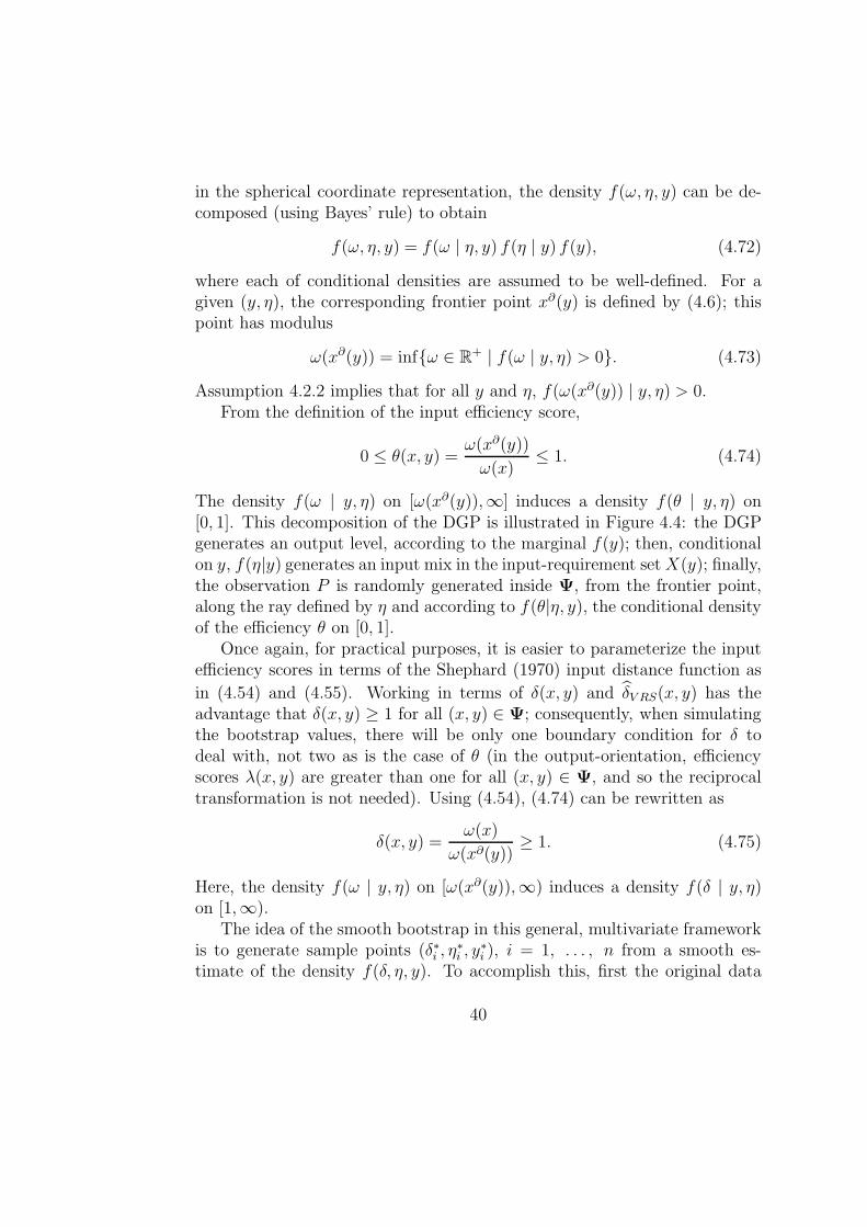
in the spherical coordinate representation, the density f(ω, η, y) can be de-composed (using Bayes’ rule) to obtain

f(ω, η, y) = f(ω | η, y) f(η | y) f(y), (4.72)

where each of conditional densities are assumed to be well-defined. For agiven (y, η), the corresponding frontier point x∂(y) is defined by (4.6); thispoint has modulus

ω(x∂(y)) = infω ∈ R+ | f(ω | y, η) > 0. (4.73)

Assumption 4.2.2 implies that for all y and η, f(ω(x∂(y)) | y, η) > 0.From the definition of the input efficiency score,

0 ≤ θ(x, y) =ω(x∂(y))

ω(x)≤ 1. (4.74)

The density f(ω | y, η) on [ω(x∂(y)),∞] induces a density f(θ | y, η) on[0, 1]. This decomposition of the DGP is illustrated in Figure 4.4: the DGPgenerates an output level, according to the marginal f(y); then, conditionalon y, f(η|y) generates an input mix in the input-requirement set X(y); finally,the observation P is randomly generated inside Ψ, from the frontier point,along the ray defined by η and according to f(θ|η, y), the conditional densityof the efficiency θ on [0, 1].

Once again, for practical purposes, it is easier to parameterize the inputefficiency scores in terms of the Shephard (1970) input distance function as

in (4.54) and (4.55). Working in terms of δ(x, y) and δV RS(x, y) has theadvantage that δ(x, y) ≥ 1 for all (x, y) ∈ Ψ; consequently, when simulatingthe bootstrap values, there will be only one boundary condition for δ todeal with, not two as is the case of θ (in the output-orientation, efficiencyscores λ(x, y) are greater than one for all (x, y) ∈ Ψ, and so the reciprocaltransformation is not needed). Using (4.54), (4.74) can be rewritten as

δ(x, y) =ω(x)

ω(x∂(y))≥ 1. (4.75)

Here, the density f(ω | y, η) on [ω(x∂(y)),∞) induces a density f(δ | y, η)on [1,∞).

The idea of the smooth bootstrap in this general, multivariate frameworkis to generate sample points (δ∗i , η

∗i , y

∗i ), i = 1, . . . , n from a smooth es-

timate of the density f(δ, η, y). To accomplish this, first the original data

40

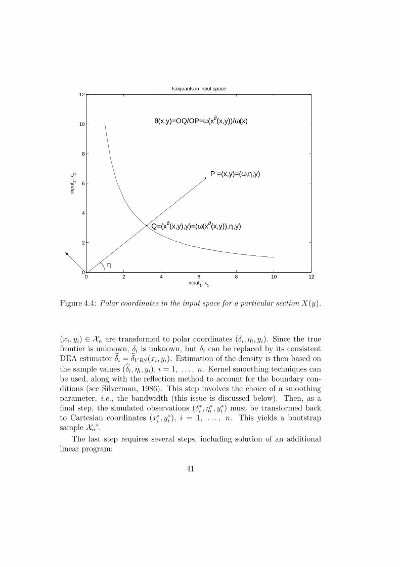
0 2 4 6 8 10 120

2

4

6

8

10

12

input1: x

1

inpu

t 2: x2

Isoquants in input space

•

•

η

P =(x,y)=(ω,η,y)

Q=(x∂(x,y),y)=(ω(x∂(x,y)),η,y)

θ(x,y)=OQ/OP=ω(x∂(x,y))/ω(x)

Figure 4.4: Polar coordinates in the input space for a particular section X(y).

(xi, yi) ∈ Xn are transformed to polar coordinates (δi, ηi, yi). Since the truefrontier is unknown, δi is unknown, but δi can be replaced by its consistentDEA estimator δi = δV RS(xi, yi). Estimation of the density is then based on

the sample values (δi, ηi, yi), i = 1, . . . , n. Kernel smoothing techniques canbe used, along with the reflection method to account for the boundary con-ditions (see Silverman, 1986). This step involves the choice of a smoothingparameter, i.e., the bandwidth (this issue is discussed below). Then, as afinal step, the simulated observations (δ∗i , η

∗i , y

∗i ) must be transformed back

to Cartesian coordinates (x∗i , y

∗i ), i = 1, . . . , n. This yields a bootstrap

sample Xn∗.

The last step requires several steps, including solution of an additionallinear program:

41

(i) Let x be any point in the x−space on the ray with angle η∗i (for instance,

take x1 = 1 and xj+1 = tan(η∗ij) for j = 1, . . . , N−1; here the subscripts

on x denote individual elements of the vector x).

(ii) For the point (x, y∗i ), compute the DEA estimator δV RS(x, y∗

i ) using thereference set Xn.

(iii) An estimator of the input-efficient level of inputs, given the output y∗i

and the direction given by the input vector xi, is given by adapting(4.6) to the bootstrap world:

x∂∗(y∗i ) =

x

δV RS(x, y∗i )

.

(iv) Compute

x∗i = δ∗i x

∂∗(y∗i )

to obtain the Cartesian coordinates x∗i .

In the procedure above, the main difficulty lies in estimating f(δ, η, y)because of the bound on δ. Simar and Wilson (2000b) reflected the points

(δi, ηi, yi) about the boundary characterized by the values δi = 1; i.e., Simarand Wilson add points (2−δi, ηi, yi), i = 1, . . . , n to the original observationsin Xn. This was also proposed by Kneip et al. (2003) where in addition, the

values δi are adjusted to smooth the DEA estimator of Ψ. These proceduresare not easy to implement. So far, there seems to be no simple way to avoidthe considerable complexity required in such a general framework.

The homogeneous smoothed bootstrap

The bootstrap procedure described above can be substantially simplified ifone is willing to make additional assumptions on the DGP. In particular,assume that the distribution of efficiency is homogeneous over the input-output space (this is analogous to an assumption of homoskedasticity inlinear regression problems). In other words, assume that

f(δ | η, y) = f(δ). (4.76)

42

This may be a reasonable assumption in many practical situations. Wilson(2003) surveys tests for independence that may be used to check where datamight satisfy the assumption in (4.76).

Adoption of the homogeneity assumption in (4.76) makes the problemsimilar to the bootstrap one would use in homoskedastic regression models(See Bickel and Freedman, 1981), i.e., where the bootstrap is based on theresiduals. In the present context, the residuals correspond to the distancesδi = δV RS(xi, yi), i = 1, . . . , n, and so the problem becomes essentiallyunivariate, avoiding the complexity of estimating a multivariate density for(δi, ηi, yi). The idea is create a bootstrap sample by projecting each observa-tion (xi, yi) onto the estimated frontier, and then projecting this point away

from the frontier randomly, resulting in points (δ∗i xi/δi, y), where δ∗i is adraw from a smooth estimate of the marginal density f(δ) obtained from the

sample of estimates δ1, . . . , δn. Hence standard, univariate kernel densityestimation, combined with the reflection method, can be used.

The steps are summarized as follows:

(i) Let f(δ) be a smooth estimate obtained from the observed δi | i =1, . . . , n, and draw a bootstrap sample (δ∗i , i = 1, . . . , n) from thisdensity estimate.

(ii) Define the bootstrap sample Xn∗ = (x∗

i , yi); i = 1, . . . , n, where

x∗i = δ∗i x

∂(yi) =δ∗i

δi

xi.

The idea is illustrated in Figure 4.5, where the “•” are the original observa-tions (xi, yi), and the “*” are the pseudo-observations (x∗

i , yi). For the point

P = (x, y), δ(x, y) = |OP |/|OQ|, δ(x, y) = |OP |/|OQV RS |, and δ∗(x, y) =

|OP |/|OQ∗V RS|. The hope is that δ∗(x, y) − δ(x, y) ∼ δ(x, y) − δ(x, y).

It is easy to understand why a naive bootstrap technique, where the δ∗iare drawn identically, uniformly, and with replacement from the set δi | i =1, . . . , n would be inconsistent. As observed by Simar and Wilson (1999a),this would yield

Prob(δ∗(x, y) = δ(x, y) | Xn) = 1 − (1 − n−1)n > 0,

withlim

n→∞Prob(δ∗(x, y) = δ(x, y) | Xn) = 1 − e−1 ≈ 0.632. (4.77)

43

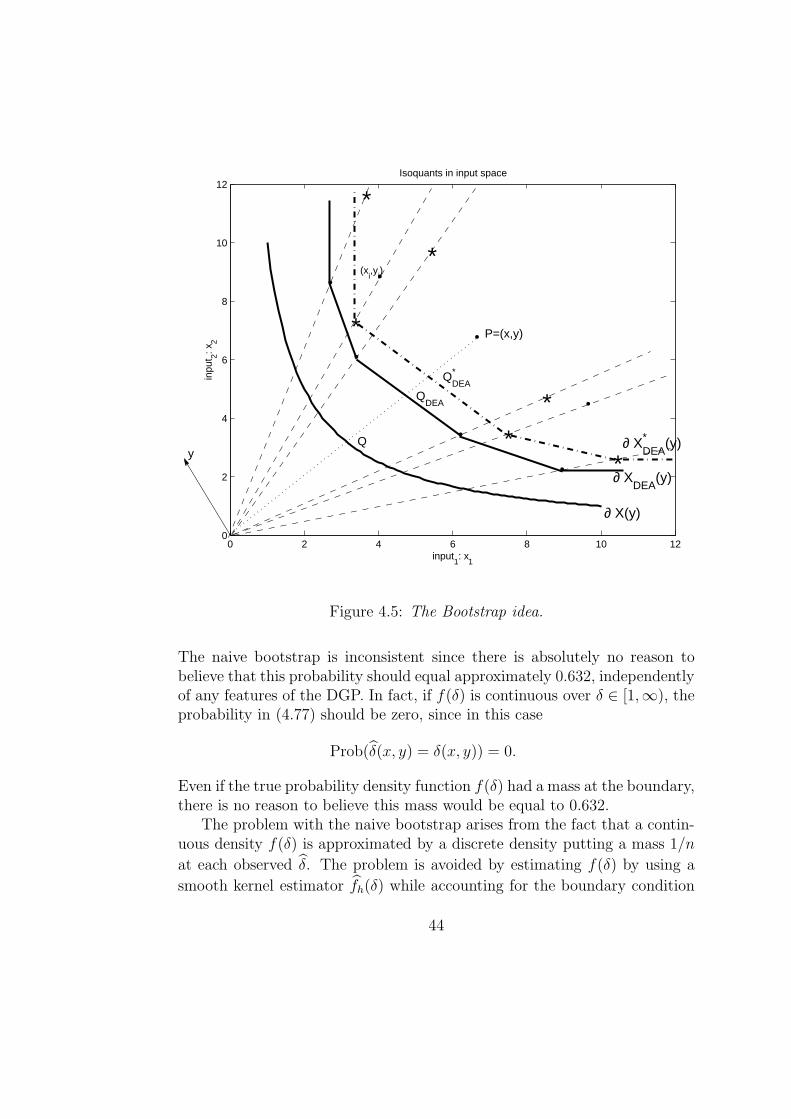
0 2 4 6 8 10 120

2

4

6

8

10

12

input1: x

1

inpu

t 2: x2

Isoquants in input space

•

•

•

•

•

•

•

P=(x,y)

y

QDEA

∂ X(y)

∂ XDEA

(y)

Q

(xi,y

i)

*

*

*

*

*

Q*DEA

* ∂ X*

DEA(y)

Figure 4.5: The Bootstrap idea.

The naive bootstrap is inconsistent since there is absolutely no reason tobelieve that this probability should equal approximately 0.632, independentlyof any features of the DGP. In fact, if f(δ) is continuous over δ ∈ [1,∞), theprobability in (4.77) should be zero, since in this case

Prob(δ(x, y) = δ(x, y)) = 0.

Even if the true probability density function f(δ) had a mass at the boundary,there is no reason to believe this mass would be equal to 0.632.

The problem with the naive bootstrap arises from the fact that a contin-uous density f(δ) is approximated by a discrete density putting a mass 1/n

at each observed δ. The problem is avoided by estimating f(δ) by using a

smooth kernel estimator fh(δ) while accounting for the boundary condition

44

δ ≥ 1, i.e., by using a nonparametric kernel estimator with the reflectionmethod. A description of how the procedure works follows.

4.3.5 Practical Considerations for the Bootstrap

Estimation of f(δ):

The standard kernel density estimator of a density f(δ) evaluated at anarbitrary point δ is given by

fh(δ) = (nh)−1

n∑

i=1

K

(δ − δi

h

), (4.78)

where h is a smoothing parameter, or bandwidth, and K(·) is a kernel func-tion satisfying K(t) = K(−t),

∫∞

−∞K(t) dt = 1, and

∫∞

−∞tK(t) dt = 0. Any

symmetric probability density function with mean zero satisfies these condi-tions. If a probability density function is used for K(·), then fh(δ) can beviewed as the average of n different densities K centered on the observedpoints δi, with h playing the role of a scaling parameter. The bandwidth his used as a tuning parameter to control the dispersion of the n densities.

Two choices must be made in order to implement kernel density estima-tion: a kernel function and the bandwidth must be selected. The standardnormal (Gaussian) probability density function is frequently used, althoughthe Epanechnikov kernel given by

K(t) =3

4(1 − t)21I(|t| ≤ 1) (4.79)

is optimal in the sense of minimizing asymptotic mean integrated squareerror (AMISE).5

The choice of kernel function is of relatively minor importance; the choiceof bandwidth has a far greater effect on the quality of the resulting estimatorin terms of AMISE. A sensible choice of h is determined, in part, by thefollowing considerations:

• as h is becomes small, fewer observations—only those closest to thepoint δ where the density is estimated—influence the estimate fh(δ);

5See Scott (1992) for details.

45

• as h is increased, increasing numbers of far-away observations play arole in determining fh(δ);

• if h → 0, the density will degenerate into the empirical density function,which is discrete with mass 1/n at each observed point δi—this caseresults in the naive bootstrap, with no smoothing;

• if h → ∞, the density will degenerate to a flat horizontal line.

The choice of bandwidth h used with kernel density estimators presents afundamental tradeoff between bias and variance. If h is chosen too small, theresulting density estimate will have high variance, but low bias; if h is chosentoo large, the density estimate will have low variance, but high bias. Optimalchoices of h are usually defined in terms of an approximation of AMISE.

The standard kernel density estimator in (4.78) does not take into accountthe boundary condition δ ≥ 1, and can be shown to be biased and inconsistentnear the boundary. The reflection method, described by Silverman (1986)and others, provides a simple way to overcome this difficulty. To implementthe method, reflect each point δi ≥ 1 around unity, yielding 2 − δi ≤ 1,i = 1, . . . , n. Next, use the standard kernel density estimator in (4.78) toestimate the density of the resulting 2n points; denote this estimate gh(t),where

gh(t) = (2nh)−1

n∑

i=1

[K

(t − δi

h

)+ K

(t − (2 − δi)

h

)]. (4.80)

Then define

fh(t) =

2gh(t) ∀ t ≥ 1,0 otherwise.

(4.81)

A method is given below for making random draws of the δ∗i s from fh(·);this does not require computation of the density estimate. Only a valuefor the selected bandwidth h is needed. The bandwidth should be chosensensibly, and several data-driven approaches exist for selecting a bandwidth.Although one might try several values of the bandwidth parameter as acheck on robustness, this potentially would be computationally burdensome.Experience has shown that the resulting inference is not very sensitive to thechoice of h, at least within broad ranges around the values returned by thedata-driven algorithms. These are discussed next.

46

Practical bandwidth selection:

Statistical theory reveals that under mild regularity conditions on the truedensity f and on the kernel function K, and for a “good” choice of h =O(n−1/5), fh(t) → f(t) as n → ∞ and fh(t) is asymptotically normally dis-tributed. In theory, optimal values of h can be found by deriving the AMISEof fh(t), which depends upon the true density f(t) and the kernel functionK(·), and then minimizing this with respect to h. Silverman (1986) providesan optimal value for h in cases where f(t) is a normal density function andK(·) is standard normal; this is referred to as the “normal reference rule,”and the corresponding value of the optimal value of h is

hNR = 1.06σn−1/5, (4.82)

where σ is the sample standard deviation of the observations used to estimatethe density. A more robust choice (with respect to the assumption of nor-mality for f(t)) is given by (again, assuming the kernel function is standardnormal)

hR = 1.06 min(σ, R/1.34

)n−1/5, (4.83)

where R is the interquartile range.In efficiency applications, the density of the efficiency scores is likely to

be far from normal, although the density of the reflected data is necessarilysymmetric. However, this density may have moments very different froma normal distribution, and may have more than one mode. Consequently,data-driven methods for choosing h are preferred to simple, ad hoc referencerules such as the ones discussed in the previous paragraph. One approachis to minimize an estimate of either mean-integrated square error (MISE)or its asymptotic version (AMISE); these approaches are called unbiasedand biased cross-validation, respectively (see Scott, 1992). The least-squarescross-validation method described by Silverman (1986) is a form of unbiasedcross-validation; this method was adapted to the DEA context by Simar andWilson (2002).

In the DEA framework, the set of estimates δi contain some number ofspurious values equal to 1. This provides spurious mass (greater than 1/n) atthe boundary value 1 in the discrete density to be smoothed. These spuriousvalues can be eliminated for purposes of selecting a bandwidth; they aremerely an artifact of the nature of the DEA estimator of Ψ. Suppose m < n

47

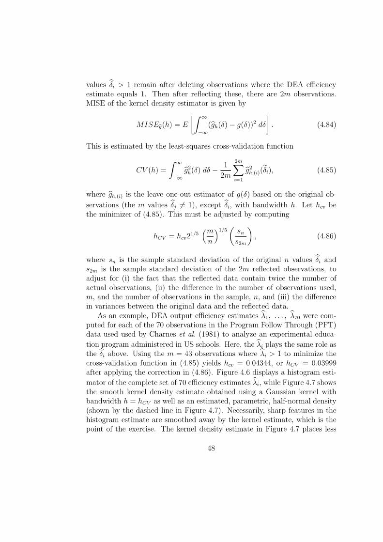
values δi > 1 remain after deleting observations where the DEA efficiencyestimate equals 1. Then after reflecting these, there are 2m observations.MISE of the kernel density estimator is given by

MISEbg(h) = E

[∫ ∞

−∞

(gh(δ) − g(δ))2 dδ

]. (4.84)

This is estimated by the least-squares cross-validation function

CV (h) =

∫ ∞

−∞

g2h(δ) dδ − 1

2m

2m∑

i=1

g2h,(i)(δi), (4.85)

where gh,(i) is the leave one-out estimator of g(δ) based on the original ob-

servations (the m values δj 6= 1), except δi, with bandwidth h. Let hcv bethe minimizer of (4.85). This must be adjusted by computing

hCV = hcv21/5(m

n

)1/5(

sn

s2m

), (4.86)

where sn is the sample standard deviation of the original n values δi ands2m is the sample standard deviation of the 2m reflected observations, toadjust for (i) the fact that the reflected data contain twice the number ofactual observations, (ii) the difference in the number of observations used,m, and the number of observations in the sample, n, and (iii) the differencein variances between the original data and the reflected data.

As an example, DEA output efficiency estimates λ1, . . . , λ70 were com-puted for each of the 70 observations in the Program Follow Through (PFT)data used used by Charnes et al. (1981) to analyze an experimental educa-

tion program administered in US schools. Here, the λi plays the same role asthe δi above. Using the m = 43 observations where λi > 1 to minimize thecross-validation function in (4.85) yields hcv = 0.04344, or hCV = 0.03999after applying the correction in (4.86). Figure 4.6 displays a histogram esti-

mator of the complete set of 70 efficiency estimates λi, while Figure 4.7 showsthe smooth kernel density estimate obtained using a Gaussian kernel withbandwidth h = hCV as well as an estimated, parametric, half-normal density(shown by the dashed line in Figure 4.7). Necessarily, sharp features in thehistogram estimate are smoothed away by the kernel estimate, which is thepoint of the exercise. The kernel density estimate in Figure 4.7 places less

48

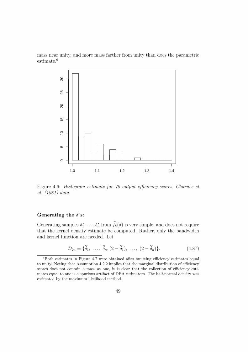
mass near unity, and more mass farther from unity than does the parametricestimate.6

1.0 1.1 1.2 1.3 1.4

05

1015

2025

30

Figure 4.6: Histogram estimate for 70 output efficiency scores, Charnes etal. (1981) data.

Generating the δ∗s:

Generating samples δ∗1, . . . , δ∗n from fh(δ) is very simple, and does not require

that the kernel density estimate be computed. Rather, only the bandwidthand kernel function are needed. Let

D2n = δ1, . . . , δn, (2 − δ1), . . . , (2 − δn). (4.87)

6Both estimates in Figure 4.7 were obtained after omitting efficiency estimates equalto unity. Noting that Assumption 4.2.2 implies that the marginal distribution of efficiencyscores does not contain a mass at one, it is clear that the collection of efficiency esti-mates equal to one is a spurious artifact of DEA estimators. The half-normal density wasestimated by the maximum likelihood method.

49

1.0 1.1 1.2 1.3 1.4

02

46

8

Figure 4.7: Kernel density estimate (solid curve) and half-normal densityestimate (dashed curve) for 70 output efficiency scores, Charnes et al. (1981)data.

Then let β∗1 , . . . , β∗

n be a naive bootstrap sample from D2n, obtained bydrawing n times, independently, uniformly, and with replacement from the2n elements of D2n. Next, perturb these draws by setting β∗∗

i = β∗i +hCV ε∗i for

each i = 1, . . . , n, where the ε∗i are independent draws from the probabilitydensity function used as the kernel function K(·).

It is straightforward to show that the β∗∗i are a random sample of size n

from gh(δ) given in (4.80) (e.g., Silverman, 1986; Efron and Tibshirani, 1993).As is typical with kernel estimation techniques, however, with finite samplesthese draws will not have the same mean and variance as the elements ofD2n. This can be corrected by computing

β∗∗∗i = β∗ +

β∗∗i − β∗

(1 + h2CV σ2

Kσ−2β )1/2

, (4.88)

where β∗ = n−1∑n

i=1 β∗i is the sample mean of the β∗

i , σ2β = n−1

∑ni=1(β

∗i −

50

β∗)2 is the sample variance of the β∗i , and σ2

K is the variance of the probabilitydensity function used for the kernel function. Finally, the draws among theβ∗∗∗

i that are less than unity must be reflected as in (4.81) by computing

δ∗i =

2 − β∗∗∗

i ∀ β∗∗∗i < 1,

β∗∗∗i otherwise.

(4.89)

The Homogeneous Bootstrap Algorithm:

The homogeneous bootstrap algorithm for obtaining a set of bootstrap esti-mates δ∗b (x, y) | b = 1, . . . , B for a given fixed point (x, y) is summarizedby the following steps:

[1] From the original data set Xn, compute δi = δ(xi, yi) ∀ i = 1, . . . , n.

[2] Select a value for h using one of the methods described above.

[3] Generate β∗1 , . . . , β∗

n by drawing with replacement from the set D2n

defined in (4.87).

[4] Draw ε∗i , i = 1, . . . , n independently from the kernel function K(·)and compute

β∗∗i = β∗

i + hCV ε∗i

for each i = 1, . . . , n.

[5] For each i = 1, . . . , n, compute β∗∗∗i as in (4.88) and then compute δ∗i

as in (4.89).

[6] Define the bootstrap sample Xn∗ = (x∗

i , yi) | i = 1, . . . , n, where

x∗i = δ∗i x

∂(yi) = δ∗i δ−1i xi.

[7] Compute the DEA efficiency estimate δ∗(x, y) for the fixed point (x, y),using the reference set Xn

∗.

[8] Repeat steps [3]–[7] B times to obtain a set of bootstrap estimates

δ∗b (x, y) | b = 1, . . . , B.

51

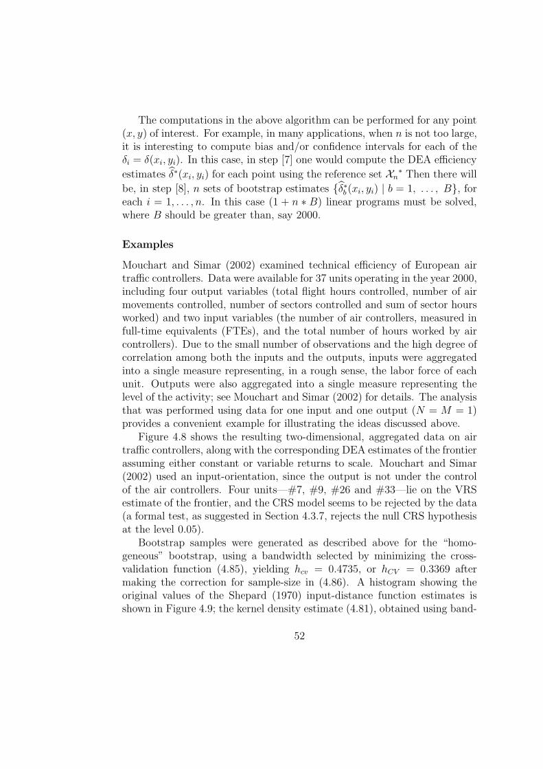
The computations in the above algorithm can be performed for any point(x, y) of interest. For example, in many applications, when n is not too large,it is interesting to compute bias and/or confidence intervals for each of theδi = δ(xi, yi). In this case, in step [7] one would compute the DEA efficiency

estimates δ∗(xi, yi) for each point using the reference set Xn∗ Then there will

be, in step [8], n sets of bootstrap estimates δ∗b (xi, yi) | b = 1, . . . , B, foreach i = 1, . . . , n. In this case (1 + n ∗ B) linear programs must be solved,where B should be greater than, say 2000.

Examples

Mouchart and Simar (2002) examined technical efficiency of European airtraffic controllers. Data were available for 37 units operating in the year 2000,including four output variables (total flight hours controlled, number of airmovements controlled, number of sectors controlled and sum of sector hoursworked) and two input variables (the number of air controllers, measured infull-time equivalents (FTEs), and the total number of hours worked by aircontrollers). Due to the small number of observations and the high degree ofcorrelation among both the inputs and the outputs, inputs were aggregatedinto a single measure representing, in a rough sense, the labor force of eachunit. Outputs were also aggregated into a single measure representing thelevel of the activity; see Mouchart and Simar (2002) for details. The analysisthat was performed using data for one input and one output (N = M = 1)provides a convenient example for illustrating the ideas discussed above.

Figure 4.8 shows the resulting two-dimensional, aggregated data on airtraffic controllers, along with the corresponding DEA estimates of the frontierassuming either constant or variable returns to scale. Mouchart and Simar(2002) used an input-orientation, since the output is not under the controlof the air controllers. Four units—#7, #9, #26 and #33—lie on the VRSestimate of the frontier, and the CRS model seems to be rejected by the data(a formal test, as suggested in Section 4.3.7, rejects the null CRS hypothesisat the level 0.05).

Bootstrap samples were generated as described above for the “homo-geneous” bootstrap, using a bandwidth selected by minimizing the cross-validation function (4.85), yielding hcv = 0.4735, or hCV = 0.3369 aftermaking the correction for sample-size in (4.86). A histogram showing theoriginal values of the Shepard (1970) input-distance function estimates isshown in Figure 4.9; the kernel density estimate (4.81), obtained using band-

52

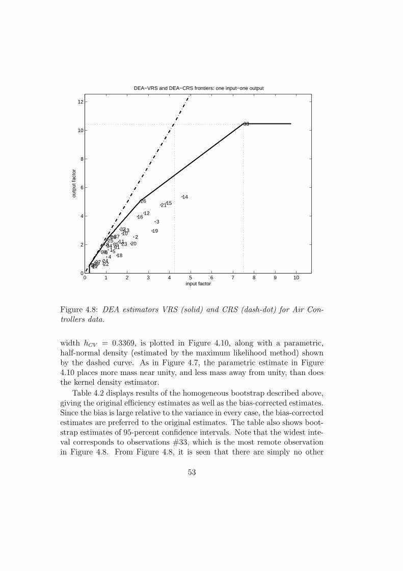
0 1 2 3 4 5 6 7 8 9 100

2

4

6

8

10

12

1

2

3

4 5 6

7 8

9

10

11

12

13

1415

16

17

18

19

20

21

22

23

24

25

26

27

28

2930

31

32

33

34 353637

input factor

outp

ut fa

ctor

DEA−VRS and DEA−CRS frontiers: one input−one output

Figure 4.8: DEA estimators VRS (solid) and CRS (dash-dot) for Air Con-trollers data.

width hCV = 0.3369, is plotted in Figure 4.10, along with a parametric,half-normal density (estimated by the maximum likelihood method) shownby the dashed curve. As in Figure 4.7, the parametric estimate in Figure4.10 places more mass near unity, and less mass away from unity, than doesthe kernel density estimator.

Table 4.2 displays results of the homogeneous bootstrap described above,giving the original efficiency estimates as well as the bias-corrected estimates.Since the bias is large relative to the variance in every case, the bias-correctedestimates are preferred to the original estimates. The table also shows boot-strap estimates of 95-percent confidence intervals. Note that the widest inte-val corresponds to observations #33, which is the most remote observationin Figure 4.8. From Figure 4.8, it is seen that there are simply no other

53

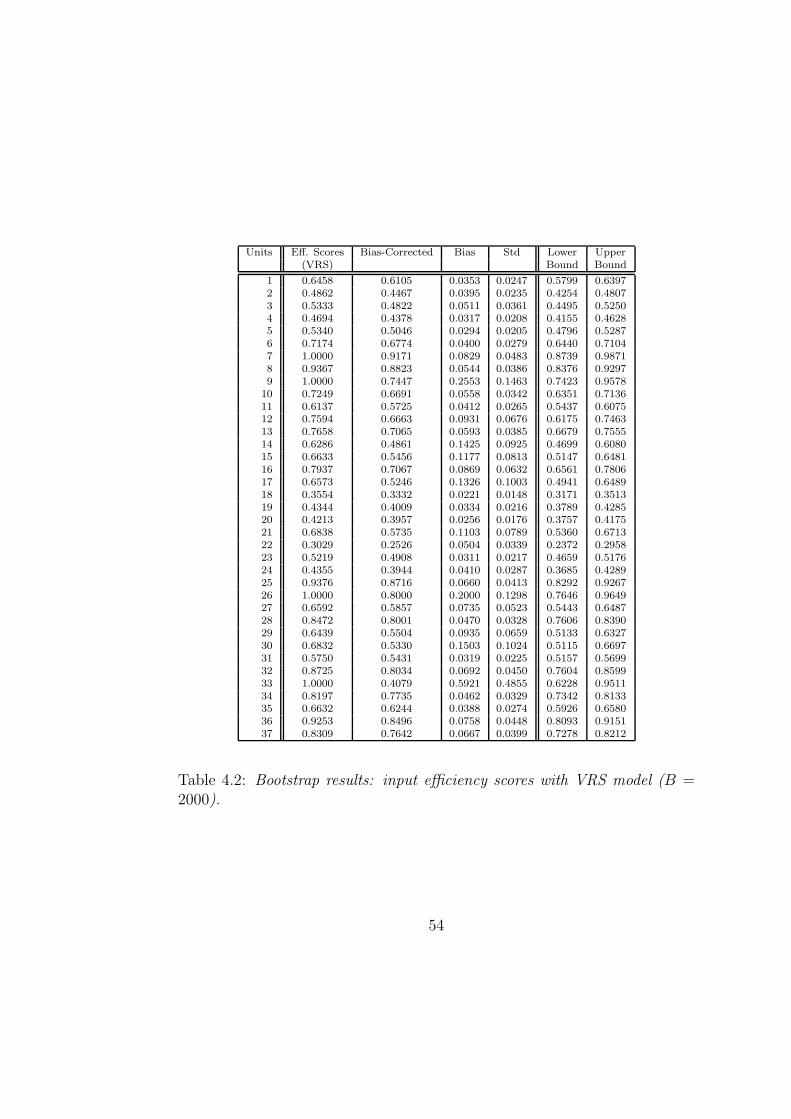
Units Eff. Scores Bias-Corrected Bias Std Lower Upper(VRS) Bound Bound

1 0.6458 0.6105 0.0353 0.0247 0.5799 0.63972 0.4862 0.4467 0.0395 0.0235 0.4254 0.48073 0.5333 0.4822 0.0511 0.0361 0.4495 0.52504 0.4694 0.4378 0.0317 0.0208 0.4155 0.46285 0.5340 0.5046 0.0294 0.0205 0.4796 0.52876 0.7174 0.6774 0.0400 0.0279 0.6440 0.71047 1.0000 0.9171 0.0829 0.0483 0.8739 0.98718 0.9367 0.8823 0.0544 0.0386 0.8376 0.92979 1.0000 0.7447 0.2553 0.1463 0.7423 0.9578

10 0.7249 0.6691 0.0558 0.0342 0.6351 0.713611 0.6137 0.5725 0.0412 0.0265 0.5437 0.607512 0.7594 0.6663 0.0931 0.0676 0.6175 0.746313 0.7658 0.7065 0.0593 0.0385 0.6679 0.755514 0.6286 0.4861 0.1425 0.0925 0.4699 0.608015 0.6633 0.5456 0.1177 0.0813 0.5147 0.648116 0.7937 0.7067 0.0869 0.0632 0.6561 0.780617 0.6573 0.5246 0.1326 0.1003 0.4941 0.648918 0.3554 0.3332 0.0221 0.0148 0.3171 0.351319 0.4344 0.4009 0.0334 0.0216 0.3789 0.428520 0.4213 0.3957 0.0256 0.0176 0.3757 0.417521 0.6838 0.5735 0.1103 0.0789 0.5360 0.671322 0.3029 0.2526 0.0504 0.0339 0.2372 0.295823 0.5219 0.4908 0.0311 0.0217 0.4659 0.517624 0.4355 0.3944 0.0410 0.0287 0.3685 0.428925 0.9376 0.8716 0.0660 0.0413 0.8292 0.926726 1.0000 0.8000 0.2000 0.1298 0.7646 0.964927 0.6592 0.5857 0.0735 0.0523 0.5443 0.648728 0.8472 0.8001 0.0470 0.0328 0.7606 0.839029 0.6439 0.5504 0.0935 0.0659 0.5133 0.632730 0.6832 0.5330 0.1503 0.1024 0.5115 0.669731 0.5750 0.5431 0.0319 0.0225 0.5157 0.569932 0.8725 0.8034 0.0692 0.0450 0.7604 0.859933 1.0000 0.4079 0.5921 0.4855 0.6228 0.951134 0.8197 0.7735 0.0462 0.0329 0.7342 0.813335 0.6632 0.6244 0.0388 0.0274 0.5926 0.658036 0.9253 0.8496 0.0758 0.0448 0.8093 0.915137 0.8309 0.7642 0.0667 0.0399 0.7278 0.8212

Table 4.2: Bootstrap results: input efficiency scores with VRS model (B =2000).

54

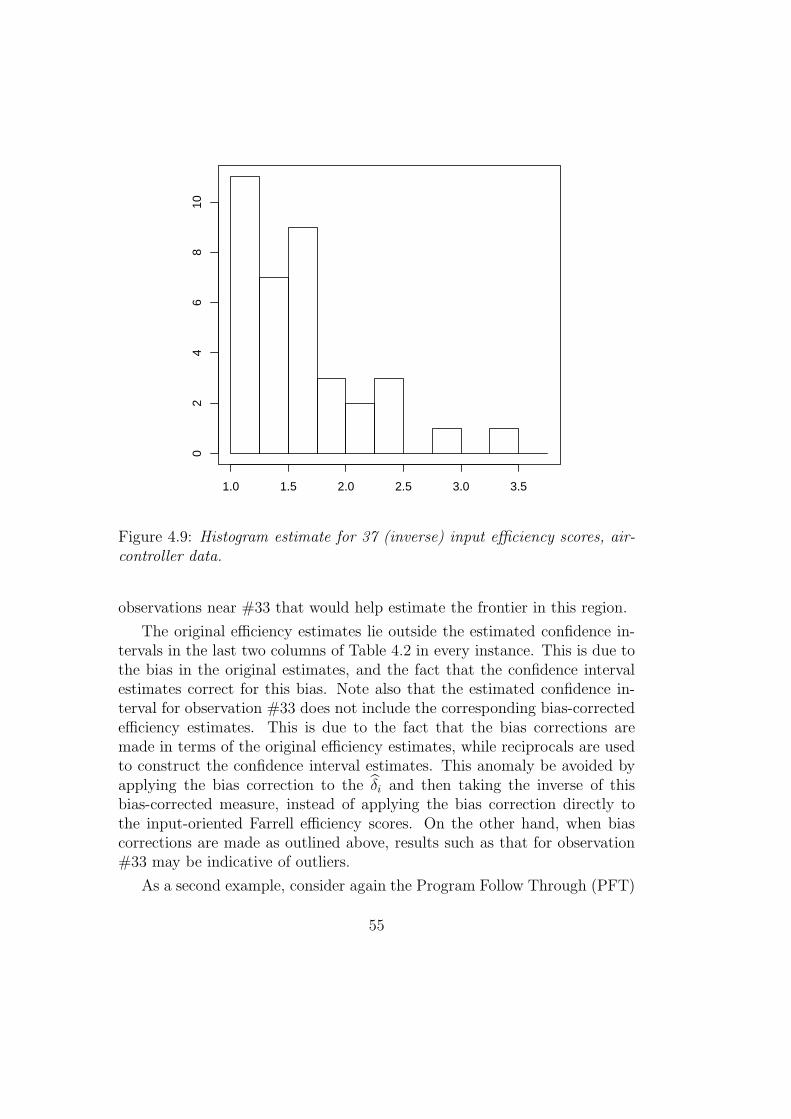
1.0 1.5 2.0 2.5 3.0 3.5

02

46

810

Figure 4.9: Histogram estimate for 37 (inverse) input efficiency scores, air-controller data.

observations near #33 that would help estimate the frontier in this region.

The original efficiency estimates lie outside the estimated confidence in-tervals in the last two columns of Table 4.2 in every instance. This is due tothe bias in the original estimates, and the fact that the confidence intervalestimates correct for this bias. Note also that the estimated confidence in-terval for observation #33 does not include the corresponding bias-correctedefficiency estimates. This is due to the fact that the bias corrections aremade in terms of the original efficiency estimates, while reciprocals are usedto construct the confidence interval estimates. This anomaly be avoided byapplying the bias correction to the δi and then taking the inverse of thisbias-corrected measure, instead of applying the bias correction directly tothe input-oriented Farrell efficiency scores. On the other hand, when biascorrections are made as outlined above, results such as that for observation#33 may be indicative of outliers.

As a second example, consider again the Program Follow Through (PFT)

55

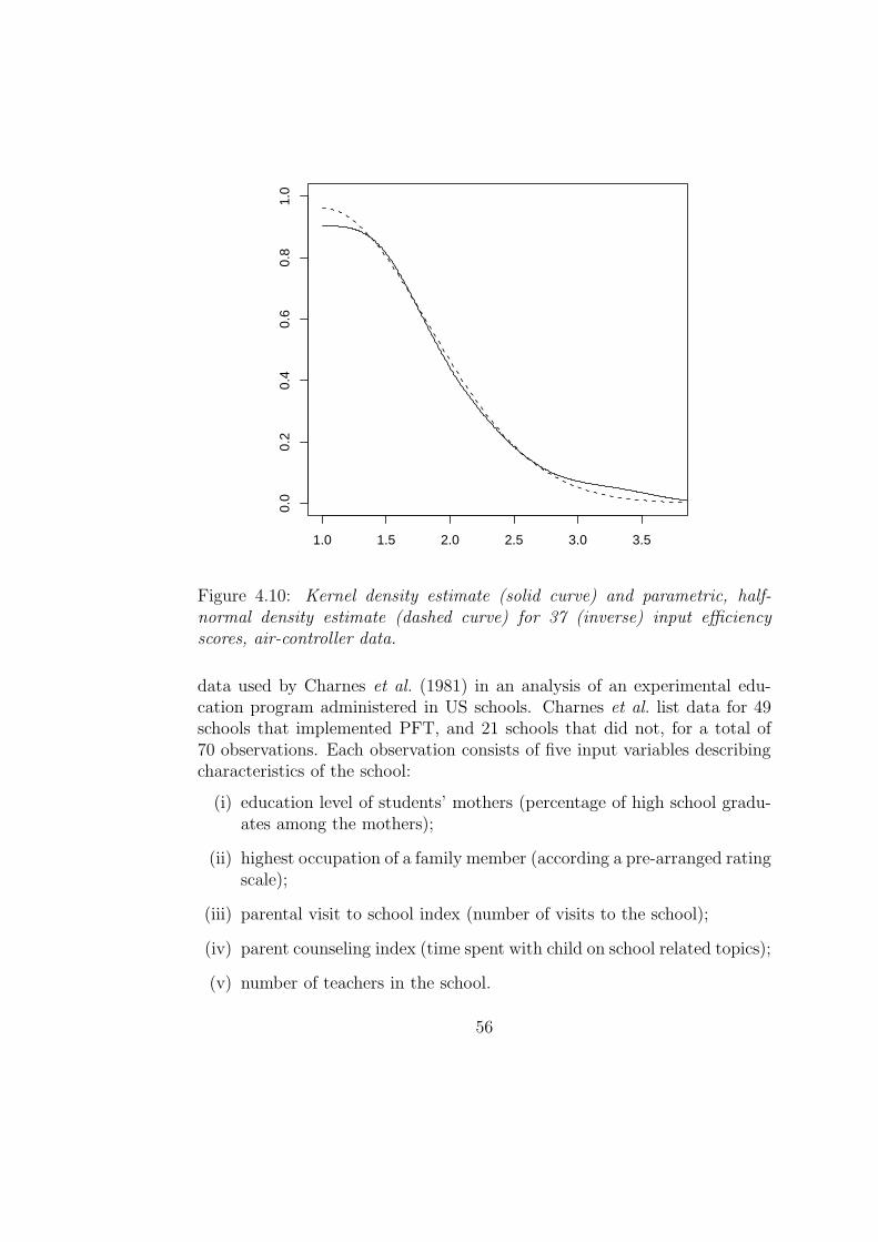
1.0 1.5 2.0 2.5 3.0 3.5

0.0

0.2

0.4

0.6

0.8

1.0

Figure 4.10: Kernel density estimate (solid curve) and parametric, half-normal density estimate (dashed curve) for 37 (inverse) input efficiencyscores, air-controller data.

data used by Charnes et al. (1981) in an analysis of an experimental edu-cation program administered in US schools. Charnes et al. list data for 49schools that implemented PFT, and 21 schools that did not, for a total of70 observations. Each observation consists of five input variables describingcharacteristics of the school:

(i) education level of students’ mothers (percentage of high school gradu-ates among the mothers);

(ii) highest occupation of a family member (according a pre-arranged ratingscale);

(iii) parental visit to school index (number of visits to the school);

(iv) parent counseling index (time spent with child on school related topics);

(v) number of teachers in the school.

56

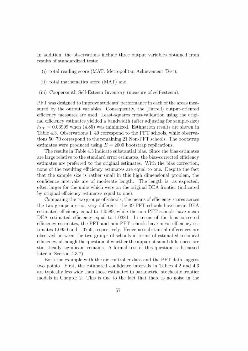
In addition, the observations include three output variables obtained fromresults of standardized tests:

(i) total reading score (MAT: Metropolitan Achievement Test);

(ii) total mathematics score (MAT) and

(iii) Coopersmith Self-Esteem Inventory (measure of self-esteem).

PFT was designed to improve students’ performance in each of the areas mea-sured by the output variables. Consequently, the (Farrell) output-orientedefficiency measures are used. Least-squares cross-validation using the origi-nal efficiency estimates yielded a bandwidth (after adjusting for sample-size)hCV = 0.03999 when (4.85) was minimized. Estimation results are shown inTable 4.3. Observations 1–49 correspond to the PFT schools, while observa-tions 50–70 correspond to the remaining 21 Non-PFT schools. The bootstrapestimates were produced using B = 2000 bootstrap replications.

The results in Table 4.3 indicate substantial bias. Since the bias estimatesare large relative to the standard error estimates, the bias-corrected efficiencyestimates are preferred to the original estimates. With the bias correction,none of the resulting efficiency estimates are equal to one. Despite the factthat the sample size is rather small in this high dimensional problem, theconfidence intervals are of moderate length. The length is, as expected,often larger for the units which were on the original DEA frontier (indicatedby original efficiency estimates equal to one).

Comparing the two groups of schools, the means of efficiency scores acrossthe two groups are not very different: the 49 PFT schools have mean DEAestimated efficiency equal to 1.0589, while the non-PFT schools have meanDEA estimated efficiency equal to 1.0384. In terms of the bias-correctedefficiency estimates, the PFT and non-PFT schools have mean efficiency es-timates 1.0950 and 1.0750, respectively. Hence no substantial differences areobserved between the two groups of schools in terms of estimated technicalefficiency, although the question of whether the apparent small differences arestatistically significant remains. A formal test of this question is discussedlater in Section 4.3.7).

Both the example with the air controller data and the PFT data suggesttwo points. First, the estimated confidence intervals in Tables 4.2 and 4.3are typically less wide than those estimated in parametric, stochastic frontiermodels in Chapter 2. This is due to the fact that there is no noise in the

57

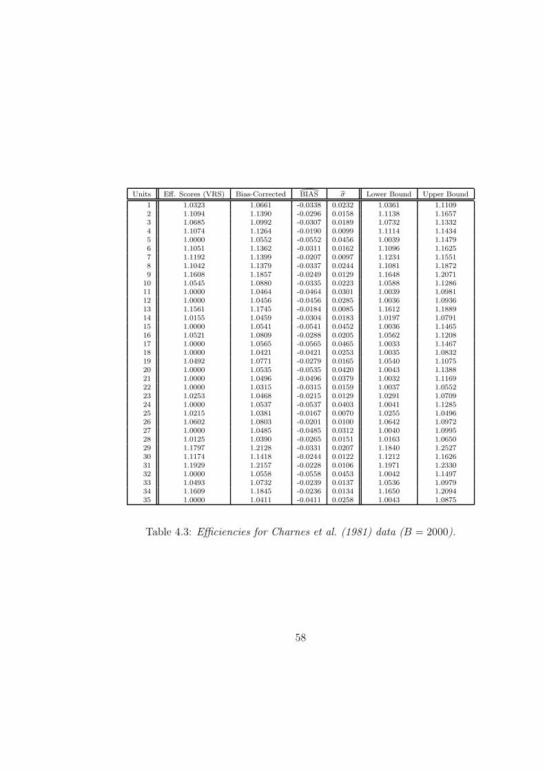
Units Eff. Scores (VRS) Bias-Corrected BIAS bσ Lower Bound Upper Bound

1 1.0323 1.0661 -0.0338 0.0232 1.0361 1.11092 1.1094 1.1390 -0.0296 0.0158 1.1138 1.16573 1.0685 1.0992 -0.0307 0.0189 1.0732 1.13324 1.1074 1.1264 -0.0190 0.0099 1.1114 1.14345 1.0000 1.0552 -0.0552 0.0456 1.0039 1.14796 1.1051 1.1362 -0.0311 0.0162 1.1096 1.16257 1.1192 1.1399 -0.0207 0.0097 1.1234 1.15518 1.1042 1.1379 -0.0337 0.0244 1.1081 1.18729 1.1608 1.1857 -0.0249 0.0129 1.1648 1.2071

10 1.0545 1.0880 -0.0335 0.0223 1.0588 1.128611 1.0000 1.0464 -0.0464 0.0301 1.0039 1.098112 1.0000 1.0456 -0.0456 0.0285 1.0036 1.093613 1.1561 1.1745 -0.0184 0.0085 1.1612 1.188914 1.0155 1.0459 -0.0304 0.0183 1.0197 1.079115 1.0000 1.0541 -0.0541 0.0452 1.0036 1.146516 1.0521 1.0809 -0.0288 0.0205 1.0562 1.120817 1.0000 1.0565 -0.0565 0.0465 1.0033 1.146718 1.0000 1.0421 -0.0421 0.0253 1.0035 1.083219 1.0492 1.0771 -0.0279 0.0165 1.0540 1.107520 1.0000 1.0535 -0.0535 0.0420 1.0043 1.138821 1.0000 1.0496 -0.0496 0.0379 1.0032 1.116922 1.0000 1.0315 -0.0315 0.0159 1.0037 1.055223 1.0253 1.0468 -0.0215 0.0129 1.0291 1.070924 1.0000 1.0537 -0.0537 0.0403 1.0041 1.128525 1.0215 1.0381 -0.0167 0.0070 1.0255 1.049626 1.0602 1.0803 -0.0201 0.0100 1.0642 1.097227 1.0000 1.0485 -0.0485 0.0312 1.0040 1.099528 1.0125 1.0390 -0.0265 0.0151 1.0163 1.065029 1.1797 1.2128 -0.0331 0.0207 1.1840 1.252730 1.1174 1.1418 -0.0244 0.0122 1.1212 1.162631 1.1929 1.2157 -0.0228 0.0106 1.1971 1.233032 1.0000 1.0558 -0.0558 0.0453 1.0042 1.149733 1.0493 1.0732 -0.0239 0.0137 1.0536 1.097934 1.1609 1.1845 -0.0236 0.0134 1.1650 1.209435 1.0000 1.0411 -0.0411 0.0258 1.0043 1.0875

Table 4.3: Efficiencies for Charnes et al. (1981) data (B = 2000).

58

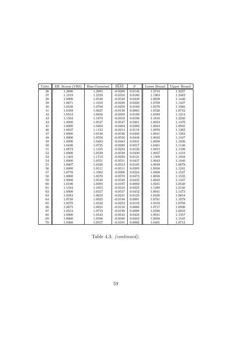
Units Eff. Scores (VRS) Bias-Corrected BIAS bσ Lower Bound Upper Bound

36 1.2686 1.2984 -0.0299 0.0146 1.2744 1.322737 1.1919 1.2229 -0.0310 0.0160 1.1963 1.248238 1.0000 1.0540 -0.0540 0.0448 1.0039 1.144639 1.0671 1.1010 -0.0339 0.0220 1.0709 1.142740 1.0530 1.0788 -0.0259 0.0160 1.0570 1.108041 1.0489 1.0627 -0.0138 0.0065 1.0526 1.074242 1.0553 1.0856 -0.0303 0.0190 1.0589 1.121443 1.1563 1.1873 -0.0310 0.0196 1.1610 1.224044 1.0000 1.0547 -0.0547 0.0461 1.0033 1.147045 1.0000 1.0404 -0.0404 0.0280 1.0043 1.094546 1.0937 1.1152 -0.0214 0.0118 1.0976 1.136547 1.0000 1.0536 -0.0536 0.0400 1.0041 1.128248 1.0000 1.0556 -0.0556 0.0448 1.0042 1.144749 1.0000 1.0483 -0.0483 0.0331 1.0038 1.102050 1.0436 1.0725 -0.0288 0.0217 1.0461 1.114051 1.0872 1.1105 -0.0233 0.0126 1.0915 1.133652 1.0000 1.0539 -0.0539 0.0430 1.0037 1.141853 1.1465 1.1715 -0.0250 0.0121 1.1509 1.191654 1.0000 1.0551 -0.0551 0.0437 1.0043 1.144055 1.0007 1.0320 -0.0313 0.0195 1.0049 1.067956 1.0000 1.0511 -0.0511 0.0395 1.0036 1.124157 1.0776 1.1082 -0.0306 0.0224 1.0808 1.152758 1.0000 1.0570 -0.0570 0.0473 1.0038 1.153559 1.0000 1.0540 -0.0540 0.0445 1.0042 1.144760 1.0196 1.0393 -0.0197 0.0092 1.0231 1.054061 1.1344 1.1655 -0.0310 0.0225 1.1389 1.214062 1.0000 1.0557 -0.0557 0.0452 1.0041 1.147363 1.0383 1.0624 -0.0241 0.0125 1.0430 1.085464 1.0738 1.0925 -0.0188 0.0091 1.0781 1.107965 1.0270 1.0522 -0.0252 0.0132 1.0310 1.075666 1.0675 1.0824 -0.0150 0.0068 1.0717 1.093667 1.0554 1.0753 -0.0199 0.0098 1.0586 1.091668 1.0000 1.0543 -0.0543 0.0424 1.0041 1.135769 1.0000 1.0586 -0.0586 0.0483 1.0038 1.154570 1.0366 1.0557 -0.0191 0.0092 1.0401 1.0712

Table 4.3: (continued).

59

models that have been estimated here, and lack of noise translates into morecertainty about underlying efficiencies.

The second point is that the confidence interval estimates provide a par-tial ordering of observations in the two datasets in terms of efficiency. Theordering is partial to the extent that estimated confidence intervals overlap.Andersen and Petersen (1993) suggested a leave-one-out (LOO) version of theDEA estimator that allows one to rank ostensibly efficient observations (i.e.,those with a convential DEA efficiency estimate equal to one); this idea hasbeen used in a number of applied papers. As remarked below in Section 4.6.1,it is not clear what the LOO estimator estimates; in any case, the method ofAndersen and Petersen does not rely on inference. The confidence intervalsestimates in Tables 4.2 and 4.3 reveal that, at least for the air controller dataand the PFT data, there is a great deal of overlap among confidence intervalsestimated for observations with an initial efficiency estimate equal to one.

4.3.6 Bootstrapping FDH efficiency scores

Since the asymptotic distribution of the FDH estimator is available in aclosed form, even in a multivariate setup, the bootstrap might be seen as lessimportant for making inference with FDH estimators than with DEA esti-mators. However, as noted above in Section 4.2.5, the limiting distributiondepends on an unknown parameter µx,y which can be consistently estimated(see Park et al., 2000), but the estimation introduces additional noise whichmay decrease the precision of inference in finite samples. Nonparametric es-timation of this parameter depends also on a smoothing parameter whichmay be difficult to choose.

It is clear that a naive bootstrap will also be inconsistent here as in thecase of DEA estimators, for largely the same reasons. In addition, FDHestimators present a further difficulty for bootstrap methods. The numberof FDH efficiency scores equal to one will necessarily be larger than in thecase of DEA estimators, increasing the spurious mass at one in the empiricaldistribution of θFDH(xi, yi), i = 1, . . . , n relative to the DEA case. Jeongand Simar (2006) show that a bootstrap based on subsampling (with orwithout replacement) of size m = [nκ], where 0 < κ < 1 provides a consistent

approximation of the sampling distribution of θFDH(x, y) − θ(x, y) (or of

θFDH(x, y)/θ(x, y) if the ratio is preferred).

The procedure is exactly the same as the one described in Section 4.3.4

60

for subsampling of DEA scores, except that here, for each subsample, theFDH estimator is used in place of the DEA estimator. As before, let Xn

∗m,b

denote a random subsample of size m < n drawn from Xn, b = 1, . . . , B andlet θ∗FDH,m,b(x, y) denote the FDH efficiency score of the fixed point (x, y)computed with this reference sample Xn

∗m,b. The set of bootstrap estimates

θ∗FDH,m,b(x, y), b = 1, . . . , B, permits construction of bias-corrected FDHscores and estimation of confidence intervals for θ, analogous to the previousdiscussion for the DEA case.

One might doubt the usefulness of the bootstrap in small samples. Monte-Carlo experiments described by Jeong and Simar (2006) indicate that thesubsampling method works somewhat well for bias-correction. For the ex-periments described there, where n = 100 and M = N = 2, with an optimalchoice of κ = 0.65 (with respect to the MSE criterion), bias is reduced by afactor of 15 along with a reduction of MSE by a factor of 2.4. Other choicesof κ between 0.5 and 1.00 also give substantial improvements for the bias andfor the mean squared error. Similar results were observed with larger sam-ple sizes and for larger dimensionality (i.e., greater numbers of inputs andoutputs). These small Monte-Carlo experiments indicate that the results arerather robust with respect to the choice of κ, and hence the precise choice ofκ does not appear to crucial, although optimal values perform better thanother values.

By contrast, for confidence intervals, the coverages obtained in the Monte-Carlo experiments of Jeong and Simar (2006) perform poorly in terms ofcoverages, except when the sample size is very large (much larger than, say,1,000 observations). The reasons for this are primarily due to the nature ofthe FDH estimator rather than that of subsampling. The value of the FDHestimate is completely determined by only one point among the FDH efficientunits in the data. So, in this case, the approximate discrete distributionobtained through subsampling tends to give too much probability mass onthis one point. Therefore, the approximation of the sampling distributionwill have very poor accuracy, particularly in the tail when the sample size istoo small. For the bias-correction, this poor accuracy is less crucial due tothe averaging used in estimating the bias of the FDH estimator. This arguesin favor of improving the performances of the FDH estimators by using somesmoothing; such an approach is described in Section 4.4.2.

61

4.3.7 Extensions of the bootstrap ideas

The bootstrap ideas developed above can be applied and extended to sev-eral other interesting and important research questions. Two extensions arebriefly discussed here: (i) the problem of testing hypotheses, which might beuseful for choosing among various model sepcifications discussed in Chapter2, and (ii) the problem of making inference on Malmquist indices and theircomponents in various decompositions that are discussed in Chapter 5.

Hypothesis testing

In addition to bias estimation and correction, and estimation of confidenceintervals, the bootstrap can also be very useful for testing various hypothesesabout efficiency or features of the DGP.

In hypothesis testing, the bootstrap can be used either to estimate thep-value of a null hypothesis or to build a critical region. Often the implemen-tation of the bootstrap makes it easy to evaluate p-values; a null hypothesisH0 is rejected at the desired level when the p-value is too small, i.e., lowerthan the desired level.

Two issues must be considered in any testing problem where the bootstrapis used. First, as for any testing procedure, an appropriate statistic that isable to discriminate between the null and the alternative hypotheses must bechosen. Any such statistic will be a function of the data; denote it by τ(Xn).Recall that the data result from a random process (i.e., the DGP); henceτ(Xn) is a random variable. In many cases, τ(Xn) will be bounded on theleft, often at zero; the idea is to determine whether the realized value τ(Xn)(i.e., the value computed from the sample observations) is large enough tocast sufficient doubt on the null hypothesis that it can be rejected. In suchcases, the p-value is defined by

p-value = Prob(τ(Xn) ≥ τobs | H0), (4.90)

where τobs is the realized value of the test statistic obtained from the observedsample. This probability can be estimated by bootstrap methods.

Let Xn∗b denote a random sample obtained by an appropriate bootstrap

algorithm using the original data Xn. Then the sampling distribution of therandom variable τ(Xn) can be approximated by the empirical Monte-Carlodistribution of τ(Xn

∗b), b = 1, . . . , B. In particular the p-value is estimated

62

by:

p-value = Prob(τ(Xn∗) ≥ τobs | Xn, H0). (4.91)

In practice, the estimated p-value is computed using the empirical version of(4.91), namely

p-value =#τ(Xn

∗b) ≥ τobs | b = 1, . . . , B

B(4.92)

It is important to note that the probabilities in (4.91)–(4.92) are condi-tional on H0. This means that the random samples Xn

∗b must be generated

appropriately under the conditions specified by the null hypothesis.As an example, recall that in the case of the Charnes et al. (1981) data on

PFT and non-PFT schools, the mean of DEA (output) efficiency estimatesfor the n1 = 49 PFT schools was 1.0589, while the mean of DEA (output)efficiency estimates for the n2 = 21 non-PFT schools was 1.0384. Supposethat the two groups have access to the same technology, and so they operatewithin the same attainable set Ψ. Further suppose that under the null hy-pothesis the two groups have the same DGP, and hence the mean efficienciesfor the two groups are equal. Denote these means by E(λ1) and E(λ2), andconsider a test of the null hypothesis

H0 : E(λ1) = E(λ2) (4.93)

against the alternative hypothesis

H1 : E(λ1) > E(λ2). (4.94)

Let Xn1 denote the sample of n1 units from group 1 (PFT schools), andlet Xn2 denote the sample of n2 units from group 2 (non-PFT schools). Thefull sample of size n = n1 + n2 is denoted by Xn = Xn1 ∪ Xn2. A reasonabletest statistic would be

τ(Xn) =n−1

1

∑i|(xi,yi)∈Xn1

λ(xi, yi)

n−12

∑i|(xi,yi)∈Xn2

λ(xi, yi), (4.95)

where λ(xi, yi) is the output-oriented DEA efficiency estimator of the unit(xi, yi) computed using the full sample Xn as the reference set (since thetwo groups face the same attainable set, Ψ). When the null is true, then

63

by construction τ(Xn) will be “close” to 1. On the other hand, when thealternative hypothesis is true, τ(Xn) will be “far” from (larger than) one.Hence the p-value for this test has the form given in (4.90), and the nullhypothesis should be rejected if the realized, observed value of τ(Xn), τobs,is too large. The bootstrap can be used to determine how large τobs must beto be “too large.”

To implement the bootstrap, the pseudo-samples Xn∗b must be generated

as if the null hypothesis is true; in the output orientation, the following stepscan performed:

[1] From the original data set Xn, compute λi = λ(xi, yi) ∀ i = 1, . . . , n.

[2] Select a value for h using one of the methods described above.

[3] Generate β∗1 , . . . , β∗

n by drawing with replacement from the set

λ1, . . . , λn, (2 − λ1), . . . , (2 − λn). (4.96)

[4] Draw ε∗i , i = 1, . . . , n independently from the kernel function K(·)and compute

β∗∗i = β∗

i + hε∗i

for each i = 1, . . . , n.

[5] For each i = 1, . . . , n, compute β∗∗∗i as in (4.88) and then compute λ∗

i

as in (4.89).

[6] Define the bootstrap sample Xn∗ = (x∗

i , yi) | i = 1, . . . , n, where

x∗i = λ∗

i x∂(yi) = λ∗

i λ−1i xi.

[7] Compute the DEA efficiency estimates λ∗(xi, yi) for each of the originalsample observations (xi, yi), using the reference set Xn

∗, to obtain a setof bootstrap estimates

λ∗(xi, yi) | i = 1, . . . , n.

[8] Use the set of bootstrap values from step [7] to compute

τ ∗b =

n−11

∑i|(xi,yi)∈Xn1

λ∗(xi, yi)

n−12

∑i|(xi,yi)∈Xn2

λ∗(xi, yi).

64

[9] Repeat steps [3]–[8] B times to obtain a set of bootstrap estimates

τ ∗b | b = 1, . . . , B.

The p-value is approximated by

p =# τ ∗

b ) > τobsB

=

∑Bb=1 1I(τ ∗

b > Tobs)

B, (4.97)

where 1I(·) is the indicator function.Implementing the above algorithm using the Charnes et al. (1981) data

with B = 2000 replications yielded an estimated p value p = 0.5220. Con-sequently, the null hypothesis cannot be reasonably rejected; the mean effi-ciencies of PFT and non-PFT schools are not significantly different at anymeaningful level.

Of course, many other test statistics (mean or median of the ratios,Kolmogoroff-Smirnoff distance, etc., . . . ) could be used to test the equalityof means. One should also realize that testing whether means are equivalentis different from testing whether the distributions of efficiency among twogroups are the same; many different distributions can be found that have thesame means.

The bootstrap procedure can be adapted to many other testing problems.Simar and Zelenyuk (2006) adapt the procedure to consider aggregation is-sues; this involves computation of weighted averages in each group in anappropriate way. Simar and Zelenyuk (2004) propose a test of the equalityof the densities of the efficiency of each group. For this test, a statistic basedon mean squared (L2) distance between nonparametric estimators of densitiesDEA efficiency scores for the two groups is used. Monte-Carlo experimentshave shown that a simple bootstrap test provides a testing procedure withappropriate nominal size and with very good power properties.

Simar and Wilson (2002) adapt the testing procedure described aboveto the problem of testing returns to scale. They investigate the propertiesof the test through intensive Monte-Carlo experiments. Their Monte Carloexperiments indicate that the bootstrap test procedure has reasonable sizeproperties and good power properties. It has also been shown in Monte-Carloexperiments (e.g., Kittelsen, 1997; or Simar and Wilson, 2002) that otherapproaches proposed in the literature not based on the bootstrap idea, butrather on dubious distributional assumptions or uncertain approximations

65

(e.g., Banker, 1996) have serious drawbacks in terms of the accuracy of thesize of the test as well as in term of the power.

Simar and Wilson (2001) provide a bootstrap test procedure for testingrestrictions in frontier models. Their methods can be used to test the rele-vance of particular inputs or outputs (analogous to t-tests or F -tests in linearregression), and to test additivity of inputs or of outputs, which is importantfor possible dimension reduction through aggregation.

Inference on Malmquist indices

When panel data are available, Malmquist indices are sometimes estimatedto examine changes in productivity over time. Various decompositions ofMalmquist indices have been proposed that allow productivity change to bedivided among changes in efficiency, technology, etc. All of these measuresinvolve ratios of distance functions. For each measure, a value of 1 indicatesno change between the two periods considered, while values greater than orless than 1 indicate some change (either improvement or a worsening, de-pending on the particular definition that is used). Thus it is interesting totest the null hypothesis of no change versus a two-sided alternative hypoth-esis of change, or perhaps a one-sided alternative hypothesis of change in aparticular direction (i.e., either worsening or improvement, but not both).

Bootstrap procedures for tests of these types, using panel data, are givenin Simar and Wilson (1999c). The idea there is similar to the ideas discussedabove, with the added complication that observations on the same unit maybe correlated across time periods. This affects how bootstrap pseudo-datamust be generated; failure to account for autocorrelations in the data willresult in a bootstrap that does not replicate the DGP, yielding uncertainand perhaps inconsistent results. Simar and Wilson (1999c) deal with thisproblem by extending the smooth bootstrap discussed earlier by estimating,and drawing from, the joint density of inputs and outputs over the two timeperiods under consideration. This allows estimation of confidence intervalsfor Malmquist indices and the various component indices obtained from thedecompositions that have been proposed in the literature.

66

4.4 Improving the FDH estimator

This section briefly discusses some recent improvements of the FDH esti-mator. The first estimator is based on the idea of correcting for bias whileavoiding the bootstrap. The second approach defines a new nonparametricenvelopment estimator for possibly non-convex production sets; this estima-tor is a smooth (linearized) version of the FDH estimator.

4.4.1 Bias-corrected FDH

By construction, the FDH estimator is highly biased. Badin and Simar (2004)proposed a simple way to derive a bias-corrected version of the FDH estima-tor. Recall from the probabilistic formulation of the production process devel-oped in Section 4.2.4, under the free disposability assumption, the Debreu-Farrell input efficiency scores at (x, y) can be defined as θ(x, y) = infθ |FX|Y (θx|y) > 0, where FX|Y (x|y) = Prob(X ≤ x | Y ≥ y). The FDH esti-mator is the empirical analog of this, obtained by replacing FX|Y with its non-

parametric estimator FX|Y,n, yielding θFDH(x, y) = infθ | FX|Y,n(θx|y) > 0.Since θFDH(x, y) is characterized only by the conditional FX|Y,n, the pop-

ulation mean of θFDH(x, y) can be computed with respect to the populationdistribution FX|Y . It can be shown that the conditional sampling distribution

of θFDH(x, y), given that Y ≥ y, is

Prob(θFDH(x, y) ≤ u | Y ≥ y) = 1 − [1 − FX|Y (ux|y)]ny ,

where ny is the number of observations (xi, yi) such that yi ≥ y. Some furtheralgebra leads to

E(θFDH(x, y) | Y ≥ y) = θ(x, y) +

∫ ∞

θ(x,y)

[1 − FX|Y (ux|y)]ny du. (4.98)

The last term in (4.98) gives an expression for the bias of the FDH estimator.Although this expression depends on unknowns (θ(x, y) and FX|Y (·|y)), thebias can be estimated by replacing the unknowns with their empirical coun-terparts, i.e., by replacing FX|Y (·|y) with FX|Y,n(·|y) and replacing θ(x, y)

with θFDH(x, y).This suggests a bias-corrected FDH estimator of θ defined by

θbcFDH(x, y) = θFDH(x, y) −∫ ∞

bθF DH(x,y)

[1 − FX|Y,n(ux|y)]ny du. (4.99)

67

The integral in (4.99) can be computed easily and rapidly using numericalmethods. The computation is much faster than the bias correction computedby the bootstrap. In addition, there are no smoothing parameters to specifyhere; when the subsampling bootstrap described in Section 4.3.6 is used,one must choose the subsample size. The method here is thus an attractivealternative to the bootstrap bias correction method.

The theoretical properties of the bias-corrected FDH estimator are in-vestigated in Badin and Simar (2004). To summarize, the bias-correctedFDH estimator and the ordinary FDH estimator share the same the sameasymptotic distribution. Without a formal proof, it can be seen here thatthe bias correction must vanish as n increases since the integral in (4.99)goes to zero as n → ∞. In finite samples, however, which is the case in anyreal application, the gain in terms of reductions in bias and MSE may beconsiderable.

Monte-Carlo experiments reported in Badin and Simar (2004) suggestthat in finite samples, the bias-corrected FDH estimator behaves well whencompared to the FDH estimator. The Monte-Carlo experiments confirm that,as expected the bias is reduced (by a factor 1.46 to 1.36 when the sample sizegrows from n = 50 to 800 for the case M = N = 1). More importantly, MSEis also found to decrease with the bias-corrected estimator (by a factor 2.12to 1.8 in the same scenario). Of course, when the sample size n is larger, thegain is less dramatic, but still worthwhile. Badin and Simar observe similarbehavior for problems involving greater dimensionality.

4.4.2 Linearly interpolated FDH: LFDH

In addition to the curse of dimensionality shared by most of the nonpara-metric techniques, the non-smoothness of the FDH estimator makes its usevery difficult for statistical inference in finite samples. Although in principlethe bootstrap provides a method for making inference (recall that the sub-sampling bootstrap provides a consistent approximation of the sampling dis-tribution of FDH estimators), simulation studies in Jeong and Simar (2006)indicate that the subsampling bootstrap is not a good idea for estimatingconfidence intervals for reasons that were discussed in Section 4.3.6.

Since under the assumptions in Section 4.2.1 the true frontier is contin-uous, one might hope to improve the performance of the FDH estimatorby smoothing its corresponding frontier. This is the idea of the linearized(LFDH) estimator introduced by Jeong and Simar (2006), who show that in-

68

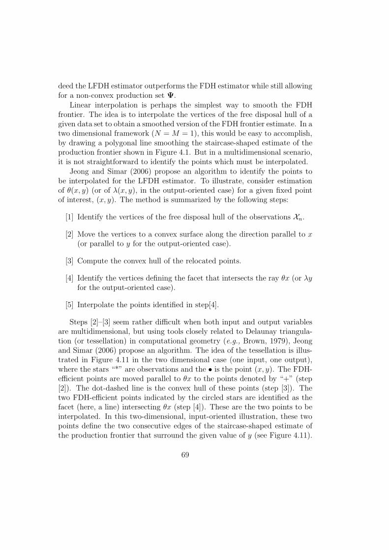
deed the LFDH estimator outperforms the FDH estimator while still allowingfor a non-convex production set Ψ.

Linear interpolation is perhaps the simplest way to smooth the FDHfrontier. The idea is to interpolate the vertices of the free disposal hull of agiven data set to obtain a smoothed version of the FDH frontier estimate. In atwo dimensional framework (N = M = 1), this would be easy to accomplish,by drawing a polygonal line smoothing the staircase-shaped estimate of theproduction frontier shown in Figure 4.1. But in a multidimensional scenario,it is not straightforward to identify the points which must be interpolated.

Jeong and Simar (2006) propose an algorithm to identify the points tobe interpolated for the LFDH estimator. To illustrate, consider estimationof θ(x, y) (or of λ(x, y), in the output-oriented case) for a given fixed pointof interest, (x, y). The method is summarized by the following steps:

[1] Identify the vertices of the free disposal hull of the observations Xn.

[2] Move the vertices to a convex surface along the direction parallel to x(or parallel to y for the output-oriented case).

[3] Compute the convex hull of the relocated points.

[4] Identify the vertices defining the facet that intersects the ray θx (or λyfor the output-oriented case).

[5] Interpolate the points identified in step[4].

Steps [2]–[3] seem rather difficult when both input and output variablesare multidimensional, but using tools closely related to Delaunay triangula-tion (or tessellation) in computational geometry (e.g., Brown, 1979), Jeongand Simar (2006) propose an algorithm. The idea of the tessellation is illus-trated in Figure 4.11 in the two dimensional case (one input, one output),where the stars “*” are observations and the • is the point (x, y). The FDH-efficient points are moved parallel to θx to the points denoted by “+” (step[2]). The dot-dashed line is the convex hull of these points (step [3]). Thetwo FDH-efficient points indicated by the circled stars are identified as thefacet (here, a line) intersecting θx (step [4]). These are the two points to beinterpolated. In this two-dimensional, input-oriented illustration, these twopoints define the two consecutive edges of the staircase-shaped estimate ofthe production frontier that surround the given value of y (see Figure 4.11).

69

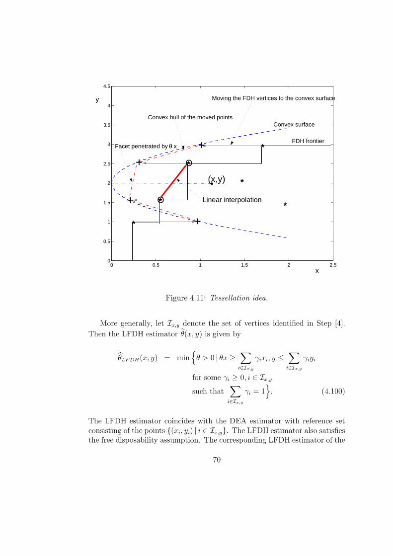
0 0.5 1 1.5 2 2.50

0.5

1

1.5

2

2.5

3

3.5

4

4.5

x

y

*

*

*

*

*

*

FDH frontier

•

Convex surface

Moving the FDH vertices to the convex surface

Convex hull of the moved points

(x,y)

O

O

Linear interpolation

+

+

+ + Facet penetrated by θ x

Figure 4.11: Tessellation idea.

More generally, let Ix,y denote the set of vertices identified in Step [4].

Then the LFDH estimator θ(x, y) is given by

θLFDH(x, y) = minθ > 0 | θx ≥

∑

i∈Ix,y

γixi, y ≤∑

i∈Ix,y

γiyi

for some γi ≥ 0, i ∈ Ix,y

such that∑

i∈Ix,y

γi = 1. (4.100)

The LFDH estimator coincides with the DEA estimator with reference setconsisting of the points (xi, yi) | i ∈ Ix,y. The LFDH estimator also satisfiesthe free disposability assumption. The corresponding LFDH estimator of the

70

attainable set Ψ is given by

ΨLFDH =

(x, y) ∈ RN+M+ | x ≥ θLFDH(u, v)u, y ≤ v,

for some (u, v) ∈ ΨFDH

(4.101)

The asymptotic distribution of n1/(N+M)(θLFDH(x, y) − θ(x, y)) is thesame as the non-degenerate limiting distribution of a random variable ζn

that can be easily simulated. In other words, the asymptotic distribution ofn1/(N+M)(θLFDH(x, y)−θ(x, y)) can be simulated by taking a large number ofrandom draws of ζn; this provides a route to inference-making. By estimatingthe mean or quantiles of ζn, a bias-corrected estimator can be constructedor confidence intervals for θ(x, y) of any desired level can be estimated (seeJeong and Simar, 2006, for details).

The Monte-Carlo experiments described in Jeong and Simar (2006) indi-cate that the LFDH estimator outperforms the FDH estimator both in termsof bias (bias is reduced by a factor more than 2) as well as MSE (MSE isreduced by a factor of the order 4), for sample sizes n = 100 or 400 and whenN = M = 2 or when N = 4 and M = 1.

The LFDH estimator involves a greater computational burden than theFDH, since it requires solution of two linear programs: one for solving theproblem in Step 3 above, and one (of limited size) for solving (4.100).

4.5 Robust Nonparametric Frontier Estima-

tors

All the nonparametric envelopment estimators of frontiers are particularlysensitive to extreme observations, or outliers. These extreme points maydisproportionately, and perhaps misleadingly, influence the evaluation of theperformance of other firms. This drawback also plagues parametric frontierestimators when deterministic frontier models are considered. One approachto this problem would be to identify any outliers in the data, and then per-haps delete them if they result from corrupted data. A number of techniquesexist for finding outliers in frontier settings (e.g., Wilson, 1993, 1995; Simar,2003a; Porembski et al., 2005). Alternatively, one can use robust estimatorsthat have been recently developed, which also offer other advantages.

71

Recent papers by Cazals et al. (2002), Daraio and Simar (2005a), Aragonet al. (2002), and Daouia and Simar (2004, 2005) have developed robustalternatives to the traditional FDH and DEA estimators. These new estima-tors involve the concept of a “partial” frontier, as opposed to the traditionalidea of a “full” frontier that envelops all the data. The new ideas replace thegoals of estimating the absolute lowest (uppermost) technically achievablelevel of input (output) for a given level of output (input) with the idea ofestimating something “close” to these quantities.

As such, the partial frontiers considered in this section are “less extreme”than the full frontier. Since estimation of partial frontiers avoids many ofthe statistical problems inherent in estimating a full frontier, partial fron-tiers provide a more useful benchmark against which firms can be compared.Natural nonparametric estimators of these partial frontiers will be proposedthat are very easy and fast to compute.

Two families of partial frontiers have been proposed: (i) order-m frontiers,where m can be viewed as a trimming parameter, and (ii) order-α quantilefrontiers, analogous to traditional quantile functions but adapted to the fron-tier problem. It turns out that the resulting nonparametric estimators havemuch better properties than the usual nonparametric (DEA or FDH) frontierestimators; the new estimators do not suffer from the curse of dimensionality,and the standard parametric

√n rate of convergence is achieved along with

asymptotic normality.

Another interesting feature is that both estimators of these partial fron-tiers are also consistent estimators of the full frontier, by allowing the order ofthe frontier (m or α) to grow (at an appropriate rate) with increasing samplesize (although for practical applications, where sample size is typically fixed,this theoretical result may be of limited use). These new estimators of thefull frontier shares the same asymptotic properties as FDH estimators. But,in finite samples, the new estimators do not envelop all the data, and so aremuch more robust with respect to outliers and extreme values in the samplethan the usual FDH or DEA estimators. As a side benefit, these “partial-order” frontiers and their estimators provide very useful tools for detectingoutliers (e.g., Simar, 2003a). The basic ideas are based on the probabilisticformulation of a production process as developed in Section 4.2.4.

72

4.5.1 Order-m frontiers

The discussion in this section is presented in terms of the input-orientation,but as before, the concepts easily adapt to the output orientation. For clar-ification, a summary of concepts for the output orientation are given at theend of this section.

Definition and basic ideas

Recall that in Section 4.2.4, the production process was modeled in termsof the probability distribution function HXY (x, y) = Prob(X ≤ x, Y ≥ y).For the input orientation, the full frontier and the resulting Debreu-Farrellefficiency scores are characterized by properties of the conditional distributionFX|Y (x|y) = Prob(X ≤ x | Y ≥ y) that describes the behavior of firms whichproduce at least level y of output. In terms of the input efficiency score,

θ(x, y) = infθ | FX|Y (θx|y) > 0, (4.102)

assuming free disposability; see (4.31).The full frontier can be viewed as the lower radial boundary of FX|Y (x|y),

or as the minimum achievable lower boundary of inputs for all possiblefirms producing at least level y of output. This is a rather extreme andabsolute (theoretical) concept: it gives the full minimum achievable level ofinput over all production plans that are technically feasible. An alternativebenchmark is obtained by defining the expected minimum input achieved byany m firms chosen randomly from the population and producing at leastoutput level y, For finite values of m, this will be seen shortly to providea potentially more useful benchmark for comparing firms in terms of theirefficiencies than the frontier ∂Ψ. It will also become apparent that if mgoes to infinity, the problem becomes identical to FDH estimation of the fullfrontier ∂Ψ.

To make things more precise, suppose an output level y is given. Considerm iid random variables Xi, i = 1, . . . , m drawn from the conditional N -variate distribution function FX(· | y), and define the set

Ψm(y) = (x′, y′) ∈ RN+M+ | x′ ≥ Xi, y′ ≥ y, i = 1, . . . , m. (4.103)

This random set is the free disposal hull of m firms that produce at least thelevel y of output. Then, for any x and the given y, the Debreu-Farrell input

73

efficiency score relative to the set Ψm(y) is

θm(x, y) = infθ | (θx, y) ∈ Ψm(y). (4.104)

The set Ψm(y) is random, since it depends on the random variables Xi with(conditional) distribution function FX(· | y). Hence the efficiency score

θm(x, y) is also random. For a given realization of the m values Xi, a re-

alization of θm(x, y) is obtained by computing

θm(x, y) = mini=1, ..., m

max

j=1, ..., p

(Xji

xj

). (4.105)

The order-m input efficiency score is defined as follows:

Definition 4.5.1. For all y such that SY (y) = Prob(Y ≥ y) > 0, the(expected) order-m input efficiency measure, the order-m input efficiencyscore is given by

θm(x, y) ≡ E(θm(x, y) | Y ≥ y), (4.106)

The order-m input efficiency score benchmarks a unit operating at (x, y)against the expected minimum input among m peers randomly drawn fromthe population of units producing at least y. This efficiency measure in turndefines an order-m input efficient frontier. For any (x, y) ∈ Ψ, the expectedminimum level of inputs of order-m for a unit producing output level y andfor an input mix determined by the vector x is given by

x∂m(y) = θm(x, y) x. (4.107)

For comparison, recall that the full frontier ∂Ψ is defined (at output level y)by x∂(y) = θ(x, y) x in (4.6).

If x is univariate, this new, order-m input frontier can be described byan input function of order-m:

x∂m(y) = φm(y) = E

[min(X1, . . . , Xm) | Y ≥ y

]

=

∫ ∞

0

[1 − FX(x | y)]m dx. (4.108)

The concept is illustrated in Figure 4.12, which resembles Figure 4.3. Fig-ure 4.12 shows the input-oriented order-m frontier for a particular value

74

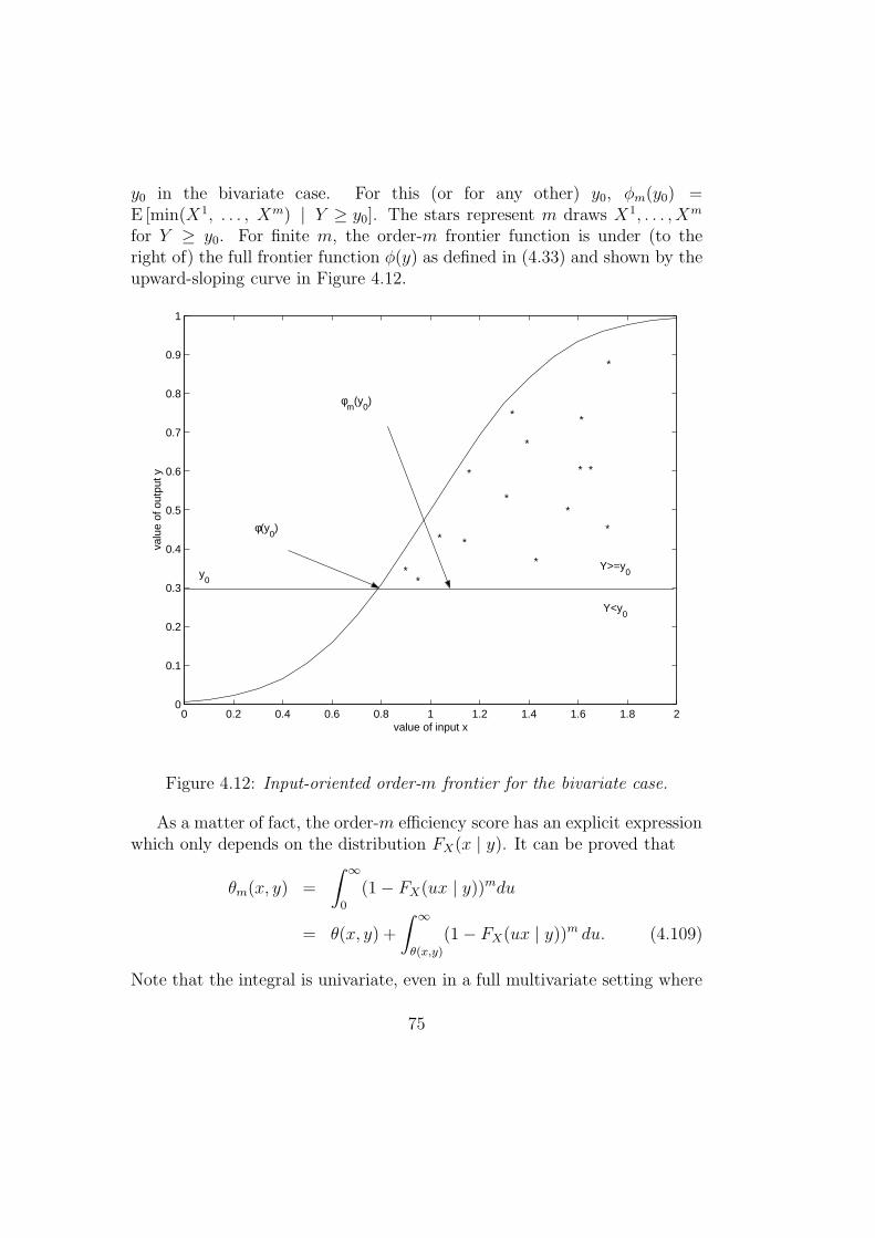
y0 in the bivariate case. For this (or for any other) y0, φm(y0) =E [min(X1, . . . , Xm) | Y ≥ y0]. The stars represent m draws X1, . . . , Xm

for Y ≥ y0. For finite m, the order-m frontier function is under (to theright of) the full frontier function φ(y) as defined in (4.33) and shown by theupward-sloping curve in Figure 4.12.

0 0.2 0.4 0.6 0.8 1 1.2 1.4 1.6 1.8 20

0.1

0.2

0.3

0.4

0.5

0.6

0.7

0.8

0.9

1

value of input x

valu

e of

out

put y

y0

Y>=y0

Y<y0

φ(y0)

φm

(y0)

*

* *

*

*

*

*

*

*

*

*

*

*

*

*

Figure 4.12: Input-oriented order-m frontier for the bivariate case.

As a matter of fact, the order-m efficiency score has an explicit expressionwhich only depends on the distribution FX(x | y). It can be proved that

θm(x, y) =

∫ ∞

0

(1 − FX(ux | y))mdu

= θ(x, y) +

∫ ∞

θ(x,y)

(1 − FX(ux | y))m du. (4.109)

Note that the integral is univariate, even in a full multivariate setting where

75

(N, M) ≥ 1. As expected, as m → ∞, the order-m frontier tends to the fullfrontier. From (4.109), it is obvious that

limm→∞

θm(x, y) = θ(x, y) (4.110)

since the integrand in (4.109) is less or equal to 1.

Nonparametric estimators

It was shown above that for the full frontier approach, the probabilistic for-mulation in Section 4.2.4 allows the plug-in principle to be used to providean appealing, alternative characterization of FDH estimators.

Following the same ideas here, an intuitive, nonparametric estimator ofθm(x, y) is obtained by plugging the empirical version of FX(x | y) into(4.109) to obtain

θm,n(x, y) = E(θm(x, y) | Y ≥ y)

=

∫ ∞

0

(1 − FX,n(ux | y))mdu,

= θFDH(x, y) +

∫ ∞

bθF DH(x,y)

(1 − FX,n(ux | y))mdu. (4.111)

This estimator involves the computation of a univariate integral that is easyto solve using numerical methods. Even for large values of N , M and m,the estimator is very fast to compute because the integral remains one-dimensional. When N = 1, an explicit analytical solution is available (seeCazals et al. 2002). For the full multivariate setting, Daraio and Simar(2005a) propose a Monte-Carlo algorithm for approximating the expectationin (4.111), thereby avoiding the need for numerical integration. However, forlarge m, computing the integral in (4.111) is faster.

Analogous to (4.107), for a firm operating at (x, y) ∈ Ψ, an estimate ofits expected minimum input level of order-m is

x∂m(y) = θm,n(x, y) x. (4.112)

Just as (4.107) can be evaluated over the range of possible output levels yto trace out the expected minimum input frontier of order m, denoted ∂Ψin

m,(4.112) can also be evaluated for the possible values of y to trace out an

estimate ∂Ψinm of ∂Ψin

m.

76

By construction, the estimator ∂Ψinm with finite m does not envelop all the

observations in the sample Xn. Consequently, the estimator is less sensitivethan either the FDH or DEA frontier estimators to extreme points or out-liers. Again, the estimator ∂Ψin

m shares the same property as its population

counterpart, ∂Ψinm; as m increases, for a fixed sample size n, ∂Ψin

m convergesto the usual FDH estimator of ∂Ψ, while ∂Ψin

m converges to ∂Ψ; i.e.,

θm,n(x, y) → θFDH(x, y), as m → ∞. (4.113)

The proof is trivial.

Statistical properties

The estimators described above in Section 4.5.1 possess some interestingproperties that are unusual among nonparametric estimators. First, for anyfixed value of m, θm,n(x, y) converges to θm(x, y) at the rate

√n, and its

asymptotic distribution is normal; i.e.,

√n[θm,n(x, y) − θm(x, y)

]d−→ N (0, σ2

in(x, y)), (4.114)

where the variance for σ2in(x, y) depends on FX(x | y); see Cazals et al. 2002

for details. This variance can be estimated consistently using the plug-inprinciple, where FX(· | y) is replaced by its empirical analog FX,n(· | y)) inthe expression for σ2

in(x, y) given by Cazals et al. Alternatively, this variancecan be estimated using a naive bootstrap, where pseudo-samples are obtainedby drawing from the empirical distribution of the observations in Xn. Thenaive bootstrap can be used (provided m is finite) since the boundaries of

support for f(x, y) are not estimated; i.e., both ∂Ψinm and ∂Ψin

m lie in theinterior of Ψ, away from ∂Ψ. Estimates of confidence intervals can also beobtained easily using a naive bootstrap approach.

Since θm(x, y) → θ(x, y) as m → ∞, one might be tempted to use

θm,n(x, y) as an estimator of θ(x, y) itself, by using large values of m. Cazalset al. (2002) show that if m = m(n) → ∞ as n → ∞ (with m increasing atan appropriate rate),

n1

p+q

[θm,n(x, y) − θ(x, y)

]d−→ Weibull(µx,y, N + M), (4.115)

where the parameter of the Weibull is the same as in Section 4.2.5. Henceif n → ∞ and m = m(n) → ∞, θm,n(x, y) shares the same properties as

77

the FDH estimator. In finite samples, however, the order-m estimator willbe more robust with respect to outliers and extreme values since it does notenvelop all the (extreme) observations in the sample.

This latter property gives another appealing feature of the order-m esti-mators. In practice, the choice of a particular value of m should be guided bythis robustness property. Since the estimator involves little computationalburden, it can be computed for several values of m (e.g., m = 25, 50, 100,150, 200, . . . ). For each value of m, one can observe the percentage of obser-vations in the sample that lie outside the resulting order-m frontier estimate(such observations are indicated by a value θm,n(xi, yi) > 1). This percentagewill decrease as m increases; as described below, this property can also beused to detect outliers. The final value of m can be chosen in terms of thedesired level of robustness; for example, one might choose a value for m thatresults in approximately 5 percent of the observations in Xn lying outside∂Ψin

m. Experience has shown that in many applications, qualitative conclu-sions are little affected by particular choices of m, provided the values of mare somewhat less than the sample size, n.

Summary for the output-oriented case

For an output-oriented analysis, suppose an input level x in the interior of thesupport of X is given, and consider m iid random variables Yi, i = 1, . . . , mdrawn from the conditional M-variate distribution function FY (y | x) =Prob(Y ≤ y | X ≤ x). Analogous to (4.103), define the random set

Ψm(x) = (x′, y) ∈ RN+M+ | x′ ≤ x, Yi ≤ y, i = 1, . . . , m. (4.116)

Then, for any y, define

λm(x, y) = supλ | (x, λy) ∈ Ψm(x)

= maxi=1,...,m

min

j=1,...,p

(Y ji

yj

). (4.117)

The order-m output efficiency measure is defined as follows:

Definition 4.5.2. For any y ∈ RM+ , the (expected) order-m output efficiency

measure, denoted by λm(x, y), is defined for all x in the interior of the supportof X by

λm(x, y) ≡ E(λm(x, y) | X ≤ x), (4.118)

78

where the expectation is assumed to exist.

Analogous to (4.109) and (4.110),

λm(x, y) =

∫ ∞

0

[1 − (1 − SY (uy | x))m] du

= λ(x, y) −∫ λ(x,y)

0

(1 − SY (uy | x))m du, (4.119)

and

limm→∞

λm(x, y) = λ(x, y). (4.120)

A nonparametric estimator of λm(x, y) is given by:

λm(x, y) =

∫ ∞

0

[1 − (1 − SY,n(uy | x))m

]du

= λn(x, y) −∫ bλn(x,y)

0

(1 − SY,n(uy | x))mdu. (4.121)

This estimator shares properties analogous to those of the input-orientedestimator. In particular, the output-oriented estimator also achieves

√n-

consistency and asymptotic normality; i.e.,

√n[λm,n(x, y) − λm(x, y)

]d−→ N (0, σ2

out(x, y)). (4.122)

In addition, as m → ∞, λm(x, y) → λ(x, y) and λm,n(x, y) → λFDH(x, y).Analogous to (4.115), if m = m(n) → ∞ at an appropriate rate as n → ∞,

n1

p+q

[λm,n(x, y) − λ(x, y)

]d−→ Weibull(µx,y, N + M) as n → ∞. (4.123)

As m = m(n) → ∞, the estimator λm,n(x, y) shares the same properties asthe FDH estimator. But, in finite samples, it will be more robust to outliersand extreme values since it will not envelop all the observations in the sample.

Examples

To illustrate the order-m estimators, consider a simple example where N =M = 1 and the upper boundary of the production set Ψ is described by

y = g(x) = (2x − x2)1/2. (4.124)

79

Suppose interest lies in the fixed point (x0, y0) = (0.5, 0.5), and that obser-vations result from independent draws from the probability density functionf(x, y) with support over the production set Ψ. Suppose also that the jointprobability density of inputs and outputs, f(x, y), is uniform over Ψ; hence

f(x, y) =

4π

∀ x ∈ [0, 1], y ∈ [0, g(x)];0 otherwise.

(4.125)

Given (4.124) and (4.125), the true order-m frontiers can be recovered.For the input-orientation, FX|Y (x | Y ≥ y) = Prob(X ≤ x | Y ≥ y) isneeded. From the joint density given in (4.125), the marginal density of y isgiven by

f(y) =

∫ 1

1−√

1−y2

f(x, y) dx

= 4π−1(1 − y2)1/2,

(4.126)

and hence the marginal distribution function of y is

F (y) = Prob(Y ≤ y)

=

1 ∀ Y > 14π−1

[12y(1 − y2)1/2 + 1

2sin−1(y)

]∀ Y ∈ [0, 1]

0 otherwise.(4.127)

Conditional on Y ≥ y, the joint density of (X, Y ) is

f(x, y | Y ≥ y) = [1 − F (y)]−1 f(x, y);

integrating with respect to Y gives the conditional density of X:

f(x | Y ≥ y) = [1 − F (y)]−1

∫ (2x−x2)1/2

y

4π−1 du

= [1 − F (y)]−1 4π−1[(2x − x2)1/2 − y

](4.128)

for all x ∈[1 −

√1 − y2

0, 1]. Integrating in (4.128) with respect to x gives

the conditional distribution function for x,

80

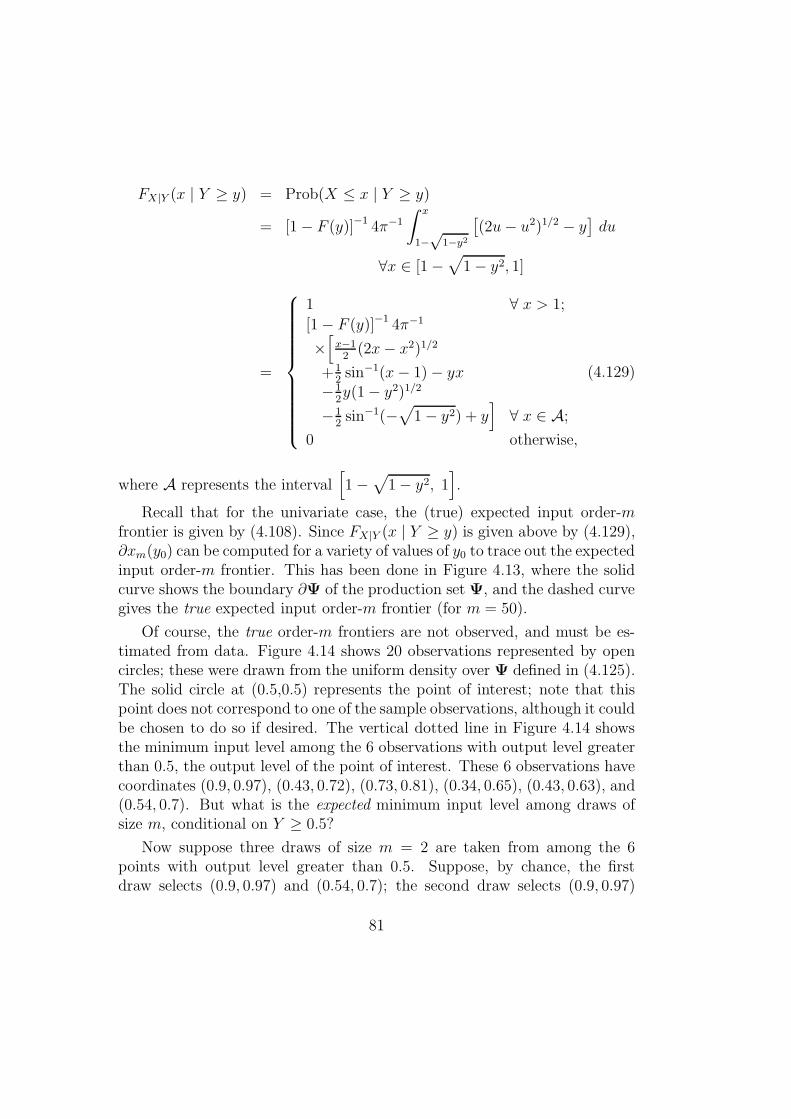
FX|Y (x | Y ≥ y) = Prob(X ≤ x | Y ≥ y)

= [1 − F (y)]−1 4π−1

∫ x

1−√

1−y2

[(2u − u2)1/2 − y

]du

∀x ∈ [1 −√

1 − y2, 1]

=

1 ∀ x > 1;

[1 − F (y)]−1 4π−1

×[

x−12

(2x − x2)1/2

+12sin−1(x − 1) − yx

−12y(1 − y2)1/2

−12sin−1(−

√1 − y2) + y

]∀ x ∈ A;

0 otherwise,

(4.129)

where A represents the interval[1 −

√1 − y2, 1

].

Recall that for the univariate case, the (true) expected input order-mfrontier is given by (4.108). Since FX|Y (x | Y ≥ y) is given above by (4.129),∂xm(y0) can be computed for a variety of values of y0 to trace out the expectedinput order-m frontier. This has been done in Figure 4.13, where the solidcurve shows the boundary ∂Ψ of the production set Ψ, and the dashed curvegives the true expected input order-m frontier (for m = 50).

Of course, the true order-m frontiers are not observed, and must be es-timated from data. Figure 4.14 shows 20 observations represented by opencircles; these were drawn from the uniform density over Ψ defined in (4.125).The solid circle at (0.5,0.5) represents the point of interest; note that thispoint does not correspond to one of the sample observations, although it couldbe chosen to do so if desired. The vertical dotted line in Figure 4.14 showsthe minimum input level among the 6 observations with output level greaterthan 0.5, the output level of the point of interest. These 6 observations havecoordinates (0.9, 0.97), (0.43, 0.72), (0.73, 0.81), (0.34, 0.65), (0.43, 0.63), and(0.54, 0.7). But what is the expected minimum input level among draws ofsize m, conditional on Y ≥ 0.5?

Now suppose three draws of size m = 2 are taken from among the 6points with output level greater than 0.5. Suppose, by chance, the firstdraw selects (0.9, 0.97) and (0.54, 0.7); the second draw selects (0.9, 0.97)

81

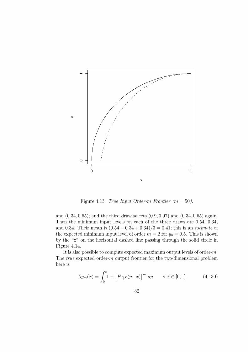
x

y

0 1

01

Figure 4.13: True Input Order-m Frontier (m = 50).

and (0.34, 0.65); and the third draw selects (0.9, 0.97) and (0.34, 0.65) again.Then the minimum input levels on each of the three draws are 0.54, 0.34,and 0.34. Their mean is (0.54 + 0.34 + 0.34)/3 = 0.41; this is an estimate ofthe expected minimum input level of order m = 2 for y0 = 0.5. This is shownby the “x” on the horizontal dashed line passing through the solid circle inFigure 4.14.

It is also possible to compute expected maximum output levels of order-m.The true expected order-m output frontier for the two-dimensional problemhere is

∂ym(x) =

∫ x

0

1 −[FY |X(y | x)

]mdy ∀ x ∈ [0, 1]. (4.130)

82

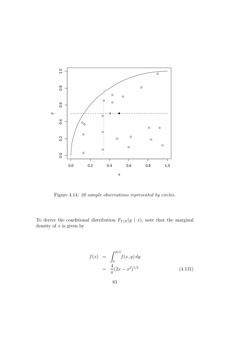
0.0 0.2 0.4 0.6 0.8 1.0

0.0

0.2

0.4

0.6

0.8

1.0

x

y x

Figure 4.14: 20 sample observations represented by circles.

To derive the conditional distribution FY |X(y | x), note that the marginaldensity of x is given by

f(x) =

∫ g(x)

0

f(x, y) dy

=4

π(2x − x2)1/2 (4.131)

83

and the marginal distribution function of x is

FX(x) = Prob(X ≤ x)

=

1 ∀ x > 1;

4π−1[

x−12

(2x − x2)1/2

+12sin−1(x0 − 1) + π

4

]∀ x ∈ [0, 1];

0 ∀ x < 0.

(4.132)

The joint density of x and y, given X ≤ x, is then f(x, y | X ≤ x) =FX(x)−1f(x, y) ∀ y ∈ [0, g(x)], X ≤ x and therefore the marginal density ofy given X ≤ x is

f(y | X ≤ x) = FX(x)−1

∫ x

1−√

1−y2

f(u, y) du

= FX(x)−14π−1[x − 1 + (1 − y2)1/2

]

∀ y ∈ [0, g(x0)]. (4.133)

Then

FY |X(y | X ≤ x) = Prob(Y ≤ y | X ≤ x)

=

1 ∀ y > g(x);

FX(x)−14π−1

(x − 1)y

+12

[y(1 − y2)1/2

+ sin−1(y)]

∀ y ∈ [0, g(x)];

0 ∀ y < 0.

(4.134)

Using the expression for FY |X(y | x) given by (4.134), ∂ym(x) can becomputed for variety of values of x to trace out the expected order-m outputfrontier. This has been done in Figure 4.15, where the solid curve shows theboundary ∂Ψ of the production set Ψ, and the dashed curve depicts the trueexpected order-m output frontier (for m = 50).

84

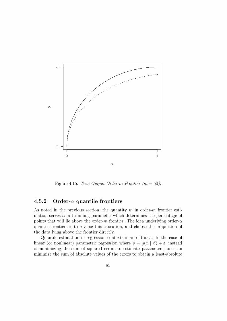
x

y

0 1

01

Figure 4.15: True Output Order-m Frontier (m = 50).

4.5.2 Order-α quantile frontiers

As noted in the previous section, the quantity m in order-m frontier esti-mation serves as a trimming parameter which determines the percentage ofpoints that will lie above the order-m frontier. The idea underlying order-αquantile frontiers is to reverse this causation, and choose the proportion ofthe data lying above the frontier directly.

Quantile estimation in regression contexts is an old idea. In the case oflinear (or nonlinear) parametric regression where y = g(x | β) + ε, insteadof minimizing the sum of squared errors to estimate parameters, one canminimize the sum of absolute values of the errors to obtain a least-absolute

85

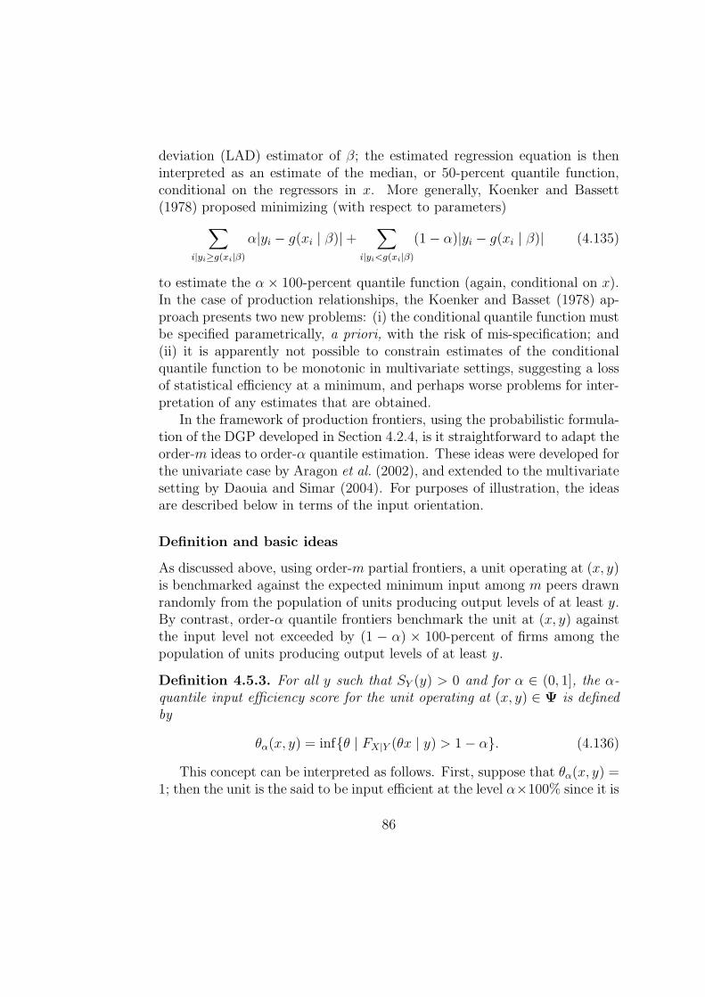
deviation (LAD) estimator of β; the estimated regression equation is theninterpreted as an estimate of the median, or 50-percent quantile function,conditional on the regressors in x. More generally, Koenker and Bassett(1978) proposed minimizing (with respect to parameters)

∑

i|yi≥g(xi|β)

α|yi − g(xi | β)| +∑

i|yi<g(xi|β)

(1 − α)|yi − g(xi | β)| (4.135)

to estimate the α × 100-percent quantile function (again, conditional on x).In the case of production relationships, the Koenker and Basset (1978) ap-proach presents two new problems: (i) the conditional quantile function mustbe specified parametrically, a priori, with the risk of mis-specification; and(ii) it is apparently not possible to constrain estimates of the conditionalquantile function to be monotonic in multivariate settings, suggesting a lossof statistical efficiency at a minimum, and perhaps worse problems for inter-pretation of any estimates that are obtained.

In the framework of production frontiers, using the probabilistic formula-tion of the DGP developed in Section 4.2.4, is it straightforward to adapt theorder-m ideas to order-α quantile estimation. These ideas were developed forthe univariate case by Aragon et al. (2002), and extended to the multivariatesetting by Daouia and Simar (2004). For purposes of illustration, the ideasare described below in terms of the input orientation.

Definition and basic ideas

As discussed above, using order-m partial frontiers, a unit operating at (x, y)is benchmarked against the expected minimum input among m peers drawnrandomly from the population of units producing output levels of at least y.By contrast, order-α quantile frontiers benchmark the unit at (x, y) againstthe input level not exceeded by (1 − α) × 100-percent of firms among thepopulation of units producing output levels of at least y.

Definition 4.5.3. For all y such that SY (y) > 0 and for α ∈ (0, 1], the α-quantile input efficiency score for the unit operating at (x, y) ∈ Ψ is definedby

θα(x, y) = infθ | FX|Y (θx | y) > 1 − α. (4.136)

This concept can be interpreted as follows. First, suppose that θα(x, y) =1; then the unit is the said to be input efficient at the level α×100% since it is

86

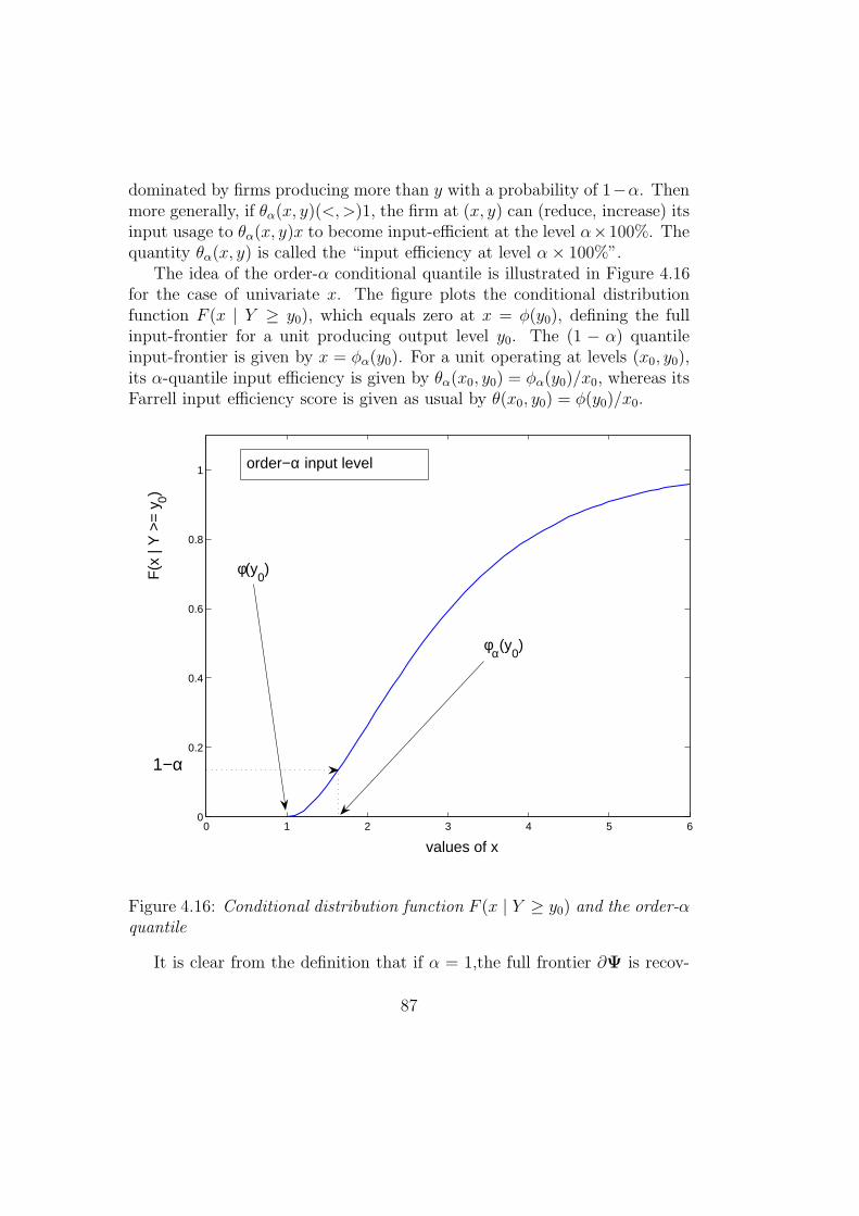
dominated by firms producing more than y with a probability of 1−α. Thenmore generally, if θα(x, y)(<, >)1, the firm at (x, y) can (reduce, increase) itsinput usage to θα(x, y)x to become input-efficient at the level α×100%. Thequantity θα(x, y) is called the “input efficiency at level α × 100%”.

The idea of the order-α conditional quantile is illustrated in Figure 4.16for the case of univariate x. The figure plots the conditional distributionfunction F (x | Y ≥ y0), which equals zero at x = φ(y0), defining the fullinput-frontier for a unit producing output level y0. The (1 − α) quantileinput-frontier is given by x = φα(y0). For a unit operating at levels (x0, y0),its α-quantile input efficiency is given by θα(x0, y0) = φα(y0)/x0, whereas itsFarrell input efficiency score is given as usual by θ(x0, y0) = φ(y0)/x0.

0 1 2 3 4 5 60

0.2

0.4

0.6

0.8

1

values of x

F(x

| Y

>=

y0)

φ(y0)

φα(y0)

order−α input level

1−α

Figure 4.16: Conditional distribution function F (x | Y ≥ y0) and the order-αquantile

It is clear from the definition that if α = 1,the full frontier ∂Ψ is recov-

87

ered; in this case, θ1(x, y) ≡ θ(x, y) is the Debreu-Farrell input measure ofefficiency. In fact, it can be proved that the convergence of θα(x, y) to θ(x, y)when α → 1 is monotone; i.e.,

limα→1

ց θα(x, y) = θ(x, y), (4.137)

where “ց” denotes monotone convergence from above.The concept of efficiency of order-α allows definition of the corresponding

efficient frontier at the level α× 100%. This production frontier is called theα-quantile efficient frontier. It may be defined as the efficient input at thelevel α × 100% for a given level of output y, and for an input mix given byan input vector x:

x∂α(y) = θα(x, y) x. (4.138)

By definition, a unit operating at the point (x∂α(y), y) ∈ Ψ has a probability

HXY (x∂α(y), y) = (1 − α)SY (y) ≤ 1 − α of being dominated. Analogous to

∂Ψinm, x∂

α(y) can be evaluated for all possible y to trace out an order-α inputfrontier, denoted ∂Ψin

α .The order-α efficiency concept comes with an important existence prop-

erty. It can be proved that if FX|Y is continuous and monotone increasing inx then, for all (x, y) in the interior of Ψ, there exists an α ∈ (0, 1] such thatθα(x, y) = 1, where α = 1−FX|Y (x|y). In other words, any point (x, y) in theinterior of Ψ belongs to some α-quantile input efficient frontier. Therefore,the value α = α(x, y) such that (x, y) ∈ ∂Ψin

α (i.e., the value of α that definesan order-α frontier containing (x, y)) can be used as a new measure of inputefficiency. Order-m frontiers do not have an analogous property, due to thediscrete, integer-valued parameter m.

Nonparametric Estimator

Here again the plug-in principle can be used to obtain an intuitive, nonpara-metric estimator of θα(x, y) replacing FX|Y (· | ·) in (4.136) with its empiricalcounterpart to obtain

θα,n(x, y) = infθ | FX|Y,n(θx|y) > 1 − α. (4.139)

Computation of this estimator is very fast. An explicit analytical formula isavailable for the case N = 1 (see Aragon et al., 2002), and a simple algorithmfor the multivariate case is given in Daouia and Simar (2004).

88

As for the estimator of the order-m efficiencies, this estimator does notenvelop all the observed data in Xn when α < 1. Hence, it is less sensitiveto extreme points and to outliers. than the traditional FDH and DEA esti-mators. This estimator also shares the same property as the correspondingpopulation concept: i.e., for a fixed sample size n, as α → 1, the order-αestimator converges to the usual FDH estimator of the full frontier. It is easyto prove that

θα,n(x, y) ց θFDH(x, y) as α → 1. (4.140)

Statistical properties

Not surprisingly, the statistical properties of the order-α quantile estimatorsare very similar to those of the order-m estimators. In particular,

√n[θα,n(x, y) − θα(x, y)

]d−→ N (0, σ2

α(x, y)). (4.141)

An expression is available for the variance term σ2α(x, y); see Daouia and

Simar (2004) for details. Hence the nonparametric order-α efficiency estima-tor is

√n-consistent with an asymptotic normal distribution.

In addition, analogous to the order-m estimators, when α = α(n) → 1 atan appropriate rate as n → ∞,

n1

N+M

[θα(n),n(x, y) − θ(x, y)

]d−→ Weibull(µx,y, N + M). (4.142)

Hence θα(n),n(x, y) shares the same asymptotic property as the FDH estimatorbut, since the corresponding frontier does not envelop all the observed datapoints, θα(n),n(x, y) is more robust to outliers in finite sample than the FDHestimator.

Summary for the output oriented case

For the output oriented case, the order-α efficiency measure can be definedas follows:

Definition 4.5.4. For all x such that FX(x) > 0 and for α ∈ (0, 1], the α-quantile output efficiency score for the unit operating at (x, y) ∈ Ψ is definedas

λα(x, y) = supλ | SY |X(λy | x) > 1 − α. (4.143)

89

If λα(x, y)(<, >)1, then the output-oriented measure gives the propor-tionate (reduction, increase) in outputs needed to move a unit operating at(x, y) ∈ Ψ in the output direction so that it is dominated by firms using lessinput (than the level x) with probability 1 − α.

Analogous to the input-oriented order-α efficiency measure, λα(x, y) con-verges monotonically to the Debreu-Farrell output efficiency measure; i.e.,

limα→1

ր λα(x, y) = λ(x, y) (4.144)

where “ր” denotes monotonic convergence from below. Moreover, for all(x, y) ∈ Ψ, (x, y) 6∈ ∂Ψ, there exists an α ∈ (0, 1] such that λα(x, y) = 1,where α = 1 − SY |X(y | x).

A nonparametric estimator of λα(x, y) is obtained by substituting theempirical counterpart of SY |X,n(· | ·) into (4.143) to obtain

λα,n(x, y) = supλ | SY |X,n(λy | x) > 1 − α; (4.145)

recall that SY |X,n was defined in Section 4.2.4. This estimator also has√

n-convergence and asymptotic normality:

√n(λα,n(x, y) − λα(x, y))

d−→ N (0, σ2out(x, y)), as n → ∞, (4.146)

and converges to the FDH estimator as α → 1:

limα→1

ր λα,n(x, y) = λFDH(x, y). (4.147)

Finally, λα,n(x, y) provides a robust estimator of the full-frontier efficiencyscores: as α = α(n) → 1 at an appropriate rate as n → ∞,

n1

N+M

[λα(n),n(x, y) − λ(x, y)

]d−→ Weibull(µx,y, N + M). (4.148)

An Example

Table 4.4 gives input-oriented FDH, α-quantile, and order-m efficiency esti-mates for the 37 European air traffic controllers introduced in Section 4.3.5.The second column gives the number nd of observations that dominate eachobservation. The third colum gives the FDH efficiency estimate, while thenext three columns give the α-quantile estimates for α = 0.90, 0.95, and 0.99.The last three columns give the order-m estimates for m = 10, 20, and 150.

90

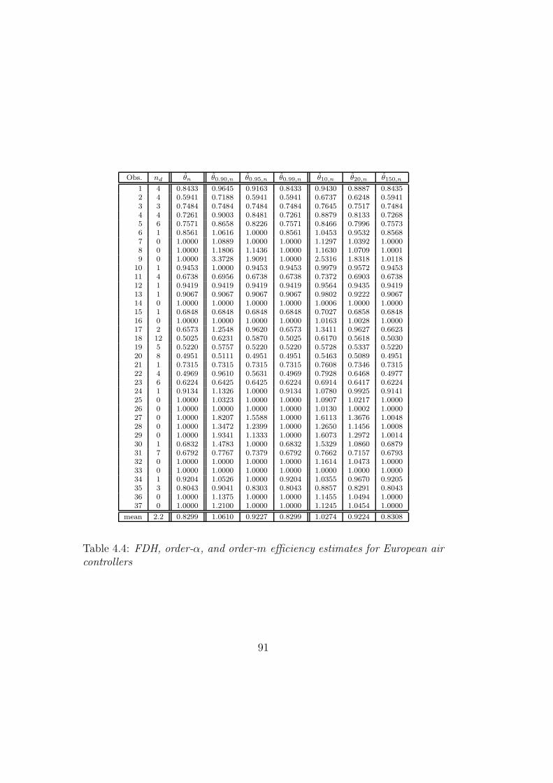
Obs. nd θn θ0.90,n θ0.95,n θ0.99,n θ10,n θ20,n θ150,n

1 4 0.8433 0.9645 0.9163 0.8433 0.9430 0.8887 0.84352 4 0.5941 0.7188 0.5941 0.5941 0.6737 0.6248 0.59413 3 0.7484 0.7484 0.7484 0.7484 0.7645 0.7517 0.74844 4 0.7261 0.9003 0.8481 0.7261 0.8879 0.8133 0.72685 6 0.7571 0.8658 0.8226 0.7571 0.8466 0.7996 0.75736 1 0.8561 1.0616 1.0000 0.8561 1.0453 0.9532 0.85687 0 1.0000 1.0889 1.0000 1.0000 1.1297 1.0392 1.00008 0 1.0000 1.1806 1.1436 1.0000 1.1630 1.0709 1.00019 0 1.0000 3.3728 1.9091 1.0000 2.5316 1.8318 1.0118

10 1 0.9453 1.0000 0.9453 0.9453 0.9979 0.9572 0.945311 4 0.6738 0.6956 0.6738 0.6738 0.7372 0.6903 0.673812 1 0.9419 0.9419 0.9419 0.9419 0.9564 0.9435 0.941913 1 0.9067 0.9067 0.9067 0.9067 0.9802 0.9222 0.906714 0 1.0000 1.0000 1.0000 1.0000 1.0006 1.0000 1.000015 1 0.6848 0.6848 0.6848 0.6848 0.7027 0.6858 0.684816 0 1.0000 1.0000 1.0000 1.0000 1.0163 1.0028 1.000017 2 0.6573 1.2548 0.9620 0.6573 1.3411 0.9627 0.662318 12 0.5025 0.6231 0.5870 0.5025 0.6170 0.5618 0.503019 5 0.5220 0.5757 0.5220 0.5220 0.5728 0.5337 0.522020 8 0.4951 0.5111 0.4951 0.4951 0.5463 0.5089 0.495121 1 0.7315 0.7315 0.7315 0.7315 0.7608 0.7346 0.731522 4 0.4969 0.9610 0.5631 0.4969 0.7928 0.6468 0.497723 6 0.6224 0.6425 0.6425 0.6224 0.6914 0.6417 0.622424 1 0.9134 1.1326 1.0000 0.9134 1.0780 0.9925 0.914125 0 1.0000 1.0323 1.0000 1.0000 1.0907 1.0217 1.000026 0 1.0000 1.0000 1.0000 1.0000 1.0130 1.0002 1.000027 0 1.0000 1.8207 1.5588 1.0000 1.6113 1.3676 1.004828 0 1.0000 1.3472 1.2399 1.0000 1.2650 1.1456 1.000829 0 1.0000 1.9341 1.1333 1.0000 1.6073 1.2972 1.001430 1 0.6832 1.4783 1.0000 0.6832 1.5329 1.0860 0.687931 7 0.6792 0.7767 0.7379 0.6792 0.7662 0.7157 0.679332 0 1.0000 1.0000 1.0000 1.0000 1.1614 1.0473 1.000033 0 1.0000 1.0000 1.0000 1.0000 1.0000 1.0000 1.000034 1 0.9204 1.0526 1.0000 0.9204 1.0355 0.9670 0.920535 3 0.8043 0.9041 0.8303 0.8043 0.8857 0.8291 0.804336 0 1.0000 1.1375 1.0000 1.0000 1.1455 1.0494 1.000037 0 1.0000 1.2100 1.0000 1.0000 1.1245 1.0454 1.0000

mean 2.2 0.8299 1.0610 0.9227 0.8299 1.0274 0.9224 0.8308

Table 4.4: FDH, order-α, and order-m efficiency estimates for European aircontrollers

91

The results illustrate that for the α-quantile estimator, increasing α to-ward unity moves the α-quantile efficiency estimates toward the FDH effi-ciency estimate. Similarly, for the order-m estimator, increasing m yieldsestimates increasingly close to the FDH efficiency estimate. Recall from Fig-ure 4.8 that observation #33 lies in a remote part of the sample space. Con-sequently, in Table 4.4, this observation yields an efficiency estimate equalto one for each of the values of α and m that were considered. Put simply,since there are no other observations near unit #33, the sample contains noinformation that would allow us to gauge the efficiency of this unit. In termsof the discussion in Chapter 1, this unit may represent “best-practice,” butthat does not mean that it lies on the boundary of the production set.

4.5.3 Outlier Detection

The traditional nonparametric, deterministic FDH and DEA frontier estima-tors are appealing because they rely on only a few mild assumptions. Theirhistory in applied use is now long. Moreover, they estimate the full frontier∂Ψ, rather than the partial frontiers described above. This feature, how-ever, is a double-edged sword: by construction, FDH and DEA estimatorsare highly sensitive to extreme values and to outliers.

Outliers are atypical observations. Some outliers are the result of record-ing or measurement errors and should be corrected (if possible) or deletedfrom the data. Outliers might also appear in a given sample if, inadvertently,observations are drawn from different DGPs. If data are viewed as havingcome from a probability distribution, then it is quite possible to observepoints with low probability. One would not expect to observe many suchpoints given their low probability, and hence they appear as outliers. Cookand Weisberg (1982) observe that outliers of this type may lead to the recog-nition of important phenomena that might otherwise have gone unnoticed;in some cases such outliers may be the most interesting part of the data.

Since FDH and DEA estimators continue to be used, outlier detection isof vital importance. In simple, bivariate scenarios where N = M = 1, onecould merely look at a scatter plot to find any outliers that might exist. Un-fortunately, in higher dimensions, detecting outliers is much more difficult.Although there is a large literature in statistics and econometrics on out-lier detection, most methods that have been proposed were designed for theproblem of conditional mean estimation and do not take aspects of frontiermodels into account; see Wilson (1993) for discussion. In the frontier setting,

92

the most worrisome outliers are those that have undue influence on the esti-mated efficiencies of other observations. Many of the standard methods foroutlier detection are also very computer intensive in multivariate settings.

A relatively small number of outlier-detection methods have been pro-posed specifically for the context of frontier estimation. It is unlikely thata single method will be able to find all outliers in all instances when thenumber of dimensions is large. Consequently, many have argued that sev-eral methods should be employed on a given data set. All outlier-detectionmethods should be viewed as diagnostic tools; the goal is to first identify a(hopefully) small set of observations for further scrutiny. See Wilson(1993),Olesen et al. (1996), and Simar (2003b) for further discussion.

Wilson (1995) proposed a procedure similar to jackknife estimation,wherein observations are deleted one-at-a-time, with efficiency for the re-maining (n−1) observations re-estimated with each deletion to gauge the in-fluence of each observation on the estimated efficiencies of other observationsin the sample. The process is then repeated, deleting pairs of observations,then repeated again while deleting triplets, etc. in order to uncover maskingeffects. Masking occurs when two (or more) outliers lie close to each other;removing only one of these will not reveal undue influence, which can onlybe discovered if the entire group of near-by outliers is removed. Althougheffective, the number of linear program solutions that must be obtained toimplement the Wilson (1995) procedure if pairs, triplets, etc. are deletedgrows combinatorially with sample size. The procedure becomes very costlyin terms of required computational time as the sample size becomes large,and consequently is not practical for use with samples larger than a fewhundred observations.

Wilson (1993) proposed another method employing an influence functionbased on the geometric volume spanned by the sample observations, andthe sensitivity of this volume with respect to deletions of singletons, pairs,triplets, etc. from the sample. Some notation is required to explain themethod. For a value ξ computed from a set of observations indexed by S =1, . . . , n, let D

(ℓ)L (ξ) denote the value computed similarly from observations

with indices S − L, where L ⊂ S and L contains ℓ elements, ℓ < n. LetD

(ℓ)L (ξ) denote the value computed similarly from observations only in L;

e.g., D(ℓ)L (ξ) = D

(ℓ)S−L(ξ). For any matrix A of full column rank, let D(ℓ)(|A|)

denote the determinant of the matrix D(ℓ)(A).

Let X be an (N×n) matrix of observations on n input vectors, and Y be

93

an (M×n) matrix of observations on the corresponding output vectors. Then

add a row of ones to X by defining the ((N + 1)× n) matrix Z =[1 X

′]′.

Define the ((N + M + 1) × n) partitioned matrix Z∗ =

[Z

′Y

′]′

. For

the case of M outputs, M ≥ 1, |Z∗Z

∗′ | = |ZZ′| · |Y Y

′ − Y Z′B| with

B = (ZZ′)−1

ZY′. For j, k = 1, . . . , M , Y jY

′k − Y jZ

′bk = Y j(Y′k −

Z′bk) = Y je

′k = Y jMZY

′k = Y jMZ

′MZY

′k = eje

′k where MZ is the

idempotent matrix (I − Z′(ZZ

′)−1Z) and ej , ek are ordinary least squares

(OLS) residuals from the regressions of Y′j, Y

′k on Z

′. Then |Z∗Z

∗′| =|ZZ

′| × |Y Y′ − Y Z

′B| = |ZZ

′| × |Ω| where Ω = [eje′k], j, k = 1, . . . , q.

The statistic

R(ℓ)L (Z∗′) = D

(ℓ)L (|Z ′

Z|) ||Z ′Z|−1[D

(ℓ)L (|Ω|)]|Ω|−1 (4.149)

represents the proportion of the geometric volume in (N + M + 1)-spacespanned by a subset of the data obtained by deleting the ℓ observations withindices in the set L, relative to the volume spanned by the entire set of nobservations.

Wilson (1993) discusses a statistical procedure for deriving significancelevels for the statistic defined in (4.149), and also describes a graphical anal-

ysis where log-ratios log[R

(ℓ)L (Z∗′)/R

(ℓ)min

], where R

(ℓ)min = minL

R

(ℓ)L (Z∗′)

,

are plotted as a function of ℓ, the number of observations deleted. Thismethod is implemented in the FEAR software package described by Wilson(2007). See Wilson (1993) for further details and empirical examples.

Simar (2003b) proposed an outlier detection strategy using the ideas ofpartial frontiers developed in the preceding sections. If a sample observationremains outside the order-m frontier as m increases, or alternatively out-side the order-α frontier as α increases, then such an observation may bean outlier. The procedure is implemented by first computing, for each sam-ple observation (xi, yi), i = 1, . . . , n, the leave-one-out order-m efficiencies

θ(i)m,n(xi, yi) for several values of m; e.g., m ∈ 10, 25, 50, 75, 00, 150, . . .,

where θ(i)m,n(xi, yi) denotes the order-m efficiency estimate for the ith obser-

vation computed after deleting the ith observation. Next, the percentage ofpoints lying outside the order-m frontier (identified by values θ

(i)m,n(xi, yi) > 1

in the input-orientation, or λ(i)m,n(xi, yi) < 1 in the output-orientation) can

be plotted as a function of m; the resulting points can be connected by linesegments to form a piecewise-linear relationship that is necessarily downwardsloping due to the properties of the order-m estimator. If there are no outliers

94

in the data set, the plotted relationship should be nearly linear. If the graphshows an elbow effect (i.e., a sharp bend, with large negative slope becomingmuch less negative at a particular value of m), firms remaining outside theorder-m frontier for the value of m where the sharp bend occurs are likelyoutliers and should be carefully scrutinized for data errors, etc. The analy-sis can be performed using both input- and output-oriented perspectives todetect potential outliers in both directions.

This method requires that threshold values be chosen for deciding whenthe values θ

(i)m,n(xi, yi) or λ

(i)m,n(xi, yi) are significantly greater or less than

one. Ideally, these threshold values should be computed from the asymp-totic standard deviations of the estimators. However, to make the proce-dure simple and easy to compute, Simar (2003b) suggests producing sev-eral diagnostic plots as described above using percentages of points withθ

(i)m,n(xi, yi) > 1+ ζ or λ

(i)m,n(xi, yi) > 1−ζ with several small, arbitrary values

of ζ ; e.g., ζ ∈ 0, 0.05, 0.10, 0.15, 0.20, . . ..Although the method proposed by Simar (2003b) does not explicitly ad-

dress the possibility of masking among outliers, if only a small number ofoutliers lie close to each other, the robustness properties of the order-m es-timator makes it likely these will be detected. Once an initial set of outliershas been identified, the analysis could be repeated after deleting the initialset of outliers. The method is implemented in the FEAR package (Wilson,2007); in addition, Matlab code for the procedure as well as several examplesare provided in Simar (2003b).

4.6 Explaining Efficiencies

For many years, researchers have sought to explain differences in estimatedefficiencies across firms. Often, researchers have in mind a set of environmen-tal factors that might be related to efficiency differences; these factors mightreflect differences in ownership type or structure, regulatory constraints, busi-ness environment, competition, etc. among the firms under analysis. Typ-ically, such factors are viewed as possibly affecting the production process,but not under the control of firms’ managers. Understanding how such fac-tors might be related to efficiency is important for determining how firms’performances might be improved. In addition, from a public policy perspec-tive, understanding these relationships is important for assessing the costs ofregulation.

95

One approach (e.g., Coelli et al., 1998) is to augment the model intro-duced in Section 4.1.1 by treating the (continuous) environmental factors zas free disposal inputs or outputs that contribute to defining the attainableset Ψ ⊂ RN

+ × RM+ × RR, and to modify the efficiency scores defined in (4.5)

and (4.9) to reflect the view that the environmental variables are beyondmanagers’ control. For example, the analog of (4.5) would be

θ(x, y | z) = infθ | (θx, y, z) ∈ Ψ. (4.150)

The FDH and DEA estimators of Ψ in this case would be defined as beforeafter adding the variables z and treating them as either inputs or outputs(if z is a vector of variables, some elements of z might be treated as inputs,while others might be treated as outputs).

There are at least two drawbacks to this approach. First, one must decidea priori what the role of z is; in other words, do the variables contained in zcontribute to, or hinder production of quantities y? Second, free-disposabilityis assumed when FDH or DEA estimators are used; in addition, convexity ofΨ is also assumed when DEA estimators are employed. For many environ-mental variables, it is difficult to find arguments for why these assumptionsmight be appropriate.

When discrete, categorical factors are considered (e.g., for-profit versusnon-profit organizations; private versus public ownership; etc.), the categor-ical variables effectively divide producers into different groups. If there areR binary, discrete categorical variables, then there are potentially 2R differ-ent groups represented among the n sample observations. In this case, it isstraightforward to adapt the bootstrap methods described in Section 4.3.7 fortesting hypothesis about differences in average efficiency, etc. across groupsto make comparisons among the 2R implied groups of firms. One might test,for example, whether the various groups face the same technology, or whetherthe distributions of efficiencies are the same across groups if they do face thesame technology.

When the environmental variables z are continuous, observations are notgrouped into a small number of categories. In this section, two approaches forinvestigating the effects of continuous environmental variables on efficiencyare discussed. The first is based on a two-stage approach that has beenwidely used in the literature but too often with dubious specifications andinvalid inference. The second approach was recently proposed by Daraio andSimar (2005a), and involves an extension of the techniques in Section 4.5.1for estimating partial frontiers.

96

4.6.1 Two-stage regression approach

A plethora of papers have employed a two-stage approach wherein nonpara-metric, DEA efficiency estimates are regressed on continuous environmentalvariables in a parametric, second-stage analysis. The idea is widespread:the internet search engine google.com reported ∼1,500 results using the keywords “dea,” “two-stage,” and “efficiency” on January 27, 2005, while thekey words “dea” and “tobit” yielded ∼825 results; in addition, Simar andWilson (2007) cite 47 published papers that use this approach.

Apparently, none of the papers written to date that have regressed DEAor FDH efficiency estimates in a second-stage model, with the exception ofSimar and Wilson (2007), define a DGP that would make a second-stageregression sensible. In addition, to the knowledge of the authors of thischapter, inference on the parameters of the second-stage regressions is invalidin these papers.

Simar and Wilson (2007) define a DGP that provides a rational basis forregressing efficiency estimates in a second-stage analysis. In addition, theysuggest bootstrap procedures to provide valid inference in the second-stageregression, as well as to increase the efficiency of estimation there. Monte-Carlo experiments confirm the improvements.

A DGP with environmental variables

The basic DGP defined in Section 4.2.1 must be modified to incorporatethe role of environmental variables Z which may influence the productionprocess. Here, X ∈ RN

+ , Y ∈ RM+ , and Z ∈ RR (the elements of Z may be

continuous or discrete). A sample Sn = (xi, yi, zi)ni=1 is observed, but of

course Ψ remains unknown. Replace Assumption 4.2.1 with the followingassumption:

Assumption 4.6.1. The sample observations (xi, yi, zi) in Sn are iid re-alizations of random variables (X, Y, Z) with probability density functionf(x, y, z), which has support Ψ×RR, where Ψ is the production set as definedin (4.1) with Prob((X, Y ) ∈ Ψ) = 1.

Note that Assumption 4.6.1 introduces a separability condition betweenthe production space for inputs inputs and outputs, Ψ, and the space of theenvironmental variables. In other words, the variables Z do not influencethe shape or boundary of Ψ; they lie in a space apart from Ψ. This is a

97

rather restrictive assumption, but this is implicit (but not stated) in all thetwo-stage regression approaches that exist to date. The alternative approachdescribed below in Section 4.6.2 will avoid this assumption. Of course, in anyinteresting case, Z is not independent with respect to (X, Y ), i.e., f(x, y |z) 6= f(x, y). However, Z may influence efficiency.

For purposes of illustration, the presentation that follows is in terms ofthe output-orientation. We will make the presentation here in the output-oriented case, where for some point (x, y) ∈ RM+N

+ , the goal is to estimatethe Debreu-Farrell output measure of efficiency λ = λ(x, y) defined in (4.9).Recall that for all (x, y) ∈ Ψ, λ(x, y) ≥ 1.

The following assumption makes explicit the mechanism by which theenvironmental variables influence efficiency:

Assumption 4.6.2. The conditioning in f(λi | zi) operates through the fol-lowing mechanism:

λi = λ(xi, yi) = β ′zi + εi ≥ 1 (4.151)

where β is a vector of parameters, and εi is a continuous iid random variable,independent of zi.

The inequality in (4.151) results in a truncated linear regression model.Of course, other specifications are possible in Assumption 4.6.2; the modelcould be made nonlinear, semi- or non-parametric. To make the second stagefully parametric, as has been done in all examples known to the authors, adistributional assumption is required for the error term in (4.151). A nor-mality assumption is adopted here, but other assumptions are also possible:

Assumption 4.6.3. The error term εi in (4.151) is distributed N(0, σ2ε ) with

left-truncation at 1 − β ′zi for each i.

Assumptions 4.6.1–4.6.3 compliments Assumptions 4.2.2–4.2.7 from Sec-tion 4.2.1 to define a data generating process that allows environmental vari-ables to influence firms’ efficiencies, thus providing a rationale for the two-stage approach. The separability condition 4.6.1 is the most severe amongthe new assumptions; this assumption creates the need for the second-stageregression. The other new assumptions merely define how the second-stagemodel should be estimated, and thus could be modified at little cost.

98

Typical two-stage approaches

Let λi, i = 1, . . . , n denote estimates of the Debreu-Farrell output efficiencymeasure for observations in Sn; these estimates are based on estimates ofΨ of Ψ, and could be obtained from DEA, FDH, LFDH, or perhaps otherestimators. Most of the two-stage studies that have appeared in the literaturehave regressed the λi on the zi using censored (tobit) regression. A numberhave argued that censored regression techniques are appropriate due to themass of estimates λi equal to one. This is nonsense.

Under the DGP defined by Assumptions 4.2.2–4.2.7 and 4.6.1–4.6.3, themodel to be estimated in the second stage, (4.151), involves a truncated,rather than censored, error term. Of course, one might drop Assumption4.2.2 and instead assume that f(x, y) has a mass along the frontier ∂Ψ, butnone of the two-stage papers have made such an assumption. In addition,if one were to adopt such an assumption, tobit regression would still beinappropriate unless one also assumed that the process governing whetherλi = 1 or λi > 1 depends on the same β ′zi that determines the magnitudeof λi when λi > 1; otherwise, one should estimate a generalized censoredregression model in the second stage (see the appendix in Simar and Wilson,2003, for details). Moreover, if one were to assume that f(x, y) possessesa mass along the frontier ∂Ψ, there are likely more efficient methods ofestimation for the first stage than FDH or DEA, which do not incorporatesuch information.

A few of the existing two-stage papers have used ordinary least squaresin the second-stage regression after transforming the bounded estimates ofefficiency using log, logistic, or log-normal transformations, and in some casesadding or subtracting an arbitrary constant to avoid division by zero or tak-ing the log of zero. Still others have used in the first-stage estimation aleave-one-out estimator of efficiency originally suggested by Andersen andPetersen (1993). Unfortunately, however, it is difficult to give a statisticalinterpretation to this estimator, even if the second-stage regressions are ig-nored. Still others have regressed ratios of efficiency estimates, Malmquistindices, or differences in efficiency estimates in the second stage; these haveavoided boundary problems, but have still not provided a coherent descrip-tion of a DGP that would make such regressions sensible.

Even if the true, truncated normal regression model in (4.151) were es-timated a second stage using the method of maximum likelihood to obtainmaximum likelihood estimators (MLEs) of β and σ, the usual, conventional

99

method of inference (based on the Cramer-Rao theorem and involving vari-ance estimates obtained from the inverse of the negative Hessian of the log-likelihood function) is flawed.

The problems arise from the fact that the dependent variable λi in (4.151)

is unobserved, and must be replaced by an estimate λi, yielding

λi ≈ ziβ + εi ≥ 1. (4.152)

Unfortunately, however,

• λi is a biased estimator of λi;

• the λi are serially correlated, in a complicated, unknown way; and

• since xi and yi are correlated with zi, the error term εi is correlatedwith zi.

The correlation among the λi arises for much the same reason that esti-mated residuals in liear regression problems are correlated, even if the trueresiduals are not. In the regression case, perturbing a single observationwill affect the slope of the estimated regression line, and hence affect theestimated residuals for all observations. Also in the regression case, thisphenomena dissappears quickly as the sample size n increases (see Maddala,1988, pp. 409–411 for discussion). Similarly, in the DEA case, perturbing anobservation on the estimated frontier (or any other observation, if it is per-turbed enough, and in the right direction) will cause the estimated frontierto shift, thereby affecting estimated efficiencies for some, perhaps all, of theother observations.

Both the correlation among the εi as well as the correlation between εi

and zi disappear asymptotically, although only at the same slow rate withwhich λi converges and not at the usual

√n-rate achieved by MLEs in stan-

dard parametric truncated regression models. Hence MLEs for β and σ areconsistent. Conventional inference, however, is based on a second-order Tay-lor approximation; the slow rate with which the serial correlation amongthe λi disappears means that higher-order terms cannot be disregarded, andhence conventional inference will be invalid in this setting.

In addition, the fact that λi is a biased estimator of λi suggests that MLEsof the parameters in (4.151) may also be biased and perhaps inefficient in a

100

statistical sense, since the MLEs are nonlinear due to the truncation. Theseproblems might be mitigated by constructing bias-corrected estimates

λi = λi − BIAS(λi)

and using these to replace λi in (4.151), yielding

λi ≈ ziβ + εi ≥ 1, (4.153)

and then estimating this model in the second stage instead of estimating(4.152).

The bootstrap methods described in Section 4.3.3 can be used to construct

the bias-corrected estimatorλi. A second, parametric bootstrap can then

be used to obtain valid confidence interval estimates for the parameters inthe second-stage regression. The entire procedure, developed in Simar andWilson (2007), consists of the following steps:

[1] Using the original data S, compute λi = λ(xi, yi), i = 1, . . . , n, byDEA.

[2] Compute maximum likelihood estimates β and σε from the (left normal)

truncated regression of λi on zi (use only estimates λi > 1 in this step).

[3] Loop over the next four steps ([3.1]–[3.4]) L1 times to obtain: Bi =λ∗

ib

L1

b=1, i = 1, . . . , n:

[3.1] For i = 1, . . . , n, draw ε∗i from N(0, σε) with left-truncation at

(1 − β ′zi).

[3.2] Compute λ∗i = β ′zi + ε∗i , i = 1, . . . , n.

[3.3] Set x∗i = xi, y∗

i = yiλi/λ∗i for all i = 1, . . . , n.

[3.4] Compute λ∗i = λ(xi, yi | Ψ

∗), i = 1, . . . , n, where Ψ

∗is obtained

by replacing (xi, yi) by (x∗i , y

∗i ).

[4] Compute the bias-corrected estimatorλi using the bootstrap estimates

in Bi and the original estimate λi.

[5] Estimate (by maximum likelihood) the truncated regression ofλi on

zi, yielding (β, σ).

101

[6] Loop over the next three steps ([6.1]–[6.3]) L2 times to obtain a set of

bootstrap estimates C =

(β∗, σ∗ε)b

L2

b=1:

[6.1] For i = 1, . . . , n, draw ε∗∗i from N(0, σ) with left-truncation at

(1 − β′

zi).

[6.2] Compute λ∗∗i =

β′

zi + ε∗∗i , i = 1, . . . , n.

[6.3] Estimate (by maximum likelihood) the truncated regression of λ∗∗i

on zi, yielding estimates (β∗

, σ∗).

[7] Use the bootstrap values in C and the original estimatesβ, σ to con-

struct estimated confidence intervals for β and σε.

Note that in a trunctated-normal regression model, with left-truncationat 1, the probability of observations on the left-hand side variable equal toone is zero. Hence, in step [2] of the algorithm above, only the estimatesfrom step [1] that are strictly greater than 1 are used to obtain estimatesof the parameters of the truncated regression model; for purposes of thetruncated regression, the estimates from step [1] equal to one are spurious.These parameter estimates obtained in step [2] are then used in steps [3]–[4]

to produce n pseudo-valuesλi that are used in step [5].

Monte-Carlo experiments reported in Simar and Wilson (2007) indicatethat existing two-stage methods using Tobit result in catastrophe both forestimation as well as inference. The experiments also suggest that the doublebootstrap described above performs very well, both in terms of coverage forestimated confidence intervals as well as root mean square error.

4.6.2 Conditional Efficiency Measures

Daraio and Simar (2005a) extend the ideas of Cazals et al. (2002) by propos-ing an intuitive way to introduce environmental factors into the productionprocess, by defining a conditional efficiency measure. The approach requiresneither an a priori assumption on the effect of Z on efficiency as in existingone-stage approaches, nor a separability condition as required by the two-stage approach. The approach follows from the probabilistic formulation ofthe production process described in Section 4.2.4 that was used for definingthe partial frontiers of Section 4.5.

102

Recall that the production process is characterized by a joint proba-bility measure of (X, Y ) on RN

+ × RM+ generating observations (xi, yi),

i = 1, . . . , n, where the support of (X, Y ) is the attainable set Ψ. Recallalso that under the free-disposability assumption, the input-oriented Debreu-Farrell efficiency measure can be defined in terms of the conditional distri-bution function where FX|Y (x | y) = Prob(X ≤ x | Y ≥ y) as in (4.31) (andthat the output-oriented Debreu-Farrell efficiency measure can be definedanalogously as in (4.32)). The corresponding FDH estimator can be definedin terms of the empirical analog of (4.31), as was done in (4.35) and (4.37).

Environmental variables can be introduced by conditioning on Z = z,and considering the joint distribution of (X, Y ) conditioned on Z = z. Aconditional measure of efficiency for a firm operating at the levels (x, y) ∈ Ψunder the environmental conditions implied by Z = z may be defined by

θ(x, y | z) = infθ | FX|Y (θx | y, z) > 0, (4.154)

where FX|Y (x | y, z) = Prob(X ≤ x | Y ≥ y, Z = z). The conditioning is onboth Y ≥ y and Z = z; there are no a priori assumptions on Z (such as Zacting as a free disposal input, or as an undesired, freely disposable output).

A nonparametric estimator of this conditional efficiency measure is ob-tained by plugging a nonparametric estimator of FX|Y (x|y, z) into (4.154).Due to the conditioning on Z = z, this requires some smoothing of z, which isaccomplished by adding a kernel-type estimator to the empirical distributionfunction to obtain

FX,n(x | y, z) =

∑ni=1 1I(xi ≤ x, yi ≥ y)K

(z−zi

h

)∑n

i=1 1I(yi ≥ y)K(

z−zi

h

) , (4.155)

where K(·) is a kernel function and h is a bandwidth of appropriate size.

The conditional FDH efficiency measure is now defined as

θn(x, y | z) = infθ | FX|Y,n(θx | y, z) > 0. (4.156)

Details for computing this estimator, and in particular for choosing the band-width, are given in Daraio and Simar (2005a). As observed there, for ker-

nels with unbounded support (e.g., the Gaussian kernel), θn(x, y | z) ≡θFDH(x, y), hence only kernels such as the Epanechnikov kernel in (4.79)that have compact support (e.g., K(u) = 0 ∀ u 6∈ [0, 1]) can be used. When

103

the kernel function has compact support, the estimator θn(x, y | z) can bewritten as

θn(x, y | z) = mini|yi≥y, |zi−z|≤h

(max

j=1,...,N

xji

xj

). (4.157)

This estimator provides a tool for investigating the effect of a partic-ular factor Z on the production process by comparing θn(x, y | z) with

θFDH(x, y). Daraio and Simar (2005a) propose regressing the ratios θn(x, y |z)/θFDH(x, y) non-parametrically on the observed values z (e.g., using aNadarya-Watson or local linear estimator); if the resulting regression curveis increasing, Z is detrimental (unfavorable) to efficiency, and if the regressioncurve is decreasing, Z is conducive (favorable) to efficiency.

Indeed, if Z is unfavorable, the environmental variable acts as an “extra,”undesired output requiring the use of more inputs in production activity, andhence Z has an adverse effect on the production process. By construction,θn(x, y | z) is always larger than θFDH(x, y), but if Z is unfavorable, θn(x, y |z) will be much larger than θFDH(x, y) for large values of Z than for small

values of Z. Hence, if Z is unfavorable, the ratios θn(x, y | z)/θFDH(x, y) willon average increase with Z.

On the other hand, if Z is favorable to the production process, thenthe environmental variable plays the role of a “substitutive” input in theproduction process, providing an opportunity to conserve input quantities xwhile producing y. In this case, Z has a positive effect on the productionprocess, and the ratios θn(x, y | z)/θFDH(x, y) will, on average, decrease whenZ increases.

Conceivably, one might discover situations where the ratios are on averageincreasing with z for some range of values of z, neutral for another range,and then perhaps decreasing for still another range of values of z. Becausethe method is fully nonparametric, it is flexible enough to detect variouspossibilities. Daraio and Simar (2005a) illustrate the method with simulateddata, confirming the method’s usefulness and its ability to detect the trueeffect of Z on the production process.

Of course, the ideas here easily adapt to the output-oriented case. Daraioand Simar (2005a) have adapted the method to the robust order-m efficiencyscores, and Daraio and Simar (2005b) have extended the idea to convextechnologies, introducing conditional DEA efficiency scores along the samelines as the conditional FDH scores discussed here.

104

4.7 Parametric Approximations of Nonpara-

metric Frontier

4.7.1 Parametric v. nonparametric models

Nonparametric estimators are very appealing because they rely on only asmall number of (typically) innocuous assumptions; no particular shape forthe attainable set and its frontier must be assumed, nor must one make anyparticular distributional assumptions for the distribution of (X, Y ) on theproduction set Ψ. Their great flexibility makes these models attractive, butthe flexibility does not come without cost. It is more difficult to interpretthe estimators in terms of the sensitivity of the production of the output toparticular inputs, or to infer the shape of production function, elasticities,etc. than is the case with parametric approaches. Also, even if inferenceis available, it is frequently more difficult to implement than with typicalparametric models. Finally, when using full frontier estimators (DEA orFDH) the curse of dimensionality makes life difficult. On the other hand,a parametric form for the production function allows easier, perhaps richereconomic interpretation, and is often easier to estimate. But, the paramet-ric specification must be a reasonable approximation of the underlying truemodel.7

In parametric approaches, a parametric family of functions must be de-fined. Here, to illustrate, a parametric family of production functions isdefined on RN

+ :

ϕ(· | θ) | θ ∈ Θ ⊆ Rk, (4.158)

where the production frontier ϕ(·; θ) can be written as a fully-specified ana-lytical function depending on a finite number k of parameters θ.8 Then theparametric model can be written as

Y = ϕ(X | θ) − U, (4.159)

where U ≥ 0, with probability one, and the random variables (X, Y ) havejoint probability distribution function F (x, y). As in all cases, the goal is to to

7One of the most commonly-used parametric models, the translog cost function, istrivially rejected by various data; see Wheelock and Wilson, 2001 and Wilson and Carey,2004, for examples).

8One could also specify a family of cost, profit, revenue, or other functions.

105

estimate this model from a random sample of observations, Xn = (xi, yi)|i =1, . . . , n.

The basic parametric approaches for deterministic models for production(or cost) functions date to the work of Aigner and Chu (1968), who proposedmathematical programs to define what are sometimes called “mathematicalprogramming” frontier estimators. Aigner and Chu (1968) proposed estimat-ing the model, in the linear case where ϕ(x | θ) = α + β ′x, by solving eitherthe constrained linear program

minα,β

n∑

i=1

|yi − α − β ′xi| (4.160)

s.t. yi ≤ α + β ′xi, i = 1, . . . , n

or the constrained quadratic program

minα,β

n∑

i=1

(yi − α − β ′xi)2

(4.161)

s.t. yi ≤ α + β ′xi, i = 1, . . . , n.

Their method is interesting since it does not imply any distributional as-sumptions, but apparently no statistical properties have been developed (sofar) for the estimators of θ. Consequently, no inference (even asymptoti-cally) is available. Without first establishing consistency of the estimatorof θ, even a bootstrap procedure would be questionable. In addition, themethod of Aigner and Chu suffers from the problem that observations farfrom the frontier will have much more weight in the objective function (espe-cially in the quadratic case) than observations near the frontier. Apart fromthe lack of intuition for this feature, the estimator is not robust with respectto outliers that may lie far away from the frontier into the interior of Ψ, inaddition to outliers in the other direction that also plague FDH and DEAestimators.

Another set of approaches based on the work of Greene (1980) has beendeveloped in the econometric literature. These consist of “regression-type”frontier estimators, using either least-squares methods adapted to the fron-tier setting (shifted and modified OLS), or maximum likelihood methods.In certain situations, shifting the regression function is very sensible. Forexample, if U is independent of X, then from (4.159),

E(Y | X = x) = ϕ(x | θ) − E(U | X = x). (4.162)

106

So, estimating the conditional mean E(Y | X = x) by regressing Y on Xand then adding an estimate (i.e., shifting) E(U | X = x) should produce areasonable estimate of the frontier function ϕ(x | θ). Greene (1980) proposesa shifted OLS procedure to estimate (4.159) in the linear case where θ =(α, β). The idea is to estimate the slope β by OLS, and then shift the resultingestimated hyperplane upward so that all the residuals are negative. Thisdefines the estimator of α which under Greene’s conditions (independencebetween U and X) is proved to be consistent.

When specifying a parametric family of distributions for U , independentof X, Greene also proposes a modified OLS and an MLE of (α, β): the modi-fied OLS corrects the OLS estimator of α by taking the particular conditionson the first moments of U into account, derived from the chosen family ofdistribution functions, to estimate the shift E(U). Greene shows that, for agamma distribution of U , the MLE shares its traditional sampling properties,if the shape parameter of the gamma distribution is large enough, to avoidunknown boundary problems.

The usefulness of this approach is limited by the strong restrictions onthe distribution of (X, U) (e.g., independence between U and X) for allthe proposed estimators (or at least E(U |X = x) = µ for shifted-OLS)and restrictions on the shape of f(u) when the corrected OLS and/or theMLE estimators are used. The required independence between X and U isespecially problematic. Since U ≥ 0, if the variance of U depends on X,which is quite likely in any application, then necessarily the mean of U mustalso depend on X; for any one-sided distribution, there is necessarily a directlink between the first and second moments.

To make the point more clearly, suppose Ψ is the unit triangle withvertices at (0,0), (1,0), and (1,1), and suppose f(x, y) is uniform over Ψ.Then simple algebra reveals that f(Y | X) = X−1 ∀ X ∈ [0, 1] and Y ∈[0, X], and E(Y | X) = 1

2X. Estimating the implied regression model

yi = βxi + vi (4.163)

by OLS and then taking β + max(v1, . . . , vn) as an estimate of the frontierfunction (which has slope equal to one and contains (0,0) and (1,1) results insomething silly. This is illustrated in Figure 4.17, where 1,000 observationsfrom the DGP described above are plotted, along with a solid line showingthe boundary of Ψ and dashed lines indicating the conditional mean esti-mate obtained with OLS and the frontier estimate resulting from shifting

107

the conditional mean regression estimate by max(v1, . . . , vn). The prob-lem is that the errors in (4.163) are heteroskedastic (it is easy to show thatVAR(v | x) = x2/12), and due to the one-sided nature of the errors when themodel is written in terms of a frontier model as in (4.159), x and v are notindependent. Any estimation procedure will capture the shape of the middle

of the cloud of data points, but is not a natural approach in the context offrontier estimation; it would be better to capture the shape of the boundary

of the observed cloud of points.

0.0 0.2 0.4 0.6 0.8 1.0

0.0

0.2

0.4

0.6

0.8

1.0

x

y

Figure 4.17: Shifted OLS estimate of the frontier.

To avoid this problem, Thiry and Tulkens (1992) and Simar (1992) pro-posed a two-stage approach, using nonparametric techniques in a first step toreach the boundary, and then fitting a parametric model on the nonparamet-

108

ric estimated frontier. However, inference in the second stage as proposedby Thiry and Tulkens was incorrect (due to the nonstandard fit in the sec-ond step, using an FDH estimator of the frontier). Simar (1992) proposed abootstrap approach, but with no theoretical justification.

Recently, Florens and Simar (2005) provided the full theory for this two-stage estimation procedure, extending the idea with the use of robust non-parametric frontier estimation in the first step. The main feature of theapproach is that it does not require strong assumptions on the DGP (as inthe regression-type approach), nor are distributional assumptions needed. Ina certain sense, this approach reconciles the parametric and nonparametricmethods, since the latter method allows one to improve the former method.These ideas are summarized below.

4.7.2 Formalization of the problem and two-stage pro-cedure

Consider the probabilistic formulation of the production process (X, Y ) ∈Ψ ⊂ RN

+ × R1+ with distribution function F (x, y). As shown in Section

4.2.4, under free disposability, the production frontier is characterized (inthe output direction) by the upper boundary of the support of FY |X(y | x) =Prob(Y ≤ y | X ≤ x):

ϕ(x) = supy | FY |X(y | x) < 1. (4.164)

The order-m frontier was defined in Section 4.5.1 by

ϕm(x) = E[max(Y 1, . . . , Y m) | X ≤ x

]

=

∫ ∞

0

(1 − [FY |X(y | x)]m)dy, (4.165)

where the random variables Y 1, . . . , Y m are generated from FY |X(y|x). Thecorresponding nonparametric estimators are, for the full frontier,

ϕn(x) = maxi|xi≤x

(yi) (4.166)

and for the order-m frontier,

ϕm,n(x) =

∫ ∞

0

(1 −

[Fc,n(y | x)

]m)dy. (4.167)

109

Now consider a parametric family of functions defined on RN+ , ϕ(· | θ) |

θ ∈ Θ. For simplicity, consider linear models where ϕ(x | θ) = g(x)θ, whereg(x) =

[g1(x) . . . gk(x)

], θ is a (k × 1) matrix of parameters, and the k

functions gj(·) are known.The goal is to estimate the value of θ ∈ Rk corresponding to the “best”

(in the sense of minimum mean integrated square difference (MISD)) para-metric approximation of the frontier function. This defines the concept ofpseudo-true values: the pseudo-true values are the values of the parametersθ which give the “best” parametric approximation of the true (but unknown)production frontier (either the order-m frontier ϕm(x), or full efficient frontierϕ(x)).

For the order-m frontier, the pseudo-true value of θ is defined as

θm = arg minθ

[n∑

i=1

(ϕm(xi) − ϕ(xi | θ))2

]. (4.168)

For the full frontier ∂Ψ, the pseudo-true value of θ is defined as

θ = arg minθ

[n∑

i=1

(ϕ(xi) − ϕ(xi | θ))2

]. (4.169)

Note that the definitions in (4.168) and (4.169) are in terms of sums ofsquared differences. By the theory of Riemann integration, these approxi-mate MISD. Other measures of the discrepancies are also possible; see Flo-rens and Simar (2005) for examples. Of course, if the parametric model isthe “true” model, (either for the frontier or for the order-m frontier), thenthe pseudo-true values of θ are equivalent to the true values of θ.

The corresponding two-stage semi-parametric estimators are defined by

θmn = arg min

θ

[n∑

i=1

(ϕm,n(xi) − ϕ(xi; θ))2

](4.170)

and

θn = arg minθ

[n∑

i=1

(ϕn(xi) − ϕ(xi; θ))2

]. (4.171)

These are obtained by replacing the unknown functions in (4.168) and (4.169)with their corresponding nonparametric estimators.

110

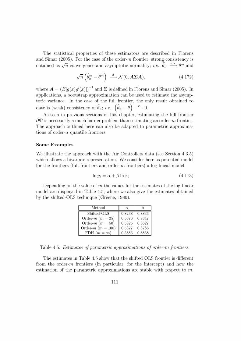
The statistical properties of these estimators are described in Florensand Simar (2005). For the case of the order-m frontier, strong consistency is

obtained as√

n-convergence and asymptotic normality; i.e., θmn

a.s.−→ θm and

√n(θm

n − θm)

d−→ N (0, AΣA), (4.172)

where A = (E[g(x)g′(x)])−1 and Σ is defined in Florens and Simar (2005). Inapplications, a bootstrap approximation can be used to estimate the asymp-totic variance. In the case of the full frontier, the only result obtained to

date is (weak) consistency of θn; i.e.,(θn − θ

)p−→ 0.

As seen in previous sections of this chapter, estimating the full frontier∂Ψ is necessarily a much harder problem than estimating an order-m frontier.The approach outlined here can also be adapted to parametric approxima-tions of order-α quantile frontiers.

Some Examples

We illustrate the approach with the Air Controllers data (see Section 4.3.5)which allows a bivariate representation. We consider here as potential modelfor the frontiers (full frontiers and order-m frontiers) a log-linear model:

ln yi = α + β ln xi (4.173)

Depending on the value of m the values for the estimates of the log-linearmodel are displayed in Table 4.5, where we also give the estimates obtainedby the shifted-OLS technique (Greene, 1980).

Method α β

Shifted-OLS 0.8238 0.8833Order-m (m = 25) 0.5676 0.8347Order-m (m = 50) 0.5825 0.8627Order-m (m = 100) 0.5877 0.8786

FDH (m = ∞) 0.5886 0.8838

Table 4.5: Estimates of parametric approximations of order-m frontiers.

The estimates in Table 4.5 show that the shifted OLS frontier is differentfrom the order-m frontiers (in particular, for the intercept) and how theestimation of the parametric approximations are stable with respect to m.

111

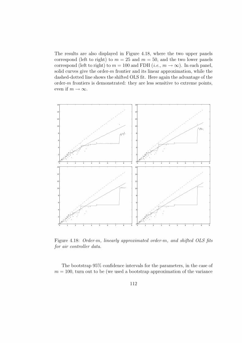
The results are also displayed in Figure 4.18, where the two upper panelscorrespond (left to right) to m = 25 and m = 50, and the two lower panelscorrespond (left to right) to m = 100 and FDH (i.e., m → ∞). In each panel,solid curves give the order-m frontier and its linear approximation, while thedashed-dotted line shows the shifted OLS fit. Here again the advantage of theorder-m frontiers is demonstrated: they are less sensitive to extreme points,even if m → ∞.

0 1 2 3 4 5 6 7 8 90

2

4

6

8

10

12

14

16

0 1 2 3 4 5 6 7 8 90

2

4

6

8

10

12

14

16

0 1 2 3 4 5 6 7 8 90

2

4

6

8

10

12

14

16

0 1 2 3 4 5 6 7 8 90

2

4

6

8

10

12

14

16

Figure 4.18: Order-m, linearly approximated order-m, and shifted OLS fitsfor air controller data.

The bootstrap 95% confidence intervals for the parameters, in the case ofm = 100, turn out to be (we used a bootstrap approximation of the variance

112

in (4.172) with B = 1000 Monte-Carlo replications):

α ∈ [0.4490, 0.6399]

β ∈ [0.7839, 0.9949].

These confidence intervals are not symmetric about the estimates of α andβ shown in Table 4.5 for m = 100, reflecting the fact that the distributionsof bootstrap values used to obtain the confindence interval estimates areasymmetric.

4.8 Open Issues and Conclusions

There remain a number of open issues and problems that need to be beaddressed in future research.

4.8.1 Allowing for noise in DEA/FDH

Allowing for noise in nonparametric frontier models is perhaps one of themost challenging issues is production analysis. The problem is hard because,without some restrictions the model is not identified (this is true even in thesimplest univariate frontier problem; see Hall and Simar, 2002, for discus-sion). Using envelopment estimators when there is noise in the data will leadto inconsistent estimation. However, Hall and Simar show that when thenoise is not to large (in terms of noise to signal ratio), the usual boundaryestimates (based on minimal, or maximal, order statistics) can be used toobtain reasonable estimators of the boundary. These ideas have been devel-oped for the multivariate setting in Simar (2003b), where stochastic versionsof FDH and DEA estimators are developed for situations where the noise isof moderate size.

Still, more general approaches are desired. Kumbhakar et al. (2006) sug-gest an approach for nonparametric stochastic frontier model using localmaximum likelihood methods. The idea is to start with a global model inthe spirit of Aigner et al. (1977), and then by localization, generate a muchmore flexible model approximating a much wider class of models than theglobal model.

Another nonparametric method for stochastic frontier models in the caseof a panel of data has been proposed by Kneip and Simar (1996). In theirapproach, identification comes from repeated observations of the same firms

113

over time. The drawback is the need of a large numbers of time periods forgetting sensible results, and the implicit assumption that inefficiency doesnot change over time. The latter assumption likely to be problematic inmany economic applications.

4.8.2 Inference with DEA/FDH estimators

Tools for statistical inference are available. But here too, improvements areneeded. For instance, other (than bootstrap) approximations of the limitingdistributions of DEA estimators that would be easy to simulate and wouldease the task of bias correction and estimation of confidence intervals aredesired, along the lines of what has been obtained for FDH estimators. Someinitial progress in this direction has been made by Jeong (2004).

With regard to the bootstrap, subsampling offers the easiest way of imple-menting inference using bootstrap methods. The remaining issue, however,is to develop an easy, reliable way of determining the optimal subsamplesizes. The smoothed bootstrap proposed Kneip et al. (2003) for the het-erogeneous case is difficult to implement; additional work is also needed todevelop algorithms that are easier to use in applied work.

4.8.3 Results for CRS case

As noted in Section 4.2.5, statistical properties of the constant returns-to-scale versions of the DEA estimators, θCRS(x, y) and λCRS(x, y), have notyet been derived. There are, to date, no proofs of consistency for theseestimators, nor have either their convergence rates or sampling distributionsbeen derived. Provided ∂Ψ displays globally constant returns-to-scale, it isdifficult to doubt that the CRS versions of the DEA estimators are consistent,but a formal proof would be nice. Their limiting distributions are requiredto establish consistency of any bootstrap that might be used for inferencewith these estimators; even with this result, some work would be required toestablish consistency of a bootstrap, since the proofs in Kneip et al. (2003)do not extend easily to the CRS case.

4.8.4 Tools for dimension reduction

Several tools are used in nonparametric regression to reduce dimensionalityin an effort to mitigate the curse of dimensionality. For example, one can

114

transfrom the exogenous data to principal-components space and examineeigenvalues to see whether some of the dimensions in principal componentsspace are nearly redundant (due to multicollinearity in the original data-space, which is common in economic applications) and might reasonably bedeleted. This approach was employed by Wheelock and Wilson (2001) andWilson and Carey (2004) to estimate cost functions for banks and hospitals.Other approaches have been suggested by Hardle (1990) and Scott (1992).

In multi-dimensional settings where DEA estimators are used, however,the estimators’ radial nature precludes many of the transformation tech-niques that might be used in regression problem. For example, the esti-mators loose their independence from units of measurement if the data aretransformed to principal-components space.

Simar and Wilson (2001) provided bootstrap tests for aggregation possi-bilities among inputs and outputs in the DEA setting. These test hypothesesabout the underlying structure of the true frontier ∂Ψ; if satisfied, inputs oroutputs can be aggregated, resulting in a reduction of dimensionality, whichleads to faster convergence rates, and hence less estimation noise for a givensample size. Given the cost incurred by the curse of dimensionality, morework on dimension reduction is needed.

4.8.5 Final conclusions

Statistical inference in now available for nonparametric frontier models, evenif not always easy to implement. Increasing availability of software pack-ages such as the new FEAR package (Wilson, 2007) implementing bootstrapmethods for inference in frontier models will encourage wider use; already,there is little excuse for not making inferences properly in frontier applica-tions.

The new concepts of order-m and order-α partial frontiers are very ap-pealing. They are robust with respect to outliers, are very easy to compute,and avoid the curse of dimensionality shared by most of the nonparametrictechniques in statistics. In addition, they provide another tool for detectingoutliers in deterministic frontier models.

A DGP has been provided that rationalizes two-stage approaches, whereefficiencies are estimated (using FDH or DEA estimators) in a first stage,and then the efficiency estimates are regressed on environmental variables ina second stage. In addition, it is now understood how inferences regardingthe second-stage regression parameters must be made. In addition, using

115

the probabilistic formulation of the production process introduced in Section4.2.4 , tools have been developed to investigate the impact of environmen-tal factors on the production process while making fewer assumptions thanrequired in the two-stage approach.

The fact that the issues discussed in Sections 4.8.1–4.8.4 remain (to date)unsolved is good news for theoreticians, if not for practitioners.

116

Bibliography

[1] Aigner, D.J.. and S.F. Chu (1968), On estimating the industry productionfunciton, American Economic Review 58, 826–839.

[2] Aigner, D. and C. A. K. Lovell, and P. Schmidt (1977), Formulation andestimation of stochastic frontier production function models, Journal ofEconometrics 6, 21–37.

[3] Andersen, P. and N.C. Petersen (1993), A procedure for ranking efficientunits in data envelopment analysis, Management Science 39, 1261–64.

[4] Aragon, Y., A. Daouia and C. Thomas-Agnan (2002), Nonparametricfrontier estimation: A conditional quantile-based approach,” Economet-ric Theory, forthcoming.

[5] Badin, L. and L. Simar (2004), A bias corrected nonparametric envelop-ment estimator of frontiers, Discussion paper #0406, Institut de Statis-tique, Universite Catholique de Louvain, Louvain-la-Neuve, Belgium.

[6] Banker, R.D. (1993), Maximum likelihood, consistency and data envelop-ment analysis: A statistical foundation, Management Science 39, 1265–1273.

[7] Banker, R.D. (1996), Hypothesis tests using data envelopment analysis,Journal of Productivity Analysis 7, 139–159.

[8] Banker, R.D., A. Charnes, and W.W. Cooper (1984), Some models forestimating technical and scale inefficiencies in data envelopment analysis,Management Science 30, 1078–1092.

[9] Bickel, P. J. and and D. A. Freedman (1981), Some asymptotic theoryfor the bootstrap, Annals of Statistics 9, 1196–1217.

117

[10] Bogetoft, P. (1996), DEA on relaxed convexity assumptions, Manage-ment Science 42, 457–465.

[11] Bogetoft, P., J.M. Tama, and J. Tind (2000), Convex input and out-put projections of nonconvex production possibility sets, ManagementScience 46, 858–869.

[12] Briec, W., K. Kerstens, and P. Vanden Eeckaut (2004), Non-convextechnologies and cost functions: definitions, duality and nonparametrictests of convexity, Journal of Economics 81, 155–192.

[13] Brown, D.F. (1979), Voronoi diagrams from convex hulls, InformationProcessing Letters 9, 223–228.

[14] Cazals, C., J.P. Florens, and L. Simar (2002), Nonparametric frontierestimation: A robust approach, Journal of Econometrics 106, 1–25.

[15] Charnes, A., W.W. Cooper, and E. Rhodes (1978), Measuring the in-efficiency of decision making units, European Journal of Operational Re-search 2, 429–444.

[16] Charnes, A., W.W. Cooper, and E. Rhodes (1981), Evaluating programand managerial efficiency: an application of data envelopment analysisto program follow through, Management Science 27, 668–697.

[17] Cheng, M.Y., J. Fan, and J.S. Marron (1997), On automatic boundarycorrections, Annals of Statistics 25, 1691–1708.

[18] Cook, R. D. and Weisberg, S. (1982), Residuals and Influence in Re-gression, New York: Chapman and Hall.

[19] Coelli, T., D.S.P. Rao, and G.E. Battese (1998), An Introduction to Ef-ficiency and Productivity Analysis, Boston: Kluwer Academic Publishers,Inc.

[20] Daouia, A. and L. Simar (2004), “Nonparametric Efficiency Analysis: AMultivariate Conditional Quantile Approach,” Discussion paper #0419,Institut de Statistique, Universite Catholique de Louvain, Louvain-la-Neuve, Belgium.

[21] Daouia, A. and L. Simar (2005), Robust nonparametric estimators ofmonotone boundaries, Journal of Multivariate Analysis, 96, 311–331.

118

[22] Daraio, C. and L. Simar (2005a), Introducing environmental variablesin nonparametric frontier models: A probabilistic approach, Journal ofProductivity Analysis 24, 93–121.

[23] Daraio, C. and L. Simar (2005b), “Conditional Nonparametric Fron-tier Models for Convex and Non-Convex Technologies: A Unifying Ap-proach,” Discussion paper #0502, Institut de Statistique, UniversiteCatholique de Louvain, Louvain-la-Neuve, Belgium.

[24] Debreu, G. (1951), The coefficient of resource utilization, Econometrica19(3), 273–292.

[25] Deprins, D., L. Simar, and H. Tulkens (1984), “Measuring Labor In-efficiency in Post Offices, in The Performance of Public Enterprises:Concepts and measurements, ed. by M. Marchand, P. Pestieau, and H.Tulkens, Amsterdam: North-Holland, 243–267.

[26] Efron, B. (1979), Bootstrap methods: another look at the jackknife,Annals of Statistics 7, 1–16.

[27] Efron, B. (1982), The Jackknife, the Bootstrap and Other ResamplingPlans, CBMS-NSF Regional Conference Series in Applied Mathematics,#38, Philadelphia: Society for Industrial and Applied Mathematics.

[28] Efron, B. and R.J. Tibshirani (1993), An Introduction to the Bootstrap,London: Chapman and Hall.

[29] Fare, R. (1988), Fundamentals of Production Theory, Berlin: Springer-Verlag.

[30] Fare, R., S. Grosskopf, and C.A.K. Lovell (1985), The Measurement ofEfficiency of Production, Boston: Kluwer-Nijhoff Publishing.

[31] Farrell, M.J. (1957), The measurement of productive efficiency, Journalof the Royal Statistical Society, Series A, 120, 253–281.

[32] Ferrier, G. D. and J.G. Hirschberg (1997), Bootstrapping confidenceintervals for linear programming efficiency scores: With an illustrationusing Italian bank data, Journal of Productivity Analysis 8, 19–33.

[33] Florens, J.P. and L. Simar, (2005), Parametric approximations of non-parametric frontier, Journal of Econometrics 124, 91–116.

119

[34] Gijbels, I., E. Mammen, B.U. Park, and L. Simar (1999), On estimationof monotone and concave frontier functions, Journal of the AmericanStatistical Association 94, 220–228.

[35] Greene, W.H. (1980), Maximum likelihood estimation of econometricfrontier, Journal of Econometrics 13, 27–56.

[36] Greene, W.H. (1993), “The Econometric Approach to Efficiency Analy-sis, in The Measurement of Productive Efficiency: Techniques and Appli-cations, ed. by H. Fried, C.A.K. Lovell and S. Schmidt, Oxford: OxfordUniversity Press.

[37] Hardle, W. (1990), Applied Nonparametric Regression, Cambridge:Cambridge University Press.

[38] Hall, P. and L. Simar (2002), Estimating a changepoint, boundary orfrontier in the presence of observation error, Journal of the AmericanStatistical Association 97, 523–534.

[39] Jeong, S.O. (2004), “Asymptotic Distribution of DEA EfficiencyScores,” Discussion paper #0425 , Institut de Statistique, UniversiteCatholique de Louvain, Louvain-la-Neuve, Belgium.

[40] Jeong, S.O. and L. Simar (2006), Linearly interpolated FDH efficiencyscore for nonconvex frontiers, Journal of Multivariate Analysis, forthcom-ing.

[41] Kittelsen, S.A.C. (1997), “Monte Carlo Simulations of DEA EfficiencyMeasures and Hypothesis Tests, unpublished working paper, SNF Oslo,Gaustadalleen 21, N–0371 Oslo, Norway.

[42] Kneip, A., B.U. Park, and L. Simar (1998), A note on the convergence ofnonparametric DEA estimators for production efficiency scores, Econo-metric Theory 14, 783–793.

[43] Kneip, A. and L. Simar (1996), A general framework for frontier esti-mation with panel data, Journal of Productivity Analysis 7, 187–212.

[44] Kneip, A., L. Simar, and P.W. Wilson (2003), “Asymptotics for DEAEstimators in Nonparametric Frontier Models,” Discussion paper #0317,Institut de Statistique, Universite Catholique de Louvain, Louvain-la-Neuve, Belgium.

120

[45] Koenker, R. and G. Bassett (1978), Regression quantiles, Econometrica46, 33–50.

[46] Koopmans, T.C. (1951), “An Analysis of Production as an EfficientCombination of Activities,” in Activity Analysis of Production and Al-location, ed. by T.C. Koopmans, Cowles Commission for Research inEconomics, Monograph 13, New York: John-Wiley and Sons, Inc.

[47] Korostelev, A., L. Simar, and A.B. Tsybakov (1995a), Efficient estima-tion of monotone boundaries, The Annals of Statistics 23, 476-489.

[48] Korostelev, A., L. Simar, and A.B. Tsybakov (1995b), On estimation ofmonotone and convex boundaries, Pub. Inst. Stat. Univ. Paris, XXXIX,1, 3–18.

[49] Kumbhakar, S.C., B.U. Park, L. Simar, and E.G. Tsionas (2006), Non-parametric stochastic frontiers: A local likelihood approach, Journal ofEconometrics, forthcoming.

[50] Maddala, G.S. (1988), Introduction to Econometrics, New York:Macmillan Publishing Company.

[51] Mouchart, M. and L. Simar (2002), “Efficiency Analysis of Air Con-trollers: First Insights,” Consulting report #0202, Institut de Statistique,Universite Catholique de Louvain, Belgium.

[52] Olesen, O.B., N.C. Petersen, and C.A.K. Lovell (1996), Summary of theworkshop discussion, Journal of Productivity Analysis 7, 341–345.

[53] Park, B., L. Simar, and C. Weiner (2000), The FDH estimator for pro-ductivity efficiency scores : Asymptotic properties, Econometric Theory16, 855–877.

[54] Porembski, M., K. Breitenstein, and P. Alpar (2005), Visualizing effi-ciency and reference relations in data envelopment analysis with an ap-plication to the branches of a German Bank, Journal of ProductivityAnalysis, forthcoming.

[55] Ritter, C. and L. Simar (1997), Pitfalls of normal-gamma stochasticfrontier models, Journal of Productivity Analysis 8, 167–182.

121

[56] Schuster, E.F. (1985), Incorporating support constraints into nonpara-metric estimators of densities, Communications in Statistics: Theory andMethods 14, 1123–1136.

[57] Scott, D.W. (1992), Multivariate Density Estimation: Theory, Practice,and Visualization, New York: John Wiley & Sons, Inc.

[58] Serfling, R.J. (1980), Approximation Theorems of Mathematical Statis-tics, New York: John Wiley & Sons, Inc.

[59] Shephard, R.W. (1970), Theory of Cost and Production Function,Princeton: Princeton University Press.

[60] Silverman, B.W. (1986), Density Estimation for Statistics and DataAnalysis, London: Chapman and Hall.

[61] Simar, L. (1992), Estimating efficiencies from frontier models with paneldata: A comparison of parametric, non-parametric and semi-parametricmethods with bootstrapping, Journal of Productivity Analysis 3, 167–203.

[62] Simar, L. (2003a), Detecting outliers in frontiers models: A simple ap-proach, Journal of Productivity Analysis 20, 391–424.

[63] Simar, L. (2003b), “How to Improve the Performances of DEA/FDHEstimators in the Presence of Noise?,” Discussion paper #0323, Insti-tut de Statistique, Universite Catholique de Louvain, Louvain-la-Neuve,Belgium.

[64] Simar, L. and P.W. Wilson (1998), Sensitivity analysis of efficiencyscores: How to bootstrap in nonparametric frontier models, ManagementScience 44, 49–61.

[65] Simar, L. and P.W. Wilson (1999a), Some problems with the Fer-rier/Hirschberg bootstrap idea, Journal of Productivity Analysis 11, 67–80.

[66] Simar, L. and P.W. Wilson (1999b), Of course we can bootstrap DEAscores! But does it mean anything? Logic trumps wishful thinking, Jour-nal of Productivity Analysis 11, 93–97.

122

[67] Simar, L. and P.W. Wilson (1999c), Estimating and bootstrappingMalmquist indices, European Journal of Operational Research 115, 459–471.

[68] Simar, L. and P.W. Wilson (2000a), Statistical inference in nonparamet-ric frontier models: The state of the art, Journal of Productivity Analysis13, 49–78.

[69] Simar, L. and P.W. Wilson (2000b), A general methodology for boot-strapping in nonparametric frontier models, Journal of Applied Statistics27, 779–802.

[70] Simar L. and P.W. Wilson (2001), Testing restrictions in nonparametricfrontier models, Communications in Statistics: Simulation and Compu-tation 30, 161–186.

[71] Simar L. and P.W. Wilson (2002), Nonparametric tests of return toscale, European Journal of Operational Research 139, 115–132.

[72] Simar, L. and P.W. Wilson (2007), Estimation and inference in two-stage, semi-parametric models of production processes, Journal of Econo-metrics 136:31–64.

[73] Simar, L. and V. Zelenyuk (2004), “On Testing Equality of Distribu-tions of Technical Efficiency Scores,” Discussion paper #0434, Institutde Statistique, Universite Catholique de Louvain, Louvain-la-Neuve, Bel-gium.

[74] Simar, L. and V. Zelenyuk (2006), Statistical inference for aggregates ofFarrell-type efficiencies, Journal of Applied Econometrics, forthcoming.

[75] Spanos, A. (1999), Probability Theory and Statistical Inference: Econo-metric Modeling with Observational Data, Cambridge: Cambridge Uni-versity Press.

[76] Thiry, B. and H. Tulkens (1992), Allowing for technical efficiency inparametric estimates of production functions: With an application tourban transit firms, Journal of Productivity Analysis 3, 41–65.

[77] Wheelock, D. C. and P.W. Wilson, (2001), New evidence on returns toscale and product mix among U.S. commercial banks, Journal of Mone-tary Economics 47, 653–674.

123

[78] Wheelock, D. C. and P.W. Wilson, (2003), “Robust Nonparametric Esti-mation of Efficiency and Technical Change in U.S. Commercial Banking,”unpublished working paper, Department of Economics, Clemson Univer-sity, Clemson, South Carolina 29630 USA.

[79] Wilson, P. W. (1993), Detecting outliers in deterministic nonparametricfrontier models with multiple outputs, Journal of Business and EconomicStatistics 11, 319–323.

[80] Wilson, P. W. (1995), Detecting influential observations in data envel-opment analysis, Journal of Productivity Analysis 6, 27–45.

[81] Wilson, P.W. (2003), Testing independence in models of productive ef-ficiency, Journal of Productivity Analysis 20, 361–390.

[82] Wilson, P.W. (2004), “A Preliminary Non-parametric Analysis of PublicEducation and Health Expenditures Developing Countries,” unpublishedworking paper, Department of Economics, Clemson University, Clemson,South Carolina 29630 USA.

[83] Wilson, P.W. (2007), FEAR: A Software Package for Frontier EfficiencyAnalysis with R, Socio-Economics Planning Sciences, forthcoming.

[84] Wilson, P.W. and K. Carey (2004), Nonparametric analysis of returns toscale and product mix among U.S. hospitals, Journal of Applied Econo-metrics 19, 505–524.

NOTE: All discussion papers from Institut de Statistique, CatholiqueUniversite Louvain, are available athttp://stat1ux.stat.ucl.ac.be/ISpub/ISdp.html.

Wilson (2007) is available athttp://www.clemson.edu/economics/faculty/wilson.

124