statistical matching: a model based approach for data integration
TRANSCRIPT

M e t h o d o l o g i e s a n d W o r k i n g p a p e r s
ISSN 1977-0375
Statistical matching: a model based approach for data integration
2013 edition

2013 edition
M e t h o d o l o g i e s a n d W o r k i n g p a p e r s
Statistical matching: a model based approachfor data integration

Europe Direct is a service to help you find answers to your questions about the European Union.
Freephone number (*):
00 800 6 7 8 9 10 11 0H(*) The information given is free, as are most calls (though some operators, phone boxes or hotels
may charge you). More information on the European Union is available on the Internet (http://europa.eu). Cataloguing data can be found at the end of this publication. Luxembourg: Publications Office of the European Union, 2013 ISBN 978-92-79-30355-5 ISSN 1977-0375 doi:10.2785/44822 Cat. No: KS-RA-13-020-EN-N Theme: General and regional statistics Collection: Methodologies & Working papers © European Union, 2013 Reproduction is authorised provided the source is acknowledged.

3 Statistical matching: a model based approach for data integration
Authors:
Aura LEULESCU (Eurostat)
Mihaela AGAFIŢEI (Eurostat)
Acknowledgements:
This work was done under the responsibility of Bettina KNAUTH, Head of Unit “Social
statistics - Modernisation and Coordination” and Jean-Louis MERCY, Head of Unit
“Quality of Life”.
Appreciation goes to the production units in Eurostat Directorate F (Social Statistics)
for their comments and support.
We thank also Pilar MARTÍN-GUZMÁN, Francisco FABUEL, Juan MARTINEZ
(Devstat) for their input on Chapter 2 - Quality of Life.
Special thanks are due to the members of the ESSNet on Data Integration, for their
constant guidance.
The views expressed in this publication are those of the authors and do not necessarily
reflect the opinion of the European Commission.


Table of contents
5 Statistical matching: a model based approach for data integration
Table of contents
Introduction 7
1 A methodological overview and implementation guidelines 10
1.1 Short introduction to statistical matching 10
1.2 Statistical matching – a stepwise approach in an applied context 12 1.2.1 Harmonisation and reconciliation of multiple sources 12 1.2.2 Analysis of the explanatory power for common variables 15 1.2.3 Matching methods 16 1.2.4 Quality assessment 19
1.3 Concluding remarks 24
2 Case study 1: Quality of Life 28
2.1 Background 28
2.2 Statistical matching: methodology and results 30 2.2.1 Harmonisation and reconciliation of sources 30 2.2.2 Analysis of the explanatory power for common variables 33 2.2.3 Matching methods 37 2.2.4 Results and quality evaluation 38
2.3 Conclusions and Recommendations 43
Annex 2-1 Common variables- metadata analysis 45
Annex 2-2 Coherence analysis: comparison confidence intervals for marginal distributions of common variables (EQLS-SILC 2007) 55
Annex 2-3 Analysis explanatory power of common variables: Rao-Scott tests results (EQLS, 2007) 66
3 Case study 2: Wage and labour statistics 70
3.1 Background 70
3.2 Statistical matching: methodology and results 70 3.2.1 Harmonisation and reconciliation of sources 70 3.2.2 Analysis of the explanatory power for common variables 73 3.2.3 Matching methods 74 3.2.4 Results and quality evaluation 74
3.3 Conclusions and Recommendations 83
Annex 3-1 Common variables- metadata analysis 84
Annex 3-2 Model log(wage) as dependent variable, Spain 2009 89
Annex 3-3 Comparison of joint distributions (based on HD) of matching variables with wage deciles (LFS imputed versus EU-SILC observed) for Spain, 2009; 91
4 Bibliography 92

Table of contents
6 Statistical matching: a model based approach for data integration
Table of content - Box
Box 1-1 Statistical matching situation 11 Box 2-1 Main target indicators in EU-SILC 29 Box 2-2 Main target variables in EQLS ─ considered for matching into EU-SILC 30 Box 2-3 Final matching variables for Spain/Finland (method1), EQLS – 2007 35 Box 3-1 Objectives 70
Table of content - Figure
Figure 2-1 Preservation of marginal distributions: observed EQLS versus imputed (%) 39 Figure 2-2 Joint distributions severe material deprivation & imputed subjective well-being
variables 40 Figure 2-3 Average life satisfaction: whole population versus AROPE 41 Figure 2-4 % people that feel socially excluded: whole population versus materially deprived 41 Figure 3-1 Relative difference in size of target population (employees) between SILC and LFS
based on the self-declared activity status 71 Figure 3-2 The average Hellinger distance by main common variables and by country, in
ascending order 72 Figure 3-3 Average similarity for joint distributions of wage deciles with main socio-demo-
graphical variables, by country 76 Figure 3-4 Impact on predefined cut-off points on wage decile distributions, Greece 2009 77 Figure 3-5 The cut-off points for wage deciles 78 Figure 3-6 Similarity of joint distributions: comparing EU-SILC with LFS observed/imputed
wage data 79 Figure 3-7 Impact of discrepancies in the distribution of main common variables on matching
results 80 Figure 3-8 Mean wage by field of education and age group, ES-2009 81 Figure 3-9 Frechet Bounds: % of people with wage below the mean by field of education
(ES, 2009) 82
Table of content - Table
Table 2-1 Coherence common variables between EU SILC and EQLS, Spain/Finland–2007 32 Table 2-2 Explanatory power common variables for Spain/Finland, EQLS – 2007 34 Table 2-3 Final matching variables for Spain/Finland (dependent variable=life satisfaction),
EQLS — 2007 36 Table 2-4 Frechet bounds for the joint distribution of life satisfaction and severe material
deprivation 42 Table 3-1 Hellinger distance values (%) by country and common variables, in ascending
order of average across countries (columns) and common variables (countries) 73

Introduction
7 Statistical matching: a model based approach for data integration
Introduction Recent initiatives highlighted the growing importance of new indicators and statistical
surveillance tools that cover cross-cutting needs and go beyond aggregates to capture
key distributional issues. In particular, the ‘GDP and beyond’ Commission
communication and the Stiglitz-Sen-Fitoussi Commission’ Report raised awareness
about the need to review and update the current system of statistics in order to address
new societal challenges and to support policy-making. This urges for integrated
statistical information that covers several socio-economic aspects.
The social statistical infrastructure is organised around specific surveys covering many
relevant aspects of the users demand: income, consumption, health, education, labour
market, social participation. However, no single survey can cover all the requested
aspects. Against this backdrop the current process of modernisation of social surveys is
focused on increasing the overall efficiency of social surveys, the responsiveness to user
needs and the analytical potential of the data collected via a better integrated system of
social surveys.
Statistical matching (also known as data fusion, data merging or synthetic matching) is
a model-based approach for providing joint statistical information based on variables
and indicators collected through two or more sources. The potential benefits of this
approach lie in the possibility to enhance the complementary use and analysis of
existing data sources (e.g. cross-cutting statistical information that encompasses a broad
range of socio economic aspects), without further increasing costs and response burden.
However, statistical matching is a complex operation which requires specific technical
expertise and raises several methodological issues.
Therefore, in December 2010 in Eurostat started a feasibility study that carried out
methodological work with a view to checking whether statistical matching could be
used in the framework of social surveys as a tool to integrate extensive information
from several existing sources.
The project focused on the ex post integration of existing micro data sets and it had a
strong practical focus on specific needs in social statistics. This first publication aims to
provide a general overview on the statistical matching methodology and its
implementation requirements in a practical context. It has three main objectives: (1) to
provide a general introduction to statistical matching with an emphasis on
implementation in an applied context, namely within the European system of social
surveys; (2) to present the main results and practical highlights from two pilot studies
on matching implemented in Eurostat (e.g. producing joint information on quality of life
indicators based on EU-SILC1and EQLS
2; study the feasibility of the technique for
production of tabulated LFS data enhanced with SILC-matched wages); (3) to draw
conclusions on the quality of results obtained through statistical matching given the
status–quo and translate into recommendations for addressing limitations in the design
stage. A second volume on statistical matching is forthcoming. It explores a new
approach to statistical matching based on the incorporation of ex-ante requirements in
the current process of redesign of social surveys.
1 EU Statistics on Income and Living Conditions
2 European Quality of Life Survey

Introduction
8 Statistical matching: a model based approach for data integration
Chapter 1 reports on the general methodological framework and guidelines for the
implementation of matching techniques. Chapters 2-3 document in detail the first
empirical case studies conducted in the matching project in Eurostat.

Introduction
9 Statistical matching: a model based approach for data integration
1.
1 A methodological overview and implementation guidelines
1 A methodological overview and implementation guidelines

1 A methodological overview and implementation guidelines
10 Statistical matching: a model based approach for data integration
1 A methodological overview and
implementation guidelines
1.1 Short introduction to statistical matching
Statistical matching (also known as data fusion, data merging or synthetic matching) is
a model-based approach for providing joint information on variables and indicators
collected through multiple sources (surveys drawn from the same population). The
potential benefits of this approach lie in the possibility to enhance the complementary
use and analytical potential of existing data sources (e.g. cross-cutting statistical
information that encompasses a broad range of socio economic aspects). Hence,
statistical matching can be a tool to increase the efficiency of use given the current data
collections.
Most often the aim of a matching exercise is to enlarge the information scope, but
matching techniques have been used also for alignment of estimates observed in
multiple surveys and for improving the precision of these estimates by integration with
larger surveys.
Two main approaches can be delineated in terms of outputs that can be obtained
through matching:
(1) the macro approach refers to the identification of any structure that describes
relationships among the variables not jointly observed of the data sets, such as
joint distributions, marginal distributions or correlation matrices (D’Orazio,
2006)
(2) the micro approach refers to the creation of a complete micro-data file where
data on all the variables is available for every unit. This is achieved by means
of the generation of a new data set from two data sets that are based on an
informative set of common variables between two ‘synthetic micro records’.
An essential feature of statistical matching is that, although the units in the concerned
data sets should come from the same population, they are usually not overlapping. You
identify and link records from different sources that correspond to similar units. This is
the basic difference compared with record linkage, where units included in the data sets
overlap that allows to link records from the different data sets that correspond to the
same unit. Therefore, record linkage deals with identical units, while statistical
matching, or synthetic linkage, deals with ‘similar’ units.
In practice, matching procedures can be regarded as an imputation problem of the target
variables from a donor to a recipient survey. Y, Z are collected through two different
samples drawn from the same population; X variables are collected in both samples and
they are correlated with both Y and Z. The relation between these common variables
with the specific variables observed only in one of the data sets - the donor data set-
will be explored and used to impute to the units of the other data set - the recipient

1 A methodological overview and implementation guidelines
11 Statistical matching: a model based approach for data integration
data set - the variables not directly observed. Thus a synthetic dataset is generated with
complete information on X,Y and Z.
Box 1-1 Statistical matching situation
Sample A (donor) Sample B (recipient) Synthetic dataset
X,Y
X,Z X, ,Z
However, this view is rather simplistic and one important methodological concern has
been raised regarding the validity of results. The origins of statistical matching can be
traced back to the mid- 1960s, when the 1966 US Tax File and the 1967 Survey of
Economic Opportunities were matched in order to provide a synthetic data set on socio-
demographic variables. Then, in the early 1970s different matching techniques were
applied to social surveys in the US (Ruggles 1974), but these techniques were severely
criticized on the grounds that they rely on assumptions neither justified nor testable
(Kadane 1978, Rodgers 1984). In particular, measures of association between Y and Z
conditional on X cannot be estimated and they are usually assumed to be 0. This is the
so called conditional independence assumption (CIA), a reference point for assessing
the quality of estimates based on matching.
When this condition holds, matching algorithms will produce accurate estimates that
reflect the true joint distribution of variables that were collected in multiple sources. It
will give the same results as a perfect linkage procedure. Unfortunately, this assumption
rarely holds in practice and it cannot be tested from the data sets. In case the conditional
independence does not hold, and no additional information is available, the model will
have identification problems and the artificial datasets produced may lead to incorrect
inferences.
The critical question that arises is: what can we learn from a matched dataset about the
joint distribution of (Y, Z), which are not jointly observed? There are two main
approaches proposed in current studies on statistical matching that take into account
these inherent limitations.
The first one focuses on uncertainty analysis techniques that assess the sensitivity of
estimated results to different assumptions (Rubin, 1980; Raessler 2002, D'Orazio et al.,
2006). In this case the focus is typically on macro objectives (e.g. estimation of specific
contingency tables) rather than the creation of micro-datasets. The second one explores
the possibility of overcoming the conditional independence assumption by using
auxiliary information. In order to overcome the conditional independence assumption,
two main types of solutions were put forward. One is the use of additional information
in the form of a small sub-set of units with complete information on the joint
distributions (Paass, 1986). The other, which covers cases when the joint collection of
specific variables is not feasible, explores the use of proxy ‘variables’ with very high
predictive power. These variables can mediate the relationship between Y and Z, and
can make plausible the conditional independence assumption.
^
Y

1 A methodological overview and implementation guidelines
12 Statistical matching: a model based approach for data integration
In all cases, the focus is on the specific estimators of interest and not on the creation of
synthetic datasets (Schaffer, 1998). The matched datasets will not usually preserve
individual level values, so the exercise should aim to preserve data distributions and
multivariate relations between target variables (Rubin 1986). Therefore, it is essential
both to control for dimensions relevant in the analysis and to properly reflect
uncertainty associated with implicit models.
In the framework of European official statistics, relevant methodological expertise on
statistical matching was developed in the frame of the ESSnet on Data Integration3. The
aim of the ESSnet on Data Integration was to promote knowledge and practical
application of sound statistical methods for the joint use of existing data sources in the
production of official statistics, and at disseminating this knowledge within the
European Statistical System. The outputs4 of the project comprise methodological
papers and case studies on statistical matching as well as software tools for data
integration (Relais for record linkage and StatMatch5 for statistical matching). These
tools are written with open source software (mainly R) and are freely available.
1.2 Statistical matching – a stepwise approach in an applied context
The application of statistical matching in a practical context usually implies a set of key
steps, related to various stages of a survey process. The selection of an appropriate
matching technique is only one of these steps and often not the most essential.
First of all, statistical matching relies on certain pre-requisites of harmonisation and
coherence of data sources to be matched. Therefore, in practice, it often requires a data
reconciliation process that enables the joint analysis of multiple data sources. Secondly,
multivariate analysis and modelling techniques need to be implemented for the selection
of matching variables. Finally, the application of matching techniques and related
quality assessment can be implemented. Every step of the process has to be monitored
carefully in order to produce accurate results.
1.2.1 Harmonisation and reconciliation of multiple sources
In order to understand whether data from two different surveys can be matched it is
necessary to evaluate if they are coherent. Coherence of the statistics produced by a
survey process is an important feature that refers to the adequacy of the data to be
reliably combined in different ways and for various uses.
The first step in a data matching process is the harmonisation of multiple sources. An
extensive methodological work on harmonisation methods and reconciliation of
3 http://www.cros-portal.eu/content/data-integration-1
4 http://www.cros-portal.eu/sites/default/files//WP2.pdf
5 http://www.cros-portal.eu/sites/default/files//WP3.2%20D%27Orazio%20-%20Updating%20StatMatch%20%28slides%29.pdf

1 A methodological overview and implementation guidelines
13 Statistical matching: a model based approach for data integration
multiple sources was done in the framework of the ESSnet on Data Integration.
D’Orazio et al (2006) mention the following eight types of reconciliation actions:
(a) harmonisation on the definition of units
(b) harmonisation of reference period
(c) completion of population
(d) harmonisation of variables
(e) harmonisation of classifications
(f) adjustment for measurement errors (accuracy)
(g) adjustment for missing data
(h) derivation of variables
Discrepancies can emerge at different levels: in the data collection (e.g. different
household definitions, different variables or filters applied to similar variables), but also
downstream in the surveys methods (calibration factors or reference sources) and in the
derived information disseminated to users (e.g. complex concepts such as household
composition, dependent child are calculated based on different criteria).
The empirical studies done in Eurostat showed that in an applied context these
standardization issues can hamper the successful application of matching methods.
Practical issues, which might arise, and their impact on the quality of matching results
are presented in the following sections, based on the different case studies. The single
analysis of metadata is not sufficient to understand if data from two surveys can be
compared and integrated. This analysis should be followed by data processing of the
two surveys.
For example, in sample surveys on households, usually the definition of the household
should be deepened in order to understand whether the two surveys share the same
definition or not. It is very important to ascertain if all the household members are
surveyed or not (e.g. data collected only for member with age >= 18, etc.). These
comparisons (e.g. of the household definition) should be accompanied by a comparison
of the estimated number of households and their distribution by region, size etc.
An essential point for the quality of results from the matching procedures is the
existence of a common set of variables that should be homogeneous in their statistical
content. In other words, the two samples A and B should estimate the same distribution
for each common variable: the two sample surveys should represent the same
population. Common variables selected as matching variables should show similar joint
and marginal empirical distributions in the two datasets.
There are different possibilities to quantify the degree of similarity/dissimilarity for
different distributions. The first and simplest one is to compute, in the two data sources
involved, the weighted frequency distributions for each variable of interest and to
calculate the differences. The maximum value of these differences can be taken as a
criterion for comparison. Coherence of the variable in the two surveys will be rejected if

1 A methodological overview and implementation guidelines
14 Statistical matching: a model based approach for data integration
this maximum difference is higher than a certain threshold. Obviously, this is simply a
rule of thumb without much theoretical background, and the threshold established is
arbitrary.
Another possibility is to quantify similarity of two distributions so that we could give a
relative measure of differences in the distributions of various common variables at
different levels. Distance metrics are used to measure distortion of distributions. Thus,
we chose the Hellinger distance (see equation below) to quantify the similarity between
probability distributions of donor and recipient data. It lies between 0 and 1 where a
value of 0 indicates a perfect similarity between two probabilistic distributions, whereas
a value of 1 indicates a total discrepancy. Unfortunately, it is not possible to set up a
threshold of acceptable values of the distance, according to which the two distributions
can be said close. However, a rule of thumb, often recurring in literature, considers two
distributions close if the Hellinger distance is not greater than 0.05.
K
i R
Ri
D
DiK
i N
n
N
niVpiVpVVHD
1
2
1
2''
2
1)()(
2
1),(
where K is the total number of cells in the contingency table, Din is the frequency of
cell i in the donor data D, Rin is the frequency of cell i in the recipient data R and N is
the total size of the specific contingency table.
We applied Hellinger distance because it is easy to interpret and allows for comparisons
across variables, surveys and countries. However, Hellinger distance shall be used with
cautions since it does not take into account variability due to sampling design or a large
number of categories and the thresholds are also set up on arbitrary basis.
The third group refers to statistical tests for the similarity of distributions (Chi square;
Kolmogorov Smirnov, Rao-Scott, Wald-Wolfowitz tests). These methods could give a
stronger base to the conclusions on similarity/discrepancy between distributions coming
from the two sources as they take into account the complex sampling designs applied in
social surveys. We have not applied such statistical test because, in Eurostat, the
sampling design information is not available for all surveys.
Additionally, when dealing with a continuous X variable, hypothesis testing for
comparing of means/totals can be done by considering the usual t-test when an estimate
of the sampling errors is available.
When the empirical distributions show substantial differences, some harmonisation
procedures can then be applied in order to improve the similarity of the distributions,
such as re-categorisations of variables or more complex calibration techniques. There
are several studies that focus on the alignment of estimates for common variables in two
or more sample surveys based on calibration and re-weighting techniques (Sarndal et al
1992; Renssen and Nieuwenbroek, 1997; Merkouris, 2004). Some of these actions may
be difficult to implement, and in some cases, no amount of work can produce
satisfactory results.

1 A methodological overview and implementation guidelines
15 Statistical matching: a model based approach for data integration
Inconsistencies between surveys can be more prevalent in some countries due to
operational differences: similar concepts or common guidelines can be implemented
differently in the various countries. Therefore, in the framework of social surveys, the
need for coherence must be addressed at different levels of the statistical process.
The best possibility of matching occurs when a survey, with a common questionnaire
providing some basic information for all the units, is divided into subsamples, each of
them containing a module with specific questions answered by the units of that
subsample (nested surveys). In this case all the conditions previously mentioned are
fulfilled: the population and reference period are the same and the definitions and
classifications of the common variables are also identical. Thus, the different modules
can be safely matched.
Although good coherence is a necessary pre-condition for matching, it does not address
limitations related to the conditional independence assumption. The modelling stage is
essential for the quality of estimates obtained in the matching procedure.
1.2.2 Analysis of the explanatory power for common variables
The choice of the matching variables is a crucial point in statistical matching. It was
often emphasised (Adamek, 1994) that the choice of suitable matching variables among
common variables has a greater impact on the validity of the matching exercise than the
matching technique effectively used.
The conditional independence assumption is the reference point. The fulfilment of this
condition guarantees that the joint distribution of matched variables Y and Z will be the
same as the one obtained from a perfect linkage procedure. This assumption will,
consequently, validate inference procedures about the actually unobserved association
and induce a strong predictive relationship between the common matching variables and
the recipient-donor measures.
This means that the validity of a matching exercise depends to a great extent on the
power of the matching variables to behave as good predictors of the specific
information to be transferred from the donor to the recipient file.
Optimally, the common variables should contain all the association shared by Y and Z.
From this point of view, inclusion of all the common variables in A and B that show
some significant relation with the variables to impute would look like a reasonable
decision. But it is good to take into account the fact that each additional variable
complicates the computational procedure and it can have a negative impact on the
quality of results. So, a moderate parsimony in the selection of the matching variables is
recommended for practical purposes.
A number of methods can be applied in order to find the optimum set of predictors.
Among these methods, multivariate techniques play a fundamental role: stepwise
regression as it allows selecting the variables with higher explanatory power for each of
the variables in the donor file that will be imputed in the recipient one; factor analysis,

1 A methodological overview and implementation guidelines
16 Statistical matching: a model based approach for data integration
that provides rules for the selection of the variables and, finally, the derivation of new
common variables with the highest possible explanatory power.
The quality of the variables is a second selection criterion. According to Cibella (2010),
it is important to choose as matching variables those with a high level of quality, with
no errors and no missing data. On the same line, Scanu (2010) states that it is advisable
to avoid the use of highly imputed variables as matching variables. For the
implementation of a successful matching process it is fundamental to have good quality
reporting on the datasets to be integrated and on the specific procedures of imputation
and calibration implemented. It is also necessary to have the imputed values in the
dataset appropriately flagged.
The specific analysis to be performed with the matching files can make advisable the
inclusion of a small number of variables, called the critical variables, which will be used
for the separation of data into groups, the so called “matching classes”, or strata. Then,
matching is done independently within strata.
One other issue to consider is that sometimes we need to impute several variables from
one dataset to another. However, it is very unlikely that the common variables should
have equal explanatory power for each of the specific variables. A common practice is
to split the variables to be matched into more or less homogeneous groups, and to
perform a statistical matching in each of the groups by using the common variables with
the highest explanatory power for that particular group. That generally means using
different matching variables, or different weights of these variables for each group. This
practice is known as “matching in groups”. It implies that a unit of the recipient set will
be most probably matched to a different unit of the donor file for each group of imputed
variables.
1.2.3 Matching methods
Many different techniques have been used for statistical matching over more than forty
years since these exercises have been implemented. Several strands can be
differentiated according to some relevant criteria:
First, there is a clear difference between the techniques that assume conditional
independence in the matching data set and those that do not assume it: the
techniques belonging to the first group will need only the information contained
in the data sets to be matched. If some additional information is available, it will
be useful only for checking purposes. On the contrary, the techniques applied to
matching exercises in which the conditional independence cannot be assumed
are based on the incorporation and use of additional information from the very
beginning.
The second classification criterion is connected with the parametric features of
the model. If it can be assumed that the joint distribution of variables belongs to
a family of known probability distributions (i.e. normal multivariate,
multinomial), the matching problem will mainly consist of parameter
estimations. That means that it can be solved with parametric techniques, among
1 A methodological overview and implementation guidelines
17 Statistical matching: a model based approach for data integration
which the maximum likelihood principle will usually play a fundamental role. If
no underlying family of distributions can be specified, non-parametric
techniques will have to be used.
Then a third source of classification is the scope given to the concept of
statistical matching. Often the goal is to obtain a complete synthetic micro data
file through effective imputation of values to the unobserved variables.
However, the use of synthetic datasets should be done with caution as
imputation approaches have limited ability to recreate individual level values.
Therefore, imputed data should be used at a sufficient level of aggregation and
for specific estimates, defined and controlled for a priori in the imputation
procedure. When only the relationship existing among the two sets of variables
is to be explored, macro-matching techniques can be adopted.
Based on these considerations we provide a synthesis of the main matching methods
and issues related to their application in a practical context. For more details on the
different methods please refer to the outputs of the ESSnet on Data Integration
(Working Package 1 of ESSnet-DI , page 42-62) and D’Orazio et al 2006 .
a. Hot deck methods
The most popular matching techniques are, by far, the non-parametric micro-matching
methods- to be used under the assumption of conditional independence- known as hot-
deck imputation procedures. A common feature of these methods is that they will
impute the non-observed variables in the recipient file with “live” values, that is, values
really existing in the donor file. A definition of distance is established, and calculated
for the common variables. Then each record of the recipient file is associated with the
nearest record in the donor file, that is, the record that shows a smallest distance. When
two or more donor records are equally distant from the recipient record, one of them is
chosen at random. Distance can be defined in many ways. The definitions of distance
more frequently employed are the Euclidian distance, the city-block metric or the
Mahalanobis distance. A weighted distance can also be adopted, reflecting the relative
relevance attributed to each of the matching variables (according to their explanatory
power or to any other consideration).
This method is known as unconstrained distance hot deck, unconstrained matching or
generalized distance method, and provides the closest possible match. Its main problem
is that each record in the donor file can be used as donor more than once, a result that is
known as polygamy. Also, some donors can remain unused. The multiple choices of
donors can reduce the information and the effective sample size. Also, the empirical
distribution of the imputed Z variable in the statistical matching file will usually not be
identical to the corresponding distribution in the donor file.
In order to limit the number of times a donor is taken, a penalty weight can be placed on
donors already used, while establishing an algorithm that avoids the factor of
dependence introduced by the order in which the donor units are taken. Alternatively, a
tolerance extra distance can be added to the observed minimum distance, and any units
within this distance can be considered as possible matches. Then several devices can be
1 A methodological overview and implementation guidelines
18 Statistical matching: a model based approach for data integration
applied for the selection of the final donor. For example, it can be selected at random
among the possible choices. It is also usual to impute to the recipient record the average
values of all the matches within the established distance, although this method will most
probably produce imputed values that will not be “live”, that is, really existing values.
The disadvantage of these alternatives to distance hot deck is that they usually increase
the average matching distance. Also, when averages are taken, variances and
covariances can be underestimated.
Another alternative is the constrained distance hot deck, which allows each record in the
donor file to be used only once, provided that the donor file is larger or equal to the
recipient file. It consists in finding the best donor for each record by minimizing the
distance between records conditioned to the preservation of the weights in both data
sets. This ensures that the empirical multivariate distribution of the variables observed
only in the donor file is exactly replicated in the synthetic file. When there are more
donors than recipients, this method leads to a typical linear programming problem, and
its solution usually requires a considerable computational effort.
b. Regression based methods
In a parametric framework, the assumption of conditional independence ensures that
data are sufficient to estimate the parameters of the model. Under this assumption the
likelihood function of the joint distribution can be calculated as a product of the
conditional likelihood functions for each of the data sets and the likelihood function of
the marginal distribution of the common variables. Then, maximum likelihood (ML)
methods can be employed for the estimation of parameters and the identification of the
distribution. Sometimes least square estimators have been employed (Rässler, 2002),
which in fact results in a very small difference with the ML estimations for large
samples. These methods have several disadvantages: regression towards the mean and
sensitivity towards misspecifications of the models. Regression based imputation
underestimates the variance of estimates and the results can be very different in
comparison with hot deck imputations.
c. Mixed methods
Also, parametric and non-parametric methods are sometimes combined in a two stage
process, trying to add to the parsimony of the parametric approach the robustness of
non-parametric techniques. Such is the case of the predictive mean matching imputation
method (Rubin, 1986) in which, in a first step, the regression parameters of Z on X are
estimated on the donor database B. These parameters are used to estimate an
intermediate value of Z for each register in the recipient file A. Then, with a suitable
distance function, a hot deck method is applied, and the record in B that is nearer to the
intermediate value in A is the one used for the final matching. Predictive mean
matching is more likely to preserve original sample distributions than expected values.
One minor drawback of PPM in this situation is that only “observed” rather than
“possible” values can be imputed.
Another interesting mixed method is the propensity score, as described in Rässler
(2002). Both data sets are extended with an additional variable taking value 1 for all the
records in file A and value 0 for all the records in data set B. Putting both files together,

1 A methodological overview and implementation guidelines
19 Statistical matching: a model based approach for data integration
a logit or probit model is estimated, taking as dependent variable the added one, and as
independent variables the common variables X (and including the regression constant).
The propensity score is defined as the estimated conditional probability of a unit to
belong to one of the groups, given X. Then a matching is performed on the basis of the
estimated propensity scores: for each recipient record a donor unit is searched with the
same or the nearest estimated propensity score.
d. Multiple imputation methods
Multiple imputation techniques are often used in the matching framework in order to
address the identification problem of the model. First proposed by Rubin in the 1970′s,
the method imputes several values (N) for each missing value, to represent the
uncertainty about which values to impute. The pooling of the results of the analyses
performed on the multiply imputed datasets implies that the resulting point estimates are
averaged over the N implicates and the resulting standard errors and p-values are
adjusted according to the variance of the corresponding N sub-samples. This variance
called the ‘between imputation variance’, provides a measure of the extra inferential
uncertainty due to missing data.
In matching, multiple imputation methods were used to build complete datasets. Used in
a Bayesian framework, multiple imputation methods rely on a model for variables with
missing data, conditional on both observed variables and some unknown parameters. In
these cases, different partial correlations between the two not jointly observed variables
are used (CIA is not assumed). These explicit models generate a posterior predictive
distribution from which imputations are drawn.
Multiple imputation has been applied mainly in a parametric setting (Moriarty and
Scheuren, 2001; Raessler, 2002). It has been used by Rässler (2002) to estimate lower
and upper bounds of the unknown parameters. More complex techniques, such as
Sequential Regression Multiple imputation account also for complex rooting and
different filters in the matched surveys, as well as different models for estimating the
missing data (Raghunathan, Reiter and Rubin 2003; Raiter 2004). Some applications for
the fully Bayesian model were developed based on several models: normal linear
regression model, logistic regression, a Poisson loglinear model, a two stage model for
truncated data (the case of wage). These give the flexibility in handling each variable on
a case by case basis. The disadvantage is that they can be computationally intense.
1.2.4 Quality assessment
The quality assessment in the context of matching needs a process approach. Each of
the steps (the quality and the coherence of data sources, modelling techniques,
matching/imputation algorithms) has a large impact on the quality of results. However,
given certain pre-requisites in terms of coherence and integration, results obtained
through statistical matching have still to be validated in terms of their potential to
provide reliable and accurate estimates.
Rässler (2002) proposes a framework for the evaluation of quality in a statistical
matching procedure. She establishes four levels of validity for a matching procedure:
(1) the marginal and joint distributions of variables in the donor sample are preserved in

1 A methodological overview and implementation guidelines
20 Statistical matching: a model based approach for data integration
the statistical matching file; (2) the correlation structure and higher moments of the
variables are preserved after statistical matching; (3) the true joint distribution of all
variables is reflected in the statistical matching file; (4) the true but unknown values of
the Z variable of the recipient units are reproduced.
It is most often straightforward to reach level 1, if you use robust methods and pre-
conditions of coherence are met. This level actually measures the matching noise that
can depend both on the amount of the sampling and non-sampling errors of the source
data sets and on the effectiveness of the chosen matching method. The second and third
levels can be checked either through simulation studies, the use of auxiliary information
or more complex techniques that reflect properly the uncertainty of the estimates.
Current studies on uncertainty analysis and multiple imputation techniques focus on the
sensitivity of parameter estimates (e.g. correlation coefficient) to different prior
assumptions. The fourth level will not be usually attained, unless the common variables
determine the variables to be imputed through an exact functional relationship. In any
case, since the true values of the variables are unknown, only simulation studies will
allow an assessment that this condition is satisfied.
Most traditional methods focus on level 1: the comparison of marginal and joint
distributions in the matched /real datasets. This is considered a minimum requirement of
a statistical matching procedure, and can be easily ascertained by specific tests/ indexes
for similarity of distributions (e.g Hellinger distances). However, this condition is not
sufficient to validate the estimates for the joint distribution of variables not collected
together. In the typical situation for matching we assume that Y and Z are statistically
independent conditional on X. P(Y,Z/X)=P(Y/X) P(Y/Z). Several papers (Kadane 1978,
Barr et al 1981, Rodgers de Vol, 1981) emphasised the limits of the conditional
independence assumption and the implications it has on the quality and usability of
estimates obtained through matching. Whenever it is not possible to justify this
assumption, as most often happens, the use of auxiliary information is needed.
For example, the purpose is to have joint information on income (from source A) and
consumption (from source B) that are never observed together based on a set of
common variables. We impute consumption in A and the new synthetic dataset should
preserve the marginal distributions of this variable as well as the cross tabulations or
correlation structure with the common variables. Good results in the reproduction of
joint distributions of consumption with the common variables can provide a measure of
robustness for the techniques applied, but they alone cannot validate the results obtained
in terms of the joint distribution of income and consumption. The creation of synthetic
micro datasets, which satisfy the first level of validity, does not automatically imply that
we can estimate the joint distribution of variables not collected together through
standard methods applied to observed datasets.
Another issue to consider is the level for which we aim to obtain estimates via statistical
matching. Traditional techniques do not consider the multilevel structure of the data
(e.g. region level). If we ignore the structure and use a single-level model (e.g.
individual effect) our analyses may be flawed because we have ignored the context in
which processes may occur. One assumption of the single-level multiple regression
model is that the measured individual units are independent while in reality the

1 A methodological overview and implementation guidelines
21 Statistical matching: a model based approach for data integration
individuals in clusters (areas) have similar characteristics. We have missed important
area level effects — this problem is often referred to as the atomistic fallacy. Therefore,
the multilevel structure of the data has to be accounted for in the imputation procedure:
the compatibility of the distributions observed for the whole sample does not translate
automatically to all domains.
In a matching exercise it is essential to properly reflect uncertainty including those
associated with prior assumptions implicit in the model. In light of these
methodological limitations there are two main approaches in terms of quality
evaluation:
a) the first one focuses on methods to estimate the uncertainty in the final estimates
and it is usually focused on macro objectives (e.g. estimation of correlation
coefficients and contingency tables). However, multiple imputation procedures
with different correlation for the variables not jointly observed can be used for
the creation of multiple synthetic micro-datasets. Methods for variance
estimation in the framework of missing data can be employed for assessing the
sensitivity of results to estimations based on the different datasets
b) the second one focuses on the identification of auxiliary information that can
reduce uncertainty and can relax the conditional independence assumption. This
can lead to partially synthetic/observed datasets and can therefore enhance the
analytical potential.
a. Uncertainty analysis
In the context of matching we do not usually obtain point estimates for the target
quantities — inherently related to the absence of joint information for the variables not
observed together (Raessler 2002, Kiesl and Raessler, 2009). There is a region in the
parametric space such that any of its points defines a parametric set compatible with the
information in the data sets. This indetermination in the context of matching is known
as ‘uncertainty’. The greater the explanatory power of the matching variables the less
uncertainty remains for creating the fused dataset. Marginal distributions can reduce
even further the set for feasible target quantities. There are two streams of work on
uncertainty analysis:
a) Interval estimates which are usually applied in a non-parametric setting. Once
again, methodologies and tools developed within the frame of the ESSnet on
data integration can help to make an assessment of quality for results based on
matched datasets. When dealing with categorical variables, the Fréchet classes
can be used to estimate plausible values for the distribution of the random
variables (Y,Z/X) compatible with the available information. Fréchet bounds
can be used as an instrument to build a measure of the degree of uncertainty in
the problem. For example, in D'Orazio et al, 2006 they provide lower and upper
bounds for the contingency table that crosses income and consumption quintiles.
These intervals contain all the values compatible with the observed data in the
two files. The more informative the common socio-demographic variables in the
two data sets are, the narrower the interval will be.
1 A methodological overview and implementation guidelines
22 Statistical matching: a model based approach for data integration
b) Multiply imputed datasets can be produced according to different values
describing the conditional association (Kiesl and Raessler, 2009). We choose a
plausible initial value for the conditional parameter on X from the parametric
space and generate m independent values for each missing record. This process
is repeated as many times as convenient with different initial values, in order to
fix bounds for the unconditional parameter. From these datasets, we can reveal
sensitivity to different assumptions about the correlation structure. An added
advantage of multiple imputation is that you can get point and interval estimates
under a fairly general set of conditions (Rubin 1987). Multiple imputation is the
natural way to reflect uncertainty about the values to impute. In general,
standard errors and mean square errors are computed based on methods specific
to the variance estimation in case of missing errors, on the line of bootstrap and
Monte Carlo simulations.
b. Auxiliary information and partially synthetic datasets
Another approach for tackling the conditional independence assumption is the use of
auxiliary information. Auxiliary information usually comes in one of the following
possible types:
a) Auxiliary parametric information, obtained from “hook” variables (e.g. a short
set of variables used as a proxy for a complex concept that is usually measured
through an extensive battery of questions);
b) A third data set (C) or an overlap of the two samples (A, B) that provides
complete information on (X,Y,Z).
In a macro-matching parametric approach the auxiliary information, generally collected
from hook variables, or through previous samples, archives or collection of data, can be
particularly useful. Hook variables can contribute to significantly increasing the
explanatory power of the common variables and therefore decrease the degree of
uncertainty, and can eventually eliminate it completely in some cases. One example in
D’Orazio et al. (2006) is the use of net monthly income deciles that prove to improve
results for the estimation of the joint distribution of more detailed income and
consumption variables.
Auxiliary datasets can also be of use in the macro matching approach. The likelihood
function can be split into two factors, and the data files A, B and C can be merged into
one file. The final report of the ESSnet on Data Integration identifies three main
methodologies that focus on the use of auxiliary datasets with complete information:
Singh et al (1993) proposes a two-step procedure for the use of auxiliary dataset
in the context of hot deck methods. First, a live value of the variable Z from the
data set C is imputed to each unit in data set A using one of the hot deck
procedures. Secondly, for each record in A, a final live value from B will be
imputed: the one corresponding to the nearest neighbour in B with a distance
calculated on the previously determined intermediate value.

1 A methodological overview and implementation guidelines
23 Statistical matching: a model based approach for data integration
Another methodology for the use of auxiliary information which takes into
account complex sample designs is provided by Renssen (1998). Renssen
identifies two approaches for providing estimates from the joint dataset, mainly
focused on the adjustment of weights:
a) The ‘calibration approach’ that is obtained under the incomplete two way
stratification. This approach consists in calibrating the weights in the
complete file (C) constraining them to reproduce in C the marginal
distributions of Y and Z estimated from files to be matched.
b) A ‘matching approach’ where a more complex estimate of P (Y, Z) can
be obtained under the synthetic two way stratification. Roughly speaking
it consists in adjusting the estimates computed under the conditional
independence assumption using residuals computed in C between
predicted and observed values for Y and Z respectively.
The third approach was proposed by Rubin (1986) and consists in appending the
two data sources A and B. In the case of an overlap of samples, difficulties in
estimating the concatenated weights can limit the applicability of this approach.
Ballin et al. (2008) suggest a Monte Carlo approach in order to estimate the
concatenated probabilities.
The use of auxiliary datasets and hook variables was proposed also in the ‘split
questionnaire design’ literature. Raghunathan and Grizzle (1995) tested the split
questionnaire design in a simulation environment where the original questionnaire was
divided into several components of variables. This approach requires that any
combination of variables, which are to be evaluated, must be jointly observed in a small
sub sample (to avoid estimation problems due to non-identification). The allocation of
variables in components was not random but done so that highly correlated variables are
in different components. This can facilitate the multiple imputation of missing
information, based on good explanatory models and without relying on the conditional
independence assumption. Using existing data from the full questionnaire, they assessed
the quality of the multiple imputation method by comparing point estimates of
proportions and the associated standard errors of variables of interest from the full
questionnaire to the multiple imputation method and the available case method (the
available case method uses only the data collected from that small sample without
imputation). They found that, in general, the estimates obtained using either the
available case method or the multiple imputation method were very similar to those
obtained from the full questionnaire. Overall, the standard error estimates from both of
these methods were larger than those obtained from the full questionnaire, but the
multiple imputation method resulted in smaller standard error estimates than the
available case method for all variables of interest. Raessler 2004 shows that in a split
questionnaire design data can be quite successfully multiply imputed.
In terms of national statistical institutes both Canada and US apply matching techniques
for creating synthetic datasets (SPSD -Canada and SIPP -US). However, they do not
rely solely on matching but on a combination of linking and matching. First of all, a set
of linking procedures are applied and then the missing data is multiply imputed based

1 A methodological overview and implementation guidelines
24 Statistical matching: a model based approach for data integration
on a model. They refer to partially synthetic datasets as there is always a limited set of
observations for which complete data is observed. This means that they do not have to
impose assumptions about the relationship between variables" and therefore conditional
independence assumption is not implicit in the imputation procedure. Confidence
intervals are computed based on both between and within imputation: the variance
between imputations reflects variability due to modelling assumptions, the variance
within imputations reflects sample variability. Therefore more than one random draw
should be made under each model to reflect sample variability.
1.3 Concluding remarks
1) A first challenge in any applied matching exercise is the harmonisation of different
data sources. Discrepancies related to different sampling designs, different concepts
and common variables as well as survey methods in terms of weighting, calibration
and treatment of missing variables can hamper the matching exercise. The
reconciliation of multiple sources is an iterative time consuming process that
requires feedback loops between existing documentation of variables, data analysis
and methodology. Actual matching occurs at the end of this integration process.
A practical requirement of matching is the existence of an analytical system
designed for joint data sources. This should provide both harmonised structures for
different datasets and validated analytical tools (e.g. for imputation and calibration).
2) Quality evaluation in the framework of matching needs to take into account several
critical factors: the quality and the coherence of the sources, the explanatory power
of common variables, the matching/imputation methods applied and methods used
to compute estimates based on the matched datasets. Once the pre-requisites of
harmonisation are met, there are several quality criteria that need to be checked:
a) Model diagnostics: variables used for matching should accumulate as much
explanatory power as possible on the variables to impute, in order to approach
the fulfilment of the conditional independence assumption.
b) Comparison of marginal distributions in the real/matched datasets: this can
provide a first quality measure of the matching process and of the robustness of
the method used for imputation. However, this is just the basic requirement, a
necessary but not sufficient condition.
c) Uncertainty analysis: An assessment of uncertainty should be included in any
matching exercise. The insight provided by the uncertainty analysis can be
useful to assess the plausibility of the conditional independence assumption.
This can open the way for defining ‘accuracy’ measures for the results obtained
through matching. This allows to better validate results, but will most probably
characterise a phenomenon in terms of trends or interval estimates, and not point
estimates. This direction can be further explored as a follow up of the work of
the ESSnet on data integration.
1 A methodological overview and implementation guidelines
25 Statistical matching: a model based approach for data integration
d) Use of auxiliary information: The existence of auxiliary information is an
essential point for any matching procedure in order to address the potential non-
fulfilment of the CIA, which is often the case. Auxiliary information can help to
address the main limitations of matching techniques, namely the reliance on
implicit models.
e) Multiple imputation methods: This stream of research developed significantly
and has several advantages: it includes exercises based on explicit models (not
hidden assumptions), complex data structures and models, incorporation of
auxiliary information and use of standard tools for the data analysis. Quality
measures can be computed, such as variance estimates and mean square error.
These measures take into account both model and sample variability.
3) In conclusion, matching applied in an ex post perspective (in the current ESS
system) needs to undertake several initial steps of reconciliation of sources before
the actual application of matching techniques. However, this process can provide
detailed documentation on existing differences at both metadata and data level and
can lead to further improvements in current processes.
A critical factor is the possibility to address the limitations inherent in statistical
matching, related to the non-fulfilment of the conditional independence assumption
and provide a measure of quality for estimates based on matched datasets.
When this assumption holds a robust matching algorithm produces valid inferences.
In this case, the preservation of marginal distributions can be considered as a
measure of quality for matching. But in practice it does not usually hold. In order to
validate the analytical potential of matched datasets we need to check its
plausibility. Hence, uncertainty analysis needs to be an integrative part of a
matching exercise in order to validate the estimates based on matched datasets.
4) Given the current process of streamlining social surveys, several steps are foreseen
for a better integration and coordination of surveys. This can provide the
opportunity to enhance the potential for matching, if planned in advance. Not only
surveys will be better harmonised, but also several aspects can be designed ex ante:
a) the choice of common variables between surveys, which can favour the
imputation in relation to specific objectives. Some studies in the frame of split
questionnaire designs have addressed the optimal ex-ante allocation of questions
between the various components of the questionnaire, so as to allow matching
and imputation
b) consider matching jointly with other options for micro-integration (linking and
use of administrative data). They are usually seen as substitutes: statistical
matching is applied when no common identifiers enable linking. However, these
alternative integration methods can often complement each other (the US SIPP
dataset)

1 A methodological overview and implementation guidelines
26 Statistical matching: a model based approach for data integration
c) consider possibilities to use auxiliary information, mainly small datasets with
common information on the two variables of interest and/or a small set of proxy
variables with high predictive power as an integrative part of the system.
d) more integrated survey models (nested surveys, split questionnaire design) are
recommended by several authors as solutions that can foster the application of
matching techniques in practice (D’Orazio et al, 2006, Raessler, 2002).

1 A methodological overview and implementation guidelines
27 Statistical matching: a model based approach for data integration
2 Case study 1: Quality of life
Case study 1: Quality of life
2 Case study 1: Quality of life

2
28
Case study 1: Quality of Life
Statistical matching: a model based approach for data integration
2 Case study 1: Quality of Life
2.1 Background
There is a growing societal and policy demand to measure well-being and quality of life
in a comprehensive way. The importance and urgency of this demand is demonstrated
by recent European initiatives. In particular, the GDP and beyond communication6 and
the Stiglitz-Sen-Fitoussi Report7 raised awareness about the need to review and update
the current system of statistics in order to support specific recommendations on the
measurement of quality of life.
Steps should be taken to improve measures of people’s health, education, personal activities and environmental conditions. In particular, substantial effort should be devoted to developing and implementing robust, reliable measures of social connections, political voice, and insecurity that can be shown to predict life satisfaction;
Surveys should be designed to assess the links between various quality-of-life domains for each person, and this information should be used when designing policies in various fields;
Measures of both objective and subjective well-being provide key information about people’s quality of life. Statistical offices should incorporate questions to capture people’s life evaluations, hedonic experiences and priorities in their own survey.
Ideally, all quality of life indicators should be captured by a single statistical instrument
in order to enable the analysis of links across dimensions and the identification of
multiply disadvantaged sub-groups. In practice, such an instrument does not currently
exist in the European Union.
In this context, statistical matching appears as a very useful technique for the integration
of several independent sources of information on quality of life, as an alternative to
implementing new surveys or extending the questionnaires of the current ones.
Therefore, a first pilot study focused on testing the feasibility of using matching
techniques in order to obtain joint distributions for various dimensions of quality of life,
drawing on variables collected through two main sources: the European Union Statistics
on Income and Living Conditions (EU-SILC) and the European Quality of Life Survey
(EQLS).
6 http://eur-lex.europa.eu/LexUriServ/LexUriServ.do?uri=com:2009:0433:FIN:EN:PDF
7 http://www.stiglitz-sen-fitoussi.fr/documents/rapport_anglais.pdf
2
29
Case study 1: Quality of Life
Statistical matching: a model based approach for data integration
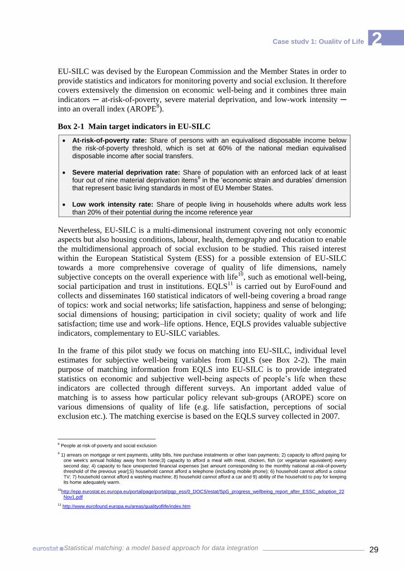
EU-SILC was devised by the European Commission and the Member States in order to
provide statistics and indicators for monitoring poverty and social exclusion. It therefore
covers extensively the dimension on economic well-being and it combines three main
indicators ─ at-risk-of-poverty, severe material deprivation, and low-work intensity ─
into an overall index (AROPE8).
Box 2-1 Main target indicators in EU-SILC
At-risk-of-poverty rate: Share of persons with an equivalised disposable income below the risk-of-poverty threshold, which is set at 60% of the national median equivalised disposable income after social transfers.
Severe material deprivation rate: Share of population with an enforced lack of at least four out of nine material deprivation items
9 in the ‘economic strain and durables’ dimension
that represent basic living standards in most of EU Member States.
Low work intensity rate: Share of people living in households where adults work less than 20% of their potential during the income reference year
Nevertheless, EU-SILC is a multi-dimensional instrument covering not only economic
aspects but also housing conditions, labour, health, demography and education to enable
the multidimensional approach of social exclusion to be studied. This raised interest
within the European Statistical System (ESS) for a possible extension of EU-SILC
towards a more comprehensive coverage of quality of life dimensions, namely
subjective concepts on the overall experience with life10
, such as emotional well-being,
social participation and trust in institutions. EQLS11
is carried out by EuroFound and
collects and disseminates 160 statistical indicators of well-being covering a broad range
of topics: work and social networks; life satisfaction, happiness and sense of belonging;
social dimensions of housing; participation in civil society; quality of work and life
satisfaction; time use and work–life options. Hence, EQLS provides valuable subjective
indicators, complementary to EU-SILC variables.
In the frame of this pilot study we focus on matching into EU-SILC, individual level
estimates for subjective well-being variables from EQLS (see Box 2-2). The main
purpose of matching information from EQLS into EU-SILC is to provide integrated
statistics on economic and subjective well-being aspects of people’s life when these
indicators are collected through different surveys. An important added value of
matching is to assess how particular policy relevant sub-groups (AROPE) score on
various dimensions of quality of life (e.g. life satisfaction, perceptions of social
exclusion etc.). The matching exercise is based on the EQLS survey collected in 2007.
8 People at-risk-of-poverty and social exclusion
9 1) arrears on mortgage or rent payments, utility bills, hire purchase instalments or other loan payments; 2) capacity to afford paying for
one week's annual holiday away from home;3) capacity to afford a meal with meat, chicken, fish (or vegetarian equivalent) every second day; 4) capacity to face unexpected financial expenses [set amount corresponding to the monthly national at-risk-of-poverty threshold of the previous year];5) household cannot afford a telephone (including mobile phone); 6) household cannot afford a colour TV; 7) household cannot afford a washing machine; 8) household cannot afford a car and 9) ability of the household to pay for keeping its home adequately warm.
10http://epp.eurostat.ec.europa.eu/portal/page/portal/pgp_ess/0_DOCS/estat/SpG_progress_wellbeing_report_after_ESSC_adoption_22Nov1.pdf
11 http://www.eurofound.europa.eu/areas/qualityoflife/index.htm

2
30
Case study 1: Quality of Life
Statistical matching: a model based approach for data integration
Box 2-2 Main target variables in EQLS ─ considered for matching into EU-SILC
Overall life satisfaction: All things considered, how satisfied would you say you are with your life these days?
Trust in institutions: Please tell me how much you personally trust each of the following institutions: the press/government/legal system/parliament/police/political parties;
Recognition: I don’t feel the value of what I do is recognised by others.
Social exclusion: I feel left out of society; Life has become so complicated today that I almost can’t find my way; Some people look down on me because of my job situation or income. …
This pilot study provides in detail the methodology for two selected countries: Finland
(FI) and Spain (ES). They represent two very different typologies of countries both for
their characteristics and the data collections methods employed. Following a standard
matching approach we produce results for EU-27, but these results should be interpreted
with caution. While there are advantages to a “one solution fits all” approach
(economies of scale in the analysis, better comparability of estimates), the detailed
analysis for the two selected countries shows that optimal solutions at national level
often require tailored approaches.
2.2 Statistical matching: methodology and results
This chapter provides in detail the methodology and results obtained from matching
EU-SILC and EQLS for the two selected countries (ES, FI), including a general
overview of results for EU-27. It follows the main four stages of the matching algorithm
described in Chapter1.
2.2.1 Harmonisation and reconciliation of sources
The first step in matching EU-SILC and EQLS consisted in analysing the two data-
sources and assessing the fulfilment of the pre-conditions for matching. The main
condition required is the existence, in both surveys, of a set of common variables both
coherent and with a high explanatory power in relation to our specific imputation needs.
In theory, the two surveys have a large number of variables in common that touch upon
several areas: demographics, household composition, labour, health, dwelling, material
deprivation, environment, income. In order to test their coherence, a detailed analysis
was carried out in terms of wording of questions, definition of concepts, measuring
scales and guidelines. Then, a careful comparison of marginal distributions and
appropriate statistical tests were implemented in order to select consistent variables for
the two countries. Comparisons have been carried out, for the marginal distributions of
each potential matching variable, between the 95% confidence intervals calculated for
EU-SILC and those in EQLS (see Annex II-2). Overlapping of these intervals for every
category implies that there are no grounds for rejecting the hypothesis of coherence of
variables.
2
31
Case study 1: Quality of Life
Statistical matching: a model based approach for data integration
Several issues were encountered in this first stage that proved the need for a better
harmonisation of variables across social surveys:
The harmonisation at meta-data level is sometimes difficult to ascertain due to
the fact that concepts that are basically equivalent are expressed with different
wording in each of the surveys. For example, the variable that refer to the
‘capacity to afford a one week holiday’ includes the possibility to stay with
relatives in the case of EU-SILC, while in EQLS this situation is specifically
excluded. This might induce different answers from the respondents. Moreover,
the categorisations of common variables are often different and sometimes it is
very difficult to find a common structure (See Annex II-1 for a detailed
comparison of common variables).
The analysis of marginal distributions for the common variables resulted in a
very limited set of coherent variables. When confidence intervals don't overlap
the variables are considered inconsistent. Several essential variables were
excluded, both socio-demographic variables (e.g. highest level of education
completed) and economic conditions related questions (ability to make ends
meet, material deprivation items). As further analysis will show, the
omission/inclusion of these variables has an important impact on the results and
conclusions based on matched datasets. We can also notice that different
variables are selected in the two countries.
An additional quality check was done to detect variables with a high item non-
response and/or small un-weighted sample size for some categories. The small
sample size of EQLS was one of the limitations of the matching exercise: many
relevant categories of the main variables are insufficiently represented in the un-
weighted sample so that estimates are not accurate or representative. For some
variables presenting a good level of consistency at metadata level, one of the
categories accumulates a very high proportion of the total sample size,
consequently leaving a very sparse sample for estimation in the other categories.
Variables that show a real un-weighted sample of less than 30 units for at least
one of the categories are considered unfit for our matching exercise. Some of the
potential matching variables have to be rejected on this ground, irrespective of
the consistency of definitions. Some other variables have to be redefined by
merging some of their categories. More specifically, for EQLS in Finland the
following variables had to be rejected: country of birth; country of citizenship;
afford to keep house adequately warm; afford a meal with meat, chicken or fish
every second day; amenities: lack of bath or shower in accommodation;
amenities: Lack of indoor flushing toilet in accommodation.
For others, we aggregated several categories: e.g. ability to make ends meet
(with great_difficulty +with_difficulty+some_difficulty vs. fairly_easily+easily+
very easily); general health status (very good+good+fair vs. bad+very bad).
When the data from Spain are considered, only two variables had to be rejected on the
grounds of scarce sample: amenities: lack of bath or shower in accommodation;
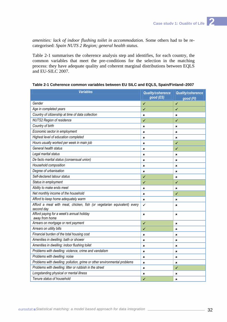
2
32
Case study 1: Quality of Life
Statistical matching: a model based approach for data integration
amenities: lack of indoor flushing toilet in accommodation. Some others had to be re-
categorised: Spain NUTS 2 Region; general health status.
Table 2-1 summarises the coherence analysis step and identifies, for each country, the
common variables that meet the pre-conditions for the selection in the matching
process: they have adequate quality and coherent marginal distributions between EQLS
and EU-SILC 2007.
Table 2-1 Coherence common variables between EU SILC and EQLS, Spain/Finland–2007
Variables Quality/coherence good (ES)
Quality/coherence
good (FI)
Gender
Age in completed years
Country of citizenship at time of data collection
NUTS2 Region of residence
Country of birth
Economic sector in employment
Highest level of education completed
Hours usually worked per week in main job
General health status
Legal marital status
De facto marital status (consensual union)
Household composition
Degree of urbanisation
Self-declared labour status
Status in employment
Ability to make ends meet
Net monthly income of the household
Afford to keep home adequately warm
Afford a meal with meat, chicken, fish (or vegetarian equivalent) every second day
Afford paying for a week's annual holiday away from home
Arrears on mortgage or rent payment
Arrears on utility bills
Financial burden of the total housing cost
Amenities in dwelling: bath or shower
Amenities in dwelling: indoor flushing toilet
Problems with dwelling: violence, crime and vandalism
Problems with dwelling: noise
Problems with dwelling: pollution, grime or other environmental problems
Problems with dwelling: litter or rubbish in the street
Longstanding physical or mental illness
Tenure status of household

2
33
Case study 1: Quality of Life
Statistical matching: a model based approach for data integration
2.2.2 Analysis of the explanatory power for common variables
A second criterion for the selection of the common variables, besides coherence, is that
they should show a good association with the target variables (variables in both surveys
not collected together for which we need to estimate the joint distribution). The optimal
situation, when the common variables contain all the association shared by the target
variables and thus fulfil the conditional independence assumption (CIA), is rarely
attainable.
So, in order to make a further selection of common variables to be used in the matching
process, their association with a broader set of target variables from EQLS (life
satisfaction, trust in institutions, perceived quality of accommodation, job satisfaction,
and social exclusion variables) was analysed using several methods.
A first method focused on pairwise correlations. We relied mainly on Rao-Scott tests,
which are a generalisation of the standard Pearson chi-squared and likelihood-ratio chi-
squared tests for testing the null hypothesis of no association/independence in
categorical variables (Agresti, 2007). Annex II-3 documents in detail the results for
each combination of variables, for both countries. It also indicates in bold variables that
show a significant association at the 5% level (p-values12
<0.05). The Rao-Scott tests
have the advantage that they incorporate complex design effects. Still, they do not
provide a measure of the strength of the association between variables. Thus, as a
complement, two traditional measures of association were calculated: the adjusted
Pearson contingency coefficient (Pearson contingency coefficient adjusted by the
number of files and columns of the table); the Cramer’s V coefficient (D’ Orazio et al.,
2006), derived from the Pearson chi-square test, adjusted by the minimum of the
degrees of freedom. They are scaled between 0 (absence of association) and 1 (perfect
association). The two coefficients of association tend to confirm the results of the Rao-
Scott tests.
In general, the results for both countries show that several common variables tend to be
strongly associated with a considerable proportion of target variables and appear as
good candidates for matching purposes. Table 2-2 provides a summary overview of a
synthetic index of the global explanatory power of each common variable (the average
of the measures of association with all variables to be imputed). We can also note that
some variables have a higher predictive power in only one country (e.g. Material
deprivation 3: A meal with meat, chicken or fish every second day), which leads to
slightly different scenarios across Member States.
12
Probability to reject the null hypothesis of no association

2
34
Case study 1: Quality of Life
Statistical matching: a model based approach for data integration
Table 2-2 Explanatory power common variables for Spain/Finland, EQLS – 2007
Variables
Spain Finland
Average adjusted
contingency coefficient
Average Cramer's
V
Average adjusted
contingency coefficient
Average Cramer's V
Gender 0.17 0.12 0.11 0.08
Age 0.30 0.14 0.25 0.12
Country of citizenship 0.18 0.13 0.16 0.11
Country of birth 0.17 0.12 0.14 0.10
NUTS 2 Region (or equivalent) 0.55 0.24 0.23 0.12
Highest level of education completed (ISCED) 0.31 0.13 0.29 0.12
General health status 0.37 0.18 0.28 0.13
De facto marital status (consensual union) 0.20 0.12 0.16 0.09
Household composition 0.16 0.12 0.18 0.13
Degree of urbanisation 0.25 0.15 0.17 0.10
Self-declared labour status 0.36 0.15 0.29 0.12
Status in employment 0.12 0.07 0.28 0.23
Ability to make ends meet 0.40 0.17 0.40 0.17
Net monthly income of household 0.33 0.17 0.31 0.16
Material deprivation 1: home adequately warm 0.34 0.25 0.11 0.08
Material deprivation 3: A meal with meat, chicken or fish every second day
0.33 0.24 0.19 0.14
Material deprivation 2: Paying for a week's annual holiday away from home
0.25 0.15 0.20 0.12
Arrears on rent or mortgage payments 0.18 0.11 0.20 0.12
Arrears on utility bills, such as electricity, water, gas
0.20 0.12 0.21 0.12
Financial burden of total housing cost 0.28 0.15 0.23 0.12
Amenities: Lack of bath or shower 0.20 0.14 0.17 0.12
Amenities: Lack of indoor flushing toilet 0.16 0.11 0.11 0.08
Problems with dwelling. Violence, crime and vandalism
0.27 0.21 0.21 0.15
Problems with dwelling. Noise 0.26 0.19 0.19 0.14
Problems with dwelling: pollution, grime or environmental problems
0.27 0.20 0.17 0.12
Problems with dwelling. Litter or rubbish in the street
0.27 0.20 0.21 0.15
Long-standing physical or mental health problem 0.29 0.18 0.22 0.13
Limitations due to a long standing illness 0.48 0.30 0.27 0.16
Tenure status of household 0.23 0.12 0.28 0.15

2
35
Case study 1: Quality of Life
Statistical matching: a model based approach for data integration
An important aspect to consider is that most of these variables didn’t meet the
conditions of quality and coherence required (highlighted in blue in Table 2-2). Another
variable with a high level of explanatory power, net monthly income, had to be rejected
for Spain for lack of quality. Thus, the strict selection of common variables, which meet
the criteria for coherence and predictive power, results in a very narrow set of matching
variables with a low potential to obtain valid results (see Box 2-3).
Box 2-3 Final matching variables for Spain/Finland (method1), EQLS – 2007
Spain Finland
Gender
Age
NUTS 2 Region
Afford a meal with meat, chicken or fish every second day (yes/no)
Self-declared labour status
Tenure status of household
Gender
Age
NUTS 2 Region
Status in employment
Net monthly income of the household
General health status (with a re-categorisation)
A second method for selecting the best predictors was based on logistic regressions to
account for multivariate relationships. The selected model was used for imputation in
the next stage. The focus in this case was on addressing the limitations related to the
conditional independence assumption for a specific pair of target variables: life
satisfaction in EQLS and AROPE indicators in SILC. Results (for ES, FI) indicate that
even if we have some good predictors for the subjective variables to be imputed, the
overall predictive power of the model it is not very high: “Percentage concordant”
which measures the fit between predicted probabilities and observed values is around
65%. However, for the CIA to hold, it is important not only the absolute level of
explanatory power of common variables, but most of all, the extent of mediation13
relative to the relationship between imputed variables and AROPE indicators.
For example, Table 2-3 reports the odds ratio for the ordinal logit with life satisfaction
as a dependent variable. Several variables have a strong effect on the likelihood to be
satisfied with your life: health status, relationship status and activity status. However,
even when controlling for these dimensions, we find a strong correlation between life
satisfaction and ‘bad’ economic conditions (e.g. a few selected items on ‘material
deprivation’ or ‘make ends meet’ which are collected in both SILC and EQLS). This
implies that the CIA does not hold and thus we cannot correctly estimate the
relationship between life satisfaction and AROPE indicators under this assumption.
13 the extent to which the common variables capture (mediate) the relationship between the imputed information (e.g. life satisfaction) and the target
variable(s) in the recipient survey (e.g. material deprivation index).
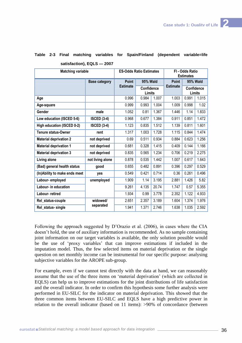
2
36
Case study 1: Quality of Life
Statistical matching: a model based approach for data integration
Table 2-3 Final matching variables for Spain/Finland (dependent variable=life
satisfaction), EQLS — 2007
Matching variable ES-Odds Ratio Estimates FI - Odds Ratio Estimates
Base category Point Estimate
95% Wald Point Estimate
95% Wald
Confidence Limits
Confidence Limits
Age 0.996 0.984 1.007 1.003 0.991 1.015
Age-square 0.999 0.993 1.004 1.009 0.998 1.02
Gender male 1.052 0.81 1.367 1.446 1.14 1.833
Low education (ISCED 5-6) ISCED (3-4) 0.968 0.677 1.384 0.911 0.851 1.472
High education (ISCED 0-2) ISCED (3-4) 1.123 0.835 1.512 1.139 0.811 1.601
Tenure status-Owner rent 1.317 1.003 1.728 1.115 0.844 1.474
Material deprivation 2 not deprived 0.69 0.511 0.934 0.884 0.623 1.256
Material deprivation 1 not deprived 0.681 0.328 1.415 0.409 0.144 1.166
Material deprivation 3 not deprived 0.835 0.565 1.234 0.706 0.219 2.275
Living alone not living alone 0.878 0.535 1.442 1.007 0.617 1.643
(Bad) general health status good 0.655 0.482 0.891 0.396 0.297 0.529
(In)Ability to make ends meet yes 0.549 0.421 0.714 0.36 0.261 0.496
Labour- employed unemployed 1.909 1.14 3.195 2.881 1.426 5.82
Labour- in education 9.261 4.135 20.74 1.747 0.57 5.355
Labour- retired 1.934 0.99 3.778 2.352 1.122 4.933
Rel_status-couple widowed/ separated
2.651 2.357 3.189 1.604 1.374 1.976
Rel_status- single 1.941 1.371 2.746 1.638 1.035 2.592
Following the approach suggested by D’Orazio et al. (2006), in cases where the CIA
doesn’t hold, the use of auxiliary information is recommended. As no sample containing
joint information on our target variables is available, the only solution possible would
be the use of ‘proxy variables’ that can improve estimations if included in the
imputation model. Thus, the few selected items on material deprivation or the single
question on net monthly income can be instrumental for our specific purpose: analysing
subjective variables for the AROPE sub-group.
For example, even if we cannot test directly with the data at hand, we can reasonably
assume that the use of the three items on ‘material deprivation’ (which are collected in
EQLS) can help us to improve estimations for the joint distributions of life satisfaction
and the overall indicator. In order to confirm this hypothesis some further analysis were
performed in EU-SILC for the indicator on material deprivation. This showed that the
three common items between EU-SILC and EQLS have a high predictive power in
relation to the overall indicator (based on 11 items): >90% of concordance (between
2
37
Case study 1: Quality of Life
Statistical matching: a model based approach for data integration
observed and predicted probabilities for the SMD indicator).The quantity “c”, which is
equivalent to the well-known ROC curve (where 0.5 corresponds to the model
randomly predicting the response, and a 1 corresponds to the model perfectly
discriminating the response), is also higher than 0.95. These diagnostics show that the
three items work relatively well in predicting the overall indicator and that they will
therefore tend to mediate the relationship between the indicator and imputed
information.
As the two criteria of coherence and predictive power lead often to divergent results, in
the next stage we performed the imputation based on two different sets of variables: 1) a
restricted one based on the set of variables both coherent and with high explanatory
power; 2) an extended set in which we relaxed the coherence requirements and we gave
prevalence to the particular significance of some variables for the fulfilment of the CIA
(general health status, ability to make ends meet and material deprivation items).
Several sensitivity tests were employed to test the effects of the different sets of
predictors and methods on the final results. Moreover, a unique model (tested for ES
and FI) was selected to be used for imputation in all EU27 countries, but allowing for
different coefficients across countries. On the one hand, a “one solution fits all”
approach across countries should be implemented with caution, as it usually does not
provide optimal results for specific countries. On the other hand, the harmonisation and
reconciliation for 27 countries is an extremely intensive and time consuming task.
2.2.3 Matching methods
Both distance unconstrained hot deck and model based methods were employed for the
imputation of variables (life satisfaction, trust in institutions and social exclusion
variables) from EQLS into EU-SILC.
For the hot deck method, a limited set of covariates that met all the coherence and
quality pre-requisites (see Table 2-3) was used. For the model based imputation, an
extended set of predictors (see Annex II-3) was chosen, mainly on the basis of their
ability to capture the relationship between imputed variables and AROPE indicators.
Both are micro-matching methods which finally provide a synthetic file containing the
complete set of variables (X, Y, Z). We assign an imputed value to every unit of the
recipient file (EU-SILC in our case) for the subjective well-being variables (Z) collected
only in EQLS.
The hot-deck method of imputation assigns to each unit of the recipient file the values
of the nearest unit in the donor file, measured with a certain definition of distance. The
standard distances (Euclidean, Manhattan or Mahalanobis) are used for continuous
variables. But in our exercise all variables are qualitative, and each of them has been
transformed, for matching purposes, into a set of binary variables. For this reason we
have considered more appropriate to work with a distance specifically built for this type
of variables. So, we have selected the distance for binary variables defined on the
similarity coefficient of Dice (also known as the Czekanowski or Sorensen similarity
coefficient). This distance (Gower, 1986) is defined as

2
38
Case study 1: Quality of Life
Statistical matching: a model based approach for data integration
ijij SD 1
Where
cba
aS ij
2
2
a being the number of indicators for which i=1 and j=1, b the number of indicators for
which i=1 and j=0 and c the number of indicators for which i=0 and j=1 (Cox and Cox,
2001).
For model based methods, we tested both imputations based on logistic regressions and
the predictive mean matching method. The covariates selected in the modelling stage,
both socio-demographic characteristics and economic variables that are correlated to
poverty measures, were used in the imputation algorithm:
Age, gender, education, marital status
Tenure status
Activity, health status
Material deprivation items (3); ability to make ends meet
The matching exercise has been implemented mostly in SAS, but for non-parametric
methods the R package Statmatch14
developed by ISTAT was used.
2.2.4 Results and quality evaluation
We analyse in detail the quality of results based on four main target variables imputed
into EU-SILC: life satisfaction, meaning in life, trust in the press, and trust in the
government. The results show that both methods of imputation presented above
preserved reasonably well the marginal distributions of the variables before and after
imputation.
However, the results tend to differ in terms of joint distributions of variables not
collected together. The inclusion in the model of a very limited number of variables
makes difficult to capture the dependence relationship between poverty indicators and
the more subjective variables to be imputed. In order to better illustrate the differences
in conclusions that are drawn from the two matching approaches we first transform the
four ordinal variables (on a scale 1-10) imputed in EU-SILC into binary indexes (e.g.
low/high quality of life -if life satisfaction =</>6). We report in Figure 2-1 for the four
binary indexes the differences between the whole population and the sub-group of
people materially deprived15
in SILC.
14 http://cran.r-project.org/web/packages/StatMatch/index.html. 15
based on the full set of 9 items.

2
39
Case study 1: Quality of Life
Statistical matching: a model based approach for data integration
Figure 2-1 Preservation of marginal distributions: observed EQLS versus imputed (%)

2
40
Case study 1: Quality of Life
Statistical matching: a model based approach for data integration
We can note that for Spain, the first results showed no significant differences in terms
of life satisfaction or recognition in life between the whole population and the
materially deprived sub-group. This is likely to be related to the prior assumptions of
conditional independence, rather than a real lack of association. In a second stage, when
we included proxies for the poverty indicators in the model, estimates show that people
materially deprived tend to cumulate negative scores also on more subjective life
assessments.
Figure 2-2 Joint distributions severe material deprivation & imputed subjective
well-being variables
Finally, we selected the model based method to impute life satisfaction and social
exclusion variables for EU-27. For social exclusion we computed binary micro-indexes
that identify people that tend to cumulate negative scores on various items (the social
exclusion index is 1 if people declare to agree with at least 2 out of 4 negative
statements16
). Figure 2-3 and 2-4 show the results in terms of life satisfaction and social
exclusion for two specific vulnerable sub-groups: the AROPE17
sub-population and the
16
I feel left out of society/Life has become so complicated today that I almost can’t find my way/I don’t feel the value of what I do is recognised by others/Some people look down on me because of my job situation or income.
17 At risk of poverty and social exclusion – see section 2
0
10
20
30
40
50
ES ES FI FI
HDECK MODEL HDECK MODEL
% people with low "life satisfaction": SMD versus whole population
Sub-group sev. mat. deprived Whole population
0
10
20
30
40
50
ES ES FI FI
HDECK MODEL HDECK MODEL
% people with low values for "recognition" : SMD versus whole population
Sub-group sev. mat. deprived Whole population
0
20
40
60
80
100
ES ES FI FI
HDECK MODEL HDECK MODEL
% people with low "trust in the press": SMD versus whole population
Sub-group sev. mat. deprived Whole population
0
20
40
60
80
100
ES ES FI FI
HDECK MODEL HDECK MODEL
% people with low "trust in the government":
SMD versus whole population
Sub-group sev. mat. deprived Whole population

2
41
Case study 1: Quality of Life
Statistical matching: a model based approach for data integration
subset of people materially deprived. In both cases, we can observe that people that face
poverty and/or material deprivation have lower scores on questions related to their
quality of life, and this holds in all member states.
Figure 2-3 Average life satisfaction: whole population versus AROPE
Figure 2-4 % people that feel socially excluded: whole population versus materially deprived
ATBE
BG
CYCZDEDK
EEEL
ESFI
FR
HU
IEIT
LT
LU
LV
MT
NL
PL
PT
RO
SE
SISK
UK
0%
10%
20%
30%
40%
50%
60%
70%
80%
90%
100%
0% 20% 40% 60% 80% 100%
% S
UB
GR
OU
P S
EV M
AT
DEP
RIV
ED
% WHOLE POPULATION
AT
BE
BG
CY
CZ
DE
DK
EE EL
ES FI
FR
HU
IE
IT LT
LU
LV
MT NL
PL
PT RO
SE
SI SK
UK
0
2
4
6
8
10
0 1 2 3 4 5 6 7 8 9
AR
OP
E SU
B-G
RO
UP
WHOLE POPULATION
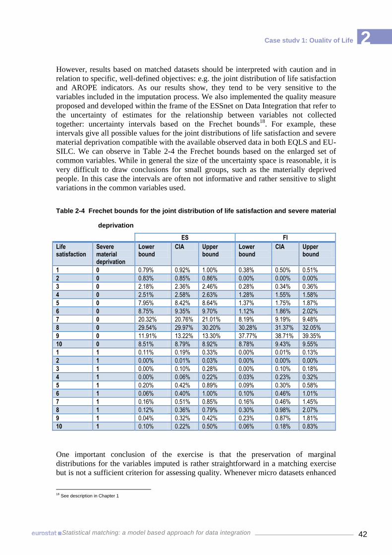
2
42
Case study 1: Quality of Life
Statistical matching: a model based approach for data integration
However, results based on matched datasets should be interpreted with caution and in
relation to specific, well-defined objectives: e.g. the joint distribution of life satisfaction
and AROPE indicators. As our results show, they tend to be very sensitive to the
variables included in the imputation process. We also implemented the quality measure
proposed and developed within the frame of the ESSnet on Data Integration that refer to
the uncertainty of estimates for the relationship between variables not collected
together: uncertainty intervals based on the Frechet bounds18
. For example, these
intervals give all possible values for the joint distributions of life satisfaction and severe
material deprivation compatible with the available observed data in both EQLS and EU-
SILC. We can observe in Table 2-4 the Frechet bounds based on the enlarged set of
common variables. While in general the size of the uncertainty space is reasonable, it is
very difficult to draw conclusions for small groups, such as the materially deprived
people. In this case the intervals are often not informative and rather sensitive to slight
variations in the common variables used.
Table 2-4 Frechet bounds for the joint distribution of life satisfaction and severe material
deprivation
ES FI
Life satisfaction
Severe material deprivation
Lower bound
CIA Upper bound
Lower bound
CIA Upper bound
1 0 0.79% 0.92% 1.00% 0.38% 0.50% 0.51%
2 0 0.83% 0.85% 0.86% 0.00% 0.00% 0.00%
3 0 2.18% 2.36% 2.46% 0.28% 0.34% 0.36%
4 0 2.51% 2.58% 2.63% 1.28% 1.55% 1.58%
5 0 7.95% 8.42% 8.64% 1.37% 1.75% 1.87%
6 0 8.75% 9.35% 9.70% 1.12% 1.86% 2.02%
7 0 20.32% 20.76% 21.01% 8.19% 9.19% 9.48%
8 0 29.54% 29.97% 30.20% 30.28% 31.37% 32.05%
9 0 11.91% 13.22% 13.30% 37.77% 38.71% 39.35%
10 0 8.51% 8.79% 8.92% 8.78% 9.43% 9.55%
1 1 0.11% 0.19% 0.33% 0.00% 0.01% 0.13%
2 1 0.00% 0.01% 0.03% 0.00% 0.00% 0.00%
3 1 0.00% 0.10% 0.28% 0.00% 0.10% 0.18%
4 1 0.00% 0.06% 0.22% 0.03% 0.23% 0.32%
5 1 0.20% 0.42% 0.89% 0.09% 0.30% 0.58%
6 1 0.06% 0.40% 1.00% 0.10% 0.46% 1.01%
7 1 0.16% 0.51% 0.85% 0.16% 0.46% 1.45%
8 1 0.12% 0.36% 0.79% 0.30% 0.98% 2.07%
9 1 0.04% 0.32% 0.42% 0.23% 0.87% 1.81%
10 1 0.10% 0.22% 0.50% 0.06% 0.18% 0.83%
One important conclusion of the exercise is that the preservation of marginal
distributions for the variables imputed is rather straightforward in a matching exercise
but is not a sufficient criterion for assessing quality. Whenever micro datasets enhanced
18
See description in Chapter 1

2
43
Case study 1: Quality of Life
Statistical matching: a model based approach for data integration
through matching are used, the focus should be on estimations of the joint distributions
for variables not collected together which gives the real value added. When important
predictors are omitted, the imputation under CIA can lead to the under-estimation of the
association between the variables not jointly observed. In this particular case study, a
better harmonisation and improved sample size for a few selected variables in EQLS
(which are highly related to both subjective measures of well-being and poverty
aspects), are essential for improving the quality of estimates based on matching.
2.3 Conclusions and Recommendations
In general, this pilot study raised several problems when matching EU-SILC with
EQLS. Two important lessons can be drawn which concern the application of statistical
matching in practice:
A very careful review of the metadata should be carried out for each of the
common variables to be used in the matching process. Often, even if similar, we
cannot establish exact equivalence of concepts and small differences can
translate in large discrepancies in the data.
The preservation of marginal distributions for the variables imputed is not a
sufficient criterion for assessing quality in statistical matching. It is essential
both to control for the dimensions relevant for the aim of the analysis and to
properly reflect uncertainty associated with implicit models. When important
predictors are omitted, the imputation under CIA, can lead to the under-
estimation of the association between the variables not jointly observed.
The lack of harmonisation for most of the variables and the low quality for particularly
relevant predictors (e.g. small sample size for material deprivation items) lead to
difficulties that cannot be tackled in the ex-post integration. The problems experienced
in the implementation of this matching exercise, and the results obtained, lead us to
suggest also a number of recommendations that, if applied to the social surveys
involved, could contribute to a better integration of surveys that cover different aspects
of quality of life.
Recommendation 1: When possible, standardization of the wording of similar questions
in all the social surveys currently collected – or to be collected – in the EU in order to
guarantee total consistency of meaning and to propitiate comparable responses should
be considered.
Recommendation 2: The inclusion of a small module with common questions in the
future waves of the two surveys considered could be very useful as auxiliary
information in order to reduce uncertainty and for checking purposes.
Recommendation 3: A better harmonisation with EU- SILC and improved sample size
for a few relevant variables in EQLS, which are highly related to both subjective
measures of well-being and monetary aspects, are essential for improving the quality of
estimates based on matching.

2
44
Case study 1: Quality of Life
Statistical matching: a model based approach for data integration
Recommendation 4: The insight provided by the uncertainty analysis can come up
useful to assess the plausibility of assumptions but the uncertainty intervals are usually
very large, as it is the case for this particular exercise. Therefore, these methods can
provide a quality indicator, but unless we have a very exhaustive model they are
generally not precise enough to be informative. The development of proper quality
measures needs to continue as a follow up of the work of the ESSnet on data
integration.

2
45 Statistical matching: a model based approach for data integration
Case study 1: Quality of Life
Annex 2-1 Common variables- metadata analysis
A. Core social variables
EU-SILC 2007 EQLS 2007 Common aggregation
Age in completed years
Month of birth RB070
Year of birth RB080
Age at last birthday.
Age HH2b Aggregated in datafile
CVhh2b Microdata variable with label “CONTINUOUS VARIABLE HH2b: AGE OF RESPONDENT”
Every aggregation is possible
Sex Sex PB150
Sex HH2a
1 Male 2 Female
Country of birth
Country of birth is defined as the country of residence of the mother at the time of birth
Country of birth
PB2010
Categorisation can be seen in Common aggregation cell
The question about country of birth (Q70) -In which country were you born?
Country of birth Q70
Categorisation can be seen in Common aggregation cell
Common EU-SILC EQLS
In this country Country Country
European Union Aggregation of countries
Aggregation of countries
Rest of Europe Aggregation of countries
Aggregation of countries
Asia, Africa or Latin America North Africa West Africa Other Africa Central and South America Near and Middle East Other Asia
Asia, Africa or Latin America
Northern America or Oceania
USA Canada Australia and Oceania
Northern America or Oceania
Country of citizenship at time of data collection
When a person has multiple citizenships, the two main citizenships should be collected. For persons with multiple citizenships and where one of the citizenship is the one of the country of residence, that citizenship should be coded.
Citizenship 1 PB220A
Citizenship 2 PB220B
Categorisation can be seen in Common aggregation cell
Citizen of [country] Q69
Country of citizenship Q70
The same as Country of birth In case of two citizenship in EU-SILC one of them must be chosen

2
46 Statistical matching: a model based approach for data integration
Case study 1: Quality of Life
EU-SILC 2007 EQLS 2007 Common aggregation
Legal marital status
MARITAL STATUS
PB190
EU-SILC recommends that Civil partnership should be treated as marriage
Current marital status Q30
The question mixes legal and de facto marital status.
Not possible
De facto marital status (consensual union)
CONSENSUAL UNION
PB200
1 yes, on a legal basis 2 yes, without a legal basis 3 no
Current marital status Q30
The question mixes legal and de facto marital status, it is not possible to differentiate legal and consensual union.
EU-SILC EQLS
1 yes, on a legal basis 2 yes, without a legal basis
1 Married or living with partner
3 no 2 Separated or divorced and not living with partner 3 Widowed and not living with partner 4 Never married and not living with partner
Self-declared labour status
SELF-DEFINED CURRENT ECONOMIC STATUS
PL030
1 Working full time 2 Working part-time 3 Unemployed 4 Pupil, student, further training, unpaid work experience 5 In retirement or in early retirement or has given up business 6 Permanently disabled or/and unfit to work 7 In compulsory military community or service 8 Fulfilling domestic tasks and care responsibilities 9 Other inactive person
-
Which of these best describes your situation? HH2D
1 at work as employee or employer/self-employed 2 employed, on child-care leave or other leave 3 at work as relative assisting on family farm or business 4 unemployed less than 12 months 5 unemployed 12 months or more 6 unable to work due to long-term illness or disability 7 retired 8 full time homemaker/ responsible for ordinary shopping and looking after the home 9 in education (at school, university, etc.) / student 10 other
EU-SILC EQLS
1 Working full time 2 Working part-time
1 at work as employee or employer/self-employed 2 employed, on child-care leave or other leave 3 at work as relative assisting on family farm or business
3 Unemployed 5 unemployed 12 months or more 6 unable to work due to long-term illness or disability
4 Pupil, student, further training, unpaid work experience
9 in education (at school, university, etc.) / student
5 In retirement or in early retirement or has given up business
7 retired
6 Permanently disabled or/and unfit to work
6 unable to work due to long-term illness or disability
8 Fulfilling domestic tasks and care 8 full time homemaker/ responsible for ordinary shopping and looking after the home
7 In compulsory military community or service 9 Other inactive person
10 other

2
47 Statistical matching: a model based approach for data integration
Case study 1: Quality of Life
EU-SILC 2007 EQLS 2007 Common aggregation
Region of residence
Region DB040
NUTS 2 digits From 2008 operation onwards, it was agreed by the Working Group (meeting in June 2008) to use the classification NUTS-08 (to replace the former classification NUTS-03). No double reporting and no back-casting are required.
Classification NUTS 2 There exists a variable by country. For example: P7ES (Spain) and P7FI (Finland)
EU-SILC EQLS
FI18 Etelä-Suomi FI20 Åland
1 Southern Finland and Aland
FI19 Länsi-Suomi 2 Western Finland
FI13 Itä-Suomi 3 Eastern Finland
FI1A Pohjois-Suomi 4 Northern Finland
Degree of urbanisation
DEGREE OF URBANISATION
DB100
1 densely populated area 2 intermediate area 3 thinly populated area -Densely populated area: This is a contiguous set of local areas, each of which has a density superior to 500 inhabitants per square kilometers, where the total population for the set is at least 50,000 inhabitants. -Intermediate area: This is a contiguous set of local areas, not belonging to a densely-populated area, each of which has a density superior to 100 inhabitants per square kilometers, and either with a total population for the set of at least 50,000 inhabitants or adjacent to a densely-populated area. -Thinly-populated area: This is a contiguous set of local areas belonging neither to a densely-populated nor to an intermediate area
Q52 is provided by the respondent and the alternatives do not correspond to the definition. Variable DOMICIL
Domicile, respondent's description
Q52
1 The open countryside 2 A village/small town 3 A medium to large town 4 A city or city suburb
EU-SILC EQLS
1.Densely populated area 4.City or city suburb
2.Intermediate populated area 3.A medium to large town
3.Thinly populated area 1. The open countryside 2. A village/small town

2
48 Statistical matching: a model based approach for data integration
Case study 1: Quality of Life
EU-SILC 2007 EQLS 2007 Common aggregation
Status in employment
Status in main employment
STATUS IN EMPLOYMENT
PL040
1 self-employed with employees 2 self-employed without employees 3 employee 4 family worker This variable refers to the main job. If multiple jobs are held or were held, the main job should be the one with the greatest number of hours usually worked.
Question Q2 can distinguish between Employed and Self-employed Question HH2D from household grid can show when respondent is a family worker
Current occupation Q2
Activity status HH2D
QUESTION Q2- SELF EMPLOYED 1. Farmer 2. Fisherman 3. Professional (lawyer, medical practitioner, accountant, architect etc.) 4. Owner of a shop, craftsmen, other self-employed person 5. Business proprietors, owner (full or partner) of a company EMPLOYED 6. Employed professional (employed doctor, lawyer, accountant, architect) 7 General management, director or top management (managing directors, director general, other director) 8. Middle management, other management (department head, junior manager, teacher, technician) 9. Employed position, working mainly at a desk 10. Employed position, not at a desk but travelling (salesman, driver, etc.) 11. Employed position, not at a desk, but in a service job (hospital, restaurant, police, fireman, etc.) 12. Supervisor 13. Skilled manual worker 14. Other (unskilled) manual worker, servant
EU-SILC EQLS Q2 EQLS HH2D
1 self-employed with employees 2 self-employed without employees
1-5 Self-employed
1 at work as employee or employer/self-employed 2 employed, on child-care leave or other leave
3 employee
6-14 Employed
4 family worker
3 at work as relative assisting on family farm or business

2
49 Statistical matching: a model based approach for data integration
Case study 1: Quality of Life
EU-SILC 2007 EQLS 2007 Common aggregation
Type of contract Type of contract in the main job This variable refers to the main job. If multiple jobs are held or were held, the main job should be the one with the greatest number of hours usually worked. This question is addressed only to employees 1 permanent job/work contract of unlimited duration 2 temporary job/work contract of limited duration
Question Q4 can distinguish between permanent/temporary job/work contract. Question HH2D from household grid can show when respondent has actually a paid work
Type of contract Q4
Activity status HH2D
1 On an unlimited permanent contract 2 On a fixed term contract of less than 12 months 3 On a fixed term contract of 12 months or more 4 On a temporary employment agency contract 5 On apprenticeship or other training scheme 6 Without a written contract 7 Other
EU-SILC EQLS Q4 EQLS HH2D
1 permanent job/work contract of unlimited duration
1 On an unlimited permanent contract
1 at work as employee or employer/self-employed 2 employed, on child-care leave or other leave 2 temporary job/work
contract of limited duration
2 On a fixed term contract of less than 12 months 3 On a fixed term contract of 12 months or more 4 On a temporary employment agency contract 5 On apprenticeship or other training scheme
Occupation in employment
PL050: Occupation (ISCO-88 (COM))
This variable refers to the main job (current main job for people at work or last main job for people do not have a job). If multiple jobs are held or were held, the main job should be the one with the greatest number of hours usually worked.
Question Q2 shows the occupation, but does not correspond to ISCO--88(COM) Question HH2D from household grid can show when respondent has actually a paid work
Current occupation Q2
Activity status HH2D
QUESTION Q2 SELF EMPLOYED 1. Farmer 2. Fisherman 3. Professional (lawyer, medical practitioner, accountant, architect etc.) 4. Owner of a shop, craftsmen, other self-employed person 5. Business proprietors, owner (full or partner) of a company EMPLOYED 6. Employed professional (employed doctor, lawyer, accountant, architect) 7 General management, director or top management (managing directors, director general, other director) 8. Middle management, other management (department head, junior manager, teacher, technician) 9. Employed position, working mainly at a desk 10. Employed position, not at a desk but travelling (salesman, driver, etc.) 11. Employed position, not at a desk, but in a
Not available

2
50 Statistical matching: a model based approach for data integration
Case study 1: Quality of Life
EU-SILC 2007 EQLS 2007 Common aggregation
service job (hospital, restaurant, police, fireman, etc.) 12. Supervisor 13. Skilled manual worker 14. Other (unskilled) manual worker, servant
Economic sector in employment
The economic activity of the local unit of the main job for respondents who are currently at work. This variable refers to the main job. If multiple jobs are held, the main job should be the one with the greatest number of hours usually worked. Coded according to NACE Rev.1.1
Not available
Not available
Highest level of education completed
Highest ISCED level attained Educational attainment of a person is the highest level of an educational programme the person has successfully completed and the study field of this programme. The educational classification used is the International Standard Classification of Education (ISCED 1997) coded according to the seven ISCED-97 categories. 0 pre-primary education 1 primary education 2 lower secondary education 3 (upper) secondary education 4 post-secondary non tertiary education 5 first stage of tertiary education (not leading directly to an advanced research qualification) 6 second stage of tertiary education
Q49 corresponds to ISCED(1) 1 None education completed (ISCED 0) 2 Primary education (ISCED 1) 3 Lower secondary education (ISCED 2) 4 Upper secondary education (ISCED 3) 5 Post-secondary including pre-vocational or vocational education but not tertiary (ISCED 4) 6 Tertiary education – first level (ISCED 5) 7 Tertiary education – advanced level (ISCED 6) 8 (Don’t know/no answer)
ISCED(1)

2
51 Statistical matching: a model based approach for data integration
Case study 1: Quality of Life
EU-SILC 2007 EQLS 2007 Common aggregation
Net monthly income of the household
It can be used HY020: Total disposable household income divided by 12 HY020 = HY010 – HY120G – HY130G – HY140G Where HY010 is TOTAL HOUSEHOLD GROSS INCOME HY120G is REGULAR TAXES ON WEALTH HY130G is REGULAR INTER-HOUSEHOLD CASH TRANSFER PAID HY140G is TAX ON INCOME AND SOCIAL CONTRIBUTIONS Another possibility is (HY020+ HY130G)/12
Q67. Please can you tell me how much your household’s NET income per month is? If you don’t know the exact figure, please give an estimate Q68 In case the respondent does not know the figure or want to provide it there is a scale with ranges.
EU-SILC EQLS
Less than €50 D
€ 50 to €99 B
€100 to €149 I
€ 150 to €199 O
€ 200 to €299 T
€ 300 to €449 G
€ 450 to €549 P
€ 550 to €674 A
€ 675 to € 899 F
€ 900 to € 1.124 E
€ 1.125 to € 1.349 Q
€ 1.350 to € 1.574 H
€ 1.575 to € 1.799 C
€ 1.800 to €2.024 L
€ 2.025 to €2.249 N
€ 2.250 to € 2.699 R
€ 2.700 to € 3.149 M
€ 3.150 to € 3.599 S
€ 3.600 to € 4.049 K

2
52 Statistical matching: a model based approach for data integration
Case study 1: Quality of Life
B. Not core social variables
EU-SILC 2007 EQLS 2007 Common aggregation
Tenure status of household
Tenure Status HH020
Which of the following best describes your accommodation?
Q16
EU-SILC EQLS
1 Owner 1 Own without mortgage (i.e. without any loans) 2 Own with mortgage
2. Tenant or subtenant paying rent at prevailing or market rate
3 Tenant, paying rent to private landlord
3 Accommodation is rented at a reduced rate (lower price that the market price)
4 Tenant, paying rent in social/voluntary/municipal housing
4 accommodation is provided free
5 Accommodation is provided rent free
Material deprivation: Ability to keep home adequately warm
Ability to keep home adequately warm HH050
For each of the following things on this card, can I just check whether your household can afford it if you want it? Keeping your home adequately warm
Q19-1
EU-SILC EQLS
1 Yes 1 Yes, can afford it
2 No 2 No, cannot afford it
Material deprivation: Capacity to afford paying for one week annual holiday away from home
Capacity to afford paying for one week annual holiday away from home
HS040
For each of the following things on this card, can I just check whether your household can afford it if you want it? 2. Paying for a week’s annual holiday away from home (not staying with relatives)
Q19-2
EU-SILC EQLS
1 Yes 1 Yes, can afford it
2 No 2 No, cannot afford it
Material deprivation: Capacity to afford a meal with meat, chicken, fish (or vegetarian equivalent) every second day
Capacity to afford a meal with meat, chicken, fish (or vegetarian equivalent) every second day
HS050
For each of the following things on this card, can I just check whether your household can afford it if you want it? 4. A meal with meat, chicken or fish every second day if you wanted it
Q19-4
EU-SILC EQLS
1 Yes 1 Yes, can afford it
2 No 2 No, cannot afford it
Ability to make ends meet
Ability to make ends meet HS120
Thinking of your household’s total monthly income: is your household able to make ends meet….?
Q57
With great difficulty With difficulty With some difficulty Fairly easily Easily Very easily

2
53 Statistical matching: a model based approach for data integration
Case study 1: Quality of Life
EU-SILC 2007 EQLS 2007 Common aggregation
Arrears on mortgage or rent payments
In the last twelve months, has the household been in arrears, i.e. has been unable to pay on time due to financial difficulties for: (a) rent (b) mortgage repayment for the main dwelling?
HS011
Has your household been in arrears at any time during the past 12 months, that is, unable to pay as scheduled any of the following? (a) Rent or mortgage payments for accommodation
Q58-a
EU-SILC EQLS
1 Yes, once 2 Yes, twice or more
1 Yes
2 No 2 No
Arrears on utility bills
In the last twelve months, has the household been in arrears, i.e. has been unable to pay on time due to financial difficulties for utility bills (heating, electricity, gas, water, etc.) for the main dwelling?
HS020
Has your household been in arrears at any time during the past 12 months, that is, unable to pay as scheduled any of the following? (b) Utility bills, such as electricity, water, gas
Q58-b
EU-SILC EQLS
1 Yes, once 2 Yes, twice or more
1 Yes
2 No 2 No
Financial burden of the total housing cost
Financial burden of the total housing cost
HS140
Is total housing cost a financial burden to the household?
Q59
1 A heavy burden 2 Somewhat a burden 3 Not burden at all
Amenities in dwelling: lack of bath or shower.
Is there a shower unit or a bathtub in your dwelling?
HH080
Do you have any of the following problems with your accommodation? (e) Lack of bath or shower
Q17-e
EU-SILC EQLS
1 Yes, for the sole use of the household 2 Yes, shared
1 No
3 No 2 Yes
Amenities in dwelling Indoor flushing.
Is there an indoor flushing toilet in your dwelling?
HH090
Do you have any of the following problems with your accommodation? (d) Lack of indoor flushing toilet
Q17-d
EU-SILC EQLS
1 Yes, for the sole use of the household 2 Yes, shared
1 No
3 No 2 Yes
Problems with dwelling. Noise
Noise from neighbours or from the street
HS170
Please think about the area where you live now – I mean the immediate neighbourhood of your home. Do you have very many reasons, many reasons, a few reasons, or no reason at all to complain about each of the following problems? (a) Noise
Q54-a
EU-SILC EQLS
1 Yes 1 Very many reasons 2 Many reasons 3 A few reasons
2 No 4 No reasons at all
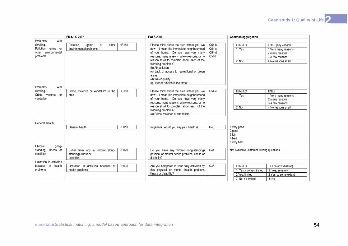
2
54 Statistical matching: a model based approach for data integration
Case study 1: Quality of Life
EU-SILC 2007 EQLS 2007 Common aggregation
Problems with dwelling. Pollution, grime or other environmental problems
Pollution, grime or other environmental problems
HS180
Please think about the area where you live now – I mean the immediate neighbourhood of your home. Do you have very many reasons, many reasons, a few reasons, or no reason at all to complain about each of the following problems? (b) Air pollution (c) Lack of access to recreational or green areas (d) Water quality (f) Litter or rubbish in the street
Q54-b Q54-c Q54-d Q54-f
EU-SILC EQLS (any variable)
1 Yes 1 Very many reasons 2 many reasons 3 A few reasons
2 No 4 No reasons at all
Problems with dwelling. Crime, violence or vandalism
Crime, violence or vandalism in the area
HS180
Please think about the area where you live now – I mean the immediate neighbourhood of your home. Do you have very many reasons, many reasons, a few reasons, or no reason at all to complain about each of the following problems? (e) Crime, violence or vandalism
Q54-e
EU-SILC EQLS
1 Yes 1 Very many reasons 2 many reasons 3 A few reasons
2 No 4 No reasons at all
General health
General health PH010
In general, would you say your health is … Q43
1 very good 2 good 3 fair 4 bad 5 very bad
Chronic (long-standing) illness or condition
Suffer from any a chronic (long-standing) illness or condition
PH020
Do you have any chronic (long-standing) physical or mental health problem, illness or disability?
Q44
Not Available –different filtering questions
Limitation in activities because of health problems
Limitation in activities because of health problems
PH030
Are you hampered in your daily activities by this physical or mental health problem, illness or disability?
Q45
EU-SILC EQLS (any variable)
1 Yes, strongly limited 1 Yes, severely
2 Yes, limited 2 Yes, to some extent
3 No, no limited 3 No
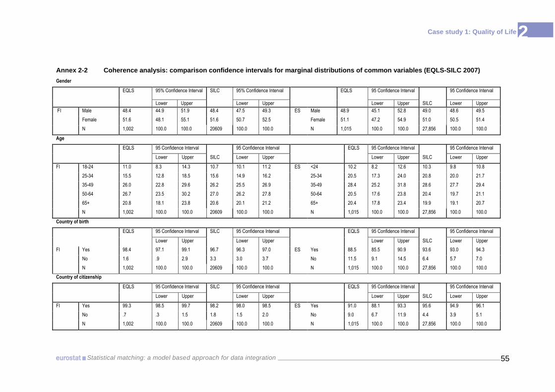
2
55 Statistical matching: a model based approach for data integration
Case study 1: Quality of Life
Annex 2-2 Coherence analysis: comparison confidence intervals for marginal distributions of common variables (EQLS-SILC 2007)
Gender
EQLS 95% Confidence Interval SILC 95% Confidence Interval EQLS 95 Confidence Interval 95 Confidence Interval
Lower Upper Lower Upper Lower Upper SILC Lower Upper
FI Male 48.4 44.9 51.9 48.4 47.5 49.3 ES Male 48.9 45.1 52.8 49.0 48.6 49.5
Female 51.6 48.1 55.1 51.6 50.7 52.5 Female 51.1 47.2 54.9 51.0 50.5 51.4
N 1,002 100.0 100.0 20609 100.0 100.0 N 1,015 100.0 100.0 27,856 100.0 100.0
Age
EQLS 95 Confidence Interval 95 Confidence Interval EQLS 95 Confidence Interval 95 Confidence Interval
Lower Upper SILC Lower Upper Lower Upper SILC Lower Upper
FI 18-24 11.0 8.3 14.3 10.7 10.1 11.2 ES <24 10.2 8.2 12.6 10.3 9.8 10.8
25-34 15.5 12.8 18.5 15.6 14.9 16.2 25-34 20.5 17.3 24.0 20.8 20.0 21.7
35-49 26.0 22.8 29.6 26.2 25.5 26.9 35-49 28.4 25.2 31.8 28.6 27.7 29.4
50-64 26.7 23.5 30.2 27.0 26.2 27.8 50-64 20.5 17.6 23.8 20.4 19.7 21.1
65+ 20.8 18.1 23.8 20.6 20.1 21.2 65+ 20.4 17.8 23.4 19.9 19.1 20.7
N 1,002 100.0 100.0 20609 100.0 100.0 N 1,015 100.0 100.0 27,856 100.0 100.0
Country of birth
EQLS 95 Confidence Interval SILC 95 Confidence Interval EQLS 95 Confidence Interval 95 Confidence Interval
Lower Upper Lower Upper Lower Upper SILC Lower Upper
FI Yes 98.4 97.1 99.1 96.7 96.3 97.0 ES Yes 88.5 85.5 90.9 93.6 93.0 94.3
No 1.6 .9 2.9 3.3 3.0 3.7 No 11.5 9.1 14.5 6.4 5.7 7.0
N 1,002 100.0 100.0 20609 100.0 100.0 N 1,015 100.0 100.0 27,856 100.0 100.0
Country of citizenship
EQLS 95 Confidence Interval SILC 95 Confidence Interval EQLS 95 Confidence Interval 95 Confidence Interval
Lower Upper Lower Upper Lower Upper SILC Lower Upper
FI Yes 99.3 98.5 99.7 98.2 98.0 98.5 ES Yes 91.0 88.1 93.3 95.6 94.9 96.1
No .7 .3 1.5 1.8 1.5 2.0 No 9.0 6.7 11.9 4.4 3.9 5.1
N 1,002 100.0 100.0 20609 100.0 100.0 N 1,015 100.0 100.0 27,856 100.0 100.0
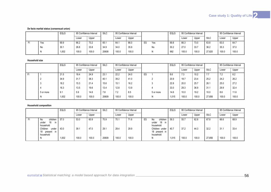
2
56 Statistical matching: a model based approach for data integration
Case study 1: Quality of Life
De facto marital status (consensual union)
EQLS 95 Confidence Interval SILC 95 Confidence Interval EQLS 95 Confidence Interval 95 Confidence Interval
Lower Upper Lower Upper Lower Upper SILC Lower Upper
FI Yes 69.9 66.2 73.2 65.1 64.1 66.0 ES Yes 69.8 66.3 73.0 63.8 63.0 64.7
No 30.1 26.8 33.8 34.9 34.0 35.9 No 30.2 27.0 33.7 36.2 35.3 37.0
N 1,002 100.0 100.0 20608 100.0 100.0 N 992 100.0 100.0 27,820 100.0 100.0
Household size
EQLS 95 Confidence Interval SILC 95 Confidence Interval EQLS 95 Confidence Interval 95 Confidence Interval
Lower Upper Lower Upper Lower Upper SILC Lower Upper
FI 1 21.5 18.4 24.9 23.1 22.2 24.0 ES 1 8.6 7.3 10.2 7.7 7.2 8.2
2 34.9 31.7 38.3 40.1 39.2 41.0 2 20.9 18.7 23.4 25.2 24.2 26.2
3 18.2 15.3 21.4 15.6 15.1 16.2 3 22.8 20.0 25.7 26.1 25.0 27.2
4 16.3 13.5 19.6 13.4 12.8 13.9 4 33.0 29.3 36.9 31.1 29.9 32.4
5 or more 9.1 5.9 14.6 7.8 7.2 8.5 5 or more 14.6 10.0 19.2 10.0 8.6 11.6
N 1,002 100.0 100.0 20609 100.0 100.0 N 1,015 100.0 100.0 27,856 100.0 100.0
Household composition
EQLS 95 Confidence Interval SILC 95 Confidence Interval EQLS 95 Confidence Interval 95 Confidence Interval
Lower Upper Lower Upper Lower Upper SILC Lower Upper
FI No children under 18 in household
57.0 53.0 60.9 70.9 70.1 71.6 ES No children under 18 in household
59.3 55.7 62.8 67.8 66.6 68.9
Children under 18 present in household
43.0 39.1 47.0 29.1 28.4 29.9 Children under 18 present in household
40.7 37.2 44.3 32.2 31.1 33.4
N 1,002 100.0 100.0 20609 100.0 100.0 N 1,015 100.0 100.0 27,856 100.0 100.0
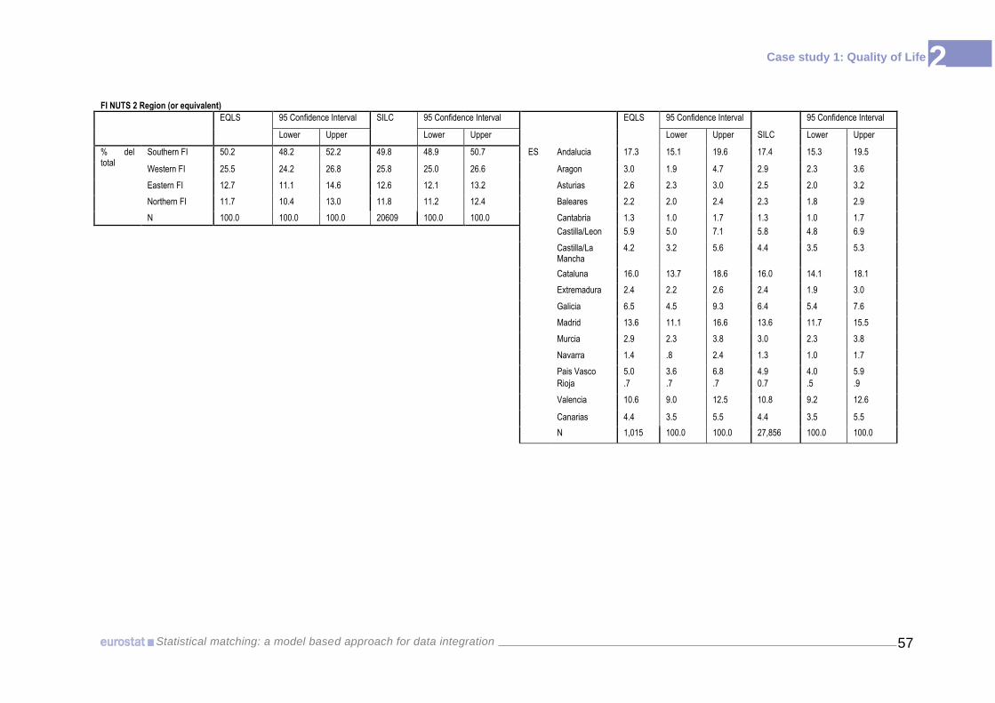
2
57 Statistical matching: a model based approach for data integration
Case study 1: Quality of Life
FI NUTS 2 Region (or equivalent)
EQLS 95 Confidence Interval SILC 95 Confidence Interval EQLS 95 Confidence Interval 95 Confidence Interval
Lower Upper Lower Upper Lower Upper SILC Lower Upper
% del total
Southern FI 50.2 48.2 52.2 49.8 48.9 50.7 ES Andalucia 17.3 15.1 19.6 17.4 15.3 19.5
Western FI 25.5 24.2 26.8 25.8 25.0 26.6 Aragon 3.0 1.9 4.7 2.9 2.3 3.6
Eastern FI 12.7 11.1 14.6 12.6 12.1 13.2 Asturias 2.6 2.3 3.0 2.5 2.0 3.2
Northern FI 11.7 10.4 13.0 11.8 11.2 12.4 Baleares 2.2 2.0 2.4 2.3 1.8 2.9
N 100.0 100.0 100.0 20609 100.0 100.0 Cantabria 1.3 1.0 1.7 1.3 1.0 1.7
Castilla/Leon 5.9 5.0 7.1 5.8 4.8 6.9
Castilla/La Mancha
4.2 3.2 5.6 4.4 3.5 5.3
Cataluna 16.0 13.7 18.6 16.0 14.1 18.1
Extremadura 2.4 2.2 2.6 2.4 1.9 3.0
Galicia 6.5 4.5 9.3 6.4 5.4 7.6
Madrid 13.6 11.1 16.6 13.6 11.7 15.5
Murcia 2.9 2.3 3.8 3.0 2.3 3.8
Navarra 1.4 .8 2.4 1.3 1.0 1.7
Pais Vasco 5.0 3.6 6.8 4.9 4.0 5.9
Rioja .7 .7 .7 0.7 .5 .9
Valencia 10.6 9.0 12.5 10.8 9.2 12.6
Canarias 4.4 3.5 5.5 4.4 3.5 5.5
N 1,015 100.0 100.0 27,856 100.0 100.0

2
58 Statistical matching: a model based approach for data integration
Case study 1: Quality of Life
Degree of urbanisation
EQLS 95 Confidence Interval SILC 95 Confidence Interval
EQLS 95 Confidence Interval 95 Confidence Interval
Lower Upper Lower Upper Lower Upper SILC Lower Upper
FI Densely populated area
16.8 12.5 22.2 27.5 26.6 28.3 ES Densely populated area
25.8 22.0 30.0 52.7 50.8 54.7
Intermediate populated area
26.0 21.3 31.3 16.4 15.7 17.1 Intermediate populated area
27.6 23.5 32.1 20.0 18.1 22.0
Thinly populated area
57.2 51.9 62.4 56.2 55.2 57.1 Thinly populated area
46.6 42.4 50.9 27.3 25.6 29.1
N 1,001 100.0 100.0 20609 100.0 100.0 N 1,014 100.0 100.0 27,856 100.0 100.0
Highest level of education
ESS 95 Confidence Interval SILC 95 Confidence Interval
EQLS 95 Confidence Interval 95 Confidence Interval
Lower Upper Lower Upper Lower Upper SILC Lower Upper
FI Less than lower secondary education (ISCED 0-1)
20.2 18.8 21.6 19.1 18.5 19.8 ES
Less than lower secondary education (ISCED 0-1)
35.8 33.6 38.1 29.5 28.5 30.6
Lower secondary education completed (ISCED 2)
14.4 13.1 15.8 10.4 9.8 10.9 Lower secondary education completed (ISCED 2)
21.0 19.2 22.9 22.7 21.8 23.7
Upper secondary education completed (ISCED 3)
35.4 33.5 37.3 41.7 40.8 42.6 Upper secondary education completed (ISCED 3)
16.6 15.0 18.2 21.9 21.1 22.7
Post-secondary non-tertiary education completed (ISCED 4)
8.7 7.4 10.1 .7 .6 .9
Tertiary education completed (ISCED 5-6)
30.0 28.3 31.9 28.8 28.0 29.6 Tertiary education completed (ISCED 5-6)
18.0 16.2 20.0 25.1 24.1 26.2
N 1,894 100.0 100.0 20502 100.0 100.0 N 1,870 100.0 100.0 26,128 100.0 100.0

2
59 Statistical matching: a model based approach for data integration
Case study 1: Quality of Life
Tenure status of household
EQLS 95 Confidence Interval SILC 95 Confidence Interval
EQLS 95 Confidence Interval 95 Confidence Interval
Lower Upper Lower Upper Lower Upper SILC Lower Upper
FI Owner 81.7 77.0 85.7 72.6 71.8 73.4 ES Owner 81.6 78.0 84.7 84.2 83.1 85.2
Payng rent at prevailing or market rate
9.3 6.8 12.7 10.5 9.9 11.2 Payng rent at prevailing or market rate
15.1 12.1 18.6 7.2 6.5 8.0
Rented at reduced rate or free
8.9 7.7 10.1 16.8 16.0 17.6 Rented at reduced rate or free
3.3 1.7 4.2 8.6 7.7 9.8
N 998 100.0 100.0 20609 100.0 100.0 N 1,009 100.0 100.0 27,856 100.0 100.0
Material deprivation 1: home adequately warm
EQLS 95 Confidence Interval SILC 95 Confidence Interval
EQLS 95 Confidence Interval 95 Confidence Interval
Lower Upper Lower Upper Lower Upper SILC Lower Upper
FI Yes, can afford if want
99.0 98.0 99.5 98.9 98.7 99.1 ES Yes, can afford if want
87.7 84.6 90.2 92.4 91.6 93.2
No, cannot afford it
1.0 .5 2.0 1.1 .9 1.3 No, cannot afford it
10.9 8.5 13.9 7.6 6.8 8.4
[Don't know] 1.4 .7 2.6 0.0 .0 .0
N 1,002 100.0 100.0 20554 100.0 100.0 N 1,015 100.0 100.0 27,848 100.0 100.0
Material deprivation 2: a week's annual holiday away from home
EQLS 95 Confidence Interval SILC 95 Confidence Interval
EQLS 95 Confidence Interval 95 Confidence Interval
Lower Upper Lower Upper Lower Upper SILC Lower Upper
FI Yes, can afford if want
84.9 82.2 87.3 82.7 82.0 83.4 ES Yes, can afford if want
70.0 66.2 73.5 63.8 62.4 65.2
No, cannot afford it
14.9 12.6 17.7 17.3 16.6 18.0 No, cannot afford it
28.1 24.5 31.9 36.2 34.8 37.6
[Don't know] .1 .0 .5 .0 .0 .0 [Don't know] 1.9 1.0 3.5 0.0 .0 .0
N 1,002 100.0 100.0 20528 100.0 100.0 N 1,015 100.0 100.0 27,850 100.0 100.0

2
60 Statistical matching: a model based approach for data integration
Case study 1: Quality of Life
Material deprivation 3: A meal with meat, chicken or fish every second day
EQLS 95 Confidence Interval SILC 95 Confidence Interval
EQLS 95 Confidence Interval 95 Confidence Interval
Lower Upper Lower Upper Lower Upper SILC Lower Upper
% FI Yes, can afford if want
98.7 97.6 99.3 97.0 96.6 97.3 ES Yes, can afford if want
96.7 95.1 97.7 97.7 97.3 98.1
No, cannot afford it
1.3 .7 2.4 3.0 2.7 3.4 No, cannot afford it
2.8 1.9 4.3 2.3 1.9 2.7
[Don't know] .5 .2 1.5 0.0 .0 .0
N 1,002 100.0 100.0 20584 100.0 100.0 N 1,015 100.0 100.0 27,851 100.0 100.0
Ability to make ends meet
EQLS 95 Confidence Interval SILC 95 Confidence Interval
EQLS 95 Confidence Interval 95 Confidence Interval
Lower Upper Lower Upper Lower Upper SILC Lower Upper
% FI Very easily 13.4 11.1 16.2 14.2 13.6 14.8 ES Very easily 5.7 3.7 8.7 1.3 1.0 1.5
Easily 32.9 29.7 36.2 26.8 26.0 27.6 Easily 26.0 22.5 29.8 15.0 14.1 16.0
Fairly easily 33.9 30.8 37.1 35.0 34.1 35.9 Fairly easily 25.8 22.2 29.6 26.7 25.5 27.9
With some difficulty
16.1 13.7 18.8 17.2 16.5 17.9 With some difficulty
29.6 25.8 33.8 30.6 29.4 31.8
With difficulty or great difficulty
2.9 1.8 4.8 6.9 6.2 7.6 With difficulty 10.4 7.5 13.5 26.5 15.7 17.6
[Don't know] .8 .4 1.6 [Don't know] 2.6 1.6 4.3 0.0 9.1 10.8
N 1,002 100.0 100.0 20527 100.0 100.0 N 1,015 100.0 100.0 27,835 100.0 100.0

2
61 Statistical matching: a model based approach for data integration
Case study 1: Quality of Life
Arrears on rent or mortgage payments
EQLS 95 Confidence Interval SILC 95 Confidence Interval
EQLS 95 Confidence Interval 95 Confidence Interval
Lower Upper Lower Upper Lower Upper SILC Lower Upper
% FI Yes 9.0 6.9 11.8 5.3 4.7 5.8 ES Yes 6.2 4.6 8.3 6.6 5.7 7.7
No 90.1 87.1 92.4 94.7 94.2 95.3 No 92.1 89.9 93.8 93.4 92.3 94.3
[Don't know] .9 .3 2.8 [Don't know] 1.7 1.0 2.9 0.0 .0 .0
N 1,002 100.0 100.0 11909 100.0 100.0 N 1,015 100.0 100.0 9,705 100.0 100.0
Arrears on utility bills, such as electricity, water, gas
EQLS 95 Confidence Interval SILC 95 Confidence Interval
EQLS 95 Confidence Interval 95 Confidence Interval
Lower Upper Lower Upper Lower Upper SILC Lower Upper
% FI Yes 9.4 7.2 12.2 4.2 3.8 4.6 ES Yes 8.0 6.0 10.7 3.9 3.4 4.4
No 90.4 87.6 92.6 95.8 95.4 96.2 No 90.8 88.0 93.0 96.1 95.6 96.6
[Don't know] .2 .1 .9 [Don't know] 1.2 .6 2.2 0.0 .0 .0
N 1,002 100.0 100.0 20538 100.0 100.0 N 1,015 100.0 100.0 27,737 100.0 100.0
Financial burden of the total housing cost
EQLS 95 Confidence Interval SILC 95 Confidence Interval
EQLS 95 Confidence Interval 95 Confidence Interval
Lower Upper Lower Upper Lower Upper SILC Lower Upper
% FI Yes, a heavy burden
3.9 2.7 5.5 16.6 15.9 17.3 ES Yes, a heavy burden
16.1 12.8 20.0 48.1 46.7 49.5
Yes, somewhat a burden
34.3 31.0 37.8 56.2 55.3 57.1 Yes, somewhat a burden
34.9 30.8 39.3 48.8 47.4 50.1
No burden at all 60.8 57.0 64.5 27.2 26.4 28.0 No burden at all
44.1 39.9 48.3 3.1 2.7 3.6
[Don't know] 1.0 .4 2.3 [Don't know] 4.9 3.3 7.3 0.0 .0 .0
N 1,002 100.0 100.0 20521 100.0 100.0 N 1,015 100.0 100.0 27,856 100.0 100.0

2
62 Statistical matching: a model based approach for data integration
Case study 1: Quality of Life
Amenities in dwelling: bath or shower
EQLS 95 Confidence Interval SILC 95 Confidence Interval
EQLS 95 Confidence Interval 95 Confidence Interval
Lower Upper Lower Upper Lower Upper SILC Lower Upper
% FI Yes 2.2 .9 5.4 1.5 1.3 1.7 ES Yes 1.4 .8 2.5 0.3 .2 .4
No 97.8 94.6 99.1 98.5 98.3 98.7 No 98.6 97.5 99.2 99.7 99.6 99.8
N 1,002 100.0 100.0 20602 100.0 100.0 N 1,015 100.0 100.0 27,856 100.0 100.0
Amenities in dwelling: indoor flushing toilet
EQLS 95 Confidence Interval SILC 95 Confidence Interval
EQLS 95 Confidence Interval 95 Confidence Interval
Lower Upper Lower Upper Lower Upper SILC Lower Upper
% FI Yes 1.6 .6 4.4 1.0 .8 1.2 ES Yes .9 .4 1.9 0.3 .2 .4
No 98.4 95.6 99.4 99.0 98.8 99.2 No 99.1 98.1 99.6 99.7 99.6 99.8
N 1,002 100.0 100.0 20602 100.0 100.0 N 1,015 100.0 100.0 27,856 100.0 100.0
Problems with dwelling. Noise
EQLS 95 Confidence Interval SILC 95 Confidence Interval
EQLS 95 Confidence Interval 95 Confidence Interval
Lower Upper Lower Upper Lower Upper SILC Lower Upper
% FI Yes 25.6 22.1 29.5 16.3 15.6 17.0 ES Yes 53.1 48.7 57.5 26.1 24.8 27.3
No 74.4 70.5 77.9 83.7 83.0 84.4 No 46.9 42.5 51.3 73.9 72.7 75.2
N 1,002 100.0 100.0 20587 100.0 100.0 N 1,015 100.0 100.0 27,848 100.0 100.0
Problems with dwelling. Air pollution, grime or other environmental problems
EQLS 95 Confidence Interval SILC 95 Confidence Interval
EQLS 95 Confidence Interval 95 Confidence Interval
Lower Upper Lower Upper Lower Upper SILC Lower Upper
% FI Yes 22.5 19.1 26.4 14.2 13.6 14.9 ES Yes 48.8 43.9 53.8 16.3 15.2 17.5
No 77.5 73.6 80.9 85.8 85.1 86.4 No 51.2 46.2 56.1 83.7 82.5 84.8
N 1,002 100.0 100.0 20576 100.0 100.0 N 1,003 100.0 100.0 27,848 100.0 100.0

2
63 Statistical matching: a model based approach for data integration
Case study 1: Quality of Life
Problems with dwelling. Recreational or green areas
EQLS 95 Confidence Interval SILC 95 Confidence Interval
EQLS 95 Confidence Interval 95 Confidence Interval
Lower Upper Lower Upper Lower Upper SILC Lower Upper
% FI Yes 6.3 4.6 8.6 14.2 13.6 14.9 ES Yes 46.1 41.8 50.6 16.3 15.2 17.5
No 93.7 91.4 95.4 85.8 85.1 86.4 No 53.9 49.4 58.2 83.7 82.5 84.8
N 998 100.0 100.0 20576 100.0 100.0 N 1,011 100.0 100.0 27,848 100.0 100.0
Problems with dwelling. Litter or rubbish in the street
EQLS 95 Confidence Interval SILC 95 Confidence Interval
EQLS 95 Confidence Interval 95 Confidence Interval
Lower Upper Lower Upper Lower Upper SILC Lower Upper
% FI Yes 28.5 25.2 32.0 14.2 13.6 14.9 ES Yes 38.7 34.3 43.2 16.3 15.2 17.5
No 71.5 68.0 74.8 85.8 85.1 86.4 No 61.3 56.8 65.7 83.7 82.5 84.8
N 999 100.0 100.0 20576 100.0 100.0 N 1,001 100.0 100.0 27,848 100.0 100.0
Problems with dwelling. Crime or vandalism
EQLS 95 Confidence Interval SILC 95 Confidence Interval
EQLS 95 Confidence Interval 95 Confidence Interval
Lower Upper Lower Upper Lower Upper SILC Lower Upper
% FI Yes 30.3 26.4 34.4 13.1 12.4 13.7 ES Yes 45.1 41.0 49.3 18.2 17.1 19.5
No 69.7 65.6 73.6 86.9 86.3 87.6 No 54.9 50.7 59.0 81.8 80.5 82.9
N 1,002 100.0 100.0 20585 100.0 100.0 N 1,008 100.0 100.0 27,847 100.0 100.0
General health status
EQLS 95 Confidence Interval SILC 95 Confidence Interval
EQLS 95 Confidence Interval 95 Confidence Interval
Lower Upper Lower Upper Lower Upper SILC Lower Upper
% FI Very good 17.7 15.0 20.8 22.2 21.1 23.3 ES Very good 23.3 20.1 26.9 15.5 14.6 16.4
Good 49.1 45.6 52.7 43.7 42.4 45.0 Good 52.3 48.4 56.1 51.3 50.3 52.4
Fair 25.2 22.4 28.1 24.5 23.3 25.7 Fair 17.5 14.7 20.7 21.3 20.6 22.1
Bad or very bad 8.0 6.0 10.0 9.6 8.5 10.9 Bad or very bad
6.9 4.8 10.1 11.9 11.1 12.6
N 1,002 100.0 100.0 9007 100.0 100.0 N 1,015 100.0 100.0 27,853 100.0 100.0

2
64 Statistical matching: a model based approach for data integration
Case study 1: Quality of Life
Long standing illness
EQLS 95 Confidence Interval SILC 95 Confidence Interval
EQLS 95 Confidence Interval 95 Confidence Interval
Lower Upper Lower Upper Lower Upper SILC Lower Upper
% FI Yes 39.4 36.0 43.0 44.6 43.3 45.9 ES Yes 15.6 13.1 18.6 25.7 24.8 26.5
No 60.1 56.5 63.6 55.4 54.1 56.7 No 83.7 80.8 86.2 74.3 73.5 75.2
[Refusal] .5 .2 1.1 [Refusal] .4 .1 1.0 0.0 .0 .0
[Don't know] .3 .0 1.9 0.0 .0 .0
N 1,002 100.0 100.0 9008 100.0 100.0 N 1,015 100.0 100.0 27,852 100.0 100.0
Self-declared labour status
EQLS 95 Confidence Interval SILC 95 Confidence Interval
EQLS 95 Confidence Interval 95 Confidence Interval
Lower Upper Lower Upper Lower Upper SILC Lower Upper
% FI At work 54.4 50.3 58.4 53.9 53.2 54.7 ES At work 49.4 45.6 53.2 51.9 52.1 54.0
Unemployed 2.9 2.0 4.2 5.5 5.1 5.9 Unemployed 5.6 3.9 7.8 6.2 4.9 5.7
In education 8.1 5.9 11.1 8.3 7.8 8.7 In education 6.5 4.6 9.1 7.1 5.7 6.6
Retired 31.5 28.1 35.0 22.5 21.9 23.0 Retired 15.1 12.8 17.6 15.3 2.0 2.4
Long term illness or disability
1.0 .5 1.9 6.0 5.5 6.5 Long term illness or disability
.9 .5 1.8 2.1 15.0 16.3
Full time home maker
2.2 1.0 4.4 3.4 3.1 3.7 Full time home maker
22.6 18.5 27.6 17.5 17.2 18.3
Other .4 .1 1.0 0.5 0.4 0.6
N 1,002 100.0 100.0 21773 100.0 100.0 N 184 100.0 100.0 28,65 100.0 100.0

2
65 Statistical matching: a model based approach for data integration
Case study 1: Quality of Life
Net monthly income of household
EQLS 95 Confidence Interval SILC 95 Confidence Interval
EQLS 95 Confidence Interval 95 Confidence Interval
Lower Upper Lower Upper Lower Upper SILC Lower Upper
% FI Less than 900€ 11.2 8.5 14.8 7.6 7.0 8.1 ES Less than 900€ 26.6 22.1 31.6 14.4 13.1 14.7
900-1800€ 19.4 16.4 22.9 22.3 21.5 23.1 900-1800€ 31.6 27.1 36.4 30.7 28.9 31.1
1800-2700€ 21.6 18.6 24.9 23.3 22.5 24.0 1800-2700€ 26.5 21.9 31.8 25.9 24.2 26.3
More than 2700€ 47.8 42.8 52.8 46.9 46.1 47.6 More than 2700€ 15.3 10.8 21.3 31.6 29.6 32.3
N 673 100.0 100.0 100.0 100.0 100.0 N 571 100.0 100.0 28,656 100.0 100.0
Status in employment
EQLS 95 Confidence Interval SILC 95 Confidence Interval
EQLS 95 Confidence Interval 95 Confidence Interval
Lower Upper Lower Upper Lower Upper SILC Lower Upper
FI Self-employed 13.8 10.3 18.1 14.0 13.4 14.7 ES Self-employed 18.9 14.7 23.8 15.2 14.6 16.0
Employed 85.0 80.6 88.6 85.6 85.0 86.3 Employed 81.1 76.2 85.3 83.6 82.8 84.3
Family worker 1.2 .4 3.5 .3 .2 .5 Family worker .0 .0 .0 1.2 1.0 1.3
N 492 100.0 100.0 16,329 100.0 100.0 N 475 100.0 100.0 23,682 100.0 100.0

2
66 Statistical matching: a model based approach for data integration
Case study 1: Quality of Life
Annex 2-3 Analysis explanatory power of common variables: Rao-Scott tests results (EQLS, 2007)
Target variables
Common variables
Subjective wellbeing (ES) Subjective wellbeing (FI)
Overall life satisfaction
Recognition Trust in the media
Trust in the government
Overall life satisfaction
Recognition Trust in the media
Trust in the government
q29 q28-6 q27-3 q27-5 q29 q28-6 q27-3 q27-5
Gender Pearson .286 .630 .676 .525 .164 .549 .459 .800
Likelihood Ratio .255 .628 .669 .522 .159 .547 .450 .793 Age Pearson .081 .150 .010 .115 .258 .231 .753 .031
Likelihood Ratio .070 .086 .015 .160 .175 .147 .707 .011
Country of birth Pearson .054 .079 .297 .163 .002 .969 .857 .671
Likelihood Ratio .023 .117 .223 .096 .100 .951 .669 .513
Country of citizenship Pearson .101 .008 .071 .104 .979 .001 .045 .003
Likelihood Ratio .055 .015 .041 .077 .929 .298 .232 .472
De facto marital status Pearson .054 .014 .101 .404 .000 .017 .581 .370
Likelihood Ratio .063 .022 .115 .437 .000 .020 .585 .389
Household type Pearson .003 .499 .798 .502 .007 .238 .782 .613
Likelihood Ratio .003 .493 .802 .496 .006 .220 .750 .532
NUTS 2 Region Pearson .000 .000 .000 .000 .432 .044 .020 .120
Likelihood Ratio .000 .000 .000 .000 .381 .036 .015 .148
Net monthly income of household Pearson .003 .213 .026 .129 .000 .000 .022 .006
Likelihood Ratio .003 .102 .017 .089 .000 .000 .020 .008
Degree of urbanisation Pearson .304 .000 .281 .509 .846 .035 .400 .854
Likelihood Ratio .302 .000 .184 .449 .815 .018 .370 .839
Highest level of education (ISCED) Pearson .084 .307 .136 .017 .000 .000 .227 .094
Likelihood Ratio .068 .169 .224 .025 .005 .001 .184 .091
Tenure status of household Pearson .005 .124 .266 .369 .014 .795 .804 .498
Likelihood Ratio .027 .206 .374 .356 .037 .655 .712 .465

2
67 Statistical matching: a model based approach for data integration
Case study 1: Quality of Life
Target variables
Common variables
Subjective wellbeing (ES) Subjective wellbeing (FI)
Overall life satisfaction
Recognition Trust in the media
Trust in the government
Overall life satisfaction
Recognition Trust in the media
Trust in the government
q29 q28-6 q27-3 q27-5 q29 q28-6 q27-3 q27-5
Material deprivation1: home adequately warm Pearson .000 .000 .001 .003 .100 .367 .604 .828
Likelihood Ratio .001 .000 .046 .046 .459 .338 .640 .760
Material deprivat ion 2:Paying for a week's annual holiday away from home (not staying with relatives)
Pearson .000 .000 .007 .633 .070 .568 .110 .065
Likelihood Ratio .000 .000 .005 .543 .137 .571 .169 .137
Material deprivation 3: A meal with meat, chicken or fish every second day i
Pearson .000 .002 .000 .000 .000 .955 .383 .154
Likelihood Ratio .045 .233 .040 .011 .030 .941 .533 .231
Ability to make ends meet Pearson .000 .000 .192 .000 .000 .000 .000 .001
Likelihood Ratio .000 .000 .099 .001 .000 .000 .001 .000
Arrears on rent or mortgage payments for accommodation Pearson .341 .622 .266 .251 .362 .044 .805 .073
Likelihood Ratio .376 .375 .384 .414 .421 .064 .719 .194
Arrears on utility bills, such as electricity, water, gas Pearson .133 .523 .580 .682 .116 .000 .801 .289
Likelihood Ratio .124 .429 .538 .657 .390 .000 .787 .567
Financial burden of the total housing cost Pearson .405 .342 .004 .015 .000 .330 .006 .002
Likelihood Ratio .538 .475 .007 .014 .002 .317 .017 .027
Amenities: Lack of indoor flushing toilet Pearson .012 .898 .040 .010 .897 .569 .356 .787
Likelihood Ratio .043 .774 .092 .070 .807 .725 .453 .744
Amenities: Lack of bath or shower Pearson .000 .860 .149 .001 .523 .173 .477 .805
Likelihood Ratio .011 .807 .183 .019 .426 .562 .502 .767
General health status Pearson .000 .078 .018 .000 .000 .000 .048 .008
Likelihood Ratio .000 .164 .037 .004 .000 .000 .080 .032
Long-standing health problem Pearson .001 .441 .205 .223 .000 .000 .034 .485
Likelihood Ratio .031 .469 .512 .291 .000 .000 .083 .547
Limitations in daily activities due to physical or mental health problem
Pearson .091 .407 .103 .875 .000 .021 .404 .478
Likelihood Ratio .041 .445 .288 .858 .001 .047 .381 .507
Self-declared labour status Pearson .000 .000 .050 .285 .001 .015 .314 .002
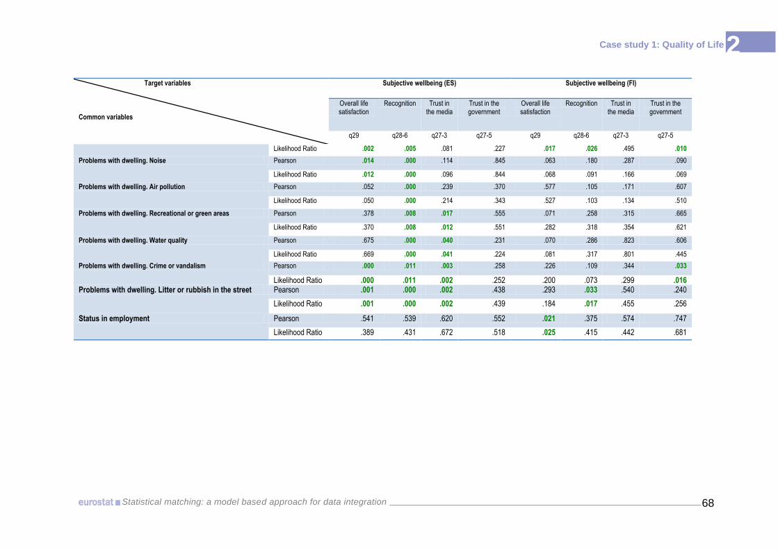
2
68 Statistical matching: a model based approach for data integration
Case study 1: Quality of Life
Target variables
Common variables
Subjective wellbeing (ES) Subjective wellbeing (FI)
Overall life satisfaction
Recognition Trust in the media
Trust in the government
Overall life satisfaction
Recognition Trust in the media
Trust in the government
q29 q28-6 q27-3 q27-5 q29 q28-6 q27-3 q27-5
Likelihood Ratio .002 .005 .081 .227 .017 .026 .495 .010
Problems with dwelling. Noise Pearson .014 .000 .114 .845 .063 .180 .287 .090
Likelihood Ratio .012 .000 .096 .844 .068 .091 .166 .069
Problems with dwelling. Air pollution Pearson .052 .000 .239 .370 .577 .105 .171 .607
Likelihood Ratio .050 .000 .214 .343 .527 .103 .134 .510
Problems with dwelling. Recreational or green areas Pearson .378 .008 .017 .555 .071 .258 .315 .665
Likelihood Ratio .370 .008 .012 .551 .282 .318 .354 .621
Problems with dwelling. Water quality Pearson .675 .000 .040 .231 .070 .286 .823 .606
Likelihood Ratio .669 .000 .041 .224 .081 .317 .801 .445
Problems with dwelling. Crime or vandalism Pearson .000 .011 .003 .258 .226 .109 .344 .033
Likelihood Ratio .000 .011 .002 .252 .200 .073 .299 .016 Problems with dwelling. Litter or rubbish in the street Pearson .001 .000 .002 .438 .293 .033 .540 .240
Likelihood Ratio .001 .000 .002 .439 .184 .017 .455 .256
Status in employment Pearson .541 .539 .620 .552 .021 .375 .574 .747
Likelihood Ratio .389 .431 .672 .518 .025 .415 .442 .681

Case study 2: Wage and Labour statistics
2 3 3
3.
3 Case study 2: Wage and labour statistics
3 Case study 2: Wage and labour statistics

Case study 2: Wage and Labour statistics
2
70 Statistical matching: a model based approach for data integration
3 3
3 Case study 2: Wage and labour statistics
3.1 Background
There is an important policy need to analyse together labour market information and
employment-related income. Within the European Statistical System (ESS) there are two key
social surveys that address these topics: EU-SILC (European Statistics on Income and Living
Conditions) and LFS (Labour Force Survey). On the one hand, EU-SILC is the reference
source at EU level for the collection of extensive income statistics, including wage
information for employees. On the other hand, LFS collects a large range of variables
relevant for labour market analysis and has a larger sample size that can improve the
precision of estimates for specific groups and domains.
In order to provide joint information on these two aspects, from 2009 onwards, LFS has been
collecting wage deciles. The exercise aims to test the use of alternative model based
techniques for matching wage information from EU-SILC into LFS. It also provides a good
opportunity to assess the quality of the data on wage deciles currently collected via the LFS.
Therefore, a second case study for the statistical matching exercise had a two-fold objective:
Box 3-1 Objectives
OBJECTIVE 1 — Analyse the coherence between wage statistics based on currently collected LFS wage deciles and EU-SILC based estimates. This comparative overview of LFS coherence with EU-SILC shall provide important insights on the quality of the information collected in LFS.
OBJECTIVE 2 — Assess the quality of wage statistics obtained through statistical matching in combination with variables collected in LFS.
The exercise and results presented are based on the analysis of data for seven countries:
Greece, Spain, France, Austria, Poland, Portugal and Slovakia. Section 2 follows the main
implementation steps19
of matching highlighting the main results in relation to the two
objectives. Section 3 summarises the main conclusions and recommendations for the
application of statistical matching techniques in this pilot study.
3.2 Statistical matching: methodology and results
3.2.1 Harmonisation and reconciliation of sources
The two data sources — EU-SILC as donor and LFS as recipient — share a large common
set of variables consistent in terms of definitions, classifications and marginal and joint
distributions. Still, we identified two main sources of possible inconsistencies: the
impossibility to use a common set of criteria to identify the target population (self-declared
activity status versus ILO status), differences in wage concepts (gross versus net wages and
current versus previous calendar year).
19
See Chapter 1
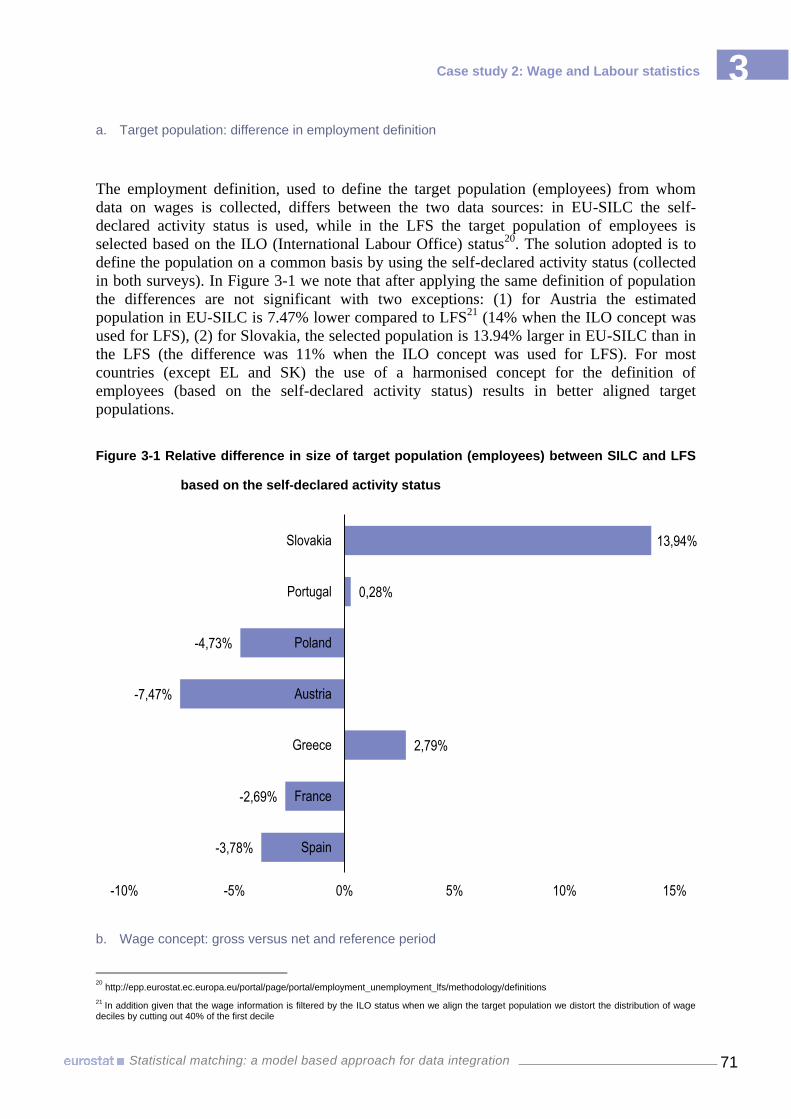
Case study 2: Wage and Labour statistics
2
71 Statistical matching: a model based approach for data integration
3 3
a. Target population: difference in employment definition
The employment definition, used to define the target population (employees) from whom
data on wages is collected, differs between the two data sources: in EU-SILC the self-
declared activity status is used, while in the LFS the target population of employees is
selected based on the ILO (International Labour Office) status20
. The solution adopted is to
define the population on a common basis by using the self-declared activity status (collected
in both surveys). In Figure 3-1 we note that after applying the same definition of population
the differences are not significant with two exceptions: (1) for Austria the estimated
population in EU-SILC is 7.47% lower compared to LFS21
(14% when the ILO concept was
used for LFS), (2) for Slovakia, the selected population is 13.94% larger in EU-SILC than in
the LFS (the difference was 11% when the ILO concept was used for LFS). For most
countries (except EL and SK) the use of a harmonised concept for the definition of
employees (based on the self-declared activity status) results in better aligned target
populations.
Figure 3-1 Relative difference in size of target population (employees) between SILC and LFS
based on the self-declared activity status
b. Wage concept: gross versus net and reference period
20
http://epp.eurostat.ec.europa.eu/portal/page/portal/employment_unemployment_lfs/methodology/definitions
21 In addition given that the wage information is filtered by the ILO status when we align the target population we distort the distribution of wage
deciles by cutting out 40% of the first decile
-3,78%
-2,69%
2,79%
-7,47%
-4,73%
0,28%
13,94%
-10% -5% 0% 5% 10% 15%
Spain
France
Greece
Austria
Poland
Portugal
Slovakia
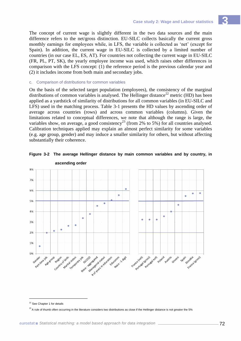
Case study 2: Wage and Labour statistics
2
72 Statistical matching: a model based approach for data integration
3 3 The concept of current wage is slightly different in the two data sources and the main
difference refers to the net/gross distinction. EU-SILC collects basically the current gross
monthly earnings for employees while, in LFS, the variable is collected as ‘net’ (except for
Spain). In addition, the current wage in EU-SILC is collected by a limited number of
countries (in our case EL, ES, AT). For countries not collecting the current wage in EU-SILC
(FR, PL, PT, SK), the yearly employee income was used, which raises other differences in
comparison with the LFS concept: (1) the reference period is the previous calendar year and
(2) it includes income from both main and secondary jobs.
c. Comparison of distributions for common variables
On the basis of the selected target population (employees), the consistency of the marginal
distributions of common variables is analysed. The Hellinger distance22
metric (HD) has been
applied as a yardstick of similarity of distributions for all common variables (in EU-SILC and
LFS) used in the matching process. Table 3-1 presents the HD values by ascending order of
average across countries (rows) and across common variables (columns). Given the
limitations related to conceptual differences, we note that although the range is large, the
variables show, on average, a good consistency23
(from 2% to 5%) for all countries analysed.
Calibration techniques applied may explain an almost perfect similarity for some variables
(e.g. age group, gender) and may induce a smaller similarity for others, but without affecting
substantially their coherence.
Figure 3-2 The average Hellinger distance by main common variables and by country, in
ascending order
22
See Chapter 1 for details
23 A rule of thumb often occurring in the literature considers two distributions as close if the Hellinger distance is not greater the 5%
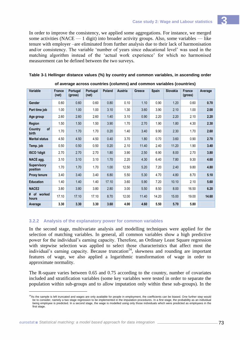
Case study 2: Wage and Labour statistics
2
73 Statistical matching: a model based approach for data integration
3 3 In order to improve the consistency, we applied some aggregations. For instance, we merged
some activities (NACE — 1 digit) into broader activity groups. Also, some variables — like
tenure with employer –are eliminated from further analysis due to their lack of harmonisation
and/or consistency. The variable ‘number of years since educational level’ was used in the
matching algorithm instead of the ‘actual work experience’ for which no harmonised
measurement can be defined between the two surveys.
Table 3-1 Hellinger distance values (%) by country and common variables, in ascending order
of average across countries (columns) and common variables (countries)
Variable France (net)
Portugal (gross)
Portugal (net)
Poland Austria Greece Spain Slovakia France (gross)
Average
Gender 0.60 0.60 0.60 0.80 0.10 1.10 0.90 1.20 0.60 0.70
Part time job 1.00 1.00 1.00 3.10 1.30 3.60 3.90 2.10 1.00 2.00
Age group 2.60 2.60 2.60 1.40 3.10 0.90 2.20 2.20 2.10 2.20
Region 1.50 1.50 1.50 3.90 1.70 2.70 1.90 1.80 4.30 2.30
Country of birth
1.70 1.70 1.70 0.20 1.40 3.40 9.90 2.30 1.70 2.60
Marital status 4.50 4.50 4.50 0.40 3.70 1.80 0.70 3.60 0.90 2.70
Temp. job 0.50 0.50 0.50 0.20 2.10 11.40 2.40 11.20 1.90 3.40
ISCO 1digit 2.70 2.70 2.70 1.80 3.90 2.50 6.90 8.00 2.70 3.80
NACE agg. 3.10 3.10 3.10 1.70 2.20 4.30 6.40 7.80 9.30 4.60
Supervisory position
1.70 1.70 1.70 1.00 12.50 5.20 7.20 2.40 9.80 4.80
Proxy tenure 3.40 3.40 3.40 6.80 5.50 5.30 4.70 4.80 8.70 5.10
Education 1.40 1.40 1.40 17.10 3.60 5.90 7.20 10.10 2.10 5.60
NACE2 3.80 3.80 3.80 2.80 3.00 5.50 8.50 8.00 16.50 6.20
# of worked hours
17.10 17.10 17.10 8.70 12.00 11.40 14.20 15.00 19.00 14.60
Average 3.30 3.30 3.30 3.60 4.00 4.60 5.50 5.70 5.80
3.2.2 Analysis of the explanatory power for common variables
In the second stage, multivariate analysis and modelling techniques were applied for the
selection of matching variables. In general, all common variables show a high predictive
power for the individual’s earning capacity. Therefore, an Ordinary Least Square regression
with stepwise selection was applied to select those characteristics that affect most the
individual’s earning capacity. Because truncation24
, skewness and rounding are important
features of wage, we also applied a logarithmic transformation of wage in order to
approximate normality.
The R-square varies between 0.65 and 0.75 according to the country, number of covariates
included and stratification variables (some key variables were tested in order to separate the
population within sub-groups and to allow imputation only within these sub-groups). In the
24
As the sample is left truncated and wages are only available for people in employment, the coefficients can be biased. One further step would be to consider, namely a two stage regression to be implemented in the imputation procedures. In a first stage, the probability as an individual being employee is predicted. In a second stage, the wage is modelled using only those individuals which were predicted as employees in the first stage.
Case study 2: Wage and Labour statistics
2
74 Statistical matching: a model based approach for data integration
3 3 end, the stratification based on part-time/full-time workers was kept in order to control for
important differentials related to the hours worked and focus on explaining differences in
average earnings. Some further checks were done for selected countries25
and additional
interaction effects were included to improve the estimates, especially for specific sub-groups.
For instance, we noted that low education has very strong significant negative effects but in
some activity sectors and occupations these relations do not hold. The set26
of common
variables finally selected for imputation is:
basic socio-demographic variables (age, gender, country of birth, education
attainment level, marital status);
region of residence;
characteristics of the main job (occupation, economic activity, full-time or part-time
status, temporary job, supervisory position)
work experience (proxy used: number of years since educational level was attained).
3.2.3 Matching methods
We tested several imputation methods27
: hot deck, regression based methods, predictive mean
matching method and probabilistic decision algorithms. This last approach allocates LFS
individuals into wage deciles through a probabilistic decisional tree based on the conditional
probability that an individual is in a specific decile. These conditional probabilities are
produced based on a logistic regression performed in EU-SILC.
Because imputation approaches have usually limited ability to recreate individual level
values, results are assessed in terms of preservation of important data distribution aspects and
multivariable relationships (Rubin 1996). Therefore, to assess the robustness of different
methods applied, we compare the extent to which the observed distributions in the donor
(EU-SILC) are preserved in the recipient (LFS) files. Hellinger distances are used again to
measure the level of similarity of the joint distributions of wage deciles with key variables.
The mixed methods28
perform the best (see Annex III-3). This is because they use a more
comprehensive model where several interactions are included and stratification by part time
and full time employees is applied.
3.2.4 Results and quality evaluation
When assessing results based on matched datasets, the final aim of the analysis should be
considered. Thus, results have to be interpreted in relation to the two-fold objective of the
exercise.
Three main criteria were considered throughout the analysis:
25
A model diagnostics analysis was performed after each model tested and outliers were excluded in order to reduce their effect on the regression parameters. No substantial effects on the final results were detected.
26 Table 1 in the end of the chapter shows as an example the model used for Spain, 2009.
27 See Chapter 1 for details.
28 The predictive mean matching method was used in two main stages (1) estimates wage on both surveys based on the model coefficients obtained in EU-SILC and (2) ‘the closest’ real donor from EU-SILC, calculated based on a distance measure between the model based wage estimates in the two surveys, is imputed in LFS . See Chapter 1 for details.

Case study 2: Wage and Labour statistics
2
75 Statistical matching: a model based approach for data integration
3 3 (1) the consistency of joint distributions (of wage deciles with matching variables) among
EU-SILC observed, LFS imputed and LFS observed;
1. a) The comparison between EU-SILC observed and LFS observed helps for
checking the coherence of common variables. In this particular case study, it helps
also to assess the quality of wage information collected in LFS with EU-SILC as a
benchmark (objective 1);
1. b) The comparison between EU-SILC observed and LFS imputed serves as a
quality criterion of matching (objective 2);
1. c) The comparison between LFS observed and LFS imputed helps to compare
how matching performs in comparison with collected information in LFS. However,
in order to draw conclusions it is essential the concurrent comparison of the three
types of distribution and the premise of using EU-SILC as a benchmark.
(2) the consistency of different parameters such as totals, means and more complex
distributional parameters (objective2);
(3) test the CIA29 for specific target variables: wage deciles and LFS variables not collected
in EU-SILC (objective2).
a. Objective 1 — assess the quality of wage information in LFS with EU-SILC as benchmark
In order to assess the quality of wage deciles collected in LFS, the cross-distributions of LFS
wage decile with the main demographic variables were compared to:
cross-distributions based on observed EU-SILC wage information (horizontal axis in
Figure 3-3) and
cross-distributions based on imputed wages from the matching exercise (vertical axis
in Figure 3-4).
Results show two main clusters of countries: Spain, France and Austria score very well for
most of the variables analysed while for Greece, Poland, Portugal and Slovakia we have large
inconsistencies. The average ‘dissimilarity’ of wage statistics between LFS and EU-SILC is
very high mainly due to distorted wage decile distribution. We can observe that the two types
of ‘dissimilarity’ are very highly correlated as estimates based on matching follow the same
trend as EU-SILC observed. However, we have a slightly higher similarity between LFS
observed and LFS imputed as we can control for differences in the distributions of the main
demographic variables.
Indeed, the most severe problem for LFS wage deciles proved to be the use of predefined
wage bands (countries in the upper right corner) instead of collecting the wage and
calculating the deciles afterwards. An erroneous approximation of cut-off points leads to
distorted30
wage deciles distribution in LFS.
29
Conditional independence assumption means that the measures of association between relevant labour variables collected only in LFS and the variable wage (decile) is assumed to be 0, conditional on the common variables used in the imputation process.
30 The target population is not equally distributed among the 10 intervals.

Case study 2: Wage and Labour statistics
2
76 Statistical matching: a model based approach for data integration
3 3 We used data for Greece to illustrate the impact of using misleading cut-off points. Thus, we
applied the predefined LFS cut-off points (from the questionnaire) to EU-SILC observed and
imputed wages in LFS. Figure 3-5 shows a good consistency of wage decile distributions
among EU-SILC observed, LFS imputed and LFS observed, given similar thresholds. Thus,
the last column shows the wage distribution according to LFS data collection and the
thresholds used in the questionnaire. We note that the collected LFS wage decile distribution
is very distorted and the population is not equally distributed in deciles. The first/ middle
column shows the wage decile distribution based on EU-SILC observed / LFS imputed wage
but using the pre-defined cut-off points (used in the LFS questionnaire) instead of calculating
them. We can see that both distributions remain distorted and follow the same pattern as LFS
collected distribution. This also highlights that, matching functions well as it provides similar
wage distribution no matter how cut-off points are fixed.
Figure 3-3 Average similarity for joint distributions of wage deciles with main socio-
demographical variables, by country
Spain
Austria
Greece Poland
France
Slovakia
Portugal
0%
5%
10%
15%
20%
25%
30%
0% 5% 10% 15% 20% 25% 30%
LF
S o
bse
rved
- L
FS
imp
ute
d
LFS observed - EU-SILC observed

Case study 2: Wage and Labour statistics
2
77 Statistical matching: a model based approach for data integration
3 3 Figure 3-4: Impact on predefined cut-off points on wage decile distributions, Greece 2009
b. Objective 2 — assess the quality of LFS wage statistics obtained through matching
To assess the quality of results obtained through statistical matching we refer to two main
criteria:
Preservation of distributions and main parameters between the donor and the
recipient;
Capture the real joint distributions and correlations for variables not collected
together.

Case study 2: Wage and Labour statistics
2
78 Statistical matching: a model based approach for data integration
3 3 Figure 3-5: The cut-off points for wage deciles
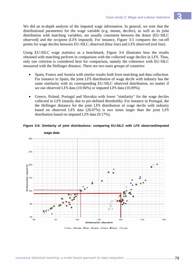
Case study 2: Wage and Labour statistics
2
79 Statistical matching: a model based approach for data integration
3 3 We did an in-depth analysis of the imputed wage information. In general, we note that the
distributional parameters for the wage variable (e.g. means, deciles), as well as its joint
distribution with matching variables, are usually consistent between the donor (EU-SILC
observed) and the recipient (LFS imputed). For instance, Figure 3-5 compares the cut-off
points for wage deciles between EU-SILC observed (blue line) and LFS observed (red line).
Using EU-SILC wage statistics as a benchmark, Figure 3-6 illustrates how the results
obtained with matching perform in comparison with the collected wage deciles in LFS. Thus,
only one criterion is considered here for comparison, namely the coherence with EU-SILC
measured with the Hellinger distance. There are two main groups of countries:
Spain, France and Austria with similar results both from matching and data collection.
For instance in Spain, the joint LFS distribution of wage decile with industry has the
same similarity with its corresponding EU-SILC observed distribution, no matter if
we use observed LFS data (10.94%) or imputed LFS data (10.09%).
Greece, Poland, Portugal and Slovakia with lower "similarity" for the wage deciles
collected in LFS (mainly due to pre-defined thresholds). For instance in Portugal, the
the Hellinger distance for the joint LFS distribution of wage decile with industry
based on observed LFS data (20.07%) is two times larger than the joint LFS
distribution based on imputed LFS data (9.17%).
Figure 3-6: Similarity of joint distributions: comparing EU-SILC with LFS observed/imputed
wage data

Case study 2: Wage and Labour statistics
2
80 Statistical matching: a model based approach for data integration
3 3 Specific matching methods
31 proved to be more robust and it is also important to control for
differences in demographic structures between the two sources. Figure 3-7 captures the
relationship between two pairs of distributions:
on the horizontal axis we have the HD that measure the similarity EU-SILC-LFS for
simple distributions of the main common variables used in matching;
on the vertical axis we have the HD that measure the similarity of joint distributions
of common variables with wage deciles.
The graph illustrates that there is a strong relation between the two measures. Hence, the
results of matching are strongly dependent on the coherence of the common variables. Even
small inconsistencies in demographic variables tend to inflate the dissimilarity indexes (HD)
when wage deciles are crossed with two or more dimensions.
Figure 3-7: Impact of discrepancies in the distribution of main common variables on matching
results
These checks can be performed as long as the imputed wage is analysed with demographic
variables that are common between EU-SILC and LFS. Additional analysis is needed when
the focus is on the joint distributions of imputed wage information and variables collected
only in LFS. One example is the analysis of wage statistics in relation to the field of
education collected only in LFS (see Figure 3-8).
The major limitation of statistical matching is its reliance on implicit assumptions32
. When
imputed wages need to be analysed with additional variable collected solely in LFS, one
31
Predictive mean matching method
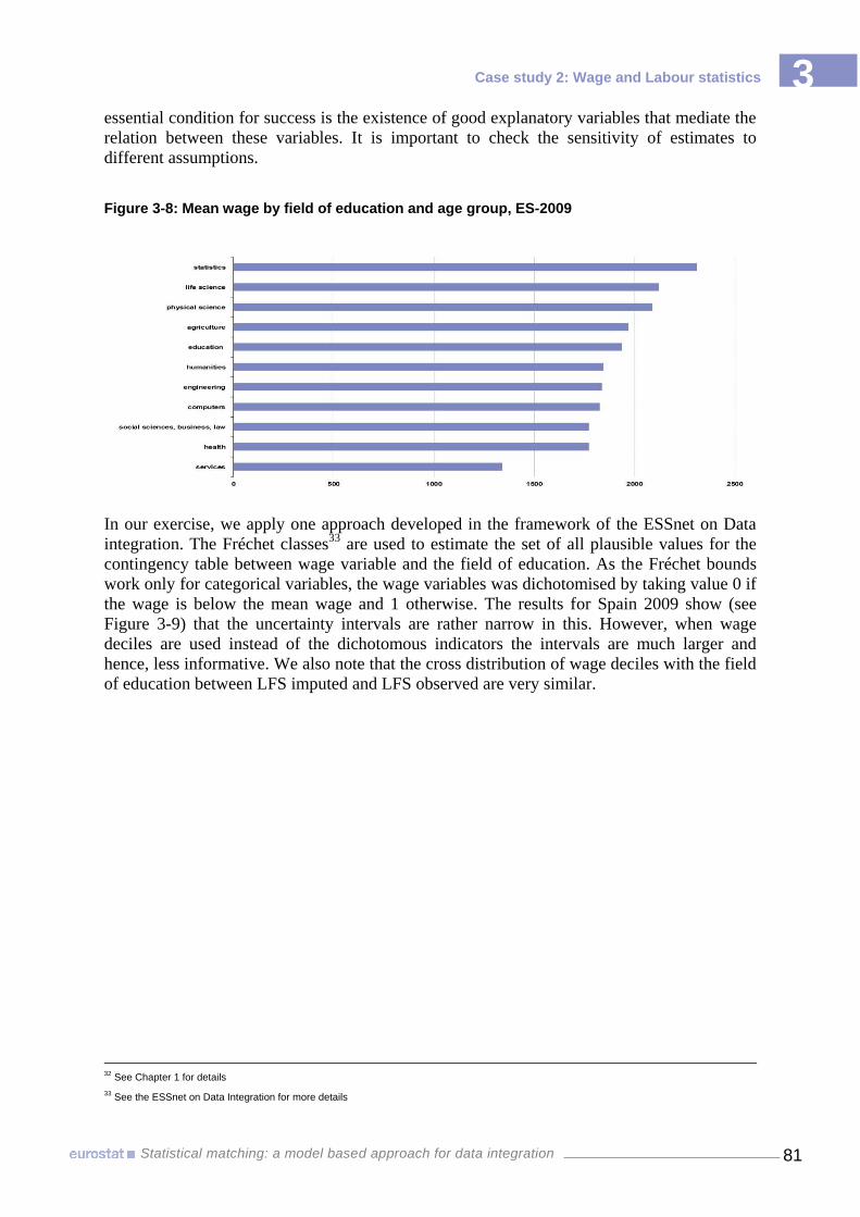
Case study 2: Wage and Labour statistics
2
81 Statistical matching: a model based approach for data integration
3 3 essential condition for success is the existence of good explanatory variables that mediate the
relation between these variables. It is important to check the sensitivity of estimates to
different assumptions.
Figure 3-8: Mean wage by field of education and age group, ES-2009
In our exercise, we apply one approach developed in the framework of the ESSnet on Data
integration. The Fréchet classes33
are used to estimate the set of all plausible values for the
contingency table between wage variable and the field of education. As the Fréchet bounds
work only for categorical variables, the wage variables was dichotomised by taking value 0 if
the wage is below the mean wage and 1 otherwise. The results for Spain 2009 show (see
Figure 3-9) that the uncertainty intervals are rather narrow in this. However, when wage
deciles are used instead of the dichotomous indicators the intervals are much larger and
hence, less informative. We also note that the cross distribution of wage deciles with the field
of education between LFS imputed and LFS observed are very similar.
32
See Chapter 1 for details
33 See the ESSnet on Data Integration for more details

Case study 2: Wage and Labour statistics
2
82 Statistical matching: a model based approach for data integration
3 3 Figure 3-9: Frechet Bounds: % of people with wage below the mean by field of education (ES,
2009)
Case study 2: Wage and Labour statistics
2
83 Statistical matching: a model based approach for data integration
3 3 3.3 Conclusions and Recommendations
Objective 1: For some countries, the LFS wage decile distribution is distorted mainly
due to the misleading placement of the 'predefined' cut-off points. Thus, for countries
such as Greece and Poland, it would be important to communicate and explain the
predefined thresholds and not use them under the assumption they correspond to the
true cut-offs points for deciles. Once thresholds are controlled for, the coherence with
both EU-SILC and imputed wage information is good.
Objective 2:
o An important factor for the joint analysis and matching of EU-SILC and LFS
is a better coherence of labour variables, including those for delimitation of
the target populations. Differences and misalignment of distributions for the
common variables used in the matching algorithm can cause discrepancies for
wage related estimates.
o Even if there are small inconsistencies in demographic variables, they tend to
inflate the dissimilarity indexes (HD) when wage deciles are crossed with
more dimensions (two and more).
o Specific matching methods34
proved to be more robust. However, results tend
to be similar and in general estimates from matching are more sensitive to
coherence pre-requisites and variables used in the model than the actual
matching method employed.
o Results show that, when pre-requisites of coherence are met matching
provides good results for marginal distributions and joint distributions that
involve dimensions controlled in the model. For the variables not observed
together more complex quality checks such as the uncertainty analysis based
on Frechet bounds are needed. However, when model assumptions hold,
statistical matching can provide good inferences for specific estimates (e.g.
wage and field of education).
o Given the current system, pre-requisites for matching are not met to the same
extent across countries. The existence of different patterns, coherence
problems and different wage/population concepts across countries requires
tailored approaches and fine-tuning for different countries.
34
Predictive mean matching method that performs the imputation in two stages: first computation of estimates and then real values are imputed based

Case study 2: Wage and Labour statistics
2
84 Statistical matching: a model based approach for data integration
3 3 Annex 3-1 Common variables- metadata analysis
Matched dataset EU-SILC LFS
Description of variable Codification Description of variable Codification Description of variable
Gender RB090 Gender SEX Gender
Male 1 Male 1 Male
Female 2 Female 2 Female
Age in completed years AGE Age in completed years AGE Age in completed years
Country of birth C_BIRTH Country of birth COBGROUP Country of birth
Native born 1 National 0 Born in the same country
Born in another EU MS 2 Within EU27 1 Born in another EU15 country
2 Born in another EU10 country
3 Born in another EU02 country
Born in a non-EU country 3 Outside EU27 900 Born in a non-EU27 country
Country of citizenship CIT_SHIP Citizenship NATGROUP Nationality
Nationals 1 National 0 National
Nationals of another EU MS 2 Within EU27 1 Citizen of another EU15 country
2 Citizen of another EU10 country
3 Citizen of another EU02 country
Nationals of a non-EU country 3 Outside EU27 900 Citizen of non-EU27 country
Marital status/de jure status PB190 Marital status MARSTAT Marital status
Unmarried 1 Never married 1 Single
Married (including registered partnership 2 Married 2 Married
Widowed 4 Widowed 3 Widowed
Divorced 3 Separated 4 Divorced or legally separated
5 Divorced

Case study 2: Wage and Labour statistics
2
85 Statistical matching: a model based approach for data integration
3 3 Matched dataset EU-SILC LFS
Description of variable Codification Description of variable Codification Description of variable
De facto marital status (consensual union) PB200 Consensual union HHPARTNR The spouse, or cohabiting partner of the person is or NOT in the same household
Person living in a consensual union 1 Yes, legal 1 The spouse, or cohabiting partner of the person is in the same household
2 Yes, without legal
Person NOT living in a consensual union 3 No 2 The spouse, or cohabiting partner of the person is not in the same household
Country of residence DB020 Country COUNTRY Country
Region of residence DB040 Region (according to NUTS at 2 digits) REGION Region
Degree of urbanisation DB100 Degree of urbanisation DEGURBA Degree of urbanisation
Densely-populated area 1 Densely 1 densely
Intermediate populated area 2 Intermediate 2 intermediate
Thinly population area 3 Thinly 3 thinly
Self-declared labour status PL030 Self-defined current economic status MAINSTAT Main labour status
FTPT Full-Time/Part-Time distinction
Carries out an activity FULL-time 1 Work fulltime 1
Carries out a job or profession, including unpaid work for a family business or holding, including an apprenticeship or paid traineeship, etc, FTPT=1 (Full-time job)
Carries out an activity PART-time 2 Work part-time 1
Carries out a job or profession, including unpaid work for a family business or holding, including an apprenticeship or paid traineeship, etc, FTPT=2 (Part-time job)
Unemployed 3 Unemployed 2 Unemployed
Pupil, student, further training, unpaid work experience
4 Pupil, student, further training, unpaid work experience 3 Pupil, student, further training, unpaid work experience
In retirement or early retirement or has given up business
5 In retirement or in early retirement or has given up business 4 In retirement or early retirement or has given up business
Permanently disabled o/and unfit to work 6 Permanently disabled o/and unfit to work 5 Permanently disabled
In compulsory military or community service 7 In compulsory military or community service 6 In compulsory military service

Case study 2: Wage and Labour statistics
2
86 Statistical matching: a model based approach for data integration
3 3 Matched dataset EU-SILC LFS
Description of variable Codification Description of variable Codification Description of variable
Fulfilling domestic tasks 8 Fulfilling domestic tasks and care responsibilities 7 Fulfilling domestic tasks
Other inactive persons 9 Other inactive persons 8 Other inactive person
Status in employment PL040 Status in employment STAPRO Professional status
PL140 Type of contract TEMP Permanency of the job
Self-employed 1 Self-employed with employees 0 Self-employed with or without employees
2 Self-employed without employees 1 Self-employed with employees
4 Family worker 2 Self-employed without employees
4 Family worker
Employee with a permanent job or work contract with unlimited period
3 Employee and PL140=1 (permanent job/work contract of unlimited duration)
3 Employee + TEMP=1 (Person has a permanent job or work contract of unlimited duration)
Employee with a temporary job or work contract with limited period
3 Employee and PL140=2 (2 temporary job/work contract of limited duration)
3 Employee + TEMP=2 (Person has temporary job/work contract of limited duration )
Occupation in employment PL050 Occupation (isco-88 (com)) ISCO4D
Managers (4 positions) 11 to 14 Managers (4 positions) 1 Legislators, senior officials and managers
Professionals (6 positions) 21 to 26 Professionals (6 positions) 2 Professionals
Technicians and associate professionals (5 positions)
31 to 35 Technicians and associate professionals (5 positions) 3 Technicians and associate professionals
Clerical support workers (4 positions) 41 to 44 Clerical support workers (4 positions) 4 Clerks
Service and sales workers (4 positions) 51 to 54 Service and sales workers (4 positions) 5 Service workers and shop and market sales workers
Skilled agricultural, fishery and forestry workers (3 positions)
61 to 63 Skilled agricultural, fishery and forestry workers (3 positions) 6 Skilled agricultural and fishery workers
Craft and related trades workers (5 positions) 71 to 75 Craft and related trades workers (5 positions) 7 Craft and related trades workers
Plant and machine operators and assemblers (3 positions)
81 to 83 Plant and machine operators and assemblers (3 positions) 8 Plant and machine operators and assemblers
Elementary occupations (6 positions) 91 to 96 Elementary occupations (6 positions) 9 Elementary occupations
Armed forces (3 positions) 01 to 03 Armed forces (3 positions) 10 Armed forces
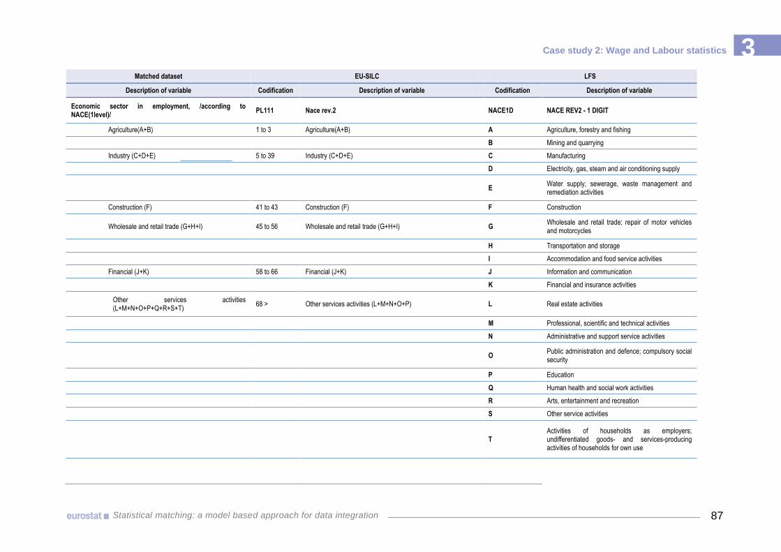
Case study 2: Wage and Labour statistics
2
87 Statistical matching: a model based approach for data integration
3 3 Matched dataset EU-SILC LFS
Description of variable Codification Description of variable Codification Description of variable
Economic sector in employment, /according to NACE(1level)/
PL111 Nace rev.2 NACE1D NACE REV2 - 1 DIGIT
Agriculture(A+B) 1 to 3 Agriculture(A+B) A Agriculture, forestry and fishing
B Mining and quarrying
Industry (C+D+E) 5 to 39 Industry (C+D+E) C Manufacturing
D Electricity, gas, steam and air conditioning supply
E Water supply; sewerage, waste management and remediation activities
Construction (F) 41 to 43 Construction (F) F Construction
Wholesale and retail trade (G+H+I) 45 to 56 Wholesale and retail trade (G+H+I) G Wholesale and retail trade; repair of motor vehicles and motorcycles
H Transportation and storage
I Accommodation and food service activities
Financial (J+K) 58 to 66 Financial (J+K) J Information and communication
K Financial and insurance activities
Other services activities (L+M+N+O+P+Q+R+S+T)
68 > Other services activities (L+M+N+O+P) L Real estate activities
M Professional, scientific and technical activities
N Administrative and support service activities
O Public administration and defence; compulsory social security
P Education
Q Human health and social work activities
R Arts, entertainment and recreation
S Other service activities
T Activities of households as employers; undifferentiated goods- and services-producing activities of households for own use

Case study 2: Wage and Labour statistics
2
88 Statistical matching: a model based approach for data integration
3 3 Matched dataset EU-SILC LFS
Description of variable Codification Description of variable Codification Description of variable
Highest level of education completed, PE040 Highest ISCED level attained HATLEVEL Highest level of education or training successfully completed
No formal education or below ISCED1 0 Pre-primary education 0 No formal education or below ISCED 1
Primary education 1 Primary education 11 ISCED 1
Lower secondary education 2 Lower secondary education 21 ISCED 2
22 ISCED 3c (shorter than 3 years)
Upper secondary education 3 (Upper) secondary education 31 ISCED 3c (3 years and more)
32 ISCED 3 a,b
30 ISCED 3 (without distinction a, b or c possible, 2 y+)
Post secondary education but not tertiary 4 Post-secondary non tertiary education 41 ISCED 4a,b
42 ISCED 4c
43 ISCED 4 (without distinction a, b or c possible)
Tertiary education, first stage 5 First stage of tertiary education 51 ISCED 5b
52 ISCED 5a
Tertiary education, second stage 6 Second stage of tertiary education 60 ISCED 6
Number of hours worked per week PL060 ‘Number of hours usually worked per week in main job’ HWACTUAL Number of hours actually worked during the reference week in the main job
‘Total number of hours usually worked in second, third …jobs’ (+ HWACTUAL2)
PL100
Managerial position PL150 Managerial position SUPVISOR Supervisory responsibilities
Yes, the persons has managerial tasks 1 Yes, the persons has managerial tasks 1 Yes
No, the persons has NOT managerial tasks 2 No, the persons has NOT managerial tasks 2 No

Case study 2: Wage and Labour statistics
2
89 Statistical matching: a model based approach for data integration
3 3
Annex 3-2 Model log(wage) as dependent variable, Spain 2009
Independent Variables Parameter Standard Pr > F
Base category Estimate Error
Intercept 5.97866 0.00154 <.0001
Age 0.01267 0.00007 <.0001
Age square -0.00007 0.00000 <.0001
Gender Female 0.13989 0.00020 <.0001
Education ISCED 0-1
ISCED2 0.08967 0.00033 <.0001
ISCED3 0.17306 0.00037 <.0001
ISCED4 0.19105 0.00110 <.0001
ISCED5 0.26815 0.00043 <.0001
ISCED6 0.37464 0.00105 <.0001
Part time -0.46045 0.00039 <.0001
Temporary contract -0.13280 0.00023 <.0001
Number hours worked 0.01167 0.00001 <.0001
Supervisory position 0.13307 0.00022 <.0001
Proxy for work experience 0.00154 0.00015 <.0001
Sector-NACE1d aggregated Agriculture
Industry 0.18421 0.00086 <.0001
Construction 0.23483 0.00095 <.0001
Trade 0.07089 0.00070 <.0001
Financial 0.16441 0.00075 <.0001
Real estate 0.07158 0.00135 <.0001
Professional, scientific and technical activities 0.05973 0.00084 <.0001
Administrative and support services 0.01899 0.00078 <.0001
Public administration 0.23403 0.00073 <.0001
Education 0.16231 0.00077 <.0001
Other 0.01696 0.00076 <.0001
Occupation Elementary occupations
Managers 0.53985 0.00071 <.0001
Professionals 0.45952 0.00043 <.0001
Technicians 0.24321 0.00039 <.0001
Clerical support workers 0.15697 0.00036 <.0001
Service and sales workers 0.06543 0.00034 <.0001
Skilled agricultural workers 0.03747 0.00091 <.0001
Craft workers 0.07585 0.00037 <.0001
Plant/machine operators 0.11369 0.00042 <.0001
Country of birth Native born
Born in another EU country -0.07207 0.00054 <.0001
Born in a non-EU country -0.05614 0.00038 <.0001

Case study 2: Wage and Labour statistics
2
90 Statistical matching: a model based approach for data integration
3 3 Independent Variables Parameter Standard Pr > F
Base category Estimate Error Degree of urbanisation
Thinly
Densely 0.05445 0.00022 <.0001
Intermediate 0.03078 0.00026 <.0001
Marital status Single
Married 0.07894 0.00023 <.0001
Widowed 0.00554 0.00080 <.0001
Separated/divorced 0.02904 0.00043 <.0001
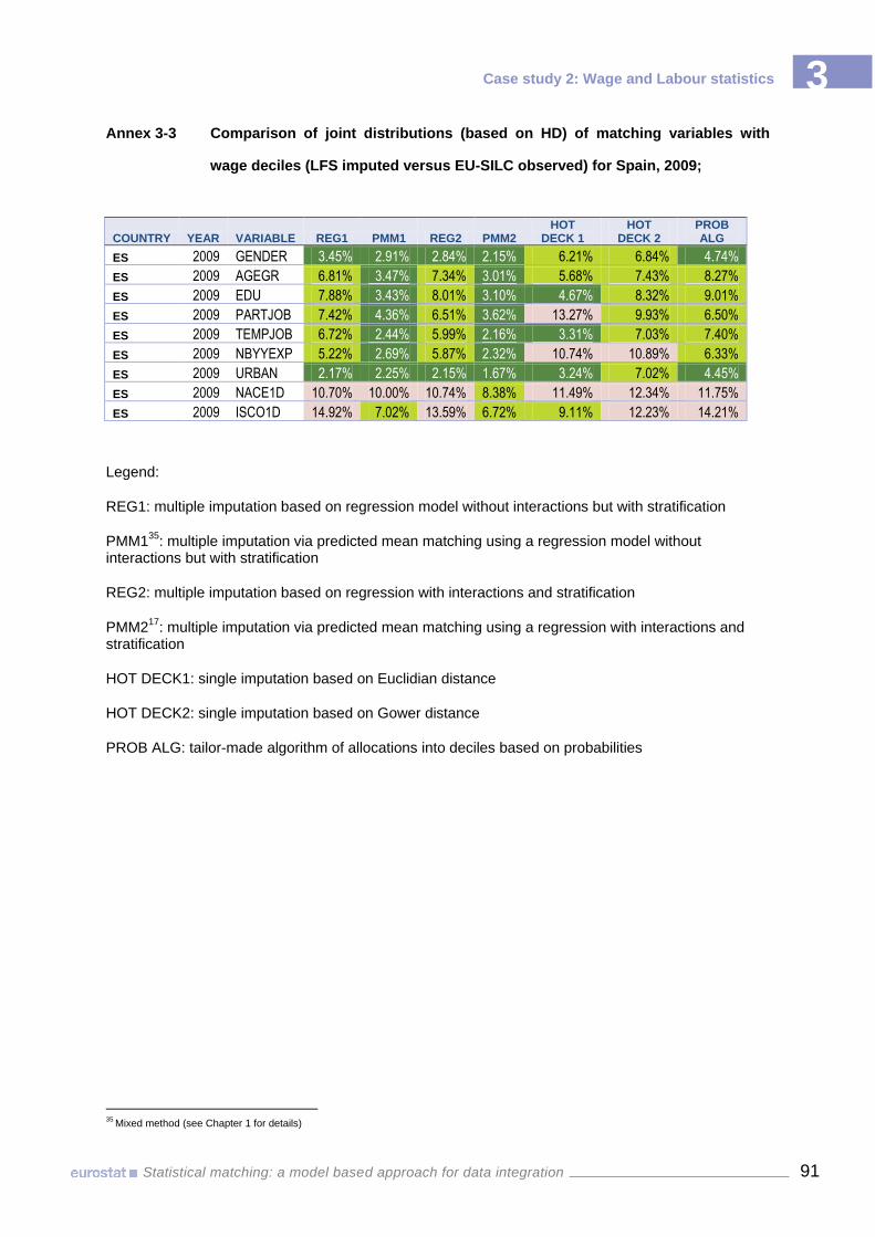
Case study 2: Wage and Labour statistics
2
91 Statistical matching: a model based approach for data integration
3 3 Annex 3-3 Comparison of joint distributions (based on HD) of matching variables with
wage deciles (LFS imputed versus EU-SILC observed) for Spain, 2009;
COUNTRY YEAR VARIABLE REG1 PMM1 REG2 PMM2 HOT
DECK 1 HOT
DECK 2 PROB ALG
ES 2009 GENDER 3.45% 2.91% 2.84% 2.15% 6.21% 6.84% 4.74%
ES 2009 AGEGR 6.81% 3.47% 7.34% 3.01% 5.68% 7.43% 8.27%
ES 2009 EDU 7.88% 3.43% 8.01% 3.10% 4.67% 8.32% 9.01%
ES 2009 PARTJOB 7.42% 4.36% 6.51% 3.62% 13.27% 9.93% 6.50%
ES 2009 TEMPJOB 6.72% 2.44% 5.99% 2.16% 3.31% 7.03% 7.40%
ES 2009 NBYYEXP 5.22% 2.69% 5.87% 2.32% 10.74% 10.89% 6.33%
ES 2009 URBAN 2.17% 2.25% 2.15% 1.67% 3.24% 7.02% 4.45%
ES 2009 NACE1D 10.70% 10.00% 10.74% 8.38% 11.49% 12.34% 11.75%
ES 2009 ISCO1D 14.92% 7.02% 13.59% 6.72% 9.11% 12.23% 14.21%
Legend:
REG1: multiple imputation based on regression model without interactions but with stratification
PMM135
: multiple imputation via predicted mean matching using a regression model without interactions but with stratification
REG2: multiple imputation based on regression with interactions and stratification
PMM217
: multiple imputation via predicted mean matching using a regression with interactions and stratification
HOT DECK1: single imputation based on Euclidian distance
HOT DECK2: single imputation based on Gower distance
PROB ALG: tailor-made algorithm of allocations into deciles based on probabilities
35
Mixed method (see Chapter 1 for details)

Bibliography
92 Statistical matching: a model based approach for data integration
4 Bibliography 1) Adamek, J.C. (1994) Fusion: combining data from separate sources, Marketing Research 6, 48-50
2) Atkinson, A.B. and Marlier, E., eds, (2010) Income and Living Conditions in Europe, EUROSTAT,
European Union
3) Ballin M., Di Zio, M, D’Orazio, M, Scanu, M, Torelli, N. (2008) File Concatenation of Survey Data: a
Computer Intensive Approach to Sampling Weights Estimation. Rivista di Statistica Ufficiale.
4) Breiman, L. (2001) Random Forests, Machine Learning 45(1), 5-32
5) Breiman, L., Friedman, J.H., Olkshen, R.A and Stone, C.J. (1984) Classification and Regression Trees,
Wadsworth
6) Consolini, P. (2010), Experiences and case studies, Report WP2, ESS-net, Statistical Methodology Project
on Integration of Surveys and Administrative Data
7) Conti P.L., Marella D., Scanu M. (2008) Evaluation of matching noise for imputation techniques based on
the local linear regression estimator. Computational Statistics and Data Analysis, 53, 354-365.
8) Conti, P.L. and Scanu, M. (2005) On the evaluation of matching noise produced by nonparametric
imputation techniques. Rivista di Statistica Ufficiale, 1/2006, 43-56.
9) Cowell, R.G.,Dawid, A.P., Lauritzen, S.,Spiegelhalter, D.J. (1999), Probabilistic Networks and Expert
Systems, Springer
10) Di Zio, M. (2010) Statistical matching methods, Report WP1 ESS-net, Statistical Methodology Project on
Integration of Surveys and Administrative Data
11) D'Orazio, M., Di Zio, M. and Scanu, M. (2006). Statistical Matching: Theory and Practice. Wiley,
Chichester.
12) D’Orazio, M (2010), Evaluation of the accuracy of statistical matching, Report WP1 ESS-net, Statistical
Methodology Project on Integration of Surveys and Administrative Data
13) D’Orazio, M. (2010). Literature review of statistical matching, Report WP1 ESS-net, Statistical
Methodology Project on Integration of Surveys and Administrative Data
14) D’ Orazio, M, DiZio, M., Scanu,M., (2006) Statistical Matching: Theory and Practice, Wiley
15) Kadane, J.B. (1978) Some statistical problems in merging data files. In Department of Treasury,
Compendium of Tax Research, pp. 159–179. Washington, DC: US Government Printing Office.
16) Liu, T.P. and Kovacevic, M.S. (1994) Statistical matching of survey data files: a simulation study,
Proceedings of the Section of Survey Research Methods. American Mathematical Association,pp 479-484
17) Moriarity, C. and Scheuren, F. (2001) Statistical matching: a paradigm for assessing the uncertainty in the
procedure. Journal of Official Statistics 17, 407–422.
18) Moriarity, C. and Scheuren, F. (2003) A note on Rubin’s statistical matching using file concatenation with
adjusted weights and multiple imputation. Journal of Business and Economic Statistics 21, 65–73.
19) Paass, G. (1986), Statistical match: evaluation of existing procedures and improvements by using additional
information, in G.H Orcutt, J.Merz and H Quinke, eds , Microanalitic Simulation Models to Support Social
and Financial Policy , pp 401-422, Elsevier
20) Raghunathan, T.E. and Grizzle, J.E. (1995) A Split Questionnaire Survey Design, Journal of the American
Statistical Association, 90, 54-63.
21) Rässler, H. (2001) Split Questionnaire Survey. Funktionale Spezifikation zur Software SQS 1.0, Raessler
automation & consulting.
22) Rässler, S. (2002), Statistical Matching, a Frequentist Theory, Practical Applications and Alternative
Bayesian Approach, Springer

Bibliography
93 Statistical matching: a model based approach for data integration
23) Rässler, S., Kiesl, H. (2009). How useful are uncertainty bounds? Some recent theory with an application to
Rubin's causal model. 57th Session of the International Statistical Institute, Durban (South Africa), 16-22
August 2009.
24) Regulation (EC) No223/2009 of the European Parliament and of the Council of 11 of March 2009 on
European Statistics
25) Renssen, R.H. (1998) Use of statistical matching techniques in calibration estimation. Survey Methodology
24, 171–183.
26) Roberts, A. (1994) Media exposure and consumer purchasing: an improved data fusion technique.
Marketing and Research Today 22, 159–172.
27) Rodgers, W.L. (1984). “An evaluation of statistical matching”. Journal of Business and Economic
Statistics, 2, 91–102.
28) Rubin, D.B. (1976) Inference and Missing Data, Biometrika, 63, 581-592.
29) Rubin, D.B. (1986) Statistical Matching Using File Concatenation with Adjusted Weights and Multiple
Imputations, Journal of Business and Economic Statistics, 4, 87- 95.
30) Rubin, D.B. (1987) Multiple Imputation for Non response in Surveys. John Wiley and Sons, New York.
31) Ruggles, N. and Ruggles, R. (1974), A strategy for merging and matching microdata sets, Annals of
Economic and Social Measurement 1(3) 353-371
32) Ruggles, N. (1999) The development of integrated data bases for social, economic and demographic
statistics. In N. Ruggles and R. Ruggles (eds) Macro- and Microdata Analyses and Their Integration, pp.
410–478. Cheltenham: Edward Elgar.
33) Scanu, M (2010), Recommendations on statistical matching, Report WP2, ESS-net, Statistical Methodology
Project on Integration of Surveys and Administrative Data
34) Schafer, J.L. (1997) Analysis of Incomplete Multivariate Data. Chapman and Hall, London.
35) Schafer, J.L. and Olsen, M.K. (1998) Multiple imputation for multivariate missing-data problems: a data
analyst's perspective. Multivariate Behavioral Research, 33, 545-571
36) Singh, A.C., Mantel, H, Kinnack, M and Rowe, G. (1993) Statistical matching: Use of auxiliary information
as an alternative to the conditional independence assumption, Survey Methodology, 19, pp 59-79
37) Singh, A.C., Mantel, H., Kinack, M. and Rowe, G. (1993). “Statistical matching: use of auxiliary
information as an alternative to the conditional independence assumption”. Survey Methodology, 19, 59–
79.
38) Singh, A.C., Armstrong, J.B., and Lemaitre, G.E. (1988) Statistical matching using log-linear imputation,
Proceedings of the Section on Survey Research Methods, American Statistical Association pp 672-677
39) Singh, A.C., Mantel, H., Kinack, M. and Rowe, G. (1990) On methods of statistical matching with and
without auxiliary information. Technical Report SSMD-90-016E, Methodology Branch, Statistics Canada.
40) Stiglitz J. E., A. Sen & J.-P. Fitoussi eds (2009) Report by the Commission on the Measurement of
Economic Performance and Social Progress, Paris. http://www.stiglitz-sen-fitoussi.fr/en/index.htm


European Commission
Statistical matching: a model based approach for data integration Luxembourg: Publications Office of the European Union 2013 — 93 pp. — 21 x 29.7 cm Theme: General and regional statistics Collection: Methodologies & Working papers ISBN 978-92-79-30355-2 ISSN 1977-0375 doi:10.2785/44822 Cat. No: KS-RA-13-020-EN-N


HOW TO OBTAIN EU PUBLICATIONS
Free publications: • one copy:
via EU Bookshop (http://bookshop.europa.eu);
• more than one copy or posters/maps: from the European Union’s representations (http://ec.europa.eu/represent_en.htm); from the delegations in non-EU countries (http://eeas.europa.eu/delegations/index_en.htm); by contacting the Europe Direct service (http://europa.eu/europedirect/index_en.htm) or calling 00 800 6 7 8 9 10 11 (freephone number from anywhere in the EU) (*). (*) The information given is free, as are most calls (though some operators, phone boxes or hotels may charge you).
Priced publications: • via EU Bookshop (http://bookshop.europa.eu).
Priced subscriptions: • via one of the sales agents of the Publications Office of the European Union
(http://publications.europa.eu/others/agents/index_en.htm).

2009 edition
Statistical Requirements CompendiuENm
KS-RA-13-020-EN
-N
Statistical Requirements Com
pendium
2009 edition
M e t h o d o l o g i e s a n d W o r k i n g p a p e r s
ISSN 1977-0375