statistical methods for drug safetydocshare01.docshare.tips/files/31056/310569218.pdf · bayesian...
TRANSCRIPT
Robert D. GibbonsUniversity of Chicago
Illinois, USA
Anup K. AmatyaNew Mexico State University
Las Cruces, USA
Statistical Methods for Drug Safety
© 2016 by Taylor & Francis Group, LLC

Editor-in-Chief
Shein-Chung Chow, Ph.D., Professor, Department of Biostatistics and Bioinformatics, Duke University School of Medicine, Durham, North Carolina
Series Editors Byron Jones, Biometrical Fellow, Statistical Methodology, Integrated Information Sciences,Novartis Pharma AG, Basel, Switzerland
Jen-pei Liu, Professor, Division of Biometry, Department of Agronomy, National Taiwan University, Taipei, Taiwan
Karl E. Peace, Georgia Cancer Coalition, Distinguished Cancer Scholar, Senior Research Scientist and Professor of Biostatistics, Jiann-Ping Hsu College of Public Health, Georgia Southern University, Statesboro, Georgia
Bruce W. Turnbull, Professor, School of Operations Research and Industrial Engineering, Cornell University, Ithaca, New York
Published Titles
Adaptive Design Methods in Clinical Trials, Second Edition Shein-Chung Chow and Mark Chang
Adaptive Designs for Sequential Treatment Allocation Alessandro Baldi Antognini and Alessandra Giovagnoli
Adaptive Design Theory and Implementation Using SAS and R, Second Edition Mark Chang
Advanced Bayesian Methods for Medical Test Accuracy Lyle D. Broemeling
Advances in Clinical Trial Biostatistics Nancy L. Geller
Applied Meta-Analysis with R Ding-Geng (Din) Chen and Karl E. Peace
Basic Statistics and Pharmaceutical Statistical Applications, Second Edition James E. De Muth
Bayesian Adaptive Methods for Clinical Trials Scott M. Berry, Bradley P. Carlin, J. Jack Lee, and Peter Muller
Bayesian Analysis Made Simple: An Excel GUI for WinBUGS Phil Woodward
Bayesian Methods for Measures of Agreement Lyle D. Broemeling
Bayesian Methods in Epidemiology Lyle D. Broemeling
Bayesian Methods in Health Economics Gianluca Baio
Bayesian Missing Data Problems: EM, Data Augmentation and Noniterative Computation Ming T. Tan, Guo-Liang Tian, and Kai Wang Ng
Bayesian Modeling in Bioinformatics Dipak K. Dey, Samiran Ghosh, and Bani K. Mallick
Benefit-Risk Assessment in Pharmaceutical Research and Development Andreas Sashegyi, James Felli, and Rebecca Noel
Biosimilars: Design and Analysis of Follow-on Biologics Shein-Chung Chow
Biostatistics: A Computing Approach Stewart J. Anderson
Causal Analysis in Biomedicine and Epidemiology: Based on Minimal Sufficient Causation Mikel Aickin
Clinical and Statistical Considerations in Personalized Medicine Claudio Carini, Sandeep Menon, and Mark Chang
© 2016 by Taylor & Francis Group, LLC
Clinical Trial Data Analysis using R Ding-Geng (Din) Chen and Karl E. Peace
Clinical Trial Methodology Karl E. Peace and Ding-Geng (Din) Chen
Computational Methods in Biomedical Research Ravindra Khattree and Dayanand N. Naik
Computational Pharmacokinetics Anders Källén
Confidence Intervals for Proportions and Related Measures of Effect Size Robert G. Newcombe
Controversial Statistical Issues in Clinical Trials Shein-Chung Chow
Data and Safety Monitoring Committees in Clinical Trials Jay Herson
Design and Analysis of Animal Studies in Pharmaceutical Development Shein-Chung Chow and Jen-pei Liu
Design and Analysis of Bioavailability and Bioequivalence Studies, Third Edition Shein-Chung Chow and Jen-pei Liu
Design and Analysis of Bridging Studies Jen-pei Liu, Shein-Chung Chow, and Chin-Fu Hsiao
Design and Analysis of Clinical Trials for Predictive Medicine Shigeyuki Matsui, Marc Buyse, and Richard Simon
Design and Analysis of Clinical Trials with Time-to-Event Endpoints Karl E. Peace
Design and Analysis of Non-Inferiority Trials Mark D. Rothmann, Brian L. Wiens, and Ivan S. F. Chan
Difference Equations with Public Health Applications Lemuel A. Moyé and Asha Seth Kapadia
DNA Methylation Microarrays: Experimental Design and Statistical Analysis Sun-Chong Wang and Arturas Petronis
DNA Microarrays and Related Genomics Techniques: Design, Analysis, and Interpretation of Experiments David B. Allison, Grier P. Page, T. Mark Beasley, and Jode W. Edwards
Dose Finding by the Continual Reassessment Method Ying Kuen Cheung
Elementary Bayesian Biostatistics Lemuel A. Moyé
Empirical Likelihood Method in Survival Analysis Mai Zhou
Frailty Models in Survival Analysis Andreas Wienke
Generalized Linear Models: A Bayesian Perspective Dipak K. Dey, Sujit K. Ghosh, and Bani K. Mallick
Handbook of Regression and Modeling: Applications for the Clinical and Pharmaceutical Industries Daryl S. Paulson
Inference Principles for Biostatisticians Ian C. Marschner
Interval-Censored Time-to-Event Data: Methods and Applications Ding-Geng (Din) Chen, Jianguo Sun, and Karl E. Peace
Introductory Adaptive Trial Designs: A Practical Guide with R Mark Chang
Joint Models for Longitudinal and Time-to-Event Data: With Applications in R Dimitris Rizopoulos
Measures of Interobserver Agreement and Reliability, Second Edition Mohamed M. Shoukri
Medical Biostatistics, Third Edition A. Indrayan
Meta-Analysis in Medicine and Health Policy Dalene Stangl and Donald A. Berry
© 2016 by Taylor & Francis Group, LLC

Mixed Effects Models for the Population Approach: Models, Tasks, Methods and Tools Marc Lavielle
Modeling to Inform Infectious Disease Control Niels G. Becker
Monte Carlo Simulation for the Pharmaceutical Industry: Concepts, Algorithms, and Case Studies Mark Chang
Multiple Testing Problems in Pharmaceutical Statistics Alex Dmitrienko, Ajit C. Tamhane, and Frank Bretz
Noninferiority Testing in Clinical Trials: Issues and Challenges Tie-Hua Ng
Optimal Design for Nonlinear Response Models Valerii V. Fedorov and Sergei L. Leonov
Patient-Reported Outcomes: Measurement, Implementation and Interpretation Joseph C. Cappelleri, Kelly H. Zou, Andrew G. Bushmakin, Jose Ma. J. Alvir, Demissie Alemayehu, and Tara Symonds
Quantitative Evaluation of Safety in Drug Development: Design, Analysis and Reporting Qi Jiang and H. Amy Xia
Randomized Clinical Trials of Nonpharmacological Treatments Isabelle Boutron, Philippe Ravaud, and David Moher
Randomized Phase II Cancer Clinical Trials Sin-Ho Jung
Sample Size Calculations for Clustered and Longitudinal Outcomes in Clinical Research Chul Ahn, Moonseong Heo, and Song Zhang
Sample Size Calculations in Clinical Research, Second Edition Shein-Chung Chow, Jun Shao and Hansheng Wang
Statistical Analysis of Human Growth and Development Yin Bun Cheung
Statistical Design and Analysis of Stability Studies Shein-Chung Chow
Statistical Evaluation of Diagnostic Performance: Topics in ROC Analysis Kelly H. Zou, Aiyi Liu, Andriy Bandos, Lucila Ohno-Machado, and Howard Rockette
Statistical Methods for Clinical Trials Mark X. Norleans
Statistical Methods for Drug Safety Robert D. Gibbons and Anup K. Amatya
Statistical Methods in Drug Combination Studies Wei Zhao and Harry Yang
Statistics in Drug Research: Methodologies and Recent Developments Shein-Chung Chow and Jun Shao
Statistics in the Pharmaceutical Industry, Third Edition Ralph Buncher and Jia-Yeong Tsay
Survival Analysis in Medicine and Genetics Jialiang Li and Shuangge Ma
Theory of Drug Development Eric B. Holmgren
Translational Medicine: Strategies and Statistical Methods Dennis Cosmatos and Shein-Chung Chow
© 2016 by Taylor & Francis Group, LLC

Robert D. GibbonsUniversity of Chicago
Illinois, USA
Anup K. AmatyaNew Mexico State University
Las Cruces, USA
Statistical Methods for Drug Safety
© 2016 by Taylor & Francis Group, LLC

CRC PressTaylor & Francis Group6000 Broken Sound Parkway NW, Suite 300Boca Raton, FL 33487-2742
© 2016 by Taylor & Francis Group, LLCCRC Press is an imprint of Taylor & Francis Group, an Informa business
No claim to original U.S. Government worksVersion Date: 20150604
International Standard Book Number-13: 978-1-4665-6185-4 (eBook - PDF)
This book contains information obtained from authentic and highly regarded sources. Reasonable efforts have been made to publish reliable data and information, but the author and publisher cannot assume responsibility for the validity of all materials or the consequences of their use. The authors and publishers have attempted to trace the copyright holders of all material reproduced in this publication and apologize to copyright holders if permission to publish in this form has not been obtained. If any copyright material has not been acknowledged please write and let us know so we may rectify in any future reprint.
Except as permitted under U.S. Copyright Law, no part of this book may be reprinted, reproduced, transmitted, or utilized in any form by any electronic, mechanical, or other means, now known or hereafter invented, including photocopying, microfilming, and recording, or in any information stor-age or retrieval system, without written permission from the publishers.
For permission to photocopy or use material electronically from this work, please access www.copy-right.com (http://www.copyright.com/) or contact the Copyright Clearance Center, Inc. (CCC), 222 Rosewood Drive, Danvers, MA 01923, 978-750-8400. CCC is a not-for-profit organization that pro-vides licenses and registration for a variety of users. For organizations that have been granted a photo-copy license by the CCC, a separate system of payment has been arranged.
Trademark Notice: Product or corporate names may be trademarks or registered trademarks, and are used only for identification and explanation without intent to infringe.
Visit the Taylor & Francis Web site athttp://www.taylorandfrancis.com
and the CRC Press Web site athttp://www.crcpress.com

To Carol, Julie, Jason and Michael and the memory
of Donna and Sid
R.D.G.
To my family and friends
A.K.A.
© 2016 by Taylor & Francis Group, LLC

© 2016 by Taylor & Francis Group, LLC
Contents
Preface xv
Acknowledgments xix
1 Introduction 1
1.1 Randomized Clinical Trials . . . . . . . . . . . . . . . . . . . 21.2 Observational Studies . . . . . . . . . . . . . . . . . . . . . . 41.3 The Problem of Multiple Comparisons . . . . . . . . . . . . . 51.4 The Evolution of Available Data Streams . . . . . . . . . . . 61.5 The Hierarchy of Scientific Evidence . . . . . . . . . . . . . . 71.6 Statistical Significance . . . . . . . . . . . . . . . . . . . . . . 81.7 Summary . . . . . . . . . . . . . . . . . . . . . . . . . . . . . 11
2 Basic Statistical Concepts 13
2.1 Introduction . . . . . . . . . . . . . . . . . . . . . . . . . . . 132.2 Relative Risk . . . . . . . . . . . . . . . . . . . . . . . . . . . 132.3 Odds Ratio . . . . . . . . . . . . . . . . . . . . . . . . . . . . 152.4 Statistical Power . . . . . . . . . . . . . . . . . . . . . . . . . 162.5 Maximum Likelihood Estimation . . . . . . . . . . . . . . . . 17
2.5.1 Example with a Closed Form Solution . . . . . . . . . 192.5.2 Example without a Closed Form Solution . . . . . . . 202.5.3 Bayesian Statistics . . . . . . . . . . . . . . . . . . . . 212.5.4 Example . . . . . . . . . . . . . . . . . . . . . . . . . . 22
2.6 Non-linear Regression Models . . . . . . . . . . . . . . . . . 232.7 Causal Inference . . . . . . . . . . . . . . . . . . . . . . . . . 25
2.7.1 Counterfactuals . . . . . . . . . . . . . . . . . . . . . . 252.7.2 Average Treatment Effect . . . . . . . . . . . . . . . . 25
3 Multi-level Models 27
3.1 Introduction . . . . . . . . . . . . . . . . . . . . . . . . . . . 273.2 Issues Inherent in Longitudinal Data . . . . . . . . . . . . . 29
3.2.1 Heterogeneity . . . . . . . . . . . . . . . . . . . . . . . 293.2.2 Missing Data . . . . . . . . . . . . . . . . . . . . . . . 293.2.3 Irregularly Spaced Measurement Occasions . . . . . . 30
ix
© 2016 by Taylor & Francis Group, LLC

x Contents
3.3 Historical Background . . . . . . . . . . . . . . . . . . . . . . 313.4 Statistical Models for the Analysis of Longitudinal and/or Clus-
tered Data . . . . . . . . . . . . . . . . . . . . . . . . . . . . 323.4.1 Mixed-effects Regression Models . . . . . . . . . . . . 32
3.4.1.1 Random Intercept Model . . . . . . . . . . . 343.4.1.2 Random Intercept and Trend Model . . . . . 36
3.4.2 Matrix Formulation . . . . . . . . . . . . . . . . . . . 373.4.3 Generalized Estimating Equation Models . . . . . . . 393.4.4 Models for Categorical Outcomes . . . . . . . . . . . . 40
4 Causal Inference 43
4.1 Introduction . . . . . . . . . . . . . . . . . . . . . . . . . . . 434.2 Propensity Score Matching . . . . . . . . . . . . . . . . . . . 44
4.2.1 Illustration . . . . . . . . . . . . . . . . . . . . . . . . 464.2.2 Discussion . . . . . . . . . . . . . . . . . . . . . . . . . 47
4.3 Marginal Structural Models . . . . . . . . . . . . . . . . . . . 504.3.1 Illustration . . . . . . . . . . . . . . . . . . . . . . . . 524.3.2 Discussion . . . . . . . . . . . . . . . . . . . . . . . . . 55
4.4 Instrumental Variables . . . . . . . . . . . . . . . . . . . . . 554.4.1 Illustration . . . . . . . . . . . . . . . . . . . . . . . . 59
4.5 Differential Effects . . . . . . . . . . . . . . . . . . . . . . . . 61
5 Analysis of Spontaneous Reports 69
5.1 Introduction . . . . . . . . . . . . . . . . . . . . . . . . . . . 695.2 Proportional Reporting Ratio . . . . . . . . . . . . . . . . . 70
5.2.1 Discussion . . . . . . . . . . . . . . . . . . . . . . . . . 725.3 Bayesian Confidence Propagation Neural Network (BCPNN) 725.4 Empirical Bayes Screening . . . . . . . . . . . . . . . . . . . 775.5 Multi-item Gamma Poisson Shrinker . . . . . . . . . . . . . 805.6 Bayesian Lasso Logistic Regression . . . . . . . . . . . . . . 835.7 Random-effect Poisson Regression . . . . . . . . . . . . . . . 87
5.7.1 Rate Multiplier . . . . . . . . . . . . . . . . . . . . . . 885.8 Discussion . . . . . . . . . . . . . . . . . . . . . . . . . . . . 91
6 Meta-analysis 93
6.1 Introduction . . . . . . . . . . . . . . . . . . . . . . . . . . . 936.2 Fixed-effect Meta-analysis . . . . . . . . . . . . . . . . . . . 94
6.2.1 Correlation Coefficient . . . . . . . . . . . . . . . . . . 946.2.2 Mean Difference . . . . . . . . . . . . . . . . . . . . . 956.2.3 Relative Risk . . . . . . . . . . . . . . . . . . . . . . . 95
6.2.3.1 Inverse Variance Method . . . . . . . . . . . 976.2.3.2 Mantel-Haenszel Method . . . . . . . . . . . 97
© 2016 by Taylor & Francis Group, LLC

Contents xi
6.2.4 Odds Ratio . . . . . . . . . . . . . . . . . . . . . . . . 986.2.4.1 Inverse Variance Method . . . . . . . . . . . 986.2.4.2 Mantel-Haenszel Method . . . . . . . . . . . 996.2.4.3 Peto Method . . . . . . . . . . . . . . . . . . 100
6.3 Random-effect Meta-analysis . . . . . . . . . . . . . . . . . . 1006.3.1 Sidik-Jonkman Estimator of Heterogeneity . . . . . . 1036.3.2 DerSimonian-Kacker Estimator of Heterogeneity . . . 1036.3.3 REML Estimator of Heterogeneity . . . . . . . . . . . 1046.3.4 Improved PM Estimator of Heterogeneity . . . . . . . 1066.3.5 Example . . . . . . . . . . . . . . . . . . . . . . . . . . 1066.3.6 Issues with the Weighted Average in Meta-analysis . . 108
6.4 Maximum Marginal Likelihood/Empirical Bayes Method . . 1096.4.1 Example: Percutaneous Coronary Intervention Based
Strategy versus Medical Treatment Strategy . . . . . . 1106.5 Bayesian Meta-analysis . . . . . . . . . . . . . . . . . . . . . 112
6.5.1 WinBugs Example . . . . . . . . . . . . . . . . . . . . 1146.6 Confidence Distribution Framework for Meta-analysis . . . . 119
6.6.1 The Framework . . . . . . . . . . . . . . . . . . . . . . 1206.6.1.1 Fixed-effects Model . . . . . . . . . . . . . . 1206.6.1.2 Random-effects Model . . . . . . . . . . . . . 121
6.6.2 Meta-analysis of Rare Events under the CD Framework 1266.7 Discussion . . . . . . . . . . . . . . . . . . . . . . . . . . . . 128
7 Ecological Methods 131
7.1 Introduction . . . . . . . . . . . . . . . . . . . . . . . . . . . 1317.2 Time Series Methods . . . . . . . . . . . . . . . . . . . . . . 132
7.2.1 Generalized Event Count Model . . . . . . . . . . . . 1357.2.2 Tests of Serial Correlation . . . . . . . . . . . . . . . . 1357.2.3 Parameter-driven Generalized Linear Model . . . . . . 1367.2.4 Autoregressive Model . . . . . . . . . . . . . . . . . . 138
7.3 State Space Model . . . . . . . . . . . . . . . . . . . . . . . . 1417.4 Change-point Analysis . . . . . . . . . . . . . . . . . . . . . 142
7.4.1 The u-chart . . . . . . . . . . . . . . . . . . . . . . . . 1437.4.2 Estimation of a Change-point . . . . . . . . . . . . . . 1457.4.3 Change-point Estimator for the INAR(1) Model . . . 146
7.4.3.1 Change-point Estimator for the Rate Param-eter . . . . . . . . . . . . . . . . . . . . . . . 147
7.4.3.2 Change-point Estimator for the DependenceParameter . . . . . . . . . . . . . . . . . . . 149
7.4.4 Change-point of a Poisson Rate Parameter with LinearTrend Disturbance . . . . . . . . . . . . . . . . . . . . 150
7.4.5 Change-point of a Poisson Rate Parameter with Leveland Linear Trend Disturbance . . . . . . . . . . . . . 153
7.4.6 Discussion . . . . . . . . . . . . . . . . . . . . . . . . . 154
© 2016 by Taylor & Francis Group, LLC

xii Contents
7.5 Mixed-effects Poisson Regression Model . . . . . . . . . . . . 155
8 Discrete-time Survival Models 161
8.1 Introduction . . . . . . . . . . . . . . . . . . . . . . . . . . . 1618.2 Discrete-time Ordinal Regression Model . . . . . . . . . . . . 1648.3 Discrete-time Ordinal Regression Frailty Model . . . . . . . 1668.4 Illustration . . . . . . . . . . . . . . . . . . . . . . . . . . . . 1698.5 Competing Risk Models . . . . . . . . . . . . . . . . . . . . . 170
8.5.1 Multinomial Regression Model . . . . . . . . . . . . . 1708.5.2 Mixed-Effects Multinomial Regression Model . . . . . 172
8.6 Illustration . . . . . . . . . . . . . . . . . . . . . . . . . . . . 1748.6.1 Model Parameterization . . . . . . . . . . . . . . . . . 1758.6.2 Results . . . . . . . . . . . . . . . . . . . . . . . . . . 1768.6.3 Discussion . . . . . . . . . . . . . . . . . . . . . . . . . 185
9 Research Synthesis 187
9.1 Introduction . . . . . . . . . . . . . . . . . . . . . . . . . . . 1879.2 Three-level Mixed-effects Regression Models . . . . . . . . . 188
9.2.1 Three-level Linear Mixed Model . . . . . . . . . . . . 1889.2.1.1 Illustration: Efficacy of Antidepressants . . . 190
9.2.2 Three-level Non-linear Mixed Model . . . . . . . . . . 1939.2.3 Three-level Logistic Regression Model for Dichotomous
Outcomes . . . . . . . . . . . . . . . . . . . . . . . . . 1979.2.3.1 Illustration: Safety of Antidepressants . . . . 198
10 Analysis of Medical Claims Data 203
10.1 Introduction . . . . . . . . . . . . . . . . . . . . . . . . . . . 20310.2 Administrative Claims . . . . . . . . . . . . . . . . . . . . . 20310.3 Observational Data . . . . . . . . . . . . . . . . . . . . . . . 20610.4 Experimental Strategies . . . . . . . . . . . . . . . . . . . . . 206
10.4.1 Case-control Studies . . . . . . . . . . . . . . . . . . . 20610.4.2 Cohort Studies . . . . . . . . . . . . . . . . . . . . . . 20710.4.3 Within-subject Designs . . . . . . . . . . . . . . . . . 208
10.4.3.1 Self-controlled Case Series . . . . . . . . . . 20910.4.4 Between-subject Designs . . . . . . . . . . . . . . . . . 211
10.5 Statistical Strategies . . . . . . . . . . . . . . . . . . . . . . . 21210.5.1 Fixed-effects Logistic and Poisson Regression . . . . . 21210.5.2 Mixed-effects Logistic and Poisson Regression . . . . . 21210.5.3 Sequential Testing . . . . . . . . . . . . . . . . . . . . 21310.5.4 Discrete-time Survival Models . . . . . . . . . . . . . . 21510.5.5 Stratified Cox Model . . . . . . . . . . . . . . . . . . . 21510.5.6 Between and Within Models . . . . . . . . . . . . . . 216
© 2016 by Taylor & Francis Group, LLC

Contents xiii
10.5.7 Fixed-effect versus Random-effect Models . . . . . . . 21710.6 Illustrations . . . . . . . . . . . . . . . . . . . . . . . . . . . 225
10.6.1 Antiepileptic Drugs and Suicide . . . . . . . . . . . . . 22510.6.2 Description of the Data, Cohort, and Key Design and
Outcome Variables . . . . . . . . . . . . . . . . . . . . 22610.6.3 Statistical Methods . . . . . . . . . . . . . . . . . . . . 22710.6.4 Between-subject Analyses . . . . . . . . . . . . . . . . 22810.6.5 Within-subject Analysis . . . . . . . . . . . . . . . . . 23210.6.6 Discrete-time Analysis . . . . . . . . . . . . . . . . . . 23310.6.7 Propensity Score Matching . . . . . . . . . . . . . . . 23310.6.8 Self-controlled Case Series and Poisson Hybrid Models 23610.6.9 Marginal Structural Models . . . . . . . . . . . . . . . 23710.6.10Stratified Cox and Random-effect Survival Models . . 23710.6.11Conclusion . . . . . . . . . . . . . . . . . . . . . . . . 238
10.7 Conclusion . . . . . . . . . . . . . . . . . . . . . . . . . . . . 242
11 Methods to be Avoided 245
11.1 Introduction . . . . . . . . . . . . . . . . . . . . . . . . . . . 24511.2 Spontaneous Reports . . . . . . . . . . . . . . . . . . . . . . 24511.3 Vote Counting . . . . . . . . . . . . . . . . . . . . . . . . . . 24611.4 Simple Pooling of Studies . . . . . . . . . . . . . . . . . . . . 24711.5 Including Randomized and Non-randomized Trials in Meta-
analysis . . . . . . . . . . . . . . . . . . . . . . . . . . . . . . 24811.6 Multiple Comparisons and Biased Reporting of Results . . . 24811.7 Immortality Time Bias . . . . . . . . . . . . . . . . . . . . . 249
12 Summary and Conclusions 253
12.1 Final Thoughts . . . . . . . . . . . . . . . . . . . . . . . . . . 253
Bibliography 255
Index 275
© 2016 by Taylor & Francis Group, LLC

© 2016 by Taylor & Francis Group, LLC

Preface
“It is a capital mistake to theorize before one has data. Insensibly one beginsto twist facts to suit theories, instead of theories to suit facts.”
(Sir Arthur Conan Doyle, Sherlock Holmes)
My (RDG) first encounter with statistical issues related to drug safetycame on the heels of then President George Bush senior taking the drug Hal-cion and throwing up on the Japanese ambassador. Sidney Wolfe of PublicCitizen immediately filed suit against the U.S. FDA and the Upjohn Companyfor a myriad of adverse effects of the drug. The FDA turned to the Instituteof Medicine (IOM) of the National Academy of Sciences to review the mat-ter. I received a call from Dr. Andy Pope of the IOM asking if I would bewilling and interested in being a member of the IOM committee that was toopine on this question. I told him that I would think about it and get backto him. I then called Dr. Joe Flaherty, Dean of the School of Medicine, andasked him if the IOM (which I had never really heard of) was some kind ofright-wing religious organization. He told me that it was, but that I should dowhatever they asked. I agreed to be a member of the committee, and it led toa series of different committees which have been among the most interesting,challenging, and rewarding scientific experiences of my career.
In terms of the safety and efficacy of the drug Halcion, during the first IOMcommittee meeting, I sat quietly and listened while the group of distinguishedscientists discussed the evidence base and voiced their opinions. The late BillBrown from Stanford and I were the two statisticians on the committee andat the end of the meeting we said, this all sounds great, but why don’t wejust get the data and find out what is really going on. This turned out tobe a really bad idea because a truck pulled up to my office with a room fullof paper supplied by Upjohn, and Don Hedeker (now at the University ofChicago) and I spent about a month digging through it. We ultimately foundthe appropriate measures of safety and efficacy for each study which we wereable to synthesize across the 25 or so randomized clinical trials (RCTs) andshow that the drug was indeed efficacious at its currently labeled dosagesand that it had a similar safety profile to the other drugs in its class. Mostimportantly we found no evidence that the drug would increase one’s level ofnausea in the presence of foreign dignitaries beyond the already elevated baserate when in the company of politicians.
The IOM report was published in 1997 (IOM, 1997) and reports in themedical (Bunney et al. 1999) and statistical literatures (Gibbons et al. 1999)
xv
© 2016 by Taylor & Francis Group, LLC

xvi Statistical Methods for Drug Safety
followed. This early experience led to two more IOM studies that involveddrug safety issues, the IOM Study on the Prevention of Suicide (Goldsmithet al. 2002) and the IOM Study on the Future of Drug Safety (Burke et al.2006). It was clear to me at this time that there were several singular statisticalfeatures of interest in the analysis of pharmacoepidemiologic data that hadyet to be explored. The issue of whether drugs, in particular antidepressants,increased the risk of suicide, a condition they were at least in part designed totreat, was one of the more interesting problems that I had encountered, andbecause of my service to the IOM committee on the prevention of suicide, Iwas asked to be on the FDA Scientific Advisory Committee which ultimatelyplaced a black box warning on all antidepressants with regards to suicidalthoughts and behavior in children, adolescents and young adults. My formerstudent now colleague and co-author of this book, Anup Amatya, and I havespent many years studying both this question and the impact of the blackbox warning on the treatment of depression in youth and on its relationshipto suicidal events. Statistically it is a very challenging area because suicidalthoughts and behavior may lead to antidepressant treatment, but the questionis can we disentangle these selection effects from the possible causal effectof antidepressant treatment on suicidal thoughts, behavior, and completion.The public health importance of this question is enormous given the largenumber of patients with depression and related mental health disorders andthe frequency with which they receive antidepressant treatment. As such,many of the illustrations of statistical methods presented in this book aredrawn from this area. If you can solve this problem, you can solve most otherpharmacoepidemiologic problems, because most other drug safety problemsare far less complicated.
I tell my students that applied statistics is a lot like dating; you shouldhang around wealthy people and marry for love. The same is true in appliedstatistics; it takes just as much effort to provide a rigorous statistical solutionto an unimportant problem as it does to solve important problems that canchange the world and improve our public health. Drug safety is certainly oneof the most important problems in this era. What I don’t tell them is thatworking at the interface between public policy and statistics is not for the faintof heart. For every person that admires your work, there is one, and often farmore, that are not at all pleased with the conclusions that you or others drawfrom your statistical work. These individuals can be quite vocal about theirdissatisfaction. My favorite blogger comment is “Dr. Gibbons should stickto his statistical knitting, he doesn’t know his front end from his rear endwhen it comes to clinical judgment.” These are generally not waters wherestatisticians have experience treading.
This book covers a wide variety of statistical approaches to pharmacoepi-demiologic data, some of which are commonly used (e.g., proportional report-ing ratios for analysis of spontaneous adverse event reports) and others whichare quite new to the field (e.g., use of marginal structural models for control-ling dynamic selection bias in analysis of large-scale longitudinal observational
© 2016 by Taylor & Francis Group, LLC

Preface xvii
data). Readers of this book will learn about linear and non-linear mixed-effectsmodels, discrete-time survival models, new approaches to the meta-analysisof rare binary adverse events and when the traditional approaches can getyou into trouble, research synthesis involving reanalysis of complete longitu-dinal patient records from RCTs (not to be confused with meta-analysis whichattempts to synthesize effect sizes), causal inference models such as propen-sity score matching, marginal structural models, differential effects; mixed-effects Poisson regression models for the analysis of ecological data such ascounty-level adverse event rates, and a wide variety of other methods use-ful for analysis of within-subject and between-subject variation in adverseevents abstracted from large scale medical claims databases, electronic healthrecords, and other observational data streams. We hope that this book pro-vides a useful resource for a wide variety of statistical methods that are usefulto pharmacoepidemiologists in their work and motivation for statistical scien-tists to work in this exciting area and develop new methods that go far beyondthe foundation provided here.
© 2016 by Taylor & Francis Group, LLC

© 2016 by Taylor & Francis Group, LLC

Acknowledgments
We are thankful to Fan Yang and Don Hedeker of the University of Chicago,and Arvid Sjolander of the Karolinska Institute for their helpful review andsuggestions. Hendricks Brown (Northwestern) was instrumental in conceivingof many of the original examples related to suicide and antidepressants andKwan Hur (Veterans Administration and the University of Chicago) helpedgreatly in the preparation of the illustrations. The book would not have beenpossible without financial support of the National Institute of Mental HealthR01 MH8012201 (Gibbons and Brown Principal Investigators) and the Centerfor Education and Research on Therapeutics (CERT) grant U19HS021093funded by the Agency for Healthcare Research and Quality (Bruce Lambert(Northwestern) Principal Investigator) 1. And of course, to my (RDG) teacher,R. Darrell Bock, Professor Emeritus at the University of Chicago, who taughtme (and in turn all of my students) how to think as a statistician and ignitedmy passion for the development of new statistical methodologies for interestingapplied problems. I (RDG) have been an expert witness on various legal casesinvolving problems in drug safety for the U.S. Department of Justice, Wyeth,Pfizer, GlaxoSmithKline, and Merck pharmaceutical companies
1This project was supported by grant number U19HS021093 from the Agency for Health-
care Research and Quality. The content is solely the responsibility of the authors and does
not necessarily represent the official views of the Agency for Healthcare Research and Qual-
ity.
xix
© 2016 by Taylor & Francis Group, LLC

1
Introduction
“All drugs are poisons, the benefit depends on the dosage.”(Philippus Theophrastrus Bombast that of Aureolus Paracelsus - 1493-1541)
As noted in the Institute of Medicine report on the Future of Drug Safety(Burke et al. 2006):
“Every day the Food and Drug Administration (FDA) works tobalance expeditious access to drugs with concerns for safety, conso-nant with its mission to protect and advance the public health. Thetask is all the more complex given the vast diversity of patients andhow they respond to drugs, the conditions being treated, and the rangeof pharmaceutical products and supplements patients use. Reviewersin the Center for Drug Evaluation and Research (CDER) at the FDAmust weigh the information available about a drug’s risk and benefit,make decisions in the context of scientific uncertainty, and integrateemerging information bearing on a drug’s risk-benefit profile through-out the lifecycle of a drug, from drug discovery to the end of its usefullife. These processes may have life-or-death consequences for individ-ual patients, and for drugs that are widely used, they may also affectentire segments of the population. The distinction between individualand population is important because it reflects complex determinationsthat FDA must make when a drug that is life-saving for a specific pa-tient may pose substantial risk when viewed from a population healthperspective. In a physicians office, the patient and the provider makedecisions about the risk and benefits of a given drug for that patient,whereas FDA has to assess risks and benefits with a view toward theireffects on the population. The agency has made great efforts to bal-ance the need for expeditious approvals with great attention to safety,as reflected in its mission to protect and advance the health of thepublic.”
Although pre-marketing clinical trials are required for all new drugs be-fore they are approved for marketing, with the use of any medication comesthe possibility of adverse drug reactions (ADRs) that may not be detectedin the highly selected populations recruited into randomized clinical trials. Aprimary aim in pharmacovigilance is the timely detection of either new ADRs
1
© 2016 by Taylor & Francis Group, LLC

2 Statistical Methods for Drug Safety
or a relevant change in the frequency of ADRs that are already known to beassociated with a certain drug that may only be detected in more typical clini-cal populations with their greater range of illness severity and more co-morbidillness and use of other medications (Egberts 2005). Moreover, less commonADRs will require larger populations to be detected, than are typically avail-able in RCTs. Historically, pharmacovigilance relied upon case studies suchas the “yellow card” system in Britain, and case control studies (Rawlins1984). The Uppsala Monitoring Center paper and classic Venning publicationsalso highlighted the importance of individual case reports for signal detection(Venning 1983). More recently, pharmacovigilance has relied upon large-scalespontaneous reporting systems in which adverse events experienced within apopulation (the entire United States or the Veterans Administration) are thefocus of analytic work. Such data are useful for the detection of rare adverseevents which are unlikely to occur for natural causes, such as youthful death,but are questionable for adverse events which occur commonly in the pop-ulation for a myriad of possible reasons. While there are many reasons thata person may feel blue, whether they are or are not exposed to a pharma-ceutical, there are far fewer alternative explanations for patients turning bluefollowing a drug exposure. The purpose of this book is to provide the appliedstatistician and pharmacoepidemiologist with a detailed statistical overviewof the various tools that are available for the analysis of possible ADRs. Tovarious degrees, these tools will fill in the gap between identification of ADRslike feeling blue and turning blue.
1.1 Randomized Clinical Trials
Drawing inferences from pharmacoepidemiologic data is complicated for manyreasons. While randomized clinical trials generally insulate one from bias inthat the process by which patients are selected for the treatment that theyreceive is governed by the laws of probability, they invariably suffer from lackof generalizability to the population that is truly of interest. This is becausethe patients who are either recruited for such trials or are willing to subjectthemselves to the experience may have little resemblance to those people whoultimately will receive the treatment in routine practice. As an example, mostpediatric antidepressant medication trials excluded children with evidence ofsuicidal ideation or behavior. These trials formed the basis for FDA analy-sis of a possible link between antidepressant treatment and suicidality (i.e., arather poor term that is intended to encompass suicidal thoughts, behaviorand completion), for which it can and has been argued that this exclusioncriterion rendered the results of the analysis of little value in terms of ourability to draw inferences to “real world” drug exposures. Pharmacoepidemi-ology is also one of the few areas where randomization itself does not insure
© 2016 by Taylor & Francis Group, LLC

Introduction 3
the absence of biased conclusions. Comparison of patients receiving an activemedication versus those receiving placebo can lead to ascertainment bias inwhich patients receiving active medication will experience more side-effectsin general than patients randomized to placebo, leading to increased contactwith medical study staff and greater likelihood of the spontaneous reportingof an adverse event of interest, regardless of whether or not there is any realcausal link between the drug and the adverse event. Returning to the pedi-atric suicide example, a variety of ascertainment biases seem likely. Depressedchildren often have suicidal thoughts and increased physician contact due toincreased risk of gastrointestinal side effects from modern antidepressant med-ications such as selective serotonergic reuptake inhibitors (SSRIs) can lead toincreased frequency of reports of suicidal thoughts among children randomizedto active SSRI treatment. Equally threatening to our ability to draw unbiasedconclusions in this area is related to suicide attempts that are made by chil-dren (or adults) in antidepressant RCTs. A suicide attempt made by takingan overdose of study medication will have serious consequence and high like-lihood of detection if the patient was randomized to active medication, butlittle likelihood of detection for a patient who attempts suicide by overdosingon placebo. The net result is an apparent association between active treatmentand a very serious adverse event that may not be causal in nature despite theunquestionable benefits of randomization.
Of course, there are many adverse events that are simply too rare to even bestudied in the context of an RCT. As an example suicide has an annual rate of11 per 100,000 in the United States and 5-10 times that rate among depressedpatients. Even then, there are no studies large enough to have the statisticalpower to examine the effects of a medication on suicide. Even in FDA’s (2006)meta-analysis of 372 RCTs consisting of almost 100,000 patients, there wereonly 8 completed suicides which were seen in equal distribution among patientsrandomized to placebo and antidepressant medication (Thomas 2006). As willbe discussed, while meta-analysis is useful for synthesizing information acrossa large number of similarly designed RCTs, meta-analysis is itself an observa-tional study of studies and insulation from bias provided by randomization inan individual study is not always guaranteed when studies are combined. Forexample, studies may recruit subjects with different indications for treatment(e.g., antiepileptic drugs are used for the treatment of epilepsy, chronic pain,and bipolar disorder), the different drugs have different mechanisms of action,and the different studies have different randomization schedules (1:1, 2:1, and3:1). Differences in the base-rate of an adverse event that may be confoundedwith randomization schedule can lead to the appearance of an association be-tween the drug exposure and the adverse event where none exists, dependingon the statistical method used for combining the data across studies. Further-more, as will be described, when the adverse event is rare, many traditionaland widely used statistical methods for meta-analysis can yield results thatare biased in the direction of finding a significant ADR when none exists.
© 2016 by Taylor & Francis Group, LLC

4 Statistical Methods for Drug Safety
1.2 Observational Studies
In contrast to RCTs, observational studies can be (1) much larger in sizemaking evaluation of even rare ADRs possible, (2) are generally more rep-resentative of routine clinical practice than RCTs, and (3) are capable ofidentifying drug interactions which may explain heterogeneity of drug safetyprofiles in the population. However, the price paid for this generalizability isthat observational studies are highly prone to selection bias. Stated simply,characteristics of the individual can lead patients and/or their physicians toselect different treatments and those characteristics become confounded withthe treatment effects. This is sometimes referred to as “confounding by indi-cation.” A classic example relates back to the suicide example in which thelikelihood of suicide and related thoughts and behavior are elevated in patientswith depression and those are the same patients who receive antidepressants;therefore, antidepressants will invariably be found to be associated with in-creased rates of suicidality in the general population. However, even if we wereto select a cohort that was restricted to patients with depression, confoundingby indication may still be in operation because among depressed patients, themost severely ill will have the highest likelihood of receiving antidepressanttreatment and reporting suicidal thoughts and/or behavior. To make mattersworse, these confounds are not static, but rather dynamic throughout thetreatment process. The choice of switching from drug A to drug B may bedue to lack of treatment response on drug A; hence, more treatment resistantpatients will receive drug B, and in some cases the presence of the adverseevent may be due to this treatment resistance and not the drug itself.
Insulation from bias when analyzing observational data is no simple task.The statistical field of causal inference is relevant, because it is based on meth-ods that under certain assumptions are capable of supporting causal inferencesfrom observational studies. The general idea is to extract something similarto a randomized controlled trial out of a larger observational dataset. Thiscan be done in a variety of different ways based on matching (e.g., propensityscore matching), weighting (e.g., marginal structural models), or identifyingan appropriate instrumental variable. An instrument is a variable which in andof itself is not an explanatory variable for the adverse effect, but is related tothe probability that the patient will receive the treatment and is uncorrelatedwith the error terms of the ADR prediction equation. As an example, Davieset al. (2013) used prior prescription of an SSRI vs. tricyclic antidepressant(TCA) by the treating physician as a surrogate instrument for the actual pre-scription the next patient received. Prior prescriptions were strongly relatedto new prescriptions; however, they were far less correlated with other mea-sured confounders relative to actual prescriptions. These findings suggest thatthere is considerable treatment selection bias for actual prescribed treatment,
© 2016 by Taylor & Francis Group, LLC

Introduction 5
but use of prior prescriptions as an instrument may eliminate this selectionbias for both observed and unobserved potential confounders.
RCTs and observational studies are in fact quite complimentary. RCTsare generally (although not always) free from bias, but they may not be gen-eralizable to the ultimate population who will use the drug. RCTs are smallby comparison to large scale observational studies, so the types of endpointsconsidered may be more distal to the actual outcome of interest (e.g., suicidalthoughts versus suicide attempts and/or completion). However, the coherenceof findings from RCTs and large scale observational studies helps to provideevidence of an ADR which is both unbiased and generalizable. It is throughthe synthesis of both lines of evidence that strong causal inferences can bederived.
1.3 The Problem of Multiple Comparisons
In the demonstration of efficacy, great care is taken in carefully defining oneor a small number of endpoints by which to judge the success of the studyand the efficacy of the intervention. This is done because of the concern thatin exploring a large number of possible endpoints, some may be statisticallysignificant by chance alone. If we ignore the effect of performing multiple com-parisons on the overall experiment-wise Type I error rate (i.e., false positiverate), then we may incorrectly conclude that there is a true effect of the drugwhen none exists. If we adjust for the number of endpoints actually examined,then the study may not have sufficient statistical power to detect one of themany endpoints considered, even if it is a real treatment related effect of thedrug.
While great care in dealing with multiple comparisons is taken in deter-mining efficacy of pharmaceuticals (particularly by the FDA), little or noattention is paid to considering multiple comparisons as they relate to safety.This is not an oversight; from a public health perspective, the danger of a falsenegative result far outweighs that of a false positive. However, in our litigioussociety, there is now a substantial cost associated with false positive resultsas well. In the context of RCTs designed to look at efficacy, pharmaceuticalcompanies routinely look at large numbers of safety endpoints, without anyadjustment for multiple comparisons. The net result is that at least for com-monly observed adverse events (e.g., 10% or more), they will invariably findat least some statistically significant findings. For example, for a Type I errorrate of 5%, the probability of at least 1 of the next 50 adverse event compar-isons being statistically significant by chance alone is 1 − (1 − .05)50 = 0.92or a 92% chance of at least one statistically significant finding. This is not agood bet. Conversely, for rare events, the likelihood of detecting a significantADR is quite low, and looking at multiple rare events does little to amplify
© 2016 by Taylor & Francis Group, LLC

6 Statistical Methods for Drug Safety
any potential signal to the level of statistical significance. There is of courseno good answer. We must evaluate all potential drug safety signals and usecoherence across multiple studies using different methodologies (both RCTsand observational studies following approval) to determine if the signal is real.Only the most obvious ADRs would be identifiable from a single study thatwas not specifically designed to look at that particular adverse event.
1.4 The Evolution of Available Data Streams
We live in a world in which “big data” are becoming increasingly available.Historically, safety decisions were based largely on case reports. With the ad-vent of RCTs, safety was evaluated study by study by analyzing spontaneouslyreported adverse events during the course of each study. Needing larger pop-ulations to assess rare ADRs, pharmacoepidemiology turned to nationwidespontaneous reporting systems. While these reporting systems provide accessto the experiences of millions of potential users, they are limited due to lack ofinformation regarding the population at risk, incomplete reporting, stimulatedreporting based on media attention, and very limited information regardingthe characteristics of the patients exposed, the nature of the exposure andconcomitant medications. The IOM report on the Future of Drug Safety ledto the establishment of new legislation (Kennedy-Enzi bill), and FDA ini-tiatives (FDA Sentinel Network) to provide new large scale ADR screeningsystems. These systems are based on integrated medical claims data from avariety of sources including private health insurance companies, and govern-ment agencies such as the Veterans Administration and Medicaid/Medicare.The advantage of these new data streams is that they are longitudinal, person-level, the population at risk is generally well characterized, and considerableinformation regarding filled prescriptions, concomitant medications, and co-morbid conditions are generally available. However, they are limited becausethey are based on insurance reimbursement codes (e.g., ICD-9/ICD-10 codes)for medical claims, and the claims may not always reflect the nature of thecondition for which treatment was received. As an example, many physiciansmay be reluctant to file claims for suicide attempt and may simply list it fordepression treatment or an accidental injury unrelated to self-harm. Obtain-ing information on cause of death is also complicated by the fact that thesedatabases are generally not linked to the National Death Index.
The availability of large integrated medical practice networks (e.g. DART-Net), using common treatment protocols and prospective measurement sys-tems will help fill gaps in the existing claims-based data structures. Further-more, the availability of the electronic health record (EHR) and new toolsto mine it may also increase the precision of measuring potential ADRs inpopulations of a size, and at a level of detail not previously considered.
© 2016 by Taylor & Francis Group, LLC

Introduction 7
1.5 The Hierarchy of Scientific Evidence
In the hierarchy of scientific evidence, we must place randomized placebo-controlled RCTs at the highest position. RCTs permit researchers to comparethe incidence, or risk, of specific outcomes, including suicidal or violent behav-ior, between patients who are exposed to the medication and similar patientswho are administered an identical-looking but chemically inactive sugar pill(placebo). The unparalleled advantage of the RCT is that the omission ofimportant variables in the design will increase measurement error, but it willnot produce bias. This is because each subject’s treatment assignment (activetreatment of interest versus placebo or an active comparator) is based on arandom process with predetermined sampling proportion (e.g., 1:1, 2:1, or 3:1).This advantage does not hold true for observational studies, where patientsor their physicians select the treatment, often on the basis of personal char-acteristics. In this case, omitted variables of importance cannot only increasemeasurement error (i.e., variability in the response of interest), but they canalso produce biased estimates of the treatment effect of interest. However, aspreviously noted, well conducted observational studies also have an importantadvantage over RCTs, in that RCTs often exclude the patients that are at thehighest risk for the event of interest. For example, some patients at serious riskfor suicide have been excluded from RCTs based on study entrance criteria.This exclusion criterion can limit generalizability to representative popula-tions of people who take these drugs. In contrast, observational studies (e.g.,pharmacoepidemiologic studies) are based on “real-world” data streams, theresults of which are typically generalizable to the routine practice. Again, itis for this reason that coherence between RCTs and observational studies isso important for drawing inferences that are both unbiased and generalizableto every-day life.
At this point it is important to draw a distinction between large-scale phar-macoepidemiologic studies that are based on person-level data, often include arelevant control group, and have clear knowledge regarding the characteristicsof the population at risk (including the number of patients exposed), ver-sus pharmacovigilance studies in which spontaneous reports of adverse events(AEs) are tallied for particular drugs, without a clear description of the pop-ulation at risk or even the number of patients taking the drug. Person-leveldata describe the experiences (drugs taken, diagnoses received, and adverseevents experienced) of each individual subject in a cohort from a well definedpopulation. As such, for any potential adverse drug reaction, we know thenumber of patients at risk, for example, the exact number of patients who didor did not take a drug and the corresponding frequency of the AE of interestin these two groups. By contrast, for spontaneous reports from pharmacovig-ilance studies, we have reports for only a small subset of those patients whotook a drug and experienced the AE. We do not know the number of patients
© 2016 by Taylor & Francis Group, LLC
8 Statistical Methods for Drug Safety
who took the drug and did not experience the AE, and we do not know thefrequency with which patients who did not take the drug experienced the AE.Indeed, a drug can have spontaneous reports of an AE and actually be pro-tective (i.e., reduce risk) if the base-rate of the AE in patients with the samecondition who did not take the drug is higher than for those who took thedrug. While “pseudo-denominators” can be obtained (Gibbons et al. 2008),based on number of prescriptions filled during a specific time-frame, this isno real substitute for knowing the exact number of patients taking the drugand the period of time during which the drug was consumed (or prescriptionfilled). In most cases, no attempt at all is made to even adjust the raw numberof AEs for the population at risk.
Pharmacovigilance data based on spontaneous reports are hypothesis gen-erating and cannot and should not be relied upon to yield causal inferencesregarding a drug-AE relationship. Causal inferences can be drawn from RCTs,and the generalizability of those inferences can be demonstrated using obser-vational (pharmacoepidemiologic) studies.
A note about meta-analysis. The objective of meta-analysis is to synthesizeevidence across a series of studies and to draw an overall conclusion. Even ifthe individual studies are RCTs, meta-analysis is an observational study ofstudies. Differences between the studies and their characteristics, can lead toa biased overall conclusion. While this does not mean that meta-analysis isnot useful, it would be wrong to draw a causal inference from such studies.Similar to other observational studies, meta-analysis can be quite useful indemonstrating generalizability of a treatment-related effect across a widervariety of patient populations.
1.6 Statistical Significance
A fundamental premise of the scientific method is the formulation and testingof hypotheses. In pharmacoepidemiology, the null hypothesis is that there isno effect of the drug exposure on the adverse event of interest. To test this hy-pothesis, we collect data, for example on the rate of heart attacks in patientstreated with a drug versus those not treated or between two different activemedications, and statistically compare the rate of the events between the twotreatment arms (i.e., conditions) of the study. We use statistical methods andcorresponding probabilities to determine the plausibility of the null hypothe-sis. Traditionally, if the probability associated with the null hypothesis of nodifference between treated and control conditions is less than 0.05 (i.e., 5%),we reject the null hypothesis in favor of the alternative hypothesis that statesthat the difference between treated and control conditions is beyond what wewould expect by chance. If the probability is 0.05 or greater, we fail to rejectthe null hypothesis and depending on many factors which include our degree
© 2016 by Taylor & Francis Group, LLC

Introduction 9
of uncertainty, the sample size, the rarity of the event, we either conclude thatthere is no difference between treated and control conditions in terms of theoutcome of interest or that further data are necessary. Note that we can neverdefinitively prove the null hypothesis.
An alternative yet in many ways complementary and potentially moreinformative approach to determining the effect of a drug on an adverse eventis to compute an odds ratio (OR) or a relative risk (RR) and correspondingconfidence interval (e.g., 95% confidence interval) for the treatment effect. Ifthe confidence interval contains the value of 1.0 then the result is deemednon-significant, similar to what was previously described for a p-value beinggreater than or equal to 0.05. The difference, however, is that the width of theconfidence interval describes the plausible values of the parameter of interest.The confidence interval indicates that if the statistical model is correct andthe study was unbiased, then in say 95% of replications of the study, the truevalue for the parameter (e.g., RR or OR) will be included within the computedconfidence interval. This does not mean that we can have 95% certainty thatthe true population value is within the computed confidence interval from thisparticular instance of the study. In some cases, the confidence interval is quitelarge, indicating that either due to the sample size or the rarity of the eventor both, we have too much uncertainty to provide a meaningful inference. Insuch cases assuming either no effect or a harmful effect (assuming the OR orRR is greater or less than 1.0) is inappropriate.
The RR is the ratio of risk of the event of interest in treated versus controlconditions. For example, if the rate is 4% in treated and 2% in control, theRR is 4/2=2. This is intuitively what we think of in terms of the effect of adrug on the risk of an event. The OR is the ratio of the probability of theevent in treated and control conditions. With respect to studies examiningrare adverse events, the RR and OR are virtually identical.
If there is no association between an exposure and a disease, the RR orOR will be 1.0. Note that even if there is no effect, half of the time the RRor OR will be greater than 1.0. As such it is quite dangerous to concludethat any RR or OR that is greater than 1.0 provides evidence of risk. Thisis why we test the null hypothesis of no effect using statistical tests and alsoreport the confidence interval to better understand the range of possible effectsthat are consistent with the observed data. An OR or RR below 1.0 meansthat those people exposed are less likely to develop the outcome. In an RCT,this is referred to as a protective effect and in an observational study anexposure that is associated with reduced risk. Again, hypothesis testing andconfidence interval estimation are critical for interpretation of both increasesand decreases in risk, since by chance alone half of the studies will producepoint estimates of the RR or OR that are above 1.0 and half will producepoint estimates of the RR or OR that are below 1.0 when the true value ofRR=OR=1.0 (i.e., no true effect of the drug exposure on the adverse event ofconcern).
It has unfortunately become the practice of many epidemiologists to infer
© 2016 by Taylor & Francis Group, LLC
10 Statistical Methods for Drug Safety
risk to any OR or RR greater than 1.0 ignoring statistical significance. Per-haps of even greater concern is the practice of attributing increased risk to adrug exposure with upper confidence limit greater than 1.0, even if the pointestimate is less than 1.0. This practice leads us to only conclude that a drugis not harmful if it is significantly protective. Since most drugs do not preventadverse events, one can only conclude from this practice that all drugs causeall adverse events, since for any finite sample under the null hypothesis of nodrug effect, the upper confidence limit for the RR or OR will exceed 1.0.
Interestingly, there is evidence of this movement almost 30 years ago (Fleiss1986). As noted by Fleiss:
“There is no doubt that significance tests have been abused in epi-demiology and in other disciplines: statistically significant associationsor differences have, in error, been automatically equated to substan-tively important ones, and statistically nonsignificant associations ordifferences have, in error, been automatically equated to ones that arezero. The proper inference from a statistically significant result is thata nonzero association or difference has been established; it is not nec-essarily strong, sizable or important, just different from zero. Likewise,the proper conclusion from a statistically nonsignificant result is thatthe data have failed to establish the reality of the effect under investi-gation. Only if the study had adequate power would the conclusion bevalid that no practically important effect exists. Otherwise, the cau-tious “not proven” is as far as one ought to go.”
However, Fleiss goes on to note that:
“In part as a reaction to abuses due to misinterpretation, a move-ment is under way in epidemiology to cleanse its literature of signif-icance tests and p-values. A movement that aimed at improving theinterpretation of tests of significance would meet with the approbationof most of my statistical colleagues, but something more disturbingis involved. The author of one submission to a journal that publishesarticles on epidemiology was asked by an editor that “all (emphasismine) references to statistical hypothesis testing and statistical signif-icance be removed from the paper.” The author of another submissionto that journal was told, “We are trying to discourage use of the con-cept of ’statistical significance,’ which is, in our view, outmoded andpotentially misleading. Thus, I would ask that you delete references top-values and statistical significance.”
As noted by Rothman et al. (2008), the confusion arises because statisticscan be viewed as having a number of roles in epidemiology; “data description isone role and statistical inference is another.” They point out that hypothesistesting uses statistics to make decisions “such as whether an association ispresent in a source population of “super-population” from which the data are
© 2016 by Taylor & Francis Group, LLC

Introduction 11
drawn.” They suggest that this view has been declining because “estimation,not decision making, is the proper role for statistical inference in science.”
We believe that there are valid roles for both hypothesis testing and inter-val estimation in pharmacoepidemiology. It is through better understandingof the meaning and interpretation of these statistical concepts that statisticalpractice will improve.
1.7 Summary
Statistical practice in pharmacoepidemiology has borrowed heavily from tra-ditional epidemiology. This has in some ways limited advances because manyof the problems encountered in pharmacoepidemiology are unique from main-stream epidemiology in particular and the medical research in general. In thefollowing chapters we provide an overview of both basic and more advancedstatistical concepts which lay the foundation for new discoveries in the fieldof pharmacoepidemiology. Some of these advancements are straightforwardapplications of statistical methodologies developed in related fields whereassome appear unique to problems encountered in drug safety. The interplaybetween statistics and practice is critical for further advances in the field.
© 2016 by Taylor & Francis Group, LLC

2
Basic Statistical Concepts
“If we doctors threw all our medicines into the sea, it would be that muchbetter for our patients and that much worse for the fishes.”
(Supreme Court Justice Oliver Wendel Holmes, MD)
2.1 Introduction
Analyses in drug safety studies involve simple to rather complex statisticalmethods. Often they involve categorical outcomes, such as whether a cer-tain adverse event occurred or not. The risk factors of interest are also oftencategorical, such as whether a patient was on a certain medication or not.Therefore, knowledge regarding analysis of 2 × 2 contingency tables is fun-damental. Analyses involving multiple risk factors require stratification orcovariate adjustment. These studies sometimes involve millions of data pointsand hundreds of covariates. Bayesian methods are particularly useful in mod-eling such high dimensional data. In this chapter, we discuss some measures ofeffect, basic modeling techniques and parameter estimation methods in bothfrequentist and Bayesian domains. It is assumed that readers are familiar withbasic statistical concepts including measures of central tendency, measures ofdispersion and sampling variability.
2.2 Relative Risk
Risk of experiencing an ADR is measured by comparing estimates of probabil-ities of an ADR in exposed or drug treated patients versus untreated patientsor patients taking an active comparator drug. The relative risk (or risk ratio)is the ratio of the observed proportions rt/rc, where rt and rc are the propor-tion of ADRs in patients who are treated with a particular drug or class ofdrugs versus untreated patients. If the data are summarized as in Table 2.1,the relative risk (RR) is estimated by the expression in (2.1).
13
© 2016 by Taylor & Francis Group, LLC

14 Statistical Methods for Drug Safety
TABLE 2.1: Contingency table of a drug-adverse event pair.
ADRyes no
Treatment a bPlacebo c d
RR =aa+bcc+d
(2.1)
The standard error of ln(RR) is
SE[ln(RR)] =
√1
a+
1
c− 1
a+ b− 1
c+ d. (2.2)
The sampling variability in the point estimate is reflected in the intervalestimate which provides a range within which the true value of the parameterwill be contained a certain percentage of the time (e.g., 95%). The confidencelevel of the interval determines the percentage of time the confidence intervalwill contain the true value of the estimated parameter. For example, the 95%confidence interval for the RR is
95% CI for RR =
(RR
e(1.96×SE[ln(RR)]), RR× e(1.96×SE[ln(RR)])
), (2.3)
which indicates that under repeated sampling, 95% of the CIs constructed asin (2.3) will contain the true RR.
In dealing with rare ADRs, the high RR does not necessarily mean thatthe treatment is harmful, because even when the absolute risk difference islow, the RR can be relatively high. For example, assume that 4 out of 10000exposed patients experience an adverse event (AE), whereas only 2 out of10000 unexposed patients experience the AE. The RR of 2 suggests incidenceof the AE is 2 times as high for drug users. Although it is a correct statement,the adverse event rate of 0.0004 and 0.0002 are so close that the absolute riskincrease is only 0.0002. Because the absolute risk increase is so small, the ADRis marginal. Another issue with using RR is that it’s calculation requires a truedenominator, i.e., population at risk. Such a denominator is typically unavail-able in classical drug safety studies which are based on passive surveillancedata where the total number of people exposed is typically unavailable.
Example
In the Hypertension Optimal Treatment Study, 9399 patients were random-ized to receive soluble aspirin 75 mg daily and 9391 patents were randomizedto receive placebo in addition to treatment with felodipine to establish the re-lation between achieved blood pressure and cardiovascular events. Aspirin is
© 2016 by Taylor & Francis Group, LLC

Basic Statistical Concepts 15
suspected to cause serious gastrointestinal (GI) bleeding. In the aspirin group77 patients had major GI bleeding and in the placebo group 37 patients hadGI bleeding. Data are summarized in Table 2.2. The relative risk and 95% CIof GI bleeding is found by evaluating equations (2.1)-(2.3).
TABLE 2.2: Contingency table of an aspirin and major GI bleeding.
ADRyes no
Aspirin 77 9322Placebo 37 9354
RR =aa+bcc+d
=77
939937
9391
= 2.08
SE[ln(RR)] =
√1
77+
1
37− 1
9399− 1
9391= 0.12
95% CI for RR =
(RR
e(1.96×SE[ln(RR)]), RR× e(1.96×SE[ln(RR)])
)
= (1.41, 3.07).
The risk of GI bleeding for patients on aspirin is 2.08 times higher thanfor patients on placebo. The 95% CI is (1.41, 3.07) and does not include thevalue 1.0 (the null hypothesis value) suggesting that the increase in the riskof GI bleeding for aspirin users is statistically significant.
2.3 Odds Ratio
Another simple way to measure the likelihood of an ADR is to compare theodds of such events for patients using active drug with the odds for placeboor no drug. The odds in favor of a certain event E is defined as the ratioP (E)/[1− P (E)]. The odds ratio is the ratio of odds in favor of the event inthe treatment group and in the control group. Odds ratios greater than 1.0suggest greater likelihood of events in the treatment group. The odds ratio isan appropriate measure of effect magnitude in retrospective studies. It closelyapproximates the RR when the event is rare. For the general data in Table2.1, the odds ratio is found by evaluating the following expression.
OR =ad
bc(2.4)
© 2016 by Taylor & Francis Group, LLC

16 Statistical Methods for Drug Safety
The standard error of ln(OR) is
SE[ln(OR)] =
√1
a+
1
b+
1
c+
1
d. (2.5)
The 95% confidence interval for OR is
95% CI for OR =
(OR
e(1.96×SE[ln(OR)]), OR× e(1.96×SE[ln(OR)])
). (2.6)
Example
Consider the data in Table 2.2. A likelihood of GI bleeding in the aspirin userscompared to placebo is found by evaluating equations (2.4)-(2.6).
OR =ad
bc=
77× 9354
37× 9322= 2.09
SE[ln(OR)] =
√1
77+
1
9322+
1
37+
1
9354= 0.2
95% CI for OR =
(2.09
e(1.96×0.2), 2.09× e(1.96×0.2)
)= (1.41, 3.09).
The likelihood of GI bleeding for patients on aspirin is 2.09 times higher thanfor patients on placebo. The 95% CI is (1.41, 3.09) and does not include thevalue 1.0 (the null hypothesis value) suggesting that the increased likelihoodof GI bleeding for aspirin users is statistically significant.
2.4 Statistical Power
Hypothesis testing is a decision making process where the null hypothesisis either rejected or retained. Note that failure to reject the null hypothesisdoes not prove that the null hypothesis is true. The decision can be correct -retaining a true null hypothesis or rejecting a false null hypothesis; or it can beincorrect - rejecting a true null hypothesis or retaining a false null hypothesis.The incorrect decision of the first type is called type I error (α) and of thesecond type is called type II error (β). Statistical power is the probability ofnot making a type II error. It depends on the significance level of the test,sample size, effect size, and whether the test is one- or two-tail. Let T and cbe the test statistic and critical value respectively, and H1 be the alternativehypothesis. Then the probabilistic expression for power is as follows:
P (|T | > |c| |H1) = 1− P (|T | ≤ |c| |H1) (2.7)
= 1− β. (2.8)
© 2016 by Taylor & Francis Group, LLC

Basic Statistical Concepts 17
Example
Consider hypothesis testing of a one sample proportion. LetX be the Bernoullirandom variable and p be the point estimate of the true proportion of successesin n trials. The null hypothesis of the right-sided test is H0 : p ≤ p0 andalternative hypothesis is H1 : p > p0(= p1). An asymptotic test of H0 againstH1 is the following z-test:
z∗ =p− p0√
p0q0n
P (z∗ > c|H0) = α
⇒ c = Φ−1(1− α) = z1−α
Power = P (z∗ > c|H1)
= P
(p− p0√
p0q0n
> c |H1
)
= P
(p− p1√
p1q1n
> c
√p0q0p1q1
−√n(p1 − p0)√
p1q1|H1
)
= P
(z > c
√p0q0p1q1
−√n(p1 − p0)√
p1q1
)
= 1− Φ
(c
√p0q0p1q1
−√n(p1 − p0)√
p1q1
)
= 1− Φ
(c√p0q0 −
√n(p1 − p0)√
p1q1
)
= 1− Φ
(z1−ασ0 −
√n(p1 − p0)
σ1
)(2.9)
The power function of (2.9) is plotted in Figure 2.1 for varying alterna-tive hypothesis values and p0 set at 0.5. Power of the test increases with theincreasing value of p1 and with the increasing sample size (n). A simple ma-nipulation of (2.9) gives the required sample size to achieve a predeterminedlevel of statistical power.
2.5 Maximum Likelihood Estimation
The likelihood function is the basis for deriving estimates of parameters froma given dataset. The likelihood function L is a probability density viewedas a function of parameters given the data; that is, the roles of data andparameters are reversed in the probability density function. In the method of
© 2016 by Taylor & Francis Group, LLC

18 Statistical Methods for Drug Safety
0.50 0.55 0.60 0.65 0.70 0.75 0.80 0.85
0.2
0.4
0.6
0.8
1.0
p1
Pow
er
n=30n=60n=90n=120
FIGURE 2.1: Power of right sided test as a function of p1 for p0 = 0.5.
maximum likelihood, the parameter values that maximize L are estimated fora given dataset. The estimated values are called maximum likelihood estimatesof the parameters. These are the most likely values of the parameters thatare produced by the observed data. Maximum likelihood estimators involveworking with first and second derivatives of the likelihood function in themultiplicative scale. Since it is more complicated to compute derivatives inmultiplicative scale, ln(L) is used for maximization. As the logarithm functionis a monotonic function of L, the maximum values of L and ln(L) occur atthe same points. The ln(L) is called the log-likelihood function.
Consider a set of observations xi from a population with probability den-sity function f(xi; θ), where i = 1, · · · , N and θ is the vector of unknownparameters. Since observations are assumed to be independent, the probabil-ity of observing a given set of observations is the product of N f(xi; θ). Thusthe likelihood and log-likelihood functionof the parameters given the observed
© 2016 by Taylor & Francis Group, LLC

Basic Statistical Concepts 19
data are:
L(θ|x) =N∏
i=1
f(xi; θ) (2.10)
ln[L(θ|x)] =N∑
i=1
f(xi; θ). (2.11)
The estimating equations of the parameters θ are:
d ln[L(θ|x)]dθ
|θ=θ
= 0; (2.12)
where θ is the value of θ which maximizes the ln[L(θ|x)] function. Variance ofθ is estimated by extracting diagonal elements of the inverse of the negative ofthe expected value of the Hessian matrix, also known as the information ma-trix, of ln[L(θ|x)] evaluated at θ. For the cases where closed form solution of(2.12) do not exist, iterative optimization techniques are used to obtain maxi-mum likelihood estimates (MLE). The MLE has desirable asymptotic proper-ties. It converges in probability to the true parameter, its variance-covarianceis the Rao-Cramer lower bound. It has an asymptotic normal distribution andthe MLE of a function of a parameter is the same function of the MLE, i.e.,MLE of g(θ) is g(θ).
2.5.1 Example with a Closed Form Solution
Consider estimating risk of an adverse event in a given population exposed to aparticular drug. LetX be the Bernoulli random variable representing incidenceor absence of the adverse event. Let p denote the unknown probability of theadverse event. If xi, i = 1. · · · , N are the observed outcomes for N patients,then the likelihood function for p is as follows:
L(p|x) =
N∏
i=1
pxi(1 − p)1−xi = p∑N
i=1 xi(1− p)N−∑N
i=1 xi
ln[L(p|x)] =N∑
i=1
xiln(p) + (N −N∑
i=1
xi)ln(1− p)
d ln[L(p|x)]dp
=
∑Ni=1 xip
− N −∑Ni=1 xi
1− p.
© 2016 by Taylor & Francis Group, LLC

20 Statistical Methods for Drug Safety
The MLE of p satisfies the following estimating equations:
∑Ni=1 xip
− N −∑Ni=1 xi
1− p= 0
⇒N∑
i=1
xi −Np = 0
⇒ p =
∑Ni=1 xiN
.
Thus, p is the average, which is the MLE of p. The variance of p is found by
evaluating inverse of −E(d2 ln[L(p|x)]
dp2
)|p=p as follows:
d2 ln[L(p|x)]dp2
=d
dp
[∑Ni=1 xip
− N −∑Ni=1 xi
1− p
]
E
(d2 ln[L(p|x)]
dp2
)= E
[−∑Ni=1 xip2
− N −∑Ni=1 xi
(1− p)2
]
p=p
= −Npp2
− N −Np
(1 − p)2
= − N
p(1− p).
Thus,
V (p) =
[−E
(d2 ln[L(p|x)]
dp2
)]−1
p=p
=p(1− p)
N.
2.5.2 Example without a Closed Form Solution
Consider again a problem of determining risk of adverse events where alongwith adverse event status Y , patient characteristics X are also available forN patients. Let yi,xi denote a pair of AE status and J risk factors, and pibe the probability of the AE for the ith patient. Thus, Y is an N × 1 vector,xi is a 1 × J + 1 vector including constant term, and X is an N × J + 1matrix. Logistic regression is a common choice for modeling the odds of theAE adjusting for known risk factors.
ln
(p
1− p
)= Xβ.
Since the ith outcome variable yi is a Bernoulli variable, the log-likelihoodfunction in terms of parameter vector β is
ln L(β) = Y TXβ − 1T ln(1 + eXβ
).
© 2016 by Taylor & Francis Group, LLC

Basic Statistical Concepts 21
Let p be a column vector of length N with elements exTi β
1+exTi
βand W be an
N × N diagonal matrix with elements exTi β
(1+exTi
β)2. Then the score equation
(i.e., first derivatives) and the Hessian matrix is given by the following twosets of equations:
d ln L(β)
dβ= XT (Y − p)
d2 ln L(β)
dβdβT= −XTWX.
The MLE for β satisfies the following estimating equation:
XT (Y − p) = 0. (2.13)
Equation (2.13) is a system of J+1 non-linear simultaneous equations withouta closed form solution. The Newton-Raphson algorithm is commonly used tosolve (2.13). The kth step of Newton-Raphson is as follows:
βk = βk−1 − [XTWX]−1XT (Y − p). (2.14)
The algorithm starts with the initial value β0 and iteration continues untilconvergence. β0 is the best guess of β. For this example, β0 can be found bylinear regression of Y on X.
2.5.3 Bayesian Statistics
From a Bayesian perspective, the unknown parameter θ is viewed as a ran-dom variable, and its probability distribution is used to characterize its uncer-tainty. Prior knowledge of θ is characterized by the prior distribution p(θ); theprobabilistic mechanism which has generated the observed data D is repre-sented by the probability model p(D|θ); and the updated distribution, knownas posterior density p(θ|D) of the parameter incorporating information fromthe observed data is obtained by using Bayes theorem. According to Bayestheorem
p(θ|D) ∝ p(D|θ)p(θ). (2.15)
p(D|θ) is viewed as a function of θ called a likelihood function. Thus, theposterior is proportional to the likelihood times the prior. In general, p(θ|D) ismore concentrated around the true value of the parameter than p(θ). Selectionof a prior density depends on what is known about the parameter beforeobserving the data. However, prior knowledge about the quantity of interestis not always available. In such cases a non-informative prior – a prior thatwould have a minimal effect, relative to the data, on the posterior inference –can be used to represent a state of prior ignorance.
© 2016 by Taylor & Francis Group, LLC

22 Statistical Methods for Drug Safety
The point estimates and the statistical inferences are based on the quanti-ties derived from the posterior distribution. A posterior mode or the posteriorexpectation (mean) is used as the point estimate of the unknown parameter.Statistical inference may be based on interval estimation known as a credibleinterval. A (1−α)% credible interval is simply a continuous interval on θ suchthat the posterior probability mass contained in that interval is (1 − α). Inother words, the probability that the true value of θ lies within the (1− α)%credible interval is (1− α).
2.5.4 Example
Consider again a problem of estimating risk of an adverse event in a givenpopulation exposed to a particular drug. Let X be the binomial random vari-able representing number of patients experiencing the adverse event and k bethe observed value. Let θ denote the unknown probability of incidence of theadverse event and N denote a total number of patients in the sample. Thus,the binomial likelihood is
p(X |θ,N) =N !
k!(N − k)!θk(1− θ)N−k. (2.16)
A very common choice for prior distribution in this situation is the beta dis-tribution. It has the following form
p(θ|β1, β2) =Γ(β1 + β2)
Γ(β1)Γ(β2)θβ1−1(1 − θ)β2−1, (2.17)
where β1 and β2 are the two parameters of the beta distribution B(β1, β2),and the gamma function is defined as Γ(c) =
∫∞0e−uuc−1du. Then posterior
probability of θ is found by Bayes theorem.
p(θ|N, k, β1, β2) ∝ p(X |θ,N)p(θ|β1, β2)
=N !
k!(N − k)!θk(1 − θ)N−k Γ(β1 + β2)
Γ(β1)Γ(β2)θβ1−1(1 − θ)β2−1
∝ θk(1− θ)N−kθβ1−1(1− θ)β2−1
= θβ1+k−1(1− θ)β2+N−k−1. (2.18)
This posterior distribution has the same form as the prior distribution. Itis a consequence of selecting a special prior called the conjugate prior forthe binomial likelihood. Priors are called conjugate priors for the likelihoodif the posterior distributions are in the same family as the prior probabilitydistributions. They are convenient tools in Bayesian statistics because theymake computations analytically tractable. The following (Table 2.3) are someadditional examples of conjugate priors.
The posterior distribution (2.18) is a beta distribution with parametersβ1+k and β2+N−k, i.e., θ|N, k, β1, β2 ∼ B(β1+k, β2+N−k), and posterior
© 2016 by Taylor & Francis Group, LLC

Basic Statistical Concepts 23
TABLE 2.3: Example of Conjugate Priors
prior likelihood posterior
N(µ0, σ20) N(µ, σ2) N
[(µ0σ20
+∑n
i xi
σ2
)/
(1
σ20
+ nσ2
),
(1
σ20
+ nσ2
)−1]
Γ(α, β) Poisson(λ) Gamma(α+∑n
i=1 xi, β + n)Dirichlet(α) Multinomial(p) Dirichlet(α +
∑ni xi)
mean β1+kβ1+β2+N
. Naturally, the posterior distribution depends on the choice ofprior. In absence of strong prior information on the rate of the AE for drugusers, a diffuse prior which assigns equal probabilities to all possibilities is areasonable choice. For this example, a flat prior a B(1, 1) can be used withouthaving undue influence on the posterior distribution. With a B(1, 1) prior, theestimated posterior mean (θ) of AE probability for drug users is k+1
N+2 . The
95% credible interval is given by (θl ≤ θ ≤ θu), where θl and θu are the 2.5th
and 97.5th percentile points of the posterior distribution, respectively.
2.6 Non-linear Regression Models
Drug safety studies commonly involve categorical or discrete outcomes, suchas the presence of an AE, severity of an AE or episodes of AE experiencein a period of time. By design or as a consequence of sample selection, sub-jects in the studies are also exposed to multiple risk factors in addition tothe drug in question. Regression is the commonly used technique to analyzethe impact of drug exposure on AE, adjusting for extraneous risk factors. Re-gression analyses of non-linear outcomes are more complex to compute and tointerpret. Non-linear regression models most commonly encountered in drugsafety studies are: binary and multinomial logistic regression, Poisson regres-sion, and time to event or Cox regression models. Parameters of each of thesemodels can be estimated using the maximum likelihood approach. Alterna-tively, these models can be viewed as a member of family of the generalizedlinear models in which case the quasi-likelihood method is used for estimatingparameters. Most statistical software packages provide a way to fit non-linearregression models.
Example
John Ulicny and his colleague at the Temple Bone Marrow Transplant Pro-gram analyzed the number of adverse events experienced by a HematopoieticCell Transplant patient in the reporting period under study. HematopoieticCell Transplantation (HCT) is performed on patients for a variety of severeillnesses, typically affecting the bone marrow and circulating blood. Adverse
© 2016 by Taylor & Francis Group, LLC

24 Statistical Methods for Drug Safety
reactions including anemia, nausea, diarrhea, and mucositis are common dueto high dose chemotherapy and radiation. Six covariates considered for adjust-ment are: temporal risk index (TRI), in-patient length of stay (LTIP), whetheror not a follow up visit has occurred (FLFLAG), an indicator to account forpersonnel change (OBSERVER), an indicator to account for carcinoma pa-tients who received fludarabine, total body irradiation as a preparative reg-imen (DREG), and transplant year (BMTYR). Poisson regression was usedto obtain adverse event rates adjusted for these covariates. Table 2.4 displaysthe parameter estimates obtained using the SAS GENMOD procedure whichuses the quasi-likelihood method. The resulting regression equation is
ln(λi) = β0 + β1TRIi + β2FLFLAGi + β3LTIPi
+β4OBSERV ERi + β5DREGi + β6BMTYRi
= 305.31 + 0.0868TRIi − 0.3898FLFLAGi + 0.9468LTIPi
+0.7258OBSERVERi + 1.5146DREGi − 0.1554BMTYRi
where λi is the mean adverse event rate for the ith individual, and the β’s arethe regression coefficients.
TABLE 2.4: Analysis of Parameter Estimates
Parameters Ref. DF Estimate Std Err Wald 95% CI χ2 p-valueIntercept 1 305.31 167.94 -23.85 634.48 3.30 0.0691TRI 1 0.0868 0.0064 0.0742 0.0994 182.98 < .0001FLFLAG 0 1 -0.3898 0.1158 -0.6167 -0.1629 11.34 0.0008FLFLAG 1 0 0 0 0 0 . .LTIP 1 0.9468 0.0937 0.7632 1.1304 102.18 < .0001OBSERVER 0 1 0.7258 0.2263 0.2822 1.1694 10.29 0.0013OBSERVER 1 0 0 0 0 0 . .DREG 1 1 1.5146 0.4789 0.5759 2.4532 10 0.0016DREG 0 0 0 0 0 0 .BMTYR 1 -0.1554 0.0839 -0.3198 0.0089 3.44 0.0638Scale 0 1 0 1 1
The results in Table 2.4 show that the TRI, LTIP, FLFLAG, OBSERVER,and DREG are significant predictors of the adverse event. The BMT yearvariable, BMTYR, is only borderline significant. After accounting for the otherfive risk factors, the adverse event rate increases by a factor of e0.0868 = 1.09 fora one unit increase in TRI; increases by a factor of 2.57 for a one unit increasein LTIP; increases by a factor of 2.07 if responsibility for assigning toxicitygrades did not change from one group of observers to another; increases by afactor of 4.52 for renal cell carcinoma patients who received fludarabine andtotal body irradiation as a preparative regimen; and it decreases by the factor0.68 if a follow up visit did not occur in the current reporting period. Eachcategory of categorical covariates is compared with its corresponding referencecategory.
© 2016 by Taylor & Francis Group, LLC

Basic Statistical Concepts 25
2.7 Causal Inference
Regulatory actions related to a drug already on the market depend on thecausal effect of the drug. Ideally, development or non-development of the out-come (ADRs) would be evaluated on the same patient when exposed, andwhen not exposed to the treatment (a drug). However, the “fundamental prob-lem of causal inference” is that we can at most observe one of these outcomes(Holland 1986). This problem arises because at any given time a patient canonly be either exposed or not exposed to the treatment. Therefore, the com-mon approach to assess the effect of treatment is to compare distinct treatedand untreated individuals. If the differences between these individuals (e.g.,age) influence the outcome, causal comparison of outcomes by treatment maynot be valid. More details on a topic of drawing causal inference from obser-vational data is covered in Chapter 4. This section reviews two fundamentalconcepts of causal inference (1) counterfactuals, and (2) average treatmenteffect.
2.7.1 Counterfactuals
Suppose Y1i and Y0i represent the i-th subjects’s ADR status if she is exposedto a certain drug and if she is not exposed to the drug, respectively. Y1iand Y0i are called potential outcomes. If both of these potential outcomeswere available, the individual treatment effect for subject i can be defined asY1i − Y0i. If Y1i − Y0i > 0 then the treatment has an adverse effect on thesubject. Let Wi indicate whether individual i is exposed to the drug, suchthat Wi = 0 if individual i is not, and Wi = 1 if individual i is, exposed tothe drug. The treatment indicator Wi is called the observed treatment. Theobserved outcome Yi is defined as
Yi = Y1iWi + Y0i(1 −Wi),
such that, if individual i is exposed to the drug, Y1i will be observed. If, onthe other hand, individual i is not exposed to the drug, Y0i will be observed.However, individual i cannot be exposed and unexposed at the same time,and thus only one of the two potential outcomes can be observed. Because wecan only observe Y1i or Y0i, but not both, up to 50% of the data are missing.The unobservable missing outcome is called the counterfactual outcome. Forexample, if Y1i is observed, then Y0i is the counterfactual. Due to the missingvalue problem, it is impossible to identify the individual effect.
2.7.2 Average Treatment Effect
Not only is the individual treatment effect impossible to identify, it is also notvery useful from a policy perspective. A more interesting and useful metric of
© 2016 by Taylor & Francis Group, LLC

26 Statistical Methods for Drug Safety
treatment evaluation is the average treatment effect (ATE), which is definedas the expectation of the individual causal effects, Y1i−Y0i. The mathematicalexpression of the ATE is as follows:
ATE = E(Y1 − Y0).
Unlike the individual treatment effect, ATE is estimable. Typically, it is solvedby utilizing information contained in the sampling process. However, the miss-ing data problem continues to pose substantial challenges. Several differentmechanisms (discussed in Chapter 4) are available to deal with the ATE iden-tification problems arising due to the missing data.
© 2016 by Taylor & Francis Group, LLC

3
Multi-level Models
“Doctors give drugs of which they know little, into bodies, of which they knowless, for diseases of which they know nothing at all.”
(Voltaire)
3.1 Introduction
In this chapter, we review statistical methods for the analysis of clustered andlongitudinal data that are commonly encountered in pharmacoepidemiologicresearch. Longitudinal data represent a collection of repeated observationswithin units. The units may represent individual patients or an ecological unitsuch as a county for which the rate of an adverse event is repeatedly measuredover time. By contrast, clustered data represent cross-sectional measurements,typically taken at a single point in time, however the units (e.g., patients) uponwhich the measurements are made, are nested within a higher order ecolog-ical structure such as clinics, medical practices, hospitals, or counties. Theendpoints or outcomes of interest can be either continuous (e.g., cholesterollevels or blood pressure) or discrete (e.g., presence or absence of a particu-lar adverse event such as a myocardial infarction). The distributional formof the continuous measurements can be normal, as in linear mixed-effects re-gression models, or it can take on a skewed distribution such as the gammadistribution. For continuous and normally distributed outcomes we will focusattention on the useful class of linear mixed-models (Laird and Ware 1982,Longford 1995, Verbeke and Molenberghs 2000, Diggle et al. 2002, Rauden-bush and Bryk 2002, Singer and Willett 2003, Fitzmaurice et al. 2004, Hedekerand Gibbons 2006, Goldstein 2011), whereas for discrete outcomes such as thepresence or absence of an adverse event or the rate of the event within a spe-cific time interval we focus on non-linear mixed-models (e.g., mixed-effectslogistic regression for a binary event and mixed-effects Poisson regression fora count of the number of events within a given time interval, see Hedekerand Gibbons (2006) for detailed overview). We note that an important case iswhen data are both clustered and longitudinal. This is termed a “three-levelmodel,” where for example, level 1 represents the measurement occasion, level
27
© 2016 by Taylor & Francis Group, LLC

28 Statistical Methods for Drug Safety
2 an individual, and level 3 a clustering unit such as a county. Multi-centerlongitudinal randomized clinical trials are an example of three-level models,because measurement occasions are nested within individuals and individualsare nested within centers. Note however, that such trials are rarely analyzedin this way, rather, the center to center variability is most frequently ignoredand more simplistic statistical models are used. However, these more sim-plistic approaches are not conservative and can lead to biased and misleadingresults when there are center-specific effects leading to correlation of responseswithin centers. By adding random person effects and random center effects wecan accommodate the complex correlational structure produced by repeatedlymeasuring the same people over time and by ecological and practice charac-teristics which produce correlated outcomes within ecological units. Viewed inthis way, meta-analysis is a type of multilevel model in which response ratesor adverse event rates under treated and control conditions are nested withinstudies. Using a mixed-effects logistic regression model, we can allow boththe background rate and the effect of treatment on the adverse event to varyfrom study to study. Again, these more advanced statistical approaches areunfortunately underrepresented in routine statistical practice.
In pharmacoepidemiology, longitudinal data related to safety endpointsare commonly encountered in both randomized clinical trials and in observa-tional studies such as analysis of person-level longitudinal medical claims data.The key ingredient is that the units of interest (e.g., patients) are repeatedlyassessed over time. At this point it is important to draw a distinction betweentime-to-event data and longitudinal data, both of which encompass time in theanalysis. In time-to-event data, which are often analyzed using survival ana-lytic methods, a given individual can only experience the event once. As suchthe times within individuals are conditionally independent and the survivaltime, in many cases censored at the end of the follow-up period, is the focusof the analysis. Events which are generally fatal are analyzed in this way. Bycontrast, longitudinal data represent events which can be repeatedly assessed,such as weight, blood pressure, cholesterol, neuropsychiatric events, non-fatalsuicidal ideation or behavior, to name a few. In this chapter we focus on lon-gitudinal data, not time-to-event data. Note however, that time-to-event datamay be collected within ecological units such as clinics, hospitals and countieswithin which survival times may be correlated. Mixed-effects models that areappropriate for clustered survival times are described in Chapters 8 and 10(also see Hedeker and Gibbons, 2006).
Since the pioneering work of Laird and Ware (1982) on the linear mixed-effects regression model, statistical methods for the analysis of longitudinaldata have advanced dramatically. Prior to this time, a standard approach toanalysis of longitudinal data principally involved using the longitudinal datato impute end-points (e.g., last observation carried forward - LOCF) and thento simply discard the valuable intermediate time-point data, favoring the sim-plicity of analyses of change scores from baseline to study completion (or thelast available measurement treated as if it was what would have been obtained
© 2016 by Taylor & Francis Group, LLC

Multi-level Models 29
had it been the end of the study). Laird and Ware (1982) showed that mixed-effects regression models could be used to perform a more complete analysisof all of the available longitudinal data under much more general assumptionsregarding the missing data (i.e., missing at random - MAR). The net resultwas a more powerful set of statistical tools for analysis of longitudinal datathat led to more powerful statistical hypothesis testshypothesis testing, moreprecise estimates of rates of change (and differential rates of change betweenexperimental and control groups), and more general assumptions regardingmissing data, for example because of study drop-out or differential length offollow-up in a medical claims database.
3.2 Issues Inherent in Longitudinal Data
While longitudinal studies provide far more information than their cross-sectional counterparts, they are not without complexities. In the followingsections we review some of the major issues associated with longitudinal dataanalysis.
3.2.1 Heterogeneity
In pharmacoepidemiology, individual differences are the norm rather than theexception. The overall mean response in a sample drawn from a populationtells us little regarding the experience of the individual. In contrast to cross-sectional studies in which it is reasonable to assume that there are independentrandom fluctuations at each measurement occasion, when the same subjectsare repeatedly measured over time, their responses are correlated over time,and their estimated trend line or curve can be expected to deviate systemati-cally from the overall mean trend line. For example, behavioral, biological andgenetic patient-level characteristics can increase the likelihood of an adverseevent to a particular medication. In many cases, these personal characteristicsmay be unobservable, leading to unexplained heterogeneity in the population.Modeling this unobserved heterogeneity in terms of variance components thatdescribe subject-level effects is one way to accommodate the correlation ofthe repeated responses over time and to better describe individual or ecolog-ical differences in the statistical characterization of the observed data. Thesevariance components are often termed “random-effects,” leading to terms likerandom-effects or mixed-effects regression models.
3.2.2 Missing Data
Perhaps the most important issue when analyzing data from longitudinal stud-ies is the presence of missing data. Stated quite simply, not all subjects remain
© 2016 by Taylor & Francis Group, LLC

30 Statistical Methods for Drug Safety
in the study for the entire length of the study. Reasons for discontinuing thestudy may be differentially related to the treatment. For example, some sub-jects may develop side-effects to an otherwise effective treatment and mustdiscontinue the study. In pharmacoepidemiology interest may be in the veryside-effect that leads to study discontinuation. In medical claims data, pa-tients may change their insurance coverage or provider, leading to censoring(i.e., discontinuation) of the medical claims record. Characteristics of patientswho are likely to change insurance coverage may in turn be related to theirhealth status and likelihood of experiencing an adverse event of interest. Al-ternatively, some subjects might achieve the full benefit of treatment early onand discontinue the study because they feel that their continued participationwill provide no added benefit. These subjects may then be weighted less thansubjects not benefiting as well from treatment and may therefore count moreheavily in the analysis because they have a longer measurement period.
The treatment of missing data in longitudinal studies is itself a vast liter-ature, with major contributions by Laird (1988), Little (1995), Rubin (1976),Little and Rubin (2002) to name a few. The basic issue is that even in arandomized and well controlled clinical trial, the subjects who were initiallyenrolled in the study and randomized to the various treatment conditionsmay be quite different from those subjects that are available for analysis atthe end of the trial. If subjects “drop-out” because they already have de-rived full benefit from an effective treatment, an analysis that only considersthose subjects who completed the trial may fail to show that the treatmentwas beneficial relative to the control condition. This type of analysis is oftentermed a completer analysis. To avoid this type of obvious bias, investigatorsoften resort to an analysis in which the last available measurement is carriedforward to the end of the study as if the subject had actually completed thestudy. This type of analysis, often termed an end-point analysis, introducesits own set of problems in that (a) all subjects are treated equally regardlessof the actual intensity of their treatment over the course of the study, and (b)the actual responses that would have been observed at the end of the study,if the subject had remained in the study until its conclusion, may in fact, bequite different than the response made at the time of discontinuation. Return-ing to our example of the study in which subjects discontinue when they feelthat they have received full treatment benefit, an end-point analysis mightmiss the fact that some of these subjects may have had a relapse had theyremained on treatment. Many other objections have been raised about thesetwo simple approaches of handling missing data, which have led to more statis-tically reasoned approaches to the analysis of longitudinal data with missingobservations.
3.2.3 Irregularly Spaced Measurement Occasions
It is not at all uncommon in real longitudinal studies either in the context ofdesigned experiments or observational studies, for individuals to vary both in
© 2016 by Taylor & Francis Group, LLC

Multi-level Models 31
the number of repeated measurements they contribute and even in the time atwhich the measurements are obtained. This may be due to drop-out or simplydue to different subjects having different schedules of availability. While thiscan be quite problematic for traditional analysis of variance based approaches(leading to highly unbalanced designs which can produce biased parameterestimates and tests of hypotheses), more modern statistical approaches to theanalysis of longitudinal data are all but immune to the “unbalancedness” thatis produced by having different times of measurement for different subjects.Indeed, this is one of the most useful features of the regression approach tothis problem, namely the ability to use all of the available data from eachsubject, regardless of when the data were specifically obtained.
3.3 Historical Background
Existing methods for the analysis of longitudinal data are an outgrowth oftwo earlier approaches for repeated measures data. The first approach, the socalled “repeated measures ANOVA” was essentially a random intercept modelthat assumed that subjects could only deviate from the overall mean responsepattern by a constant that was equivalent over time. A more reasonable viewis that the subject-specific deviation is both in terms of the baseline response(i.e., intercept) and in terms of the rate of change over time (i.e., slope or set oftrend parameters). This more general structure could not be accommodatedby the repeated measures ANOVA. The random intercept model assumptionleads to a compound-symmetric variance-covariance matrix for the repeatedmeasurements in which the variances and covariances of the repeated measure-ments are constant over time. In general, for continuous outcomes, we oftenfind that variances increase over time and covariances decrease as time-pointsbecome more separated in time. Finally, based on the use of least-squares esti-mation, the repeated measures ANOVA breaks down for unbalanced designs,such as those in which the sample size decreases over time due to subjectdiscontinuation. Based on these limitations, the repeated measures ANOVAand related approaches are rarely used for the analysis of longitudinal data.
The second early approach for analysis of repeated measures data wasa multivariate growth curve, or MANOVA model (Potthoff and Roy 1964,Bock 1975). The primary advantage of the MANOVA approach versus theANOVA approach is that the MANOVA assumes a general form for the corre-lation of repeated measurements over time, whereas the ANOVA assumes themuch more restrictive compound-symmetric form. The disadvantage of theMANOVA model is that it requires complete data. Subjects with incompletedata are removed from the analysis, leading to potential bias. In addition,both MANOVA and ANOVA models focus on comparison of group meansand provide no information regarding subject-specific growth curves. Finally,
© 2016 by Taylor & Francis Group, LLC

32 Statistical Methods for Drug Safety
both ANOVA and MANOVA models require that the time points are fixedacross subjects (either evenly or unevenly spaced) and are treated as a classi-fication variable in the ANOVA or MANOVA model. This precludes analysisof unbalanced designs in which different subjects are measured on differentoccasions. Finally, software for the MANOVA approach often makes it diffi-cult to include time-varying covariates, which are often essential to modelingdynamic relationships between predictors and outcomes, for example concomi-tant medications which are added or deleted to naturalistic treatment regi-mens in observational studies.
3.4 Statistical Models for the Analysis of Longitudinaland/or Clustered Data
In an attempt to provide a more general treatment of longitudinal/clustereddata, with more realistic assumptions and associated missing data mecha-nisms, statistical researchers have developed a wide variety of more rigorousapproaches to the analysis of longitudinal and clustered data. Among these,the most widely used include mixed-effects regression models (Laird andWare,1982), and generalized estimating equations (GEE) models (Zeger and Liang1986). Variations of these models have been developed for both discrete andcontinuous outcomes and for a variety of missing data mechanisms. The pri-mary distinction between the two general approaches is that mixed-effectsmodels are “full-likelihood” methods and GEE models are “partial-likelihood”methods. The advantage of statistical models based on partial-likelihood isthat (a) they are computationally easier than full-likelihood methods, and(b) they easily generalize to a wide variety of outcome measures with quitedifferent distributional forms. The price of this flexibility, however, is thatpartial likelihood methods are more restrictive in their assumptions regardingmissing data than their full-likelihood counterparts. In addition, full-likelihoodmethods provide estimates of person-specific effects (e.g., person-specific trendlines) that are quite useful in understanding inter-individual variability in thelongitudinal response process and in predicting future responses for a givensubject or set of subjects from a particular subgroup (e.g., a clinic, hospital, orcounty). In the following sections we will focus our attention on full-likelihoodmethods and only briefly discuss partial-likelihood methods.
3.4.1 Mixed-effects Regression Models
Mixed-effects regression models (MRMs) are now widely used for the analysisof longitudinal and clustered data (Hedeker and Gibbons 2006). Variants ofMRMs have been developed under a variety of names: random-effects models(Laird and Ware, 1982), variance component models (Dempster et al. 1981)
© 2016 by Taylor & Francis Group, LLC

Multi-level Models 33
multilevel models (Goldstein 2011), two-stage models (Bock 1989), randomcoefficient models (De Leeuw and Kreft 1986), mixed-models (Longford 1987,Wolfinger 1993), empirical Bayes models (Hui and Berger 1983, Strenio et al.1983), hierarchical linear models (Bryk and Raudenbush 1992, Raudenbushand Bryk 2002) and random regression models (Bock 1983a,b, Hedeker et al.1988). A basic characteristic of these models is the inclusion of random-effectsinto regression models in order to account for the correlation produced bythe clustering of data within experimental units (subjects, clinics, hospitals,counties). These random subject effects thus describe each unit’s deviationfrom the overall population mean. For example, in the case of a longitudinaldata they can describe how an individual subject’s rate of change in cholesterollevel deviates from the overall population mean. In clustered data, the random-effect may describe how the rate of suicide for a particular county deviatesfrom the overall national average.
There are several features that make MRMs especially useful for analysisof longitudinal data. First, subjects are not assumed to be measured the samenumber of times, thus, subjects with incomplete data across time are includedin the analysis. The ability to include subjects with incomplete data is animportant advantage relative to procedures that require complete data acrosstime because (a) by including all data, the analysis has increased statisticalpower, and (b) complete-case analysis may suffer from biases to the extentthat subjects with complete data may not be representative of the largerpopulation of subjects. Because time can be treated as a continuous variablein MRMs, subjects do not have to be measured at the same time-points. Thisis useful for analysis of longitudinal studies where follow-up times are notuniform across all subjects. Both time-invariant and time-varying covariatescan be easily included in the model. Thus, changes in the outcome variablemay be due to both stable characteristics of the subject (e.g., their genderor race) as well as characteristics that change across time (e.g., concomitantmedications and comorbid conditions).
To help fix ideas, we consider the following simple linear regression modelfor the measurement y of individual i (i = 1, 2, . . . , N subjects) on occasion j(j = 1, 2, . . . ni occasions):
yij = β0 + β1tij + β2(tij × Trti) + εij . (3.1)
Ignoring subscripts, this model represents the regression of the outcomevariable y on the independent variable time (denoted t). The subscripts keeptrack of the particulars of the data, namely whose observation it is (subscripti) and when the observation was made (the subscript j). The independentvariable t gives a value to the level of time, and may represent time in weeks,months, etc. Since y and t carry both i and j subscripts, both the outcomevariable and the time variable are allowed to vary by individuals and occasions.The variable Trti is a binary variable that indicates the treatment (e.g., drugof interest) prescribed (or randomized) to individual i. When Trt is dummycoded as a 1 or 0, with 1 indicating membership in the treatment group, the
© 2016 by Taylor & Francis Group, LLC

34 Statistical Methods for Drug Safety
regression coefficient β0 is the mean of y when t = 0, β1 is the slope or rateof change for the control group, and β2 is the difference in slopes between thetreatment and control groups.
In linear regression models, the errors εij are assumed to be normallyand independently distributed in the population with zero mean and com-mon variance σ2. This independence assumption makes the typical generallinear regression model unreasonable for longitudinal data. This is becausethe outcomes y are observed repeatedly from the same individuals, and so itis much more reasonable to assume that errors within an individual are cor-related to some degree. Furthermore, the above model posits that the changeacross time is the same for all individuals since the model parameters (β0, theintercept or initial level, and β1, the linear change across time) do not varyby individuals except in terms of treatment assignment. For both of thesereasons, it is useful to add individual-specific effects into the model that willaccount for the data dependency and describe differential time-trends for dif-ferent individuals. This is precisely what MRMs do. The essential point isthat MRMs therefore can be viewed as augmented linear regression models.Note also that here and elsewhere in this chapter, we do not include a maineffect for treatment in the model. That is, we assume that at baseline, thereis no difference in the expected outcomes between treatment groups. This isa reasonable assumption in a clinical trial where participants are randomizedprior to receiving treatment. Alternatively, in an observational study wheretreatment (or exposure) is not randomized, it usually makes sense to include amain effect for treatment to account for differences between treatment groupsat baseline.
3.4.1.1 Random Intercept Model
A simple extension of the linear regression model described in Equation 3.1is the random intercept model, which allows each subject to deviate from theoverall mean response by a person-specific constant that applies equally overtime:
yij = β0 + β1tij + β2(tij × Trti) + υ0i + εij (3.2)
where υ0i represents the influence of individual i on his/her repeated observa-tions. Notice that if individuals have no influence on their repeated outcomes,then all of the υ0i terms would equal 0. However, it is more likely that sub-jects will have positive or negative influences on their longitudinal data, andso the υ0i terms will deviate from 0. Since individuals in a sample are typ-ically thought to be representative of a larger population of individuals, theindividual-specific effects υ0i are treated as random-effects. That is, the υ0iare considered to be representative of a distribution of individual effects inthe population. The most common form for this population distribution isthe normal distribution with mean 0 and variance σ2
υ. In addition, the modelassumes that the errors of measurement (εij) are conditionally independent,which implies that the errors of measurement are independent conditional on
© 2016 by Taylor & Francis Group, LLC

Multi-level Models 35
20
21
22
23
24
25
26
20
21
22
23
24
25
26
Time
Dependent
Vari
able
0 1 2 3 4 0 1 2 3 4
Random intercept model
Average TrendIndividual Trends
Time
Dependent
Vari
able
Random intercept and slope model
Average TrendIndividual Trends
FIGURE 3.1: Simulated longitudinal data based on a random intercept model(left panel) and a random intercept and slope model (right panel). The solidbold line represents the overall population (average) trend. The dashed linesrepresent individual trends.
the random individual-specific effects υ0i. Since the errors now have the in-fluence due to individuals removed from them, this conditional independenceassumption is much more reasonable than the ordinary independence assump-tion associated with the linear regression model in Equation 3.1. The randomintercept model is depicted graphically in the left panel of Figure 3.1.
As can be seen, individuals deviate from the regression of y on t in aparallel manner in this model (since there is only one subject effect υ0i) (forsimplicity, here we assume the treatment effect β2 = 0). In this figure thesolid line represents the population average trend, which is based on β0 andβ1. Also depicted are ten individual trends, both below and above the pop-ulation (average) trend. For a given sample there are N such lines, one foreach individual. The variance term σ2
υ represents the spread of these lines. Ifσ2υ is near-zero, then the individual lines would not deviate much from the
population trend and individuals do not exhibit much heterogeneity in theirchange across time. Alternatively, as individuals differ from the populationtrend, the lines move away from the population trend line and σ2
υ increases.In this case, there is more individual heterogeneity in time-trends.
© 2016 by Taylor & Francis Group, LLC

36 Statistical Methods for Drug Safety
3.4.1.2 Random Intercept and Trend Model
For longitudinal data, the random intercept model is often too simplistic for anumber of reasons. First, it is unlikely that the rate of change across time is thesame for all individuals. It is more likely that individuals differ in their time-trends; not everyone changes at the same rate. Furthermore, the compoundsymmetry assumption of the random intercept model is usually untenablefor most longitudinal data. In general, measurements at points close in timetend to be more highly correlated than measurements further separated intime. Also, in many studies subjects are more similar at baseline due to entrycriteria, and change at different rates across time. Thus, it is natural to expectthat variability will increase over time.
For these reasons, a more realistic MRM allows both the intercept andtime-trend to vary by individuals:
yij = β0 + β1tij ++β2(tij × Trti) + υ0i + υ1itij + εij . (3.3)
In this model, β0 is the overall population intercept, β1 is the overall popula-tion slope for the group with Trt coded 0, and β2 indicates how the populationslopes vary between treatment groups (by specifically indicating how the slopefor Trt coded 1 is different than the slope for Trt coded 0). In terms of therandom-effects, υ0i is the intercept deviation for subject i, and υ1i is the slopedeviation for subject i (relative to their treatment group). As before, εij is anindependent error term distributed normally with mean 0 and variance σ2. Aswith the random intercept model, the assumption regarding the independenceof the errors is one of conditional independence, that is, they are independentconditional on υ0i and υ1i. With two random individual-specific effects, thepopulation distribution of intercept and slope deviations is assumed to be bi-variate normal N(0,Συ), with the random-effects variance-covariance matrixgiven by
Συ =
[σ2υ0
συ0υ1
συ0υ1 σ2υ1
]. (3.4)
The model described in Equation 3.3 can be thought of as a personal trendor change model since it represents the measurements of y as a function oftime, both at the individual υ0i and υ1i and population β0 and β1 (plus β2)levels. The intercept parameters indicate the starting point, and the slopeparameters indicate the degree of change over time. The population interceptand slope parameters represent the overall (population) trend, while the indi-vidual parameters express how subjects deviate from the population trends.The right panel of Figure 3.1 represents this model graphically.
As can be seen, individuals deviate from the average trend both in termsof their intercept and in terms of their slope. As with the random interceptmodel, the spread of the lines around the average intercept is measured byσ2υ0
in Equation 3.4. The variance of the slopes around the average trend ismeasured by σ2
υ1in Equation 3.4. By allowing the individual slopes to vary,
it is now possible for individual trends to be positive even though the overall
© 2016 by Taylor & Francis Group, LLC

Multi-level Models 37
trend is negative. The term συ0υ1 in Equation 3.4 measures the association(covariance) between the random intercept and slope. When this quantity isnegative, individuals with larger intercepts (β0 + υi0) will have steeper slopes(β1 + υi1).
3.4.2 Matrix Formulation
A more compact representation of the MRM is afforded using matrices andvectors. This formulation helps to summarize statistical aspects of the model.For this, the MRM for the ni × 1 response vector y for individual i can bewritten as:
yini×1
= Xi
ni×pβ
p×1
+ Zi
ni×rυir×1
+ εini×1
(3.5)
with i = 1 . . .N individuals and j = 1 . . . ni observations for individual i.Here, yi is the ni × 1 dependent variable vector for individual i, Xi is theni×p covariate matrix for individual i, β is the p×1 vector of fixed regressionparameters, Zi is the ni × r design matrix for the random-effects, υi is ther× 1 vector of random individual effects, and εi is the ni × 1 residual vector.
For example, in the random intercepts and slopes MRM just considered,for a participant in the treatment group (Trti = 1) we would have
yi =
yi1yi2. . .. . .yini
and Xi =
1 ti1 ti11 ti2 ti2. . . . . .. . . . . .1 tini tini
and Zi =
1 ti11 ti2. . . . . .. . . . . .1 tini
for the data matrices, and
β =
β0β1β2
and υi =
[υ0iυ1i
]
for the population and individual trend parameter vectors, respectively. Thedistributional assumptions about the random-effects and residuals are:
υi ∼ N (0,Συ)
εi ∼ N (0, σ2Ini).
As a result, it can be shown that the expected value of the repeated measuresyi is
E(yi) = Xiβ (3.6)
© 2016 by Taylor & Francis Group, LLC

38 Statistical Methods for Drug Safety
and the variance-covariance matrix of yi is of the form:
V (yi) = ZiΣυZ′i + σ2Ini . (3.7)
For example, with r = 2, n = 3, and
Xi =
1 0 01 1 11 2 2
and Zi =
1 01 11 2
the expected value of y is
β0β0 + β1 + β2β0 + 2β1 + 2β2
and the variance-covariance matrix equals
σ2Ini+
σ2υ0
σ2υ0
+ συ0υ1 σ2υ0
+ 2συ0υ1
σ2υ0
+ συ0υ1 σ2υ0
+ 2συ0υ1 + σ2υ1
σ2υ0
+ 3συ0υ1 + 2σ2υ1
σ2υ0
+ 2συ0υ1 σ2υ0
+ 3συ0υ1 + 2σ2υ1
σ2υ0
+ 4συ0υ1 + 4σ2υ1
which allows the variances and covariances to change across time. For example,if συ0υ1 is positive, then clearly the variance increases across time. Diminishingvariance across time is also possible if, for example, −2συ0υ1 > σ2
υ1. Other
patterns are possible depending on the values of these variance and covarianceparameters.
Models with additional random-effects are also possible, as are models thatallow autocorrelated errors, that is εi ∼ N (0, σ2Ωi), Here, Ω might, for exam-ple, represent an autoregressive (AR) or moving average (MA) process for theresiduals. Autocorrelated error regressionmodels are common in econometrics.Their application within an MRM formulation is treated by Chi and Reinsel(1989) and Hedeker (1989), and extensively described in Verbeke and Molen-berghs (2000). By including both random-effects and autocorrelated errors, awide range of variance-covariance structures for the repeated measures is pos-sible. This flexibility is in sharp contrast to the traditional ANOVA modelswhich assume either a compound symmetry structure (univariate ANOVA) ora totally general structure (MANOVA). Typically, compound symmetry is toorestrictive and a general structure is not parsimonious. MRMs, alternatively,provide these two and everything in between, and so allow efficient modelingof the variance-covariance structure of the repeated measures.
© 2016 by Taylor & Francis Group, LLC

Multi-level Models 39
3.4.3 Generalized Estimating Equation Models
In the 1980s, alongside development of MRMs for analysis of longitudinaland/or clustered data, GEE models were developed (Liang and Zeger 1986,Zeger and Liang 1986). Essentially, GEE models extend generalized linearmodels (GLMs) to the case of correlated data. Thus, this class of modelshas become very popular especially for the analysis of categorical and countoutcomes, though they can be used for continuous outcomes as well. One dif-ference between GEE models and MRMs is that GEE models are based onquasi-likelihood estimation, and so the full-likelihood of the data is not speci-fied. GEE models are termed marginal models, and they model the regressionof y on x and the within-subject dependence (i.e., the association parameters)separately. The term “marginal” in this context indicates that the model forthe mean response depends only on the covariates of interest, and not on anyrandom-effects or previous responses. In terms of missing data, GEE assumesthat the missing data are Missing Completely at Random (MCAR) as opposedto MAR which is assumed by the models employing full-likelihood estimation.
Conceptually, GEE reproduces the marginal means of the observed data,even if some of those means have limited information because of subjectdrop-out. Standard errors are adjusted (i.e., inflated) to accommodate thereduced amount of independent information produced by the correlation ofthe repeated observations over time. By contrast, mixed-effects models usethe available data from all subjects to model temporal response patterns thatwould have been observed had the subjects all been measured to the end ofthe study. Because of this, estimated mean responses at the end of the studycan be quite different for GEE versus MRM, if the future observations arerelated to the measurements that were made during the course of the study. Ifthe available measurements are not related to the missing measurements (e.g.,following dropout), GEE and MRM will produce quite similar estimates. Thisis the fundamental difference between GEE and MRM, that is, the assump-tion that the missing data are dependent on the observed responses for a givensubject during that subject’s participation in the study. It is hard to imaginethat a subject’s responses that would have been obtained following dropoutwould be independent of their observed responses during the study. This leadsto a preference for full-likelihood approaches over quasi or partial likelihoodapproaches, and MRM over GEE, at least for longitudinal data. There is cer-tainly less of an argument for a preference for data that are only clustered(e.g., patients nested within clinics), in which case advantages of MAR overMCAR are not as germane.
A basic feature of GEE models is that the joint distribution of a subject’sresponse vector yi does not need to be specified. Instead, it is only the marginaldistribution of yij at each time point that needs to be specified. To clarifythis further, suppose that there are two time-points and suppose that weare dealing with a continuous normal outcome. GEE would only require usto assume that the distribution of yi1 and yi2 are two univariate normals,
© 2016 by Taylor & Francis Group, LLC

40 Statistical Methods for Drug Safety
rather than assuming that yi1 and yi2 form a (joint) normal distribution.Thus, GEE avoids the need for multivariate distributions by only assuming afunctional form for the marginal distribution at each time point. This leadsto a simpler quasi-likelihood approach for estimating the model parameters,rather than the full-likelihood approach of the MRM. The disadvantage, asmentioned above, is that because a multivariate distribution is not specifiedfor the response vector, the assumption for the missing data are more stringentfor the GEE than the full-likelihood estimated MRMs.
3.4.4 Models for Categorical Outcomes
Reflecting the usefulness of mixed-effects modeling and the importance of cat-egorical outcomes in many areas of research, generalization of mixed-effectsmodels for categorical outcomes has been an active area of statistical research.For dichotomous response data, several approaches adopting either a logistic orprobit regression model and various methods for incorporating and estimatingthe influence of the random-effects have been developed (Gibbons 1981, Sti-ratelli et al. 1984, Wong and Mason 1985, Gibbons and Bock 1987, Conaway1989, Goldstein 2011). Here, we briefly describe a mixed-effects logistic re-gression model for the analysis of binary data. Extensions of this model foranalysis of ordinal, nominal and count data are described in detail by Hedekerand Gibbons (2006).
To set the notation, we again let i denote the sampling units (subjects,clinics, hospitals, counties) and let j denote the clustering of observationswithin unit i (e.g., repeated measurement occasions within patient i). Assumethat there are i = 1, . . . , N units and j = 1, . . . , ni clustered measurementswithin unit i. Let Yij be the value of the dichotomous outcome variable, coded0 or 1. The logistic regression model is written in terms of the log odds (i.e.,the logit) of the probability of a response, denoted pij . Considering first arandom-intercept model, augmenting the logistic regression model with a sin-gle random-effect yields:
ln
[pij
1 + pij
]= x′
ijβ + υi0 (3.8)
where xij is the (p+1)×1 covariate vector (includes a 1 for the intercept), β isthe (p+1)×1 vector of unknown regression parameters, and υi0 is the randomunit (e.g., patient or county) effect. These random-effects are assumed to bedistributed in the population as N(0, σ2
υ). For convenience and computationalsimplicity, in models for categorical outcomes the random-effects are typicallyexpressed in standardized form. For this, υ0i = συθi and the model is givenas:
ln
[pij
1 + pij
]= x′
ijβ + συθi. (3.9)
Notice that the random-effects variance term (i.e., the population standard
© 2016 by Taylor & Francis Group, LLC

Multi-level Models 41
deviation συ is now explicitly included in the regression model. Thus, it andthe regression coefficients are on the same scale, namely, in terms of the log-odds of a response.
The model can also be expressed in terms of a latent continuous variabley, with the observed dichotomous variable Y being a manifestation of theunobserved continuous y. Here, the model is written as:
yij = x′ijβ + συθi + εij (3.10)
in which case the error term εij follows a standard logistic distribution underthe logistic regression model (or a standard normal distribution under theprobit regression model). This representation helps to explain why the regres-sion coefficients from a mixed-effects logistic regression model do not typicallyagree with those obtained from a fixed-effects logistic regression model, or forthat matter from a GEE logistic regression model which has regression coef-ficients that agree in scale with the fixed-effects model. In the mixed-model,the conditional variance of the latent y given x equals σ2
υ + σ2ε , whereas in
the fixed-effects model this conditional variance equals only the latter termσ2ε (which equals either π2/3 or 1 depending on whether it is a logistic or
probit regression model, respectively). As a result, equating the variances ofthe latent y under these two scenarios yields:
βM ≈√σ2υ + σ2
ε
σ2ε
βF
where βF and βM represent the regression coefficients from the fixed-effectsand (random-intercepts) mixed-effects models, respectively. In practice, Zegeret al. (1988) have found that (15/16)2π2/3 works better than π2/3 for σ2
ε inequating results of logistic regression models.
Several authors have commented on the difference in scale and interpreta-tion of the regression coefficients in mixed-models and marginal models, likethe fixed-effects and GEE models (Neuhaus et al. 1991, Zeger et al. 1988). Re-gression estimates from the mixed-model have been termed “subject-specific”to reinforce the notion that they are conditional estimates, conditional on therandom (subject) effect. Thus, they represent the effect of a regressor on theoutcome controlling for, or holding constant, the value of the random subjecteffect. Alternatively, the estimates from the fixed-effects and GEE models are“marginal” or “population-averaged” estimates which indicate the effect ofa regressor averaging over the population of subjects. This difference of scaleand interpretation only occurs for non-linear regression models like the logisticregression model. For the linear model this difference does not exist.
© 2016 by Taylor & Francis Group, LLC

4
Causal Inference
“Essentially, all models are wrong, but some are useful.”(George Box)
4.1 Introduction
In this chapter, we review methods for drawing causal inference from ob-servational data. Of course, while this is an important goal in epidemiologyin general and pharmacoepidemiology in particular, in practice, we rarelyachieve it. Rather, we attempt to insulate our findings from bias to the great-est extent possible by conducting analyses with assumptions which when metsupport causal inferences. It is often difficult if not impossible to know withcertainty that such assumptions are ever met. As an example, methods suchas propensity score matching and marginal structural models eliminate staticand dynamic confounding respectively under the assumption that all relevantconfounders have been measured. Of course, this is an untestable assumption.However, we can determine the magnitude of the effect of an unmeasured con-founder that would be required to change the conclusion of the analysis andin turn the plausibility of the existence of such an unmeasured confounder. Inpharmacoepidemiology, one of the most important unmeasured confounders isseverity of illness. We measure concomitant medications, comorbid diagnoses,hospitalizations, and prior experiences of the adverse effect before the drugexposure, but in general, we have no direct measure of the severity of illnessof the patient at baseline or following the initial exposure. This limits ourability to draw causal inferences from these observational studies which formthe basis for most work in pharmacoepidemiology. In the following sections,we review different design and analytic methods which minimize bias and takeus down the path of causal inference.
43
© 2016 by Taylor & Francis Group, LLC

44 Statistical Methods for Drug Safety
4.2 Propensity Score Matching
Propensity score matching (Rosenbaum and Rubin 1983) is a remarkable toolfor identifying and adjusting for bias in the analysis of observational data. Thegeneral idea is to provide a way to balance cases (treated) and controls in termsof multiple potential confounders (e.g., those taking a particular drug versusthose not taking the drug for the treatment of a particular condition). Match-ing on the odds of being treated (i.e., the propensity score), based solely onthe confounders, can provide balance between the groups leading to unbiasedbetween group comparisons, conditional on the relevance and completenessof the observed confounders. Equally important, matching on the propensityscore can also identify the presence of bias that is inherent in the particu-lar between group comparison of interest that cannot be controlled throughsimple adjustment. For example, in the now classic example of relationshipbetween smoking and mortality (Cochran 1968), pipe smoking is seen to havethe highest risk of mortality not cigarette smoking. However, pipe smokerswere on average older than cigarette smokers, so the actual comparison waspotentially between a 30 year old cigarette smoker and a 70 year old pipesmoker. Stratification on age produced an unbiased comparison (at least withrespect to observed covariates) that showed a clear effect of cigarette smok-ing on mortality, relative to both cigar and pipe smoking throughout the lifecycle. Propensity score matching is therefore a multivariate extension of thesingle univariate stratification procedure described by Cochran (1968). Whilepropensity score matching assumes that all of the confounders are measured,sensitivity analysis can be used to determine the degree to which conclusionscould be altered by unmeasured confounders (i.e., hidden bias).
There are two general methods of correctly implementing propensity scorematching (Rubin 2004). First, when the number of subjects in each conditionis large (n > 100 per group), then stratification on the propensity score intoquintiles (see Cochran, 1968 for a description of why quintiles is a good choice)is often the method of choice. Stratification on the propensity score allows oneto determine if there is bias due to non-overlap of treatment conditions withinquintiles or heterogeneity of the treatment effect across quintiles even if thereis complete overlap.
A valid alternative to stratification is matching. There are three generaltypes of matching. The first, direct matching or paired matching or fixed ra-tio or greedy matching obtains a fixed number (1:1, 2:1, 3:1,. . . ) of nearestavailable potential control matches for each treated subject (Hansen 2004). Alimitation of fixed ratio matching is that as the number matched controls (foreach treated subject) increases so does the bias. A variation on direct match-ing, termed variable matching allows the number of controls to vary fromone matched set to another. Ming and Rosenbaum (2000) have shown thatvariable matching can result in further reduction in bias relative to direct
© 2016 by Taylor & Francis Group, LLC

Causal Inference 45
constant ratio approaches. The second approach, optimal matching or full-matching (Rosenbaum 1991, Gu and Rosenbaum 1993), subdivides a sampleinto a collection of matched sets consisting either of a treated subject andone or more controls or a control subject and one or more treated subjects. Alimitation of full-matching is that there can be quite large discrepancies be-tween the number of control and treated subjects within a subsample. Hansen(2004) extended the method of full-matching by introducing restrictions whichlimit the relative numbers of treated and control subjects in any matched set.The third approach, called fine balance matching (Rosenbaum et al. 2007),combines the ideas of stratification and matching into a single method. Theapproach begins by constructing a nominal variable with k categories (e.g.,age and sex cross classification), for which an exact balance of treated andcontrol subjects is achieved by allocating treated and control subjects intoeach of the k cells. Next, optimal matching is then performed without regardfor the nominal variable (i.e., a matched pair can consist of treated and controlsubjects from different strata defined by the nominal variable). When there isa large reservoir of controls, direct matching strategies can do nearly as wellas optimal matching algorithms (Rosenbaum and Rubin 1985).
Unfortunately, those two classes of statistically valid approaches to propen-sity score matching (i.e., stratification and matching) represent the minorityof cases in which propensity score matching has appeared in the publishedreports in the medical literature. Rather, propensity scores are used predomi-nantly as a statistical analysis tool by including the propensity score as a co-variate in a regression model. There are several problems with this approach.First, it relies upon a strong assumption of linearity between propensity scoreand the outcome of interest. There is no prior reason to believe that sucha simple linear relation exists. Second, unlike matching strategies using thepropensity score, the regression approach provides no insight into the degreeof balance of potential confounders between cases and controls. There is noth-ing to alert us to the possibility that we are comparing 40 year old cigarettesmokers to 70 year old pipe smokers. Since we cannot rely upon the methodto identify bias, we cannot count on the results of the regression based ap-proach to insulate conclusions from bias. Further discussion of this issue andmore general overview of the use of propensity score matching in medical re-search can be found in Rubin (1997), D’Agostino (1998), Rubin (2004), andD’Agostino and D’Agostino (2007).
The issue of missing data in propensity score matching is often overlooked.Propensity score matching assumes that missing observations are missing atrandom, implying that the mechanism by which data were missing is unre-lated to information not contained in the observed data. Following D’Agostinoet al. (2001), we can create indicator variables for additional level of missingcategory for categorical covariates. For continuous missing covariates, a binaryvariable for whether or not each variable was missing can be added, and inthe case of a missing value, a value of zero can be imputed for the missingmeasurement. An alternative approach to the use of missing value indica-
© 2016 by Taylor & Francis Group, LLC

46 Statistical Methods for Drug Safety
tors, when the number of potential confounders is relatively small, is to usedifferent regression models based on which set of potential confounders aremissing. The propensity scores based on these different regression models canthen be combined without bias or introducing extra variability (Rosenbaumand Rubin 1983).
Rosenbaum and Rubin (1984) (Theorem B.1) showed that adjustment forthe generalized propensity score in expectation balances the observed covari-ate information and the pattern of missing covariates, where the generalizedpropensity score is defined as the probability of treatment assignment givenboth the observed covariates and the pattern of the missing data. One issue inestimation of a propensity score model is what functional form of the covari-ates to include in the logistic model. Depending on the application, continuous,discrete, and missing indicators for continuous variables can be included, alongwith interactions and squared terms. Subsequently it is useful to verify thatbalancing of the covariate distributions between treated and control patientshas been achieved overall and/or within each stratum.
4.2.1 Illustration
Varenicline, a nicotine receptor partial agonist, received FDA approval for usein smoking cessation. Benefits from varenicline in terms of smoking cessationare generally two to three times greater than unassisted attempts at quitting(Cahill et al. 2008, 2009). Post-marketing surveillance evidence that vareni-cline may be associated with increased risk of neuropsychiatric events, suchas depression and suicidal thoughts and behavior, led to an FDA black boxwarning. Gibbons and Mann (2013) studied efficacy (smoking cessation) ofvarenicline, and safety (neuropsychiatric events) in both randomized clinicaltrials (RCTs) and a large observational study conducted by the Department ofDefense (DoD) (Meyer et al. 2013). Here we focus on the large-scale observa-tional study, which was designed to compare adverse neuropsychiatric adverseevent rates in inpatients and outpatients taking varenicline versus nicotine re-placement therapy (NRT) (n=35,800). The DoD study was a retrospectivecohort study comparing acute (30 day and 60 day) rates of neuropsychiatricevents from the Military Health System. The time-frame (August 1, 2006 toAugust 31, 2007) was prior to FDA warnings to minimize selection effectsand stimulated reporting due to the extensive media coverage of these warn-ings. There were 19,933 patients treated with varenicline and 15,867 patientstreated with NRT. The data were restricted to new users defined by not re-ceiving treatment with either varenicline or NRT for the prior 180 days. Theprimary endpoints for the observational study were anxiety, depression, druginduced mental disorder, episodic and mood disorder, other psychiatric disor-der, post traumatic stress disorder, schizophrenia, suicide attempt, transientmental disorder.
Unadjusted rates of neuropsychiatric disorders were compared betweenvarenicline and NRT using Fisher’s exact test. Propensity score matching was
© 2016 by Taylor & Francis Group, LLC

Causal Inference 47
used to create a 1:1 matched set of varenicline and NRT treated patientsin terms of demographic characteristics, and historical (past year) comorbidphysical illness and psychiatric illnesses, and psychiatric and smoking cessa-tion medications (see Table 4.1). Rates were compared using GEE. Table 4.1reveals that prior to matching, large standardized differences (i.e., greater than10%) were found for age, Charlson comorbidity score, bupropion, other smok-ing medications, SSRIs, race, and sex. Following propensity score matching,all standardized differences were less than 3%. This indicates that propensityscore matching worked extremely well at balancing the groups in terms of themeasured potential confounders.
The unadjusted overall rates of neuropsychiatric events were 2.38% forvarenicline and 3.17% for NRT (p<0.0001). Following propensity score match-ing, the rates were 2.28% for varenicline and 3.16% for NRT (OR=0.72,95% CI (0.62, 0.83), p<0.0001). Decreases in drug induced mental disorders(OR=0.10, 95% CI (0.04, 0.24), p<0.0001), and other psychiatric disorders(OR=0.20, 95% CI (0.04, 0.91), p<0.04) were also found (see Table 4.2). Theonly disorder more frequently observed in varenicline treated patients wastransient mental disorder; however, there were few such events (9 cases forvarenicline 0.05% versus 4 cases for NRT 0.03%), and the results were notstatistically significant (0.06% for varenicline versus 0.02% for NRT followingpropensity score matching). In general, the results with and without propen-sity score matching were quite similar. When patients with a neuropsychiatricevent (i.e., disorder or suicide attempt) in the previous year were excluded, re-sults were also quite similar. The unadjusted overall rates of neuropsychiatricevents were 0.53% for varenicline and 1.13% for NRT (p<0.0001). Followingpropensity score matching, the rates were 0.52% for varenicline and 1.09% forNRT (OR=0.47, 95% CI (0.35, 0.65), p<0.0001).
4.2.2 Discussion
While propensity score matching is an enormously useful and innovativemethod for exploring and reducing bias in observational studies, it is mostoften used incorrectly in medical research. A good propensity score analysisexamines whether or not balance is achieved, and allows the investigator tomake inferences within the balanced sets of cases and controls. We note thatdirect matching (e.g., 1:1 matching) uses a subset of all available subjects andstratification involves the construction of subclasses that are restricted to onlytreated and control subjects with substantial overlap in their covariate dis-tributions. However deleting subjects can compromise generalizability, whichcan also be a source of bias. These are inherent limitations that underlie theanalysis of observational data. In contrast, the use of the propensity score asa covariate allows us to use all available subjects in the analysis, which canminimize bias. However, the covariate approach does not alert us to the pos-sibility of hidden bias due to non-overlapping covariate distributions betweencases and controls, and the strong assumption of a linear relationship between
© 2016 by Taylor & Francis Group, LLC

48
Statistica
lMeth
odsforDrugSafety
TABLE 4.1: Frequency Distributions for Variables Used in Matching
Before Matching After MatchingVariables Varenicline NRT Standardized Varenicline NRT Standardized
N=19933 N=15867 Difference N=13215 N=13215 DifferenceN(%)/Mean(SD) N(%)/Mean(SD) N(%)/Mean(SD) N(%)/Mean(SD)
Age 42.1 (14.3) 35.1 (12.6) 52.31 36.8 (12.4) 36.8 (12.8) 0.41Charlson comorbidity score 0.37 (0.97) 0.21 (0.77) 18.25 0.23 (0.76) 0.24 (0.83) 1.93
Diagnoses in previous yearAnxiety 1054 (5.29) 692 (4.36) 4.31 594 (4.49) 619 (4.68) 0.90Chronic pain 78 (0.39) 36 (0.23) 2.96 29 (0.22) 35 (0.26) 0.92Delusional disorder 3 (0.02) 5 (0.03) 1.08 3 (0.02) 4 (0.03) 0.47Depressive disorder 1097 (5.50) 694 (4.37) 5.22 592 (4.48) 630 (4.77) 1.37Drug-induced mental disorder 45 (0.23) 42 (0.26) 0.79 31 (0.23) 33 (0.25) 0.31Episodic and mood disorder 879 (4.41) 595 (3.75) 3.34 510 (3.86) 529 (4.00) 0.74Other non-organic psychosis 34 (0.17) 25 (0.16) 0.32 16 (0.12) 20 (0.15) 0.82Personality disorder 101 (0.51) 121 (0.76) 3.22 76 (0.58) 83 (0.63) 0.69PTSD 247 (1.24) 237 (1.49) 2.19 164 (1.24) 173 (1.31) 0.61Schizophrenia 41 (0.21) 30 (0.19) 0.37 25 (0.19) 25 (0.19) 0.00Substance abuse 280 (1.40) 382 (2.41) 7.34 225 (1.70) 240 (1.82) 0.86Suicide attempt 14 (0.07) 21 (0.13) 1.95 13 (0.10) 14 (0.11) 0.24Transient mental disorder 48 (0.24) 38 (0.24) 0.03 30 (0.23) 32 (0.24) 0.31Neuropsychiatric (all above) 2595 (13.02) 1762 (11.10) 5.88 1477 (11.18) 1539 (11.65) 1.48
Prescriptions in previous yearAny antipsychotic medication 560 (2.81) 451 (2.84) 0.20 343 (2.60) 371 (2.81) 1.31Bupropion 2074 (10.40) 2301 (14.50) 12.43 1419 (10.74) 1507 (11.40) 2.12Pain medication 14149 (70.98) 10905 (68.73) 4.92 9190 (69.54) 9170 (69.39) 0.33Any psychiatric medication 7629 (38.27) 5260 (35.42) 5.92 4403 (33.32) 4567 (34.56) 2.62Sleep medication 2263 (11.35) 1345 (8.48) 9.64 1174 (8.88) 1220 (9.23) 1.21Other smoking cessation meds 424 (2.13) 1061 (6.69) 22.35 415 (3.14) 434 (3.28) 0.82SSRIs 2964 (14.87) 1759 (11.09) 11.28 1521 (11.51) 1593 (12.05) 1.69TCAs 849 (4.26) 502 (3.16) 5.80 419 (3.17) 463 (3.50) 1.85
Marital statusMarried 10746 (53.91) 8831 (55.66) 3.51 7586 (57.40) 7689 (58.18) 1.58Other 9187 (46.09) 7036 (44.34) 5629 (43.60) 5526 (41.82)
RaceWhite 10071 (50.52) 9388 (59.17) 17.43 7738 (58.55) 7723 (58.44) 0.23Other 9862 (49.48) 6479 (40.83) 5477 (41.45) 5492 (41.56)
SexFemale 8763 (43.96) 5094 (32.11) 24.61 4814 (36.43) 4737 (35.85) 1.21Male 11168 (56.04) 10770 (67.89) 8399 (63.57) 8476 (64.15)
© 2016 by Taylor &
Francis Group, LLC

CausalInferen
ce49
TABLE 4.2: Neuropsychiatric Events Before and After Matching
Before PS Matching After PS MatchingVarenicline NRT Varenicline NRTN = 19,933 N = 15,867 N = 13,215 N = 13,215
Diagnosis N (%) N (%) p-value N (%) N (%) p-value OR 95% CIAnxiety Disorder 151 (0.76%) 132 (0.83%) 0.44 92 (0.70%) 110 (0.83%) 0.23 0.84 0.63-1.10Depressive Disorder 113 (0.57%) 108 (0.68%) 0.18 71 (0.54%) 92 (0.70%) 0.12 0.77 0.57-1.05Drug Induced Mental Disorder 7 (0.04%) 70 (0.44%) <0.0001 6 (0.05%) 59 (0.45%) <0.0001 0.10 0.04-0.24Episodic and Mood Disorder 190 (0.95%) 152 (0.96%) 0.99 118 (0.89%) 128 (0.97%) 0.56 0.92 0.72-1.18Other Psychiatric Disorder 3 (0.02%) 10 (0.06%) 0.02 2 (0.02%) 10 (0.08%) 0.04 0.20 0.04-0.91Post Traumatic Stress Disorder 64 (0.32%) 86 (0.54%) 0.002 45 (0.34%) 65 (0.49%) 0.07 0.69 0.47-1.01Schizophrenia 10 (0.05%) 15 (0.09%) 0.16 9 (0.07%) 12 (0.09%) 0.66 0.75 0.32-1.78Suicide Attempt 2 (0.01%) 4 (0.03%) 0.42 2 (0.02%) 3 (0.02%) 0.99 0.67 0.11-3.99Transient Mental Disorder 9 (0.05%) 4 (0.03%) 0.41 8 (0.06%) 3 (0.02%) 0.23 2.67 0.71-10.06
Neuropsychiatric Disorders(All Above) 475 (2.38%) 503 (3.17%) <0.0001 301 (2.28%) 417 (3.16%) <0.0001 0.72 0.62-0.83
© 2016 by Taylor &
Francis Group, LLC

50 Statistical Methods for Drug Safety
the propensity score and the outcome of interest can further bias statisticalinferences regarding between group differences in observational studies.
4.3 Marginal Structural Models
In the previous section we used propensity score matching to balance thedistributions of measured potential confounders between treated and controlconditions in an observational study. The characteristics of interest were staticin the sense that they were either measured at baseline or considered to beinvariant over time. In many situations of interest in drug safety, this may notbe the case. The treatment selection process can be dynamic and the selectionof a specific treatment of interest may evolve over time as other characteris-tics of the patient’s experience (e.g., non-response to an alternate treatment orseverity of illness change over time). In this case, the simple propensity scoremay fail to capture the true determinants of treatment and therefore fail toadjust for confounders that vary over time. One solution to this problem isbased on the idea of marginal structural models (MSM), Robins et al. (2000).The fundamental idea of MSM is that there are two dynamic models, one forthe treatment selection process and the other for the dynamic effect of treat-ment on the outcome of interest. The first model is used to derive weightswhich when applied to the second stage model create a pseudo-populationwhich is similar to what would be observed if the treatment assignment weresequentially randomized, thereby eliminating the confounding between char-acteristics of the individuals which change over time and can affect both thelikelihood of future treatment and the outcome of treatment (e.g., changes inseverity of depression). This approach is relatively new to the area of drugsafety.
The statistical analysis is comprised of two stages. In the first stage, a lo-gistic regression model is used to predict usage of the drug exposure of interestat each of the t time-points conditional on fixed covariates (e.g., demograph-ics and prior history of the adverse event of interest), and time-varying co-variates (comorbid conditions, concomitant medications, hospitalizations, andnon-pharmacologic treatments such as psychotherapy). The predicted proba-bility of treatment at time-point t is computed as the continued product ofprobabilities from baseline to time-point t. The inverses of these estimatedprobabilities are then used as weights W (t) in the second stage analysis thatrelate actual treatment (dynamically determined on a month by month ba-sis) to the adverse event using either a longitudinal statistical model such asGEE or a mixed-effects logistic regression model for adverse events which arerepeatedly experienced (Hedeker and Gibbons 2006) or some form of time-to-event model (e.g., discrete-time survival model (Efron 1988)) for those cases inwhich we are interested in the time to the first occurrence of the adverse event.
© 2016 by Taylor & Francis Group, LLC

Causal Inference 51
In practice, W (t) is highly variable and sometimes takes extremely small val-ues causing problems in inverse weighting. To overcome this problem, Robinset al. (2000) suggested use of the stabilized weight:
SW (t) =
t∏
k=0
f[A(k) | A(k − 1), V
]
f[A(k) | A(k − 1), L(k)
] (4.1)
where L is the set of all baseline and time-varying covariates, V is a subsetof L consisting of only the baseline covariates (i.e., time invariant effects),A(k) is the actual treatment assignment at time k, A(k − 1) is the treatmenthistory, and f [x] is the probability of actual assignment of a treatment at timepoint k conditioning on both treatment assignment history up to time (k− 1)and baseline covariates. The standardized weights should have mean close to1.0. The net result is that using MSM we are able to control for the effectsof time-dependent confounders that are affected by prior treatment. At eachtime-point the weight is the inverse of the probability of receiving treatmentgiven all factors that affect the likelihood of receiving treatment. Robins et al.(2000) showed that this method creates a pseudo-population that resemblesdata from a sequentially randomized experiment, under the assumption thatall of the factors that determine treatment are observed. Conceptually, MSMis similar to a propensity score which takes on time-specific values and is usedas a weight in a second stage analysis rather than used to match treated andcontrol subjects.
A limitation of standard MSM is that it requires all confounders to beobserved, measured, and explicitly included in the stage 1 model. In manycases, this assumption may be invalid. For example, depressive severity is notmeasured, and it is a key determinant of the treatment selection process. Onepossible solution to this problem is to generalize the MSM approach further,by using a mixed-effects logistic regression to model the treatment selectionprocess in stage 1. Leon and Hedeker (2007) have studied a similar specifi-cation using dynamic propensity score stratification and have found evidencethat the inclusion of a random-effect in the propensity score dramatically re-duces bias associated with unmeasured confounders. This was based on a verysimple model specification (random intercept model), which could easily beexpanded further to include random-effects over time and clustering withinecological strata such as clinics, hospitals, or geographic units such as counties.
MSM has been used previously in drug safety studies to examine the effec-tiveness of beta blockers (Delaney et al. 2009), angiotensin receptor blockerson mortality in patients with chronic heart failure (Yang and Joffe 2012), para-calcitral and survival in hemodialysis patients (Miller et al. 2012), the effectof aspirin on cardiovascular mortality (Cook et al. 2002), estrogen and pro-gesterone on coronary heart disease (Toh and Manson 2013), and comparingthe effects of different antidepressants on completed suicide in adult veterans(Valenstein et al. 2012).
© 2016 by Taylor & Francis Group, LLC

52 Statistical Methods for Drug Safety
4.3.1 Illustration
Gibbons et al. (2014) used MSM to adjust for dynamic confounding in thetreatment selection process for children and adolescents being treated withantidepressants and its possible association with suicidal behavior (attemptsand intentional self harm). They studied this question in parallel in two largemedical claims databases (MarketScan and LifeLink) covering over 100 mil-lion lives. These datasets contain complete longitudinal information on clinicalutilization in inpatient and outpatient settings and all filled prescriptions forinsured employees and their dependents. Identical specifications were used forboth datasets. They selected all data during the period of 2004 through 2009for patients with a new diagnosis of depression (ICD-9: 296.2*, 296.3*, 300.4,or 311) in patients ages 5-17. The index date was the date of the depressiondiagnostic claim. Patients who, during the 6 months prior to study entry, hadinsurance coverage, no diagnosis of depression, bipolar disorder or schizophre-nia, and any antidepressant or antipsychotic medication claims were included.Subjects were followed for up to 180 days. The medical claims data were usedto create a monthly person-time dataset, with 6 monthly observation periodsfrom the index depression episode date. A patient who was available duringall 6 months of follow-up and did not make a suicide attempt would have6 monthly observations with an event code of 0 for all 6 records. A patientwho had his/her coverage revoked after 3 months and did not make a suicideattempt would have 3 monthly observations with an event code of 0 for all3 records. A patient who made a suicide attempt in month 4 would have atotal of 4 records with event codes of 0 for the first 3 months and a code of 1on the 4th month. A drug was considered present during a given month if aprescription was filled in that month or a carryover from a prior month wasfilled (i.e., days supply extended into the next month). If a prescription wasfilled in the month of a suicide attempt, the drug was considered present ifthe prescription was filled prior to the attempt. Prior suicide attempts wereincluded as an important covariate in the model and were assessed during thesix month period prior to the index date. A suicide attempt on the same dayas the index date was treated as a prior suicide attempt.
Table 4.3 presents the distributions of the potential confounders in thetwo databases. A curious result is that the rate of suicide attempts was almostdouble for both treated and untreated occasions in the LifeLink database thanin the MarketScan database. An even larger discrepancy was seen for suicideattempts in the 6 months prior to the new index episode. While the authorsidentify regional differences between the two databases that might accountfor some of this difference, the observation raises questions about the waysand perhaps even the integrity with which such data are collected. On a morepositive note; however, it should be noted that although the overall rate ofsuicide attempts differed between the two datasets, the difference betweentreated and untreated time-intervals was remarkably similar between the twodatasets as were the results of the MSM analysis. Further study of regional
© 2016 by Taylor & Francis Group, LLC

Causal Inference 53
differences in suicide rates and factors that may influence differential rates ofsuicide related claims in different medical claims databases should be a highpriority in pharmacoepidemiology.
TABLE 4.3: Distribution of Covariates Used in MSM
MarketScan LifeLinkCovariates Mean or % Mean or %Demographics
Age 14.3 14.1Female 58.0 56.4
Comorbid ConditionsPrior Suicide Attempts 0.2 1.3ADHD 7.7 13.3Anxiety Spectrum Disorder 7.2 10Bipolar Disorder 3.9 5.6Psychotic Disorder 5.6 4.3Seizure Disorder 0.6 0.9Conduct Disorder 1.8 3.9
Medication UseAntihistamines 1.5 2.4Antipsychotics 2.7 2.0Antiepileptics 2.0 2.3Anxiolytics 1.0 0.8Lithium 0.2 0.2Narcotic Analgesics 1.3 1.3Sedative/Hypnotics 0.4 0.4
Health Service UsePsych Hospitalization 3.6 1.9Psychotherapy Visit 41.9 37.4
Table 4.4 presents the results of the 1st stage treatment selection model.In general, the predictors of treatment were quite similar between the twodatasets. The major predictors of increased likelihood of receiving antidepres-sant treatment were age, and receiving other CNS medications (antiepileptics,antipsychotics, anxiolytics, and sedative/hypnotics). Patients with comorbidanxiety disorder were also at increased likelihood of receiving antidepressanttreatment. By contrast, patients diagnosed with bipolar disorder were lesslikely to receive antidepressant treatment. Given the large sample sizes, themajority of associations were statistically significant. A notable exception wasprior suicide attempts, which interestingly neither increased nor decreased thelikelihood of receiving treatment.
For the MarketScan Data, there were a total of 55,284 subjects who metcriteria for the study. The average age was 14.3 years. 58.0% were female. Theoverall annualized suicide attempt rate was 12*(173/338922)*100 = 0.61%(0.53% off treatment versus 1.03% on treatment). The average standardizedweight was 1.05 (standard deviation (SD) = 0.66). The overall unweighted and
© 2016 by Taylor & Francis Group, LLC

54 Statistical Methods for Drug Safety
TABLE 4.4: Dynamic Predictors of Antidepressant Treatment
MarketScan LifeLinkVariable OR 95% CI p-value OR 95% CI p-valueMonth 0 0.71 0.69-0.74 <.0001 0.88 0.86-0.89 <.0001Month 1 1.50 1.46-1.54 <.0001 1.32 1.30-1.33 <.0001Month 2 1.30 1.27-1.34 <.0001 1.23 1.22-1.24 <.0001Month 3 1.20 1.17-1.24 <.0001 1.15 1.13-1.16 <.0001Month 4 1.12 1.09-1.15 <.0001 1.07 1.06-1.0 <.0001Sex (Male) 1.06 1.02-1.09 0.002 1.21 1.18-1.23 <.0001Age 1.63 1.51-1.75 <.0001 1.31 1.26-1.36 <.0001Age2 0.99 0.98-0.99 <.0001 0.99 0.99-1.00 <.0001Prior Attempt 1.07 0.77-1.50 0.681 1.02 0.93-1.11 0.707ADHD 1.07 1.01-1.13 0.014 1.25 1.22-1.29 <.0001Anxiety 1.58 1.50-1.66 <.0001 1.83 1.78-1.89 <.0001Bipolar 0.86 0.80-0.93 0.000 0.33 0.31-0.35 <.0001Conduct Disorder 1.09 0.98-1.21 0.116 1.10 1.05-1.15 <.0001Psychotic Disorder 1.21 1.14-1.29 <.0001 1.19 1.14-1.24 <.0001Seizure 1.17 0.99-1.38 0.062 0.91 0.84-0.98 0.015Narcotic Analgesics 1.07 0.99-1.16 0.081 1.05 1.02-1.08 0.002Antiepileptics 2.28 2.10-2.47 <.0001 1.80 1.71-1.90 <.0001Antihistamine 1.41 1.30-1.52 <.0001 1.31 1.27-1.35 <.0001Lithium 1.19 0.87-1.63 0.269 1.42 1.20-1.67 <.0001Antipsychotics 4.17 3.90-4.46 <.0001 2.42 2.30-2.56 <.0001Anxiolytics 2.28 2.07-2.50 <.0001 1.52 1.44-1.60 <.0001Sedative/Hypnotics 2.86 2.48-3.29 <.0001 1.66 1.53-1.80 <.0001Psych Hospitalization 0.70 0.65-0.75 <.0001 1.15 1.12-1.18 <.0001Psychotherapy Visit 1.30 1.27-1.33 <.0001 1.12 1.11-1.13 <.0001Note: Month 5 is the reference
unadjusted analysis revealed increased risk of suicide attempt with treatment(OR = 1.99, 95% CI = 1.39, 2.85). The unweighted covariate adjusted analysisdecreased the risk estimate slightly, but remained significant (OR=1.84, 95%CI = 1.29, 2.64). The weighted MSM analysis revealed a non-significant rela-tionship between antidepressant treatment and suicide attempts (OR=1.21,95% CI = 0.79, 1.88). For the LifeLink Data, a total of 165,744 subjects metcriteria for the study. The average age was 14.1 years. 56.0% were female. Theoverall annualized suicide attempt rate was 12*(1172/910271)*100 = 1.55%(1.30% off treatment versus 2.54% on treatment). The average standardizedweight was 1.05 (SD = 0.55). The overall unweighted and unadjusted analy-sis revealed increased risk of suicide attempt with treatment (OR=1.94, 95%CI = 1.72, 2.20). The unweighted covariate adjusted analysis decreased therisk estimate but remained significant at (OR=1.66 95% CI = 1.47, 1.87).The weighted MSM analysis revealed a non-significant relationship betweenantidepressant treatment and suicide attempts (OR=1.05, 95% CI = 0.92,1.19). Quite similar results were found when the analysis was restricted toSSRIs.
These findings reveal that dynamic confounding in the treatment selectionprocess is responsible for most, if not all of the association between antide-pressant treatment and suicide attempts in children and adolescents.
© 2016 by Taylor & Francis Group, LLC

Causal Inference 55
4.3.2 Discussion
The use of between-subject comparisons in pharmacoepidemiology is limitedby our ability to access data on all important confounders which may leadone patient down the path of receiving one treatment or another. The abilityto perform within-subject comparisons in which periods for which the patientreceived the treatment are compared to periods in which the patient did notreceive the treatment, can eliminate many sources of between-subject biasby using each subject as their own control. Nevertheless, there are dynamicconfounders that may influence the likelihood of receiving treatment at agiven point in the patient’s illness and those variables may in turn be relatedto the adverse event of interest, producing non-causal association betweenthe drug exposure and the adverse event, even when analyzed within-subjectsand adjusting for measured confounders. Marginal structural models provideone approach to insulating such analyses from bias, under the assumptionthat all dynamic confounders are measured. Future statistical research usingrandom-effects models may help relax this strong assumption, by includingunmeasured person-specific effects into the adjustment weighting.
4.4 Instrumental Variables
Instrumental variable (IV) methods are used to estimate causal treatment ef-fects from observational data. In many practical applications, especially withobservational studies of adverse drug reactions, there are no data available onall the factors that determine treatment assignment or self-selection into treat-ment. Thus, it is not always possible to use regression analysis to adjust forcovariates or match treatment groups statically (e.g., propensity score match-ing) or dynamically (e.g., marginal structural models) because key covariatesare not observed. IV methods exploit an exogenous source of variation thataffects an outcome y only by way of a treatment assignment x. The exogenoussource of variation is called the instrument, denoted by z. In economics, in-strumental variables are typically framed as structural equation models, whichare stochastic models that describe a set of equations representing causal re-lationship among variables.
Following Angrist et al. (1996), consider the following simple linear system:yi = β0 + β1xi + ui and x
∗i = α0 + α1zi + vi . In this model, x is an indicator
variable that equals 1 if the latent variable x∗ > c, where c is a threshold. Thelatent formulation emphasizes the fact that participating in the treatment is achoice that is affected by the variable z. In the example given in Angrist et al.(1996), x represents veteran status, y is a health outcome (e.g., suicidalityin an interval of time), and the instrument z is the observed draft status.The parameter of interest is β1, which represents the causal effect of veteran
© 2016 by Taylor & Francis Group, LLC

56 Statistical Methods for Drug Safety
status on this health outcome while α1 measures the strength of the draftstatus to the probability of being a veteran. The equations above describea model of choice: whether a person decides to enroll in the army dependson many factors for example, mental health status/suicidality, and some ofthese factors confound the relationship between treatment and outcome. Ineconomic terminology, the receipt of treatment x is said to be an “endogenousregressor,” and as a consequence, x is correlated with the error term ε becausethe error term contains unobservable confounders. In statistical terminology,the receipt of treatment x is said to be “non-ignorable” (Angrist et al. 1996,Rubin 1978).
The instrument z must satisfy two conditions to be a valid instrument.First, the instrument z must be a good predictor of treatment receipt, orcov(xi, zi) 6= 0. The second requirement, often called the “exclusion restric-tion,” is that the instrument must be uncorrelated with the error term u,or cov(ui, zi) = 0. The exclusion restriction implies that the effect of the in-strument on the outcome y must be only through an effect on the treatmentand not because the instrument is correlated with an unobservable factor thataffects the outcome. This automatically holds for the example, as a lotterydetermines the draft status. Therefore draft status cannot be correlated withany of the factors that confound the relationship between x and y. If draft sta-tus were conditionally randomized on some observable characteristic, like age,then the exclusion restriction can still be satisfied by including age as a co-variate in both equations. Only the first assumption can be empirically tested,although a sensitivity analysis can be used to determine the extent to whichviolations of these assumptions could account for the observed results. Thevalidity of the exclusion restriction depends on substantive knowledge aboutthe factors that determine treatment selection and the relationship betweenthe instrument and treatment receipt.
For the system of equations above, the parameter of interest can be esti-mated by
βIVi = cov(yi, zi)/cov(xi, zi). (4.2)
Angrist et al. (1996) reframed IV methods using the Rubin Causal Model(RCM) and principal stratification. In particular, they spelled out the assump-tions behind the method and clarified the interpretation of the IV estimand.Rather than measuring the causal treatment effect of x on y in the popula-tion, βIVi estimates a Local Average Treatment Effect (LATE) that appliesto those individuals who were treated because of the variation induced by theinstrument the “compliers” in the principal stratification framework. In thecontext of a randomized trial with partial compliance, in which the instru-ment is treatment assignment, the IV method estimates the treatment effectof those who were induced to comply because they were assigned to the treat-ment group. In contrast, a comparison of average outcomes between treatedand not treated groups provides an intent-to-treat estimate of the treatmenteffect.
© 2016 by Taylor & Francis Group, LLC
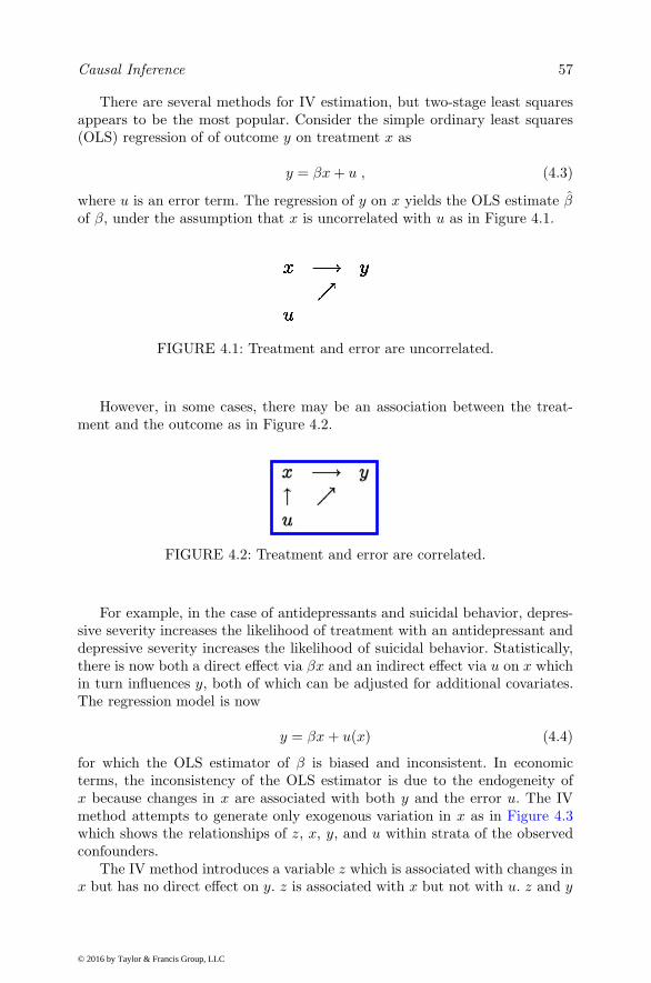
Causal Inference 57
There are several methods for IV estimation, but two-stage least squaresappears to be the most popular. Consider the simple ordinary least squares(OLS) regression of of outcome y on treatment x as
y = βx+ u , (4.3)
where u is an error term. The regression of y on x yields the OLS estimate βof β, under the assumption that x is uncorrelated with u as in Figure 4.1.
FIGURE 4.1: Treatment and error are uncorrelated.
However, in some cases, there may be an association between the treat-ment and the outcome as in Figure 4.2.
FIGURE 4.2: Treatment and error are correlated.
For example, in the case of antidepressants and suicidal behavior, depres-sive severity increases the likelihood of treatment with an antidepressant anddepressive severity increases the likelihood of suicidal behavior. Statistically,there is now both a direct effect via βx and an indirect effect via u on x whichin turn influences y, both of which can be adjusted for additional covariates.The regression model is now
y = βx+ u(x) (4.4)
for which the OLS estimator of β is biased and inconsistent. In economicterms, the inconsistency of the OLS estimator is due to the endogeneity ofx because changes in x are associated with both y and the error u. The IVmethod attempts to generate only exogenous variation in x as in Figure 4.3which shows the relationships of z, x, y, and u within strata of the observedconfounders.
The IV method introduces a variable z which is associated with changes inx but has no direct effect on y. z is associated with x but not with u. z and y
© 2016 by Taylor & Francis Group, LLC

58 Statistical Methods for Drug Safety
FIGURE 4.3: The IV method.
are related, but the only through the indirect path of z being correlated withx which in turn determines y. Note that by the previously stated assumptions,z is excluded from being a predictor of y. Mathematically this leads to
βIV =dy/dz
dx/dz. (4.5)
Consistent estimation of dy/dz can be obtained by the OLS regression of yon z with slope estimate (z′z)−1z′y, and dx/dz by the OLS regression of xon z with slope estimate (z′z)−1z′x, which leads to
βIV =(z′z)−1z′y
(z′z)−1z′x= (z′x)−1z′y. (4.6)
A valid instrument must be a strong predictor of treatment in order to ob-tain consistent/valid inference. An instrument that is not a strong predictorof treatment is referred to as a “weak instrument.” A weak instrument im-plies an unstable estimate of the LATE treatment effects with poor properties(Bound et al. 1995). A common empirical strategy in the presence of a weakinstrument is to augment it with more instruments. Chamberlain and Imbens(2004) proposed random-effects IV estimators for models with one endoge-nous regressor and many instrumental variables. They add a random-effectsstructure to the model describing the relationship between the treatment andthe instruments, considering the variance of the random coefficients as an un-known parameter. They show that their estimators have better finite sampleproperties but asymptotically their estimators have the same properties asother alternatives in the literature (Bound et al. 1995).
In pharmacoepidemiology, a natural instrument is the local area (hospital,county, state) rates of prescriptions of the drug(s) of interest as instrumentsfor the treatment selection process for an individual patient in that local area.Other local area characteristics (such as access to health care, income, urban,rural, · · · ) can be included as instruments as as well. In addition to the typicaleconometric modeling described above, mixed-effects regression models can beused to predict person-level drug utilization as a mixture of local area levelobserved characteristics (i.e., drug prescription rates) and unobserved charac-teristics that are absorbed into the empirical Bayes estimate of the ecologicalunit-specific effect. Note that to our knowledge, this has not previously beenconsidered.
© 2016 by Taylor & Francis Group, LLC

Causal Inference 59
4.4.1 Illustration
Davies et al. (2013) examined the use of physician prescribing preferences forinstruments for antidepressant prescriptions that they issued their patients.They examined whether physician’s previous prescriptions of tricyclic antide-pressants (TCAs) versus SSRIs were valid instruments for the patient-levelantidepressant treatment selections. As outcomes, they examined hospital ad-mission for self harm or death by suicide. The data were collected from 600general practices in the United Kingdom representing 11 million patients.
The assumptions of this IV analysis are that (1) the instrumental variableis associated with the actual prescription, i.e., physician’s preferences for aparticular antidepressant in previous patients are associated with the actualprescription that they issue for the current patient, (2) the instrumental vari-able does not directly affect the outcome i.e., physician’s preferences for aparticular antidepressant are unlikely to affect their patient’s outcomes, and(3) the instrumental variable is not associated with unmeasured confound-ing conditional on measured confounding, i.e., physician’s preferences for aparticular antidepressant may not be associated with potential confoundingfactors (e.g., an individual with a history of suicidal behavior) because pa-tients’ choices of physicians are “quasi-random,” and the preference based onprevious prescriptions is not associated with the next patient’s characteristics.
A total of 897,983 patients prescribed either an SSRI or TCA were identi-fied during the period of January 1995 through June 2010. There were a totalof 6,555 physicians drawn from 612 practices. A total of 484,858 patients weregiven a TCA and 401,877 were given a SSRI. Within 3 months of the firstprescription, there were 608 cases of death by suicide or hospital admissionfor self harm (600 per 100,000). Evidence for confounding with baseline char-acteristics was strong. Those prescribed TCAs were 21.3 percentage pointsmore likely to be over 40 and 22.5 percentage points more likely to have hadmore than five prescriptions of any type in the year before the antidepressantprescription was issued. Overall medical comorbidities were also 8.8 percent-age points higher based on the Charlson index. By contrast, these differenceswere far more muted when based on physician preferences, with differencesof 2.5%, 2.1%, and 1.2% for the difference between TCA and SSRI prescrip-tions for patients older than 40, more than five prescriptions and Charlsonindex (see Table 4.5). The difference in covariate imbalance between actualand prior prescriptions as measured by the Mahalanobis difference was 83%lower for prior relative to actual prescriptions. This indicates that not onlyis physician preference a good instrument in that it is strongly related toactual prescriptions, it is also unrelated to the observed confounding factorsadding support to the validity of the exclusion restriction which also includesunobserved confounders and cannot be empirically proven.
Prior prescriptions were found to be strongly associated with actual pre-scriptions. Physicians who previously prescribed a TCA were 14.9 percentagepoints more likely to prescribe TCAs. Physicians who previously prescribed
© 2016 by Taylor & Francis Group, LLC

60
Statistica
lMeth
odsforDrugSafety
TABLE 4.5: Potential Confounders in Prior Year - TCAs vs. SSRIs
Actual Prescription Prior Prescription Risk Difference per 100Actual Physician’s Prior
Variable TCAs (%) SSRIs (%) TCAs (%) SSRIs (%) Prescription Prescription
N 484,858 401,877 484,692 402,043BMI > 25 kg/m2 57.7 50.7 55.0 54.1 7.08 0.92Hospitalized 0.4 0.3 0.4 0.4 0.10 -0.02> 13 consultations 76.8 58.6 69.2 67.7 18.42 1.50Older than 40 71.9 50.8 63.5 61.0 21.28 2.50> 5 prescriptions 71.1 48.9 62.0 59.9 22.45 2.13Male 37.7 39.6 38.8 38.3 -1.83 0.46Ever smoked 40.9 56.8 47.2 49.3 -16.11 -2.15Depression diagnosis 43.2 62.0 50.6 53.1 -19.01 -2.56Prior self-harm 5.8 5.8 5.9 5.7 -0.04 0.16Prior hypnotic 16.5 12.8 14.6 15.1 3.78 -0.59Prior antipsychotic 2.4 2.0 2.3 2.2 0.42 0.05Charlson index > 0 42.1 33.4 38.7 37.5 8.83 1.18% Treated before 2004 50.8 45.9 50.8 45.8 4.95 5.04Mahalanobis distance(MD) 18.5 16.8 17.9 17.6 1.75 0.29
% Reduction in MD -83%
© 2016 by Taylor &
Francis Group, LLC
Causal Inference 61
paroxetine were 27.7 percentage points more likely to prescribe paroxetine totheir next patient. In terms of the outcome, fewer patients prescribed TCAshad a hospital admission for self-harm or died by suicide than those prescribedSSRIs (risk difference per 100 patients prescribed [RD], -0.11; 95% confidenceinterval -0.14, -0.08. In contrast, the risk difference calculated using one priorprescription as the instrumental variable was attenuated by approximately50% toward the null (RD = -0.04; 95% CI, -0.21, 0.13), although the CI waswider (less precise) and the null hypothesis of no difference between the con-ventional and instrumental variable analyses could not be rejected (Hausmantest: p=0.45).
These findings reveal that at least to some extent, the observed differ-ence between patients treated with TCAs and SSRIs is moderated by patientcharacteristics which form the basis for differential treatment decisions. Theresults of this study also suggest that treatment preference data can be usedas a valid instrument in drug safety studies and that further application inthis area is warranted. Expanding the current analysis by including prefer-ences by hospital and physician or even looking at state and county levelpreferences may lead to the construction of even stronger instruments. Usingrandom-effects models which can incorporate both fixed and random-effectsat multiple levels (e.g., doctor, hospital, state) may also be useful in that wecan capture both observed and unobserved determinants of treatment selec-tion that may be independent of patient-level characteristics and even morehighly related to actual treatment received.
4.5 Differential Effects
In the previous sections, we have described several approaches to minimizingbias in analysis of observational data. Propensity score matching and marginalstructural models can remove bias associated with observed (i.e., measured)confounders, but not unobserved confounders. By contrast, instrumental vari-ables can remove bias due to observed and unobserved confounders; however, agood instrument is not always available. While matching removes differencesin observed confounders by comparing people who are similar, differentialcomparisons compare people who are inherently different in an attempt tomatch them on unmeasured confounders. Here we describe a general method-ology termed “differential effects” by Rosenbaum (2006), which are immune tocertain unobserved biases, called “generic unobserved bias” when they affectdifferent treatments in similar ways. Studying each treatment individuallymight lead to biased conclusions, but when both treatments are examinedsimultaneously in people who took only one or the other, unobserved biascan in many cases be controlled. As such, differential comparisons focus onthose subjects who received only one of the two treatments, either a or b,
© 2016 by Taylor & Francis Group, LLC

62 Statistical Methods for Drug Safety
ignoring those subjects who received neither or both. If the unobserved con-founders affect both treatments equally, then they are termed generic biasesand the differential effect is unbiased. Again, study of either treatment inisolation (relative to no treatment) would exhibit bias and potentially mis-leading conclusions. The basic idea is to stratify the sample on the basis ofobserved confounders and then compare people who took one of two possibletreatments within these strata in the hopes that the unmeasured confoundersequally affect both treatments and are therefore also controlled. The trick isto construct a comparison in which the unobserved confounder does not dif-ferentially affect one treatment alternative over the other. Note that if bothtreatments are known or even suspected to affect the outcome in the sameway, they might both have substantial effects yet zero differential effects. Assuch, it is important to choose the comparators wisely. For example, in look-ing at the relationship between SSRIs and suicidal behavior, we might selectpsychotherapy as a comparator, since they are both used in the treatmentof depression, but one has a potential pharmacologic adverse effect and theother cannot. The caveat; however, is that if antidepressants are used to treatmore severely ill patients than psychotherapy and depressive severity is un-measured, then this can lead to differential bias (a bias that affects the twotreatments differently), a bias for which differential effects are not immune.Here the best we can do is to conduct a sensitivity analysis to determine themagnitude of the unmeasured confounder that would be required to producethe observed data.
Rosenbaum motivates his discussion with the problem of studying injuriesresulting from car accidents. He points out that a problem in studying acci-dents is that car crashes vary in severity and that adequate data on speed,road traction, traffic patterns are rarely available. Seat belts may reduce in-jury, but individuals who use seat belts may be more cautious drivers whichmay in turn reduce the force of the crash and resulting injury. To study thisproblem and fix ideas, Rosenbaum considers an example originally describedby Evans (1986), in which the fatality of two people traveling in the front seatof a car during a crash that produced at least one fatality is considered. Table4.6 presents results of crashes where only one person died and only one personwas wearing a seat belt, stratified into nine categories by age.
In Table 4.6 there were a total of 189+111=300 crashes in which the driverwas unbelted, with odds of 189/111 of 1.7:1 that the unbelted driver died,whereas in the 153+363=516 crashes in which the driver was belted and thepassenger was unbelted, the odds were 363/153 or 2.4:1 that the unbeltedpassenger died. In all of these cases, the unmeasured characteristics were thesame for the driver and passenger because they were in the same car. Thisis called a double pairs design. Risk may be different in the passenger anddriver seats, but both are studied and can be adjusted for. Unbelted driverswith belted passengers may be different than belted drivers with unbeltedpassengers, so there may be differential biases in addition to the generic biasesthat are removed in this design.
© 2016 by Taylor & Francis Group, LLC

Causal Inference 63
TABLE 4.6: Car Accident Mortality Data from Evans (1986)
DriverNot belted Belted
Age Stratum s PassengerDriver, Passenger Belted Not belted
Driver died, passenger survived s=1 75 36Driver survived, passenger died 16 to 24, 16 to 24 22 92Driver died, passenger survived s=2 6 6Driver survived, passenger died (16 to 24, 25 to 34) 4 20Driver died, passenger survived s=3 2 4Driver survived, passenger died (16 to 24, ≥35) 2 17Driver died, passenger survived s=4 12 8Driver survived, passenger died (25 to 34, 16 to 24) 6 15Driver died, passenger survived s=5 22 24Driver survived, passenger died (25 to 34, 25 to 34) 17 30Driver died, passenger survived s=6 3 6Driver survived, passenger died (25 to 34, ≥35) 6 21Driver died, passenger survived s=7 4 8Driver survived, passenger died (≥35, 16 to 24) 0 8Driver died, passenger survived s=8 5 9Driver survived, passenger died (≥35, 25 to 34) 2 16Driver died, passenger survived s=9 60 52Driver survived, passenger died (≥35, ≥35) 52 144Driver died, passenger survived All strata 189 153Driver survived, passenger died combined 111 363
Rosenbaum (2006) formalizes the distinctions between no bias, genericbias, and differential bias in the following way. Assume a finite population ofN units divided into S strata s = 1, . . . , S that are defined by one or morepre-treatment covariates x. The strata are assumed to be homogeneous in theobserved covariates such that xsi = xsj for all s. There are two factors, eachat treatment or control levels, where Zsik = 1 if the ith unit in stratum sreceives treatment k, for k = 1, 2 and Zsik = 0 otherwise. For example in ourexample, Zsi1 = 1 and Zsi2 = 0 indicates that the driver was belted and thepassenger was unbelted. Let πabsi = pr(Zsi1 = a, Zsi2 = b). In a completelyrandomized experiment π11si = π10si = π01si = π11si, for all s and i. The πabsidescribe a units chance of exposure to treatment in the population. For eachunit i in stratum s, there are four potential responses (r11si, r10si, r01si, r00si)only one of which is observed rabsi. For example, rabsi is a pair of binaryvariables indicating whether the driver and passenger would survive underseat belt pattern a, b. The effect of the ith unit in stratum s of treatmentcombination a, b as opposed to treatment combination a′b′ is a comparisonof potential response rabsi to potential response ra′b′si. For example, in crash(s, i), r11si = (1, 1) and r10si = (1, 0) then both the driver and the passengerwould have lived if both had worn a seat belt, whereas only the driver wouldhave survived if only the driver had worn a seat belt.
The differential effect is the comparison of r10si with r01si. Note that theremay be no differential effect, but a substantial overall effect where, for ex-ample, a single unbelted person might be lethal to both occupants such thatr00si = r10si = r01si = (0, 0), but if both wore a seat belt both would havesurvived r11si = (1, 1). Each unit receives only one treatment combination
© 2016 by Taylor & Francis Group, LLC

64 Statistical Methods for Drug Safety
Zsi1 = a and Zsi2 = b and we observed the response rabsi. Letting Rsi be theone observed response of the ith unit in stratum s, then
Rsi = Zsi1Zsi2r11si + Zsi1(1 − Zsi2)r10si
+(1− Zsi1)Zsi2r01si + (1− Zsi1)(1− Zsi2)r00si. (4.7)
In Rosenbaum’s framework, treatment assignment is said to be free of un-observed bias (i.e., it is ignorable) if πabsi does not depend on i. This is ofcourse true under randomization, but may not be for an observational study.In an observational study that is free of unobserved bias, the πabsi may varyacross strata based on observed covariates, but not for characteristics thatwere not measured. In this case, it is reasonable to combine the results acrossthe strata, adjusting for the strata as is done for example using the Mantel-Haenszel method. In essence, this is identical to a stratified randomized ex-periment, where subjects within strata are randomized to the four treatmentpatterns. Of course, in our example, the propensity to wear seat belts dependson other factors beyond age, such as safe-driving practices, and, therefore, thecondition is not satisfied in an observational study.
Unobserved generic bias occurs when there is a relevant unobserved co-variate usi, which we would have liked to have controlled for through strat-ification, but were unable to do so because it was not measured. usi mightreflect the safe driving practices of the driver of the car. Let ρsi = π10si/π01siwhich is the odds of treatment pattern (Zsi1 = 1, Zsi2 = 0) relative to pat-tern (Zsi1 = 0, Zsi2 = 1). In our example, ρsi is the odds of a belted driverand unbelted passenger relative to an unbelted driver and belted passenger.Rosenbaum (2006) defines the case of generic unobserved bias if ρsi varieswith s, but not with i
ρsi =π10siπ01si
= λs (4.8)
for all s and i. The key here is to identify those cases in which there may bebias from unobserved usi but it is only generic unobserved bias, because itonly depends on s. When the condition above is not true, Rosenbaum callsthis “differential unobserved bias.” Here, two units i and i′ within the samestratum s may have different values of ρsi and ρsi′ .
Rosenbaum (2006) provides some general methods to test the assumptionof a generic bias and perform sensitivity analyses to determine the magnitudeof an unobserved confounder that would be required to produce the observeddifference. The general idea may in fact be quite useful in pharmacoepidemi-ologic studies. For example, the rate of suicide attempts can be contrasted forpatients who received either an SSRIs or a TCAs, but not both. In parallel,the rate of suicide attempts can be contrasted for patients who received SS-RIs+psychotherapy or TCAs+psychotherapy but not both, and similarly forother concomitant treatments. If SSRIs are stimulating suicide attempts, weexpect to see an excess of suicide attempts in many if not most comparisons
© 2016 by Taylor & Francis Group, LLC

Causal Inference 65
of SSRIs with other treatments for depression. In contrast, if there is an ex-cess of suicide attempts among people treated with SSRIs vs. no treatment,but not an excess compared to other treatments for depression, then thispattern is compatible with confounding by indication. While use of multipletreatments is a reasonable measure of depressive severity and/or treatmentresistance, there may be additional unobserved biases that remain betweenthe two treatments (e.g., SSRI vs. TCA). These would arise if the clinicalindications for an SSRI differed from those for a TCA, and no doubt that istrue to some extent. For example, suicidal patients are often treated with SS-RIs rather than TCAs because overdose of SSRIs is non-fatal. We can explorethe effects of additional hidden bias through sensitivity analysis (Rosenbaum2006). Suppose we find when comparing TCA versus SSRI, suicide rates seemsimilar. A sensitivity analysis asks how large the differential biases have tobe to alter this conclusion. Similarly if suicide is more common with SSRIs,we can determine how large the differential bias would have to be if, in fact,there is no difference. Thus we can determine the robustness of our findings toremaining unobserved differential bias. As previously noted, comparison be-tween SSRIs and psychotherapy are of particular interest because it controlsfor pharmacologic effects. If suicide and/or suicide attempt rates are similar,it rules out the possibility of a pharmacologic adverse effect.
Additional covariates can be added to this approach using the method ofdifferential propensity scores (Rosenbaum 2006). The differential propensityscore is the usual propensity score (Rosenbaum 2002) confined to the individ-uals who took one of the treatments but not both. In this case, the differentialpropensity score equals the propensity score that would have been calculatedif the unobserved covariate had been measured. Available covariates include,age, sex, race, marital status, diagnosis, comorbidity, previous attempts, pre-vious history of depression, antidepressant treatment history. Thus we can (1)remove bias due to measured characteristics, (2) remove generic bias due tocommon effects of depressed people seeking treatment, and (3) assess mag-nitude of differential bias (e.g., due to differences in people who seek antide-pressant treatment versus those who seek psychotherapy) necessary to changeconclusions.
Returning to the example on car accidents, Rosenbaum (2006) notes theincreased relative risk of 1.4 of an unbelted passenger death relative to an un-belted driver, when only one was unbelted and the accident resulted in a singledeath. Under the assumption of generic unobserved bias, the null hypothesisis the distribution of S = 9 independent hypergeometric distributions, whichhe tests using the Mantel Haenszel test (Mantel and Haenszel 1959). Underthe null hypothesis and if there were only generic unobserved biases, we wouldexpect 128.7 unbelted driver fatalities rather than the 189 that were observed(p<0.0001). Rosenbaum concludes that “Wearing seat belts may be associatedwith unmeasured safe-driving practices, but if these biases are generic, affect-ing passenger and driver the same way, then there is no doubt that seat beltssave lives.” He then conducts a sensitivity analysis to determine the magni-
© 2016 by Taylor & Francis Group, LLC

66 Statistical Methods for Drug Safety
tude of the unobserved differential bias that would be required to change thisconclusion. Specifically, we need to determine if there was a covariate usi thatwas not measured, how large of an imbalance would be required between abelted driver and unbelted passenger (Zsj1, Zsj2 = (1, 0)) versus an unbelteddriver and belted passenger (Zsj1, Zsj2 = (0, 1)) in order to produce the overallobserved difference which leads to the conclusion of a protective effect of seat-belts. The answer can be found by convolution of S extended hypergeometricdistributions as described by Rosenbaum (1995). Let Λ be the multiplier ofthe increased likelihood of (Zsj1, Zsj2 = (1, 0)) versus (Zsj1, Zsj2 = (0, 1)).If Λ = 1 then there is no differential bias. For Λ = 2, p=0.0000071; Λ = 3,p=0.043; and Λ = 4, p=0.55. As such, it would require a differential bias ofΛ = 4 or an unmeasured confounder which made a belted driver and unbeltedpassenger 4 times more likely than an unbelted driver and belted passengerto have produced the appearance of a protective effect of wearing seat-belts.
We can extract some additional information from this example, using themethods to be described in Chapter 6 on full-likelihood random-effects meta-analysis. In meta-analysis, the strata represent studies; however, we can usethose same methods to examine differential effects, where the strata representcommon observed covariate values. The advantage is that we cannot onlyestimate the overall protective effect of seat-belts and the differential effectbetween passengers and drivers as fixed-effects, but we can also estimate thecorresponding random-effects which describe variability across the strata inthe overall likelihood of death and variability in the differential effect across thecovariate strata which represents a measure of the magnitude of the effect ofunmeasured covariates which contribute to both the overall and the differentialeffects (see section 6.3). To do this, we rearrange the data in terms of thenumber of fatalities when the driver was belted and the number of fatalitieswhen the passenger was belted, and the corresponding total sample sizes (seeTable 4.7). Given the design, N minus the number of belted driver fatalities isthe number of driver fatalities when the driver was unbelted. So for examplein age stratum 1, there were 22 driver fatalities when the driver was beltedand 97-22=75 driver fatalities when the driver was unbelted (see Table 4.6).
Applying these methods to the current problem reveals that based onBayesian Information Criterion (BIC, Schwarz (1978)), the best fitting modelwas a random intercept model. This finding suggests that the strata differin the overall incidence of fatalities, but the difference between passengerand driver fatality was not significant. Overall, there is a 51% reduction infatalities when a seat-belt was worn (OR=0.49, 95% CI 0.40, 0.60, p<0.0001).The estimated fatality rate among passengers was reduced by 39% (OR=0.61,95% CI=0.45, 0.81) when belted and among drivers by 57% (OR=0.43, 95%CI=0.24, 0.78). The difference between fatality rates between belted driversand passengers was 29% (OR=0.71, 95% CI=0.52, 0.95, p=.03). There doesappear to be a differential effect in terms of the rate of fatalities between belteddrivers and passengers. However, the variability in this difference across thestrata due to unmeasured variables was not significant. The estimated random
© 2016 by Taylor & Francis Group, LLC

Causal Inference 67
TABLE 4.7: Reformatted Car Accident Mortality Data
Age Stratum s Passenger Belted Driver Belted# Died N # Died N
16 to 24, 16 to 24 22 97 36 12816 to 24, 25 to 34 4 10 6 2616 to 24, ≥35 2 4 4 2125 to 34, 16 to 24 6 18 8 2325 to 34, 25 to 34 17 39 24 5425 to 34, ≥35 6 9 6 27≥35, 16 to 24 0 4 8 16≥35, 25 to 34 2 7 9 25≥35, ≥35 52 112 52 196
intercept variance was 0.032, so even at two standard deviation units abovethe mean effect for wearing a seat-belt, there is still a reduction in fatality of
100(1 − e−.72−2√0.032) = 30%. A forest plot of the odds ratios of deaths for
belted drivers to passengers is displayed in Figure 4.4. The overall odds ratiofor the difference between drivers and passengers in Figure 4.4 is based on theDersimonian and Laird estimator which is close to but not identical to thefull-likelihood estimate.
FIGURE 4.4: Forest plot: Odds ratio of death (belted driver/passenger).
© 2016 by Taylor & Francis Group, LLC

5
Analysis of Spontaneous Reports
“The person who takes medicine must recover twice, once from the diseaseand once from the medicine.”
(William Osler, M.D.)
5.1 Introduction
An important source of signals in drug safety has been, and will continue tobe, the observations of clinicians who report adverse drug reactions (ADRs).Automated methods are routinely used to mine databases of spontaneous re-ports to detect drug safety signals. Data mining is the discovery of interesting,unexpected, or valuable structures in large datasets. Modern data mining com-bines statistics with ideas, tools, and methods from computer science, machinelearning, database technology, and other classical data analytical technologies(Hand 1998). In the context of signal detection in the pharmaceutical sectorthe interest is to detect local structures or patterns and to determine if they arereal or chance occurrences. Patterns are usually embedded in a mass of irrele-vant data. Interesting patterns can arise due to artifacts of the data recordingprocess or genuine discoveries about underlying mechanism. Therefore, decid-ing whether a pattern is ‘interesting’ should be done using knowledge fromexperts to understand exactly what is being described. Increasing number oflarge databases maintained by various regulatory agencies and pharmaceuticalcompanies around the world provide opportunity for some novel explorationin post marketing drug safety.
The World Health Organization (WHO) database is the largest interna-tional database of case reports of spontaneous reporting of suspected ADRs.To improve the detection of previously unknown serious ADRs and knowledgeabout regulatory action taken in response to ADR reports, FDA introducedthe MedWatch program in June 1993. Each of the databases, held by Upp-sala Monitoring Center (UMC) and FDA AERS database, now contains overtwo million reports of ADRs. Similar databases exist in various Europeanand other countries including India, China, Taiwan, and Iran. These sponta-neous reporting system (SRS) databases are overwhelming and complex for
69
© 2016 by Taylor & Francis Group, LLC

70 Statistical Methods for Drug Safety
safety reviewers using only traditional statistical methods. The data-miningalgorithms (DMAs) have been developed to screen large SRS databases forstatistical dependencies between drugs and AEs. Each of the signal detectionmethods has its distinguishing features and no single method is suitable forall circumstances.
Several statistical methods are available for post marketing safetysurveillance. Hauben and Zhou (2003) grouped them into two categories:denominator-dependent methods and numerator-based methods. Spontaneousreporting centers and drug safety research units routinely use various numer-ator based methods such as empirical Bayes screening (EBS) (a variant ofwhich is used by the FDA), Bayesian Confidence Propagation Neural Net-work (BCPNN used by the WHO), reporting odds ratios (RORs), incidencerate ratio (IRR), and proportional reporting ratio (PRR). Denominator basedmethods include cumulative sum techniques, time scan method and Poissonmethods.
5.2 Proportional Reporting Ratio
The Proportional Reporting Ratio (PRR) is the simplest method available forsignal detection. Its computational form is similar to the well-known relativerisk calculation for 2× 2 tables in epidemiology. However, studies have shownthat it can be as powerful as other sophisticated methods available whenapplied to events that are not rare. Let us assume that there are a total of Nreports in the database of which n reports involve a particular drug (or druggroup) of interest, E reports involve interesting events, and x reports involveboth the drugs and events of interest. These counts are summarized in thefollowing 2× 2 contingency table.
TABLE 5.1: Contingency Table of a Drug-Adverse Event Pair.
Does the event involve adrug(s) of interest?
yes no totalEvents x E − x ENon-events n− x N−n−E+x N − ETotal n N − n N
The PRR of events E is defined as follow (Evans et al. 2001, Bate and Evans2009).
PRR =xn
E−xN−n
(5.1)
© 2016 by Taylor & Francis Group, LLC

Analysis of Spontaneous Reports 71
The standard error of the ln(PRR) is
SE[ln(PRR)] =
√1
x+
1
n− x− 1
E− 1
N − E. (5.2)
The 95% confidence interval for ln(PRR) is then estimated as ln(PRR) ±1.96 × SE[ln(PRR)] and, taking the exponential, the following result is ob-tained for the 95% confidence interval for PRR.
95% CI for PRR =
(PRR
e(1.96×SE[ln(PRR)]), PRR× e(1.96×SE[ln(PRR)])
)(5.3)
A lower 95% CI of a PRR higher than 1.0 indicate a disproportionatereporting of events involving a particular drug. One of the limitations of PRRis that the large number of reports of particular kind effectively inflate thedenominator for that drug reducing the magnitude of PRR for other signalswith that drug. The PRR method generates a large volume of potential signalswhen applied to large databases. To counter this problem remedial measuressuch as triage criteria can be applied to reduce the volume of signals that areevaluated.
Example
Roxicodone is indicated for the management of moderate to severe pain wherethe use of an opioid analgesic is appropriate. As with other opioids in clinicaluse, serious adverse reactions such as cardiac arrest may be associated withroxicodone therapy. In the first quarter of 2010, the FDA received 213488reports of serious drug-ADRs combinations. Among those 6360 reported car-diac arrest, 100 involved roxicodone and 31 reported both roxicodone andcardiac arrest. The relevant frequency counts are presented in Table 5.2. Thecalculation of the PRR is as follows.
TABLE 5.2: Example of PRR Calculation - Roxicodone and Cardiac Arrest
Does the event involveRoxicodone?
yes no totalCardiac arrest 31 2988 3019All other events 69 210398 210469Total 100 213388 213488
PRR =31
100
/2988
213388= 22.13
and
© 2016 by Taylor & Francis Group, LLC

72 Statistical Methods for Drug Safety
Lower 95% CI limit of ln[PRR] = 2.80.
There is no gold standard on the thresholds that should be adopted for signaldetection. The lower limit of 95% CI of ln[PRR] > 0 is one reasonable choiceof threshold. Using this threshold, the lower limit of 95% CI for the logarithmis positive, the signal is generated on the basis of PRR. This does not implyany kind of causal relationship between roxicodone and the occurrence of theadverse event of cardiac arrest. Further analysis by pharmacovigilance expertsmust now determine the validity of this signal. The initial decision on whethera drug-event pair should be further investigated depends on thresholds appliedto the estimates of the PRR and other statistics.
5.2.1 Discussion
PRR is a statistical aid to signal generation from spontaneous reporting sys-tem databases. PRR indicates differential reporting of possible reactions fora given drug compared to all other drugs in the database. It is crucial toremember that a signal identified based on the PRR is indicative of the dis-proportionate reporting of events and not their occurrence (Moore et al. 2003,2005). The validity of the PRR rests on equal reporting rates for the differentdrugs. However, all adverse drug reactions are not reported in spontaneous re-port databases and the reporting rate for a particular drug is highly dependenton the public perception of the safety of the drug (notoriety bias) and the timesince its approval (Weber effect) (Weber 1984). Consequently, PRR may varysignificantly over different time frame of evaluations. Furthermore, PRR canbe highly unreliable due to extreme sampling variability when observed fre-quencies of drug-ADR combination are small, resulting in high false-positiverates. Remedial measures such as considering only drug-ADR combinationswith 3 or more cases and raising the PRR threshold to 2 have been suggestedto reduce the false-positive signals (Evans et al. 2001). Alternative Bayesianmethods (covered in the next sections) have shown to be less sensitive to thesampling variation.
5.3 Bayesian Confidence Propagation Neural Network(BCPNN)
Bayesian Confidence Propagation Neural Network (Bate et al. 1998) can han-dle large data sets, is robust in handling missing data, and may be used withcomplex variables. It allows finding and quantifying relationships betweendrugs and AEs that differ significantly from the background of interrelation-ships in the database. For an individual report in the database, a prior proba-
© 2016 by Taylor & Francis Group, LLC

Analysis of Spontaneous Reports 73
bility that a specific ADR is listed in it is denoted by P(A), a prior probabilitythat a specific drug is listed is denoted by P(D) and a prior probability that thedrug - AE pair are present together in it is denoted by P(A,D). The strengthof the association between an AE and a drug is measured by the informationcomponent (IC) defined as (Bate et al. 1998):
IC = log2P (A,D)
P (A)P (D). (5.4)
As new quarterly data become available, the corresponding posterior prob-abilities are calculated and the updated IC is used to generate new signals.A convenient choice of the form of prior is the beta distribution for all threedensities. In the absence of prior information an a priori assumption is madeof equal probability distributions for P(A) and P(D). Let α1 and α0 be theparameters governing the beta distributions of P(A) and P(D); γ11 and γ bethe parameters of the beta distribution of p(A,D); ci, cj , and cij be the re-port counts of ith AE, jth drug and combination of ith drug with the jthAE respectively; and C be the total number of reports in the database. Thecorresponding expected value of each distribution is the estimator of P(A),P(D), and P(A,D). The normal approximation of variance of IC [V(IC)] is(Bate et al. 1998, Orre et al. 2000):
V (IC) ≈(
1
log2
)2 [C − cij + γ − γ11
(cij + γ11)(1 + C + γ)+
C − ci + α− α1
(ci + α1)(1 + C + α)
+C − cj + α− α1
(cj + α1)(1 + C + α)
], (5.5)
where α = α1+α0. As more data become available, the estimate of IC becomesmore accurate and the confidence interval of IC becomes narrower. An IC withlower 95% CI> 0 that increases with sequential time scans may be used as acriterion for signal detection.
Example
Rosiglitazone is used to treat type 2 diabetes by making patients more sensi-tive to their own insulin. Since its approval by regulators in the United Statesand Europe, the use of rosiglitazone has been suspected of increasing the riskof heart attack. Recently, its use has been restricted only to people who are al-ready taking rosiglitazone and people whose blood sugar cannot be controlledby other medications. The FDA AERS database contains thousands of reportsof rosiglitazone along with variety of adverse events. Table 5.3 gives the resultof the FDA AERS database search for each quarter from 1999 to 2010.
Rosiglitazone was approved by regulators in the United States and Europein May, 1999. Figure 5.1 shows the time scan obtained when a run was done ofrosiglitazone (regardless of its specific role) and cardiac arrest from the third
© 2016 by Taylor & Francis Group, LLC

74 Statistical Methods for Drug Safety
TABLE 5.3: Reports of Cardiac Arrest for Rosiglitazone in the FDA AERS.
year qtr cij drug ae C P(A) P(B) P(A,B) IC1999 3 1 14 184 9594 0.00156 0.01928 0.00021 2.7894941999 4 5 44 195 8216 0.00266 0.02058 0.00029 2.412672000 1 15 93 264 9295 0.00411 0.02214 0.00053 2.5475962000 2 19 115 312 9301 0.00539 0.02378 0.00076 2.5659512000 3 19 95 323 10037 0.0062 0.02504 0.00093 2.5863632000 4 19 116 266 9480 0.00687 0.02579 0.00107 2.5887062001 1 20 149 243 10285 0.00753 0.02609 0.00117 2.5758682001 2 20 137 244 10016 0.00809 0.02622 0.00126 2.5665492001 3 24 182 233 10489 0.00867 0.0262 0.00134 2.5556252001 4 48 218 275 10979 0.00928 0.02616 0.00145 2.5787352002 1 21 123 325 10567 0.00973 0.02621 0.00154 2.5909962002 2 36 148 323 13961 0.01005 0.02619 0.00161 2.6168642002 3 14 124 277 14290 0.01026 0.02606 0.00166 2.6343092002 4 14 126 295 14405 0.01039 0.02589 0.00168 2.6456962003 1 15 106 228 13343 0.01046 0.02567 0.0017 2.6580482003 2 48 292 324 14454 0.01061 0.02547 0.00172 2.6697482003 3 34 190 383 18769 0.01073 0.02526 0.00174 2.6838322003 4 11 131 357 18337 0.01078 0.02504 0.00174 2.6934022004 1 22 147 400 15049 0.01081 0.02487 0.00175 2.6995532004 2 22 136 367 15421 0.01082 0.02474 0.00174 2.7048952004 3 39 160 370 18484 0.01081 0.0246 0.00175 2.7155092004 4 20 146 495 19729 0.01078 0.02448 0.00174 2.7228392005 1 22 155 429 18188 0.01074 0.02439 0.00174 2.7283132005 2 15 166 438 18659 0.0107 0.0243 0.00173 2.7302392005 3 41 185 624 21938 0.01066 0.02426 0.00172 2.7328632005 4 17 206 565 20912 0.01061 0.02424 0.00171 2.7309212006 1 35 219 812 21412 0.01058 0.02428 0.0017 2.7253872006 2 39 221 1065 21327 0.01054 0.02443 0.00169 2.714782006 3 12 127 249 12133 0.01052 0.02455 0.00168 2.7050212006 4 12 111 293 12918 0.01049 0.02464 0.00167 2.696092007 1 12 105 255 14761 0.01046 0.02471 0.00167 2.6887672007 2 18 192 242 12489 0.01044 0.02475 0.00166 2.6813642007 3 26 204 327 15051 0.01043 0.02479 0.00165 2.6744962007 4 17 127 295 13266 0.01042 0.02481 0.00164 2.6683732008 1 5 62 239 16506 0.0104 0.02481 0.00163 2.6636662008 2 8 81 340 15931 0.01037 0.02481 0.00162 2.6593682008 3 141 406 461 17770 0.01037 0.02481 0.00163 2.662862008 4 102 264 403 16430 0.01037 0.0248 0.00164 2.6714382009 1 241 665 514 18487 0.01043 0.02481 0.00167 2.690082009 2 197 719 581 18246 0.01052 0.02482 0.00171 2.7119432009 3 352 1210 811 19815 0.01069 0.02486 0.00178 2.7400842009 4 322 1144 795 21649 0.01092 0.02492 0.00186 2.7710542010 1 240 815 780 23376 0.01117 0.02498 0.00195 2.8019322010 2 540 1736 1073 21988 0.01151 0.02508 0.00206 2.8376332010 3 1462 4370 2174 30847 0.0121 0.02527 0.00227 2.89117
quarter of 1999 to the third quarter of 2010. The lower 95% confidence limitis higher than 0 from the beginning of the scan indicating a possible signalsoon after the marketing of the drug. The signal continued to strengthenuntil 2005 as more data became available and the estimate of IC becamemore precise. There is a slight decline in IC from the end of 2005 to 2007.Interestingly, in September 2005, GSK concluded its own meta-analysis ofdata concerning rosiglitazone’s effect on diabetics and informed the FDA thatthe data “may” signal an increased (32%) risk for heart attacks in diabetics.One possible explanation of the decline in IC in that time period could bethe cautious use of the drug by the community of endocrinologists due toa mounting evidence regarding the increased cardiovascular risks associatedwith rosiglitazone. The signal gains strength once again from 2008. A meta-analysis in May 2007 reported that the use of rosiglitazone was associated with
© 2016 by Taylor & Francis Group, LLC

Analysis of Spontaneous Reports 75
2.4
2.5
2.6
2.7
2.8
2.9
Time (year)
IC
99 00 01 02 03 04 05 06 07 08 09 10
FIGURE 5.1: IC and 95% CI for Rosiglitazone and cardiac arrest.
a significantly increased risk of heart attack. In 2007, four independent, peer-reviewed medical research studies were published showing that rosiglitazoneincreased diabetics’ pre-existing cardiovascular risks. These data, coupled withthe FDA’s own study led to a black box warning (FDA’s most serious drugsafety warning) on rosiglitazone’s product label to inform consumers of suchrisks beginning on November 14, 2007. Consequently, the sales of avandiadeclined and the reporting of cardiac events has increased in FDA’s AERSfurther strengthening of signal from 2008.
Example
Digoxin is commonly indicated for atrial fibrillation and atrial flutter withrapid ventricular response. Due to the narrow margin between effectiveness
© 2016 by Taylor & Francis Group, LLC

76 Statistical Methods for Drug Safety
and toxicity, it is suspected of several severe adverse effects including severeallergic reaction. The retrospective time scan of Digoxin and rash is shown inFigure 5.2 and the details of IC computation is given in Table 5.4 for eachquarter from 1998 to 2010.
TABLE 5.4: Reports of Rash for Digoxin in the FDA AERS.
year qtr cij drug ae C IC P(A) P(B) P(A,B)1998 1 7 270 223 8703 0.1976 0.03113 0.02573 0.000921998 2 6 242 214 7729 0.0283 0.03115 0.02630 0.000841998 3 4 197 180 7628 -0.0286 0.03033 0.02598 0.000771998 4 4 201 212 8433 -0.0705 0.02940 0.02579 0.000721999 1 7 288 248 9666 -0.0893 0.02907 0.02571 0.000701999 2 7 316 278 9495 -0.1165 0.02914 0.02586 0.000701999 3 7 281 245 9594 -0.1275 0.02918 0.02593 0.000691999 4 5 269 209 8216 -0.1425 0.02930 0.02596 0.000692000 1 3 237 230 9295 -0.1643 0.02929 0.02594 0.000682000 2 1 246 227 9301 -0.1984 0.02922 0.02590 0.000662000 3 3 239 190 10037 -0.2248 0.02908 0.02575 0.000642000 4 5 250 172 9480 -0.2396 0.02894 0.02554 0.000632001 1 2 234 146 10285 -0.2513 0.02876 0.02525 0.000612001 2 2 258 168 10016 -0.2643 0.02860 0.02494 0.000592001 3 5 245 154 10489 -0.2688 0.02843 0.02460 0.000582001 4 3 234 245 10979 -0.2751 0.02823 0.02433 0.000572002 1 6 241 343 10567 -0.2819 0.02804 0.02418 0.000562002 2 6 285 387 13961 -0.2889 0.02782 0.02409 0.000552002 3 3 293 340 14290 -0.2988 0.02758 0.02402 0.000542002 4 6 258 362 14405 -0.3061 0.02732 0.02397 0.000532003 1 8 252 346 13343 -0.3089 0.02706 0.02395 0.000522003 2 3 355 449 14454 -0.3184 0.02683 0.02397 0.000522003 3 6 312 490 18769 -0.3273 0.02657 0.02400 0.000512003 4 12 311 442 18337 -0.3287 0.02630 0.02403 0.000502004 1 10 276 549 15049 -0.3292 0.02604 0.02411 0.000502004 2 5 246 457 15421 -0.3307 0.02577 0.02420 0.000502004 3 5 272 531 18484 -0.3334 0.02549 0.02430 0.000492004 4 5 292 559 19729 -0.3371 0.02521 0.02441 0.000492005 1 9 272 674 18188 -0.3408 0.02493 0.02454 0.000482005 2 14 322 656 18659 -0.3414 0.02466 0.02470 0.000482005 3 5 246 665 21938 -0.3429 0.02438 0.02486 0.000482005 4 6 296 639 20912 -0.3452 0.02409 0.02502 0.000472006 1 5 309 802 21412 -0.3500 0.02382 0.02520 0.000472006 2 5 239 695 21327 -0.3553 0.02354 0.02538 0.000472006 3 9 163 412 12133 -0.3580 0.02328 0.02555 0.000462006 4 6 170 365 12918 -0.3594 0.02303 0.02570 0.000462007 1 2 159 423 14761 -0.3613 0.02279 0.02584 0.000462007 2 6 147 402 12489 -0.3622 0.02257 0.02597 0.000462007 3 1 153 370 15051 -0.3634 0.02235 0.02609 0.000452007 4 3 118 317 13266 -0.3641 0.02213 0.02618 0.000452008 1 5 128 387 16506 -0.3636 0.02192 0.02627 0.000452008 2 4 1203 463 15931 -0.3695 0.02181 0.02635 0.000442008 3 6 855 472 17770 -0.3782 0.02175 0.02642 0.000442008 4 6 271 391 16430 -0.3856 0.02169 0.02648 0.000442009 1 5 223 419 18487 -0.3919 0.02162 0.02653 0.000442009 2 8 479 434 18246 -0.3979 0.02156 0.02657 0.000432009 3 6 539 388 19815 -0.4039 0.02152 0.02660 0.000432009 4 6 352 471 21649 -0.4093 0.02147 0.02661 0.000432010 1 4 394 468 23376 -0.4145 0.02142 0.02662 0.000432010 2 6 423 458 21988 -0.4194 0.02138 0.02662 0.000432010 3 9 399 587 30847 -0.4229 0.02132 0.02660 0.00042
The time scan starts with positive IC with lower 95% confidence well below0. The IC decreases throughout the time scan towards a distinct negativevalue. As the number of reports of the drug and AE increase, the associated95% confidence intervals diminish. The figure demonstrates the diminishingpossibility of a causal relationship between Digoxin and rash. This definite
© 2016 by Taylor & Francis Group, LLC

Analysis of Spontaneous Reports 77
−0.
4−0.
3−0.
2−0.1
0.0
0.1
0.2
Time (year)
IC
98 99 00 01 02 03 04 05 06 07 08 09 10
FIGURE 5.2: IC and 95% confidence for digoxin and rash over a period oftime.
negative IC represents a situation where joint reporting of Digoxin and rash arenot frequent relative to the expected frequency under independence. Thereforeassociation between Digoxin and rash would not be signaled based on ICcriteria.
5.4 Empirical Bayes Screening
Empirical Bayes screening was originally developed by William DuMouchel(DuMouchel 1999) and applied to FDA databases of spontaneous reports as
© 2016 by Taylor & Francis Group, LLC

78 Statistical Methods for Drug Safety
a tool to detect signals of AEs that were gender specific. This method com-putes the baseline (expected) frequency under row and column independenceassumption for multiple two-way tables. As Hauben and Zhou (2003) noted,under such assumption the proportional representation of an AE for a particu-lar drug, and the proportional representation of that AE in the entire databaseshould be the same. Therefore, the higher is the magnitude of discrepancy be-tween the two, stronger is the signal for the drug-event combination.
Following DuMouchel (1999), let each observed count Nij of drug-eventcombinations in the database be a draw from a Poisson distribution withvarying unknown means µij . However, as a measure of disproportionality, the
interest is not on µ directly but on the ratio λij =µ(ij)
Eij. Furthermore, instead
of estimating each individual λij , they are assumed to follow a common priordistribution. DuMouchel (1999) suggested the following mixture of two gammadistributions as a candidate for such prior distribution.
π(λ;α1, β1, α2, β2, P ) = P g(λ;α1, β1) + (1− P )g(λ;α2, β2), (5.6)
whereg(λ;α, β) = βαλα−1e−βλ/Γ(α).
The gamma distribution is an easy choice because it is the conjugate distri-bution of the Poisson. Thus the posterior distribution of each λ is again thegamma distribution of (5.6) but with updated parameters as follows:
λ|N = n ∼ π(λ;α1 + n, β1 + E,α2 + n, β2 + E,Qn) (5.7)
where E =Ni.N.j
N is the expectation of Nij under row and column indepen-dence for row total Ni. and column total N.j. The Qn is a posterior probabilitythat λ came from first component of the mixture, given N = n. It has thefollowing expression.
Qn =P f(n, α1, β1, E)
Pr(N = n)(5.8)
In expression (5.8), Pr(N = n) is the marginal distribution of each Nij for theknown θ = (α1, β1, α2, β2, P ) and E. It is a mixture of two negative-binomialdistributions, f(α, β,E). The f(α, β,E) and P (N = n) have the followingexpressions
f(α, β,E) = (1 + β/E)−n(1 + E/β)−α × Γ(α+ n)
Γ(α)n!(5.9)
P (N = n) = P f(n, α1, β1, E) + (1− P )f(n;α2, β2, E). (5.10)
The following empirical Bayes measure (EBlog2) is used to rank the “inter-estingness” of cell counts.
EBlog2ij = E[log2λij |Nij ] =E[log(λij)|Nij ]
log(2), (5.11)
© 2016 by Taylor & Francis Group, LLC

Analysis of Spontaneous Reports 79
where
E[log(λij)|Nij = n] = Qn[Ψ(α1 + n)− log(β1 + Eij)]
+ (1−Qn)[Ψ(α2 + n)− log(β2 + Eij)],
and Ψ(x) is the derivative of log[Γ(x)], also known as the digamma func-tion. Alternatively, EBGM ij = eE[log(λij)|Nij=n] has been suggested whichhas a direct interpretation as the geometric mean of a “true” reporting rate(DuMouchel 1999). Additionally, the lower 5th percentile of the posterior dis-tribution of λ (EB05) can be used for ranking the cell counts and EB05 > 2has been recommended as a cut-off for signal detection (Szarfman et al. 2002).
The estimate of θ is required to evaluate (5.8) and (5.11). The estimate isobtained by considering the marginal distribution of each Nij which is givenin (5.10). The likelihood function is the product of density functions of eachNij expressed as the function of θ:
L(θ) =∏
ij
P f(Nij , α1, β1, Eij) + (1 − P )f(Nij ;α2, β2, Eij) . (5.12)
The estimate of θ is the maximum likelihood estimator obtained from max-imization of L(θ). The maximization involves an iterative search in five-dimensional space; therefore, it must be handled carefully and the startingvalues of the parameters must be chosen appropriately so that the algorithmconverges in a reasonable number of iterations. The authors of the methodhave recommended θ = (α1 = 0.2, β1 = 0.1, α2 = 2, β2 = 4, P = 1/3) for thestarting values.
Example
The AERS database for the first quarter of year 2010 contains adverse eventreports of 114681 cases received by the FDA from 01-OCT-2009 to 31-DEC-2009. Each case involves multiple drugs and adverse events, which means thata number of reported drug-ADR combinations is much larger than 114681.After applying a set of pre-defined exclusion criteria, the number of drug-AEcombinations reports reduced to 213488. We chose this time period arbitrarilyand performed an unstratified analysis for the purpose of illustration. For theproper analysis, one must choose all data available for the time interval of in-terest and perform an appropriate stratified analysis. To initiate computation,the initial values of the hyperparameters are set at α1 = 0.2, β1 = 0.06, α2 =1.4, β2 = 1.8, and P = 0.1, and the resulting estimates of the hyperparame-ters are: α1 = 0.009, β1 = 0.011, α2 = 2.000, β2 = 1.235, and P = 0.733. Wecalculate EBlog2 to rank each drug-ADR in the database. The top 20 andbottom 20 drug-ADR combinations and their corresponding EBlog2 valuesare listed in Table 5.5. The table shows that the ranking based on EBlog2 andRR = n11/E are not exactly the same. Although RR is easily interpretable,it suffers from the extreme sampling variation when baseline and observed
© 2016 by Taylor & Francis Group, LLC

80 Statistical Methods for Drug Safety
frequencies are small. The EBGM estimates are interpreted as the shrinkageestimator of “true” RR and are not as susceptible to sampling variability asRR.
5.5 Multi-item Gamma Poisson Shrinker
The Gamma Poisson Shrinker presented in the Section 5.4 ranks the drug-AEpair by the EBGM. However, it is not capable of finding higher order asso-ciations which is usually the case when two or more drugs in combinationproduce severe adverse events. The most recent example of such interactionis the case of percocet, a drug that is used for controlling breakthrough pain.Another drug, acetaminophen, in general is a very safe medication, but un-fortunately, high doses of acetaminophen lead to liver damage. It is also acommon ingredient in many commonly used over-the-counter drugs includ-ing cough medication. Percocet combines acetaminophen with a short actingnarcotic. The FDA advisory panel has recently recommended a ban on per-cocet because patients who take percocet for long periods of time often needhigher doses to achieve the same pain reduction effect. As a consequence, theyare getting more acetaminophen, raising the possibility of serious damage totheir livers, specially if they are also using one of the OTC drugs containingacetaminophen.
Multi-item Gamma Poisson shrinker (MGPS) (DuMouchel and Pregibon2001) is a natural extension of GPS for detecting such multi-drug-AE asso-ciations. It uses the same estimation technique with some additional steps.The term item in MGPS includes both the drugs and the AEs. Let Nj be thenumber of reports that include only one item (e.g., drug j); let Njk be thenumber of reports that include both item j and item k and so forth, where1 < j < k < J , and J is the total number of items under consideration. UsingDuMouchel and Pregibon (2001) notation, we define the following quantities:
Pj =NjN, proportion of reports involving item j
Pjk =NjkN
, proportion of reports involving item j and item k
P1···J =N1···KN
, proportion of reports involving items 1, · · · , JEj = NPj , baseline frequency of reports involving item j
Ejk = NPjPk, baseline of reports involving item j and item k
E1···J = NP1 · PK , baseline of reports involving items 1, · · · , J.
The equations (5.6) to (5.12) with corresponding values of N1···k and E1···k
© 2016 by Taylor & Francis Group, LLC

Analysis
ofSpontaneousRepo
rts81
TABLE 5.5: The Top 20 and Bottom 20 Drug-ADR.
drug event count expectedcount
EBlog2 EBGM n11/E log2(n11/E)
drugmargin
eventmargin
DRN 6583 AEN 1035 27 0.0095 10.3616 1315.673 2839.496 11.471 35 58DRN 1650 AEN 4731 14 0.0012 10.1586 1143.013 11860.444 13.534 18 14DRN 6856 AEN 1492 22 0.0088 10.1141 1108.257 2508.940 11.293 48 39DRN 1721 AEN 2223 13 0.0013 10.0358 1049.708 10166.095 13.311 21 13DRN 3843 AEN 1035 15 0.0041 9.9456 986.115 3680.828 11.846 15 58DRN 58 AEN 2499 19 0.0137 9.5705 760.320 1386.286 10.437 133 22DRN 6449 AEN 153 9 0.0034 9.2469 607.550 2668.600 11.382 80 9DRN 4794 AEN 4881 21 0.0239 9.2138 593.767 878.551 9.779 243 21DRN 4800 AEN 35 11 0.0077 9.1599 572.008 1421.530 10.473 59 28DRN 5802 AEN 3237 7 0.0010 9.1305 560.484 7116.267 12.797 15 14DRN 6449 AEN 402 8 0.0030 9.1058 550.971 2668.600 11.382 80 8DRN 6449 AEN 570 8 0.0030 9.1058 550.971 2668.600 11.382 80 8DRN 6449 AEN 576 8 0.0030 9.1058 550.971 2668.600 11.382 80 8DRN 6931 AEN 4148 19 0.0233 9.0904 545.116 814.840 9.670 262 19DRN 3774 AEN 2409 8 0.0040 8.9989 511.613 1976.741 10.949 54 16DRN 170 AEN 5061 10 0.0081 8.9910 508.804 1241.209 10.278 172 10DRN 6931 AEN 797 15 0.0184 8.9645 499.559 814.840 9.670 262 15DRN 4794 AEN 1362 17 0.0228 8.9492 494.274 746.769 9.545 243 20DRN 6449 AEN 3207 7 0.0026 8.9402 491.210 2668.600 11.382 80 7DRN 4762 AEN 35 7 0.0028 8.9260 486.400 2541.524 11.311 21 28
DRN 302 AEN 3518 6 4.8689 0.2920 1.224 1.232 0.301 1399 743DRN 388 AEN 413 16 13.0414 0.2918 1.224 1.227 0.295 947 2940DRN 5646 AEN 983 6 4.8702 0.2917 1.224 1.232 0.301 695 1496DRN 2742 AEN 5005 9 7.3228 0.2916 1.224 1.229 0.298 416 3758DRN 5973 AEN 2105 5 4.0525 0.2916 1.224 1.234 0.303 971 891DRN 5268 AEN 200 6 4.8706 0.2916 1.224 1.232 0.301 438 2374DRN 3569 AEN 3963 5 4.0527 0.2915 1.224 1.234 0.303 1391 622DRN 3172 AEN 1056 20 16.3130 0.2915 1.224 1.226 0.294 3198 1089DRN 6649 AEN 4465 3 2.4139 0.2914 1.224 1.243 0.314 1952 264DRN 77 AEN 3721 4 3.2346 0.2913 1.224 1.237 0.306 1621 426DRN 1577 AEN 5028 4 3.2349 0.2912 1.224 1.237 0.306 494 1398DRN 5107 AEN 1963 7 5.6916 0.2909 1.223 1.230 0.299 1819 668DRN 8029 AEN 16 5 4.0552 0.2908 1.223 1.233 0.302 1235 701DRN 5986 AEN 3349 16 13.0512 0.2908 1.223 1.226 0.294 1468 1898DRN 7819 AEN 4410 4 3.2366 0.2906 1.223 1.236 0.306 1512 457DRN 77 AEN 2294 6 4.8747 0.2906 1.223 1.231 0.300 1621 642DRN 5986 AEN 200 20 16.3243 0.2905 1.223 1.225 0.293 1468 2374DRN 5880 AEN 465 11 8.9681 0.2901 1.223 1.227 0.295 1166 1642DRN 6167 AEN 1008 5 4.0583 0.2900 1.223 1.232 0.301 380 2280DRN 5880 AEN 1440 17 13.8781 0.2899 1.223 1.225 0.293 1166 2541
© 2016 by Taylor &
Francis Group, LLC

82 Statistical Methods for Drug Safety
are used to estimate the EBGM for corresponding kth order of multi-itemassociations. However, interpreting the higher order association is more com-plicated. As the originator of the method pointed out “when an analyst findsthat the frequency of a triple or quadruple is much greater than independencewould predict, what exactly has been found? Suppose a triplet ABC is unusu-ally frequent. Is that just because AB and/or AC and/or BC are unusuallyfrequent, or is there something special about the triple that all three occurfrequently in transactions [reports]. In general, it would be quite valuable toautomatically pick out the multi-item associations that cannot be explainedby the pairwise association in the item set.”
This problem is addressed by using the log-linear models with all two factorinteraction terms. The log-linear models can be used to model 2J frequencytables, where J > 2. Denote the counts in the table by mj1j2···jJ , where eachj take a value of 1 if that particular report contains the jth item. A modelthat allows for two-way association is as follows:
log(µj1j2···jJ )=α+ β1j1 + β2j2 + · · ·+ β3jJ + γ12j1j2
+ γ13j1j3 + γ23j2j3 + · · ·+ γJ−1,JjJ−1jJ .(5.13)
The all-two-factor model implies
E(mj1j2···jJ ) = µj1j2···jJ = abj11 bj22 · · · bjJ3 cj1j212 cj1j313 cj2j323 · · · cjJ−1jJ
J−1,J ,
where multiplicative terms are the exponential of the parameters of equation(5.13). According to such a model, expected counts of the reports containingnone of the item and all of the items are E(m00···0) = a and E(m11···1) =ab1b2 · · · b3c12c13c23 · · · cJ−1,J , respectively. In estimating the parameters ofall-two-way log-linear models, it is recommended to use the expected shrinkageestimate of two way counts given by µjk = EBGM jk × Ejk which are morestable than the raw counts. In doing so the elements of the 2×2 table becomeµjk, nj−µjk, nk−µjk, N −nj−nk+µjk. Finally, the expected count for eachitem set greater than 2 from the all-two-factor model based on all two-waydistributions is defined as
Eall2F = E(m11···1) = ab1b2 · · · b3c12c13c23 · · · cJ−1,J .
The number of reports involving the item set which are not explained by thepairwise association of items in the item set is estimated as
EXCESS2 = EBGM1···J × E1···J − Eall2F .
The negative value of EXCESS2 is possible but interpreting such a numberis not recommended. Rather, the focus is on large values of EXCESS2 whichindicate complex relationship involving more than two items. EXCESS2, how-ever, cannot point to the source that caused the large EXCESS2. For example,if we know that the EXCESS2 measure for ABCD is large we cannot knowwhether it is due to ABC, ABD, or ABCD. It requires more complex analysesthat involve higher order log-linear model (Wu et al. 2003).
© 2016 by Taylor & Francis Group, LLC

Analysis of Spontaneous Reports 83
5.6 Bayesian Lasso Logistic Regression
Confounding by co-medication and masking are two issues that severely limitthe use of disproportional reporting analyses. Confounding by co-medicationoccurs when two or more drugs are involved. For example, drug A and B mayappear together more often with the report of a particular ADR, which wouldelevate disproportional reporting signals for each individual drug A and B.However, in reality, only the drug B is associated with the ADR. Because,drug A is used together with drug B, the association between drug A andthe ADR appears stronger than it really is. Whereas, masking occurs when astrong association between a drug and a particular ADR weaken the signal forother related combinations involving that ADR. For example, NSAID drugsand GI bleeding is known to show a strong association, which attenuatesthe disproportional reporting signals for other reactions involving NSAIDs. Aregression based analysis provides a way to correct for these issue to a certaindegree. As the outcome of interest is a dichotomous variable (ADR present orabsent), logistic regression is a natural choice. An entire spontaneous reportdatabase is screened by studying each ADR reported in that database one ata time. In order to accomplish this task, imagine (following the notation inCaster (2007)) that n reports in the database are structured in the followingmanner:
([a11, . . . a1r1 ]
T, [d11, . . . d1s1 ]
T), . . . , ([an1, . . . anrn ]
T, [dn1, . . . dnsn ]
T),
where aij and dik represent the j-th ADR and k-th drug, respectively, inthe i-th report. Such that aij ∈ A = α1, . . . , α|A|, the set of all ADRs;dik ∈ D = δ1, . . . , δ|D|, the set of all drugs; and |A| and |D| denote thenumber of ADRs and drugs in the database, respectively. According to theordinary logistic regression model, a model describing the probability of thej-th ADR conditional on the set of drug indicator variables xi is
P (yi = 1|xi) =exp(β0 + βTxi)
1 + exp(β0 + βTxi), (5.14)
where
yi =
1 if aij = αj for some k ∈ 1, . . . , ri0 otherwise
and
xip =
1 if dil = δp for some l ∈ 1, . . . , si0 otherwise
if xip is the p-th element of xi. In general, the maximum likelihood methodprovides the solution of β. The maximization of likelihood function is achievedby implementing the Newton-Raphson algorithm. The algorithm is convenient
© 2016 by Taylor & Francis Group, LLC

84 Statistical Methods for Drug Safety
and attractive because the Hessian matrix involved in the computation can beused to calculate the standard error of β. However, one of the steps in the op-timization involves inversion of the Hessian matrix which poses a major com-putational burden for high dimensional problems. Screening a SRS databaseis one such problem that involves a large number of drugs often exceedingthe order of 104. Therefore, the computational complexity and numerical ill-conditioning hinder the use of ordinary logistic regression for analysis of SRS.To overcome these issues, Genkin et al. (2007) proposed the Bayesian logisticregression that is analogous to the lasso logistic regression (LLR). The LLRimposes the following L1 constraint on the parameters:
p∑
j=0
|βj | ≤ t. (5.15)
From the Bayesian prospective, the same constraint on the parameters isachieved by placing the following Laplace prior distribution on the βj , in-dependently.
f(βj |λ) =1
2exp(−λ|βj |) (5.16)
This prior distribution has mean 0, mode 0, and variance 2/λ2. Furthermore,the hyperparameter λ is a one-to-one transformation of bound t (Hastie et al.2001) which allows it to be used as a tuning parameter. This prior and thelogistic likelihood function yield the following posterior log-likelihood:
l(β) = K −n∑
i=1
log(1 + exp(−βTxiyi)
)−
p∑
j=0
(log
2
λ+ λ|βj |
), (5.17)
where K is the normalizing constant, and |D| denotes the number of drugsreported in the i-th report. The maximum a posteriori (MAP) estimate of βis obtained by maximizing this posterior log-likelihood. A key advantage ofthis approach is that the Laplace prior (5.16) favors sparseness in the fittedmodel, which means that the posterior point estimates for many of the modelparameters are not only shrunken toward the zero but are expected to be ex-actly zero. This feature along with an efficient algorithm allows the effectiveuse of LLR for screening SRS databases. The cyclic coordinate descent algo-rithm (Luenberger 1984) tuned for Gaussian prior (Zhang and Oles 2001) andmodified further for the Laplace prior distribution (Genkin et al. 2007) canbe used for efficient calculation of a mode of the posterior log-likelihood equa-tion (5.17). As noted by Genkin et al. (2007) and Caster (2007), the cycliccoordinate descent algorithm breaks down a multidimensional optimizationproblem into a series of univariate optimization problems. Particularly, it op-timizes an objective function with respect to only one parameter at a time,holding all other variables constant. After this one dimensional optimization,it proceed to perform optimization with respect to the next parameter. The
© 2016 by Taylor & Francis Group, LLC

Analysis of Spontaneous Reports 85
first pass of the iteration continues until the optimization with respect to thelast parameter. When all variables have been visited, the algorithm returns tothe first variable and starts over again. Multiple passes are made until somepre-defined convergence criterion is met.
When fitting LLR, each pass of one-dimensional optimization involves find-ing βnewj —one at a time—that maximizes the posterior log-likelihood, assum-ing that all other βj ’s are held at their current value. For the posterior log-likelihood equation (5.17), finding βnewj is equivalent to finding the z thatoptimizes (Caster 2007):
g(z) =
n∑
i=1
log(1 + exp((βj − z)xijyi − βTxiyi)
)+ λ|z|. (5.18)
A closed form solution for g(z) does not exist. Hence, a numerical optimizationprocedures such as Newton-Raphson must be implemented to obtain iterativesolution. With a careful manipulation of the Zhang and Oles (2001) implemen-tation for Gaussian prior, Genkin et al. (2007) derived the following updateequation
∆βj =
−∆j if ∆υj < −∆j
∆υj if −∆j ≤ ∆υj ≤ ∆j
∆j if ∆j ≤ ∆υj
(5.19)
for
∆υj =
n∑
i=1
xijyi
1 + exp(βTxiyi)− λ sgn(βj)
∑ni=1 x
2ijF (β
Txiyi,∆jxij),
where, for some δ > 0, F () is defined as
F (r, δ) =
1/4 if |r| ≤ δ1/(2 + exp(|r| − δ) + exp(δ − |r|), otherwise.
(5.20)
Two outstanding issues require further adjustments. First, when βj = 0, ∆υj isundefined because sgn(βj) is undefined. In such situation, sgn(βj) is assigned1 or -1 depending on the value that decreases g() when βj=0. Second, g() isnot guaranteed to decrease if the update changes the sign of βj . When suchsituations arise, βnewj is set to 0. More details on the implementation of thealgorithm and selection of the hyperparameter values are provided in Genkinet al. (2007) and Caster (2007).
LLR was originally developed for regression prediction. The use of LLR inSRS analysis is entirely different from the prediction problem. Therefore, theusual techniques for determining optimal values of the hyperparameters, suchas cross-validation, are not applicable in this type of analysis. Furthermore,signal generation from SRS requires setting a signaling threshold, which is notincluded in the development of the LLR method.
© 2016 by Taylor & Francis Group, LLC
86 Statistical Methods for Drug Safety
Caster (2007) assumed a prior variance of 1 and signaling threshold ofβ > 0 when evaluating the LLR for signal generation. The simulation studyconsidered a scenario where a drug A is highly associated with ADR X whileanother drug B—reported more frequently with drug A—is at the most weaklyassociated with the X. Results demonstrated that the LLR is capable of cor-rectly flagging the true association between A and X while suppressing aspurious relationship (due to co-medication) between B and X. In contrast,information criterion (IC) measure indiscriminately flagged both A and B aspotential suspects for the ADR X. These analyses suggested that the LLR iscapable of correcting a potential confounding by co-medication. Additionally,Caster (2007) applied the LLR to the WHO drug safety database focusingon three ADRs: Lactic Acidosis, Hypertriglyceridaemia, and HaemorrhagicCystitis, that are known to have issues with confounding by co-medication.
The analysis of lactic acidosis revealed similar results as observed insimulation studies. Three classes of anti-diabetes drugs were considered (1)biguanides, (2) slfonylurea, and (3) thaizolidinediones. Among these drugclasses, biguanides are known to cause lactic acidosis (two drugs in this classwere withdrawn from the market). Sole reports of the drugs in the biguanideclass were relatively high and were flagged by both LLR and IC. However, solereports of the drugs in slfonylurea class were much lower than the reports con-taining these drugs and one of the biguanides. This suggests high frequency ofco-medication of slfonylurea with biguanides (Metformin in particular). Con-sequently, slfonylurea received low signal scores (below a threshold) by theLLR, whereas they received positive scores (exceeding a threshold) by IC. Onthe other hand, for the drugs in the thaizolidinediones class, there were veryfew—sole or co-medicated—reports of lactic acidosis. As a result, the thaizo-lidinediones received lowered signal scores by both methods, even though therewere more sole reports than co-medicated reports.
Anti-HIV drugs were considered for the analysis of hypertriglyceridaemiaevents. Unlike the lactic acidosis example, there was no obvious confounderin this case, as the drugs were all co-medicated without having a substantialnumber of sole drug reports. As a result, all Anti-HIV drugs received lowersignal scores by the LLR, whereas they received higher scores by IC. Caster(2007) explained this result as “signal sharing” where the LLR allows all drugsto share the same signal. In contrast, the IC measure does not adjust for co-medication and assigns high signal scores for all drugs.
The LLR was also evaluated in the presence of masked effects. As men-tioned before, masking is the attenuation of signal for a drug and ADR due tothe presence of a strong signal for that drug and some other ADR. Results ofthe simulation indicate that, in the presence of masking, the LLR is capableof generating a stronger signal compared to the IC measure. However, thedifference in the signal score between two methods were not as dramatic as itwas in the co-medication situation.
To study the LLR’s ability to control masking for the WHO safetydatabase, Caster (2007) selected the drug cerivastatin. The potential ADR
© 2016 by Taylor & Francis Group, LLC

Analysis of Spontaneous Reports 87
of this drug causing rabdomyolysis leading to severe kidney damage was es-tablished in 2001. Since then the cerivastatin-rabdomyolysis combination hasbeen seriously over-reported. Such over-reporting is a recipe for the weaken-ing of signals for other drugs involving rabdomyolysis. The LLR (using lower95% confidence interval as signaling threshold) found 21 new drugs, not foundby IC, that are potentially causing this particular ADR. Of which, six werealso found to be reported in the literature. However, Caster (2007) cautionsthat the new associations found may not be entirely due to unmasking, asthe results depend on the selected signaling threshold and hyperparametervalue. As a result of systematic comparison between the LLR and IC, Caster(2007) recommended prior variance of 0.2 which provides the same precision(fraction of generated signals that are correct) as IC while increases recall(fraction of true associations signaled by the method) by 10%. Caster et al.(2010) study concluded that the LLR based analysis eliminated false positivesand false negatives due to other covariates. LLR identified some establisheddrug safety signals earlier than disproportionality-based methods. However, italso failed to identify some other known drug safety issues as early as otherestablished measures. Due to this failure and the lack of empirical basis forestimated regression coefficients, Caster et al. (2010) recommends using LLRin parallel to other methods for ADR surveillance.
5.7 Random-effect Poisson Regression
Random-effect Poisson regression is a straightforward application of statisti-cal theory to post-marketing safety data analysis (see Gibbons et al. 2008). Itrequires spontaneous reports as well as external data in the form of estimatedbackground incidence of AEs and level of drug utilization. The method canbe implemented using either empirical Bayes (EB) or full Bayes estimationof rate multipliers for each drug within a class of drugs, for a particular AE,based on a mixed-effects Poisson regression model. Point estimates and 95%confidence (posterior) intervals are obtained for the rate multiplier for eachdrug (e.g., antidepressants), which are then used to determine whether a par-ticular drug has an increased risk of association with a particular AE (e.g.,suicide). Confidence (posterior) intervals that do not include 1.0 provide evi-dence for either significant protective or harmful associations of the drug andthe AE.
Suppose there are c drugs under study and the adverse effect of each drugis counted at J time points. Let tj be the jth time point and yij be the numberof AE counts for drug i at time point j. Also, let nij be the number of subjectswho took drug i at time point j and log(nij) is an offset. Denote the meannumber of AEs of drug i at time j by λij . The mixed-effect Poisson regression
© 2016 by Taylor & Francis Group, LLC

88 Statistical Methods for Drug Safety
model is:
f(yij ;λij) =e−λijλ
yijij
yij !(5.21)
where the mean parameter λij is linked to linear predictors through the loglink,
ηij = log(λij)
= log(nij) + xTj bi
= log(nij) + xTj βi + xTj ui, (5.22)
where xTj is a p × 1 vector of the time covariate [t0j , t1j , · · · , tp−1
j ], bi is un-centered random coefficient vector with bi ∼ G(Φ), the bis are independentover drugs, G is the assumed distribution for the bi, with distribution depend-ing on a vector of hyperparameters, Φ, and ui is a random-effect centered at0, such that ui = bi − β.
Three approaches may be used to estimate the Poisson regression model:empirical Bayes (EB), parametric full Bayes (FB) approach, and a semi-parametric FB approach. The main differences among three approaches re-side on how G is specified and estimated. In the EB and FB approaches, Gis assumed to be a normal distribution, with Ψ defined by mean vector andcovariance-matrix parameters. In the EB approach, Ψ is inferred by point-estimation using maximum marginal likelihood, while in the parametric FBapproach, a prior is placed on Ψ , and inference focuses on the posterior dis-tribution of Ψ . In the semiparametric FB approach, a prior is placed directlyon G, with support on the set of all (measurable) distributions G, with thisprior defined by hyperparameter Ψ.
The main focus in statistical inference is the rate multiplier for each drug.It is an exponential of the centered random intercept, eu01 , as defined below.Posterior distributions are used in all FB approaches for the inference of therandom-effect (rate multiplier). EB assumes that the variance of the random-effect is known in obtaining the posterior distribution of ui0 although in factit is estimated with imprecision, while the FB approaches do not impose suchassumption.
5.7.1 Rate Multiplier
A mean of the linear predictor over time for drug i is
ηi =1
J
J∑
j=1
ηij (5.23)
=1
J
J∑
j=1
log(nij) +1
J
J∑
j=1
xTj βi +1
J
J∑
j=1
xTj ui (5.24)
= ni + β + ui (5.25)
© 2016 by Taylor & Francis Group, LLC

Analysis of Spontaneous Reports 89
where ni =1J
∑Jj=1 log(nij), β = 1
J
∑Jj=1 x
Tj βi, and ui =
1J
∑Jj=1 x
Tj ui. Tak-
ing exponentials of both sides of (5.25),
λi = eηi
= enieβeui
= eni λmi (5.26)
where eλ = eβ and mi = eui . The λi, λ, and mi are called a rate of drugi, a mean rate (over drugs), and a rate multiplier for drug i, respectively. Amultiplier of 1 reflects a drug with an adverse event report rate equal to theoverall rate for the drugs, a multiplier of 2 reflects a doubling of the rate, anda multiplier of 0.5, half of the rate. Although λ is called a mean rate, it is nota mean of rates over drugs but an exponential of a mean of log rates.
Unlike other methods that do not require a denominator, this procedurerequires either an exact denominator or a proxy denominator. For example, ifcomplete medical records database such as the Veterans Administration (VA)database is used as an alternative to the AERS system, we can determine thenumber of subjects who were prescribed a particular drug. This is an exam-ple of an exact denominator. No such denominator is available for the AERSdata; however, a proxy denominator such as the number of prescriptions of aparticular drug during a time interval of interest can be obtained from a va-riety of sources including the National Ambulatory Medical Care EvaluationSurvey (NAMCES) and National Hospital Ambulatory Medical Care Evalua-tion Survey (NHAMCES) and IMS Health databases. In general, large samplesizes are required to justify the use of these methods.
Example
In September 2004, the FDA’s Neuro-Psychopharmacologic Advisory Com-mittee and Pediatric Advisory Committee concluded that there was sufficientevidence to support a causal link between antidepressants and pediatric sui-cidality. One month later in October 2004, the FDA ordered pharmaceuticalcompanies to add to antidepressant advertisements, package inserts, and in-formation sheets developed for patients and clinicians, a “black box” warning(a statement in prominent, bold-faced type and framed by a black border)regarding pediatric use. In 2006 the FDA extended the black box warning toyoung adults, ages 18-25 (Thomas 2006). Although the black box warning isfor all antidepressants, concern has focused primarily on the newer antidepres-sants SSRIs and SNRIs as compared to TCAs, which predominantly affect thenoradranergic system. In this example, we analyzed all available spontaneousreports of suicidality associated with antidepressant use in the U.S., between1998-2004.
To illustrate the method (Gibbons et al. 2008), analyzed MedWatch data(1998-2004) for antidepressants (generic, brand name(s)) categorized into
© 2016 by Taylor & Francis Group, LLC
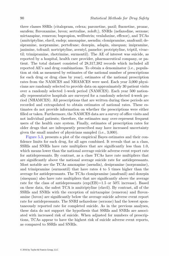
90 Statistical Methods for Drug Safety
three classes SSRIs (citalopram, celexa; paroxetine, paxil; fluoxetine, prozac,sarafem; fluvoxamine, luvox; sertraline, zoloft;), SNRIs (nefazodine, serzone;mirtazapine, remeron; bupropion, wellbutrin; venlafaxine, effexor), and TCAs(amitriptyline, elavil, endep; amoxapine, asendin; clomipramine, anafranil; de-sipramine, norpramine, pertofrane; doxepin, adapin, sinequan; imipramine,janimine, tofranil; nortriptyline, aventyl, pamelor; protriptyline, triptil, vivac-til; trimipramine, rhotrimine, surmontil). The AE of interest was suicide, asreported by a hospital, health care provider, pharmaceutical company, or pa-tient. The total dataset consisted of 28,317,382 records which included allreported AE’s and drug combinations. To obtain a denominator (i.e., popula-tion at risk as measured by estimates of the national number of prescriptionsfor each drug or drug class by year), estimates of the national prescriptionrates from the NAMCES and NHAMCES were used. Each year 3,000 physi-cians are randomly selected to provide data on approximately 30 patient visitsover a randomly selected 1-week period (NAMCES). Each year 500 nation-ally representative hospitals are surveyed for a randomly selected 4-week pe-riod (NHAMCES). All prescriptions that are written during these periods arerecorded and extrapolated to obtain estimates of national rates. These es-timates do not provide information on whether the prescriptions were eitherfilled or taken. Furthermore, the NAMCES data are a survey of office visits andnot individual patients; therefore, the estimates may over-represent frequentusers of the health care system. Finally, estimates of prescription rates forolder drugs that are infrequently prescribed may have increased uncertaintygiven the small number of physicians sampled (i.e., 3,000).
Figure 5.3, presents a plot of the empirical Bayes estimates and their con-fidence limits for each drug, for all ages combined. It reveals that as a class,SSRIs and SNRIs have rate multipliers that are significantly less than 1.0,which means lower than the national average suicide adverse event report ratefor antidepressants. By contrast, as a class TCAs have rate multipliers thatare significantly above the national average suicide rate for antidepressants.Most notable are the TCAs amoxapine (asendin), desipramine (norpramine),and trimipramine (surmontil) that have rates 4 to 5 times higher than theaverage for antidepressants. The TCAs clomipramine (anafranil) and doxepin(sinequan) also have rate multipliers that are significantly above the averagerate for the class of antidepressants (exp(EB)=1.5 or 50% increase). Basedon these data, the safest TCA is amitriptyline (elavil). By contrast, all of theSSRIs and SNRIs with the exception of mirtazapine (remeron) and fluvox-amine (luvox) are significantly below the average suicide adverse event reportrate for antidepressants. The SNRI nefazedone (serzone) had the lowest spon-taneously reported rate for completed suicide. As in the previous analyses,these data do not support the hypothesis that SSRIs and SNRIs are associ-ated with increased risk of suicide. When adjusted for numbers of prescrip-tions, TCAs appear to have the highest risk of suicide adverse event reports,as compared to SSRIs and SNRIs.
© 2016 by Taylor & Francis Group, LLC

Analysis of Spontaneous Reports 91
FIGURE 5.3: Bayes estimates and confidence intervals - multiplier of overallrate.
5.8 Discussion
ADR surveillance using statistical methods is still an area of active research.After several years of effort by many researchers, no single method can claimabsolute superiority. This is partly because of the complexity of the SRS dataand uncontrolled collection of self-reported entries riddled with the problems ofunder-reporting, over-reporting, and duplicate reporting. Further, as a conse-quence of modern advances in medicine, patients are more likely to be treatedwith multiple drugs and not surprisingly multiple drugs are mentioned in al-most all the spontaneous reports. These characteristics of SRS data presentboth challenges and opportunities for methodological developments. More re-cently, various techniques have emerged that have focused primarily on theminimization of false discovery rate (Ahmed et al. 2009, 2010a,b, 2012) andidentification of drug-drug interaction (Eugene et al. 2000, Almenoff et al.2003, Noren et al. 2008, Villerd et al. 2010, Qian et al. 2010, DuMoucheland Harpaz 2012). Despite use of several different well established methods,automatic signal detection methods cannot and are not designed to replacepharmacovigilance expertise. However, their ability to efficiently explore largespontaneous reporting system databases and detect relevant signals quicklycompared with traditional pharmacovigilance makes them powerful tools. As
© 2016 by Taylor & Francis Group, LLC

92 Statistical Methods for Drug Safety
access to higher quality and more complete data streams (medical claims,electronic health records, ...) become available, these methods may prove evenmore useful for ADR discovery and large scale screening.
© 2016 by Taylor & Francis Group, LLC

6
Meta-analysis
“Our figures show approximately four and one half million hospitaladmissions annually due to the adverse reactions to drugs. Further, the
average hospital patient has as much as thirty percent chance, depending howlong he is in, of doubling his stay due to adverse drug reactions.”(Milton Silverman, M.D. Professor of Pharmacology, University of
California)
6.1 Introduction
The impact of meta-analysis in drug safety has never been greater than inthe recent years. High profile cases against blockbuster drugs such as vioxxand avandia have brought meta-analysis to the forefront of the discussion inthe drug safety community. It has become both an indispensable and a highlycontroversial tool for analyzing rare outcomes in medical and pharmaceuticalresearch. It is indispensable because each individual study or trial is usuallynot large enough to contain a sufficient number of events for a meaningfulanalysis. For example the rate of suicidal events (ideation and behavior) isapproximately 0.001. In order to estimate and test the efficacy or the safetyof drugs in relation to such events with acceptable precision, a large numberof subjects must be included in the trial. Meta-analyses combine results frommany similar studies and provide a combined estimate with large effectivesample size. Meta-analyses are also controversial because of the potential forvarious biases and for inappropriate methodological choices. There are twoprimary methodological choices of meta-analyses in the frequentest domain:(1) fixed-effects meta-analyses which assume that the variation in observedeffect estimates across the studies are due to sampling variability alone; and(2) random-effect meta-analyses which assume that there is a systematic com-ponent in the variation of observed effect estimates across the studies and isquantified by a heterogeneity parameter. Bayesian meta-analysis is also pop-ular for combining results from multiple studies. For each methodology thereare a multitude of estimation techniques, each with their respective strengthsand weaknesses.
93
© 2016 by Taylor & Francis Group, LLC

94 Statistical Methods for Drug Safety
6.2 Fixed-effect Meta-analysis
Let θi be a measure of effect size and σ2i be the variance of the corresponding
measure in the ith of K studies included in the meta-analysis. Many differentmetrics can be used to measure effect size, for example, the Pearson product-moment correlation coefficient; standardized mean difference; odds ratios, riskratios, risk differences, etc. Regardless of a metric used, the true effect size θis estimated by combining effect sizes from individual studies as follows:
θ =
∑Ki=1 wiθi∑Ki=1 wi
, (6.1)
where,
wi =1
σ2i
. (6.2)
Clearly, individual studies are weighted by the inverse of a variance wi, so thatthe contribution of each study reflects the precision of individual measuresof the effect size. The sampling variance of this combined effect size is thereciprocal of the sum of weights. So, its standard error is:
SE(θ) =
√1
∑Ki=1 wi
. (6.3)
The null hypothesis of H0 : θ = θ is tested against the alternate hypothesisH1 : θ 6= θ using the following Wald test:
z =θ − θ
SE(θ). (6.4)
The (1 − α)100% confidence interval for the effect size is constructed as θ ±z(1−α/2)×SE(θ), where z(1−α/2) is a (1−α/2) percentile point of the standardnormal distribution.
6.2.1 Correlation Coefficient
The commonly used metric of effect size to measure linear association be-tween two continuous variables is the correlation coefficient, ρ. The estimatedcorrelation within an individual study of size ni is denoted by ri, which asymp-
totically follows N(ρ, (1−ρ
2)2
ni
). Most often, however, ri is normalized using
Fisher’s transformation to obtain a random variable z which has variance in-dependent of the unknown parameter ρ. The transformation has the followingexpression:
zri =1
2log
1 + ri1− ri
. (6.5)
© 2016 by Taylor & Francis Group, LLC
Meta-analysis 95
The transformed variable z follows N(ξ, σ2), where ξ = 12 log
1+ρ1−ρ and σ2 =
1n−3 . The combined transformed correlation coefficient across K studies givenby the weighted average estimator of equation (6.1) is:
z =
∑Ki=1 wizri∑Ki=1 wi
, (6.6)
where, wi = ni − 3. The variance of the overall z is∑Ki=1 ni − 3K and the
(1− α)100% CI is z ± z(1−α/2)
/√∑Ki=1 ni − 3K .
6.2.2 Mean Difference
Studies with continuous outcomes often compare the mean outcome from twopopulations. The two populations may differ with respect to the treatmentregimen, program intervention, or exposure. Let x1i and x2i be the estimatedmean outcomes; s21i and s
22i be the variances; and n1i and n2i be the sample
sizes in the first and the second population, respectively. The impact of theexposure or the intervention is estimated by the difference between outcomemeans of each group, xdi = x1i − x2i. A pooled variance across two groups is
s2pi =(n1i−1)s21i+(n2i−1)s22i
n1i+n2i−2 and an estimated variance σ2di of xdi is as follows:
σ2di =
n1i + n2i
n1in2is2pi . (6.7)
The estimate of common mean difference (θ) across K studies is estimatedusing the general expression in (6.1) as follows:
θ =
∑Ki=1 wixdi∑Ki=1 wi
, (6.8)
where,
wi =1
σ2di
, and V ar(θ) =1
∑Ki=1 wi
. (6.9)
There are alternative expressions available for V ar(θ), which are not coveredin this text.
6.2.3 Relative Risk
Prospective studies of a binary outcome, measure effect size as a ratio of risksfor the two groups. The measure is called relative risk or the risk ratio (RR).It is a measure with straight forward interpretation and with wide applicationin epidemiological studies. The outcome of the ith trial with binary outcomecan be summarized in the following 2× 2 contingency table.
© 2016 by Taylor & Francis Group, LLC

96 Statistical Methods for Drug Safety
TABLE 6.1: Contingency Table of a Drug-Adverse Event Pair in ithTrial/Study.
Eventyes no total
Treatment xTi nTi − xTi nTiControl xCi nCi − xCi nCiTotal mEi mNEi Ni
In Table 6.1 xTi and xCi are the number of individuals presented with ad-verse events in the treatment and the control conditions, respectively. Further,nTi and nCi are the number of participants in the treatment and the controlgroups, respectively. The RR of an adverse event for a study is calculated asfollows:
RRi =xTi/nTixCi/nCi
. (6.10)
Although, computation of relative risk is easy, its variance estimation is notstraight forward, and the domain is not symmetric about its null value. There-fore, the logarithmic transformed relative risk, ln(RR) is commonly used in-stead of RR which better approximates the large sample distribution and alsoincludes the entire real line in its domain. Since the logarithm is a mono-tonically increasing function, ln(RR) can be easily transformed back to itsoriginal scale. Log transform creates some undesirable complexity in meta-analysis. As ln(0) is not defined, studies without an event in either groupcannot be included in the meta-analysis. In order to avoid such complexity, asmall constant a called a continuity correction, is added to the cell count ofthe elements in Table 6.1. The estimate of ln(RRi) with continuity correctionfor an individual study is expressed as follows:
ln(RRi) = ln
[(xTi + a)/(nTi + a)
(xCi + a)/(nCi + a)
]. (6.11)
Variance of the estimate in (6.11) following the delta method is as follows:
V ar[ln(RRi)] =1
xTi + a− 1
nCi + a+
1
xCi + a− 1
nCi + a. (6.12)
There are two ways of combining relative risks from multiple studies or trials.One way is to use the general inverse variance method described in equations(6.1) to (6.4). The other way is to use the Mantel-Haenszel method whichwas originally developed for combining odds/risk ratios across the stratified2 × 2 tables. The Mantel-Haenszel method is attractive because it naturallyaccommodates zero event studies as long as events are observed in one of thetwo treatment arms. A study is eliminated only when the event is not observedin both treatment arms.
© 2016 by Taylor & Francis Group, LLC

Meta-analysis 97
6.2.3.1 Inverse Variance Method
Derivation of an estimate of the combined risk ratio in the inverse variancemethod follows from the general expression of the fixed-effect estimate of effectsize, where ln(RRi) replaces θi and V ar[ln(RRi)] replaces σ
2i in equation (6.1).
Consequently, the combined estimate, ln(RR), from K studies is given by
ln(RR) =
K∑
i=1
1
V ar[ln(RRi)]
[ln
(xTi + a)
(nTi + a)− ln
(xCi + a)
(nCi + a)
]
K∑
i=1
1
V ar[ln(RRi)]
, (6.13)
and the variance of ln(RR) is(6.14)
V ar[ln(RR)] =
K∑
i=1
1
V ar[ln(RRi)]. (6.15)
A null hypothesis of RR = 1 is tested using the Wald statistic in equation (6.4)and (1−α)100% confidence interval of the combined relative risk is calculated
as
[RR exp
(z(1−α/2)
√V ar[ln(RR)]
), RR
exp(z(1−α/2)
√V ar[ln(RR)]
)
].
6.2.3.2 Mantel-Haenszel Method
The Mantel-Haenszel method is an heuristic estimate of the assumed com-mon risk ratio across the studies. A distinct advantage of this method overthe inverse variance method is that it allows studies with zero event in onetreatment arm without needing continuity correction. The Mantel-Haenszelmethod estimate of the common risk ratio is
RRMH =
∑Ki=1 xTinCi/Ni∑Ki=1 xCinTi/Ni
, (6.16)
which can be expressed as a weighted average estimate as follows:
RRMH =
∑Ki=1 wiRRi∑Ki=1 wi
, (6.17)
wherewi = xCinTi /Ni . (6.18)
Unlike the inverse variance method, the weights in equation (6.18) are notreciprocals of the variances of relative risk estimates from individual studies.Therefore, the variance of the common RR estimate is not as simple. Severalapproximations of the asymptotic variance have been proposed. The most
© 2016 by Taylor & Francis Group, LLC

98 Statistical Methods for Drug Safety
accurate estimate is the Robins-Breslow-Greenland estimate of variance forln(RRMH). It has the following form:
V ar[ln(RRMH )] =
K∑
i=1
nTinCi
N2i
mEi
(K∑
i=1
xTinCi
Ni
)(K∑
i=1
xCinTi
Ni
). (6.19)
The null hypothesis of equal risks in treatment and control subjects, i.e.,RRMH = 1, may be tested by the following 1 degree of freedom χ2-test, whichis obtained based on the assumption of a conditional binomial distribution forthe events xTi in Table 6.1:
X2MH =
[K∑
i=1
(xTi − nTimEi)/Ni
]2
K∑
i=1
nTinCimEimNEi
Ni(Ni − 1)
. (6.20)
6.2.4 Odds Ratio
Large scale drug safety studies are not conducted routinely unless mandatedby the FDA. Initial safety concerns often originate from the combined evi-dences of studies which are conducted to assess efficacy of a treatment. Drugsafety studies are, therefore, usually retrospective in nature. The effect sizemeasure commonly used in the retrospective studies of a binary outcome isthe odds ratio. Odds ratios share many of the same numerical issues of therelative risk including a non-symmetry about its null value, a need for loga-rithmic transformation, and a problem with zero studies. Therefore, similarapproaches are employed to obtain an estimate of the common odds ratioacross multiple studies. When the event is rare (less than 5%) the OR andRR are quite similar.
The observed frequencies of events from the retrospective studies can besummarized in the same way as Table 6.1.
6.2.4.1 Inverse Variance Method
The simplest estimation of combined odds ratio once again follows from thegeneral expression of fixed-effect estimate of effect size, where ln(ORi) replaces
the θi and V ar[ln(ORi)] replaces the σ2i in the equations (6.1). Thus, the
© 2016 by Taylor & Francis Group, LLC

Meta-analysis 99
combined estimate ln(OR) from K studies is given by
ln(OR) =
K∑
i=1
1
V ar[ln(ORi)]ln
[(xTi + a)(nCi − xCi + a)
(xCi + a)(nTi − xTi + a)
]
K∑
i=1
1
V ar[ln(ORi)]
, (6.21)
and the variance of ln(OR) is
V ar[ln(OR)] =K∑
i=1
1
V ar[ln(ORi)], (6.22)
where
V ar[ln(ORi)] =1
xTi + a+
1
xCi + a+
1
nTi − xTi + a+
1
nCi − xCi + a.
The null hypothesis is tested using the Wald statistic in equation (6.4) andthe (1 − α)100% confidence interval of the combined odds ratio is calculated
as
[OR exp
(z(1−α/2)
√V ar[ln(OR)]
), OR
exp(z(1−α/2)
√V ar[ln(OR)]
)
].
6.2.4.2 Mantel-Haenszel Method
The Mantel-Haenszel method estimate of common odds ratio is
ORMH =
∑Ki=1 xTi(nCi − xCi)/Ni∑Ki=1 xCi(nTi − xTi)/Ni
, (6.23)
which can be expressed as a weighted average estimate as follows:
ORMH =
∑Ki=1 wiORi∑Ki=1 wi
, (6.24)
where
wi =xCi(nTi − xTi)
Ni. (6.25)
Again the weights in equation (6.25) are not reciprocals of the variances ofodds ratio estimates from individual studies. The Robins-Breslow-Greenlandestimate of variance for ln(ORMH ) is of the following form:
V ar[ln(ORMH )] =S3
2S21
+S5
2S1S2+
S4
2S22
, (6.26)
where S1 =
K∑
i=1
xTi(nCi − xCi)
Ni, S2 =
K∑
i=1
xCi(nTi − xTi)
Ni,
S3 =K∑
i=1
xTi(nCi − xCi)(xTi + nCi − xCi)
N2i
,
© 2016 by Taylor & Francis Group, LLC

100 Statistical Methods for Drug Safety
S4 =
K∑
i=1
xCi(nTi − xTi)(xCi + nTi − xTi)
N2i
, and
S5 =
K∑
i=1
xCi(nTi − xTi)(xTi + nCi − xCi) + xTi(nCi − xCi)(xCi + nTi − xTi)
N2i
.
A null hypothesis of equal odds in treatment and control subjects, i.e.,ORMH = 1, may be tested by the following χ2-test:
X2MH =
[K∑
i=1
xTi(nCi − xCi)− xCi(nTi − xTi)
Ni
]2. (6.27)
6.2.4.3 Peto Method
Peto method is popular for combining results when the events are moder-ately rare. For this method studies without events do not present numericaldifficulty. Let us define the following quantities for the 2× 2 table in 6.1
Ei =(xTi + xCi)nTi
Ni, (6.28)
and
Vi =(xTi + xCi)(Ni − xTi − xCi)nTinCi
N2i (Ni − 1)
. (6.29)
For the fixed marginal totals, Ei and Vi are the mean and the variance of xTiwhich follow hypergeometric distribution under the null hypothesis of oddsratio equal to one. Then for K independent tables, the pooled estimate ofln(OR) is as follows:
ln(OR)Peto =
∑Ki=1(xTi − Ei)∑K
i−1 Vi, (6.30)
and
V ar[ln(OR)Peto] =1
∑Ki−1 Vi
. (6.31)
The combined odds ratio estimated using this method, however, is not a con-sistent estimator. It performs well only for balanced designs with odds ratioclose to 1.
6.3 Random-effect Meta-analysis
Random-effect meta-analysis takes a slightly different approach than its fixed-effect counterpart in that the overall effect size parameter θ is viewed as the
© 2016 by Taylor & Francis Group, LLC

Meta-analysis 101
mean of a random quantity as opposed to a fixed constant. The random quan-tity in question is the “true” effect size θi in the individual studies includedin the meta-analysis. Additionally, the θi’s are assumed to be a sample ofeffect sizes from a population of all possible studies with mean effect size θand variance τ2. The observed effect size θi is regarded as a realized value ofthe random quantity θi. Hence, in random-effect meta-analysis there is not asingle “true” population parameter. Each θi is a “true” parameter for the ith
study. The aim is to estimate a mean effect size of these individual “true” effectsizes. The most commonly used distribution to model the behavior of randomeffect sizes is a normal distribution. Thus, it is assumed that θi ∼ N(θi, σ
2)and θi ∼ N(θ, τ2) which lead to the following estimate of the overall mean
effect size, θ:
θ =
∑Ni=1 wiθi∑Ni=1 wi
, (6.32)
where,
wi =1
σ2i + τ2
. (6.33)
The sampling variance of the mean effect size is the reciprocal of the sum ofweights and the standard error is:
SE(θ) =
√√√√(
1∑N
i=1 wi
). (6.34)
Therefore, the sampling variance of the random-effect estimate of the meaneffect size is a function of both the sampling error of θi about θi and theunderlying variability of the θi. In the context of meta-analysis, the under-lying variability of θi is called the study heterogeneity and measured by theheterogeneity parameter τ2. Addition of the heterogeneity parameter in theweights of the expression (6.33) inflates the standard error of the mean effectestimate.
In equation (6.33), τ2 is assumed to be known. However, in practice it mustbe estimated from the sample of studies included in the meta-analysis. Sev-eral estimates of between-study variance are available. Among those estimatesmost commonly used estimate, Q, is based on the weighted sum of squarederrors. The Q-statistic also known as Cochran’s Q-test has the following form:
© 2016 by Taylor & Francis Group, LLC

102 Statistical Methods for Drug Safety
Q =
K∑
i=1
wi0(θi − θ)2, where wi0 =1
σ2i
, and (6.35)
E(Q) = τ2K∑
i=1
wi0−τ2∑K
i=1w2i0∑K
i=1 wi0+
K∑
i=1
wi0σ2i −∑K
i=1 w2i0σ
2i∑K
i=1 wi0(6.36)
= τ2K∑
i=1
wi0 −τ2∑K
i=1 w2i0∑K
i=1 wi0+ (K − 1). (6.37)
Using the expression (6.36), an estimate of τ2 is obtained by matching firstorder moment of Q with Q; i.e., Q = E(Q) and rearranging the terms (Der-Simonian and Laird 1986). The process yields the following estimate of τ2:
τ2 =Q− (K − 1)
K∑
i=1
wi0 −∑K
i=1 w2i0
K∑
i=1
wi0
. (6.38)
If the estimate yields a negative value, then it is set to zero because thebetween-study variance cannot be negative. The estimator in (6.38) is a singlestep non-iterative solution. However, it has downward bias that increases withthe decreasing event rates. Other alternative estimators of heterogeneity arediscussed in the following section.
The only difference between expressions to calculate the overall effect sizein the fixed-effect and the random-effect analysis is the additional τ2 termin the expression of the weight in equation (6.33). When the between-studyvariance is absent or small, the fixed-effect and random-effect estimates ofthe overall mean are the same. A statistical test of significance of hetero-geneity relies on the Q-statistic in equation (6.35). For a large number ofstudies, Q follows a χ2 distribution with K − 1 degrees of freedom. Thus,a critical value of the test of heterogeneity, at α level of significance, is the(1−α)100th percentile point of the χ2
K−1 distribution. Although, it is a widelyused test of heterogeneity, statistical power of this test has been shown to beinadequate, especially for small values of τ2 and for non-Gaussian outcomes.Alternatively, the I2 statistic is used to quantify heterogeneity (Higgins andThompson 2002). It is independent of a number of studies and the treatmenteffect metric. The I2 statistic is derived from Q as follows:
I2 = max
0,Q− (K − 1)
Q
. (6.39)
I2 is interpreted as the percentage of variability due to heterogeneity be-tween studies. I2 value of 30% indicates the presence of moderate heterogene-ity and 50% indicates the presence of strong heterogeniety. The value of the I2
© 2016 by Taylor & Francis Group, LLC

Meta-analysis 103
statistic depends on the precision of the estimate of individual effect sizes ofthe included studies. The value increases with number of patients included inthe studies in a meta-analysis regardless of the underlying study heterogeneity(Rucker et al. 2008). Therefore, I2 values must be interpreted cautiously.
6.3.1 Sidik-Jonkman Estimator of Heterogeneity
The Sidik-Jonkman (Sidik and Jonkman 2005) estimator is simple, non-iterative and always non-negative. It has less bias when the heterogeneityvariance is moderate to large. The estimation method is developed in theframework of a linear regression model with no covariates. The estimate, τ2SH ,is found by using the weighted residual sum of squares as follows:
τ2SH =1
K − 1
K∑
i=1
υ−1i (θi − θ)2, (6.40)
where υi = ri + 1 and ri = σ2i /τ
2. The estimator τ2SH depends on the un-known parameter τ2 through ri. A crude estimate of τ2 for defining ri for thecomputation of τ2SH from equation (6.40) is obtained as:
τ20 =1
K
K∑
i=1
(θi − θ)2, (6.41)
where θ = 1K
∑Ki=1 θi. An interval estimate of τ2SH is found by assuming that
(K − 1)τ2SH/τ2 has approximately a χ2-distribution with K − 1 degrees of
freedom. Thus, an approximate (100− 1)α% confidence interval for τ2 givenα is obtained as
(K − 1)τ2SHχ2K−1,1−α/2
≤ τ2 ≤ (K − 1)τ2SHχ2K−1,α/2
. (6.42)
Figure 6.1 shows the SJ estimates of τ2 for varying baseline risk rates in binaryevent studies. It reveals the overestimating tendency of the SJ estimator atthe null value of heterogeneity for the rare events. On the other hand, formoderate event rates, the SJ estimator shows remarkable accuracy.
6.3.2 DerSimonian-Kacker Estimator of Heterogeneity
The original non-iterative estimate of τ2 can be improved by a two-step process(DerSimonian and Kacker 2007). First, the intermediate estimate of τ2 isobtained using equation (6.38). Second, the weights wi0 in (6.36) are replacedby wi in (6.33) where τ2 is substituted with the estimate τ2 obtained in the
© 2016 by Taylor & Francis Group, LLC

104 Statistical Methods for Drug Safety
0.0 0.2 0.4 0.6 0.8 1.0
0.0
0.2
0.4
0.6
0.8
1.0
Baseline rate
τ2
τ2=0
τ2=0.2
τ2=0.4
τ2=0.6
τ2=0.8
τ2=1
FIGURE 6.1: Sidik-Jonkman estimator of heterogeneity for different baselinerisks.
first step. The resulting two-step estimator (τ2DSK) has following expression.
τ2DSK =
(K∑
i=1
wi(θi − θ)2
)−
K∑
i=1
wiσ2i −
K∑
i=1
w2i σ
2i
K∑
i=1
wi
K∑
i=1
wi −
K∑
i=1
w2i
K∑
i=1
wi
. (6.43)
An additional step usually improves the estimate of heterogeneity. The secondstep of the process depends on having a non-zero estimate of intermediateτ2. In rare event studies, equation (6.38) often fails to detect even moderateheterogeneity resulting in a zero intermediate estimate and consequently a zerofinal estimate of heterogeneity. Thus, for rare event studies, the advantage ofa two-step estimate is diminished.
6.3.3 REML Estimator of Heterogeneity
Fully iterative solution of heterogeneity is obtained using maximum likeli-hood theory. According to the standard random-effect model in Section 6.3,
© 2016 by Taylor & Francis Group, LLC

Meta-analysis 105
θi follows a N(θ, τ2 + σ2i ) distribution. The log-likelihood function is
l(θ, τ2|θi) = −1
2
K∑
i=1
ln[2π(σ2i + τ2)]− 1
2
K∑
i=1
θi − θ
σ2i + τ2
, τ2 ≥ 0. (6.44)
The maximum likelihood estimator is found by maximizing this likelihoodfunction with respect to θ and τ2. Unfortunately, closed form solution of theestimating equation does not exist. Hence, the solution is obtained by iteratingbetween the following two equations until convergence (Hardy and Thompson1996).
θMLE =K∑
i=1
θi(σ2i + τ2MLE)
/ K∑
i=1
1
(σ2i + τ2MLE)
. (6.45)
τ2MLE =
K∑
i=1
(θi − θMLE)2 − σ2
i
(σ2i + τ2MLE)
2
/ K∑
i=1
1
(σ2i + τ2MLE)
2. (6.46)
A 95% confidence interval of τ2 is obtained by a profile likelihood ratio teststatistic. It is defined as a set of τ2 estimates which satisfy the followingcondition:
l(θ, τ2) ≥ l(θMLE , τ2MLE)− 3.84/2. (6.47)
Alternatively, the estimate and confidence interval of τ2 may be obtainedusing the restricted maximum likelihood (REML) estimate which overcomes atendency of ML methods to underestimate variances. The following restrictedlikelihood lR of τ2 is given by Viechtbauer (2007):
lR = −1
2
K∑
i=1
ln(σ2i + τ2)− 1
2ln
K∑
i=1
1
σ2i + τ2
− 1
2
K∑
i=1
(θi − θ)2
σ2i + τ2
(6.48)
where θ =∑Ki=1
θi(σ2
i +τ2)
/∑Ki=1
1(σ2
i +τ2). Then the REML estimate of τ2 is
obtained by iteratively solving the following estimating equation:
τ2REML =
K∑
i=1
(θi − θREML)2 − σ2
i
(σ2i + τ2REML)
2
/ K∑
i=1
1
(σ2i + τ2REML)
2+
1
σ2i + τ2REML
.
(6.49)A 95% confidence interval based on profile likelihood ratio test is given by aset of τ2 which satisfy following condition
lR(τ2) ≥ lR(τ
2REML)− 3.84/2. (6.50)
© 2016 by Taylor & Francis Group, LLC

106 Statistical Methods for Drug Safety
6.3.4 Improved PM Estimator of Heterogeneity
An alternative fully iterative approach to estimate τ2 is provided by Pauleand Mandel (1982) and is based on the following estimating equation:
F (τ2) =∑
i
wi(θi − θ)2 − (k − 1) = 0. (6.51)
A unique solution of (6.51), τ2PM , can be determined by numerical iterationstarting with τ2 = 0. If F (τ2) is negative for all positive τ2, τ2PM is set to 0.This method is a natural approximation to the restricted maximum likelihoodmethod. When the normality assumption holds and the estimate of within-study variances are regarded as the true within-study variance, Paule andMandel’s approach is statistically optimal. But the assumption of normalityis not required to apply this method which makes it more robust when thatassumption does not hold (DerSimonian and Kacker (2007)). Note that τ2PMis based on σi which varies from study to study.
Studies with binary outcome usually report number of success and sam-ple size in each arm. In such cases, the variance estimator may be improvedby borrowing strength from all studies when estimating each within-studyvariance σ2
i as follows:
σ2i (∗) =
1
(nTi + 1)
[e
(−µ−θ+ τ2
2
)+ 2 + e
(µ+θ+ τ2
2
)]
+1
(nCi + 1)
[e−µ + 2 + eµ
], (6.52)
where µ =∑K
i=1 µi and θ =∑K
i=1 θi. The µi and θi are the estimated logodds of success and log odds ratio measure of effect size, respectively. A newestimator, denoted by τ2IPM , is the solution to a modified version of (6.51),where the weights wi are replaced by the shared-strength weights wi(∗) =
1τ2+σ2
i (∗). This is in line with the Bohning et al. (2002) recommendation of
using a population averaged version of the study-specific variances as weights.
6.3.5 Example
Rosiglitazone is widely used to treat patients with type 2 diabetes mellitus.For the past few years the scientific community has expressed concerns re-garding its adverse effect on cardiovascular morbidity and mortality. In 2007a group of scientists from the Cleveland clinic lead by Steven E. Nissen con-ducted a meta-analysis of 42 trials of rosiglitazone. A total of 15,565 patientswere randomly assigned to regimens that included rosiglitazone, and 12,282were assigned to comparator groups with regimens that did not include rosigli-tazone. Myocardial infarction (MI) was one of the adverse event considered.Only 38 of 42 trials had at least one MI event. The remaining four trialswere eliminated from further analysis because the effect estimates were not
© 2016 by Taylor & Francis Group, LLC

Meta-analysis 107
possible for these trials. The following forest plot shows number of patientsand number of events in each treatment arm, the estimated odds ratios andassociated 95% CI for each trial, and the overall odds ratio and 95% CI esti-mate using Peto method. The estimates of the overall odds ratio using otherestimators are listed in the Table 6.2. Peto method yields the largest andstatistically significant estimate of the overall odds ratio (OR=1.43, p=0.03),whereas the other three methods: inverse variance (I), Mantel-Haenszel (MH),and DerSimonian-Laird (DL), yield statistically non-significant (p=0.15) es-timates. As we noted earlier the Peto method is susceptible to bias whencombining highly unbalanced studies such as studies in this example.
The forest plot shows large heterogeneity in the estimated odds ratio fromthe individual studies. However, the estimates of between study heterogene-ity in the Table 6.3 are near 0 for all but Sidik-Jonkman (SJ) method. Thediscrepancy in observed and the estimated heterogeneity could be due to tworeasons. First, the forest plot shows effect estimates in their original scale,where as heterogeneity is estimated for the effect in the logarithmic scalewhich attenuates the magnitude of the between study differences. Second, av-erage baseline event rates of MI in these studies are about 6/1000. The usualheterogeneity estimates do not perform well in such rare event cases. In con-trast, the SJ estimator showed moderate heterogeneity. However, simulationstudy has shown that for rare events the SJ estimators have a tendency tooverestimate when the true heterogeneity is near 0 (Sidik and Jonkman 2005).
TABLE 6.2: Estimate of Overall Odds Ratio.
Method OR 95 % CI of OR pI 1.24 [0.9201; 1.6814] 0.15MH 1.24 [0.9275; 1.6572] 0.14Peto 1.43 [1.0309; 1.9788] 0.03DL 1.24 [0.9201; 1.6814] 0.15
TABLE 6.3: Estimates and Test of Heterogeneity.
Method τ2
DL 0SJ 0.26REML 0ML 0IPM 0I2 0Q-test pvalue 0.99
© 2016 by Taylor & Francis Group, LLC

108 Statistical Methods for Drug Safety
Study
Fixed effect modelRandom effects modelHeterogeneity: I−squared=0%, tau−squared=0, p=0.8102
1234567891011121314151617181920212223242526272829303132333435363738
Events
2 2 1 0 1 0 1 5 1 1 0 2 2 2 2 1 1 2 3 0 0 1 1 0 2 1 1 1 1 1 1 1 1 1 1 11527
Total
14376
357 391 774 213 232 43 121 110 382 284 294 563 278 418 395 203 104 212 138 122 175 56 39 561 116 148 231 89 168 1172 204 288 254 314 442 394 2635 1456
ExperimentalEvents
0 1 1 1 0 1 0 2 0 0 1 0 1 0 1 1 2 0 1 1 1 0 0 2 3 0 0 0 0 0 2 0 0 0 0 0 941
Total
11635
176 207 185 109 116 47 124 114 384 135 302 142 279 212 198 106 99 107 139 120 173 58 38 276 111 143 242 88 172 377 185 280 272 154 112 124 2634 2895
Control
0 0.1 1 10 1000
Odds Ratio
OR
1.431.43
4.461.060.140.054.480.157.572.507.434.370.143.501.964.521.000.500.494.522.770.130.137.667.200.050.647.147.757.317.573.750.467.197.934.443.503.721.651.33
95%−CI
[1.03; 1.98] [1.03; 1.98]
[0.23; 85.24] [0.10; 11.47] [0.00; 4.66] [0.00; 3.28]
[0.07; 286.49] [0.00; 7.46]
[0.15; 381.85] [0.56; 11.25] [0.15; 374.34] [0.07; 289.87] [0.00; 7.01]
[0.11; 111.28] [0.20; 18.91] [0.24; 85.20] [0.09; 11.09] [0.03; 9.26] [0.05; 4.72] [0.24; 85.58] [0.39; 19.87] [0.00; 6.71] [0.00; 6.74]
[0.15; 386.16] [0.14; 363.08] [0.00; 0.92] [0.11; 3.73]
[0.14; 360.22] [0.15; 390.96] [0.14; 368.25] [0.15; 381.46] [0.04; 361.05] [0.05; 4.49]
[0.14; 362.32] [0.16; 400.65] [0.07; 287.64] [0.03; 461.09] [0.04; 367.95] [0.74; 3.68] [0.80; 2.21]
W(fixed)
100%−−
1.2% 1.9% 0.9% 0.6% 0.6% 0.7% 0.7% 4.7% 0.7% 0.6% 0.7% 0.9% 2.1% 1.2% 1.8% 1.2% 2.1% 1.2% 2.7% 0.7% 0.7% 0.7% 0.7% 1.2% 3.4% 0.7% 0.7% 0.7% 0.7% 0.5% 2.1% 0.7% 0.7% 0.6% 0.4% 0.5%16.5%41.2%
W(random)
−−
100%
1.2% 1.9% 0.9% 0.6% 0.6% 0.7% 0.7% 4.7% 0.7% 0.6% 0.7% 0.9% 2.1% 1.2% 1.8% 1.2% 2.1% 1.2% 2.7% 0.7% 0.7% 0.7% 0.7% 1.2% 3.4% 0.7% 0.7% 0.7% 0.7% 0.5% 2.1% 0.7% 0.7% 0.6% 0.4% 0.5%16.5%41.2%
FIGURE 6.2: Meta-analysis of rosiglitazone trials. The fixed-effect estimate isobtained using the Peto method.
6.3.6 Issues with the Weighted Average in Meta-analysis
The weighted average estimator, such as the DL estimator, has been in use forseveral decades. Classical statistical theory has established that the weightedaverage is the most efficient estimator of the population mean of a randomvariable, on the assumption that the weights used in estimation are not re-lated to the random variable in question. In meta-analysis the validity of thisassumption is questionable. While it is not as clear in studies with normallydistributed continuous outcomes, the correlation between weights and indi-vidual effect estimates in studies with a binary outcome is undeniable. Theweighted average estimator of overall effect is biased when such correlationexists. Shuster (2010) derived the following expression for the expected valueof the overall effect estimator for the random-effect model (6.33)
E(θ) = K × Cov(Wiθi) + θ, (6.53)
© 2016 by Taylor & Francis Group, LLC

Meta-analysis 109
where Wi = wi/∑wi. He also showed that only the unweighted mean is
the unbiased estimator of the overall effect in these conditions. A similarconclusion was reached by Bhaumik et al. (2012) and recommended usingunweighted mean with 0.5 continuity correction when necessary. Hence, resultsof the weighted average estimate must be interpreted with caution.
6.4 Maximum Marginal Likelihood/Empirical BayesMethod
An alternative to the method of moments, is the maximum marginal likelihood(MML) method. A distinct advantage of the MML approach is that studieswith zero events in both arms can be included without adjustments suchas continuity corrections. Furthermore, the overall treatment effect and theheterogeneity parameter(s) can be simultaneously estimated.
Consider an observed 2×2 Table 6.1 for the ith study for a meta-analysis ofK studies. Let pti and pci be the event probabilities in treatment and controlgroups, respectively, of the ith study; ǫ1 ∼ N(0, σ2
µ) and ǫ2 ∼ N(0, τ2); andTji be a treatment indicator variable, i.e., Tj = 0 for j = c and Tj = 1 forj = t. The log-odds of adverse events in the jth group can be modeled asfollows. The model allows for heterogeneity in both the baseline risk and thetreatment effect.
ln
(pji
1− pji
)= µ+ ǫ1i + (θ + ǫ2i)Tji (6.54)
(ǫ1ǫ2
)∼ N
((00
),
(σ2µ ρσµτ
ρσµτ τ2
)). (6.55)
The likelihood function based on the observations from the ith study is writtenas follows:
l(xi|ǫ) = pxti
ti qnti−xti
ti pxci
ci qnci−xci
ci , (6.56)
where xi = (xti, xci) is the vector pattern of responses from study i. Then,for the parameter vector β = (µ, θ,Σ), the marginal likelihood for study i isgiven by
h(β;xi) = h(xi) =
∫
ǫ
l(xi|ǫ)g(ǫ)dǫ, (6.57)
where g(ǫ) represents the standard multivariate normal density. Now, the fulllog-likelihood for k studies can be written as
logL =k∑
i=1
log h(xi), (6.58)
© 2016 by Taylor & Francis Group, LLC

110 Statistical Methods for Drug Safety
and for an arbitrary parameter vector, η, the first derivatives of the log-likelihood with respect to η are
∂ logL
∂η=
k∑
i=1
1
h(xi)
∂h(xi)
∂η, (6.59)
where∂h(xi)
∂η=
∫
ǫ
∂ log l(xi|ǫ)∂η
l(xi|ǫ)g(ǫ)dǫ . (6.60)
The integration on the random effect space (i.e., ǫ) in the marginal like-lihood equation in (6.57) can be approximated numerically using Gauss-Hermite quadrature to any practical degree of accuracy. The integration inGauss-Hermite quadrature is approximated by a summation on a specifiednumber of quadrature nodes and the corresponding quadrature weights. Bothadaptive (based on selecting quadrature nodes in accordance with provisionalestimates of the posterior mean and variance) and nonadaptive versions ofthe algorithm are available Hedeker and Gibbons (2006). Optimal points andweights for the standard normal univariate density were given by Stroud andSecrest (1966), and this method is now in widespread use in nonlinear mixed-effects regression models. Solution of the likelihood equations can be obtainediteratively using the Newton-Raphson algorithm. At convergence, the diago-nal elements of the inverse of the information matrix provide the variance ofthe estimated parameters.
The MML models are fitted using commercial software packages such asSAS, STATA, SuperMix, etc. The linearized approximation can be fitted usingthe GLIMMIX procedure in SAS or the glmer package in R. The following SAScode illustrates the NLMIXED implementation of the MML meta-analysis.
6.4.1 Example: Percutaneous Coronary Intervention BasedStrategy versus Medical Treatment Strategy
Percutaneous coronary intervention or PCI (commonly known as angioplasty)is the standard treatment for patients with acute coronary disease; however,the effects of PCI in the treatment of patients with stable coronary artery dis-ease have not received thorough examination. Schomig et al. (2008) conducteda meta-analysis of 17 RCTs that compared PCI to medication management(MED) in patients with stable coronary artery disease aimed at synthesizingevidence of efficacy of PCI versus MED. Briefly, the study included a total of7513 patients (3675 PCI and 3838 MED) with the average length of follow-upof 51 months. The sample consisted of mostly elderly men (82%) and 54%had experienced an (MI). In the PCI group, 271 patients died and in theMED group 335 died. Among the 13 studies that reported cardiac mortal-ity, the PCI and MED arms had a combined 115/2814 and 151/2805 cardiac
© 2016 by Taylor & Francis Group, LLC

Meta-analysis 111
deaths, respectively. Finally, MI rates were provided in all 17 studies, report-ing 319 in the PCI group and 357 in the MED group. The original authorsused Cochran’s Q-test to assess heterogeneity and performed Mantel-Haenszel(MH) and DerSimonian and Laird methods to estimate the overall treatmenteffect. Tests of heterogeneity (Cochran’s Q statistic) were not significant foreither total mortality (p=.263) or cardiac mortality (p=.161), but was sig-nificant for MI (p=.003). The fixed-effect (MH) model showed a significantprotective effect of PCI on total mortality (OR = 0.80, CI = 0.68-0.95), andcardiac mortality (OR = 0.74, CI = 0.57-0.96), and approached significancefor MI (OR = 0.91, CI = 0.77-1.06). The random-effect (DL) model showeda significant protective effect of PCI on total mortality (OR = 0.80, CI =0.64-0.99), an effect that approached significance for cardiac mortality (OR= 0.74, CI = 0.51-1.06), and a nonsignificant effect for MI (OR = 0.90, CI =0.66-1.23) that was in the same protective direction as the other effects. Onthe basis of these results, the authors concluded that a PCI-based invasivestrategy may improve long term survival compared with a medical treatmentin patients with stable coronary artery disease. Table 6.4 shows the frequenciesof each type of even for these 17 studies.
TABLE 6.4: Example 1: Data from a Meta-analysis of Studies Comparing PCIto MED in the Treatment of Patients with Stable Coronary Artery Disease.
Number of events in PCI group Number of events in MED groupStudy MI Cardiac
deathAllcausemortal-ity
# Obs. MI Cardiacdeath
All causemortality
# Obs.
1 2 0 0 44 0 1 1 442 14 - 16 115 8 - 15 1123 6 - 9 51 6 - 10 504 7 - 2 192 18 - 20 3665 2 1 1 21 0 1 1 236 5 1 1 177 4 1 1 1647 5 4 6 72 3 2 6 728 3 1 2 90 0 2 4 919 10 4 6 149 12 14 17 15110 32 20 43 504 23 24 43 51411 18 32 45 153 18 33 40 14812 1 0 0 50 0 0 0 5113 32 - 19 503 59 - 24 50514 5 2 2 104 7 1 1 10115 23 24 28 205 31 25 35 20316 11 3 6 96 40 22 22 10517 143 23 85 1149 128 25 95 1138
A re-analysis of the cardiac mortality data is presented in Table 6.6 alongwith the NLMIXED code snippet used for this analysis in Table 6.5. Therewere 13 studies with an average of 215 subjects per study per arm. The es-timated baseline incidence rate is -3.22 based the MML model, which corre-sponds to a baseline rate of 4%. The analysis reveals that the primary variancecomponent is for the baseline incidence rate. The estimated odds ratio is 0.75(95% CI 0.42–1.33), and the estimated treatment variance is 0.23. While thepoint estimate is similar to the moment-based methods, the full-likelihood
© 2016 by Taylor & Francis Group, LLC

112 Statistical Methods for Drug Safety
method reveals considerably more uncertainty in the estimate.
TABLE 6.5: The NLMIXED Code for PCI Example
PROC NLMIXED DATA=pci qpoints= 11;PARMS b0= −4 b1= −0.1 v0= 1.4 c01= −0.5 v1= 0.2;eta = b0 + b1∗Group + u0 + u1∗Group;expeta = exp(eta);prob = expeta/(1+expeta);model x ∼ binomial(n,prob);RANDOM u0 u1 ∼ NORMAL([0, 0], [v0, c01, v1]) SUBJECT=studyid;ESTIMATE ’re corr’ c01/SQRT(v0*v1);RUN;
TABLE 6.6: Analysis of PCI vs MED for Cardiac Mortality Data
Parameters Estimate Std. err p-val
θ -0.28 0.217 0.303σ2µ 1.411 0.737 0.076
σµτ -0.267 0.345 0.488τ2 0.235 0.243 0.348ρ -0.464 0.421
The MML model also allow flexibility of modeling with single variancecomponents either in the baseline rate or in the treatment effect. However,there is a risk of model mis-specification when using a single variance compo-nent. In such cases the effect estimates can be severely biased and the type Ierror can be substantial Amatya et al. (2014).
6.5 Bayesian Meta-analysis
The Bayesian approach to meta-analysis provides a flexible modeling strat-egy that naturally accounts for uncertainty in all of the parameter estimates.Unlike the frequentest approach, the Bayesian framework can be easily ex-tended to non-normal distribution of random effects. This approach allowsadditional information from other trials or studies to be incorporated in theform of a prior distribution. Perhaps the most interesting advantage of theapproach is its ability to make predictions about the outcomes of future stud-ies. The Bayesian approach requires computing the posterior distributions ofthe parameter which often are computationally intensive. Fortunately, rapid
© 2016 by Taylor & Francis Group, LLC

Meta-analysis 113
development in Monte Carlo technique and computing power have made thesecomplex computations feasible.
The generic Bayesian meta-analysis model places a prior distribution onboth the effect parameter and the heterogeneity parameter as follows:
θi ∼ f(θi|θi, σ2i ) (6.61)
θi ∼ π(θi|θ, τ2) (6.62)
θ ∼ h(θ) (6.63)
τ2 ∼ h(τ2) (6.64)
p(θ, τ, θi|θi) ∝ h(θ)h(τ2)
K∏
i=1
π(θi|θ, τ2)K∏
i=1
f(θi|θi, σ2i ) (6.65)
Inference regarding a parameter is made from the mode of the posteriordistribution (6.65). Computation of the posterior mode in closed form can bevery complex. Monte Carlo methods such as Gibbs sampling make computa-tion feasible by exploiting computational power of new computers.
An example of Gibbs sampling is presented in meta-analysis of randomizedcontrolled trials comparing sodium monobuorophosphate (SMFP) to sodiumBuoride (NaF) dentifrices (toothpastes) in the prevention of caries develop-ment by Abrams and Sanso (1998). Nine studies were included in the analysisof change in the decayed missing (due to caries) filled surface (DMFS) dentalindex from baseline. The following Bayesian model was used to model thedifference in mean responses θi for the ith study:
θi ∼ N(θi, σ2i /ni), (6.66)
θi ∼ N(µ, τ2), (6.67)
τ2 ∼ IG(a, b), (6.68)
π(σ2i ) ∝ 1/σ2
i , (6.69)
where ni = nTinCi/(nTi + nCi), σi is the within-study variance and IG(a,b)is an inverse gamma distribution. The µ is assumed to follow a locally uni-form prior distribution. When the conditional posterior distribution may beobtained in closed form as in this example, Gibbs sampling may be used toobtain the estimate of posterior mode. The conditional posterior distributionsfor the model in this example are as follows:
P (θi|µ,σ2, τ2, θ, σ2,n) = N
(θi
∣∣∣ θini/σ2i + µ/τ2
ni/σ2i + 1/τ2
,1
ni/σ2i + 1/τ2
)
P (µ|θ,σ2, τ2, θ, σ2,n) = N(µ∣∣∣∑
θi/K, τ2/K
)
P (σ2i |θ, µ, τ2, θ, σ2,n) = IG
(σ2i |ni, 2/[ni(θi − θi)
2 + σ2i ])
where i = 1, · · · , K, and
© 2016 by Taylor & Francis Group, LLC

114 Statistical Methods for Drug Safety
P (τ2|θ, µ,σ2, θ, σ2,n) = IG(τ2|K/2 + a, 2/
∑(θi − µ)2 + b
).
Then the marginal posterior distribution is estimated by sampling from eachof the posterior conditional distributions, in turn conditioning on the currentdraw of the unknown model parameters. For the complete treatment of thisexample readers are referred to the original paper (Abrams and Sanso 1998).
6.5.1 WinBugs Example
The example 6.3.5 analyzed 42 trials of rosiglitazone using fixed and random-effect methods. The major issue in meta-analyzing these data is the high pro-portion of trials without a single event in either treatment arm. Such “zerostudies” either must be excluded from the analyses or some form of continuitycorrection must be applied. Both of these remedies have potential for biasingthe final result. Bayesian modeling techniques provide an efficient alternativewhich naturally accommodate sparse data. WinBugs is a powerful computa-tional tool for Bayesian analyses which shifts the computational burden fromanalyst to computer. With help of the software program an analyst can fo-cus on modeling aspects of the analyses without having to invest significantamount of effort on the computational details.
One of the adverse effects monitored in the rosiglitazone trials was theincidence of MI among the participants. Let rTi and rCi be the MI incidencesamong nTi and nCi participants randomized to treatment and to placebo,respectively. Further, assume that pTi and pCi are the probabilities of ex-periencing MI among participants in ith trial under treatment and placebo,respectively. The observed data may be modeled as follows under the Bayesianframework:
rTi ∼ binomial(pTi, nTi)
rCi ∼ binomial(pCi, nCi)
µi = logit(pCi)
logit(pTi) = µi + θi
θi ∼ N(θ, τ2).
The model presented above can be easily implemented in the WinBugs pro-gram (Warn et al. 2002). There are three components of the program: first,the model segment; second, the observed data; and third, initial values of thestochastic nodes. Together they form a complete program as follows:model
for (i in 1:k)r.c[i] ∼ dbin(pi.c[i], n.c[i]);
r.t[i] ∼ dbin(pi.t[i], n.t[i]);
© 2016 by Taylor & Francis Group, LLC

Meta-analysis 115
mu[i] <- logit(pi.c[i]);
logit(pi.t[i]) <- mu[i] + delta[i];
delta[i] ∼ dnorm(theta, precision.tau);
pi.c[i] ∼ dunif(0,1);
theta ∼ dnorm(0, 0.1);
precision.tau <- 1/(tau*tau);
tau ∼ dunif(0, 2);
# data
list( n.t=c(357, 391, 774, 213, 232, 43, 121, 110, 382, 284,
294, 563, 278, 418, 395, 203, 104, 212, 138, 196, 122, 175, 56,
39, 561, 116, 148, 231, 89, 168, 116, 1172, 706, 204, 288, 254,
314, 162, 442, 394, 2635, 1456),
n.c =c( 176, 207, 185, 109, 116, 47, 124, 114, 384, 135, 302,
142, 279, 212, 198, 106, 99, 107, 139, 96, 120, 173,
58, 38, 276, 111, 143, 242, 88, 172, 61, 377, 325, 185,
280, 272, 154, 160, 112, 124, 2634, 2895),
r.t = c(2, 2, 1, 0, 1, 0, 1, 5, 1, 1, 0, 2, 2, 2, 2, 1, 1, 2, 3,
0, 0, 0, 1, 1, 0, 2, 1, 1, 1, 1, 0, 1, 0, 1, 1, 1, 1, 0,
1, 1, 15, 27),
r.c = c(0, 1, 1, 1, 0, 1, 0, 2, 0, 0, 1, 0, 1, 0, 1, 1, 2, 0, 1,
0, 1, 1, 0, 0, 2, 3, 0, 0, 0, 0, 0, 0, 0, 2, 0, 0, 0, 0,
0, 0, 9, 41), k=42)
# initial values
list( theta = 0.5, tau=0.01, pi.c = c(0.886, 0.483, 0.439,
0.191, 0.845, 0.187, 0.071, 0.025, 0.234, 0.522, 0.167, 0.812,
0.492, 0.196, 0.894, 0.759, 0.041, 0.917, 0.251, 0.139,
0.944, 0.775, 0.932, 0.273, 0.470, 0.813, 0.366, 0.184,
0.830, 0.834, 0.856, 0.941, 0.203, 0.391, 0.853, 0.358,
0.576, 0.781, 0.591, 0.004, 0.432, 0.335),
delta = c(0.004, 0.003, 0.001, 0.000, 0.004, 0.001, 0.000,
0.005, 0.001, 0.000, 0.002, 0.002, 0.001, 0.001, 0.004, 0.000,
0.001, 0.003, 0.001, 0.004, 0.004, 0.002, 0.003, 0.003, 0.001,
0.002, 0.001, 0.001, 0.001, 0.001, 0.003, 0.001, 0.004, 0.005,
0.002, 0.003, 0.003, 0.001, 0.002, 0.003, 0.003, 0.001)
The WinBugs program computes posterior distributions of parameters basedon MCMC methods. Therefore, it is important to monitor convergence andadequate mixing of simulation using tools available in the program. After con-vergence, the posterior mode of each parameter can be calculated based on theposterior simulation discarding the burn-in runs. The posterior distributionsof θ and τ (not τ2) are displayed in Figure (6.3).
© 2016 by Taylor & Francis Group, LLC

116 Statistical Methods for Drug Safety
(b) Posterior distribution of θ.(a) Posterior distribution of τ .
FIGURE 6.3: Posterior distributions of τ and θ.
TABLE 6.7: Bayesian Meta-Analyses of 42 Rosiglitazone Trials.
Mean 2.5% 25% 50% 75% 97.5%OR 0.613 0.395 0.536 0.617 0.713 0.905τ2 0.228 0.012 0.101 0.226 0.380 0.816
The posterior estimate of combined odds ratio and heterogeneity fromthe above modeling is given in Table 6.7. The results in Table 6.7 show aposterior estimate of the odds ratio of 0.613 with 95% credible interval of(0.395, 0.904), which is markedly different from the moment-based estimatorsin Table 6.2. What could be the reason for such a dramatic discrepancy whichessentially alters the conclusion in the opposite direction? An answer can befound in Figure 6.4. The figure displays the effect of changing parameters ofthe prior distribution of a probability of MI incidence for subjects randomizedto placebo. At the population level it is a prevalence of MI in diabetic patents.The figure illustrates that the posterior log odds ratio remains below 0 as theprior becomes increasingly vague as is the case for the results in Table 6.7.However, one might argue that the prevalence of MI cannot possibly be higherthan 0.1% and apply an informative prior of uniform(0, 0.01). Use of such priorresults in a positive log odds ratio and is in closer agreement with the moment-based results. The figure essentially shows that if one is willing to bet a priorithat the prevalence of MI is extremely rare, less than 6/1000, in a diabeticpopulation, then the observed data support an elevated risk of MI amongrosiglitazone users. In the absence of such prior information, the observeddata do not support the conclusion obtained for the moment-based analyses.
This example clearly demonstrates the effect of the prior distribution onthe conclusion of the meta-analysis. One way to minimize such influence is touse a hierarchical Bayesian approach. In this approach a hyper-prior is placedon the prior distribution of pc. Continuing with the rosiglitazone example,a beta(a, b) prior distribution may be used to model pc and a gamma(s, r)hyper-prior may be placed on the parameters of the beta distribution. Thefully Bayesian model now becomes:
© 2016 by Taylor & Francis Group, LLC

Meta-analysis 117
0.00 0.02 0.04 0.06 0.08
−1.
0−0.
50.0
0.5
1.0
1.5
2.0
2.5
max pc
logO
R
FIGURE 6.4: Posterior mean and 95% credible interval of θfor varying upper limits of prior distribution of pc ∼ unif(0,max pc).
rTi ∼ binomial(pTi, nTi)
rCi ∼ binomial(pCi, nCi)
µi = logit(pCi)
logit(pTi) = µi + θi
pCi ∼ beta(a, b)
θi ∼ N(θ, τ2)
a ∼ gamma(s, r)
b ∼ gamma(s, r)
where, gamma(s, r) = rs
Γ(s)xs−1e−rs for x > 0, r > 0 and s > 0. The corre-
sponding WinBugs model segment is written as follows:
model for (i in 1:k) r.c[i] ∼ dbin(pi.c[i], n.c[i]);
r.t[i] ∼ dbin(pi.t[i], n.t[i]);
© 2016 by Taylor & Francis Group, LLC

118 Statistical Methods for Drug Safety
mu[i] <- log(pi.c[i]);
log(pi.t[i]) <- mu[i] + delta[i];
delta[i] ∼ dnorm(theta, precision.tau);
pi.c[i] ∼ dbeta(alpha,beta);
theta ∼ dnorm(0, 0.1);
alpha ∼ dgamma(0.001,0.25);
beta ∼ dgamma(1, 0.25);
precision.tau <- 1/(tau*tau);
tau ∼ dunif(0, 2);
.
Estimates obtained from the model are presented in Table 6.8 for differentcombinations of parameters of the gamma hyper-prior distribution. The pos-terior means of the log odds ratio are clearly more consistent between 0.11(OR=1.12) and 0.16 (OR=1.17) over different specifications of hyper-priordistribution. These estimates of log odds ratio are closer to the estimates ob-tained from the moment-based methods. With regards to τ2, it is interestingthat the value decreases from 0.228 when pic were treated as independent to0.06 when pic were treated as a sample from a common gamma distribution.
TABLE 6.8: Hierarchical Bayesian Analysis of 42 Rosiglitazone Trials UsingDifferent Gamma Hyper-prior Distributions.
α β log odds ratio (θ) τ2
s r mean mean mean 2.5% 97.5% mean 2.5% 97.5%0.01 6.787 0.411 32.95 0.145 -0.243 0.511 0.063 0.0002 0.5230.002 15.283 0.484 49.39 0.150 -0.246 0.513 0.062 0.0001 0.5870.006 10.386 0.445 39.84 0.129 -0.28 0.488 0.070 0.0001 0.5460.003 5.412 0.391 29.647 0.146 -0.262 0.52 0.069 0.0001 0.6180.001 1.215 0.353 22.137 0.126 -0.261 0.483 0.070 0.0003 0.6210.007 5.667 0.398 30.499 0.154 -0.235 0.535 0.065 0.0001 0.6270.006 1.718 0.35 22.657 0.146 -0.22 0.486 0.064 0.0001 0.6350.006 6.167 0.404 31.747 0.128 -0.272 0.512 0.068 0.0001 0.7020.003 16.076 0.488 50.308 0.145 -0.238 0.51 0.066 0.0002 0.5780.004 6.577 0.409 32.398 0.142 -0.234 0.537 0.060 0.0001 0.6240.466 7.875 0.423 35.107 0.130 -0.262 0.526 0.064 0.0001 0.6153.812 1.437 0.406 25.133 0.113 -0.303 0.529 0.064 0.0000 0.5173.411 5.974 0.453 34.192 0.110 -0.313 0.47 0.072 0.0002 0.6163.316 11.691 0.511 44.916 0.103 -0.271 0.492 0.064 0.0000 0.4962.699 19.686 0.57 59.036 0.118 -0.283 0.492 0.066 0.0001 0.4772.08 2.013 0.385 24.722 0.126 -0.291 0.514 0.069 0.0001 0.5302.362 9.968 0.483 41.096 0.105 -0.32 0.559 0.068 0.0001 0.5810.862 4.548 0.4 29.092 0.123 -0.293 0.486 0.068 0.0003 0.5934.067 14.267 0.544 50.355 0.104 -0.32 0.462 0.066 0.0001 0.5842.667 0.321 0.373 21.696 0.134 -0.251 0.493 0.062 0.0000 0.656
© 2016 by Taylor & Francis Group, LLC

Meta-analysis 119
6.6 Confidence Distribution Framework for Meta-analysis
Confidence distribution (CD) has its roots in Fisher’s fiducial distribution the-ory. Although the history of CD is not new, its utility in modern statisticalproblems has not been fully explored. Recent interest in CD and its applica-tion is facilitated by the formal definition of CD by Schweder and Hjort (2002)and Singh et al. (2005). They defined a confidence distribution for a param-eter θ as a function Hn(·) = Hn(Xn, ·) on ℵ → [0, 1] such that (i) for eachsample set Xn in the sample set space ℵ, Hn(·) is a continuous cumulativedistribution function in the parameter space Θ; and (ii) at the true parametervalue θ = θ0, Hn(θ0) = Hn(Xn, θ0), as a function of sample set Xn, has auniform distribution U(0, 1). The function Hn(·) is an asymptotic confidencedistribution, if (ii) is met only asymptotically. Thus, a confidence distributionis a sample dependent distribution function on the parameter space that hasdesired frequentest properties. Although, the CD is not a distribution on θ,it contains a wealth of information on θ. In that sense CD is a frequentest’sanalog of the Bayesian posterior distribution. In the context of hypothesistesting of the form H0 : θ ≤ θ0, Hn(θ0) provides a p-value regardless of thevalue of θ0. Conversely, any pair of confidence quantiles forms the confidenceinterval (H−1
n (α1)), H−1n (α2)) with α2 − α1 degree of confidence.
The simplest and most direct way to construct a CD is through pivotalstatistics. A pivot is a function of a sample Xn, the parameter of interest,and some other known parameters, and does not involve any other unknownparameters. It’s true CDF is generally analytically tractable and does notinvolve any unknown parameter. Suppose Q(Xn, θ) is a such function and Gnis its continuous CDF. Then, the exact CD for θ is given by (Singh et al. 2005,see):
Hn(x) =
Gn(Q(Xn, θ)), if Q is increasing in θ
1−Gn(Q(Xn, θ)), if Q is decreasing in θ .(6.70)
Example 1: Normal mean and known variance.
Consider estimation of the population mean for the normal distribution with
mean µ and known variance σ2. The standard pivot is Q(Xn, µ) = Xn−µσ/
√n,
which has the standard normal CDF, Φ. Using the substitution scheme givenin (6.70), the CD for µ is
Hn(x) = 1− Φ
(Xn − x
σ/√n
)= Φ
(x− Xn
σ/√n
). (6.71)
© 2016 by Taylor & Francis Group, LLC

120 Statistical Methods for Drug Safety
Example 2: Normal mean and unknown variance.
When the population variance is unknown, a standard pivot is Q(Xn, µ) =Xn−µsn/
√n, where sn is a sample standard deviation. The pivot has Students t-
distribution with n − 1 degrees of freedom. Following the method in (6.70),the CD for µ can be expressed as:
Hn(x) = 1− P
(Tn−1 ≤ Xn − x
sn/√n
)= P
(Tn−1 ≤ x− Xn
sn/√n
); (6.72)
where Tn−1 ∼ tdf = n− 1.For σ2, the usual pivot is Q(Xn, σ
2) = (n− 1)s2n/σ2 that has χ2
n−1 distri-bution. Using the above substitution method, the CD for σ2 is
Hn(x) = P(χ2n−1 ≥ (n− 1)s2n/x
2), x ≥ 0 (6.73)
where χ2n−1 is a random variable that has the χ2
n−1 distribution.
6.6.1 The Framework
A unifying framework for meta-analysis through combining CDs from individ-ual studies was proposed by Xie et al. (2011). In contrast to the traditionalmeta-analysis where a combined estimate is obtained from weighted individ-ual point estimates, the combined confidence distribution function is obtainedby appropriately weighting the individual distribution estimators. In doingso, the combined CD achieves various optimality conditions depending on thecharacteristics of the weights used for combining individual CDs.
A general framework for meta-analysis involves the following recipe forCD combination. Suppose Hi(θ) = Hi(Xi, θ), i = 1, . . . , k are CD functionsfor the parameter θ from k independent samples Xi with sample size ni. Acombined confidence distribution function (Hc) is constructed as
Hc = Gcgc(H1(θ), . . . , Hk(θ)), (6.74)
where gc(u1, . . . , uk) = w1F−10 (u1)+ . . .+wkF
−10 (uk) is a monotonic function
that has cumulative distribution function Gc(t) = P (gc(U1, . . . , Uk) ≤ t) forUi ∼ U [0, 1]. The cumulative distribution functions F0(·) are weighted by fixedpositive weights wi ≥ 0. The recipe (6.74) encompasses most commonly usedmeta-analysis approaches in this chapter.
6.6.1.1 Fixed-effects Model
A fixed-effects model assumes that individuals in a study are an independentsample from the population sharing the same parameter. Thus, a parameterestimate from each study is a realization from a population of study estimates.The parameter estimates from k studies are assumed to follow an asymptotic
© 2016 by Taylor & Francis Group, LLC

Meta-analysis 121
normal distribution. Let θ be the central parameter of interest and θi is theestimate from the ith independent study. Thus,
θi ∼ N(θ, σ2i ). (6.75)
Under the fixed-effects model assumption, the pivot for the ith study is
Q(Xn, θ) =θi − θ
σi.
As σi is assumed known, Q(Xn, θ) ∼ N(0, 1). Thus, following the equation(6.70), the CD function from the ith study is
Hi(θ) = 1− Φ
(θi − θ
σi
)= Φ
(θ − θiσi
).
Then, a combined CD function can be constructed by taking F0(t) = Φ(t)and wi = 1/σi in (6.74). Such that,
g(H1(θ) + . . .+Hk(θ)) =1
σ1Φ−1(H1(θ)) + . . .+
1
σkΦ−1(Hk(θ)).
As
k∑
i=1
1
σiΦ−1(Hi(θ)) ∼ N
(0,
k∑
i=1
1
σ2k
)implies Gc(t) = Φ
t√∑
ki=1
1
σ2i
,
Hc(θ) = Φ
1σ1Φ−1
(Φ(θ−θ1σ1
))+ . . .+ 1
σkΦ−1
(Φ(θ−θkσk
))
(∑ki=1
1σ2i
)1/2
(6.76)
= Φ
∑ki=1
θ−θiσ2i(∑k
i=11σ2i
)1/2
= Φ
(k∑
i=1
1
σ2i
)1/2(θ −
∑ki=1 θi/σ
2i∑k
i=1 1/σ2i
) .(6.77)
Equation (6.77) allows the estimation of θ by a normal CD function that has
mean∑k
i=1 θi/σ2i∑
ki=1 1/σ2
i
and variance(∑k
i=1 1/σ2i
)−1
. Note that these expressions
match exactly with the ones in the equation (6.1).
6.6.1.2 Random-effects Model
As described in the Section 6.3, the random-effects model assumes thatθi|(θi, σ2
i ) ∼ N(θi, σ2i ) and θi|(θ, τ2) ∼ N(θ, τ2), which together leads to
θi ∼ N(θi, σ2i + τ2) and the following CD for the ith study
Hi(θ) = 1− Φ
(θi − θ
(σ2i + τ2)1/2
)= Φ
(θ − θi
(σ2i + τ2)1/2
).
© 2016 by Taylor & Francis Group, LLC

122 Statistical Methods for Drug Safety
Following the derivation in the Section 6.6.1.1 and substituting wi = 1/(σ2i +
τ2)1/2, the combined CD function for random-effects model is given by
Hc(θ) = Φ
(k∑
i=1
1
σ2i + τ2
)1/2(θ −
∑ki=1 θi/(σ
2i + τ2)
∑ki=1 1/(σ
2i + τ2)
) ,
where the mean of combined CD function is θc =∑k
i=1 wi θi∑ki=1 wi
and the variance is(∑k
i=11
σ2i +τ
2
)−1
. These expressions match equations (6.33) and (6.34) given
in the Section 6.3.
Example
The withdrawal of rofecoxib (vioxx) has raised the safety concerns about apotential class effect of cyclooxygenase-2 (COX-2) inhibitors (coxib) and allnon-steroidal anti-inflammatory drugs (NSAIDs). Chen and Ashcroft (2007)assessed the risk of MI for all coxibs in the meta-analysis of 38 trials (82,489patients). As a part of the assessment, they compared all coxibs against non-selective NSAIDs. Table 6.9 contains the cases of MI reported in those trials.The Trials were identified by searching MEDLINE, EMBASE, the CochraneDatabase of Systematic Reviews, and the Cochrane Central Register of Con-trolled Trials. They included trials of coxibs that had been licensed in theUK or US (celecoxib, rofecoxib, valdecoxib, parecoxib, etoricoxib, and lumira-coxib).
The forest plot in Figure 6.5 shows the number of MI events and samplesize in each study included in the analysis. A continuity correction of 0.5was added to treatment arms with a 0 event. The odds ratio estimate of MIcomparing Coxibs against NSAIDs is also shown in the figure. Both fixed-effect(OR=1.49, 95% CI: 1.14−1.95) and random-effect (OR=1.44, 95% CI: 1.08−1.93) estimates indicate elevated risk of MI associated with Coxibs comparedto NASAIDs. The near identical estimates between fixed- and random-effectsestimate is expected as there was no evidence of heterogeneity among thetrials (I2 = 0.00%, p-value for heterogeneity=0.87).
The figure 6.6 shows confidence densities of log odds ratio estimates fromeight randomly chosen trials along with the combined confidence density. Table6.9 lists mean and median log odds ratios, standard deviations, and 95%confidence intervals estimated from the confidence distribution of individualtrials. It also shows the corresponding quantities estimated from the combinedconfidence distribution of the estimates from the 38 trials. The combined oddsratio estimate obtained from CD approach is 1.44 with 95% CI: 1.08− 1.93.These estimates are identical to the random-effect estimates obtained fromthe traditional method because CD approach also utilizes an inverse varianceweighted estimate (see (6.77)).
© 2016 by Taylor & Francis Group, LLC

Meta-analysis 123
TABLE 6.9: Fixed-Effects CD Estimates of θ and the Corresponding 95% CIs.
Study mean median stddev LCL UCL1 -0.420 -0.420 1.734 -3.818 2.9782 0.000 0.000 1.733 -3.397 3.3973 2.367 2.367 1.501 -0.575 5.3094 0.704 0.704 1.734 -2.694 4.1025 -0.433 -0.433 1.734 -3.831 2.9666 -0.011 -0.011 1.417 -2.788 2.7667 0.265 0.265 1.583 -2.838 3.3678 1.610 1.610 1.049 -0.446 3.6669 0.690 0.690 1.736 -2.713 4.09210 0.551 0.551 0.325 -0.086 1.18811 -0.687 -0.687 1.734 -4.086 2.71212 -0.704 -0.704 1.733 -4.101 2.69413 -0.167 -0.167 0.674 -1.488 1.15414 0.051 0.051 1.735 -3.348 3.45115 0.473 0.473 0.383 -0.278 1.22516 0.004 0.004 1.736 -3.398 3.40617 0.038 0.038 1.743 -3.378 3.45418 0.587 0.587 0.395 -0.187 1.36119 -0.332 -0.332 0.586 -1.481 0.81620 -0.005 -0.005 1.734 -3.403 3.39221 -0.703 -0.703 1.416 -3.479 2.07322 -0.050 -0.050 1.734 -3.448 3.34923 -0.004 -0.004 1.734 -3.403 3.39424 -0.330 -0.330 1.003 -2.296 1.63725 -1.417 -1.417 1.734 -4.816 1.98126 -0.659 -0.659 1.003 -2.624 1.30727 -0.007 -0.007 1.227 -2.412 2.39928 1.109 1.109 1.157 -1.159 3.37629 -1.113 -1.113 1.736 -4.516 2.29030 1.705 1.705 0.544 0.638 2.77131 1.606 1.606 1.096 -0.541 3.75432 0.661 0.661 1.733 -2.737 4.05833 -2.999 -2.999 1.485 -5.910 -0.08834 1.026 1.026 1.462 -1.840 3.89235 0.293 0.293 1.583 -2.810 3.39636 -1.047 -1.047 1.416 -3.823 1.72937 -1.399 -1.399 1.583 -4.501 1.70338 -0.706 -0.706 1.416 -3.482 2.070combined CD 0.368 0.368 0.147 0.079 0.656
© 2016 by Taylor & Francis Group, LLC

124 Statistical Methods for Drug Safety
Study
Fixed effect modelRandom effects modelHeterogeneity: I−squared=0%, tau−squared=0, p=0.8717
1234567891011121314151617181920212223242526272829303132333435363738
Events
1.0 0.5 4.0 1.0 1.0 1.0 2.010.0 1.026.0 0.5 0.5 4.0 1.018.0 1.0 1.018.0 5.0 1.0 1.0 1.0 1.0 2.0 0.5 2.0 2.0 3.0 0.522.0 5.0 1.0 0.5 8.0 2.0 1.0 0.5 1.0
Total
45879
663 366 602 326 693 270 636 8850 144 3987 258 425 458 323 3593 249 79
4741 4376 561 524 454 458 376 442 516 463 390 174 4047 2785 424 520 504 654 642 423 483
ExperimentalEvents
0.5 1.0 0.5 0.5 0.5 1.0 0.5 1.0 0.515.0 1.0 1.0 5.0 0.511.0 0.5 0.510.0 7.0 0.5 1.0 0.5 0.5 2.0 1.0 2.0 1.0 1.0 1.0 4.0 1.0 0.5 5.0 0.5 0.5 1.0 2.0 1.0
Total
36610
218 732 798 329 225 267 207 4424 143 3981 260 421 485 170 3518 125 41
4730 4397 279 260 216 228 271 215 268 230 392 115 4029 2772 410 264 87 219 226 419 239
Control
0.01 0.1 1 10 100
Odds Ratio
OR
1.49 1.44
0.66 1.0010.67 2.02 0.65 0.99 1.30 5.00 1.99 1.74 0.50 0.49 0.85 1.05 1.61 1.00 1.04 1.80 0.72 0.99 0.50 0.95 1.00 0.72 0.24 0.52 0.99 3.03 0.33 5.50 4.98 1.94 0.05 2.79 1.34 0.35 0.25 0.49
95%−CI
[1.14; 1.95] [1.08; 1.93]
[0.02; 19.65] [0.03; 29.88] [0.56; 202.19] [0.07; 60.47] [0.02; 19.40] [0.06; 15.89] [0.06; 29.01] [0.64; 39.10] [0.07; 59.88] [0.92; 3.28] [0.02; 15.06] [0.02; 14.79] [0.23; 3.17] [0.04; 31.54] [0.76; 3.40] [0.03; 30.13] [0.03; 31.62] [0.83; 3.90] [0.23; 2.26] [0.03; 29.74] [0.03; 7.95] [0.03; 28.47] [0.03; 29.79] [0.10; 5.14] [0.01; 7.25] [0.07; 3.69] [0.09; 11.01] [0.31; 29.27] [0.01; 9.87] [1.89; 15.97] [0.58; 42.69] [0.06; 57.87] [0.00; 0.92] [0.16; 49.03] [0.06; 29.84] [0.02; 5.64] [0.01; 5.49] [0.03; 7.93]
W(fixed)
100%−−
0.8% 0.7% 0.5% 0.6% 0.8% 1.1% 0.8% 1.5% 0.6%16.6% 1.1% 1.1% 5.3% 0.7%12.3% 0.7% 0.7%11.1% 7.7% 0.7% 1.5% 0.8% 0.7% 2.6% 1.5% 2.9% 1.5% 1.1% 1.3% 4.4% 1.1% 0.6% 7.4% 0.9% 0.8% 1.6% 2.2% 1.5%
W(random)
−−
100%
0.7% 0.7% 1.0% 0.7% 0.7% 1.1% 0.9% 2.0% 0.7%20.5% 0.7% 0.7% 4.8% 0.7%14.7% 0.7% 0.7%13.9% 6.3% 0.7% 1.1% 0.7% 0.7% 2.2% 0.7% 2.2% 1.4% 1.6% 0.7% 7.3% 1.8% 0.7% 1.0% 1.0% 0.9% 1.1% 0.9% 1.1%
FIGURE 6.5: Assessment of MI risk of Coxib vs. NSAID using traditionalmoment-based meta-analysis methods.
© 2016 by Taylor & Francis Group, LLC

Meta-analysis 125
−6 −4 −2 0 2 4 6
Log OR
den
sity
[ ]
#3
[ ]
#6
[ ]
#8
[ ]
#11
[ ]
#14
[ ]
#29
[ ]
#30
[ ]
#36
[ ]
#combined.density
FIGURE 6.6: Fixed-effects CD estimates of θ. Only eight randomly selectedstudies are shown.
© 2016 by Taylor & Francis Group, LLC
126 Statistical Methods for Drug Safety
6.6.2 Meta-analysis of Rare Events under the CD Frame-work
Rare event studies present some unique challenges for traditional meta-analysis methods. A zero event in either or the both treatment arms of astudy either necessitates continuity correction or renders the study noninfor-mative. A few different approaches for determining an appropriate continuitycorrection have been suggested in the literature. However, there is little con-sensus regarding this issue. The CD framework provides a way to combine allof the rare event studies, including studies with zero event on both treatmentarms. The method was developed by Tian et al. (2009) and Liu et al. (2014)for risk difference and odds ratio measures, respectively.
Liu et al. (2014) use exact p-value functions as the CD functions for in-dividual studies and combine them by applying the general CD combinationmethod. Suppose Ψ is the parameter of central interest and a hypothesis ofinterest is
H0 : Ψ = Ψ∗vs.H1 > Ψ∗.
The p-value function p(Ψ) is a function derived from varying the value of Ψ∗
in the parameter space of Ψ. The formal definition of the p-value for the givenobservations is:
p(Ψ;Xn) = P(T ≥ t|Ψ∗), (6.78)
where T is a pivot statistic that has a distribution function F (T ), and t is arealized value computed from sample Xn. If Ψ
0 is the true value of Ψ, then
p(Ψ0;Xn) = P(T ≥ t|Ψ0) = 1− P(T ≤ t|Ψ0) = 1− F0(t), (6.79)
where F0 is the distribution of T under the null hypothesis. As distributionfunction implies F0 to be at least left-continuous, it follows that P(T ≥ t|Ψ0) =P(F0(T ) ≥ F0(t)). Thus, equation (6.79) can be written as follows:
P(T ≥ t|Ψ0) = P(F0(T ) ≥ F0(t)|Ψ0) = 1− F0(t)
P(F0(T ) ≤ F0(t)|Ψ0) = F0(t). (6.80)
Equation (6.80) implies that F0(T ) follows a uniform distribution. This alsoimplies that 1− F0(T ) is uniformly distributed. Thus, p(Ψ;Xn) is uniformlydistributed under the null hypothesis. Therefore, the p-value function is avalid confidence distribution.
The p-value function proposed for combining rare event studies is basedon mid-p adaptation of Fisher’s exact test for the odds ratio. Using this exacttest, the p-value function for the odds ratio Ψ is obtained as follows (see Liuet al. 2014) :
pi(Ψ) ≡ pi(Ψ;xTi, xTi) = PrΨ(XTi > xTi|Ti = ti)+1
2PrΨ(XTi = xTi|Ti = ti),
(6.81)
© 2016 by Taylor & Francis Group, LLC

Meta-analysis 127
where XTi is assumed to follow a hypergeometric distribution conditional onTi = XTi + XCi. Then for Li = max(0, ti − nCi) and Ui = min(nTi, ti), itfollows that
PrΨ(XTi = xTi|Ti = ti) =
(nTixTi
)(nCi
ti − xTi
)ΨxTi
Ui∑
s=Li
(nTis
)(nCiti − s
)Ψs
, Li ≤ xTi ≤ Ui.
(6.82)The statistic pi(Ψ
0) asymptotically follows U(0, 1). However, asymptotically,the probability of having zero events in any study is zero. Additionally, for rareevents the deviation of pi(Ψ
0) from U(0, 1) can be substantial. Nonetheless,Liu et al. (2014) justified using the general idea of a CD combining algorithmin the finite sample setting by providing a way to adjust type I error rateand guidelines for selecting weights that increase the combination efficiency.They also showed that not only can zero events studies be included in thisapproach, but also they contribute meaningfully by increasing uncertainty inthe overall inference outcome.
The impact of zero studies is appropriately adjusted for the sample size ofthe corresponding studies by using the weights
wi ∝[nTiπTi(1− πTi)−1 + nCiπCi(1− πCi)−1
]−1/2. (6.83)
The wis require the estimates of πCi and πTi. The simple estimate of theseprobabilities using sample proportions are not stable for the rare events. Liuet al. (2014) proposed to model πCi using the beta distribution Beta(β1, β2).The parameters of this beta distribution are estimated as follows:
(β1, β2, Ψ) = argmaxβ1,β2,Ψ
k∑
i=1
Log
∫ 1
0
fψ(xCi, xTi|πCi)fβ1,β2(πCi)dπCi, (6.84)
where fβ1,β2(πCi) = πβ1−1Ci (1 − πCi)
β2−1/∫ 0
1πβ1−1Ci (1 − πCi)
β2−1d(xCi),fψ(xCi, xTi|πCi) = c(xCi, xTi)π
xCi
Ci (1− πCi)nCi−xCiπxTi
Ti (1− πTi)nTi−xTi , and
πTi = (ΨπCi)/(1−πCi+ΨπCi). The empirical conditional density of πCi is ob-
tained by substituting the estimates (β1, β2, Ψ) for the corresponding param-eters in fβ1,β2,Ψ(πCi|xCi, xTi) ∝ fψ(xCi, xTi|πCi)fβ1,β2
(πCi) whose mean is
taken as the estimate πCi of πCi. Consequently, πTi = (ΨπCi)/(1−πCi+ΨπTi).This estimation approach produces non-zero estimates of πTi and πCi evenwhen xTi = xCi = 0 for the ith study. This particular characteristic of theestimation procedure allows inclusion of zero-event studies without continuitycorrection. In the situation of xTi = 0 ∀i, limiting weights are used. Theseweights are calculated for limΨ→0 as follows:
limΨ→0
(wi/
k∑
i=1
wi
)2
=nCixCi/(1− xCi)∑ki=1 nCixCi/(1− xCi)
.
© 2016 by Taylor & Francis Group, LLC

128 Statistical Methods for Drug Safety
The case where xCi = 0 ∀i is handled similarly.
Example
The Coxibs vs. NSAIDs example data contain 15 trials that have zero eventson the NSAID arm and 7 trials that have zero event on the Coxib arm. The15 trials do not yield any information on the magnitude of event rates in theNSAIDs group. Similarly, the 7 trials do not yield any information on themagnitude of event rates in the Coxib group. Thus, the first set of trials lacksany information on how large the odds ratio is and the second set of trials lacksany information on how small the odds ratio is. The lack of such information isreflected in the corresponding confidence curves in the Figure 6.7. For example,trial 16 has zero events in the NSAID arm and provides no information onhow large the odds ratio is. Therefore, the upper confidence interval for the logodds ratio goes to ∞. Whereas trial 25 has zero events in the Coxibs arm andprovides no information on how small the odds ratio is. Therefore, the lowerconfidence interval for the log odds ratio goes to −∞. The mean and medianlog odds ratios, standard deviations, and 95% confidence interval estimatesbased on exact CD are listed in the Table 6.10. The combined CD estimateof θ = 0.527 (95% CI=0.23 0.83) is also shown in the table (OR=1.694).
6.7 Discussion
The methods covered in this chapter all have their respective strengths andweaknesses. However, most display undesirable characteristics when appliedto studies with extremely low event rates as is commonly the case in drugsafety. In such cases, the moment-based methods are biased, the MML meth-ods are under powered and the Bayesian methods are highly dependent onchoice of prior distribution. A possible alternative, for combining homoge-neous effect sizes, is an exact method. It is computationally intensive, butprovides inference based on the exact distribution of observations withouthaving to make asymptotic assumptions. Several commercial computer pro-grams, e.g., StatXact, SAS, STATA, etc., are available for exact meta-analysis.Recently, there has been new developments based on the concept of confi-dence distribution. It has unified different meta-analytic approaches underthe idea of fiducial inference (Xie et al. 2011). For rare event studies, ithas an attractive feature of not requiring arbitrary continuity correction. Inaddition, it is capable of dealing with highly outlying studies by incorpo-rating a set of data dependent adaptive weights. However, rigorous evalua-tion of the CD based method is lacking for rare events in the presence oftreatment effect heterogeneity (τ2). The R-package gmeta is freely availablefrom http://stat.rutgers.edu/home/gyang/researches/gmetaRpackage/ which
© 2016 by Taylor & Francis Group, LLC

Meta-analysis 129
implements this unifying framework for meta-analysis. It is incumbent on ana-lysts to be mindful of available methods and their properties when conductingmeta-analysis of drug safety data.
TABLE 6.10: Summary of Individual and Combined Confidence Curves Basedon Exact CD Method
mean median stddev 95% LCL 95% UCLstudy-01 ∞ ∞ ∞ -4.060 ∞study-02 -∞ -∞ ∞ -∞ 3.6376study-03 ∞ ∞ ∞ 0.176 ∞study-04 ∞ ∞ ∞ -2.935 ∞study-05 ∞ ∞ ∞ -4.074 ∞study-06 -0.010 -0.011 1.632 -3.669 3.6559study-07 ∞ ∞ ∞ -2.368 ∞study-08 1.605 1.489 1.109 -0.176 4.6965study-09 ∞ ∞ ∞ -2.951 ∞study-10 0.551 0.547 0.327 -0.081 1.2117study-11 -∞ -∞ ∞ -∞ 2.9522study-12 -∞ -∞ ∞ -∞ 2.9350study-13 -0.169 -0.160 0.696 -1.604 1.2121study-14 ∞ ∞ ∞ -3.585 ∞study-15 0.474 0.468 0.387 -0.276 1.2585study-16 ∞ ∞ ∞ -3.632 ∞study-17 ∞ ∞ ∞ -3.599 ∞study-18 0.588 0.580 0.399 -0.182 1.4011study-19 -0.334 -0.323 0.600 -1.571 0.8424study-20 ∞ ∞ ∞ -3.642 ∞study-21 -0.652 -0.702 1.631 -4.366 2.9645study-22 ∞ ∞ ∞ -3.686 ∞study-23 ∞ ∞ ∞ -3.641 ∞study-24 -0.328 -0.329 1.078 -2.595 1.9384study-25 -∞ -∞ ∞ -∞ 2.2237study-26 -0.656 -0.658 1.077 -2.921 1.6090study-27 0.022 -0.068 1.360 -2.590 3.3819study-28 1.110 1.022 1.261 -1.136 4.3819study-29 -∞ -∞ ∞ -∞ 2.5303study-30 1.710 1.673 0.553 0.704 2.9270study-31 1.592 1.501 1.175 -0.372 4.7760study-32 ∞ ∞ ∞ -2.978 ∞study-33 -∞ -∞ ∞ -∞ -0.8859study-34 ∞ ∞ ∞ -0.968 ∞study-35 ∞ ∞ ∞ -2.342 ∞study-36 -0.967 -1.045 1.631 -4.713 2.6209study-37 -∞ -∞ ∞ -∞ 1.2347study-38 -0.655 -0.705 1.631 -4.369 2.9619
Combined CD 0.527 0.527 0.154 0.230 0.835
© 2016 by Taylor & Francis Group, LLC
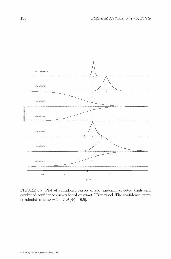
130 Statistical Methods for Drug Safety
4202−4−
Log OR
confiden
ce c
urv
e
[
#study−04
[ ]
#study−08
[ ]
#study−15
[
#study−16
]
#study−25
][
#study−30
[ ]
#combined.cv
FIGURE 6.7: Plot of confidence curves of six randomly selected trials andcombined confidence curves based on exact CD method. The confidence curveis calculated as cv = 1− 2|H(Ψ)− 0.5|.
© 2016 by Taylor & Francis Group, LLC

7
Ecological Methods
“Literature is my legal wife and medicine my mistress. When I get tired ofone, I spend the night with the other.”
(Anton Pavlovich Chekhov (1860-1904), Russian author, playwright)
7.1 Introduction
Ecological methods investigate group level aggregate data. These methods aremotivated mainly due to the relative low cost and convenience of the data,limited availability of individual-level data, design limitations of individualstudies, interest in ecologic effect, and simplicity of analysis and presentation(Morgenstern 1995). For very rare events (e.g., death by suicide) that occurat rates on the order of 1 in 10,000, there may be few options for routine drugsurveillance. One approach is to use ecological data that attempt to relatechanges in prescription rates of particular drugs or classes of drugs to theAE rate of interest. These more global associations clearly do not supportcausal inferences, but can be hypothesis generating and help support infer-ences drawn from other studies, in some cases based on surrogate endpoints(e.g., suicide attempts and/or ideation). In some cases, natural experimentssuch as a black box warning provide an opportunity to evaluate the positive ornegative consequences of decreased access to the drug on the event of interest.Here we may compare national rates of the AE before and after the publichealth warning, to determine if the warning has had the anticipated effect. Ifthe warning is specific to a strata of the population, comparison of changes inthat strata versus those for which the warning did not apply provides strongerinferences.
The traditional approach to ecological analysis typically involves eitherlog-linear or Poisson regression analysis of rates over time, using exposurebased on prescription rates during the same time-period. Serial correlation canbe accommodated using Huber-White robust standard errors that allow forarbitrary autocorrelation pattern (Huber 1967,White 1980, 1982).Where datafrommultiple countries are combined, both fixed-effects (Ludwig and Marcotte2005) and random-effects models (Hedeker and Gibbons 2006) can be used to
131
© 2016 by Taylor & Francis Group, LLC
132 Statistical Methods for Drug Safety
allow each country to have its own linear time trend. For the fixed-effects log-linear model, weighted least squares can be used to adjust for heterogeneityin the residual errors, using each country’s population as a weight. A similarapproach can be taken using a mixed-effects Poisson regression model whereeach country’s population is used as an offset (see Hedeker and Gibbons 2006).
A more informative approach was suggested by Goldsmith et al. (2002)in which AE rates are stratified by demographic characteristics such as age,race, and sex within counties, and a mixed-effects Poisson regression model isused to analyze the data, treating the county as the unit of analysis. Countypopulation is used as an offset in the Poisson regression model. To evaluatedrug-AE interactions, county-level prescription rates of the drug or drugs canbe added to the model to determine if changes in prescription rates are as-sociated with changes in the AE rate. When longitudinal data are available,we can tease apart between-county effects from within-county effects by ex-pressing prescription rates as two variables, one of the mean over time andthe other for the yearly deviations from the mean (also see Chapter 10). Theformer provides an estimate of the between-county effect whereas the latterprovides an estimate of the within-county effect. Both within-county drug ef-fect can be treated as a random-effect in the model, so that the relationshipbetween prescription rates and AE rates can vary from county to county (i.e.,treatment heterogeneity). The methodology has been described in detail byGibbons et al. (2005, 2006).
7.2 Time Series Methods
Post marketing surveillance of therapeutic drugs involves continuous monitor-ing of safety data over a period of time. A sequence of data points, typicallyrate of adverse events per unit utilization of drugs at the population level,are aggregated at successive fixed time intervals (e.g., each quarter). Theseaggregate data represent the average incidence of adverse events during a par-ticular time period. Time series data are naturally generated when drugs aremonitored for safety outside the controlled environment of clinical trials.
Let yt be the number of ADR cases observed over tth time interval. Assume,that the drug utilization during the tth time period is nt. The drug utilizationcan be measured directly as the number of individuals exposed to the drug,or using other proxy measures such as number of pills dispensed, numberof prescriptions written, number of patients with a relevant condition, etc.Obviously, the validity of estimates and inference of safety depends on theaccuracy and relevance of such proxy measures.
The visual display of rates over the monitoring period provides valuableinsight into the trends of ADRs. Since 1990, numerous jurisdictions in theUnited States (US) have reported increases in drug poisoning mortality. Dur-
© 2016 by Taylor & Francis Group, LLC

Ecological Methods 133
ing the same time period, the use of opioid analgesics has increased markedlyas part of more aggressive pain management. The study by Paulozzi et al.(2006) documented a dramatic increase in poisoning mortality rates. Figure7.1 is the time series plot of unintentional opioid drug poisoning mortalityrates from 1979 to 1998. The figure shows increasing trend in mortality raterelated to opioid poisoning. In this example, the trend is clearly visible with-out any further statistical aids. Smoothing techniques are used when trendsare not apparent. A common method for obtaining the trend is to use lin-ear filters on a given time series. A simple class of linear filters are movingaverages with equal weights:
Tt =1
2a+ 1
a∑
i=−ayt+i.
79 81 83 85 87 89 91 93 95 97
2040
6080
100
Years
Dea
th r
ate
per
10
million
ObservedMA (a=3)
FIGURE 7.1: Unintentional opiate drug poisoning mortality rate.
The filtered value of a time series at a given period t is represented bythe average of the values yt−a, . . . , yt, . . . , yt+a. The smoothed line obtainedby the moving average is more helpful in visualizing trends when high resolu-tion data are available. Regression models can also be used to fit parametric
© 2016 by Taylor & Francis Group, LLC

134 Statistical Methods for Drug Safety
models to time series data. A natural candidate model for the time seriesof counts taking non-negative integer values is the Poisson regression. ThePoisson regression model for the event count on the tth time period is
ln(λt) = ln(exposuret) + β1t+ β′xt, (7.1)
where β is a vector of regression coefficients, and xt is a vector of covariates.The parameters of the model (7.1) are easily estimated by likelihood methods.The model can be used to estimate deterministic trend in the observed dataas in Figure 7.2. However, the model is not appropriate for inference becausethe model requires observations to be i.i.d Poisson random variable. Timeseries data most certainly violate the i.i.d assumption. The successive obser-vations are more likely to be correlated in time series data that induces over-or under-dispersion in count data. Methods have been developed to allow forboth over- or under-dispersion in the Poisson model.
79 81 83 85 87 89 91 93 95 97
2040
6080
100
Years
Dea
th r
ate
per
10
million
Observedfitted
FIGURE 7.2: Unintentional opiate drug poisoning mortality rate.
© 2016 by Taylor & Francis Group, LLC

Ecological Methods 135
7.2.1 Generalized Event Count Model
The time series count data in ecological investigation of drug safety are sel-dom serially correlated. However, the count data are either under- or over-dispersed. Over-dispersion arises due to unobserved heterogeneity and conta-gion effects. In such situations, pure time series methods may not be necessaryto model the count data. When the nature of dispersion is known, a specificdistribution can be used to allow such dispersion. For example, a negative-binomial model is used to allow for over-dispersion. Under-dispersion, on theother hand, can occur due to a negative contagion. Truncated event countmodels with a reparameterized binomial distribution is a possible alternativeto deal with under-dispersion. In order to choose an appropriate model, oneneeds to conduct a test to determine the type of dispersion. Furthermore,the incorrect choice among the different alternatives can lead to inconsistencyas well as inefficiency. The generalized event count distribution overcomesthe model selection issue. The generalized event count distribution is a twoparameter probability distribution with the following log-likelihood function(King 1989):
lnL(λi, σ2|yi) = Ci − yiln(σ
2) +
yi∑
j=1
ln[λi + (σ2 − 1)(j − 1)], (7.2)
where
Ci =
−eλi for σ2 = 1−eλi ln(σ2)(σ2 − 1)−1 for σ2 > 1−eλi ln(σ2)(σ2 − 1)−1 − ln(Di) for 0 < σ2 < 1,
Di =
(−λiσ2
−1+1
)
∑
m=0
Γ(
−λi
σ2−1 + 1)
yi!Γ(
−λi
σ2−1 − yi + 1)(1− σ2)yi(σ2)
−λiσ2
−1−yi .
The maximization of this log likelihood function with respect to the twoparameters gives estimates of λ and σ2 without specifying whether the dataare over-, under-, or Poisson dispersed. The log-likelihood in (7.2) reduces toa Poisson log-likelihood for σ2 = 1, to a negative-binomial for σ2 > 1, and toa reparameterized binomial for 0 < σ2 < 1. Regression parameters, as usual,are estimated by modeling λi = exp(x′
iβ).
7.2.2 Tests of Serial Correlation
As indicated in the previous section, in the absence of serial correlation, astatic regression with variance adjusted for over- or under-dispersion is ade-quate for both estimation and inference. Formal hypothesis testing methodsare available to ascertain significance of the observed serial correlation. Thesetests can indicate if any time series corrections are necessary. Let zt denote
© 2016 by Taylor & Francis Group, LLC

136 Statistical Methods for Drug Safety
the standardized residual from a static Poisson regression model such thatzt =
yt−λt√wt
, where λt = λ(xt,β), wt = (λt, α), and α is a dispersion param-
eter. The residuals are standardized so that zt have asymptotically constantvariance. Following Box-Jenkins modeling in the continuous case, the esti-mated autocorrelation ρk at lag k is given by (Cameron and Trivedi 2013):
ρk =
∑Tt=k+1 ztzt−k∑T
t=1 z2t
. (7.3)
The overall test for serial correlation that guards against incorrect standard-ization is
Tk =
∑Tt=k+1 ztzt−k√∑Tt=k+1 z
2t z
2t−k
. (7.4)
Tk is asymptotically distributed as N [0, 1] under the null hypothesis thatρj = 0, j = 1, . . . , k. The related overall test for serial correlation is basedon the sum of the first l squared Tk statistics. The statistic is known as theBox-Pierce portmanteau statistic (TBP ).
TBP =
l∑
k=1
(Tk)2 (7.5)
TBP is asymptotically χ2(l) under the null hypothesis of no serial correlationup to lag k.
After removing deterministic trend, the test for serial correlation at lagk = 2 for opioid drug poisoning mortality data shows a statistically non-significant result (Tk = 1.59, p = 0.44). Therefore, static regression allowingfor over-dispersion is sufficient for further inferential analysis.
7.2.3 Parameter-driven Generalized Linear Model
The model described in the previous section can help solve the problem of over-dispersion in ecological count data. The explicit assumption in those modelsis that the observations are independent. The presence of significant serialcorrelation violates the independence assumption. Zeger (1988) presented aparameter-driven model in which autocorrelation is introduced through la-tent process ǫt. A sequence of event counts yt is assumed to be independentconditional on this latent process. The mean and variance of yt is given by
ut = E(yt|ǫt) = exp(x′tβ)ǫt, wt = var(yt|ǫt). (7.6)
The latent process ǫt is assumed to be a stationary process with expected valueof 1, variance σ2 and covariances cov(ǫt, ǫt−k) = ρkǫσ2 for 0 ≤ k ≤ T −1. Thenthe unconditional moments of yt are given by
µt = E(yt) = exp(x′tβ), var(yt) = µt + σ2µ2
t . (7.7)
© 2016 by Taylor & Francis Group, LLC

Ecological Methods 137
An estimating equation based on quasi-likelihood is used to obtain the con-sistent estimates of β. For independent data, the estimate of β is the root ofthe following estimating equation Zeger et al. (1988):
U(β) =∂µ′
∂βV −1(y − µ) = 0. (7.8)
The V is a T × T diagonal matrix. However, for time series data, V willinclude off-diagonal elements such that V = A+ σ2ARǫA, where
A =
µ1 0 . . . 00 µ2 . . . 0...
.... . .
...0 0 . . . µT
,
and
Rǫ =
1 ρǫ(1) ρǫ(2) . . . ρǫ(T − 1)ρǫ(1) 1 ρǫ(1) . . . ρǫ(T − 2)...
......
. . ....
ρǫ(T − 1) ρǫ(T − 2) ρǫ(T − 3) . . . 1
.
The solution of (7.8) requires the inversion of V which is a T × T matrix. Tosimplify the computation, Zeger (1988) proposed a modification in which theactual autocorrelation matrix Rǫ is approximated by a band diagonal matrixof a finite autoregressive process of a given order. If S = diag(µt + σ2µt),
then V is approximately V R = S1/2R(ρ)S1/2. The inverse of V R is easilyobtained by decomposing R(ρ), such that
V −1R ≈ S−1/2L′LS−1/2,
where L is a matrix that applies a linear filter to the data. For example, inthe case of pth-order autoregressive process
Ltyt = yt − ρ1yt−1 − . . .− ρkyt−k for k < t.
Thus, L is a (T − k)× T matrix. To further illustrate the form of L, supposek = 2. Then
L =
−ρ2 −ρ1 1 0 . . . 00 −ρ2 −ρ1 1 . . . 0...
......
.... . .
...0 0 . . . −ρ2 −ρ1 1
.
The estimate of β is obtained using an iterative algorithm. Following theiterative least-squares procedure, estimates of β at the (p + 1)th iteration of
© 2016 by Taylor & Francis Group, LLC

138 Statistical Methods for Drug Safety
the process are given by
βp+1 =
(LS−1/2 ∂µ
∂β′
)′(LS−1/2 ∂µ
∂β′
)−1(LS−1/2 ∂µ
∂β′
)′ (LS−1/2Z
),
(7.9)
where Z =(∂µ∂β′
)β + (y − µ) and the right-hand side is evaluated using βp
for β. Then, the asymptotic variance-covariance matrix of β is given by Zeger(1988) as:
VβR= I−1
0 I1I−10 , (7.10)
where I0= limn→∞
(∂µ′
∂βVR
−1 ∂µ
∂β/n
)and I1= lim
n→∞
(∂µ′
∂βV
R
−1V VR−1 ∂µ
∂β/n
).
The marginal mean µt of the generalized log-linear parameter-driven modelin this section does not depend on the latent process. Therefore, the inter-pretation of regression coefficients do not depend on assumptions about theunobservable process, ǫt. The variance function of the model has the negative-binomial form which allows over-dispersion relative to the Poisson. The degreeof over-dispersion depends on the marginal mean µt.
7.2.4 Autoregressive Model
The serially correlated error model is a special case of an autoregressive mov-ing average model. The serial correlation in errors implies that yt has a mov-ing average representation. A straightforward way of specifying a time seriesmodel is to specify lagged dependent variable in a log-linear model where theconditional mean is exp(x′tβ + ρyt−1) . The model, however, is explosive forρ > 0 (Cameron and Trivedi 2013). Zeger and Qaqish (1988) introduced thefollowing more natural multiplicative model
µt|t−1 = exp(x′tβ + ρ lny∗t−1) (7.11)
without specifying any distributional assumption. Assumptions are made onlyon first and second conditional moments. The y∗t−1 is a transformation of yt−1
defined as eithery∗t−1 = max(c, yt−1), 0 < c < 1
ory∗t−1 = yt−1 + c, c > 0
so that yt−1 = 0 is not an absorbing state. The model can be broadened byconsidering an AR(1) error model
µt|t−1 = exp(x′tβ + ρ(ln y∗t−1 − x′
t−1β))
= exp(x′tβ)
(y∗t−1
x′t−1β
)ρ. (7.12)
© 2016 by Taylor & Francis Group, LLC

Ecological Methods 139
Further, the conditional variance of the response is assumed to be
V ar(yt|t− 1) = υt = φV (µt|t−1), (7.13)
where φ is an unknown dispersion parameter, and V (µt|t−1) is a variancefunction. The model (7.12) can be further generalized as follows (Zeger andQaqish 1988) :
µt|t−1 = exp
(x′tβ +
q∑
i=1
θiln y∗t−1 − x′t−1β
). (7.14)
Let γ ′ = (β′, θ′) and assume that c is known. The parameters of model (7.14)can be estimated by a quasi-likelihood approach (McCullagh and Nelder 1989).The estimate γ is the root of the log-QL estimating equation
U(γ) =
T∑
t=1
∂µt|t−1
∂γυ−1t (yt − µt|t−1)
=
T∑
t=1
Zt(yt − µt|t−1) (7.15)
where Z ′t =
(x′t, (ln y
∗t−1 − x′
t−1β), . . . , (ln y∗t−q − x′
t−qβ)). Equation (7.15)
has the form of generalized linear model score function. The difference isthat Z ′
t depends on unknown parameters. Consequently, a second level ofiteration is necessary to solve (7.15) using an iteratively re-weighted least-squares approach. Note that µt|t−1 can be expressed as follows:
µt|t−1 = exp
(x′tβ +
q∑
i=1
θiln y∗t−1),
where xt = xt−∑qi=1 θixt−q is a time-filtered version of xt. Hence, the model
parameters can be estimated by regressing yt on xt and ln y∗t−1. The following
iteration is suggested by Zeger and Qaqish (1988):
1. Given θ(k)
, calculate xt and let Dt = (ln y∗t−1, . . . , ln y∗t−q).
2. Estimate β(k+1)
, the coefficients for calculating x(k)t , and θ
(k+1),
the coefficients for Dt, using iteratively re-weighted least squares.
3. Repeat steps 1 and 2 to convergence of parameter estimates (ordeviance).
If c is unknown, then it can be considered as an additional parameter to beestimated. The previous algorithm requires an additional step to solve for c.
After step 2 the following estimating equation is solved for c(k+1) given β(k+1)
and θ(k+1)
.
U(γ) =T∑
t=1
wt(c)[yt − µt|t−1] = 0, (7.16)
© 2016 by Taylor & Francis Group, LLC

140 Statistical Methods for Drug Safety
where γ = (β′, θ′, c), wt(c) =∑qi=1 θiI(yt−i < c) and I(.) is the indicator
function. Under regularity conditions for the conditional density of yt|Dt andconditional on Dt √
T (γ − γ)T→∞→ N(0,V −1),
where
V = limn→∞
1
n
T∑
i=1
ZtZ′tυt.
The scale parameter φ appearing in (7.13) can be estimated consistently by
φ =
∑Ti=1 r
2t
T − p,
where p is a number of elements in γ, and rt denotes Pearson residuals, whichare defined by
rt =yt − µt|t−1√V (µt|t−1)
,
for t = 1, . . . , T . Held et al. (2005) have argued that the introduction ofparameter c and the regularization of past counts yt−1 through their expectedvalues in the model equation (7.12) is slightly unnatural. They proposed adifferent approach where previous counts act directly on the conditional meanµt|t−1. Thus, the new model is now
µt|t−1 = exp(x′tβ) + ρyt−1. (7.17)
The model can be easily reformulated to include seasonality and temporaltrend as follows:
µt|t−1 = exp(β0 + β1t+
S∑
s=1
(βssin(ωst) + γscos(ωst)) + ρyt−1, (7.18)
where the Fourier frequencies ωs are ωs = 2sπ/S. The model parameters canbe easily estimated by maximum likelihood method using generic optimizingroutines, e.g., the optim() function in the R software. The Poisson model canbe replaced with negative-binomial model to allow for over-dispersion. Themean structure of negative-binomial model remains the same as in (7.17) butthe variance σt increases to
σt = µt + µt/ψ,
with the additional parameter ψ > 0.
© 2016 by Taylor & Francis Group, LLC

Ecological Methods 141
7.3 State Space Model
A state space representation of time series specifies a measurement and tran-sition equation. State space methods offer a unified approach to a wide rangeof models and techniques. It relates observations yt, t = 1, 2, . . ., on a responsevariable Y to unobserved “states” or “parameters” αt by an observation modelfor yt given αt. For event counts, the measurement equation is an event-countdistribution, while the transition equation describes how the dynamics of theevent count distribution parameters evolves. A number of state space modelshave been proposed for count data. These models have been limited by un-availability of software for easy implementation and difficulty in interpretationof the model coefficients. A variant of state space model called the PoissonExponentially Weighted Moving Average Model (PEWMA) is a simple andfast method for modeling persistent event count time series (Brandt et al.2000). The measurement equation in PEWMA describes how the observednumber of events arises as a function of a mean number of events in the past.The state equation describes the importance of past events for predicting thenumber of events in the current period. After specifying a model in state spaceform, the Kalman filter is used to estimate the model parameters.
PEWMA assumes that the observed counts at time t are drawn from aPoisson marginal distribution, i.e.,
Pr(yt|µt) =[µytt exp(−µt)
yt!
]. (7.19)
The unobserved mean µt is parameterized by the multiplicative equation
µt = µ∗t−1exp(x
′tβ), (7.20)
where β is a K×1 vector of coefficients and x′t a 1×K vector of covariates. A
time varying component µ∗t−1 is a smoothed mean of the previous observations
and is estimated by the Kalman filter. The covariate vector x′t does not include
a constant. Including a constant allows for the introduction of a deterministictrend in the model. The stochastic mechanism for the transition from µt−1 toµt is described by following multiplicative transition equation (Brandt et al.2000):
µt = exp(rt)µt−1ηt, (7.21)
where ηt ∼ Beta (ωat−1, (1 − ω)at−1) with E(ηt) = ω for 0 < ω < 1. Theparameter ω captures discounting in the conditional mean function for theevent counts. The parameter rt describes the growth in the series and insuresthat µt > 0. To identify the model, a gamma prior distribution is specified forµt−1, such that
Pr(µ∗t−1; at−1, bt−1) =
exp(−bt−1µ∗t−1)µ
∗t−1
at−1−1bat−1
t−1
Γ(at−1). (7.22)
© 2016 by Taylor & Francis Group, LLC

142 Statistical Methods for Drug Safety
Using these assumptions, the joint predictive density, conditional on Yτ forobservations yτ+1, . . . , YT is (see Brandt et al. 2000):
Pr(yτ+1, . . . , YT ) =T∏
t=τ+1
Pr(yt|Yt−1)
=
T∏
t=τ+1
∫ ∞
0
Pr(Yt|µt)Pr(µt|Yt−1). (7.23)
It is a negative-binomial distribution of the form Pr(k, r, p) = Γ(k+r)k!Γ(r) p
k(1−p)rwith k = yt, r = ωat−1, and p = (1 + ωbt−1e
−x′
tβ−rt)−1. The log-likelihoodfunction for unknown parameters based on predictive density in (7.23) is
ln L(ω,β|at−1, bt−1, yt, Xt)
=T∑
τ+1
ln Γ(yt + ωat−1)− ln(yt!)
−lnΓ(ωat−1) + ωat−1ln (ωbt−1exp(−x′tβ − rt))
−(ωat−1 + yt)ln (1 + ωbt−1exp(−x′tβ − rt)) . (7.24)
The estimates of parameters and hyper-parameter is obtained by maxi-mizing (7.24) with respect to ω and β. The maximization require analyticalexpression of at−1, bt−1 and rt which are calculated using the Kalman fil-ter. The Kalman filter for PEWMA is defined by following recursive systembeginning with starting values of at−1 and β.
rt = Ψ(at−1)−Ψ(ωat−1),where Ψ is the digamma function
at|t−1 = ωat−1 and bt|t−1 = ωbt−1exp(−x′tβ − rt)
at = at|t−1 + yt and bt = bt|t−1 + 1.
7.4 Change-point Analysis
The goal of pharmacovigilance is to identify the change in the incidence ofadverse drug reaction in a timely manner. The change-point analysis is theprocess of detecting distributional changes within time-ordered observations ofadverse event rates. In the simplest case of a single change-point, the problemis to determine the unknown location of time point τ where the change hasoccurred. More formally, an ordered sequence of observations y1, . . . , yτ and
© 2016 by Taylor & Francis Group, LLC

Ecological Methods 143
yτ+1, . . . , yT are assumed to follow two distinct models. The change-point anal-ysis can determine whether the rate of adverse events has changed (elevated)during the life span of the drug. If such change has occurred, the change-pointanalysis identifies the approximate time of increase in incidence rate. In morecomplex situations, change may occur in multiple locations and/or multipleparameters during a long period of observation. A change-point analysis isperformed only after all the data have been collected. Therefore, some way toidentify that the change has occurred is needed. Traditionally, control chartsare used to detect changes. Recently, sequential testing methods have beenused for vaccine surveillance. We begin by describing a Shewhart type controlchart known as u-chart.
7.4.1 The u-chart
A u-chart is an attribute control chart used for monitoring the percent ofsamples having the condition, relative to either a fixed or varying samplesize. U-charts show how the process, measured by number of ADRs amongpopulation at risk per observation period, changes over time. This chart plotsthe rate of ADR for each period as a point on a line. The horizontal linesare drawn at the mean number of ADRs and at the upper and lower controllimits. However, for ADR monitoring the lower limit is usually set to 0. Thedistribution of the number of ADRs is assumed to be Poisson with mean equalto λ. This assumption is the basis for calculating the upper and lower controllimits. The control limits are calculated as:
UCL = λ+ 3√λ
CL = λ
LCL = λ− 3√λ,
where UCL, CL, and LCL denote the upper control limit, control limit, and thelower control limit. In doing so, the adequacy of the normal approximationto the Poisson distribution is assumed. Additionally, it is assumed that astandard value for λ is available. In absence of standard λ, it may be estimatedfrom the set of baseline observations. Let Y be the number of ADRs in thepopulation at risk of n before the drug exposure. Then, the parameters of ucharts are:
UCL = y + 3
√y
nCL = y
LCL = y − 3
√y
n,
where y represents the observed average rate of ADRs in the baseline data. To
© 2016 by Taylor & Francis Group, LLC

144 Statistical Methods for Drug Safety
improve the performance of the u-chart, modification of the above parametersbased on Cornish-Fisher expansion has been suggested. However, improvementachieved by such modification has not been substantiated especially for theincrease in rate parameter.
We illustrate the u-chart by using Paulozzi et. al (2006) data. The authorscommented that various states reported up to three fold increase in opiatedeaths from 1990 to 2001. They linked the increase in reported opioid deaths tochange that occurred in the way US health professionals managed chronic painduring roughly the same time. The general belief among professionals that therisk of addiction should not prevent the use of prescription opioid analgesicsto manage chronic, non-malignant pain led them to acknowledge that opioidanalgesics had a legitimate and important role in managing chronic pain. Theauthors speculated that this change in thinking probably contributed to thedramatic increase in prescriptions written for opioid analgesics from 1990 to2002. We chart the opioid mortality data from 1979 to 2001 to see when theu-chart raises the alarm signaling “out of control” death rate. Figure 7.3 showsthat the u-statistics exceed the UCL around 1992.
FIGURE 7.3: Unintentional opiate drug poisoning mortality rate.
The u-chart is plotted based on only the current observation, which makesit insensitive to small changes. Therefore, alternatives like the exponentiallyweighted moving average (EWMA) control chart have been proposed thatconsider past information. In addition, the observations in time series are often
© 2016 by Taylor & Francis Group, LLC

Ecological Methods 145
serially correlated. In order to address these issues, Weiss proposed variationof EWMA chart (Weiss and Testik 2009, Weiss 2011) and CUSUM chart fora Poisson INAR(1) process.
7.4.2 Estimation of a Change-point
Let y1, . . . , yT be a sequence of independent observations following a Poissondistribution with means λt for t = 1, 2, . . . , T . Here, T is either the timewhen the “out of control” signal has been given or the monitoring has beenterminated for some other reason. The detection of a step change-point isequivalent to testing the following hypothesis:
H0 : λ1 = λ2 = . . . = λτ = λ; vs. H1 : λτ+1 = λ2 = . . . = λT = λ′. (7.25)
Chen and Gupta (2011) describe an intuitive method to estimate change-pointτ by treating the problem of testing the change-point hypothesis as a modelselection problem. They described their method as follows. Under the H0, themaximum likelihood function is given by
L0(λ) =exp(−τλ)λ
∑τt=1 yt∏τ
t=1 yt!,
where λ = MT , with M =
∑Tt=1 yt. Therefore, the Schwartz information crite-
rion under H0 (SIC0)is given by
SIC0 = −2logL0(λ) + log T
= 2M − 2M log
(M
c
)+ 2log
T∏
t=1
yt! + logT.
Under H1, the maximum likelihood function is given by
L1(λ, λ′) =
τ∏
t=1
exp(−λ)λytyt!
T∏
t=τ+1
exp(−λ′)λ′yt
yt!
=exp(−τλ)λ
∑τt=1 yt∏τ
t=1 yt!
exp(−(T − τ)λ′)λ∑T
t=τ+1 yt
∏Tt=τ+1 yt!
,
where λ = Mτ
τ and λ′ =M ′
τ
T−τ with M ′τ with Mτ =
∑τt=1 yt and M ′
τ =∑Tt=τ+1 yt. Therefore, the Schwartz information criterion under H1(SIC1) is
given by
SIC1 = −2logL1(λ, λ′) + 2log T
= 2Mτ −Mτ logMτ
τ+ 2M ′
τ −M ′τ log
M ′τ
T − τ× 2log
T∏
t=1
yt! + 2log T.
© 2016 by Taylor & Francis Group, LLC

146 Statistical Methods for Drug Safety
According to Schwarz criterion, the model with the lower value of SIC ispreferred. Based on this principle, we reject H0 if
SIC0 > min1≤τ≤T−1
SIC1(τ)
or
min1≤τ≤T−1
[Mlog
M
T−Mτ log
Mτ
τ−M ′
τ logM ′τ
T − τ
]<
1
2log
1
T.
The resulting estimate of change-point location τ is
[τ = argmin
1≤τ≤T−1SIC1(τ).
](7.26)
For the time sequence with multiple change-points, a method known asbinary segmentation procedure is widely used to determine the number andlocation of change-points. A general description of the binary segmentationtechniques is summarized in Chen and Gupta (2011). The steps involved inthis iterative process are as follows:
1. Test for a single change-point hypothesis as in 7.25. If H0 is notrejected then stop as there is no change-point. Otherwise, go to thenext step.
2. Divide the sequence of observations at y1, y2, . . . , yT into two sub-sequences where change-point τ is detected in 1. The two subse-quences are y1, y2, . . . , yτ and yτ+1, y2, . . . , yT .
3. Test for a single change-point hypothesis within each subsequence.
4. Repeat the process until no further subsequences have change-points.
5. The collection of change-point locations found by 1–4 are denoted byτ1, τ2, . . . , τq, where q is the estimated number of change-points.
The binary segmentation procedure identifies three change-point locations inthe opioid death data. The detected change-points are at 1991, 1993 and 1994.The change-point detection method presented so far does not allow serialdependence and assumes step change in the rate parameter. These methodsmay not be sufficient when observations are correlated or there is a change intrend.
7.4.3 Change-point Estimator for the INAR(1) Model
The INAR(1) model is defined as
Yt = α Yt−1 + ǫt,
where ǫt are i.i.d according to Poisson(λ) and Y0 ≈ Poisson(λ/(1−α)). Basedon the model, the Yt comprise a stationary Markov chain with marginal dis-tribution Poisson(λ/(1−α)) whose conditional distribution can be written as
© 2016 by Taylor & Francis Group, LLC

Ecological Methods 147
(see Al-Osh and Alzaid 1987):
f(yt|yt−1) = exp(−λ)(yt−1!)C(yt−1, yt), (7.27)
where C(xt−1, xt) =∑k=0m
αk(1−α)xt−1−kλxt−k
k!(xt−k)!(xt−1−k)! and m = min(xt, xt−1). The
likelihood function of an INAR(1) model in terms of conditional distributionsof each observation is expressed as
fy0,...,yT (yt, . . . , yT |α, λ) = fy0(y0)fy1|y0(y1|y0)T∏
t=2
fyt|yt−1(yt|yt−1). (7.28)
The INAR(1) model depends on the rate parameter λ and the dependenceparameter α. A change can occur on either parameters during the course ofobservation. Torkamani et al. (2014) have developed a method to estimatechange-point in each of these two parameters. It is assumed that the changeoccurs as a step function at the (τ + 1)th observation.
7.4.3.1 Change-point Estimator for the Rate Parameter
Torkamani et al. (2014) suggested estimating the rate parameter assumingthe same α before and after the change-point. The baseline ADR rate λ0 anddependence parameter α are assumed to be known quantities. A new value ofthe rate parameter is denoted by λ1. Then, the log-likelihood function of thisprocess with a change-point at τ is obtained as (see Torkamani et al. 2014)
l(λ1, τ |y) =−λ0
(1− α)+ ln
[(λ0/(1− α))y0
y0!
]+
τ∑
t=1
ln(yt−1!)− τ(λ0)
+
τ∑
t=1
ln [Cλ0(yt−1, yt)] +
T∑
t=τ+1
ln(yt−1!)− (T − τ)(λ1)
+
T∑
t=τ+1
ln [Cλ1 (yt−1, yt)] . (7.29)
The unknown parameters λ1 and τ can be estimated by maximizing the log-likelihood function in equation (7.29). As, τ is a discrete variable with knownfinite values, a maximum log-likelihood can be calculated for each possiblevalue of τ . Thus, for a given value of τ , the first derivative of the log-likelihoodwith respective to λ is
∂l(λ1, τ |y)∂λ1
= −(T − τ) +
T∑
t=τ+1
Cλ1(yt−1, yt − 1)
Cλ1(yt−1, yt). (7.30)
A closed-form solution does not exist for the equation in (7.30). Therefore,
© 2016 by Taylor & Francis Group, LLC

148 Statistical Methods for Drug Safety
an estimate of λ1 is obtained using the Newton-Raphson method, which re-quires expression for second derivative. The expression for second derivativeis given in Torkamani et al. (2014) as follows:
∂2l(λ1, τ |y)∂λ21
=
T∑
t=τ+1
Cλ1(yt−1, yt − 2)Cλ1(yt−1, yt)− Cλ1(yt−1, yt − 1)2
Cλ1 (yt−1, yt)2.
(7.31)An estimate of λ1 is obtained by iteratively solving
λk+11 = λk1 − ∂l(λ1, τ |y)
∂λ1
[∂2l(λ1, τ |y)
∂λ21
]−1
.
The procedure starts with initial value λ01 = λ0 and is terminated when |λk+11 −
λk1 | < ν, where ν is a pre-specified convergence criterion.
TABLE 7.1: Example to Estimate the Change-Point in Opioid Mortality DataWhen λ0 = 15.0
year yt t λ1(t) loglik1979 151980 14 1 16.303 -109.5681981 18 2 17.110 -108.5651982 24 3 17.749 -107.5921983 22 4 18.230 -106.8511984 27 5 19.155 -105.0681985 36 6 19.787 -103.9441986 39 7 20.039 -103.8531987 25 8 20.599 -103.0391988 33 9 22.426 -98.94341989 39 10 23.255 -97.87281990 37 11 24.184 -96.76961991 34 12 26.054 -93.36351992 50 13 28.726 -88.33691993 66 14 29.258 -90.73691994 66 15 28.902 -95.18541995 80 16 31.208 -94.22491996 77 17 30.346 -99.68841997 87 18 34.845 -98.74671998 98 19 36.867 -103.497
Table 7.1 shows the result of applying this method to the opioid mortalitydata. The estimate of new rate parameter at each potential change-point isshown on the λ1(t) column and the corresponding value of the likelihoodfunction is shown in the next column. The value of t that maximizes the log-likelihood (-88.33) indicates the estimated time of change at 13th (year 1991)observation.
© 2016 by Taylor & Francis Group, LLC

Ecological Methods 149
7.4.3.2 Change-point Estimator for the Dependence Parameter
The dependence parameter can be estimated by following a similar procedure.The time-ordered sequence of observations is assumed to have baseline depen-dence parameter value of α0. The rate parameter is assumed to remain con-stant at λ. Assuming that the dependence parameter changes at the (τ +1)thobservation, the log-likelihood function can be written as (Torkamani et al.2014, see):
l(α1, τ |y) =−λ
(1− α0)+ ln
[(λ/(1− α0))
y0
y0!
]+
τ∑
t=1
ln(yt−1!)− τ(λ)
+
τ∑
t=1
ln [Cα0(yt−1, yt)] +
T∑
t=τ+1
ln(yt−1!)− (T − τ)(λ)
+T∑
t=τ+1
ln [Cα1(yt−1, yt)] . (7.32)
The partial derivative of the log-likelihood function with respect to α1 is
∂l(α1, τ |y)∂α1
=
T∑
t=τ+1
(xt − α1xt−1)− λ[Cα1(yt−1, yt − 1)/Cα1(yt−1, yt)]
α1(α1 − 1). (7.33)
A closed-form solution does not exist for the equation 7.33. A second partialderivative is needed to implement the Newton-Raphson method to obtain theMLE. Torkamani et al. (2014) provided an expression of the second partialderivative as follows:
∂2l(α1, τ |y)∂α2
1
=
T∑
τ+1
−yt−1[α1(1 − α1)]− (1− 2α1)(yt − α1yt−1)
[α1(1− α1)]2
+(1− 2α1)λ
[α1(1− α1)]2× Cα1(yt−1, yt − 1)
Cα1(yt−1, yt)− λ
α1(1− λ1)
× C′α1(yt−1, yt − 1)Cα1(yt−1, yt)− C′
α1(yt−1, yt)Cα1(yt−1, yt − 1)
[Cα1 (yt−1, yt)]2,
where
C′α1(yt−1, yt) =
m∑
k=0
αk(1− α)xt−1−kλxt−k
k!(xt − k)!(xt−1 − k)!
[k
α1+yt−k − k
1− α1
].
As stated previously, these methods are used in combination with a controlchart (e.g., c-EWMA). Therefore, weaknesses inherent in such control chartsalso apply to the change-point analysis described in this section. For small
© 2016 by Taylor & Francis Group, LLC

150 Statistical Methods for Drug Safety
TABLE 7.2: Change-Point Estimate for Dependence Parameter
year yt t α1(t) loglik1979 151980 14 1 0.504 -131.8171981 18 2 0.519 -131.6551982 24 3 0.529 -131.4231983 22 4 0.538 -131.1341984 27 5 0.556 -130.3591985 36 6 0.567 -129.7671986 39 7 0.573 -129.411987 25 8 0.585 -128.7281988 33 9 0.629 -125.1871989 39 10 0.640 -124.2031990 37 11 0.653 -123.0861991 34 12 0.681 -120.3231992 50 13 0.716 -116.3911993 66 14 0.719 -116.7361994 66 15 0.714 -118.7361995 80 16 0.742 -117.8771996 77 17 0.730 -121.6131997 87 18 0.794 -120.9321998 98 19 0.811 -125.163
changes, simulation results have shown that number of observation elapsedbetween real change and the alert signal from a control chart can be high.The same simulation study has also indicated that the maximum differencebetween the real change time and its estimate is less than 2 in most of thesituations.
For the opioid mortality data, assuming an event rate of 27 death per10,000,000 and baseline α0 = 0.5, the change-point of dependence parame-ter is once again estimated to be at 13th observation. The new value of thedependence parameter is estimated to be 0.716.
7.4.4 Change-point of a Poisson Rate Parameter with LinearTrend Disturbance
The change-point estimating procedure presented so far are designed primarilyfor a step change in the parameter of interest. Perry et al. (2006) proposed anestimator for the change-point of a Poisson rate parameter where the type ofchange is a linear trend. A linear trend occurs when the rate begins to changelinearly from its baseline value over time. Assume that the ADR count of aparticular type is initially distributed as Poisson with known rate λ = λ0.After an unknown point in time τ the rate parameter changes to unknownvalue λ = λt for t = τ + 1, ...., where λi > λ0 and the functional form of λi isspecified as
© 2016 by Taylor & Francis Group, LLC

Ecological Methods 151
λi = λ0 + β(t− τ). (7.34)
The β in the equation (7.34) is the slope of the linear trend disturbance.Assuming an ADR rate change occurred at τ , the likelihood function is givenby
L(τ, β) =
τ∏
t=1
exp(−λ0)λyt0yt!
T∏
t=τ+1
exp[−λ0 + β(t− τ)][λ0 + β(t− τ)]yt
yt!,
(7.35)where, yt is the event count at the tth time point. The MLE of the τ is the valueof τ that maximizes the likelihood in (7.35). The log-likelihood equation isobtained by taking the logarithm of that in (7.35). The log-likelihood functionreduces to the following expression:
logL(τ, β)=K−1
2β(T−τ)(T+1−τ)+log(λ0)
τ∑
t=1
yt+
T∑
t=τ+1
ytlog (λ0 + β(t− τ)) ,
(7.36)whereK is a constant. The partial derivative of (7.36) with respect to β yields
∂logL(τ, β)
∂β= −1
2(T − τ)(T + 1− τ) +
τ∑
t=τ+1
yt(t− τ)
λ0 + β(t− τ). (7.37)
There is no closed form solution for β in equation (7.37). Hence, for a knownvalue of τ , an estimate of β is obtained using Newton’s method. The updatingequation (see Perry et al. 2006) for implementing Newton’s method is
βτ,k+1 = βτ,k −F1
F2(7.38)
where βτ,0 = 0,
F1 = −1
2(T − τ)(T + 1− τ) +
τ∑
τ+1
yt(t− τ)
λ0 + βτ,k(t− τ),
and
F2 = −τ∑
t=1
yt(t− τ)
λ0 + βτ,k(t− τ).
This provides an estimate of β at each τ without requiring an explicit closed-form expression. Denote such an estimate by βτ . A profile likelihood estimateof τ is obtained by substituting βτ , for β in (7.36) over all possible change-points. Hence,
© 2016 by Taylor & Francis Group, LLC

152 Statistical Methods for Drug Safety
τ = argmax1≤τ≤T
[
−1
2β(T − τ )(T + 1− τ ) + log(λ0)
τ∑
t=1
yt +
T∑
t=τ+1
ytlog (λ0 + β(t− τ ))
]
.
(7.39)
Figure 7.4 is a plot of profile log-likelihood for the example data. The base-line event rate is specified as λ0 = 26, which is approximately the average ofthe first 10 data points. A change-point is detected at τ = 10. The exam-ple data exhibit strong positive trend in rate parameter from the beginning.Therefore, the change-point location is highly dependent on the value of thebaseline rate parameter.
FIGURE 7.4: change-point model with trend disturbance for opiate drug poi-soning mortality rate, λ0 = 26.
© 2016 by Taylor & Francis Group, LLC

Ecological Methods 153
7.4.5 Change-point of a Poisson Rate Parameter with Leveland Linear Trend Disturbance
The model can be generalized further to include changes in level as well as thetrend of the rate parameter. The mean function µ(t) = N(t)λ(t) is assumedto be a piecewise continuous function of the index variable t (Pawitan 2014),with unknown regression parameters β = (β1,β2) and the change-point τaccording to
µ(t) =
µ1(t)(t,β1) for t < τµ2(t)(t,β2) for t ≥ τ.
(7.40)
For Poisson regression with jump discontinuity between µ1 and µ2, therate parameters can be modeled as
log (λ(t)) =
β01 + β11t for t < τ
β02 + β12(t− τ) for t ≥ τ.(7.41)
On the other hand, if we want a continuous function of λ(t), then rateparameters can be modeled as
log (λ(t)) =
β01 + β11t for t < τ
β01 + β11τ + β12(t− τ) for t ≥ τ.(7.42)
Regardless of the model for λ(t), the likelihood function for Poisson model isgiven by
L(τ, β) =
τ∏
t=1
exp(−µ1(t,β1))µ1(t,β1)yt
yt!
T∏
t=τ+1
exp(−µ2(t,β2))µ2(t,β2)yt
yt!.
(7.43)The log-likelihood equation is obtained by taking the logarithm of that inequation (7.43).
logL(τ, β) = K+
τ∑
t=1
yt log µ1(t,β1)−µ1(t,β1)+
T∑
t=τ+1
yt log µ2(t,β2)−µ2(t,β2),
(7.44)whereK is a constant. The partial derivative of (7.44) with respect to β yields
∂logL(τ,β)
∂β=
τ∑
t=1
(yt
µ1(t,β1)− 1
)∂µ1(t,β1)
∂β1
+
T∑
t=τ+1
(yt
µ1(t,β2)− 1
)∂µ1(t,β2)
∂β2
.
(7.45)
The equation (7.45) is solved for each value of τ and the likelihood equation
© 2016 by Taylor & Francis Group, LLC

154 Statistical Methods for Drug Safety
is evaluated at the estimated value of β. Since equation (7.45) does not have aclose-form solution, the Newton-Raphson method is commonly used to solveit iteratively. A profile likelihood estimate τ is obtained by choosing
τ = argmax1≤τ≤T
[τ∑
t=1
yt log µ1(t, β1)− µ1(t, β1) +
T∑
t=τ+1
yt log µ2(t,β2)− µ2(t, β2)
].
(7.46)Figure 7.5 shows the profile log-likelihood for the example data based on
model 7.42, with a maximum at τ = 13. The estimated parameters are:
β01 = −13.38 (se = 0.025)
β11 = 0.08 (se = 0.0025)
β12 = 0.12 (se = 0.003).
7.4.6 Discussion
The analytic methods discussed in this chapter are complicated due to thenon-linear nature of the count data. Software for implementing these meth-ods are either available as a stand alone program or as freely available Rpackages. For example, Brandt provides a stand alone R program for thePEWMA model. The Comprehensive R Archive Network has several softwarepackages for change-point analysis. The one that is most relevant to this dis-cussion is the Surveillance package. It provides functions for the modeling anddetecting change-point in time series of counts, proportions and categoricaldata, as well as for the modeling of continuous-time epidemic phenomena.Similarly, the Changepoint package implements various mainstream and spe-cialized change-point methods for finding single and multiple change-pointswithin data. The MCMCpack package provides a suite of functions includinga Bayesian Poisson change-point model. The time series analysis proceduresspecific to non-continuous data are not available in frequently used commercialsoftware such as SAS or SPSS.
Sequential analysis techniques are gaining popularity in the early detectionof the adverse events, especially, in the area of vaccine safety. These techniquesare usually based on the generalized likelihood ratio test which requires someform of MCMC simulation to determine the critical value of the test statistic(or stopping rule). Sequential analysis methods have shown to shorten thestudy length by allowing periodic reviews of patients accrued.
Finally, most of the methods described up to this point assume stationarytime series data. The example opioid mortality data do not strictly conformto this property. Therefore, the results pertaining to the data may not bevalid for inference. Nonetheless, the data adequately illustrate the use of therelevant analytic methods.
© 2016 by Taylor & Francis Group, LLC

Ecological Methods 155
FIGURE 7.5: Profile log-likelihood of the change parameter τ .
7.5 Mixed-effects Poisson Regression Model
The theoretical basis of mixed-effect Poisson regression model is formulatedin chapter 5. This model is suitable for rare event data in which the observednumber of events in a given region may be small (including zero), and thenumber at risk (i.e., population size) may vary from region to region. Themodel estimates overall event rate conditional on a set of covariates, and canalso be used to estimate covariate adjusted region-specific estimates of eventrates.
We illustrate an application of a mixed-effects Poisson regression model toexamine the association between antidepressant medication prescription rateand suicide rate in children aged 5-14, by analyzing associations at the county
© 2016 by Taylor & Francis Group, LLC
156 Statistical Methods for Drug Safety
level across the United States. The National Center for Health Statistics ofthe CDC maintains the National Vital Statistics including suicide rate data.suicide rates for 1996-1998 were obtained from the CDC for each US countyby sex, race, and age. County-level antidepressant prescription rate data [IMSHealth (Plymouth Meeting, PA)] came from a random sample of 20,000 phar-macies (stratified by type, size, and region) from the 36,000 pharmacies in theIMS database, representing over half of all retail pharmacies in the continentalU.S. The data do not include hospital prescriptions. For each county, prescrip-tion rates (number of pills per county) were obtained for SSRIs (citalopram,paroxetine, fluoxetine, fluvoxamine, and sertraline).
The relation between SSRI antidepressant prescriptions and suicide rateadjusted for county-specific case-mix (sex, race, and income) is examined bya mixed-effects Poisson regression model. This model is suitable because theobserved number of suicides in a given county may be small (including zero),and the number at risk (i.e., population size) may vary from county to county.The model estimates overall suicide rate conditional on sex, race, income, andantidepressant prescription, and can also be used to estimate covariate ad-justed county-specific estimates of suicide rates. In terms of antidepressantdrug prescription, the natural logarithm of number of pills per person peryear is used to adjust for differential population size of counties, and to elimi-nate excessive influence of counties with extremely high or low antidepressantprescription rates. In the model, sex, race, and income were considered fixed-effects and the intercept and antidepressant SSRI prescription effects weretreated as random effects. This model specification allows the suicide rateand the relationship between antidepressants and suicide to vary across coun-ties. As such, county-specific changes in suicide rates attributable to changesin SSRI prescriptions can be estimated, adjusted for the sex and race compo-sition of each county. The effect of policy changes (e.g., adding or eliminatingSSRIs) can be estimated by accumulating the county-specific estimates overall counties. To test the possibility that the observed associations are simplydue to access to quality health care, median county-level income, and numberof psychiatrists and child psychiatrists in the county were included as covari-ates. To decompose the overall relationship into intra-county and inter-countycomponents, a model was fitted using the county mean SSRI prescription andyearly deviation from the mean (hybrid model described in Chapter 10).
The observed number of childhood (ages 4-15) suicides from 1996-1998 was933 and the estimated rate (based on actual SSRI use) was 836, a difference of32 suicides per year (10%). Maximum marginal likelihood estimates(MMLE),standard errors (SE), and associated probabilities are presented in Table 7.3.
Empirical Bayes estimates of county-level suicide rates adjusted for effectsof race and sex were obtained (see Figure 7.6). An empirical Bayes estimateof 1.0 represents an adjusted rate equal to the national rate, an empiricalBayes estimate of 2.0 represents a doubling of the national rate, and an em-pirical Bayes estimate of 0.5 represents half of the national rate. Similar tothe adult population, highest adjusted rates are typically found in some of the
© 2016 by Taylor & Francis Group, LLC

Ecological Methods 157
TABLE 7.3: Maximum Marginal Likelihood Estimates, Standard Errors, andProbability Values for the Clustered Poisson Regression Model
Effect MMLE SE p-valueIntercept -3.82279 0.23437 0.00001Log (SSRI) -0.17238 0.05836 0.00314Sex -1.05543 0.08076 0.00001Race -0.35843 0.11892 0.00258Sex by Race 0.07412 0.235 0.75244Year 0.04334 0.04067 0.28656County Variance 0.26602 0.18475 0.07496SSRI Variance 0.11508 0.0062 0.00001
less densely populated areas of the western U.S., such as Arizona, Utah, andMontana, many of which include areas with American Indian reservations(Figure 7.6). For example, Apache County in Arizona include Hopi Indianreservations, Uintah County in Utah includes Ouray, Rosebud, and YellowStone counties in Montana include Northern Cheyenne. By contrast, adjustedsuicide rates are lowest in the large cities such as Chicago, New York, Boston,Los Angeles, San Diego, Seattle, Miami, and the eastern seaboard in gen-eral. There are a few exceptions, for example, Laredo Texas that has a lowadjusted suicide rate. The overall relationship between prescribed SSRIs andsuicide rate was statistically significant (MMLE=−0.17, p < .003). The nega-tive MMLE indicates that SSRI prescriptions are associated with a decreasein suicide rate.
The average population of children aged 5-14 in 1996-1998 was 38,812,743,and the number of suicides over this three-year period was 933, (0.8 per100,000 per year). If there were no SSRI prescriptions, the model estimates253 more suicides per year (an 81% increase). These effects are apparent inthe raw data (see Figure 7.7). For the lowest deciles (low SSRI prescriptionrate) the overall observed suicide rate is as high as 1.7 per 100,000, whereasfor the highest deciles (high SSRI prescription rate) the suicide rate is as lowas 0.7 per 100,000.
To control for access to quality mental health care, two additional anal-yses were performed. First, median income for each county from the 2000U.S. Census was included as a predictor in the model. While income is in-versely related to suicide rate (MMLE= −0.01, p < 0.0006), the SSRI effectremained significant (MMLE= −0.12, p < 0.04). Second, we adjusted for ac-cess to mental health care by including the number of psychiatrists and childpsychiatrists per county in the model. Again, the SSRI effect remained signif-icant (MMLE= −.14, p < .02).
Finally, the SSRI effect was decomposed into between and within-county effects. A significant between-county effect was observed as be-fore: namely a negative association between SSRI prescriptions and suicide(MMLE=−0.15, p < 0.007). within-county effects were not significant indi-
© 2016 by Taylor & Francis Group, LLC

158 Statistical Methods for Drug Safety
cating that fluctuations in SSRI prescriptions for children over the three yeartime interval within counties was not associated with either increases or de-creases in suicide rate.
FIGURE 7.6: Statistical (empirical Bayes) estimates of county-specific ad-justed annual suicide rates in the United States. An empirical Bayes estimateof 1.0 indicates that the rate for the county was equal to the national rate of0.8 per 100,000 in 5-14 year olds. An empirical Bayes estimate of 2.0 repre-sents a doubling of the national rate, and an empirical Bayes estimate of 0.5represents half of the national rate. The estimates are based on all data from1996-1998, adjusted for age, sex, and race.
© 2016 by Taylor & Francis Group, LLC

Ecological Methods 159
1
0.4
0.8
1.2
1.6
2.0
Rate
2 3 4 5 6
Deile of SSRI
7 8 9 10
FIGURE 7.7: The relationship between SSRI prescriptions and observed sui-cide rate per 100,000, in the United States 1996-1998.
© 2016 by Taylor & Francis Group, LLC

8
Discrete-time Survival Models
“In the name of Hippocrates, doctors have invented the most exquisite formof torture ever known to man: survival.”
(Louis Bunuel (1900-1983), Spanish Film-maker)
8.1 Introduction
A fundamental tool in pharmacoepidemiology is understanding the determi-nants of time to the first adverse event. While there is often interest in thenumber of events during the period of measurement, time to the first eventis the purest measure of the safety (or lack there of) of a drug. A majoradvantage of time to event analysis or survival analysis is that it provides anatural solution to the problem of censoring. In time to event models a subjectcan either experience the event during the observation period, be measuredthroughout the entire observation period but fail to experience the event, orhave a more limited window of observation due to factors such as changeor discontinuation of insurance coverage, loss to follow-up or death. Subjectswho are terminated from study without experiencing the event of interest aretermed censored. The ability to accommodate censoring in statistical analysisis fundamental in pharmacoepidemiology. Of course an entire book could bedevoted to the topic of survival analysis, and indeed many books have beenwritten on the subject (e.g., Kalbfleisch and Prentice 2011, Elandt-Johnsonand Johnson 1999, Miller 2011, Hosmer et al. 2008, Fleming and Harrington2011). In this text we discuss so called “discrete-time survival models” becausethey can easily accommodate many of the features of time to event data thatare characteristic of drug safety studies.
Efron (1988) first noted the connection between survival analysis and logis-tic regression for analysis of survival data that are discrete or grouped withintime intervals. While the Kaplan-Meier estimator and associated life-tablemethods including the proportional hazard general linear model or so called“Cox regression” model (Cox 1972) are considered nonparametric because thehazard function need not be specified, they can be inefficient compared to theparametric survival models to be described in this chapter. Furthermore, as
161
© 2016 by Taylor & Francis Group, LLC

162 Statistical Methods for Drug Safety
noted by Hedeker and Gibbons (2006), the parametric versions of these modelsbased on the original idea of Efron (1988) allow them to quite easily accommo-date time-varying covariates, non-proportional hazards, random-effects due toclustering or so called frailty models, and competing risks, either individuallyor in combination (see Hedeker et al. (2000) and Gibbons et al. (2003)).
To fix ideas, it is useful to begin with Efron’s original characterization ofthe problem. Efron showed that parametric survival models could be fitted bywhat he termed “partial logistic regression” a name he selected based on Cox(1975) theory of partial-likelihood. Note that these models of course can befitted using full-likelihood methods as well. He showed that by discretizing thedata into a number of small time intervals the method is quite similar to theKaplan-Meier estimator, which it reduces to when the number of parametersused to describe the survival function becomes large (for example when timeis treated as a categorical data and “dummy-coded” contrasts to baseline areused. When the number of time-points is large (e.g., greater than 10), a lowdegree polynomial is often sufficient to characterize the time function.
To illustrate the method, he used data from the now famous head and neckcancer study which compared radiation therapy alone to radiation therapyplus chemotherapy, the data for the radiation arm only are displayed belowin Table 8.1.
In Table 8.1, ni represents the number of patients at risk at the beginning ofmonth i, si the number of patients who died during month i, and s′i the numberof patients lost to follow-up during month i. As an example, in the tenthmonth, there were n10 = 19 patients at risk in the beginning of the month,s10 = 2 who died, and s′10 = 1 patient lost to follow-up. The estimated Kaplan-Meier survival curves are displayed in Figure 8.1. The combined treatment(Arm B) has significant benefit over radiation alone (p=0.01).
Following Efron (1988) we assume that the number of deaths si is binomi-ally distributed given ni | si ≈ Bi(ni, hi), independently for i = 1, 2, . . . , N .It follows that si has the discrete density
(nisi
)hsii (1− hi)
ni−si , si = 0, 1, 2, . . . , ni. (8.1)
Here hi represents the probability that the patient died in the ith time intervalconditional on surviving to the beginning of the ith interval (i.e., the discretehazard rate). The corresponding survival function is therefore
Gi =∏
1≤j<i(1 − hj), (8.2)
which is the probability that the patient did not die during the first i−1 timeintervals and therefore survived to at least the beginning of the ith interval.The life-table method simply estimates hi by hi = si/ni and then substitutes
hi for hi to compute the life-table survival estimate
© 2016 by Taylor & Francis Group, LLC

Discrete-time Survival Models 163
TABLE 8.1: Data for Arm A of the Head-and-Neck-Cancer Study Discretizedby Month
Month n s s’ Month n s s’1 51 1 0 25 7 0 02 50 2 0 26 7 0 03 48 5 1 27 7 0 04 42 2 0 28 7 0 05 40 8 0 29 7 0 06 32 7 0 30 7 0 07 25 0 1 31 7 0 08 24 3 0 32 7 0 09 21 2 0 33 7 0 010 19 2 1 34 7 0 011 16 0 1 35 7 0 012 15 0 0 36 7 0 013 15 0 0 37 7 1 114 15 3 0 38 5 1 015 12 1 0 39 4 0 016 11 0 0 40 4 0 017 11 0 0 41 4 0 118 11 1 1 42 3 0 019 9 0 0 43 3 0 020 9 2 0 44 3 0 021 7 0 0 45 3 0 122 7 0 0 46 2 0 023 7 0 0 47 2 1 124 7 0 0
Total 628 42 9
Gi =∏
1≤j<i(1 − hj). (8.3)
However, Efron suggested that instead, we estimate hi by logistic regres-sion, where
λi = log[hi/(1− hi)] (8.4)
and
hi =1
1 + exp(−λi). (8.5)
The logistic regression model specifies
λi = xiβ (8.6)
© 2016 by Taylor & Francis Group, LLC

164 Statistical Methods for Drug Safety
0 20 40 60 80
0.0
0.2
0.4
0.6
0.8
1.0
Months
B
A
FIGURE 8.1: Kaplan-Meier estimated survival curves (A=Radiation,B=Radiation+Chemotherapy)
where β is a p × 1 vector of unknown parameters and x is a 1 × p covariatevector which at a minimum contains the time interval midpoints; for example,
xi = (1, ti, t2i , t
3i ) , i = 1, 2, . . . , N. (8.7)
Efron compared the standard life-table estimate to the cubic time modelabove and a cubic-linear spline model (cubic before 11 months and linearthereafter). Figure 8.2 compares the parametric versus nonparametric survivalcurves for Arm A (radiation only). In Figure 8.2, the triangles are based onthe cubic time function and the filled circles represent the cubic-linear spline.It is clear that both models do an excellent job of reproducing the life-table.
Figure 8.3 shows an almost perfect fit of the cubic-linear spline to thelife-table for Arm B (radiation plus chemotherapy).
8.2 Discrete-time Ordinal Regression Model
When the number of time-intervals is relatively small (e.g., < 10), the para-metric survival model can be estimated using an ordinal logistic regressionmodel (see Hedeker and Gibbons (2006) for a review). For this, assume thattime is represented by the positive values c = 1, 2, . . . , C. For each subject,
© 2016 by Taylor & Francis Group, LLC

Discrete-time Survival Models 165
0 10 20 30 40
0.0
0.2
0.4
0.6
0.8
1.0
Months
LTCubicCubic linear
FIGURE 8.2: Comparison of parametric versus nonparametric survival curves(arm A=radiation only)
0 20 40 60 80
0.0
0.2
0.4
0.6
0.8
1.0
Months
LTCubic linear
FIGURE 8.3: Comparison of parametric (cubic-linear spline)versus nonpara-metric survival curves (arm B=Radiation+Chemotherapy)
© 2016 by Taylor & Francis Group, LLC

166 Statistical Methods for Drug Safety
observation continues until time Yij at which point either an event occurs(dij = 1) or the observation is censored (dij = 0), where censoring indicatesbeing observed at c but not at c+1. Define Pijc as the probability of death (orsome other relevant outcome such as the first experience of an adverse event),up to and including time interval c, that is,
Pijc = Pr[Yij = c] (8.8)
and so the probability of survival beyond time interval c is simply 1 − Pijc,which is the “survivor function.” McCullagh (1980) proposed the followinggrouped-time version of the continuous-time proportional hazards model us-ing the complementary log-log link function to provide interpretation of theestimated model parameters in terms of hazard ratios instead of odds ratiosas is traditional in logistic regression using a logistic link function:
log[−log(1− Pijc)] = λcx′ijβ. (8.9)
The corresponding cumulative failure probability is therefore
Pijc = 1− exp(−exp(λc + x′ijβ)). (8.10)
In this model, xij can only include covariates that do not vary with time(also see Prentice and Gloeckler 1978). The threshold terms λc represent thelogarithm of the integrated baseline hazard (i.e., when x = 0). While theabove model is the same as that described in McCullagh (1980), it is writtenso that the covariate effects are of the same sign as the Cox proportionalhazard model. A positive coefficient for a regressor then reflects increasinghazard (i.e., lower values of Y ) with greater values of the regressor.
8.3 Discrete-time Ordinal Regression Frailty Model
The idea of frailty dates back to Greenwood and Yule (1920) on accidentproneness, and represents a convenient way of adding random-effects whichexplain unobserved heterogeneity into survival models. If certain individualswere really prone to having accidents, and “accident proneness” was observ-able, then among individuals with the same level of proneness, accidents wouldbe independent within individuals (i.e., conditional independence). This is thebasic idea of a random-effect model; namely, the correlation between membersof a defined cluster such as a hospital, county, or state, having similar charac-teristics which produce correlation among their responses. In general, manyof these characteristics are unobserved and by adding a random effect to themodel we are essentially computing a unit-specific residual that describes howthe sum of the effects of these unmeasured characteristics produces a system-atic deviation from the overall response. In longitudinal data, random-effect
© 2016 by Taylor & Francis Group, LLC
Discrete-time Survival Models 167
models permit unobserved characteristics to modify the rate of change overtime for a given individual. In survival analysis, a frailty is an unobserved ran-dom proportionality factor that modifies the hazard function of an individualor of related individuals. There are two classes of frailty models, univariateand multivariate. In the univariate case, the variability of the survival data issegmented into a part that depends on observed risk factors and is thereforepredictable and a part that is initially unpredictable because it is based onunmeasured characteristics. By contrast, in the multivariate case, the data areclustered in some way (e.g., within research centers in a multi-center RCT) orin cases where recurrence of the disease in the same individual is of interest.Here we can add random-effects to the model in an attempt to accommodatethe dependence within observed clusters. This cluster-specific random effectis the frailty.
To explore these models in connection with discrete-time survival models,we follow the approach taken by Hedeker and Gibbons (2006). Adding (stan-dardized) random-effects to the fixed-effects discrete time survival model ofMcCullagh (1980),
log[−log(1− Pijt)] = λc + x′ijβ + z′
ijTθi, (8.11)
where zij is the design matrix for the r random-effects for the jth time periodnested within the ith subject. This is a mixed-effects ordinal regression modelwith complementary log-log link function instead of the logistic. Though thelogistic model was originally proposed by Efron (1988) in the present context,its regression coefficients are not invariant to time interval length, requiringthe intervals to be of equal length. This is not true for the complementarylog-log link function, which has the added advantage of providing coefficientsinterpretable as hazard ratios rather than odds ratios.
In the ordinal treatment, survival time is represented by the ordered out-come Yij , which is designated as being censored or not. Alternatively, eachsurvival time can be represented as a set of dichotomous dummy codes indi-cating whether or not the observation failed in each time interval that wasexperienced (Allison 1982, D’Agostino et al. 1990, Singer and Willett 1993).Specifically, each survival time Yij is represented as a vector with all zerosexcept for its last element, which is equal to dij (i.e., =0 if censored and =1for an event). The length of the vector for observation ij equals the observedvalue of Yij (assuming that the survival times are coded as 1, 2, ..., C). Thesemultiple time indicators are then treated as distinct observations in a logisticregression model. In the multivariate case, a given cluster’s response vectorY i is then of size
∑ni
j=1 Yij × 1. This latter approach is particularly usefulfor handling time-dependent covariates and fitting non-proportional hazardsmodels because the covariate values can change across time.
For this approach, define pijc to be the probability of failure in time intervalc, conditional on survival prior to c:
pijc = Pr [Yij = c | Yij ≥ c] . (8.12)
© 2016 by Taylor & Francis Group, LLC

168 Statistical Methods for Drug Safety
Similarly, 1 − pijc is the probability of survival beyond time interval c, con-ditional on survival prior to c. The discrete-time proportional hazards frailtymodel is then written as
log[−log(1− pijc)] = x′ijcβ + z′
ijTθi (8.13)
where now the covariates x can vary across time and so are denoted as xijc.The first elements of x are usually time-point dummy codes. Because thecovariate vector x now varies with c, this approach automatically allows fortime-dependent covariates, and relaxing the proportional hazards assumptiononly involves including interactions of covariates with the time-point dummycodes, or continuous polynomial time trends.
Under the complementary log-log link function, the two approaches (ordi-nal and binary) yield identical results for the parameters that do not dependon c. Comparing these two approaches, notice that for the ordinal approacheach observation consists of only two pieces of data: the (ordinal) time of theevent and whether it was censored or not. Alternatively, in the dichotomousapproach each survival time is represented as a vector of dichotomous indi-cators, where the size of the vector depends upon the timing of the event(or censoring). Thus, the ordinal approach can be easier to implement andoffers savings in terms of the dataset size, while the dichotomous approachis superior in its treatment of time-dependent covariates and relaxing of theproportional hazards assumption.
Hedeker and Gibbons (2006) prepared the following table to help comparethe two approaches.
TABLE 8.2: Ordinal and Dichotomous Representations of Discrete-Time Sur-vival Data.
Ordinal BinaryDependent Event Dependent
Outcome Variable Indicator Variablecensor at t1 y = 1 d = 0 y1 = 0event at t1 y = 1 d = 1 y1 = 1censor at t2 y = 2 d = 0 y1 = 0
y2 = 0event at t2 y = 2 d = 1 y1 = 0
y2 = 1censor at t3 y = 3 d = 0 y1 = 0
y2 = 0y3 = 0
event at t3 y = 3 d = 1 y1 = 0y2 = 0y3 = 1
Note that for the binary model experiencing the event is coded 1 so that
© 2016 by Taylor & Francis Group, LLC

Discrete-time Survival Models 169
lower coefficient values indicate decreased risk of experiencing the event andtherefore increased survival time.
8.4 Illustration
Gibbons et al. (2007) studied a cohort of 226,866 veterans who had a newdiagnosis of major depressive disorder (MDD) without a history of MDD orantidepressant treatment in the previous 2 years. The sample was restrictedto patients aged 19 and older, and was weighted towards patients over 25years of age. Comparisons of suicide attempt rates were made both withinpatients (before and after initiation of treatment) and between individuals(i.e., comparison of those taking and not taking antidepressant medication).The suicide attempt rate was significantly lower for patients treated with anSSRI only (monotherapy) compared with those without antidepressant treat-ment (123/100,000 for SSRIs vs 335/100,000 for no antidepressant; OR=0.37;p<0.0001). In patients treated with an SSRI only, the rate of suicide attemptswas significantly lower after treatment (123/100,000) than before treatment(221/100,000) (relative risk 0.56; p < 0.0001). Analyses stratified by age didnot confirm the FDA’s findings of increased suicidality for 18-24 year-olds.Comparison of suicide attempt rates for depressed patients not treated withantidepressants, versus those patients treated with SSRIs only, yielded con-sistent estimates of decreased risk with treatment for patients aged 18 to 25years (OR=0.35; 95%CI 0.14, 0.85; p < 0.021), 26 to 45 years (OR=0.44; 95%CI 0.29, 0.65; p < 0.0001), 46 to 65 years (OR=0.42; 95% CI 0.30, 0.59; p <0.0001) and >65 years (OR=0.38; 95%CI 0.16, 0.91; p < 0.036). Differences insuicide attempt rates before and after treatment initiation were also unrelatedto age. The difference between the VA data and the FDA data in young adultsis not due to differences in active treatment suicide attempt rates (477/100,000VA vs 551/100,000 FDA), but rather the difference in suicide attempt rates inuntreated patients versus placebo controls 1368/100,000 VA vs 268/100,000FDA. Lack of treatment in an observational study, and receiving placebo in anRCT appear to be associated with quite different suicide attempt rates. Thereare several possible explanations. First, it may be that patients in RCTs arenot representative of the patients seen in routine practice, and that patientsselected for RCTs are less suicidal. By contrast, in routine practice, the mostsuicidal patients may not be offered antidepressant treatment for fear of exac-erbating their suicidal tendencies based on the recent regulatory attention tothis issue. Second, patients receiving placebo in RCTs may still receive sup-portive clinical contact, which may decrease their suicidal tendencies, whereasthe patients in the VA who do not receive medication may not be receivingany other form of supportive care. Any of these potential sources of selectioncan lead to bias in observational studies. The VA data have been reanalyzed
© 2016 by Taylor & Francis Group, LLC

170 Statistical Methods for Drug Safety
using a discrete-time survival model (Gibbons and Mann 2011). Their analy-sis revealing a significant decrease in suicide attempt rate during months withSSRI (monotherapy) treatment (hazard ratio [HR]=0.17; 95% CI 0.10, 0.28;p < 0.0001). This compares favorably with the observed data, for which themonthly suicide attempt rate was 207/805,525 (0.026%) for untreated monthsand 17/328,648 (0.005%) for treated months, yielding a raw HR of 0.19. Over-all, the suicide attempt rate decreased with time from the index episode (seeFigure 8.4). The top panel of Figure 8.4 is the estimated hazard function un-der the proportional hazards assumption, whereas the bottom panel relaxesthat assumption (i.e., non-proportional hazards model where hazard ratio isnot constant over time). Figure 8.4 (bottom panel) reveals that the differencein suicide attempt rate is largest early in treatment (favoring SSRI treatment)but hazard rates are essentially equivalent by approximately nine months fol-lowing the index depression episode.
8.5 Competing Risk Models
A distinct advantage of the discrete-time parametric representation of themore traditional Cox proportional hazard model is the ability to easilyextend the model to include random-effects, time-varying covariates, non-proportional hazards, and competing risks. The use of these models in com-peting risk survival models is perhaps least well known, yet is a direct gener-alization of the models for a single risk presented to this point. The basic ideais to use the binary representation and replace the logistic regression modelfor a binary outcome with a multinomial logistic regression for a nominal out-come. As an example, if we are interested in the effects of a drug exposure onstroke, death by other causes than stroke is a competing risk, because onceexperienced one is no longer at risk for stroke. We could simply censor theobservation at the time of death, however, death is an important outcome inand of itself and quite different than simply being lost to follow-up. In thisexample, there are C = 3 unique events (death not due to stroke, stroke, andcensored). When the data are clustered, perhaps within ecological units orsubjects are repeatedly measured on multiple episodes for repeatable events,mixed-effects versions of the multinomial regression model can be used. In thefollowing sections we describe the general model and present an interestingapplication.
8.5.1 Multinomial Regression Model
When the subjects are not clustered within higher order units (e.g., clinics,counties, ...) and there is a single outcome for each subject, then a simplemultinomial regression model will suffice (Cox 1970, Bock 1970, Nerlove and
© 2016 by Taylor & Francis Group, LLC
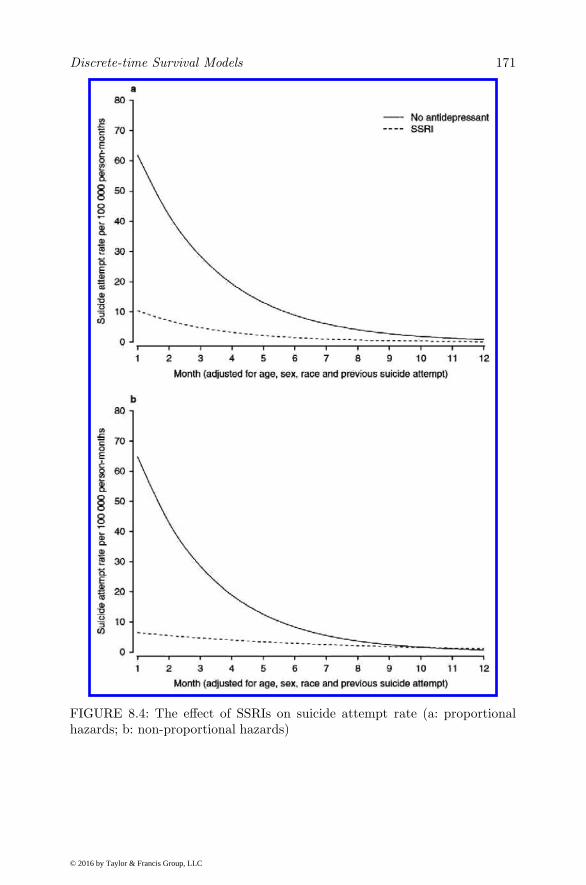
Discrete-time Survival Models 171
FIGURE 8.4: The effect of SSRIs on suicide attempt rate (a: proportionalhazards; b: non-proportional hazards)
© 2016 by Taylor & Francis Group, LLC

172 Statistical Methods for Drug Safety
Press 1973, Plackett 1974, Agresti 1990). This is, in fact the traditional com-peting risk drug safety problem described above. For subject i, the probabilitythat yi = c (i.e., the response occurs for subject i in category c) is given by
Pic = P (yi = c | β) =exp(zijc)
1 +∑C
h=1 exp(zih)for c = 1, 2, . . .C (8.14)
Pi0 = P (yi = 0 | β) =1
1 +∑C
h=1 exp(zih). (8.15)
Estimation is achieved via maximum likelihood similar to logistic regressionfor binary outcomes. The fundamental difference is that we now have C − 1regression functions, corresponding to contrasts between the C categories.Using this model in place of a standard logistic regression in a discrete-timesurvival model produces a competing risk discrete-time survival model withone category for censoring (i.e., subjects who experienced none of the C − 1events) and C−1 categories for the competing events of interest. During eachdiscrete-time interval (e.g., month) a subject may have any of the C−1 eventsof interest; however, once an event occurs the subject’s record ends. A subjectwho never experiences the event will have yit = 0 for all t.
8.5.2 Mixed-Effects Multinomial Regression Model
Hedeker (2003) developed a general mixed-effects multinomial logistic regres-sion model extending earlier work by Daniels and Gatsonis (1997), Revelt andTrain (1998), and Hartzel et al. (2001), also see Hedeker and Gibbons (2006).This model can be used when the data are either clustered or longitudinal(repeatable events within individuals). Let i denote the level-2 units (e.g.,hospitals), and let j denote the level-1 units (e.g., patients within hospitals).Assume that there are i = 1, . . .N level-2 units and j = 1, . . . , ni (subjectswithin each level 2 unit). In the discrete-time survival model, the ni unitsinclude the set of all available time intervals (e.g. months) for all subjects inunit i. Let yij be the value of the nominal outcome variable. Adding random-effects to the multinomial logistic regression model gives the probability forsubject j in unit i, responding in category yij = c conditional on β and α as:
Pijc = P (yij = c | β,α) =exp(zijc)
1 +∑Ch=1 exp(zijh)
(8.16)
Pij0 = P (yij = 0 | β,α) =1
1 +∑Ch=1 exp(zijh)
. (8.17)
for c = 1, 2, . . . , C, where zijc = x′ijβic+w′
ijαc. Here,wij is the p×1 covariatevector, and xij is the design vector for the r random-effects, both vectors beingfor the jth subject nested within unit i. Correspondingly, αc is a p× 1 vector
© 2016 by Taylor & Francis Group, LLC

Discrete-time Survival Models 173
of unknown fixed regression parameters, and βik is a r× 1 vector of unknownrandom-effects for level-2 unit i. For the general case of multiple random-effects, their distribution is assumed to be multivariate normal with meanvector µc and covariance matrix Σc. Notice, that the regression coefficientvectors β and α carry the c subscript. Thus, for each of the p covariates andr random-effects, there will be C parameters to be estimated. Additionally,the random effect variance-covariance matrix Σc is allowed to vary with c.
It is convenient to standardize the random-effects by letting βic = T cθi+µc, where T cT
′c = Σc is the Cholesky decomposition of Σc. The model is now
given as
zijc = x′ij(T cθi + µc) +w′
ijαc , (8.18)
where θi are mutually independent N(0, 1) variates.Parameter estimation is described in detail by Hedeker (2003) and Hedeker
and Gibbons (2006). Note that in the case of a discrete-time survival model,the ni level-1 units represent the total number of person-time-intervals (e.g.,person-months) for the subjects in cluster i.
Hazard Rates and Cumulative Survival:
Once we have estimated the model parameters, we may also wish to display thehazard rates (e.g., over time) for different exposure patterns. In addition, wemay want to also display the cumulative survival curves for different exposures.Consider a model with two random-effects (e.g., one for stroke and one fordeath from any other cause). We can estimate the probability of each outcomeconditional on a particular covariate vector (e.g., exposure pattern) as
Pij2 =exp(σ2θi + µ2 +w′
ijα2)
1 + exp(σ1θi + µ1 +w′ijα1) + exp(σ2θi + µ2 +w′
ijα2)(8.19)
Pij1 =exp(σ1θi + µ1 +w′
ijα1)
1 + exp(σ1θi + µ1 +w′ijα1) + exp(σ2θi + µ2 +w′
ijα2)(8.20)
Pij0 =1
1 + exp(σ1θi + µ1 +w′ijα1) + exp(σ2θi + µ2 +w′
ijα2).(8.21)
These are referred to as “unit-specific” probabilities because they indicate re-sponse probabilities for particular values of the random unit effect θi (Neuhauset al. 1991, Zeger et al. 1988). Replacing the parameters with their estimatesand denoting the resulting unit-specific probabilities as Pss, marginal probabil-ities Pm are then obtained by integrating over the random-effect distribution,namely Pm =
∫θ Pss g(θ) dθ. Numerical quadrature can be used for this in-
tegration as well. These marginal probabilities represent the hazard rate fora particular competing risk of interest (e.g., mortality or stroke) expressedas a rate per unit time. The cumulative survival rate is then computed by
© 2016 by Taylor & Francis Group, LLC

174 Statistical Methods for Drug Safety
summing the time-specific risks over time, adjusting for the changing numberof subjects at risk at that time point.
Intra-class Correlation
The intra-class or intra-cluster correlation is a useful method of expressingthe magnitude of the level-2 variance component. For the random-interceptmodel, we denote the underlying response tendency associated with categoryc for person-time j in level-2 unit i as Yijc. The random-intercept model forthe latent variable Yijc is therefore,
Yijc = w′ijαc + σcθi + εijc c = 0, . . . , C . (8.22)
Assuming c = 0 as the reference category, α0 = σ0 = 0, the model can berewritten as
Yijc = w′ijαc + σcθi + (εijk − εij0) c = 1, . . . , C , (8.23)
(see Hedeker, 2003). The level-1 residuals εijc are distributed according toa type I extreme-value distribution (Maddala 1983, page 60). Furthermore,the standard logistic distribution is obtained as the difference of two inde-pendent type I extreme-value variates (McCullagh and Nelder 1989). As aresult, the level-1 variance is given by π2/3, which is the variance of the stan-dard logistic distribution. The intra-class correlation is therefore estimated asrc = σ2
c/(π2/3 + σ2
c ), where σ2c is the estimated level-2 variance for category
c assuming a normally distributed random-effect distribution.
8.6 Illustration
In 1998, then Secretary of the Department of Health and Human ServicesDonna Shalala noticed geographic inequities in median waiting time for livertransplantation of 30 versus 300 days within adjacent organ allocation areas.Dr. Shalala was concerned that life and death outcomes were “accidents of ge-ography.” In the fall of 1998, Congress requested that the Institute of Medicine(IOM) conduct a study to evaluate the potential impact of pending regula-tions developed by the Department of Health and Human Services on a set ofimportant specific issues related to organ procurement and transplantation.A large part of the IOM committee’s work focused on a review and analysisof approximately 68,000 liver transplant waiting list records that describe ev-ery change in status made by every patient on the Organ Procurement andTransplantation Network (OPTN) waiting list for liver transplants from 1995through the first quarter of 1999. The methodology and results of the analysisare described in the original IOM (1999) of Medicine (1999) report and inGibbons et al. (2003).
© 2016 by Taylor & Francis Group, LLC
Discrete-time Survival Models 175
The objective of the analysis was to determine the degree to which therewas geographic heterogeneity in liver transplantation rates and to identifypossible inefficiencies in the system that would account for the large observeddifferences in waiting times across geographic units. At the time, there were62 organ procurement organizations (OPOs) which were responsible for organallocation within discrete geographic areas in the United States. The OPOscovered quite different population sizes ranging from 1 million or less to ap-proximately 10 million lives. The system was local in nature, such that if anorgan was donated in OPO 10 it would have to be transplanted or at leastoffered to all patients on the waiting list in OPO 10 prior to sharing the or-gan with a different OPO. At the time, patients where classified in statuscategories of 1, 2A, 2B, and 3, where status 1 represented the most severelyill patients with approximately a week to live, followed by status 2A and 2Bwho’s life expectancy was measured in weeks or months, followed by status 3patients who were currently in no eminent danger of death if not transplanted.However, prioritization for transplantation was based on waiting time and noton severity of illness or likelihood of death. As such, an organ could be allo-cated to a less severely ill patient who had been waiting longer than a moreseverely ill patient who was in greater need of the transplant. In addition, thelocal nature of the allocation system led to cases in which a status 3 patientwas transplanted in an OPO when a status 1 patient in the adjacent OPOdied. By a simple examination of the actual transplant data, it became imme-diately apparent that the large geographic discrepancies in transplant rateswere produced by differences across the OPOs in when to list patients in termsof the progression of their illness. Some OPOs listed patients early, when theywere in status 3 to maximize their time on the list and likelihood of transplan-tation once their illness progressed. Other OPOs only listed more severely illpatients. Since approximately 70% of the patients on the wait-list were status3, the median waiting time was for a status 3 patient, the more listed in aspecific OPO, the longer the median waiting time. OPOs that restricted theirlist to status 1 and 2 either transplanted the patients or they died, leadingto a much shorter waiting time. To model the more subtle determinants ofthe allocation system, the committee realized that they would need to (a) ac-commodate competing risks of death while waiting and transplantation, and(b) random OPO effects to examine geographic variability (inequity). To thisend, they used a discrete time competing risk frailty model to simultaneouslyevaluate the competing risks of wait-list mortality and transplantation. In thefollowing, we describe the model parameterization and some of the key resultsof the IOM committee’s analyses.
8.6.1 Model Parameterization
Stratified analyses were performed separately for the time spent in each statuslevel, with the exception of 2A for which there were too few subjects. For status1, time refers to days, whereas for status 2B and 3, time refers to months. In
© 2016 by Taylor & Francis Group, LLC
176 Statistical Methods for Drug Safety
all analyses, the outcome measure is the nominal measure of transplant, wait-list death, or other. Other can be shifting to another status level and neverreturning to the status level in question, being too sick to transplant, beingdelisted, being transplanted at another center, or still waiting. In terms ofcovariates, there were age (0-5, 6-17, 18 and over), sex (female=0, male=1),race (black=1 else 0), blood type (O or B = 1 else 0) and OPO transplantvolume (small, medium, and large based on number of transplanted patientsin 1995-1999). For blood type, a contrast between types O and B versus A andAB was used because the former two can only receive donation from a subsetof donors whereas the latter can receive donation from almost all potentialdonors.
8.6.2 Results
A summary of several statistics of interest that help characterize the sampleand waiting time distributions is presented in Table 8.3. Maximum marginallikelihood estimates, standard errors, and corresponding probabilities for Waldtest statistics are presented in Table 8.4, separately for status levels 1, 2B, and3, respectively. In the following we provide an overview of the most importantfindings.
Geographic Inequity:
In terms of geographic inequity, systematic OPO-specific effects accountedfor less than 5% of the total variance (i.e., intra-cluster correlation of 0.045)in transplantation rates for status 1 patients (see Table 8.3). The geographicdistribution for the most severely ill patients is therefore reasonably equitablewith mean waiting time of 4.8 days (see Table 8.3). In contrast, OPO-specificeffects accounted for 13% of the variability in transplantation rates for status2B patients (see Table 8.4) and 35% of the variability for status 3 patients(see Table 8.4). This implies that the systematic variation in waiting timeacross OPOs is almost completely determined by variations in waiting timesfor the less severely ill patients, with little variation for the most severely illpatients. This finding is further illustrated in Figure 8.5 where the empiricalBayes (EB) estimates of the OPO-specific adjusted transplantation effects aredisplayed.
The interpretation of the EB estimate is OPO i’s deviation from the pop-ulation rate, adjusted for covariates. As such, the y axis in Figure 8.5 is in alog-odds scale, where values of 1, 2, and 3 represents increases in the likelihoodof transplantation by factors of 2.7, 7.4, and 20.1, respectively. Negative valuesrepresent corresponding decreases in probability of transplantation relative tothe overall population rate.
Moreover, while transplantation rates of these less severely ill patients varysignificantly, they have little relationship to mortality. In all cases, systematicOPO differences in pre-transplantation mortality rates accounted for less than
© 2016 by Taylor & Francis Group, LLC
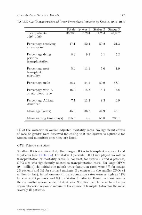
Discrete-time Survival Models 177
TABLE 8.3: Characteristics of Liver Transplant Patients by Status, 1995–1999
Totals Status 1 Status 2 Status 3Total patients, 33,286 5,294 14,264 26,9071995–1999
Percentage receiving 47.1 52.4 50.2 21.3a transplant
Percentage dying 8.3 9.2 6.1 5.2prior totransplantation
Percentage post- 5.4 11.1 5.0 1.9transplantmortality
Percentage male 58.7 54.1 59.9 58.7
Percentage with A 16.0 15.3 15.4 15.8or AB blood type
Percentage African 7.7 11.2 8.3 6.9American
Mean age (years) 45.0 36.3 44.9 46.1
Mean waiting time (days) 255.6 4.8 56.8 285.1
1% of the variation in overall adjusted mortality rates. No significant effectsof race or gender were observed indicating that the system is equitable forwomen and minorities once they are listed.
OPO Volume and Size:
Smaller OPOs are more likely than larger OPOs to transplant status 2B and3 patients (see Table 8.4). For status 1 patients, OPO size played no role intransplantation or mortality rates. In contrast, for status 2B and 3 patients,OPO size was significantly related to transplantation rates. For large OPOs(9+ million) the initial one month transplantation rates were 5% for status2B patients and 3% for status 3 patients. By contrast in the smaller OPOs (4million or less), initial one-month transplantation rates were as high as 17%for status 2B patients and 9% for status 3 patients. Based on these resultsthe committee recommended that at least 9 million people be included in anorgan allocation region to maximize the chance of transplantation for the mostseverely ill patients.
© 2016 by Taylor & Francis Group, LLC

178 Statistical Methods for Drug Safety
FIGURE 8.5: OPO-specific Bayes estimates (σ1θi) of transplantation rates bystatus category adjusted for competing risk of mortality and model covariates(e.g., sex, race, blood type).
The Effect of Sharing:
Further evidence in support of the committee’s broader sharing recommen-dation was drawn from several regional and state-wide sharing arrangementsamong two or more OPOs, most typically for status 1 patients. The results ofthese “natural experiments” revealed that sharing significantly increased thestatus 1 transplantation rate from 42% without sharing to 52% with sharing,lowered average status 1 waiting times from 4 to 3 days, and decreased sta-tus 1 pre-transplantation mortality from 9% to 7%. Not surprisingly, sharingsignificantly decreased the rate of transplantation for less severely ill patients.For example, among small OPOs that served a population of 2 million or less,the status 3 transplantation rate decreased from 31% for those OPOs that didnot share to 6% for those that did share, making more organs available formore severely ill patients. Though sharing decreased status 3 transplantationrates, there was no concomitant increase in pre-transplantation mortality ofstatus 3 patients.
© 2016 by Taylor & Francis Group, LLC

Discrete-time Survival Models 179
Waiting Times and Need for Transplant:
The committee also studied the relationship of transplantation and pre-transplantation mortality to waiting time, since this was a major factor inthe original allocation system. For status 1 patients, the rates were constantover the first 12 days of listing at approximately 15% for transplantation perday and 3% for mortality (see Figure 8.6 panel A), but for status 2B and 3 pa-tients both rates decreased rapidly over time (see Figure 8.6 panels B and C).For status 2B, transplantation rates decreased from 12% to 5% per month overa 12 month period while pre-transplant mortality rates decreased from 3% to0.3% per month. For status 3 patients, transplantation rates decreased from4% to 0.05% per month over a 12 month period and pre-transplant mortalityrates decreased from 2% to 0.2% per month.
Figure 8.7 displays estimated cumulative time-to-event distributions forstatus 1 (panel A), status 2B (panel B), and status 3 (panel C). Inspection ofFigure 8.7 reveals that after 12 days 80% of the status 1 patients at risk aretransplanted whereas 10% die while waiting. For status 2B, 60% of patientsat risk through 12 months are transplanted and 7% die while waiting. Forstatus 3, 20% of patients at risk through 12 months are transplanted and 8%die while waiting. These estimates differ somewhat from the observed rates inTable 8.3 because subjects were not always observed for these period of timesdue to becoming too ill to transplant (and removed from the list) or changingstatus category.
© 2016 by Taylor & Francis Group, LLC

180
Statistica
lMeth
odsforDrugSafety
TABLE 8.4: Mixed-Effects Competing Risk Survival Models for Patient Time in Status Levels 1, 2B, and 3—MaximumLikelihood Estimates (Standard Errors)
Status 1 Status 2B Status 3Transplant versus OtherIntercept −1.829 (0.276) −2.077 (0.129) −3.593 (0.210)Day (1), month (2B, 3) 0.016 (0.015) −0.092 (0.016) *** −0.220 (0.030) ***
Age 0–5 vs. ≥ 18 −0.907 (0.188) *** 0.470 (0.103) *** 1.156 (0.154) ***
Age 6–17 vs. ≥ 18 −0.362 (0.234) 0.135 (0.243) 0.844 (0.268) **
Gender (1 = male) −0.098 (0.198) 0.126 (0.087) 0.054 (0.186)Race (1 = black) −0.275 (0.268) 0.134 (0.222) 0.158 (0.304)Blood type (1 = B or O) −0.076 (0.196) −0.577 (0.062) *** −0.477 (0.098) ***
OPO volume (M vs. L) −0.054 (0.319) 0.590 (0.157) *** 1.179 (0.149) ***
OPO volume (S vs. L) 0.261 (0.336) 0.560 (0.187) ** 0.757 (0.228) ***
Random OPO effect SD 0.393 (0.144) ** 0.689 (0.064) *** 1.335 (0.162) ***
Mortality versus OtherIntercept −3.685 (0.482) −3.313 (0.227) −3.654 (0.172)Day (1), month (2B, 3) 0.023 (0.047) −0.213 (0.039) *** −0.216 (0.041) ***
Age 0–5 vs. Adult −0.968 (0.378) ** −0.195 (0.381) −2.119 (2.099)Age 6-17 vs. Adult −1.001 (0.551) −0.516 (0.641) −1.193 (2.000)Gender (1 = male) 0.077 (0.371) 0.014 (0.191) −0.063 (0.268)Race (1 = black) 0.162 (0.448) −0.082 (0.359) 0.027 (0.544)Blood type (1 = B or O) 0.003 (0.433) −0.005 (0.164) −0.017 (0.231)OPO volume (M vs. L) 0.203 (0.491) 0.202 (0.126) −0.526 (0.300)OPO volume (S vs. L) −0.230 (0.930) 0.355 (0.151) ** −0.658 (0.358)
Random OPO effect SD 0.042 (0.298) 0.116 (0.049) ** 0.137 (0.157)∗p < .05, ∗∗p < .01, ∗∗∗p < .001.
© 2016 by Taylor &
Francis Group, LLC

Discrete-time Survival Models 181
(a) Estimated hazard rates for status 1
(b) Estimated hazard rates for status 2B
FIGURE 8.6: Continued on next page
© 2016 by Taylor & Francis Group, LLC

182 Statistical Methods for Drug Safety
(c) Estimated hazard rates for status 3
FIGURE 8.6: Estimated hazard rates for (a) status 1, (b) status 2B, and (c)status 3 patients awaiting liver transplantation. The hazard rate describesthe likelihood of transplantation or mortality at a given point in time (usingone whole day (status 1) or one whole month (status 2B and 3) as the unit)adjusted for the competing risks(i.e., transplantation or mortality) and themodel covariates (e.g., sex, race, blood type).
© 2016 by Taylor & Francis Group, LLC

Discrete-time Survival Models 183
(a) Estimated cumulative time-to-event distributions for status 1
(b) Estimated cumulative time-to-event distributions for status 2B
FIGURE 8.7: Continued on next page
© 2016 by Taylor & Francis Group, LLC

184 Statistical Methods for Drug Safety
(c) Estimated cumulative time-to-event distributions for status 3
FIGURE 8.7: Estimated cumulative time-to-event distributions for (a) status1, (b) status 2B, and (c) status 3 patients awaiting liver transplantation. Thecumulative time-to-event distribution describes the overall adjusted likelihoodof transplantation or mortality up to a particular point in time.
© 2016 by Taylor & Francis Group, LLC

Discrete-time Survival Models 185
8.6.3 Discussion
From a statistical perspective, this case study is useful in that it illustratesthe important role that statisticians play in the development of public policy.Clearly, without the analysis of these data, the IOM committee would nothave reached these conclusions, and the life-saving changes in the regulationswould not have occurred. This example also illustrates that relatively complexstatistical methods can, in fact, be used to evaluate important public policyquestions and to communicate the results to a largely non-statistical audience,including the U.S. Congress. The notion, that complex statistical methods willhinder the dissemination of research findings to policy makers and the public,was not borne out.
The analysis revealed that the rate of liver transplantation of the mostseverely ill (status 1) patients is relatively homogeneous across OPOs. How-ever, the allocation of organs is not efficient because many organs that couldbe used for transplantation of status 1 patients are being transplanted intoless severely ill patients, especially in smaller OPOs due to the local natureof the original allocation system. The IOM analysis revealed that this inef-ficiency resulting from small OPOs is minimized when allocation areas com-prise a minimum population of 9 million people. Their analysis of existingbroader sharing arrangements confirmed this result by demonstrating thatbroader sharing of organs led to an overall increase in the rate at which themost severely ill patients were transplanted and a concomitant decrease inthe excess transplantation of the least severely ill patients, without increasingpre-transplantation mortality.
© 2016 by Taylor & Francis Group, LLC

9
Research Synthesis
“Philosophy, like medicine, has plenty of drugs, few good remedies, andhardly any specific cures.”
(Sbastien-Roch Nicolas De Chamfort (1741 - 1794), French writer)
9.1 Introduction
Meta-analysis is useful for the combination of effect sizes which may be mea-sured using a variety of different metrics. By contrast, research synthesis in-volves a reanalysis of the complete original data commonly measured and col-lected from a number of different studies. The advantage of research synthesisover meta-analysis is that we can use all available data from each subject andeach study even if the timeframes are not identical (e.g., weekly versus monthlyassessments) as long as the overall timeframe is comparable. The analysis oflongitudinal data is generally not possible in meta-analysis where the unitof analysis is a statistic which summarizes the results of each study. For ex-ample, in meta-analysis we might combine information on average change intreated and control subjects where sample size and both measures of meanchange and its variability (e.g., standard deviation of change scores) are avail-able from each study. This requirement raises issues related to the treatment ofmissing data, where we must choose a method of imputation of the endpoint ofinterest. For example, we can use last observation carried forward (LOCF) inwhich the last available measurement is used as a proxy for the measurementthat would have been obtained had the subject completed the study. In manycases, however, all that may be available are the summary statistics for thosesubjects that completed the study. These statistics may be quite biased in thatthey have little to do with the totality of subjects that were randomized to thetreated and control conditions of interest. In many cases, a mixture of bothtypes of data are present, leading to pooled estimates with questionable valid-ity. The same is not true for research synthesis where all available data fromeach subject are available and form the basis of the pooled analysis. Here wecan model the within person and within study components of variance whichproduce both person-specific and study-specific deviations from the overall re-
187
© 2016 by Taylor & Francis Group, LLC

188 Statistical Methods for Drug Safety
sponse process. This approach to research synthesis is more firmly groundedin statistical theory in that it is much more robust to the presence of missingdata. The usual models operate under the “missing at random” assumption(Rubin 1976) and even models for “not missing at random” (Rubin 1976) arepossible if data regarding the missing data process are also available. As usedhere, the term research synthesis implies a reanalysis of the data preservingthe nesting of subjects within studies and allowing the trajectories and eventhe effect of treatment to vary from subject to subject and study to study.
Statistically, research synthesis is based on three-level linear or non-linearmixed-effects regression models. Gibbons et al. (2012a,b) have illustrated themethodology for both the benefits and safety of the antidepressants fluoxetineand venlafaxine, where they synthesized the complete longitudinal data fromall randomized patients enrolled in 41 such studies. They examined rates ofchange in both efficacy as measured by the Hamilton Depression Rating Scale(HAM-D) or Child Depression Rating Scale (CDRS) and safety as measuredby the rate of change in suicidal thoughts and behavior based on both sponta-neous reports of attempts and prospective clinician measurements of ideationand behavior. These rates of change were allowed to vary from patient to pa-tient and study to study. Separate analyses were performed for youth, adults,and the elderly so that the same outcome measure would be available for eachanalysis. A combined analysis of all adult data was also conducted since bothadult and the elderly samples both used the same outcome measure. Thesedata are used to illustrate the general methodology that will now be presented.
9.2 Three-level Mixed-effects Regression Models
Research synthesis involves the nesting of repeated measurements within in-dividuals and the nesting of individuals within studies. In general we use datafrom RCTs as the basis for the analysis so that biases associated with ob-servational studies are for the most part eliminated. However, study to studyvariability can be produced by indications for treatment and differences indesign of the studies, so the statistical combination of the complete data frommultiple studies does not support the same level of causal inference had all ofthe subjects been enrolled in a single large well controlled RCT.
9.2.1 Three-level Linear Mixed Model
As noted above, consider a research synthesis of all available longitudinaldata from each subject from N studies comparing a treatment versus relevantcontrol condition. Following Hedeker and Gibbons (2006) we have i = 1 . . .Nstudies, j = 1 . . .ni subjects in study i, and k = 1 . . .nij observations forsubject j in study i. Further denote Ni =
∑ni
j=1 nij , which is the total number
© 2016 by Taylor & Francis Group, LLC

Research Synthesis 189
of observations within study i. Suppose that we wanted to fit a model witha single random study effect (i.e., intercept) and two random subject effects(i.e., intercept and trend). In terms of the random effects, this model couldbe written as follows:
yi 1yi 2yi 3. . .. . .. . .yi ni
=
1 Zi 1 0 0 . . . 01 0 Zi 2 0 . . . 01 0 0 Zi 3 . . . 0. . . . . . . . . . . . . . . . . .. . . . . . . . . . . . . . . . . .. . . . . . . . . . . . . . . . . .1 0 0 0 . . . Zi ni
γiυi 1υi 2υi 3. . .υi ni
+
εi 1εi 2εi 3. . .. . .. . .εi ni
or,
yi = Ziυ∗i + εi
where γi ∼ N (0, σ2γ), υij ∼ N (0,Σβ), and εijk ∼ N (0, σ2
ε ). With a singlerandom study effect, the number of random-effects equals r+1, where r is thenumber of random subject effects. However, for a given study i the dimensionof υ∗ equals ni × r + 1, which we denote as Ri, the i subscript indicates thatthis value varies depending on the size of the study. Adding covariates to thismodel yields
yi = X iβ +Ziυ∗i + εi, (9.1)
where X i is a known Ni × p design matrix for the fixed-effects, β is the p× 1vector of unknown fixed regression parameters, Zi is a known Ni ×Ri designmatrix for the random-effects, υ∗
i is the Ri × 1 vector of unknown random-effects, and εi is the Ni × 1 error vector.
As a result, the observations y and random coefficients υ∗ have the jointmultivariate normal distribution:
[yiυ∗i
]∼ N
([Xiβ
0
],
[ZiΣiZ
′i + σ2
εIi ZiΣi
ΣiZ′i Σi
])
where the random coefficients υ∗i and variance-covariance matrix Σi are given
as:
γiυi1υi2. . .υini
∼ N
000. . .0
σ2γ 0 0 . . . 00 Συ 0 . . . 00 0 Συ . . . 0. . . . . . . . . . . . . . .0 0 0 . . . Συ
.
The i subscript for the variance covariance matrix Σi merely reflects the
© 2016 by Taylor & Francis Group, LLC

190 Statistical Methods for Drug Safety
number of observations within the study, not the number of parameters whichis the same for all studies.
The mean of the posterior distribution of υ∗, given yi, yields the EAPestimator (“Expected A Posteriori”) of the study effects and individual trendparameters:
υi∗i =
[Z ′i(σ
2εIi)
−1Zi +Σ−1i
]−1Z ′i(σ
2εIi)
−1(yi −X iβ)
with covariance matrix
Σθ|yj =[Z ′j(σ
2εIj)
−1Zj +Σ−1j
]−1
.
Differentiating the log-likelihood, logL =∑N
i=1 log h(yi) , yields:
∂ logL
∂β= σ2
ε
N∑
i=1
X ′iui
∂ logL
∂Σ∗ =1
2
N∑
i=1
D′iG
′ivec
[Σ−1i (Σθ|yj + υi
∗i (υi
∗i )
′ −Σi)Σ−1i
]
∂ logL
∂σ2ε
=1
2σ−4ε
N∑
i=1
−niσ2 + u′iui + tr
[Σθ|yjZ
′iZi
]
where ui = yi − Ziυi∗i − Xiβ, and vechΣi = DiΣ
∗. In this notation, Σ∗
represents the vector with only the unique variance-covariance parameters,and Di is a matrix of ones and zeros that is necessary to pick off only thecorrect terms.
9.2.1.1 Illustration: Efficacy of Antidepressants
Concerns have been raised that the efficacy of antidepressant treatment hasbeen overstated (Turner et al. 2008). They found that among 74 FDA reg-istered RCTs that were published, 94% were positive but only 51% of allregistered trials were positive. Meta-analyses have suggested that antidepres-sants are only effective in the most severely ill patients (Kirsch et al. 2008).While provocative, these finding raise as many questions as they attempt toanswer. The first is a so-called “vote-counting method” consisting of a simpletally of the significance dichotomized at the 5% level of each study. For exam-ple it could be that the larger studies were published and those studies werethe only studies that had sufficient statistical power to detect a significant dif-ference between treated and control conditions. One could imagine a situation
© 2016 by Taylor & Francis Group, LLC

Research Synthesis 191
in which none of the individual studies yielded a statistically significant find-ing, but the true effect in the population was significant and of public healthimportance. With respect to the moderation by severity of depression at base-line, it is hard to imagine how this could even be analyzed using meta-analysisin which all that is available is the average severity level for each study. Therelationship between severity of illness and efficacy of treatment exists at thelevel of the individual and is not reliably assessed using study-level aggregatedinformation.
To study this question more rigorously, Gibbons et al. (2012a) obtainedcomplete person-level longitudinal data from 12 adult (2,635 patients and14,048 measurements), 4 geriatric (960 patients and 5,209 measurements),and 4 youth (708 patients and 2,536 measurements) RCTs of fluoxetine and21 adult trials of venlafaxine (immediate release (IR) 11 adult studies with2,421 patients and 10,634 measurements and for extended release (ER) therewere 10 adult studies with 2,461 patients and 12,481 measurements). Analysisfocused on the CDRS for children and the HAM-D for adults, which were usedto estimate rate of change as well as response and remission rates at 6 weeks.
These data were analyzed using three-level linear mixed-effects regressionmodels as described above. Level 1 represents the measurement occasion, level2 the patient, and level 3 the study. An overall analysis was performed for bothdrugs (fluoxetine and venlafaxine IR and ER) in adults and geriatrics. Youthwere not included in the combined analysis because they were assessed withthe CDRS. Separate analyses were performed for fluoxetine adult, geriatric,and youth trials, and venlafaxine IR and ER adult trials. The intercept andslope of the time trends were random-effects at both patient and study lev-els, allowing time-trends to vary across patients and studies. Heterogeneityof treatment effect was tested by including a random treatment by time in-teraction. Time was number of days from treatment initiation. The primaryeffect of interest was change in slope between treatment and control over 6weeks. Six weeks was selected because it was the minimum trial duration andtherefore study and length of treatment were unconfounded. A variety of pa-rameterizations of time were considered, but the best fitting model was basedon a simple linear function of time through 6 weeks.
Adult Studies
To estimate response and remission rates in the presence of missing data,empirical Bayes estimates of each subject’s trend was used to impute a CDRSor HAM-D score at day 42, if the actual day 42 score was missing. For adultsand geriatric patients, response was a 50% reduction in HAM-D score at weeksix, and remission was HAM-D<8. For youth, response was a 50% reductionin CDRS score at week six and remission was CDRS-R<28. Number neededto treat (NNT) was also computed for each endpoint and sample.
To provide an overview of the results, we present the findings for the over-all analysis for fluoxetine and venlafaxine IR and ER in adults and geriatrics.
© 2016 by Taylor & Francis Group, LLC

192 Statistical Methods for Drug Safety
The estimated average rate of change over 6 weeks was -11.82 HAM-D unitsfor drug versus -9.26 HAM-D units for placebo MMLE = -2.55, SE = 0.20,p<0.0001), indicating 28% greater improvement for drug. Estimated lineartime trends and observed daily mean scores are presented in Figure 9.1. Vari-ation in the treatment effect over studies was not statistically significant (SD= 0.16, p=0.06).
FIGURE 9.1: Overall observed and estimated time-trends for adults.
The estimated response rate for drug was 58.4% versus 39.9% for placebo(OR=2.11, 95% CI 1.93-2.31, p<0.001, NNT=5.41). Remission rates were43.0% versus 29.3% for drug and placebo respectively (OR=1.82, 95% CI1.66-2.00, p<0.001, NNT=7.30).
No effect of baseline severity on treatment efficacy was found for eitherdichotomous (p=0.27) or continuous (p=0.10) baseline severity measures. Forpatients with low severity, rate of change in symptoms over 6 weeks was -9.40for drug versus -7.20 for placebo. For high severity patients the rate of changewas -12.85 for drug versus -10.07 for placebo. The estimated difference was2.20, 95% CI 1.65-2.76 for low severity and 2.78, 95% CI 2.26-3.29 for highseverity. Estimated response rates were 54.8% vs. 37.3% (difference of 17.5%)for treated vs. placebo low severity patients and 57.7% vs. 40.5% (differenceof 17.2%) for high severity patients. Estimated remission rates were 49.9% vs.36.6% (difference of 13.3%) for treated vs. placebo low severity patients and37.8% vs. 25.1% (difference of 12.7%) for high severity patients.
© 2016 by Taylor & Francis Group, LLC

Research Synthesis 193
Youth Studies
The estimated average rate of change over 6 weeks was -15.96 CDRS unitsfor placebo and -20.58 CDRS units for fluoxetine (MMLE = -4.62, SE = 1.26,p<0.0001), indicating 30% greater improvement for fluoxetine.
The estimated response rate for fluoxetine was 29.8% versus 5.7% forplacebo (OR=6.66, 95% CI 3.07-14.48, p<0.001, NNT=4.16). Remission rateswere 46.6% versus 16.5% for fluoxetine and placebo respectively (OR=4.23,95% CI 2.64-6.77, p<0.001, NNT=3.33. The finding of higher remission thanresponse rates questions the validity of the CDRS remission threshold scoreof 28.
No effect of baseline severity on treatment efficacy was found (p=0.90). Forlow severity patients, the rate of change in symptoms was -17.60 for fluoxetineversus -12.56 for placebo. For high severity patients the rate of change was-28.86 for fluoxetine versus -24.40 for placebo. The estimated difference was5.04, 95% CI 2.56-7.52 for low severity and 4.45, 95% CI -0.58-9.49 for highseverity. Estimated response rates were 23.0% vs. 3.2% (difference of 19.8%)for treated vs. placebo low severity patients and 40.2% vs. 17.2% (differenceof 23.0%) for high severity patients. Estimated remission rates were 54.1% vs.19.4% (difference of 20.6%) for treated vs. placebo low severity patients and28.9% vs. 7.5% (difference of 21.4%) for high severity patients.
Discussion
The results of this research synthesis reveal clear efficacy of antidepressantmedications across the lifespan which translate into important clinical dif-ferences in terms of response and remission rates. Previous findings that theeffect is restricted to the most severely ill patients based on meta-analysisusing average study-level severity is not confirmed when patient-level dataform the basis for the analysis. Interestingly, the largest effect of treatment isseen in children. Although not described here, the efficacy of antidepressantsin the elderly was statistically significant, but clinically marginal with NNTsof 17 and 39 for response and remission, respectively. The reanalysis of thesedata in contrast to the meta-analysis of these data reveal a far more detailedpicture of the efficacy of these medications. While the overall mean differenceis on the order of only 3 points on a 40 point scale, small differences in themean response translate to large gains in the tails of the distribution in termsof response and remission rates.
9.2.2 Three-level Non-linear Mixed Model
For a binary, ordinal, count, or time-to-event outcome, the linear mixed-modeldescribed above is no longer valid because the link function is no longer theidentity. As a result, the integrals in the likelihood function must be evaluatednumerically leading to a more computationally complex solution. Nevertheless,this type of problem is easily solved as long as the number of random-effects
© 2016 by Taylor & Francis Group, LLC

194 Statistical Methods for Drug Safety
is relatively small. For example a model with random intercept and trend atboth subject and study levels has four random-effects and is computationallytractable despite the number of studies and subjects. Following Hedeker andGibbons (2006) we present a general derivation using a probit link function;however, the logistic model is a simple extension of the general result.
Stacking the unobservable latent response vectors of each subject within astudy (yij), the three-level model for the resulting Ni response vector for theith study, i = 1, 2, . . . , N , can be written as follows:
yi 1yi 2yi 3. . .. . .yi ni
yiNi×1
=
1i 1 Zi 1 0 0 . . . 01i 2 0 Zi 2 0 . . . 01i 3 0 0 Zi 3 . . . 0. . . . . . . . . . . . . . . . . .. . . . . . . . . . . . . . . . . .1i ni 0 0 0 . . . Zi ni
Zi
Ni×((ni×r)+1)
υ0 iυi1υi2υi3. . .υini
υ∗i
((ni×r)+1)×1
+
1i 1 Xi 1
1i 2 Xi 2
1i 3 Xi 3
. . . . . .
. . . . . .1i ni Xi ni
Xi
Ni×(p+1)
β0β1. . .βp
β
(p+1)×1
+
ei 1ei 2ei 3. . .. . .ei ni
eiNi×1
,
where the following independent components are distributed, β0 i ∼N (0, σ2
(3)), υij ∼ N (0,Σ(2)), and ei ∼ N (0, σ2εIni). Notice, there are ni
subjects in study i and Ni total observations for study i (the sum of all re-peated observations for all subjects within the study). The number of randomsubject-level effects is r, and the number of fixed covariates in the model (ex-cluding the intercept) is p. In the case of binary responses, each person has annij × 1 vector yij of underlying response strengths, an nij × r design matrixZij for their r random-effects υij , and a nij×p matrix of covariates Xij . Thecovariate matrix usually includes the random effect design matrix so that theoverall intercept, linear term, etc., is estimated and thus the random-effectsrepresent deviations from these overall terms.
A characteristic of the probit model is the assumption that there is an un-observable latent variable (yijk) related to the actual binary response througha “threshold concept” (Bock 1975). We assume the underlying latent variableyijk is continuous and that the binary response yijk = 1 occurs when yijkexceeds a threshold γ (i.e., P (yijk = 1) = P (yijk > γ)). In terms of the latentresponse strength for subject j in study i on occasion k (yijk) we obtain
© 2016 by Taylor & Francis Group, LLC

Research Synthesis 195
yijk = β0i + z′ijkυij + x′
ijkβ + εijk . (9.2)
With the above mixed regression model for the latent variable yijk, theprobability that yijk = 1 (a positive response occurs), conditional on therandom-effects υ∗, is given by:
Pr(yijk = 1|υ∗) = (2πσ2ε )
− 12
∫ ∞
γ
exp
[− 1
2σ2ε
(yijk − υ0i − z′ijkυij − x′
ijkβ)2
]dy
= Φ[−(γ − sijk)/σε] (9.3)
where sijk = β0i + z′ijkυij + x′
ijkβ, and Φ(·) represents the cumulative stan-dard normal density function. Without loss of generality, the origin and unitof z may be chosen arbitrarily. For convenience, let γ = 0, and to insureidentifiability let σε = 1.
Let yi be the vector pattern of binary responses from study i for the niindividuals examined at the nij time-points. Assuming independence of theresponses conditional on the random-effects, the probability of any patternyi, given υ∗
i , is equal to the product of the probabilities of the individualresponses (both between and within individuals in cluster i):
ℓ(yi | υ∗i ) =
ni∏
j=1
nij∏
k=1
[Φ(sijk)]yijk [1− Φ(sijk)]
1−yijk . (9.4)
Then the marginal probability of yi is expressed as the following integral ofthe likelihood, ℓ(·), weighted by the prior density g(·):
h(yi) =
∫
υ∗
ℓ(yi | υ∗i ) g(υ
∗) dυ∗ , (9.5)
where g(υ∗) represents the distribution of υ∗ in the population.
Orthogonalization of the Model Parameters
For numerical solution of the likelihood equations, Gibbons and Bock (1987)orthogonally transform the response model using the Cholesky decomposition
of Συ∗ (Bock, 1975). Specifically, let υ∗ = T ∗θ∗, where T ∗T ∗′
= Συ∗ is theCholesky decomposition of Συ∗ . Then θ∗ = T ∗−1υ∗, and so, E(θ∗) = 0 andV(θ∗) = T ∗−1Συ∗(T ∗−1)′ = I. The reparameterized model is then
sijk = σ(3)θ0i + z′ijkTθij + x′
ijkβ , (9.6)
where θ0i and θij are the standardized random-effects for cluster i and indi-vidual j in cluster i respectively. Notice that since only a single random clustereffect is assumed, σ(3) is a scalar while T is the Cholesky (i.e., square root)factor of the r × r matrix Σ(2). The marginal probability then becomes
© 2016 by Taylor & Francis Group, LLC

196 Statistical Methods for Drug Safety
h(yi) =
∫
θ∗
ℓ(yi | θ,β) g(θ∗) dθ∗ , (9.7)
where g(θ∗) is the multivariate standard normal density.The major problem with this representation of the marginal probability
is that the dimensionality of θ∗ is (ni × r) + 1 and numerical integration ofequation (9.7) would be exceedingly slow and computationally intractable if(ni × r) + 1 is greater than 10. Note, however, that conditional on the study-effect θ(3), the responses from the ni subjects in study i are independent;therefore, the marginal probability can be rewritten as:
h(yi) =
∫
θ(3)
ni∏
j=1
∫
θ(2)
nij∏
k=1
[Φ(sijk)]1−yijk [1 − Φ(sijk)]
yijk
g(θ(2))dθ(2)
g(θ(3))dθ(3) ,
(9.8)
where θ(2) are the r subject-level random-effects. Here the integration is ofdimensionality r+1 and is tractable as long as the number of level two random-effects is no greater than three or four. In longitudinal studies, we typicallyhave one or two random-effects at level two (e.g., a random intercept and/ortrend for each individual) and one or two random-effects at level three (e.g.,random study intercept and linear trend).
Estimation
The estimation of the covariate coefficients α and the population parametersin T requires differentiation of the log likelihood function with respect to theseparameters. The log likelihood for the patterns from the N clusters can bewritten as:
logL =
N∑
i
log h(yi) . (9.9)
Let η represent an arbitrary parameter vector; then forα, v(T ) (which denotesthe unique elements of the Cholesky factor T ), and σ(3), we get:
∂ logL
∂η=
N∑
i=1
h−1(yi)
∫
θ(3)
ℓi(θ(3)) (9.10)
ni∑
j=1
h−1(yij)
∫
θ(2)
nij∑
k=1
(yijk − Φ(sijk)
Φ(sijk)[1 − Φ(sijk)]
)
ℓij(θ)φ(sijk)∂sijk∂η
g(θ(2))dθ(2)
g(θ(3))dθ(3) , (9.11)
where
© 2016 by Taylor & Francis Group, LLC

Research Synthesis 197
ℓij(θ) = ℓij(θ(2), θ(3)) =
nij∏
k=1
[Φ(sijk)]1−yijk [1− Φ(sijk)]
yijk , (9.12)
ℓi(θ(3)) =
ni∏
j=1
∫
θ(2)
ℓij(θ)g(θ(2))dθ(2) (9.13)
=
ni∏
j=1
h(yij) ,
and
∂sijk∂β
= xijk∂sijk∂v(T )
= Jr(θ(2) ⊗ zijk)∂sijk∂σ(3)
= θ(3) ,
and Jr is the transformation matrix of Magnus and Neudecker (1995) whicheliminates the elements above the main diagonal.
As in the two-level case described by Gibbons and Bock (1987) and Gib-bons et al. (1994) the method of scoring can be used to provide MMLEs andnumerical integration on the transformed θ space can be performed (Stroudand Secrest 1966). An advantage of numerical integration is that alternativeprior distributions for the random-effects can be considered. Thus, for exam-ple, we can compare parameter estimates for a normal versus rectangular priorto determine the degree to which our estimates are robust to deviation fromthe assumed normality of the distribution for the random-effects.
9.2.3 Three-level Logistic Regression Model for Dichoto-mous Outcomes
In the previous discussion we have focused on a three-level random-effectsprobit regression model, however, many researchers are more familiar withthe logistic regression model. Fortunately, modification of the response func-tion and associated likelihood equations is trivial as Gibbons et al. (1994) andHedeker and Gibbons (1994) have shown for two-level logistic regression mod-els. Following Gibbons et al. (1994) we replace the normal response function(i.e., the CDF, or cumulative distribution function) Φ(zijk) with
Ψ(sijk) =1
1 + exp[−sijk], (9.14)
and the normal density function φ(zijk) (i.e., the PDF, or probability densityfunction) with the product
Ψ(sijk)(1−Ψ(sijk)) . (9.15)
© 2016 by Taylor & Francis Group, LLC

198 Statistical Methods for Drug Safety
As in the normal case, we let γ = 0, however, the residual variance correspond-ing to the standard logistic distribution is π2/3. Application of the logistic re-sponse function is attractive in many cases in which the response probabilityis small because the logistic distribution has greater tail probability than thenormal distribution.
9.2.3.1 Illustration: Safety of Antidepressants
In 2004 the FDA issued a black box warning for antidepressants and risk ofsuicide in children and adolescents. The original warning was based on a meta-analysis of adverse event reports of suicidal thoughts and behaviors from 25RCTs. These trials were typically short-term and limited to the newer an-tidepressant classes of SSRIs) and SNRIs. Results of the analysis revealed anoverall odds ratio of OR=1.78 (95% CI =1.14-2.77) indicating that the rateof suicidal thoughts and behavior was significantly higher in children random-ized to active antidepressant treatment relative to placebo. A similar analysisconducted by FDA on prospectively measured suicidal thoughts and behaviorin the youth studies, failed to detect any evidence of increased risk of antide-pressant treatment in these same studies (Hammad 2004). The FDA analysisignored the timing of the suicidal events and did not adjust for differentialtime on treatment.
Gibbons et al. (2012b) analyzed both prospective clinician ratings of sui-cidal thoughts and behavior augmented with spontaneous reports of suici-dal behavior from the same 41 RCTs described in the previous illustration.Data were analyzed using a three-level mixed-effects ordinal regression modelwith categories absent, thoughts, ideation, and behavior. For safety, all datathrough 12 weeks were used where available. The dichotomous event rates(thoughts, ideation, and attempts combined) for treated and control patientsfor each drug (fluoxetine and venlafaxine) and age group (youth, adult, el-derly for fluoxetine and IR and ER in adults for venlafaxine) are displayed inTable 9.1. For youth, there is no discernible pattern. On four weeks placebowas higher than treated, on other four weeks treated was higher than placebo,and on one week they had identical rates. Of the 36 other weekly comparisonsthere were only 7 (19%) in which treated was higher than placebo in terms ofthe rate of suicidal thoughts and behavior.
© 2016 by Taylor & Francis Group, LLC

Resea
rchSyn
thesis
199
TABLE 9.1: Observed Percentage (n) of Suicidal Events Over Time
Fluoxetine VenlafaxineYouth Adult Elderly IR ER
Week Placebo Treatment Placebo Treatment Placebo Treatment Placebo Treatment Placebo Treatment0 20.6 (315) 18.8 (393) 5.4 (1008) 4.7 (1627) 3.2 (470) 2.7 (490) 6.3 (919) 5.5 (1502) 1.6 (994) 1.7 (1467)1 13.2 (114) 14.4 (139) 3.6 ( 883) 2.4 (1364) 2.5 (354) 1.6 (368) 4.9 (716) 2.5 (1061) 1.0 (871) 0.9 (1276)2 14.8 (189) 9.5 (253) 4.5 ( 904) 2.1 (1382) 1.8 (393) 1.7 (409) 2.8 (719) 1.3 (1096) 1.0 (903) 0.6 (1264)3 8.8 (148) 8.8 (205) 2.2 ( 731) 1.7 (1261) 2.2 (360) 0.5 (370) 1.7 (662) 1.2 (1034) 1.1 (819) 0.5 (1145)4 14.3 (105) 5.8 (139) 2.2 ( 683) 1.1 (1151) 1.9 (364) 1.4 (360) 1.7 (641) 0.4 ( 965) 0.7 (807) 0.3 (1182)5 15.6 ( 90) 11.5 ( 96) 1.3 ( 609) 0.7 (1006) 1.6 (313) 2.1 (339) 1.5 (196) 0.9 ( 321) 0.5 (199) 1.8 ( 278)6 8.4 (167) 10.9 (183) 1.7 ( 529) 1.2 ( 910) 1.6 (309) 0.6 (310) 1.3 (397) 1.0 ( 619) 0.7 (614) 0.6 ( 900)7 9.0 ( 78) 14.6 ( 96) 1.5 ( 335) 0.4 ( 491) 1.3 (160) 2.8 (144) 1.0 (196) 1.1 ( 357) 1.2 (169) 0.7 ( 276)8 4.0 ( 50) 8.8 ( 68) 0.7 ( 297) 1.2 ( 259) 1.9 ( 53) 1.5 ( 66) 0.0 (117) 0.6 ( 177) 0.2 (448) 0.6 ( 725)
9+ 13.6 ( 81) 4.8 (105) 0.0 ( 396) 0.0 ( 288) 3.7 (108) 0.0 (118) 1.8 ( 57) 0.0 ( 116) 0.7 (300) 0.6 ( 690)
© 2016 by Taylor &
Francis Group, LLC

200 Statistical Methods for Drug Safety
Overall Analysis of Suicidal Events in Adults
In the combined adult population a statistically significant decrease in suicidalevents over time was found (MMLE=-0.2091, SE=0.0289, p<0.0001). Thisfinding is displayed graphically in terms of the probability of each suicidalevent class in Figure 9.2. The rate of change was 58% faster in treated patientsrelative to controls, which results in an estimated 78.9% decrease in probabilityof suicidal events for controls after 8 weeks of study participation and a 90.5%decrease for treated patients. Figure 9.2 displays the estimated probabilitiesfor each of the three ordinal response categories in treated and control patientsrespectively. The solid lines represent the estimated probabilities for controls,and the dashed lines represent estimated probabilities for treated patients.The top set of curves are for “wishes he were dead or any thoughts of possibledeath to self” or worse, the middle set are for “suicide ideas or gestures,”and the bottom set are for “suicide attempts or suicides.” Figure 9.2 revealsthat the majority of suicidal events (19% at baseline) was of low severity(thoughts of death), followed by ideation with a baseline rate of 3%, andsuicide attempts or completion at 0.1% at baseline. The beneficial effect oftreatment on probability of suicidal events is apparent at approximately 2weeks following treatment initiation.
FIGURE 9.2: Probabilities of suicidal events in adult fluoxetine and venlafax-ine studies.
Gibbons and colleagues (2012b) then conducted a mediational analysis
© 2016 by Taylor & Francis Group, LLC

Research Synthesis 201
to determine the extent to which changes in depression severity accountedfor the difference in suicidal event rates between treated and control sub-jects. The mediation model on all adult (including elderly) patients revealedthe following. First, there was a significant overall faster reduction in de-pressive symptoms (excluding suicidal thoughts and behavior) over time fortreatment versus control (treatment difference at 12 weeks MMLE=-4.0337,SE=0.2730, p<0.0001). This estimate indicates an average estimated differ-ence in depressive severity of 4.03 HAM-D units between treated and controlpatients at 12 weeks. Second, they found a statistically significant main ef-fect of depressive severity on contemporaneous suicide risk (MMLE=0.3070,SE=0.0094, p<0.0001) indicating that depressive severity is positively associ-ated with suicidal events. The treatment by depressive severity interaction wasnot statistically significant, indicating that the relationship between depres-sive severity and suicidal events was similar for treated and control patients(MMLE=0.0159, SE=0.0127, p=.2085). Following adjustment for depressiveseverity, the treatment by time interaction was still statistically significant(MMLE=-0.0620, SE=0.0314, p=0.0482); however, it was dramatically re-duced from the model that did not adjust for depressive severity (see Figure9.3). The percentage of the overall treatment effect attributable to media-tion was 77%. This finding reveals that the majority of the beneficial effectof antidepressant treatment on suicide risk is mediated through the effect ofantidepressant treatment on depressive severity.
To interpret these findings in terms of population-averaged effects, wetransformed these individual level effect parameters for models into popu-lation average rates of suicide ideation or attempts over time, adjusted forthe mediator. Figure 9.3 illustrates this mediational effect by plotting themarginal probability of suicide risk for each threshold in treated and controlpatients adjusting for depressive severity. In terms of depressive severity, wehave selected a hypothetical patient who begins the trial severely depressed(HAM-D = 30) and improves at a rapid rate of 0.35 HAM-D units per daythrough 12 weeks. In contrast to the clear intervention differences in Figure9.2, Figure 9.3 reveals that there is essentially no difference in suicide riskattributable to treatment once the effect of depressive severity is controlled.
Analysis of Suicidal Events in Youth
For youth treated with fluoxetine, the treatment by time interaction wasnot statistically significant (MMLE=0.0809, SE=0.0595, p=0.1739) indicat-ing that we could find no difference between treated and control patients interms of suicide risk. The marginal odds ratios indicated a 61.3% decrease inprobability of suicidal thoughts or behavior for controls after 8 weeks of studyparticipation and a 50.3% decrease for treated patients. Youth patients on flu-oxetine decreased their depressive symptoms faster than patients on placebo(treatment difference at 12 weeks MMLE=-3.8976, SE=1.5238, p<0.01). Astatistically significant main effect of depressive severity (MMLE=0.1261,
© 2016 by Taylor & Francis Group, LLC

202 Statistical Methods for Drug Safety
FIGURE 9.3: Probabilities of suicidal events adjusting for depression severityin adult fluoxetine and venlafaxine studies.
SE=0.0116, p<0.0001) on suicidal events was found, indicating that depres-sive severity is positively associated with suicidal events. The treatment bydepressive severity interaction was not statistically significant, indicating thatthe relationship between depressive severity and suicidal events was the samefor treated and control patients (MMLE=-0.0046, SE=0.0141, p=0.7422). De-spite a strong association between depressive severity and suicidal events inyouth, treatment with fluoxetine was not found to be related to suicide eventswhen compared to placebo.
Discussion
Results of this analysis revealed that in adults, antidepressant treatment isprotective in terms of suicidal events relative to placebo. This effect appearsto be largely mediated by the reduction in the severity of depressive symp-tomatology which is significantly larger for treated than control subjects. Inyouth, antidepressant treatment was also successful in significantly decreasingthe severity of depression relative to placebo; however, for youth there wasno reduction or increase in suicidal events with active treatment. Apparentlysuicidal risk in children is driven by other factors than depression, perhapssocial in nature.
© 2016 by Taylor & Francis Group, LLC

10
Analysis of Medical Claims Data
“A single death is a tragedy; a million deaths is a statistic.”(Joseph Stalin)
10.1 Introduction
There are several advantages of the use of medical claims data for post-marketing surveillance. First, they represent person-level data, similar toRCTs and spontaneous reports, but unlike spontaneous reports, we knowthe population at risk. Second, several medical claims databases such as theVeterans Administration (VA) or PharMetrics databases contain longitudinalinformation on adverse events, concomitant medications, and comorbid diag-noses both before and after the drug exposure. Third, the populations thatcan be sampled are often large enough to study even the rarest of events suchas suicide attempts and completion, whereas meta-analyses of RCTs are of-ten restricted to more distal measures such as suicidal ideation, which mayhave little to do with suicide completion, the adverse event of interest. Theprimary limitation of medical claims data is that they are observational, andany association identified may or may not represent a causal link betweenthe drug and the adverse event. The primary objective is to design and ana-lyze an observational study such that many of the benefits of a randomizedstudy are preserved. In the following, we describe some of the experimentalstrategies relevant to analysis of observational pharmacoepidemiologic dataand the associated statistical methods that can be used in conjunction withsuch designs.
10.2 Administrative Claims
Administrative claims databases have a long history in pharmacoepidemiol-ogy (Strom 2006), but as noted by Madigan et al. (2014) their recent use
203
© 2016 by Taylor & Francis Group, LLC

204 Statistical Methods for Drug Safety
has grown dramatically given advances in computational methods, high speedserver technology and the processing and storage of large data streams. Theseare real-world resources which track utilization and adverse events in patientswho are often more representative of routine practice than those patients whoenroll in RCTs. These data are longitudinal in nature, reflecting reimburse-ment claims for both treatment and the filling of prescriptions including thedate of service and/or prescription and length of supply. As such, medicalor administrative claims data represent event histories where the timing ofexposures and adverse events can be reconstructed in a reasonably completelongitudinal record for each subject. The fact that each patient’s record variesin length adds complexity to the analytic process. In the United States whereinsurance reimbursement is dependent on filing a claim that contains diagnos-tic and treatment information, a cohort can be constructed based on an indexdiagnosis. It is often useful to restrict the diagnosis to a new episode by requir-ing no claims for that diagnosis for a fixed period before the index diagnosis(e.g., 1 or 2 years) and no filled prescriptions for medications used to treat thecondition of interest (e.g., no previous treatment with antidepressants for apatient with a new diagnosis of depression). These designs have been referredto as “new user” or “incident user” designs (Schneeweiss 2010). The ability todefine a cohort in terms of a new index diagnosis is valuable because it helpsminimize variability in patient characteristics and even severity of illness atbaseline. When defined in this way, the indication for treatment can be rea-sonably well controlled. In contrast, many other countries that have universalhealth care (e.g., Sweden) do not require coding of diagnostic information inadministrative records. It is for this reason that cohorts in these countries aremore frequently defined by the initiation of a new treatment episode. The dis-advantage is that patients receiving the medication may do so for a multitudeof different indications introducing heterogeneity in background severity levelsand potential masking of some drug safety signals. A more subtle difference isthat when the cohort is defined by an index diagnosis, some subjects may notbe treated for a period of time (if ever) and comparisons before and after initi-ation of treatment or between-subjects treated and not treated with the samediagnosis are possible. Of course there may be other important differencesbetween patients with the same diagnosis who do and do not receive treat-ment (e.g., severity of illness). It is for these reasons that it is important tocollect data on comorbid diagnoses and concomitant medications in an effortto control for the treatment selection process both statically and dynamically.
There are distinct disadvantages of U.S. administrative databases relativeto those in countries with universal health care. First, U.S. claims databasesare typically based on insurance claims, and one must therefore have insurancein order to be recorded. This limits generalizability of the results to patientswho can afford insurance or to those who are employed and insurance is pro-vided to them. In the U.S. patients often change their insurance provider,and, therefore, it is not uncommon to have longitudinal information which islimited to a few year time window. This is generally not true for administra-
© 2016 by Taylor & Francis Group, LLC

Analysis of Medical Claims Data 205
tive records from countries that have universal health care where data acrossthe lifespan of an individual is often available, allowing for the assessmentof much longer term risks to be investigated. Furthermore, data collected inthese countries do not suffer from selection biases based on economic factorswhich govern access to health care.
As noted by Madigan et al. (2014) administrative claims data are far fromperfect. For example, diagnoses may be recorded to justify maximum reim-bursement or to rule out a condition that the patient does not have. Recordverification studies have yielded mixed results (Pladevall et al. 1996, Don-ahue et al. 1997, Tunstall-Pedoe 1997, Garcıa Rodrıguez and Perez Gutthann1998, Strom 2001, Lee et al. 2005, So et al. 2006, Harrold et al. 2007, Lewiset al. 2007, Leonard et al. 2008, Miller et al. 2008, Varas-Lorenzo et al. 2008,Wilchesky et al. 2004, Hennessy et al. 2010, Wahl et al. 2010).
The choice of comparator is also an important consideration. In studies ofthe smoking cessation drug varenicline, RCTs generally compared vareniclineto placebo. However, in administrative claims data, there would generally notbe a claim for “cold turkey,” and comparison to nicotine replacement therapyis generally conducted. The choice of comparator is important because in somecases, some drugs are reserved for the most severely ill patients or warningsrelated to the use of the drug in a certain population may limit its use in moresevere cases. This is a distinct advantage of within-subject designs where anactive comparator is not required, but rather pre versus post drug exposurecomparisons are performed or periods of time with and without drug exposureare compared within the same individual.
Perhaps the most worrisome issue with administrative claims data is bias.One of the key sources of bias is confounding by indication. For example,patients with depression are at higher risk of suicide and more likely to takeantidepressants than those without depression, hence one will always find anoverall positive association between antidepressants and suicide. Similarly, anaive analysis would indicate that minoxidil, a drug for treating baldness,causes baldness since all people taking minoxidil are balding and many mayin fact worsen following treatment, particularly if it is initiated later in thecourse of male pattern baldness and is therefore less effective in either reversingor halting progression of hair loss. While it might appear that within-subjectdesigns are immune from such bias, that is not true at all. The decision to ini-tiate treatment may be associated with the severity of illness and the severityof illness may be associated with an adverse event. Following the black boxwarning for antidepressants and suicide in youth, the rate of antidepressanttreatment decreased (Gibbons et.al. 2009), and it may be that only the mostseverely ill children also at highest risk of suicide were provided antidepres-sant treatment, thereby producing confounding by severity of indication (i.e.,depressive illness) and suicidal adverse events.
© 2016 by Taylor & Francis Group, LLC

206 Statistical Methods for Drug Safety
10.3 Observational Data
Randomized clinical trials eliminate bias by ensuring that the probability ofbeing treated does not depend on factors related to the outcome of interest.This is achieved through randomization. When the sample is large enough,randomization insures that all potential confounders, both observed and un-observed, are balanced across the experimental and control conditions of theexperiment. If important covariates are either not included or not collectedin the experiment, it may decrease precision of our estimate of the treatmenteffect, but it will not produce bias. The same is not true, however, for observa-tional studies. Bias in our estimate of the treatment versus control differencecan easily be produced for numerous reasons and all observational studiesregardless of how well controlled and how clever the statistical modeling ofthe data are subject to such bias. The previous chapter on causal inferencehighlights several experimental design and statistical analytic approaches tocontrolling for hidden bias, but none are foolproof and none can truly replacerandomization. However, observational studies remain a critically importanttool for studying drug safety. They can involve sample sizes of sufficient sizeto study rare events whose frequency is too small to be studied in RCTs. Theyalso allow us to study the generalizability of findings from RCTs to real-worldpatient populations who will ultimately take the medication of interest.
Madigan et al. (2014) reviewed statistical approaches to studying obser-vational data with emphasis on drug safety. They reviewed the work of theObservational Medical Outcomes Partnership (Stang et al. 2010) which wasdesigned to examine operating characteristics of various methods for the anal-ysis of observational data. In the following, we review several of the analyticmethods used in their study and report their results on each method’s abilityto identify known drug adverse event relations and negative controls.
10.4 Experimental Strategies
10.4.1 Case-control Studies
Case-control studies can be particularly useful for the analysis of rare adverseevents. The basic idea is to identify a sample of cases who have experiencedthe adverse event of interest and a set of controls who are similar to the casesin terms of a series of observable characteristics, but who have not experi-enced the adverse event. The goal of the analysis is to then compare the rateof exposure (i.e., a particular drug) between the cases and the controls. If asignificant difference is identified (typically based on a conditional logistic re-gression analysis) then there is evidence that the drug is related to the adverse
© 2016 by Taylor & Francis Group, LLC

Analysis of Medical Claims Data 207
event. In some cases propensity score matching can be used to identify controlsthat are matched in probability on a large number of potential confoundersto the cases. More often, however, the cases and controls are matched on asmaller set of observable characteristics (e.g., age and sex) and other potentialconfounders are included as covariates in the analysis (Mansson et al. 2007).
The major limitation of case-control studies in drug surveillance is that thesomewhat limited number of observed potential confounders are inadequatefor matching the cases and controls in terms of severity of illness. Since themore severely ill patients may have increased likelihood of both taking thedrug and experiencing the adverse event, the drug appears to be associatedwith the adverse event when both are simply related to severity of illness. Asan example, consider the tri-variate relationship between depression, suicidal-ity, and treatment with an SSRI. The most severely depressed patients havethe highest likelihood of both being treated with a newer antidepressant andexhibiting suicidal behavior. Case-control studies have identified links betweenantidepressant treatment and suicidality (Olfson and Marcus 2009). However,suicide attempt rate among cases prior to taking antidepressant medication isoften considerably higher than among matched controls, leading to confound-ing by indication that has not been resolved through matching or covariateadjustment. As an example, Gibbons et al. (2009) found that among patientswith bipolar depression, those treated with an antiepileptic drug (AED) werefive times more likely to make a suicide attempt following the index diagnosisbut prior to initiation of treatment than patients who were not treated withan AED or lithium. However, while propensity score matching which includedadjustment for suicide attempt in the year prior to the index diagnosis, elim-inated bias for many potential confounders such as concomitant medicationand comorbid diagnoses, it did not eliminate the difference in suicide attemptrates following the index diagnosis but before initiation of treatment (70.52per 1000 patient years for treated and 38.07 per 1000 patient years for un-treated (OR=1.85; 95% CI, 1.22-2.81; P=.004). These effects have nothing todo with the exposure (which in all of these cases occurred after the suicideattempt, but rather, confounding produced by selection effects which lead onepatient down the path of medication, and another not. Interestingly, after ini-tiation of treatment, there was no difference in suicide attempt rates beforeand after treatment: 12.88 per 1000 patient years for the treated and 10.46 per1000 patient years for those not treated with an AED or lithium (OR=1.23;95% CI,0.89-1.71; P=.22).
10.4.2 Cohort Studies
A cohort study is one in which a sample from a well defined population isidentified based on a set of pre-specified criteria. In drug surveillance thereare two general approaches to conducting a cohort study. The cohort canbe defined in terms of an illness (e.g., cardiovascular disease) or based onan exposure; for example all patients taking a statin. In addition to defining
© 2016 by Taylor & Francis Group, LLC

208 Statistical Methods for Drug Safety
the indication for inclusion of patients into the cohort we must also define thetimeframe. In some cases we may wish to identify new cases who are defined asnot having been diagnosed with the disease of interest or treated with the drugor drugs of interest for a period of k years, and having a minimum of k yearsor months of observation following initial exposure to the drug. This type ofstrategy works well for databases with long-term enrollment patterns such asthe VA, but may be less ideal for managed care databases where patients aretypically continuously enrolled for a shorter period of time. In this case, thecohort study can be designed to have a fixed time window before and after theindication (either diagnostic date or first treatment date), for example a periodof one year before and after the indication. The primary advantage of collectingdata before and after diagnosis or drug exposure is that we can evaluate therate of the adverse event both before and after the start of treatment. If thedrug is producing the adverse event, then rates should generally be higherfollowing initiation of the drug rather than before it. In some cases, however,the natural course of the disease is related to the decreased likelihood of theadverse event, and the comparison of pre versus post exposure adverse eventrates is to some extent confounded with the natural course of the disease.Strategies for disentangling this type of confound are presented in the followingsections.
Unlike the case-control study in which we are comparing exposures betweenthose patients with and without the adverse event, the typical cohort studycompares adverse event rates between those patients with and without thedrug exposure. By having data prior to the exposure, we can often adjust forseverity of illness by including whether the patient has a history of the adverseevent prior to diagnosis, and then compare post diagnostic adverse event ratesbetween those receiving the drug treatment and those not receiving it.
10.4.3 Within-subject Designs
Within-subject designs are those in which the same patients are repeatedlymeasured over time, typically before and after initiating drug treatment. Thebasic idea is to compare the rate of the adverse event before and after theexposure to the drug. Of course, this design strategy cannot be used withfatal adverse events. The strength of the design is that we are comparing theadverse event rate in patients all of whom ultimately will select to use thedrug, before and after they ultimately do. As such, the selection effects dueto time-stationary confounders (e.g., genetic factors) are eliminated becausethe analysis is restricted to only those patients who will at some time takethe medication. It does not, however, eliminate selection effects due to timevarying confounders (e.g., severity of illness). In this case, the natural courseof the disease (e.g., decrease in the severity of symptomatology over time) canbecome confounded with the pre-post nature of the design. In some cases, theemergence of the adverse event may even lead to treatment. For example, asuicide attempt may lead to the identification of the depressive disorder which
© 2016 by Taylor & Francis Group, LLC

Analysis of Medical Claims Data 209
may in turn lead to treatment. By regression effect alone, we would expect theadverse event to decrease and this decrease could incorrectly be attributed toa protective effect of the drug. Fortunately, it is unlikely that such regressioneffects would mask a negative effect of the drug; however, when the indicationfor treatment is positively related to the likelihood of the adverse event, onemust take great care in properly adjusting for the natural course of the disease.
Within-subject designs are also useful for understanding the effects of pat-tern or intensity of exposure on the adverse event rate. For example, breakingthe surveillance time into discrete intervals (e.g., months), allows the analystto explore the temporal association between drug exposure and the adverseevent, where drug exposure on month t becomes a time-varying covariate inthe model. This type of analysis permits the inclusion of both within-subjectand between-subject effects, where patients who never receive the drug havea drug indicator xt = 0 for all values of t, and those that do take the drughave xt = 0 for those months that they did not take the drug and xt = 1 forthose months that they did take the drug. Alternatively, for those patientsthat take the drug, we can set xt = 1 for all values of t following the monthof exposure, or following a minimum exposure time (e.g., 30 days or more).This type of within-subject design affords the investigator a finer view of therelationship between drug exposure and the adverse event rate and also allowsfor adjustment of time since the index episode (e.g., depression) so that thenatural course of the illness can be disentangled from the possible effect of thedrug.
10.4.3.1 Self-controlled Case Series
Farrington (1995) proposed a special case of a within-subject design, calledthe SCCS (SCCS) method in the context of vaccine safety. The SCCS usesexposed cases only (i.e., individuals who have experienced the outcome ofinterest and received the treatment at some point in their data record). Themethod estimates the strength of association between a time-varying exposureand an outcome of interest. The method was originally developed to study theassociation between vaccinations and aseptic meningitis (Miller et al. 1993).Data on episodes of aseptic meningitis in children aged 1-2 over a definedcalendar period were obtained from laboratory and hospital records and thenlinked to vaccination records. Inference is derived by computing the ratioof the rate of the event during an exposure period to the rate of events inthe absence of the exposure. A similar approach was described by Maclure(1991), the case-crossover method in which exposures immediately precedingthe adverse event time are compared to exposures during one or more controlperiods at times far removed from the appearance of the event of interest. Themethod assumes stationarity of the exposure distribution which is not requiredfor the case series method. More specifically, the SCCS method assumes thatthe adverse events arise from a non-homogeneous Poisson process, where drugexposure may influence the time-varying event rate. The model assumes that
© 2016 by Taylor & Francis Group, LLC

210 Statistical Methods for Drug Safety
patient i has an individual unknown event rate eφi and exposure status (0,1)during each time period (day, week, month), which has a multiplicative effecton the baseline rate eβj . Patient i is observed for Ti discrete time periods, sothe event rate for patient i during period t is
λit = eφi+xitβ , (10.1)
where xit = 1 if patient i is exposed to the drug during time interval t,otherwise xit = 0. The usual approach to estimation is based on maximumlikelihood conditioning on the total number of adverse events experiencedby patient i, i.e. conditional maximum likelihood estimation using the totalnumber of events as a sufficient statistic for φi to eliminate the patient-specificeffects in the likelihood. The model parameters can also be estimated usingmarginal maximum likelihood as described in section 5.5. Here, patient is theclustering variable, and for each patient we have T measurement occasions.The drug exposure is treated as a time-varying covariate and can be expandedto simultaneously evaluate the effect of J drugs. A model with a random in-tercept allows the baseline risk to vary over individuals making it essentiallyidentical to the traditional SCCS model. However, the drug effect(s) can alsotake on person-specific values, allowing the effect of the drug(s) to be het-erogeneous over individuals. The random-effect approach makes the addedassumption that the random-effect is unrelated to the exposure variable andthat the random-effect deviations have a parametric form, typically normal,which have limited their use. A more detailed comparison of various random-effect versus fixed-effect solutions to this problem is presented in detail laterin this chapter (also see Allison (2009)).
Note that in many ways discrete-time survival models are quite similar toSCCS models. The difference is that discrete-time survival models censor thedata at the point of the first event and are not restricted to the analysis ofcases only, although there is no reason that they cannot be. Although theyare based on logistic regression instead of a Poisson regression, when multi-ple drugs are considered, there is no reason why SCCS models could not beestimated using a logistic regression model as well, since we would generallyonly consider a single event during each time interval. Generally discrete-timesurvival models use a log-log link function to provide estimates that are inter-pretable as hazard ratios, but again the interpretation of the model parametersbetween the two models when restricted to the first event are essentially thesame. Note that if a single event is considered, then the need for conditionalmaximum likelihood estimation is obviated and traditional maximum likeli-hood can be used. When multiple time-to-event episodes are considered forthe same subjects, a “stratified Cox regression model” (Allison 1995) can beused to produce a similar fixed-effect solution based on conditional maximumlikelihood estimation to the Poisson-based SCCS model. We discuss the strat-ified Cox model and its random-effect counterparts in greater detail in thefollowing sections.
© 2016 by Taylor & Francis Group, LLC

Analysis of Medical Claims Data 211
10.4.4 Between-subject Designs
Between-subject designs involve comparison of patients who took the drugversus those that did not. Often it is most useful to compare monotherapyversus no therapy, at least with respect to the other drugs within the relevantclass of drugs. Concomitant drug therapy with related classes of drugs can beincluded in the statistical model as covariates. For example, the class of drugsof interest may be SSRIs, and we may consider SSRI monotherapy either withrespect to all other antidepressants (e.g., other SSRIs, SNRIs, and TCAs) orwith respect to the other SSRIs. In the latter case, concomitant use of SNRIsand TCAs as well as antipsychotics and anxiolytics should be included ascovariates in the analysis of the relationship between SSRIs and the adverseevent of interest. The importance of considering monotherapy is that patientsusing multiple drugs within the same class may be of greater initial severityand/or treatment resistant and may in general have higher rates of adverseevents that are related to the indication of interest (e.g., depression). The goalof the analysis is to compare the effects of taking a particular drug versus nottaking that drug, not on the use of several drugs versus no drug.
The primary limitation of between-subject designs is that they are subjectto confounding by indication and/or severity of the indication. In generalmore severely ill patients will be treated with pharmacotherapy; therefore,we would expect them to have a greater incidence of adverse effects thatare related to the severity of illness. Various matching strategies, such aspropensity score matching are helpful for reducing bias; however, only to theextent that the potential confounders are available and measurable. This isyet another reason that it is so important to obtain data on adverse events,concomitant treatment, and concomitant diagnoses prior to treatment withthe drug of interest. While within-subject designs eliminate time-stationaryconfounding, between-subject designs in and of themselves neither eliminateor even reduce any confounding.
A final complication of between-subject designs is time. If a cohort is de-fined in terms of an index episode of a particular disorder, and the likelihoodof the adverse event decreases or increases with time from the index episode,then time from the index episode may confound the drug effect of interest.To the extent that patients are not treated with the drug at the time of di-agnosis, the treated patients will have a period of risk further away from theindex episode than the untreated controls and as a consequence may havea lower rate of the adverse event that has nothing to do with the drug. Tosolve this problem we need to match treated and untreated patients in termsof the timing of treatment in addition to other demographic and prognosticfactors. However, the untreated patients do not have a time of treatment.In this case, we can match treated and control patients on other potentialconfounders, and then match each pair in terms of time of risk based on thetreated patient. In this way, confounding between time from index diagnosis
© 2016 by Taylor & Francis Group, LLC

212 Statistical Methods for Drug Safety
and treatment initiation is no longer a factor in the comparison of control andtreated patients.
10.5 Statistical Strategies
10.5.1 Fixed-effects Logistic and Poisson Regression
Logistic regression can be used when interest is restricted to the first adverseevent, whereas Poisson regression can be used when the focus of analysis ison multiple adverse events within a given time frame. Fixed-effects modelsare used for between-subject comparisons that consider a single drug anda single adverse event. For simple within-subject comparisons a conditionallogistic or Poisson regression model can be used (Allison, 1995), the param-eters of which can be estimated using (GEE). Hedeker and Gibbons (2006)provide a general overview of these models. A note of caution, the term “fixed-effects” can be confusing because it is used to refer to quite different things indifferent disciplines. In economics, fixed-effects models are typically used toanalyze longitudinal or clustered data to provide a within-unit inference byconditioning on a sufficient statistic for the clustering variable or simply in-troducing “fixed-effects” for the clustering unit (e.g., subject or county). Theuse of fixed-effects for the clusters is the distinguishing feature of the model,even though there typically are other fixed-effects in the model (e.g., otherregressors), which is perhaps why economists refer to these as “fixed-effects”models. By contrast, in statistics, fixed-effects are typically the terms in amodel which do not vary across clustering units in a mixed-effects model thatcontains both “fixed-effects” and “random-effects.” Similarly, statisticians of-ten refer to a fixed-effects model as a model that has no random-effects inaddition to the residual (i.e., the parameter estimates do not have a distri-bution in the population). In drug safety, SCCS and stratified Cox modelsare examples of fixed-effects models in the econometric sense as they involveclustered data and use of conditional maximum likelihood estimation, whereasthe beta coefficient for sex in a mixed-effects logistic regression for a repeatedbinary outcome is a fixed-effect in a mixed-effect regression model. Alterna-tively, a discrete-time survival model for a single time-to-event outcome in asingle sample of patients is an example of a fixed-effect model in the statisticalsense, but not in the econometric sense.
10.5.2 Mixed-effects Logistic and Poisson Regression
When the data are clustered and/or longitudinal, mixed-effects logistic orPoisson regression models can be used (Hedeker and Gibbons 2006). An ex-ample of where mixed-effects models are of particular importance is when
© 2016 by Taylor & Francis Group, LLC

Analysis of Medical Claims Data 213
multiple drugs and/or adverse events are considered simultaneously. Here, theunit of clustering is the drug-adverse event interaction. We may compare therate of each adverse event for each drug before and after exposure in an overallanalysis, where time (pre versus post exposure) is treated as a random-effectin the model. Empirical Bayes estimates of the random time effect for eachdrug-adverse event interaction and corresponding posterior variances can beused to construct confidence intervals that can in turn be used to screen largenumbers of drug adverse event interactions simultaneously. Similar approachescan be used for between-subject comparisons (nested within drugs and adverseevents) and coherence between within-subject and between-subject results canbe used as a guide for selecting drug-adverse event interactions that are of con-cern and in need of further study. As previously noted, “fixed-effects” models(in the econometric sense) such as the SCCS or stratified Cox models can alsobe used to analyze clustered or longitudinal data (but not both). Three-levelmixed-effects models can be used to analyze data that are both clustered andlongitudinal (e.g., a multi-center longitudinal randomized controlled clinicaltrial).
10.5.3 Sequential Testing
Members of the FDA Sentinel Initiative have developed a series of sequentialtesting strategies for post-marketing surveillance which go far beyond tradi-tional pharmacovigilance methods based on analysis of spontaneous reports.These methods are applied to integrated electronic health-care databases andare based on a between-subject prospective incident user concurrent controlcohort design. These methods are particularly useful for a new drug A whichis to be compared to an existing drug B early after its entry into the marketand sequentially evaluated thereafter. The advantage of the general approachis that it will improve our ability to quickly detect potential safety signals.The limitation of the approach is that it is a between-subject comparison,and it may be difficult to control for differences between patients willing totake a new drug versus a well known alternative, differences which in somecases may be related to severity of illness and may also be related to adverseevents of interest. Nevertheless, the methodology may be of considerable usein “signal refinement” which is a preliminary step before conducting a moreextensive phase IV observational study or confirmatory randomized clinicaltrial (Cook et al. 2012). In the following we provide a general overview of themethodology. More details are provided in Cook et al. (2012).
The data to be collected will be analyzed at specific points in time denotedt = 1, . . . , T . Individual i is either exposed to the new drug Di = 1 or to thecontrol drug Di = 0. Each subject either has the adverse event of interestbefore the end of the analysis t, Yi(t) = 1 or does not Yi(t) = 0. The expo-sure time Ei(t) denotes the cumulative time prior to analysis t. For a singleexposure such as a vaccine, Ei(t) = 1 for all subjects. Typically, exposuretime is censored at the time that the patient is no longer enrolled in the med-
© 2016 by Taylor & Francis Group, LLC

214 Statistical Methods for Drug Safety
ical plan, occurrence of the outcome, or the treatment is discontinued and/orswitched. Time-varying treatments are not considered in this type of design.We also assume that there is a set of baseline confounders Zi for each individ-ual. Time-varying confounders are not considered in this type of design. Thetreatment and control groups can be stratified or matched on the set of base-line confounders Z. Test statistics such as relative risk, hazard ratio, or oddsratio can be used to test the null hypothesis of no difference between treatedand control subjects at each analysis point t. If the test statistic exceeds apredefined threshold c(t) we conclude that there is an association between thenew drug and the adverse event of interest; otherwise, the study continues tothe next analysis time or the pre-defined end of the study (Cook et al. 2012).At each analysis t new exposed subjects can be added as well as additionalanalysis time for previously enrolled subjects. The critical value c(t) is selectedto maintain the overall type I error rate across all analyses taking into accountboth multiplicity and skewed distribution of the test statistic based on earlierexceedances.
Cook et al. (2012) present a series of different sequential testing proce-dures based on this general framework. The Lan-Demets method is a groupsequential approach that uses error spending (Lan and DeMets 1983), wherethe error function α(t) can be based on several different boundary functionsincluding Pococks boundary function (Pocock 1982) or the OBrien-Flemingboundary function (O’Brien and Fleming 1979).
The Group Sequential Likelihood Ratio Test (LRT), has been used in vac-cine safety studies for a single time exposure. The most common test is thebinomial max SPRT (Kulldorff et al. 2011) which is based on matched expo-sure strata where each exposed subject is matched to one or more unexposedindividuals having the same categorical confounders Z.
The Conditional Sequential Sampling Procedure (CSSP) (Li 2009) wasdesigned to handle chronic exposures. Using the entire sample, strata are con-structed using categorical confounders and comparisons are performed withinthese strata at each analysis t and then the test statistics are combined acrossstrata to provide an overall test for that drug and adverse event. The CSSPapproach works best for rare events, small number of strata, and analysistimes are well separated.
The Group Sequential Estimating Equation Approach controls for con-founding using regression and can be applied to both single and chronic expo-sures. The approach is based on GEE for either logit or Poisson link functions.The generality of the method is based on its use of a regression model to con-trol for confounding; however, if the event is rare this model may be difficultto estimate due to a small number of events.
A comparison of three of the four methods using a fictitious example inwhich the actual RR=2.0 found similar results for all three methods (Cooket al. 2012). All three methods signaled at the second analysis. These methodshold promise for improving the surveillance of new drugs as they emerge on themarket. Comparison of a new drug to existing drug with a better known safety
© 2016 by Taylor & Francis Group, LLC

Analysis of Medical Claims Data 215
profile raises additional questions which must be considered if this generalmethodology is to take hold in practice.
10.5.4 Discrete-time Survival Models
Discrete-time survival analysis or person-time logistic regression (Efron 1988,Gibbons et al. 2003) allows us to use drug exposure as a time-varying co-variate in estimating the hazard rate of an adverse event on a month bymonth (or other discrete time interval) basis. Unlike the previous analyseswhere exposure was considered constant from the time of treatment initiationthrough the end of the follow-up period, in this analysis, treatment is evalu-ated within discrete time intervals and can change from present to absent inany one of 2t possible patterns. This analysis can combine patients who didnot take the drug with non-medication months for patients who did take thedrug, and compares them to active treatment months. Discrete-time survivalmodels can determine the effects of duration and pattern of exposure on ouroverall conclusions. We can also adjust for month, which allows the risk ofthe adverse event to decrease (or increase) over time. Mixed-effects versionsof these models can accommodate clustering of the patients within ecologicalunits such as hospitals, clinics, counties, ..., or the simultaneous analysis ofmultiple episodes for a given individual. As described in Chapter 8, they canalso accommodate competing risks such as experience of the adverse event ordeath.
10.5.5 Stratified Cox Model
The stratified Cox model (Allison 1995) is a “fixed-effects” solution for theCox regression model that can be used for analysis of clustered time-to-eventdata. The data for each individual can be clustered within higher order unitssuch as clinics, studies, or families (e.g., twin studies) or the individual can bethe clustering unit and each individual can be repeatedly studied during differ-ent time intervals in which the event of interest can occur multiple times overthe entire time interval. Similar to the statistical approach taken for SCCSdesigns based on conditional maximum likelihood, a fixed-effects solution canbe implemented here as well. Essentially, we stratify the sample in terms of theclustering variable and the model allows each unit in the analysis (e.g., personor study) to have its own hazard function. As in the SCCS approach, the infer-ence is “within-unit” so that time-stationary confounding is eliminated. Thisis an extremely useful tool for drug safety because it allows for the experienceof multiple treatment episodes or time periods to be combined within an in-dividual or to incorporate the dependence produced by a single time-to-eventrecord from each individual being recorded within higher-order units such asfamilies, clinics, hospitals, or studies. This latter example (clustering withinstudies) provides a type of research synthesis when interest lies in understand-ing the effect of an exposure on time to an adverse event. Here the stratified
© 2016 by Taylor & Francis Group, LLC

216 Statistical Methods for Drug Safety
Cox model provides a way of synthesizing the within-study effect, eliminatingthe between study differences from the estimate of the within-study exposureeffect.
To provide a basic statistical framework, the Cox proportional hazardmodel for survival time Tj for observation j given exposure x can be writ-ten as
λ(tj | x) = λ0(tj) exp(βxj) , (10.2)
where λ(tj | x) is the conditional hazard function at time tj given exposurexj , and λ0(t) is the baseline hazard. When the data are clustered,
λ(tij | xi) = λ0i(tij) exp(βxij) , (10.3)
where λ(tijxi) is the conditional hazard function at time tij given exposurevector xi in cluster i, and λ0i(t) is a cluster-specific baseline hazard. Forexample, in the case of subjects nested within studies, xi denotes the set oftime-invariant exposures of the ni individuals in study i. By contrast, whenthe clustering unit is the individual and each individual has multiple follow-upepisodes, then xi represents the time-varying (within-person) exposure statusat each point in time (both within and between repeated follow-up intervals).
Sjolander et al. (2013) presents a detailed discussion of these models inthe context of methods for the analysis of twin data, where the clusteringunit is the family. In terms of estimation they consider several approaches forestimating β. For example, using a frailty model (a random intercept model)the baseline hazard λ0i(t) can be factored into λ0i(t) = λ0(t)zi, where zi is therandom-effect or frailty term. The limitation of this approach is that it assumesthat z and x are independent, which is unlikely in practice. Alternatively,treating zi as fixed parameters and maximizing the partial-likelihood over βand the z’s jointly (dummy-coding the clustering units) is likely to produceinconsistent estimates as the number of clusters becomes large and the numberof individuals or observations within the clusters is small (Allison 2009). Themethod that they do recommend is based on conditional maximum likelihood,similar to the SCCS approach, because it leads to consistent estimates of βeven if the cluster-specific baseline hazard is associated with the exposurevariable and even if the number of individuals or observations within thecluster is small. This is what is referred to as the stratified Cox model byAllison (1995).
10.5.6 Between and Within Models
An alternative approach to the analysis of dynamic exposure data is the so-called between-within (BW) or “hybrid” model (Neuhaus and Kalbfleisch1998, Neuhaus and McCulloch 2006). The basic idea is to decompose thebetween-cluster and within-cluster effects into uniquely estimable componentsby expressing xi in terms of its mean xi and the deviations from the mean
© 2016 by Taylor & Francis Group, LLC

Analysis of Medical Claims Data 217
x′ij = xij − xi. Random-effects models are then used to uniquely estimate thewithin and between exposure effects in the following generalized linear model
g E(Yij | xi) = αi + βBxi + βWx′ij . (10.4)
The advantage of this approach is that it allows the random-effect αi to beassociated with xi through βB, which is a measure of shared confounding. Aspointed out by Sjolander et al. (2013) βB provides a test of the independenceassumption between αi and xi. When βB = 0 the independence assumption isviable. A distinct advantage of the BW model over the conditional likelihoodapproach is that the latter is limited to those subjects (or clusters) for whichboth the exposure and the outcome of interest occurred. This can severelylimit statistical power relative to the BW approach which includes all availableinformation from all clustering units. Sjolander et al. (2013) have recentlyextended the BW idea to survival analysis
λ(tij | xi) = λ0i(tij)ziexp(βBxi + βWx′ij) , (10.5)
where the independence assumption is restricted to zi and x′i. Based on their
simulation studies, they find that the BW model is robust against modelmisspecification and provides a more powerful test of βW than the stratifiedCox model.
An overlooked assumption regarding methods based on conditional like-lihood such as the self-selected case series or stratified Cox model is the as-sumption of no treatment heterogeneity. This is implicit in the assumptionthat βW is invariant over the clustering units. A natural extension of the BWmethod is to include correlated random-effects for both the baseline hazardand βW as in
λ(tij | xi) = λ0i(tij)ziexp(βBxi + βWix′ij) . (10.6)
This is a natural extension of mixed-effects regression models and allows theBW model to incorporate treatment heterogeneity across the clusters. Thesame idea can be applied to any generalized linear model, including the Poissonregression model used in the SCCS method. Examples of this are discussed inthe following sections.
Finally we note that for multi-center or multi-study research synthesis ofrandomized clinical trials, randomization eliminates confounding such that βBis zero by design. In this case, a traditional mixed-effects regression model orfrailty model will provide unbiased estimates of βW (also see Sjolander et.al.,2013).
10.5.7 Fixed-effect versus Random-effect Models
The debate over whether to use fixed-effects versus random-effects models hasa long history that predates their use in drug safety. Economists and statis-ticians have had heated debates regarding the use of these models for many
© 2016 by Taylor & Francis Group, LLC

218 Statistical Methods for Drug Safety
of the same reasons discussed in the previous sections. Economists are oftenuncomfortable with the assumption of joint normality for the distribution ofrandom-effects in the model and the independence assumption between therandom-effects and predictors in the mixed-effects models. By contrast, statis-ticians are often uncomfortable with the reduced statistical power associatedwith fixed-effects models which are restricted to the subset of case-exposuresin the overall dataset. It is important to note that mixed-effects models wereinitially developed by statisticians for controlled experiments with clusteredunits (e.g., split-plot designs). Here the independence assumption holds bydesign, so the mixed-effect model is clearly preferable. However, the problemof independence of the random-effects and predictors arose when these modelswere transferred from controlled experiments to observational studies wherethe independence assumption is often violated. In addition, the notion thatthe sample of subjects is representative of some population of subjects is not apart of the fixed-effects approach, but is key in the mixed model. Although nota typical issue in these debates is the strong assumption of the fixed-effects ap-proach on the absence of treatment heterogeneity across the clustering units,which is probably more the rule than the exception and as previously dis-cussed can be easily added within the mixed-model framework. Furthermore,as shown by several investigators, the assumption of independence betweenthe random-effects and the predictors in the mixed-effects models can be re-laxed by decomposing the within-cluster and between-cluster effects into thecluster mean and within-cluster deviations from the mean and uniquely es-timating βB and βW (Neuhaus and Kalbfleisch 1998, Raudenbush and Bryk2002, Sjolander et al. 2013).
In an effort to better understand these issues, Hedeker and Gibbons (2015)have conducted an extensive simulation study of the comparison of fixed andrandom-effect models based on proportional hazard models (stratified Coxmodel versus mixed-effects discrete-time survival model) where the clusteringunit is the individual and each individual has multiple followup periods inwhich the time to a discrete and repeatable event is measured. More formallythey considered the case in which subject i (i = 1, . . . , N) is evaluated onepisode j (j = 1, . . . , ni) in terms of a time-to-event outcome. The eventoccurs at some discrete time within each episode (e.g., a week or a month).A given episode is of length nij , and the event yij can be censored. The maincovariate is a time-varying exposure variable xijk, where k denotes a discretetime point within episode j. They considered the following four models:
• Conditional model (fixed-effect model) with time-varying exposure xijk.
• Mixed-effects model with time-varying exposure xijk .
• Mixed-effects model with the between-subject (BS) and within-subject (WS)decomposition: xi and (xijk − xi).
© 2016 by Taylor & Francis Group, LLC

Analysis of Medical Claims Data 219
• Mixed-effects model with only the WS component: (xijk − xi) (a variationof the adaptive centering approach; Raudenbush (2009)).
The various simulation studies included the following conditions:
• 1000 datasets.
• N=200 subjects, each with 5 repeated survival episodes (ni = 5 for allsubjects).
• For each episode, there are 6 discrete time periods.
• The outcome is time of first event considering the 6 time periods (nij = 1to 6; censoring at time 6 if the event never occurs).
• The covariate is a time-varying exposure xijk (0 or 1) which can vary acrosssubjects, episodes, and time periods.
The first simulation was a homogeneous exposure hybrid (BW) model.They simulated a latent variable Y ∗
ijk for subject i, episode j, and period k,with exposure xijk (0 or 1) based on the following model:
Y ∗ijk = β0 + βBxi + βW (xijk − xi) + υi + εijk (10.7)
where
• xi = the CDF of the random standard normal variate for subject i,
• xijk = a random Bernoulli variate with π = xi ,
• υi = a random normal subject effect with mean 0 and variance σ2υ ,
• εijk = a random standard logistic distribution with mean 0 and varianceπ2/3.
If Y ∗ijk > 0 then the event occurs in period k. Note that in the definitions
provided above, xi is the “true” exposure mean for subject i which is usuallynot equal to the observed mean which was used in the simulations, since in
© 2016 by Taylor & Francis Group, LLC

220 Statistical Methods for Drug Safety
practice the true mean is unknown. For each subject and (repeated) episode,a subject contributes up to 6 records as in the following examples:
ID y BS effect WS effect description1 1 x1 x1jk = 0/1 event at first period
2 0 x2 x2jk = 0/1 event at second period2 1 x2 x2jk = 0/1
6 0 x6 x6jk = 0/1 event at sixth period6 0 x6 x6jk = 0/16 0 x6 x6jk = 0/16 0 x6 x6jk = 0/16 0 x6 x6jk = 0/16 1 x6 x6jk = 0/1
7 0 x7 x7jk = 0/1 censored at sixth period7 0 x7 x7jk = 0/17 0 x7 x7jk = 0/17 0 x7 x7jk = 0/17 0 x7 x7jk = 0/17 0 x7 x7jk = 0/1
The parameter specifications were as follows:
• β0 = −.5,
• βWS = −0.4,
• βBS = −0.4, 0, 0.4,
• Intra-class correlation (ICC) = .3 for repeated survival outcomes acrossepisodes
σ2υ = π2/3
ICC
1− ICC= 1.41,
• Correlations of -0.25, 0, .25 between BS exposure xi and random subjecteffect υi (non-zero correlation is a violation of random-effects model as-sumption).
The following models were compared:
• Conditional model with time-varying exposure xijk,
• Random intercept model with time-varying exposure xijk (assumes WS=BSeffect),
© 2016 by Taylor & Francis Group, LLC

Analysis of Medical Claims Data 221
• Random intercept model with subject mean exposure xi (BS effect) andtime-varying exposure deviation (xijk − xi) (WS effect),
• Random intercept model with only the time-varying exposure deviation(xijk − xi) (WS effect; adaptive centering approach).
The random intercept models also included time-period indicators (baselinehazard). Results of these simulations are described in the following tables.
TABLE 10.1: Homogeneous Exposure Data: Random Intercept Model withTime-varying Exposure (βWS = −0.4)
Conditional with Random Intercept withSpecifications Time-varying Exposure Time-varying Exposure
BS-corr BS-effect avg est coverage rejection avg est coverage rejection-0.25 -0.40 -0.404 0.954 0.728 -0.497 0.881 0.972-0.25 0.00 -0.400 0.958 0.700 -0.455 0.933 0.941-0.25 0.40 -0.408 0.935 0.714 -0.426 0.950 0.913
0.00 -0.40 -0.411 0.948 0.723 -0.407 0.948 0.8700.00 0.00 -0.403 0.950 0.686 -0.367 0.942 0.8040.00 0.40 -0.404 0.954 0.708 -0.327 0.923 0.708
0.25 -0.40 -0.404 0.959 0.718 -0.306 0.895 0.6560.25 0.00 -0.398 0.954 0.678 -0.267 0.831 0.5110.25 0.40 -0.402 0.960 0.661 -0.232 0.767 0.396
TABLE 10.2: Homogeneous Exposure Data: Random Intercept Model withWS and BS Exposure Effects (βWS = −0.4)
Conditional with Random Intercept withSpecifications Time-varying Exposure WS Deviation & BS Effect
BS-corr BS-effect avg est coverage rejection avg est coverage rejection-0.25 -0.40 -0.404 0.954 0.728 -0.399 0.954 0.834-0.25 0.00 -0.400 0.958 0.700 -0.397 0.955 0.812-0.25 0.40 -0.408 0.935 0.714 -0.409 0.955 0.844
0.00 -0.40 -0.411 0.948 0.723 -0.406 0.952 0.8290.00 0.00 -0.403 0.950 0.686 -0.405 0.958 0.8400.00 0.40 -0.404 0.954 0.708 -0.404 0.963 0.838
0.25 -0.40 -0.404 0.959 0.718 -0.401 0.945 0.8330.25 0.00 -0.398 0.954 0.678 -0.401 0.948 0.8160.25 0.40 -0.402 0.960 0.661 -0.406 0.954 0.823
Results of these simulations reveal that the conditional model (stratifiedCox model) yields good estimates, coverage, and power (see Tables 10.1-10.3).The random intercept model with simple time-varying exposure did poorly be-cause of violation of the assumption of independence of the random-effect andthe exposure variable, unless BS=WS and there is zero correlation betweenthe random intercept and the exposure variable xi. However, the hybrid model
© 2016 by Taylor & Francis Group, LLC

222 Statistical Methods for Drug Safety
TABLE 10.3: Homogeneous Exposure Data: Random Intercept Model withWS Effect Only (βWS = −0.4)
Conditional with Random Intercept withSpecifications Time-varying Exposure WS Deviation Effect Only
BS-corr BS-effect avg est coverage rejection avg est coverage rejection-0.25 -0.40 -0.404 0.954 0.728 -0.396 0.954 0.834-0.25 0.00 -0.400 0.958 0.700 -0.395 0.955 0.812-0.25 0.40 -0.408 0.935 0.714 -0.408 0.955 0.843
0.00 -0.40 -0.411 0.948 0.723 -0.405 0.953 0.8280.00 0.00 -0.403 0.950 0.686 -0.404 0.960 0.8400.00 0.40 -0.404 0.954 0.708 -0.405 0.963 0.838
0.25 -0.40 -0.404 0.959 0.718 -0.402 0.947 0.8350.25 0.00 -0.398 0.954 0.678 -0.403 0.947 0.8180.25 0.40 -0.402 0.960 0.661 -0.409 0.953 0.825
with both BS and WS effects or the model with just the WS effects providedexcellent results with improved power over the stratified Cox model. Theseresults assume a constant exposure effect over subjects.
In the second simulation study, the homogeneous exposure assumption wasrelaxed based on the following model:
Y ∗ijk = β0 + βBS xi + βWS(xijk − xi) + υ0i + υ1ixijk + εijk
′ (10.8)
and parameter specifications:
• β0 = −.5,
• βWS = −0.4,
• βBS = −0.4, 0, 0.4,
• ICC = .2 and .362, correlation = -.2
Σ =
[.8225 −.2480
−.2480 1.8664
],
• ICC = .2 and .294, correlation = 0
Σ =
[.8225 0
0 1.3708
],
• ICC = .2 and .234, correlation = .2
Σ =
[.8225 .1820.1820 1.0068
].
© 2016 by Taylor & Francis Group, LLC

Analysis of Medical Claims Data 223
TABLE 10.4: Heterogeneous Exposure Hybrid Model: (βWS = −0.4) Corr =0 between BS Exposure Effect and Random Intercept
Heterogeneous Exposure ConditionalSpecifications WS Deviation & BS Effect Time-varying Exposure
BS-effect RE-corr avg est coverage rejection avg est coverage rejection-0.40 -0.20 -0.409 0.945 0.555 -0.324 0.876 0.555-0.40 0.00 -0.408 0.951 0.614 -0.367 0.911 0.624-0.40 0.20 -0.408 0.949 0.674 -0.400 0.930 0.702
0.00 -0.20 -0.400 0.946 0.539 -0.343 0.877 0.5590.00 0.00 -0.390 0.952 0.588 -0.376 0.921 0.6360.00 0.20 -0.402 0.961 0.657 -0.412 0.924 0.709
0.40 -0.20 -0.400 0.960 0.553 -0.364 0.900 0.6110.40 0.00 -0.406 0.945 0.615 -0.402 0.900 0.7040.40 0.20 -0.411 0.950 0.643 -0.436 0.916 0.764
TABLE 10.5: Heterogeneous Exposure WS Effect Only: (βWS = −0.4) Corr= 0 between BS Exposure Effect and Random Intercept
Heterogeneous Exposure Heterogeneous ExposureSpecifications WS Deviation & BS Effect WS Deviation Only
BS-effect RE-corr avg est coverage rejection avg est coverage rejection-0.40 -0.20 -0.409 0.945 0.555 -0.352 0.942 0.484-0.40 0.00 -0.408 0.951 0.614 -0.359 0.938 0.539-0.40 0.20 -0.408 0.949 0.674 -0.365 0.944 0.603
0.00 -0.20 -0.400 0.946 0.539 -0.392 0.946 0.5420.00 0.00 -0.390 0.952 0.588 -0.381 0.951 0.5950.00 0.20 -0.402 0.961 0.657 -0.393 0.957 0.662
0.40 -0.20 -0.400 0.960 0.553 -0.428 0.958 0.6320.40 0.00 -0.406 0.945 0.615 -0.430 0.947 0.6810.40 0.20 -0.411 0.950 0.643 -0.433 0.945 0.701
TABLE 10.6: Heterogeneous Exposure Data: (βWS = −0.4) Corr = -0.25between BS Exposure Effect and Random Intercept
Heterogeneous Exposure ConditionalSpecifications WS Deviation & BS Effect Time-varying Exposure
BS-effect RE-corr avg est coverage rejection avg est coverage rejection-0.40 -0.20 -0.367 0.944 0.468 -0.280 0.813 0.477-0.40 0.00 -0.392 0.951 0.574 -0.331 0.888 0.555-0.40 0.20 -0.433 0.951 0.701 -0.398 0.923 0.698
0.00 -0.20 -0.359 0.945 0.444 -0.302 0.859 0.5040.00 0.00 -0.399 0.956 0.597 -0.364 0.907 0.6320.00 0.20 -0.434 0.952 0.726 -0.416 0.923 0.745
0.40 -0.20 -0.355 0.943 0.461 -0.310 0.853 0.5070.40 0.00 -0.393 0.951 0.589 -0.379 0.912 0.6750.40 0.20 -0.437 0.954 0.728 -0.449 0.920 0.800
© 2016 by Taylor & Francis Group, LLC

224 Statistical Methods for Drug Safety
TABLE 10.7: Heterogeneous Exposure Data: (βWS = −0.4) Corr = 0.25 be-tween BS Exposure Effect and Random Intercept
Heterogeneous Exposure ConditionalSpecifications WS Deviation & BS Effect Time-varying Exposure
BS-effect RE-corr avg est coverage rejection avg est coverage rejection-0.40 -0.20 -0.442 0.945 0.649 -0.382 0.901 0.661-0.40 0.00 -0.409 0.948 0.602 -0.383 0.911 0.663-0.40 0.20 -0.368 0.944 0.584 -0.378 0.924 0.662
0.00 -0.20 -0.451 0.933 0.625 -0.398 0.899 0.6880.00 0.00 -0.412 0.953 0.620 -0.402 0.912 0.6800.00 0.20 -0.366 0.961 0.551 -0.384 0.942 0.653
0.40 -0.20 -0.442 0.952 0.605 -0.404 0.910 0.6980.40 0.00 -0.406 0.957 0.604 -0.413 0.929 0.6970.40 0.20 -0.374 0.954 0.567 -0.411 0.925 0.695
Results of the second simulation study (Tables 10.4-10.7) reveal that inthe presence of treatment heterogeneity, the conditional model does not yieldgood estimates or coverage. The random intercept and exposure model withonly the WS component gives good results under zero BS effect (and zerocorrelation between random intercept and exposure) but somewhat biasedresults in other situations. The random intercept and exposure model withBS and WS components gives good results in general, but exhibits small biaswhen both random-effects are correlated and correlation exists between therandom intercept and exposure, although coverage remains good.
Finally, Hedeker and Gibbons (2015) addressed the question of non-normality of the random effect distribution on parameter estimates of thewithin-subject exposure effect. To test this, they simulated data based onhomogeneous exposure model drawing random-effects from a uniform distri-bution (-2 to 2), but analyzed the data using a random-effect hybrid modelassuming normally distributed random effects.
TABLE 10.8: Homogeneous Exposure Data: Random-effects from a UniformDistribution (βWS = −0.4)
Conditional with Random Intercept withSpecifications Time-varying Exposure WS Deviation & BS Effect
BS-corr BS-effect avg est coverage rejection avg est coverage rejection-0.25 -0.40 -0.404 0.951 0.671 -0.398 0.941 0.780-0.25 0.00 -0.400 0.955 0.674 -0.396 0.962 0.794-0.25 0.40 -0.408 0.952 0.705 -0.407 0.960 0.813
0.00 -0.40 -0.412 0.952 0.685 -0.410 0.948 0.8080.00 0.00 -0.400 0.933 0.653 -0.397 0.941 0.7850.00 0.40 -0.410 0.951 0.676 -0.407 0.953 0.793
0.25 -0.40 -0.406 0.958 0.650 -0.406 0.959 0.7950.25 0.00 -0.407 0.961 0.651 -0.404 0.959 0.7730.25 0.40 -0.404 0.961 0.639 -0.398 0.948 0.760
Table 10.8 reveals that the parameter estimates for the within-subject ex-
© 2016 by Taylor & Francis Group, LLC

Analysis of Medical Claims Data 225
posure effect (βW ) are unbiased for both the fixed-effect and random-effectmodels when the distribution of the random effects is non-normal. As in theother simulations, the random-effect hybrid model has increased statisticalpower relative to the conditional stratified Cox model.
In summary, blind usage of conditional models can be inefficient (homoge-neous exposure effect) or suffer from considerable bias when there is treatmentheterogeneity. The hybrid (BW) model performs well under most conditionsincluding correlation between the random-effect and exposure variable andmaximizes statistical power because it makes use of all available data. Sjolan-der et.al. (2013) has identified extreme conditions in which the BW modelproduced biased results, although these conditions were not realistic. To ourknowledge, similar studies for other response types (e.g., Poisson) have notbeen conducted; however, we would expect that results would be similar forall non-linear mixed-effects models (see Neuhaus and McCulloch (2006) forbinary outcomes).
10.6 Illustrations
In the following, we illustrate several of the previously described methods withreal data examples.
10.6.1 Antiepileptic Drugs and Suicide
Anticonvulsant medications are life saving in the treatment of seizure disor-ders and are also extensively used for other indications such as mood disordersand trigeminal neuralgia. In March of 2005, the FDA sent letters to sponsorsof 11 antiepileptic drugs (AEDs) requesting the submission of suicidality datafrom RCTs. The data consisted of suicide-related adverse event reports anda search for suicide-related terms in electronic data bases related to the stud-ies. The 11 AEDs included gabapentin, divalproex, felbamate, lamotrigine,levetiracetam, oxcarbazepine, pregabalin, tiagabine, topiramate, zonisamide,and carbamazepine. FDA conducted a meta-analysis of 199 placebo-controlledtrials including 43,892 patients (27,863 in drug treatment groups and 16,029in placebo). 0.43% of the patients in drug treatment groups reported suicidalbehavior or ideation versus 0.22% of the patients in placebo groups. 2.1 per1000 (95% CI: 0.7, 4.2) more treated patients reported suicidal behavior orideation than placebo controls. On January 31, 2008, FDA issued an alertto health care providers warning of increased risk of suicidal thoughts andbehavior with AEDs. On July 10, 2008 FDA’s scientific advisory committeevoted that there was a significant association between AEDs and suicidalitybut voted against a black box warning. Gibbons et al. (2008) studied the as-sociation between AEDs and suicidal behavior in a cohort of 47,918 patients
© 2016 by Taylor & Francis Group, LLC

226 Statistical Methods for Drug Safety
with bipolar disorder with a minimum of a one-year window of informationbefore and after the index date of their illness. Patients with bipolar disorderare at the highest risk of suicide among any of the indications for treatmentwith AEDs. In some cases the AED is prescribed as a treatment for bipo-lar disorder and in some cases a treatment for a comordid condition such asneuropathic pain or epilepsy.
10.6.2 Description of the Data, Cohort, and Key Design andOutcome Variables
Data for this study came from the PharMetrics Patient Centric Database,the largest national patient-centric database of longitudinal integrated healthcare claims data commercially available at that time. The PharMetrics dataare nationally representative and not statistically different from the 2000 U.S.Census distributions of age, gender, and region. The universe of data arecomprised of medical, specialty, facility, and pharmacy paid claims from morethan 85 managed care plans nationally, representing more than 47 millioncovered lives. In the following, the various methodologies described in thischapter are illustrated using this longitudinal cohort study. Many but not allof these analyses are reported in Gibbons et al. (2008).
Data were collected during fiscal years 2000 through 2006. All patientswith an ICD-9 diagnosis of bipolar disorder (ICD-9 codes: 296.0x, 296.1x,and 296.4x-296.8x) who were continuously enrolled in the same health careplan for at least one year before and after the index diagnosis date wereincluded in the sample. A total of 47,918 patients met these criteria, andthere were 1,226 patients with at least one suicide attempt. The ICD-9 codesused to identify suicide attempts were E950-E959, where subcategories areE950-E952 (self-inflicted poisoning), E953 (self-inflicted injury by hanging),E954 (drowning), E955 (self-inflicted injury by firearms), E956 (self-inflictedinjury by cutting), E957 (self-inflicted injury by jumping from high places),E958 (other/unspecified self-inflicted injury), and E959 (late effects of self-inflicted injury). Based on this definition, suicide attempts include deliberateself harm.
To help insulate findings from bias analyses were restricted to AEDmonotherapy. AED monotherapy was defined for the one-year period follow-ing the index episode as taking only one of the 11 AEDs and not takinglithium. Concomitant antidepressant, other anticonvulsant, and antipsychoticmedications were included as covariates. Lithium monotherapy was also ex-amined. Comparator groups included (a) patients who received none of the 11AEDs or lithium following diagnosis, and (b) patients who received no CNSmedication.
© 2016 by Taylor & Francis Group, LLC

Analysis of Medical Claims Data 227
10.6.3 Statistical Methods
Between-subject comparisons were based on Poisson regression models usingthe number of patient exposure days as an offset. Poisson regression analysiswas used for between-subject comparisons of no medication (i.e., 11 AEDsand lithium) to pre-treatment and post-treatment AED and lithium condi-tions, respectively. GEE was used for within-subject analyses that comparedsuicide attempt rates before and after initiation of therapy. Comparing noAED/lithium treatment to the pre-treatment period allows examination ofselection effects. The term pre-treatment indicates prior to the initiation ofAED or Li+ monotherapy from the time of diagnosis. To adjust for other po-tential confounders, all models included concomitant other anticonvulsants,antidepressants, antipsychotics, previous suicide attempts (in the year priorto the index diagnosis), age, sex, and year (2000-2006) as covariates. Resultswere expressed as event rate ratios (ERR) and associated confidence intervals(CI). The ERR is a rate multiplier which reflects the increased rate associatedwith treatment versus no treatment. An ERR of 2.0 reflects a doubling of therate whereas an ERR of 0.5 reflects one-half the risk.
A series of sensitivity analyses were performed to examine the robustnessof findings to various model parameterizations. These sensitivity analyses in-cluded (a) monotherapy defined up to the first suicide attempt or one year, (b)same as (a) but restricted to patients with at least a 30 day supply of an AED,(c) same as (a) but excluding patients with suicide attempts on the day of theindex diagnosis. As a further sensitivity analysis (d) a discrete-time survivalmodel was fitted to these data, where AED treatment was modeled as a time-varying covariate, and the hazard rate of suicide attempts was estimated on amonth by month basis. Unlike the previous analyses where exposure was con-sidered constant from the time of treatment initiation through the one-yearfollow-up, in this analysis, treatment was evaluated on a month by monthbasis. This analysis combines patients who did not take an AED with non-medication months for patients who did take an AED, and compares themto active treatment months. This analysis determines the effects of durationand pattern of exposure on conclusions. This model also adjusted for month,which allowed the risk of suicide attempt to decrease (or increase) over time.An additional sensitivity analysis (e) was the same as (d) but was restrictedto those highest risk patients who made a suicide attempt in the year prior tothe index episode.
The final sensitivity analysis (f) was conducted in an attempt to provide acausal inference. In this analysis propensity score matching was used to obtaina 1:1 matched sample of patients who took AED monotherapy versus thosewho did not take an AED or lithium, where potential confounders includedthe previously described covariates. For each pair (i.e., AED versus no-AEDor lithium) the number of days post diagnosis for the treated patient wasused to define the exposure period. A simple comparison of rates betweenthe AED and non-AED groups (pre and post-exposure) was then performed
© 2016 by Taylor & Francis Group, LLC
228 Statistical Methods for Drug Safety
using GEE. This analysis provides a causal inference to the extent that thepropensity score matching adjusts for confounding between patients treatedand not treated, and the matching on date of treatment initiation adjusts forthe natural course of suicide attempts over time.
10.6.4 Between-subject Analyses
Table 10.9 presents number of patients at risk, number of suicide attempts,patient years of exposure, and rate of suicide attempts per 1000 patient years(PYs) of exposure before and after initiation of treatment during the year fol-lowing the index diagnosis. These statistics are provided for each of the AEDs,lithium, the combination of all AEDs, no AEDs or lithium, and no CNS treat-ment at all. Table 10.9 reveals that there were a total of 13,385 patients whoreceived one of the 11 AEDs and 25,432 patients who did not receive anyof the 11 AEDs or lithium. Post-treatment suicide attempt rates for AEDs(13/1000 PY) and lithium (18/1000 PY) were comparable to no treatmentrates (13/1000 PY). Of the 25,432 patients who did not receive an AED orlithium, 11,207 (44%) also did not receive any other CNS medication. Theirsuicide attempt rate was 15/1000 PY. Felbamate, levetiracetam, pregabalin,tiagabine, and zonisamide had insufficient data for drug-level analysis. Fig-ure 10.9 presents a graphical summary of suicide attempt rates by treatment(before and after treatment initiation).
Following treatment there was no overall significant difference in suicideattempt rates for patients treated with an AED (13/1000 PY) versus patientsnot treated with an AED or lithium (13/1000 PY), ERR = 0.88, (CI: 0.72-1.08), p<0.22. Similar results were seen for the individual AEDs, with theexception of topiramate (27/1000 PY ERR=1.87, (CI: 1.22-2.87), p<0.004)and carbamazepine (29/1000 PY, ERR=2.37, (CI:1.21-4.61), p<0.01) whichhad significantly greater post-treatment risk relative to no treatment (seeTable 10.10). A small but significant post-treatment increase for lithium versusno treatment was also found (ERR=1.46, (CI: 1.04-2.03), p<0.03). Overall,AEDs were associated with lower suicide attempt rates than lithium (13/1000versus 18/1000, ERR=0.62, (CI: 0.44-0.89), p<0.008); however, pre-treatmentsuicide attempt rates were not significantly higher for patients treated withlithium (99/1000 PY) relative to AEDs (72/1000 PY; adjusted ERR is 0.80,(0.51-1.25), p = 0.325). While not statistically significant, the increased rateof suicide attempts observed before treatment for lithium might account forthe modestly higher post-treatment rate for lithium relative to AEDs (i.e.,they were at greater risk to start suggesting a possible selection effect).
The suicide attempt rate for patients treated with no CNS drug (15/1000PY) was significantly higher (ERR=0.19, (CI: 0.08-0.47), p<0.0003) thanpatients treated with an AED only (3/1000 PY), i.e., AED monotherapybut no other CNS drug. In the absence of concomitant treatment, AEDswere associated with significantly decreased risk of suicide attempt relativeto untreated patients, despite an almost three-fold increased risk prior to
© 2016 by Taylor & Francis Group, LLC

Analysis
ofMedica
lClaim
sData
229
TABLE 10.9: Suicide Attempt Rate per 1,000 Person Years Before and After Treatment by AED, Lithium, and No Treatment
Before Treatment After TreatmentDrug N Attempts Person Years Rate Attempts Person Years Rate
1000 PYs 1000 PYsGabapentin 1,229 13 213 61 13 1,016 13Divalproex 4,581 40 412 97 38 4,169 9Felbamate naLamotrigine 4,412 24 613 39 50 3,799 13Levetiracetam 42 0 6 0 0 36 0Oxcarbazepine 1,463 30 164 183 20 1,299 15Pregabalin 85 0 29 0 0 56 0Tiagabine 80 0 16 0 0 64 0Topiramate 1,063 11 184 60 24 879 27Zonisamide 84 2 11 182 0 73 0Carbamazepine 346 2 40 50 9 306 29Any of 11 AEDs 13,385 122 1,688 72 154 11,697 1311 AEDs only 1,910 9 204 44 5 1,706 3Lithium 2,518 23 233 99 40 2,285 18No AED or Li+ 25,432 334 25,432 13No Medication 11,207 170 11,207 15
© 2016 by Taylor &
Francis Group, LLC

230
Statistica
lMeth
odsforDrugSafety
TABLE 10.10: Event Rate Ratios (Confidence Intervals) Comparing Suicide Rates Before and After Treatment with AEDand Lithium and Against No Drug
Drug Post-Drug vs. No Drug Pre-Drug vs. No Drug Post-Drug vs. Pre-DrugERR 95% CI p ERR 95% CI p ERR 95% CI p
Gabapentin 1.16 (0.66-2.05) .60 6.11 (3.46-10.79) .0001 0.15 (0.05-0.47) .001Divalproex 0.72 (0.51-1.02) .06 7.27 (5.16-10.25) .0001 0.10 (0.05-0.19) .0001Lamotrigine 0.85 (0.62-1.16) .31 2.49 (1.63-3.81) .0001 0.33 (0.19-0.59) .0001Oxcarbazepine 0.98 (0.62-1.56) .94 10.78 (7.31-15.86) .0001 0.09 (0.04-0.24) .0001Topiramate 1.87 (1.22-2.87) .004 3.96 (2.15-7.29) .0001 0.52 (0.18-1.48) .22Carbamazepine 2.37 (1.21-4.61) .01 3.21 (0.80-12.94) .10 0.76 (0.10-6.01) .80Lithium 1.46 (1.04-2.03) .03 7.19 (4.65-11.11) .0001 0.23 (0.11-0.49) .0001Any AED 0.88 (0.72-1.08) .22 4.88 (3.91-6.09) .0001 0.19 (0.11-0.26) .0001AED only 0.19 (0.08-0.47) .0003 2.85 (1.46-5.57) .002 0.05 (0.02-0.18) .0001ERR Event Rate Ratio ERR=2.0 indicates a doubling, ERR=0.5 indicates a halving.Adjusted for other AEDs, antidepressants, antipsychotics, suicide attempts in prior year,age, sex, and year.
© 2016 by Taylor &
Francis Group, LLC

Analysis of Medical Claims Data 231
FIGURE 10.1: Suicide attempt rates before and after treatment by treatmenttype. AED indicates antiepileptic drug.
treatment (44/1000 versus 15/1000, ERR=2.85, (CI: 1.46-5.57), p<0.002,see Tables 10.9 and 10.10), and exhibited significant reduction with treat-ment. The post-treatment adjusted suicide attempt rate was one twentieth ofthe pre-treatment rate (44/1000 versus 3/1000, ERR=0.05, (CI: 0.02-0.18),p<0.0001), see Table 10.10.
The sensitivity analyses reported here are for all AEDs combined. Simi-lar results were found for the individual AEDs, but they have less statisticalpower because of reduced sample size. All of the sensitivity analyses were re-stricted to a single suicide attempt per individual. The first sensitivity analysisdefined monotherapy prior to the first suicide attempt if present (see Table10.11). The odds ratio for any AED versus no AED or lithium was OR=0.58,CI=0.48-0.71, p<0.0001 (12.6/1000 PY versus 15.3/1000 PY). The secondsensitivity analysis only considered the AED to be present if the cumulativeprescription(s) consisted of a 30 day or more supply (see Table 10.12), andrevealed quite similar results OR=0.58, CI=0.47-0.71, p<0.0001 (12.5/1000PY versus 15.3/1000 PY). The third sensitivity analysis excluded suicide at-
© 2016 by Taylor & Francis Group, LLC
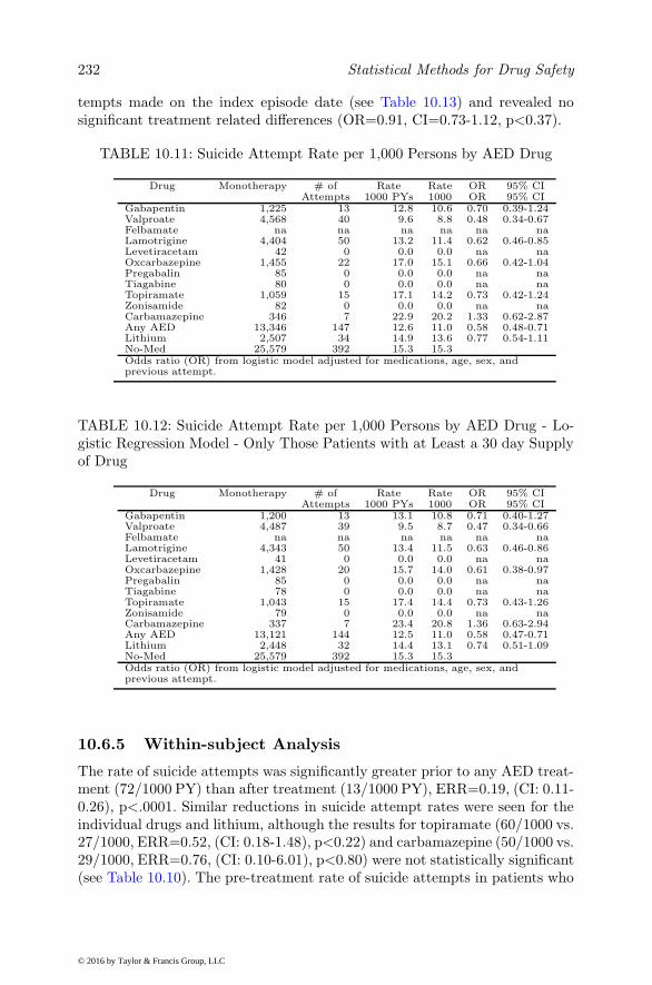
232 Statistical Methods for Drug Safety
tempts made on the index episode date (see Table 10.13) and revealed nosignificant treatment related differences (OR=0.91, CI=0.73-1.12, p<0.37).
TABLE 10.11: Suicide Attempt Rate per 1,000 Persons by AED Drug
Drug Monotherapy # of Rate Rate OR 95% CIAttempts 1000 PYs 1000 OR 95% CI
Gabapentin 1,225 13 12.8 10.6 0.70 0.39-1.24Valproate 4,568 40 9.6 8.8 0.48 0.34-0.67Felbamate na na na na na naLamotrigine 4,404 50 13.2 11.4 0.62 0.46-0.85Levetiracetam 42 0 0.0 0.0 na naOxcarbazepine 1,455 22 17.0 15.1 0.66 0.42-1.04Pregabalin 85 0 0.0 0.0 na naTiagabine 80 0 0.0 0.0 na naTopiramate 1,059 15 17.1 14.2 0.73 0.42-1.24Zonisamide 82 0 0.0 0.0 na naCarbamazepine 346 7 22.9 20.2 1.33 0.62-2.87Any AED 13,346 147 12.6 11.0 0.58 0.48-0.71Lithium 2,507 34 14.9 13.6 0.77 0.54-1.11No-Med 25,579 392 15.3 15.3Odds ratio (OR) from logistic model adjusted for medications, age, sex, andprevious attempt.
TABLE 10.12: Suicide Attempt Rate per 1,000 Persons by AED Drug - Lo-gistic Regression Model - Only Those Patients with at Least a 30 day Supplyof Drug
Drug Monotherapy # of Rate Rate OR 95% CIAttempts 1000 PYs 1000 OR 95% CI
Gabapentin 1,200 13 13.1 10.8 0.71 0.40-1.27Valproate 4,487 39 9.5 8.7 0.47 0.34-0.66Felbamate na na na na na naLamotrigine 4,343 50 13.4 11.5 0.63 0.46-0.86Levetiracetam 41 0 0.0 0.0 na naOxcarbazepine 1,428 20 15.7 14.0 0.61 0.38-0.97Pregabalin 85 0 0.0 0.0 na naTiagabine 78 0 0.0 0.0 na naTopiramate 1,043 15 17.4 14.4 0.73 0.43-1.26Zonisamide 79 0 0.0 0.0 na naCarbamazepine 337 7 23.4 20.8 1.36 0.63-2.94Any AED 13,121 144 12.5 11.0 0.58 0.47-0.71Lithium 2,448 32 14.4 13.1 0.74 0.51-1.09No-Med 25,579 392 15.3 15.3Odds ratio (OR) from logistic model adjusted for medications, age, sex, andprevious attempt.
10.6.5 Within-subject Analysis
The rate of suicide attempts was significantly greater prior to any AED treat-ment (72/1000 PY) than after treatment (13/1000 PY), ERR=0.19, (CI: 0.11-0.26), p<.0001. Similar reductions in suicide attempt rates were seen for theindividual drugs and lithium, although the results for topiramate (60/1000 vs.27/1000, ERR=0.52, (CI: 0.18-1.48), p<0.22) and carbamazepine (50/1000 vs.29/1000, ERR=0.76, (CI: 0.10-6.01), p<0.80) were not statistically significant(see Table 10.10). The pre-treatment rate of suicide attempts in patients who
© 2016 by Taylor & Francis Group, LLC

Analysis of Medical Claims Data 233
TABLE 10.13: Suicide Attempt Rate per 1,000 Persons by AED Drug - Lo-gistic Regression Model - Excluding Suicide Date = Index Date
Drug Monotherapy # of Rate Rate OR 95% CIAttempts 1000 PYs 1000 OR 95% CI
Gabapentin 1,225 13 12.8 10.6 1.13 0.63-2.03Valproate 4,568 40 9.6 8.8 0.74 0.53-1.05Felbamate na na na na na naLamotrigine 4,404 50 13.2 11.4 0.98 0.71-1.35Levetiracetam 42 0 0.0 0.0 na naOxcarbazepine 1,455 22 17.0 15.1 1.05 0.67-1.64Pregabalin 85 0 0.0 0.0 na naTiagabine 80 0 0.0 0.0 na naTopiramate 1,059 15 17.1 14.2 1.18 0.69-2.03Zonisamide 82 0 0.0 0.0 na naCarbamazepine 346 7 22.9 20.2 1.99 0.92-4.30Any AED 13,346 147 12.6 11.0 0.91 0.73-1.12Lithium 2,507 34 14.9 13.6 1.22 0.84-1.77No-Med 25,579 255 10.0 10.0Odds ratio (OR) from logistic model adjusted for medications, age, sex, andprevious attempt.
ultimately received AED treatment was significantly higher than the no treat-ment suicide attempt rate (ERR=4.88, (CI: 3.91-6.09), p<0.0001) suggestingthat patients who receive AED treatment were more severely impaired andtherefore at greater risk of suicide. A similar result was found for lithium (seeTable 10.10).
10.6.6 Discrete-time Analysis
A discrete-time survival model was used to examine the association betweentreatment defined on a monthly basis to the first suicide attempt. A significantdecrease in suicide attempt rate associated with AED treatment (OR=0.59,CI=0.47-0.75, p<0.0001) was found. Figure 10.2 presents the estimated haz-ard functions (post-diagnosis) for treated and untreated patients. Overall thesuicide attempt rate decreases with time; however, the rates are lower in AEDtreated patients throughout. Restricting the analysis to only those patients(n=662) that made a suicide attempt in the year prior to the index diagno-sis revealed an even larger decrease in suicide attempt rate associated withtreatment (OR=0.35, CI=0.17-0.74, p<0.005).
10.6.7 Propensity Score Matching
To further control for possible treatment selection, patients were matched onboth a 1:1 propensity score (i.e., matching of patients that did and did nottake an AED on a series of potential confounders including prior suicide at-tempts and other anticonvulsant, antidepressant, and antipsychotic use beforeand after AED treatment initiation, and initial exposure date assignment (i.e.,time from diagnosis of bipolar disorder to initiation of AED treatment) foreach pair based on the patient who took the AED. Table 10.14 presents thecovariate distributions for AED and no-AED groups before and after match-
© 2016 by Taylor & Francis Group, LLC

234 Statistical Methods for Drug Safety
FIGURE 10.2: Hazard functions for suicide rates over time. Comparisons ofpatients treated with an AED vs patients not treated with an AED wereadjusted for age, sex, concomitant treatment, previous suicide attempt, andyear.
ing. Table 10.14 presents differences in means for age, and proportions (allother variables), and standardized differences (mean or proportion differencedivided by pooled standard deviation). As a rule of thumb, standardized dif-ferences of 10% or less are considered well matched (Austin 2007). Table 10.14reveals large imbalances prior to matching, which disappear in the matchedsample. Comparison of the AED and no-AED groups revealed that prior totreatment, the rate of suicide attempts was 70.52/1000 PY for treated and38.07/1000 PY for untreated (OR=1.85, 95% CI=(1.22-2.81), p<0.0037). Fol-lowing treatment the suicide attempt rate was 12.88/1000 PY for the treatedand 10.46/1000 for untreated (OR=1.23, CI=(0.89-1.71), p<0.22). These re-sults reveal that even after matching, the pre-treatment suicide attempt rateis significantly elevated; however, following treatment there is no significantdifference in suicide attempt rates between those who did and did not receiveAED treatment.
© 2016 by Taylor & Francis Group, LLC

Analysis
ofMedica
lClaim
sData
235
TABLE 10.14: Comparison of Patient Characteristic Distributions in Original and Propensity Score Matched Samples
Original Dataset (n=38,817) Matched Dataset (n=25,574)No-Med AED STD Diff No-Med AED STD Diff
Male 40.2 40.0 0.5 40.3 40.1 0.5Previous suicide attempt 1.1 1.6 4.0 1.4 1.6 1.4Anticonvulsant before index date 5.2 11.8 23.9 9.1 10.5 4.8Anticonvulsant after index date 6.0 14.9 29.6 10.9 13.0 6.7Antidepressant before index date 39.4 66.9 57.5 67.3 65.5 3.9Antidepressant after index date 42.4 70.6 59.4 71.9 69.3 5.8Antipsychotic before index date 13.1 23.6 27.4 21.4 22.5 2.6Antipsychotic after index date 19.9 41.1 47.3 36.1 38.7 5.4Age 35.4 (15.9) 34.6 (15.2) 4.9 34.6 (15.5) 34.7 (15.3) 0.7Percentage or mean and standard deviation
© 2016 by Taylor &
Francis Group, LLC

236 Statistical Methods for Drug Safety
10.6.8 Self-controlled Case Series and Poisson HybridModels
To this point in the analysis, we have restricted our attention to AEDmonotherapy over a one year period. To provide a more general frameworkwe now consider a six month window from the index episode and permitany combination of AED therapy across the 11 AEDs that led to the FDAwarning. Furthermore, in the analyses presented in this section we only ad-just the relationship between time-varying AED exposure and suicide attemptfor potentially time-varying confounders (lithium, other anticonvulsants, an-tidepressants, and antipsychotic medications). Since these are within-personcomparisons, we further restrict the analysis to the 17,370 subjects who tookat least one AED during the 6 month period from diagnosis of bipolar illness.This included 104,220 monthly observations and 217 suicide attempts in 187individuals. The hybrid model that we consider here decomposes the AEDexposure into the average of exposed months and the deviation of each monthfrom that average. For example, if a patient was prescribed an AED on 3 of the6 months the average is 0.5 and the months off AED therapy have a deviationof -0.5 and those on AED therapy 0.5. The Poisson model is fitted with randomintercept and deviation effects to accommodate both person-specific variationin the base-rate and treatment heterogeneity. To adjust for concomitant med-ications, terms in the model were included for treatment with lithium, otheranticonvulsants, antidepressants, and antipsychotic medications at each pointin time. As a comparison, we also fit a conditional model (SCCS) to the samedata.
Results of the analysis of the SCCS analysis revealed a significant effect ofAED exposure on suicide attempts, RR=1.60 95% CI=(1.13, 2.28). Resultsof the analysis for the hybrid model reveal significant confounding for the BSeffect RR=0.30 95% CI=(0.17, 0.51) but a non-significant WS exposure effectRR=1.33 95% CI=(0.43, 4.14). While the BS effect reflects differences betweenindividuals which may be confounded with other unmeasured characteristics,it is interesting to note that those subjects receiving more consistent AEDtreatment have significantly lower probability of making a suicide attempt.Within individuals, there is a greater likelihood of making a suicide attempt ontreated months but this effect was not statistically significant using the hybridmixed-effects model. Of course, this effect could be produced by dynamicconfounding where risk of suicide attempt and treatment are correlated withchanges in severity of illness. Note that the SCCS is restricted to the analysisof subjects who both took an AED and made a suicide attempt. This ignoresinformation on subjects who took an AED and did not make a suicide attemptwhich is incorporated in the hybrid model. If we similarly restrict the hybridmodel to the case-exposure subsample, the within-subject effect is estimated asRR=1.50 95% CI=(1.07, 2.11), which is slightly smaller than the conditionalestimator, but larger than the exposure only cohort. Restricting the sample
© 2016 by Taylor & Francis Group, LLC

Analysis of Medical Claims Data 237
to the case-exposure subset may increase dynamic confounding with severityof illness.
10.6.9 Marginal Structural Models
To examine the possibility of dynamic confounding, we used a marginal struc-tural model for time to first suicide attempt to analyze the dataset used in theprevious section (i.e., six months of follow-up not restricted to AED monother-apy). All 47,918 patients with a new index episode of bipolar disorder wereused in this analysis whether or not they took an AED. Discrete-time sur-vival models were used to analyze these data. The simple unweighted analysiswithout covariate adjustment yielded a significantly increased risk of suicideattempt with any AED treatment OR=1.77 95% CI=(1.42, 2.20). Statisti-cal adjustment for age, sex, prior suicide attempt, concomitant medications(antidepressants, other anticonvulsants, antipsychotics and lithium) and co-morbid disorders (ADHD, anxiety spectrum disorders, psychotic disorders,seizure disorders, and conduct disorders) had little effect on the estimatedassociation OR=1.72 95% CI=(1.38, 2.15). By contrast, the MSM weightedanalysis revealed evidence of a protective effect of AED treatment both withOR=0.78 95% CI=(0.62, 0.98) and without OR=0.80 95% CI=(0.63, 1.01)covariate adjustment. These findings reveal that simple covariate adjustmentmay be insufficient to remove the dynamic confounding in the treatment se-lection process.
The previous analyses represent a mixture of between-subject and within-subject effects. It should be noted that a hybrid model can also be used forthese analyses, where the dynamic AED treatment effect can be decomposedinto between and within components as the mean and deviation of the monthlyAED treatments. The simple unweighted and unadjusted analysis reveals amarginal within-subject effect OR=1.51 95% CI=(1.03, 2.22), which disap-pears after MSM weighting OR=1.18 95% CI=(0.80, 1.75). Note that theweighted average effect is significantly protective OR=0.63 95% CI=(0.46,0.85) indicating that increased treatment was associated with decreased risk ofa suicide attempt. Covariate adjustment decreased the unweighted OR=1.4195% CI=(0.97, 2.04) and weighted OR=1.10 95% CI=(0.75, 1.61) associa-tions. These findings reveal that the benefit observed in the original MSManalysis was due in large part to between-subject effects where subjects withmore AED treatment have lower suicide attempt rate. Within subjects theweighted analysis reveals no association between AED treatment and suicideattempts.
10.6.10 Stratified Cox and Random-effect Survival Models
The bipolar dataset is not well suited to analysis using a stratified Cox modelbecause there is no obvious clustering unit besides the individual and no obvi-ous way to partition the within subject data into episodes based on the rarity
© 2016 by Taylor & Francis Group, LLC
238 Statistical Methods for Drug Safety
of the suicide attempt outcome. Interestingly as illustrated in the previousexample, the hybrid model permits a decomposition of between and within-subject effects even without random-effects. This is unique to a time-to-eventmodel, because it is the only model where the exposure variable can be time-varying but the outcome is not repeatedly experienced. To illustrate use of themodels in the more general clustered case we turn to an example originallydescribed by Gibbons et al. (2012a,b) on suicidal ideation and behavior datafrom 41 randomized longitudinal placebo-controlled clinical trials of fluoxe-tine and venlafaxine. Here the clustering variable is study, and study-specificvariability in both the background rate and treatment effect can be includedin the corresponding mixed-effects model. Given randomization, there is nopossible correlation between the study-specific random-effect and exposurevariable (i.e., antidepressant treatment) so concern regarding the violation ofthe independence assumption does not apply. For the first illustration usingthese data, we restrict attention to the entire adult population (37 studies and5,821 subjects aged 18 and older), see Table 10.15. The models included termsfor treatment, age, and sex on time to suicidal event. For the stratified Coxmodel, the treatment effect (expressed as a hazard ratio) was HR=0.66, 95%CI=(0.56, 0.77). Identical results were obtained for the mixed-effects discrete-time survival model with a random intercept HR=0.66, 95% CI=(0.56, 0.77),and similar results when the model is extended to include treatment hetero-geneity HR=0.66, 95% CI=(0.56, 0.79). The same is not true, however, whenthe data are restricted to young adults, ages 18-24, for which the black boxwarning was extended by the U.S. FDA in 2006. There were 32 studies, 378subjects, and 44 suicidal events for this age group (see Table 10.16). Here,the stratified Cox model yielded HR=1.12, 95% CI=(0.55, 2.26), whereas thediscrete-time survival model yielded HR=1.00, 95% CI=(0.54, 1.85). The fun-damental difference here is that 12 of the 32 studies had zero events and there-fore did not contribute to the likelihood of the stratified Cox model. Whenthe event rate is low and the sample is limited, the random-effect approachmay provide both increased statistical power and reduction in bias comparedto the stratified Cox model. This is a similar result as previously shown inthe comparison of fixed effect versus full-likelihood random-effect methods formeta-analysis of rare binary events in Chapter 6.
10.6.11 Conclusion
Drawing causal inference from observational data is complicated in general,but even more complicated for the study of suicide. First, suicide and sui-cide attempts are rare events, and their determinants are difficult to estimateprecisely in all but the largest samples. Second, suicide is related to the indi-cation for treatment (i.e., a psychiatric disorder) and is therefore difficult todisentangle from the possible effects of treatment. Third, a suicide attemptcan lead to the identification of the psychiatric disorder that can in turn leadto treatment. It is not uncommon to find patients who have a suicide attempt,
© 2016 by Taylor & Francis Group, LLC
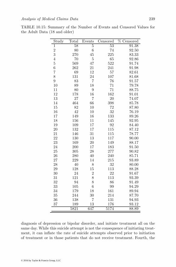
Analysis of Medical Claims Data 239
TABLE 10.15: Summary of the Number of Events and Censored Values forthe Adult Data (18 and older)
Study Total Events Censored % Censored1 58 5 53 91.382 80 6 74 92.503 270 45 225 83.334 70 5 65 92.865 569 47 522 91.746 262 21 241 91.987 69 12 57 82.618 131 24 107 81.689 83 7 76 91.5710 89 18 71 79.7811 80 9 71 88.7512 178 16 162 91.0113 27 7 20 74.0714 464 66 398 85.7815 82 10 72 87.8016 42 10 32 76.1917 149 16 133 89.2618 156 11 145 92.9519 109 17 92 84.4020 132 17 115 87.1221 146 31 115 78.7722 130 13 117 90.0023 169 20 149 88.1724 200 17 183 91.5025 305 28 277 90.8226 280 40 240 85.7127 229 14 215 93.8928 40 8 32 80.0029 128 15 113 88.2830 24 2 22 91.6731 121 8 113 93.3932 94 8 86 91.4933 105 6 99 94.2934 179 18 161 89.9435 244 30 214 87.7036 138 7 131 94.9337 189 13 176 93.12
5821 647 5174 88.89
diagnosis of depression or bipolar disorder, and initiate treatment all on thesame day. While this suicide attempt is not the consequence of initiating treat-ment, it can inflate the rate of suicide attempts observed prior to initiationof treatment or in those patients that do not receive treatment. Fourth, the
© 2016 by Taylor & Francis Group, LLC

240 Statistical Methods for Drug Safety
TABLE 10.16: Summary of the Number of Events and Censored Values forthe Young Adult Data (18 to 24)
Study Total Events Censored % Censored1 4 0 4 100.002 7 1 6 85.713 21 4 17 80.954 2 1 1 50.005 38 5 33 86.846 24 2 22 91.677 7 0 7 100.008 5 1 4 80.009 7 2 5 71.4310 12 4 8 66.6711 3 1 2 66.6712 15 1 14 93.3313 6 0 6 100.0014 1 0 1 100.0015 9 0 9 100.0016 7 0 7 100.0017 11 3 8 72.7318 2 0 2 100.0019 8 0 8 100.0020 5 0 5 100.0021 7 0 7 100.0022 16 1 15 93.7523 15 3 12 80.0024 12 1 11 91.6725 9 2 7 77.7826 8 2 6 75.0027 8 1 7 87.5028 52 6 46 88.4629 25 2 23 92.0030 13 0 13 100.0031 12 1 11 91.6732 7 0 7 100.00
378 44 334 88.36
natural course of psychiatric illnesses exhibits a decrease in suicide attemptsover time from diagnosis. This can make it appear that the suicide attemptrate is higher prior to treatment initiation than after, giving the false appear-ance of a protective effect. Fifth, patients who receive treatment often haveincreased severity of illness and may therefore be at increased suicidal risk tobegin with.
These analyses reveal no evidence that AEDs increase risk of suicide at-tempts relative to patients not treated with an AED or lithium. Among pa-tients not receiving any concomitant CNS treatment, the suicide attempt rate
© 2016 by Taylor & Francis Group, LLC

Analysis of Medical Claims Data 241
in AED treated patients was significantly lower than untreated patients. Theseanalyses also reveal that there is a selection effect in that the pre-treatmentsuicide attempt rate is 5 times higher than the rate in untreated patients. Ifpre-treatment suicide attempt rates reflect severity of illness, it is the moreseverely impaired patients who receive treatment with an AED or lithium.Nevertheless, the post-treatment suicide attempt rate is significantly reducedrelative to their elevated pre-treatment levels to the level found at or belowpatients not receiving treatment. This finding suggests a possible protective ef-fect of AED treatment on suicidality. Possible exceptions are topiramate andcarbamazepine which did not show significant reduction in suicide attemptrates with treatment and had post-treatment suicide attempt rates signifi-cantly higher than untreated levels. Nevertheless, even for these two AEDs,there was no evidence that they increased suicide rates.
Sensitivity analyses revealed that these findings are robust to duration oftreatment, defined as duration of 30 days or more, or defined on a monthlybasis. The later analysis reveals that despite the systematic decreases in sui-cide attempt rates over time, there remains a statistically significant decreasein suicide attempt rate for patients treated with an AED. Similar results werefound for multiple attempts or a single attempt per person. Similar resultswere observed when monotherapy was defined for the entire year followingthe index episode or just until the first suicide attempt. Excluding all sui-cide attempts that occurred on the index episode date produced an oddsratio less than 1.0, but was no longer statistically significant. This findingsuggests that some of the difference between patients treated with an AEDand those not treated may be due to the identification of bipolar disorder be-cause of the suicide attempt. Propensity score matching was used to furtherexamine this possibility, by matching AED treated and untreated patientsin terms of potential confounders and pre and post-treatment periods basedon the treatment initiation day for the treated patient. Treated patients stillhad elevated pre-treatment suicide attempt rate, but no difference followingtreatment. AED treatment therefore appears to produce a larger decrease insuicide attempt rates because the patients who ultimately receive AED treat-ment have a higher rate of suicide attempts prior to receiving treatment. Theexception to this is the case of patients who received no CNS treatment at allversus those that only received an AED, where the post AED treatment ratewas significantly lower than the no treatment rate (3/1000 patient years ver-sus 15/1000 patient years). Finally, restricting attention to those patients athighest risk for suicide attempt (i.e., those patients making a suicide attemptin the year prior to the index episode) revealed an even larger significant re-duction in suicide attempt rate with AED treatment, suggesting that benefitof AED treatment may be greatest for the highest risk patients.
When we relax the requirement of AED monotherapy and include pa-tients who might take multiple AEDs during the first six months followingtheir index diagnosis of a new bipolar disorder, the naive analyses do suggesta positive association between treatment with an AED and suicide attempt.
© 2016 by Taylor & Francis Group, LLC

242 Statistical Methods for Drug Safety
Decomposing this effect into between-subject and within-subject componentsreveals that the protective effect is explained largely by a positive associationbetween the proportion of time a patient receives AED treatment during thefirst six months following diagnosis. The within-subject association is not sta-tistically significant, but is in the direction of increased risk during monthsthat patients receive treatment. Marginal structural models reveal that thistrend is due to dynamic confounding, which when accounted for by weightingyields an odds ratio close to 1.0. Although we generally view the between-subject effect as merely a confounder, here it suggests that if patients receivetreatment with an AED, the more consistent that treatment the lower the riskof a suicide attempt.
Finally, we have also illustrated the use of a stratified Cox model anda mixed-effects discrete-time survival model for analysis of clustered survivaldata in a research synthesis of 37 studies of antidepressant treatment in adults.When the number of studies is large and the number of subjects within thosestudies is large, and when all studies record events, both approaches yield vir-tually identical results. However, when the number of subjects within studiesis smaller and some studies have no events of interest, the stratified Cox modelcan exhibit bias similar to fixed-effects models used in meta-analysis of rarebinary events.
10.7 Conclusion
In many ways, this chapter is the heart of this book. With the emergenceand accessibility of “big data” comes the responsibility for their careful andthoughtful analysis. These are generally observational data and have no im-munity to bias. Size does not insulate one from bias as shown repeatedly inthis chapter. Of the various methods described here, it should be directly ap-parent that those methods which focus on within-subject associations are theleast prone to bias. Even here, however, dynamic confounding can play a roleproviding the appearance of an association between two time-series which areboth merely related to a third dynamic confounder, for example changes inthe severity of illness. Given their wide use and generally good performancefor work in drug safety, we have provided a detailed review of fixed-effects ap-proaches for analysis of clustered and longitudinal data. These include SCCSand stratified Cox models. Both are extremely important and useful tools forhigh quality work in drug safety. Nevertheless we have illustrated that thereare conditions in which their generally good performance is compromised interms of limited statistical power and even bias in the presence of treatmentheterogeneity. We have drawn attention to less well known alternatives basedon mixed-effects regression models and ways around their sometimes restric-
© 2016 by Taylor & Francis Group, LLC
Analysis of Medical Claims Data 243
tive assumptions which have diminished enthusiasm for their general use inthis area.
© 2016 by Taylor & Francis Group, LLC

11
Methods to be Avoided
“I don’t use drugs, my dreams are frightening enough.”(M.C. Escher)
11.1 Introduction
As evidenced in the previous chapters, there are a great many statistical ap-proaches to the analysis of drug safety data. Not all methods are good forall problems and as we have seen, methods which exploit dynamic exposureswithin individuals may well provide the greatest promise for future work inthis area. Nevertheless, there are some approaches, often widely used in prac-tice, which should be avoided as they are so prone to bias, misleading, anduninterpretable results that they are better off left alone. In this chapter, wetry to highlight what these methods are and why they should be avoided andfor what purposes.
11.2 Spontaneous Reports
For many years the primary tool used by pharmaceutical companies and theU.S. FDA involved the collection of spontaneous reports from patients, doc-tors, lawyers, ... , regarding drugs that they have taken and adverse eventsthat they have experienced. Chapter 5 provides a detailed review of statisti-cal approaches to the analysis of such data. While some methods are morepromising than others, it is our opinion that such data are so limited that theyshould only be considered for very specific purposes. Problems associated withthe use of spontaneous reports in drug safety include (1) confounding by indi-cation (i.e., patients taking a particular drug may have a disease that is itselfassociated with a higher incidence of the AE (e.g., antidepressants, depression,and suicide)), (2) systematic underreporting, (3) questionable representative-ness of patients, (4) effects of publicity in the media on numbers of reports,
245
© 2016 by Taylor & Francis Group, LLC

246 Statistical Methods for Drug Safety
(5) extreme duplication of reports, (6) attribution of the event to a single drugwhen patients may be exposed to multiple drugs, and (7) extensive amountsof missing data. These limitations degrade the capacity for optimal data min-ing and analysis (Hauben et al. 2007). Spontaneous reports are useful for theidentification of very rare adverse events early in a drug’s history of use whichhave little or anything to do with the indication for which the drug is used.For example, taking a drug and turning a bright shade of blue is a very differ-ent thing than taking a drug and feeling blue. If the drug is given to patientswho are at increased risk of depression, the frequency of patients reportingthat they feel blue will undoubtedly be elevated relative to other side-effects(disproportionality), but the association provides no basis for causal infer-ence. Turning blue is a very different matter and the evidence of even a smallnumber of cases of patients turning blue after a drug exposure is importantwhether it is disproportional or not. Many have taken this type of example(turning blue) as support for the in-discriminant use of such data (sponta-neous reports) to draw inferences regarding examples of the latter (feelingblue). We now have much better data and methods for drawing inferencesfor more common adverse events (e.g., analysis of large-scale observationaldatasets such as medical claims data), and they should replace analysis ofspontaneous reports for all but the most unusual occurrences.
11.3 Vote Counting
In chapter 6, we provide an extensive review of meta-analytic techniques forresearch synthesis, pointing out their various strengths and weaknesses, par-ticularly for analysis of rare adverse events. Unfortunately, there are manycases where a simple tally of the number of positive studies is reported andtaken as evidence for efficacy, safety, or the lack thereof. This is a practicethat should clearly be avoided. One can easily imagine a series of small stud-ies which are underpowered to detect an association between treatment andan adverse event such that none of the individual studies report a statisticallysignificant association and the vote count is 0 in terms of evidence in favor ofsuch an association. In the aggregate, however, the association may well beclinically and statistically significant given the increased statistical power ofthe combined analysis. The reverse can also be true. A series of biased stud-ies can yield a high vote count in favor of an association that is an artificialbyproduct of confounding. Another problem with vote-counting is that it ig-nores sample size, and the results of a series of small studies may provide ahigh or low vote count which is discordant with the greatest mass of the datawhich might be restricted to a few large and well controlled studies. A goodexample relates to the question of whether antidepressants cause birth de-fects. Several studies which have compared mothers who took antidepressants
© 2016 by Taylor & Francis Group, LLC

Methods to be Avoided 247
versus those that did not have shown increased risk of birth defects (includingcardiac birth defects) in mothers who took antidepressants during the firsttrimester (see Alwan et al. 2007, Louik et al. 2007). However, Jimenez-Solemet al. (2012) did a similar comparison, but instead of comparing mother’s whodid or did not take antidepressants during pregnancy, which is confounded bydepression, they compared mothers who halted antidepressant treatment dur-ing pregnancy versus those who continued taking antidepressants. Here theauthors found that while children of exposed mothers had increased risk of car-diac malformations relative to unexposed mothers (OR=2.01, 95% CI=1.60,2.53), the same difference was seen between mothers who halted their use ofantidepressants during pregnancy and non-exposed mothers (OR=1.85, 95%CI=1.07, 3.20), probability value for the difference = 0.94. Vote countingwould likely yield strong evidence in support of an association which mayhave little to do with the exposure to antidepressants and much more to dowith the effects of depression on other exposures (e.g., people with depressionhave a higher rate of smoking) which are in turn related to birth defects.
11.4 Simple Pooling of Studies
Another bad approach to synthesizing evidence across studies is to simply poolthem and perform an overall analysis on the combined data without takingthe clustering of observations within studies into account. This is an all toocommon practice. Not only can this provide incorrect standard errors andtests of hypotheses, it can also produce biased results. For example, imaginea series of randomized controlled trials of which half used 1:1 randomizationto treatment versus control and the other half used 3:1 randomization. Moreseverely ill patients might risk enrollment in an RCT that provided threetimes the likelihood of receiving active treatment, but might not enroll if thechance was only 50%. If severity of illness is associated with the likelihoodof the adverse event, then there would be more events in the 3:1 randomizedtrials, and since there are three times as many treated patients in these trials,this would give the appearance that the drug increased the risk of the adverseevent. Even more dangerous would be the attribution that one can draw acausal inference from these data because the individual trials were randomized.Of course a proper meta-analysis would adjust for this imbalance and accountfor differences in the baseline risk between the studies in estimating the overalltreatment effect.
© 2016 by Taylor & Francis Group, LLC

248 Statistical Methods for Drug Safety
11.5 Including Randomized and Non-randomized Trialsin Meta-analysis
It is all too common to see a research synthesis which involves a mixture ofrandomized (Phase II or III) and non-randomized trials (Phase I). This is asimilar problem to the previous example in that studies in which everyonereceives treatment will often include more severely ill patients who would oth-erwise not enroll in a study in which they have a chance of being randomizedto placebo. If severity of illness is related to adverse event of interest, theresults of such an analysis will provide incorrect evidence of a relationshipbetween the drug and the adverse event. This is true even if a proper meta-analysis is performed because in the studies without randomization there isno control condition and severity of illness will be confounded with the effectof treatment.
11.6 Multiple Comparisons and Biased Reporting ofResults
While less of a factor in the peer reviewed literature, in litigation it is not un-common to see an expert report in which hundreds or even thousands of resultsare reviewed and a handful of those results which are statistically significant inthe desired direction are reported without discussion of disconfirming resultsor any information on the number of results reviewed. This is often the rulerather than the exception because in RCTs, summary results for large num-bers of potential adverse events are routinely reported without any adjustmentfor multiplicity. While this makes sense for the purpose of regulatory reviewwhere there is greater concern of a false negative than a false positive, this canlead to biased and misleading summaries of a literature or a set of publishedand unpublished studies where the focus is on litigation. To make mattersworse, it is often the case that results that are not statistically significant arereported in this way without regard to their confidence interval or distanceof the point estimate from the null. In extreme cases, experts will attributerisk to any odds ratio or relative risk greater than 1.0 and safety to any oddsratio or relative risk less than 1.0. Of course, if the null hypothesis is true andthe OR=RR=1.0, then we would expect 50% of the estimated ORs and RRsto be less than 1.0 and 50% to be greater than 1.0 by chance alone. Thesedata which provide evidence of no association between the exposure and theadverse event of interest can therefore be used to support either a protectiveor harmful association depending on the prerogative of the reviewer. This typeof practice is a very unfortunate consequence of our legal system.
© 2016 by Taylor & Francis Group, LLC

Methods to be Avoided 249
11.7 Immortality Time Bias
Immortality time bias refers to the span of time during the observation periodwhere the event of interest could not have occurred (Suissa 2007). The classicexamples are two studies from the 1970s on the benefit of heart transplanton survival time. In the first study 15 treated patients who received a hearttransplant survived an average of 111 days (including waiting time for theorgan) were compared to 42 patients on the wait-list who survived an averageof only 74 days (Messmer et al. 1969). In the second study survival was 200days for the 20 patients in the transplant group versus 34 days for the 14wait-list controls. As noted by Gail (1972) inclusion of the period of timespent waiting for transplant in the survival time of the transplanted groupprovides a biased upward estimate of the survival time for the transplantedgroup because the subjects in the transplanted group must survive until thetime of transplant.
In pharmacoepidemiology, immortal time bias occurs when the time be-tween the cohort entry and initiation of treatment is attributed to the exposurecondition. If the event is not repeatable or interest is in time to the first event,the time between cohort entry and exposure is immortal since subjects whoexperience the event are not included and the time during which the eventcannot occur is added to the exposure group only. As noted by Suissa (2007),the solution is to treat exposure as a time-dependent exposure in a time-to-event model or to classify the period prior to the first exposure as unexposed.A second example of immortal time bias occurs when the cohort is defined onthe basis of having two or more exposures. The period of time between the firstexposure and the second is immortal because the subject must survive untilthe second exposure in order to be considered. Subjects who died after thefirst exposure cannot be included in the exposed group; therefore, biasing theirestimated survival time. A third example involves definition of the exposedgroup as having both a diagnosis and exposure (i.e., filled prescription) on thesame day and a comparison group of subjects who were not exposed duringthe first year from diagnosis. Groups are then compared during a follow-upperiod. In order to be in the control group, the patients must survive for ayear, during which the survival time for the controls is ignored. A graphicalexample originally presented by Levesque et al. (2010) is presented in Figure11.1.
Suissa (2007) demonstrated the effect of misclassified and excluded immor-tal time by showing effectiveness of two drug classes, inhaled beta-agonists(IBA) and gastrointestinal drugs (GID), that are not known to treat cardio-vascular disease (CVD). He selected the base cohort using health insurancedatabases from Saskatchewan, Canada. The cohort included those patientshospitalized for primary diagnosis of CVD. To illustrate the immortal timebias arising from misclassification and exclusion, he formed two cohorts. The
© 2016 by Taylor & Francis Group, LLC

250 Statistical Methods for Drug Safety
FIGURE 11.1: Examples of immortality bias.
first cohort was formed by defining cohort entry as a hospital discharge datefollowing the CVD diagnosis, and the exposure was defined at the first pre-scription of IBA during the first 180 days of follow up. A total of 1542 subjectswere included in the study, of whom 771 did not fill an IBA prescription dur-ing the 180-day period, i.e, unexposed. They contributed 674.6 person-yearsto the study and 148 deaths were observed resulting into 21.9 deaths per 100subjects per year. Among the remaining 771 subjects who did fill an IBAprescription during the 180-day period, 114 died during follow up. The to-tal person-time contributed by the exposed group was 713.0 person-year, ofwhich 102.4 person-years were observed between entry and exposure. The rateof death in this group was 16 per 100 exposure years. The death rate ratio cal-culated from this misclassified approach showed 0.73 (0.57-0.93) times lower
© 2016 by Taylor & Francis Group, LLC

Methods to be Avoided 251
death rate for patients treated with IBA, even though the drug has never beenassociated with CVD treatment prior to this analysis. Clearly, the follow uptime between hospital discharge date and dispensing of IBA prescription isimmortal for the exposed group. The correctly classified analysis transfers theunexposed person-time to the denominator of the unexposed group risk. Theresulting total person-time in the unexposed is increased by 102.4 person-yearand decreased by the same amount in the exposed. Consequently, the correctrate of death in unexposed is 19.2 per 100 subjects per year and in exposedis 18.7 per 100 exposure per year. The resulting death rate ratio is 0.95 (0.77-1.25) and correctly shows that the IBA is not significantly effective in reducingmortality among CVD patients.
The second cohort was selected such that the immortal time is excludedfrom the exposure follow up. The cohort was formed by first selecting 640subjects who received GID in the first year after discharge. The unexposedgroup included 640 subjects who did not receive GID in the first year after dis-charge. The exposed subjects were followed for 1-year after the GID exposureand unexposed subjects were followed for 1-year after the day of discharge. Ofthe 640 exposed subjects, 99 died during the follow up and total person-timecontribution was 581.3 person-years. Of the 640 unexposed subjects, 125 diedduring a 1-year follow up. A total of 561.0 person-years were observed for theunexposed group. The rate ratio comparing the exposed to unexposed groupwas 0.78 (0.61-0.99) indicating a significant reduction in death rate amongthe exposed group. However, a proper accounting of 131.5 person-years thatpreceded exposure as unexposed person-time changed the rate ratio to 0.94(0.73-1.20), indicating non-significant reduction in mortality rate attributableto GID treatment.
These two analyses that purposefully introduced immortal time in cohortselection highlight the danger in conducting observational studies. The im-mortal time bias is pervasive in the literature. Several reviews have revealeda number of studies that suffer from this bias. Suissa (2007) has listed 20observational studies of the effects of various drugs on mortality and mor-bidity. Some of those studies were published in reputable journals such theJournal of the American Medical Association. Suissa and Azoulay (2012) alsoreviewed studies of the risk of cancer associated with metformin use and found13 observational studies on the subject that have incurred the same bias.
Two general strategies for eliminating such bias are (a) to treat exposureas a time-dependent variable comparing rates of repeatable events within in-dividuals or simply as a time-varying predictor in a time to a single eventanalysis, and (b) in a cohort defined in terms of a new diagnosis, matchingcontrol observation periods to the time after index diagnosis of the exposurefor each of the treated subjects. An example of the matching is to begin theobservation period for a control subject 10 days after diagnosis as a match foran exposed subject who began pharmacologic treatment 10 days after diagno-sis. Of course, day 1 of the observation period would begin on day 10 followingthe index diagnosis for both subjects. Here the first 10 days are immortal in
© 2016 by Taylor & Francis Group, LLC

252 Statistical Methods for Drug Safety
both exposed and unexposed subjects, thereby eliminating bias associatedwith the immortality. The matching strategy provides a way of eliminatingimmortality bias in a between-subject comparison, whereas treating exposureas a time-varying effect can be used to estimate the within-subject exposureeffect using methods described in Chapter 10.
© 2016 by Taylor & Francis Group, LLC

12
Summary and Conclusions
“Words are, of course, the most powerful drug used by mankind.”(Rudyard Kipling)
12.1 Final Thoughts
Drug safety is an international priority. However, all drugs have adverse effects;what ultimately matters is if the benefits of a drug outweigh the risks. To thisend, a scientifically accurate characterization of risks and benefits is essential.A drug like varenicline which is the most effective anti-smoking treatmentin existence has a black box warning for neuropsychiatric events and suiciderisk despite the absence of a signal derived from RCTs and large-scale wellcontrolled observational studies. The evidence in support of this associationis restricted to spontaneous reports of such events. It seems unlikely that thefrequency of spontaneous reports is indicative of a causal association in theabsence of any signal based on higher quality randomized and observationaldata (Gibbons and Mann 2013). Nevertheless, the black box warning has lim-ited use of this highly effective smoking cessation medication the consequencesof which must include increased risk of lung cancer and death. There is some-thing seriously wrong with this risk-benefit equation.
We have reviewed a wide variety of statistical approaches for the analysisof drug safety data, many of which will hopefully lead to improved futurepractice and increased interest by statisticians in conducting future statisticalresearch in this important area. Drug safety is clearly an area which benefitsfrom the availability of “big data.” However, big data in and of themselvesis not the solution. These data must be paired with thoughtful designs andanalyses to prevent bias and false discovery. The need for rigorous statisticalthinking and practice is all the more important as the size of available datastreams increase. These are observational data and their perils have been wellknown to statisticians and epidemiologists for decades.
While we have outlined many different approaches to providing a detailedreview of a putative drug adverse event association, an important directionof future research should be in the area of the use of these methods for large-
253
© 2016 by Taylor & Francis Group, LLC

254 Statistical Methods for Drug Safety
scale screening of millions of possible drug adverse event interactions. Wehave highlighted some of these approaches but much more work in this areais needed.
As in all areas of science, we must look for coherence across findings fromdifferent perspectives using different types of studies, both randomized andobservational, prior to drawing inferences. We must also look for disconfirmingevidence and not simply build a research platform to support a preconceivednotion. The consequences of both failing to detect a drug safety signal andfalsely concluding that there is a safety concern when one does not exist areenormous in terms of the protection of public health and maximizing humancapital.
© 2016 by Taylor & Francis Group, LLC
Bibliography
K. Abrams and B. Sanso. Approximate Bayesian inference for random effectsmeta-analysis. Statistics in Medicine, 17(2):201–218, 1998.
A. Agresti. Categorical Data Analysis. John Wiley & Sons, 1990.
I. Ahmed, F. Haramburu, A. Fourrier-Reglat, F. Thiessard, C. Kreft-Jais,G. Miremont-Salame, B. Begaud, and P. Tubert-Bitter. Bayesian phar-macovigilance signal detection methods revisited in a multiple comparisonsetting. Statistics in Medicine, 28(13):1774–1792, 2009.
I. Ahmed, C. Dalmasso, F. Haramburu, F. Thiessard, P. Broet, and P. Tubert-Bitter. False discovery rate estimation for frequentist pharmacovigilancesignal detection methods. Biometrics, 66(1):301–309, 2010a.
I. Ahmed, F. Thiessard, G. Miremont-Salame, B. Begaud, and P. Tubert-Bitter. Pharmacovigilance data mining with methods based on false dis-covery rates: a comparative simulation study. Clinical Pharmacology &Therapeutics, 88(4):492–498, 2010b.
I. Ahmed, F. Thiessard, G. Miremont-Salame, F. Haramburu, C. Kreft-Jais,B. Begaud, and P. Tubert-Bitter. Early detection of pharmacovigilancesignals with automated methods based on false discovery rates. Drug Safety,35(6):495–506, 2012.
M. A. Al-Osh and A. A. Alzaid. First order integer-valued autoregressive (inar(1)) process. Journal of Time Series Analysis, 8(3):261–275, 1987.
P. D. Allison. Discrete-time methods for the analysis of event histories. Soci-ological Methodology, 13(1):61–98, 1982.
P. D. Allison. Survival Analysis Using the SAS System: A Practical Guide.SAS Institute, 1995.
P. D. Allison. Fixed Effects Regression Models. Sage Los Angeles, 2009.
J. S. Almenoff, W. DuMouchel, L. A. Kindman, X. Yang, and D. Fram. Dis-proportionality analysis using empirical Bayes data mining: a tool for theevaluation of drug interactions in the post-marketing setting. Pharmacoepi-demiology and Drug Safety, 12(6):517–521, 2003.
255
© 2016 by Taylor & Francis Group, LLC

256 Statistical Methods for Drug Safety
S. Alwan, J. Reefhuis, S. A. Rasmussen, R. S. Olney, and J. M. Friedman.Use of selective serotonin-reuptake inhibitors in pregnancy and the risk ofbirth defects. New England Journal of Medicine, 356(26):2684–2692, 2007.
A. Amatya, D. K. Bhaumik, S. Normand, J. Greenhouse, E. Kaizar, B. Neelon,and R. D. Gibbons. Likelihood-based random effect meta-analysis of binaryevents. Journal of Biopharmaceutical Statistics, 2014.
J. D. Angrist, G. W. Imbens, and D. B. Rubin. Identification of causal effectsusing instrumental variables. Journal of the American Statistical Associa-tion, 91(434):444–455, 1996.
P. C. Austin. Propensity-score matching in the cardiovascular surgery lit-erature from 2004 to 2006: a systematic review and suggestions for im-provement. The Journal of Thoracic and Cardiovascular Surgery, 134(5):1128–1135, 2007.
A. Bate and S. J. W. Evans. Quantitative signal detection using spontaneousadr reporting. Pharmacoepidemiology and Drug Safety, 18(6):427–436, 2009.
A. Bate, M. Lindquist, I. R. Edwards, S. Olsson, R. Orre, A. Lansner, andR. M. De Freitas. A Bayesian neural network method for adverse drugreaction signal generation. European Journal of Clinical Pharmacology, 54(4):315–321, 1998.
D. K. Bhaumik, A. Amatya, S. T. Normand, J. Greenhouse, E. Kaizar,B. Neelon, and R. D. Gibbons. Meta-analysis of rare binary adverse eventdata. Journal of the American Statistical Association, 107(498):555–567,2012.
R. Bock. Multilevel Analysis of Educational Data. Academic Press, 1989.
R. D. Bock. Estimating multinomial response relations. In R. C. Bose, editor,Contributions to Statistics and Probability, pages 453–479. University ofNorth Carolina Press, Chapel Hill, NC, 1970.
R. D. Bock. Multivariate Statistical Methods in Behavioral Research. McGraw-Hill, 1975.
R. D. Bock. The discrete Bayesian. In H. Wainer and S. Messick, editors,Mod-ern Advances in Psychometric Research, pages 103–115. Erlbaum, Hillsdale,N.J., 1983a.
R. D. Bock. Within-subject experimentation in psychiatric research. In R. D.Gibbons and M. W. Dysken, editors, Statistical and Methodological Ad-vances in Psychiatric Research, pages 59–90. Spectrum New York, 1983b.
D. Bohning, U. Malzahn, E. Dietz, P. Schlattmann, C. Viwatwongkasem, andA. Biggeri. Some general points in estimating heterogeneity variance withthe DerSimonian and Laird estimator. Biostatistics, 3(4):445–457, 2002.
© 2016 by Taylor & Francis Group, LLC

Bibliography 257
J. Bound, D. A. Jaeger, and R. M. Baker. Problems with instrumental vari-ables estimation when the correlation between the instruments and the en-dogenous explanatory variable is weak. Journal of the American StatisticalAssociation, 90(430):443–450, 1995.
P. T. Brandt, J. T. Williams, B. O. Fordham, and B. Pollins. Dynamic mod-eling for persistent event-count time series. American Journal of PoliticalScience, pages 823–843, 2000.
A. S. Bryk and S. W. Raudenbush. Hierarchical Linear Models: Applicationsand Data Analysis Methods. Sage Publications, Inc, 1992.
W. E. Bunney, D. L. Azarnoff, B. W. Brown, R. Cancro, R. D. Gibbons, J. C.Gillin, S. Hullett, K. F. Killam, D. J. Kupfer, J. H. Krystal, et al. Reportof the institute of medicine committee on the efficacy and safety of halcion.Archives of General Psychiatry, 56(4):349–352, 1999.
S. P. Burke, A. Baciu, K. Straton, D. Blumenthal, A. Breckenridge, A. Charo,S. Edgman-Levitan, S. Ellenberg, R. D. Gibbons, and Others. The Futureof Drug Safety: Promoting and Protecting the Health of the Public. NationalAcademy Press, Washington D.C., 2006.
K. Cahill, L. F. Stead, and T. Lancaster. Nicotine receptor partial agonistsfor smoking cessation. The Cochrane Library, 2008.
K. Cahill, L. Stead, and T. Lancaster. A preliminary benefit-risk assessmentof varenicline in smoking cessation. Drug Safety, 32(2):119–135, 2009.
A. C. Cameron and P. K. Trivedi. Regression Analysis of Count Data. Num-ber 53. 2013.
O. Caster. Mining the who drug safety database using lasso logistic regression.UUDM Project Report, 16, 2007.
O. Caster, G. N. Noren, D. Madigan, and A. Bate. Large-scale regression-based pattern discovery: The example of screening the who global drugsafety database. Statistical Analysis and Data Mining, 3(4):197–208, 2010.
G. Chamberlain and G. Imbens. Random effects estimators with many in-strumental variables. Econometrica, 72(1):295–306, 2004.
J. Chen and A. K. Gupta. Parametric Statistical Change Point Analysis: withApplications to Genetics, Medicine, and Finance. Springer, 2011.
L. Chen and D. M. Ashcroft. Risk of myocardial infarction associated with se-lective cox-2 inhibitors: Meta-analysis of randomised controlled trials. Phar-macoepidemiology and Drug Safety, 16(7):762–772, 2007.
E. M. Chi and G. C. Reinsel. Models for longitudinal data with random effectsand ar (1) errors. Journal of the American Statistical Association, 84(406):452–459, 1989.
© 2016 by Taylor & Francis Group, LLC

258 Statistical Methods for Drug Safety
W. G. Cochran. The effectiveness of adjustment by subclassification in re-moving bias in observational studies. Biometrics, pages 295–313, 1968.
M. R. Conaway. Analysis of repeated categorical measurements with condi-tional likelihood methods. Journal of the American Statistical Association,84(405):53–62, 1989.
A. J. Cook, R. C. Tiwari, R. D. Wellman, S. R. Heckbert, L. Li, P. Heagerty,T. Marsh, and J. C. Nelson. Statistical approaches to group sequentialmonitoring of postmarket safety surveillance data: current state of the artfor use in the mini-sentinel pilot. Pharmacoepidemiology and Drug Safety,21(S1):72–81, 2012.
N. R. Cook, S. R. Cole, and C. H. Hennekens. Use of a marginal structuralmodel to determine the effect of aspirin on cardiovascular mortality in thephysicians’ health study. American Journal of Epidemiology, 155(11):1045–1053, 2002.
D. R. Cox. Analysis of binary data, 1970. Methuen, London, pages 103–8,1970.
D. R. Cox. Regression models and life-tables. Journal of the Royal StatisticalSociety, 34(2):187–220, 1972.
D. R. Cox. Partial likelihood. Biometrika, 62(2):269–276, 1975.
R. B. D’Agostino. Tutorial in biostatistics: propensity score methods for biasreduction in the comparison of a treatment to a non-randomized controlgroup. Statistics in Medicine, 17(19):2265–2281, 1998.
R. B. D’Agostino and R. B. D’Agostino. Estimating treatment effects usingobservational data. Journal of American Medical Association, 297(3):314–316, 2007.
R. B. D’Agostino, M. Lee, A. J. Belanger, L. Cupples, K. Anderson, andW. B. Kannel. Relation of pooled logistic regression to time dependent Coxregression analysis: the Framingham Heart Study. Statistics in Medicine, 9(12):1501–1515, 1990.
R. B. D’Agostino, S. Grundy, L. M. Sullivan, P. Wilson, et al. Validation of theframingham coronary heart disease prediction scores: results of a multipleethnic groups investigation. Journal of American Medical Association, 286(2):180–187, 2001.
M. J. Daniels and C. Gatsonis. Hierarchical polytomous regression modelswith applications to health services research. Statistics in Medicine, 16(20):2311–2325, 1997.
© 2016 by Taylor & Francis Group, LLC

Bibliography 259
N. M. Davies, D. Gunnell, K. H. Thomas, C. Metcalfe, F. Windmeijer, andR. M. Martin. Physicians’ prescribing preferences were a potential instru-ment for patients’ actual prescriptions of antidepressants. Journal of Clin-ical Epidemiology, 66(12):1386–1396, 2013.
J. De Leeuw and I. Kreft. Random coefficient models for multilevel analysis.Journal of Educational and Behavioral Statistics, 11(1):57–85, 1986.
J. C. Delaney, M. D. Daskalopoulou, S. Stella, and S. Suissa. Traditionalversus marginal structural models to estimate the effectiveness of β-blockeruse on mortality after myocardial infarction. Pharmacoepidemiology andDrug Safety, 18(1):1–6, 2009.
A. P. Dempster, D. B. Rubin, and R. K. Tsutakawa. Estimation in covariancecomponents models. Journal of the American Statistical Association, 76(374):341–353, 1981.
R. DerSimonian and R. Kacker. Random-effects model for meta-analysisof clinical trials: an update. Contemporary Clinical Trials, 28(2):105–114,2007.
R. DerSimonian and N. Laird. Meta-analysis in clinical trials. ControlledClinical Trials, 7(3):177–188, 1986.
P. Diggle, P. Heagerty, K. Liang, and S. Zeger. Analysis of Longitudinal Data.Oxford University Press, 2002.
J. G. Donahue, S. T. Weiss, M. A. Goetsch, J. M. Livingston, D. K. Greineder,and R. Piatt. Assessment of asthma using automated and full-text medicalrecords. Journal of Asthma, 34(4):273–281, 1997.
W. DuMouchel. Bayesian data mining in large frequency tables, with an ap-plication to the FDA spontaneous reporting system. The American Statis-tician, 53(3):177–190, 1999.
W. DuMouchel and R. Harpaz. Regression-adjusted gps algorithm (RGPS).Technical report, Oracle Health Sciences, 2012. White paper.
W. DuMouchel and D. Pregibon. Empirical Bayes screening for multi-itemassociations. In Proceedings of the Seventh ACM SIGKDD InternationalConference on Knowledge Discovery and Data Mining, KDD ’01, pages 67–76, New York, NY, USA, 2001. ACM.
B. Efron. Logistic regression, survival analysis, and the Kaplan-Meier curve.Journal of the American Statistical Association, 83(402):414–425, 1988.
T. G. Egberts. Causal or casual? Pharmacoepidemiology and Drug Safety, 14(6):365–366, 2005.
© 2016 by Taylor & Francis Group, LLC

260 Statistical Methods for Drug Safety
R. C. Elandt-Johnson and N. L. Johnson. Survival Distributions. John Wiley& Sons, Inc., 1999.
V. P. Eugene, A. Egberts, E. R. Heerdink, and H. Leufkens. Detecting drug–drug interactions using a database for spontaneous adverse drug reactions:an example with diuretics and non-steroidal anti-inflammatory drugs. Eu-ropean Journal of Clinical Pharmacology, 56(9-10):733–738, 2000.
L. Evans. The effectiveness of safety belts in preventing fatalities. AccidentAnalysis & Prevention, 18(3):229–241, 1986.
S. J. Evans, P. C. Waller, and S. Davis. Use of proportional reporting ra-tios (PRRs) for signal generation from spontaneous adverse drug reactionreports. Pharmacoepidemiology and Drug Safety, 10(6):483–486, 2001.
C. P. Farrington. Relative incidence estimation from case series for vaccinesafety evaluation. Biometrics, pages 228–235, 1995.
G. M. Fitzmaurice, N. M. Laird, and J. H. Ware. Applied Longitudinal Data.NJ: John Wiley & Sons, Inc., 2004.
J. L. Fleiss. Significance tests have a role in epidemiologic research: reactionsto am walker. American Journal of Public Health, 76(5):559–560, 1986.
T. R. Fleming and D. P. Harrington. Counting Processes and Survival Anal-ysis, volume 169. John Wiley & Sons, 2011.
M. H. Gail. Does cardiac transplantation prolong life? A reassessment. Annalsof Internal Medicine, 76(5):815–817, 1972.
L. A. Garcıa Rodrıguez and S. Perez Gutthann. Use of the UK general practiceresearch database for pharmacoepidemiology. British Journal of ClinicalPharmacology, 45(5):419–425, 1998.
A. Genkin, D. D. Lewis, and D. Madigan. Large-scale Bayesian logistic re-gression for text categorization. Technometrics, 49(3):291–304, 2007.
R. D. Gibbons. Trend in Correlated Proportions. PhD dissertation, Universityof Chicago, 1981.
R. D. Gibbons and R. D. Bock. Trend in correlated proportions. Psychome-trika, 52(1):113–124, 1987.
R. D. Gibbons and J. J. Mann. Strategies for quantifying the relationshipbetween medications and suicidal behaviour. Drug Safety, 34(5):375–395,2011.
R. D. Gibbons and J. J. Mann. Varenicline, smoking cessation, and neuropsy-chiatric adverse events. American Journal of Psychiatry, 170(12):1460–1467, 2013.
© 2016 by Taylor & Francis Group, LLC
Bibliography 261
R. D. Gibbons, D. Hedeker, S. C. Charles, and P. Frisch. A random-effectsprobit model for predicting medical malpractice claims. Journal of theAmerican Statistical Association, 89(427):760–767, 1994.
R. D. Gibbons, B. Brown, D. L. Azarnoff, W. E. Bunney, R. Cancro, J. C.Gillin, S. Hullett, K. F. Killam, J. H. Krystal, D. J. Kupfer, et al. Assessmentof the safety and efficacy data for the hypnotic halcion (r): Results of ananalysis by an institute of medicine committee. Journal of the AmericanStatistical Association, 94(448):993–1002, 1999.
R. D. Gibbons, N. Duan, D. Meltzer, A. Pope, E. D. Penhoet, N. N. Dubler,C. Francis, B. Gill, E. Guinan, M. Henderson, et al. Waiting for organtransplantation: results of an analysis by an institute of medicine committee.Biostatistics, 4(2):207–222, 2003.
R. D. Gibbons, K. Hur, D. K. Bhaumik, and J. J. Mann. The relationshipbetween antidepressant medication use and rate of suicide. Archives ofGeneral Psychiatry, 62(2):165–172, 2005.
R. D. Gibbons, K. Hur, D. K. Bhaumik, and J. J. Mann. The relationship be-tween antidepressant prescription rates and rate of early adolescent suicide.American Journal of Psychiatry, 163(11):1898–1904, 2006.
R. D. Gibbons, C. Brown, K. Hur, S. Marcus, D. Bhaumik, and J. Mann. Re-lationship between antidepressants and suicide attempts: an analysis of theveterans health administration data sets. American Journal of Psychiatry,164(7):1044–1049, 2007.
R. D. Gibbons, E. Segawa, G. Karabatsos, A. Amatya, D. K. Bhaumik,H. Brown, K. Kapur, S. M. Marcus, K. Hur, and J. J. Mann. Adaptivecentering with random effects: An alternative to the fixed effects model forstudying time-varying treatments in school settings. Statistics in Medicine,27(11):1814–1833, 2008.
R. D. Gibbons, K. Hur, C. H. Brown, and J. J. Mann. Relationship betweenantiepileptic drugs and suicide attempts in patients with bipolar disorder.Archives of General Psychiatry, 66(12):1354–1360, 2009.
R. D. Gibbons, C. H. Brown, K. Hur, J. M. Davis, and J. J. Mann. Suicidalthoughts and behavior with antidepressant treatment: reanalysis of the ran-domized placebo-controlled studies of fluoxetine and venlafaxine. Archivesof General Psychiatry, 69(6):580–587, 2012a.
R. D. Gibbons, K. Hur, C. H. Brown, J. M. Davis, and J. J. Mann. Bene-fits from antidepressants: synthesis of 6-week patient-level outcomes fromdouble-blind placebo-controlled randomized trials of fluoxetine and ven-lafaxine. Archives of General Psychiatry, 69(6):572–579, 2012b.
© 2016 by Taylor & Francis Group, LLC

262 Statistical Methods for Drug Safety
R. D. Gibbons, M. Coca Perraillon, K. Hur, R. M. Conti, R. J. Valuck, andD. A. Brent. Antidepressant treatment and suicide attempts and self-inflicted injury in children and adolescents. Pharmacoepidemiology andDrug Safety, 2014.
S. K. Goldsmith, T. C. Pellmar, A. M. Kleinman, and W. E. Bunney. Reducingsuicide: A National Imperative. National Academies Press, 2002.
H. Goldstein. Multilevel Statistical Models, volume 922. John Wiley & Sons,2011.
X. S. Gu and P. R. Rosenbaum. Comparison of multivariate matching meth-ods: Structures, distances, and algorithms. Journal of Computational andGraphical Statistics, 2(4):405–420, 1993.
T.A. Hammad. Review and evaluation of clinical data., 2004. URLhttp://www.fda.gov/ohrms/dockets/ac/04/briefing/
2004-4065b1-10-TAB08-Hammads-Review.pdf.
D. J. Hand. Data mining: Statistics and more? The American Statistician,52(2):112–118, 1998.
B. B. Hansen. Full matching in an observational study of coaching for the sat.Journal of the American Statistical Association, 99(467):609–618, 2004.
R. J. Hardy and S. G. Thompson. A likelihood approach to meta-analysiswith random effects. Statistics in Medicine, 15:619–629, 1996.
L. R. Harrold, K. G. Saag, R. A. Yood, T. R. Mikuls, S. E. Andrade,H. Fouayzi, J. Davis, K. A. Chan, M. A. Raebel, and W. A. Von. Va-lidity of gout diagnoses in administrative data. Arthritis Care & Research,57(1):103–108, 2007.
J. Hartzel, A. Agresti, and B. Caffo. Multinomial logit random effects models.Statistical Modelling, 1(2):81–102, 2001.
T. Hastie, R. Tibshirani, and J. Friedman. The Elements of Statistical Learn-ing. Springer, New York, 2001.
M. Hauben and X. Zhou. Quantitative methods in pharmacovigilance. DrugSafety, 26(3):159–186, 2003.
M. Hauben, S. Horn, and L. Reich. Potential use of data-mining algorithms forthe detection of surpriseadverse drug reactions. Drug Safety, 30(2):143–155,2007.
D. Hedeker. Random Regression Models with Autocorrelated Errors. PhDdissertation, University of Chicago, Department of Psychology, 1989.
D. Hedeker. A mixed-effects multinomial logistic regression model. Statisticsin Medicine, 22(9):1433–1446, 2003.
© 2016 by Taylor & Francis Group, LLC

Bibliography 263
D. Hedeker and R. D. Gibbons. A random-effects ordinal regression model formultilevel analysis. Biometrics, pages 933–944, 1994.
D. Hedeker and R. D. Gibbons. Longitudinal Data Analysis, volume 451. JohnWiley & Sons, 2006.
D. Hedeker and R. D. Gibbons. A comparison of fixed-effect and random-effect models for survival analysis. Technical report, University of Chicago,Center for Health Statistics, 2015.
D. Hedeker, R. D. Gibbons, C. Waternaux, and J. M. Davis. Investigatingdrug plasma levels and clinical response using random regression models.Psychopharmacology Bulletin, 25(2):227–231, 1988.
D. Hedeker, O. Siddiqui, and F. B. Hu. Random-effects regression analysisof correlated grouped-time survival data. Statistical Methods in MedicalResearch, 9(2):161–179, 2000.
L. Held, M. Hohle, and M. Hofmann. A statistical framework for the analysisof multivariate infectious disease surveillance counts. Statistical Modeling,5(3):187–199, 2005.
S. Hennessy, C. E. Leonard, C. P. Freeman, R. Deo, C. Newcomb, S. E.Kimmel, B. L. Strom, and W. B. Bilker. Validation of diagnostic codesfor outpatient-originating sudden cardiac death and ventricular arrhythmiain medicaid and medicare claims data. Pharmacoepidemiology and DrugSafety, 19(6):555–562, 2010.
P. T. Higgins and S. G. Thompson. Quantifying heterogeneity in a meta-analysis. Statistics in Medicine, 21(11):1539–1558, 2002.
P. W. Holland. Statistics and causal inference. Journal of the AmericanStatistical Association, 81(396):945–960, 1986.
D. Hosmer, S. Lemeshow, and S. May. Applied Survival Analysis. NJ, Wiley,2008.
P. J. Huber. The behavior of maximum likelihood estimates under nonstan-dard conditions. In Proceedings of the Fifth Berkeley Symposium on Math-ematical Statistics and Probability, volume 1, pages 221–233, 1967.
S. L. Hui and J. O. Berger. Empirical Bayes estimation of rates in longitudinalstudies. Journal of the American Statistical Association, 78(384):753–760,1983.
E. Jimenez-Solem, J. T. Andersen, M. Petersen, K. Broedbaek, J. K. Jensen,S. Afzal, G. H. Gislason, C. Torp-Pedersen, and H. E. Poulsen. Exposureto selective serotonin reuptake inhibitors and the risk of congenital malfor-mations: a nationwide cohort study. British Medical Journal, 2(3), 2012.
© 2016 by Taylor & Francis Group, LLC

264 Statistical Methods for Drug Safety
J. D. Kalbfleisch and R. L. Prentice. The Statistical Analysis of Failure TimeData, volume 360. John Wiley & Sons, 2011.
G. King. Variance specification in event count models: From restrictive as-sumptions to a generalized estimator. American Journal of Political Sci-ence, pages 762–784, 1989.
I. Kirsch, B. J. Deacon, T. B. Huedo-Medina, A. Scoboria, T. J. Moore, andB. T. Johnson. Initial severity and antidepressant benefits: a meta-analysisof data submitted to the food and drug administration. PLoS medicine, 5(2):e45, 2008.
M. Kulldorff, R. L. Davis, M. Kolczakar, E. Lewis, T. Lieu, and R. Platt.A maximized sequential probability ratio test for drug and vaccine safetysurveillance. Sequential Analysis, 30(1):58–78, 2011.
N. M. Laird. Missing data in longitudinal studies. Statistics in Medicine, 7(1-2):305–315, 1988.
N. M. Laird and J. H. Ware. Random-effects models for longitudinal data.Biometrics, pages 963–974, 1982.
K. K. Gordon Lan and D. L. DeMets. Discrete sequential boundaries forclinical trials. Biometrika, 70(3):659–663, 1983.
D. S. Lee, L. Donovan, P. C. Austin, Y. Gong, P. P. Liu, J. L. Rouleau,and J. V. Tu. Comparison of coding of heart failure and comorbidities inadministrative and clinical data for use in outcomes research. Medical Care,43(2):182–188, 2005.
A. C. Leon and D. Hedeker. Quintile stratification based on a misspecifiedpropensity score in longitudinal treatment effectiveness analyses of ordinaldoses. Computational Statistics and Data Analysis, 51(12):6114–6122, 2007.
C. E. Leonard, K. Haynes, A. R. Localio, S. Hennessy, J. Tjia, A. Cohen, S. E.Kimmel, H. I. Feldman, and J. P. Metlay. Diagnostic e-codes for commonlyused, narrow therapeutic index medications poorly predict adverse drugevents. Journal of Clinical Epidemiology, 61(6):561–571, 2008.
L. E. Levesque, J. A. Hanley, A. Kezouh, and S. Suissa. Problem of immortaltime bias in cohort studies: example using statins for preventing progressionof diabetes. British Medical Journal, 340, 2010.
J. D. Lewis, R. Schinnar, W. B. Bilker, X. Wang, and B. L. Strom. Validationstudies of the health improvement network (thin) database for pharma-coepidemiology research. Pharmacoepidemiology and Drug Safety, 16(4):393–401, 2007.
L. Li. A conditional sequential sampling procedure for drug safety surveillance.Statistics in Medicine, 28(25):3124–3138, 2009.
© 2016 by Taylor & Francis Group, LLC

Bibliography 265
K. Liang and S. L. Zeger. Longitudinal data analysis using generalized linearmodels. Biometrika, 73(1):13–22, 1986.
R. Little and D. B. Rubin. Statistical Analysis With Missing Data. Wiley,2002.
R. J. Little. Modeling the drop-out mechanism in repeated-measures studies.Journal of the American Statistical Association, 90(431):1112–1121, 1995.
D. Liu, R. Y. Liu, and M. Xie. Exact meta-analysis approach for discrete dataand its application to 2× 2 tables with rare events. Journal of the AmericanStatistical Association, 2014.
N. T. Longford. A fast-scoring algorithm for maximum likelihood estimationin unbalanced mixed models with nested random effects. Biometrika, 74(4):817–827, 1987.
N. T. Longford. Random Coefficient Models. Springer, 1995.
C. Louik, A. E. Lin, M. M. Werler, S. Hernandez-Dıaz, and A. A. Mitchell.First-trimester use of selective serotonin-reuptake inhibitors and the risk ofbirth defects. New England Journal of Medicine, 356(26):2675–2683, 2007.
J. Ludwig and D. E. Marcotte. Anti-depressants, suicide, and drug regulation.Journal of Policy Analysis and Management, 24(2):249–272, 2005.
D. G. Luenberger. Introduction to Linear and Nonlinear Programming.Addison-Wesley, Reading, MA, second edition, 1984.
M. Maclure. The case-crossover design: a method for studying transient effectson the risk of acute events. American Journal of Epidemiology, 133(2):144–153, 1991.
G. S. Maddala. Limited-dependent and Qualitative Variables in Econometrics.Number 3. Cambridge University Press, 1983.
D. Madigan, P. E. Stang, J. A. Berlin, M. Schuemie, J. M. Overhage, M. A.Suchard, W. Dumouchel, A. G. Hartzema, and P. B. Ryan. A systematicstatistical approach to evaluating evidence from observational studies. An-nual Review of Statistics and Its Application, 1:11–39, 2014.
J. R. Magnus and H. Neudecker. Matrix Differential Calculus with Applica-tions in Statistics and Econometrics. John Wiley & Sons, 1995.
R. J. Mansson, M. Marshall, W. Sun, and S. Hennessy. On the estimation anduse of propensity scores in case-control and case-cohort studies. AmericanJournal of Epidemiology, 166(3):332–339, 2007.
N. Mantel and W. Haenszel. Statistical aspects of the analysis of data fromretrospective studies of disease. Journal of National Cancer Institute, 22(4):719–748, 1959.
© 2016 by Taylor & Francis Group, LLC

266 Statistical Methods for Drug Safety
P. McCullagh. Regression models for ordinal data. Journal of the RoyalStatistical Society. Series B (Methodological), pages 109–142, 1980.
P. McCullagh and J. A. Nelder. Generalized Linear Models. Chapman andHall, London, England, 1989.
B. J. Messmer, R. D. Leachman, J. J. Nora, and D. A. Cooley. Survival-timesafter cardiac allografts. The Lancet, 293(7602):954–956, 1969.
T. E. Meyer, L. G. Taylor, S. Xie, D. J. Graham, A. D. Mosholder, J. R.Williams, D. Moeny, R. P. Ouellet-Hellstrom, and T. S. Coster. Neuropsy-chiatric events in varenicline and nicotine replacement patch users in themilitary health system. Addiction, 108(1):203–210, 2013.
D. R. Miller, S. A. Oliveria, D. R. Berlowitz, B. G. Fincke, P. Stang, and D. E.Lillienfeld. Angioedema incidence in US veterans initiating angiotensin-converting enzyme inhibitors. Hypertension, 51(6):1624–1630, 2008.
E. Miller, P. Farrington, M. Goldracre, S. Pugh, A. Colville, A. Flower,J. Nash, L. MacFarlane, and R. Tettmar. Risk of aseptic meningitis af-ter measles, mumps, and rubella vaccine in UK children. The Lancet, 341(8851):979–982, 1993.
J. E. Miller, M. Z. Molnar, C. P. Kovesdy, J. J. Zaritsky, E. Streja, I. Salusky,O. A. Arah, and K. Kalantar-Zadeh. Administered paricalcitol dose and sur-vival in hemodialysis patients: a marginal structural model analysis. Phar-macoepidemiology and Drug Safety, 21(11):1232–1239, 2012.
R. G. Miller. Survival analysis, volume 66. John Wiley & Sons, 2011.
K. Ming and P. R. Rosenbaum. Substantial gains in bias reduction frommatching with a variable number of controls. Biometrics, 56(1):118–124,2000.
N. Moore, G. Hall, M. Sturkenboom, R. Mann, R. Lagnaoui, and B. Be-gaud. Biases affecting the proportional reporting ratio (prr) in spontaneousreports pharmacovigilance databases: the example of sertindole. Pharma-coepidemiology and Drug Safety, 12(4):271–281, 2003.
N. Moore, F. Thiessard, and B. Begaud. The history of disproportionalitymeasures (reporting odds ratio, proportional reporting rates) in sponta-neous reporting of adverse drug reactions. Pharmacoepidemiology and DrugSafety, 14(4):285–286, 2005.
H. Morgenstern. Ecologic studies in epidemiology: concepts, principles, andmethods. Annual Review of Public Health, 16(1):61–81, 1995.
M. Nerlove and S. J. Press. Univariate and Multivariate Log-linear and Lo-gistic Models, volume 1306. Rand Corporation, Santa Monica, CA, 1973.
© 2016 by Taylor & Francis Group, LLC

Bibliography 267
J. M. Neuhaus and J. D. Kalbfleisch. Between-and within-cluster covariateeffects in the analysis of clustered data. Biometrics, pages 638–645, 1998.
J. M. Neuhaus and C. E. McCulloch. Separating between-and within-clustercovariate effects by using conditional and partitioning methods. Journalof the Royal Statistical Society: Series B (Statistical Methodology), 68(5):859–872, 2006.
J. M. Neuhaus, J. D. Kalbfleisch, and W. W. Hauck. A comparison of cluster-specific and population-averaged approaches for analyzing correlated binarydata. International Statistical Review/Revue Internationale de Statistique,pages 25–35, 1991.
G. N. Noren, R. Sundberg, A. Bate, and I. R. Edwards. A statistical method-ology for drug–drug interaction surveillance. Statistics in Medicine, 27(16):3057–3070, 2008.
P. C. O’Brien and T. R. Fleming. A multiple testing procedure for clinicaltrials. Biometrics, pages 549–556, 1979.
Institute of Medicine. Organ Procurement and Transplantation: AssessingCurrent Policies and the Potential Impact of the DHHS Final Rule. NationalAcademy Press, Washington D.C., 1999.
M. Olfson and S. C. Marcus. National patterns in antidepressant medicationtreatment. Archives of General Psychiatry, 66(8):848–856, 2009.
R. Orre, A. Lansner, A. Bate, and M. Lindquist. Bayesian neural networkswith confidence estimations applied to data mining. Computational Statis-tics and Data Analysis, 34(4):473–493, 2000.
R. C. Paule and J. Mandel. Consensus values and weighting factors. Journalof Research of the National Bureau of Standards, 87(5):377–385, 1982.
L. J. Paulozzi, D. S. Budnitz, and Y. Xi. Increasing deaths from opioid anal-gesics in the United States. Pharmacoepidemiology and Drug Safety, 15(9):618–627, 2006.
Y. Pawitan. Change-point problem with biostatistical applications. In WileyStatsRef: Statistics Reference Online. Wiley Online Library, 2014.
M. B. Perry, J. J. Pignatiello, and J. R. Simpson. Estimating the change pointof a poisson rate parameter with a linear trend disturbance. Quality andReliability Engineering International, 22(4):371–384, 2006.
R. L. Plackett. The Analysis of Categorical Data. Griffin, London, 1974.
M. Pladevall, D. C. Goff, M. Z. Nichaman, F. Chan, D. Ramsey, C. Ortiz,and D. R. Labarthe. An assessment of the validity of ICD code 410 toidentify hospital admissions for myocardial infarction: The corpus christiheart project. International Journal of Epidemiology, 25(5):948–952, 1996.
© 2016 by Taylor & Francis Group, LLC

268 Statistical Methods for Drug Safety
S. J. Pocock. Interim analyses for randomized clinical trials: the group se-quential approach. Biometrics, pages 153–162, 1982.
R. F. Potthoff and S. N. Roy. A generalized multivariate analysis of variancemodel useful especially for growth curve problems. Biometrika, 51(3-4):313–326, 1964.
R. L. Prentice and L. A. Gloeckler. Regression analysis of grouped survivaldata with application to breast cancer data. Biometrics, pages 57–67, 1978.
Y. Qian, X. Ye, W. Du, J. Ren, Y. Sun, H. Wang, B. Luo, Q. Gao, M. Wu,and J. He. A computerized system for detecting signals due to drug–druginteractions in spontaneous reporting systems. British Journal of ClinicalPharmacology, 69(1):67–73, 2010.
S. W. Raudenbush. Adaptive centering with random effects: An alternativeto the fixed effects model for studying time-varying treatments in schoolsettings. Education, 4(4):468–491, 2009.
S. W. Raudenbush and A. S. Bryk. Hierarchical Linear models: Applicationsand Data Analysis Methods, volume 1. Sage, 2002.
M. D. Rawlins. Postmarketing surveillance of adverse reactions to drugs.British Medical Journal (Clinical Research ed.), 288(6421):879, 1984.
D. Revelt and K. Train. Mixed logit with repeated choices: households’ choicesof appliance efficiency level. Review of Economics and Statistics, 80(4):647–657, 1998.
J. M. Robins, M. A. Hernan, and B. Brumback. Marginal structural modelsand causal inference in epidemiology. Epidemiology, 11(5):550–560, 2000.
P. R. Rosenbaum. A characterization of optimal designs for observationalstudies. Journal of the Royal Statistical Society. Series B (Methodological),pages 597–610, 1991.
P. R. Rosenbaum. Quantiles in nonrandom samples and observational studies.Journal of the American Statistical Association, 90(432):1424–1431, 1995.
P. R. Rosenbaum. Observational Studies. Springer, second edition, 2002.
P. R. Rosenbaum. Differential effects and generic biases in observational stud-ies. Biometrika, 93(3):573–586, 2006.
P. R. Rosenbaum and D. B. Rubin. The central role of the propensity scorein observational studies for causal effects. Biometrika, 70(1):41–55, 1983.
P. R. Rosenbaum and D. B. Rubin. Reducing bias in observational studiesusing subclassification on the propensity score. Journal of the AmericanStatistical Association, 79(387):516–524, 1984.
© 2016 by Taylor & Francis Group, LLC

Bibliography 269
P. R. Rosenbaum and D. B. Rubin. The bias due to incomplete matching.Biometrics, pages 103–116, 1985.
P. R. Rosenbaum, R. N. Ross, and J. H. Silber. Minimum distance matchedsampling with fine balance in an observational study of treatment for ovar-ian cancer. Journal of the American Statistical Association, 102(477):75–83,2007.
K. J. Rothman, S. Greenland, and T. L. Lash. Modern Epidemiology. Lippin-cott Williams & Wilkins, 2008.
D. B. Rubin. Inference and missing data. Biometrika, 63(3):581–592, 1976.
D. B. Rubin. Bayesian inference for causal effects: The role of randomization.The Annals of Statistics, pages 34–58, 1978.
D. B. Rubin. Estimating causal effects from large data sets using propensityscores. Annals of Internal Medicine, 127(8 Part 2):757–763, 1997.
D. B. Rubin. On principles for modeling propensity scores in medical research.Pharmacoepidemiology and Drug Safety, 13(12):855–857, 2004.
G. Rucker, G. Schwarzer, J. Carpenter, and M. Schumacher. Undue reliance onI2 in assessing heterogeneity may mislead. BMC Medical Research Method-ology, 8(1):79, 2008.
S. Schneeweiss. A basic study design for expedited safety signal evalua-tion based on electronic healthcare data. Pharmacoepidemiology and DrugSafety, 19(8):858–868, 2010.
A. Schomig, J. Mehilli, A. de Waha, M. Seyfarth, J. Pache, and A. Kas-trati. A meta-analysis of 17 randomized trials of a percutaneous coronaryintervention-based strategy in patients with stable coronary artery disease.Journal of the American College of Cardiology, 52(11):894–904, 2008.
G. Schwarz. Estimating the dimension of a model. The Annals of Statistics,6(2):461–464, 1978.
T. Schweder and N. Hjort. Confidence and likelihood. Scandinavian Journalof Statistics, 29(2):309–332, 2002.
J. J. Shuster. Empirical vs natural weighting in random effects meta-analysis.Statistics in Medicine, 29(12):1259–1265, 2010.
K. Sidik and J. N. Jonkman. Simple heterogeneity variance estimation formeta-analysis. Journal of the Royal Statistical Society: Series C (AppliedStatistics), 54(2):367–384, 2005.
J. D. Singer and J. B. Willett. Its about time: Using discrete-time survivalanalysis to study duration and the timing of events. Journal of Educationaland Behavioral Statistics, 18(2):155–195, 1993.
© 2016 by Taylor & Francis Group, LLC

270 Statistical Methods for Drug Safety
J. D. Singer and J. B. Willett. Applied Longitudinal Data Analysis: ModelingChange and Event Occurrence. Oxford University Press, 2003.
K. Singh, M. Xie, and W. E. Strawderman. Combining information from inde-pendent sources through confidence distributions. The Annals of Statistics,33(1):159–183, 2005.
A. Sjolander, P. Lichtenstein, H. Larsson, and Y. Pawitan. Between–withinmodels for survival analysis. Statistics in Medicine, 32(18):3067–3076, 2013.
L. So, D. Evans, and H. Quan. ICD-10 coding algorithms for defining comor-bidities of acute myocardial infarction. BMC Health Services Research, 6(1):161, 2006.
P. E. Stang, P. B. Ryan, J. A. Racoosin, J. Overhage, A. G. Hartzema, C. Re-ich, E. Welebob, T. Scarnecchia, and J. Woodcock. Advancing the sciencefor active surveillance: rationale and design for the observational medicaloutcomes partnership. Annals of Internal Medicine, 153(9):600–606, 2010.
R. Stiratelli, N. Laird, and J. H. Ware. Random-effects models for serialobservations with binary response. Biometrics, pages 961–971, 1984.
J. F. Strenio, H. I. Weisberg, and A. S. Bryk. Empirical Bayes estimationof individual growth-curve parameters and their relationship to covariates.Biometrics, pages 71–86, 1983.
B. L. Strom. Data validity issues in using claims data. Pharmacoepidemiologyand Drug Safety, 10(5):389–392, 2001.
B. L. Strom. Pharmacoepidemiology. John Wiley & Sons, 2006.
A. H. Stroud and D. Secrest. Gaussian Quadrature Formulas. Prentice Hall,1966.
S. Suissa. Immortal time bias in observational studies of drug effects. Phar-macoepidemiology and Drug Safety, 16(3):241–249, 2007.
S. Suissa and L. Azoulay. Metformin and the risk of cancer time-related biasesin observational studies. Diabetes Care, 35(12):2665–2673, 2012.
A. Szarfman, S. G. Machado, and R. T. ONeill. Use of screening algorithmsand computer systems to efficiently signal higher-than-expected combina-tions of drugs and events in the US FDA’S spontaneous reports database.Drug Safety, 25(6):381–392, 2002.
P. L. Thomas. U.S. Food and Drug Administration clinical review relation-ship between antidepressant drugs and suicidality in adults, 2006. URLhttp://www.fda.gov/ohrms/dockets/ac/06/briefing/2006-4272b1-01-
FDA.pdf. [accessed on 22 July 2007].
© 2016 by Taylor & Francis Group, LLC

Bibliography 271
L. Tian, T. Cai, M. A. Pfeffer, N. Piankov, P. Cremieux, and L. J. Wei. Exactand efficient inference procedure for meta-analysis and its application tothe analysis of independent 2× 2 tables with all available data but withoutartificial continuity correction. Biostatistics, 10(2):275–281, 2009.
S. Toh and J. E. Manson. An analytic framework for aligning observationaland randomized trial data: application to postmenopausal hormone therapyand coronary heart disease. Statistics in Biosciences, 5(2):344–360, 2013.
E. A. Torkamani, S. Niaki, M. Aminnayeri, and M. Davoodi. Estimating thechange point of correlated poisson count processes. Quality Engineering, 26(2), 2014.
H. Tunstall-Pedoe. Validity of ICD code 410 to identify hospital admissionfor myocardial infarction. International Journal of Epidemiology, 26(2):461–462, 1997.
E. H. Turner, A. M. Matthews, E. Linardatos, R. A. Tell, and R. Rosenthal.Selective publication of antidepressant trials and its influence on apparentefficacy. New England Journal of Medicine, 358(3):252–260, 2008.
M. Valenstein, H. M. Kim, D. Ganoczy, D. Eisenberg, P. N. Pfeiffer, K. Down-ing, K. Hoggatt, M. Ilgen, K. L. Austin, K. Zivin, et al. Antidepressantagents and suicide death among us department of veterans affairs patientsin depression treatment. Journal of Clinical Psychopharmacology, 32(3):346, 2012.
C. Varas-Lorenzo, J. Castellsague, M. R. Stang, L. Tomas, J. Aguado, andS. Perez-Gutthann. Positive predictive value of ICD-9 codes 410 and 411 inthe identification of cases of acute coronary syndromes in the SaskatchewanHospital automated database. Pharmacoepidemiology and Drug Safety, 17(8):842–852, 2008.
G. R. Venning. Identification of adverse reactions to new drugs. II - how were18 important adverse reactions discovered and with what delays? BritishMedical Journal (Clinical Research ed.), 286(6361):289, 1983.
G. Verbeke and G. Molenberghs. Linear Mixed Models for Longitudinal Data.Springer, 2000.
W. Viechtbauer. Confidence intervals for the amount of heterogeneity in meta-analysis. Statistics in Medicine, 26(1):37–52, 2007.
J. Villerd, Y. Toussaint, and A. Lillo-Le Louet. Adverse drug reaction min-ing in pharmacovigilance data using formal concept analysis. In MachineLearning and Knowledge Discovery in Databases, pages 386–401. 2010.
P. M. Wahl, K. Rodgers, S. Schneeweiss, B. F. Gage, J. Butler, C. Wilmer,
© 2016 by Taylor & Francis Group, LLC

272 Statistical Methods for Drug Safety
M. Nash, G. Esper, N. Gitlin, and N. Osborn. Validation of claims-based di-agnostic and procedure codes for cardiovascular and gastrointestinal seriousadverse events in a commercially-insured population. Pharmacoepidemiol-ogy and Drug Safety, 19(6):596–603, 2010.
D. E. Warn, S. G. Thompson, and D. J. Spiegelhalter. Bayesian random effectsmeta-analysis of trials with binary outcomes: methods for the absolute riskdifference and relative risk scales. Statistics in Medicine, 21(11):1601–1623,2002.
J. P. Weber. Epidemiology of adverse reactions to nonsteroidal antiinflamma-tory drugs. Advances in Inflammation Research, 1984.
C. H. Weiss. Detecting mean increases in poisson INAR(1) processes withEWMA control charts. Journal of Applied Statistics, 38(2):383–398, 2011.
C. H. Weiss and M. C. Testik. CUSUMmonitoring of first-order integer-valuedautoregressive processes of poisson counts. Journal of Quality Technology,41(4):389–400, 2009.
H. White. A heteroskedasticity-consistent covariance matrix estimator and adirect test for heteroskedasticity. Econometrica: Journal of the EconometricSociety, pages 817–838, 1980.
H. White. Maximum likelihood estimation of misspecified models. Economet-rica: Journal of the Econometric Society, pages 1–25, 1982.
M. Wilchesky, R. M. Tamblyn, and A. Huang. Validation of diagnostic codeswithin medical services claims. Journal of Clinical Epidemiology, 57(2):131–141, 2004.
R. Wolfinger. Laplace’s approximation for nonlinear mixed models.Biometrika, 80(4):791–795, 1993.
G. Y. Wong and W. M. Mason. The hierarchical logistic regression modelfor multilevel analysis. Journal of the American Statistical Association, 80(391):513–524, 1985.
X. Wu, D. Barbara, and Y. Ye. Screening and interpreting multi-item as-sociations based on log-linear modeling. In Proceedings of the ninth ACMSIGKDD International Conference on Knowledge Discovery and Data Min-ing, pages 276–285, 2003.
M. Xie, K. Singh, and W. E. Strawderman. Confidence distributions and aunifying framework for meta-analysis. Journal of the American StatisticalAssociation, 106(493), 2011.
W. Yang and M. M. Joffe. Subtle issues in model specification and estimationof marginal structural models. Pharmacoepidemiology and Drug Safety, 21(3):241–245, 2012.
© 2016 by Taylor & Francis Group, LLC
Bibliography 273
S. L. Zeger. A regression model for time series of counts. Biometrika, 75(4):621–629, 1988.
S. L. Zeger and K. Liang. Longitudinal data analysis for discrete and contin-uous outcomes. Biometrics, pages 121–130, 1986.
S. L. Zeger and B. Qaqish. Markov regression models for time series: a quasi-likelihood approach. Biometrics, pages 1019–1031, 1988.
S. L. Zeger, K. Liang, and P. S. Albert. Models for longitudinal data: ageneralized estimating equation approach. Biometrics, pages 1049–1060,1988.
T. Zhang and F. J. Oles. Text categorization based on regularized linearclassification methods. Information Retrieval, 4(1):5–31, 2001.
© 2016 by Taylor & Francis Group, LLC

Index
I2 statistic, 102, 103Q-statistic, 101, 102u-chart, 143
absorbing state, 138accident proneness, 166acetaminophen, 80acute coronary disease, 110adapin, 90adaptive centering, 219, 221ADHD, 237administrative claims data, 204, 205administrative claims databases, 203adverse drug reaction, 1–6, 13–15, 25,
55, 69, 71–73, 79, 81, 83, 86,87, 91, 92, 132, 143, 147, 150,151
adverse event, 2, 3, 5, 7–10, 13, 14, 19,20, 22–24, 46, 50, 55, 70, 72,73, 76, 78–80, 87, 90
adverse event rate, 14, 24AERS, 75, 79, 89alternative hypothesis, 16, 17amitriptyline, 90amoxapine, 90anafranil, 90analysis of variance, 31, 32, 38angioplasty, 110anti-diabetes drugs, 86anti-HIV drugs, 86antidepressants, 2–4, 51–54, 57, 59,
62, 65, 87, 89, 90, 155, 156,169, 188, 190, 193, 198, 201,202, 204, 205, 207, 211, 226,227, 233, 236–238, 242, 245–247
antiepileptics, 3, 53, 207, 225–228,231–234, 236, 237, 240–242
antipsychotics, 211, 226, 227, 233,236, 237
anxiety spectrum disorders, 237anxiolytics, 53, 211ascertainment bias, 3asendin, 90aseptic meningitis, 209aspirin, 14–16aspirin on cardiovascular mortality,
51asymptotic normal distribution, 19,
121asymptotic test, 17ATE, 26atrial fibrillation, 75atrial flutter, 75autocorrelated errors, 38autocorrelation, 131, 136, 137automatic signal detection methods,
91autoregressive, 38autoregressive moving average model,
138autoregressive process, 137avandia, 75, 93aventyl, 90average treatment effect, 25, 26
baldness, 205baseline covariates, 51baseline hazard, 166, 216, 217, 221Bayes, 87, 156, 158Bayes theorem, 21, 22Bayesian, 13, 21, 22, 72, 84, 112–114,
116, 128
275
© 2016 by Taylor & Francis Group, LLC

276 Index
Bayesian Confidence Propagation Neu-ral Network, 70, 72
Bayesian framework, 112, 114Bayesian Information Criterion, 66Bayesian Lasso Logistic Regression,
83Bayesian logistic regression, 84Bayesian meta-analysis, 93, 112, 113Bayesian Poisson change-point model,
154Bayesian posterior distribution, 119BCPNN, 70, 72Bernoulli random variable, 17, 19Bernoulli variate, 219beta blockers, 51beta distribution, 22, 73, 116, 127between-county effect, 132between-study variance, 101, 102between-subject, 204, 209, 212, 213,
218, 220–222, 224, 227, 228,236, 237, 242, 252
between-subject designs, 211between-within, 216bias, 2–5, 7, 8, 28, 31, 43–47, 50,
51, 55, 61–66, 108, 112, 128,205–207, 211, 224–226, 238,242, 245, 251–253
BIC, 66big data, 6, 242, 253biguanides, 86binary data, 40, 193–195binary segmentation procedure, 146binomial distribution, 135binomial likelihood, 22binomial max SPRT, 214binomial random variable, 22bipolar disorder, 3, 52, 53, 207, 226,
233, 236, 237, 239, 241birth defects, 246, 247bivariate normal, 36black box warning, 46, 75, 89, 131,
198, 205, 225, 238, 253Box-Jenkins modeling, 136Box-Pierce portmanteau statistic, 136bupropion, 90
BW model, 217, 219, 225
carbamazepine, 225, 228, 232, 241cardiac arrest, 71–73cardiovascular disease, 249cardiovascular events, 14case-control studies, 206–208case-crossover method, 209case-exposure, 218, 236, 237categorical outcomes, 13, 40causal association, 253causal effect, 55causal inference, 4, 5, 8, 43, 131, 188,
206, 227, 228, 238, 246, 247causal link, 3causal treatment effect, 55, 56CDER, 1CDF, 119, 197, 219CDRS, 188, 191, 193celecoxib, 122celexa, 90censored, 28, 161, 166–168, 170censoring, 161, 166, 168, 172Center for Drug Evaluation and Re-
search, 1cerivastatin-rabdomyolysis combina-
tion, 87change-point analysis, 142, 143, 149,
154Cholesky decomposition, 173, 195Cholesky factor, 196chronic exposures, 214chronic heart failure, 51chronic pain, 3citalopram, 90, 156clomipramine, 90closed form solution, 19–21cluster-specific baseline hazard, 216clustered data, 27, 32, 33, 39clustered survival data, 242clustered time-to-event data, 215clustering, 28, 33, 40CNS drug, 228co-medication, 83, 86Cochran’s Q-test, 101, 111
© 2016 by Taylor & Francis Group, LLC

Index 277
coherence, 5–7cohort, 4, 7cohort study, 207, 208combined CD function, 121, 122competing risk, 162, 170, 172, 173,
175, 178competing risk frailty model, 175competing risk survival models, 170complementary log-log link function,
166–168complete-case analysis, 33completer analysis, 30compound symmetry, 31, 36, 38concomitant medications, 6conditional binomial distribution, 98conditional hazard function, 216conditional independence, 35, 36, 166conditional logistic, 212conditional logistic regression, 206conditional maximum likelihood esti-
mation, 210, 212conditional posterior distribution, 113Conditional Sequential Sampling Pro-
cedure, 214conduct disorders, 237confidence distribution, 119–122, 126–
128, 130confidence interval, 14, 16confidence limit, 10confirmatory randomized clinical trial,
213confounded, 3, 4confounders, 43–47, 50–52, 55–57, 59,
61, 62, 206–208, 211, 214,227, 233, 241
confounding, 50, 59, 86, 246confounding by indication, 4, 65, 205,
207, 211, 245conjugate distribution, 78conjugate prior, 22consistent estimator, 100contagion effects, 135continuity correction, 96, 97, 109, 114,
122, 126–128control chart, 143, 144, 149, 150
convergence criterion, 85Cornish-Fisher expansion, 144correlation coefficient, 94, 95count data, 40counterfactual, 25county-level suicide rates, 156covariance, 31, 37, 38covariate adjustment, 13Cox regression, 23, 161, 215Coxibs, 122, 124, 128credible interval, 22, 23CSSP, 214cubic time model, 164cumulative distribution function, 197cumulative failure probability, 166cumulative sum techniques, 70cumulative survival curves, 173cumulative survival rate, 173CUSUM chart, 145CVD, 249–251cyclic coordinate descent algorithm,
84cyclooxygenase-2 (COX-2) inhibitors,
122
DARTNet, 6data mining, 69data-mining algorithms, 70deliberate self harm, 226denominator-dependent methods, 70Department of Defense, 46Department of Health and Human
Services, 174depression, 4, 6, 46, 50, 52, 62, 65, 191,
201, 202, 204, 205, 207, 209,211, 239, 245–247
Dersimonian and Laird estimator, 67DerSimonian-Kacker estimator, 103design matrix, 37desipramine, 90dichotomous response data, 40differential biases, 62, 65differential effect, 62, 63, 66differential propensity score, 65differential unobserved bias, 64
© 2016 by Taylor & Francis Group, LLC
278 Index
diffuse prior, 23digamma function, 79, 142Digoxin, 75–77direct matching, 44, 45, 47Dirichlet, 23discrete outcomes, 23discrete-time parametric representa-
tion, 170discrete-time survival model, 50, 161,
167, 170, 172, 173, 210, 212,215, 227, 233, 238
disproportional reporting analyses, 83disproportionality, 246disproportionality-based methods, 87divalproex, 225DL, 107, 108, 111DMAs, 70DoD, 46double pairs design, 62doxepin, 90drop-out, 29–31, 39drug safety signals, 6drug-drug interaction, 91duplicate reporting, 91dynamic confounding, 43, 52, 54, 236,
237, 242dynamic exposures, 245dynamic propensity score stratifica-
tion, 51
EAP estimator, 190EB, 87, 88, 90, 176EBGM, 79, 80, 82EBS, 70ecological investigation, 135ecological methods, 131ecological structure, 27ecological unit, 27effect size, 94, 95, 97, 98, 100–103,
106, 128, 187effects of publicity, 245effexor, 90efficacy, 5EHR, 6elavil, 90
electronic health record, 6EMBASE, 122empirical Bayes, 33, 58, 78, 87, 88, 90,
156, 158, 176, 191, 213empirical Bayes screening, 70, 77end-point analysis, 30endep, 90endogeneity, 57endogenous regressor, 56, 58epidemiology, 10, 11, 43epilepsy, 3, 226ERR, 227, 228, 230–233error spending, 214errors of measurement, 34estimating equations, 19–21etoricoxib, 122event counts, 136, 141event rate ratios, 227event-count distribution, 141EWMA, 144, 149exact meta-analysis, 128exact method, 128EXCESS2, 82exclusion criterion, 2, 7exclusion restriction, 56, 59exogenous variation, 57Expected A Posteriori, 190experiment-wise Type I error rate, 5exponentially weighted moving aver-
age, 144exposure only cohort, 236extreme duplication of reports, 246
false discovery, 253false discovery rate, 91false negative, 5false positive, 5FDA, 1–3, 5, 6, 46, 69–71, 74, 75, 77,
79, 80, 89, 98, 169, 190, 198,225, 236, 238, 245
FDA AERS database, 69, 73FDA Sentinel Initiative, 213FDA Sentinel Network, 6felbamate, 225, 228fiducial inference, 128
© 2016 by Taylor & Francis Group, LLC

Index 279
fine balance matching, 45Fisher’s exact test, 46, 126Fisher’s transformation, 94fixed ratio matching, 44fixed-effects, 97, 98, 100, 102, 111,
120, 122, 131, 156, 210, 212,213, 215, 217, 218, 225, 242
fixed-effects log-linear model, 132fixed-effects logistic regression, 41fixed-effects meta-analyses, 93fixed-effects model, 120, 121, 212, 218,
242flat prior, 23fludarabine, 24fluoxetine, 90, 156, 188, 191, 193, 198,
201, 202, 238fluvoxamine, 90, 156forest plot, 67, 107Fourier frequencies, 140frailty, 166, 167frailty model, 162, 167, 216, 217frailty term, 216full-likelihood, 32, 39, 40, 67full-likelihood method, 112, 162full-likelihood random-effects meta-
analysis, 66full-matching, 45
gabapentin, 225Gamma, 23gamma distribution, 27, 78, 113, 118gamma function, 22gamma hyper-prior distribution, 118Gamma Poisson Shrinker, 80gamma prior distribution, 141gastrointestinal (GI) bleeding, 15gastrointestinal drugs, 249Gauss-Hermite quadrature, 110Gaussian prior, 84, 85GEE, 32, 39–41, 47, 212, 214, 227, 228generalizability, 2, 4, 7, 8, 47, 204, 206generalizable, 5, 7generalized event count distribution,
135generalized likelihood ratio test, 154
generalized linear model, 23, 39, 217generalized log-linear parameter-driven
model, 138generic bias, 62–65generic unobserved bias, 61, 65geographic heterogeneity, 175geographic inequity, 176geometric mean, 79GI bleeding, 15, 16, 83Gibbs sampling, 113GID, 249, 251GLIMMIX, 110GLMs, 39greedy matching, 44Group Sequential Estimating Equa-
tion Approach, 214Group Sequential Likelihood Ratio
Test, 214growth curves, 31
Haemorrhagic Cystitis, 86HAM-D, 188, 191, 192, 201hazard function, 161, 167, 170, 233hazard rate, 170, 173, 215, 227hazard ratio, 166, 170, 210, 214, 238HCT, 23heart attack, 73–75heart transplant, 249Hematopoietic Cell Transplantation,
23Hessian matrix, 19, 21heterogeneity, 4, 29, 35, 44, 101–104,
107, 109, 111, 116, 122, 128,132, 135, 166
heterogeneity parameter, 93, 101, 109,113
hidden bias, 44, 47, 65, 206hierarchical Bayesian approach, 116hierarchical linear models, 33high dimensional data, 13homogeneous exposure hybrid, 219homogeneous exposure model, 224Huber-White robust standard errors,
131hybrid model, 221, 236–238
© 2016 by Taylor & Francis Group, LLC

280 Index
hyper-prior, 116, 118hypergeometric distribution, 65, 66,
100, 127hyperparameter, 79, 84, 85, 87, 88Hypertriglyceridaemia, 86hypertriglyceridaemia, 86hypothesis testing, 9–11, 16, 17, 29
IBA, 249–251IC, 73, 74, 76, 77, 86, 87ICD-9 codes, 226ICD-9 diagnosis, 226ICD-9/ICD-10 codes, 6imipramine, 90immortal time bias, 249, 251imputation, 187IMS Health, 89, 156in-patient length of stay, 24INAR(1) model, 146, 147incidence rate ratio, 70incident user, 204incident user concurrent control co-
hort design, 213incomplete data, 31, 33inconsistency, 135index diagnosis, 204, 207, 211, 226–
228, 233, 241, 251individual treatment effect, 25, 26inefficiency, 135information component, 73information criterion, 86information matrix, 19, 110inhaled beta-agonists, 249instrument, 4, 5, 55, 56, 58, 59, 61instrumental variable, 4, 55, 58, 59, 61insulin, 73intent-to-treat, 56intentional self harm, 52intercept deviation, 36interval estimate, 14interval estimation, 9, 11intra-class correlation, 174intra-cluster correlation, 174, 176inverse variance method, 96, 97
inverse variance weighted estimate,122
IOM, 1, 6, 174, 175, 185IRR, 70iteratively re-weighted least-squares,
139IV, 55, 56IV analysis, 59IV estimation, 57IV method, 55–57
janimine, 90joint predictive density, 142jump discontinuity, 153
Kalman filter, 141, 142Kaplan-Meier estimator, 161, 162Kennedy-Enzi bill, 6
lactic acidosis, 86lamotrigine, 225Lan-Demets method, 214Laplace prior distribution, 84lasso logistic regression, 84last observation carried forward, 28,
187LATE, 56, 58LCL, 143least-squares estimation, 31levetiracetam, 225, 228life-table, 164life-table estimate, 164life-table method, 161, 162life-table survival estimate, 162LifeLink, 52, 54likelihood, 15, 16, 18, 21, 22likelihood function, 17–19, 21, 79, 83,
84linear filter, 133, 137linear mixed-effects regression model,
27, 28linear mixed-model, 27, 193linear regression model, 34, 35linear trend, 150, 151lithium, 207, 226–228, 231–233, 236,
237, 240, 241
© 2016 by Taylor & Francis Group, LLC

Index 281
litigation, 248liver damage, 80liver transplantation, 174, 175, 185LLR, 84–87Local Average Treatment Effect, 56LOCF, 28, 187log-likelihood equation, 151, 153log-likelihood function, 18, 20, 105,
135, 142, 147, 149, 151log-linear, 131log-linear model, 82, 138log-log link function, 210logistic, 40, 41logistic distribution, 41, 198logistic link function, 166logistic model, 46, 194logistic regression, 40, 41, 50, 83, 84,
163, 166, 170, 172, 197, 210logistic response function, 198logit, 214longitudinal, 27, 28, 32, 39, 50, 52,
203, 204, 212, 213, 226, 238longitudinal cohort study, 226longitudinal data, 27–31, 33–36, 39,
132, 166, 187, 188, 191, 213,242
longitudinal studies, 29, 30, 33LRT, 214LTIP, 24lumiracoxib, 122lung cancer, 253luvox, 90
MA, 38machine learning, 69Mahalanobis difference, 59major depressive disorder, 169managed care databases, 208managed care plans, 226MANOVA, 31, 32, 38Mantel Haenszel test, 65Mantel-Haenszel method, 64, 96, 97,
99MAR, 29, 39marginal, 39, 41
marginal distribution, 39, 40, 78, 79marginal likelihood, 109, 110marginal maximum likelihood, 210marginal models, 39, 41marginal odds ratios, 201marginal posterior distribution, 114marginal probability, 195, 196, 201marginal structural model, 4, 43, 50,
55, 61, 237, 242MarketScan, 52, 53Markov chain, 146masking, 83, 86Matching, 44matching, 44, 45, 47, 61maximum likelihood, 18, 23, 140maximum likelihood estimates, 18, 19maximum likelihood estimator, 79,
105maximum likelihood function, 145maximum marginal likelihood, 88,
109, 156, 176MCAR, 39MCMC, 115, 154MDD, 169mean difference, 95mean of the posterior distribution,
190measurement error, 7mediation model, 201mediational analysis, 200Medicaid/Medicare, 6medical claims data, 6, 28–30, 52, 53,
203MEDLINE, 122MedWatch, 69, 89meta-analysis, 3, 8, 28, 74, 93, 94, 96,
101, 103, 106, 108–110, 112,113, 116, 120, 122, 124, 126,129, 187, 190, 191, 193, 198,225, 238, 242, 246–248
metformin, 251MGPS, 80MH, 107, 111MI, 106, 107, 110, 111, 114, 116, 122,
124
© 2016 by Taylor & Francis Group, LLC

282 Index
minoxidil, 205mirtazapine, 90missing at random, 29, 45, 188missing covariates, 45, 46missing data, 26, 29, 30, 32, 39, 40,
45, 46, 187, 188, 191, 246missing data mechanisms, 32mixed-effect Poisson regression, 155mixed-effects, 40mixed-effects discrete-time survival
model, 218, 238, 242mixed-effects logistic regression, 27,
28, 40, 41, 50, 51, 212mixed-effects models, 28, 32, 39–41,
212, 218, 225mixed-effects multinomial logistic re-
gression, 172mixed-effects ordinal regressionmodel,
167mixed-effects Poisson regression, 27,
87, 132, 155, 156mixed-effects regression models, 29,
32, 242mixed-model, 33, 41MLE, 19–21, 149, 151MML, 109, 110MML methods, 128MML model, 110–112MMLE, 156, 157, 197mode of the posterior distribution,
113moment-based estimators, 116moment-based methods, 111, 128monotherapy, 211, 226, 227, 231, 241Monte Carlo technique, 113mood disorders, 225moving average, 38MRM, 32–34, 36–40MSM, 50–52, 54, 237Multi-center longitudinal randomized
clinical trials, 28Multi-item Gamma Poisson Shrinker,
80Multi-item Gamma Poisson shrinker,
80
multilevel model, 28, 33multinomial logistic regression, 23,
170, 172multinomial regression model, 170,
172multiplicity, 248multivariate growth curve, 31multivariate normal density, 109multivariate standard normal density,
196Myocardial infarction, 106
National Ambulatory Medical CareEvaluation Survey, 89
National Center for Health Statisticsof the CDC, 156
National Death Index, 6National Hospital Ambulatory Medi-
cal Care Evaluation Survey,89
National Vital Statistics, 156natural experiments, 131nefazodine, 90negative controls, 206negative-binomial, 78, 135, 138, 140,
142neuropathic pain, 226neuropsychiatric events, 28, 46, 47,
253new user, 204Newton-Raphson, 21, 83, 85, 110, 148,
149, 154nicotine replacement therapy, 46, 205NLMIXED, 110–112NNT, 191–193nominal, 40nominal outcome, 170, 172non-homogeneous Poisson process,
209non-ignorable, 56non-informative prior, 21non-linear mixed-model, 27non-linear regression model, 41non-normality of the random effect
distribution, 224
© 2016 by Taylor & Francis Group, LLC

Index 283
non-proportional hazards, 162, 170non-proportional hazards model, 167,
170non-steroidal anti-inflammatory drugs,
122nonlinear mixed-effects regressionmod-
els, 110normal CD function, 121normal distribution, 34, 40, 41, 94,
101, 119norpramine, 90nortriptyline, 90not missing at random, 188notoriety bias, 72NRT, 46, 47NSAID, 83, 122, 128null hypothesis, 8–10, 15–17numerator-based methods, 70
observational data, 4, 25, 43, 44, 47,55, 61, 206, 238, 242, 253
Observational Medical Outcomes Part-nership, 206
observational studies, 3–9, 28, 30, 32,34, 43, 46, 47, 50, 55, 64, 188,206, 218, 251
odds ratio, 9, 10, 15, 67, 94, 98–100,106, 107, 111, 116, 118, 122,126, 128, 166, 214, 231, 241,242, 248
offset, 132, 227OLS, 57OLS estimator, 57OLS regression, 58opiate deaths, 144opioid analgesic, 71, 133, 144opioid drug poisoning, 133, 136opioid mortality data, 144, 148, 150,
154OPO, 175–178, 180, 185optimal matching, 45optimization problem, 84OPTN, 174ordinal, 40, 193, 200ordinal logistic regression model, 164
ordinary least squares (OLS) regres-sion, 57
Organ Procurement and Transplanta-tion Network, 174
organ procurement organizations, 175OTC, 80over-dispersion, 135, 136, 140over-reporting, 87, 91overdose, 3oxcarbazepine, 225OBrien-Fleming boundary function,
214
p-value function, 126paired matching, 44pamelor, 90parametric full Bayes, 88parametric survival model, 161, 162,
164parecoxib, 122paroxetine, 90, 156partial logistic regression, 162partial-likelihood, 32, 162, 216paxil, 90PCI, 110–112PDF, 197Pearson product-moment correlation
coefficient, 94Pearson residuals, 140pediatric suicide, 3percocet, 80percutaneous coronary intervention,
110person-specific effects, 32person-time, 250, 251person-time dataset, 52person-time logistic regression, 215person-time-intervals, 173pertofrane, 90Peto method, 100, 107PEWMA, 141, 142, 154pharmacoepidemiologic data, 203pharmacoepidemiologic studies, 7pharmacoepidemiology, 2, 6, 8, 11,
© 2016 by Taylor & Francis Group, LLC

284 Index
28–30, 43, 53, 55, 58, 161,249
pharmacovigilance, 1, 2, 7, 8, 72, 91,213
PharMetrics Patient Centric Database,226
phase IV observational study, 213pivot, 119–121pivot statistic, 119, 126placebo, 3, 7, 14–16Pococks boundary function, 214point estimate, 14, 17, 22Poisson, 23, 78, 135, 138, 143, 146,
150, 210, 225Poisson distribution, 78, 143, 145Poisson Exponentially Weighted Mov-
ing Average Model, 141Poisson INAR(1) process, 145Poisson link functions, 214Poisson log-likelihood, 135Poisson marginal distribution, 141Poisson methods, 70Poisson model, 134, 140, 153, 236Poisson random variable, 134Poisson rate parameter, 150, 153Poisson regression, 23, 24, 87, 131,
134, 153, 210, 212, 227Poisson regression model, 88, 132,
134, 136, 212, 217, 227population average, 35population trend, 35, 36population-averaged, 41, 201Post marketing surveillance, 132post traumatic stress disorder, 46post-marketing surveillance, 46, 203,
213posterior, 21, 23posterior conditional distributions,
114posterior density, 21posterior distribution, 22, 23, 78, 79,
88, 112, 115, 116posterior expectation, 22posterior mean, 23posterior mean and variance, 110
posterior mode, 22, 113, 115posterior probability, 22, 73potential confounders, 5potential outcomes, 25power function, 17pre-transplantation mortality, 176,
178, 179, 185pregabalin, 225, 228principal stratification, 56prior, 21–23, 73, 78, 84, 86–88prior density, 21prior distribution, 21, 22, 112, 113,
116, 117, 128, 197prior probability, 73probability density, 17probability density function, 17, 18,
197probability distribution, 21, 22probit link function, 194probit model, 194probit regression, 41profile likelihood estimate, 151, 154profile likelihood ratio test, 105profile log-likelihood, 152, 154propensity score, 44–47, 50, 51, 65,
233propensity score matching, 4, 43–47,
50, 55, 61, 207, 211, 227, 228,241
proportional hazard model, 161, 166,170, 216, 218
proportional hazards assumption, 168,170
proportional reporting ratio, 70protective effect, 9protriptyline, 90proxy denominator, 89prozac, 90PRR, 70–72pseudo-denominators, 8pseudo-population, 50, 51psychotic disorders, 237public policy, 185
quadrature nodes, 110
© 2016 by Taylor & Francis Group, LLC

Index 285
quadrature weights, 110quasi-likelihood, 23, 24, 39, 40, 137,
139
R-package, 128rabdomyolysis, 87random coefficient models, 33random intercept model, 31, 34–36,
51, 66, 216, 221random regression models, 33random study effect, 189random subject effects, 189random-effect, 33, 34, 36–40, 51, 58,
61, 66, 88, 101, 102, 111, 114,122, 132, 162, 166, 167, 170,172, 173, 189, 191, 193–197,210, 213, 216–218, 221, 225,238
random-effect hybrid model, 224, 225random-effect meta-analysis, 93, 100,
101random-effect Poisson regression, 87random-effects, 29, 40, 122, 167, 173,
212, 217, 218, 220, 224, 238random-effects IV estimators, 58random-effects model, 32, 55, 61, 104,
121, 122, 131, 166random-effects variance-covariancema-
trix, 36random-intercept model, 40, 174randomization, 2, 3randomization schedules, 3randomized clinical trials, 1, 2, 217Rao-Cramer lower bound, 19rare adverse events, 246rare binary events, 238, 242rare event data, 155rare event studies, 104, 126, 128rare events, 131, 206, 214, 238rate multiplier, 87–89rate multipliers, 87, 90RCM, 56RCT, 2–8, 46, 167, 169, 188, 190, 191,
198, 203–206, 225, 247, 248regression, 21, 23, 24
regression analysis, 23regression coefficients, 24regression effect, 209relative risk, 9, 70, 95–98, 214, 248remeron, 90REML, 105REML Estimator of Heterogeneity,
104reparameterized binomial, 135repeated measures ANOVA, 31reporting odds ratios, 70research synthesis, 187, 188, 193, 215,
217, 242, 246, 248restricted maximum likelihood, 105,
106retrospective cohort study, 46retrospective time scan, 76rhotrimine, 90risk difference, 14, 61, 94risk factors, 13, 20, 23, 24risk ratio, 13, 94–97risk-benefit equation, 253Robins-Breslow-Greenland estimate of
variance, 98, 99rofecoxib, 122RORs, 70rosiglitazone, 73–75, 106, 108, 114,
116roxicodone, 71, 72RR, 9, 10, 13–15, 79, 80, 95–98Rubin Causal Model, 56
sample size, 9, 16, 17, 31sampling proportion, 7sampling variability, 13, 14sarafem, 90SAS, 110, 128SCCS, 209, 210, 212, 213, 215–217,
236, 242schizophrenia, 46, 52Schwartz information criterion, 145score equation, 21seasonality, 140seizure disorders, 225, 237selection bias, 4, 5
© 2016 by Taylor & Francis Group, LLC

286 Index
selection effect, 46, 207, 208, 227, 228,241
selective serotonergic reuptake in-hibitors, 3
self-harm, 6, 61semiparametric FB, 88sensitivity analysis, 44, 56, 62, 64, 65,
227, 231, 241sequential analysis, 143, 154, 213, 214sequential time scans, 73sequentially randomized, 50sequentially randomized experiment,
51serial correlation, 131, 135, 136, 138,
145serial dependence, 146sertraline, 90, 156serzone, 90shared confounding, 217Shewhart type control chart, 143shrinkage estimator, 80side-effects, 30Sidik-Jonkman estimator of hetero-
geneity, 104signal detection, 69, 70, 72, 73, 79signal generation, 72, 85, 86signal refinement, 213signal sharing, 86significance tests, 10simple linear regression model, 33sinequan, 90SJ estimator, 103, 107skewed distribution, 27slfonylurea, 86slope deviation, 36SMFP, 113smoking and mortality, 44smoking cessation, 46, 47, 205SNRI, 89, 90, 198, 211sodium Buoride (NaF) dentifrices,
113sodium monobuorophosphate, 113split-plot designs, 218spontaneous report, 83
spontaneous reporting system, 2, 6,69, 72, 91
spontaneous reporting systems, 70spontaneous reports, 7, 8, 69, 77, 87,
89, 91, 188, 198, 203, 213,245, 246, 253
SRS, 69, 70, 84, 85, 91SSRI, 3, 4, 47, 54, 59, 61, 62, 64,
65, 89, 90, 156–159, 169, 170,198, 207, 211
stabilized weight, 51stable Coronary Artery Disease, 111stable coronary artery disease, 110,
111standard deviation, 41standard logistic distribution, 198,
219standardized differences, 47, 234standardized mean difference, 94standardized weight, 51, 53, 54STATA, 110, 128state equation, 141state space models, 141state space representation, 141stationarity, 209stationary process, 136statistical power, 3, 5, 17, 33, 102, 190,
217, 218, 225, 231, 238, 242,246
StatXact, 128stimulated reporting, 6, 46stratification, 13, 44, 45, 47, 64stratified, 62, 64, 214stratified Cox model, 210, 212, 213,
215–218, 221, 222, 225, 237,238, 242
structural equation models, 55Students t-distribution, 120subject-specific, 31, 41sufficient statistic, 210, 212suicidal, 201, 202suicidal behavior, 52, 57, 59, 62, 207,
225suicidal events, 93, 198, 200, 202suicidal ideation, 28, 203, 238
© 2016 by Taylor & Francis Group, LLC

Index 287
suicidal ideation or behavior, 2suicidal thoughts, 2–5, 188, 198, 201suicidal thoughts and behavior, 46suicidality, 89suicide, 51, 53, 59, 61, 65, 87, 90, 131,
156, 157, 198, 200–203, 205,225, 226, 233, 238, 241, 245
suicide attempt, 3, 5, 6, 46, 47, 52–54, 64, 65, 131, 169, 170, 200,203, 207, 208, 226–228, 231–234, 236–242
suicide rate, 155–159suicide risk, 253super-population, 10SuperMix, 110surmontil, 90surrogate endpoints, 131surveillance, 14survival analysis, 161, 167, 217survival analytic methods, 28survival function, 162survival time, 28, 167–169, 216, 249survivor function, 166Sweden, 204systematic underreporting, 245
TCA, 4, 59, 61, 64, 65, 89, 90, 211temporal association, 209temporal risk index, 24test for serial correlation, 136thaizolidinediones, 86three-level mixed-effects ordinal re-
gression model, 198three-level model, 27, 28, 188, 191,
213three-level random-effects probit re-
gression model, 197threshold concept, 194tiagabine, 225, 228time series, 133–135, 141, 144, 154time series data, 134, 137, 154time series methods, 135time series model, 138time-dependent confounders, 51time-dependent covariates, 167, 168
time-dependent exposure, 249time-invariant, 33time-invariant exposures, 216time-scan method, 70time-stationary confounders, 208time-stationary confounding, 211, 215time-to-event data, 28time-to-event model, 238, 249time-trends, 34–36time-varying confounders, 214, 236time-varying covariate, 32, 33, 50, 51,
162, 170, 209, 210, 215, 227time-varying event rate, 209time-varying exposure, 209, 218–221tofranil, 90topiramate, 225, 228, 232, 241transformation matrix, 197transition equation, 141transplantation, 174–179, 185treatment heterogeneity, 132, 217,
218, 224, 225, 236, 238, 242treatment resistance, 4treatment selection, 53, 56, 59, 61,
204, 233, 237treatment selection process, 50–52,
54, 58TRI, 24tricyclic antidepressant, 4, 59trigeminal neuralgia, 225trimipramine, 90triptil, 90tuning parameter, 84two-level logistic regression models,
197two-stage least squares, 57two-stage models, 33type 2 diabetes, 73, 106type I error, 16type I error rate, 127type I extreme-value distribution, 174type II error, 16
u-chart, 143, 144UCL, 143, 144UMC, 69
© 2016 by Taylor & Francis Group, LLC

288 Index
unbalanced designs, 31, 32unbiased, 3, 5, 7, 9under-dispersion, 134, 135under-reporting, 91uniform distribution, 119, 126, 224unit-specific, 166, 173universal health care, 204, 205unmeasured confounder, 43, 62, 66Uppsala Monitoring Center, 2, 69
VA, 89, 203, 208vaccinations, 209vaccine safety, 154, 214vaccine surveillance, 143valdecoxib, 122varenicline, 46, 47, 205, 253variable matching, 44variance, 20, 31, 34–36, 38, 40, 41,
94–97, 99–101, 103, 105–107,110–113, 119–122
variance component models, 32variance components, 29variance-covariance matrix, 38variance-covariance structure, 38venlafaxine, 90, 188, 191, 198, 238Venning publications, 2Veterans Administration, 2, 89vioxx, 93, 122vivactil, 90vote-counting, 190, 246, 247
wait-list mortality, 175Wald statistic, 97, 99Wald test, 176weak instrument, 58Weber effect, 72weight, 50, 51weighted average estimate, 97, 99, 109weighted average estimator, 95, 108weighted least squares, 132, 139weighting, 4, 51, 55wellbutrin, 90WHO, 69, 70, 86WinBugs, 114, 115, 117within-county effect, 132, 157
within-study effect, 216within-subject, 209, 213, 218, 224,
236–238, 242, 252within-subject analyses, 227within-subject comparisons, 55, 212within-subject design, 205, 208, 209,
211World Health Organization, 69WS, 218, 219, 224, 236WS effect, 221, 222
z-test, 17zoloft, 90zonisamide, 225, 228
© 2016 by Taylor & Francis Group, LLC