statistical overview of 5 years of hcci fuel and engine ... · statistical overview of 5 years of...

Statistical Overview of 5 Years of HCCI Fuel and Engine Data from ORNL Bruce G. Bunting

Oak Ridge National LaboratoryRomain Lardet

AVL List GMBHRobert W. Crawford

Rincon Ranch Consulting

2 Managed by UT-Battellefor the U.S. Department of Energy Business sensitive, not for public use

Goal of analysis

• Demonstrate power of statistical methods for understanding engine response to fuels– Show how cetane relates to fuel variables

• Cetane appears to be the most important diesel range fuel variable for predicting for engine response

– Show how engine response relates to fuel variables• Determine most important fuel variables for future experiments• Optimize fuel characteristics for this engine

• Look for future opportunities to apply techniques and knowledge base

• We can only present a small sampling of outputs here• Will follow with a full technical paper


Data set analyzed for this presentation

• All diesel range fuel data from ORNL HCCI single cylinder engine

• 9 experimental series of fuels, covering 2005 to 2009– Conventional, biodiesel, oil sands, oil shale, surrogate, primary and

secondary reference, FACE– 95 fuels total, 18 fuel related variables selected

• 1879 engine data points, 24 engine related variables selected– All at 1800 rpm, 10.5 C/R– Varying fuel rate and combustion phasing– Engine is simple and correspondingly easy to model

• 3 variable model: fuel rate, airflow, intake temperature• 2 variable model: IMEP and MFB50 (must remove points where

boosting or throttling was used (6% of data)

• Data set is 82% ‘full’, i.e., 18% of data is missing– Dilemma between including more data points or more variables


ORNL HCCI engine• Modified from Hatz single cylinder diesel

• Fully premixed, dilute, with ignition controlled by intake heating

• Simple platform for fuels research– Performance dominated by fuel effects– Uses minimal fuel– Can run almost anything– Easy to model

• Some experiments included boosting and throttling

INTAKE AIR HEATER

ATOMIZING INJECTOR

ENGINE

BELT DRIVE

CONSTANT SPEEDMOTORING DYNO

INTAKE AIR HEATER

ATOMIZING INJECTOR

ENGINE

BELT DRIVE

CONSTANT SPEEDMOTORING DYNO

Power output and economy

150

160

170

180

190

200

210

220

230

240

250

355 360 365 370 375

MFB50, atdc

ISFC

, gm

/kw

-hr

2.5

3

3.5

4

4.5

5

IMEP

, bar

ISFC

IMEP

Emissions

0

20

40

60

80

100

120

355 360 365 370 375

MFB50, atdc

NO

X pp

m0

1000

2000

3000

4000

5000

6000

HC

and

CO

ppm

NOX

HC

CO

Power output and economy

150

160

170

180

190

200

210

220

230

240

250

355 360 365 370 375

MFB50, atdc

ISFC

, gm

/kw

-hr

2.5

3

3.5

4

4.5

5

IMEP

, bar

ISFC

IMEP

ISFC

IMEP

Emissions

0

20

40

60

80

100

120

355 360 365 370 375

MFB50, atdc

NO

X pp

m0

1000

2000

3000

4000

5000

6000

HC

and

CO

ppm

NOX

HC

CO

NOX

HC

COEMISSIONS ANDECONOMYTRADEOFFS VS.COMBUSTIONPHASING


Two approaches used in analysis• AVL CAMEO© powertrain calibration software package

– Very flexible, easy to use, modeling, optimization, mapping, and graphics tools– Normally used to map and optimize engine response to control variables– Fuel variables can be considered as an addition to engine control variables– For this work, we analyzed a subset of fuels for a more detailed study of bio-

fuel effects– For this work, we used 2nd order models with interactions, auto offset and

transformation of DVs, auto selection of significant terms

• Statistical analysis using PCA representation of fuels– We have previously showed that principal components to be an efficient way to

represent data sets with correlated variables, such as fuels– PCA does not eliminate correlations, but allows correlations to be carried

through statistical analysis– In some cases, principal components represent actual degrees of freedom,

such as specific blending streams– For this work, we analyzed entire data set– For this work, we used 1st order models with interactions, Ln transformation of

DVs, manual selection of significant terms


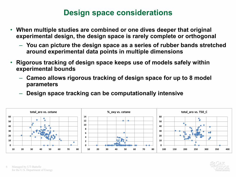
Design space considerations

• When multiple studies are combined or one dives deeper that original experimental design, the design space is rarely complete or orthogonal– You can picture the design space as a series of rubber bands stretched

around experimental data points in multiple dimensions

• Rigorous tracking of design space keeps use of models safely within experimental bounds– Cameo allows rigorous tracking of design space for up to 8 model

parameters– Design space tracking can be computationally intensive

0

2

4

6

8

10

12

14

10 20 30 40 50 60 70 80

%_oxy vs. cetane

0

10

20

30

40

50

60

10 20 30 40 50 60 70 80

total_aro vs. cetane

0

10

20

30

40

50

60

100 150 200 250 300 350 400

total_aro vs. T50_C


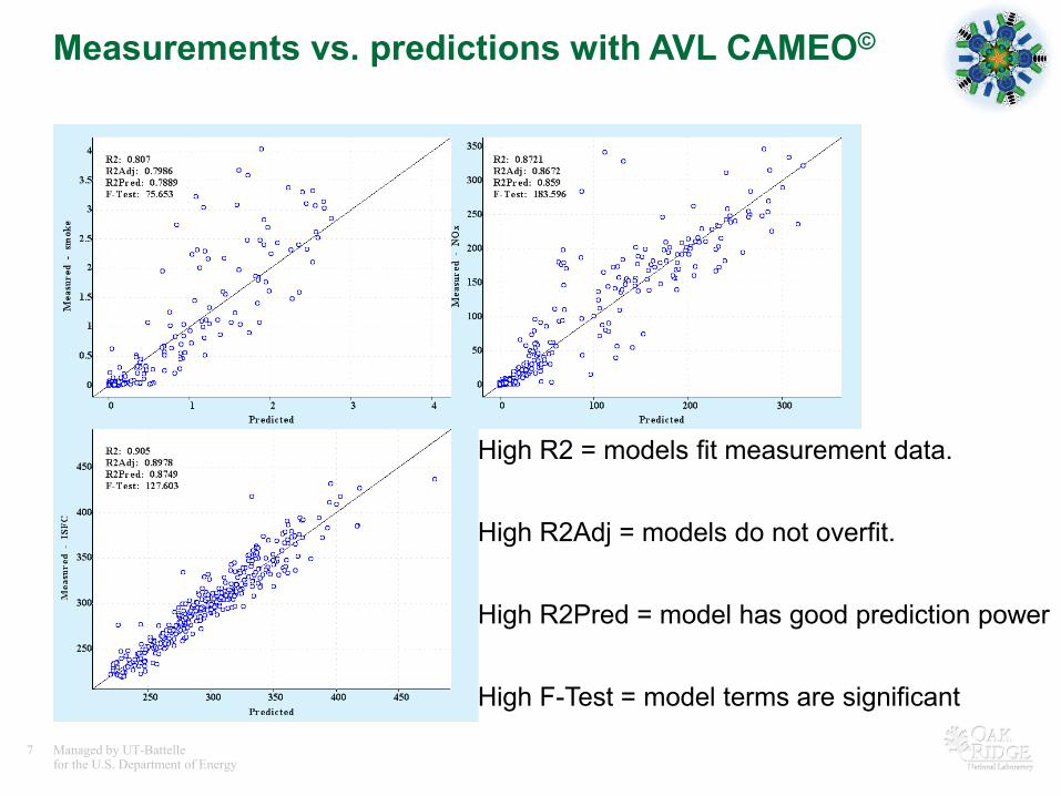
Measurements vs. predictions with AVL CAMEO©

High R2 = models fit measurement data.

High R2Adj = models do not overfit.

High R2Pred = model has good prediction power

High F-Test = model terms are significant


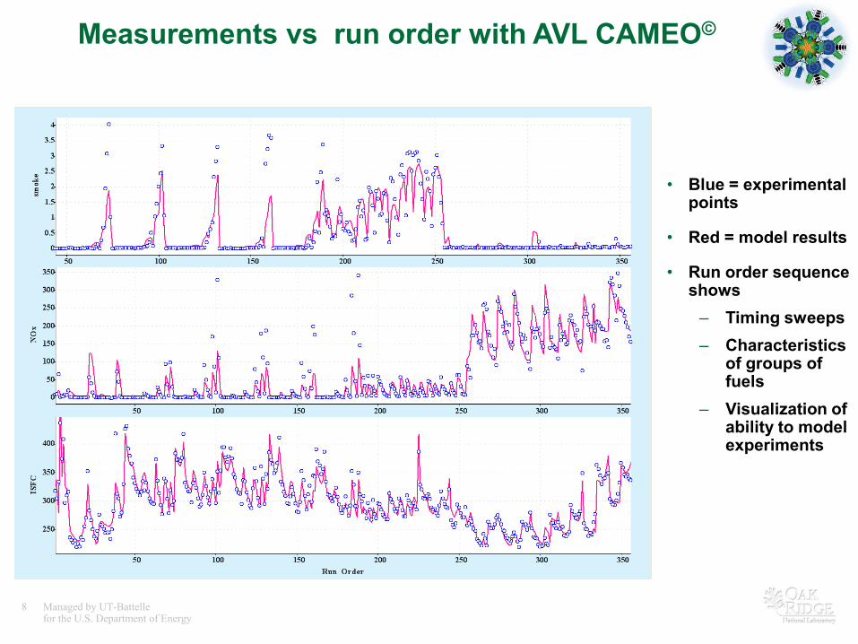
• Blue = experimental points

• Red = model results

• Run order sequence shows

– Timing sweeps– Characteristics

of groups of fuels

– Visualization of ability to model experiments

Measurements vs run order with AVL CAMEO©


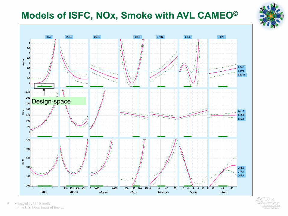
Models of ISFC, NOx, Smoke with AVL CAMEO©

Design-space


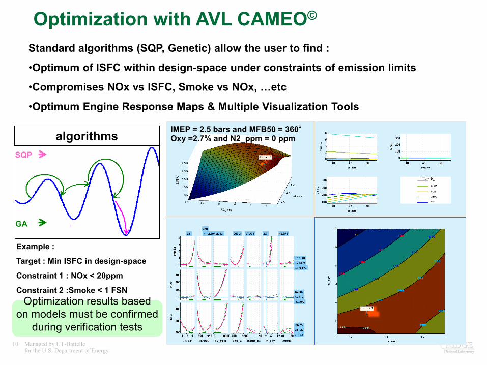
Optimization with AVL CAMEO©

Standard algorithms (SQP, Genetic) allow the user to find :

•Optimum of ISFC within design-space under constraints of emission limits

•Compromises NOx vs ISFC, Smoke vs NOx, …etc

•Optimum Engine Response Maps & Multiple Visualization Tools

GA

SQP

algorithms

Example :

Target : Min ISFC in design-space

Constraint 1 : NOx < 20ppm

Constraint 2 :Smoke < 1 FSNOptimization results based

on models must be confirmed during verification tests

IMEP = 2.5 bars and MFB50 = 360°Oxy =2.7% and N2_ppm = 0 ppm


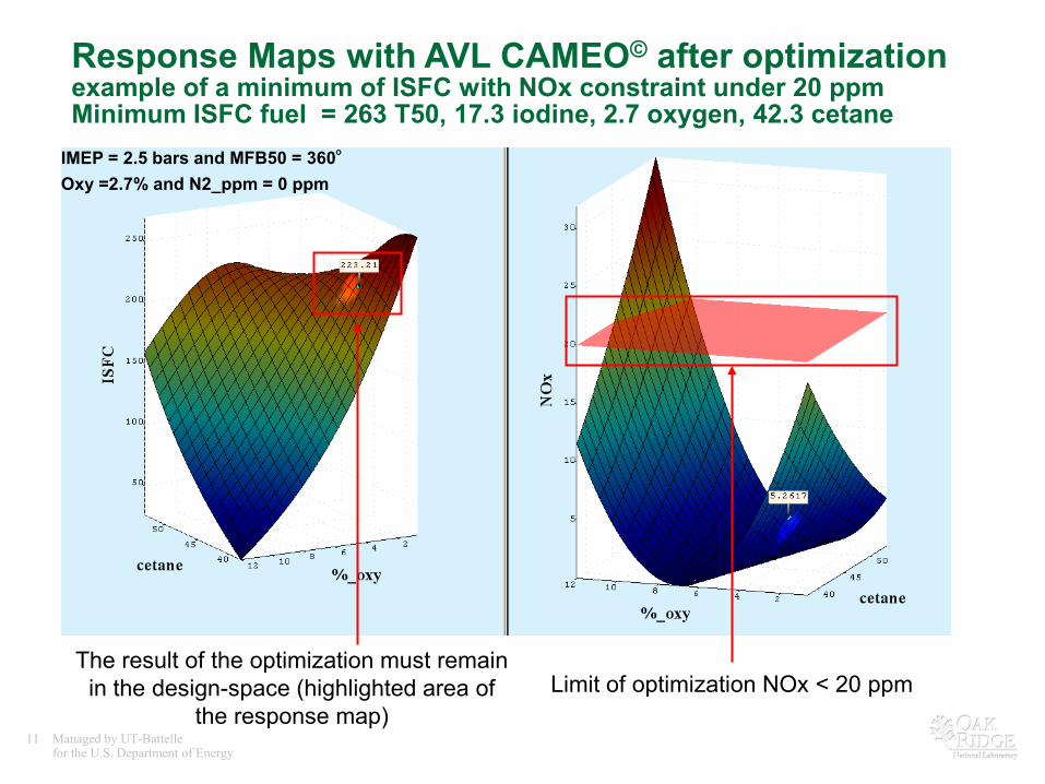
Response Maps with AVL CAMEO© after optimizationexample of a minimum of ISFC with NOx constraint under 20 ppmMinimum ISFC fuel = 263 T50, 17.3 iodine, 2.7 oxygen, 42.3 cetane

The result of the optimization must remain in the design-space (highlighted area of

the response map)Limit of optimization NOx < 20 ppm

IMEP = 2.5 bars and MFB50 = 360°Oxy =2.7% and N2_ppm = 0 ppm


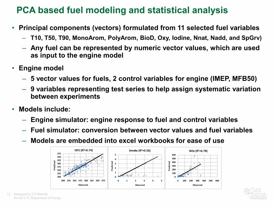
PCA based fuel modeling and statistical analysis

• Principal components (vectors) formulated from 11 selected fuel variables– T10, T50, T90, MonoArom, PolyArom, BioD, Oxy, Iodine, Nnat, Nadd, and SpGrv)– Any fuel can be represented by numeric vector values, which are used

as input to the engine model

• Engine model– 5 vector values for fuels, 2 control variables for engine (IMEP, MFB50)– 9 variables representing test series to help assign systematic variation

between experiments

• Models include:– Engine simulator: engine response to fuel and control variables– Fuel simulator: conversion between vector values and fuel variables– Models are embedded into excel workbooks for ease of use

200225250275300325350375

200 225 250 275 300 325 350 375

Pred

icte

d

Observed

ISFC (R2=0.74)

0

1

2

3

4

5

0 1 2 3 4 5

Pred

icte

d

Observed

Smoke (R2=0.56)

0

100

200

300

400

500

600

0 100 200 300 400 500 600

Pred

icte

d

Observed

NOx (R2=0.78)


Fuel and engine simulatorsExperimental Range

Vec 1 Vec 2 Vec 3 Vec 4 Vec 510.7 4.8 4.4 5.5 2.0-5.2 -5.5 -2.8 -1.5 -3.0

Vector 1 Steps 160 104 73 71 510.052

T10 deg C 215Vector 2 T50 deg C 257

0.0 T90 deg C 30656 MonoArom wt % 18.9

PolyArom wt% 7.7Vector 3 BioD vol % 6.1

0.0 Oxy wt % 0.928 Iodine number 5

Natural ppm 564Vector 4 Added ppm 111

0.0 SpGrv gm/cm3 0.84915

Cetane number 44.7Vector 5

0.031

Maximum ValueMinimum Value

18.9

7.76.1

0.9

5

0.0

2.0

4.0

6.0

8.0

10.0

12.0

14.0

16.0

18.0

20.0

Chemistry (%)

564

111

0

100

200

300

400

500

600

Nitrogen (ppm)

45

05

1015202530354045505560657075

Cetane

215

257

306

0

50

100

150

200

250

300

350

Boiling Points (deg C)

0.85

0.00

0.10

0.20

0.30

0.40

0.50

0.60

0.70

0.80

0.90

1.00

Sp Grav (g/cm3)

NOTE: The simulator comes loaded with a 150-pt sample of the entire dataset. 0.01 0.0 0.0 0.19 0.01 0.26 0.19 0.08 0.00

lamda ISFC ITE Smoke ISHC ISCO ISNOx COV dPdCA LTHR IMEP MFB50 V 1 V 2 V 3 V 4 V 5 dSer1 dSer2 dSer3 dSer4 dSer5B dSer6 dSer7 dSer8 dSer9

number gm/kwhfraction FSN ppm ppm ppm % bar/deg % bar CA (atdc) number number number number number number number number number number number number number number

Maximum Value 4.87 437 0.5 5.2 6,961 9,082 449 47.9 21.6 10 4.2 18 10.7 4.8 4.4 5.5 2.0 1.00 1.00 1.00 1.00 1.00 1.00 1.00 1.00 1.00Mean Value 2.89 272 0.3 0.4 1,992 1,372 38 5.5 6.0 2 2.2 -1 0.0 0.0 0.0 0.0 0.0 0.01 0.04 0.02 0.19 0.01 0.26 0.19 0.08 0.00

Minimum Value 1.34 168 0.2 0.0 669 280 0 1.3 0.7 0 0.7 -15 -5.2 -5.5 -2.8 -1.5 -3.0 0.00 0.00 0.00 0.00 0.00 0.00 0.00 0.00 0.00

Case number gm/kwh fraction FSN ppm ppm ppm % bar/deg % bar CA (atdc) number number number number number number number number number number number number number number1 2.34 221 0.33 0.1 3,536 2,382 1 4.4 2.2 1 3.1 9 -0.7 0.5 -0.1 -0.7 -0.3 0 1 0 0 0 0 0 0 02 1.89 242 0.30 0.2 2,688 852 20 2.8 9.5 1 3.0 -1 -0.4 1.1 -0.2 -0.2 0.5 0 1 0 0 0 0 0 0 03 1.92 248 0.29 0.2 2,523 741 24 2.7 10.9 1 2.9 -4 -0.4 1.1 -0.2 -0.2 0.5 0 1 0 0 0 0 0 0 04 1.90 235 0.30 0.2 2,401 888 12 2.6 8.8 1 3.1 -2 -0.7 0.3 0.0 -0.8 -0.6 0 1 0 0 0 0 0 0 05 2.01 236 0.29 0.2 1,673 898 8 2.2 8.2 2 3.0 -7 -1.6 -1.6 -0.8 -1.1 -3.0 0 1 0 0 0 0 0 0 06 2.31 272 0.27 0.2 1,402 622 13 3.4 8.9 0 2.3 -11 -0.7 0.5 -0.1 -0.7 -0.3 0 0 1 0 0 0 0 0 07 3.47 272 0.28 0.1 2,397 3,094 0 9.3 1.4 0 1.5 1 -0.7 0.5 -0.1 -0.7 -0.3 0 0 1 0 0 0 0 0 08 2.20 267 0.27 0.2 1,514 692 13 3.3 9.1 0 2.5 -9 -0.7 0.5 -0.1 -0.7 -0.3 0 0 1 0 0 0 0 0 09 2.57 292 0.28 0.2 2,216 818 23 5.0 7.9 1 2.4 1 1.5 2.4 1.1 -1.0 0.6 0 0 0 1 0 0 0 0 0

10 3.11 278 0.30 0.1 2,344 874 11 6.5 4.9 0 1.9 3 -1.8 -0.1 0.0 0.0 0.6 0 0 0 1 0 0 0 0 011 3.32 275 0.30 0.1 1,864 485 16 4.6 7.3 0 1.7 -3 -3.0 -1.2 -0.4 0.4 0.5 0 0 0 1 0 0 0 0 012 3.28 273 0.31 0.1 2,043 588 14 5.1 6.2 0 1.8 -1 -3.0 -1.2 -0.4 0.4 0.5 0 0 0 1 0 0 0 0 013 3.00 281 0.30 0.1 2,340 1,011 8 6.6 4.9 0 2.1 4 -0.9 0.6 0.2 -0.7 0.2 0 0 0 1 0 0 0 0 014 2.68 283 0.29 0.2 1,944 585 26 4.8 9.3 0 2.3 -1 -0.9 0.6 0.2 -0.7 0.2 0 0 0 1 0 0 0 0 015 3.40 284 0.30 0.1 2,657 1,641 4 8.3 3.2 1 1.9 6 -0.4 0.2 0.4 -0.6 -0.5 0 0 0 1 0 0 0 0 016 2.94 288 0.29 0.2 1,957 736 17 5.4 7.3 1 2.1 -1 -0.4 0.2 0.4 -0.6 -0.5 0 0 0 1 0 0 0 0 017 2.91 255 0.33 0.1 2,894 1,394 4 7.5 2.9 0 2.6 11 -1.6 -0.3 0.1 -0.3 0.2 0 0 0 1 0 0 0 0 018 2.80 260 0.32 0.1 2,649 1,053 9 6.7 3.9 0 2.5 9 -1.8 -0.1 0.3 -0.2 0.6 0 0 0 1 0 0 0 0 019 3.12 255 0.33 0.1 3,521 2,299 2 10.4 1.6 0 2.3 15 -1.8 -0.1 0.3 -0.2 0.6 0 0 0 1 0 0 0 0 020 3.29 289 0.29 0.1 2,551 1,489 4 8.2 3.5 1 1.9 5 -0.2 0.8 0.2 -0.8 0.0 0 0 0 1 0 0 0 0 021 2.88 282 0.30 0.2 2,121 867 11 5.7 6.4 1 2.2 1 -0.6 0.4 0.0 -0.8 -0.4 0 0 0 1 0 0 0 0 0

dSer4 dSer5BdSer1 dSer6 dSer7 dSer8V 3 V 4 V 5 dSer2 dSer3

For studies, set the control variables as in Row 2

lamda ISFC ITE ISHC ISCO dSer9V 2IMEP MFB50ISNOxSmoke dPdCA LTHRCOV V 1

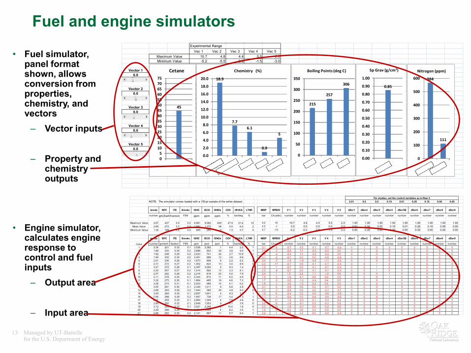
• Fuel simulator, panel format shown, allows conversion from properties, chemistry, and vectors

– Vector inputs

– Property and chemistry outputs

• Engine simulator, calculates engine response to control and fuel inputs

– Output area

– Input area


PCA fuel model

• Each of the 5 principal components above (vectors) is a linear combination of 11 fuel variables using coefficients shown

– Each vector is orthogonal– There are 11 vectors in total, but these first 5 describe

90% of fuel variability

• This fuel model was developed to calculate cetane, and does not contain cetane as an input variable

– Cetane model predicts about as well as ASTM D613 reproducibility (within ≈ 3.3, 19 of 20 measurements)

• Fuel vector values are used as input to the engine simulator

Mean Std Dev Prin1 Prin2 Prin3 Prin4 Prin5T10 deg C 216 34 0.391 0.118 0.300 -0.022 -0.163T50 deg C 258 34 0.400 0.209 0.187 -0.192 -0.226T90 deg C 306 34 0.343 0.313 0.012 -0.337 -0.190MonoArom wt % 18.7 7.8 -0.299 0.133 0.288 0.083 0.493PolyArom wt % 7.5 6.9 0.158 0.473 -0.271 0.263 0.378BioD vol % 6.3 14.3 0.350 -0.379 -0.242 0.062 0.138Oxy wt % 0.9 1.8 0.345 -0.388 -0.198 0.120 0.179Iodine number 4.9 11.3 0.310 -0.365 0.153 0.275 0.107Nnat ppm 653 2,112 0.034 -0.056 0.717 0.407 -0.056Nadd ppm 118 700 -0.014 0.247 -0.286 0.710 -0.466SpGrv gm/cm3 0.848 0.023 0.341 0.332 0.030 0.092 0.466

10

20

30

40

50

60

70

80

10 30 50 70 90

Pred

icte

d Ce

tane

Num

ber

Observed Cetane Number

BioDieselConventionalFACEOil SandsOil Shale


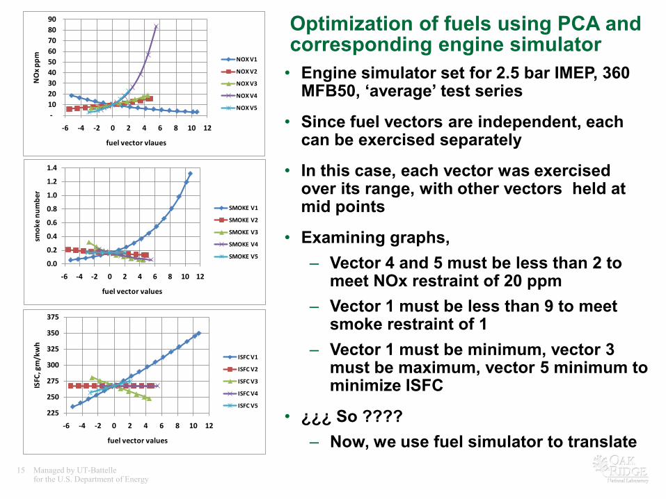
Optimization of fuels using PCA and corresponding engine simulator• Engine simulator set for 2.5 bar IMEP, 360

MFB50, ‘average’ test series

• Since fuel vectors are independent, each can be exercised separately

• In this case, each vector was exercised over its range, with other vectors held at mid points

• Examining graphs,– Vector 4 and 5 must be less than 2 to

meet NOx restraint of 20 ppm– Vector 1 must be less than 9 to meet

smoke restraint of 1– Vector 1 must be minimum, vector 3

must be maximum, vector 5 minimum to minimize ISFC

• ¿¿¿ So ????– Now, we use fuel simulator to translate

-10 20 30 40 50 60 70 80 90

-6 -4 -2 0 2 4 6 8 10 12

NO

x pp

m

fuel vector vlaues

NOX V1

NOX V2

NOX V3

NOX V4

NOX V5

0.0

0.2

0.4

0.6

0.8

1.0

1.2

1.4

-6 -4 -2 0 2 4 6 8 10 12

smok

e nu

mbe

r

fuel vector values

SMOKE V1

SMOKE V2

SMOKE V3

SMOKE V4

SMOKE V5

225

250

275

300

325

350

375

-6 -4 -2 0 2 4 6 8 10 12

ISFC

, gm

/kw

h

fuel vector values

ISFC V1

ISFC V2

ISFC V3

ISFC V4

ISFC V5


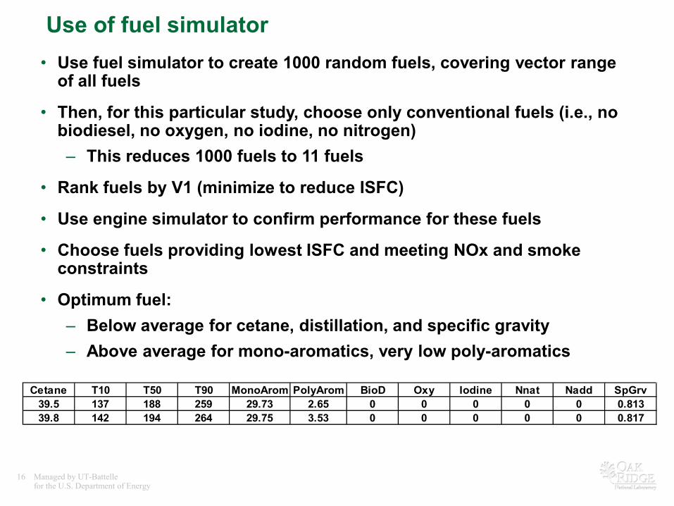
Use of fuel simulator• Use fuel simulator to create 1000 random fuels, covering vector range

of all fuels

• Then, for this particular study, choose only conventional fuels (i.e., no biodiesel, no oxygen, no iodine, no nitrogen)– This reduces 1000 fuels to 11 fuels

• Rank fuels by V1 (minimize to reduce ISFC)

• Use engine simulator to confirm performance for these fuels

• Choose fuels providing lowest ISFC and meeting NOx and smoke constraints

• Optimum fuel:– Below average for cetane, distillation, and specific gravity– Above average for mono-aromatics, very low poly-aromatics

Cetane T10 T50 T90 MonoArom PolyArom BioD Oxy Iodine Nnat Nadd SpGrv39.5 137 188 259 29.73 2.65 0 0 0 0 0 0.81339.8 142 194 264 29.75 3.53 0 0 0 0 0 0.817


Conclusions• Statistical analysis can help unlock complex data sets, allowing

determination of relationships and effects

• ‘Messy’ data sets can be fully mined for information, as long as one is careful with model behavior and extrapolation

• Variables used to represent fuels included:– Cetane, T50, oxygen, iodine, nitrogen (CAMEO, for oxygen

containing fuels)– T10, T50, T90, mono-aro, poly-aro, bio-diesel, oxygen, iodine,

nitrogen (both), SG (PCA, all fuels)

• A large data set like this offers too many degrees of freedom for a single optimization, one must fix some engine and fuel variables

• Models can be used to find fuels meeting desired performance targets under a wide variety of chemistry or property targets– Examples given for biofuels and conventional diesel fuels


Accomplishments for 2010, plans for 2011

• Combined and analyzed multiple data sets of diesel range fuels– Gasoline range data would logically be next

• Evaluated two commercial codes for statistical analysis– This presentation highlights AVL CAMEO

• Developed generalized PCA modeling capability for fuels– This presentation also highlights PCA representation of fuels

• Completed funds-in project for CRC on gasoline HCCI fuel effects (AVFL13C)

• SAE paper on HCCI engine response for FACE diesel fuels

• 2011 plans – on hold pending funding decisions– Technical paper covering results in more detail– Similar analysis for gasoline range fuels– Other funds-in projects

statistical overview of 5 years of hcci fuel and engine ... · statistical overview of 5 years of...

Documents