statistical parametric mapping of functional mri data using - diva
TRANSCRIPT
Statistical Parametric Mapping of Functional MRI data
Using
Spectral Graph Wavelets
Hamid Behjat
August 2012
LiTH-IMT/MASTER-EX--12/018—SE

Linköping University (LIU) Ecole Polytechnique Fédérale de Lausanne (EPFL)
Statistical Parametric Mapping of Functional MRI data
Using
Spectral Graph Wavelets
by
Hamid Behjat
LiTH-IMT/MASTER-EX--12/018—SE
Thesis adviser: Prof. Dimitri Van De Ville
Medical Image processing Lab, EPFL
Thesis supervisor: Nora Leonardi
Medical Image processing Lab, EPFL
Thesis Examiner: Prof. Hans Knutsson
Department of Biomedical Engineering, LIU
August 2012


Abstract
In typical statistical parametric mapping (SPM) of fMRI data, the functionaldata are pre-smoothed using a Gaussian kernel to reduce noise at the cost oflosing spatial specificity. Wavelet approaches have been incorporated in suchanalysis by enabling an efficient representation of the underlying brain activitythrough spatial transformation of the original, un-smoothed data; a successfulframework is the wavelet-based statistical parametric mapping (WSPM) whichenables integrated wavelet processing and spatial statistical testing. However,in using the conventional wavelets, the functional data are considered to lie on aregular Euclidean space, which is far from reality, since the underlying signal lieswithin the complex, non rectangular domain of the cerebral cortex. Thus, usingwavelets that function on more complex domains such as a graph holds promise.The aim of the current project has been to integrate a recently developed spec-tral graph wavelet transform as an advanced transformation for fMRI braindata into the WSPM framework. We introduce the design of suitable weightedand un-weighted graphs which are defined based on the convoluted structureof the cerebral cortex. An optimal design of spatially localized spectral graphwavelet frames suitable for the designed large scale graphs is introduced. Wehave evaluated the proposed graph approach for fMRI analysis on both simu-lated as well as real data. The results show a superior performance in detectingfine structured, spatially localized activation maps compared to the use of con-ventional wavelets, as well as normal SPM. The approach is implemented in anSPM compatible manner, and is included as an extension to the WSPM toolboxfor SPM.
KEYWORDS: Statistical testing, functional MRI, Spectral graph theory,Graph wavelet transform, Wavelet thresholding

Acknowledgements
To begin with, I would like to first of all express my sincere gratitude to mythesis advisor Prof. Dimitri Van De Ville not only for giving me the opportunityto develop my master thesis in his remarkable group (MIPLab at EPFL), but alsofor his insightful inputs, positive feedback and not to forget his great and uniquepersonality. Dimitri has truly been one of the most admirable people that I have metthrough the course of my life in terms of both knowledge and personality.
I am sincerely grateful to my supervisor Nora Leonardi. I would like to thank Norafor her help in getting me started with the whole new idea of spectral graph wavelets,for all her time and patience in giving guidance throughout the project and for manyof her technical helps when it came to documenting my results and writing my thesis.
Success is not just about knowledge. Without the encouragement, patience andsupport of my beloved wife, Naeimeh, this project would have not seen the light ofday. I owe my deepest gratitude to her for all her love and support not only in thecourse of the current project but throughout my master studies.
I would also like to acknowledge the GREEDY pool provided by the IT Domain(DIT) of EPFL. GREEDY is a computing grid which scavenges unused computingcycles throughout the EPFL campus. Without such computing power, the extensiveevaluations and simulations of the current project would have not been possible.
I am also grateful to many friends and colleagues whom I met during my projectat EPFL; Ulugbeck Kamilov for his words of wisdom, Jonas Richiardi for his inputon running algorithms on the server, Ricard Delgado Gonzalo for his help on posterdesign, and also, Melissa Saenz, Isik Karahanoglu, Pedram Pad, Emrah Boston andRotem Kopel whom I enjoyed their company.
I would also like to thank Prof. Hans Knutsson for accepting to be my examiner;it is a pleasure to receive an evaluation of my work by Hans, an expert in medicalimage analysis. Also, my special thanks goes to Prof. Goran Salerud, the director ofstudies for the biomedical engineering master program, for his generous and limitlesssupport throughout my master studies.
Last but not the least, I would like to express my gratitude to my parents whomhave always been a source of encouragement throughout my academic career.


Contents
1 Introduction 1
2 Background 32.1 fMRI . . . . . . . . . . . . . . . . . . . . . . . . . . . . . . . . . . . . . 32.2 Statistical Parametric Mapping (SPM) . . . . . . . . . . . . . . . . . . 3
2.2.1 Design and Estimation . . . . . . . . . . . . . . . . . . . . . . . 42.2.2 Contrast . . . . . . . . . . . . . . . . . . . . . . . . . . . . . . . 52.2.3 Statistical Inference . . . . . . . . . . . . . . . . . . . . . . . . 5
2.3 Graphs . . . . . . . . . . . . . . . . . . . . . . . . . . . . . . . . . . . . 62.3.1 Matrices associated with a graph . . . . . . . . . . . . . . . . . 62.3.2 Eigenspace of graphs . . . . . . . . . . . . . . . . . . . . . . . . 7
2.4 Wavelet Transforms . . . . . . . . . . . . . . . . . . . . . . . . . . . . 82.4.1 Classical wavelet transform . . . . . . . . . . . . . . . . . . . . 82.4.2 Graph Fourier transform . . . . . . . . . . . . . . . . . . . . . . 102.4.3 Spectral graph wavelet transform . . . . . . . . . . . . . . . . . 11
3 Methods and Materials 153.1 Pre-Processing . . . . . . . . . . . . . . . . . . . . . . . . . . . . . . . 15
3.1.1 Pre-processing of functional data . . . . . . . . . . . . . . . . . 153.1.2 Pre-processing of the structural data . . . . . . . . . . . . . . . 17
3.2 Graph design . . . . . . . . . . . . . . . . . . . . . . . . . . . . . . . . 193.2.1 Graph design approach I . . . . . . . . . . . . . . . . . . . . . . 193.2.2 Graph design approach II . . . . . . . . . . . . . . . . . . . . . 203.2.3 Other graph design approaches . . . . . . . . . . . . . . . . . . 22
3.3 Wavelet design . . . . . . . . . . . . . . . . . . . . . . . . . . . . . . . 223.4 Wavelet-based SPM using spectral graph wavelets . . . . . . . . . . . 23
3.4.1 Wavelet domain model fitting . . . . . . . . . . . . . . . . . . . 253.4.2 Wavelet domain processing . . . . . . . . . . . . . . . . . . . . 253.4.3 Spatial domain statistical inference . . . . . . . . . . . . . . . . 273.4.4 Absolute value wavelet reconstruction using local graphs . . . . 28
3.5 Materials . . . . . . . . . . . . . . . . . . . . . . . . . . . . . . . . . . 293.5.1 Synthetic data set . . . . . . . . . . . . . . . . . . . . . . . . . 293.5.2 Real data sets . . . . . . . . . . . . . . . . . . . . . . . . . . . . 31
3.6 SPM compatible implementation . . . . . . . . . . . . . . . . . . . . . 32
i

CONTENTS ii
4 Results 334.1 Simulation results . . . . . . . . . . . . . . . . . . . . . . . . . . . . . 34
4.1.1 Evaluation of graph design approaches . . . . . . . . . . . . . . 344.1.2 Effect of varying the graph domain . . . . . . . . . . . . . . . . 344.1.3 Effect of varying spectrum coverage of filters . . . . . . . . . . 364.1.4 Effect of varying the number of wavelet scales . . . . . . . . . . 384.1.5 WSPMsg vs WSPM and SPM . . . . . . . . . . . . . . . . . . 38
4.2 Experimental results . . . . . . . . . . . . . . . . . . . . . . . . . . . . 404.2.1 Auditory data set . . . . . . . . . . . . . . . . . . . . . . . . . 404.2.2 Visual data set . . . . . . . . . . . . . . . . . . . . . . . . . . . 44
5 Discussion 475.1 Optimal settings of design criteria . . . . . . . . . . . . . . . . . . . . 47
5.1.1 Filter design in terms of spectrum coverage . . . . . . . . . . . 475.1.2 Number of wavelet scales . . . . . . . . . . . . . . . . . . . . . 475.1.3 Graph domain extent . . . . . . . . . . . . . . . . . . . . . . . 485.1.4 Graph design approach . . . . . . . . . . . . . . . . . . . . . . 48
5.2 General comments . . . . . . . . . . . . . . . . . . . . . . . . . . . . . 485.3 Computational cost . . . . . . . . . . . . . . . . . . . . . . . . . . . . . 49
6 Conclusion and Outlook 516.1 Outlook . . . . . . . . . . . . . . . . . . . . . . . . . . . . . . . . . . . 51
6.1.1 Extension to multi subject studies . . . . . . . . . . . . . . . . 516.1.2 Enhancement of graph design . . . . . . . . . . . . . . . . . . . 526.1.3 Adaptation to new graph wavelets transforms . . . . . . . . . . 52
List of Figures
3.1 Overall view of the proposed approach . . . . . . . . . . . . . . . . . . 163.2 Preprocessing steps for the structural and functional volumes. . . . . 183.3 Graph design approaches . . . . . . . . . . . . . . . . . . . . . . . . . 203.4 Transformation used in defining graph edge weights . . . . . . . . . . . 213.5 Filter design in terms of graph spectrum coverage . . . . . . . . . . . . 233.6 WSPM framework . . . . . . . . . . . . . . . . . . . . . . . . . . . . . 243.7 Partial GM used in synthetic data . . . . . . . . . . . . . . . . . . . . 303.8 Synthetic activation pattern . . . . . . . . . . . . . . . . . . . . . . . . 31
4.1 Graph domain extent . . . . . . . . . . . . . . . . . . . . . . . . . . . . 354.2 Overlay of synthetic activation on graph domain . . . . . . . . . . . . 364.3 Evaluation of filter design in terms of graph spectrum coverage . . . . 374.4 Evaluation on synthetic data set . . . . . . . . . . . . . . . . . . . . . 394.5 Evaluation on real data: auditory data set . . . . . . . . . . . . . . . . 414.6 Evaluation on real data: auditory data set . . . . . . . . . . . . . . . . 434.7 Evaluation on real data: visual data set . . . . . . . . . . . . . . . . . 444.8 Evaluation on real data: visual data set . . . . . . . . . . . . . . . . . 454.9 Evaluation on real data: visual data set . . . . . . . . . . . . . . . . . 46
5.1 Inaccurate spatial localization of activation by SPM . . . . . . . . . . 50
iii


List of Tables
4.1 Evaluation of graph design approaches . . . . . . . . . . . . . . . . . . 344.2 Evaluation of graph domain extent . . . . . . . . . . . . . . . . . . . . 354.3 Evaluation of filter design in terms of spectrum coverage . . . . . . . . 364.4 Evaluation of the number of graph wavelet scales . . . . . . . . . . . . 384.5 Optimal settings for the graph wavelet approach . . . . . . . . . . . . 384.6 Evaluation on synthetic data set . . . . . . . . . . . . . . . . . . . . . 394.7 Evaluation on real data: auditory data set . . . . . . . . . . . . . . . . 424.8 Evaluation on real data: visual data set . . . . . . . . . . . . . . . . . 45
v


Chapter 1
Introduction
Functional Magnetic Resonance Imaging (fMRI) is a conventional neuroimaging tech-nique used in the study of brain functionality. The blood-oxygen-level-dependentsignal, which is sought lies within fMRI data that are highly convoluted with noise. Intypical analysis of fMRI data using the statistical parametric mapping (SPM) frame-work [1], the functional data are smoothed using a Gaussian kernel to reduce noise atthe cost of losing spatial specificity.
Fourier analysis methods are common practice in many signal processing tasks.Although the basis used in the Fourier transform, i.e. complex exponentials, are lo-calized in frequency, they have a global support. The great strength of using waveletmethods in signal processing is within their power to localize the signal in both spaceand frequency. For fMRI analysis, the assumption is that the underlying cortical activ-ity in the cerebral cortex is spatially localized and could thus be effectively representedby localizing the signal using wavelets. Wavelet-based statistical parametric mapping(WSPM), which has been developed over the past few years by Van De Ville et al,[2, 3], is a unified framework that enables the integration of wavelet processing andspatial statistical testing of fMRI data. The results from this approach have shown theeffectiveness of using the discrete wavelet transform in parametric hypothesis testingof fMRI data. Aside from that, Hammond et al, have recently introduced a novelwavelet transform using spectral graph theory, where a spectral graph wavelet trans-form (SGWT) can be applied to functions defined on vertices of a graph [4]. Thepromising results from the WSPM framework and the novel SGWT method motivatesthe implementation and study of parametric hypothesis testing of fMRI data usinggraph wavelets.
Aside from that, in typical signal processing methods that are used to analyzefMRI data, the functional data is considered to be located on a regular Euclideanspace. However, taking into account the complex structure of the cerebral cortexon which the neural activity takes place, it seems wise to define a non-Euclideandomain for such an analysis. By using methods that enable the processing of data ontopologically complicated domains such as the grey matter, we have the hypothesisthat better results can be achieved since the neural activity can be better tracked.
Although the use of discrete wavelet transforms in fMRI analysis has lead topromising results due to their spatial localization power, there still seems to be spaceto improve the results by adopting wavelets that take into account the complex domainwhere the signal lies, i.e. the cerebral cortex. There is very limited related work in this
1
CHAPTER 1. INTRODUCTION 2
direction, and we consider the present work as one of the pioneers in this direction.A single related work is the work by Ozkaya et al. [5] in which they have presented ascheme for designing anatomically adapted wavelets using the lifting scheme to con-struct a customized wavelet basis, whose natural domain is the cerebral cortex. Theinitial results that they have presented is promising which has further motivated thepresent work.
The aim of the current project has been to integrate the recently developed spec-tral graph wavelet transform as an advanced transform for fMRI brain mapping intothe WSPM framework. This includes the design of an appropriate graph adapted tothe anatomy of the brain, finding optimal settings in using the graph wavelets, im-plementation of the approach into an SPM friendly version and evaluation of the newproposed approach on both simulated data and real data.
Chapter 2
Background
2.1 fMRI
Functional magnetic resonance imaging is a noninvasive bioimaging modality. Theprinciple behind it is the detection of the blood-oxygen-level-dependent (BOLD) signalwhich was first introduced by Ogawa in 1990 [6]. The BOLD signal is created as a resultof the difference between the magnetic properties of oxygenated and deoxygenatedblood. That is, as a region of brain becomes active, the blood consumption locallyincreases and thus more blood is pumped to that region. However, there is not acomplete balance between this increase in consumption and the increase in blood flow;more oxygenated blood blood becomes available in the region than needed and thisslight increase in oxygenated blood leads to what we call the BOLD signal.
In order to detect the BOLD signal, a series of T2*-weighted images of the brainover a period of time is required; these recordings are called functional volumes. How-ever, in order to achieve a desirable temporal resolution, the repetition time (TR) be-tween the volumes should be kept very small; for this purpose, Echo-Plannar-Imagingis common practice. Using this technique, an image of the whole brain can be acquiredin a period as short as two seconds. However, this high temporal acquisition comes atthe cost of a very low spatial resolution compared to the standard anatomical images;the BOLD signal that we seek has a weak contrast and is drown in noise. Therefore,incorporating signal processing techniques is essential for the analysis of fMRI data.
2.2 Statistical Parametric Mapping (SPM)
Statistical parametric mapping (SPM), which was first introduces by Friston et al. [1],is unified framework used for the analysis of fMRI data; it is a parametric hypothesis-driven method. Initially, the functional data are smoothed using a suitable Gaussianfilter. A general linear model is then used to search for patterns of activation of theBOLD signal within the time-course of the functional voxels that match the hypothesisthat are put to test. In this section, we will have a brief look at the procedure thatis taken in SPM in analysis of the functional data. This will in term help us betterunderstand the wavelet approach used for this type of analysis which is described inchapter 3.4.
3
CHAPTER 2. BACKGROUND 4
2.2.1 Design and Estimation
As described in section 2.1, the data that we acquire from a brain fMRI study includesa series of scans of the subjects brain, Nt scans, and thus a time-series representingthe BOLD response of each voxel of the brain can be constructed. Assuming that wehave Nv voxels1 in the whole volume of functional data, and taking into account thatan fMRI study may include multiple subjects, Ns, the temporal behavior of the k -thvoxel in the i -th subject’s brain can be described as
yki = [v1i [k] . . .vNt
i [k]]T i = 1, . . . , Ns (2.1)
where yki is a Nt × 1 vector which represents the temporal change in intensity at thedesired voxel.
Modeling the temporal behavior of the intensity of the voxels using Nr experimen-tal conditions (regressors) would require a design matrix, X, of size Nt × Nr. SPMis a mass-univariate approach which means that a general linear model (GLM) is fit-ted independently to the time-series of each of the voxels [1]. Thus, the same designmatrix would be used for all the voxels in a single subject’s brain. However, althoughthe number and type of regressors is kept constant for all subjects in a multi-subjectstudy, the temporal shape of the regressors is not necessarily the same for differentsubjects; an example would be a design matrix which includes the estimated move-ment regressors. Therefore, we differentiate the design matrix of each subject by anindex, i. Thus, by having the time-series of the voxels as well as the design matrix,we can model the BOLD response at the k -th voxel of the i -th subject as
yki = Xiβki + εki i = 1, . . . , Ns (2.2)
where βki is a Nr × 1 vector of regression parameters and εki is a Nt × 1 vector ofresidual errors. The elements of vector βki are the effect sizes, i.e. the effect that eachof the Nr regressors have had on the the BOLD response at the k -th voxel of the i -thsubject.
Assuming that the the design matrix is of full rank, i.e. rank(X) = Nr, and thatthe error component is independently and identically Gaussian distributed, N (0, σ2I),the optimal ordinary least squares(OLS) estimate of the effect sizes can be computed[3, 1]. We would first need to form a normal equation; the OLS estimate is finallyachieved by applying the pseudo-inverse of the design matrix, i.e. (Xi
TXi)−1Xi
T , tothe measurement data at each voxel k, yki ,
XiTyki = Xi
TXiβki
βki = (XiTXi)
−1XiTyki . (2.3)
The corresponding estimate of the residual errors of this mapping can be described as
εki = yki −Xiβki . (2.4)
For a geometrical interpretation we can think of this transformation as mapping ofthe functional data from an Nv-dimensional space into an Nr-dimensional parameterspace, which the columns of the design matrix define the axis of this new space. Foreach subject, two matrices can be defined in this transformation, the projection matrix,P and the residual forming matrix, R, which are defined as
1Note that a functional volume of data with Nv voxels can be represented as a vector, v,with dimension Nv × 1.
CHAPTER 2. BACKGROUND 5
Pi = Xi(XiTXi)
−1XiT = XiX
+i (2.5)
Ri = I − Pi (2.6)
where X+i is the short-hand notation used for the pseudo-inverse.
The corresponding estimate of the standard deviation of the error can be achievedby dividing the sum of squares of the estimated error by the degrees of freedom
σki =
√εkiTεki
tr(Ri)(2.7)
where tr(Ri) = rank(Ri) = Nt − Nr. However, it should be noted that this is onlytrue if Nt is sufficiently large, more than 40 scans. This is an assumption that we takethroughout this report for the rest of the calculations as it is the case for nearly allfMRI studies. However, the implementation of the WSPM also takes into account thecase where there are only a limited number of scans, and in this case, the computationof τw and τs is adjusted [2].
2.2.2 Contrast
In order to extract the desired information, an appropriate contrast should be appliedto the estimated parameters. This contrast can be either a T-test contrast or an F-test contrast depending on what we are questioning. In this study, we will basicallyconsider T-tests which can be expressed by a contrast vector of size Nr × 1.
By applying the contrast to the estimated effect sizes and also the residual errorsthe desired t-value at the k -th voxel of the i -th subject can be calculated as
tki =cTβki
σki
√cT (Xi
TXi)−1c(2.8)
Note that we use the same contrast vector for the test at all voxels and for all subjectsand thus we will not use any indexing for this vector.
2.2.3 Statistical Inference
SPM is a mass univariate method meaning that we perform the same type of teston each and every voxel in the desired mask of the brain; this leads to the so calledmultiple testing problem. Assuming that we have Nv voxels in our brain mask, if wemake inference with a significance level of α at each individual test, this would meanthat the expected number of false positives is not α but α×Nv which is known as thefamily-wise error (FWE) rate, αFWE ; thus, a correction for multiple comparison is inplace. In representing statistical results, SPM uses a family-wise correction based onGaussian Random Field theory [1].

CHAPTER 2. BACKGROUND 6
2.3 Graphs
A graph, G can be simply seen as a set of vertices, V = {v1, v2, ...vNv}, which areconnected together in a special order by a set of edges, E, where each edge is denotedby a pair of unordered indices, (i, j) corresponding to the two connected nodes, viand vj . In the general case, each edge can have a direction as well as a weight. Inthis study, as we will see in section 3.2, we will consider designing both weighted andunweighted graphs, and will only define undirected graphs with no loops. Note that,an unweighted graph can be seen as a weighted graph with unit weight, i.e. 1, for alledges.
2.3.1 Matrices associated with a graph
Adjacency Matrix (A)
The adjacency matrix, A, of such a graph with Nv vertices is an Nv ×Nv symmetricmatrix with indices given by
Ai,j =
{ei,j if(i, j) is an edge,
0 otherwise.(2.9)
where ei,j indicates the weight given to the connection between two vertices, vi andvj . We can either have a binary representation of our graph in which case the weightgiven to all edges is one, or we can have a weighted graph, i.e. having different weightsfor different edges. For the graphs that we construct for the current application, wedo not have self connection of nodes, i.e. Ai,i = 0.
It also important to note what type of connectivity we consider to define theneighborhood. In 2D, we can define a 4-connectivity or 8-connectivity, which wouldin term become 6-connectivity and 26-connectivity in 3D, respectively. To get anintuition of what we mean by 26-connectivity neighborhood in 3D, imagine a 3-by-3Rubik’s cube; there are 27 small cubes, and the central cube has 26 neighbors in 3D,i.e. its surrounding colored cubes.
For the current application, in which we will design graphs defined on the brain,the type of neighborhood that we consider to construct the adjacency matrix of ourgraphs is of this type, i.e. 26-connectivity in 3D.
Degree Matrix (D)
Another characteristic matrix of a graph is the degree matrix, D; this matrix is squareand diagonal and of the same size as A, and its elements can be defined as
Di,i =∑j
Ai,j (2.10)
where j runs over all columns in a row or vice versa. In other words, the diagonalelements of D represents the degree of the graph vertices.
Laplacian matrix (L)
The graph Laplacian is a very central notion in the study of graphs and there is awhole field dedicated to the study of its properties and their relation to the graphstructure, spectral graph theory. There exists two main variants of a graph Laplacian:
CHAPTER 2. BACKGROUND 7
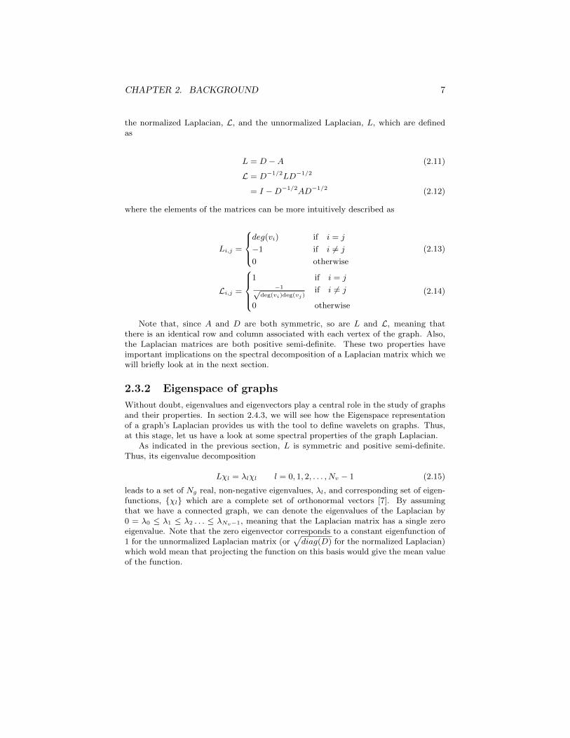
the normalized Laplacian, L, and the unnormalized Laplacian, L, which are definedas
L = D −A (2.11)
L = D−1/2LD−1/2
= I −D−1/2AD−1/2 (2.12)
where the elements of the matrices can be more intuitively described as
Li,j =
deg(vi) if i = j
−1 if i 6= j
0 otherwise
(2.13)
Li,j =
1 if i = j
−1√deg(vi)deg(vj)
if i 6= j
0 otherwise
(2.14)
Note that, since A and D are both symmetric, so are L and L, meaning thatthere is an identical row and column associated with each vertex of the graph. Also,the Laplacian matrices are both positive semi-definite. These two properties haveimportant implications on the spectral decomposition of a Laplacian matrix which wewill briefly look at in the next section.
2.3.2 Eigenspace of graphs
Without doubt, eigenvalues and eigenvectors play a central role in the study of graphsand their properties. In section 2.4.3, we will see how the Eigenspace representationof a graph’s Laplacian provides us with the tool to define wavelets on graphs. Thus,at this stage, let us have a look at some spectral properties of the graph Laplacian.
As indicated in the previous section, L is symmetric and positive semi-definite.Thus, its eigenvalue decomposition
Lχl = λlχl l = 0, 1, 2, . . . , Nv − 1 (2.15)
leads to a set of Ng real, non-negative eigenvalues, λl, and corresponding set of eigen-functions, {χl} which are a complete set of orthonormal vectors [7]. By assumingthat we have a connected graph, we can denote the eigenvalues of the Laplacian by0 = λ0 ≤ λ1 ≤ λ2 . . . ≤ λNv−1, meaning that the Laplacian matrix has a single zeroeigenvalue. Note that the zero eigenvector corresponds to a constant eigenfunction of1 for the unnormalized Laplacian matrix (or
√diag(D) for the normalized Laplacian)
which wold mean that projecting the function on this basis would give the mean valueof the function.
CHAPTER 2. BACKGROUND 8
2.4 Wavelet Transforms
Although the eigenfunctions of the graph Laplacian represent an orthonormal basisfor representing functions on graphs and they are localized in terms of eigenvalues(similar to frequency as for functions defined on regular Euclidean space) but theyhave a global support. Thus, similar to Fourier basis used in the analysis of functionlying in a in Euclidean space, such a basis is not optimal for analyzing piece-wisesmooth functions lying on a graph. The solution would be to define a wavelet analysisapproach for such functions. Wavelets are an excellent tool, widely used for analyzingfunction that show local discontinuities [10]; an example of their Euclidean space usageis on image data where we have local discontinuities and edges that can be very wellcaptured by optimal wavelets.
The use of conventional wavelet transforms defined on Euclidean spaces in sta-tistical parametric mapping of fMRI data as a denoising tool has lead to promisingresults [2, 3, 16]. These results motivates the implementation of wavelets defined onmore complex non-Euclidean domains, such as spectral graph wavelets [4] for this typeof analysis. To this aim, we will first have a brief look at the conventional (tensor-product) wavelet transform and some of its properties, and then we will give a morethorough explanation of the spectral graph wavelets.
The wavelet transform is based on two main mathematical operation, scaling andtranslation. However, it is not straight forward how to apply the scaling operationon a signal which lies on the vertices of a graph. There exists different methodsexplored by different authors to implement the idea of multi-resolution analysis ongraphs [11, 12, 13] but in the current work we focus on a recent implementation ofthe spectral graph wavelet transform introduced by Hammond et al. [4], which alsoprovides a scheme for fast Chebyshev polynomial approximation of the transform;the approach that they have proposed is to take the problem to the Fourier domainand define the required scaling in this domain. Thus, before dipping directly intothe construction of the spectral graph wavelets, we will have a look and see how therequired scaling for the classical wavelet transforms can be defined in the Fourierdomain, and to then see how this could be adopted to the define a similar transformon graphs.
2.4.1 Classical wavelet transform
Wavelet transforms are a powerful multi-resolution analysis tool that enable decompo-sition of a signal on a wavelet orthonormal basis which allows simultaneous localizationin space and frequency. Such transformation, can provide a better representation ofa signal than its original domain as well as its representation in a transform domainsuch as the Fourier domain which is based on global basis function; this is speciallytrue for signals which their primary information content lies in localized singularities,such as edges in images, that can not be represented globally [4].
The idea is based on the use of two main operations on the signal: shifting andscaling. Using these two operations a signal f(x) can be represented as the sum ofshifted and scaled versions of the so called wavelet functions, ψ(x), and shifted versionsof the the so called scaling function, φ(x); the scaling functions and the wavelet func-tions act as low-pass and bandpass functions, respectively. These shifted and dilatedkernels are the new basis that we use to represent our signal. This decomposition canbe formulated as,
CHAPTER 2. BACKGROUND 9
f =∑k
∑s
fψ[s, k]ψs,k +∑k
fφ[k]φk (2.16)
where fφ[k] and fψ[s, k] are the low-pass and bandpass coefficients of the transform,and the parameters s and k are the desired scale and translation, respectively. Thetransformation coefficients can be mathematically expressed as the inner-product ofthe signal and the corresponding scaling functions and wavelets,
fφ[k] = 〈φk|f〉 (2.17)
fψ[s, k] = 〈ψs,k|f〉 . (2.18)
Although it is the discrete wavelet transform (DWT) that has practical applica-tion, we will at this stage look at the continuous wavelet transform (CWT) to betterelaborate on the notion of wavelets and also to use some of the resulting equation inthe CWT case for ease of description of the ideas for SGWT, specifically, the Fourierdomain representations.
In what follows for the description of CWT, we will consider 1-D wavelets forsimplicity. By having a mother wavelet, ψ, the desired wavelets at different scales andlocations can be defined as followed
ψs,t(x) =1
sψ
(x− ts
)(2.19)
where ψs,t(x) indicates the wavelet at scale s and location t. Having defined thedesired wavelets, the wavelet coefficients at each location and scale can be achieved bycomputing the inner product of the signal f(x) and the wavelets,
fw(s, t) = 〈ψs,t|f〉
=
∫ ∞−∞
1
sψ∗(x− ts
)f(x)dx. (2.20)
Provided that the mother wavelet satisfies the admissibility condition which isdefined as ∫ ∞
0
|ψ(ξ)|2
ξdξ = C (2.21)
where ψ(ξ) indicates the Fourier transform of the mother wavelet, an inverse transformcan be defined for the transform as [4, 10]
f(x) =1
C
∫ ∞0
∫ ∞−∞
fw(s, t)ψs,t(x)dtds
s. (2.22)
Fourier representation of wavelet scaling
Assuming that we have a fixed scale, the wavelet transform (2.20) can be thought ofas an operator with only one input variable, the translation parameter t, that can beapplied on the desired function as
(T sf)(t) = fw(s, t). (2.23)

CHAPTER 2. BACKGROUND 10
Now, by expressing (2.20) in terms of convolution
(T sf)(t) =
∫ ∞−∞
ψs(t− x)f(x)dx
= (ψs ? f)(t) (2.24)
where we have defined ψs(x) as
ψs(x) =1
sψ∗(−xs
). (2.25)
Now that we have a convolution term, we may easily compute the Fourier transformof (2.24) and also further simplify it using the well known scaling properties of theFourier transform as
(T sf)(ω) = ˆψs(ω)f(ω)
= ψ∗(sω)f(ω) (2.26)
where we have used theˆ symbol to indicate the Fourier domain. By computing theinverse Fourier transform of (2.26) we achieve [4]
(T sf)(x) =1
2π
∫ ∞−∞
ejωxψ∗(sω)f(ω)dω (2.27)
As can be clearly seen in (2.27), with this approach, we have come to an equationwhere we can see the scaling term as a parameter than only effects the argument ofthe Fourier domain representation of the mother wavelet, and can thus be completelytransfered to that domain. As we will see in section 2.4.3, this is a very interestingobservation as it would allow taking the problematic notion of scaling in graph domainsto the so called graph Fourier domain.
Wavelet localization
What is meant by wavelet localization is simply the placement of a wavelet at aparticular coordinate of interest either in Euclidean space or a node of a graph; thiscan be achieved by applying the wavelet generating kernel to an impulse functiondefining the coordinate as
(T sδt)(x) =1
sψ∗(t− xs
)(2.28)
for the wavelets at different scales, s. Also, it should be noted that the same idea canbe used for localizing the scaling function.
2.4.2 Graph Fourier transform
Knowing that the eigenvalue decomposition of the graph Laplacian leads to a setof orthonormal eigenfunctions, it is interesting to note that these functions can beconsidered as the orthonormal basis for a transform domain within which we canrepresent global smooth functions which lie on the graph; such basis can be thoughtequivalent to the Fourier domain global basis [15]. However, functions on graphs aremore piece-wise smooth than being globally smooth and thus it would not be very

CHAPTER 2. BACKGROUND 11
appropriate to directly use such basis for representing functions on graphs, and it ishere that wavelets analysis come in to play as they can provide localization not onlyin a spectral domain but also in spatial domain.
In the previous section we showed how scaling of the wavelets can be defined inthe Fourier domain; the question now would be, how to define the Fourier transformfor a signal lying on a graph? This is exactly where the graph Laplacian comes intoplay. In a nutshell, the eigenvalues of the graph Laplacian, λ , take a similar role asthe frequency elements, ω, in the normal Euclidean space.
A very interesting observation about the Fourier transform is that the complexexponentials which define this transform in 1-D, eiwx, are the eigenfunctions of the
1-D Laplacian operator, i.e. d2
dx2[4]. Thus, by looking at the expression for the 1-D
inverse Fourier transform
f(x) =1
2π
∫f(w)eiωxdω (2.29)
we can see this as if we are expanding our function, f(x), in a new basis defined by theeigenfunctions of the 1-D Laplacian operator. Now, by considering the graph Laplaciandefining the eigenspace of a graph as described in section 2.3.1, we can interestinglyextend the idea of eigenfunctions of the 1-D Laplacian defining the Fourier transformto a graph’s Laplacian matrix and define the graph Fourier transform [4]; for a functionf ∈ RNv which lies on the vertices of a graph G, its graph Fourier transform is definedas
f(l) = 〈χl|f〉
=
Nv∑n=1
χ∗l (n)f(n). (2.30)
and the inverse of the transform can also be computed in analogy to (2.29) as
f(n) =
Nv−1∑l=0
f(l)χl(n). (2.31)
2.4.3 Spectral graph wavelet transform (SGWT)
At this stage, we have the two main required tools to define the spectral graph wavelettransform: one being the representation of wavelet scaling in the Fourier domain andthe other being the graph Fourier transform.
Denoting the desired spectral graph wavelet generating kernel as g and the waveletoperator as Tg, the application of this operator to the graph signal f would correspondto modulating the Fourier domain representation of the signal, f , as [4]
Tgf(l) = g(λl)f(l) (2.32)
Now that we have defined the desired scaling in the Fourier domain, we compute theinverse graph Fourier transform of (2.32)as in (2.31) to achieve the desired transform
(Tgf)(m) =
Nv−1∑l=0
g(λl)f(l)χl(m) (2.33)

CHAPTER 2. BACKGROUND 12
By applying these wavelet operators to impulse functions on each and every singlevertice of the graph, in a similar manner as we explained for the classical waveletssection 2.4.1, the desired spectral graph wavelets localized at different vertices can beachieved as
ψj,n = T jg δn
ψj,n(m) =
Nv−1∑l=0
g(jλl)χ∗l (n)χl(m) (2.34)
where we denote the wavelet operator at scale j by T jg .Having defined the spectral graph wavelets, the corresponding spectral graph
wavelet coefficients can be achieved by computing their inner product with a givenfunction f as
wψ(j, n) = 〈ψj,n|f〉
=
Nv−1∑l=0
g(jλl)f(l)χl(n). (2.35)
Similar to the idea in classical wavelets where we define a (low-pass) scaling func-tion, it is convenient to take a similar approach as to define a second class of waveformto better encode the low frequency content of the function that lies on the graph [4].We denote the scaling function generating kernel as h. The localized scaling functionsand their corresponding spectral graph coefficients can be computed in a similar wayas we did for the spectral wavelets as
wφ(n) = 〈φn|f〉
=
Nv−1∑l=0
h(λl)f(l)χl(n). (2.36)
The inverse of this transform can be computed, in a similar way as in classicalwavelets, provided that an appropriate wavelet generating kernel be chosen so as tosatisfy the admissibility condition. In the present work, we adapt the Parseval waveletframes developed by Leonardi et al. [17], to satisfy the admissibility condition andalso to conserve energy in the transform domain; in this way, we can have an easyreconstruction of the signal. The scaling function and wavelet generating kernels aredefined as
g(λ) =
sin(π2ν( 1
λ1|λ| − 1)
)if λ1 ≤ λ ≤ λ2,
cos(π2ν( 1
λ2|λ| − 1)
)if λ2 ≤ λ ≤ λ3,
h(λ) =
{1 if λ ≤ λ1,
cos(π2ν( 1
λ1|λ| − 1)
)if λ1 ≤ λ ≤ λ2,

CHAPTER 2. BACKGROUND 13
where ν(x) = x4(35−84x+70x2−20x3) and λ1 = 23, λ2 = 2λ1 and λ3 = 4λ1 [17]; also,
assuming that we have an estimate of the largest eigenvalue in the graph spectrumbeing λmax and that we require wavelets at P scales, the scales are defined as
j = 2pλ−1max for p = 0, . . . , P − 1. (2.37)
However, in this study, we use a slightly modified version of the current design interms of the definition of the scales so as to come up with a different coverage of thespectrum which is found to be more appropriate on large scale graphs which we definefor the brain (section 3.3)
Chebyshev polynomial approximation
As described in section 2.3.2, the diagonalization of the Laplacian matrix is required inorder to compute the transform. Taking into account the number of vertices2 that isrequired to construct our graphs which would in term result in extremely large Lapla-cian matrices, it would seem impossible to compute such a transform. Hammond et al.have tackled this problem by introducing a fast Chebyshev polynomoial approxima-tion algorithm which avoids the need for the diagonalization step[4]. In this proposedapproximation, it is sufficient to only have an estimate of the largest eigenvalue whichcan be easily computed using current available algorithms3. Although interesting, thedetails of this approximation and its derivation is out of the scope of this report, andthe enthusiastic reader is referred to [4] for a thorough explanation.
2In Chapter 4 we will see that with the approach taken in this study, constructing graphsfor the full coverage of the brain would result in graphs with up to 60000 nodes.
3The largest eigenvalue of any matrix can be computed using the Arnoldi algorithm whichis an option available in MATLAB’s built-in eig function.


Chapter 3
Methods and Materials
In this section we will see how the idea the of spectral graph wavelet transform canbe implemented on fMRI data to introduce a new promising modality to the WSPMframework. Basically, we will see how MRI anatomical data can be used to definea domain on which the functional data lies and the spectral graph wavelets can beapplied. Figure 3.1 shows an overall view of the proposed method, and the differentsteps will be explained in sections 3.1-3.4. First, the required preprocessing steps willbe described. Next, we will see the procedure for designing a graph on the brain andproducing the desired spectral graph wavelets. Then, we will go through the details ofthe graph adapted WSPM framework through which we do our main wavelet domainprocessing as well as final spatial statistical inference. In section 3.5, we will introducethe simulated and real data sets that are used for evaluating the performance of theproposed approach.
3.1 Pre-Processing
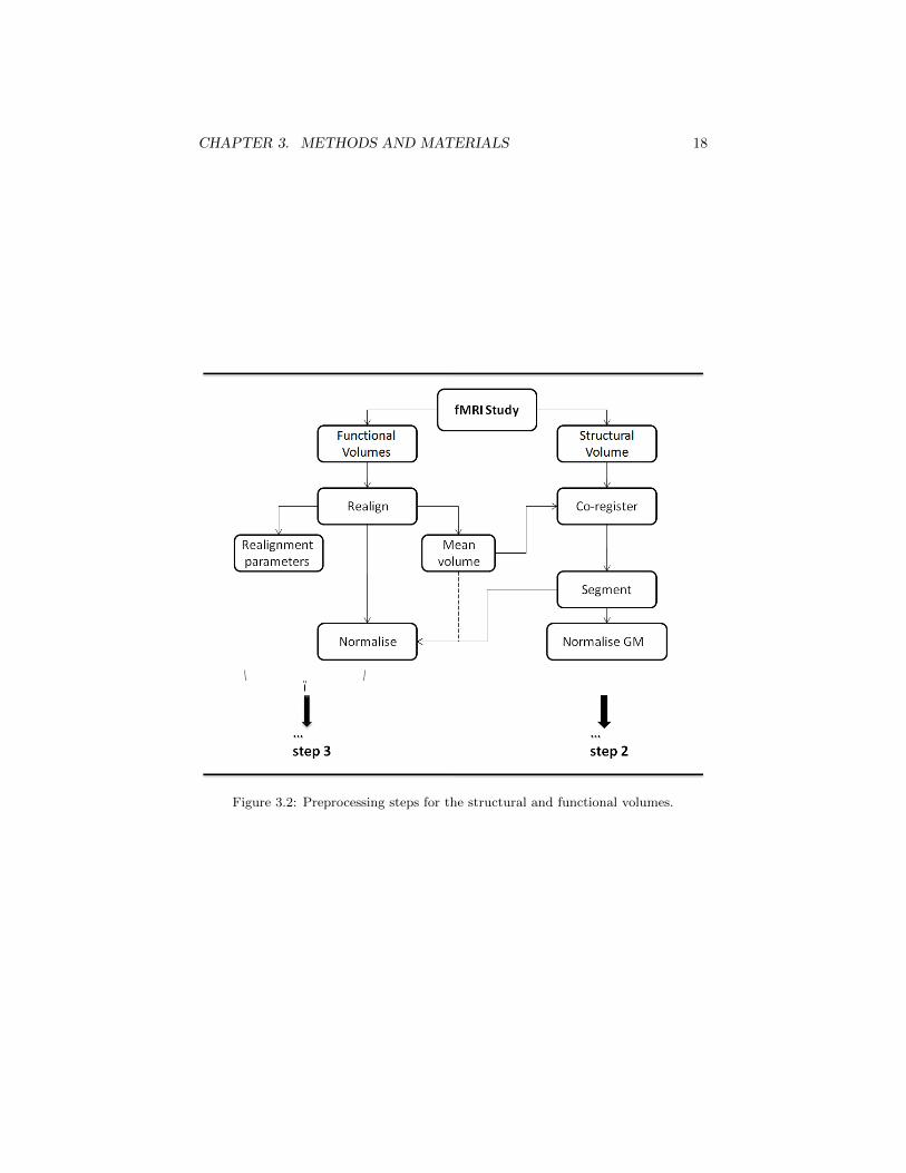
Preprocessing is an essential step in all fMRI analysis. Typically, the functional datashould always be pre-processed whereas the necessity of preprocessing the structuraldata depend on the application. However, in our graph approach, both pre-processingsteps are essential. An overview of the pre-processing step is depicted in Figure 3.2.All the preprocessing in this study was done using the latest release of SPM, SPM8.
3.1.1 Pre-processing of functional data
As a first spatial preprocessing step, all the functional volumes are initially realignedwith the first acquired image. In this phase, a mean functional volume is also computedwhich would be in term used for the normalization of the functional volumes as well asin the co-registration phase of structural volume preprocessing. Also, the movementparameters are estimated, which result in six realignment parameters1. Although thismotion correction step removes most of the undesired variance between the functionalvolumes, it is also common practice to include the estimated motion parameters in thedesign matrix of the GLM as confounds to further reduce movement artifacts [8].
1Three representing translation in 3D space and the other three representing 3D rotaion
15

CHAPTER 3. METHODS AND MATERIALS 16
Figure 3.1: Overall view of the graph wavelet analysis approach for statitical para-metric mapping of fMRI data.
CHAPTER 3. METHODS AND MATERIALS 17
At this stage, depending on the acquisition of the data, a temporal preprocessingstep, slice timing correction, might also be required in which the differences in imageacquisition time between slice are corrected.
Next, as a second step of spatial preprocessing, the functional data are normalizedin to the so called Montreal Neurological Institute (MNI) space using the mean func-tional volume (or the anatomical volume depending on which suits best for acquireddata). Although this step might not be necessary in all SPM analysis studies, butit is an essential step in our graph approach: we require a one-to-one correspondencebetween the voxels of the functional data and the anatomical data as the desired graphwill be defined using the structural volume (see section 3.2), and the data from thefunctional volumes would be placed at vertices of this graph; thus, the functional vol-umes and the structural volumes should also be normalized to an MNI space with thesame specification in terms of voxel sizes.
3.1.2 Pre-processing of the structural data
As a first first step, the structural volume is co-registered with the mean functionalvolume. Next, the resulting co-registered volume is segmented, resulting in three prob-ability maps defining the subjects grey matter (GM), white matter (WM) and cere-brospinal fluid (CSF). The GM is then normalized to an MNI space of the same voxelsize as the normalized functional volumes. Normalization to MNI space with reso-lution ranging from 1.5-3 mm were tested in this study. Although normalization toMNI space with 3 mm resolution is more computationally optimal, the structure ofthe cerebral cortex is lost to a great extent at this resolution. An optimal resolution inwhich we can keep a reasonable representation of the cortical surface is 2 mm, and thisresolution has been chosen in presenting the results for the synthetic data set and theauditory data set (see chapter 4). Also, higher resolution normalization is not suitabledue to the low resolution acquisition of the functional data. Depending on the graphdesign approach that we adopt (see section 3.2), the WM could also be required inwhich case this volume should also be normalized to the same space as the functionalvolumes and the GM volume.
Regarding the normalization of both the structural and functional data, it shouldbe noted that the main requirement for our graph approach is to have one-to-onecorrespondence between the GM and functional data; thus, there is no necessity tonormalize the data to MNI space if we can have an appropriate correspondence inanother space2. However, the MNI space is a standard well recognized space forfMRI studies, and the results represented through within this space can be easilycommunicated between researchers. Also, for extending the approach to multi-subjectstudies, normalizing the data to the MNI space is appropriate since in that case wewould like to use the average GM of the subjects and thus we would need a standardspace to represent the individual subjects.
2In chapter 4, we will see that the second real data set is not represented in the MNI space.
CHAPTER 3. METHODS AND MATERIALS 18
Figure 3.2: Preprocessing steps for the structural and functional volumes.
CHAPTER 3. METHODS AND MATERIALS 19
3.2 Graph design
Defining an appropriate graph on the brain in terms of structure and connectionsis an essential part of the current graph fMRI analysis framework. In this section,we will see how we can define such a graph. In this work we have taken two mainapproaches ; in the first approach, we design a graph based on a-priori knowledge ofonly the structure of the grey matter. In the second approach we not only consider thestructure but also consider the uncertainty that we have regarding each voxel trulybeing GM or not. There are also other design approaches that we have consideredin this study which have however, lead to lower overall performances than the twooutlined approaches; these methods hold promise to lead to more significant resultsprovided further modifications be done and thus, a brief description on these ideas willalso be presented in section 3.2.3.
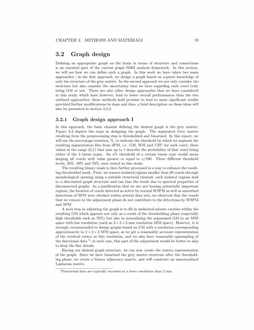
3.2.1 Graph design approach I
In this approach, the basic element defining the desired graph is the grey matter.Figure 3.3 depicts the steps in designing the graph. The segmented Grey matterresulting form the preprocessing step is thresholded and binarized. In this report, wewill use the percentage notation, %, to indicate the threshold by which we segment theresulting segmentation files from SPM, i.e. GM, WM and CSF; for each voxel, threevalues in the range (0,1) that sum up to 1 describe the probability of that voxel beingeither of the 3 tissue types. An x% threshold of a certain tissue type would meankeeping all voxels with value greater or equal to x/100. Three different thresholdlevels, 30%, 50% and 70%, were tested in this study.
The resulting binary mask is then further processed in a way to enhance the result-ing thresholded mask. First, we remove isolated regions smaller than 20 voxels throughmorphological opening using a suitable structural element; such isolated regions leadto a discounted graph structure and can bias the result due to spectral properties ofdisconnected graphs. As a justification that we are not loosing potentially importantregions, the location of voxels detected as active by normal WSPM as well as smootheddetections of SPM were checked within several data sets; we observed that the voxelsthat we remove in the adjustment phase do not contribute to the detections by WSPMand SPM.
A next step in adjusting the graph is to fill in undesired minute cavities within theresulting GM which appears not only as a result of the thresholding phase (especiallyhigh thresholds such as 70%) but also in normalizing the segmented GM to an MNIspace with low resolution (such as 3× 3× 3 mm resolution MNI space). However, it isstrongly recommended to design graphs based on GM with a resolution correspondingapproximately to 2× 2× 2 MNI space, as we get a reasonably accurate representationof the cerebral cortex at this resolution, and we also have reasonable upsampling ofthe functional data 3; in such case, this part of the adjustment would be better to skipto keep the fine details.
Having our desired graph structure, we can now create the matrix representationof the graph. Since we have binarized the grey matter structure after the threshold-ing phase, we create a binary adjacency matrix, and will construct an unnormalizedLaplacian matrix.
3Functional data are typically recorded at a lower resolution than 2 mm.
CHAPTER 3. METHODS AND MATERIALS 20
Figure 3.3: Graph design approach
3.2.2 Graph design approach II
In this second approach we consider designing weighted graphs as opposed to theunweighted graphs that we created in the first approach. An overall representation ofthe approach can be seen in Figure 3.3. As in the fist approach, the segmented GMis initially thresholded to a certain level; as in design approach I, three different levelsof thresholding, i.e. 30%, 50% and 70%, were tested. However, this time, we do notbinarize the remaining mask and instead keep the GM probability values of the voxelssurviving the threshold and use these values for defining a weight between neighboringvoxels instead of assigning binary weights as we did in the first design approach.
The aim of designing a weighted graph in this approach is to take into accountthe local uncertainty of whether a voxel is Grey matter or not; this in term enablesthe design of local wavelets that better diffuse in a direction where we have a highercertainty of being Grey matter than other directions.
In the graph adjustment phase, isolated components are removed in the sameway as in the first approach, and a conservative approach is taken in adding extragraph nodes in which the value of such nodes are set to a value less than the valuecorresponding to the threshold4
Although a threshold of 50% seems to be a reasonable level for definig the GMwhere we expect the true activation to lie, the non-perfect nature of segmentationalgorithms suggests using lower threshold to be on the safe side. Also, it is very
4The value of extra added voxels is set to 0.1 less than the probability value correspondingto the threshold; for example, in a graph constructed with a 50% threshold, we set the valueof extra voxels to 0.4.
CHAPTER 3. METHODS AND MATERIALS 21
typical to see detections outside the 50% grey matter region in most SPM detectionmaps and also in WSPM in a lower extent. Having the power to control the directionof diffusion, i.e. adjusting wavelet diffusuion with the probability of tissue type, alsogives the freedom to further reduce the Grey matter threshold and to thus designlarger graphs and not miss out possible activations in mislabeled voxels.
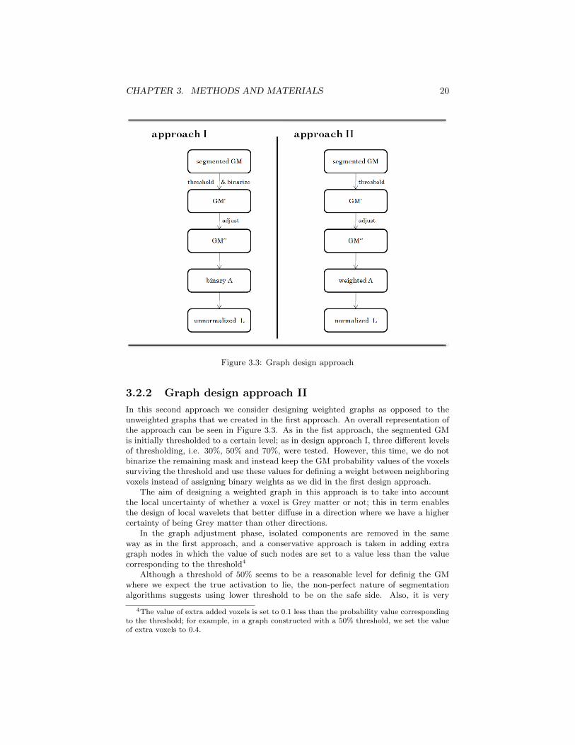
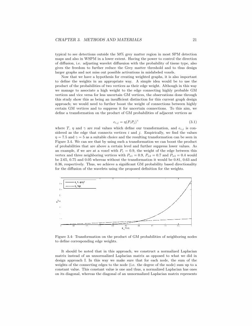
Now that we have a hypothesis for creating weighted graphs, it is also importantto define the weights in an appropriate way. A simple idea would be to use theproduct of the probabilities of two vertices as their edge weight. Although in this waywe manage to associate a high weight to the edge connecting highly probable GMvertices and vice versa for less uncertain GM vertices, the observations done throughthis study show this as being an insufficient distinction for this current graph designapproach; we would need to further boost the weight of connections between highlycertain GM vertices and to suppress it for uncertain connections. To this aim, wedefine a transformation on the product of GM probabilities of adjacent vertices as
ei,j = η(PiPj)γ (3.1)
where T , η and γ are real values which define our transformation, and ei,j is con-sidered as the edge that connects vertices i and j. Empirically, we find the valuesη = 7.5 and γ = 5 as a suitable choice and the resulting transformation can be seen inFigure 3.4. We can see that by using such a transformation we can boost the productof probabilities that are above a certain level and further suppress lower values. Asan example, if we are at a voxel with Pc = 0.9, the weight of the edge between thisvertex and three neighboring vertices with Pn1 = 0.9, Pn2 = 0.7 and Pn3 = 0.4 wouldbe 2.65, 0.75 and 0.05 whereas without the transformation it would be 0.81, 0.63 and0.36, respectively. Thus, we achieve a significant GM probability based directionalityfor the diffusion of the wavelets using the proposed definition for the weights.
Figure 3.4: Transformation on the product of GM probabilities of neighboring nodesto define corresponding edge weights.
It should be noted that in this approach, we construct a normalized Laplacianmatrix instead of an unnormalized Laplacian matrix as opposed to what we did indesign approach I. In this way we make sure that for each node, the sum of theweights of the connecting edges to the node (i.e. the degree of the node) sum up to aconstant value. This constant value is one and thus, a normalized Laplacian has oneson its diagonal, whereas the diagonal of an unnormalized Laplacian matrix represents

CHAPTER 3. METHODS AND MATERIALS 22
the corresponding degree of the nodes.
3.2.3 Other graph design approaches
Other graph design approaches were also considered in this study. One main approachwas to consider including prior knowledge of WM as well as the GM in constructing abrain graph.
It is known that he energy consumption in white matter is one fourth of that of graymatter, and it is also an example of tissue types with sparse vascularization and lowhemodynamic response efficiency (HRE)5 [19], which would mean the weak presence orabsence of the BOLD signal in white matter. Thus, it would not make sense to includeWM regions in our graph to search for activations. However, intuitively it seems thatby restricting the domain to just GM we create some sort of brick-wall that surroundthe domain. Although this assumption is suitable on the CSF neighboring regions ofGM, it does not completely confirm to reality on the inner boundary of GM where itconnects to WH. Also, considering the wavelets that are locally created at the inneredges of GM, their spatial shape would be significantly affected by this construction.These reasoning provided the motivation for considering a design in which we includethe WM as well as the GM. In this way we restrict our domain from one end to theCSF but allow diffusion between the GM and WM.
This approach was tested on real data6 but lead to a lower performance than theother two approaches. Although the lower performance indicates the unsuitability ofthe approach, this result is itself interesting as it provides a proof of the fact thata better knowledge of the exact domain on which the signal lies leads to a highersensitivity as we can better track the activation pattern by creating domain-adjustedwavelets.
3.3 Wavelet design
As we saw in section 2.3.2, the eigenvectors of the graph Laplacian represent theunderlying graph structure in a systematic way. Thus, functions lying on a graph canbe very well encoded by capturing their representation through the graphs differenteigenvectors. By using the spectral graph wavelet transform, the signal lying on thegraph can be encoded using a lowpass scaling function as well as several bandpasswavelets. Other than the importance of the number of scales used, the very essentialfact that was observed in this study is the importance of the design of our scalingfunction and wavelet kernels in terms of their coverage range of the graph Laplacianspectrum, i.e. the range of eigenvalues that each of the kernels capture. Thus, it isvery essential to know how to partition the eigenspace of the graph as to which rangeof spectrum to be captured by the scaling function and the wavelet kernels at differentscales.
In this section, we will introduce a slight modification of the spectral graph waveletframes. By introducing an extra parameter, κ, we modify the definition of the waveletscales from what we saw in equation (2.37) in section 2.4.3 and calculate them as
5The efficiency of the coupling between neural activity and the vascular response is denotedas HRE [19]; this value is significant in determining the amplitude and spatial resolution ofthe BOLD signal.
6We only tried this approach on real data since as we will see in section 4.1, the design ofour synthetic data provides no motivation on using this approach.
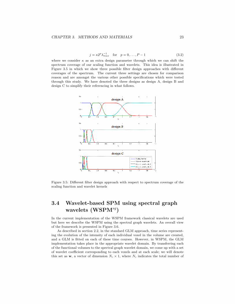
CHAPTER 3. METHODS AND MATERIALS 23
j = κ2pλ−1max for p = 0, . . . , P − 1 (3.2)
where we consider κ as an extra design parameter through which we can shift thespectrum coverage of our scaling function and wavelets. This idea is illustrated inFigure 3.5 in which we show three possible filter design approaches with differentcoverages of the spectrum. The current three settings are chosen for comparisonreason and are amongst the various other possible specifications which were testedthrough this study. We have denoted the three designs as design A, design B anddesign C to simplify their referencing in what follows.
Figure 3.5: Different filter design approach with respect to spectrum coverage of thescaling function and wavelet kernels
3.4 Wavelet-based SPM using spectral graphwavelets (WSPMsg)
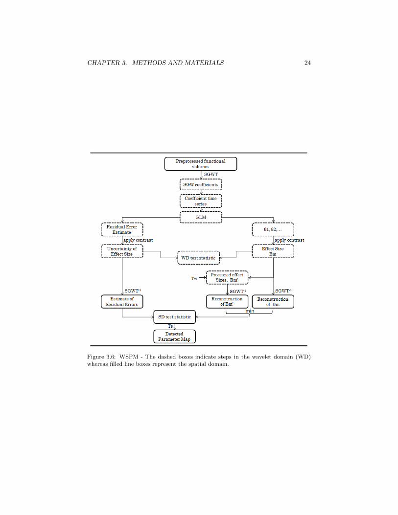
In the current implementation of the WSPM framework classical wavelets are usedbut here we describe the WSPM using the spectral graph wavelets. An overall viewof the framework is presented in Figure 3.6.
As described in section 2.2, in the standard GLM approach, time series represent-ing the evolution of the intensity of each individual voxel in the volume are created,and a GLM is fitted on each of these time courses. However, in WSPM, the GLMimplementation takes place in the appropriate wavelet domain. By transferring eachof the functional volumes to the spectral graph wavelet domain, we come up with a setof wavelet coefficient corresponding to each voxels and at each scale; we will denotethis set as w, a vector of dimension Nc × 1, where Nc indicates the total number of
CHAPTER 3. METHODS AND MATERIALS 24
Figure 3.6: WSPM - The dashed boxes indicate steps in the wavelet domain (WD)whereas filled line boxes represent the spatial domain.
CHAPTER 3. METHODS AND MATERIALS 25
coefficients for each volume7. Then, by concatenating the corresponding coefficients atime series representing the evolution of each wavelet coefficient can be constructed
ykw = [w1[k] . . .wNt [k]]T (3.3)
where ykw is a Nt × 1 vector which represents the temporal change in intensity of thethe k-th wavelet coefficient.
3.4.1 Wavelet domain model fitting
At this stage, the temporal behavior of each of the wavelet coefficients can be modeledby a GLM in a similar fashion as it was described in section 2.2 for the voxels in thespatial domain
ykw = Xβkw + εkw (3.4)
where βkw is a Nr × 1 vector of regression parameters and εkw is a Nt × 1 vector ofresidual errors. The elements of vector βkw are the effect sizes, i.e. the effect thateach of the Nr regressors have had on the the BOLD response at the k -th waveletcoefficient.
3.4.2 Wavelet domain processing
Having computed the regression parameters for all the coefficients, in a similar fashionas we derived the equation for t-values for normal SPM in section 2.2.2, we can derivethe wavelet domain t-value at the k-th wavelet coefficient as
tkw =cTβkw
σkw√
cT (XTX)−1c(3.5)
where c is the contrast vector (the same contrast vector that we use for normal spatialdomain processing in SPM), and σkw is the estimate of the standard deviation at theconsidered wavelet coefficient
σkw =
√εkw
T εkwtr(R)
(3.6)
with εkw being the estimate of the residual error
εkw = ykw −Xβkw. (3.7)
Unprocessed parameter map, u[n]
The unprocessed map is the parameter map that is reconstructed back from the waveletdomain into the spatial domain using all of the wavelet coefficients; thus no denoising.By noting that the term in the numerator of (3.5) denotes the k-th wavelet coefficientof the unprocessed parameter map, the terms can be concatenated to create an Nc×1vector of coefficients as
7As an example, if we have a graph with Nv vertices, its spectral graph wavelet decom-position using one scaling function and m wavelet scales would result in Nc = Nv × (m + 1)wavelet.

CHAPTER 3. METHODS AND MATERIALS 26
uw,i = [β1w . . .β
Ncw ]
Tc (3.8)
and the reconstruction of the unprocessed parameter map could then be computed as
u =
Nc∑k=1
uw[k]ψk (3.9)
where the ψj terms indicate the corresponding spectral graph wavelets to each wavelet
coefficient8. Note that, this map corresponds to the linear parameter map which couldbe achieved by running the GLM directly on the un-smoothed data in the spatialdomain. In what follows, we will see that this map would be required for bias correctionof the processed parameter map.
Processed parameter map
The thresholding done at this stage on the wavelet domain t-values will not havea spatial statistical meaning; it is considered as a denoising step and the optimalthreshold value, τw, is treated as a general parameter of the algorithm [2].
Having thresholded the wavelet domain t-values, only those wavelet coefficientsthat their corresponding t-value has survived the threshold will be used to reconstructthe parameter map back into spatial domain to create the desired processed parametermap, u.
u =
Nc∑k=1
H(|tkw| − τw)uw[k]ψk (3.10)
where H is the Heaviside step function defined as
H(x) =
{0 if x < 0,
1 otherwise(3.11)
Improved processed parameter map
The goal at this stage is to reduce the spatial bias in the final detected parametermap. As described by Van De Ville et al. [3], an example of such bias would be thecase in which weak activations in the parameter map may not very well represent thereal underlying activity if only a limited subset of corresponding wavelet coefficientshave survived the wavelet thresholding phase. In a nutshell, bias reduction can beachieved by comparing the denoised parameter map, ui, against the linear estimate,ui, and only trusting the denoised map at locations where the estimate is not higherthan that of the linear map. This can be mathematically expressed as
u = min(u, u) ≤ u (3.12)
8Note that we have indicated the scaling function and the wavelet functions with the sameindexing.
CHAPTER 3. METHODS AND MATERIALS 27
3.4.3 Spatial domain statistical inference
Note that, although we had a thresholding phase in the wavelet domain, that thresh-olding had no statistical meaning and it is through a second thresholding of t-valuesconstructed in the spatial domain that we can do the desired statistical testing. Wedenote the threshold used for this second spatial domain thresholding as τs. First, wewill briefly see how optimal values for τw and τs can be calculated then we will expressthe final statistical test which results in the final detected map [2, 3].
Optimal τw and τs computation
On one hand, the goal is to derive a spatially varying threshold, q[n]9, such that underthe null hypothesis, the desired significance level ,α, is not exceeded by the probabilityof reconstruction of the processed parameter map at that point, u,
P
[Nc∑k=1
H(|tkw| − τw)uw[k]ψk(n) ≥ q[n]
]≤ α. (3.13)
Going through the details and derivations which we will not cover in this report10,we would come up with a relation for the desired spatial threshold, τs, as a functionof the wavelet threshold τw and the desired significance level, α, as
τs =1√2πα
exp
(−τ
2w
2
)(3.14)
Knowing τs, the spatially varying threshold, q[n], can now be seen as
q[n] = τsΛ[n] (3.15)
where Λ[n] is a weighted sum of the absolute value reconstruction of the wavelet basis,with their corresponding weights being the standard deviation of the estimate of theresidual error in the model fitting (equation 2.7); Λ[n] can be mathematically expressedas
Λ =
Nc∑k=1
σkw|ψk|. (3.16)
Note that equation (3.14) holds for many different combinations of τs and τw;however, as described in [2], an optimal combination of thresholds can be computed asthe solutions to an optimization problem which minimizes the worst-case error betweenthe unprocessed and the detected parameter, which in term, boils down to minimizingthe sum of the two thresholds, i.e. τw + τs, subject to a constraint11. For the casethat Nt > 50, which is a reasonable assumption for almost all fMRI studies, we haveenough data to estimate the noise variance, and thus, a closed-form solution to theoptimization can be found as
τw =√−W−1(−2πα2), τs = 1/τw, (3.17)
9Note that, in this section, n is the notation used for specifying the spatial location in 3D,i.e. n = [xn, yn, zn]T
10Although interesting, this would be out of the scope of this short report, but the en-thusiastic reader is refered to the original paper for the complete description and derivations[2].
11See [2] for the details on this constraint.
CHAPTER 3. METHODS AND MATERIALS 28
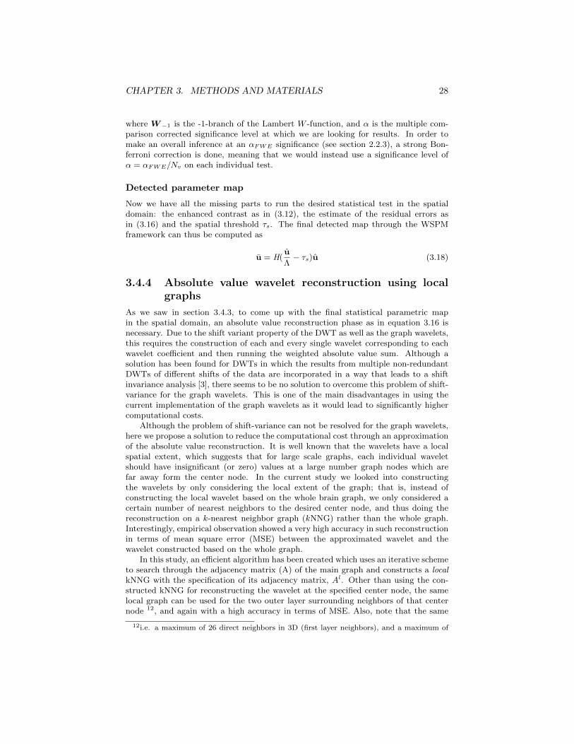
where W−1 is the -1-branch of the Lambert W -function, and α is the multiple com-parison corrected significance level at which we are looking for results. In order tomake an overall inference at an αFWE significance (see section 2.2.3), a strong Bon-ferroni correction is done, meaning that we would instead use a significance level ofα = αFWE/Nv on each individual test.
Detected parameter map
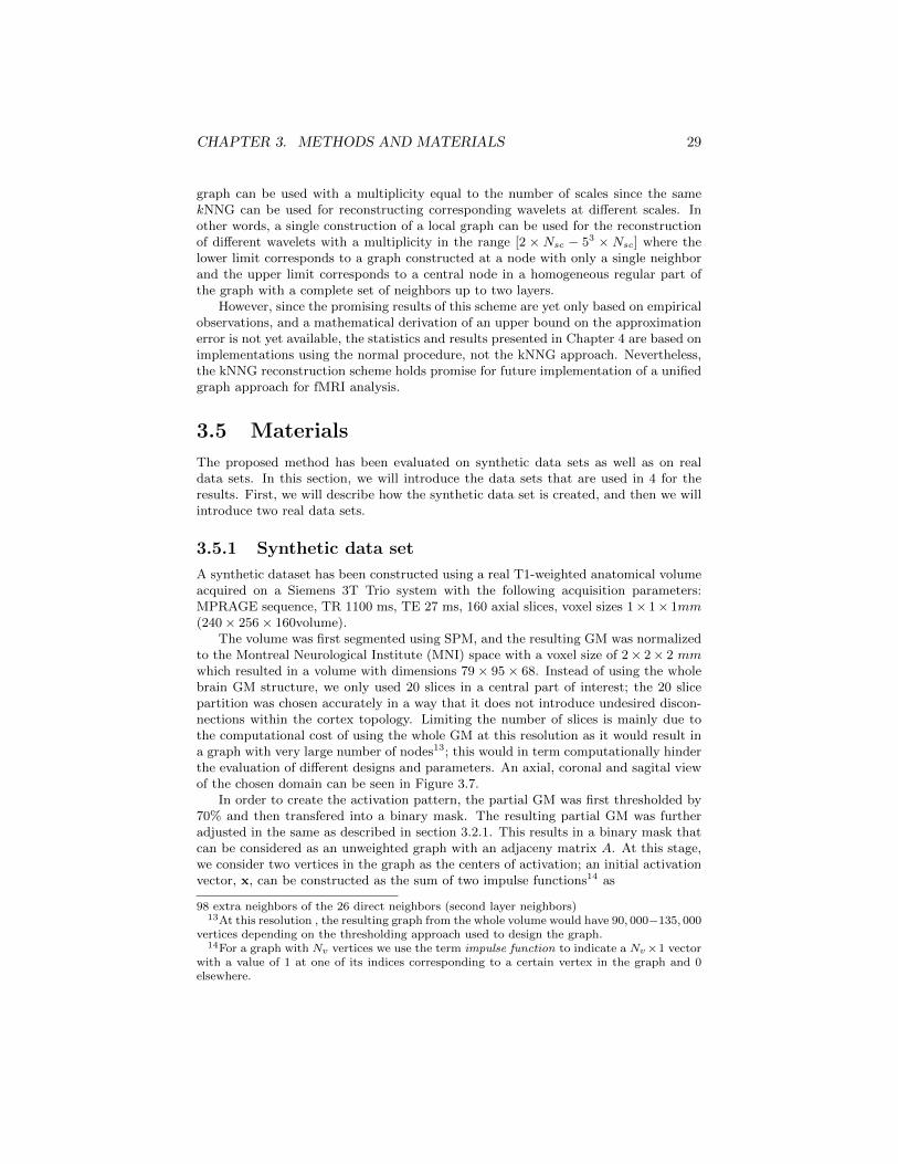
Now we have all the missing parts to run the desired statistical test in the spatialdomain: the enhanced contrast as in (3.12), the estimate of the residual errors asin (3.16) and the spatial threshold τs. The final detected map through the WSPMframework can thus be computed as
u = H(u
Λ− τs)u (3.18)
3.4.4 Absolute value wavelet reconstruction using localgraphs
As we saw in section 3.4.3, to come up with the final statistical parametric mapin the spatial domain, an absolute value reconstruction phase as in equation 3.16 isnecessary. Due to the shift variant property of the DWT as well as the graph wavelets,this requires the construction of each and every single wavelet corresponding to eachwavelet coefficient and then running the weighted absolute value sum. Although asolution has been found for DWTs in which the results from multiple non-redundantDWTs of different shifts of the data are incorporated in a way that leads to a shiftinvariance analysis [3], there seems to be no solution to overcome this problem of shift-variance for the graph wavelets. This is one of the main disadvantages in using thecurrent implementation of the graph wavelets as it would lead to significantly highercomputational costs.
Although the problem of shift-variance can not be resolved for the graph wavelets,here we propose a solution to reduce the computational cost through an approximationof the absolute value reconstruction. It is well known that the wavelets have a localspatial extent, which suggests that for large scale graphs, each individual waveletshould have insignificant (or zero) values at a large number graph nodes which arefar away form the center node. In the current study we looked into constructingthe wavelets by only considering the local extent of the graph; that is, instead ofconstructing the local wavelet based on the whole brain graph, we only considered acertain number of nearest neighbors to the desired center node, and thus doing thereconstruction on a k-nearest neighbor graph (kNNG) rather than the whole graph.Interestingly, empirical observation showed a very high accuracy in such reconstructionin terms of mean square error (MSE) between the approximated wavelet and thewavelet constructed based on the whole graph.
In this study, an efficient algorithm has been created which uses an iterative schemeto search through the adjacency matrix (A) of the main graph and constructs a localkNNG with the specification of its adjacency matrix, Al. Other than using the con-structed kNNG for reconstructing the wavelet at the specified center node, the samelocal graph can be used for the two outer layer surrounding neighbors of that centernode 12, and again with a high accuracy in terms of MSE. Also, note that the same
12i.e. a maximum of 26 direct neighbors in 3D (first layer neighbors), and a maximum of
CHAPTER 3. METHODS AND MATERIALS 29
graph can be used with a multiplicity equal to the number of scales since the samekNNG can be used for reconstructing corresponding wavelets at different scales. Inother words, a single construction of a local graph can be used for the reconstructionof different wavelets with a multiplicity in the range [2 × Nsc − 53 × Nsc] where thelower limit corresponds to a graph constructed at a node with only a single neighborand the upper limit corresponds to a central node in a homogeneous regular part ofthe graph with a complete set of neighbors up to two layers.
However, since the promising results of this scheme are yet only based on empiricalobservations, and a mathematical derivation of an upper bound on the approximationerror is not yet available, the statistics and results presented in Chapter 4 are based onimplementations using the normal procedure, not the kNNG approach. Nevertheless,the kNNG reconstruction scheme holds promise for future implementation of a unifiedgraph approach for fMRI analysis.
3.5 Materials
The proposed method has been evaluated on synthetic data sets as well as on realdata sets. In this section, we will introduce the data sets that are used in 4 for theresults. First, we will describe how the synthetic data set is created, and then we willintroduce two real data sets.
3.5.1 Synthetic data set
A synthetic dataset has been constructed using a real T1-weighted anatomical volumeacquired on a Siemens 3T Trio system with the following acquisition parameters:MPRAGE sequence, TR 1100 ms, TE 27 ms, 160 axial slices, voxel sizes 1× 1× 1mm(240× 256× 160volume).
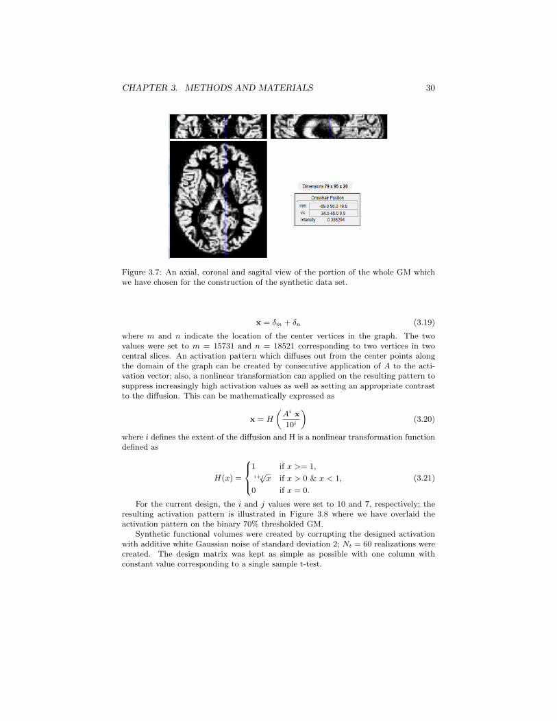
The volume was first segmented using SPM, and the resulting GM was normalizedto the Montreal Neurological Institute (MNI) space with a voxel size of 2× 2× 2 mmwhich resulted in a volume with dimensions 79× 95× 68. Instead of using the wholebrain GM structure, we only used 20 slices in a central part of interest; the 20 slicepartition was chosen accurately in a way that it does not introduce undesired discon-nections within the cortex topology. Limiting the number of slices is mainly due tothe computational cost of using the whole GM at this resolution as it would result ina graph with very large number of nodes13; this would in term computationally hinderthe evaluation of different designs and parameters. An axial, coronal and sagital viewof the chosen domain can be seen in Figure 3.7.
In order to create the activation pattern, the partial GM was first thresholded by70% and then transfered into a binary mask. The resulting partial GM was furtheradjusted in the same as described in section 3.2.1. This results in a binary mask thatcan be considered as an unweighted graph with an adjaceny matrix A. At this stage,we consider two vertices in the graph as the centers of activation; an initial activationvector, x, can be constructed as the sum of two impulse functions14 as
98 extra neighbors of the 26 direct neighbors (second layer neighbors)13At this resolution , the resulting graph from the whole volume would have 90, 000−135, 000
vertices depending on the thresholding approach used to design the graph.14For a graph with Nv vertices we use the term impulse function to indicate a Nv×1 vector
with a value of 1 at one of its indices corresponding to a certain vertex in the graph and 0elsewhere.
CHAPTER 3. METHODS AND MATERIALS 30
Figure 3.7: An axial, coronal and sagital view of the portion of the whole GM whichwe have chosen for the construction of the synthetic data set.
x = δm + δn (3.19)
where m and n indicate the location of the center vertices in the graph. The twovalues were set to m = 15731 and n = 18521 corresponding to two vertices in twocentral slices. An activation pattern which diffuses out from the center points alongthe domain of the graph can be created by consecutive application of A to the acti-vation vector; also, a nonlinear transformation can applied on the resulting pattern tosuppress increasingly high activation values as well as setting an appropriate contrastto the diffusion. This can be mathematically expressed as
x = H
(Ai x
10i
)(3.20)
where i defines the extent of the diffusion and H is a nonlinear transformation functiondefined as
H(x) =
1 if x >= 1,i+j√x if x > 0 & x < 1,
0 if x = 0.
(3.21)
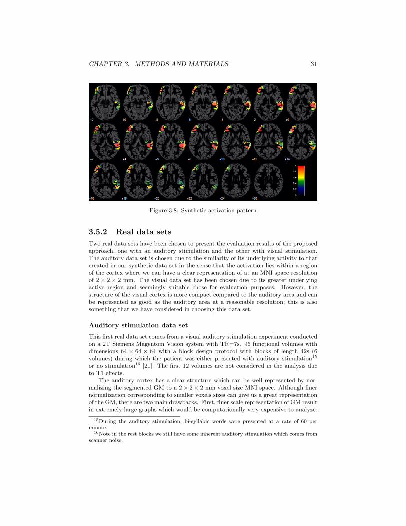
For the current design, the i and j values were set to 10 and 7, respectively; theresulting activation pattern is illustrated in Figure 3.8 where we have overlaid theactivation pattern on the binary 70% thresholded GM.
Synthetic functional volumes were created by corrupting the designed activationwith additive white Gaussian noise of standard deviation 2; Nt = 60 realizations werecreated. The design matrix was kept as simple as possible with one column withconstant value corresponding to a single sample t-test.
CHAPTER 3. METHODS AND MATERIALS 31
Figure 3.8: Synthetic activation pattern
3.5.2 Real data sets
Two real data sets have been chosen to present the evaluation results of the proposedapproach, one with an auditory stimulation and the other with visual stimulation.The auditory data set is chosen due to the similarity of its underlying activity to thatcreated in our synthetic data set in the sense that the activation lies within a regionof the cortex where we can have a clear representation of at an MNI space resolutionof 2 × 2 × 2 mm. The visual data set has been chosen due to its greater underlyingactive region and seemingly suitable chose for evaluation purposes. However, thestructure of the visual cortex is more compact compared to the auditory area and canbe represented as good as the auditory area at a reasonable resolution; this is alsosomething that we have considered in choosing this data set.
Auditory stimulation data set
This first real data set comes from a visual auditory stimulation experiment conductedon a 2T Siemens Magentom Vision system with TR=7s. 96 functional volumes withdimensions 64 × 64 × 64 with a block design protocol with blocks of length 42s (6volumes) during which the patient was either presented with auditory stimulation15
or no stimulation16 [21]. The first 12 volumes are not considered in the analysis dueto T1 effects.
The auditory cortex has a clear structure which can be well represented by nor-malizing the segmented GM to a 2× 2× 2 mm voxel size MNI space. Although finernormalization corresponding to smaller voxels sizes can give us a great representationof the GM, there are two main drawbacks. First, finer scale representation of GM resultin extremely large graphs which would be computationally very expensive to analyze.
15During the auditory stimulation, bi-syllabic words were presented at a rate of 60 perminute.
16Note in the rest blocks we still have some inherent auditory stimulation which comes fromscanner noise.

CHAPTER 3. METHODS AND MATERIALS 32
Second, as it is well known, the functional data are recorded in a much lower resolutionwhich in term makes their normalization to very fine MNI space unreasonable.
Visual stimulation data set
The second real data set comes from a visual stimulation experiment conducted on aSiemens Magnetom TrioTim 3T scanner with the following acquisition parameters forthe structural volume and the functional volumes as:
• Structural data: MPRAGE T1 scan, TR=2500 ms, TI=1100 ms, 224 coronalslices (1 mm), in plane resolution: 0.9× 0.9 mm.
• Functional data: EPI T2∗ scan, TR=1s, 435 scans, TE=30 ms, 16 axial slices(5 mm), in plane resolution: 1.8× 1.8 mm.
The stimulation protocol alternated between random short-flashed visual stimula-tion of face or checkerboard. The stimulation remained for 0.5s and was followed bya 17.5s resting period during which a small cross-hair was shown in the middle of thefield-of-view.
3.6 SPM compatible implementation
The proposed methodology in the current study has been programmed in MATLAB,in an SPM compatible manner. The method is already integrated into the WSPMframework implementation to a good extent. After further adjustments, the newWSPM toolbox will be made available as the next major release from the homepageof the hosting laboratory, MIPLab [22].
Chapter 4
Results
The proposed graph wavelet fMRI analysis method has been evaluated on both syn-thetic data as well as real data. We propose an evaluation based on a synthetic dataset and two real data sets. There are several interesting aspects and design parametersin the current graph approach which we will consider for evaluation on the simulateddata set as we know the ground truth. These parameters are as followed
• Graph design approach
• Graph domain extent
• Graph spectrum coverage of filters
• Number of wavelet scales
Having found an optimal setting based on the evaluations on the synthetic dataset, this setting will in term be used for the analysis on the real data sets. For boththe synthetic and the real data sets, we will compare the results achieved with WSPMusing spectral graph wavelets to that achieved by WSPM using classical wavelets andalso normal SPM.
Before we proceed to the results, a few notes are in place. For the Chebyshevapproximation, different orders have been tested in this study (ranging form 10-100,results not presented) and in what follows, unless stated otherwise, 50 Chebyshevpolynomial have been used to calculate the spectral graph transforms as this numberof polynomials seems to be sufficient for the approximations on our brain graphs;using less polynomial in some cases lead to a decrease in performance and using ahigher values lead to no significance improvement. Also, unless specified otherwise,the statistical inferences are all based on a family-wise corrected significance level of5%.
33

CHAPTER 4. RESULTS 34
4.1 Simulation results
Knowing the ground truth regarding the activation in our synthetic dataset, the per-formance of the evaluated methods can be assessed in terms of sensitivity1 and speci-ficity1. However, noting that in the current synthetic design, the true number ofinactive voxels, 42742, is much greater than that of true active voxels, 4707, and thusit would be quite difficult to get a feeling of the performance in terms of specificitypresented in percentages2 (as to see how many false positive (FP) were detected).Thus, instead of presenting figures denoting specificity, we indicate the number of FPdetections which could be more intuitive.
4.1.1 Evaluation of graph design approaches
In this section, we will compare the performance achieved using design approach I tothat of design approach II. Table 4.1 summarizes the results achieved using the twoapproaches using graph wavelets at four scales. In general, we see a nice performancefor both approaches but a better performance in using approach II in which we haveincorporated knowledge of the probability of each vertex being GM.
approach I approach IISensitivity 78% 84.5%FPs 241 271
Table 4.1: Evaluation of two design approaches: approach I based on defining a binarygraph on GM, and approach II based on constructing a weighted graph on GM.
4.1.2 Effect of varying the graph domain
The hypothesis that we have regrading the domain is that the better knowledge thatwe have of the precise domain where the activation lies, the better the performance interms of sensitivity and specificity; a better sensitivity in the sense that a higher a prioriknowledge of the GM can lead to better adaptation of the graph wavelets to a morerealistic domain, and a better specificity in the sense that we do not allow diffusionin regions that are most probably WM or CSF. However, with design approach IIwhich allows controlling the shaping of the wavelets depending on the probability ofthe underlying domain being GM, we hope to still keep the specificity high even withthe extension of the domain to regions with less probability of being GM. Figure 4.1shows several slices of the resulting graph domain based on thresholding the segmentedGM at three different levels.
Although the activation within the synthetic data set was created using a graphconstructed from the GM threshold by 70%, we do not restrict the construction ofour main graph to this domain; instead, we explore the performance of the methodby constructing graphs with three different domains based on thresholding the GM by
1Sensitivity, which represents accuracy, is defined as the ratio of the number of true positive(TP) detections over the real number of active voxels, whereas Specificity, which representsefficiency, is defined as the ratio of the number of true negative detections over the real numberof inactive voxels.
2The percentages would usually be in the range 98-99% and only differ in a fraction of apercent.

CHAPTER 4. RESULTS 35
Figure 4.1: Binary representation of three different graph domains, constructed basedon thresholding the GM by 70%, 50% and 30% (from top to bottom) and then applyingthe further adjustments as described in section 3.2.2.
30%, 50% and 70% and then adjusting the domains using the method described fordesign approach II. Figure 4.2 shows an overlay of the synthetic activation on thesethree domains.
Table 4.2 summarizes some facts regarding the defined domains as well the results.We see that the more compact, accurate 70% thresholded based domain leads tosuperior results. However, due to the imperfect nature of the segmentation process, inreality we could not have such an accurate correspondence between the domain thatwe define and the real domain within which the BOLD signal lies; thus, consideringthe 50% thresholded domain for this synthetic data set seems more like what we canexpect in reality.
GM 70% GM 50% GM 30%Nodes 37883 47449 56201Sensitivity 87% 84.5% 82%FPs 31 271 343
Table 4.2: Evaluation of the effect of varying the extent of the graph. A lower GMthreshold corresponds to enlarging the domain by also including voxels with lowerprobability of being GM as the vertices of our graph.
Another observation is that by further extending the domain and consequentlyloosing the fine structure of the cortex, not only does the algorithm detect more falsepositives but also the sensitivity decreases. This is interesting in the sense that itshows that a better estimate of the real cerebral cortex within which the activationlies can lead to better spatial adaptation of the graph wavelets, and thus, the activationpattern can better be tracked and detected.
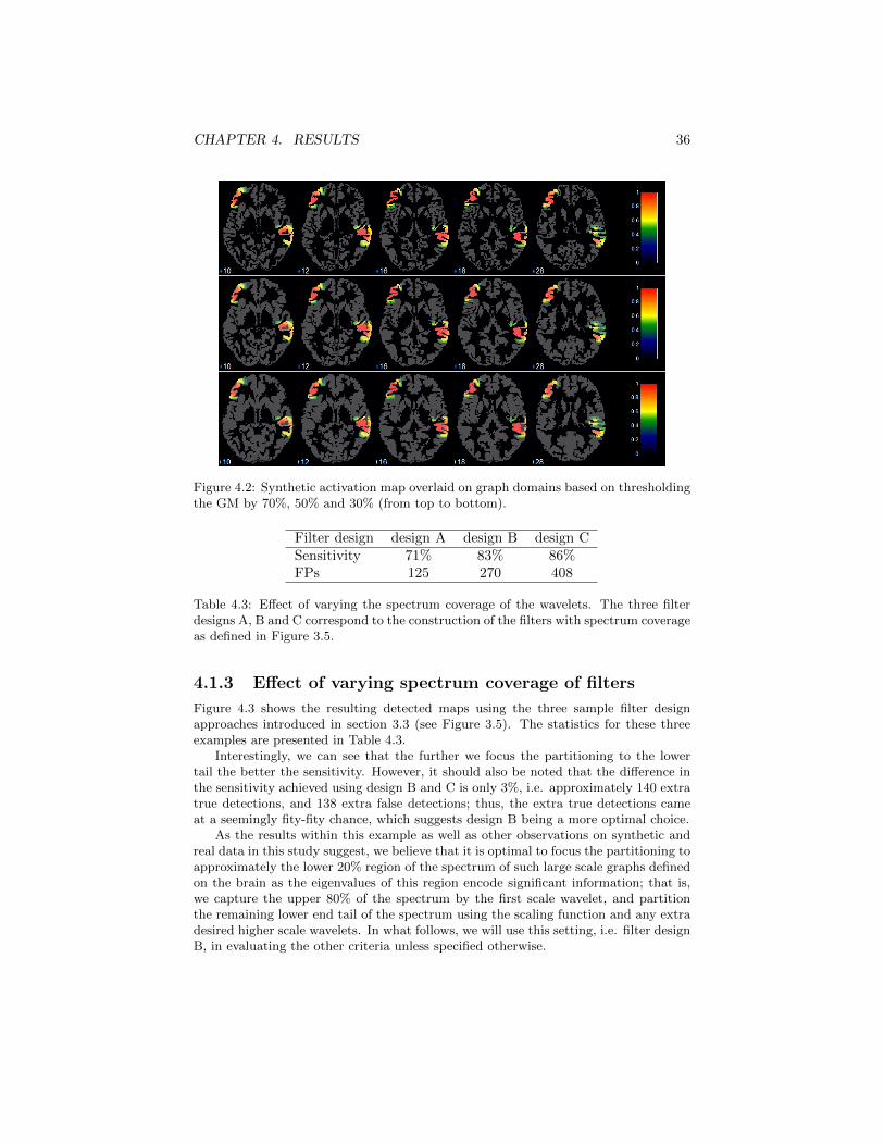
CHAPTER 4. RESULTS 36
Figure 4.2: Synthetic activation map overlaid on graph domains based on thresholdingthe GM by 70%, 50% and 30% (from top to bottom).
Filter design design A design B design CSensitivity 71% 83% 86%FPs 125 270 408
Table 4.3: Effect of varying the spectrum coverage of the wavelets. The three filterdesigns A, B and C correspond to the construction of the filters with spectrum coverageas defined in Figure 3.5.
4.1.3 Effect of varying spectrum coverage of filters
Figure 4.3 shows the resulting detected maps using the three sample filter designapproaches introduced in section 3.3 (see Figure 3.5). The statistics for these threeexamples are presented in Table 4.3.
Interestingly, we can see that the further we focus the partitioning to the lowertail the better the sensitivity. However, it should also be noted that the difference inthe sensitivity achieved using design B and C is only 3%, i.e. approximately 140 extratrue detections, and 138 extra false detections; thus, the extra true detections cameat a seemingly fity-fity chance, which suggests design B being a more optimal choice.
As the results within this example as well as other observations on synthetic andreal data in this study suggest, we believe that it is optimal to focus the partitioning toapproximately the lower 20% region of the spectrum of such large scale graphs definedon the brain as the eigenvalues of this region encode significant information; that is,we capture the upper 80% of the spectrum by the first scale wavelet, and partitionthe remaining lower end tail of the spectrum using the scaling function and any extradesired higher scale wavelets. In what follows, we will use this setting, i.e. filter designB, in evaluating the other criteria unless specified otherwise.
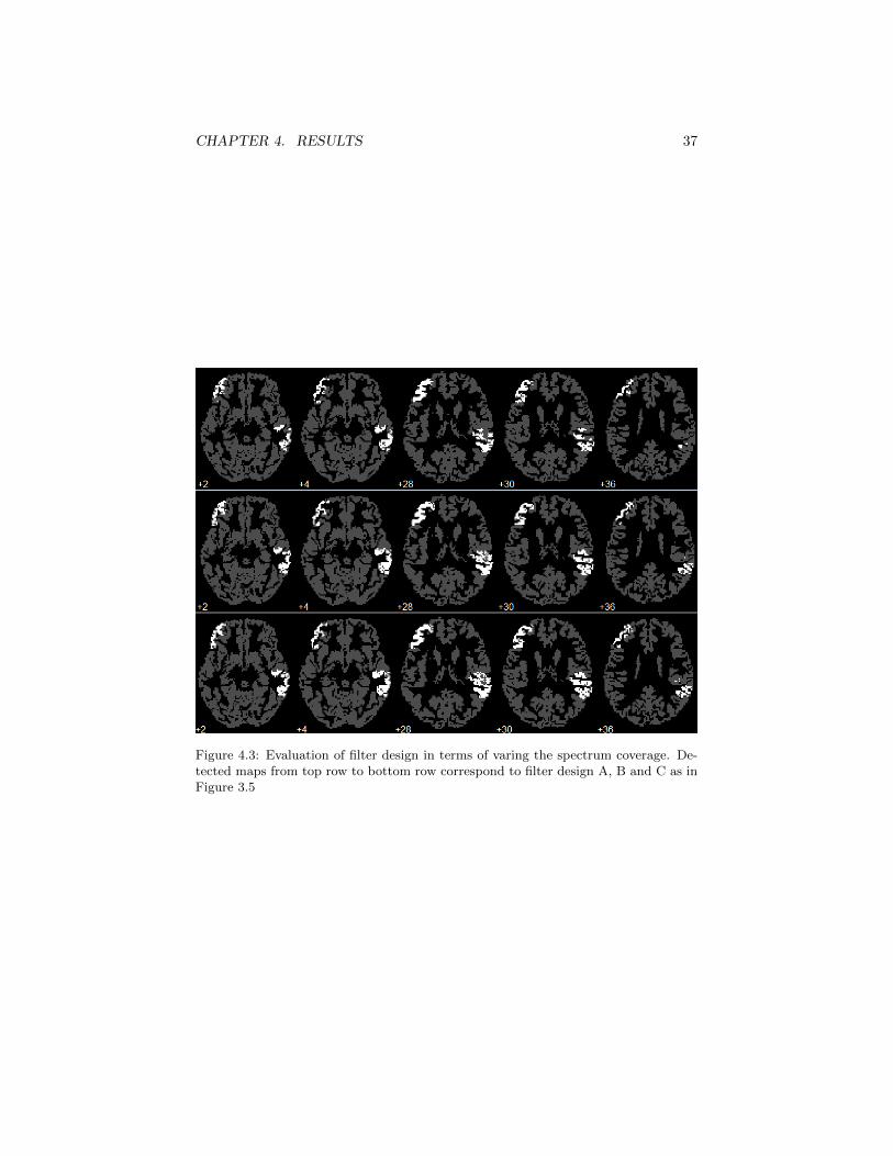
CHAPTER 4. RESULTS 37
Figure 4.3: Evaluation of filter design in terms of varing the spectrum coverage. De-tected maps from top row to bottom row correspond to filter design A, B and C as inFigure 3.5

CHAPTER 4. RESULTS 38
4.1.4 Effect of varying the number of wavelet scales
The hypothesis that we investigate in this section is to see whether increasing thenumber of scales could enhance the performance by capturing activations at some finescale decoded by a certain range of eigenvalues. Before we proceed a note on notationis in place; in what follows, we would denote the sum of the wavelet scales and thescaling function as the number of scales; as an example, four scales would mean theuse of wavelets at three scales plus the scaling function.
Table 4.4 shows the statistics achieved by varying the number of scales from twoto five. First of all, we can see an increase in sensitivity by increasing the number ofscales from two to three. By further increasing the number of scales to four, we see aplateau in performance in terms of specificity with a slight decrease in sensitivity. Itcan be seen that we have a plateau in performance in using three or more scales whichsuggests three or four scales as being an appropriate choice.
Number of scales 2 3 4 5 6Sensitivity 81% 84.5% 83% 83% 82%FPs 298 271 270 269 264
Table 4.4: Effect of varying the number of scales used for the wavelet decomposition.
4.1.5 WSPMsg vs WSPM and SPM
We will now compare the results achieved using the new proposed graph waveletanalysis method to that of normal SPM and WSPM using classical wavelets. Basedon the evaluation in the previous sections, we adopt the optimal settings for designingthe graph and the graph wavelets. Table 4.5 summarizes the specifications used forthe graph wavelet approach.
Graph design approach approach IIGM threshold 50%Wavelet Scales 3Filter specification design BChebyshev order 50
Table 4.5: Specification of parameters used for the graph wavelet approach.
For the SPM analysis, two different levels of Gaussian smoothing have been consid-ered: FWHM= 4mm and 6mm. For the analysis using the classical wavelets, 2D and3D redundant standard orthogonal wavelets with a single level of decomposition wereused3. As a reference, a voxel-by-voxel t-test on the unsmoothed data was also donewhich resulted in only 72 detections. This clearly shows the sufficiency of the addednoise, and also highlights the significance of the denoising power of wavelet methodswhich function on the unsmoothed data.
Table 4.6 gives a summary of statistics resulting from the different approaches andFigure 4.4 shows the detection maps resulting from the three approaches at several
3The specifications chosen for the classical wavelets are in accordance to the suggestionsgiven by the developers of the classical WSPM method as being the relative optimal settings.
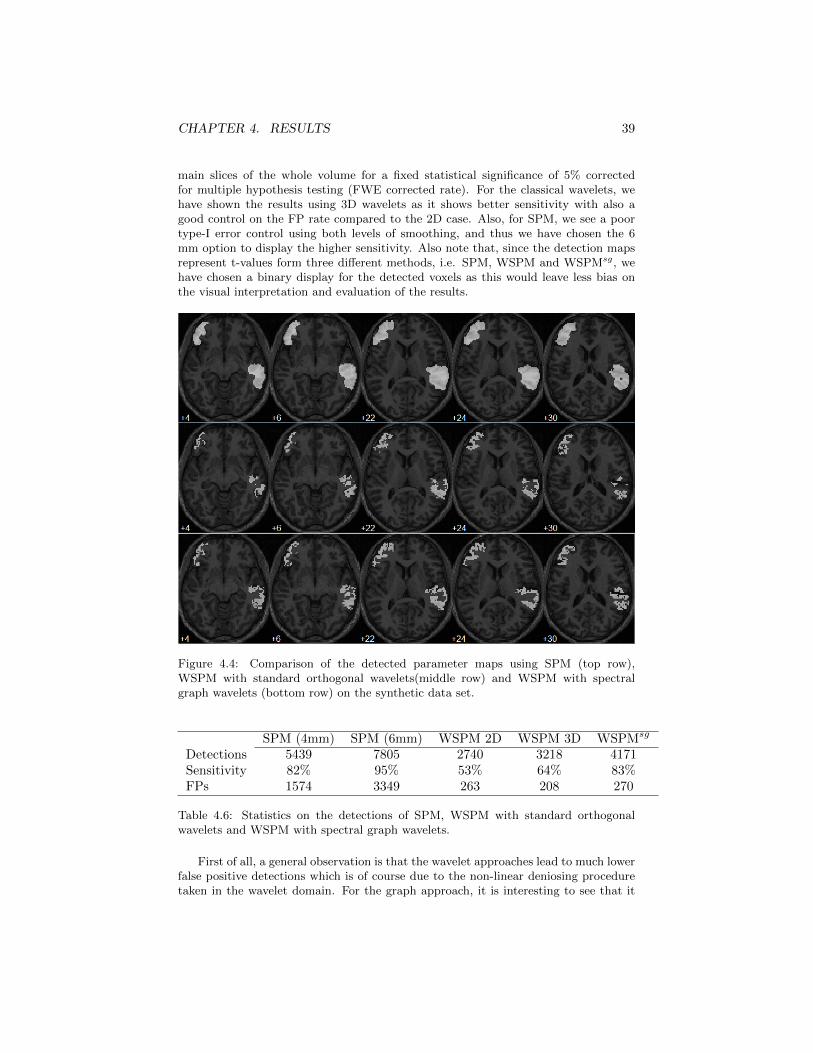
CHAPTER 4. RESULTS 39
main slices of the whole volume for a fixed statistical significance of 5% correctedfor multiple hypothesis testing (FWE corrected rate). For the classical wavelets, wehave shown the results using 3D wavelets as it shows better sensitivity with also agood control on the FP rate compared to the 2D case. Also, for SPM, we see a poortype-I error control using both levels of smoothing, and thus we have chosen the 6mm option to display the higher sensitivity. Also note that, since the detection mapsrepresent t-values form three different methods, i.e. SPM, WSPM and WSPMsg, wehave chosen a binary display for the detected voxels as this would leave less bias onthe visual interpretation and evaluation of the results.
Figure 4.4: Comparison of the detected parameter maps using SPM (top row),WSPM with standard orthogonal wavelets(middle row) and WSPM with spectralgraph wavelets (bottom row) on the synthetic data set.
SPM (4mm) SPM (6mm) WSPM 2D WSPM 3D WSPMsg
Detections 5439 7805 2740 3218 4171Sensitivity 82% 95% 53% 64% 83%FPs 1574 3349 263 208 270
Table 4.6: Statistics on the detections of SPM, WSPM with standard orthogonalwavelets and WSPM with spectral graph wavelets.
First of all, a general observation is that the wavelet approaches lead to much lowerfalse positive detections which is of course due to the non-linear deniosing proceduretaken in the wavelet domain. For the graph approach, it is interesting to see that it
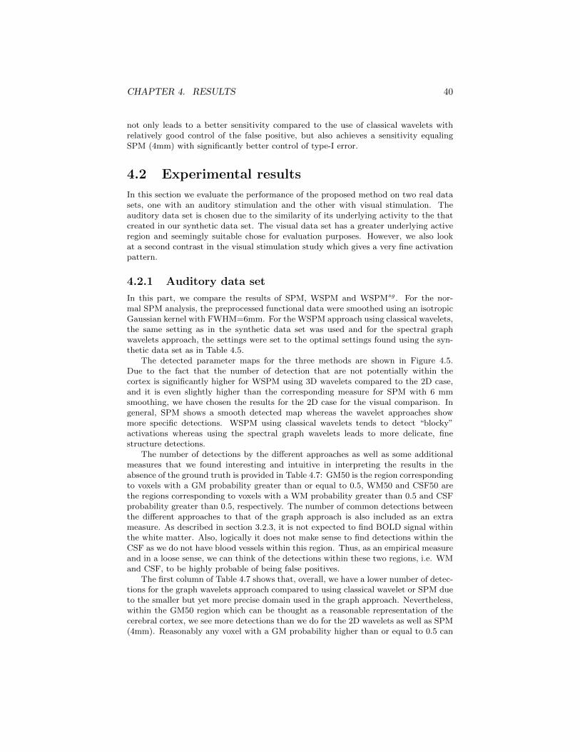
CHAPTER 4. RESULTS 40
not only leads to a better sensitivity compared to the use of classical wavelets withrelatively good control of the false positive, but also achieves a sensitivity equalingSPM (4mm) with significantly better control of type-I error.
4.2 Experimental results
In this section we evaluate the performance of the proposed method on two real datasets, one with an auditory stimulation and the other with visual stimulation. Theauditory data set is chosen due to the similarity of its underlying activity to the thatcreated in our synthetic data set. The visual data set has a greater underlying activeregion and seemingly suitable chose for evaluation purposes. However, we also lookat a second contrast in the visual stimulation study which gives a very fine activationpattern.
4.2.1 Auditory data set
In this part, we compare the results of SPM, WSPM and WSPMsg. For the nor-mal SPM analysis, the preprocessed functional data were smoothed using an isotropicGaussian kernel with FWHM=6mm. For the WSPM approach using classical wavelets,the same setting as in the synthetic data set was used and for the spectral graphwavelets approach, the settings were set to the optimal settings found using the syn-thetic data set as in Table 4.5.
The detected parameter maps for the three methods are shown in Figure 4.5.Due to the fact that the number of detection that are not potentially within thecortex is significantly higher for WSPM using 3D wavelets compared to the 2D case,and it is even slightly higher than the corresponding measure for SPM with 6 mmsmoothing, we have chosen the results for the 2D case for the visual comparison. Ingeneral, SPM shows a smooth detected map whereas the wavelet approaches showmore specific detections. WSPM using classical wavelets tends to detect “blocky”activations whereas using the spectral graph wavelets leads to more delicate, finestructure detections.
The number of detections by the different approaches as well as some additionalmeasures that we found interesting and intuitive in interpreting the results in theabsence of the ground truth is provided in Table 4.7: GM50 is the region correspondingto voxels with a GM probability greater than or equal to 0.5, WM50 and CSF50 arethe regions corresponding to voxels with a WM probability greater than 0.5 and CSFprobability greater than 0.5, respectively. The number of common detections betweenthe different approaches to that of the graph approach is also included as an extrameasure. As described in section 3.2.3, it is not expected to find BOLD signal withinthe white matter. Also, logically it does not make sense to find detections within theCSF as we do not have blood vessels within this region. Thus, as an empirical measureand in a loose sense, we can think of the detections within these two regions, i.e. WMand CSF, to be highly probable of being false positives.
The first column of Table 4.7 shows that, overall, we have a lower number of detec-tions for the graph wavelets approach compared to using classical wavelet or SPM dueto the smaller but yet more precise domain used in the graph approach. Nevertheless,within the GM50 region which can be thought as a reasonable representation of thecerebral cortex, we see more detections than we do for the 2D wavelets as well as SPM(4mm). Reasonably any voxel with a GM probability higher than or equal to 0.5 can
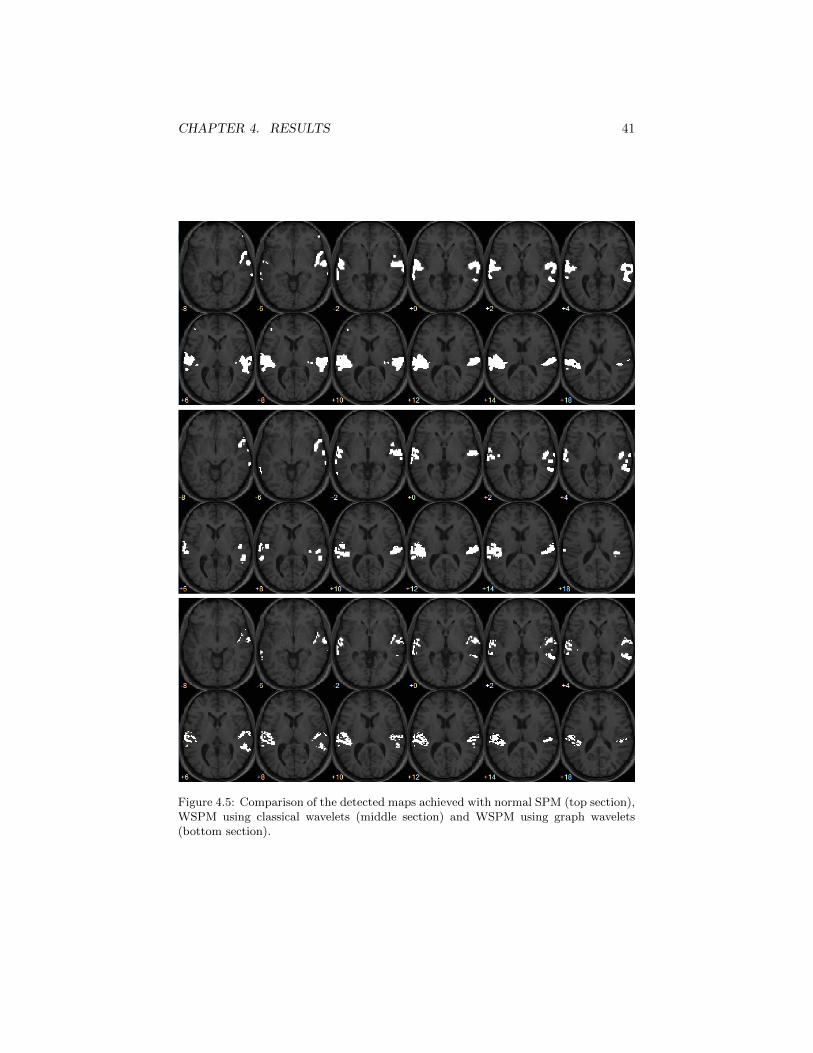
CHAPTER 4. RESULTS 41
Figure 4.5: Comparison of the detected maps achieved with normal SPM (top section),WSPM using classical wavelets (middle section) and WSPM using graph wavelets(bottom section).
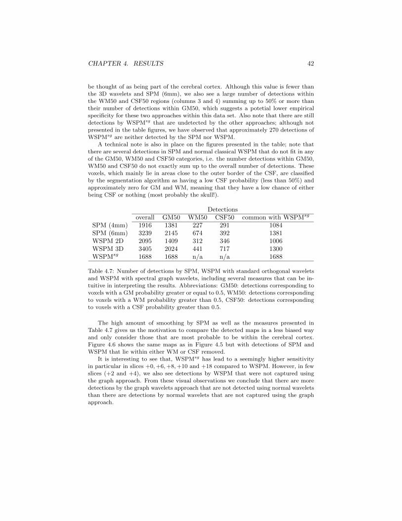
CHAPTER 4. RESULTS 42
be thought of as being part of the cerebral cortex. Although this value is fewer thanthe 3D wavelets and SPM (6mm), we also see a large number of detections withinthe WM50 and CSF50 regions (columns 3 and 4) summing up to 50% or more thantheir number of detections within GM50, which suggests a potetial lower empiricalspecificity for these two approaches within this data set. Also note that there are stilldetections by WSPMsg that are undetected by the other approaches; although notpresented in the table figures, we have observed that approximately 270 detections ofWSPMsg are neither detected by the SPM nor WSPM.
A technical note is also in place on the figures presented in the table; note thatthere are several detections in SPM and normal classical WSPM that do not fit in anyof the GM50, WM50 and CSF50 categories, i.e. the number detections within GM50,WM50 and CSF50 do not exactly sum up to the overall number of detections. Thesevoxels, which mainly lie in areas close to the outer border of the CSF, are classifiedby the segmentation algorithm as having a low CSF probability (less than 50%) andapproximately zero for GM and WM, meaning that they have a low chance of eitherbeing CSF or nothing (most probably the skull!).
Detectionsoverall GM50 WM50 CSF50 common with WSPMsg
SPM (4mm) 1916 1381 227 291 1084SPM (6mm) 3239 2145 674 392 1381WSPM 2D 2095 1409 312 346 1006WSPM 3D 3405 2024 441 717 1300WSPMsg 1688 1688 n/a n/a 1688
Table 4.7: Number of detections by SPM, WSPM with standard orthogonal waveletsand WSPM with spectral graph wavelets, including several measures that can be in-tuitive in interpreting the results. Abbreviations: GM50: detections corresponding tovoxels with a GM probability greater or equal to 0.5, WM50: detections correspondingto voxels with a WM probability greater than 0.5, CSF50: detections correspondingto voxels with a CSF probability greater than 0.5.
The high amount of smoothing by SPM as well as the measures presented inTable 4.7 gives us the motivation to compare the detected maps in a less biased wayand only consider those that are most probable to be within the cerebral cortex.Figure 4.6 shows the same maps as in Figure 4.5 but with detections of SPM andWSPM that lie within either WM or CSF removed.
It is interesting to see that, WSPMsg has lead to a seemingly higher sensitivityin particular in slices +0,+6,+8,+10 and +18 compared to WSPM. However, in fewslices (+2 and +4), we also see detections by WSPM that were not captured usingthe graph approach. From these visual observations we conclude that there are moredetections by the graph wavelets approach that are not detected using normal waveletsthan there are detections by normal wavelets that are not captured using the graphapproach.
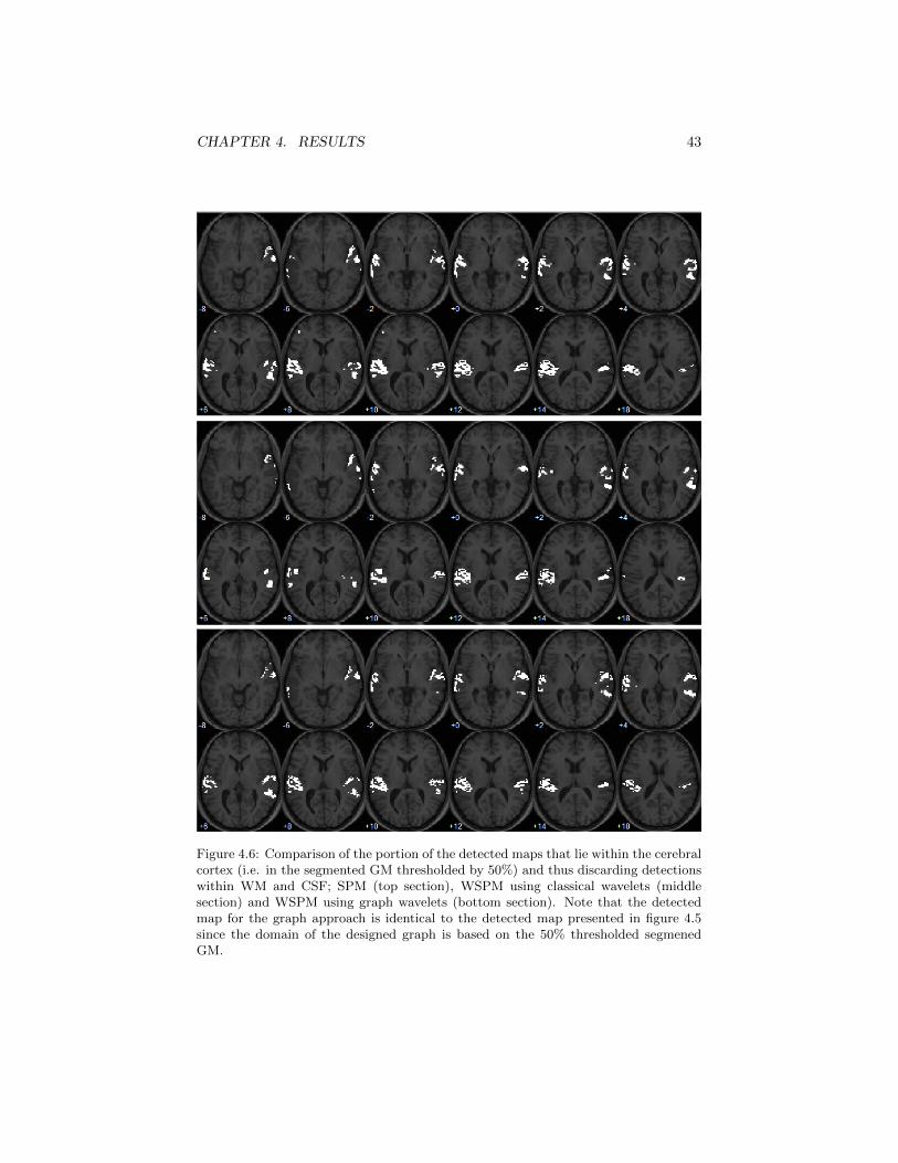
CHAPTER 4. RESULTS 43
Figure 4.6: Comparison of the portion of the detected maps that lie within the cerebralcortex (i.e. in the segmented GM thresholded by 50%) and thus discarding detectionswithin WM and CSF; SPM (top section), WSPM using classical wavelets (middlesection) and WSPM using graph wavelets (bottom section). Note that the detectedmap for the graph approach is identical to the detected map presented in figure 4.5since the domain of the designed graph is based on the 50% thresholded segmenedGM.
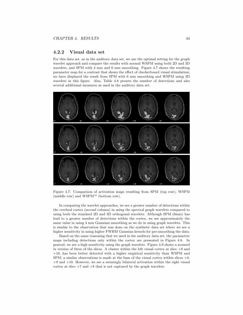
CHAPTER 4. RESULTS 44
4.2.2 Visual data set
For this data set, as in the auditory data set, we use the optimal setting for the graphwavelet approach and compare the results with normal WSPM using both 2D and 3Dwavelets, and SPM with 4 mm and 6 mm smoothing. Figure 4.7 shows the resultingparameter map for a contrast that shows the effect of checkerboard visual stimulation;we have displayed the result from SPM with 6 mm smoothing and WSPM using 3Dwavelets in this figure. Also, Table 4.8 presets the number of detections and alsoseveral additional measures as used in the auditory data set.
Figure 4.7: Comparison of activation maps resulting from SPM (top row), WSPM(middle row) and WSPMsg (bottom row).
In comparing the wavelet approaches, we see a greater number of detections withinthe cerebral cortex (second column) in using the spectral graph wavelets compared tousing both the standard 2D and 3D orthogonal wavelets. Although SPM (6mm) haslead to a greater number of detections within the cortex, we see approximately thesame value in using 4 mm Gaussian smoothing as we do in using graph wavelets. Thisis similar to the observation that was done on the synthetic data set where we see ahigher sensitivity in using higher FWHM Gaussian kernels for pre-smoothing the data.
Based on the same reasoning that we used in the auditory data set, the parametricmaps including detections only within the cortex are presented in Figure 4.8. Ingeneral, we see a high sensitivity using the graph wavelets. Figure 4.9 shows a zoomedin version of three of the slices. A cluster within the left visual cortex at slice +8 and+10, has been better detected with a higher empirical sensitivity than WSPM andSPM; a similar observations is made at the base of the visual cortex within slices +8,+9 and +10. However, we see a seemingly bilateral activation within the right visualcortex at slice +7 and +8 that is not captured by the graph wavelets.

CHAPTER 4. RESULTS 45
Detectionsoverall GM50 WM50 CSF50 common with WSPMsg
SPM 4 mm 1644 1130 227 260 776SPM 6 mm 1975 1338 321 283 843WSPM 2D 1159 763 114 256 572WSPM 3D 1438 964 146 295 722WSPMsg 1106 1106 n/a n/a 1106
Table 4.8: Several figures on the detected voxels by SPM, WSPM with standardorthogonal wavelets and WSPM with spectral graph wavelets, which can be intuitivein interpreting the results as the ground truth is not known. The abbreviations are asin Table 4.7.
Figure 4.8: Comparison of detected parameter maps using SPM (top row), WSPM(middle row) and WSPMsg (bottom row) by only considering detections within theGM thresholded by 50% to provide an equal ground for comparison.
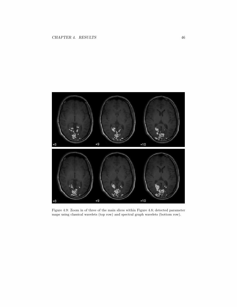
CHAPTER 4. RESULTS 46
Figure 4.9: Zoom in of three of the main slices within Figure 4.8; detected parametermaps using classical wavelets (top row) and spectral graph wavelets (bottom row).
Chapter 5
Discussion
In this chapter, we will first have a discussion on the design criteria that were intro-duced for the presented graph approach in statistical mapping of fMRI data. Next,we will have some other general comments regarding the approach, and will finallyconsider the drawback of computation cost and recapitulate the introduced approachto reduce this cost as well as other possibilities.
5.1 Optimal settings of design criteria
In this section, we will consider the design criteria that were introduced at the begin-ning of chapter 4. We will try to come up with conclusions on their optimal choicebased on the presented evaluation results.
5.1.1 Filter design in terms of spectrum coverage
As we have seen, specifying the scaling function and wavelets kernels as of whichrange of the spectrum each should cover is an essential step. For our designed braingraphs, empirical observations show that capturing approximately the upper 80% tailof the spectrum with a single scale, and partitioning the remaining lower 20% of theeigenspace with the sacling function and the remaining wavelet scales leads to optimalresults. These settings are based on empirical observations, and potentially even bettersettings may be achieved with more detailed study of the spectrum. Although the fullspectrum of small scale graphs can be well studied through diagonalization of theLaplacian, it is not so trivial for large scale graphs with current available software.
5.1.2 Number of wavelet scales
Having found a suitable range within the spectrum to introduce finer scales, the nextstep would be to decide on the number of wavelet scales. As the simulations andexperimental results suggest, using the scaling function and two to three wavelet scalesseems to be suitable choice. However, the hypothesis that even a greater number ofscales can provide better results still remains. We believe that potentially betterresults can be achieved by introducing extra finer wavelet scales provided that datawith higher spatial resolution could be acquired.
47
CHAPTER 5. DISCUSSION 48
5.1.3 Graph domain extent
We have seen that designing a cortex domain based on 50% thresholding of the seg-mented grey matter seems a good compromise betwwen accuracy in representing thecortex topolgy as well as being on the safe side not to lose potential missclassifiedvoxels by the segmentaion algorithm. Morover, the drop in sensitivity that can beseen in lowering the threshold and making larger graphs gives an intuitive insight; thisis an interesting observation as it shows that having a more accurate representaion ofthe domain leads to better detection of the activation pattern. Another note that isin place regrading the graph domain extent is that, using high GM thresholds such as70% is only applicable for moderate to high resolution GM segmentaions (in terms ofMNI space resolution) since in lower resolutions such thresholding would fail to keepthe full topolgy of the cortex.
5.1.4 Graph design approach
In general, both presented graph design approaches have lead to efficient results, butwith better performance in using the weighted graph design. However, it seems tobe sufficient to consider design approach I when constructing brain graphs based onhigh GM thresholds such as 70% as the remining voxels under such a threshold canbe all thought of as being part of the cerebral cortex. On the other hand, using graphdesign approach II can be more efficient when constructing graphs based on a lowerthreshold, such as 30% and alson 50%, to compensate for the uncertainty of the graphnodes being truely part of the cerebral cortex.
5.2 General comments
There are also several other comments and issues concerning the proposed method,which we will briefly go through in this section.
Classical wavelets work within a Euclidean space and a region of interest can beat best created within a cubic structure in 3D (or rectangular domain in 2D). Inthis writer’s view, the ability to define a desired complex, irregular domain on whichwavelets can be used for fMRI analysis is a powerful tool. Moreover, such a toolenables defining local regions of interest such as the auditory cortex and in this way,also compensating for the computational cost. As long as the defined domain is largeenough to cover the expected activation region with an extra extension as to not effectthe spatial adaptation of the wavelets within the region of interest, the approach wouldlead to efficient results based on the same reasoning that we brought in section 3.4.4in using the local graph reconstruction scheme.
The proposed approach significantly relies on the accuracy of the representationof the segmented grey matter within a suitably high resolution space; we can expect abetter spatial adaptation of the wavelets by having a more accurate representation ofthe cortex. More accurate representation of the cortex can be achieved with accuratesegmentation as well as accurate interpolation in down sampling the GM to lowerresolution. Also, such accuracy in the segmentation and normalization gives confidencein knowing to have included all the required voxels to represent the underlying BOLDsignal after certain thresholding of the GM probability map.
Without considering the computational cost imposed on calculating the spectralgraph wavelet transforms, intuitively it would seem interesting to consider designinga graph to represent the cortex at higher resolutions such as 1 mm cubic voxel size
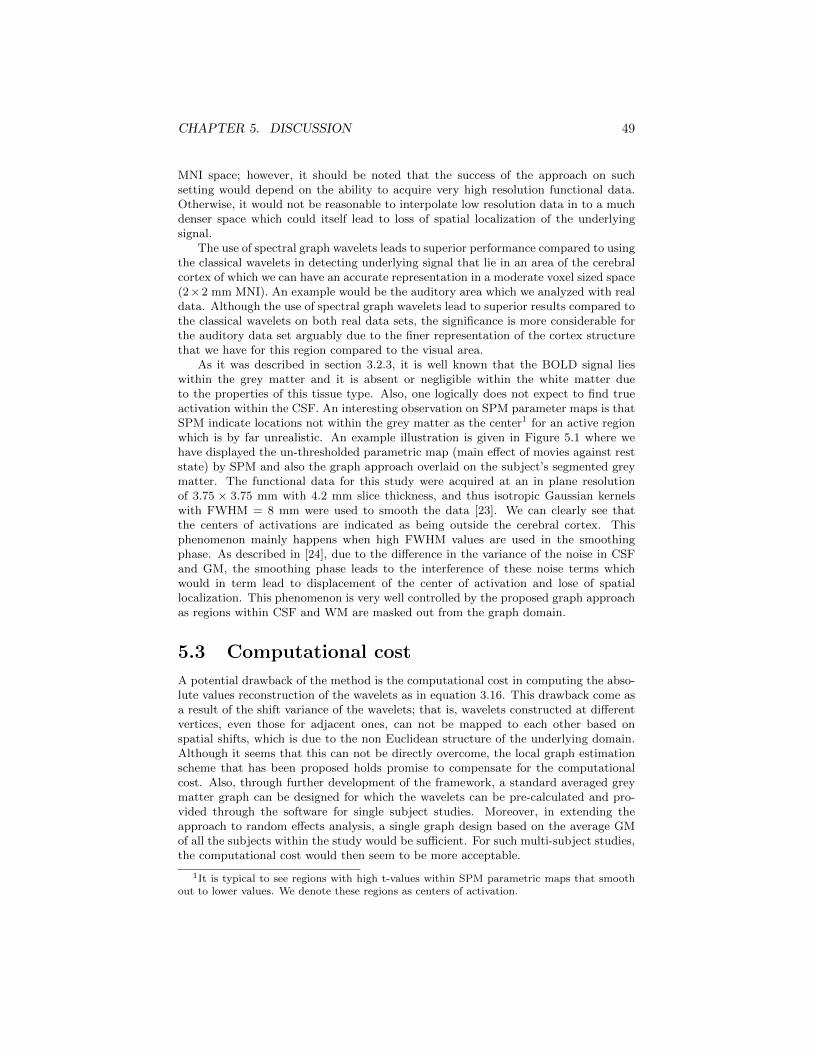
CHAPTER 5. DISCUSSION 49
MNI space; however, it should be noted that the success of the approach on suchsetting would depend on the ability to acquire very high resolution functional data.Otherwise, it would not be reasonable to interpolate low resolution data in to a muchdenser space which could itself lead to loss of spatial localization of the underlyingsignal.
The use of spectral graph wavelets leads to superior performance compared to usingthe classical wavelets in detecting underlying signal that lie in an area of the cerebralcortex of which we can have an accurate representation in a moderate voxel sized space(2×2 mm MNI). An example would be the auditory area which we analyzed with realdata. Although the use of spectral graph wavelets lead to superior results compared tothe classical wavelets on both real data sets, the significance is more considerable forthe auditory data set arguably due to the finer representation of the cortex structurethat we have for this region compared to the visual area.
As it was described in section 3.2.3, it is well known that the BOLD signal lieswithin the grey matter and it is absent or negligible within the white matter dueto the properties of this tissue type. Also, one logically does not expect to find trueactivation within the CSF. An interesting observation on SPM parameter maps is thatSPM indicate locations not within the grey matter as the center1 for an active regionwhich is by far unrealistic. An example illustration is given in Figure 5.1 where wehave displayed the un-thresholded parametric map (main effect of movies against reststate) by SPM and also the graph approach overlaid on the subject’s segmented greymatter. The functional data for this study were acquired at an in plane resolutionof 3.75 × 3.75 mm with 4.2 mm slice thickness, and thus isotropic Gaussian kernelswith FWHM = 8 mm were used to smooth the data [23]. We can clearly see thatthe centers of activations are indicated as being outside the cerebral cortex. Thisphenomenon mainly happens when high FWHM values are used in the smoothingphase. As described in [24], due to the difference in the variance of the noise in CSFand GM, the smoothing phase leads to the interference of these noise terms whichwould in term lead to displacement of the center of activation and lose of spatiallocalization. This phenomenon is very well controlled by the proposed graph approachas regions within CSF and WM are masked out from the graph domain.
5.3 Computational cost
A potential drawback of the method is the computational cost in computing the abso-lute values reconstruction of the wavelets as in equation 3.16. This drawback come asa result of the shift variance of the wavelets; that is, wavelets constructed at differentvertices, even those for adjacent ones, can not be mapped to each other based onspatial shifts, which is due to the non Euclidean structure of the underlying domain.Although it seems that this can not be directly overcome, the local graph estimationscheme that has been proposed holds promise to compensate for the computationalcost. Also, through further development of the framework, a standard averaged greymatter graph can be designed for which the wavelets can be pre-calculated and pro-vided through the software for single subject studies. Moreover, in extending theapproach to random effects analysis, a single graph design based on the average GMof all the subjects within the study would be sufficient. For such multi-subject studies,the computational cost would then seem to be more acceptable.
1It is typical to see regions with high t-values within SPM parametric maps that smoothout to lower values. We denote these regions as centers of activation.

CHAPTER 5. DISCUSSION 50
Figure 5.1: Un-thresholded parametric maps from SPM (top row) and WSPM usinggraph wavelets (bottom row) overlaid on the subjects segmented grey matter. Aninaccurate spatial representation of underlying activation can be seen by SPM dueto the smoothing of functional data, whereas the underlying theory for the proposedgraph approach enables precise spatial localization.
Chapter 6
Conclusion and Outlook
A new graph modality for wavelet-based statistical parametric mapping (WSPM) offMRI data has been proposed. Functional data are mapped on graph nodes repre-senting the convoluted structure of the cerebral cortex, and spatially localized graphwavelets that adjust to the topology of the cortex are applied to capture the underlyingBOLD signal at a coarse as well as fine spatial scales. The graph edges are defined aseither binary, or weighted based on individual voxels’ grey matter probabilities. Anoptimal setting for the Parseval wavelet frame has been introduced based on the extentof graph spectrum coverage by the scaling and wavelet kernels. An iterative schemefor wavelet reconstruction approximation based on local graphs has been introducedto compensate for the computational cost of the absolute value wavelet reconstruc-tion. Evaluations on simulated data show an improved sensitivity, better type-I errorcontrol compared to the WSPM approach using both 2D and 3D standard orthogonalwavelets. Experimental results on real data also show an improved empirical sensitiv-ity on detecting activation within the cerebral cortex. The approach is implementedin an SPM friendly version and is included as an extension to the WSPM toolbox forSPM.
6.1 Outlook
There are a lot of ideas and hypothesis in developing the current framework but there isalways the limit of time that hinders faster progress. The main outlook of the currentwork go in three directions. In what follows, a short description of the hypothesis andinsights will be presented. The three sections are ordered in terms of priority throughwhich the ideas will be considered in potential future work.
6.1.1 Extension to multi subject studies
The ultimate outlook of the current project is to extend the proposed framework tomulti-subject studies. In multi subject studies, also known as random-effects analysis,the aim is to run statistical test that look at the variance between subjects as opposedto a single subject analysis, also known as fixed-effects analysis, in which we areinterested in the variance within each subject and the variance between subjects isassumed to be fixed and of no interest. Thus, random-effects analysis enables us to
51

CHAPTER 6. CONCLUSION AND OUTLOOK 52
make inference about the population from which sample subjects have been chosenfrom and not only the subjects at hand.
We believe that the presented graph approach hold great promise for its extensionto random-effects analysis. Within a multi subject study, the average GM of thesubjects, can be the best guideline to design spatially adaptive wavelets to encode theunderlying effect sizes of each subject in a way to capture common activations withinthe average GM which is of interest.
The extension of the framework to multi subject studies (random-effects analysis) isbeing explored. Initial results on multi-subject study simulations (results not presentedin the current report) have shown promising results. After evaluations on a suitablereal data set as well as further simulations, the results will be presented in future work.In this way, we would hopefully have a unified framework that covers a wider range offMRI studies.
6.1.2 Enhancement of graph design
Different possibilities can be thought of as to how to enhance the structure of thedefined brain graph and particularly the edge weights, but one main consideration isto incorporate diffusion tensor imaging (DTI) data in the design. DTI enables fibertracking within brain’s white matter tissue leading to accurate encoding of structuralconnections between cortical regions [25]. The hypothesis that we have is that co-activation of brain regions can be very well encoded be designing weighted graphsbased on DTI information. As an example, the potential bilateral activation withinthe visual cortex that was not detected by the graph approach (see Figure 4.8) canpossibly be detected by incorporating tractography information on the connectionsbetween Brodmann areas within the occipital lobe.
6.1.3 Adaptation to new graph wavelets transforms
Aside from the computational cost that is imposed due to the nature of the statis-tical analysis taken within WSPM, the spectral graph wavelet transform also has aninherent drawback in that the filter bank designs is not critically sampled; that is, wehave a redundant transformation with a redundancy equal to the number of waveletscales plus one. The downsampling/upsampling operations as in the classical wavelettransforms are not so straight forward to be implemented on graph nodes, but a recentstudy has suggested a new graph wavelet transform to overcome this drawback [26];a scheme for downsampling/upsampling operations on graphs which enabling criticalsampling has been introduced, and the problem of spectrum folding has been tackled.Incorporating such graph wavelet transforms to the fMRI analysis scheme presented inthis paper would seem to make the approach more efficient in terms of computationalcost.
Bibliography
[1] K.J. Friston, A.P. Holmes, K.J. Worsley, J.P. Poline, C.D. Frith, R.S.J. Frack-owiak, “Statistical parametric maps in functional imaging: a general linear ap-proach,” Human Brain Mapping 2, pp. 189-210, 1995.
[2] D. Van De Ville, T. Blu, and M. Unser, “Integrated Wavelet Processing and Spa-tial Statistical Testing of fMRI Data,” NeuroImage, vol. 23, no. 4, pp. 14721485,2004.
[3] D. Van De Ville, M.L. Seghier, F. Lazeyras, T. Blu, and M. Unser, “WSPM:Wavelet-based statistical parametric mapping,” NeuroImage, vol. 37, no. 4, pp.12051217, 2007.
[4] D.K. Hammond, P. Vandergheynst, and R. Gribonval, “Wavelets on graphs viaspectral graph theory,” Appl Comp Harm Anal, vol. 30, pp. 129-150, 2011.
[5] S.G. Ozkaya, D. Van De Ville, “Anatomically adapted wavelets for integratedstatistical analysis of fMRI data,” Proceedings of the Eighth IEEE InternationalSymposium on Biomedical Imaging: From Nano to Macro, pp. 469-472, 2011.
[6] S. Ogawa, T. Lee, A. Nayak, and P. Glynn, “Oxygenation-sensitive contrast inmagnetic resonance image of rodent brain at high magnetic fields,” MagneticResonance in Medicine, vol.14, pp. 6878, 1990.
[7] F.R.K. Chung, “Spectral graph theory” AMS Publications, 1997.
[8] K. Friston, S. Howard, R. Frackowiak, and R. Turner, “Movement related effectsin fMRI time series,” Magnetic Resonance in Medicine, vol. 35, pp. 346355, 1996.
[9] S. Mallat, “A theory for multiresolution signal decomposition: the wavelet de-composition,” IEEE Transactions on Pattern Analysis and Machine Intelligence11, pp. 674693, 1989.
[10] S. Mallat, “A Wavelet Tour of Signal Processing,” Academic Press, San Diego(CA), 1998.
[11] M. Jansen, G.P. Nason, B.W. Silverman, “Multiscale methods for data on graphsand irregular multidimensional situations,” J. R. Stat. Soc. Ser. B Stat. Methodol.vol. 71, no. 1, pp. 97125, 2009.
[12] R.R. Coifman, M. Maggioni, “Diffusion wavelets,” Appl. Comput. Harmon. Anal.vol. 21, pp. 5394, 2006.
[13] M. Maggioni, H. Mhaskar, “Diffusion polynomial frames on metric measurespaces,” Appl. Comput. Harmon. Anal. vol. 24, no. 3, pp. 329353, 2008.
53

BIBLIOGRAPHY 54
[14] J. B. Weaver, Y. Xu, D. M. Healy, and L. D. Cromwell, “Filtering noise fromimages with wavelet transforms,” Magn. Reson. Med., vol. 21, no. 2, pp. 288295,1991.
[15] S. Mahadevan, “Representation Discovery using Harmonic Analysis,” Morganand Claypool Publishers, 2008.
[16] D. Van De Ville, T. Blu, and M. Unser,“Surfing the brain An overview of wavelet-based techniques for fMRI data analysis,” IEEE Engineering in Medicine andBiology Magazine, vol. 25, no. 2, pp. 6578, March-April 2006.
[17] NA. Leonardi, D. Van De Ville, “Wavelet Frames on Graphs Defined by fMRIFunctional Connectivity,” Proceedings of the Eighth IEEE International Sympo-sium on Biomedical Imaging: From Nano to Macro. pp. 2136-2139, 2011.
[18] GE Sarty, “Computing Brain Activity Maps from fMRI Time-Series Images,”Cambridge, 2007.
[19] N.K. Logothetis, B.A. Wandell, “Interpreting the BOLD signal,” Annu Rev Phys-iol, vol. 66, pp. 735-69, 2004.
[20] D. Van De Ville, M. Unser, “False discovery rate for wavelet-based statisticalparametric mapping,” IEEE Journal of Selected Topics in Signal Processing, vol.2, no. 6, pp. 897-906, 2008
[21] Rees, G., Friston, K., 1997. Single subject epoch (block) auditory fMRI activationdata. http://www.fil.ion.ucl.ac.uk/spm/data/.
[22] http://miplab.epfl.ch/
[23] H. Eryilmaz, D. Van De Ville, S. Schwartz, P. Vuilleumier, “Impact of Tran-sient Emotions on Functional Connectivity During Subsequent Resting State: AWavelet Correlation Approach,” NeuroImage, vol. 54, no. 3, pp. 24812491, 2011.
[24] M. Reimold, M. Slifstein, A. Heinz, W. Mueller-Schauenburg, R. Bares, “Effectof spatial smoothing on t-maps: arguments for going back from t-maps to maskedcontrast images,” J. Cereb. Blood Flow Metab. vol. 26, pp. 751759, 2006.
[25] D. Le Bihan, J.-F. Mangin, C. Poupon, C.A. Clark, S. Pappata, N. Molko, H.Chabriat, “Diffusion tensor imaging: Concepts and applications,” Journal of Mag-netic Resonance Imaging, vol. 13, no. 4, pp. 534-546, 2001.
[26] S.K. Narang, A. Ortega, “Perfect reconstruction two-channel wavelet filter banksfor graph structured data,” IEEE Transactions on Signal Processing, vol. 60, no.6, pp. 27862799, 2012.
[27] http://greedy.epfl.ch/