1

Statistical Quality Control

2

Learning Objectives Describe categories of SQC Explain the use of descriptive statistics

in measuring quality characteristics Identify and describe causes of

variation Describe the use of control charts Identify the differences between x-bar,

R-, p-, and c-charts

3

Learning Objectives –con’t Explain process capability and process

capability index Explain the concept six-sigma Explain the process of acceptance sampling

and describe the use of OC curves Describe the challenges inherent in

measuring quality in service organizations

4

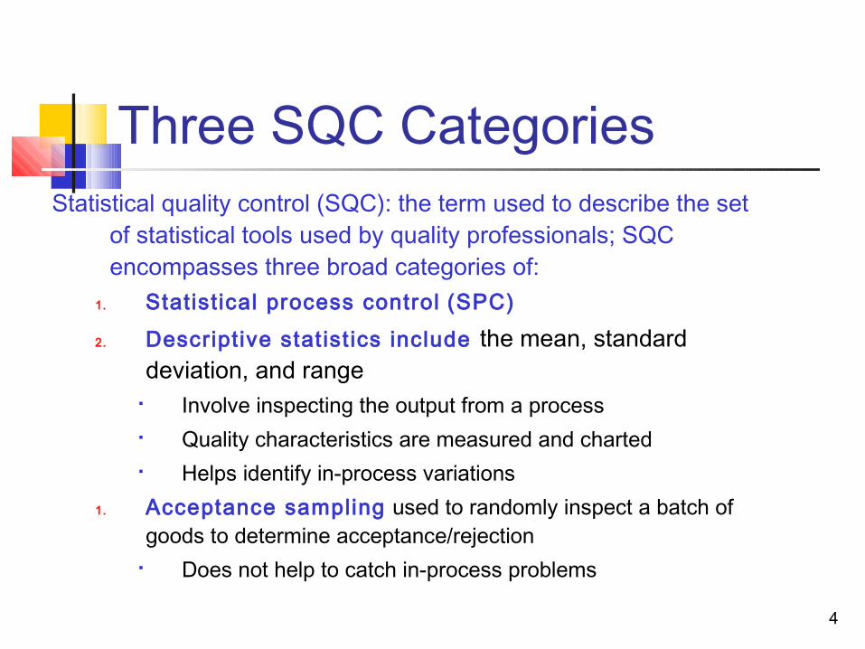
Three SQC CategoriesStatistical quality control (SQC): the term used to describe the set

of statistical tools used by quality professionals; SQC encompasses three broad categories of:

1. Statist ical process control (SPC)

2. Descript ive stat ist ics include the mean, standard deviation, and range

Involve inspecting the output from a process Quality characteristics are measured and charted Helps identify in-process variations

1. Acceptance sampling used to randomly inspect a batch of goods to determine acceptance/rejection

Does not help to catch in-process problems

5

Sources of Variation Variation exists in al l processes. Variation can be categorized as either:

Common or Random causes of variat ion, or

Random causes that we cannot identify Unavoidable, e.g. slight differences in process variables

like diameter, weight, service time, temperature Assignable causes of variation

Causes can be identified and eliminated: poor employee training, worn tool, machine needing repair

6

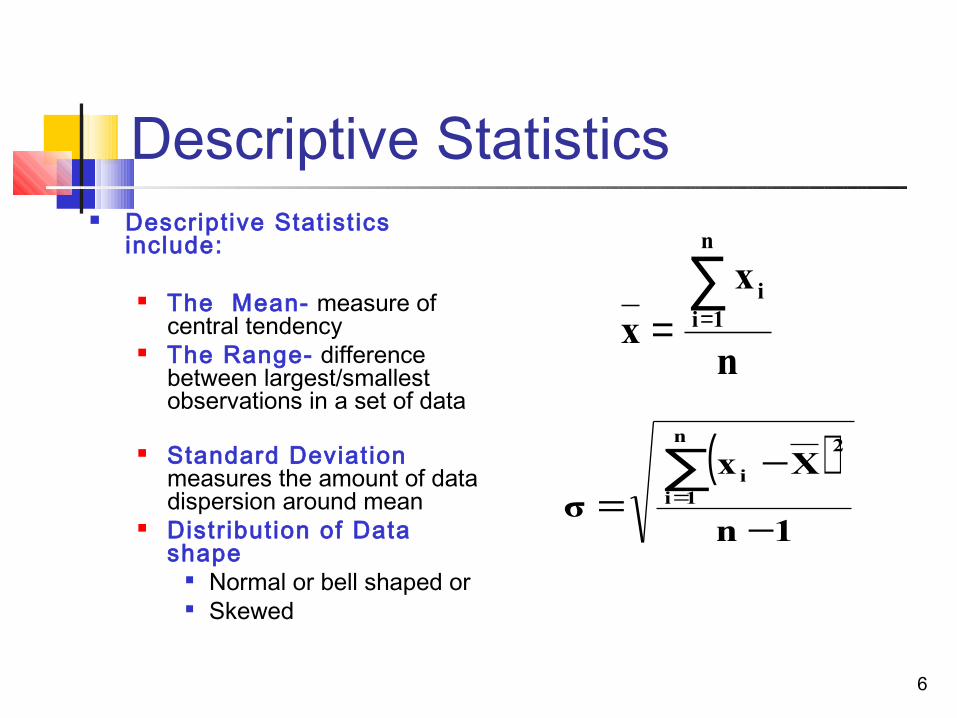
Descriptive Statistics Descriptive Statist ics

include:

The Mean- measure of central tendency

The Range- difference between largest/smallest observations in a set of data

Standard Deviat ion measures the amount of data dispersion around mean

Distribution of Data shape

Normal or bell shaped or Skewed

n

xx

n

1ii∑

==

( )1n

Xxσ

n

1i

2

i

−

−=

∑=

7

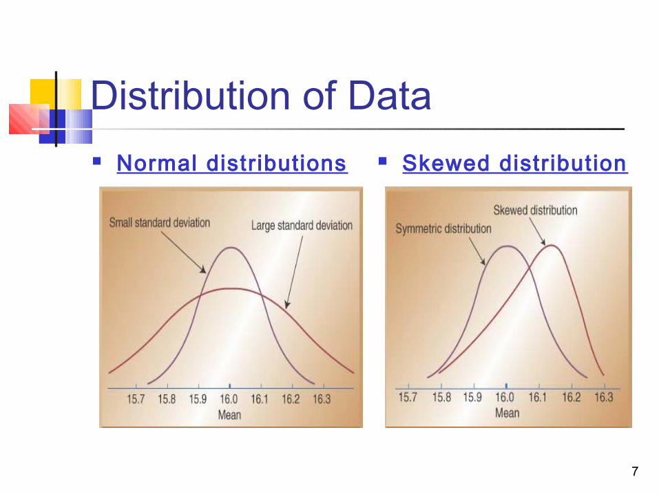
Distribution of Data Normal distributions Skewed distr ibution

© Wiley 2010 8

SPC Methods-Developing Control Charts

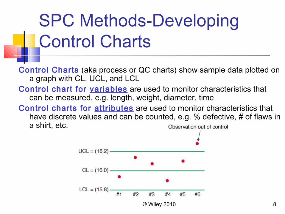
Control Charts (aka process or QC charts) show sample data plotted on a graph with CL, UCL, and LCL

Control chart for variables are used to monitor characteristics that can be measured, e.g. length, weight, diameter, time

Control charts for attr ibutes are used to monitor characteristics that have discrete values and can be counted, e.g. % defective, # of flaws in a shirt, etc.

9

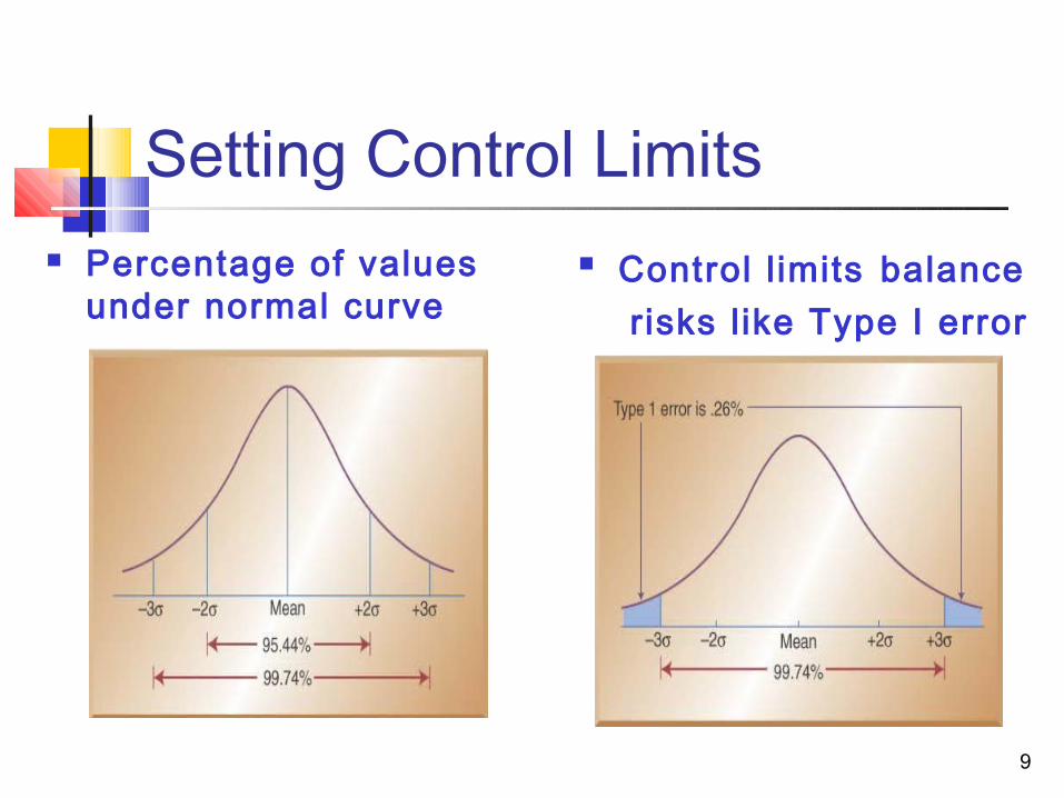
Setting Control Limits Percentage of values

under normal curve

Control l imits balance r isks l ike Type I error

10

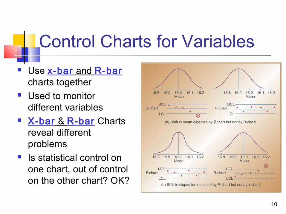
Control Charts for Variables Use x-bar and R-bar

charts together Used to monitor

different variables X-bar & R-bar Charts

reveal different problems

Is statistical control on one chart, out of control on the other chart? OK?

11

Control Charts for Variables Use x-bar charts to monitor the

changes in the mean of a process (central tendencies)

Use R-bar charts to monitor the dispersion or variability of the process

System can show acceptable central tendencies but unacceptable variability or

System can show acceptable variability but unacceptable central tendencies

12

xx

xx

n21

zσxLCL

zσxUCL

sample each w/in nsobservatio of# the is

(n) and means sample of # the is )( wheren

σσ ,

...xxxx x

−=

+=

=++

=

kk

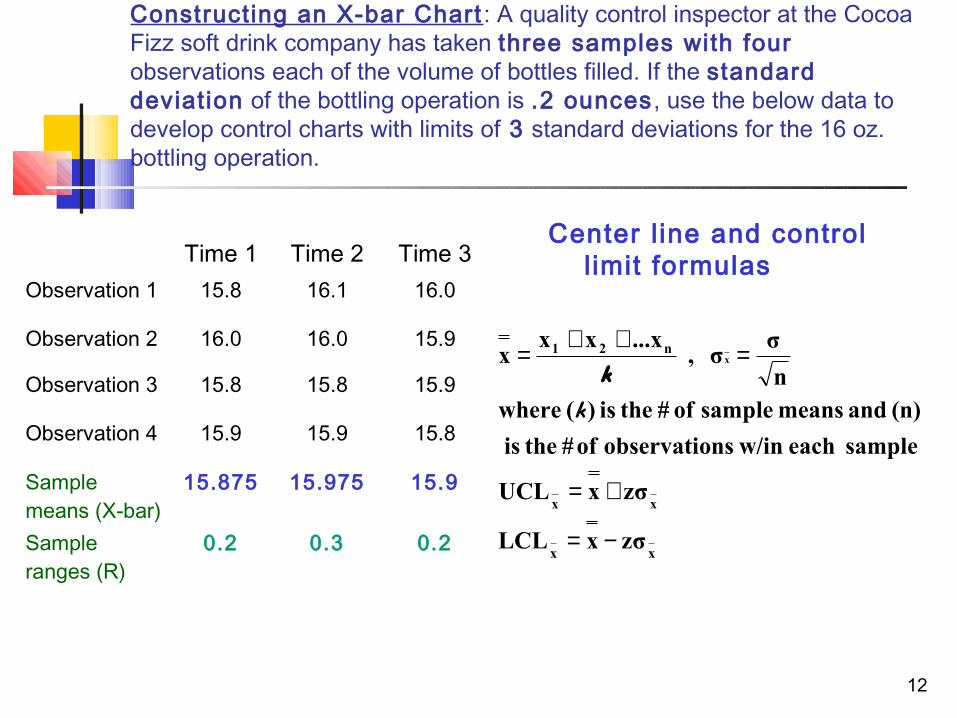
Constructing an X-bar Chart : A quality control inspector at the Cocoa Fizz soft drink company has taken three samples with four observations each of the volume of bottles filled. If the standard deviat ion of the bottling operation is .2 ounces, use the below data to develop control charts with limits of 3 standard deviations for the 16 oz. bottling operation.

Center l ine and control l imit formulasTime 1 Time 2 Time 3

Observation 1 15.8 16.1 16.0

Observation 2 16.0 16.0 15.9

Observation 3 15.8 15.8 15.9

Observation 4 15.9 15.9 15.8

Sample means (X-bar)

15.875 15.975 15.9

Sample ranges (R)

0.2 0.3 0.2

13

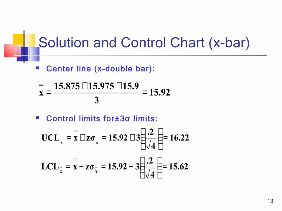
Solution and Control Chart (x-bar) Center l ine (x-double bar):

Control l imits for±3σ l imits:

15.923

15.915.97515.875x =++=

15.624

.2315.92zσxLCL

16.224

.2315.92zσxUCL

xx

xx

=

−=−=

=

+=+=

14

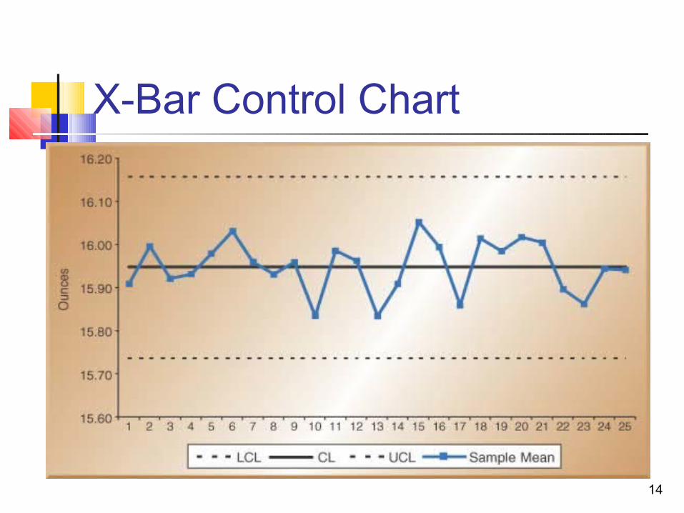
X-Bar Control Chart

15

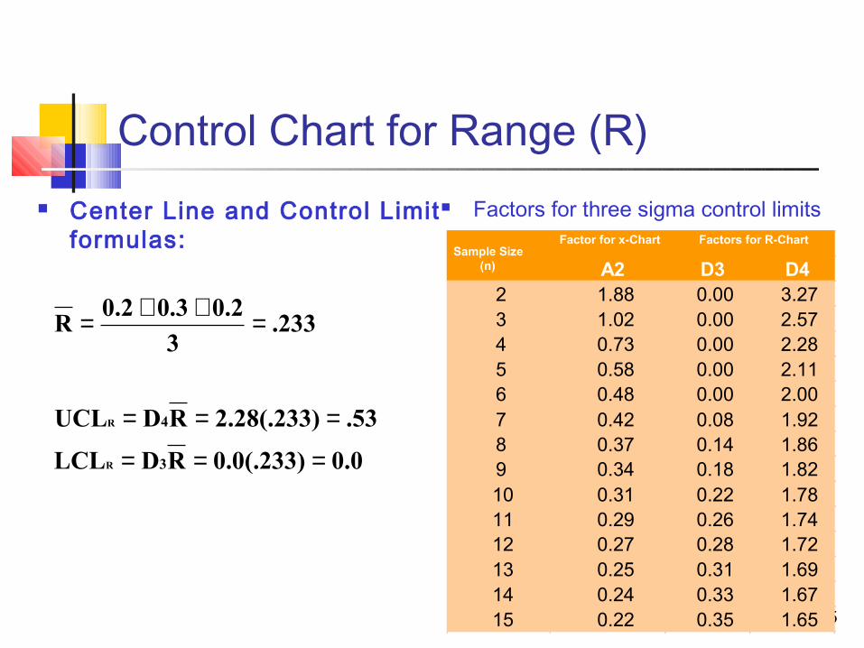
Control Chart for Range (R) Center Line and Control Limit

formulas: Factors for three sigma control limits

0.00.0(.233)RDLCL

.532.28(.233)RDUCL

.2333

0.20.30.2R

3

4

R

R

===

===

=++=

Factor for x-Chart

A2 D3 D42 1.88 0.00 3.273 1.02 0.00 2.574 0.73 0.00 2.285 0.58 0.00 2.116 0.48 0.00 2.007 0.42 0.08 1.928 0.37 0.14 1.869 0.34 0.18 1.8210 0.31 0.22 1.7811 0.29 0.26 1.7412 0.27 0.28 1.7213 0.25 0.31 1.6914 0.24 0.33 1.6715 0.22 0.35 1.65

Factors for R-ChartSample Size (n)

16

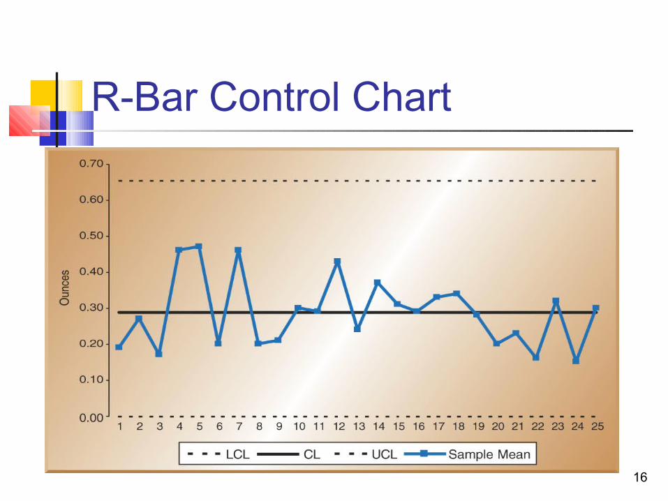
R-Bar Control Chart

17

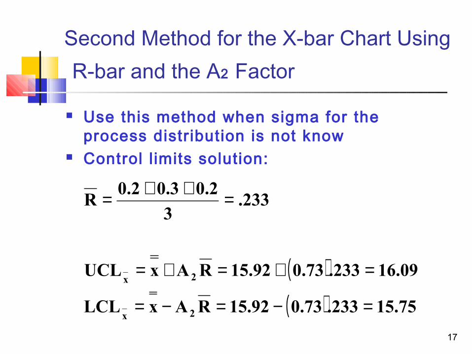
Second Method for the X-bar Chart Using R-bar and the A2 Factor

Use this method when sigma for the process distr ibution is not know

Control l imits solution:

( )( ) 15.75.2330.7315.92RAxLCL

16.09.2330.7315.92RAxUCL

.2333

0.20.30.2R

2x

2x

=−=−=

=+=+=

=++=

18

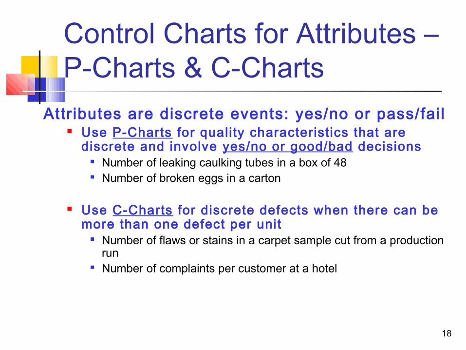
Control Charts for Attributes –P-Charts & C-Charts

Attr ibutes are discrete events: yes/no or pass/fail Use P-Charts for quality characteristics that are

discrete and involve yes/no or good/bad decisions Number of leaking caulking tubes in a box of 48 Number of broken eggs in a carton

Use C-Charts for discrete defects when there can be more than one defect per unit

Number of flaws or stains in a carpet sample cut from a production run

Number of complaints per customer at a hotel

19

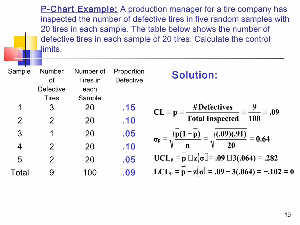
P-Chart Example: A production manager for a tire company has inspected the number of defective tires in five random samples with 20 tires in each sample. The table below shows the number of defective tires in each sample of 20 tires. Calculate the control limits.

Sample Number of

Defective Tires

Number of Tires in

each Sample

Proportion Defective

1 3 20 .152 2 20 .103 1 20 .054 2 20 .105 2 20 .05

Total 9 100 .09

Solution:

( )( ) 0.1023(.064).09σzpLCL

.2823(.064).09σzpUCL

0.6420

(.09)(.91)

n

)p(1pσ

.09100

9

Inspected Total

Defectives#pCL

p

p

p

=−=−=−=

=+=+=

==−=

====

20

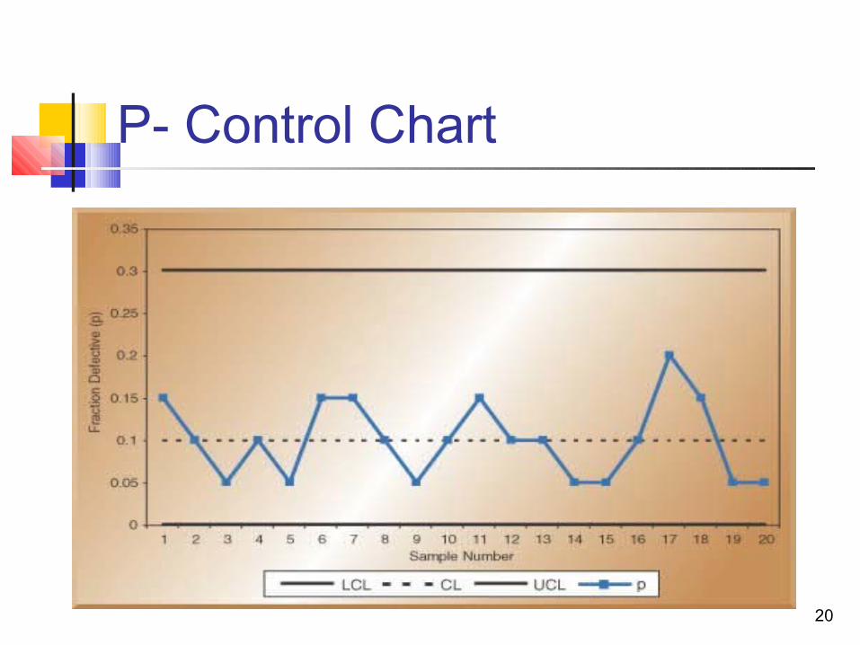
P- Control Chart

21

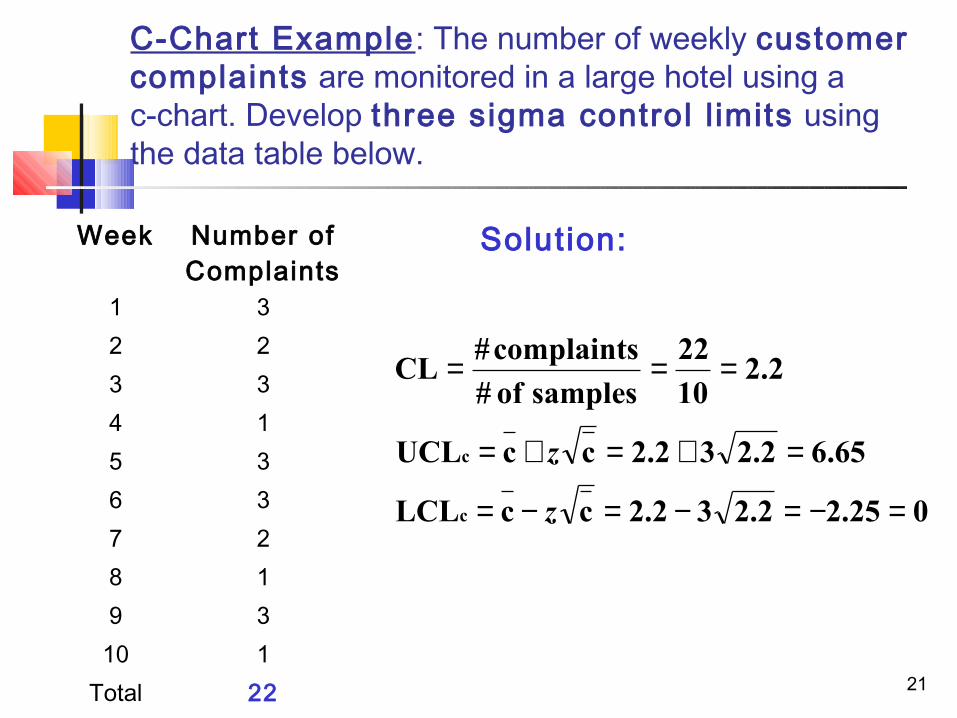
C-Chart Example: The number of weekly customer complaints are monitored in a large hotel using a c-chart. Develop three sigma control l imits using the data table below.

Week Number of Complaints

1 32 23 34 15 36 37 28 19 3

10 1Total 22

Solution:

02.252.232.2ccLCL

6.652.232.2ccUCL

2.210

22

samples of #

complaints#CL

c

c

=−=−=−=

=+=+=

===

z

z

22

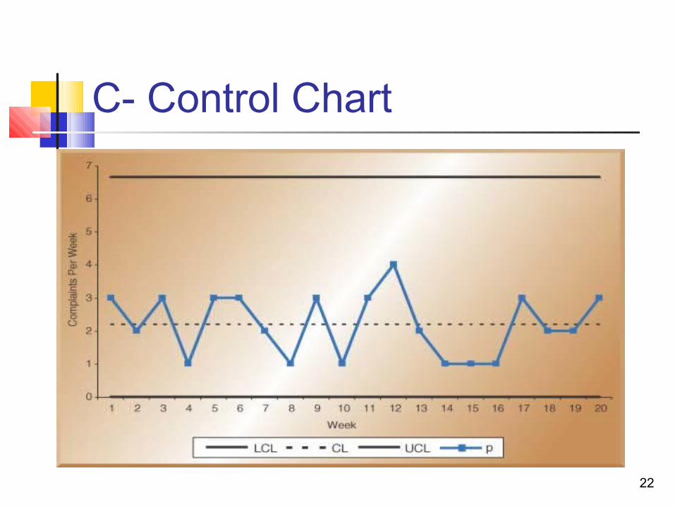
C- Control Chart

© Wiley 2010 23

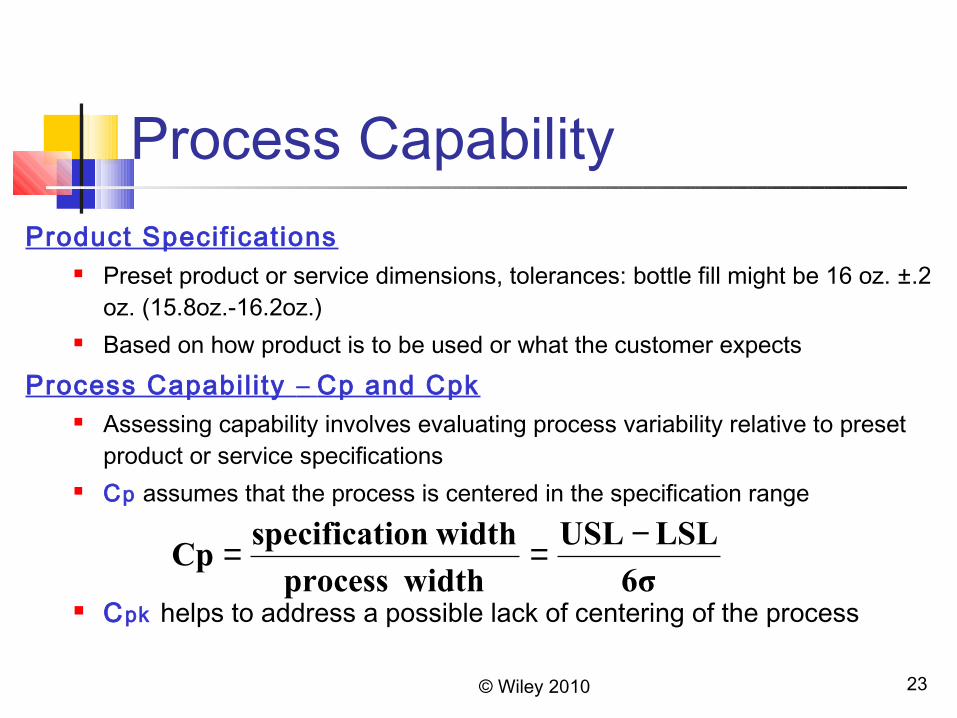
Process CapabilityProduct Specif ications

Preset product or service dimensions, tolerances: bottle fill might be 16 oz. ±.2 oz. (15.8oz.-16.2oz.)

Based on how product is to be used or what the customer expects

Process Capabil i ty – Cp and Cpk Assessing capability involves evaluating process variability relative to preset

product or service specifications Cp assumes that the process is centered in the specification range

Cpk helps to address a possible lack of centering of the process6σ

LSLUSL

width process

width ionspecificatCp

−==

24

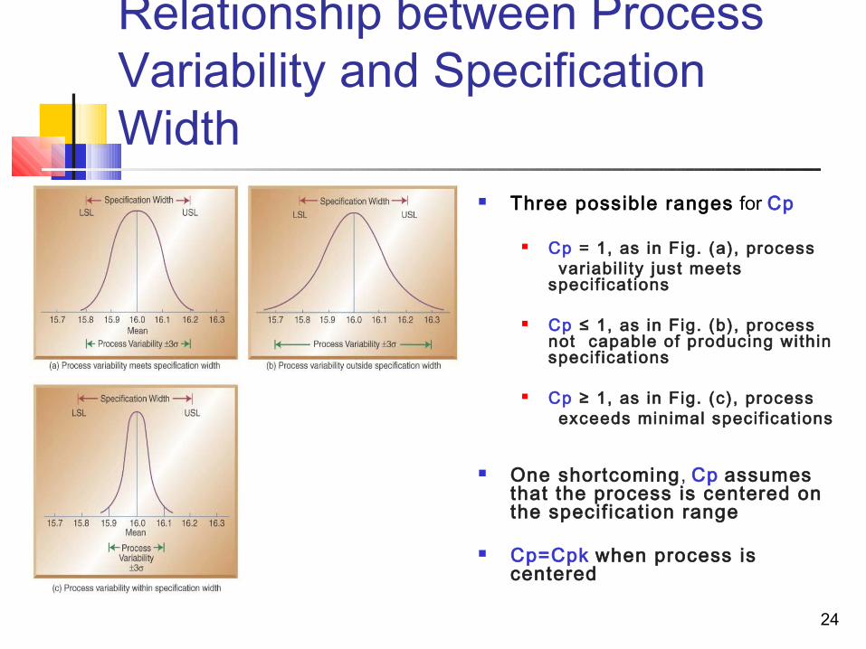
Relationship between Process Variability and Specification Width

Three possible ranges for Cp

Cp = 1, as in Fig. (a), process variabil i ty just meets

specif icat ions

Cp ≤ 1, as in Fig. (b), process not capable of producing within specif icat ions

Cp ≥ 1, as in Fig. (c), process exceeds minimal specif ications

One shortcoming, Cp assumes that the process is centered on the specif ication range

Cp=Cpk when process is centered

25

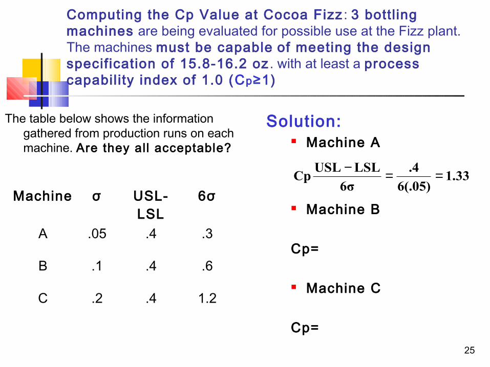
Computing the Cp Value at Cocoa Fizz : 3 bottl ing machines are being evaluated for possible use at the Fizz plant. The machines must be capable of meeting the design specif ication of 15.8-16.2 oz . with at least a process capabil i ty index of 1.0 (Cp≥1)

The table below shows the information gathered from production runs on each machine. Are they all acceptable?

Solution: Machine A

Machine B

Cp=

Machine C

Cp=

Machine σ USL-LSL

6σ

A .05 .4 .3

B .1 .4 .6

C .2 .4 1.2

1.336(.05)

.4

6σ

LSLUSLCp ==−

© Wiley 2010 26

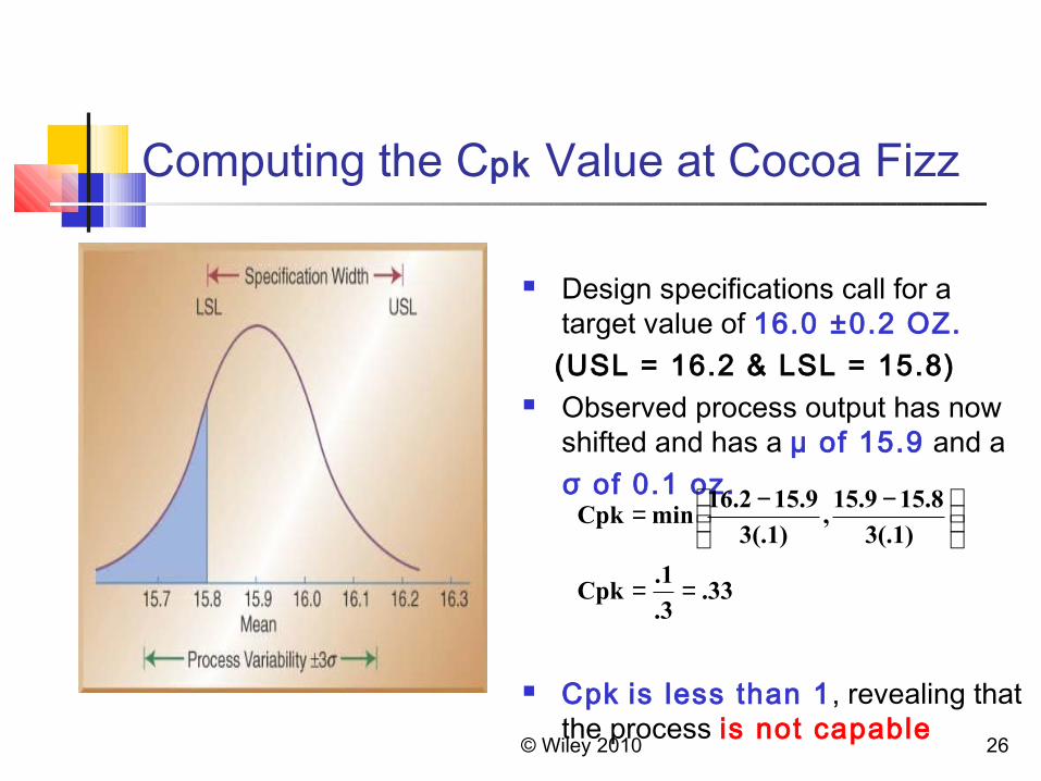
Computing the Cpk Value at Cocoa Fizz

Design specifications call for a target value of 16.0 ±0.2 OZ.

(USL = 16.2 & LSL = 15.8) Observed process output has now

shifted and has a µ of 15.9 and a σ of 0.1 oz.

Cpk is less than 1, revealing that the process is not capable

.33.3

.1Cpk

3(.1)

15.815.9,

3(.1)

15.916.2minCpk

==

−−=

27

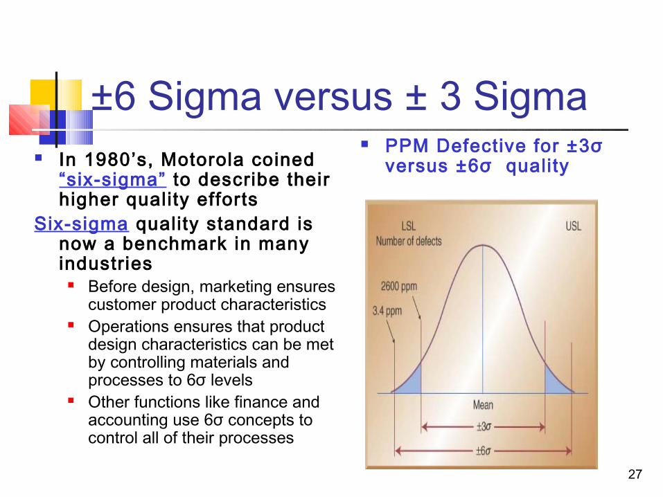
±6 Sigma versus ± 3 Sigma In 1980’s, Motorola coined

“six-sigma” to describe their higher quality efforts

Six-sigma quality standard is now a benchmark in many industries

Before design, marketing ensures customer product characteristics

Operations ensures that product design characteristics can be met by controlling materials and processes to 6σ levels

Other functions like finance and accounting use 6σ concepts to control all of their processes

PPM Defective for ±3σ versus ±6σ quality

28

Acceptance SamplingDefined: the third branch of SQC refers to the process

of randomly inspecting a certain number of items from a lot or batch in order to decide whether to accept or reject the entire batch

Different from SPC because acceptance sampling is performed either before or after the process rather than during

Sampling before typically is done to supplier material Sampling after involves sampling finished items before shipment

or finished components prior to assembly Used where inspection is expensive, volume is high,

or inspection is destructive

29

Acceptance Sampling PlansGoal of Acceptance Sampling plans is to determine the criteria for

acceptance or rejection based on: Size of the lot (N) Size of the sample (n) Number of defects above which a lot wil l be rejected (c) Level of confidence we wish to attain

There are single, double, and mult iple sampling plans Which one to use is based on cost involved, time consumed, and cost

of passing on a defective item

Can be used on either variable or attr ibute measures, but more commonly used for attr ibutes

30

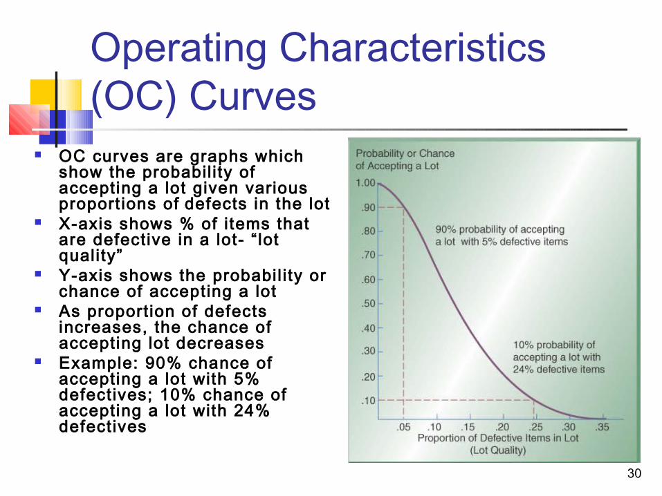
Operating Characteristics (OC) Curves

OC curves are graphs which show the probabil i ty of accepting a lot given various proport ions of defects in the lot

X-axis shows % of i tems that are defective in a lot- “ lot quali ty”

Y-axis shows the probabil i ty or chance of accepting a lot

As proport ion of defects increases, the chance of accepting lot decreases

Example: 90% chance of accepting a lot with 5% defectives; 10% chance of accepting a lot with 24% defectives

31

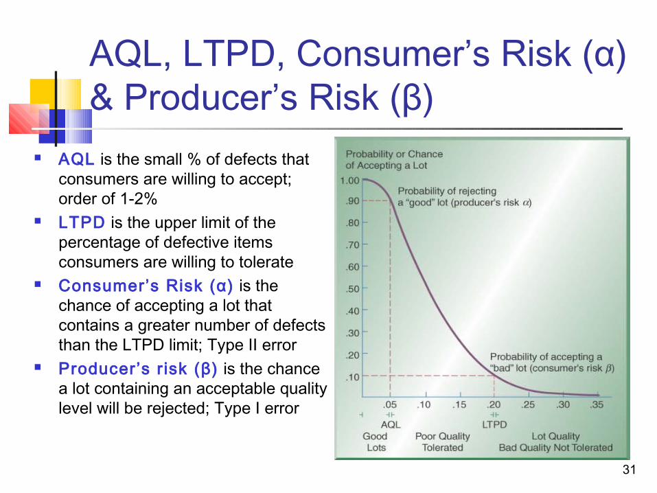
AQL, LTPD, Consumer’s Risk (α) & Producer’s Risk (β)

AQL is the small % of defects that consumers are willing to accept; order of 1-2%

LTPD is the upper limit of the percentage of defective items consumers are willing to tolerate

Consumer’s Risk (α) is the chance of accepting a lot that contains a greater number of defects than the LTPD limit; Type II error

Producer’s r isk (β) is the chance a lot containing an acceptable quality level will be rejected; Type I error

32

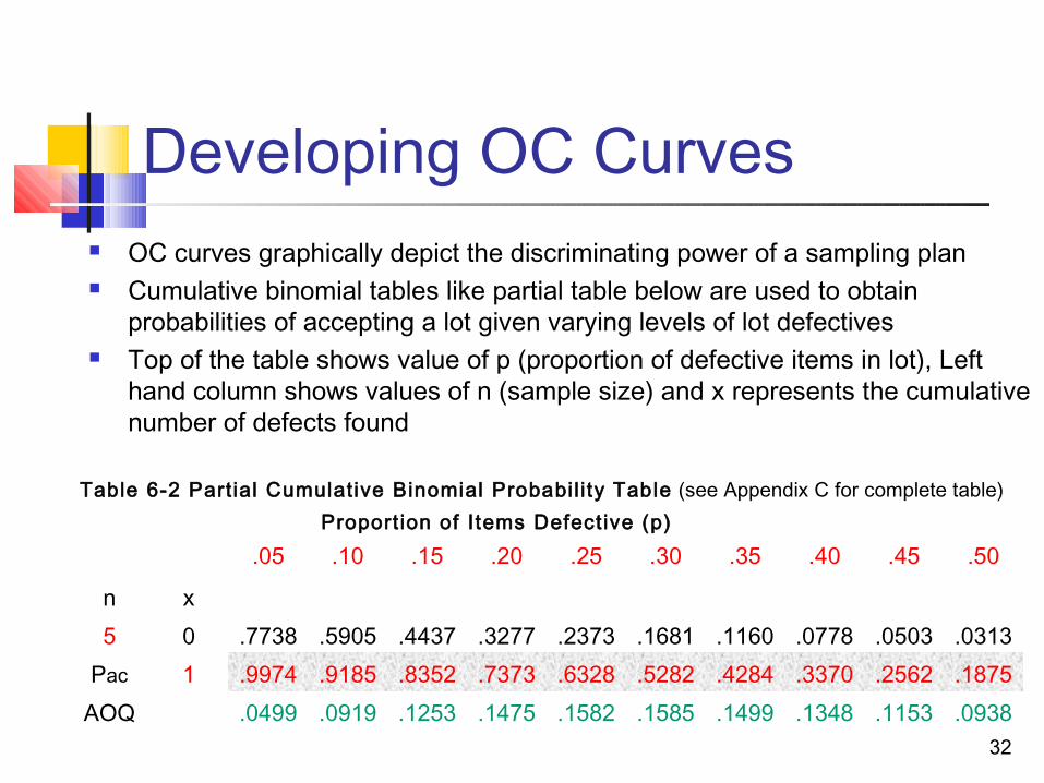
Developing OC Curves OC curves graphically depict the discriminating power of a sampling plan Cumulative binomial tables like partial table below are used to obtain

probabilities of accepting a lot given varying levels of lot defectives Top of the table shows value of p (proportion of defective items in lot), Left

hand column shows values of n (sample size) and x represents the cumulative number of defects found

Table 6-2 Partial Cumulative Binomial Probabi l i ty Table (see Appendix C for complete table) Proport ion of Items Defect ive (p)

.05 .10 .15 .20 .25 .30 .35 .40 .45 .50

n x5 0 .7738 .5905 .4437 .3277 .2373 .1681 .1160 .0778 .0503 .0313

Pac 1 .9974 .9185 .8352 .7373 .6328 .5282 .4284 .3370 .2562 .1875AOQ .0499 .0919 .1253 .1475 .1582 .1585 .1499 .1348 .1153 .0938

33

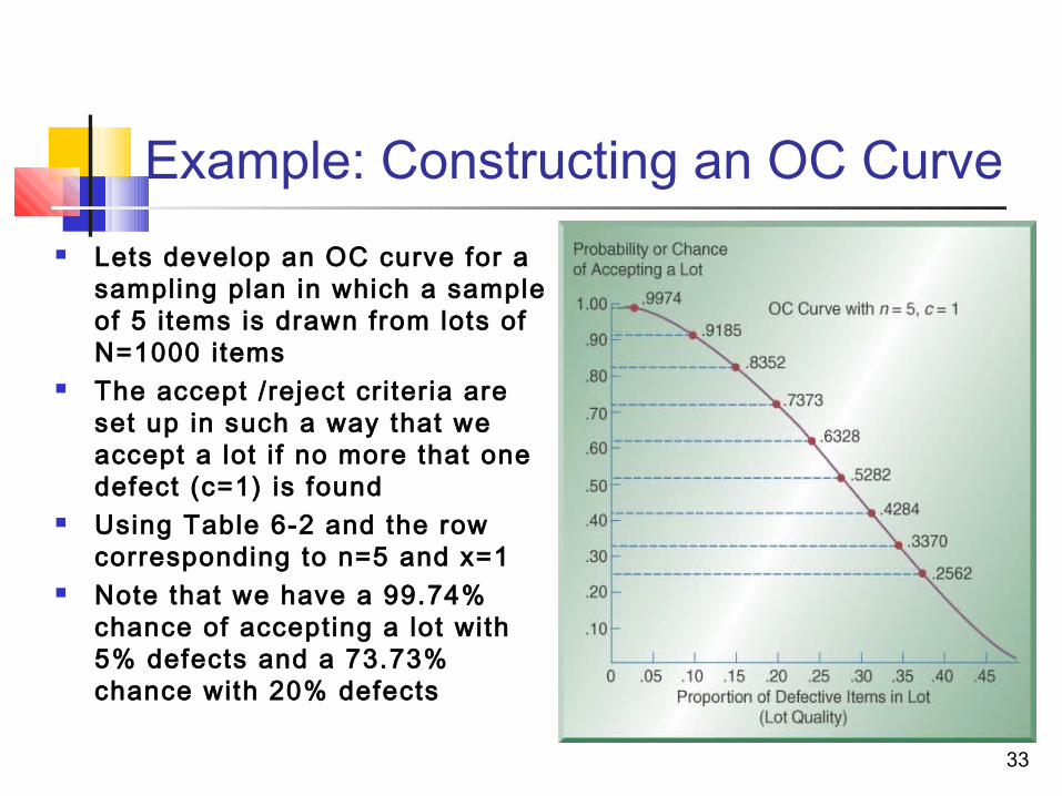
Example: Constructing an OC Curve Lets develop an OC curve for a

sampling plan in which a sample of 5 items is drawn from lots of N=1000 items

The accept /reject criteria are set up in such a way that we accept a lot i f no more that one defect (c=1) is found

Using Table 6-2 and the row corresponding to n=5 and x=1

Note that we have a 99.74% chance of accepting a lot with 5% defects and a 73.73% chance with 20% defects

34

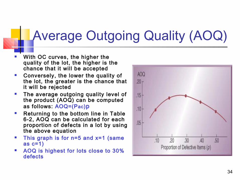
Average Outgoing Quality (AOQ) With OC curves, the higher the

quality of the lot, the higher is the chance that it wil l be accepted

Conversely, the lower the quality of the lot, the greater is the chance that it wi l l be rejected

The average outgoing quality level of the product (AOQ) can be computed as fol lows: AOQ=(Pac)p

Returning to the bottom line in Table 6-2, AOQ can be calculated for each proportion of defects in a lot by using the above equation

This graph is for n=5 and x=1 (same as c=1)

AOQ is highest for lots close to 30% defects

35

Implications for Managers How much and how often to inspect?

Consider product cost and product volume Consider process stability Consider lot size

Where to inspect? Inbound materials Finished products Prior to costly processing

Which tools to use? Control charts are best used for in-process production Acceptance sampling is best used for inbound/outbound

36

SQC in Services Service Organizations have lagged behind manufacturers

in the use of statistical quality control Statistical measurements are required and it is more

diff icult to measure the quality of a service Services produce more intangible products Perceptions of quality are highly subjective

A way to deal with service quali ty is to devise quantif iable measurements of the service element

Check-in time at a hotel Number of complaints received per month at a restaurant Number of telephone rings before a call is answered Acceptable control limits can be developed and charted

© Wiley 2010 37

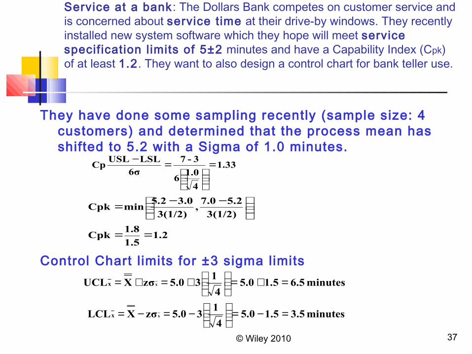
Service at a bank: The Dollars Bank competes on customer service and is concerned about service t ime at their drive-by windows. They recently installed new system software which they hope will meet service specif ication l imits of 5±2 minutes and have a Capability Index (Cpk) of at least 1.2. They want to also design a control chart for bank teller use.

They have done some sampling recently (sample size: 4 customers) and determined that the process mean has shifted to 5.2 with a Sigma of 1.0 minutes.

Control Chart l imits for ±3 sigma limits

1.21.5

1.8Cpk

3(1/2)

5.27.0,

3(1/2)

3.05.2minCpk

==

−−=

1.33

4

1.06

3-7

6σ

LSLUSLCp =

=−

minutes 6.51.55.04

135.0zσXUCL xx =+=

+=+=

minutes 3.51.55.04

135.0zσXLCL xx =−=

−=−=

38

SQC Across the Organization

SQC requires input from other organizational functions, influences their success, and used in designing and evaluating their tasks Marketing – provides information on current and future

quality standards Finance – responsible for placing financial values on

SQC efforts Human resources – the role of workers change with

SQC implementation. Requires workers with right skills Information systems – makes SQC information

accessible for all.