statistical relational learning notes
TRANSCRIPT

Statistical Relational Learning Notes
Ganesh Ramakrishnan and Ashwin Srinivasan
January 10, 2009

2

Contents
1 Sets, Relations and Logic 31.1 Sets and Relations . . . . . . . . . . . . . . . . . . . . . . . . . . 3
1.1.1 Sets . . . . . . . . . . . . . . . . . . . . . . . . . . . . . . 31.1.2 Relations . . . . . . . . . . . . . . . . . . . . . . . . . . . 4
1.2 Logic . . . . . . . . . . . . . . . . . . . . . . . . . . . . . . . . . . 131.3 Propositional Logic . . . . . . . . . . . . . . . . . . . . . . . . . . 14
1.3.1 Syntax . . . . . . . . . . . . . . . . . . . . . . . . . . . . . 151.3.2 Semantics . . . . . . . . . . . . . . . . . . . . . . . . . . . 171.3.3 Inference . . . . . . . . . . . . . . . . . . . . . . . . . . . 271.3.4 Resolution . . . . . . . . . . . . . . . . . . . . . . . . . . . 281.3.5 Davis-Putnam Procedure . . . . . . . . . . . . . . . . . . 401.3.6 Local Search Methods . . . . . . . . . . . . . . . . . . . . 441.3.7 Default inference under closed world assumption . . . . . 451.3.8 Lattice of Models . . . . . . . . . . . . . . . . . . . . . . 50
1.4 First-Order Logic . . . . . . . . . . . . . . . . . . . . . . . . . . . 551.4.1 Syntax . . . . . . . . . . . . . . . . . . . . . . . . . . . . . 561.4.2 Semantics . . . . . . . . . . . . . . . . . . . . . . . . . . . 641.4.3 From Datalog to Prolog . . . . . . . . . . . . . . . . . . . 711.4.4 Lattice of Herbrand Models . . . . . . . . . . . . . . . . . 741.4.5 Inference . . . . . . . . . . . . . . . . . . . . . . . . . . . 751.4.6 Subsumption Revisited . . . . . . . . . . . . . . . . . . . . 801.4.7 Subsumption Lattice over Atoms . . . . . . . . . . . . . . 811.4.8 Covers of Atoms . . . . . . . . . . . . . . . . . . . . . . . 861.4.9 The Subsumption Theorem Again . . . . . . . . . . . . . 891.4.10 Proof Strategies Once Again . . . . . . . . . . . . . . . . 901.4.11 Execution of Logic Programs . . . . . . . . . . . . . . . . 931.4.12 Answer Substitutions . . . . . . . . . . . . . . . . . . . . 971.4.13 Theorem Proving for Full First-Order Logic . . . . . . . . 99
1.5 Adequacy . . . . . . . . . . . . . . . . . . . . . . . . . . . . . . . 99
2 Exploring a Structured Search Space 1012.1 Subsumption Lattice over Clauses . . . . . . . . . . . . . . . . . 101
2.1.1 Lattice Structure of Clauses . . . . . . . . . . . . . . . . . 1032.1.2 Covers in the Subsume Order . . . . . . . . . . . . . . . 108
3

4 CONTENTS
2.2 The Implication Order . . . . . . . . . . . . . . . . . . . . . . . . 1092.3 Inverse Reduction . . . . . . . . . . . . . . . . . . . . . . . . . . 1122.4 Generality order and ILP . . . . . . . . . . . . . . . . . . . . . . 1122.5 Incorporating Background Knowledge . . . . . . . . . . . . . . . 115
2.5.1 Plotkin’s relative subsumption (B) . . . . . . . . . . . . 1162.5.2 Relative implication (|=B) . . . . . . . . . . . . . . . . . . 1222.5.3 Buntine’s generalized subsumption (≥B) . . . . . . . . . . 124
2.6 Using Generalization and Specialization . . . . . . . . . . . . . . 1262.7 Using the Cover Structure: Refinement Operators . . . . . . . . 126
2.7.1 Example . . . . . . . . . . . . . . . . . . . . . . . . . . . . 1272.7.2 Ideal Refinement Operators . . . . . . . . . . . . . . . . . 1282.7.3 Refinement Operators on Clauses for Subsumption . . . . 1302.7.4 Refinement Operators on Theories . . . . . . . . . . . . . 133
2.8 Inverse Resolution . . . . . . . . . . . . . . . . . . . . . . . . . . 1332.8.1 V-operator . . . . . . . . . . . . . . . . . . . . . . . . . . 1332.8.2 Predicate Invention: W-operator . . . . . . . . . . . . . . 135
2.9 Summary . . . . . . . . . . . . . . . . . . . . . . . . . . . . . . . 139
3 Linear Algebra 1433.1 Linear Equations . . . . . . . . . . . . . . . . . . . . . . . . . . . 1433.2 Vectors and Matrices . . . . . . . . . . . . . . . . . . . . . . . . . 1453.3 Solution of Linear Equations by Elimination . . . . . . . . . . . . 149
3.3.1 Elimination as Matrix Multiplication . . . . . . . . . . . . 1513.4 Solution of Linear Equations by Matrix Inversion . . . . . . . . . 156
3.4.1 Inverse Matrices . . . . . . . . . . . . . . . . . . . . . . . 1563.4.2 Gauss-Jordan Elimination . . . . . . . . . . . . . . . . . 158
3.5 Solution of Linear Equations using Vector Spaces . . . . . . . . . 1603.5.1 Vector Spaces and Matrices . . . . . . . . . . . . . . . . . 1603.5.2 Null Space . . . . . . . . . . . . . . . . . . . . . . . . . . 162
3.6 Elimination for Computing the Null Space (Ax = 0) . . . . . . . 1633.6.1 Pivot Variables and Row Echelon Form . . . . . . . . . . 1633.6.2 Reduced Row Echelon Form . . . . . . . . . . . . . . . . 1663.6.3 Solving Ax = b . . . . . . . . . . . . . . . . . . . . . . . 168
3.7 Independence, Basis, and Dimension . . . . . . . . . . . . . . . . 1733.7.1 Independence . . . . . . . . . . . . . . . . . . . . . . . . . 1743.7.2 Basis and Dimension . . . . . . . . . . . . . . . . . . . . . 175
3.8 Matrix Spaces . . . . . . . . . . . . . . . . . . . . . . . . . . . . 1783.9 Orthogonality and Projection . . . . . . . . . . . . . . . . . . . . 180
3.9.1 Projection Matrices . . . . . . . . . . . . . . . . . . . . . 1813.9.2 Least Squares . . . . . . . . . . . . . . . . . . . . . . . . 1813.9.3 Orthonormal Vectors . . . . . . . . . . . . . . . . . . . . . 1833.9.4 Gram-Schmidt Orthonormalization . . . . . . . . . . . . 1853.9.5 Fourier and Wavelet Basis . . . . . . . . . . . . . . . . . . 186
3.10 Determinants . . . . . . . . . . . . . . . . . . . . . . . . . . . . . 1873.10.1 Formula for determinant . . . . . . . . . . . . . . . . . . 1923.10.2 Formula for Inverse . . . . . . . . . . . . . . . . . . . . . . 194

CONTENTS 5
3.11 Eigenvalues and Eigenvectors . . . . . . . . . . . . . . . . . . . . 1953.11.1 Solving for Eigenvalues . . . . . . . . . . . . . . . . . . . 1963.11.2 Some Properties of Eigenvalues and Eigenvectors . . . . . 1973.11.3 Matrix Factorization using Eigenvectors . . . . . . . . . . 202
3.12 Positive Definite Matrices . . . . . . . . . . . . . . . . . . . . . . 2033.12.1 Equivalent Conditions . . . . . . . . . . . . . . . . . . . . 2043.12.2 Some properties . . . . . . . . . . . . . . . . . . . . . . . 205
3.13 Singular Value Decomposition . . . . . . . . . . . . . . . . . . . 2063.13.1 Pseudoinverse . . . . . . . . . . . . . . . . . . . . . . . . . 208
4 Convex Optimization 2114.1 Introduction . . . . . . . . . . . . . . . . . . . . . . . . . . . . . . 211
4.1.1 Mathematical Optimization . . . . . . . . . . . . . . . . . 2114.1.2 Some Topological Concepts in <n . . . . . . . . . . . . . . 2124.1.3 Optimization Principles for Univariate Functions . . . . . 2144.1.4 Optimization Principles for Multivariate Functions . . . . 2294.1.5 Absolute extrema and Convexity . . . . . . . . . . . . . . 250
4.2 Convex Optimization Problem . . . . . . . . . . . . . . . . . . . 2514.2.1 Why Convex Optimization? . . . . . . . . . . . . . . . . . 2514.2.2 History . . . . . . . . . . . . . . . . . . . . . . . . . . . . 2524.2.3 Affine Set . . . . . . . . . . . . . . . . . . . . . . . . . . . 2534.2.4 Convex Set . . . . . . . . . . . . . . . . . . . . . . . . . . 2534.2.5 Examples of Convex Sets . . . . . . . . . . . . . . . . . . 2554.2.6 Convexity preserving operations . . . . . . . . . . . . . . 2584.2.7 Convex Functions . . . . . . . . . . . . . . . . . . . . . . 2634.2.8 Convexity and Global Minimum . . . . . . . . . . . . . . 2644.2.9 Properties of Convex Functions . . . . . . . . . . . . . . . 2664.2.10 Convexity Preserving Operations on Functions . . . . . . 277
4.3 Convex Optimization Problem . . . . . . . . . . . . . . . . . . . 2784.4 Duality Theory . . . . . . . . . . . . . . . . . . . . . . . . . . . . 280
4.4.1 Lagrange Multipliers . . . . . . . . . . . . . . . . . . . . . 2804.4.2 The Dual Theory for Constrained Optimization . . . . . 2864.4.3 Geometry of the Dual . . . . . . . . . . . . . . . . . . . . 2904.4.4 Complementary slackness and KKT Conditions . . . . . 293
4.5 Algorithms for Unconstrained Minimization . . . . . . . . . . . . 2974.5.1 Descent Methods . . . . . . . . . . . . . . . . . . . . . . . 2984.5.2 Newton’s Method . . . . . . . . . . . . . . . . . . . . . . . 3034.5.3 Variants of Newton’s Method . . . . . . . . . . . . . . . . 3074.5.4 Gauss Newton Approximation . . . . . . . . . . . . . . . 3074.5.5 Levenberg-Marquardt . . . . . . . . . . . . . . . . . . . . 3094.5.6 BFGS . . . . . . . . . . . . . . . . . . . . . . . . . . . . . 3094.5.7 Solving Systems Large Sparse Systems . . . . . . . . . . 3114.5.8 Conjugate Gradient . . . . . . . . . . . . . . . . . . . . . 319
4.6 Algorithms for Constrained Minimization . . . . . . . . . . . . . 3224.6.1 Equality Constrained Minimization . . . . . . . . . . . . 3224.6.2 Inequality Constrained Minimization . . . . . . . . . . . 325

6 CONTENTS
4.7 Linear Programming . . . . . . . . . . . . . . . . . . . . . . . . 3284.7.1 Simplex Method . . . . . . . . . . . . . . . . . . . . . . . 3314.7.2 Interior point barrier method . . . . . . . . . . . . . . . . 338
4.8 Least Squares . . . . . . . . . . . . . . . . . . . . . . . . . . . . 3424.8.1 Linear Least Squares . . . . . . . . . . . . . . . . . . . . 3434.8.2 Least Squares with Linear Constraints . . . . . . . . . . 3484.8.3 Least Squares with Quadratic Constraints . . . . . . . . . 3514.8.4 Total Least Squares . . . . . . . . . . . . . . . . . . . . . 352
5 Statistics 3535.1 Variables . . . . . . . . . . . . . . . . . . . . . . . . . . . . . . . 3535.2 Descriptive Statistics . . . . . . . . . . . . . . . . . . . . . . . . . 354
5.2.1 Histograms . . . . . . . . . . . . . . . . . . . . . . . . . . 3545.2.2 Scatter Diagram . . . . . . . . . . . . . . . . . . . . . . . 357
5.3 Summary statistics . . . . . . . . . . . . . . . . . . . . . . . . . . 3575.4 Standard measures of location . . . . . . . . . . . . . . . . . . . . 357
5.4.1 Standard measures of spread and association . . . . . . . 3595.4.2 Correlation coefficient . . . . . . . . . . . . . . . . . . . . 3605.4.3 Ecological Correlation . . . . . . . . . . . . . . . . . . . . 363
5.5 Normal approximation . . . . . . . . . . . . . . . . . . . . . . . . 3645.5.1 Standard Normal Curve . . . . . . . . . . . . . . . . . . . 3645.5.2 General Normal Curve . . . . . . . . . . . . . . . . . . . . 3655.5.3 Standard Units . . . . . . . . . . . . . . . . . . . . . . . . 365
5.6 Regression . . . . . . . . . . . . . . . . . . . . . . . . . . . . . . . 3665.6.1 The Regression Effect . . . . . . . . . . . . . . . . . . . . 3715.6.2 SD Line . . . . . . . . . . . . . . . . . . . . . . . . . . . . 371
5.7 Probability and sampling . . . . . . . . . . . . . . . . . . . . . . 3715.8 Binomial distribution . . . . . . . . . . . . . . . . . . . . . . . . . 3715.9 Interval estimation . . . . . . . . . . . . . . . . . . . . . . . . . . 3715.10 Some standard significance tests . . . . . . . . . . . . . . . . . . 371
6 Searching on Graphs 3736.1 Search . . . . . . . . . . . . . . . . . . . . . . . . . . . . . . . . . 373
6.1.1 Depth First Search . . . . . . . . . . . . . . . . . . . . . . 3756.1.2 Breadth First Search (BFS) . . . . . . . . . . . . . . . . . 3766.1.3 Hill Climbing . . . . . . . . . . . . . . . . . . . . . . . . . 3766.1.4 Beam Search . . . . . . . . . . . . . . . . . . . . . . . . . 378
6.2 Optimal Search . . . . . . . . . . . . . . . . . . . . . . . . . . . . 3796.2.1 Branch and Bound . . . . . . . . . . . . . . . . . . . . . . 3806.2.2 A∗ Search . . . . . . . . . . . . . . . . . . . . . . . . . . . 381
6.3 Constraint Satisfaction . . . . . . . . . . . . . . . . . . . . . . . . 3816.3.1 Algorithms for map coloring . . . . . . . . . . . . . . . . . 3836.3.2 Resource Scheduling Problem . . . . . . . . . . . . . . . . 385

CONTENTS 7
7 Graphical Models 3877.1 Semantics of Graphical Models . . . . . . . . . . . . . . . . . . . 388
7.1.1 Directed Graphical Models . . . . . . . . . . . . . . . . . 3887.1.2 Undirected Graphical Models . . . . . . . . . . . . . . . . 3947.1.3 Comparison between directed and undirected graphical
models . . . . . . . . . . . . . . . . . . . . . . . . . . . . . 3977.2 Inference . . . . . . . . . . . . . . . . . . . . . . . . . . . . . . . . 399
7.2.1 Elimination Algorithm . . . . . . . . . . . . . . . . . . . 4007.2.2 Sum-product Algorithm . . . . . . . . . . . . . . . . . . . 4027.2.3 Max Product Algorithm . . . . . . . . . . . . . . . . . . . 4067.2.4 Junction Tree Algorithm . . . . . . . . . . . . . . . . . . . 4117.2.5 Junction Tree Propagation . . . . . . . . . . . . . . . . . 4147.2.6 Constructing Junction Trees . . . . . . . . . . . . . . . . 4157.2.7 Approximate Inference using Sampling . . . . . . . . . . . 419
7.3 Factor Graphs . . . . . . . . . . . . . . . . . . . . . . . . . . . . . 4297.4 Exponential Family . . . . . . . . . . . . . . . . . . . . . . . . . 4317.5 A Look at Modeling Continuous Random Variables . . . . . . . . 4337.6 Exponential Family and Graphical Models . . . . . . . . . . . . . 437
7.6.1 Exponential Models and Maximum Entropy . . . . . . . 4397.7 Model fitting . . . . . . . . . . . . . . . . . . . . . . . . . . . . . 443
7.7.1 Sufficient Statistics . . . . . . . . . . . . . . . . . . . . . . 4447.7.2 Maximum Likelihood . . . . . . . . . . . . . . . . . . . . . 4467.7.3 What the Bayesians Do . . . . . . . . . . . . . . . . . . . 4487.7.4 Model Fitting for Exponential Family . . . . . . . . . . . 4507.7.5 Maximum Likelihood for Graphical Models . . . . . . . . 4527.7.6 Iterative Algorithms . . . . . . . . . . . . . . . . . . . . . 4547.7.7 Maximum Entropy Revisted . . . . . . . . . . . . . . . . 457
7.8 Learning with Incomplete Observations . . . . . . . . . . . . . . 4597.8.1 Parameter Estimation for Mixture Models . . . . . . . . . 4607.8.2 Expectation Maximization . . . . . . . . . . . . . . . . . . 462
7.9 Variational Methods for Inference . . . . . . . . . . . . . . . . . . 466
8 Statistical Relational Learning 4738.1 Role of Logical Abstraction in SRL . . . . . . . . . . . . . . . . . 4748.2 Inductive Logic Programming . . . . . . . . . . . . . . . . . . . . 4758.3 Probabilistic ILP Settings . . . . . . . . . . . . . . . . . . . . . . 477
8.3.1 Probabilistic setting for justification . . . . . . . . . . . . 4798.4 Learning from Entailment . . . . . . . . . . . . . . . . . . . . . . 483
8.4.1 Constraining the ILP Search . . . . . . . . . . . . . . . . 4868.4.2 Example: Aleph . . . . . . . . . . . . . . . . . . . . . . . 487
8.5 Probabilistic Learning from Entailment . . . . . . . . . . . . . . 4958.5.1 Structure and Parameter Learning . . . . . . . . . . . . . 4968.5.2 Example: Extending FOIL . . . . . . . . . . . . . . . . . 4978.5.3 Example: Stochastic Logic Programming . . . . . . . . . 498
8.6 Learning from Interpretations . . . . . . . . . . . . . . . . . . . . 4988.7 Learning from Probabilistic Interpretations . . . . . . . . . . . . 499

CONTENTS 1
8.7.1 Example: Markov Logic Networks . . . . . . . . . . . . . 5008.7.2 Example: Bayesian Logic Programs . . . . . . . . . . . . 502
8.8 Learning from Proofs . . . . . . . . . . . . . . . . . . . . . . . . . 5068.9 Probabilistic Proofs . . . . . . . . . . . . . . . . . . . . . . . . . 507
8.9.1 Example: Extending GOLEM . . . . . . . . . . . . . . . . 5098.10 Summary . . . . . . . . . . . . . . . . . . . . . . . . . . . . . . . 511

2 CONTENTS

Chapter 1
Sets, Relations and Logic
‘Crime is common. Logic is rare. Therefore it is upon the logicrather than the crime that you should dwell.’ Sherlock Holmes inConan Doyle’s The Copper Breeches.
1.1 Sets and Relations
1.1.1 Sets
A set is a fundamental concept in mathematics. Simply speaking, it consistsof some objects, usually called its elements. Here are some basic notions aboutsets that you must already know about:
– A set S with elements a, b and c is usually written as S = a, b, c. Thefact that a is an element of S is usually denoted by a ∈ S.
– A set with no elements is called the “empty set” and is denoted by ∅.
– Two sets S and T are equal (S = T ) if and only if they contain preciselythe same elements. Otherwise S 6= T .
– A set T is a subset of a set S (T ⊆ S) if and only if every element of T isalso an element of S. If T ⊆ S and S ⊆ T then S = T . Sometimes T ⊆ Smay sometimes also be written as S ⊇ T . If T ⊆ S and S has at leastone element not in T , then T ⊂ S (T is said to be “proper subset” of S).Again, T ⊂ S may sometimes be written as S ⊃ T .
We now look at the meanings of the union, intersection, and equivalence ofsets. The intersection, or product, of sets S and T , denoted by S ∩ T or ST orS · T consists of all elements common to both S and T . ST ⊂ S and ST ⊆ Tfor all sets S and T . Now, if S and T have no elements in common, then theyare said to be disjoint and ST = ∅. It should be easy for you to see that ∅ ⊆ Sfor all S and ∅ · S = ∅ for all S. The union, or sum, of sets S and T , denoted
3

4 CHAPTER 1. SETS, RELATIONS AND LOGIC
by S ∪ T or S + T , is the set consisting of elements that belong at least to Sor T . Once again, it should be a straightforward matter to see S ⊆ S + T andT ⊆ S + T for all S and T . Also, S + ∅ = S for all S. Finally, if there is aone-to-one correspondence between the elements of set S and set T , then S andT are said to be equivalent (S ∼ T ). Equivalence and subsets form the basisof the definition of an infinte set: if T ⊂ S and S ∼ T then S is said to be aninfinite set. The set of natural numbers N is an example of an infinite set (anyset S ∼ N is said to be countable set).
1.1.2 Relations
A finite sequence is simply a set of n elements with a 1− 1 correspondence withthe set 1, . . . , n arranged in order of succession (an ordered pair , for example,is just a finite sequence with 2 elements). Finite sequences allow us to formalisethe concept of a relation. If A and B are sets, then the set A×B is called thecartesian product of A and B and is denoted by all ordered pairs (a, b) suchthat a ∈ A and b ∈ B. Any subset of A × B is a binary relation, and is calleda relation from A to B. If (a, b) ∈ R, then aRb means “a is in relation R to b”or, “relation R holds for the ordered pair (a, b)” or “relation R holds between aand b.” A special case arises from binary relations within elements of a singleset (that is, subsets of A × A). Such a relation is called a “relation in A” or a“relation over A”. There are some important kinds of properties that may holdfor a relation R in a set A:
Reflexive. The relation is said to be reflexive if the ordered pair (a, a) ∈ R forevery a ∈ A.
Symmetric. The relation is said to be symmetric if (a, b) ∈ R iff (b, a) ∈ R fora, b ∈ A.
Transitive. The relation is said to be transitive if (a, b) ∈ R and (b, c) ∈ R,then (a, c) ∈ R for a, b, c ∈ A.
Here are some examples:
• The relation ≤ on the set of integers is reflexive and transitive, but notsymmetric.
• The relation R = (1, 1), (1, 2), (2, 1), (2, 2), (3, 3), (4, 4) on the set A =1, 2, 3, 4 is reflexive, symmetric and transitive.
• The relation ÷ on the set N defined as the set (x, y) : ∃z ∈ N s.t. xz = yis reflexive and transitive, but not symmetric.
• The relation ⊥ on the set of lines in a plane is symmetric but neitherreflexive nor transitive.

1.1. SETS AND RELATIONS 5
It should be easy to see a relation like R above is just a set of ordered pairs.Functions are just a special kind of binary relation F which is such that if(a, b) ∈ F and (a, c) ∈ F then b = c. Our familiar notion of a function F froma set A to a set B is one which associates with each a ∈ A exactly one elementb ∈ B such that (a, b) ∈ F . Now, a function from a set A to itself is usuallycalled a unary operation in A. In a similar manner, a binary operation in A isa function from A × A to A (recall A × A is the Cartesian product of A withitself: it is sometimes written as A2). For example, if A = N , then addition (+)is a binary operation in A. In general, an n-ary operation F in A is a functionfrom An to A, and if it is defined for every element of An, then A is said to beclosed with respect to the operation F . A set which is closed for one or moren-ary operations is called an algebra, and a sub-algebra is a subset of such a setthat remains closed with respect to those operations. For example:
• N is closed wrt the binary operations of + and ×, and N along with +,×form an algebra.
• The set E of even numbers is a subalgebra of algebra of N with +,×. Theset O of odd numbers is not a subalgebra.
• Let S ⊆ U and S′ ⊆ U be the set with elements of U not in S (the unaryoperation of complementation). Let U = a, b, c, d. The subsets of Uwith the operations of complementation, intersection and union form analgebra. (How many subalgebras are there of this algebra?)
Equivalence Relations
Any relation R in a set A for which all three properties hold (that is, R isreflexive, symmetric, and transitive) is said to be an “equivalence relation”.Suppose, for example, we are looking at the relation R over the set of naturalnumbers N , which consists of ordered pairs (a, b) such that a + b is even1 Youshould be able to verify that R is an equivalence relation over N . In fact, Rallows us to split N into two disjoint subsets: the set of odd numbers O and theset of even numbers E such that N = O ∪ E and R is an equivalence relationover each of O and E . This brings us to an important property of equivalencerelations:
Theorem 1 Any equivalence relation E over a set S partitions S into disjointnon-empty subsets S1, . . . , Sk such that S = S1 ∪ · · · ∪ Sk.
Let us see how E can be used to partition S by constructing subsets of S in thefollowing way. For every a ∈ S, if (a, b) ∈ E then a and b are put in the samesubset. Let there be k such subsets. Now, since (a, a) ∈ E for every a ∈ S,every element of S is in some subset. So, S = S1 ∪ · · · ∪ Sk. It also follows thatthe subsets are disjoint. Otherwise there must be some c ∈ Si, Sj . Clearly, Si
1Equivalence is often denoted by ≈. Thus, for an equivalence relation E, if (a, b) ∈ E, thena ≈ b.

6 CHAPTER 1. SETS, RELATIONS AND LOGIC
and Sj are not singleton sets. Suppose Si contains at least a and c. Further letthere be a b 6∈ Si but b ∈ Sj . Since a, c ∈ Si, (a, c) ∈ E and since c, b ∈ Sj ,(c, b) ∈ E. Thus, we have (a, c) ∈ E and (c, b) ∈ E, which must mean that(a, b) ∈ E (E is transitive). But in this case b must be in the same subset as aby construction of the subsets, which contradicts our assumption that b 6∈ Si.The converse of this is also true:
Theorem 2 Any partition of a set S partitions into disjoint non-empty subsetsS1, . . . , Sk such that S = S1 ∪ · · · ∪ Sk results in an equivalence relation over S.
(Can you prove that this is the case? Start by constructing a relation E, with(a, b) ∈ E if and only if a and b are in the same block, and prove that E is anequivalence relation.)
Each of the disjoint subsets S1, S2, . . . are called ”equivalence classes”, andwe will denote the equivalence class of an element a in a set S by [a]. That is,for an equivalence relation E over a set S:
[a] = x : x ∈ S, (a, x) ∈ E
What we are saying above is that the collection of all equivalence classes ofelements of S forms a partition of S; and conversely, given a partition of the setS, there is an equivalence relation E on S such that the sets in the partition(sometimes also called its ”blocks”) are the equivalence classes of S.
Partial Orders
Given an equality relation = over elements of a set S, a partial order over Sis a relation over S that satisfies the following properties:
Reflexive. For every a ∈ S, a a
Anti-Symmetric. If a b and b a then a = b
Transitive. If a b and b c then a c
Here are some properties about partial orders that you should know (you willbe able to understand them immediately if you take, as a special case, asmeaning ≤ and ≺ as meaning <):
• If a b and a 6= b then a ≺ b
• b a means a b, b a means a ≺ b
• If a b or b a then a, b are comparable, otherwise they are not compa-rable.
A set S over which a relation of partial order is defined is called a partiallyordered set . It is sometimes convenient to refer to a set S and a relation Rdefined over S together by the pair < S,R >. So, here are some examples ofpartially ordered sets < S,>:

1.1. SETS AND RELATIONS 7
Figure 1.1: The lattice structure of 〈S,〉, where S is the power set of a, b, c.
• S is a set of sets, S1 S2 means S1 ⊆ S2
• S = N , n1 n2 means n1 = n2 or there is a n3 ∈ N such that n1+n3 = n2
• S is the set of equivalence relations E1, . . . over some set T , EL EMmeans for u, v ∈ T , uELv means uEMv (that is, (u, v) ∈ EL means(u, v) ∈ EM ).
Given a set S = a, b, . . . if a ≺ b and there is no x ∈ S such that a ≺ x ≺ bthen we will say b covers a or that a is a downward cover of b. Now, supposeSdown be a set of downward covers of b ∈ S. If for all x ∈ S, x ≺ b impliesthere is an a ∈ Sdown s.t. x a ≺ b, then Sdown is said to be a complete set ofdownward covers of b. Partially ordered sets are usually shown as diagrams likein Figure 1.1.The diagrams, as you can see, are graphs (sometimes called Hasse graphs orHasse diagrams). In the graph, vertices represent elements of the partiallyordered set. A vertex v2 is at a higher level than vertex v1 whenever v1 ≺ v2,and there is an edge between the two vertices only if v2 covers v1 (that is, v2
is an immediate predecessor). The graph is therefore really a directed one, inwhich there is a directed edge from a vertex v2 to v1 whenever v2 covers v1.Also, since the relation is anti-symmetric, there can be no cycles. So, the graphis a directed acyclic graph, or DAG.
In the diagram in Figure ?? on the left, S is the set of non-empty subsetsof a, b, c and denotes the subset relationship (that is, S1 S2 if and onlyif S1 ⊂ S2). The diagram on the right is an example of a chain, or a totallyordered set.
You should be able to see that a finite chain of length n can be put in aone-to-one correspondence to a finite sequence of natural numbers (1, . . . , n)(the correct way to say this is that a finite chain is isomorphic with a finitesequence of natural numbers). In general, a partially ordered set S is a chainif for every pair a, b ∈ S, a ≺ b or b ≺ a. There is a close relationship betweena partially ordered set and a chain. Suppose S is a partially ordered set. We

8 CHAPTER 1. SETS, RELATIONS AND LOGIC
can always associate a function f from the elements of S to N (the set ofnatural numbers), so that if a ≺ b for a, b ∈ S, then f(a) < f(b). f is calleda consistent enumeration of S, and is not unique and we can use it to define achain consistent with S. (We will leave the proof of the existence a consistentenumeration for you. One way would be to use the method of induction onthe number of elements in S: clearly there is such an enumeration for |S| = 1.Assume that an enumeration exists for |S| = n− 1 and prove it for |S| = n.)
Some elements of a partially ordered set have special properties. Let< S,>be a p.o. set and T ⊆ S. Then (in the following, you should read the symbol ∃as being shorthand for “there exists”, and ∀ as “for all”):
− Least element of T − Greatest element of T
a ∈ T s.t. ∀t ∈ T a t a ∈ Ts.t. ∀t ∈ T a t
− Least element, if it exists, − Greatest element, if it exists
is unique. If T = S this is is unique. If T = S then this is
the “zero” element the “unity” element
− Minimal element of T − Maximal element of T
a ∈ T 6 ∃t ∈ T s.t. t ≺ a a ∈ T 6 ∃t ∈ T s.t. t a
− Minimal element need − Maximal element need
not be unique not be unique
− Lower bound of T − Upper bound of T
b ∈ S s.t. b t ∀t ∈ T b ∈ S s.t. b t ∀t ∈ T
− Glb g of T − Lub g of T
b g ∀b, g : lbs of T b g ∀b, g : ubs of T
− If it exists, the glb is unique − If it exists the lub is unique
As you would have observed, there is a difference between a least element anda minimal element (and correspondingly, between greatest and maximal ele-ments). The requirement of a minimal (maximal) upper bound is, in somesense, a weakening of the requirement of a least (greatest) upper bound. If xand y are both lub’s of some set T ⊆ S, then y x and z y, so then x ≈ y.This means that all lub’s of T are equivalent. Dually, if x and y are glb’s of someT , then also x ≈ y. Thus, if a least element exists, then it is unique: this is notnecessarily the case with a minimal element. Also, least and greatest elementsmust belong to the set T , but lower and upper bounds need not.For this example, S has: (1) one upper bound b; (2) no lower bound; (3) agreatest element b; (4) no least element; (5) no greatest lower bound; (6) twominimal elements a and e; and (7) one maximal element b. Can you identifywhat the corresponding statements are for T?

1.1. SETS AND RELATIONS 9
Figure 1.2: a, b has no lub here.
The glb and lub are sometimes also taken to be binary operations on apartially ordered set S, that assigns to an ordered pair in S2 the correspondingglb or lub. The first operation is called the product or meet and is denoted by ·or u. The second operation is sometimes called the sum or join and is denotedby + or t.
In a quasi-ordered set, a subset need not have a lub or glb. We will take anexample to illustrate this. Let S = a, b, c, d, and let be defined as a c,b c, a d and d b. Then since c and d are incomparable, the set a, b hasno lub in this quasi-order. See Figure 1.2.
Similarly, a set need not have a maximal or a minimal, nor upward or down-ward covers. For instance, let S be the infinite set y, xl, x2, x3, . . ., and let be a quasi-order on S, defined as y ≺ . . . xn+1 ≺ xn ≺ . . . ≺ x2 ≺ x1. Thenthere is no upward cover of y: for every xn, there always is an xn+l such thaty ≺ xn+1 ≺ xn. In this case, y has no complete set of upward covers.
Note that a complete set of upward covers for y need not contain all upwardcovers of y. However, in order to be complete, it should contain at least oneelement from each equivalence class of upward covers. On the other hand,even the set of all upward covers of y need not be complete for y. For theexample given above, the set of all upward covers of y is empty, but obviouslynot complete.
A notion of some relevance later is that of a function f defined on a partiallyordered set < S,>. Specifically, we would like to know if the function is: (a)monotonic; and (b) continuous. Monotonicity first:
A function f on < S,> is monotonic if and only if for all u, v ∈ S,u v means f(u) f(v)
Now, suppose a subset S1 of S have a least upper bound lub(S1) (with someabuse of notation: here lub(X) is taken to be the lub of the elements in set X).Such subsets are called “directed” subsets of S. Then:
A function f on < S,> is continuous if and only if for all directedsubsets Si of S, f(lub(Si)) = lub(f(x) : x ∈ Si).

10 CHAPTER 1. SETS, RELATIONS AND LOGIC
That is, if a directed set Si has a least upper bound lub(Si), then the setobtained by applying a continuous function f to the elements of Si has leastupper bound f(lub(Si)). Functions that are both monotonic and continuous onsome partially ordered set < S,> are of interest to us because they can beused, for some kinds of orderings, to guarantee that for some s ∈ S, f(s) = s.That is, f is said to have a “fixpoint”.
Lattices
A lattice is just a partially ordered set < S,> in which every pair of elementsa, b ∈ S has a glb (represented by u) and a lub (represented by t). From thedefinitions of lower and upper bounds, we are able to show that in any suchpartially ordered set, the operations will have the following properties:
• a u b = b u a, and a t b = b t a (that is, they are are commutative).
• a u (b u c) = (a u b) u c, and a t (b t c) = (a t b) t c (that is, they areassociative).
• a u (a t b) = a, and a t (a u b) = a (that is, they are “absorptive”).
• a u b = a and a t b = b.
We will not go into all the proofs here, but show one for illustration. Since au bis the glb of a and b, aub a. Clearly then at (aub), which is the lub of a anda u b, is a. This is one of the absorptive properties above. You should also beable to see, from these properties, that a lattice can also be seen simply as analgebra with two binary operations u and t that are commutative, associativeand absorptive.
Theorem 3 A lattice is an algebra with the binary operations of t and u.
Here is an example of a lattice: let S be all the subsets of a, b, c, and forX,Y ∈ S, X Y means X ⊆ Y , X uY = X ∩Y and X tY = X ∪Y . Then< S,⊆> is a lattice. The empty set ∅ is the zero element, and S is the unityelement of the lattice. More generally, a lattice that has a zero or least element(which we will denote ⊥), and a unity or greatest element (which we will denote>) is called a bounded lattice. In such lattices, the following necessarily hold:a t > = >; a u > = a; a t ⊥ = a; and a u ⊥ = ⊥. A little thought shouldconvince you that a finite lattice will always be bounded: if the lattice is theset S = a1, . . . , an then > = a1 t · · · t an and ⊥ = a1 u · · · u an. (But, doesthe reverse hold: will a bounded lattice always be finite?)
Two properties of subsets of lattices are of interest to us. First, a subsetM of a lattice L is called a sublattice of L if M is also closed under the samebinary operations of t and u defined for L (that is, M is a lattice with thesame operations as those of L). Second, if a lattice L has the property thatevery subset of L has a lub and a glb, then the L is said to be a completelattice. Clearly, every finite lattice is complete. Further, since every subset of

1.1. SETS AND RELATIONS 11
L has a lub and a glb, this must certainly be true of L itself. So, L has a lub,which must necessarily be the greatest element of L. Similarly, L has a glb,which must necessarily be the least element of L. In fact, the elements of L areordered in such a way that each element is on some path from > to ⊥ in theHasse diagram. An example of an ordered set that is always a complete latticeis the set of all subsets of a set S, ordered by ⊆, with binary operations ∩ and∪ for the glb and lub. This set, the “powerset” of S, is often denoted by 2S .So, if S = a, b, c, 2S is the set ∅, a, b, c, a, b, a, c, b, c, a, b, c.Clearly, every subset of s of 2S has both a glb and a lub in S.
There are two important results concerning complete lattices and functionsdefined on them. The Knaster-Tarski Theorem tells us that every monotonicfunction on a complete lattice < S,> has a least fixpoint.
Theorem 4 Let < S,> be a complete lattice and let f : S → S be a monotonicfunction. Then the set of fixed points of f in L is also a complete lattice < P,>(which obviously means that f has a greatest as well as a least fixpoint).
Proof Sketch:2 Let D = x|x f(x). From the very definition of D, itfollows that every fixpoint is in D. Consider some x ∈ D. Then because f ismonotone we have f(x) f(f(x)). Thus,
∀ x ∈ D, f(x) ∈ D (1.1)
Let u = lub(D) (which should exist according to our assumption that <S,> is a complete lattice. Then x u and f(x) f(u), so x f(x) f(u).Therefore f(u) is an upper bound of D. However, u is the least upper bound,hence u f(u), which in turn implies that, u ∈ D. From (1.1), it follows thatf(u) ∈ D. From u = lub(D), f(u) ∈ D and u f(u), it follows that f(u) = u.Because every fixpoint is in D we have that u is the greatest fixpoint of f .Similarly, it can be proved that if E = x|f(x) x, then v = glb(E) is a fixedpoint and therefore the smallest fixpoint of f . 2
Kleene’s First Recursion Theorem tells us how to find the element s ∈ S thatis the least fixpoint, by incrementally constructing lubs starting from applyinga continuous function to the least element of the lattice (⊥).
Theorem 5 Let S be a complete partial order and let f : S → S be a contin-uous (and therefore monotone) function. Then the least fixed point of f is thesupremum of the ascending Kleene chain of f:
⊥ f(⊥) f(f(⊥)) . . . fn(⊥) . . .
In the special case that is ⊆, the incremental procedure starts with theempty set ∅, and progressive lub’s are obtained by application of the set-unionoperation ∪. We will not give the proofs of this result here.
2Can you complete the proof?

12 CHAPTER 1. SETS, RELATIONS AND LOGIC
Figure 1.3: Example lattice for illustrating the concept of lattice length.
A final concept we will need is the concept of the length of a lattice. For apair of elements a, b in a lattice L such that a b, the interval [a, b] is the setx : x ∈ L, a x b. Now, consider a subset of [a, b] that contains botha and b, and is such that any pair of elements in the subset are comparable.Then that subset is a chain from a to b: if the number of elements in the subsetis n, then the length of the chain is n − 1. Maximal chains from a to b arethose of the form a = x1 ≺ x2 ≺ · · · ≺ xn = b such that each xi is coveredby xi+1. If all maximal chains from a to b are finite, then the longest of thesedefines the length of the interval [a, b]. For a bounded lattice, the length of theinterval [⊥,>] defines the length of the lattice. So, in the lattice in Figure 1.3,there are two maximal chains between ⊥ and >, of lengths 2 and 3 (what arethese?). The length of lattice is thus equal to 3. Now, it should be evident thatfinite lattices will always have a finite length, but it is possible for lattices tohave a finite length, but have infinitely many elements. For example, the latticeL = ⊥,>, x1, x2, . . . such that ⊥ ≺ xi ≺ > has a finite length (all maximalchains are of length 2). (Indeed, it is even possible to have an infinite set inwhich maximal chains are of finite, but increasing in lengths of 1, 2 . . ..)
Quasi-Orders
A quasi-order Q in a set S is a binary relation over S that satisfies the followingproperties:
Reflexive. For every a ∈ S, aQa
Transitive. If aQb and bQc then aQc
You can see that a quasi-order differs from an equivalence relation in that sym-metry is not required. Further, it differs from a partial order because no equalityis defined, and therefore the property of anti-symmetry property cannot be de-fined either. There are two important properties of quasi-orders, which we willpresent here without proof:

1.2. LOGIC 13
• If a quasi-order Q is defined on a set S = a, b, . . ., and we define a binaryrelation E as follows: aEb iff aQb and bQa. Then E is an equivalencerelation.
• Let E partition S into subsets X,Y, . . . of equivalent elements. Let T =X,Y, . . . and be a binary relation in T meaning X Y in T if andonly if xQy in S for some x ∈ X, y ∈ Y . Then T is partially ordered by.
What these two properties say is simply this:
A quasi-order order Q over a set S results in a partial ordering overa set of equivalence classes of elements in S.
1.2 Logic
Logic, the study of arguments and ‘correct reasoning’, has been with us forat least the better part of two thousand years. In Greece, we associate itsorigins with Aristotle (384 B.C.–322 B.C.); in India with Gautama and the Nyayaschool of philosophy (3rd Century B.C.?); and in China with Mo Ti (479 B.C.–381 B.C.) who started the Mohist school. Most of this dealt with the use andmanipulation of syllogisms. It would only be a small injustice to say that littleprogress was made until Gottfried Wilhelm von Leibniz (1646–1716). He madea significant advance in the use of logic in mathematics by introducing symbolsto represent statements and relations. Leibniz hoped to reduce all errors inhuman reasoning to minor calculational mistakes. Later, George Boole (1815–1864) established the connection between logic and sets, forming the basis ofBoolean algebra. This link was developed further by John Venn (1834–1923)and Augustus de Morgan (1806–1872). It was around this time that CharlesDodgson (1832–1898), writing under the pseudonym Lewis Carroll, wrote anumber of popular logic textbooks. Fundamental changes in logic were broughtabout by Friedrich Ludwig Gottlob Frege (1848–1925), who strongly rejectedthe idea that the laws of logic are synonymous with the laws of thought. ForFrege, the former were laws of truth, having little to say on the processes bywhich human beings represent and reason with reality. Frege developed a logicalframework that incorporated propositions with relations and the validity ofarguments depended on the relations involved. Frege also introduced the deviceof quantifiers and bound variables, thus laying the basis for predicate logic, whichforms the basis of all modern logical systems. All this and more is describedby Bertrand Russell (1872–1970) and Alfred North Whitehead (1861–1947) intheir monumental work, Principia Mathematica. And then in 1931, Kurt Godel(1906–1978) showed much to the dismay of mathematicians everywhere thatformal systems of arithmetic would remain incomplete.
Rational agents require knowledge of their world in order to make rationaldecisions. With the help of a declarative (knowledge representation) language,this knowledge (or a portion of it) is represented and stored in a knowledge
14 CHAPTER 1. SETS, RELATIONS AND LOGIC
base. A knowledge-base is composed of sentences in a language with a truththeory (logic), so that someone external to the system can interpret sentences asstatements about the world (semantics). Thus, to express knowledge, we needa precise, declarative language. By a declarative language, we mean that
1. The system believes a statement S iff it considers S to be true, since onecannot believe S without an idea of what it means for the world to fulfillS.
2. The knowledge-based must be precise enough so that we must know, (1)which symbols represent sentences, (2) what it means for a sentence to betrue, and (3) when a sentence follows from other sentences.
Two declarative languages will be discussed in this chapter: (0 order or)propositional logic and first order logic.
1.3 Propositional Logic
Formal logic is concerned with statements of fact, as opposed to opinions, com-mands, questions, exclamations etc. Statements of fact are assertions that areeither true or false, the simplest form of which are called propositions. Here aresome examples of propositions:
The earth is flat.
Humans are monkeys.
1 + 1 = 2
At this stage, we are not saying anything about whether these are true or false:just that they are sentences that are one or the other. Here are some examplesof sentences that are not propositions:
Who goes there?
Eat your broccoli.
This statement is false.
It is normal to represent propositions by letters like P,Q, . . .. For exam-ple, P could represent the proposition ‘Humans are monkeys.’ Often, simplestatements of fact are insufficient to express complex ideas. Compound state-ments can be combining two or more propositions with logical connectives (orsimply, connectives). The connectives we will look at here will allow us to formsentences like the following:
It is not the case that P
P and Q
P or Q
P if Q

1.3. PROPOSITIONAL LOGIC 15
The P ’s and Q’s above are propositions, and the words underlined are theconnectives. They have special symbols and names when written formally:
Statement Formally Name
It is not the case that P ¬P Negation
P and Q P ∧Q Conjunction
P or Q P ∨Q Disjunction
P if Q P ← Q Conditional
There is, for example, a form of argument known to logicians as the disjunctivesyllogism. Here is one due to the Stoic philosopher Chrysippus, about a dogchasing a rabbit. The dog arrives at a fork in the road, sniffs at one path andthen dashes down the other. Chrysippus used formal logic to describe this:3
Statement Formally
The rabbit either went down Path A or Path B. P ∨QIt did not go down Path A. ¬PTherefore it went down Path B. ∴ Q
Here P represents the proposition ‘The rabbit went down Path A’ and Q theproposition ‘The rabbit went down Path B.’ To argue like Chrysippus requiresus to know how to write correct logical sentences, ascribe truth or falsity topropositions, and use these to derive valid consequences. We will look at allthese aspects in the sections that follow.
1.3.1 Syntax
Every language needs a vocabulary . For the language of propositional logic, wewill restrict the vocabulary to the following:
Propositional symbols: P,Q, . . .
Logical connectives4 : ¬,∧,∨,←Brackets: (, )
The next step is to specify the rules that decide how legal sentences are to beformed within the language. For propositional logic, legal sentences or well-formed formulæ (wffs for short) are formed using the following rules:
1. Any propositional symbol is a wff;
2. If α is a wff then ¬α is a wff; and
3There is no suggestion that the principal agent in the anecdote employed similar meansof reasoning.

16 CHAPTER 1. SETS, RELATIONS AND LOGIC
3. If α and β are wffs then (α ∧ β), (α ∨ β), and (α← β) are wffs.
Wffs consisting simply of propositional symbols (Rule 1) are sometimes calledatomic wffs and others compound wffs Informally, it is acceptable to drop out-ermost brackets. Here are some examples of wffs and ‘non-wffs’:
Formula Comment
(¬P ) Not a wff. Parentheses are only allowed
with the connectives in Rule 3
¬¬P P is wff (Rule 1),
¬P is wff (Rule 2),
∴ ¬¬P is wff (Rule 2)
(P ← (Q ∧R)) P,Q,R are wffs (Rule 1),
∴ (Q ∧R) is a wff (Rule 3),
∴ (P ← (Q ∧R)) is a wff (Rule 3)
P ← (Q ∧R) Not a wff, but acceptable informally
((P ) ∧ (Q)) Not a wff. Parentheses are only allowed
with the connectives in Rule 3
(P ∧Q ∧R) Not a wff. Rule 3 only allows two symbols
within a pair of brackets
One further kind of informal notation is widespread and quite readable. Theconditional (P ← ((Q1 ∧Q2) . . . Qn))) is often written as (P ← Q1, Q2, . . . Qn)or even P ← Q1, Q2, . . . Qn.
It is one thing to be able to write legal sentences, and quite another matterto be able to assess their truth or falsity. This latter requires a knowledge ofsemantics, which we shall look at shortly.
Normal Forms
Every formulae in propositional logic is equivalent to a formula that can bewritten as a conjunction of disjunctions. That is, something like (A∨B)∧ (C ∨D) ∧ · · · . When written in this way the formula is said to be in conjunctivenormal form or CNF. There is another form, which consists of a disjunction ofconjunctions, like (A∧B)∨ (C ∧D)∨ · · · , called the disjunctive normal form orDNF. In general, a formula F in CNF can be written somewhat more crypticallyas:
F =n∧i=1
m∨j=1
Li,j
and a formula G in DNF as:

1.3. PROPOSITIONAL LOGIC 17
G =n∨i=1
m∧j=1
Li,j
Here,
∨Fi is short for F1 ∨ F2 ∨ · · · and
∧Fi is short for Fi ∧ F2 ∧ · · · . In
both CNF and DNF forms above, the Li,j are either propositions or negationsof propositions (we shall shortly call these “literals”).
1.3.2 Semantics
There are three important concepts to be understood in the study of semanticsof well-formed formulæ: interpretations, models, and logical consequence.
Interpretations
For propositional logic, an interpretation is simply an assignment of either trueor false to all propositional symbols in the formula. For example, given the wff(P ← (Q ∧R)) here are two different interpretations:
P Q R
I1 : true false true
I2 : false true true
You can think of I1 and I2 as representing two different ‘worlds’ or ‘contexts’.After a moment’s thought, it should be evident that for a formula with Npropositional symbols, there can never be more than 2N possible interpretations.
Truth or falsity of a wff only makes sense given an interpretation (by theprinciple of bivalence, any interpretation can only result in a wff being eithertrue or false). Clearly, if the wff simply consists of a single propositional symbol(recall that this was called an atomic wff), then the truth-value is simply thatgiven by the interpretation. Thus, the wff P is true in interpretation I1 andfalse in interpretation I2. To obtain the truth-value of compound wffs like(P ← (Q ∧ R)) requires a knowledge the semantics of the connectives. Theseare usually summarised in a tabular form known as truth tables. The truthtables for the connectives of interest to us are given below.
Negation. Let α be a wff5. Then the truth table for ¬α is as follows:
α ¬αfalse true
true false
Conjunction. Let α and β be wffs. The truth table for (α ∧ β) is as follows:
5We will use Greek characters like α, β to stand generically for any wff.
18 CHAPTER 1. SETS, RELATIONS AND LOGIC
α β (α ∧ β)
false false false
false true false
true false false
true true true
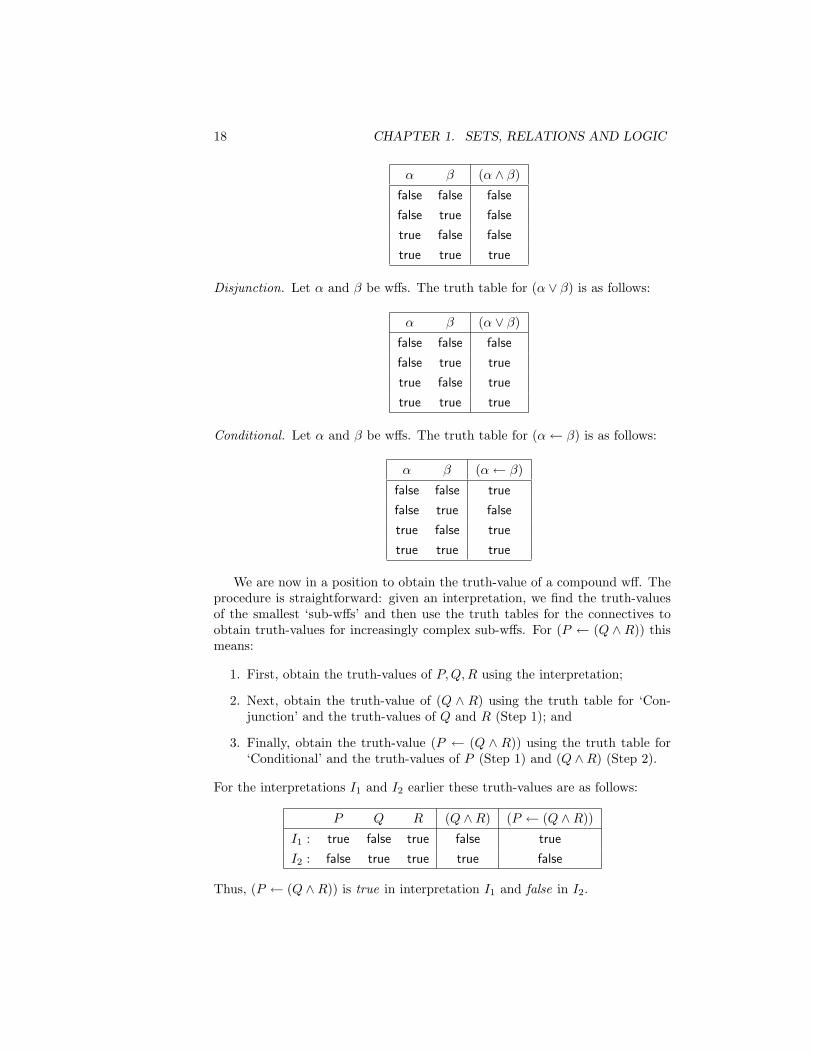
Disjunction. Let α and β be wffs. The truth table for (α ∨ β) is as follows:
α β (α ∨ β)
false false false
false true true
true false true
true true true
Conditional. Let α and β be wffs. The truth table for (α← β) is as follows:
α β (α← β)
false false true
false true false
true false true
true true true
We are now in a position to obtain the truth-value of a compound wff. Theprocedure is straightforward: given an interpretation, we find the truth-valuesof the smallest ‘sub-wffs’ and then use the truth tables for the connectives toobtain truth-values for increasingly complex sub-wffs. For (P ← (Q ∧ R)) thismeans:
1. First, obtain the truth-values of P,Q,R using the interpretation;
2. Next, obtain the truth-value of (Q ∧ R) using the truth table for ‘Con-junction’ and the truth-values of Q and R (Step 1); and
3. Finally, obtain the truth-value (P ← (Q ∧ R)) using the truth table for‘Conditional’ and the truth-values of P (Step 1) and (Q ∧R) (Step 2).
For the interpretations I1 and I2 earlier these truth-values are as follows:
P Q R (Q ∧R) (P ← (Q ∧R))
I1 : true false true false true
I2 : false true true true false
Thus, (P ← (Q ∧R)) is true in interpretation I1 and false in I2.

1.3. PROPOSITIONAL LOGIC 19
Models
Every interpretation (that is, an assignment of truth-values to propositionalsymbols) that makes a well-formed formula true is said to be a model for thatformula. Take for example, the two interpretations I1 and I2 above. We havealready seen that I1 is a model for (P ← (Q ∧ R)); and that I2 is not a modelfor the same formula. In fact, I1 is also a model for several other wffs like: P ,(P ∧R), (Q∨R), (P ← Q), etc. Similarly, I2 is a model for Q, (Q∧R), (P ∨Q),(Q← P ), etc.
As another example, let P,Q,R be the set of all atoms in the language,and α be the formula ((P ∧ Q) ↔ (R → Q)). Let I be the interpretation thatmakes P and R true, and Q false (so I = P,R). We determine whether α istrue or false under I as follows:
1. P is true under I, and Q is false under I, so (P ∧Q) is false under I.
2. R is true under I, Q is false under I, so (R→ Q) is false under I.
3. (P ∧Q) and (R→ Q) are both false under I, so α is true under I.
Since α is true under I, I is a model of α. Let I ′ = P. Then (P ∧ Q) isfalse, and (R → Q) is true under I ′. Thus α is false under I ′, and I ′ is not amodel of α.
The definition of model can be extended to a set of formulæ; an interpretationI is said to be a model of a set of formulæ Σ if I is a model of all formulæ α ∈ Σ.Σ is then said to have I as a model. We will offer an example to illustratethis extended definition. Let Σ = P, (Q ∨ I), (Q → R), and let I = P,R,I ′ = P,Q,R, and I” = P,Q be interpretations. I and I ′ satisfy all formulasin Σ, so I and I ′ are models of Σ. On the other hand, I” falsifies (Q→ R), soI” is not a model of Σ.
At this point, we can distinguish amongst two kinds of formulæ:
1. A wff may be such that every interpretation is a model. An example is(P ∨¬P ). Since there is only one propostional symbol involved (P ), thereare at most 21 = 2 interpretations possible. The truth table summarisingthe truth-values for this formula is:
P ¬P (P ∨ ¬P )
I1 : false true true
I2 : true false true
(P ∨ ¬P ) is thus true in every possible ‘context’. Formulæ like these, forwhich every interpretation is a model are called valid or tautologies
2. A wff may be such that none of the interpretations is a model. An exampleis (P ∧ ¬P ). Again there is only one propostional symbol involved (P ),and thus only two interpretations possible. The truth table summarisingthe truth-values for this formula is:

20 CHAPTER 1. SETS, RELATIONS AND LOGIC
P ¬P (P ∧ ¬P )
I1 : false true false
I2 : true false false
(P ∧ ¬P ) is thus false in every possible ‘context’. Formulæ like these,for which none of the interpretations is a model are called unsatisfiable orinconsistent
Finally, any wff that has at least one interpretation as a model is said to besatisfiable.
Logical Consequence
We are often interested in establishing the truth-value of a formula given thatof some others. Recall the Chrysippus argument:
Statement Formally
The rabbit either went down Path A or Path B. P ∨QIt did not go down Path A. ¬PTherefore it went down Path B. ∴ Q
Here, we want to establish that if the first two statements are true, then the thirdfollows. The formal notion underlying all this is that of logical consequence. Inparticular, what we are trying to establish is that some well-formed formula αis the logical consequence of a conjunction of other well-formed formulæ Σ (or,that Σ logically implies α). This relationship is usually written thus:
Σ |= α
Σ being the conjunction of several wffs, it is itself a well-formed formula6. Log-ical consequence can therefore also be written as the following relationship be-tween a pair of wffs:
((β1 ∧ β2) . . . βn) |= α
It is sometimes convenient to write Σ as the set β1, β2, . . . , βn which is un-derstood to stand for the conjunctive formula above. But how do we determineif this relationship between Σ and α does indeed hold? What we want is thefollowing: whenever the statements in Σ are true, α must also be true. In formalterms, this means: Σ |= α if every model of Σ is also model of α. Decoded:
6There is therefore nothing special needed to extend the concepts of validity and unsatisfi-ability to conjunctions of formulæ like Σ. Thus, Σ is valid if and only if every interpretation isa model of the conjunctive wff (in other words, a model for each wff in the conjunction); andit is unsatisfiable if and only if none of the interpretations is a model of the conjunctive wff.It should be apparent after some reflection that if Σ is valid, then all logical consequences ofit are also valid. On the other hand, if Σ is unsatisfiable, then any well-formed formula is alogical consequence.

1.3. PROPOSITIONAL LOGIC 21
• Recall that a model for a formula is an interpretation (assignment of truth-values to propositions) that makes that formula true;
• Therefore, a model for Σ is an interpretation that makes ((β1 ∧β2) . . . βn)true. Clearly, such an interpretation will make each of β1, β2, . . . , βn true;
• Let I1, I2, . . . , Ik be all the interpretations that satisfy the requirementabove: that is, each is a model for Σ and there are no other models forΣ (recall that if there are N propositional symbols in Σ and α together,then there can be no more than 2N such interpretations);
• Then to establish Σ |= α, we have to check that each of I1, I2, . . . , Ik isalso a model for α (that is, each of them make α true).
The definition of logical entailment can be extended to the entailment of setsof formulæ. Let Σ and Γ be sets of formulas. Then Γ is said to be a logicalconsequence of Σ (written as Σ |= Γ), if Σ |= α, for every formula α ∈ Γ. Wealso say Σ (logically) implies Γ.
We are now in a position to see if Chrysippus was correct. We wish to seeif ((P ∨Q) ∧ ¬P ) |= Q. From the truth tables on page 17, we can construct atruth table for ((P ∨Q) ∧ ¬P ):
P Q (P ∨Q) ¬P ((P ∨Q) ∧ ¬P )
I1 : false false false true false
I2 : false true true true true
I3 : true false true false false
I4 : true true true false false
It is evident that of the four interpretations possible only one is a model for((P ∨Q) ∧ ¬P ), namely: I2. Clearly I2 is also a model for Q. Therefore, everymodel for ((P ∨Q)∧¬P ) is also a model for Q7. It is therefore indeed true that((P ∨Q)∧¬P ) |= Q. In fact, you will find you can ‘move’ formulæ from left toright in a particular manner. Thus if:
((P ∨Q) ∧ ¬P ) |= Q
then the following also hold:
(P ∨Q) |= (Q← ¬P ) and ¬P |= (Q← (P ∨Q))
These are consequences of a a more general result known as the deduc-tion theorem, which we look at now. Using a set-based notation, let Σ =β1, β2, . . . , βi, . . . , βn. Then, the deduction theorem states:
7Although I4 is also a model for Q, the test for logical consequence only requires us toexamine those interpretations that are models of ((P ∨Q) ∧ ¬P ). This precludes I4.

22 CHAPTER 1. SETS, RELATIONS AND LOGIC
Theorem 6
Σ |= α if and only if Σ− βi |= (α← βi)
.
Proof: Consider first the case that Σ |= α. That is, every model of Σ is a modelof α. Now assume Σ− βi 6|= (α← βi). That is, there is some model, say M ,of Σ − βi that is not a model of (α ← βi). That is, βi is true and α is falsein M . That is M is a model for Σ− βi and for βi, but not a model for α. Inother words, M is a model for Σ but not a model for α which is not possible.Therefore, if Σ |= α then Σ − βi 6|= (α ← βi). Now for the “only if” part.That is, let Σ − βi |= (α ← βi). We want to show that Σ |= α. Once again,let us assume the contrary (that is, Σ 6|= α. This means there must be a modelM for Σ that is not a model for α. However, since Σ = β1, β2, . . . , βi, . . . , βn,M is both a model for Σ− βi and a model for each of the βi. So, M cannotbe a model for (α ← βi). We are therefore in a position that there is a modelM for Σ − βi that is not a model of (α ← βi), which contradicts what wasgiven. 2
The deduction theorem isn’t restricted to propositional logic, and holds for first-order logic as well. It can be invoked repeatedly. Here is an example of using ittwice:
Σ |= α if and only if Σ− βi, βj |= (α← (βi ∧ βj))
With Chrysippus, applying the deduction theorem twice results in:
(P ∨Q),¬P |= Q if and only if ∅ |= (Q← ((P ∨Q) ∧ ¬P ))
If ∅ |= (Q ← ((P ∨ Q) ∧ ¬P )) then every model for ∅ must be a model for(Q ← ((P ∨ Q) ∧ ¬P )). By convention, every interpretation is a model for ∅8.It follows that every interpretation must be a model for (Q← ((P ∨Q)∧¬P )).Recall that this is just another way of stating that (Q ← ((P ∨ Q) ∧ ¬P )) isvalid (page 19)9.
What is the difference between the concepts of logical consequence denotedby |= and the connective → in a statement such as Σ |= Γ? where, Σ = (P ∧Q), (P → R) and Γ = P,Q,R? And how do these two notions of implicationrelate to the phrase ‘if....then’, often used in propositions or theorems? Wedelineate the differences below:
8That is, we take the empty set to denote a distinguished proposition True that is truein every interpretation. Correctly then, the formula considered is not ((β1 ∧ β2) . . . βn))) but(True ∧ ((β1 ∧ β2) . . . βn)))).
9To translate declarative knowledge into action (as in the case of the dog from Chrysippus’sanecdote), one of two possible strategies can be adopted. The first is called ‘Negative selection’which involves excluding any provably futile actions. The second is called ‘Positive selection’which involves suggesting only actions that are provably safe. There can be some actions thatare neither provably safe nor provably futile.

1.3. PROPOSITIONAL LOGIC 23
1. The connective→ is a syntactical symbol called ‘if ... then’ or ‘implication’,which appears within formulæ. The truth value of the formula (α → ξ)depends on the particular interpretation I we happen to be considering:according to the truth table, (α→ ξ) is true under I if α is false under Iand/or ξ is true under I; (α→ ξ) is false otherwise.
2. The concept of ‘logical consequence’ or ‘(logical) implication’, denoted by’|=’ describes a semantical relation between formulæ. It is defined in termsof all interpretations: ’α |= ξ’ is true if every interpretation that is a modelof α, is also a model of ξ.
3. The phrase ’if. .. then’, which is used when stating, for example, propo-sitions or theorems is also sometimes called ’implication’. This describesa relation between assertions which are phrased in (more or less) naturallanguage. It is used for instance in proofs of theorems, when we state thatsome assertion implies another assertion. Sometimes we use the symbols’ ’ or . ¡=’ for this. If assertion A implies assertion B, we say that B is anecessary condition for A (i.e., if A is true, B must necessarily be true),and A is a. Ilufficient condition for B (i.e., the truth of B is sufficient tomake A true). In (’tum A implies B, and B implies A, we write ”A iff B”,where ’iff’ abbreviates ’if, and only if’.
Closely related to logical consequence is the notion of logical equivalence. Apair of wffs α and β are logically equivalent means:
α |= β and β |= α
This means the truth values for α and β are the same in all cases, and is usuallywritten more concisely as:
α ≡ β
Examples of logically equivalent formulæ are provided by De Morgan’s laws:
¬(α ∨ β) ≡ ¬α ∧ ¬β
¬(α ∧ β) ≡ ¬α ∨ ¬β
Also, if True denotes the formula that is true in every interpretation and Falsethe formula that is false in every interpretation, then the following equivalencesshould be self-evident:
α ≡ (α ∧ True)
α ≡ (α ∨ False)

24 CHAPTER 1. SETS, RELATIONS AND LOGIC
More on the Conditional
We are mostly concerned with rules that utilise the logical connective ←. Thismakes this particular connective more interesting than the others, and it is worthnoting some further details about it. Although we will present these here usingexamples from the propositional logic, the main points are just as applicable toformulæ in the predicate logic.
Recall the truth table for the conditional from page 18:
α β (α← β)
false false true
false true false
true false true
true true true
There is, therefore, only one interpretation that makes (α← β) false. This maycome as a surprise. Consider for example the statement:
The earth is flat ← Humans are monkeys
An interpretation that assigns false to both ‘The earth is flat’ and ‘Humans aremonkeys’ makes this statement true (line 1 of the truth table). In fact, the onlyworld in which the statement is false is one in which the earth is not flat, andhumans are monkeys10. Consider now the truth table for (α ∨ ¬β):
α β ¬β (α ∨ ¬β)
false false true true
false true false false
true false true true
true true false true
It is evident from these truth tables that every model for (α ← β) is a modelfor (α ∨ ¬β) and vice-versa. Thus:
(α← β) ≡ (α ∨ ¬β)
Thus, the conditional:
(Fred is human ← (Fred walks upright ∧ Fred has a large brain))
is equivalent to:
10The unusual nature of the conditional is due to the fact that it allows premises andconclusions to be completely unrelated. This is not what we would expect from conditionalstatements in normal day-to-day discourse. For this reason, the ← connective is sometimesreferred to as the material conditional to distinguish it from a more intuitive notion.

1.3. PROPOSITIONAL LOGIC 25
(Fred is human ∨ ¬ (Fred walks upright ∧ Fred has a large brain))
Or, using De Morgan’s Law (page 23) and dropping some brackets for clarity:
Fred is human ∨ ¬ Fred walks upright ∨ ¬ Fred has a large brain
In this form, each of the premises on the right-hand side of the the originalconditional (Fred walks upright, Fred has a large brain) appear negated in the finaldisjunction; and the conclusion (Fred is human) is unchanged. For a reason thatwill become apparent later we will use the term clauses to denote formulæ thatcontain propositions or negated propositions joined together by disjunction (∨).We will also use the term literals to denote propositions or negated propositions.Clauses are thus disjunctions of literals.
It is common practice to represent a clause as a set of literals, with thedisjunctions understood. Thus, the clause above can be written as:
Fred is human, ¬ Fred walks upright, ¬ Fred has a large brain
The equivalence α ← β ≡ α ∨ ¬β also provides an alternative way of pre-senting the deduction theorem.
On page 22 the statement of this theorem was:
Σ |= α if and only if Σ− βi |= (α← βi)
This can now be restated as:
Σ |= α if and only if Σ− βi |= (α ∨ ¬βi)
The theorem thus operates as follows: when a formula moves from the left of |=to the right, it is negated and disjoined (using ∨) with whatever exists on theright. The theorem can also be used in the “other direction”: when a formulamoves from the right of |= to the left, it is negated and conjoined (using ∧ or ∪in the set notation) to whatever exists on the left. Thus:
Σ |= (α ∨ ¬β) if and only if Σ ∪ ¬α |= ¬β
A special case of this arises from the use of the equivalence α ≡ (α ∨ False)(page 23):
Σ |= α if and only if Σ |= (α ∨ False) if and only if Σ ∪ ¬α |= False
The formula False is commonly written as 2 and the result above as:
Σ |= α if and only if Σ ∪ ¬α |= 2
The conditional (α← β) is sometimes mistaken to mean the same as (α∧β).Comparison against the truth table for (α ∧ β) shows that these two formulæare not equivalent:

26 CHAPTER 1. SETS, RELATIONS AND LOGIC
α β (α ∧ β)
false false false
false true false
true false false
true true true
There are a number of ways in which (α ← β) can be translated in English.Some of the more popular ones are:
If β, then α α, if β β implies α
β only if α β is sufficient for α α is necessary for β
All β’s are α’s
Note the following related statements:
Conditional (α← β)Contrapositive (¬β ← ¬α)
It should be easy to verify the following equivalence:
Conditional ≡ Contrapositive (α← β) ≡ (¬β ← ¬α)
Errors of reasoning arise by assuming other equivalences. Consider for examplethe pair of statements:
S1 : Fred is an ape ← Fred is humanS2 : Fred is human ← Fred is an ape
S2 is the sometimes called the converse of S1. An interpretation that assignstrue to ‘Fred is an ape’ and false to ‘Fred is human’ is a model for S1 but nota model for S2. The two statements are thus not equivalent.
More on Normal Forms
We are now able to state two properties concerning normal forms:
1. If F is a formula in CNF and G is a formula in DNF, then ¬F is aformula in DNF and ¬G is a formula in CNF. This is a generalisation ofDe Morgan’s laws and can be proved using the technique of mathematicalinduction (that is, show truth for a formula with a single literal; assumetruth for a formula with n literals; and then show that it holds for aformula with n+ 1 literals.)

1.3. PROPOSITIONAL LOGIC 27
2. Every formula F can be written as a formula F1 in CNF and a formula F2
in DNF. It is straightforward to see that any formula F can be written asa DNF formula by examining the rows of the truth table for F for whichF is true. Suppose F consists of the propositions A1, A2, . . . , An. Theneach such row is equivalent to some conjunction of literals L1, L2, . . . , Ln,where Li is equal to Ai if Ai is true in that row and equal to ¬Ai otherwise.Clearly, the disjunction of each row for which F is true gives the DNFformula for F . We can get the corresponding CNF formula G by negatingthe DNF formula (using the property above), or by examining the rowsfor which F is false in the truth table.
It should now be clear that a CNF expression is nothing more than a conjunctionof a set of clauses (recall a clause is simply a disjunction of literals). It is thereforepossible to convert any propositional formula F into CNF—either using thetruth table as described, or using the following procedure:
1. Replace all conditionals statements of the form A← B by the equivalentform using disjunction (that is, A ∨ ¬B). Similarly replace all A ↔ Bwith (A ∨ ¬B) ∧ (¬A ∨B).
2. Eliminate double negations (¬¬A replaced by A) and use De Morgan’slaws wherever possible (that is, ¬(A ∧ B) replaced by (¬A ∨ ¬B) and¬(A ∨B) replaced by (¬A ∧ ¬B)).
3. Distribute the disjunct ∨. For example, (A ∨ (B ∧ C)) is replaced by(A ∨B) ∧ (A ∨ C).
An analogous process converts any formula to an equivalent formula in DNF. Weshould note that during conversion, formulæ can expand exponentially. How-ever, if only satisfiability should be preserved, conversion to CNF formula canbe done polynomially.
1.3.3 Inference
Enumerating and comparing models is one way of determining whether oneformula is a logical consequence of another. While the procedure is straightfor-ward, it can be tedious, often requiring the construction of entire truth tables.A different approach makes no explicit reference to truth values at all. Instead,if α is a logical consequence of Σ, then we try to show that we can infer orderive α from Σ using a set of well-understood rules. Step-by-step applica-tion of these rules results in a proof that deduces that α follows from Σ. Therules, called rules of inference, thus form a system of performing calculationswith propositions, called the propositional calculus11. Logical implication canbe mechanized by using a propositional calculus. We will first concentrate on aparticular inference rule called resolution.
11In general, a set of inference rules (potentially including so called logical axioms) is calleda calculus.

28 CHAPTER 1. SETS, RELATIONS AND LOGIC
1.3.4 Resolution
Before proceding further, some basic terminology from proof theory may behelpful (this is not specially confined to the propositional calculus). Proof theoryconsiders the derivability of formulæ, given a set of inference rules R. Formulægiven initially are called axioms and those derived are theorems. That formulaα is a theorem of a set of axioms Σ using inference rules R is denoted by:
Σ `R α
When R is obvious, this is simply written as Σ ` α. The axioms can be valid(that is, all interpretations are models), or problem-specific (that is, only someinterpretations may be models). The axioms together with the inference rulesconstitute what is called an inference system. The axioms together with all thetheorems that are derivable from it is called a theory . A theory is said to beinconsistent if there is a formula α such that the theory contains both α and¬α.
We would like the theorems derived to be logical consequences of the axiomsprovided. For, if this were the case then by definition, the theorems will be truein all models of the axioms (recall that this is what logical consequence means).They will certainly be true, therefore, in any particular ‘intended’ interpretationof the axioms. Ensuring this property of the theorems depends entirely on theinference rules chosen: those that have this property are called sound . That is:
if Σ `R α then Σ |= α
Some well-known sound inference rules are:
Modus ponens: β, α← β ` α
Modus tollens: ¬α, α← β ` ¬β
Theorems derived by the use of sound inference rules can be added to the originalset of axioms. That is, given a set of axioms Σ and a theorem α derived usinga sound inference rule, Σ ≡ Σ ∪ α.
We would also like to derive all logical consequences of a set of axioms andrules with this property at said to be complete:
if Σ |= α then Σ `R α
Axioms and inference rules are not enough: we also need a strategy to select andapply the rules. An inference system (that is, axioms and inference rules) alongwith a strategy is called a proof procedure. We are especially interested here in aspecial inference rule called resolution and a strategy called SLD (the meaningof this is not important at this point: we will come to it later). The result is aproof procedure called SLD-resolution. Here we will simply illustrate the ruleof resolution for manipulating propositional formulæ, and use an unconstrainedproof strategy. A description of SLD will be left for a later section.
Suppose we are given as axioms the conditional formulæ (using the informalnotation that replaces ∧ with commas):

1.3. PROPOSITIONAL LOGIC 29
β1 : Fred is an ape ← Fred is human
β2 : Fred is human ← Fred walks upright, Fred has a large brain
Then the following is a theorem resulting from the use of resolution:
α : Fred is an ape ← Fred walks upright, Fred has a large brain
That α is indeed a logical consequence of β1∧β2 can be checked by constructingtruth tables for the formulæ: you will find that every interpretation that makesβ1 ∧β2 true will also make α true. More generally, here is the rule of resolutionwhen applied to a pair of conditional statements:
(P ← Q1, . . . , Qi, . . . Qn), (Qi ← R1, . . . Rm) `P ← Q1, . . . , Qi−1, R1, . . . Rm, Qi+1, . . . , Qn
The equivalence from page 24 (α← β ≡ α∨¬β) allows resolution to be presentedin a different manner (we have taken the liberty of dropping some brackets here):
(P ∨ ¬Q1 ∨ . . .¬Qi ∨ . . . ∨ ¬Qn), (Qi ∨ ¬R1 ∨ . . . ∨ ¬Rm) `P ∨ ¬Q1 ∨ . . . ∨ ¬Qi−1 ∨ ¬R1 ∨ . . . ∨ ¬Rm ∨ ¬Qi+1 ∨ . . . ∨ ¬Qn
On page 25, we introduced the terms clauses and literals. Thus, resolutionapplies to a pair of ‘parent’ clauses that contain complementary literals ¬L andL. The result (the ‘resolvent’) is a clause containing all literals from each clause,except the complementary pair. Or, more abstractly, let C1 and C2 be a pair ofclauses, and let L ∈ C1 and ¬L ∈ C2. Then, the resolvent of C1 and C2 is theclause:
R = (C1 − L) ∪ (C2 − ¬L)
Resolution of a pair of unit clauses—those that contain just single literals Land ¬L—results in the the empty clause12, or 2, which means that the parentclauses were inconsistent.
We can show that resolution is a sound inference rule.
Theorem 7 Suppose R is the resolvent of clauses C1 and C2. That is, C1, C2 `R. The resolution is sound, that is, C1, C2 |= R.
Proof:: We want to show that if C1 and C2 are true and R is a resolvent ofC1 and C2 then R is true. Let us assume C1 and C2 are true, and that R wasobtained by resolving on some literal L in C1 and C2. Further, let C1 = C ∨ L
12Note the difference between an empty clause 2 and empty set of clauses . An interpre-tation I logically entails C iff there exists an l ∈ C such that I |= l. I logically entails Σ if forall C ∈ Σ, I |= C. Thus, by definition, for all interpretations I, I 6|= 2 and I 6|= 2, whereasI |= .

30 CHAPTER 1. SETS, RELATIONS AND LOGIC
and C2 = D ∨ ¬L, giving R = C ∨D. Now, L is either true or false. SupposeL is true. Then clearly C1 is true, but since ¬L is false and C2 is true (byassumption), it must be that D, and hence R must be true. It is easy to seethat we similarly arrive to the same conclusion about R even if L was false. 2
So, the theorems obtained by applying resolution to a set of axioms are alllogical consequences of the axioms. In general, we will denote a clause C derivedfrom a set of clauses Σ using resolution by Σ `R C. This means that there isa finite sequences of clauses R1, . . . , Rk = C such that each Ci (where Ci isa clause being resolved upon in the ith resolution step) is either in Σ or is aresolvent of a pair of clauses already derived (that is, from R1, . . . , Ri−1) .Now, although it is the case that if Σ `R α then Σ |= α, the reverse does nothold. For example, a moment’s thought should convince you that:
Fred is an ape, Fred is human |= Fred is an ape ← Fred is human
However, using resolution, there is no way of deriving Fred is an ape ← Fred ishuman from Fred is an ape and Fred is human. As an inference rule, resolution isthus incomplete13. However, it does have an extremely useful property knownas refutation completeness. This is that if a formula Σ is inconsistent, then theempty clause 2 will be eventually derivable by resolution. We will distinguishbetween the two completeness by referring to general completeness as affirmationcompleteness.
Thus, since Fred is an ape ← Fred is human is a logical consequence of Fredis an ape and Fred is human, then the formula:
Σ : Fred is an ape, Fred is human, ¬(Fred is an ape ← Fred is human)
must be inconsistent. This can be verified using resolution. First, the clausalform of (Fred is an ape ← Fred is human) is (Fred is an ape ∨ ¬ Fred is human).Using De Morgan’s Law on this clausal form, we can see that ¬(Fred is an ape← Fred is human) is equivalent to ¬ Fred is an ape ∧ Fred is human. We can nowrewrite Σ :
Σ′ : Fred is an ape, Fred is human, ¬Fred is an ape
Resolution of the pair Fred is an ape, ¬Fred is an ape would immediately resultin the empty clause 2. The general steps in a refutation proof procedure usingresolution are therefore:
• Let S be a set of clauses and α be a propositional formula. Let C =S ∪ ¬α.
• Repeatedly do the following:
1. Select a pair of clauses C1 and C2 from C that can be resolved onsome proposition P .
13It can be however proved that resolution is affirmation complete with respect to atomicconclusions.

1.3. PROPOSITIONAL LOGIC 31
2. Resolve C1 and C2 to give R.
3. If R = 2 then stop. Otherwise, if R contains both a proposition Qand its negation ¬Q then discard R. Otherwise add R to C.
In general, we know that any formula F can be converted to a conjunctionof clauses. We can distinguish between the following sets. Res0(F ), whichis simply the set of clauses in F . Resn(F ), for n > 0, which is the clausescontaining all clauses in Resn−1(F ) and all clauses obtained by resolving a pairof clauses from Resn−1(F ). Since there are only a finite number of propositionalsymbols in F and a finite number of clauses in its CNF, we can see that therewill only be a finite number of clauses that can be obtained using resolution.That is, there is some m such that Resm(F ) = Resm−1(F ). Let us call thisfinal set consisting of all the original clauses and all possible resolvents Res∗(F ).Then, the property of refutation-completeness for resolution can be stated moreformally as follows:
Theorem 8 For some formula F , 2 ∈ Res∗(F ) if and only if F is unsatisfiable.
Though the resolution rule by itself is not (affirmation) complete for clausesin general, this property states that it is complete with respect to unsatisfiablesets of clauses. The complete proof of this will be provided on page 33. To getyou started however, we show that if 2 ∈ Res∗(F ) then F is unsatisfiable. Wecan assume that 2 6∈ Res0(F ), since 2 is not a disjunction of literals. Thereforethere must be some k for which 2 6∈ Resk(F ) and 2 ∈ Resk+1(F ). This canonly mean that both L and ¬L are in Resk(F ). That is L and ¬L are obtainedfrom F by resolution. By the property of soundness of resolution, this meansthat F |= (L ∧ ¬L). That is, F is unsatisfiable.
There are also other proof processes that are refutation-complete. Examplesof such processes are the Davis-Putnam Procedure14, Tableaux Procedure, etc.In the worst case, the resolution search procedure can take exponential time.This, however, very probably holds for all other proof procedures. For CNFformulae in propositional logic, a type of resolution process called the Davis-Putnam Procedure (backtracking over all truth values) is probably (in practice)the fastest refutation-complete process.
The Subsumption Theorem
A property related to logical implication is that of subsumption. A propositionalclause C subsumes a propositional clause D if C ⊆ D. What does this mean?It just means that every literal in C appears in D. Here are a pair of clauses Cand D such that C subsumes D:
C : Fred is an ape
D : Fred is an ape← Fred is human
14It can be proved that the Davis-Putnam procedure is sound as well as complete.

32 CHAPTER 1. SETS, RELATIONS AND LOGIC
In general, it should be easy to see that if C and D are clauses such that C ⊆ D,then C |= D. In fact, for propositional logic, it is also the case that if C |= Dthen C subsumes D (we see why this is so shortly).
The notion of subsumption acts as the basis for an important result linkingresolution and logical implication, called the subsumption theorem:
Theorem 9 If Σ is a set of clauses and D is a clause. Then Σ |= D if andonly if D is a tautology or there is a clause C such that there is a derivation ofC from Σ using resolution (Σ `R C) and C subsumes D.
By “derivation of a clause C” here, we mean the same as on page 30, that is,there is a sequence of clauses R1, . . . , Rk = C such that each Ri is either in Σ oris a resolvent of a pair of clauses in R1, . . . , Ri−1. In effect, the SubsumptionTheorem tells us that logical implication can be decomposed into a sequence ofresolution steps, followed by a subsumption step:
C
subsumes
D
Proof of Subsumption Theorem:We will show that “only if” part of the theorem holds using the method of
induction on the size of Σ:
1. Let |Σ| = 1. That is Σ = α1. Let Σ |= D. Since the only result ofapplying resolution to Σ is α1, we need to show that α1 ⊆ D. Supposeα1 6⊆ D. Let L be a literal in α1 that is not inD. Let I be an interpretationthat assigns L to true and all literals in D to false. Clearly I is a model forα1 but not a model for D, which is not possible since Σ |= D. Therefore,α1 ⊆ D.
2. Let the theorem hold for |Σ| = n. We will see that it follows that itholds for |Σ| = n + 1. Let Σ = α1, . . . , αn+1 and Σ |= D. By theDeduction Theorem, we know that this means Σ−αn+1 |= (D ← αn+1),or Σ − αn+1 |= (D ∨ ¬αn+1). Let us set Σ′ = Σ − αn+1, and letL1, . . . , Lk be the literals in αn+1 that do not appear in D. That is αn+1 =L1 ∨ · · · ∨Lk ∨D′, where D′ ⊆ D. Σ′ |= (D ∨¬αn+1), you should be ableto see that Σ′ |= (D ∨ ¬Li) for 1 ≤ i ≤ k. Since |Σ′| = n and we

1.3. PROPOSITIONAL LOGIC 33
believe, by the induction hypothesis, that the subsumption theorem holdsfor |Σ′| = n, there must be some βi for each Li, such that Σ′ `R βi andβi ⊆ (D ∨ ¬Li). Suppose ¬Li 6∈ βi. Then βi ⊆ D, which means thatβi subsumes D. Since Σ′ |= βi and Σ |= Σ′, the result follows. Nowsuppose ¬Li ∈ βi. That is, βi = ¬Li ∨ β′i, where β′i ⊆ D. Clearly,we can resolve this with αn+1 = L1 ∨ · · · ∨ Li ∨ · · · ∨ Lk ∨ D′ to giveL1 ∨ · · · ∨Li−1 ∨β′i ∨ · · · ∨Lk ∨D′. Progressively resolving against each ofthe βi, we will be left with the clause C = β′1∨β′2∨· · ·∨β′k∨D′. Since C isthe result of resolutions using a clause from Σ (that is αn+1) and clausesderivable from Σ′ ⊂ Σ, it is evident that Σ `R C. Also, since β′i ⊆ D andD′ ⊆ D, C ⊆ D and the result follows.
You should be able to see that the proof in the other direction (the “if” part)follows easily enough from the soundness of resolution. 2
An immediate consequence of the Subsumption Theorem is that refutation-completeness of resolution follows.Proof of Theorem 8
Recall what refutation completeness of resolution means: if Σ is a set ofclauses that is unsatisfiable, then the empty clause 2 is derivable using reso-lution. If Σ is unsatisfiable, then Σ |= 2. From the Subsumption Theorem,we know that if Σ |= 2, there must be a clause C such that Σ `R C and Csubsumes 2. But the only clause subsuming 2 is 2 itself. Hence C = 2, whichmeans that if Σ |= 2 then Σ `R 2.
Proofs Using Resolution
So far, we have no strategy for directing the clauses obtained using resolution.Clauses are derived using any pair of clauses with complementary literals, andthe process simply continues until we find the clause we want (for example,2 if we are interested in a proof of unsatisfiability). This procedure is clearlyquite inefficient, since there is almost nothing constraining a proof, other thanthe presence of complementary literals. A “proof” for a clause C then ends uplooking something like this:
C
Being creatures of limited patience and resources, we would like more directedapproach. We can formalise this by changing our notion of a derivation. Recall

34 CHAPTER 1. SETS, RELATIONS AND LOGIC
what we have been using so far: the derivation of a clause C from a set ofclauses Σ means there is a sequence of clauses R1, . . . , Rk = C such that eachCi is either in Σ or is a resolvent of a pair of clauses in R1, . . . , Ri−1. Thisresults in the unconstrained form of a proof for C. We will say that there isa linear derivation for C from Σ if there is a sequence R0, . . . , Rk = C suchthat R0 ∈ Σ and each Ri (1 ≤ i ≤ k) is a resolvent of Ri−1 and a clauseCi ∈ Σ∪ R0, . . . , Ri−2. With a little thought, you should be able to convinceyourself that this will result in a derivation with a “linear” look:
C
Here, you can see that each new resolvent forms one of the clauses for the nextresolution step. The other clause—sometimes called the “side clause”—can beany one of the clauses in Σ or a previous resolvent. For reasons evident from thediagram above, the proof strategy is called linear resolution, and we will extendour notation to indicate both the inference rule and the proof strategy. ThusΣ `LR C will mean that C is derived from Σ using linear resolution. We canrestrict things even further, by requiring side clauses to be only from Σ. Theresulting proof strategy, called input resolution is important as it is a generalisedform of SLD resolution, first mentioned on page 28.
While the restrictions imposed by the proof strategies ensure that proofsare more directed (and hence efficient), it is important at this point to ask: atwhat cost? Of course, since we are still using resolution as an inference rule,the individual (and overall) inference steps remain sound. But what about com-pleteness? By this we mean refutation-completeness, since this is the only kindof completeness we were able to show with unconstrained resolution. In fact, itis the case that linear resolution retains the property of refutation-completeness,but input resolution for arbitrary clauses does not. That input resolution is notrefutation complete can be proved using a simpe counter-example:
C0 : Fred is an ape ← Fred is human
C1 : Fred is an ape ← ¬ Fred is human
C2 : ¬ Fred is an ape ← Fred is human
C3 : ¬ Fred is an ape ← ¬ Fred is human
Now, a little effort should convince you that this set of clauses is unsatisfiable.But input resolution will simply yield a sequence of resolvents: Fred is human,Fred is an ape, Fred is human, . . . .

1.3. PROPOSITIONAL LOGIC 35
Figure 1.4: Part of case 1 of the proof for theorem 10.
Theorem 10 If Σ is an unsatisfiable set of clauses, and C ∈ Σ such that Σ\Cis satisfiable, then there is a linear refutation of Σ with C as top clause.
Proof:We can assume Σ is finite. Let n be the number of distinct atoms occurring
in literals in literals in Σ. We prove the lemma by induction on n
1. If n = 0, then Σ = 2. Since Σ \ C is satisfiable, C = 2.
2. Suppose the lemma holds for n ≤ m, and suppose m + 1 distinct atomsappear in Σ. We distinguish two cases.
• Case 1: Suppose C = L, where L is a literal. We first delete allclauses from Σ which contain the literal L (so we also delete C itselffrom Σ). Then we replace clauses which contain the literal ¬L byclauses constructed by deleting these ¬L (so for example, Ll∨¬L∨L2
will be replaced by L1 ∨L2). Call the finite set obtained in this wayΓ.Note that neither the literal L, nor its negation, appears in clausesin Γ. If M were a Herbrand model of Γ, then M ∪ L (i.e., theHerbrand interpretation which makes L true, and is the same as Mfor other literals) would be a Herbrand model of Σ. Thus since Σ isunsatisfiable, Γ must be unsatisfiable.Now let Σ′ be an unsatisfiable subset of Γ, such that every propersubset of Σ′ is satisfiable. Σ′ must contain a clause D′ obtained froma member of Σ which contained ¬L, for otherwise the unsatisfiableset Σ′ would be a subset of Σ\C, contradicting the assumption thatΣ \ C is satisfiable. By construction of Σ′, we have that Σ′ \ D′is satisfiable. Furthermore, Σ′ contains at most m distinct atoms, soby the induction hypothesis there exists a linear refutation of Σ′ withtop clause D′. See the Figure 1.4 for illustration.Each side clause in this refutation that is not equal to a previouscenter clause, is either a member of Σ or is obtained from a member

36 CHAPTER 1. SETS, RELATIONS AND LOGIC
Figure 1.5: The complete picture of case 1 of the proof for theorem 10.
of Σ by means of the deletion of ¬L. In the latter kind of sideclauses, put back the deleted ¬L literals, and add these ¬L to alllater center clauses. Note that afterwards, these center clauses maycontain multiple copies of ¬L. In particular, the last center clausechanges from 2 to ¬L ∨ . . . ∨ ¬L. Since D′ is a resolvent of C andD = ¬L ∨ D′ ∈ Σ, we can add C and D as parent clauses on topof the previous top clause D′. That way, we get a linear derivationof ¬L ∨ . . . ∨ ¬L from Σ, with top clause C. Finally, the literals in¬L ∨ . . . ∨ ¬L can be resolved away using the top clause C = L asside clause. This yields a linear refutation of Σ with top clause C(see Figure 1.5).
• Case 2:Suppose C = L ∨ C ′, where C ′ is a non-empty clause. C ′ cannotcontain ¬L, for otherwise C would be a tautology, contradicting theassumption that Σ is unsatisfiable while Σ\C is satisfiable. ObtainΣ′ from Σ by deleting clauses containing ¬L, and by removing theliteral L from the remaining clauses. Note that C ′ ∈ Σ′. If M werea Herbrand model of Σ′, then M ∪ ¬L is a Herbrand model of Σ.Thus since Σ is unsatisfiable, Σ′ is unsatisfiable.Furthermore, because Σ\C is satisfiable, there is a Herbrand modelM ′ of Σ \ C. Since Σ is unsatisfiable, M ′ is not a model of C. Lis a literal in C, hence L must be false under M ′. Every clause inΣ′ \ C ′ is obtained from a clause in Σ \ C by deleting L from it.Since M ′ is a model of every clause in Σ \ C and L is false underM ′, every clause in Σ′ \ C ′ is true under M ′. Therefore M ′ is amodel of Σ′ \ C ′, which shows that Σ′ \ C ′ is satisfiable.Then by the induction hypothesis, there exists a linear refutation ofΣ′ with top clause C ′. Now similar to case 1, put back the previouslydeleted L literals to the top and side clauses, and to the appropriatecenter clauses. This gives a linear derivation of L ∨ . . . ∨ L from Σwith top clause C.

1.3. PROPOSITIONAL LOGIC 37
Note that L ∪ (Σ \ C) is unsatisfiable, because L is false in anyHerbrand model of Σ \ C, as shown above. On the other hand,Σ \ C is satisfiable. Thus by case 1 of this proof, there exists alinear refutation of L ∪ (Σ \ C) with top clause L. Since L is afactor of L ∨ . . . ∨ L, we can put out linear derivation of L ∨ . . . ∨ L“on top” of this linear refutation of L ∪ (Σ \ C) with top clauseL, thus obtaining a linear refutation of Σ with top clause C.
2
The incompleteness of input also means that the Subsumption Theorem willnot hold for input resolution in general. What, then, can we say about SLDresolution? The short answer is that it too is incomplete. But, for a restrictedform of clauses, input and SLD resolution are complete. The restriction isto Horn clauses: recall that these are clauses that have at most 1 positiveliteral. Indeed, it is this restriction that forms the basis of theorem-proving inthe Prolog language, which is restricted (at least in its pure form) to Hornclauses, albeit in first-order logic (but the result still holds in that case as well).
Proofs Using SLD Resolution
Before we get to SLD, we first make our description of input resolution a littlemore precise: the derivation of a clause C from a set of clauses Σ using inputresolution means there is a sequence of clauses R0, . . . , Rk = C such that R0 ∈ Σand each Ri (1 ≤ i ≤ k) is a resolvent of Ri−1 and a clause Ci ∈ Σ. Now, weadd further restrictions. Let Σ be a set of Horn clauses. Further, let Ri bea resolvent of a selected negative literal in Ri−1 and the positive literal of adefinite clause Ci ∈ Σ. The selection rule is called the “computation rule” andthe resulting proof strategy is called SLD resolution (“Selected Linear Definite”resolution). We illustrate this with an example. Let Σ be the set of clauses:
C0 : ¬ Fred is an ape
C1 : Fred is an ape ← Fred is human, Fred has hair
C2 : Fred is human
C3 : Fred has hair
A little thought should convince you that Σ |= 2. We want to see if Σ `SLD 2.It is evident that C0 and C1 resolve. The resolvent is R1:
C0 : ¬ Fred is an ape
C1 : Fred is an ape ← Fred is human, Fred has hair
R1 : ← Fred is human, Fred has hair
C2 : Fred is human
C3 : Fred has hair

38 CHAPTER 1. SETS, RELATIONS AND LOGIC
Figure 1.6: Example of SLD-deduction of 2 from Σ.
Since we are using SLD, one of the resolvents for the next step has to be R1.The other resolvent has to be one of the Ci’s. Suppose our selection rule selectsthe “rightmost” literal first for resolution (that is, ¬ Fred has hair in R1) Thisresolves with C3, giving R2 : ¬ Fred is human, which in turn resolves with C2 togive 2. The SLD (input) resolution diagram for this is presented in Figure 1.6.
It is more common, especially in the logic-programming literature, to presentinstead the search process confronting a SLD-resolution theorem prover in theform of a tree-diagram, called an SLD-tree. Such a tree effectively contains allpossible derivations that can be obtained using a particular literal selection rule.Each node in the tree is a “goal” of the form ← L1, L2, . . . , Lk. That is, it isa clause of the form (¬L1 ∨ ¬L2 ∨ · · · ∨ ¬Lk). Given a set of clauses Σ, thechildren of a node in the SLD-tree are the result of resolving with clauses in Σ(nodes representing the empty clause 2 have no children). The SLD-tree forthe example we just looked at is shown in Figure 1.7
We can now see what refutation-completeness for Horn clauses for SLD-resolution means in terms of SLD-trees. In effect, this means that if a set ofclauses is unsatisfiable then there will be a leaf in the SLD-tree with the emptyclause 2. Further, the computation rule will not alter this (informally, youcan see that different computation rules will simply move the location of the 2
around). We will have more to say on SLD-resolution with first-order logic in alater section. There, we will see that in addition to the computation rule, we willalso need a “search” rule that determines how the SLD-tree is searched. Search

1.3. PROPOSITIONAL LOGIC 39
Figure 1.7: Example SLD-tree with C0 at root.
trees there can have infinite branches, and although completeness is unaffectedby the choice of the computation rule (that is, there will be a 2 in the tree if theset of first-order clauses is unsatisfiable), we may not be able to reach it with afixed search rule.
Theorem 11 If Σ is an unsatisfiable set of horn clauses, then there is an SLDrefutation of Σ.
Proof:We can assume Σ is finite. Let n be the number of facts (clauses consisting
of a single positive literal) in Σ. We prove the lemma by induction on n
1. If n = 0, then 2 ∈ Σ for otherwise the empty set would be a Herbrandmodel of I.
2. Suppose the lemma holds for 0 ≤ n ≤ m, and suppose m+ 1 distinct factsappear in Σ. If 2 ∈ Σ the lemma is obvious, so suppose 2 6∈ Σ.
Let, A be a fact in Σ. We first delete all clauses from Σ; which have Aas head (so we also delete the fact A from Σ). Then we replace clauseswhich have A in their body by clauses constructed by deleting these atomsA from the body (so for example, B ← A,B1, . . . , Bk will be replaced byB ← B1, . . . , Bk). Call the set obtained in this way Σ′. If M is a model ofΣ′, then M ∪A is a Herbrand model of Σ. Thus since Σ is unsatisfiable,

40 CHAPTER 1. SETS, RELATIONS AND LOGIC
Figure 1.8: Illustration of the proof for theorem 11. The SLD refutation of Σ′
is on the left and that for Σ is on the right.
Σ′ must be unsatisfiable. Σ′ only contains m facts, so by the inductionhypothesis, there is an SLD-refutation of Σ′. If this refutation only usesclauses from Σ′ which were also in Σ then this is also an SLD-refutation ofΣ, so then we are done. Otherwise, if C is the top clause or an input clausein this refutation and C 6∈ Σ, then C was obtained from some C ′ ∈ Σ bydeleting all atoms A from the body of Σ. For all such C, do the following:restore the previously deleted copies of A to the body of C (which turns Cinto C ′ again), and add these atoms A to all later resolvents. This way, wecan turn the SLD-refutation of Σ′ into an SLD-derivation of ← A, . . . , Afrom Σ. See Figure 1.8 for illustration, where we add previously deletedatoms A to the bodies of R0 and C2. Since also A ∈ Σ, we can constructan SLD-refutation of Σ, using A a number of times as input clause toresolve away all members of the goal ← A, . . . , A.
2
1.3.5 Davis-Putnam Procedure
The inference problem addressed so far (particularly through the resolutionprocedure) is to determine if a proposition α logically follows from a givenlogical theory Σ. As we saw, this is achieved by reducing the problem to acoNP-complete15 unsatisfiability problem; based on the contradiction theorem,it amounts to negating the goal formula α, add it to the theory and test theconjunction for unsatisfiability.
However, often, one is faced with the requirement for a model M for a logicaltheory Σ. This can turn out to be easier problem than the usual problem of
15A decision problem C is Co-NP-complete if it is in Co-NP and if every problem in Co-NP is polynomial-time many-one reducible to it. The problem of determining whether agiven boolean formula is tautology is a coNP-complete problem as well. A problem C is amember of co-NP if and only if its complement C is in complexity class NP. For example, thesatisfiability problem is an NP-complete problem. Therefore the unsatisfiability problem is acoNP-complete problem.

1.3. PROPOSITIONAL LOGIC 41
inference, since it is enough to find one model for the theory, as against trying allpossible truth assignments as in the case of solving an unsatisfiability problem.For example, theory might describe constraints on the different parts of a car.And you are interested in a model that satisifes all the constraints. In terms ofsearch, you search the space of assignment and stop when you find an assignmentthat satisifies the theory.
While the resolution procedure can be modified so that it gives you a model,the Davis-Putnam-Logemann-Loveland (DPLL) procedure is a more efficientprocedure for solving SAT problems. Given a set of clauses Σ defined over a setof variables V, the Davis-Putnam procedure DPLL(Σ) returns ‘satisfiable’ if issatisfiable. Otherwise return ‘unsatisfiable’.
The DPLL(Σ) procedure consists of the following steps. The first two stepsspecify termination conditions. The last two rules actually work on the clausesin Σ.
1. If Σ = ∅, return ‘satisfiable’. This convention was introduced on pages 22when we introduced logical entailment, as also in the footnote on page 29.
2. If 2 ∈ Σ return ‘unsatisfiable’. This convention was discussed in thefootnote on page 29.
3. Unit-propagation Rule: If Σ contains any unit-clause C = c (c.f.page 29 for definition), assign a truth-value to the variable in literal c thatsatisfies c, ‘simplify’ Σ to Σ′ and (recursively) return DPLL(Σ′). Therationale here is that if Σ has any unit clase C = c, the only way tosatisfy C is to make c true. The simplification of Σ to Σ′ is achieved by:
(a) removing all clauses from Σ that contain the literal c (since all suchclauses will now be true)
(b) removing the negation of literal c (i.e., ¬c) from every clause in Σthat contains it
4. Splitting Rule: Select from V, a variable v which has not been assigneda truth-value. Assign one truth value t to it, simplify Σ to Σ′ and (recur-sively) call DPLL(Σ′) .
(a) If the call returns ‘satisfiable’ (i.e., we made a right choice for truthvalue of v), then return ‘satisfiable’.
(b) Otherwise (that is, if we made a wrong choice for truth value of v),assign the other truth-value to v in Σ, simplify to Σ′′ and returnDPLL(Σ′′).
The DPLL procedure can construct a model (if there exists one) by doinga book-keeping over all the assignments. This procedure is complete (that is,it constructs a model if there exists one), correct (the procedure always findsa trutn assignment that is a model) and guaranteed to terminate (since the

42 CHAPTER 1. SETS, RELATIONS AND LOGIC
space of possible assignments is finite and since DPLL explores that space sys-tematically). In the worst case, DPLL requires exponential time, owing to thesplitting rule. This is not surprissing, given the NP-completeness of the SATproblem. Heuristics are needed to determine (i) which variable should be in-stantiated next and (ii) to what value the instantiated varaible should be set.In all SAT competitions16 so far, Davis Putnam-based procedures have shownthe best performance.
As an illustration, we will use the DPLL procedure to determine a modelfor Σ = a, b,¬c, ¬a,¬b, c, a,¬b. Since Σ is neither an empty setnor contains the empty clause, we move on to step 3 of the procedure. Σcontains a single unit clause c, which we will set to true and simplify thetheory to Σ1 = a, b, ¬a,¬b, a,¬b. Next, we apply the splitting rule.Let us choose a and set it to ‘false’. This yields Σ2 = b, ¬b. It canbe verified that Σ2 ≡ 2. We therefore backtrack and set a to ‘true’. Thisyields Σ3 = ¬b. Thereafter, application of unit propagation yields Σ4 = ,which is satisfiable according to step 1 of the procedure. Thus, using the DPLLprocedure, we obtain a model for Σ as M = a, c.
As another example, consider Σ = a,¬b,¬c,¬d, b,¬d, c,¬d, d. Aswe will see, application to DPLL to this problem does not involve any backtrack-ing, making the task relatively easier. Σ is neither an empty set nor containsthe empty clause. Hence we apply the unit propagation rule 3 on d to obtainΣ1 = a,¬b,¬c, b, c. We can again apply unit propagation to Σ1 on bto obtain Σ2 = a,¬c, c. Finally, we can apply unit propagation to Σ2 onc and then to a obtain Σ4 = , which is satisfiable. This yields a modelM = d, b, c, a of Σ.
The DPLL procedure is similar to the traditional constraint propagationprocedure. The splitting rule in DPLL is similar to the backtracking step inconstraint propagation, while the unit propagation rule is similar to the un-avoidable steps of consistency checking and forward propagation in traditionalCP.
Davis Putnam on Horn Clauses
The Davis Putnam procedure is polynomial on horn clauses. Why this is so willbecome apparent through the following sequence of arguments:
1. Since the DPLL steps (1 through 4) could atmost throw out a clause orthrow out a literal within a clause, it is obvious that simplifications inDPLL on Horn clauses always generate Horn clauses.
2. A set of Horn clauses without unit clauses can be always satisfied by anassignment of ‘false’ to all variables (since all clauses will have atleast onenegative literal).
3. The first sequence of applications of the unit propagation rule in DPLLshould either lead to the empty clause (which is satisfiable) or should lead
16http://www.satcompetition.org/

1.3. PROPOSITIONAL LOGIC 43
to a set of Horn clauses that has no unit clause (which is also satisfiableaccording to statement (2) above).
4. Thus, for Horn clauses, it suffices to apply steps 1 through 3 of the DPLLprocedure. Since no backtracking is involved and since steps 1 through 3can apply atmost n times (n being the number of variables in the theory),for Horn clauses, DPLL is polynomial in the number of variables.
5. Even if step 4 of DPLL were applied in the case of Horn clauses, thetime taken would still be polynomial in the number of variables. This isbecause, assigning a value ‘false’ to the variable chosen in step 4 cannotchange the satisfiability, whereas, assigning a value ‘true’ can either leadto an immediate contradiction (after unit propagation) or will not affectsatisfiability at all.
Phase Transitions
We saw that in the worst case, DPLL requires exponential time. Couldn’t wedo better in the average case? For CNF-formulæ in which the probability for apositive appearance, negative appearance and non-appearance in a clause is 1/3,DP needs on average quadratic time [Gol79]. In retrospect, it was discoveredthat the formulæ in [Gol79] have a very high probability of being satisfiable.Thus, these formulæ are not representative of those encountered in practice.The idea of phase transition was conjectured by [CKT91] to identify hard tosolve problem instances:
All NP-complete problems have at least one order parameter andthe hard to solve problems are around a critical value of this orderparameter. This critical value (a phase transition) separates oneregion from another, such as over-constrained and under-constrainedregions of the problem space.
This conjecture was initially confirmed for the graph coloring and Hamilton pathproblems and later for other NP-complete problems, including SAT. In the caseof SAT problem, an example of the order parameter is ratio of the number ofvariables to the number of clauses.
1. For higher settings of the parameter, the problem is over-constrained (theformulæ are unsatisfiable). If the probability of a solution is close to 0,this fact can usually be determined early in the search.
2. For lower settings of the parameter, the problem is under-constrained (theformulæ are easily satisfiable). When the probability of a solution is closeto 1, there are many solutions, and the first search path of a backtrackingsearch is usually successful.
When this parameter is varied, the problem moves from the over-constrainedto the under-constrained region (or vice versa). At phase the transition points,

44 CHAPTER 1. SETS, RELATIONS AND LOGIC
half of the problems are satisfiable and half are not. It is typically in thisregion that algorithms have difficulty in solving the problem17. Cook andMitchell [CM97] empirically found that for a 3-SAT problem, the phase transi-tion occurs at a clause:variables ratio of around 4.3 (in this experiment, clauseswere generated by choosing variables for a clause and complementing eachvariable with probability 0.5). As an illustration, in the 2003 version of theSAT competition, the largest instances solved using greedy SAT solvers con-sisted of 100, 000 variables and 1, 000, 000 clauses (clause:variable ratio of 10),whereas the smallest unsolved instances comprised 200 variables and 1, 000clauses (clause:variable ratio of 5). It was also reported in [CM97] that theruntime for the DPLL procedure peaks at the phase transition. In the phasetransition region, the DPLL algorithm often near successes. Many benchmarkproblems are located in the phase transition region, though they have a specialstructure in addition.
1.3.6 Local Search Methods
Local search methods are standard search procedures for optimization prob-lems. A local search method explores the neighborhood of the current solutionand tries to enhance the solution till it cannot do any better. The hope is toproduce better configurations through local modifications. The value of a con-figuration in a logical problem could be measured using the number of satisfiedconstraints/clauses. However, for logical problems, local maxima are inappro-priate; it is required to satisfy all clauses in the theory and not just some. Butthrough random restarts or by noise injection, local maxima can be escaped. Inpractice, local search performs quite well for finding satisfying assignments ofCNF formulæ, especially for under-constrained or over-constrained SAT prob-lems.
GSAT and WalkSat [SKC93] are two local search algorithms to solve booleansatisfiability problems in CNF. They start by assigning a random value to eachvariable. If the assignment satisfies all clauses, the algorithm terminates, return-ing the assignment. Otherwise, an unsatified clause is selected and the value ofexactly one variable changed. Due to the conjunctive normal form, flipping onevariable will result in that clause becoming satisfied. The above is then repeateduntil all the clauses are satisfied. WalkSAT and GSAT differ in the methods usedto select the variable to flip. While GSAT makes the change which minimizesthe number of unsatisfied clauses in the new assignment, WalkSAT selects thevariable that, when flipped, results in no previously satified clauses becomingunsatified (some sort of downward compatibility requirement). MaxWalkSat isa variant of WalkSat designed to solve the weighted satisfiability problem, inwhich each clause is associated with a weight. The goal in MaxWalkSat is to findan assignment (which may or may not satisfy the entire formula) that maximizesthe total weight of the clauses satisfied by that assignment. These algorithms
17Note that hard instances can also exist in regions of the more easily satisfiable or unsat-isfiable instances.

1.3. PROPOSITIONAL LOGIC 45
perform very well on the randomly generated formulæ in the phase transitionregion. Monitoring the search procedure of these greedy solvers reveals that inthe begginning, each procedure is very good at reducing the number of unsatis-fied clauses. However, it takes a long time to satisfy the few remaining clauses(called plateaus). The GSAT algorithm is outlined in Figure 1.9.
INPUT: A set of clauses Σ, MAX-FLIPS, and MAX-TRIES.OUTPUT: A satisfying truth assignment of Σ, if found.for i = 1 to MAX-TRIES doT = a randomly-generated truth assignment.for j:=1 to MAX-FLIPS do
if T satisfies Σ thenreturn T
end ifv = a propositional variable such that a change in its truth assignmentgives the largest increase in the number of clauses of Σ that are satisfiedby T .T = T with the truth assignment of v reversed.
end forend forreturn “Unsatisfiable”.
Figure 1.9: Procedure GSAT.
1.3.7 Default inference under closed world assumption
Given any set of formulae Σ, the closed-world assumption is the assumptionthat Σ determines all the knowledge there is to be had about the formulae inthe language. Thus, if we consider any proposition18 A then A is taken to betrue exactly when Σ (logically) implies A, but is otherwise taken to be false.
The closed-world assumption underlies the mode of reasoning known as de-fault inference. There are many situations, both in ordinary daily life and inspecific technical computing matters (such as explaining the theory of finite fail-ure and the relationship it bears to reasoning with negative information), whendefault inference is a necessary supplement to deductive inference. Consider thissimple example of a single clause axiom Σ = A ← B for which B(Σ) is justA,B. Under the closed-world assumption, we may infer ¬A for any groundatom A ∈ B(Σ) that us not implied by Σ. This is a constrained19 applicationof the rule of default inference:
18In the first order logic programming context, the propositions in which we are primarilyinterested are the atoms of the Herbrand base.
19Constrained because (i) Σ is assumed to be inconsistent, else Σ would necessarily implyboth A and ¬A (ii) only the case where A is atomic is considered, otherwise if Σ implied, say,neither A nor ¬A, then the default rule would infer both ¬A and ¬A, which would again beinconsistent.

46 CHAPTER 1. SETS, RELATIONS AND LOGIC
Infer ¬A in default of Σ implying A
Motivated by the desire to draw sound conclusions about negative infor-mation, we will consider two constructions that provide consequence-orientedmeaning for default inference under the closed-world assumption.
1. CWA(Σ) : The combination of Σ with the default conclusions inferredfrom it is denoted by CWA(Σ) and is defined by
CWA(Σ) = Σ ∪ ¬A | A ∈ B(Σ) and not Σ |= A
For the above example, CWA(Σ) = A← B,¬A,¬B.Soundness for the default inference of negative conclusions under theclosed-world assumption can be referred to the the logical constructionCWA(Σ) as follows:
for all A ∈ B(Σ), CWA(Σ) |= ¬A if Σ `CWA ¬A
There some practical problems with CWA:
(a) One problem is that, we have no immediate way of writing downCWA(Σ), for we cannot directly discern which particular negativefacts ¬A to include in it; we would have to infer them all first.
(b) A more serious defect is that, whilst CWA(Σ) is always consistentwhen Σ is definite20, it is likely to be inconsistent otherwise. Forexample, if Σ comprises just the clause A ∨ B, then CWA(Σ) =A ∨B,¬A,¬B which is inconsistent.
2. CWA(Σ) : For default inference applied to indefinite programs, we referthe soundness criterion to completion COMP(Σ). It is also known as thecompleted database of Σ. Unlike CWA(Σ), it can be written down more-or-less directly and is consistent for all well-structured programs. In thecase of propositional logic, the construction is particularly simple:
(a) Initialize COMP(Σ) = ∅.(b) Assume that Σ is any set of clauses of the form (A← body).
(c) For each A mentioned in Σ but not defined in Σ, construct ¬A andadd it to COMP(Σ).
(d) For each A having a definition in Σ of the form
A← body − 1. . .
. . .
A← body − n20Exercise: Prove.

1.3. PROPOSITIONAL LOGIC 47
construct the clause A iff (body − 1 ∨ . . . ∨ body − n) and add it toCOMP(Σ),
Comp(Σ) can also be viewed as the result of simplifying Σ ∪ only-if(Σ),where only-if(Σ) comprises every completed definition of the form ¬A forA 6∈ Σ as well as (q → α) for every completed definition (q iff α) ∈COMP(Σ).Following are some characteristics of completions
(a) In general it is also a more economical construction in the sensethat it implies, but does not necessarily declare, various negativepropositions which CWA(Σ) would have to declare explicitly. As anexample, if Σ = A ← B, COMP(Σ) = ¬B,A iff B. While Σneither implies A nor implies B, Comp(P ) implies both ¬A and ¬B,which is exactly the same outcome obtained using CWA(Σ) instead.Observe, however, that CWA(Σ) declares ¬A explicitly whereasComp(Σ) does not.
(b) Generally, completion is more conservative than the closed-world as-sumption in the negative facts that it implies. For example, withΣ1 = A← A, CWA(Σ1) |= ¬A, whereas COMP(Σ1) 6|= ¬A. Simi-larly, with Σ2 = A← ¬B, CWA(Σ2) |= ¬A∧¬B (is inconsistent),whereas COMP(Σ2) 6|= ¬A though COMP(Σ2) |= ¬B.
(c) On the other hand, COMP can be sometimes less conservative; forΣ3 = A ← ¬A, COMP(Σ3) |= everything, whereas CWA(Σ3) |=A and CWA(Σ3) 6|= ¬A.
(d) Completed definitions capture the programmer’s intentions more fullythan do uncompleted definitions in the original program. For compu-tational purposes however, the program alone happens to be sufficientfor deducing all intended answers.
(e) In cases where Σ is indefinite, the elementary consequences of COMP(Σ)may arise from the joint contributions of Σ and only-if(Σ) and notfrom either of them alone.
(f) There is a syntactic bias built into the process of program com-pletion. For example, if Σ1 = A ← ¬B and Σ2 = B ← ¬Atheir respective completions are COMP(Σ1) = A iff ¬B,¬B andCOMP(Σ2) = B iff ¬A,¬A. These completions are not logicallyequivalent despite the fact that the original programs are. The dif-ference between their completions deliberately reflects the differencebetween the procedural intentions suggested by the programs’ syn-taxes: the first program anticipates queries of the form ?A whilst thesecond anticipates queries of the form ?B.
Finite Failure Extension
We look at one further extension of SLD-resolution that is of special interest tous, namely, the idea of negation as “failure to prove”. We know that SLD
48 CHAPTER 1. SETS, RELATIONS AND LOGIC
alone is able to deal soundly and completely with all positive atomicqueries A posed to this database. But with the finite failure facilitywe can now also ask directly, in our extended language, whether someatom is not in the database.
This extension enables one to express, via a call ‘fail A’, the condition thata call A shall finitely fail. In Prolog the fail operator is denoted by ‘not’ and isreferred to as ’negation by failure’. The operational meaning of ‘fail’ is summedup by the finite failure rule:
A call ‘fail A’ succeeds iff its subcall A finitely fails.
This rule can be incorporated directly into the execution strategy for vir-tually no cost in terms of implementation overheads - to evaluate a call ‘failA’, the interpreter merely evaluates A in the standard way and then respondsto the outcome as just prescribed. The phrase ’A finitely fails’ means that theexecution tree generated by the evaluation of A must be a finitely failed tree -that is, it must have finite depth, finite breadth and all the computations con-tained within it must terminate with failure. By contrast, should one or more ofthose computations terminate with success then the call ‘fail A’ is itself deemedto have finitely failed. Finally, if the evaluation of of A neither succeeds norfinitely fails, then the same holds for the evaluation of ‘fail A’
The rule of “negation as finite failure” states that if all branches of an SLD-tree finitely fail for Σ ∪ ← A for a set of definite clauses Σ and a groundliteral A, we can derive the ground literal ¬A as a result. This combination ofSLD-resolution and negation-as-failure results in the proof strategy we calledSLDNF-resolution. Once again, let us look at an example:
C0 : ¬ Fred is an ape
C1 : Fred is an ape ← not Fred is human, Fred is a primate
C3 : Fred is a primate
Here, not stands for “not provable” (which is not the same as ¬). C0 and C1
resolve to give R1 : ← not Fred is human, Fred is a primate. With a rightmostliteral computation rule as before, the next resolvent is R2 : ← not Fred ishuman. It is evident that Fred is human is not provable and 2 results.
SLDNF is sound and complete for propositional definite clauses. However,there are some important issues in extending SLD with finite failure to first orderlogic such as (i) incompleteness when applied to activated non-ground fail callsand (ii) unsoundness in certain cases. To solve the latter, more serious problem,a selection policy called safe computation rule is used in practice; this policysacrifices completeness for the sake of soundness. These and other concepts suchas floundering will be discussed in a later section.
The SLD finite failure set
Relative to a given Σ and a given inference system R, the SLD finite failureFF (Σ, R) set comprises exactly propositional atoms for which the query ?q

1.3. PROPOSITIONAL LOGIC 49
finitely fails. We shall restrict our attention throughout to the case where Σ isdefinite and R is SLD. Once we know what the finite failure set is relative toSLD inference, we shall also be able to say something about the execution bySLDNF of queries containing ‘fail calls’ - subject, of course, to the assumptionthat the chosen computation rule is safe. The more general situation where ‘fail’calls may occur also in clause bodies, is significantly more complicated, and willnot be addressed here. For queries of the form ?q using a definite Σ under someSLD computation rule R partitions B(Σ) into three species of atoms
1. SS(Σ, R), or those for which ?q succeeds. Since, if ?q succeeded in oneSLD tree, it succeeded in all SLD trees, the capacity for ?q to succeed isindependent of the computation rule. So this set can be simply denotedby SS(Σ).
2. FF (Σ, R), or those for which ?q finitely fails
3. IF (Σ, R), or those for which ?q infinitely fails.
However, ?q may finitely fail under one computation rule yet infinitely failunder another. A simple example is where Σ comprises just the clause q ← B∧q.Under the standard leftmost call rule, the query ?q finitely fails, whereas itinfinitely fails under a rule which always selects the rightmost call. Thus theboundary between FF (Σ, R) and IF (Σ, R) depends upon R. There is a simpletheoretical way of eliminating this dependence upon R. We invoke the idea of aparticular sort of computation rule which ensures that any call introduced intoa computation is selected after some arbitrary but finite number of executionsteps. Such a rule is called a fair computation rule. Considering the exampleagain, we might allow a fair computation rule to select ‘q’ calls any finite numberof times, but sooner or later the fairness requirement would demand that an ‘A’call be selected, thus immediately forcing finite failure. With this new concept,we can now state the following facts: ?q finitely fails under some computationrule iff it finitely fails under all fair computation rules21 We can denote byFF (Σ), the set of all atoms q for which ?q has some finitely failed fair SLD-tree,and by IF (Σ), the set of all atoms q for which ?q has some infinitely failed fairSLD-tree. FF (Σ) is called the (fair-) SLD finite failure set of Σ. Referring againto the example above, we shall have FF (Σ) = q, A and IF (Σ) = ∅.
Suppose queries were also allowed to contain ‘fail’ calls besides atomic ones,but with Σ still restricted to be definite. The following statements then holdtrue:
for all q ∈ B(Σ), q ∈ FF (Σ) iff ?fail q succeeds under SLDNFq ∈ SS(Σ) iff ?q succeeds under SLDNF
We can interpret finite failure (i) in terms of the position of FF (Σ) withinthe lattice of interpretations and (ii) in terms of the classical negation (¬), which
21Although fair computation rules are not normally implemented, they certainly tidy upour mathematical account of finite failure.; equivalently, at least one of its SLD-trees is finitelyfailed iff all of its fair SLD-trees are finitely failed.

50 CHAPTER 1. SETS, RELATIONS AND LOGIC
provides a semantics for ‘fail’, and some soundness and completeness results forSLDNF, based upon the logical consequences of COMP(Σ).
Completion Semantics for SLDNF
For pure Horn-clause programs and queries, we had a particularly simple con-nection between logical meaning and operational meaning:
for all q ∈ B(Σ), Σ |= q iff q ∈ SS(Σ)
The construction of a consequence-oriented semantics for the finite failure ex-tension is more problematic. A program containing fail is not a construct ofclassical logic and so is not amenable to the notion of classical logical conse-quence. Nevertheless, a variety of analogous connections have been suggested.The best-known of these is based upon the so-called completion semantics, whichrelies upon two ideas:
1. Interpreting ‘fail’ as the classical negation connective ¬ (this is why fail iscommonly referred to as ‘negation by failure’).
2. Relating the success or finite failure of calls to logical consequences ofCOMP(Σ) rather than of Σ alone.
On this basis we can then characterize, in logical terms, the soundness ofexecution of atomic queries under the (safe-)SLDNF implementation of fail:
for all q ∈ B(Σ), COMP(Σ) |= q if ?q succeeds under SLDNFCOMP(Σ) |= ¬q if ? fail q succeeds under SLDNF
These results hold even if ‘fai;’ calls occur in Σ. The ‘only-if’ part in the twostatements above, which characterizes the completeness for SLDNF holds onlywhen Σ is definite (so Σ will obviously not contain ‘fail’ calls).
There are two caveats in the above statement(s): (i) COMP(Σ) may itselfbe inconsistent and (ii) the SLDNF uses some safe computation rule. Also,the simplification of analysis of finite failure using fair computation rules is notpossible when the query contains ‘fail’ calls.
1.3.8 Lattice of Models
For any Σ that is a set of definite clausal formula, it can be shown that theset M(Σ) of models is a complete lattice ordered by set-inclusion (that is, formodels M1,M2 ∈ M(Σ), M1 M2 if and only if M1 ⊆ M2), and with thebinary operations of ∩ and ∪ as the glb and lub respectively. Recall that acomplete lattice has a unique least upper bound and a unique greatest lowerbound. Since we are really talking about sets thar are ordered by set-inclusion,this means that there is a a unique smallest one (the size being measured bythe number of elements). This is called the minimal model of the formula, andit can be shown that this must be the intersection of all models for the formula.We will illustrate with an example. Consider a Σ consisting of the followingclauses:
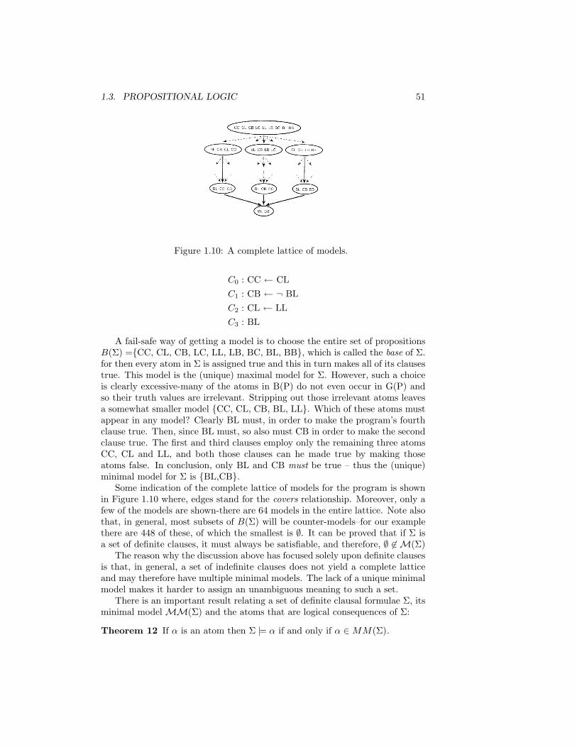
1.3. PROPOSITIONAL LOGIC 51
Figure 1.10: A complete lattice of models.
C0 : CC ← CLC1 : CB ← ¬ BLC2 : CL ← LLC3 : BL
A fail-safe way of getting a model is to choose the entire set of propositionsB(Σ) =CC, CL, CB, LC, LL, LB, BC, BL, BB, which is called the base of Σ.for then every atom in Σ is assigned true and this in turn makes all of its clausestrue. This model is the (unique) maximal model for Σ. However, such a choiceis clearly excessive-many of the atoms in B(P) do not even occur in G(P) andso their truth values are irrelevant. Stripping out those irrelevant atoms leavesa somewhat smaller model CC, CL, CB, BL, LL. Which of these atoms mustappear in any model? Clearly BL must, in order to make the program’s fourthclause true. Then, since BL must, so also must CB in order to make the secondclause true. The first and third clauses employ only the remaining three atomsCC, CL and LL, and both those clauses can he made true by making thoseatoms false. In conclusion, only BL and CB must be true – thus the (unique)minimal model for Σ is BL,CB.
Some indication of the complete lattice of models for the program is shownin Figure 1.10 where, edges stand for the covers relationship. Moreover, only afew of the models are shown-there are 64 models in the entire lattice. Note alsothat, in general, most subsets of B(Σ) will be counter-models–for our examplethere are 448 of these, of which the smallest is ∅. It can be proved that if Σ isa set of definite clauses, it must always be satisfiable, and therefore, ∅ 6∈ M(Σ)
The reason why the discussion above has focused solely upon definite clausesis that, in general, a set of indefinite clauses does not yield a complete latticeand may therefore have multiple minimal models. The lack of a unique minimalmodel makes it harder to assign an unambiguous meaning to such a set.
There is an important result relating a set of definite clausal formulae Σ, itsminimal model MM(Σ) and the atoms that are logical consequences of Σ:
Theorem 12 If α is an atom then Σ |= α if and only if α ∈MM(Σ).

52 CHAPTER 1. SETS, RELATIONS AND LOGIC
The proof of theorem 12 makes use of the so-called model intersection prop-erty:
Theorem 13 If M1, . . . ,Mn are any models for a definite clause set Σ thentheir intersection is a model of Σ.
Proof: It is easy to show this by induction. For any k < n, let Ik denoteM1 ∩ . . . ∩Mk. Now consider any clause C ∈ Σ:
C : A← B1 ∧ . . . ∧BmWe shall prove that, for all k ≤ n, Ik satisfies C.
1. Base case (k = 1): I1 = M1 and therefore satisfies C.
2. Induction step (1 ≤ k ≤ n): Assume that Mk satisfies C;
if Ik satisfies C then either Bi 6∈ Ik for some ior Bi ∈ Ik for all i, and A ∈ Ik
if Mk+1 satisfies C then either Bi 6∈Mk+1 for some ior Bi ∈Mk+1 for all i, and A ∈Mk+1
it then follows that either Bi 6∈ Ik ∩Mk+1 for some iOR Bi ∈ Ik ∩Mk+1 for all i, and A ∈ Ik ∩Mk+1
And hence Ik+1 satisfies C
Thus for all k ≤ n, Ik satisfies C and-by a similar argument – every otherclause in Σ.
2
We next prove theorem 12 making use of theorem 13.Proof of theore 12: EXERCISE
We will first prove that the intersection I∗ of all the models of Σ is theminimal model MM(Σ), using contradiction as follows:
Suppose I∗ is not the minimal modelthen there must exist some model Mj such that Mj ⊂ I∗
then there must exist some atom q such that q 6∈Mj and q ∈ I∗
but q ∈ I∗ implies that q ∈Mi, for all i, contradicting q ∈Mj
therefore the initial assumption is false.
Using this result it is now easy to prove the relationship between MM(Σ)and any atomic consequence q of Σ:
If Σ |= q then q is true in every model of Σthen q ∈ I∗
then q ∈MM(Σ)
if q ∈MM(Σ) then q is true in every model of Σthen Σ |= q

1.3. PROPOSITIONAL LOGIC 53
2
Thus, the minimal model of a definite clausal formula is identical to the setof all ground atoms logically implied by that formula, which was defined as thesuccess set SS(Σ). Thus, the minimal model provides, in effect, the meaning(or semantics) of the formula. We shall see later that this is just one of severalways of giving significance to a program’s minimal model.
We can envisage a procedure for enumerating the models of a formula. Con-sider the powerset of the base B(Σ). Now, we know that this powerset orderedby ⊆ necessarily forms a complete lattice, with binary operations ∩ and ∪.Some subset of this powerset is the set of all models, which we know is also alattice ordered by ⊆ with the same binary operations. So, the model lattice isa sublattice of the lattice obtained from the powerset of the base. Suppose nowwe start at some point s in this sublattice, and we move to a new point thatconsists only of those atoms of the formula made true by the model s. Let uscall these atoms s1. Then, a little thought should convince you that s1 is alsoa member of the sublattice of models. Repeating the process with s2 we canmove to models s2, s3 and so on. Will this procedure converge eventually on theminimal model? Not necessarily, since we could end up moving back-and-forthbetween points of the sub-lattice. (When will this happen, and how can weensure that we do converge on the minimal model?).
A slightly more general process can be formalised as the application of afunction TΣ that, for a set of clauses Σ, generates an interpretation (not neces-sarily a model) from another. That is:
Ik+1 = TΣ(Ik)
whereTΣ(I) = a : a← body ∈ Σ and body ∈ I
It can be shown that TΣ is both monotonic and continuous on the completelattice obtained by ordering the powerset of the base by ⊆. So, we know fromthe Knaster-Tarski Theorem mentioned on page 11, that there must be a leastfixpoint for TΣ in this lattice. We can prove that the procedure of obtainingIk+1 from application of TΣ to Ik will yield that fixpoint, and further, that thisfixpoint will be the minimal model.
Theorem 14 MM(Σ) is the least fixpoint of TΣ.
Proof: The definition of TΣ requires thatfor all I ⊆ B(Σ) and for all q, q ∈ TΣ(I) iff (∃body)[(q ← body) ∈ Σ and body ∈
I]whereas, the definition of a model requires thatfor all I ⊆ B(Σ), I is a model for Σ iff for all q, q ∈ I if (∃body)[(q ← body) ∈
Σ and body ∈ I].These two sentences jointly imply

54 CHAPTER 1. SETS, RELATIONS AND LOGIC
for all I ⊆ B(Σ)I is a model for Σ iff for all q, q ∈ I if q ∈ TΣ(I)
iff TΣ(I) ⊆ Iiff I is a pre-fixpoint of TΣ
Where, for a function f on < S,>, an element u ∈ S is a pre-fixpoint of f ifand only if f(u) u. Then, we can recall from the proof of the Knaster-Tarskitheorem on page 11 that the least fix point is also the least pre-fixpoint. Hence,since the models are exactly the pre-fixpoints, the least model MM(Σ), whichis the glb of all the pre-fix points, must be the least pre-fixpoint. Finally, bythe Knaster-Tarski theorem, MM(Σ) must also be the least fixpoint. 2
So we now have several equivalent characterizations of the minimal model,including the success set SS(Σ) and the new one posed in terms of the leastfixpoint of TΣ, denoted LFP (TΣ)
Mathematical Characterization of Finite Failure
It so happens that there is a somewhat related (to the TΣ function) methodof constructing the finite failure set FF (Σ). The set of atoms which occur asheadings in Σ is simply TΣ(B(Σ)), as is plain from the definition of TΣ. Thesimplest way for ?q to fail finitely is for there to be no clause in Σ who headingunifies with q. In this case the failure is said to occur within depth k = 1 and theset of all such atoms q ∈ B(Σ) is denoted by FF (Σ, 1) and can be characterizedvery easily using the TΣ function as
FF (Σ, 1) = B(Σ)− TΣ(B(Σ))
Generalizing this principle, FF (Σ) just contains each atom q for which ?qfinitely fails within some depth k ∈ N .
FF (Σ) = ∪k∈NFF (Σ, k) = B(Σ)− ∩k∈NT kΣ(B(Σ))
When we start at the top element B(Σ) of our lattice of interpretations,repeated application of the TΣ function generates a monotonically decreasingsequence B(Σ) ⊇ TΣ(B(Σ)) ⊇ T 2
Σ(B(Σ)) . . ., whose limit is the greatest lowerbound (glb) TΣ ↓ of
T kΣ(B(Σ)) | k ∈ N
. Thus, the mathematical characteri-
zation of FF (Σ) (independent of the execution mechanism) is
FF (Σ) = B(Σ)− TΣ ↓
Based on this equivalence, what is the value of FF (Σ) for the last example thatwe discussed?
It can be proved that TΣ ↑= LFP (TΣ) = MM(Σ) ⊆ TΣ ↓. There is anassymetry in the relationship between the limits and the extremal fixpointsof TΣ. Whereas, TΣ ↑ is always equal to the least fix point LFP (TΣ), TΣ ↓does not always equal the greatest fix point GFP (TΣ), though it does holdfor most ‘sensible’ Σ (at the least for non-recursive clauses and in the case of

1.4. FIRST-ORDER LOGIC 55
first order logic, for function-free programs). The region between TΣ ↑ and TΣ ↓corresponds to IF (Σ), which comprises exactly those atoms which fail infinitely.In practice, most sensible programs have IF (Σ) = ∅, leading to TΣ ↑= TΣ ↓ andtherefore B(Σ) = SS(Σ) ∪ FF (Σ).
1.4 First-Order Logic
Suppose you wanted to express logically the statement: ‘All humans are apes.’One of two ways can be used to formalise this in propositional logic. We can usea single proposition that stands for the entire statement, or with a well-formedformula consisting of a lot of conjunctions: Human1 is an ape ∧ Human2 is anape . . .. Using a single proposition does not give any indication of the structureinherent in the statement (that, for example, it is a statement about two setsof objects—humans and apes—one of which is entirely contained in the other).The conjunctive expression is clearly tedious in a world with a lot of humans.Things can get worse. Consider the following argument:
Some animals are humans.
All humans are apes.
Therefore some animals are apes.
That the argument is valid is evident: yet it is beyond the power of proposi-tional logic to establish it. If, for example, we elected to represent each of thestatements with single propositions then all we would end up with is:
Statement Formally
Some animals are humans. P
All humans are apes. Q
Therefore some animals are apes. ∴ R
But the formal argument is clearly invalid, as it is easy to think up argumentswhere P,Q are true and R is false. What is needed is in fact something alongthe following lines:
Statement Formally
Some animals are humans. Some P are Q
All humans are apes. All Q are R
Therefore some animals are apes. ∴ some P are R
Here, P,Q, and R do not stand for propositions, but for terms like animals,humans and apes. The use of terms like these related to each other by theexpressions ‘some’ and ‘all’ will allow us to form sentences like the following:

56 CHAPTER 1. SETS, RELATIONS AND LOGIC
All P are Q
No P are Q
Some P are Q
Some P are not Q
The expressions ‘some’ and ‘all’ are called quantifiers, which when combinedwith the logical connectives introduced in connection with proposition logic(¬,∧,∨,←), results in the powerful framework of first-order or predicate logic.
1.4.1 Syntax
The language of predicate logic introduces many new constructs that are notfound in the simpler, propositional case. We will first introduce these informally.
Constants. It is conventional in predicate logic to use lowercase letters to denoteproper names of objects. For example, in the sentence ‘Fred is human’, Fredcould be represented as fred.
Variables. Consider the statements:
All humans are apes
Some apes are not human
Using the letter x as a variable that can stand for individual objects, these canbe expressed as:
For all x, if x is human then x is an ape
For some x, x is an ape and x is not human
Quantifiers. The language of predicate logic introduces the symbol ∀, calledthe universal quantifier , to denote ‘for all.’ The symbol ∃, called the existentialquantifier , is used to denote ‘for some’ or, more precisely, ‘for at least one.’ Thesentences above can therefore be written as:
∀x (if x is human then x is an ape)
∃x (x is an ape and x is not human)
Predicates. In their simplest case, these are are symbols used to attribute prop-erties to particular objects. It is conventional in logic (but ungrammatical inEnglish) to write the subject after the predicate. Thus the sentence ‘Fred ishuman’ would be formalised as Human(fred) 22. More generally, predicatesymbols can be used to represent relations between two or more objects. Thus,
22Logicians are a parsimonius lot: they would represent ‘Fred is human’ as Hf . Therepresentation here is non-standard, but preferred for clarity.

1.4. FIRST-ORDER LOGIC 57
‘Fred likes bananas’ can be represented as: Likes(fred, bananas). The gen-eral form is therefore a predicate symbol, followed by one or more argumentsseparated by commas and enclosed by brackets. The number of arguments issometimes called the arity of the predicate symbol, and the predicate symbol isoften written along with its arity (for example, Likes/2). Formalising sentenceslike those above would result in quantified variables being arguments:
∀x (if Human(x) then Ape(x))
∃x (Ape(x) and not Human(x))
Or, using the logical connectives that we have already come across:
∀x(Ape(x)← Human(x))∃x(Ape(x) ∧ ¬Human(x))
Functions. Consider the statement: ‘The father of Fred is human.’ Although wehave not named Fred’s father, it is evident that a a unique individual is beingreferred to, and it possible to denote him by using a function symbol. One wayto formalise the statement is: Human(father(fred)). Here, it is understoodthat father(fred) denotes Fred’s father. A function symbol is one which, whenattached to one or more terms denoting objects produces an expression thatdenotes a single object. It is important that that the result is unique: a functionsymbol could not be used to represent, for example, ‘parent of Fred.’ As withpredicates, the number of arguments of the function is sometimes called its arity.
The following points would not be evident from this informal presentation:
1. Variables need not designate different objects. Thus, in ∀x∀yLikes(x, y),x and y could refer to the same object;
2. The choice of variable names is unimportant. Thus, ∀x∀yLikes(x, y) hasthe same meaning as ∀y∀zLikes(y, z);
3. The same variable name, if quantified differently, need not designate thesame object. Thus, in ∀x∀yLikes(x, y) ∧ ∀x∀yHates(y, x) the x, y inLikes(· · · ) need not be same as the x, y in Hates(· · · );
4. The order of quantifiers can matter when ∀ and ∃ are mixed. Thus,∃x∀yLikes(x, y) has a different meaning to ∀y∃xLikes(x, y). Howeverchanging the order has no effect if the quantifiers are all of the same type.Thus, ∀x∀yLikes(x, y) has the same meaning as ∀y∀xLikes(x, y);
5. “Free” variables in a formula are those that are not quantified. For ex-ample, in the formula ∀xLikes(x, y), y is a free variable. In contrast,quantified variables are called “bound” variables. It may not be immedi-ately apparent that a variable can have both free and bound occurrencesin a formula. For example in ∃x(Likes(x, y)∧∃yDisLikes(y, x)), the vari-able y is free in the Likes and bound in Dislikes. x on the other hand is

58 CHAPTER 1. SETS, RELATIONS AND LOGIC
bound in both (by the outermost quantifier). It is normal to call a formulawith no free variables a sentence, and it only really makes sense to askabout the truth of sentences;
6. Negation should be treated with caution. Thus, in ‘Some apes are nothumans’, ‘not’ plays the role of complementation, by stating that the setof apes and the set of non-humans have at least one member in common.This can be formalised as ∃x(Ape(x)∧¬Human(x)). One the other hand,‘not’ plays the role of true negation in ‘It is not true that some apes arehumans’ formalised as ¬∃x(Ape(x) ∧Human(x));
7. It can be tricky to match English sentences to ones that use ∀ and ∃.Thus, in ‘If something has a tail then it is not an ape’, the use of ‘some-thing’ suggests that formalisation would involve ∃. The statement is, infact, a general one about apes not having tails, and involves universalquantification: ∀x(¬Ape(x)← Tail(x));
8. By denoting ‘at least one’, the existential quantifier ∃ includes ‘exactly one’and ‘all’. This does not coincide exactly with the usual English notion of‘some’, which denotes more than one, but less than all.
We can now examine the formal rules for constructing well-formed formulæin predicate logic. For the language of predicate logic, we will restrict thevocabulary to the following:
Constant symbols: A string of one or more lowercase letters(except those denoting variables)
Variable symbols: A lowercase letter(except those denoting constants)
Predicate symbols: Uppercase letter, followed by zero or more letters
Function symbols: Lowercase letter, followed by zero or more letters(except those denoting constants or variables)
Quantifier symbols: ∀, ∃
Logical connectives: ¬,∧,∨,←
Brackets: (, )
In addition, we will sometimes employ the device of using subscripts to denoteunique symbols (for example, x1, x2, . . . for a string of variables).
With this vocabulary, a term is simply a constant, variable or a functionalexpression (that is, a function applied to a tuple of terms). The following are allexamples of terms: x, fred, father(fred), father(father(fred)), father(x).

1.4. FIRST-ORDER LOGIC 59
These, however, are not terms: Likes(fred, bananas), Likes(fred, father(fred)),father(Likes(fred, bananas)). An atomic formula, sometimes simply called anatom is a predicate symbol applied to a tuple of terms. Thus, Likes(fred, bananas)Likes(fred, father(fred)), Likes(x, father(x)) are all examples of atoms. Fi-nally, a ground atomic formula or a ground atom is an atom without any vari-ables. Well-formed formulæ (wffs) are then formed using the following rules:
1. Any ground atomic formula is a wff;
2. If α is a wff then ¬α is a wff;
3. If α and β are wffs then (α ∧ β), (α ∨ β), and (α← β) are wffs; and
4. If α is wff containing a constant c and αc/x be the result of replacing oneor more occurences of c with a variable x that does not appear in α. Then∀xαc/x and ∃xαc/x are wffs.
Rules 1–3 are like their propositional counterparts (page 15). Rule 4 is new,and requires further explanation. It is the only way variables are introducedinto a formula. As an example, take the following statement: (Human(fred)∧Likes(fred, bananas)). That this a wff follows from an application of Rules 1and 3. The following formulæ are all wffs, following a single application of Rule4:
∀x(Human(x) ∧ Likes(fred, bananas))∃x(Human(x) ∧ Likes(fred, bananas))
∀x(Human(fred) ∧ Likes(x, bananas))∃x(Human(fred) ∧ Likes(x, bananas))
∀x(Human(x) ∧ Likes(x, bananas))∃x(Human(x) ∧ Likes(x, bananas))
∀x(Human(fred) ∧ Likes(fred, x))∃x(Human(fred) ∧ Likes(fred, x))
A single application of Rule 4 therefore only introduces a single new variable.Subsequent applications will introduce more. For example, take the first formulaabove: ∀x(Human(x) ∧ Likes(fred, bananas)). The following wffs all resultfrom applying Rule 4 to this statement:
∀y∀x(Human(x) ∧ Likes(y, bananas))∃y∀x(Human(x) ∧ Likes(y, bananas))
∀y∀x(Human(x) ∧ Likes(fred, y))∃y∀x(Human(x) ∧ Likes(fred, y))

60 CHAPTER 1. SETS, RELATIONS AND LOGIC
As with propositional logic, it is acceptable to drop outermost brackets:
(∀x(Ape(x)← Human(x)) ∧ ∃x(Ape(x) ∧ ¬Human(x)))
can be written as:
∀x(Ape(x)← Human(x)) ∧ ∃x(Ape(x) ∧ ¬Human(x))
Clausal Form
We are now in a position to expand on the notion of clauses and literals, firstintroduced on page 25. Consider the conditional statement:
∀x(Ape(x)← Human(x))
Recall the following from page 24:
(α← β) ≡ (α ∨ ¬β)
This means:
∀x(Ape(x)← (Human(x))) ≡ ∀x(Ape(x) ∨ ¬Human(x))
The term in brackets on right-hand side is an example of a clause in first-orderlogic. In general, formulæ consisting of universally-quantified clauses all lookalike:23
∀x1∀x2 . . . (α1 ∧ α2 . . .)
That is, they consist of a prefix that consists only of universally quantifiers, andeach αi, or clause, is a quantifier-free formula that looks like:
αi = (β1 ∨ β2 ∨ . . . βn)
where each βj , or literal . Thus, as in propositional logic, a clause is a disjunctionof literals. Each literal, however, is not a proposition, but is either an atomicformula (like Ape(x), sometimes called a positive literal) or a negated atomicformula (like ¬Human(x), sometimes called a negative literal). It is sometimesconvenient to use ∀x to denote ∀x1∀x2 · · · and to adopt a set-based notationto represent a clausal formula: ∀xα1,∀xα2, . . .. Here it is understood thatthe formula stands for a conjunction of clauses. Often, the quantification istaken to be understood and left out. Further, individual clauses are themselvessometimes written as sets of literals:
αi = β1, β2, . . . , βn
Clausal forms are of particular interest, computationally speaking. The lan-guage of logic programs (usually written in the Prolog language). is, at least inits ‘pure’ form, equivalent to clausal-form logic. Here is an example:
23We will take a few liberties here by not including some brackets.

1.4. FIRST-ORDER LOGIC 61
Logic Program in Prolog Clausal Form
grandfather(X,Y):- ∀x∀y∀z(Grandfather(x, y) ∨father(X,Z), ¬Father(x, z) ∨parent(Z,Y). ¬Parent(z, y)),
father(henry,jane). Father(henry, jane),
parent(jane,john). Parent(jane, john)
There are three clauses in this example. The first clause has three literalsand the remainder have one literal each. Further, each clause has exactly onepositive literal: such clauses are called definite clauses. More generally, clausesthat contain at most one positive literal are called Horn clauses. From now on,we may sometimes write clauses in a lazy manner that is somewhere in betweenthe syntax of Prolog and the true clausal form:
Logic Program in Prolog
grandfather(X,Y):- father(X,Z), parent(Z,Y).
Clausal Form
∀x∀y∀z(Grandfather(x, y) ∨ ¬Father(x, z) ∨ ¬Parent(z, y))
Lazy Clausal Form
Grandfather(x, y)← Father(x, z), Parent(z, y)
Skolem Functions and Constants
Skolemization refers to a process of replacing an existentially quantified variablein a formula by a new term; it is merely the process of providing a name forsomething that already exists. Whether the new term is a functional expressionor a constant depends on where the existential quantifier appears in the formula.If it is preceded by one or more universal quantifiers, like:
∀x1 . . . ∀xn∃y αthen a single skolemization step replaces all occurences of y in α by the functionalexpression f(x1, . . . , xn). Here f(· · · ) is a function symbol, called a Skolemfunction, that does not appear anywhere in the formula. Thus, skolemizationof the formula ∀x∃yLikes(x, y) results in ∀xLikes(x, f(x)). In general, if theexistential quantifier appears in between some universal quantifiers:
∀x1 . . . ∀xi−1∃y∀xi+1 · · · ∀xn αthen all occurences of y in α can be replaced by the functional expressionf(x1, . . . , xi−1). A special case arises if the existential quantifier precedes zeroor more universal quantifiers:

62 CHAPTER 1. SETS, RELATIONS AND LOGIC
∃y∀x1 . . . ∀xn α
In this case, a single skolemization step replaces all occurences of y in α by aSkolem function of arity 0 (that is, a constant) c. Here c is a constant symbol,called a Skolem constant , that does not appear anywhere in the formula. Thus,skolemization of the formula ∃y∀xLikes(x, y) results in ∀xLikes(x, c). You cansee that in both cases, a single step of Skolemization reduces the number ofexistential quantifiers in a formula φ by 1. Let us denote this single step bys(φ). It should be easy to see that repeatedly performing Skolemization steps(that is, s(s(· · · s(φ)))) will result in a formula with just universal quantifiers.
Normal Forms
Universally-quantified clausal forms are a special case of specific kind of normalform for first-order formula, which we are now able to present, having describedthe process of Skolemization. A formula is said to be in prenex normal form orPNF if all its quantifiers are in front. That is, the formula looks something likeQ1x1 . . . Qnxnφ, where the Qi is either a ∀ or ∃. Further, if φ is a conjunction ofdisjunction of literals, then the formula is said to be in conjunctive prenex normalform. It can be shown that every first-order formula φ can be expressed by anequivalent one φ′ in conjunctive PNF. Here is an example: suppose we want tofind the conjunctive PNF for φ : (∃x∀yDisLikes(x, y) ∧ ∀x∃yLikes(x, y)). Wefirst rename variables to give φ′ : (∃x∀yDisLikes(x, y) ∧ ∀u∃vLikes(u, v)). Wecan then move the quantifiers to the left giving: φ′′ : ∃x∀y∀u∃v(DisLikes(x, y)∧Likes(u, v)), which is in conjunctive PNF.
For reasons that will become apparent, we are further interested here onlyin formulae in conjunctive PNFs in which all the quantifiers are universal ones(that is, ∀). Such formulæare said to be in Skolem normal form, or SNF. ASNF can be obtained from the conjunctive PNF by applying the Skolemizationprocess to eliminate ∃ quantifiers. For example, suppose we want to “Skolemize”the formula φ above. We first find the conjunctive PNF (φ′′ above). Using theSkolemization procedure described earlier, we replace x by a Skolem constantand v by a Skolem function. The SNF of φ is φS : ∀y∀u(Dislikes(c, y) ∧Likes(u, f(u))).
We can now return to clausal forms. Here are the steps for converting aformula into a set of clauses in clausal form:
1. Rename variables to ensure there are no variables with the same names indifferent quantifiers;
2. Eliminate ←’s and iff’s;
• α1 iff α2 ⇒ (α1 ← α2) ∧ (α2 ← α1)
• α1 ← α2 ⇒ α1 ∨ ¬α2
3. Move ¬’s inwards;

1.4. FIRST-ORDER LOGIC 63
• ¬(∃X)α⇒ (∀X)¬α• ¬(∀X)α⇒ (∃X)¬α• ¬(α1 ∨ α2)⇒ ¬α1 ∧ ¬α2
• ¬(α1 ∧ α2)⇒ ¬α1 ∨ ¬α2
• ¬¬α⇒ α
4. Distribute ∨’s over ∧’s;
• α ∨ (α1 ∧ α2)⇒ (α ∨ α1) ∧ (α ∨ α2)
• Assuming X does not occur in α1: α1 ∨ (∀α2)⇒ (∀X)(α1 ∨ α2)
• Assuming X does not occur in α1: α1 ∨ (∃α2)⇒ (∃X)(α1 ∨ α2)
5. Distribute ∀’s;
• (∀X)(α1 ∧ α2)⇒ (∀X)α1 ∧ (∀X)α2
At this stage, the PNF form is generated.
6. Skolemise existentially quantified variables;
• (∀X1)(∀X2) . . . (∀Xn)(∃Y )α(Y )⇒ (∀X1)(∀X2) . . . (∀Xn)α(f(X1, X2, . . . Xn))
If further applications of step 6 are possible, then they should be carriedout.
7. Rewrite as clauses by dropping universal quantifiers; and
8. Standardise variables apart.
Here are some statements from a book by Lewis Carroll, written in first-orderlogic:
S1 : ∀x(Scented(x)← Coloured(x)) ∧
S2 : ∀x(DisLike(x)← ¬GrownOpen(x)) ∧
S3 : ¬(∃x(GrownOpen(x) ∧ ¬Coloured(x))) ∧
S4 : ¬∀x((DisLike(x)← ¬Scented(x)))
You should find that these sentences, when converted by the steps above,give the following set of clauses:
C1 : ¬Coloured(x), Scented(x)
C2 : GrownOpen(y), DisLike(y)
C3 : ¬GrownOpen(z), Coloured(z)
C4 : ¬Scented(c)

64 CHAPTER 1. SETS, RELATIONS AND LOGIC
C5 : ¬DisLike(c)
Recall that representing a clause by a set L1, L2, . . . , Lk, is just short-formfor the disjunction L1 ∨L2∨ · · ·Lk; and the actual clausal form for the formulaF : S1∧S2∧S3∧S4∧S5 is C : ∀x∀y∀z(C1∧C2∧C3∧C4∧C5). Is F equivalentto C? To answer this, we need to understand how meanings are assigned tofirst-order formulæ.24
1.4.2 Semantics
As with propositional logic, the semantics of predicate logic is primarily con-cerned with interpretations, models, and logical consequence. Of these, it isonly the notion of interpretation that requires a re-examination.
Interpretations
Recall that interpretations in propositional logic were simply assignments oftrue or false to propositional symbols. Matters are not as simple in predicatelogic for two reasons. First, we have to deal with the additional complexity ofexpressions arising from a richer vocabulary. Thus, the truth-value (meaning)of Likes(fred, bananas) will depend on the meanings of each of the symbolsLikes, fred and bananas. Second, we have to interpret sentences that containquantifiers.
Informally, let us see what is required in constructing an interpretation thatallows us to understand Likes(fred, bananas). Before we begin, remove anypre-conceptions of what the words in the statement mean in English: for us theyare simply a predicate symbol (Likes) and two constant symbols (fred, bananas)in some ‘formal-world’. The first step then is to identify a domain of objects inthe ‘real-world’.
Next, we associate constant symbols in our formal-world to objects in thereal-world (just to avoid any pre-conceptions, we have scrambled things a littlebit):
24But the answer is “no”: the problem, as you might have guessed, comes about because ofthe Skolemization step.

1.4. FIRST-ORDER LOGIC 65
bananas
fred
and associate the predicate symbols to a relation in the real-world:
Likes
We can now see that Likes(fred, bananas) is false as the objects correspond-ing to the ordered pair < fred, bananas > are not in the real-world relationrepresented by Likes.
Formally, an interpretation in predicate logic is a specification of:
1. A domain D;
2. A mapping of constants to elements in D;
3. A mapping of each n-argument predicate symbol to a relation on Dn,where Dn = < d1, . . . , dn > | di ∈ D is the n-fold Cartesian product;and
4. A mapping of each n-argument function symbol to a function from Dn →D
You will also see sometimes that the term “structure” is used to describe whatwe have called an interpretation. In such cases, a distinction is made betweenthe vocabulary , which consists of the constants, functions and predicate symbols;the and the structure, which consists of the domain D and the three mappings.We will continue to use “interpretation” to retain a similarity to propositionallogic.

66 CHAPTER 1. SETS, RELATIONS AND LOGIC
Given an interpretation, every atom—a predicate symbol with a tuple ofterms as arguments—is assigned a truth-value according to whether the objectsdesignated by the arguments are in the relation designated by the predicatesymbol.
Well-formed formulæ in predicate logic consist of more than atoms. Wealso need rules for assigning truth-values to formulæ that contain logical con-nectives (¬,∧,∨,←) and quantifiers (∀,∃). The semantics of the logical con-nectives in predicate logic are the same as those in propositional logic. Thus,as before, assigning meanings to formulæ with these connectives requires theuse of the truth tables on page 17. For example, the formula Human(fred) ∧Likes(fred, bananas) is true only if the interpretation results in both the atomsHuman(fred) and Likes(fred, bananas) being true. What though, of formulæthat contain quantified variables? The rules for these are:
1. Any wff ∀xα is true if and only if for every domain element that we canassociate with x, α is true;
2. Any wff ∃xα is true if and only if for some domain element that we canassociate with x, α is true.
Models and Logical Consequence
The meanings of these, and related concepts, are unchanged from propositionallogic. Thus:
Models. Any interpretation that makes a wff true is called a model for thatformula;
Validity and Unsatisfiability. A formula for which all interpretations are modelsis said to be valid. A formula for which none of the interpretations are amodel is said to be unsatisfiable. A formula that has at least one modelis said to be satisfiable;
Consequence. Given a conjunction of wffs Σ represented as the set β1, . . . , βnand a wff α if Σ |= α then every model for Σ is a model for α;
Deduction Theorem. Given a conjunction of wffs Σ = β1, . . . , βn and a wff α,Σ |= α if and only if Σ− βi |= (α← βi). The proof is the same as wasfor that in the propositional case (c.f. theorem 6);
Equivalence. Given a pair of wffs α and β, if α |= β and β |= α then α and βare equivalent (α ≡ β).
The following relations hold in the predicate logic (as usual, α, β are wffs):

1.4. FIRST-ORDER LOGIC 67
¬(α ∨ β) ≡ ¬α ∧ ¬β De Morgan’s law¬(α ∧ β) ≡ ¬α ∨ ¬β De Morgan’s law(α← β) ≡ (α ∨ ¬β)(α← β) ≡ (¬β ← ¬α) Conditional ≡ Contrapositive¬∀xα ≡ ∃x¬α¬∃xα ≡ ∀x¬α∀xα ≡ ∀yαx/y Renaming of x by y∃xα ≡ ∃yαx/y Renaming of x by y∀x∀yα ≡ ∀y∀xα∃x∃yα ≡ ∃y∃xα∀x(α ∧ β) ≡ (∀xα ∧ ∀xβ) Distributivity of ∀∃x(α ∨ β) ≡ (∃xα ∨ ∃xβ) Distributivity of ∃∀xα |= ∃xα(∀xα ∨ ∀xβ) |= ∀x(α ∨ β)∃x(α ∧ β) |= (∃x ∧ ∃xβ)∀xαy/f(x) |= ∀x∃yα Non-equivalence of Skolemized form∀xαy/c |= ∃y∀xα Non-equivalence of of Skolemized form
More on Normal Forms
We stated earlier that any first-order formula could be converted to a conjunctiveprenex normal form, or conjunctive PNF. We further saw how a formula φ =Q1x1 . . . Qnxnφ0(x1, . . . , xn) could be “Skolemized” to give a formula φS inSkolem Normal Form, or SNF. The interest in SNFs lies in the following fact:
Theorem 15 φ is satisfiable if and only if φS is satisfiable (you should be ableto convince yourself that checking for satisfiability is equivalent to checking forlogical consequence).
Proof sketch: Recall that φS = s(s(· · · s(φ))) where s(·) denotes a single step ofSkolemization. Now, it is sufficient to show that φ is satisfiable if and only ifs(φ) is satisfiable (the full proof will follow by induction). We can also assumethat φ is in conjunctive PNF. Now s(φ) results in either replacing a variable bya Skolem constant or by a Skolem function. Since the former is just a specialcase of the latter, we will just consider the case when s(φ) results in replacinga variable by a Skolem function. Let Qi be the existential quantifier removedby the Skolemization step, and let ψ(x1, . . . , xi) = Qi+1 . . . Qnφ0(x1, . . . , xn).Suppose ∀x1 . . . ∀xi−1∃xiψ(x1, . . . , xi) has some model M . Let Mf extend M byinterpreting f in such a way that Mf is a model for ψ(c1, . . . , ci−1, f(c1, . . . , ci−1))for all possible values c1, . . . , ci−1 ∈ M for the variables x1, . . . , xi−1. Then,clearly, Mf is a model for ∀x1 . . . ∀xi−1ψ(x1, . . . , xi−1, f(x1, . . . , xi−1)). Now

68 CHAPTER 1. SETS, RELATIONS AND LOGIC
consider the converse. Suppose ∀x1 . . . ∀xi−1ψ(x1, . . . , xi−1, f(x1, . . . , xi−1)) hassome model M then, it follows from the meaning of ∃ that M is also a modelfor ∀x1 . . . ∀xi−1∃xiψ(x1, . . . , xi). It follows therefore that φ is satisfiable if andonly if s(φ) is satisfiable. 2
We end this section on a note of caution: φ and s(φ) are not equivalent.That is, Skolemization does not preserve logical equivalence. A simple exampleshould convince you of this. Let φ = ∃xFirst(x) and s(φ) = First(c). Clearly,we can find models for ∃First(x) that are not models of First(c).
Herbrand Interpretations
The 4-step specification above makes an interpretation in predicate logic muchmore elaborate than its counterpart in propositional logic (which was simplyan assignment of true or false to propositions). The reference to ‘real-world’objects, relations, and functions adds a further degree of complexity: how is allthis to be conveyed to an automated procedure? In fact, many of these problemscan be side-stepped by confining attention only to a domain that consists solelyof formal symbols. Called the Herbrand universe (UL), this is simply all theground (or variable-free) terms that can be constructed using the constants andfunction symbols available in a first order language L. Consider as example alanguage that consists of:
Constant symbol: zero
Predicate symbol: Nat/1Function symbols: pred, succ
The Herbrand universe UL in this instance consists of terms like zero, pred(zero),succ(zero), pred(succ(zero)), succ(pred(zero)) and so on. The Herbrand baseBL is the set of all ground atoms that can be constructed using the predicatesymbols and terms from the Herbrand universe UL. Here, the Herbrand base BLconsists of atoms likeNat(zero), Nat(pred(zero)), Nat(succ(zero)), Nat(pred(succ(zero)))and so on. A Herbrand interpretation IL is—quite like the propositional case—simply an assignment of true to some subset of BL and false to the rest. In fact,it is common practice to associate ‘Herbrand interpretation’ only with the sub-set assigned true: it being understood that all other atoms in the Herbrand baseare assigned false. Thus, Nat(zero) is an IL that assigns true to Nat(zero)and false to all other atoms in BL.
Herbrand Models
Since a model is an interpretation that makes a well-formed formula true, aHerbrand model ML is simply a Herbrand interpretation IL that makes a well-formed formula true. Let us return to the example presented earlier:
Constant symbol: zero
Predicate symbol: Nat/1Function symbols: pred, succ

1.4. FIRST-ORDER LOGIC 69
Recall from page 68, that:
Herbrand universe (UL): zero, pred(zero), succ(zero), pred(succ(zero)), . . .Herbrand base (BL): Nat(zero), Nat(pred(zero)), Nat(succ(zero)), . . .
Further, a Herbrand interpretation is simply a subset of the Herbrand basecontaining all atoms that are true. Thus, I1 = Nat(zero) is a Herbrandinterpretation in which Nat(zero) is true and all other atoms in the Herbrandbase are are false. We can now examine whether I1 is a Herbrand model for theformula:
Σ1 : Nat(zero) ∧ ∀x(Nat(succ(x))← Nat(x))
Being a conjunctive expression, we require I1 to be a Herbrand model for bothNat(zero) and ∀x(Nat(succ(x))← Nat(x)). I1 is clearly a model for Nat(zero)as this atom is assigned true in the interpretation. But what about the condi-tional? The rule for the universal quantifier (page 66) dictates that the condi-tional statement is true if it is true for every element that the variable x can beassociated with. In other words, the interpretation is a model for every elementthat x can be associated with. In the Herbrand world, x can be associated withany element of the Herbrand universe (zero, succ(zero), pred(zero) and so on).Suppose x was associated with zero. Then we would require I1 to be a model forNat(succ(zero)) ← Nat(zero). Since I1 assigns Nat(succ(zero)) to false andNat(zero) to true, I1 is not a model for Nat(succ(zero)) ← Nat(zero) (line 2in the truth-table for the conditional on page 17). Thus, I1 is not a Herbrandmodel for ∀x(Nat(succ(x)) ← Nat(x)) and in turn for Σ1. Consider, on theother hand, the formula:
Σ2 : Nat(zero) ∧ ∀x(Nat(x)← Nat(pred(x)))
As before, suppose x was associated with zero. The conditional then becomesNat(zero) ← Nat(pred(zero)). With interpretation I1, Nat(zero) is true andNat(pred(zero)) is false. I1 is therefore a model for this formula (line 3 in thetruth table for the conditional). All other associations for x result in both sidesof the conditional being false and I1 being a model for each such formula (line 1in the truth table). Thus, I1 makes ∀x(Nat(x)← Nat(pred(x))) true for everyelement that x can be associated with, and is a model for it and in turn for Σ2.
Herbrand models are particularly relevant to the study of clausal forms(page 60). Recall that these are conjunctions of clauses, each of which containsonly universally quantified variables and consists of a disjunction of literals.Both Σ1 and Σ2 above can be written in clausal form:
Σ1′ : Nat(zero) ∧ ∀x(Nat(succ(x)) ∨ ¬Nat(x))
Σ2′ : Nat(zero) ∧ ∀x(Nat(x) ∨ ¬Nat(pred(x)))

70 CHAPTER 1. SETS, RELATIONS AND LOGIC
The ground instantiation of a clausal formula is the conjunction of ground(variable-free) clauses that result by replacing variables with terms from theHerbrand universe. For example, the ground instantiation of Σ2
′ is:
G(Σ2′) : Nat(zero) ∧
(Nat(zero) ∨ ¬Nat(pred(zero))) ∧(Nat(pred(zero)) ∨ ¬Nat(pred(pred(zero)))) ∧(Nat(succ(zero)) ∨ ¬Nat(pred(succ(zero)))) ∧. . .
You can therefore think of the ground instantantiation as making explicit themeaning of the universal quantifier ∀. Now, it should be clear that a Herbrandinterpretation will determine the truth-value for all clauses in the ground in-stantiation of a clausal formula.
We present another example illustrating Herbrand models. Consider thefollowing program P :
likes(john,X) ← likes(X, apples)
likes(mary, apples) ←
Suppose the language L contained no symbols other than those in P . Then,B(P ) is the set likes(john, john), likes(john, apples), likes(apples, john), likes(john,mary),likes(mary, john), likes(mary, apples), likes(apples,mary), likes(mary,mary),likes(apples, apples). Now, likes(mary, apples), likes(john,mary) is a sub-set of B(P ), and is a Herbrand interpretation. Moreover, it is also a Herbrandmodel for P . Similarly, likes(mary, apples), likes(john,mary), likes(mary, john)is also a model for P . The ground instantiation G(P ) for this program is:
likes(john, john) ← likes(john, apples)
likes(john,mary) ← likes(mary, apples)
likes(john, apples) ← likes(apples, apples)
likes(mary, apples) ←
It can be verified25 that the interpretation likes(mary, apples), likes(john,mary)is a model for the G(P ) above.
The importance of Herbrand models for clausal formulæ stems from thefollowing property:
Theorem 16 A clausal formula Σ has a model if and only if its ground instan-tiation G(Σ) has a Herbrand model.
Proof: ⇒: Suppose Σ has a model M . Then we define the following Herbrandinterpretation I as follows. Let P be an n-ary predicate symbol occurring in Σ.Then we define the function IP from UnL to T, F as follows: IP (tl, . . . , tn) = Tif P (t1, ..., tn) is true under M , and IP (t1, ..., tn) = F otherwise. It can easilybe shown that I = ∪P∈ΣIP is a Herbrand model of Σ.⇐: This is obvious (a Herbrand model is a model). 2
25EXERCISE.

1.4. FIRST-ORDER LOGIC 71
In other words, there must be some assignment of truth-values to atomsin the Herbrand base that makes all clauses in Σ true. In the example above,the Herbrand interpretation I1 = Nat(zero) that assigns Nat(zero) to trueand everything else to false, is clearly a model for G(Σ2
′). Therefore, from theproperty stated here, we can say that Σ2
′ has a model.If we are dealing only with a definite clausal formula— a clausal formula in
which all clauses have exactly one positive literal (Σ1′ and Σ2
′ are both of thistype)—then more is known about the Herbrand models of the formula. Recallthat a Herbrand model is nothing more than a set of ground atoms, which whenassigned true, make the formula true.
1.4.3 From Datalog to Prolog
The statement “Any animal that has hair is a mammal” can be written as aclause using monadic predicates (i.e. predicates with arity 1):
∀X is mammal(X) ← has hair(X)
Usually clauses are written without explicit mention of the quantifiers:
is mammal(X) ← has hair(X)
is mammal(X) ← has milk(X)
is bird(X) ← has feathers(X)
. . .
Datalog
Datalog is a subset of the language of first order language; it has all the compo-nents of first order logic (variables, constants and recursion), except functions.A Datalog “expert” system will encode these rules using monadic predicates as:
is mammal(X) :- has hair(X).is mammal(X) :- has milk(X).is bird(X) :- has feathers(X).is bird(X) :- can fly(X), has eggs(X).is carnivore(X) :- is mammal(X), eats meat(X).is carnivore(X) :- has pointed teeth(X), has claws(X), has pointy eyes(X).cheetah(X) :- is carnivore(X), has tawny colour(X), has dark spots(X).tiger(X) :- is carnivore, has tawny colour(X), has black stripes(X).penguin(X) :- is bird(X), cannot fly(X), can swim(X).
Now here are some statements26 particular to animals:
has hair(peter). fat(peter).has green eyes(peter). has tawny colour(peter).eats meat(peter). has black stripes(peter).has milk(bob). eats meat(bob)has tawny colour(bob). has dark spots(bob).can fly(bob).
26EXERCISE: What are the logical consequences of all the clauses?

72 CHAPTER 1. SETS, RELATIONS AND LOGIC
Figure 1.11: Graph representing ‘parent of’ relation.
However, monadic predicates: not expressive enough. While monadic predicateslets us make statements like “Every son has a parent”:
∀X∃Y parent(Y ) ← son(X)
for more complex relationships, we will need predicates of arity > 1. Usually,relationships can be described pictorially by a directed acyclic graph (DAG)as in Figure 1.11 The parent-child relation could also be specified as a set ofordered pairs < X,Y >, or, as a set of definite clauses
parent(tom, jo) ←parent(pam, jo) ←parent(tom, liz) ←parent(pam, liz) ←
Consider the predecessor relation, namely, all ordered tuples < X,Y > s.t.X is an ancestor of Y . This set will include Y ’s parents, Y ’s grandparents, Y ’sgrandparents’ parents, etc.
pred(X, Y ) ← parent(X, Y )pred(X,Z) ← parent(X, Y ), parent(Y, Z)pred(X,Z) ← parent(X, Y 1), parent(Y 1, Y 2), parent(Y 2, Z). . .
As can be seen through this example, variables and constants are not enough:we need recursion:
∀X,Z X is a predecessor of Z if1. X is a parent of Z; or2. X is a parent of some Y , and Y is a predecessor of Z
The predecessor relation is thus
pred(X,Y ) ← parent(X,Y )pred(X,Z) ← parent(X,Y ), pred(Y, Z)
and can be pictorially depicted as in 1.12

1.4. FIRST-ORDER LOGIC 73
Figure 1.12: The predecessor relation.
Prolog = Predicates + Variables + Constants + Functions
Datalog (first order logic without functions) is however not expressive enough.To express arithmetic operations, lists of objects, etc. it is not enough to simplyallow variables and constants as terms. We will also need function symbols assupported in Prolog.
Consider Peano’s postulates for the set of natural numbers N .
1. The constant 0 is in N
2. if X is in N then s(X) is in N
3. There are no other elements in N
4. There is no X in N s.t. s(X) = 0
5. There are no X,Y in N s.t. s(X) = s(Y ) and X 6= Y
We can write a definite clause definition using 1 constant symbol and 1 unaryfunction symbol for enumerating the elements of N :
natural(0) ←natural(s(X)) ← natural(X)
The elements of N can be now generated by asking:
natural(N)?
Prolog also supports lists. Lists are simply collections of objects. For e.g.1, 2, 3 . . . or 1, a, dog, . . .. Lists are defined as follows:
1. The constant nil is a list
2. If X is a term, and Y is a list then .(X,Y ) is a list
So the list 1, 2, 3 is represented as:

74 CHAPTER 1. SETS, RELATIONS AND LOGIC
.(1, .(2, .(3, nil)))
Usually logic programming systems use a “[” “]” notation, in which the constantnil is represented as [] and the list 1, 2, 3 is [1, 2, 3]. In this notation, the symbol| is used to separate a list into a “head” (the elements to the left of the |) anda “tail” (the list to the right of the |). Thus:
List Represented as Values of variables
[1, 2, 3] [X|Y ] X = 1, Y = [2, 3]
[[1, 2], 3] [X|Y ] X = [1, 2], Y = [3]
[1] [X|Y ] X = 1, Y = []
[1|2] [X|Y ] X = 1, Y = 2
[1] [X,Y ]
[1, 2, 3] [X,Y |Z] X = 1, Y = 2, Z = [3]
1.4.4 Lattice of Herbrand Models
The discussion in this section is more or less similar to the discussion in Sec-tion 1.3.8 and the reader is referred to the proofs in that Section for proofs ofmost statements that will be made in this section. The only difference is thatwhile Section 1.3.8, in this section, we will talk about Herbrand models.
For a definite clausal formula, it can be shown that the set H of Herbrandmodels is a complete lattice ordered by set-inclusion (that is, for Herbrandmodels M1,M2 ∈ H, M1 M2 if and only if M1 ⊆M2), and with the binaryoperations of ∩ and ∪ as the glb and lub respectively. Recall that a completelattice has a unique least upper bound and a unique greatest lower bound. Sincewe are really talking about sets that are ordered by set-inclusion, this meansthat there is a a unique smallest one (the size being measured by the number ofelements). This is called the minimal model of the formula, and it can be shownthat this must be the intersection of all Herbrand models for the formula.
In the example above, Σ2′ has several Herband models (Nat(zero) and
Nat(zero), Nat(pred(zero)) are two examples). Of these Nat(zero) is thesmallest, and is the minimal model. There is an important result relating adefinite clausal formula Σ, its minimal model MM(Σ) and the ground atomsthat are logical consequences of Σ:
Theorem 17 If α is a ground atom then Σ |= α if and only if α ∈MM(Σ).
Here MM(·) denotes the minimal model. Thus, the minimal model of a definiteclausal formula is identical to the set of all ground atoms logically implied bythat formula. Thus, the minimal model provides, in effect, denotes the meaning(or semantics) of the formula. The proof of this theorem follows nearly fromtheorem 12 that was proved earlier.
We can envisage a procedure for enumerating the Herbrand models of aformula. Consider the powerset of the Herbrand base of the formula. Now,

1.4. FIRST-ORDER LOGIC 75
we know that this powerset ordered by ⊆ necessarily forms a complete lattice,with binary operations ∩ and ∪. Some subset of this powerset is the set of allHerbrand models, which we know is also a lattice ordered by ⊆ with the samebinary operations. So, the model lattice is a sublattice of the lattice obtainedfrom the powerset of the Herbrand base. Suppose now we start at some points in this sublattice, and we move to a new point that consists only of thoseground atoms of the formula made true by the model s. Let us call these atomss1. Then, a little thought should convince you that s1 is also a member of thesublattice of Herbrand models. Repeating the process with s2 we can move tomodels s2, s3 and so on. Will this procedure converge eventually on the minimalmodel? Not necessarily, since we could end up moving back-and-forth betweenpoints of the sub-lattice. (When will this happen, and how can we ensure thatwe do converge on the minimal model?).
A slightly more general process can be formalised as the application of afunction TP that, for a clausal formula P , generates an interpretation (notnecessarily a model) from another. That is:
Ik+1 = TP (Ik)
whereTP (I) = a : a← body ∈ G(P ) and body ∈ I
where G(P ) is the ground instantiation of P as before. It can be shown that TPis both monotonic and continuous on the complete lattice obtained by orderingthe powerset of the Herbrand base by ⊆. So, we know from the Knaster-TarskiTheorem mentioned on page 11, that there must be a least fixpoint for TP inthis lattice. We can prove that the procedure of obtaining Ik+1 from applicationof TP to Ik will yield that fixpoint, and further, that this fixpoint will be theminimal model. As an inference procedure though, it is not really very practical:especially if all we needed to do is check if a particular atom was a logicalconsequence. It gets worse if the minimal model is not finite, in which case theprocedure may not terminate in a finite number of steps. For all these reasons,we will need to do better.
1.4.5 Inference
Consider the following set of clauses S:
likes(john, flowers) ←likes(mary, food) ←likes(mary,wine) ←likes(john,wine) ←likes(john,mary) ←likes(paul,mary) ←
If you entered these clauses into a program capable of executing logic pro-grams (some implementation of Prolog), and asked:
likes(john,X)?

76 CHAPTER 1. SETS, RELATIONS AND LOGIC
you will get a number of answers:
X = flowersX = wineX = mary
On the other hand, if the query were
likes(john,X), likes(mary,X)?
the answer should be:
X = wine
How this works will be examined in shortly. For now, consider likes(john,X)? .An intuitive procedure will be:
1. Start search from 1st clause
2. Search for any clause whose head has predicate likes/2, and 1st argumentis john
3. If no clause is found return otherwise goto 4
4. X is associated (“instantiated”) with the 2nd argument of the head literal,the clause position marked, and the value associated with X is output
5. Start search from clause marked, and goto 2
As in the propositional case, we will only be concerned here with the rule ofresolution. In a broad sense, this remains similar to its propositional counterpart(page 29: it applies to clauses with a pair of complementary literals, and theresult (or resolvent) is a clause with the complementary pair removed. Howeverthe intricacies of predicate logic require a bit more care. Take the following pairof conditionals (and their clausal forms):
Conditional Clausal Form
∀x(Ape(x)← Human(x)) ∀x(Ape(x) ∨ ¬Human(x))Human(fred)← Human(fred) ∨ ¬Human(father(fred))
Human(father(fred))
For resolution to apply, we require the clausal forms to contain a pair of com-plementary literals. We nearly do have such a pair: ¬Human(x) in the firstclause and Human(fred) in the second. It is apparent that if variable x in thefirst clause were to be restricted to the term fred, then we would indeed havea complementary pair, and the resolvent is:
Resolvent Clausal Form
Ape(fred)← Ape(fred) ∨ ¬Human(father(fred))Human(father(fred))

1.4. FIRST-ORDER LOGIC 77
A single resolution step in predicate logic thus involves ‘substituting’ terms forvariables so that a complementary pair of literals results. Here, such a pair wouldresult if we could somehow ‘match’ the literals Human(x) and Human(fred).The resulting mapping of variables to terms is called the unifier of the twoliterals. Thus, mapping x to fred is a unifier for the literals Human(x) andHuman(fred).
Substitution
More generally, a substitution is a mapping from variables to terms that isusually denoted as θ = v1/t1, v2/t2, . . . , vn/tn. Applying a substition θ to awell-formed formula α results in a substitution instance, usually denoted by αθ.Thus, applying the substitution θ = x/fred to α : ∀x(Ape(x)∨¬Human(x))results in the substitution instance αθ : (Ape(fred) ∨ ¬Human(fred)). Weusually require substitutions to have the following properties:
1. They should be functions. That is, each variable to the left of the / shouldbe distinct. Thus, x/fred, x/bill is not a legal substitution; and
2. They should be idempotent . That is, each term to the right of the /should not contain a variable that appears to the left of the /. Thus,x/father(x) is not a legal substitution. This test is sometimes calledthe “occurs-check”. The occur-check disallows self-referential bindingssuch as X/f(X). However, the temptation to omit the occur-check inunification algorithms is very strong, owing to the high processing costof including it; it is the only test in the comparison cycle which has toscrutinize the inner contents of terms, whereas all other tests examine onlythe terms’ principal (outermost) symbols.
A pair of substitutions can be composed (‘joined together’). For example, com-posing x/father(y) with y/fred results in x/father(fred). In general,the result of composing substitutions
θ1 = u1/s1, . . . , um/sm
θ2 = v1/t1, . . . , vn/tn
is (this may not be a legal substituition):
θ1 θ2 = u1/s1θ2, . . . , um/smθ2 ∪ vi/ti|vi 6∈ u1, . . . , um
Theorem 18 If α is a universally quantified expression that is not a term (i.e.,a literal or a conjunction or disjunction of literals), and θ is a substitution, thenthe following holds: α |= αθ. For example, P (x)∨¬Q(y) |= P (a)∨¬Q(y), wherewe have used the substitution x/a.

78 CHAPTER 1. SETS, RELATIONS AND LOGIC
Proof sketch: The proof for this example is easy: suppose I is a model, withdomain D, of P (x)∨¬Q(y). Then for all d1 ∈ D, and for all d2 ∈ D, IP (d1) = Tor IQ(d2) = F . Suppose a is mapped to domain element d by I, then for alld ∈ D, IP (d) = T or IQ(d) = F . Hence I is a model of P (a) ∨ ¬Q(y). It isclear that for different α or θ, a similar proof can always be given. Hence alwaysα |= αθ. 2
Unifiers
We are now in a position to state more formally the notion of unifiers. Tosay that a substitution θ is a unifier for formulæ α1 and α2 means α1θ =α2θ. However, there can be many unifiers. For example, the formulæ α1 :∀x∀zParent(father(x), z) and α2 : ∀yParent(y, fred) have as unifiers θ1 =x/fred, y/father(fred), z/fred and θ2 = y/father(x), z/fred. In the firstcase α1θ1 = α2θ1 = Parent(father(fred), fred); and in the second case α1θ2 =α2θ2 = ∀xParent(father(x), x). Notice that θ2 is, in some sense, more ‘general’than θ1 as it imposes less severe constraints on the variables. There is, in fact,a most general unifier (or mgu) for a pair of formulæ. The substitution θ is amost general unifier for α1 and α2 if and only if:
1. α1θ = α2θ (that is, θ is a unifier for α1 and α2); and
2. For any other unifier σ for α1 and α2, there is a substitution µ such thatσ = θ µ (that is, α1σ is a substitution instance of α1θ).
In the example just shown, θ2 is the most general unifier.Returning now to resolution, we can state the main steps involved for a pair
of clauses C1 and C2:
1. Rename all variables in clause C2 so that they cannot be confused withthose in C1 (for the variables in C2 are independent of those in C1 andthe renamed clause is equivalent to C2). This is sometimes called “stan-dardising the clauses apart”;
2. Identify complementary literals and see if an mgu exists;
3. Apply mgu and form the resolvent C.
Here is an example:
Formula Clausal Form
C1 : ∀x(Ape(x)← Human(x)) ∀x(Ape(x) ∨ ¬Human(x))C2 : ∀x(Human(x)← Human(father(x))) ∀x(Human(x) ∨ ¬Human(father(x)))
The 3 steps above are:
1. Standardise apart. The two clauses are now:

1.4. FIRST-ORDER LOGIC 79
C1 : ∀x(Ape(x) ∨ ¬Human(x))C2 : ∀y(Human(y) ∨ ¬Human(father(y)))
2. Identify complementary literals and mgu. It is evident that ¬Human(x)in C1 and Human(y) in C2 are complementary. Their mgu is θ = x/y;
3. Apply mgu and form resolvent. The resolvent C is as shown below:
C : ∀x(Ape(x) ∨ ¬Human(father(x)))
As with propositional logic, the set-based notation used for clauses (page 60)allows us to present resolution in a compact (algebraic) form:
R = (C1 − L)θ ∪ (C2 − M)θ
The difference to propositional logic is, of course, the appearance of θ, themgu of literals L and ¬M . In fact, there is another problem that we haveavoided. Suppose our clauses C1 and C2 are C1 : ∀x∀y(Human(x)∨Human(y))and C2 : ∀u∀v(¬Human(u) ∨ ¬Human(v)). Now it is clear that C1, C2 isunsatisfiable. But, unfortunately, we will not be able to get to the empty clause2 using resolution as we have just described it. Here is one possible resolvent:R : ∀y∀v(Human(y)∨¬Human(v)). In fact, every possible resolvent of the twoclauses will contain two literals, as will resolvents using those resolvents, and soon. What we really want to do is to eliminate redundant literals in any clause.For example, C1 should really just be ∀xHuman(x) and C2 should really just be∀uHuman(u). The procedure that removes redundant literals in this manner iscalled factoring .
Factoring
Formally, if C is a clause, L1, . . . , Ln(n ≥ 1) some unifiable literals from C,and θ an mgu for the set L1, . . . , Ln, then the clause obtained by deletingL2θ, . . . , Lnθ from Cθ is called a factor of C. For example, Q(a) ∨ P (f(a))is a factor of the clause ¬Q(a) ∨ P (f(a)) ∨ P (y) using y/f(a) as an mgu forP (f(a)), P (y). Also, Q(x)∨P (x, a) is a factor of Q(x)∨Q(y)∨Q(z)∨P (z, a).
Operationally, it finds a substitution that unifies one or more literals ina clause, and retains only a single copy of the unified literals. Semanticallyspeaking, a literal L is redundant in a clause C, if it is equivalent to a clausewithout that literal. That is C−L ≡ C. Note that every non-empty clause Cis a factor of C itself, using the empty substitution ∅ as mgu for one literal in C.It can easily be shown if C ′ is a factor of C, then C |= C ′. We leave this to thereader to prove27 From now on, we will assume that this elimination procedurehas been executed on clauses, and we are only dealing with their “factors”.
27Exercise.

80 CHAPTER 1. SETS, RELATIONS AND LOGIC
Resolution
The rule of resolution remains sound for clauses in the predicate logic. That is,if C1 and C2 are clauses and R is a resolvent, then C1, C2 |= R. The presenceof variables and substitutions makes the proof of this a little more involved.
Theorem 19 Suppose R is the result of resolving on literal L in C1 and Min C2. Let θ be the most general unifier of L and ¬M that is used to obtainR. Then, the soundness of a single step of resolution means C1, C2 |= (C1 −L)θ ∪ (C2 − M)θ.
Proof: Let M be a model for C1 and C2. Now, we know that either (a) Lθ istrue and Mθ is false in M ; or (b) Lθ is false and Mθ is true in M . Suppose theformer. Since M is a model for C2, it is a model for C2θ (based on theorem 18).Therefore, at least one other literal (C2 − M)θ must be true in M . In otherwords, M is a model for (C1 − L)θ ∪ (C2 − M)θ. Case (b) similarly resultsin M being a model for (C1 − L)θ and hence for R. So, a single resolutionstep is sound - the soundness of a proof consisting of several resolutions stepscan be shown quite easily using the technique of induction. 2
Recall the second property of resolution from propositional logic, namelythat of refutation-completeness. In other words, if a formula (or a set of for-mulæ) is inconsistent, then the empty clause 2 is derivable by the use of reso-lution. This property continues to hold for resolution in first-order logic. Butbefore we look at that, we revisit an important result.
1.4.6 Subsumption Revisited
Recall that in propositional logic, a clause C subsumed a clause D if C ⊆ D.In first-order logic, this generalises as follows. A clause C subsumes a clause Dif there is some substitution θ such that Cθ ⊆ D. What does this mean? Itmeans that after applying the substitution θ to C, every literal in C appears inD. Here are a pair of clauses C and D such that C subsumes D:
C : Primate(x)← Ape(x)
D : Primate(Henry)← Ape(Henry), Human(Henry)
Here, a substitution of θ = x/Henry applied to C makes Cθ ⊆ D. In general:
Theorem 20 If C and D are clauses such that Cθ ⊆ D for some substitutionθ, then C |= D.
Proof: Since C is a universally quantified formula, by theorem 18, we must haveC |= Cθ. Also, since clauses are disjunctions of literals and Cθ ⊆ D, clearly,Cθ |= D and the result follows. 2
However, unlike propositional logic, the reverse does not hold. That is,C |= D does not necessarily mean that C subsumes D. Here is an example ofthis:

1.4. FIRST-ORDER LOGIC 81
C : Human(x)← Human(father(x))
D : Human(y)← Human(father(father(y)))
With a little thought (let us not get too entangled in the species problem here),you should be able to convince yourself that C |= D. But you will find itimpossible to find a substitution θ that will make Cθ ⊆ D. What makes thedifference to the propositional case? The difference between implication andsubsumption in first-order logic arises because of self-recursive clauses of thekind shown: a short, but influential paper by Georg Gottlob shows that it isindeed only the self-recursive case that results in the difference.
1.4.7 Subsumption Lattice over Atoms
The subsumption relation is an example of a quasi-order. Let us take the simplecase of definite clauses with a single literal (that is, atoms). Consider the set Aof all atoms in some language, and A+ = A ∪ >,⊥. Let the binary relation be such that:
• > l for all l ∈ A+
• l ⊥ for all l ∈ A+
• l m iff there is a substitution θ such that lθ = m, for l,m ∈ A
We will represent a list of elements e1, . . . , en as the(as the language Prologdoes) by [e1, . . . , en], and let l = Mem(x, [x, y]) and m = Mem(1, [1, 2]) thenl m with θ = x/1, y/2. It is easy to see that is a quasi-order over A+:clearly l l, with the empty substitution θ = ∅ (that is, is reflexive). Now,let l m and m l. That is, there are some substitutions θ1 and θ2 such thatlθ1 = m and mθ2 = l. That is, (lθ1) θ2 = n. With θ = θ1 θ2 it follows thatl l.
Since is a quasi-order, we know a partial ordering must result from thepartition of A+ into a set of equivalence classes A+
E . In fact, the partitions are[>], [⊥], X1, . . . where [l] denotes all atoms that are alphabetic variants28 ofl. That is, if l,m ∈ Xi then there are substitutions µ and σ s.t. lµ = m andmσ = l. That is, is a partial ordering over the set of equivalence classes ofatoms (A+
E). (Mem(x1, [x1, y1]),Mem(x2, [x2, y2]) . . . are examples of membersof an equivalence class.)
Recall that the difference between subsumption and implication in first-order logic arose with the appearance of self-recursive clauses. Since there is nopossibility of this with atoms in first-order logic, subsumption and implicationare equivalent, and we can see that logical implication (models) over atoms isalso a quasi-order over atoms.
28Two atoms are subsume-equivalent iff they are variants. This is not true for clauses ingeneral.

82 CHAPTER 1. SETS, RELATIONS AND LOGIC
As soon as we have a quasi-order, we can effectively construct a partial-orderover equivalence classes. So, the quasi-order of subsumption over atoms resultsin a partial order over equivalence classes of atoms. In fact, A+
E is a lattice withthe binary operations u and t defined on elements of A+
E as follows (here, wehave used [·] to represent an equivalence class):
• [⊥] u [l] = [⊥], and [>] u [l] = [l]
• If l1, l2 ∈ A have a most general unifier (see page 78) θ then [l1] u [l2] =[l1θ] = [l2θ].
This can be proved as follows. Let [u] ∈ A+E such that [l1] [u] and
[l2] [u], then we need to show that [l1θ] [u]. If [u] = [⊥], this isobvious. If [u] is conventional, then there are substitutions σ1 and σ2
such that [l1σ1] = [u] = [l2σ2]. Here we can assume σ1 only acts onvariables in l1, and σ2 only acts on variables in l2. Let σ = σ1∪σ2. Noticethat σ is a unifier for [l1], [l2]. Since θ is an mgu for [l1σ1], [l2σ2], thereis a γ such that θγ = σ. Now [l1θγ] = [l1σ] = [l1σ1] = [u], so [l1θ] [u].
• If l1, l2 ∈ A do not have a most general unifier θ then [l1] u [l2] = [⊥].
Since l1 and l2 are not unifiable, there is no conventional atom u such that[l1] [u] and [l2] [u]. Hence [l1] u [l2] = [⊥].
• [⊥] t [l] = [l], and [>] t [l] = [>]
• If l1 and l2 have an “anti-unifier” m then [l1] t [l2] = [m]; otherwise[l1] t [l2] = [>]
Henceforth, we will drop the square backets [·] to denote equivalence classesand will instead implicitly assume their presence. The “anti-unifier” in thejoin operation is not something we have come across before, and needs someexplanation. To get started, let us look at the atom Mem(1, [1, 2]). The list [1, 2]written out in long-hand is really a term composed of the constants 1, 2 and theempty list, which we will denote by the constant nil. That is, [1, 2] is really theterm list(1, list(2, list(nil))), where list is a function, andMem(1, [1, 2]) is reallyMem(1, list(1, list(2, nil))). Now, we can devise a “term-place” notation toidentify the occurrence of each term in any atom. InMem(1, list(1, list(2, nil))),the 1 is a term that occurs in two places: in the first argument (or “place”) ofMem, and as the first argument of the second place of Mem. We can denotethese two occurrences as (1, 〈1〉) and (1, 〈2, 1〉). Similarly, we can encode theoccurrences of other terms: (2, 〈2, 2, 1〉) and (nil, 〈2, 2, 2〉).
You should convince yourself that the occurrence of every term t in an atomcan indeed be represented by the pair (t, p), where p is a sequence of places. Wenow have all we need to be able to describe the anti-unification algorithm for apair of literals with the same predicate symbol (adapted from Plotkin, 1970):
Input: A pair of atoms l1 and l2 with the same predicate symbol
Output: l1 t l2

1.4. FIRST-ORDER LOGIC 83
1. Let l = l1 and m = l2, θ = ∅, σ = ∅2. If l = m return l and stop.
3. Try to find terms t1 and t2 that have the same (leftmost) place in land m respectively, such that t1 6= t2 and either t1 and t2 begin withdifferent function symbols, or at least one of them is a variable.
4. If there is no such t1, t2, return l and stop.
5. Choose a variable x that does not occur in either l or m and wherevert1 and t2 occur in the same place in l and m, replace each of themby x
6. Set θ to θ ∪ x/t1 and σ to σ ∪ x/t27. Go to Step 3
The Table 1.1 shows the progressive construction of lubs starting with termsand culminating in literals.
Lub Definition Examples
lub of termslub(t1, t2)
1. lub(t, t) = t,
2. lub(f(s1, . . . , sn), f(t1, . . . , tn)) =f(lub(s1, t1), . . . , lub(sn, tn)),
3. lub(f(s1, . . . , sm), g(t1, . . . , tn)) = V , wheref 6= g, and V is a variable which representslub(f(s1, . . . , sm), g(t1, . . . , tn)),
4. lub(s, t) = V , where s 6= t and at least one of sand t is a variable; in this case, V is a variablewhich represents lub(s, t).
• lub([a, b, c], [a, c, d]) = [a,X, Y ].
• lub(f(a, a), f(b, b)) = f(lub(a, b), lub(a, b)) =f(V, V ) where V stands for lub(a, b).
• When computing lggs one must be careful touse the same variable for multiple occurrencesof the lubs of subterms, i.e., lub(a, b) in thisexample. This holds for lubs of terms, atomsand clauses alike.
lub of atomslub(a1, a2)
1. lub(P (s1, . . . , sn), P (t1, . . . , tn)) =P (lub(s1, t1), . . . , lub(sn, tn)), if atomshave the same predicate symbol P ,
2. lub(P (s1, . . . , sm), Q(t1, . . . , tn)) is unde-fined if P 6= Q.
lub of literalslub(l1, l2)
1. if l1 and l2 are atoms, then lub(l1, l2) is com-puted as defined above,
2. if both l1 and l2 are negative literals, l1 = a1,l2 = a2, then lub(l1, l2) = lub(a1, a2) =lub(a1, a2),
3. if l1 is a positive and l2 is a negative literal, orvice versa, lub(l1, l2) is undefined.
• lub(Parent(ann,mary), Parent(ann, tom)) =Parent(ann,X).
• lub(Parent(ann,mary), Parent(ann, tom)) =undefined.
• lub(Parent(ann,X), Daughter(mary, ann)) =undefined.
Table 1.1: Table showing progressive definitions of lubs, starting with terms andculminating in literalss.
Let us look at an example of constructing the anti-unifier of Mem(1, [1, 2])and Mem(2, [2, 4]. That is, l1 = Mem(1, list(1, list(1, list(2, nil)))) and l2 =Mem(2, list(2, list(2, list(4, nil)))). You should be able to work through the

84 CHAPTER 1. SETS, RELATIONS AND LOGIC
Figure 1.13: Illustration of the proof of theorem 22.
steps of the algorithm to find that it terminates with l = m = Mem(x, list(x,list(y, nil))) with θ = x/1, y/2 and σ = x/2, y/4.
But is the procedure correct? That is, does it really return a lub of apair of atoms l1 and l2? Suppose the procedure returned an atom l, and letθ = x1/s1, . . . , xk/sk and σ = x1/t1, . . . , xk/tk. That is lθ = l1 and lσ = l2.Now suppose there is some other atom l′ such that l′ l1 and l′ l2. Then,we have to show that l′ l for any such l′.
The proof of this is a bit laborious and will dealt with subsequently. Thetruth of the next lemma is easy to see:
Theorem 21 After each iteration of the Anti-Unification Algorithm, there areterms s1, . . . , si and t1, . . . , ti such that:
1. θ = z1/s1, . . . , zi/si and σ = z1/t1, . . . , zi/ti.
2. lθ = l1 and mσ = l2.
3. For every 1 ≤ j ≤ i, sj and tj differ in their first symbol.
4. There are no 1 ≤ j, k ≤ i such that j 6= k, sj = sk and tj = tk.
Theorem 22 Let l1 and l2 be two atoms with the same predicate symbol. Thenthe Anti- Unification Algorithm with l1 and l2 as inputs returns l1 t l2.
Proof: It is easy to see that the algorithm terminates after a finite number ofsteps, for any l1, l2. Let u be the atom that the algorithm returns, and letθ = z1/s1, . . . , zi/si and σ = z1/t1, . . . , zi/ti be the final values of θ and σin the computation of u (so u equals the final values of l and m in the executionof the algorithm). Then uθ = l1 and uσ = l2 by Theorem 21, part 2. Supposev is an atom such that v l1 and v l2. In order to show that u = l1 t l2, wehave to prove v u.
Let w = u u v, which exists by the proof on page 82. Then u w andv w. Since w = u u v, u l1 and v l1, we must have w l1. Similarly

1.4. FIRST-ORDER LOGIC 85
w l2. Thus there are substitutions γ, µ, ν, such that uγ = w, l1 = wµ = uγµand l2 = wν = uγν. Then uθ = l1 = uγµ and uσ = l2 = uγν (see Figure 1.13for illustration). Hence, if x is a variable occurring in u, then xθ = xγµ andxσ = xγν.
We will now show that u and w = uγ are variants, by showing that γ is arenaming substitution for u. Suppose it is not. Then γ maps some variable xin u to a term that is not a variable, or γ unifies two distinct variables x, y inu.
Suppose x is a variable in u, such that xγ = t, where t is a term that is nota variable. If x is not one of the zj ’s, then xγµ = xθ = x, contradicting theassumption that xγ = t is not a variable. But on the other hand, if x equalssome zj , then tµ = xγµ = xθ = sj and tν = xγν = xσ = tj . Then sj and tjwould both start with the first symbol of t, contradicting theorem 21, part 3.So this case leads to a contradiction.
Suppose x and y are distinct variables in u such that γ unifies x and y.Then,
1. If neither x nor y is one of the zj ’s, then xγµ = xθ = x 6= y = yθ = yγµ,contradicting xγ = yγ
2. If x equals some zj and y does not, then xγµ = xθ = sj and xγν = xσ =tj , so xγµ 6= xγν by theorem 21, part 3. But yγµ = yθ = y = yσ = yγν,contradicting xγ = yγ.
3. Similarly for the case where y equals some zj and x does not.
4. If x = zj and y = zk, then j 6= k, since x 6= y. Furthermore, sj = xθ =xγµ = yγµ = yθ = sk and tj = xσ = xγν = yγν = yσ = tk. But thiscontradicts theorem 21, part 4.
Thus, the assumption that γ unifies two variables in u also leads to a con-tradiction. Thus γ is a renaming substitution for u, and hence u and w arevariants. Finally, since v w, we have v u. 2
It is however a more straightforward matter to see the following:
Theorem 23 If A+E is a set of equivalance classes of atoms A augmented by
the two elements > and ⊥, then for any pair of elements l1, l2 ∈ A+E, l1 t l2
always exists.
Proof: The possibilities for each of l1 and l2 are that they are either: (1) somevariant of >; (2) some variant of ⊥; or (3) an atom from S. It can be verifiedthat l1 u l2 is defined in all 9 cases.
1. If l1 = > or l2 = >, then l1 t l2 = >. If l1 = ⊥, then l1 t l2 = l2. Ifl2 = ⊥, then l1 t l2 = l1.
2. If l1 and l2 are conventional atoms with the same predicate symbol, l1t l2is given by the Anti-Unification Algorithm.

86 CHAPTER 1. SETS, RELATIONS AND LOGIC
Figure 1.14: An example subsumption lattice over atoms.
3. If l1 and l2 are conventional atoms with different predicate symbols, thenl1 t l2 = >.
2
Now that we have established the existence of an lub and glb of any l1, l2 ∈A+E , we have shown that the set of atoms ordered by subsumption, is a lattice.
Theorem 24 Let A be the set of atoms. Then < A+E ,> is a lattice.
Figure 1.14 shows an example subsumption lattice over atoms in S+ = >, ⊥, mem(1, [1, 3]), mem(1, [1, 2]), mem(2, [2, 3]), mem(1, [1, A]), mem(A, [A,B]),
mem(A, [A, 3]), mem(A, [B,C]), mem(A, [B|C]) mem(A,B) Note that
• l = mem(A, [A,B]) mem(1, [1, 2]) = m since with θ = A/1, B/2,lθ = m
• mem(A1, [A1, B1]),mem(A2, [A2, B2]) . . . are all members of the sameequivalence class
Recall that, for atoms l,m ∈ S, subsumption is equivalent to implication. Thatis, if l |= m then l m. Least-general-generalisation of atoms will be enounteredin Lab Nos. 5, 6.
What about subsumption over clauses with more than just one literal? Is thisstill a quasi-order, with a lattice structure over equivalence classes of clauses?The short answer is “yes”, but more on this in Chapter 2.
1.4.8 Covers of Atoms
What about the covers relation in the subsumption lattice of atoms? Recallthat covers are the smallest non-trivial steps between individual atoms that wecan take in the lattice. Since l2 is a downward cover of l1 iff l1 is an upwardcover of l2, we will first restrict attention to downward covers.

1.4. FIRST-ORDER LOGIC 87
Downward Covers
Theorem 25 Let l1 be a conventional atom, f an n-ary function symbol (recallthat f can be of zero arity and therefore a constant), z a variable in l1, andx1, . . . , xn, distinct variables not appearing in l1. Let
1. θ = z/f(x1, . . . , xn) and
2. σ = xi/xj, i 6= j
Then l2 = l1θ and l3 = l1σ are both downward covers of l1. In fact, everydownward cover of l1 must of one of these two forms (note that a special instanceof the first case is when the function f has arity 0 and is therefore a constant).The substitutions θ and σ are termed elementary substitutions. In ILP, these 3operations define a “downward refinement operator”
Proof:Proof for (1): It is clear that l1 and l2 are not variants, so l1 l2. Suppose
there is a m such that l1 ml2. Then there are γ, µ, such that l1γ = m andmµ = l2, hence l1γµ = l2 = l1θ. Here γ only acts on variables in l1, and µ onlyacts on variables in m.
Let (x, p) be a term occurrence in l1, where x is a variable. Suppose x 6= z,then xθ = x, so (x, p) must also be a term occurrence in l2. Hence xγ must bea variable, for otherwise (xγµ, p) in l2 would contain a constant or a function.Thus γ must map all variables other than z to variables. Furthermore, γ cannotunify two distinct variables in l1, for then l2 would also have to unify these twovariables, which is not the case.
If zγ is also a variable, then γ would map all variables to variables, andsince γ cannot unify distinct variables, it would map all distinct variables inl1 to distinct variables. But then γ would be a renaming substitution for l1,contradicting l1 m. Hence γ must map z to some term containing a functionsymbol.
Now the only way we can have l1γµ = l2, is if zγ = f(y1, . . . , yn) for distinctyi not appearing in l1, and no variable in l1 is mapped to some yi by γ. Butthen l1γ and l2 would be variants, contradicting l1γ = m l2. Therefore sucha m does not exist, and l2 is a downward cover of l1.
Proof for (2): It is clear that l1 l3. Suppose there is a m such thatl1 m l3. Then there are γ, µ, such that l1γ = m and mµ = l3, hencel1γµ = l3 = l1σ. Here γ only acts on variables in l1, and µ only on variablesin m. Note that γ and µ can only map variables to variables, since otherwisel1γµ = l3 would contain more occurrences of functions or constants than l1,contradicting l1σ = l3, since σ does not add any occurrences of function symbolsto l1.
If γ does not unify any variables in l1, then l1 and m would be variants,contradicting l1 m. If γ unifies any other variables than z and x, then we couldnot have l1γµ = l3. Hence γ must unify z and x, and cannot unify any othervariables. But then l1γ and l3 would be variants, contradicting l1γ = m l3.Therefore such a m does not exist, and l3 is a downward cover of l1 2

88 CHAPTER 1. SETS, RELATIONS AND LOGIC
Application of the elementary substitutions on > results in its downwardcovers called most general atoms, that consist of all n-ary predicate symbols,each with n-distinct variables as arguments. Dually, l2 is an upward cover of l1iff l1 is a downward cover of l2. Thus the upward covers of some conventionalatom l1 are also of two types, which can be constructed by inverting the two el-ementary substitutions discussed in theorem 25. Trivially, every ground atom29
is an upward cover of ⊥.Further, it can be proved that given two atoms l1 and l2 such that l1 l2
(l2 l1), there is a finite sequence of downward (upward) covers from l1 (l2) toa variant of l2 (l1). This means that if we want to get from l1 to (a variant of) l2,we only need to consider downward (upward) covers of l1, downward (upward)covers of downward (upward) covers of l1, etc. In fact, there is a finite downwardcover chain algorithm for this purpose, which is outlined in Figure 1.15.
INPUT: Conventional atoms l,m, such that l m.OUTPUT: A finite chain l = l0 l1 . . . ln−1 ln = m, where eachli+1 is a downward cover of li.Set l0 = l and i = 0, let θ0 be such that lθ0 = m; (1)if No term in θi contains a function or a constant; (2) then
Goto 3.else if x/f(t1, . . . , tn) is a binding in θi (n ≥ 0) then
Choose new distinct variables zl, . . . , zn;Set li+1 = lix/f(z1, . . . , zn);Set θi+1 = (θi \ x/f(t1, . . . , tn)) ∪ z1/t1, . . . , zn/tn;Set i to i+ 1 and goto 2;
end ifif There are distinct variables x, y in li, such that xθi = yθi (3) then
Set li+1 = lix/y;Set θi+1 = θi \ x/xθi;Set i to i+ 1 and goto 3;
else if Such x, y do not exist thenSet n = i and stop;
end if
Figure 1.15: Finite Downward Cover Chain Algorithm.
The subsumption ordering on atoms can be summarized through the follow-ing example:
• l = mem(A, [A,B]) mem(1, [1, 2]) = m since with θ = A/1, B/2,lθ = m
• mem(A1, [A1, B1]),mem(A2, [A2, B2]) . . . are all members of the sameequivalence class
29Number of ground atoms can be infinite if the language consists of a function symbol ofarity ≥ 1.

1.4. FIRST-ORDER LOGIC 89
Upward Covers
To construct a finite chain of upward covers to l1, starting from l2, where l1 l2,the algorithm 1.15 needs to be reversed. While algorithm 1.15 first instantiatesvariables to functions and constants, and then unifies some variables, the reversealgorithm ”undoes” unifications and instantiations using inverse substitution(which is, strictly speaking, not a function).
One asymmetry of the downward and upward cases concerns the upwardcovers of ⊥. In case of a language without constants but with at least onefunction symbol of arity ≥ 1, the bottom element ⊥ has no upward covers atall, let alone a finite complete set of upward covers. In case of a language withat least one constant and at least one function symbol of arity ≥ 1, there are aninfinite number of conventional ground atoms, each of which is an upward coverof ⊥. Together these ground atoms comprise a complete set of upward covers of⊥, but again ⊥ has no finite complete set of upward covers in this case. However,each conventional atom does have a finite complete set of upward covers. Thetop element > does not have any upward covers at all, but it has the empty setas a finite complete set of upward covers, since no element lies ”above” >.
1.4.9 The Subsumption Theorem Again
The Subsumption Theorem holds for first-order logic, just as it did for proposi-tional logic:
If Σ is a set of first-order clauses and D is a first-order clause. ThenΣ |= D if and only if D is a tautology or there is a clause C suchthat there is a derivation of C from Σ using resolution (Σ `R C)and C subsumes D.
By “derivation of a clause C” here, we mean the same as in propositional logic(page 30), that is, there is a sequence of clauses R1, . . . , Rk = C such that eachRi is either in Σ or is a resolvent of a pair of clauses in R1, . . . , Ri−1. Whileextending the proof of theorem 9, the proof of this is a bit involved and we donot present it here: we refer you to [NCdW97] for a complete proof that showsthat the result does indeed hold.
An immediate consequence is that the refutation-completeness of resolutionfollows for first-order logic as well. It is not possible, therefore, to decide, usingresolution, whether a set Σ of Horn clauses is, in fact, unsatisfiable (that is,Σ |= 2: in fact, we will see later that the roots of this undecidability is morefundamental than just to do with Horn clauses or resolution).30 All that we aresaying with refutation-completeness is that if Σ |= 2 then there is a resolution
30This gives us another difference between implication and subsumption. Unlike implication,subsumption between a pair of clauses is decidable, although not necessarily efficiently in allcases. We can informally show that it is decidable whether a clause C subsumes a clause D.If C D, then there is a substitution θ which maps each li ∈ C to some lj ∈ D. If C containsn literals, and D contains m literals, then there are mn ways in which the literals in C canbe paired up with literals in D. Then we can decide C D by checking whether for at leastone of those mn ways of pairing the n literals in C to some of the m literals in D, there is a

90 CHAPTER 1. SETS, RELATIONS AND LOGIC
proof that ends in 2. We cannot, however use an algorithm with a resolution-based theorem prover to determine if some set Σ is, in fact, unsatisfiable. Whatcan go wrong? Well, if a 2 is found, then the algorithm can terminate with“success”. But, it may end up with cases where it will be impossible to tell ifthe resolution process will terminate. We will see an example of this shortly.
1.4.10 Proof Strategies Once Again
Recall what we have been using so far: the derivation of a clause C from a setof clauses Σ means there is a sequence of clauses R1, . . . , Rk = C such thateach Ci is either in Σ or is a resolvent of a pair of clauses in R1, . . . , Ri−1.This remains unchanged for first-order logic, and results in the unconstrainedform of a proof for C. So, just as in the propositional case, we will say thatthere is a linear derivation for C from Σ if there is a sequence R0, . . . , Rk = Csuch that R0 ∈ Σ and each Ri (1 ≤ i ≤ k) is a resolvent of Ri−1 and a clauseCi ∈ Σ ∪ R0, . . . , Ri−2. By requiring side clauses to be only from Σ, weobtain (as before) the strategy called input resolution. Also, as in propositionallogic, linear resolution is refutation-complete but input (and SLD) resolutionfor arbitrary clauses is not, except when restricted to Horn clauses.
To recap refutation, consider P |= q. Based on the deduction theorem:
P |= q ≡ P |= (q ←) iff:
P |= (FALSE ←∼ q) iff:
P ∪ ∼ q |= FALSE
That is P |= q iff P ∪ ∼ q is unsatisfiable. Thus, logical consequence can bechecked by refutation.
We will illustrate general resolution in first order logic with an example.First of all, resolving a pair of clauses requires a substitution that unifies a pairof complementary literals.
Let D = logical(A),¬android(A) and θ = A/Y
Dθ =
The resolvent of C,D is E = likes(X,Y ),¬vulcan(X),¬android(Y )
E = (C − l)θ ∪ (D − m)θ = (Cθ − lθ) ∪ (Dθ − mθ) where lθ = ¬mθThe typical resolution steps are:
Step 0. Given a pair of clauses:C1 : likes(steve,X) ← buys(X, ilp book)
C2 : buys(X, ilp book) ← sensible(X), rich(X)
Step 1. Rename all variables apart.
θ such that liθ = mj , for each (li,mj) in the pairing. If so, there is a θ such that Cθ ⊆ D,and hence C D. If not, then there is no such θ, and C 6 D.

1.4. FIRST-ORDER LOGIC 91
C1 : likes(steve, A) ← buys(A, ilp book)
C2 : buys(B, ilp book) ← sensible(B), rich(B)
Step 2. Identify complementary literals and see if mgu exists.buys(B, ilp book)θ = buys(A, ilp book)θ
θ = A/B
Step 3. Apply θ and form resolvent C.1. Let C1θ = h1∨ ∼ l1∨ ∼ l2 . . .∨ ∼ lj
2. Let C2θ = l1∨ ∼ m1∨ ∼ m2 . . .∨ ∼ mk3. Then C = h1∨ ∼ m1 ∨ . . .∨ ∼ mk∨ ∼ l2 . . .∨ ∼ lj
Two questions arise with SLD-resolution: how is the negative literal to beselected from the Ri−1; and if more than one clause in Σ can resolve withthe selected literal, which one should be selected? We illustrate this with anexample. Let Σ be the set of clauses:
C0 : ∀x1∀x2¬Grandparent(x1, x2)C1 : ∀x∀y∀z(Grandparent(x, y) ∨
¬Parent(x, z) ∨ ¬Parent(z, y))C2 : Parent(henry, jane)C3 : Parent(jane, john)
A little thought should convince you that Σ |= 2. We want to see if Σ `SLD 2.It is evident that C0 and C1 resolve with mgu x1/x, x2/y. The resolvent isR1:
C0 : ∀x1∀x2¬Grandparent(x1, x2)C1 : ∀x∀y∀z(Grandparent(x, y) ∨
¬Parent(x, z) ∨ ¬Parent(z, y))R1 : ∀u∀v∀w(¬Parent(u,w) ∨ ¬Parent(w, v))C2 : Parent(henry, jane)C3 : Parent(jane, john)
Since we are using SLD, one of the resolvents for the next step has to beR1. The other resolvent has to be one of the Ci’s. Clearly, R1 can resolvewith either C2 or C3. Which one should be selected? Having selected one ofC2 or C3, it is clear that either of the negative literals in R1 (¬Parent(u,w)or ¬Parent(w, v)) could act as the complementary literal. Which one shouldbe selected? These two issues—which clause and which literal—are decided bya search rule and a computation rule respectively. A simple search rule is toselect clauses in the order they have been shown. A simple computation rule isto select the “leftmost” literal first. In fact, these are the rules used by mostProlog systems. With this search and computation rule, you should be ableto derive the empty clause 2. Here is the input resolution diagram for this(Exercise - fill this in):

92 CHAPTER 1. SETS, RELATIONS AND LOGIC
Figure 1.16: An example SLD-tree.
You should be able to draw the diagram for a different choice of search andcomputation rule: for example a search rule that select clauses in reverse orderof appearance, and a “rightmost” literal first computation rule. It is morecommon, especially in the logic-programming literature, to present instead thesearch process confronting a SLD-resolution theorem prover in the form of atree-diagram, called an SLD-tree. Such a tree effectively contains all possiblederivations that can be obtained using a particular computation rule. Eachnode in the tree is a “goal” of the form ← L1, L2, . . . , Lk. That is, it is a clauseof the form ∀x1∀x2 · · · (¬L1 ∨ ¬L2 ∨ · · · ∨ ¬Lk). Given a set of clauses Σ, thechildren of a node in the SLD-tree are the result of resolving with clauses inΣ (nodes representing the empty clause 2 have no children). SLD-trees havethree kinds of branches: those that end in 2 (“success” branches); those thatend in goals (clauses) that cannot be resolved any further (“failure” branches);and those that continue indefinitely (infinite branches).31 An example SLD treeis produced in Figure 1.16
We can now visualise the effect of the proof strategy, search and computationrules. The SLD proof strategy effectively determines the nodes that can appearin the SLD-tree. Assuming some convention for drawing the tree, the effect of
31We do not like these.

1.4. FIRST-ORDER LOGIC 93
changing the computation rules is then to alter the ordering of nodes in an SLD-tree. The search rule represents the procedural aspect of actually conductingthe search (for example, in forcing a depth-first search of the tree). We canalso clarify how completeness is affected by these choices. First, the refutation-completeness for Horn (and definite) clauses for SLD-resolution can be restatedas meaning that if a set of clauses is unsatisfiable then there will be a leafin the SLD-tree with the empty clause 2. It can be shown that the choiceof computation rule will not alter this (informally, you can see that differentcomputation rules will simply move the location of the 2 around). If thereis a 2 in the tree, will a specific search rule always find it? The answer is“no”: an example is shown below, in which a search rule that does a depth-first search (enumerating clauses in the conventional leftmost first manner), willnever recover from the infinite branch. This was illustrated on page 97.
1.4.11 Execution of Logic Programs
Executing definite-clause definitions can sometimes lead to non-termination(“infinite loops”) or even unsound behaviour (recall the idiosyncratic behaviourof not/1 in the propositional case). How are logic programs executed?
1. Execution of propositional logic programs
2. Execution of programs without recursion or negation
3. Execution of programs with recursion but no negation
4. Execution of programs with recursion and negation
Searching for answers: Proplog
Consider the following program:
1. is mammal ← has hair
2. is mammal ← has milk
3. is carnivore ← is mammal, eats meat
4. is carnivore ← has pointed teeth, has claws, has forward eyes
5. is cheetah ← is carnivore, has tawny colour, has dark spots
6. is tiger ← is carnivore, has tawny colour, has dark stripes
7. has hair ←
8. eats meat ←
9. has tawny colour ←
10. has dark spots ←
11. is dangerous ← is cheetah
12. is dangerous ← is tiger

94 CHAPTER 1. SETS, RELATIONS AND LOGIC
Figure 1.17: The search space for query is dangerous?.
Recall, based on the discussion of SLD resolution starting on page 37 thatthe search space for the query is dangerous? will be as shown in Figure 1.17
Even with this simple Proplog program, a number of choices have to be whensearching this space to see if is dangerous is a logical consequence of clauses1− 12. As discussed ealier, research into proof procedures in logic programminghas been concerned with searching such spaces efficiently keeping in mind theproperties of soundness or completeness:
• Anything that is derived should be a logical consequence
• Any logical consequence should be derivable
Typically, executing a logic program involves solvingqueries of the form: l1, l2, . . . , ln?where the li are literals. Two problems confront us when solving this query:
1. Which literal of the li should be solved first?
• the rule governing this is called the computation rule
2. Which clause should be selected first, when more than one can be used tosolve the literal selected?
• the rule governing this is called the search rule
For a given program and query, the computation rule determines a tree ofchoices. The search rule determines the order in which this tree is searched(i.e. depth-first, breadth-first etc.). Computation proceeds as follows. Given aprogram P and a query: l1, l2, . . . , lj−1, lj , . . . ln?
1. Use the computation rule to select lj
2. Use the search rule to select a clause: lj ← b1,b2, . . .bk in P that cansolve lj . If none found, STOP
3. Solve the query: l1, l2, . . . , lj−1,b1,b2, . . .bk . . . ln?

1.4. FIRST-ORDER LOGIC 95
Figure 1.18: Search space for query isdangerous? using the leftmost literal firstcomputation rule in Figure 1.17.
• As will be seen shortly, the head of the clause selected does not have tomatch exactly the literal selected. It will be enough if the two can unify ,i.e. there is some substitution of variables for terms in the two literalsthat makes them the same.
• The step of replacing the literal selected with the literals comprising thebody of the clause (Step 3) is an application of the rule of inference,resolution
In Figure 1.18 is the earlier query with a computation rule that selects theleftmost literal first in the query: The search rule will determine how this tree issearched for a leaf terminating in SUCCESS (for e.g. depth-first left-to-right,depth-first, right-to-left etc.)
• Different choices will affect efficiency, and sometimes even the ability tofind the SUCCESS leaf
• Trees like this are known as SLD-trees: a reference to the trees obtainedusing a particular computation rule in conjunction with the inference ruleof resolution for definite clause programs.
What about proofs for datalog programs without recursion? Consider againthe example
1. gparent(X,Z) ← parent(X, Y ), parent(Y, Z)
2. parent(tom, jo) ←
3. parent(jo, bob) ←
4. parent(jo, jim) ←
The rightmost literal first computation rule yields the proof tree in Fig-ure 1.19 What about Datalog programs with recursion? Consider the followingprogram:
1. less than(X, Y ) ← succ(Y,X)
2. less than(X, Y ) ← succ(Z, Y ), less than(Z, Y )

96 CHAPTER 1. SETS, RELATIONS AND LOGIC
Figure 1.19: Search space for query gparent(tom,Z)? using the rightmost literalfirst computation rule.
Figure 1.20: Search space for query less than(one,Y)? using the leftmost literalfirst computation rule.
3. succ(two, one) ←
4. succ(three, two) ←
Leftmost literal rule for the query less than(one,Y) yield the search tree inFigure 1.20
What about completeness with respect to the choice of computation andsearch rules? One way to search the trees obtained so far is depth-first, left-to-right. Since clauses that appear first (reading top to bottom) in the programhave been drawn on the left, this search rule selects clauses in order of ap-pearance in the program. In fact, most logic programs are executed using thefollowing:
Computation rule. Leftmost literal first
Search rule. Depth first search for clauses in order of appearance
However, will a logic-programming system with an arbitrary computation rule,and a depth-first search of clauses in some fixed order always find a leaf termi-nating in SUCCESS (if one exists)? The answer to this is a No.

1.4. FIRST-ORDER LOGIC 97
Figure 1.21: Two proof trees with different computation rules for the querybachelor(X)?.
Finite failure: programs with negation
Consider the following program:1. bachelor(X) ← not(married(X)),male(X)
2. married(john) ←
3. male(john) ←
4. male(bill) ←
Two trees for the query bachelor(X)? with different computation rules areoutlined in Figure 1.21. where, the query not(q)? succeeds iff q? “finitely fails”.A finitely failed tree is such that it has finite depth, finite depth and all com-putations end in FAIL As discussed for propositional logic in Section 1.22, thequery not(q)? succeeds iff q? “finitely fails”. A finitely failed tree is a derivationtree of finite depth, finite depth and for which, all computations end in FAIL.Given a program P , a computation rule R and a search rule S, one could thinkof all the ground queries that can be asked of P . For e.g. with the programwith less than/2 and succ/2 clauses, these are of the form: less than(one,two)?,
less than(two,one)? . . ., succ(one,two)? . . . Such queries fall into 3 categories:
1. Those which are answered yes because a SUCCESS branch is found
2. Those which are answered no because the query finitely fails
3. Those that are neither in categories 1 or 2
The three categories of ground clauses are depicted in Figure 1.22.
1.4.12 Answer Substitutions
The example we have just seen is a simple form of the kind of refutation-basedtheorem proving using resolution adopted by systems based on logic program-ming. There, we are typically interested in “answer substitutions” for a query,given some set of definite clauses Σ (recall that these are a special kind of Horn

98 CHAPTER 1. SETS, RELATIONS AND LOGIC
Figure 1.22: Three categories of ground clauses.
clause, in which there is exactly one positive literal). That is, we want to knowif there are any substitutions for x1, . . . , xn such that Q(x1, . . . , xn) is a logicalconsequence of Σ? That is, we are seeking substitutions for x1, . . . , xn such that:
Σ |= ∃x1∃x2 . . . ∃xnQ(x1, x2 . . . , xn)
holds. Substitutions for the x1, . . . , xn are then said to be correct answers.Using ∃xQ(x) to denote the formula on the right, we can apply the deduction
theorem in manner shown on page 25:
Σ |= ∃xQ(x) if and only if Σ ∪ ¬∃xQ(x) |= 2
Since ¬∃xα ≡ ∀x¬α (page 66):
Σ |= ∃xQ(x) if and only if Σ ∪ ∀x¬Q(x) |= 2
Now, Σ is a set definite clauses and ∀x¬Q(x) is a Horn clause. Taking as anarticle of faith what we said earlier about the refutation completeness of SLD-resolution: Σ ∪ ∀x¬Q(x) |= 2 then Σ ∪ ∀x¬Q(x) `SLD 2. This providesone way of determining computed answers for x1, . . . , xn such that Q(x1, . . . , xn)is a logical consequence of a set of Horn clauses Σ? Answers are obtained by:
1. Adding ∀x¬Q(x) to Σ. The result is a set of clauses;
2. Finding all substituitions for x1, . . . , xn that result in a derivation of 2
using SLD-resolution.
Are computed answers always correct? If some care is taken to ensure thereare no variables shared between queries and clauses in Σ before commencing anSLD derivation, the answer to this question is “yes”. (In fact, if we are only inchecking for a proof for 2, then these additional precautions are not needed.)We know, of course, that resolution is refutation-complete. And we also knowthat the minimal model of Σ, or MM(Σ) is identical to the ground atomiclogical consequences of Σ. That is, MM(Σ) consists of all ground atoms q such
1.5. ADEQUACY 99
that Σ |= q. The set of ground atoms q for which Σ∪¬q `SLD 2 is called thesuccess set of Σ, or SS(Σ). You should now be able to convince yourself thatSS(Σ) = MM(Σ).
The resolution procedure as described here has a limitation concerned withterm evaluation
• Consider a function sqr/1 that accepts a natural number and returns its square
• The mgu algorithm cannot unify p(sqr(2)) and p(2)
Extensions are possible to overcome this
• Resolution with “paramodulation” performs term rewrites to achieve this
• But, logic programming systems use a special predicate that forces term evalu-ation
• Thus, p(sqr(2)) is usually written as X is 2 ∗ 2, p(X). p(X) unifies with p(4)after forced evaluation the value of X by the is/2 predicate
Finally, the extension of SLD to negation-as-failure requires some care.SLDNF-resolution for first-order clauses is only sound if we are checking theproof of a ground literal.
1.4.13 Theorem Proving for Full First-Order Logic
1.5 Adequacy
We now turn to the questions of what can, and cannot be achieved by using arepresentation based on Horn clauses, and inference based on SLD-resolution.First of all, the representation problem. Based on the work of Stephen Kleene,we know that the class of partial recursive functions is effectively computable.By the latter, we mean that these functions can be calculated by a Turingmachine. By the former, we mean a function (more on functions later) thattakes a fixed number of natural numbers as arguments and returns a singlenatural number as a result (the “partial” part comes from the fact that thefunction may not be defined for all values of its arguments). In fact, Kleeneactually proved that the class of partially recursive functions is identical to theclass of functions computable by a Turing machine, which are the only problemssolvable by a computer. Now, it has been shown that every partial recursivefunction can be represented by a definite clause program, and every evaluationof such a function can be encoded as a query in the form we have seen earlier. So,in principle at least, the language of Horn clauses is adequate for representingall computable problems.
But representability does not mean convenient representability. It is for thelatter reasons it may be preferable to use different logics, or even other pro-gramming languages. We have had a glimpse earlier of how theorem-provingfor first-order logic can be accomplished by converting these statements to Hornclauses. So we know that such conversions can be done, and attention turns tothe soundness and completeness of the inference mechanisms which we have

100 CHAPTER 1. SETS, RELATIONS AND LOGIC
already considered—specifically, SLD-based resolution—for Horn clause pro-grams. To summarise, ignoring for the moment, the business of search andcomputation rules:
• Without the “occurs”-check (page 77), SLD resolution can be unsound. Inpractice logic programming systems like Prolog omit this check, hopingthat the situations where it was needed would not come up.
• The extension of SLD resolution with negation-as-failure can be unsoundif attempting to prove atoms that are non-ground.
• SLD-resolution is refutation-complete for Horn clauses.
• SLD-resolution is not affirmation-complete for Horn clauses.
• For general clauses, resolution is refutation-complete if we perform factor-ing.
• For general clauses, resolution is not affirmation-complete.
When we add on the constraints imposed by the search rule, we lose evenrefutation-completeness with some kinds of “unfair” search rules (we saw anexample of this earlier, when a depth-first search of the SLD-tree went downan infinite path). But, assuming we are using a fair rule, we can confirm thevalidity any sentence that is valid. On the other hand, we cannot deal withproblems that are unsolvable, or reliably identify an implication that does nothold. That is, the property of validity is only semi-decidable. This is not es-pecially because of the use of Horn clauses or SLD-resolution, but because itis an unavoidable aspect of first-order logic. It is known, for example, from aresult due to Schmidt-Schauss in 1988 that implication between a pair of gen-eral clauses in first-order logic is undecidable (that is, we will never be able toconstruct a procedure that will terminate in all cases with the answer). In 1992,it was shown by Marcinkowski and Pacholski that even implication between apair of Horn clauses is undecidable.

Chapter 2
Exploring a StructuredSearch Space
ILP is concerned with the automatic construction of “general” logical state-ments from “specific” ones. For example, given mem(1, [1, 2]) ← constructmem(A, [A|B])←. What do the words “general” and “specific” mean in a logi-cal setting? Can statements of increasing (decreasing) generality be enumeratedin an orderly manner? These are questions about the mathematics of “general-ity” ILP identifies “generality” with |=. That is, C1 is “more general” than C2
iff C1 |= C2 The relation |= results in a quasi-ordering over a set of clauses. ILPsystems are programs that search such quasi-ordered sets.
The result (theorem 24) that < A+E ,> is a lattice shows that the set of
atoms is well structured. The more structured a set is, the better it is suited tobe searched for candidates to include in a theory. This search usually procedesby small upward steps (generalization) or downward steps (specialization) in thelattice. In this chapter, we will first dwell upong the subsumption lattice overclauses If we want to generalize or specialize a set of clauses to a single clause,we can use a least generalization or greatest specialization of this set. On theother hand, we may also want to generalize or specialize an individual clauseto another individual clause using the idea of covers - the smallest non-trivialsteps between individual clauses that we can take in the lattice.
Subsumption is the generality order that is used most often in ILP. It isused much more than logical implication. The reasons for this are mainly prac-tical: subsumption is more tractable and more efficiently implementable thanimplication. For instance, subsumption between clauses is decidable whereasimplication is not (Section 1.4.9).
2.1 Subsumption Lattice over Clauses
Let C and D be clauses. We say C D iff C subsumes D and C D iffC properly subsumes D. Clearly, the relation on clauses is reflexive and
101

102 CHAPTER 2. EXPLORING A STRUCTURED SEARCH SPACE
transitive. Thus it imposes a quasi-order on the set of clauses. Since is aquasi-order, we know a partial ordering must result from the partition of theset of clauses C into a set of equivalence classes1 CE .
An example of subsumption ordering on clause-sets is produced below:
mem(A, [A|B])←,mem(A, [B,A|C])←
mem(1, [1, 2])←,mem(2, [1, 2])←
A clause is always subsume-equivalent with a clause that does not containliterals more than once. So for example P (x)∨Q(a)∨P (x) is obviously subsume-equivalent with P (x)∨Q(a). Similarly, the order of literals in a clause does notmatter much. For instance, P (a)∨P (b) ≡ P (b)∨P (a). This amounts to treatinga clause as a set of literals, instead of a disjunction of literals. Thus we mayuse the set P (a), Q(x) to represent the clauses Q(x) ∨ P (a), P (a) ∨ Q(x) ∨P (a), Q(x) ∨ P (a) ∨Q(x), etc.
However, the above condition does not give a sufficient condition for subsume-equivalence. While two atoms are subsume-equivalent iff they are variants, thisis not true for clauses in general. For instance, C = P (x, x) ≡ P (x, x), P (x, y) =D, since C ⊆ D and Dy/x ≡ C, yet C and D are not variants. In fact, thesubsume-equivalence class of this C contains an infinite number of clauses whichare not variants. For example, for each n, the clauseDn = P (x, x), P (x, x1), P (x1, x2), . . . , P (xn1 , xn)is subsume-equivalent with C = P (x, x).
While subsume-equivalent clauses need not be variants, reduced subsume-equivalent clauses are however variants. A clause C is said to be reduced if thereis no proper subset D of C (D ⊂ C) such that C ≡ D. Equivalently, a clause Cis reduced if there is no substitution θ such that Cθ is a proper subset of C. Areduced clause D such that C ≡ D and D ⊆ C is called a reduction of C. Thus,C = P (x, y), P (y, x) is reduced whereas D = P (x, x), P (x, y), P (y, x) is notreduced, since D′ = P (x, x) ⊂ D and D ≡ D′ is a reduction of D. Note that asubset of a reduced clause need not be reduced itself; if C = ¬Q(x, a),¬Q(y, a)and D = P (x, y),¬Q(x, a),¬Q(y, a) then D is reduced, while C ⊂ D is notreduced, since Cx/y is a proper subset of C. Thus, a reduced clause is acanonical member of the subsume-equivalence class. It can be obtained using thealgorithm outlined in Figure 2.1. The algorithm itself is based on the followingtheorem:
Theorem 26 Let C be a clause. If for some θ, Cθ ⊆ C, then there is a reducedclause D ⊆ Cθ such that C ≡ D.
Proof: Let C1 = Cθ. Since C |= Cθ and Cθ |= C, clearly C ≡ C1. If C1 isreduced, then let D = C1, and we are done. Otherwise, there is a substitution
1Note that applying the same substitution θ to two subsume-equivalent clauses may yieldtwo clauses which are no longer subsume-equivalent. For example, if C = P (x, y), P (z, u)and D = P (x, y), then C ≡ D. Let θ = y/f(x), z/f(x), u/x. Then Cθ =P (x, f(x)), P (J(x), x) and Dθ = P (x, f(x)), which are no longer equivalent.

2.1. SUBSUMPTION LATTICE OVER CLAUSES 103
θ1 such that C2 = C1θ1 ⊂ C1. So C2 is a proper subset of C1 which is subsume-equivalent to C1. Since C1 ≡ C, we also have C2 ≡ C, in fact Cθθl = C2 ⊂ C.If C2 is still not reduced, we can go on defining 3 = C2θ2 ⊂ C2, etc. Since C aonly contains a finite number of literals, this cannot go on indefinitely. Hencewe must arrive at a D = Cn such that D is reduced and C ≡ D. 2
INPUT: A clause C.OUTPUT: A reduction D of C.Set D = C, θ =;repeat
Set D to Dθ;Find a literal l ∈ D and a substitution θ such that Dθ ⊆ D \ l;
until Such a (l, θ) does not exist;return D.
Figure 2.1: Plotkin’s reduction algorithm.
2.1.1 Lattice Structure of Clauses
It can be proved that every finite set S of (general or horn) clauses has a greatestlower bound under subsumption (also called greatest specialization under sub-sumption or GSS in the ILP literature), as well as a least upper bound undersubsumption (also called least generalization under subsumption or LGG in theILP literature). This holds both for clausal languages C, and for Horn languagesH.
Greatest Specialization Under Subsumption
It, is straightforward to show that the GSS of some finite set S of clausesin C is simply the union of all clauses in S after they are standardized apart(EXERCISE). Proving the existence of a GSS of every finite set of Horn clausesin H requires a little more work. We will assume that H contains an artificialbottom element2 ⊥, such that C ⊥ for every C ∈ H, and ⊥ C for everyC ∈ H.
Theorem 27 Let H be the Horn language H, with an additional bottom element⊥ ∈ H. Then for every finite non-empty S ⊆ H, there exists a GSS (glb) of Sin H.
Proof: Suppose S = D1, . . . , Dn ⊆ H. Without loss of generality we assumethe clauses in S are standardized apart, D1, . . . , Dk are the definite programclauses in S, and Dk+l, . . . , Dn are the definite goals in S.
1. If k = 0 (i.e., if S only contains goals), then it is easy to show thatD1 ∪ . . . ∪Dn is a GSS of S in H.
2Note that ⊥ is not subsume-equivalent with other tautologies. Two tautologies need notbe subsume-equivalent either.

104 CHAPTER 2. EXPLORING A STRUCTURED SEARCH SPACE
Figure 2.2: D is a GSS of D1 and D2.
2. If k ≥ 1 and the set D+1 , . . . , D
+k (the set of heads of clauses in S), is
not unifiable, then ⊥ is a GSS of S in H.
3. Otherwise, let σ be an mgu for D+1 , . . . , D
+k , and let D = D1σ∪. . .∪Dnσ
(note that actually Diσ = Di for k + 1 ≤ i ≤ n, since the clauses in Sare standardized apart). Since D has exactly one literal in its head, itis a definite program clause. Furthermore, we have Di D for every1 ≤ i ≤ n, since Diσ ⊆ D.
To show that D is a GSS of S inH, suppose C ∈ H is some clause such thatDi C for every 1 ≤ i ≤ n. For every 1 ≤ i ≤ n, let θi be such thatDiθi ⊆C, and θi only acts on variables in Di. Let θ = θ1 ∪ . . . ∪ θn. For every1 ≤ i ≤ k, D+
i θ = D+i θi = C+, so theta is a unifier for D+
1 , . . . , D+k .
But σ is an mgu for this set, so there is a γ such that θ = σγ. NowDγ = D1σγ ∪ . . . ∪Dnσγ = D1θ ∪ . . . ∪Dnθ = D1θ1 ∪ . . . ∪Dnθn ⊆ C.Hence D C, so D is a GSS of S in H. See Figure 2.2 for illustration ofthe case where n = 2.
For example, D = P (a)← P (f(a)), Q(y) is a GSS of D1 : P (x)← P (f(x))and D2 : P (a) ← Q(y). Note that D can be obtained by applying σ =x/a (the mgu for the heads of D1 and D2) to D1 ∪D2, the GSS of D1
and D2 in C.
2
Least Generalization Under Subsumption
Proving the existence of the least generalization LGG (lub) is a little harder. LetC and D be clauses. A selection of C and D is a pair of compatible literals (l,m),such that l ∈ C, m ∈ D. Two literals are said to be compatible if they have thesame sign and predicate symbol. For example, C = P (x), P (y), . . . , P (a) andD = Q(b), P (a), . . . , P (b) have three selections: (P (x), P (a)), (P (y), P (a)),and (¬P (a),¬P (b)). Given two clauses C and D, there is only a finite numberof selections. Suppose C and D have a total of n selections. Then we can

2.1. SUBSUMPTION LATTICE OVER CLAUSES 105
order these in a sequence S = (l1,m1), (l2,m2), . . . , (ln,mn), and construct twocompatible ordered clauses CS = l1∨ . . .∨ ln and DS = m1∨ . . .∨mn. TreatingCS = ∨(l1, . . . , ln) and DS = ∨(m1, . . . ,mn) as atoms, it can be shown that thelub of CS and DS constructed using the anti-unification algorithm on page 84is also an LGS of C and D. As an example, if
• G = l1, l2, l3, for l1 = P (f(a), f(x)), l2 = P (f(x), g(a)), l3 = Q(a)
• d = m1,m2, for m1 = P (f(b), x), m2 = P (y, g(b)).
then, the set of all selections of C andD can be ordered in the following sequence:
S = (l1,m1), (l1,m2), (l2,m1), (l2,m2)
leading to the constructing of the following clauses:
CS = ∨(l1, l1, l2, l2)
DS = ∨(m1,m1,m2,m2)Note that the order and duplication of literals is not ignored in the atomic order.The clauses CS and DS are compatible, and have the following lub:
ES = P (f(z1), z2) ∨ P (z3, z4) ∨ P (f(z5), z6) ∨ P (z7, g(z1))
This lub of CS and DS can be shown to be also an LGS of C and D and can bereduced to the LGS E = P (f(z1), z2), P (z7, g(z1)). Note that the predicateQ does not appear in the lub or LGS.
Theorem 28 Let C be a clausal language. Let C,D ∈ C be clauses, and S bea sequence of all selections of C and D. Then an lub(CS , DS) is an LGS ofC,D.
Proof: First of all if C and D are clauses, and S a sequence of (not necessarilyall) selections of C and D. Then lub(CS , DS) C and lub(CS , DS) D. Thisis easy to see. If ES = lub(CS , DS), then E CS . Also, CS C, since theliterals in CS form a subset of C. Hence E C, by the transitivity of .Similarly E D.
Let F = l1, . . . , lm be a clause such that F C and F D. Inorder to establish that E is an LGS of C,D, we need to prove F E.Since F C and F D, there are θ1 and θ2, and l1, . . . , lm ∈ C andm1, . . . ,mm ∈ D, such that liθ1 = li, and liθ2 = mi, for every 1 ≤ i ≤ m.Then S′ = (l1,m1), . . . , (lm,mm) is a sequence of selections of C and D.Let CS′ = ∨(l1, . . . , lm), DS′ = ∨(m1, . . . ,mm), let G = ∨(k1, . . . ,km) belub(CS′ , DS′), and σ1 and σ2 be such that Gσ1 = CS′ and Gσ2 = DS′ . Since∨(l1, . . . , lm)θ1 = CS′ and ∨(l1, . . . , lm)θ2 = CS′, there must be a γ such that∨(l1, . . . , lm)γ = ∨(k1, . . . ,km). Thus we have the situation given in Figure 2.3.∨(l1, . . . , lm)γ = G, so we have F G. Since every selection in S′ also
occurs in S, we can prove3 that G E. Hence F E. 2
Thus the LGS of any two clauses exists, and can be computed by the methodmade explicit in the algorithm in Figure 2.4
3We leave this an EXERCISE. You will need to iron out duplications from S and S′ andpermute them so that S′ is a prefix of S.
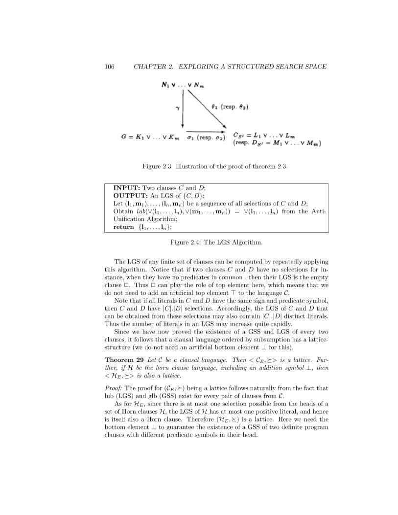
106 CHAPTER 2. EXPLORING A STRUCTURED SEARCH SPACE
Figure 2.3: Illustration of the proof of theorem 2.3.
INPUT: Two clauses C and D;OUTPUT: An LGS of C,D;Let (l1,m1), . . . , (ln,mn) be a sequence of all selections of C and D;Obtain lub(∨(l1, . . . , ln),∨(m1, . . . ,mn)) = ∨(l1, . . . , ln) from the Anti-Unification Algorithm;return l1, . . . , ln;
Figure 2.4: The LGS Algorithm.
The LGS of any finite set of clauses can be computed by repeatedly applyingthis algorithm. Notice that if two clauses C and D have no selections for in-stance, when they have no predicates in common - then their LGS is the emptyclause 2. Thus 2 can play the role of top element here, which means that wedo not need to add an artificial top element > to the language C.
Note that if all literals in C and D have the same sign and predicate symbol,then C and D have |C|.|D| selections. Accordingly, the LGS of C and D thatcan be obtained from these selections may also contain |C|.|D| distinct literals.Thus the number of literals in an LGS may increase quite rapidly.
Since we have now proved the existence of a GSS and LGS of every twoclauses, it follows that a clausal language ordered by subsumption has a lattice-structure (we do not need an artificial bottom element ⊥ for this).
Theorem 29 Let C be a clausal language. Then < CE ,> is a lattice. Fur-ther, if H be the horn clause language, including an addition symbol ⊥, then< HE ,> is also a lattice.
Proof: The proof for (CE ,) being a lattice follows naturally from the fact thatlub (LGS) and glb (GSS) exist for every pair of clauses from C.
As for HE , since there is at most one selection possible from the heads of aset of Horn clauses H, the LGS of H has at most one positive literal, and henceis itself also a Horn clause. Therefore (HE ,) is a lattice. Here we need thebottom element ⊥ to guarantee the existence of a GSS of two definite programclauses with different predicate symbols in their head.

2.1. SUBSUMPTION LATTICE OVER CLAUSES 107
Thus, the p.o. set of equivalence classes of atoms CE (HE) is a lattice withthe binary operations u and t defined on elements of CE (HE) as follows (notethat ⊥ ∈ C is the empty set ∅):
• [⊥] u [C] = [⊥], and [>] u [C] = [C]
• If C1, C2 ∈ C (C1, C2 ∈ H) have a GSS (glb) D then [C1] u [C2] = [D] =[C2θ] otherwise [C1] u [C2] = [⊥]
• [⊥] t [C] = [C], and [>] t C] = [>]
• If C1 and C2 have LGS (lub) M then [C1] t [C2] = [M ] otherwise [C1] t[C2] = [>]
For C,
• the GSS is simply the union C1 ∪ C1 (union translates to ‘or’ing the twoclauses)
• the LGS of C1 and C2 is obtained using the LGS algorithm outlined inFigure 2.4
whereas, for H,
• the GSS (or meet operation) is given as follows: If the set of positiveliterals (heads) in C1∪C2 have an mgu θ, then GSS(C1, C2) = (C1∪C2)θ.Otherwise GSS(C1, C2) = ⊥
• the LGS of C1 and C2 is obtained using the LGS algorithm outlined inFigure 2.4.
2
As an example, ifH = 2, ⊥,
is tiger(tom) ← has stripes(tom), is tawny(tom) ,
is tiger(bob) ← has stripes(bob), is white(bob) ,
is tiger(tom) ← has stripes(tom) ,
is tiger(tom) ← is tawny(tom) ,
is tiger(bob) ← has stripes(bob) ,
is tiger(bob) ← is white(tom) ,
is tiger(X) ← has stripes(X) ,
is tiger(X) ← is tawny(X) ,
is tiger(X) ← is white(X) ,
is tiger(X) ←
then the diagram of p.o. set HE is as outlined in Figure 2.5

108 CHAPTER 2. EXPLORING A STRUCTURED SEARCH SPACE
Figure 2.5: The lattice of HE for the is tiger relation.
2.1.2 Covers in the Subsume Order
The least generalization and the greatest specialization respectively concern gen-eralizing or specializing a set of clauses to a single clause. What about general-izing and specializing single clauses? We will address this issue by investigatingcovers of clauses in the subsumption order.
It can be shown that there exist clauses which have no complete set of upwardcovers in the subsumption order. In fact, there are clauses which have no upwardcovers at all. For example, the clause C = P (x1, x1) has no upward cover in< C,>. This can be proved by defining
Cn = P (xi, xj) | i 6= j and 1 ≤ i, j ≤ n, n ≥ 2
and noting that each Cn properly subsumes Cn+1 and C. That is C2 C3 . . . Cn . . . C. From this result, we know that C has no complete set of upwardcovers.
Dually, for the downward cover there exists a clause C which has no finitecomplete set of downward covers4. So if this particular C does have a completeset of downward covers, this set must he infinite. This result is sufficient to laterprove the negative result that an ideal downward refinement operator does notexist for the subsumption order. One such C is
C = P (x1, x2), P (x2, x1)
If we define5
En = P (y1, y2), P (y2, y3), . . . , P (yn−1, yn), P (yn, y1), n ≥ 2
andCn = C ∪ En, n ≥ 3
4Whether all clauses have a (sometimes infinite) complete set of downward covers remainsan open question.
5The clauses En have a special structure called a cycle.

2.2. THE IMPLICATION ORDER 109
then it can be shown that for any n = 3k (k ≥ 1), C Cn. Further, bycontradiction, one can show that there is no downward cover D of C, such thatD C3k for every k ≥ 1 and subsequently, that, C has no finite complete setof downward covers in < C,>.
2.2 The Implication Order
It is easy to see that implication is reflexive and transitive, and hence a quasiorder. Implication between (Horn) clauses is undecidable, but using implica-tion as a generality order is more desirable than using subsumption, for someimportant reasons:
1. It is better able to deal with recursive clauses. A clause C which impliesanother clause D, need not subsume this D. For instance, take
C = P (f(x))← P (x)D = P (f2(x))← P (x)
Then C |= D, but C 6 D. Subsumption is too weak in this case. Afurther sign of this weakness is the fact that two tautologies need not besubsume equivalent, even though they are logically equivalent.
2. For the construction of least generalizations, subsumption is again notfully satisfactory and can over-generalize. For example,
• If S consists of the clauses D1 = P (f2(a)) ← P (a) and D2 =P (f(b)) ← P (b), then the LGS of S is P (f(y)) ← P (x). the otherhand, the clause P (f(x))← P (x) seems more appropriate as a leastgeneralization of S, since it implies D1 and D2, and is implied by theLGS. However, it does not subsume D1.
• Even for clauses without function symbols, the subsumption ordermay still be unsatisfactory. Consider D1 = P (x, y, z) ← P (y, z, x)and D2 = P (x, y, z) ← P (z, x, y). The clause D1 is a resolvent ofD2 with D2, and D2 is a resolvent of D1 with D1; so D1 and D2
are logically equivalent. This means that D1 is a least generaliza-tion under implication (LGI) of the set D1, D2. Yet the LGS ofthese two clauses is P (x, y, z)← P (u, v, w), which is clearly an over-generalization.
As these examples also show, the subsumption order is particularly unsat-isfactory if we consider recursive clauses: clauses where the same predicatesymbol occurs both in a positive and a negative literal. Thus it is desir-able to make the step from the subsumption order to the more powerfulimplication order.

110 CHAPTER 2. EXPLORING A STRUCTURED SEARCH SPACE
Figure 2.6: Least generalization and greatest specialization in first-order logic.
3. A further advantage of the implication order is that one can easily comparea set of clauses (a theory) with another theory or clause. For example, ifΣ = (P ← Q), (Q← R) and C = P ← R, then we have Σ |= C. On theother hand, subsumption cannot be used here to compare the generalityof Σ and C, because neither member of Σ subsumes C.
The main results on the implication order can be summed up as follows:
1. If α1 and α2 are two arbitrary first-order formulas, then it can be easilyshown that their least generalization under implication (LGI) is just α1 ∧α2, and their greatest specialization under implication (GSI) is just α1∨α2.See Figure 2.6. However, if αl and α2 are clauses, αl ∧ α2 is not a clause.Instead of using αl ∧ α2, we have to find some least clause as LGI, whichimplies both clauses αl and α2. Such a clause appears quite hard to findsometimes, as we will see subsequently. However, αl∨α2 remains a clauseand remains the GSI under the subsumption order on clauses.
2. Every finite set of clauses Σ which contains at least one function-freenontautologous clause, has a computable least generalization (LGI) underimplication in C. A related observation is that the problem whether Σ |=C, where Σ is a finite set of ground clauses and C is a ground clause, isdecidable. This can be proved as follows: Let C = L1 ∨ . . .∨Ln and A bethe finite set of all ground atoms occurring in Σ and C. Now:
Σ |= C iff Σ ∪ ¬L1, . . . ,¬Ln is unsatisfiableiff Σ ∪ ¬L1, . . . , Ln has no Herbrand modeliff no subset of A is a Herbrand model of Σ ∪ ¬L1, . . . , Ln
Since A is finite, the last statement is decidable. What follows from thisis that the problem whether Σ |= C, where Σ is a finite set of function-freeclauses and C is a clause, is decidable. The algorithm for computing LGIis outlined in Figure 2.7.

2.2. THE IMPLICATION ORDER 111
INPUT: A finite set S of clauses, containing at least one non-tautologousfunction-free clause;OUTPUT: An LGl of S in C;Remove all tautologies from S, call the remaining set S ′;Let m be the number of distinct terms (including subterms) in S ′, let V =x1, . . . xm;Let G be the (finite) set of all clauses which can be constructed from predi-cate symbols and constants in S ′ and variables in V ;Let U1, . . . , Un be the set of all subsets of G;Let Hi be an LGS (computed using algorithm in Figure 2.4) of Ui, for every1 ≤ i ≤ n;Remove from H1, . . . ,Hn all clauses which do not imply S ′ (since each Hi
is function-free, this implication is decidable), and standardize the remainingclauses H1, . . . ,Hq apart. ;return H = H1 ∪ . . . ∪Hq;
Figure 2.7: The LGI Algorithm.
3. Every finite set of clauses has a greatest specialization (GSI) under impli-cation in C. A GSI of a finite set S is the same as the GSS of S (referSection 2.1.1), namely the union of the clauses in S after these are stan-dardized apart.
Finding least generalizations (under implication) of sets of clauses is com-mon practice in ILP. On the other hand, the greatest specialization, whichis the dual of the least generalization, is used hardly ever. Nevertheless,the GSI of two clauses D; and D2 might be useful. For example, supposewe have one positive example e+, and two negative examples e−1 ande
−2 ,
and suppose that D1 implies e+ and e−1 , while D2 implies e+ and e−2 .Then it might very well be that the GSI of D1 and D2 still implies e+,but is consistent with respect to e−1 , e
−2 . Thus we could obtain a correct
specialization by taking the GSI of D1 and D2.
4. As a corollary, if C is a function-free clausal language, then < C, |=> is alattice.
5. There exist pairs of Horn clauses which do not have an LGI in H.
6. Similarly, there exist pairs of Horn clauses which do not have a GSI in H.
7. For general clauses which all contain function symbols, the LGI-questionis still open.
8. For covers, the negative results from the subsumption order carryover tothe implication order.
• Some clauses, such as P (x1, x2), have no upward covers.

112 CHAPTER 2. EXPLORING A STRUCTURED SEARCH SPACE
• Some clauses, such as P (x1, x2), P (x2, x1), have no finite completeset of downward covers.
2.3 Inverse Reduction
Plotkin’s reduction algorithm (Figure 2.1) finds a reduction D of C. In thissection we present an algorithm which does the inverse: given a reduced clauseD, the algorithm constructs (possibly non-reduced) members C of the subsume-equivalence class of D. This will be useful in our treatment of refinement oper-ators. Since the subsume-equivalence class of D is infinite, we have to limit thescope of the algorithm. This is done by restricting the number of literals is C.
We will next state a lemma, which will find use subsequently.
Theorem 30 Let C and D be clauses. If D is a reduction of C, then there isa substitution θ such that Cθ = D and Lθ = L for every LθD.
Proof: Suppose D is a reduction of C, then there is a σ such that Cσ ⊆ D.Then also Dσ ⊆ Cσ ⊆ D, since D ⊆ C. If Dσ 6= D, then D would not bereduced, hence Dσ = Cσ = D.
Since σ is injective, for all L1, L2 ∈ D, if L1σ 6= L2σ then L1σ 6= L2σ, forotherwise |Dσ| < |D|. Hence if L1σ = L2σ, then L1 = L2. For each L ∈ D,consider the following infinite sequence:
L,Lσ, Lσ2, Lσ3, . . .
Since Dσ = D, each literal in this sequence is a member of D. D containsonly a finite number of literals, so for some i < j we must have Lσi = Lσj .Then from the injectivity, also L = Lσj−1. For this L, define n(L) = j − i.Notice that L = Lσm if m is a multiple of n(L). Let k be the least commonmultiple of all n(L). Then Lσk = L for every L ∈ D.
Define θ = σk. Then since Cσ = D and Dσ = D, we have Cθ = D. 2
From theorem 30, we know that for every non-reduced C such that D ⊂ Cand D ≡ C, we can find a θ such that Cθ = D and θ only acts on variables notappearing in D. Thus C can be reduced by mapping E = C \D to literals inD. In the inverse direction, we can find C by adding a set E to D,such that Eθ ⊆ D, where θ does not act on variables in D. This is theidea used in the algorithm in Figure 2.8. If D is a reduced clause and m is somepositive integer, then the algorithm finds a variant of every non-reduced C withm or less literals in the subsume-equivalence class of D.
As an illustration of the algorithm in Figure 2.8, if D = P (x, x) and m = 3,then upto variants, M1 ∈ P (x, y), P (y, y) andM2 = P (y, z), P (x, z), P (y, x), P (z, z).
2.4 Generality order and ILP
The subsumption and implication orders discussed thus far are important forlearning for the following reasons:

2.4. GENERALITY ORDER AND ILP 113
INPUT: A reduced clause D and an integer m;OUTPUT: Variants of every C such that D ≡ C and |C| ≤ m;Set k = 0;If |D| ≤ m, then output D;while l < (m− |D|) do
Set l to l + 1;for Every sequence L1, . . . , Li such that each Li ∈ D, but the Li’s arenot necessarily distinct do
Find every (up to variants) set E = M1, . . . ,Mt such that
1. Every Mi contains at least one new variable not in D, and
2. If x1, . . . , xn are all those new variables, then there is a θ =x1/t1, . . . , xn/tn, such that Miθ = Li, for i = 1, . . . , t.
;return D ∪ E;
end forend while
Figure 2.8: The Inverse Reduction Algorithm: It finds a variant of every non-reduced equivalent clause (equivalent to D) with m or less literals.
• They provide a generality ordering for hypotheses, thus structuring thehypothesis space.
• They can be used to prune large parts of the search space.
1. When generalizing C to C ′, C ′ C, all the examples covered byC will also be covered by C ′ (since if B ∪ C |= e (e being anexample) holds then also B ∪ C ′ |= e holds). This property is usedto prune the search of more general clauses when e is a negativeexample: if e is inconsistent (covers a negative example)then all its generalizations will also be inconsistent. Hence,the generalizations of C do not need to be considered.
2. When specializing C to C ′, C C ′, an example not covered by C willnot be covered by any of its specializations either (since if B∪C 6|= eholds then also B ∪ C ′ 6|= e holds). This property is used to prunethe search of more specific clauses when e is an uncovered positiveexample: if C does not cover a positive example none of itsspecializations will. Hence, the specializations of C do not needto be considered.
• The generality orderings provide the basis for two important ILP tech-niques:
1. bottom-up building of least general generalizations from training ex-amples, relative to background knowledge, and

114 CHAPTER 2. EXPLORING A STRUCTURED SEARCH SPACE
2. top-down searching of refinement graphs.
The principal generality orderings of interest are subsumption (θ) and im-plication (|=). For clauses C,D, subsumption is not equivalent to implication
if C θ D then C |= D
but
not vice− versa
For example, the above holds for:C : natural(s(X))← natural(X)
D : natural(s(s(X)))← natural(X)
Recall the subsumption theorem; it is a key theorem linking subsumptionand implication:
If Σ is a set of clauses and D is a clause, then Σ |= D iff D is atautology, or there exists a clause D′ θ D which can be derivedfrom Σ using some form of resolution.
When Σ contains a single clause C then the only clauses that can be derivedare the result of self-resolutions of C. Thus, the difference between C |= Dand C θ D arises when C is self-recursive or D is tautological
Is there a principled approach for comparing generality orderings? Fortu-nately, the answer is yes.
Given a set of clauses S, clauses C,D ∈ S and quasi-orders 1 and2 on S, then 1 is stronger than 2 if C 2 D implies C 1 D.If also for some C,D ∈ S C 62 D and C 1 D then 1 is strictlystronger than 2
It can be seen that as per above definition, the implication ordering is strictlystronger than the subsumption ordering. Quasi-orders that are increasinhglyweaker can be devised from stronger ones. Here are some other generalityorderings, listed in decreasing order of strength.
– C |= D iff C |= D
– C θ iff there is a substitution θ s.t. C ⊆ D
– C θ′ D iff every literal in D is compatible to a literal in C and C θ D.
– C θ′′ D iff |C| ≥ |D| and C θ′ D
What generality ordering should we choose for the ILP search procedure?We would like the strongest ordering that is practical In terms of tractability,logical implication between clauses is undecidable (even for Horn clauses). Sub-sumption is decidable but NP-complete (even for Horn clauses). Restrictionsto the form of clauses can make subsumption efficient. Here are two examplerestrictions that make subsumption efficient.

2.5. INCORPORATING BACKGROUND KNOWLEDGE 115
• Determinate Horn clauses. There exists an ordering of literals in C andexactly one substitution θ s.t. Cθ ⊆ D.
• k− local Horn clauses. Partition a Horn clause into k “disjoint” sub-partsand perform k independent subsumption tests.
The strongest quasi-order that is practical appears to be subsumption. Eventhat often requires restrictions (such as the two listed above) on the clausesbeing compared.
In summary, the subsumption order on clausal languages is used most oftenin ILP as the generality order (in contrast to the implication order), owing toits following properties:
1. Further, subsumption is more tractable and efficiently implementable.Subsumption between clauses is a decidable relation, whereas implicationis not. The flip side is that subsumption is a weaker relation.
2. Equivalence classes under subsumption can be represented by a singlereduced clause. Reduction can be undone by inverse reduction (c.f. Sec-tion 2.3).
3. Every finite set of clauses (function free or not )has a least generalization(LGS) and greatest specialization (GSS) under subsumption in C. Hence< C,> is a lattice. The same is not true for the implication quasi-ordering |= (for restricted languages lubs for |= may well exist).
Order lub glb
θ√ √
|= ×√
4. Every finite set of Horn clauses has a least generalization (LGS) and great-est specialization (GSS) under subsumption in H. Hence < H,> is alattice. The same does not hold for the implication order.
5. The negative results for covers hold for subsumption as well as implication.
2.5 Incorporating Background Knowledge
Why does background knowledge matter? The answer is that combining theexamples With what we already know often allows for the construction of amore satisfactory theory than can be glanced from the examples by themselves.To illustrate this, we consider [Bun88] the following two clauses as positiveexamples (not just ground atoms as examples):
D1 = CuddlyPet(x)← Small(x), F luffy(x), Dog(x)D2 = CuddlyPet(x)← Fluffy(x), Cat(x)

116 CHAPTER 2. EXPLORING A STRUCTURED SEARCH SPACE
Given only these clauses, the most obvious way to generalize them is to taketheir LGS or LGI, which is the rather general clause C = CuddlyPet(x) ←Fluffy(x).
However, suppose we have the following definite program B which expressesour background knowledge.
B1 Pet(x)← Cat(x)B2 Pet(x)← Dog(x)B3 Small(x)← Cat(x)
Given B, we may also use the following clause as generalization:
D = CuddlyPet(x)← Small(x), F luffy(x), P et(x).
since D together with B implies both examples. Note that without the back-ground knowledge B, our clause D neither subsumes nor implies the examples.If we interpret this example in human terms, the generalization D is much moresatisfactory than C. After all, not every fluffy object (such as a teddy bear) isa cuddly pet. Thus the use of background knowledge allows us to find a bettertheory. Given the usefulness of background knowledge, it is important to outlinea formalized way to reckon with it in our generality order.
There are three generality orders which are able to take background knowl-edge into account: (i) Plotkin’s relative subsumption (B), (ii) Relative impli-cation (|=B) and Buntine’s (iii) Generalized subsumption (≥B). Relative sub-sumption and relative implication apply to arbitrary clauses and the backgroundknowledge B may be an arbitary finite set of clauses. Generalized subsumptiononly applies to definite program clauses and the background knowledge shouldbe a definite program. We will state the existence of least generalizations ineach of these orders, both in case we are dealing with a Horn language H, andfor a general clausal language C. Further, each of the three orders can be re-lated to some kind of deduction. Since empty background knowledge reducesrelative and generalized subsumption to ordinary subsumption, and relative im-plication to ordinary implication, the negative results on covers for subsumptionand implication carry over to the three orders: some clauses do not have finitecomplete sets of upward or downward covers in these orders. As to the existenceand non-existence of least generalizations or greatest specializations in the threeorders, we will only pay attention to least generalizations, since these are usedmuch more often than their dual. In general, for all three, least generaliza-tions do not always exist in the presence of background knowledge. However,certain restrictions on the background knowledge guarantee the existence of aleast generalization for each of the three.
2.5.1 Plotkin’s relative subsumption (B)Definition 1 Let C and D be clauses, and B be a set of clauses. We sayC B D, if there is a substitution θ such that B |= ∀(Cθ → D) (note thatC → D need not be a clause).

2.5. INCORPORATING BACKGROUND KNOWLEDGE 117
With respect to the last example, we can verify that B3 B1,E F , whereE = CuddlyPet(x)← Small(x), F luffy(x), P et(x) and F = CuddlyPet(x)←Fluffy(x), Cat(x). Informally, this can be seen as follows: suppose for everyx it holds that if x is a cat, then x is small (i.e., C is true). Using B1, we alsohave that if x is a cat, then x is a pet. Thus if x is a fluffy cat, then x is small,fluffy, and a pet, and by E, x is a cuddly pet (i.e., D is true). Following aresome properties of relative subsumption:
1. Reflexivity and transitivity are easily proved, so relative subsumption isa quasi-order on clauses. Note that each set of clauses B induces itsown quasi-order: the quasi-orders induced by B = P (a) and B =P (a), P (b) are different. Note also that if D is a tautology, then C B Dfor any C and B. Furthermore, it is also easy to see that if C B D andB ⊆ B′, then C B′ D.
2. Relative subsumption is strictly stronger than subsumption.
(a) Firstly, it is easy to see that subsumption implies relative subsump-tion. If C D, then C B D, for some B. But then ∀(Cθ D) isa tautology, and B |= ∀(Cθ → D) for any B. Hence if C D, thenC B D.
(b) Now consider propositional atoms P , Q, and R. Let C = P , D = Q,and B = Q← P. Then B |= (C → D), so C B D. Since C 6 D,we see that relative subsumption does not imply subsumption. Thiseven holds for the case where B is empty and D is a tautology: ifB = ∅, C = Q, and D = P ← P , then C B D, but C 6 D.
3. If C and D are non-tautologous clauses, and B a finite set of ground literalssuch that B ∩D = ∅, then6 C B D iff C (D ∨ B).
4. Relative subsumption coincides with ordinary subsumption for non-tautologousclauses and empty background knowledge7. That is, if C and D are non-tautologous clauses, then C B D iff C D.
5. C B D iff there exists a deduction of DfromC ∪ B in which C occursat most once as a leaf. The proof of this long and windy and will not bedealt with here.
6. Least generalizations under relative subsumption (abbreviated to LGRSs)need not exist in the general case. The following counter example, adaptedfrom [NIb88] shows the non-existence of LGRSs both for the case of aclausal language C, and for a Horn language H.
Let
D1 = Q(a) D2 = Q(b)B = P (a, y), P (b, y)
6Prove: EXERCISE7Prove: EXERCISE

118 CHAPTER 2. EXPLORING A STRUCTURED SEARCH SPACE
It can be shown there is no LGRS of D1, D2 relative to B. Consider thefollowing infinite sequence of clauses:
C1 = Q(x)← P (x, f(x))C2 = Q(x)← P (x, f(x)), P (x, f2(x))C3 = Q(x)← P (x, f(x)), P (x, f2(x)), P (x, f3(x))
It is easy to see that Ci B Ci+1 for every i ≥ 1. We also have Ci B Di
and Ci B D2, for every i ≥ 1. Suppose some clause D is an LGRS ofD1, D2 relative to B, then we should have C B D, for every i ≥ 1.Then by point 5 above, for every i ≥ 1, there exists a deduction of Dfrom Ci ∪B in which Ci occurs at most once as a leaf. Ci cannot occurzero times as a leaf, because then a clause from B would simply subsumeD, which is impossible. Thus for every i ≥ 1, there exists a deduction ofD from Ci ∪ B, in which C, occurs once as a leaf. It cannot be thatevery Ci subsumes D, for then D would contain an instance of the termf i(x), for every i ≥ 1. Thus for some j the deduction of D from Cj ∪Binvolves at least one resolution step. Since the members of B are atomsand Cj only occurs once as a leaf, the parent clauses in the first resolutionstep must be Cj and a member of B. Suppose this member of B is P (a, y).Then P (a, y) must be unified with an atom of the form P (x, f ′′(x)) in thebody of Cj . Then the head of the clause Cj is instantiated to Q(a). Thishead will not be changed anymore in later resolution steps, so D wouldhave Q(a) as head - but then there is no deduction of D2 = Q(b) fromD ∪ B.
Similarly, if the member of B in the resolution step had been P (b, y)instead of P (a, y), D would have had Q(b) as head, and there would beno deduction of D1 = Q(a) from D ∪ B. Either way, the assumptionthat D is an LGRS of D1, D2 relative to B leads to a contradiction.
7. We however can identify a restriction on the background knowledge whichguarantees existence (and computability) of an LGRS of any finite set of(horn) clauses. If C (H) is a (horn) clausal language and B ⊆ C (B ⊆ H)is a finite set of ground literals, then every finite non-empty set S ⊆ C(S ⊆ H) of clauses has an LGRS in C (H). This can proved as follows: Ifa clause D is a tautology or B ∩D 6= ∅, then B |= D, hence for any clauseC we have C B D. Remove from S all tautologies and all D for whichB ∩D 6= ∅, call the remaining set S ′. If S ′ is empty, any tautology is anLGRS of S. If S ′ = D1, ..., Dn is non-empty, then it follows easily frompoint 3) above that an LGS of (D1 ∨ B), . . . , (Dn ∨ B) (or equivalentlyof (D1 ← B), . . . , (Dn ← B)) in C is an LGRS of S ′ in C, and hence alsoof S. The existence of such an LGS follows from Theorem 28. Thus ifthe background knowledge B is a finite set of ground literals, then we canconstruct an LGRS of a set S = D1, . . . , Dn simply by constructing anLGS of T = (D1 ∨B), . . . , (Dn ∨B). Additionally, if all clauses in S are

2.5. INCORPORATING BACKGROUND KNOWLEDGE 119
horn clauses and each literal in B is a ground atom, then each Di ∨ B isalso a horn clause and so will the LGS of T . So the result follows for H.This result has been exploited in the GOLEM system.
8. The non-existence of finite chains of covers, in lattices of (Horn) clausesordered by subsumption carries over to the lattice of clauses ordered byrelative subsumption.
Relative Subsumption and ILP
We will develop further on point (7) discussed above. When presented withan example e, candidate hypothesis in the form of a clause C and backgroundknowledge B, what does it mean for clause C to “relatively subsume” examplee. Recall normal subsumption: C e means ∃θ s.t. Cθ ⊆ e. This also meansCθ |= e or |= (e← Cθ).
e : gfather(henry, john)←B : father(henry, jane)←
father(henry, joe)←parent(jane, john)←parent(joe, robert)←
C : gfather(X,Y )← father(X,Z), parent(Z, Y )
For this B,C, e with θ = X/henry, Y/john, Z/jane, B ∪ Cθ |= e Thatis: C B e or equivalently, B |= (e← Cθ) (by subsumption theorem). However,note that C 6 e. Clearly if B = ∅ normal subsumption between clauses results.Using the Deduction Theorem
B |= (e← Cθ) ≡ B ∪ Cθ |= e
≡ B ∪ e |= Cθ
≡ Cθ |= B ∪ e≡ |= (B ∪ e← Cθ)
That is, C B e means C B ∪ e or C |= B ∪ e. Recall that if C1 C2 thenC1 |= C2. In fact, if C1,2 are not self-recursive, then C1 C2 ≡ C1 |= C2
Let a1∧a2 . . . be the ground literals true in all models of B ∪ e, that is theseare all the members of the minimal model MM(G(B ∪ e)) (c.f. theorem 12 aswell as theorem 17). Then
B ∪ e |= a1 ∧ a2 . . .
a1 ∧ a2 ∧ . . . |= B ∪ e ≡ e← B
Let ⊥(B, e) = a1 ∧ a2 ∧ . . .. Note that ⊥(B, e) (the ‘most specific clause’ givenB, e) may not always be finite. If B and e are both ground, it follows that⊥(B, e) ≡ (e← B).

120 CHAPTER 2. EXPLORING A STRUCTURED SEARCH SPACE
Now, if D ⊥(B, e) then D |= ⊥(B, e) and therefore D |= B ∪ e. Now, bytransitivity of |=, if D |= ⊥(B, e) then because ⊥(B, e) |= e← B, it should followthat D |= e← B. It can be further shown that if D, e are not self-recursive andD ⊥(B, e) then D B ∪ e (that is, D (e← B) or D B e). In fact, if C, eare non self-recursive then
C ⊥(B, e) ≡C |= B ∪ e ≡C B ∪ e ≡C e← B
An example of finding ⊥ is:
B:gfather(X,Y) ← father(X,Z), parent(Z,Y)father(henry,jane) ←mother(jane,john) ←mother(jane,alice) ←
ei:gfather(henry,john) ←
Conjunction of ground atoms provable from B ∪ ei:¬parent(jane,john) ∧father(henry,jane) ∧mother(jane,john) ∧mother(jane,alice) ∧¬gfather(henry,john)
⊥(B, ei):gfather(henry,john) ∨ parent(jane,john) ←
father(henry,jane),mother(jane,john),mother(jane,alice)
Di:parent(X,Y) ← mother(X,Y)
Mode declarations
Finding a clauseDi that subsumes⊥(B, ei) is hampered by the fact that⊥(B, ei)may be infinite! One workaround is to use a constrained subset of definiteclauses to construct finite most-specific clauses. This can be enabled usingmode declarations. An example set of mode declarations for the problemjust considered is:
modeh(*,gfather(+person,-person))
modeh(*,parent(+person,-person))
modeb(*,father(+person,-person))

2.5. INCORPORATING BACKGROUND KNOWLEDGE 121
modeb(*,parent(+person,-person))
modeb(*,mother(+person,-person))
A definite mode language is defined as follows.
Definition 2 Let C : h← b1, . . . , bn be a definite clause with an ordering overliterals. Let M be a set of mode declarations. C is in the definite mode languageL(M) iff
1. h is the atom of a modeh declaration in M with every place-marker of+type and −type replaced with variables, and every place marker of #typereplaced by a ground term.
2. Every atom bi in body of C is an atom in a modeb declaration in M with+,−,# places being replaced as above.
3. Every variable of +type in bi is either of +type in h or or −type in a bj(1 ≤ j < i)
Given a set of mode declarations M it is always possible to decide if a clause Cis in L(M). Next, we define depth of variables.
Definition 3 Let C be a definite clause, v be a variable in an atom in C, andUv all other variables in body atoms of C that contain v
d(v) =
0 if v in head of C(maxu∈Uvd(u)) + 1 otherwise
For example, if C : gfather(X,Y )← father(X,Z), parent(Z, Y )
Then d(X) = d(Y ) = 0, d(Z) = 1. Putting together the definitions of modelanguage and depth, we next define depth bounded definite mode language.
Definition 4 Let C be a definite clause with an ordering over literals. Let Mbe a set of mode declarations. C is in the depth-bounded definite mode languageLd(M) iff all variables in C have depth at most d
As an example, the clause for gfather/2 earlier is in L2(M).We will state some properties of ⊥(B, ei) without their proofs. For every
⊥(B, ei) it is the case that:
There is a ⊥d(B, ei) in Ld(M) s.t. ⊥d(B, ei) ⊥(B, ei)
⊥d(B, ei) is finite
If C ⊥d(B, ei) then C ⊥(B, ei)
⊥(B, ei) may not be Horn
⊥(B, ei) may not be finite

122 CHAPTER 2. EXPLORING A STRUCTURED SEARCH SPACE
Least upper bound of Horn clauses e1, e2 is:
lggB(e1, e2) = lgg(⊥(B, e1),⊥(B, e2))
Greatest lower bound of Horn clauses e1, e2 is:
glbb(e1, e2) = glb(⊥(B, e1),⊥(B, e2))
Let us take an example of finding ⊥i:
⊥(B, ei):
gfather(henry,john) ∨ parent(jane,john) ←father(henry,jane),mother(jane,john),mother(jane,alice)
modes:
modeh(*,parent(+person,-person))modeb(*,mother(+person,-person))modeb(*,father(+person,-person))
⊥0(B, ei):
parent(X,Y) ←
⊥1(B, ei):
parent(X,Y) ←mother(X,Y),mother(X,Z)
2.5.2 Relative implication (|=B)Definition 5 Let C and D be clauses, and B be a set of clauses. C (logically)implies D relative to B, denoted C |=B D, if C ∪ B |=B D.
For example, if B = P (a), C = P (f(x)) ← P (x) and D = P (f2(a)), thenC |=B D, because there is a deduction of D from C ∪ B. However, we haveC 6B D because C has to be used more than once in the deduction of D.Following are some properties of relative subsumption:
1. Relative implication is perhaps the most obvious way to take backgroundknowledge into account.
2. Obviously relative implication is reflexive and transitive so it can serve asa quasi-order on a set of clauses.

2.5. INCORPORATING BACKGROUND KNOWLEDGE 123
3. It is also obvious that if C |= D then C |=B D. The converse need nothold though. Consider C = P (a) ← P (b), D = P (a), and B = P (b):then C |=B D, but C 6|= D. ’
4. Relative subsumption implies relative implication but not conversely. IfC B D, then B |= ∀(Cθ → D) (for some θ). If C |=B D then C ∪ B |=D, which is equivalent to B |= ∀(C)→ ∀(D) by the deduction theorem.
5. C |=B D iff there exists a deduction of D from C ∪ B (contrast thiswith that for relative subsumption). This is another testimony to the factthat relative implication is a strictly stronger quasi-order than relativesubsumption.
6. The negative results for existence of least generalizations under implicationcarry over to relative implication (LGRI), since ordinary logical implica-tion is just a special case of relative implication. Further, the only positiveresult for LGI that was stated on page 110 in point (2) is also negative forLGRI. As an example, consider
D1 = P (a) D2 = P (b)B = (P (a) ∨ ¬Q(x)), (P (b) ∨ ¬Q(x))
It can be shown that the set S = D1, D2 has no LGRI relative to B in C.Suppose indeed D is an LGRI of S relative to B. Note that if D containsthe literal P (a), then the Herbrand interpretation which makes P (a) true,and which makes all other ground atoms false, would be a model of B∪Dbut not of D2, so then we would have D 6|=B D2. Similarly, if D containsP (b) then D 6|=B D1. Hence D cannot contain P (a) or P (b). Now let d be aconstant not appearing in D. Let C = P (x)∨Q(d), then C |=B S. By thedefinition of an LGRI, we should have C |=B D. Then by the SubsumptionTheorem, there must be a derivation from B ∪ C of a clause E, whichsubsumes D. The set of all clauses which can be derived (in 0 or moreresolution steps) from B∪C is B∪C∪(P (a)∨P (x)), (P (b)∨P (x).But none of these clauses subsumes D, because D does not contain theconstant d, nor the literals P (a) or P (b). Hence C 6|=B D, contradictingthe assumption that D is an LGRI of S relative to B in C. Thus, ingeneral an LGRI of S relative to B need not exist.
7. We can identify a special case in which the existence of an LGRI is guaran-teed. Let C and D be clauses, and B be a finite set of fundion-free groundliterals. Then C |=B D iff C |= (D ∪ B). Further, if S ⊆ C is a finite setof clauses, containing at least one D for which D ∪ B is non-tautologousand function-free, then S has an LGRI in C. As a special case of this, ifC is itself function free clausal language, then for any finite S ⊆ C, S hasan LGRI in C.This can be proved as follows: Suppose C |=B D i.e., C ∪ B |= D. LetM be a model of C. Then we need to show that M is also a model of

124 CHAPTER 2. EXPLORING A STRUCTURED SEARCH SPACE
D ∪ B. If M is not a model of B, then it is a model of at least one literalin B, and hence of the clause D ∪ B. If on the other hand, M is a modelof B then M is also a model of D, because C ∪ B |= D. Then M is alsoa model of D ∪ B. This prove the ‘only if’ part.
Now suppose C |= (D ∪B). Let M be a model of C ∪ B. Then we needto show that M is also a model of D. Now, M is a model of C and henceof the clause D ∪ B. But M is also a model of B, and hence not a modelof B. Therefore, M must be a model of D. This proves the ‘if’ part.
Now if S = D1, D2, . . . , Dn, it follows that an LGI in C of T = (D1 ∪B), . . . , (Dn ∪ B) is also an LGRI of S in C (which exists according topoint 2 on page 110).
2.5.3 Buntine’s generalized subsumption (≥B)Definition 6 Let C and D be definite program clauses and B be a definiteprogram, comprising the background knowledge. We say that C ≥B D (g-subsumes), if for every Herbrand model M of B and every ground atom A suchthat D covers A under M , we have that C covers A under M . Definite clauseC is said to ‘cover’ atom A under M if there exists a ground substitution θ forC (that is, Cθ is ground), such that M is a model for C−θ and C+θ = A.
Generalized subsumption applies only to definite program clauses. Looselyspeaking, generalized subsumption says that for definite clauses C and D, Cis more general that D, in any situation consistent with what we already know(through B), C can be used to prove at least as many results as D. For example,if B consists of the background knowledge on page 116 and C and D are definedsomewhat similar to D1 and D2 as
C = CuddlyPet(x)← Small(x), P et(x)D = CuddlyPet(x)← Cat(x)
then, we can show that C ≥B D. For suppose M is a Herbrand model of B andD covers some grond atom A = CuddlyPet(t) under M , then for θ = x/t,D−θ = Cat(t) is true under M . Since M is a model of B, in particular ofB1 and B3, Pet(t) and Small(t) must be true under M as well. Then C−θ =Small(t)∧Pet(t) is true under M , and C+θ = A, so C also covers A under M .Hence C ≥B D. In natural language, this can be rephrased as
If small pets are cuddly pets, then cats are cuddly pets,since we already know that cats are small pets.
Some of the properties of ≥B are:
1. Just as subsumption implies relative subsumption, subsumption also im-plies g-subsumption. Suppose C D. Then Cθ ⊆ D, so C+θ = D+ andC−θ ⊆ D−θ for some θ. If D covers some A under some I, there is a γ suchthat D−γ, is true under I and D+γ = A. But then C+θγ = D+γ = A,

2.5. INCORPORATING BACKGROUND KNOWLEDGE 125
and C−γ ⊆ D−γ, is true under I, so C covers A under I as well. Hence,if C D, then C ≥B D.
The converse need not hold: if B = P (a), C = Q(a) ← P (a) andD = Q(a), then C ≥B D but C 6 D.
2. Generalized subsumption is reflexive and transitive with respect to somedefinite program B, so it can serve as a quasi-order on a set of definiteclauses.
3. C ≥B D iff there exists an SLD-deduction of D, with C as top clause andmembers of B as input clauses. It follows from this that g-subsumptionreduces to ordinary subsumption in the presence of empty backgroundknowledge, as was the case for relative subsumption. That is, if C and Dare definite program clauses, then C ≥∅ D iff C D.
4. From the previous point, it follows that if C and D are definite programclauses, and B is a definite program, then if C ≥B D, it follows thatC B D. That is, g-subsumption implies relative subsumption. But theconverse does not hold. This is sufficient to prove that if an LGG (lub)does not exist under relative subsumption (such as for the example
5. An LGGS of a finite set S (of definite program clauses which all have thesame predicate symbol in their respective heads) always exists either if
(a) All clauses in S are atoms, and the background knowledge B impliesonly a finite number of ground atoms (i.e., MB is finite)
(b) S and B are all function-free (see [Bun88]).
(c) B is ground. This case differs from the first, because B may implyonly a finite number of ground examples, and still be non-grounditself. For example, B = P (a), (Q(x)← P (x)).
Actually, these three cases are special cases of the following theorem:
Theorem 31 Let H be a Horn language and B be a definite program.Let S = D1, . . . , Dn ⊆ H be a finite non-empty set of definite programclauses, such that all Di, have the same predicate symbol in their head.Furthermore, for every 1 ≤ i ≤ n, let σi be a Skolem substitution for Di,with respect to B ∪ S, and Mi be the least Herbrand model of B ∪D−i σi.If every Mi is finite, then there exists an LGGS of S in H.
Thus if the least Herbrand models mentioned in the theorem are indeedfinite, then we can find an LGGS of a set D1, . . . , Dn simply by con-structing an LGS of (D+
1 ∪M1), . . . , (D+n σn ∪Mn).

126 CHAPTER 2. EXPLORING A STRUCTURED SEARCH SPACE
2.6 Using Generalization and Specialization
The normal problem of inductive logic programming is to find a correct theory, aset of clauses which implies all given positive examples and which is consistentwith respect to the given negative examples. Usually, it is not immediatelyobvious which set of clauses we should pick as our theory. Rather, we will have tosearch among the permitted clauses for a set of clauses with the right properties.If a positive example is implied by the theory, we should search for a more generaltheory. On the other hand, if the theory is not consistent with respect to thenegative examples, we should search for a more specific theory - for instance,by replacing a clause in the theory by more specific clauses - such that thetheory becomes consistent. Thus, the two most important operations in ILP aregeneralization and specialization. Repeated application of such generalizationand specialization steps may finally yield a correct theory.
To systematically facilitate this search, it would be very handy if the set ofclauses that has to be searched, is somehow structured. Fortunately, this is soas seen in chapter 1. We had seen several alternatives for what it means forsome clause to be more general than another clause. Since generalization (ordually, specialization) can proceed along the lines of such a generality order,using such an order can direct the search for a correct theory. For example,least generalizations can be used to generalize given finite sets of examples.
2.7 Using the Cover Structure: Refinement Op-erators
One way to weaken a existing theory which is too strong is to find a falsemember of the theory Σ, and delete this clause from the theory. However,deleting a clause might make the theory in turn too weak. A way to strengthenthe theory again, is to add weaker versions of previously deleted clauses. Forinstance, suppose the clause P (x) is false under I, and has been deleted fromΣ. It might be that P (f(x)), which is a “refinement” of P (x), is true under I.Thus the theory might be strenghened by adding P (f(x)) to it.
The finite downward and upward cover chain algorithm provide the generaldirection of search in any search over the lattice structure over theories (atomicor otherwise). In top-down search, we want to find some unknown specializationl2 of l1. Then we should use substitutions to try and find a chain of downwardcovers starting from l1 as in Algorithm 1.15. Since such finite chains alwaysexist for atoms, we can restrict attention to downward covers of l1, downwardcovers of downward covers of l1, etc. Recall from the algorithm in Figure 1.15that the progress from li to li+1 is achieved by applying one of the followingsubstitutions:
1. X/f(X1, . . . , Xk) where X is a variable in li, X1, . . . , Xk are distinct variablesthat do not appear in li, and f is some k-ary function symbol in the language
2. X/c where X is a variable in li, and c is some constant in the language
3. X/Y where X,Y are distinct variables in li

2.7. USING THE COVER STRUCTURE: REFINEMENT OPERATORS 127
In ILP, these 3 operations define a “downward refinement operator”On the other hand, in bottom-up search we want to find some unknown
generalization l1 of l2. In that case, we should use inverse substitutions to finda chain of upward covers from l2 to l1.
A systematic way to find refinements of clauses, is by using a refinementoperator. There are two kinds of refinement operators: upward and downwardones. An upward refinement operator computes a set of generalizations of agiven clause, a downward refinement operator computes a set of specializations.What constitutes a ‘specialization’ or ‘generalization’ of a clause, is determinedby a generality order (such as subsumption, implication, relative subsumption,relative implication, etc.) on clauses. Then we can say that C is a generalizationof D (dually: C is a specialization of D), if C D holds. In each of these orders,the empty clause 2 is the most general clause.
Downward refinement operators compute sets of specializations of a clause,upward ones compute sets of generalizations. Refinement operators are definedfor a set of formulae S with a quasi-ordering . There are two refinementoperators.
– ρ is a downward refinement operator if ∀C ∈ S : ρ(C) ⊆ D|D ∈S and C D
– δ is an upward refinement operator if ∀C ∈ S : δ(C) ⊆ D|D ∈ S and D C
For example, with an equality theory = /2, D ∈ ρ(C) (downward refinementoperator) if
D =
p(X1, X2, . . . , Xnp ) if C = 2 and p/np ∈ L
and the Xi are distinct
C ∪ ¬l otherwise
where
l =
V = W where V,W occur in C
V = f(X1, X2, . . . , Xnf ) where V occurs in C
and f/nf ∈ L and
the Xi are distinct
q(X1, X2, . . . , Xnq ) where q/nq ∈ Land the Xi occur in C
is an example of a refinement operator.
2.7.1 Example
We assume the set of clauses Ch is ordered by such a generality order .Shapiro’s top-down approach only employs a downward refinement operator ρ,so ρ(C) is a set of specializations of a given clause C. We start with Σ = 2.This is clearly too strong, since it implies any clause. Hence we want to find spe-cialisatione of 2, We use the set ρ(2) for this. If ρ(2) is still too strong, its falsemembers in turn be replaced by their refinements, and so on. Thill allows usto search stepwisely through the generality order. This stepwise approach will

128 CHAPTER 2. EXPLORING A STRUCTURED SEARCH SPACE
Figure 2.9: Paths through the refinement operator ρ.
only work if there is a path (a number of refinement steps) from Box to everyclause in atleast one correct theory, For instance, suppose Σ = D2, D3, D4 isa correct theory. Let the refinement operator ρ be such, that ρ(2) = C1, C2,ρ(C1) = C3, C4, ρ(C2) = D3, D4, ρ(C3) = D1, and ρ(C4) = D2, D3.Starting from 2, we can reach Σ by considering ρ(2), ρ(C1), ρ(C2), ρ(C4). SeeFigure 2.9
2.7.2 Ideal Refinement Operators
The sets of one-step refinements, n-step refinements, and refinements of someC ∈ C, are respectively:
ρ1(C) = ρ(C)
ρn(C) = D | there is an E ∈ ρn−l(C) such that D ∈ ρ(E), n ≥ 2
ρ∗(C) = ρ1(C) ∪ ρ2(C) ∪ ρ3(C) . . .
A ρ-chain from C to D is a sequence C = C0, C1, . . . , Cn = D, such thatC−i ∈ ρ(Ci−1) fpr every 1 ≤ i ≤ n. A refinement operator induces a refinementgraph. This is a directed graph which has the members of C as nodes (herevariant clauses in C can be viewed as the same node), and which contains anedge from C to D just in case D ∈ ρ(C). This refinement graph is the space thatis searched for candidates to include in the theory (we will later see refinementsover theories).
Some desirable properties of ρ (and dually δ) are that they be:
1. Locally Finite: ∀C ∈ C: ρ(C) is finite and computable. Otherwise ρ willbe of limited use in practice.
2. Complete: ∀C D: ∃E ∈ ρ∗(C) s.t. E ∼ D. That is, every spe-cialization should be reachable by a finite number of applications of theoperator.
3. Proper: ∀C ∈ C : ρ(C) ⊆ D|D ∈ S and C D. That is, it is betteronly to compute proper generalizations of a clause, for otherwise repeated

2.7. USING THE COVER STRUCTURE: REFINEMENT OPERATORS 129
application of the operator might get stuck in a sequence of equivalentclauses (such as the application of inverse reduction in Section 2.3), with-out ever achieving any real specialization.
A refinement operator is ideal if it is locally finite, complete, and proper. Anideal refinement operator induces a refinement graph in which only a finitenumber of edges start from each node (locally finiteness), in which there existsa path of finite length from C to a member of the equivalence class ofD wheneverC D (completeness), and which contains no cycles (by properness).
It can be shown that ideal downward ρA and upward δA refinement oper-ators exist for the simplest of our quasi-orders: the set of atoms ordered bysubsumption.
Definition 7 Let A be the set of atoms in a language. The downward refine-ment operator ρA for A is defined as follows:
1. For every variable z in an atom A and every n-ary function symbol f inthe language, let x1, . . . , xn be distinct variables not appearing in A. LetρA(A) contain Az/f(x1, . . . , xn).
2. For every variable z in A and every constant a in the language let ρA(A)contain Az/a.
3. For every two distinct variables x and z in A, let ρA(A) contain Az/x.
Note that ρA(A) may still contain variants. For instance, ρA(P (x, y)) con-tains both P (x, x) and P (y, y). Clearly, in a practical application we can ignoreany redundant variants. The three different kinds of atoms in ρ(A) correspondexactly to the three kinds of downward covers that we discussed in theorem 25.It can be proved easily from the properties of sets of covers of atoms describedon page 87 that if A contains a finite number of constants function and predicatesymbols, then ρA is ideal.
An ideal upward refinement operator δA can be defined straightforwardly asfollows:
Definition 8 Let A be the set of atoms in a language. The upward refinementoperator δA for A is defined as follows:
1. For every t = f(x1, . . . , xn) in A, for which x1, . . . , xn are distinct vari-ables and each occurrence of some xi in A is within an occurrence of t,δA(A) contains an atom obtained by replacing all occurrences of t in A bysome new variable z not in A.
2. For every constant a in A and every non-empty subset of the set of oc-currences of a in A, δA(A) contains an atom obtained by replacing thoseoccurrences of a in A by some new variable z not in A.
3. For every variable x in A and every non-empty proper subset of the setof occurrences of x in A, δA(A) contains an atom obtained by replacing
130 CHAPTER 2. EXPLORING A STRUCTURED SEARCH SPACE
those occurrences of x in A by some new variable z not in A. Note that inthis last item, we cannot replace all occurrences of x by a new variable z,for then we would get a variant of A. For instance, P (z, a, z) is a variantof A = P (x, a, x).
As in the case of ρA, it easily follows that δA is locally finite, complete andproper. We do not even have to presuppose a finite number of constants functionand predicate symbol for this, because when constructing JA(A) w only haveto deal With the fimte number of symbols in A-there is no need to introducenew constants, functions or predicates.
2.7.3 Refinement Operators on Clauses for Subsumption
Unfortunately, the ideal conditions described for atoms cannot all be met atthe same time for more complex orders. Ideal refinement operators do not existfor full clausal languages or Horn languages ordered by subsumption or by thestronger orders. This negative result is a concequence of the fact that finitecomplete sets of covers do not always exist8. We had seen (c.f. Section 2.1.2)that the existence of finite chains in lattices of atoms ordered by subsumptiondoes not carry over to Horn clauses ordered by subsumption. This had followedfrom the observation that there are clauses which have no finite and completeset of downward covers. This makes it impossible to devise an ILP program thatuses a refinement operator that is both complete and non-redundant. Therefore,there are no upward (downward) refinement operators that are locally finite aswell as complete as well as proper for sets of clauses That is, for clausal languagesordered by subsumption θ or stronger orders, ideal refinement operators donot exist.
In order to define a refinement operator for full clausal languages, it will berequired to drop one of the three properties of idealness. Of the three conditionsof locally finiteness, completeness and properness, finiteness seems indispens-able: an infinite set ρ(C) of refinements of a clause C cannot be handled well,because it would then be impossible to test all members of ρ(C) in finite time.Furthermore, it is obvious that completeness is also a very valuable property, ifyou want to be able to guarantee that a solution will always be found wheneverone exists. Of the three ideal properties, properness seems the least importantand can be compromised. Ideal refinement operators can be approximated by
1. Dropping the requirement of properness: Locally finiteness and complete-ness are considered to be the two most important properties, so droppingthe ’properness’ is a common practice. We will define downward (ρL) andupward (δU ) refinement operators that are locally finite and complete,but improper. For subsumption, such refinement operators exist, both forthe downward and for the upward case. If C subsumes D, then Cθ ⊆ Dfor some substitution θ. Thus specialization under subsumption can be
8In fact, it can be proved that if there exists an ideal downward (upward) refinementoperator for < C,>, then every C ∈ C will have a finite complete set of downward (upward)covers

2.7. USING THE COVER STRUCTURE: REFINEMENT OPERATORS 131
achieved by applying (elementary) substitutions and adding literals. Infact, when adding literals, it is sufficient to add only most general liter-als, since these can always be instantiated by a substitution later on toget the right literals. A literal P (x1, . . . , xn) or ¬P (x1, . . . , xn) is mostgeneral with respect to a clause C, if x1, . . . , xn are distinct variables notappearing in C.
Definition 9 Let C be a clausal language. The locally finite and completedownward refinement operator ρL for < C,> is defined as follows:
(a) Apply a substitution to a clause C in one of the following ways:
i. For every variable z in a clause C and every n-ary function sym-bol f in the language, let x1, . . . , xn be distinct variables not ap-pearing in C. Let ρL(C) contain Cz/f(x1, . . . , xn).
ii. For every variable z in C and every constant a in the language,let ρL(C) contain Cz/a.
iii. For every two distinct variables x and z in C, let ρL(C) containCz/x.
(b) Add a literal to a clause C: For every n-ary predicate symbol P inthe language, let x1, . . . , xn be distinct variables not appearing in C.Then ρL contains both C∪P (x1, . . . , xn) and C∪¬P (x1, . . . , xn).Note that the literals P (x1, . . . , xn) and ¬P (x1, . . . , xn) that are addedto C by the fourth item in the definition are most general with respectto C.
The proof of locally finiteness and completeness is straightforward. Sinccewe already know that no ideal operators exist for this case, ρL cannotbe proper. For instance, if C = P (x) and D = P (x), P (y), thenD ∈ ρL(C) and C ∼ D. However, this D is needed in a ρL-chain from C toP (a)P (b) as follows: P (x), P (x), P (y), P (a), P (y), P (a), P (b).Notice that for every 2 6= C, we have 2 C, so ρ∗(2) contains a clausewhich is subsume-equivalent to C. In other words: If we start with theempty clause (as Shapiro’s Model Inference Algorithm does), then forevery C ∈ C, a clause C ′ such that C ∼ C ′ can be reached by means ofρL.
Definition 10 Let C be a clausal language. The locally finite and com-plete upward refinement operator δu for < C,> is defined as follows:
(a) Apply one of the following inverse substitution operations:
i. For every t = f(x1, . . . , xn) in C, for which all xi are distinctvariables and each occurrence of xi in a clause C is within anoccurrence of t, δu(C) contains the clause obtained by replacingall occurrences of t in C by some new variable z not previouslyin C.

132 CHAPTER 2. EXPLORING A STRUCTURED SEARCH SPACE
ii. For every constant a in C and every non-empty subset of the setof occurrences of a in C = dup(C, a), if D is the ordered clauseobtained by replacing those occurrences of a in C by the newvariable z, then δu(C) contains D, where D is the set of literalsin the ordered clause D.dup(C, t) is defined as follows. If C = L1, . . . , Ln is a clauseand t a term occurring in C and suppose t occurs k1 times inL1, k2 times in L2, etc. Then dup(C, t) = C is an ordered clauseconsisting of 2k1 copies of L1, 2k2 copies of L2, . . . and 2kn copiesof Ln. Note that if some L ∈ C does not contain the term t, thenC contains L 20 = 1 times, as it should.
iii. For every variable x in C and every non-empty proper subset ofthe set of occurrences of x in C = dup(C, x), if D is the orderedclause obtained by replacing those occurrences of x in C by thenew variable z, then δu(C) contains D.
(b) Remove a literal from the body of a clause: If C = D ∪ Land L is a most general literal with respect to D, then δu(C) containsD.
2. By bounding the language: If we want to retain all three ideal properties, itseems that the only possibility is to restrict the search space. There existideal refinement operators for reduced finite clausal languages, orderedby subsumption. The fact that there always exists an ideal refinementoperator for finite sets is mainly of theoretical interest. Thus in practice,we usually prefer more constructive-though possibly improper-refinementoperators over such very elaborate ideal operators.
3. Dropping the requirement of completeness: Refinement operators are usedvery often in ILP systems, for instance in MIS [Sha81b], SIM [LD90,Lin92], FOIL [Qui90, QC93], CLAUDIEN [DB93], LINUS [LD94], andProgol [Mug95]. For reasons of efficiency, those operators are usually lessgeneral than the ones discussed here, and often incomplete. Nevertheless,the complete operators defined here form a good starting point for theconstruction of practical refinement operators.
An approximation to the ideal downward refinement operator, as adoptedin Aleph is:
(a) Adding a literal drawn from ⊥ip(X,Y )← q(X) becomes p(X,Y )← q(X), r(Y )
(b) Equating two variables of the same typep(X,Y )← q(X) becomes p(X,X)← q(X)
(c) Instantiate a variable with a general functional term or constantp(X,Y )← q(X) becomes p(3, Y )← q(3)
Optimal cover-refinement operators do not exist for clausal languages or-dered by subsumption.

2.8. INVERSE RESOLUTION 133
2.7.4 Refinement Operators on Theories
Definition 11 Let C be a clausal language, containing only a finite number ofconstants, function symbols, and predicate symbols. Let S be the set of finitesubsets of C. The downward refinement operator ρI for < S, |=> is defined asfollows:
1. (Σ ∪ R | R is a resolvent of C1, C2 ∈ Σ) ∈ ρI(Σ).
2. If Σ = C1, . . . , Cn, then (Σ ∪ ρI(Ci)) ∈ ρI(Σ), for each 1 ≤ i ≤ n.
3. If Σ = C1, . . . , Cn, then (Σ \ Ci) ∈ ρI(Σ), for each 1 ≤ i ≤ n.
Note that every theory in ρI(Σ) that is specified by one of the first two items inthe definition of ρI is logically equivalent to Σ. This shows that ρI is not proper.The completeness of ρI follows from the Subsumption Theorem, which tells usthat logical implication can be implemented by a combination of resolution andsubsumption.
2.8 Inverse Resolution
Since induction can be seen as the inverse of deduction, and resolution is ourmain tool for deduction, using inverse resolution for induction seems a sensi-ble idea. Deduction moves from the general rules to the special case, whileinduction intends to find the general rules from special cases (examples). Mug-gleton and Buntine [MB88] introduced inverse resolution as a tool for induction.Their paper was followed by a wave of interest and research into the propertiesof inverse resolution [Wir89, HS91, Mug91b, Mug92b, Mug92c, RP89, RP90,Rou92, NF91, Ide93c, Ide92, Ide93b, Ide93a, LN92, SADB92, Tay93, SA93,BG93]. Inverting resolution is nowadays still a prominent generalization oper-ator for bottom-up approaches to ILP. However, the theoretical foundation ofthis idea needs much more investigation. Moreover, in the application of in-verse resolution, many indeterminacies arise: many different choices of literals,clauses and substitutions lay open. Accordingly, inverse resolution generates avery large search space of possibilities.
Muggleton and Buntine introduced two operators for this: the V-operatorand the W-operator.
2.8.1 V-operator
The V-operator, outlined as a non-deterministic9 algorithm in Figure 2.10, gen-eralizes two given clauses C1, R to C1, C2, such that R is an instance of aresolvent of C1 and C2. The setting for the V-operator is pictorially depictedin Figure 2.11. The goal in inverse resolution is to construct a derivation of apositive example A (usually a ground atom) which hitherto was not implied by
9Since, in step 1, the algorithm has to choose one among many different possible θ1’s,
which all satisfy C′1 ⊆ R.

134 CHAPTER 2. EXPLORING A STRUCTURED SEARCH SPACE
the theory. Using the algorithm for the V-operator, we can invert one resolutionstep, for given C1 and R. By repeatedly applying the V-operator, we are ableto invert any SLD-derivation.
INPUT: Horn clauses C1 = L1 ∨ C′
1 and R, where C′
1θ1 ⊆ R for some θ1.OUTPUT: A Horn clause C2, such that R is an instance of a resolvent ofC1 and C2.Choose a substitution θ1 such that C
′
1θ1 ⊆ R.Choose an L2 and C
′
2 such that L1θ1 = ¬L2θ2 and C′
2θ2 = R − C ′1θ1, forsome θ2.return C2 = L2 ∨ C
′
2.
Figure 2.10: The V-operator.
The simplest situation is where C1 = L1, so where C′
1 is empty. Then fora given θ1, any C2 and θ2 with C2θ2 = ¬L1θ1 ∨ R will do. Since L1θ1 ∨ R isan instance of any of these possible C2’s, it is clear that C2 = ¬L1θ1 ∨R is the”minimal” of all possible C2’s, for a fixed θ1.
As an example application of inverse resolution, let C1 = P (x) ∨ ¬Q(f(x)),L1 = P (x), and R = Q(g(y))∨¬Q(f(g(y))). We assume C1θ1 and C2θ2 do notoverlap.
1. Here only one θ1 is possible, namely θ1 = x/g(y).
2. L2 and C′
2 should be such that, for some θ2, L1θ1 = P (g(y)) = ¬L2θ2 andR−C ′1θ1 = Q(g(y)) = C
′
2θ2. Figure 2.12 shows all possible C2 = L2 ∨C′
2
(unique up to renaming of variables) of two literals, from top to bottomin decreasing order of generality. Small generalization and specializationsteps are relevant for the V-operator. In this case, we are often interestedin finding a ‘minimal’ C2, as in Figure 11.3, where C2 = ¬L1θ1 ∨ (R −C′
1θ1 = ¬P (g(y)) ∨ Q(g(y)) is the minimal choice and can be obtainedusing the covers relation between clauses in the implication/subsumption
Figure 2.11: The setting for the V-operator.

2.8. INVERSE RESOLUTION 135
Figure 2.12: C2 derived using V-operator.
order studied in Section 2.1.2. The other C2’s can then be found by takingsmall generalization steps starting from the minimal C2.
Note that for some C2, R itself is not a resolvent of C1 and C2. For instance,if we let C2 = ¬P (z)∨Q(y), then the resolvent of C1 and C2 is ¬Q(f(z))∨Q(y),of which R is an instance.
We sometimes have to duplicate some literals in R before applying the V-operator, in order to be able to find the desired parent clauses, such that C
′
1θ1
and C′
2θ2 overlap.Note that there are many indeterminacies here, which make an unrestricted
search through all possible invertible derivations very inefficient. Within theV-operator itself, many different choices for θ1, L2 and C
′
2 are possible. Andeven before we can use the V-operator, we have to decide which clause fromthe old theory or the background knowledge to use as C1, and which literals toduplicate in R. Thus the total number of possibilities may become very largesometimes, which can make application of inverse resolution very inefficient.
In Figures 2.13 and 2.14, we contrast linear derivation against inverse linearderivation.
2.8.2 Predicate Invention: W-operator
One of the problems inductive learning algorithms have to face, is the fact thatit is sometimes necessary to invent new predicates. For instanCe; suppose wewant our algorithm to induce clauses from examples about family life. It wouldbe very unfortunate if the system did not possess a predicate for the concept of’parent’. If we have not given such a predicate to the system in advance, thesystem should be able to invent this predicate for itself. If we examine the V-operator carefully, it is clear that this operator cannot invent new predicates: allpredicates appearing in any of the possible C2 that we might construct alreadyappear in C1 or R. However, by putting two V-settings side-by-side, we get aW-shape. The W-operator combines two V-operators: it generalizes two givenclauses R1, R2 to C1, C2, C3, such that R1 is an instance of a resolvent of

136 CHAPTER 2. EXPLORING A STRUCTURED SEARCH SPACE
Figure 2.13: The linear derivation tree for e2 = Daughter(mary, ann)from background knowledge B = b1, b2 where b1 = Female(mary) andb2 = Parent(ann,mary) and from a hypothesis H = c where c =Daughter(x, y)← Female(x), Parent(y, x).
Figure 2.14: The inverse linear derivation tree for H = c where c =Daughter(x, y) ← Female(x), Parent(y, x) from background knowledge B =b1, b2 where b1 = Female(mary) and b2 = Parent(ann,mary) and from anexample e2 = Daughter(mary, ann).

2.8. INVERSE RESOLUTION 137
Figure 2.15: Generalization of R1, R2 to C1, C2, C3 by the W-operator.
C1 and C2, and R2 is an instance of a resolvent of C2 and C3. In addition, theW-operator is also able to invent new predicates.
We will present an example which shows the idea behiod the W-operator.Suppose we have two Horn clausesR1 = Grandfather(x, y)← Father(x, z), Father(z, y)and R2 = Grandfather(a, b) ← Father(a, c),Mother(c, b), and suppose wewant to generalize these clauses. The Woperator constructs clauses C1, C2, C3,such that R1 is an instance of a resolvent of C1 and C2, and R2 is an instanceof a resolvent of C2 and C3. Thus, the W-operator generalizes R1, R2 toC1, C2, C3. In Figure 2.15, we give possible C1, C2, C3 which can serve thispurpose. The important point to notice about the figure is that the predicateParent, which appears in C1, C2 and C3, did not appear in the clauses R1 and R2
we started with. Thus in generalizing R1, R2 to C1, C2, C3, the W-operatorhas itself introduced a new predicate. The invention of this new predicate isquite useful, since it allows us to write out the definition of a ‘Grandfather’ ina very succint way in C2: x is the grandfather of y, if x is the father of some z,and z is a parent of y. Note that any predicate name may be assigned the roleof Parent here, including ‘old’ names such as Grandfather or Mother, since thispredicate is resolved away in the two resolution steps anyway.
The general setting for the W-operator is pictured in Figure 2.16. Given R1
and R2, the W-operator constructs C1, C2, C3, with the property that R1 isan instance of a resolvent of C1 and C2, and R2 is an instance of a resolventof C2 and C3. What we want to find, are C1 = L1 ∨ C
′
1, C2 = L2 ∨ C − 2′,
C3 = L3 ∨ C′
3, θ1, θ2, σ1 and σ2, such that L1θ1 = ¬L2θ2, L2σ1 = ¬L3σ2,R1 = C
′
1θ1 ∨ C′
2θ2 and R2 = C′
2σ1 ∨ C′
3σ2. Thus L1 and L2 are resolved uponin deriving R1, while L2 and L3 are resolved upon in deriving R2. µ is an mgufor L1 and ¬L2, and ν is an mgu for ¬L2 and L3. Hence L1 and L3 must eitherbe both positive, or both negative. Note that L1, L2, L3 do not appear in R1
and R2, which gives the opportunity for inventing a new predicate.The idea behind the construction of C1, C2 and C3 using the W-operator is
sketched below:
1. Given R1 and R2, we first try to find a C′
2 such that C′
2θ2 ⊆ R1 and

138 CHAPTER 2. EXPLORING A STRUCTURED SEARCH SPACE
Figure 2.16: The setting for the W-operator.
C′
2σ1 ⊆ R2, for some θ2 and σ1. Let D1 = C′
2θ2 and D2 = C′
2σ1. Clearly,many different C
′
2’s can give the same D1 and D2. These C′
2’s can beconsidered as generalizations of D1, D2. We would like to begin with aminimal C
′
2. This motivates the use of the notion of a ‘least generaliza-tion’ of clauses discussed in Section 2.1.1. If we have found a minimal C
′
2,the other possible C
′
2’s can be found by taking small generalization steps,starting from the minimal C
′
2. This motivates the use of ‘covers’ (mini-mal generalizations or specializations of that clause) and consequently therefinement operator of the clause.
If such a C′
2 cannot be found - which means, intuitively, that R1 and R2
have ‘nothing in common’ - we should let C′
2 be empty.
2. If we have chosen an appropriate C′
2, we can complete C2 by choosing alsoL2. In principle, any L2 will do.
3. Once we have decided which clause to take as C2, then a C1 and C3 canbe found independently. C1 can be constructed by the V-operator fromC2 and R1, and C3 can be constructed by the V-operator from C2 andR2.
Consider Figure 2.15 again. Given R1 and R2, how did we find C1, C2
and C3? First we note that (Grandfather(x, y) ∨ ¬Father(x, z))ε ⊆ R1, and(Grandfather(x, y)∨¬Father(x, z))x/a, y/b, z/c ⊆ R2. Hence C
′
2 = Grandfather(x, y)∨Father(x, z) is an appropriate choice. Secondly, we have to choose L2. Letus say we take L2 = ¬Parent(z, y). This gives C2 = Grandfather(x, y) ←Father(x, z), Parent(z, y). Thirdly, the V-operator can find C1 = Parent(z, y)←Father(z, y) from C2 and R1. Similarly, it can construct the clause C3 =Parent(c, b)←Mother(c, b) from C2 and R2. Thus the W-operator generalizesR1, R2 to C1, C2, C3.

2.9. SUMMARY 139
2.9 Summary
In this chapter, we discussed the following generalization operations:
1. Relative least general generalization (lgg/lub) with respect to subsumption(LGRS) as well as implication order (LGRI). This is utilized by systemssuch as GOLEM [Muggleton and Feng 92]. The progressive constructionof lubs for the subsumption order, starting with terms and culminating inclauses is illustrated in Table 2.1.
GOLEM is a bottom-up, non-interactive, batch single-predicate learner,which employs LRGS/
2. The upward refinement operator δu.
3. Inverse resolution in terms of the V and W operators. This is utilized inILP systems such as CIGOL (W-operator) [Muggleton and Buntine 88],MARVIN (V-operator) [Sammu and Banerji 86] and ITOU (V-operator)[Rouveirol 92].
CIGOL is a bottom-up, interactice, incremental, multiple predicate learnerthat uses the W-operator for predicate invention. The user is askedwhether the induced clauses are true in the interpretation intended bythe user and how invented predicates should be named.
The following specialization techniques were also discussed:
1. Relative greatest specialization with respect to subsumption as well asimplication order. This is rarely used in practice.
2. The downward refinement operator ρL. This is utilized in ILP systemssuch as MIS (model inference system) [Shapiro 83], FOIL [Quinlan andCameron-Jone 93] and its successors mFOIL [Dzeroski 91], CLAUDIEN[L. De Raedt and Bruynooghe 93], PROGOL [Muggleton 95], MOBAL[Morik, Wrobel, Kietz and Emde 93], RDT [J-U Kietz and Wrobel 92],FOCL [Brunk and Pazzani 91], MARKUS [Grobelnik 92] and MPL [DeRaedt et al 1993].
MIS is a top-down, interactive, incremental, multiple-predicate learner,restricted to Horn clauses. FOIL is a top-down, non-interactive, batchsingle-predicate learner, upgrading Quinlan’s earlier decision tree learnerID3 [Quinlan 86] which learns function free normal programs using the(set) ‘covering’ approach. CLAUDIEN is a top-down, non-interative batchlearner which uses Herbrand interpretations as (positive only) examples.CLAUDIEN is one of the very few systems that induces full, rather thandefinite or normal program clauses. PROGOL is a top-down, non-interactive,batch, multi-predicate learner that learns clauses using an A∗-like heuris-tic algorithm to search top-down through a refinement graph, while re-stricting attention to clauses that subsume some bottom-clause ⊥d(B, e)(c.f. page 120). RDT is top-down, non-interactive, batch, multi-predicate

140 CHAPTER 2. EXPLORING A STRUCTURED SEARCH SPACE
learner that learns function-free normal programs, using a set of groundliterals as background knowledge (or reduced to that form as in GOLEM)and where language bias is introduced into the refinement operators us-ing a rule schema. A rule schema is a clause with predicate-variablesinstead of ordinary predicate symbols Only clauses that can be obtainedby instantiating the predicate-variables in one of the given rule schemasto ordinary predicate symbols may be used in the theory. It also uses apredicate topology to further restrict the search for what predicate symbolscan be added to the body, given a predicate symbol in the head. MOBALmakes use of RDT as one of its components.
3. There is another specialization technique called unfolding, which was notdiscussed so far. SPECTRE [Bostrom 95], IMPUT [Alexin, Gyimothy andBostrom 96] and JIGSAW [Ade and Bostron 95] use unfolding. SPECTREis a top-down, non-interactive, batch, single-predicate learner.
Systems such as CLINT make use of a hybrid of top-down (unfolding) andbottom-up (abduction) approaches.

2.9. SUMMARY 141
Lub Definition Examples
lub of termslub(t1, t2)
1. lub(t, t) = t,
2. lub(f(s1, . . . , sn), f(t1, . . . , tn)) =f(lub(s1, t1), . . . , lub(sn, tn)),
3. lub(f(s1, . . . , sm), g(t1, . . . , tn)) = V , wheref 6= g, and V is a variable which representslub(f(s1, . . . , sm), g(t1, . . . , tn)),
4. lub(s, t) = V , where s 6= t and at least one of sand t is a variable; in this case, V is a variablewhich represents lub(s, t).
• lub([a, b, c], [a, c, d]) = [a,X, Y ].
• lub(f(a, a), f(b, b)) = f(lub(a, b), lub(a, b)) =f(V, V ) where V stands for lub(a, b).
• When computing lggs one must be careful touse the same variable for multiple occurrencesof the lubs of subterms, i.e., lub(a, b) in thisexample. This holds for lubs of terms, atomsand clauses alike.
lub of atomslub(a1, a2)
1. lub(P (s1, . . . , sn), P (t1, . . . , tn)) =P (lub(s1, t1), . . . , lub(sn, tn)), if atomshave the same predicate symbol P ,
2. lub(P (s1, . . . , sm), Q(t1, . . . , tn)) is unde-fined if P 6= Q.
lub of literalslub(l1, l2)
1. if l1 and l2 are atoms, then lub(l1, l2) is com-puted as defined above,
2. if both l1 and l2 are negative literals, l1 = a1,l2 = a2, then lub(l1, l2) = lub(a1, a2) =lub(a1, a2),
3. if l1 is a positive and l2 is a negative literal, orvice versa, lub(l1, l2) is undefined.
• lub(Parent(ann,mary), Parent(ann, tom)) =Parent(ann,X).
• lub(Parent(ann,mary), Parent(ann, tom)) =undefined.
• lub(Parent(ann,X), Daughter(mary, ann)) =undefined.
lub of clauseslub(C1, C2)
1. Let C1 = l1, . . . , ln and C2 =k1, . . . , km.
2. Then lub(C1, C2) =lij = lub(li, kj) | li ∈
C1, kj ∈ C2 and lub(li, kj) is defined .
• If C1 = Daughter(mary, ann) ←Female(mary), Parent(ann,mary)and C2 = Daughter(eve, tom) ←Female(eve), Parent(tom, eve), thenlub(C1, C2) = Daughter(X, Y ) ←Female(X), Parent(Y,X), where Xstands for lub(mary, eve) and Y standsfor lub(ann, tom).
rlgg(a1, a2) lub(a1 ← B, a2 ← B) rlgg(Daughter(mary, ann), Daughter(eve, tom) =Daughter(X, Y ) ← Female(X), Parent(Y,X)where B denotes the conjunction of the lit-erals Parent(ann,mary), Parent(ann, tom),Parent(tom, eve), Parent(tom, ian), Female(ann),Female(mary), Female(eve).
Table 2.1: Table showing progressive definitions of lubs, starting with terms andculminating in rlgg between clauses.

142 CHAPTER 2. EXPLORING A STRUCTURED SEARCH SPACE

Chapter 3
Linear Algebra
Dixit algorizmi . Or, “So said al-Khwarizmi”, being the openingwords of a 12th century Latin translation of a work on arithmetic byal-Khwarizmi (ca. 780–840).
3.1 Linear Equations
Elementary algebra, using the rules of completion and balancing developed byal-Khwarizmi, allows us to determine the value of an unknown variable x thatsatisfies an equation like the one below:
10x− 5 = 15 + 5x
An equation like this that only involves an unknown (like x) and not itshigher powers (x2, x3), along with additions (or subtractions) of the unknownmultiplied by numbers (like 10x and 5x) is called a linear equation. We nowknow, of course, that the equation above can be converted to a special form(“number multiplied by unknown equals number”, or ax = b, where a and b arenumbers):
5x = 20
Once in this form, it becomes easy to see that x = b/a = 4. Linear algebrais, in essence, concerned with the solution of several linear equations in severalunknowns. Here is a simple example of two equations and two unknowns x andy, written in a uniform way, with all unknowns (variables) to the left of theequality, and all numbers (constants) to the right:
143

144 CHAPTER 3. LINEAR ALGEBRA
Figure 3.1: Solving linear equations: the geometric view.
2x− y = 0
−x+ 2y = 3
We woud like to find values of x and y for which these equations are true.School geometry tells us how to visualise this: each equation is a straight line inthe xy plane, and since we want a value of x and y for which both equations aretrue, we are really asking for the values of x and y that lie on both lines (that is,the point of intersection of the two lines: see Fig. 3.1). Of course, if the lines donot meet at a point, then there are no values of x and y that satisfy the equations.And we can continue to solve problems like these geometrically: more unknownsmeans lines become higher-dimensional flat surfaces (“hyperplanes”), and moreequations means we are looking for the single point of intersection of all thesesurfaces. Visually though, this is challenging for all but a small minority of us,geared as we are to live in a world of three spatial dimensions.

3.2. VECTORS AND MATRICES 145
Linear algebra, an extension of elementary algebra, gives us a way of lookingat the solution of any number of linear equations, with any number of variableswithout suffering from this visual overload. In effect, equations are once againconverted to the simple form we just saw, that is, Ax = b, although A and b areno longer just numbers. In fact, we will see that A is a matrix , and that x andb are vectors (and in order not to confuse them with variables and numbers, wewill from now on use the bold-face notation x and b). Linear algebra, shows usthat solutions, if they exist, can be obtained in three different ways:
1. A direct solution, using techniques called elimination and back substitu-tion.
2. A solution by “inverting” the matrix A, to give the solution x = A−1b.
3. A vector space solution, by looking at notions called the column space andnullspace of A.
Understanding each of these requires a minimal understanding of vectors andmatrices, which we give in a somewhat compressed form here.
3.2 Vectors and Matrices
It is easiest to think of a vector as a generalisation of a single number. Apair of numbers can be represented by a two-dimensional vector . Here is thetwo-dimensional vector representation of the pair (2,−1):
u =
[2−1
]This kind of vector is usually called a “column” vector. Geometrically, such avector is often visualised by an arrow in the two-dimensional plane as shownon the left in Fig. ??. Multiplying such a vector by any particular number, say2, multiplies each component by that number. That is, 2u represents the pair(4,−2). Geometrically, we can see that multiplication by a number—sometimescalled scalar multiplication—simply makes gives a vector with a “longer” arrowas shown on the right in the figure (assuming, of course, that we are not dealingwith zero-length vectors). In general, multiplication of a (non-zero) vector uby different (non-zero) numbers a result in lines either in the direction of u (ifa > 0) or in the opposite directionSuppose we now consider a second vector v corresponding to the pair (−1, 2),and ask: what is u + v. This simply adds the individual components. In ourexample:
u =
[2−1
]v =
[−12
]u + v =
[2− 1−1 + 2
]=
[11
]

146 CHAPTER 3. LINEAR ALGEBRA
Geometrically, the addition of two vectors gives a third, which can visualised asthe diagonal of the parallelogram formed by u and v (Fig. ??, left). It should bestraightforward to visualise that any point on the plane containing the vectors uand v can be obtained by some linear combination au + bv, and that the spaceof all linear combinations is simply the full two-dimensional plane containing uand v (Fig. ??, right). For the two-dimensional example here, this plane is justthe usual xy plane (we will see that this is the vector space <2).Although we have so far only looked at vectors with two components, linearalgebra is more general. It allows us to use the same operations with vectors ofany size. Suppose our vectors u and v are three-dimensional. Linear combina-tions now still fill a plane containing the two vectors. But, this is no longer thexy plane, since the vectors generated by the linear combinations are points inthree-dimensional space (we will see later, that is some “subspace” of the vectorspace <3). Addition of a third vector w will also not necessarily result in apoint on this plane, and the space of linear combinations au + bv + cw couldfill the entire three-dimensional space.
Let us return now to the two equations that we saw in the previous section:
2x− y = 0
−x+ 2y = 3
It should be easy to see how these can be written in “vector” form:
x
[2−1
]+ y
[−12
]=
[03
](3.1)
That is, we are asking if there is some linear combination of the column vectors[2,−1] and [−1, 2] that gives the column vector [0, 3]. And this is the point ofdeparture with the usual geometric approach: we visualise solutions of equationsnot as points of intersections of surfaces, but as linear combination of vectors(of whatever dimension): see Fig. 3.2.
To get it into a form that is even more manageable, we need the concept ofa “coefficient matrix”. A matrix is simply a rectangular array of numbers, andthe coefficient matrix for the left hand side of the linear combination above is:
A =
[2 −1−1 2
]
This is a 2 × 2 (“two by two”) matrix, meaning it has 2 rows and 2 columns.You can see that the columns of the matrix are simply the column vectors ofthe linear combination. Let:

3.2. VECTORS AND MATRICES 147
Figure 3.2: Solving linear equations: the geometric view from linear algebra.

148 CHAPTER 3. LINEAR ALGEBRA
x =
[x
y
]and b =
[03
]
Then, the matrix equation representing the same linear combination is:
Ax = b (3.2)
This, as you can see, is just as simple, at least in form. as the very first equationwe started with (5x = 20). We still need to know what Ax means. ComparingEquations 3.2 and 3.2, Ax = x (column 1 of A) + y (column 2 of A).
This extends easily enough to equations with more variables. Here are threelinear equations in three unknowns:
2x− y = 0
−x+ 2y − z = −1
−3y + 4z = 4
The coefficient matrix A is:
A =
2 −1 0−1 2 −10 −3 4
The right hand side of the matrix equation is:
b =
0−14
What we are trying to do is to find values of x, y and z such that:
x(column 1 of A) + y(column 2 of A) + z(column 3 of A) =
0−14

3.3. SOLUTION OF LINEAR EQUATIONS BY ELIMINATION 149
It is easy to see now that the solution we are after is x = 0, y = 0, z = 1. Or, invector form, the solution to the matrix equation Ax = b is:
x =
001
In general, things are not so obvious and it may be the case that for some
values of A and b, no values of x, y and z would solve Ax = b. For example,b may be a point in 3-dimensional space that could not be “reached” by anylinear combinations of the vectors comprising the columns of A. Here is a simpleexample:
A =
1 0 10 1 10 0 0
b =
001
Seqences of mathematical operations—algorithms, if you will—have been
devised to check if solutions exist, and obtain these solutions mechanically whenthey exist. There are three such approaches we will look at: obtaining solutionsby elimination (the simplest), obtaining solutions by matrix inversion (a bitmore complex), and finally, a vector space solution (the hardest). We look ateach of these in turn.
3.3 Solution of Linear Equations by Elimination
We will now examine a systematic method as “elimination”—first presented byGauss, for solving a linear system of equations. The basic idea is to progressivelyeliminate variables from equations. For example, let us look once again at thetwo equations we saw earlier:
2x− y = 0
−x+ 2y = 3
Elimination first multiplies both sides of the second equation by 2 (this clearlyleaves it unchanged):
−2x+ 4y = 6
We can also add equal amounts to the left and right sides without changing theequation. So, adding the left hand side of the first equation to the left hand

150 CHAPTER 3. LINEAR ALGEBRA
side of this new equation, and the right hand side of the first equation to theright hand side of this new equation also does not alter anything:
(−2x+ 4y) + (2x− y) = 6 + 0 or 3y = 6
So, the two original equations are the same as:
2x− y = 03y = 6
You can see that x has been “eliminated” from the second equation and the setof equations have been said to be transformed into an upper triangular form.In this form, it is easy to see that y = 6/3 = 2. The value of x can thenbe obtained by substituting back this value for y in the first equation, to give2x − 2 = 0 or x = 1. The different steps in the elimination process can beexpressed clearly using matrices, which we do now. As a running example, wewill use the following set of 3 equations:
x+ 2y + z = 2
3x+ 8y + z = 12
4y + z = 2
We now know what the coefficient matrix for these equations is:
A =
1 2 13 8 10 4 1
A point of notation. The entry in row 1, column 1 of A will be denoted a11; row1, column 2 will be a12 and so on. So, in the matrix above, a11 = 1, a12 = 2etc.. In general, the entry in row i, column j will be denoted aij .
Before we plunge into the details of the matrix operations, let us just gothrough the procedure mechanically (taking on faith for the moment that thesteps are indeed valid ones). Our first elimination step is to eliminate x from thesecond equation. We multiply the first equation by a multiplier and subtract itfrom the second equation with the goal of eliminating the x coefficient in thesecond equation. We will call it the (2, 1) step. The first element of the firstrow a11 determines the value of the multiplier (3 in this case) and it is called apivot. For reasons that will become clear, pivots should not be 0. The resultantcoefficient matrix is:

3.3. SOLUTION OF LINEAR EQUATIONS BY ELIMINATION 151
A1 =
1 2 10 2 −20 4 1
The next step will be to get a 0 in the first column of the third row (a31) of A1.Since this is already the case, we do not really need to do anything. But, justto be pedantic, let us take it as giving a coefficient matrix A2, which is just thesame as A1:
A2 =
1 2 10 2 −20 4 1
We now move on to eliminating a32 in A2. Using a22 in A2 as the next pivot,we subtract from the third row a multiple (2) of the second row. The resultantcoefficient matrix is now:
A3 =
1 2 10 2 −20 0 5
A3 is called an upper triangular matrix for obvious reasons (and sometimesdenoted by U). We will see shortly that with the sequence of operations thatwe have just done, the left hand side of the original matrix equation Ax istransformed into A3x by progressively multiplying by a sequence of matricescalled “elimination matrices”.
3.3.1 Elimination as Matrix Multiplication
Let us go back to the original matrix equation:
1 2 13 8 10 4 1
x
y
z
=
2122
We take a step back and look again at the first elimination step (“multiplyequation 1 by 3 and subtract from equation 2”). The effect of this step is tochange the right-hand side second equation from 12 to 12− 3× 2 = 6 and leavethe right-hand sides of all other equations unchanged. In matrix notation, theright hand side, after the first elimination step, is:

152 CHAPTER 3. LINEAR ALGEBRA
b1 =
262
A little calculation should be sufficient to convince yourself that b1 can beobtained by pre-multiplying b by the matrix:
E =
1 0 0−3 1 00 0 1
That is, b1 = Eb. You can check this by doing the usual linear combination ofthe columns of E with the components of b, but the following “row-by-column”view—which is simply the linear combination expanded out—may be even morehelpful:
a11 a12 a13
a21 a22 a23
a31 a32 a33
b1
b2
b3
=
a11b1 + a12b2 + a13b3
a21b1 + a22b2 + a23b3
a31b1 + a32b2 + a33b3
So, if the elimination step multiplies the left-hand side of of the matrix equationAx = b by the matrix E, then to make sure nothing is changed, we have to dothe same to the left-hand side. That is, the elimination step changes the left-hand side to EAx. But now we are stuck—EA is a product of two matrices,which we have not come across before. What does this mean?
Well, we know what we would like EA to mean. We would like EA = A1.That is:
1 0 0−3 1 00 0 1
1 2 1
3 8 10 4 1
=
1 2 10 2 −20 4 1
(3.3)
Taking a vector as simply being a matrix with a single column, we would like toextend the old matrix-vector multiplication (Ax) idea to general matrix-matrixmultiplication. Suppose B is a matrix comprised of the column vectors b1, b2
and b3. Then AB is a matrix that has columns Ab1, Ab2, and Ab3. So, in theexample above, EA is a matrix that has columns Ea1, Ea2 and Ea3 (where a1,a2 and a3 are the columns of A). Let us work out what these are:

3.3. SOLUTION OF LINEAR EQUATIONS BY ELIMINATION 153
Ea1 =
1 0 0−3 1 00 0 1
1
30
=
1× 1 + 0× 3 + 0× 0−3× 1 + 1× 3 + 0× 00× 1 + 0× 3 + 1× 0
=
100
This is the first column of the matrix A1 on the right-hand side of Equation3.3.1. You can check that Ea2 and Ea3 do indeed give the other two columnsof A1. Once again, there is a “row-by-column” view of multiplying two matricesthat you will often find helpful: a11 a12 a13
a21 a22 a23
a31 a32 a33
b11 b12 b13
b21 b22 b23
b31 b32 b33
=
a11b11 + a12b21 + a13b31 a11b12 + a12b22 + a13b32 a11b13 + a12b23 + a13b33
a21b11 + a22b21 + a23b31 a21b12 + a22b22 + a23b32 a21b13 + a22b23 + a23b33
a31b11 + a32b21 + a33b31 a31b12 + a32b22 + a33b32 a31b13 + a32b23 + a33b33
At this point, it is important that you are aware of some properties of matrixmultiplication. First, multiplying matrices A and B is only meaningful if thenumber of columns of A is the same as the number of rows of B. If A is anm× n matrix, and B is an n× k matrix, then AB is an m× k matrix. Second,just like with ordinary numbers, matrix multiplication is “associative”; that is,(AB)C = A(BC) (with numbers, (3×4)×5 = 3× (4×5). But, unlike ordinarynumbers, matrix multiplication is not “commutative”. That is AB 6= BA (butwith numbers, 3× 4 = 4× 3).
It is the associativity of matrix multiplication that allows us to build upa sequence of matrix operations representing elimination. Let us return onceagain to the matrix equation we started with:
1 2 13 8 10 4 1
x
y
z
=
2122
We have seen, how, by multiplying both sides by the elimination matrix E(which we will now call E21, for reasons that will be obvious), gives:
E21(Ax) = (E21A)x = E21b
or:
A1x = E21b

154 CHAPTER 3. LINEAR ALGEBRA
where A1 = E21A. Without more elaboration, we now simply present the elim-ination matrices E31 and E32 that correspond to the remaining two eliminationsteps.
E31 =
1 0 00 1 00 0 1
E32 =
1 0 00 1 00 −2 1
The general rule for constructing an elimination matrix is this. If we are look-ing at n equations in m unknowns, and an elimination step involves multiplyingequation j by a number q and subtracting it from equation i, then the elimi-nation matrix Eij is simply the n ×m “identity matrix” I, with aij = 0 in Ireplaced by −q. For example, with 3 equations in 3 unknowns, and an elimina-tion step that “multiplies equation 2 by 2 and subtracts from equation 3”:
I =
1 0 00 1 00 0 1
E32 =
1 0 00 1 00 −2 1
Each elimination step therefore results in a multiplication of both sides ofAx = b by the corresponding elimination matrix. In our example, the threeelimination steps give:
E32E31E21(Ax) = E32E31E21b
which, using the property of associativity of matrix multiplication is:
(E32(E31(E21A)))x = (E32E31E21)b
Or:
Ux = (E32E31E21)b = c (3.4)
where U is the upper triangular matrix E32A2 = E32(E31A1 = E32(E31(E21A)).Here:
U =
1 2 10 2 −20 0 5
c =
26−10
(3.5)

3.3. SOLUTION OF LINEAR EQUATIONS BY ELIMINATION 155
Before we leave this section, there is one aspect of elimination that we havenot yet considered. Let us look at the same equations as before, but in thefollowing order:
4y + z = 2x+ 2y + z = 2
3x+ 8y + z = 12The coefficient matrix A is then:
A =
0 4 11 2 13 8 1
(3.6)
Now clearly, no amount of elimination can get this matrix into an upper tri-angular form, since that would require a non-zero entry for a11. Since thereis no reason to keep the equations in this particular order, we can exchangetheir order until we reach the one we had in the previous section. Just as asingle elimination step can be expressed as multiplication by an eliminationmatrix, exchange of a pair of equations can be expressed by multiplication by apermutation matrix.
The general rule for constructing a permutation matrix is this. If we arelooking at m equations in n unknowns, and we want to exchange equations iand j, then the permutation matrix Pij is simply the m × n “identity matrix”I, with rows i and j swapped:
I =
1 0 00 1 00 0 1
P12 =
0 1 01 0 00 0 1
Multiplying a matrix A by P12 will swap rows 1 and 2 of A:
0 1 01 0 00 0 1
0 4 1
1 2 13 8 1
=
1 2 10 4 13 8 1
What happens if, in spite of all exchanges, elimination still results in a 0 inany one of the pivot positions? Then we consider the process to have failed,and the equations do not have a solution. Assuming this does not happen,we will reach a point where the original equation Ax = b is transformed intoUx = c (as we did in Equation 3.4). The final step is that of back-substitution,in which variables are progressively assigned values using the right-hand side ofthis transformed equation (in Equation 3.3.1, z = −2, back-substituted to givey = 1, which finally yields x = 2).

156 CHAPTER 3. LINEAR ALGEBRA
3.4 Solution of Linear Equations by Matrix In-version
So, it is possible to represent the steps leading to the solution of a set of linearequations by elimination entirely as a sequence of matrix multiplications. Wenow look at obtaining the solution by considering matrix “inversion”. Whatwe are trying to do is to really find a matrix analog for division with ordinarynumbers. There, with an equation like 5x = 20, we are able to get the answerimmediately using division: x = 20/5. Can we not do the same with matrices?That is, given Ax = b, can we not get x = b/A. Well, not quite. But we canget close: we find x = A−1b, where A−1 is the matrix equivalent of 1/A, and iscalled the inverse of the matrix.
3.4.1 Inverse Matrices
The starting point is just the same as with numbers. We know a/a = aa−1 = 1for a non-zero number a. For matrices, we want to find A−1 such that AA−1 = Iwhere I is the identity matrix. Actually, with matrices, we can ask for inversesin two different ways: AA−1 and A−1A, called for obvious reasons, right andleft inverses of A (recall that since matrix multiplication does not necessarilycommute, these could be different).
Let us start with m× n (“square”) matrices. Our definition of an inverse issimply this: if there exists a matrix A−1
L such that A−1L A = I, where I is the
N × N identity matrix, then A−1L is called the left inverse of A. On the other
hand, if there exists a matrix A−1R such that AA−1
R = I, then A−1R is called the
right inverse of A. Now, for square matrices, it is easy to see that the left andright inverses are the same:
A−1L (AA−1
R ) = (AA−1L )A−1
R
Or,
A−1L = A−1
R
So, for square matrices at least, we can simply talk about “the inverse” A−1.The question that now concerns us is: do all square matrices have an inverse?The short answer is “no”. Here is a matrix that is not invertible:
A =
[1 32 6
](3.7)
We can see the conditions under which an inverse exists by referring back to thematrix equation that formed the basis of solution by elimination:

3.4. SOLUTION OF LINEAR EQUATIONS BY MATRIX INVERSION 157
Ax = b
Let us assume that A−1 exists. Then, the solution reached by elimination wouldsimply be:
x = A−1b (3.8)
Therefore, if the inverse exists, then elimination must produce an upper trian-gular matrix with non-zero pivots. In fact, the condition works both ways—ifelimination produces non-zero pivots then the inverse exists (you can see veryquickly that elimination applied to the matrix A in Equation 3.4.1 would givegive a row of 0s). Otherwise, the matrix is not invertible, or singular . Anotherway to look at this is that the matrix will be singular if its “determinant” is 0.We will look at what this means later (in Section 3.10), but it is related to theelimination producing non-zero pivots.
If the inverse exists, then the only solution to the matrix equation Ax = bis x = A−1b. This gives another way to test for the singularity of a matrix:if there are solutions other than x = 0 to Ax = 0. For example, with A inEquation 3.4.1, the vector x = [3,−1] is a solution to Ax = 0.
A final observation may be evident from the example in Equation 3.4.1. Amatrix is singular if the columns (or rows) are not linearly independent.
Now let us consider a slight variant of the matrix A in Equation 3.4.1:
A =
[1 32 7
]
We believe that this matrix is invertible. How can we determine it’s inverse?Let the inverse be
A−1 =
[a c
b d
](3.9)
The system of equations AA−1 = I can be written as:
[1 32 7
][a c
b d
]=
[1 00 1
]

158 CHAPTER 3. LINEAR ALGEBRA
Again, recall the view of matrix multiplication in which each column on theright hand side is a linear combination of the columns of A:
[1 32 7
][a
b
]=
[10
]
and
[1 32 7
][c
d
]=
[01
]
So, once we solve these two sets of linear equations, we can assemble A−1 fromthe values of a, b, c, and d. We are back, therefore, to solving linear systems ofequations— the Gaussian elimination procedure for a single set of linear equa-tions with a single column vector on the right-hand side has to be generalised.The process used is called the Gauss-Jordan procedure.
3.4.2 Gauss-Jordan Elimination
The Guass-Jordan elimination method addresses the problem of solving severallinear systems Axi = bi (1 ≤ i ≤ N) at once, such that each linear system hasthe same coefficient matrix A but a different right hand side bi.
From Section 3.3, we know that Gaussian elimination is nothing more thanmultiplication by elimination matrices, that transforms a coefficient matrix Ainto an upper-triangular matrix U :
U = E32(E31(E21A)) = (E32E31E21)A
Here Eij is an elimination matrix constructed as we described before (replacingthe appropriate 0 in the identity matrix with a non-zero number). Of course,we might, in general, be required to perform row permutation operations andthey will simply as appear as multiplication by permutation matrices. But, letus ignore this complication for the moment. Suppose now we applied furtherelimination steps until U was transformed into the identity matrix. This meansmultiplication by more matrices:
I = E13(E12(E23(E32(E31(E21A))))) = (E13E12E23E32E31E21)A = BA(3.10)

3.4. SOLUTION OF LINEAR EQUATIONS BY MATRIX INVERSION 159
By definition B = (E13E12E23E32E31E21) must be A−1. And this is whatGauss-Jordan does: it simply runs the elimination steps further until the upper-triangular matrix is converted into the identity matrix. So, A−1 can be com-puted by applying the same sequence of elimination steps to the identity matrix.A standard technique for carrying out the same elimination steps on two ma-trices A and B is to create an augmented matrix [A B] and carry out theelimination on this augmented matrix. Gauss-Jordan can therefore be sum-marised in a single line: perform elimination steps on the augmented matrix[A I] (representing the equation AB = I) to give the augmented matrix [I A−1](representing the equation IB = A−1). Or, in matrix multiplication terms: Weillustrate the process with the example matrix we looked at earlier:
[1 3 1 02 7 0 1
]Row2−2×Row1=⇒
[1 3 1 00 1 −2 1
]Row1−3×Row2=⇒
[1 0 7 −30 1 −2 1
]
One could verify that the inverse of A is given by
A−1 =
[7 −3−2 1
](3.11)
Gauss-Jordan therefore gives us a method to construct the inverse of a co-efficient matrix A, and therefore directly solve Ax = b as x = A−1b.
What if A is not a square matrix but rather a rectangular matrix of sizem × n, such that m 6= n. Does there exist a notion of A−1? The answerdepends on the rank of A.
• If A is full row rank and n > m, then AAT is a full rank m ×m matrixand therefore (AAT )−1 exists. The matrixAT (AAT )−1 yields the identitymatrix when multiplied to A on its right, i.e., AAT (AAT )−1 = I and iscalled the right inverse of A. When the right inverse of A is multipliedon its left, we get the projection matrix AT (AAT )−1A, which projectsmatrices onto the row space of A.
• If A is full column rank and m > n, then ATA is a full rank n× n matrixand therefore (ATA)−1 exists. The matrix (ATA)−1AT yields the identitymatrix when multiplied to A on its left, i.e., (AAT )−1ATA = I and iscalled the left inverse of A. When the left inverse of A is multiplied on itsright, we get the projection matrix A(ATA)−1AT , which projects matricesonto the column space of A.
What if A is neither full row rank nor full column rank? In Section 3.13, wedefine the pseudoinverse of any m × n matrix, without any restrictions on itsrank.

160 CHAPTER 3. LINEAR ALGEBRA
3.5 Solution of Linear Equations using VectorSpaces
We now turn to the third approach for solving linear equations. This is, insome sense, the most abstract, and involves the idea a vector spaces. A vectorspace is a collection of vectors that, informally speaking, may be multiplied by anumber and added. More formally, a vector space is a set of vectors on which twooperations are defined: vector addition and scalar multiplication. Additionally,these two operations satisfy certain natural conditions which we will elaborateshortly. A well-known example is the vector space <2. This consists of all 2dimensional column vectors with real-valued components (this is also just theentire xy plane). Similarly, the space <n comprises all n dimensional columnvectors with real-valued components.
More generally, if a set of vectors V is to qualify as a “vector space” then twovector operations—addition and scalar multiplication—have to be defined, andthey have to result in vectors within the set V. The set, or space V is then saidto be “closed” under the operations of addition and scalar multiplication. Now,given vectors u and v in a vector space, all scalar multiples of vectors au andbv are in the space, as is their sum au + bv. That is, all linear combinations ofelements in the space are also elements of the space ((V ) is closed under linearcombination). If a subset (VS) of any such space is itself a vector space (thatis, (VS) is also closed under linear combination) then (VS) is called a subspaceof (V ). All this may seem a bit abstract, and some examples may help:
1. The set of vectors <2 consisting of all two-dimensional vectors with real-valued components is a vector space. Adding any two vectors in the setgives a vector that is also in the set. Scalar multiplication of any vector inthe set is a vector also in <2 (you may find these easy to see by visualisingthe vectors in the xy plane).
2. The set of vectors (<2)+ consisting of all two-dimensional vectors in thepositive quadrant is not a vector space. Adding a pair of vectors in (<2)+results in a vector in (<2)+). But, unfortunately, multiplying by a scalarmay not. For example, every vector −3v (v ∈ (<2)+) does not belong to(<2)+.
3. The subset <3S of <3 consisting of vectors of any length through the origin
(0, 0, 0) is a subspace of <3. Adding vectors in <3S clearly results in an
element of the set, as does multiplication by a scalar. It is important thatthe origin (0, 0, 0) is included: otherwise, multiplication of a vector by 0would result in a vector not in the subset.
3.5.1 Vector Spaces and Matrices
Our condition on vector spaces has nothing really to do with vectors: all weneed is that a pair of operations, addition and scalar multiplication be defined

3.5. SOLUTION OF LINEAR EQUATIONS USING VECTOR SPACES 161
on a set of elements. So, we are now ready to go a further step, and drop therestriction that vector spaces consist only of vectors. We can, for example, talkof a “vector” space M consisting of all 2× 2 matrices. It is easy to check thatthis is indeed closed under (matrix) addition and scalar multiplication (we havenot come across this before: it is simply the multiplication of every elementof the matrix by the number comprising the scalar). Just as with vectors, asubspace of M is then some subset that is also a vector space.
Vector spaces of matrices provide a novel way of looking at the solution ofAx = b. Recall that Ax is simply a linear combination of the columns of thematrix A. All possible linear combinations of the columns produce a set of allpossible column vectors (in effect, all possible b’s). This set is called the columnspace of A, or C(A). Given b, therefore, when we ask: is there a solution toAx = b, we are really asking if the particular b we are given is in the columnspace of A. An example may help. Consider the matrix A:
A =
1 1 22 1 33 1 44 1 5
The column space C(A) is a subspace of <4 (are you sure you understand why
this is so?). We can ask an number of questions now. What is in this subspace?Obviously, each column of A is in C(A). Additionally, C(A) contains all linearcombinations of the columns of A. Is C(A) the entire 4−dimensional space <4?If not, how much smaller is C(A) compared to <4?
Equivalently, we can pose this problem as follows. Consider the linear systemAx = b. For which right hand sides b does a solution x always exist? Asolution x definitely does not exist for every right hand side b, since there are4 equations in 3 unknowns. Let us analyse this further by writing down thesystem of equations
Ax =
1 1 22 1 33 1 44 1 5
x1
x2
x3
=
b1
b2
b3
(3.12)
Our first point is that there are many vectors b which cannot be expressedas the linear combination of the columns of A. That leads to the question, whichright hand side b allows the equation to be solved. One value of b for which theequation can be solved is the zero vector, for which the corresponding solutionis x = 0. Three other trivial values of b are the values corresponding to everycolumn of A. In particular, we can solve Ax = b whenever b is in the column

162 CHAPTER 3. LINEAR ALGEBRA
space C(A). When b is a combination of columns of A, the combination tellsus what exactly x must be.
Do all the columns of A contribute something ‘new’ to the space C(A)1? Inother words, can we get the same space C(A) using less than three columns ofA? In this particular example, the third column of A is a linear combination ofthe first two columns of A. C(A) is therefor a 2−dimensional subspace of <4.In general, if A is an m× n matrix, C(A) is a subspace of <m.
3.5.2 Null Space
The null space of a matrix A, referred to as N(A), is the space of all solutionsto the equation Ax = 0. The null space of an m× n matrix A is a subspace of<n.
Cosinder the example matrix A discussed in the previous section. Its nullspace is a subspace of <3. We will try to figure out the null space of the matrixA by observing the following system of equations:
Ax =
1 1 22 1 33 1 44 1 5
x1
x2
x3
=
000
(3.13)
One obvious solution to the system is the zero vector. The null space willalways contain the zero vector. Making use of the observation that the columnsof A are linearly dependent, we find a second solution to the system as:
x∗ =
11−1
(3.14)
Thus, x∗ is in the null space N(A). Every multiple of x∗ is also in the nullspace. Each element of the null space N(A) is of the form
c.x∗ =
c
c
−c
(3.15)
1In subsequent sections, we will refer to these columns as pivot columns.

3.6. ELIMINATION FOR COMPUTING THE NULL SPACE (AX = 0) 163
where c ∈ <. Thus, the null space N(A) is the line passing through the zerovector [0 0 0] and [1 1 − 1].
Do solutions to Ax = 0 always yield a vector space? The answer is yes andthis can be proved by observing that if Av = 0 and Aw = 0, then A(v+w) = 0and A(pv) = 0 where p ∈ <. In general, there are two equivalent ways ofspecifying a subspace.
1. The first way is to specify a bunch of vectors whose linear combinationswill yield the subspace.
2. The second way is to specify a system of equations of the form Ax = 0and any vector x the satisfies the system is an element of the subspace.
What about the set of all solutions to the equation Ax = b - do elementsof this set form a space? The answer is a no. An easy way to see this is thatthe zero vector is not a solution to this system (unless b is the zero vector) andhence the solutions cannot form a space.
3.6 Elimination for Computing the Null Space(Ax = 0)
In the last section we defined the null space of a matrix A. In this section,we will turn the definition into an algorithm using the elimination techniquediscussed in Section 3.3. We will take as an example, the following rectangularmatrix A
A =
1 2 2 22 4 6 83 6 8 10
(3.16)
3.6.1 Pivot Variables and Row Echelon Form
We note rightaway that column 2 of A is a multiple of column 1 - it is in the samedirection as column 1 and is therefore not indepedent. We expect to discoverthat in the elimination process for computing the null space N(A). In termsof rows, we observe that the third row is the sum of the first two rows. Thus,the rows are also not independent - and again we hope to discover that in theelimination process.
In essence, what elimination does is change the matrix A and consequentlyits column space, while leaving the null space of A intact. We first choose theelement in position [1, 1] as the pivot element and perform the steps (2, 1) and(3, 1) (recall the definition of a step from Section 3.3) to get the transformedmatrix A1.
164 CHAPTER 3. LINEAR ALGEBRA
A1 =
[1] 2 2 20 0 2 40 0 2 4
(3.17)
We have got the first column in the desirable form. So next, we try to usethe element in position [2, 2] as the pivot element. But unfortunately it is a 0.We look below it position [3, 2] hoping for a non-zero element so that we can doa row exachange. But there is a zero below as well! That tells us that secondcolumn is dependent on the first column.
Since we have nothing to do with the second column, we move to the thridcolumn and choose the entry [2, 3] as the pivot. We perform the next eliminationstep (3, 2), and obtain a third row of zeros. We will denote the resultant matrixby U . Note that the pivots are marked in boxes.
U =
[1] 2 2 20 0 [2] 40 0 0 0
(3.18)
The matrix U is in the row echelon form. A matrix is said to be in rowechelon form if it satisfies the following requirements:
1. All nonzero rows are above any rows of all zeroes.
2. The leading coefficient of a row is always strictly to the right of the leadingcoefficient of the row above it.
While reducing from the matrix A to U , we used only two pivots. In fact,we have already discovered the most important number about the matrix A.The number of pivots is 2 - which is also the rank of the matrix.
Fact: The rank of a matrix is the number of pivots used while reducing it to therow echelon form using elimination.
We can now solve Ux = 0, which has the same solution as Ax = 0 (sincethe elimination steps on zero vector always yield a zero vector). Thus, the nullspace of U is the same as that of A. How do we describe these solutions? Wewill first write down the equations corresponding to Ux = 0.
x1 + 2x2 + 2x3 + 2x4 = 0
2x3 + 4x4 = 0
We will descrie the solution by first separating out the two columns contain-ing the pivots, referred to as pivot columns and the remaining columns, referred

3.6. ELIMINATION FOR COMPUTING THE NULL SPACE (AX = 0) 165
to as free columns. Variables corresponding to the free columns are called freevariables, since they can be assigned any value. Variables corresponding to thepivot columns are called pivot variables, and their values can be determinedbased on the values assigned to the free variables. In our example, variables x2
and x4 are free variables while x1 and x3 are the pivot variables.Let us say we use the following assignment of values to free variables: x2 = 1,
x4 = 0. Then, by back substition, we get the following values: x1 = −2 andx3 = 0. Thus, the following vector x′ is a solution to the system Ux = 0 (andconsequently the solution to Ax = 0) and therefore lies in N(A).
x′ =
−2100
(3.19)
This solution reiterates our first observation, viz., that column 2 is a multipleof column 1.
We will find some more vectors in the null space. Any multiple c.x′, c< isalso in N(A). Note that c.x′ is a line. Are these the only vectors in N(A)?Actually, no – we obtained this set of vectors by assigning only one set of valuesto the free variables x2 and x4. We assign another set of values x2 = 0, x4 = 1,and obtain the values of x1 and x3 by back-substitution to get another vectorx′′ in N(A).
x′′ =
20−21
(3.20)
Now we are in a position to specify all vectors in N(A). The null space willcontain all linear combinations of the two special solutions x′ and x′′. Everyvector in N(A) therefore has the form given in (3.21):
ax′ + bx′′, a ∈ <, b ∈ < (3.21)
What is the number of special (linearly independent) solutions for Ax = 0if A is an m × n matrix? As we saw earlier, the rank r of a matrix equals thenumber of pivots. The number of free variables is given by
no. of free variables = n− r

166 CHAPTER 3. LINEAR ALGEBRA
The number of special solutions is exactly equal to the number of free vari-ables. In the above example, we had n = 4, r = 2 and therefore number of freevariables was 2. The steps for characterizing the null space of a matrix A canbe summarized as follows:
1. Reduce A to the row echelon form.
2. If r is the number of pivots, find the k = n− r free variables.
3. Make k different assignments to the free variables. For each assignment,use backsubstitution (using the row echelon form) to find the values of thepivot variables. Each assignemt to the free variables yields a vector in thenull space.
3.6.2 Reduced Row Echelon Form
We will take a second look at the matrix U that we obtained by elimination.
U =
[1] 2 2 20 0 [2] 40 0 0 0
(3.22)
The last row of U is composed of zeroes. This is because row 3 of A was a linearcombination of rows 1 and 2 and this fact was discovered by elimination. Howcan we clean U up further? We can do elimination upwards to get zeros aboveas well as below the pivots. Elimination step (2, 1) on U yields the matrix U ′.
U ′ =
[1] 2 0 −20 0 [2] 40 0 0 0
(3.23)
Further, we will make all pivot elements equal to 1 by dividing the corre-sponding row by the pivot element. This yields the matrix R.
R =
[1] 2 0 −20 0 [1] 20 0 0 0
(3.24)
The matrix R has zeroes above and below each pivot. This matrix is calledthe reduced row echelon form (rref) of A. Matlab has the function rref(A) thatreturns the reduced row echelon form of A. The system of equations Rx = 0 isgiven as

3.6. ELIMINATION FOR COMPUTING THE NULL SPACE (AX = 0) 167
x1 + 2x2 − 2x4 = 0
x3 + 2x4 = 0
The solution to this system is the same the solution to the original system ofequations Ax = 0. By simple back-substitution, the vector x can be expressedas:
x =
x1
x2
x3
x4
=
−2 21 00 −20 1
[x2
x4
](3.25)
Note that the specification of the null space in equation 3.25 is the same asthat in equation 3.21.
Let us suppose that we have already got a matrix A in the reduced rowechelon form (rref) R. Further, let us pretend that the pivot columns I comebefore the free columns F . The matrix R can be written as
R =
[I F
0 0
](3.26)
This block matrix is a very typical rref. We can easily do all the specialsolutions at once. We will create a null basis N whose columns are the specialsolutions; i.e., RN = 0. The following N satisfies this system:
N =
[−FI
]=
−2 20 −21 00 1
(3.27)
In fact there is a Matlab command null(A) that returns the null basis of A.It first computes the rref of A and then composes N using the free columns ofA as well as the identity matrix of size equal to the rank of A.
Next, we will llustrate the same sequence of steps on the transpose matrixAt to obtain its row echelon form U and observe the pivots, rank and null space.The solution to Atx = 0 is a column vector of size 3. Notice that the rank ofthe transpose is again 2 and is the same as the number of pivot columns. Thereis a single free column corresponding to the free variable x3.

168 CHAPTER 3. LINEAR ALGEBRA
[1] 2 32 4 62 6 82 8 10
E2,1,E3,1,E4,1=⇒
1 2 30 0 00 2 20 4 4
P2,3=⇒
1 2 30 [2] 20 0 00 4 4
E4,2=⇒
[1] 2 30 [2] 20 0 00 0 0
(3.28)
Suppose we make the following assignment to the free variable x3 = −c.Then the solution is given by
−c−cc
= c
−1−11
(3.29)
Thus, the null space of At is a line. Taking the elimination steps forward,we can get the reduced row echelon form (as a block matrix) R for matrix At.
[1] 2 30 [2] 20 0 00 0 0
E1,2=⇒
[1] 0 10 [2] 20 0 00 0 0
(Row22 )
=⇒
[1] 0 10 [1] 10 0 00 0 0
of the form⇐⇒
[I F
0 0
]
(3.30)
The null basis N is
N =
[−FI
]=
[−FI
]=
−1−11
(3.31)
3.6.3 Solving Ax = b
In this sub-section we will illustrate how to completely solve the system Ax = b,if there is a solution. If there is no solution, we will need to identify this factand if there is some solution, we need to identify how many solutions it has.Our running example will be a system of equations with the same coefficientmatrix A that was considered in the previous section (3.6).

3.6. ELIMINATION FOR COMPUTING THE NULL SPACE (AX = 0) 169
Ax =
1 2 2 22 4 6 83 6 8 10
x1
x2
x3
x4
=
b1
b2
b3
(3.32)
The third row is the sum of rows 1 and 2. In other words, if we add the lefthand sides, we get the third left hand sides. So we can predict right away whatelimination will discover about the right hand side. What is the condition thatb1, b2 and b3 satisfy so that there is a solution? Since the sum of the first twoleft hand sides equals the third left hand side, we require that b1 + b2 = b3.
Let us see how elimination discovers this fact. If some combination on theleft hand side gives zeros, the same combination on the right hand side shouldgive zeros. Tacking on the vector of b’s as another column to the matrix A, weget the augmented matrix [A b]. Applying the elimination steps E2,1 and E3,1
to the augmented matrix, followed by the elimination step E3,2, we get:
[A b] =
1 2 2 2 b1
2 4 6 8 b2
3 6 8 10 b3
E2,1,E3,1=⇒
[1] 2 2 2 b1
0 0 [2] 4 b2 − 2b10 0 2 4 b3 − 3b1
E3,2=⇒
[1] 2 2 2 b1
0 0 [2] 4 b2 − 2b10 0 0 0 b3 − b1 − b2
(3.33)
The condition for solvability is therefore b3 − b1 − b2 = 0. Thus, the systemof equations will have a solution for b = [5 1 6]T .
We will now discuss the solvability conditions on the right hand side of asystem of equations to ensure that the system of equations Ax = b is solvable.We will provide a definition in terms of the column space.
The system of equations Ax = b is solvable when b is in the column spaceC(A).
Another way of describing solvability is:The system of equations Ax = b is solvable if a combination of the rows of
A produces a zero row, the requirement on b is that the same combination ofthe components of b has to yield zero.
It is not immediately apparent that the two systems of equations are equiv-alent. We will come back to discuss this in a later part of the course. We willproceed to the case when the system of equations does have a solution.
Assuming that the systems of equations Ax = b is solvable, what is thealgorithm (or sequence of steps) to find the complete solution? We will start byfinding one particular solution.

170 CHAPTER 3. LINEAR ALGEBRA
1. xparticular2: Set all free variables (corresponding to columns with no piv-ots) to 0. In the example above, we should set x2 = 0 and x4 = 0.
2. Solve Ax = b for pivot variables.
This leaves us with the equations
x1 + 2x3 = b12x3 = b2 − 2b1
Adopting the normal back substitution method, we get
x3 =b2 − 2b1
2x1 = b2 + 3b1 (3.34)
Thus the particular solution is
xparticular =
b2 + 3b1
0b2−2b1
2
0
For example, if we choose b = [5 1 6]T , we get
xparticular =
−2032
0
The sequence of steps is (a) check for solvability conditons (b) substitute
some values for the free variables and obtain values for pivot variables. Howdo we find the complete solution to Ax = b? It is easy to see that any vectorxnullspace in the null space of the matrix A can be added to xparticular and theresultant vector will still remain a solution. Thus, a general solution to thesystem Ax = b is
xcomplete = xparticular + xnullspace (3.35)
Let us write out the complete solution to this example (recall the null spacefor this matrix from Equation 3.25).
2Since there are many solutions, one could have one’s own way of finding one solution.

3.6. ELIMINATION FOR COMPUTING THE NULL SPACE (AX = 0) 171
xcomplete =
−2032
0
+
−2 21 00 −20 1
[c1
c2
](3.36)
This pattern shows up in all of mathematics, whenever we have linear equa-tions. The reason for this is that
Axcomplete = A(xparticular + xnullspace) = b + 0 = b
In words, this means that if we have one solution, we can add on anythingin the null space. This gives us the ‘complete’ solution. Note that while thenull vector can be scaled arbitrarily, the same does not hold for the particularsolution.
Let us say we want to plot all solutions to this equation. The plot shouldbe in <4 because there are 4 unknowns. Does the set of solutions to Ax = bform a subspace? No, because the space of solutions to this system is not closedunder the scaling operation. The null space is a 2-dimensional3 subspace inside<4. The set of solutions to Ax = b does not however pass through the origin,because it must pass through xparticular and then onward. It is like a sub-spaceshifted away from the origin!
In summary, the algorithm is to go through elimination, find a particularsolution and then a special solution. We will now visualize the bigger pictureby answering some questions. Consider an m× n matrix A of rank r.
Q1. What is the relationship between m and r? We know certainly thatr ≤ m and r ≤ n. This because, each row as well as column can contain onlyone pivot and therefore the number of pivots should be less than the number ofrows as also less than the number of columns.
Q2. What happens when the rank r is as big as it can be? There are twopossibilities here, depending on what the numbers m and n are.
Q3. In the case that A is full column rank, i.e., r = n, what can we inferabout the null space and the complete solution? Full column rank implies thatthere is a pivot in every column, that is, there are n pivots. As a result,thereare no free variables. The implication is that the null space will only have the0 vector. Therefore, the complete solution is just xparticular; there is just onesolution, if there is one at all. Thus, the number of solutions is either 0 or 1.There are many applications in reality where the columns are independent andhave nothing to look for in the null space, leading to just a particular solution.
We will illustrate by squeezing in an example.
3The dimension of the subspace corresponds to the number constants you can choose.

172 CHAPTER 3. LINEAR ALGEBRA
A =
1 32 16 15 1
(3.37)
The rank of this matrix is 2; elimination will yield exactly 2 pivots. Carryingout the elimination process to the end, we can get the following reduced rowechelon form for this matrix:
Arref =
1 00 10 −170 −14
(3.38)
The first two rows are not independent, but the other rows are combinationsof the first two rows. It is a case of full column rank. Ax = b is a system offour equations in two unknowns. If the right hand side is not consistent withthe 4 equations, we will get zero solutions. The right hand side b = [4 3 7 6]T
is consistent with the equations and yields one solution. Similarly, the righthand side b which is the sum of the two independent columns of A also givesone unique solution x = [1 1]T . We will maintain the natural symmetry of thisdiscussion by next looking at full row rank.
Q4. In the case that A is full row rank, i.e., r = m, what can we infer aboutthe null space and the complete solution? Elimination will lead to m pivots;every row will have a pivot. What is the implication on solvability, i.e., forwhich right hand sides will we have a solution to Ax = b? Since we do nothave any zero rows, we can solve the system for every right hand side b. Thisresolves the question about the existence of a solution. How many free variableswill we have? Since n ≥ r, we will be left with n− r = n−m free variables.
An easy way to obtain an example here (matrix B) is to transpose the abovefull column rank example matrix A.
B = AT =
[1 2 6 53 1 1 1
](3.39)
Elimination yields the following row reduced echelon form with two pivots:
[1 0 4 30 1 −11 −8
](3.40)

3.7. INDEPENDENCE, BASIS, AND DIMENSION 173
Figure 3.3: Summary of the properties of the solutions to the system of equationsAx = b.
The number of free variables is 2.Q5. In the case that A is full rank, i.e., r = m = n, what can we infer about
the null space and the complete solution?This is the most important case of all. We will illustrate with an example.
A =
[1 23 1
](3.41)
The reduced row echelon form for this matrix is
A =
[1 00 1
](3.42)
The matrix is invertible; invertible matrices come out naturally in the rrefwhich is the identity matrix. Which are the satisfiable right hand sides b for thesystem Ax = b? Since there are no zero rows, there are no constraints on theright hand side. What is the null space of A? It is the zero vector only. Sincethe rank is also m, the only solution is the particular solution, and is thereforea unique solution.
Figure 3.3 summarizes the properties of the solutions to the system of equa-tions Ax = b for different inequality constraints between m, n and r. The ranksummarizes the possible solutions, except the exact entries in the solutions.
3.7 Independence, Basis, and Dimension
In this section, we will develop the ideas of linear independence of vectors, thespace vectors span, basis for vector spaces and finally the dimension of vectorspaces. We will assign clear meanings to these terms.

174 CHAPTER 3. LINEAR ALGEBRA
To set the appropriate background, we will begin with a highly importantfact which was mentioned earlier. Let us say we have the system Ax = 0, whereA is an m × n matrix and m < n. That is, we have more unknowns thanequations. The conclusion is that there there are some non-zero vectors in thenull space of A. If we perform elimination on A, we will get some pivots andsome free columns that do not have pivots because there will be n − m freevariables. We can assign non-zero values to the free variables and automaticallyobtain values for the pivot variables. We will resume from this point.
3.7.1 Independence
Independence Vectors x1,x2, . . . ,xn are independent if no linear combinationgives the zero vector, except the zero combination. That is, ∀c1, c2, . . . , cn ∈
<, such that not all of the ci’s are simultaneously 0,n∑i
cixi 6= 0 .
For example, in a two dimensional space, a vector x and twice the vector 2xare dependent, because (−2)× x + (1)× 2x = 0. As another example, supposewe have the vectors v1 and a zero vector vector v2, they are dependent because(0)× v1 + (100)× v2 = 0.
On the other hand, two non-zero vectors v1 and v2 in a two dimensionalspace that make an angle 0 < θ < π
2 with each other will be independent. Ifwe however add a third vector v3 from the two dimensional space to the set,the three vectors will now be dependent. How do we determine the truth of theabove two statements? We could do this as follows. We construct a matrix Awith the vectors as three columns A = [v1 v2 v3]. This matrix is a 2× 3 matrix.Does there exist a non-zero solution to the following system?
Ac =[
v1 v2 v3
] c1
c2
c3
=
[00
](3.43)
It can be easily proved that a non-zero vector [c1 c2 c3]T exists. We willrestate the definition for independence in terms of the columns v1,v2, . . . ,vn ofa matrix A.
Independence The columns v1,v2, . . . ,vn of a matrix A are independent ifthe null-space of A is the zero vector. The columns of A are dependentonly if Ac = 0 for some c 6= 0.
In other words, the rank of the matrix A, whose columns are independent isthe number of columns n. And in the reduced echelon form, all columns will bepivot columns with no free variables. If the columns are dependent, the rank ofA will be less than n, and there will be free variables.

3.7. INDEPENDENCE, BASIS, AND DIMENSION 175
What does it mean for a bunch of vectors to span a space? Recall thatwe could take all combinations of the columns of a matrix to yield the columnspace. This column space is the space spanned by the columns of the matrix.
Space spanned by vectors: Vectors v1,v2, . . . ,vn span a space means thatthe space consists of all linear combinations of the vectors. Thus, the spacespanned by the columns v1,v2, . . . ,vn of a matrix A, is the column spaceof A.
3.7.2 Basis and Dimension
The vectors v1,v2, . . . ,vn, need not be independent in order to span a space.We are specifically interested in a set of vectors that span a space and are atthe same time linearly independent. This set of vectors is in some sense, theright number of vectors; even without a single vector from this set, the spacecannot be defined. This set is called the basis.
Basis for a space: The basis for a space is a set of vectors v1,v2, . . . ,vnwith two properties, viz., (1) The vectors v1,v2, . . . ,vn are independentand (2) These vectors span the space.
The definition of basis is hinged on the preceeding two definitions - the basisis the set of vectors that is necessary and sufficient for spanning the space. Asan example, one basis for the four dimensional space <4 is:
1000
,
0100
,
0010
,
0001
(3.44)
It is easy to verify that the above vectors are independent; if a combinationof the vectors using the scalars in [c1, c2, c3, c4] should yield the zero vector, wemust have c1 = c2 = c3 = c4 = 0. Another way of proving this is by making thefour vectors the columns of a matrix. The resultant matrix will be an identitymatrix. The null space of an identity matrix is the zero vector. The above basisis often called the standard basis for <4.
This is not the only basis of <4. Consider the following three vectors
2000
,
0020
,
0002
(3.45)
176 CHAPTER 3. LINEAR ALGEBRA
These vectors are certainly independent. But they do not span <4. This canbe proved by showing that the following vector in <4 cannot be expressed as alinear combination of these vectors.
0200
(3.46)
In fact, if this vector is added to the set of three vectors in (3.45), together,they define another basis for <4. And this could be proved by introducing themas columns of a matrix A, subject A to row reduction and check if there are anyfree variables (or equivalently, whether all columns are pivot columns). If thereare no free variables, we can conclude that the vectors form a basis for <4. Thisis also equivalent to the statement that if the matrix A is invertible, its columnsform a basis for its column space. This statement can be generalized to <n: ifan n× n matrix A is invertible, its coulumns for a basis for <n.
While there can be many bases for a space, a commonality between all thebases is that they have exactly the same number of vectors. This unique size ofthe basis is called the dimension of the space.
Dimension: The number of vectors in any basis of a vector space is called thedimension of the space.
Do the vectors in (3.45), form a basis for any space at all? The vectors areindependent and therefore span the space of all linear combinations of the threevectors. The space spanned by these vectors is a hyperplane in <4. Let A beany matrix. By definition, the columns of A span the column space C(A) of A.If there exists a c 6= 0 such that, Ac = 0, then the columns of A are not linearlyindependent. For example, the columns of the matrix A given below are notlinearly independent.
A =
1 2 3 12 3 5 23 4 7 3
(3.47)
A choice of c = [−1 0 0 1]T gives Ac = 0. Thus, the columns of A do notform a basis for its columns space. What is a basis for C(A)? A most naturalchoice is the first two columns of A; the thid column is the sum of the first andsecond columns, while the fourth column is the same as the first column. Also,column elimination4 on A yields pivots on the first two columns. Thus, a basisfor C(A) is
4Column elimination operations are very similar to row elimination operations.

3.7. INDEPENDENCE, BASIS, AND DIMENSION 177
123
, 2
34
(3.48)
Another basis for C(A) consists of the first and third columns. We note thatthe dimension of C(A) is 2. We also note that the rank of A is the number ofits pivots columns, which is exactly the dimension of C(A). This gives us a nicetheorem.
Theorem 32 The rank of a matrix is the same as the dimension of its columnspace. That is, rank(A) = dimension (C(A)).
What about the dimension of the null space? We already saw that c =[−1 0 0 1]T is in the null space. Another element of the null space is c′ =[1 1 − 1 0]T . These vectors in the null space specify combinations of the columnsthat yield zeroes. The two vectors c and c′ are obviously independent. Do thesetwo vectors span the entire null space? The dimension of the null space is thesame as the number of free variables, which happens to be 4 − 2 = 2 in thisexample. Thus the two vectors c and c′ must indeed span the null space. Infact, it can be proved that the dimension of the null space of an m× n matrixA is n− rank(A).
The space spanned by the rows of a matrix is called the row space. We canalso define the row space of a matrix A as the column space of its transpose AT .Thus the row space of A can be specified as C(AT ). The null space of A, N(A)is often called the right null space of A, while the null space of AT , N(AT ) isoften referred to as its left null space. How do we visualize these four spaces?N(A) and C(AT ) of an m× n matrix A are in <n, while C(A) and N(AT ) arein <m. How can we construct bases for each of the four subspaces? We notethat dimensions of C(A) and the rank of C(AT ) should be the same, since rowrank of a matrix is its column rank. The bases of C(A) can be obtained as theset of the pivot columns.
Let r be the rank of A. Recall that the null space is constructed by linearcombinations of the special solutions of the null space (3.5.2) and there is onespecial solution for each assignment of the free variables. In fact, the numberof special solutions exactly equals the number of free variables, which is n− r.Thus, the dimension of N(A) will be n− r. Similarly, the dimension of N(AT )will be m− r.
Let us illustrate this on the sample matrix in (3.47).
1 2 3 12 3 5 23 4 7 3
E2,1,E3,1=⇒
1 2 3 10 −1 −1 00 −2 −2 0
E3,2=⇒ (R =)
1 2 3 10 −1 −1 00 0 0 0
(3.49)

178 CHAPTER 3. LINEAR ALGEBRA
The reduced matrix R has the same row space as A, by virtue of the natureof row reduction. In fact, the rows of A can be retrieved from the rows of Rby reversing the linear operations involved in row elimination. The first tworows give a basis for the row space of A. The dimension of C(AT ) is 2, whichis also the rank of A. To find the left null space of A, we look at the systemyTA = 0. Recall the Gauss-Jordan elimination method from Section 3.4.2 thataugments A with an m ×m identity matrix, and performs row elimination onthe augmented matrix.
[A Im×m]rref=⇒ [R Em×m]
The rref will consist of the reduced matrix augmented with the eliminationmatrix reproduced on its right. For the example case in 3.49, we apply the sameelimination steps to obtain the matrix E below:
1 0 00 1 00 0 1
E2,1,E3,1=⇒
1 0 0−2 1 0−3 0 1
E3,2=⇒ (E =)
1 0 0−2 1 01 −2 1
(3.50)
Writing down EA = R,
1 0 0−2 1 01 −2 1
1 2 3 1
2 3 5 23 4 7 3
=
1 2 3 10 −1 −1 00 0 0 0
(3.51)
We observe that the last row of E specifies a linear combination of the rowsof A that yields a zero vector (corresponding to the last row of R). This is theonly vector that yields a zero row in R and is therefore the only element in thebasis of the left null space of A, that is, N(AT ). The dimension of N(AT ) is 1.
As another example, consider the space S of vectors v ∈ <3 where v =[v1 v2 v3]T such that v1 +v2 +v3 = 0. What is the dimension of this subspace?Note that this subspace is the right null space N(A) of a 1×3 matrix A = [1 1 1],since Av = 0. The rank, r = rank(A) is 1, implying that the dimension ofthe right null space is n − r = 3 − 1 = 2. One set of basis vectors for S is[−1 1 0], [−1 0 1]. The column space C(A) is <1 with dimension 1. The leftnull space N(AT ) is the singleton set 0 and as expected, has a dimension ofm− r = 1− 1 = 0.
3.8 Matrix Spaces
We will extend the set of examples of vector spaces discussed in Section 3.5 witha new vector space, that of allm×nmatrices with real entries, denoted by <m×n.

3.8. MATRIX SPACES 179
It is easy to verify that the space of all matrices is closed under operations ofaddition and scalar multiplication. Additionally, there are interesting subspacesin the entire matrix space <m×n, viz.,
• set S of all n× n symmetric matrices
• set U of all n× n upper triangular matrices
• set L of all n× n lower triangular matrices
• set D of all n× n diagonal matrices
LetM = <3×3 be the space of all 3× 3 matrices. The dimension ofM is 9.Each element of this basis has a 1 in one of the 9 positions and the remainingentries as zeroes. Of these basis elements, three are symmetric (those havinga 1 in any of the diagonal positions). These three matrices form the basis forthe subspace of diagonal matrices. Six of the nine basis elements of M form thebasis of U while six of them form the basis of L.
The intersection of any two matrix spaces is also a matrix space. For ex-ample, S ∩ U is D, the set of diagonal matrices. However the union of any twomatrix spaces need not be a matrix space. For example, S ∪ U is not a matrixspace; the sum S +U, S ∈ S, U ∈ U need not belong to S ∪U . We will discussa special set comprising all linear combinations of the elements of union of twovector spaces V1 and V2 (i.e., V1 ∪ V2), and denote this set by V1 ⊕ V2. Bydefinition, this set is a vector space. For example, S+U =M, which is a vectorspace.
A property fundamental to many properties of matrices is the expression fora rank 1 matrix. A rank 1 matrix can be expressed as the product of a columnvector with a row vector (the row vector forming a basis for the matrix). Thus,any rank 1 matrix X can be expressed as
Xm×n = uT v =
u1
u2
u3
.
.
um
[v1 v2 . . . vn
](3.52)
LetMm×n be the set of all m×n matrices. Is the subset ofMm×n matriceswith rank k, a subspace? For k = 1, this space is obviously not a vector spaceas is evident from the sum of rank 1 matrices, A1 and B1, which is not a rank1 matrix. In fact, the subset of Mm×n matrices with rank k is not a subspace.
A1 +B1 =
1 2 12 4 11 2 1
+
4 4 22 2 14 4 2
=
5 6 34 6 25 6 3
(3.53)

180 CHAPTER 3. LINEAR ALGEBRA
3.9 Orthogonality and Projection
In this section we will discuss the orthogonality of subspaces. Two vectors xand y are said to be orthogonal iff, their dot product is 0. In the eucledianspace, the dot product of the two vectors is xT y. The condition xT y = 0 isequivalent to the pythagorous condition between the vectors x and y that formthe perpendicular sides of a right triangle with the hypotenuse given by x + y.The pythagorous condition is ||x||2 + ||y||2 = ||x + y||2, where the norm is theeucledian norm, given by ||x||2 = xTx. This equivalence can be easily provedand is left to the reader as an exercise. By definition, the vector 0 is orthogonalto every other vector.
We will extend the definition of orthogonality to subspaces; a subspace U isorthogonal to subspace V iff, every vector in U is orthogonal to every vector inV. As an example:
Theorem 33 The row space C(AT ) of an m× n matrix A is orthogonal to itsright null space N(A).
Proof: Ax = 0, ∀x ∈ N(A). On the other hand, ∀ y ∈ C(AT ), ∃ z ∈<m, s.t., y = AT z. Therefore, ∀ y ∈ C(AT ), x ∈ N(A),yTx = zTAx =z.0 = 0. 2
Not only are C(AT ) and the right null space N(A) orthogonal to each other,but they are also orthogonal complements in <n, that is, N(A) contains allvectors that are orthogonal to some vector in C(AT ).
Theorem 34 The null space of A and its row space are orthogonal comple-ments.
Proof: We note, based on our discussion in Section 3.7.2 that the dimensions ofthe row space and the (right) null space add up to n, which is the number ofcolumns of A. For any vector y ∈ C(AT ), we have ∃ z ∈ <m, s.t., y = AT z.Suppose ∀ y ∈ C(AT ), yTx = 0. That is, ∀ z ∈ <m, zTAx = 0. This ispossible only if Ax = 0. Thus, necessarily, x ∈ N(A). 2
Along similar lines, we could prove that the column space C(A) and the leftnull space N(AT ) are orthogonal complements in <m. Based on theorem 34,we prove that there is a one-to-one mapping between the elements of row spaceand column space.
Theorem 35 If x ∈ C(AT ), y ∈ C(AT ) and x 6= y, then, Ax 6= Ay.
Proof: Note that Ax and Ay are both elements of C(A). Next, observe thatx − y ∈ C(AT ), which by theorem 34, implies that x − y /∈ N(A). Therefore,Ax−Ay 6= 0 or in other words, Ax 6= Ay. 2
Similarly, it can be proved that if x ∈ C(A), y ∈ C(A) and x 6= y, then,ATx 6= ATy. The two properties together imply a one-to-one mapping betweenthe row and column spaces.

3.9. ORTHOGONALITY AND PROJECTION 181
3.9.1 Projection Matrices
The projection of a vector t on a vector s is a vector p = cs, c ∈ < (in the samedirection as s), such that t − cs is orthogonal to s. That is, sT (t − cs) = 0 orsT t = csT s). Thus, the scaling factor c is given by c = sT t
sT s. The projection of
the vector t on a vector s is then
p = stT ssT s
(3.54)
Using the associative property of matrix multiplication, the expression for pcan be re-written as
p = P t (3.55)
where, P = ssT 1sT s
is called the projection matrix.The rank of the projection matrix is 1 (since it is a column mutiplied by
a row). The projection matrix is symmetric and its column space is a linethrough s. For any d ∈ <, P (ds) = ds, that is, the projection of any vector inthe direction of s is the same vector. Thus, P 2 = P .
3.9.2 Least Squares
In Section 3.6.3, we saw a method for solving the system Ax = b (A being anm × n matrix), when a solution exists. Howevever, a solution may not exist,especially when m > n, that is when the number of equations is greater thanthe number of variables. In Section 3.6.3, we saw that the rref looks like [I 0]T ,where I is an n × n identity matrix. It could happen that the row reductionyields a zero submatrix in the lower part of A, but the corresponding elementsin b are not zeroes. In other words, b may not be in the column space of A.In such cases, we are often interested in finding a ‘best fit’ for the system; asolution x that satisfies Ax = b as well as possible.
We define the best fit in terms of a vector p which is the projection of bonto C(A) and solve Ax = p. We require that b − p is orthogonal to C(A),which means
AT (b−Ax) = 0 (3.56)

182 CHAPTER 3. LINEAR ALGEBRA
The vector e = b − Ax is the error vector and is in N(AT ). The equation(3.9.2) can be rewritten as
(ATA)x = ATb (3.57)
A matrix that plays a key role in this problem is ATA. It is an n × nsymmetric matrix (since (ATA)T = ATA). The right null space N(ATA) is thesame as N(A)5. It naturally follows that the ranks of ATA and A are the same(since, the sum of the rank and dimension of null space equal n in either case).Thus, ATA is invertible exactly if N(A) has dimension 0, or equivalently, A isa full column rank.
Theorem 36 If A is a full column rank matrix (that is, its columns are inde-pendent), ATA is invertible.
Proof: We will show that the null space of ATA is 0, which implies that thesquare matrix ATA is full column (as well as row) rank is invertible. That is,if ATAx = 0, then x = 0. Note that if ATAx = 0, then xTATAx = ||Ax|| = 0which implies that Ax = 0. Since the columns of A are linearly independent,its null space is 0 and therefore, x = 0. 2
Assuming that A is full column rank, the equation (3.9.2) can be rewrittenas
x = (ATA)−1ATb. (3.58)
Therefore the expression for the projection p will be
p = A(ATA)−1ATb (3.59)
This expression is the n-dimensional equivalent of the one dimensional ex-pression for projection in (3.9.1). The projection matrix in (3.59) is given byP = A(ATA)−1AT . We will list the solution for some special cases:
• If A is an n×n square invertible matrix, its column space is the entire <nand the projection matrix will turn out to be the identity matrix.
• Also, if b is in the column space C(A), then b = At for some t in<n andconsequently, Pb = A(ATA)−1(ATA)t = At = b.
5The proof is left as an exercise.

3.9. ORTHOGONALITY AND PROJECTION 183
• On the other hand, if b is orthogonal to C(A), it will lie in N(AT ), andtherefore, ATb = 0, implying that p = 0.
Another equivalent way of looking at the best fit solution x is a solution thatminimizes the square of the norm of the error vector
e(x) = ||Ax− b||2 (3.60)
Setting de(x)dx = 0, we get the same expression for x as in (3.9.2). The solution
in 3.9.2 is therefore often called the least squares solution. Thus, we saw twoviews of finding a best fit; first was the view of projecting into the column spacewhile the second concerned itself with minimizing the norm squared of the errorvector.
We will take an example. Consider the data matrix A and the coefficientmatrix b as in (3.61).
Ax =
2 −1−1 21 1
[ x1
x2
]=
133
(3.61)
The matrix A is full column rank and therefore ATA will be invertible. Thematrix ATA is given as
ATA =
[6 −3−3 6
]
Substituting the value of ATA in the system of equations (3.9.2), we get,
6x1 − 3x2 = 2− 3x1 + 6x2 = 8
The solution of which is, x1 = 45 , x2 = 26
15 .
3.9.3 Orthonormal Vectors
A collection of vectors q1,q2, . . . ,qn is said to be orthonormal iff the followingcondition holds ∀ i, j:
qTi qj
0 if i 6= j
1 if i = j(3.62)

184 CHAPTER 3. LINEAR ALGEBRA
A large part of numerical linear algebra is built around working with or-thonormal matrices, since they do not overflow or underflow. Let Q be a matrixcomprising the columns q1 through qn. It can be easily shown that
QTQ = In×n
When Q is square, Q−1 = QT . Some examples of matrices with orthonormalcolumns are:
Qrotation =
[cos(θ) −sin(θ)sin(θ) cos(θ)
], Qreflection =
[cos(θ) sin(θ)sin(θ) −cos(θ)
],
QHadamard =12
1 1 1 11 −1 1 −11 1 −1 −11 −1 −1 1
, Qrect =
1 00 10 0
(3.63)
The matrix Qrotation when multiplied to a vector, rotates it by an angle θ,whereas Qreflection reflects the vector at an angle of θ/2. These matrices presentstandard varieties of linear transformation, but in general, premultiplication byan m × n matrix transforms from an input space in <m to an input space in<n. The matrix QHadamard is an orthonormal matrix consisting of only 1’s and−1’s. Matrices of this form exist only for specific dimensions such as 2, 4, 8,16, etc., and are called Hadamard matrices6. The matrix Qrect is an examplerectangular matrix whose columns are orthonormal.
Suppose a matrix Q has orthonormal columns. What happens when weproject any vector onto the column space of Q? Substituting A = Q in (3.59),we get7:
p = Q(QTQ)−1QTb = QQTb (3.64)
Making the same substitution in (3.9.2),
x = (ATQ)−1QTb = QTb (3.65)
The ith component of x, is given by xi = qTi b.LetQ1 be one orthonormal basis andQ2 be another orthonormal basis for the
same space. Let A be the coefficient matrix for a set of points represented usingQ1 and B be the coefficient matrix for the same set of points represented usingQ2. Then Q1A = Q2B, which implies that B can be computed as B = QT2 Q1A.This gives us the formula for changing basis.
6An exhaustive listing of different types of matrices can be found at http://en.wikipedia.org/wiki/List_of_matrices.
7Note that QTQ = I. However, QQT = I only if Q is a square matrix.

3.9. ORTHOGONALITY AND PROJECTION 185
3.9.4 Gram-Schmidt Orthonormalization
The goal of the Gram-Schmidt orthonormalization process is to generate aset of orthonormal vectors q1,q2, . . . ,qn, given a set of independent vectorsa1,a2, . . . ,an. The first step in this process is to generate a set of orthogonalvectors t1, t2, . . . , tn from a1,a2, . . . ,an. To start with, t1 is chosen to be a1.Next, the vector t2 is obtained by removing the projection of a2 on t1, from a2,based on (3.9.1). That is,
t2 = a2 −1
aT1 a1a1aT1 a2 (3.66)
This is carried out iteratively for i = 1, 2, . . . , n, using the expression below:
ti = ai −1
tT1 t1t1tT1 ai −
1tT2 t2
t2tT2 ai − . . .−1
tTi−1ti−1ti−1tTi−1ai (3.67)
This gives us the orthogonal vectors t1, t2, . . . , tn. Finally, the orthonormalvectors q1,q2, . . . ,qn are obtained by the simple expression
qi =1||ti||
ti (3.68)
Let A be the matrix with columns a1,a2, . . . ,an and Q, the matrix withcolumns q1,q2, . . . ,qn. It can be proved that C(V ) = C(Q), that is, the ma-trices V and Q have the same column space. The vector ai can be expressedas
ai =n∑k=1
(aTi qk)qk (3.69)
The ith column of A is a linear combination of the columns of Q, withthe scalar coefficient aTi qk for the kth column of Q. By the very constructionprocedure of the Gram-Schmidt orthonormalization process, ai is orthogonal toqk for all k > i. Therefore, (3.69) can be expressed more precisely as
ai =i∑
k=1
(aTi qk)qk (3.70)
Therefore, matrix A can be decomposed into the product of Q with a uppertriangular matrix R; A = QR, with Rk,i = aTi qk. Since aTi qk = 0, ∀ k > i, wecan easily see that R is upper traingular.

186 CHAPTER 3. LINEAR ALGEBRA
3.9.5 Fourier and Wavelet Basis
The hermetian inner product of a complex vector x with another complex vectory is xTy, and is also denoted by xHy. A complex matrix Q is called orthonormalif Q
TQ = I. Consider the complex number c = cos( 2π
n ) + icos( 2πn ). Then,
wn = 1. The fourier matrix Fn is defined as
Fn =1n
1 1 . . . 11 c . . . cn−1
. . . . . .
1 ck−1 . . . c(k−1)(n−1)
. . . . . ,
1 cn−1 . . . c(n−1)(n−1)
(3.71)
The (hermetian) inner products of distinct columns Fn are 0, while theinner product of a column with itself is 1. Therefore, the columns of Fn areorthonormal and form a basis for <n. Consequently, the inverse of Fn is itsconjugate transpose F
T
n .Further, F2k , k ≥ 1 can expressed as
F2k ==
[I D
I −D
][F2k−1 02k−1
02k−1 F2k−1
]
0 1 0 0 . . . 0 00 0 0 1 . . . 0 0. . . . . . . . .
0 0 0 0 . . . 0 11 0 0 0 . . . 0 00 0 1 0 . . . 0 0. . . . . . . . .
0 0 0 0 . . . 1 0
︸ ︷︷ ︸
P
(3.72)
where, D = diag(1, c, c2, . . . , c2k
) and 02k is a 2k×2k matrix of 0’s. This factor-ization, applied recursively, can reduce the time for computing F2k from O(n2)to O(n log n). This is the idea behind the fast fourier transform algorithm.Though the factorization discussed here, applies to only to powers of 2, thereexist FFT algorithms [?] for any number (including primes).
An advantage of representing a vector in <n (for example, a√n×√n sub-
block of an image matrix) using the fourier basis is that certain basis componentsof the representation could be ignored to achieve minimally lossy compressionof matrices such as image matrices. Another orthogonal basis that is used for

3.10. DETERMINANTS 187
minimally lossy matrix compression is the wavelet basis. A sample wavelet basismatrix W for <8 is
W =
1 1 1 0 −1 0 0 01 1 1 0 −1 0 0 01 1 −1 0 0 −1 0 01 1 −1 0 0 −1 0 01 −1 0 1 0 0 −1 01 −1 0 1 0 0 −1 01 −1 0 −1 0 0 0 −11 −1 0 −1 0 0 0 −1
(3.73)
The discrete wavelet transform can be computed efficiently using a fast wavelettransform algorithm which is less computationally complex, taking O(n) timeas compared to O(nlogn) for the fast fourier transform.
3.10 Determinants
Every square matrix A has a real number associated with it, called its deter-minant and it is denoted by det(A). In this sequel, we will often refer to thefollowing n× n matrix A:
A =
a11 a12 . . . a1n
a21 a22 . . . a2n
. . . . . .
ak1 ak2 . . . akn
. . . . . .
an1 an2 . . . ann
(3.74)
We will describe four fundamental properties of the determinant, which es-sentially define the determinant.
1. The determinant of the identity matrix I is 1. That is, det(I) = 1.
2. When two rows of A are permuted (c.f. Section 3.3.1), the sign of the de-terminant changes. That is det (Perm(A, j, k)) = −det(A), where Perm(A, j, k)returns a matrix formed by exchanging the jth and kth rows of A for any1 ≤ j, k ≤ n.
3. If any row of A is scaled by t ∈ <, the determinant also gets scaled by t.Thus, if

188 CHAPTER 3. LINEAR ALGEBRA
S(A, k, t) =
a11 a12 . . . a1n
a21 a22 . . . a2n
. . . . . .
tak1 tak2 . . . takn
. . . . . .
an1 an2 . . . ann
(3.75)
then
det (S(A, k, t)) = t× det(A) (3.76)
The function S(A, k, t) returns a matrix eaxactly with all the entries of A,except for the kth row, which is scaled by t ∈ <.
4. The sum of the determinants of two n × n matrices, A and B, with all(n − 1) rows the same, except for the kth row, 1 ≤ k ≤ n, equals thedeterminant of an n×n matrix C that has the same n−1 rows from A/B,but with the kth row being the sum of the kth rows of A and B. Thus, if
B =
a11 a12 . . . a1n
a21 a22 . . . a2n
. . . . . .
bk1 bk2 . . . bkn
. . . . . .
an1 an2 . . . ann
(3.77)
and,
C =
a11 a12 . . . a1n
a21 a22 . . . a2n
. . . . . .
ak1 + bk1 ak2 + bk2 . . . akn + bkn
. . . . . ,
an1 an2 . . . ann
(3.78)

3.10. DETERMINANTS 189
thendet(C) = det(A) + det(B)
Using these basic properties of determinants, we infer some derived prop-erties:
1. If a matrix A has two equal rows, its determinant must be 0.
Proof: Let B be the matrix obtained by permuting the two equal rows ofA. By the second property of determinants, det(B) = −det(A). Since thepermuted rows are the same, B = A, which implies that det(B) = det(A).The two equalities on determinants of A and B imply that det(A) = 0. 2
2. The determinant of A obtained by subtracting ρ ∈ < times the jth rowfrom the kth row leaves the determinant unaltered. Therefore, if
E =
a11 a12 . . . a1n
a21 a22 . . . a2n
. . . . . .
ak1 − ρaj1 ak2 − ρaj2 . . . akn − ρajn. . . . . .
an1 an2 . . . ann
(3.79)
we will havedet(E) = det(A)
Proof:
det(E) = det(A) + det
a11 a12 . . . a1n
a21 a22 . . . a2n
. . . . . .
−ρaj1 −ρaj2 . . . −ρajn. . . . . .
an1 an2 . . . ann
= det(A)− ρ× det
a11 a12 . . . a1n
a21 a22 . . . a2n
. . . . . .
aj1 aj2 . . . ajn
. . . . . .
an1 an2 . . . ann
= det(A) (3.80)

190 CHAPTER 3. LINEAR ALGEBRA
The first step follows from the fourth fundamental property of determi-nants, the second follows from the third fundamental property, while thethird step is a consequence of the first derived property of determinants.2
This property shows that the row elimination steps discussed in Sec-tion 3.3.1, leave the determinant unchanged.
3. If any kth row of A is 0, then det(A) = 0 Proof: Consider a matrix A′
that has the same rows as A for all 1 ≤ i ≤ n, except for the i = k. Letthe kth row of A′ be the same as its jth row, for some 1 ≤ j ≤ n, suchthat j 6= k. Note that by the first derived property, det(A′) = 0. Thematrix A can be obtained from A′ by subtracting the jth row of A′ fromits kth row. By the second derived property, det(A) = det(A′). Thus,det(A) = 0. Another simpler proof is that S(A, k, 0) = A which impliesthat det(A) = det (S(A, k, 0)) = 0 × det(A) = 0 (by third fundamentalproperty of determinants). 2
4. The determinant of an upper triangular matrix U is the product of itsdiagonal entries.Proof: Row elimination operations can be performed on an upper train-gular matrix U to yield a diagonal matrix D (c.f. Section 3.4.2 on Gauss-Jordan elimination), while neither performing any row exchanges nor al-tering the diagonal entries of U . By the second derived property of de-terminants, det(D) = det(U). Using the first fundamental property ofdeterminants, det(D) can be proved to be the product of its diagonalentries, which is also the product of the diagonal entries of U . 2
In fact, most mathematical softwares compute the determinant of a matrixA by first reducing it to an upper triangular matrix U by row eliminationon A (which preserves the determinant, by virtue of the second derivedproperty) and then compute the product of the diagonal entries (whichalso happen to be the pivots) of U . If some α row exchanges are performedduring the reduction of A to U , the product of the diagonal entries, multi-plied by (−1)α yields the determinant of A. As an example, consider the2× 2 matrix A2:
A2 =
[a11 a12
a21 a22
](3.81)
Using the derived property (2), the matrix A′
2 can proved to have samedeterminant as A.
A′
2 =
[a11 a12
0 a22 − a21∗a12a11
](3.82)

3.10. DETERMINANTS 191
A′
2 is an upper triangular matrix with det(A′
2) given by
det(A′
2) = a11a22 − a21 ∗ a12 (3.83)
Therefore,
det(A) = a11a22 − a21 ∗ a12 (3.84)
5. The determinant of a matrix A is 0 iff A is singular (or non-invertible).
Proof Sketch: We will consider the proof in two parts. When A is singular,elimination, with some possible permutations, yields (as discussed in Sec-tion 3.4.1) an upper traingular matrix with some diagonal (pivot) entriesthat are 0s. Therefore, by the derived property (4), det(A) = 0. WhenA is non-singular, elimination yields an upper triangular matrxi with nozero entries. Consequently, we will have det(A) 6= 0. 2
6. The determinant of the product of two matrices A and B is the productof their determinants8, i.e., det(AB) = det(A)× det(B).
A corollary of this property is that det(A−1) = 1det(A) because det(A−1)det(A) =
det(I) = 1. Similarly, det(An) = (det(A))n and det(A1A2 . . . An) =det(A1)det(A2) . . . det(An).
In this context, it will be appropriate to point out that determinants alsohave relationship with volumes of solids. The determinant of matrix A in(3.74), is the volume of an n−dimensional parallelotope, with corners at(0, 0, . . . , 0), (a11, a12, . . . , a1n), . . ., (an1, an2, . . . , ann). The parallelotopecorresponding to In×n is an n−dimensional unit hypercube in n dimen-sions and has a volume of 1. An orthonormal matrix Q represents a hy-percube in n dimensions and has volume given by det(Q) =
√det(I) = 1.
If Q is orthogonal (and not necessarily orthonormal), its volume isn∏i=1
si,
where si is the factor by which the ith row of Q should be scaled, so thatthe row has unit norm. Determinants make easy the task of computingareas of parallelotopes. If the parallelotope does not have any corner atthe origins, the coordinates of the corners can be computed relative anyone of the corners and the area can be computed using determinants.
7. The determinant of a square matrix A equals the determinant of its trans-pose, i.e., det(A) = det(AT ).
8Recall that determinant does not have the linear additive property.

192 CHAPTER 3. LINEAR ALGEBRA
Proof Sketch: We can decompose A as a LU , where L is a lower traingularmatrix and U is an upper traingular matrix. That is A = LU . Conse-quently, AT = UTLT . By derived property (6), det(A) = det(L)det(U)and det(AT ) = det(UT )det(LT ). Since the diagonal entries of LT and UT
are the same as the diagonal entries of L and U respectively, and since de-rived property (4) states that the determinants of L, LT , U and UT are justproducts of their respective diagonal entries, we have det(A) = det(AT ).2
By virtue of this property, all the properties of determinants discussed sofar with respect to scaling or exchanging rows hold for similar manipula-tions on the columns, since column operations on A are row operations onAT .
3.10.1 Formula for determinant
In (3.84), we showed the formula for the determinant of a 2 × 2 matrix A2.The formula can also be obtained by using the basic property (4), decomposingdet(A2) into the sum of determinants of 4 matrices, with one surviving elementper row. We will use the notation |.| instead of det ([.]) to denote the determinantof a matrix.
det(A2) =
∣∣∣∣∣ a11 a12
a21 a22
∣∣∣∣∣ =
∣∣∣∣∣ a11 0a21 0
∣∣∣∣∣+
∣∣∣∣∣ a11 00 a22
∣∣∣∣∣+
∣∣∣∣∣ 0 a12
a21 0
∣∣∣∣∣+
∣∣∣∣∣ 0 a12
0 a22
∣∣∣∣∣ = a11a22 − a12a21 (3.85)
Of these, there are only two nonzero terms; the terms with zero columnsor zero rows have 0 determinant. The determinant of a 3 × 3 matrix can besimilarly computed, by decomposing the determinant as the sum of 3×3×3 = 27determinants. However, many of the determinants in the sum turn out to be 0,either because of zero rows or zero columns. Each of the non-zero terms haveexactly one entry for each row and each column. Thus, the determinant of a3× 3 matrix can be expressed as

3.10. DETERMINANTS 193
det(A3) =
∣∣∣∣∣∣∣a11 a12 a13
a21 a22 a23
a31 a32 a33
∣∣∣∣∣∣∣ =
∣∣∣∣∣∣∣a11 0 00 a22 00 0 a33
∣∣∣∣∣∣∣+
∣∣∣∣∣∣∣a11 0 00 0 a23
0 a32 0
∣∣∣∣∣∣∣+
∣∣∣∣∣∣∣0 a12 00 0 a23
a31 0 0
∣∣∣∣∣∣∣+
∣∣∣∣∣∣∣0 a12 0a21 0 00 0 a33
∣∣∣∣∣∣∣+
∣∣∣∣∣∣∣0 0 a13
0 a22 0a31 0 0
∣∣∣∣∣∣∣+
∣∣∣∣∣∣∣0 0 a13
a21 0 00 a32 0
∣∣∣∣∣∣∣= a11a22a33 − a11a23a32 + a12a23a31 − a12a21a33 − a13a22a31 + a13a21a32
= a11 (a22a33 − a23a32)− a12 (a21a33 − a23a31) + a13 (a21a32 − a22a31)
= a11
∣∣∣∣∣ a22 a23
a32 a33
∣∣∣∣∣︸ ︷︷ ︸cofactor of a11
+a12 (−1)
∣∣∣∣∣ a21 a23
a31 a33
∣∣∣∣∣︸ ︷︷ ︸minor of a12︸ ︷︷ ︸
cofactor of a12
+a13
∣∣∣∣∣ a21 a22
a31 a32
∣∣∣∣∣︸ ︷︷ ︸cofactor of a13
(3.86)
In (3.86), the determinant of A3 is decomposed into the sum of signed deter-minants of smaller 2×2 matrices called co-factors, each scaled by a correspond-ing factor. The sign of the co-factors depend on the number of row permutationsrequired to get the matrix in a diagonal form; the sign is (−1)num perms whichhappens to be (−1)i+j . In general, for an n× n matrix A, the minor of a termaij is the determinant of an (n− 1)× (n− 1) sub-matrix of A that has the rowi and column j removed, while its co-factor is the minor multiplied by (−1)i+j .The minor for aij is denoted by Mij and its co-factor by Cij . Minors of theform Mii are called principal minors.
The general formula for the determinant of an n × n matrix contains n!terms, corresponding to all permutations of the choice of the column index forthe non-zero entries corresponding to each row index. That is,
det(A) =∑
(p1,p2,...,pn)∈Perm(1,2,...,n)
a1p1a2p2 . . . apn (3.87)
In terms of co-factors, the formula for determinant is
det(A) =n∑k=1
aikCik (3.88)
for any 1 ≤ i ≤ n.

194 CHAPTER 3. LINEAR ALGEBRA
3.10.2 Formula for Inverse
Let A be an n×n invertible matrix. In Section 3.4.1, we saw an elegant algorithmfor computing A−1. In (3.89), we present a closed form expression for A−1 interms of the co-factors of A, even though the expression is very expensive tocompute.
A−1 =1
det(A)
C11 C12 . . . C1n
C21 C22 . . . C2n
. . . . . .
Ck1 Ck2 . . . Ckn
. . . . . .
Cn1 Cn2 . . . Cnn
T
=1
det(A)CT (3.89)
We denote the matrix in (3.89) consisting of the co-factors of A, by C. It canbe easily verified that the expression in (3.89) is indeed A−1.
AA−1 =1
det(A)
n∑j=1
a1jC1j
n∑j=1
a1jC2j . . .
n∑j=1
a1jCnj
n∑j=1
a2jC1j
n∑j=1
a2jC2j . . .
n∑j=1
a2jCnj
. . . . . .
. .
n∑j=1
aijCij .
. . . . . .n∑j=1
anjC1j
n∑j=1
anjC2j . . .
n∑j=1
anjCnj
=1
det(A)
det(A) 0 . . . 00 det(A) . . . 0. . . . . .
. . det(A) .
. . . . . .
0 0 . . . det(A)
= In×n(3.90)
Recall from (3.88) that det(A) =n∑j=1
aijCij for any 1 ≤ i ≤ n. However,
n∑j=1
aijCkj = 0, if i 6= k. This is because, for i 6= k,n∑j=1
aijCkj is the determinant

3.11. EIGENVALUES AND EIGENVECTORS 195
of a matrix that has identical ith and kth rows and hence equals 0, by the derivedproperty (1) for matrices.
The formula (3.89) for matrix inverse (if it exists) can be substituted in(3.4.1) to yield the Cramer’s rule for solving the system Ax = b. The Cramer’srule is:
x = A−1b =1
det(A)
n∑j=1
bjC1j
n∑j=1
bjC2j
.
.n∑j=1
bjCnj
=1
det(A)
det(B1)det(B2)
.
.
det(Bn)
(3.91)
Bi is a matrix obtained by replacing the ith column of A with the vector band keeping all other columns unaltered. This rule is never used in practicalcomputations; the explicit formula only helps in analysis or derivation.
3.11 Eigenvalues and Eigenvectors
Let A be an n× n square matrix. Consider the function f : <n → <n, definedas f(x) = Ax. Suppose we are interested in vectors x, for which, f returns avector in the same direction as x. Such vectors are called eigenvectors of A.
Eigenvector: Vector x ∈ <n is called an eigenvector of an n× n matrix A, iff
Ax = λx, ∃ λ ∈ < (3.92)
The scalar λ is called an eigenvalue of A, corresponding to the eigenvec-tor x.
We will consider some special examples of eigenvectors and eigenvalues.

196 CHAPTER 3. LINEAR ALGEBRA
• For the simple case of λ = 0, any x ∈ N(A) is an eigenvalue of A. Thus,if A is singular, so that N(A) 6= , λ = 0 and x ∈ N(A) are a valideigenvalue-eigenvector pair.
• If A happens to be a projection matrix, (c.f., Section 3.9.1), i.e.,
A = ssT1
sT s
for some s ∈ <n. Recall that, Ax = x for any x in the column space ofA. Therefore, x = ρs is an eigenvector of A for any ρ ∈ <, with 1 as thecorresponding eigenvalue. As discussed above, any x ∈ N(A) is also aneigenvector of A with a corresponding eigenvalue of 0. However, for anyother x /∈ C(A), Ax = cs and therefore x is not an eigenvector.
Consider the permutation matrix P23 in (3.93):
P23 =
1 0 00 0 10 1 0
(3.93)
By inspection, we find that P23 has atleast three eigenvectors, viz., x1 =[1 0 0] with eigenvalue λ1 = 1, x2 = [0 1 1] with eigenvalue λ2 = 1,and x3 = [0 − 1 1] with eigenvalue λ3 = −1. Does P23 have any moreeigenvectors? The answer is no. It turns out that any n× n matrix has exactlyn orthonormal eigenvectors. Moreover, the trace of a matrix (i.e., the sum ofits diagonal entries) always equals the sum of the eigenvalues corresponding tothe orthonormal eigenvectors.
tr(A) =n∑i=1
λi
Thus, if we knew n − 1 eigenvalues of a matrix, we could easily determineits nth eigenvalue. We will defer this discussion to a later part of this chapter.
3.11.1 Solving for Eigenvalues
The equation (3.92) defining the criterion for an eigenvalue x can we re-writtenas in (3.94).
(A− λI)x = 0 (3.94)
3.11. EIGENVALUES AND EIGENVECTORS 197
For a solution x to exist, A − λI must be singular (i.e., non-invertible) and xmust lie in the null space N(A−λI). Therefore, det(A−λI) = 0 is a necessaryand sufficient condition for λ to be an eigenvalue. Once the eigenvalue λ isdetermined, the corresponding eigenvectors can be determined by computingN(A − λI), a procedure that has been already discussed in Section 3.5.2. Wewill therefore first discuss the procedure for computing the solution to
det(A− λI) = 0 (3.95)
As an example, when we apply the criterion in (3.95), to the matrix P23, weget solutions as shown in (3.96):
det(P23 − λI) = (1− λ)λ2 = 0⇒ λ = 1 or λ = −1 (3.96)
Substituting these two values into the system (A − λI)x = 0, we get onematrix for each possible value of λ. It can be verified that the basis for the nullspace of (A−λI) obtained using the elimination process discussed in Section 3.6(particularly, equation 3.27) is indeed [1 0 0]T and [0 1 1]T for eigenvalueλ1 = 1, and [0 − 1 1] for eigenvalue λ3 = −1.
3.11.2 Some Properties of Eigenvalues and Eigenvectors
How are the eigenvectors and eigenvalues of a matrix affected when transforma-tions are performed on the matrix? Below, we list some properties of eigenvalueswith respect to matrix transformations.
1. If Ax = λx, then (A + kI)x = (λ + k)x. That is, the eigenvalues ofA+λI are the eigenvalues of A, incremented by k, without any change incorresponding eigenvectors.
2. Consider the matrix R in (3.97):
R =
[0 3−2 0
](3.97)
The eigenvalues of R can be found as follows: det(R − λI) = λ2 + 6 =0 ⇒ λ = ±
√6i. The eigenvalues of a matrix could be complex numbers
as this example illustrates. In fact, eigenvalues always appear as complexconjugates, as in this example.

198 CHAPTER 3. LINEAR ALGEBRA
3. Let λ be an eigenvalue of A and x its corresponding eigenvector, i.e.,Ax = λx. It can be shown that the complex conjugates λ and x also forman eigenvalue-eigenvector pair for A. Thus, Ax = λx. If A happens tohave only real entries, then, Ax = λx.
4. The eigenvalues of upper and lower traingular matrices can be computedvery easily. By derived property (4) of determinants, the determinant ofan upper traingular matrix is the product of its diagonal entries. Let U bean n× n upper traingular matrix, with uij being the entry correspondingto the ith row and jth column. First we note that U − λI will also beupper traingular, since I is upper traingular and since the sum of uppertraingular matrices is also upper traingular (the space of upper traingularmatrices is a vector space, as shown in Section 3.8). Now, det(U − λI) =n∏i=1
(uii−λ) = 0. The eigenvalues correspond to solutions of this equation;
they are λi = uii, 1 ≤ i ≤ n. The eigenvectors can be computed by solvingthe systems (U −λiI)xi = 0 by simple back-subtitutions, as illustrated inSection 3.3.1.
5. If x is an eigenvector of A with a corresponding eigenvalue λ, we have Ax =λx. Therefore, A2x = A(Ax) = λAx = λ2x. Thus, x is an eigenvector ofA2 as well, with a corresponding eigenvalue of λ2. This statement can begeneralized: If x is an eigenvector of A with a corresponding eigenvalueλ, x is also an eigenvector of Ak, with corresponding eigenvector λk.
6. The eigenvectors v1,v2, . . . ,vn of a matrix A are linearly independentif all its eigenvalues λ1, λ2, . . . , λn are different. This can be proved bycontradiction9 However, the eigenvectors, could be independent even ifeigenvalues are repeated; but it is not always true. For instance, anytraingular matrix having some identical diagonal elements (as in the caseof the identity matrix) has linearly independent eigenvectors, even thoughsome eigenvalues are identical.
7. In many engineering problems, we are faced with the system of equations
bi+1 = Abi, ∀ i ≥ 0 (3.98)
That is, bi = Aib0. If A has n linearly independent eigenvectors (so thatthey span <n), these systems can be solved efficiently, by expressing b0
as a linear combination of the eigenvectors v1,v2, . . . ,vn of A.
b0 =n∑k=1
ckvk
9Exercise.

3.11. EIGENVALUES AND EIGENVECTORS 199
where, ck ∈ <, ∀ 1 ≤ k ≤ n. Consequently, any bi, i ≥ 0 can be computedefficiently as
bi =n∑i=k
λikckvk (3.99)
8. Consider the fibonacci sequence fi+2 = fi + fi+1i ≥ 0, with f0 = 0 andf1 = 1. The recurrance relation can be written as a linear system (3.100).
[fi+2
fi+1
]︸ ︷︷ ︸
bi+1
=
[1 11 0
]︸ ︷︷ ︸
A
=
[fi+1
fi
]︸ ︷︷ ︸
bi
(3.100)
Note that b0 = [0 1]T . The system of equations (3.100) is of the same formbi+1 = Abi, ∀ 0 ≤ i ≤ n discussed above and therefore, the expression forbi can be derived using (3.99), after computing values of λ1, v1, c1 and λ2,v2 and c2. The values of λ1 = 1
2 (1 +√
5) = 1.6180 and λ2 = 12 (1−
√5) =
−0.6180 can be computed by solving det(A− λI) = 0. Substituting thesevalues of λ, eigenvectors v1 and v2 can be obtained as in (3.101).
v1 =
[−0.8507−0.5257
],v2 =
[0.5257−0.8507
](3.101)
A closed form expression is bi = c1(1.6180)i[−0.8507 −0.525]T−c2(0.6180)i[0.525 −0.8507]T .
Another application of this general technique is in differential equations.Let us say we are given the differential equation x′′+a1x
′+a2x = 0. Thisequation can be equivalently expressed as
y′ =
[−a1 −a2
1 0
]︸ ︷︷ ︸
A
y (3.102)
where, y = [x′ x]T . The nth derivative of x can expressed in a closedform by determining the eigenvalues and eigenvectors of A.

200 CHAPTER 3. LINEAR ALGEBRA
9. If λ is an eigenvalue of a matrix A, then it is also an eigenvalue of AT .This is because det(A − λI) = det
((A− λI)T
)= det(AT − λI). The
eigenvectors for the same eigenvalues could however differ between A andAT .
10. Another general property of any square matrix is that the sum of itseigenvalues equals its trace. Additionally, the product of its eigenvaluesequals its determinant. Consequently, for any 2× 2 matrix, if the trace isnegative and the determinant positive, the real parts of both its eigenvaluesmust be negative.
11. A Markov matrix10 M is an n× n matrix such that (1) all its entries are≥ 0 and (2) the sum of all entries in each column is 1. An example Markovmatrix M3 is
M =
0.1 0.25 0.3 0.350.2 0.25 0.3 0.050.3 0.25 0.4 0.150.4 0.25 0 0.45
(3.103)
A very special property of markov matrices is that exactly one eigenvalueof any markov matrix equals 1 and the rest of its eigenvalues are strictlyless than 0. For example, theM3 has following eigenvalues: 1.0000,−0.2168, 0.3428, 0.0740.The first part of this property can be proved as follows. The matrixM −I is singular, because the sum of the rows is a zero vector. Therefore,det(M − I) = 0. Thus, λ = 1 must be an eigenvalue of M .
In probabilistic models, we often have systems of the form pi+1 = Api, ∀ i ≥0, similar to equation (3.98). A closed form solution can be obtained usingthe idea of (3.99)
pi =n∑i=k
λikckvk
where, v1,v2, . . . ,vn are the eigenvectors of M and its eigenvalues areλ1, λ2, . . . , λn. If λ1 = 1, then λi < 1,∀ 2 ≤ i ≤ n. Hence, as i → ∞,pi → c1v1.
12. If A is an n × n matrix with real valued entries and is symmetric, i.e.,A = AT , then, its eigenvalues are real. Further, the eigenvectors of asymmetric matrix can be chosen to be orthogonal. In mathematics, thisis called the spectral theeorem while in mechanics it is called the principalaxis theorem.
10The matrix entries of a markov entries represent probabilities of transitionswithin/between states.

3.11. EIGENVALUES AND EIGENVECTORS 201
Theorem 37 If A is symmetric then (1) all its eigenvalues are real and(2) there exists and orthonormal basis Q of A, consisting of its eigenvec-tors.
Proof for part (1): Let λ be an eigenvalue of A and x be its correspondingeigenvector; Ax = λx. Then, premultiplying both sides by xT , we get
xTAx = λxTx (3.104)
As mentioned earlier, the complex conjugates λ and x also form an eigenvalue-eigenvector pair for a real matrix A; Ax = λx. This implies that xTAT =xTA = λxT and therefore,
xTAx = λxTx (3.105)
We note that the left hand sides of (3.104) and (3.105) are the same.Equating the right hand sides of these equations,
λxTx = λxTx (3.106)
xTx is always real and non-negative. It is 0 only if x = 0. Therefore,λ = λ⇒ λ ∈ <. 2
13. If A is a real symmetric matrix, the number of positive pivots and numberof negative pivots are respectively equal to the number of positive andnegative eigenvalues.
14. Two n×n matrices A and B are called similar if there exists an invertiblen×n matrix M such that M−1BM = A. A property of similar matrices isthat they have same determinants, since det(A) = det(M−1)det(B)det(M) =
1det(M)det(B)det(M) = det(B). A more fundamental property is that sim-ilar matrices have the same eigenvalues, though they could differ in theireigenvectors.
Theorem 38 If A and B are similar matrices, they have the same eigen-values.
Proof: Let λ be an eigenvalue of A. Since A and B are similar, thereexists an invertible matrix M such that, M−1BM = A. Ax = λx ⇒(MAM−1)Mx = λMx⇒ B(Mx) = λ(Mx), that is, if λ is an eigenvalue

202 CHAPTER 3. LINEAR ALGEBRA
of A and x is the corresponding eigenvector, then λ is an eigenvalue of Band Mx is its corresponding eigenvector.
Similarly, Bx = λx ⇒ (M−1AM)M−1x = λM−1x ⇒ B(M−1x) =λ(M−1x), that is, if λ is an eigenvalue of B and x is the correspondingeigenvector, then λ is an eigenvalue of A and M−1x is its correspondingeigenvector. 2
At this point, we state the observation that matrices of the form kIn×n areonly similar to themselves, since, for any invertible matrixM , M−1(kIn×n)M =kIn×n.
3.11.3 Matrix Factorization using Eigenvectors
Let A be an n×n matrix, with n eigenvectors v1,v2, . . . ,vn and correspondingeigenvalues λ1, λ2, . . . , λ1. Let V be a matrix with the eigenvectors as columns.Postmultiplying A by V , we get
AV = [λ1v1 λ2v2 . . . λnvn] = [v1 v2 . . . vn]
λ1 0 . . . 00 λ2 . . . 0. . . . . .
. . λk .
. . . . . .
0 0 . . . λn
︸ ︷︷ ︸
Eigenvalue matrix Λ
= V Λ
that is, AV = V Λ. The diagonal matrix Λ consists of eigenvalues along itsdiagonal and is called the eigenvalue matrix.
If the eigenvectors are linearly independent, V is invertible. PremultiplyingAV by V −1,
V −1AV = Λ
Another equivalent equation is
A = V ΛV −1 (3.107)
This procedure of premultiplying a matrix by the inverse of its eigenvectormatrix and post-multipyling it by the eigenvector matrix to obtain a diago-nal matrix of its eigenvalues, is called diagonalization. Diagonalization can begeneralized to powers of k:
Ak = V ΛkV −1
Thus, eigenvalues and eigenvectors provide a great way to understand the powersof a matrix. Further, if |λi| < 1, Λk → 0, as k → ∞. Therefore, if |λi| < 1,

3.12. POSITIVE DEFINITE MATRICES 203
Ak → 0, as k → ∞. As another example, if we define eρA =∞∑n=0
1n!
(Aρ)n,
where ρ ∈ <, then using the above property, it can be shown that eρA =V eρΛV −1 = V diag(eρλ1 , eρλ2 , . . . , eρλn)V −1, where diag(c1, c2, . . . , cn) returnsan n× n diagonal matrix with the ith diagonal entry as ci.
If A is symmetric, the eigenvector matrix V could be chosen to be a matrixof orthonormal vectors, denoted by Q. Note that Q−1 = QT . Thus, for asymmetric A, the equation (3.107) can be re-written as:
A = QΛQT =n∑i=1
λi(qiqTi ) (3.108)
From Section 3.9.1, we recall that (qiqTi ) is a projection matrix. Moreover, ifi 6= j, (qiqTi ) is orthogonal to (qjqTj ). This gives us another perspective ofsymmetric matrices - as a linear combination of orthogonal projection matrices.Also, since Q is of rank 1 and invertible, we can infer that A is similar to Λ.The diagonal matrix Λ can be thought of as a canonical form for the familyof matrices similar to A. However, if A is not a full rank matrix, there existsan ‘almost diagonal form’, called the Jordan form [?], which is similar to A,containing the eigenvalues of A along its diagonal, with the only other non-zeroentries being along the super-diagonal.
One more illustration of the utility of matrix factorization using eigenvec-tors is the interpretation of level sets involving the quadratic form xTAx =xTQΛQTx for a symmetric matrix A. The level set of a real-valued function fof x ∈ <n is a set of the form x|f(x) = c, where c is a constant. Using theeigenvalue factorization of matrices, the level set x|xTQΛQTx = c can be in-terpreted as an ellipsoid in n dimensions, with each eigenvector-eigenvalue pairspecifying the direction and the length respectively of an axis of the ellipsoid.
3.12 Positive Definite Matrices
Positive definite matrix: A positive definite (p.d.) matrix is a symmetricmatrix with all positive eigenvalues. That M is a p.d. matrix is alsodenoted by M > 0.
By virtue of property of symmetric matrices, all the pivots in the rref of a p.d.matrix are also positive. Since the determinant of matrix equals the product ofits eigenvalues, the determinant of a p.d. matrix is also positive; however, it isnot necessary that a matrix with positive determinant is also p.d.
A matrix is called positive semi-definite (p.s.d.), if all its eigenvalues arenon-negative. That M is p.s.d. is also denoted by M ≥ 0.

204 CHAPTER 3. LINEAR ALGEBRA
3.12.1 Equivalent Conditions
We will list down some necessary and sufficient conditions for a matrix A to bepositive definite or positive semi-definite:
1. A matrix A is p.d. iff all its principal minors (c.f. Section 3.10.1) arepositive. As an example, if A is a 2× 2 matrix, we must have a11 > 0 anda11a22 − a12a21 > 0 in order for A to be p.d. On the other hand, if all itsprincipal minors are non-negative, the matrix is p.s.d.
2. Another equivalent definition for positive definiteness is: A matrix A isp.d. iff, ∀ x 6= 0, xTAx > 0. This condition can be rewritten as ∀ x 6=
0,n∑i=1
n∑j=1
aijxixj > 0. If ∀ x 6= 0, xTAx ≥ 0, A is p.s.d.
3. The condition ∀ x 6= 0,n∑i=1
n∑j=1
aijxixj > 0 involves a quadratic expres-
sion. The expression is guaranteed to be greater than 0 ∀ x 6= 0 iff it can
be expressed asn∑i=1
λi
i−1∑j=1
βijxij + xii
2
, where λi ≥ 0. This is possible
iff A can be expressed as LDLT , where, L is a lower traingular matrix with1 in each diagonal entry and D is a diagonal matrix of all positive diago-nal entries. Or equivalently, it should be possible to factorize A as RRT ,where R = LD1/2 is a lower traingular matrix. Note that any symmetricmatrix A can be expressed as LDLT , where L is a lower traingular matrixwith 1 in each diagonal entry and D is a diagonal matrix; positive definite-ness has only an additional requirement that the diagonal entries of D bepositive. This gives another equivalent condition for positive definiteness:Matrix A is p.d. if and only if, A can be uniquely factored as A = RRT ,where R is a lower traingular matrix with positive diagonal entries. Thisfactorization of a p.d. matrix is reffered to as Cholesky factorization.
Recall that Guass elimination on a matrix A yields its factorization asA = LU and the diagonal entries of L are pivots. Therefore, if A issymmetric matrix such that Guass elimination on it yields positive pivots,A is positive definite.
To illustrate the equivalence of the above definitions of positive definiteness,consider the matrix P below:
P =
1 1 2 11 10 14 42 14 21 91 4 9 20
(3.109)

3.12. POSITIVE DEFINITE MATRICES 205
The matrix is positive definite and this can be proved by showing any of thefollowing properties:
1. All the eigenvalues of P , viz., λ1 = 0.1644, λ2 = 0.9371, λ3 = 14.4091, λ4 =36.4893 are positive. and therefore P > 0.
2. The principal minors of P are 1, 9, 9 and 81. All the four principal minorsare positive and thus P > 0.
3. Matrix P can be factorized as LLT , where
L =
1 0 0 01 3 0 02 4 1 01 1 3 3
(3.110)
Since L is lower traingular and since all its diagonal entries are positive, P > 0.
3.12.2 Some properties
We will list some properties of positive definite matrices, using an appropriatedefinition of positive definiteness as required.
1. If matrices A > 0 and B > 0, then A + B > 0. This follows from thefact that ∀ x 6= 0, xTAx > 0 and ∀ x 6= 0, xTBx > 0 implies that∀ x 6= 0, xT (A+B)x > 0. Similarly, AB > 0 and for any c > 0, cA > 0.
2. If A > 0, then ∀ x 6= 0, xTAx > 0 implies (xTAx)T = xTATx > 0, thatis, AT > 0.
3. Let A be an m×n matrix. Recall from Section 3.9.2, the important matrixATA which happened to be an n × n matrix. If A is full column rank,the only vector in its null space is 0. Note that ∀ x 6= 0, xTATAx =||Ax||2 > 0. Thus, ATA is always p.d. if A is non-singular.
4. Every p.d. matrix is invertible and its inverse is also p.d. That is, if A > 0then A−1 exists and A−1 > 0.
5. If A > 0, the diagonal entries of A are real and positive. Consequently,the trace tr(A) is also positive.
Testing for positive definiteness of a matrix arises in several applications,including optimization. Determining the local minimum of a function f(x), x ∈D, D ⊆ <k involves determining points x at which ∇f(x) = 0 and ∇2f(x) > 0(positive curvature at x).
206 CHAPTER 3. LINEAR ALGEBRA
3.13 Singular Value Decomposition
In Section 3.11.3, we discussed that a full rank symmetric matrix can be factor-ized into QΛQT , where, Q is an orthonormal matrix and Λ is a diagonal matrix.This factorization can be extended to any matrix and it is called Singular ValueDecomposition, abbreviated as SVD. The singular value decomposition of anym × n matrix A is factorization of A as UΣV T , where Σ is a diagonal matrixand U and V are orthonormal matrices.
We will contruct the matrices U and V as follows. Let r be the rank of Aand let
• u1,u2, . . . ,ur be an orthonormal basis for the column space of A.
• vr+1,vr+2, . . . ,vn be an orthonormal basis for the null space of A.
• ur+1,ur+2, . . . ,um be an orthonormal basis for the null space of AT .
• v1,v2, . . . ,vr be such that xi = ATui and vi = 1||xi||xi.
The relationship between ui and vi is therefore ATui = σiivi, with
σii =
||ATui|| if i ≤ r
0 if i > r(3.111)
This system of equations can written in matrix form as
ATU = V Σ (3.112)
where, u1,u2, . . . ,um are the columns of U and v1,v2, . . . ,vn are the columnsof V . Σ is an n× n diagonal matrix with its ijth entry given by σij , such that
σij =
0 if i 6= j
||ATui|| if i = j and i ≤ r0 if i = j and i > r
(3.113)
It can be shown that v1,v2, . . . ,vr are orthonormal and form a basis for therow space of A. Theorem 34 stated that the row space C(AT ) and right nullspace N(A) are orthogonal complements. Similarly, the column space C(A) andleft null space N(AT ) are orthogonal complements. Therefore, u1,u2, . . . ,umis an orthonormal basis for <m, while v1,v1, . . . ,vn is an orthonormal basis for<n.
Since U−1 = UT , we can rewrite (3.112) as

3.13. SINGULAR VALUE DECOMPOSITION 207
A = UΣV T (3.114)
Furthermore, AAT = UΣ2UT and ATA = V Σ2V T , which are spectral decom-positions, implying that the columns of U and V and eigenvectors of AAT andATA respectively and the diagonal entries of Σ are square roots of the eigenval-ues of AAT (or equivalently ATA).
As an example, if P is the full rank, symmetric matrix in (3.109), the ma-trices U , Σ and V are
U =
−165/2423 76/4167 637/688 −892/2403−467/1012 373/992 −577/1726 −757/1036−367/508 48/133 318/1909 869/1536−172/337 −407/477 −329/5765 −211/2328
(3.115)
Σ =
1715/47 0 0 0
0 11657/809 0 00 0 477/509 00 0 0 265/1612
(3.116)
V =
−165/2423 76/4167 637/688 −892/2403−467/1012 373/992 −577/1726 −757/1036−367/508 48/133 318/1909 869/1536−172/337 −407/477 −329/5765 −211/2328
(3.117)
On the other hand, if P is a singular matrix of rank 2, given by
P =
1 3 12 3 13 6 2
(3.118)
then P can be decomposed into the following matrices:
U =
−1301/3398 794/1101 −780/1351−450/1039 −715/1033 −780/1351−337/413 203/6999 780/1351
(3.119)

208 CHAPTER 3. LINEAR ALGEBRA
Σ =
2565/299 0 00 687/1076 00 0 0
(3.120)
V =
−799/1854 −647/717 0−1814/2119 453/1108 −228/721−567/1987 151/1108 684/721
(3.121)
Notice that, since P is singular and of rank 2, its null space has dimension1 and one of its eigenvalues is 0.
3.13.1 Pseudoinverse
The SVD of a matrix that is not full rank (such as P in (3.118)) can be used tocompute its so-called Moore-Penrose pseudoinverse.
Pseudoinverse: The pseudoinverse A+ of an m×n matrix A is a unique n×mmatrix, satisfying all the following criteria:
1. AA+A = A
2. A+AA+ = A+
3. (AA+)T
= AA+
4. (A+A)T
= A+A
The pseudoinverse of a non-singular square matrix is the same as its inverse.A pseudoinverse of a rectangular matrix of full column rank is the left inverse,while a pseudoinverse of a rectangular matrix of full row rank is the right inverse(c.f. Section 3.4.2).
Consider an n× n diagonal matrix Σ having rank k.
Σ =
σ11 0 . . . 0 0 . . . 00 σ22 . . . 0 0 . . . 0. . . . . . . . . . .
. . . . . . . . . . .
0 0 . . . σkk 0 . . . 00 0 . . . 0 0 . . . 0. . . . . . . . . . .
. . . . . . . . . . .
0 0 . . . 0 0 . . . 0
(3.122)

3.13. SINGULAR VALUE DECOMPOSITION 209
The pseudoinverse Σ+ of Σ is:
Σ+ =
1σ11
0 . . . 0 0 . . . 00 1
σ22. . . 0 0 . . . 0
. . . . . . . . . . .
. . . . . . . . . . .
0 0 . . . 1σkk
0 . . . 00 0 . . . 0 0 . . . 0. . . . . . . . . . .
. . . . . . . . . . .
0 0 . . . 0 0 . . . 0
(3.123)
The pseudoinverse P+ of any non full rank matrix P can be computedusing its singular value decomposition UΣV T and the pseudoinverse Σ+ of thediagonal matrix Σ as:
P+ = V Σ+U (3.124)

210 CHAPTER 3. LINEAR ALGEBRA

Chapter 4
Convex Optimization
4.1 Introduction
4.1.1 Mathematical Optimization
The problem of mathematical optimization is to minimize a non-linear costfunction f0(x) subject to inequality constraints fi(x) ≤ 0, i = 1, . . . ,m andequality constraints hi(x) = 0, i = 1, . . . , p. x = (x1, . . . , xn) is a vector ofvariables involved in the optimization problem. The general framework of anon-linear optimization problem is outlined in (4.1).
minimize f0(x)subject to fi(x) ≤ 0, i = 1, . . . ,m
hi(x) = 0, i = 1, . . . , pvariable x = (x1, . . . , xn)
(4.1)
It is obviously very useful and arises throughout engineering, statistics, es-timation and numerical analysis. In fact there is the tautology that ‘everythingis an optimization problem’, though the tautology does not convey anythinguseful. The most important thing to note first is that the optimization problemis extremely hard in general. The solution and method is very much dependenton the property of the objective function as well as properties of the functionsinvolved in the inequality and equality constraints. There are no good methodsfor solving the general non-linear optimization problem. In practice, you haveto make some compromises, which usually translates to finding locally optimialsolutions efficiently. But then you get only suboptimial solutions, unless you arewilling to do global optimizations, which is for most applications too expensive.
There are important exceptions for which the situation is much better; theglobal optimum in some cases can be found efficiently and relaibly. Three bestknown exceptions are
211

212 CHAPTER 4. CONVEX OPTIMIZATION
1. least-squares
2. linear programming
3. convex optimization problems - more or less the most general class ofproblems that can be solved efficiently.
Least squares and linear programming have been around for quite some timeand are very special types of convex optimization problems. Convex program-ming was not appreciated very much until last 15 years. It has drawn attentionmore recently. In fact many combinatorial optimization problems have beenidentified to be convex optimization problems. There are also some exceptionsbesides convex optimization problems, such as singular value decomposition(which corresponds to the problem of finding the best rank-k approximation toa matrix, under the Frobenius norm) etc., which has an exact global solution.
We will first introduce some general optimization principles. We will sub-sequently motivate the specific class of optimization problems called convexoptimization problems and define convex sets and functions. Next, the theoryof lagrange multipliers will be motivated and duality theory will be introduced.As two specific and well-studied examples of convex optimization, techniquesfor least squares and linear programming will be discussed to contrast themagainst generic convex optimization. Finally, we will dive into techniques forsolving general convex optimization problems.
4.1.2 Some Topological Concepts in <n
The definitions of some basic topological concepts in <n could be helpful in thediscussions that follow.
Definition 12 [Balls in <n]: Consider a point x ∈ <n. Then the closed ballaround x of radius ε is defined as
B[x, ε] = y ∈ <n|||y − x|| ≤ ε
Likewise, the open ball around x of radius ε is defined as
B(x, ε) = y ∈ <n|||y − x|| < ε
For the 1-D case, open and closed balls degenerate to open and closed intervalsrespectively.
Definition 13 [Boundedness in <n]: We say that a set S ⊂ <n is boundedwhen there exists an ε > 0 such that S ⊆ B[0, ε].
In other words, a set S ⊆ <n is bounded means that there exists a number ε > 0such that for all x ∈ S, ||x|| ≤ ε.
Definition 14 [Interior and Boundary points]: A point x is called an in-terior point of a set S if there exists an ε > 0 such that B(x, ε) ⊆ S.

4.1. INTRODUCTION 213
In other words, a point x ∈ S is called an interior point of a set S if thereexists an open ball of non-zero radius around x such that the ball is completelycontained within S.
Definition 15 [Interior of a set]: Let S ⊆ <n. The set of all points lyingin the interior of S is denoted by int(S) and is called the interior of S.That is,
int(S) = x|∃ε > 0 s.t. B(x, ε) ⊂ S
In the 1−D case, the open interval obtained by excluding endpoints from aninterval I is the interior of I, denoted by int(I). For example, int([a, b]) = (a, b)and int([0,∞)) = (0,∞).
Definition 16 [Boundary of a set]: Let S ⊆ <n. The boundary of S, de-noted by bnd(S) is defined as
bnd(S) =y|∀ ε > 0, B(y, ε) ∩ S 6= ∅ and B(y, ε) ∩ SC 6= ∅
For example, bnd([a, b]) = a, b.
Definition 17 [Open Set]: Let S ⊆ <n. We say that S is an open set when,for every x ∈ S, there exists an ε > 0 such that B(x, ε) ⊂ S.
The simplest examples of an open set are the open ball, the empty set ∅ and<n. Further, arbitrary union of opens sets is open. Also, finite intersection ofopen sets is open. The interior of any set is always open. It can be proved thata set S is open if and only if int(S) = S.
The complement of an open set is the closed set.
Definition 18 [Closed Set]: Let S ⊆ <n. We say that S is a closed setwhen SC (that is the complement of S) is an open set.
The closed ball, the empty set ∅ and <n are three simple examples of closedsets. Arbitrary intersection of closed sets is closed. Furthermore, finite union ofclosed sets is closed.
Definition 19 [Closure of a Set]: Let S ⊆ <n. The closure of S, denotedby closure(S) is given by
closure(S) = y ∈ <n|∀ ε > 0,B(y, ε) ∩ S 6= ∅
Loosely speaking, the closure of a set is the smallest closed set containing the set.The closure of a closed set is the set itself. In fact, a set S is closed if and only ifclosure(S) = S. A bounded set can be defined in terms of a closed set; a set S isbounded if and only if it is contained inside a closed set. A relationship betweenthe interior, boundary and closure of a set S is closure(S) = int(S) ∪ bnd(S).

214 CHAPTER 4. CONVEX OPTIMIZATION
4.1.3 Optimization Principles for Univariate Functions
Maximum and Minimum values of univariate functions
Let f be a function with domain D. Then f has an absolute maximum (or globalmaximum) value at point c ∈ D if
f(x) ≤ f(c), ∀x ∈ D
and an absolute minimum (or global minimum) value at c ∈ D if
f(x) ≥ f(c), ∀x ∈ DIf there is an open interval I containing c in which f(c) ≥ f(x), ∀x ∈ I,
then we say that f(c) is a local maximum value of f . On the other hand, ifthere is an open interval I containing c in which f(c) ≤ f(x), ∀x ∈ I, then wesay that f(c) is a local minimum value of f . If f(c) is either a local maximumor local minimum value of f in an open interval I with c ∈ I, the f(c) is calleda local extreme value of f .
The following theorem gives us the first derivative test for local extremevalue of f , when f is differentiable at the extremum.
Theorem 39 If f(c) is a local extreme value and if f is differentiable at x = c,then f ′(c) = 0.
Proof: Suppose f(c) ≥ f(x) for all x in an open interval I containing c and thatf ′(c) exists. Then the difference quotient f(c+h)−f(c)
h ≤ 0 for small h ≥ 0 (sothat c + h ∈ I). This inequality remains true as h → 0 from the right. In thelimit, f ′(c) ≤ 0. Also, the difference quotient f(c+h)−f(c)
h ≥ 0 for small h ≤ 0(so that c+ h ∈ I). This inequality remains true as h→ 0 from the left. In thelimit, f ′(c) ≥ 0. Since f ′(c) ≤ 0 as well as f ′(c) ≥ 0, we must have f ′(c) = 01.2
The extreme value theorem is one of the most fundamental theorems in cal-culus concerning continuous functions on closed intervals. It can be stated as:
Theorem 40 A continuous function f(x) on a closed and bounded interval[a, b] attains a minimum value f(c) for some c ∈ [a, b] and a maximum valuef(d) for some d ∈ [a, b]. That is, a continuous function on a closed, boundedinterval attains a minimum and a maximum value.
We must point out that either or both of the values c and d may be attainedat the end points of the interval [a, b]. Based on theorem (39), the extreme valuetheorem can extended as:
Theorem 41 A continuous function f(x) on a closed and bounded interval [a, b]attains a minimum value f(c) for some c ∈ [a, b] and a maximum value f(d)for some d ∈ [a, b]. If a < c < b and f ′(c) exists, then f ′(c) = 0. If a < d < band f ′(d) exists, then f ′(d) = 0.
1By virtue of the squeeze or sandwich theorem

4.1. INTRODUCTION 215
Figure 4.1: Illustration of Rolle’s theorem with f(x) = 9 − x2 on the interval[−3,+3]. We see that f ′(0) = 0.
Next, we state the Rolle’s theorem.
Theorem 42 If f is continuous on [a, b] and differentiable at all x ∈ (a, b) andif f(a) = f(b), then f ′(c) = 0 for some c ∈ (a, b).
Figure 4.1 illustrates Rolle’s theorem with an example function f(x) = 9−x2
on the interval [−3,+3].The mean value theorem is a generalization of the Rolle’s theorem, though
we will use the Rolle’s theorem to prove it.
Theorem 43 If f is continuous on [a, b] and differentiable at all x ∈ (a, b),then there is some c ∈ (a, b) such that, f ′(c) = f(b)−f(a)
b−a .
Proof: Define g(x) = f(x)− f(b)−f(a)b−a (x− a) on [a, b]. We note rightaway that
g(a) = g(b) and g′(x) = f ′(x) − f(b)−f(a)b−a . Applying Rolle’s theorem on g(x),
we know that there exists c ∈ (a, b) such that g′(c) = 0. Which implies thatf ′(c) = f(b)−f(a)
b−a . 2
Figure 4.2 illustrates the mean value theorem for f(x) = 9 − x2 on theinterval [−3, 0]. We observe that the tanget at x = −1 is parallel to the secantjoining −3 to 0. One could think of the mean value theorem as a slanted versionof Rolle’s theorem. A natural corollary of the mean value theorem is as follows:
Corollary 44 Let f be continuous on [a, b] and differentiable on (a, b) withm ≤ f ′(x) ≤ M, ∀x ∈ (a, b). Then, m(x − t) ≤ f(x) − f(t) ≤ M(x − t), ifa ≤ t ≤ x ≤ b.
Let D be the domain of function f . We define
1. the linear approximation of a differentiable function f(x) as La(x) =f(a) + f ′(a)(x − a) for some a ∈ D. We note that La(x) and its firstderivative at a agree with f(a) and f ′(a) respectively.

216 CHAPTER 4. CONVEX OPTIMIZATION
Figure 4.2: Illustration of mean value theorem with f(x) = 9−x2 on the interval[−3, 0]. We see that f ′(−1) = f(0)−f(−3)
3 .
Figure 4.3: Plot of f(x) = 1x , and its linear, quadratic and cubic approximations.
2. the quadratic approximatin of a twice differentiable function f(x) as theparabola Qa(x) = f(a) + f ′(a)(x − a) + 1
2f′′(a)(x − a)2. We note that
Qa(x) and its first and second derivatives at a agree with f(a), f ′(a) andf ′′(a) respectively.
3. the cubic approximation of a thrice differentiable function f(x) is Ca(x) =f(a)+f ′(a)(x−a)+ 1
2f′′(a)(x−a)2 + 1
6f′′′(a)(x−a)3. Ca(x) and its first,
second and third derivatives at a agree with f(a), f ′(a), f ′′(a) and f ′′′(a)respectively.
The coefficient2 of x2 in Qa(x) is 12f′′(a). Figure 4.3 illustrates the linear,
quadratic and cubic approximations to the function f(x) = 1x with a = 1.
2The parabola given by Qa(x) is strictly convex if f ′′(a) > 0 and is strictly concave iff ′′(a) < 0. Strict convexity for functions of single variable will be defined on page 222.

4.1. INTRODUCTION 217
In general, an nth degree polynomial approximation of a function can befound. Such an approximation will be used to prove a generalization of themean value theorem, called the Taylor’s theorem.
Theorem 45 The Taylor’s theorem states that if f and its first n derivativesf ′, f ′′, . . . , f (n) are continuous on the closed interval [a, b], and differentiable on(a, b), then there exists a number c ∈ (a, b) such that
f(b) = f(a)+f ′(a)(b−a)+12!f ′′(a)(b−a)2+. . .+
1n!f (n)(a)(b−a)n+
1(n+ 1)!
f (n+1)(c)(b−a)n+1
Proof: Define
pn(x) = f(a) + f ′(a)(x− a) +12!f ′′(a)(x− a)2 + . . .+
1n!f (n)(a)(x− a)n
and
φn(x) = pn(x) + Γ(x− a)n+1
The polynomials pn(x) as well as φn(x) and their first n derivatives matchf and its first n derivatives at x = a. We will choose a value of Γ so that
f(b) = pn(b) + Γ(b− a)n+1
This requires that Γ = f(b)−pn(b)(b−a)n+1 . Define the function g(x) = f(x) − φn(x)
that measures the difference between function f and the approximating functionφn(x) for each x ∈ [a, b].
• Since g(a) = g(b) = 0 and since g and g′ are both continuous on [a, b], wecan apply the Rolle’s theorem to conclude that there exists c1 ∈ [a, b] suchthat g′(c1) = 0.
• Similarly, since g′(a) = g′(c1) = 0, and since g′ and g′′ are continuouson [a, c1], we can apply the Rolle’s theorem to conclude that there existsc2 ∈ [a, c1] such that g′′(c2) = 0.
• In this way, Rolle’s theorem can be applied successively to g′′, g′′′, . . . , g(n−1)
to imply the existence of ci ∈ (a, ci−1) such that g(i)(ci) = 0 for i =3, 4, . . . , n + 1. Note however that g(n+1)(x) = f (n+1)(x) − 0 − (n + 1)!Γwhich gives us the value of Γ as f(n+1)(cn+1)
(n+1)! .
Thus,
f(b) = f(a)+f ′(a)(b−a)+12!f ′′(a)(b−a)2+. . .+
1n!f (n)(a)(b−a)n+
f (n+1)(cn+1)(n+ 1)!
(x−a)n+1
2

218 CHAPTER 4. CONVEX OPTIMIZATION
Figure 4.4: The mean value theorem can be violated if f(x) is not differentiableat even a single point of the interval. Illustration on f(x) = x2/3 with theinterval [−3, 3].
Note that if f fails to be differentiable at even one number in the interval,then the conclusion of the mean value theorem may be false. For example, iff(x) = x2/3, then f ′(x) = 2
3 3√x and the theorem does not hold in the interval[−3, 3], since f is not differentiable at 0 as can be seen in Figure 4.4.
We will introduce some definitions at this point:
• A function f is said to be increasing on an interval I in its domain D iff(t) < f(x) whenever t < x.
• The function f is said to be decreasing on an interval I ∈ D if f(t) > f(x)whenever t < x.
These definitions help us derive the following theorem:
Theorem 46 Let I be an interval and suppose f is continuous on I and dif-ferentiable on int(I). Then:
1. if f ′(x) > 0 for all x ∈ int(I), then f is increasing on I;
2. if f ′(x) < 0 for all x ∈ int(I), then f is decreasing on I;
3. if f ′(x) = 0 for all x ∈ int(I), iff, f is constant on I.
Proof: Let t ∈ I and x ∈ I with t < x. By virtue of the mean value theorem,∃c ∈ (t, x) such that f ′(c) = f(x)−f(t)
x−t .
• If f ′(x) > 0 for all x ∈ int(I), f ′(c) > 0, which implies that f(x)−f(t) > 0and we can conclude that f is increasing on I.
• If f ′(x) < 0 for all x ∈ int(I), f ′(c) < 0, which implies that f(x)−f(t) < 0and we can conclude that f is decreasing on I.

4.1. INTRODUCTION 219
Figure 4.5: Illustration of the increasing and decreasing regions of a functionf(x) = 3x4 + 4x3 − 36x2
• If f ′(x) = 0 for all x ∈ int(I), f ′(c) = 0, which implies that f(x)−f(t) = 0,and since x and t are arbitrary, we can conclude that f is constant on I.
2
Figure 4.5 illustrates the intervals in (−∞,∞) on which the function f(x) =3x4 + 4x3 − 36x2 is decreasing and increasing. First we note that f(x) is dif-ferentiable everywhere on (−∞,∞) and compute f ′(x) = 12(x3 + x2 − 6x) =12(x − 2)(x + 3)x, which is negative in the intervals (−∞,−3] and [0, 2] andpositive in the intervals [−3, 0] and [2,∞). We observe that f is decreasing inthe intervals (−∞,−3] and [0, 2] and while it is increasing in the intervals [−3, 0]and [2,∞).
There is a related sufficient condition for a function f to be increasing/decreasingon an interval I, stated through the following theorem:
Theorem 47 Let I be an interval and suppose f is continuous on I and dif-ferentiable on int(I). Then:
1. if f ′(x) ≥ 0 for all x ∈ int(I), and if f ′(x) = 0 at only finitely manyx ∈ I, then f is increasing on I;
2. if f ′(x) ≤ 0 for all x ∈ int(I), and if f ′(x) = 0 at only finitely manyx ∈ I, then f is decreasing on I.
For example, the derivative of the function f(x) = 6x5 − 15x4 + 10x3 vanishesat 0, and 1 and f ′(x) > 0 elsewhere. So f(x) is increasing on (−∞,∞).
Are the sufficient conditions for increasing and decreasing properties of f(x)in theorem 46 also necesssary? It turns out that it is not the case. Figure 4.6shows that for the function f(x) = x5, though f(x) is increasing in (−∞,∞),f ′(0) = 0.
In fact, we have a slightly different necessary condition for an increasing ordecreasing function.

220 CHAPTER 4. CONVEX OPTIMIZATION
Figure 4.6: Plot of f(x) = x5, illustrating that though the function is increasingon (−∞,∞), f ′(0) = 0.
Theorem 48 Let I be an interval, and suppose f is continuous on I and dif-ferentiable in int(I). Then:
1. if f is increasing on I, then f ′(x) ≥ 0 for all x ∈ int(I);
2. if f is decreasing on I, then f ′(x) ≤ 0 for all x ∈ int(I).
Proof: Suppose f is increasing on I, and let x ∈ int(I). Them f(x+h)−f(x)h >
0 for all h such that x+h ∈ int(I). This implies that f ′(x) = limh→0
f(x+h)−f(x)h ≥
0. For the case when f is decreasing on I, it can be similarly proved thatf ′(x) = lim
h→0
f(x+h)−f(x)h ≤ 0. 2
Next, we define the concept of critical number, which will help us derive thegeneral condition for local extrema.
Definition 20 [Critical number]: A number c in the domain D of f is calleda critical number of f if either f ′(c) = 0 or f ′(c) does not exist.
The general condition for local extrema is stated in the next theorem; itextends the result in theorem 39 to general non-differentiable functions.
Theorem 49 If f(c) is a local extreme value, then c is a critical number of f .
That the converse of theorem 49 does not hold is illustrated in Figure 4.6;0 is a critical number (f ′(0) = 0), although f(0) is not a local extreme value.Then, given a given critical number c, how do we discern whether f(c) is a localextreme value? This can be answered using the first derivative test:
Procedure 1 [First derivative test]: Let c be an isolated critical number off . Then,

4.1. INTRODUCTION 221
Figure 4.7: Example illustrating the derivative test for function f(x) = 3x5 −5x3.
1. f(c) is a local minimum if f(x) is decreasing in an interval [c− ε1, c]and increasing in an interval [c, c+ε2] with ε1, ε2 > 0, or equivalently,the sign of f ′(x) changes from negative in [c − ε1, c] to positive in[c, c+ ε2] with ε1, ε2 > 0.
2. f(c) is a local maximum if f(x) is increasing in an interval [c− ε1, c]and decreasing in an interval [c, c+ε2] with ε1, ε2 > 0, or equivalently,the sign of f ′(x) changes from positive in [c − ε1, c] to negative in[c, c+ ε2] with ε1, ε2 > 0.
3. If f ′(x) is positive in an interval [c − ε1, c] and also positive in aninterval [c, c − ε2], or f ′(x) is negative in an interval [c − ε1, c] andalso negative in an interval [c, c− ε2] with ε1, ε2 > 0, then f(c) is nota local extremum.
As an example, the function f(x) = 3x5 − 5x3 has the derivative f ′(x) =15x2(x+1)(x−1). The critical points are 0, 1 and −1. Of the three, the sign off ′(x) changes at 1 and −1, which are local minimum and maximum respectively.The sign does not change at 0, which is therefore not a local supremum. Thisis pictorially depicted in Figure 4.7 As another example, consider the function
f(x) =
−x if x ≤ 01 if x > 0
Then,
f ′(x) =
−1 if x < 00 if x > 0
Note that f(x) is discontinuous at x = 0, and therefore f ′(x) is not defined atx = 0. All numbers x ≥ 0 are critical numbers. f(0) = 0 is a local minimum,whereas f(x) = 1 is a local minimum as well as a local maximum ∀x > 0.

222 CHAPTER 4. CONVEX OPTIMIZATION
Figure 4.8: Plot for the strictly convex function f(x) = x2 which has f ′′(x) =2 > 0, ∀x.
Strict Convexity and Extremum
We define strictly convex and concave functions as follows:
1. A differentiable function f is said to be strictly convex (or strictly concaveup) on an open interval I, iff, f ′(x) is increasing on I. Recall from theo-rem 46, the graphical interpretation of the first derivative f ′(x); f ′(x) > 0implies that f(x) is increasing at x. Similarly, f ′(x) is increasing whenf ′′(x) > 0. This gives us a sufficient condition for the strict convexity ofa function:
Theorem 50 If at all points in an open interval I, f(x) is doubly differ-entiable and if f ′′(x) > 0, ∀x ∈ I, then the slope of the function is alwaysincreasing with x and the graph is strictly convex. This is illustrated inFigure 4.8.
On the other hand, if the function is strictly convex and doubly differen-tiable in I, then f ′′(x) ≥ 0, ∀x ∈ I.
There is also a slopeless interpretation of strict convexity as stated in thefollowing theorem:
Theorem 51 A differentiable function f is strictly convex on an openinterval I, iff
f(ax1 + (1− a)x2) < af(x1) + (1− a)f(x2) (4.2)
whenver x1, x2 ∈ I, x1 6= x2 and 0 < a < 1.

4.1. INTRODUCTION 223
Proof: First we will prove the necessity. Suppose f ′ is increasing on I.Let 0 < a < 1, x1, x2 ∈ I and x1 6= x2. Without loss of generalityassume that x1 < x2
3. Then, x1 < ax1 + (1 − a)x2 < x2 and thereforeax1 + (1− a)x2 ∈ I. By the mean value theorem, there exist s and t withx1 < s < ax1 + (1−a)x2 < t < x2, such that f(ax1 + (1−a)x2)−f(x1) =f ′(s)(x2 − x1)(1 − a) and f(x2) − f(ax1 + (1 − a)x2) = f ′(t)(x2 − x1)a.Therefore,
(1− a)f(x1)− f(ax1 + (1− a)x2) + af(x2) =a [f(x2)− f(ax1 + (1− a)x2)]− (1− a) [f(ax1 + (1− a)x2)− f(x1)] =
a(1− a)(x2 − x1) [f ′(t)− f ′(s)]
Since f(x) is strictly convex on I, f ′(x) is increasing I and therefore,f ′(t) − f ′(s) > 0. Moreover, x2 − x1 > 0 and 0 < a < 1. This impliesthat (1 − a)f(x1) − f(ax1 + (1 − a)x2) + af(x2) > 0, or equivalently,f(ax1 + (1− a)x2) < af(x1) + (1− a)f(x2), which is what we wanted toprove in 4.2.
Next, we prove the sufficiency. Suppose the inequality in 4.2 holds. There-fore,
lima→0
f(x2 + a(x1 − x2))− f(x2)a
≤ f(x1)− f(x2)
that is,
f ′(x2)(x1 − x2) ≤ f(x1)− f(x2) (4.3)
Similarly, we can show that
f ′(x1)(x2 − x1) ≤ f(x2)− f(x1) (4.4)
Adding the left and right hand sides of inequalities in (4.3) and (4.4), andmultiplying the resultant inequality by −1 gives us
(f ′(x2)− f ′(x1)) (x2 − x1) ≥ 0 (4.5)
Using the mean value theorem, ∃z = x1 + t(x2 − x1) for t ∈ (0, 1) suchthat
3For the case x2 < x1, the proof is very similar.

224 CHAPTER 4. CONVEX OPTIMIZATION
f(x2)− f(x1) = f ′(z)(x2 − x1) (4.6)
Since 4.5 holds for any x1, x2 ∈ I, it also hold for x2 = z. Therefore,
(f ′(z)− f ′(x1))(x2 − x1) =1t(f ′(z)− f ′(x1))(z − x1) ≥ 0
Additionally using 4.6, we get
f(x2)−f(x1) = (f ′(z)−f ′(x1))(x2−x1)+f ′(x1)(x2−x1) ≥ f ′(x1)(x2−x1)(4.7)
Suppose equality holds in 4.5 for some x1 6= x2. Then equality holds in4.7 for the same x1 and x2. That is,
f(x2)− f(x1) = f ′(x1)(x2 − x1) (4.8)
Applying 4.7 we can conclude that
f(x1) + af ′(x1)(x2 − x1) ≤ f(x1 + a(x2 − x1)) (4.9)
From 4.2 and 4.8, we can derive that
f(x1 + a(x2 − x1)) < (1− a)f(x1) + af(x2) = f(x1) + af ′(x1)(x2 − x1)(4.10)
However, equations 4.9 and 4.10 contradict each other. Therefore, equalityin 4.5 cannot hold for any x1 6= x2, implying that
(f ′(x2)− f ′(x1)) (x2 − x1) > 0
that is, f ′(x) is increasing and therefore f is convex on I. 2
2. A differentiable function f is said to be strictly concave on an open intervalI, iff, f ′(x) is decreasing on I. Recall from theorem 46, the graphicalinterpretation of the first derivative f ′(x); f ′(x) < 0 implies that f(x) isdecreasing at x. Similarly, f ′(x) is monotonically decreasing when f ′′(x) >0. This gives us a sufficient condition for the concavity of a function:

4.1. INTRODUCTION 225
Figure 4.9: Plot for the strictly convex function f(x) = −x2 which has f ′′(x) =−2 < 0, ∀x.
Theorem 52 If at all points in an open interval I, f(x) is doubly differ-entiable and if f ′′(x) < 0, ∀x ∈ I, then the slope of the function is alwaysdecreasing with x and the graph is strictly concave. This is illustrated inFigure 4.9.
On the other hand, if the function is strictly concave and doubly differen-tiable in I, then f ′′(x) ≤ 0, ∀x ∈ I.
There is also a slopeless interpretation of concavity as stated in the fol-lowing theorem:
Theorem 53 A differentiable function f is strictly concave on an openinterval I, iff
f(ax1 + (1− a)x2) > af(x1) + (1− a)f(x2) (4.11)
whenver x1, x2 ∈ I, x1 6= x2 and 0 < a < 1.
The proof is similar to that for theorem 51.
Figure 4.10 illustrates a function f(x) = x3 − x + 2, whose slope decreasesas x increases to 0 (f ′′(x) < 0) and then the slope increases beyond x = 0(f ′′(x) > 0). The point 0, where the f ′′(x) changes sign is called the inflectionpoint; the graph is strictly concave for x < 0 and strictly convex for x > 0. Alongsimilar lines, we can diagnose the function f(x) = 1
20x5 − 7
12x4 + 7
6x3 − 15
2 x2;
it is strictly concave on (−∞,−1] and [3, 5] and strictly convex on [−1, 3] and[5,∞]. The inflection points for this function are at x = −1, x = 3 and x = 5.
The first derivative test for local extrema can be restated in terms of strictconvexity and concavity of functions.

226 CHAPTER 4. CONVEX OPTIMIZATION
Figure 4.10: Plot for f(x) = x3 + x + 2, which has an inflection point x = 0,along with plots for f ′(x) and f ′′(x).
Procedure 2 [First derivative test in terms of strict convexity]: Let c bea critical number of f and f ′(c) = 0. Then,
1. f(c) is a local minimum if the graph of f(x) is strictly convex on anopen interval containing c.
2. f(c) is a local maximum if the graph of f(x) is strictly concave onan open interval containing c.
If the second derivative f ′′(c) exists, then the strict convexity conditions forthe critical number can be stated in terms of the sign of of f ′′(c), making useof theorems 50 and 52. This is called the second derivative test.
Procedure 3 [Second derivative test]: Let c be a critical number of f wheref ′(c) = 0 and f ′′(c) exists.
1. If f ′′(c) > 0 then f(c) is a local minimum.
2. If f ′′(c) < 0 then f(c) is a local maximum.
3. If f ′′(c) = 0 then f(c) could be a local maximum, a local maximum,neither or both. That is, the test fails.
For example,
• If f(x) = x4, then f ′(0) = 0 and f ′′(0) = 0 and we can see that f(0) is alocal minimum.
• If f(x) = −x4, then f ′(0) = 0 and f ′′(0) = 0 and we can see that f(0) isa local maximum.
• If f(x) = x3, then f ′(0) = 0 and f ′′(0) = 0 and we can see that f(0) isneither a local minimum nor a local maximum. (0, 0) is an inflection pointin this case.
4.1. INTRODUCTION 227
• If f(x) = x + 2 sinx, then f ′(x) = 1 + 2 cosx. f ′(x) = 0 for x = 2π3 ,
4π3 ,
which are the critical numbers. f ′′(
2π3
)= 2 sin 2π
3 = −√
3 < 0⇒ f(
2π3
)=
2π3 +√
3 is a local maximum value. On the other hand, f ′′(
4π3
)=√
3 > 0⇒ f
(4π3
)= 4π
3 −√
3 is a local minimum value.
• If f(x) = x + 1x , then f ′(x) = 1 + 1
x2 . The critial numbers are x = ±1.Note that x = 0 is not a critical number, even though f ′(0) does not exist,because 0 is not in the domain of f . f ′′(x) = 2
x3 . f ′′(−1) = −2 < 0 andtherefore f(−1) = −2 is a local maximum. f ′′(1) = 2 > 0 and thereforef(1) = 2 is a local minimum.
Global Extrema on Closed Intervals
Recall the extreme value theorem (theorem 40). An outcome of the extremevalue theorem is that
• if either of c or d lies in (a, b), then it is a critical number of f ;
• else each of c and d must lie on one of the boundaries of [a, b].
This gives us a procedure for finding the maximum and minimum of a continuousfunction f on a closed bounded interval I:
Procedure 4 [Finding extreme values on closed, bounded intervals]: 1.Find the critical points in int(I).
2. Compute the values of f at the critical points and at the endpoints ofthe interval.
3. Select the least and greatest of the computed values.
For example, to compute the maximum and minimum values of f(x) =4x3 − 8x2 + 5x on the interval [0, 1], we first compute f ′(x) = 12x2 − 16x + 5which is 0 at x = 1
2 ,56 . Values at the critical points are f( 1
2 ) = 1, f( 56 ) = 25
27 .The values at the end points are f(0) = 0 and f(1) = 1. Therefore, the minimumvalue is f(0) = 0 and the maximum value is f(1) = f( 1
2 ) = 1.In this context, it is relevant to discuss the one-sided derivatives of a function
at the endpoints of the closed interval on which it is defined.
Definition 21 [One-sided derivatives at endpoints]: Let f be defined ona closed bounded interval [a, b]. The (right-sided) derivative of f at x = ais defined as
f ′(a) = limh→0+
f(a+ h)− f(a)h
Similarly, the (left-sided) derivative of f at x = b is defined as
f ′(b) = limh→0−
f(b+ h)− f(b)h

228 CHAPTER 4. CONVEX OPTIMIZATION
Essentially, each of the one-sided derivatives defines one-sided slopes at theendpoints. Based on these definitions, the following result can be derived.
Theorem 54 If f is continuous on [a, b] and f ′(a) exists as a real number oras ±∞, then we have the following necessary conditions for extremum at a.
• If f(a) is the maximum value of f on [a, b], then f ′(a) ≤ 0 or f ′(a) = −∞.
• If f(a) is the minimum value of f on [a, b], then f ′(a) ≥ 0 or f ′(a) =∞.
If f is continuous on [a, b] and f ′(b) exists as a real number or as ±∞, thenwe have the following necessary conditions for extremum at b.
• If f(b) is the maximum value of f on [a, b], then f ′(b) ≥ 0 or f ′(b) =∞.
• If f(b) is the minimum value of f on [a, b], then f ′(b) ≤ 0 or f ′(b) = −∞.
The following theorem gives a useful procedure for finding extrema on closedintervals.
Theorem 55 If f is continuous on [a, b] and f ′′(x) exists for all x ∈ (a, b).Then,
• If f ′′(x) ≤ 0, ∀x ∈ (a, b), then the minimum value of f on [a, b] is eitherf(a) or f(b). If, in addition, f has a critical number c ∈ (a, b), then f(c)is the maximum value of f on [a, b].
• If f ′′(x) ≥ 0, ∀x ∈ (a, b), then the maximum value of f on [a, b] is eitherf(a) or f(b). If, in addition, f has a critical number c ∈ (a, b), then f(c)is the minimum value of f on [a, b].
The next theorem is very useful for finding global extrema values on openintervals.
Theorem 56 Let I be an open interval and let f ′′(x) exist ∀x ∈ I.
• If f ′′(x) ≥ 0, ∀x ∈ I, and if there is a number c ∈ I where f ′(c) = 0,then f(c) is the global minimum value of f on I.
• If f ′′(x) ≤ 0, ∀x ∈ I, and if there is a number c ∈ I where f ′(c) = 0,then f(c) is the global maximum value of f on I.
For example, let f(x) = 23x− secx and I = (−π2 , π2 ). f ′(x) = 2
3 − secx tanx =23 −
sin xcos2 x = 0 ⇒ x = π
6 . Further, f ′′(x) = − secx(tan2 x + sec2 x) < 0 on(−π2 , π2 ). Therefore, f attains the maximum value f(π6 ) = π
9 −2√3
on I.As another example, let us find the dimensions of the cone with minimum
volume that can contain a sphere with radius R. Let h be the height of thecone and r the radius of its base. The objective to be minimized is the volumef(r, h) = 1
3πr2h. The constraint betwen r and h is shown in Figure 4.11; the
traingle AEF is similar to traingle ADB and therefore, h−RR =
√h2+r2
r . Our

4.1. INTRODUCTION 229
Figure 4.11: Illustrating the constraints for the optimization problem of findingthe cone with minimum volume that can contain a sphere of radius R.
first step is to reduce the volume formula to involve only one of r24 or h. Thealgebra involved will be the simplest if we solved for h. The constraint givesus r2 = R2h
h−2R . Substituting this expression for r2 into the volume formula, we
get g(h) = πR2
3h2
(h−2R) with the domain given by D = h|2R < h <∞. Note
that D is an open interval. g′ = πR2
32h(h−2R)−h2
(h−2R)2 = πR2
3h(h−4R)(h−2R)2 which is 0
in its domain D if and only if h = 4R. g′′ = πR2
32(h−2R)3−2h(h−4R)(h−2R)2
(h−2R)4 =πR2
32(h2−4Rh+4R2−h2+4Rh)
(h−2R)3 = πR2
38R2
(h−2R)3 , which is greater than 0 in D. There-fore, g (and consequently f) has a unique minimum at h = 4R and correspond-ingly, r2 = R2h
h−2R = 2R2.
4.1.4 Optimization Principles for Multivariate Functions
Directional derivative and the gradient vector
Consider a function f(x), with x ∈ <n. We start with the concept of thethe direction at a point x ∈ <n. We will represent a vector by x and the kth
component of x by xk. Let uk be a unit vector pointing along the kth coordinateaxis in <n; ukk = 1 and ukj = 0, ∀j 6= k An arbitrary direction vector v at x is avector in <n with unit norm (i.e., ||v|| = 1) and component vk in the directionof uk. Let f : D → <, D ⊆ <n be a function.
Definition 22 [Directional derivative]: The directional derivative of f(x)at x in the direction of the unit vector v is
Dvf(x) = limh→0
f(x + hv)− f(x)h
(4.12)
4Since r appears in the volume formula only in terms of r2.

230 CHAPTER 4. CONVEX OPTIMIZATION
provided the limit exists.
As a special case, when v = uk the directional derivative reduces to the partialderivative of f with respect to xk.
Dukf(x) =∂f(x)∂xk
Theorem 57 If f(x) is a differentiable function of x ∈ <n, then f has a di-rectional derivative in the direction of any unit vector v, and
Dvf(x) =n∑k=1
∂f(x)∂xk
vk (4.13)
Proof: Define g(h) = f(x + vh). Now:
• g′(0) = limh→0
g(0+h)−g(0)h = lim
h→0
f(x+hv)−f(x)h , which is the expression for the
directional derivative defined in equation 4.12. Thus, g′(0) = Dvf(x).
• By definition of the chain rule for partial differentiation, we get another
expression for g′(0); g′(0) =n∑k=1
∂f(x)∂xk
vk
Therefore, g′(0) = Dvf(x) =n∑k=1
∂f(x)∂xk
vk 2
The theorem works if the function is differentiable at the point, else it is notpredictable. The above theorem leads us directly to the idea of the gradient.We can see that the right hand side of (4.13) can be realized as the dot product
of two vectors, viz.,[∂f(x)∂x1
, ∂f(x)∂x2
, . . . , ∂f(x)∂xn
]Tand v. Let us denote ∂f(x)
∂xiby
fxi(x). Then we assign a name to the special vector discovered above.
Definition 23 [Gradient Vector]: If f is differentiable function of x ∈ <n,then the gradient of f(x) is the vector function ∇f(x), defined as:
∇f(x) = [fx1(x), fx2(x), . . . , fxn(x)]
The directional derivative of a function f at a point x in the direction of a unitvector v can be now written as
Dvf(x) = ∇T f(x).v (4.14)

4.1. INTRODUCTION 231
What does the gradient ∇f(x) tell you about the function f(x)? We will il-lustrate with some examples. Consider the polynomial f(x, y, z) = x2y+z sinxyand the unit vector vT = 1√
3[1, 1, 1]T . Consider the point p0 = (0, 1, 3). We will
compute the directional derivative of f at p0 in the direction of v. To do this, wefirst compute the gradient of f in general: ∇f =
[2xy + yz cosxy, x2 + xz cosxy, sinxy
]T .Evaluating the gradient at a specific point p0, ∇f(0, 1, 3) = [3, 0, 0]T . The di-rectional derivative at p0 in the direction v isDvf(0, 1, 3) = [3, 0, 0]. 1√
3[1, 1, 1]T =
√3. This directional derivative is the rate of change of f at p0 in the direction
v; it is positive indicating that the function f increases at p0 in the direction v.All our ideas about first and second derivative in the case of a single variablecarry over to the directional derivative.
As another example, let us find the rate of change of f(x, y, z) = exyz atp0 = (1, 2, 3) in the direction from p1 = (1, 2, 3) to p2 = (−4, 6,−1). We firstconstruct a unit vector from p1 to p2; v = 1√
57[−5, 4,−4]. The gradient of f
in general is ∇f = [yzexyz, xzexyz, xyexyz] = exyz[yz, xz, xy]. Evaluatingthe gradient at a specific point p0, ∇f(1, 2, 3) = e6 [6, 3, 2]T . The directionalderivative at p0 in the direction v is Duf(1, 2, 3) = e6[6, 3, 2]. 1√
57[−5, 4,−4]T =
e6−26√57
. This directional derivative is negative, indicating that the function f
decreases at p0 in the direction from p1 to p2.While there exist infinitely many direction vectors v at any point x, there is
a unique gradient vector∇f(x). Since we seperated Dvf(x) as the dot prouductof ∇f(x) with v, we can study ∇f(x) independently. What does the gradientvector tell us? We will state a theorem to answer this question.
Theorem 58 Suppose f is a differentiable function of x ∈ <n. The maximumvalue of the directional derivative Dvf(x) is ||∇f(x|| and it is so when v hasthe same direction as the gradient vector ∇f(x).
Proof: The cauchy schwartz inequality when applied in the eucledian spacestates that |xT .y| ≤ ||x||.||y|| for any x,y ∈ <n, with equality holding iff xand y are linearly dependent. The inequality gives upper and lower bounds onthe dot product between two vectors; −||x||.||y|| ≤ xT .y ≤ ||x||.||y||. Applyingthese bounds to the right hand side of 4.14 and using the fact that ||v|| = 1, weget
−||∇f(x)|| ≤ Dvf(x) = ∇T f(x).v ≤ ||∇f(x)||
with equality holding iff v = k∇f(x) for some k ≥ 0. Since ||v|| = 1, equalitycan hold iff v = ∇f(x)
||∇f(x)|| . 2
The theorem implies that the maximum rate of change of f at a point x isgiven by the norm of the gradient vector at x. And the direction in which therate of change of f is maximum is given by the unit vector ∇f(x
||∇f(x|| .An associated fact is that the minimum value of the directional derivative
Dvf(x) is −||∇f(x|| and it occurs when v has the opposite direction of thegradient vector, i.e., − ∇f(x
||∇f(x|| . This fact is often used in numerical analysiswhen one is trying to minimize the value of very complex functions. The method

232 CHAPTER 4. CONVEX OPTIMIZATION
Figure 4.12: 10 level curves for the function f(x1, x2) = x1ex2 .
of steepest descent uses this result to iteratively choose a new value of x bytraversing in the direction of −∇f(x).
Consider the function f(x1, x2) = x1ex2 . Figure 4.12 shows 10 level curves
for this function, corresponding to f(x1, x2) = c for c = 1, 2, . . . , 10. The ideabehind a level curve is that as you change x along any level curve, the functionvalue remains unchanged, but as you move x across level curves, the functionvalue changes.
We will define the concept of a hyperplane next, since it will be repeatedlyreferred to in the sequel.
Definition 24 [Hyperplane]: A set of points H ⊆ <n is called a hyperplaneif there exists a vector v ∈ <n and a point q ∈ <n such that
∀ p ∈ H, (p− q)Tv = 0
or in other words, ∀p ∈ H,pTv = qTv. This is the equation of a hy-perplane orthogonal to vector v and passing through point q. The spacespanned by vectors in the hyperplane H which are orthogonal to vector v,forms the orthogonal complement of the space spanned by v.
Hyperplane H can also be equivalently defined as the set of points p such thatpTv = c for some c ∈ < and some v ∈ <n, with c = qTv in our definition.(This definition will be referred to at a later point.)
What if Dvf(x) turns out to be 0? What can we say about ∇f(x) and v?There is a useful theorem in this regard.
Theorem 59 Let f : D → < with D ∈ <n be a differentiable function. Thegradient ∇f evaluated at x∗ is orthogonal to the tangent hyperplane (tangentline in case n = 2) to the level surface of f passing through x∗.

4.1. INTRODUCTION 233
Proof: Let K be the range of f and let k ∈ K such that f(x∗) = k. Consider thelevel surface f(x) = k. Let r(t) = [x1(t), x2(t), . . . , xn(t)] be a curve on the levelsurface, parametrized by t ∈ <, with r(0) = x∗. Then, f(x(t), y(t), z(t)) = k.Applying the chain rule
df(r(t))dt
=n∑i=1
∂f
∂xi
dxi(t)dt
= ∇T f(x(t))dr(t)dt
= 0
For t = 0, the equations become
∇T f(x∗)dr(0)dt
= 0
Now, dr(t)dt represents any tangent vector to the curve through r(t) which lies
completely on the level surface. That is, the tangent line to any curve at x∗
on the level surface containing x∗, is orthogonal to ∇f(x∗). Since the tangenthyperplane to a surface at any point is the hyperplane containing all tangentvectors to curves on the surface passing through the point, the gradient is per-pendicular to the tangent hyperplane to the level surface passing through thatpoint. The equation of the tangent hyperplane is given by (x−x∗)T∇f(x∗) = 0.2
Recall from elementary calculus, that the normal to a plane can be foundby taking the cross product of any two vectors lying within the plane. Thegradient vector at any point on the level surface of a function is normal to thetangent hyperplane (or tangent line in the case of two variables) to the surfaceat the same point, but can however be conveniently obtained using the partialderivatives of the function at that point.
We will use some illustrative examples to study these facts.
1. Consider the same plot as in Figure 4.12 with a gradient vector at (2, 0) asshown in Figure 4.13. The gradient vector [1, 2]T is perpendicular to thetangent hyperplane to the level curve x1e
x2 = 2 at (2, 0). The equation ofthe tangent hyperplane is (x1 − 2) + 2(x2 − 0) = 0 and it turns out to bea tangent line.
2. The level surfaces for f(x1, x2, x3) = x21 +x2
2 +x23 are shown in Figure 4.14.
The gradient at (1, 1, 1) is orthogonal to the tangent hyperplane to thelevel surface f(x1, x2, x3) = x2
1 + x22 + x2
3 = 3 at (1, 1, 1). The gradientvector at (1, 1, 1) is [2, 2, 2]T and the tanget hyperplane has the equation2(x1−1)+2(x2−1)+2(x3−1) = 0, which is a plane in 3D. On the otherhand, the dotted line in Figure 4.15 is not orthogonal to the level surface,since it does not coincide with the gradient.
3. Let f(x1, x,x3) = x21x
32x
43 and consider the point x0 = (1, 2, 1). We will
find the equation of the tangent plane to the level surface through x0.The level surface through x0 is determined by setting f equal to itsvalue evaluated at x0; that is, the level surface will have the equationx2
1x32x
43 = 122314 = 8. The gradient vector (normal to tangent plane) at

234 CHAPTER 4. CONVEX OPTIMIZATION
Figure 4.13: The level curves from Figure 4.12 along with the gradient vectorat (2, 0). Note that the gradient vector is perpenducular to the level curvex1e
x2 = 2 at (2, 0).
Figure 4.14: 3 level surfaces for the function f(x1, x2, x3) = x21+x2
2+x23 with c =
1, 3, 5. The gradient at (1, 1, 1) is orthogonal to the level surface f(x1, x2, x3) =x2
1 + x22 + x2
3 = 3 at (1, 1, 1).

4.1. INTRODUCTION 235
Figure 4.15: Level surface f(x1, x2, x3) = x21 + x2
2 + x23 = 3. The gradient at
(1, 1, 1), drawn as a bold line, is perpendicular to the tangent plane to the levelsurface at (1, 1, 1), whereas, the dotted line, though passing through (1, 1, 1) isnot perpendicular to the same tangent plane.

236 CHAPTER 4. CONVEX OPTIMIZATION
(1, 2, 1) is ∇f(x1, x2, x3)|(1,2,1) = [2x1x32x
43, 3x2
1x22x
43, 4x
21x
32x
33]T∣∣(1,2,1)
=[16, 12, 32]T . The equation of the tangent plane at x0, given the normalvector ∇f(x0) can be easily written down: ∇f(x0)T .[x − x0] = 0 whichturns out to be 16(x1 − 1) + 12(x2 − 2) + 32(x3 − 1) = 0, a plane in 3D.
4. Consider the function f(x, y, z) = xy+z . The directional derivative of f in
the direction of the vector v = 1√14
[1, 2, 3] at the point x0 = (4, 1, 1) is
∇T f∣∣(4,1,1)
. 1√14
[1, 2, 3]T =[
1y+z , −
x(y+z)2 , − x
(y+z)2
]∣∣∣(4,1,1)
. 1√14
[1, 2, 3]T =[12 , −1, −1
]. 1√
14[1, 2, 3]T = − 9
2√
14. The directional derivative is nega-
tive, indicating that the function decreases along the direction of v. Basedon theorem 58, we know that the maximum rate of change of a functionat a point x is given by ||∇f(x)|| and it is in the direction ∇f(x)
||∇f(x)|| . Inthe example under consideration, this maximum rate of change at x0 is 3
2and it is in the direction of the vector 2
3
[12 , −1, −1
].
5. Let us find the maximum rate of change of the function f(x, y, z) = x2y3z4
at the point x0 = (1, 1, 1) and the direction in which it occurs. Thegradient at x0 is ∇T f
∣∣(1,1,1)
= [2, 3, 4]. The maximum rate of change at
x0 is therefore√
29 and the direction of the corresponding rate of change is1√29
[2, 3, 4]. The minimum rate of change is−√
29 and the correspondingdirection is − 1√
29[2, 3, 4].
6. Let us determine the equations of (a) the tangent plane to the paraboloidP : x1 = x2
2 + x23 + 2 at (−1, 1, 0) and (b) the normal line to the tangent
plane. To realize this as the level surface of a function of three variables, wedefine the function f(x1, x2, x3) = x1−x2
2−x23 and find that the paraboloid
P is the same as the level surface f(x1, x2, x3) = −2. The normal to thetangent plane to P at x0 is in the direction of the gradient vector∇f(x0) =[1,−2, 0]T and its parametric equation is [x1, x2, x3] = [−1+ t, 1−2t, 0].The equation of the tangent plane is therefore (x1 + 1)− 2(x2 − 1) = 0.
We can embed the graph of a function of n variables as the 0-level surface ofa function of n + 1 variables. More concretely, if f : D → <, D ⊆ <n then wedefine F : D′ → <, D′ = D×< as F (x, z) = f(x)−z with x ∈ D′. The functionf then corresponds to a single level surface of F given by F (x, z) = 0. In otherwords, the 0−level surface of F gives back the graph of f . The gradient of Fat any point (x, z) is simply, ∇F (x, z) = [fx1 , fx2 , . . . , fxn ,−1] with the first ncomponents of ∇F (x, z) given by the n components of ∇f(x). We note that thelevel surface of F passing through point (x0, f(x0) is its 0-level surface, whichis essentially the surface of the function f(x). The equation of the tangenthyperplane to the 0−level surface of F at the point (x0, f(x0) (that is, thetangent hyperplane to f(x) at the point x0), is ∇F (x0, f(x0))T .[x − x0, z −f(x0)]T = 0. Substituting appropriate expression for ∇F (x0), the equation ofthe tangent plane can be written as

4.1. INTRODUCTION 237
(n∑i=1
fxi(x0)(xi − x0
i )
)−(z − f(x0)
)= 0
or equivalently as,(n∑i=1
fxi(x0)(xi − x0
i )
)+ f(x0) = z
As an example, consider the paraboloid, f(x1, x2) = 9− x21 − x2
2, the corre-sponding F (x1, x2, z) = 9−x2
1−x22−z and the point x0 = (x0, z) = (1, 1, 7) which
lies on the 0-level surface of F . The gradient ∇F (x1, x2, z) is [−2x1, −2x2, −1],which when evaluated at x0 = (1, 1, 7) is [−2, −2, −1]. The equation of thetangent plane to f at x0 is therefore given by −2(x1 − 1)− 2(x2 − 1) + 7 = z.
Recall from theorem 39 that for functions of single variable, at local extremepoints, the tangent to the curve is a line with a constant component in thedirection of the function and is therefore parallel to the x-axis. If the functionis is differentiable at the extreme point, then the derivative must vanish. Thisidea can be extended to functions of multiple variables. The requirement in thiscase turns out to be that the tangent plane to the function at any extreme pointmust be parallel to the plane z = 0. This can happen if and only if the gradient∇F is parallel to the z−axis at the extreme point, or equivalently, the gradientto the function f must be the zero vector at every extreme point.
We will formalize this discussion by first providing the definitions for localmaximum and minimum as well as absolute maximum and minimum values ofa function of n variables.
Definition 25 [Local maximum]: A function f of n variables has a localmaximum at x0 if ∃ε > 0 such that ∀ ||x − x0|| < ε. f(x) ≤ f(x0). Inother words, f(x) ≤ f(x0) whenever x lies in some circular disk aroundx0.
Definition 26 [Local minimum]: A function f of n variables has a localminimum at x0 if ∃ε > 0 such that ∀ ||x − x0|| < ε. f(x) ≥ f(x0). Inother words, f(x) ≥ f(x0) whenever x lies in some circular disk aroundx0.
These definitions are exactly analogous to the definitions for a function ofsingle variable. Figure 4.16 shows the plot of f(x1, x2) = 3x2
1 − x31 − 2x2
2 + x42.
As can be seen in the plot, the function has several local maxima and minima.We will next state a theorem fundamental to determining the locally extreme
values of functions of multiple variables.
Theorem 60 If f(x) defined on a domain D ⊆ <n has a local maximumor minimum at x∗ and if the first-order partial derivatives exist at x∗, thenfxi(x
∗) = 0 for all 1 ≤ i ≤ n.

238 CHAPTER 4. CONVEX OPTIMIZATION
Figure 4.16: Plot of f(x1, x2) = 3x21 − x3
1 − 2x22 + x4
2, showing the various localmaxima and minima of the function.
Proof: The idea behind this theorem can be stated as follows. The tangenthyperplane to the function at any extreme point must be parallel to the planez = 0. This can happen if and only if the gradient ∇F = [∇T f, −1]T is parallelto the z−axis at the extreme point. Or equivalently, the gradient to the functionf must be the zero vector at every extreme point, i.e., fxi(x
∗) = 0 for 1 ≤ i ≤ n.To formally prove this theorem, consider the function gi(xi) = f(x∗1, x
∗2, . . . , x
∗i−1, xi, x
∗i+1, . . . , x
∗n).
If f has a local extremum at x∗, then each function gi(xi) must have a localextremum at x∗i . Therefore g
′
i(x∗i ) = 0 by theorem 39. Now g
′
i(x∗i ) = fxi(x
∗) sofxi(x
∗) = 0. 2
Applying theorem 60 to the function f(x1, x2) = 9−x21−x2
2, we require thatat any extreme point fx1 = −2x1 = 0⇒ x1 = 0 and fx2 = −2x2 = 0⇒ x2 = 0.Thus, f indeed attains its maximum at the point (0, 0) as shown in Figure 4.17.
Definition 27 [Critical point]: A point x∗ is called a critical point of a func-tion f(x) defined on D ⊆ <n if
1. If fxi(x∗) = 0, for 1 ≤ i ≤ n.
2. OR fxi(x∗) fails to exist for any 1 ≤ i ≤ n.
A procedure for computing all critical points of a function f is:
1. Compute fxi for 1 ≤ i ≤ n.
2. Determine if there are any points where any one of fxi fails to exist. Addsuch points (if any) to the list of critical points.
3. Solve the system of equations fxi = 0 simultaneously. Add the solutionpoints to the list of saddle points.

4.1. INTRODUCTION 239
Figure 4.17: The paraboloid f(x1, x2) = 9 − x21 − x2
2 attains its maximum at(0, 0). The tanget plane to the surface at (0, 0, f(0, 0)) is also shown, and so isthe gradient vector ∇F at (0, 0, f(0, 0)).
Figure 4.18: Plot illustrating critical points where derivative fails to exist.

240 CHAPTER 4. CONVEX OPTIMIZATION
Figure 4.19: The hyperbolic paraboloid f(x1, x2) = x21−x2
2, which has a saddlepoint at (0, 0).
As an example, for the function f(x1, x2) = |x1|, fx1 does not exist for(0, s) for any s ∈ < and all of them are critical points. Figure 4.18 shows thecorresponding 3−D plot.
Is the converse of theorem 60 true? That is, if you find an x∗ that satisifesfxi(x
∗) = for all 1 ≤ i ≤ n, is it necessary that x∗ is an extreme point? Theanswer is no. In fact, points that violate the converse of theorem 60 are calledsaddle points.
Definition 28 [Saddle point]: A point x∗ is called a saddle point of a func-tion f(x) defined on D ⊆ <n if x∗ is a critical point of f but x∗ does notcorrespond to a local maximum or minimum of the function.
We saw the example of a saddle point in Figure 4.7, for the case n = 1. Theinflection point for a function of single variable, that was discussed earlier, is theanalogue of the saddle point for a function of multiple variables. An examplefor n = 2 is the hyperbolic paraboloid5 f(x1, x2) = x2
1 − x22, the graph of
which is shown in Figure 4.19. The hyperbolic paraboloid opens up on x1-axis(Figure 4.20 and down on x2-axis (Figure 4.21) and has a saddle point at (0, 0).
To get working on figuring out how to find the maximum and minimumof a function, we will take some examples. Let us find the critical points off(x1, x2) = x2
1 + x22 − 2x1 − 6x2 + 14 and classify the critical point. This
function is a polyonomial function and is differentiable everywhere. It is aparaboloid that is shifted away from origin. To find its critical points, we willsolve fx1 = 2x1−2 = 0 and fx2 = 2x2−6 = 0, which when solved simultaneously,yield a single critical point (1, 3). For a simple example like this, the functionf can be rewritten as f(x1, x2) = (x1 − 1)2 + (x2 − 3)2 + 4, which implies thatf(x1, x2) ≥ 4 = f(1, 3). Therefore, (1, 3) is indeed a local minimum (in fact aglobal minimum) of f(x1, x2).
5The hyperbolic paraboloid is shaped like a saddle and can have a critical point called thesaddle point.

4.1. INTRODUCTION 241
Figure 4.20: The hyperbolic paraboloid f(x1, x2) = x21 − x2
2, when viewed fromthe x1 axis is concave up.
Figure 4.21: The hyperbolic paraboloid f(x1, x2) = x21 − x2
2, when viewed fromthe x2 axis is concave down.

242 CHAPTER 4. CONVEX OPTIMIZATION
However, it is not always so easy to determine if a critical point is a pointof local extreme value. To understand this, consider the function f(x1, x2) =2x3
1 +x1x22 +5x2
1 +x22. The system of equations to be solved are fx1 = 6x2
1 +x22 +
10x1 = 0 and fx2 = 2x1x2 + 2x2 = 0. From the second equation, we get eitherx2 = 0 or x1 = −1. Using these values one at a time in the first equation, weget values for the other variables. The critical points are: (0, 0), (− 5
3 , 0), (−1, 2)and (−1,−2). Which of these critical points correspond to extreme values of thefunction? Since f does not have a quadratic form, it is not easy to find a lowerbound on the function as in the previous example. However, we can make useof the taylor series expansion for single variable to find polynomial expansionsof functions of n variables. The following theorem gives a systematic method,similar to the second derivative test for functions of single variable, for findingmaxima and minima of functions of multiple variables.
Theorem 61 Let f : D → < where D ⊆ <n. Let f(x) have continuous partialderivatives and continuous mixed partial derivatives in an open ball R containinga point x∗ where ∇f(x∗) = 0. Let ∇2f(x) denote an n × n matrix of mixedpartial derivatives of f evaluated at the point x, such that the ijth entry of thematrix is fxixj . The matrix ∇2f(x) is called the Hessian matrix. The Hessianmatrix is symmetric6. Then,
• If ∇2f(x∗) is positive definite, x∗ is a local minimum.
• If ∇2f(x∗) is negative definite (that is if −∇2f(x∗) is positive definite),x∗ is a local maximum.
Proof: Since the mixed partial derivatives of f are continuous in an open ballcontaining R containing x∗ and since ∇2f(x∗) 0, it can be shown that thereexists an ε > 0, with B(x∗, ε) ⊆ R such that for all ||h|| < ε, ∇2f(x∗ + h) 0.Consider an increment vector h such that (x∗ + h) ∈ B(x∗, ε). Define g(t) =f(x∗ + th) : [0, 1]→ <. Using the chain rule,
g′(t) =n∑i=1
fxi(x∗ + th)
dxidt
= hT .∇f(x∗ + th)
Since f has continuous partial and mixed partial derivatives, g′ is a differ-entiable function of t and
g′′(t) = hT∇2f(x∗ + th)h
Since g and g′ are continous on [0, 1] and g′ is differentiable on (0, 1), we canmake use of the Taylor’s theorem (45) with n = 1 and a = 0 to obtain:
g(1) = g(0) + g′(0) +12g′′(c)
6By Clairauts Theorem, if the partial and mixed derivatives of a function are continuouson an open region containing a point x∗, then fxixj (x∗) = fxjxi (x
∗), for all i, j ∈ [1, n].

4.1. INTRODUCTION 243
for some c ∈ (0, 1). Writing this equation in terms of f gives
f(x∗ + h) = f(x∗) + hT∇f(x∗) +12hT∇2f(x∗ + ch)h
We are given that ∇f(x∗) = 0. Therefore,
f(x∗ + h)− f(x∗) =12hT∇2f(x∗ + ch)h
The presence of an extremum of f at x∗ is determined by the sign of f(x∗+h) − f(x∗). By virtue of the above equation, this is the same as the sign ofH(c) = hT∇2f(x∗ + ch)h. Because the partial derivatives of f are continuousin R, if H(0) 6= 0, the sign of H(c) will be the same as the sign of H(0) =hT∇2f(x∗)h for h with sufficiently small components. Therefore, if ∇2f(x∗)is positive definite, we are guaranteed to have H(0) positive, implying that fhas a local minimum at x∗. Similarly, if −∇2f(x∗) is positive definite, we areguaranteed to have H(0) negative, implying that f has a local maximum at x∗.2
Theorem 61 gives sufficient conditions for local maxima and minima of func-tions of multiple variables. Along similar lines of the proof of theorem 61, wecan prove necessary conditions for local extrema in theorem 62.
Theorem 62 Let f : D → < where D ⊆ <n. Let f(x) have continuous par-tial derivatives and continuous mixed partial derivatives in an open region Rcontaining a point x∗ where ∇f(x∗) = 0. Then,
• If x∗ is a point of local minimum, ∇2f(x∗) must be positive semi-definite.
• If x∗ is a point of local maximum, ∇2f(x∗) must be negative semi-definite(that is, −∇2f(x∗) must be positive semi-definite).
The following corollary of theorem 62 states a sufficient condition for a pointto be a saddle point.
Corollary 63 Let f : D → < where D ⊆ <n. Let f(x) have continuous par-tial derivatives and continuous mixed partial derivatives in an open region Rcontaining a point x∗ where ∇f(x∗) = 0. If ∇2f(x∗) is neither positive semi-definite nor negative semi-definite (that is, some of its eigenvalues are positiveand some negative), then x∗ is a saddle point.
Thus, for a function of more than one variable, the second derivative testgeneralizes to a test based on the eigenvalues of the function’s Hessian matrix atthe stationary point. Based on theorem 61, we will derive the second derivativetest for determining extreme values of a function of two variables.
Theorem 64 Let the partial and second partial derivatives of f(x1, x2) be con-tinuous on a disk with center (a, b) and suppose fx1(a, b) = 0 and fx2(a, b) = 0so that (a, b) is a critical point of f . Let D(a, b) = fx1x1(a, b)fx2x2(a, b) −[fx1x2(a, b)]2. Then7,
7D here stands for the discriminant.

244 CHAPTER 4. CONVEX OPTIMIZATION
• If D > 0 and fx1x1(a, b) > 0, then f(a, b) is a local minimum.
• Else if D > 0 and fx1x1(a, b) < 0, then f(a, b) is a local maximum.
• Else if D < 0 then (a, b) is a saddle point.
Proof: Recall the definition of positive definiteness; a matrix is positive definiteif all its eigenvalues are positive. For the 2× 2 matrix ∇2f in this problem, theproduct of the eigenvalues is det(∇2f) = fx1x1(a, b)fx2x2(a, b) − [fx1x2(a, b)]2
and the sum of the eigenvalues is fx1x1(a, b) + fx2x2(a, b). Now:
• If det(∇2f(a, b)) > 0 and if additionally fx1x1(a, b) > 0 (or equivalently,fx2x2(a, b) > 0), the product as well as the sum of eigenvalues will bepositive, implying that the eigenvalues are positive and therefore∇2f(a, b)is positive definite, According to theorem 61, this is a sufficient conditionfor f(a, b) to be a local minimum.
• If det(∇2f(a, b)) > 0 and if additionally fx1x1(a, b) < 0 (or equivalently,fx2x2(a, b) < 0), the product of the eigenvalue is positive whereas thesum is negative, implying that the eigenvalues are negative and therefore∇2f(a, b) is negative definite, According to theorem 61, this is a sufficientcondition for f(a, b) to be a local maximum.
• If det(∇2f(a, b)) < 0, the eigenvalues must have opposite signs, implyingthat the∇2f(a, b) is neither positive semi-definite nor negative-semidefinite.By corollary 63, this is a sufficient condition for f(a, b) to be a saddle point.
2
We saw earlier that the critical points for f(x1, x2) = 2x31+x1x
22+5x2
1+x22 are
(0, 0), (− 53 , 0), (−1, 2) and (−1,−2). To determine which of these correspond
to local extrema and which are saddle, we first compute compute the partialderivatives of f :
fx1x1(x1, x2) = 12x1 + 10fx2x2(x1, x2) = 2x1 + 2fx1x2(x1, x2) = 2x2
Using theorem 64, we can verify that (0, 0) corresponds to a local minimum,(− 5
3 , 0) corresponds to a local maximum while (−1, 2) and (−1,−2) correspondto saddle points. Figure 4.22 shows the plot of the function while pointing outthe four critical points.

4.1. INTRODUCTION 245
Figure 4.22: Plot of the function 2x31 +x1x
22 + 5x2
1 +x22 showing the four critical
points.
We will take some more examples:
1. Consider a significantly harder function f(x, y) = 10x2y − 5x2 − 4y2 −x4 − 2y4. Let us find and classify its critical points. The gradient vectoris ∇f(x, y) = [20xy − 10x − 4x3, 10x2 − 8y − 8y3]. The critical pointscorrespond to solutions of the simultaneous set of equations
20xy − 10x− 4x3 = 010x2 − 8y − 8y3 = 0
(4.15)
One of the solutions corresponds to solving the system −8y3 + 42y −25 = 08 and 10x2 = 50y − 25, which have four real solutions9, viz.,(0.8567, 0.646772), (−0.8567, 0.646772), (2.6442, 1.898384), and (−2.6442, 1.898384).Another real solution is (0, 0). The mixed partial derivatives of the func-tion are
fxx = 20y − 10− 12x2
fxy = 20xfyy = −8− 24y2
(4.16)
Using theorem 64, we can verify that (2.6442, 1.898384) and (−2.6442, 1.898384)correspond to local maxima whereas (0.8567, 0.646772) and (−0.8567, 0.646772)correspond to saddle points. This is illustrated in Figure 4.23.
8Solving this using matlab without proper scaling could give you complex values. Withproper scaling of the equation, you should get y = −2.545156 or y = 0.646772 or y = 1.898384.
9The values of x corresponding to y = −2.545156 are complex

246 CHAPTER 4. CONVEX OPTIMIZATION
Figure 4.23: Plot of the function 10x2y− 5x2− 4y2−x4− 2y4 showing the fourcritical points.
2. The function f(x, y) = x sin y has the gradient vector [sin y, x cos y].The critical points correspond to the solutions to the simultaneous set ofequations
sin y = 0x cos y = 0
(4.17)
The critical points are10 (0, nπ) for n = 0,±1,±2, . . .. The mixed partialderivatives of the function are
fxx = 0fxy = cos yfyy = −x sin y
(4.18)
which tell us that the discriminant function D = − cos2 y is always nega-tive. Therefore, all the critical points turn out to be saddle points. Thisis illustrated in Figure 4.24.
Along similar lines of the single variable case, we next define the globalmaximum and minimum.
Definition 29 [Global maximum]: A function f of n variables, with domainD ⊆ <n has an absolute or global maximum at x0 if ∀ x ∈ D, f(x) ≤f(x0).
10Note that the cosine does not vanish wherever the sin vanishes.

4.1. INTRODUCTION 247
Figure 4.24: Plot of the function x sin y illustrating that all critical points aresaddle points.
Definition 30 [Global minimum]: A function f of n variables, with domainD ⊆ <n has an absolute or global minimum at x0 if ∀ x ∈ D, f(x) ≥f(x0).
We would like to find the absolute maximum and minimum values of a func-tion of multiple variables in a closed interval, along similar lines of the methodyielded by theorem 41 for functions of single variable. The procedure was to eval-uate the value of the function at the critical points as well as the end points of theinteral and determine the absolute maximum and minimum values by scanningthis list. To generalize the idea to function of multiple variables, we point outthat the analogue of finding the value of the function at the boundaries of closedinterval in the single variable case is to find the function value along the bound-ary curve, which reduces the evaluation of a function of multiple variables toevaluating a function of a single variable. Recall from the definitions on page 212that a closed set in <n is a set that contains its boundary points (analogous toclosed interval in <) while a bounded set in <n is a set that is contained inside aclosed ball, B[0, ε]. An example bounded set is
(x1, x2, x3)|x2
1 + x22 + x2
3 ≤ 1
.An example unbounded set is (x1, x2, x3)|x1 > 1, x2 > 1, x3 > 1. Based onthese definitions, we can state the extreme value theorem for a function of nvariables.
Theorem 65 Let f : D → < where D ⊆ <n is a closed bounded set and f becontinuous on D. Then f attains an absolute maximum and absolute minimumat some points in D.
The theorem implies that whenever a function of n variables is restrictedto a bounded space, it has an absolute maximum and an absolute minimum.Following theorem 60, we note that the locally extreme values of a functionoccur at its critical points. By the very definition of local extremum, it cannotoccur at the boundary point of D. Since every absolute extremum is also a

248 CHAPTER 4. CONVEX OPTIMIZATION
Figure 4.25: The region bounded by the points (0, 3), (2, 0), (0, 0) on which weconsider the maximum and minimum of the function f(x, y) = 1 + 4x− 5y.
local extremum, the absolute maximum and minimum of a function on a closed,bounded set will either happen at the critical points or at the boundary. Theprocedure for finding the absolute maximum and minimum of a function on aclosed bounded set is outlined below and is similar to the procedure 4 for afunction of single variable continuous on a closed and bounded interval:
Procedure 5 [Finding extreme values on closed, bounded sets]: To findthe absolute maximum and absolute minimum of a continuous function fon a closed bounded set D;
• evaluate f at the critical points of f on D• find the extreme values of f on the boundary of D• the largest of the values found above is the absolute maximum, and
the smallest of them is the absolute mininum.
We will take some examples to illustrate procedure 5.
1. Consider the function f(x, y) = 1 + 4x − 5y defined on the region Rbounded by the points (0, 3), (2, 0), (0, 0). The region R is shown inFigure 4.25 and is bounded by three line segments
• B1: x = 0, 0 ≤ y ≤ 3
• B2: y = 0, 0 ≤ x ≤ 2
• and B3: y = 3− 32x, 0 ≤ x ≤ 2.
The linear function f(x, y) = 1 + 4x − 5y has no critical points, since∇f(x, y) = [4, 5]T is defined everywhere, though it cannot disappear atany point. In fact, linear functions have no critical points and the extremevalues are always assumed at the boundaries; this forms the basis of linearprogramming. We will find the extreme values on the boundaries.

4.1. INTRODUCTION 249
Figure 4.26: The region R bounded by y = x2 and y = 4 on which we considerthe maximum and minimum of the function f(x, y) = 1− xy − x− y.
• On B1, f(x, y) = f(0, y) = 1 − 5y, for y ∈ [0, 3]. This is a singlevariable extreme value problem for a continuous function. Its largestvalue is assumed at y = 0 and equals 1 while the smallest value isassumed at y = 3 and equals −14.
• On B2, f(x, y) = f(x, 0) = 1 + 4x, for x ∈ [0, 2]. This is again asingle variable extreme value problem for a continuous function. Itslargest value is assumed at x = 2 and equals 9 while the smallestvalue is assumed at x = 0 and equals 1.
• On B3, f(x, y) = 1 + 4x − 5 (3− (3/2)x) = −14 + (23/2)x, for x ∈[0, 2]. This is also a single variable extreme value problem for acontinuous function. Its largest value is assumed at x = 2 and equals9 while the smallest value is assumed at x = 0 and equals −14.
Thus, the absolute maximum is attained by f at (2, 0) while the absoluteminimum is attained at (0, 3). Both extrema are at the vertices of thepolygon (triangle) This example illustrates the general procedure for de-termining the absolute maximum and minimum of a function on a closed,bounded set. However, the problem can become very hard in practice asthe function f gets complex.
2. Let us look at a harder problem. Let us find the absolute maximum andthe absolute minimum of the function f(x, y) = 1 − xy − x − y on theregion R bounded by y = x2 and y = 4. This is not a linear function anylonger. The region R is shown in Figure 4.26 and is bounded by
• B1: y = x2, −2 ≤ x ≤ 2
• B2: y = 4, −2 ≤ x ≤ 2
Since f(x, y) = 1 − xy − x − y is differentiable everywhere, the criticalpoint of f is characterized by ∇f(x, y) = [−y − 1, x − 1]T = 0, that is

250 CHAPTER 4. CONVEX OPTIMIZATION
x = −1, y = −1. However, this point does not lie in R and hence, thereare no critical points, in R. Along similar lines of the previous problem,we will find the extreme values of f on the boundaries of R.
• On B1, f(x, y) = 1 − x3 − x − x2, for x ∈ [−2, 2]. This is a singlevariable extreme value problem for a continuous function. Its criticalpoints correspond to solutions of 3x2 + 2x + 1 = 0. However, thisequation has no real solutions11 and therefore, the function’s extremevalues are only at the boundary points; the minimum value −13 isattained at x = 2 and the maximum value 7 is attained at x = −2.
• On B2, f(x, y) = 1 − 4x − x − 4 = −3 − 5x, for x ∈ [−2, 2]. Thisis again a single variable extreme value problem for a continuousfunction. It has no critical points and extreme values correspond tothe boundary points; its maximum value 7 is assumed at x = −12while the minimum value −13 is assumed at x = 2.
Thus, the absolute maximum value 7 is attained by f at (−2, 4) while theabsolute minimum value −13 is attained at (2, 4).
3. Consider the same problem as the previous one, with a slightly differentobjective function, f(x, y) = 1 + xy − x − y. The critical point of f ischaracterized by ∇f(x, y) = [y − 1, x − 1]T = 0, that is x = 1, y = 1.This lies within R and f takes the value 0 at (1, 1). Next, we find theextreme values of f on the boundaries of R.
• On B1, f(x, y) = 1 + x3 − x− x2, for x ∈ [−2, 2]. Its critical pointscorrespond to solutions of 3x2 − 2x − 1 = 0. Its solutions are x = 1and x = − 1
3 . The function values corresponding to these points aref(1, 1) = 0 and f(−1/3, 1/9) = 32/27. At the boundary points, thefunction assumes the values f(−2, 4) = −9 and f(2, 4) = 3. Thus,the maximum value on B1 is f(2, 4) = 3 and the minimum value isf(−2, 4) = −9.
• On B2, f(x, y) = 1 + 4x−x− 4 = −3 + 3x, for x ∈ [−2, 2]. It has nocritical points and extreme values correspond to the boundary points;At the boundary points, the function assumes the values f(−2, 4) =−9 and f(2, 4) = 3, which correspond to the minimum and maximumvalues respectively of f on B2.
Thus, the absolute maximum value 3 is attained by f at (2, 4) while theabsolute minimum value −9 is attained at (−2, 4).
4.1.5 Absolute extrema and Convexity
Theorem 61 specified a sufficient condition for the local minimum of a differ-entiable function with continuous partial and mixed partial derivatives, while
11The complex solutions are x = − 13
+ i 13
√2 and x = − 1
3− i 1
3
√2.

4.2. CONVEX OPTIMIZATION PROBLEM 251
theorem 62 specified a necessary condition for the same. Can these conditionsbe extended to globally optimal solutions? The answer is that the extensionsto globally optimal solutions can be made for a specific class of optimizationproblems called convex optimization problems. In the next section we introducethe concept of convex sets and convex functions, enroute to discussing convexoptimization.
4.2 Convex Optimization Problem
A function f(.) is called convex if its value at the scalar combination of twopoints x and y is less than the same scalar combination of the function at thetwo points. In other words, f(.) is convex if and only if:
f(αx+ βy) ≤ αf(x) + βf(y)if α+ β = 1, α ≥ 0, β ≥ 0
(4.19)
For a convex optimization problem, the objective function f(x) as well asthe inquality functions gi(x), i = 1, . . . ,m are convex. The equality constraintsare linear, i.e., of the form, Ax = b.
minimize f(x)subject to gi(x) ≤ 0, i = 1, . . . ,m
Ax = b
(4.20)
Least squares and linear programming are special cases of convex optimiza-tion problems. Like in the case of linear programming, there are no analyticalsolutions for convex optimization problems. But they can be solved reliably,efficiently and optimally. There are not many well developed software for thegeneral class of convex optimization problems, though there are several softwarepackages in matlab, C, etc., and many free softwares as well. The computationtime is polynomial but more complicated to be expressed exactly because thecomputation time depends on the cost of validating the function values and theirderivates. Modulo that, computation time for convex optimization problems issimilar to that for linear programming problems.
To pose pratical problems as convex optimization problems is more diffi-cult than to recognize least squares and linear programs. There exist manytechniques to reformulate problems in the convex form. However, surprisingly,many problems in practice can be solved via convex optimization.
4.2.1 Why Convex Optimization?
We will see in this sequel, that generic convex programs, under mild computabil-ity and boundedness assumptions, are computationally tractable. Many convex

252 CHAPTER 4. CONVEX OPTIMIZATION
programs admit theoretically and practically efficient solution methods. Convexoptimization admits duality theory, which can be used to quantitatively estab-lish the quality of an approximate solution. Even though duality may not yielda closed-form solution, it often facilitates nontrivial reformulations of the prob-lem. Duality theory also comes handy in confirming if an approximate solutionis optimal.
In contrast to this, rarely does it happen that a global solution can beefficiently found for nonconvex optimization programs12. For most nonconvexprograms, there are no sound techniques for certifying the global optimalality ofapproximate solutions or estimating how non-optimal an approximate solutionis.
4.2.2 History
Numerical optimization started in the 1940s with the development of the sim-plex method for linear programming. The next obvious extension to linearprogramming was by replacing the linear cost function with a quadratic costfunction. The linear inequality constraints were however maintained. This firstextension took place in the 1950s. We can expect that the next step would havebeen to replace the linear constraints with quadratic constraints. But it didnot really happen that way. On the other hand, around the end of the 1060s,there was another non-linear, convex extension of linear programming calledgeometric programming. Geometric programming includes linear programmingas a special case. Nothing more happened until the beginning of the 1990s. Thebeginning of the 1990s was marked by a big explosion of activities in the areaof convex optimizations, and development really picked up. Researches formu-lated different and more general classes of convex optimization problems that areknown as semidefinite programming, second-order cone programming, quadrat-ically constrained quadratic programming, sum-of-squares programming, etc.
The same happened in terms of applications. Since 1990s, applications havebeen investigated in many different areas. One of the first application areas wascontrol, and the optimization methods that were investigated included semi-definite programming for certain control problem. Geometric programming hadbeen around since late 1960s and it was applied extensively to circuit designproblems. Quadratic programming found application in machine learning prob-lem formulations such as support vector machines. Semi-definite programmingrelaxations found use in combinatorial optimization. There were many otherinteresting applications in different areas such as image processing, quantuminformation, finance, signal processing, communications, etc.
This first look at the activities involving applications of optimization clearlyindicates that a lot a of development took place around the 1990s. Further,people extended interior-point methods (which were already known for linear
12Optimization problems such as singular value decomposition are some few exceptions tothis.
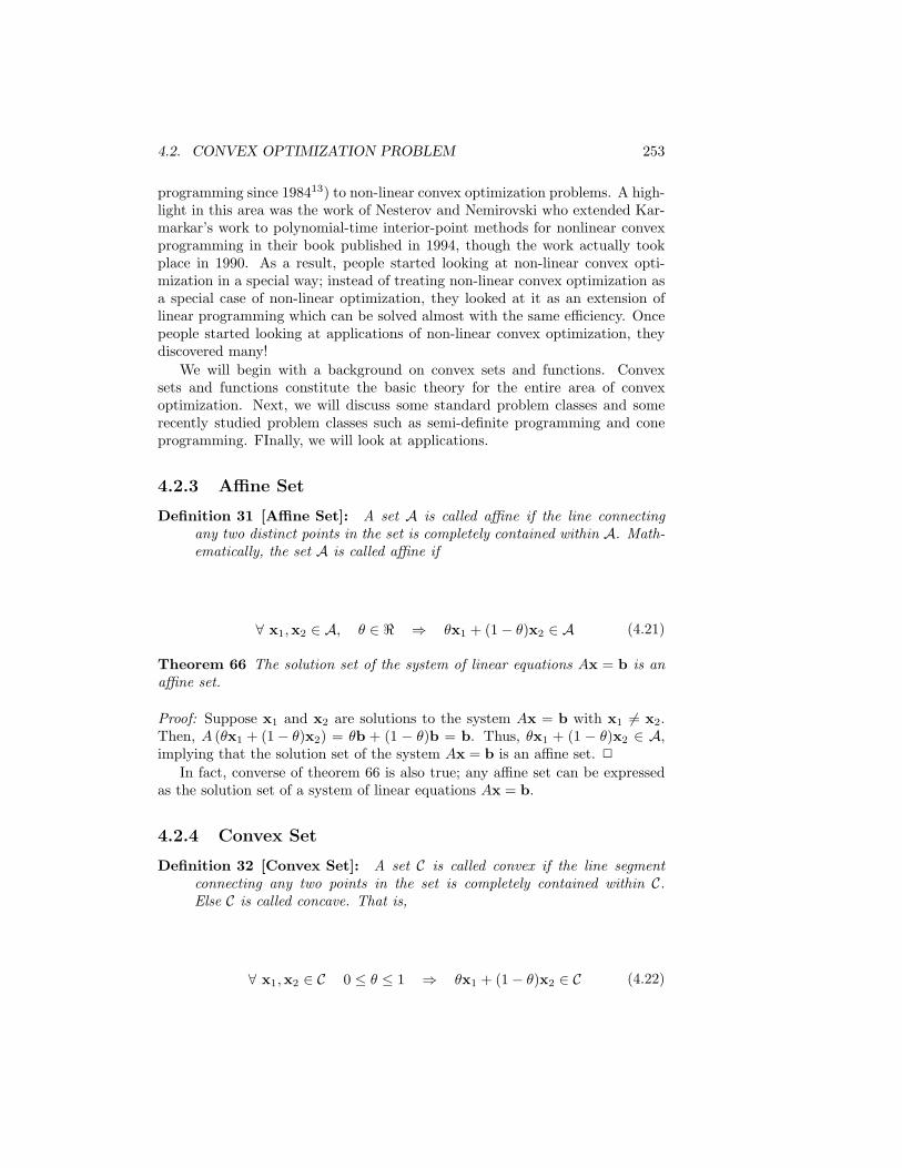
4.2. CONVEX OPTIMIZATION PROBLEM 253
programming since 198413) to non-linear convex optimization problems. A high-light in this area was the work of Nesterov and Nemirovski who extended Kar-markar’s work to polynomial-time interior-point methods for nonlinear convexprogramming in their book published in 1994, though the work actually tookplace in 1990. As a result, people started looking at non-linear convex opti-mization in a special way; instead of treating non-linear convex optimization asa special case of non-linear optimization, they looked at it as an extension oflinear programming which can be solved almost with the same efficiency. Oncepeople started looking at applications of non-linear convex optimization, theydiscovered many!
We will begin with a background on convex sets and functions. Convexsets and functions constitute the basic theory for the entire area of convexoptimization. Next, we will discuss some standard problem classes and somerecently studied problem classes such as semi-definite programming and coneprogramming. FInally, we will look at applications.
4.2.3 Affine Set
Definition 31 [Affine Set]: A set A is called affine if the line connectingany two distinct points in the set is completely contained within A. Math-ematically, the set A is called affine if
∀ x1,x2 ∈ A, θ ∈ < ⇒ θx1 + (1− θ)x2 ∈ A (4.21)
Theorem 66 The solution set of the system of linear equations Ax = b is anaffine set.
Proof: Suppose x1 and x2 are solutions to the system Ax = b with x1 6= x2.Then, A (θx1 + (1− θ)x2) = θb + (1 − θ)b = b. Thus, θx1 + (1 − θ)x2 ∈ A,implying that the solution set of the system Ax = b is an affine set. 2
In fact, converse of theorem 66 is also true; any affine set can be expressedas the solution set of a system of linear equations Ax = b.
4.2.4 Convex Set
Definition 32 [Convex Set]: A set C is called convex if the line segmentconnecting any two points in the set is completely contained within C.Else C is called concave. That is,
∀ x1,x2 ∈ C 0 ≤ θ ≤ 1 ⇒ θx1 + (1− θ)x2 ∈ C (4.22)

254 CHAPTER 4. CONVEX OPTIMIZATION
Figure 4.27: Examples of convex and non-convex sets.
Figure 4.27 shows examples of convex and non-convex (concave) sets. Sincean affine set contains any line passing through two distinct points in the set, italso contains any line segment connecting two points in the set. Thus, an affineset is our first example of a convex set.
A set C is a convex cone if it is covex and additionally, for every point x ∈ C,all non-negative multiples of x are also in C. In other words,
∀x1,x2 ∈ C θ1, θ2 ≥ 0 ⇒ θ1x1 + θ2x2 ∈ C (4.23)
Combinations of the form θ1x1 + θ2x2 for θ1 ≥ 0, θ2 ≥ 0 are called conic com-binations. We will state a related definition next - that of the convex hull of aset of points.
Definition 33 [Convex Hull]: A convex combination of the set of pointsS = x1,x2, . . . ,xk is any point x of the form
x =k∑i=1
θixi withk∑i=1
θi = 1 and θi ≥ 0 (4.24)
The convex hull conv(S) of the set of points S is the set of all convexcombinations of points in S. The convex hull of a convex set S is S itself.
13The first practical polynomial time algorithm for linear programming by Karmarkar (1984)involved interior-point methods.

4.2. CONVEX OPTIMIZATION PROBLEM 255
Figure 4.28: Example of a hyperplane in <2.
4.2.5 Examples of Convex Sets
We will look at simple but important examples of convex sets. We will also lookat some operations that preserve convexity.
A hyperplane is the most common example of a convext set. A hyperplaneis the set of solutions to a linear system of equations of the form aTx = b witha 6= 0 and was defined earlier in definition 24. A half space is a solution setover the linear inequality aTx ≤ b, a 6= 0. The hyperplane aTx = b bounds thehalf-space from one side.
Formally,
Hyperplane: x|aTx = b, a 6= 0. Figure 4.28 shows an example hyperplanein <2. a is the normal vector.
Halfspace: x|aTx ≤ b, a 6= 0. Figure 4.29 shows an example half-space in<2.
The hyperplane is convex and affine, whereas the halfspace is merely convexand not affine.
Another simple example of a convex set is a closed ball in <n with radius rand center xc which is an n-dimensional vector.
B[xc, r] = xc + ru | ||u||2 ≤ 1
where u is a vector with norm less than or equal to 1. The open ball B(xc, r)is also convex. Replacing r with a non-singular square matrix A, we get anellipsoid given by
xc +Au | ||u||2 ≤ 1
which is also a convex set. Another equivalent representation of the ellipsoid canbe obtained by observing that for any point x in the ellipsoid, ||A−1(x−xc)||2 ≤1, that is (x − xc)T (A−1)TA−1(x − xc) ≤ 1. Since (A−1)T = (AT )−1 and

256 CHAPTER 4. CONVEX OPTIMIZATION
Figure 4.29: Example of a half-space in <2.
Figure 4.30: Example of a ellipsoid in <2.
A−1B−1 = (BA)−1, the ellipsoid can be equivalently defined asx|(x− xc)TP−1(x− xc) ≤ 1
where P = (AAT ) is a symmetric matrix. Furthermore, P is positive definite,since A is non-singular (c.f. page 205).
Matrix A determines the size of the ellipsoid; the eigenvalue λi of A deter-mines the length of the ith semi-axis of the ellipsoid (see page number 203).The ellipsoid is another example of a convex set and is a generalization of theeucledian ball. Figure 4.30 illustrates an ellipsoid in <2.
A norm ball is a ball with an arbitrary norm. A norm ball with center xcand radius r is given by
x | ||x− xc|| ≤ r
By the definition of the norm, a ball in that norm will be convex. The normball with the ∞−norm corresponds to a square in <2, while the norm ball withthe 1−norm in <2 corresponds to the same square rotated by 45. The normball is convex for all norms.
The definition of cone can be extended to any arbitrary norm to define a

4.2. CONVEX OPTIMIZATION PROBLEM 257
Figure 4.31: Example of a cone in <2.
norm cone. The set of all pairs (x, t) satisfying ||x|| ≤ t, i.e.,
(x, t) | ||x|| ≤ t
is called a norm coneWhen the norm is the eucledian norm, the cone (which looks like an ice-
cream cone) is called the second order cone. Norm cones are always convex.Figure 4.31 shows a cone in <2. In general, the cross section of a norm cone hasthe shape of a norm ball with the same norm. The norm cone for the ∞−normis a square pyramid in <3 and the cone for 1−norm in <3 is the same squarepyramid rotated by 45.
A polyhedron is another convex set which is given as the solution set of afinite set of linear equalities and inequalities. In matrix form, the inequalitiescan be stated as
Ax b A ∈ <m×n
Cx = d C ∈ <p×n(4.25)
where stands for component-wise inequality of the form≤14. A polyhedroncan also be represented as the intersection of a finite number of halfspaces andhyperplanes. Figure 4.32 depicts a typical polyhedron in <2. An affine set is aspecial type of polyhedron.
A last simple example is the positive semi-definite cone. Let Sn be the setof all symmetric n × n matrices and Sn+ ⊂ Sn be the set of all positive semi-definite n × n matrices. The set Sn+ is a convex cone and is called the positivesemi-definite cone. Consider a positive semi-definite matrix S in <2. Then Smust of the form
14The component-wise inequality corresponds to a generalized inequality K with K = <n+.

258 CHAPTER 4. CONVEX OPTIMIZATION
Figure 4.32: Example of a polyhedron in <2.
Figure 4.33: Example of a positive semidefinite cone in <2.
S =
[x y
y z
](4.26)
We can represent the space of matrices S2+ of the form S ∈ S2
+ as a threedimensional space with non-negative x, y and z coordinates and a non-negativedeterminant. This space corresponds to a cone as shown in Figure 4.33.
4.2.6 Convexity preserving operations
In practice if you want to establish the convexity of a set C, you could either
1. prove it from first principles, i.e., using the definition of convexity or
2. prove that C can be built from simpler convex sets through some basicoperations which preserve convexity.

4.2. CONVEX OPTIMIZATION PROBLEM 259
Figure 4.34: Plot for the function in (4.28)
Some of the important operations that preserve complexity are:
Intersection
The intersection of any number of convex sets is convex15. Consider the set S:
S =
x ∈ <n | |p(t)| ≤ 1 for |t| ≤ π
3
(4.27)
wherep(t) = x1 cos t+ x2 cos 2t+ . . .+ xm cosmt (4.28)
Any value of t that satisfies |p(t)| ≤ 1, defines two regions, viz.,
<≤(t) = x | x1 cos t+ x2 cos 2t+ . . .+ xm cosmt ≤ 1
and
<≥(t) = x | x1 cos t+ x2 cos 2t+ . . .+ xm cosmt ≥ −1
Each of the these regions is convex and for a given value of t, the set ofpoints that may lie in S is given by
<(t) = <≤(t) ∩ <≥(t)
This set is also convex. However, not all the points in <(t) lie in S, sincethe points that lie in S satisfy the inequalities for every value of t. Thus, S canbe given as:
S = ∩|t|≤π3<(t)
15Exercise: Prove.

260 CHAPTER 4. CONVEX OPTIMIZATION
Figure 4.35: Illustration of the closure property for S defined in (4.27), form = 2.
Affine transform
An affine transform is one that preserves
• Collinearity between points, i.e., three points which lie on a line continueto be collinear after the transformation.
• Ratios of distances along a line, i.e., for distinct colinear points p1,p2,p3,||p2−p1||||p3−p2|| is preserved.
An affine transformation or affine map between two vector spaces f : <n →<m consists of a linear transformation followed by a translation:
x 7→ Ax + b
where A ∈ <n×m and b ∈ <m. In the finite-dimensional case each affine trans-formation is given by a matrix A and a vector b.
The image and pre-image of convex sets under an affine transformation de-fined as
f(x) =n∑i
xiai + b
yield convex sets16. Here ai is the ith row of A. The following are examples ofconvex sets that are either images or inverse images of convex sets under affinetransformations:
1. the solution set of linear matrix inequality (Ai, B ∈ Sm)
x ∈ <n | x1A1 + . . .+ xnAn B16Exercise: Prove.

4.2. CONVEX OPTIMIZATION PROBLEM 261
is a convex set. Here A B means B − A is positive semi-definite17.This set is the inverse image under an affine mapping of the positive semi-definite cone. That is, f−1 (cone) =
x ∈ <n |B − (x1A1 + . . .+ xnAn) ∈ Sm+
=
x ∈ <n|B ≥ (x1A1 + . . .+ xnAn).
2. hyperbolic cone (P ∈ Sn+), which is the inverse image of the norm coneCm+1 = (z, u)|||z|| ≤ u, u ≥ 0, z ∈ <m =
(z, u)|zT z− u2 ≤ 0, u ≥ 0, z ∈ <m
is a convex set. The inverse image is given by f−1 (Cm+1) =
x ∈ <n |
(Ax, cTx
)∈ Cm+1
=
x ∈ <n|xTATAx− (cTx)2 ≤ 0
. Setting, P = ATA, we get the equationof the hyperbolic cone:
x | xTPx ≤ (cTx)2, cTx ≥ 0
Perspective and linear-fractional functions
The perspective function P : <n+1 → <n is defined as follows:
P : <n+1 → <n such thatP (x, t) = x/t dom P = (x, t) | t > 0
(4.29)
The linear-fractional function f is a generalization of the perspective functionand is defined as: <n → <m:
f : <n → <m such thatf(x) = Ax+b
cTx+ddom f = x | cTx + d > 0
(4.30)
The images and inverse images of convex sets under perspective and linear-fractional functions are convex18.
Consider the linear-fractional function f = 1x1+x2+1x. Figure ?? shows an
example convex set. Figure ?? shows the image of this convex set under thelinear-fractional function f .
Supporting Hyperplane Theorem
On page 4.1.4, we introduced the concept of the hyperplane. For disjoint convexsets, we state the separating hyperplane theorem.
Theorem 67 If C and D are disjoint convex sets, i.e., C ∩ D = φ, then thereexists a 6= 0, with a b ∈ < such that
aTx ≤ b for x ∈ C,aTx ≥ b for x ∈ D.That is, the hyperplane
x|aTx = b
separates C and D. The seperating
hyperplane need not be unique though.17The inequality induced by positive semi-definiteness corresponds to a generalized inequal-
ity K with K = Sn+.18Exercise: Prove.

262 CHAPTER 4. CONVEX OPTIMIZATION
Proof: We first note that the set S = x− y|x ∈ C,y ∈ D is convex, since itis the sum of two convex sets. Since C and D are disjoint, 0 /∈ S. Consider twocases:
1. Suppose 0 /∈ closure(S). Let E = 0 and F = closure(S). Then, theeuclidean distance between E and F , defined as
dist(E ;F) = inf ||u− v||2|u ∈ E ,v ∈ Fis positive, and there exists a point f ∈ F that achieves the minimumdistance, i.e., ||f ||2 = dist(E ,F). Define a = f , b = ||f ||2. Then a 6= 0 andthe affine function f(x) = aTx− b = fT (x− 1
2 f) is nonpositive on E andnonnegative on F , i.e., that the hyperplane
x|aTx = b
separates E and
F . Thus, aT (x − y) > 0 for all x − y ∈ S ⊆ closure(S), which impliesthat, aTx ≥ aTy for all x ∈ C and y ∈ D.
2. Suppose, 0 ∈ closure(S). Since 0 /∈ S, it must be in the boundary of S.
• If S has empty interior, it must lie in an affine set of dimension lessthan n, and any hyperplane containing that affine set contains Sand is a hyperplane. In other words, S is contained in a hyperplanez|aT z = b
, which must include the origin and therefore b = 0. In
other words, aTx = aTy for all x ∈ C and all y ∈ D gives us a trivialseparating hyperplane.
• If S has a nonempty interior, consider the setS−ε = z|B(z, ε) ⊆ Swhere B(z, ε) is the Euclidean ball with center z and radius ε > 0.S−ε is the set S, shrunk by ε. closure (S−ε) is closed and convex,and does not contain 0, so as argued before, it is separated from 0by atleast one hyperplane with normal vector a(ε) such thata(ε)T z ≥ 0 for all z ∈ SεWithout loss of generality assume ||a(ε)||2 = 1. Let εk, for k =1, 2, . . . be a sequence of positive values of εk with lim
k→∞εk = 0. Since
||a(εk)||2 = 1 for all k, the sequence a(εk) contains a convergentsubsequence, and let a be its limit. We havea(εk)T z ≥ 0 for all z ∈ S−εkand therefore aT z ≥ 0 for all z ∈ interior(S), and aT z ≥ 0 for allz ∈ S, which meansaTx ≥ aTy for all x ∈ C, and y ∈ D.
2
Theorem 59 stated that the gradient evaluated at a point on a level set isorthogonal to the tangent hyperplane to the level set at that point. We nowstate the definition of a supporting hyperplane, which is special type of tangenthyperplane.
Definition 34 [Supporting Hyperplane]: The supporting hyperplane to aset C at a boundary point x0 is defined as
x|aTx = aTx0, a 6= 0, aTy ≤ aTx0, ∀ y ∈ C

4.2. CONVEX OPTIMIZATION PROBLEM 263
Figure 4.36: Example of a supporting hyperplane.
Figure 4.36 shows a supporting hyperplane at the point x0 on the boundaryof a convex set C.
For convex sets, there is an important theorem regarding supporting hyper-planes.
Theorem 68 If the set C is convex, then there exists a supporting hyperplaneat every boundary point of C. As in the case of the seperating hyperplane, thesupporting hyperplane need not be unique.
Proof: If the interior of C is nonempty, the result follows immediately by ap-plying the separating hyperplane theorem to the sets x0 and interior(C). Ifthe interior of C is empty, then C must lie in an affine set of dimension less thann, and any hyperplane containing that affine set contains C and x0, and is a(trivial) supporting hyperplane. 2
4.2.7 Convex Functions
Definition 35 [Convex Function]: A function f : D → < is convex if D isa convex set and
f(θx + (1− θ)y) ≤ θf(x) + (1− θ)f(y) ∀ x,y ∈ D 0 ≤ θ ≤ 1 (4.31)
Figure 4.37 illustrates an example convex function. A function f : D → <is strictly convex if D is convex and
f(θx + (1− θ)y) < θf(x) + (1− θ)f(y)) ∀ x,y ∈ D 0 ≤ θ ≤ 1(4.32)

264 CHAPTER 4. CONVEX OPTIMIZATION
Figure 4.37: Example of convex function.
A function f : D → < is called uniformly or strongly convex if D is convexand there exists a constant c > 0 such that
f(θx + (1− θ)y) ≤ θf(x) + (1− θ)f(y))− 12cθ(1− θ)||x− y|| ∀ x,y ∈ D 0 ≤ θ ≤ 1(4.33)
A function f : <n → < is said to be concave if the function −f is convex.Examples of convex functions on the set of reals < as well as on <n and <m×nare show in Table 4.1. Examples of concave functions on the set of reals < areshow in Table 4.2. If a function is both convex and concave, it must be affine,as can be seen in the two tables.
Function type Domain Additional Constraints
The affine function: ax+ b < Any a, b ∈ <The exponential function: eax < Any a ∈ <Powers: xα <++ α ≥ 1 or α ≤ 1
Powers of absolute value: |x|p < p ≥ 1
Negative entropy: x log x <++
Affine functions of vectors: aTx + b <n
p-norms of vectors: ||x||p =
(n∑i=1
|xi|p)1/p
<n p ≥ 1
inf norms of vectors: ||x||∞ = maxk |xk| <n
Affine functions of matrices: tr(ATX) + b =m∑i=1
n∑j=1
AijXij + b <m×n
Spectral (maximum singular value) matrix norm: ||X||2 = σmax(X) = (λmax(XTX))1/2 <m×n
Table 4.1: Examples of convex functions on <, <n and <m×n.
4.2.8 Convexity and Global Minimum
One of the most fundamental and useful chracteristics of convex functions isthat any point of local minimum point for a convex function is also a point ofglobal minimum.

4.2. CONVEX OPTIMIZATION PROBLEM 265
Function type Domain Additional Constraints
The affine function: ax+ b < Any a, b ∈ <Powers: xα <++ 0 ≤ α ≤ 1
logarithm: log x <++
Table 4.2: Examples of concave functions on <.
Theorem 69 Let f : D → < be a convex function on a convex domain D. Anypoint of locally minimum solution for f is also a point of its globally minimumsolution.
Proof: Suppose x ∈ D is a point of local minimum and let y ∈ D be a point ofglobal minimum. Thus, f(y) < f(x). Since x corresponds to a local minimum,there exists an ε > 0 such that
∀ z ∈ D, ||z− x|| ≤ ε⇒ f(z) ≥ f(x)
Consider a point z = θy + (1 − θ)x with θ = ε2||y−x|| . Since x is a point of
local minimum (in a ball of radius ε), and since f(y) < f(x), it must be that||y − x|| > ε. Thus, 0 < θ < 1
2 and z ∈ D. Furthermore, ||z− x|| = ε2 . Since f
is a convex functionf(z) ≤ θf(x) + (1− θ)f(y)
Since f(y) < f(x), we also have
θf(x) + (1− θ)f(y) < f(x)
The two equations imply that f(z) < f(x), which contradicts our assumptionthat x corresponds to a point of local minimum. That is f cannot have a pointof local minimum, which does not coincide with the point y of global minimum.2
Since any locally minimum point for a convex function also corresponds toits global minimum, we will drop the qualifiers ‘locally’ as well as ‘globally’ whilereferring to the points corresponding to minimum values of a convex function.For any stricly convex function, the point corresponding to the gobal minimumis also unique, as stated in the following theorem.
Theorem 70 Let f : D → < be a strictly convex function on a convex domainD. Then f has a unique point corresponding to its global minimum.
Proof: Suppose x ∈ D and y ∈ D with y 6= x are two points of global minimum.That is f(x) = f(y) for y 6= x. The point x+y
2 also belongs to the convex setD and since f is strictly convex, we must have
f
(x + y
2
)<
12f(x) +
12f(y) = f(x)
which is a contradiction. Thus, the point corresponding to the minimum of fmust be unique. 2

266 CHAPTER 4. CONVEX OPTIMIZATION
In the following section, we state some important properties of convex func-tions, including relationships between convex functions and convex sets, andfirst and second order conditions for convexity. We will also draw relationshipsbetween the definitions of convexity and strict convexity stated here, with thedefinitions on page 222 for the single variable case.
4.2.9 Properties of Convex Functions
We will first extend the domain of a convex function to all <n, while retainingits convexity and preserving its value in the domain.
Definition 36 [Extended value extension]: If f : D → <, with D ⊆ <n isa convex function, then we define its extended-valued extension f : <n → <as
f(x) =
f(x) if x ∈ D∞ if x /∈ D
(4.34)
In what follows, we will assume if necessary, that all convex functions areimplicitly extended to the domain <n. A useful technique for verifying theconvexity of a function is to investigate its convexity, by restricting the functionto a line and checking for the convexity of a function of single variable. Thistechnique is hinged on the following theorem.
Theorem 71 A function f : D → < is (strictly) convex if and only if thefunction φ : Dφ → < defined below, is (strictly) convex in t for every x ∈ <nand for every h ∈ <n
φ(t) = f(x + th)
with the domain of φ given by Dφ = t|x + th ∈ D.
Proof: We will prove the necessity and sufficiency of the convexity of φ for aconvex function f . The proof for necessity and sufficiency of the strict convexityof φ for a strictly convex f is very similar and is left as an exercise.
Proof of Necessity: Assume that f is convex. And we need to prove thatφ(t) = f(x + th) is also convex. Let t1, t2 ∈ Dφ and θ ∈ [0, 1]. Then,
φ(θt1 + (1− θ)t2) = f (θ(x + t1h) + (1− θ)(x + t2h))≤ θf ((x + t1h)) + (1− θ)f ((x + t2h)) = θφ(t1) + (1− θ)φ(t2) (4.35)
Thus, φ is convex.Proof of Sufficiency: Assume that for every h ∈ <n and every x ∈ <n,
φ(t) = f(x + th) is convex. We will prove that f is convex. Let x1,x2 ∈ D.Take, x = x1 and h = x2 − x1. We know that φ(t) = f (x1 + t(x2 − x1)) isconvex, with φ(1) = f(x2) and φ(0) = f(x1). Therefore, for any θ ∈ [0, 1]

4.2. CONVEX OPTIMIZATION PROBLEM 267
f (θx2 + (1− θ)x1) = φ(θ)≤ θφ(1) + (1− θ)φ(0) ≤ θf(x2) + (1− θ)f(x1) (4.36)
This implies that f is convex. 2
Next, we will draw the parallel between convex sets and convex functions byintroducing the concept of the epigraph of a function.
Definition 37 [Epigraph]: Let D ⊆ <n be a nonempty set and f : D →<. The set (x, f(x)|x ∈ D is called graph of f and lies in <n+1. Theepigraph of f is a subset of <n+1 and is defined as
epi(f) = (x, α)|f(x) ≤ α, x ∈ D, α ∈ < (4.37)
In some sense, the epigraph is the set of points lying above the graph of f .Similarly, the hypograph of f is a subset of <n+1, lying above the graph off and is defined by
hyp(f) = (x, α)|f(x) ≥ α, x ∈ D, α ∈ < (4.38)
There is a one to one correspondence between the convexity of function f andthat of the set epi(f), as stated in the following theorem.
Theorem 72 Let D ⊆ <n be a nonempty convex set, and f : D → <. Then fis convex if and only if epi(f) is a convex set.
Proof: Let f be convex. For any (x1, α1) ∈ epi(f) and (x2, α2) ∈ epi(f) andany θ ∈ (0, 1),
f(θx1 + (1− θ)x2) ≤ θf(x1) + (1− θ)f(x2)) ≤ θα1 + (1− θ)α2
SinceD is convex, θx1+(1−θ)x2 ∈ D. Therefore, (θx1 + (1− θ)x2, θα1 + (1− θ)α2) ∈epi(f). Thus, epi(f) is convex if f is convex. This proves the necessity part.
To prove sufficiency, assume that epi(f) is convex. Let x1,x2 ∈ D. So,(x1, f(x1)) ∈ epi(f) and (x2, f(x2)) ∈ epi(f). Since epi(f) is convex, for θ ∈(0, 1),
(θx1 + (1− θ)x2, θα1 + (1− θ)α2) ∈ epi(f)
which implies that f(θx1 +(1−θ)x2) ≤ θf(x1)+(1−θ)f(x2)) for any θ ∈ (0, 1).This proves the sufficiency. 2
There is also a correspondence between the convexity of a function and theconvexity of its sublevel sets.

268 CHAPTER 4. CONVEX OPTIMIZATION
Definition 38 [Sublevel Sets]: Let D ⊆ <n be a nonempty set and f : D →<. The set
Lα(f) = x|x ∈ D, f(x) ≤ α
is called the α−sub-level set of f .
The correspondence between the convexity of f and its α−sub-level set is statedin the following theorem. Unlike the correspondence with the epigraph, thecorrespondence with the α−sub-level set is not one to one.
Theorem 73 Let D ⊆ <n be a nonempty convex set, and f : D → < be aconvex function. Then Lα(f) is a convex set for any α ∈ <.
Proof: Consider x1,x2 ∈ Lα(f). Then by definition of the level set, x1,x2 ∈ D,f(x1) ≤ α and f(x2) ≤ α. From convexity of D it follows that for all θ ∈ (0, 1),x = θx1 + (1− θ)x2 ∈ D. Moreover, since f is also convex,
f(x) ≤ θf(x1) + (1− θ)f(x2) ≤ θα+ (1− θ)α = α
which implies that x ∈ Lα(f). Thus, Lα(f) is a convex set. 2The converseof this theorem does not hold. To illustrate this, consider the function f(x) =x2
1+2x21. The 0-sublevel set of this function is (x1, x2) | x2 ≤ 0, which is convex.
However, the function f(x) itself is not convex.An important property of a convex function is that it is continuous in the
interior of its domain.
Theorem 74 Let f : D → < be a convex function with D ⊆ <n being a convexset. Let S ⊂ D be an open convex set. Then f is continuous on S.
Proof: Let us consider a point x0 ∈ S. Since S is an open convex set, we canfind n+ 1 points x1,x2, . . . ,xn+1 such that the interior of the convex hull
C =
x|x =
n+1∑i=1
aixi, ai ≥ 0,n+1∑
1
ai = 1
is not empty and x0 ∈ interior(C). Let M = max1≤i≤n+1
f(xi). Then, for any
x =n+1∑i=1
aixi ∈ C,
f(x) = f
(n+1∑i=1
aixi
)≤n+1∑i=1
aif(xi) ≤M
Since x0 ∈ C, there exists a δ > 0 such that B(x0, δ) ⊂ C, where, B(x0, δ) =x|||x− x0|| ≤ δ. Therefore, x0 can be expressed as a convex combination of(x0 + θh and x0 − h for some h ∈ B(x0, δ) and some θ ∈ [0, 1].
x0 =1
1 + θ(x0 + θh) +
θ
1 + θ(x0 − h)

4.2. CONVEX OPTIMIZATION PROBLEM 269
Since f is convex on C,
f(x0) ≤ 11 + θ
f(x0 + θh) +θ
1 + θf(x0 − h)
From this, we can conclude that
f(x0 + θh)− f(x0) ≥ θ (f(x0 − f(x0 − h)) ≥ −θ (M − f(x0)) (4.39)
On the other hand,
f(x0 + θh) ≤ θf(x0 + h) + (1− θ)f(x0)
which implies that
f(x0 + θh)− f(x0) ≤ θ (f(x0 + h)− f(x0) ≤ θ (M − f(x0)) (4.40)
From equations 4.39 and 4.40, we can infer that
|f(x0 + θh)− f(x0)| ≤ θ|f(x0)−M |
For a given ε > 0, select δ′ ≤ δ such that δ′|f(x0)−M | ≤ εδ. Then d = θh with||h|| = δ, implies that d ∈ B(x0, δ) and f(x0 + d)− f(x0)| ≤ ε. This proves thetheorem. 2
Analogous to the definition of increasing functions introduced on page num-ber 218, we next introduce the concept of monotonic functions. This concept isvery useful for characterization of a convex function.
Definition 39 Let f : D → <n and D ⊆ <n. Then
1. f is monotone on D if for any x1,x2 ∈ D,
(f(x1)− f(x2))T (x1 − x2) ≥ 0 (4.41)
2. f is strictly monotone on D if for any x1,x2 ∈ D with x1 6= x2,
(f(x1)− f(x2))T (x1 − x2) > 0 (4.42)
3. f is uniformly or strongly monotone on D if for any x1,x2 ∈ D, there isa constant c > 0 such that
(f(x1)− f(x2))T (x1 − x2) ≥ c||x1 − x2||2 (4.43)

270 CHAPTER 4. CONVEX OPTIMIZATION
First-Order Convexity Conditions
The first order convexity condition for differentiable functions is provided bythe following theorem:
Theorem 75 Let f : D → < be a differentiable convex function on an openconvex set D. Then:
1. f is convex if and only if, for any x,y ∈ D,
f(y) ≥ f(x) +∇T f(x)(y − x) (4.44)
2. f is strictly convex on D if and only if, for any x,y ∈ D, with x 6= y,
f(y) > f(x) +∇T f(x)(y − x) (4.45)
3. f is strongly convex on D if and only if, for any x,y ∈ D,
f(y) ≥ f(x) +∇T f(x)(y − x) +12c||y − x||2 (4.46)
for some constant c > 0.
Proof:Sufficiency: The proof of sufficiency is very similar for all the three state-
ments of the theorem. So we will prove only for statement (4.44). Suppose(4.44) holds. Consider x1,x2 ∈ D and any θ ∈ (0, 1). Let x = θx1 + (1− θ)x2.Then,
f(x1) ≥ f(x) +∇T f(x)(x1 − x)f(x2) ≥ f(x) +∇T f(x)(x2 − x) (4.47)
Adding (1− θ) times the second inequality to θ times the first, we get,
θf(x1) + (1− θ)f(x2) ≥ f(x)
which proves that f(x) is a convex function. In the case of strict convexity,strict inequality holds in (4.47) and it follows through. In the case of strongconvexity, we need to additionally prove that
θ12c||x− x1||2 + (1− θ)1
2c||x− x2||2 =
12cθ(1− θ)||x2 − x1||2

4.2. CONVEX OPTIMIZATION PROBLEM 271
Figure 4.38: Figure illustrating Theorem 75.
Necessity: Suppose f is convex. Then for all θ ∈ (0, 1) and x1,x2 ∈ D, wemust have
f(θx2 + (1− θ)x1) ≤ θf(x2) + (1− θ)f(x1)
Thus,
∇T f(x1)(x2 − x1) = limθ→0
f (x1 + θ(x2 − x1))− f (x1)θ
≤ f(x2)− f(x1)
This proves necessity for (4.44). The necessity proofs for (4.45) and (4.46) arevery similar, except for a small difference for the case of strict convexity; thestrict inequality is not preserved when we take limits. Suppose equality doeshold in the case of strict convexity, that is for a strictly convex function f , let
f(x2) = f(x1) +∇T f(x1)(x2 − x1) (4.48)
for some x2 6= x1. Because f is stricly convex, for any θ ∈ (0, 1) we can write
f (θx1 + (1− θ)x2) = f (x2 + θ(x1 − x2)) < θf(x1) + (1− θ)f(x2) (4.49)
Since (4.44) is already proved for convex functions, we use it in conjunction with(4.48), and (4.49), to get
f(x2)+θ∇T f(x2)(x1−x2) ≤ f (x2 + θ(x1 − x2)) < f(x2)+θ∇T f(x2)(x1−x2)
which is a contradiction. Thus, equality can never hold in (4.44) for any x1 6= x2.This proves the necessity of (4.45). 2
The geometrical interpretation of theorem 75 is that at any point, the linearapproximation based on a local derivative gives a lower estimate of the function,i.e. the convex function always lies above the supporting hyperplane at thatpoint. This is pictorially depicted in Figure 4.38. There are some implicationsof theorem 75 for strongly convex functions. We state them next.

272 CHAPTER 4. CONVEX OPTIMIZATION
Definition 40 [Some corollaries of theorem 75 for strongly convex functions]:For a fixed x, the right hand side of the inequality (4.46) is a convexquadratic function of y. Thus, the critical point of the RHS should corre-spond to the minimum value that the RHS could take. This yields anotherlower bound on f(y).
f(y) ≥ f(x)− 12c||∇f(x)||22 (4.50)
Since this holds for any y ∈ D, we have
miny∈D
f(y) ≥ f(x)− 12c||∇f(x)||22 (4.51)
which can be used to bound the suboptimality of a point x in terms of||∇f(x)||2. This bound comes handy in theoretically understanding theconvergence of gradient methods. If y = min
y∈Df(y), we can also derive a
bound on the distance between any point x ∈ D and the point of optimalityy.
||x− y||2 ≤2c||∇f(x)||2 (4.52)
Theorem 75 motivates the definition of the subgradient for non-differentiableconvex functions, which has properties very similar to the gradient vector.
Definition 41 [Subgradient]: Let f : D → < be a convex function definedon a convex set D. A vector h ∈ <n is said to be a subgradient of f at thepoint x ∈ D if
f(y) ≥ f(x) + hT (y − x)
for all y ∈ D. The set of all such vectors is called the subdifferential of fat x.
For a differentiable convex function, the gradient at point x is the only subgradi-ent at that point. Most properties of differentiable convex functions that hold interms of the gradient also hold in terms of the subgradient for non-differentiableconvex functions. Theorem 75 gives a very simple optimality criterion for a dif-ferentiable function f .
Theorem 76 Let f : D → < be a convex function defined on a convex set D.A point x ∈ D corresponds to a minimum if and only if
∇T f(x)(y − x) ≥ 0
for all y ∈ D.

4.2. CONVEX OPTIMIZATION PROBLEM 273
If ∇f(x) is nonzero, it defines a supporting hyperplane to D at the point x.Theorem 77 implies that for a differentiable convex function defined on an openset, every critical point must be a point of (global) minimum.
Theorem 77 Let f : D → < be differentiable and convex on an open convexdomain D ⊆ <n. Then x is a critical point of f if and only if it is a (global)minimum.
Proof: If x is a global minimum, it is a local minimum and by theorem 60, itmust be a critical point and therefore ∇f(x) = 0. Conversely, let ∇f(x) = 0,By theorem 75, we know that for all y ∈ D,
f(y) ≥ f(x) +∇T f(x)(y − x)
Substituting ∇f(x) = 0 in this inequality, we get for all y ∈ D,
f(y) ≥ f(x)
That is, x corresponds to a (global) minimum. 2
Based on the definition of monotonic functions in definition 39, we show therelationship between convexity of a function and monotonicity of its gradient inthe next theorem.
Theorem 78 Let f : D → < with D ⊆ <n be differentiable on the convex setD. Then,
1. f is convex on D if and only if is its gradient ∇f is monotone. That is,for all x,y ∈ <
(∇f(x)−∇f(y))T (x− y) ≥ 0 (4.53)
2. f is strictly convex on D if and only if is its gradient ∇f is strictly mono-tone. That is, for all x,y ∈ < with x 6= y,
(∇f(x)−∇f(y))T (x− y) > 0 (4.54)
3. f is uniformly or strongly convex on D if and only if is its gradient ∇f isuniformly monotone. That is, for all x,y ∈ <,
(∇f(x)−∇f(y))T (x− y) ≥ c||x− y||2 (4.55)
for some constant c > 0.
274 CHAPTER 4. CONVEX OPTIMIZATION
Proof:Necessity: Suppose f is uniformly convex on D. Then from theorem 75,
we know that for any x,y ∈ D,
f(y) ≥ f(x) +∇T f(x)(y − x)− 12c||y + x||2
f(x) ≥ f(y) +∇T f(y)(x− y)− 12c||x + y||2
Adding the two inequalities, we get (4.55). If f is convex, the inequalities holdwith c = 0, yielding (4.54). If f is strictly convex, the inequalities will be strict,yielding (4.54).
Sufficiency: Suppose ∇f is monotone. For any fixed x,y ∈ D, consider thefunction φ(t) = f (x + t(y − x)). By the mean value theorem applied to φ(t),we should have for some t ∈ (0, 1),
φ(1)− φ(0) = φ′(t) (4.56)
Letting z = x + t(y − x), (4.56) translates to
f(y)− f(x) = ∇T f(z)(y − x) (4.57)
Also, by definition of monotonicity of ∇f , (from (4.53)),
(∇f(z)−∇f(x))T (y − x) =1t
(∇f(z)−∇f(x))T (z− x) ≥ 0 (4.58)
Combining (4.57) with (4.58), we get,
f(y)− f(x) = (∇f(z)− f(x))T (y − x) +∇T f(x)(y − x)≥ ∇T f(x)(y − x) (4.59)
By theorem 75, this inequality proves that f is convex. Strict convexity canbe similarly proved by using the strict inequality in (4.58) inherited from strictmonotonicity, and letting the strict inequality follow through to (4.59). For thecase of strong convexity, from (4.55), we have
φ′(t)− φ′(0) = (∇f(z)− f(x))T (y − x)
=1t
(∇f(z)− f(x))T (z− x) ≥ 1tc||z− x||2 = ct||y − x||2 (4.60)

4.2. CONVEX OPTIMIZATION PROBLEM 275
Therefore,
φ(1)− φ(0)− φ′(0) =∫ 1
0
[φ′(t)− φ′(0)]dt ≥ 12c||y − x||2 (4.61)
which translates to
f(y) ≥ f(x) +∇T f(x)(y − x) +12c||y − x||2
By theorem 75, f must be strongly convex. 2
Second Order Condition
For twice continuously differentiable convex functions the convexity conditioncan be characterized as follows.
Theorem 79 A twice differential function f : D → < for a nonempty openconvex set D
1. is convex if and only if its domain is convex and its Hessian matrix ispositive semidefinite at each point in D. That is
∇2f(x) 0 ∀ x ∈ D (4.62)
2. is strictly convex if its domain is convex and its Hessian matrix is positivedefinite at each point in D. That is
∇2f(x) 0 ∀ x ∈ D (4.63)
3. is uniformly convex if and only if its domain is convex and its Hessianmatrix is uniformly positive definite at each point in D. That is, for anyv ∈ <n and any x ∈ D, there exists a c > 0 such that
vT∇2f(x)v ≥ c||v||2 (4.64)
In other words∇2f(x) cIn×n
where In×n is the n × n identity matrix and corresponds to the pos-itive semidefinite inequality. That is, the function f is strongly convexiff ∇2f(x) − cIn×n is positive semidefinite, for all x ∈ D and for someconstant c > 0, which corresponds to the positive minimum curvature off .

276 CHAPTER 4. CONVEX OPTIMIZATION
Proof: We will prove only the first statement in the theorem; the other twostatements are proved in a similar manner.
Necessity: Suppose f is a convex function, and consider a point x ∈ D.We will prove that for any h ∈ <n, hT∇2f(x)h ≥ 0. Since f is convex, bytheorem 75, we have
f(x + th) ≥ f(x) + t∇T f(x)h (4.65)
Consider the function φ(t) = f(x + th) considered in theorem 71, defined onthe domain Dφ = [0, 1]. Using the chain rule,
φ′(t) =n∑i=1
fxi(x + th)dxidt
= hT .∇f(x + th)
Since f has partial and mixed partial derivatives, φ′ is a differentiable functionof t on Dφ and
φ′′(t) = hT∇2f(x + th)h
Since φ and φ′ are continous on Dφ and φ′ is differentiable on int(Dφ), wecan make use of the Taylor’s theorem (45) with n = 3 to obtain:
φ(t) = φ(0) + t.φ′(0) + t2.12φ′′(0) +O(t3)
Writing this equation in terms of f gives
f(x + th) = f(x) + thT∇f(x) + t212hT∇2f(x)h +O(t3)
In conjunction with (4.65), the above equation implies that
t2
2hT∇2f(x)h +O(t3) ≥ 0
Dividing by t2 and taking limits as t→ 0, we get
hT∇2f(x)h ≥ 0
Sufficiency: Suppose that the Hessian matrix is positive semidefinite ateach point x ∈ D. Consider the same function φ(t) defined above with h = y−xfor y,x ∈ D. Applying Taylor’s theorem (45) with n = 2 and a = 0, we obtain,
φ(1) = φ(0) + t.φ′(0) + t2.12φ′′(c)
for some c ∈ (0, 1). Writing this equation in terms of f gives
f(x) = f(y) + (x− y)T∇f(y) +12
(x− y)T∇2f(z)(x− y)

4.2. CONVEX OPTIMIZATION PROBLEM 277
where z = y + c(x−y). Since D is convex, z ∈ D. Thus, ∇2f(z) 0. It followsthat
f(x) ≥ f(y) + (x− y)T∇f(y)
By theorem 75, the function f is convex. 2
Examples of differentiable/twice differentiable convex functions, along withthe value of their respective gradients/hessians are tabulated in Table 4.3.
Function type Constraints Gradient/Hessian
Quadratic : 12xTAx + bTx + c A 0 ∇2f(x) = P
Quadratic over linear: x2
y ≥ 0 y > 0 ∇2f(x, y) = 2y3
[y2 −xy−xy x2
]Log-sum-exp: log
n∑k=1
exp(xk) ∇2f(x) = 1(1T z)2
((1T z) diag(z)− zzT
)where z = [ex1 , ex1 , . . . , exn ]
Negative Geometric mean: −
(n∏k=1
xk
) 1n
x ∈ <n++ ∇2f(x) =
∏i=1
nx1/ni
n2
(n diag( 1
x21, . . . , 1
x2n
)− qqT)
Table 4.3: Examples of twice differentiable convex functions on <.
4.2.10 Convexity Preserving Operations on Functions
In practice if you want to establish the convexity of a function f , you couldeither
1. Prove it from first principles, i.e., using the definition of convexity or
2. If f is twice differentiable, show that ∇2f(x) 0
3. Show that f is obtained from simple convex functions by operations thatpreserve complexity. Following are operations on functions that preservecomplexity (proofs omitted, since they are trivial):
• Nonnegative weighted sum: f =n∑i=1
αifi is convex if each fi for
1 ≤ i ≤ n is convex and αi ≥ 0, 1 ≤ i ≤ n.
• Composition with affine function: f(Ax + b) is convex if f isconvex. For example:
– The log barrier for linear inequalities, f(x) = −m∑i=1
log(bi−aTi x),
is convex since − log(x) is convex.– Any norm of an affine function, f(x) = ||Ax+ b||, is convex.
• Pointwise maximum: If f1, f2, . . . , fm are convex, then f(x) =max f1(x), f2(x), . . . , fm(x) is also convex, For example:

278 CHAPTER 4. CONVEX OPTIMIZATION
– Sum of r largest components of x ∈ <n f(x) = x[1] +x[2] + . . .+x[r], where x[1] is the ith largest component of x, is a convexfunction.
• Pointwise supremum: If f(x, y) is convex in x for every y ∈ S,then g(x) = sup
y∈Sf(x, y) is convex. For example:
– The function that returns the maximum eigenvalue of a symmet-ric matrix X, viz., λmax(X) = sup
y∈Sf(x, y) is a convex function
of the symmetrix matrix X.
• Composition with functions: Let h : <k → < with h(x) =∞,∀ x /∈ dom h and g : <n → <k. Define f(x) = h(g(x)). f isconvex if
– gi is convex, h is convex and nondecreasing in each argument– or gi is concave, h is convex and nonincreasing in each argument
Some examples illustrating this property are:– exp g(x) is convex if g is convex
–m∑i=1
log gi(x) is concave if gi are concave and positive
– logm∑i=1
exp gi(x) is convex if gi are convex
– 1/g(x) is convex if g is concave and positive• Infimum: If f(x, y) is convex in (x, y) and C is a convex set, theng(x) = inf
y∈Cf(x, y) is convex. For example:
– Let f(x,S) that returns the distance of a point x to a convex setS. That is f(x,S) = inf
y∈S||x− y||. Then f(x,S) is a convex.
• Perspective Function: The perspective of a function f : <n → < isthe function g : Rn×< → <, g(x, t) = tf(x/t). Function g is convexif f is convex on domg = (x, t)|x/t ∈ domf, t > 0. For example,
– The perspective of f(x) = xTx is (quadratic-over-linear) functiong(x, t) = xT x
t and is convex.– The perspective of negative logarithm f(x) = − log x is the rel-
ative entropy function g(x, t) = t log t− t log x and is convex.
4.3 Convex Optimization Problem
Formally, a convex program is defined as
minx∈X
cTx (4.66)

4.3. CONVEX OPTIMIZATION PROBLEM 279
where X ⊂ <n is a convex set and x is a vector of n optimization or decisionvariables. In applications, convex optimization programs usually arise in theform:
minimize f(x)subject to gi(x) ≤ 0, i = 1, . . . ,m
Ax = b
variable x = (x1, . . . , xn)
(4.67)
If it is given that the functions f, g1, . . . , gm are convex, by theorem 73, thefeasible set X of this problem, which is the intersection of a finite number of0−sub-level sets of convex functions is also convex. Therefore, this problem canbe posed as the following convex optimization problem:
minx=(t,u)∈X
t
X = (t, u)|f(u) ≤ t, g1(u) ≤ 0, g2(u) ≤ 0, . . . , gm(u) ≤ 0(4.68)
The set X is convex, and hence the problem in (4.68) is a convex optimizationproblem. Further, every locally optimal point is also globally optimal. Thecomputation time of algorithms for solving convex optimization problems isroughly proportional to max
(n2, n2m,C
), where C is the cost of evaluating
f , the gi’s and their first and second derivatives. There are many reliable andefficient algorithms for solving convex optimization problems. However, it isoften difficult to recognize convex optimization problems in practice.
Examples
Consider the optimization problem
minimize f(x) = x21 + x2
2
subject to g1(x) = x11+x2
2≤ 0
h(x) = (x1 + x2)2 = 0
(4.69)
We note that the optimiation problem above is not a convex problem ac-cording to our definition, since g1 is not convex and h is not affine. However, wenote that the feasible set (x1, x2) | x1 = −x2, x1 ≤ 0 is convex (recall thatthe converse of theorem 73 does not hold - the 0-sublevel set of a non convexfunction can be convex). This problem can be posed as an equivalent (but notidentical) convex optimization problem:

280 CHAPTER 4. CONVEX OPTIMIZATION
minimize f(x) = x21 + x2
2
subject to x1 ≤ 0x1 + x2 = 0
(4.70)
4.4 Duality Theory
Duality is a very important component of nonlinear and linear optimizationmodels. It has a wide spectrum of applications that are very popular. It arisesin the basic form of linear programming as well as in interior point methodsfor linear programming. The duality in linear programming was first observedby Von Neumann, and later formalized by Tucker, Gale and Kuhn. In thefirst attempt at extending duality beyond linear programs, duals of quadraticprograms were next developed. It was subsequently observed that you canalways write a dual for any optimization problem and the modern Lagrange-based ‘constructive’19 duality theory followed in the late 1960s.
An extremely popular application of duality happens to be in the quadraticprogramming for Support Vector Machines. The primal and dual both happento be convex optimization programs in this case. The Minimax theorem20, afundamental theorem of Game Theory, proved by John von Neumann in 1928,is but one instance of the general duality theory. In the consideration of equi-librium in electrical networks, current are ‘primal variables’ and the potentialdifferences are the ‘dual variables’. In models of economic markets, the ‘primal’variables are production and consumption levels while the ‘dual’ variables areprices (of goods, etc.). Dual price-based decomposition methods were developedby Danzig. In the case of thrust structures in mechanics, forces are primal vari-ables and the displacements are the dual variables. Dual problems and theirsolutions are used for proving optimality of solutions, finding near-optimal so-lutions, analysing how sensitive the solution of the primal is to perturbations inthe right hand side of constraints, analysing convergence of algorithms, etc.
4.4.1 Lagrange Multipliers
Consider the following quadratic function of x ∈ <n.
F (x) = xTAx− xTb (4.71)
where A is an n × n square matrix. Consider the unconstrained minimizationproblem
19As we will see, the theory helps us construct duals that are useful in practice.20The name Minimax was invented by Tucker.

4.4. DUALITY THEORY 281
minx∈D
F (x) (4.72)
A locally optimum solution x to this objective can be obtained by setting∇F (x) = 0. This condition translates to Ax = b. A sufficient condition for xto be a point of local minimum is that ∇2F (x) 0. This condition holds iff,A 0, that is, A is a positive definite matrix. Given that A 0, A must beinvertible (c.f. Section 3.12.2) and the unique solution is x = A−1b.
Now suppose we have a constrained minimization problem
miny∈<n
12yTBy
subject to ATy = b(4.73)
where y ∈ <n, A is an n ×m matrix, B is an n × n matrix and b is a vectorof size m. To handle constrained minimization, let us consider minimization ofthe modified objective function L(y, λ) = 1
2yTBy + λT (ATy − b).
miny∈<n,λ∈<m
12yTBy + λT (ATy − b) (4.74)
The function L(y, λ) is called the lagrangian and involves the lagrange multi-plier λ ∈ <m. A sufficient condition for optimality of L(y, λ) at a point L(y∗, λ∗)is that ∇L(y∗, λ∗) = 0 and ∇2L(y∗, λ∗) 0. For this particular problem:
∇L(y∗, λ∗) =
[By∗ +Aλ∗
ATy∗ − b
]=
[00
]and
∇2L(y∗, λ∗) =
[B A
AT 0
] 0
The point (y∗, λ∗) must therefore satisfy, ATy∗ = b and Aλ∗ = −By∗. If Bis taken to be the identity matrix, n = 2 and m = 1, the minimization problem(4.73) amounts to finding a point y∗ on a line a11y1 +a12y2 = b that is closest tothe origin. From geometry, we know that the point on a line closest to the originis the point of intersection p∗ of a perpendicular from the origin to the line. Onthe other hand, the solution for the minimum of (4.74), for these conditionscoincides with p∗ and is given by:
y1 =a11b
(a11)2 + (a12)2
y2 =a12b
(a11)2 + (a12)2

282 CHAPTER 4. CONVEX OPTIMIZATION
That is, for n = 2 and m = 1, the solution to (4.74) is the same as the solu-tion to (4.72) Can this construction be used to always find optimal solutionsto a minimization problem? We will answer this question by first motivatingthe concept of lagrange multipliers and in Section 4.4.2, we will formalize thelagrangian dual.
Lagrange Multipliers with Equality Constraints
The concept of lagrange multipliers can be attributed to the mathematicianLagrange, who was born in the year 1736 in Turin. He largely worked onmechanics, the calculus of variations probability, group theory, and numbertheory. He was party to the choice of base 10 for the metric system (rather than12). We will here give a brief introduction to lagrange multipliers; Section 4.4.2will discuss the Karush-Kuhn-Tucker conditions, which are a generalization oflagrange multipliers.
Consider the equality constrained minimization problem (with D ⊆ <n)
minx∈D
f(x)
subject to gi(x) = 0 i = 1, 2, . . . ,m(4.75)
A direct approach to solving this problem is to find a parametrization of theconstraints (as in the example on page 228) such that f is expressed in termsof the parameters, to give an unconstrained problem. For example if there is asingle constraint of the form xTAx = k, and A 0, then the coordinate systemcan be rotated and x can be rescaled so that we get the constraint y′y = k.Further, we can substitute with parametrization of the yi’s as
y1 = k sin θ1 sin θ2 . . . sin θn−1
y2 = k sin θ1 sin θ2 . . . cos θn−1
. . . . . . . . .
However, this is not possible for general constraints. The method of lagrangemultipliers presents an indirect approach to solving this problem.
Consider a schematic representation of the problem in (4.75) with a singleconstraint, i.e., m = 1 in Figure 4.39. The figure shows some level curves of thefunction f . The constraint function g1 is also plotted with dotted lines in thesame figure. The gradient of the constraint ∇g1 is not parallel to the gradient∇f of the function21 at f = 10.4; it is therefore possible to move along theconstraint surface so as to further reduce f . However, as shown in Figure 4.39,∇g1 and ∇f are parallel at f = 10.3, and any motion along g1(x) = 0 will
21Note that the (negative) gradient at a point is orthogonal to the contour line going throughthat point. This was proved in Theorem 59.

4.4. DUALITY THEORY 283
Figure 4.39: At any non-optimal and non-saddle point of the equality con-strained problem, the gradient of the constraint will not be parallel to that ofthe function.
increase f , or leave it unchanged. Hence, at the solution x∗, ∇f(x∗) must beproportional to −∇g1(x∗), yielding, ∇f(x∗) = −λ∇g1(x∗), for some constantλ ∈ <; λ is called a Lagrange multiplier. In several problems, the value of λ itselfneed never be computed and therefore λ is often qualified as the undeterminedlagrange multiplier.
The necessary condition for an optimum at x∗ for the optimization problemin (4.75) with m = 1 can be stated as in (4.76), where the gradient is now n+ 1dimensional with its last component being a partial derivative with respect toλ.
∇L(x∗, λ∗) = ∇f(x∗) + λ∗∇g1(x∗) = 0 (4.76)
The solutions to (4.76) are the stationary points of the lagrangian L; they are notnecessarily local extrema of L. L is unbounded: given a point x that doesn’t lieon the constraint, letting λ→ ±∞ makes L arbitrarily large or small. However,under certain stronger assumptions, as we shall see in Section 4.4.2, if the strongLagrangian principle holds, the minima of f minimize the Lagrangian globally.
We will extend the necessary condition for optimality of a minimizationproblem with single constraint to minimization problems with multiple equalityconstraints (i.e., m > 1. in (4.75)). Let S be the subspace spanned by ∇gi(x)at any point x and let S⊥ be its orthogonal complement. Let (∇f)⊥ be thecomponent of ∇f in the subspace S⊥. At any solution x∗, it must be true thatthe gradient of f has (∇f)⊥ = 0 (i.e., no components that are perpendicular toall of the ∇gi), because otherwise you could move x∗ a little in that direction(or in the opposite direction) to increase (decrease) f without changing anyof the gi, i.e. without violating any constraints. Hence for multiple equalityconstraints, it must be true that at the solution x∗, the space S contains the

284 CHAPTER 4. CONVEX OPTIMIZATION
Figure 4.40: At the equality constrained optimum, the gradient of the constraintmust be parallel to that of the function.
vector ∇f , i.e., there are some constants λi such that ∇f(x∗) = λi∇gi(x∗).We also need to impose that the solution is on the correct constraint surface(i.e., gi = 0, ∀i). In the same manner as in the case of m = 1, this can be
encapsulated by introducing the Lagrangian L(x, λ) = f(x) −m∑i=1
λi∇gi(x),
whose gradient with respect to both x, and λ vanishes at the solution.This gives us the following necessary condition for optimality of (4.75):
∇L(x∗, λ∗) = ∇
(f(x)−
m∑i=1
λigi(x)
)= 0 (4.77)
Lagrange Multipliers with Inequality Constraints
Instead of a single equality constraint g1(x) = 0, we could have a single inequal-ity constraint g1(x) ≤ 0. The entire region labeled g1(x) ≤ 0 in Figure 4.41then becomes feasible. At the solution x∗, if g1(x∗) = 0, i.e., if the constraintis active, we must have (as in the case of a single equality constraint) that ∇fis parallel to ∇g1, by the same argument as before. Additionally, it is neces-sary that the two gradients must point in opposite directions; otherwise a moveaway from the surface g1 = 0 and into the feasible region would further reducef . Since we are minimizing f , if the Lagrangian is written as L = f + λg1,we must have λ ≥ 0. Therefore, with an inequality constraint, the sign of λ isimportant, and λ ≥ 0 becomes a constraint.
However, if the constraint is not active at the solution ∇f(x∗) = 0, thenremoving g1 makes no difference and we can drop it from L = f + λg1, whichis equivalent to setting λ = 0. Thus, whether or not the constraints g1 = 0 areactive, we can find the solution by requiring that the gradients of the Lagrangianvanish, and also requiring that λg1(x∗) = 0. This latter condition is one of the

4.4. DUALITY THEORY 285
Figure 4.41: At the inequality constrained optimum, the gradient of the con-straint must be parallel to that of the function.
important Karush-Kuhn-Tucker conditions of convex optimization theory thatcan facilitate the search for the solution and will be more formally discussed inSection 4.4.2.
Now consider the general inequality constrained minimization problem
minx∈D
f(x)
subject to gi(x) ≤ 0 i = 1, 2, . . . ,m(4.78)
With multiple inequality constraints, for constraints that are active, as in thecase of multiple equality constraints, ∇f must lie in the space spanned by the
∇gi’s, and if the Lagrangian is L = f +m∑i=1
λigi, then we must additionally
have λi ≥ 0, ∀i (since otherwise f could be reduced by moving into the feasibleregion). As for an inactive constraint gj (gj < 0), removing gj from L makes
no difference and we can drop ∇gj from ∇f = −m∑i=1
λi∇gi or equivalently set
λj = 0. Thus, the above KKT condition generalizes to λigi(x∗) = 0, ∀i. Thenecessary condition for optimality of (4.78) is summarily given as
∇L(x∗, λ∗) = ∇
(f(x)−
m∑i=1
λigi(x)
)= 0
∀i λigi(x) = 0 (4.79)
A simple and often useful trick called the free constraint gambit is to solveignoring one or more of the constraints, and then check that the solution satisfiesthose constraints, in which case you have solved the problem.

286 CHAPTER 4. CONVEX OPTIMIZATION
4.4.2 The Dual Theory for Constrained Optimization
Consider the general inequality constrained minimization problem in (4.78),restated below.
minx∈D
f(x)
subject to gi(x) ≤ 0, i = 1, 2, . . . ,m(4.80)
There are three simple and straightforward steps in forming a dual problem.
1. The first step involves forming the lagrange function by associating a priceλi, called a lagrange multiplier, with the constraint involving gi.
L(x, λ) = f(x) +n∑i=1
λigi(x) = f(x) + λTg(x)
2. The second step is the construction of the dual function L∗(λ) which isdefined as:
L∗(λ) = minx∈D
L(x, λ) = minx∈D
f(x) + λTg(x)
What makes the theory of duality constructive is when we can solve forL∗ efficiently - either in a closed form or some other ‘simple’ mechanism.If L∗ is not easy to evaluate, the duality theory will be less useful.
3. We finally define the dual problem:
maxλ∈<m
L∗(λ)
subject to λ ≥ 0(4.81)
It can be immediatly proved that the dual problem is a concave maximizationproblem.
Theorem 80 The dual function L∗(λ) is concave.
Proof: Consider two values of the dual variables, viz., λ1 ≥ 0 and λ2 ≥ 0. Letλ = θλ1 + (1− θ)λ2 for any θ ∈ [0, 1]. Then,
L∗(λ) = minx∈D
f(x) + λT g(x)
= minx∈D
θ[f(x) + λT1 g(x)
]+ (1− θ)
[f(x) + λT2 g(x)
]≥ min
x∈Dθ[f(x) + λT1 g(x)
]+ min
x∈D(1− θ)
[f(x) + λT2 g(x)
]= θL∗(λ1) + (1− θ)L∗(λ2)

4.4. DUALITY THEORY 287
This proves that L∗(λ) is a concave function. 2
The dual is concave (or the negative of the dual is convex) irrespective of theprimal. Solving the dual is therefore always a convex programming problem.Thus, in some sense, the dual is better structured than the primal. However, thedual cannot be drastically simpler than the primal. For example, if the primalis not an LP, the dual cannot be an LP. Similarly, the dual can be quadraticonly if the primal is quadratic.
A tricky thing in duality theory is to decide what we call the domain orground set D and what we call the constraints gi’s. Based on whether constraintsare explicitly stated or implicitly stated in the form of the ground set, the dualproblem could be very different. Thus, many duals are possible for the givenprimal.
We will look at two examples to give a flavour of how the duality theoryworks.
1. We will first look at linear programming.
minx∈<n
cTx
subject to −Ax + b ≤ 0
The lagrangian for this problem is:
L(x, λ) = cTx + λTb− λTAx = bTλ+(cT −ATλ
)x
The next step is to get L∗, which we obtain using the first derivative test:
L∗(λ) = minx∈<n
bTλ+(cT −Aλ
)Tx =
bTλ if ATλ = c
−∞ if ATλ 6= c
The function L∗ can be thought of as the extended value extension of thesame function restricted to the domain
λ|ATλ = c
. Therefore, the dual
problem can be formulated as:
maxλ∈<m
bTλ
subject to ATλ = c
λ ≥ 0
(4.82)
This is the dual of the standard LP. What if the original LP was thefollowing?

288 CHAPTER 4. CONVEX OPTIMIZATION
minx∈<n
cTx
subject to −Ax + b ≤ 0 x ≥ 0
Now we have a variety of options based on what constraints are intro-duced into the ground set (or domain) and what are explicitly treated asconstraints. Some working out will convince us that treating x ∈ <n asthe constraint and the explicit constraints as part of the ground set is avery bad idea. One dual for this problem is the same as (4.82).
2. Let us look at a modified version of the problem in (4.83).
minx∈<n
cTx−∑ni=1 lnxi
subject to −Ax + b = 0
x > 0
Typically, when we try to formulate a dual problem, we look for constraintsthat get in the way of conveniently solving the problem. We first formulatethe lagrangian for this problem.
L(x, λ) = cTx−n∑i=1
lnxi+λTb−λTAx = bTλ+xT(c−ATλ
)−
n∑i=1
lnxi
The domain (or ground set) for this problem is x > 0, which is open.
The expression for L∗ can be obtained using the first derivative test, whilekeeping in mind that L can be made arbitrarily small (tending to −∞)unless (c−ATλ) > 0. This is because, even if one component of c−ATλ isless than or equal to zero, the value of L can be made arbitrarily small bydecreasing the value of the corresponding component of x in the
∑ni=1 lnxi
part. Further, the sum bTλ+(c−ATλ
)Tx−
∑ni=1 lnxi can be separated
out into the individual components of λi, and this can be exploited whiledetermining the critical point of L.
L∗(λ) = minx>0
bTλ+ n+n∑i=1
ln1
(c−ATλ)i=
bTλ if (c−ATλ) > 0
−∞ otherwise
Finally, the dual will be
maxλ∈<m
bTλ+ n+∑ni=1 ln 1
(c−ATλ)i
subject to −ATλ+ c > 0

4.4. DUALITY THEORY 289
As noted earlier, the theory of duality remains a theory unless the dual lendsitself to some constructive evaluation; not always is the dual a useful form.
The following Weak duality theorem states an important relationship be-tween solutions to the primal (4.80) and the dual (4.81) problems.
Theorem 81 If p∗ ∈ < is the solution to the primal problem in (4.80) andd∗ ∈ < is the solution to the dual problem in (4.81), then
p∗ ≥ d∗
In general, if x is any feasible solution to the primal problem (4.80) and λ is afeasible solution to the dual problem (4.81), then
f(x) ≥ L∗(λ)
Proof: If x is a feasible solution to the primal problem (4.80) and λ is a feasiblesolution to the dual problem, then
f(x) ≥ f(x) + λTg(λ) ≥ minx∈D
f(x + λTg(λ) = L∗(λ)
This proves the second part of the theorem. A direct consequence of this is that
p∗ = minx∈D
f(x) ≥ minλ≥0
L∗(λ) = d∗
2
The weak duality theorem has some important implications. If the primalproblem is unbounded below, that is, p∗ = −∞, we must have d∗ = −∞, whichmeans that the Lagrange dual problem is infeasible. Conversely, if the dualproblem is unbounded above, that is, d∗ = ∞, we must have p∗ = ∞, whichis equivalent to saying that the primal problem is infeasible. The difference,p∗ − d∗ is called the duality gap.
In many hard combinatorial optimization problems with duality gaps, weget good dual solutions, which tell us that we are guaranteed of being some k %within the optimal solution to the primal, for some satisfactorily low values ofk. This is one of the powerful uses of duality theory; constructing bounds foroptimization problems.
Under what conditions can one assert that d∗ = p∗? The condition d∗ = p∗ iscalled strong duality and it does not hold in general. It usually holds for convexproblems but there are exceptions to that - one of the most typical being thatof the semi-definite optimization problem. The semi-definite program (SDP) isdefined, with the linear matrix inequality constraint (c.f. page 260) as follows:
minx∈<n
cTx
subject to x1A1 + . . .+ xnAn +G 0Ax = b
(4.83)

290 CHAPTER 4. CONVEX OPTIMIZATION
Sufficient conditions for strong duality in convex problems are called constraintqualifications. One of the most useful sufficient conditions for strong duality iscalled the Slaters constraint qualification.
Definition 42 [Slaters constraint qualification]: For a convex problem
minx∈D
f(x)
subject to gi(x) ≤ 0, i = 1, . . . ,mAx = b
variable x = (x1, . . . , xn)
(4.84)
strong duality holds (that is d∗ = p∗) if it is strictly feasible. That is,
∃x ∈ int(D) : gi(x) < 0 i = 1, 2, . . . ,m Ax = b
However, if any of the gi’s are linear, they do not need to hold with strictinequalities.
Table 4.4 summarizes some optimization problems, their duals and con-ditions for strong duality. Strong duality also holds for nonconvex problems
Problem type Objective Function Constraints L∗(λ) Dual constraints Strong duality
Linear Program cTx Ax ≤ b −bTλ ATλ+ c = 0 Feasible primalλ ≥ 0 and dual
Quadratic Program 12xTQx + cTx for Q ∈ Sn++ Ax ≤ b − 1
2
(c−ATλ
)TQ−1
(c−ATλ
)+ bTλ λ ≥ 0 Always
Entropy maximization xi∑ni=1 lnxi Ax ≤ b −bTλ− µ− e−µ−1
∑ni=1 e
−aTi λ λ ≥ 0 Primal constraintsxT1 = 1 ai is the ith column of A are satisfied.
Table 4.4: Examples of functions and their duals.
in extremely rare cases. One example of this is minimization of a nonconvexquadratic function over the unit ball.
4.4.3 Geometry of the Dual
We will study the geometry of the dual in the column space <m+1. The columngeometry of the dual will require definition of the following set:
I = (s, z) | s ∈ <m, z ∈ <, ∃x ∈ D with gi(x) ≤ si ∀1 ≤ i ≤ m, f(x) ≤ z
The set I is a subset of <m+1, where m is the number of constraints. Considera plot in two dimensions, for n = 1, with s1 along the x−axis and z along they−axis. For every point, x ∈ D, we can identify all points (s1, z) for s1 ≥ g1(x)

4.4. DUALITY THEORY 291
Figure 4.42: Example of the set I for a single constraint (i.e., for n = 1).
and z ≥ f(x) and these are points that lie to the left and above the point(g1(x), f(x)). An example set I is shown in Figure 4.42. It turns out that allthe intuitions we need are in two dimensions, which makes it fairly convenient tounderstand the idea. It is straightforward to prove that if the objective functionf(x) is convex and each of the constraints gi(x), 1 ≤ i ≤ n is a convex function,then I must be a convex set. Since the feasible region for the primal problem(4.78) is the region in I with s ≤ 0, and since all points above and to the rightof a point in I also belong to I, the solution to the primal problem correspondsto the point in I with s = 0 and least possible value of z. For example, inFigure 4.42, the solution to the primal corresponds to (0, δ1).
Let us define a hyerplane Hλ,α, parametrized by λ ∈ <m and α ∈ < as
Hλ,α =
(s, z)∣∣λT .s + z = α
Consider all hyperplanes that lie below I. For example, in the Figure 4.42,both hyperplanes Hλ1,α1 and Hλ2,α2 lie below the set I. Of all hyperplanesthat lie below I, consider the hyperplane whose intersection with the line s =0, corresponds to as high a value of z as possible. This hyperplane must besupporting hyperplane. Incidentally, Hλ1,α1 happens to be such a supportinghyperplane. Its point of intersection (0, α1) precisely corresponds to the solutionto the dual problem. Let us derive this statement formally after setting up somemore notation.
We will define two half-spaces corresponding to Hλ,α
H+λ,α =
(s, z)
∣∣λT .s + z ≥ α
H−λ,α =
(s, z)∣∣λT .s + z ≤ α
Let us define another set L as
L = (s, z) |s = 0

292 CHAPTER 4. CONVEX OPTIMIZATION
Note that L is essentially the z or function axis. The intersection of Hλ,α withL is the point (0, α). That is
(0, α) = L⋂Hλ,α
We would like to manipulate λ and α so that the set I lies in the half-spaceH+λ,α as tightly as possible. Mathematically, we are interested in the problem
of maximizing the height of the point of intersection of L with Hλ,α above thes = 0 plane, while ensuring that I remains a subset of H+
λ,α.
max α
subject to H+λ,α ⊇ I
By definitions of I, H+λ,α and the subset relation, this problem is equivalent to
max α
subject to λT .s + z ≥ α ∀(s, z) ∈ I
Now notice that if (s, z) ∈ I, then (s′, z) ∈ I for all s′ ≥ s. This was alsoillustrated in Figure 4.42. Thus, we cannot afford to have any component of λnegative; if any of the λi’s were negative, we could cranck up si arbitrarily toviolate the inequality λT .s + z ≥ α. Thus, we can add the constraint λ ≥ 0 tothe above problem without changing the solution.
max α
subject to λT .s + z ≥ α ∀(s, z) ∈ Iλ ≥ 0
Any equality constraint h(x) = 0 can be expressed using two inequality con-straints, viz., h(x) ≤ 0 and −h(x) ≤ 0, implying that its corresponding lagrangemultiplier should be exactly 0. This problem can again be proved to be equiva-lent to the following problem, using the fact that every point on ∂I must be ofthe form (g1(x), g2(x), . . . , gm(x), f(x)) for some x ∈ D.
max α
subject to λT .g(x) + f(x) ≥ α ∀x ∈ Dλ ≥ 0
We will remind the reader at this point that L(x, λ) = λT .g(x) + f(x). Theabove problem is therefore the same as

4.4. DUALITY THEORY 293
max α
subject to L(x, λ) ≥ α ∀x ∈ Dλ ≥ 0
Since, L∗(λ) = minx∈D
L(x, λ), we can deal with the equivalent problem
max α
subject to L∗(λ) ≥ αλ ≥ 0
This problem can be restated as
max L∗(λ)subject to λ ≥ 0
This is precisely the dual problem. We thus get a geometric interpretation ofthe dual.
Again referring to Figure 4.42, we note that if the set I is not convex, therecould be a gap between the z−intercept (0, α1) of the best supporting hyperplaneHλ1,α1 and the closest point (0, δ1) of I on the z−axis, which corresponds tothe solution to the primal. In fact, when the set I is not convex, we cannever prove that there will be no duality gap. And even when the set I isconvex, bizzaire things can happen; for example, in the case of semi-definiteprogramming, the set I, though convex, is not at all well-behaved and thisyields a large duality gap, as shown in Figure 4.43. In fact, the set I is openfrom below (the dotted boundary) for a semi-definite program. We could createvery simple problems with convex I, for which there are duality gaps. For well-behaved convex functions (as in the case of linear programming), there are noduality gaps. Figure 4.44 illustrates the case of a well-behaved convex program.
4.4.4 Complementary slackness and KKT Conditions
We now state the conditions between the primal and dual optimal points for anarbitrary function. These conditions, called the Karush-Kuhn-Tucker conditions(abbreviated as KKT conditions) state a necessary condition for a solution tobe optimal with zero duality gap. Consider the following general optimizationproblem.

294 CHAPTER 4. CONVEX OPTIMIZATION
Figure 4.43: Example of the convex set I for a single constrained semi-definiteprogram.
Figure 4.44: Example of the convex set I for a single constrained well-behavedconvex program.

4.4. DUALITY THEORY 295
minx∈D
f(x)
subject to gi(x) ≤ 0, i = 1, . . . ,mhj(x) = 0, j = 1, . . . , p
variable x = (x1, . . . , xn)
(4.85)
Suppose that the primal and dual optimal values for the above problem areattained and equal, that is, strong duality holds. Let x be a primal optimal and(λ, µ) be a dual optimal point (λ ∈ <m, µ ∈ <p). Thus,
f(x) = L∗(λ, µ)= min
x∈Df(x) + λTg(x) + µTh(x)
≤ f(x) + λTg(x) + µTh(x)≤ f(x)
The last inequality follows from the fact that λ ≥ 0, g(x) ≤ 0, and h(x) = 0.We can therefore conclude that the two inequalities in this chain must hold withequality. Some of the conclusions that we can draw from this chain of equalitiesare
1. That x is a minimizer for L(x, λ, µ) over x ∈ D. In particular, if the func-tions f , g1, g2, . . . , gm and h1, h2, . . . , hp are differentiable (and thereforehave open domains), the gradient of L(x, λ, µ) must vanish at x, since anypoint of global optimum must be a point of local optimum. That is,
∇f(x) +m∑i=1
λi∇gi(x) +p∑j=1
µj∇hj(x) = 0 (4.86)
2. That
λTg(x) =n∑i=1
λigi(x) = 0
Since each term in this sum is nonpositive, we conclude that
λigi(x) = 0 for i = 1, 2, . . . ,m (4.87)
This condition is called complementary slackness and is a necessary con-dition for strong duality. Complementary slackness implies that the ith

296 CHAPTER 4. CONVEX OPTIMIZATION
optimal lagrange multiplier is 0 unless the ith inequality constraint is ac-tive at the optimum. That is,
λi > 0 ⇒ gi(x) = 0gi(x) < 0 ⇒ λi = 0
Let us further assume that the functions f , g1, g2, . . . , gm and h1, h2, . . . , hpare differentiable on open domains. As above, let x be a primal optimal and(λ, µ) be a dual optimal point with zero duality gap. Putting together theconditions in (4.86), (4.87) along with the feasibility conditions for any pri-mal solution and dual solution, we can state the following Karush-Kuhn-Tucker(KKT) necessary conditions for zero duality gap.
(1) ∇f(x) +∑mi=1 λi∇gi(x) +
∑pj=1 µj∇hj(x) = 0
(2) gi(x) ≤ 0 i = 1, 2, . . . ,m(3) λi ≥ 0 i = 1, 2, . . . ,m(4) λigi(x) = 0 i = 1, 2, . . . ,m(5) hj(x) = 0 j = 1, 2, . . . , p
(4.88)
When the primal problem is convex, the KKT conditions are also sufficientfor the points to be primal and dual optimal with zero duality gap. If f is convex,gi are convex and hj are affine, the primal problem is convex and consequently,the KKT conditions are sufficient conditions for zero duality gap.
Theorem 82 If the function f is convex, gi are convex and hj are affine, thenKKT conditions in 4.88 are necessary and sufficient conditions for zero dualitygap.
Proof: The necessity part has already been proved; here we only prove thesufficiency part. The conditions (2) and (5) in (4.88) ensure that x is primalfeasible. Since λ ≥ 0, L(x, λ, µ) is convex in x. Based on condition (1) in (4.88)and theorem 77, we can infer that x minimizes L(x, λ, µ). We can thus concludethat
L∗(λ, µ) = f(x) + λTg(x) + µTh(x)= f(x)
In the equality above, we use hj(x) = 0 and λigi(x) = 0. Further,
d∗ ≥ L∗(λ, µ) == f(x) ≥ p∗
The duality theorem (theorem 81) however states that p∗ ≥ d∗. This impliesthat
d∗ = L∗(λ, µ) == f(x) = p∗

4.5. ALGORITHMS FOR UNCONSTRAINED MINIMIZATION 297
This shows that x and (λ, µ) correspond to the primal and dual optimals re-spectively and the problem therefore has zero duality gap. 2
In summary, for any convex optimization problem with differentiable objec-tive and constraint functions, any points that satisfy the KKT conditions areprimal and dual optimal, and have zero duality gap.
The KKT conditions play a very important role in optimization. In some rarecases, it is possible to solve the optimization problems by finding a solution tothe KKT conditions analytically. Many algorithms for convex optimization areconceived as, or can be interpreted as, methods for solving the KKT conditions.
4.5 Algorithms for Unconstrained Minimization
We will now study some algorithms for solving convex problems. These tech-niques are relevant for most convex optimization problems that do not yieldthemselves to closed form solutions. We will start with unconstrained mini-mization.
Recall that the goal in unconstrained minimization is to solve the convexproblem
minx∈D
f(x)
We are not interested in f , whose solution can be obtained in closed form.For example, minimizing a quadratic is very simple and can be solved by linearequations, an example of which was discussed in Section 3.9.2. Let us denote theoptimal solution of the minimization problem by p∗. We will assume that f isconvex and twice continuously differentiable and that it attains a finite optimalvalue p∗. Most unconstrained minimization techniques produce a sequence ofpoints x(k) ∈ D, k = 0, 1, . . . such that f
(x(k)
)→ p∗ as k →∞ or, ∇f
(x(k)
)→
0 as k → ∞. Iterative techniques for optimization, further require a startingpoint x(0) ∈ D and sometimes that epi(f) is closed. The epi(f) can be inferredto be closed either if D = <n or f(x)→∞ as x→ ∂D. The function f(x) = 1
xfor x > 0 is an example of a function whose epi(f) is closed.
While there exist convergence proofs (including guarantees on number ofoptimization iterations) for many convex optimization algorithms, the proofsassume many conditions,many of which are either not verifiable or involve un-known constants (such as the Lipshitz constant). Thus, most convergence proofsfor convex optimization problems are useless in practice, though it is good toknow that there are conditions under which the algorithm converges. Since con-vergence proofs are only of theoretical importance, we will make the strongestpossible assumption under which convergence can be proved easily, which is thatthe function f is strongly convex (c.f. Section 4.2.7 for definition of strong con-vexity) with the strong convexity constant c > 0 for which ∇2f(x) cI ∀x ∈ D.

298 CHAPTER 4. CONVEX OPTIMIZATION
Further, it can be proved that for a strongly convex function f , ∇2f(x) DIfor some constant D ∈ <. The ratio D
c is an upper bound on the conditionnumber of the matrix ∇2f(x).
4.5.1 Descent Methods
Descent methods for unconstrained optimization have been in use since the last70 years or more. The general idea in descent methods is that the next iteratex(k+1) is the current iterate x(k) added with a descent or search direction ∆x(k)
(a unit vector), which is multiplied by a scale factor t(k), called the step length.
x(k+1) = x(k) + t(k)∆x(k)
The incremental step is determined while ensuring that f(x(k+1)) < f(x(k)).We assume that we are dealing with the extended value extension of the convexfunction f (c.f. definition 36), which returns∞ for any point outside its domain.However, if we do so, we need to make sure that the initial point indeed lies inthe domain D.
A single iteration of the general descent algorithm (shown in Figure 4.45)consists of two main steps, viz., determining a good descent direction ∆x(k),which is typically forced to have unit norm and determining the step size usingsome line search technique. If the function f is convex, and we require thatf(x(k+1)) < f(x(k)) then, we must have ∇T f(x(k+1))(x(k+1) − x(k)) < 0. Thiscan be seen from the necessary and sufficient condition for convexity stated inequation (4.44) within Section 4.2.9 and restated here for reference.
f(x(k+1)) ≥ f(x(k)) +∇T f(x(k))(x(k+1) − x(k))
Since t(k) > 0, we must have
∇T f(x(k))∆x(k) < 0
That is, the descent direction ∆x(k) must make an obtuse angle (θ ∈(π2 ,
3π2
))
with the gradient vector.
Find a starting point x(0) ∈ Drepeat
1. Determine ∆x(k).2. Choose a step size t(k) > 0 using raya search.3. Obtain x(k+1) = x(k) + t(k)∆x(k).4. Set k = k + 1.
until stopping criterion (such as ||∇f(x(k+1))|| < ε) is satisfied
aMany textbooks refer to this as line search, but we prefer to call it ray search, since thestep must be positive.
Figure 4.45: The general descent algorithm.

4.5. ALGORITHMS FOR UNCONSTRAINED MINIMIZATION 299
There are many different empirical techniques for ray search, though it mat-ters much less than the search for the descent direction. These techniques reducethe n−dimensional problem to a 1−dimensional problem, which can be easy tosolve by use of plotting and eyeballing or even exact search.
1. Exact ray search: The exact ray search seeks a scaling factor t thatsatisfies
t = argmint>0
f(x + t∆x) (4.89)
2. Backtracking ray search: The exact line search may not be feasibleor could be expensive to compute for complex non-linear functions. Arelatively simpler ray search iterates over values of step size starting from1 and scaling it down by a factor of β ∈ (0, 1
2 ) after every iteration tillthe following condition, called the Armijo condition is satisfied for some0 < c1 < 1.
f(x + t∆x) < f(x) + c1t∇T f(x)∆x (4.90)
Based on equation (4.44), it can be inferred that the Armijo inequalitycan never hold for c1 = 1; for c1 = 1, the right hand side of the Armijocondition gives a lower bound on the value of f(x + t∆x). The Armijocondition simply ensures that t decreases f sufficiently. Often, anothercondition is used for inexact line search in conjunction with the Armijocondition.
∣∣∆xT∇f(x + t∆x)∣∣ ≤ c2 ∣∣∆xT∇f(x)
∣∣ (4.91)
where 1 > c1 > c2 > 0. This condition ensures that the slope of thefunction f(x+t∆x) at t is less than c2 times that at t = 0. The conditionsin (4.90) and (4.91) are together called the strong Wolfe conditions. Theseconditions are particularly very important for non-convex problems.
A finding that is borne out of plenty of empirical evidence is that exact raysearch does better than empirical ray search in a few cases only. Further, theexact choice of the value of β and α seems to have little effect on the convergenceof the overall descent method.
The trend of specific descent methods has been like a parabola - startingwith simple steepest descent techniques, then accomodating the curvature hes-sian matrix through a more sophisticated Newton’s method and finally, tryingto simplify the Newton’s method through approximations to the hessian inverse,

300 CHAPTER 4. CONVEX OPTIMIZATION
culminating in conjugate gradient techniques, that do away with any curvaturematrix whatsoever, and form the internal combustion engine of many sophis-ticated optimization techniques today. We start the thread by describing thesteepest descent methods.
Steepest Descent
Let v ∈ <n be a unit vector under some norm. By theorem 75, for convex f ,
f(x(k))− f(x(k) + v) ≤ −∇T f(x(k))v
For small v, the inequality turns into approximate equality. The term−∇T f(x(k))vcan be thought of as (an upper-bound on) the first order prediction of decrease.The idea in the steepest descent method [?] is to choose a norm and then deter-mine a descent direction such that for a unit step in that norm, the first orderprediction of decrease is maximized. This choice of the descent direction can bestated as
∆x = argmin∇T f(x)v | ||v|| = 1
The algorithm is outlined in Figure 4.46.
Find a starting point x(0) ∈ D.repeat
1. Set ∆x(k) = argmin∇T f(x(k))v | ||v|| = 1
.
2. Choose a step size t(k) > 0 using exact or backtracking ray search.3. Obtain x(k+1) = x(k) + t(k)∆x(k).4. Set k = k + 1.
until stopping criterion (such as ||∇f(x(k+1))|| ≤ ε) is satisfied
Figure 4.46: The steepest descent algorithm.
The key to understanding the steepest descent method (and in fact manyother iterative methods) is that it heavily depends on the choice of the norm. Ithas been empirically observed that if the norm chosen is aligned with the grossgeometry of the sub-level sets22, the steepest descent method converges fasterto the optimal solution. If the norm chosen is not aligned, it often amplifiesthe effect of oscillations. Two examples of the steepest descent method are thegradient descent method (for the eucledian or L2 norm) and the coordinate-descent method (for the L1 norm). One fact however is that no two normsshould give exactly opposite steepest descent directions, though they may pointin different directions.
Gradient Descent
A classic greedy algorithm for minimization is the gradient descent algorithm.This algorithm uses the negative of the gradient of the function at the current
22The alignment can be determined by fitting, for instance, a quadratic to a sample of thepoints.

4.5. ALGORITHMS FOR UNCONSTRAINED MINIMIZATION 301
point x∗ as the descent direction ∆x∗. It turns out that this choice of ∆x∗
corresponds to the direction of steepest descent under the L2 (eucledian) norm.This can be proved in a straightforward manner using theorem 58. The algo-rithm is outlined in Figure 4.47. The steepest descent method can be thought
Find a starting point x(0) ∈ Drepeat
1. Set ∆x(k) = −∇f(x(k)).2. Choose a step size t(k) > 0 using exact or backtracking ray search.3. Obtain x(k+1) = x(k) + t(k)∆x(k).4. Set k = k + 1.
until stopping criterion (such as ||∇f(x(k+1))||2 ≤ ε) is satisfied
Figure 4.47: The gradient descent algorithm.
of as changing the coordinate system in a particular way and then applying thegradient descent method in the changed coordinate system.
Coordinate-Descent Method
The co-ordinate descent method corresponds exactly to the choice of L1 normfor the steepest descent method. The steepest descent direction using the L1
norm is given by
∆x = −∂f(x)∂xi
ui
where,∂f(x)∂xi
= ||∇f(x)||∞
and ui was defined on page 229 as the unit vector pointing along the ith co-ordinate axis. Thus each iteration of the coordinate descent method involvesoptimizing over one component of the vector x(k) and then updating the vec-tor. The component chosen is the one having the largest absolute value in thegradient vector. The algorithm is outlined in Figure 4.48.
Convergence of Steepest Descent Method
For the gradient method, it can be proved that if f is strongly convex,
f(x(k)− p∗ ≤ ρk(f(x(0) − p∗
)(4.92)
The value of ρ ∈ (0, 1) depends on the strong convexity constant c (c.f. equation(4.64) on page 275), the value of x(0) and type of ray search employed. Thesuboptimality f(x(k)) − p∗ goes down by a factor ρ < 1 at every step andthis is referred to as linear convergence23. However, this is only of theoretical
23A series s1, s2, . . . is said to have

302 CHAPTER 4. CONVEX OPTIMIZATION
Find a starting point x(0) ∈ D.Select an appropriate norm ||.||.repeat
1. Let ∂f(x(k))
∂x(k)i
= ||∇f(x||∞ .
2. Set ∆x(k) = −∂f(x(k))
∂x(k)i
ui.
3. Choose a step size t(k) > 0 using exact or backtracking ray search.4. Obtain x(k+1) = x(k) + t(k)∆x(k).5. Set k = k + 1.
until stopping criterion (such as ||∇f(x(k+1))||∞ ≤ ε) is satisfied
Figure 4.48: The coordinate descent algorithm.
importance, since this method is often very slow, indicated by values of ρ, veryclose to 1. Use of exact line search in conjunction with gradient descent also hasthe tendency to overshoot the next best iterate. It is therefore rarely used inpractice. The convergence rate depends greatly on the condition number of theHessian (which is upperbounded by D
c ). It can be proved that the number ofiterations required for the convergence of the gradient descent method is lower-bounded by the condition number of the hessian; large eigenvalues correspondto high curvature directions and small eigenvalues correspond to low curvaturedirections. Many methods (such as conjugate gradient) try to improve uponthe gradient method by making the hessian better conditioned. Convergencecan be very slow even for moderately well-conditioned problems, with conditionnumber in the 100s, even though computation of the gradient at each step isonly an O(n) operation. The gradient descent method however works very wellif the function is isotropic, that is if the level-curves are spherical or nearlyspherical.
The convergence of the steepest descent method can be stated in the sameform as in 4.92, using the fact that any norm can be bounded in terms of theEuclidean norm, i.e., there exists a constant η ∈ (0, 1] such that
||x|| ≥ η||x||2
1. linear convergence to s if limi→∞
|si+1−s||si−s|
= δ ∈ (0, 1). For example, si = (γ)i has linear
convergence to s = 0 for any γ < 1. The rate of decrease is also sometimes calledexponential or geometric. This is considered quite slow.
2. superlinear convergence to s if limi→∞
|si+1−s||si−s|
= 0. For example, si = 1i!
has superlinear
convergence. This is the most common.
3. quadratic convergence to s if limi→∞
|si+1−s||si−s|2
= δ ∈ (0,∞). For example, si = (γ)2i has
quadratic convergence to s = 0 for any γ < 1. This is considered very fast in practice.

4.5. ALGORITHMS FOR UNCONSTRAINED MINIMIZATION 303
4.5.2 Newton’s Method
Newton’s method [?] is based on approximating a function around the currentiterate x(k) using a second degree Taylor expansion.
f(x) ≈ f(x) = f(x(k))+∇T f(x(k))(x−x(k))+12
(x−x(k))T∇2f(x(k))(x−x(k))
If the function f is convex, the quadratic approximation is also convex. Newton’smethod is based on solving it exactly by finding its critical point x(k+1) as afunction of x(k). Setting the gradient of this quadratic approximation (withrespect to x) to 0 gives
∇T f(x(k)) +∇2f(x(k))(x(k+1) − x(k)) = 0
solving which yields the next iterate as
x(k+1) = x(k) −(∇2f(x(k))
)−1
∇f(x(k)) (4.93)
assuming that the Hessian matrix is invertible. The term x(k+1) − x(k) canbe thought of as an update step. This leads to a simple descent algorithm,outlined in Figure 4.49 and is called the Newton’s method. It relies on theinvertibility of the hessian, which holds if the hessian is positive definite as inthe case of a strictly convex function. In case the hessian is invertible,choleskyfactorization (page 204) of the hessian can be used to solve the linear system(4.93). However, the Newton method may not even be properly defined if thehessian is not positive definite. In this case, the hessian could be changed toa nearby positive definite matrix whenever it is not. Or a line search could beadded to seek a new point having a positive definite hessian.
This method uses a step size of 1. If instead, the stepsize is chosen usingexact or backtracking ray search, the method is called the damped Newton’smethod. Each Newton’s step takes O(n3) time (without using any fast matrixmultiplication methods).
The Newton step can also be looked upon as another incarnation of thesteepest descent rule, but with the quadratic norm defined by the (local) Hessian∇2f(x(k)) evaluated at the current iterate x(k), i.e.,
||u||∇2f(x(k)) =(u∇2f(x(k))u
) 12
The norm of the Newton step, in the quadratic norm defined by the Hessian ata point x is called the Newton decrement at the point x and is denoted by λ(x).Thus,
λ(x) = ||∆x||∇2f(x) = ∇T f(x)(∇2f(x)
)−1∇f(x)
The Newton decrement gives an ‘estimate’ of the proximity of the current iteratex to the optimal point x∗ obtained by measuring the proximity of x to the

304 CHAPTER 4. CONVEX OPTIMIZATION
Find a starting point x(0) ∈ D.Select an appropriate tolerance ε > 0.repeat
1. Set ∆x(k) = −(∇2f(x(k))
)−1∇f(x).
2. Let λ2 = ∇T f(x(k))(∇2f(x(k))
)−1∇f(x(k)).3. If λ2
2 ≤ ε, quit.4. Set step size t(k) = 1.5. Obtain x(k+1) = x(k) + t(k)∆x(k).6. Set k = k + 1.
until
Figure 4.49: The Newton’s method.
minimum point of the quadratic approximation f(x). The estimate is 12λ(x)2
and is given as12λ(x)2 = f(x)−min f(x)
Additionally, λ(x)2 is also the directional derivative in the Newton direction.
λ(x)2 = ∇T f(x)∆x
The estimate 12λ(x)2 is used to test the convergence of the Newton algorithm
in Figure 4.49.Next, we state an important property of the Newton’s update rule.
Theorem 83 If ∆x(k) = −(∇2f(x(k))
)−1∇f(x(k)), ∇2f(x(k)) is symmetricand positive definite and ∆x(k) 6= 0, then ∆x(k) is a descent direction at x(k),that is, ∇T f(x(k))∆x(k) < 0.
Proof: First of all, if ∇2f(x−1) is symmetric and positive definite, then it isinvertible and its inverse is also symmetric and positive definite. Next, we seethat
∇T f(x(k))∆x(k) = −∇T f(x)(∇2f(x(k))
)−1
∇f(x(k)) < 0
because(∇2f(x)
)−1 is symmetric and positive definite. 2
The Newton method is independent of affine changes of coordinates. Thatis, if optimizating a function fx) using the Newton’s method with an initialestimate x(0) involves the series of iterates x(1),x(2), . . . ,x(k), . . ., then optimiz-ing the same problem using the Newton’s method with a change of coordinatesgiven by x = Ay and the intial estimate y(0) such that x(0) = Ay(0) yields theseries of iterates y(1),y(2), . . . ,y(k), . . ., such that x(k) = Ay(k). This is a greatadvantage over the gradient method, whose convergence can be very sensitiveto affine transformation.
Another well known feature of the Newton’s method is that it converges veryfast, if at all. The convergence is extremely fast in the vicinity of the point of

4.5. ALGORITHMS FOR UNCONSTRAINED MINIMIZATION 305
optimum. This can be loosely understood as follows. If x∗ is the critical pointof a differentiable convex function f , defined on an open domain, the function isapproximately equal to its second order taylor approximation in the vicinity ofx∗. Further, ∇f(x∗) = 0. This gives the following approximation at any pointx in the vicinity of x∗.
f(x) ≈ f(x∗) +∇T f(x∗)(x− x∗) +12
(x− x∗)T∇2f(x∗)(x− x∗)
= f(x∗) +12
(x− x∗)T∇2f(x∗)(x− x∗)
Thus, the level curves of a convex function are approximately ellipsoids near thepoint of minimum x∗. Given this geometry near the minimum, it then makessense to do steepest descent in the norm induced by the hessian, near the pointof minimum (which is equivalent to doing a steepest descent after a rotation ofthe coordinate system using the hessian). This is exactly the Newton’s step.Thus, the Newton’s method24 converges very fast in the vicinity of the solution.
This convergence analysis is formally stated in the following theorem and isdue to Leonid Kantorovich.
Theorem 84 Suppose f(x) : D → < is twice continuously differentiable on Dand x∗ is the point corresponding to the optimal value p∗ (so that ∇f(x∗) = 0).Let f be strongly convex on D with constant c > 0. Also, suppose ∇2f(x∗) isLipschitz continuous on D with a constant L > 0 (which measures how well fcan be approximated by a quadratic function or how fast the second derivativeof f changes), that is
||∇2f(x)−∇2f(y)||2 ≤ L||x− y||2
Then, there exist constants α ∈ (0, c2
L ) and β > 0 such that
1. Damped Newton Phase: If ||∇2f(x)||2 ≥ α, then f(x(k+1))−f(x(k)) ≤−β. That is, at every step of the iteration in the damped Newton phase,the function value decreases by atleast β and the phase ends after at mostf(x(0))−p∗
β iterations, which is a finite number.
2. Quadratically Convergent Phase: If ||∇2f(x)||2 < α, then L2c2 ||∇f(x(k+1))||2 ≤(
L2c2 ||∇f(x(k))||2
)2. When applied recursively this inequality yields
L
2c2||∇f(x(k))||2 ≤
(12
)2k−q
where q is iteration number, starting at which ||∇2f(x(q))||2 < α. Usingthe result for strong convexity in equation (4.50) on page 271, we canderive
24Newton originally presented his method for one-dimensional problems. Later on Raphsonextended the method to multi-dimensional problems.

306 CHAPTER 4. CONVEX OPTIMIZATION
f(x(k))− p∗ ≤ 12c||∇f(x(k))||22 ≤
2c3
L2
(12
)2k−q+1
(4.94)
Also, using the result in equation (4.52) on page 271, we get a bound onthe distance between the current iterate and the point x∗ corresponding tothe optimum.
||x(k) − x∗||2 ≤2c||∇f(x(k))||2 ≤
c
L
(12
)2k−q
(4.95)
Inequality (4.94) shows that convergence is quadratic once the second conditionis satisfied after a finite number of iterations. Roughly speaking, this meansthat, after a sufficiently large number of iterations, the number of correct digitsdoubles at each iteration25. In practice, once in the quadratic phase, you do noteven need to bother about any convergence criterion; it suffices to apply a fixedfew number of Newton iterations to get a very accurate solution. Inequality(4.95) states that the sequence of iterates converges quadratically. The Lips-chitz continuity condition states that if the second derviative of the functionchanges relatively slowly, applying Newton’s method can be useful. Again, theinequalities are technical junk as far as practical application of Newton’s methodis concerned, since L, c and α are generally unknown, but it helps to understandthe properties of the Newton’s method, such as its two phases and identify themin problems. In practice, Newton’s method converges very rapidly, if at all.
As an example, consider a one dimensional function f(x) = 7x− lnx. Thenf ′(x) = 7 − 1
x and f ′′(x) = 1x2 . The Newton update rule at a point x is
xnew = x − x2(7− 1
x
). Starting with x(0) = 0 is really infeasible and useless,
since the updates will always be 0. The unique global minimizer of this functionis x∗ = 1
7 . The range of quadratic convergence for Newton’s method on thisfunction is x ∈
(0, 2
7
). However, if you start with an initial infeasible point
x(0) = 0, the function will quadratically tend to −∞!There are some classes of functions for which theorem 84 can be applied very
constructively. They are
• −∑mi=1 lnxi
• − ln t2 − xTx for t > 0
• − ln det(X)
Further, theorem 84 also comes handy for linear combinations of these functions.These three functions are also at the heart of modern interior points methodtheory.
25Linear convergence adds a constant number of digits of accuracy at each iteration.

4.5. ALGORITHMS FOR UNCONSTRAINED MINIMIZATION 307
4.5.3 Variants of Newton’s Method
One important aspect of the algorithm in Figure 4.49 is the step (1), whichinvolves solving a linear system ∇2f(x(k))∆x(k) = ∇f(x(k)). The system canbe easy to solve if the Hessian is a 100×100 sparse matrix, but it can get hairy ifit is a larger and denser matrix. Thus it can be unfair to claim that the Newton’smethod is faster than the gradient descent method on the grounds that it takesa fewer number of iterations to converge as compared to the gradient descent,since each iteration of the Newton’s method involves inverting the hessian tosolve a linear system, which can take time26 O(n3) for dense systems. Further,the method assumes that the hessian is positive definite and therefore invertible,which might not always be so. Finally, the Newton’s method might make huge-uncontrolled steps, especially when the hessian is positive semi-definite (forexample, if the function is flat along the direction corresponding to a 0 or nearly0 eigenvalue). Due to these disadvantages, most optimization packages do notuse Newton’s method.
There is a whole suite of methods called Quasi-Newton methods that useapproximations of the hessian at each iteration in an attempt to either do lesswork per iteration or to handle singular hessian matrices. These methods fallin between gradient methods and Newton’s method and were introduced in the1960’s. Work on quasi-Newton methods sprang from the belief that often, in alarge linear system, most variables should not depend on most other variables(that is, the system is generally sparse).
We should however note that in some signal and image processing problems,the hessian has a nice structure, which allows one to solve the linear system∇2f(x(k))∆x(k) = ∇f(x(k)) in time much less than O(n3) (often in time com-parble to that required for quasi Newton methods), without having to explicitlystore the entire hessian. We next discuss some optimization techniques that usespecific approximations to the hessian ∇2f(x) for specific classes of problems,by reducing the time required for computing the second derivatives.
4.5.4 Gauss Newton Approximation
The Gauss Newton method decomposes the objective function (typically for aregression problem) as a composition of two functions27 f = lm; (i) the vectorvalued model or regression function m : <n → <p and (ii) the scalar-valuedloss (such as the sum squared difference between predicted outputs and targetoutputs) function l. For example, if mi is yi − r(ti,x), for parameter vectorx ∈ <n and input instances (yi, ti) for i = 1, 2, . . . , p, the function f can bewritten as
f(x) =12
p∑i=1
(yi − r(ti,x))2
26O(n2.7) to be precise.27Here, n is the number of weights.

308 CHAPTER 4. CONVEX OPTIMIZATION
An example of the function r is the linear regression function r(ti,x) = xT ti.Logistic regression poses an example objective function, which involves a cross-entropy loss.
f(x) = −p∑i=1
(yi log
(σ(xT ti)
)+ (1− yi) log
(σ(−xT ti)
))where σ(k) = 1
1+e−kis the logistic function.
The task of the loss function is typically to make the optimization work welland this gives freedom in choosing l. Many different objective functions sharea common loss function. While the sum-squared loss function is used in manyregression settings, cross-entropy loss is used in many classification problems.These loss functions arise from the problem of maximizing log-likelihoods insome reasonable way.
The Hessian ∇2f(x) can be expressed using a matrix version of the chainrule, as
∇2f(x) = Jm(x)T∇2l(m)Jm(x)︸ ︷︷ ︸Gf (x)
+p∑i=1
∇2mi(x)(∇l(m))i
where Jm is the jacobian28 of the vector valued function m. It can be shownthat if ∇2l(m) 0, then Gf (x) 0. The term Gf (x) is called the Gauss-Newton approximation of the Hessian ∇2f(x). In many situtations, Gf (x) isthe dominant part of ∇2f(x) and the approximation is therefore reasonable.For example, at the point of minimum (which will be the critical point for aconvex function), ∇2f(x) = Gf (x). Using the Gauss-Newton approximation tothe hessian ∇2f(x), the Newton update rule can be expressed as
∆x = (Gf (x))−1∇f(x) = (Gf (x))−1JTm(x)∇l(m)
where we use the fact that (∇f(x))i =∑pk=1
∂l∂mk
∂mk∂xi
, since the gradient of acomposite function is a product of the jacobians.
For the cross entropy classification loss or the sum-squared regression lossl, the hessian is known to be positive semi-definite. For example, if the lossfunction is the sum of squared loss, the objective function is f = 1
2
∑pi=1mi(x)2
and ∇2l(m) = I. The Newton update rule can be expressed as
∆x = (Jm(x)TJm(x))−1Jm(x)Tm(x)
Recall that (Jm(x)TJm(x))−1Jm(x)T is the Moore-Penrose pseudoinverse Jm(x)+
of Jm(x). The Gauss-Jordan method for the sum-squared loss can be interpretedas multiplying the gradient ∇l(m) by the pseudo-inverse of the jacobian of m
28The Jacobian is a p× n matrix of the first derivatives of a vector valued function, wherep is arity of m. The (i, j)th entry of the Jacobian is the derivative of the ith output with
respect to the jth variable, that is ∂mi∂xj
. For m = 1, the Jacobian is the gradient vector.

4.5. ALGORITHMS FOR UNCONSTRAINED MINIMIZATION 309
instead of its transpose (which is what the gradient descent method would do).Though the Gauss-Newton method has been traditionally used for non-linearleast squared problems, recently it has also seen use for the cross entropy lossfunction. This method is a simple adoption of the Newton’s method, with theadvantage that second derivatives, which can be computationally expensive andchallenging to compute, are not required.
4.5.5 Levenberg-Marquardt
Like the Gauss-Newton method, the Levenberg-Marquardt method has its mainapplication in the least squares curve fitting problem (as also in the minimumcross-entropy problem). The Levenberg-Marquardt method interpolates be-tween the Gauss-Newton algorithm and the method of gradient descent. TheLevenberg-Marquardt algorithm is more robust than the Gauss Newton algo-rithm - it often finds a solution even if it starts very far off the final minimum. Onthe other hand, for well-behaved functions and reasonable starting parameters,this algorithm tends to be a bit slower than the Gauss Newton algorithm. TheLevenberg-Marquardt method aims to reduce the uncontrolled step size oftentaken by the Newton’s method and thus fix the stability issue of the Newton’smethod. The update rule is given by
∆x = − (Gf (x) + λ diag(Gf ))− 1JTm(x)∇l(m)
where Gf is the Gauss-Newton approximation to ∇2f(x) and is assumed tobe positive semi-definite. This method is one of the work-horses of modernoptimization. The parameter λ ≥ 0 adaptively controlled, limits steps to anelliptical model-trust region29. This is achieved by adding λ to the smallesteigenvalues of Gf , thus restricting all eigenvalues of the matrix to be above λ sothat the elliptical region has diagonals of shorter length that inversely vary asthe eigenvalues (c.f. page 3.11.3). While this method fixes the stability issues inNewtons method, it still requires the O(n3) time required for matrix inversion.
4.5.6 BFGS
The Broyden-Fletcher-Goldfarb-Shanno30 (BFGS) method uses linear algebrato iteratively update an estimate B(k) of
(∇2f(x(k))
)−1(the inverse of the
curvature matrix), while ensuring that the approximation to the hessian inverseis symmetric and positive definite. Let ∆x(k) be the direction vector for the kth
step obtained as the solution to
∆x(k) = −B(k)∇f(x(k))
The next point x(k+1) is obtained as
x(k+1) = x(k) + t(k)∆x(k)
29Essentially the algorithm approximates only a certain region (the so-called trust region)of the objective function with a quadratic as opposed to the entire function.
30The the 4 authors wrote papers for exactly the same method at exactly at the same time.

310 CHAPTER 4. CONVEX OPTIMIZATION
where t(k) is the step size obtained by line search. Let ∆g(k) = ∇f(x(k+1)) −∇f(x(k)). Then the BFGS update rule is derived by imposing the followinglogical conditions:
1. ∆x(k) = −B(k)∇f(x(k)) with B(k) 0. That is, ∆x(k) is the minimizerof the convex quadratic model
Q(k)(p) = f(x(k)) +∇T f(x(k))p +12pT(B(k)
)−1
p
2. x(k+1) = x(k) + t(k)∆x(k), where t(k) is obtained by line search.
3. The gradient of the functionQ(k+1) = f(x(k+1))+∇T f(x(k+1))p+ 12pT
(B(k+1)
)−1p
at p = 0 and p = −t(k)∆x(k) agrees with gradient of f at x(k+1) and x(k)
respectively. While the former condition is naturally satisfied, the latterneed to be imposed. This quasi-Newton condition yields(
B(k+1))−1 (
x(k+1) − x(k))
= ∇f(x(k+1))−∇f(x(k)).
This equation is called the secant equation.
4. Finally, among all symmetric matrices satisfying the secant equation,B(k+1) is closest to the current matrix B(k) in some norm. Differentmatrix norms give rise to different quasi-Newton methods. In particular,when the norm chosen is the Frobenius norm, we get the following BGFSupdate rule
B(k+1) = B(k) +R(k) + S(k)
where,
R(k) =∆x(k)
(∆x(k)
)T(∆x(k)
)T ∆g(k)−B(k)∆g(k)
(∆g(k)
)T (B(k)
)T(∆g(k)
)TB(k)∆g(k)
andS(k) = u
(∆x(k)
)TB(k)∆x(k)uT
with
u =∆x(k)(
∆x(k))T ∆g(k)
− B(k)∆g(k)(∆g(k)
)TB(k)∆g(k)
We have made use of the Sherman Morrison formula that determines howupdates to a matrix relate to the updates to the inverse of the matrix.
The approximation to the Hessian is updated by analyzing successive gra-dient vectors and thus the Hessian matrix does not need to be computed atany stage. The initial estimate B(0) can be taken to be the identity matrix, sothat the first step is equivalent to a gradient descent. The BFGS method hasa reduced complexity of O(n2) time per iteration. The method is summarized

4.5. ALGORITHMS FOR UNCONSTRAINED MINIMIZATION 311
Find a starting point x(0) ∈ D and an approximate B(0) (which could beI).Select an appropriate tolerance ε > 0.repeat
1. Set ∆x(k) = −B(k)∇f(x(k)).2. Let λ2 = ∇T f(x(k))B(k)∇f(x(k)).3. If λ2
2 ≤ ε, quit.4. Set step size t(k) = 1.5. Obtain x(k+1) = x(k) + t(k)∆x(k).6. Compute ∆g(k) = ∇f(x(k+1))−∇f(x(k)).7. Compute R(k) and S(k).8. Compute B(k+1) = B(k) +R(k) + S(k).6. Set k = k + 1.
until
Figure 4.50: The BFGS method.
in Figure 4.50 The BFGS [?] method approaches the Newton’s method in be-haviour as the iterate approaches the solution. They are much faster than theNewton’s method in practice. It has been proved that when BFGS is appliedto a convex quadratic function with exact line search, it finds the minimizerwithin n steps. There is a variety of methods related to BFGS and collectivelythey are known as Quasi-Newton methods. They are preferred over the New-ton’s method or the Levenberg-Marquardt when it comes to speed. There is avariant of BFGS, called LBFGS [?], which stands for ”Limited memory BFGSmethod”. LBFGS employs a limited-memory quasi-Newton approximation thatdoes not require much storage or computation. It limites the rank of the inverseof the hessian to some number γ ∈ < so that only nγ numbers have to be storedinstead of n2 numbers. For general non-convex problems, LBFGS may fail whenthe initial geometry (in the form of B(0)) has been placed very close to a saddlepoint. Also, LBFGS is very sensitive to line search.
Recently, L-BFGS has been observed [?] to be the most effective parameterestimation method for Maximum Entropy model, much better than improvediterative scaling [?] (IIS) and generalized iterative scaling [?] (GIS).
4.5.7 Solving Systems Large Sparse Systems
In many convex optimization problems such as least squares, newton’s methodfor optimization, etc., one has to deal with solving linear systems involving largeand sparse matrices. Elimination with ordering can be expensive in such cases.A lot of work has gone into solving such problems efficiently31 using iterative
31Packages such as LINPack (which is now renamed to LAPACK), EiSPACK, MINPACK,etc., which can be found under the netlib respository, have focused on efficiently solving largelinear systems under general conditions as well as specific conditions such as symmetry orpositive definiteness of the coefficient matrix.

312 CHAPTER 4. CONVEX OPTIMIZATION
methods instead of direct elimination methods. An example iterative methodis for solving a system Ax = b by repeated multiplication of a large and sparsematrix A by vectors to quickly get an answer x that is sufficiently close to theoptimal solution x∗. Multiplication of an n× n sparse matrix A having k non-zero entries with a vector of dimension n takes O(kn) time only, in contrast toO(n3) time for Gauss elimination. We will study three types of methods forsolving systems with large and sparse matrices:
1. Iterative Methods.
2. Multigrid Methods.
3. Krylov Methods.
The most famous and successful amongst the Krylov methods has been theconjugate gradient method, which works for problems with positive definite ma-trices.
Iterative Methods
The central step in an iteration is
Pxk+1 = (P −A)xk + b
where xk is the estimate of the solution at the kth step, for k = 0, 1, . . .. If theiterations converge to the solution, that is, if xk+1 = xk one can immediatlysee that the solution is reached. The choice of matrix P , which is called thepreconditioner, determines the rate of convergence of the solution sequence tothe actual solution. The initial estimate x0 can be arbitrary for linear systems,but for non-linear systems, it is important to start with a good approximation.It is desirable to choose the matrix P reasonably close to A, though settingP = A (which is referred to as perfect preconditioning) will entail solving thelarge system Ax = b, which is undesirable as per our problem definition. If x∗
is the actual solution, the relationship between the errors ek and ek+1 at thekth and (k + 1)th steps respectively can be expressed as
Pek+1 = (P −A)ek
where ek = xk − x∗. This is called the error equation. Thus,
ek+1 = (I − P−1A)ek = Mek
Whether the solutions are convergent or not is controlled by the matrix M .The iterations are stationary (that is, the update is of the same form at everystep). On the other hand, Multigrid and Krylov methods adapt themselvesacross iterations to enable faster convergence. The error after k steps is givenby
ek = Mke0 (4.96)

4.5. ALGORITHMS FOR UNCONSTRAINED MINIMIZATION 313
Using the idea of eigenvector decomposition presented in (3.99), it can beproved that the error vector ek → 0 if the absolute values of all the eigenvaluesof M are less than 1. This is the fundamental theorem of iteration. In thiscase, the rate of convergence of ek to 0 is determined by the maximum absoluteeigenvalue of M , called the spectral radius of M and denoted by ρ(M).
Any iterative method should attempt to choose P so that it is easy to com-pute xk+1 and at the same time, the matrixM = I−P−1A has small eigenvalues.Corresponding to various choices of the preconditioner P , there exist differentiterative methods.
1. Jacobi: In the simplest setting, P can be chosen to be a diagonal matrixwith its diagonal borrowed from A. This choice of A is correponds to theJacobi method. The value of ρ(M) is less than 1 for the Jacobi method,though it is often very close to 1. Thus, the Jacobi method does converge,but the convergence can be very slow in practice. While the residualr = Ax − b converges rapidly, the error x = x − x∗ decreases rapidly inthe beginning, but the rate of decrease of x reduces as iterations proceed.This happens because x = A−1r and A−1 happens to have large conditionnumber for sparse matrices. In fact, it can be shown that Jacobi can takeupto nβ iterations to reduce the error x by a factor β.
We will take an example to illustrate the Jacobi method. Consider thefollowing n× n tridiagonal matrix A.
A =
2 −1 0 . . . 0 0 0 . . . 0−1 2 −1 . . . 0 0 0 . . . 0. . . . . . . . . . . . .
. . . . . . . . . . . . .
0 0 0 . . . −1 2 −1 . . . 00 0 0 . . . 0 −1 2 . . . 0. . . . . . . . . . . . .
. . . . . . . . . . . . .
0 0 0 . . . 0 0 0 . . . 2
(4.97)
The absolute value of the ith eigenvalue of M is cos jπn+1 and its spectral
radius is ρ(M) = cos πn+1 . For extremely large n, the spectral radius is
approximately 1 − 12
(πn+1
)2
, which is very close to 1. Thus, the Jacobisteps converge very slowly.
2. Gauss-Seidel: The second possibility is to choose P to be the lower-triangular part of A. The method for this choice is called the Gauss-Siedel method. For the example tridiagonal matrix A in (4.97), matrix

314 CHAPTER 4. CONVEX OPTIMIZATION
P − A will be the strict but negated upper-triangular part of A. Forthe Gauss-Seidel technique, the components of xk+1 can be determinedfrom xk using back-substitution. The Gauss-sidel method provides only aconstant factor improvement over the Jacobi method.
3. Successive over-relaxation: In this method, the preconditioner is obtainedas a weighted composition of the preconditioners from the above two meth-ods. It is abbreviated as SOR. In history, this was the first step of progressbeyond Jacobi and Gauss-Seidel.
4. Incomplete LU: This method involves an incomplete elimination on thesparse matrix A. For a sparse matrix A, many entries in its LU decompo-sition will comprise of nearly 0 elements; the idea behind this method isto treat such entries as 0’s. Thus, the L and U matrices are approximatedbased on the tolerance threshold; if the tolerance threshold is very high,the factors are exact. Else they are approximate.
Multigrid Methods
Multigrid methods come very handy in solving large sparse systems, especiallydifferential equations using a hierarchy of discretizations. This approach oftenscales linearly with the number of unknowns n for a pre-specified accuracythreshold. The overall multi-grid algorithm for solving Ahuh = bh with residualgiven by rh = b−Auh is
1. Smoothing: Perform a few (say 2-3) iterations on Ahu = bh using eitherJacobi or Gauss-sidel. This will help remove high frequency components ofthe residual r = b−Ahu. This step is really outside the core of the multi-grid method. Denote the solution obtained by uh. Let rh = b−Ahuh.
2. Restriction: Restrict rh to coarse grid by setting r2h = Rrh. That is,rh is downsampled to yield r2h Let k < n characterize the coarse grid.Then, the k × n matrix R is called the restriction matrix and it takes theresiduals from a finer to a coarser grid. It is typically scaled to ensure thata vector of 1’s on the fine mesh gets transformed to a vector of 1’s on acoarse mesh. Calculations on the coarse grid are way faster than on thefiner grid.
3. Solve A2he2h = r2h with A2h = RAhN , which is a natural construction forthe coarse mesh operation. This could be done by running few iterationsof Jacobi, starting with e2h = 0.
4. Interpolation/Prolongation: This step involves interpolating the cor-rection computed on a coarses grid to a finer grid. Interpolate back toeh = Ne2h. Here N is a k×n interpolation matrix and it takes the resid-uals from a coarse to a fine grid. It is generally a good idea to connect Nto R by setting N = αRT for some scaling factor α. Add eh to uh. The

4.5. ALGORITHMS FOR UNCONSTRAINED MINIMIZATION 315
analytical expression for eh is
eh = N(A2h)−1RAh(u− uh) =(N(RAN)−1RAh(u− uh)
)︸ ︷︷ ︸S
(u− uh)
A property of the n×nmatrix S is that S2 = S. Thus, the only eigenvaluesof S are 0 and 1. Since S is of rank k < n, k of its eigenvalues are 1 andn − k are 0. Further, the eigenvectors for the 1 eigenvalues, which arein the null space of I − S form the coarse mesh (and correspond to lowfrequency vectors) whereas the eigenvectors for the 0 eigenvalues, whichare in the null space of S form the fine mesh (and correspond to highfrequency vectors). We can easily derive that k eigenvalues of I − S willbe 0 and n− k of them will be 1.
5. Finally as a post-smoothing step, iterate Auh = bh starting from theimproved uh + eh, using Jacobi or Gauss-Sidel.
Overall, the error ek after k steps will be of the form
ek = (M t(I − S)M t)e0 (4.98)
where t is the number of Jacobi steps performed in (1) and (5). Typically tis 2 or 3. When you contrast (4.98) against (4.96), we discover that ρ(M) ≥≥ρ(M t(I−S)M t). As t increases, ρ(M t(I−S)M t) further decreases by a smallerproportion.
In general, you could have multiple levels of coarse grids corresponding to2h, 4h, 8h and so on, in which case, steps (2), (3) and (4) would be repeatedas many times with varying specifications of the coarseness. If A is an n × nmatrix, multi-grid methods are known to run in O(n2) floating point operations(flops). The multi-grid method could be used an iterative method to solve alinear system. Alternatively, it could be used to obtain the preconditioner.
Linear Conjugate Gradient Method
The conjugate gradient method is one of the most popular Krylov methods.The Krylov matrix Kj , for the linear system Au = b is given by
Kj =[b Ab A2b . . . Aj−1b
]The columns of Kj are easy to compute; each column is a result of a matrixmultiplication A with the previous column. Assuming we are working withsparse matrices, (often symmetric matrices such as the Hessian) these compu-tations will be inexpensive. The Krylov space Kj is the column space of Kj .The columns of Kj are computed during the first j steps of an iterative methodsuch as Jacobi. Most Krylov methods opt to choose vectors from Kj instead of afixed choice of the jth column of Kj . A method such as MinRes chooses a vector

316 CHAPTER 4. CONVEX OPTIMIZATION
uj ∈ Kj that minimizes b − Auj . One of the well-known Krylov methods isthe Conjugate gradient method, which assumes that the matrix A is symmetricand positive definite and is faster than MinRes. In this method, the choice ofuj is made so that b− Auj⊥Kj . That is, the choice of uj is made so that theresidual rj = b − Auj is orthogonal to the space Kj . The conjugate gradientmethod gives an exact solution to the linear system if j = n and that is howthey were originally designed to be (and put aside subsequently). But later,they were found to give very good approximations for j << n.
The discussions that follow require the computation of a basis for Kj . Itis always prefered to have a basis matrix with low condition number32, and anorthonormal basis is a good choice, since it has a condition number of 1 (thebasis consisting of the columns of Kj turns out to be not-so-good in practice).The Arnoldi method yields an orthonormal Krylov basis q1,q2, . . . ,qj to getsomething that is numerically reasonable to work on. The method is summarizedin Figure 4.51. Though the underlying idea is borrowed from Gram-Schmidtat every step, there is a difference; the vector t is t = AQj as against simplyt = qj . Will it be expensive to compute each t? Not if A is symmetric. Firstwe note that by construction, AQ = QH, where qj is the jth column of Q.Thus, H = QTAQ. If A is symmetric, then so is H. Further, since H has onlyone lower diagonal (by construction), it must have only one higher diagonal.Therefore, H must be symmetric and tridiagonal. If A is symmetric, it sufficesto subtract only the components of t in the direction of the last two vectorsqj−1 and qj from t. Thus, for a symmetric A, the inner ‘for’ loop needs toiterate only over i = j − 1 and i = j.
Since A and H are similar matrices, they have exactly the same eigenvalues.Restricting the computation to a smaller number of orthonormal vectors (forsome k << n), we can save time for computing Qk and Hk. The k eigenvaluesof Hk are good approximations to the first k eigenvalues of H. This is calledthe Arnoldi-Lanczos method for finding the top k eigenvalues of a matrix.
As an example, consider the following matrix A.
A =
0.5344 1.0138 1.0806 1.83251.0138 1.4224 0.9595 0.82341.0806 0.9595 1.0412 1.02401.8325 0.8234 1.0240 0.7622
32For any matrix A, the condition number κ(A) =
σmax(A)σmin(A)
, where σmax(A) and σmin(A)
are maximal and minimal singular values of A respectively. Recall from Section 3.13 thatthe ith eigenvalue of ATA (the gram matrix) is the square of the ith singular value of A.
Further, if A is normal, κ(A) =∣∣∣λmax(A)λmin(A)
∣∣∣, where λmax(A) and λmin(A) are eigevalues of
A with maximal and minimal magnitudes respectively. All orthogonal, symmetric, and skew-symmetric matrices are normal. The condition number measures how much the columns/rowsof a matrix are dependent on each other; higher the value of the condition number, more isthe linear dependence. Condition number 1 means that the columns/rows of a matrix arelinearly independent.

4.5. ALGORITHMS FOR UNCONSTRAINED MINIMIZATION 317
Set q1 = 1||b||b. //The first step in Gram schmidt.
for j = 1 to n− 1 dot = Aqj .for i = 1 to j do
//If A is symmetric, it will be i = max(1, j − 1) to j.Hi,j = qTi t.t = t−Hi,jqi.
end forHj+1,j = ||t||.qj+1 = 1
||t||t.end fort = Aqn.for i = 1 to n do
//If A is symmetric, it will be i = n− 1 to n.Hi,n = qTi t.t = t−Hinqi.
end forHj+1,j = ||t||.qj+1 = 1
||t||t.
Figure 4.51: The Arnoldi algorithm for computing orthonormal basis.
and the vector b
b =[
0.6382 0.3656 0.1124 0.5317]T
The matrix K4 is
K4 =
0.6382 1.8074 8.1892 34.65160.3656 1.7126 7.5403 32.70650.1124 1.7019 7.4070 31.97080.5317 1.9908 7.9822 34.8840
Its condition number is 1080.4.
The algorithm in Figure 4.51 computed the following basis for the matrixK4.
Q4 =
0.6979 -0.3493 0.5101 -0.36160.3998 0.2688 0.2354 0.84410.1229 0.8965 0.1687 -0.39080.5814 0.0449 -0.8099 -0.0638

318 CHAPTER 4. CONVEX OPTIMIZATION
The coefficient matrix H4 is
H4 =
3.6226 1.5793 0 01.5793 0.6466 0.5108 0
0 0.5108 -0.8548 0.48690 0 0.4869 0.3459
and its eigenvalues are 4.3125, 0.5677, −1.2035 and 0.0835. On the other hand,the following matrix H3 (obtained by restricting to K3) has eigenvalues 4.3124,0.1760 and −1.0741.
The basic conjugate gradient method selects vectors in xk ∈ Kk that ap-proach the exact solution to Ax = b. Following are the main ideas in theconjugate gradient method.
1. The rule is to select an xk so that the new residual rk = b − Axk isorthogonal to all the previous residuals. Since Axk ∈ Kk+1, we must haverk ∈ Kk+1 and rk must be orthogonal to all vectors in Kk. Thus, rk mustbe a multiple of qk+1. This holds for all k and implies that
rTk ri = 0
for all i < k.
2. Consequently, the difference rk − rk−1, which is a linear combination ofqk+1 and qk, is orthogonal to each subspace Ki for i < k.
3. Now, xi−xi−1 lies in the subspace Ki. Thus, ∆r = rk−rk−1 is orthogonalto all the previous ∆x = xi−xi−1. Since rk− rk−1 = −A(xk−xk−1), weget the following ‘conjugate directions’ condition for the updates
(xi − xi−1)TA(xk − xk−1) = 0
for all i < k. This is a necessary and sufficient condition for the orthogo-nality of the new residual to all the previous residuals. Note that while theresidual updates are orthogonal in the usual inner product, the variableupdates are orthogonal in the inner product with respect to A.
The basic conjugate gradient method consists of 5 steps. Each iteration ofthe algorithm involves a multiplication of vector dk−1 by A and computation oftwo inner products. In addition, an iteration also involves around three vectorupdates. So each iteration should take time upto (2+θ)n, where θ is determinedby the sparsity of matrix A. The error ek after k iterations is bounded as follows.
||ek||A = (xk − x)TA(xk − x) ≤ 2
(√κ(A)− 1√κ(A) + 1
)k||e0||
The ‘gradient’ part of the name conjugate gradient stems from the fact thatsolving the linear system Ax = b is corresponds to finding the minimum value

4.5. ALGORITHMS FOR UNCONSTRAINED MINIMIZATION 319
x0 = 0, r0 = b, d0 = r0, k = 1.repeat
1. αk = rTk−1rk−1
dTk−1Adk−1. //Step length for next update. This corresponds to
the entry Hk,k.2. xk = xk−1 + αkdk−1.3. rk = rk−1 − αkAdk−1. //New residual obtained using rk − rk−1 =−A(xk − xk−1).4. βk = rTk rk
rTk−1rk−1. //Improvement over previous step. This corresponds
to the entry Hk,k+1.5. dk = rk + βkdk−1. //The next search direction, which should beorthogonal to the search direction just used.k = k + 1.
until βk < θ.
Figure 4.52: The conjugate gradient algorithm for solving Ax = b or equiva-lently, for minimizing E(x) = 1
2xTAx− xTb.
of the convex (for positive definite A) energy function E(x) = 12xTAx−bTx = r
by setting its gradient Ax− b to the zero vector. The steepest descent methodmakes a move along at the direction of the residual r at every step but itdoes not have a great convergence; we land up doing a lot of work to makea little progress. In contrast, as reflect in the step dk = rk + βkdk−1, theconjugate gradient method makes a step in the direction of the residual, butonly after removing any component βk along the direction of the step it justtook. Figures 4.53 and 4.54 depict the steps taken by the steepest descentand the conjugate descent techniques respectively, on the level-curves of thefunction E(x) = 1
2xTAx−xTb, in two dimensions. It can be seen that while thesteepest descent technique requires many iterations for convergence, owing to itsoscillations, the conjugate gradient method takes steps that are orthogonal withrespect to A (or are orthogonal in the transfomed space obtained by multiplyingwith A), thus taking into account the geometry of the problem and takinga fewer number of steps. If the matrix A is a hessian, the steps taken byconjugate gradient are orthogonal in the local Mahalonobis metric induced bythe curvature matrix A. Note that if x(0) = 0, the first step taken by bothmethods will be the same.
The conjugate gradient method is guaranteed to reach the minimum of theenergy function E in exactly n steps. Further, if A has only r distinct eigen-values, then the conjugate gradient method will terminate at the solution in atmost r iterations.
4.5.8 Conjugate Gradient
We have seen that the Conjugate Gradient method in Figure 4.52 can beviewed as a minimization algorithm for the convex quadratic function E(x) =

320 CHAPTER 4. CONVEX OPTIMIZATION
Figure 4.53: Illustration of the steepest descent technique on level curves of thefunction E(x) = 1
2xTAx− xTb.
Figure 4.54: Illustration of the conjugate gradient technique on level curves ofthe function E(x) = 1
2xTAx− xTb.
12xTAx − xTb. Can the approach be adapted to minimize general nonlinearconvex functions? Nonlinear variants of the conjugate gradient are well stud-ied [?] and have proved to be quite successful in practice. The general conjugategradient method is essentially an incremental way of doing second order search.
Fletcher and Reeves showed how to extend the conjugate gradient methodto nonlinear functions by making two simple changes33 to the algorithm inFigure 4.52. First, in place of the exact line search formula in step (1) for thestep length αk, we need to perform a line search that identifies an approximateminimum of the nonlinear function f along d(k−1). Second, the residual r(k),which is simply the gradient of E (and which points in the direction of decreasingvalue of E), must be replaced by the gradient of the nonlinear objective f , whichserves a similar purpose. These changes give rise to the algorithm for nonlinearoptimization outlined in Figure 4.55. The search directions d(k) are computedby Gram-Schmidt conjugation of the residuals as with linear conjugate gradient.The algorithm is very sensitive to the line minimization step and it generallyrequires a very good line minimization. Any line search procedure that yieldsan αk satisfying the strong Wolfe conditions (see (4.90) and (4.91)) will ensurethat all directions d(k) are descent directions for the function f , otherwise, d(k)
may cease to remian a descent direction as iterations proceed. We note thateach iteration of this method costs on O(n), as against the Newton or quasi-newton methods which cost atleast O(n2) owing to matrix operations. Mostoften, it yields optimal progress after h << n iterations. Due to this property,the conjugate gradient method drives nearly all large-scale optimization today.
33We note that in the algorithm in Figure 4.52, the residuals r(k) in successive iterations(which are gradients of E) are orthogonal to each other, while the corresponding updatedirections are orthogonal with respect to A. While the former property is difficult to enforcefor general non-linear functions, the latter condition can be enforced.

4.5. ALGORITHMS FOR UNCONSTRAINED MINIMIZATION 321
Select x(0), Let f0 = f(x(0)), f0 = ∇f(x(0)), d(0) = −∇f0, k = 1.repeat
1. Compute αk by line search.2. Set x(k) = x(k−1) + αkd(k−1).3. Evaluate f (k) = ∇f(x(k)).
4. βk = (f (k))T f (k)
(f (k−1))T f (k−1).
5. dk = −f (k) + βkd(k−1).k = k + 1.
until ||f(k)||
f (0) < θ OR k > maxIter.
Figure 4.55: The conjugate gradient algorithm for optimizing nonlinear convexfunction f .
It revolutionalized optimization ever since it was invented in 1954.Variants of the Fletcher-Reeves method use different choices of the parameter
βk. An important variant, proposed by Polak and Ribiere, defines βk as
βPRk =
(f (k))T (
f (k) − f (k−1))(
f (k))T
f (k)
The Fletcher-Reeves method converges if the starting point is sufficiently closeto the desired minimum. However, convergence of the Polak-Ribiere methodcan be guaranteed by choosing
βk = maxβPRk , 0
Using this value is equivalent to restarting34 conjugate gradient if βPRk < 0.In practice, the Polak-Ribiere method converges much more quickly than theFletcher-Reeves method. It is generally required to restart the conjugate gradi-ent method after every n iterations, in order to get back conjugacy, etc.
If we choose f to be the strongly convex quadratic E and αk to be theexact minimizer, this algorithm reduces to the linear conjugate gradient method,Unlike the linear conjugate gradient method, whose convergence properties arewell understood and which is known to be optimal (see page 319), nonlinearconjugate gradient methods sometimes show bizarre convergence properties. Ithas been proved by Al-Baali that if the level set L =
x|f(x) ≤ f(x(0)
of a
convex function f is bounded and in some open neighborbood of L, f is Lipshitzcontinuously differentiable and that the algorithm is implemented with a linesearch that satisfies the strong Wolfe conditions, with 0 < c1 < c2 < 1, then
limk→∞
inf ||f (k)|| = 0
34Restarting conjugate gradient means forgetting the past search directions, and start itanew in the direction of steepest descent.

322 CHAPTER 4. CONVEX OPTIMIZATION
In summary, quasi-Newton methods are robust. But, they require O(n2)memory space to store the approximate Hessian inverse, and so they are notdirectly suited for large scale problems. Modificationsof these methods calledLimited Memory Quasi-Newton methods use O(n) memory and they are suitedfor large scale problems. Conjugate gradient methods also work well and arewell suited for large scale problems. However they need to be implementedcarefully, with a carefully set line search. In some situations block coordinatedescent methods (optimizing a selected subset of variables at a time) can bevery much better suited than the above methods.
4.6 Algorithms for Constrained Minimization
The general form of constrained convex optimization problem was given in (4.20)and is restated below.
minimize f(x)subject to gi(x) ≤ 0, i = 1, . . . ,m
Ax = b
(4.99)
For example, when f is linear and gi’s are polyhedral, the problem is a linearprogram, which was stated in (4.83) and whose dual was discussed on page 287.Linear programming is a typical example of constraint minimization problemand will form the subject matter for discussion in Section 4.7. As anotherexample, when f is quadratic (of the form xTQx+bTx) and gi’s are polyhedral,the problem is called a quadratic programming problem. A special case ofquadratic programming is the least squares problem, which we will take up indetails in Section 4.8.
4.6.1 Equality Constrained Minimization
The simpler form of constrained convex optimization is when there is only theequality constrained in problem (4.99) and it turns out to be not much differentfrom the unconstrained case. The equality constrained convex problem can bemore explicitly stated as in (4.100).
minimize f(x)subject to Ax = b
(4.100)
where f is a convex and twice continuously differentiable function and A ∈ <p×nhas rank p. We will assume that the finite primal optimal value p∗ is attainedby f at some point x. The following fundamental theorem for the equality con-strained convex problem (4.100) can be derived using the KKT conditions stated

4.6. ALGORITHMS FOR CONSTRAINED MINIMIZATION 323
in Section 4.4.4 that were proved to be necessary and sufficiency conditions foroptimality of a convex problem with differentible objective and constraint func-tions.
Theorem 85 x is optimal point for the primal iff there exists a µ such that thefollowing conditions are satisfied.
∇f(x) +AT µ = 0
Ax = b(4.101)
The term ∇f(x) + AT µ is sometimes called the dual residual (rd) while theterm Ax−b is referred to as the primal residual (rp). The optimality conditionbasically states that both rd and rp should both be 0 and the the success of thistest is a certificate of optimality.
As an illustration of this theorem, consider the constrained quadratic prob-lem
minimize 12xTAx + bTx + c
subject to Px = q(4.102)
By theorem 85, the necessary and sufficient condition for optimality of a point(x, λ) is [
A PT
P 0
]︸ ︷︷ ︸KKT matrix
[x
λ
]=
[−b
q
]
The KKT matrix35 is nonsingular iff, P + ATA 0. In such an event, thesystem of n+ p linear equations in n+ p unknowns will have a unique solutioncorresponding to the point of global minimum of (4.102). The linearly con-strained least squared problem is a specific example of this and is discussed inSection 4.8.2.
Eliminating Equality Constraints
Figure 3.3 summarized the number of solutions to the system Ax = b underdifferent conditions. In particular, when the rank of A is the number of itsrows (p) and is less than the number of its columns (n), there are infinitelymany solutions. This was logically derived in (3.35), and we restate it here forreference:
xcomplete = xparticular + xnullspace
where the three vectors are defined with respect to the reduced row echelonform R of A (c.f. Section 3.6.2):
35This matrix comes up very often in many areas such as optimization, mechanics, etc.

324 CHAPTER 4. CONVEX OPTIMIZATION
1. xcomplete: specifies any solution to Ax = b
2. xparticular: is obtained by setting all free variables (corresponding tocolumns with no pivots) to 0 and solving Ax = b for pivot variables.
3. xnullspace: is any vector in the null space of the matrix A, obtained as alinear combination of the basis vectors for N(A).
Using formula (3.27) on page 167 to derive the null basis N ∈ <n×n−p(that is, AN = 0 and the columns of N span N(A)), we get the following freeparameter expression for the solution set to Ax = b:
x |Ax = b =Nz + xparticular
∣∣z ∈ <n−pWe can express the constrained problem in (4.100) in terms of the variables
z ∈ <n−p (that is through an affine change of coordinates) to get the followingequivalent problem:
minimizez∈<n−1
f(Nz + xparticular) (4.103)
This problem is equivalent to the original problem in (4.100), has no equalityconstraints and has p fewer variables. The optimal solutions x and µ to theprimal and dual of (4.100) respectively can be expressed in terms of the optimalsolution z to (??) as:
x = N z + xparticularµ = −(AAT )−1A∇f(x)
(4.104)
Any iterative algorithm that is applied to solve the problem (4.104) willensure that all intermediate points are feasible, since for any z ∈ <n−p, x =Fz + xparticular is feasible, that is, Ax = b. However, when the Newton’smethod is applied, the iterates are independent of the exact affine change ofcoordinates induced by the choice of the null basis F (c.f. page 304). TheNewton update rule ∆z(k) for (4.103) is given by the solution to:
N∇2f(Nz(k) + xparticular)NT∆z(k) = N∇f(Nz(k) + xparticular)
Due the affine invariance of Newton’s method, if z(0) is the starting iterateand x(0) = Nz(0) + xparticular, the kth iterate x(k) = Nz(k) + xparticular isindependent of the choice of the null basis N . We therefore do not need seperateconvergence analysis. The algorithm for the Newton’s method was outlined inFigure 4.49. Techniques for handling constrained optimization using Newton’smethod given an infeasible starting point x(0) can be found in [?].

4.6. ALGORITHMS FOR CONSTRAINED MINIMIZATION 325
4.6.2 Inequality Constrained Minimization
The general inequality constrained convex minimization problem is
minimize f(x)subject to gi(x) ≤ 0, i = 1, . . . ,m
Ax = b
(4.105)
where f as well as the gi’s are convex and twice continuously differentiable. Asin the case of equality constrained optimization, we will assume that A ∈ <p×nand has rank p. Further, we will also assume that the finite primal optimal valuep∗ is attained by f at some point x. Finally, we will assume that the Slatersconstraint qualification (c.f. page 290) conditions hold so that strong dualityholds and the dual optimum is attained. Linear programs (LP), quadraticallyconstrained quadratic programs (QCQP) (all listed in table 4.4 on page 290) andgeometric programs36 (GP) are some examples of convex optimization problemswith inequality constraints. An example geometric program (in its convex form)is
minimizey∈<n
log(∑q
k=1 eaTk y+bk
)subject to log
(∑rk=1 e
cTk y+dk)≤ 0 i = 1, 2, . . . , p
gTi y + hi i = 1, 2, . . . ,m
(4.106)
Semi-definite programs (SDPs) do not satisfy conditions such as zero dualitygap, etc., but can be handled by extensions of interior-point methods to prob-lems having generalized inequalities.
Logarithmic Barrier
One idea for solving a minimization problem with inequalities is to replace theinequalities by a so-called barrier term. The barrier term is subtracted from theobjective function with a weight µ on it. The solution to (4.105) is approximatedby the solution to the following problem.
minimize B(x, µ) = f(x)− µ∑mi=1 ln (−gi(x))
subject to Ax = b(4.107)
36Although geometric programs are not convex in their natural form, they can, however, betransformed to convex optimization problems, by a change of variables and a transformationof the objective and constraint functions.

326 CHAPTER 4. CONVEX OPTIMIZATION
The objective function B(x, µ) is called the logarithmic barrier function. Thisfunction is convex, which can be proved by invoking the composition rules de-scribed in Section 4.2.10. It is also twice continuously differentiable. The bar-rier term, as a function of x approaches +∞ as any feasible interior point xapproaches the boundary of the feasible region. Because we are minimizing,this property prevents the feasible iterates from crossing the boundary and be-coming infeasible. We will denote the point of optimality x(µ) as a function ofµ.
However, the optimal solution to the original problem (a typical examplebeing the LP discussed in Section 4.7) is typically a point on the boundaryof the feasible region (we will see this in the case of linear programming inSection 4.7). To obtain such a boundary point solution, it is necessary to keepdecreasing the parameter µ of the barrier function to 0 in the limit. As avery simple example, consider the following inequality constrained optimizationproblem.
minimize x2
subject to x ≥ 1
The logarithmic barrier formulation of this problem is
minimize x2 − µ ln (x− 1)
The unconstrained minimizer for this convex logarithmic barrier function isx(µ) = 1
2 + 12
√1 + 2µ. As µ → 0, the optimal point of the logarithmic barrier
problem approaches the actual point of optimality x = 1 (which, as we cansee, lies on the boundary of the feasible region). The generalized idea, that asµ→ 0, f(x)→ p∗ (where p∗ is the optimal for (4.105)) will be proved next.
Properties of the estimate f(x(µ))
The following are necessary and sufficient conditions for x(µ) to be a solutionto (4.107) for a fixed µ (see KKT conditions in (4.88)):
1. The point x(µ) must be strictly feasible. That is,
Ax(µ) = b
andgi(x(µ)) < 0
2. There must exist a η ∈ <p such that
∇f(x(µ)) +m∑i=1
−µgi(x(µ))
∇gi(x(µ)) +AT η = 0 (4.108)

4.6. ALGORITHMS FOR CONSTRAINED MINIMIZATION 327
Defineλi(µ) =
−µgi(x(µ))
andη(µ) = ηµ
We claim that the pair (λ(µ), η(µ)) is dual feasible. The following steps proveour claim
1. Since gi(x(µ)) < 0 for i = 1, 2, . . . ,m, λ(µ) 0.
2. Based on the proof of theorem 82, we can infer that L(x, λ, η) is convexin x.
L(x, λ, η) = f(x) +m∑i=1
λigi(x) + ηT (Ax− b)
Since the lagrangian is convex in x and since it is differentiable on itsdomain, from (4.108), we can conclude that x(µ) is a critical point ofL(x, λ, η) and therefore minimizes it for (λ(µ), η(µ)).
3. That is, the dual L∗(λ(µ), η(µ)) is defined and therefore, (λ(µ), η(µ)) isdual feasible.
L∗(λ(µ), η(µ)) = f(x(µ))+m∑i=1
λigi(x(µ))+η(µ)T (Ax(µ)−b) = f(x(µ))−mµ
(4.109)
From the weak duality theorem 81, we know that d∗ ≤ p∗, where d∗ and p∗ arethe primal and dual optimals respectively, for (4.105). Since L∗(λ(µ), η(µ)) ≤ d∗(by definition), we will have from (4.109), f(x(µ))−mµ ≤ p∗. Or equivalently,
f(x(µ))− p∗ ≤ mµ (4.110)
The inequality in (4.110) forms the basis of the barrier method; it confirms theintuitive idea that x(µ) converges to an optimal point as µ → 0. We will nextdiscuss the barrier method.
The Barrier Method
The barrier method is a simple extension of the unconstrained minimizationmethod to inequality constrained minimization. This method is based on theproperty in (4.110). This method solves a sequence of unconstrained (or linearlyconstrained) minimization problems, using the last point found as the startingpoint for the next unconstrained minimization problem. It computes x(µ) for a

328 CHAPTER 4. CONVEX OPTIMIZATION
sequence of decreasing values of µ, until mµ ≤ ε, which guarantees that we havean ε-suboptimal solution of the original problem. It was originally proposedas the sequential unconstrained minimization technique (SUMT) technique byFiacco and McCormick in the 1960s. A simple version of the method is outlinedin Figure 4.56.
Find a strictly feasible starting point x, µ = µ(0) > 0, α > 0.Select an appropriate tolerance ε > 0.repeat
1. Centering Step: Compute x(µ) by minimizing B(x, µ) (optionallysubject to Ax = b) starting at x.2. Update x = x(µ).3. If mµ ≤ ε, quit.4. Decrease µ: µ = αµ.
until
Figure 4.56: The Barrier method.
The centering step (1) can be executed using any of the descent techniquesdiscussed in Section 4.5. It can be proved [?] that the duality gap is mµ(0)αk
after k iterations. Therefore, the desired accuracy ε can be achieved by the
barrier method after exactly
log
(mµ(0)
ε
)−log(α)
steps.
Successive minima x(µ) of the Barrier function B(x, µ) can be shown to havethe following properties. Let µ < µ for sufficiently small µ, then
1. B(x(µ), µ) < B(x(µ), µ)
2. f(x(µ)) ≤ f(x(µ))
3. −∑mi=1 ln (−gi(x(µ))) ≥ −
∑mi=1 ln (−gi(x(µ)))
When a strictly feasible point x is not known, the barrier method is pre-ceded by a preliminary stage, called phase I, in which a strictly feasible point iscomputed (if it exists). The strictly feasible point found during phase I is thenused as the starting point for the barrier method. This is discussed in greaterdetails in [?].
4.7 Linear Programming
Linear programming has been widely used in the industry for maximizing profits,minimizing costs, etc. The word linear implies that the cost function is linearin the form of an inner product.
The inputs to the program are
1. c, a cost vector of size n.

4.7. LINEAR PROGRAMMING 329
2. An m× n matrix A.
3. A vector b of size m.
The unknown is a vector x of size n, and this is what we will try to determine.In linear programming (LP), the task is to minimize a linear objective func-
tion of the formn∑j=1
cjxj , subject to linear inequality constraints37 of the form
n∑j=1
aijxj ≥ bi, i = 1, . . . ,m and xi > 0. The problem can be stated as in
(4.111). In contrast to the LP specification on page 287, where the constraintx ≥ 0 was absorbed into the more general constraint −Ax + b ≤ 0, here wechoose to specify it as a seperate constraint.
minx∈<n
xT c
subject to −Ax + b ≤ 0 x ≥ 0(4.111)
The flip side of this problem is that it has no analytical formula as a solution.However, that does not make a big difference in practice, because there existreliable and efficient algorithms and software for linear programming. The com-putational time is roughly proportional to n2m, if m ≥ n. This is basically thecost of one iteration in an interior point method.
Linear programming (LP ) problems are harder to recognize in practice andoften need reformulations to get into the standard form in (4.111). Minimizinga piecewise linear function of x is not an LP , thought it can be written andsolved as an LP . Other problems involving 1 or ∞ norms can also be writtenas linear programming problems.
The basis for linear programing was mentioned on page 248; linear functionshave no critical points and therefore, by theorem 60, the extreme values arealways assumed at the boundary of the feasible set. In the case of linear pro-grams, the feasible set is itself defined by linear inequalities: x| −Ax + b ≤ 0.Applying the argument recursively, it can be proved that the extreme values fora linear program are assumed at some corners (i.e., vertices) of the feasible set.A corner is the intersection point of n different planes, each given by a singleequation. That is, a corner point is obtained by turning n of the n+m inequali-ties into equalities and finding their intersection38 An edge is the intersection ofn − 1 inequalities and connects two corners. Geometrically, it can be observedthat when you maximize or minimize some linear function, as your progress inone direction in the search space, the objective will either increase monotoni-cally or decrease monotonically. Therefore, the maximum and minimum will befound at the corners of the allowed region.
37It is a rare feature to have linear inequality constraints.38In general, there are
(n+m)!n!m!
intersections.

330 CHAPTER 4. CONVEX OPTIMIZATION
Figure 4.57: Example of the feasible set of a linear program for n = 3.
The feasible set is in the form of a finite interval in n dimensions. Figure 4.57pictorially depicts a typical example of the feasible region for n = 3. Theconstraints Ax ≥ b and x ≥ 0 would allow a tetrahedron or pyramid in thefirst (or completely positive) octant. If the constraint was an equality, Ax = b,the feasible set would be the shaded traingle in the figure. In general for any n,the constraint Ax ≥ b,x ≥ 0 would yield as the feasible set, a polyhedron. The
task of maximizing (or miminizing) the linear objective function xT c =n∑i=1
cixi
translates to finding a solution at one of the corners of the feasible region.Corners are points where some of the inequality constraints are tight or active,and others are not. At the corners, some of the inequality constraints translateto equalities. It is just a question of finding the right corner.
Why not just search all corners for the optimal answer? The trouble is thatthere are lots of corners. In n dimensions, with m constraints, the number ofcorners grows exponentially and there is no way to check all of them. There isan interesting competition between two quite different approaches for solvinglinear programs:
1. The simplex method
2. Interior point barrier method

4.7. LINEAR PROGRAMMING 331
4.7.1 Simplex Method
The simplex algorithm [?] is one of the fundamenetal methods for linear pro-gramming, developed in the late 1940s by Dantzig. It is the best establishedapproach for solving linear problems. In the worst case, the algorithm takes anumber of steps that is exponential in n; but, in practice it is the most efficientmethod for solving linear programs.
The simplex method first constructs an admissible solution at a corner(which can be quite a bit of a job) of the polyhedron and then moves alongits edges to vertices with successively higher values of the objective functionuntil the optimum is reached. The movement along an edge originating at avertex is performed by ‘loosening’ one of the inequalities that were tight at thevertex. The inequality chosen for ‘loosening’ is the one promising the fastestdrop in the objective function xT c. The rate of decrease along an edge canbe measured using the gradient of the objective. This procedure is carried outiteratively, till the method encounters a vertex which has no edge (constraint)that is a promising descent direction (which means that the cost goes up alongall edges incident at that vertex). Since an edge corresponding to decreasingvalue of the objective cannot correspond to its increasing value, no edge will betraversed twice in this process.
We will first rewrite the constraints Ax ≥ b in the above LP as equations,by introducing a new non-negative ”slack” variable sj for the jth constraint (forall j’s) and subtracting it from the left-hand side of each inequality:
Ax− s = b
or equivalently in matrix notation
[−A + I][
x s]
= −b
We will treat the m× n+m matrix M = [−A I] as our new coefficient matrixand y = [x s]T as our new variable vector. With this, the above constraint canbe rewritten as
My = −b
The feasible set is now governed by these m equality constraints and the n+mnon-negativity constraints x ≥ 0 and y ≥ 0. The original cost vector c isextended to a vector d by appending m more zero components. This leaves uswith the following problem, equivalent to the original LP (4.111).
miny∈<n+m
yTd
subject to My = −b y ≥ 0(4.112)
We will assume that the matrix A (and therefore M) is of full row rank, thatis of rank m. In practice, a preprocessing phase is applied to the user-supplied

332 CHAPTER 4. CONVEX OPTIMIZATION
data to remove some redundancies from the given constraints to get a full rowrank matrix.
The following definitions and observations will set the platform for the sim-plex algorithm, which we will describe subsequently.
1. A vector y is a basic feasible point if it is feasible and if there exists asubset B of the index set 1, 2, ..., n such that
(a) B contains exactly m indices.
(b) y ≥ 0.
(c) yi ≥ 0 can be inactive (that is yi > 0) only if i ∈ B. In other words,i /∈ B ⇒ yi = 0.
(d) If mi is the ith column of M , the m ×m matrix B defined as B =[mi]i∈B is nonsingular.
A set B satisfying these properties is called a basis for the problem (4.112).The corresponding matrix B is called the basis matrix. Any variable yifor i ∈ B is called a basic variable, while any variable yi for i /∈ B is calleda free variable.
2. It can be seen that all basic feasible points of (4.112) are corners of thefeasible simplex S = x|Ax ≥ b,x ≥ 0 and vice versa. In other words, acorner of S corresponds to a point y in the new representation that has ncomponents as zeroes.
3. Any two corners connected by an edge will have exactly m − 1 commonbasic variables. Each corner has n incident edges (corresponding to theaddition of any one of n new basic variables and the corresponding dropof a basic variable).
4. Further, it can be proved that
(a) If (4.112) has a nonempty feasible region, then there is at least onebasic feasible point
(b) If (4.112) has solutions, then at least one such solution is a basicoptimal point
(c) If (4.112) is feasible and bounded, then it has an optimal solution.
This is known as the fundamental theorem of linear programming.
Using the ideas and notations presented above, the simplex algorithm canbe outlined as follows.
1. Each iterate generated by the simplex algorithm is a basic feasible pointof (4.112).

4.7. LINEAR PROGRAMMING 333
2. Entering free variable: The next iterate is determined by moving alongan edge from one basic feasible solution to another. As discussed above,movement along an edge will mean that m− 1 variables will remain basicwhile one will become free. On the other hand, a new free variable willbecome basic. The real decision is which variable should be removed fromthe basis and which should be added. The idea in the simplex algorithmis to include that free variable yk, which has the most negative componentdk (something like steepest descent in the L1 norm).
3. Leaving basic variable: The basic variable from the current basis that willleave next is determined using a pivot rule. A commonly applied pivotrule is to determine the leaving basic variable through the constraint (saythe jth one) that has the smallest non-negative ratio of the right handside b
′
j of the constraint to the coefficient m′
jk of the entering variable yk.If the coefficients of yk are negative in all the constraints, it implies anunbounded case; the cost can be made −∞ by arbitrarily increasing thevalue of yk.
4. In order to facilitate the easy identification of leaving basic variables, webring the equations into a form such that the basic variables stand bythemselves. This is done by treating the new entering variable yk as a‘pivot’ in the jth equation and substituting its value in terms of the othervariables in the jth equation into the other equations (as well as the costfunction yTd). In this form,
(a) the protocol is that variables corresponding to all columns of M thatare in unit form are basic variables, while the rest are free variables.
(b) the choice of an equality in the step above automatically entails thechoice of the leaving variable - the basic variable yl corresponding torow j will be the next leaving variable.
5. In a large problem, it is possible for a leaving variable to reenter the basisat a later stage. Unless there is degeneracy, the costs keep going downand it can never happen that all of the m basic variables are the sameas before. Thus, no corner is revisited and the method must end at theoptimal corner or conclude that the cost is unbounded below. Degenracyis said to occur if more than the usual n components of x are 0 (in whichcase, cycling might occur but extremely rarely).
Since each simplex step involves decisions (choice of entering and leavingbasic variables) and row operations (pivoting etc.), it is convenient to fit thedata into a large matrix or tableau. The operations of the simplex methodoutlined above can be systematically translated to operations on the tableau.
1. The starting tableau is just a bigger m+ 1×m+ n matrix
T =
[M −b
d 0
]

334 CHAPTER 4. CONVEX OPTIMIZATION
2. Our first step is to get one basic variable alone on each row. Without loss ofgenerality, we will renumber the variables and rearrange the correspondingcoefficients of M so that at every iteration, y1, y2, . . . ym are the basicvariables and the rest are free (i.e., 0). The first m columns of A form anm×m square matrix B and the last n form an m×n matrix N . The costvector d can also be split as dT = [dTB dTN ] and the variable vector canbe split as yT = [yTB yTN ] with yN = 0. To operate with the tableau, wewill split it as [
B N −b
dTB dTN 0
]
Performing Gauss Jordan elimination on the columns corresponding tobasic variables, we get the equations into the form that will be preservedacross iterations. [
I B−1N −B−1b
dTB dTN 0
]Further, we will ensure that all the columns corresponding to basic vari-ables are in the unit form.[
I B−1N −B−1b
dTB − dTBI = 0 dTN − dTBB−1N dTBB
−1b
]
This corresponds to a solution yB = −B−1b with cost dTy = −dTBB−1b,
which is the negative of the expression on the right hand bottom corner.
3. In the above tableau, the components of the expression r = dTN−dTBB−1N
are the reduced costs and capture what it costs to use the existing set offree variables; if the direct cost in dN is less than the saving due to useof the other basic variables, it will help to try a free variable. This guidesus in the choice of the entering variable. If r = dTN − dTBB
−1N has anynegative component, then the variable corresponding to the most negativecomponent is picked up as the next entering variable and this choice cor-responds to moving from a corner of the polytope S to an adjacent cornerwith lower cost. Let yk be the entering variable and dk the correspondingcost.
4. As the entering component yk is increased, to maintain My = −b, thefirst component yj that decreases to 0 becomes the leaving variable andtransforms from a basic to a free variable. The other components of yBwould have moved around but would remain positive. Thus, the one thatdrops to zero should satisfy
j = argmint=1,2,...,m (B−1N)tk>0
(−B−1b
)t
(B−1N)tk

4.7. LINEAR PROGRAMMING 335
Note that the minimum is taken only over the positive components(B−1N
)tk
.If there are no positive components, the next corner is infinitely far awayand the cost can be reduced forever to yield a minimum cost of −∞.
5. With the new choice of basic variables, steps (2)-(4) are repeated till thereduced cost is completely non-negative. The variables corresponding tothe unit columns in the final tableau are the basic variables at the opti-mum.
What we have not discussed so far is how to obtain the initial basic feasiblepoint. If x = 0 satisfies Ax ≥ b, we can have an initial basic feasible point withthe basic variables comprising of s and x constituting the free variables. Thisis illustrated through the following example. Consider the problem
minx1,x2,x3∈<
−15x1 − 18x2 − 20x3
subject to − 16x1 − 1
4x2 − 12x3 ≥ −60
−40x1 − 50x2 − 60x3 ≥ −2880−25x1 − 30x2 − 40x3 ≥ −2400x1 ≥ 0, x2 ≥ 0, x3 ≥ 0
The initial tableau is16
14
12 1 0 0
40 50 60 0 1 025 30 40 0 0 1−15 −18 −20 0 0 0
∣∣∣∣∣∣∣∣∣∣60
28802400
0
The most negative component of the reduced cost vector is for k = 3. The
pivot row number is 2 = argmint=1,2,...,m (B−1N)tk>0
(B−1b)t
(B−1N)tk. Thus, the leaving basic
variable is s2 (the basic variable corresponding to the second row) while theentering free variable is x3. Performing Gauss elimination to obtain columnk = 3 in the unit form, we get
− 16 − 1
6 0 1 − 1120 0
23
56 1 0 1
60 0− 5
3 − 103 0 0 − 2
3 1− 5
3 − 43 0 0 1
3 0
∣∣∣∣∣∣∣∣∣∣3648480960
This tableau corresponds to the solution x1 = 0, x2 = 0, x3 = 48, s1 = 0, s2 =36, s3 = 480 and cost cTx = −960 (negative of the number on the right handbottom corner). Since the reduced cost vector has still some negative compo-nents, it is possible to find a basic feasible solution with lower cost. Using themost negative component of the reduced cost vector, we select the next pivot

336 CHAPTER 4. CONVEX OPTIMIZATION
element to be m21 = 23 . Again performing Gaussian elimination, we obtain the
tableau corresponding to the next iterate.0 1
2414 1 − 1
240 01 5
432 0 1
40 00 − 5
452 0 − 5
8 10 3
452 0 3
8 0
∣∣∣∣∣∣∣∣∣∣48726001080
Note that the optimal solution has been found, since the reduced cost vectoris non-negative. The optimal solution is x1 = 72, x2 = 0, x3 = 0, s1 = 48, s2 =0, s3 = 600 and cost cTx = −1080
What if x = 0 does not satisfy Ax ≥ b? The choice of s as the basicvariables and x as the free variables will not be valid. As an example, considerthe problem
minx1,x2,x3∈<
30x1 + 60x2 + 70x3
subject to x1 + 3x2 + 4x3 ≥ 142x1 + 2x2 + 3x3 ≥ 16x1 + 3x2 + 2x3 ≥ 12x1 ≥ 0, x2 ≥ 0, x3 ≥ 0
The initial tableau is−1 −3 −4 1 0 0−2 −2 −3 0 1 0−1 −3 −2 0 0 130 60 70 0 0 0
∣∣∣∣∣∣∣∣∣∣−14−16−12
0
With the choice of basic and free variables as above, we are not even in thefeasible region to start off with. In general, if we have any negative number inthe last column of the tableau, x = 0 is not in the feasible region. Further,we have no negative numbers in the bottom row, which does not leave us withany choice of cost reducing free variable. But this is not of primary concern,since we first need to maneuver our way into the feasible region. We do thisby moving from one basic point (that is, a point having not more than n zerocomponents) to another till we land in the feasible region, which is indicatedby all positive components in the extreme right hand column. This movementfrom one basic point to another is not driven by negative components in thecost vector, but rather by the negative components in the right hand column.The new rules for moving from one basic point to another are:
1. Pick39 any negative number in the far right column (excluding the lastrow). Let this be in the qth row for q < m+ 1.
39Note that there is no priority here.

4.7. LINEAR PROGRAMMING 337
2. In the qth row, move40 to left to a column number k where there is anothernegative number. The variable yk will be the next entering variable.
3. Choose pivot element mjk which gives the smallest positive ratio of anelement in the jth row of the last column to the element mjk. The leavingvariable will be yj .
4. Once the pivot element is chosen, proceed as usual to convert the pivotelement to 1 and the other elements in the pivot column to 0.
5. Repeat steps (1)-(4) on the modified tableau until there is no negativeelement in the right-most column.
Applying this procedure to the tableau above, we pick m2,1 = −2 as ourfirst pivot element and do row elimination to get the first column in unit form.
0 −2 − 52 1 − 1
2 01 1 3
2 0 − 12 0
0 −2 − 12 0 − 1
2 10 30 25 0 15 0
∣∣∣∣∣∣∣∣∣∣−68−4−240
We pick m35 = − 1
2 as our next pivot element and do similar row eliminationoperations to obtain
0 0 −2 1 0 −11 3 2 0 0 −10 4 1 0 1 −20 −30 10 0 0 30
∣∣∣∣∣∣∣∣∣∣−2128−360
We have still not obtained a feasible basic point. We choose m16 = −1 as thenext pivot and do row eliminations to get the next tableau.
0 0 2 −1 0 11 3 4 −1 0 00 4 5 −2 1 00 −30 −50 30 0 0
∣∣∣∣∣∣∣∣∣∣21412−420
This tableau has not negative numbers in the last column and gives a basicfeasible point x1 = 14, x2 = 0, x3 = 0. Once we obtain the basic feasible point,we rever to the standard simplex procedure discussed earlier. The most negativecomponent of the reduced cost vector is −50 and this leads to the pivot elementm13 = 2. Row elimination yields
0 0 1 − 12 0 1
2
1 3 0 1 0 −20 4 0 1
2 1 − 52
0 −30 0 5 0 25
∣∣∣∣∣∣∣∣∣∣1107−370
40Note that there is no priority here either.

338 CHAPTER 4. CONVEX OPTIMIZATION
Our next pivot element is m32 = 4. Row elimination yields0 0 1 − 1
2 0 12
1 0 0 58 − 3
4 − 18
0 1 0 18
14 − 5
8
0 0 0 354
152
254
∣∣∣∣∣∣∣∣∣∣119474
− 6352
We are done! The reduced cost vector has no more negative components. Theoptimal basic feasible point is x1 = 4.75, x2 = 1.75, x3 = 1 and the optimal costis 317.5.
Revised Simplex Method
The simplex method illustrated above serves two purposes:
1. Doing all the eliminations completely makes the idea clear.
2. It easier to follow the process when working out the solution by hand.
For computational purposes however, it is uncommon now to use the methodas described earlier. This is because, once r is computed, none of the columnsabove r, (except for that corresponding to the leaving variable) are used. There-fore, computing them is a useless effort. Doing the eliminations completely ateach step cannot be justified practically. Instead, the more efficient version ofthe simplex method, as outlined below, is used by software packages. It is calledthe revised simplex method and is essentially the simplex method itself, boileddown.
Compute the reduced costs r = dN − (dB)B−1N .while r 6≥ 0 do
1. Let rk be the most negative component of r.2. Compute v = B−1ni, where ni is the ith column of N .
3. Let j = argmint=1,2,...,m (B−1ni)t>0
(−B−1b)t
(B−1ni)t.
4. Update B (or B−1) and xB = B−1b to reflect the jth leaving columnand the kth entering variable.Compute the new reduced costs r = dN − (dB)B−1N .
end while
Figure 4.58: The revised simplex method.
4.7.2 Interior point barrier method
Researchers have dreamt up pathological examples for the simplex method, forwhich the simplex method takes an exponential amount of time. In practice,however, the simplex method is one of the most efficient methods for a majority

4.7. LINEAR PROGRAMMING 339
of the LPs. Application of interior point methods to LP have led to a newcompetitor to the simplex method in the form of interior point methods forlinear programming. In contrast to the simplex algorithm, which finds theoptimal solution by progressing along points on the boundary of a polyhedralset, interior point methods traverse to the optimal through the interior of thefeasible region (polyhedral set in the case of LPs). The first in this league was theiterative Karmarkar’s method [?], developed by Narendra Karmarkar in 1984.Karmarkar also proved that the algorithm was polynomial time. This line ofresearch was inspired by the ellipsoid method for linear programming, outlinedby Leonid Khachiyan in 1979; the ellipsoid algorithm itself was introduced byNaum Z. Shor, et. al. in 1972 and used by Leonid Khachiyan [?] to prove thepolynomial-time solvability of linear programs r linear programming , which wasthe first such algorithm known to have a polynomial running time.
This competitor to the simplex method takes a Newton’s method-like ap-proach through the interior of the feasible region. Newton steps are taken tillthe ‘barrier’ is encountered. It stirred up the world of optimization and in-spired the whole class of barrier methods. Following this, a lot of interest wasgenerated in the application of the erstwhile interior point methods for generalnon-linear constrainted optimization problems. The Karmarkar’s algorithm isnow replaced by an improved logarithmic barrier method that makes use of theprimal as well as the dual for solving an LP. Shanno and Bagchi [?] showed thatKarmarkars method is just a special case of the logarithmic barrier functionmethod. We will restrict our discussion to the primal-dual barrier method [?].
The dual (4.113) for the linear program (4.111) can be derived in mannersimilar to the dual on page 287.
maxλ∈<m
λTb
subject to ATλ ≤ c
λ ≥ 0
The weak duality theorem (theorem 81) states that the objective function valueof the dual at any feasible solution is always less than or equal to the objectivefunction value of the primal at any feasible solution. That is, for any primalfeasible x and any dual feasible λ,
cTx− bTλ ≥ 0
For this specific case, the weak duality is easy to see: bTλ ≤ xTATλ ≤ xT c.Further, it can be proved using the Farkas’ lemma that if the primal has an
optimal solution x∗ (which is assumed to be bounded), then the dual also hasan optimal solution41 λ∗, such that cTx∗ = bTλ∗.
The following steps will set the platform for the interior point method.41For an LP and its dual D, there are only four possibilities:
1. (LP) is bounded and feasible and (D) is bounded and feasible.

340 CHAPTER 4. CONVEX OPTIMIZATION
1. As on page 4.7.1, we will rewrite the constraints Ax ≥ b in the aboveLP as equations, by introducing a new non-negative ”slack” variable sjfor the jth constraint (for all j’s) and subtracting it from the left-handside of each inequality. This gives us the constraint My = −b, whereM = [−A I] and y = [x s]T . As before, the original cost vector c isextended to a vector d by appending m more zero components. This givesus the following problem, equivalent to the original LP (??).
miny∈<n+m
yTd
subject to My = −b
y ≥ 0
(4.113)
Its dual problem is given by
maxλ∈<m
−λTb
subject to MTλ ≤ d(4.114)
2. Next, we set up the barrier method formulation of the dual of the linearprogram. Letting µ > 0 be a given fixed parameter, which is decreasedduring the course of the algorithm. We also insert slack variables ξ =[ξ1, ξ2, . . . , ξn]T ≥ 0. The barrier method formulation of the dual is thengiven by:
maxλ∈<m
−λTb + µ∑ni=1 ln (ξi)
subject to MTλ+ ξ = d(4.115)
The conditions ξi ≥ 0 are no longer needed since ln (ξi) → ∞ as ξi → 0,if ξi > 0. This latter property means that ln (ξi) serves as a barrier,discouraging ξi from going to 0.
3. To write the first-order necessary conditions for a minimum, we set thepartial derivatives of the Lagrangian
L(y, λ, ξ) = −λTb + µ
n∑i=1
ln (ξi)− yT(MTλ+ ξ − d
)2. (LP) is infeasible and (D) is unbounded and feasible.
3. (LP) is unbounded and feasible and (D) is infeasible.
4. (LP) is infeasible and (D) is infeasible.
This can be proved using the Farkas’ Lemma.

4.7. LINEAR PROGRAMMING 341
with respect to y, λ, ξ to zero. This results in the set of following threeequations:
MTλ+ ξ = d
My = −b
diag(ξ) diag(y)1 = µ1
(4.116)
which include the dual and primal feasibility conditions excluding y ≥ 0and ξ ≥ 0.
4. We will assume that our current point y(k) is primal feasible and the cur-rent point (λ(k), ξ(k)) is dual feasible. We determine a new search direction(∆y(k),∆λ(k),∆ξ(k)
)so that the new point
(y(k) + ∆y(k), λ(k) + ∆λ(k), ξ(k) + ∆ξ)(k)
)satisfies (4.116). This gives us the so-called Newton equations:
MT∆λ+ ∆ξ = 0
M∆y = 0
(yi + ∆yi)(ξi + ∆ξi) = µ i = 1, 2, . . . , n
(4.117)
Ignoring the second order term ∆yi∆ξi in the third equation, and solvingthe system of equations in (4.117), we get the following update rules:
∆λ(k) = −(M diag(y(k)) diag(ξ(k))−1MT
)−1M diag(ξ(k))−1
(µ1− diag(y(k)) diag(ξ(k))1
)∆ξ(k) = −MT∆λ(k)
∆y(k) = diag(ξ(k))−1(µ1− diag(y(k)) diag(ξ(k))1
)− diag(y(k)) diag(ξ(k))−1∆ξ(k)
(4.118)
An affine variant of the algorithm can be developed by setting µ = 0 inthe equations (4.118).
5. ∆y(k) and (∆λ(k),∆ξ(k)) correspond to partially constrained Newton steps,which might not honour the constraints y(k)+∆y(k) ≥ 0 and ξ(k)+∆ξ(k) ≥0. Since we have a separate search direction ∆y(k) in the primal space anda separate search direction (∆λ(k),∆ξ(k)) in the dual space, we could com-pute the maximum step length t(k)
(max,P ) that maintains the pending primal
inequality y(k)+t(k)(max,P )∆y(k) ≥ 0 and the maximum step length t(k)
(max,D)
that maintains the pending dual inequality ξ(k) + t(k)(max,D)∆ξ
(k) ≥ 0.
6. Now we have a feasible primal solution y(k+1) and feasible dual solution(λ(k+1), ξ(k+1)) given by

342 CHAPTER 4. CONVEX OPTIMIZATION
y(k+1) = y(k) + t(k)(max,P )∆y(k)
λ(k+1) = λ(k) + ∆λ(k)
ξ(k+1) = ξ(k) + t(k)(max,D)∆ξ
(k)
(4.119)
7. For user specified small thresholds of ε1 > 0 and ε2 > 0, if the duality gapdTy(k+1) + bTλ(k+1) is not sufficiently close to 0, i.e.,
dTy(k+1) + bTλ(k+1) > ε1
for a µ not yet sufficiently close to 0, i.e.,
µ > ε2
we decrease µ by a user specified factor ρ < 1 (such as ρ = 0.1).
µ = µ× ρ
8. Set k = k + 1. If µ was not modified in step (7), the duality gap issufficiently small and the termination condition has been reached. SoEXIT. Else, the last condition in (4.116) no longer holds with the modifiedvalue of µ. So steps (4)-(7) are re-executed.
In practice, the interior point method for LP gets down the duality gap towithin 10−8 in just 20-80 steps (which is still slower than the simplex methodfor many problems), independent of the size of the problem specified throughvalues of m and n.
4.8 Least Squares
Least squares was motivated in Section 3.9.2, based on the idea of projection.Least squares problems appear very frequently in practice. The objective forminimization in the case of least squares is the square of the eucledian norm ofAx−b, where A is a m×n matrix, x is a vector of n variables and b is a vectorof m knowns.
minx∈<n
||Ax− b||22 (4.120)
Very often one has a system of linear constraints on problem (4.120).
minx∈<n
||Ax− b||22subject to CTx = 0
(4.121)

4.8. LEAST SQUARES 343
This problem is called the least squares problem with linear constraints.In practice, incorporating the constraints CTx = 0 properlymakes quite a
difference. In lots of regularization problems, the least squares problem oftencomes with quadratic constraints in the following form.
minx∈<n
||Ax− b||22subject to ||x||22 = α2
(4.122)
This problem is termed as the least squares problem with quadratic constraints.The classical statistical model assumes that all the error occurs in the vector
b. But sometimes, the data matrix A is itself not very well known, owing toerrors in the variables. This is the model we have in the simplest version of thetotal least squares problem, which is stated as follows.
minx∈<n,E∈<m×n,r∈<m
||E||2F + ||r||22
subject to (A+ E)x = b + r(4.123)
While there is always a solution to the least squares problem (4.120), there isnot always a solution to the total least squares problem (4.133). Finally, youcan have a combination of linear and quadratic constraints in a least squaresproblem to yield a least squares problem with linear and quadratic constraints.
We will briefly discuss the problem of solving linear least squares problemsand total least squares problems with linear or a quadratic constraint (due toregularization) The importance of lagrange multipliers will be introduced in theprocess. We will discuss stable numerical methods when the data matrix Ais singular or near singular. We will also present iterative methods for largeand sparse data matrices. There are many applications of least squares prob-lems, which include statistical methods, image processing, data interpolationand surface fitting and finally geometrical problems.
4.8.1 Linear Least Squares
As a user of least squares in practice, one of the most important things to beknown is that when A is of full column rank, it has an analytical solution givenby x∗ (which was derived in Section 3.9.2 and gives a dual interpretation).
Analytical solution: x∗ = (ATA)−1ATb (4.124)
This analytic solution can also be obtained by observing that
1. ||y||22 is a convex function for y ∈ <m.

344 CHAPTER 4. CONVEX OPTIMIZATION
2. Square of the convex eucledian norm function, applied to an affine trans-form is also convex. Thus ||Ax− b||22 is convex.
3. Every critical point of a convex function defined on an open domain cor-responds to its local minimum. The critical point x∗ of ||Ax−b||22 shouldsatisfy
∇(Ax− b)T (Ax− b) = 2ATAx∗ − 2ATb = 0
Thus,x∗ = (ATA)−1ATb
corresponds to a point of local minumum of (4.120) if ATA is invertible.
This is the classical way statisticians solve least squares problem. It can besolved very efficiently, and there exist many softwares that implement this solu-tion. The computation time is linear in the number of rows of A and quadraticin the number of columns. For extremely large A, it can become important tolook at the structure of A to solve it efficiently, but for most problems, it isefficient. In practice least-squares is very easy to recognize as an objective func-tion. There are a few standard tricks to increase the flexibility. For example,constraints can be handled to a certain extent by adding weights. When thematrix A is not full column rank, the solution to (4.120) may not be unique.
We should note that while we get a closed form solution to the problemof minimizing the square of the eucledian norm, it is not so for most othernorms such as the infinity norm. However, there exist iterative methods forsolving least squares with infinity norm that yield a solution in as much timeas is taken in computing the solution using the analytical formula in 4.124.Therefore, having a closed form solution is not always computationally helpful.In general, the method of solution to a least squares problem depends on thesparsity as well as the size of A and the degree of accuracy desired.
In practice, however, it is not recommended to solve least squares problemusing the classical equation in 4.124 since the method is numerically unsta-ble. Numerical linear algebra instead recommends the QR decomposition toaccurately solve the least squares problem. This method is slower, but morenumerically stable than the classical method. In theorem ??, we state a theorythat compares the analytical solution (4.124) and the QR approach to the leastsquares problem.
Let A be an m × n matrix of either full row or full column rank. For thecase of n > m, we saw on page ?? (summarised in Figure 3.3) that the systemAx = b will have at least one solution which means that minimum value of theobjective function will be 0, corresponding to the solution. We are interested inthe case m ≥ n, for which there will either be no solution or a single solutionto Ax = b and we are interested in one that minimizes ||Ax− b||22.
1. We first decompose A into the product of an orthonormal m×m matrixQ with an upper traingular m× n matrix R, using the gram-schmidt or-

4.8. LEAST SQUARES 345
thonormalization process42 discussed in Section 3.9.4. The decompositioncan also be performed using the Householder43 transformation or Givensrotation. Householder transformation has the added advantage that newrows or columns can be introduced without requiring a complete redo ofthe decomposition process. The last m − n rows of R will be zero rows.Since Q−1 = QT , the QR decomposition yields the system
QTA =
[R1
0
]
2. Applying the same orthogonal matrix to b, we get
QTb =
[c
d
]
where d ∈ <m−n.
3. The solution to the least squares problem is found by solving R1x = c.The solution to this can be found by simple back-substitution.
The next theorem examines how the least squares solution and its residual||Ax − b|| are affected by changes in A and b. Before stating the theorem, wewill introduce the concept of the condition number.
Condition Number
The condition number associated with a problem is a measure of how numericallywell-posed the problem is. A problem with a low condition number is said tobe well-conditioned, while a problem with a high condition number is said to beill-conditioned. For a linear system Ax = b, the condition number is defined asmaximum ratio of the relative error in x (measured using any particular norm)divided by the relative error in b. It can be proved (using the Cauchy Shwarzinequality) that the condition number equals ||A−1A|| and is independent of b.It is denoted by κ(A) and is also called the condition number of the matrix A.
κ(A) = ||A−1A||
If ||.||2 is the L2 norm, then
κ(A) =σmax(A)σmin(A)
= ||A||2||(ATA)−1AT ||2
42The classical Gram-Schmidt method is often numerically unstable. Golub [?] suggests amodified Gram-Schmidt method that is numerically stable.
43Householder was a numerical analyst. However, the first mention of the Householdertransformation dates back to the 1930s in a book by Aikins, a statistician and a numericalanalyst.

346 CHAPTER 4. CONVEX OPTIMIZATION
where σmax(A) and σmin(A) are maximal and minimal singular values of Arespectively. For a real square matrix A, the square roots of the eigenvalues ofATA, are called singular values. Further,
κ(A)2 = ||A||22||(ATA)−1||22
Theorem 86 By ||.||, we will refer to the L2 norm. Let
x∗ = argmin ||Ax− b||
x = argmin ||(A+ δA)x− (b + δb||
where A and δA are in <m×n with m ≥ n. Let b and δb be in <m with b 6= 0.Let us set
r∗ = b−Ax∗
r = b−Ax
andρ∗ = ||Ax∗ − b||
If
ε = max
||δA||||A||
,δbb
<σn(A)σ1(A)
andsin θ =
ρ∗
||b||6= 1
then,||x− x∗||||x∗||
≤ ε
2κ(A)cos θ
+ tan θκ(A)2
+O(ε2)
In this inequality most critical term for our discussion is κ(A)2 and this isthe term that can kill the analytical solution to least squares. Now matter howaccurate an algorithm you use, you still have κ(A)2, provided tan θ is non-zero. Now tan θ does not appear if you are solving a linear system, but if yousolve a least squares problem this term appears, bringing along κ(A)2. Thus,solving least squares problem is inherently more difficult and sensitive than linearequations. The perturbation theory for the residual vector depends just on thecondition number κ(A) (and not its square):
||r− r∗||||b||
≤ ε 1 + 2κ(A)min 1,m− n+O(ε2) +O(ε2)
However, having a small residual does not necessarily imply that you will havea good approximate solution.
The theorem implies that the sensitivity of the analytical solution x∗ fornon-zero residual problems is measured by the square of the condition number.Whereas, sensitivity of the residual depends just linearly on κ(A). We note thatthe QR method actually solves a nearby least squares problem.

4.8. LEAST SQUARES 347
Linear Least Squares for Singular Systems
To solve the linear least squares problem (4.120) for a matrix A that is of rankr < minm,n, we can compute the pseudo-inverse (c.f. page 208) A+ andobtain the least squares solution44 as
x = A+b
A+ can be computed by first computing a singular orthogonal factorization
A = Q
[R 00 0
]ZT
where QTQ = Im×m and ZTZ = In×n and R is an r × r upper traingularmatrix. A+ can be computed in a straightforward manner as
A+ = Z
[R−1 0
0 0
]QT
The above least squares solution can be justified as follows. Let
QTb =
[c
d
]and
ZTx =
[w
y
]Then
||Ax− b||2 = ||QTAZZTx−QTb||2 = ||Rw − c||2 + ||d||2
The least squares solution is therefore given by
x = Z
[R−1c
0
]One particular decomposition that can be used is the singular value decompo-sition (c.f. Section 3.13) of A, with QT ≡ UT and Z ≡ V and UTAV = Σ. Thepseudo-inverse A+ has the following expression.
A+ = V Σ−1UT
It can be shown that this A+ is the unique minimal Frobenius norm solution tothe following problem.
A+ = argminX∈<n×m
||AX − Im×m||
44Note that this solution not only minimizes ||Ax− b|| but also minimizes ||x||. This mayor may not be desirable.

348 CHAPTER 4. CONVEX OPTIMIZATION
This also shows that singular value decomposition can be looked upon as anoptimization problem.
A greater problem is with systems that are nearly singular. Numericallyand computationally it seldom happens that the rank of matrix is exactly r. Aclassical example is the following n × n matrix K, which has a determinant of1.
K =
1 −1 . . . −1 −1 . . . −10 1 . . . −1 −1 . . . −1. . . . . . . . . . .
. . . . . . . . . . .
0 0 . . . 1 −1 . . . −10 0 . . . 0 1 . . . −1. . . . . . . . . . .
. . . . . . . . . . .
0 0 . . . 0 0 . . . 1
The eigenvalues of this matrix are also equal to 1, while its rank is n. However,a very small perturbation to this matrix can reduce its rank to n− 1; the rankof K−2−(n−1)In×n is n−1! Such catastrophic problems occur very often whenyou do large computations. The solution using SVD is applicable for nearlysingular systems as well.
4.8.2 Least Squares with Linear Constraints
We first reproduce the least squares problem with linear constraints that wasstated earlier in (4.121).
minx∈<n
||Ax− b||2
subject to CTx = 0
Let C ∈ <n×p, A ∈ <m×n and b ∈ <m. We note that ||Ax − b||2 is a convexfunction (since L2 norm is convex and this function is the L2 norm applied toan affine transform). We can thus solve this constrained problem by invokingthe necessary and sufficient KKT conditions discussed in Section 4.4.4. Theconditions can be worked out to yield[
ATA C
CT 0
][x
λ
]=
[ATb
0
]We need to now solve not only for the unknowns x, but also for the lagrangemultipliers; we have increased the dimensionality of the problem to n+p. If x =
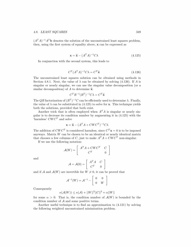
4.8. LEAST SQUARES 349
(ATA)−1ATb denotes the solution of the unconstrained least squares problem,then, using the first system of equality above, x can be expressed as
x = x− (ATA)−1Cλ (4.125)
In conjunction with the second system, this leads to
CT (ATA)−1Cλ = CT x (4.126)
The unconstrained least squares solution can be obtained using methods inSection 4.8.1. Next, the value of λ can be obtained by solving (4.126). If A issingular or nearly singular, we can use the singular value decomposition (or asimilar decomposition) of A to determine x.
CTR−1(RT )−1Cλ = CT x
TheQR factorization of (RT )−1C can be efficiently used to determine λ. Finally,the value of λ can be substituted in (4.125) to solve for x. This technique yieldsboth the solutions, provided that both exist.
Another trick that is often employed when ATA is singular or nearly sin-gular is to decrease its condition number by augmenting it in (4.125) with the‘harmless’ CWCT and solve
x = x− (ATA+ CWCT )−1Cλ
The addition of CWCT is considered harmless, since CTx = 0 is to be imposedanyways. Matrix W can be chosen to be an identical or nearly identical matrixthat chooses a few columns of C, just to make ATA+ CWCT non-singular.
If we use the following notation:
A(W ) =
[ATA+ CWCT C
CT 0
]and
A = A(0) =
[ATA C
CT 0
]and if A and A(W ) are invertible for W 6= 0, it can be proved that
A−1(W ) = A−1 −
[0 00 W
]Consequently
κ(A(W )) ≤ κ(A) + ||W ||2||C||2 + α||W ||for some α > 0. That is, the condition number of A(W ) is bounded by thecondition number of A and some positive terms.
Another useful technique is to find an approximation to (4.121) by solvingthe following weighted unconstrained minimization problem.

350 CHAPTER 4. CONVEX OPTIMIZATION
minx∈<n
||Ax− b||2 + µ2||CTx||2
For large values of µ, the solution x(µ) of the unconstrained problem is a goodappproximation to the solution x of the constrained problem (4.121). We canuse the generalized singular value decompositions of matrices A and CT , thatallows us to simultaneously diagonalize A and CT .
UTAX = diag(α1, . . . , αm)
V TCTX = diag(γ1, . . . , γm)
where U and V are orthogonal matrices and X is some general matrix. Thesolution to the constrained problem can be expressed as
x =p∑i=1
uTi bαi
xi
The analytical solution x(µ) is then given as
x(µ) =p∑i=1
αiuTi bα2i + µ2γ2
i
xi + x
It can be easily seen that as µ2 →∞, x(µ)→ x.Generally, if possible, it is better to eliminate the constraints, since this
makes the problem better conditioned. We will discuss one final approach tosolving the linearly constrained least squares problem (4.121), which reducesthe dimensionality of the problem by eliminating the constraints. It is hingedon computing the QR factorization of C.
QTC =
(R
0
)p
n− p(4.127)
This yields
AQT =(A1 A2
)(4.128)
and
QTx =
(y
z
)p
n− p(4.129)

4.8. LEAST SQUARES 351
The constrained problem then becomes
minx∈<n
||b−A1y −A2z||2
subject to RTy = 0
Since R is invertible, we must have y = 0. Thus, the solution x to the con-strained least squares problem can be determined as
x = QT
(0
z
)(4.130)
wherez = argmax
z||b−A2z||2
It can be proved that the matrix A2 is atleast as well-conditioned as the matrixA. Often, the original problem is singular and imposing the constraints makesit non-singular (and is reflected in a non-singular matrix A2.
4.8.3 Least Squares with Quadratic Constraints
The quadratically constrained least squares problem is often encountered inregularization problems and can be stated as follows.
minx∈<n
||Ax− b||22subject to ||x||22 = α2
Since the objective function as well as the constraint function are convex, theKKT conditions (c.f. Section 4.4.4) are necessary and sufficient conditions forthe optimality of the problem at the primal-dual variable pair given by (x, µ).The KKT conditions lead to the following equations
(ATA+ µI)x = ATb (4.131)xTx = α2 (4.132)
The expression in (4.131) is the solution to what the statisticians sometimesrefer to as the ridge regression problem. The solution to the problem underconsideration has the additional constraint though, that the norm of the solutionvector x should equal |α|. The two equations above yield the so-called secularequation stated below.
bTA(ATA+ µI)−2ATb− α2 = 0

352 CHAPTER 4. CONVEX OPTIMIZATION
Further, the matrix A can be diagonalized using its singular value decom-position A = UΣV T to obtain the following equation which is to be solved.
n∑i=1
β2i
σ2i
(σ2i + µ)2
− α2 = 0
4.8.4 Total Least Squares
The total least squares problem is stated as
minx∈<n,E∈<m×n,r∈<m
||E||2F + ||r||22
subject to (A+ E)x = b + r

Chapter 5
Statistics
Descriptive Statistics are used to describe the basic features of the data gatheredfrom an experimental study. They provide summary statistics about the sampleand the measures. In conjuction with graphical descriptive statistics, they formthe basis of almost every quantitative analysis of data. Summary statisticsinclude measures such as mean, median, mode, standard deviation, correlation(between two variables) etc. For example, the average height of the students ina room summarizes the heights of students in the room. Graphical descriptivestatistics comprises of plots (such as scatter plots), charts (such as pi-charts,bar-charts), lines and histograms that describe some real world or simulateddata without having you look at every single value. A graphical statistic in theform of a histogram or pi-chart of the heights of the students in a room, providesa broader summary.
In the later part of this chapter, we will introduce probability and sampling,with focus on application to data analysis. Some other topics to be discussedinclude confidence intervals, significance tests, hypothesis testing, etc. An ex-ample use of hypothesis testing in the drug industry is to decide statistically(based on past records) whether or not a specific drug is safe.
5.1 Variables
A variable is an attribute of any system which may change its value while it isunder observation. For example, the number of people in the age group 75− 79in Canada is a variable. There are two basic types of variables, viz., qualitativevariables and quantitative variables. Qualitative variables take on values thatare words. Examples of qualitative variables include marital status, nationality,color of skin, gender, etc. On the other hand, qualitative variables take onnumeric values. Further, the qualitative variables could be either discrete orcontinuous based on whether the variable could take on only whole numbervalues or any number respectively. Examples of discrete quantitative variablesare number of people in a New York, number of cars in Germany or anything that
353

354 CHAPTER 5. STATISTICS
can be counted. Money, height, weight, age, etc., are examples of continuousvariables. The study of statistics is more concerned with qualititative variablesthan quantitative variables.
5.2 Descriptive Statistics
The histogram will be our first example of a (graphical) descriptive statistic. Ahistogram provides a picture of the data for single-variable data. We will there-after discuss the scatter plot (or scatter diagram), which serves as a graphicaldescription of data of two variables.
5.2.1 Histograms
A histogram is a graphical display of tabulated frequencies. A histogram showswhat proportion of cases fall into each of several or many specified categories.In a histogram, it is the area of the bar that denotes the value, not the height.This is a crucial distinction to note, especially when the categories are not ofuniform width. Table 5.1 shows a slightly modified estimate of the populationof Canada by age group 1 for the year 2007. The first column records the classintervals. Class intervals are ranges that the variable is divided into. Eachclass interval includes the left endpoint but not the right (by convention). Thepopulation (second column) is recorded in the thousands. The third column hasa record of the percentage of the population that happens to fall in each agegroup.
There are three steps to be followed when plotting a histogram for tabulatedfrequencies as in Table 5.1.
1. Convert counts to percentages percent as shown in the third column ofTable 5.1.
percentage =count
total number of values
2. Compute height for each class-interval as height = percentwidth of range as shown
for the fourth column of Table 5.1.
3. Draw axes and label them. Label the class intervals (age groups in thiscase) along the x−axis and the heights along the y−axis.
4. Along each class interval on the x−axis, draw a rectange of correspondingheight and width as shown in Figure 5.1. This is precisely the histogramfor the tabulated data in Table 5.1.
Figure 5.1 shows the histogram corresponding to Table 5.1. Note that thesum total area of all the bars is 100 (percent).
Histograms for discrete and continuous variables look slightly different. Forhistograms of continuous variables, class intervals (such as age ranges) are
1Source: http://www40.statcan.ca/l01/cst01/demo10a.htm

5.2. DESCRIPTIVE STATISTICS 355
0
0.2
0.4
0.6
0.8
1
1.2
1.4
1.6
1.8
0--4 5--9 10--14 15--19 20--24 25--29 30--34 35--39 40--44 45--49 50--54 55--59 60--64 65--69 70--74 75--79 80--84 85--89 90--95
Age
% p
op
ula
tio
n/i
nte
rva
l-w
idth
Figure 5.1: Histogram for Table 5.1.
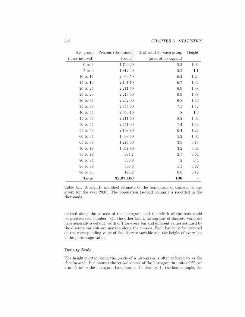
356 CHAPTER 5. STATISTICS
Age group Persons (thousands) % of total for each group Height(class interval) (count) (area of histogram)
0 to 4 1,740.20 5.3 1.065 to 9 1,812.40 5.5 1.1
10 to 14 2,060.50 6.2 1.2415 to 19 2,197.70 6.7 1.3420 to 24 2,271.60 6.9 1.3825 to 29 2,273.30 6.9 1.3830 to 34 2,242.00 6.8 1.3635 to 39 2,354.60 7.1 1.4240 to 44 2,640.10 8 1.645 to 49 2,711.60 8.2 1.6450 to 54 2,441.30 7.4 1.4855 to 59 2,108.80 6.4 1.2860 to 64 1,698.60 5.2 1.0465 to 69 1,274.60 3.9 0.7870 to 74 1,047.90 3.2 0.6475 to 79 894.7 2.7 0.5480 to 84 650.8 2 0.485 to 89 369.3 1.1 0.2290 to 95 186.2 0.6 0.12
Total 32,976.00 100 -
Table 5.1: A slightly modified estimate of the population of Canada by agegroup for the year 2007. The population (second column) is recorded in thethousands.
marked along the x−axis of the histogram and the width of the bars couldbe positive real number. On the other hand, histograms of discrete variableshave generally a default width of 1 for every bar and different values assumed bythe discrete variable are marked along the x−axis. Each bar must be centeredon the corresponding value of the discrete variable and the height of every baris the percentage value.
Density Scale
The height plotted along the y-axis of a histogram is often referred to as thedensity scale. It measures the ‘crowdedness’ of the histogram in units of ‘% perx unit’; taller the histogram bar, more is the density. In the last example, the

5.3. SUMMARY STATISTICS 357
unit was census. Using Table 5.1 and the corresponding density estimates inFigure 5.1, one can estimate that the percentage of population aged between 75and 77 years of age is around 2.7
5 ×3 = 1.62%. This is assuming that the densityof population in the age group 75 − 79 is evenly distributed throughout theinterval (that is the bar is really flat). But a close look at the bars surroundingthat for 75−79 will suggest that the density in the interval 75−59 is probably notquite evenly distributed. While it would accurate and lossless to have populationcounts corresponding to every age (instead of intervals), such data may not be aseasy to digest as the population estimates based on intervals. There is a tradeoffbetween summarization and elaborate accounting or equivalently between widerbars and lots of bars.
5.2.2 Scatter Diagram
Suppose we are prodived data comparing the marks (out of 100) obtained bysome 500 students in the mathematics subjects in the year 1 and year 2 of acertain college. Consider a plot with ‘year 1 marks’ plotted along the x-axis and‘year 2 marks’ plotted around the y-axis. The scatter diagram (or plot) for thismarks data will consist of a point marked per student with its coordinates giveby ‘(marks in year 1, marks in year 2)’. Figure 5.2 shows the scatter plot forsome such hypothetical data. The dotted vertical and horizontal lines mark theaverage marks for year 1 and year 2 respectively. It can be seen from the plotthat most students either performed well in both years or performed poorly inboth years.
A point corresponding to an observation that is numerically far away fromthe rest of the points in a scatter plot is called an outlier. Statistics derived fromdata sets that include outliers can be misleading. Figure 5.3 shows the scatterplot of Figure 5.2 with an outlier introduced (in the form of a black point). Theoutlier results in a relatively drastic change in mean values of marks for years1 and 2. While the mean value along the x-axis drops from 50.72 to 50.68, themean value along the y-axis increases from 55.69 to 55.74.
5.3 Summary statistics
Summary statistics are numbers that summarize different features of a dataset.There are summary statistics such as mean, median, standard deviation for dataof single variables and measures such as correlation coefficient for two variables.
5.4 Standard measures of location
The arithmatic mean µ (or simply the mean) is one of the most popular summarystatistics and it is the average value assumed by the variable. If a variable Vassumes values given by the set of data V = v1, v2, . . . , vN, then the mean µ

358 CHAPTER 5. STATISTICS
Figure 5.2: A sample scatter plot.
Figure 5.3: The sample scatter plot of Figure 5.2 with an outlier (30, 80) .

5.4. STANDARD MEASURES OF LOCATION 359
of V is computed as
µ =
N∑i=1
vi
N
The mean is also the balancing point on a histogram; that is, if you think ofthe x−axis of the histogram as the beam of weight balance and weights to beproportional to the areas of the bars, then the fulcrum placed at the mean pointwill ensure that the beam stays horizontal.
Another measure of ‘center’ for a list of numbers is the median. The medianis the number ν such that at least half the numbers in V are less than or equalto ν and at least half the numbers are greater than or equal to ν. In order todetermine the median, you need to sort the numbers (in either the ascendingor descending order) and just pick the center. If more than one value qualifiesas the middle value, their average (arithmatic mean) is taken to be the median.The median is the point on the x-axis of a histogram such that half of the totalarea of the bars lies to its left and half to its right.
As an example, the average of the set V ′ = 1, 3, 4, 5, 7 is 4, while its medianis also 4. On the other hand, if the last number in this set is changed from 7to 12 to yield the set V ′′ = 1, 3, 4, 5, 12, then the median remains 4, whilethe mean changes to 5. Thus, the median cares more for the number of valuesto its left and right rather than the actual values to its left and right. For theset V ′′′ = 1, 1, 3, 4, 5, 12, the mean is 13
3 , whereas the median is the averageof 3 and 4, which is 3.5. In general, for a symmetric histogram, the arithmaticmean equals the median. For a longer (shorter) right tail, the arithmatic meanis greater (smaller) than the median.
In most applications, mean is preferred over median as a measure of cen-ter. However, when the data is very skewed, median is preferred over meanas a measure of center. For example, while computing summary statistics forincomes, median is often preferred over mean, since you do not want a few veryhuge incomes to affect your measure of center. Similarly, median is preferredover mean as a measure of center of housing prices.
An often encountered measure is percentile. The kth percentile of a set ofvalues of a variable is the value (or score) of the variable below which k percentof the data points may be found. The 25th percentile is also known as the firstquartile; the 50th percentile happens to be the median.
5.4.1 Standard measures of spread and association
The measures of center discussed thus far do not capture how spread out thedata is. For example, if the average height of a class is 5 feet, 6 inches (5′ 6′′),it could be that everyone in the class has the same height or that someone inthe class is just 4′ 5′′ and the tallest student is 6′ 3′′. The interquartile rangeis an illustrative but rarely used measure of the spread of data. It is definedas the distance between the 25th percentile and the 75th percentile. Generally,smaller the interquartile range, smaller will be the spread of the data.

360 CHAPTER 5. STATISTICS
An often used measure of spread is the standard deviation (SD), whichmeasures the typical distance of a data point from the arithmatic mean. Itis computed as the root mean square2 (rms) of deviations from the artih-matic mean. That is, given a variable V that assumes values given by theset V = v1, v2, . . . , vN, if µ is the arithmatic mean of V, then the standarddeviation σ of V is
σ =
√√√√√√N∑i=1
v2i
N
The SD of the set V ′ = 1, 3, 4, 5, 7 is 2, which is a tyipcal distance of anynumber in V ′ from the mean µ = 4. Formulated by Galton in the late 1860s,the standard deviation remains the most common measure of statistical spreador dispersion. The square of standard deviation is called variance.
Effect of change of scale
What is the effect of modifying the data V on the summary statistics of the datasuch as arithmatic mean, median and standard deviation? The effect of somedata modifications have been studied in the past and are enumerated below.
1. Adding a constant to every number of the data: The effect is that arith-matic mean and median go up by that constant amount, while the stan-dard deviation remains the same. This is fairly intuitive to see.
2. Scaling the numbers in data by a positive constant: The effect is that thearithmatic mean, the median and the standard deviation get scaled by thesame positive constant.
3. Multiplying numbers in data by −1: The average and the median getmultiplied by −1, whereas standard deviation remains the same.
5.4.2 Correlation coefficient
Correlation coefficient (r) measures the strength of the linear relationship be-tween two variables. If the points with coordinates specified by the values ofthe two variables are close to some line, the points are said to be stronglycorrelated, else they are weakly correlated. More intuitively, the correlation co-efficient measures how well the points are clustered around a line. Also called,linear association, the correlation coefficient r between sets of N values X and Yassumed by variables x and y respectively can be computed using the followingthree steps.
2The root mean square (rms) measures the typical ‘size’ or ‘magnitude’ of the numbers. Itis the square root of the mean of the squares of the numbers. For example, the rms of the set1, 3, 4, 5, 7 is
√20 = 4.47.

5.4. STANDARD MEASURES OF LOCATION 361
1. Convert the values in X and Y into a set of values in standard unit, viz.,Xsu and Ysu respectively. Recall that computing standard units requiresknowledge about the mean and standard deviation and could therefore bean expensive step.
2. Let Psu = psu = xsuysu |xsu ∈ Xsu, ysu ∈ Ysu .
3. Let µsu be the arithmatic mean of values in Psu. The the correlationcoefficient r = µsu.
Thus, if µx and µy are the means of x and y, and σx and σy are the respectivestandard deviations, then
r =
∑vx∈X ,vy∈Y
vx − µxσx
× vy − µyσy
N(5.1)
The sample scatter plot of Figure 5.2 is reproduced in Figure 5.4 with four re-gions marked, which are all bordered by the average lines. Points (vx, vy) inregions (1) and (3) contribute as positive quantities in the summation expres-sion for r, whereas points (vx, vy) in regions (2) and (4) contribute as negativequantities. The correlation coefficient has no units and is always between −1and +1; if r is +1 (−1), the points are on a line with positive (negative) slope. Asimple case for which r = 1 is when all values assumed by y are scalar multiplesof the corresponding values of x. If r = 0, the variables are uncorrelated. Twospecial but (statistically) uninteresting cases with r = 0, are when either of thevariables always takes a constant value. Other interesting cases with r = 0 arewhen the scatter plot is symmetrical with respect to any horizontal or verticalline.
As an example, the correlation coefficient between the marks in years 1 and2, for the data in Figure 5.2 is a positive quantity 0.9923. On the other hand,the correlation coefficient between the weight and mileage of cars is generallyfound to be negative. O-rings are one of the most common gaskets used inmachine design. The failure of an O-ring seal was determined to be the causeof the Space Shuttle Challenger disaster on January 28, 1986. The material ofthe failed O-ring was a fluorinated elastomer called FKM, which is not a goodmaterial for cold temperature applications. When an O-ring is cooled below itsglass transition temperature (Tg), it loses its elasticity and becomes brittle. Infact, the correlation coefficient between the extent of damage to the O-ring andtemperature has been found to be negative.
There are some words of caution that one should exercise while interpretingand applying scatter plots:
1. Extrapolation is generally not a good idea for determining exact values.This is because, outside the range of values considered, the linear relation-ship might not hold.

362 CHAPTER 5. STATISTICS
Figure 5.4: The sample scatter plot of Figure 5.2 reproduced with four regionsmarked based on positive and negative contributions to the correlation coeffi-cient.
2. Even if you cannot do extrapolations, scatter plots can be informative andcould give us hints about general trends (such as whether the value of onevariable will increase with increase in value of the other variable).
While correlation measures only the strength of the linear association be-tween two variables, the relationship could also be non-linear. In such cases, thescatter plot could show a strong pattern that is not linear (as an example, thescatter plot could assume the shape of a boomerang) and therefore, the quantityr is not as meaningful.
A word of caution before we move on; correlation does not imply causation,while it could definitely make one curious about a possible causal relationship.Just because the GPAs of students and their incomes are positively correlated,we cannot infer that high GPAs are caused by high incomes or vice verca. Therecould be latent cause of both observations, resulting in the positive correlation.For example, there is generally a positive correlation between the number ofteachers and the number of failing students at a high school. But this mainlybecause generally, larger a school, larger is the number of teachers, greater is thestudent population and consequently, more are the number of failing students.Therefore, instead of treating the scatter diagram or the correlation measureas a proof of causation, these could be used as indicators that might possiblysignal causation.

5.4. STANDARD MEASURES OF LOCATION 363
Effect of change of scale
The effects of change of scale on correlation are far simpler than they happenedto be for arithmatic mean and standard deviation. We will list some effects onSD of changing a single variable. The effects of changing values of both variablescan be derived by systematically considering effects produced by changing valueof each variable.
1. When a constant is added or subtracted from every value of any singlevariable, the correlation coefficient stays the same, since such an operationinvolves translating all points and average lines by the same constant valuealong the corresponding axis. Consequently, the relative positions withrespect to the closest line (or the standard units) remain the same.
2. When every value of any single variable is multiplied by the same constant,the correlation coefficient remains the same, since the standard units ofthe points remain the same (since the average and SD get scaled by thesame amount as the values).
3. When every value of any single variable is multiplied by −1, the signs ofthe values of each variable in standard units change (the value and meanchange signs, whereas, the SD does not). Thus, r gets multiplied by −1.However, if each value of both the variables is multiplied by −1, the overallcorrelation coefficient will remain unchanged.
4. When the values of x are switched with the values of y, the correlation co-efficient stays the same, since the terms within the summation expressionfor r in (5.1) remain the same.
5.4.3 Ecological Correlation
In contrast to a correlation between two variables that describe individuals,ecological correlation is a correlation calculated based on averages (or medians)of subgroups. The subgroups could be determined based on properties of thedata and ecological correlation is just the correlation between means of thesubgroups. For instance, the subgroups of students within a class could bedetermined by sections within the class or by zipcode of the residential area(which is indicative of the affluence) of the students. The ecological correlationbetween the incomes and the grades of students in a class could then be thestandard correlation coefficient between the arithmatic means of the incomesand grades of students within each section or zipcode category. Some researcherssuggest that the ecological correlation gives a better picture of the outcome ofpublic policy actions [?]. However, what holds true for the group may nothold true for the individual and this discrepancy is often called the ecologicalfallacy. It is important to keep in mind that the ecological correlation capturesthe correlation between the values of the two variables across the subgroups(such as the zip code of residence) and not across individual students. Theecological correlation can help one draw a conclusion such as ‘Students from

364 CHAPTER 5. STATISTICS
Figure 5.5: The standard normal curve.
wealthier zip codes have, on average, higher GPAs’. A recurring observation isthat correlations for subgroup averages are usually larger than correlations forindividuals.
5.5 Normal approximation
5.5.1 Standard Normal Curve
A standard normal curve is given by
f(x) =1√2πe−
x22
where 2π ≈ 3.14159... and e ≈ 2.71828.... Figure 5.5 shows the standard normalcurve.
To find the area under a normal curve between −∞ and any x, there existsa standard (area) table of precomputed values, which you need to only lookup.The normal curve has some interesting properties.
1. The total area under the standard normal curve is 1. Therefore, when therhs of the normal curve is multipled by 100, the normal curve turns outto be a histogram - the total are under the curve of f ′(x) = 100√
2πe−
x22 is
100.

5.5. NORMAL APPROXIMATION 365
2. The standard normal curve is symmetric about 0. This is revealed by thefact that x2 = (−x)2. Consequently, it follows from an earlier discussionthat the normal curve has the same mean and median value of 0.
3. The standard deviation of the standard normal curve is 1.
4. The value of y decays very rapidly as x drifts away from 0. This is alsoreflected in the fact that an area of 0.998 is spanned by the normal curvelying between x = −4.45 and x = 4.45. The area table mentioned above, infact ends at the value of x = 3.009. Further, the area between x = −1 andx = 1 is 68.2% (roughly two thirds) while that between−2 and 2 is 95.45%.That is, around 68% of the area is within one standard deviation of theaverage while roughly 95% of the area is within two standard deviationsof the average.
Table 5.2 lists the value of f(x) and the area between −∞ and x for differentvalues of x. Such a table is called the density table. The motivation behinddiscussing the normal curve is that many histograms look like the normal curve.The idea of much of mathematics and statistics is to make problems look likeproblems solved before.
5.5.2 General Normal Curve
The standard normal curve is centered around 0 and has a spread, though inpractice, you will encounter normal curves that are not centered around 0. Forexample, the histogram of the heights (measured in inches) of people has theshape of a normal curve, but centered around a non-trivial height and having aspread different from 1. The general normal curve is specified by
f(x;µ, σ) =x− µ√
2πe−
(x−µ)2
2σ
The mapping between a general normal curve and a standard normal curveis specified using the idea of standard units, which will be discussed next.
5.5.3 Standard Units
Standard units (SU) tell how many standard deviation units (SDs) above orbelow average a particular value on a general curve is. Thus a standard unitof 1 corresponds to distance equal to standard deviation σ from the average µ.The number of standard deviations sd of a value v is computed as
sd =v − µσ
Thus, the SU of 78 for a mean value of 72 and a SD of 6 is 1 unit aboveaverage. Around 100−68
2 = 16% of the points on a normal curve are abovethe standard unit of 1 and therefore, the point 78 corresponds to a percentilerank of 100 − 16 = 84 for the normal curve. On the other hand, the point
366 CHAPTER 5. STATISTICS
corresponding to percentile rank of 90 is obtained by looking up the standardunit as 1.30 corresponding to the approximate area value of 80 (i.e., 80.64) inthe density table, which translates to a value of 72 + 1.3 × 6 = 79.8 (for themean and SD values of 72 and 6 respectively). In this way, the percentile ranktells you what percentage of the area under a normal curve is below a particularvalue.
5.6 Regression
Regression is a technique used for the modeling and analysis of numerical dataconsisting of values of a dependent variable y (response variable) and of a vectorof independent variables x (explanatory variables). The dependent variable inthe regression equation is modeled as a function of the independent variables,corresponding parameters (“constants”), and an error term. However, the re-lationship between y and need not be causal (as in the case of correlation).Regression is used in several ways; one of the most often used ways is to es-timate the average y value corresponding to a given x value. As an example,you might want to guess the inflation next year, based on the inflation duringthe last three years. We will take three examples and discuss how ‘good’ theaverage estimate of the dependent variable could be.
1. In the case of the scatter diagram in Figure 5.6, one could make use ofregression to estimate the average possible marks of a student in ‘year 2’,given her marks in ‘year 1’. In this case, the correlation coefficient (0.993)is very close to 1. The mean values for x and y are 60.26 and 60.33 respec-tively while the corresponding standard deviations are 10.48 and 10.54respectively. The graph that shows the average y value corresponding toeach x value is called the graph of averages. It can be seen in Figure 5.6,that the average values guessed for y corresponding to different x valuesare very close to a line and have very little variation across the line. Such aline is called the regression line. The regression line is a smoothed versionof the graph of averages.
2. In contrast, if the x variable represented a student’s score in mathematicsand the y variable respresented her score in physics, the correlation mightnot be as strong. For a typical scatter plot as in Figure 5.7 for such data,the variance across every average estimate of y for every x value is largerand the correlation coefficient is further away from 1 (0.801 to be precise).
3. In the case of two uncorrelated variables (i.e., r ≈ 0) such a person’sheight and his average scores in mathematics, the average value of y givenany particular value of x will be more or less the same. The variance willalso be large.
It turns out actually that if x is one SD above its average µx, the corre-sponding predicted value of y is r SDs above its average µy. The point (µx, µy)is in fact termed as the point of averages. In the third example discussed above,

5.6. REGRESSION 367
Figure 5.6: A scatter plot for data similar to that in Figure 5.2, along with theregression line. The mean values for x and y are 60.26 and 60.33 respectivelywhile the corresponding standard deviations are 10.48 and 10.54 respectively.The correlation coefficient is 0.993.

368 CHAPTER 5. STATISTICS
Figure 5.7: A scatter plot for the marks of students of some class in mathematics(x-axis) against physics (y-axis), along with the regression line. The mean valuesfor x and y are 60.34 and 60.01 respectively while the corresponding standarddeviations are 9.82 and 12.06 respectively. The correlation coefficient is 0.801.

5.6. REGRESSION 369
with r ≈ 0, the predicted y hard changes with the value of x. For the firstexample, the predicted y changes the most with the value of x.
The linear regression method concerns itself with finding points on the re-gression line, for a given table of data values with each row consisting of valuesof the independent variable x and the dependent variable y for a particular datapoint. The following three steps comprise the linear regression method.
1. Compute the correlation coefficient r between x and y. For the data inFigure 5.6, the correlation coefficient was 0.993.
2. Convert any given value of x into its standard units. Multiply this numberby r to get the predicted value of y in its standard units. This step isessentially the regression step. For example, with respect to Figure 5.6,consider x = 76. This number in standard units will be 76−60.26
10.48 = 1.50.The predicted value of y in standard units will be 1.49.
3. Convert the value of y from standard units into normal units. The valueof 0.993 for y in standard units will correspond to 0.993× 10.54 + 60.33 =70.80.
The regression line discussed above is for predicting value of y based on x(the usual notion of line). It is also possible to perform regression to predictvalue of x based on value of y, to yield another kind of regression line.
As an exercise, let us predict (using linear regression on the data in Fig-ure 5.6) the marks for a student in year 2, given that she obtained 63 marks inyear 1. The predicted value for marks in year 2 will be 60.33+
(0.993× 63−60.26
10.48
)×
10.54 = 63.07, which compares favourably with the actual value of y = 63.53.As another exercise, with respect to the scatter plot in Figure 5.6, suppose
a student is at 31st percentile in year 1. What is a good guess for this stu-dent’s percentile rank in year 2? We note that the scatter diagram is ‘footballshaped’ (or tilted oval) which is an indication that the two variables roughlyfollow a normal distribution3 First we will determine the standard units for xcorresponding to the 31st percentile by looking up the value in standard unitscorresponding to an area of 100−31
100 = 0.69 in standard normal Table 5.2. Thevalue happens to be around 0.50. Multiplying this by the correlation coefficientr = 0.993, we get the standard units of the approximated y value to be 0.497.The corresponding percentile rank can be again obtained using the normal tableto be 100× (1− 0.6879) = 31.21, i.e., around 31 percentile. Note that we reallydid not make use of any of estimates for mean or standard deviation, since allcomputations dealt only with standard units.
What about the spread of values around the average predicted by linearregression? How accurate is regression? For each point in the scatter diagram,the actual value of y will not typically be on the regression line. The predictionerror at a point x is defined as the difference between the actual and predictedvalues of y at that point. Analogous to the definition of the standard deviation,
3Later, we will discuss techniques that will help verify such assumptions.

370 CHAPTER 5. STATISTICS
the spread for linear regression is measured as the RMS of prediction errorsand is called the RMS error. Linear regression should be suitable for datasetsfor which the RMS error is very close to sum of the deviations from averageacross all points. While RMS error can be used in the context of any predictionmethod, for the case of linear regression, the RMS error can be simplified to thefollowing formula:
erms = σy√
1− r2 (5.2)
where σy is the SD for y.On the other hand, if the prediction method were to always predict the
overall average µy of y regardless of the value of x, the RMS error would be thestandard deviation σy of y (by definition). We can readily see that if r ∈ (−1, 1),prediction using regression will always yield a lower value of erms than will anaive prediction using the average µy.
Mathematically, if r = ±1, all the points must be on a line (with slope r),resulting in 0 prediction errors and erms = 0. On the other hand, if r = 0and erms = σy. This is because there is no linear relationship between x andy, implying that it does not help to know x while predictin y; you can alwaysguess y to be µy and could do no better. For any other r ∈ (−1, 0) ∪ (0, 1),erms ∈ (0, σy). If erms is close to 0, it means that the predictions are veryaccurate. Whereas, if erms is close to σy, the predictions must be far fromaccurate.
What about answer to a question such as ‘what percentage of all valuesare within one unit of RMS error of the regression line for a fixed value ofx’? The answer will be around 68%, assuming that the points approximatelyfollow a normal curve and that the average values of y for any given x ap-proximately coincide with the point (x, rx) on the regression line, so that oneunit of RMS error approximately corresponds to one standard deviation. Fora football shaped scatter diagram, the normality condition can be assumed tohold for both x and y as well as for all points with a fixed value of x. Usingthis information, let us answer the following question: of all the students con-sidered in Figure 5.6 who obtained a score of 65 in year 1, what percentage ofthem obtained over 67 in year 2? First of all, the average marks in year 2, forstudents who obtained 65 in year 1, predicted using linear regression will be60.33 +
(0.993× 65−60.26
10.48
)× 10.54 = 65.06. The RMS error can be computed
using (5.2) to be√
1− (0.993)2 × 10.09 = 1.19. The question then reduces to‘what percentage of values on a normal curve with mean 65.06 and SD 1.19 areabove 67?’ The answer to this can be easily obtained by looking up the standardnormal table for the percentage area that is above 1.63 standard units, whichis 100× (1− 0.9484) = 5.16%.
Further, a football shaped scatter diagram is homoscedastic, i.e., it has ap-proximately the same spread around the regression line for every value of x. Tocite a practical example, we would expect different divisions within a class tohave the same mean and SD values for scores in a particular year, irrespectiveof their sizes. Of course, divisions with smaller sizes may have a smaller range

5.7. PROBABILITY AND SAMPLING 371
of scores than larger divisions.
5.6.1 The Regression Effect
The regression effect is also called ‘regression to the mean’. This effect is es-sentially the fact that for r ∈ (−1, 1), and both x and y in standard units, thepredicted (based on linear regression) y value will be closer to the mean thanthan the x value. This is because, if x is 1 SD above average, then the predictedvalue of y will be r ∈ (−1, 1) SDs above average. Thus, if a student performsexceptionally well in the first year, the predicted performance of the student inthe second year will not be as good. A corollary of this effect is that if y1 isthe predicted average value of y variable for a value x1 of the x variable, thenthe predicted average value of x2 of the x variable based on value y1 will be lessthan x1.
5.6.2 SD Line
The SD line is a line that passes through the point of averages in a scatter plotand has slope equal to the ratio of standard deviation of y to that of x multipliedby sgn(r). Points on the SD line are the same in standard units for both x andy. It can be proved that if r = 1, the SD and regression lines will coincide. Onthe other hand, further is r away from 1, further will
5.7 Probability and sampling
5.8 Binomial distribution
5.9 Interval estimation
5.10 Some standard significance tests

372 CHAPTER 5. STATISTICS
z +0.00 +0.01 +0.02 +0.03 +0.04 +0.05 +0.06 +0.07 +0.08 +0.09
0.0 0.5000 0.5040 0.5080 0.5120 0.5160 0.5199 0.5239 0.5279 0.5319 0.53590.1 0.5398 0.5438 0.5478 0.5517 0.5557 0.5596 0.5636 0.5675 0.5714 0.57530.2 0.5793 0.5832 0.5871 0.5910 0.5948 0.5987 0.6026 0.6064 0.6103 0.61410.3 0.6179 0.6217 0.6255 0.6293 0.6331 0.6368 0.6406 0.6443 0.6480 0.65170.4 0.6554 0.6591 0.6628 0.6664 0.6700 0.6736 0.6772 0.6808 0.6844 0.68790.5 0.6915 0.6950 0.6985 0.7019 0.7054 0.7088 0.7123 0.7157 0.7190 0.72240.6 0.7257 0.7291 0.7324 0.7357 0.7389 0.7422 0.7454 0.7486 0.7517 0.75490.7 0.7580 0.7611 0.7642 0.7673 0.7704 0.7734 0.7764 0.7794 0.7823 0.78520.8 0.7881 0.7910 0.7939 0.7967 0.7995 0.8023 0.8051 0.8078 0.8106 0.81330.9 0.8159 0.8186 0.8212 0.8238 0.8264 0.8289 0.8315 0.8340 0.8365 0.83891.0 0.8413 0.8438 0.8461 0.8485 0.8508 0.8531 0.8554 0.8577 0.8599 0.86211.1 0.8643 0.8665 0.8686 0.8708 0.8729 0.8749 0.8770 0.8790 0.8810 0.88301.2 0.8849 0.8869 0.8888 0.8907 0.8925 0.8944 0.8962 0.8980 0.8997 0.90151.3 0.9032 0.9049 0.9066 0.9082 0.9099 0.9115 0.9131 0.9147 0.9162 0.91771.4 0.9192 0.9207 0.9222 0.9236 0.9251 0.9265 0.9279 0.9292 0.9306 0.93191.5 0.9332 0.9345 0.9357 0.9370 0.9382 0.9394 0.9406 0.9418 0.9429 0.94411.6 0.9452 0.9463 0.9474 0.9484 0.9495 0.9505 0.9515 0.9525 0.9535 0.95451.7 0.9554 0.9564 0.9573 0.9582 0.9591 0.9599 0.9608 0.9616 0.9625 0.96331.8 0.9641 0.9649 0.9656 0.9664 0.9671 0.9678 0.9686 0.9693 0.9699 0.97061.9 0.9713 0.9719 0.9726 0.9732 0.9738 0.9744 0.9750 0.9756 0.9761 0.97672.0 0.9772 0.9778 0.9783 0.9788 0.9793 0.9798 0.9803 0.9808 0.9812 0.98172.1 0.9821 0.9826 0.9830 0.9834 0.9838 0.9842 0.9846 0.9850 0.9854 0.98572.2 0.9861 0.9864 0.9868 0.9871 0.9875 0.9878 0.9881 0.9884 0.9887 0.98902.3 0.9893 0.9896 0.9898 0.9901 0.9904 0.9906 0.9909 0.9911 0.9913 0.99162.4 0.9918 0.9920 0.9922 0.9925 0.9927 0.9929 0.9931 0.9932 0.9934 0.99362.5 0.9938 0.9940 0.9941 0.9943 0.9945 0.9946 0.9948 0.9949 0.9951 0.99522.6 0.9953 0.9955 0.9956 0.9957 0.9959 0.9960 0.9961 0.9962 0.9963 0.99642.7 0.9965 0.9966 0.9967 0.9968 0.9969 0.9970 0.9971 0.9972 0.9973 0.99742.8 0.9974 0.9975 0.9976 0.9977 0.9977 0.9978 0.9979 0.9979 0.9980 0.99812.9 0.9981 0.9982 0.9982 0.9983 0.9984 0.9984 0.9985 0.9985 0.9986 0.99863.0 0.9987 0.9987 0.9987 0.9988 0.9988 0.9989 0.9989 0.9989 0.9990 0.9990
Table 5.2: Area under the standard normal curve between−∞ and z for differentvalues of z.
Chapter 6
Searching on Graphs
Consider the following problem:
Cab Driver Problem A cab driver needs to find his way in a city from onepoint (A) to another (B). Some routes are blocked in gray (probably be-cause they are under construction). The task is to find the path(s) from(A) to (B). Figure 6.1 shows an instance of the problem..
Figure 6.2 shows the map of the united states. Suppose you are set to thefollowing task
Map coloring problem Color the map such that states that share a boundaryare colored differently..
A simple minded approach to solve this problem is to keep trying colorcombinations, facing dead ends, back tracking, etc. The program could run fora very very long time (estimated to be a lower bound of 1010 years) before itfinds a suitable coloring. On the other hand, we could try another approachwhich will perform the task much faster and which we will discuss subsequently.
The second problem is actually isomorphic to the first problem and to prob-lems of resource allocation in general. So if you want to allocate aeroplanes toroutes, people to assignments, scarce resouces to lots of tasks, the approacheswe will show in this chapter will find use. We will first address search, thenconstraints and finally will bring them together.
6.1 Search
Consider the map of routes as in Figure 6.3. The numbers on the edges aredistances. Consider the problem of organizing search for finding paths from S(start) to G (goal).
We humans can see the map geometrically and perhaps guess the answer.But the program sees the map only as a bunch of points and their distances.We will use the map as a template for the computer at every instance of time.
373

374 CHAPTER 6. SEARCHING ON GRAPHS
Figure 6.1: Routes in a city. The problem is to find the shortest path frompoint (A) to point (B).
Figure 6.2: The map of the united states of America. The task is to color themap such that adjacent states have different colors.

6.1. SEARCH 375
Figure 6.3: Map of routes. The numbers on the edges are distances.
At the beginning, the computer knows only about S. The search algorithmexplores the possibilities for the next step originating from s. The possible nextsteps are A and B (thus excluding G). Further, from A, we could go to B or E.From B, we could go to A or C. From A, we could also go back to S. But wewill never bother biting our own tail in this fasion; that is, we will never makea loop. Going ahead, from B, we could only go to C. From C, we can progressonly to D and thereafter we are stuck on that path. From A, we could makea move to E and them from E to G. Figure 6.4 shows the exhaustive tree ofpossible paths (that do not bite their own tail) through this map. The processof finding all the paths is called the British Museum Algorithm1.
But the British Museum algorithm can be very expensive. In fact, some ofthese searches can be exponential. If you had to look through a tree of chessmoves for example, in the beginning it is essentially exponential, which is a badnews since it will imply 1010 years or so. We need a more organized approachfor searching through these graphs. There exist many such organized methods.Some are better than others, depending on the graph. For example, a depth firstsearch may be good for one problem but horrible for another problem. Wordslike depth first search, breadth first search, beam search, A∗ search, etc., formthe vocabulary of the search problem in Artificial Intelligence.
The representation we use will define the constraints (for example, the rep-resentation of the routes in Figure 6.3 defines the notion of proximity betweennodes and also defines constraints on what sequences of vertices correspond tovalid paths.
6.1.1 Depth First Search
This algorithm2 boils down to the following method: Starting at the source,every time you get a choice for the next step, choose a next step and go ahead.We will have the convention that when we forge ahead, we will take the first
1The British Museums are considered some of the largest in the world.2Fortunately, the names given to these algorithms are representative of the algorithms
actually do.

376 CHAPTER 6. SEARCHING ON GRAPHS
Figure 6.4: The tree of all possible paths from S to G through the map inFigure 6.3.
choice. Thus, a depth first search on the map in Figure 6.3 will tread alongthe path in Figure 6.5. In practice, what is used is a combination of depthfirst search and backup. What this means is that when a dead end is hit, themethod goes back to the last state. In practice, this method could yield verycomplicated solutions.
6.1.2 Breadth First Search (BFS)
The way BFS organizes its examination of the tree is layer by layer; the algo-rithm first explores one layer of solutions (A or B), then forges ahead to anotherlayer (B or E or A or C) and so on. Figure 6.6 illustrates the BFS traversal forthe map in Figure 6.3. In practice, this search could expend a lot of time inuseless parts of the graph. But it yields the shortest path in terms of numberof number of streets covered.
6.1.3 Hill Climbing
Both BFS and DFS are completely uninformed about geography; neither infor-mation about distance nor direction is exploited. But often it helps if you haveoutside information about how good a place is to be in. For instance, in themap in Figure 6.3, between E and D, it is much better to be in E because thatgets you closer to the goal. It makes less sense in general to head off to the right

6.1. SEARCH 377
Figure 6.5: The DFS tree from S to G through the map in Figure 6.3.
Figure 6.6: The BFS tree from S to G through the map in Figure 6.3.

378 CHAPTER 6. SEARCHING ON GRAPHS
Figure 6.7: The choices based on hill climbing for the route from S to G throughthe map in Figure 6.3.
if you know that the goal is on the left. It is heuristically good to be closer tothe goal, though sometimes it may turn out not to be a good idea. So we couldmake use of heuristic information of this kind. And this forms the idea behindhill climbing. It is an idea drafted on top of depth first search. When initially atS, you could move to A or B. When you look at A and B, you that one of themis closer to the goal G and you choose that for the next move. And B happensto be closer to G, which you pick for the next move; but this turns out to bea bad idea as we will see. Nevertheless, it looks good from the point of view ofthe short-sighted hill climbing algorithm. From B, the possible choices are Aand C. And A is a natural choice for hill-climbing, owing to its proximity to G.From A onwards, the choices are straightforward - you move to E and then toG. Figure 6.7 shows the route from S to G as chalked out by hill climbing.
Hill climbing always is greedy because it plans only for one step at a time.The method requires a metric such as distance from the goal.
6.1.4 Beam Search
We drafted hill climbing on top of depth first search. Is there a similar thing wecould do with breadth first search? And the answer is ‘yes’. And this approach

6.2. OPTIMAL SEARCH 379
Figure 6.8: The choices based on beam search for the route from S to G throughthe map in Figure 6.3.
is called beam search The problem with breadth first search is that it tends tobe exponential. But what we could do to work around is to throw away atevery level of BFS, all but the ‘most promising’ of the paths so far. The mostpromising step is defined as that step which will get us ‘closest’ to the goal. Theonly difference from the hill climbing approach is that beam search does notpick up just one path, it picks up some fixed number of paths to carry down.Let us try beam search on the map in Figure 6.3. For this simple example,let us keep track of two paths at every level. We will refer to the BFS planin Figure 6.6. From S, we could move to A or B and we keep track of bothpossibilities. Further, from A, there are two possibilities, viz., B and E, whilefrom B there are two possibilities in the form of A and C. Of the four paths,which two should we retain? The two best (in terms of the heuristic measureof how far we are from the goal) are B and E. Carrying forward from thesepoints, we arrive at G in a straight-forward manner as shown in Figure 6.8.
While the vanila breadth first search is exponential in the number of levels,beam search has a fixed width and is therefore a constant in terms of numberof levels. Beam search is however not guranteed to find a solution (though theoriginal BFS is guaranteed to find one). This is a price we pay for saving ontime. However, the idea of backing up can be employed here; we could back upto the last unexplored path and try from there.
6.2 Optimal Search
For optimal search, we will start with the brute force method which is exponen-tial and then slap heuristics on top to reduce the amount of work, while stillassuring success.

380 CHAPTER 6. SEARCHING ON GRAPHS
Figure 6.9: The tree of all possible paths from S to G through the map inFigure 6.3, with cumulative path lengths marked at each node.
6.2.1 Branch and Bound
Suppose the problem is to find the best possible path (in terms of distances)between S and G in the map as in Figure 6.3. An oracle suggests that the pathSAEG is the shortest one (its length is 13). Can we determine if SAEG isindeed the shortest path? One method to answer this question is to verify ifevery other path is at least that long.
From S, we could go to A or B. The cumulative path length to B is 5. FromB, you could either go to A or C. The cumulative path length upto A or C is8. At this point, from A, you could go to E while from C you could move to D,with cumulative path lengths of 13 each and so on. Figure 6.9 shows the treeof possible paths from S to G, with cumulative path length (from S) marked ateach node. It is evident from the figure that all paths to G have length greaterthan or equal to 13. We can therefore conclude that the shortest path to G fromS is SAEG and has length 13.
Most often we do not have any oracle suggesting the best path. So we haveto think how to work without any oracle telling us what the best path is. Oneway is to find a path to the goal by some search technique (DFS or beam search)and use that as a reference (bound) to check if every other path is longer thanthat. Of course, our first search may not yield the best path, and hence wemight have to change our mind about what the best path (bound) is as wekeep trying to verify that the best one we got so far is in fact the best oneby extending every other path to be longer than that. The intuition we workwith is to always push paths that do not reach the goal until their length isgreater than a path that does reach the goal. We might as well work only withshortest paths so far. Eventually, one of those will lead to the goal, with whichwe will almost be done, because all the other paths will be about that lengthtoo, following which we just have to keep pushing all other paths beyond thegoal. This method is called branch and bound.

6.3. CONSTRAINT SATISFACTION 381
Figure 6.10: The pruned search tree for branch and bound search.
In the example in Figure 6.9, the shortest path upto B from S was of length5 initially, which used as a bound, could eliminate the path SAB and thereforesave the computation of the path SABCD. Similarly, the initial path to A,SA of length 4, sets a bound of 4 for the shortest path to A and can thuseliminate the consideration of the path SBA beyond A. Figure 6.10 illustratesthe application of branch and bound to prune the BFS search tree of Figure 6.9.Crossed out nodes indicate search paths that are excluded because they yieldpaths that are longer than bounds (for the corresponding nodes). This crossingout using bounds is a variation on the theme of the dynamic programmingprinciple.
6.2.2 A∗ Search
The branch and bound algorithm can also be slapped on top of the hill climbingheuristic or the beam search heuristic. In each of these cases, the bound can becomputed as the sum of the accumulated distance and the eucledian distance.
When the branch and bound technique is clubbed with shortest distanceheuristic and dynamic programming principle, you get what is traditionallyknown as A∗ search. Understanding A∗ search is considered the culmination ofoptimal search. It is guaranteed to find the best possible path and is generallyvery fast.
6.3 Constraint Satisfaction
What we have discussed so far is mechanisms for finding the path to the goal(which may not be optimal). Rest of the discussion in this chapter will focuson resource allocation. Research allocation problems involve search. Too oftenpeople associate search only with maps. But maps are merely a convenient way3
to introduce the concept of search and the search problem is not restricted tomaps. Very often, search does not involve maps at all. Let us again consider the
3Maps involve making a sequence of choices and therefore could involve search amongstthe choices.

382 CHAPTER 6. SEARCHING ON GRAPHS
Figure 6.11: The sketch of a simple region for which we try to solve the mapcoloring problem.
“Map coloring problem” (refer to Figure 6.2). It involves searching for sequenceof choices. Instead of the large city of USA, let us consider the simpler countryof Simplea as in Figure 6.11. Let us say we need to pick a color from the setR,G,B, Y .
Let us say we number the regions arbitrarily. One approach is to try coloringthem in the order of increasing numbers, which is a horrible way! This isparticularly because the order chosen could be horrible. To color the region,let us start by considering the possible colors that could be assigned to eachregion. State number 1 could be assigned any of R, B, G or Y . Suppose wetake a depth first search approach for this coloring job. Now we need to colorthe region number 2. Since we adopt depth first search, let us say we pick thecolor of R for region 1. And as we go from region to region, we keep rotatingthe set of colors.
The prescription for DFS is that you keep plunging head until you hit a deadend where you cannot do anything. But the problem is that we cannot inferwe have hit a dead end till we assign colors to all 15 regions, to realise that thefollowing constraint has been violated: no two adjacent regions should have thesame color. And even if we backup a step or two, we will have to explore all 15regions to infer if we have reached a dead end. At this rate, the projected timefor successful coloring of the states in a US map is 1010 years4! That is no wayto perform search. The culprit is the particular order in which we chose to colorthe regions. Figure 6.12 shows an example instance of random assignment ofcolors that leads to a dead-end (with no suitable color left for region number 15).We introduce the idea of constraint checking precisely to address this problem.It is essentially a (DFS) tree trimming method.
First of all, we will need some terminology.
1. Variables (V): V is a set of variables. Variables names will be referredto in upper case, whereas their specific instatiations will be referred to inlower case.
2. Domain (D): The domain D is the bag of values that the variables cantake on. Di is the domain of the Vi ∈ V . A good example of a domain
4The United states has 48 contiguous states. If the number of colors is 4, the branchingfactor of DFS will be 4 and the height will be 48. Thus, the number of computations will be448 or 296 which is of the order of 1027 and since the length of a year is the order of 107,it will take in the order of 1011 years assuming that a computation is performed in a nanosecond.

6.3. CONSTRAINT SATISFACTION 383
Figure 6.12: A sequence of bad choices for the map coloring problem.
would be R,B,G, Y . In the map coloring problem, all variables havethe same domain.
3. Constraints (C): A constraint is a boolean function of two variables. Cijrepresents the constraint between variables Xi and Xj . Cij(xi, xj) = trueiff, the constraint is satisfied for the configuration Xi = xi, xi ∈ Di andXj = xj , xj ∈ Dj . Else, Cij(xi, xj) = false. The form of the constraintfunction could vary from problem to problem. An example of a constraintis: no two adjacent regions should not have the same color. Note thatthere need not be a Cij for all i and j. For instance, in the map coloringproblem, the only constraints are those involving adjacent regions, suchas region 15 with the regions 1, 2, 3 and 4.
Suppose we are trying to explore if region number i = 15 is going to objectto any coloring scheme. First we define the constraint Cj , i = 15, j ∈ 1, 2, 3, 4as follows:
Cij(x, y), i = 15, j ∈ 1, 2, 3, 4 is true iff x 6= y.We can state the check as in Figure 6.13.
for x ∈ Di (i = 15) dofor All constraints Cij do
Set Xi = x iff ∃y ∈ Dj such that Cij(x, y) = trueend for
end for
Figure 6.13: The algorithm for constraint checking
6.3.1 Algorithms for map coloring
When assigning a color to each region, we could do different types of checks.
1. Check all: At one end of the spectrum, while assigning a color to a region,we check constraint satisfaction with respect to all regions (no matter howfar they are from the region under consideration). This is an extreme caseand potentially, we could consider all variants of what to check and whatnot to check. The check is only a speedup mechanism. It neither ensuresnor prevents a solution. We could get a solution (if there is one) usingdepth first search and no search, thought it might take 1010 years. If we

384 CHAPTER 6. SEARCHING ON GRAPHS
want to have minimum number of checks such that they are really helpful,our method for deciding what to check will be checks on regions that arein the immediate vicinity of the last region that had a color assigned.
2. Check Neighbors: Check for constraint satisfaction, only all regions in theimmediate neigborhood of the last region that had a color assigned. Thisis at another end of the spectrum.
3. Check Neighbors of Neighbors: Check for constraint satisfaction, only allregions in the immediate neigborhood of the last region that had a colorassigned as well as well as regions in the immediate neighborhood of theneighbors.
4. Check Neighbors of ‘unique’ neighbors: Check for constraint satisfaction,only all regions in the immediate neigborhood of the last region that hada color assigned as well as well as regions in the immediate neighborhoodof the ‘unique’ neighbors. A neighbor is ‘unique’, if the constraint set forthe region has been reduced to a single element (which means that it hasa very tight constraint).
We will evaluate the above approaches on two fronts, viz.,
1. Number of assignments performed: An assignment corresponds to puttinga color on a region. If we are very lucky, we might be able to color themap of the United states with just 48 assignments (that is we never had tobackup). Constraint checking will enable the algorithm realise that it willsoon hit a dead end and will have to back up. In practical situations, wecould expect a bit of backup and also expect the constraints to show yousome dead ends. So it could happen that the constraint checking reducesthe number of assignments to some number slightly above the ideal (say52).
2. Number of checks performed: A check corresponds to determining whichcolor could be assigned to a region based on the color assigned so far toanother regions.
A simple experiment for coloring the Unites States reveals the statistics inTable 6.1.
The message we can extract from Table 6.1 is that some of the constraintchecking is essential, else it takes 1010 years. We can conclude that full pro-pogation is probably not a worthy effort. Because full propogation, relativeto propogation through unique values yielded the same number of assignmentsbut relatively fewer checks. When we compare heuristic 2 against heuristic 4,we find that there is a tradeoff between number of assignments and number ofchecks. Checking all is simply a waste of time. The net result is that people tendto invoke either of heuristics 2 and 4. From the point of view of programmingsimplicity, one might just use heuristic number 2.

6.3. CONSTRAINT SATISFACTION 385
SrNo Constraint Sat Heuristic Assignments Checks
1 Check all 54 7324
2 Check neighbors 78 417
3 Check neighbors 54 2806of neighbors
4 Check neighbors 54 894of ‘unique’ neighbors
Table 6.1: Number of assignments and checks for each of the constraint sat-isfaction heuristics for the problem of coloring the map of the USA using 4colors.
The computational complexity of the discussed methods is still exponential5.But usually, the constraints try to suppress the exponential nature.
6.3.2 Resource Scheduling Problem
Let us forget about maps for a while and talk about airplanes. An upstartairline is trying to figure out how many airplanes they need. They have aschedule outlining when and where they need to fly planes. And the task is tofigure out the minimum number of airplanes that need to be purchased. Forevery airplane saved, let us say the reward is saving on half the cost of theairplane.
F1, F2, . . . , Fn are the flights. Table 6.2 shows the schedule for the flights.
Flight No. From To Dept. Time Arr. Time
F1 Boston LGA 10:30 11:30
F2 Boston LGA 11:30 12:30
F3 Boston LGA 12:30 13:30
F4 Boston LGA 13:30 14:30
F4 Boston LAX 14:30 15:30
F6 . . . . . . . . .
. . . . . . . . . . . .
F15 Boston LAX 11:00 15:30
Table 6.2: Number of assignments and checks for each of the constraint sat-isfaction heuristics for the problem of coloring the map of the USA using 4colors.
To fly this schedule, we have some number m = 4 of airplanes: P1, P2, P3, P4.5Note that these are NP complete problems. Any polynomial time algorithm will fetch
field medals.
386 CHAPTER 6. SEARCHING ON GRAPHS
Of course, we do not want to fly any plane empty (dead head).The assignment P1 → F1, P2 → F2, P3 → F3 and P4 → F4 will leave no
airplane for flight F5. But if we could fly P1 back from New York (LGA), thesame plane could be used for flight F4, thus sparing P4 for F5. We can drawthe correspondence between this problem and the map coloring problem; the 4airplanes correspond to 4 colors while the flights correspond to regions. The taskis to assign planes (colors) to flights (regions), at all times honoring constraintsbetween the flights. The constraints are slightly different from the ones we hadin the US map. The constraint is that no airplane can be on two routes atthe same time. This implies that there is a constraint between flights F1 andF2. Similarly, there is a constraint between the pairs < F2, F3 >, < F3, F5 >,< F4, F5 >, < F1, F5 >, < F2, F5 > and < F3, F5 >. We assume that theturn around duration for F1 (which is of a one hour duration) will end by 14:30hours, which sounds reasonable. Thus, there is no constraint < F1, F4 >.
You schedule planes the same way you do map coloring. An assignmentis tried and constraints for all unassigned flights are checked to ensure thatthere is at least one airplane that can fly each flight. There is one importantdifference between the flight scheduling problem and the map coloring problem:we know that we can color maps with 4 colors6, but we do not know how manyairplanes it is going to take to fly a schedule. Hence, we will need to try theflight scheduling problem with different number of airplanes.
Let us say we over-resource the map coloring problem with 7 colors insteadof 4. A sample run yields 48 assignments (that is no backup was required) and274 checks. With 6 colors, you get 48 assignments and 259 checks. If on theextreme end, you used only 3 colors, you could never color Texas.
Frequently the problem is over-constrained and there is no solution withavailable resources (like say coloring the United States with 2 or 3 colors). Inthose circumstances, constraints can be turned into preferences so that someregions will not be allowed to be adjacent to regions of the same color. Orwe might have to allow some ‘dead-hit’ flights. And on top of preferences, wecould layer beam-search or some other search that tries to minimize the penaltycumulated or maximize the number of constraints that are satisfied.
6The 4 color theorem.

Chapter 7
Graphical Models
Graphical models [Lau96, CGH97, Pea88, Jor98, Jen01] provide a pictorial rep-resentation of the way a joint probability distribution factorizes into a productof factors. They have been widely used in the area of computer vision, con-trol theory, bioinformatics, communication, signal processing, sensor networks,neurovision, etc.
There is a relation between the conditional independence properties of ajoint distribution and its factorization properties. Each of these properties canbe represented graphically. This allows us to
1. organize complicated mathematics through graph based algorithms forcalculation and computation and thus save complicated computations (inmany cases, map the pictorial representation onto computations directly)
2. gain new insights into existing models; it is a standard practice to modifyan existing model by addition/delection of nodes or links and adopt it tothe problem at hand
3. motivate new models by simply ammending pictures
However, everything that you could do in graphical models using picturescould also be done without pictures, by grinding through all the mathematicswhile consistently using the innocuous-looking sum (7.1) and product (7.2) rulesof probability
Pr (X) =∑y∈Y
Pr (X = x, Y = y) (7.1)
Pr (X = x, Y = y) = Pr (X = x | Y = y) Pr (Y = y) (7.2)
387

388 CHAPTER 7. GRAPHICAL MODELS
where X and Y are discrete random variables, assuming values x ∈ X =x1, x2, . . . , xm and y ∈ Y = y1, y2, . . . , yn respectively. A combination ofthe two rules yields the Bayes theorem:
Pr (X = xi, Y = yj) =Pr (X = xi | Y = yj) Pr (Y = yj)
Pr (X = xi)
=Pr (X = xi | Y = yj) Pr (Y = yj)∑
yj∈YPr (X = xi | Y = yj) Pr (Y = yj)
(7.3)
The two main kinds of graphical models are directed and undirected models.The problems we will address in graphical models include
1. Inference: Broadly, there are two inference techniques for graphical mod-els, viz., exact and approximate inference. Exact inference is appropriateif the graphic is a tree, since it is a linear time algorithm. But for complexgraphical models, exact inference may or may not be appropriate, sinceexact algorithms could be very slow. In such cases, approximate inferenceschemes are often resorted to. Markov chain monte carlo (which is exactif there were an infinite amount of computing resources and approximateotherwise) and variational inference (by approximating the analytical formfor the posterior distribution) are two popular techniques. While varia-tional techniques scale better, their other strengths and weaknesses arecomplementary to those of MCMC. An often adopted stepping stone forexplaining variational inference is the expectation maximization algorithm(EM) and we will take the same route.
2. Learning:
7.1 Semantics of Graphical Models
We will first discuss the semantics of graphical models, both directed and undi-rected. In the sections that follow, we will discuss the computational aspects ofgraphical models - in particular, inferencing and learning techniques.
7.1.1 Directed Graphical Models
We will start with the example of a directed graphical model. Consider an arbi-trary joint distribution Pr (X1 = x1, X2 = x2, X3 = x3) over three discrete ran-dom variables X1, X2 and X3 that assume values x1 ∈ X1, x2 ∈ X2 and x3 ∈ X3
respectively. Denoting1 Pr (Xi = xi) by p(xi) and Pr (X1 = x1, X2 = x2, X3 = x3)by p(x1, x2, x3) and applying the product rule of probability successively, we ob-tain
1As a convention, we will use capital letters to denote random variables and lower caseletters to denote their realizations.

7.1. SEMANTICS OF GRAPHICAL MODELS 389
p(x1, x2, x3) = p(x1)p(x2, x3 | x1) = p(x1)p(x2 | x1)p(x3 | x1, x2) (7.4)
The successive application of the product rule is often termed as the chain rule.We should note that this rule applies even if x1, x2 and x3 happen to be continu-ous random variables (in which case p is a density function) or vectors of randomvariables. We should note that this factorization is quite non-symmetrical inthe three random variables. This factorization can be represented in the form ofthe following directed graph: There is one node for each variable. We draw a di-rected edge between every conditioning variable (i.e. the corresponding node) tothe conditioned variable. The way to go from a graph to the factorization of thejoint distribution is to write down the product of the conditional distribution ofevery node (i.e., the corresponding variable) conditioned on its parents withinthe graph. In the example above, x1 had no parent, and therefore the termcorresponds to its conditional p(x1) turned out to be its marginal distribution.
The factorization in the last example holds for any joint distribution over anythree variables and the graph is therefore uninformative. In fact, any completelyconnected graph will be uninformative, as we will soon see. What interests usin graphical models is not the presence of edges but rather, the absence ofedges. Since the graph in the previous example had no missing edges, it wasuninteresting.
Definition 43 Let R = X1, X2, . . . , Xn be a set of random variables, witheach Xi (1 ≤ i ≤ n) assuming values xi ∈ Xi. Let XS = Xi | i ∈ S whereS ⊆ 1, 2, . . . , n. Let G =< V, E > be a directed acyclic graph with verticesV = 1, 2, . . . , n and E ⊆ V × V such that each edge e = (i, j) ∈ E is a directededge. We will assume a one to one correspondence between the set of variablesR and the vertex set V; vertex i will correspond to random variable Xi. Letπi be the set of vertices from which there is edge incident on vertex i. Thatis, πi = j | j ∈ V, (j, i) ∈ E. Then, the family F(G) of joint distributionsassociated with the DAG2 G is specified by the factorization induced by G asfollows:
2As we saw earlier, the family of probability distributions specified by the related formalismof undirected graphical models is somewhat different.

390 CHAPTER 7. GRAPHICAL MODELS
F(G) =
p(x)
∣∣∣∣∣p(x) =n∏i=1
p(xi | xπi), p(xi | xπi)∀ 1 ≤ i ≤ n ≥ 0,∑xi∈Xi
p(xi | xπi) = 1
(7.5)
where, x denotes the vector of values [x1, x2, . . . , xn] and xi is the value assumedby random variable Xi and xπi denotes the vector of values from x, composedfrom positions in πi.
For notational convenience with directed acyclic graphs, it is a commonpractice to assume a topological ordering on the indices of vertices in V sothat πi ⊆ µi−1 = 1, 2, . . . , i − 1. Note that, by the chain rule, the followingfactorization always holds:
p(x) =n∏i=1
p(xi | xµi−1) (7.6)
Making use of the sum rule, in conjunction with (7.5), for any p ∈ F(G), wehave
p(xµi) =∑
xi+1∈Xi+1,...,xn∈Xn
p(x)
=∑
xi+1∈Xi+1,...,xn∈Xn
p(x1)p(x2 | xπ2) . . . p(xi | xπi) (7.7)
Since the vertex indices are topologically ordered, it can be proved using theprinciple of induction (working backwards from n) on the basis of the sum rulein (7.7), that for any p ∈ F(G):
p(xµi) =i−1∏j=1
p(xi | xπi) (7.8)
Contrasting (7.6) against (7.5), we can think of the set of probability dis-tribution F(G) as a sort of restricted class of distributions that arises fromthrowing away some of the dependencies. In particular, if p ∈ F(G) then
p(xi | xµi−1) = p(xi | xπi)
that is, Xi is independent of Xµi−1 , given Xπi . The independence is denotedby: Xi ⊥ Xµi−1 | Xπi . This leads us to another approach to defining the classof probability distributions based on a DAG G.

7.1. SEMANTICS OF GRAPHICAL MODELS 391
Definition 44 Let R = X1, X2, . . . , Xn be a set of random variables, witheach Xi (1 ≤ i ≤ n) assuming values xi ∈ Xi. Let XS = Xi | i ∈ S whereS ⊆ 1, 2, . . . , n. Let G =< V, E > be a directed acyclic graph with verticesV = 1, 2, . . . , n and E ⊆ V×V such that each edge e = (i, j) is a directed edge.Let πi = j | j ∈ V, (j, i) ∈ E. Then, the family C(G) of joint distributionsassociated with the DAG G is specified by the conditional independence inducedby G as follows:
C(G) =
p(x)
∣∣∣∣∣Xi ⊥ Xµi−1 | Xπi ∀ 1 ≤ i ≤ n,∑x
p(x) = 1
(7.9)
We will next show that the class F(G) defined in terms of factorizations isequivalent to the class C(G) defined in terms of independences. This is calledthe Hammersley Clifford theorem.
Theorem 87 The sets F(G) and C(G) are equal. That is p ∈ F(G) iff p ∈ C(G)
Proof: ⇐: We will first prove that F(G) ⊆ C(G). Let p ∈ F(G). We will provethat p ∈ C(G), that is, p(xi | xµi−1 ,xπi) = p(xi | xπi). This trivially holds fori = 1, since xπi = ∅. For i = 2:
p(x1, x2) = p(x1)p(x1 | x2) = p(x1)p(x1 | xπ2)
where, the first equality follows by chain rule, whereas the second equality fol-lows by virtue of (7.8). Consequently,
p(x1 | x2) = p(x1 | xπ2)
Assume that p(xi | xµi−1) = p(xi | xπi) for i ≤ k. For i = k + 1, it follows fromchain rule and from (7.8) that
p(xµk+1) =k+1∏i=1
p(xi | xµi−1) =k+1∏i=1
p(xi | xπi)
Making use of the induction assumption for i ≤ k in the equation above, we canderive that
p(xk | xµk−1) = p(xk | xπk)
By induction on i, we obtain that p(xi | xµi−1) = p(xk | xπi) for all i. That is,p ∈ C(G). Since this holds for any p ∈ F(G), we must have that F(G) ⊆ C(G).⇒: Next we prove that C(G) ⊆ F(G). Let p′ ∈ C(G) satisfy the conditional
independence assertions. That is, for any 1 ≤ i ≤ n, p′(xi | xµi−1) = p′(xi | xπi).Then by chain rule, we must have:
p′(xµn) =n∏i=1
p′(xi | xµi−1) =k+1∏i=1
p′(xi | xπi)

392 CHAPTER 7. GRAPHICAL MODELS
Figure 7.1: A directed graphical model.
which proves that p′ ∈ F(G) and consequently that C(G) ⊆ F(G) 2
As an example, we will discuss the directed graphical model, as shown in Fig-ure 7.1. Based on theorem 87, the following conclusions can be drawn from thegraphical representation of a family of distributions represented by Figure 7.1.
1. Given the value of X3, the values of X1, X2 and X4 will be completely un-informative about the value of X5. That is, (X5 ⊥ X1, X2, X4 | X3).Similarly, given the value of X2, the values of X1 and X3 will be completelyuninformative about the value of X4. That is, (X4 ⊥ X1, X3 | X2).
2. Secondly, since p ∈ F(G), we have
p(x1, x2, x3, x4, x5) = p(x1)p(x2)p(x3 | x1, x2)p(x4 | x2)p(x5|x3)
What about other independence assertions? Is X5 independent of X4 givenX2? Is X3 independent of X4, given X2? The answer to both these questionshappens to be yes. And these could be derived using either of the equivalentdefinitions of graphical models. In fact, some such additional conditional in-dependence assertions can always follow from the two equivalent definitions ofgraphical models. Before delving into these properties, we will define an impor-tant concept called d-separation, introduced by Pearl [Pea88].
Definition 45 A set of nodes A in a directed acyclic graph G is d-separatedfrom a set of nodes B by a set of nodes C, iff every undirected path from avertex A ∈ A to a vertex B ∈ B is ‘blocked’. An undirected path between A andB is blocked by a node C either (i) if C ∈ C and both the edges (which might bethe same) on the path through C are directed away from C (C is then called atail-to-tail node) or (ii) if C ∈ C and of the two edges (which might be the same)on the path through C, one is directed toward C while the other is directed awayfrom C (C is then called a head-to-tail node) or (iii) if C 6∈ C and both the edges(which might be the same) on the path through C are directed toward C (C isthen called a head-to-head node).
In Figure 7.1, node X2 blocks the only path between X3 and X4, node X3
blocks the path between X2 and X5. Whereas, node X3 does not block the

7.1. SEMANTICS OF GRAPHICAL MODELS 393
path between X1 and X2. Consequently, X3 and X4 are d-separated byX2, while X2 and X5 are d-separated by X3. However, X1 andX2 are not d-separated by X3, since X3 is a head-to-head node. X3 doesnot d-separate X1 and X2 even though it separates them. Thus, not every pairof (graph) separated nodes in the graph need be d-separated. We next definea family of probability distribution that have independences characterized byd-separation.
Definition 46 The set of probability distributions D(G) for a DAG G is definedas follows:
D(G) = p(x) |XA ⊥ XB | XC , whenever A and B are d− separated by C (7.10)
It can be proved that the notion of conditional independence is equivalent tothe notion of d-separation in DAGs. That is,
Theorem 88 For any directed acyclic graph G, D(G) = C(G) = F(G).
Thus, in Figure 7.1. X3 ⊥ X4 | X2 and X2 ⊥ X5 | X3. Whereas,X1 6⊥ X2 | X3. We could think of X1 and X2 as completing explanationsfor X3. Thus, given a value of X3, any value of X1 will, to some extent ‘explainaway’ the value of X3, thus withdrawing the independence of X2. In terms of areal life example, if X1, X2 and X3 are discrete random variables correspondingto ‘the color of light’, ‘the surface color’ and ‘the image color’ respectively, then,given the value of X3 (image color), any value of X1 (color of light) will explainaway the color of the image, thus constraining the values that X3 (surfacecolor) might take. On the other hand, X1 ⊥ X2 | . What about theindependence of X1 and X2 given X5? The path X1, X3, X5, X3, X2 involves ahead-to-head node X5 and therefore, X1 6⊥ X2 | X5. The Bayes ball algorithmprovides a convenient algorithmic way for deciding if XA ⊥ XB | XC , by usingthe d-separation property.
Bayesian Networks and Logic
The logical component of Bayesian networks essentially corresponds to a propo-sitional logic program. This has already been observed by Haddawy [1994] andLangley [1995]. Langley, for instance, does not represent Bayesian networksgraphically but rather uses the notation of propositional definite clause pro-grams. Consider the following program. This program encodes the structureof the blood type Bayesian network in Figure 7.2. Observe that the randomvariables in this notation correspond to logical atoms. Furthermore, the di-rect influence relation in the Bayesian network corresponds to the immediateconsequence operator.

394 CHAPTER 7. GRAPHICAL MODELS
Figure 7.2: The graphical structure of a Bayesian network modeling the inheri-tance of blood types within a particular family.
PC(ann). PC(brian).MC(ann). MC(brian).MC(dorothy) : −MC(ann), PC(ann). PC(dorothy) : −MC(brian), PC(brian).BT (ann) : −MC(ann), PC(ann). BT (brian) : −MC(brian), PC(brian).BT (dorothy) : −MC(dorothy), PC(dorothy).
7.1.2 Undirected Graphical Models
We will move on to an undirected graphical models (also known as MarkovRandom fields) primer, while drawing parallels with the directed counterpart.An undirected graph G is a tuple < V, E > where E ⊆ V × V and such thateach edge e = (i, j) ∈ E is a directed edge. While the conditional independenceproperty for directed graphical models was tricky (involving concepts such as d-separation, etc.), the conditional independence property for undirected modelsis easier to state. On the other hand, the factorization property for directedgraphical models simply involved local conditional probabilities as factors. Itis however not as simple with undirected graphical models. Taking the easierroute, we will first define the conditional independence property for undirectedgraphical models. Toward that, we introduce the notion of graph separation.
Definition 47 Given an undirected graph G =< V, E >, and A,B, C ⊆ V, wesay that C separates A from B in G if every path from any node A ∈ A to anynode B ∈ B passes through some node C ∈ C. C is also called a separator or avertex cut set in G.
In Figure 7.3, the set A = X1, X7, X8 is separated from B = X3, X4, X5by the (vertex cut) set C = X2, X6. It is easy to see that separation is sym-metric in A and B. This simple notion of separation gives rise to a conditionalindpendence assertion for undirected graphs. A random vector XC for C ⊆ V

7.1. SEMANTICS OF GRAPHICAL MODELS 395
Figure 7.3: A directed graphical model.
is said to be markov with respect to a graph G if XA ⊥ XB | XC whenever Cseparates A from B. That is, the random variables corresponding to the vertexcut set acts like a mediator between the values assumed by variables in A andB so that the variables in A and B are independent of each other, if we knewthe values of variables in C. It is straightforward to develop a ‘reachability’algorithm (as with the bayes ball algorithm) for undirected graphs, to assessconditional independence assumptions. Based on the definition of markov ran-dom vector, we next define the familyM(G) of distributions associated with anundirected graph G.
Definition 48 Let R = X1, X2, . . . , Xn be a set of random variables, witheach Xi (1 ≤ i ≤ n) assuming values xi ∈ Xi. Let XS = Xi | i ∈ Swhere S ⊆ 1, 2, . . . , n. Let G =< V, E > be an undirected graph with verticesV = 1, 2, . . . , n and E ⊆ V × V such that each edge e = (i, j) ∈ E is anundirected edge. Then, the family M(G) of joint distributions associated with Gis specified as follows:
M(G) = p(x) |XA ⊥ XB | XC ∀ A,B, C ⊆ V, whenever C seperates A from B(7.11)
As in the case of directed models, there is another family of probabilitydistributions that could be specified for a given undirected graph G based on afactorization assertion. The main difference is that, while the factorization forDAGs was obtained in terms of local conditional probabilities or local marginals,it turns out that this factorization is not possible for a general undirected graph(specifically when it has a cycle). Instead there is another notion of ‘local’ forundirected graphs – there should be no function involving any two variablesXi and Xj where (i, j) 6∈ E (otherwise, such a term will not break further,prohibiting assertions about conditional independences). Instead, we will havea function φC(XC) for every clique C ⊆ V, since a clique is a subset of verticesthat all ‘talk to’ one another. The most general version of factorization will beone for which there is a function corresponding to each maximal clique; all other

396 CHAPTER 7. GRAPHICAL MODELS
factorizations involving factors over smaller cliques will be specialized versions.These functions will be referred to as compatibility or potential functions. Apotential or compatibility function on a clique C is a non-negative real valuedfunction φC(xC) defined over all instantiations x ∈ X1 × X2 × . . . × Xn of X.Other than these restrictions, the potential function can be arbitrary.
Definition 49 Let R = X1, X2, . . . , Xn be a set of random variables, witheach Xi (1 ≤ i ≤ n) assuming values xi ∈ Xi. Let XS = Xi | i ∈ Swhere S ⊆ 1, 2, . . . , n. Let G =< V, E > be an undirected graph with verticesV = 1, 2, . . . , n and E ⊆ V × V such that each edge e = (i, j) ∈ E is anundirected edge. Then, the family M(G) of joint distributions associated with Gis specified as follows:
F(G) =
p(x)
∣∣∣∣∣p(x) =1Z
∏C∈Π
φC(xC), such that φC(xC) ∈ <+,∀C ∈ Π
(7.12)
where, Π is the set of all cliques in G, x denotes the vector of values [x1, x2, . . . , xn],xi ∈ Xi is the value assumed by random variable Xi and where each φC is a po-tential function defined over the clique C ⊆ V. Without loss of generality, we canassume that Π is the set of maximal cliques in G. The normalization constantZ is called the partition function and is given by
Z =∑
x1∈X1,...,xn∈Xn
∏C∈Π
φC(xC) (7.13)
The potential functions are typically represented as tables – each row listinga unique assignment of values to the random variables in the clique and thecorresponding potential. Thus, the value φC(xC) can be obtained by a simpletable lookup.
The form of the potential function can be chosen based on the particularapplication at hand. For instance, the clique potential can be decomposed intoa product of potentials defined over each edge of the graph. When the do-main of each random variable is the same, the form of the potential can bechosen to either encourage or discourage similar configurations (such as sim-ilar disease infection for patients who are related) at adjacent nodes. Thepotential function is often interpreted as an energy function in the model-ing of crystals, protein folding, etc., where a minimum energy configurationis desirable. Frequently, the energy function is assumed to have the formφC(XC) = exp (−θC(XC)), which leads to the factorization as an exponentialform distribution p(x) = exp (−
∑C∈Π
θC(xC)− logZ). The quantities θC(XC) are
called sufficient statistics.

7.1. SEMANTICS OF GRAPHICAL MODELS 397
From our discussion on the equivalence of directed and undirected trees interms of conditional independencies, we may be tempted to conclude that thefactors for the undirected tree can be the local conditional probabilities. Thisis easily established if we prove that for strictly positive distributions, the def-inition of an undirected graphical model in terms of conditional independencesis equivalent to the definition in terms of factorization, that is, M(G) = F(G).
Theorem 89 For strictly positive distributions,M(G) = F(G). That is,M(G)∩D+ = F(G) ∩ D+, where, D+ = p(x) |p(x) > 0,∀x ∈ X1 ×X2 . . .×Xn .
Proof: The proof that M(G) ⊆ F(G) is a bit involved and requires Mobiusinversion. On the other hand, that F(G) ⊆M(G) can be shown as follows. Forany given A,B ⊆ V that are separated by C ⊆ V, consider the partitions P1, P2
and P3 of Π:P1 = K |K ∈ ΠandK ⊆ A ∩ C and K 6⊆ C
P2 = K |K ∈ ΠandK ⊆ B ∩ C and K 6⊆ C
P3 = K |K ∈ ΠandK ⊆ C
Now, p(x) can be factorized into factors involving cliques in P1, P2 and P3.Consequently,
p(xA,xB,xC)p(xB,xC)
=
∏K∈P1
φK(xK)∏K∈P2
φK(xK)∏K∈P3
φK(xK)∑xA
∏K∈P1
φK(xK)∏K∈P2
φK(xK)∏K∈P2
φK(xK)=
∏K⊆A∪C
φK(xK)∑xA
∏K⊆A∪C
φK(xK)= p(xA | xC)
2
While conditional independence is useful for modeling purposes, factoriza-tion is more useful for computatinal purposes.
7.1.3 Comparison between directed and undirected graph-ical models
Is there any difference between the undirected and directed formalisms? Arethey equally powerful? Or is more powerful than the other. It turns out thatthere are families of probability distributions which can be represented usingundirected models, whereas they have no directed counterparts. Figure 7.4shows one such example. Imagine that random variables X1 and X3 representhubs in a computer network, while X2 and X4 represent computers in the net-work. Computers do not interact directly, but only through hubs. Similarly,hubs interact only through computers. This leads to two independences: (i)conditioned on X1 and X3 (the hubs), nodes X2 and X4 (the computers) be-come independent and (ii) conditioned on X2 and X4, nodes X1 and X3 becomeindependent. However, with a directed acyclic graph on four nodes, we will al-ways have some head-to-head node and therefore, it is impossible to simultane-souly satisfy both conditions (i) and (ii) using a DAG. Larger bipartitie graphs

398 CHAPTER 7. GRAPHICAL MODELS
Figure 7.4: An undirected graphical model which has no equivalent directedmodel.
Figure 7.5: A directed graphical model which has no equivalent undirectedmodel.
will have similar conditional independence assertions, which are inexpressiblethrough DAGs.
Similarly, there are familiies of probability distibutions which can be rep-resented using directed models, whereas they have no undirected counterparts.Figure 7.5 shows one such example and corresponds to the ‘explaining away’ phe-nomenon, which we discussed earlier in this chapter. The node X3 is blockedif not observed (so that X1 ⊥ X2 | ∅), whereas it is unblocked if its valueis known (so that X1 6⊥ X2 | X3). Can you get this behaviour with anundirected graph? The answer is no. This is because, with an undirected graph,there is no way of getting dependence between X1 and X2 if they were aprioriindependent.
On the other hand, for graphical models such as markov chains, dropping thearrows on the edges preserves the independencies, yielding an equivalent undi-rected graphical model. Similarly, directed trees are fundamentally no differentfrom undirected trees.
An important point to note is that it is the absence of edges that char-acterizes a graphical model. For any graphical model, it is possible that thecompatibility functions (or local conditional probabilities) assume a very spe-cial form so that there are more (conditional) independences that hold than

7.2. INFERENCE 399
what is indicated by the graphical model (which means that some of the edgesin the graph could be redundant).
7.2 Inference
In this section, we discuss the problem of determining the marginal distributionp(xA), the conditional distribution p(xA | xB) and the partition function Z,given a graphical model G =< V, E > and for anyA,B ⊆ V. We will assume thatthe conditional probability tables (for directed models) or the potential functiontable (for undirected models) are already known. The sum and product rules ofprobability yield the following formulae3 for the marginal, the conditional4 andthe partition function5 respectively:
p(xA) =∑xV\A
p(x)
p(xA | xO) =p(xA,xO)p(xO)
Z =∑
x∈X1×X2×...Xn
∏C∈Π
φC(xC)
All these problems are somewhat similar, in that they involve summation overa very high dimensional space. Computing any of these quantities will involvenumber of computations that are atleast exponential in the size of V \A. This isnot feasible in many practical applications, where the number of nodes will runinto the hundreds or the thousands. As we will see, there is ample redundancyin these computations. We will briefly discuss a simple and pedagogical algo-rithm called the elimination algorithm that provides the intuition as to how thestructure of the graph could be exploited to answer some of the questions listedabove. More clever algorithms such as the sum-product algorithm that capturesredundancies more efficiently will be discussed subsequently.
A problem fundamentally different from the three listed above is that ofmaximum aposteriori optimization - determining the mode of a conditional dis-tribution.
xA = argmaxxA
p(xA | xO)
For discrete problems, this is an integer linear programming problem. For gen-eral graphs, you cannot do much better than a brute force, whereas, for specialgraphs (such as trees), this mode can be computed efficiently.
3For continuous valued random variables, you can expect the summation to be replacedby integration in each formula.
4The problem of computing conditionals is not fundamentally different from the problemof computing the marginals, since every conditional is simply the ratio of two marginals.
5The partition function needs to be computed for parameter estimation.

400 CHAPTER 7. GRAPHICAL MODELS
7.2.1 Elimination Algorithm
The elimination algorithm provides a systematic framework for optimizing com-putations by rearranging sums and products, an instance of which we saw in theproof of theorem 89. Consider the simple directed graph in Figure 7.1. Let ussay each random variable takes values from the set v1, v2, . . . , vk. Brute forcecomputation of p(x1 | x5) = p(x1,x5)
p(x5) will involve k × k3 = k4 computations forthe numerator and k×k4 = k5 computations for the denominator. To take intoaccount conditioning, we introduce a new potential function δ(xi, x′i) which isdefined as follows:
δ(xi, x′i) =
1 if xi = x′i0 otherwise
and simply write the conditional as
p(x1 | x5) =p(x1, x5)p(x5)
=∑
x2,x3,x4,x′5
p(x′5|x3)δ(x5, x′5)p(x3|x1, x2)p(x4|x2)p(x2)
That is, whenever a variable is observed, you imagine that you have imposedthe indicator function for that observation into the joint distribution. Giventhis simplicification, we will focus on efficiently computing p(x1), assuming thatthe δ function will be slapped onto the corresponding factor while computingconditionals.
Using the structure of the graphical model (implicit in the topological or-dering over the indices) , we can rearrange the sums and products for p(x1|x5)
p(x1 | x5) =
∑x2
p(x2)
∑x3
p(x3|x1, x2)
(∑x4
p(x4|x2)
)∑x′5
p(x′5|x3)δ(x5, x′5)
(7.14)
where brackets have been placed at appropriate places to denote domains ofsummation.
Analysing this computational structure inside-out,
1. We find two innermost factors to be common across all the summations,viz.,
mx4(x2) =∑x4
p(x4|x2)
mx5(x3) =∑x′5
p(x′5|x3)δ(x5, x′5)
where mx4 is a message function of x2 and is obtained using k × k = k2
computations and mx5 is a message function of x3 and similarly obtainedusing k2 computations.

7.2. INFERENCE 401
2. Further, we can decipher from (7.14), the following message function mx3
of x1 and x2 which can be computed using k3 operations:
mx3(x1, x2) =∑x3
p(x3|x1, x2)mx4(x2)mx′5(x3)
3. Putting all the messages together, we get the message function mx2 of x1,computable with k2 operations.
mx2(x1) =∑x2
mx3(x1, x2)
Thus, the summation over the factorization can be expressed as a flow ofmessage from one node to another; when the message from a node passes onto another, the former gets stripped or eliminated. In the step (1), nodes x4
and x5 got stripped. In step (2), node x3 was stripped and finally, in step (3),x2 got stripped. This yields an elimination ordering6 [x4, x5, x3, x2]. The orderof computation is thus brought down from O(k5) to O(max(k2, k3)) = O(k3)computations. While some researchers could argue that this may not be asubstantial decrease, for larger graphs the gain in speed using this procedure isalways substantial.
More formally, consider a root to leaf ordering I of the nodes, where r isthe root node (equivalently, an ordering that corresponds to leaf stripping).Figure 7.1 shows a numbering of the nodes corresponding to such an ordering.We will define as the current active set A(k), a set of indices of general potentialfunctions. At each step of the algorithm the potential functions are of threedifferent types: (i) some of the local conditional probabilities p(xi|xπi), (ii)some of the indicators δ(xj , x′j) of the observed nodes and (iii) some messages(c.f. page 400) generated so far. More formally, the active set of potentialsis given by Ψα(xα)α∈A(k) , with α being a generic index that ranges oversets of nodes. A(0) is initialized as the set of all cliques that are associatedwith potential functions in the graphical model. For example, in Figure 7.1,A(0) = 1, 2, 3, 2, 1, 2, 4, 3, 5. Then, A(k) can be computed usingthe algorithm presented in Figure 7.6.
When the active set construction is complete, the desired conditional/marginalprobability can be obtained as
p(xr | xo) =Ψrxr∑xr
Ψrxr
A flip side of the elimination algorithm is that it requires a ‘good’ eliminationorder to be first determined. The number of elimination orderings is obviouslya large value of (n − 1)!, where n is the number of nodes. Finding a goodelimination ordering is an NP hard problem and heuristics have been the onlyrecourse. We will not discuss the elimination algorithm any further, but insteadjump to the more efficient sum-product algorithm.
6Since either x4 and x5 may get stripped first, [x5, x4, x3, x2] is also a valid eliminationordering.

402 CHAPTER 7. GRAPHICAL MODELS
1. Construct an elimination ordering of the nodes so that the target nodeat which condition/marginal is desired, is last in the ordering.2. Initialize A(0) to the set of all cliques on which potentials are defined.Set k = 0.for Each i ∈ I do
4. Compute Ψβi(xβi) =∏
α∈A(k)|i∈α
Ψα(xα) where, βi = i ∪j | ∃α ∈ A(k), i, j ⊂ α
. That is, Ψβi(xβi) is a product of potentials
that have shared factors with i.5. Message Computation: Compute the message communicated toxi by stripping out xi through summing over xi. Mi(xγi) = Ψγi(xγi) =∑xi
Ψβi(xβi), where, γi = βi\i, that is, γi is the resudial left after strip-
ping out i from βi and the message Mi depends only on this residual.The computational complexity is determined by the size of the residuals.6. Stripping out factors: Remove all α such that i ∈ α and add γi tothe current active set to obtain A(k+1).
A(k+1) = A(k) \ α ∈ A(k) | i ∈ α ∪ γi
end for
Figure 7.6: Procedure for constructing the active set, and the message at thedesired target node t.
7.2.2 Sum-product Algorithm
The sum-product algorithm builds on the idea of ‘messages’ as motivated bythe elimination algorithm. It involves local computations at nodes, to gener-ate ‘messages’ which are related by nodes along their edges to their neighbors.This formalism enables simultaneous computation of marginals, conditionalsas well as modes for several variable sets. This algorithm generalizes specialalgorithms such as viterbi, the forward-backward algorithm, kalman filtering,gaussian elimination as well as the fast fourier transform.
We will initially restrict our attention to undirected trees and will latergeneralize the algorithm. Figure 7.7 shows an example tree structured graph-ical model. Since the cliques consist of edges and individual nodes, the po-tential functions are basically either node potentials φp(xp) or edge potentialsφp,q(xp, xq). The joint distribution for the tree is
p(x) =1Z
∏p∈V
φp(xp)∏
(p,q)∈E
φp,q(xp, xq) (7.15)
Note that, all discussions that follow, hold equally well for directed trees, withthe special parametrization φp,q(xp, xq) = p(xp|xq) if xp ∈ πxq and φp(xp) =

7.2. INFERENCE 403
Figure 7.7: A tree graphical model.
p(xp).We will deal with conditioning in a manner similar to the way we dealt
with conditioning in the case of directed graphical models. For every observedvariable Xo = xo, we impose the indicator function δ(xo, x′o) onto φo(x′o). Then,for a set of observed variables XO, the conditional then takes the form:
p(x | xO) =1ZO
∏p∈V\O
φp(xp)∏o∈O
φo(x′o)δ(xo, x′o)
∏(p,q)∈E
φp,q(xp, xq) (7.16)
Thus, modifying the compatibility functions appropriately reduces the condi-tional problem to an instance of the base problem.
The crux of the sum-product algorithm is the following observation on theapplication of the leaf stripping and message construction procedure in Fig-ure 7.6 to a tree-structured graphical model.
Theorem 90 When a node i is eliminated, γi = p, where p is the uniqueparent of node i. This means, we can write the message as Mi→p.
Proof Sketch: This can be proved by induction on the number of steps in theleaf-stripping (elimination) order. You will need to show that at every step,βi = i, p, where p is the unique parent of i. Consequently, γi = p and wecan derive the (recursive) expression for Mi→p(xp) as
Mi→p(xp) = Ψxp(xp) =∑xi
φi(xi)φi,p(xi, xp)︸ ︷︷ ︸SUM
∏q∈N (i)\p
Mq→i(xi)︸ ︷︷ ︸PRODUCT
(7.17)
Note that the proof of this statement will again involve induction. 2

404 CHAPTER 7. GRAPHICAL MODELS
Figure 7.8: An illustration of (7.17) on a part of a tree structured (undirected)graphical model.
Figure 7.8 illustrates an application of (7.17) on a part of a tree structuredgraphical model.
Theorem 90 provides a very useful observation; the message is not a functionof the vector of all nodes eliminated so far (which could have assumed km possi-ble values for m eliminated nodes having k possible values each), but is insteadis a function only of the child from which the message is being passed. Thisallows us to move from the elimination algorithm to the sum-product algorithm.In particular, the parts underlined as ‘SUM’ and ‘PRODUCT’ in (7.17) formthe basis of the sum-product algorithm. In the sum-product algorithm, at everytime step, the computation in (7.17) is performed at every node; each node doeslocal computations and passes ‘updated’ messages to each of its neighbors. Inthis way, the computations are not tied to any particular elimination ordering.
Theorem 91 Consider an undirected tree structured graphical model G = (V, E)with factorization given by (7.15). Let each random variable Xi, i ∈ V assumek possible values from X = α1, α2, . . . , αk. For each edge (u, v), define non-negative messages along both directions: Mv→u(αi) along v → u and Mu→v(αi)along u→ v for each αi ∈ X . If r is the iteration number, then the update rule
M (r+1)u→v (xv) =
1
Z(r)u→v
∑xu
φu(xu)φu,v(xu, xv)∏
q∈N (u)\v
M (r)q→u(xu)
︸ ︷︷ ︸˜
M(r+1)u→v (xv)
can be executed parallely at every node u along every edge u, v originating at uand will converge, resulting in a fix-point for each M (r∗)
u→v(xv) for some r∗. Thatis, there exists an r∗ such that M (r∗+1)
u→v (xv) = M(r∗)u→v(xv) for all (u, v) ∈ E. At
convergence,
p(xv) = φ(xv)∏
u∈N (v)
Mu→v(xv) (7.18)

7.2. INFERENCE 405
Note that Z(r)u→v is the normalization factor (required for ensuring numerical sta-
bility across iterations but not otherwise) and can be computed at each iterationas
Z(r)u→v =
∑xv
˜M
(r+1)u→v (xv)
Theorem 91 does away with the need for any elimination ordering on thenodes and lets computations at different nodes happen in parallel. It leads tothe sum-product algorithm7 for trees, which is summarized in Figure 7.9. Theso-called flooding8 schedule does a ‘for’ loop at each iteration of the algorithm,for each node in V. By Theorem 91, the procedure will converge. In fact, it canbe proved that the algorithm will converge after at most κ iterations, where κis the diameter (length of the longest path) of G. The intuition is that messagepassing needs the message from every node to reach every other node and thiswill take κ iterations for that to happen in the sum-product algorithm.
Initialize M(0)u→v(xv) for each (u, v) ∈ E to some strictly positive random
values.Set r = 0.repeat
for Each u ∈ V dofor Each v ∈ N (u) doM
(r+1)u→v (xv) = 1
Z(r)u→v
∑xu
φu(xu)φu,v(xu, xv)∏
q∈N (u)\v
M (r)q→u(xu).
end forend forSet r = r + 1.
until M (r)u→v(xv) = M
(r−1)u→v (xv) for each (u, v) ∈ E and each xv ∈ X
Set r∗ = r − 1.
Figure 7.9: The sum-product algorithm for a tree, using the flooding schedule.It converges for r∗ ≤ κ, κ being the tree diameter.
There have been modern, interesting uses of message passing techniques ongraphs with cycles, such as in the field of sensor networks, where locally paral-lelizable algorithms such as message passing are highly desirable. While there isnothing that stops us in principle from applying the algorithm in Figure 7.9 togeneral graphs having cycles, the theory does not guarantee anything at all - nei-ther in terms of convergence nor in terms of the number of iterations. However,in solving partial differential equations, the message passing algorithm is oftenused. The algorithm is widely used on certain interesting cyclic graphs in the
7SIMPLE EXERCISE : Implement the algorithm using Matlab.8The flooding schedule somewhat mimics the flow of water or some liquid through a net-
work; water flows in to a node along an edge and then spreads through the other edges incidenton the node.

406 CHAPTER 7. GRAPHICAL MODELS
field of communications. For special problems such as solving linear systems,this method converges9 on graphs with cycles as well.
However, a schedule such as in Figure 7.9 will typically incur a heavy com-munication cost, owing to message transmissions. While the flooding scheduleis conceptually easy in terms of parallelization, an alternative schedule calledthe serial schedule is often preferred when parallelization is not of paramountimportance. The serial schedule minimizes the number of messages passed. Inthis schedule, a node u transmits message to node v only when it has receivedmessages from all other nodes q ∈ N (u) \ v. This algorithm will pass a messageonly once along every direction of each edge (although during different steps).Thus, the scheduling begins with each leaf passing a message to its immediateneighbor. An overhead involved in the serial schedule is that every node needsto keep track of the edges along which it has received messages thus far. Forchip level design, the highly parallelizable flooding schedule is always preferredover the serial schedule.
A point to note is that while the algorithm in Figure 7.9 is guaranteed toconverge within κ steps, in practice, you might want to run the algorithm forfewer steps, until the messages reasonably converge. This strategy is especiallyadopted in the belief propagation algorithm, which consists of the following stepsat each node of a general graphical model, until some convergence criterion ismet:
1. form product of incoming messages and local evidence
2. marginalize to give outgoing message
3. propagate one message in each direction across every link
The belief propagation algorithm will be discussed later.
7.2.3 Max Product Algorithm
The max product algorithm solves the problem of determining the mode or peakof a conditional distribution, specified by a graphical model G, first addressedon page 399.
xA = argmaxxA
p(xA | xO)
where XO is the set of observed variables, having observed values xO, and XAare the query variables.
Before looking at the procedure for finding the model of a distribution, wewill take a peek at an algorithm for determining the maximum value of p(x),assuming it to be a distribution over an undirected tree G. This algorithm isclosely related to the sum product algorithm and can easily be obtained fromthe sum-product algorithm by replacing the ‘SUM’ with a ‘MAX’ in (7.17). Thisis because, maximums can be pushed inside products and computations can be
9For solving linear systems, the message passing algorithm is more efficient than Jacobi,though less efficient than conjugate gradient.

7.2. INFERENCE 407
structured in a similar manner as in the sum product algorithm. This placesmax-product in the league of message passing algorithms.
The sum-product and max-product algorithms are formally very similar.Both methods are based on the distributive law10:
• For sum-product: ab+ ac = a(b+ c).
• For max-product (whenever a ≥ 0): max ab, ac = a×max b, c.
Initialize M(0)u→v(xv) for each (u, v) ∈ E to some strictly positive random
values.Set r = 0.repeat
for Each u ∈ V dofor Each v ∈ N (u) doM
(r+1)u→v (xv) = 1
Z(r)u→v
maxxu
φu(xu)φu,v(xu, xv)∏
q∈N (u)\v
M (r)q→u(xu).
end forend forSet r = r + 1.
until M (r)u→v(xv) = M
(r−1)u→v (xv) for each (u, v) ∈ E and each xv ∈ X
Set r∗ = r − 1.
Figure 7.10: The max-product algorithm for a tree, using the flooding schedule.It converges for r∗ ≤ κ, κ being the tree diameter.
The max-product and sum-product algorithms can be implemented in a com-mon framework, with a simple flag to toggle between the two. The convergenceof the max-product algorithm in Figure 7.10 is very similar to the proof of theconvergence of the sum-product algorithm in Figure 7.9 (the proof is rooted inTheorem 91). After convergence of the max-product algorithm in Figure 7.10,the maxium value of Pr(X = x) can be retrieved as
maxx
Pr(X = x) = maxxr
φ(xr)∏
u∈N (r)
Mu→r(xr) (7.19)
where, we assume that xr is the root of the tree. However, we need to gobeyond the maximum value of a distribution; we need to find the point atwhich the maximum is attained. To traceback this, and in general to computeargmax
xA
p(xA | xO) we will introduce some additional machinery.
As before (c.f. page 403), the conditioning can be obtained as in (7.16).
10See commutative semirings for the general algebriac framework. Also refer to work ongeneralized distributive laws.

408 CHAPTER 7. GRAPHICAL MODELS
Definition 50 We define the singleton marginal of a distribution p(x) as
µs(xs) =1α
maxx\xs
p(x) (7.20)
and the pairwise marginal as
νs(xs, xt) =1α
maxx\xs,xt
p(x) (7.21)
whereα = max
xp(x)
The max marginals are analogs of marginilization, but with the summationreplaced by the max operator over all variables, except xs in the former or(xs, xt) in the latter. While µs(xs) gives a vector of max-marginals for thevariable Xs, νs(xs, xt) corresponds to a matrix of values, for the pair of variables(Xs, Xt). You can easily convince yourself that the maximum value of any max-marginal is 1 and it will be attained for atleast one value xs for each variableXs.
How can the marginals be tracedback efficiently? And how can they beuseful? The marginals encode preferences in the form of sufficient statistics.For example:
µ1(x1) =1α
maxx2,x3,...,xn
p(x)
In fact, we can look at the local maximal configurations, when they are uniqueand traceback the (unique) global maximal configuration. This is stated in thefollowing powerful theorem.
Theorem 92 If argmaxxs
µs(xs) = x∗s ∀s ∈ V (that is, there is a unique value
of variable Xs that maximizes µs(xs) for every s ∈ V), then x∗ = x∗1, x∗2, . . . , x∗n =argmax
xp(x) is the unique MAP configuration.
Proof Sketch: The theorem can be equivalently stated as follows: if µi(x∗i ) >µi(xi) for all xi 6= x∗i , and for all i ∈ V, then p(x∗) ≥ p(x) for all x 6= x∗. Thiscan be proved by contradiction as follows. Suppose x′ ∈ argmax
xp(x). Then,
for any s ∈ V,
µs(x′s) = maxx
p(x) = maxxs
maxx\xs
p(x) > µs(xs) ∀ xs
But by definition
maxxs
maxx\xs
p(x) = maxxs
µs(xs) = x∗s
Thus, x′s = x∗s. Since s ∈ V was arbitrary, we must have x′ = x∗. 2
The singleton max marginal µs(xs) can be directly obtained as an outcomeof the max-product algorithm:

7.2. INFERENCE 409
µs(xs) ∝ φs(xs)∏
u∈N (s)
Mu→s(xs) (7.22)
What if x1s, x
2s ⊆ µs(xs)? That is, if µs(xs) violates the assumption in the-
orem 92? Then we have to start worrying about what is happening on the edges,through the medium of the max marginal νs,t(xs, xt). All we do is randomlysample from the set of configurations that have maximum probability, withoutcaring which one we really get. We first randomly sample from argmax
xr
µr(xr)
at the root r of the tree and then keep randomly sample for a configurationfor a child s, given its parent t (i.e. for an edge) argmax
xs
νst(xs, xt) which re-
spects the pairwise coupling. The following theorem states the general tracebackmechanism.
Theorem 93 Given a set of singleton max-marginals, µs | s ∈ V and a set ofpairwise marginals: νst | (s, t) ∈ E on a tree G =< V, E >, x∗ = (x∗1, . . . , x
∗n),
constructed using the following procedure is a maximal configuration, that isx∗ ∈ argmax
xp(x).
1. Let r be the root. Let x∗r ∈ argmaxxr
µr(xr).
2. In root to leaf order, choose x∗s ∈ argmaxxs
νst(xs, x∗t )
Proof: We will first prove that x∗ is optimal for the root term. For any arbitraryx, by step 1,
µr(xr) ≤ µr(x∗r) (7.23)
If t→ s is an edge, then we have by definition of the singleton max-marginal
argmaxxs
νst(xs, xt) = µt(xt)
Thus,νst(xs, xt)µt(xt)
≤ 1
Since x∗s ∈ argmaxxs
νst(xs, x∗t ) by step 2, we must have νst(x∗s, x∗t ) = µt(x∗t ) and
therefore, the following upperbound
νst(xs, xt)µt(xt)
≤ νst(x∗s, x∗t )
µt(x∗t )(7.24)

410 CHAPTER 7. GRAPHICAL MODELS
for all edges t→ s. With repeated application of step 2, we can stitch togetherthe local optimality conditions (7.23) and (7.24) to get
µr(xr)∏t→s
νst(xs, xt)µt(xt)
≤ µr(x∗r)∏t→s
νst(x∗s, x∗t )
µt(x∗t )(7.25)
Just as the singleton max marginals (7.22) can be expressed in terms of themessages from the max product algorithm, the edge max-marginals can alsobe expressed similarly, by restricting attention to the pair of variables (xs, Xt)instead of the world of singletons Xs, and by avoiding accounting for the messageMs→t or Mt→s between the pair:
νst(xs, xt) ∝ φs(xs)φt(xt)φst(xs, xt)∏
u∈N (s)\t
Mu→s(xs)∏
u∈N (t)\s
Mu→t(xt)
(7.26)
Combining (7.22) with (7.26), we get
νst(xs, xt)µs(xs)µt(xt)
∝ φst(xs, xt)Mt→s(xs)Ms→t(xt)
(7.27)
Applying (7.27) and (7.25) in the factorization for p(x), we get11, we obtain
p(x) ≤ p(x∗)
Since x was arbitrary, we must have x∗ ∈ argmaxx
p(x). 2
An outcome of the proof above is that for trees, the factorization can bewritten in terms of max-marginals instead of the potential functions:
p(x) ∝ µr(xr)∏t→s
νts(xs, xt)µt(xt)
The above form is a directed form of factorization and does not hold for generalgraphs that may contain cycles. For general graphs, it can be further provedthat the following factorization holds
p(x) ∝∏s∈E
µs(xs)∏
(s,t)∈E
νts(xs, xt)µs(xs)µt(xt)
11EXERCISE: Prove.
7.2. INFERENCE 411
7.2.4 Junction Tree Algorithm
In many applications, the graphs are not trees. We have not discussed anypricipled techniques for finding marginals and modes for graphs that are nottrees, though we have discussed them for trees. The elimination algorithm dis-cussed earlier is applicable for some general graphs, but the question of whatelimination should be chosen, needs to be addressed. The junction tree algo-rithm is very much related to the elimination algorithm, but is a more principledapproach for inferencing in directed acyclic graphs. Like the sum-product algo-rithm, the junction tree algorithm can ‘recycle’ computations. This is unlike thegeneral elimination algorithm, whose computation was focused completely ona single node. The work on junction trees is primarily attributed to Lauritzenand Spielgelhalter (1998). The correspondence between the graph-theoretic as-pect of locality and the algorithmic aspect of computational complexity is madeexplicit in the junction tree framework.
For a graph with nodes, it is an intuitive idea to consider clustering com-pletely connected nodes, form a tree connecting these clusters and finally per-form message passing the tree. This idea can be formalized using the conceptof a clique tree.
Definition 51 Given a graph G =< V, E > with a set Π ⊆ 2V of maximalcliques, a clique tree TG is a tree, whose vertices correspond the maximal cliquesΠ of G and such that there is an edge between two nodes in the tree only if12 thereis an edge in G between two nodes across the corresponding maximal cliques.
Let us take some examples:
• For the acylcic graph G with V = 1, 2, 3, 4, 5, 6, E = (1, 2), (1, 3), (2, 4), (2, 5), (3, 6),the (not so interesting) clique tree TG =< Π, EΠ > would be Π = [1, 2], [1, 3], [2, 4], [2, 5], [3, 6]and EΠ = ([1, 2], [2, 4]), ([1, 2], [2, 5]), ([1, 2], [1, 3]), ([1, 3], [3, 6]).
• For the cyclic graph G with V = 1, 2, 3, 4, E = (1, 2), (1, 3), (2, 4), (3, 4), (2, 3),the clique tree TG =< Π, EΠ > would have Π = [1, 2, 3], [2, 3, 4] andEΠ = ([1, 2, 3], [2, 3, 4]). We will adopt the practice of labeling the edgeconnecting nodes corresponding to two maximal cliques C1 and C2, withtheir intersection C1 ∩ C2, which will be called the separator set. In thesecond example here, the separator set for vertices [1, 2, 3] and [2, 3, 4] is[2, 3].
• For the slightly different cyclic graph G with V = 1, 2, 3, 4, E = (1, 2), (1, 3), (2, 4), (3, 4),there are many possible clique trees. One possible clique tree TG =<Π, EΠ > would have Π = [1, 2], [1, 3], [2, 4], [3, 4] and EΠ = ([1, 2], [1, 3]), ([1, 2], [2, 4]), ([1, 3], [3, 4]).It is a bit worrisome here that [2, 4] and [3, 4] are not connected, since amyopic or ‘local’ sum-product algorithm, running on the clique tree mightmake a wrong inference that [2, 4] and [3, 4] do not share anything incommon. In this example, for instance, the message coming from [2, 4],
12Since we are interested in a clique ‘tree’, it may be required to drop certain edges in thederived graph. This can be seen through the third example.

412 CHAPTER 7. GRAPHICAL MODELS
through [1, 2] to [3, 4] has marginalized over X4. But this is incorrect,since [3, 4] include the variable X4.
With the last example in mind, we will refine the notion of a clique tree to ajunction tree, in order to ensure that local computations are guaranteed to pro-duce globally consistent answers; that different copies of the same randomvariable have ways of communicating with each other.
Definition 52 A junction tree for a graph G =< V, E > having a set Π ⊆ 2V
of maximal cliques, is a particular type of clique tree TG such that for any twoC1, C2 ∈ Π, C1 ∩C2 is a subset of every separator set on the unique path from C1to C2 in TG. This property of junction trees is called the running intersectionproperty.
Based on this definition, the clique trees for the first two examples are junctiontrees, whereas that for the third is not a junction tree. In fact, there are nojunction tree for the third example. Let us consider another example.
• Consider the cyclic graph G with V = 1, 2, 3, 4, 5, E = (1, 2), (1, 3), (2, 3), (2, 4), (3, 4), (3, 5).There are many possible clique trees for G. One possible clique tree TG =<Π, EΠ > has Π = [1, 2, 3], [2, 3, 4], [3, 4, 5] and EΠ = ([1, 2, 3], [2, 3, 4]), ([2, 3, 4], [3, 4, 5])and this happens to also be a junction tree. Another clique tree with samevertex set Π and E ′Π = ([1, 2, 3], [3, 4, 5]), ([2, 3, 4], [3, 4, 5]) is not a junc-tion tree, since node 2 which is in the intersection of [1, 2, 3] and [2, 3, 4] isnot on every separator on the path between these two nodes. This illus-trates that how you generate your clique tree matters; some clique treesmay happen to be junction trees, while some may not.
• For the cyclic graph G with V = 1, 2, 3, 4, E = (1, 2), (1, 3), (2, 4), (3, 4),considered in the third example above, there are no junction trees possible.
The global picture on a graph is specified by the factorization property:
p(x) ∝∏C∈Π
φC(xC) (7.28)
On the other hand, the local message passing algorithm should honor constraintsset by the separator set; that the configuration of variables in the separatorset are the same in both its neighbors. More precisely, if we define the setxC = xi,C |i ∈ C for each C ∈ Π, then, for each separator set C1 ∩ C2, theseparator sets define the constraints in the form
∏i∈C1C2
δ (xi,C1 = xi,C2) (7.29)

7.2. INFERENCE 413
The factorization that message passing on TG =< Π, C′ > should see with theset of additional constraints will involve multiple copies of each random variable,but will be tied together through the δ constraints in (7.29):
p(xi,C , ∀i ∈ C, ∀C ∈ Π) ∝∏C∈Π
φC(xC)∏
(C1,C2)∈EΠ
∏i∈C1∩C2
δ (xi,C1 = xi,C2) (7.30)
The (localized) sum-product algorithm will work precisely on the junction treeTG with factorization as specified in (7.30). The factorization in (7.30) is in factequivalent to the factorization in (7.28). In (7.30), the multiple copies of xi’scancel out aginst the constraints δ constraint. The is called the junction treeproperty and is formally stated in the next proposition.
Theorem 94 For a graph G having distribution p(x) as in (7.28) and for itsjunction tree TG having distribution p specified by (7.30), the p distribution sat-isfies the following property:
p(xi,C , ∀i ∈ C, ∀C ∈ Π) =
p(x) if xi,C1 = xi,C2 |∀C1, C2 ∈ Π, ∀ i ∈ C1 ∩ C2
0 otherwise
That is, the new distribution p is faithful to the original distribution. The tran-sitivity due to the running intersection property of junction trees is exactly whatyou need for this desirable property to hold.
The proof of this theorem is trivial, given the junction tree assumption. Asan exercise, you may verify the truth of this statement for all the junction treeexamples considered so far. The message passing formalisms in Figures 7.9and 7.10, when applied to the junction tree, will land up not accepting con-tributions from inconsistent configurations, owing to the δ constraint and willtherefore discover the true marginal/mode.
Theorem 95 Suppose that G has a junction tree TG =< Π, EΠ >. Then run-ning the sum-product or max-product algorithm on the distribution p defined in(7.28) will output the correct marginals or modes respectively, for p defined forG, in (7.30). The φC(xC) can be thought of as node potentials for TG, whileδ (xi,C1 = xi,C2) are the edge potentials.
Theorem 95 presentes a transformation of the original problem to a problem ona right kind of tree on which the running intersection property holds so thatmarginals and modes are preserved. The proof of this theorem is also simple.In practice, the message passing algorithm need not create multiple copies ofthe shared variables; the sharing can be imposed implicitly.

414 CHAPTER 7. GRAPHICAL MODELS
7.2.5 Junction Tree Propagation
The junction tree propagation algorithm is the sum-product algorithm appliedto the junction tree, with factorization specified by (7.30). It is due to Shaferand Shenoy [SS90]. Consider the message update rule from the algorithm inFigure 7.9.
M (r+1)u→v (xv) =
1
Z(r)u→v
∑xu
φu(xu)φu,v(xu, xv)∏
q∈N (u)\v
M (r)q→u(xu)
If neighbors u and v are replaced by neighboring cliques C1 and C2 respectively,the equation becomes
M(r+1)C1→C2(xC2) =
1
Z(r)C1→C2
∑x′C1
φC1(x′C1)∏
i∈C1∩C2
δ(x′i,C1 = xi,C2
)︸ ︷︷ ︸based on separator set C1∩C2
∏C3∈N (C1)\C2
M(r)C3→C1(x′C1)
The constraint based on the separator set ensures that configurations that arenot consistent do not contribute to the outermost summation
∑x′C1
. The expres-
sion for the message can therefore be equivalently written as
M(r+1)C1→C2(xC2) =
1
Z(r)C1→C2
∑x′C1\C2
φC1(x′C1\C2 ,xC2)∏
C3∈N (C1)\C2
M(r)C3→C1(x′C1)
(7.31)
Note that in (7.31), the constraints based on separator sets are implicitly cap-tured in the summation
∑x′C1\C2
over only a partial set of variables from x′C1 .
Further, the message M (r+1)C1→C2(xC2) is not a function of the complete vector xC2
but is only a function of xC2∩C1 . Rewriting (7.31) to reflect this finding, we have
M(r+1)C1→C2(xC2∩C1) =
1
Z(r)C1→C2
∑x′C1\C2
φC1(x′C1\C2 ,xC2∩C1)∏
C3∈N (C1)\C2
M(r)C3→C1(x′C1∩C3)
(7.32)
This finding is important, since it helps reduce the computational complexity ofthe algorithm. You need to send messages whose sizes do not depend on the sizeof the cliques themselves but only on the size of the separator sets. Thus, if eachvariable was multinomial with k possible values, then the message size wouldbe k|C1∩C2| instead of k|C2|. Thus, the complexity of junction tree propagationis exponential in the size of the separator sets. Typically however, the size ofseperator sets are not much smaller than the cliques themselves.

7.2. INFERENCE 415
The junction tree propagation will converge, by the convergence property ofthe sum-product algorithm. After convergence, the marginals can be obtainedas
p(xC) = φC(xC)∏
D∈N (C)
MD→C(xC∩D) (7.33)
7.2.6 Constructing Junction Trees
How do we obtain a junction tree for a graph. And what classes of graphs havejunction trees? We already saw an example of a graph that did not have anyjunction tree; G =< V, E >, V = 1, 2, 3, 4, E = (1, 2), (1, 3), (2, 4), (3, 4).We also saw an example for which a particular clique tree was not a junctiontree, though it had another clique tree that was a junction tree: G′ with Π =1, 2, 3, 4, 5, EΠ = (1, 2), (1, 3), (2, 3), (2, 4), (3, 4), (3, 5). The junction tree <V ′t, Et > has V ′t = [1, 2, 3], [2, 3, 4], [3, 4, 5] and E ′t = ([1, 2, 3], [2, 3, 4]), ([2, 3, 4], [3, 4, 5]),which corresponds to the elimination ordering [1, 3, 2, 4, 5]. While the clique treeV ′′t = V ′t and E ′′t = ([1, 2, 3], [3, 4, 5]), ([2, 3, 4], [3, 4, 5]) is not a junction treeand corresponds to the elimination ordering [1, 2, 4, 5, 3]. We can see that theconstruction of the junction tree really depends on the choice of a ‘nice’ elimina-tion ordering. One difference between G and G′ is that, while in the former, youcannot eliminate any node without adding additional edges, in the latter, youhave an elimination ordering [1, 3, 2, 4, 5] that does not need to add extra edges.For G′, the elimination ordering [1, 2, 3, 4, 5] will not yield a junction tree.
This leads to the definition of a triangulated graph, one of the key prop-erties of any graph which can be transformed into a junction tree. In fact, arequirement will be that an elimination algorithm is ‘good’ for junction treeconstruction only if it leads to a triangulated graph.
Definition 53 A cycle is chordless if no two non-adjacent vertices on the cycleare joined by an edge. A graph is triangulated it is has no chordless cycles.
Thus, the graph G with V = 1, 2, 3, 4, E = (1, 2), (1, 3), (2, 4), (3, 4) is not tri-angulated, whereas, the graph G′ with Π′ = 1, 2, 3, 4, 5, E ′Π = (1, 2), (1, 3), (2, 3), (2, 4), (3, 4), (3, 5)is triagulated. In fact, every triangulated graph has at least one junction tree.Another equivalent characterization of a triangulated graph is as a decomposablegraph.
Definition 54 A graph G =< V, E > is decomposable either if it is complete orif V can be recursively divided into three disjoint sets A, B and S such that
1. S separates A and B and
2. S is fully connected (i.e., a clique).
3. A ∪ S and B ∪ S are also decomposable.

416 CHAPTER 7. GRAPHICAL MODELS
Following are examples of decomposable graphs:
• V = 1, 2, 3, E = (1, 2), (2, 3).
• V = 1, 2, 3, 4, E = (1, 2), (2, 3), (3, 4), (4, 1), (2, 4). Application of elim-ination procedure on this graph, say starting with 3 should lead in 2 and 4being connected together, which are already connected in this graph. Thisshows the connection between decomposable graphs and elimination.
However, for V = 1, 2, 3, 4 and E = (1, 2), (2, 3), (3, 4), (4, 1), G is not de-composable.
Recall from Section 7.2.1, the elimination algorithm, which eliminated onenode at a time, while connecting its immediate neighbors. Thus, for any undi-rected graph, by the very construction of the elimination algorithm, it is obviousthat the reconstituted graph, output by the elimination algorithm is always tri-angulated. This can be proved by induction on the number of vertices in thegraph13. The statement is trivial for the base case of a one node graph.
The following theorem is a fundamental characterization of graphs that havejunction trees.
Theorem 96 The following are equivalent ways of characterizing a graph G:
1. G is decomposable.
• (This captures the ‘divide-and-conquer’ nature of message passingalgorithms. In fact, the message passing algorithm exploited
a divide and conquer strategy for computation on trees.)
2. G is triangulated.
• (Elimination can result in a triangulated graph.)
3. G has a junction tree.
• (If the graph is triangulated, it must have at least one junction tree.And junction tree is a good canonical data structure for conductingcomputations on general graphs.)
Some practical impacts of this theorem are listed itemized in brackets by theside of each of the equivalent characterizations of G. The equivalence of the firstand second statements in the theorem can be proved very simply by inductionon the number of nodes in the graph.
The first step in the junction tree algorithm is triangulating a graph. Thismight mean adding extra edges or increasing clique size. But this cannot beharmful14, since the potential function can be defined over a larger clique
13Prove: EXERCISE.14What characterizes a graphical models is not the presence of edges, but the absence of
edges. As an the extreme example, a completel graph potentially subsumes every graphicalmodel.

7.2. INFERENCE 417
as the product of potential functions over its sub-parts. Given a triangu-lated graph, we know that it must have a junction tree by virtue of theo-rem 96. How can a junction tree be constructed from a triangulated graph?The first step would be to isolate all its cliques. Going back to the secondexample on page 412, the triangulated graph G with V = 1, 2, 3, 4, 5, E =(1, 2), (1, 3), (2, 3), (2, 4), (3, 4), (3, 5) has three maximal cliques: Π = [1, 2, 3], [2, 3, 4], [3, 4, 5].There are different ways to connect up the cliques to form a tree. One possi-ble clique tree TG =< Π, EΠ > has EΠ = ([1, 2, 3], [2, 3, 4]), ([2, 3, 4], [3, 4, 5])and this happens to also be a junction tree. Another clique tree has E ′Π =([1, 2, 3], [3, 4, 5]), ([2, 3, 4], [3, 4, 5]) is not a junction tree, since node 2 whichis in the intersection of [1, 2, 3] and [2, 3, 4] is not on every separator on the pathbetween these two nodes.
While you can discover a junction tree by exhaustive search, that is an in-feasible idea.However, the search for a junction tree can be performed efficientlyby making use of the following theorem.
Theorem 97 Let G =< V, E > be a triangulated graph with V = X1, X2, . . . , Xnand with Π being the set of maximal cliques. Let TG be a spanning tree forthe clique graph of G, having Π = C1, C2, . . . , Cm as the set of vertices andEΠ = e1, e2, . . . , em−1 as the set of edges (|Π| = m and |EΠ| = m − 1). LetS(e) be the separator associated15 with any edge e ∈ EΠ. We will define theweight16 of the spanning tree as
w(TG) ∈m−1∑i=1
|S(ei)| =m−1∑i=1
n∑j=1
[Xj ∈ S(ei)] (7.34)
where [condition] is the indicator function that assumes value 1 if and only ifcondition is satisfied and is 0 otherwise. Then, if
TG = argmaxTG
w(TG)
TG must be a junction tree.
Proof: First we note that for any variable Xj , the number of separator sets inTG in which Xj appears is upper bounded by the number of cliques in which Xj
appears.
m−1∑i=1
[Xj ∈ S(ei)] ≤m∑i=1
[Xj ∈ Ci] (7.35)
15Since any edge e in the cliqe graph is of the form (C1, C2), where C1, C2 ∈ Π, the separatorassociated with e can be viewed as a function S(e) = C1 ∩ C2.
16For the example above with EΠ = ([1, 2, 3], [2, 3, 4]), ([2, 3, 4], [3, 4, 5]), the weightis 2 + 2 = 4, and this also happens to be a junction tree. For E ′Π =([1, 2, 3], [3, 4, 5]), ([2, 3, 4], [3, 4, 5]), the weight is 1 + 2 = 3 and this is not a junction tree.

418 CHAPTER 7. GRAPHICAL MODELS
Equality will hold if and only if the running intersection property holds for Xj
in TG . By interchanging the order of summations in (7.34) and applying theinequality in (7.35), it follows that
w(TG) =m−1∑i=1
n∑j=1
[Xj ∈ S(ei)] ≤n∑j=1
(m∑i=1
[Xj ∈ Ci]− 1
)
Interchanging the summations in the rightmost term yields an upper-bound onw(TG), which can be attained if and only if TG is a junction tree (that is, if andonly if equality holds in (7.35) for all 1 ≤ j ≤ n)
w(TG) ≤m∑i=1
|Ci| − n
We know from lemma 96 that if G is triangulated, it must have a junction tree.Given that G is triangulated, TG = argmax
TGw(TG) must be a junction tree and
will satisfy w(TG) =m∑i=1
|Ci| − n. 2
The maximum weight spanning tree problem in (7.34) can be solved exactlyby executing the following step m− 1 times, after intializing EallΠ to all possible‘legal’ edges between nodes in Π and EΠ =
1. For i = 2 to m− 1, if
e = argmaxe∈acyclic(EΠ,EallΠ )
|S(e)|
then set EΠ = EΠ ∪ e and EallΠ = EallΠ \ e.
Here, acyclic(EΠ, EallΠ ) =e ∈ EallΠ |EΠ ∪ e has no cycles
. This can be effi-
ciently implemented using Kruksal and Prim’s algorithm. The only additionalrequirement is that this problem requires specialized data structure to quicklycheck if e ∈ acyclic(EΠ, EallΠ ), that is, if addition of e to the current set ofedges would induce any cycle. This discussion is also relevant for learning treestructured graphical models such that the structure maximizes some objectivefunction on the data.
In Figure 7.11, we present the overall junction tree algorithm. Typically,junction tree propagation is the most expensive step (and is the main ‘online’step) and has complexity O
(m|Cmax|k
), where k is the maximum number of
states for any random variable and Cmax is the largest clique. The treewidthτ of a graph is defined as τ = Cmax − 1 in the optimal triangulation. Thus,the junction tree propagation algorithm scales exponentially in the treewidth τ .There are many elimination orderings/triangulations. The best triangulationis the one that leads to smallest value of Cmax. The problem of finding thebest elimination ordering or of finding the best junction tree is NP-hard. In

7.2. INFERENCE 419
Input: A graph G =< V, E >.Pre-processing:
1. Moralization: Convert a directed graph to an undirected graph byconnecting parents.
2. Introduce delta functions for observed variables.
Triangulation: Triangulate the graph.Junction tree construction: Construct a junction tree from the triangu-lated graph.Junction tree propagation: Using sum-product or max-product, propa-gate messages on the junction tree.
Figure 7.11: The high-level view of the Junction tree algorithm.
practice, there are many heuristics that work well. Though NP-hard in a worstcase sense, this problem is much easier in the average case.
Many problems do not have bounded treewidth. The junction tree algorithmis limited in its application to families of graphical models that have boundedtreewidth. Many common graphical models, such as grid structured graphicalmodel that is commonplace in image processing have very high treewidth. Thetreewidth of an n × n grid (i.e., n2 nodes) scales as O(n). Thus, junction treebecomes infeasible for grids as large as 500 × 500, though it is applicable intheory.
7.2.7 Approximate Inference using Sampling
While the generic junction tree method is principled, it is limited to graphs withbounded treewidth. There are several approximate inference methods that couldbe considered as alternatives, in practice. One class of approximate inferencetechniques is the class of sampling methods.
Monte Carlo Methods
The general umbrella problem underlying Monte Carlo sampling methods is
E[f ] =∫p(x)f(x)dx (7.36)
where f(x) is some function defined on some possibly high dimensional spacein <n and p is a distribution defined on the same space. For f(x) = x, E[f ]turns out to be the mean. For f(x) = δ(x = x′), E[f ] becomes the marginalprobability p(X = x′) or more general, for f(x) = δ(x ≤ x′), E[f ] becomesthe tail probability p(x ≥ x′). The goal of sampling methods, such as Monte

420 CHAPTER 7. GRAPHICAL MODELS
Carlo methods is to approximate such integrals over such possibly high di-mensional space using sampling techniques. If we could collect iid samples17
x = (x(1),x(2), . . . ,x(m)) from p(.), then
f =1m
m∑i=1
f(x(i))
is a Monte Carlo estimate of E[f ]. Since x is a collection of random samplesfrom p(.), f is also a random variable. We could ask some questions about suchan estimator:
• Is f unbiased? That is, on an average, will the estimator produce the rightquantity? The estimator is unbiased if
E[f ] = Ex[f ]
Using the linearity property of expectation,
Ex[f ] =1m
m∑i=1
E[f(x(i))
]= E[f ]
that is, the estimator f is indeed unbiased and gives the right answer onan average.
• The unbiased requirement on the part of the estimator only requires thesample mean to match the expected mean, on an average. It may alsobe desirable that the variance be stable. A related expecation is that asthe number m of samples increases, the estimate should get closer to theactual answer. In fact, this is true for the estimator just discussed. It canbe shown that if f has finite variance,
var(f) =1m2
m∑i=1
var(f(x(i))
)=
m∑i=1
var(f(x(i))
)m
(7.37)
or equivalently, the spread for var(f) is 1√m
times the spread for f . From
this, we can infer that as m→∞, var(f)→∞.
The discussion thus far was centered around the assumption that we candraw samples from p(.). This area of sampling has warranted seperate atten-tion for research. Even generation of pseudo random numbers is not straightfor-ward18. As another example, it is not straightforward to sample efficiently from
17The difference between x here and in the case of maximum likelihood estimation is thatin the latter case, x is data provided, whereas here, we consider x sampled from the modelitself. However, the analytical form is similar.
18If a distribution function can be ‘inverted’ a common strategy is to pass a unform distri-bution through it to generate samples.

7.2. INFERENCE 421
a typically graphical model-like distribution (especially if it is multi-model) suchas
p(x) =1Z
expax4 + bx3 + cx2 + dx+ e
︸ ︷︷ ︸℘(x)
where, the ℘(x) part is easy to compute, whereas 1Z is hard to compute.
We will not look at a series of attempts at sampling from a distribution p(.).
Adopting Numeric Methods
One natural way out is to adopt standard numerical methods, such as the stan-dard numerical recipe for evaluating an integral from first principles - creatingdiscrete intervals and then letting the intervals shrink.
1. Discretize the space of x (such as the real line) into k discrete points,x1, x2, . . . , xk
2. Compute an approximation to z as z =k∑i=1
℘(xi).
3. The samples can then be drawn from one of k points based on the distri-bution pd:
pd(xi) =℘(xi)z
The new distribution has point masses at the samples x1, x2, . . . , xk. Asthe number of grows larger, the approximation will get better
While a controllable approximation that works well in one dimension, how welldoes such a discretization method scale to higher dimensions. The number ofdiscrete points scales exponentially19 in the number of dimensions as kn (n beingthe dimensionality). Thus, discretization is not feasible in higher dimensions.Another factor in favour of Monte Carlo methods, vis-a-vis numerical techniquesis that the statement (7.37) for the Monte Carlo estimator is really independentof the dimensionality n.
Rejection Sampling
Rejection sampling, which dates back to von Neumann in 1950’s assumes thatin addition to the decomposition p(x) = z
℘(x) with ℘(x) easy to compute and 1Z
is hard to compute, we also have a proposal distribution q(x) that is relativelyeasy to (exactly) sample from. q could be one of Gaussians, Cauchy, or someother member of the exponential family.
q(x) =zqq(x)
19This problem also goes under the name of the curse of dimensionality - the task that iseasy in a single dimension becomes extremely complex at higher dimensions.
422 CHAPTER 7. GRAPHICAL MODELS
Rejection sampling also assumes that you have a constant M such that q(x)scaled by the constant yields an upper bound for the original distribution ℘(x).
℘(x) ≤Mq(x)
The way rejection sampling works is:
1. First generate a sample y ∼ q(x).
2. Secondly, sample u from a uniform distribution between 0 and Mq(y):u ∼ U [0,Mq(y)].
• If u < ℘(y), then accept y as a realization of ℘(x).
• Otherwise, reject y.
We will see that this random procedure itself induces a distribution prejover x that happens to be the same as ℘(x). For any y that is an output of therejection sampling procedure, its probability of being generated by the procedureis the product of the probability q(y) of choosing y and the probability ℘(y)
Mq(y)
of accepting y:
prejgen(y) =1
zprejgenq(y)
(℘(y)Mq(y)
)=
1zprejgenzq
℘(y)
where, the normalization constant 1zprejgen
is defined as
zprejgen =∫y′q(y′)
(℘(y′)Mq(y′)
)dy′ =
∫y′
1zq℘(y′)dy′ =
zpzq
Combined, these two equalities mean that
prejgen(y) =1
zprejgenzq℘(y) =
zqzprejgenzqzp
℘(y) =1zp℘(y) = p(y)
In practice, it crucially matters how small you can make the reject region,since you would not like to spend too many sampling cycles to generate eachsample y. So it will be best to choose a q that follows ℘ very closely. A measureof this ‘following closely’ is the ratios of the area Aacc under ℘(x) to the areaAtot under Mq(x). This can be thought of as the acceptance probability prejacc.
prejacc =
∫x
℘(x)dx∫x
Mq(x)dx=AaccMzq
=AaccAtot
One of the concerns with rejection sampling in high dimensions is that sinceprejacc ∝ 1
M , the number of attempts before getting a single sample will scale as M .For instance, suppose X and Y are independent Gaussians with slightly different

7.2. INFERENCE 423
variances - p(x) = N (x,0, σ2pI) and q(y) = N (y,0, σ2
qI). where ρ ∈ (0, 1.1].For rejection sampling, we will need to choose an M > ℘(x)
q(x) for every x ∈ <n.
For this Gaussian, we will require that M > ℘(0)q(0) = exp
n log σq
σp
. Note that
if σq is even slightly larger than σp, then M will increase exponentially with n.That is, we will have to do exponentially many rejection trials before getting asample accepted.
In summary, while rejection sampling is useful in low dimensions, it breaksdown in higher dimensions. Markov chain monte carlo (MCMC) builds on re-jection sampling. While rejection sampling in memoriless - in the sense thatrejected samples are naively abandoned, MCMC preserves rejected samples us-ing memory.
Importance Sampling
Importance sampling is a more general form of Monte Carlo sampling method.Recall that Monte Carlo sampling was to solve the problem
E[f ] =∫p(x)f(x)dx (7.38)
and the Monte Carlo estimate collects iid samples x = (x(1),x(2), . . . ,x(m)) fromp(.) and computes the weighted sum
f =1m
m∑i=1
f(x(i))
The idea of importance sampling is to generate samples y from an alternativeq which is somewhat easier to sample than p. However, how do we make use ofy in estimation? Assuming that q(x) > 0 whenever f(x)p(x) > 0, we rewritethe expression for E[f ] as
E[f ] =∫p(x)f(x)q(x)
q(x)dx
Defining g(x) = p(x)f(x)q(x) , we just re-express
Ep[f ] = Eq[g]
This motivates the study of the Monte Carlo estimate g based on samples yfrom q.
g =1m
m∑i=1
g(y(i)) =1m
m∑i=1
p(y(i))f(y(i))q(y(i))
(7.39)

424 CHAPTER 7. GRAPHICAL MODELS
The estimate g is called the importance sampling estimate. The terms p(y(i))q(y(i))
are called importance weights. It can be shown that g is unbiased, that is,
Ep[f ] = Ey[g]
Like for the case of the Monte Carlo estimate, it can also be shown that if g hasfinite variance then,
var(g) =m∑i=1
var(g(y(i))
)m
(7.40)
or equivalently, the spread for var(g) is 1√m
times the spread for g.Importance sampling is useful when q is easier to sample than p. Backing
off a bit, it may happen that q is itself of the form
q(y) =1zqq(y)
where q(y) is easy to compute while the normalization constant zq is not. Thisis especially true in the case of graphical models, for which q(y) is simply theproduct of some compatibility functions or exponentiated weighted sum of suf-ficient statistics (exponential family). Similarly, it is often that p(x) = 1
zp℘(x).
In such a case, we can write
g =1m
m∑i=1
p(y(i))f(y(i))q(y(i))
=1m
m∑i=1
℘(y(i))f(y(i))q(y(i))
zqzp
For this formulation, ℘(y(i))q(y(i))
are called the importance weights im(y(i)). Also,
zp/q =zpzq
=1zq
∫℘(x)dx =
∫℘(x)
q(x)q(x)
=∫℘(x)q(x)
q(x)dx
which is again the expectation under q of im(y). The Monte Carlo estimatezp/q for zp/q = zp
zqis
zp/q =1m
m∑i=1
im(y(i)) =1m
m∑i=1
℘(y(i))q(y(i))
This gives you a modified Monte Carlo estimate, which can be contrasted against(7.39).
g′ =
1m
m∑i=1
p(y(i))f(y(i))q(y(i))
1m
m∑i=1
℘(y(i))q(y(i))
=
m∑i=1
f(y(i))im(y(i))
m∑i=1
im(y(i)
(7.41)

7.2. INFERENCE 425
This modified Monte Carlo estimate uses samples y from q and also does notrequire explict computation of p. Rather it needs to compute only ℘.
Importance sampling considerably widens the scope of Monte Carlo methods,since it provides flexibility of choosing q. In fact, even if you could sample fromp, it can be useful to use a q, especially when f lies in the tail region(s) of p.Since q lets you reshape what you sample from, the modified g can help shift themass over to regions of p such that getting information from f becomes muchmore likely. In practice, adapting q to the shape of f can also lead to reductionin the variance of g.
Finally, importance sampling can be useful even when you can draw samplesfrom p(.). For example, say Xi ∈ 0, 1, for 1 ≤ i ≤ n are n binary randomvariables with p(Xi = 1) = ε for a very small ε, close to 0. Let the Xi’s beindependent (though the example could hold for many non-independent Xi’s aswell). Let us say, we are interested in estimating
p
n∑i=1
xi
n
≥ 0.5
As can be seen, that
n∑i=1
xi
n ≥ 0.5 is a very rare event. Importance samplingcan be used to model such rare events which are otherwise computationallyinfeasible to simulate.
Like in the case of rejection sampling and numerical techniques, there areproblems that importance sampling techniques have in high dimensional spaces.
Markov Chain Monte Carlo
Markov Chain Monte Carlo (MCMC) methods are a suite of methods based onsetting up a markov chain to generate samples from a target distribution
p(x) =1z℘(x)
where z may not be easy to compute. The basic idea here is to set up a Markovchain X1 → X2 → . . . Xn and a sequence of distributions q so that as t → ∞,q(.|X(t)) → p. While these methods have a flavour of rejection sampling, theyare not memoryless; rejected samples are not entirely discarded. Introduced byphysicists Metropolis, Rosenbluth, Teller in 1953, these methods were general-ized by Hastings in 1970.
The Metropolis-Hastings algorithm is one of the more popular examples fromthis class. It is outlined in Figure 7.12. It builds on the rejection sampling tech-nique, with two main differences. More importantly, a sample is not discardedif rejected; the value of Xt+1 is set to Xt. Secondly, the acceptance probabilitydetermines if it is more likely to go X(t) → y or y→ X(t).

426 CHAPTER 7. GRAPHICAL MODELS
Input: A target distribution p(x) = 1z℘(x).
Initialize: X(1) ∼ q(x) for some arbitrary q.for t = 1, 2, . . . do
1. Sample y from the conditional probability distribution q(.|X(t)).2. Sample u ∼ Uniform[0, 1].3. Define the acceptance probability as
A(X(t),y) = min
1,℘(y)q(X(t)|y)℘(X(t))q(y|X(t))
4. Set
X(t+1) =
y, if u ≤ A(X(t),y) //AcceptX(t) otherwise //Reject, but do not discard.
end for
Figure 7.12: The Metropolis-Hastings algorithm.
In the special case of symmetry, that is if q(y|X(t)) = q(X(t)|y),
A(X(t),y) = min
1,℘(y)℘(X(t))
the algorithm acts like a gradient algorithm with some randomness. To see this,note that if ℘(y) ≥ ℘(X(t)), the algorithm will always accept. Else it acceptswith probability ℘(y)
℘(X(t) < 1; the logic is that you do not always want to rejecteven if you were to go downhills, since you might want to wriggle out of localmodes. So you reject, but probabilistically. Thus, the algorithm always tries tosample from regions of the space where the density is more.
We will eventually see that if q(y|X(t)) → p(y) as t → ∞. Enroute toproving this, we will require to understand the limiting behaviour of Markovchains as number of states goes to ∞.
1. The Metropolis-Hastings algorithm in Figure 7.12 generates a first or-der Makov chain. Assume for simplicity that the Markov chain is finitestate and that X(i) ∈ x1,x2, . . . ,xk. For many graphical models, kcould be exponential in the number of nodes in the graphical model. Forthe Markov chain X(1),X(2),X(3), . . . generated by the algorithm in Fig-ure 7.12, X(1) ∼ q(.) while the transition X(t) → X(t+1) is specified bythe homogeneous (i.e. fixed across time steps) conditional distribution
Γ(X(t+1)|X(t)) = A(X(t),y)q(y|X(t))
That is, the transition function for the algorithm is the combination ofthe original proposal distribution and the probability of acceptance in the

7.2. INFERENCE 427
accept/reject step. Then, by the steps (1) and (4) of the algorithm inFigure 7.12,
q(X(t+1)) =∑X(t)
q(X(t))Γ(X(t+1)|X(t))
In matrix notation, this translates to
qt+1 = qTt T (7.42)
where, Γ[i, j] = Γ(X(t+1) = xj |X(t) = xi) and qt[i] = q(X(t) = xi). Byits very definition, Γ is row-stochastic, that is,
Γ1 = 1
We would like q → p, where p is the targetted probability vector. Thefollowing sequence of arguments will help arrive at conditions under whichthis will happen.
2. Let r be the fix point of update equation (7.42). Then r is also invariant20
with respect to Γ. Thus, once the distribution qt hits an invariant r, itstays in qt.
3. In order to have an invariant vector, the matrix must be non-negative(Γ ≥ 0) and must be row-stochastic, which it is. The matrix Γ is notsymmetric in general. The Perroon Forbenius theorem states that forany non-negative, row-stochastic matrix A, its spectral radius ρ(A) =
maxi=1,2,...,n
|λi(A)| satisfies the condition ρ(A) = 1 and that it has a left
eigenvector v ≥ 0 such that vTA = v. Since the matrix Γ is both non-negative and row-stochastic, a consequence of this theorem is that r =
1k∑i=1
vk
v will be invariant with respect to Γ.
4. The above conditions and arguments state in principle that there is poten-tially a fix point for (7.42). In general, the fix point need not be unique; fora diagonal matrix, there are several invariant distributions. It can shownthat an irreducible matrix Γ (i.e., every state is reachable from everyother state with strictly positive probability) will have a unique invariantdistribution r.
20A vector r ∈ <k is invariant with respect to matrix Γ if r represents a probability dis-tribution (i.e., rT 1 = 1 and r ≥ 0) and is fixed under the updates of Γ, that is rTΓ = r.As an example, you can verify that for random walks on a graph G =< V, E > with 0 jump
probability, r such that vi = di∑i∈V
diis invariant, di being the degree of vertex i.

428 CHAPTER 7. GRAPHICAL MODELS
5. But will the algorithm in Figure 7.12 converge to the fix point? To en-able convergence, another necessary condition is that the Markov chainshould be aperiodic (so that qt does not keep toggling between values) orequivalently, have a period of 1.
6. With all the armour discussed so far, we state the following theorem,central to the correct convergence of the algorithm in Figure 7.12:
Theorem 98 For any finite-chain irreducible aperiodic Markov Chain,the sequence qt+1 = qTt Γ converges, for an arbitrary q1, to the uniqueinvariant distribution r of the chain.
The next few steps are dedicated to proving that (i) the Metropolis-Hastings algorithm satisfies the pre-requisites for this theorem under cer-tain conditions and (ii) that the target distribution is indeed invariantwith respect to the Markov chain in the Metropolis-Hastings algorithm.
7. The next step is to establish that the matrix Γ defined as
Γ(X(t+1)|X(t)) = A(X(t),y)q(y|X(t))
is irreducible and aperiodic. The Metropolis-Hastings algorithm is verygeneral, allowing fairly arbitrary proposal distribution. Both these proper-ties can be established if q(y|X(t)) > 0 for all y, so that Γ(X(t+1)|X(t)) > 0for all y. For complex models such as graphical models, the q should bedesigned so as to make that task of sampling from q efficient. Gibbssampling is one such example.
8. The final step is in showing that the target distribution p is invariant forthe Markov chain Γ. That is, for every y,∑
x
p(x)Γ(y|x) = p(y)
This can be shown by first noting that the Metropolis Hastings Markovchain Γ satisfies the detailed balance condition with respect to p, whichmeans
p(x)Γ(y|x) = p(y)Γ(x|y)
This can be proved by simply substituting for Γ(y|x). This leads to thedesired result ∑
x
p(x)Γ(y|x) =∑x
p(y)Γ(x|y) = p(y)
since Γ is row-stochastic.
While the algorithm in Figure 7.12 works in principle, it can be very slow,taking small steps into valleys. In practice, many refinements are made to thealgorithm to make it work fast.

7.3. FACTOR GRAPHS 429
Gibbs Sampling
Gibbs sampling is a simple subclass of Metropolis-Hastings algorithm in whichthe transitions Γ are intuitive and easy to draw from. It is especially relevantfor graphical models, which have a large state space of size cn if each randomvariable can take c values and the graph has n nodes. Let G =< V, E > be agraph with n nodes. The Gibbs sampling procedure involves two main steps, asoutlined in Figure 7.13 It is very natural to think of Gibbs sampling in terms of
Input: A target distribution p(x) = 1z℘(x) over a graph G =< V, E >.
Initialize: X(1) = x(1) for some arbitrary q.for step t = 1, 2, . . . do
for i = 1, . . . , n doSample: x(t+1)
i ∼ p(xi | x(t+1)1,i−1 ∪ x(t)
i+1,n.end for
end for
Figure 7.13: The Gibbs sampling algorithm.
the graphical model; the sampling is very much simplified given the conditionalindependence property - that a node is indepent of all other nodes, given itsMarkov blanket. Thus, each distribution in the sampling step is the probabilityof a node given its Markov blanket. This procedure depends on the ordering ofnodes, though. Though a very popular inference procedure for graphical models,it could take an extemely long time to converge.
For discrete random variables, the graph of configurations is in general ahypercube. While MCMC potentially allows jumps from one node to anotherin the hypercube, Gibbs sampling restricts every step to be along an edge ofthe hypercube. This can lead to poor convergence. There are many smarteralgorithms that take larger, but calculated steps in the hypercube, leading tobetter convergence, without incurring excessive computational cost for individ-ual steps.
7.3 Factor Graphs
We have seen that both directed and undirected models can be specified in oneof two equivalent ways each; conditional independence and factorization. Thesemantics for directed and undirected models are however different. While thetwo specifications are equivalent, factorization can be specified at different levelsof granularity or could be defined using different forms of potential functionsand is therefore richer. For instance, factorization could be over maximal cliquesor over smaller cliques or even over edges, while all these specifications couldmap to the same conditional independence properties demanding specializationin the conditional independence assertions.
Consider a triangular graph, given by the adjacency matrix

430 CHAPTER 7. GRAPHICAL MODELS
A =
1 1 11 1 11 1 1
The factorization for this graph could be presented as
p(x1, x2, x3) ∝ φ123(x1, x2, x3)
However, the following factorization is also a valid one for the graph
p(x1, x2, x3) ∝ φ12(x1, x2)φ23(x2, x3)φ13(x1, x3)
Such problems interest statisticians a lot, since existence of interactions betweenvariables influence diagnosis and/or treatments in the medical domain, for ex-ample. Is it possible to graphically differentiate between the two factorizations?Factor graphs precisely serve this purpose. In some sense, there is more informa-tion being embedded in the second factorization; the bonafide triplet interactionhas been decomposed into pairwise interactions. And this information is repre-sented as ‘factor nodes’ in factor graphs. Corresponding to each factor in thefactorization, factor graphs host a node. The nodes in the original graphicalmodel are also retained. But edges are changed; there will be an edge betweenthe factor node and each node whose random variable the factor is a functionof.
Definition 55 Given a graphical model G =< V, E >, with a factorizationp(x) =
∏a∈F
φa(xa) with F ⊆ 2V , that is compatible with the independence as-
sumptions asserted by the edges E, the factor graph Gf =< V∪F , Ef > is definedby Ef = (q, a) | q ∈ V, a ∈ F , q ∈ a The factor graph Gf is said to encode thefactorization of G.
The set of factor nodes F is a set of placeholders for particular terms in thefactorization. Factor graphs can be looked upon as a ‘graphical way’ of repre-senting hypergraphs (which can have a single edge spanning multiple vertices),where each hyperedge can be thought of as spanning all vertices that figuretogether in some potential function in the factorization.
As an example, the factor graph for p(x1, x2, x3) ∝ φ123(x1, x2, x3) will begiven by V = 1, 2, 3, F = a and Ef = (1, a), (2, a), (3, a). Whereas, thefactor graph for p(x1, x2, x3) ∝ φ12(x1, x2)φ13(x1, x3)φ23(x2, x3) will be givenby V = 1, 2, 3, F = a, b, c and Ef = (1, a), (2, a), (1, b), (3, b), (2, c), (3, c).
Any undirected/directed graph without any specialized factorization speci-fied can also be converted into a factor graph. Thus, if V = 1, 2, 3, 4, 5, 6, 7, 8,E = (1, 2), (2, 3), (3, 4), (2, 5), (3, 4), (4, 5), (4, 7), (5, 7), (5, 6), (6, 8), (7, 8), thenGf can be read off the maximal cliques; F = a, b, c, d, e and Ef = (1, a), (2, a), (3, a), (2, b), (5, b), (3, c), (4, c), (5, d), (4, d), (7, d), (5, e), (7, e), (8, e), (6, e).As another example, consider a hidden markov model with V = 1, 2, 3, 4, 5, 6, 7, 8, 9, 10

7.4. EXPONENTIAL FAMILY 431
and E = (1, 2), (1, 6), (2, 3), (2, 7), (3, 4), (3, 8), (4, 5), (4, 9), (5, 10). Then thefactor graph will have F = a, b, c, d, p, q, r, s and Ef = (1, a), (2, a), (2, b), (3, b), (3, c), (4, c), (4, d), (5, d), (1, p), (6, p), (2, q), (7, q), (3, r), (8, r), (4, s), (9, s), (5, t), (10, t).As a final example, consider a markov decision process, which is a purely di-rected model and which has five ‘control’ variables in addition to the 10 forthe HMM described above (decision process because there is a control thathelps you decide the behaviour of the evolution across states in the HMM).It will be specified by V = 1, 2, 3, 4, 5, 6, 7, 8, 9, 10, 11, 12, 13, 14, 15 and E =(1, 2), (1, 6), (11, 1), (2, 3), (2, 7), (12, 2), (3, 4), (3, 8), (13, 3), (4, 5), (4, 9), (14, 4), (5, 10), (15, 5).What will be the factor graph corresponding to this graph? Note that, eventhough there are no directed triangles in this graph, nodes 1 throug 5 have twoparents each and the corresponding factors are conditional probabilities of theform p(x1|x6, x11), p(x2|x7, x12), etc. Thus, the factor graph will have a nodefor each such factor connected to three nodes each.
All the factor graph examples considered thus far are factor trees. The sum-product and max-prodyct algorithms are exact on factor trees. Though theyassume slightly different forms, the essential ideas are the same. There is noconsistent reason for the factor graph being a better representation than thegraphical model representation.
7.4 Exponential Family
The exponential family captures many common discrete21 and continuous22
graphical model formulations at an abstract level. It provides a rich (thoughnot exhaustive) toolbox of models. The multinomial distribution which modelsrandom variables taking k discrete values is what we have looked at so far.Gaussian is one of the most widely used continuous distributions. The poissondistribution helps model distribution over random variables that can take anyintegral value (as against just k discrete values).
Definition 56 For a given vector of functions f(x) = [f1(x), . . . , fk(x)] and aparameter vector η ∈ <k, the exponential family of distributions is defined as
p(x, η) = h(x) expηT f(x)−A(η)
(7.43)
where the h(x) is a conventional reference function and A(η) is the log normal-ization constant23 designed as
A(η) = log
[∫x∈Range(X)
exp ηT f(x)h(x)dx
]
The domain of the parameters η will be restricted to Domain(η) =η ∈ <k | A(η) < +∞
.
A(η) plays a fundamental role in hypothesis testing, parameter estimation, etc.,21Density with respect to the Counting measure.22Density with respect to the Lebesgue measure.23The same as logZ for graphical models.

432 CHAPTER 7. GRAPHICAL MODELS
though often not very easy to estimate. The central component here is the log-linear form. The parametrization η ∈ <k, is also called the canonical parametriza-tion. The function f(x) is a sufficient statistic function.
As an example, the Gaussian density function can be expressed in the expo-nential form. If X ∼ N (µ, σ2) is a univariate Gaussian distribution, then itsnormal parametrization is
p(x, µ, σ2) =1√2πσ
exp− 1
2σ2(x− µ)2
This density can be manipulated and shown to be a member of the exponentialfamily
p(x, µ, σ2) =1√2π
expµ
σ2x− 1
2σ2x2 − 1
2σ2µ2 − log σ
= p(x, η)
The parameter vector for the exponential form is η =[µσ2 ,− 1
2σ2
]while the
feature function vector is f(x) = [x, x2]. The log normalization constant isA(η) = 1
2σ2µ2 + log σ ≡ − η2
14η2
+ 12 log (−2η2), which determines Domain(η) =
η ∈ <2 | η2 < 0
. Finally h(x) = 1√2π
for this example. The number of de-grees of freedom (reflected through two parameters in the moment parametriza-tion) will precisely be the number of canonical parameters. The canonicalparametrization extended24 to the multivariate Gaussian counterpart will bediscussed in Section 7.5.
As a second example, consider the bernoulli distribution. A bernoulli randomvariable X ∈ 0, 1 can model the outcome of any coin-flipping experiment. Itcan be expressed as
p(x, µ) = µx(1− µ)1−x
where µ is the probability of X = 1. Rearranging the terms, we get the expo-nential form for bernoulli distribution as
p(x, µ) = exp(
logµ
1− µ
)x+ log (1− µ)
= p(x, η)
with parameter vector specified as η =[log µ
1−µ
]which gives µ as a logistic
function (log of likelihood ratio or log-odds ratio) of η1 and f(x) = [x]. The lognormalization constant is A(η) = − log (1− µ) ≡ log 1 + eη125 while h(x) = 1.Also, Domain(η) = <. In general, if you started coupling together multipledistributions and try expressing them in exponential form, determining η couldbecome a very hard problem.
As a third example, consider the poisson26 random variable X ∈ N (set ofnatural numbers). Its density function is given by
p(x, µ) =µxe−µ
x!24EXERCISE.25EXERCISE.26When London was being bombed in World war 2, experts were trying to model where the
bomb would next fall using a 2D poisson distribution.

7.5. A LOOK AT MODELING CONTINUOUS RANDOM VARIABLES 433
Poisson distributions are often used to model events, such as the ringing of atelephone. The mean parameter µ controls the density or frequency with whichthe event is happening. The canonical parametrization for this distribution canbe obtained using a routine rewrite as
p(x, µ) =1x!
exp (logµ)x− µ
where h(x) = 1x! , η = [logµ], f(x) = [x], A(η) = µ = eη1 with Domain(η) = <.
In all examples considered so far, we algebriacally converted the densityfunction from a moment parametrization to a canonical representation as amember of the exponential family. How about going backwards from a canonicalform to moment parametrization? The vector of moment parameters is definedas µ = [µ1, µ2, . . . µk] = [E[f1(X)], E[f2(X)], . . . , E[fk(X)]]. That is, we can getthe moment parameters by taking expectations of the sufficient statistics fi(X)that sit in the exponent of the canonical form. And the expecation of the ith
component of this function can be proved to be the same as ∂A∂ηi
. That is
∇A(η)i =∂A
∂ηi= E[f(X)] = µi (7.44)
Further, it can be proved that
∇2A(η)ij =∂2A
∂ηi∂ηj= cov fi(X), fj(X) = E [(fi(X)− µi)(fj(X)− µj)] = µij
The proof of the two above statements are straightforward and use the prop-erty that A(η) is infinitely differentiable. To illustrate this, we will revisit thecanonical parametrization for the Gaussian example.
p(x, µ, σ2) =1√2π
expµ
σ2x− 1
2σ2x2 − 1
2σ2µ2 − log σ
= p(x, η)
The moments can be derived to me µ1 = E[x] = µ and µ2 = E[x2] = σ2 + µ.Similarly, for the poisson distribution, the moment parameter is simply [µ] asalso var(X) = µ. For the bernoulli distribution, E(X) = µ and var(X) =(1− µ)µ.
7.5 A Look at Modeling Continuous RandomVariables
A normal or gaussian distribution is one of the most widely (ab)used proba-bility distributions. They come up in the central limit theorem in the sumsof independent or weakly dependent random variables, whose normalized sumcoverges to a gaussian (justifying their wide use). They are very often used

434 CHAPTER 7. GRAPHICAL MODELS
to model noise. Example graphical models that use gaussian distribution areGaussian graphical models, Gauss-Markov time series, etc.
Another reason for their wide use is computational. In the case of continuousrandom variables, messages are functions rather than vectors. In general, thiscan often force us to quantize the messages. But in the case of gaussians (and ingeneral for exponential models which we will shortly see), the message passingcan be performed in terms of sufficient statistics. Kalman filters are a specialcase of message passing that pass sufficient statistics as messages.
The form of the density function for Gaussian distribution, with x, µ ∈ <nand Σ ∈ <n×n is
p(x, µ,Σ) =1
(2π)12√det(Σ)
exp
12
(x− µ)TΣ−1(x− µ)
(7.45)
where µ is the mean vector and Σ 0 is the covariance matrix27. It can be veri-
fied that µ is indeed the mean vector; µ = E[X] =∫<n
xp(x, µ,Σ)dx. Similarly,
it can be verified that Σ = E[(X−µ)(X−µ)T ]. The quantity 1
(2π)12√det(Σ)
is the
normalization constant and can be computed as∫<n
exp−1
2(x− µ)TΣ−1(x− µ)
dx.
If n = 1, the integral is easy to compute. For computing integrals for multivari-ate problem, it is a good idea to reduce the matrix Σ by diagonalization.
What sits in the exponent of the density function is a quandratic term. Thecontours of constant probability are ellipsoids, with shape determined by Σ−1
and center as µ (which does not affect the shape of the ellipsoid). For example,if Σ−1 is diagonal, the axes of the ellipsoid will be aligned along the coordinateaxes.
The parametrization (µ,Σ) is called the moment parametrization of theGaussian; µ is the first order moment of x while Σ is the matrix of second ordercentered moment. There is another canonical parametrization of the Gaussianwhich is related to the sum-product algorithm. The parameters are a new vectorand a new matrix:
η = Σ−1µ
and a new matrixΩ = Σ−1
With a bit of algebra, the Gaussian density can be re-expressed in terms of thecanonical parameters as:
p(x, η,Ω) = expηTx− 1
2xTΩx + x
(7.46)
27Recall that a matrix is positive definite if all its eigenvalues are strictly positive or equiv-alently, ∀z 6= 0, zTΣx > 0.

7.5. A LOOK AT MODELING CONTINUOUS RANDOM VARIABLES 435
where
x = −12n log (2π)− log |Ω|+ ηTΩ−1η
is a constant, analogous to the normalization constant in the moment parametriza-tion of the Gaussian density in (7.45). The parametrization for (7.45) is morenaturally suited for graphical models, because, as we will see, the canonicalparameters can be directly related to the compatibility functions when youstart breaking up the Gaussian into a graphical model-like factorization. Typ-ically, graphical model factorizations invoke canonical parameters. The aboveparametrization is often referred to as N (η,Ω).
Equation (7.46 gives a quadratic form in the exponent and is a special caseof the exponential family representation, which happens to be a very generalconcept. Note that all logarithms are to the base e. The quadratic term in theexponent can be rewritten as a trace:
xTΩx = trace(ΩxxT )
where trace(A) is the sum of the diagonal entries of A and happens to be linear.The Gaussian density using this transformation is obtained in its log-normalform, which has an exponent linear in its features of x and xxT .
It can be shown that linear functions of Gaussian random vectors are Gaus-
sian;n∑i=0
Yi ∼ N (0, (n + 1)σ2) if each Yi ∼ N (0, σ2). Also, if Xi =n∑j=0
Yi then
p(xi+1 | xi) = exp− 1
2σ2 (xi+1 − xi)2
and the random variables Xi form amarkov chain with factorization
p(x) = exp− 1
2σ2x2
0
n∏i=1
exp− 1
2σ2(xi+1 − xi)2
We can verify that for this markov chain, E[X1] = EX0
[EX1|X0 [X1 | X0]
]=
EX0 [X0 + E[Y0]] = 0 and in general E[Xi] = 0. Also, E[X1X2] = 2σ2.The canonical parameters for p(x) can be read off the factorization as η = 0
and a tridiagonal, sparse
Ω =
2 −1 0 . . . 0−1 2 −1 . . . 00 −1 2 . . . 00 0 −1 . . . 0. . . . . . .
. . . . . . −10 0 0 . . . 2

436 CHAPTER 7. GRAPHICAL MODELS
The matrix Ω is sparse, because the graph is sparse (just a markov chain).Missing edges translate to zeros; for any graph, if there is no edge between Xi
and Xj , Ωij = 0.Factor analysis is another example application of gaussian density functions.
Principal component analysis and Karhunen Loeve transform are limiting casesof factor analysis. The motivation here is dimensionality reduction for caseswhen Y ∈ <n and n is very large, such as the size of an image for a naive1 − d raster scanned pixel vector representation. The complete vector neednot really capture the intrinsic dimensionality of the object being described(such as a face). Factor analysis is useful if you think that the data should belying in some lower (d << n) dimensional space28. Let ω1, ω2, . . . , ωd ∈ <nbe d (linearly independent) basis vectors. Consider the linear subspace M =
y ∈ <n∣∣∣∣∣y =
d∑i=1
xiωi, xi ∈ <, ωi ∈ <n
. Factor analysis tries to induce a
probabilitic distribution over the subspace M , by defining X ∼ N (0d, Id×d)and
Yn×1 = µn×1 + Ωn×dXd×1 + Kn×1
where the ith column of Ω is ωi, K ∼ N (0, D) is gaussian noise (capturing theassumption that the model may not be exactly correct) and µ ∈ <d is the shift(in subspace <n) vector. Though very naive, it has not stopped researchersand especially practitioners from using it successfully. The components ωi’sare extracted from a large database using eigenvalue analysis (such as eigenfaceanalysis in image processing literature).
The graphical model representation for factor analysis is very simple; V =X1, X2, . . . , Xd,Y and E = (X1,Y), (X2,Y), . . . , (Xd,Y). The Xi’s aremarginally independent as indicated by G. Further, we can infer that E[Y] = µand
Σ = E[(Y − µ)(Y − µ)T
]= E
[(ΩX + K)(ΩX + K)T
]= ΩΩT +D
Finally, you can show that
(Xd×1
Yn×1
)∼ N
((0d×1
µn×1
),
(Id×d ΩTd×nΩn×d
(ΩΩT +D
)n×n
))
In practice, it is useful to infer a distribution for X (distribution on weights fordifferent eigenfaces) used to synthesize a particular observation Y = y (such asa face image). That is, it can be required to infer p(X | y). Fortunately29, thisturns out to be a Guassian and this can be inferred using the Bayes rule and
28There is a lot of interest these days in identifying the manifold (especially non-linearsubspaces, such as spheres) in which the data lies. In the classical technique of factor analysis,we make a very restrictive assumption that the data lies in some linear subspace.
29The conditional distribution need not always stay in the same family. But for Gaussians,the conditional distribution stays in the same family.

7.6. EXPONENTIAL FAMILY AND GRAPHICAL MODELS 437
algebraic operations on matrices. In particular, the following property turns outto be useful. If
(X
Y
)∼ N
((µ1
µ2
),
(Σ11 Σ12
Σ21 Σ22
))
then, µX|y = µ1 + Σ12Σ−122 (y − µ2), V ar(X | y) = Σ11 − Σ12Σ−1
22 Σ21 andV ar(X | y) Σ11 = V ar(X). The last expression indicates that observationover Y should reduce uncertainity over X.
7.6 Exponential Family and Graphical Models
We will now discuss the exponential family in the setting of graphical mod-els. Particularly, we will discuss how to stitch together exponential models ongraphs. Many, if not all graphical models take an exponential form. We willmainly discuss undirected graphs. Recall from (7.12), the standard factorizationfor an undirected graphical model
p(x) =1Z
∏C∈Π
φC(xC)
where φC is a compatibility or potential function and Π is the set of all maximalcliques. All we do in exponential form is rewrite it in the log form to get anadditive decomposition. This does not always hold, since will need that all φCare non-negative in order to take their logs.
p(x) = exp
∑C∈Π
log φC(xC)− logZ
The above additive decomposition is essentially in exponential form, thoughnot quite in the exponential family form (we still need to specify the canonicalparameters). As an example, consider a Gaussian graphical model with X ∼N (0,Ω) (canonical parametrization) defined on a tree G =< V, E > with noisyobservations Y = CX + V, V ∼ N (0, R). Then the conditional distributionp(X | Y = y) is also Gaussian, which can be decomposed according to the treestructure of G.
p(x|y) ∝∏s∈V
p(ys|xs)∏
(s,t)∈E
exp−1
2[xs xt]Jst[xs xt]T
where,
Jst =
[Ωs(t) ΩtsΩst Ωt(s)
]

438 CHAPTER 7. GRAPHICAL MODELS
with Ωs(t) specified so that Ωss =∑
t∈N (s)
Ωs(t). In this representation, it is pos-
sible to do message passing using the canonical parameters in the sum/productupdates (the basis of Kalman filters).
You could also have bernoulli random variables at every node (for example,to model the spread of a contagious disease in a social network of people) and onemight be interested in building a probability distribution over the social network.Then, with every node Xs ∼ Ber(λs) ∈ 0, 1 (canonical parametrization) andchoosing30 φst = exp λstfst(xs, xt) where, fst = xsxt+(1−xs)(1−xt) definedso that it takes value 1 iff xs = xt (both are diseased or healthy) and is 0otherwise, we have the following factorization:
p(x) =∏s∈V
exp λsxs∏
(s,t)∈E
exp λstfst(xs, xt) (7.47)
If λst = 0, it indicates no coupling between the related individuals. For areasonably contagious disease, we expect λst to be non-negative atleast. Thevalue of θs indicates the belief that an individual Xs was intially diseased; higherthe value, more will be the belief. Though not directly reflecting the marginalprobability, λs is an indicator of the log-odds ratio.
Let us consider another instance - a problem of counting the vertex coveringsin a graph using the sum-product formalism. We will associate a random vari-able Xi ∈ 0, 1 with each node in the graph. Then, the following exponentialform for p(x) will serve our purpose:
p(x, η) = exp
η
n∑i=1
xi −A(η)
∏(s,t)∈E
(1− (1− xs)(1− xt))
where h(x) =∏
(s,t)∈E
(1− (1− xs)(1− xt)) ensures that we indeed have a vertex
cover and f(x) =n∑i=1
xi. It can be proved that as η → −∞ (which means
you are increasingly penalizing larger coverings), the distribution goes to the
minimum cardinality vertex covering (i.e.,n∑i=1
xi).
If a graphical model were to be used to represent a language model for spell-checking or validity, etc. of an input string x of length upto n, you can havea substantially fewer number of parameters than if you were to have a naivepotential over all 26 characters in an alphabet leading to a table of size 26n.This parameter reduction can be achieved by having indicator feature functions
30Remember that in a graphical model, we are free to choose the form of the potentialfunctions so that they match the semantics. Here we pick edge potentials that reflect thecoupling between health of related individuals, thereby shaping the distribution.

7.6. EXPONENTIAL FAMILY AND GRAPHICAL MODELS 439
f(x) corresponding to interesting (and not all) substrings such as ‘ion’, ‘ing’. Tomodel such apriori information about ’striking patterns’, it is useful to think ofgraphical models in the following reduced parametrization form, where featurefunction fα can represent some such information as a feature function:
p(x, η) = h(x) exp
∑C∈Π
∑α∈IC
ηαfα(xC)−A(η)
(7.48)
where IC is the index for clique C so that fα(xC) corresponds to only thoseinteresting features that are local in terms of clique C.
7.6.1 Exponential Models and Maximum Entropy
The data fitting principle of maximum entropy, which is suitable for learningmodels from data leads naturally to graphical models in exponential form andalso gives nice semantics to the weights in the exponential family. There aremany problems with constraints on distributions, but where the informationis not complete. For instance, if we knew that for two binary random vari-ables X,Y ∈ 0, 1 and for their paired observations, 2/3 times X takes value0, 3/4 times, Y takes value 1 and if you are asked, to specify the fraction oftimes (X,Y ) = (0, 0), what would you answer with the insufficient specifica-tion? Or going back to our diseased network model, if you are given obser-vations on healths of similarly networked people and were to translate theseobservations into constraints on the moments (and/or the joint quantities), howwould you determine the parameters of the probability distribution? Therecould be many distributions/parameters that are consistent with the obser-vations. What principle should be adopted for making a good choice of theparameters/distribution?
More concretely, say you are given some (feature) functions fα(x) with α ∈ Iand are also given some observations µα on the expected values of the functions,called empirical moments. The observations could come either from data or fromphysical constraints. We are interested in the family of distributions that areconsistent with these constraints.
P(µ) =
p(.)
∣∣∣∣∣∑x
p(x)fα(x) = µα ∀α ∈ I
Note that the family could be an empty set if the set of constraints are incon-sistent. However, we will assume that the constraints are consistent. We areinterested in choosing a particular p from P(µ) in a principled manner. Max-imum entropy is one such principled method. Entropy is, roughly speaking, ameasure of uncertainity or randomness. It has played a vital role in physics,chemisty, statistics, computer science, communication31, etc.
31Entropy plays a fundamental role in deciding how far you could compress a sequence ofbits.

440 CHAPTER 7. GRAPHICAL MODELS
Definition 57 The entropy H(p) of the distribution p on a random variable(vector) X is given by the expected value of the log of the distribution. Dependingon whether the random variable (vector) is continuous or discrete, we will havetwo different definitions of expectation (and therefore for the entropy). Fordiscrete random variable (vector) X,
H(p) = −∑x
p(x) log p(x)
whereas, for continuous valued random variable X,
H(p) = −∫x
p(x) log p(x)dx
It can be easily proved that H(p) ≥ 0 (convention being that 0 log 0 = 0).H(p) = 0 if and only if X is deterministically always some a, making p(a) = 1and p(x) = 0, ∀x 6= a. H(p) is maximal for the uniform distribution.
The principle of maximum entropy can be now defined:
Definition 58 Given P(µ) =
p(.)
∣∣∣∣∣∑x
p(x)fα(x) = µα ∀α ∈ I
, choose
p = argmaxp∈P(µ)
H(p)
The intuition here is to balance across the constraints. It is also called theprinciple of least commitment since the goal is to simultaneously respect thedata and not commit to anything more.
Theorem 99 The maximum entropy solution exists and is unique. The uniquesolution takes the form
p(x) ∝ exp
∑α∈I
ηαfα(x)
(7.49)
Proof: The first thing to note is that P(µ) is a convex32 (linear), closed33 andbounded set of distributions. Further, H(p) is continuous, and this, in con-junction with the nature of P(µ), guarantees that a maximum will be attained.Also, H(p) is strictly concave34, implying that the maximum will be unique.
The canonical parameters are actually the Langrange multipliers. Considerthe Lagrangian L(p, η, λ):
L(p, η, λ) = H(p) +∑α∈I
ηα
[µα −
∑x
p(x)fα(x)
]+ λ[1−
∑x
p(x)]
32What if the set is empty?33Which means the optimum cannot escape to the boundary.34Since ∂2H
∂p2 = − 1p< 0.

7.6. EXPONENTIAL FAMILY AND GRAPHICAL MODELS 441
The KKT necessary and sufficient conditons (see (4.88) on page 296) for opti-mality of (p(x), η, λ) yield:
1. ∂L∂p = 0 ⇒ log p(x)−
∑α∈I
ηαfα(x)− λ = 0. That is,
p(x) = exp
∑α∈I
ηαfα(x)
eλ (7.50)
2.∑x
p(x) = 1. Substituting for p(x) from (7.50), we get
eλ =1∑
x
exp
∑α∈I
ηαfα(x)
which is a constant.
This proves that p(x) ∝ exp
∑α∈I
ηαfα(x)
. 2
This result shows how exponential families can arise in a fairly natural way.It can be further shown that a slight generalization of the maximum entropyprinciple, called the Kullkack-Leibler divergence very naturally leads to the max-imum likelihood principle.
Definition 59 The Kullkack-Leibler (KL) divergence D(p||q) between two dis-tributions p(.) and q(.) is given by the expectation over p(.) of the log-likelihoodratio of p(.) over q(.).
D(p||q) =∑x
p(x) logp(x)q(x)
For distributions p(.) and q(.) over continuous valued random variables
D(p||q) =∫x
p(x) logp(x)q(x)
dx
Like any distance, the KL divergence is always non-negative. Also, p ≡ q ifand only if D(p||q) = 0. However, by inspection, we can infer that D(p||q) isassymetric, unlike metrics. That is D(p||q) 6= D(q||p). If q(.) were the uniformdistribution D(p||q) = H(p) + c, where c is some constant.
We will next define a slight generalization of the maximum entropy principle.Recall the definition of P(µ). Now let q be some additional prior or referencedistribution. The generalized definition goes as:

442 CHAPTER 7. GRAPHICAL MODELS
Definition 60 Given P(µ) =
p(.)
∣∣∣∣∣∑x
p(x)fα(x) = µα ∀α ∈ I
and a ref-
erence distribution q(x), choose
p = argminp∈P(µ)
D(p||q)
The interpretation here is: get as close as possible to the reference distribution,while respecting the data in the form of the constraint set P(µ). For the max-imum entropy principle, the reference distribution happened to be the uniformdistribution. Note that we have an ‘argmin’ here instead of an ‘argmax’.
Theorem 100 The solution to the minimum KL divergence problem in defini-tion 60 exists and is unique. The unique solution takes the form
p(x) ∝ q(x) exp
∑α∈I
ηαfα(x)
The reference distribution q(x) plays the role of the function h(x) in the expo-nential form.
Proof: The proof of existence and uniqueness here are the same as that forthe counterpart in the proof of theorem 99. The only change will be the KKTnecessary and sufficient conditions for optimality of (p(x), η, λ) (see (4.88) onpage 296).
Consider the Lagrangian L(p, η, λ):
L(p, η, λ) = D(p||q) +∑α∈I
ηα
[µα −
∑x
p(x)fα(x)
]+ λ[1−
∑x
p(x)]
The KKT necessary and sufficient conditons yield:
1. ∂L∂p = 0 ⇒ log p(x)−
∑α∈I
ηαfα(x)− λ− log q(x) = 0. That is,
p(x) = q(x) exp
∑α∈I
ηαfα(x)
eλ (7.51)
2.∑x
p(x) = 1. Substituting for p(x) from (7.50), we get
eλ =1∑
x
q(x) exp
∑α∈I
ηαfα(x)
which is a constant.
This proves that p(x) ∝ q(x) exp
∑α∈I
ηαfα(x)
. 2

7.7. MODEL FITTING 443
7.7 Model fitting
Thus far we have discussed graphical models and inference in these models. Buthow do learn the potential functions associated with a model or the canonicalparameters associated with the exponential form, given some data from thereal world that describes the phenomena? This opens up a new interestingfundamental question: ‘how to infer models from data?’. We will also need ameasure of how ‘good’ a model is and this is often driven by the end goal. Thesediscussions forms the topic of discussion for this section.
Consider a coin tossing experiment, in which X ∼ Ber(µ) where µ =Pr (X = 1). Let us say we observe a sequence of coin tosses: [x(1), x(2), . . . , x(m)].Can we use this data to infer something about µ? There are two primary waysto do this.
1. The Bayesian school of thought views the Bayes rule as the fundamentalmethod for inventing model from the data:
p(θ | x) =p(x | θ)p(θ)
p(x)
where θ is the underlying model parameter, p(x | θ) is the likelihoodterm, p(θ | x) is the posterior that summarizes the remaining uncertaintyin θ, given that you have observed the data x. This simple statementhas consequences on the way you might view parameters; by imposing adistribution over θ, you are encoding the belief that the parameter itselfis a random quantity. This requires viewing all parameters as randomvariables. The Bayesian technique views µ as a random quantity followinga Beta(a, b) distribution35 on [0, 1].
µ ∼ Beta(a, b) ∝ µa−1(1− µ)b−1
The Bayesian tries to model the inherent uncertainity in the statisticianabout the value of the parameter (µ). The Bayesian thus has a more orless fixed procedure for folding in the data into the model.
2. The frequentist’s way of measuring probabilities is as numbers measuredas outcomes over repeated trials as against the subjective notion of prob-ability adopted by the Bayesians. The frequentist would object to theBayesian view on several counts: (i) the subjectivity of the procedure; isthere a sound justification for the choice of µ ∼ Beta(a, b) and for the par-ticular choice of a and b? (ii) that different results for the same data setcould be obtained by different statisticians adhering to different choices ofthe prior. The frequentist belief is that one should be completely objectivewith the data; the data should speak so that you get the same model, nomatter who builds the model. It does not make sense for the probability
35The shape of the Beta distribution depends on the value of the parameters - it could beeither uniform or bell-shaped.

444 CHAPTER 7. GRAPHICAL MODELS
of a coin throwing up heads to be a random variable. However, the fre-quentist does not have any fixed procedure for inventing a model from thedata. The frequentist thus considers several estimators for the parameters.One estimator is the sample mean of the data. Any estimator is assessedfor its properties such as bias, variability, etc. Variability asks: How muchwould the estimated value vary if the data sample changed? How will theestimate behave if we repeated the experiement several times?
Both Bayesian and frequentist views are compatible with graphical models.Also, the two views agree that there could be different models for different(coin-tossing) experiments. The Bayesian view often gives you a good way ofgenerating good procedures (that is, procedures with good properties) whereasthe frequentist view often gives you a very good way of evaluating a procedure.
7.7.1 Sufficient Statistics
Let X be a random variable. In the present discussion, we will often assume itto correspond to a vector of observations (that is data). Any function τ(X) iscalled a statistic. From the Bayesian point of view, a statistic τ(X) is sufficientfor the parameter variable θ if θ ⊥ X | τ(X). This relation can be expressedgraphically as a markov chain with V = X, τ(X), θ, E = (X, τ(X)), (τ(X), θ).Intuitively, this means that the function of the observations τ(X) is what isessential in data to explain the characteristics of θ and that all the dependencebetween X and θ is being mediated by τ(X). τ(X) is typically much smallerthan X itself.
From the frequentist point of view, θ is an unknown fixed parametrizationthat we would like to estimate. The sufficiency for a frequentist is that
p(x | τ(x); θ) = p(x | τ(x))
That is, the family of distributions specified by the parametrization θ becomesindependent of θ when conditioned on the sufficient statistic τ(x); it indicatesthat we have conditioned on sufficient information to capture any informationfrom θ.
A view of sufficiency unified across the Bayesian and frequetist perspectivescan be obtained by treating it as a statement about factorization:
p(x, τ(x), θ) = φ1(τ(x), θ)φ2(τ(x),x)
It can be proved that this is indeed a unified view of sufficiency, consistentwith the Bayesian and frequentist views. Though there is a difference in in-terpretations, it amounts to the same factorization. Note the similarity of thefactorization here with that for general graphical models. As we will see, for thegraphical model family, sufficiency properties can be read out, just on the basisof their factorization. Further, the sufficiency property stands our clearly forexponential family. Given iid data36 x = (x(1),x(2), . . . ,x(n)) each from some
36This assumption is common-place because it makes computations very simple and decom-posable. It is often not the case, since there could be dependence in the sampling.

7.7. MODEL FITTING 445
exponential family, and given an η (which corresponds to the θ being discussedthus far in the context of model estimation), we can easily infer that
p(x1,m; η) =m∏i=1
p(x(i); η) =
(m∏i=1
h(x(i))
)︸ ︷︷ ︸
φ2(τ(x),x)
exp
ηT
(m∑i=1
f(x(i))
)−mA(η)
︸ ︷︷ ︸
φ1(τ(x),η)
This algebra tells us that the quantity τ(x) =m∑i=1
f(x(i)) is the sufficient statis-
tic. Note that φ1 can potentially depened on τ(x), though it does not dependin this case. The key to estimating η are the sufficient statistics τ(x). We willalso realize that the prefactor h(x) does not play a significant role here.
The quantity
µ =1m
m∑i=1
f(x(i)) =∑x
℘(x)f(x)
is called the empirical moment parameter vector, where the empirical distribu-tion ℘(x) is obtained by placing point mass at data points.
℘(x) =1m
m∑i=1
δ(x− x(i))
The empirical moment parameters are a special type of empirical moments dis-cussed on page 439. Note that the empirical moment parameters are simplythe sufficient statistics scaled down by the number of data points. The empiri-cal moment parameter vector can be contrasted against the moment parametervector µ = [E[f1(X)], E[f2(X)], . . . , E[fk(X)]] for exponential families, as de-fined on page 433. The two differ in the probability distributions with respectto which they compute their expectations; while the former computes with re-spect to the empirical distribution, the latter computes with respect to the truedistribution.
As an example, consider the Ising model, defined on a graph G =< V, E >,which is a member of the exponential family. It is distribution is very similarto that of the disease network model (7.47), only difference is that only the firstterm xsxt is retained in the definition of fst(x).
p(x, η) ∝ exp
∑s∈V
ηsxs +∑
(s,t)∈E
ηstxsxt
By appropriately identifying the feature function vector f and η of size |V|+ |E|each, we can determine the empirical moments to be
µs =1m
m∑i=1
xis

446 CHAPTER 7. GRAPHICAL MODELS
and
µst =1m
m∑i=1
xisxit
which are just the marginal counts.What about empirical moments for the reduced parametrization discussed
earlier in (7.48) on page 439?
p(x, η) = h(x) exp
∑C∈Π
∑α∈IC
ηαfα(xC)−A(η)
Given iid data x =(x(1),x(2), . . . ,x(m)
), the following factorization holds if each
x(i) follows the distribution specified by the reduced parametrization. Since theapriori information is captured using indicative feature functions, you can havea reduced set of sufficient statistics.
p(x1,m; η) =m∏i=1
p(x(i); η) =
(m∏i=1
h(x(i))
)︸ ︷︷ ︸
φ2(τ(x),x)
exp
∑α
ηα
m∑i=1
∑C∈Π|α∈IC
fα(x(i))
−mA(η)
︸ ︷︷ ︸φ1(τ(x),η)
The form of the empirical moments in this case pools over all cliques that arerelevant for a particular feature type fα (for instance, in a grid, some featuresmay be commonly defined/parametrized across all vertical edges while othersacross all horizontal edges) and then pools over all data:
µα =m∑i=1
∑C∈Π|α∈IC
fα(x(i))
The reduced parametrization assumes some kind of homogenity in the model.More precisely, it makes the statistical assumption that the parameter ηα isindependent of the exact position in G and is determined by the local graphicalstructure. This parametrization assuming homogenity is often desirable since itgets a more stable estimator with less variance even using relatively less data.In fact, the reduced parametrization yields a new exponential family with muchlower dimensions, in which the parameters ηα enter in a purely linear way37.The issues of when and how to pool data are important ones in modeling.
7.7.2 Maximum Likelihood
The likelihood function interests both Bayesian and frequentists alike. Recallthat likelihood p(x | θ) was one part of the Bayes rule. The frequentist inter-pretation of this quantity is as ‘the likelihood of a fixed x as θ varies’ whereasthe Bayesian interpretation of this quantity is as ‘the conditional probability of
37A widely used different class of exponential families is called curved exponential families,in which the parameters ηα enter in non-linear ways.

7.7. MODEL FITTING 447
a varying x given a fixed θ.’ The frequentist thus views likelihood as a functionof theta L(θ) that measures, in some sense, the goodness of θ as it is variedfor the particular sample of data in hand. It is often useful to talk about thelog-likelihood instead38.
Definition 61 Given a sample x =x(1),x(2), . . . ,x(m)
, the log-likelihood
(LL) is defined as
LL(θ; x) =1m
log p(x | θ)
Note that the 1m term does not really change the optimization and its usage is
conventionally just to normalize the log-likelihood.
The maximum likelihood estimate (MLE) is defined next.
Definition 62 Given a sample x =x(1),x(2), . . . ,x(m)
, the maximum likeli-
hood estimate (MLE) θMLE of θ is defined as
θMLE = argmaxθ
LL(θ; x)
As the name suggests, this principle treats log-likelihood as a measure of goodnessof the parameter and picks that value which maximizes the LL. Though notagainst Bayesian principles, MLE has been of greater interest to the frequentists.The estimate θMLE is called a point estimate, since the method gives you just asingle point.
Let us try to fit (that is, adjust the parameters of) a scalar GaussianN (µ, σ2)to some data
x(1), x(2), . . . , x(m)
using the MLE principle. We will assume
that the data is iid. This will mean that the joint distribution over the datawill factorize into individual data instances, given the parameters.
LL(µ; x) =1m
m∑i=1
log p(x(i) | µ) = − 12m
log 2π − 12m
M∑i=1
(x(i) − µ)2
The LL is a quadratic in µ (that is θ), which achieves its maximum at
µMLE =1m
m∑i=1
x(i)
as expected. The data determines the shape of the likelihood and MLE looksfor the point µMLE that maximizes the LL.
This example of parameter estimation for the simple Gaussian is one of themotivations for using MLE; MLE corresponds to an intuitively appealing esti-mation for the mean parameter. Secondly MLE has good asymptotic properties.
38Since it is a monotonic transformation between the likelihood and log-likelihood, it doesnot really matter much whether we look at the former or the latter. It is usually moreconvenient to look at the log-likelihood (LL).

448 CHAPTER 7. GRAPHICAL MODELS
A frequentist takes more interest in the asymptotic properties of the estimator.We can look upon θMLE as a random variable, since the data x was itself ran-dom and θMLE is a function of the data. As the amount of data grows, anyreasonable estimator should behave ‘well’. One yardstick of good behaviour ofthe estimator is consistency, that is, if there was some true underlying θ∗, wewould like
θMLEm→∞→ θ∗
Under most conditions, MLE estimators are consistent. Generally, it can beworrisome if the estimator does not converge to the true answer even withinfinite amount of data.
Another yardstick of good behaviour is that asymptotically, the estimator’sspread around the true value of the parameter must be Gaussian-like. MLEestimators honor this feature as well; with increasing m, the distribution ofθMLE tends to be Gaussian with the true mean θ∗ and the spread Σ given bythe Fisher information matrix39.
In small sample regimes (that is, if you do not have too much data), MLEdoes not behave well. In such settings, the frequentist adds a penalty term,called the regularization term (such as µ2 in the above example) to the likelihoodobjective to somehow prevent the estimator from drifting away based on a smallm.
7.7.3 What the Bayesians Do
The Bayesians focus more on the posterior p(θ | x), which is the likelihoodmultiplied by a prior.
p(θ | x) ∝ p(x | θ)p(θ)
For example, let x(i) ∼ N (µ, 1) for 1 ≤ i ≤ m and let µ ∼ N (ν, σ2). The param-eter µ is a random variable, whereas the hyperparameters µ′ and σ are fixed. Thechoice of the values µ′ and σ could significantly influence the posterior. Thereis a class of models40 called the ‘hierarchical Bayes models’ that put a prior onthe hyper-parameters, priors again on the hyper-hyper-parameters and so on.It stops (for pragmatic reasons) when the abstration has been sufficiently per-formed so that it matters little what the fixed values of the hypern-parametersare.
The posterior for this example, takes the form
p(θ | x1,m) ∝ exp
−1
2
m∑i=1
(x(i) − µ)2
exp
− 1
2σ2(µ− ν)2
The Bayesian is not interested just in the point estimate, but moreso in the entireposterior distribution. In this case (a special instance of Kalman filters) the pos-terior again turns out to be a Gaussian; µx1,m ∼ N (E(µ | x1,m), V ar(µ | x1,m)).
39Related to this is the Cramer-Rao lower bound.40The broader area is called Robust Bayesian statistics.
7.7. MODEL FITTING 449
A little calculation should convince you that µx1,m ∼ N(
mσ2
mσ2+1 µMLE + 1mσ2+1ν, V ar(µ | x1,m)
).
How does the posterior behave as m→∞? We can easily see that with increas-ing amount of data, the likelihood will completely swamp the prior. That is,E(µ | x1,m) m→∞→ µMLE . So the choice of the hyper-parameters is irrelevant asthe size of the data goes to ∞. Thus, MLE behaves well asymptotically evenfrom the Bayesian point of view. Unlike the frequentist, the Bayesian does notneed to explicitly handle the small sample regimes.
In general, the posterior might not have a finite parametrization. In suchcases, the Bayesians do compute point estimates. Examples of point estimatescomputed by Bayesians are:
1. Bayes estimate: This is the mean of the posterior:
θBayes =∫θp(θ | x1,m)dθ
2. MAP estimate: This is the mode of the posterior:
θMAP = argmaxθ
1m
log p(θ | x1,m)
The MAP estimate is very much related to the MLE. Invoking the Bayesrule and ignoring the term involving log p(x1,m),
θMAP = argmaxθ
1m
log p(x1,m | θ)+1m
log p(θ) (7.52)
=iid
argmaxθ
1m
m∑i=1
logp(x(i) | θ)
+
1m
log p(θ)
The first term in the decomposition is the data likelihood term, while thesecond term is the prior term. Let us study this decomposition.
(a) This decomposition suggests that if the prior is uniform, θMAP =θMLE .
(b) Secondly, in the asymptotic case, as m → ∞, the prior componentfades away (since it has no dependence on m in the numerator) incontrast to the likelihood term41. In fact, as m → ∞, θMAP →θMLE .
(c) If the prior is assumed to be Gaussian, then the prior term will assumethe form of a quadratic penalty. This is the same as a quadraticregularization term for MLE. With different choices of priors on θ,you get different regularizations. For example, a Laplacian prior on θresults in L1 regularization. For example, Lasso is L1 regularizationfor a regression problem. How the choice of regularization affectsthese estimators is an area of active research.
41One could use the central limit theorem or law of large numbers to study the behaviourof the likelihood term as m→∞.

450 CHAPTER 7. GRAPHICAL MODELS
7.7.4 Model Fitting for Exponential Family
We will initiate the discussion of model fitting in exponential families by lookingat maximum likelihood (ML) estimation. Just as for most other properties ofexponential models, there is something crisper that we can state about the MLproperties of exponential models. The optimization conditions will turn out totake special and easily interpretable forms.
Recall the specification of any member of the exponential family from (7.43).
p(x | η) = h(x) expηT f(x)−A(η)
We will now see how the empirical moment parameters, defined on page 445and discussed subsequently become relevant for parameter estimation. Given iidobservations x =
x(1),x(2), . . . ,x(n)
, the normalized LL for this distribution
decouples as a sum
LL(η; x) =1m
log p(x | η) (7.53)
=1m
ηT
m∑i=1
f(x(i))−mA(η)
+ log h(x) (7.54)
=
1mηT
m∑i=1
f(x(i))
−A(η) + log h(x) (7.55)
=ηTµ(x)
−A(η) + log h(x) (7.56)
where µ(x) = 1m
m∑i=1
f(x(i)) is the vector of empirical moment parameters. Since
h(x) is not a function of the parameter (and instead, is a constant offset), itfollows that the MLE for the exponential family takes the form
µML ∈ argmaxη∈Domain(η)
ηTµ(x)−A(η)
This is a very crisp formulation of sufficiency; given data, all you need to com-pute are µ(x), forget the data x and focus on solving the optimization problem.Since A(η) is infinitely differentiable and since the remainder of the objectiveis linear, we could make use of the first order necessary optimality conditionsfrom (4.44) on page 270:
∇LL(η; x) = 0
That is,µ(x)−∇A(η) = µ(x)− E(f(X)) = 0
where, we may recall from (7.44) on page 433 that ∇A(η) is the vector ofmoments predicted by the model. This important condition

7.7. MODEL FITTING 451
µ(x) = E(f(X)) (7.57)
is called the moment matching condition42 and it states that for maximizing thelikelihood, we need to match the empirical moments to the model moments. Ingeneral, these coupled d equations are complex and non-linear ones, that are notvery easy to solve, though there are some exceptions. The necessary conditionssuggest that the parameters should be learnt in such a way that if you drewsamples from the model, they should look like the given data.
As example, let X be a bernoulli random variable. Recollect the specificationof the bernoulli distribution as a member of exponential family from page 7.4:η = log µ
1−µ , f(x) = x and A(η) = log 1 + eη. This leads to the followingmoment matching conditions
µ =1m
m∑i=1
x(i) = A′(η) =eη
1 + eη
The empirical moments is the fraction of heads that come up in the m cointosses of the experiment. The expression for η will be
η = log(
µ
1− µ
)which corresponds to the logs-odd ratio. When does this have a solution? Ithas a solution if µ ∈ (0, 1) but not if i = 1 or i = 0, which can happen if all thecoin tosses landed up with heads or tails43. If µ ∈ (0, 1
2 ), η < 0 and if µ ∈ ( 12 , 1),
η > 0. So if µ = 1, strictly speaking the MLE does not exist. Note that if wewere to use the original formulation of the bernoulli distribution on page 432,moment matching would have yielded the MLE as µ = µ. For large amounts ofdata, using the weak law of large numbers, you can be convinced that this losscan be recovered using even the exponential formulation.
As another example, let us revist the multivariate normal distribution in thecanonical form first uncovered in (7.46):
p(x, η,Ω) = expηTx− 1
2trace(ΩxxT ) + x
where
η = Σ−1µ
andΩ = Σ−1
42This is related to moment matching rooted in classical statistics. Though not relateddirectly to maximum likelihood, these two boil down to the same criteria for the exponentialfamily.
43This is not impossible, especially if the tossing is done by some magician such as PersiWarren Diaconis or by a machine built by him.

452 CHAPTER 7. GRAPHICAL MODELS
Moment matching will yield the model first order and second order momentsin terms of the empirical mean and the empirical second order moment matrixrespectively. That is,
E[x] = µ =1m
m∑i=1
x(i) = µ
and
E[xxT ] = Σ + µµT =1m
m∑i=1
x(i)(x(i))T
Solving this system, we get ΩML as the inverse of the sample covariance matrix
ΩML =
(1m
m∑i=1
x(i)(x(i))T− µµT
)−1
(which exists if the sample covariance matrix has full rank) and
ηML = ΩMLµ
In practice (such as in text mining problems), it can happen that many fea-tures are never observed and consequently, the corresponding empirical momentparameters will be 0. Similarly, for the multivariate Gaussian example, if you donot have sufficient data, the sample covariance matrix may not have full rank.More precisely, we need to pay heed to Domain(η), since the optimal valuescould reside on the boundary. This is addressed using regularization through apenalized log-likelihood objective.
7.7.5 Maximum Likelihood for Graphical Models
For general large graphical models, the moment matching is not at all easy tosolve. It has therefore been a practice to often resort to iterative algorithms forsolving the set of moment matching equations. We will illustrate this difficultythrough the Ising model (c.f. page 445), which is a model on an undirectedgraph G =< V, E >.
p(x, η) = exp
∑s∈V
ηsxs +∑
(s,t)∈E
ηstxsxt −A(η)
Let us say we have iid data x = (x(1),x(2), . . . ,x(m)). The empirical momentsare
µs =1m
m∑i=1
xis
and
µst =1m
m∑i=1
xisxit

7.7. MODEL FITTING 453
The d = |V|+ |E| moment matching equations will be
∑x∈0,1|V|
exp
∑s∈V
ηsxs +∑
(s,t)∈E
ηstxsxt −A(η)
xs = µs
and ∑x∈0,1|V|
exp
∑s∈V
ηsxs +∑
(s,t)∈E
ηstxsxt −A(η)
xsxt = µst
The task is to estimate the values of the |V| + |E| sized vector η. The log-normalization constant A(η) is in turn very complex and involves
A(η) =∑
x∈0,1|V|exp
∑s∈V
ηsxs +∑
(s,t)∈E
ηstxsxt −A(η)
In general, though the equations are intuitive (asserting that parameters bepicked to match the data), solving them is very very complex. What if thegraph were a tree? Then the solution can be obtained efficiently, as we will seesubsequently. Also, A(η) as well as the marginal p(x; η) could be computed inpolynomial time leading to efficient inference as well. Thus, solving the momentmatching equations is closely linked to the graph structure. In general, solv-ing the estimation problem inevitably involves solution to the marginalizationproblem, which can at least be performed efficiently for tree structured models.
Let us consider some graphical models, whose estimation problems are easy.Consider a markov chain with V = X1, X2, X3, X4, E = (X1, X2), (X2, X3), (X3, X4).Though it can be thought of as a directed model, we will choose an exponentialfactorization that will link it to the general exponential machinery. Let each Xi
have k possible states. Also, let
λst =∑
i = 1, j = 1kλst,ij(δ(xs, i)δ(xt, j))
where δ(x, i)δ(y, j) is an indicator feature function for each fixed (i, j) pair andis expressible as a k × k matrix. λst,ij ’s are the canonical parameters. We canthen adopt the exponential form
p(x;λ) = exp λ12(x1, x2) + λ23(x2, x3) + λ34(x3, x4)
Given data x = (x(1),x(2), . . . ,x(m)), the empirical moment parameters (suffi-cient statistics scaled down by m) can be computed to be
µst(xs, xt) =1m
m∑i=1
δ(xs = x(i)s )δ(xt = x
(i)t )
for (s, t) ∈ (1, 2), (2, 3), (3, 4) and
µs(xs) =1m
m∑i=1
δ(xs = x(i)s )

454 CHAPTER 7. GRAPHICAL MODELS
for s ∈ 1, 2, 3, 4.These simply correspond to the empirical marginal probability ℘(xs, xt).
The moment matching conditions can be satisfied44 by the following assignmentsto the canonical parameters:
λ12,12 = logµ12(x1, x2)
λ23,23 = logµ23(x2, x3)µ2(x2)
λ34,34 = logµ34(x3, x4)µ3(x3)
Thus, the canonical parameters can be computed in closed form. The task issimilarly simple for trees - the basic intuition has been captured in this markovchain example. However, the simple solution suggested in this four node exampledoes not hold for a cyclic graph having 4 nodes with edges defined as E =(X1, X2), (X2, X3), (X3, X4), (X4, X1).
The task is also equally simple, with closed form solutions for the class ofdecomposable graphs (which could be graphs with cycles), defined on page 415in definition 54.
7.7.6 Iterative Algorithms
We will now move to more general graphs and describe iterative algorithms forsolving fixed point equations. We will assume that the potential functions aredefined on maximal cliques.
p(x, φ) ∝∏C∈Π
φC(xC) ≡ exp
∑C∈Π
θC(xC)
The general setting for maximum likelihood optimization is that we have tosolve a set of fixed point equations
F(η) = Eη[f(X)]− µ = 0
(such as µα =m∑i=1
∑C∈Π|α∈IC
fα(x(i)) in the case of reduced parametrization - c.f.
page 446). For this system, we will investigate an iterative solution of the form
η(t+1) = η(t) + f(η(t))
so that at the fixed point η(t∗), f(η(t∗)
)= 0 and therefore η(t∗+1) = η(t∗). t is
the time step.This general algorithm is called Iterative Proportional Fitting (IPF) and
goes as follows for a general undirected graph G =< V, E >:44EXERCISE: Prove.

7.7. MODEL FITTING 455
1. Start with some initial factorization (which could be uniform)
p(x) ∝∏C∈Π
φ(0)C (xC) ≡ exp
∑C∈Π
θ(0)C (xC)
2. For t = 1 onwards, let C’ range stepwise over the cliques in Π. Update
φ(t+1)C′ (xC′) = φ
(t)C′ (xC′)
µC′(xC′)
µ(t)C′ (xC′)
(7.58)
where, µ(t)C′ (xC′) is the current model marginal, computed as45
µ(t)C′ (xC′) =
1Zφ(t)
∑xV\C′
p(x;φ(t))
While the model marginals can be computed efficiently for tree structuredor even decomposable graphs using message passing formalisms, we mayhave to resort to approximate inferencing for general graphs. µC′ are theempirical marginals that are precomputed from data x as
µC′(xC′) =1m
m∑i=1
δ(xC′ ,x
(i)C′
)Equivalently one may also use the following update rule:
θ(t+1)C′ (xC′) = θ
(t)C′ (xC′) + log
µC′(xC′)
µ(t)C′ (xC′)
(7.59)
The algorithm is called iterative proportional fitting because at every step, thepotentials are updated proportional to how well the empirical moment param-eters fit the model moments for a clique C′.
Convergence of the iterative algorithm
It is easy to see that at the fix point t = t∗, the algorithm will yield the MLEφ(t∗) since, for all C ∈ Π,
F(φ(t∗)) = µ(t∗)C (xC)− µC(xC) = 0
45You could formulate this problem using a set of δC feature functions, and λC,vC canonicalparameters, as was adopted in the example on page 453. Here, vC is a configuration vectorthat could be assumed by variables on clique C.
456 CHAPTER 7. GRAPHICAL MODELS
But we also need to show that the updates will always converge to the fix point.We first observe that after updating using step (7.59) (or equivalently, (7.58)),the moment matching will be achieved for clique C′.
µ(t+1)C′ (xC′) = µC′(xC′)
Why is this so? By definition,
µ(t+1)C′ (xC′) =
1Zθ(t+1)
∑xV\C′
p(x; θ(t+1)) =1
Zθ(t+1)
∑xV\C′
exp
θ(t)C′ (xC′) +
∑C∈Π,C6=C′
θ(t)C (xC)
That is, every factor that is not in C′ is not changing with respect to the previousstep. Expanding upon this, using the update equation (7.59),
µ(t+1)C′ (xC′) =
1Zθ(t+1)
∑xV\C′
exp
θ(t)C′ (xC′) + log
µC′(xC′)
µ(t)C′ (xC′)
+∑
C∈Π,C6=C′θ
(t)C (xC)
=1
Zθ(t+1)
µC′(xC′)
µ(t)C′ (xC′)
∑xV\C′
exp
∑C∈Π
θ(t)C (xC)
since µC′(xC′) and µ(t)C′ (xC′) are independent of the inner summation. This leads
to
µ(t+1)C′ (xC′) =
Zθ(t)
Zθ(t+1)
µC′(xC′)
µ(t)C′ (xC′)
∑xV\C′
p(xC′ ; θ(t)
By definition,µ
(t)C′ (xC′) =
∑xV\C′
p(xC′ ; θ(t)
Thus,
µ(t+1)C′ (xC′) =
Zθ(t)
Zθ(t+1)µC′(xC′)
Since both empirical and model moments are expected to sum to 1 across allcliques in the graph, we should have
1 =∑C′∈Π
µ(t+1)C′ (xC′) =
∑C′∈Π
Zθ(t)
Zθ(t+1)µC′(xC′) =
Zθ(t)
Zθ(t+1)
Consequently, we will have that once the update step (7.59) is applied, momentmatching will hold on C′.
µ(t+1)C′ (xC′) = µC′(xC′)
This takes us one step forward. But are these step updates guranteed to lead toconvergence? To see that convergence holds, we will note that the IPF algorithmis an instance of the coordinate-wise ascent algorithm (c.f. page 301). Thisbecomes obvious by stating the log-likelihood objective
LL(θ; x) =1m
(∑C∈Π
θCµC′(xC′)
)−A(θC | C ∈ Π)

7.7. MODEL FITTING 457
and viewing it as a function of θC′
g(θC′) = LL(θC′ ;
θC = θ
(t)C | C 6= C
′,x)
The first order necessary optimality condition for g(θC′) precisely yield the mo-ment matching equation for C′. Since g(θC′) can be shown to be concave, thefirst order necessary conditions are also sufficient. The fact that the applicationof coordinate descent in this setting will lead to convergence follows from thefact that LL(θ; x) is strongly concave.
7.7.7 Maximum Entropy Revisted
The IPF algorithm exploited the idea of matching moments in order to maximizelikelihood. Recall from Section 7.6.1, the maximum entropy principle that seeksto find ℘(.) ∈ P(µ) that maximizes H(p). P is the set of all distributions thatsatisfy empirical moment constraints µα:
P(µ) =
p(.)
∣∣∣∣∣∑x
p(x)fα(x) = µα ∀α ∈ I
The problem of maximum entropy was also shown to be equivalent to the prob-lem of minimizing the KL divergence between p and the reference uniform dis-tribution u:
pME = argmaxp∈P(µ)
H(p) = argminp∈P(µ)
D(p||u) (7.60)
On the other hand, the problem of maximum likelihood estimation problem isspecified as
pMLE = argmaxη
1m
m∑i=1
log p(x(i); η)
To help us establish the connection between the two, we will define the data xdriven empirical distribution as
℘x(x) =1m
m∑i=1
δ(x = x(i))
This definition yields an alternative expression for the MLE as the minimizer ofthe KL divergence between the empirical distribution and the model distribu-tion.

458 CHAPTER 7. GRAPHICAL MODELS
pMLE = argmaxη
(1m
m∑i=1
℘x log p(x(i); η)
)(7.61)
= argmaxη
(1m
m∑i=1
℘x log p(x(i); η)
)+
(1m
m∑i=1
℘x log℘x
)(7.62)
= argmaxη
−D (℘x||p(x; η))
= argminη
D (℘x||p(x; η))
= argminp∈E(f)
D (℘x||p(.)) (7.63)
where, E(f) is the exponential family of distributions having f as the vector offeature functions that also figure in the specification of constraints in P (µ):
E(f) =p(.)
∣∣p(x; η) ∝ expηT f(x)
We will now show the equivalence of specifications in (7.60) and (7.63). The
discussion so far will be relevant in our proof. On the one hand, we have seen in(7.49) in theorem 99 that the constraint in E(f) is satisified by any solution to(7.60). While on the other hand, we know that the moment matching conditionsfor (7.63) in (7.57) are precisely the constraints in P(µ).
Theorem 101 pMLE = pML for exponential families, where:
pMLE = argminp∈E(f)
D (℘x||p(.))
andpME = argmin
p∈P(µ)
D(p||u)
Two differences between these formulations are:
1. While pMLE involves optimization over the second argument in the KLdivergence, pME involves optimization over the first argument.
2. The entry point of the data is also toggled in the two; while pME has dataentering through constraint set P, pMLE has data entering through thecost function.
This is characteristic of dual problems.
Proof: This can be proved by first showing that the problem in (7.60) is thedual of (7.63). Next we will need to apply duality theory in Theorem 82, whichstates that for convex cost function and convex inequality constraint set, theKKT conditions are necessary and sufficient conditions for zero duality gap.It can be proved that (7.60) is convex and that the parameters for pMLE aresolutions to the KKT conditions.

7.8. LEARNING WITH INCOMPLETE OBSERVATIONS 459
The theorem can also be proved by invoking the so called pythagorean theo-rem46 for general class of distance that includes distributions. In this particularcase, it can be shown that for all p ∈ P(µ) ∩ E(f) and for all pP ∈ P(µ) andpE ∈ E(f),
D(pP ||pE) = D(pP ||p) +D(p||pE)
If q, p ∈ P(µ)∩E(f), then it will turn out by simple application of the theoremthat D(q||p) +D(p||q) = 0, which implies that p = q. That is, P(µ) ∩E(f) is asingleton and p should correspond to both pMLE and pML. 2
7.8 Learning with Incomplete Observations
Thus far, we have focussed on learning parameters for graphical models usingcomplete observations; the underlying model was p(x; θ) and the observations(data) were x = (x(1),x(2), . . . ,x(n)). An example of such a learning task waspresented in the case of Markov chains on page 453. Consider the hidden markovmodel from page 430 with V = X1, X2, X3, X4, X5, Y1, Y2, Y3, Y4, Y5 and E =(X1, X2), (X1, Y1), (X2, X3), (X2, Y2), (X3, X4), (X3, Y3), (X4, X5), (X4, Y4), (X5, Y5).where nodes X1, X2, X3, X4, X5 are hidden variables and nodes Y1, Y2, Y3, Y4, Y5are the observed variables.
Mixture models are another set of popular example, which feature hiddenvariables. Many real world problems are characterized by distinct classes/subpopulationsthat the data falls into and can be modeled using mixture models.
Definition 63 Let Z ∈ z1, z2, . . . , zk be a multinomial variable indicatingmixture component. Let X be a random variable (vector), whose distribution isspecified, conditioned on different values zi of Z as
p(x|zi; θi) ∼ fi(x; θi)
Then the finite mixture model is defined as
p(x)k∑i=1
p(zi)fi(x; θi)
with k being the number of mixture components, Z called the mixture indi-cator component, fi(x; θi) termed as the density of the ith mixture compo-nent with parameters θi. The quantities p(zi) = πi are also called mixingweights, representing the proportion of the population in subpopulation i. Thus,π = [π1, π2, . . . , πk] and θ = [θ1, θ2, . . . , θk] are the paramaters of a finite mix-ture model, with a fixed value of k. As a graphical model, the mixture modelcan be represented as a two node graph: G =< V, E > with V = X, Z andE = (X, Z).
46The right angle here is not the conventional one, but a notional one.

460 CHAPTER 7. GRAPHICAL MODELS
As an example, the density of each mixture component could be Gaussian withθi = (µi,Σi).
fi(x; θi) ∼ N (µi,Σi)
The distribution p(x) is then called a mixture of Gaussians. In general, it notGaussian itself.
How can the parameters be learnt in the presence of incomplete data? Inthe case of the HMM example, we might be provided only with observations yfor Y and expected to learn the parameters. Or in the case of mixture models,we might be presented only with instances of X in the form of x and required tolearn parameters π and θ. We will illustrate parameter learning for the mixturemodel problem.
7.8.1 Parameter Estimation for Mixture Models
It can be shown that learning for mixture models is an easy problem if the datais fully observed in the form (x, z) =
[(x(1), z(1)), (x(2), z(2)), . . . , (x(m), z(m))
].
The joint distribution can be decomposed as
p(x, z; θ) = p(z)p(x | z, θ)
If p(x | z, θ) is Gaussian and since p(z) is multinomial, the joint will be in expo-nential form with Gaussian and multinomial sufficient statistics. The maximumlikelihood estimation will boil down to moment matching with respect to thesesufficient statistics, leading to an easy estimation problem.
In the incomplete data setting, we are given only x while observations z onthe mixture components are hidden. The likelihood can still be expressed andmaximized:
LL(π, θ; x) =1m
m∑i=1
log p(x(i); θ) =1m
m∑i=1
log
k∑j=1
πjfj(x(i); θj)
subject to the constraints that πj ≥ 0 andk∑j=1
πj = 1.
Unfortunately, log cannot be distributed over a summation and that createsthe main bottleneck. In case the densities are Gaussians, the objective to bemaximized will be
LL(π, µ,Σ; x) =1m
m∑i=1
log
k∑j=1
πjN(x(i);µj ,Σj
)
subject to the constraints that πj ≥ 0 andk∑j=1
πj = 1.

7.8. LEARNING WITH INCOMPLETE OBSERVATIONS 461
1. M-step: Writing down the KKT necessary and sufficient optimality con-ditions (see (4.88) on page 296) for this maximization problem, subject toits associated inequality and linear equality constraints yields:
(a) For µj
µj =
m∑i=1
p(zj | x(i), µ,Σ)x(i)
m∑i=1
k∑j=1
p(zj | x(i), µ,Σ)
(7.64)
(b) And for Σj
Σ′j =
m∑i=1
p(zj | x(i), µ,Σ)(x(i) − µj
)(x(i) − µj
)Tm∑i=1
k∑j=1
p(zj | x(i), µ,Σ)
(7.65)
These steps are called the M − steps or the maximization steps, sincethey are obtained as necessary and sufficient conditions of optimality fora maximization problem.
2. E-step: The posterior p(zj | x(i), µ,Σ) and the prior πj in (7.65) and(7.64) can be determined using Bayes rule as
(a)
p(zj | x(i), µ,Σ) =πjf(x;µj ,Σj)k∑a=1
πaf(x;µa,Σa)
(b)
πj =1m
m∑i=1
p(zj | x(i), µ,Σ)
The problem is that we do not get a closed form solution here; what weobtain are a set of coupled, non-linear equations and need to iterate betweenthese steps to arrive at the fix point. This is where the expectation maximization(EM) algoriothm comes in. We now will specify the EM algorithm in a moregeneral setting.

462 CHAPTER 7. GRAPHICAL MODELS
7.8.2 Expectation Maximization
Let X be a set of observed variables and Z be a set of hidden variables for somestatistical model. Let x be m observations on X. In this general setting, wereally need not assume that the samples in x are iid (though you could). Wewill assume that the MLE problem would have been easy47 if z was observeddata for the hidden variables Z (such as in the case of the mixture model). Thecomplete data log-likelihood would have been:
LL(θ; x, z) =1m
log p(x, z; θ)
Given a predictive distribution q(z|x), the expected complete data log-likelihoodis a function of the observed x and θ and is defined as
LLE(θ; x) =∑z
q(z|x) log p(x, z; θ) (7.66)
The expected complete data log-likelihood is an auxilliary function that gives alower bound on the actual log-likelihood we want to optimize for. The actuallog-likelihood in this general setting will be:
LL(θ; x) =1m
log
∑z
p(x, z; θ)
For example, the actual log-likelihood with iid assumption will be:
LL(θ; x) =1m
m∑i=1
log
∑z
p(x(i), z; θ)
Theorem 102 For all θ and every possible distribution q(z|x), following holds:
LL(θ; x) ≥ LLE(θ; x) +1mH(q) (7.67)
Equality holds if and only if
q(z|x) = p(z|x; θ)
Proof: First of all
LL(θ; x) =1m
log
∑z
q(z|x)p(x, z; θ)q(z|x)
47The trick in such a setting is to identify the model, X and Z so that you make the MLE
problem easy in the presence of complete data.

7.8. LEARNING WITH INCOMPLETE OBSERVATIONS 463
Using the Jensen’s inequality (since log is a strictly convex function),
LL(θ; x) ≥ 1m
∑z
q(z|x) log p(x, z; θ)︸ ︷︷ ︸LLE(θ;x)
− 1m
∑z
q(z|x) log q(z|x)︸ ︷︷ ︸H(q)
Equality holds if and only if p(x,z;θ)q(z|x) is a constant, that is,
q(z|x) ∝ p(x, z; θ) = p(z|x; θ)p(x; θ) ∝ p(z|x; θ)
This can happen if and only if q(z|x) = p(z|x; θ). 2
A consequence of theorem 102 is that
maxθ
LL(θ; x) = maxθ
maxq
LLE(θ; x) +1mH(q) (7.68)
The EM algorithm is simply coordinate ascent on the auxilliary func-tion LLE(θ; x) + 1
mH(q). The expectation and maximization steps at timeinstance t can be easily identified for the formulation in (7.68) as
1. Expectation Step:
q(t+1) = argmaxq
LLE(θ(t); x)+1mH(q) = argmax
q−D
(q(z|x)||p(z|x; θ(t))
)+log
x; θ(t)
(7.69)
Since, LLE(θ(t); x)+ 1mH(q) ≤ log
x; θ(t)
by theorem 102, the maximum
value is attained in (7.69) for q(z|x) = p(z|x; θ(t)). Thus, the E-step canbe summarized by
q(t+1)(x|x) = p(z|x; θ(t)) (7.70)
The E-step can involve procedures such as sum-product for obtainingmarginals and/or conditions, if the distribution is defined on a graphi-cal model, to obtain p(z|x; θ(t)).
2. Maximization Step:
θ(t+1) = argmaxθ
LLE(θ; x) +1mH(q(t+1))
Since the maximization is over θ and since H(q) is independent of θ, wecan rewrite the M-step to be
464 CHAPTER 7. GRAPHICAL MODELS
θ(t+1) = argmaxθ
LLE(θ; x) = argmaxθ
∑z
q(z|x) log p(x, z; θ) (7.71)
In essence, the M-step looks very much like an ordinary maximum like-lihood estimation problem, but using predicted values of z. The M-stepmay not have a closed form solution, in which case, it may be required toresort to iterative techniques such as IPF (7.7.6).
Let us take some examples to illustrate the generic EM procedure outlinedhere. It is particularly useful if the term log p(x, z; θ) were to split up into smallerterms (such as sum of sufficient statistics in the case of exponential models).Consider the Gauss Markov process specified by Zt+1 = θZT +Wt, where Z0 ∼N (0, 1) and Wt ∼ N (0, 1). Let θ ∈ < be the parameter to be estimated. Thegraphical model representation is V = Z1, Z2, Z2, . . . , Zn, X1, X2, . . . , Xn andE = (Z1, Z2), (Z1, X1), (Z2, Z3), (Z2, Z2), . . . , (Zn−1, Zn), (Zn−1, Xn−1), (Zn, Xn).
Say what we observe are noisy, indirect observations Xt = Zt + Vt, Vt ∼N (0, σ2) being the observation noise. Let x be a set of m iid observations forX while Z remains hidden. Both X and Z are vectors of random variables ofsize n each. Then,
LL(θ; x) =1m
m∑i=1
p(x(i); θ)
=1m
m∑i=1
log
∫z
n∏t=1
1√2πσ
exp
−1
2(x(i)t − zt)2
σ2p(z; θ)dz
(7.72)
which is a mess! In contrast, the lower-bound component LLE allows us tomove the integration outside the logarithm, enabling more simplification:
LLE(θ; x) =1m
∫z
q(z|x) log p(xz; θ)dz
=1m
∫z
q(z|x)m∑i=1
log p(x(i)z; θ)dz
=1m
∫z
q(z|x)m∑i=1
[log p(z, θ) +
n∑t=1
log(
1√2πσ2
)− 1
2σ2(x(i)t − zt)2
]dz
As can be seen above, p(x(i)|z; θ) is independent of θ and therefore, the termq(z|x) log p(x(i)|z; θ) can be brought out as a separate constant (since that partof the integral will not change with θ). This leads to the following simplifiedexpression for LLE

7.8. LEARNING WITH INCOMPLETE OBSERVATIONS 465
LLE(θ; x) =1m
∫z
q(z|x) log p(xz; θ)dz
= C +1m
∫z
q(z|x) [log p(z1) + log p(z2|z1; θ) + . . .+ log p(zn|zn−1; θ)] dz
= C ′ +1m
∫z
q(z|x) [log p(z2|z1; θ) + . . .+ log p(zn|zn−1; θ)] dz
In the E-step, the Kalman filter can be used to compute p(z|x; θ(t+1)) in termsof θ(t). In the M-step, first order necessary optimality conditions on LLE willyield θ(t+1).
Recall from Section 7.7.7, equation (7.63) that the likelihood maximizationproblem can be viewed as a problem of minimizing the KL divergence betweenthe empirical distribution and the model distribution.
pMLE = argminp∈E(f)
D (℘x||p(x; θ))
While the likelihood maximization perspective lead to a lower-bounding strategyin the form of EM, an alternative upper-bounding strategy can also be adoptedto view EM, though it is only the older bound in disguise. Making use oftheorem 102, we can prove that for all distributios q(z|x) and any parameter θ,the following always holds:
D (℘(x)||p(x; θ)) ≤ D (℘(x)q(z|x)||p(x, z; θ)) (7.73)
This statement says that the KL divergence between the empirical and modeldistributions that maximum likelihood tries to minimize is upperbounded bythe KL divergence between the ‘completed’ empirical and model distributions.As before, it can also be shown that the bound is tight if and only if q(z|x) =p(z|x; θ). The E-step will remain the same as before. Only, the M-step willslightly change:
1. KL divergence perspective of E-Step:
q(t+1)(z|x) = argminq
D(℘(x)q(z|x)||p(x, z; θ(t))
)2. KL divergence perspective of M-Step:
θ(t+1) = argminθ
D(℘(x)q(t+1)(z|x)||p(x, z; θ)
)These modified E and M steps correspond to coordinate descent in constrast tothe earlier perspective of coordinate ascent.
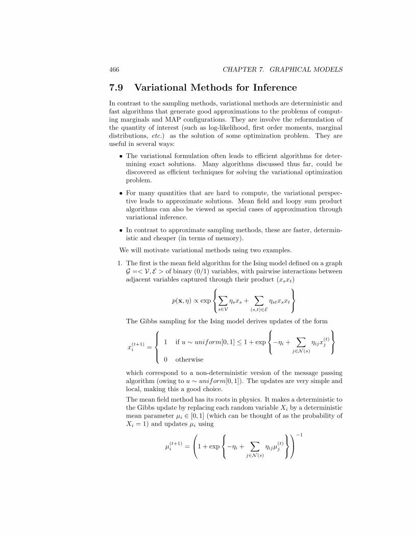
466 CHAPTER 7. GRAPHICAL MODELS
7.9 Variational Methods for Inference
In contrast to the sampling methods, variational methods are deterministic andfast algorithms that generate good approximations to the problems of comput-ing marginals and MAP configurations. They are involve the reformulation ofthe quantity of interest (such as log-likelihood, first order moments, marginaldistributions, etc.) as the solution of some optimization problem. They areuseful in several ways:
• The variational formulation often leads to efficient algorithms for deter-mining exact solutions. Many algorithms discussed thus far, could bediscovered as efficient techniques for solving the variational optimizationproblem.
• For many quantities that are hard to compute, the variational perspec-tive leads to approximate solutions. Mean field and loopy sum productalgorithms can also be viewed as special cases of approximation throughvariational inference.
• In contrast to approximate sampling methods, these are faster, determin-istic and cheaper (in terms of memory).
We will motivate variational methods using two examples.
1. The first is the mean field algorithm for the Ising model defined on a graphG =< V, E > of binary (0/1) variables, with pairwise interactions betweenadjacent variables captured through their product (xsxt)
p(x, η) ∝ exp
∑s∈V
ηsxs +∑
(s,t)∈E
ηstxsxt
The Gibbs sampling for the Ising model derives updates of the form
x(t+1)i =
1 if u ∼ uniform[0, 1] ≤ 1 + exp
−ηi +∑
j∈N (s)
ηijx(t)j
0 otherwise
which correspond to a non-deterministic version of the message passingalgorithm (owing to u ∼ uniform[0, 1]). The updates are very simple andlocal, making this a good choice.
The mean field method has its roots in physics. It makes a deterministic tothe Gibbs update by replacing each random variable Xi by a deterministicmean parameter µi ∈ [0, 1] (which can be thought of as the probability ofXi = 1) and updates µi using
µ(t+1)i =
1 + exp
−ηi +∑
j∈N (s)
ηijµ(t)j
−1

7.9. VARIATIONAL METHODS FOR INFERENCE 467
Thus, the mean field algorithm is exactly a message passing algorithm, buthas some semantics related to sampling techniques. We will see that themean field algorithm is a specific instance of variational methods and itcan be formulated as coordinate descent on a certain optimization problemand subsequently be analysed for convergence, etc.
2. The loopy sum-product (also called the loopy belief propagation) methodis another instance of variational methods. ‘Loopy’ here means on graphswith cycles. If the tree width were low, you could create a junction treeand perform message passing, but what if the tree width were large, suchas with a grid. This algorithm is the most naive application of the sum-product updates (originally developed for trees in Section 7.2.2) and applyit to graphs with cycles. This naive procedure has had extraordinarysuccess in the fields of signal processing, compute vision, bioinformaticsand most importantly, in communication networks, etc.
The message passing algorithm, when applied on a tree, breaks it intosubtrees and passes messages between subtrees, which are independent(share no variable). But the moment you add an edge connecting any twosubtrees, they are not independent any more. Passing messages around incycles can lead to over-counting (analogous to gossip spreading in a socialnetwork). Thus, the message passing algorithm ceases to remain an exactalgorithm and does not even gurantee convergence.
What turns out to be actually very important is how long are the cycleson which messages are being propagated; for long cycles, the effects ofover-counting can be weakened. More technically speaking, the behaviourwill depend on
(a) The girth of the graph (length of cycles): For larger girth, you couldrun the message passing for many iterations before you land up withovercounting.
(b) The strength of the potentials are, or in other words, how close toindependence is the model. For example, in the Ising model itself,based on the coupling induced through terms of the form xsxt, if thecoupling is weak, almost close to independence, the algorithm willbe perfect, giving almost exact answers. There is a region of tran-sition, based on strengthening of the coupling terms, beyond whichthe algorithm breaks down.
3. The idea behind variational methods is to represent the quantity of interest(such as the marginal or mode over a graphical model) as the solution toan optimization problem. For example, the solution to Ax = b (as in thecase of inferencing for Kalman filters) with A 0 and b ∈ <n can berepresented as the solution to
x = argminx
12xTAx− bTx

468 CHAPTER 7. GRAPHICAL MODELS
This is precisely a variational formulation for the linear system Ax = b.If the system of equations Ax = b is large48 the solution x = A−1b maynot be easy to compute, in the event of which, iterative (and sometimesapproximate) solutions to the optimization problem can be helpful. One ofthe most succesful techniques for solving such systems (without invertingmatrices) is the conjugate gradient method, discussed in Section 4.5.8,that solves the system in exactly O(n) steps.
4. As will be seen on page 432 in Section 7.4, the bernoulli distribution canbe expressed as
p(x, η) = exp ηx−A(η)
for X ∈ 0, 1. A(η) = log (1 + eη). We saw in Section 7.4 that the meanis given by
µ = Eη = ∇A(η) =eη
1 + eη= (1 + e−η)−1
The key is in noting that µ corresponds to the ‘slope of’ a supportinghyperplane (see Figure 4.38 on page 271) for epi(A(η)) in a (η,A(η)) space.Thus, we are interested in all the hyperplanes that lie below epi(A(η)),with intercept C along the axis for A(η):
µT η − C ≤ A(η)
and want to get as close to a supporting hyperplane as possible
C∗ = supηµT η −A(η) = A∗(µ)
Borrowing ideas from duality theory (c.f. Section 4.4), we call the functionsupηµT η −A(η) as the dual function A∗(µ). C∗ is the intercept for the
supporting hyerplane. In the case of the bernoulli example, we have
A∗(µ) = supηµT η−log 1 + eη =
(1− µ) log (1− µ) + µ logµ if µ ∈ (0, 1)∞ otherwise
Under nice conditions (such as under Slaters constraint qualification dis-cussed in definition 42 on page 290), the operation of taking duals issymmetric ((A∗)∗ = A), that is,
A(θ) = supµµT η −A∗(µ)
Under the conditions of zero duality gap, it should happen that if
µ(η) = argmaxµ
µT η −A∗(µ)
48Of course, as we saw in Section 7.5, such a system comes up in the case of solution toKalman filters, but can be computed efficiently by exploiting the tree structure of the graphin inverting the matrix. The discussion here is for general graphs.

7.9. VARIATIONAL METHODS FOR INFERENCE 469
is the primal optimum, then µT η − A∗(µ) is the supporting hyperplaneto A(η), meaning that µ is the mean we were seeking. This yields avariational representatation for the original problem of finding the mean.The dual itself is also useful in determining the log-normalization constantfor problems such as parameter estimation. We can confirm in the simplebernoulli case that indeed
µ(η) = µ(η) =eη
1 + eη
We will now generalize the variational formulation of the bernoulli case tothe exponential family.
p(x; θ) = expθT f(x)−A(θ)
where, x ∈ <n and f : <n → <d. Let us say we are interested in computing thefirst order moments
µ = E[f(x)] (7.74)
Following a similar line of argument as for the case of the bernoulli distribution,we define the dual as
A∗(µ) = supθ
µT θ −A(µ)
The key ingredients in this calculation are to set the gradient with respect to θto 0, as a necessary first order condition.
µ−∇A(θ) = 0 (7.75)
This looks like the moment matching problem that results from maximum likeli-hood estimation. The only difference is that µ need not come from data, it is theargument to A∗(η). When will (7.75) have a solution? In the simple bernoullicase, we already saw that we will have a solution η = − logµ − log 1− µ ifµ ∈ (0, 1). As another example, for the univariate Gaussian, f(x) = [x, x2] andA(η) = 1
2σ2µ2 + log σ ≡ − η2
14η2
+ 12 log (−2η2) (as seen on page 432). The system
(7.75) can be shown to have a solution only if µ2−µ21 > 0, that is if the variance
is positive. For two examples, the conditions under which solutions exist to(7.75) are extremely simple - it should be possible to generate data using thedistribution.
Assuming that a solution θ(µ) exists to (7.75), and exploiting the fact thatθ(µ) satisfies moment matching conditions (7.75)
∑x
p(x; θ(µ))f(x) = µ (7.76)

470 CHAPTER 7. GRAPHICAL MODELS
and using the property that
A(µ) =∑x
A(µ)p(x; θ(µ))
the dual will have the form
A∗(µ) = θT (µ)µ−A(µ)
= θT (µ)
(∑x
p(x; θ(µ))f(x)
)−A(µ)
=∑x
p(x; θ(µ))(θT (µ)f(x)−A(µ)
)=
∑x
p(x; θ(µ)) log p(x; θ(µ))
= −H(p(x; θ(µ))) (7.77)
That is, the dual is precisely the negative entropy −H(p(x; θ(µ))) of the distri-bution whose parameters θ(µ) are obtained by moment matching. The dual forthe bernoulli case which resembled an entropy was by no means a coincidence!IfM is the set of all possible moments that make a solution to the system (7.75or equivalently 7.76) feasible, that is
M =
µ ∈ <d
∣∣∣∣∣∑x
p(x; θ)f(x) = µ for some p(.)
then the dual could also be expressed as
A∗(µ) =
−max H(p(x; θ(µ))) such that E[f(x)] = µ for µ ∈M∞ otherwise
Another way of characterizing M is as the set of all first order moments thatcould be generated by p(x; θ). In any case, M is often very had to characterizeand loop belief propagation etc. are often used to approximate it.
Finally, we will write down the variational problem as a reformulation of(7.74), of which mean field, (loopy) sum-product, Gauss Seidel, Jacobi, etc canbe found to be special cases. Writing down the dual of the dual of (7.77), andassuming zero duality gap, we get a reformulation of (7.74):
A(θ) = supµ∈M
µT θ −A∗(µ)
(7.78)
Again, A(θ) is a very hard function to compute, mainly becauseM is simple tocharacterize. This maximumization problem is concave, since A∗(η) is concave

7.9. VARIATIONAL METHODS FOR INFERENCE 471
and the constraint set M is convex. Under zero duality gap conditions (whichholds in this case), the optimal point will be achieved at µ(θ) = E[f(x)].
We will us take some examples to illustate the use of variational techniques.For problems of estimating moments, f could be the feature functions. Forproblems of estimating marginals, f can be chosen to be the indicator function.
The simplest example is for a two node chain: V = X1, X2, E = (X1, X2),X1, X2 ∈ 0, 1 and
p(x; θ) ∝ exp θ1x1 + θ2x2 + θ12x1x2
The moments are: µi = E[Xi] = p(Xi = 1) and µ12 = E[X1X2] = p(X1 =1, X2 = 1). The set M is
M =
µ ∈ <3
∣∣∣∣∣∑x
p(x; θ)f(x) = µ for some p(.)
= µi ∈ [0, 1], 0 ≤ µ12 ≤ min(µ1, µ2), 1 + µ12 − µ1 − µ2 ≥ 0
Let us next write down the dual in terms of the entropy of the distribution
A∗(µ) = −H(p(x;µ)) =∑x1,x2
p(x1, x2) log p(x1, x2)
= µ12 logµ12 + (µ1 − µ12) log (µ1 − µ12) + (µ2 − µ12) log (µ2 − µ12)+ (1 + µ12 − µ1 − µ2) log (1 + µ12 − µ1 − µ2) (7.79)
The corresponding variational problem will be
A(θ) = maxµ∈M
θ1µ1 + θ2µ2 + θ12µ12 −A∗(µ)
Though this can be solved using the method of Lagrange multipliers (c.f., Sec-tion 4.4.1), etc., we expect the optimal solution to the variational problem tobe
µ1 =1z
∑x1∈0,1,x2∈0,1
x1 exp θ1x1 + θ2x2 + θ12x1x2 =exp θ1 + exp θ1 + θ2 + θ12
1 + exp θ1 + exp θ2 + exp θ1 + θ2 + θ12
There are many applications of variational inference to quantity estimationproblems that have either no exactly solutions, or that have solutions not com-putable in polynomial time. Further, variational principles can be used to studyhow the approximate algorithms behave; whether they have fix points, whetherthey converge. what answers do they give, etc.. For instance, in belief prop-agation from a variational perspective, the messages correspond to lagrangemultipliers (for active constraints in M) that are passed around.
In general, the sets M are very complex. For example, with a complete 7node graph, there will be O(3 × 10⁸) constraints. For an n node tree, you willhave 4(n − 1) constraints. The variational principle provides the foundationfor many approximate methods such as the Naive mean field algorithm, whichrestricts optimization to a ‘tractable’ set of M, such as one for which the jointdistribution over a graphical model is factorized by treating the variables ascompletely independent.

472 CHAPTER 7. GRAPHICAL MODELS

Chapter 8
Statistical RelationalLearning
One of the central open questions of artificial intelligence is concerned withcombining (i) expressive knowledge representation formalisms such as relationaland first-order logic with (ii) principled probabilistic and statistical approachesto inference and learning. Why? Here are some reasons:
1. The fields of knowledge representation and inductive logic programmingstress the importance of relational and logical representations that providethe flexibility and modularity to model large domains. They also high-light the importance of making general statements, rather than makingstatements for every single aspect of the world separately.
2. The fields of statistical learning and uncertainty in artificial intelligenceemphasize that agents that operate in the real world must deal with un-certainty. An agent typically receives only noisy or limited informationabout the world; actions are often non-deterministic; and an agent hasto take care of unpredictable events. Probability theory provides a soundmathematical foundation for inference and learning under uncertainty.
3. Machine learning, in general, argues that an agent needs to be capable ofimproving its performance through experience.
Thus, the combination of expressive knowledge representation with prob-abilistic approaches to inference and learning is needed in order to face thechallenges of real-world applications, which are complex and heterogeneous.Most traditional artificial intelligence and machine learning systems, however,are able to handle either uncertainty or rich relational structures but not both.
Statistical learning, reinforcement learning, and data mining methods havetraditionally been developed for data in attribute-value form only; data is repre-sented in matrix form: columns represent attributes, and rows represent exam-
473

474 CHAPTER 8. STATISTICAL RELATIONAL LEARNING
ples. Indeed, matrices are simple and efficient matrix operations can be used.In turn, a matrix form makes it possible to devise efficient algorithms.
Many, if not most, real-world data sets, however, are not in matrix form.Applications contain several entities and relationships among them. Inductivelogic programming and relational learning have been developed for coping withthis type of data.They do not, however, handle uncertainty in a principled way.
It is therefore not surprising that there has been a significant interest inintegrating statistical learning with first order logic and relational representa-tions. This newly emerging research field is known under the name of statisticalrelational learning and probabilistic logic learning, and may be briefly definedas follows:
Definition 64 Statistical relational learning deals with machine learning anddata mining in relational domains where observations may be missing, partiallyobserved, and/or noisy.
Instead of giving a probabilistic characterization of logic programming suchas [Ng and Subrahmanian, 1992], this line of research stresses the machinelearning aspect.
8.1 Role of Logical Abstraction in SRL
Employing relational and logical abstraction within statistical learning has threeadvantages:
1. Variables, i.e., placeholders for entities allow one to make abstraction ofspecific entities.
2. Unification allows one to share information among entities.
3. In many applications, there is a rich background theory available, whichcan efficiently and elegantly be represented as sets of general regularities.
Thus, instead of learning regularities for each single entity independently,statistical relational learning aims at finding general regularities among groupsof entities. The learned knowledge is declarative and compact, which makes itmuch easier for people to understand and to validate. Although, the learnedknowledge must be recombined at run time using some reasoning mechanismsuch as backward chaining or resolution, which bears additional computationalcosts, statistical relational models are more flexible, context-aware, and offer,in principle, the full power of logical reasoning. Further, background knowl-edge often improves the quality of learning as it focuses learning on relevantpatterns, i.e., restricts the search space. While learning, relational and logicalabstraction allow one to reuse experience: learning about one entity improvesthe prediction for other entities; it might even generalize to objects, which havenever been observed before. Thus, relational and logical abstraction can makestatistical learning more robust and efficient. This has been proven beneficial in

8.2. INDUCTIVE LOGIC PROGRAMMING 475
many fascinating real-world applications in citation analysis, web mining, webnavigation, web search, natural language processing, robotics, computer vision,social network analysis, bio-and chemo-informatics, electronic games, and activ-ity recognition. For instance, Liao et al. [2005] applied Taskar et al.s relationalMarkov networks to a problem related to the ride sharing service, namely learn-ing and inferring transportation routines.
Whereas most of the existing works on statistical relational learning havestarted from a statistical and probabilistic learning perspective and extendedprobabilistic formalisms with relational aspects, several pieces of research takea different perspective, starting from inductive logic programming (ILP) andstudying how inductive logic programming formalisms, settings and techniquescan be extended to deal with probabilities.
8.2 Inductive Logic Programming
ILP is a research field at the intersection of machine learning and logic program-ming [Muggleton and De Raedt, 1994]. It is often also called multi-relationaldata mining (MRDM) [D.zeroski and Lavra.c, 2001]. It aims at a formal frame-work as well as practical algorithms for inductively learning relational descrip-tions (in the form of logic programs) from examples and background knowledge.However, it does not explicitly deal with uncertainty such as missing or noisyinformation. Dealing explicitly with uncertainty makes probabilistic ILP morepowerful than ILP and, in turn, than traditional attribute-value approaches.Moreover, there are several benefits of an ILP approach to statistical relationallearning.
1. Classical ILP learning settings, as we will argue, naturally carry over tothe probabilistic case. The probabilistic ILP settings make abstractionof specific probabilistic relational and first order logical representationsand inference and learning algorithms yielding general statistical relationallearning settings.
2. Many ILP concepts and techniques such as more-general-than, refinementoperators, least general generalization (lub), and greatest lower bound (glb)can be reused. Therefore, many ILP learning algorithms such as QuinlansFOIL and De Raedt and Dehaspes Claudien can easily be adapted.
3. The ILP perspective highlights the importance of background knowledgewithin statistical relational learning. The research on ILP and on artificialintelligence in general has shown that background knowledge is the key tosuccess in many applications.
4. An ILP approach should make statistical relational learning more intuitiveto those coming from an ILP background and should cross-fertilize ideasdeveloped in ILP and statistical learning.

476 CHAPTER 8. STATISTICAL RELATIONAL LEARNING
Formally, ILP is concerned with finding a hypothesis H (a logic program,i.e. a definite clause program) from a set of positive and negative examples E+
and E−.Consider learning a definition for the Daughter/2 predicate, i.e., a set of
clauses with head predicates over Daughter/2, given the following facts as learn-ing examples:
E+: Daughter(dorothy, ann).Daughter(dorothy, brian).
E−: Daughter(rex, ann).Daughter(rex, brian).
Additionally, we have some general knowledge called background knowledgeB, which describes the family relationships and sex of each person:
Mother(ann, dorothy). Female(dorothy). Female(ann).Mother(ann, rex). Father(brian, dorothy). Father(brian, rex).
From this information, we could induce the following H:
Daughter(C,P ) : − Female(C),Mother(P,C).Daughter(C,P ) : − Female(C), Father(P,C).
which perfectly explains the examples in terms of the background knowledge,i.e., E+ are entailed by H together with B, but E− are not entailed.
Definition 65 Given a set of positive and negative examples E+ and E− oversome language LE, a background theory B, in the form of a set of definiteclauses, a hypothesis language LH , which specifies the clauses that are allowedin hypotheses, and a covers relation covers(e,H,B) ∈ 0, 1, which basicallyreturns the classification of an example e with respect to H and B, find a hy-pothesis H∗ ∈ H that covers (with respect to the background theory B) all pos-itive examples in E+ (completeness) and none of the negative examples in E−(consistency).
In a noisy learning setting, the goal is to find a hypothesis H∗ ∈ H thatmaximizes an objectice score(E , H,B).
H∗ = argmaxH
score(E , H,B)
The (i) language LE chosen for representing the examples together with the(ii) covers relation determines the inductive logic programming setting De Raedt[1997]. There are three broad settings, viz.,
1. learning from entailment [Plotkin, 1970]
2. learning interpretations [Helft, 1989, De Raedt and D.zeroski, 1994]
3. an intermediate setting called learning from proofs [Shapiro 1983]

8.3. PROBABILISTIC ILP SETTINGS 477
8.3 Probabilistic ILP Settings
The inductive logic programming settings can be extended to the probabilisticcase. When working with probabilistic ILP representations, there are essentiallytwo changes:
1. Probabilistic Clauses: Clauses in H and B are annotated with probabilisticinformation, and Here, we use the following probability notations. WithX, we denote a (random) variable. Furthermore, x denotes a state andX (resp. x) a set of variables (resp. states). We will use Pr to denote aprobability distribution, e.g., Pr (x), and p to denote a probability value,e.g., p(X = x) and p(X = x).
2. Probabilistic Covers: The covers relation becomes probabilistic. A prob-abilistic covers relation softens the hard covers relation employed in tra-ditional ILP and is defined as the probability of an example given thehypothesis and the background theory. A probabilistic covers relationtakes as arguments an example e, a hypothesis H and possibly the back-ground theory B, and returns the probability value Pr (e|H,B) ∈ [0, 1] ofthe example e given H and B, i.e., covers(e,H,B) = Pr (e|H,B).
Using the probabilistic covers relation above, our first attempt at a definitionof the probabilistic ILP learning problem is as follows:
Definition 66 Given a probabilistic-logical language LH and a set E of ex-amples over some language LE, find the hypothesis H∗ in LH that maximizesPr (E|H∗,B).
Under the usual i.i.d. assumption, i.e., examples are sampled independentlyfrom identical distributions, this results in the maximization of
Pr (E|H∗,B) =∏e∈E
P (e|H∗,B) =∏e∈E
covers(e,H∗,B)
Similar to the ILP learning problem, the language LE selected for repre-senting the examples together with the probabilistic covers relation determinesdifferent learning setting. Guided by Definition 66, we will introduce severalprobabilistic ILP settings for statistical relational learning. The main idea isto lift traditional ILP settings by associating probabilistic information withclauses and interpretations and by replacing ILPs deterministic covers relationby a probabilistic one. In the discussion, we will have one trivial but importantobservation:
Observation: Derivations might fail.
The probability of a failure is zero and, consequently, failures are neverobservable. Only succeeding derivations are observable, i.e., the probabilities ofsuch derivations are greater than zero. As an extreme case, recall the negative

478 CHAPTER 8. STATISTICAL RELATIONAL LEARNING
examples E− employed in the ILP learning problem on page 8.2. They aresupposed to be not covered, i.e.,
p(E−|H,B) = 0
In that example, Rex is a male person; he cannot be the daughter of ann.Thus, Daughter(rex, ann) was listed as a negative example. Negative exam-ples conflict with the usual view on learning examples in statisticallearning. In statistical learning, we seek to find that hypothesis H∗, which ismost likely given the learning examples:
H∗ = Hargmax
p(H|E) = Hargmax
p(E|H)p(H)p(E)
with p(E) > 0
Thus, examples E are observable, i.e., p(E) > 0. Therefore, we refine thepreliminary probabilistic ILP learning problem definition 66. In contrast to thepurely logical case of ILP, we do not speak of positive and negative examplesanymore but of possible and impossible ones.
Definition 67 Given a set E = Ep ∪ Ei of possible and impossible examplesEp and Ei (with Ep ∩ Ei = ∅) over some example language LE, a probabilisticcovers relation covers(e,H,B) = P (e|H,B), a probabilistic logical language LHfor hypotheses, and a background theory B, find a hypothesis H∗ in LH suchthat H∗ = argmax
Hscore(E , H,B) and the following constraints hold:
∀ep ∈ Ep : covers(ep, H∗,B) > 0 and ∀ei ∈ Ei : covers(ei, H∗,B) = 0
The scoring function is some objective score, usually involving the probabilisticcovers relation of the possible examples such as the observed likelihood∏
ep∈Ep
covers(ep, H∗,B)
some penalized variant thereof.
The probabilistic ILP learning problem of Definition 67 unifies ILP andstatistical learning in the following sense:
1. Using a deterministic covers relation (which is either 1 or 0) yields theclassical ILP learning problem, see Definition 65.
2. On the other hand, sticking to propositional logic and learning from pos-sible examples, i.e., P (E) > 0, only yields traditional statistical learning.
3. Definition 67 makes abstraction of many particular kinds of problems.
• In density estimation, the joint probability distribution of some ran-dom variables is estimated

8.3. PROBABILISTIC ILP SETTINGS 479
• Whereas, in classification and regression the dependency of a discreterespectively continuous target variable given the value of some othervariables is estimated.
4. Furthermore, several types of learning can be distinguished.
• In supervised learning, the training examples contain informationabout all variables including the target variable.
• In reinforcement learning, the training examples contain only indirecttarget information such as the classifier did well or not (in the formof some reward).
• Finally, in unsupervised learning, no values of the target variable areobserved.
5. Another important distinction is whether all the random variables vari-ables are observed, or whether some of them are hidden, e.g., they arespecified in the background knowledge and never observed.
6. We can also formulate the learning problem as either of the following:
• As a ‘point estimation problem, i.e., the goal is to find a single besthypothesis H∗.
• As a ‘Bayesian learning problem’, where the goal is to return a pos-terior distribution over hypotheses.
7. Finally, learning might refer to the structure, i.e., the underlying logicprogram of the hypothesis, the parameters, or both. To come up withalgorithms solving probabilistic ILP learning problems, say for densityestimation, one typically distinguishes two subtasks because H = (L, λ) isessentially a logic program L annotated with probabilistic parameters λ:
• Parameter estimation where it is assumed that the underlying logicprogram L is fixed, and the learning task consists of estimating theparameters λ that maximize the likelihood.
• Structure learning where both L and λ have to be learned from thedata.
Similar to that for traditional ILP, there are three probabilistic ILP set-tings, which extend the purely logical ones. The three ILP settings and theirprobabilistic extensions are outlined in the following sections.
8.3.1 Probabilistic setting for justification
There are two important components in SRL:
Abduction. Process of hypothesis formation. The logical setting for abductionis what traditional ILP is mostly about.

480 CHAPTER 8. STATISTICAL RELATIONAL LEARNING
Justification. The degree of belief assigned to an hypothesis given a certainamount of evidence.
Recall the Bayes’ Theorem
p(h|E) =p(h).p(E|h)
p(E)
The best hypothesis in a set H (ignoring ties)
H = argmaxh∈H p(h|E)
We will consider the following learning framework.
Let X be a countable set of instances (encodings of all objects of interest)and DX be a probability measure on X
Let C ⊆ 2X be a countable set of concepts and DC be a probablity measureon 2X
Let H be a countable set of hypotheses1 and DH be a probability measure(prior) over H
Let the concept represented by h ∈ H be c(h) ∈ C
Let C and H be such that– for each C ∈ C, there is an h ∈ H s.t. C = c(h)
– for each C ∈ C, DC(C) =∑h∈H|C=c(h) P (h)
Target concept T is chosen using the distribution DC
Let g(h) denote the proportion (w.r.t. the instance space) of the conceptrepresented by a hypothesis h ∈ H
– That is, g(h) =∑x∈c(h) DX (x)
– g(h) is a measure of the “generality” of h
Noise Free Data
Following is a model for noise free data.
1Note that H also been used earlier to denote the space of horn clauses. This time, it isused to denote the space of hypothesis, which anyways happens to be within the space of hornclauses.

8.3. PROBABILISTIC ILP SETTINGS 481
Given E = E+ ∪ E−
p(h|E) ∝ DH(h)∏e∈E+
p(e|h)∏e∈E−
p(e|h)
Or
P (h|E) ∝ DH(h)∏e∈E+
DX(e)g(h)
∏e∈E−
DX(e)1− g(h)
Assuming p positive and n negative examples
P (h|E) ∝ DH(h)
(∏e∈E
DX(e)
)(1
g(h)
)p(1
1− g(h)
)n
Maximal P (h|E) means finding the hypothesis that maximises
logDH(h) + p log1
g(h)+ n log
11− g(h)
If there are no negative examples, then this becomes
logDH(h) + p log1
g(h)
Let us answer some questions at this point:
1. What is the distribution DH(h):
A common assumption is that “larger” programs are less likely (incoding terminology, require more bits to encode)
As an exampleDH(h) = 2−|h|
That islogDH(h) = −|h|

482 CHAPTER 8. STATISTICAL RELATIONAL LEARNING
2. What is generality function g(h)?
Recall that g(h) =∑x∈c(h)DX(x)
– c(h) may be infinite
– DX is usually unknown (and is a mapping to the reals)
Have to be satisfied with approximate estimates of g(h)
Estimation procedure
(a) Randomly generate a finite sample of n instances using a knowndistribution (for eg. uniform)
(b) Determine the number of these instances (say c) entailed by h(c) g(h) ≈ c+1
n+2
3. What about noisy data? This will be addressed in the next subsection.
A Model for Noisy Data
Following is a model for justification in the presence of noisy data.
For any hypothesis h the examples E = E+ ∪ E− can now be partitioned asfollows
1. TP = e|e ∈ E+ and e ∈ c(h) (true positives)
2. FN = e|e ∈ E+ and e 6∈ c(h) (false negatives)
3. FP = e|e ∈ E− and e ∈ c(h) (false positives)
4. TN = e|e ∈ E− and e 6∈ c(h) (true negatives)
Recall
p(h|E) ∝ DH(h)∏e∈E+
p(e|h)∏e∈E−
p(e|h)
Now ∏e∈E+
p(e|h) =∏e∈TP
(DX(e)(1− ε)
g(h)+DX(e)ε
) ∏e∈FN
DX(e)ε

8.4. LEARNING FROM ENTAILMENT 483
∏e∈E−
p(e|h) =∏e∈TN
(DX(e)(1− ε)
1− g(h)+DX(e)ε
) ∏e∈FP
DX(e)ε
So, with FPN = FP ∪ FN
p(h|E) ∝ DH(h)
(∏e∈E
DX(e)
)(1− εg(h)
)|TP |(1− ε
1− g(h)
)|TN|ε|FPN|
Maximal P (h|E) means finding the hypothesis that maximises
logDH(h) + |TP | log1− εg(h)
+ |TN | log1− ε
1− g(h)+ |FPN |logε
Another model for noisy data is outlined below:
8.4 Learning from Entailment
Learning from entailment is by far the most popular ILP setting and it is ad-dressed by a wide variety of well-known ILP systems such as FOIL [Quinlanand Cameron-Jones, 1995], Progol [Muggleton, 1995], and Aleph [Srinivasan,1999]. When learning from entailment, the examples are definite clauses and ahypothesis H covers an example e with respect to the background theory B ifand only if B ∪H |= e, i.e., each model of B ∪H is also a model of e.
In many well-known systems, such as FOIL, one requires that the examplesare ground facts. To illustrate the above setting, consider the following exampleinspired on the well-known mutagenicity application [Srinivasan et al., 1996].
Consider the following facts in the background theory B, which describe partof molecule 225.

484 CHAPTER 8. STATISTICAL RELATIONAL LEARNING
Molecule(225). Logmutag(225, 0.64).Lumo(225,−1.785). Logp(225, 1.01).Nitro(225, [f1 4, f1 8, f1 10, f1 9]). Atom(225, f1 1, c, 21, 0.187).Atom(225, f1 2, c, 21,−0.143). Atom(225, f1 3, c, 21,−0.143).Atom(225, f1 4, c, 21,−0.013). Atom(225, f1 5, o, 52,−0.043).Bond(225, f1 1, f1 2, 7). Bond(225, f1 2, f1 3, 7).Bond(225, f1 3, f1 4, 7). Bond(225, f1 4, f1 5, 7).Bond(225, f1 5, f1 1, 7). Bond(225, f1 8, f1 9, 2).Bond(225, f1 8, f1 10, 2). Bond(225, f1 1, f1 11, 1).Ring size 5(225, [f1 5, f1 1, f1 2, f1 3, f1 4]). Bond(225, f1 11, f1 12, 2).Hetero aromatic 5 ring(225, [f1 5, f1 1, f1 2, f1 3, f1 4]). Bond(225, f1 11, f1 13, 1).. . . . . .
Consider now the positive example Mutagenic(225). It is covered by thefollowing H:
Mutagenic(M) :- Nitro(M,R1), Logp(M,C), C > 1.
together with the background knowledge B, because H ∪B entails the example.To see this, we unify Mutagenic(225) with the clauses (H) head. This yields
Mutagenic(225) : − Nitro(225, R1), Logp(225, C), C > 1.
Now, Nitro(225, R1) unifies with the third ground atom (left-hand side column)in B, and Logp(225, C) with the second one on the right. Because 1.01 > 1, wefound a proof of mutagenic(225).
There are, broadly speaking, three types of ILP approaches for learning fromentailment: top-down approaches, bottom-up approaches and hybrid approaches.
1. Top-down approaches start from short clauses, iteratively adding literalsto their bodies as long as they do not become to overly general. Basically,in top-down approaches, hypotheses are generated in a pre-determinedorder, and then tested against the examples. More precisely:
(a) They start with the most general hypothesis, i.e., clauses of the formDaugther(C,P ) : −True, where all arguments are distinct variables.
(b) After seeing the first example that contradicts the hypothesis, i.e.,after seeing the first negative example, the hypothesis is specializedby specializing the general clause.
(c) The clause is specialized typically in two ways:
• by applying a substitution,• by adding a literal, i.e., an atom or its negation to the body, and

8.4. LEARNING FROM ENTAILMENT 485
For instance, we can specialize Daughter(C,P ) : −True and considerDaughter(C,P ) : −Female(C) andDaughter(C,P ) : −Mother(P,C)for further investigations. Several possibilities (and successive spe-cializations) have to be tried before one finds a clause that coverssome positive examples but no negative ones such asDaugther(C,P ) :−Female(C),Mother(P,C).
(d) If some positive examples are still not covered, these techniques typ-ically add a new, maximally general clause to the hypothesis andessentially iterate the process in step 1c as before, until all positiveexamples are covered and no negative example is covered.
(e) The background knowledge B is typically viewed as a logic program(i.e. a definite clause program) that is provided to the inductivelogic programming system and fixed during the learning process. Thehypothesis H together with the background theory B should coverall positive and none of the negative examples.
Top-down approaches are often employed by ILP systems that learn fromentailment. More precisely, these systems often employ a separate-and-conquer rule-learning strategy [Furnkranz, 1999]. In an outer loop of thealgorithm, they follow a set-covering approach [Mitchell, 1997] in whichthey repeatedly search for a rule covering many positive examples andnone of the negative examples. They then delete the positive examplescovered by the current clause and repeat this process until all positiveexamples have been covered. In the inner loop of the algorithm, theytypically refine a clause by unifying variables, by instantiating variablesto constants, and/or by adding literals to the clause.Figure 8.1 presents the generic framework for top-down ILP systems whileFigure 8.2 outlines one of the original ILP systems, MIS.
2. Bottom-up approaches start from long clauses, iteratively removing liter-als until they would become overly general. While top-down approachessuccessively specialize a very general starting hypothesis, bottom-up ap-proaches successively generalize a very specific hypothesis. This is basi-cally done
(a) by deleting literals (or clauses),(b) by turning constants into variables and/or(c) by turning bounded variables into new variables.
At each step, the theory is generalized by taking the least general gener-alization (under .-subsumption) of pairwise clauses. Of course, care mustbe taken that the generalized theory does not covernegative examples.
3. Hybrid approaches that mix top-down and bottom-up searches. Hybridapproaches are usually employed for multiple predicate learning [De Raedtet al., 1993] and theory revision [Wrobel, 1996].

486 CHAPTER 8. STATISTICAL RELATIONAL LEARNING
Initialize Ecur = E ;Initialize H = ∅;//Start coveringrepeat
Initialize C = T ←;//Start specializationrepeat
Find the best refinement Cbest ∈ ρL(C);Assign C = Cbest;
until Necessity stopping criterion is satisfied;Add C to H to get new hypothesis H′ = H ∪ C;Remove positive examples covered by C from Ecur to get new training setE ′cur = Ecur −
⋃e∈E+
cur|covers(B,H′,e)=1e;
Assign Ecur = E ′cur, H = H′;until Sufficiency stopping criterion is satisified;
Figure 8.1: A general strategy for top-down ILP approaches.
8.4.1 Constraining the ILP Search
It should be stressed that ILP is a difficult problem. Practical ILP systemsfight the inherent complexity of the problem by imposing all sorts of constraints,mostly syntactic in nature. Such constraints include
1. Language and search biases: These are sometimes summarized as declar-ative biases, (see [Nedellec et al., 1996] for an overview). Essentially,the main source of complexity in ILP steams from the variables in theclauses. In top-down systems, the branching factor of the specializationoperator increases with the number of variables in the clauses. Followingare frequently adopted techniques for reducing this branching factor byintroducing language and search bias.
(a) Introducing types for predicates can rule out main potential substitu-tions and unifications. As an example, the type definition type(Father(person, person))specifies that both argument of atoms over Father/2 have to be per-sons.
(b) Refinement operators can also be used to encode a language bias,since they can be restricted to generate only a subset of the languageLH . For instance, refinement operators can easily be modified togenerate only constant-free and function-free clauses.
(c) Other methods use a kind of grammar construction to explicitly de-clare the range of acceptable clauses, see e.g. Cohen [1994].
(d) Lookaheads are an example of a search bias. In some cases, an atommight never be chosen by our algorithm because it will not, in itself,

8.4. LEARNING FROM ENTAILMENT 487
Initialize hypothesis H to a (possibly empty) set of clauses in LH ;loop
Read the next (positive or negative) example;repeat
if There exists an e ∈ E− covered by H thenDelete incorrect clauses from H.
end ifif There exists an e ∈ E+ not covered by H then
With breadth-first search of the refinement graph develop a clause Cwhich covers e and add it to H;
end ifuntil H is complete and consistent;return Hypothesis H;
end loop
Figure 8.2: A simplified version of the MIS algorithm by [Shapiro 1983].whichis the general strategy of top-down approaches.
result in a better score. However, such an atom, while not usefulin itself, might introduce new variables that make a better coveragepossible by adding another atoms later on [Quinlan, 1991] 7. It isusually solved by allowing the algorithm to look ahead in the searchspace. Instead of considering refinements with a single atom, oneconsiders larger refinements consisting of multiple atoms [Blockeeland De Raedt, 1997].
2. Bound on number of distinct variables: One can also put a bound in thenumber of distinct variables that can occur in clauses.
3. Mode declarations: Mode declarations are another well-known ILP de-vise. They are used to describe input-output behaviour of predicatedefinitions. For example, we might specify mode(Daugther(+,−)) andmode(Father(−,+)), meaning that the + arguments must be instanti-ated, whereas the − arguments will be bounded to the answer.
In general, a model can suffer from either underfitting or overfitting. Amodel that is not sufficiently complex can fail to fully detect the underlyingrule of a complicated data set, leading to underfitting. A model that is toocomplex may fit the noise, not just the underlying rule, leading to overfittingand, for instance, wild predictions.
8.4.2 Example: Aleph
As an example for the learning from entailments setting, we will discuss Aleph.Given background knowledge B and positive examples E+ = e1 ∧ e2 . . ., nega-tive examples E− = f1 ∧ f2 ∧ . . ., the generic ILP system Aleph, is concerned

488 CHAPTER 8. STATISTICAL RELATIONAL LEARNING
with finding a hypothesis H = D1 ∧ . . . that satisfies (note: ∪ and ∧ usedinterchangeably)
Prior Satisfiability. B ∧ E− 6|= 2
Prior Necessity. B 6|= E+
Posterior Sufficiency. B ∧H |= E+ and B ∧Dj |= e1 ∨ e2 ∨ . . .
Posterior Satisfiability. B ∧H ∧ E− 6|= 2
If more than one H satisfies this, the one with highest posterior probabilityis chosen. The Di can be found by examining clauses that “relatively subsume”at least one example, making use of plotkin’s relative subsumption discussedelaborately in Section 2.5.1. This gives the following sufficient implementationof Aleph, given B, E .
1. H0 = B, i = 0, E+ = e1, . . . , en
2. repeat
(a) increment i
(b) Obtain the most specific clause ⊥(B, ei)(c) Find the clause Di that: subsumes ⊥(B, ei); and is consistent with
the negative examples;
(d) Hi = Hi−1 ∪ Di
3. until i > n
4. return Hn
As discussed in Section 2.5.1, there are problems with this implementation.Particularly,
– ⊥(B, ei) may be infinite
– This implementation may perform a lot of redundant computation (Di ∈Hi−1)
– This implementation need not return the hypothesis with maximum pos-terior probability
So we next present a “Greedy” implementation for Aleph, given B, E .1. H0 = B, E+
0 = E+, i = 0.
2. Repeat
(a) Increment i
(b) Randomly choose a positive example ei from E+i−1
(c) Obtain the most specific clause ⊥(B, ei)

8.4. LEARNING FROM ENTAILMENT 489
Figure 8.3: The train-spotting example for illustrating Aleph.
(d) Find the clause Di that: subsumes ⊥(B, ei); and is consistent with thenegative examples; and maximises p(Hi−1 ∪ Di|e+
i ∪ E−) where e+
i arethe examples in E+ made redundant by Hi−1 ∪ Di
(e) Hi = Hi−1 ∪ Di(f) E+
i = E+i−1\e
+i
3. until E+i = ∅
4. return Hi
However, this implementation does not address the problem that ⊥(B, ei)may be infinite and that it need not return in the hypothesis with maximumposterior probability. The problem of infinite ⊥(B, ei) may be addressed bymaking use of mode declarations introduced on page 120. This gives a revised“Greedy” implementation for Aleph, given B, E , d.
1. H0 = B, E+0 = E+, i = 0
2. Repeat
(a) Increment i
(b) Randomly choose a positive example ei from E+i−1
(c) Obtain the most specific clause ⊥d(B, ei)(d) Find the clause Di that: subsumes ⊥(B, ei); and is consistent with the
negative examples; and maximises p(Hi−1 ∪ Di|e+i ∪ E
−) where e+i are
the examples in E+ made redundant by Hi−1 ∪ Di(e) Hi = Hi−1 ∪ Di(f) E+
i = E+i−1\e
+i
3. until E+i = ∅
4. return Hi
As an example, let us consider the trainspotting problem (c.f. Figure 8.3)to illustrate the discussion thus far.
We will use the following mode declarations for the trainspotting example.

490 CHAPTER 8. STATISTICAL RELATIONAL LEARNING
:- modeh(1,eastbound(+train)).
:- modeb(1,short(+car)).
:- modeb(1,closed(+car)).
:- modeb(1,long(+car)).
:- modeb(1,open_car(+car)).
:- modeb(1,double(+car)).
:- modeb(1,jagged(+car)).
:- modeb(1,shape(+car,#shape)).
:- modeb(1,load(+car,#shape,#int)).
:- modeb(1,wheels(+car,#int)).
:- modeb(*,has_car(+train,-car)).
Further, the examples E+ and E− for this example will be:
Positive Negative
eastbound(east1). eastbound(west6).
eastbound(east2). eastbound(west7).
eastbound(east3). eastbound(west8).
eastbound(east4). eastbound(west9).
eastbound(east5). eastbound(west10).
whereas, the background knowledge B will comprise:
% type definitions
car(car_11). car(car_12). ...
car(car_21). car(car_22). ...
...
shape(elipse). shape(hexagon). ...
...
% eastbound train 1
has_car(east1,car_11). has_car(east1,car_12). ...
shape(car_11,rectangle). shape(car_12,rectangle). ...
open_car(car_11). closed(car_12).
long(car_11). short(car_12). ...
...
% westbound train 6
has_car(west6,car_61). has_car(west6,car_62). ...
long(car_61). short(car_62).
shape(car_61,rectangle). shape(car_62,rectangle).
...
The outcome of a simple search in Aleph, for the trainspotting setting isoutlined next:
eastbound(A) :-
has_car(A,B).

8.4. LEARNING FROM ENTAILMENT 491
[5/5]
eastbound(A) :-
has_car(A,B), short(B).
[5/5]
eastbound(A) :-
has_car(A,B), open_car(B).
[5/5]
eastbound(A) :-
has_car(A,B), shape(B,rectangle).
[5/5]
...
[theory]
[Rule 1] [Pos cover = 5 Neg cover = 0]
eastbound(A) :-
has_car(A,B), short(B), closed(B).
[pos-neg] [5]
We will next discuss the search and redundancy aspects of Aleph. Thereare two stages in the clause-by-clause construction of hypothesis, which aresummarized below:
1. Search
2. Remove redundant clauses once best clause is found
Aleph has provision for bottom-up as well as top-down search for movingabout in the lattice. The following refinement steps can be used in Aleph.
General-to-specific search: start at 2, and move by
1. Adding a literal drawn from ⊥ip(X,Y )← q(X) becomes p(X,Y )← q(X), r(Y )

492 CHAPTER 8. STATISTICAL RELATIONAL LEARNING
Figure 8.4: The conversion of (relative) subsumption lattice to tree.
2. Equating two variables of the same type
p(X,Y )← q(X) becomes p(X,X)← q(X)
3. Instantiate a variable with a general functional term or constant
p(X,Y )← q(X) becomes p(3, Y )← q(3)
Specific-to-general search: start at ⊥i
Dual operations to above (ie. remove literal etc.)
Progol does a general-to-specific search
Next, we discuss some search methods. The subsumption lattice can berepresented as a directed acyclic graph. However, the DAG can be convertedto a tree such that root is the first node (2 or ⊥i) and children of a nodeare refinements. The conversion of a lattice to a search tree is illustrated inFigure 8.4
Searching the lattice is therefore equivalent to searching a tree. Out goal isto find the node (goal node) that has greatest “compression”. There are twobasic types of tree search: depth-first (DF) and breadth-first (BF) as discussedin chapter 6. DF and BF are “blind”. More guidance is desirable at any nodes. The guidance can be in one or more of the following forms:
• gs: cost of optimal path from root to s
• hs: estimated cost of optimal path to goal from s
The different kinds of guided search can be summarized as follows:
Hill-climbing: DF with hs
Best-first: BF with hs
Best-cost: BF with gs
A∗: BF with gs and hs

8.4. LEARNING FROM ENTAILMENT 493
Progol does an A∗-like search – uses utilit instead of costs. For a clause Cat a node
ps = |e : e ∈ E+ and B ∧ C ∧ e |= 2|ns = |e : e ∈ E− and B ∧ C ∧ e |= 2|cs = |C| − 1
ls = l.b. on literals needed
hs = −(ns + cs + ls)
gs = ps
fs = gs + hs
Compression of a clause at node s = ps − ns − cs Progol seeks clauses withcs < c and ns = 0 and guaranteed to have maximum ps − cs − hs. Progol hasseveral admissable pruning strategies to reduce search.
E.g. Let children(s) = S. If f(s) > ps′ − cs′ for s′ ∈ S then prune(s’)
We next outline an optimal search algorithm that uses branch-and-bound.bb(i, ρ, f) : Given an initial element i from a discrete set S; a successor function ρ :
S → 2S ; and a cost function f : S → <, return H ⊆ S such that H contains theset of cost-minimal models. That is for all hi,j ∈ H, f(hi) = f(hj) = fmin andfor all s′ ∈ S\H f(s′) > fmin.
1. Active := 〈i〉.2. best :=∞3. selected := ∅4. while Active 6= 〈〉5. begin
(a) remove element k from Active
(b) cost := f(k)
(c) if cost < best
(d) begin
i. best := cost
ii. selected := kiii. let Prune1 ⊆ Active s.t. for each j ∈ Prune1, f(j) > best where
f(j) is the lowest cost possible from j or its successors
iv. remove elements of Prune1 from Active
(e) end
(f) elseif cost = best
i. selected := selected ∪ k(g) Branch := ρ(k)
(h) let Prune2 ⊆ Branch s.t. for each j ∈ Prune2, f(j) > best wheref(j) is the lowest cost possible from j or its successors
(i) Bound := Branch\Prune2
(j) add elements of Bound to Active

494 CHAPTER 8. STATISTICAL RELATIONAL LEARNING
6. end
7. return selected
Different search methods result from specific implementations of Active:
– Stack: depth-first search
– Queue: breadth-first search
– Prioritised Queue: best-first search
There are two types of redundancies in the hypothesis H:
1. Redundancy 1: Literal Redundancy:
Literal l is redundant in clause C ∨ l relative to background B iff
B ∧ (C ∨ l) ≡ B ∧ C
It can be shown that the literal l is redundant in clause C ∨ l relativeto the background B iff
B ∧ (C ∨ l) |= C
The clause C is said to be reduced (c.f. Section 2.1, page 102) withrespect to background knowledge B iff no literal in C is redundant.
2. Redundancy 2: Clause redundancy:
Clause C is redundant in the B ∧ C iff B ∧ C ≡ B.
It can be shown that clause C is redundant in B ∧ C iff
B |= C ≡ B ∧ C |= 2
A set of clauses S is said to be reduced iff no clause in S is redundant
Progol uses this procedure to determine (and remove) examples maderedundant by clause found in the search.Example
ej : gfather(henry, john)←
B : father(henry, jane)←father(henry, joe)←parent(jane, john)←parent(joe, robert)←
Dj : gfather(X,Y )← father(X,Z), parent(Z, Y )

8.5. PROBABILISTIC LEARNING FROM ENTAILMENT 495
ej is redundant in B ∧Dj ∧ ej since B ∧Dj ∧ ej |= 2
There are several implementation issues that need further thought.
Question. Will the clause-by-clause search method yield the best set of clauses?If no, why not?
Question. Is it possible to do a theory-by-theory search?
Question. Is it possible devise a complete search that is non-redundant? If no,why not?
8.5 Probabilistic Learning from Entailment
Probabilistic learning from entailment has been investigated for learning stochas-tic logic programs [Muggleton, 2000a,b, Cussens, 2001, Muggleton, 2002] andfor parameter estimation of PRISM programs [Sato and Kameya, 2001, Kameyaet al., 2004] from possible examples only.
In order to integrate probabilities in the entailment setting, we need to finda way to assign probabilities to clauses that are entailed by an annotated logicprogram. Since most ILP systems working under entailment employ groundfacts for a single predicate as examples, we will restrict our attention to assignprobabilities to facts for a single predicate2.
More formally, let us annotate a logic program H consisting of a set of clausesof the form q ← bi, where p is an atom of the form p(V1, . . . , Vn) with the Vidifferent variables, and the bi are different bodies of clauses. Furthermore, weassociate to each clause in H the probability values p(bi|q); they constitute theconditional probability distribution that for a random substitution θ for whichqθ is ground and true (resp. false), the query biθ succeeds (resp. fails) in theknowledge base B. Recall that the query q succeeds in B if there is a substitutionσ such that B |= qσ. Furthermore, we assume the prior probability of q is givenas p(q), which denotes the probability that for a random substitution θ, pθ istrue (resp. false). This can then be used to define the covers relation p(qθ | H,B)as follows (we delete the B as it is fixed):
p(qθ|H) = p(qθ | b1θ, . . . , bkθ) =p(b1θ, . . . , bkθ|qθ)× p(qθ)
p(b1θ, . . . , bkθ)
For instance, applying the naive Bayes assumption yields
p(qθ|H) =
∏i
p(biθ|qθ)× p(qθ)
p(b1θ, . . . , bkθ)(8.1)
2It remains an open question as how to formulate more general frameworks for workingwith entailment.

496 CHAPTER 8. STATISTICAL RELATIONAL LEARNING
Finally, since p(qθ | H) + p(¬qθ | H) = 1, we can compute p(qθ|H) withoutp(b1θ, . . . , bkθ) through normalization.
As an example, consider again the mutagenicity domain and the followingannotated logic program:
(0.01, 0.21) : Mutagenetic(M)← Atom(M, , , 8, )(0.38, 0.99) : Mutagenetic(M)← Bond(M, ,A, 1), Atom(M,A, c, 22, ), Bond(M,A, 2)
We denote the first clause by b1 and the second one by b2. The vectorson the left-hand side of the clauses specify p(biθ = true | qθ = true) andp(biθ = true | qθ = false) respectively. The covers relation (assuming theNaive Bayes assumption) assigns probability 0.97 to example 225 because bothfeatures fail for θ = M/225. Hence
p(Mutagenetic(225) = true, b1θ = false, b2θ = false) = p(b1θ = false|Mutagenetic(225) = true)× p(b2θ = false|Mutagenetic(225) = true)× p(Mutagenetic(225) = true)= 0.99× 0.62× 0.31 ≈ 0.19
and
p(Mutagenetic(225) = false, b1θ = false, b2θ = false) = 0.79×0.01×0.68 ≈ 0.005
This yields
P (Mutagenetic(225) = true | b1θ = false, b2θ = false) =0.19
0.19 + 0.005≈ 0.97
8.5.1 Structure and Parameter Learning
Next, we outline typical solutions to the problems of structure and parame-ter learning in the setting of probabilistic learning from entailment (as well asinterpretation).
1. The problem of parameter estimation is concerned with estimating thevalues of the parameters λ of a fixed probabilistic program H = (L, λ)that best explains the examples E . So, λ is a set of parameters and canbe represented as a vector. To measure the extent to which a model fitsthe data, one usually employs the likelihood of the data, i.e. P (E|L, λ),though other scores or variants could be used as well.
When all examples are fully observable, maximum likelihood reduces tofrequency counting. In the presence of missing data, however, the maxi-mum likelihood estimate typically cannot be written in closed form. It is anumerical optimization problem, and all known algorithms involve nonlin-ear optimization The most commonly adapted technique for probabilistic

8.5. PROBABILISTIC LEARNING FROM ENTAILMENT 497
logic learning is the Expectation-Maximization (EM) algorithm [Dempsteret al., 1977, McLachlan and Krishnan, 1997]. EM is based on the observa-tion that learning would be easy (i.e., correspond to frequency counting),if the values of all the random variables would be known. Therefore, itestimates these values, maximizes the likelihood based on the estimates,and then iterates. More specifically, EM assumes that the parametershave been initialized (e.g., at random) and then iteratively performs thefollowing two steps until convergence:
(a) (E-Step): On the basis of the observed data and the present pa-rameters of the model, it computes a distribution over all possiblecompletions of each partially observed data case.
(b) (M-Step): Treating each completion as a fully observed data caseweighted by its probability, it computes the improved parameter val-ues using (weighted) frequency counting. The frequencies over thecompletions are called the expected counts.
2. What if we need to learn both the structure L and the parameters λof the probabilistic program H = (L, λ) from the data? Often, furtherinformation is given as well. As in ILP, the additional knowledge can takevarious different forms, including a language bias that imposes restrictionson the syntax of L, and an initial hypothesis (L, λ) from which the learningprocess can start.
Nearly all (score-based) approaches to structure learning perform a heuris-tic search through the space of possible hypotheses. Typically, hill-climbingor beam-search is applied until the hypothesis satisfies the logical con-straints and the score(H, E) is no longer improving. The steps in thesearch-space are typically made using refinement operators, see Section 2.7.
Logical constraints often require that the possible examples are coveredin the logical sense. For instance, when learning stochastic logic programsfrom entailment, the possible example clauses must be entailed by thelogic program.
8.5.2 Example: Extending FOIL
Building on [Landwehr et al., 2005], we will next illustrate a promising, alterna-tive approach with less computational complexity, which adapts FOIL [Quinlanand Cameron-Jones, 1995] with the conditional likelihood as described in Equa-tion (8.1) as the scoring function score(L, λ, E). This idea has been followedwith nFOIL, see [Landwehr et al., 2005] for more details.
Given a training set E containing positive and negative examples (i.e. trueand false ground facts), this algorithm stays in the learning from possible ex-amples only to induce a probabilistic logical model to distinguish between thepositive and negative examples. It computes Horn clause features b1, b2, . . . inan outer loop. It terminates when no further improvements in the score are ob-tained, i.e, when score(b1, . . . , bi, λi, E) < score(bi, . . . , bi+1, λi+1, E), where

498 CHAPTER 8. STATISTICAL RELATIONAL LEARNING
λ denotes the maximum likelihood parameters. A major difference with FOILis, however, that the covered positive examples are not removed. The innerloop is concerned with inducing the next feature bi+1 top-down, i.e., from gen-eral to specific. To this aim it starts with a clause with an empty body, e.g.,Mutagenic(M). This clause is then specialized by repeatedly adding atoms tothe body, e.g., Mutagenic(M)← Bond(M,A, 1), Muta(M)← Bond(M,A, 1), Atom(M,A, c, 22, ),etc. For each refinement b
′
i+1 we then compute the maximum-likelihood param-eters λ
′
i+1 and score(b1, . . . , b′
i+1, . . . , E). The refinement that scores best,say bi+1, is then considered for further refinement and the refinement processterminates when
score(b1, . . . , bi+1, λi+1, E) < score(b1, . . . , b′′
i+1, λ′′
i+1, E)
It has been experimentally found that nFOIL performs well compared toother ILP systems on traditional ILP benchmark data sets. mFOIL and Aleph,two standard ILP systems, are never significantly better than nFOIL (pairedsampled t-test, p = 0.05). nFOIL achieves significantly higher predictive accu-racies than mFOIL on Alzheimer amine, toxic, and acetyl. Compared to Aleph,nFOIL achieves significantly higher accuracies on Alzheimer amine and acetyl(paired sampled t-test, p = 0.05). For more details, we refer to [Landwehr etal., 2005].
8.5.3 Example: Stochastic Logic Programming
Cussens [2001] and Sato and Kameya [2001], solve the parameter estimationproblem for stochastic logic programs respectively PRISM programs, and Mug-gleton [2000a, 2002] presents an approach to structure learning of stochasticlogic programs: adding one clause at a time to an existing stochastic logic pro-gram. The essentially use equation (8.4) as covers relation and, hence, employthe learning from entailment setting while making use of the semantics of prob-abilistic proofs. Here, the examples are ground atoms entailed by the targetstochastic logic program. However, the Naive Bayes framework studied priorto this example has a much lower computational complexity. Also, learningstochastic logic programs from atoms only is much harder than learning themfrom proofs because atoms carry much less information than proofs.
8.6 Learning from Interpretations
The learning from interpretations setting [De Raedt and Dzeroski, 1994] up-grades boolean concept-learning in computational learning theory [Valiant, 1984].When learning from interpretations, the examples are Herbrand interpretations3
and a hypothesis H covers an example e with respect to the background theoryB if and only if B ∪ e is a model of H.
As an example, consider the interpretation I, which is the union of B and e:3Recall that Herbrand interpretations are sets of true ground facts and they completely
describe a possible situation.

8.7. LEARNING FROM PROBABILISTIC INTERPRETATIONS 499
B = Father(henry, bill), Father(alan, betsy), Father(alan, benny), Father(brian, bonnie), Father(bill, carl), Father(benny, cecily), Father(carl, dennis),Mother(ann, bill),Mother(ann, betsy), Mother(ann, bonnie),Mother(alice, benny),Mother(betsy, carl), Mother(bonnie, cecily),Mother(cecily, dennis), Founder(henry), Founder(alan), Founder(ann), Founder(brian), Founder(alice)e = Carrier(alan), Carrier(ann), Carrier(betsy).
The interpretation I is covered by the clause H:
Carrier(X) : − Mother(M,X), Carrier(M), Father(F,X), Carrier(F ).
because I is a model of C, i.e., for all substitutions θ such that body(C)θ ⊆ I,it holds that head(C)θ ∈ I.
The key difference between learning from interpretations and learning fromentailment is that interpretations carry much more, even complete information.Indeed, when learning from entailment, an example can consist of a single fact,whereas when learning from interpretations, all facts that hold in the exam-ple are known. Therefore, learning from interpretations is typically easier andcomputationally more tractable than learning from entailment, c.f., [De Raedt,1997].
ILP systems that learn from interpretations work in a similar fashion asthose that learn from entailment. There is, however, one crucial difference and itconcerns the generality relationship: When learning from entailment, G is moregeneral than S if and only if G |= S,whereas when learning from interpretations,when S |= G. Another difference is that learning from interpretations is wellsuited for learning from positive examples only. For this case, a complete searchof the space ordered by θ-subsumption is performed until all clauses cover allexamples [De Raedt and Dehaspe, 1997].
8.7 Learning from Probabilistic Interpretations
The large majority of statistical relational learning techniques proposed so farfall into the learning from interpretations setting including parameter estimationof probabilistic logic programs [Koller and Pfeffer, 1997], learning of probabilis-tic relational models [Getoor et al., 2002], parameter estimation of relationalMarkov models [Taskar et al. 2002], learning of object-oriented Bayesian net-works [Bangs et al., 2001], learning relational dependency networks [Neville andJensen, 2004], learning logic programs with annotated disjunctions [Vennekenset al., 2004, Riguzzi, 2004] and most recently, learning Bayesian logic programs[Kersting et. al. 2000,2005].
In order to integrate probabilities in the learning from interpretations set-ting, we need to find a way to assign probabilities to interpretations coveredby an annotated logic program. In the past few years, this issue has received alot of attention and various different approaches have been developed such asprobabilistic-logic programs [Ngo and Haddawy, 1997], probabilistic relationalmodels [Pfeffer, 2000], relational Baysian networks Jager [1997], and Bayesianlogic programs [Kersting, 2000, Kersting and De Raedt, 2001b]. Here, we focuson two methods:

500 CHAPTER 8. STATISTICAL RELATIONAL LEARNING
1. Undirected Graphical Model: Domingos and Richardsons [2004] Markovlogic networks (MLNs) and
2. Directed Graphical Model: Kersting and De Raedt’s [2001b] Bayesian logicprograms.
8.7.1 Example: Markov Logic Networks
Markov logic networks combine Markov networks [Pearl, 1991], which repre-sent probability distributions over propositional interpretations, with first orderlogic. The idea underlying Markov logic networks is to view logical formulas assoft constraints on the set of possible worlds, i.e., as soft constraints on inter-pretations: if a world violates one formula, it is less probable but not necessarilyimpossible as in classical logic. The fewer formulas a world violates, the moreprobable it is. In a Markov logic network, this is realized by associating a weightwith each formula that reflects how strong the constraint is. More precisely, aMarkov logic network consists of weighted first-order predicate logic formulaeΣ = C1, C2, . . . , Cm. The weights wC of a formula C specify a bias for groundinstances to be true in a logical model.
Consider the following example taken from [Richardson and Domingos, 2005].Friends-smokers is a small Markov logic network that calculates the probabilityof a person P having lung cancer Ca(P ) based whether or not a person or herfriends Fr(P, P ′) smokes Sm(P ) respectively Sm(P ′). This can be encodedusing the following Markov logic formulas:
1.5 : ∀X : Sm(X)⇒ Ca(X)1.1 : ∀X,Y : Fr(X,Y )⇒ (Sm(X) ⇐⇒ Sm(Y ))
For a given finite domain (roughly speaking a finite set of constants) D =d1, d2, . . . , dn, the Markov logic network defines a probability distribution overinterpretations I over domain D and the relations occurring in the Markov logicnetwork via
P (I|H,B) =1
Z(I)
∏C∈H∪B
enC(I).wC =1
Z(I)
∏C∈H∪B
φC(I)nC(I) (8.2)
where nC(I) is the number of true groundings of C in I, φC(I) = ewC , and Bis a possible background theory.
Markov logic networks can be viewed as proving templates for constructingMarkov networks. Given a set D constants,
• the nodes correspond to the ground atoms in the Herbrand base of thecorresponding set of formulas Σ
• and there is an edge between two nodes if and only if the correspondingground atoms appear together in at least one grounding of one formulaCi ∈ Σ.

8.7. LEARNING FROM PROBABILISTIC INTERPRETATIONS 501
Figure 8.5: The Markov network induced by the friends-smoker Markov logicnetwork assuming anna and bob as constants.
Assuming anna and bob as constants, the friends-smoker Markov logic net-work induces the Markov network in Figure 8.5.
Note that given different sets of constants, the Markov logic network willproduce different Markov networks. From Equation (8.2), we can see that anexample e consists of
• a logical part, which is a Herbrand interpretation of the annotated logicprogram, and
• a probabilistic part, which is a partial state assignment of the randomvariables occurring in the logical part.
To see this, consider that a possible example I in the friends-smokers domain is
Friends(anna, bob) = true, Friends(bob, anna) = true, Friends(anna, anna) =?,F riends(bob, bob) = true, Smokes(anna) = false, Smokes(bob) =?,Cancer(anna) =?, Cancer(bob) = false
where ? denotes an unobserved state. The covers relation for e can now becomputed using any Markov network inference engine based on Equation (8.2).
Nearly all (score-based) approaches to structure learning perform a heuris-tic search through the space of possible hypotheses. Typically, hill-climbingor beam-search is applied until the hypothesis satisfies the logical constraintsand the score(H, E) is no longer improving. The steps in the search-space aretypically made using refinement operators, see Section 2.7.
As described in Section 8.5, logical constraints often require that the pos-sible examples are covered in the logical sense. For instance, when learningMarkov logic networks, the possible interpretations must be models of the un-derlying logic program. Thus, for a probabilistic program H = (LH , λH) and abackground theory B = (B, λB) it holds that ∀ep ∈ Ep : p(e|H,B) > 0 if andonly if covers(e,LH ,B) = 1, where LH (respectively B) is the underlying logic

502 CHAPTER 8. STATISTICAL RELATIONAL LEARNING
program (logical background theory) and covers(e,LH ,B) is the purely logicalcovers relation, which is either 0 or 1.
Kok and Domingos [2005] proposed a beam-search based approach for learn-ing clausal Markov logic networks from possible examples only. Recall that aclausal Markov logic program consists of weighted clauses, i.e., disjunction ofliterals. The clauses without associated weights constitute a clausal program L,and the weights the parameters λ. Starting with some initial clausal Markovlogic network H = (L, λ), the parameters maximizing score(L, λ, E) are com-puted. Then, refinement operators (Section 2.7) generalizing respectively spe-cializing L are used to to compute all neighbours of L in the hypothesis space.Literals are added and deleted, and signs of literals are flipped. Each neigh-bour is scored, yielding new hypotheses (L′, λ′). To speed-up scoring, Kok andDomingos employ a variant of the pseudo-log-likelihood∑
i = 1n log p(Xi = xi|MBx(Xi)
where x is the Herbrand base, xi is the ith ground atoms truth value, andMBx(Xi) is the state of Xis Markov blanket in the data, where, the Markovblanket of a node is its set of neighbouring nodes. The b best ones withscore(L′, λ′, E) > score(L, λ, E) are kept. On these b best ones, the refiningand scoring process is iteratively applied again until no new clauses improvethe score or a maximal number of literals is reached. The clause with high-est score in all iterations is added to H, and the process is continued until noimprovement in score of the current best hypothesis is obtained.
8.7.2 Example: Bayesian Logic Programs
Recall from Chapter 7 that a Bayesian network specifies a joint probabilitydistribution over a finite set of random variables and consists of two components:(1) a qualitative or logical one that encodes the local influences among therandom variables using a directed acyclic graph, and (2) a quantitative one thatencodes the probability densities over these local influences.
Despite these interesting properties, Bayesian networks also have a majorlimitation: they are essentially propositional representations.
For an illustrative example, imagine the task of modeling the localization ofgenes/proteins. When using a Bayesian network, every gene is a single randomvariable. There is no way of formulating general probabilistic regularities amongthe localizations of the genes such as the localization L of gene G is influenced bythe localization L′ of another gene G′ that interacts with G. The propositionalnature and limitation of Bayesian networks are similar to those of traditionalattribute-value learning techniques, which have motivated work on upgradingthese techniques within ILP. This in turn also explains the interest in upgradingBayesian networks towards using first order logical representations.
Bayesian logic programs (BLPs) unify Bayesian networks with (definite clause)logic programming, which allows one to overcome the propositional characterof Bayesian networks and the purely logical nature of logic programs. From a

8.7. LEARNING FROM PROBABILISTIC INTERPRETATIONS 503
knowledge representation point of view, BLPs can be distinguished from alter-native frameworks by having both
1. Logic programs (i.e. definite clause programs, which are sometimes calledpure Prolog programs) as well as
2. it Bayesian networks as an immediate special case.
This is realized through the use of a small but powerful set of primitives.Indeed, similar to that for markov logic networks, the underlying idea of BLPsis to establish a one-to-one mapping between
1. ground atoms in the least Herbrand model (MM(Σ) and random variables,and
2. between the immediate consequence operator and the direct influence re-lation.
Therefore, BLPs can also handle domains involving structured terms as wellas continuous random variables. We will briefly describe BLPs, their represen-tation language, their semantics, and a query-answering process, and presentthe learning of BLPs from data based on [Kersting 200, Kersting and De Raedt2005].
The least Herbrand model of a BLP together with its direct influence relationis viewed as a (possibly infinite) Bayesian network. BLPs inherit the advantagesof both Bayesian networks and definite clause logic, including
1. the strict separation of qualitative and quantitative aspects and conse-quently,
2. the introduction of a graphical representation, which stays close to thegraphical representation of Bayesian networks.
Indeed, BLPs can naturally model any type of Bayesian network (includ-ing those involving continuous variables) as well as any type of ‘pure’ Prologprogram (including those involving functors). In fact, BLPs can model hiddenMarkov models and stochastic grammars, and cal also be related to other firstorder extensions of Bayesian networks.
The framework for learning BLPs is an instance of the probabilistic learningfrom interpretations setting as described in Section 2.4.3. It is unifying
as it combines traditional Bayesian network learning and ILP principles.Therefore, the BLP framework builds upon
• Many of the results for Bayesian network learning from the Uncertaintyin AI community, see e.g. [Heckerman, 1995],
• Many of the results from the ILP community,
• The EM and gradient ascent algorithms for parameter estimation,

504 CHAPTER 8. STATISTICAL RELATIONAL LEARNING
• The general structure learning mechanisms from the field of Bayesian net-works, and
• The clausal discovery and learning from interpretations settings from ILPfor probabilistic learning from interpretations.
Consider the family disease example from page 393. Now, imagine anothertotally separated family, which could be described by a similar Bayesian net-work. The graphical structure and associated conditional probability distribu-tion for the two families are controlled by the same intensional regularities. Butthese overall regularities cannot be captured by a traditional Bayesian network.So, we need BLPs to represent these overall regularities. The central notion ofBLPs is that of a Bayesian clause.
Definition 68 A Bayesian (definite) clause C is an expression of the formA|A1, . . . , An where n ≥ 0, the A,A1,←, An are Bayesian atoms and all Bayesianatoms are (implicitly) universally quantified. When n = 0, C is called a Bayesianfact and expressed as A. The differences between a Bayesian clause and a logicalclause are:
1. the atoms P (t1, . . . , tk) and predicates P/k are Bayesian, which meansthat they have an associated finite set S(P/k) of possible states (the ideaseasily generalize to discrete and continuous random variables, modulo thewell-known restrictions for Bayesian networks)
2. ‘— is used instead of ‘:- to highlight the conditional probability distribution.
For instance, consider the Bayesian clause C : BT (X) | MC(X), PC(X)where S(BT/1) = a, b, ab, 0 and S(MC/1) = S(PC/1) = a, b, 0. Intu-itively, a Bayesian predicate P/k generically represents a set of random vari-ables. More precisely, each Bayesian ground atom g over P/k represents arandom variable over the states S(g) = S(P/k). For example, BT (ann) rep-resents the blood type of a person named Ann as a random variable over thestates a, b, ab, 0. Apart from that, most logical notions carry over to BLPs.So, we can speak of Bayesian predicates, terms, constants, substitutions, propo-sitions, ground Bayesian clauses, Bayesian Herbrand interpretations etc. Forthe sake of simplicity we will sometimes omit the term Bayesian as long as noambiguities arise. We will assume that all Bayesian clauses are range-restricted,i.e., V ar(head(C)) ⊆ V ar(body(C)). Range restriction is often imposed inthe database literature; it allows one to avoid the derivation of non-ground truefacts. As already indicated while discussing Figure 7.2, a set of Bayesian clausesencodes the qualitative or structural component of the BLPs. More precisely,ground atoms correspond to random variables, and the set of random variablesencoded by a particular BLP corresponds to its least Herbrand domain. In ad-dition, the direct influence relation corresponds to the immediate consequence.
Consider again, the following

8.7. LEARNING FROM PROBABILISTIC INTERPRETATIONS 505
M(ann, dorothy). Ff(brian, dorothy).PC(ann). PC(brian).MC(ann). MC(brian).MC(X) |M(Y,X),MC(Y ), PC(Y ). PC(X)|F (Y,X),MC(Y ), PC(Y ).BT (X) |MC(X), PC(X).
For each Bayesian predicate, the identity function is the combining rule.The conditional probability distributions associated with the Bayesian clausesBT (X)|MC(X), PC(X) andMC(X)|M(Y,X),MC(X), PC(Y ) are representedas tables. The other distributions are correspondingly defined. The Bayesianpredicates M/2 and F/2 have as possible states true, false.
MC(X) PC(X) Pr (BT (X))
a a (0.97, 0.01, 0.01, 0.01)b a (0.01, 0.01, 0.97, 0.01). . . . . . . . .
0 0 (0.01, 0.01, 0.01, 0.97)
M(Y,X) MC(Y ) PC(Y ) Pr (MC(X))
true a a (0.98, 0.01, 0.01)true b a (0.01, 0.98, 0.01). . . . . . . . . . . .
false a a (0.33, 0.33, 0.33). . . . . . . . . . . .
To keep the exposition simple, we will assume that cpd(C) is represented asa table. More elaborate representations such as decision trees or rules would bepossible too. The distribution CPD(c) generically represents the conditionalprobability distributions associated with each ground instance Cθ of the clauseC.
In general, one has several clauses that may even make conflicting statementson conditional probability distributions. As another example, consider clausesC1 = BT (X)|MC(X) and C2 = BT (X)|PC(X) and assume corresponding sub-stitutions thetai that ground the clauses Ci such that head(C1θ1) = head(C2θ2).In contrast to BT (X)|MC(X), PC(X), they specify cpd(C1θ1) and cpd(c2θ2),but not the desired distribution Pr (head(C1θ1)|body(C1) ∪ body(C2)).
So called combining rules are the standard solution to obtain the distributionrequired.
Definition 69 A combining rule is a function that maps finite sets of condi-tional probability distributions Pr (A|Ai1 , ..., Aini )|i = 1, ...,m onto one (com-bined) conditional probability distribution Pr (A|B1, . . . , Bk) with B1, . . . , Bk ⊆∪mi=1Ai1 , . . . , Aini .

506 CHAPTER 8. STATISTICAL RELATIONAL LEARNING
Figure 8.6: An example proof tree (which is covered by the definite clausegrammar on page 8.8).
We assume that for each Bayesian predicate P/k there is a correspondingcombining rule cr(P/k), such as noisy or (see e.g.[Jensen, 2001]) or average.The latter assumes n1 = . . . = nm and S(Aij ) = S(Akj ), and computes theaverage of the distributions over S(A) for each joint state over j ∈ S(Aij ).
8.8 Learning from Proofs
Because learning from entailment (with ground facts as examples) and interpre-tations occupy extreme positions with respect to the information the examplescarry, it is interesting to investigate intermediate positions. Ehud Shapiros[1983] Model Inference System (MIS) fits nicely within the learning from en-tailment setting where examples are facts. However, to deal with missing infor-mation, Shapiro employs a clever strategy: MIS queries the users for missinginformation by asking them for the truth-value of facts. The answers to thesequeries allow MIS to reconstruct the trace or the proof of the positive examples.
When learning from proofs, the examples are ground proof-trees and anexample e is covered by a hypothesis H with respect to the background theoryB if and only if e is a proof-tree for H ∪ B. At this point, there exist variouspossible forms of proof-trees. Here, we will, assume that the proof-tree is givenin the form of a ground and-tree where the nodes contain ground atoms. Moreformally, a tree t is a proof-tree for a logic program Σ if and only if t is a rootedtree where for every node n ∈ t with children(n) satisfies the property thatthere exists a substitution θ and a clause C ∈ Σ such that n = head(C)θ. andchildren(n) = body(C).
Consider the following definite clause grammar.
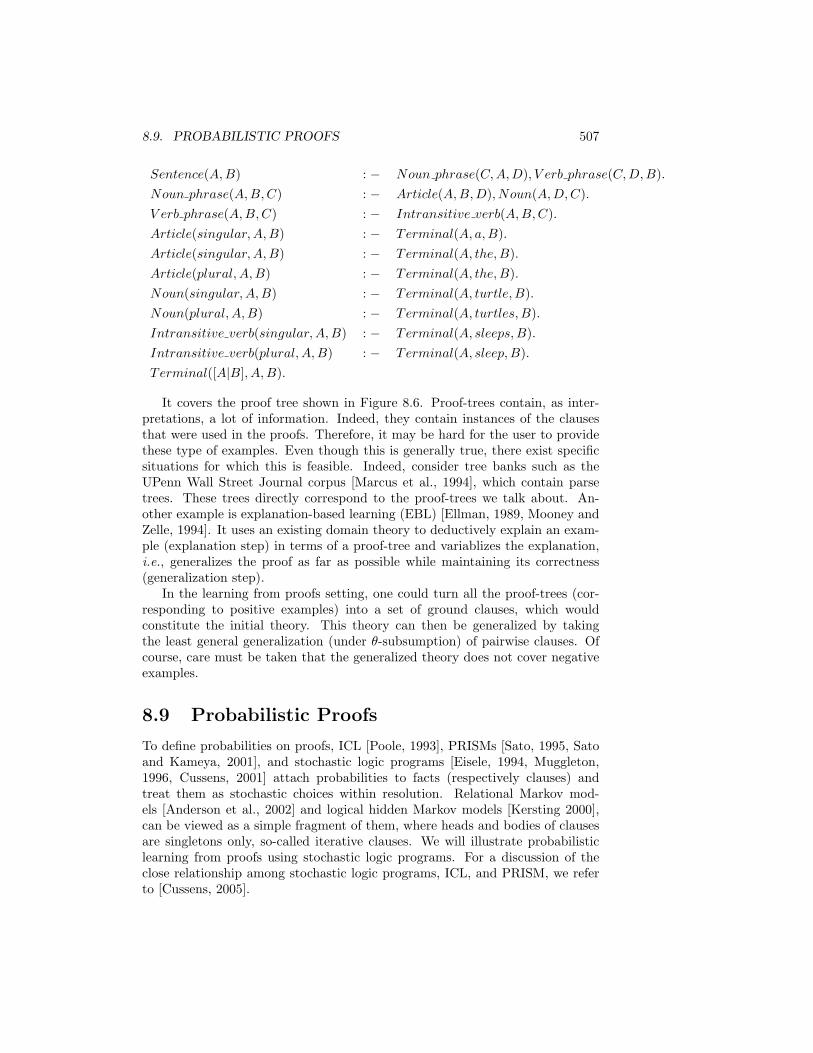
8.9. PROBABILISTIC PROOFS 507
Sentence(A,B) : − Noun phrase(C,A,D), V erb phrase(C,D,B).Noun phrase(A,B,C) : − Article(A,B,D), Noun(A,D,C).V erb phrase(A,B,C) : − Intransitive verb(A,B,C).Article(singular,A,B) : − Terminal(A, a,B).Article(singular,A,B) : − Terminal(A, the,B).Article(plural, A,B) : − Terminal(A, the,B).Noun(singular,A,B) : − Terminal(A, turtle, B).Noun(plural, A,B) : − Terminal(A, turtles,B).Intransitive verb(singular,A,B) : − Terminal(A, sleeps,B).Intransitive verb(plural, A,B) : − Terminal(A, sleep,B).Terminal([A|B], A,B).
It covers the proof tree shown in Figure 8.6. Proof-trees contain, as inter-pretations, a lot of information. Indeed, they contain instances of the clausesthat were used in the proofs. Therefore, it may be hard for the user to providethese type of examples. Even though this is generally true, there exist specificsituations for which this is feasible. Indeed, consider tree banks such as theUPenn Wall Street Journal corpus [Marcus et al., 1994], which contain parsetrees. These trees directly correspond to the proof-trees we talk about. An-other example is explanation-based learning (EBL) [Ellman, 1989, Mooney andZelle, 1994]. It uses an existing domain theory to deductively explain an exam-ple (explanation step) in terms of a proof-tree and variablizes the explanation,i.e., generalizes the proof as far as possible while maintaining its correctness(generalization step).
In the learning from proofs setting, one could turn all the proof-trees (cor-responding to positive examples) into a set of ground clauses, which wouldconstitute the initial theory. This theory can then be generalized by takingthe least general generalization (under θ-subsumption) of pairwise clauses. Ofcourse, care must be taken that the generalized theory does not cover negativeexamples.
8.9 Probabilistic Proofs
To define probabilities on proofs, ICL [Poole, 1993], PRISMs [Sato, 1995, Satoand Kameya, 2001], and stochastic logic programs [Eisele, 1994, Muggleton,1996, Cussens, 2001] attach probabilities to facts (respectively clauses) andtreat them as stochastic choices within resolution. Relational Markov mod-els [Anderson et al., 2002] and logical hidden Markov models [Kersting 2000],can be viewed as a simple fragment of them, where heads and bodies of clausesare singletons only, so-called iterative clauses. We will illustrate probabilisticlearning from proofs using stochastic logic programs. For a discussion of theclose relationship among stochastic logic programs, ICL, and PRISM, we referto [Cussens, 2005].

508 CHAPTER 8. STATISTICAL RELATIONAL LEARNING
Stochastic logic programs are inspired on stochastic context free grammars[Abney, 1997, Manning and Schutze, 1999]. The analogy between context freegrammars and logic programs is that
1. grammar rules correspond to definite clauses,
2. sentences (or strings) correspond to atoms, and
3. productions correspond to derivations.
Furthermore, in stochastic context-free grammars, the rules are annotated withprobability labels in such a way that the sum of the probabilities associated tothe rules defining a non-terminal is 1.0 (see this relation with the closed worldassumption discussed in Section 1.3.7).
Eisele and Muggleton have exploited this analogy to define stochastic logicprograms. These are essentially definite clause programs, where each clause Chas an associated probability label pC such that the sum of the probabilitiesassociated to the rules defining any predicate is 1.0 (though Cussens [1999]considered less restricted versions as well). This framework allows ones to assignprobabilities to proofs for a given predicate q given a stochastic logic programH ∪ B in the following manner. Let Dq denote the set of all possible groundproofs for atoms over the predicate q. For simplicity reasons, it will be assumedthat there is a finite number of such proofs and that all proofs are finite (butagain see [Cussens, 1999] for the more general case). Now associate to eachproof tq ∈ Dq the probability
vt =∏C
pnC,tC
where the product ranges over all clauses C and nC,t denotes the number of timesclause C has been used in the proof tq. For stochastic context free grammars,the values vt correspond to the probabilities of the production.
However, the difference between context free grammars and logic programsis that in grammars two rules of the form n← q, n1, . . . , nm and q ← q1, . . . , qkalways resolve to give n ← q1, . . . , qk, n1, . . . , nm, whereas resolution mayfail due to unification. Therefore, the probability of a proof tree t in Dq, i.e.,a successful derivation is
p(t|H,B) =vt∑
s∈Dq
vt(8.3)
The probability of a ground atom a is then defined as the sum of all the prob-abilities of all the proofs for that ground atom.
p(a|H,B) =s∈Dq∑
s is a proof for a
vs (8.4)

8.9. PROBABILISTIC PROOFS 509
As an example, consider a stochastic variant of the definite clause grammar inthe example on page 507 with uniform probability values for each predicate. Thevalue vu of the proof (tree) u in the example on the page 507 is p(vu) = 1
3 ×12 ×
12 = 1
12 . The only other ground proofs s1, s2 of atoms over the predicte Sentenceare those of Sentence([a, turtle, sleeps], []) and Sentence([the, turtle, sleeps], []).Both get the value p(vs1) = p(vs2) = 1. Because there is only one proof for eachof the sentences,
p(Sentence([the, turtles, sleep], [])) = vu =13
For stochastic logic programs, there are at least two natural learning settings.
1. Motivated by Equation (8.3), we can learn them from proofs. This makesstructure learning for stochastic logic programs relatively easy, becauseproofs carry a lot of information about the structure of the underlyingstochastic logic program. Furthermore, the learning setting can be con-sidered as an extension of the work on learning stochastic grammars fromproof-banks. It should therefore also be applicable to learning unificationbased grammars. We will present a probabilistic ILP approach within thelearning from proofs setting subsequently in this section.
2. On the other hand, we can use Equation (8.4) as covers relation and, hence,employ the learning from entailment setting as mentioned in Section 8.5.3.Here, the examples are ground atoms entailed by the target stochasticlogic program. Learning stochastic logic programs from atoms only ismuch harder than learning them from proofs because atoms carry muchless information than proofs.
8.9.1 Example: Extending GOLEM
Given a training set E containing ground proofs as examples, one possible ap-proach to learning from possible proofs only combines ideas from the early ILPsystem Golem [Muggleton and Feng, 1992] that employs Plotkins [1970] leastgeneral generalization(LGG) with bottom-up generalization of grammars andhidden Markov models [Stolcke and Omohundro, 1993]. The resulting algorithmemploys the likelihood of the proofs score(L, λ, E) as the scoring function. Itstarts by taking as L0 the set of ground clauses that have been used in theproofs in the training set and scores it to obtain λ0. After initialization, thealgorithm will then repeatedly select a pair of clauses in Li, and replace the pairby their LGG (lub) to yield a candidate L′. The candidate that scores best isthen taken as Hi+1 = (Li+1, λi+1), and the process iterates until the score nolonger improves.
One interesting issue is that strong logical constraints can be imposed on theLGG. These logical constraints directly follow from the fact that the exampleproofs should still be valid proofs for the logical component L of all hypothesesconsidered. Therefore, it makes sense to apply the LGG only to clauses that de-fine the same predicate, that contain the same predicates, and whose (reduced)

510 CHAPTER 8. STATISTICAL RELATIONAL LEARNING
LGG also has the same length as the original clauses. In general, the length(number of literals) of the LGG of m (ground) clauses of length at most n isnm, see [Muggleton and Feng, 1992].
As an example, consider the following target stochastic logic program:
1 : S(A,B)← NP (Number,A,C), V P (Number, C,B).12 : NP (Number,A,B)← det(A,C), n(Number, C,B).12 : NP (Number,A,B)← pronom(Number,A,B).12 : V P (Number,A,B)← V (Number,A,B).12 : V P (Number,A,B)← V (Number,A,C), NP (D,C,B).1 : Det(A,B)← Term(A, the,B).14 : N(s,A,B)← Term(A,man,B).14 : N(s,A,B)← Term(A, apple,B).14 : N(pl, A,B)← Term(A,men,B).14 : N(pl, A,B)← Term(A, apples,B).14 : V (s,A,B)← Term(A, eats,B).14 : V (s,A,B)← Term(A, sings,B).14 : V (pl, A,B)← Term(A, eat,B).14 : V (pl, A,B)← Term(A, sing,B).1 : Pronom(pl, A,B)← Term(A, you,B).1 : Term([A|B], A,B).
From this program, (independent) training sets of 50, 100, 200, and 500proofs were generated. For each training set, 4 different random initial sets ofparameters were tried. The learning algorithm was run on each data set start-ing from each of the initial sets of parameters. The algorithm stopped when alimit of 200 iterations was exceeded or a change in log-likelihood between twosuccessive iterations was smaller than 0.0001. In all runs, the original structurewas induced from the proof-trees. Moreover, already 50 proof-trees suffice torediscover the structure of the original stochastic logic program. Further exper-iments with 20 and 10 samples respectively show that even 20 samples suffice tolearn the given structure. Sampling 10 proofs, the original structure is rediscov-ered in one of five experiments. This supports that the learning from proof treessetting carries a lot information. Furthermore, the method scales well. Runson two independently sampled sets of 1000 training proofs yield similar results:the original structure was learned in both cases. More details can be found in[De Raedt et al., 2005].
Other statistical relational learning frameworks that have been developedwithin the learning from proofs setting are relational Markov models [Andersonet al., 2002] and logical hidden Markov models [Kersting 2000?].

8.10. SUMMARY 511
Figure 8.7: The level of information on the target probabilistic program pro-vided by probabilistic ILP settings: shaded parts denote unobserved informa-tion. Learning from entailment provides the least information. Only roots ofproof tree are observed. In contrast, learning from proofs or traces provides themost information. All ground clauses and atoms used in proofs are observed.Learning from interpretations provides an intermediate level of information. Allground atoms but not the clauses are observed.
8.10 Summary
The three learning settings are graphically compared in Figure 8.7.

512 CHAPTER 8. STATISTICAL RELATIONAL LEARNING

References
[CGH97] E. Castillo, J. M. Gutierrez, and A. S. Hadi. Expert systems andprobabilistic network models. Springer-Verlag, 1997.
[CKT91] Peter Cheeseman, Bob Kanefsky, and William M. Taylor. Wherethe Really Hard Problems Are. In Proceedings of the Twelfth In-ternational Joint Conference on Artificial Intelligence, IJCAI-91,Sidney, Australia, pages 331–337, 1991.
[CM97] Stephen A. Cook and David G Mitchell. Finding hard instancesof the satisfiability problem: A survey. In Du, Gu, and Pardalos,editors, Satisfiability Problem: Theory and Applications, volume 35,pages 1–17. American Mathematical Society, 1997.
[Gol79] A. Goldberg. Average case complexity of the satisfiability problem.In Proceedings of the 4th Workshop on Automated Deduction, pages1–6, Austin, Texas, USA, 1979.
[Jen01] F. V. Jensen. Bayesian Networks and Decision Graphs. Springer,2001.
[Jor98] M. I. Jordan. Learning in Graphical Models. MIT Press, 1998.
[Lau96] S. L. Lauritzen. Graphical Models. Clarendon Press, Oxford, 1996.
[NCdW97] Shan Wei Nienhuys-Cheng and Ronald de Wolf. Foundations ofInductive Logic Programming. Springer Verlag, Germany, 1997.
[Pea88] J. Pearl. Probabilistic Reasoning in Intelligent Systems: Networksof Plausible Inference. Morgan Kaufmann, 1988.
[SKC93] Bart Selman, Henry A. Kautz, and Bram Cohen. Local searchstrategies for satisfiability testing. In Michael Trick and David Sti-fler Johnson, editors, Proceedings of the Second DIMACS Challangeon Cliques, Coloring, and Satisfiability, Providence RI, 1993.
[SS90] Glenn Shafer and Prakash P. Shenoy. Probability propagation. Ann.Math. Artif. Intell., 2:327–351, 1990.
513