statistical techniques for data analysis in cosmology -...

Statistical techniquesfor

data analysis in Cosmology

Licia Verde

ICREA & ICC UB-IEEC

http://icc.ub.edu/~liciaverde

arXiv:0712.3028; arXiv:0911.3105 Numerical recipes (the “bible”)

outline• Lecture 1: Introduction Bayes vs

Frequentists, priors, the importance ofbeing Gaussian, modeling and statisticalinference, some useful tools.

• Lecture 2: Monte Carlo methods.Different type of errors. Going beyondparameter fitting.

• Lecture 3: forecasting: Fisher matrixapproach. Introduction to model selection.

Conclusions.

There is a BIG difference between

χ

reduced&2

2χ

Only for multivariate Gaussian with constant covariance

Number of parameters

Example: for multi-variate Gaussian

ln2! L2!=

Errors

From: “Numerical recipes” Ch. 15

If likelihood is Gaussian and Covariance is constant

example Cash 1979

Observation of N clusters is Poisson

……. expected …….

Experimental bin (mass, SZ decrement, X-ray lum, z…)

Define

Between 2 different models is chisquared-distributed!

Unbinned or small bins occupancy 1 or 0 only

Marginalization

example

Other data sets

If independent, multiply the two likelihoods

(can use some of them as “priors”)

Beware of inconsistent experiments!

Spergel 2007

Monte Carlo methods

Monte Carlo methods

a) Monte Carlo error estimation

b) Monte Carlo Markov Chains

Your brain does it!

Spot the differences…

Intro to: Monte Carlo

Simple problem: what’s the mean of a large number of objects?

What’s the mean height of people in PV?

If N is very large this is untractable soo…

If n<<N but still a fair sample, great!

In probability:

In Bayesian inference:

You can show that:

The estimator is unbiased and you can quantify the variance of the estimator:The error shrinks like S1/2

Very simple example:

1

10

4 times the red area

There are better ways to compute π, so use mcmc only when right to use…

Historical note

history

Monte Carlo methodsa) Monte Carlo error estimation

Back to parameter estimation and confidence regions

Conceptual interpretation in cosmology

α true Set of parameters known only to Mother Nature

Statistically realized

Observable universeα

Measurement (with its errors)

Do Measured data You (the experimenter)Can see

want

NOT a unique realization of α true

αoanalysis

There could be infinitely many realizations (hypothetical data sets)

Each one with best fit parameters

Expect:

If I knew the distribution of That’d be all I need

Trick: say that (hope)

In many cases we can simulate the distribution of

Make many synthetic realizations of universes whereis the truth; mimic the observational process in all thesemock universes, estimate the best fit parameters from each;map Very important tool

How to sample from theprobability distribution?

• For some well known univariate probabilitydistributions there are numerical routineshttp://cg.scs.carleton.ca/~luc/rnbookindex.html

• In other cases there may be numerical techniques tosample P(x) [more later]

• Importance sampling: (if you know how to samplefrom Q but not from P)

Some Q are more suitable for P than others….

Monte Carlo Markov ChainsSo you have a higher-dimensional probability distribution, you want to sample in a way proportional to it , with a random walk

Start at an arbitrary point

Burn-inGoal: density of pointsproportional to the probability

MCMC gives approximated, correlated samples from the target distribution

Take Markov steps


http://cosmologist.info/cosmomc/

Using software as black box is ALWAYS a BAD idea

Grid-based approach

What if you have (say) 6 parameters?

You’ve got a problem !

Operationally:m

!

8!

e.g., 2 params: 10 x 10


Explore likelihood surface

6 params, 20 pixels/dim= evals

say 1.6 s/eval

~1200 days!

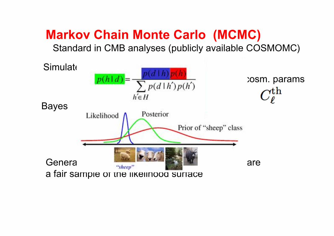
Markov Chain Monte Carlo (MCMC)

Simulate the posterior distribution

Standard in CMB analyses (publicly available COSMOMC)

Bayes

Set of cosm. params

Generate random draws from the posterior that are a fair sample of the likelihood surface

Markov Chain Monte Carlo (MCMC)

Random walk in parameter space

At each step, sample one point in parameter space

The density of sampled points! posterior distribution

marginalization is easy: just project points and recompute their density

FAST: before 7

10 likelihood evaluations, now< 5

10

Adding external data sets is often very easy

Operationally (Metropolis-Hastings):

1. Start at a random location in parameter space:oldi

α L old

2. Try to take a random step in parameter space: newi

α L new

3a. If Lnew! Lold Accept (take and save) the step,

“new”--> “old” and go to 2.

3b. If new< L

oldL Draw a random number x uniform in 0,1

If x ! L new

L old

do not take the step (i.e. save “old”)and go to 2.

< L new

L oldIf x do as in 3a.

KEEP GOING….

“Take a random step”

The probability distribution of the step is the “proposal distribution”, which you should not change once the chain has started.

The proposal distribution (the step-size) is crucial to the MCMC efficiency.

Steps too small step poor mixing

Steps too big step poor acceptance rate

“fair sample of the likelihood surface”, remember?

The importance of stepsize

Step number

Likelihood Poor exploration

Poor exploration

The importance of stepsize

Take a random step

For statisticians: transition operators

Detailed balance: (beware of boundaries….)

When the MCMC has forgotten about the starting locationand has well explored the parameter spaceyou’re ready to do parameter estimation.

Burn-inUSE a MIXING and CONVERGENCE criterion!!!

Recommended: start 4 to 8 chains at well separated pointsM chains, N elements

Vector with parameters valueChain mean

Mean of distrib.

Variance between chains

And within

Always >1 by construction

Require <1.03

Gelmans and Rubin convergence

Unconverged chains are just nonsense

Metropolis-Hastings is NOT the only implementation,

Other options are: Gibbs SamplerRejection methodHamiltonian Monte-CarloSimulated annealing (though you do not get an MCMC)

Beware of DEGENERACIES

Reparameterization.

h

c! 2

hc

!

e.g., Kososwsky et al. 2002

Even “better”:

Cosmomc has the option of computing the covariance for the parametersFind the axis of the multi dim. degeneraciesperform a rotation and re-scaling to obtain azimutally symmetric contours

An improve MCMC efficiency by factor of up to 10

It is still a linear operation

Where’s the prior ?

Once you have the MCMC output:

The density of points in parameter space gives you the posterior distribution

To obtain the marginalized distribution, just project the points

To obtain confidence intervals, - integrate the “likelihood” surface

-compute where e.g. 68.3% of points lie

To add to the analysis another dataset (that does not require extra parameters) renormalize the weight by the “likelihood” of the new data set.

To each point in parameter space sampled by the MCMC give a weightproportional to the number of times it was saved in the chain

No need to re-run!

warning: if new data set is not consistent with the old one--> nonsense

Hamann et al. arXiv:0705.0440

Errors, what errors?

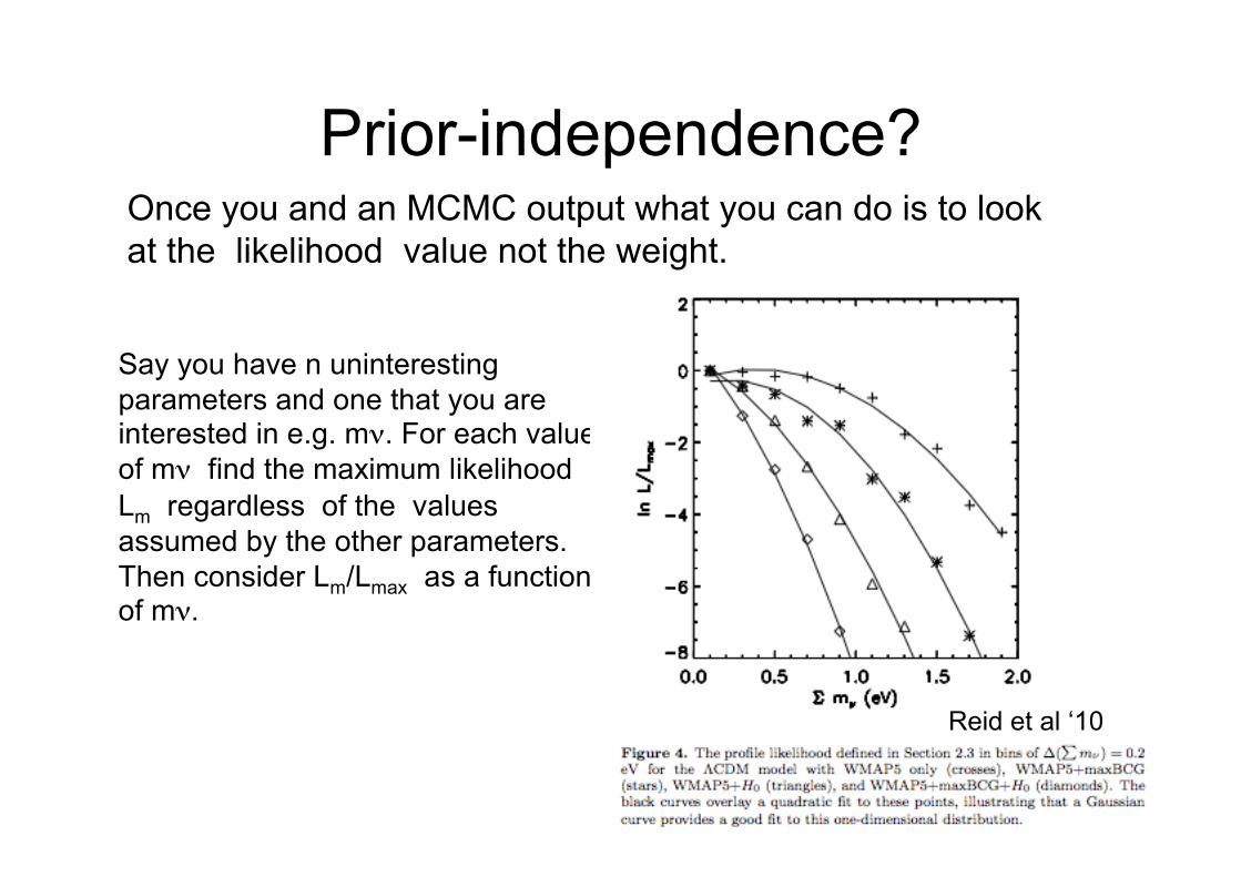
Prior-independence?Once you and an MCMC output what you can do is to look at the likelihood value not the weight.

Say you have n uninterestingparameters and one that you areinterested in e.g. mν. For each valueof mν find the maximum likelihoodLm regardless of the valuesassumed by the other parameters.Then consider Lm/Lmax as a functionof mν.

Reid et al ‘10

http://lambda.gsfc.nasa.govYou can do it yourself!

In particular:http://lambda.gsfc.nasa.gov/product/map/dr4/parameters.cfm

Beyond parameter fitting: model testing

Akaike Information criterion (Akaike 1974; Liddle 04)

k=Number of parameters

Bayesian Information criterion

N=Number of data points

(Schwarz 78, Liddle 04)

Bayesian Evidence

it does not focus on the best-fitting parameters of themodel, but rather asks “of all the parameter values you thought were viable before the data came along, how well on average did they fit the data?”

Computationally expensive! (there are packages to help out there e.g. cosmonest)

Bayes

Bayes, for parameter fitting

Bayes for the MODEL itself

Suggested exercises• Go and download the H(z) data from table 2 of the link from

http://icc.ub.edu/~liciaverde/clocks.html make a plot in the Ωm -ΩΛplanemarginalizing over Ho. You can do that using a grid or using a MCMCapproach.

• Add a prior given by the measurement of Ho of Riess et al.http://arxiv.org/pdf/0905.0695

• Download one of the WMAP chains, plot confidence limits for a fewparameters and for an example of couple of parameters.

• Importance-sample it to add information from e.g. the Ho measurement or theH(z) measurements.

• Or try to compute profile likelihood for one of the parameters and compare theresults with the standard MCMC error.

If you are familiar with numerical integrals you can try he SNeIA sample

e.g., http://supernova.lbl.gov/Union/

If you are a wizard with computers you can try to install cosmomc and run chains.

Key concepts today

Recap: Likelihoods and chisquared

Confidence levels; confidence regions

Monte Carlo methods

Monte-Carlo errors

MCMC

What confidence intervals

Beyond parameter fitting (intro)

For discussion: statistical errors vs. systematic errors

Interesting literature start appearing…

Beyond parameter fittingGoing minimally parametric

Instead of fitting a function to the data, use a basis function(wavelets, principal components etc…)

Other popular options are:

Use bins

Piecewise linear

Working example: the shape of the primordial P(k)

Parameter fitting e.g., : P(k)= A (k/k0)n-1

Spergel et al 07

How do you know you are not “fitting the noise”?

How do you know the model (e.g. power law, running) is OK?

Minimally parametric techniqueBased on smoothing splines

Splines: Piecewise polynomial (usually cubic) fit. Describe P(k) with splines

Smoothing: Suitable for looking for smooth deviations from power laws

Knots: Discrete values of k,ki. P(ki) will be “free” parameters. Do spline for the knots

Sealfon et al (2005); Verde, Peris (2008); Peiris, Verde (2010); Bird et al (2010)

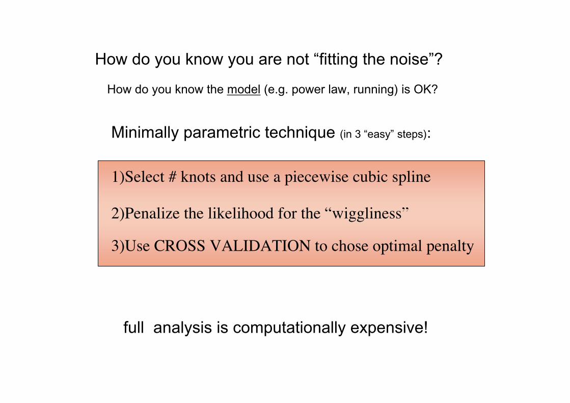
How do you know you are not “fitting the noise”?

How do you know the model (e.g. power law, running) is OK?

Minimally parametric technique (in 3 “easy” steps):

1)Select # knots and use a piecewise cubic spline

3)Use CROSS VALIDATION to chose optimal penalty

2)Penalize the likelihood for the “wiggliness”

full analysis is computationally expensive!

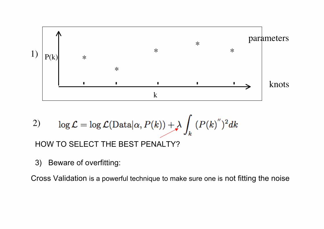
P(k)

k

**

**

*

knots

parameters

1)

2)

Cross Validation is a powerful technique to make sure one is not fitting the noise

3) Beware of overfitting:

HOW TO SELECT THE BEST PENALTY?

linearquadratic Join the dots


Leave one out cross validation:

(example shown for linear model)

(CV score)


In this example:

Leave one out CV is the ideal: does not waste much databut it is very expensive

CV score


The training/test set approach is similar to leave one out CV.

Train on subset of the data

(this may remind you of training sets for photo-z)

Statisticians prefer:

& compare different models

While “leave 1 out” CV would be ideal, it is too computationally intensive; we do 2-fold CV.

Split the data in 2 samples (CV1, CV2)for each penalty value do a MCMC. Compute the likelihood for the best fit model from CV1 and data of CV2 and viceversa. The sum of these two log likelihoods give the CV score. The optimal penalty is the one that minimizes the CV score.

lnk

lnPNon-analyticTransfer function

Peiris, Verde 2010

statistical techniques for data analysis in cosmology -...

Documents