Statistical validation of structured population models for

Daphnia magna

Kaska Adoteyea,b, H.T. Banksa,b, Karissa Crossc, Stephanie Eytchesonc,Kevin B. Floresa,b, Gerald A. LeBlancc, Timothy Nguyenb, Chelsea Rossa,

Emmaline Smithb, Michael Stemkovskic, Sarah Stokelya

aCenter for Research in Scientific ComputationbDepartment of Mathematics

cToxicology Program, Department of Biological SciencesNorth Carolina State University, Raleigh, NC, United States

May 27, 2015

Abstract

In this study we use statistical validation techniques to verify density-dependent mech-anisms hypothesized for populations of Daphnia magna. We develop structured pop-ulation models that exemplify specific mechanisms, and use multi-scale experimentaldata in order to test their importance. We show that fecundity and survival rates areaffected by both time-varying density-independent factors, such as age, and density-dependent factors, such as competition. We perform uncertainty analysis and showthat our parameters are estimated with a high degree of confidence. Further, we per-form a sensitivity analysis to understand how changes in fecundity and survival ratesaffect population size and age-structure.

Key Words: Sensitivity analysis; structured population model; uncertainty quantification;density-dependence; multi-scale data; Daphnia magna

Corresponding author: H.T. Banks (htbanks@ncsu.edu)

1

1 Introduction

Structured population models (SPMs) are well characterized for describing aggregate eco-logical data across a wide variety of species [14, 18]. Numerous studies have emphasized thepractical utility of SPMs in conservation biology [16, 22, 50, 51] and hazard assessments[25, 26, 49, 54] by making predictions of population decline or recovery. Importantly,SPMs have been used to analyze factors influencing the imperilment of endangered speciespopulations [17, 29, 31, 33, 55].

The predictive value of a SPM, or of any mathematical model, relies on the degree offidelity of the model to existing data and in the uncertainty in parameters estimated fromthat data. Several factors involving data information content can affect the uncertaintyin parameters estimated for a structured population model. Beyond the usual issues inoptimizing the measurement frequency, variance, and resolution of the structured variable(age/size), a central problem affecting SPM parameter uncertainty is that aggregate datamay not support the simultaneous estimation of parameters describing multiple biologicalscales. This “individual dynamics/aggregate data” problem [9] arises due to the interrela-tion of individual dynamics and aggregate behavior described by SPMs. For example, themathematical equations describing a fecundity rate in the model might involve a density-independent rate multiplied by a density-dependent rate. Since a lower density-independentrate can be compensated for by a higher density-dependent rate, the multiplication cre-ates a correlation that contributes to a higher level of uncertainty when these rates areconcurrently estimated.

An additional confounding factor in estimating parameters for SPMs is encounteredwhen density-independent demographic rates are time- or age-dependent. For example,the rates describing fecundity and survival are known to vary with age in many species.In addition, these age-dependent rates may also be affected by exposure of the organismto exogenous chemicals or other stressful environmental conditions. Although SPMs canbe readily modified to describe age-dependent demographic parameters, the accurate esti-mation of those parameters can be prohibited by practical limitations, e.g., computationaltractability [3, 56]. Moreover, the individual dynamics/aggregate data problem is exacer-bated because time-dependence is mathematically treated by extending a single parameterto a function described by several parameters.

One approach to redressing the “individual dynamics/aggregate data” problem is tocollect, when feasible, demographic data from organisms grown in isolation. This data isthen used to estimate density-independent parameters comprised in the demographic rates,which are then fixed in the population model. This enables the estimation of the remainingdensity-dependent parameters in the population model from longitudinal aggregate data.An added advantage to this approach is that age-dependent rates can also be estimatedor directly represented by the collected organismal data, removing the rather complexproblem of estimating these rates from aggregate data alone.

Here, we present this approach for estimating density- and age-dependent demographic

2

rates in SPMs for Daphnia magna. This species of water flea has been characterizedby the National Institutes of Health as a model organism for biomedical research [40]. D.magna is also widely used in ecotoxicology to assess the hazard of exogenous chemicals, e.g.,pesticides, on ecosystems [35, 36, 52, 53]. These assessments, however, have mainly focusedon endpoints below the population-level of biological organization, i.e., at the molecular,cellular, or organism levels. SPMs can be used to propagate organismal assessments tothe population-level, thereby enabling the causal association of organismal responses toecosystem adversity.

Among the recent literature, several mathematical models were developed to describethe longitudinal dynamics of daphnid populations. Erickson, et al. [23], formulated aSPM to investigate the impact of stochastic fecundity and survival on the ability of theirmodel to describe data from pesticide treated populations. Importantly, the model fromthis study was calibrated to data that only captured the early population growth phaseof daphnids. Thus, it has not been determined whether a SPM with stochastic demo-graphics can accurately describe the long-term dynamics of daphnid populations, which isqualitatively different from the early growth phase [46]. Preuss, et al. [46], validated anindividual-based model in order to predict the effect of variable algae concentration levelson daphnid population dynamics. Other recent efforts [19, 20, 21, 24] to develop daphnidSPMs have focused on qualitative analysis of the general population dynamics rather thanmodel validation.

Here, we collected both individual and population-level data and developed multi-ple daphnid SPMs in order to test the importance of several biological assumptions.Specifically, we mathematically tested the validity of assuming a time-delay in density-dependent fecundity. We collected daily reproduction data on thirty daphnids to preciselyinvestigate age-dependent fecundity rates for accurate representation in a SPM. We alsovalidated a mathematical description of density-dependent survival and tested whetherdensity-dependent fecundity and survival could be more accurately modeled as a functionof total biomass rather than the total population size. Our investigation of delayed density-dependent fecundity is motivated by previous experimental evidence found in [27, 45]; wenote that this assumption has not been tested in the context of SPMs in recent literatureand with modern daphnid culture methodology. We also collected precise growth rate dataon thirty daphnids (starting at within 2-hours of birth) to calibrate our age-structuredobservations of juvenile and adult daphnids. We employed quantitative model comparisontechniques to assess the validity of our underlying assumptions. Finally, we performedquantitative sensitivity and uncertainty analyses on the SPM with the most accurate bio-logical assumptions among the SPMs we considered.

3

2 Methods

2.1 Population models

Each model we describe in the sections below is a specification of the following structuredpopulation model:

p(t+ 1, 1)p(t+ 1, 2)p(t+ 1, 3)

...p(t+ 1, imax)

=

a(t, 1) a(t, 2) a(t, 3) . . . a(t, imax)b(t, 1) 0 0 . . . 0

0 b(t, 2) 0 . . . 0...

. . . . . ....

0 0 0 . . . b(t, imax − 1)

p(t, 1)p(t, 2)p(t, 3)

...p(t, imax)

. (1)

The population is divided into one-day age classes, ranging from neonates at age i = 1 toa maximum lifespan at age i = imax, where the number of daphnids of age i at a time t isp(t, i). Here, we assume imax = 74 based on our individual level experiments, and based onsimulations of our models fit to experimental data, i.e., the maximum life span observedin the simulations was always less than 74 days. The fecundity of each age class i is givenby a(t, i) and the survival probability is given by b(t, i).

We generated several models to investigate the importance of several density-dependentmechanisms in modeling D. magna populations. Significance of the different mechanismswas assessed by using statistical comparison tests between different models fit to the samestructured population data. We specified the functional forms for a(t, i) and b(t, i) inequation (1) to generate four different structured population models for this assessment,which we refer to as models A through D (Table 1). The four models we consider areorganized by the sequential generalization of the functional forms for fecundity and survival,i.e., models A and D have the least and most number of parameters, respectively.

2.1.1 Delayed density-dependent fecundity

To evaluate the importance of delayed density-dependent fecundity, we generated modelsA and B (Table 1) with parameters θ = (µ, q) to be estimated. In model A, we assumedensity-dependent fecundity for all daphnid age classes. We used a functional form forfecundity that decreases with total population size N(t) [30](see a(t, i) in Table 1a). Thestrength of the density-dependent effect on fecundity is represented by the parameter q;the fecundity is density-independent when q = 0. Model A assumes a density- and age-independent survival probability, i.e., the constant µ. We did not consider age-dependentsurvival here, thus the probability µ is the same for each age class. We will considergeneralizations of µ in future work and note that constant survival probability has beenused previously for structured population modeling of daphnids [27, 45].

Model B generalizes model A by considering a delayed effect of density on fecundity.This generalization is based on previous studies which showed that the number of offspring

4

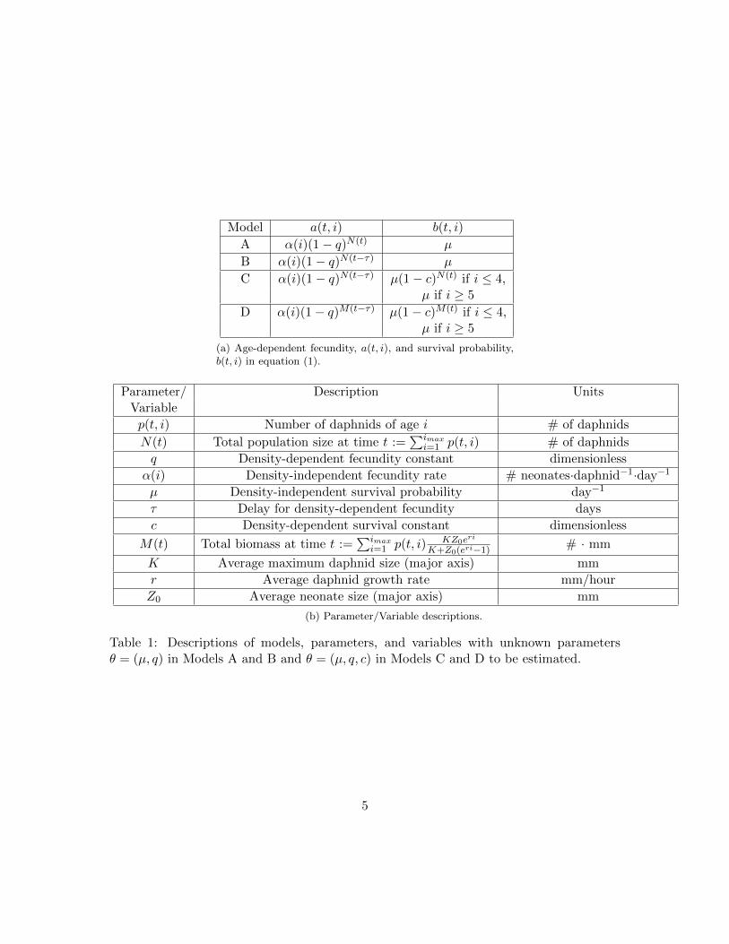
Model a(t, i) b(t, i)

A α(i)(1− q)N(t) µ

B α(i)(1− q)N(t−τ) µ

C α(i)(1− q)N(t−τ) µ(1− c)N(t) if i ≤ 4,µ if i ≥ 5

D α(i)(1− q)M(t−τ) µ(1− c)M(t) if i ≤ 4,µ if i ≥ 5

(a) Age-dependent fecundity, a(t, i), and survival probability,b(t, i) in equation (1).

Parameter/ Description UnitsVariable

p(t, i) Number of daphnids of age i # of daphnids

N(t) Total population size at time t :=∑imax

i=1 p(t, i) # of daphnids

q Density-dependent fecundity constant dimensionless

α(i) Density-independent fecundity rate # neonates·daphnid−1·day−1

µ Density-independent survival probability day−1

τ Delay for density-dependent fecundity days

c Density-dependent survival constant dimensionless

M(t) Total biomass at time t :=∑imax

i=1 p(t, i) KZ0eri

K+Z0(eri−1)# · mm

K Average maximum daphnid size (major axis) mm

r Average daphnid growth rate mm/hour

Z0 Average neonate size (major axis) mm

(b) Parameter/Variable descriptions.

Table 1: Descriptions of models, parameters, and variables with unknown parametersθ = (µ, q) in Models A and B and θ = (µ, q, c) in Models C and D to be estimated.

5

produced by gravid female daphnids in their current cohort was unaffected by increasesin population density. Instead, increased population density had an effect on subsequentcohorts [27, 45]. Since daphnids in their reproductive stage produce neonates approximatelyevery 3 days, we bounded the time-delayed fecundity effect, τ , between 0 and 6 days.

2.1.2 Density- and age-dependent survival

We next evaluated whether density and age were important factors for modeling survival indaphnid populations. To test this, we created model C (with parameters θ = (µ, q, c) to beestimated), which generalizes model B by including a reduced fitness for daphnids classifiedas juveniles in our data, i.e., less than 5 day old daphnids (see Figure 1). This generalizationis based on the observation that larger daphnids consume more algae than smaller daphnids[48]. The restriction of density-dependent survival to juvenile daphnids is in agreementwith previous studies which suggested that the survival of adult daphnids is not affectedby competition [41]. This competitive effect is likely an important consideration for thedaphnids in our population experiments, since our populations were fed a constant amountof algae each day. Indeed, previous modeling studies have suggested that daphnid survivalrates would best be modeled as an age- or size-dependent function rather than as a constant[15, 28, 44, 46].

2.1.3 A density-dependent model with biomass

Lastly, we evaluated whether total biomass could more accurately capture the density-dependence of fecundity and survival than the total number of individuals in our daphnidpopulations. This consideration is in concordance with the generalization in model C,which relies on the observation that larger daphnids contribute more heavily to competi-tion through resource depletion than smaller daphnids [48]. To test our hypothesis aboutbiomass dependency, we generated Model D (again with parameters θ = (µ, q, c) to beestimated) by replacing the total population size, N(t), in model C by total biomass, M(t)(see Table 1). To model total biomass, we calculated a weighted population value using afunction that relates age to size. Specifically, we found that the logistic function accuratelymodels the average size of daphnids as a function of age based on fits to individual levelexperimental data (Figure 2). Consequently, we used the logistic function to weight thedaphnid size in the model for the total biomass M(t) (see Table 1b).

2.2 Laboratory studies

We conducted two studies in the laboratory to generate data for refining and parameterizingour mathematical model. The first study was performed at the individual daphnid level totrack the baseline fecundity and growth rates in isolation, i.e., density-independent rates.The second study was performed at the population-level, in duplicate, for 102 days. Theindividual level data was used to estimate the density-independent parameters used in our

6

0 50 100 150 200 250 3000

0.5

1

1.5

2

2.5

3

3.5

4

Time (Hours)

Maj

or A

xis

Leng

th (m

m)

Figure 1: Calibration of the maximum size for classification of juveniles. We determinedthe maximum juvenile daphnid size by simulating the logistic growth curve with meanparameter values from the nonlinear mixed effects model (Figure 2, Table 2). The poresize of the mesh we used to separate juveniles from adults was 1.62 mm, and this value isplotted as a horizontal line. The vertical line gives the average daphnid age at which theirmajor axis length is equal to the mesh pore size. Based on this calculation, we inferredthat the maximum age at which daphnids can fit through the mesh was 4 days old. Thus,we chose to classify juveniles in our models as ≤ 4 days old.

7

0 20 400

2

4Daphnid 1

0 500

2

4Daphnid 2

0 10 200

2

4Daphnid 3

0 10 200

2

4Daphnid 4

0 20 400

2

4Daphnid 5

0 50 1000

2

4Daphnid 6

0 10 200

5Daphnid 7

Maj

or A

xis

Leng

th (m

m)

0 20 400

2

4Daphnid 8

0 500

5Daphnid 9

0 50 1000

5Daphnid 10

0 10 200

2

4Daphnid 11

0 500

5Daphnid 12

0 50 1000

2

4Daphnid 13

0 10 200

2

4Daphnid 14

0 50 1000

5Daphnid 15

0 20 400

2

4Daphnid 16

0 20 400

2

4Daphnid 17

0 20 400

2

4Daphnid 18

0 500

5Daphnid 19

0 10 200

2

4Daphnid 20

0 20 400

2

4Daphnid 21

0 500

5Daphnid 22

Time (Days)0 10 20

0

2

4Daphnid 23

0 50 1000

5Daphnid 24

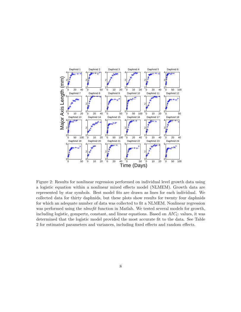
Figure 2: Results for nonlinear regression performed on individual level growth data usinga logistic equation within a nonlinear mixed effects model (NLMEM). Growth data arerepresented by star symbols. Best model fits are drawn as lines for each individual. Wecollected data for thirty daphnids, but these plots show results for twenty four daphnidsfor which an adequate number of data was collected to fit a NLMEM. Nonlinear regressionwas performed using the nlmefit function in Matlab. We tested several models for growth,including logistic, gompertz, constant, and linear equations. Based on AICC values, it wasdetermined that the logistic model provided the most accurate fit to the data. See Table2 for estimated parameters and variances, including fixed effects and random effects.

8

population model. The population data was then used to estimate the remaining density-dependent parameters. Cultured daphnids were maintained using previously describedprotocols and conditions [52]. Cultured daphnids were kept in media reconstituted fromdeionized water [1]. Cultured daphnids for both studies were maintained in an incubatormaintained at 20 degrees Celsius with a 16-h light, 8-h dark cycle. The daphnids used inour study came from a colony that was maintained at North Carolina State University forover 20 years (clone NCSU1 [47]).

2.2.1 Individual study

Thirty daphnids were longitudinally observed to estimate population average rates of fe-cundity and growth. Less than 2-h old neonates were placed individually into 50mL beakerscontaining 40mL of media each. Media was changed daily. Daphnids were fed dailywith 7.0 × 106 cells of algae (Pseudokirchneriella subcapitata) and 0.2 mg (dry weight)TetrafinTM fish food suspension prepared as described previously [42]. The number ofneonates produced by each individual daphnid was recorded and then removed daily. Fe-cundity measurements were performed until no daphnids remained (74 days). The size ofeach individual daphnid was measured with a digital microscope (Celestron, Torrance, CA,USA) at periodic intervals until they died, starting at less than two hours old. The majoraxis was used to determine size, since the maximum possible length was used to classifydaphnids into different size classes, i.e., juveniles and adults (see below).

2.2.2 Population study

A 102-day population study was conducted, in replicate, using D. magna. Two beakerscontaining 1L of media each were both seeded with five 6-day-old female daphnids. Wenote that these daphnids did not reproduce prior to the beginning of the population study.Each 1L beaker was fed twice daily (at approximately 10 a.m. and 3 p.m.) with 1.4× 108

cells of algae (P. subcapitata) and 4 mg dry weight of fish food suspension. The media waschanged and the number of daphnids were counted every Monday, Wednesday, and Fridaythrough the first 40 days of the experiment and once weekly thereafter. During counting,daphnids were separated into two size classes (which we call the juvenile class and adultclass) using a fine mesh net with a 1.62-mm pore size. The total number of daphnids wasthen counted for each size class. Importantly, we note that classification into the juvenile oradult group only defines the size of the daphnid, and does not define whether the daphnidhad reached a reproductive stage.

2.3 Estimation of density-independent rates

We used data from our individual level study to estimate the density-independent fecundityrate, which we call α(i). We parameterized the function α(i) defined at age i by directlyusing the average number of neonates produced per daphnid per day observed in our

9

0 10 20 30 40 50 60 700

2

4

6

8

10

12

14

16

Time (Days)

Num

ber

Of O

ffspr

ing

Figure 3: The number of neonates produced per female daphnid per day. Data were col-lected from thirty female daphnid whose birth was known to within two hours of accuracy.Daily data are represented by star symbols and connecting lines are drawn to show generaltrends. This data was used to parameterize the age-dependent function α(i) (see Table 1).

individual level study (Figure 3). We note that we attempted to approximate α(i) usingalternative formulations, e.g., periodic or piece wise constant functions estimated from thedensity-independent fecundity data. However, we found that using the data directly forα(i) resulted in the most accurate fits of the resulting population models to populationdata.

We used the individual level growth (size) data to estimate the relationship betweenage and size. We considered several functional forms for f(i), the average size of a femaledaphnid at age i, within a nonlinear mixed effects model framework and found that thelogistic equation f(i) = KZ0eri

K+Z0(eri−1)most accurately fit the data for individual daphnid

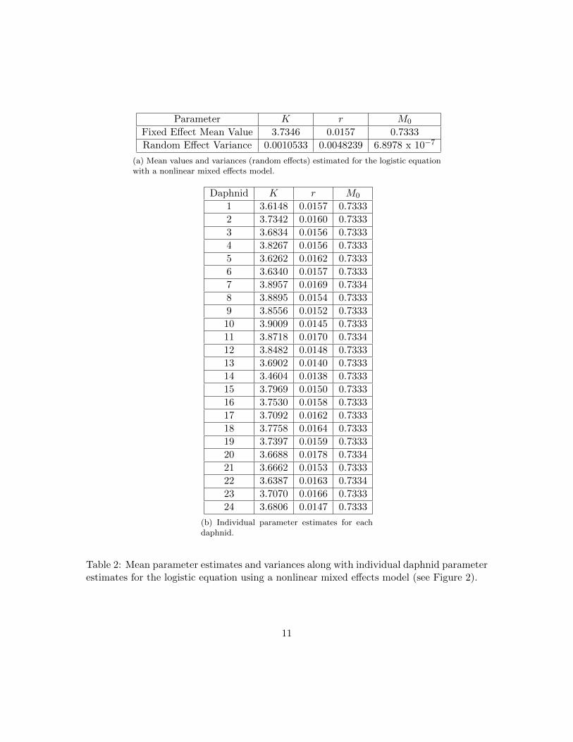
growth (Figure 2, Table 2). Based on the mean parameter values estimated with thenonlinear mixed effects model, we inferred that the daphnids classified as juveniles in ourpopulation experiments were less than or equal to 4 days old, and that adults were greaterthan 5 days old (Figure 1). The function f(i) was also used to replace total population sizewith a model for total population biomass in one of the population models we describedabove. We note that we determined that the average size f(i) was sufficient to replace thetotal population size, as opposed to using the full distribution of sizes obtained from thenonlinear mixed effects model, since the range of individual parameter values in Table 2was deemed to be too slim to merit more than a delta distribution approximation. Thatis, since the obtained distributions around K, r, and M0 were so slim, we determinedthat using a distribution around K, r, and M0 in the population model would not give anadequate improvement over using the averages of K, r and M0 in f(i).

10

Parameter K r M0

Fixed Effect Mean Value 3.7346 0.0157 0.7333

Random Effect Variance 0.0010533 0.0048239 6.8978 x 10−7

(a) Mean values and variances (random effects) estimated for the logistic equationwith a nonlinear mixed effects model.

Daphnid K r M0

1 3.6148 0.0157 0.7333

2 3.7342 0.0160 0.7333

3 3.6834 0.0156 0.7333

4 3.8267 0.0156 0.7333

5 3.6262 0.0162 0.7333

6 3.6340 0.0157 0.7333

7 3.8957 0.0169 0.7334

8 3.8895 0.0154 0.7333

9 3.8556 0.0152 0.7333

10 3.9009 0.0145 0.7333

11 3.8718 0.0170 0.7334

12 3.8482 0.0148 0.7333

13 3.6902 0.0140 0.7333

14 3.4604 0.0138 0.7333

15 3.7969 0.0150 0.7333

16 3.7530 0.0158 0.7333

17 3.7092 0.0162 0.7333

18 3.7758 0.0164 0.7333

19 3.7397 0.0159 0.7333

20 3.6688 0.0178 0.7334

21 3.6662 0.0153 0.7333

22 3.6387 0.0163 0.7334

23 3.7070 0.0166 0.7333

24 3.6806 0.0147 0.7333

(b) Individual parameter estimates for eachdaphnid.

Table 2: Mean parameter estimates and variances along with individual daphnid parameterestimates for the logistic equation using a nonlinear mixed effects model (see Figure 2).

11

2.4 Parameter Estimation

Parameters were estimated from the population data using a vector ordinary least squares(OLS) framework [9, 11]. For each model, we consider a vector of parameters θ to estimate.Based on our individual level modeling, the number of juveniles and adults are given byJ(t, θ) =

∑4i=1 p(t, i) and A(t, θ) =

∑imax5 p(t, i), respectively. The corresponding observa-

tion vector is given by f(t, θ) = [J(t, θ), A(t, θ)]T . We assumed a constant statistical errormodel of the form

Yj = f(tj , θ0) + Ej , j = 1, 2, ..., n,

where Yj is a random variable with realizations yj (i.e., the data) and f(tj , θ0) is themodel observation with the hypothesized “true” parameter vector θ0. The error terms Ejare assumed independent and identically distributed (i.i.d) random variables with meanE[Ej ] = 0 and V0 =var(Ej)=diag(σ21,0, σ

22,0). An estimate, θ, for the true parameter vector

θ0 is obtained by implementing an iterative algorithm (see [9] for details).The inverse problems were computed using two routines in Matlab. The first routine

is a direct search algorithm implemented by Daniel Finkel as direct, which can be found athttp://www4.ncsu.edu/~ctk/Finkel_Direct/. This was used with the following options:options.maxevals = 400; options.maxits = 400; options.maxdeep = 400;, and the outputwas used as the initial condition for the gradient based Matlab search routine lsqnonlin.The routine lsqnonlin was run with the options ’TolFun’ and ’TolX’ set equal to 1e-20, andthe option ’MaxFunEvals’ set equal to 400. The output of lsqnonlin was then used as ourparameter estimate θ.

2.5 Model Comparisons

2.5.1 Model Hypothesis Testing

We used a statistical model comparison test [7, 11] to evaluate the significance in consideringvarious components, e.g., delayed density-dependence, for models A through C. Briefly, thismethodology evaluates the significance of a χ2 statistic generated by the residual sum ofsquares to test the null hypothesis, H0, that a certain parameter or set of parameters isnot needed to describe the system. We note that this method requires nested models. Forexample, model A is “nested” in model B because model B reduces to model A when τ = 0.If we can reject the null hypothesis H0 then we conclude that the parameters in questioncannot be taken equal to zero and infer that they are needed to accurately describe thedata . For further details and previous applied examples of this methodology see [7, 32, 11].

2.5.2 Akaike Information Criteria

The Akaike Information Criterion (AIC) score gives an approximately unbiased form ofthe Kullback-Leibler Distance, or a measure of the distance between a model and thecorresponding data [9]. The AIC score is used to compare the accuracy of different models

12

to the same data set; a lower AIC score indicates higher accuracy. We note that the AICscore is applicable to more model comparisons than the χ2 based test described above,since it does not require the compared models to be nested.

The AIC score for independent multivariate normally distributed observations in thecase of nonlinear models is given by AIC = nνln(RSSnν ) + nν(1 + ln(2π)) + 2(p+ 1), whereRSS is the residual sum of squares [9, 13]. The AIC score corrected for small sample size(n/p < 40, n = number of data points, p = number of parameters) in the case of multi-

variate observations (ν = number of observables) is given by AICC = AIC + 2 p(ν+p+1)n−(ν+p+1) ,

where p is the total number of unknown parameters estimated in the mathematical andstatistical models. Here, we take p = p, since we do not estimate directly the variancesσ21,0 and σ22,0 in addition to the p parameters for the mathematical model. We note thatalthough this AICC formula was derived for multivariate linear regression models [12], theauthors claimed that this formula can be generalized to multivariate nonlinear regressionmodels. We tacitly assume this can be done and hence use the above formulae for ourAICC analysis here.

2.6 Parameter Uncertainty Quantification

We calculated standard errors and 95% confidence intervals for the estimated parametersθ using asymptotic theory, and used bootstrapping for verification. We provide a briefdescription of the application of these two methods here, but for more details see [9, 11].

2.6.1 Asymptotic Theory

The observation variance V0 in the vector OLS framework using a constant statistical errormodel is, given estimates θ, approximated by

V0 ≈ V = diag

1

n− p

n∑j=1

[yj − f(tj , θ)][yj − f(tj , θ)]T

.

The resulting approximation of the covariance matrix is given by

Σn =

n∑j=1

DTj (θ)V −1Dj(θ)

−1

,

where the 2 x p matrix Dj(θ) is given by

Dj(θ) =

∂J(tj ,θ)∂θ1

...∂J(tj ,θ)∂θp

∂A(tj ,θ)∂θ1

...∂A(tj ,θ)∂θp

,

13

where p = 2 in Models A and B and p = 3 in Models C and D. Then asymptotic theory[9, 11] yields that the OLS estimator has a limiting distribution given approximately by aN (θ, Σn) distribution.

We calculated standard errors and 95% confidence intervals [9, 11] in order to quantifythe uncertainty in estimating each element of the parameter estimate θ for our best modelwith vector observation f(t, θ). The standard error and 95% confidence interval of the

kth parameter θk are given by SE(θk) =√

Σnkk and [θk − 1.96SE(θk), θk + 1.96SE(θk)],

respectively [11].

2.6.2 Bootstrapping

Bootstrapping is implemented for an estimated parameter vector θ by first calculatingstandardized residuals

rij =

√n

n− p

(yij − fi(tj , θ)

), j = 1, ..., n,

where n is the number of data points, p is the number of parameters, i = J or A representseither the juvenile or adult observation. Here, fJ(tj , θ) = J(tj , θ) and fA(tj , θ) = A(tj , θ).Bootstrap sample points are created by sampling the standardized residuals for each ob-servation (J or A) and adding them to the respective model solutions, either J(tj , θ) or

A(tj , θ). We created M = 1000 simulated bootstrap data sets in this fashion and thenconducted M inverse problems to fit the model to each of these simulated data sets. Forthe mth simulated bootstrap data set, we then find the corresponding parameter estimateθm. The mean, variance, and standard errors for θ are approximated by the followingformulas [9]:

θBOOT =1

M

M∑m=1

θm,

V ar(θBOOT ) =1

M − 1

M∑m=1

(θm − θBOOT )(θm − θBOOT )T ,

SEk(θBOOT ) =

√V ar(θBOOT )kk.

The 95 % confidence interval for each θk is calculated as the range between the 25-thand 975-th entries in the ordered set of M parameter estimates from bootstrapping.

14

0 1 2 3 4 5 60.6

0.8

1

1.2

1.4

1.6

1.8

2

2.2x 106

Fecundity Delay

OLS

Cos

t

Optimal Time Delay

Replicate 1

Replicate 2

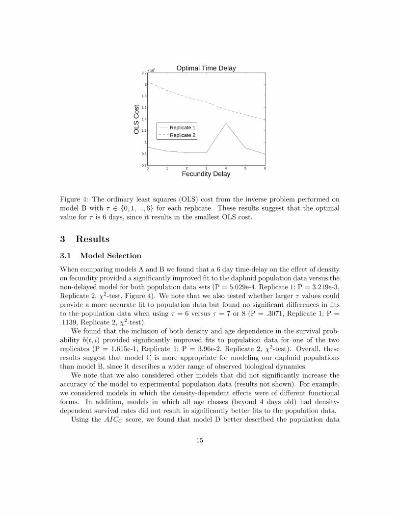
Figure 4: The ordinary least squares (OLS) cost from the inverse problem performed onmodel B with τ ∈ {0, 1, ..., 6} for each replicate. These results suggest that the optimalvalue for τ is 6 days, since it results in the smallest OLS cost.

3 Results

3.1 Model Selection

When comparing models A and B we found that a 6 day time-delay on the effect of densityon fecundity provided a significantly improved fit to the daphnid population data versus thenon-delayed model for both population data sets (P = 5.029e-4, Replicate 1; P = 3.219e-3,Replicate 2, χ2-test, Figure 4). We note that we also tested whether larger τ values couldprovide a more accurate fit to population data but found no significant differences in fitsto the population data when using τ = 6 versus τ = 7 or 8 (P = .3071, Replicate 1; P =.1139, Replicate 2, χ2-test).

We found that the inclusion of both density and age dependence in the survival prob-ability b(t, i) provided significantly improved fits to population data for one of the tworeplicates (P = 1.615e-1, Replicate 1; P = 3.96e-2, Replicate 2, χ2-test). Overall, theseresults suggest that model C is more appropriate for modeling our daphnid populationsthan model B, since it describes a wider range of observed biological dynamics.

We note that we also considered other models that did not significantly increase theaccuracy of the model to experimental population data (results not shown). For example,we considered models in which the density-dependent effects were of different functionalforms. In addition, models in which all age classes (beyond 4 days old) had density-dependent survival rates did not result in significantly better fits to the population data.

Using the AICC score, we found that model D better described the population data

15

from both replicates than model C. For replicate 1, the AICC for models C and D were656.47 and 635.32, respectively. For replicate 2, the AICC for models C and D were 690.18and 663.24, respectively. The evidence ratio, based on the calculation of Akaike weights[13, p. 74-79], for model D versus model C was 3.918 × 103 for the replicate 1 data set.The evidence ratio for model D versus model C was 7.082 × 104 for the replicate 2 dataset. These results highly suggest that model D is better than model C at representing thepopulation data from both replicates. Hence, dependence of birth and death demographicson population density is most likely a function of a total biomass rather than the absolutenumber of daphnids counted regardless of size or age. See Figures 5 and 6 for fits ofmodel D to the population data. Moreover, the parameter estimates for both replicateswere strikingly similar, indicating that our validation of model D is repeatable despite thepossibility of biological variability between population experiments.

16

0 10 20 30 40 50 60 70 80 90 1000

200

400

600

800

1000

1200

1400

1600

1800

Time (days)

Num

ber

of ju

veni

les

Replicate 1

68 % Confidence Band

Model Simulation

Data

0 10 20 30 40 50 60 70 80 90 1000

200

400

600

800

1000

1200

1400

1600

1800

Time (days)

Num

ber

of ju

veni

les

Replicate 2

68 % Confidence Band

Model Simulation

Data

0 10 20 30 40 50 60 70 80 90 1000

200

400

600

800

1000

1200

1400

1600

1800

Time (days)

Num

ber

of a

dults

Replicate 1

68 % Confidence Band

Model Simulation

Data

0 10 20 30 40 50 60 70 80 90 1000

200

400

600

800

1000

1200

1400

1600

1800

Time (days)

Num

ber

of a

dults

Replicate 2

68 % Confidence Band

Model Simulation

Data

0 10 20 30 40 50 60 70 80 90 1000

200

400

600

800

1000

1200

1400

1600

1800

Time (days)

Tot

al N

umbe

r of

Dap

hnia

Replicate 1

68 % Confidence Band

Model Simulation

Data

0 10 20 30 40 50 60 70 80 90 1000

200

400

600

800

1000

1200

1400

1600

1800

Time (days)

Tot

al N

umbe

r of

Dap

hnia

Replicate 2

68 % Confidence Band

Model Simulation

Data

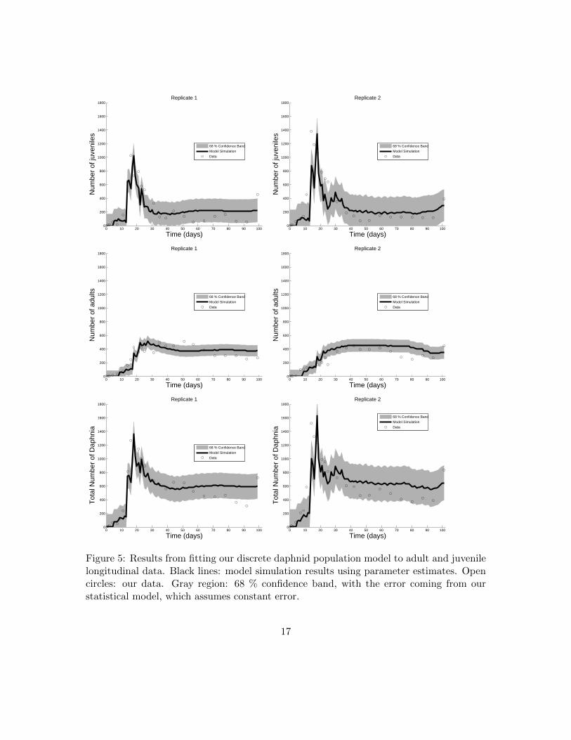
Figure 5: Results from fitting our discrete daphnid population model to adult and juvenilelongitudinal data. Black lines: model simulation results using parameter estimates. Opencircles: our data. Gray region: 68 % confidence band, with the error coming from ourstatistical model, which assumes constant error.

17

0 10 20 30 40 50 60 70 80 90 1000

200

400

600

800

1000

1200

1400

1600

1800

Time (days)

Num

ber

of ju

veni

les

Replicate 1

95 % Confidence Band

Model Simulation

Data

0 10 20 30 40 50 60 70 80 90 1000

200

400

600

800

1000

1200

1400

1600

1800

Time (days)

Num

ber

of ju

veni

les

Replicate 2

95 % Confidence Band

Model Simulation

Data

0 10 20 30 40 50 60 70 80 90 1000

200

400

600

800

1000

1200

1400

1600

1800

Time (days)

Num

ber

of a

dults

Replicate 1

95 % Confidence Band

Model Simulation

Data

0 10 20 30 40 50 60 70 80 90 1000

200

400

600

800

1000

1200

1400

1600

1800

Time (days)

Num

ber

of a

dults

Replicate 2

95 % Confidence Band

Model Simulation

Data

0 10 20 30 40 50 60 70 80 90 1000

200

400

600

800

1000

1200

1400

1600

1800

Time (days)

Tot

al N

umbe

r of

Dap

hnia

Replicate 1

95 % Confidence Band

Model Simulation

Data

0 10 20 30 40 50 60 70 80 90 1000

200

400

600

800

1000

1200

1400

1600

1800

Time (days)

Tot

al N

umbe

r of

Dap

hnia

Replicate 2

95 % Confidence Band

Model Simulation

Data

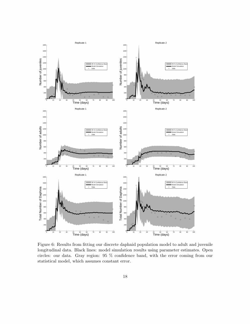
Figure 6: Results from fitting our discrete daphnid population model to adult and juvenilelongitudinal data. Black lines: model simulation results using parameter estimates. Opencircles: our data. Gray region: 95 % confidence band, with the error coming from ourstatistical model, which assumes constant error.

18

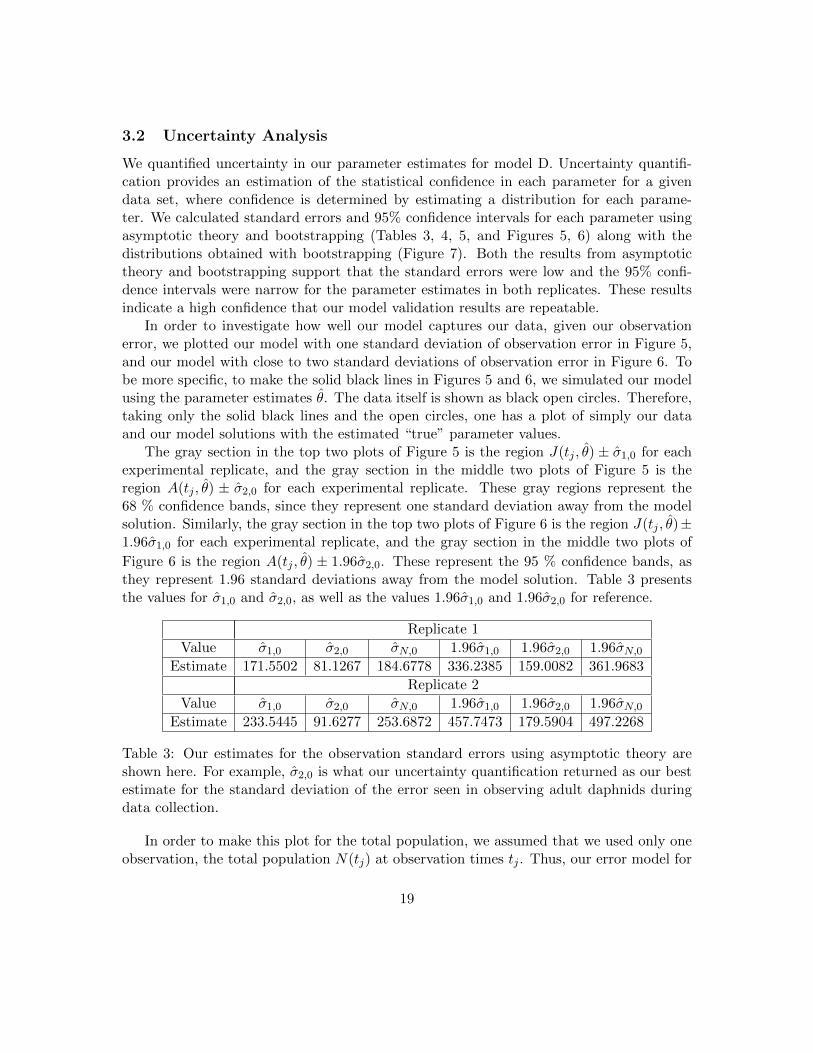
3.2 Uncertainty Analysis

We quantified uncertainty in our parameter estimates for model D. Uncertainty quantifi-cation provides an estimation of the statistical confidence in each parameter for a givendata set, where confidence is determined by estimating a distribution for each parame-ter. We calculated standard errors and 95% confidence intervals for each parameter usingasymptotic theory and bootstrapping (Tables 3, 4, 5, and Figures 5, 6) along with thedistributions obtained with bootstrapping (Figure 7). Both the results from asymptotictheory and bootstrapping support that the standard errors were low and the 95% confi-dence intervals were narrow for the parameter estimates in both replicates. These resultsindicate a high confidence that our model validation results are repeatable.

In order to investigate how well our model captures our data, given our observationerror, we plotted our model with one standard deviation of observation error in Figure 5,and our model with close to two standard deviations of observation error in Figure 6. Tobe more specific, to make the solid black lines in Figures 5 and 6, we simulated our modelusing the parameter estimates θ. The data itself is shown as black open circles. Therefore,taking only the solid black lines and the open circles, one has a plot of simply our dataand our model solutions with the estimated “true” parameter values.

The gray section in the top two plots of Figure 5 is the region J(tj , θ) ± σ1,0 for eachexperimental replicate, and the gray section in the middle two plots of Figure 5 is theregion A(tj , θ) ± σ2,0 for each experimental replicate. These gray regions represent the68 % confidence bands, since they represent one standard deviation away from the modelsolution. Similarly, the gray section in the top two plots of Figure 6 is the region J(tj , θ)±1.96σ1,0 for each experimental replicate, and the gray section in the middle two plots of

Figure 6 is the region A(tj , θ) ± 1.96σ2,0. These represent the 95 % confidence bands, asthey represent 1.96 standard deviations away from the model solution. Table 3 presentsthe values for σ1,0 and σ2,0, as well as the values 1.96σ1,0 and 1.96σ2,0 for reference.

Replicate 1

Value σ1,0 σ2,0 σN,0 1.96σ1,0 1.96σ2,0 1.96σN,0Estimate 171.5502 81.1267 184.6778 336.2385 159.0082 361.9683

Replicate 2

Value σ1,0 σ2,0 σN,0 1.96σ1,0 1.96σ2,0 1.96σN,0Estimate 233.5445 91.6277 253.6872 457.7473 179.5904 497.2268

Table 3: Our estimates for the observation standard errors using asymptotic theory areshown here. For example, σ2,0 is what our uncertainty quantification returned as our bestestimate for the standard deviation of the error seen in observing adult daphnids duringdata collection.

In order to make this plot for the total population, we assumed that we used only oneobservation, the total population N(tj) at observation times tj . Thus, our error model for

19

Daphnid Classification Replicate % Accuracy Fraction

Juvenile 1 80 % 20/25

Adult 1 68 % 17/25

Total 1 84 % 21/25

Juvenile 2 84 % 21/25

Adult 2 84 % 21/25

Total 2 92 % 23/25

Table 4: The percentage (% accuracy) and fraction of observed data points that werecontained in the 68 % confidence bands of our model solution. Results are shown for thenumber of juveniles, number of adults, and total population size for each replicate

Replicate Parameter Estimate Standard Error 95 % C.I.

1 µ 9.5051×10−1 1.0428×10−2 (9.2889×10−1,9.7214×10−1)

1 q 1.7206×10−3 1.5426×10−4 (1.4007×10−3,2.0405×10−3)

1 c 1.5153×10−4 2.9689×10−5 (8.9972×10−5,2.1310×10−4)

2 µ 9.8559×10−1 8.1785×10−3 (9.6863×10−1,1.0025)

2 q 1.3542×10−3 1.7762×10−4 (9.8590×10−4,1.7225×10−3)

2 c 2.8005×10−4 4.1701×10−5 (1.9358×10−4,3.6652×10−4)

(a) Parameter estimates, asymptotic standard errors, and asymptotic 95% confidence intervals (C.I.) formodel D.

Replicate Parameter Estimate Standard Error 95 % C.I.

1 µ 9.5051×10−1 8.7505×10−3 (8.8922×10−1,9.2551×10−1)

1 q 1.7206×10−3 2.3202×10−4 (2.0358×10−3,2.9980×10−3)

1 c 1.5153×10−4 2.3608×10−5 (-4.8952×10−5,4.8953×10−5)

2 µ 9.8559×10−1 2.3660×10−2 (9.3715×10−1,1.0355)

2 q 1.3542×10−3 3.2867×10−4 (6.8486×10−4,2.0517×10−3)

2 c 2.8005×10−4 9.7547×10−5 (8.3218×10−5,4.8888×10−4)

(b) Parameter estimates, bootstrap standard errors, and bootstrap 95% confidence intervals (C.I.) for modelD.

Table 5: Results from uncertainty quantification with asymptotic theory and bootstrappingfor model D.

20

the total population is now specified as

Yj = f(tj , θ0) + Ej , j = 1, 2, . . . , n

where Yj is a random variable with realizations yj = N(tj) (i.e., the data), f(tj , θ0) =N(tj , θ0) = J(tj , θ0) +A(tj , θ0) is the discrete model solution with the hypothesized “true”parameter vector θ0, where N(t, θ0) is the total number of daphnids given by our modelat time t. The error terms Ej are assumed to be i.i.d random variables with mean zeroand variance V0 = σ2N,0. From our uncertainty quantification we have an estimate for our

observation error V0 = σ2N,0.

Therefore, the gray section in the bottom two plots of Figure 5 is the region N(tj , θ)±σN,0 for each experimental replicate. These gray regions represent the 68 % confidencebands, since they represent one standard deviation away from our model solution. Thegray section in the bottom two plots of Figure 6 is the region N(tj , θ)± 1.96σN,0 for eachexperimental replicate. These gray regions represent the 95 % confidence bands, since theyrepresent 1.96 standard deviations away from the model solution. Table 3 also gives thevalues for σN,0 and 1.96σN,0 for reference while Table 4 contains the obtained accuracy ofour modeling effort using the 68 % confidence bands.

21

0 1 2 3

x 10−4

0

200

400

600

800

c

Fre

quen

cy

Replicate 1

1 2 3

x 10−3

0

20

40

60

80

100

120

q

Replicate 1

0.85 0.9 0.95 10

50

100

150

200

µ

Replicate 1

0 2 4 6

x 10−4

0

50

100

150

c

Fre

quen

cy

Replicate 2

0 1 2 3

x 10−3

0

50

100

150

q

Replicate 2

0.85 0.9 0.95 10

100

200

300

400

500

µ

Replicate 2

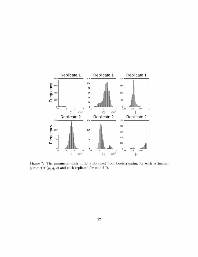
Figure 7: The parameter distributions obtained from bootstrapping for each estimatedparameter (µ, q, c) and each replicate for model D.

22

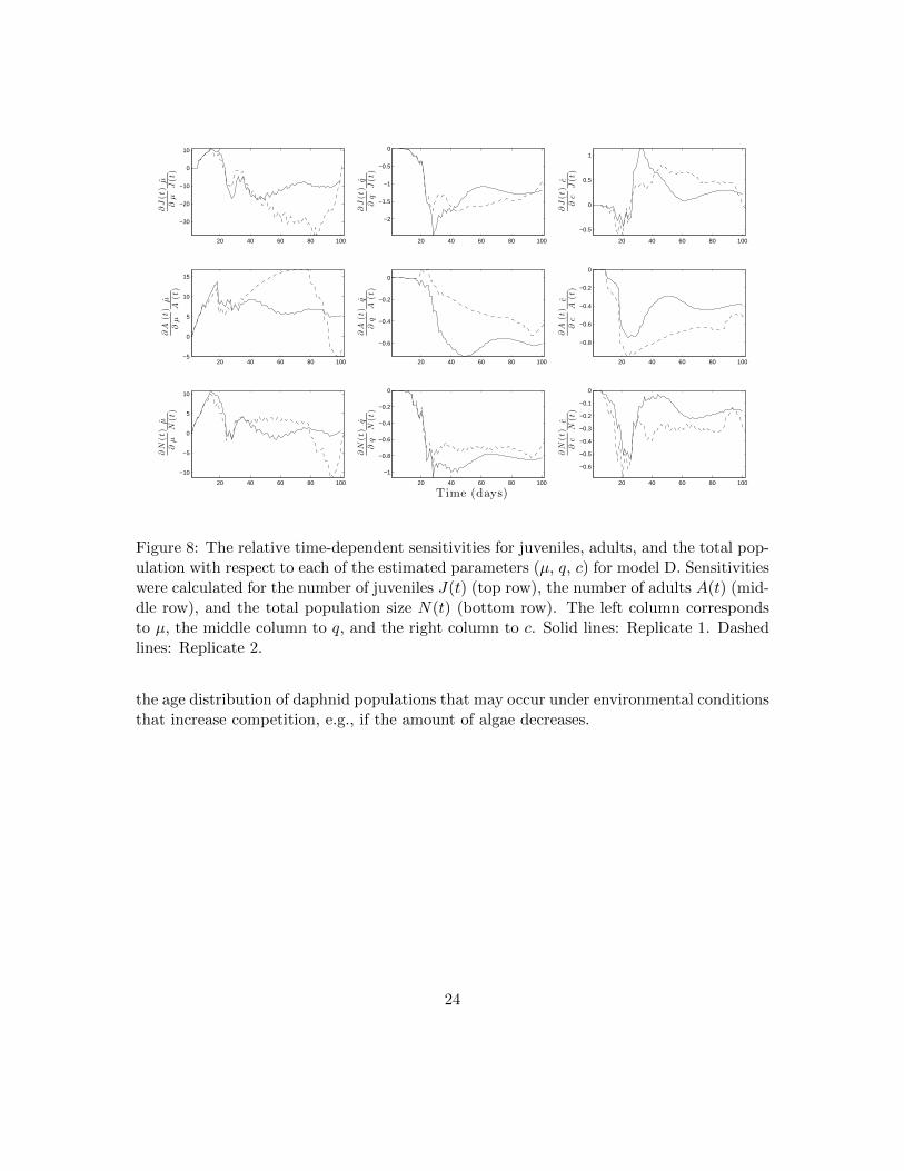
3.3 Parameter Sensitivities

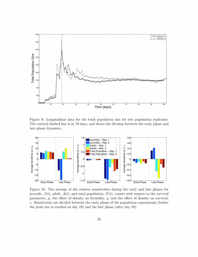
We applied a sensitivity analysis to our best validated model (model D) to understand howchanges in estimated parameters governing fecundity and survival affect population sizeand structure. We calculated the relative time-dependent sensitivity functions for juvenile,adult, and total population size (Figure 8). Interestingly, we observed that the maximumtotal population size for our two replicates was achieved on day 19, dividing the populationdynamics into two phases, which we call the “early phase” and the “late phase” (Figure 9).In the early phase (≤ 19 days) of the population experiments, the population grows rapidlyand exceeds its carrying capacity. In the late phase of the population experiments (> 19days), the total population size converges towards steady state levels as an excess juvenilepopulation rapidly dies off or progresses to the adult stage. Dividing our sensitivity analysisbetween these two phases revealed that the effect of increasing fecundity or survival is bothtemporally and life-stage dependent (Figure 10).

We found that the juvenile, adult, and total population sizes were most sensitive tochanges in µ in both the early and late phase as compared to the other estimated param-eters q and c. The sensitivity analysis indicates that increasing the survival parameter µwill increase the juvenile population in the early phase and decrease it in the late phase,whereas an increased µ increases the adult population size in both the early and late phase.Although increased survival increases the total population size in the early phase, the latephase is much less sensitive. These findings suggest that increases in the survival parameterµ will cause a shift in the population distribution towards the adult stage and that thisshift mainly occurs during the early phase of population growth.

Our sensitivity analysis indicates that increasing q, the effect of density on fecundity,has a greater effect in the late phase of the population experiment than in the early phasefor the juvenile, adult, and total population size. This result is expected, since a lowerfecundity rate should lead to lower population sizes overall and within specific life stages.We hypothesize that the late phase is more heavily influenced by a decreased density-dependent fecundity rate than the early phase because of the time delayed effect. If so,this would imply that most of the offspring in the early phase are produced by femaledaphnids whose fecundity has not yet been effected by density.

Lastly, our sensitivity analysis indicates that increasing c, the effect of density on thesurvival of juveniles, leads to lower numbers of juveniles and adults, and a lower totalpopulation size in the early phase. This relationship is more pronounced in the late phasefor both the number of adults and total population size. Unexpectedly, our sensitivityanalysis indicates that increasing the parameter c can cause the number of juveniles toincrease during the late phase of the population experiments.

Taken together, these findings suggest that a higher density-dependent juvenile survivalprobability can cause a shift towards juveniles in the equilibrium age distribution of daphnidpopulations, even though the total population size decreases overall. Our results highlightthe importance of mathematical modeling to understand non-intuitive temporal shifts in

23

20 40 60 80 100

−30

−20

−10

0

10

∂J(t)

∂µ

µ

J(t)

20 40 60 80 100

−2

−1.5

−1

−0.5

0

∂J(t)

∂q

qJ(t)

20 40 60 80 100

−0.5

0

0.5

1

∂J(t)

∂c

cJ(t)

20 40 60 80 100−5

0

5

10

15

∂A

(t)

∂µ

µ

A(t)

20 40 60 80 100

−0.6

−0.4

−0.2

0

∂A

(t)

∂q

qA

(t)

20 40 60 80 100

−0.8

−0.6

−0.4

−0.2

0

∂A

(t)

∂c

cA

(t)

20 40 60 80 100

−10

−5

0

5

10

∂N

(t)

∂µ

µ

N(t)

20 40 60 80 100

−1

−0.8

−0.6

−0.4

−0.2

0

Time (days)

∂N

(t)

∂q

qN

(t)

20 40 60 80 100

−0.6

−0.5

−0.4

−0.3

−0.2

−0.1

0

∂N

(t)

∂c

cN

(t)

Figure 8: The relative time-dependent sensitivities for juveniles, adults, and the total pop-ulation with respect to each of the estimated parameters (µ, q, c) for model D. Sensitivitieswere calculated for the number of juveniles J(t) (top row), the number of adults A(t) (mid-dle row), and the total population size N(t) (bottom row). The left column correspondsto µ, the middle column to q, and the right column to c. Solid lines: Replicate 1. Dashedlines: Replicate 2.

the age distribution of daphnid populations that may occur under environmental conditionsthat increase competition, e.g., if the amount of algae decreases.

24

10 20 30 40 50 60 70 80 90 1000

200

400

600

800

1000

1200

1400

1600

1800

Time (days)

Tot

al P

opul

atio

n S

ize

Replicate 1Replicate 2

Figure 9: Longitudinal data for the total population size for two population replicates.The vertical dashed line is at 19 days, and shows the division between the early phase andlate phase dynamics.

Early Phase Late Phase−20

−15

−10

−5

0

5

10

15

20

Aver

age

Sens

itivi

ty w

.r.t. µ

Early Phase Late Phase−1.5

−1

−0.5

0

0.5

1

1.5

Aver

age

Sens

itivi

ty w

.r.t.

q

Juveniles − Rep. 1Juveniles − Rep. 2Adults − Rep. 1Adults − Rep. 2Total Population − Rep. 1Total Population − Rep. 2

Early Phase Late Phase−0.8

−0.6

−0.4

−0.2

0

0.2

0.4

0.6

0.8

Aver

age

Sens

itivi

ty w

.r.t.

c

Figure 10: The average of the relative sensitivities during the early and late phases forjuvenile, J(t), adult, A(t), and total population, N(t), counts with respect to the survivalparameter, µ, the effect of density on fecundity, q, and the effect of density on survival,c. Sensitivities are divided between the early phase of the population experiments (beforethe peak size is reached on day 19) and the late phase (after day 19).

25

4 Conclusions and Discussion

We tested several hypotheses concerning the significance of several biological assumptionsin describing daphnid populations with a structured population model. One assumptionwe evaluated, delayed density-dependent fecundity, had been suggested previously [27,45]. Importantly, this hypothesized mechanism was not quantitatively verified due to alack of statistical comparison tools at the time they were proposed. We applied a χ2

based model comparison test and found strong statistical evidence for a time delay indensity dependent fecundity. We also found statistical evidence for the assumption thatintraspecific competition mainly affects juvenile daphnids, previously suggested in [15,28, 44, 46]. Lastly, we determined that the effect of density on daphnid demographicsis more accurately modeled as a function of total biomass, rather than total populationsize [27, 48]. Our findings indicate that the assumptions we investigated can improvethe accuracy of future daphnid population modeling efforts and may provide increasedaccuracy in other daphnid models which may not have considered all of these assumptions[19, 20, 21, 23, 24, 27, 46].

We found that parameterizing the density-independent components of demographicrates with individual level data enabled the estimation of density-dependent parametersfrom aggregate structured population data. The most complex density-independent com-ponent that we discovered was for daphnid fecundity (Figure 3). Our data revealed a clearperiodic pattern in the timing of offspring production in which daphnids begin releasingneonates at 9-days-old. Notably, the maximum offspring production rate is significantlyhigher in the first 4 broods than in subsequent broods (P = 0.0011, Mann-Whitney U-test). To the best of our knowledge, fecundity oscillations with a consistent frequencyand time-dependent amplitude has not previously been observed for daphnids. We notethat without employing individual level time-dependent fecundity data, our attempts to fitdaphnid population data gave extremely poor results (data not shown). We suspect thatthe collection of similarly precise individual level data will be necessary to parameterizestructured models from field data of daphnid populations. For example, daphnids could besampled in the field and cultured/observed under experimental conditions similar to theirnatural environment. Alternatively, one may be able to employ computational methodsdesigned to estimate time-dependent rates from aggregate data alone [2, 3, 4, 5, 6, 8, 9, 10].However, these methods have only been previously applied to density-independent struc-tured population models, and thus they remain largely untested and underdeveloped indensity-dependent scenarios.

An underlying challenge in performing hazard assessments is to generate a highly re-peatable baseline control for comparison. For our best validated model (Model D), the pa-rameter estimates, uncertainty quantification, temporal variations in sensitivity patterns,and overall degree of accuracy to the data were all extremely similar between replicates(Figures 6 and 10, Tables 4 and 5). These results highlight the need for comprehensivelyevaluating biological assumptions about daphnid populations grown under non-stressed en-

26

vironmental conditions, i.e., the control case. Our results also suggest the need for furtherimprovement, since Model D underestimated the early phase (≤ 19 days) growth rate andthe time at which the peak size was reached for the juvenile population in the second repli-cate. One possible adjustment that may increase the accuracy of model D is to incorporatean age-dependent daphnid survival probability. From our sensitivity analysis, we infer thatincreasing the juvenile survival probability will likely remedy the underestimation of theearly phase growth rate (Figure 10). For simplicity, we assumed a constant parameterµ for the density-independent survival probability in the modeling efforts reported here;however, this assumption is a current focus of our ongoing investigations.

Acknowledgements

This research was supported in part by the National Institute of Allergy and InfectiousDiseases under grant number NIAID R01AI071915-10, in part by the Air Force Office of Sci-entific Research under grant number AFOSR FA9550-12-1-0188, in part by the NationalScience Foundation under Research Training Grant (RTG) DMS-1246991, NSF Under-graduate Biomathematics grant number DBI-1129214, NSF grant number DMS-0946431,in part by the EPA under US EPA STAR grant RD-835165, and in part by the NIEHSunder training grant ES7046.

References

[1] W.S. Baldwin, G.A. LeBlanc, Identification of multiple steroid hydroxylases in Daph-nia magna and their modulation by xenobiotics, Environ. Toxicol. Chem. 13 (1994):1013-1021.

[2] H.T. Banks, L.W. Botsford, F. Kappel, C. Wang, Modeling and estimation in sizestructured population models, LCDS-CCS Report 87-13, Brown University. Proc. 2ndCourse on Mathematical Ecology, (Trieste, December 8-12, 1986) Word Press (1988),Singapore, 521-541.

[3] H.T. Banks, J.L. Davis, S.L. Ernstberger, S. Hu, E. Artimovich, A.K. Dhar, Exper-imental design and estimation of growth rate distributions in size-structured shrimppopulations, Inverse Probl. 25 (2009): 095003.

[4] H.T. Banks, J.L. Davis, S.L. Ernstberger, S. Hu, E. Artimovich, A.K. Dhar, C.L.Browdy, A comparison of probabilistic and stochastic formulations in modeling growthuncertainty and variability, J. Biological Dynamics 3 (2009):130-148.

[5] H.T. Banks, J.L. Davis, S. Hu, A computational comparison of alternatives to in-cluding uncertainty in structured population models, In Three Decades of Progress inSystems and Control, (X. Hu, et. al., eds.), Springer, New York, 19-33 (2010).

27

[6] H.T. Banks, B.G. Fitzpatrick, Estimation of growth rate distributions in size struc-tured population models, Quarterly of Applied Mathematics, 49 (1991):215-235.

[7] H.T. Banks and B.G. Fitzpatrick, Statistical methods for model comparison in param-eter estimation problems for distributed systems, Journal of Mathematical Biology 28(1990): 501-527.

[8] H.T. Banks, B.G. Fitzpatrick, L.K. Potter, Y. Zhang, Estimation of probability dis-tributions for individual parameters using aggregate population data, In StochasticAnalysis, Control, Optimization, and Applications, (W. McEneaney, G. Yin, and Q.Zhang, eds.), Birkhauser, Boston, (1989).

[9] H.T. Banks, S. Hu, W.C. Thompson, Modeling and Inverse Problems in the Presenceof Uncertainty, CRC Press, New York, 2013.

[10] H.T. Banks, K. Kunisch, Estimation Techniques for Distributed Parameter Systems,Birkhausen, Boston, 1989.

[11] H.T. Banks, H.T. Tran, Mathematical and Experimental Modeling of Physical andBiological Processes, CRC Press, New York, 2009.

[12] Edward J. Bedrick and Chih-Ling Tsai, Model selection for multivariate regression insmall samples, Biometrics, 50 (1994), 226-231.

[13] K.P. Burnham, D.R. Anderson, Model Selection and Inference: A PracticalInformation-Theoretic Approach (2nd edition), Springer-Verlag, New York, 2002.

[14] H. Caswell, Matrix Population Models: Construction, Analysis, and Interpretation(2nd edition), Sinauer, Sunderland, MA, 2001

[15] M. Cleuvers, B. Goser, H.T. Ratte. Life-strategy shift by intraspecific interaction inDaphnia magna: change in reproduction from quantity to quality, Oecologia 110 (3)(1997): 337-345.

[16] D.T. Crouse, L.B. Crowder, H. Caswell, A stage-based population model for logger-head sea turtles and implications for conservation, Ecology 68 (1987): 1412-1423.

[17] D. Doak, P. Kareiva, B. Klepetka, Modeling population viability for the desert tortoisein the western Mojave Desert, Ecol. Appl. 4 (1994), 446-460.

[18] D.F. Doak, W.F. Morris, Quantitative Conservation Biology: Theory and Practice ofPopulation Viability Analysis, Sinauer, Sunderland, MA, 2002.

[19] M. El-Doma, A size-structured dynamics model of Daphnia. Applied MathematicsLetters 25 (2012): 1041-1044.

28

[20] M. El-Doma, Stability analysis of a size-structured population dynamic model of Daph-nia, International Journal of Pure and Applied Mathematics 70 (2) (2011): 189-209.

[21] M. El-Doma, Daphnia: Biology and Mathematics Perspectives, Nova Science Publish-ers, Hauppauge, NY, 2014.

[22] P. Endels, H. Jacquemyn, R. Brys, M. Hermy, Rapid response to habitat restorationby the perennial Primula veris as revealed by demographic monitoring. Plant Ecol.176 (2005): 143-156.

[23] R.A. Erickson, S.B. Cox, J.L. Oates, T.A. Anderson, C.J. Salice, K.R. Long. A Daph-nia population model that considers pesticide exposure and demographic stochasticity,Ecological Modeling, 275 (2014):37-47.

[24] J.Z. Farkas, T. Hagen, Linear stability and positivity results for a generalized size-structured Daphnia model with inflow, Applicable Analysis 86 (2007): 1087-1103.

[25] V. Forbes, P. Calow, V. Grimm, T.I. Hayashi, T. Jager, A. Katholm, A. Palmqvist, R.Pastorok, D. Salvito, R.M. Sibly, J. Spromberg, J. Stark, R.A. Stillman, Adding valueto ecological risk assessment with population modeling, Human Ecol. Risk Assess., 17(2011), 287–299.

[26] V. Forbes, P. Calow, V. Grimm, T. Hayashi, T. Jager, A. Palmqvist, R. Pastorok,D. Salvito, R. Sibly, J. Spromberg, J. Stark, R.A. Stillman, Integrating populationmodeling into ecological risk assessment, Integrated Environ. Assess. Management, 6(2010), 191–193

[27] P.W. Frank, Prediction of population growth form in Daphnia pulex cultures, TheAmerican Naturalist 94 (878) (1960): 357-372.

[28] P.W. Frank, C.D. Boll, R.W. Kelly, Vital statistics of laboratory cultures of Daphniapulex as related to density, Physiological Zoology 30 (4) (1957): 287-305.

[29] M. Fujiwara, H. Caswell, Demography of the endangered North Atlantic right whale,Nature 414 (2001): 537-54.

[30] C. Guisande, Reproductive strategy as population density varies in Daphnia magna(Cladocera), Freshwater Biology 29 (3) (1993): 463-467.

[31] D.G. Hole, M.J. Whittingham, R.B. Bradbury, G.Q.A. Anderson, P.L.M. Lee, J.D.Wilson, J.R. Krebs, Widespread local house-sparrow extinctions. Nature 418 (2002):931-932.

[32] T. Huffman, K. Link, J. Nardini, L. Poag, K.B. Flores, H.T. Banks, B. Blasco, J.Jungfleisch, J. Diez, A mathematical model of RNA3 recruitment in the Brome Mosaic

29

Virus replication cycle, International Journal of Pure and Applied Mathematics 89 (2)(2013): 251-274.

[33] W.L. Kendall, J.E. Hines, J.D. Nichols, Adjusting multistate capture-recapture modelsfor misclassification bias: Manatee breeding proportions, Ecology 84 (2003): 1058-1066.

[34] W. Lampert, Response of the respiratory rate of Daphnia magna to changing foodconditions, Oecologia 70 (4) (1986): 495-501.

[35] G.A. LeBlanc, C.V. Rider, An integrated addition and interaction model for assessingtoxicity of chemical mixtures, Toxicological Sciences 87 (2) (2005):520-528.

[36] G.A. LeBlanc, Y.H. Wang, C.N. Holmes, G. Kwon, E.K. Medlock, A transgenerationalendocrine signaling pathway in crustacea, PLoS One 8 (4) (2013): e61715.

[37] P.H. Leslie, On the use of matrices in certain population mathematics, Biometrika 33(3) (1945): 183-212.

[38] J.W. MacArthur, W.H.T. Baillie, Metabolic activity and duration of life. I. Influenceof temperature on longevity in Daphnia magna, Journal of Experimental Zoology, 53(2) (1929) :221-242.

[39] F. Martinez-Jeronimo, R. Villasenor, G. Rios, F. Espinosa, Effect of food type andconcentration on the survival, longevity, and reproduction of Daphnia magna, Hydro-biologia 287 (1994): 207-214.

[40] National Institutes of Health. Daphnia. Model Organisms for Biomedical Research.http://www.nih.gov/science/models/daphnia/.

[41] W.E. Neill. Experimental studies of microcrustacean competition, community compo-sition and efficiency of resource utilization, Ecology 56 (1975): 809-826.

[42] A.W. Olmstead, G.A. LeBlanc, The environmental-endocrine basis of gynandromor-phism in a crustacean, International Journal of Biological Sciences 3 (2007): 77-84.

[43] B. Pietrzak, M. Grzesuik, A. Bednarska, Food quantity shapes life history and survivalstrategies in Daphnia magna (Cladocera), Hydrobiologia 643 (2010): 51-54.

[44] K. G. Porter, J. D. Orcutt Jr., J. Gerritsen, Functional response and fitness in ageneralist filter feeder, Daphnia magna (Cladocera: Crustacea), Ecology 64 (4) (1983)735-742.

[45] D.M. Pratt, Analysis of population development in Daphnia at different temperatures,The Biological Bulletin 85 (2) (1943): 116-140.

30

[46] T.G. Preuss, M. Hammers-Wirtz, U. Hommen, M.N. Rubach, H.T. Ratte, Develop-ment and validation of an individual-based Daphnia magna population model: Theinfluence of crowding on population dynamics, Ecological Modeling 220 (2009): 310-329.

[47] C.V. Rider, T.A. Gorr, A.W. Olmstead, B.A. Wasilak, G.A. LeBlanc, Stress signaling:coregulation of hemoglobin and male sex determination through a terpenoid signalingpathway in a crustacean, Journal of Experimental Biology 208 (2005): 15-23.

[48] J.H. Ryther. Inhibitory effects of phytoplankton upon the feeding of Daphnia magnawith reference to growth, reproduction, and survival, Ecology 35 (4) (1954): 522-533.

[49] J.D. Stark, J.E. Banks, Selective pesticides: are they less hazardous to the environ-ment? Bioscience 51 (2001), 980-982.

[50] D.M. Thomson, Matrix models as a tool for understanding invasive plant and nativeplant interactions, Conserv. Biol. 19 (2005): 917-928.

[51] J.R. Vonesh, O. De la Cruz, Complex life cycles and density dependence: assessing thecontribution of egg mortality to amphibian declines, Oecologia 133 (2002): 325-333.

[52] Y.H. Wang, G. Kwon, H. Li, G.A. LeBlanc, Tributyltin synergizes with 20-hydroxyecdysone to produce endocrine toxicity, Tox. Sci. 123 (2011): 71-79.

[53] H.Y. Wang, A.W. Olmstead, H. Li, G.A. LeBlanc. The screening of chemicals forjuvenoid-related endocrince activity using the water flea Daphnia magna, AquaticToxicology 74 (2005):193-204.

[54] U. Wennergren, J.D. Stark, Modeling long-term effects of pesticides on populations:beyond just counting dead animals, Ecol. Appl. 10 (2000): 295-302.

[55] P.H. Wilson, Using population projection matrices to evaluate recovery strategies forSnake River Spring and Summer Chinook salmon, Conserv. Biol. 17 (2003): 782-794.

[56] S.N. Wood, Obtaining birth and mortality patterns using structured population tra-jectories, Ecolog. Monogr. 64 (1994): 23-24.

31