statistics for applications lecture 12 notes · summarizing data summarizing data mit 18.443 dr....

Summarizing Data

Summarizing Data

MIT 18.443

Dr. Kempthorne

Spring 2015

MIT 18.443 Summarizing Data 1

Summarizing Data

Overview Methods Based on CDFs Histograms, Density Curves, Stem-and-Leaf Plots Measures of Location and Dispersion

Outline

1 Summarizing Data Overview Methods Based on CDFs Histograms, Density Curves, Stem-and-Leaf Plots Measures of Location and Dispersion


Summarizing Data


Summarizing Data

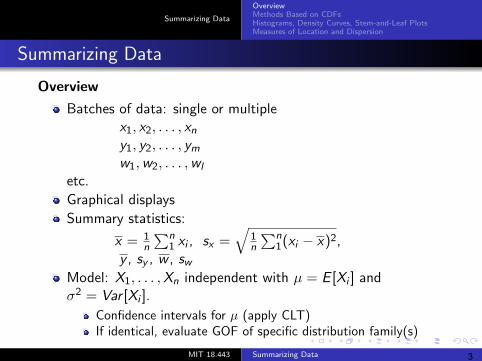
Overview

Batches of data: single or multiple x1, x2, . . . , xn

y1, y2, . . . , ym

w1, w2, . . . , wl

etc. Graphical displays Summary statistics: 1 n 1 n x = 1 xi , sx = (xi − x)2 ,n n 1

y , sy , w , sw

Model: X1, . . . , Xn independent with µ = E [Xi ] and σ2 = Var [Xi ].

Confidence intervals for µ (apply CLT) If identical, evaluate GOF of specific distribution family(s)


Summarizing Data


Summarizing Data

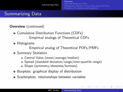
Overview (continued)

Cumulative Distribution Functions (CDFs) Empirical analogs of Theoretical CDFs

Histograms Empirical analog of Theoretical PDFs/PMFs

Summary Statistics Central Value (mean/average/median) Spread (standard deviation/range/inter-quartile range) Shape (symmetry/skewness/kurtosis)

Boxplots: graphical display of distribution

Scatterplots: relationships between variables


Summarizing Data


Outline



Summarizing Data


Methods Based on Cumlative Distribution Functions

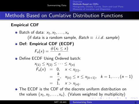
Empirical CDF

Batch of data: x1, x2, . . . , xn

(if data is a random sample, Batch ≡ i .i .d . sample)

Def: Empirical CDF (ECDF) #(xi ≤ x)

Fn(x) = n

Define ECDF Using Ordered batch: x(1) ≤ x(2) ≤ · · · ≤ x(n) Fn(x) = 0, x < x(1),

k = , x(k) ≤ x ≤ x(k+1), k = 1, . . . , (n − 1)

n = 1, x > x(n).

The ECDF is the CDF of the discrete uniform distribution on the values {x1, x2, . . . , xn}. (Values weighted by multiplicity)


. . 5

Summarizing Data


Methods Based on CDFs

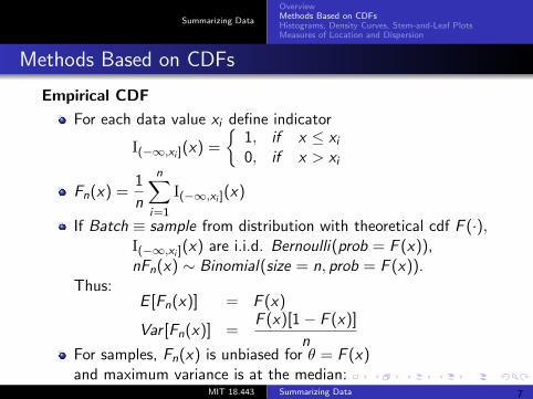
Empirical CDF

For each data value xi define indicator d

I(−∞,xi ](x) = 1, 0,

if if

x ≤ xi x > xi

1 nn

Fn(x) = n

I(−∞,xi ](x) i=1

If Batch ≡ sample from distribution with theoretical cdf F (·), I(−∞,xi ](x) are i.i.d. Bernoulli(prob = F (x)), nFn(x) ∼ Binomial(size = n, prob = F (x)).

Thus: E [Fn(x)] = F (x)

F (x)[1 − F (x)]Var [Fn(x)] =

n For samples, Fn(x) is unbiased for θ = F (x) and maximum variance is at the median:

x = x 5 : F (x 5) = 0. MIT 18.443 Summarizing Data 7

=

intervals for all x θ F x

Summarizing Data


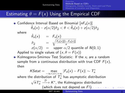
Estimating θ F (x) Using the Empirical CDF

Confidence Interval Based on Binomial [nFn(x)] θ̂n(x) − z(α/2)σ̂ˆ < θ < θ̂n(x) + z(α/2)σ̂ˆθ θ

where θ̂n(x) = Fn(x)

Fn(x)[1−Fn(x)]σ̂θ̂ = n

z(α/2) = upper α/2 quantile of N(0, 1) Applied to single values of (x , θ = F (x)) Kolmogorov-Smirnov Test Statistic: If the xi are a random sample from a continuous distribution with true CDF F (x), then

KSstat = max |Fn(x) − F (x)| ∼ T ∗ n−∞<x<+∞

where the distribution of T ∗ has asymptotic distribution n D√

nT ∗ −−→ K ∗ , the Kolmogorov distribution n (which does not depend on F !)

=⇒ Simultaneous confidence ( , = ( )) MIT 18.443 Summarizing Data

√

=

8

of resistivit

Summarizing Data


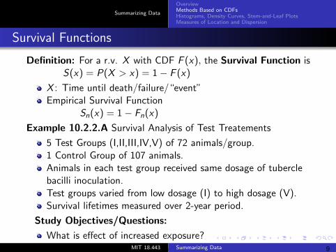
Survival Functions

Definition: For a r.v. X with CDF F (x), the Survival Function is S(x) = P(X > x) = 1 − F (x)

X : Time until death/failure/“event” Empirical Survival Function

Sn(x) = 1 − Fn(x)

Example 10.2.2.A Survival Analysis of Test Treatements

5 Test Groups (I,II,III,IV,V) of 72 animals/group. 1 Control Group of 107 animals. Animals in each test group received same dosage of tubercle bacilli inoculation. Test groups varied from low dosage (I) to high dosage (V). Survival lifetimes measured over 2-year period.

Study Objectives/Questions:

What is effect of increased exposure? How does effect vary with level y?MIT 18.443 Summarizing Data 9

Summarizing Data


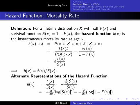
Hazard Function: Mortality Rate

Definition: For a lifetime distribution X with cdf F (x) and surivival function S(x) = 1 − F (x), the hazard function h(x) is the instantaneous mortality rate at age x :

h(x) × δ = P(x < X < x + δ | X > x) f (x)δ δf (x)

= = P(X > x) 1 − F (x) f (x)

= δ S(x)

=⇒ h(x) = f (x)/S(x). Alternate Representations of the Hazard Function

df (x) S(x)dxh(x) = = − S(x) S(x)

= − d (log[S(x)]) = − d (log[1 − F (x)])dx dx


Summarizing Data


Hazard Function: Mortality Rate

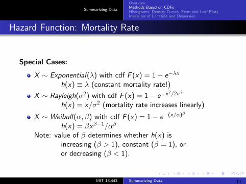
Special Cases:

X ∼ Exponential(λ) with cdf F (x) = 1 − e−λx

h(x) ≡ λ (constant mortality rate!) −x2/2σ2

X ∼ Rayleigh(σ2) with cdf F (x) = 1 − eh(x) = x/σ2 (mortality rate increases linearly)

−(x/α)β X ∼ Weibull(α, β) with cdf F (x) = 1 − e

h(x) = βxβ−1/αβ

Note: value of β determines whether h(x) is increasing (β > 1), constant (β = 1), or or decreasing (β < 1).


Summarizing Data


Hazard Function

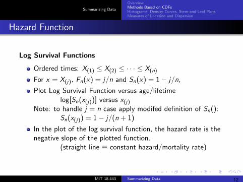
Log Survival Functions

Ordered times: X(1) ≤ X(2) ≤ · · · ≤ X(n)

For x = X(j), Fn(x) = j/n and Sn(x) = 1 − j/n,

Plot Log Survival Function versus age/lifetime log[Sn(x(j))] versus x(j)

Note: to handle j = n case apply modifed definition of Sn(): Sn(x(j)) = 1 − j/(n + 1)

In the plot of the log survival function, the hazard rate is the negative slope of the plotted function.

(straight line ≡ constant hazard/mortality rate)


Summarizing Data


Quantile-Quantile Plots

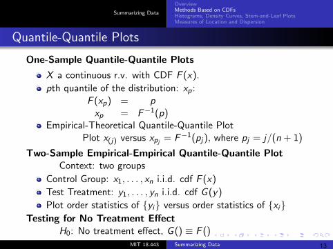
One-Sample Quantile-Quantile Plots

X a continuous r.v. with CDF F (x). pth quantile of the distribution: xp:

F (xp) = p xp = F −1(p)

Empirical-Theoretical Quantile-Quantile Plot Plot x(j) versus xpj = F −1(pj ), where pj = j/(n + 1)

Two-Sample Empirical-Empirical Quantile-Quantile Plot Context: two groups

Control Group: x1, . . . , xn i.i.d. cdf F (x) Test Treatment: y1, . . . , yn i.i.d. cdf G (y) Plot order statistics of {yi } versus order statistics of {xi }

Testing for No Treatment Effect H0: No treatment effect, G () ≡ F ()


Summarizing Data


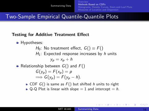
Two-Sample Empirical Quantile-Quantile Plots

Testing for Additive Treatment Effect

Hypotheses: H0: No treatment effect, G () ≡ F () H1: Expected response increases by h units

yp = xp + h

Relationship between G () and F () G (yp) = F (xp) = p =⇒ G (yp) = F (yp − h).

CDF G () is same as F () but shifted h units to right Q-Q Plot is linear with slope = 1 and intercept = h.


Summarizing Data


Two-Sample Empirical Quantile-Quantile Plots

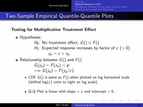
Testing for Multiplicative Treatment Effect

Hypotheses: H0: No treatment effect, G () ≡ F () H1: Expected response increases by factor of c (> 0)

yp = c × xp

Relationship between G () and F () G (yp) = F (xp) = p =⇒ G (yp) = F (yp/c).

CDF G () is same as F () when plotted on log horizontal scale (shifted log(c) units to right on log scale).

Q-Q Plot is linear with slope = c and intercept = 0.


Summarizing Data


Outline



Summarizing Data


Histograms, Density Curves, Stem-and-Leaf Plots

Methods For Displaying Distributions (relevant R functions)

Histogram: hist(x , nclass = 20, probability = TRUE )

Density Curve: plot(density(x , bw = ”sj”))

Kernel function: w(x) with bandwidth h) i x wh(x) = 1 wh h

nfh(x) = 1 n i=1 wh(x − Xi )

Options for Kernel function: Gaussian: w(x) = Normal(0, 1) pdf

=⇒ wh(x − Xi ) is N(Xi , h) density Rectangular, triangular, cosine, bi-weight, etc. See: Scott, D. W. (1992) Multivariate Density Estimation. Theory, Practice and Visualization. New York: Wiley

Stem-and-Leaf Plot: stem(x)

Boxplots: boxplot(x)

MIT 18.443 Summarizing Data

∑

17

Summarizing Data


Displaying Distributions

Boxplot Construction Vertical axis = scale of sample X1, . . . , Xn

Horizontal lines drawn at upper -quartile, lower − quartile and vertical lines join the box Horizontal line drawn at median inside the box Vertical line drawn up from upper -quartile to most extreme data point

within 1.5 (IQR) of the upper quartile. (IQR=Inter-Quartile Range) Also, vertical line drawn down from lower -quartile to most extreme data point

within 1.5 (IQR) of the lower -quartile Short horizontal lines added to mark ends of vertical lines Each data point beyond the ends of vertical lines is marked with ∗ or .


Summarizing Data


Outline



Summarizing Data


Measures of Location and Dispersion

Location Measures

Objective: measure center of {x1, x2, . . . , xn}

Arithmetic Mean 1 n x = n i=1 xi .

Issues: not robust to outliers.

Median n+1x[j∗], j∗ = if n is odd 2median({xi }) = x

[∗ j]+x[j ∗ +1] n 2 , j∗ = 2 if n is even

Note: confidence intervals for η = median(X ) of form [x[k], x[n+1−k]]

Rice Section 10.4.2 applies binomial distribution for #(Xi > η)


∑

20

Summarizing Data



Location Measures

Trimmed Mean: x .trimmedmean = mean(x , trim = 0.10) 10% of of lowest values dropped 10% of highest values dropped mean of remaning values computed

(trim = parameter must be less than 0.5) M Estimates

Least-squares estimate: Choose µ̂ to minimize n 2n Xi − µ

σi=1

MAD estimate: Choose µ̂ to minimize nn Xi − µ| |

σ i=1

(minimize mean absolute deviation)


Summarizing Data



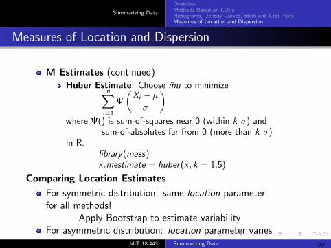
M Estimates (continued) Huber Estimate: Choose m̂u to minimize

nn Xi − µΨ

σ i=1

where Ψ() is sum-of-squares near 0 (within k σ) and sum-of-absolutes far from 0 (more than k σ)

In R: library(mass) x .mestimate = huber(x , k = 1.5)

Comparing Location Estimates

For symmetric distribution: same location parameter for all methods!

Apply Bootstrap to estimate variability For asymmetric distribution: location parameter varies


( )

22

Summarizing Data


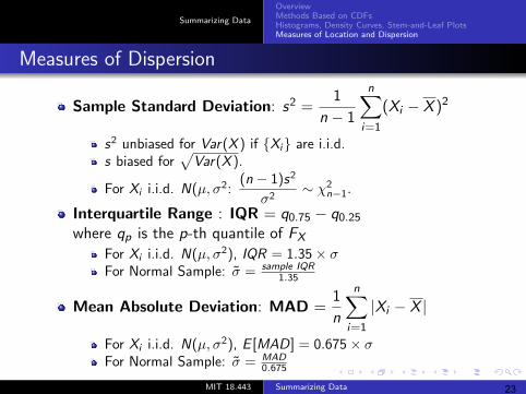
Measures of Dispersion nn

2Sample Standard Deviation: s =1

(Xi − X )2

n − 1 i=1

s2 unbiased for Var(X ) if {Xi } are i.i.d. f s biased for Var(X ).

2(n − 1)sFor Xi i.i.d. N(µ, σ2:

σ2 ∼ χ2

n−1.

Interquartile Range : IQR = q0.75 − q0.25

where qp is the p-th quantile of FX

For Xi i.i.d. N(µ, σ2), IQR = 1.35 × σ sample IQR For Normal Sample: σ̃ = 1.35

nn1 Mean Absolute Deviation: MAD = |Xi − X |

n i=1

For Xi i.i.d. N(µ, σ2), E [MAD] = 0.675 × σ MADFor Normal Sample: σ̃ = 0.675


MIT OpenCourseWarehttp://ocw.mit.edu

18.443 Statistics for ApplicationsSpring 2015

For information about citing these materials or our Terms of Use, visit: http://ocw.mit.edu/terms.

http://ocw.mit.edu

http://ocw.mit.edu/terms

statistics for applications lecture 12 notes · summarizing data summarizing data mit 18.443 dr....

Documents