statistics for ees introduction to r and descriptive...
TRANSCRIPT

Statistics for EESIntroduction to R and Descriptive
Statistics
Dirk Metzler
15. April 2013
Contents
Contents
1 Intro: What is Statistics? 1
2 Data Visialization 22.1 Histograms und Density Polygons . . . . . . . . . . . . . . . . 42.2 Stripcharts and Boxplots . . . . . . . . . . . . . . . . . . . . . 92.3 Example: Darwin Finches . . . . . . . . . . . . . . . . . . . . 122.4 Conclusions . . . . . . . . . . . . . . . . . . . . . . . . . . . . 14
3 Summarizing Data Numerically 153.1 Median and other Quartiles . . . . . . . . . . . . . . . . . . . 153.2 Mean, Standard Deviation and Variance . . . . . . . . . . . . 16
1 Intro: What is Statistics?
It is easy to lie with statistics. It is hard to tell the truth without it.
Andrejs Dunkels
1

What is Statistics?
Nature is full of VariabilityHow to make sense of variable data?
Use mathematical theory of randomness:[0.5ex] Probability.
Statistics = Data Analysis based on Probabilistic Models
Descriptive Statistics
Descriptive Statistcs is the first look at the data.
Statistics Software R
http://www.r-project.org
2 Data Visialization
Data Example
2
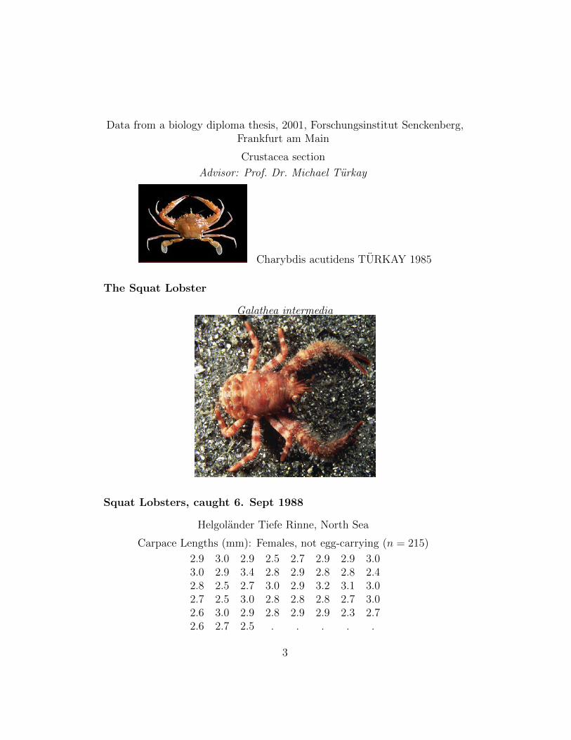
Data from a biology diploma thesis, 2001, Forschungsinstitut Senckenberg,Frankfurt am Main
Crustacea section
Advisor: Prof. Dr. Michael Turkay
Charybdis acutidens TURKAY 1985
The Squat Lobster
Galathea intermedia
Squat Lobsters, caught 6. Sept 1988
Helgolander Tiefe Rinne, North Sea
Carpace Lengths (mm): Females, not egg-carrying (n = 215)
2.9 3.0 2.9 2.5 2.7 2.9 2.9 3.03.0 2.9 3.4 2.8 2.9 2.8 2.8 2.42.8 2.5 2.7 3.0 2.9 3.2 3.1 3.02.7 2.5 3.0 2.8 2.8 2.8 2.7 3.02.6 3.0 2.9 2.8 2.9 2.9 2.3 2.72.6 2.7 2.5 . . . . .
3

●
●
●●
●
●●
●
●
●
●
●
●
●
●●
●
●
●
●
●
●
●
●
●
●●
●
●
●
●
●
●
●
●
●
●
●
●
●
●
●
●
●
●
●
●
●
●
●
●
●
●●
●
●
●
●
●
●
●
●
●
●
●
●
●
●●
●●
●
●
●●
●
●
●
●
●
●
●
●
●
●
●
●
●
●
●
●
●
●
●
●
●
●
●
●
●
●
●●
●
●●
●
●
●
●
●
●
●
●
●
●
●
●●
●
●
●●
●
●
●●
●
●
●
●
●
●
●
●
●
●
●
●
●
●●●
●
●
●
●
●
●
●
●
●
●
●
●
●
●
●
●
●
●●
●
●
●
●
●
●
●
●
●
●
●
●
●
●
●
●
●
●●
●
●
●
●
●
●
●
●
●
●
●
●
●
●
●
●
●
●
●●
●
●●
●
●
●
●
●
●
●
●●
●
●
0 50 100 150 200
2.0
2.5
3.0
Female Galathea, not carrrying eggs, caught 6. Sept. '88, n=215
Index
Car
apax
Len
gth
[mm
]
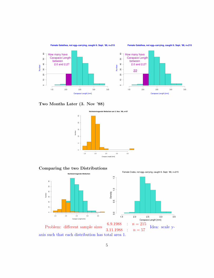
2.1 Histograms und Density Polygons
6. Sept. '88, n=215
Carapax Length [mm]
Num
ber
1.5 2.0 2.5 3.0 3.5
010
2030
4050
60
1.5 2.0 2.5 3.0 3.5
010
20
30
40
50
60
Carapace Length [mm]
Female Galathea, not egg−carrying, caught 6. Sept. ’88, n=215
Num
ber
1.5 2.0 2.5 3.0 3.5
010
20
30
40
50
60
Carapace Length [mm]
Female Galathea, not egg−carrying, caught 6. Sept. ’88, n=215
Num
ber
How many have
Carapace Lengthbetween
2.0 and 2.2?
1.5 2.0 2.5 3.0 3.5
010
20
30
40
50
60
Carapace Length [mm]
Female Galathea, not egg−carrying, caught 6. Sept. ’88, n=215
Num
ber
How many have
Carapace Lengthbetween
2.0 and 2.2?
4
1.5 2.0 2.5 3.0 3.5
010
20
30
40
50
60
Carapace Length [mm]
Female Galathea, not egg−carrying, caught 6. Sept. ’88, n=215
Num
ber
How many have
Carapace Lengthbetween
2.0 and 2.2?
1.5 2.0 2.5 3.0 3.5
010
20
30
40
50
60
Carapace Length [mm]
Female Galathea, not egg−carrying, caught 6. Sept. ’88, n=215
Num
ber
How many have
Carapace Lengthbetween
2.0 and 2.2?
22
Two Months Later (3. Nov ’88)
Nichteiertragende Weibchen am 3. Nov. '88, n=57
Carapax Length [mm]
Num
ber
1.5 2.0 2.5 3.0 3.5
05
1015
2025
Comparing the two DistributionsNichteiertragende Weibchen
Carapax Length [mm]
Num
ber
1.5 2.0 2.5 3.0 3.5
010
2030
4050
60
1.0
1.5
0.5
0.0
2.0 3.0 3.51.5
Density
Female Crabs, not egg−carrying, caught 6. Sept. ’88, n=215
Carapace Length [mm]
2.5
Problem: different sample sizes6.9.1988 : n = 215
3.11.1988 : n = 57Idea: scale y-
axis such that each distribution has total area 1.
5
1.0
1.5
0.5
0.0
2.0 3.0 3.51.5
Density
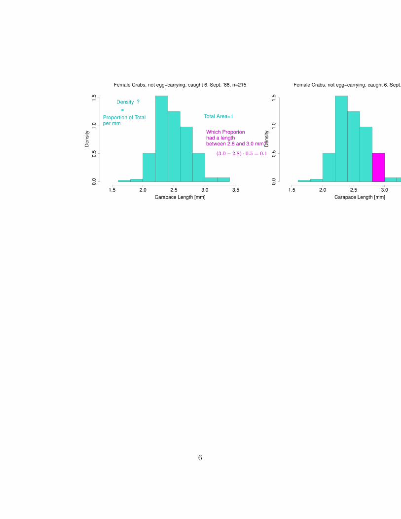
Female Crabs, not egg−carrying, caught 6. Sept. ’88, n=215
Carapace Length [mm]
2.5
1.0
1.5
0.5
0.0
2.0 3.0 3.51.5
Density
Female Crabs, not egg−carrying, caught 6. Sept. ’88, n=215
Carapace Length [mm]
2.5
=Density ?
Proportion of Totalper mm
Total Area=1
Which Proporionhad a lengthbetween 2.8 and 3.0 mm?
(3.0− 2.8) · 0.5 = 0.1
6
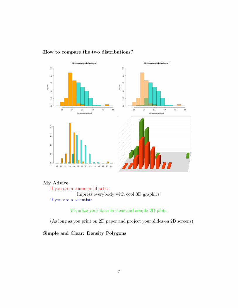
How to compare the two distributions?
Nichteiertragende Weibchen
Carapax Length [mm]
Den
sity
1.5 2.0 2.5 3.0 3.5 4.0
0.0
0.5
1.0
1.5
2.0
2.5
Nichteiertragende Weibchen
Carapax Length [mm]
Den
sity
1.5 2.0 2.5 3.0 3.5 4.0
0.0
0.5
1.0
1.5
2.0
2.5
1.3 1.5 1.7 1.9 2.1 2.3 2.5 2.7 2.9 3.1 3.3 3.5 3.7 3.9
0.0
0.5
1.0
1.5
2.0
My AdviceIf you are a commercial artist:
Impress everybody with cool 3D graphics!If you are a scientist:
Visualize your data in clear and simple 2D plots.
(As long as you print on 2D paper and project your slides on 2D screens)
Simple and Clear: Density Polygons
7
1.0
1.5
0.5
0.0
2.0 3.0 3.51.5
Density
Female Crabs, not egg−carrying, caught 6. Sept. ’88, n=215
Carapace Length [mm]
2.5
6. Sept. '88, n=215
Carapax Length [mm]
Den
sity
1.5 2.0 2.5 3.0 3.5
0.0
0.5
1.0
1.5
3. Nov. '88, n=57
Carapax Length [mm]
Den
sity
1.5 2.0 2.5 3.0 3.5
0.0
0.5
1.0
1.5
2.0
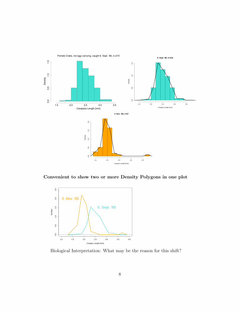
Convenient to show two or more Density Polygons in one plot
1.0 1.5 2.0 2.5 3.0 3.5 4.0
0.0
0.5
1.0
1.5
2.0
2.5
Carapax Length [mm]
Num
ber 6. Sept. '88
3. Nov. '88
Biological Interpretation: What may be the reason for this shift?
8

2.2 Stripcharts and Boxplots
1.5 2.0 2.5 3.0 3.5
3.11
.88
6.9.
88
Carapax
1.5 2.0 2.5 3.0 3.5
3.11
.88
6.9.
88
Carapax
●●● ●
●●
●●
●● ●●● ●●● ●
●●
●●
●● ●●● ●●
●●●● ●● ●
●●
●●
●●●●●● ●
●● ●●
●●● ●●●
●
● ●●●● ●● ●●●
●●
●●●●●
● ● ●● ●●●●● ●●●●● ●●
●●●●
●●● ●● ●
●● ●●●● ● ●● ●
●● ●●●● ●●●● ●●
●●
●● ●●●
●● ●● ●●
● ●●●●
●●●
● ●●●●
●● ●
●● ●●●● ●●
●● ●●
●● ●●● ●● ● ●● ●● ●●● ●● ●●
●●●●● ●●
●●●
●● ●●●
● ●●●
●●
●●●●● ●●
●●●●● ●
●●●● ●● ●
●●
●●● ●
●●●●
●● ●● ●
● ●●●● ●● ●●●●●
●●●●●
●● ●
●●● ●●
●●●●●
●●● ●
1.5 2.0 2.5 3.0 3.5
3.11
.88
6.9.
88
Carapax
1.5 2.0 2.5 3.0 3.5
3.11
.88
6.9.
88
Carapax
● ●●●●
●●●
3.11
.88
6.9.
88
1.5 2.0 2.5 3.0 3.5
Stripchart + Boxplots, horizontal
● ●●●●
●●●
3.11
.88
6.9.
88
1.5 2.0 2.5 3.0 3.5
Boxplots, horizontal
●
●
●●●
●●●
3.11.88 6.9.88
1.5
2.0
2.5
3.0
3.5
Boxplots, vertikal
Simplify to understand
Histograms and density polygonsallow a comprehensive view on the data.
Sometimes too comprehensive.
9

Comparison of four groupsD
icht
e
8 10 12 14
0.00
Dic
hte
8 10 12 14
0.00
Dic
hte
8 10 12 14
0.0
Dic
hte
8 10 12 14
0.0
12
34
8 10 12 14
The Boxplot
2.0 2.5 3.0 3.5
Carapace Length [mm]
Boxplot, simple type
2.0 2.5 3.0 3.5
Carapace Length [mm]
Boxplot, simple type
2.0 2.5 3.0 3.5
Carapace Length [mm]
Boxplot, simple type
50 % of the data 50 % of the data
2.0 2.5 3.0 3.5
Boxplot, simple type
Carapace Length [mm]
50 % of the data 50 % of the data
Median
10

2.0 2.5 3.0 3.5
Boxplot, simple type
Carapace Length [mm]
50 % of the data 50 % of the data
MedianMin Max
2.0 2.5 3.0 3.5
Boxplot, simple type
Carapace Length [mm]
MedianMin Max
25% 25% 25% 25%
2.0 2.5 3.0 3.5
Boxplot, simple type
Carapace Length [mm]
MedianMin Max
25% 25% 25% 25%
1. Quartile 3. Quartile
2.0 2.5 3.0 3.5
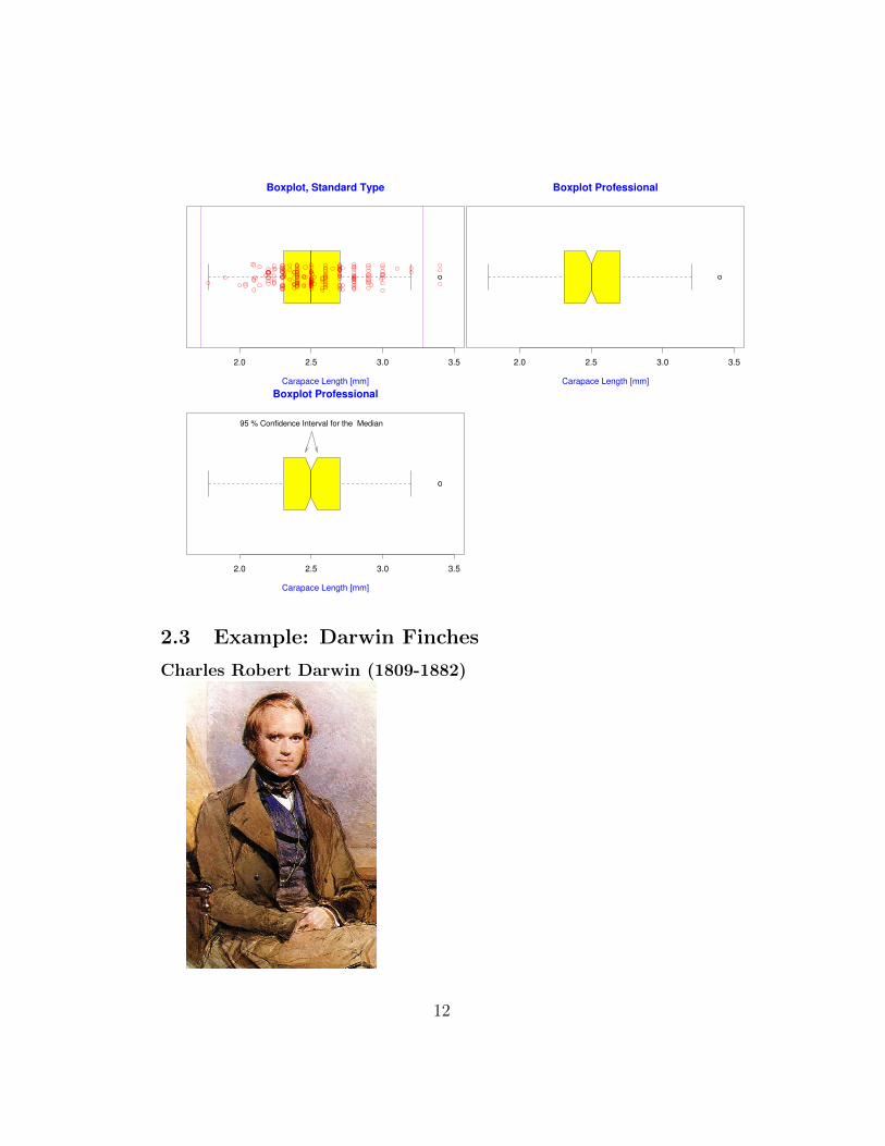
Boxplot, Standard Type
Carapace Length [mm]
2.0 2.5 3.0 3.5
Carapace Length [mm]
Boxplot, Standard Type
Interquartile Range
2.0 2.5 3.0 3.5
Carapace Length [mm]
Boxplot, Standard Type
Interquartile Range
1.5*Interquartile Range 1.5*Interquartile Range
11
2.0 2.5 3.0 3.5
Carapace Length [mm]
Boxplot, Standard Type
2.0 2.5 3.0 3.5
Boxplot Professional
Carapace Length [mm]
95 % Confidence Interval for the Median
2.0 2.5 3.0 3.5
Boxplot Professional
Carapace Length [mm]
2.3 Example: Darwin Finches
Charles Robert Darwin (1809-1882)
12
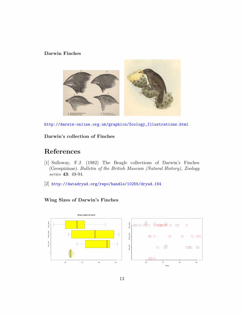
Darwin Finches
http://darwin-online.org.uk/graphics/Zoology_Illustrations.html
Darwin’s collection of Finches
References
[1] Sulloway, F.J. (1982) The Beagle collections of Darwin’s Finches(Geospizinae). Bulletin of the British Museum (Natural History), Zoologyseries 43: 49-94.
[2] http://datadryad.org/repo/handle/10255/dryad.154
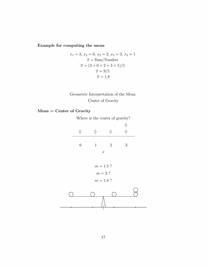
Wing Sizes of Darwin’s Finches
Flo
r_C
hrl
SC
ris_C
hat
Snt
i_Ja
ms
60 70 80 90
Wing Lengths by Island
60 70 80 90
Flo
r_C
hrl
SC
ris_C
hat
Snt
i_Ja
ms
WingL
13

Flo
r_C
hrl
SC
ris_C
hat
Snt
i_Ja
ms
60 70 80 90
Wing Lengths by Island
●●●
● ●●●●●
●●● ●
●● ●●●● ●●
●● ●●●●●●●● ● ●●
●●● ●●● ●●● ●●●
47.5 52.5 57.5 62.5 67.5 72.5 77.5 82.5 87.5 92.5 97.5
Barplot of Wing Lengths (Numbers)
01
23
45
6
●
●
●
●
SCris_ChatFlor_ChrlSnti_Jams
Histogramm (Densities!) with transparen colors
Wing Lengths
Den
sity
50 60 70 80 90
0.00
0.05
0.10
0.15
0.20
SCris_ChatFlor_ChrlSnti_Jams
50 60 70 80 90 100
0.00
0.05
0.10
0.15
0.20
Density Polygons
Wing Lengths
Den
sity
●
●
●
●
SCris_ChatFlor_ChrlSnti_Jams
Beak Sizes of Darwin’s Finches
●
Cam.par Cer.oli Geo.dif Geo.for Geo.ful Geo.sca Pla.cra
510
1520
Beak Sizes by Species
●
Cam.par Cer.oli Geo.dif Geo.for Geo.ful Geo.sca Pla.cra
510
1520
Beak Sizes by Species
●●
●
●
●
●
●
●●●
●●
●
●
●
●
●
●●
●●●●●
●
● ●●●
●●●●●
●
●
●
●●●
●
●
● ●
●
●
2.4 Conclusions
Conclusions
14

• Histograms give detailed information.
• Density Polygons allow multiple comparisons.
• Boxplots can simplify large datasets.
• Stripcharts more appropriate for small datasets.
• Sophisticated graphics with 3D or semi-transperent colors do not al-ways improve clarity.
3 Summarizing Data Numerically
Idea
It is often possible to summarize essential information about a samplenumerically.
e.g.:
• How large? Location Parameters
• How variable? Dispersion Parameters
Already known from Boxplots
Location (How large?)
MedianDispersion (How variable?)
Inter quartile range (Q3 −Q1)
3.1 Median and other Quartiles
The median is the 50% quantile of the data.i.e.: half of the data are smaller or equal to the median, the other half are
larger or equal.
15

The Quartiles
The first Quartile, Q1: A quarter of the observations are smaller than orequal to Q1. Three quarters are larger or equal.
i.e. Q1 is the 25%-Quantile
The third Quartile, Q3: Tree quarters of the observations are smaller thanor equal to Q3. One quarter are larger or equal.
i.e. Q3 is the 75%-Quantile
3.2 Mean, Standard Deviation and Variance
Most frequently usedLocation Parameter: The Mean x
Dispersion Parameter: The Standard Deviation s
NOTATION:
Given data named x1, x2, x3, . . . , xn
it is common to write x for the mean.
DEFINITION:
Mean[1ex] =[1ex]
Sum of oberved values
Number of Observations
Sum
Number
The formula for the mean of x1, x2, . . . , xn:
x = (x1 + x2 + · · ·+ xn)/n
=1
n
n∑i=1
xi
16
Example for computing the mean
x1 = 3, x2 = 0, x3 = 2, x4 = 3, x5 = 1
x = Sum/Number
x = (3 + 0 + 2 + 3 + 1)/5
x = 9/5
x = 1.8
Geometric Interpretation of the Mean
Center of Gravity
Mean = Center of Gravity
Where is the center of gravity?
♦
♦ ♦ ♦ ♦
0 1 2 3
x
m = 1.5 ?
m = 2 ?
m = 1.8 ?
17

18

Conjecture: Ratio higher for sexually mature female crabs.
Example:
3.11.88
19

The Standard Deviation
How far do typical overservations deviate from the mean?
20

1 2 3 41 2 3 4
Mean = 2.8
Deviation
typical
=?= 4 − 2,8 = 1,2= 4 − 2.8 = 1.2= 3 − 2.8 = 0.2= 2 − 2,8 = −0,8= 1 − 2,8 = −1,8
Die Standard Deviation σ (“sigma”) ist a slightly weired weighted mean ofthe deviations:
σ =√
Sum(Deviations2)/n
The formula for the Standard Deviation of x1, x2, . . . , xn:
σ =
√√√√ 1
n
n∑i=1
(xi − x)2
σ2 = 1n
∑ni=1(xi − x)2 is the Variance.
Rule of Thumb for the Standard DeviationIn more or less bell-shaped (i.e. single peak, symmetic) distributions:
21

ca. 2/3 are located between x−σ und x+σ.
0.0
0.2
0.4
0.6
0.8
1.0
prob
abili
ty d
ensi
ty
x −− σσ x x ++ σσ
Standard Deviation of Carapace lengths from 6.9.88
females, not carrying eggs, caught 6. Sept. '88
Carapax Length [mm]
Den
sity
2.0 2.5 3.0
0.0
0.5
1.0
1.5 x == 2.53
females, not carrying eggs, caught 6. Sept. '88
Carapax Length [mm]
Den
sity
2.0 2.5 3.0
0.0
0.5
1.0
1.5 x == 2.53x == 2.53σσ == 0.28
σσ2 == 0.077
In this case 72% are between x− σ and x+ σ
Variance of Carapace lengths from 6.9.88All Carace Lengths in North Sea: X = (X1, X2, . . . , XN).Carapace Length
in our Sample: S = (S1, S2, . . . , Sn=215)Sample Variance:
σ2S =
1
n
215∑i=1
(Si − S)2 ≈ 0,0768
Can we use 0.0768 as estimation for σ2X , the variance in the whole popula-
tion?Yes, we can! However, σ2S is on average by a factor of n−1
n(= 214/215 ≈
0, 995) smaller than σ2X .
22

VariancesVariance in the Population: σ2
X = 1N
∑Ni=1(Xi −X)2
Sample Variance: σ2S = 1
n
∑ni=1(Si − S)2
(Corrected) Sample Variance:
s2 =n
n− 1σ2S
=n
n− 1· 1
n·
n∑i=1
(Si − S)2
=1
n− 1·
n∑i=1
(Si − S)2
Usually, “Standard Deviation (SD) of S” refers to the corrected s.
Example: Computing SDGiven Data x =? x = 10/5 = 2 Sum
x 1 3 0 5 1 10
x− x −1 1 −2 3 −1 0
(x− x)2 1 1 4 9 1 16
s2 = Sum((x− x)2
)/(n− 1)
= 16/(5− 1) = 4
s = 2
23