statistics from pltw
DESCRIPTION
Introduction to StatisticsTRANSCRIPT

Introduction to Statistics
(modified for Science)
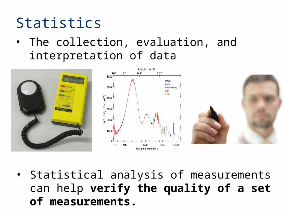
Statistics• The collection, evaluation, and interpretation of
data
• Statistical analysis of measurements can help verify the quality of a set of measurements.
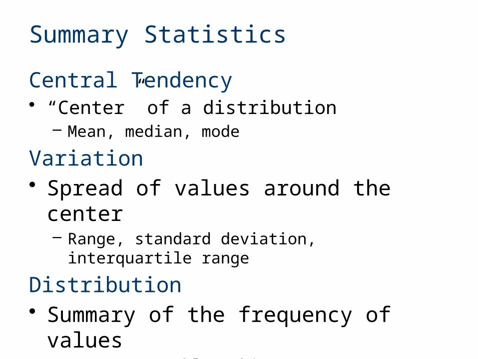
Summary Statistics
Central Tendency• “Center” of a distribution
– Mean, median, mode
Variation• Spread of values around the center
– Range, standard deviation, interquartile range
Distribution• Summary of the frequency of values
– Frequency tables, histograms, probability distributions, (normal distribution)
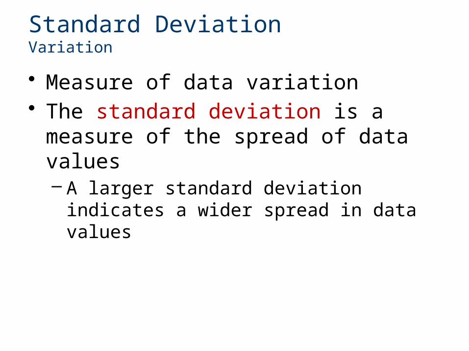
• Measure of data variation• The standard deviation is a measure of
the spread of data values– A larger standard deviation indicates a wider
spread in data values
Standard Deviation Variation
Standard Deviation Variation
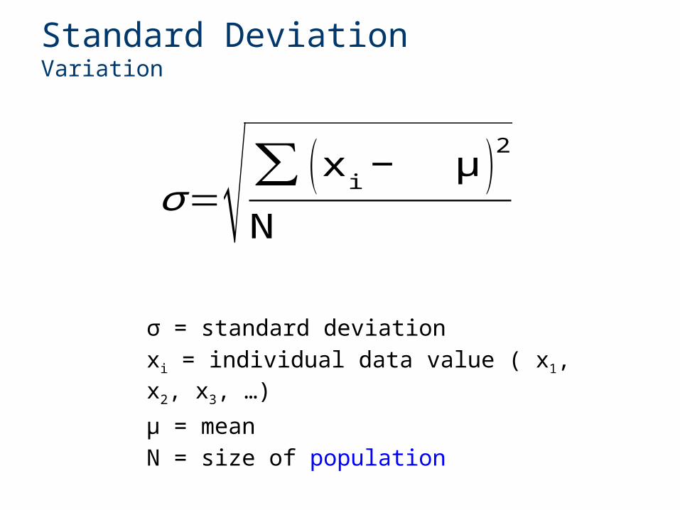
σ=√∑ (x i− μ )2
N
σ = standard deviation
xi = individual data value ( x1, x2, x3, …)
μ = mean
N = size of population
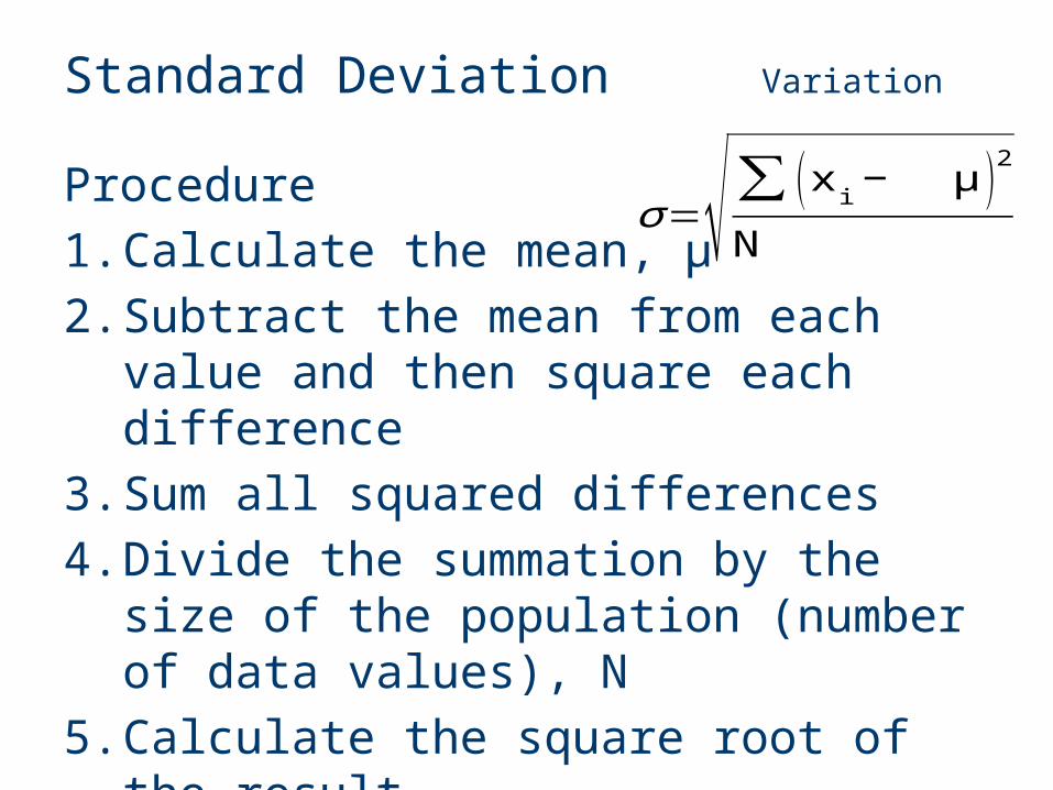
Standard Deviation Variation
Procedure
1. Calculate the mean, μ
2. Subtract the mean from each value and then square each difference
3. Sum all squared differences
4. Divide the summation by the size of the population (number of data values), N
5. Calculate the square root of the result
σ=√∑ (x i− μ )2
N
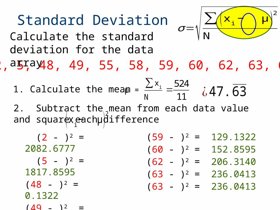
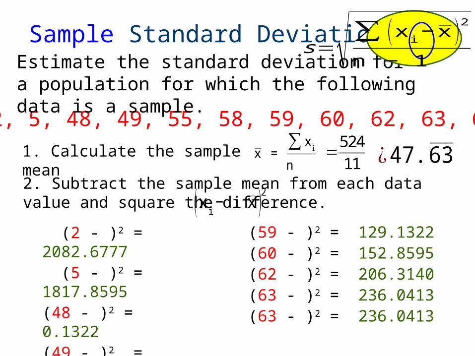
Standard Deviation
2, 5, 48, 49, 55, 58, 59, 60, 62, 63, 63
Calculate the standard deviation for the data array
524
111. Calculate the mean
2. Subtract the mean from each data value and square each difference
(2 - )2 = 2082.6777 (5 - )2 = 1817.8595(48 - )2 = 0.1322(49 - )2 = 1.8595(55 - )2 = 54.2231(58 - )2 = 107.4050
(59 - )2 = 129.1322(60 - )2 = 152.8595(62 - )2 = 206.3140(63 - )2 = 236.0413(63 - )2 = 236.0413
(x i− μ )2μ =
∑ x iN
σ=√∑ (x i− μ )2
N
¿ 47.63
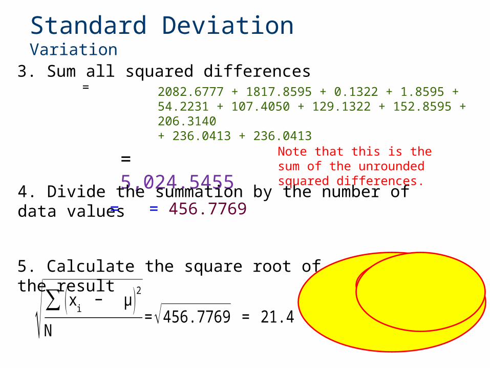
Standard Deviation Variation
3. Sum all squared differences 2082.6777 + 1817.8595 + 0.1322 + 1.8595 + 54.2231 + 107.4050 + 129.1322 + 152.8595 + 206.3140 + 236.0413 + 236.0413
= 5,024.5455
4. Divide the summation by the number of data values
5. Calculate the square root of the result
=
= = 456.7769
√∑ (x i − μ )2
N=√456.7769 = 21.4
Note that this is the sum of the unrounded squared differences.
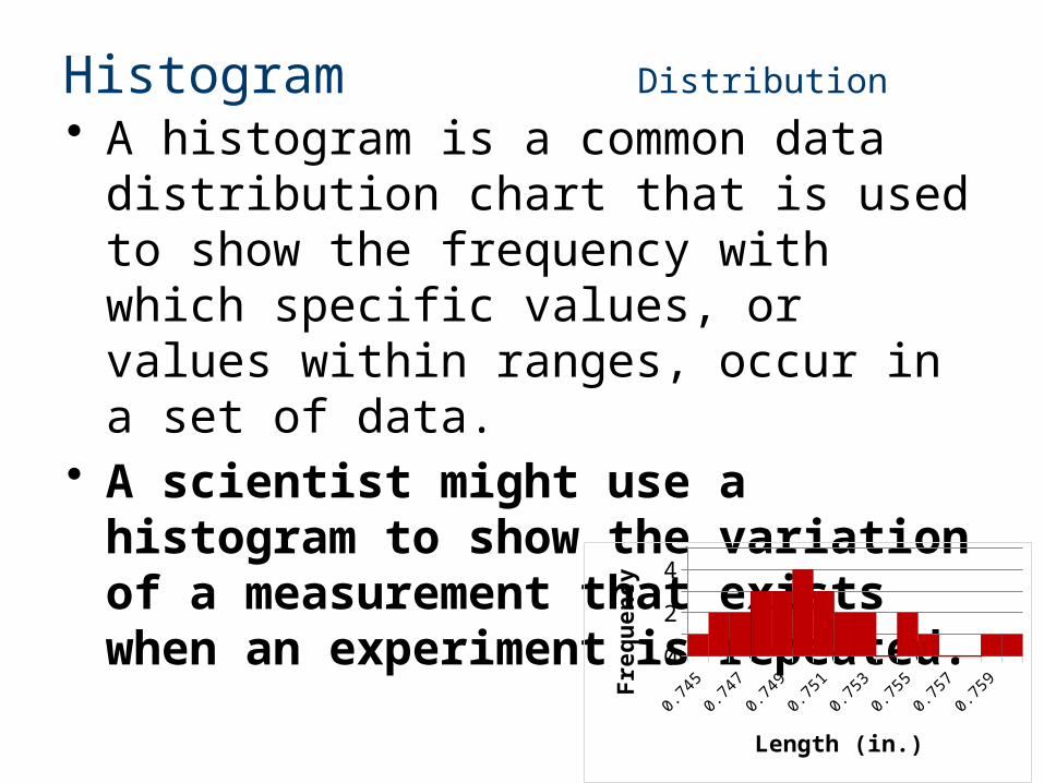
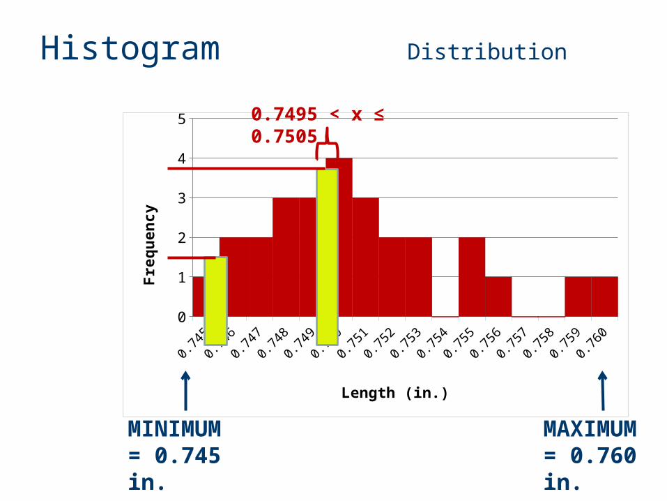
• A histogram is a common data distribution chart that is used to show the frequency with which specific values, or values within ranges, occur in a set of data.
• A scientist might use a histogram to show the variation of a measurement that exists when an experiment is repeated.
Histogram Distribution
0.74
50.
747
0.74
90.
751
0.75
30.
755
0.75
70.
759
0
2
4
Length (in.)
Fre
qu
en
cy
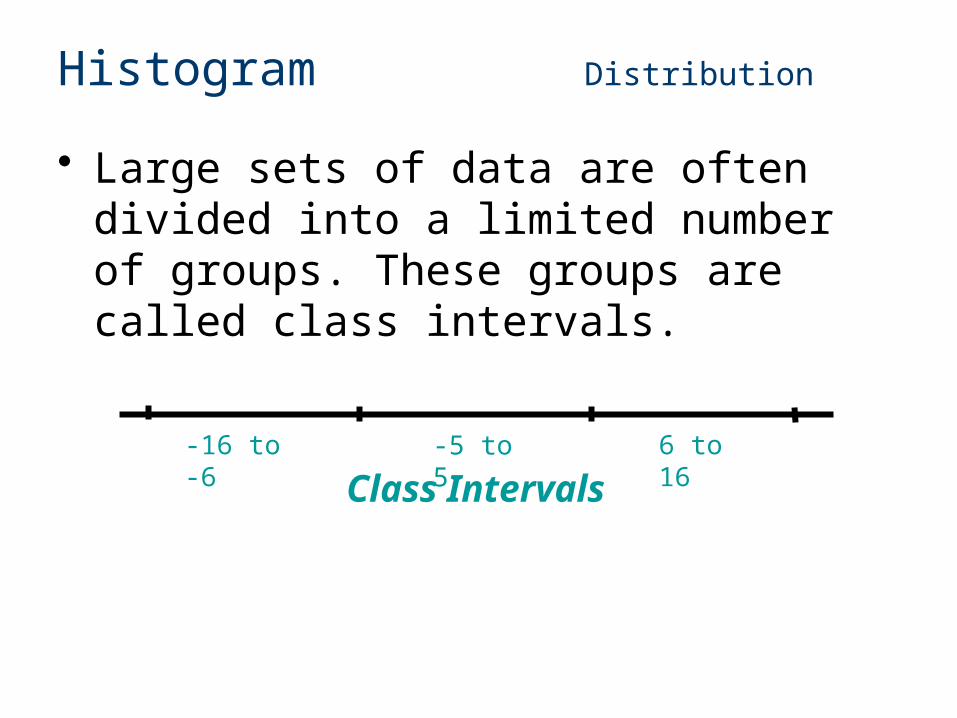
• Large sets of data are often divided into a limited number of groups. These groups are called class intervals.
-5 to 5
Class Intervals6 to 16-16 to -6
Histogram Distribution

• The number of data elements in each class interval is shown by the frequency, which is indicated along the Y-axis of the graph.
Fre
qu
ency
1
3
5
7
-5 to 5 6 to 16-16 to -6
Histogram Distribution
3
ExampleF
req
uen
cy
1
2
4
6 to 10 11 to 151 to 5
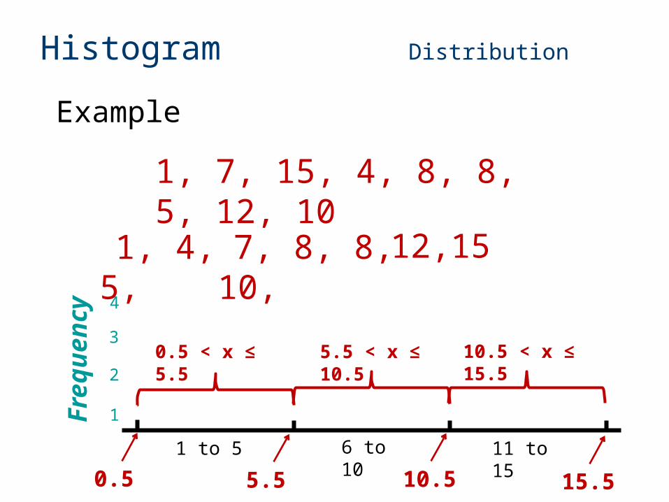
1, 7, 15, 4, 8, 8, 5, 12, 10
12,15 1, 4, 5, 7, 8, 8, 10,
Histogram Distribution
0.5 5.5 10.5 15.5
0.5 < x ≤ 5.5 5.5 < x ≤ 10.5 10.5 < x ≤ 15.5
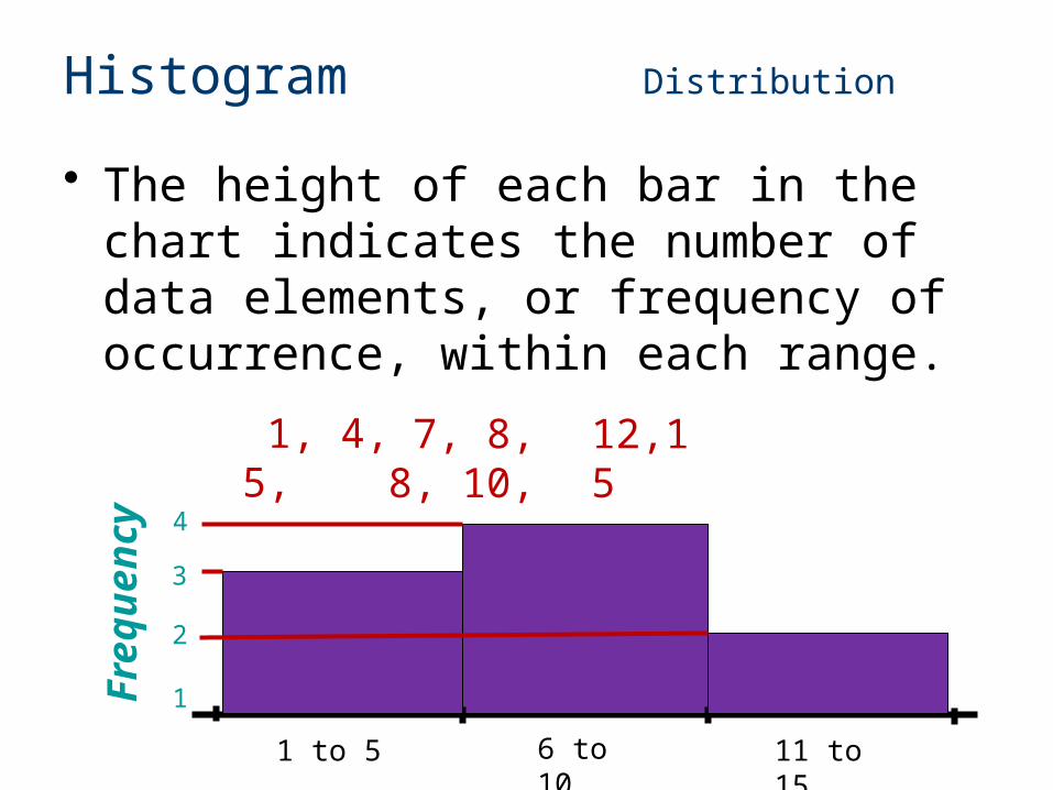
• The height of each bar in the chart indicates the number of data elements, or frequency of occurrence, within each range.
Histogram Distribution
3
Fre
qu
ency
1
2
4
6 to 10 11 to 151 to 5
12,15 1, 4, 5, 7, 8, 8, 10,
0.745
0.746
0.747
0.748
0.749
0.750
0.751
0.752
0.753
0.754
0.755
0.756
0.757
0.758
0.759
0.760
0
1
2
3
4
5
Length (in.)
Fre
qu
en
cy
MINIMUM = 0.745 in.
MAXIMUM = 0.760 in.
Histogram Distribution
0.7495 < x ≤ 0.7505
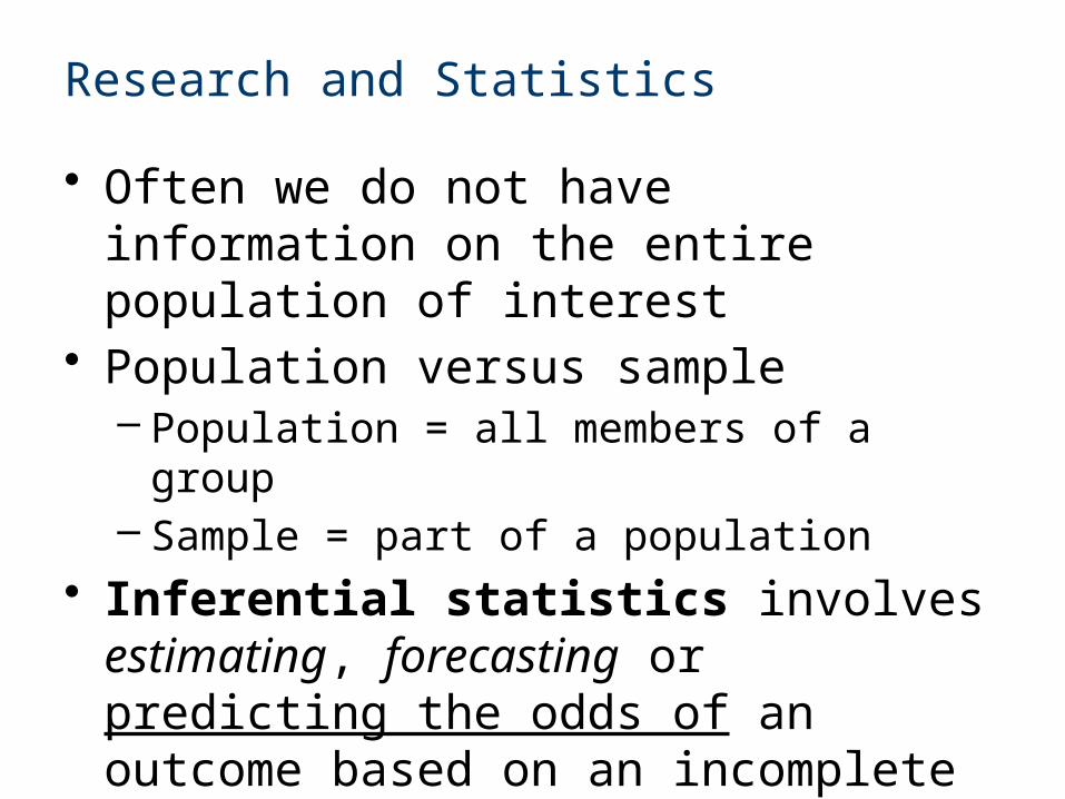
• Often we do not have information on the entire population of interest
• Population versus sample– Population = all members of a group– Sample = part of a population
• Inferential statistics involves estimating, forecasting or predicting the odds of an outcome based on an incomplete set of data– use sample statistics
Research and Statistics
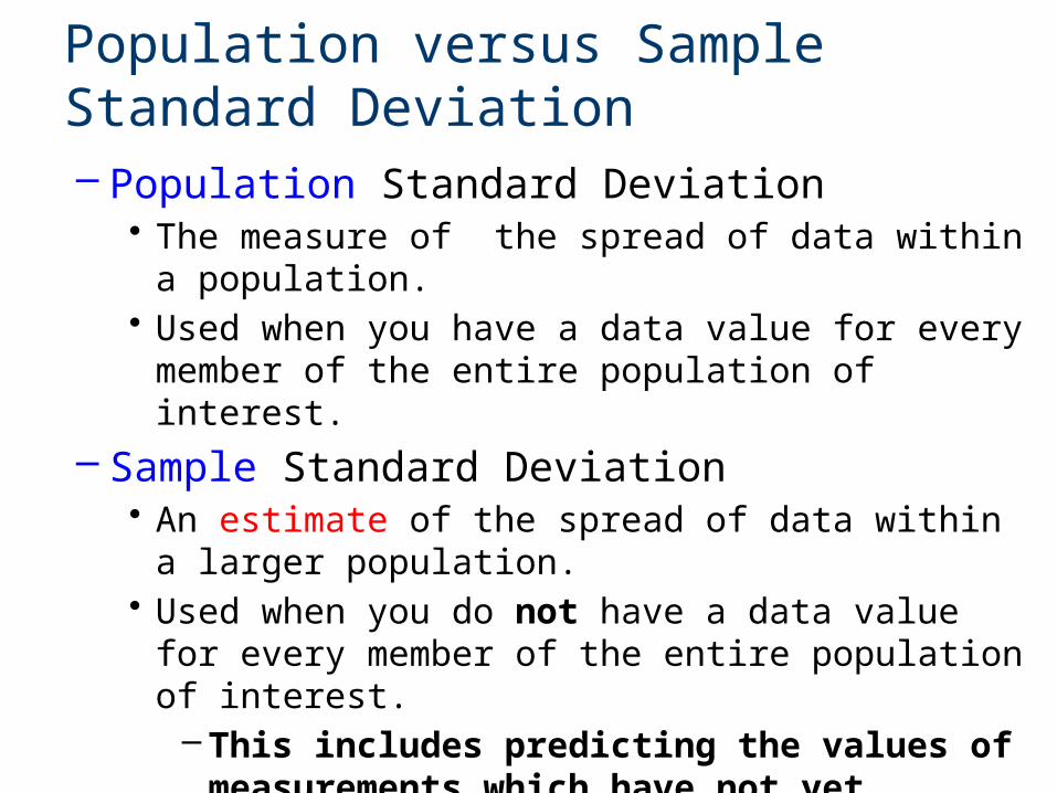
Population versus Sample Standard Deviation– Population Standard Deviation
• The measure of the spread of data within a population. • Used when you have a data value for every member of
the entire population of interest.
– Sample Standard Deviation• An estimate of the spread of data within a larger
population.• Used when you do not have a data value for every
member of the entire population of interest.– This includes predicting the values of
measurements which have not yet occurred.• Uses a subset (sample) of the data to generalize the
results to the larger population.
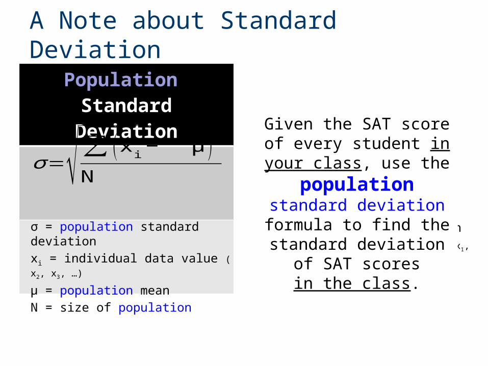
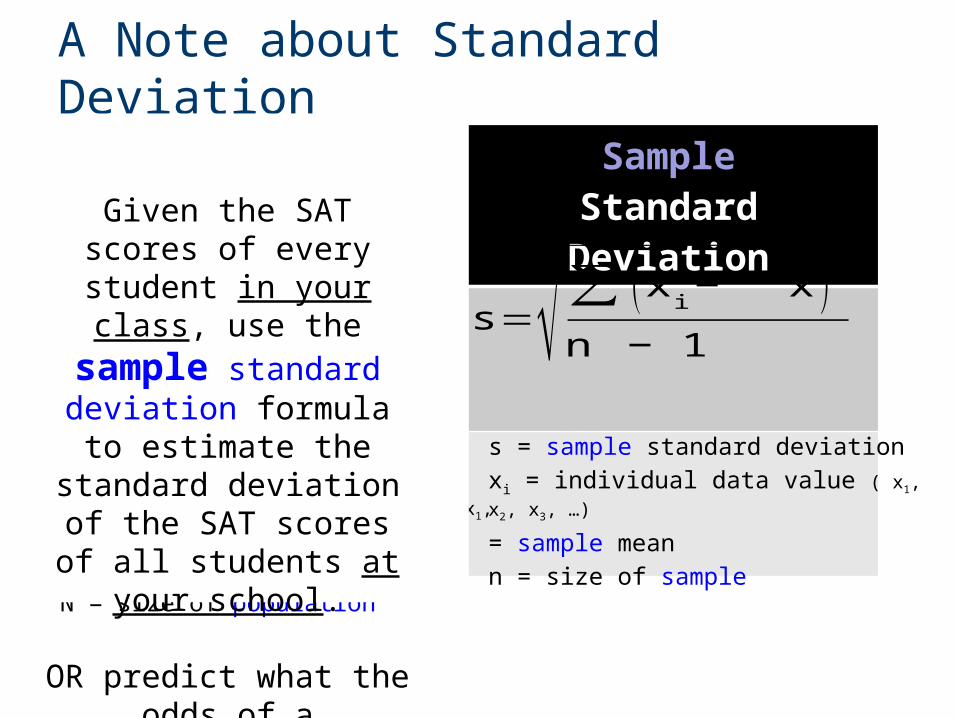
Population Standard Deviation
SampleStandard Deviation
A Note about Standard Deviation
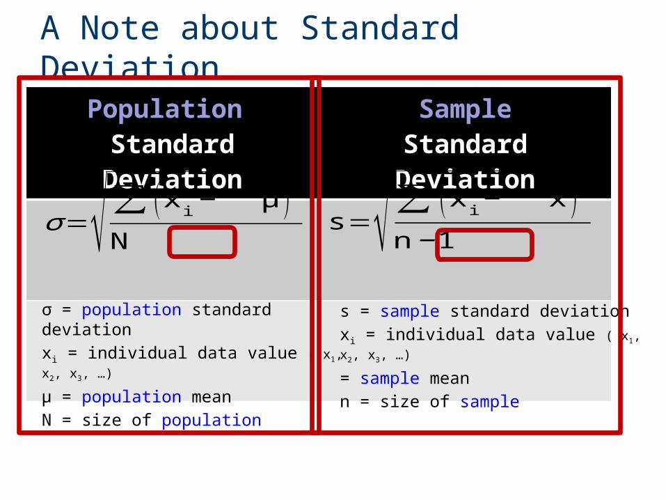
σ = population standard deviation
xi = individual data value ( x1, x2, x3, …)
μ = population mean
N = size of population
σ=√∑ (x i− μ )2
Ns=√∑ (x i− x )2
n−1
s = sample standard deviation
xi = individual data value ( x1, x2, x3, …)
= sample mean
n = size of sample

Sample Standard Deviation Variation
Procedure:
1. Calculate the sample mean,.
2. Subtract the mean from each value and then square each difference.
3. Sum all squared differences.
4. Divide the summation by the number of data values minus one, n - 1.
5. Calculate the square root of the result.
s=√∑ (x i− x )2
n−1
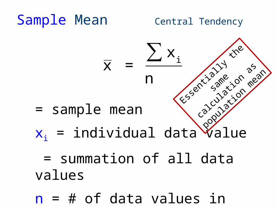
Sample Mean Central Tendency
= sample mean
xi = individual data value
= summation of all data values
n = # of data values in the sample
x = ∑ x in
Essen
tially
the
sam
e ca
lculat
ion a
s
popu
lation
mea
n
Sample Standard Deviation
2, 5, 48, 49, 55, 58, 59, 60, 62, 63, 63
Estimate the standard deviation for a population for which the following data is a sample.
524
111. Calculate the sample mean
2. Subtract the sample mean from each data value and square the difference.
(2 - )2 = 2082.6777 (5 - )2 = 1817.8595(48 - )2 = 0.1322(49 - )2 = 1.8595(55 - )2 = 54.2231(58 - )2 = 107.4050
(59 - )2 = 129.1322(60 - )2 = 152.8595(62 - )2 = 206.3140(63 - )2 = 236.0413(63 - )2 = 236.0413
s=√∑ (x i−x )2
n − 1
¿ 47.63x = ∑ x in
(x i− x )2
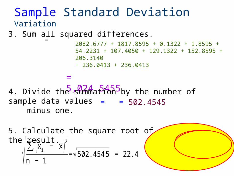
Sample Standard Deviation Variation
= 5,024.5455
=
= = 502.4545
√∑ (x i − x )2
n − 1=√502.4545 = 22.4
3. Sum all squared differences.
4. Divide the summation by the number of sample data values minus one.
5. Calculate the square root of the result.
2082.6777 + 1817.8595 + 0.1322 + 1.8595 + 54.2231 + 107.4050 + 129.1322 + 152.8595 + 206.3140 + 236.0413 + 236.0413

Population Standard Deviation
SampleStandard Deviation
A Note about Standard Deviation
σ = population standard deviation
xi = individual data value ( x1, x2, x3, …)
μ = population mean
N = size of population
σ=√∑ (x i− μ )2
Ns=√∑ (x i− x )2
n − 1
s = sample standard deviation
xi = individual data value ( x1, x2, x3, …)
= sample mean
n = size of sample
As n → N, s → σSo for very large numbers of measurements, s σ
Population Standard Deviation
SampleStandard Deviation
A Note about Standard Deviation
σ = population standard deviation
xi = individual data value ( x1, x2, x3, …)
μ = population mean
N = size of population
σ=√∑ (x i− μ )2
Ns=√∑ (x i− x )2
n − 1
s = sample standard deviation
xi = individual data value ( x1, x2, x3, …)
= sample mean
n = size of sample
Given the SAT score of every student in your
class, use the population standard deviation formula to find the standard deviation of
SAT scoresin the class.
Population Standard Deviation
SampleStandard Deviation
A Note about Standard Deviation
σ = population standard deviation
xi = individual data value ( x1, x2, x3, …)
μ = population mean
N = size of population
σ=√∑ (x i− μ )2
Ns=√∑ (x i− x )2
n − 1
s = sample standard deviation
xi = individual data value ( x1, x2, x3, …)
= sample mean
n = size of sample
Given the SAT scores of every student in your
class, use the sample standard deviation formula to estimate the standard
deviation of the SAT scores of all students at
your school.
OR predict what the odds of a particular score are…
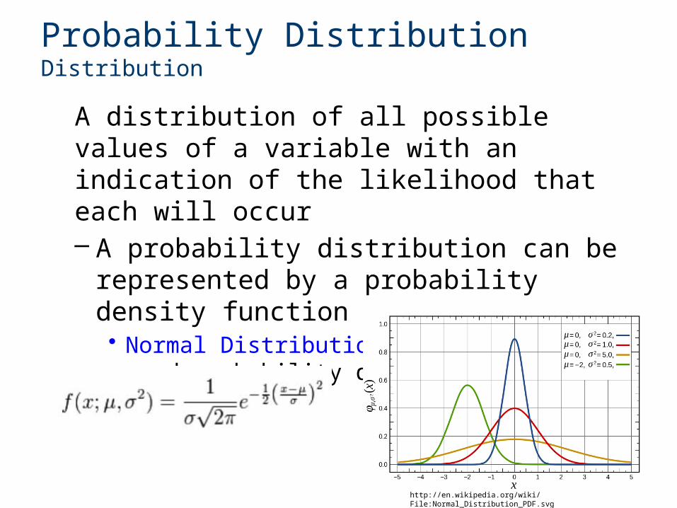
A distribution of all possible values of a variable with an indication of the likelihood that each will occur– A probability distribution can be represented
by a probability density function• Normal Distribution – most commonly used
probability distribution
Probability Distribution Distribution
http://en.wikipedia.org/wiki/File:Normal_Distribution_PDF.svg
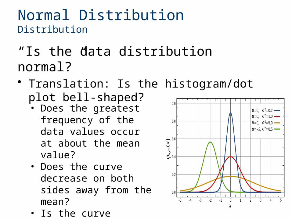
“Is the data distribution normal?”• Translation: Is the histogram/dot plot bell-
shaped?
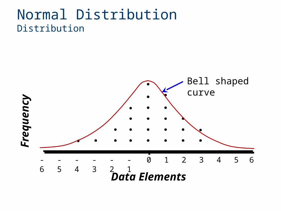
Normal Distribution Distribution
• Does the greatest frequency of the data values occur at about the mean value?
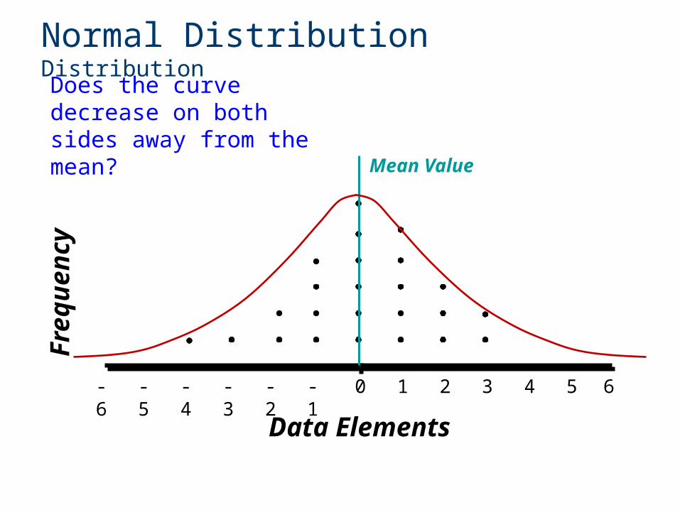
• Does the curve decrease on both sides away from the mean?
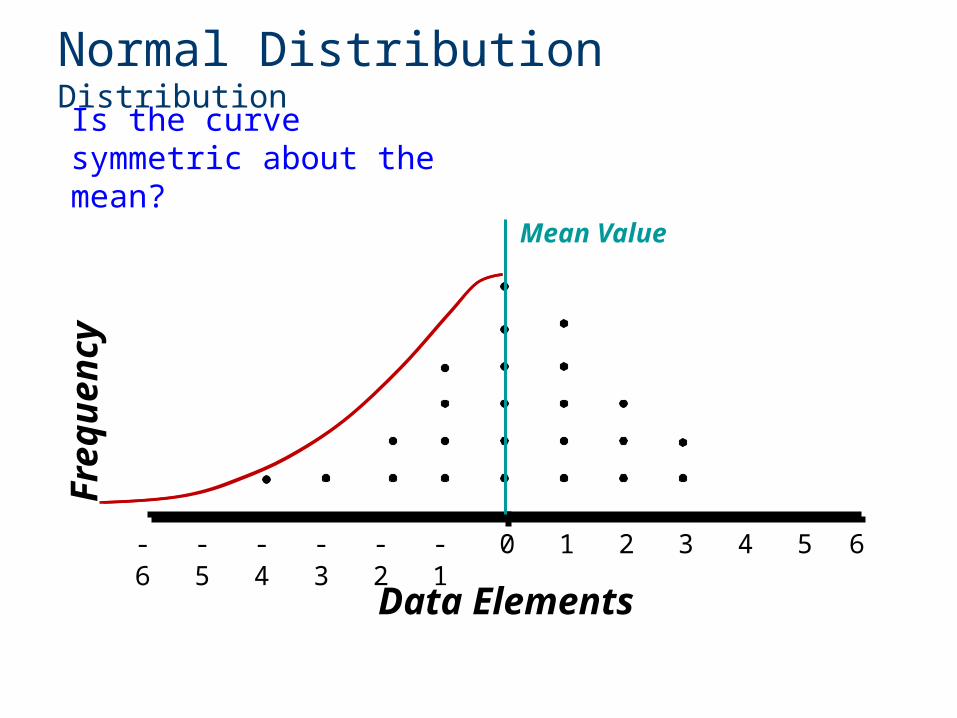
• Is the curve symmetric about the mean?
Fre
qu
ency
Data Elements
0 1 2 3 4 5 6-1-2-3-4-5-6
Bell shaped curve
Normal Distribution Distribution

Fre
qu
ency
Data Elements
0 1 2 3 4 5 6-1-2-3-4-5-6
Mean Value
Normal Distribution Distribution
Does the greatest frequency of the data values occur at about the mean value?
Fre
qu
ency
Data Elements
0 1 2 3 4 5 6-1-2-3-4-5-6
Mean Value
Normal Distribution Distribution
Does the curve decrease on both sides away from the mean?
Fre
qu
ency
Data Elements
0 1 2 3 4 5 6-1-2-3-4-5-6
Mean Value
Normal Distribution Distribution
Is the curve symmetric about the mean?
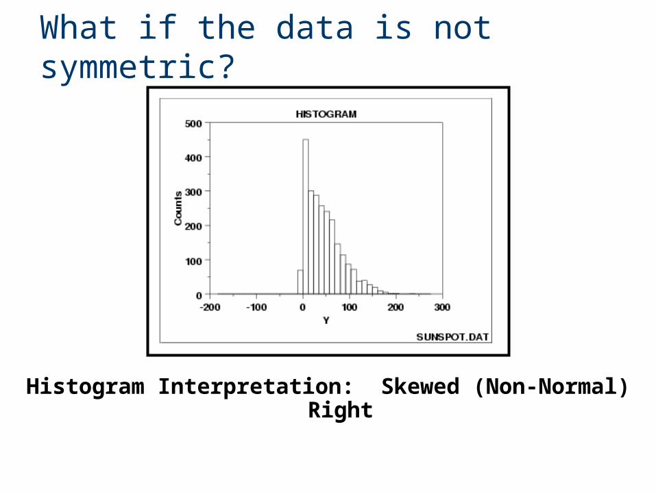
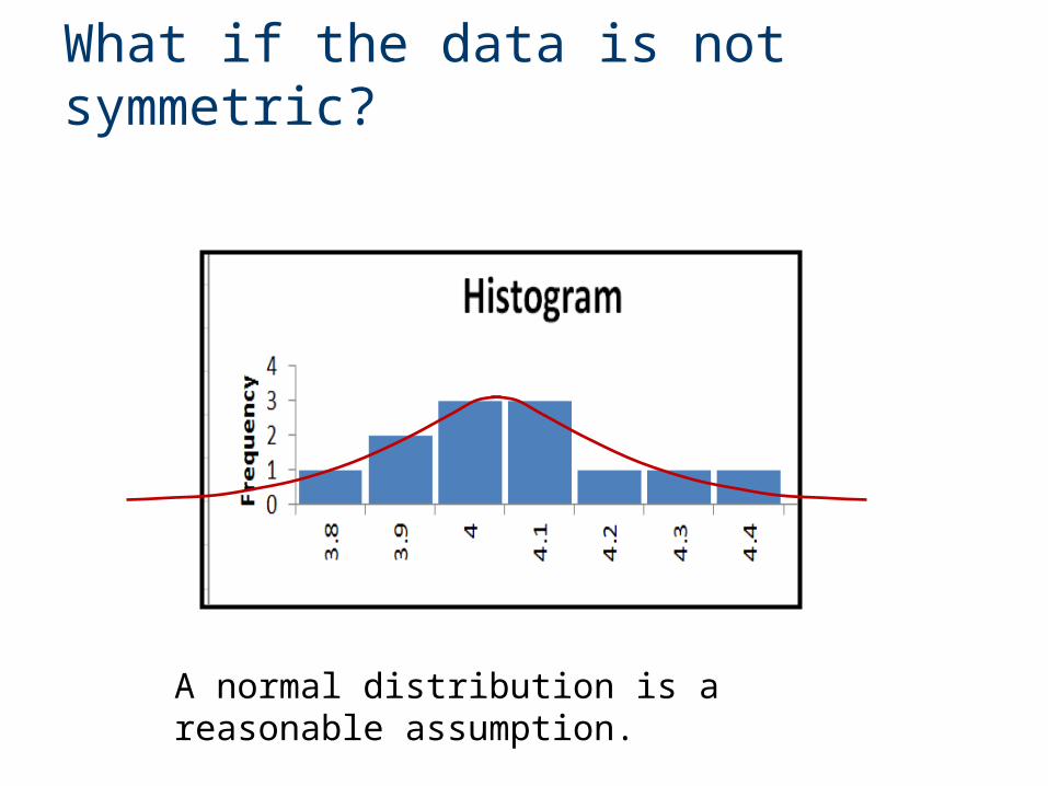
What if the data is not symmetric?
Histogram Interpretation: Skewed (Non-Normal) Right
What if the data is not symmetric?
A normal distribution is a reasonable assumption.
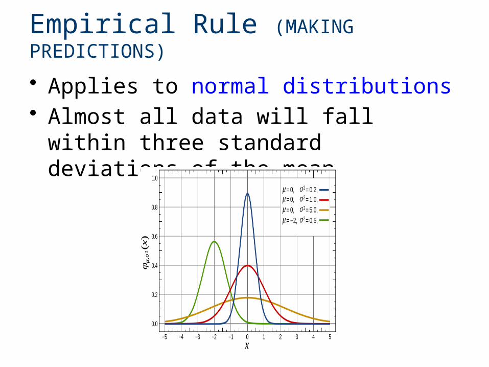
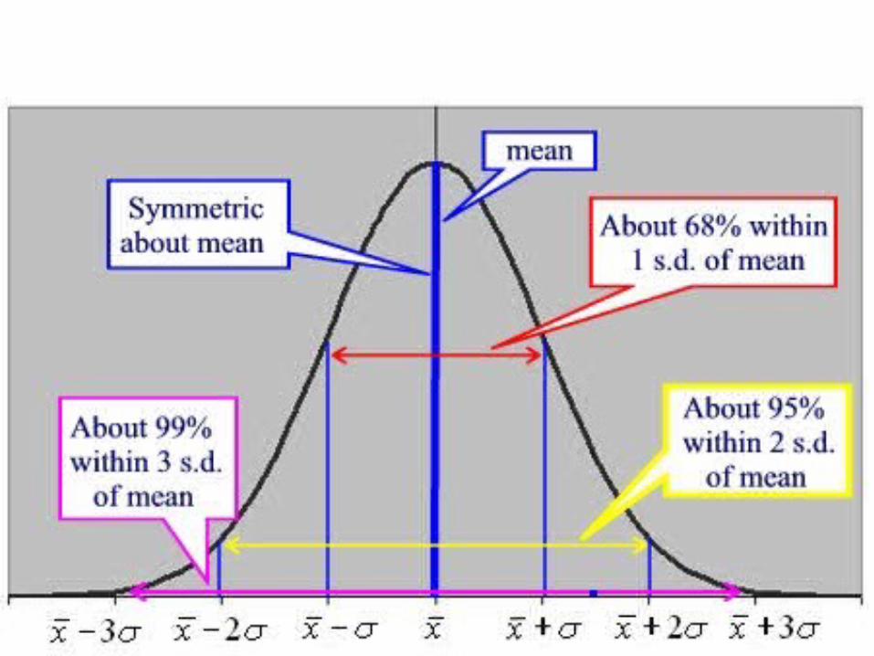
• Applies to normal distributions• Almost all data will fall within three
standard deviations of the mean
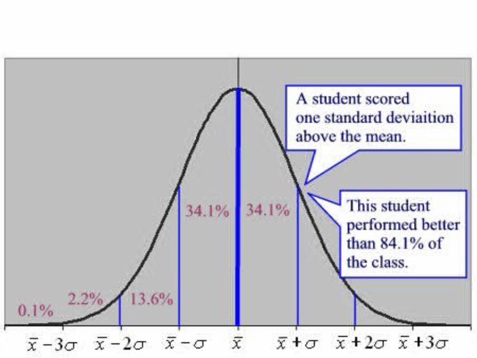
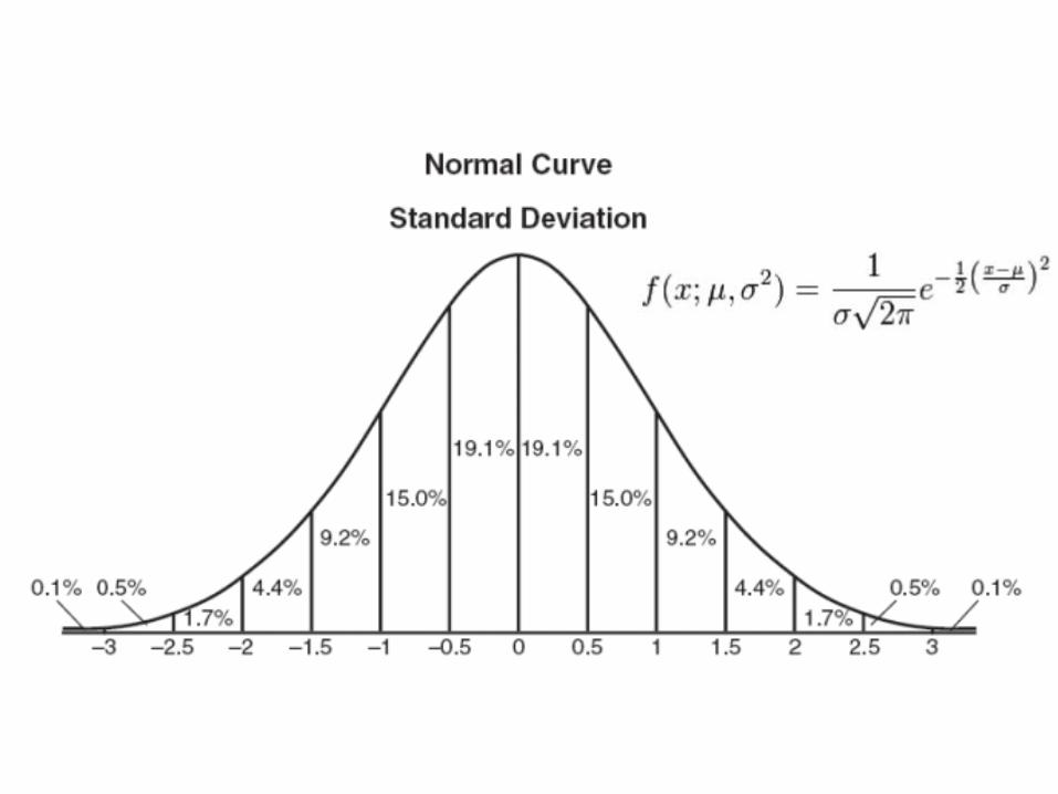
Empirical Rule (MAKING PREDICTIONS)
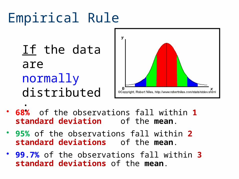
• 68% of the observations fall within 1 standard deviation of the mean.
• 95% of the observations fall within 2 standard deviations of the mean.
• 99.7% of the observations fall within 3 standard deviations of the mean.
Empirical Rule
If the data are normally distributed:
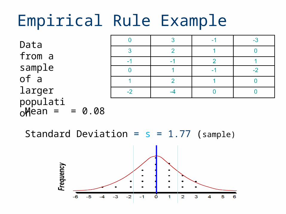
Empirical Rule ExampleData from a sample of a larger population
Mean = = 0.08
Standard Deviation = s = 1.77 (sample)
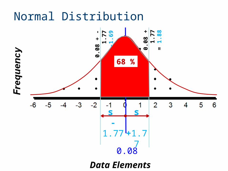
Data Elements
Normal Distribution
0.08
s +1.77
s -1.77
0.08
+ 1
.77
= 1
.88
0.08
+ -
1.7
7=
-1.
69
68 %
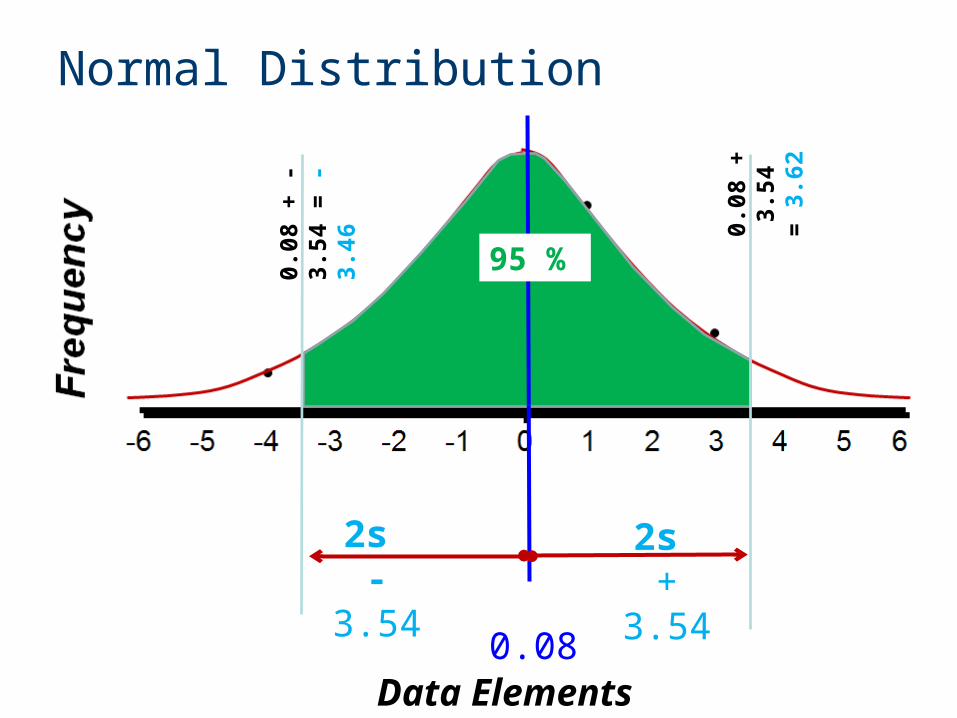
Data Elements
Normal Distribution
2s - 3.54
2s + 3.54
0.08
+ 3
.54
= 3
.62
0.08
+ -
3.54
=
- 3
.46
95 %
0.08
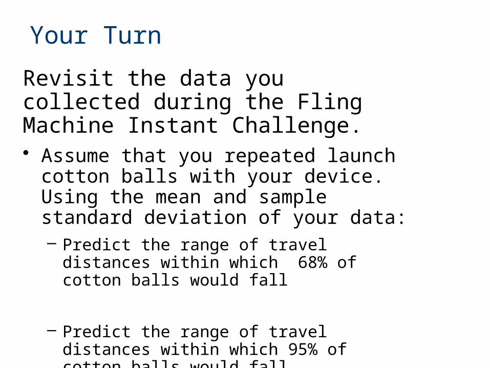
Your Turn
Revisit the data you collected during the Fling Machine Instant Challenge. • Assume that you repeated launch cotton
balls with your device. Using the mean and sample standard deviation of your data: – Predict the range of travel distances within
which 68% of cotton balls would fall
– Predict the range of travel distances within which 95% of cotton balls would fall
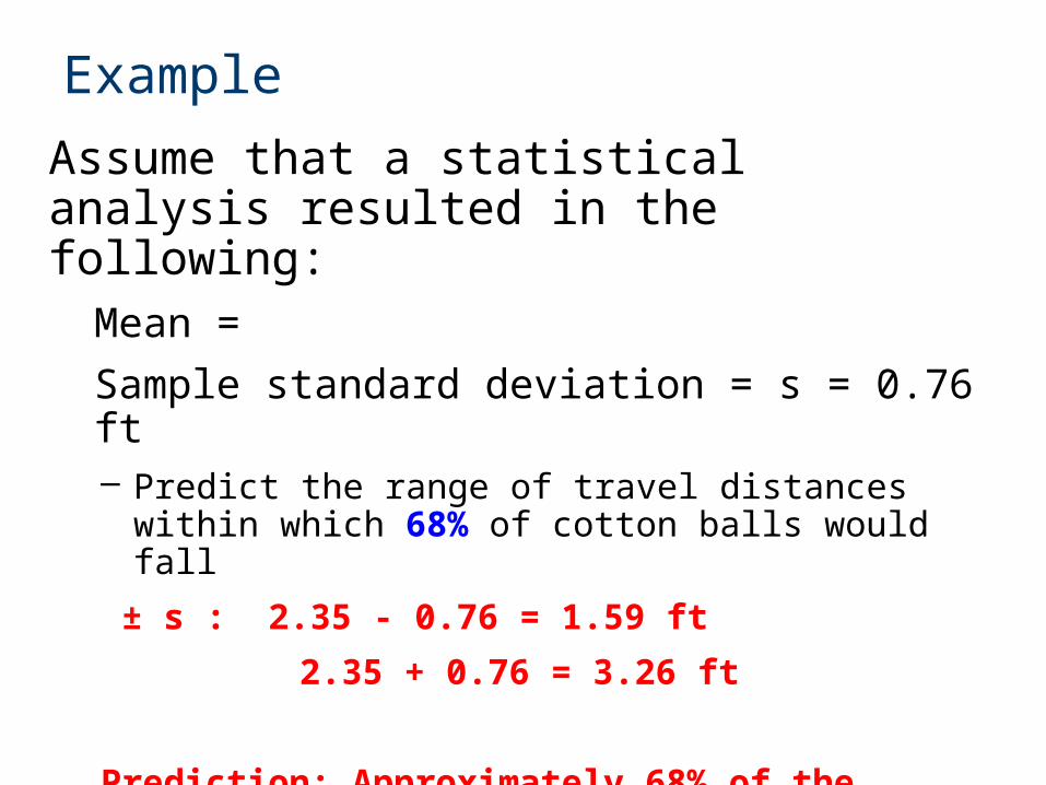
Example
Assume that a statistical analysis resulted in the following:
Mean =
Sample standard deviation = s = 0.76 ft– Predict the range of travel distances within which 68%
of cotton balls would fall
± s : 2.35 - 0.76 = 1.59 ft
2.35 + 0.76 = 3.26 ft
Prediction: Approximately 68% of the launches will result in a travel distance between 1.59 ft and 3.26 ft.
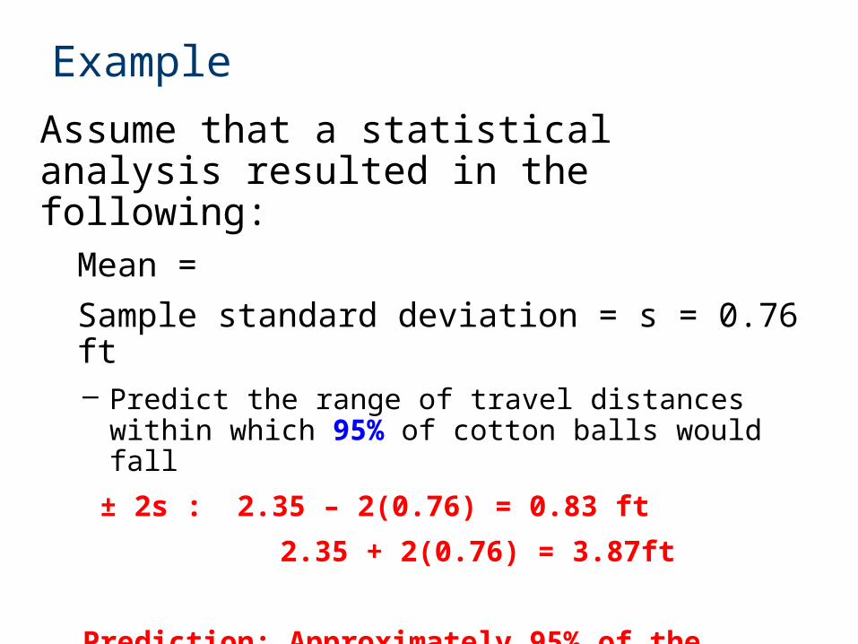
Example
Assume that a statistical analysis resulted in the following:
Mean =
Sample standard deviation = s = 0.76 ft– Predict the range of travel distances within which 95%
of cotton balls would fall
± 2s : 2.35 – 2(0.76) = 0.83 ft
2.35 + 2(0.76) = 3.87ft
Prediction: Approximately 95% of the launches will result in a travel distance between 0.83 ft and 3.86 ft.
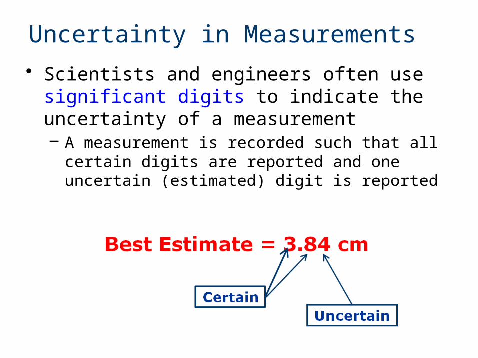
Uncertainty in Measurements
• Scientists and engineers often use significant digits to indicate the uncertainty of a measurement– A measurement is recorded such that all certain digits
are reported and one uncertain (estimated) digit is reported
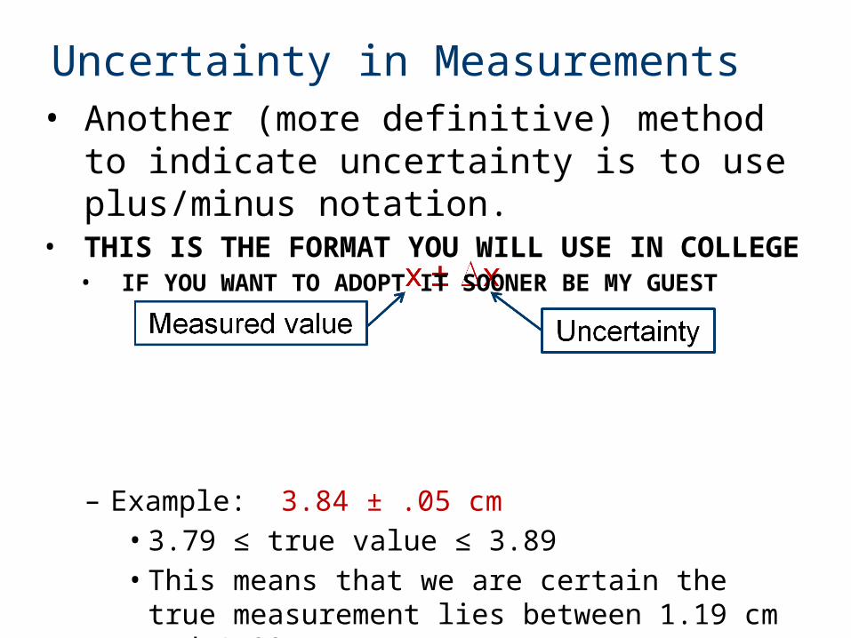
Uncertainty in Measurements• Another (more definitive) method to indicate
uncertainty is to use plus/minus notation.• THIS IS THE FORMAT YOU WILL USE IN
COLLEGE• IF YOU WANT TO ADOPT IT SOONER BE MY GUEST
– Example: 3.84 ± .05 cm • 3.79 ≤ true value ≤ 3.89• This means that we are certain the true
measurement lies between 1.19 cm and 1.29 cm
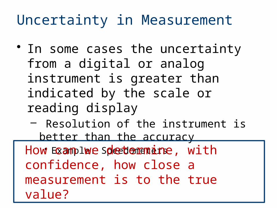
Uncertainty in Measurement
• In some cases the uncertainty from a digital or analog instrument is greater than indicated by the scale or reading display– Resolution of the instrument is better than the
accuracy• Example: Speedometers
How can we determine, with confidence, how close a measurement is to the true value?
Uncertainty in Measurement
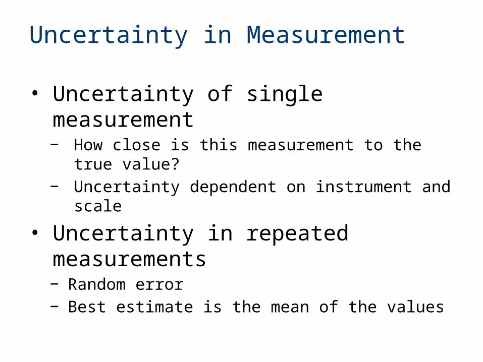
• Uncertainty of single measurement− How close is this measurement to the true value?− Uncertainty dependent on instrument and scale
• Uncertainty in repeated measurements− Random error− Best estimate is the mean of the values
Accuracy and Precision
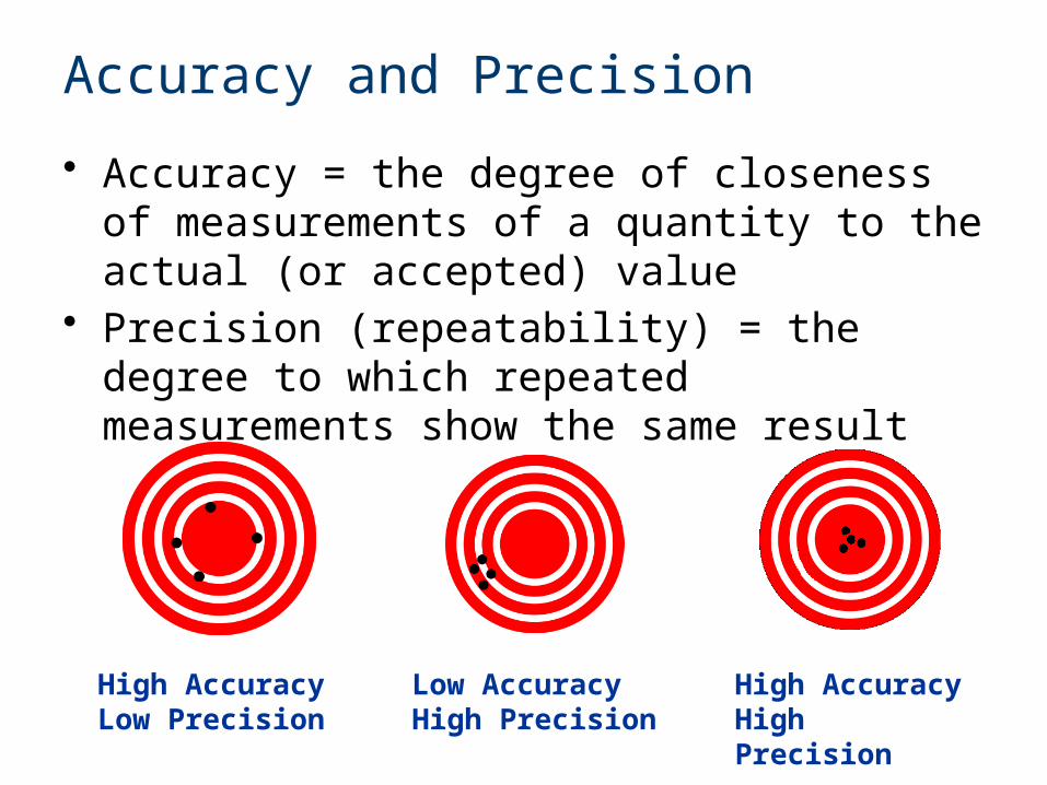
• Accuracy = the degree of closeness of measurements of a quantity to the actual (or accepted) value
• Precision (repeatability) = the degree to which repeated measurements show the same result
High AccuracyLow Precision
Low AccuracyHigh Precision
High AccuracyHigh Precision
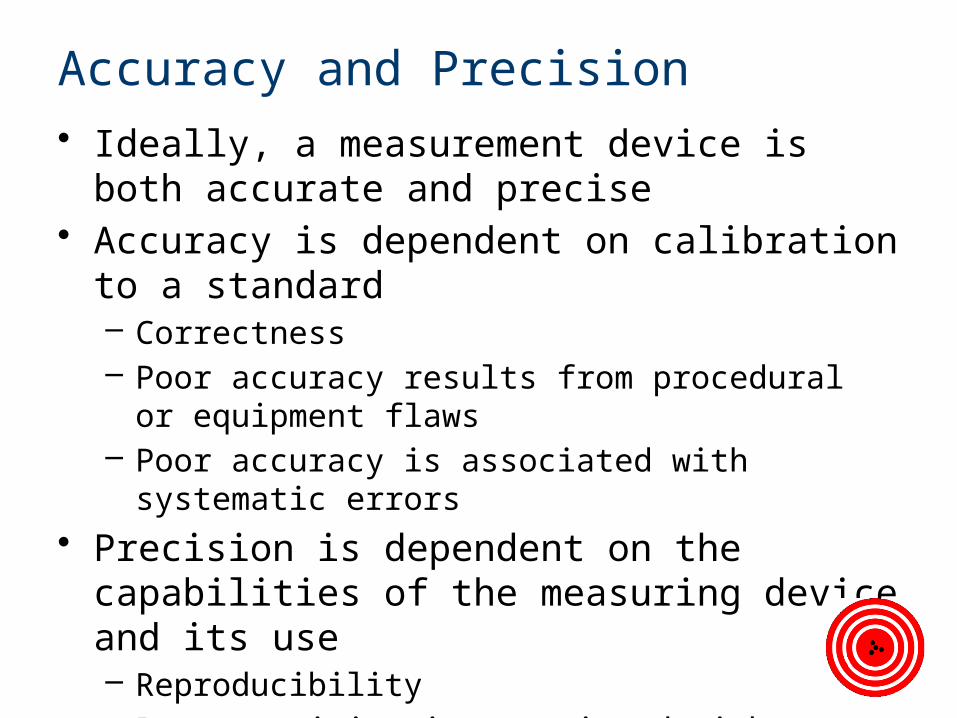
Accuracy and Precision• Ideally, a measurement device is both accurate
and precise• Accuracy is dependent on calibration to a
standard– Correctness– Poor accuracy results from procedural or equipment
flaws– Poor accuracy is associated with systematic errors
• Precision is dependent on the capabilities of the measuring device and its use– Reproducibility– Poor precision is associated with random error
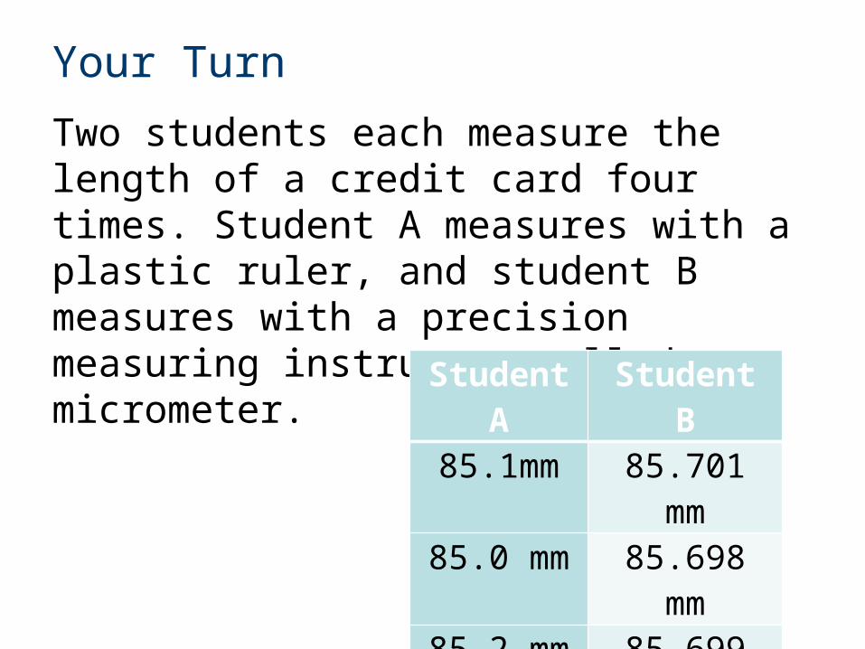
Your Turn
Two students each measure the length of a credit card four times. Student A measures with a plastic ruler, and student B measures with a precision measuring instrument called a micrometer.
Student A Student B85.1mm 85.701 mm
85.0 mm 85.698 mm
85.2 mm 85.699 mm
84.9 mm 85.701 mm
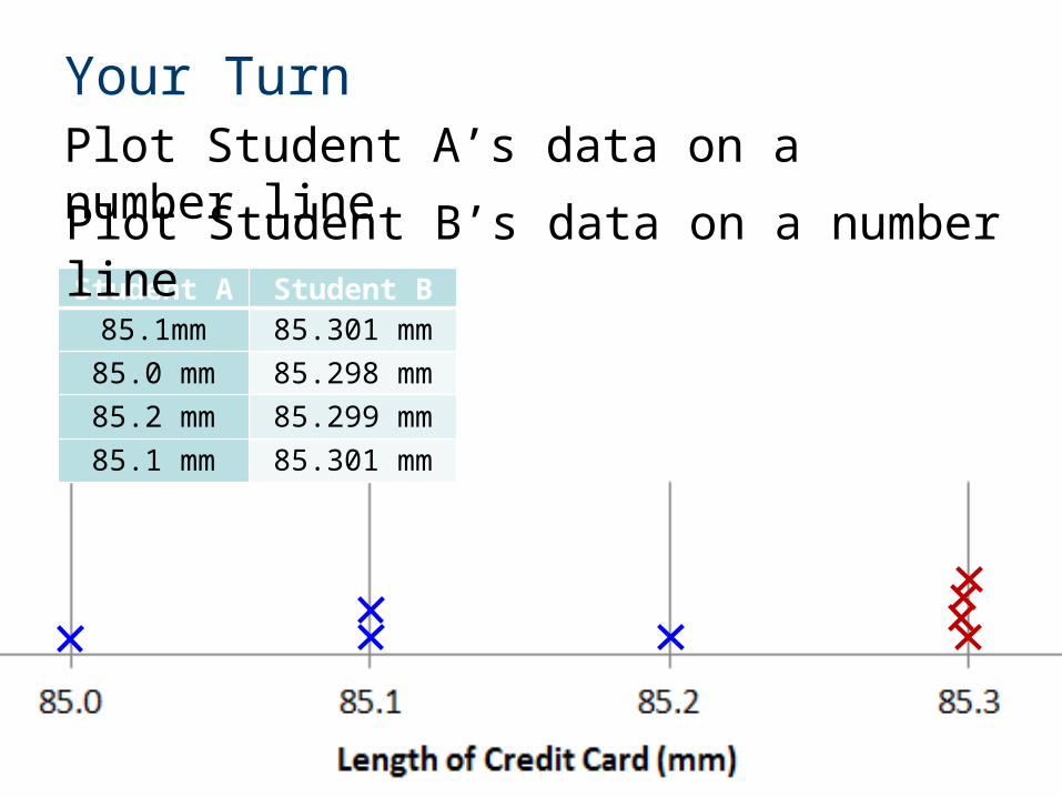
Your TurnPlot Student A’s data on a number line
Student A Student B85.1mm 85.301 mm
85.0 mm 85.298 mm
85.2 mm 85.299 mm
85.1 mm 85.301 mm
Plot Student B’s data on a number line
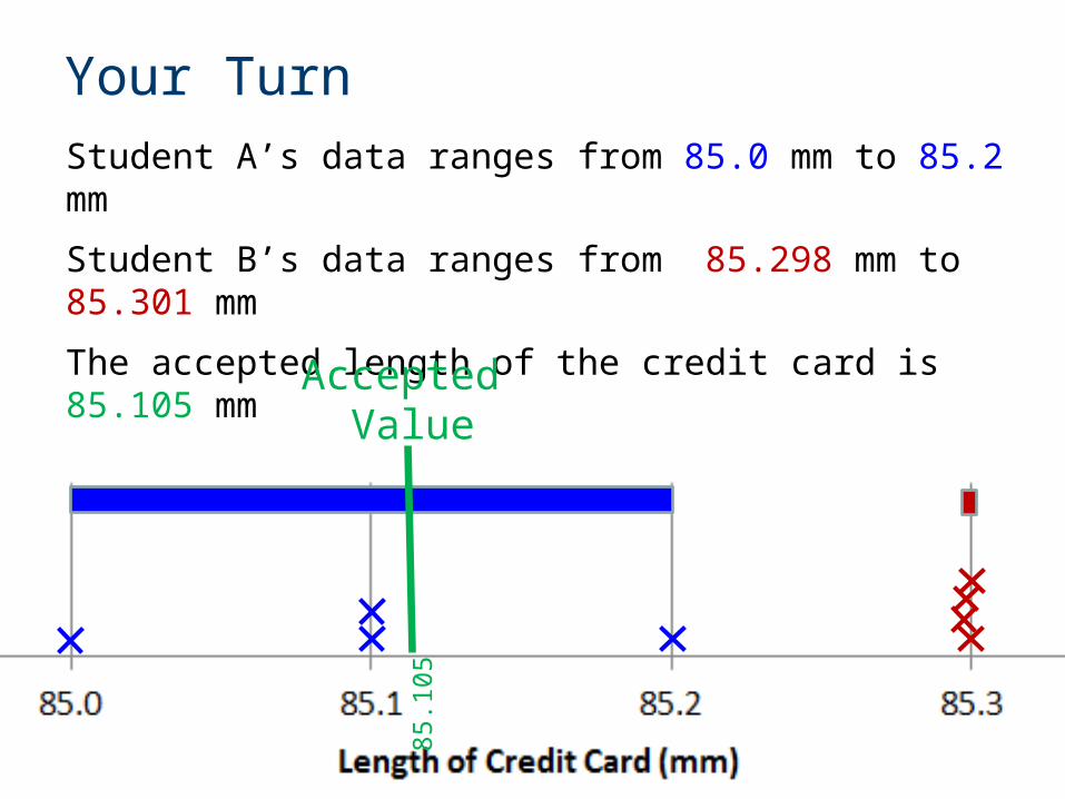
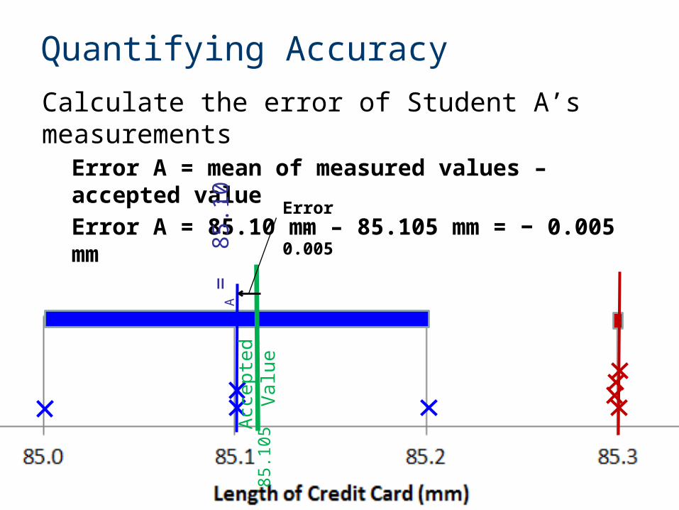
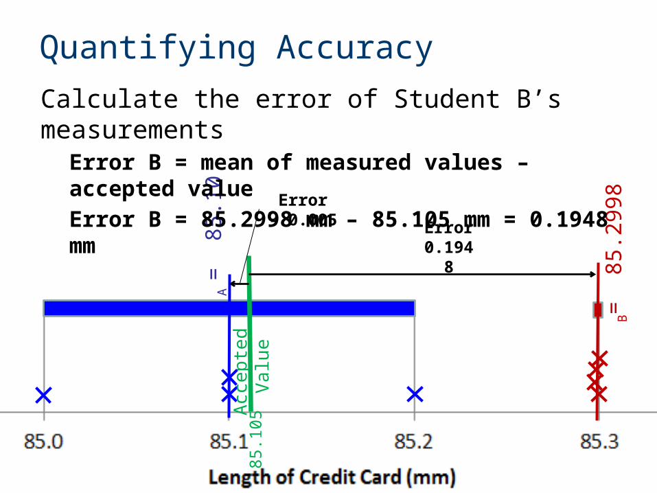
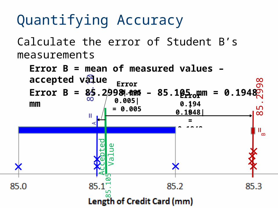
Your TurnStudent A’s data ranges from 85.0 mm to 85.2 mm
Student B’s data ranges from 85.298 mm to 85.301 mm
The accepted length of the credit card is 85.105 mm
85.1
05
Accepted Value
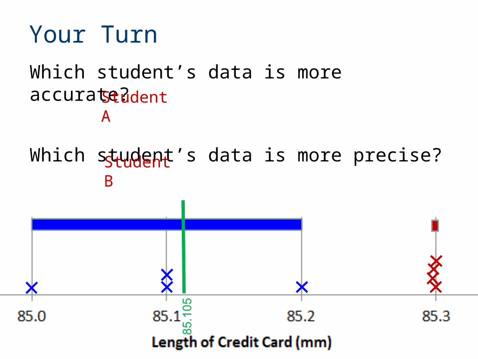
Your Turn
Which student’s data is more accurate?
Which student’s data is more precise?
Student A
Student B
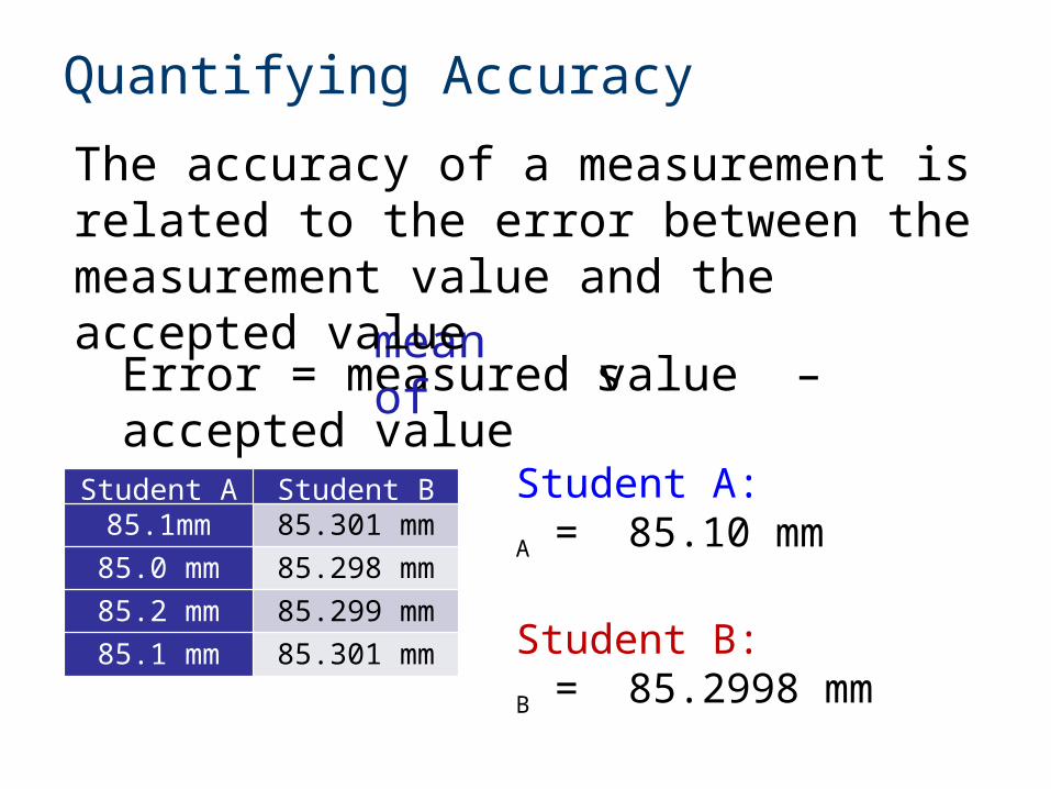
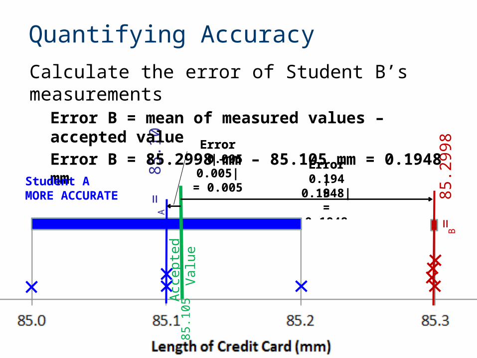
Quantifying Accuracy
Error = measured value – accepted valuemean of
s
Student A Student B85.1mm 85.301 mm
85.0 mm 85.298 mm
85.2 mm 85.299 mm
85.1 mm 85.301 mm
Student A:
A = 85.10 mm
Student B:
B = 85.2998 mm
The accuracy of a measurement is related to the error between the measurement value and the accepted value
Quantifying Accuracy
Calculate the error of Student A’s measurementsError A = mean of measured values – accepted value
Error A = 85.10 mm – 85.105 mm = − 0.005 mm
A =
85
.10
85.1
05
Error- 0.005
Acc
ep
ted
V
alu
e
Quantifying Accuracy
A =
85
.10
Acc
ep
ted
V
alu
e85
.105
Error- 0.005 Error
0.1948
B=
85
.299
8
Calculate the error of Student B’s measurementsError B = mean of measured values – accepted value
Error B = 85.2998 mm – 85.105 mm = 0.1948 mm
Error|0.1948|= 0.1948
Quantifying Accuracy
A =
85
.10
Acc
ep
ted
V
alu
e85
.105
Error- 0.005 Error
0.1948
B=
85
.299
8
Calculate the error of Student B’s measurementsError B = mean of measured values – accepted value
Error B = 85.2998 mm – 85.105 mm = 0.1948 mm
Error|- 0.005|= 0.005
Error|0.1948|= 0.1948
Quantifying Accuracy
A =
85
.10
Acc
ep
ted
V
alu
e85
.105
Error- 0.005 Error
0.1948
B=
85
.299
8
Calculate the error of Student B’s measurementsError B = mean of measured values – accepted value
Error B = 85.2998 mm – 85.105 mm = 0.1948 mm
Error|- 0.005|= 0.005
Student AMORE ACCURATE
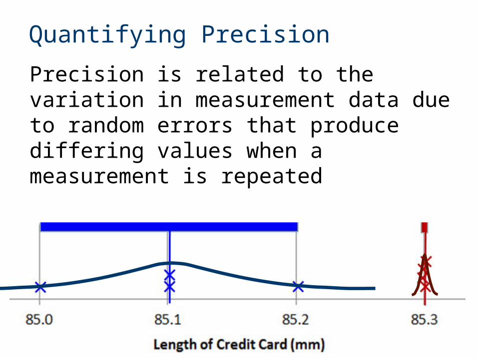
Quantifying Precision
Precision is related to the variation in measurement data due to random errors that produce differing values when a measurement is repeated
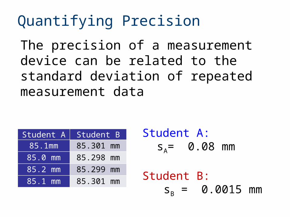
Quantifying Precision
Student A Student B85.1mm 85.301 mm
85.0 mm 85.298 mm
85.2 mm 85.299 mm
85.1 mm 85.301 mm
Student A: sA= 0.08 mm
Student B: sB = 0.0015 mm
The precision of a measurement device can be related to the standard deviation of repeated measurement data
Quantifying Precision
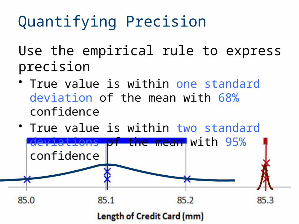
Use the empirical rule to express precision• True value is within one standard deviation of the
mean with 68% confidence• True value is within two standard deviations of the
mean with 95% confidence
Quantifying Precision
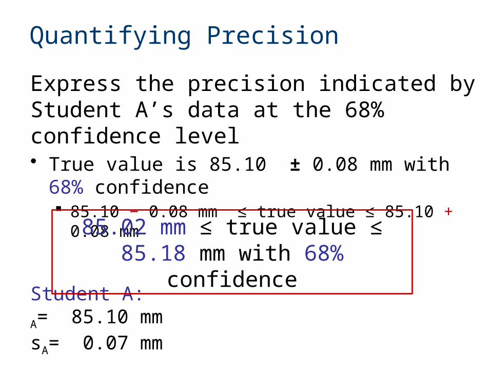
Express the precision indicated by Student A’s data at the 68% confidence level• True value is 85.10 ± 0.08 mm with 68%
confidence 85.10 − 0.08 mm ≤ true value ≤ 85.10 + 0.08 mm
Student A:
A= 85.10 mmsA= 0.07 mm
85.02 mm ≤ true value ≤ 85.18 mm with 68% confidence

Quantifying Precision
Express the precision indicated by Student A’s data at the 95% confidence level• True value is 85.10 ± 2(0.08) mm with 95%
confidence 85.10 − 0.16 mm ≤ true value ≤ 85.10 + 0.16 mm
Student A:
A= 85.10 mmsA= 0.07 mm
84.94 mm ≤ true value ≤ 85.26 mm with 95% confidence
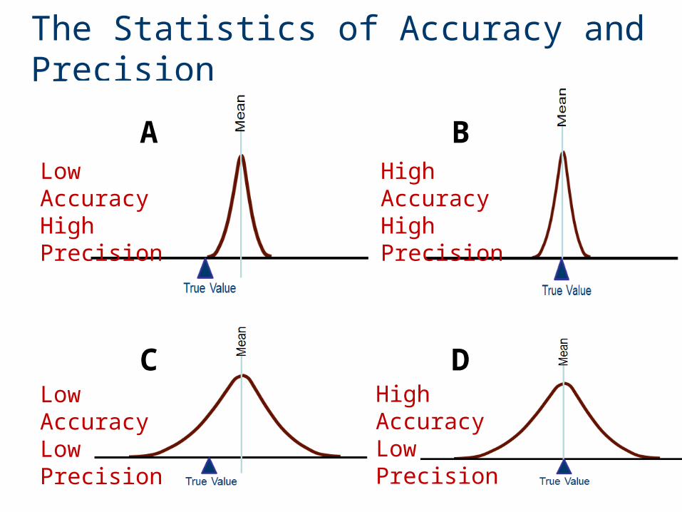
The Statistics of Accuracy and Precision
A B
C D
High AccuracyHigh Precision
Low AccuracyLow Precision
High AccuracyLow Precision
Low AccuracyHigh Precision