statistics of unnatural images - computer sciencedhulena/math_126_project_report.pdfabstract:...
TRANSCRIPT

Statistics of Unnatural Images Nimit Dhulekar
MATH 126: Current Problems in
Applied Mathematics:
Mathematical Methods & Models in
Visual Neuroscience

Table of Contents:
Abstract:................................................................................................................3 Introduction: ..........................................................................................................3 Discussion: ...........................................................................................................4 Conclusion: .........................................................................................................28 References: ........................................................................................................29
Abstract:
Natural images follow certain regularities, particularly in second-order statistics. Studies by [1-7] have shown that the power spectrum of natural images falls off at the rate 1/fα with α = 2. In this project we investigate whether unnatural
images also exhibit this property. We also compute the angular and rotational power spectrum of these images. By unnatural images, we imply images that are not seen commonly in nature and also are not used extensively in research. We choose 3 categories of such images; namely celestial, underwater and micro scale. A corollary goal of this project was to see how well the ensemble power spectral density approximates the power spectrum of individual images.
Introduction:
Extensive research has been done on natural images statistics. But there have been no similar studies done on unnatural images. Unnatural images are different from natural images in many respects. In some cases they require special cameras to capture the image. This is true for both celestial and micro scale images. On one hand powerful telescope cameras are required to capture images of distant heavenly bodies. On the other hand powerful microscopes are required to collect images of the microbial world. Techniques such as confocal microscopy, darkfield illumination, brightfield illumination etc are required to obtain focussed images. For underwater photography special water-resistant cameras are used. The photographers also have to take into account the amount of illumination, the motion of the flora or fauna they are trying to capture, the wear and tear of the equipment because of the salt content in water etc. These challenges and limitations make unnatural images quite different from natural images. Thus it is interesting to investigate whether such images also follow certain regularities in second-order statistics. For the purpose of this project, the celestial images were randomly chosen from http://antwrp.gsfc.nasa.gov/apod/archivepix.html. The underwater images were taken from a multitude of websites by searching through Google images. The micro scale images were taken from the Nikon Small World Gallery http://www.nikonsmallworld.com/gallery/year/2009/1 Sample images belonging to each category are displayed in Figure 1. For each category more than 150 images are considered of size 512 by 512. The images are converted to gray scale before being used.

Figure 1: Sample images from all 3 categories of unnatural images
Discussion:
The mean power spectra (using polar coordinates) is given by
in which the shape of the spectra is a function of orientation. The function As(θ )
is the amplitude scaling factor for each orientation and α s(θ ) is the frequency
exponent as a function of orientation. Both these factors contribute to the shape of the power spectra. Taking the log of the above equation, we can estimate the values ofα .
For the purpose of the implementation we use the following formulation of the power spectrum formula
where F(u,v) is the 2-D Fourier transform of the image and F*(u,v) is its complex conjugate. All images are of size M by N where M and N are both 512. L is the number of images in the set (> 150).
Celestial Images
Underwater Images
Micro scale Images
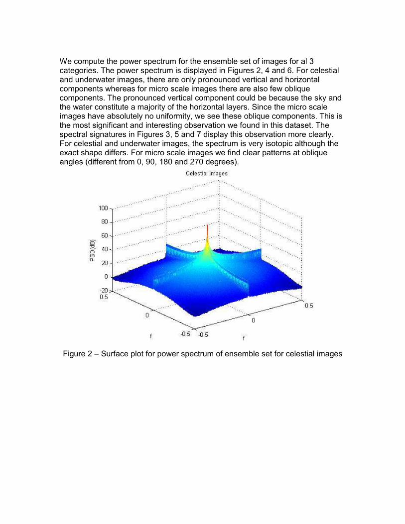
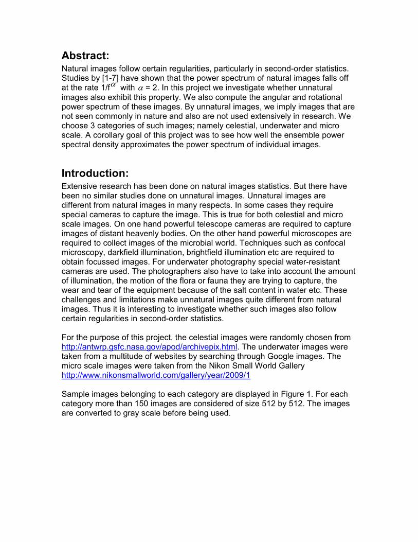
We compute the power spectrum for the ensemble set of images for al 3 categories. The power spectrum is displayed in Figures 2, 4 and 6. For celestial and underwater images, there are only pronounced vertical and horizontal components whereas for micro scale images there are also few oblique components. The pronounced vertical component could be because the sky and the water constitute a majority of the horizontal layers. Since the micro scale images have absolutely no uniformity, we see these oblique components. This is the most significant and interesting observation we found in this dataset. The spectral signatures in Figures 3, 5 and 7 display this observation more clearly. For celestial and underwater images, the spectrum is very isotopic although the exact shape differs. For micro scale images we find clear patterns at oblique angles (different from 0, 90, 180 and 270 degrees).
Figure 2 – Surface plot for power spectrum of ensemble set for celestial images
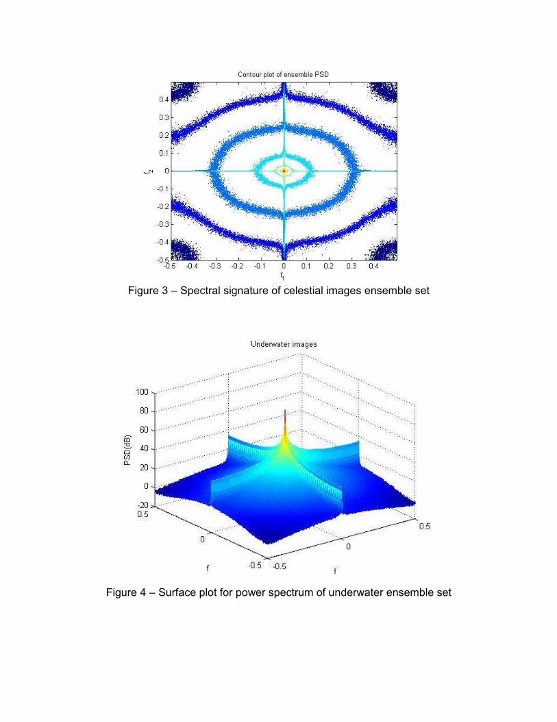
Figure 3 – Spectral signature of celestial images ensemble set
Figure 4 – Surface plot for power spectrum of underwater ensemble set

Figure 5 – Spectral signature of underwater ensemble set
Figure 6 – Surface plot for power spectrum for micro scale ensemble set

Figure 7 – Spectral signature of micro scale ensemble set
The following figures (8-16) display individual components, namely vertical, horizontal and oblique of the ensemble set of images, for all categories of images along with theα computed as the slope of the line which best approximates the
shape of the power spectrum. The values ofα have been tabulated in Table 1.
The average value ofα for each category is approximately 2. This is a statistic
that unnatural images seem to share with natural images (see 6-7 for description of power law in natural images).
Figure 8 – Celestial images ensemble power spectrum estimate (Horizontal)
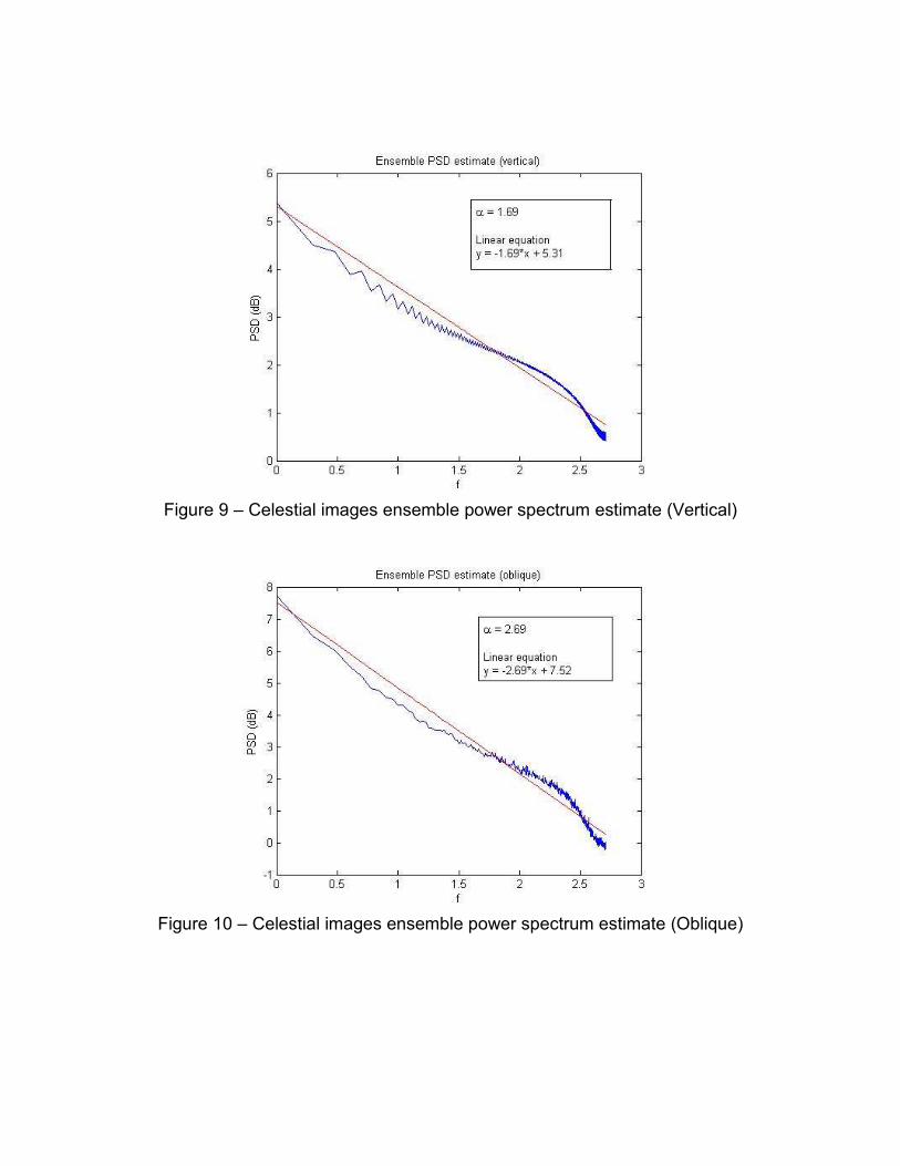
Figure 9 – Celestial images ensemble power spectrum estimate (Vertical)
Figure 10 – Celestial images ensemble power spectrum estimate (Oblique)

Figure 11 – Underwater images ensemble power spectrum estimate (Horizontal)
Figure 12 – Underwater images ensemble power spectrum estimate (Vertical)

Figure 13 – Underwater images ensemble power spectrum estimate (Oblique)
Figure 14 – Micro scale images ensemble power spectrum estimate (Horizontal)

Figure 15 – Micro scale images ensemble power spectrum estimate (Vertical)
Figure 16 – Micro scale images ensemble power spectrum estimate (Oblique)
Horizontal Vertical Oblique Average
Celestial 1.47 1.69 2.69 1.95
Underwater 1.83 1.95 3.18 2.32
Micro scale 1.79 2.01 3.14 2.31
Table 1: Values ofα for ensemble image sets
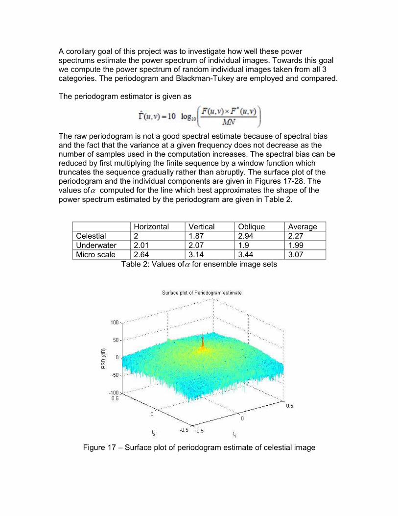
A corollary goal of this project was to investigate how well these power spectrums estimate the power spectrum of individual images. Towards this goal we compute the power spectrum of random individual images taken from all 3 categories. The periodogram and Blackman-Tukey are employed and compared. The periodogram estimator is given as
The raw periodogram is not a good spectral estimate because of spectral bias and the fact that the variance at a given frequency does not decrease as the number of samples used in the computation increases. The spectral bias can be reduced by first multiplying the finite sequence by a window function which truncates the sequence gradually rather than abruptly. The surface plot of the periodogram and the individual components are given in Figures 17-28. The values ofα computed for the line which best approximates the shape of the
power spectrum estimated by the periodogram are given in Table 2.
Horizontal Vertical Oblique Average
Celestial 2 1.87 2.94 2.27
Underwater 2.01 2.07 1.9 1.99
Micro scale 2.64 3.14 3.44 3.07
Table 2: Values ofα for ensemble image sets
Figure 17 – Surface plot of periodogram estimate of celestial image
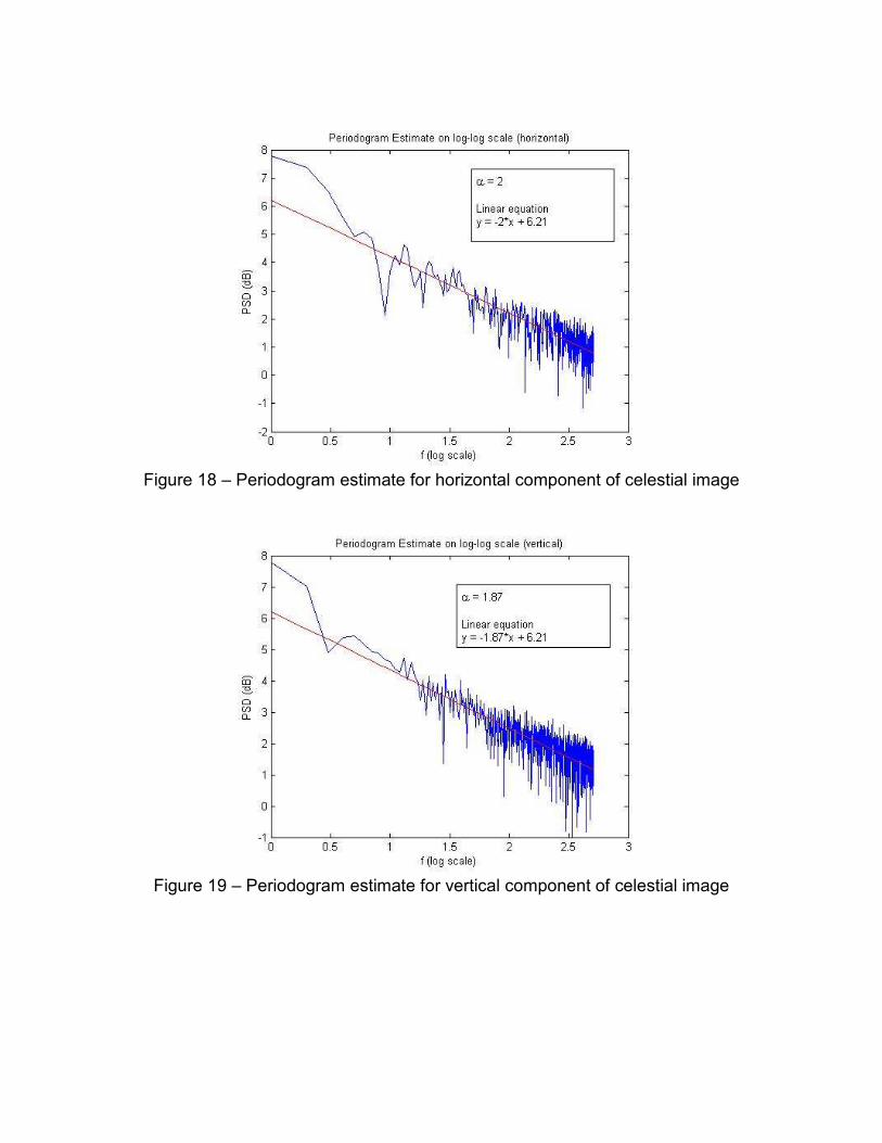
Figure 18 – Periodogram estimate for horizontal component of celestial image
Figure 19 – Periodogram estimate for vertical component of celestial image

Figure 20 – Periodogram estimate for oblique component of celestial image
Figure 21 – Surface plot of periodogram estimate of underwater image

Figure 22 – Periodogram estimate for horizontal component of underwater image
Figure 23 – Periodogram estimate for vertical component of underwater image
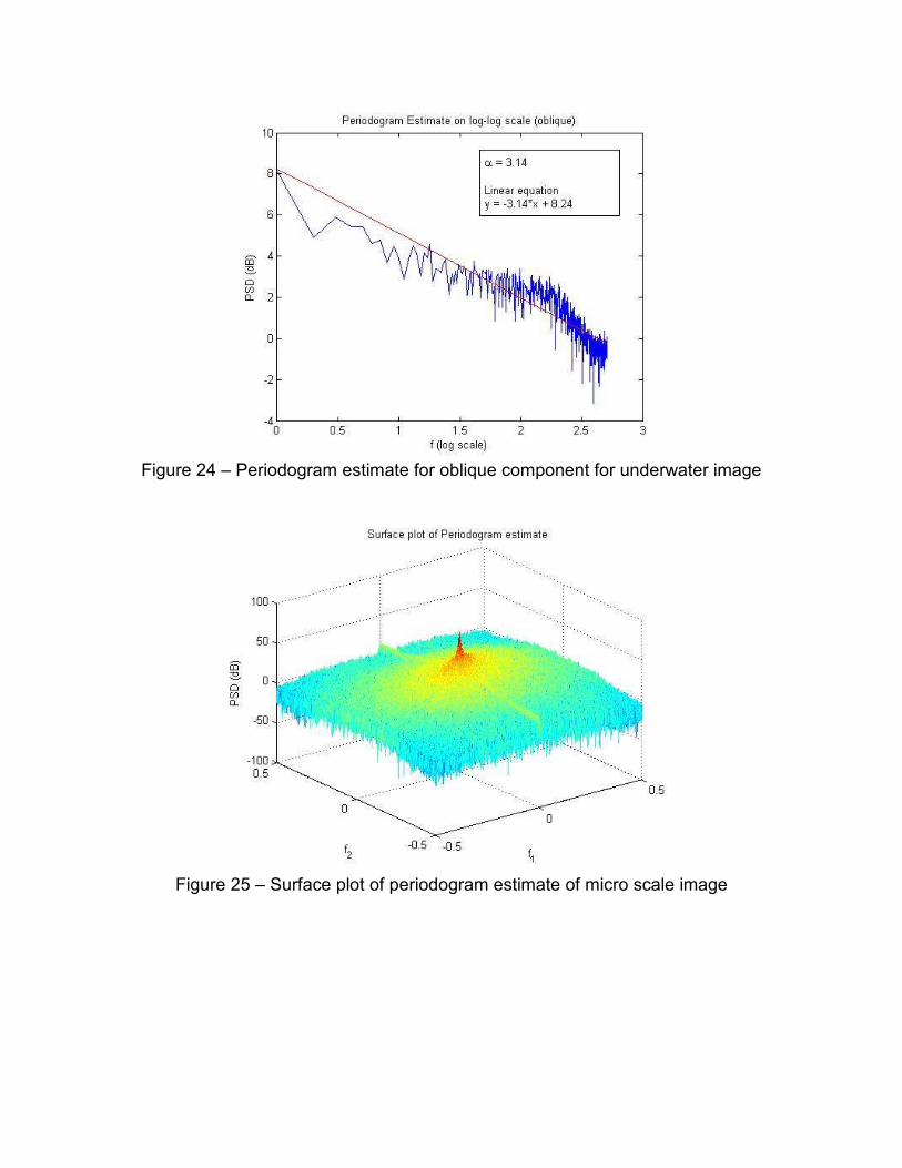
Figure 24 – Periodogram estimate for oblique component for underwater image
Figure 25 – Surface plot of periodogram estimate of micro scale image
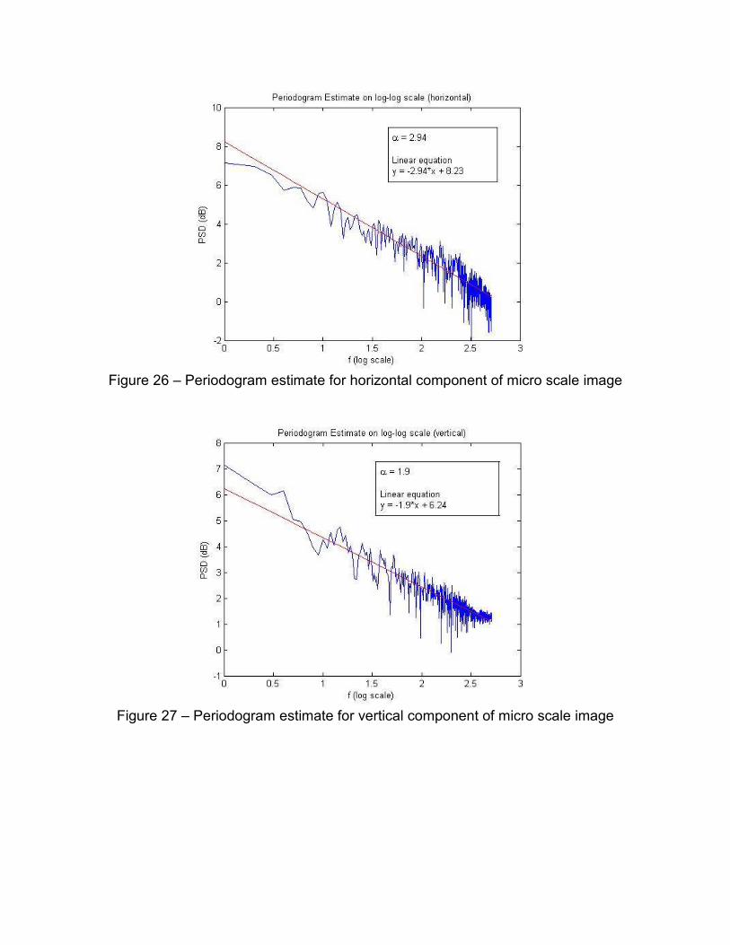
Figure 26 – Periodogram estimate for horizontal component of micro scale image
Figure 27 – Periodogram estimate for vertical component of micro scale image
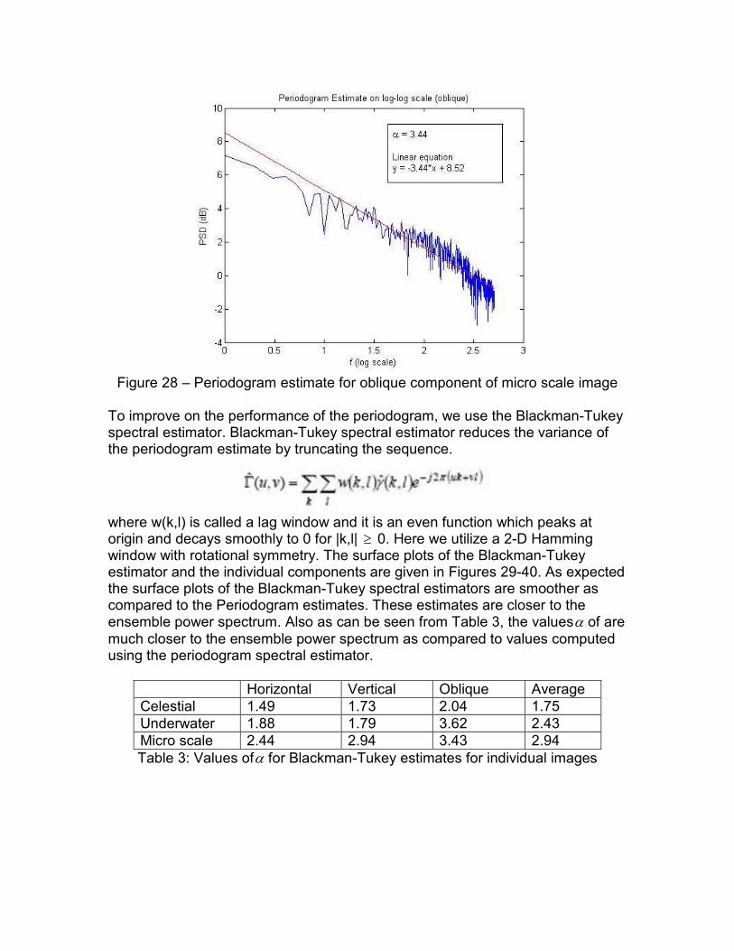
Figure 28 – Periodogram estimate for oblique component of micro scale image
To improve on the performance of the periodogram, we use the Blackman-Tukey spectral estimator. Blackman-Tukey spectral estimator reduces the variance of the periodogram estimate by truncating the sequence.
where w(k,l) is called a lag window and it is an even function which peaks at origin and decays smoothly to 0 for |k,l| ≥ 0. Here we utilize a 2-D Hamming window with rotational symmetry. The surface plots of the Blackman-Tukey estimator and the individual components are given in Figures 29-40. As expected the surface plots of the Blackman-Tukey spectral estimators are smoother as compared to the Periodogram estimates. These estimates are closer to the ensemble power spectrum. Also as can be seen from Table 3, the valuesα of are
much closer to the ensemble power spectrum as compared to values computed using the periodogram spectral estimator.
Horizontal Vertical Oblique Average
Celestial 1.49 1.73 2.04 1.75
Underwater 1.88 1.79 3.62 2.43
Micro scale 2.44 2.94 3.43 2.94
Table 3: Values ofα for Blackman-Tukey estimates for individual images
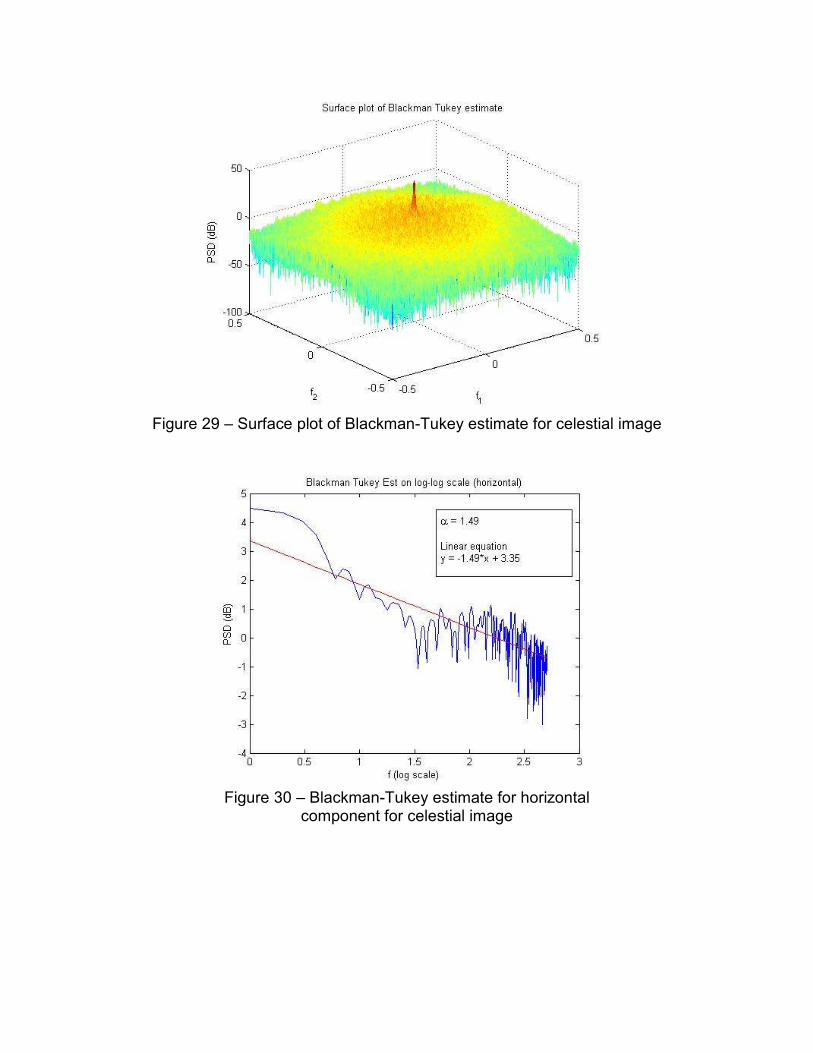
Figure 29 – Surface plot of Blackman-Tukey estimate for celestial image
Figure 30 – Blackman-Tukey estimate for horizontal
component for celestial image

Figure 31 – Blackman-Tukey estimate for vertical component for celestial image
Figure 32 – Blackman-Tukey estimate for oblique component for celestial image

Figure 33 – Surface plot of Blackman-Tukey estimate for underwater image
Figure 34 – Blackman-Tukey estimate of horizontal
component for underwater image
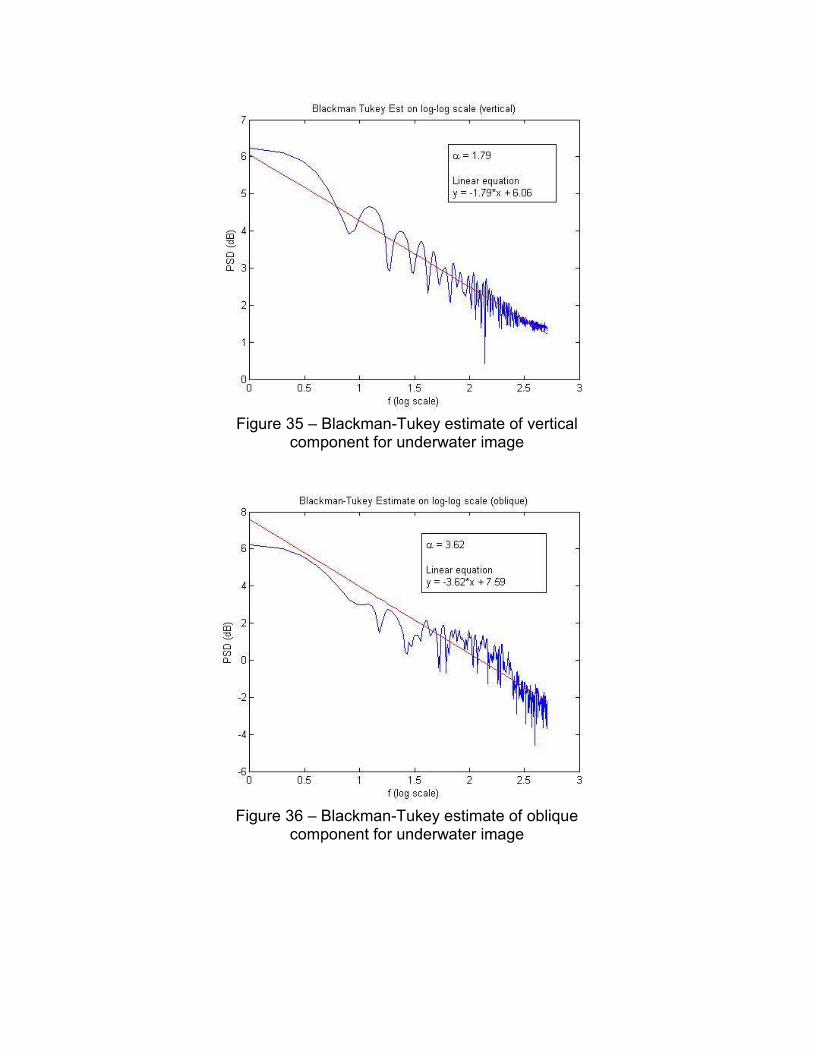
Figure 35 – Blackman-Tukey estimate of vertical
component for underwater image
Figure 36 – Blackman-Tukey estimate of oblique
component for underwater image
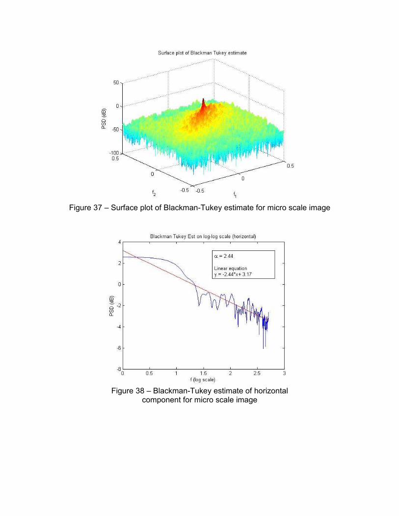
Figure 37 – Surface plot of Blackman-Tukey estimate for micro scale image
Figure 38 – Blackman-Tukey estimate of horizontal
component for micro scale image

Figure 39 – Blackman-Tukey estimate of vertical
component for micro scale image
Figure 40 – Blackman-Tukey estimate of oblique
component for micro scale image
Having seen that the power spectrum can be estimated to a certain degree of accuracy, we look at the rotational and angular averages of the power spectra of these images. The rotational average of the power spectrum is computed for each frequency. To avoid artefacts in the analysis, only the frequency range between 10 and 256 cycles per image was used. The angular average is

computed for angles in the range (- ππ : ). Figures 41-46 display the rotationally
averaged and angularly averaged power spectrum of the entire ensemble set for all 3 categories of images. The rotationally averaged power spectrum seems to be concentrated between 1010 and 1014. The angularly averaged power spectrum is most peaky for the micro scale images. This follows from the surface plots seen where it was clear that micro scale images have significant power also at oblique angles.
Figure 41 – Rotationally averaged power spectrum for
the ensemble set of celestial images
Figure 42 – Angularly averaged power spectrum for
the ensemble set of celestial images
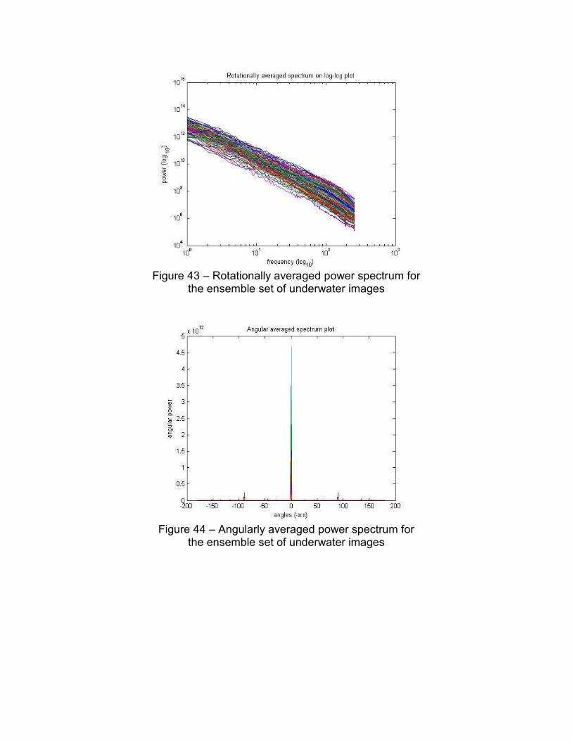
Figure 43 – Rotationally averaged power spectrum for
the ensemble set of underwater images
Figure 44 – Angularly averaged power spectrum for
the ensemble set of underwater images
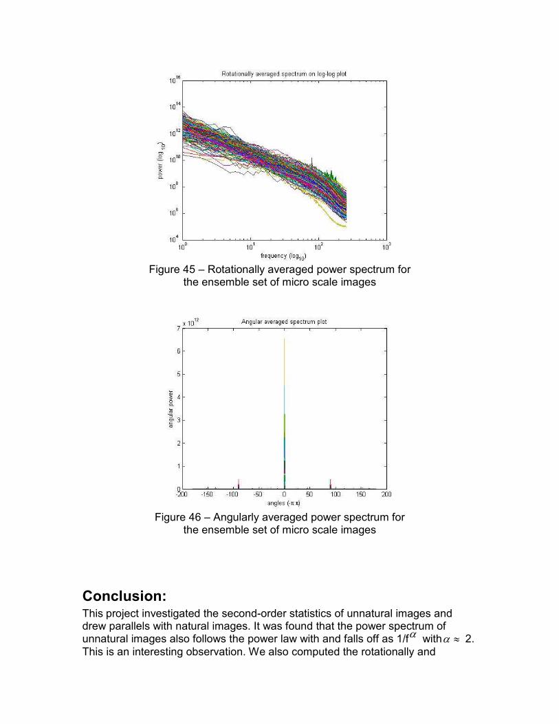
Figure 45 – Rotationally averaged power spectrum for
the ensemble set of micro scale images
Figure 46 – Angularly averaged power spectrum for
the ensemble set of micro scale images
Conclusion:
This project investigated the second-order statistics of unnatural images and drew parallels with natural images. It was found that the power spectrum of unnatural images also follows the power law with and falls off as 1/fα with ≈α 2.
This is an interesting observation. We also computed the rotationally and
angularly averaged power spectrum of unnatural images and found that micro scale images seem to have the most power. A reason for this could simply be the absolute randomness of these images as compared to underwater and celestial images. Another reason could be the techniques used to generate these images such as confocal microscopy, darkfield illumination, brightfield illumination etc.
References: [1] G. J. Burton and I. R. Moorhead. Color and spatial structure in natural scenes. Appl. Opt. 26 157–70.1987 [2] D. J. Field. Relations between the statistics of natural images and the response properties of cortical cells. J. Opt. Soc. Am. 4 2379–94. 1987 [3] D. J. Field. What is the goal of sensory coding? Neural Comput. 6 559–601. 1994 [4] D. J. Tolhurst, Y. Tadmor and C. Tang. The amplitude spectra of natural images. Ophthalmic Physiol. Opt. 12 229–32. 1992 [5] A. Torralba and A. Oliva Statistics of natural image categories. Comput. Neural Syst. 14 (2003) 391–412. 2003 [6] D. L. Ruderman and W. Bialek. Statistics of natural images - scaling in the woods. Phys. Rev. Lett. 73, 814-817. 1994 [7] E. P. Simoncelli and B. A. Olshausen. Natural image statistics and neural representation. Annu. Rev. Neurosci. 24, 1193-1216. 2001 [8] A. Schuster. On the investigation of hidden periodicities with application to a supposed 26 day period of meteorological phenomena. Terrestrial Magnetism and Atmospheric Electricity, 3, 13-41, 1898.