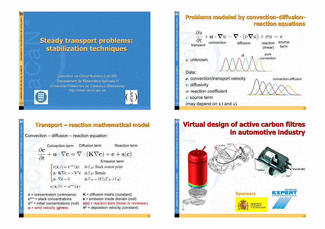
Laboratori de Càlcul Numèric (LaCàN) Departament de Matemàtica Aplicada III

Universitat Politècnica de Catalunya (Barcelona) http://www-lacan.upc.es

Steady transport problems: stabilization techniques

! 2

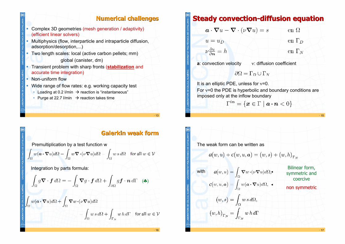
Problems modeled by convection-diffusion-reaction equations

u: unknown

Data: a: convection/transport velocity !: diffusivity ": reaction coefficient s: source term (may depend on x,t and u)

transient convection diffusion reaction

(linear) source term

pure convection

convection-diffusion

! 3

Transport – reaction mathematical model

Convection – diffusion – reaction equation:

Convection term Diffusion term Reaction term

Emission term

K = diffusion matrix (constant) e = emission inside domain (null) s(c) = reaction term (linear or nonlinear) Vd = deposition velocity (constant)

c = concentration (unknowns) cemi = stack concentrations cini = initial concentrations (null) u = wind velocity (given)

! 4

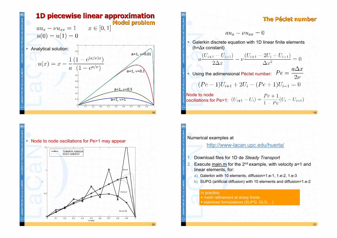
Sponsors

Virtual design of active carbon filtres in automotive industry

! 5

Vehicle emissions

!  Fuel evaporation accounts for 50% of vehicle emissions !  Regulations in U.S. and Europe are increasingly strict:

from LEV (Low Emission Vehicle) to ZEV (Zero Emission Vehicle)

! 6

Emission control: active carbon filters

!  Active carbon filters mitigate evaporative emissions !  Canister of injected plastic with three openings:

tank, atmosphere, engine !  Different materials: active carbon, plastic, air chambers,

foams, fleece.

Canister: different

materials

! 7 ! 8

Emission control: active carbon filters

!  When vehicle is parked, hydro-carbons are stored in the active carbon (adsorption or loading)

!  When vehicle is running, hydro-carbons are drawn into the engine (desorption or purge)

! 9

Difficulties in canister design

!  Complex 3D geometries

!  Different materials

!  Strict design requirements: •  Pressure drop •  Breakthrough and

working capacity •  Bleed emissions

(three-diurnal test)

! 10

1st Flow of fuel vapor

!  Active carbon: porous media theory

v is Darcy velocity

!  Air chambers: potential flow prescribed pressure drop

!  Air-carbon interface: uniform pressure

continuity of vapor flow

[A. Rodríguez-Ferran, J. Sarrate and A. Huerta, IJNME 2004]

! 11

2nd Hydro-carbons: transport and mass transfer

!  Two-porosity model

!  Three fractions of hydro-carbons (HC)

•  Interparticle fluid

•  Intraparticle fluid

•  Adsorbed AC

c [g/m3]

cpore [g/m3]

q [g HC/g AC]

! 12

Convection-diffusion-reaction equation

•  Reaction term

•  Diffusion term

•  Convection term

! 13

Numerical challenges

!  Complex 3D geometries (mesh generation / adaptivity) (efficient linear solvers)

!  Multiphysics (flow, interparticle and intraparticle diffusion, adsorption/desorption,...)

!  Two length scales: local (active carbon pellets; mm) global (canister, dm)

!  Transient problem with sharp fronts (stabilization and accurate time integration)

!  Non-uniform flow !  Wide range of flow rates: e.g. working capacity test

•  Loading at 0.2 l/min " reaction is “instantaneous” •  Purge at 22.7 l/min " reaction takes time

! 15

Steady convection-diffusion equation

a: convection velocity !: diffusion coefficient

It is an elliptic PDE, unless for !=0. For !=0 the PDE is hyperbolic and boundary conditions are imposed only at the inflow boundary

! 16

Galerkin weak form

Premultiplication by a test function w

(#)

Integration by parts formula:

! 17

The weak form can be written as

with

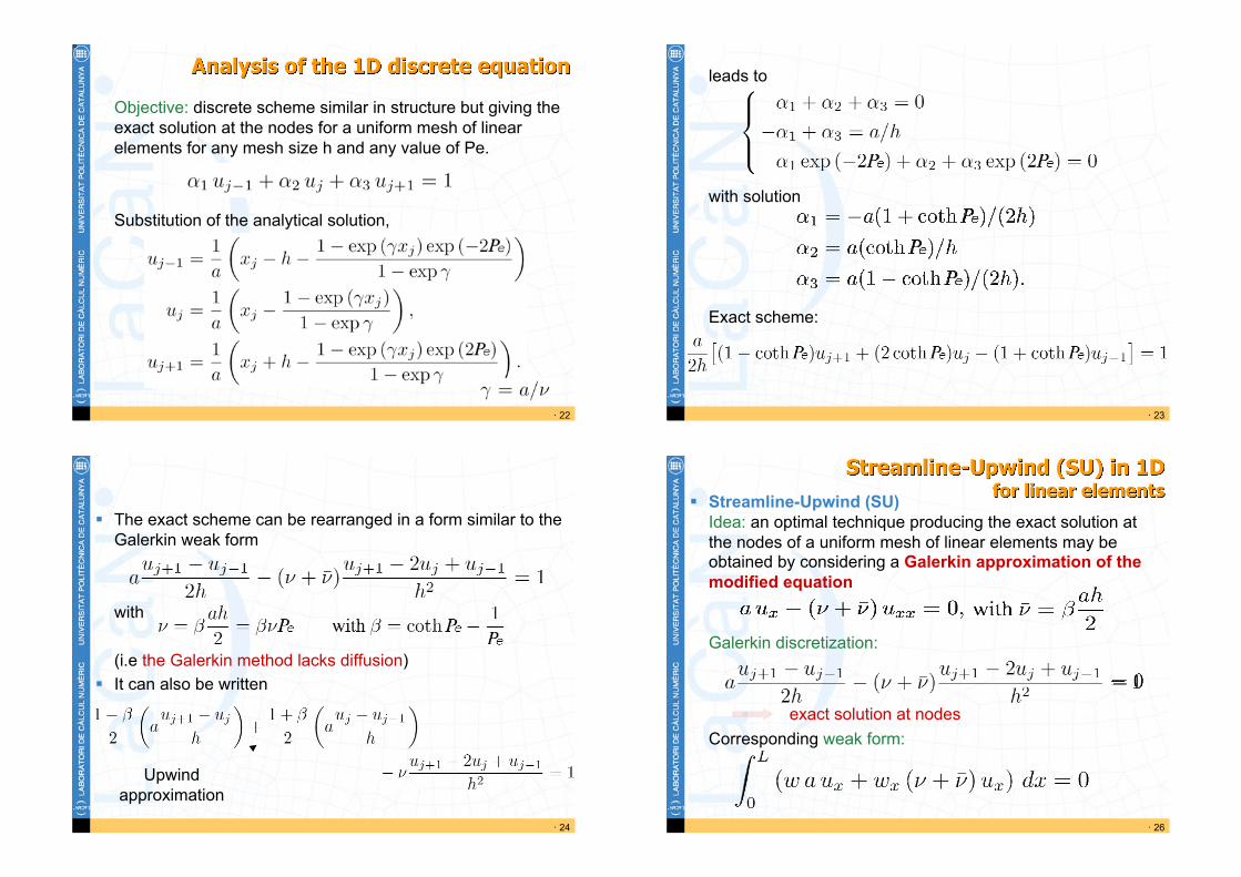
! 18

!  Analytical solution:

Model problem 1D piecewise linear approximation

! 19

!  Galerkin discrete equation with 1D linear finite elements (h="x constant)

!  Using the adimensional Péclet number:

Node to node oscillations for Pe>1:

The Péclet number

! 20

!  Node to node oscillations for Pe>1 may appear

! 21

Numerical examples at http://www-lacan.upc.edu/huerta/

1.  Download files for 1D de Steady Transport 2.  Execute main.m for the 2nd example, with velocity a=1 and

linear elements, for: a)  Galerkin with 10 elements, diffusion=1.e-1, 1.e-2, 1.e-3 b)  SUPG (artificial diffusion) with 10 elements and diffusion=1.e-2

In practice: !  mesh refinement at sharp fronts !  stabilized formulations (SUPG, GLS,…)

! 22

Analysis of the 1D discrete equation

Objective: discrete scheme similar in structure but giving the exact solution at the nodes for a uniform mesh of linear elements for any mesh size h and any value of Pe.

Substitution of the analytical solution,

! 23

leads to

with solution

Exact scheme:

! 24

!  The exact scheme can be rearranged in a form similar to the Galerkin weak form

with

(i.e the Galerkin method lacks diffusion) !  It can also be written

Upwind approximation

! 26

Streamline-Upwind (SU) in 1D for linear elements

!  Streamline-Upwind (SU) Idea: an optimal technique producing the exact solution at the nodes of a uniform mesh of linear elements may be obtained by considering a Galerkin approximation of the modified equation

Galerkin discretization:

Corresponding weak form: exact solution at nodes

! 27

!  1D exact nodal solution for a constant source term

! 28

1st drawback: non-consistent !  results for a non-constant source term:

! 29

a

2st drawback: streamline in 2D-3D

!  Artificial diffusion

the solution is smoothed in all directions, not only in the convection direction!

!  Stream-line Upwind (SU)

for instance, for

Artificial diffusion must be added only for streamline

direction

non-consistent

! 30

STABILIZATION TECHNIQUES !  GOAL: stabilize the convective term in a consistent manner,

that is, ensuring that the exact solution is also a solution of the weak formulation

!  Convection-diffusion-reaction equation:

!  Residual of the PDE

Note that:

! 31

!  Stabilized consistent formulation

!  Streamline-Upwind Petrov-Galerkin (SUPG)

!  Galerkin least-squares (GLS)

depending on the method

! 32

!  results for a non-constant source term:

! 33

STABILIZATION TECHNIQUES (1D)

!  GOAL: stabilize the convective term in a consistent manner, that is, ensuring that the exact solution is also a solution of the weak formulation.

!  SUPG:

added diffusion

linear FE

! 34

!  For a constant source term s, assembling the terms yields:

exact nodal solution for

! 35

!  SU and SUPG produce exact nodal solutions for constant s. SUPG performs better for general source terms.

! 36

Streamline-Upwind Petrov-Galerkin (SUPG)

!  Streamline-Upwind Petrov-Galerkin (SUPG)

Remark 1: the SUPG method may be obtained multiplying by a the strong form

" Petrov-Galerkin formulation the test space and interpolation space do not coincide

Remark 2: for , the weighting function coincides with SU however in SUPG the perturbation is applied to all terms

! 37

!  Discrete problem:

stabilization parameter:

SU stabilization term additional terms to keep consistency

! 38

!  Drawback: the added stabilization term is not symmetric

" technical difficulties in establishing the stability of SUPG

!  The Galerkin/Least squares stabilization technique overcomes this difficulty adding a symmetric stabilization term

non-symmetric

! 39

Galerkin / Least-squares (GLS)

!  Galerkin least-squares (GLS)

!  Discrete problem: symmetric term

! 40

!  Remark 1: SUPG and GLS are identical for the convection-diffusion equations with linear elements

Remark 2: influence of the different terms

for linear elements, GLS is SUPG with the Galerkin term weighted times more.

The instabilities introduced by Galerkin are a little more amplified in GLS compared with SUPG.

! 41

!  and linear elements

! 42

STABILIZATION PARAMETER FOR 2D AND 3D

!  The optimal selection of is still an area of current research.

Bilinear quadrilateral elements:

! 43

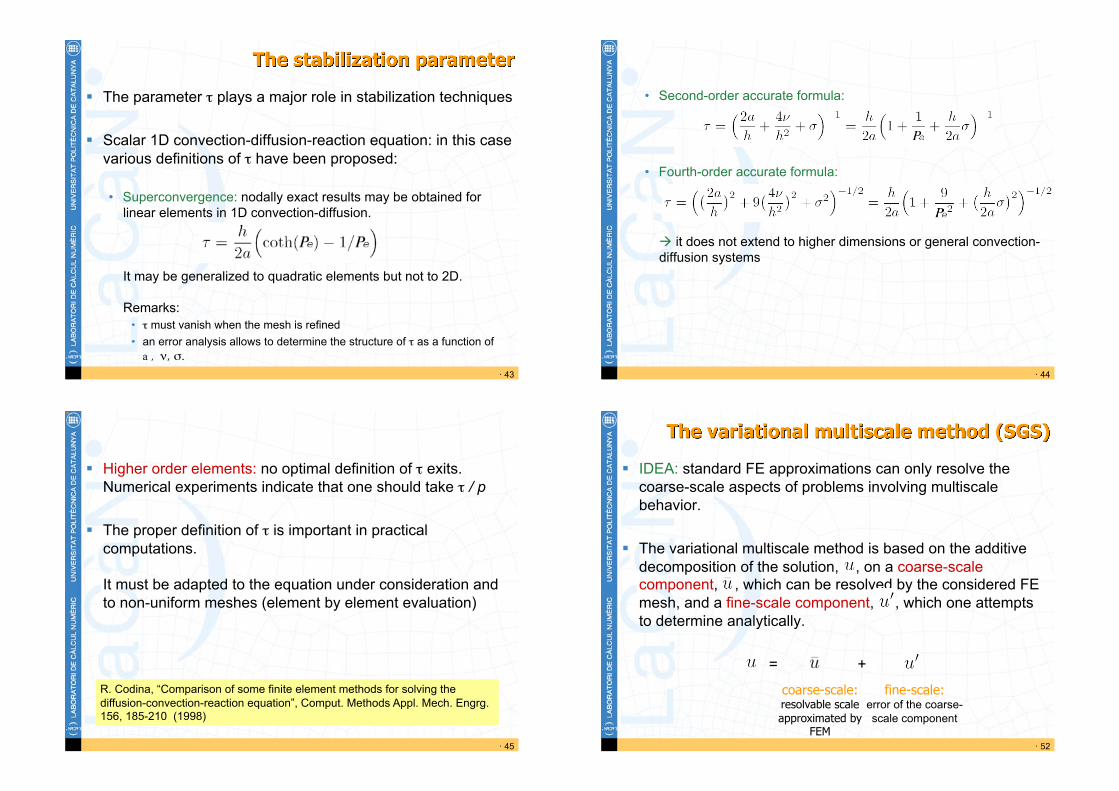
The stabilization parameter

!  The parameter $ plays a major role in stabilization techniques

!  Scalar 1D convection-diffusion-reaction equation: in this case various definitions of $ have been proposed:

•  Superconvergence: nodally exact results may be obtained for linear elements in 1D convection-diffusion.

It may be generalized to quadratic elements but not to 2D.

Remarks: •  $ must vanish when the mesh is refined •  an error analysis allows to determine the structure of $ as a function of a , !, ".

! 44

•  Second-order accurate formula:

•  Fourth-order accurate formula:

" it does not extend to higher dimensions or general convection-diffusion systems

! 45

!  Higher order elements: no optimal definition of $ exits. Numerical experiments indicate that one should take $ / p

!  The proper definition of $ is important in practical computations.

It must be adapted to the equation under consideration and to non-uniform meshes (element by element evaluation)

R. Codina, “Comparison of some finite element methods for solving the diffusion-convection-reaction equation”, Comput. Methods Appl. Mech. Engrg. 156, 185-210 (1998)

! 52

The variational multiscale method (SGS)

!  IDEA: standard FE approximations can only resolve the coarse-scale aspects of problems involving multiscale behavior.

!  The variational multiscale method is based on the additive decomposition of the solution, , on a coarse-scale component, , which can be resolved by the considered FE mesh, and a fine-scale component, , which one attempts to determine analytically.

= +

coarse-scale: resolvable scale approximated by

FEM

fine-scale: error of the coarse-scale component

! 53

!  Model problem:

!  Multiscale decomposition:

! 54

Now, using that and are linearly independent the previous problem decomposes into:

Resolved scales / coarse scale:

Unresolvable scales / fine scale: solved analytically as a function of

! 55

!  Unresolvable scales / fine scale: it is standard to impose along the finite element edges in order to localize the fine-scale problem in the interior of each finite element.

!  Euler-Lagrange equations:

where and is the projection onto

residual of the coarse (resolvable) FE solution

! 56

!  The assumption along with the assumption that the velocity field is divergence free yield:

where

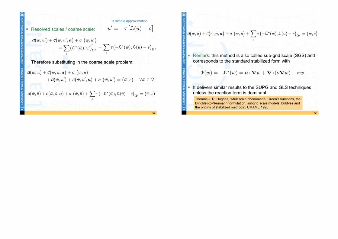
! 57

!  Resolved scales / coarse scale:

Therefore substituting in the coarse scale problem:

a simple approximation

! 58

!  Remark: this method is also called sub-grid scale (SGS) and corresponds to the standard stabilized form with

!  It delivers similar results to the SUPG and GLS techniques unless the reaction term is dominant

Thomas J. R. Hughes, “Multiscale phenomena: Green's functions, the Dirichlet-to-Neumann formulation, subgrid scale models, bubbles and the origins of stabilized methods”, CMAME 1995