steadyandunsteadylaminarﬂowsofnewtonianandgeneralized ... · ∗correspondence to: f. t. pinho,...

INTERNATIONAL JOURNAL FOR NUMERICAL METHODS IN FLUIDSInt. J. Numer. Meth. Fluids 2008; 57:295–328Published online 13 November 2007 in Wiley InterScience (www.interscience.wiley.com). DOI: 10.1002/fld.1626

Steady and unsteady laminar flows of Newtonian and generalizedNewtonian fluids in a planar T-junction

A. I. P. Miranda1,‡, P. J. Oliveira2,§ and F. T. Pinho3,4,∗,†

1Departamento de Matematica, Universidade da Beira Interior, Rua Marques D’Avila e Bolama,6201-001 Covilha, Portugal

2Departamento de Engenharia Electromecanica, Universidade da Beira Interior, Centro de Materiais Texteise Papeleiros, Rua Marques D’Avila e Bolama, 6201-001 Covilha, Portugal

3Centro de Estudos de Fenomenos de Transporte, Faculdade de Engenharia da Universidade do Porto,Rua Dr. Roberto Frias s/n, 4200-465 Porto, Portugal

4Universidade do Minho, Largo do Paco, 4704-553 Braga, Portugal

SUMMARY

An investigation of laminar steady and unsteady flows in a two-dimensional T-junction was carried out forNewtonian and a non-Newtonian fluid analogue to blood. The flow conditions considered are of relevanceto hemodynamical applications and the localization of coronary diseases, and the main objective was toquantify the accuracy of the predictions and to provide benchmark data that are missing for this prototypicalgeometry. Under steady flow, calculations were performed for a wide range of Reynolds numbers andextraction flow rate ratios, and accurate data for the recirculation sizes were obtained and are tabulated.The two recirculation zones increased with Reynolds number, but the behaviour was non-monotonic withthe flow rate ratio. For the pulsating flows a periodic instability was found, which manifests itself by thebreakdown of the main vortex into two pieces and the subsequent advection of one of them, while thesecondary vortex in the main duct was absent for a sixth of the oscillating period. Shear stress maximawere found on the walls opposite the recirculations, where the main fluid streams impinge onto the walls.For the blood analogue fluid, the recirculations were found to be 10% longer but also short lived than thecorresponding Newtonian eddies, and the wall shear stresses are also significantly different especially inthe branch duct. Copyright q 2007 John Wiley & Sons, Ltd.

Received 29 May 2007; Revised 2 August 2007; Accepted 29 August 2007

KEY WORDS: T-junction; Newtonian; instability; blood analogue; Carreau–Yasuda model; two-dimensional

∗Correspondence to: F. T. Pinho, Centro de Estudos de Fenomenos de Transporte, Faculdade de Engenharia daUniversidade do Porto, Rua Dr. Roberto Frias s/n, 4200-465 Porto, Portugal.

†E-mail: [email protected]‡E-mail: [email protected]§E-mail: [email protected]

Contract/grant sponsor: Fundacao para a Ciencia e Tecnologia; contract/grant number: PBICT/C/QUI/1980/95Contract/grant sponsor: FEDER; contract/grant number: POCTI/EME/48665/2002

Copyright q 2007 John Wiley & Sons, Ltd.

296 A. I. P. MIRANDA, P. J. OLIVEIRA AND F. T. PINHO

1. INTRODUCTION

The numerical investigation of blood flows in veins and arteries is essential for a better under-standing of the relationship between hemodynamics and cardiovascular diseases, a major causeof death in developed countries [1–5]. This continues to motivate research in this field, and thereis today a drive to efficiently combine engineering and medicine tools [6]. In this context, animportant flow geometry is the flow in bifurcating T-junctions [7].

In a large number of investigations on blood flow, the rheology is simplified and it is assumedthat blood has a linear stress/strain relationship [5, 8–11]. This simplification may be acceptableto a first approximation, especially in large blood vessels under steady conditions, but a morerealistic fluid description is required for more accurate fluid dynamics. Indeed, it is well knownthat blood exhibits a complex rheology, behaving in a non-linear fashion, and this is even moreevident whenever flows are unsteady and complex, such as in recirculating unsteady flows.

Accurate numerical investigations of complex three-dimensional unsteady flows require thesimultaneous application of, at least, second-order discretization schemes applied on sufficientlyrefined meshes, and an accurate representation of fluid rheology. To verify that codes and numericalmethods comply with these conditions, they are used first to calculate benchmark flows, such asthe steady laminar lid-driven cavity flow for Newtonian fluids [12], the steady laminar flow in a 4:1sudden contraction, or confined flows around cylinders with viscoelastic fluids [13, 14]. However,there is a lack of benchmark data sets for flows of relevance to hemodynamical applications,especially flows involving unsteadiness, a state of things that this work aims to reduce. Specifically,this paper investigates steady and pulsating flows of Newtonian and, to a lesser extent, of generalizedNewtonian fluids (GNF) through a planar 90◦ T-junction, which is an adequate prototype ofcomplex three-dimensional flows of biofluids in junctions and bifurcations. The aim is two-fold:to investigate the degree of space and time refinement required to obtain very accurate results,and to obtain values of quantities such as the size of the separated flow regions and shear stresseson walls at relevant Reynolds numbers and flow rate ratios for fluids possessing an adequate fluidrheology.

Blood is a suspension of platelets and cells in plasma, which is a mixture of water and longmolecules such as proteins and enzymes. The cells are deformable and can also agglomerate intothe so-called rouleaux which orientate and deform anisotropically [15, 16]. Cell agglomeration isdetermined by the shear rate as well as by the concentration of macromolecules in the plasma(fibrinogen), amongst other things. As a consequence of this complexity, blood is a thixotropic fluid[17], possessing an yield stress [18], and exhibiting elasticity [19] and a shear-thinning viscosity[20], as is well recognized by some authors [5]. Still, it is often considered by many researchersthat flow characteristics of blood can be well modelled by a Newtonian equation when it occursin large blood vessels and under steady flow conditions [1, 21–23]. However even in large bloodvessels, flow unsteadiness leads to regions of low deformation rate where the viscoelasticity ofblood becomes especially relevant and affecting the stress field. This has been shown by Vlastoset al. [19], who measured blood rheology under combined oscillatory and steady shear, andrecently by Bachmann et al. [24], who measured the flows of Newtonian and non-Newtonianblood analogs in a pediatric ventricle with handmade ball and cage valves at normal physiologicconditions and showing the dramatic differences in wall shear stresses. Therefore, the assumptionof Newtonian behaviour of blood should be taken with caution and there is the need to investigatein more detail the dynamics of non-Newtonian fluids under unsteady flow conditions of relevanceto hemodynamics. Such investigation should address first the effects of variable viscosity coupled

Copyright q 2007 John Wiley & Sons, Ltd. Int. J. Numer. Meth. Fluids 2008; 57:295–328DOI: 10.1002/fld

STEADY AND UNSTEADY LAMINAR FLOWS IN A T 297

with unsteadiness, as in this contribution, followed by an assessment of the role of viscoelasticity,which will be addressed in a forthcoming paper. As a matter of fact, recent research [25] hasshown that even in the absence of elasticity the shear thinning of viscosity is enough to complicatematters and to ensure that complete dynamic similarity between blood and a Newtonian modelfluid becomes an impossible task.

Studies on bifurcating flows were done as early as the 1920s by Vogel [26], who quantifiedpressure losses in a T-junction. The widespread use of T-junctions in piping networks and thecorresponding pressure losses have been a major motivation for research on steady T-junction flows,as recently reviewed by Costa et al. [27]. In living organisms bifurcating flows have characteristicsof their own, such as flow unsteadiness, non-linear rheology, specific flow geometries (the angle ofbifurcation is usually less than 90◦ and the vessels have taper), which justify the following morefocused review.

The availability of optical diagnostic techniques from the 1970s onwards has paved the wayto detailed investigations of liquid flows in complex geometries of relevance to hemodynamics.Karino et al. [28] visualized vortex shedding from the corner of a bifurcation and its relationshipwith the curvature of the edge of the T-junction. Liepsch et al. [29] used laser-Doppler anemometry(LDA) to measure the steady laminar flow of water in a bifurcation formed by rectangular ductshaving an aspect ratio of 8:1 and performed the corresponding numerical calculations assumingtwo-dimensional flow and using first-order discretization schemes for convection. The numericaland experimental results agreed qualitatively, showing the existence of a main recirculation in thebranch duct and a secondary eddy starting inside the junction at the wall opposite the branch ductand going into the main duct.

Numerical calculations of steady flow by Khodadadi et al. [30], using a finite volume method,were carried out in the same two-dimensional geometry of Liepsch et al. [29] and included heattransfer, but they relied on the hybrid scheme for convection, another first-order discretizationscheme. At high Reynolds numbers and high values of the flow rate ratio, a third recirculationregion was found in the downstream main duct. This research was later extended by Khodadadiet al. [31], who have carried out simulations and experiments on pulsatile flow using LDA. Theirunsteady flow calculations relied as well on first-order discretization schemes for both the space andtime discretizations that, as we know today, are not accurate due to excessive numerical diffusionespecially in the recirculation regions where mis-alignment between velocity vectors and meshis large. However, the experimental data set of Khodadadi et al. [31] is very comprehensive andprovides local velocity measurements that are useful to check the accuracy of numerical methods,as we have done here. Subsequently, Khodadadi [32] presented further experimental and numericaldata, namely the shear stress along the walls, which is of relevance to establish the relationshipbetween cardiovascular disease, flow recirculation and the magnitude of shear stresses. In theseinvestigations by Khodadadi et al., discrepancies between predictions and experimental data werefound in the main recirculation and were partly attributed to three-dimensional effects in theexperiments, but especially to excessive numerical diffusion which was quantified in Khodadadiet al. [30].

The same two-dimensional bifurcation was used again by Moravec and Liepsch [33], whoperformed further experiments with LDA using Newtonian and non-Newtonian fluids. Subse-quently, Liepsch and Moravec [34] investigated pulsating flows in rigid and distensible arteries andin the latter case they found that the wall elasticity reduced the size of the secondary recirculation.Rindt and Stenehoven [35] investigated numerically the unsteady flow in a rigid carotid artery, buthave not validated their numerical predictions. Also of relevance to hemodynamics, the investigation



of Ravensbergen et al. [9] has concentrated on junction flow, rather than the bifurcating flow ofinterest in the present work.

What is clear from this review is the lack of proper validation and assessment of numerical accu-racy in works on steady and pulsatile flows of Newtonian as well as non-Newtonian fluids throughT-junctions, and that constitutes the objective of the present investigation. In this first contribution,the emphasis is on quantitative results for the Newtonian two-dimensional case, of benchmarkquality, before embarking upon more complicated three-dimensional and non-Newtonian calcula-tions. Nevertheless, some GNF simulations are also presented, enough to show how misleading theassumption of constant viscosity can be. In a second paper we shall deal with the GNF case in moredepth. The remaining part of this paper is organized as follows: the governing equations and thenumerical methods used are presented in Section 2. The results and discussion section is organizedin four parts: the first part starts with the presentation of the flow geometry, computational domainand meshes used, then it discusses issues of mesh convergence and space discretization and finallyit presents accurate predictions of steady T-junction laminar flow of Newtonian fluids as a functionof the flow rate ratio and Reynolds number. The second part assesses the time accuracy of unsteadyflow calculations by comparing predictions of unsteady laminar channel flow of Newtonian fluidswith the corresponding analytical solution. Results are presented in part three for the unsteadyflow in a diverging laminar 90◦ T-junction with a Newtonian fluid and finally, in part 4, for aGeneralized Newtonian fluid. In all cases, the fluids selected have properties that closely followthose of blood. The paper ends with a summary of the main conclusions.

2. GOVERNING EQUATIONS AND NUMERICAL METHOD

The governing equations were those of mass conservation and momentum balance for isothermalincompressible time-dependent flows, expressed here in index notation. They are

�ui�xi

=0 (1)

��ui�t

+��(uiu j )

�x j=− �p

�xi+ ��i j

�x j(2)

where � is the fluid density, ui is the component of the velocity vector along coordinate xi , p isthe pressure and �i j is the extra stress tensor. The extra stress tensor is given by the rheologicalconstitutive equation for the GNF model:

�i j =�(�)�i j (3)

where the rate of deformation tensor (�i j ) is defined as �i j ≡ui, j +u j,i and the scalar � is relatedto the second invariant of �i j , namely

�=√

12 �kl �kl (4)

The viscosity function here adopted was the five-parameter Carreau–Yasuda (CY) model:

�=�∞+(�0−�∞)[1+(��)a](n−1)/a (5)



where �0 is the zero-shear-rate viscosity, �∞ is the infinite-shear-rate viscosity, � is a time constant,n is the power law region exponent and a is a non-dimensional parameter related to the smoothnessof the transition between the zero-shear-rate constant viscosity plateau and the power law viscosityregion. A common value of a is 2, which provides a good fitting to experimental data of manyfluids, in which case the model is simply called Carreau model. Setting n=1, the fluid becomesNewtonian with viscosity coefficient �=�0.

Equations (1)–(5) were solved numerically with a finite volume method identical to that used inprevious works by the authors [14, 36, 37]; hence, only a brief account is given here emphasizingthe discretization of the inertial term. The momentum and continuity equations were initiallywritten in a non-orthogonal coordinate system, but keeping the Cartesian velocity and stress tensorcomponents as the main dependent variables. These differential equations were then transformedinto algebraic equations by means of a finite volume discretization on a collocated, non-orthogonalmesh, as described by Oliveira et al. [36]. The space discretization of all terms relied on high-orderaccurate schemes: central differences for the diffusive terms and the CUBISTA scheme of Alveset al. [38] for the convective terms, which are formally of second and third order on uniform meshes,respectively. For the temporal discretization of the unsteady term of the momentum equation, thethree time level scheme described by Oliveira [37] was used, which is also formally of second-orderaccuracy.

The discretized momentum equation for the velocity component ui (of vector u) at a generalcell P is given by

aPu∗P =∑

FaFu∗

F +{−∇p∗+∇·s∗+SHOSu + �VP

�t(2u(n)

P −0.5u(n−1)P )

}(6)

where the central coefficient aP =1.5�VP/�t+∑F aF , with VP the volume of the cell centred

at P , �t the time step and the neighbour coefficients aF =D f +Ff having diffusive (D f ) andconvective contributions (Ff ). In the coefficient aF the convective contributions are of first order(upwind scheme, UDS), since the high-resolution CUBISTA scheme is implemented via deferredcorrection, see Oliveira et al. [36] and Alves et al. [38], and the difference between the CUBISTAand the first-order convective fluxes is dealt with explicitly in SHOSu . Computation of convectivefluxes of momentum was also carried out using the second-order linear upwind (LUDS) and centraldifference (CDS) schemes, which were also implemented into the code via the deferred correctionapproach, in which cases SHOSu contains the difference between the fluxes calculated with theLUDS/CDS scheme and the UDS.

The velocity field u∗ obtained from the implicit solution of Equation (6) is still imperfect andwill not satisfy continuity at the next iteration level/time step (superscripts ∗∗ and (n+1)),

∇ ·u∗∗ =0 (7)

therefore, the intermediate velocity u∗ and pressure p∗ need to be corrected. The corrected velocity(u∗∗) is determined from a factored form of the momentum equation:

(1.5

�VP

�t

)u∗∗P +∑

FaFu∗

P =∑FaFu∗

F −∇p∗∗+∇·s∗+SHOSu + �VP

�t(2u(n)

P −0.5u(n−1)P ) (8)

where the inertial and the pressure gradient terms only have been updated to the new iterationlevel (∗∗).



The pressure correction is p′ = p∗∗− p∗, where p∗ denotes the existing or previous iterationlevel, and it is calculated with a Poisson-like pressure correction equation derived by subtractingEquation (6) from Equation (8), while imposing the continuity condition (Equation (7)). Theequation for p′ is

a pP p

′P =∑

Fa pF p

′F −∇·u∗ (9)

with a pP =∑

F apF , a

pF = A2

f /(1.5�VP/�t) and A f denoting cell-face areas.In this work the stress is an explicit function of the deformation rate tensor, but was solved

separately since the calculations were carried out using a viscoelastic code, where the stress iscalculated by a differential constitutive equation. Here,

�∗i j =�(�∗∗)�∗∗

i j (10)

where the superscript ∗∗ applies to the newly calculated, continuity-satisfying velocity fromEquation (8). When starting the next time step, after converging the iterations within the presenttime, we do sn+1=s∗, un+1=u∗∗ and pn+1= p∗∗.

The linearized sets of algebraic equations to be solved (Equations (6) and (9)) are of the form

aP�P =∑FaF�F +b (11)

where the summation for index F is over the six cell neighbours of cell P . The systems of equationsare solved iteratively with the conjugate gradient method preconditioned with an incomplete LUdecomposition for the symmetric p′ equation, and the bi-conjugate gradient method for the velocitycomponents.

There are two levels of iteration in this time-dependent algorithm. An inner set of iterationsinside the solvers is pursued until the initial residuals on entering the solver decay by two orders ofmagnitude, and an outer iteration level, inside a time step �t , because the momentum equation (6)depends on the stress field, the stress depends on the velocity field, the factored momentumequation (8) is only approximate and there are explicit non-linearities in the advective terms ofmomentum and in the viscosity function. These outer iterations are repeated through Equations (6)–(10) until s∗, p∗∗ and u∗∗ do not change. This is controlled by the normalized L1 residuals ofthe equations, which are required to be below a tolerance of 10−4, and only then the calculationproceeds to the next time level.

There are three types of boundary conditions relevant to the present flow problems: inlets, outletsand solid walls. At the inlet, the streamwise velocity component and the shear stress componentare prescribed, based on available analytical solutions. Typically, the velocity follows a parabolicshape for the steady flows and the Womersley solution for the pulsating flows. At the walls theno-slip condition is applied directly, as a Dirichelet condition, and the shear stress is calculatedfrom the local velocity distribution. Finally, at the two outlets of the T-junction one can eitherprescribe the pressure, and the flow split is an outcome of the calculation, or prescribe the flowrates in each of the outlets. We have decided for the latter, since we wish to vary the flow rateratio � as a controlling, given parameter. It is important to notice that, when the flow rates areprescribed, the problem is not well posed if the flow rates are not fixed separately for each outlet. Inpractice, for the implementation of this outlet boundary conditions, the u∗ obtained after solutionof the momentum equations (6) is linearly extrapolated to the two outlet planes, and then a bulkvelocity correction is applied separately to the outlet along the main duct, so that the outlet flow



rate here is exactly Q2=(1−�)Q1 (Q1 is imposed at inlet), and the outlet flow rate along the sidebranch is Q3=�Q1. In this way, overall mass conservation is satisfied exactly before solving thepressure equation (9), a necessary condition for the existence of a solution for this equation.

Following the methodology of Roache [39], the code implementing this numerical method hasbeen verified and validated several times with Newtonian and non-Newtonian inelastic fluids. Twosuch cases are the detailed steady annular flow predictions of Escudier et al. [40, 41] against exper-imental data from several authors and including also extensive verifications using several meshesand Richardson extrapolation to the limit. Regarding the bifurcating flow geometry, Section 3.1.1is entirely devoted to verification for steady flow, Section 3.2 verifies issues of time dependencyand the validations against several sets of experimental data for steady flow and one unsteadyanalytical solution are presented in Sections 3.1.2 and 3.2, respectively.

3. RESULTS AND DISCUSSION

Here we present results for steady and unsteady laminar diverging flow in a two-dimensional 90◦ T-junction, but prior to the parametric investigation an assessment is made of numerical uncertaintiesby studies of the effects of mesh refinement, numerical interpolation scheme and time step uponthe numerical results. The effects of mesh refinement and the results for the steady flow in the 90◦T-junction are dealt with in Section 3.1, the effects of time discretization and the correspondinguncertainties are dealt with in Section 3.2 with reference to the analytical solution for periodicflow in a channel and then Section 3.3 presents results for the Newtonian unsteady flow in thediverging T-junction. Finally, Section 3.4 deals with the unsteady diverging T-junction flow for anon-Newtonian Carreau fluid analogue to blood.

Hence, there are two geometries in this section: the channel flow in Section 3.2 and the 90◦T-junction everywhere else. The description of the channel flow geometry is very specific and isleft for Section 3.2 where the time-dependent procedure is verified and validated.

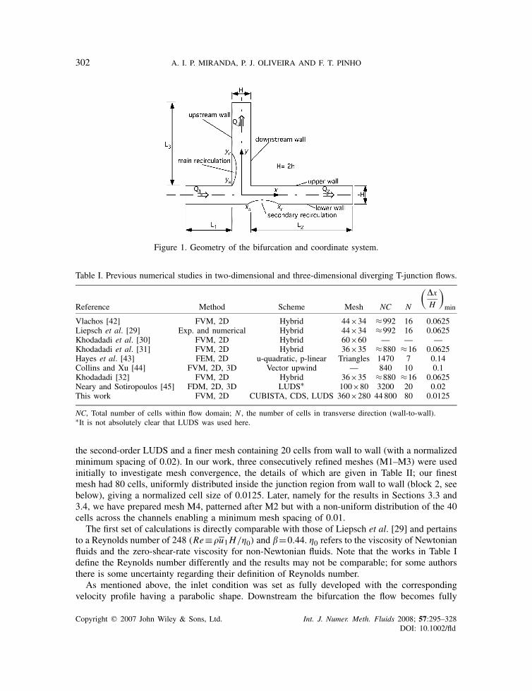
The T-junction flow geometry is the same as that of Khodadadi et al. [30, 31] and Khodadadi [32]and is schematically represented in Figure 1. The origin of the coordinate system is at the centre ofthe bifurcation. The inlet duct is denoted with subscript 1, and the main and branch outlet ducts aredenoted by subscripts 2 and 3, respectively. All ducts have the same width, H . The flow rate ratiois defined as �≡Q3/Q1, where Q1 and Q3 are the inlet duct and branch duct flow rates per unitspan, respectively. In each duct the bulk velocity is defined as the ratio between the correspondingflow rate and duct width, as in u1=Q1/H . The main recirculation is in the branch duct starting aty= ys and ending at y= yr , thus defining a normalized recirculation length of YR =(yr − ys)/H .This nomenclature is adapted for the secondary recirculation found in the main duct and alignedwith the x-direction with the necessary adaptations leading to XR =(xr −xs)/H .

3.1. Steady laminar diverging flow of Newtonian fluids in a 90◦ T-junction

3.1.1. Effects of mesh refinement and discretization scheme. The laminar flow under investiga-tion here is the steady two-dimensional diverging flow of Newtonian fluids in the 90◦ T-junction.Previous works from the literature on this flow are summarized in Table I. The numerical inves-tigations relied on rather coarse meshes and most calculations were performed using first-orderdiscretization schemes for advection known to be excessively diffusive on such coarse grids. Theexception seems to be the more recent work of Neary and Sotiropoulos [45], which apparently used



Figure 1. Geometry of the bifurcation and coordinate system.

Table I. Previous numerical studies in two-dimensional and three-dimensional diverging T-junction flows.(

�x

H

)minReference Method Scheme Mesh NC N

Vlachos [42] FVM, 2D Hybrid 44×34 ≈992 16 0.0625Liepsch et al. [29] Exp. and numerical Hybrid 44×34 ≈992 16 0.0625Khodadadi et al. [30] FVM, 2D Hybrid 60×60 — — —Khodadadi et al. [31] FVM, 2D Hybrid 36×35 ≈880 ≈16 0.0625Hayes et al. [43] FEM, 2D u-quadratic, p-linear Triangles 1470 7 0.14Collins and Xu [44] FVM, 2D, 3D Vector upwind — 840 10 0.1Khodadadi [32] FVM, 2D Hybrid 36×35 ≈880 ≈16 0.0625Neary and Sotiropoulos [45] FDM, 2D, 3D LUDS∗ 100×80 3200 20 0.02This work FVM, 2D CUBISTA, CDS, LUDS 360×280 44 800 80 0.0125

NC, Total number of cells within flow domain; N , the number of cells in transverse direction (wall-to-wall).∗It is not absolutely clear that LUDS was used here.

the second-order LUDS and a finer mesh containing 20 cells from wall to wall (with a normalizedminimum spacing of 0.02). In our work, three consecutively refined meshes (M1–M3) were usedinitially to investigate mesh convergence, the details of which are given in Table II; our finestmesh had 80 cells, uniformly distributed inside the junction region from wall to wall (block 2, seebelow), giving a normalized cell size of 0.0125. Later, namely for the results in Sections 3.3 and3.4, we have prepared mesh M4, patterned after M2 but with a non-uniform distribution of the 40cells across the channels enabling a minimum mesh spacing of 0.01.

The first set of calculations is directly comparable with those of Liepsch et al. [29] and pertainsto a Reynolds number of 248 (Re≡�u1H/�0) and �=0.44. �0 refers to the viscosity of Newtonianfluids and the zero-shear-rate viscosity for non-Newtonian fluids. Note that the works in Table Idefine the Reynolds number differently and the results may not be comparable; for some authorsthere is some uncertainty regarding their definition of Reynolds number.

As mentioned above, the inlet condition was set as fully developed with the correspondingvelocity profile having a parabolic shape. Downstream the bifurcation the flow becomes fully



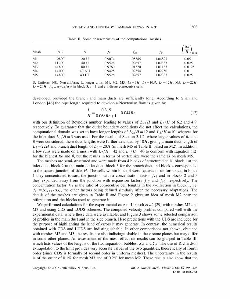
Table II. Some characteristics of the computational meshes.(

�x

H

)minMesh NC N fx1 fx2 fy3

M1 2800 20 U 0.9074 1.05385 1.04827 0.05M2 11200 40 U 0.9526 1.02657 1.02385 0.025M3 44800 80 U 0.9760 1.01320 1.01185 0.0125M4 14000 40 NU 0.9425 1.02554 1.02750 0.01M5 14800 40 UL 0.9526 1.02657 1.02385 0.025

U, Uniform; NU, Non-uniform; L, longer arms. M1, M2, M3: L1=3H , L2=10H , L3=12H ; M5: L2=22H ,L3=20H . fy3 ≡�yi+1/�yi in block 3; i+1 and i indicate consecutive cells.

developed, provided the branch and main ducts are sufficiently long. According to Shah andLondon [46] the pipe length required to develop a Newtonian flow is given by

L

H= 0.315

0.068Re+1+0.044Re (12)

with our definition of Reynolds number, leading to values of L2/H and L3/H of 6.2 and 4.9,respectively. To guarantee that the outlet boundary conditions did not affect the calculations, thecomputational domain was set to have longer lengths of L2/H =12 and L3/H =10, whereas forthe inlet duct L1/H =3 was used. For the results of Section 3.1.2, where larger values of Re and� were considered, these duct lengths were further extended by 10H , giving a main duct length ofL2=22H and branch duct length of L3=20H (in mesh M5 of Table II, based on M2). In addition,a few runs were made on a mesh with L2/H =42 and L3/H =40 to conform with Equation (12)for the highest Re and �, but the results in terms of vortex size were the same as on mesh M5.

The meshes are semi-structured and were made from 4 blocks of structured cells: block 1 at theinlet duct, block 2 at the main outlet duct, block 3 for the branch duct and block 4 correspondedto the square junction of side H . The cells within block 4 were squares of uniform size, in block1 they concentrated toward the junction with a concentration factor fx1 and in blocks 2 and 3they expanded away from the junction with expansion factors fx2 and fy3, respectively. Theconcentration factor fx1 is the ratio of consecutive cell lengths in the x-direction in block 1, i.e.fx1 ≡�xi+1/�xi , the other factors being defined similarly after the necessary adaptations. Thedetails of the meshes are given in Table II and Figure 2 gives an idea of mesh M2 near thebifurcation and the blocks used to generate it.

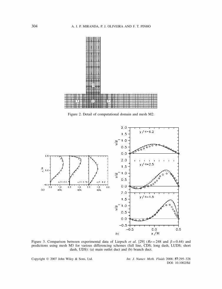
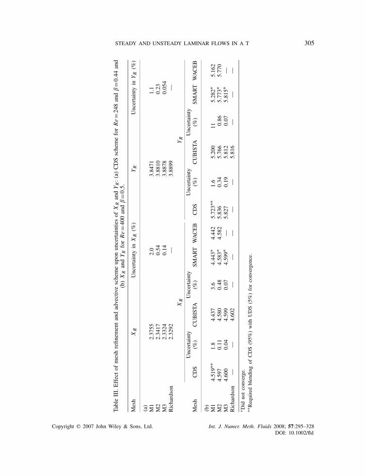
We performed calculations for the experimental case of Liepsch et al. [29] with meshes M2 andM3 and using CDS and LUDS schemes. The computed velocity profiles compared well with theexperimental data, where these data were available, and Figure 3 shows some selected comparisonof profiles in the main duct and in the side branch. Here predictions with the UDS are included forthe purpose of highlighting the kind of errors it may generate. In contrast, the numerical resultsobtained with CDS and LUDS are indistinguishable. In other comparisons not shown, obtainedwith meshes M2 and M3, the results are also indistinguishable in these same planes but may differin some other planes. An assessment of the mesh effect on results can be grasped in Table III,which lists values of the lengths of the two separation bubbles, XR and YR . The use of Richardsonextrapolation to the limit provides very accurate values of the two quantities, theoretically of fourthorder (since CDS is formally of second order in uniform meshes). The uncertainty in the resultsis of the order of 0.1% for mesh M3 and of 0.2% for mesh M2. These results also show that the



Figure 2. Detail of computational domain and mesh M2.

Figure 3. Comparison between experimental data of Liepsch et al. [29] (Re=248 and �=0.44) andpredictions using mesh M3 for various differencing schemes (full line, CDS; long dash, LUDS; short

dash, UDS): (a) main outlet duct and (b) branch duct.



TableIII.Effectof

meshrefin

ementandadvectiveschemeupon

uncertaintiesof

XRandYR:(a)CDSschemeforRe=2

48and

�=0

.44and

(b)XRandYRforRe=4

00and

�=0

.5.

Mesh

XR

Uncertainty

inXR(%

)YR

Uncertainty

inYR(%

)

(a)

M1

2.37

552.0

3.84

711.1

M2

2.34

170.54

3.88

100.23

M3

2.33

240.14

3.88

780.05

4Richardson

2.32

92—

3.88

99—

XR

YR

Uncertainty

Uncertainty

Uncertainty

Uncertainty

Mesh

CDS

(%)

CUBISTA

(%)

SMART

WACEB

CDS

(%)

CUBISTA

(%)

SMART

WACEB

(b)

M1

4.51

9∗∗

1.8

4.43

73.6

4.44

3∗4.44

25.72

3∗∗

1.6

5.20

011

5.28

2∗5.16

2M2

4.59

70.11

4.58

00.48

4.58

3∗4.58

25.83

60.34

5.76

60.86

5.77

3∗5.77

0M3

4.60

00.04

4.59

90.07

4.59

9∗—

5.82

70.19

5.81

20.07

5.81

5∗—

Richardson

——

4.60

2—

——

——

5.81

6—

——

∗ Did

notconverge.

∗∗Requiredblending

ofCDS(95%

)with

UDS(5%)forconvergence.



order of convergence for the CDS scheme was between 1.9 and 2.3 for XR and YR , respectively,i.e. close to the theoretical value.

Table III also contains XR and YR data for Re=400 and �=0.5 using CDS and CUBISTA,as well as the high-resolution schemes SMART of Gaskell and Lau [47] and WACEB of Songet al. [48] used to help confirm the results obtained with the CUBISTA scheme. For XR thepredictions of CUBISTA and CDS already agree for mesh M3 to within 0.1%, whereas for YRCDS is taking longer than CUBISTA to converge to a mesh-independent value. The data obtainedwith the CUBISTA scheme are converging monotonically to a constant value, but the simulationwith CDS for mesh M1 is not yet in the monotonic convergence region as seen in Table III(b).In fact, for this calculation it was actually necessary to blend 5% of UDS (with 95% CDS)in order to eliminate some numerical stability problems. Owing to the differences between thepredictions of CDS and CUBISTA, similar calculations were carried out with the WACEB andSMART high-resolution schemes, which are also based on the QUICK scheme and consequentlyare also formally of third order in uniform meshes. These simulations with SMART and WACEBconfirmed the predictions of CUBISTA, as is also shown in Table III. On meshes M2 and M3 theresults of CUBISTA were not as close to the extrapolated data as those of CDS, but in all casesCUBISTA was more robust than CDS from the point of view of iterative convergence.

It is clear from the above that the use of mesh M2 in combination with CUBISTA providesvery robust iterative convergence in combination with sufficiently accurate values; in particular,for the predictions of XR and YR the uncertainties are below 1% and therefore can be consideredat this stage as benchmark data, a significant improvement over existing literature data for thisflow, which were obtained 10–15 years ago with coarser meshes and using low-order differencingschemes of the upwind type.

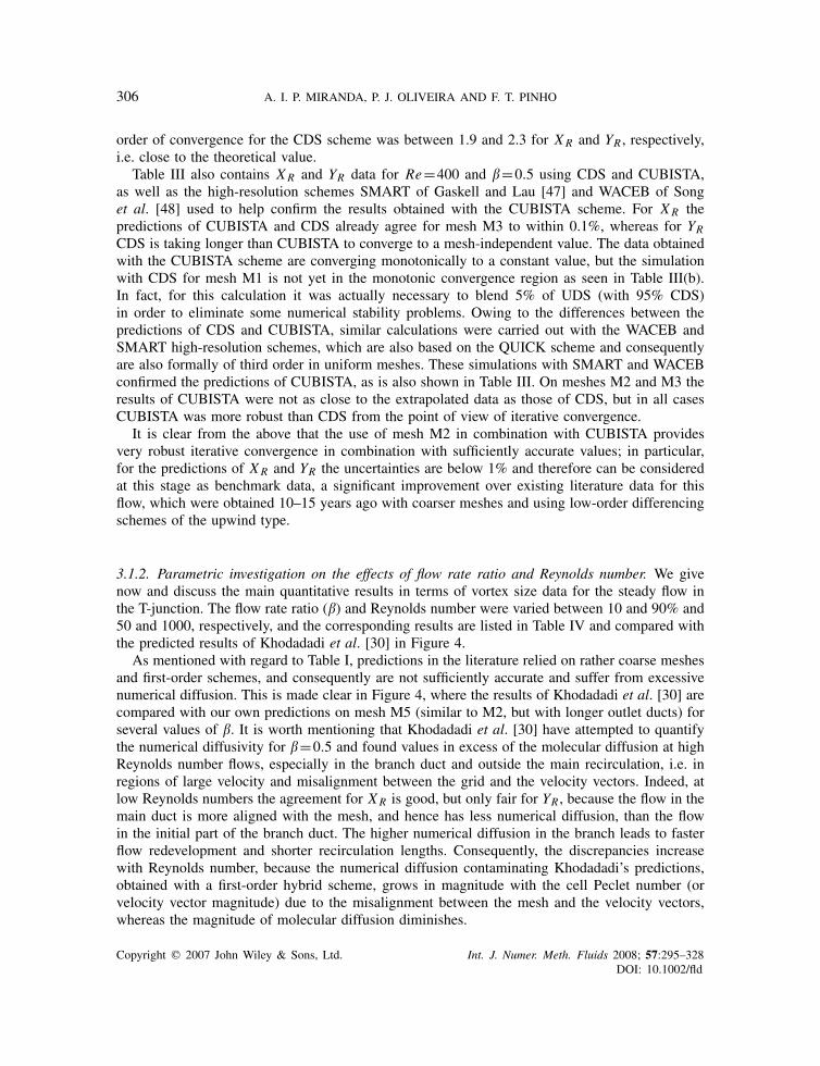
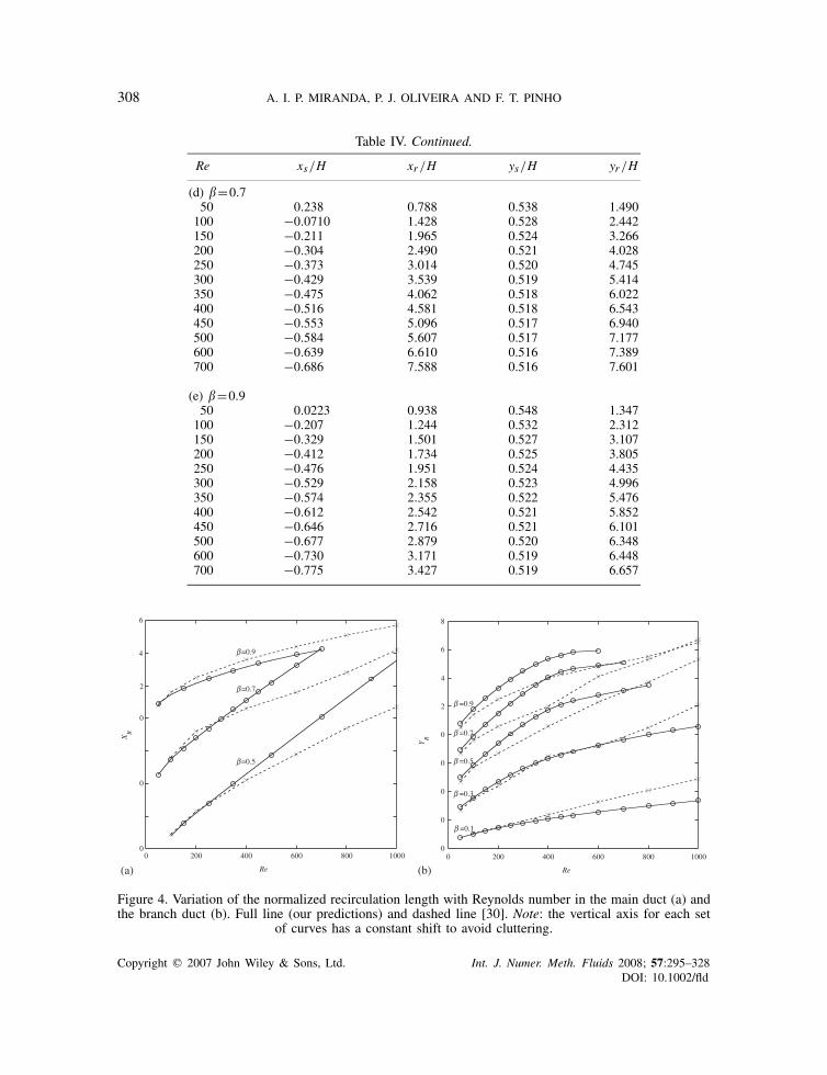
3.1.2. Parametric investigation on the effects of flow rate ratio and Reynolds number. We givenow and discuss the main quantitative results in terms of vortex size data for the steady flow inthe T-junction. The flow rate ratio (�) and Reynolds number were varied between 10 and 90% and50 and 1000, respectively, and the corresponding results are listed in Table IV and compared withthe predicted results of Khodadadi et al. [30] in Figure 4.

As mentioned with regard to Table I, predictions in the literature relied on rather coarse meshesand first-order schemes, and consequently are not sufficiently accurate and suffer from excessivenumerical diffusion. This is made clear in Figure 4, where the results of Khodadadi et al. [30] arecompared with our own predictions on mesh M5 (similar to M2, but with longer outlet ducts) forseveral values of �. It is worth mentioning that Khodadadi et al. [30] have attempted to quantifythe numerical diffusivity for �=0.5 and found values in excess of the molecular diffusion at highReynolds number flows, especially in the branch duct and outside the main recirculation, i.e. inregions of large velocity and misalignment between the grid and the velocity vectors. Indeed, atlow Reynolds numbers the agreement for XR is good, but only fair for YR , because the flow in themain duct is more aligned with the mesh, and hence has less numerical diffusion, than the flowin the initial part of the branch duct. The higher numerical diffusion in the branch leads to fasterflow redevelopment and shorter recirculation lengths. Consequently, the discrepancies increasewith Reynolds number, because the numerical diffusion contaminating Khodadadi’s predictions,obtained with a first-order hybrid scheme, grows in magnitude with the cell Peclet number (orvelocity vector magnitude) due to the misalignment between the mesh and the velocity vectors,whereas the magnitude of molecular diffusion diminishes.



Table IV. Main and secondary recirculation lengths as a function of Re and �.

Re xs/H xr/H ys/H yr/H

(a) �=0.150 0 0 0.516 1.294100 0 0 0.510 1.549150 0 0 0.507 1.769200 0 0 0.506 1.964250 0 0 0.504 2.142300 0 0 0.504 2.307350 0 0 0.503 2.461400 0 0 0.502 2.603450 0 0 0.502 2.734500 0 0 0.502 2.859600 0 0 0.501 3.090700 0 0 0.501 3.301800 0 0 0.500 3.500900 0 0 0.500 3.691

1000 0 0 0.500 3.875

(b) �=0.350 0 0 0.5247 1.452100 0 0 0.5154 2.095150 0 0 0.5115 2.668200 0.452 0.865 0.5102 3.204250 0.233 1.269 0.509 3.699300 0.120 1.586 0.508 4.141350 0.0401 1.884 0.508 4.520400 −0.0229 2.178 0.507 4.836450 −0.0751 2.472 0.507 5.108500 −0.120 2.769 0.507 5.349600 −0.194 3.374 0.506 5.784700 −0.254 3.992 0.506 6.175800 −0.304 4.622 0.506 6.524900 −0.346 5.260 0.506 6.8261000 −0.386 5.902 0.505 7.106

(c) �=0.550 0 0 0.532 1.538100 0.217 1.001 0.523 2.400150 0.00682 1.561 0.518 3.171200 −0.111 2.080 0.515 3.898250 −0.194 2.603 0.513 4.585300 −0.258 3.136 0.512 5.222350 −0.311 3.678 0.512 5.793400 −0.356 4.224 0.512 6.272450 −0.395 4.775 0.511 6.641500 −0.429 5.328 0.511 6.903600 −0.488 6.440 0.511 7.289700 −0.548 7.556 0.511 7.643800 −0.583 8.674 0.510 7.983900 −0.620 9.797 0.510 8.281

1000 −0.654 10.90 0.510 8.576



Table IV. Continued.

Re xs/H xr/H ys/H yr/H

(d) �=0.750 0.238 0.788 0.538 1.490100 −0.0710 1.428 0.528 2.442150 −0.211 1.965 0.524 3.266200 −0.304 2.490 0.521 4.028250 −0.373 3.014 0.520 4.745300 −0.429 3.539 0.519 5.414350 −0.475 4.062 0.518 6.022400 −0.516 4.581 0.518 6.543450 −0.553 5.096 0.517 6.940500 −0.584 5.607 0.517 7.177600 −0.639 6.610 0.516 7.389700 −0.686 7.588 0.516 7.601

(e) �=0.950 0.0223 0.938 0.548 1.347100 −0.207 1.244 0.532 2.312150 −0.329 1.501 0.527 3.107200 −0.412 1.734 0.525 3.805250 −0.476 1.951 0.524 4.435300 −0.529 2.158 0.523 4.996350 −0.574 2.355 0.522 5.476400 −0.612 2.542 0.521 5.852450 −0.646 2.716 0.521 6.101500 −0.677 2.879 0.520 6.348600 −0.730 3.171 0.519 6.448700 −0.775 3.427 0.519 6.657

0

0

0

2

4

6

0 200 400 600 800 1000

Re

XR

=0.5

=0.7

=0.9

0

0

0

0

0

0 200 400 600 800 1000

Re

2

4

6

8

YR

=0.1

=0.3

=0.5

=0.7

=0.9

(a) (b)

Figure 4. Variation of the normalized recirculation length with Reynolds number in the main duct (a) andthe branch duct (b). Full line (our predictions) and dashed line [30]. Note: the vertical axis for each set

of curves has a constant shift to avoid cluttering.



Inspection of Figure 4 reveals that the length of the main recirculation increases both withthe Reynolds number and the flow rate ratio. For the secondary recirculation its length alsoincreases with Reynolds number, but has a non-monotonic behaviour with �. At low values of �the recirculation increases, followed by a decrease at higher flow rate ratios. Note that an increasein the value of � effectively represents a decrease in the flow rate exiting the main duct.

In the branch duct, the flow separates immediately after the upstream inlet corner and theincrease in recirculation length with Reynolds number is essentially due to the correspondingdownstream motion of the reattachment point, as can be verified in Table IV. On the other hand, forthe secondary eddy attached to the lower horizontal wall, not only the reattachment point movesfurther downstream with Reynolds number but also the separation point actually moves upstream,both contributing to an increase in recirculation length. However, the effect of flow rate ratio uponxs and xr is not always the same: at a constant Reynolds number, the separation point alwaysmoves upstream with increasing values of �, whereas the reattachment location moves downstreamfor values of � up to 0.5 and then move backwards, in the upstream direction, for values of �>0.5.The consequence is an increase in XR for �<0.5, followed by a decrease in XR for �>0.5.

3.2. Assessment of the time discretization method: pulsating laminar channel flow of Newtonianfluids

To assess the performance of the time discretization scheme and in particular to quantify theuncertainty of the time-dependent calculations as a function of the time step, predictions weremade for pulsating laminar channel flow of Newtonian fluids generated by an imposed, sinusoidalpressure gradient of the form:

−1

�

dp

dx=Ks+KO cos(t) (13)

where −�KO is the amplitude of the oscillating pressure gradient of frequency superimposed in asteady pressure gradient of magnitude −�Ks . A non-dimensional frequency is usually expressed asthe Womersley number, =h/

√�/ where �=�0/�, and the period of the oscillation TO=2�/

will serve as time scale in the next figures. This case has an analytical solution, which can befound in the literature [49, 50]. In the Appendix at the end, we will give the main results of thatsolution, which are useful for the comparison with predictions of the present section. The flowgeometry here corresponds to the inlet plane to the T-junction (see Figure 1), a planar channelwith half-height h=H/2. The origin of the coordinate system is at the symmetry plane and thetransverse coordinate is y.

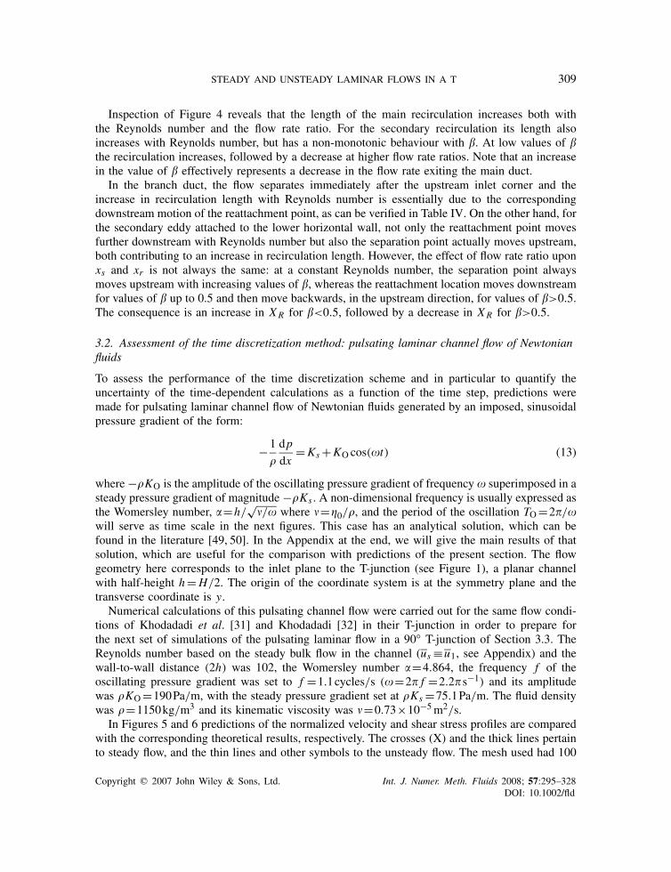
Numerical calculations of this pulsating channel flow were carried out for the same flow condi-tions of Khodadadi et al. [31] and Khodadadi [32] in their T-junction in order to prepare forthe next set of simulations of the pulsating laminar flow in a 90◦ T-junction of Section 3.3. TheReynolds number based on the steady bulk flow in the channel (us ≡u1, see Appendix) and thewall-to-wall distance (2h) was 102, the Womersley number =4.864, the frequency f of theoscillating pressure gradient was set to f =1.1cycles/s (=2� f =2.2�s−1) and its amplitudewas �KO=190Pa/m, with the steady pressure gradient set at �Ks =75.1Pa/m. The fluid densitywas �=1150kg/m3 and its kinematic viscosity was �=0.73×10−5m2/s.

In Figures 5 and 6 predictions of the normalized velocity and shear stress profiles are comparedwith the corresponding theoretical results, respectively. The crosses (X) and the thick lines pertainto steady flow, and the thin lines and other symbols to the unsteady flow. The mesh used had 100



0

0.5

1

1.5

2

-1 -0.5 0 0.5 1

y/h

u/u s

Figure 5. Comparison between analytical (lines) and computed (symbols) velocity profiles for Newtonianchannel flow: steady flow (thick line and X); unsteady flow within a cycle, =4.864, KO/Ks =2.530(thin line; � represent data at 45 and 225◦). Only half the data were plotted. Note: To avoid cluttering

half, the profiles were plotted at y/h>0, the other half at y/h<0.

control volumes in the transverse direction. Following standard practice in channel flow analysis,the velocity plotted was normalized by the bulk flow velocity (u/u1) and the shear stress (�xy)with 1

3 of the wall shear stress (�xy/[�u1/h]). The theoretical stress is given by Equation (A5) inthe Appendix.

For steady flow the agreement is excellent, with errors not exceeding 0.9% and shows that themesh is adequate in terms of spacing.

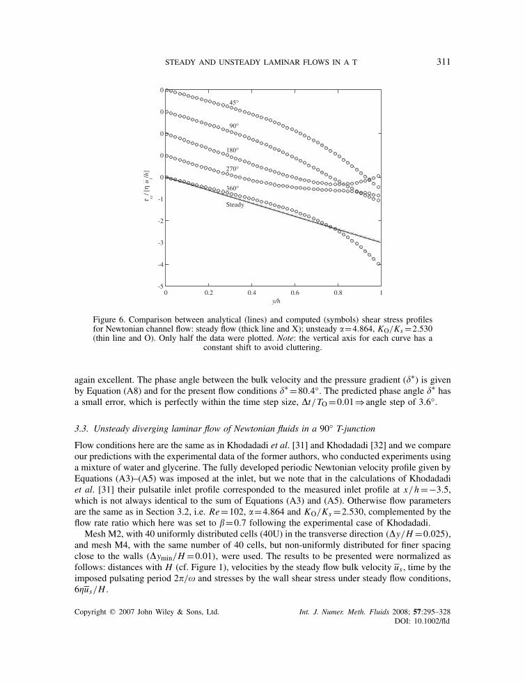
Unsteady flow calculations were carried out with the same mesh and a time step normalizedwith the oscillating period �t/TO=0.01, where TO=2�/. Comparison between the theoreticaland predicted velocity profiles along a complete cycle is excellent, as shown also in Figure 5,suggesting that a normalized time step of 1% of the period of an oscillation is adequate for accurateunsteady flow predictions. It is emphasized that this conclusion only holds because the temporalscheme is second-order accurate. The profiles at opposite parts of the cycle are not identical as isclearly seen in the comparison between the profiles for steady flow and for 180 and 360◦. Whenthe flow is decelerating (180◦) the profile is sharper, whereas it tends to be more full when theflow accelerates (360◦). The comparison between the predicted and analytical normalized shearstress profiles is shown in Figure 6 and the match between both sets is again excellent.

The pressure gradient has a minimum at t=180◦, a maximum at 360◦, and is zero at t=0 and90◦. Inspection of the velocity profiles in Figure 5 shows that the velocity is out of phase with thepressure gradient by about 90◦. The evolution with time of the calculated and theoretical maximum(uc/us) and bulk (u/us) velocities is plotted in Figure 7 in normalized form and the comparison is



0

0.20 0.4 0.6 0.8 1y/h

0

0

0

0

-1

-2

-3

-4

-5

xy[

u 1/h]

Steady

Figure 6. Comparison between analytical (lines) and computed (symbols) shear stress profilesfor Newtonian channel flow: steady flow (thick line and X); unsteady =4.864, KO/Ks =2.530(thin line and O). Only half the data were plotted. Note: the vertical axis for each curve has a

constant shift to avoid cluttering.

again excellent. The phase angle between the bulk velocity and the pressure gradient (�∗) is givenby Equation (A8) and for the present flow conditions �∗ =80.4◦. The predicted phase angle �∗ hasa small error, which is perfectly within the time step size, �t/TO=0.01⇒angle step of 3.6◦.

3.3. Unsteady diverging laminar flow of Newtonian fluids in a 90◦ T-junction

Flow conditions here are the same as in Khodadadi et al. [31] and Khodadadi [32] and we compareour predictions with the experimental data of the former authors, who conducted experiments usinga mixture of water and glycerine. The fully developed periodic Newtonian velocity profile given byEquations (A3)–(A5) was imposed at the inlet, but we note that in the calculations of Khodadadiet al. [31] their pulsatile inlet profile corresponded to the measured inlet profile at x/h=−3.5,which is not always identical to the sum of Equations (A3) and (A5). Otherwise flow parametersare the same as in Section 3.2, i.e. Re=102, =4.864 and KO/Ks =2.530, complemented by theflow rate ratio which here was set to �=0.7 following the experimental case of Khodadadi.

Mesh M2, with 40 uniformly distributed cells (40U) in the transverse direction (�y/H =0.025),and mesh M4, with the same number of 40 cells, but non-uniformly distributed for finer spacingclose to the walls (�ymin/H =0.01), were used. The results to be presented were normalized asfollows: distances with H (cf. Figure 1), velocities by the steady flow bulk velocity us , time by theimposed pulsating period 2�/ and stresses by the wall shear stress under steady flow conditions,6�us/H .



0.6

0.8

1

1.2

1.4

1.6

1.8

2

0 0.2 0.4 0.6 0.8 1

t / T0

uc/u

1

u/u1

Figure 7. Evolution with time of the centre-plane (�,uc/u1) and space-averaged bulk (O, u/u1) velocities,=4.864, KO/Ks =2.530. Calculations with �t/TO=0.01, symbols; theory, lines.

As sketched in Figure 1 and in accordance with the steady flow results of Section 3.1, theunsteady flow in the T-junction also has a primary recirculation attached to the upstream wall ofthe branch duct and a secondary recirculation at the lower wall of the main duct. The preciselocation of these regions and their time evolution are fundamental to understand the relationshipbetween hemodynamics and vascular diseases. Figure 8 indicates the progression with time ofthe coordinates of the separation and reattachment points of both recirculating regions during acomplete cycle. Note that Xr = xr/H = XR .

Refinement of the mesh close to the bifurcation and walls does not significantly improve theprediction of the separation and reattachment points. Similarly, refinement of the time step from�t/TO=0.01 to �t∗ =0.001 only improves the prediction of the sudden variations of the plottedquantities because of the better resolution and it is remarkable that the sudden reduction in the maineddy size is equally well predicted when using a coarser time step which is 10 times larger thanthe finer time step, thus showing the advantages of the second-order time discretization method.Unless otherwise stated, henceforth the results to be presented rely on mesh M4 and a time step of0.01, which is perfectly adequate to obtain accurate values. This more refined mesh near the wallwas selected because we wanted to use the same mesh here and in the non-Newtonian predictionsof Section 3.4, where the fluid is expected to exhibit larger velocity gradients near the walls onaccount of shear thinning.

The secondary separation (separation in the main duct) starts after the pressure gradient goesthrough a maximum and grows in length when the pressure gradient is already decreasing. The



-1

0

1

2

3

0 0.2 0.4 0.6 0.8 1

0 45 90 135 180 225 270 315 360

M4, 0.01 (Cycle 1)M2, 0.01 (Cycle 1)M2, 0.001 (Cycle 1)M4, 0.01 (Cycle 2)

t/T0

Xr, Y

r, Xs, Y

s

t

Yr

Xr=x

r/H

Ys

Xs

t/T0

Figure 8. Evolution with time of the loci of beginning and end of the two recirculations for Newtonianflow. Effects of mesh refinement using uniform (M2) and non-uniform (M4) meshes, of time-step size

(�t/TO) and cycles in time (Re=102,=4.864,KO/Ks =2.530).

effect of inertia is clear in the initial acceleration of the flow, when it goes through an adversepressure gradient and comes back to a phase of favourable pressure gradient. The growth of thesecondary eddy is both due to the upstream movement of the separation point and the downstreammotion of the reattachment point, as commented above for the steady flow condition. For a while(scaled time ranging from around 0.93 to 0.13 in the next cycle), there is no secondary recirculatingregion. In contrast, the main separation, which starts at the corner of the branch duct, is alwayspresent. It grows with a delay relative to the pressure gradient until the moment when it suddenlyshrinks to a small size to reinitiate the cycle. This abrupt length reduction is due to a physical andmathematical instability associated with the non-linearity of the phenomenon, because the precisemoment when the recirculation shortens varies as more flow periods are simulated suggesting thatthis problem has two solutions, as also shown in the comparison between the curves for cycle 1 andcycle 2 in Figure 8. What we denote here by ‘cycle 1’ and ‘cycle 2’ refer to two fully establishedsituations obtained after running the simulations for several periods (more than 30) of the imposedpulsating pressure gradient. ‘Cycle 1’ occurs first and the numerical solution appears to be invariantwith time for a number of cycles (2–4). However, as discussed below, the solution bifurcates tothe situation denoted ‘cycle 2’, which therefore seems more stable than ‘cycle 1’ and remains timeinvariant after that. This bifurcation was found to exist with both meshes (M2 and M4) as well asfor different time steps, so it is not a numerical artefact.

The normalized critical time at which an abrupt reduction is recorded in the main recirculationsize is initially equal to 0.86 (cycle 1), but at later times it suddenly drops to 0.81 (cycle 2) andremains at that value henceforth. Both this unstable behaviour and the sudden decrease in Yr have



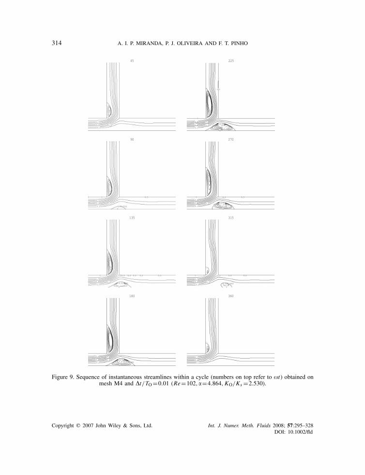
Figure 9. Sequence of instantaneous streamlines within a cycle (numbers on top refer to t) obtained onmesh M4 and �t/TO=0.01 (Re=102,=4.864,KO/Ks =2.530).



Figure 10. Zoom of instantaneous streamlines in the range t/TO∈[0.813,0.88]. Calculations using�t/TO=0.001 (Re=102,=4.864,KO/Ks =2.530).



-2

0

2

y/H= +0.5

y/H= -0.5

-2

0

2

y/H= +0.5

y/H= -0.5

yx1

/[6

u/H

]yx

1/[

6u

/H]

yx1

/[6

u/H

]yx

1/[

6u

/H]

-2

0

2

y/H= +0.5

y/H= -0.5

-4

-2

0

2

-2 -1 0 1 2 3 4 5 6

x/H

y/H= +0.5

y/H= -0.5

(a)

(b)

(c)

(d)

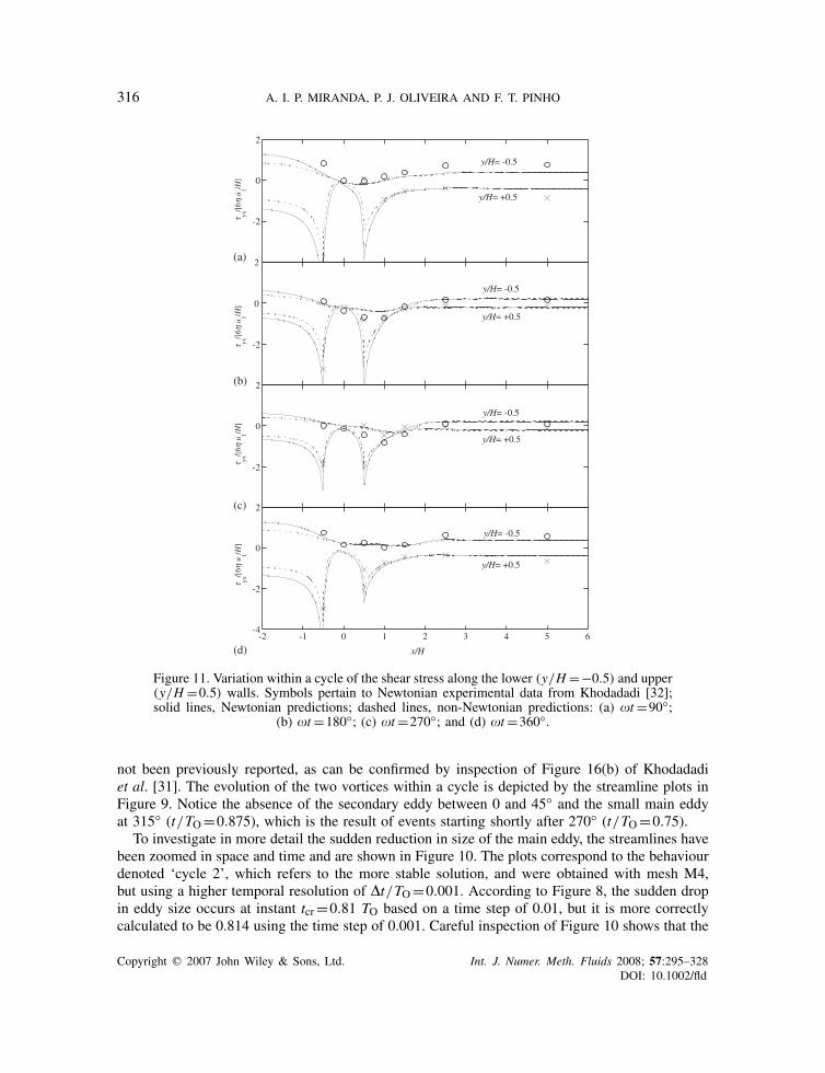
Figure 11. Variation within a cycle of the shear stress along the lower (y/H =−0.5) and upper(y/H =0.5) walls. Symbols pertain to Newtonian experimental data from Khodadadi [32];solid lines, Newtonian predictions; dashed lines, non-Newtonian predictions: (a) t=90◦;

(b) t=180◦; (c) t=270◦; and (d) t=360◦.

not been previously reported, as can be confirmed by inspection of Figure 16(b) of Khodadadiet al. [31]. The evolution of the two vortices within a cycle is depicted by the streamline plots inFigure 9. Notice the absence of the secondary eddy between 0 and 45◦ and the small main eddyat 315◦ (t/TO=0.875), which is the result of events starting shortly after 270◦ (t/TO=0.75).

To investigate in more detail the sudden reduction in size of the main eddy, the streamlines havebeen zoomed in space and time and are shown in Figure 10. The plots correspond to the behaviourdenoted ‘cycle 2’, which refers to the more stable solution, and were obtained with mesh M4,but using a higher temporal resolution of �t/TO=0.001. According to Figure 8, the sudden dropin eddy size occurs at instant tcr=0.81 TO based on a time step of 0.01, but it is more correctlycalculated to be 0.814 using the time step of 0.001. Careful inspection of Figure 10 shows that the



-4

-2

0

2

0.5 1.5 2.5 3.5 4.5 5.5 y/H

x/H= +0.5

x/H= -0.5

xy/[

6u 1/H

]xy

/[6

u 1/H]

xy/[

6u 1/H

]xy

/[6

u 1/H]

-4

-2

0

2

0.5 1.5 2.5 3.5 4.5 5.5 y/H

x/H= +0.5

x/H= -0.5

-4

-2

0

2

0.5 1.5 2.5 3.5 4.5 5.5y/H

x/H= +0.5

x/H= -0.5

-4

-2

0

2

0.5 1.5 2.5 3.5 4.5 5.5 6.5

y/H

x/H= +0.5

x/H= -0.5

(a)

(b)

(c)

(d)

Figure 12. Variation within a cycle of the shear stress along the upstream (x/H =−0.5) anddownstream (x/H =0.5) walls. Symbols pertain to Newtonian experimental data from Khodadadi[32]; solid lines, Newtonian predictions; dashed lines, non-Newtonian predictions: (a) t=90◦;

(b) t=180◦; (c) t=270◦; and (d) t=360◦.

main vortex separates from the wall and breaks into two vortices, with the downstream part beingshed, leading to the unstable and discontinuous behaviour of this vortex. Therefore, the behaviourof the main and secondary eddies is quite distinct and this situation is expected to occur in strongbifurcations. Henceforth, and unless otherwise stated, the remaining figures pertain to the morestable flow condition, ‘cycle 2’.

Another result of relevance to hemodynamics is the evolution of the shear stress with time. Thepredicted profiles of �xy scaled with inlet wall values (�xy/(6�us/H)) are plotted as solid lines inFigures 11 and 12 and compared with experimental data (symbols) presented by Khodadadi [32].Figure 11 plots data along the lower and upper walls of the main duct (y/H =−0.5 and +0.5,respectively) and Figure 12 does the same along the upstream and downstream walls of the



Figure 13. Sequence of instantaneous contour maps of normalized shear stress (�xy/(6�u1/H)) withina cycle (numbers on top refer to t) obtained on mesh M4 and �t/TO=0.01 for Newtonian flow.

branch duct (x/H =−0.5 and +0.5, respectively). The dashed lines pertain to predictions fornon-Newtonian fluids to be discussed in the next section.

Our calculations of the shear stress for Newtonian fluids are in reasonable agreement with theexperimental data and a couple of issues should be discussed before proceeding. First, the imposedinlet condition for our calculations correspond to a pulsatile fully developed flow and this does notmatch closely the measured inlet condition, as already mentioned. Secondly, Khodadadi [32] didnot measure directly the shear stresses on the walls, but calculated them from the measurementsof the tangential velocity component close to the wall; therefore, his stress data do not includecontributions from the normal gradient of the transverse velocity component, which is not negligiblenear the branch and where there is flow separation and reattachment. The two sharp negative peaksin the plots of Figure 11 mark the corners of the branch pipe and between them there is no wall.

The biggest discrepancy between the predicted and measured shear stresses is seen where thepressure gradient changes from favourable to adverse, a feature that does not come as a surprise,given the limitations of the measurements alluded above. Generally, the evolution of the shear stressalong the walls is well correlated with flow separation, precisely the recirculating zones where thelowest stresses are seen. These are the regions of possible formation and accumulation of lipids andblood clots leading to atherosclerosis [51]. On the walls opposing the vortices, maximum stresses



are observed, especially where the flow impinges the wall, and these higher stresses are responsiblefor the deterioration of the endothelium of arteries. High stresses can also rupture red blood cellsreleasing haemoglobin in the blood [52, 53]. It is therefore pretty clear that an adequate assessmentof shear stress effects on blood vessel walls relies heavily on the exact prediction of recirculationflow sizes. Thus, the benchmark data of Section 3.1.2 are amply justified: any predictive codewill need to be verified against that data before embarking in more complex three-dimensionalsimulations.

Within the flow domain the evolution of the normalised xy shear stress with time is depictedin the instantaneous contour plots of the calculated shear stress of Figure 13 showing that themaximum stresses indeed take place at walls and the low stresses within the separated flow regions.It can also be observed how the dynamics of the main recirculation in the branch along one period(cf. Figure 9) influences the shear stress distribution in that area of the flow and on the upstreamwall. Owing to the symmetry of the stress tensor �xy =�yx , the interpretation of the shear forcesacting on the duct walls is straightforward after the consideration of the commonly accepted stressconvention.

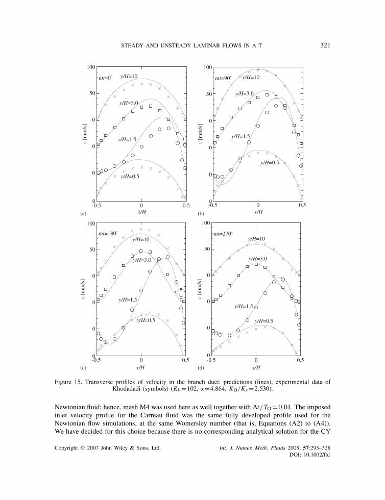
A final more detailed comparison between our numerical predictions and the comprehensiveexperimental data of Khodadadi et al. [31] is presented in the plots of Figures 14 and 15, showingtransverse profiles of the streamwise velocity in the main and branch ducts, respectively. Thesedata were again obtained on mesh M4 using �t/TO=0.001, whereas the experimental data arethe raw data provided by Prof. Khodadadi, here used without any post-processing.

Predictions are remarkably close to the experimental data at all times within the cycle, withsome small differences traced back to the different inlet conditions, and the comparison is actuallybetter than between the experiments and the calculations performed in their original paper [31].

3.4. Unsteady diverging laminar flow of a generalized Newtonian fluid in a 90◦ T-junction

To evaluate the effect of a non-linear viscosity on the flow characteristics, numerical predictionsof the unsteady flow in the 90◦ T bifurcation were carried out for a Carreau fluid model under thesame conditions as in Section 3.3 (�=0.7). The fluid properties selected were those of Banerjee etal. [54], who fitted the CY model (Equation (5)) to the experimental blood data of Cho and Kensey[55] to obtain: n=0.3568; Carreau parameter a=2; zero shear rate viscosity, �0=0.056Pas;infinite shear rate viscosity, �∞ =0.00345Pas; and time constant �=3.313s. In these calculationsthe viscosity of the fluid varies from point to point and is calculated locally with Equation (5).From these values, and for the same flow rate and � of previous section, it is possible to estimateaverage shear rates at the inlet and outlet branch ducts and the corresponding average viscositiesgiven by

�1= u10.5H

=14.9s−1→�1=0.0073Pas

�3= u30.5H

=10.4s−1→�3=0.0088Pas

These viscosity values are close to the constant viscosity used in the Newtonian calculations ofSections 3.2 and 3.3 (�=0.0084Pas); hence, their results are comparable with the CY results ofthis section.

On the basis of numerical tests, the influence of both mesh and time-step refinements on thequality of predictions for the Carreau fluid was found to be similar to those obtained with the



-0.5

0

0.5

0 50 100 150 200 250 300 350

y/H

0 0 0 0 0 0 50u [mm/s]

x/H= -3.5

x/H= -0.5

x/H=+0.5 x/H= +1.0 x/H= +1.5 x/H= +2.5 x/H= +10

(a)

t= 0˚

-0.5

0

0.5

0 50 100 150 200 250 300 350

y/H

y/H

y/H

x/H= -3.5

x/H= -0.5 x/H= +0.5

x/H= +1.0 x/H= +1.5 x/H= +2.5 x/H= +10(b)

t= 90˚

0 0 0 0 0 0 50

-0.5

0

0.5

0 50 100 150 200 250 300 350

x/H= -3.5

x/H= -0.5

x/H= +0.5 x/H= +1.0 x/H= +1.5 x/H= +2.5 x/H= +10

(c)

t= 180˚

0 0 0 0 0 0 50

-0.5

0

0.5

0

x/H= -3.5

x/H= -0.5 x/H= +0.5 x/H= +1.0 x/H= +1.5 x/H= +2.5 x/H= +10

(d)

t= 270˚

0 0 0 0 0 0 50

u [mm/s]

u [mm/s]

u [mm/s]

Figure 14. Transverse profiles of velocity in the main duct; predictions (lines), experimental data ofKhodadadi (symbols) (Re=102, =4.864, KO/Ks =2.530).



0-0.5 0 0.5

x/H

0

0

0

50

100

t=0˚

y/H=0.5

y/H=1.5

y/H=3.0

y/H=10

0

50

100

150

200

250

-0.5 0 0.5x/H

0

0

0

50

100

v [m

m/s

]

v [m

m/s

]t=90˚

y/H=0.5

y/H=1.5

y/H=3.0

y/H=10

0-0.5 0 0.5

x/H x/H

0

0

0

50

100

t=180˚

y/H=0.5

y/H=1.5

y/H=3.0

y/H=10

0

50

100

150

200

250

-0.5 0 0.5

vv

0

0

0

50

100

v [m

m/s

]

v [m

m/s

]

t=270˚

y/H=0.5

y/H=1.5

y/H=3.0

y/H=10

(a) (b)

(d)(c)

Figure 15. Transverse profiles of velocity in the branch duct: predictions (lines), experimental data ofKhodadadi (symbols) (Re=102, =4.864, KO/Ks =2.530).

Newtonian fluid; hence, mesh M4 was used here as well together with �t/TO=0.01. The imposedinlet velocity profile for the Carreau fluid was the same fully developed profile used for theNewtonian flow simulations, at the same Womersley number (that is, Equations (A2) to (A4)).We have decided for this choice because there is no corresponding analytical solution for the CY



-1

0

1

2

3

0 0.2 0.4 0.6 0.8 1

0 60 120 180 240 300 360

NewtonianGNF

Xr, Y

r, Xs, Y

s

t/T0

t

Yr

Xr=x

r/H

Xs

Ys

Figure 16. Beginning, end and size of the two recirculation regions in time cycle 2 forNewtonian and generalized Newtonian (Carreau–Yasuda model) fluids. Computations using

the three-time level method and �t/TO=0.01.

viscosity model and in this way one can compare the two cases (Newtonian and non-Newtonian)for exactly the same imposed inlet conditions.

Overall, the flow characteristics for the Carreau fluid were the same as for the Newtonian case,but longer recirculations were predicted on account of the lower viscosities found in high shearregions. Figure 16 plots the evolution within a period of the loci of the beginning and end of thetwo recirculation regions for a well-established situation after many initial periods; thus, underthe conditions designated as ‘cycle 2’ in Section 3.3. Although the eddies are longer for theshear-thinning fluid, they also exist for a shorter period of time than the corresponding Newtonianeddies. As observed for the Newtonian fluid, the abrupt critical decrease in size of the main vortexis also seen here, but now it takes place earlier within the period, at around 270◦. The secondaryrecirculation in the main duct also starts at a later time in the cycle, at t/TO≈ 0.17 against theNewtonian value of t/TO≈0.12. However, it is interesting to notice that this vortex, attached tothe lower wall along the main duct, disappears at exactly the same moment along the period (att/TO≈0.93) for the Newtonian and the non-Newtonian fluids. This may be explained by noticingthat the reattachment point of this vortex is in a zone of very low-velocity gradients (see streamlinesin Figure 9 for the Newtonian case); hence, the shear-rate dependency of viscosity is at work onlymarginally.

Generally speaking, the longer recirculations give rise to smaller normalized shear stresses at thewalls, as can be seen in Figures 11 and 12, where the dashed lines pertain to the non-Newtonianfluid. For this fluid the stresses were normalized as for the Newtonian fluid, i.e. using 6�u1/H



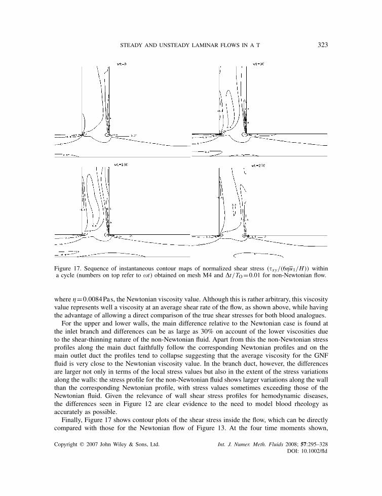
Figure 17. Sequence of instantaneous contour maps of normalized shear stress (�xy/(6�u1/H)) withina cycle (numbers on top refer to t) obtained on mesh M4 and �t/TO=0.01 for non-Newtonian flow.

where �=0.0084Pas, the Newtonian viscosity value. Although this is rather arbitrary, this viscosityvalue represents well a viscosity at an average shear rate of the flow, as shown above, while havingthe advantage of allowing a direct comparison of the true shear stresses for both blood analogues.

For the upper and lower walls, the main difference relative to the Newtonian case is found atthe inlet branch and differences can be as large as 30% on account of the lower viscosities dueto the shear-thinning nature of the non-Newtonian fluid. Apart from this the non-Newtonian stressprofiles along the main duct faithfully follow the corresponding Newtonian profiles and on themain outlet duct the profiles tend to collapse suggesting that the average viscosity for the GNFfluid is very close to the Newtonian viscosity value. In the branch duct, however, the differencesare larger not only in terms of the local stress values but also in the extent of the stress variationsalong the walls: the stress profile for the non-Newtonian fluid shows larger variations along the wallthan the corresponding Newtonian profile, with stress values sometimes exceeding those of theNewtonian fluid. Given the relevance of wall shear stress profiles for hemodynamic diseases,the differences seen in Figure 12 are clear evidence to the need to model blood rheology asaccurately as possible.

Finally, Figure 17 shows contour plots of the shear stress inside the flow, which can be directlycompared with those for the Newtonian flow of Figure 13. At the four time moments shown,



the stresses for the non-Newtonian flow are generally lower than those for the Newtonian bloodanalogue, but note that some correspond to different moments as far as the dynamics of the vorticesare concerned (cf. Figure 16). In spite of this note of caution, by contrasting Figures 13 and 17 wesee that stress concentration is alleviated for the GNF case and the regions of high shear stressesare smaller in size.

4. CONCLUSIONS

A finite volume methodology, implementing at least second-order accurate methods in space andtime, is used to investigate in detail steady and unsteady flows in a two-dimensional T-junctionin the laminar regime for Newtonian and a non-Newtonian Carreau fluid. The flow conditionsinvestigated are of relevance to hemodynamic applications and the main objective here was toquantify the accuracy of the predictions and to provide benchmark quality data prior to a morein-depth research programme with non-Newtonian inelastic and viscoelastic fluids.

For the steady flow, calculations were performed for Reynolds numbers varying between 50and 1000 and flow rate ratios in the range of 0.1–0.9. The two recirculation lengths were seento increase with Reynolds number, but regarding the effect of the flow rate ratio the behaviourwas non-monotonic. For values of � below 0.5 both recirculations increased followed by adecrease with further increases in �. Vortex data useful for benchmarking are given under tabulatedform.

For the pulsating Newtonian flow in the T-junction, the investigation was carried out for anextraction ratio of �=0.7, a Reynolds number of 102 and a Womersley number of =4.864.Although the main recirculation in the side branch was always present, there is an instability thatbreaks the main vortex into two pieces at t/TO≈ 0.81 and convects part of the vortex structuredownstream. The secondary vortex was found to be absent for a sixth of the time, for this valueof �. The shear stress on the walls was also quantified and found to reach maxima at the wallsopposite the recirculations, where the main stream impinges the wall. Very good match betweenour predictions and the experimental data of Khodadadi et al. [31] was achieved for local quantitiessuch as velocity and shear stresses, along a time period, thus giving support to the quality of thatmeasured data set, which has been scarcely used.

The main features of the pulsating flow for a non-Newtonian Carreau fluid analogue to blood aresimilar to those of the Newtonian analogue, with both recirculations being about 10% longer andalso short lived than the corresponding Newtonian eddies. A phenomenon similar to that found forthe Newtonian case is also present, with the main vortex in the branch breaking into two structuresat 3

4 time along the period, and the smaller structure being advected by the flow along the branch.However, the stresses for the non-Newtonian fluid are generally lower than the Newtonian stressesand by a large amount that can be as large as 30% at the walls of the separated flow regions. Giventhe important relationship between wall stresses and hemodynamic diseases, these differences haveimplications and are a clear evidence to the need for properly representing the true rheology ofblood if accurate predictions and investigations of blood flows are to be carried out.

Furthermore, the new finding related to the division of the main recirculating region atabout 3

4 of the pulsating period, with subsequent dragging of that portion of the vortex bythe flow through the branch may be connected with some coronary diseases resulting fromclotting of small vessels with lipids and other solid-like material that tend to accumulate in suchrecirculations.



APPENDIX A: ANALYTICAL SOLUTION FOR PULSATING LAMINAR CHANNEL FLOWOF NEWTONIAN FLUIDS

The analytical solution for pulsating laminar channel flow of Newtonian fluids is presented insome classical books [49, 50]. It is summarized here because it is an essential ingredient to thetime-dependent validations of Section 3.2 and, in addition, it serves as inlet boundary conditionin Sections 3.3 and 3.4. The channel in question coincides with the inlet plane to the T-junction(plane 1, see Figure 1), having a half-height h=H/2, with the origin of the y axis at the symmetryplane and streamwise coordinate x .

The flow is assumed to develop instantly leading to the following linear momentum equation(quasi-steady approximation):

�u�t

=��2u�y2

− 1

�

dp

dx(A1)

where the pressure gradient follows the sinusoidal variation of Equation (13) and with the no-slipboundary condition imposed at the walls (y=±h). Since Equation (A1) is linear, the solution canbe decomposed into the sum of steady (us) and oscillating (uO) contributions:

u(y, t)=us(y)+uO(y, t) (A2)

The steady velocity profile is the classical parabolic expression, here expressed in normalizedform by adopting as velocity scale KO/ and introducing the Womersley number (=h/

√�/)

[50]:

Us(Y )≡ us(y)

KO/= 2

2

Ks

KO[1−Y 2] (A3)

where Y = y/h. To the constant part of the pressure gradient �Ks it corresponds a steady bulkvelocity, us =h2Ks/3�, which is identical to the average inlet velocity of the main text u1.

The analytical solution for the oscillating contribution is more difficult to derive, and is givenby (see Reference [50]):

U0(Y,T )≡ uO(y, t)

KO/=

[1− M(Y, )

J ( )

]sin(T )− N (Y, )

J ( )cos(T ) (A4)

with =/√2,T =t , and the definitions:

J ( )=C2( )+S2( ), C(x)=cosh(x)cos(x), S(x)=sinh(x)sin(x)

M(Y, )=C( Y )C( )+S( Y )S( ), N (Y, )=C( Y )S( )+S( Y )C( )

While the above results for the velocity profile of pulsating channel flow can be found intextbooks, we needed further information such as shear stress and average velocity variations,which was derived as part of the present work. The shear stress is obtained by differentiation of



the velocity profile (�xy =��u/�y) and was found to be

�xy�KO/(h)

= −

J ( ){[(A−B)C( )+(A+B)S( )]sin(T )

+[(A−B)S( )−(A+B)C( )]cos(T )}−2Ks

KOY (A5)

where A=sinh( Y )cos( Y ) and B=cosh( Y )sin( Y ).The centreline velocity (uc) is the maximum instantaneous velocity at each time and is obtained

by setting y=0 in Equations (A3) and (A4). The phase angle of uc relative to the pressure gradientwas calculated and is given by

�=arctan

(− J ( )−M(0, )

N (0, )

)(A6)

This angle approaches 90◦ when N (0, )→0, which is the case for large Womersley numbers(�2). Another quantity of interest is the normalized instantaneous bulk velocity, obtained byintegration of the velocity profile:

u(t)≡∫ h

0u(y, t)dy= KO

[sin(T )− �sin(T )+�cos(T )

2J ( )

](A7)

where

� = exp( )[P sin( )+Q cos( )]+exp(− )[P sin( )−Q cos( )]� = exp( )[P cos( )−Q sin( )]−exp(− )[P cos( )+Q sin( )]

P = C( )+S( )

2 and Q= C( )−S( )

2

The phase angle between the bulk velocity and the pressure gradient can then be obtained bycalculating the angle between the two corresponding complex quantities, and is given by

�∗ =arctan

(2J ( )−�

�

)(A8)

The velocity profile of Equation (A2), together with Equations (A3) and (A4), and the shearstress and average velocity profiles given by Equations (A5) and (A7), respectively, will be usedin the main text.

ACKNOWLEDGEMENTS

The authors acknowledge the grants PBICT/C/QUI/1980/95 and POCTI/EME/48665/2002 fromFundacao para a Ciencia e Tecnologia (FCT, Portugal) and FEDER, and Professor Khodadadi forproviding the raw data of Khodadadi et al. [31].



REFERENCES

1. Ku DN. Blood flow in arteries. Annual Review of Fluid Mechanics 1997; 29:399–434.2. Berger SA, Jou L-D. Flows in stenotic vessels. Annual Review Fluid Mechanics 2000; 32:347–382.3. Taylor CA, Draney MT. Experimental and computational methods in cardiovascular fluid mechanics. Annual

Review of Fluid Mechanics 2004; 36:197–231.4. Popel AS, Johnson PC. Microcirculation and hemorheology. Annual Review of Fluid Mechanics 2005; 37:43–69.5. Deutsch S, Tarbell JM, Manning KB, Rosenberg G, Fontaine AA. Experimental fluid mechanics of pulsatile

artificial blood pumps. Annual Review of Fluid Mechanics 2006; 38:65–86.6. Thilmany J. Ask the supercomputer. Mechanical Engineering 2006; 128:36–38.7. Fung YC. Biomechanics: Circulation. Springer: Heidelberg, 1997.8. Pedley TJ. The Fluid Mechanics of Large Blood Vessels. Cambridge University Press: Cambridge, 1980.9. Ravensbergen J, Krijger JKB, Hillen B, Hoogstraten HW. Merging flows in an arterial confluence: the vertebro-

basilar junction. Journal of Fluid Mechanics 1995; 304:119–141.10. Balducci A, Grigioni M, Querzoli G, Romano GP, Daniele C, D’Avenio G, Barbaro V. Investigation of the flow

field downstream of an artificial heart valve by means of PIV and PTV. Experiments in Fluids 2004; 36:204–213.11. Cenedese A, Del Prete Z, Miozzo M, Querzoli G. A laboratory investigation of the flow in the left ventricle of

a human heart with prosthetic, tilting-disk valves. Experiments in Fluids 2005; 39:322–335.12. Ghia U, Ghia KN, Shin CT. High-Re solutions for incompressible flow using the Navier–Stokes equations and

a multigrid method. Journal of Computational Physics 1982; 48:387–411.13. Brown RA, McKinley GH. Report on the VIII International Workshop on Numerical Methods in Viscoelastic

Flows. Journal of Non-Newtonian Fluid Mechanics 1994; 52:407–413.14. Alves MA, Oliveira PJ, Pinho FT. Benchmark solutions for the flow of Oldroyd-B and PTT fluids in planar

contractions. Journal of Non-Newtonian Fluid Mechanics 2003; 110:45–75.15. Mazumdar JN. Biofluid Mechanics. World Scientific: Singapore, 1992.16. Owens RG. A new microstructure-based constitutive model for human blood. Journal of Non-Newtonian Fluid

Mechanics 2006; 140:57–70.17. Thurston GB. Rheological parameters for the viscosity, viscoelasticity and thixotropy of blood. Biorheology 1979;

16:149–162.18. Picart C, Piau JM, Galliard H, Carpenter P. Human blood yield stress and its hematocrit dependence. Journal of

Rheology 1998; 42:1–12.19. Vlastos G, Lerche D, Koch B, Samba O, Pohl M. The effect of parallel combined steady and oscillatory shear

flows on blood and polymer solutions. Rheologica Acta 1997; 36:160–172.20. Wells RE, Merrill EW, Gabelnick H. Shear rate dependence of viscosity of blood interaction of red cells and

plasma proteins. Transactions of the Society of Rheology 1962; 6:19–24.21. Perktold K, Resch M, Florian H. Pulsatile non-Newtonian flow characteristics in a three-dimensional human

carotid bifurcation model. ASME Journal of Biomechanical Engineering 1991; 113:464–475.22. Perktold K, Peter RO, Resch M, Langs G. Pulsatile non-Newtonian flow in three-dimensional carotid bifurcation

models: a numerical study of flow phenomena under different bifurcation angles. Journal of BiomechanicalEngineering (ASME) 1991; 113:507–515.

23. Ballyk PD, Steinman DA, Ethier CR. Simulation of non-Newtonian blood flow in an end-to-side anastomosis.Biorheology 1994 31:565–586.

24. Bachmann C, Hugo G, Rosenberg G, Deutsch S, Fontainee AA, Tarbell JM. Fluid dynamics of a pediatricventricular assist device. Artificial Organs 2000; 24:362–372 [see also Erratum in Artificial Organs 2000; 24:989].

25. Gray JD, Owen I, Escudier MP. Dynamic scaling of unsteady shear-thinning non-Newtonian fluid flows in alarge-scale model of a distal anastomosis. Experiments in Fluids 2007; 43:535–546.

26. Vogel G. Investigation of the loss in right-angled pipe branches. Mitt. Hydraulischen Instituts der Tech. HochschuleMunchen 1926; 1:75–90 (Translated by Voetsch C, Technical Memorandum n. 299, US Bureau of Reclamation,1932).

27. Costa NP, Maia R, Pinho FT, Proenca MF. Edge effects on the flow characteristics in a 90◦ tee junction. Journalof Fluids Engineering (ASME) 2006; 128(6):1204–1217.

28. Karino T, Kwong HHM, Goldsmith HL. Particle flow behaviour in models of branching vessels. I—Vortices in90 T-junctions. Biorheology 1979; 16:231–248.

29. Liepsch D, Moravec S, Rastogi AK, Vlachos NS. Measurement and calculations of laminar flow in a ninetydegree bifurcation. Journal of Biomechanics 1982; 15:473–485.



30. Khodadadi JM, Nguyen TM, Vlachos NS. Laminar forced convective heat transfer in a two-dimensional 90◦bifurcation. Numerical Heat Transfer 1986; 9:677–695.

31. Khodadadi JM, Vlachos NS, Liepsch D, Moravec S. LDA measurements and numerical prediction of pulsatilelaminar flow in a plane 90-degree bifurcation. Journal of Biomechanical Engineering 1988; 110:129–136.

32. Khodadadi JM. Wall pressure and shear stress variations in a 90-deg bifurcation during pulsatile laminar flow.Journal of Fluids Engineering 1991; 113:111–115.

33. Moravec S, Liepsch D. Flow investigations in a model of a three-dimensional human artery with Newtonian andnon-Newtonian fluids. Biorheology 1983; 20:745–759.

34. Liepsch D, Moravec S. Pulsatile flow of non-Newtonian fluid in distensible models of human arteries. Biorheology1984; 21:571–586.

35. Rindt CCM, Steenhoven AAV. Modelling flow properties in biofluids. Journal of Biomechanical Engineering1996; 118:90–96.

36. Oliveira PJ, Pinho FT, Pinto GA. Numerical simulation of non-linear elastic flows with a general collocatedfinite-volume method. Journal of Non-Newtonian Fluid Mechanics 1998; 79:1–43.

37. Oliveira PJ. Method for time-dependent simulations of viscoelastic flows: vortex shedding behind cylinder. Journalof Non-Newtonian Fluid Mechanics 2001; 101:113–137.

38. Alves MA, Oliveira PJ, Pinho FT. A convergent and universally bounded interpolation scheme for the treatmentof advection. International Journal for Numerical Methods in Fluids 2003; 41:47–75.

39. Roache PJ. Quantification of uncertainty in computational fluid dynamics. Annual Review of Fluid Mechanics1997; 29:123–160.

40. Escudier MP, Gouldson IW, Oliveira PJ, Pinho FT. Effects of inner cylinder rotation on laminar flow of aNewtonian fluid through an eccentric annulus. International Journal of Heat and Fluid Flow 2000; 21:92–103.

41. Escudier MP, Oliveira PJ, Pinho FT, Smith S. Fully-developed laminar flow of non-Newtonian liquids throughannuli: comparison of numerical calculations with experiments. Experiments in Fluids 2002; 33:101–111.

42. Vlachos NS. Laminar flow through a plane 90◦ bifurcation. Technical Report, Imperial College of Science andTechnology, London, U.K., 1978.

43. Hayes RE, Nandakumar K, Nasr-El-Din H. Steady laminar flow in a 90 degree planar branch. Computers andFluids 1989; 17:537–553.

44. Collins MW, Xu XY. A predictive scheme for flow in arterial bifurcations: comparison with laboratorymeasurements. Biomechanical Transport Processes. Plenum Press: New York, 1990; 125–133.

45. Neary VS, Sotiropoulos F. Numerical investigation of laminar flows through 90-degree diversion of rectangularcross-section. Computers and Fluids 1996; 25:95–118.

46. Shah RK, London AL. Laminar Flow Forced Convection in Ducts. Academic Press: New York, 1978.47. Gaskell PH, Lau AKC. Curvature compensated convective transport: SMART, a new boundedness preserving

transport algorithm. International Journal for Numerical Methods in Fluids 1988; 8:617–641.48. Song B, Liu GR, Lam KY, Amano RS. On a higher-order discretisation scheme. International Journal for

Numerical Methods in Fluids 2000; 32:881–897.49. Schlichting H, Gersten K. Boundary-Layer Theory (8th edn). Springer: Berlin, 2000; 137.50. Landau LD, Lifshitz EM. Fluid Mechanics. Pergamon Press, Addison-Wesley: London, Reading, MA, 1959.

Translation from Russian edition of 1953; 95.51. Caro CG, Fitz-Gerald JM, Schroter RC. Atheroma and arterial wall shear. Proceedings of the Royal Society of

London B 1971; 177:109–159.52. Blackshear PL. Mechanical haemolysis in flowing blood. Biomechanics—Its Foundations and Objectives, Fung YC,

Perrone N, Anliker M (eds). Prentice-Hall, Inc.: Englewood Cliffs, NJ, U.S.A., 1972; 501–528.53. Champion JV, North PF, Coakley WT, Williams AR. Shear fragility of human erythrocytes. Biorheology 1971;

8:23–29.54. Banerjee RK, Cho YI, Kensey KR. A study of local hydrodynamics in a 90◦ branched vessel with extreme

pulsatile flows. International Journal of Computational Fluid Dynamics 1998; 9:23–42.55. Cho YI, Kensey KR. Effects of the non-Newtonian viscosity of blood on flows in a diseased arterial vessel. Part

1: Steady flows. Biorheology 1991; 28:241–262.


steadyandunsteadylaminarﬂowsofnewtonianandgeneralized ... · ∗correspondence to: f. t. pinho,...

Documents