MAN/HEP/2021/003

K → µ+µ− as a clean probe of short-distance physics

Avital Dery,∗ Mitrajyoti Ghosh,† and Yuval Grossman‡

Department of Physics, LEPP, Cornell University, Ithaca, NY 14853, USA

Stefan Schacht§

Department of Physics and Astronomy, University of Manchester,

Manchester, M13 9PL, United Kingdom

Abstract

The K → µ+µ− decay is often considered to be uninformative of fundamental theory parameters

since the decay is polluted by long-distance hadronic effects. We demonstrate that, using very

mild assumptions and utilizing time-dependent interference effects, B(KS → µ+µ−)`=0 can be

experimentally determined without the need to separate the ` = 0 and ` = 1 final states. This

quantity is very clean theoretically and can be used to test the Standard Model. In particular, it

can be used to extract the CKM matrix element combination |VtsVtd sin(β + βs)| ≈ |A2λ5η| with

hadronic uncertainties below 1%.

∗ avital.dery@cornell.edu† mg2338@cornell.edu‡ yg73@cornell.edu§ stefan.schacht@manchester.ac.uk

1

arX

iv:2

104.

0642

7v2

[he

p-ph

] 2

7 Ju

l 202

1

I. INTRODUCTION

Rare flavor changing neutral current (FCNC) kaon decays [1–7] provide a unique way to

probe the flavor sector of the Standard Model (SM) and, in particular, CP-violating effects.

The program to measure the decay rates of K+ → π+νν [8] and KL → π0νν [9] is aimed

at determining the CKM parameters with very high theoretical precision. In particular, the

KL → π0νν decay rate can be used to extract [10–12]

|VtsVtd sin(β + βs)| ≈ |A2λ5η| , (1)

where A, λ, and η are the Wolfenstein parameters and β + βs is one of the angles in the ds

unitarity triangle such that [13]

β = arg

(−VcdV

∗cb

VtdV ∗tb

), βs = arg

(−VtsV

∗tb

VcsV ∗cb

), β + βs − π = arg

(−VtsV

∗td

VcsV ∗cd

). (2)

Experimentally, working with decays that involve charged leptons is much simpler than

the above-mentioned neutrino modes. Nonetheless, the focus of the current kaon program

is on the neutrino final states, primarily because decays to charged leptons are believed not

to be theoretically clean. There are so-called long-distance effects that introduce hadronic

uncertainties, making extractions of clean theory parameters challenging.

In this paper, we show that we can get very clean theoretical information from decays of

kaons into charged leptons. This can be done only for the neutral kaons, by exploiting the

interference effects between KS and KL. We focus on K → µ+µ−, for which the relevant

CKM observable is that of Eq. (1). The theoretical precision in this case is superb, with

hadronic uncertainties below the 1% level.

The importance of the interference terms in K → µ+µ− was emphasized in Ref. [14].

In this paper, we generalize their results and demonstrate that one can get a very clean

determination of the parameter combination in Eq. (1) by studying the interference terms.

Before we get into the details, below we explain the main idea. We first recall the situation

with KL → π0νν. The reason that this decay mode is theoretically clean is that it is to a

very good approximation pure CP-violating. As such, it is all calculable using perturbation

theory and we do not have to worry about non-calculable long-distance effects, as they are

to a very good approximation CP conserving.

The issue with K → µ+µ− is that the final state is a mixture of ` = 0 and ` = 1

partial wave configurations. Thus, both KS and KL decays are not pure CP-violating,

2

and both decays have non-calculable long distance effects. Yet, if we could experimentally

distinguish between the ` = 0 and ` = 1 final states, the situation would be similar to

KL → π0νν, as we could separate the CP-violating part that we can calculate. In particular,

the ` = 0 amplitude has significant CP violation effects in the SM, and the decay mode

KS → (µ+µ−)`=0 is very clean theoretically. What we show in this work is that under some

mild assumptions we can extract the rate, that is, B(KS → (µ+µ−)`=0) without separating

the ` = 0 and ` = 1 final states. This can be done by isolating the interference terms.

Leptonic kaon decays have been studied for a long time [15–31]. Rare kaon decays have a

lot of potential for the discovery of physics beyond the SM [32–50]. Also on the experimental

side a lot of advances took place in the quest for rare kaon decays [8, 9, 51–57].

The SM predictions for K → µ+µ− [14, 58–60] and the corresponding long-distance

contributions [58, 61–63] have been studied in great detail. The same goes for KS → γγ

and KS → γl+l− [61] as well as kaon decays into four leptons [64]. See also the reviews

Refs. [65, 66].

II. NOTATION AND FORMALISM

We use the following standard notation [67], where the two neutral kaon mass eigenstates,

|KS〉 and |KL〉, are linear combinations of the flavor eigenstates:

|KS〉 = p|K0〉+ q|K0〉, |KL〉 = p|K0〉 − q|K0〉. (3)

The mass and width averages and differences are denoted by

m =mL +mS

2, Γ =

ΓL + ΓS2

, (4)

∆m = mL −mS, ∆Γ = ΓL − ΓS.

We define the decay amplitudes of |K0〉 and |K0〉 to a final state f ,

Af = 〈f |H|K0〉, Af = 〈f |H|K0〉, (5)

and the parameter λf ,

λf ≡q

p

AfAf

. (6)

We use an arbitrary normalization, such that Af and Af have the same normalization.

3

An amplitude is called relatively real if Imλf = 0 and relatively imaginary if Reλf = 0.

Any amplitude can be written as a sum of a relatively real and a relatively imaginary part.

In any neutral meson system, the quantities Af , Af , and q/p depend on the phase con-

vention. However, |Af |, |Af |, |q/p|, and λf are phase convention independent and are hence

physical.

Consider a beam of neutral kaons. The time dependent decay rate as a function of proper

time is given by [67] (dΓ

dt

)= Nff(t), (7)

where Nf is a time-independent normalization factor and the function f(t) is given as a sum

of four functions

f(t) = CLe−ΓLt + CS e

−ΓSt + 2 [Csin sin(∆mt) + Ccos cos(∆mt)] e−Γt. (8)

The form of Eq. (8) is valid for any neutral kaon beam (that is, not only for a pure state) and

also for a sum over several final states. We refer to the set of coefficients, {CL, CS, Csin, Ccos},as the experimental parameters. Note that CL is the coefficient of the KL decay term, CS of

the KS decay term, while Csin and Ccos come with the interference terms between KL and

KS. For convenience we also define

C2Int. = C2

cos + C2sin . (9)

The C coefficients implicitly depend on the composition of the beam and on the relevant

final states. The dependence on the final states enters via the parameters

{|Af | , |Af | , |q/p| , arg(λf )}. (10)

We denote these as the theory parameters.

For an initial |K0〉 and |K0〉 beam, respectively, and a single final state, f , the coefficients

are explicitly given by [67]

CK0

L =1

2|Af |2

(1 + |λf |2 − 2Reλf

), CK0

L =1

2|Af |2

(1 + |λf |−2 − 2Reλ−1

f

),

CK0

S =1

2|Af |2

(1 + |λf |2 + 2Reλf

), CK0

S =1

2|Af |2

(1 + |λf |−2 + 2Reλ−1

f

),

CK0

sin = −|Af |2Imλf , CK0

sin = −|Af |2Imλ−1f ,

CK0

cos =1

2|Af |2

(1− |λf |2

), CK0

cos =1

2|Af |2

(1− |λf |−2

). (11)

4

In the following we focus on decays into CP-eigenstate final states. For a given final state,

f , we define ηf = 1 if it is CP-even and ηf = −1 if it is CP-odd. We define the CP-even

and CP-odd amplitudes

ACP-evenf ≡ 1√

2Af (1 + ηfλf ) , ACP-odd

f ≡ 1√2Af (1− ηfλf ) . (12)

We make several assumptions and approximations as we go on. Our first approximation

is

(i) CP violation (CPV) in mixing is negligible.

Although our main interest is CP violating physics, CPV in mixing is sub-dominant

in the effects we consider. We therefore neglect it throughout the paper and work in

the limit ∣∣∣qp

∣∣∣ = 1. (13)

This approximation is known to work to order εK ∼ 10−3 which we neglect from this point

on.

Under the above assumption, the full set of decay-mode-specific independent physical

parameters can be taken to be

{|Af |, |Af |, arg (λf )}. (14)

Furthermore, in the limit of no CPV in mixing, the CP amplitudes of Eq. (12) correspond

to the amplitudes for the decays of KS and KL. For example, for f = π+π−, ηf = 1 and to

a very good approximation λf = 1 and thus ACP-oddπ+π− = 0. In the case of K → πνν, ηf = 1

and λf is to a very good approximation a pure phase, so that the amplitude for KL → πνν

gives sensitivity to the phase arg(λf ) [32].

In the following it will be useful to replace the set of independent physical parameters of

Eq. (14) with the equivalent set of physical parameters:

{|ACP-evenf |, |ACP-odd

f |, arg(ACP-evenf

∗ACP-oddf

)}. (15)

In particular, the time dependence for a beam of initial |K0〉 into a CP-even final state is

given by the coefficients

CK0

L = |ACP-oddf |2, CK0

S = |ACP-evenf |2,

CK0

cos = Re(ACP-odd*f ACP-even

f ), CK0

sin = −Im(ACP-odd*f ACP-even

f ), (16)

5

For a CP-odd final state it is given by

CK0

L = |ACP-evenf |2, CK0

S = |ACP-oddf |2,

CK0

cos = Re(ACP-odd*f ACP-even

f ), CK0

sin = Im(ACP-odd*f ACP-even

f ). (17)

For an initial |K0〉 state the result is obtained by multiplying Ccos and Csin by −1 in Eqs. (16)

and (17).

We also define

ϕf = arg(ACP-odd*f ACP-even

f ), (18)

such that we can write for a CP-even final state

CK0

cos = |ACP-odd*f ACP-even

f | cosϕf , CK0

sin = −|ACP-odd*f ACP-even

f | sinϕf . (19)

For a CP-odd final state we have analogously

CK0

cos = |ACP-odd*f ACP-even

f | cosϕf , CK0

sin = |ACP-odd*f ACP-even

f | sinϕf . (20)

III. THE K → µ+µ− DECAY

In the decay of a neutral kaon into a pair of muons, there are two orthogonal final states

that are allowed by conservation of angular momentum — muons with a symmetric wave

function (` = 0) and muons with an anti-symmetric wave function (` = 1). Note that since

the leptons are fermions, the state with ` = 0 has negative parity and so it is CP odd, and

the state with ` = 1 is CP even. The four relevant amplitudes can be written in terms of

the CP amplitudes of Eq. (12) as

ACP-even` =

1√2A`

(1− (−1)`λ`

), ACP-odd

` =1√2A`

(1 + (−1)`λ`

), (21)

with ` = 0, 1. Note that we keep the normalization arbitrary, but if we want to maintain

the same normalization for both A0 and A1 then we require a relative phase space factor

between them, β2µ, with

βµ ≡(

1− 4m2µ

m2K

) 12

, (22)

see for details Appendix B.

6

Note that under the approximation |q/p| = 1, Eq. (21) allows us to write the CP-even

and -odd amplitudes as amplitudes for the decays of the mass eigenstates |KS〉 and |KL〉:

ACP-odd0 = A(KS → µ+µ−)`=0 ,

ACP-even0 = A(KL → µ+µ−)`=0 ,

ACP-odd1 = A(KL → µ+µ−)`=1 ,

ACP-even1 = A(KS → µ+µ−)`=1. (23)

When measuring the total time dependent decay rate for K → µ+µ−, the two di-muon

configurations, ` = 0, 1 add incoherently. The form of the function f(t) defined in Eq. (8),

is unchanged. Theoretically, each of the C’s is given by an implicit sum over the relevant

amplitude expressions for different `’s. Thus we have two sets of decay-mode-specific physical

theory parameters,

{|ACP-even` |, |ACP-odd

` |, ϕ` ≡ arg(ACP-odd*` ACP-even

`

)}, (24)

with ` = 0, 1, bringing us to a total of six unknown physical parameters.

It is well known that the decay K → µ+µ− receives long-distance and short-distance

contributions [59, 68–70]. The long-distance contribution is dominated by diagrams with two

intermediate on-shell photons, while the short-distance contribution is defined as originating

from the weak effective Hamiltonian. The distinction between long-distance and short-

distance physics is somewhat ambiguous. It is clear that the short-distance physics is to a

good approximation dispersive (real), since it is dominated by heavy particles in the loops.

However, long-distance diagrams contribute both to the absorptive (imaginary) amplitude

and, when taken off-shell, also to the dispersive amplitude.

In the following we make one extra simplifying assumption, which results in reducing the

number of unknown parameters for K → µ+µ−. We consider only models where

(ii) The only source of CP violation is in the ` = 0 amplitude.

What we mean by this assumption is that only the ` = 0 amplitude has Im(λ`) 6= 0.

As we discuss in Section V and in Appendix C, this assumption is fulfilled to a very good

approximation within the SM and in any model in which the leading leptonic operator is

vectorial.

7

We can then draw an important conclusion from the above assumption:

ACP-odd1 = 0. (25)

This implies that the number of unknown parameters is reduced by two, leaving a single

parameter, |ACP-even1 |, for the ` = 1 final state. Thus, we are left with the following list of

four unknown physical parameters,

|ACP-odd0 |, |ACP-even

0 |, |ACP-even1 |, arg(ACP-odd*

0 ACP-even0 ). (26)

In the rest of the paper we demonstrate how it is possible to extract these parameters, and

specifically |ACP-odd0 | = A(KS → µ+µ−)`=0, which, as we explain below, is a clean probe of

the SM.

IV. EXTRACTING B(KS → µ+µ−)`=0

As portrayed in Eq. (8), the time-dependent decay rate for an arbitrary neutral kaon

initial state is given in general by the sum of four independent functions of time that depend

on the experimentally extracted parameters

{CL, CS, Ccos, Csin}. (27)

Within our assumptions, these coefficients depend on the following four theory parameters

{|ACP-odd0 |, |ACP-even

0 |, |ACP-even1 |, ϕ0 ≡ arg(ACP-odd*

0 ACP-even0 )}. (28)

We consider a case of a beam that at t = 0 was a pure K0 beam (that is, no K0). Using

Eq. (11) we obtain that the result for this case is given by

CL = |ACP-even0 |2, (29)

CS = |ACP-odd0 |2 + β2

µ|ACP-even1 |2,

Ccos = Re(ACP-odd*0 ACP-even

0 ) = |ACP-odd*0 ACP-even

0 | cosϕ0,

Csin = Im(ACP-odd*0 ACP-even

0 ) = |ACP-odd*0 ACP-even

0 | sinϕ0.

We see that the four experimental parameters can be used to extract the four theory pa-

rameters. In particular, we find

|ACP-odd0 |2 =

C2cos + C2

sin

CL=C2Int.

CL, (30)

8

where C2Int. = C2

cos + C2sin was defined in Eq. (9). Having the magnitude of the amplitude

we can deduce the branching ratio in terms of other observables,

B(KS → µ+µ−)`=0 = B(KL → µ+µ−)× τSτL×(CintCL

)2

. (31)

Eq. (31) is our main result. It demonstrates that we can extract B(KS → µ+µ−)`=0 from

the experimental time dependent decay rate.

A few comments are in order regarding Eq. (31):

1. Our ability to extract B(KS → µ+µ−)`=0 comes from the interference terms. It cannot

be extracted from pure KL or KS terms.

2. A measurement of the interference terms additionally amounts to a measurement of

the phase ϕ0, which is not calculable from short-distance physics.

3. In order to extract B(KS → µ+µ−)`=0 we need only three of the four experimental

parameters. The fourth parameter, CS, can then be used to extract |ACP-even1 |, or

equivalently B(KS → µ+µ−)`=1. Yet, this is not our main interest, as |ACP-even1 | is not

calculable from short-distance physics.

4. For a pure K0 beam, CS and CL in Eq. (29) are unchanged while Ccos and Csin pick

up a minus sign, and Eq. (31) is unchanged.

While we have only discussed a pureK0 beam in this section, as long as we have sensitivity

to the interference terms, it is possible to determine |ACP-odd0 |. In particular, as long as the

kaon decays in vacuum, one can write the branching ratio B(KS → µ+µ−)`=0 in terms of

B(KL → µ+µ−) in the following way:

B(KS → µ+µ−)`=0 = DF × B(KL → µ+µ−)× τSτL×(CintCL

)2

. (32)

where DF is a dilution factor that takes into account the particular composition of the kaon

beam. We discuss two cases, that of a mixed beam, and of a KL beam with regeneration,

in Appendix A.

V. CALCULATING B(KS → µ+µ−)`=0

We move to discuss the theoretical calculation of B(KS → µ+µ−)`=0.

9

A. General calculation

We define

A` = ASD` + ALD` . (33)

The short-distance (SD) amplitude, ASD` , is the one that can be calculated perturbatively

from the effective Hamiltonian of any model. Note that at leading order in the perturbative

calculation it carries no strong phase. By definition, the long-distance (LD) amplitude, ALD` ,

is the part that is not captured by that calculation. In general, it carries a strong phase.

We further define

λSD` =q

p

ASD

`

ASD`, λLD` =

q

p

ALD

`

ALD`. (34)

Note that since we assume that the SD amplitude carries no strong phase, we have |λSD` | = 1.

We now adopt one more working assumption, that is, we consider only models where:

(iii) The long-distance physics is CP conserving.

That is, we only consider cases where ALD` is relatively real, that is, Im(λLD`

)= 0.

In particular, this assumption implies that we can trust the perturbative calculation for the

CP-violating amplitude, using specific operators described by quarks.

We are now ready to discuss the CP-odd amplitudes. Because of assumption (ii) we have

ACP-odd1 = 0. Thus we only need to consider the ` = 0 CP-odd amplitude. Using Eqs. (12)

and (21) we write it as

ACP-odd0 =

1√2ASD0 (1 + λSD0 ) . (35)

Then, using the fact that |λSD0 | = 1, we get

|ACP-odd0 |2 = |ASD0 |2

[1 + Re(λSD0 )

]= |ASD0 |2

[1− cos

(2φSD0

)]= 2|ASD0 |2 sin2 φSD0 . (36)

where we define

φSD0 =1

2arg(−λSD0

). (37)

Note that the result is independent of the way we choose to split the amplitude into long-

and short-distance physics as long as the part we call “long-distance” is relatively real.

Moreover, we can subtract from ASD0 any part that is relatively real without affecting the

result. We use this freedom below when we discuss the SM prediction.

We conclude that in any model that satisfies our assumptions, we need to calculate |ASD0 |2

and sin2 φSD0 in order to make a prediction for B(KS → µ+µ−)`=0.

10

VudV∗us

VcdV∗cs

VtdV∗ts

θuc θut

θct

FIG. 1: The “ds” unitarity triangle, see Refs. [13, 71]. The plot is not to scale.

B. SM calculation

Next we discuss the situation in the SM and remark on more generic models. The

SM short-distance prediction has been discussed in Ref. [59]. Here we do not present any

new arguments, but instead we review the results in the literature, explicitly stating the

assumptions made, and present the results in a basis independent way.

In order to discuss the situation in the SM we look at the “ds” unitarity triangle, that

we plot in Fig. 1. The angles are given as [13]:

θct ≡ arg

(−VtdV

∗ts

VcdV ∗cs

)= π − β − βs ∼ λ0 , (38)

θut = arg

(−VudV

∗us

VtdV ∗ts

)= β + βs − θuc ∼ λ0 , (39)

θuc = arg

(− VcdV

∗cs

VudV ∗us

)∼ λ4 . (40)

In what follows, when we discuss the SM prediction, we make one more approximation:

(iv) We neglect effects of O(λ4). In particular, we set θuc = 0.

With this approximation we then write

q

p= −

(VcdV

∗cs

V ∗cdVcs

)[1 +O(λ4)

]≈ −

(VcdV

∗cs

V ∗cdVcs

). (41)

where in the last step we used θuc = 0.

We are now ready to show that in the SM the long-distance amplitude is CP conserving,

complying with assumption (iii) above. The claim is that the CKM factors in the long-

distance amplitudes are to a good approximation VusV∗ud. The reason is that rescattering

effects, which are what results in the long-distance contributions, are dominated by tree

level decays followed by QCD rescattering. The most important one is K → γγ, which is

11

dominated by the π0 poles [59, 62]. We thus have

λLD0 =q

p

ALD

0

ALD0

= −(VcdV

∗cs

V ∗cdVcs

)(VudV

∗us

V ∗udVus

)⇒ Im(λLD0 ) = 0. (42)

where in the last step we use θuc = 0. The fact that Im(λLD0 ) = 0 implies that the long-

distance amplitude is CP conserving.

We next discuss working assumption (ii) above, that is, that CP violation enters only for

` = 0. Within the SM the short-distance effects are due to the following Hamiltonian

Heff = −GF√2

α

2π sin2 θW[V ∗csVcdYNL + V ∗tsVtdY (xt)] [(sd)V−A(µµ)V−A] + h.c., (43)

with xt = m2t/m

2W , and the loop function Y (xt) ≈ 0.950±0.049 and YNL = O(10−4) [60, 72].

Thus the leading SM short-distance physics operator is

(sd)V−A(µµ)V−A + h.c. . (44)

This operator contributes only to the ` = 0 final state [59]. For completeness, we provide a

short derivation of this known result in Appendix C.

A few comments are in order:

1. Scalar operators could also lead to CP violation in the ` = 1 amplitude through short-

distance effects. However, in the SM, the contribution of these operators to the rate

are suppressed with respect to the operator in Eq. (43) by a factor of (mK/mW )2 ∼10−5 [73], and can be safely neglected for the extraction of SM parameters.

2. Only the axial-times-axial part of the hadronic times leptonic currents of Eq. (44) is

relevant for K → µ+µ− (see Appendix C).

We conclude that the approximations and assumptions we work under are valid in the SM

up to very small deviations, of order λ4 ∼ εK ∼ 10−3. Thus, within the SM, the only source

of a CP violating phase is the weak effective Hamiltonian given in Eq. (43). Moreover, any

extension of the SM in which the leptonic operator remains vectorial rather than a scalar

would satisfy our set of assumptions. For example also models with right-handed currents

fall under this category. Thus, within the SM and any such extension it is straightforward

to extract a prediction for B(KS → µ+µ−)`=0 purely from short-distance physics.

We are now ready to discuss the SM prediction for B(KS → µ+µ−)`=0. We recover the

result, given in Ref. [59], using phase convention independent expressions (see Appendix B).

12

We first redefine ASD0 by subtracting the charm contribution, which is relatively real under

the approximation θuc = 0. Then we can write

λSD0 =q

p

ASD

0

ASD0

= −(VcdV

∗cs

V ∗cdVcs

)(V ∗tdVtsVtdV ∗ts

)= −e−2iθct ⇒ sin2 φSD0 = sin2 θct. (45)

The calculation of |ASD0 |2 and the phase space integral is reviewed in Appendix B. The

result is given in Eq. (B8):

B(KS → µ+µ−)`=0 =βµ τS

16πmK

∣∣∣∣GF√2

2αemπ sin2 θW

mKmµ × Y (xt) × fK × VtsVtd sin θct

∣∣∣∣2 (46)

≈ 1.64 · 10−13 ×∣∣∣∣ VtsVtd sin θct(A2λ5η)best fit

∣∣∣∣2 ,where we use

(A2λ5η)best fit = 1.33 · 10−4. (47)

Eq. (46) is very precise. There are a few sources of uncertainties that enter here. They

are all under control:

1. The only hadronic parameter is the kaon decay constant, which is well known from

charged kaon decays. Isospin breaking effects can also be incorporated in lattice QCD

if needed [74], reducing the ultimate hadronic uncertainties below the 1% level.

2. We have neglected subleading terms, that is, we neglected the term proportional to

YNL ∼ 10−4 from Eq. (43), as well as CPV effects of order εK .

3. Parametric errors, including the dependence of the loop function Y (xt) on mt/mW ,

are small, as the errors on the top and W masses are below the 1% level.

4. Only leading order results in the loop expansion are used. Higher order terms are

expected to be suppressed by a loop factor, which is of order 1%. If needed, higher

orders in the loop function can be incorporated in order to reduce this uncertainty.

5. We only consider the leading SM operator, which is vectorial. At higher order scalar

operators are also present, but these effects are suppressed by O(m2K/m

2W ) [73].

We conclude that a measurement of B(KS → µ+µ−)`=0 would be a very clean independent

measurement of the following combination of CKM elements

|VtsVtd sin θct| = |VtsVtd sin(β + βs)| ≈ A2λ5η , (48)

13

which coincides with Eq. (1).

A similar analysis can be done in any model that satisfies the assumptions we have made.

In particular, these results hold in any model that generates the same operator as in the

SM. In such a model the prediction would be amended by replacing the SM values for

the CKM parameters and the loop function with the respective values in the model under

consideration.

We end this section with two remarks

1. There are models where we can have a significant contribution to the CP-odd ampli-

tude from scalar operators [37], in which case our assumption (ii) is not satisfied.

2. In addition to our quantity of interest, B(KS → µ+µ−)`=0, under the same set of

assumptions it is also possible to calculate the short-distance contribution to ACP-even0 ,

that is, A(KL → µ+µ−)SD`=0. Then, assuming given values for the CKM parameters,

the measurement of the interference terms is also a measurement of the long-distance

amplitude A(KL → µ+µ−)LD`=0, and in particular of its unknown sign [14].

VI. EXPERIMENTAL CONSIDERATIONS

We now turn to discuss the feasibility of the extraction of B(KS → µ+µ−)`=0. As is

apparent from Eq. (31) we need to experimentally extract CInt. and CL. Of these, CL has

already been measured, and we can expect that in the future it will be measured with even

higher precision. The question is how well can CInt. be extracted.

Below we estimate the number of kaons that is needed to perform the measurement

assuming the SM. For that we need the values in the SM of the relevant amplitudes. While

the method we discuss does not require any estimation of the amplitudes, we use these

estimates to illustrate the expected magnitude of the interference terms, and to estimate

the needed statistics to perform the measurements. Of the three amplitudes, |ACP-odd0 | can

be calculated perturbatively, |ACP-even0 | can be extracted directly from the measured value of

B(KL → µ+µ−), and |ACP-even1 | can only be estimated a priori by relying on non-perturbative

calculations from the literature, that suffer from large hadronic uncertainties. We provide

the details of these estimations in Appendix B. They result in the following values for the

14

0 1 2 3 4 5 60.0

0.5

1.0

1.5

t (τS)

f(t)

φ0 0.6

0 1 2 3 4 5 60.0

0.5

1.0

1.5

t (τS)

φ0 2

Sum of all terms

Exponentsonly

(no interference)

FIG. 2: The expected approximate time dependence within the SM, using the coefficients

of Eq. (49), for two values of ϕ0 = arg(ACP-odd0

∗ACP-even

0 ). The difference between the

dashed magenta curve and the solid black one is a measure of interference effects.

experimental parameters:

(CK0

L )SM = |ACP-even0 |2 ≡ 1, (49)

(CK0

S )SM = |ACP-odd0 |2 + β2

µ|ACP-even1 |2 ≈ 0.43,

(CK0

Int.)SM = |ACP-even0 ||ACP-odd

0 | ≈ 0.12,

where we have used a normalization such that the coefficient (CK0

L )SM is set to be unity.

Using these estimates, we plot the time dependence of the rate in Fig. 2, for two values

of the unknown phase, ϕ0 = arg(ACP-odd0

∗ACP-even

0 ). For illustration, we also plot the time

dependence excluding the interference terms (see caption). We use the range t . 6τS as for

larger times the beam is almost a pure KL beam. The relative magnitude of the interference

terms is apparent in the difference between the two plotted curves. We find the relative

integrated effect to be of order 3% to 6%, depending on the value of ϕ0.

Based on the above, we can roughly estimate the number of required kaons. We have

B(KL → µ+µ−) = (6.84 ± 0.11) · 10−9 [67], and only about 1% of the KL particles decay

inside our region of interest, t . 6τS. Since the coefficients in Eq. (49) are not very small,

we can use this to estimate that the number of useful events is roughly a fraction of 10−10

out of the kaons. Thus, for example, in order to get O(1000) events in the interesting region

we need O(1013) K0 particles to start with. We do not expect this preliminary estimate to

15

be strongly affected by backgrounds or reconstruction efficiencies.

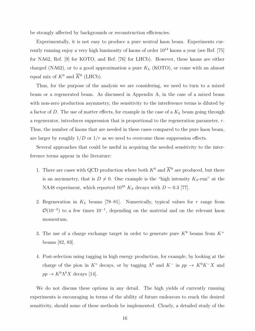
Experimentally, it is not easy to produce a pure neutral kaon beam. Experiments cur-

rently running enjoy a very high luminosity of kaons of order 1014 kaons a year (see Ref. [75]

for NA62, Ref. [9] for KOTO, and Ref. [76] for LHCb). However, these kaons are either

charged (NA62), or to a good approximation a pure KL (KOTO), or come with an almost

equal mix of K0 and K0 (LHCb).

Thus, for the purpose of the analysis we are considering, we need to turn to a mixed

beam or a regenerated beam. As discussed in Appendix A, in the case of a mixed beam

with non-zero production asymmetry, the sensitivity to the interference terms is diluted by

a factor of D. The use of matter effects, for example in the case of a KL beam going through

a regenerator, introduces suppression that is proportional to the regeneration parameter, r.

Thus, the number of kaons that are needed in these cases compared to the pure kaon beam,

are larger by roughly 1/D or 1/r as we need to overcome these suppression effects.

Several approaches that could be useful in acquiring the needed sensitivity to the inter-

ference terms appear in the literature:

1. There are cases with QCD production where both K0 and K0 are produced, but there

is an asymmetry, that is D 6= 0. One example is the “high intensity KS-run” at the

NA48 experiment, which reported 1010 KS decays with D ∼ 0.3 [77].

2. Regeneration in KL beams [78–81]. Numerically, typical values for r range from

O(10−2) to a few times 10−1, depending on the material and on the relevant kaon

momentum.

3. The use of a charge exchange target in order to generate pure K0 beams from K+

beams [82, 83].

4. Post-selection using tagging in high energy production, for example, by looking at the

charge of the pion in K∗ decays, or by tagging Λ0 and K− in pp → K0K−X and

pp→ K0Λ0X decays [14].

We do not discuss these options in any detail. The high yields of currently running

experiments is encouraging in terms of the ability of future endeavors to reach the desired

sensitivity, should some of these methods be implemented. Clearly, a detailed study of the

16

experimental requirements is needed in order to arrive at a reliable estimate for the expected

sensitivity.

We close this section with a remark about the time dependence. A measurement of the full

time dependence would result in the best sensitivity. However, in principle, a measurement

of the integral over four different time intervals suffices to get the needed information. In

practice, CL is already known, CS can be extracted from a beam with D = 0, and then we

would need two time intervals using a beam with D 6= 0 or r 6= 0.

VII. CONCLUSION AND OUTLOOK

We have demonstrated how, under well-motivated approximations and assumptions, it is

possible to cleanly test the SM using a measurement of the time-dependent decay rate of

K → µ+µ−. A necessary ingredient is sensitivity to the interference between the KL and

KS amplitudes, as can be seen from Eq. (31), which is our main result. The relevant SM

parameter of interest is

|VtsVtd sin(β + βs)| , (50)

which is exactly the CKM parameter combination that appears in KL → π0νν . Thus, our

proposal is to use K → µ+µ− as an additional independent measurement of the same SM

quantity.

As we discuss in detail, the point to emphasize is that the extraction is theoretically very

clean. There are several assumptions that were made in setting up the method, as well as in

the calculation within the SM. All of these are valid within the SM to a few per-mill, giving

a total uncertainty below the 1% level. This is comparable to the best probing methods

for the angle β and related quantities, that is, the CP asymmetries in B → ψKS and the

decay rate of KL → π0νν. The assumptions we rely on are additionally respected by any

extension of the SM in which the relevant leptonic current is vectorial.

The approach we discuss can in principle be extended to other decay modes. Most

promising are the decays K → πe+e− and K → πµ+µ−. The generalization is not trivial as

these decays involve more partial waves beyond ` = 0, 1. We plan to discuss these modes in

a future publication.

Our very preliminary estimates indicate that these measurements can be carried out in

17

next generation kaon experiments. This is encouraging, and more detailed feasibility studies

are called for.

ACKNOWLEDGMENTS

We thank G. D’Ambrosio, T. Kitahara, and Y. Nir for useful comments on the manuscript.

The work of AD is partially supported by the Israeli council for higher education postdoc-

toral fellowship for women in science. The work of YG is supported in part by the NSF

grant PHY1316222. S.S. is supported by a Stephen Hawking Fellowship from UKRI under

reference EP/T01623X/1.

Appendix A: Extracting B(KS → µ+µ−)`=0 without a pure kaon beam

In the main text, we demonstrated how we can determine B(KS → µ+µ−)`=0 for the case

of a pure K0 beam in empty space. Here we present a discussion on two other cases which

are more related to realistic experimental situations. The first case is when we have a beam

with unequal initial number of K0 and K0. The second case is when we have a pure KL

beam going via a regenerator before the kaons decay. In both cases, it is possible to extract

the branching ratio B(KS → µ+µ−)`=0 cleanly as in Eq. (31), with the addition of a dilution

factor as in Eq. (32).

1. A mixed beam of K0 and K0

Consider a beam which initially consists of an incoherent mixture of kaons and anti-kaons.

We define the production asymmetry,

D =NK0 −NK0

NK0 +NK0

. (A1)

such that the fractions of K0 and K0 particles are given respectively by

NK0

NK0 +NK0

=1 +D

2,

NK0

NK0 +NK0

=1−D

2. (A2)

Note that D = 1 corresponds to a pure K0 beam, while D = −1 corresponds to a pure K0

beam.

18

The decay rate to a final state f is given by the incoherent sum

dΓ

dt=

1 +D

2

(dΓK0

dt

)+

1−D2

(dΓK0

dt

), (A3)

such that its form is given by Eq. (8) with the following coefficients:

CL = |ACP-even0 |2, (A4)

CS = |ACP-odd0 |2 + β2

µ|ACP-even1 |2,

Ccos = D |ACP-odd*0 ACP-even

0 | cosϕ0,

Csin = D |ACP-odd*0 ACP-even

0 | sinϕ0.

It is then straightforward to extract our parameter of interest. For D 6= 0 we obtain

|ACP-odd0 |2 = DF

Ccos2 + Csin

2

CL, DF =

1

D2. (A5)

In terms of the branching ratios we have

B(KS → µ+µ−)`=0 = DF × B(KL → µ+µ−)× τSτL×(CintCL

)2

, (A6)

We learn that the beam asymmetry serves as a dilution factor compared to the case of a

pure K0 or K0 beam. Note that if D = 0 (which means that the beam is an equal admixture

of K0 and K0), one cannot use the beam to measure B(KS → µ+µ−)`=0.

We close with a remark regarding the LHCb search for the KS rate [51]. To a very good

approximation at LHCb we have D = 0. In that case the interference terms cancel and we

are left with just CL and CS. Thus, without any further analysis to tag the flavor of the

kaon, LHCb is working on extracting the CS term that includes the decay to both the ` = 0

and ` = 1 states.

2. KL propagating through a slab of matter

When kaons travel through matter, the time dependence of the kaon wave function is

modified via the inclusion of the momentum dependent regeneration parameter [78–81, 84,

85].

We define

reiα = −πNm

(∆f

∆λ

), (A7)

19

where r and α are real, and

∆f ≡ f − f , ∆λ ≡ ∆m− i

2∆Γ. (A8)

Here, f (f) is the difference of forward scattering amplitudes for kaons (anti-kaons), and N

is the density of scattering centers in the regenerator. Note that r and α are physical and

can be determined from experiment.

Let us consider a pure KL beam, which is produced by letting the KS (and interferences)

terms decay away. Then we put a regenerator of length L in the path of the beam. Let tL

be the time taken by the kaon to travel through the regenerator. We define t = 0 to be the

time the kaon emerges from the regenerator. We then study the time dependence of the

kaon wave function at later times. For simplicity, in the following we present the result to

leading order in r.

The normalized decay rate is given by Eq. (8), with the coefficients:

CL = |ACP-even0 |2,

CS = 0,

Csin = −r |ACP-even0 ACP-odd

0 |(sin(α− ϕ0)− etL∆Γ/2 sin(α− ϕ0 + ∆mtL)

),

Ccos = r |ACP-even0 ACP-odd

0 |(cos(α− ϕ0)− etL∆Γ/2 cos(α− ϕ0 + ∆mtL)

). (A9)

We can check that for tL = 0 (which means that the regenerator thickness is negligible) or

r = 0 (the regenerator material is just vacuum), the interference terms vanish as it should.

Using the above, we find the dilution factor DF , for tL 6= 0 and r 6= 0 to be

DF =1

2r2

(cosh(∆ΓtL/2)− sinh(∆ΓtL/2)

cosh(∆ΓtL/2)− cos(∆mtL)

). (A10)

We learn that the dilution parameter depends on both r and tL. The extraction of the rate

is given by Eq. (A6).

We close with two remarks

1. As we already emphasized, the interference terms are the key to the extraction of

B(KS → µ+µ−)`=0. Having D 6= 0 or r 6= 0 are some of the ways of obtaining

interference terms in the time dependence of the kaon beam.

2. More generally one may also have combinations with both non-zero D and r, as well

as a general initial state. The calculation is straightforward, though tedious and does

not provide much further insight, and so we do not show it here.

20

Appendix B: SM Calculations

In the following we first derive the SM prediction for B(KS → µ+µ−)`=0, and then derive

approximate numerical estimates for the experimental parameters within the SM.

1. SM calculation

Using the standard formula for two body decays [67], as well as the results of Eqs. (45)

and (36), we write

B(KS → (µ+µ−)`=0) =βµτS

16πmK

× 2∑|MSD(KS → (µ+µ−)`=0)|2 × sin2 θct, (B1)

where the sum is over the outgoing spin, as usual. Note thatM is proportional to A, defined

in Eq. (5) but it uses the standard normalization that is used when making calculations.

We write the matrix element for the short-distance contribution as

MSD = gSM〈µµ|O`|0〉 × 〈0|OH |K〉, (B2)

where

O` = (µLγρµL), 〈0|OH |K〉 ≡ −i pρK fK . (B3)

For the kaon decay constant we employ here the convention

〈0|sγµγ5d|K0(p)〉 = ipµfK0 . (B4)

The coupling, gSM, can be read from Eq. (43) (note that (µµ)V−A = 2(µLγρµL))

gSM = −GF√2

αemπ sin2 θW

[V ∗csVcdYNL + V ∗tsVtdY (xt)] . (B5)

Since under our assumption of θuc = 0 the part proportional to V ∗csVcd is relatively real, we

can further define

gSM = −GF√2

αemπ sin2 θW

V ∗tsVtdY (xt). (B6)

As long as what we are after is the CP violating decay rate, we can use gSM.

Squaring the amplitude and summing over spins, we find∑|MSD

K→µµ|2 =[− pρKpσKf 2

K

]|gSM|2 Tr

[u(k1)γρPLv(k2)v(k2)PLγσu(k1)

](B7)

= −|gSM|2 f 2Kp

ρKp

σKTr

[γρPL(/k2 −mµ)PLγσ(/k1 +mµ)

]= |gSM|2 f 2

Km2µp

ρKp

σKTr

[γρ

1

2(1− γ5)γσ

]= 2|gSM|2f 2

Km2µm

2K .

21

Using Eq. (B1) we find

B(KS → (µ+µ−)`=0) =βµτS

16πmK

4|gSM|2f 2Km

2µm

2K sin2 θct (B8)

=βµ τS

16πmK

∣∣∣∣GF√2

2αemπ sin2 θW

mKmµ × Y (xt) × fK × VtsVtd sin θct

∣∣∣∣2 ,in agreement with Eqs. (37) and (39) of Ref. [59].

We next get numerical estimates. We use the lattice QCD result [74] for the hadronic

parameter, assuming isospin symmetry:

fK = 155.7± 0.3 MeV . (B9)

We use the following values for the measured parameters [67],

mK = 497.61 MeV, mµ = 105.658 MeV, (B10)

GF = 1.166378× 10−5 GeV−2, αem = 1/129,

sin2 θW = 0.23, Y (xt) = 0.95,

τL = 5.116× 10−8 s, τS = 8.95× 10−11 s,

and for the CKM values we use

|VtsVtd sin θct| = A2λ5η, with A = 0.79, λ = 0.2265, η = 0.357, (B11)

to arrive at the prediction

B(KS → (µ+µ−)`=0) ≈ 1.64 · 10−13 ×∣∣∣∣ VtsVtd sin θct(A2λ5η)best fit

∣∣∣∣2 , (B12)

with

(A2λ5η)best fit = 1.33 · 10−4. (B13)

2. SM approximate values for the experimental parameters

In order to estimate the magnitude of the effect we are after and to illustrate the expected

time dependence, we require approximate values for the remaining two branching ratios

within the SM. First, we use the measured branching ratio,

B(KL → µ+µ−)exp. = B(KL → (µ+µ−)`=0)exp. = (6.84± 0.11) · 10−9, (B14)

22

which sets the value of the parameter CL.

The remaining branching ratio, B(KS → µ+µ−)`=1, can only be estimated a priori by

relying on non-perturbative calculations from the literature that suffer from large hadronic

uncertainties. Nonetheless, we use these results to get an estimate for its magnitude. Below

we use the prediction for the long-distance contribution, [14]

B(KS → µ+µ−)LDSM = B(KS → µ+µ−)`=1 ≈ 4.99 · 10−12. (B15)

Note that while we quote results to three significant digits, the theoretical uncertainties are

much larger. Altogether we have

B(KS → µ+µ−)`=0 ≈ 1.64 · 10−13, (B16)

B(KL → µ+µ−)`=0 ≈ 6.84 · 10−9,

B(KS → µ+µ−)`=1 ≈ 4.99 · 10−12.

The first is the result of the calculation from the SM effective Hamiltonian, the second is the

experimental measured value, and the third uses the non-perturbative estimation together

with the calculated SM short-distance contribution.

For illustration of the time dependence, we choose to normalize the C coefficients such

that CL = 1. The numerical values for the coefficients, as defined in Eqs. (8) and (9), for

the case of a pure K0 or K0 beam, are then given by:

(CL)SM ≡ 1, (B17)

(CS)SM =τLτS

B(KS → µ+µ−)`=0 + B(KS → µ+µ−)`=1

B(KL → µ+µ−)`=0

≈ 0.43,

(CInt.)SM =

√τL B(KS → µ+µ−)`=0

τS B(KL → µ+µ−)`=0

≈ 0.12 .

There is one more experimental parameter, the phase ϕ0. It is related to the strong phase

and we do not provide any estimate for it.

Appendix C: The short-distance operator

For completeness, we explain below the well-known results that the short-distance SM

amplitude cannot generate an ` = 1 state, and that only the axial parts of both the hadronic

and leptonic currents contribute in two-body pseudo-scalar decays.

23

Our starting point is the factorization of the matrix element

M = 〈µ+µ−|OµLOHµ|K〉 = 〈µ+µ−|Oµ

L|0〉 × 〈0|OHµ|K〉, (C1)

where

OµH = (sd)V−A, Oµ

L = (µµ)V−A. (C2)

The leading breaking of this factorization is from the photon loop, and thus it is suppressed

by roughly O(αEM/4π) ∼ 10−3.

Considering the leptonic part is sufficient to explain why short-distance physics does

not contribute to the K → (µ+µ−)`=1 amplitude. For two spinors ψ and χ, we recall the

transformation of the V − A operator under CPT [86]:

Θψγµ(1− γ5)χΘ† = −χγµ(1− γ5)ψ , (C3)

where Θ = CPT is the CPT operator. This implies

ΘOµLΘ† = −Oµ

L. (C4)

Using

Θ|µ+µ−〉` = (−1)`+1|µ+µ−〉`, Θ|0〉 = |0〉, (C5)

we conclude

〈(µ+µ−)`|OµL|0〉 = 〈(µ+µ−)`|ΘΘ†Oµ

LΘΘ†|0〉 = (−1)`〈(µ+µ−)`|OµL|0〉. (C6)

From the above we see that M, defined in Eq. (C1), vanishes when ` is odd.

As for the axial part of the hadronic current, the argument is the same as the well-known

one for charged pion decay, that we recall below. Consider

〈0|V µ − Aµ|K(pK)〉. (C7)

The kaon is a pseudo-scalar and the vacuum is parity-even. Thus, the matrix element of

V µ must transform as a pseudovector, and the matrix element of Aµ must transform as

a vector. The only available physical observable is the kaon momentum, pK , which is a

vector. It is impossible to construct a product of any number of pµK that transforms like as

a pseudovector. We conclude that

〈0|V µ|K〉 = 0. (C8)

24

In order to see that also for the leptonic current only the axial part is relevant, we write

the matrix element in the following form, leaving the vector and axial-vector components of

the leptonic operator general:

M∼ pαK u(k2)γα(B + Aγ5)v(k1) (C9)

Then,∑|M|2 ∝ Tr

[(/k2 +mµ)/pK(B + Aγ5)(/k1 −mµ)(B∗ + A∗γ5)/pK

](C10)

= 4(|B|2 − |A|2

)[2(k1 · pK)(k2 · pK)−m2

K(k1 · k2)]− 4

(|B|2 + |A|2

)m2µm

2K

Using two-body kinematics, we have

(k1 · pK) = (k2 · pK) =1

2m2K , (C11)

(k1 · k2) =1

2m2K −m2

µ.

Plugging this in to Eq. (C10), the |B|2 terms drop out and we are left only with the terms

proportional to |A|2, ∑|M|2 ∝ |A|2m2

µm2K , (C12)

i.e., only the axial-vector part of the operator is relevant.

[1] T. Inami and C. S. Lim, Prog. Theor. Phys. 65, 297 (1981), [Erratum: Prog.Theor.Phys. 65,

1772 (1981)].

[2] J. S. Hagelin and L. S. Littenberg, Prog. Part. Nucl. Phys. 23, 1 (1989).

[3] C. O. Dib, Phys. Lett. B 282, 201 (1992).

[4] G. Buchalla and A. J. Buras, Nucl. Phys. B 412, 106 (1994), arXiv:hep-ph/9308272.

[5] G. D’Ambrosio and G. Isidori, Int. J. Mod. Phys. A 13, 1 (1998), arXiv:hep-ph/9611284.

[6] A. Pich, in Workshop on K Physics (1996) arXiv:hep-ph/9610243.

[7] A. J. Buras and R. Fleischer, Adv. Ser. Direct. High Energy Phys. 15, 65 (1998), arXiv:hep-

ph/9704376.

[8] E. Cortina Gil et al. (NA62), JHEP 11, 042 (2020), arXiv:2007.08218 [hep-ex].

[9] J. K. Ahn et al. (KOTO), (2020), arXiv:2012.07571 [hep-ex].

25

[10] A. J. Buras, D. Buttazzo, J. Girrbach-Noe, and R. Knegjens, JHEP 11, 033 (2015),

arXiv:1503.02693 [hep-ph].

[11] G. Buchalla and A. J. Buras, Nucl. Phys. B 548, 309 (1999), arXiv:hep-ph/9901288.

[12] F. Mescia and C. Smith, Phys. Rev. D 76, 034017 (2007), arXiv:0705.2025 [hep-ph].

[13] R. F. Lebed, Phys. Rev. D 55, 348 (1997), arXiv:hep-ph/9607305.

[14] G. D’Ambrosio and T. Kitahara, Phys. Rev. Lett. 119, 201802 (2017), arXiv:1707.06999 [hep-

ph].

[15] B. R. Martin, E. De Rafael, and J. Smith, Phys. Rev. D 2, 179 (1970).

[16] A. Pais and S. B. Treiman, Phys. Rev. 176, 1974 (1968).

[17] L. M. Sehgal, Phys. Rev. 181, 2151 (1969).

[18] N. H. Christ and T. D. Lee, Phys. Rev. D 4, 209 (1971).

[19] L. M. Sehgal, Phys. Rev. 183, 1511 (1969), [Erratum: Phys.Rev.D 4, 1582 (1971)].

[20] G. V. Dass and L. Wolfenstein, Phys. Lett. B 38, 435 (1972).

[21] M. K. Gaillard and B. W. Lee, Phys. Rev. D 10, 897 (1974).

[22] M. K. Gaillard, B. W. Lee, and R. E. Shrock, Phys. Rev. D13, 2674 (1976).

[23] A. J. Buras, Phys. Rev. Lett. 46, 1354 (1981).

[24] L. Bergstrom, E. Masso, P. Singer, and D. Wyler, Phys. Lett. 134B, 373 (1984).

[25] C. Q. Geng and J. N. Ng, Phys. Rev. D41, 2351 (1990).

[26] E. B. Bogomolny, V. A. Novikov, and M. A. Shifman, Sov. J. Nucl. Phys. 23, 435 (1976),

[Yad. Fiz.23,825(1976)].

[27] B. W. Lee, J. R. Primack, and S. B. Treiman, Phys. Rev. D7, 510 (1973).

[28] M. B. Voloshin and E. P. Shabalin, JETP Lett. 23, 107 (1976), [Pisma Zh. Eksp. Teor.

Fiz.23,123(1976)].

[29] R. E. Shrock and M. B. Voloshin, Phys. Lett. 87B, 375 (1979).

[30] P. Herczeg, Phys. Rev. D 27, 1512 (1983).

[31] H. Stern and M. K. Gaillard, Annals Phys. 76, 580 (1973).

[32] Y. Grossman and Y. Nir, Phys. Lett. B 398, 163 (1997), arXiv:hep-ph/9701313.

[33] J. Aebischer, A. J. Buras, and J. Kumar, JHEP 12, 097 (2020), arXiv:2006.01138 [hep-ph].

[34] R. Mandal and A. Pich, JHEP 12, 089 (2019), arXiv:1908.11155 [hep-ph].

[35] M. Endo, T. Goto, T. Kitahara, S. Mishima, D. Ueda, and K. Yamamoto, JHEP 04, 019

(2018), arXiv:1712.04959 [hep-ph].

26

[36] C. Bobeth and A. J. Buras, JHEP 02, 101 (2018), arXiv:1712.01295 [hep-ph].

[37] V. Chobanova, G. D’Ambrosio, T. Kitahara, M. Lucio Martinez, D. Martinez Santos, I. S.

Fernandez, and K. Yamamoto, JHEP 05, 024 (2018), arXiv:1711.11030 [hep-ph].

[38] C. Bobeth, A. J. Buras, A. Celis, and M. Jung, JHEP 07, 124 (2017), arXiv:1703.04753

[hep-ph].

[39] M. Endo, T. Kitahara, S. Mishima, and K. Yamamoto, Phys. Lett. B 771, 37 (2017),

arXiv:1612.08839 [hep-ph].

[40] M. Tanimoto and K. Yamamoto, PTEP 2016, 123B02 (2016), arXiv:1603.07960 [hep-ph].

[41] A. J. Buras, JHEP 04, 071 (2016), arXiv:1601.00005 [hep-ph].

[42] A. J. Buras, D. Buttazzo, and R. Knegjens, JHEP 11, 166 (2015), arXiv:1507.08672 [hep-ph].

[43] M. Blanke, A. J. Buras, B. Duling, K. Gemmler, and S. Gori, JHEP 03, 108 (2009),

arXiv:0812.3803 [hep-ph].

[44] F. Mescia, C. Smith, and S. Trine, JHEP 08, 088 (2006), arXiv:hep-ph/0606081.

[45] N. G. Deshpande, D. K. Ghosh, and X.-G. He, Phys. Rev. D 70, 093003 (2004), arXiv:hep-

ph/0407021.

[46] A. Crivellin, G. D’Ambrosio, M. Hoferichter, and L. C. Tunstall, Phys. Rev. D 93, 074038

(2016), arXiv:1601.00970 [hep-ph].

[47] T. Kitahara, T. Okui, G. Perez, Y. Soreq, and K. Tobioka, Phys. Rev. Lett. 124, 071801

(2020), arXiv:1909.11111 [hep-ph].

[48] R. Ziegler, J. Zupan, and R. Zwicky, JHEP 07, 229 (2020), arXiv:2005.00451 [hep-ph].

[49] X.-G. He, X.-D. Ma, J. Tandean, and G. Valencia, JHEP 08, 034 (2020), arXiv:2005.02942

[hep-ph].

[50] S. Gori, G. Perez, and K. Tobioka, JHEP 08, 110 (2020), arXiv:2005.05170 [hep-ph].

[51] R. Aaij et al. (LHCb), Phys. Rev. Lett. 125, 231801 (2020), arXiv:2001.10354 [hep-ex].

[52] F. Ambrosino et al. (KLEVER Project), (2019), arXiv:1901.03099 [hep-ex].

[53] R. Aaij et al. (LHCb), Eur. Phys. J. C 77, 678 (2017), arXiv:1706.00758 [hep-ex].

[54] G. Amelino-Camelia et al., Eur. Phys. J. C 68, 619 (2010), arXiv:1003.3868 [hep-ex].

[55] E. Abouzaid et al. (KTeV), Phys. Rev. Lett. 99, 051804 (2007), arXiv:hep-ex/0702039.

[56] R. Lollini (NA62), Acta Phys. Polon. Supp. 14, 41 (2021).

[57] A. Cerri et al., CERN Yellow Rep. Monogr. 7, 867 (2019), arXiv:1812.07638 [hep-ph].

[58] G. Ecker and A. Pich, Nucl. Phys. B 366, 189 (1991).

27

[59] G. Isidori and R. Unterdorfer, JHEP 01, 009 (2004), arXiv:hep-ph/0311084 [hep-ph].

[60] M. Gorbahn and U. Haisch, Phys. Rev. Lett. 97, 122002 (2006), arXiv:hep-ph/0605203.

[61] G. Colangelo, R. Stucki, and L. C. Tunstall, Eur. Phys. J. C 76, 604 (2016), arXiv:1609.03574

[hep-ph].

[62] D. Gomez Dumm and A. Pich, Phys. Rev. Lett. 80, 4633 (1998), arXiv:hep-ph/9801298.

[63] M. Knecht, S. Peris, M. Perrottet, and E. de Rafael, Phys. Rev. Lett. 83, 5230 (1999),

arXiv:hep-ph/9908283 [hep-ph].

[64] G. D’Ambrosio, D. Greynat, and G. Vulvert, Eur. Phys. J. C 73, 2678 (2013), arXiv:1309.5736

[hep-ph].

[65] V. Cirigliano, G. Ecker, H. Neufeld, A. Pich, and J. Portoles, Rev. Mod. Phys. 84, 399 (2012),

arXiv:1107.6001 [hep-ph].

[66] A. J. Buras, F. Schwab, and S. Uhlig, Rev. Mod. Phys. 80, 965 (2008), arXiv:hep-ph/0405132.

[67] P. A. Zyla et al. (Particle Data Group), PTEP 2020, 083C01 (2020).

[68] L. Littenberg, in PSI Zuoz Summer School on Exploring the Limits of the Standard Model

Zuoz, Engadin, Switzerland, August 18-24, 2002 (2002) arXiv:hep-ex/0212005 [hep-ex].

[69] D. Greynat and E. de Rafael, in 14th Rencontres de Blois on Matter - Anti-matter Asymmetry

Chateau de Blois, France, June 17-22, 2002 (2003) arXiv:hep-ph/0303096 [hep-ph].

[70] G. D’Ambrosio, G. Isidori, and J. Portoles, Phys. Lett. B423, 385 (1998), arXiv:hep-

ph/9708326 [hep-ph].

[71] R. Aleksan, B. Kayser, and D. London, Phys. Rev. Lett. 73, 18 (1994), arXiv:hep-ph/9403341.

[72] G. Buchalla, A. J. Buras, and M. E. Lautenbacher, Rev. Mod. Phys. 68, 1125 (1996),

arXiv:hep-ph/9512380 [hep-ph].

[73] T. Hermann, M. Misiak, and M. Steinhauser, JHEP 12, 097 (2013), arXiv:1311.1347 [hep-ph].

[74] S. Aoki et al. (Flavour Lattice Averaging Group), Eur. Phys. J. C 80, 113 (2020),

arXiv:1902.08191 [hep-lat].

[75] A. Kleimenova (NA62), PoS DIS2019, 122 (2019).

[76] A. A. Alves Junior et al., JHEP 05, 048 (2019), arXiv:1808.03477 [hep-ex].

[77] E. Mazzucato, Nucl. Phys. B Proc. Suppl. 99, 81 (2001).

[78] R. H. Good, R. P. Matsen, F. Muller, O. Piccioni, W. M. Powell, H. S. White, W. B. Fowler,

and R. W. Birge, Phys. Rev. 124, 1223 (1961).

[79] A. Bohm, P. Darriulat, C. Grosso, V. Kaftanov, K. Kleinknecht, H. L. Lynch, C. Rubbia,

28

H. Ticho, and K. Tittel, Phys. Lett. B 27, 594 (1968).

[80] K. Kleinknecht, Fortsch. Phys. 21, 57 (1973).

[81] A. Angelopoulos et al. (CPLEAR), Phys. Lett. B 413, 422 (1997).

[82] P. B. Siegel, W. B. Kaufmann, and W. R. Gibbs, Phys. Rev. C 30, 1256 (1984).

[83] W. A. Mehlhop, S. S. Murty, P. Bowles, T. H. Burnett, R. H. Good, C. H. Holland, O. Piccioni,

and R. A. Swanson, Phys. Rev. 172, 1613 (1968).

[84] W. Fetscher, P. Kokkas, P. Pavlopoulos, T. Schietinger, and T. Ruf, Z. Phys. C72, 543 (1996).

[85] H. R. Quinn, T. Schietinger, J. P. Silva, and A. E. Snyder, Phys. Rev. Lett. 85, 5284 (2000),

arXiv:hep-ph/0008021 [hep-ph].

[86] G. C. Branco, L. Lavoura, and J. P. Silva, Int. Ser. Monogr. Phys. 103, 1 (1999).

29