stefanie runde design and analysis of fmri experiments - kip
TRANSCRIPT

RUPRECHT-KARLS-UNIVERSITÄT HEIDELBERG
Stefanie Runde
Design and Analysis offMRI Experiments
ProbingBrain Activity
Induced byTactile Stimulation
Diplomarbeit
HD-KIP-00-27
KIRCHHOFF-INSTITUT FÜR PHYSIK


Design and Analysis offMRI Experiments
ProbingBrain Activity
Induced byTactile Stimulation
This diploma thesis has been carried out by Stefanie Rundeat the
KIRCHHOFF-INSTITUTE OF PHYSICS
UNIVERSITY OF HEIDELBERG
under the supervision of
Prof. Dr. Karlheinz Meier


Faculty of Physics andAstronomy
University of Heidelberg
Diploma thesisin Physics
submitted by
Stefanie Runde
born in Karlsruhe
September 2000


Abstract
This thesis presents the design and analysis of fMRI experiments on the processing oftactile information in the human brain. For this purpose the principles of neurology andfMRI relevant for the experiments are introduced. A pneumatically driven tactile dis-play, whose non-interference with the fMRI image acquisition is verified, is used to effecttactile stimulation. The somatotopic representations in the primary and the secondarysomatosensory cortex are successfully mapped at two distinct points (index finger andfoot) for three healthy, seeing subjects. The analysis is performed by means of statisticalparametric mapping of t-scores, a hypothesis testing approach based on the general linearmodel. The tactile stimulations elicited activation of the primary motor cortex for almostall image series in spite of precautions with regard to the subjects’comfort and immobil-ity. The reproducibility of the resulting brain activities is examined in terms of location,extent and significance. It turns out that the location of the most significant point of acti-vity can be reliably reproduced using three dimensional maps of t-scores while extent andintensity are subject to large random variations.
Inhalt
In dieser Arbeit werden Design und Analyse von fMRI Experimenten zur Erforschung derVerarbeitung taktiler Informationen im menschlichen Gehirn vorgestellt. Dazu werdendie notwendigen Grundlagen der Neurologie und der funktionellen Magnetresonanzspek-troskopie erarbeitet. Taktile Stimulationen werden mit Hilfe eines pneumatischen tak-tilen Displays erzeugt. Es wird gezeigt, daß das taktile Display die fMRI Bildaufnahmenicht beeinflußt. Die somatotopische Reprasentation im primaren und im sekundaren so-matosensorischen Kortex an je zwei diskreten Punkten (dem Zeigefinger und dem Fuß)wird bei drei gesunden, sehenden Probanden ermittelt. Die Analyse basiert auf dem soge-nannten ‘Statistical Parametric Mapping’. Dabei werden den Aktivitatsverlauf im Gehirnmodellierende Hypothesen mittels linearer Regression getestet. Obwohl versucht wurdemotorische Reize zu minimieren, wird durch taktile Stimulationen in fast allen Fallender primare Motorcortex mit angeregt. Die Reproduzierbarkeit der gefundenen Gehirn-aktivitaten wird auf Ort, Ausdehnung und Signifikanz untersucht. Es stellt sich heraus,daß der Ort der starksten Aktivitat anhand von 3-D Karten der t-Werten verlasslich re-produziert werden kann, wahrend Ausdehnung und Intensitat großeren Schwankungenunterliegen.


Contents
Introduction 1
1 Processing Tactile and Motor Stimulation 31.1 The Brain’s Functional Organization . . . . . . . . . . . . . . . . . . . . 31.2 The Cerebral Cortex . . . . . . . . . . . . . . . . . . . . . . . . . . . . 41.3 The Somatosensory Pathways . . . . . . . . . . . . . . . . . . . . . . . 51.4 Somatosensory Receptors . . . . . . . . . . . . . . . . . . . . . . . . . . 51.5 Somatosensory Cortical Regions . . . . . . . . . . . . . . . . . . . . . . 6
1.5.1 Functionality . . . . . . . . . . . . . . . . . . . . . . . . . . . . 61.5.2 Location . . . . . . . . . . . . . . . . . . . . . . . . . . . . . . 71.5.3 Modality-Specific Organization . . . . . . . . . . . . . . . . . . 71.5.4 Somatotopic Organization of SI and SII . . . . . . . . . . . . . . 8
1.6 Motor Task Processing . . . . . . . . . . . . . . . . . . . . . . . . . . . 9
2 Basics of fMRI 112.1 Concepts of Nuclear Magnetic Resonance . . . . . . . . . . . . . . . . . 112.2 Principles of Magnetic Resonance Imaging . . . . . . . . . . . . . . . . 122.3 Echo-Planar Imaging . . . . . . . . . . . . . . . . . . . . . . . . . . . . 132.4 The BOLD Effect . . . . . . . . . . . . . . . . . . . . . . . . . . . . . . 142.5 Artifacts and Noise . . . . . . . . . . . . . . . . . . . . . . . . . . . . . 15
2.5.1 Artifacts . . . . . . . . . . . . . . . . . . . . . . . . . . . . . . . 152.5.2 Noise . . . . . . . . . . . . . . . . . . . . . . . . . . . . . . . . 15
2.6 MRI-System in Strasburg . . . . . . . . . . . . . . . . . . . . . . . . . . 16
3 The Pneumatically driven Tactile Display 193.1 Description of the PTD . . . . . . . . . . . . . . . . . . . . . . . . . . . 193.2 Functionality of the PTD . . . . . . . . . . . . . . . . . . . . . . . . . . 203.3 The Visor software and Pattern Generation . . . . . . . . . . . . . . . . . 22
4 Statistical Parametric Mapping 254.1 Preprocessing . . . . . . . . . . . . . . . . . . . . . . . . . . . . . . . . 26
4.1.1 Principles of Spatial Transformations in Brain Imaging . . . . . . 264.1.2 Realignment (Within Modality Coregistration) . . . . . . . . . . 26
I

II CONTENTS
4.1.3 Between Modality Coregistration . . . . . . . . . . . . . . . . . 274.1.4 Normalization . . . . . . . . . . . . . . . . . . . . . . . . . . . 274.1.5 Smoothing . . . . . . . . . . . . . . . . . . . . . . . . . . . . . 29
4.2 Statistical Models . . . . . . . . . . . . . . . . . . . . . . . . . . . . . . 304.2.1 The General Linear Model . . . . . . . . . . . . . . . . . . . . . 304.2.2 Low Frequency Confounds . . . . . . . . . . . . . . . . . . . . . 314.2.3 t-Test . . . . . . . . . . . . . . . . . . . . . . . . . . . . . . . . 314.2.4 Contrasts . . . . . . . . . . . . . . . . . . . . . . . . . . . . . . 324.2.5 Inference . . . . . . . . . . . . . . . . . . . . . . . . . . . . . . 33
4.2.5.1 Hypothesis Testing . . . . . . . . . . . . . . . . . . . 334.2.5.2 The Multiple Comparison Problem . . . . . . . . . . . 334.2.5.3 Bonferroni Correction . . . . . . . . . . . . . . . . . . 334.2.5.4 Random Field Theory and Euler Characteristic . . . . . 33
4.3 Using SPM99 for Statistical Analysis . . . . . . . . . . . . . . . . . . . 354.3.1 Setting up a Design Matrix in SPM99 . . . . . . . . . . . . . . . 354.3.2 Using the Thresholding Function in SPM99 . . . . . . . . . . . . 374.3.3 Automatisation of the Analysis . . . . . . . . . . . . . . . . . . . 38
5 Experiments 405.1 Experimental Setup . . . . . . . . . . . . . . . . . . . . . . . . . . . . . 40
5.1.1 Subjects and Experimental Setting . . . . . . . . . . . . . . . . . 405.1.2 Mounting of the modules . . . . . . . . . . . . . . . . . . . . . . 41
5.2 Mapping SI for One Subject . . . . . . . . . . . . . . . . . . . . . . . . 425.2.1 Experimental Procedure . . . . . . . . . . . . . . . . . . . . . . 425.2.2 SPM Analysis . . . . . . . . . . . . . . . . . . . . . . . . . . . 43
5.3 Tactile versus Motor Stimulation . . . . . . . . . . . . . . . . . . . . . . 485.3.1 Experimental Procedure . . . . . . . . . . . . . . . . . . . . . . 485.3.2 SPM Analysis and Overlap . . . . . . . . . . . . . . . . . . . . . 48
5.4 Reproducibility of Motor Stimulation . . . . . . . . . . . . . . . . . . . 505.5 Reproducibility of Tactile Stimulation . . . . . . . . . . . . . . . . . . . 51
5.5.1 Experimental Procedure . . . . . . . . . . . . . . . . . . . . . . 515.5.2 SPM Analysis . . . . . . . . . . . . . . . . . . . . . . . . . . . 52
5.6 Intersubject Analysis . . . . . . . . . . . . . . . . . . . . . . . . . . . . 615.7 Non-interference of the PTD with the MRI . . . . . . . . . . . . . . . . . 665.8 t-Scores Reviewed . . . . . . . . . . . . . . . . . . . . . . . . . . . . . 67
5.8.1 Signal and Cascades . . . . . . . . . . . . . . . . . . . . . . . . 675.8.2 Autocovariance . . . . . . . . . . . . . . . . . . . . . . . . . . . 705.8.3 Fourier Transformation . . . . . . . . . . . . . . . . . . . . . . . 71
Summary and Outlook 75
A Directions and Planes in the Human Brain 77

CONTENTS III
B Affine Transformations in Preprocessing 78B.1 General Affine Transformation . . . . . . . . . . . . . . . . . . . . . . . 78B.2 Voxel to Real World Coordinates . . . . . . . . . . . . . . . . . . . . . . 78B.3 Realignment . . . . . . . . . . . . . . . . . . . . . . . . . . . . . . . . . 79B.4 Affine Normalization . . . . . . . . . . . . . . . . . . . . . . . . . . . . 79
C Coordinates in SPM99 80C.1 Talairach Coordinate System . . . . . . . . . . . . . . . . . . . . . . . . 80C.2 The MNI brain . . . . . . . . . . . . . . . . . . . . . . . . . . . . . . . 80
D Examples for Batch-Files in SPM99 82

IV CONTENTS

Introduction
The Electronic Vision Group at the Kirchhoff Institute for Physics has been founded in1994 with the initial goal to develop a practical tactile vision substitution system (TVSS).The TVSS was intended to supplement the orientation of blind or visually impaired per-sons by making use of their tactile perception. This initial research goal has recentlybeen achieved. A small, single chip camera with image sensors based on CMOS technol-ogy performs the image acquisition [Loo99]. The main step of the image processing takesplace in the EDDA chip (EDge Detection Array), which converts analog greyscale imagesfrom the camera into a digitally coded edge image [Sch99]. The Virtual Tactile Display(VTD) constitutes the output device of the project based on piezoelectric actuators assem-bled in a movable tactile output unit. It can be moved around a two dimensional surface toexplore the line structure of a virtual raised image [Mau98]. A mobile image processingcomputer completes the TVSS. It comprises a miniaturized PC in combination with ad-ditional electronics for image processing purposes, cooperates with the camera chip andEDDA and can address the VTD as well as other peripheral devices. For more informa-tion on the Electronic Vision Group see also [Vis00].While the Electronic Vision Project initially focussed on using the infrastructure avail-able at the ASIC Laboratory for Microelectronics to develop intelligent vision chips, itsoon became clear that the interdisciplinary nature of the project offers exciting researchopportunities also in neighbouring fields. The project was extended to include a divisionthat is concerned with basic research on tactile perception. The motivation of this work isto optimize the information transfer via the tactile channel to the human brain. In orderto investigate the processing of tactile stimulation in the human brain experiments ap-plying fMRI are performed. Functional Magnetic Resonance Imaging (fMRI) presents anon-invasive method capable of monitoring the change in blood oxygenation due to brainactivity. It is used to record the human brain’s response to well-defined, reproducible tac-tile stimulations, which are generated by a Pneumatically driven Tactile Display (PTD)developed within the scope of this project.This thesis presents the results of first fMRI experiments with three seeing subjects us-ing the PTD for tactile stimulation. Their aim is to map the somatotopy of the primarysomatosensory cortex (the ‘somatosensory homunculus’). In addition the relationship oftactile and motor activation of the human brain and their reproducibility are investigated.Another experiment with a brain phantom probes the interference between the PTD andthe MRI image acquisition.The first chapter of this thesis is dedicated to those structures of the human brain that are
1

most important for processing tactile and motor stimulation. The next one introduces theprinciples of fMRI completing the theoretical background for the experiments. The PTDis presented in chapter three. The analysis of the fMRI data is performed with the softwarepackage SPM991 that uses statistical parametric maps of t-scores to locate activation sitesin the human brain. Additionally the data at detected activation sites is inspected by stan-dard correlation analysis methods to verify their significance. The statistical knowledgerequired to work with SPM99 is summarized in chapter four while chapter five presentsthe results from the analyzed experiments.
1Wellcome Department of Cognitive Neurology, London, UK

Chapter 1
Processing Tactile and MotorStimulation in the Human Brain
The conducted experiments involve mostly tactile stimulation but also some motor tasksfor reference purpose. This chapter focuses on a presentation of structures of the humanbrain that are involved in processing tactile and motor stimulation. Following short in-troductions on theories of the human brain’s functional organization and the structure ofthe cerebral cortex, the somatosensory information pathway is sketched and a summaryof the different peripheral receptors is given. Then an overview of those parts of the brain(mostly in the cerebral cortex) concerned with tactile perception and their somatotopicorganization will be presented. The relevant regions are the primary and secondary so-matosensory cortex as well as the related association areas. Finally motor task processingis introduced.
1.1 The Brain’s Functional Organization
Historically two different and opposing theories dominated the concepts of brain func-tionality in the nineteenth century: The aggregate field view and locationalism. The latterclaimed that every mental function, including emotion, is carried out by a single, preciselylocalized and specialized area of the brain. On the contrary, the followers of the aggregatefield view believed that all parts of the brain especially the cerebral hemispheres partic-ipate in all mental functions. In 1876 C. Wernicke introduced the idea of ‘distributedprocessing’ that still dominates the present concept of brain functionality. He suggestedthat the most basic mental function (those concerned with simple perceptual and motoractivities) are localized to single cortical areas. More complex intellectual functions arethen made possible by interconnection between those functional sites. The current theoryon brain functionality is a more elaborate version of Wernicke’s ‘distributed processing’[Kan91]. Thereby the brain’s functional organization is based on two fundamental prin-ciples: functional integrationand functional segregation. Functional segregation implies
3

4 CHAPTER 1. PROCESSING TACTILE AND MOTOR STIMULATION
that a cortical region is specialized for some aspects of perceptual or motor processing andthat this area is anatomically segregated in the cerebral cortex. A mental function maythen involve many of those functionally segregated areas whose interaction is mediatedby the functional integration among them. The techniques available to analyze functionalbrain images can be grouped as multivariate and univariate approaches on a procedurallevel which correspond to the theories of functional segregation and integration respec-tively [Fra97]. The univariate approaches are collectively brought under the heading ofStatisticalParametricMapping(Chapter 4).
1.2 The Cerebral Cortex
The Cerebral Cortex is located on the surface of the brain and is highly convoluted. Ele-vated convolutions, called gyri, are separated by grooves called sulci (or fissures if they aredeep). In each of the brain’s two cerebral hemispheres the overlying cortex is divided intofour anatomically distinct lobes: The frontal, parietal, temporal and occipital lobe (seefig. 1.1).
Figure 1.1: The 4 lobes of the cerebral cortex[Mar96]. The frontal and the parietal lobe areseparated by the central sulcus (bold line).
The different lobes are specialized for re-markably distinct functions. The frontal lobeis mainly concerned with control of move-ment, the parietal lobe with somatic sensationand proprioception1. They are separated bythe central sulcus. The occipital lobe is im-portant for vision, the temporal lobe for hear-ing, speech, various sensory functions as wellas aspects of learning memory and emotion.The following sections will be mainly con-cerned with the primary somatosensory cor-tex located in the parietal lobe. Section 1.6focuses on the frontal lobe due to its impor-tance for movement.One approach to parcel the cerebral cortex isof histological nature based on cellular char-acteristics. The most widely used classification was proposed by K. Brodman in 1909and contains 52 cytoarchitectonic areas (Brodman areas) [Afi98]. It is remarkable that thehistological and functional classifications are correlated, i. e. that different Brodman areasresemble different functional areas. In particular this is true for the primary somatosen-sory cortex as will be explained in section 1.5.3.
1limb position sense

1.3. THE SOMATOSENSORY PATHWAYS 5
1.3 The Somatosensory Pathways
The somatic (or bodily) senses consist of four distinct modalities: limb position sense,touch, thermal sensation, and pain. Two parallel ascending pathways transmit the somaticinformation to the primary somatosensory cortex. The ‘dorsal column-medial lemniscalsystem’ mediates touch and limb position while the ‘anterolateral system’ subserves painand temperature sense (and to a much lesser extend touch). Starting at a peripheral sensoryreceptor the information is passed on to the spinal cord and then the brain stem. Fromthere it continues through the thalamus to the primary somatosensory cortex (see fig. 1.2).Sensory information that enters the spinal cord from the left side of the body crosses overto the right side of the nervous system (either within the spinal cord or in the brainstem)before being conveyed to the cerebral cortex. Thus each hemisphere of the cerebral cortexis concerned primarily with sensory (and motor) processes on the contralateral side of thebody.
Figure 1.2: Illustration of the somatosensory pathways: dorsal column-medial and anterolateral[Kan91].
1.4 Somatosensory Receptors
The sensation of touch is mediated by mechanoreceptors. Mechanoreceptors can be di-vided into two major functional groups. The slowly adaptingones respond continuouslyto a persistent stimulus while rapidly adaptingmechanoreceptors respond only at the on-set (and often also at the termination) of the stimulus. Slowly adapting receptors are

6 CHAPTER 1. PROCESSING TACTILE AND MOTOR STIMULATION
Merkel’s receptorsin superficial skin and Ruffini’s corpusclesin subcutaneous tissue.Meissner’sand Pacinian corpusclesbelong to the group of rapidly adapting receptors andare also located in superficial skin and subcutaneous tissue respectively.Hairy and glabrous (hairless) skin do not contain the same mechanoreceptors. Hairyskin has hair follicle receptors, that respond to flutter stimulation, and Merkel’s recep-tors (slowly adapting) while glabrous skin incorporates Meissner’s corpuscles (rapidlyadapting) and Merkel’s receptors. The mechanoreceptors of the subcutaneous tissue areidentical for both skin types (see fig. 1.3).
Figure 1.3: The cutaneous and subcutaneous mechanoreceptors [Kan91].
1.5 Somatosensory Cortical Regions
1.5.1 Functionality
There are three major somatosensory cortical areas. The primary somatosensory cortex(SI) receives the direct projection from the thalamus. It then projects to the secondarysomatosensory cortex (SII)and the somatosensory association area(see fig. 1.5). Theprimary somatosensory cortex is the most important part for sensory perception. Ablationof SI will result in the loss of all modalities of sensation in the immediate postoperativeperiod. Pain and temperature sensation will return in form of a crude awareness butdiscriminative touch and proprioception are lost forever. Removal of SII will cause severeimpairment in the discrimination of both shape and texture. The secondary somatosensorycortex is also important for the conscious perception of noxious stimuli. In addition thereis some evidence that vibrational stimulation is primarily processed in SII [Mal99]. Thesomatosensory association area is concerned with higher order processing. Damage to thelatter will produce complex abnormalities in attending to sensations from the contralateralhalf of the body.

1.5. SOMATOSENSORY CORTICAL REGIONS 7
1.5.2 Location
The primary somatosensory cortex is located in the postcentral gyrus of the parietal lobe.Its position is posterior to the central sulcus and anterior to the postcentral sulcus (seefig. 1.4). In the sagittal plane (the plane separating the two hemispheres) it ends at thecingulate sulcus (see fig. 1.7). The lateral sulcus, which also anatomically separates theparietal from the temporal lobe, terminates the postcentral sulcus on the lateral surface ofthe cerebral cortex (see fig. 1.4).The secondary somatosensory cortex is mostly located in the superior bank and depth ofthe lateral sulcus (parietal operculum) and on the most inferior aspect of the postcentralgyrus. It is hidden from a superficial view of the brain. The somatosensory associationarea can be found in the superior parietal lobe and extends further into the posterior partof the parietal cortex.
Figure 1.4: Dorsal and lateral view of the brain [Mar96].
1.5.3 Modality-Specific Organization
The postcentral sulcus corresponds to Brodman areas 1, 2 and 3. Area 3 is further dividedinto 2 parts: 3b on the posterior wall of the central sulcus and 3a in the depth of the cen-tral sulcus (see fig. 1.5). As in other cortical areas regions with different cytoarchitecturewithin the primary somatosensory cortex subserve different functions. Brodman areas 2and 3a receive information from receptors located in deep structures, such as muscles andjoints, areas 1 and 3b from mechanoreceptors of the skin (see fig. 1.5). In each of theseareas a separate representation of the body can be found (see the following paragraph).The representations in 1 and 3b are complete and highly detailed while that in areas 2 and3a appear more coarse. Areas 2 and 3a are important in limb position sense and shape dis-crimination of grasped objects while areas 1 and 3b are responsible for touch perception.
8 CHAPTER 1. PROCESSING TACTILE AND MOTOR STIMULATION
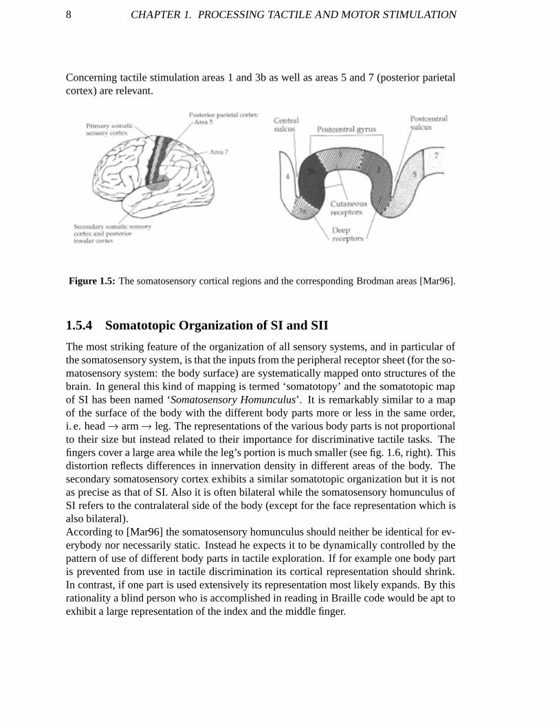
Concerning tactile stimulation areas 1 and 3b as well as areas 5 and 7 (posterior parietalcortex) are relevant.
Figure 1.5: The somatosensory cortical regions and the corresponding Brodman areas [Mar96].
1.5.4 Somatotopic Organization of SI and SII
The most striking feature of the organization of all sensory systems, and in particular ofthe somatosensory system, is that the inputs from the peripheral receptor sheet (for the so-matosensory system: the body surface) are systematically mapped onto structures of thebrain. In general this kind of mapping is termed ‘somatotopy’ and the somatotopic mapof SI has been named ‘Somatosensory Homunculus’. It is remarkably similar to a mapof the surface of the body with the different body parts more or less in the same order,i. e. head ! arm! leg. The representations of the various body parts is not proportionalto their size but instead related to their importance for discriminative tactile tasks. Thefingers cover a large area while the leg’s portion is much smaller (see fig. 1.6, right). Thisdistortion reflects differences in innervation density in different areas of the body. Thesecondary somatosensory cortex exhibits a similar somatotopic organization but it is notas precise as that of SI. Also it is often bilateral while the somatosensory homunculus ofSI refers to the contralateral side of the body (except for the face representation which isalso bilateral).According to [Mar96] the somatosensory homunculus should neither be identical for ev-erybody nor necessarily static. Instead he expects it to be dynamically controlled by thepattern of use of different body parts in tactile exploration. If for example one body partis prevented from use in tactile discrimination its cortical representation should shrink.In contrast, if one part is used extensively its representation most likely expands. By thisrationality a blind person who is accomplished in reading in Braille code would be apt toexhibit a large representation of the index and the middle finger.

1.6. MOTOR TASK PROCESSING 9
Figure 1.6: Motor (left) and somatosensory (right) homunculus.
1.6 Motor Task Processing
In section 1.2 the frontal lobe has been identified to be the cerebral cortical area respon-sible for the control of movement. The pertinent areas are classified as primary motorarea (MI), supplementary motor area (MII)and premotor area. The latter two are alsoknown collectively as the nonprimary motor cortex. MI governs the initiation of highlyskilled fine movements (e.g. sewing) but also of simple motor tasks. MII is crucial in thetemporal organization of movement. Its role for simple motor task is less significant thanthat of MI. The premotor area is concerned with voluntary motor function dependent onsensory inputs (visual, auditory, somatosensory).The cerebellum is also involved in theprocessing of motor tasks.The primary somatosensory and the primary motor cortex are direct anatomical neigh-bours. The first is located on the postcentral gyrus, the latter on the precentral gyrus withthe central sulcus separating them. MI is bordered by the lateral and the cingulate sul-cus on the lateral and medial side respectively as is SI. A precise but disproportionatesomatotopic representation of the different body parts determines the motor homunculus(see fig. 1.6), the analogue to the somatosensory homunculus. MII can be found on themedial surface of the frontal lobe anterior to the medial extension of MI. The premotorarea extends MII laterally and is located anterior to MI (see fig. 1.7). The primary and thenonprimary motor cortex correspond to Brodman areas 4 and 6 respectively.

10 CHAPTER 1. PROCESSING TACTILE AND MOTOR STIMULATION
Figure 1.7: The motor areas in the cerebral cortex [Mar96].
The cerebellum also plays a key role in movement. It does not affect the excitability ofmotor neurons directly, but it does so indirectly through actions on the descending motorpathways. Damage to the cerebellum results in erratic an uncoordinated movement.
After the key features of somatosensory and motor information processing in the humanbrain have been introduced now, the question arises of how to measure brain activity inthe pertinent cerebral cortical regions (and the cerebellum for motor activity). The nextchapter is devoted to functional magnetic resonance imaging.

Chapter 2
Basics of fMRI
Brain activity is monitored by means of functionalMagneticResonanceImagingin thereported experiments. MRI is a non-invasive imaging technique based upon the inter-action between a non-zero nuclear spin and an external magnetic field. Echo-PlanarImagingis an ultra-fast imaging method that allows to take 3-D images of a human headwithin only a few seconds. The functionally sensitive contrast used originates in the BloodOxygenationLevelDependenteffect. It is caused by the different magnetic properties ofoxygenated and deoxygenated haemoglobin.
2.1 Concepts of Nuclear Magnetic Resonance
In a static external magnetic field B0 a nuclear spin of I = 12 can occupy two different
energy levels due to the Zeemann-interaction. Their population can be described by theBoltzmann factor N�
N+ = e�∆EkT . ∆E = ~ωcorresponds to the energy difference between the
two states. Transitions between the two states involve photons of the Larmor-frequencyω= γB (where γ is the gyromagnetic ratio) and can be caused by a short pulse of radiofrequency energy which is generated by a rf-coil (the same rf-coil that also detects theimage signal in MRI). A ‘90�-pulse’ will rotate the net magnetization M0 from its initialposition along the z-axis into the xy-plane. The longitudinal magnetization after the rf-
pulse is governed by MZ = M0(1�e�t
T1 ).T1 is the spin-latticeor longitudinal relaxation time. Dephasing of the spins takes place
according to MXY = MXY0e�
tT2 . T2 is called the spin-spinor transverserelaxation time. T2
is always less than or equal to T1. There are several potential causes for loss of coherence.True T2 originates in the movement of adjacent spins due to molecular interaction. Mainfield inhomogeneities result in Tinhom
2 and sample-induced inhomogeneities, i.e. differ-ences in magnetic susceptibility, in Tsuscept
2 . These yield a total transverse relaxation timeT�
2 according to 1T�2
=1T2+
1Tinhom
2+
1Tsuscept
2[Bro99].
Figure 2.1 depicts a commonly used spin-echo imaging sequence. Here the 90�-pulse isfollowed by a 180�-pulse (spin flip), which aligns M0 anti parallel to the z-axis and causesa reversal of the phases relative to the resonant frequency. The signal S depends on both
11

12 CHAPTER 2. BASICS OF FMRI
T1 and T2 according to S� ρ(1�e�
TRT1 )e
�
TET�2 where ρ is the spin density, TR the repetition
time and TE the echo time (see fig 2.2).
Figure 2.1: The signal of a spin-echo se-quence [Hor00]; FID = Free Induction Decay.
t
Figure 2.2: The time scheme of an spin-echosequence [Hor00].
2.2 Principles of Magnetic Resonance Imaging
A natural choice for probing the body with MRI techniques is the 1H nucleus. It owns aspin of 1/2 and is the most abundant isotope for hydrogen. The body tissues are primarilycomposed of water and fat, both of which contain hydrogen. Its gyromagnetic ratio islarge resulting in strong sensitivity to the applied magnetic field.MRI is based on the Larmor frequency’s dependence on the magnetic field strength. Themagnetic field is made spatially dependent through the application of magnetic field gra-dients in order to assign different proton frequencies to different regions. These gradientsare only small linear perturbations to the main magnetic field B0 typically producing fielddistortions of less than 1 %. The gradients are applied for short periods of time and arethus termed gradient pulses.Three different gradients are required to obtain a 3-D image: slice selection Gs, frequencyencoding Gf and phase encodinggradient Gφ. Convention is to choose the z-axis parallelto B0 and Gs. The presence of magnetic field gradients requires an expanded version ofthe Larmor equation namely ωi = γ(B0 + ~G �~ri) where ωi is the frequency of the nuclearspin at position~ri and ~G is the total gradient.The slice selection gradient Gs is applied in conjunction with the rf-pulse so that only thespins in the selected slice are affected. The phase encoding gradient is then applied inthe y-direction. When it is turned off the spins resume their initial ω but they are nowout of phase by an amount that is determined by the duration and magnitude of GΦ, i.e.GΦ leaves a y-dependence of the phase. Finally the frequency encoding gradient GΦ isapplied along the x-axis introducing a x-dependence of the frequency. Now every spin-packet (sum of all spins in a voxel1) in the selected slice has a unique combination offrequency and phase. Figures 2.2 and 2.3 show the time scheme of a spin-echo and an
1volume element

2.3. ECHO-PLANAR IMAGING 13
echo-planar imaging sequence.The phase encoding gradient is the one that is modified during image acquisition. For aresolution of 64 pixels in the phase encoding direction, GΦ is varied in 64 steps. At eachstep one line of k-space along the frequency encoding direction is read out.The field of view (FOV) and thus the voxel size for a given resolution is determined bythe gradient for every direction. A resolution of 64� 64 in the xy-plane and a voxel sizeof 4�4�5mm3 yields a FOV of 25:6�25:6cm2. The choice of the FOV is critical sincewrap around (aliasing) occurs when the digitization rate is less than the spectral width, i.e.the frequencies in the signal (see also 2.5). The wrap around artifact is the occurrence ofa part of the imaged anatomy, which is located outside the FOV, inside the FOV. The fieldof view also influences the signal to noise ratio (SNR): a smaller FOV yields a smallerSNR.
2.3 Echo-Planar Imaging
EPI is an ultra-fast imaging method particularly useful in fMRI as it is capable of mon-itoring changes in blood oxygenation with a spatial resolution in the order of a few mil-limeters (about the same as for PET) and a temporal resolution of less than 100 ms perslice. It is characterized by a series of very rapid gradient reversals in the frequency en-coding direction. Conventional imaging sequences record one line of k-space during eachphase encoding step, i.e. only one line every TR. Echo-Planar Imaging on the contrarymeasures all lines of k-space in one slice in a single TR period. Figures 2.3 and 2.4 showthe time scheme of an EPI sequence.
t
Figure 2.3: The time scheme of an EPI sequence [Hor00].
t
Figure 2.4: Zoom into thetime scheme of an EPI sequence[Hor00].

14 CHAPTER 2. BASICS OF FMRI
2.4 The BOLD Effect
The Blood Oxygenation Level Dependent effect generates the contrast for fMRI. Haemoglobinis an inherent magnetic-susceptibility-induced T�
2 -shortening intravascular contrast agentfound in every tissue. Oxygenated haemoglobin (HbO2) contained in arterial blood is dia-magnetic and thus hardly affects the magnetic susceptibility, i. e. it does not greatly affecttissue T�
2 . Deoxygenated haemoglobin (Hb) is significantly more paramagnetic (due to 4unpaired electrons) disturbing the local magnetic field and reducing tissue T�
2 .Neuronal activation causes an increased Cerebral Blood Flow (CBF) to the activated re-gion as well as an increase in Cerebral Blood Volume (CBV) and oxygen delivery. AsCBF increases more than CBV, oxygen delivery quickly exceeds slight increases in localoxygen needs owing to the activation. Thus any activated voxel will, after a short delay,contain a surplus of HbO2. Thus the tissue T�
2 is prolonged and signal increased [Tra98].The BOLD contrast activation changes are approximately linear as a function of mainmagnetic field strength [Fri94a]. At field strengths of 1.5-2.0 Tesla signal changes of 1-2 % can be expected [Box95] but larger signals are also possible especially in the vicinityof large blood vessels.
Figure 2.5: The BOLD signal response also called the haemodynamic response function[Jez99].
Figure 2.5 depicts a typical BOLD signal with an initial ’dip’ due to increased oxygenneed. In SI a peak in the fMRI BOLD signal is reached between 5-8 seconds after theonset of stimulus corresponding to a haemodynamicresponsefunctionwith a FWHM ofapproximately 6 seconds [Ban93]. A post-stimulus undershot is observed that is causedby an excess of Hb since it takes longer for the CBV than the CBF to return to normal.The spatial as well as the temporal resolution of fMRI may ultimately be limited by thecharacteristics of the BOLD effect. Blood vessels during stimulation become more oxy-genated over an area of a few milimeters in diameter around the site of neuronal activity.The haemodynamic response function peaks in the order of a few seconds. Rapid imag-ing techniques like EPI can acquire a single-slice image in less than 100 ms. Thus thetemporal resolution is intrinsically restricted to the haemodynamic response.

2.5. ARTIFACTS AND NOISE 15
2.5 Artifacts and Noise
2.5.1 Artifacts
Since fMRI techniques are sensitized to T�
2 they are responsive to all kinds of magneticsusceptibility differences, as they occur e. g. between air, bone and different tissue types.These inhomogeneities can cause geometric distortions of the image, which are particu-larly critical in EPI due to its very low frequency per point in the phase encoding direction.Another common problem with EPI images are Nyquist ghosts, i. e. low intensity (� 1%)secondary images which appear a half FOV away from the real image. They are due totiming or phase differences between the odd and even echoes in the echo train. Figure 2.6shows an image (n1 2 011.img) taken during one of the reported experiments that ex-emplifies the occurrence of a Nyquist ghost. The presented axial section of a raw EPIimage was brightened to make the ghost appear.
Figure 2.6: An example of a Nyquistghost.
wideband noise
pow
er s
pect
rum
frequency
cardiac and respiratory cycles
1/f low frequency noise
Figure 2.7: The typical power spectrum of noisein an fMRI image.
2.5.2 Noise
The noise spectrum of the fMRI signal comprises a low-frequency and wideband com-ponent. In addition periodic physiological noise sources can appear as focal peaks in thespectrum for short TR (TR < 6s). Figure 2.7 schematically illustrates the noise spectrumof a fMRI signal. The actual signal of frequency f0 would appear as a high focal peak atf0. The non-periodic, low-frequency noise components arise because of long term phys-iological shifts, movement related noise remaining after realignment or of instrumentalinstability. This noise component typically exhibits a 1/f characteristic. The widebandnoise originates in the r.f. coil and within the subject. It determines the SNR of the MRI

16 CHAPTER 2. BASICS OF FMRI
images. The cardiac and the respiratory cycle are periodic noise sources in fMRI. Thecardiac cycle causes periodic blood flow and pulsatile bulk motion due to induced pres-sure variation, which can extend through the entire brain. Generalized variation in bloodoxygenation and bulk displacement of the head in reaction to breathing is brought aboutby the respiratory cycle. In entire brain EPI the TR is typically a several seconds (4 and 5 sin the conducted experiments). The cardiac and the respiratory cycle exhibit frequenciesof about 1 and 0.25 Hz correspondingly. These are above the Nyquist limits of 0.125 and0.1 Hz for the given TRs so aliasing takes place.
2.6 MRI-System in Strasburg
ball
PTD
panic
compressedair supply
Figure 2.8: The MRI scanner at the Faculty of Medicine of the University Louis Pasteur, Stras-burg, France without and with a subject.
The fMRI measurements are performed with the MRI scanner (Bruker, Karlsruhe) of theBiological Physics Institute of the Faculty of Medicine at the University Louis Pasteurin Strasburg, France. It is used both for clinical application and for research. Figure 2.8shows the MRI scanner with and without a subject. For every subject a series of functionalEPI-scans was performed with an echo-time TE = 43 ms and a repetition time of TR = 4 sor TR = 5 s. Additionally a structural, high-resolution T2-weighted (Turbo-RARE) scanwas made for each subject.The superconductive NoTi magnet (Oxford Co, weight = 2 t) produces a magnetic field of2 Tesla. The homogeneity is 0.1 ppm in a 40 cm sphere centered in the magnet. The insidediameter of the tube is 55 cm with gradients and body coil inserted and reduced to 33 cmwith the EPI gradient coil inserted. Maximum gradient strengths are 30 mT
m . The rf headcoil is a quadrature bird cage coil (see fig. 2.9) of 28 cm in outside and 25 cm in usefulinside diameter. The rf coil is a transmit and receive coil. It both creates the B-field thatrotates the net magnetization and detects the transverse magnetization.Two concentric solenoids provide active shielding where the external one acts to counterthe field and shield the room. This results in a 0.5 mT peripheral magnetic field of 6 m in

2.6. MRI-SYSTEM IN STRASBURG 17
the z-direction and 3 m in the x- and y-directions. Data acquisition is performed with theNMR spectrometer software tomikonand the imaging software ParaVision 2.0(Bruker).The image data is initially in Bruker format and later converted to ANALYZE format forfurther processing. The ANALYZE format uses a header file with every image file thatcontains relevant information, like dimensions, voxel size, etc.. The header file can becustomized. The image file is a concatenation of image lines along the x-direction of aleft-handed coordinate system. For details see [Ana00].
Figure 2.9: A bird cage head coil typically used in fMRI [Hor00]

18 CHAPTER 2. BASICS OF FMRI

Chapter 3
The Pneumatically driven TactileDisplay
Experiments investigating the processing of tactile stimulation in the human brain requirea dedicated device that can generate well-defined, adjustable and reproducible stimuli. Inan fMRI environment this device cannot rely on electronic elements as they are likelyto fail and may even locally change the magnetic field which inevitably leads to imagedistortion. Ferromagnetic materials have to be avoided for the same and for securityreasons. The device has to be small as the tube of the MRI system is only 55 cm in insidediameter.Some devices have been successfully applied in fMRI experiments of tactile stimulation.Pneumatic fingerclips have been employed by C. Stippich in clinical applications. Theycan deliver ‘fully automated tactile stimulation’ [Sti99]. Another successfully applieddevice is a piezoceramic vibrotactile stimulator. It does not seem to disturb the MRIimage acquisition in spite of the high voltages needed for the piezo [Har00]. Both ofthese devices stimulate single areas of the skin. Within the scope of this project a newPneumatically drivenTactile Displayhas been developed by T. Maucher1.
3.1 Description of the PTD
The PTD is a modular, two-dimensional device that is designed to present tactile patternswithout disturbing the MRI image acquisition. The display itself does not include anyelectronic or ferromagnetic parts and the control units are placed outside the magnet.A variety of tactile stimulation comprising both static and vibrational patterns of variablefrequencies can be performed. These patterns can be interactively adjusted via a dedicatedsoftware. The display is made up of 16 modules (fig. 3.1), each one consisting of 4pneumatically driven tactile elements (taxels). A great deal of flexibility is provided by themodularity of the PTD. The 16 modules can be arranged to form a regular square matrix of8� 8 taxels, which are spaced in intervals of 15 mm so that an area of 100 mm� 100 mm
1Phd student at the Kirchhoff-Institute for Physics (KIP) of the University of Heidelberg
19

20 CHAPTER 3. THE PNEUMATICALLY DRIVEN TACTILE DISPLAY
is regularly filled. It is also possible to attach single modules to different parts of thebody. This was done in the experiments that will be reported. Each one of the 64 taxelscan be addressed individually with a maximum frequency of 20 Hz, i. e. each taxel has amaximum temporal resolution of 50 ms.
air
stamp
15mm
10mm
piston
15mm
support
4 x
pad
Figure 3.1: Detailed drawing of one module of the PTD [Mau00].
Every taxel consists of a stamp of 1 mm in diameter which contacts the skin and is drivenby a piston of 2.5 mm in diameter (see fig. 3.1). Air pressures between 3 and 7 bar resultin a maximum force on the stamp between 1.3 and 2.3 N. The air pressure, and thus theforce, can be adjusted by means of the pressure regulator (see fig. 3.2). The stamps arefree to move 10 mm in the vertical direction. A taxel is ON when the stamp exceeds itsshaft and OFF when it is completely inside. The distance between the skin and the stampis controlled by a silicon support pad. The area of the pad is much bigger than the contactarea of the stamp and should not influence the tactile stimulation.
3.2 Functionality of the PTD
Control of the PTD involves 2 main components: the PTD control unit, basically consist-ing of pneumatic switches and the electronic interface, and a PC with a digital I/O card(DAQ24) and the Visor software. Figure 3.2 schematically illustrates the PTD systemwith its components. A picture of the PTD control unit is presented in figure 3.3. Mod-ules fixed on different body parts can be seen in figures 5.3 and 5.4.The PC is connected to the electronic interface via the DAQ24 card and its appendantcable. There are 13 lines. 8 of them serially submit a line of data each to the electronicinterface. The data is in form of an activation pattern or state (Section 3.3). The other 5lines serve control purposes. One of the lines transmits the trigger signal from the elec-tronic interface to the PC, a second one the trigger error in case of readout failure. The PCtransmits a clock, a strobe and a trigger reset to the electronic interface on the remaining 3lines. The clock describes the timing of the serially submitted data and the strobe ensuressimultaneousness.

3.2. FUNCTIONALITY OF THE PTD 21
PTD Control Unit
Interface
MRI systemfrom Trigger
PC
Tubes
Plastic
DAQ24Digital I/O Card
SoftwareVisor
������������������������������������������������������������
������������������������������������������������������������
Data
Valve terminal
PressurizedAir
PneumaticMain Switch
PressureRegulator
Valve terminal
Module
Stamps
������
Valve terminal
��������������������
Valve terminal
Electronic
Tri
gger
con
trol
Figure 3.2: Schematic of the PTD system. The electronic interface links the MRI system (trigger),the PC and the PTD. It controls the trigger and transmits the data to the PTD.
The electronic interface is composed of 3 parts. The serial-parallel converter distributesthe data that arrives on 8 serial lines to 8� 8 parallel ones that forward the data to thepneumatic switches. The serial Transmittor-Transmittor Logic (TTL) level of 5 V is trans-formed to the standard level of the pneumatic switches of 24 V. The third part is a triggercontroller. The electronic interface receives a trigger impulse from the MRI system at thebeginning of each image acquisition. If the data has not been read out by the PC when thenext trigger arrives a trigger error occurs.64 pneumatic switches, a pressure regulator and a pneumatic main switch make up thepneumatic ‘circuit’. The pressure regulator reduces the air pressure of 8 bar from the

22 CHAPTER 3. THE PNEUMATICALLY DRIVEN TACTILE DISPLAY
compressor to 3 - 7 bar. 7 bar is the maximum pressure that is compatible with the inte-grated pneumatic elements. The pneumatic switches are grouped into 4 valve terminals.Each valve terminal consists of 16 pneumatic switches and can thus address 16 taxels(4 modules). Plastic tubes with an inside diameter of 2 mm and 6 m length connect themodules to the valve terminals.
Figure 3.3: A picture of the PTD control unit.
3.3 The Visor software and Pattern Generation
When the electronic interface receives a trigger signal from the MRI, the trigger jumps tohigh and a signal is transmitted to the PC via the trigger line. The PC returns a triggerreset and a data set with the corresponding clock followed by a strobe signal. Each dataset describes one state of the PTD, i. e. which taxels are on and which ones are off. Thedata is only forwarded to the PTD once the strobe signal has arrived to ensure simulta-neousness. One PTD state after another is sent to the PTD via the electronic interfacewith a user definable frequency f = 1/t. The maximum frequency that is compatible withthe damping of the plastic tubes that connect the PTD to the pneumatic control unit isf = 20 Hz (t = 50 ms). Data transmission itself takes less than two milliseconds. Figure 3.4illustrates the time scheme of the data transmission.Pattern generation is controlled by an extension to the Visor software2, which was alsodeveloped by T. Maucher. Version 1.0 was adapted for a PTD with 4 modules, i. e. 4� 4taxels and is the one that was used in the conducted experiments. The PTD has beenextended to 8 modules by now and the software has been upgraded to Version 2.0.Figure 3.5 shows a screenshot of the Visor software’s user interface (V1.0).The main window of Visor is the pneumatic control window. The options ‘on’ and
2written by J. Schemmel, Postdoc at the Kirchhoff-Institute for Physics of the University of Heidelbergin the framework of this project

3.3. THE VISOR SOFTWARE AND PATTERN GENERATION 23
triggerinput
triggerreset
data at el.interface
data atPTD time
strobe
trigger
t
Figure 3.4: Time scheme of data transmission from the PC to the PTD via the electronic interface.The diagram is not to scale. The period t can be defined via the Visor software.
‘off’ set the time during which the stamps of the PTD are on and off in a single pe-riod t=1/‘frequency’. The period t corresponds to ‘time/line’ in the pneumatic controlwindow. Additionally a ‘break’ can be added to each period, so the frequency is actuallyf = 1/(t + break).The patterns can be entered either manually by choosing ‘manual’ or automatically bychoosing ‘prog’ for the ‘data’ option in the image control section. The ‘manual’ inputis usually only used for control purposes. The pattern can be defined by means of the‘manual input’ section. The manual input can also be applied to save a pattern to a file.In most cases a paradigm fileis employed for automatic pattern generation.The file contains data linesof the following format.
Name trigger flags cycles Data1, Data2, : : : DataN
Every ‘DataX’ is composed of 4 integers, that describe the state of one module each.DataX = 0 4 0 1 implies that the 3rd taxel of the 2nd module and the 1st taxel of the 4th
module are on while all other taxels are off. The data line is repeated until as many triggersignals as are defined by ‘trigger’ have been received. Then the next data line is executed.The number of cycles corresponds to N. Two flags can be set. The first one is either ‘t’for trigger or ‘c’ for clock. If it is set to ‘c’ the program does not expect any triggers butinstead executes each data line as many times as defined by the variable ‘trigger’. If thesecond flag is ‘y’ for yes the program ignores the ‘DataX’ and instead generates randompatterns. Usually specific patterns are called for and this flag is set to ‘n’. Checking the‘stop pneumatic’ button turns the pneumatic system off.

24 CHAPTER 3. THE PNEUMATICALLY DRIVEN TACTILE DISPLAY
The ‘personal settings’ window can be used to enter additional information about experi-ment, the instructor and the subject. This information is added to the log-file that is writtenafter each run. It also contains the ‘start/stop’ option. ‘Stop’ inhibits program execution.The last window depicted in fig. 3.5 serves as a control window.
Figure 3.5: Screenshot of the user interface of the Visor software (V1.0) that controls the patterngeneration for the PTD.

Chapter 4
Statistical Parametric Mapping
For each of our experiments certain tactile stimuli with a specific timing are presentedto the subject by means of the PTD. Every functional brain image acquired with fMRImethods consists of approximately 100 000 voxels(volume elements). The signal at ev-ery voxel is recorded at N points in time, so there are about 100 000 signals that need tobe investigated. The analytical approach that is adopted here is based functional segrega-tion (see section 1.1), i. e. it is expected that a well-defined stimulus causes activation ofspecific regions of the brain only. It is a univariate method that investigates every voxelseparately. One possibility is to calculate the correlation coefficient between the observedand the expected time course. Another approach is implemented by the software-packageSPM99 (Wellcome Department of Cognitive Neurology, London, UK) written in MAT-LAB1. Here a test of significance, usually a t-test, is applied to each voxel yielding animage of t-scores, a so-called StatisticalParametricMap.Before the actual analysis commences several preprocessing steps are required. Prepro-cessing steps consist of various spatial transformations that are concerned with mappingone or more images onto a reference image: Realignmentis done to correct for motion ofthe subject. Coregistrationof a morphological image to a functional image series allowsfor precise localization of an activation in the individual brain. Applying normalizationa multi-subject analysis can be performed and coordinates can be reported in a referencecoordinate system. Smoothingensures the validity of inference and generally enhancesthe signal to noise ratio (see section 2.4).A hypothesis about the behaviour of the signals of interest, including possible confounds,needs to be set up. This hypothesis is implemented in the ‘design matrix’ and relies onthe GeneralLinear Model. Evaluating the model and applying ‘contrasts’ results in Sta-tistical Parametric Maps of t-scores. These SPMs are finally assessed according to theRandomField Theory. This means that they are thresholdedto comply with a certainsignificance, i. e. in the end it is possible to determine the probability that the residualactivations reflect real physiological changes.
1MathWorks, Inc.
25

26 CHAPTER 4. STATISTICAL PARAMETRIC MAPPING
4.1 Preprocessing
In the following an overview of the essential preprocessing steps, namely realignment,between modality coregistration, normalization and smoothing, is given. Figure 4.1 ex-emplifies the effects of these spatial transformations.
4.1.1 Principles of Spatial Transformations in Brain Imaging
Spatial Transformations in Brain Imaging can be broadly divided into label basedandnon-label based. Label based transformations rely on certain landmarks, e. g. anteriorand posterior commisures. The superposition of these landmarks is optimized. Non-labelbased approaches treat both object and reference image as unlabeled continuous objects.These attempts identify a spatial transformation that minimizes some index of differencebetween the two images, generally the sum of squared differences. The crucial point ofboth kinds of transformations is to find appropriate constraints according to which theyare effected. SPM99 applies only non-label based spatial transformations since they arenot limited by the reproducibility of landmarks.There are two major steps involved in mapping one or more object images to a referenceimage: registrationand transformation. During registration the parameter values are cal-culated, that describe the transformation by minimizing the residual sum of squaresof thedifference between the voxel values of the reference and the object image. Transforma-tion requires resampling of the object image(s) which usually involves sampling betweenthe centres of voxels. Hence an interpolation method is needed. In SPM99 sinc inter-polation is the preferred higher order interpolation method. Resampling introduces somesmoothing of the raw data.
4.1.2 Realignment (Within Modality Coregistration)
In brain imaging the different image acquisition methods or modes are termed ‘modal-ities’. A PET2 image will look very different from a T1 (MRI) image, which again hasmuch better resolution than a T2 (MRI) image, etc. Within modality coregistration takescare of mapping object images to a reference image of the same modality.Movement related variance components in fMRI present one of the most serious con-founds of analysis. Hence the most common application of within modality coregistrationis motion correction (realignment). One image of the functional image series is chosenas the reference image that the other images are realigned to. An additional reason for re-alignment is that it increases the sensitivity of detecting an activation. The t-test used bySPM99 is based on the signal change relative to the residual variance, which is increasedby movement artifacts.A rigid body registration with 6 parameters (3 for translation and 3 for rotation) is usedfor realignment in SPM99 (see appendix B.3). The amount of necessary realignment isin general very small (about 1 mm and tenths of degrees), but can nevertheless introduce
2Positron Emission Tomography

4.1. PREPROCESSING 27
serious confounds. The movement of the subject is minimized by taping its head to thehead restraint it rests on (see fig. 5.1).
4.1.3 Between Modality Coregistration
Between modality coregistration is used to map images of different modalities onto eachother. It is, for example, often desirable to register a structural image (e. g. T2-weighted)to a functional image series (EPI). This is again a rigid body transformation but the regis-tration cannot be simply performed by minimizing the residual sum of squares due to thedifferent modalities. In the first step the affine transformations (see appendix B.1), thatregister the structural image and the first image of the functional image series to templateimages of the respective modalities, is determined. These transformations are constrainedin such a way that only the parameters that describe the rigid body transformation are al-lowed to differ. Next the images are segmented using probability images (provided by theMontreal Neurological Institute, Canada) of gray matter, white matter and cerebo-spinalfluid. At last the image partitions can be simultaneously coregistered to produce the finalsolution.The procedure has been successfully applied to the coregistration of T1 to T2, both T1 andT2 to PET and T2 to EPI. Between modality coregistration of a structural image (T2) toa functional image series (EPI) is used to accurately localize activation sites of a singlesubject.
4.1.4 Normalization
In order to allow for comparison of different subjects it is necessary to warp the corre-sponding images into roughly the same standard space. Spatial normalization is useful fordetermining what happens generically over individuals. Additionally activation sites fromspatially normalized images can be reported in standard Euclidian coordinates within astandard space. The coordinate system adopted by SPM99 is that described by Talairachand Tournoux ([Tal88]) but uses the MNI3 152 average (ICBM4 brain) as a template(see also appendix C.2). This template has been determined by averaging MRI scans of152 brains yielding an average image that is larger than the one used by Talairach andTournoux. The Talairach coordinate system uses the Anterior Commissureas the origin.Its axes are defined by the line through the superior edge of the AC and the inferior edgeof the Posterior Commisure- the AC-PC line - and the interhemispheric, sagittal plane(see also appendix C.1). The AC and the PC are fibre tracts that connect the two cerebralhemispheres. The AC connects the middle and the temporal gyri, the PC midbrain anddiencephalon structures. Unfortunately it is not possible to perform a proper transforma-tion between the MNI and the Talairach space since the brains vary significantly in shape.This makes it difficult to compare SPM99 results to results reported in Talairach space.Since individual brains vary in shape and size more parameters are needed to describe the
3Montreal Neurological Institute4International Consortium for Brain Mapping

28 CHAPTER 4. STATISTICAL PARAMETRIC MAPPING
Figure 4.1: Overview of the preprocessing steps involving a functional image series and a cor-responding structural image. The depicted sections all pass through the origin. The images(m1 1 010.img and mt2.img) were taken on 28:6:00 of subject M.

4.1. PREPROCESSING 29
spatial transformation, i. e. a rigid body transformation is not sufficient. The first step innormalization is to correct for the variation in position and size of the image comparedto a template image of the same modality. This involves determining the optimum 12 pa-rameter of the affine transformation: 3 for translation, 3 for rotation, 3 for shear and 3 forzoom (see appendix B.4). Optimization is again effected by minimizing the residual sumof squares. The second step corrects more subtle differences by means of a non-linearregistration taking into account only smoothly varying deformations. These deformationsare modelled by a linear combination of smooth basis functions (see [Fra97], Ch. 3 and[SPM97], Ch. 2).
4.1.5 Smoothing
Some smoothing of the raw data is intrinsically introduced by resampling the images ashas been mentioned above. Additional smoothing is done by convoluting the data with aGaussian kernel. Now inferences about the data can be drawn using Gaussian RandomField Theory. In particular thresholding can be performed by correcting with the EulerCharacteristic instead of the Bonferroni correction, which is more conservative.Smoothing also potentially increases signal to noise according to the matched filter the-orem ([Ros82]). This theorem states that the filter that will give optimum resolution ofsignal from noise is a filter that is matched to the signal. Usually neither exact size norshape of the signal are known. A rule of thumb for fMRI signals is to try a Gaussiankernel of FWHM of about 2 to 3 times the voxel size.

30 CHAPTER 4. STATISTICAL PARAMETRIC MAPPING
4.2 Statistical Models
4.2.1 The General Linear Model
In physics the GeneralLinear Model is widely known as regression analysis, the mostsimple form of which is the linear regression Yj = βxj + µ+ ej . An experiment yields atime series of N observationsYj acquired at times t j at every voxel, where j = 1 : : :N is thescan number. For fMRI brain images every observation relates to the blood oxygenationlevel. The approach of the GLM is to model the observed time series at every voxel as alinear combination of L explanatory functions f l
(t j) plus a residual error or ‘noise’ term:
Yj = f 1(t j)β1+ :::+ f l
(t j)βl + :::+ f L(t j)βL +ej (4.1)
The basis functions f 1(t j); : : : ; f L
(t j) are chosen so that they span the space of possiblefMRI responses. The βl are the unknown parameters that Eqn. 4.1 needs to be solved for.The errors ej are assumed to be independent and identically distributed normal randomvariables with zero mean. Equation 4.1 can be expressed in matrix form:
0BBBBB@
Y1...
Yj...
YJ
1CCCCCA
=
0BBBBB@
f 1(t1) � � � f l
(t1) � � � f L(t1)
.... . .
.... . .
...f 1(t j) � � � f l
(t j) � � � f L(t j)
.... . .
.... . .
...f 1(tN) � � � f l
(tN) � � � f L(tN)
1CCCCCA
0BBBBB@
β1...
βl...
βL
1CCCCCA
+
0BBBBB@
e1...el...
eL
1CCCCCA
(4.2)
The matrix X = fxjl g is the design matrix(see section 4.3.1). Its columns are the dis-cretized basis functions. interest and effects of no interest respectively.The number of basis functions L is usually less than the number of observations N (forthe conducted experiments N=200), i. e. the problem is overdetermined. Thus the simul-taneous equations implied by the GLM cannot be solved so the parameters that best fit thedata are estimated by - again - minimizing the residual sum of squares5 S.
S=
NXj=1
e2j =
NXj=1
(Yj � f 1(t j)β1� :::� f L
(t j)βL)2 (4.3)
∂S∂βl
= 2 �NX
j=1
� f l(t j)(Yj � f 1
(t j)β1� :::� f L(t j)βL) = 0 8 βl (4.4)
) ~β= (XTX)�1XT~Y (4.5)
Every voxel in the analyzed brain volume is now attributed a parameter set~β. For everycomponent βi a separate image is created by SPM99 called ’beta 000i.img’.
5The values of the residual sums of squares are saved as ’ResMS.img’ in SPM99.

4.2. STATISTICAL MODELS 31
4.2.2 Low Frequency Confounds
Low frequency confounds such as baseline drifts and aliased cardiac and respiratory ef-fects (see section 2.5.2) are modelled in the design matrix by means of the high-passfilter. The design matrix is extended by R columns. A suitable set of basis functions forthe high-pass filter are discrete cosine functions of the form
fr(t) = cos
�rπ� t� t1
tN� t1
�
where t1 � � �tN are the acquisition times of the N scans. The index r ranges from 1, whichgives a half cosine cycle, to a user specified maximum R. The cut-off R should be chosensuch that the period of fr(t) is below that of the experimental design. Choosing a cut-offof twice the period of the experimental design ensures that the signal is not accidentallymodelled as a confound, i. e. filtered out. The name ’high-pass filter’ is somewhat mis-leading for it does not eliminate the low frequencies but instead includes them in themodel.
4.2.3 t-Test
The t-test (also known as Student t-test) is concerned with making inferences about asample mean x for a small number of observations. Assume we draw a simple randomsample from a normally distributed population N(µ;σ2
) and calculate the mean x and thestandard error s. By means of the t-test it is possible to determine the probability of gettinga certain value for the mean [Bor99]. The t-statistic with n-1 degrees of freedom (df) isgiven by equation (4.6).
t =x�µs=p
n(4.6)
The shape of the t-distribution depends on the degrees of freedom (� sample size) andapproaches the normal distribution for df!∞ (fig. 4.2).
Figure 4.2: The t-distribution approaches the normal distribution (z) for largedegrees of freedom or many observations [Moo95].
A certain t0 yields the probability p of getting a value t � t0.By means of the least squares method every voxel is assigned a parameter estimate~β.

32 CHAPTER 4. STATISTICAL PARAMETRIC MAPPING
These are normally distributed according to N�~β; σ2
�. Linear compounds called con-
trasts~c~β (section 4.2.4) are also normally distributed as N�~c~β; σ2~cT
(XTX)�1~c�
where~c
is a column vector of the same length as~β.The residual variance σ2 is estimated by the residual mean squareσ2, the residual sum ofsquares divided by the appropriate degrees of freedom:
σ2=
~e2
N� pp�Rank(X) (4.7)
The t-statistic (4.8) yields a t-distribution with d f = N� p.
tN�p �~cT~β�~cT~βp
σ2~cT(XTX)�1~cT(4.8)
This is the t-test used by SPM99, which is based on the signal change relative to theresidual variance.
4.2.4 Contrasts
To understand contrasting in SPM99 it is important to note that the software distinguishesbetween ‘effects of interest’ and ‘effects of no interest’. The effects of interest com-prise only those parameters that describe the ideal signal, e. g. the heights of the box-carfunctions. Additionally some regressors can be modelled as effects of interest (see sec-tion 4.3.1). Everything else (offset, high-pass filter, etc.) is modelled as effects of nointerest.Hypotheses d =~cT~β can be assessed by means of different column vectors~c. These aresubject to certain restrictions (see [SPM97], Ch. 3). Contrast weights are requested onlyfor the parameters of interest, weights for other parameters are set to zero. For the designsimplemented in SPM99, the contrast weights must sum to zero with the exception of adesign with one effect of interest. The latter design can search for activated voxels via~c= [1 0] and for deactivated ones via~c= [�1 0]. A design with 2 effects of interest (E1 &E2) can be assessed with~cT
= [1 �1 0] and~cT= [�1 1 0]. These correspond to a search
for voxels that are activated during E1 and deactivated during E2 and those that behavevice versa.Having chosen an appropriate contrast and calculated the corresponding t-value for ev-ery voxel the result is a statistical parametric map of t-values. SPM99 creates an imageof every SPMftg called spmT 000i.img where i corresponds to the numbering of thecontrast. The contrast values are also saved in con 000i.img.

4.2. STATISTICAL MODELS 33
4.2.5 Inference
4.2.5.1 Hypothesis Testing
The reasoning of Hypthesis Testing is the following. The Null Hypothesis H0 is that agiven sample behaves just like the entire population. For comparing means this impliesthat the sample mean does not deviate from the population mean. The Alternative Hy-pothesis Ha expects a certain divergence, i. e. a larger or a smaller sample mean. For thet-test this means that a t-statistic t0 with its corresponding p-value (fig. 4.2) has a proba-bility p to have occurred by chance and of (1-p) to reflect a real change. Thus applying athreshold of p = p0 to a collection of t-scores filters those values that have a probabilityof (1-p) to be false positives. The appropriate choice of threshold is critical as will beexplained in the next sections.
4.2.5.2 The Multiple Comparison Problem
In a typical SPM of t-statistics (SPMftg) there are about 100 000 values, one for eachvoxel. Now, even if H0 is true some t-scores will appear to be significant at a standardstatistical threshold, e. g. p = 0.05 simply because there are so many. The multiple com-parison problem is the question of how high the threshold needs to be to ensure reasonableconfidence in the significance of the residual t-scores.
4.2.5.3 Bonferroni Correction
The traditional way to correct for the multiple comparison problem is to apply a Bonfer-roni Correction (BC). Here a certain rate of false positives α that are to be accepted isgiven, typically α = 0:05, i. e. one of 20 ‘activations’ may be just by chance. The BCthen yields a threshold of p=
αnumber o f tests. Unfortunately the Bonferroni Correction can
only be applied to independent scores. This is not given for fMRI data since there isstrong spatial correlation. Spatial correlations in statistical parametric maps are causedby several factors:- Due to low resolution an individual voxel will contain some signal from the surround-
ing tissue.- Resampling during realignment and normalisation causes some smoothing.- Most analyses work on smoothed images.
For correlated data the Bonferroni Correction is far too conservative and would wipe outreal ‘activations’.
4.2.5.4 Random Field Theory and Euler Characteristic
An appropriate correction of the multiple comparison problem for spatially correlateddata requires an estimation of the degree of correlation. The approach adapted by SPM99is to use RandomField Theory. Three basic steps are involved in the application of RFT:Determining the number of RESolution ELementsin an image, working out the Euler

34 CHAPTER 4. STATISTICAL PARAMETRIC MAPPING
Characterisiticfor different thresholds and finally using the expected EC to correct thethreshold for the required control of false positives.A RESEL is defined as a block of voxels of the same size as the FWHM of the smooth-ness of the image. The number of RESELs can be regarded as an estimate of the numberof independent observations in an image. The number of RESELs depends mainly on thenumber of voxels and the FWHM but also on the shape and the volume of the image. InSPM99 the smoothness of the image is not equivalent to the FWHM of the smoothingkernel but is instead calculated from the residuals of the statistical analysis.The Euler Characteristic is a property of the image after it has been thresholded. TheEC can be thought of as the number of ‘activities’ surviving the threshold. At any giventhreshold the EC can be estimated if the number of RESELs in the image and the shape ofthe volume containing the voxels is known ([Wor96]). The EC’s dependence of the vol-
Figure 4.3: The Euler Characteristic as a function of threshold z for an imageof 256 RESELs [Bre99].
ume’s shape is significant only for small volumes and can be neglected when the FWHMis small compared to the volume. Fig. 4.3 depicts the expected EC for a thresholded im-age as a function of the threshold z, where z refers to the standard normal distribution.T-scores are easily converted into z-scores using a voxel by voxel t-to-z probability trans-formation such that Φ(z) = Ψ(t) where Φ is the standard normal distribution and Ψ thet-distributionThe expected EC is a good estimate of the probability of observing one or more ‘activ-ities’ at the given threshold. Any remaining ‘activities’ after an applied threshold x thatgives an expected EC of p = 0.05 can be said to have a probability of 5% or less to haveoccurred by chance.

4.3. USING SPM99 FOR STATISTICAL ANALYSIS 35
4.3 Using SPM99 for Statistical Analysis
4.3.1 Setting up a Design Matrix in SPM99
SPM99 distinguishes between ‘effects of interest’ and ‘effects of no interest’ as alreadymentioned in section 4.2.4. In general, confounds are modelled as effects of no inter-est, e. g. the high-pass filter, while the functions whose linear combinations make up the‘ideal’ signal as well as additional parameters and regressors are effects of interest. Ad-ditional parameters can be used to model e. g. a linear reduction in the signal due toadaptation. Regressors can be applied to model motion effects rather than correct forthem by means of realignment. The design matrix is specified in SPM99 via the ‘fMRImodels’ button in the section ’model specification & parameter estimation’. SPM99saves the design matrix and related information by writing two MATLAB-variable filesSPMcfg.mat and SPM fMRIDesMtx.mat. SPM fMRIDesMtx.mat contains theactual design matrix in the variable xX.X while SPMcfg.mat stores additional infor-mation like the exact user input, filenames, etc.The simple experimental design presented in this section serves to exemplify the imple-mentation of the GLM in SPM99. It consists of an ’active phase’ during which a stimulusis presented to the subject and of a ’compare phase’ during which the subject is at rest.Each phase lasts for 10 scans and each scan takes 3.9 s (= TR). In total 200 images aretaken. The expected time course at an activated voxel will basically be of a box-car shapebut lagged by one image due to the slow onset of the haemodynamic response function.SPM99 models the rest phase as an effect of no interest or an offset with f f2
(t j)g= 1 8 jwhile the active phase corresponds to a box-car function with mean zero and is an effectof interest. The parameters to be estimated β1 and β2 reflect the amplitude of the box-carand a offset that is of no interest. Without modeling any confounds, additional parametersor regressors the design matrix in SPM99 will be as follows:
0BBBBBBBBBBBBBB@
Y1
Y2...
Y11
Y12...
Y21...
Y200
1CCCCCCCCCCCCCCA
=
0BBBBBBBBBBBBBBB@
�0:5 1+0:5
...+0:5
�0:5...
...�0:5
...1
1CCCCCCCCCCCCCCCA
�β1
β2
�+
0BBBBBBBBBBBBBBB@
e1
...
eL
1CCCCCCCCCCCCCCCA
(4.9)
The following table lists the SPM99 prompts with the corresponding user specificationsfor the given experimental design. In addition further modeling options are explained.

36 CHAPTER 4. STATISTICAL PARAMETRIC MAPPING
SPM99 prompt Variable Comment
What would you like to do? specify andestimate amodel
Seperate specification and es-timation is possible.
Scans and sessions...Number of sessions... 1Select scans for session 1 ..Interscan Interval fsecg 3.9 This is the repetition time
(TR).
Session 1/1Number of conditions or trials 1 SPM99 only counts the ef-
fects of interest.Name for condition/trial 1 trial 1
Trial specificationSOA variable SOA = Sequence Of Analyse;
if ’fixed’ this corresponds tothe period of the design.
Vector of onsets fscansg - trial 1 1:20:200 MATLAB code for[1 21 41 : : : 181]; a non-lagged function would startwith 0.
Variable durations? no The active phase is always ofthe same length.
Parametric specificationparametric modulation none This could be used to model
e. g. adaptation to stimulus.Session 1/1: trial 1
Are these trials events or epochs? epochs Each phase lasts for 10 � 3.9 s;long-lasting stimuli like thisare epochs.
Select type of response fixedresponse(box-car)
Convolve with hrf? yes The box-car shaped functionis convoluted with the hrf;this is not really necessary forlong epochs.
Add temporal derivatives? noEpoch length fscansg for trial 1 10 This is how long the active
phase lasts; the length of therest phase is then calculatedtaking the SOA into account.
4.3. USING SPM99 FOR STATISTICAL ANALYSIS 37
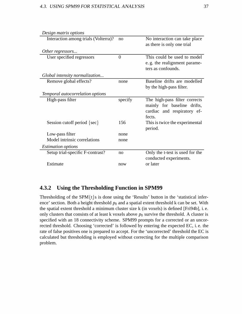
Design matrix optionsInteraction among trials (Volterra)? no No interaction can take place
as there is only one trial
Other regressors...User specified regressors 0 This could be used to model
e. g. the realignment parame-ters as confounds.
Global intensity normalization...Remove global effects? none Baseline drifts are modelled
by the high-pass filter.
Temporal autocorrelation optionsHigh-pass filter specify The high-pass filter corrects
mainly for baseline drifts,cardiac and respiratory ef-fects.
Session cutoff period fsecg 156 This is twice the experimentalperiod.
Low-pass filter noneModel intrinsic correlations none
Estimation optionsSetup trial-specific F-contrast? no Only the t-test is used for the
conducted experiments.Estimate now or later
4.3.2 Using the Thresholding Function in SPM99
Thresholding of the SPMftgs is done using the ‘Results’ button in the ‘statistical infer-ence’ section. Both a height threshold p0 and a spatial extent threshold k can be set. Withthe spatial extent threshold a minimum cluster size k (in voxels) is defined [Fri94b], i. e.only clusters that consists of at least k voxels above p0 survive the threshold. A cluster isspecified with an 18 connectivity scheme. SPM99 prompts for a corrected or an uncor-rected threshold. Choosing ‘corrected’ is followed by entering the expected EC, i. e. therate of false positives one is prepared to accept. For the ‘uncorrected’ threshold the EC iscalculated but thresholding is employed without correcting for the multiple comparisonproblem.

38 CHAPTER 4. STATISTICAL PARAMETRIC MAPPING
4.3.3 Automatisation of the Analysis
SPM99 can also be run in batch mode. The preprocessing options as well as design matrixand contrasts can be entered as nested structures. A short script performs the requestedsteps falling back on these structures. Even though the batch mode is still in beta-testingand has a few problems it nevertheless saves a lot of tedious parameter specification withthe user interface. In trying to get the batch mode to work several problems occurred. TheSPM99 analysis of these experiments has been performed using a network that comprisesa Sun Solaris and a HP Unix workstation as well as a Linux PC. Working with certainprograms (nedit or netscape) on the linux PC changes the keybindings and the batch-files won’t work any more. SPM99 also seems to have problems with certain directorystructures. It is not possible to start the batch scripts from the directory they are filed in.The structures that the batch modus relies on are poorly documented. There are a fewexample files, but some of them are corrupt. The second source of information is theSPM99 help function, but it is incomplete and very brief.The batch modus can be started with ‘spm bch(’directory/batch-script.m’,’FMRI’)’. Thefollowing file ‘analyses.m’ is an example for the script that coordinates the analysis withSPM99.
analysis.m
%---------------------------------------------------------------% user variables defined here%---------------------------------------------------------------
tp=[3 6 8 7 8 1 2 1 2];ix=[1 1 1 1 1 1 1 2 1];wd=[1 1 1 1 1 2 2 3 3];mf=[1 2 2 3 3 4 4 4 4];
%---------------------------------------------------------------% batch variables defined here for analyses%---------------------------------------------------------------
analyses = struct(’type’, tp, ...’index’, ix, ...’work_dir’, wd, ...’mfile’, mf );
%-------------------------------------------
type = {’model’,’contrasts’,’defaults_edit’,’headers’,...’means’,’realignment’,’normalisation’,’smooth’};
%-------------------------------------------
work_dir = {’/misctmp/vision/ex_28jun00/m1.1/’,...’/misctmp/vision/ex_28jun00/RESULTS/m1.1/sr’,...’/misctmp/vision/ex_28jun00/RESULTS/m1.1/snr’};

4.3. USING SPM99 FOR STATISTICAL ANALYSIS 39
%-------------------------------------------
mfile = {’/misctmp/vision/ex_28jun00/RESULTS/batch/defaults.m’,...’/misctmp/vision/ex_28jun00/RESULTS/batch/prepro1.m’,...’/misctmp/vision/ex_28jun00/RESULTS/batch/prepro2.m’,...’/misctmp/vision/ex_28jun00/RESULTS/batch/stat.m’};
The structure analysis is successively evaluated. Its components are row vectors thatcontain indices into the structurestype, work dir and mfile. The componentindexcontains indices into the structures that are defined in the MATLAB files (m-files) speci-fied by mf and are of the type indicated by the corresponding element of tp. The structurework dir indicates which directory the results are to be written to.The m-files are listed in full in appendix D. In the given example the m-file ’defaults.m’contains a main structure defaults edit that is again composed of indices into thestructures that are responsible for the different default settings. The m-file ‘prepro1.m’comprises the structures realign and smooth that define the the parameters that needto be specified for realignment and smoothing. For the second type of preprocessing therealigned files are also normalized and smoothed afterwards. The corresponding param-eters are contained in the structures normalize and smooth from m-file ‘prepro2.m’.The design matrices are specified in ‘stat.m’. There are two instances of the structuremodel. The first one takes care of the first design matrix that models the realigned andsmoothed data (sr-data).h The second one contains the parameters for the model for thesnr-data. Additionally a structure contrasts is embodied in ‘stat.m’ that specifies thecontrast to be applied.The main script ’analyses.m’ hence first sets the relevant defaults and performs the firstkind of preprocessing, i. e. realignment and smoothing (sr) on a set of raw data. In thenext step the second kind of preprocessing is done by taking the realigned scans, whichare first normalized and afterwards smoothed (resulting in snr-data). After the prepro-cessing steps have been performed the design matrix and contrasts for the sr-data and thesnr-data are defined successively. It is to be noted that the index for the second designmatrix is 2. This means the second instance of the structure model is in charge.

Chapter 5
Experiments
Three fMRI experiments using single modules of PTD are reported in this chapter with theaim to investigate the processing of tactile stimulation in the human brain for the seeingsubjects. In the first experiment the somatosensory homunculus is mapped for one malesubject in three sessions at three distinct points: the index finger, the arm and the foot.The same subject is also imaged during a motor task with the index finger to compare thetactile to a motor stimulation. During the ‘rest’ or ‘compare’ phases of the sessions withthis subject another motor task is performed with the contralateral index finger. By this‘compare’ motor stimulation the reproducibility of motor activation is probed.In the second experiment both index finger and foot are alternately stimulated in everysession. There were two subjects and six sessions for each subject. The main goal of thisexperiment is to examine the reproducibility of tactile stimulation. A frequency encodingis applied to the sessions to examine whether the tactile stimulation is related to the fre-quency. An intersubject analysis is finally performed on the three subjects to investigatereproducibility of tactile activations across subjects. Another experiment with a dummybrain serves to ensure that the PTD does not perturb the MRI image acquisition.
5.1 Experimental Setup
5.1.1 Subjects and Experimental Setting
All experiments were performed with the MRI scanner of the Biological Physics Instituteof the Faculty of Medicine at the University Louis Pasteur in Strasburg, France that isdescribed in section 2.6. Only single modules were mounted on index finger, arm andfoot of the subjects. The PTD control unit and the laptop with the are situated about 2 maway from the MRI magnet. Pressurized air is provided by a compressor that is placedoutside the building. The MRI system provides the trigger signals. There is one trigger atthe beginning of each image acquisition process. To account for saturation three dummyimages are made before the first image is taken [Mau00]. MRI image acquisition is con-trolled from an adjacent room.
40

5.1. EXPERIMENTAL SETUP 41
Figure 5.1: A blindfolded subject equipped withear plugs and headphones. The head is taped tothe head restraint.
The volunteers are blindfolded to restrictvisual stimulation to a minimum. As thecoils of the magnet cause a lot of noise thesubjects are equipped with ear plugs andheadphones. The headphones can also beused to talk to the subjects. In order tominimize movement the volunteer’s headis taped to the head restraint it rests on.Figure 5.1 depicts a blindfolded volunteerwith his head fixed to the head restraint andthe headphones. Every subject holds a so-called ‘panic ball’ while it is in the MRItube. When the subject squeezes the panicball an alarm goes off and the subject isimmediately pulled out of the tube.
5.1.2 Mounting of the modules
Mounting the modules turned out to be more critical than expected. For the experimentsthat involved the index finger the module was inserted in a Styrofoam box. The subject’sarm lies on an arm rest and its hand is fixed to the Styrofoam box in such a way thatthe module is right underneath the index finger. Figure 5.2 depicts subject M with her
Figure 5.2: For tactile stimulation of the indexfinger, the module is inserted in a Styrofoam box.
right hand fixed to the Styrofoam box withfabric straps. For the arm and the footstimulations a square piece of teflon coatedcardboard was attached to the module. Itwas then mounted on the arm/foot withfabric straps as is depicted in figures 5.3and 5.4.Great care was taken not to evoke any mo-tor responses from the subject since motoractivity generally produces stronger sig-nals in the brain than tactile stimulationdoes. A motor activity might complicatethe detection of the brain activation in-duced by tactile stimulation for two rea-sons. One is that motor and somatosensorycortex are very close together. The other isthat it makes the detection of the tactile activations more difficult. A motor activation ofthe brain is not only elicited by real movement of a body part but also by the mere urge tomove. If the subject feels uncomfortable with the mounted module or has to exert itself tokeep the stimulated limb in place, activation of the motor cortex will most likely result.The tightness of the straps is crucial for all sessions. If the straps are too tight a constant
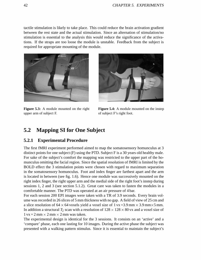
42 CHAPTER 5. EXPERIMENTS
tactile stimulation is likely to take place. This could reduce the brain activation gradientbetween the rest state and the actual stimulation. Since an alternation of stimulation/nostimulation is essential to the analysis this would reduce the significance of the activa-tions. If the straps are too loose the module is unstable. Feedback from the subject isrequired for appropriate mounting of the module.
Figure 5.3: A module mounted on the rightupper arm of subject F.
Figure 5.4: A module mounted on the instepof subject F’s right foot.
5.2 Mapping SI for One Subject
5.2.1 Experimental Procedure
The first fMRI experiment performed aimed to map the somatosensory homunculus at 3distinct points for one subject (F) using the PTD. Subject F is a 30 years old healthy male.For sake of the subject’s comfort the mapping was restricted to the upper part of the ho-munculus omitting the facial region. Since the spatial resolution of fMRI is limited by theBOLD effect the 3 stimulation points were chosen with regard to maximum separationin the somatosensory homunculus. Foot and index finger are farthest apart and the armis located in between (see fig. 1.6). Hence one module was successively mounted on theright index finger, the right upper arm and the medial side of the right foot’s instep duringsessions 1, 2 and 3 (see section 5.1.2). Great care was taken to fasten the modules in acomfortable manner. The PTD was operated at an air pressure of 4 bar.For each session 200 EPI images were taken with a TR of 3.9 seconds. Every brain vol-ume was recorded in 26 slices of 5 mm thickness with no gap. A field of view of 25 cm anda slice resolution of 64� 64 voxels yield a voxel size of 1 vx =3.9 mm� 3.9 mm�5 mm.In addition a structural T2 scan with a resolution of 128� 128� 80 vx and a voxel size of1 vx = 2 mm� 2 mm� 2 mm was taken.The experimental design is identical for the 3 sessions. It consists on an ‘active’ and a‘compare’ phase, each one lasting for 10 images. During the active phase the subject waspresented with a walking pattern stimulus. Since it is essential to maintain the subject’s

5.2. MAPPING SI FOR ONE SUBJECT 43
concentration it is presented with a task. The frequency of the walking pattern is variedpseudo-randomly from one active phase to the next one. There is a ‘target’ frequency of1 Hz and a ‘distractor’ frequency of 0.8 Hz. For a walking pattern of frequency fwp = 1 Hzeach taxel is successively on for 200 ms each followed by a 200 ms break. During thefirst two trials the subject is knowingly presented with the target frequency. For the fol-lowing trials the volunteer is asked to count how many times the target appears. Duringthe compare phase the PTD module is turned off. The subject silently lists the days ofthe week backwards to help keep the subject’s concentration. Tapping its left index fingersimultaneously constitutes a robust motor task for reference purposes and to give a firstestimate of reproducibility of motor activation.
5.2.2 SPM Analysis
Preprocessing, Model and Threshold
Preprocessing of the data comprises realignment and smoothing. The brain volumes ofall sessions are realigned to the first image of session 2 (arm). Additionally the structuralT2 image is coregistered to the realigned functional image series. Smoothing is done witha Gaussian kernel of FWHM = 8 mm� 8 mm� 10 mm. Coordinates are reported in anindividual coordinate system with its origin at the anterior commissure. The coordinatesare used only for determining the relative positions of clusters. It contains no direct in-formation about the anatomical location of the activation. The first column of the designmatrix consists of a box-car function lagged by one image to account for the slow riseof the haemodynamic response function. Additionally it is convoluted with the hrf anda high-pass filter (see section 4.2.2) is applied. The second column contains the offsetthat is of no interest. Evaluating the three functional image series with this design matrixresults in 2 parameter images for each experiment. The approximated amplitudes of thefitted box-car functions make up the first one (beta 0001.img). The second image ismade up of the offsets (beta 0002.img). A contrast ~c= [1 0] yields the activationsduring the active phases. Thereby statistical parametric maps of t-scores are generatedthat reflect the similarity of the fitted box-car function to the modelled box-car function(see section 4.2.3). Thresholding of these SPMftgs is done at a corrected p = 0.001 anda spatial extent k = 5 vx. All activities that remain after this threshold has been appliedcan be said to have a probability of less than 0.1 % to have occurred by chance (see sec-tion 4.2.5.4).
Detected Brain Activity
Figure 5.5 shows ‘glass’ brain coordinate systems (see also appendix C.1) with projec-tions of all activity clusters that are significant at this threshold for each session. Thisis how results are typically presented in SPM99. The glass brains are not adapted to theindividual coordinate system that the clusters are reported in. They represent the MNIcoordinate system. Hence the clusters that occur close to the brain’s surface are placedmuch lower in the glass brain. Normalized data (see section 4.1.4) would instead match

44 CHAPTER 5. EXPERIMENTS
the glass brain MNI coordinate system. The glass brains from SPM99’s result section areinteractive, i. e. the spatial pointer can be place on a particular cluster to help locate it inspace and extract its coordinates. Additionally a list of the coordinates of the maximumt-scores in each depicted cluster can be printed. With non-normalized data this presenta-tion is only useful to get a first impression of the location of the clusters and their relativepositions.
Figure 5.5: Glass brain coordinate systems with projections of activity clusters are the typicalSPM99 output. For subject F, sessions 1, 2 and 3, contrasted for the active phase, a threshold ofpcorr = 0.001 and k = 5 vx is applied. The design matrix as it is represented in SPM99 is depictedin the right upper corner. The greyscale represents the values of the column entries.
In the main region of interest (primary somatosensory cortex SI on the contralateral cere-bral hemisphere) the given threshold yields a large cluster of 101 voxels with a maximumt = 16.3 at (44, -40, 40) for session 1 (index). Several activity clusters survive the thresh-old for sessions 2 and 3. For session 3 (foot) two highly significant clusters appear inthe proximity of the region of interest. The first one exhibits a maximum t = 8.81 at (16, -60, 45) and spans 21 voxels. It is located medial (smaller x) and posterior (smaller y)to the index activity cluster as expected from the somatosensory homunculus. Close bythere is a second cluster of 11 voxels with a maximum t = 8.65 at (4, -36, 45). It is anteriorboth to the first foot and the index activity clusters and probably corresponds to the pri-mary motor cortex MI. For session 3 this threshold results in a small cluster of 7 voxels

5.2. MAPPING SI FOR ONE SUBJECT 45
with a maximum t = 6.31 at (24, -60, 50) and a second more significant one with t = 8.25at (48, -44, 15). While the first cluster is very close to the first foot activity cluster andthus probably corresponds to the arm representation of the somatosensory homunculus,the second one might reflect activation of SII. The small size of the first ‘arm cluster’ isnot surprising since the representation of the arm in the somatosensory homunculus (seefig. 1.6) is also relatively small.
Mapping of Brain Activity
Figure 5.6: Left: Coronal slices of the structural scan of subject F with superimposed SPMftgsfrom the 3 sessions thresholded at t = 5.5 (pcorr = 0.001 at df = 198). The top slice (y = -56) is themost anterior one. Right: Sagittal slice of the same mapped brain volume. The top slice (x = 16)is the most medial one. All slices are spaced with 1 vx = 4 mm.

46 CHAPTER 5. EXPERIMENTS
Only superposition of thresholded SPMftgs onto a coregistered structural scan of thesubject can accurately localize the activity clusters of non-normalized data. This has tobe done by identifying certain structures through comparison to a brain atlas. Figure 5.6depicts series of coronal and sagittal slices of the coregistered structural scan of subjectF with superimposed SPMftgs from foot, arm and index finger. The lateral, central,postcentral and precentral sulci were localized by visual inspection [Nol95]. In MRIimages sulci are generally white and gyri black.The top coronal slice (y = -56) resembles the somatosensory homunculus with the footlocated medially to the arm and followed by the index finger. Continuing to more anteriorslices the arm and foot clusters disappear. This makes sense since the angle between theplane formed by the central sulcus and the z-axis and the interhemispheric plane is lessthan 90�, i. e. the foot is situated posterior to the index finger. The central sulcus canbe identified on the sagittal slices. The three activity clusters are located in the directproximity of the central sulcus. The index finger lateral and anterior, the foot medial andposterior and the arm in between.
Figure 5.7: Axial slices showing the foot acitity clusters in SI and MI (SI is anterior to MI) forsubject F.
In the lower coronal slices the second arm cluster appears. A mere look at the SPM99glass brains would have identified it as an activation of SII. Figure 5.6 shows that it islocated where one would expect the facial representation in SI, which is anterior to SII,above the lateral sulcus. No funded explanation for the occurrence of this cluster can beoffered here. One guess might be, that the subject has moved his lips during the activephases of the experiment. Any movement automatically involves tactile stimulation. Thelips have a very large representation in both somatosensory and motor homunculi, so evenslight movements can evoke brain activation. It is also possible that the stimulus is causedby twitching of the facial muscles.

5.2. MAPPING SI FOR ONE SUBJECT 47
Figure 5.8: Coronal slices showing thefoot activity clusters in SI and SII forsubject F.
As mentioned above there are two foot activity clus-ters in the superior part of the brain. The secondone has not yet been localized precisely. Figure 5.7depicts a series of axial slices of the coregisteredstructural scan with only the SPMftg from session 2thresholded at t = 6 superimposed. The second clus-ter appears anterior to the SI foot activity clusterand the central sulcus that has again been spottedby visual inspection. This cluster is situated in theprimary motor cortex (MI) on the border to the sup-plementary motor area (MII). Hence there had tobe motor stimulation. Since the motor and the so-matosensory activity clusters are well separated theunwanted motor cluster does not perturb the analy-sis.So far the focus has been on the primary somatosen-sory cortex neglecting the secondary somatosen-sory cortex. The conducted analysis yields only oneactivity cluster of interest for session 1, so there isno activation of SII at the given significance. Ses-sion 2 on the contrary yields a bilateral representa-tion of SII. SII is located in the depth of the lateralsulcus. Figure 5.8 depicts a series of coronal sliceswith again only the SPMftg from session 2 super-imposed. The bilateral activation of SII can bestbe seen on the middle slice. The ipsilateral1 acti-vation area is a little posterior to the contralateralone2. Both activations are highly significant and itcan be concluded that stimulation of the foot withthe PTD is apt to cause activation of the secondarysomatosensory cortex additionally to that of SI.
Summary
Tactile stimulation of the right index finger, arm and foot with the PTD has resulted inbrain activations in SI resembling the expected somatotopic map both in position andsize. The activations take place along the central sulcus with the foot activation on themedial side followed by the arm and the index finger activations towards the lateral side.The index activation is the largest one (101 voxels) followed by the SI foot cluster of21 voxels and the arm with only 7 voxels. There is an unexplained brain activation of thatarea in SI that should be primarily responsible for processing facial tactile stimulationthat occurred during the stimulation of the arm. Stimulation of the foot with the PTD also
1‘on the same side’2Ipsi- and contralateral refer to the stimulation not the other activations

48 CHAPTER 5. EXPERIMENTS
involves bilateral activation of SII and effects stimulation of the motor cortex for subjectF. The activity clusters of somatosensory and motor stimulation are well separated, so themotor activation does not confound the analysis. It can be concluded that the reportedtactile experiments with the PTD succeeded in mapping the somatosensory homunculusat three distinct points. The stimulation of the index finger appears to be the most stableand well-defined one. SII was involved only in processing the foot stimulation. Motorstimulation could not be avoided completely in spite of careful mounting of the modules.
5.3 Tactile versus Motor Stimulation
5.3.1 Experimental Procedure
Motor tasks intrinsically involve tactile stimulation due to the deep receptors (Brodmanareas 3a and 2) but usually the cutaneous receptors are also stimulated. When bendingand stretching a finger, for example, the skin of different parts of the finger touch. On thecontrary tactile stimulation does not necessarily cause motor stimulation, although thiscan happen as was seen in the previous section for subject F, session 2. The separation ofmotor and tactile brain activation resulting from the corresponding stimulation of the rightindex finger is investigated in this section. For this purpose another fMRI experimentwith subject F (session 4) concerned with motor stimulation of the right index fingerwas performed. The experimental procedure is basically the same as for the three tactilesessions from the last section. During the active phase the subject alternately bends andstretches his right index finger. During the compare phase he silently lists the days of theweek backwards, but does not tap his left finger as he did for the compare phases of thethree tactile sessions. The PTD is used to ‘trigger’ the phases, i. e. to let the subject knowwhen to start bending and stretching his finger and when to stop. It is mounted on the lefthand in the same way it was for tactile stimulation of the index finger (see fig 5.2).
5.3.2 SPM Analysis and Overlap
The SPM analysis is performed exactly the same way as for sessions 1, 2 and 3 involvingtactile stimulation. The threshold of pcorr = 0.001 and k = 5 vx yields 2 relevant activitycluster. The first one comprises 69 voxels with its maximum t = 11.9 at (40, -40, 45), thesecond on 11 voxels with a maximum t = 8.02 at (56, -36, 30). A third cluster in the cere-bellum is observed but is of no further interest. The cerebellum is expected to be involvedin motor task processing (see section 1.6). Figure 5.9 depicts a series of sagittal slices ofthe structural scan with the motor and the tactile SPMftgs superimposed next to a seriesthat shows only the tactile activities. The two motor clusters are very close together, thesecond one seems to be an extension of the first one. The motor clusters are located an-terior to the tactile one as expected. They overlap by 38 voxels, i. e. 47.5 % of the motorcluster are also active during a mere tactile stimulation and 37.6 % of the voxels activeduring tactile stimulation also exhibit activation during motor stimulation.

5.3. TACTILE VERSUS MOTOR STIMULATION 49
The overlap was calculated by means of a self-written MATLAB script (overlap.m).It uses the structure SPM that SPM99 calculates during thresholding in its ‘results’ sec-tion. SPM is a structure that contains information on the SPMftg, the correspondingt-distribution and on thresholding details. It includes a matrix with the coordinates of thevoxels that survived thresholding as well as an array with the corresponding t-scores. Thecoordinate matrices of the two SPMftgs are compared and the overlap determined.It is not possible to totally separate the motor and the tactile brain activations in subjectF. The motor activation extends to the postcentral gyrus as expected (see fig. 5.9). Thetactile activation in SI also ‘leaks’ into the precentral gyrus. It is nevertheless possible todistinguish between an activation due to tactile stimulation of the index finger with thePTD and a motor activation from the same index finger in subject F as the overlap of thetwo is less than 50 %.
Figure 5.9: A series of sagittal slices with the motor and the tactile activations in MI and SI nextto a series of the same slices with only the tactile activations in SI for subject F.

50 CHAPTER 5. EXPERIMENTS
5.4 Reproducibility of Motor Stimulation
During the compare phases of the three tactile experiments the subject tapped his con-tralateral finger and silently listed the days of the week backwards. This is primarily amotor stimulation, so activation clusters in MI and in the cerebellum are to be expected.The compare phase was identical in all three experiments so it can be used to estimate thereproducibility of the results for motor tasks.Regions that exhibit activity during the compare phase can be extracted by applying acontrast of ~c= [-1 0]. Since motor tasks are generally very robust a higher threshold ofpcorr = 10�5 and k = 30 voxels is effected. For all 3 sessions this threshold yielded clus-ters in both MI and the cerebellum. The clusters with their maximum t-scores are listedin table 5.1. All maximum t-scores are located in MI.
Session & Phase Coordinates [mm] t-score cluster size [vx]1 (index, compare) (-40, -36, 40) 20.0 1252 (arm, compare) (-40, -36, 45) 25.7 1803 (foot, compare) (-36, -32, 40) 20.7 1204 (motor, active) ( 40, -40, 45) 11.9 69
Table 5.1: The maxima of the activities in MI for the compare phases of the 3 tactile sessions andthe active phase of session 4.
All maxima of the clusters from the compare phases are located within a neighbourhoodof 4 voxels.. Even the cluster from the active phase from session 4 peaks at almost thesame point in the opposite cerebral hemisphere. The cluster from session 1 and 3 arealmost of the same size and the maximum t-scores are very similar. Session 2 yields alarger cluster (about 1.5 times the size of the other two) and a higher maximum t-score.Hence the overlap of the other clusters with this one is relatively small. Table 5.2 containsthe overlap in percent of the clusters.
cluster from overlaps with cluster from session [%]session 1 2 3
1 (index) 88.0 87.22 (arm) 61.1 61.73 (foot) 90.8 92.5
Table 5.2: The overlap of the clusters from the compare phases of the 3 tactile sessions.
The clusters from sessions 1 and 3 are almost identically reproduced. In addition to almostidentical maximum t-scores in both location and value, their cluster size differs by only 5voxels and they overlap by 109 voxels (87.2 % and 90.8 %). Cluster 2 is larger and moresignificant than clusters 1 and 3. About 90 % of clusters 1 and 3 are contained in cluster 2.

5.5. REPRODUCIBILITY OF TACTILE STIMULATION 51
In summary it can be said that the motor activations are well reproducible. In particular thecoordinates of the most significant voxel can be reproduced with a deviation of only onevoxel. Cluster size and maximum t-value are subject to larger deviations (max. ∆t = 5.7and max. ∆k = 60 vx).
5.5 Reproducibility of Tactile Stimulation
5.5.1 Experimental Procedure
Experiments with two other subjects (M and N) were performed with the main goal toinvestigate the reproducibility of activations due to tactile stimulations. Subjects M andN are a 21 years old healthy female and a 22 years old healthy male. Index finger andfoot were chosen as stimulation sites as they turned out to be suitable locations for well-defined, significant brain activation for subject F. Their brain activations are also expectedto be farthest apart in the somatosensory homunculus as confirmed by analysis of sessions1 and 3 with subject F.In the experiment with subject F the active and the compare phases lasted for 10 scanseach. The resulting brain activation was highly significant. For this experiment the lengthof active and compare phases were reduced to 7 and 3 scans respectively to save time.While index finger and foot were stimulated in separate sessions for the first experimentthey are now alternately stimulated in a single session. This means there are two activephases in each session separated by a short compare phase. One module is mounted onthe right index finger of the subject, a second one on the medial side of its left foot’s instepas described in section 5.1.2. A walking pattern is applied to the first module for 7 scans(active phase index). Then a compare phase lasting for 3 scans follows during which thesubject silently lists the days of the week backwards. Afterwards the same walking pat-tern is applied to the second module for 7 scans (active phase foot) followed again by acompare phase of 3 scans. This is repeated 10 times (200 scans in total). To maintain thesubject’s attention the direction of the walking pattern is pseudo-randomly varied fromone period to the next. The subject tries to count the occurences of the walking pattern inthe initial direction.There were 6 sessions for each subject. For the first 3 sessions (M[N]1.1, M[N]1.2M[N]1.3) the modules were mounted on the right index finger and the left foot, for the last3 sessions (M[N]2.1, M[N]2.2 M[N]2.3) on the left index finger and the right foot. Thusa comparison to the activation of the opposite cerebral hemisphere can be made. Therewere always 3 sessions performed in one run. This means the subject was inside the MRItube for about one hour at a time. There was a 1.5 hour break for each subject betweenthe two runs. Unfortunately a program error occurred during the second run for subject Nand the PTD did not work properly. Therefore run N2.x is not included in the analysis.In addition to the reproducibility the frequency dependence of the stimulations performedby the PTD is investigated. The frequency of the walking pattern is varied within thesessions. There are 3 different frequencies. For frequency A (B/C) the 4 taxels are suc-

52 CHAPTER 5. EXPERIMENTS
cessively activated for 50 ms (200 ms / 350 ms) each with no break, which corresponds toa frequency of 5 Hz (1.25 Hz / 0.7 Hz). M[N]1.1 is performed with frequency B, M[N]1.2and M[N]1.3) with frequencies C and A respectively (frequency encoding BCA). In thesecond run the frequency encoding was ABC.The modules are operated at an air pressure of 5.9 bar. For each session 200 imageswere taken with a TR of 5 s. 32 slices of 4 mm thickness with no gap make up onebrain volume. One slice consists of 64�64 voxels. With a FOV of 25.6 cm this yieldsa voxel size of 1 vx = 4 mm� 4 mm� 4 mm. The resolution of the structural T2 scan is128� 128� 80 vx with 1 vx = 2 mm� 2 mm� 2 mm.
5.5.2 SPM Analysis
Preprocessing, Model and Threshold
Preprocessing was performed similar to that of the first experiment with subject F. Thedata was realigned for each run (1 run = 3 sessions) to the first image of the first session.The structural T2 scan was coregistered to the same image. Smoothing was performedwith a Gaussian kernel of FWHM = 8 mm� 8 mm� 8 mm. Coordinates are again re-ported in the same kind of individual coordinate systems as for the first experiment.The design matrix comprises two effects of interest and one effect of no interest. The firstcolumn is also a box-car function lagged by one image with a period of 20 images. The‘on’ phase of the box-car function lasts for 7 images, the ‘off’ phase for 13 images. Thesecond column is a box-car function lagged by 11 images. The first column models thestimulation of the index finger, the second one that of the foot. The third column containsthe offset that is an effect of no interest. The box-car functions are again convoluted withthe haemodynamic response function. A high-pass filter with a cut-off period of 200 s isapplied.A contrast of~c= [1 �1 0 ] yields a contrast image (con 0001.img) of the approximatedheight of the first minus the approximated height of the second box-car. The correspond-ing SPMftg reflects the significance of each voxel for being active during the stimulationof the index finger and inactive during stimulation of the foot. An SPMftg relating tothe significance of voxels being active during stimulation of the foot and inactive duringstimulation of the index finger can be obtained with a contrast of~c= [�1 1 0 ]. The samethreshold as for the first experiment is applied (pcorr = 0:001 and k = 5 vx) to the SPMftgs.
Detected Brain Activity
This threshold yields index finger activation clusters in the contralateral primary so-matosensory cortex for all sessions. These clusters are large (up to 250 vx) and havehighly significant maxima (10:4� t� 26). The larger ones ‘leak’ into the primary motorcortex. The high significances and the large cluster sizes are probably due to the high pres-sure of 5.9 bar (compared to 4 bar in the experiment with subject F). Index finger activa-tion cluster in the secondary somatosensory cortex are visible in eight out of nine sessions.They are smaller than the clusters in SI (5 to 72 vx) and less significant (6:1� t� 12:6).
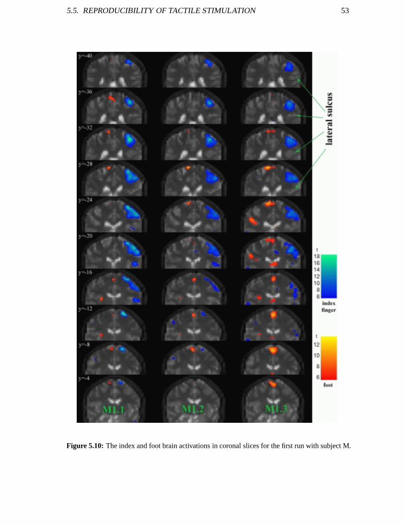
5.5. REPRODUCIBILITY OF TACTILE STIMULATION 53
Figure 5.10: The index and foot brain activations in coronal slices for the first run with subject M.

54 CHAPTER 5. EXPERIMENTS
In session M2.2 the activations in the primary and the secondary somatosensory cortexare not separable at the given threshold. While these activation clusters in the contralat-eral SI and SII were to be expected there are some other ones on the ipsilateral SI andMI that are rather surprising. In four out of nine sessions an activation of the ipsilateralprimary somatosensory cortex occurred. In two out of these four the ipsilateral primarymotor cortex was also involved. In another session only the ipsilateral MI exhibited arather small activation.In eight out of nine sessions foot activation clusters appear in SI at the given threshold.Cluster size ranges from 11 to 39 vx with maximum significance of 8:3� t� 13:7 exceptfor session M1.3. In session M1.3 the foot activation clusters in SI and MI are indistin-guishable and form one large cluster of 90 vx. The foot activation clusters in SII are ofcomparable size and significance (7 to 36 vx and 7:1� t� 11:9. Subject M did not exhibitactivation of SII for the foot during session M1.2 nor during the entire second run (M2.x).While the foot stimulation did not evoke any motor response from subject N, there areactivation clusters in MI in all sessions for subject M.
Mapping of Brain Activity
Figures 5.10, 5.11 and 5.12 depict the superpositions of the SPMftgs thresholded at(pcorr = 0:001) for both contrasts onto the structural scans in series of coronal slices forthe three analyzed runs. The figures illustrate the large size of the index finger activationsin the proximity of SI. Only in N1.3 and M2.3 they are reduced to 41 and 81 voxels re-spectively.In figure 5.10 the index finger activations of SII are clearly visible in the lateral sulcus.Since there was no spatial threshold applied for the superposition of the activations on thestructural slices a small index finger activation of SII is visible in M1.3 on slice y = -20.The foot activations in SII can also be discerned in slices y = -20 to y = -12. The indexactivations in SI are very large and extend deep into the brain. For M1.1 and M1.2 thefoot activations in SI and MI are well separated. The ones in SI span the slices y = -36 toy = -24. There is an ipsilateral activation in MI for session M1.2 (slices y = -12 and -8).The overlap of the clusters in M1.x is 128 vx in index and 6 vx in foot activation of SI.There is no overlap in the index activations of SII while the clusters from the foot activa-tions in SII overlap by 5 vx. For the calculation of the overlap the combined height andspatial threshold is used.For subject N the index activations in SI are closer to the brain surface. During the firstsession an activation on the ipsilateral SI for both index and foot become visible. Theindex finger activation of SII is present in all sessions. Subject N exhibits a stronger footactivation in SII than in SI. For session N1.2 the one in SI is even eliminated by the spa-tial threshold of k = 5 vx and only appears on the coronal slices in figure 5.11. The indexclusters overlap by 41 and 10 voxels in SI and SII, the foot clusters by 0 and 19 voxelsrespectively.

5.5. REPRODUCIBILITY OF TACTILE STIMULATION 55
Figure 5.11: The index and foot brain activations in coronal slices for the first run with subject N.

56 CHAPTER 5. EXPERIMENTS
For the second run with subject M both index and foot activation of SI takes place in theopposite cerebral hemispheres than for the first run. There is no foot activation of SII butthe index finger cluster is present in figure 5.12. The foot activations in SI and MI are wellseparated for all three sessions. In sessions M2.1 and M2.2 there is again an activationof the ipsilateral SI. The overlap comprises 64 and 5 voxels in SI and SII for the indexactivation and 22 and 4 voxels correspondingly for the foot activation.
Summary
There are index finger activations in the contralateral SI and SII for all analyzed sessionsfor both subjects. One of these activations in SII (M1.3) is smaller than 5 vx. Foot acti-vation clusters in SI also appear in all sessions, but one (N1.2) is again smaller than 5 vx.There are foot activations in SII in all sessions of the first runs for both subjects. Duringthe second run for subject M only one small (< 5 vx) foot activation shows in SII duringsession M2.2.For subject N the foot activations in SII are more significant than those in SI. Activationsin SII are often linked to the degree of concentration according to C. Stippich3 . Thiswould indicate that subject N focussed intensely on his task. Reduction of concentrationwith preceding sessions could also explain the lack of foot SII activation in the secondrun for subject M.For both subjects activation of the ipsilateral SI and MI occurred in some sessions, butnot in all. All stimulations evoke activity in the motor cortex although the modules weremounted carefully. This might be avoided by operating the PTD at a lower air pressure.The stimulation of the index finger involves activation of MI that is not separated fromthe activation in SI for both subjects. The two are ‘melted together’. On the contrary thestimulation of the foot caused activation of MI only in subject M and it is disjoint fromthe activation of SI with the exception of session M1.3.The foot activity cluster is located medial to the index finger activation in SI for all ses-sions corresponding to the expected somatotopic map of SI. Since the index finger clusterin SI is large and not separable from the index finger MI activation, it is difficult to judgewhether it is posterior or anterior to the foot activation. Nevertheless it extends anteriorto the foot cluster in all cases. The foot cluster in SII is found medial to the index fingeractivation along the lateral sulcus for all relevant sessions. It can be summarized that notonly the somatotopy of SI but also that of SII has been successfully mapped for the indexfinger and the foot in subjects M and N.The next step is to evaluate the reproducibility of tactile activations for each subject. Thisis done by comparing the respective maximum t-scores, their coordinates and correspond-ing cluster sizes, which are listed in tables 5.3 to 5.8. In section 5.4 the reproducibilityof motor activation was examined and it turned out that the coordinates of the maximumt-scores were well reproduced while the t-values themselves and the cluster sizes variedon a larger scale.
3Department of Neuroradiology, University of Heidelberg, Medical School

5.5. REPRODUCIBILITY OF TACTILE STIMULATION 57
Figure 5.12: The index and foot brain activations in coronal slices for the 2nd run with subject M.

58 CHAPTER 5. EXPERIMENTS
Reproducibility of Brain Activity
The coordinates of the maximum t-scores of the clusters are well reproduced for mostmajor clusters. For subject N the coordinates of the maximum t-scores of the foot clustersin SI and SII are reproduced exactly. Those of the index clusters in SI and SII are at leastdirect neighbours. Only the most significant locations of ipsilateral activations of SI/MI(detected only in N1.1 and N1.2) are 1.2 cm apart.In the first run with subject M the coordinates of the maximum t-scores of the index SI,the index SII and the foot MI clusters are reproduced adjacent to each other. The maximaof the foot SI cluster are found at identical locations. In SII the second maximum of thefoot cluster of M1.3 is one voxel apart from the first maximum of M1.1 (there is no clusterfor M1.2).For the index SI cluster the maximum from M2.3 deviates by approximately 3 cm fromthe other two maxima, which are adjacent to each other. In index SII the maxima fromM2.1 and M2.3 are 1.6 cm apart. A maximum for M2.2 cannot be determined as SI andSII are indistinguishable. The maxima in the ipsilateral SI for index finger stimulation,which was only detected in M2.1 and M2.1, are located next to each other. Exact repro-duction of the foot activations in SI is recorded while there was no activity in SII duringrun M2. The foot MI maxima of M2.1 and M2.2 are found at the same locations and thatof M2.3 neighbours the second maxima of M2.1 and M2.1.So far only the coordinates of the maximum t-values within each run were compared.For subject M two runs were analyzed. The coordinates of both runs can be comparedif one run is mirrored on the interhemispheric plane (x ! -x). One should keep in mindthough, that the human brain is not necessarily exactly symmetric. The adjacent maximaof the index SI clusters from sessions M2.1 and M2.2 can be found superior (by 3 vx) andposterior (by 0 - 2 vx) to the maxima from run M1. On the contrary, the correspondingmaximum from M2.3 is located inferior (by 2 vx) and anterior (by 3 - 4 vx) to the mostsignificant voxels from M1.x. The activations detected in SII for index finger stimulationdeviate by approximately 2 vx in all directions when comparing the two runs for subjectM. The maxima of the foot SI activations were duplicated at the exact same locationswithin both runs. Those from M2 are located inferior by 3 vx, posterior by 5 vx and me-dial by 1 vx to the maxima from M1. In the proximity of the foot in SII no comparison canbe made as no activation was detected for the second run with subject M. Comparing themaxima of the foot activations in MI is less straight forward (see table 5.8). The maximaof run 2 tend to be situated more superior (by 1 - 2 vx), more lateral (by 0 - 4 vx) and moreposterior (by 0 - 4 vx).

5.5. REPRODUCIBILITY OF TACTILE STIMULATION 59
Index finger activations in contralateral SISession Coordinates [mm] t-score cluster size [vx]
M1.1 (36, -32, 36) 18.0 241M1.2 (36, -32, 36) 16.0 199M1.3 (36, -36, 36) 13.3 213
N1.1 (48, -16, 40) 26.0 250N1.2 (48, -16, 36) 21.5 163N1.3 (48, -16, 40) 11.1 41
M2.1 (-32, -40, 48) 18.2 290M2.2 (-32, -36, 48) 20.5 284M2.3 (-36, -20, 28) 10.4 812ndmax (-32, -36, 48) 10.3
Table 5.3: Maxima of index finger activity clusters in contralateral SI.
Index finger activations in contralateral SIISession Coordinates [mm] t-score cluster size [vx]
M1.1 (48, -20, 0) 9.6 18M1.2 (48, -20, -4) 7.0 8
N1.1 (56, -8, -8) 11.6 26N1.2 (56, -8, -8) 12.6 49N1.3 (52, -12, -8) 9.2 16
M2.1 (-40, -24, 4) 9.8 723rd max (-52, -12, -4) 7.8M2.2 SI and SII ‘melted together’M2.3 (-52, -16, -4) 6.1 5
Table 5.4: Maxima of index finger activity clusters in contralateral SII.
Index finger activations in ipsilateral SI and MISession Coordinates [mm] t-score cluster size [vx] comment
M1.2 (-48, -8, 32) 6.3 5 ipsilateral MI
N1.1 (-72, -4, 20) 13.0 77 ipsilateral SI/MIN1.2 (-64, 4, 24) 7.6 19 ipsilateral SI/MI
M2.1 (52, -28, 20) 7.2 16 ipsilateral SIM2.2 (52, -28, 24) 7.6 14 ipsilateral SI
Table 5.5: Maxima of index finger activity clusters in ipsilateral SI and MI.

60 CHAPTER 5. EXPERIMENTS
Foot activations in contralateral SISession Coordinates [mm] t-score cluster size [vx]
M1.1 (-12, -28, 56) 8.3 15M1.2 (-12, -28, 56) 11.2 11M1.3 (-12, -28, 56) 13.5 90
N1.1 (-20, -32, 52) 8.5 39N1.3 (-20, -32, 52) 11.0 30
M2.1 (8, -48, 44) 11.5 26M2.2 (8, -48, 44) 12.5 31M2.3 (8, -48, 44) 13.7 22
Table 5.6: Maxima of foot activity clusters in contralateral SI.
Foot activations in contralateral SIISession Coordinates [mm] t-score cluster size [vx]
M1.1 (-28, -16, 4) 7.1 7M1.3 (-48, -24, 16) 9.3 222nd max (-32, -16, 4) 7.7
N1.1 (-44, -12, 0) 10.3 27N1.2 (-44, -12, 0) 11.9 22N1.3 (-44, -12, 0) 10.9 36
Table 5.7: Maxima of foot activity clusters in contralateral SII.
Foot activations in contralateral MISession Coordinates [mm] t-score cluster size [vx]
M1.1 (0, -16, 48) 6.9 8M1.2 (0, -12, 48) 8.5 18M1.3 SI and MI ‘melted together’
M2.1 (16, -28, 56) 9.6 202nd max (8, -20, 52) 6.7M2.2 (16, -28, 56) 10.9 382nd max (8, -20, 48) 8.4M2.3 (8, -16, 48) 7.3 5
Table 5.8: Maxima of foot activity clusters in contralateral MI.

5.6. INTERSUBJECT ANALYSIS 61
Summary
16 clusters are detected in the regions of interest in 3 runs with 2 subjects, 3 of these clus-ters are found in the ipsilateral cerebral hemisphere. The coordinates of the maximumt-scores of 4 clusters were reproduced exactly for the 3 sessions of each run. 5 maximawere reproduced as face to face neighbours, i. e. with a deviation of only 1 vx or 4 mmand one maximum as edge to edge neighbours (∆ = 5.6 mm). Taking the second and thethird maxima of the clusters into account 2 more locations are reproduced as face to faceneighbours, another one as edge to edge neighbours and one with a deviation of 2 vx inthe x-direction. For one region of interest a cluster was present in only one session sono comparison can be made. The last one of the 16 clusters shows the largest maximumto maximum deviation of 12 mm. The deviation when comparing left and right cerebralhemisphere in subject M is up to 24 mm. As the human brain is not necessarily symmetricthis is not unexpected. Neither the values of the t-scores nor the cluster sizes are repro-ducible. There is no adaptation effect or any correlation to the frequency discernable ineither t-values, cluster sizes or location maximum t-values.As the t-score depends on the quality of the estimation and on the residual variance, de-viations in the t-value are to be expected. This uncertainty also justifies taking the secondand third maxima of the activation clusters into account for evaluating the reproducibilityof activation sites. The cluster size is linked strongly to the t-scores. With the coordinatesof the most significant voxels, the most important spot for processing tactile informationin the human brain can be accurately reproduced for each subject. In chapter 5.8 the sig-nificance of the voxels will be further investigated, but first an intersubject analysis withnormalized data is performed.
5.6 Intersubject Analysis
Preprocessing, Model and Threshold
In the previous sections each subject was analyzed individually using the superpositionsof the SPMftgs onto the coregistered structural scans. In this section the results from allsubjects are compared to each other. For this purpose a reference coordinate system needsto be defined. SPM99 used the MNI coordinate system (see appendix C). The data fromeach subject is normalized to the standard MNI brain (see section 4.1.4) after realign-ment. The normalization parameters used are listed in the batch-file prepro2.m in ap-pendix D. The images are resampled to 1 vx = 2 mm� 2 mm� 2 mm. After normalizationthe images were smoothed with a Gaussian kernel of FWHM = 4 mm� 4 mm� 4 mm.The design matrices for all experiments as well as the applied contrasts are identical tothose used for the individual analyses. The same corrected height threshold of p = 0.001but with a larger spatial extent threshold of k = 20 vx is applied to the SPMftgs for theactive phases of all experiments.

62 CHAPTER 5. EXPERIMENTS
Detected Brain Activity
The normalized data exhibits contralateral SI activity clusters for both index finger andfoot in all sessions for all subjects. SII activation was also detected in all cases withonly two exceptions: In session M1.3 no index finger activity and in session M2.3 nofoot activity occurred. Subjects M and F also showed an activation of contralateral MIfor the foot stimulation. Index finger activation of MI took place only for M2.3 andF. Finally there was also ipsilateral SI activation for the index finger in some sessions(M1.2, N1.1, N1.2, M2.1, M2.1 and F). Tables 5.9 to 5.15 list the maximum t-scores withthe corresponding coordinates and voxel sizes classified by the stimulated brain region.
Index finger activations in contralateral SISession Coordinates [mm] t-score cluster size [vx]
M1.1 (44, -36, 58) 21.9 1106M1.2 (44, -36, 58) 22.0 973M1.3 (42, -20, 48) 15.2 8032nd max (46, -36, 60) 13.0
N1.1 (50, -18, 58) 27.3 1089N1.2 (52, -18, 56) 21.9 680N1.3 (54, -18, 56) 11.3 193
M2.1 (-36, -46, 68) 17.9 1104M2.2 (-34, -44, 70) 21.2 1288M2.3 (-30, -40, 72) 10.1 93
F (50, -22, 62) 21.9 464
Table 5.9: Maxima of index activity clusters in contralateral SI for normalized data.
Index finger activations in contralateral SIISession Coordinates [mm] t-score cluster size [vx]
M1.1 (56, -16, 14) 13.7 98M1.2 (58, -16, 10) 9.7 84
N1.1 (58, -10, 2) 16.5 179N1.2 (58, -10, 2) 15.0 251N1.3 (54, -14, 4) 11.3 84
M2.1 (-44, -22, 16) 12.6 353M2.2 (-44, -24, 16) 12.2 3953rdmax (-54, -16, 8) 10.4M2.3 (-50, -16, 8) 7.7 51
F (44, -14, 12) 10.5 86
Table 5.10: Maxima of index activity clusters contralateral SII for normalized data.

5.6. INTERSUBJECT ANALYSIS 63
Index finger activations in ipsilateral SISession Coordinates [mm] t-score cluster size [vx]
M1.2 (-50, -20, 48) 8.9 54
N1.1 (-62, -18, 36) 12.6 3513rdmax (-58, -8, 38) 10.8N1.2 (-58, -8, 38) 10.3 662ndmax (-62, -18, 36) 7.6
M2.1 (64, -18, 38) 6.9 21M2.2 (64, -18, 38) 8.3 81
F (-48, -44, 14) 8.0 25
Table 5.11: Maxima of index activity clusters in ipsilateral SI for normalized data.
Index finger activations in contralateral MISession Coordinates [mm] t-score cluster size [vx]
M2.3 (-36, -22, 46) 13.9 251
F (44, -24, 66) 11.7 4322ndmax (40, -24, 48) 11.7
Table 5.12: Maxima of index finger activity clusters in contralateral MI for normalized data.
Foot activations in contralateral SISession Coordinates [mm] t-score cluster size [vx]
M1.1 (-12, -36, 80) 11.8 124M1.2 (-12, -34, 80) 13.9 51M1.3 (-12, -34, 80) 15.2 92
N1.1 (-12, -42, 70) 10.7 118N1.2 (-12, -38, 72) 7.8 20N1.3 (-12, -38, 72) 11.5 83
M2.1 (12, -48, 64) 15.3 139M2.2 (12, -48, 64) 17.2 164M2.3 (12, -48, 64) 18.5 111
F (16, -48, 74) 9.6 55
Table 5.13: Maxima of foot activity clusters in contralateral SI for normalized data.

64 CHAPTER 5. EXPERIMENTS
Foot activations in contralateral SIISession Coordinates [mm] t-score cluster size [vx]
M1.1 (-32, -22, 12) 10.3 63M1.2 (-32, -22, 14) 12.3 97M1.3 (-56, -34, 32) 11.9 2913rd max (-34, -22, 16) 10.1
N1.1 (-38, -22, 16) 13.1 131N1.2 (-38, -22, 16) 12.8 100N1.3 (-36, -24, 14) 11.7 150
M2.1 (36, -20, 16) 7.6 20M2.2 (36, -20, 14) 8.1 23
F (56, -28, 4) 8.8 462nd max (48, -28, 12) 7.4
Table 5.14: Maxima of foot activity clusters in contralateral SII for normalized data.
Foot activations in contralateral MISession Coordinates [mm] t-score cluster size [vx]
M1.1 (-2, -18, 68) 10.0 101M1.2 (0, -20, 68) 12.0 165M1.3 (0, -16, 70) 13.5 297
M2.1 (8, -16, 74) 8.3 25M2.2 (8, -18, 72) 11.9 63M2.3 (8, -18, 74) 11.7 36
F (4, -22, 68) 8.8 60
Table 5.15: Maxima of foot activity clusters in contralateral SI for normalized data.
The maximum t-scores of the normalized data are generally larger than the correspondingones of the non-normalized data. This is mainly due to the resampling during normal-ization, which involves sinc interpolation and increases the signal to noise ratio. Thenormalized clusters are mostly smaller than the corresponding non-normalized ones. TheM1.1 index finger activity cluster in SI, for example, consists of 241 non-normalizedvoxels or of 1106 normalized voxels, which correspond to 15.4 cm3 and 8.85 cm3 respec-tively. The ‘shrinking’ of the activation volume also originates in the resampling process.On the border of the activity clusters interpolation between pure noise voxels and voxelswith a small signal is performed, which eliminates the small signal in most cases. Thenormalization process also includes zooming and warping of the individual brain, whichmay change the size of the activation clusters either way depending on the size and shape

5.6. INTERSUBJECT ANALYSIS 65
of the individual brain The normalized coordinates of the maximum t-scores are well re-produced within each run for each individual subject as expected. In the following thereproducibility across subjects will be investigated.
Summary
Regarding the index activation in SI the maximum t-scores from sessions N1.1 and Fare closest to each other (0.6 cm) while those from N1.2 and M2.3 are farthest apart(3.6 cm). It is rather surprising that the first and the second maxima from session M1.3were swapped by the normalization process. The separation of the maximum t-values inindex finger SII activation ranges from 0.9 cm (M2.1 and F) to 2.4 cm (N1.2 and M2.2).The detected ipsilateral activations of SI in the normalized data exhibits the largest maxi-mum separation of all clusters of interest. The maxima from session N1.1 and run M2 areonly 0.3 cm apart while those from F and N1.2 differ by 4.4 cm. Index finger activations inMI were only detected for sessions M2.3 and F and the corresponding maxima are located2.2 cm from each other. The x-coordinates for the activation of SI due to stimulation ofthe foot are reproduced exactly for subjects M and N and deviate by only 2 vx for subjectF. The minimum and maximum separations are 0.8 cm and 2.1 cm for M1.1 versus N1.2and M1.3 and M2.1 respectively. It is surprising that the maximum deviation occurs forthe same subject on opposite cerebral hemispheres. In general the foot activation in SI forM2 and F are found posterior to those for M1 and N1. In SII the foot activations are atleast 0.3 cm (N1.2 and M2.1) and at most 2.9 cm (M1.3 and F) apart. The separation ofthose in MI differ between 0.7 cm (F and M2.2) and 1.2 cm (M1.1 and M2.1). Again themaximum separation occurs for one subject. Table 5.16 summarizes the minimum andmaximum distances between the coordinates of the most significant voxels for each areaof interest.
Minimum and maximum distances of maximum t-scores for each region [mm]Index Foot
SI SII MI ipsilat. SI SI SII MI
2.8 8.9 21.6 2.8 8.2 2.8 6.936.3 24.2 21.6 41.7 21.3 28.6 11.8
Table 5.16: Minimum and maximum distances of most significant voxels for each region of inter-est.
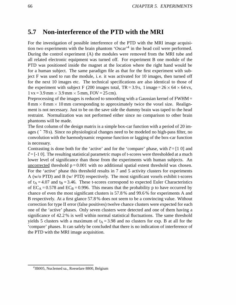
66 CHAPTER 5. EXPERIMENTS
5.7 Non-interference of the PTD with the MRI
For the investigation of possible interference of the PTD with the MRI image acquisi-tion two experiments with the brain phantom ‘Oscar’4 in the head coil were performed.During the control experiment (A) the modules were removed from the MRI tube andall related electronic equipment was turned off. For experiment B one module of thePTD was positioned inside the magnet at the location where the right hand would befor a human subject. The same paradigm file as that for the first experiment with sub-ject F was used to run the module, i. e. it was activated for 10 images, then turned offfor the next 10 images etc. The technical specifications are also identical to those ofthe experiment with subject F (200 images total, TR = 3.9 s, 1 image = 26� 64� 64 vx,1 vx = 3.9 mm� 3.9 mm� 5 mm, FOV = 25 cm).Preprocessing of the images is reduced to smoothing with a Gaussian kernel of FWHM =8 mm� 8 mm� 10 mm corresponding to approximately twice the voxel size. Realign-ment is not necessary. Just to be on the save side the dummy brain was taped to the headrestraint. Normalization was not performed either since no comparison to other brainphantoms will be made.The first column of the design matrix is a simple box-car function with a period of 20 im-ages (= 78 s). Since no physiological changes need to be modeled no high-pass filter, noconvolution with the haemodynamic response function or lagging of the box-car functionis necessary.Contrasting is done both for the ‘active’ and for the ‘compare’ phase, with ~c= [1 0] and~c= [-1 0]. The resulting statistical parametric maps of t-scores were thresholded at a muchlower level of significance than those from the experiments with human subjects. Anuncorrected threshold p = 0.001 with no additional spatial extent threshold was chosen.For the ‘active’ phase this threshold results in 7 and 5 activity clusters for experimentsA (w/o PTD) and B (w/ PTD) respectively. The most significant voxels exhibit t-scoresof tA = 4.07 and tB = 3.46. These t-scores correspond to expected Euler Characteristicsof ECA = 0.578 and ECB = 0.996. This means that the probability p to have occurred bychance of even the most significant clusters is 57.8 % and 99.6 % for experiments A andB respectively. At a first glance 57.8 % does not seem to be a convincing value. Withoutcorrection for type II error (false positives) twelve chance clusters were expected for eachone of the ‘active’ phases. Only seven clusters were detected and one of them having asignificance of 42.2 % is well within normal statistical fluctuations. The same thresholdyields 5 clusters with a maximum of tA = 3.98 and no clusters for exp. B at all for the‘compare’ phases. It can safely be concluded that there is no indication of interference ofthe PTD with the MRI image acquisition.
4JB005, Nuclemed sa., Roeselare 8800, Belgium

5.8. T-SCORES REVIEWED 67
5.8 t-Scores Reviewed
In the last chapters the functional brain image series were analyzed by means of a voxel byvoxel hypothesis testing approach. The hypothesis was set up by using the general linearmodel and a parameter estimation was performed. These parameters were then used toevaluate the significance of each voxel via a student’s t-test. The t-test used by SPM99 isbased on the signal change relative to the approximated residual variance, where ‘signalchange’ refers to a linear compound of the estimated parameters of interest. The t-scoresdepend on the quality of the estimation and on the noise level in the signal. In this chapterthe data of selected voxels is analyzed in more detail to obtain a better understanding ofthe t-values. The following analysis shall also verify the presence and the quality of thesignals.
5.8.1 Signal and Cascades
The relationship of the t-score to the quality of the signal is investigated at a basic levelin this section. A signal with a high t-score should basically be of a box-car shape withperiod T, lagged by one image. Ideally it would reflect a lagged box-car convoluted withthe haemodynamic response function, but this effect is probably occluded by the noise. Ifa periodic structure underlies the signal and is merely covered up by uncorrelated noise,it should become apparent in a periodic superposition of the signal. Using equation 5.1to cascade the signal upon itself the uncorrelated noise should be diminished while thesignal remains.
C( j) =TN�
NT �1Xk=0
S(k �T + j) 1� j � 20 (5.1)
N - length of signalT - period of box-car function
The signals that will be analyzed in this section are taken from the experiments withsubjects M and N. Each signal consists of N = 200 data points. The data is already pre-processed, i. e. realignment and smoothing has been performed. For voxels that are ac-tive during the index finger stimulation the time scheme should be a box-car of periodT = 20 images. Images 2 - 8 should exhibit a larger signal than images 1 and 9 - 20 in eachperiod. For voxels that are active during the foot stimulation, the signals from images12 - 18 should exceed those from the other images in every period.At first the signals of voxels with different significances are compared. The left sidesof figures 5.13, 5.14 and 5.15 show the signal at an insignificant (t = 0.2), a significant(t = 7) and a highly significant (t = 18) voxel. The insignificant voxel does not exhibit anyperiodic structure. There is only noise with amplitudes of up to 80 points in greyvaluecorresponding to about 2 % of the mean signal S. With a little imagination the signal ofthe voxel with a t-score of 7 shows a periodic structure, but it is ambiguous. The signalamplitude is less than 1 % of the mean. Only the signal with a very high significance can

68 CHAPTER 5. EXPERIMENTS
be identified as basically corresponding to a box-car shape with an amplitude of about1.6 % of S. The signal is still confounded by noise of approximately 0.8 % of the mean.Hence the signal to noise ratio is in the order of 2 to 1.
2 4 6 8 10 12 14 16 18 20
−0.2
−0.15
−0.1
−0.05
0
0.05
0.1
0.15
0.2
0.25
Superposition Index jD
evia
tion
from
Mea
n [%
]
M1.1 (0 0 0) t=0.2
50 100 150 2003580
3600
3620
3640
3660
3680
3700
Image Index
Gre
yval
ue
M1.1 (0 0 0) t=0.2
Figure 5.13: Signal and cascaded signal of an insignificant voxel (t = 0.2), i. e. one that is notinvolved in processing the presented stimulation.
2 4 6 8 10 12 14 16 18 20
−0.4
−0.2
0
0.2
0.4
0.6
Superposition Index j
Dev
iatio
n fr
om M
ean
[%]
M1.2 (48 −20 −4) t=7.0
50 100 150 2002370
2380
2390
2400
2410
2420
2430
2440
2450
2460
Image Index
Gre
yval
ue
M1.2 (48 −20 −4) t=7.0
Figure 5.14: Signal and cascaded signal of a significant voxel (t = 7) in SII for session M1.2.
The deviation of the signals cascaded according to equation 5.1 from the mean signal inpercent is depicted in the right parts of figures 5.13, 5.14 and 5.15. Cascading the signalfrom the insignificant voxel does not yield an apparent structure. Only the amplitude ofthe noise is reduced to about 0.5 % of the signal mean as would be expected for uncorre-lated noise. The cascade of the voxel with a significance of t = 7 does show a larger signalfor 2 � j � 8 as would a box-car function lagged by one image. The expected lag of 1image, that has been modeled in the design matrix for the analysis with SPM99, becomes

5.8. T-SCORES REVIEWED 69
apparent in the steep initial rise to 0.6 % above the mean signal for the 2nd image. It isfollowed by a decrease and the signals remains at about 0.4 % above Suntil it drops to 0for the 9th image. The lower part of the box-car is not as obvious as there are still largevariations akin to those in fig. 5.13. The cascade of the highly significant voxel (t = 18)resembles the single lagged box-car in a reasonable fashion. There is still a decrease inthe upper part of the box-car and the lower part is not flat either, but this could not beexpected from a signal with only 10 measurements per data point.
50 100 150 2002460
2480
2500
2520
2540
2560
2580
2600
Image Index
Gre
yval
ue
M1.1 (36 −32 36) t=18.0
2 4 6 8 10 12 14 16 18 20
−0.5
0
0.5
1
Superposition Index j
Dev
iatio
n fr
om M
ean
[%]
M1.1 (36 −32 36) t=18.0
Figure 5.15: Signal and cascaded signal of a highly significant voxel (t = 18) in SI for sessionM1.1
2 4 6 8 10 12 14 16 18 20
−1
−0.5
0
0.5
1
Superposition Index j
Dev
iatio
n fr
om M
ean
[%]
N1.1 (48 −20 36) t=17.6
50 100 150 2001590
1600
1610
1620
1630
1640
1650
1660
1670
Image Index
Gre
yval
ue
N1.1 (48 −20 36) t=17.6
Figure 5.16: Signal and cascaded signal of a highly significant voxel (t = 17.6) in SI for sessionN1.1

70 CHAPTER 5. EXPERIMENTS
There is an apparent baseline drift in the signal in figure 5.15. In the design matrix ofSPM99 this is modeled by means of the high-pass filter, so it should not confound theparameter estimation. Hence this drift should not influence the t-value. To emphasize thispoint figure 5.16 shows the signal and the cascaded signal of a voxel with a comparablesignificance (t = 17.6). This signal from session N1.1 does not drift like the one fromsession M1.1, but its t-score is still smaller. In addition the cascaded signal in fig. 5.16 ismuch clearer than the one in fig. 5.15.The cascaded signals can of course not be used as a quantitative measure for the qualityof the signal. The signals do not comprise enough data points and the signal to noise ratiois usually too high (about 2 to 1) to allow for a reasonable elimination of the uncorre-lated noise. Averaging the cascades from neighbouring voxels does not really improvethe cascades for smoothing has introduced a strong correlation between the neighbours.Increasing the size of the neighbourhood will reduce correlation but also signal to noisefor less significant voxels are inevitably included. The cascades nevertheless emphasizethe basic form of the signal and serve as a qualitative illustration.
5.8.2 Autocovariance
Autocorrelation is measure for correlation within the signal of one voxel (compared tocorrelation that compares the signal of several voxels to each other or to a reference sig-nal). An autocovariance function normalized to the variance of the signal is calculatedfor selected voxels according to equation 5.2 to look into its possibilities of evaluating thesignificance of a signal. The normalization introduces a dependence of the amplitude ofthe autocovariance function on the noise. The signal was subject to cyclic addition beforecalculating the autocovariance.
AC(∆i) =1N� 1AC(0)
NXk=1
[S(k)� S] � [S(k+∆i)� S] (5.2)
The autocovariance function of the insignificant voxel with t = 0.2 (see fig. 5.17, left)does not exhibit a periodic signal and has small amplitudes (up to � 0.15) as expected.A higher significance is reflected in a periodicity of the autocovariance function as infig. 5.17, right) and a higher amplitude. Maxima are reached for multiples of 20, butthe shape of the curve is not smooth as it is when the significance increases (fig. 5.18).The drift that can be observed in the signal for voxel (36,-32,36) in session M1.1 (seealso fig. 5.15) is reflected in the autocovariance function. The autocovariance function ofvoxel (48,-20,36) from session N1.1 owns a larger amplitude and lacks the drift that ispresent in fig. 5.18, left side even though its t-score is lower.The autocovariance can be used to evaluate the significance of the signal. The smootherthe shape of the autocovariance and the larger its amplitude, the clearer was the originalsignal. Both the cascade and the autocovariance functions of voxels (36,-32,36) from ses-sion M1.1 and (48,-20,36) from session N1.1 suggest that the latter one’s signal is moresignificant in spite of the t-scores that indicate the opposite.

5.8. T-SCORES REVIEWED 71
20 40 60 80 100
−0.3
−0.2
−0.1
0
0.1
0.2
0.3
0.4
0.5
Difference in Image Indices ∆ i
Aut
ocov
aria
nce
M1.2 (48 −20 −4) t=7.0
20 40 60 80 100−0.15
−0.1
−0.05
0
0.05
0.1
0.15
Difference in Image Indices ∆ i
Aut
ocov
aria
nce
M1.1 (0 0 0) t=0.2
Figure 5.17: The autocovariance functions for voxels with t = 0.2 and t = 7.0 calculated with equa-tion 5.2.
20 40 60 80 100−0.6
−0.4
−0.2
0
0.2
0.4
0.6
Difference in Image Indices ∆ i
Aut
ocov
aria
nce
M1.1 (36 −32 36) t=18.0
20 40 60 80 100
−0.6
−0.4
−0.2
0
0.2
0.4
0.6
Difference in Image Indices ∆ i
Aut
ocov
aria
nce
N1.1 (48 −20 36) t=17.6
Figure 5.18: The autocovariance functions for voxels with t = 18.0 and t = 17.6 calculated withequation 5.2.
5.8.3 Fourier Transformation
A discrete fourier transformation is performed on the signals of the same selected voxelswith different t-scores. The corresponding power spectra are displayed in figures 5.19and 5.20. The first element of the power spectrum is omitted as it corresponds to the sumof all data points of the signal and would stretch the scale too much. The signal of theinsignificant voxel with t = 0.2 obviously contains many frequencies indicating that thereis only noise. The power spectrum of the voxel with t = 7.0 looks like what a typical fMRIsignal is expected to look like. The cardiac and respiratory cycles of generally about 1 and0.25 Hz respectively are aliased into the range 0 � f � FNyquist. The Nyquist frequencycorresponds to FNyquist= 0.1 Hz for a signal with TR = 5 s. Hence the cardiac frequency off = 1 Hz would be aliased to 0 Hz and the respiratory one of f = 0.25 Hz to 0.05 Hz. The

72 CHAPTER 5. EXPERIMENTS
cardiac and the respiratory were not measured, so it is not possible to say which one ofthe small peaks at 0.02, 0.04 and 0.06 Hz in the power spectrum they correspond to. The1/f low-frequency noise can also be discerned (see also 2.5.2). The actual signal withf0 = 0.01 Hz yields the largest peak with about 4 times the amplitude of the peaks for theperiodic noise in the signal of voxel (48,-20,-4) in session M1.2. The peaks correspondingto f0 = 0.01 Hz in the highly significant voxels in figure 5.20 are more explicit. They bothhave about 18 times the height of the periodic noise peaks. It is interesting that the 1/fnoise is very low for subject N (right plot) while it is comparatively large for subject M(left plot). The level of 1/f noise does not seem to influence the t-value.
0 0.02 0.04 0.06 0.08 0.10
0.5
1
1.5
2
2.5
3
3.5x 10⁵
Frequency [Hz]
Pow
ersp
ectr
um
M1.1 (0 0 0) t=0.2
0 0.02 0.04 0.06 0.08 0.10
1
2
3
4
5
6
7
8x 10⁵
Frequency [Hz]
Pow
ersp
ectr
um
M1.2 (48 −20 −4) t=7.0
Figure 5.19: Power spectrum of voxels with t = 0.2 and t = 7.0.
0 0.02 0.04 0.06 0.08 0.10
1
2
3
4
5
6x 10⁶
Frequency [Hz]
Pow
ersp
ectr
um
M1.1 (36 −32 36) t=18.0
0 0.02 0.04 0.06 0.08 0.10
0.5
1
1.5
2
2.5
3
3.5
4
4.5x 10⁶
Frequency [Hz]
Pow
ersp
ectr
um
N1.1 (48 −20 36) t=17.6
Figure 5.20: Power spectrum of voxels with t = 18.0 and t = 17.6.

5.8. T-SCORES REVIEWED 73
The power spectrum of a signal yields further verification of the significance of the signal.The high peaks in fig. 5.20 demonstrate the high significance while the smaller peak infig. 5.19 for the less significant voxel (t = 7.0) shows that the signal is less explicit. In thefollowing it will be investigated whether it is possible to detect the presence of a signalin the brain by determining the averaged power spectrum from a large part of the brain orwhether it will be eliminated by the noise. Figure 5.21 depicts the averaged power spec-trum from all voxels within a bounding box of [0:68,-60:0,-12:72] (in mm). This boundingbox corresponds to the upper two thirds of the left cerebral hemisphere including both theprimary and the somatosensory cortex as well as the motor cortex. The averaged powerspectrum exhibits a large 1/f low frequency noise component and small periodic noisepeaks at 0.02 and 0.04 Hz. The signal at 0.01 Hz is still present, but has been diminishedand cannot be distinguished from the periodic noise peaks with confidence. The signal inthis area was very strong (two major clusters of 241 and 18 vx respectively and t-scoreswithin 5:5� t � 18) and usually lesser signals are still considered significant. The fouriertransformation cannot confidently detect the presence of a periodic structure in a fMRIsignal if an averaged power spectrum is used. significance of the voxel.
0 0.02 0.04 0.06 0.08 0.10
1
2
3
4
5
6
7
8x 10⁵
Frequency [Hz]
Pow
ersp
ectr
um
M1.1, bb=[0:68,−60:0,−12:72]
Figure 5.21: Averaged power spectrum of all voxels within a bounding box of [0:68,-60:0,-12:72].

74 CHAPTER 5. EXPERIMENTS

Summary and Outlook
First fMRI experiments on healthy, seeing subjects were performed with a new pneumati-cally driven tactile display to investigate the processing of tactile stimulation in the humanbrain. They succeeded in mapping the expected somatotopic representation in the con-tralateral primary somatosensory cortex for three subjects at two distinct points (the indexfinger and the foot). For one subject the representation of the arm in SI was also located.The tactile stimulation with the PTD did not only cause brain activation in SI but also inSII and MI. In some sessions ipsilateral activation of SI, SII or MI was also detected. Theobserved activation of SII also exhibits a somatotopic map similar to that of SI.Even though great care was taken to avoid motor stimulation the primary motor cortexwas activated. This leads to the assumption that the somatosensory and the motor cor-tex are strongly interconnected. The experiments with subjects M and N result in onelarge index finger activation that spans both SI and MI. The PTD was operated at an airpressure of 5.9 bar for these experiments. Only 4 bar were applied for the experimentwith subject F whose index finger activation is focussed in SI and merely ‘leaks’ into MI.Hence using the PTD with a smaller air pressure is likely to reduce the motor stimulation.A measurement of the force exerted by one taxel of the PTD is currently performed atthe Department of Clinical and Biological Psychology of the University of Mannheim.Aside from the pressure dependence, the influence of the frequency on the taxel force isof particular interest.In one of the performed experiments the frequency of the walking pattern applied to onemodule of the PTD was varied pseudo-randomly between 0.7 Hz, 1.23 Hz and 5 Hz. Thevariation does not appear to influence either the activation cluster size, the maximum t-value or its location. Before the dependence of the brain activation on the frequency isfurther examined it is important to clarify the relationship of both frequency and brainactivation to the applied force.An adaptation effect over the period of one hour was not discernable. It seems that healthysubjects can concentrate on the tactile stimulations performed with the PTD for at leastone hour without their brain’s response to the stimulus being reduced.The reproducibility of the brain activations was also analyzed. The coordinates of themaximum t-scores are well reproduced for each individual subject (within one cerebralhemisphere) while the actual t-values and the cluster sizes are subject to large randomvariations. The deviation of activations due to tactile as well as motor stimulation is lessthan 1.2 cm and for most cases even less than 0.5 cm. For one subject the reproducibilityacross the cerebral hemispheres was examined and it turned out that the coordinates of
75

76 CHAPTER 5. EXPERIMENTS
the maximum t-scores are subject to deviations up to 2.4 cm. The reproducibility of thelocations of the maximum t-scores in the intersubject analysis varied between 3 mm to4 cm. An experiment with a brain phantom shows that the PTD does not perturb the fMRIimage acquisition.The reported experiments with seeing subjects induced activation of the somatosensoryand the motor cortex. A next step could be to perform experiments with blind subjects toexamine whether they exhibit activation of the same brain areas or if other areas, e. g. thevisual cortex, are also involved. It would also be useful to be able to compare the degreesof activation in blind and seeing subjects. Statistical parametric mapping is unfortunatelynot well-suited to evaluate the intensity distribution of the activation. The t-scores do notprovide a reliable measure of the degree of activity and the thresholded statistical para-metric maps should rather be regarded as a black and white map of significance versusno significance. A new approach based on wavelet transforms might be more appropriatefor comparing the intensities of activations as it results in a profile of activity [Tur99].Wavelet transform methods differ from traditional Fourier methods by their inherent abil-ity of localizing information in the time-frequency domain while by means of a Fouriertransformation the information of either time or frequency is lost.Statistical parametric mapping has nevertheless succeeded in precisely localizing activa-tion sites. It should be possible to perform future analyses using SPM99 much faster soincreasing the statistic should be considered. The main speed factor is that the analysishas been automated using the newly implemented batch modus of SPM99. All analysissteps except for thresholding can be performed automatically now. Thresholding is stillrather time-consuming since it is often necessary to try different thresholds for all datasets. Automatisation of thresholding with SPM99 is desirable.The intersubject analysis using normalized data yielded rather large deviations in the lo-calization of activations. It seems to be preferable to analyze each subject individually bysuperposition of the activations onto structural scans. A new extension to SPM99 allowsto print series of coronal, sagittal or axial slices of those superpositions. This also speedsup the analysis as it eludes tedious inspection with SPM99’s interactive user interface.Having shown the authenticity of the data detected with SPM99 and using the PTD fortactile stimulation new experiments do not need to restrict themselves to simple tactilestimulation. The next step could be to proceed to investigations into pattern recognition.Only a better understanding of how complex tactile stimulations and patterns are pro-cessed by both blind and seeing subjects can finally help to optimize information transfervia the tactile channel to the human brain.

Appendix A
Directions and Planes in the HumanBrain
The terminology of neuroanatomy is specialized to describe both the absolute position ofstructures and their relative position. Two major axes, the dorsal-ventral and the rostral-caudal axis, describe the organization of the central nervous system. For animals, e. g. amouse the rostral-caudal axis runs approximately in a straight line from the nose to thetail. The dorsal-ventral axis is perpendicular to the rostral-caudal axis and runs from theback to the abdomen. In humans the situation is a bit more complicated (see fig. A.1).The rostral-caudal axis does not follow a straight line but instead undergoes a bend (orflexure) at the midbrain. The terms inferior and superior are used to describe structureslocated rostral to this bend. The planes in which anatomical sections or slices are madeare named horizontal (or axial), coronal and (para-) sagittal (see fig. A.1).
Figure A.1: Directions and Planes in the Brain
77

Appendix B
Affine Transformations inPreprocessing
B.1 General Affine Transformation
The affine transformation is a simple and well defined spatial transformation. In 3-Dit is given by 12 parameters. For each point (x1;x2;x3) in an image mapping into thecoordinates of another Euclidean space is given by
0BB@
y1
y2
y3
1
1CCA=
0BB@
m11 m12 m13 m14
m21 m22 m23 m24
m31 m32 m33 m34
0 0 0 1
1CCA
0BB@
x1
x2
x3
1
1CCA
Several transformations can be combined in one by simply multiplying the transformationmatrices to form a single matrix.Rigid body transformations are a subset of the more general affine transformations. In 3dimensions a rigid body transformation is defined by six parameters.
B.2 Voxel to Real World Coordinates
The matrix Mf is responsible for converting voxel coordinates to ‘real world’ coordinates.If an image f has a voxel size of xmm� ymm� zmmand an origin (in voxels) (X;Y;Z)then
Mf =
0BB@
x 0 0 (�x�X)
0 y 0 (�y�Y)
0 0 z (�z�Z)0 0 0 1
1CCA ; M�1
f =
0BB@
1x 0 0 X0 1
y 0 Y
0 0 1z Z
0 0 0 1
1CCA
78

B.3. REALIGNMENT 79
B.3 Realignment
The realignment of an image f to an image g, performed as a preprocessing step in SPM99,is a rigid body transformation with the transformation matrix Mrealign. The parameters qaccount for translation (q1;q2;q3) in x, y and z as well as for rotation (q4;q5;q6) aroundthe x-, y-, and z-axis.
Mrealign= M�1f
0BB@
1 0 0 q1
0 1 0 q2
0 0 1 q3
0 0 0 1
1CCA
| {z }Translations
�
0BB@
1 0 0 00 cosq4 sinq4 00 �sinq4 cosq4 00 0 0 1
1CCA
| {z }Pitch
�
0BB@
0 cosq5 sinq5 01 0 0 00 �sinq5 cosq5 00 0 0 1
1CCA
| {z }Roll
�
0BB@
0 cosq6 sinq6 00 �sinq6 cosq6 01 0 0 00 0 0 1
1CCA
| {z }Yaw
�Mg
Mf and Mg map from voxel to real world coordinates.
B.4 Affine Normalization
For affine spatial transformation an additional 6 parameters are needed: 3 zooms (q7;q8;q9)
in x, y and z and 3 shears (q10;q11;q12) in xy, xz and yz.
M = M�1f
0BB@
1 0 0 q1
0 1 0 q2
0 0 1 q3
0 0 0 1
1CCA
| {z }Translations
�
0BB@
1 0 0 00 cosq4 sinq4 00 �sinq4 cosq4 00 0 0 1
1CCA
| {z }Pitch
�
0BB@
0 cosq5 sinq5 01 0 0 00 �sinq5 cosq5 00 0 0 1
1CCA
| {z }Roll
�
0BB@
0 cosq6 sinq6 00 �sinq6 cosq6 01 0 0 00 0 0 1
1CCA
| {z }Yaw
�
0BB@
q7 0 0 00 q8 0 00 0 q9 00 0 0 1
1CCA
| {z }Zoom
�
0BB@
1 q10 q11 00 1 q12 00 0 1 00 0 0 1
1CCA
| {z }Shear
�Mg

Appendix C
Coordinates in SPM99
C.1 Talairach Coordinate System
The Talairach Coordinate System (TCS) is determined by a line through the superioredge of the Anterior Commissureand the inferior edge of the PosteriorCommisure- theAC-PC line - and the interhemispheric, sagittal plane. The AC is also the origin of thecoordinate system. Fig. C.1 illustrates the TCS.Why the commisures? Both commisures are relatively easy to locate on structural scans.On functional scans (EPI) it is hard to make out the PC but the AC can still be located withconfidence. The main idea of the TCS was actually to provide comparability of individualbrains.A brain is divided into cuboids, the dimensions of which vary with the principal axes. Thevolume defined by the plane to the interhemispheric plane and passing through the AC-PCline and th lowest point of the temporal cortex is, for example, divided in 4 equidistantsections, etc.. It is a proportional grid system. This feature is not relevant here sincemulti-subject comparison is performed on normalized brains.
C.2 The MNI brain
In order to define a brain that is more representative of the population than the single brainused by Talairach and Tournoux, members of the Montreal Neurological Institute did alarge number of MRI scans on normal subjects. Every brain was then linearly matched tothe Talairach brain. The transform consisted of 9 parameters (3 translations, 3 rotationsand 3 zooms). Two average brains were created: a 305 and a 152 average. SPM99 usesthe 152 average brain. The MNI linear transform has not matched the brains completelyto the Talairach brain, so the MNI brains turned out to be slightly larger. The differencesare larger on the outer parts of the brain and are at maximum in the order of 10 mm. Fromthe AC to its top the MNI brain is about 5 mm taller and 5 mm longer. Its temporal lobesgo about 10 mm deeper (the lowest slice is at z = -50 compared to z = -40 in the Talairachatlas). The AC, which serves as origin, is 4 mm below that of the Talairach brain.
80

C.2. THE MNI BRAIN 81
Figure C.1: The Talairach Coordinate System with the origin located in the AC.
It is not possible to do an exact transformation from the MNI to the Talairach brain, butthere are some approximations (see [Bre99]). This is unfortunate since the Talairach atlasdepicts the designated Brodman’s areas. So far there is no published MNI atlas definingBrodman’s areas on the MNI brain.

Appendix D
Examples for Batch-Files in SPM99
defaults.m
%---------------------------------------------------------------% batch variables defined here for analysis ’defaults_edit’%---------------------------------------------------------------
defaults_edit(1) = struct( ...’type_area’, [1 2 3 4], ...’index’, [1 1 1 1] );
type_area = {’Misc’,’Printing’,’RealignCoreg’,’Normalisation’,...’Hdr’,’Statistics’,’Reset’};
%====================== Misc DefaultsMisc = struct( ...
’log_to_file’, 1, ...’log_file_name’, ’spm.log’, ...’cmdline’, 0, ...’grid’, 0.4 );
%====================== Printing DefaultsPrinting = struct( ...
’printing_mode’, 3, ... % ps to file’postscript_filename’, ’spm’, ...’postscript_type’, 8, ... % 8 is eps level 2;’default_printer’, 0, ...’printer_name’, ’’, ...’post_type’, ’-dpsc’, ...’graphics_filename’, ’spm’, ...’graph_type’, 4, ...’print_string’, ’’ );
%====================== RealignCoreg DefaultsRealignCoreg = struct( ...
’separate_combine’, 1, ... % combine coregistration% and realignment
82

83
’create’, 1 ,...’adjust’, 1,... % adjust sampling errors’mask’, 1,... % mask object brain’reg_quality’, 1.00, ... % registration quality’weight_reg’, 0 ); % allow weighting
%====================== Normalisation DefaultsNormalisation = struct( ...
’defaults’, 1, ... % 1 - parameter estimation’estimates’, 0, ... % Neurological Convention (R is R)’custom_norm’, -1, ... % -1 - allow customized
% 1 - disallow’nonlin_func_nb’, 13, ... % non-linear basis functions’func_nb’, 0, ...’nonlin_ite_nb’, 12, ... % non-linear iterations’nonlin_regular’, 0.01, ... % strength of regularization’mask_brain’, 1, ... % 1 yes’bounding_box’, 1, ... % default bounding box’voxel_sizes’, 3 ); % 3 <-> 2*2*2 mm
prepro1.m
%---------------------------------------------------------------% user variables defined here%---------------------------------------------------------------
datadir=’/misctmp/vision/ex_28jun00/M/ex1/’;Fr = {spm_get(’files’,datadir,’m1_1*.img’)};Frs = {spm_get(’files’,datadir,’rm1_1*.img’)};
%---------------------------------------------------------------% batch variables defined here for analysis ’realign’%---------------------------------------------------------------
realign = struct(...’subject_nb’, 1, ... % number of subjects’num_sessions’,1, ... % number of sessions for each subject’sessions’, [1], ... % index into structure sessions’option’, 3, ... % 1 - only registration
% 2 - only transformation% 3 - both
’modality’, 1, ... % 1 - within modality% 2 - between modality
’reslice_method’, -9, ... % interpolation method: -9 <-> sinc’create’, 3, ... % 3 - mean image + all images’mask’, 1, ... % 1 - mask voxels outside the brain’adjust_sampling_errors’, 0);
%---------------------------------------------------------------
sessions(1) = struct(...’images’, {{Fr}});

84 APPENDIX D. EXAMPLES FOR BATCH-FILES IN SPM99
%---------------------------------------------------------------% batch variables defined here for analysis ’smooth’%---------------------------------------------------------------
smooth = struct(...’FWHMmm’, [8 8 8], ...’files’, {{Frs}} );
prepro2.m
%---------------------------------------------------------------% user variables defined here%---------------------------------------------------------------
datadir=’/misctmp/vision/ex_28jun00/M/ex1/’;Fn = {spm_get(’files’, datadir,’rm1_1*.img’)};Fns = {spm_get(’files’, datadir,’nrm1_1*.img’)};
%---------------------------------------------------------------% batch variables defined here for analysis ’normalize’%---------------------------------------------------------------% attention: defaults have to be set to allow customized% normalization for these settings to take effect
normalize = struct(...’option’,3, ... % 1 - determine parameters only
% 2 - perform transformation% 3 - 1+2
’nbsubjects’,1, ... % number of subjects’estimates’,1,... % 0 - radiological convention
% 1 - neurological convention’object_masking’, 0, ... % mask object brain during
% registration’objmask’, {{’’}}, ... % file containing mask’template’, ...’SPM_dir/templates/EPI.img’, ... % template image for normalization’image’,{{Fn1}}, ... % image to determine parameters from’matname’, ... % file to write parameters to{{’filename.mat’}}, ...’images’, {{Fn}}, ... % images to write normalized’type’, 1, ... % default normalization = 0
% custom normalization = 1’nonlin_func_nb’, 13, ... % number of non-linear basis fcts
% (0:14); 13 = 7*8*7’func_nb’, 0, ... % number of basis functions
% (only for ‘custom’)’nonlin_ite_nb’, 12,... % number of non-linear iterations’nonlin_regular’, 0.01, ... % Extremely heavy (1.0) to very
% light regularization (0.0001)’mask_brain’, 1, ... % mask object brain during
% transformation in order

85
% not to count exterior voxels’interp’, -9, ... % interpolation type:
% 0 <-> nearest neighbour (fast)% 1 <-> bilinear (slower)% -9 <-> sinc (slowest, but best)
’bounding_box’, 3, ... % 0 - custom% 1 - default% (-78:78,-112:76,-50:85)
’direction1’, [-10;10], ... % only if ‘custom’’direction2’, [-10;10], ...’direction3’, [-10;10], ...’voxel_sizes’, 3, ... % voxel size after normalization:
% 0 - custom, 3 - 2*2*2 mm’voxel_sizes_custom’, [2 2 2] ); % if ‘custom’ ‘for voxel_sizes’
%---------------------------------------------------------------% batch variables defined here for analysis ’smooth’%---------------------------------------------------------------
smooth = struct(...’FWHMmm’, [4 4 4], ...’files’, {{Fns}} );
stat.m
%---------------------------------------------------------------% user variables defined here%---------------------------------------------------------------
datadir = ’/misctmp/vision/ex_28jun00/M/ex1/’;Fsr = {spm_get(’files’,datadir ,’srm1_1*.img’)};Fsnr = {spm_get(’files’,datadir ,’snrm1_1*.img’)};
%---------------------------------------------------------------% batch variables defined here for analysis ’model’%---------------------------------------------------------------
model = struct( ...’types’, 4, ... % specify and estimate’global_effects’, {’None’}, ... % no global normalization’burst_mode’, 0, ...’HF_fil’, ’specify’, ... % high-pass filter’HF_cut’, [200], ... % cut-off = RT * SOA * 2’LF_fil’, ’none’, ... % low-pass filter’LF_cut’, 4, ... % cut-off’int_corr’, ’none’, ... % internal correlation?’now_later’, 1, ... % estimate ‘now’ or ‘later’’stop_writing’, 0, ... % overwrite existing design
% matrix? (y/n) <-> (0/1)’trial_fcon’, 0, ... % trial specific F-contrasts’RT’, 5, ... % RT [s]’replicated’, 0, ... % are sessions replicated?
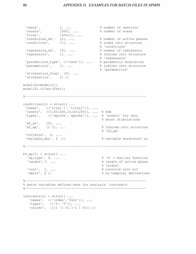
86 APPENDIX D. EXAMPLES FOR BATCH-FILES IN SPM99
’nsess’, 1, ... % number of sessions’nscans’, [200], ... % number of scans’files’, {{Fsr}}, ...’conditions_nb’, [2], ... % number of active phases’conditions’, [1], ... % index into structure
% ‘conditions’’regressors_nb’, [0], ... % number of regressors’regressors’, [], ... % indices into structure
% ‘regressors’’parametrics_type’, {{’none’}}, ... % parametric modulation’parametrics’, [], ... % indices into structure
% ‘parametrics’’stochastics_flag’, [0], ...’stochastics’, [] );
model(2)=model(1);model(2).files={Fsnr};
%---------------------------------------------------------------
conditions(1) = struct( ...’names’, {{’trial 1’,’trial2’}}, ...’onsets’, {{1:20:200,11:20:200}}, ... % SOA’types’, {{’epochs’,’epochs’}}, ... % ‘events’ for very
% short stimulations’bf_ev’, [0], ...’bf_ep’, [1 1], ... % indices into structure
% ‘bf_ep’’volterra’, 0, ...’variable_dur’, 0 ); % variable durations? no
%---------------------------------------------------------------
bf_ep(1) = struct( ...’ep_type’, 4, ... % ‘4’ = box-car function’length’,7, ... % length of active phase
% [scans]’conv’, 1, ... % convolve with hrf’deriv’, 0 ); % no temporal derivatives
%---------------------------------------------------------------% batch variables defined here for analysis ’contrasts’%---------------------------------------------------------------
contrasts(1) = struct( ...’names’, {{’index’,’foot’}}, ...’types’, {{’T’,’T’}}, ...’values’, {{[1 -1 0],[-1 1 0]}} );

Bibliography
[Afi98] A.K. Afifi, R.A. Bergman, Functional Neuroanatomy, McGraw-Hill, NewYork (1998)
[Ana00] htt p : ==www:mayo:edu=bir=analyze=AnalyzeFileIn f o:html
[Ban93] P.A. Bandettini, MRI studies of brain activation: temporal characteristics.In: Functional MRI of the brain, Berkeley: SMRM, California 143-151(1993)
[Bor99] J. Bortz, Statistik ,Springer-Verlag, Berlin (1999)
[Box95] J.L. Boxerman, P.A. Bandettini, The intravascular contribution to fMRIsignal change: Monte Carlo modeling and diffusion weighted studie invivo, Mag. Res. Med. 34, 4-10 (1995)
[Bre99] M. Brett, Medical Research Council - Cognition and Brain Science Unit -Imaging, Homepage (1999)htt p : ==www:mrc�cbu:cam:ac:uk=Imaging=
[Bro99] M.A. Brown, R.C. Semelka, MRI Principles and Applications, 2nd edition,Wiley-Liss, New York (1999)
[Fra97] R.S.J. Frackowiak, K.J. Friston, C.D. Frith, R.J. Dolan, J.C. Mazziotta,Human Brain Function, Academic Press, San Diego (1997)
[Fri94a] K. Friston, P. Jezzard, R. Turner, Analysis of functional MRI time series,Human Brain Mapping 1, 153-171 (1994)
[Fri94b] K. Friston, K.J. Worsley, R.S.J. Frackowiak, Assessing the Significanceof Focal Activations Using Their Spatial Extent, Human Brain Mapping1:210-220 (1994)
[Fri95] K. Friston, J. Ashburner,J.B. Poline, Spatial Registration and Normaliza-tion of Images, Human Brain Mapping 2:165-189 (1995)
[Har00] G. Harrington, C. Wright, H. Downs, A New Vibrotactile Stimulator forFunctional MRI, Human Brain Mapping 10:140-145 (2000)
87

88 BIBLIOGRAPHY
[Hor00] J.P. Hornak, The Basics of MRI, Rochester, NY (2000)htt p : ==www:cis:rit :edu=htbooks=mri=bmri:htm
[Jae97] B. Jaehne, Digitale Bildverarbeitung, Springer, Berlin Heidelberg (1997)
[Jez99] P. Jezzard, Basic Physics of fMRI, FMRIB, Oxford University, UK (1999)htt p : ==www: f mrib:ox:ac:uk=� peter j=lectures=hbm1=sld001:htm
[Kan91] E.R. Kandel (Editor), Principles of Neural Science, 4th edition, PrenticeHall International, London (1991)
[Loo99] M. Loose, A Self-Calibrating CMOS Image Sensor with Logarithmic Re-sponse, Phd-Thesis, HD-IHEP 99-07, Heidelberg (1999)
[Mal99] J.A. Maldjian, A. Gottschalk, R.S. Patel, Mapping of Secondardy So-matosensory Activation Induced by Vibrational Stimulation: an fMRIStudy, Brain Research 824 (1999) 291-295
[Mar96] J.H. Martin, Neuroanatomy, 2nd edition, Appleton and Lange, Stamford,Conn. (1996)
[Mau00] T. Maucher, S. Runde, K. Meier, E. Sampaio, C. Scheiber, Evaluation ofa new pneumatically driven tactile display for fMRI-studies by mappingthe human somatosensory cortex, submitted to Magnetic Resonance inMedicine, July 2000
[Mau98] T. Maucher, Aufbau und Test eines taktilen Seh-Ersatzsystems, Thesis,HD-IHEP 98-11, Heidelberg (1998)
[Moo95] D.S. Moore, The Basic Practice of Statistics, W.H. Freeman and company,New York (1995)
[Nol95] J. Nolte, J.B. Angevine, Jr., The Human Brain in Photographs and Dia-grams, Mosby, St. Louis, MO (1995)
[Ros82] A. Rosenfeld, A.C. Kak, Digital Picture Processing, Volume 2, AcademicPress, Orlando (1982)
[Sch99] J. Schemmel, An Integrated Analog Network for Image Processing, Phd-Thesis, HD-IHEP 99-08, Heidelberg (1999)
[SPM97] SPM short course notes (1997)htt p : ==www: f il :ion:ucl:ac:uk=spm=course=notes:html
[Sti99] C. Stippich, R. Hofmann, D. Kapfer, Somatotopic mapping of the humanprimary somatosensory cortex by fully automated tactile stimulation us-ing functional magnetic resonance imaging, Neurosci-Lett. 277(1):25-8(1999)

BIBLIOGRAPHY 89
[Tal88] J. Talairach, P. Tournoux, Co-Planar Stereotaxic Atlas of the HumanBrain, Georg Thieme Verlag, Stuttgart (1988)
[Tra98] I. Tracey, Brief Introduction to FMRI - Physiology, FMRIB, Oxford Uni-versity, UK (1998)htt p : ==www: f mrib:ox:ac:uk= f mri intro=physiology:html
[Tur99] F.E. Turkheimer, M. Brett, D. Visvikis, V.J. Cunningham, MultiresolutionAnalysis of Emission Tomography Images in the Wavelet Domain, Journalof Cerebral Blood Flow and Metabolism 19(11):1189-1208 (1999)
[Vis00] Homepage of the Electronic Vision Grouphtt p : ==www:kip:uni�heidelberg:de=vision=
[Wor96] K.J. Worsley, S. Marrett, Searching Scale Space for Activation in PETImages, Human Brain Mapping 4: 74-90 (1996)

90 BIBLIOGRAPHY

Acknowledgements
At this point I would like to thank everybody who contributed to this work, namely:
Prof. Dr. K. Meier for the opportunity to work on this very interesting - and in the regimeof physics rather unconventional - project.
Prof. Dr. J. Bille for taking on the part of second referee.
Thorsten for proof-reading, great teamwork and his always enchanting company through-out the year.
All members of the Electronic Vision Group for their interest in the project and the goodvibes within the group.
Dr. C. Scheiber for his support in all questions concerning fMRI and SPM99.
M. Brett for his prompt answers and helpful MATLAB-scripts.
My parents for always supporting me in no matter what.
Frank for proof-reading, for Australia and for bringing out the best in me.