Draft version June 14, 2018Preprint typeset using LATEX style emulateapj v. 08/13/06

DRIVEN AND DECAYING TURBULENCE SIMULATIONS OF LOW-MASS STAR FORMATION: FROMCLUMPS TO CORES TO PROTOSTARS

Stella S. R. OffnerDepartment of Physics, University of California, Berkeley

Richard I. KleinDepartment of Astronomy, University of California Berkeley, Berkeley CA 94720, USA, and Lawrence Livermore National Laboratory,

P.0. Box 808, L-23, Livermore, CA 94550, USA

Christopher F. McKeeDepartments of Physics and Astronomy, University of California Berkeley, Berkeley, CA 94720, USA

Draft version June 14, 2018

ABSTRACTMolecular clouds are observed to be turbulent, but the origin of this turbulence is not well under-

stood. As a result, there are two different approaches to simulating molecular clouds, one in whichthe turbulence is allowed to decay after it is initialized, and one in which it is driven. We use theadaptive mesh refinement (AMR) code, Orion, to perform high-resolution simulations of molecularcloud cores and protostars in environments with both driven and decaying turbulence. We includeself-gravity, use a barotropic equation of state, and represent regions exceeding the maximum gridresolution with sink particles. We analyze the properties of bound cores such as size, shape, linewidth,and rotational energy, and we find reasonable agreement with observation. At high resolution, thedifferent rates of core accretion in the two cases have a significant effect on protostellar system devel-opment. Clumps forming in a decaying turbulence environment produce high-multiplicity protostellarsystems with Toomre-Q unstable disks that exhibit characteristics of the competitive accretion modelfor star formation. In contrast, cores forming in the context of continuously driven turbulence andvirial equilibrium form smaller protostellar systems with fewer low-mass members. Our simulationsof driven and decaying turbulence show some statistically significant differences, particularly in theproduction of brown dwarfs and core rotation, but the uncertainties are large enough that we are notable to conclude whether observations favor one or the other.Subject headings: ISM: clouds – stars:formation – methods: numerical – hydrodynamics – turbulence

1. INTRODUCTION

Contemporary star formation occurs exclusively indense molecular clouds (MCs). Such regions exhibit largenon-thermal line widths generally attributed to super-sonic turbulence (Larson 1981). Although debate contin-ues on the origin and characteristics of this turbulence,it is now recognized that turbulence is a necessary el-ement of star formation and plays an important role inthe shape of the core initial mass function (IMF), the life-times of molecular clouds, and the star formation rate.

Simulations have shown that supersonic turbulence de-cays with an e-folding time of approximately one cloudcrossing time if there is no energy input to sustain it(Stone et al. 1998; Elmegreen & Scalo 2004; Mac Low &Klessen 2004). If turbulence decays as quickly in molec-ular clouds then star formation must happen rapidly asthe cloud looses turbulent pressure support and under-goes global collapse. In this senario, star formation oc-curs on a dynamical timescale and MCs must be transientdynamic structures (Elmegreen 2000; Hartmann 2001).If however, turbulence is fed from large scales or pro-tostellar winds, expanding HII regions, and other pro-cesses provide sufficient energy injection to balance dis-sipation produced by shocks, then MCs may arrive at

Electronic address: soffner@berkeley.edu

a quasi-equilibrium state (e.g., Tan, Krumholz & Mc-Kee 2006). Although there are many possible sourcesfor turbulent energy, the dominant source and the spe-cific characteristics of turbulence remain poorly under-stood. Recent effort has been directed at this issue andsome observations of low-mass star forming regions, e.g.L1551, find evidence for ongoing turbulence injectionin the form of winds and jets, which maintains roughvirial balance over several cloud dynamical times (Swift& Welch 2007). While turbulent support is maintained,only a small number of overdense regions will becomegravitationally unstable and form stars in a dynamicaltime, leading to a low star formation rate and allowingMCs to live for several dynamical times.

The two different views of cloud dynamics are relatedto, but distinct from, the two major approaches to sim-ulating turbulent molecular clouds. The fact that thereare two competing approaches to the simulation of suchclouds is a direct reflection of our lack of understandingof the origin of the turbulence in these clouds (McKee &Ostriker 2007). In one method, the turbulence is initial-ized and then allowed to decay (e.g. Klessen et al. 1998;Bonnell et al. 2003; Bate et al. 2002; Tilley & Pudritz2004). The primary problem with this approach is thatthe turbulence decays to levels that are much lower thanthose observed. Advocates of this method argue that

arX

iv:0

806.

1045

v1 [

astr

o-ph

] 5

Jun

200

8

2

the gravitational collapse that ensues after the decay ofthe turbulence can be observationally confused with tur-bulence (e.g. Vazquez-Semadeni et al. 2006), but it isdifficult to see how to maintain a low star formation effi-ciency if much of the gas is in a state of gravitational col-lapse. The other approach to cloud simulation is to drivethe turbulence so that it does not decay (e.g. Padoan &Nordlund 1999; Gammie et al. 2003; Li et al. 2004;Jappsen et al. 2005). This approach allows one to studythe processes that occur at a given level of turbulence,which can be set to match that in a given cloud, butit suffers from the disadvantage that the driving is un-physical. This approach is a good match for the case ofquasi-equilibrium clouds, and it can be made consistentwith the case of transient clouds if it is assumed that thesimulation box represents only a small part of the molec-ular cloud, so that the decay time for the turbulence islong compared to the dynamical time of the simulation.

The near universal shape of the stellar IMF across di-verse star forming environments has sparked much de-bate and generated diverse theories. Padoan & Nordlund(2004) suggest that the functional form of the IMF can bederived from the power spectrum and probability densityfunction characteristic of supersonic turbulence. Larson(2005) proposes that the peak of the IMF is set by theBonnor-Ebert mass at the minimum cloud temperature,which is related to the dust-gas coupling and gas coolingefficiency. In the competitive accretion model, Bonnell etal. (2004) invoke high stellar densities at the centers ofclusters to propose that the relative position of the starsin the gas reservoir determines their mass. Accordingto this model, the IMF is determined by mass segrega-tion, such that low-mass stars form in the lower densitygas at the edges of the cluster and higher mass starsform in the centers, where their masses can be furtherincreased by the coalescence of smaller protostars. Inaddressing the origin of the IMF, numerical simulationshave been largely inconclusive in discriminating betweenmodels given that a wide range of conditions (virial pa-rameters, resolution, code algorithms, included physics)have all succeeded in reproducing the IMF shape.

A large amount of computational effort has been di-rected towards studying self-gravitating turbulent cloudsboth with and without magnetic fields (e.g. Klessen2001; Bonnell et al. 2003; Li et al. 2004). A number ofsimulations succeed in reproducing various observed coreproperties such as the IMF and Larson’s laws (Padoan& Nordlund 1999; Gammie et al. 2003; Tilley & Pudritz2004; Li et al. 2004; Jappsen et al. 2005; Bate & Bonnell2005). However, most simulations lack the resolution tospan the turbulent inertial range (Klein et al. 2007) toaccurately render the evolution of cores into stars in acluster environment.

In this paper, we perform numerical AMR simulationswith our code Orion to investigate the role of driven anddecaying turbulence on low-mass star formation. We fol-low the evolution of star forming cores in a turbulentbox to show that turbulent feedback is correlated withthe multiplicity of stellar systems, the shape of the IMF,and the dominant protostellar accretion model. In §2,we discuss the methodology of Orion and the initial con-ditions. In §3, we analyze core properties in driven anddecaying turbulence at low resolution. In §4, we presentresults from a few high resolution studies of the proto-

stellar core evolution inside selected cores formed in thecontext of driven and decaying turbulence. Finally, §5contains conclusions. In a companion paper (Offner etal. 2008, hereafter Paper II) we investigate the effects ofdriven and undriven turbulence on the properties of thecores from which the stars form.

2. CALCULATIONS

2.1. Numerical MethodsOur simulations are performed using the parallel adap-

tive mesh refinement (AMR) code, Orion, which uses aconservative second order Godunov scheme to solve theequations of compressible gas dynamics (Truelove et al.1998; Klein 1999). Orion solves the Poisson equation us-ing multi-level elliptic solvers with multi-grid iteration.Throughout our calculations, we use the Truelove crite-rion to determine the addition of new AMR grids (Tru-elove et al. 1997),

ρ < ρJ =J2πc2sG(∆xl)2

, (1)

where ∆xl is the cell size on level, l, and we adopt aJeans number of J = 0.25. We insert sink particles inregions of the flow that have exceeded this density on themaximum level (Krumholz et al. 2004). Sink particlesserve as numerical markers of collapsing regions and also,after sufficient mass accretion and lifetime, protostellarobjects. We impose a merger criterion that combines sinkparticles that approach within two grid cells of one an-other but prohibits nearby objects from merging if bothhave masses exceeding 0.1 M. This limit divides starsfrom substellar objects such as brown dwarfs and has theeffect of tracking all significantly massive objects. Parti-cles that represent temporary violations of the Jeans con-dition and have little bound mass tend to accrete littleand ultimately merge with their more substantial neigh-bors. The combination of sink particles and AMR withthe Jeans criterion allows us to accurately and efficientlycontinue our calculation to high resolution without thetime constraints imposed by a large base grid size andwithout the consequences of artificial fragmentation.

2.2. Initial Conditions and Simulation ParametersIsothermal self-gravitating gas is scale free, so we give

the key cloud properties as a function of fiducial val-ues for the mean number density of hydrogen nuclei, nH,and gas temperature, T . We chose a characteristic 3-Dturbulent Mach number, M=8.4, such that the cloud isapproximately virialized:

αvir =5σ2

GM/R∼ 1.67. (2)

It is then easy to scale the simulation results to the as-trophysical region of interest. For the adopted values ofthe virial parameter and Mach number, the box length,mass, and 1-D velocity dispersion are given by

L= 2.9 T11/2n

−1/2H,3 pc , (3)

M = 865 T13/2n

−1/2H,3 M , (4)

σ1D = 0.9 T11/2 km s−1 , (5)

tff = 1.37 n−1/2H,3 Myr , (6)

3

where nH, 3 = nH/(103 cm−3) and T1 = T/(10 K) andwhere we have also listed the free-fall time for the gas inthe box for completeness. For nH, 3 ∼ T1 ∼ 1, the simu-lation approximately satisfies the observed linewidth-sizerelation (Solomon et al. 1987; Heyer & Brunt 2004). Forthe remainder of this paper, all results will be given as-suming the fiducial scaling values nH = 1100 cm−3 andT=10 K, which are appropriate for the Perseus Molecu-lar Cloud (Paper II), but they may be adjusted to differ-ent conditions using equations (2)-(5). In terms of theBonnor-Ebert mass,

MBE =1.182c3

(G3ρ)1/2= 4.71

T3/21

n1/2H, 3

M, (7)

the simulation has a mass of 184MBE. If the Jeansmass is defined as MJ = ρL3

J , where LJ = (πc2s/Gρ)1/2

is the Jeans length, then MJ = (π3/2/1.18)MBE =18.9T 3/2

1 /n1/2H, 3 M.

Our turbulent periodic box study is comprised of twostages. The first stage simulates the large scale isother-mal environment of a turbulent molecular cloud withself-gravity. In this “low resolution” stage, we only addenough AMR levels to resolve the shape and structureof collapsing clumps and cores. This first stage has twoparts. First, to obtain the initial turbulent spectrum,we turn off self-gravity and use the method describedin MacLow (1999), in which velocity perturbations areapplied to an initially constant density field. These per-turbations correspond to a Gaussian random field withflat power spectrum in the range 3 ≤ k ≤ 4 where k isthe wavenumber normalized to kphysL/2π. At the end oftwo cloud crossing times, the turbulence follows a Burg-ers P (k) ∝ k−2 power spectrum as expected for hydro-dynamic systems of supersonic shocks. For the secondpart, we turn on gravity and follow the subsequent grav-itational collapse for two scenarios. It should be notedthat some workers (e.g. Bate et al. 2003) do not allowself-consistent turbulent density fluctuations to build upbefore turning on gravity. Any choice of initializationfor a turbulent, self-gravitating cloud is necessarily ap-proximate, but in our view it is preferable to have self-consistent density and velocity fluctuations in the ini-tial conditions. In the simulation that we will refer towith the letter D (driven), we continue turbulent drivingto maintain virial equilibrium, while in the other, notedwith U (undriven), we halt the energy injection and allowthe turbulence to decay.

In the second stage, we select a few emerging coresfor further study in each turbulent box, and we followtheir fragmentation and evolution into protostellar sys-tems at high resolution using a barotropic equation ofstate (EOS). We add additional grid refinement to the re-gions we select, which continue to evolve within the lowresolution context of the box. This method capitalizeson the AMR methodology to achieve a high resolutionstudy of the development and properties of protostellarcores with realistic initial and boundary conditions. Fol-lowing all the cores over a free-fall time with AMR ratherthan a subset to the maximum resolution would requiremore than a million CPU hours on 1.5 GHz processors.In contrast, our stage two approach with AMR requires∼50,000 CPU hours per high resolution box.

In the first stage, it is reasonable to assume that thelow density gas in the cluster is isothermal and scale-free, reflecting the efficient radiative cooling of the gas.However, as the gas compresses and becomes opticallythicker there is a critical density at which the radiationis trapped. Ideally, we would directly solve for the ra-diation transfer using an appropriate opacity model toaccurately determine the gas temperature at these highdensities. However, even approximations such as the Ed-dington and diffusion approximations do not sufficientlyeconomize the equations of radiation transfer such thatthey are affordable over the resolution and timescalesnecessary for this calculation. Consequently, we adopta bartotropic equation of state to emulate the effect ofradiation transfer. The gas pressure is given by

P = ρc2s +(ρ

ρc

)γρcc

2s , (8)

where cs = (kBT/µ)1/2 is the sound speed, γ = 5/3, theaverage molecular weight µ = 2.33mH, and the stiffeningdensity ρc is given by ρc/ρ0 = 2.8× 108. The value of µreflects an assumed gas composition of nHe = 0.1nH. Thevalue of the stiffening density determines the transitionfrom isothermal to adiabatic regimes. It introduces acharacteristic scale into the previously scale-free isother-mal conditions. The isothermal scaling relations aboveremain valid as long as the ratio of stiffening density tothe average box density is presumed to be constant. Wechose a value of the stiffening density, ρc = 2 × 10−13 gcm−3, to agree with the ρ(T ) relation calculated by Ma-sunaga et al. (1999), who perform a full angle-dependentradiation hydrodynamic simulation of a spherically sym-metric collapsing cloud core. Unfortunately, we sacrificesome accuracy in using the barotropic approximation inlieu of radiative transfer, since an EOS assumes that gastemperature is a single valued function of density. Simu-lations have shown that gas temperature in calculationsusing radiation transfer vs. a barotropic EOS can differby a factor of several and potentially produce differentfragmentation (Boss et al. 2000; Whitehouse & Bate2006).

The low resolution initial stage uses a 1283 base gridwith 4 levels of factors of 2 in grid refinement, givingan effective resolution of 20483. The high resolution corestudy has 9 levels of refinement for an effective resolutionof 65, 5363 such that the smallest cell size corresponds to∼10 AU for our fiducial values.

3. BOUND CLUMP PROPERTIES IN THELOW-RESOLUTION TURBULENT BOX

3.1. Clump Definition

At the end of a free-fall time, tff = (3π/32Gρ0)1/2,with gravity we analyze the core properties and comparethe driven and decaying turbulent results. At this time,the large scale driven turbulent simulation has 32 sinkparticles with 14.2% of the total mass accreted. The de-caying turbulence simulation has 20 sink particles con-taining 13.6% of the mass. Because the sink particlesmark collapsing cores rather than individual protostarsat this stage, these percentages should be viewed as anupper limit to the actual star formation rate. Nonethe-less, these numbers are not too much larger than the theprediction of a 7% star formation rate per free fall time

4

given by Krumholz & McKee (2005) for our assumedconditions and neglecting outflows. In the undriven sim-ulation, the turbulence decays significantly in 1tff andno new sink particles are formed after ∼ 0.75tff . With-out continued driving, there is insufficient energy to cre-ate the large scale compressions responsible for seedingnew cores. After significant turbulent support is lost,the cloud deviates from virial equilibrium and the gasfalls onto existing over-densities rather than forming newcores.

In presenting the results from the low resolution sim-ulations, we restrict ourselves to the analysis of ob-jects that can best be described as “star-forming boundclumps” (see McKee & Ostriker 2007), which are gener-ally gravitationally bound but may form several systemsof stars. In the following sections, we will adopt the ter-minology “core” to refer to the bound condensations outof which a single protostar (i.e. sink particle) or smallmultiplicity protostellar system forms. Hence, we do notapply a Clumpfind algorithm, as described by Williamset al. (1994), which also captures unbound and tran-sient over-densities. Instead, we define a bound core as asink particle with envelope satisfying four criteria. First,the density in the included cells must exceed the averageshock compressions, i.e., ρ ≥ ρ0 · M1D

2, which also en-sure a single peak for each core. Second, the total massin the core must be greater than the local Bonner-Ebertmass, signifying that the core will collapse. Each cell,i, forming a core must also be individually gravitation-ally bound to it such that |EiKE| < |EiPE|. Finally, thecells included must lie inside a virial radius, R, such thatαvir ≤ 2, where the 1-D velocity dispersion, σ, is given bythe sum of the turbulent and thermal components of thegas velocity: σ2 = σ2

NT + c2s . We vary the density cutoffby a factor of two and find that changes in the data fitsremain within 1-sigma error. Thus, our results are notoverly sensitive to our core definition. The larger of thesecores may eventually form a cluster of stars and may bestbe described as star-forming clumps. The smaller coreswill likely form only a single protostellar system. At thelow resolution stage of analysis it is difficult to predictthe outcome, and so the line between higher mass star-forming clumps and lower mass cores is ill-defined.

Note that in our methodology, the presence of a sinkparticle does not guarantee the eventual formation of aprotostar, only that the Jeans condition has been ex-ceeded at some time during the simulation. In each sim-ulation, there are a few sink particles that do not possesenvelopes satisfying these criteria. However, all cores in-cluded in our analysis are defined to be gravitationallybound, collapsing objects rather than transient overden-sities in the flow and hence are predisposed to developprotostellar systems.

3.2. Clump PropertiesThere are a number of core physical properties that

are comparable to observations, and we investigate thesehere at 1 tff . Figures 1 - 5 show the bound core dataplotted with best fit lines. We exclude objects from thefit that have R =

√ab ≤ 4∆x, where a and b are the

lengths of the major and minor axes.

3.2.1. Density Profiles

Fig. 1.— The figure shows the log of the core masses as a function

of log size (R =√ab) for the driven (left) and decaying (right)

boxes at 1 tff . The slopes have fits of 1.03±0.26 and 1.27±0.19,respectively.

Fig. 2.— The figure shows the core aspect ratios for the driven(left) and decaying (right) boxes at 1 tff . The median aspect ra-tios for each case are (b/a, c/a) = (0.76, 0.40) and (b/a, c/a) =(0.73,0.54), respectively.

Fig. 3.— The figure shows the log core velocity dispersions as

a function of log size (R =√ab) for the driven (left) and decay-

ing (right) boxes at 1 tff . The slopes have fits of 0.54±0.25 and0.19±0.11, respectively.

5

Fig. 4.— The figure shows the rotational parameter, β, as a

function of size (R =√ab) for the driven (left) and decaying (right)

boxes at 1 tff . The crosses give the 2-D projected value, while thediamonds give the 3-D value. For run D, the median β values are0.05 (crosses) and 0.05 (diamonds). For run U, the median β valuesare 0.08 (crosses), 0.19 (diamonds).

As plotted in Figure 1, we find that compared to coresin run U, the cores in run D have a slightly flatter trend ofM(R) ∝ R, consistent with Bonnor-Ebert spheres, whichare characterized by ρ(r) ∝ r−2.0. In run U, the coreshave profiles that are closer to a free-fall profile, whereρ(r) ∝ r−1.5. Cores that are supported or collapsingslowly will tend to resemble pressure-confined isother-mal spheres (Kirk et al 2005, Di Francesco et al. 2007)as in run D, where turbulence is providing more exter-nal pressure support. In run U, where the turbulencehas decreased significantly, cores tend quickly to infalland collapse as unbound gas becomes gravitationally at-tracted to the largest overdensities. However, the slopesof the cores in the two simulations are within 1-sigma er-ror due to significant scatter, so that the trends are notsignificantly different.

3.2.2. ShapeAs shown in Figure 2, both distributions of bound cores

have similar morphologies and tend to be mainly tri-axial. It is thought that in the presence of magneticfields, which we do not include, cores will flatten alongthe field lines (Basu & Ciolek 2004). However, idealMHD simulations by Li et al. (2004) also find that theircores are mostly prolate and triaxial1. In any event, thedifficulty of deprojecting observed cores makes the trueshape distribution ambiguous. Run D has median ma-jor and minor aspect ratios of b/a =0.76 and c/a=0.40,while the decaying cores have median aspect ratios ofb/a=0.73 and c/a=0.54. The net medians of the shapedistributions 0.58 (D) and 0.52 (U) are similar to thoseobserved for different star-forming regions which fall inthe range 0.50-0.67 (Jijina et al. 1999).

3.2.3. Velocity DispersionIn Figure 3, we plot the velocity dispersion as a func-

tion of core size for comparison against Larson’s (1981)

1 Li et al. 2004 and other references use the word “core” to referto their bound over-densities. For consistency, we continue to useour own definition of cores and cores (see § 3.1).

linewidth-size relation. For low-mass star forming re-gions, σNT ∝ R0.5 with some sensitivity to core sizes andclustering (Jijina et al. 1999). We find exponents of 0.54(D) and 0.19 (U). The slope of run D is within the rangeof observed slopes for low-mass regions. Although thescatter in our data appears large, our χ2 fit slope erroris comparable to the range of fit errors (±0.1 − ±0.19)that Jijina et al. report. Plume et al (2000) observedmassive cores with a completely flat slope, and indeed,the cores in run U are more massive with a mean massof 12 Mversus 8 Mfor the driven, but not significantlyso (see §3.2.6). A Kolmogorov-Smirnov (KS) test of thedistributions of velocity dispersions indicates definitivelythat the populations are quite dissimilar at the >> 99%level. The difference in slope between the two simula-tions is possibly due to crowding in the decaying tur-bulent case caused by insufficient global turbulent sup-port against gravitational attraction. Jijina et al. (1999)showed that clustered objects have a significantly flatterlinewidth-size relation slope. Note, that the magnitudesof the velocity dispersions in run U, although flatter, arehigher, which is consistent with quickly collapsing ratherthan turbulently supported cores.

3.2.4. RotationTypically, rotational energy makes up only a small

fraction of the core gravitational energy. The rotationalparameter β is defined as the ratio of the rotational ki-netic energy to the gravitational potential energy. For auniform density sphere this can be written:

βrot =13

Ω2R3

GM(9)

Observationally, Ωpos = Ω2x + Ω2

y is the angular ve-locity projected in the plane of the sky, such thatβrot,obs = 2

3βrot. Goodman et al. (1993), studyinga selection of dense cores in NH3, find that βrot,obs isroughly constant as a function of size and find values of2 × 10−3 < βrot,obs < 1.4 with median βrot ∼ 0.02. Ob-servations of dense cores using N2H+, which primarilytraces n > 105cm−3, quiescent gas gives similar medianvalue of βrot,obs ∼ 0.01 (Caselli et al. 2002). For the pur-pose of comparison, we evaluate βrot in two ways. First,we follow the convention of the observers and evaluateβrot,obs by assuming that the cores are projected con-stant density spheres. Second we sum over all the 3-Ddata to calculate Erot/Egrav. For a singular isothermalsphere, Erot/Egrav = 1

3βrot.Figure 4 confirms that βrot for both runs is indepen-

dent of the core size, and there is fairly large scatter.The total range of βrot values for observation and sim-ulation is roughly the same. We find a range of 0.0005< βrot,obs < 0.2 for the driven case and 0.006 < βrot,obs <0.3 for the decaying case. However, overall our values area factor of 2 to 4 higher than those found by Goodmanet al. Run D has a lower median βrot,obs ∼ 0.05, whilerun U has very few low βrot,obs cores and so has a me-dian βrot,obs ∼ 0.08. When we use the complete gasproperties to calculate Erot/Egrav, we find median val-ues of 0.05 and 0.19 for the D and U cores, respectively.Jappsen & Klessen (2005) perform gravoturbulent drivensimulations of cores and find a median Erot/Egrav ∼ 0.05,in agreement with our result. The higher βrot,obs values

6

Fig. 5.— The figure shows the log of the core specific angular

momentum as a function of log size (R =√ab) for the driven

(left) and decaying (right) boxes at 1 tff . The crosses give the 2Dprojected value, while the diamonds give the 3D value. For runD, the slopes have fits of 1.91±0.65 (diamond), 1.14±0.31 (cross).For run U, the slopes have fits of 1.14±0.35 (diamond), 1.50±0.23(cross).

measured in the cores in the undriven simulation may bea side effect of the smaller turbulent support: Since theU cores are moving more slowly, they may more easilyaccrete gas from farther away, which has higher angularmomentum. (We thank the referee for this comment.)Although a KS test verifies that the two βrot,obs popula-tions are distinct, neither is a good match for observationsince both have median values that are higher than ob-served.

One possible explanation for the factor of 3-5 differ-ence between simulation and observation is that mag-netic fields play a significant role in decreasing core rota-tion. A number of recent simulations of isolated rotatingmagnetized cloud cores have shown that magnetic brak-ing is an efficient means of outward angular momentumtransport (Hosking & Whitworth 2004; Machida et al.2004; Machida et al. 2006; Bannerjee & Pudriz 2006).The oblate cores formed in the ideal MHD simulation ofLi et al. (2004) show a median βrot,3D similar to ours(Li, private communication), however, all their cores aresupercritical by an order of magnitude.

Another possibility to account for the difference in me-dian β is that observers typically investigate isolatedcores, which are easier to distinguish and analyze buttend to be less turbulent. However, our study specificallyconcerns bound cores forming in a turbulent cluster. Us-ing Larson’s laws, βrot ∝ v2

rot/(GM/R) ∝ R/(GM/R) ∝1/Σ 'const. However, there is large scatter and a fewexceptions of clouds with non-constant column density,Σ, such that measurements of βrot could be sensitive todifferences in column density in various MCs.

3.2.5. Angular MomentumThere is also a substantial difference between the spe-

cific angular momentum in the two cases as illustratedin Figure 5. We plot both the 3D total specific angularmomentum of the cores, which is obtained by directlysumming the angular momentum of the individual cellscomprising a clump, and the 2D specific angular momen-tum, by totaling the projected momentum along a line

of sight. In run D, the specific angular momentum fits,j2D(R) ∝ R1.1 and j3D(R) ∝ R1.9, bracket the expectedj(R) ∝ R1.5 based upon the linewidth δv ∝ R1/2 andassumption of virial balance (Goodman et al. 1993; thisargument suggests the same value for both the 2D and3D cases). The specific angular momentum fits in runU are more similar but still a little flat, j2D(R) ∝ R1.5

and j3D(R) ∝ R1.1. Because the decaying cores are lessturbulent, they will be inclined to have less variation ofangular momentum than their driven counterparts. Thecores in run D overshoot the expected relationship forj3D, while the decaying cores undershoot by a similaramount. In either case, we expect that the simulatedangular is affected by the absence of braking effects frommagnetic fields, which we do not include in these sim-ulations. Nonetheless, we find that the measured rangeof j ∼ 1021 − 1022 cm2 s−1 to be consistent with ob-servational estimates and the 2D angular momentum es-timates to be statistically similar to one another, butflatter than the measured j2D ∝ R1.6±0.2 (Goodman etal. 1993; see Fig. 5).

3.2.6. Core Mass FunctionMeasurements of the core mass function (CMF) show

that its shape strongly resembles the stellar initial massfunction (IMF) (Lada et al. 2006). The high mass end,in particular, seems to share a similar power law index.As a key characteristic of star formation, the core andstar mass functions for driven and undriven turbulencehas been extensively numerically studied. Ballesteros-Paredes et al. (2006) and Padoan et al. (2007) find amass function of the form dN/dlog(m) ∝ m−1.3 for coresin driven hydrodynamic turbulence, even without thepresence of self-gravity. Klessen (2001) finds that bothdriven turbulence with 1 ≤ k ≤ 2 and undriven turbu-lence produce a core spectrum with a similar slope to thatof the measured IMF. A number of isothermal SPH sim-ulations of decaying turbulence have shown agreementwith the observed IMF despite different initial turbu-lent conditions in which a turbulent velocity spectrum isinitialized on a constant density field and then allowedto decay in the presence of self-gravity (e.g. Klessen &Burkert 2001; Bate el al. 2002; Bonnell et al. 2003; Tilley& Pudritz 2004; Bonnell et al. 2006). In this method,the turbulence does not reach a steady state and thesimulated cloud is not virialized as observed.

For the purpose of comparison, we plot the CMF forthe simulations D and U at 1 tff in Figure 6. The tworuns produce 30 and 19 bound cores, respectively. Un-fortunately, the statistics at the high mass end are toosmall to be able to rule out either distribution on the ba-sis of agreement with the Salpeter slope. Although theagreement looks better for the driven cores, we find thatthe mass distributions are in fact statistically similar ac-cording to a KS test.

Overall, the simulations have statistically different dis-tributions of angular momentum, rotational parameter,and velocity dispersion. The decline of turbulent com-pressions in the undriven run appears to make some sig-nificant changes and causing fewer new condensations tobe formed. As turbulent pressure support is lost, thecontracting gas instead falls onto existing cores resultingin less turbulent, more quickly rotating cores than in thedriven case. However, it is not possible at this time to

7

Fig. 6.— The figure shows the sink (dashed line) and core (solidline) mass distributions for the driven (left) and decaying (right)runs at 1 tff . The straight time has a slope of -1.3.

say which approach corresponds more closely with obser-vation.

4. PROTOSTELLAR CORES AT HIGH RESOLUTION

4.1. OverviewIn this section, we present our computational results

for the evolution of the protostellar systems containedin a few selected cores using 5 or 6 additional levels ofrefinement. We accomplish our study by inserting a re-finement box around the core of interest before a sinkparticle is introduced on level 4 so that cells inside thebox continue to higher densities and refine according tothe Jeans criterion, while cells in the remainder of thesimulation refine only to a maximum level of 4 as be-fore. The lengths of the high resolution boxes are typ-ically 0.25-0.5 pc depending on the size of the enclosedclump. As a result, the boxes contain a region ∼200-2000times volumetrically smaller than the simulation domain.The total initial mass in the boxes ranges from 4-12 M,which easily encompasses the bound core and all collaps-ing regions associated with it. In this way, we can per-form a high resolution study of selected collapsing coreswith realistic initial conditions and consistent boundaryconditions taken from the surrounding lower resolutiongrids computationally cheaply and efficiently. In eachportion of the box, sink particles are introduced whenthe corresponding maximum refinement level is reached.At high resolution, each sink particle represents a single“protostellar core.” Thus, we are able to follow the clumpfragmentation at high resolution, without the need to re-run the entire calculation at that resolution.

We chose six cores for further study. In cases U1aand U1b, we test for convergence by following the samecores at two different resolutions. In cases D2 and U2,we choose an early collapsing object that is present inboth the driven and decaying simulations to highlightthe differences between the calculations. The cores U1,D2, and U2 have initial bound masses greater than 2.5M. We also study two smaller driven and undrivencores, D3 and U3. As a result, we observe the effect ofturbulent support on protostellar system development.The physical properties of the selected cores are given inTable 1. Table 2 gives the three dimensionless quantitiesrelating to the box surrounding each core: M, αvir, and

the self-gravity parameter,

µ ≡ M

c3s/(G3/2ρ1/2), (10)

where αvir can then be written as

αvir =56

(M2

µ2/3

). (11)

These three parameters characterize the amount ofturbulence in the core vicinity, the degree of self-gravitization of the gas, and the extent to which balanceis achieved between the two. Table 2 indicates that allthe small boxes are subsonic and thus the influence ofgravity is dominating the gas in the regions around thecores.

Note that when we cease driving in run U, the turbu-lent cascade continues and the turbulent decay rate isdetermined by the Mach number and the domain size asdescribed by Mac Low (1999). At any given time, theeffect of the decay on the cores forming in the high reso-lution subdomain depends upon the amount of turbulentdecay in the large box. The 1-D velocity dispersion inTable 1 is an indicator of the change in turbulent energywhen the core of interest is collapsing.

4.2. Convergence StudyBefore embarking on further analysis, it is important

to show that the results at the calculation resolution aresuitably converged. In particular, it is necessary to shownot only that there is no artificial fragmentation but thatthe number of fragments is constant with increasing res-olution. For our convergence study we consider a box inthe decaying turbulence run, U1, which encloses a longfilament that collapses to form a number of small over-dense fragments along its length. We run this calculationwith 9 (U1b) and 10 (U1a) levels of refinement, whichcorresponds to a minimum cell size of ∼10 and 5 AU,respectively. Figures 7, 8 and 9 show the two simula-tions at 16 kyr, 23 kyr, and 53 kyr, respectively, afterthe formation of the first sink particle. Tables 3 and 4give the sink particle masses and the fragment masses atthese times. We define the fragments as discrete cores ofbound gas with density greater than 2× 10−16 g cm−3.

We find that both resolutions produce the same num-ber of collapsing fragments and yield a similar collectionof sink particles. Most of the fragment masses for thetwo resolutions differ by at most a few percent, whilesink particle masses may differ by 50%. At a particularinstant in time, discrepancies between the number of sinkparticles in the two runs can occur due to several factors.First, the addition of extra levels allows the higher res-olution simulation to collapse for a longer time withoutexceeding the Jeans criterion. Thus, a sink particle ul-timately forms in both cases at the same location butat slightly different times. Another possibility is that asink particle forms in both simulations at similar loca-tions, but in one it mergers with a larger neighbor. Afinal possibility is that the region that collapses in thehigher resolution becomes thermally supported before asink is formed. In all these cases the gas physics canbe quite similar but the introduction of sink particle candiffer due to small details. For example, at 3 kyr the lowresolution simulation has formed sink particles in each

8

TABLE 1Low resolution core properties for each case when the sink particle has 0.1

M.

U1a/U1b D2 U2 D3 U3

Core Mass (M) 10.71 5.05 4.32 1.59 2.80Lmax (pc) 0.45 0.23 0.19 0.03 0.08Shape 1:0.28:0.05 1: 0.37:0.09 1:0.66:0.26 1:0.69:0.60 1:0.78:0.24vrms (km/s) 0.42 0.32 0.36 0.33 0.45nave(105cm−3) 1.44 1.08 1.01 4.06 1.25αvir 1.5 1.12 1.90 1.06 2.24βrot 0.052 0.025 0.011 0.028 0.047tff(104yr) 8.9 10.3 10.7 5.3 5.9M1D

a 2.4 4.9 3.9 4.9 3.0

a m1D is the velocity dispersion of the entire box, which is fixed at 4.9 for the drivencases.

TABLE 2Turbulent box properties for the whole domain and

the small boxes containing the cores.

D/U at t=0 U1a/U1b D2 U2 D3 U3

M3D 8.37 0.71 0.80 0.72 0.38 0.74µbox 206.82 19.03 10.74 12.41 2.6 4.59αvir 1.67 0.06 0.11 0.08 0.06 0.16

Note. — The values for the small boxes are determinedusing the length Lsmall=0.25 pc.

filamentary fragment with condensation masses rangingfrom 1.5 × 10−2 − 8 × 10−2M (see Table 4), while thehigher resolution run has not reached sufficient densityfor any sink particles to form. This rather odd filamen-tary structure is created and confined by the ram pres-sure of intersecting shocks. As a result it forms somewhatsmaller bound clouds than the minimum Bonnor-Ebertmass associated with the local pressure (P ' 3× 106 dycm−2) at ρ ' 10−14 g cm−3. The smallest sink particlesformed in the filament later merge as shown in Figure8 when the gas in the filament streams onto the disk-protostar system.

At later times and for small masses the correspondingsink particle properties differ the most significantly, par-ticularly at the lower mass end as shown in Table 3. Dueto the intrinsically chaotic and dynamically unstable na-ture of three or more body systems, at later times theevolution of the two calculations begins to diverge. Thisis unsurprising because not only do the calculations havedifferent AMR grid structures, but the particle membersof the system are introduced at slightly different timesand initial masses. Despite this, the masses and config-uration still show reasonable agreement at 80 kyr.

4.3. Influence of Turbulence on Stellar PropertiesInterstellar turbulence undoubtedly has a substantial

effect on cloud lifetimes and core creation, however, itsrelationship with core fragmentation and evolution is lesscertain. The level of turbulence in cores is partially de-pendent on how much mass and energy the envelope ex-changes with the surrounding turbulent gas. In turn,the properties of the parent core influence the rate ofprotostellar core formation and accretion. If substantialmass continues to fall onto the clump, as in the case ofglobal contraction, then external flow patterns will im-pinge upon on the system development, increasing the

TABLE 3Masses of the stars in M for decayingsimulations at two different resolutions

at two different times after theformation of the first sink particle.

∆ t 23 kyr 53 kyrResolution 5 AU 10 AU 5 AU 10 AU

0.834 0.705 1.224 0.9250.000 0.216 0.000 0.3690.264 0.262 0.571 0.4550.171 0.175 0.762 0.7680.000 0.036 0.106 0.141· · · · · · 0.061 0.036· · · · · · 0.128 0.180

Note. — The subscripts 10 (U1a) and 9 (U1b)represent the number of AMR levels. The sinkparticle absence in the second row of the highresolution column is due to an early merger (m ¡0.1M with the neighbor listed in the first row.

Fig. 7.— The figure shows the log column density of a core inthe decaying turbulence simulation U1b (left) and U1a (right) withresolution of 10 AU and 5 AU 16 kyr after the formation of thefirst sink particle.

accretion rate and possibly causing fragmentation. Ifhowever, the core accretes at a relatively low level in themanner of Bondi-Hoyle accretion in a turbulent mediumthen the core will accrete much less over time (Krumholzet al. 2006; Krumholz et al. 2005). Protostars formingin such a core limit to the Bondi-Hoyle accretion rate as

9

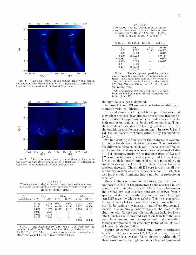
Fig. 8.— The figure shows the log column density of a core inthe decaying turbulence simulation U1b (left) and U1a (right) 23kyr after the formation of the first sink particle.

Fig. 9.— The figure shows the log column density of a core inthe decaying turbulence simulation U1b (left) and U1a (right) 53kyr after the formation of the first sink particle.

TABLE 4Core gas mass (M) including embedded sinks for thedecaying simulations at two different resolutions at

three different times.

∆ t 16 kyr 23 kyr 53 kyrResolution 5 AU 10 AU 5 AU 10 AU 5 AU 10 AU

0.741 0.758 0.997 0.997 1.907 1.9050.124 0.124 0.280 0.283 0.827 0.8060.077 0.077 0.177 0.180 0.136 0.1910.040 0.037 · · · · · · · · · · · ·0.035 0.033 · · · · · · · · · · · ·0.291 0.259 · · · · · · · · · · · ·· · · · · · · · · · · · 0.106 0.036

Note. — The subscripts 10 (U1a) and 9 (U1b) represent thenumber of AMR levels. The minimum density of the gas is ρ =2×10−16 g cm−3. The ’...’ represent cores that have merged withothers and cannot be individually distinguished.

TABLE 5Masses of the protostars in both drivenand decaying simulations at 260 kyr (the

larger cores, D2 and U2) and 130 kyr(the smaller cores, D3 and U3).

D2 (M) U2 (M) D3 (M) U3(M)

1.221 1.811 0.639 0.5861.047 1.002 0.453 x 0.5521.049 0.933 · · · 0.3480.490 x 0.223 · · · x 0.114

x 0.382 x 0.131 · · · 0.0480.329 0.059 · · · x 0.0470.281 x 0.034 · · · · · ·0.207 x 0.030 · · · · · ·· · · x 0.023 · · · · · · a

Note. — The x’s represent particles that areejected from the system by dynamical interac-tions. The time of first sink particle formationafter the onset of gravity for each of the cores is270, 680, 250, and 660 kyr for D2, D3, U2, andU3, respectively.aOne additional BD mass sink particles have

been excluded as numerical disk fragmentationfrom column U2.

the high density gas is depleted.In cases D2 and D3 we continue turbulent driving to

maintain virial equilibrium.To avoid directly adding artificial perturbations that

may affect the core development or seed new fragmenta-tion, we do not apply any velocity perturbations to thehigh resolution regions inside the refinement box. Thus,the turbulence cascades into the highly-refined box fromthe outside in a self-consistent manner. In cases U2 andU3, the simulation continues without any turbulent in-jection.

We find striking differences in the protostellar systemsformed in the driven and decaying cores. The most obvi-ous difference between the D and U runs is the differencein the number and mass of sink particles formed (Table5). For example, initially the fragmentation of D2 andU2 is similar temporally and spatially, but U2 eventuallyforms a slightly larger number of objects particularly atsmall masses as the level of turbulence in the two sim-ulations diverges. The small D3 core forms a small sta-ble binary system at early times, whereas U3, which isalso fairly small, fragments into a number of protostellarmembers.

Despite the small-number statistics, we are able tocompare the IMF of the protostars to the observed initialmass function via the KS test. The KS test determinesthe probability that a given data set is drawn from aspecified statistical distribution, in this case, the singlestar IMF given by Chabrier (2005). This test is accuratefor input sets of 4 or more data points. We achieve abest fit by scaling the masses by an adjustable normal-ization, ε = m∗/msink, where msink is the mass of thesink particle. Given that this simulation lacks feedbackeffects such as outflows and radiation transfer, the sinkparticle masses represent an upper limit and the scalingfactor corresponds to an efficiency factor of ε=0.25-0.75(Matzner & McKee 2000).

Figure 10 shows the scaled cumulative distributionfunction (cdf) for the runs D2, U2, and U3, and the cdfof the Chabrier is overlaid for comparison. Although allthree runs can have a high confidence level of agreement

10

Fig. 10.— The figure shows the cumulative distribution function(solid line) at t=0.26Myr for D2 (left), U2+U3 (right),where thedotted line is the Chabrier 2005 IMF fit. The dashed vertical linerepresents the point of largest disagreement. The probability thatthe data are drawn from the Chabrier IMF is 67% and 59%, re-spectively, where the efficiency scale factors of the simulations are0.4 and 1.0, respectively.

with the measured IMF, the normalization values andthe shapes of the distributions are quite different. Forexample, the smaller stellar population of D2 has fewerlow-mass objects and hence has a smaller efficiency scal-ing factor of ∼ 0.4 with highest likelihood of being drawnfrom the IMF of 67%. Conversely, U2+U3 distributioncontains collections of low-mass objects and intermediatemass objects, where the largest disagreement occurs inthe middle of the two populations. A scaling factor of 1.0gives the best agreement of 59%. A scaling factor nearunity implies that protostellar mass loss has a negligi-ble effect on the final mass of the star, contrary to sometheoretical expectations (Shu et al 1987; Nakano et al.1995; Matzner & McKee 2000). For the D2 distribution,the largest disagreement occurs at the higher mass end,indicating that if the protostars continue to accrete massand no new protostars are formed, then it is likely thatthe high probability of agreement with the IMF will bemaintained while the scale factor shifts to a lower value.The U2+U3 have a larger scale factor due to the signif-icant number of low mass objects with accretion haltedby dynamical ejection. These objects will be unlikelyto accrete additional mass and are essentially fixed. Forthe undriven runs, the largest disagreement occurs in themiddle of the distribution, indicating a widening differ-ence between the sub-stellar fixed-mass ejected objectsand those that remain in the gas reservoir and continueaccreting. Further running time will more likely makethe gap wider and agreement worse.

The efficiency scale factor is also dependent upon thenormalization we have chosen. The minimum mass thatwe are able to resolve in these simulations is proportionalto the Jeans mass evaluated at the maximum level ofrefinement. Because the Jeans mass is inversely relatedto the density, normalizing the results to a density higherthan our fiducial value of n = 1100 cm−3 will producelower mass objects and shift the IMF peak towards lowermass. This will also increase the efficiency factor used toscale the distribution to the universal IMF.

Studying the time evolution of the two simulations

shows the origin of the different stellar populations. Insimulation D2, the initial collapse and core fragmentationproduces three well separated objects that remain fairlyfar apart. A few additional objects form, but they donot suffer large gravitational interactions with the pri-maries and so remain in the high density regions andcontinue accreting. By contrast, in U2 and U3 the lackof global turbulent support causes mass to fall onto theearly formed protostellar cores resulting in contractionof the clump. This causes all the protostars to gravitatetowards the core center. As the protostellar proximityincreases, the accretion disks interact and become grav-itationally unstable (see discussion in § 4.6). Fragmen-tation ensues. The stellar systems become increasinglydynamically unstable with the addition of these smalllatecomers, which rapidly suffer strong gravitational in-teractions with the larger protostars and are thrown outof the high density reservoir of gas. Their small envelopesare stripped away, thus truncating the accretion processand effectively fixing their stellar masses (see Figure 11).This truncation process occurs for approximately half ofthe objects formed in the undriven simulations (see dis-cussion of brown dwarfs in § 4.5)

4.4. AccretionThere are two main accretion paradigms. In both mod-

els, star formation begins with the outside-in formationof gravitationally bound cores and their inside-out col-lapse. However, the core accretion model proposes thatthe main protostellar accretion phase takes place earlyon and continues until the entire core mass is accreted orexpelled (Shu et al 1987; Nakano et al. 1995; Matzner& McKee 2000), after which accretion becomes negligi-ble. Thus, the initial core size and subsequent feedbackeffects limit the mass of the protostars. In contrast, thecompetitive accretion model proposes that stars begin ina core as wandering, accreting 0.1 M seeds, whose fi-nal mass is determined by the protostar’s location in theclump (Bonnell et al. 1997, 2001). Mass segregation isa common feature of this model, such that the largestmass objects inhabit the region of highest gravitationalpotential and the smallest objects inhabit the less densegas, usually having been ejected from the center by grav-itational interactions.

In our results, there are two accretion phases. Initially,there is a transient period of high accretion during whichthe initial infalling gas accretes onto the newly formedsink particle and gas is depleted from the cells insidethe accretion region. This phase is model independentand occurs while the newly created sink particle regionreaches pressure equilibrium with the surrounding gas.Generally less than 10% of the accretion occurs duringthis time. During the second phase, the accretion rateapproximates the Shu model for core accretion,

M∗ = c3s/G, (12)

(Shu et al. 1987), although in most cases the accretionrate is gradually declining. This solution is valid untilthe rarefaction wave reaches the core, i.e. when approx-imately half of the original core mass has been accreted(McLaughlin & Pudritz 1997; McKee & Tan 2002). Afterthat, the accretion rate diminishes as the density of thesurrounding gas decreases, but our simulations end be-

11

Fig. 11.— The figures show the sink particle mass as a functionof time for runs D2, D3, U3, and U2 shown clockwise from top left.Each particle is represented by a different style line.

fore it is possible to determine if this final stage actuallyoccurs.

To illustrate the differences between the protostellarsystems, we have plotted the mass as a function of timefor all sink particles, the instantaneous mass accretionrate for the first two formed objects, the time-averagedaccretion rate, and the total mass in sink particles asa function of time. The turbulent core accretion andcompetitive accretion models describe the evolution ofthe stellar population in cases D2 and U2, respectively.In the former case, objects are mainly formed from corefragmentation with separations larger than 1000 AU. Theaverage accretion onto the protostars initially agrees withthe Shu model but, modulo fluctuations, diminishes overtime as the core mass depletes (Figure 12). Meanwhile,the core envelope accretes according to the Bondi-Hoylemodel of turbulent accretion (Krumholz et al. 2006). Fordriven turbulent environments the overall Mach numberwill remain sufficiently high such that the core will notgain a substantial amount of mass during the core dy-namical time and the main accretion phase of the form-ing protostars will be limited by this time. However,in the decaying turbulent case loss of turbulent pressuresupport potentially causes significant additional mass toaccrete onto the core, resulting in a more constant proto-stellar accretion rate (Figure 12, bottom row). However,the differences in the accretion rates of the most massiveobjects are subtle due to the significant fluctuations.

Perturbations to the accretion disks and clumpiness ofthe infalling gas cause fairly large variability in the sinkparticle accretion rate as illustrated in Figure 12. How-ever, we do not observe that most of the mass is depositedin short intervals by clumpiness in the disk as noted byBasu et al. (2006), who model 2D axi-symmetric diskswith magnetic fields. The absence of this effect in ourcalculations is most likely due to our Cartesian geometryrather than lack of magnetic fields (Basu, private com-munication). The r − φ geometry used by Basu et al. ismore suitable for disk treatment and has lower numericalviscosity, which may suppress small scale clumpiness.

Due to differences in core accretion, the two cases pro-duce much different stellar populations. In the drivencases, in which fewer objects form, protostars accretemore smoothly and do not undergo strong dynamical in-

Fig. 12.— The figures show the instantaneous sink particleaccretion rate as a function of time for runs D2, D3, U3, and U2shown clockwise from top left. Only the history of the two firstforming particles is shown.

teractions with their neighbors. However, in the decayingcases, the strong infall pushes the protostars to the corecenter and the large number of nearby objects accret-ing from the central reservoir of gas causes the smallestobjects to be kicked out of the cluster. This can be ob-served in Figure 12 (U3) as a precipitous drop off in theaccretion rate for individual objects or as flatlining ofthe object mass (Figure 13, bottom row). Differences be-tween the number of objects are caused by turbulent sup-port, which prohibits new mass from infalling onto theclump. High accretion causes fragmentation and drivesforming objects to the gravitational center, where theydynamically interact. This close proximity results in ob-ject ejection and destabilization of the accretion disks,which leads to new fragmentation. The differences inaccretion rate and stellar population between the twocases suggests that the maintenance of turbulence, pro-tostellar accretion, and stellar population are intimatelyrelated (Krumholz et al. 2005). In spite of individualaccretion fluctuations, the total accretion of the objectsfrom the core is dominated by the largest objects, suchthat the fraction of the core accreted is relatively smoothover time as shown by Figure 14.

4.5. Brown DwarfsBrown dwarfs (BD) are observed to comprise ∼10-30 %

of all luminous objects in star forming regions (Andersenet al. 2006; Luhman et al. 2007). For example, in theChabrier (2005) IMF, with which we compare, BDs withmasses M∗ ≤ 0.08M comprise ∼20% of the total num-ber of objects. Understanding the population, origins,and connection between planets and hydrogen-burningstars is essential in formulating a successful theory ofstar formation. Observations remain particularly am-biguous concerning the primary formation mechanism ofBDs, sparking many theories. Of these, proposals for BDformation by turbulent fragmentation, ejection, or viadisk fragmentation have the most potential for generat-ing BDs in sufficient numbers (Padoan & Nordlund 2004;Reipurth & Clarke 2001; Whitworth et al. 2007). Sim-ulations provide an important vehicle for testing thesetheories, and we discuss the BD population of our simu-lations in this section.

12

Fig. 13.— The figures show the averaged sink particle accretionrate for the first two sink particles as a function of time for runsD2, D3, U3, and U2 shown clockwise from top left. The average istaken over 10 consecutive timesteps, and the solid flat line indicatesthe value of c3s/G.

Fig. 14.— The figures show the total mass accreted normalizedto the initial bound core mass as a function of time for runs D2,D3, U3, and U2 shown clockwise from top left.

Our driven turbulence simulations D2 and D3 do notproduce any sink particles of final substellar mass, whichare primarily created in our simulations by prematurelytruncated accretion. However, if BDs are formed viathe same mechanism as stars, accrete from a disk, andproduce outflows (Luhman et al. 2007) then the sameefficiency factor will be valid for scaling all the objects inthe simulation. The decaying turbulence simulations U2and U3, however, produce a much larger initial numberof BDs, 33%. This agrees with the competitive accretionparadigm: Bate et al. (2002) find that ∼44 % of theobjects that form in their 50M decaying turbulent cloudsimulation qualify as BDs, which is much higher than theobserved fraction. Their calculation is initialized withuniform density and an initial turbulent velocity field,however they do not drive the turbulence, so that theturbulence never achieves a steady relaxed state. Despitethis difference, their result is in qualitative agreementwith the BD formation mechanism and number fractionof our decaying turbulence runs.

Ideally, we would like to understand the BD popula-

tion in various star forming regions as a function of theirgeneral properties. The turbulent fragmentation modelpredicts an upper limit on the total mass available forthe formation of BDs as a function of the Mach numberand average number density (Padoan & Nordlund 2004).According to their model, the total gas mass availableto make BDs from turbulent compressions is 0.4% of thetotal gas mass or 3.7 M as a function of our simulationMach number and density. If the SFR per free fall timefor the driven and decaying runs is respectively 14.3%and 13.6% then the total maximum possible mass in BDdue to turbulent fragmentation as a fraction of the actualmass turned into stars is 2.8% and 2.9%. For compari-son, the fraction of the actual luminous mass turned intoBDs according to the Chabrier IMF is ∼2%. Our highresolution protostellar systems have a BD mass fractionof 0.0% and 3.2% for D2, and U2 + U3, respectively,using the efficiency factor from Figure 10 and includ-ing M∗ ≤ 0.08M in the BD mass total. However, theturbulent fragmentation model gives only the maximumfraction of gas that can be converted to BDs by turbulentcompressions and it does not include possible BD forma-tion in disks (Goodwin & Whitworth, 2007). Fragmenta-tion of disks and dynamical ejection is responsible for allof the BDs in the decaying simulation. Thus, comparisonbetween the decaying turbulence models and turbulentfragmentation prediction is misleading.

The absence of BDs in the driven runs is reasonable ifBDs actually form via turbulent fragmentation. In sucha process, small low-mass objects form from small low-mass cores. Since we have not chosen any particularlysmall cores for high resolution study, we would not ex-pect to find many BDs. Thus, scaling to the stellar IMF,which has a peak at ∼ 0.2 M requires a small efficiencyfactor. The core distribution is set by the low resolutionturbulent initial conditions. The minimum expected coremass is the Bonnor-Ebert mass evaluated at the maxi-mum turbulent gas density. According to the turbulentfragmentation model, this maximum is set by the prob-ability density function (PDF) of the gas density. Theresolution and Mach number of our simulation yield adensity PDF that falls off at ∼ 1.3 × 10−18 g cm−3 orMBE ' 0.2M. The minimum mass estimated from thisdensity agrees with the minimum sink particle mass atthe end of a free fall time at low resolution. Since thismass is well above the maximum BD mass, it also ex-plains the low abundance of low-mass objects at highresolution in the driven simulation. Moreover, this sug-gests that the driven high-resolution IMF distribution isincomplete at the low-mass end such that scaling to theactual IMF may be optimistic and result in underesti-mating the core efficiency factor.

One observational measure of the BDs in a regionis given by the ratio of low-mas stars to BDs: R =N(0.08− 1.0M)/(N(0.02− 0.08). Measurements of lo-cal star-forming regions give a range of R ' 2 − 5 (e.g.Andersen et al. 2006). For the driven and decayingsimulations, respectively, we find R > 7 and R = 3.0,although these numbers are clearly sensitive to the low-statistics of our simulations. These ratios are most prop-erly represent lower limits because we have not includedthe effects of radiative transfer, which have been shown tosuppress fragmentation (Krumholz et al. 2007). Over-all, the driven high-resolution BD mass fraction more

13

closely agrees with the turbulent fragmentation predic-tion, whereas the undriven BD mass fraction agrees moreclosely with competitive accretion results, which predictlarger BD numbers and mass fractions. Given that BDformation via disk fragmentation dominates in the un-driven case, it is unsurprising that these statistics do notagree well with the turbulent fragmentation model andare quite different from one another.

4.6. Disk StabilityAnalytically, gravitational disk instability is dictated

by the Toomre Q parameter, which is given by

Q =csκ

πGΣ, (13)

where κ is the epicyclic frequency, and Σ is the surfacedensity. For values of Q . 1, the disk becomes unsta-ble to gravitational fragmentation. Spiral arms developfor low Q values and fragmentation ensues when Q ap-proaches 1 from above. This fragmentation manifests asa density increase at those locations. The early frag-mentation in D2 and U2 generally occurs near the diskperimeters, where it is coldest (e.g. Figure 15). In thesimulations, sources of disk instability are due to a combi-nation of perturbations from clumpy infalling gas, grav-itational influence of nearby bodies (i.e. other sink par-ticles), and from actual collisions between disks. Sincethe sink accretion radius is racc = 4∆x, we neglect theinnermost 4 cells in the analysis. We define the disk gaswhere ρ ≥ 2 × 10−16 g cm−3, which agrees fairly wellwith disk boundaries determined visually. In general, wefind disk radii between 150-300AU and surface densitiesof a few g cm−2, values similar to observed properties oflow-mass disks (Andrews & Williams 2006).

The stability of a disk and the onset of gravitationalinstability have been shown to be correlated with theaccretion rate of the disk itself (e.g. Bonnell 1994; Whit-worth et al. 1995; Hennebelle et al. 2004; Matzner &Levin 2005). Higher disk accretion rates increase thelikelihood of disk instability. This fact agrees with ourobservation that more instances of disk fragmentationoccur in simulations U2 and U3, where there is larger in-fall onto the clump, in contrast to the case D2 where thedisks remain fairly stable. The level of disk instability isdirectly visible in the plots of the sink particle accretionrates (Figure 12); very noisy and irregular accretion cor-responds to clumping and disturbance of the disk. Thesimulations where sinks have many close neighbors showthe highest rates of disk instability and episodic accre-tion. Note that in Figure 12 of run U4, the ejection of acompanion substantially reduces the accretion rate fluc-tuations of the remaining protostar.

There has been considerable recent discourse on thenecessary criteria for resolving disks and preventing ar-tificial fragmentation (Nelson 2006; Klein et al. 2007;Vorobyov & Basu 2005; Durisen et al. 2007). Since wedo find that our disks fragment, this is a topic of con-cern. Most recent simulations, including ours, have usedthe Jeans condition as defined by Truelove et al. (1997)or Bate & Burkert (1997) to set the minimum refine-ment of meshes and particles, respectively, in the diskunder study. However, Nelson (2006) argues that thiscriterion is inadequate and inappropriate for cylindricaldisk geometry. Additional possible sources of error in

our calculation may arise from sink particle gravitationalsoftening, numerical viscosity, and the cartesian natureof the AMR grid. We address these issues here.

In calculating the gravitational sink particle-particleand sink particle-gas interactions, we use a constant soft-ening length 0.5∆xmax, where ∆xmax is the grid spacingon the maximum level. This is much smaller than boththe disk radius and the size of the accretion region, soit should have little effect on the behavior of the disk.In general, we find that the observed disk fragmentationoccurs as cores forming in the ends of spiral arms, wellaway from the center of the disk (see Figure 15).

Nelson (2006) requires two specific criteria for adequatedisk resolution. The first is a Toomre condition,

T ≥ ∆xl

λT, (14)

where T is the Toomre number, and λT is the neutralstable wavelength defined by:

λT =2c2sQGΣ

(15)

and ∆xl is the cell spacing on level, l. The above criterionis analogous to the Jeans criterion defined in Truelove etal.,

J ≥ ∆xl

λJ. (16)

For our simulations, a disk radius of 200 AU is cov-ered by 20 or 40 cells, which is fairly marginal resolu-tion, but we will show it is, in fact, sufficient. We plotthe azimuthally averaged density and Toomre Q param-eter (equation 13) as a function of radius in Figure 16.Density enhancements are correlated with low ToomreQ in each refinement case. We also plot the right handsides of equations (14) and (16) as functions of radius inFigure 17. In all cases, these quantities are under thefiducial value of 1/4. The over resolution in the centralpart is due to the requirement that all cells surroundinga sink particle be refined to the maximum level in orderto encompass the accretion region.

Figure 15 indicates the borders between AMR grids,so some disk regions within 200 AU become derefined,and ∆xl → ∆xl−1. However, these regions still satisfythe refinement criteria by a good margin.

The second criterion formulated by Nelson appliesspecifically to SPH codes. It postulates the necessityof resolving the disk scale height at the midplane by foursmoothing lengths. Nelson argues that insufficient res-olution of the vertical structure produces errors in theforce balance, thus favoring artificial fragmentation. Ifwe assume a one-to-one conversion between smoothinglengths and grid cells, we can apply it to our calcula-tion. Figure 17 shows azimuthally averaged quantitiesfor an accretion disk for ∼2.5, 5, and 10 AU maximumresolution. The lowest resolution run fails to adequatelyresolve the disk scale height, but we do not see extrafragmentation. We may not see this effect because Nel-son formulated and tested his criteria for SPH ratherthan grid-based codes. It is also possible that the one-to-one analog of smoothing length to ∆x is not the cor-rect conversion. However, most disagreement is in theinner regions where the artificial viscosity is high, which

14

Fig. 15.— The figure shows the log column density (g cm−2)of an accretion disk in run D2 with ll levels of refinement. Twofragments have formed at the edges of the spiral disk structure.The solid black lines denote grid boundaries. a

suppresses any potential fragmentation. In order to de-termine the cause of the discrepancy, further explorationwith a full grid high resolution study of disks is necessary.

A careful study of the sink particle accretion in adisk is given in Krumholz et al. (2004). For a Kep-lerian disk, Orion agrees well with analytic results ex-cept for some irregularities when the radius of the disk,r ∼ rB = GM/c2s , the Bondi radius. However, our sim-ulations have r << rB during the main accretion phaseand should be unaffected. Also of concern is the magni-tude of the numerical viscosity, which has the potentialto suppress fragmentation if it is sufficiently high. Usingthe definition of α viscosity defined in Krumholz et al.(2004), we can estimate the magnitude of this viscosityas a function of disk radius:

α'78rB

∆x

( r

∆x

)−3.85

(17)

'0.8M1T−110 ∆x2.85

5 r−3.85150 , (18)

where r150 is the radial distance from the central star inunits of 150 AU, M1 is the stellar mass is units of M,∆x5 is the cell size in units of 5 AU, normalized to themaximum level of refinement, and T10 is the gas tem-perature in units of 10K. This expression shows fairlylarge sensitivity to the cell size and disk radius. Due tothe large α value in the inner region of the disk, artifi-cial viscosity is likely to significantly influence the diskproperties within the inner 100 AU. Large values of αcould potentially suppress disk fragmentation. Proto-stellar disks around low-mass protostars, which are fairlythin and have a low ionization fraction, have been mea-sured to have viscosities of α ∼ 0.01 (King et. al 2007;Andrews & Williams 2006).

We find that all disks form exactly two fragments atthe same radial locations where Q ∼ 1. Convergence ofthe disk density distribution and number of fragments isour main concern. The averaged quantities are slightlydifferent in the three cases, although the general trendsare the same. In the lower resolution case the fragmen-tation is less pronounced, however two sink particles areintroduced at these locations. It is certainly true that thefragments are not well resolved at the lowest resolution,and we are only marginally resolving the disks. Hence

Fig. 16.— The figure shows azimuthally averaged disk propertiesas a function of log radius (AU) for a disk with ∼ 2.5 AU (top),5.0 AU (middle) and 10.0 AU (bottom) resolution. The left plotsshows log ρ for the edge on view of the disk. Plots on the rightshow log Q vs. log r. The central region corresponding to the sinkparticle accretion region is excluded from the plot.

we do not devote much discussion in this paper to diskproperties. Serious study of disks requires much higherresolution than we adopt in this paper and is best studiedin cylindrical or polar coordinate geometry to minimizethe effects of Cartesian cell imprinting.

Given that observations find stellar systems have typi-cally 2-3 stars (Goodwin & Kroupa 2005), the large num-ber of objects produced in the high resolution decayingsimulations seems somewhat anomalous. However, theactual initial multiplicity is more difficult to determinethan multiplicity among field stars due to the difficultyof detecting small obscured objects, some of which mayhave separations below the resolvable limit. In addi-tion, systems with more than two bodies are unstableand decay through gravitational interactions ultimatelydecreasing the multiplicity of stellar systems over time.We witness this behavior in the decaying turbulence pro-tostellar systems, which expel low-mass members.

Nonetheless, it is likely that a few of these small frag-ments are numerical products, resulting from our equa-tion of state. For example, Boss et al. (2000) andKrumholz et al. (2006) both find that fragmentationis sensitive to thermal assumptions and the inclusion ofradiative transfer, since heating tends to enhance diskstability. Price & Bate (2007) show that magnetic fieldstend to suppress and delay both fragmentation and spiraldisk structure. It is probable that inclusion of radiativefeedback and magnetic fields would suppress some of thesmall objects that we find in the undriven runs. However,the absence of these objects in the driven simulations in-dicates a striking difference in the accretion rate, systemstability, and fragmentation history with turbulent feed-back.

5. CONCLUSIONS

In this paper we use turbulent simulations with AMRto illustrate distinctions between driven and decaying

15

Fig. 17.— The figure shows azimuthally averaged disk propertiesas a function of log radius (AU) for a disk with ∼ 2.5 AU (top), 5.0AU (middle) and 10.0 AU (bottom) resolution. The first columnshows plots of J (dashed line) and T (solid line) vs. log r, wherethe horizontal line marks the fiducial value of 0.25. The secondcolumn shows the number of cells in the disk vertical scale heightas a function of log r. The solid line is the required resolution ofthe vertical scale height according to the Nelson criteria and thedashed line is our resolution. The central region corresponding tothe sink particle accretion region is excluded from the plot.

turbulence. Despite identical initial conditions in thetwo simulations, we find significant differences betweenthe two cases after one free-fall time. Our simulations ne-glect the effect of magnetic fields, which are poorly obser-vationally constrained and occupy a place of ambiguousbut potentially large importance (Crutcher 1999). Oursimulations also lack radiation transfer, instead relyingon the barotropic approximation, which may affect thecore fragmentation and protostellar multiplicity in ourresults.

We find that the properties of the cores in driven anddecaying turbulence at low resolution are not sufficientlydifferent to completely dismiss one turbulent environ-ment. This is in part due to the large scatter in ourresults. For example, we find that the cores in the differ-ent environments have similar shapes and mass-size rela-tions. However, we find that cores in the driven simula-tion have less rotational energy, which is in better agree-ment with observations (Goodman et al. 1993; Caselli etal. 2002). The linewidth-size relation of the cores form-ing in driven turbulence is also closer to the observed re-lation for low-mass regions (e.g. Jijina & Adams 1999),while the linewidth-size relation of cores in the decayingsimulation is quite flat. We find that driven turbulenceproduces a greater number of cores than decaying turbu-lence with the potential for new star formation occurringlonger than a single dynamical time. In contrast, the de-caying simulation stops forming new condensations be-fore one global free-fall time.

The largest differences between the two cases are ap-parent at high resolution. We show that our high reso-lution simulations are converged and that the resolution

is sufficient to capture core fragmentation, despite beingmarginal for determining the detailed properties of disks.We find that the presence or absence of global virial bal-ance has only a subtle influence on individual accretionrate of the largest object forming in the core at leastfor the first few core free fall times. However, the coresforming in a decaying turbulence environment show clearsigns of competitive accretion such that a core’s accretionrate is tied to its dynamical history and and its locationin the clump. This supports the results of Krumholz etal. (2005) who show that simulations exhibiting com-petitive accretion do so because of lack of a source ofturbulence.

The loss of turbulent feedback in the decaying run af-fects the dynamic behavior of the forming protostars,resulting in significant disk fragmentation, and BD for-mation by ejection. This leads to overproduction of BDsin comparison to the observed IMF (e.g. Chabrier 2005).In contrast, the driven simulations form few BDs, whichcan be understood in the context of the turbulent frag-mentation model for star formation, which predicts BDsto mainly form from small highly compressed cores. Ob-servations of low-mass star forming regions do not findlarge velocity differences or significant spatial segrega-tion between BDs and low-mass objects as obtained inthe decaying simulation.

While our simulations of driven and decaying turbu-lence show some statistically significant differences, par-ticularly in the production of brown dwarfs and core ro-tation, the uncertainties are large enough that we are notable to conclude whether observations favor one or theother. However, in Paper II we use simulated line profilesto estimate core velocity dispersions and centroid veloci-ties, and we find that decaying turbulence leads to highlysupersonic infall onto protostars, which has not been ob-served. Our results thus give some support to the useof driven turbulence for modeling regions of star forma-tion, but a conclusive determination of which approachis better awaits larger simulations with the inclusion ofmagnetic fields, protostellar outflows and thermal feed-back.

We thank P.S. Li, M. Krumholz and R. Fisher forhelpful discussions and suggestions. Support for thiswork was provided under the auspices of the US Depart-ment of Energy by Lawrence Livermore National Labora-tory under contacts B-542762 (S.S.R.O.) and DE-AC52-07NA27344 (R.I.K.); NASA ATP grant NNG06GH96G(CFM and RIK); grant AST-0606831 (CFM and RIK);and National Science Foundation under Grant No.PHY05-51164 (CFM and SSRO). Computational re-sources were provided by the NSF San Diego Supercom-puting Center through NPACI program grant UCB267;and the National Energy Research Scientific ComputerCenter, which is supported by the Office of Science ofthe U.S. Department of Energy under contract numberDE-AC03-76SF00098, though ERCAP grant 80325.

REFERENCES

Andersen, M., Meyer, M. R., Oppenheimer, B., Douglas, C., &Carpenter, J. 2006, ApJ, 132, 2296

Andrews, S. M., & Williams, J. P. 2006, ApJ, 659, 705

16

Banerjee, R., & Pudritz, R. E. 2006, ApJ, 641, 949Basu S., & Ciolek G. E. 2004, ApJ, 607, L39Bate M. R. 2004, A&SS, 292, 197Bate M. R. & Bonnell, I. A. 2005 MNRAS, 356, 1201Bate M. R., Bonnell, I. A., & Bromm, V. 2002, MNRAS, 332, L65Bate M. R., & Burkert, A. 1997, MNRAS, 288, 1060Bonnell I.A. 1994, MNRAS, 269, 837Bonnell I.A., Bate, M.R., Clarke, C.J. & Pringle, J.E. 1997,

MNRAS, 285, 201Bonnell I.A., Bate, M.R., & Vine S.G. 2003, MNRAS, 343, 413Bonnell I.A., Clarke, C.J., & Bate, M.R. 2006, MNRAS, 324, 1296Bonnell I.A., Clarke, C.J., Bate, M.R., & Pringle, J.E. 2001,

MNRAS, 368, 573Bonnell I.A., Vine S.G. & Bate, M.R. 2004, MNRAS, 349, 735Boss A. P., Fisher R. T., Klein R. T., & McKee C.F. 2000, ApJ,

528, 325Burkert, A. & Bodenheimer, P. 2000, ApJ, 543, 822Caselli, P., Benson, P. J., Myers, P. C., & Tafalla, M. 2002, ApJ,

571, 334Chabrier, G. 2005, ASSL, 327, 41Crutcher R. M. 1999, ApJ, 520, 706di Francesco J., Evans N. J., II, Caselli P., Myers P. C., Shirley Y.,

Aikawa Y., &Tafalla, M. 2007, Protostars and Planets V, 17Dib, S., Kim, J., & Shadmehri, M. 2007, astro-ph/0706.0950Durisen R. H., Boss A. P., Mayer L., Nelson A. F., Quinn T., &

Rice, W. K. M. 2007, Protostars and Planets V, 607Elmegreen, B. G. & Scalo, J. 2004. ARA&A, 42, 211Gammie C. F., Lin Y.-T., Stone J. M., & Ostriker E. C. 2003, ApJ,

592, 203Goodman, A. A., Benson, P.J., Fuller, G.A., & Myers, P. C. 1993,

ApJ, 406, 528Goodwin, S. P., & Kroupa, P. 2005, A&A, 439, 565Goodwin, S.P., & Whitworth 2007, astro-ph/0703106Hartmann, L. 2001, AJ 121, 1030Hennebelle, P., Whitworth, A. P., Cha, S. -H, & Goodwin, S.P.

2004, MNRAS, 348, 687Heyer, M. H. & Brunt, C. M. 2004, ApJ, 615, 45Hosking, J. G. & Whitworth, A. P. 2004, MNRAS, 347, 1001Jappsen, A.-K. & Klessen, R. S. 2005, A&A 423, 1Jappsen, A.-K., Klessen, R. S., Larson, R. B., Li, Y., & Mac Low,

M.-M. 2005 ApJ, 620, 19Klein, R. I. 1999, JCAM, 109, 123Klein R. I., Inutsuka, S.-I., Padoan, P., & Tomisaka, K. 2007,

Protostars and Planets V, 99Klessen, R. S. 2001, ApJ, 556, 837Klessen, R. S. & Burkert, A. 2001, ApJ, 549, 386Klessen R. S., Burkert A., & Bate M. R. 1998, ApJ, 501, L205Klessen, R. S., Heitsch, F., & Mac Low, M-M. 2000, ApJ, 535, 887Krumholz, M. R., Klein, R.I. & McKee C. M. 2007, ApJ, 656, 959Krumholz, M. R., Klein, R.I. & McKee C. M. 2004, ApJ, 611, 399Krumholz, M. R., McKee, C. F. & Klein, R.I. 2006, ApJ, 638, 369

Krumholz, M. R., McKee, C. F. & Klein, R.I. 2005, Nature, 438,332

Krumholz, M. R., & McKee, C. F. 2005, ApJ, 630, 250Krumholz, M. R., & Tan, J. C. 2007, ApJ, 656, 959Lada C. J. 2006, ApJ, 640, L63Lada C. J., Alves, J. F., & Lombardi, M. 2007, Protostars and

Planets V, 3Larson R. B. 1981, MNRAS, 194, L809Larson R. B. 2005, MNRAS, 359, 211Li P.S., Norman M. L., Mac Low M.-M., & Heitsch F. 2004, ApJ,

605, 800Luhman, K. L., Joergens, V. Lada, C., Muzerolle, J, Pascucci, I.,

& White. R. 2007, PPV, 443Mac Low, M.-M. 1999, ApJ, 524, 169Mac Low M.-M., & Klessen R. S. 2004, RMP, 76, 125Machida, M. N., Inutsuka, S., & Matsumoto, T. 2006, 647, 151Machida, M. N., Tomisaka, K., & Matsumoto, T. 2004, MNRAS,

348, 1Masunaga, H., Miyama, S. M., & Inutsuka, S. 1998, ApJ, 495, 346Matzner, C. D., & McKee, C. F. 2000, ApJ, 545, 364Matzner, C. D., & Levin, Y. 2005, ApJ, 628, 817McLaughlin, D. E. & Pudritz, R. E. 1997, ApJ, 476, 750McKee, C. F., & Ostriker, E. C. 2007, ARAA, 45. 565Nakano, T., Hasegawa, T., & Norman, C. 1995, ApJ, 450, 183Nelson A. F. 2006, MNRAS, 373, 1039Offner, S.S.R., Krumholz, M.R., Klein, R.I., & McKee, C.F. 2008,

AJ(accepted).Padoan, P., & Nordlund, A. 1999, ApJ, 526, 279Padoan, P., & Nordlund, A. 2002, ApJ, 576, 870

Price, D. J., & Bate, M. R. 2007, astro-ph/0702410Reipurth, B. & Clarke, C. 2001, AJ, 122, 432Shu, F. H., Adams, F. C, & Lizano, S. 1987, ARA&A, 25, 23Tan, J. C., Krumholz, M. R., & McKee, C. F. 2006, ApJ, 641, L121Tilley D. A. & Pudritz R. E. 2004, MNRAS, 353, 769Truelove, J. K., Klein, R. I., McKee, C. F., Holliman, J. H. II,

Howell, L. H., & Greenough, J. A. 1997, ApJ, 289, L179Truelove, J. K., Klein, R. I., McKee, C. F., Holliman, J. H. II,

Howell, L. H., Greenough, J. A., & Woods, D. T. 1998, ApJ,495, 821

Solomon, P. M., Rivolo, A. R., Barrett, J., & Yahil, A. 1987, ApJ,319, 730

Stone, J. M., Ostriker, E. C., & Gammie, C. F. 1998, ApJ, 508,L99

Swift, J. & Welch, W. j. 2007, accepted to ApJS.Vazquez-Semadeni, E., Ryu, D. Passot, T, Gonzales, R. F. & Gazol,

A. 2006, ApJ, 643, 245Whitehouse, S. C. & Bate, M. R. 2006, MNRAS, 367, 32Whitworth, A. P., Chapman, S.J., Bhattal, A. S., Disney, M. J.,

Pongracic, H. Turner, & J. 1995, MNRAS, 277, 727Williams, J. P., Geus, E. J., & Blitz, L. 1994, ApJ, 428, 693